Minimum Error Tool Path Generation Method

and

An Interpola tor Design Technique

for Ultra-precision Multi-Aris CNC Machining

Hong Liang

A Thesis

in

The Department

of

Mectianical Engineering

Presented in Partial Fulfilment of the Requirements

for the Deçree of Doctor of Philosophy ai

Concordia University

Montreal, Quebec. Canada

July 1999

@ Hong Liang, 1999

National Library of Canada

Bibliothèque nationale du Canada

Acquisitions and Acquisitions et Bibliographie Services services bibliographiques

395 Wellington Street 395, rue Wellington Ottawa ON K 1 A ON4 Ottawa ON K i A ON4 Canada Canada

Your hie Votre teference

Our Iile Narre reference

The author has granted a non- exclusive licence allowing the National Library of Canada to reproduce, loan, distribute or sel1 copies of this thesis in microform, paper or electronic formats.

The author retains ownership of the copyright in this thesis. Neither the thesis nor substantial extracts fkom it may be printed or otherwise reproduced without the author' s permission.

L'auteur a accordé une licence non exclusive permettant à la Bibliothèque nationale du Canada de reproduire, prêter, distribuer ou vendre des copies de cette thèse sous la forme de microfiche/film, de reproduction sur papier ou sur format électronique.

L'auteur conserve la propriété du droit d'auteur qui protège cette thèse. Ni la thèse ni des extraits substantiels de celle-ci ne doivent être imprimés ou autrement reproduits sans son autorisation.

ABSTRACT

Minimum Error Tool Path Ceneration Method and

An Interpolator Design Technique for Ultra-precision Multi-axis CNC Machining

Hong Liang, Ph.D. Concordia University, 1999

This thesis investigates an ultra-precision multi-ais CNC machining problem encountered in

machining sculptured surfaces. Conventional multi-axis CNC machining uses straight line

segments to connect consecutive data points, and uses linear interpolation technique to

generate the command siçnals for positions beiween machining data points. However. due

to the multi-ais simultaneous and coupled translational and rotational movements. the actual

machining motion trajectory is a non-linear curve. The non-linear curve seçments deviate

tiom the linearly interpolated straight line seçments. resulting in non-linearity errors. which

in turn cause obstacles to ensuring high precision machining.

The problem in multi-axis CNC machining is that non-linearity errors result in total

machining error which is beyond the range of the machining tolerance. The problem arises

h m the fan that the linear interpolation technique generates commands for positions along

a straight iine segment, while rotational movements superimposed onto translational

movements cause the cutting point movinç along a curved machining motion trajectory. The

machining motion trajectory depends on both multi-axis CNC machine tool configuration and

the machining rotational rnovements. The machining rotational movements are kinematically

iii

related to cutter orientation variations. Thus. The factors causing the multi-mis CNC

machining error problem are the spatially varying cutter orientations and the utilization of

linear interpolation method .

A novel off-fine tool path generation methodology for is developed and reponed in

this thesis in order to soive the non-linearity error problem in ultra-precision multi-axis CNC

machining. The new off-line tool path generation method reduces non-lineanty errors by

modifyinç cutter orientation chanses based on machine kinematics and machining motion

trajectory. A software routine for implementinç the new tool path generation methodology

is developed. A simulation of the process for machining a sculp tured surface by applying the

novel methodology iilustrates that it increases machininç precision considerably.

A novel interpolator design technique for solvinç the non-linearity error problem in

ultra-precision multi-axis CNC machining is aiso presented. A 3D circular interpolation

principle is developed which is capable of trackinç sphericai curves with low position errors

and uniform feedrates. On the basis of this (3D circular) interpolator. a cornbined 3D linear

and circular ( M C ) interpoiator is proposed for five-auis CNC machining. The proposed 3D

L&C interpolaior is able to drive the pivot of rotational movements along a predesiçned 3D

cuve and conduct the cutting point along a linear spatial path. so that the elirnination of non-

linearity errors in five-axis CNC machining is achirved. A software interpolation routine of

the 3D L&C interpolator is developed, and a cornputer simulation illustrating the machining

of a sculptured surface validates the novel technique.

ACKNOWLEDGEMENT

I would like to extend the sincerest gratitude and appreciation to my thesis

supervisors, Dr. J. Svoboda and Dr. H. Hong, for their time, encouragement, guidance and

directive supervision, moral and financial support during the course of this research. 1 feel

extremely fortunate to have had the opportunity of working with them and sharing their

expenence and insight. 1 am grateful to rny former thesis supervisors. Dr. R. Cheng and Dr.

C. Wu, for giving me the opportunity of experiencing the current industry issues.

In addition. 1 would like to thank Mr. T. Luong and Mr. L. Gagnon. of Pratt &

Whitney Canada Inc.. for many usefùl discussions, suggestions and comments I have received

from thern through this research.

Last but not least 1 owe many thanks to my family and especially my parents for their

encouragements and help at al1 stages of my studies. 1 am very ~rateful to my husband and

my daughter for their patience, encouragements and support durinç this work. Without their

unwavering support this would not have been possible.

TABLE OF CONTENTS

Page LIST OF FIGURES ........................................................................................ ix

LIST OF TABLES ........................................................................................ xi

NOMENCLATURE ..................................................................................... xi i

LIST OF ASBREWATIONS ........................................................................ xvi

CHAPTER 1 iNTRODUCTION

1 .1 CNC Machining. NC Programming and Posrprocessin~ ................... 1

1.2 Sculptured Surfaces Machining Metliods .......................................... 4

1.3 Mu1ti.A.k CNC Machining Chnrncteristics and Machining Errors . . . , 9

1.4 The Non-Lineanty Error Problem in Multi4xis CNC hlachining . 13

CHAPTER 2 LITERATURE REVIEU"

2.1 Introduction . . . . . . . . . . . . . . . . . . . . . . . . . . . . . . . . . . . . . . . . . . . . . . . . . . . . . . . . . . . . . . . . . . . . t 5

2.2 Tool Path Generation Approaches ........................................... 17

2.3 Command Generation Techniques ...........................................

CHAPTER 3 THE OBJECTIVES

3.1 Thesis Objectives . . . . . . . . . . . . . . . . . . . . . . . . . . . . . . . . . . . . . . . . . . . . . . . . . . . . . . . . . . . . . . .

3.2 Thesis Outline and Methodolog . . . . . . . . . . . . . . . . . . . . . . . . . . . . . . . . . . . . . . . .

CHAPTER 4 MTMMUM ERROR TOOL PATH GENERATION bETHOD

4.1 Introduction ..............................................................................

4.2 Five-Axis CNC Machininç Tool Path Generation Methods .........

4.3 Development of Machine Kinematic Models ................................

4.4 Development of Machining Motion Trajectory Mode1 ....................

4.5 Minimum Error Tool Path Generation Methodolojy ....................

4.6 Software for Implementinç the .Ai go rithm ................................

4.7 Surnrnary ..............................................................................

Chapter 5 . AN APPLICATION OF THE MlMMUM ERROR TOOL PATH GENERATTON METHOD

5 . 1 Introduction ............................................................................

.............................. 5.2 Case Study Using the 'Linearization Process'

5.2 Case Study Using the 'Minimum Error Tool Path Generation Method'

Chapter 6 . A 3D C O M B M D L M A R AND ClRCLnAR INTERPOLATOR DESIGN TECHNIQUE

..................................................................................... 6.1 Introduction

. . . . . . . . . . . . . . . . . . . . . . . . . . . . . . . . . . . . . . . . . 6.2 The Conventional Interpolation Methods

. . . . . . . . . . . . . . . . . . . . . . . 6.3 The 2D and 3D DDA Linear Interpolation Principles

6.4 The 2D DDA Circular Interpolation Principle . . . . . . . . . . . . . . . . . . . . . . . . . . . .

. . . . . . . . . . 6.5 Development of a 3D DDA Circular Interpolation Principle

............... 6.6 A 3D Combined Linear and Circular Interpolation Principle

6.7 The Software Interpolation Routine ...................................................

6.8 Sumrnary ........................................................................................

CHAPTER 7 AN APPLICATION OF

THE NTERPOLATOR DESIGN TECHNIQUE

7.1 Introduction ..............................................................................

7.2 Interpolation Preparatory Data Processing .........................................

... 7.3 Simulation of Machining Arfoil Surfaces Using Linear Interpolation

7.4 Simulation of Machining Airfoil Surfaces Using

the Proposed Interpolator ..................................................................

vii

CHAPTER 8 CONCLUSION &: RECOMblENDATION FOR FUTURE RESEARCH

8.1 Condusion .......................................................................... 149

8.2 Recommendation for Future Research .......................................... 152

.................. APPENDIX A Development of Machine Kinematic Models 163

APPENDIX B Development of Cubic Spline Representation of

Tool Path . . . . . . . . . . . . . . . . . . . . . . . . . . . . . . . . . . . . . . . . . . . . . . . . . . . . . . . . . . . . . . . . . . . . . 177

APPENDIX C Development of a Combined 3D Linear & Circular

Interpolation Principle ..................................................... 18-4

viii

Figure 1.1

Figure 1.2

Figure 4.1

Figure 4.2

Figure 4.3

Fiçure 1.4

Figure 4.5

Figure 4.6

Figure 4.7

Figure 4.8

Figure 4.9

Figure 4.1 0

LIST OF FIGURES

A Schematic of the Point Milling Process ............................

The Multi-Axis CNC Machining Errors .............................

Airfoil Surfaces of An Irnpeller ........................................

The Marginal Point Technique for Determininç

. . . . . . . . . . . . . . . . . . . . . . . . . . . . . . . . . . . . . . . . Point Millinç Cutter Orientation

The Bind Inclining Technique for Determininç

Flank Millinç Cutter Locations . . . . . . . . . . . . . . . . . . . . . . . . . . . . . . . . . . . . . .

. ................. The Home Position of the OM- 1 Milling Centre

Schematics of Rotation Transformation .............................

.................. The Rotations about the Moving and Fixed Frames

Position Change due to Rotation in x-z Plane ..................

Position Change due to Rotation in x-y Plane ................... 77

A Machining Position of the OM-1 Millinç Centre ................... 78

Flow Chart of the 'Minimum Error Tool Path Generation

Method' Software ................................................................ 84

Figure 6.1 2D Linear Interpolation .................................................... 103

Figure 6.2 3D Linear Interpolation ................................................. 106

Figure 6.3 2D DDA Circular Interpolation .......................................... 108

Figure 6.4 3D DDA Circular Interpolation .......................................... 116

.... Figure 6.5 Flow Chart of the 3D Linear & Circular Interpolation Routine 130

Figure 7.1 The Cuttinç Curve on the Blade Surface

in Workpiece Coordinate System ............................................ 140

Figure 7.2 The Cutter Locations for Machining the Blade Surface ............... 140

. . . . . . . . . . . . . . . . . . . . . . . . . . . . . . . Figure 7.3 The Linearly Interpolatrd CC Point Path 132

Figure 7.4 The Interpolated Pivot Point Path by the 3D L&C Interpolator ...... 146

........ Figure 7.5 The Interpolated CC Point Path by the 3D L&C Interpolator 147

LIST OF TABLES

........ Table 5 .1 Sample Fil-codes from the AIGP's Linearization Process 90

..... Table 5.2 Sample Modified Rotary Angle Changes & Cutter Orientations 93

Table 5.3 Machining Errors at Sample Moves .......................................... 95

Table 6.1 3D DDA Circular Interpolation Errors ............................... 121

Table 7.1 Cornparison of the Machining Errors from the Linear Interpolation

Method and the '3D Combined Linear & Circular Interpolation

............................................................................. Technique' 148

NOMENCLATURE

Brno,

rotation angle about the machine B, avis ..........

.......... assumed fixed rotational axis

rotation angle about the machine Cm mis ..........

.......... assumed fixed rotational axis

.......... machine rotational variables

.......... machine rotational variables

moving rotational a i s ..........

moving rotational axis ..........

.......... the start coordinate of the B,, axis rotation rnovement for each move

.......... the start coordinate of the C,, axis rotation rnovernent for each move

.......... the end coordinate of the B , avis rotation movement for each move

.......... the end coordinate of the Cm avis rotation movement for each move

.......... difference between the interpolated x-point and the end point of the

segment

.......... difference between the interpolated y-point and the end point of the

segment

.......... difference between the in~erpolated z-point and the end point of the

segment

.......... the rotation pivot of the B,, axis and the C,, axis

.......... fixture length (in chapter 4)

......... feedrate (in chapter 6&7)

interpolation period ..........

workpiece stacking position ..........

.......... tool gage length

.......... segment length

interpolation increment ..........

.......... segment length in x-mis direction

xii

.......... segment length in y-axis direction

.......... segment length in z-axis direction

.......... the x-coordinate of the workpiece frarne origin W. r. t. the machine

coordinate system

.......... the y-coordinate of the workpiece frame origin W. r. t. the machine

coordinate system

.......... the z-coordinate of the workpiece frame origin W. r. t. the machine

coordinate system

.......... the rotated x-coordinate of the workpiece frame origin W. r. t. the

machine coordinate system

.......... the rotated y-coordinate of the workpiece frame oriçin W. r. t. the

machine coordinate system

.......... the rotated z-coordinatr of the workpiece frarne oriçin W. r t . the

machine coordinate system

.......... position of the B , axis pivot

.......... position of the C,, axis pivot

.......... rotation transformation matrix

.......... the i-th interpolated increment in x-axis

.......... the i-th interpolated increment in y-asis

.......... the i-th interpolated increment in z-asis

.......... direction cosine of cutter orientation angle a

......... direction cosine of cutter orientation ansle p

.......... direction cosine of cutter orientation angle y

.......... surface local cuwature

.......... distance between the cutter contact point and the rotation pivot P

.......... the unit normal vector to the y-z coordinate plane in Cartesian

coordinate system

.......... the unit normal vector to the x-z coordinate plane in Cartesian

coordinate system

xiii

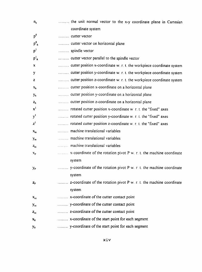
the unit normal vector to the x-y coordinate plane in Canesian ..........

coordinate system

.......... cutter vector

.......... cutter vector on horizontal plane

.......... spindle vector

cutter vector parallel to the spindle vector ..........

cutter position x-coordinate W. r. t. the workpiece coordinate systern ..........

cutter position y-coordinate W. r. t. the workpiece coordinate system ..........

cutter position z-coordinate W. r. t. the workpiece coordinate system ..........

cutter position x-coordinate on a horizontal plane ..........

cutter position y-coordinate on a horizontal plane ..........

.......... cutter position z-coordinate on a horizontal plane

.......... rotated cutter position x-coordinate W. r. t. the "fixed" axes

.......... rotated cutter position y-coordinate W. r. t . the "tixed" axes

.......... rotated cutter position z-coordinate W. r. t . the "fixed" axes

machine translational variables ..........

machine translational variables . . . . . . . . . .

.......... machine translational variables

. . . . . . . . x-coordinate of the rotation pivot P W. r t . the machine coordinate

system

.......... y-coordinate of the rotation pivot P W. r t . the machine coordinate

systern

.......... z-coordinate of the rotation pivot P W. r. t . the machine coordinate

system

.......... x-coordinate of the cutter contact point

.......... y-coordinate of the cutter contact point

.......... z-coordinate of the cutter contact point

.......... x-coordinate of the start point for each segment

.......... y-coordinate of the stan point for each segment

x i v

z-coordinate of the start point for each segment ..........

x-coordinate of the end point for each segment ..........

y-coordinate of the end point for each segment ..........

z-coordinate of the end point for each segment ..........

the linearly interpolated rotation centre x-coordinate ..........

the linearly interpolated rotation centre y-coordiiiate ..........

the linearly interpolated rotation centre z-coordinate ..........

cutter axis orientation ansle relative to the x axis of the workpiece ..........

coordinate system

cutter axis orientation angle relative to the y asis of the workpiece ..........

coordinate system

cutter axis orientation angle relative to the z asis of the workpiece ..........

coordinate system

.......... segment length between a pair of adjacent points

ailowable non-linearity error ..........

.......... non-linearity error

maximum non-linearity error ..........

.......... linearity error

linear interpolation scale factor ..........

circular interpolation scale factor ..........

the latitude angle ..........

.......... the longitude angle

.......... the rotational movements interpolation pararneter

LIST OF ABBREVIATIONS

AIGP = automation intelligence generalization postprocessor

APT = automatically programmed tools

BLU = basic length-unit

CAM = cornputer-aided manufactunng

CC = cutter contact

CLDATA = cutter location data

CNC = cornputer(-ized) numerical control

DDA = digital diflerentiai analyzer

FRN = feedrate number

ipm = inch per minute

L&C = linear and circular

MCP = machine control point

MCU = machine control unit

NC = numericai control

OM- l = OMINIMILL series- l

rpm = revolution per minute

2D = two-dimensional

3 0 = ihree-dimensional

x v i

CHAPTER 1

INTRODUCTION

1.1 CNC Machining, NC Programming and Postprocessing

Cornputer-aided manufacturing (CAM) is the utilization of computers to assist in the process

of manufactunng. CAM includes the on-line and the off-fine applications of the digital

method. Computer Numencal Control (CNC) machininç is the on-line application, which uses

a computer with a machine control unit (MCU) to generate commands for controllinç the

machining process. The off-line application is the utilization of computers in production

planning and non-real-tirne assistance in the manufacturing processes. Examples of off-iine

CAM are the preparation of NC part proçrams (referred also as tool paths) or the display of

the tool paths in machininç simulation.

In CNC machining, the MCU plays a key role in the on-line control of machininç. The

functions of the MCU include ( 1 ) reading and decodinç the information from the tool path

data and distributing the data among the controlled axes; (2) the tool centre control.

automatic tool selection, and the various compensation functions; (3) the feedrate

calculations, and the preparatory functions, the spindle motions and the miscellaneous

tùnctions control; (4) the interpolation to supply velocity commands between successive data

points; (5) control of simultaneous multi-axis movements; (6 ) on-line diagnostics and

troubleshooting; (7) display of machining information on the CRT screen and (8) the

communication between the MCU itself and the extemal devices. The overall design of a

CNC system first requires the selection of the appropriate control techniques (reference-pulse

or sample-data) and the optimal setting of the control-loop parameters. Subsequently, the

appropriate interpolation routines must be written. The f'bnction of interpolation is to generate

the successive tool positions, called commands, for each segment of the cutting curve based

on the initial and the final machining tool positioris and the desired temporal parameters such

as feedrates. The interpolation method is the core of the CNC system, since the accuracy of

calculated intermediate position directly affects the machining precision of the whole system

and the time for computing the intermediate positions directly affects the controlled axis

velocity, which in turn, affects the quality of the machined surface and the machining time.

The off-line application of CAM includes NC pan programming and postprocessing.

NC part programming involves the collection of all data required to produce the part. the

calculation of a tool path along which the machine operations will be performed, and the

arrangement of the given and calculated data in a standard format which could be convened

to an acceptable form for a particular CNC machine. Most CAM systems generate one or

more types of neutral language files containing instructions for CNC machining. The

Automatically Programmed Tools (APT) language is the most comprehensive and popular

system for NC pan programming. The APT language enables a programmer to provide the

MCU of a CNC machine with geometric descriptions of the workpiece surfaces and to specifL

the tool movements. The output of the APT system, which is called the cutter location data

(CLDATA), defines the tool path with machining conditions (the feedrate, depth of cut and

the spindle speed). In order to realize the machining, the neutral instructions must be

transfomed to the specific instructions required by a panicular machine tool. The

postprocessors are the interfacing tools between APT systems and CNC machines.

A postprocessor is a software which is used for translating neutral instructions from

the APT system into the specific instructions required by a CNC machine tool. The CLDATA

defines the tool path with cuttinç conditions in the pan coordinate system. Each Llachine

Control UnitMachine Tool (MCUMT) configuration. however. has its own machine

coordinate system. Therefore. a postprocessor translates the CLDATA in a pan coordinate

system to the NC-codes in the machine coordinate system. With the APT part programming

standard. the postprocessor writes the instructions as a series of commands in a standard

format. Each command contains ail required data: the preparatory fùnctions codes (G codes)

for preparinç the MCU to perform a specific mode of operation; the miscellaneous fùnction

codes (h.I codes) which penain to the auxiliary information: the geometry descriptions of the

workpiece dimensions and cutting conditions. such as the feedrate. the spindle speed and the

tool words. A postprocessor usually consists of five elernents: input, motion. auxiliay.

output and control. The main portion of a postprocessor is the motion elernent which includes

the geometric and the dynamic packages. The çeometry package performs the coordinate

transformation of CLDATA tiom the part coordinate system into NC-codes in the panicular

machine coordinate system. It also checks the tool path and makes corrections where

necessary to ensure that the tool path is within the specified machining tolerance. In addition,

the geometric package prevents the movement instructions to the MCU from exceeding the

machine tool axes limits. The dynamic package modifies the feedrates where necessary and

establishes the distances for acceleration and deceleration to prevent overshoots and

undershoots.

1.2 Sculptured Surfaces Machining Methods

A sunace that can only be represented as the image of a suficiently regular mapping of a set

of points in a domain into a 3D space is called sculptured surface [ I l . A sculptured surface

can be represented by a set of curves that connect the design points of the surface. Two main

approaches are commonly used for obtaining the curved surfaces: the first approach exploits

the parametnc curves representation. while the second uses contouring planes (frequently.

geometrically equally-spaced parallel planes) to intersect the surface for obtaining a curved

surface.

In the tirst approach. straight lines in a paramerric domain are used to define the

parametnc curves P(u,v) on the actual surface in Cartesian space. By setting one parameter.

Say v, a set of cutting curve functions P(u. v,) defines the entire surface. The parametric

curves approach includes schemes of the isoparametric curves and the variable parametric

curves. With isoparametric curves. tool paths are uniformly distributed across the parametric

domain. The step-over interval (which is the distance between tool passes. referred to as

cutting curves) is the same in the parametnc domain. The step-forward distance (which is the

segment length along a cutting curve) is the sarne in the parametric domain and are

independent of the surface geometric propenies and of the machining tolerances. This

approach is simple and generaily efficient because the tool contact curves are easy to retneve

from the surface definitions. However, because the geometric properties of the machined

surface are not taken into account, the relationship betwren the parametric coordinate and

its corresponding Cartesian coordinate is not uniform. Therefore, the accuracy and efficiency

of the isoparametric surface representation may Vary depending on the geometry of the

machined surfaces. With variable parametic curves representation, the tool path is generated

by using the local geometnc properties of the machined surface (the local surface tangents,

nomals and curvatures). The step-fonvard distance and the step-over interval determined on

the basis of these geometric propenies wiil Vary over the machined surface.

Using the contouring planes approach, the resultinç numerically derived non-

parametric curves are used to drive the milling tools. With this approach. the tool path

generation can be carried out by employinrl_ either the offset surface method or the direct

intersection curves techniques. The offset surface method involves the computation of the

offset surface of the machined surface. afler which, the intersection curves of the cutting

planes with the offset surface will be the path of the cutter centre of a bal-end mil]. In this

method, the cutter contact (CC) point path is a space curve. In contrast, usinç the direct

intersection curves technique. the CC point moves along the intersection curves of the cuttinç

plane with the machined surface, so that the CC point path is a plane curve on the cuttinç

plane. The cutter centre in this case. in general, moves along a space curve. For unbounded

surface machining, both the direct intersection curve technique and the offset surface method

can be used to generate tool paths. Usually, the direct intersection curve technique results in

a preferable tool path because the CC points are 'restricted' to the cutting plane. However,

when machining bounded surfaces (which are bounded on one or more sides by surfaces) the

offset surface technique is easier. In this case, the cutter centre moves along a plane curve,

which is formed by connecting the intersection curves of the cutting plane with the offset

surface and the bounded surfaces. With the contounng curves representation method, the

variable step-forward distance and step-over interval can be determined by using the local

surface geometry and the machining tolerance. The advantage of the contouring plane curves

method is that the tool path is a plane curve, so that the distributed tool path is relatively

uniform. However. the rnethod requires proper selection of cutting planes. in that the spacing

and the direction of the cutting plane must be properly determined.

Comrnon methods for machining sculptured surfaces include point milling. end milling

and flank milling techniques. Point milling technique is the traditional rnachininç approach.

in which ball-nosed end-mills with rither the cylindrical shape or the conical shape are used.

In point milling, a curved surface is cut by the bail-end of a cutter following a dense set of

parametric curves on the mathematically rnodelled surface interpolatinç the surface design

curves [2. 31. The histoncal reasons for usinç the ball-end mil1 are that (1) it is easy to

position in relation to curved surfaces. (2) ball-end rnills generally require simple and short

NC machining programs, (3) ball-end mills often only require two-dimensionai cutter

compensation [4]. In addition, conical shaped ball-end mills are especially suitable for

machining long twisted surfaces with narrow siots between the surfaces because conical

shaped cutters provide rigidity and prevent tool chatter. The major advantage of using point

milling technique is that almost any smooth surface can be point milled. Ball-end mills,

however, cut dong an arc that extends from the cutter mis to a point on the spherical profile

of the ball-end. During rnachining. the cutting point on the spherical surface changes, which

results in a variation in cutting speed. When the cutting point is at the portion of the sphere

near the axis of rotation, the cutting speed is nearly equal to zero which produces a rough

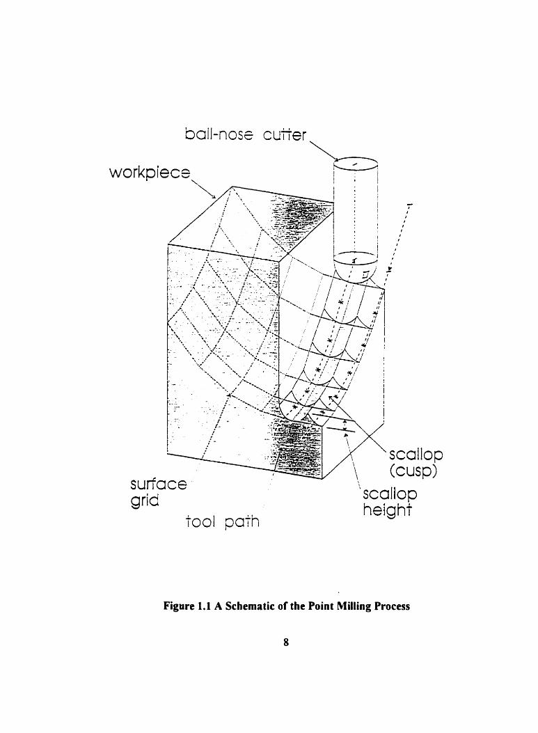
surface. Another disadvantage of point milling is that by its nature. it produces scalloped

sunace finish. Fig. 1.1 shows a schematic of the point milling process (31. The height of the

scalloped ndges is directly related to the ball-end radius and the number of cuts over the

surface.

When machins the flat or low curvature surfaces. end mills with square ends are

used. The profile of an end miIl can be made to closely match that of a cumed surface by

inclining it correctly to the surface normal The effective radius of curvature of the profile of

an end mil1 can Vary from infinity to the cutter radius. as the inclination of the cutter to the

surface normal changes from zero to 90 degrees [-Il. Hence. compared to the ball-end point

milling, a better geometric match can be achieved by usinç end mills. End-rnillinç also

produces scalloped surfaces. but the scallop height on the machined surface can be reduced

by properly inclininç the cutter. hother important factor with end milling is that the material

is always cut at the periphery of the cutter at a full and predetermined cutting speed. It is easy

to ensure a constant feedrate and thus to obtain better surface finish. However, end mills pose

tremendous dificulty in the calculaticn of collision-free cutter orientations for complicated

machining. Whiie the end milling technique is suitable for machining of large low-curvature

surfaces, it is not the best choice for machininç long and twisted or high-curvature surfaces.

ball-nose cu3er

workpiece

tool pain

Figure 1.1 A Schematic o f the Point Milling Process

The flank milling technique enables a trernendous increase in productivity and

improvement on surface finish for machining sculptured surfaces. In flank milling machining,

ball-nosed end-mills with either cylindrical shape or conical shape are comrnonly used. By

using flank milling, the curved surfaces are cut by both the cutting edges on the bali-nose and

on the side surface (either conical or cylindrical ) of a cutter. In conventional flank milling the

entire surface is obtained afler one single pass of the cutter through the blank material [2, 5,

6 . 71. The flank milling technique tends to give a good. clean surface finish. This is a

productivity improvement factor because it reduces the time required for surface polishinç.

However. tool path generation for flank rnilling machining is very cornplex. It is generally

held that a curved surface is flank millable if it can be closely approximated by a mled surface

[8]. Furthemore, the milled surface rnay deviate from the mled surface (sornetimes quite

significantly) owing to the twist of the surface along a straight line element. In fact. Wu [ 2 ]

demonstrated that the mled surface criterion for tlank rnilling is neither necessaq nor

sufticient. Many complex arbitrary surfaces are closely tlank millabie and can be rendered

exactly flank millabie with one or more passes per surface.

1.3 Multi-Axis CNC Machining Characteristics and Machining Errors

For machining sculptured surfaces. a tool path is required to contain the spatially varying

cutter positions and its mis orientations (referred to as the cutter locations) in order to

achieve better cutter accessibility for machininç non-single-valurd surfaces. Five-ais CNC

machining provides more flexibility for the realization of these cutter location spatial changes. .

In fact, rotational rnovements themselves in five-axis CNC machining provide beiter cutter

accessibility and also result in better surface finish. However, five-axis CNC machining

involves complex kinernatic issues. The coordinated translational and rotational movements

are non-iinear fundons of the cutter locations. These coordinated motion functions not only

depend upon the machine configuration, but also upon the rnachining set-up information, such

as the relative positions of the fixture and the pan mounted on the machine. A different sei

of functions is required for each CNC machiiie tool configuration. In addition. the

simultaneous translational and rotational movements are involved, because each new cutter

avis orientation requires the motion of at least one other (usually more) axis There are also

coupling effects of the rotary movements on the translational movements. because changing

the orientation of the cutter avis will affect the position of the cutter. These simultaneous and

coupled movements cause the cutter contact point (CC point) rnovinç in a non-linear manner.

As a result, the total machininç error in ench motion step is made up frorn two sources.

Many factors contribute to CNC machining errors. One of the factors is due to the

MCU interpolation method. Conventional CNC machines support the functions of 2D or 3D

linear and 2D circular interpolations. The most common method in multi-axis CNC machining

is the 'position contourinç' technique. Essentially. this method connects a straight line between

each consecutive machining data point and then linear interpolation is used to generate the

required cornmands for positions dong each araight line segment. As shown in Fig. 1.2, a line

segment is used to connect two consecutive machining data points (the spindle chuck is the

machine control point. MCP) either for the machining of a concave desired surface (a) or

for the machining of a convex desired surface (b). Linear interpolation generates intermediate

6, --- linearity error

6, --- non-linearity error

Figure 1.2 The hlulti-Axis CNC Machining Errors

position points along the line segment. The desired surface is the design cutting curve (either

concave or convex). The linear segment approximates the design cutting curve resulting in

the lùiearity error, 6,. Apart from the linearity error, there is an additional machining enor in

five-axis machining. Due to cutter orientation changes. the actual cutter contact point

trajectory is a non-hear segment (since the cutter gage lençth is constant and MCP is

interpolated along the line segment). rather than a line segment. The CC point's non-linear

trajectory deviat es from the linearly interpolated line segment resul ting in the additional

machining error, referred to as the non-linearity error. 6,. Thus. the total machininç error for

each rnachining step includes the linearity and the non-linearity errors. In the case that the

desired surface is concave cutting cuve (see Fig. 1 . la) , the total rnachining error equal to the

difference of the non-linearity error from the linearity error: b,,,, = 6, -6, (since the non-

linearity error is usually smaller than the linesnty error). That is. the non-linearity error

compensates the total machininç error. Theretbre. it is not required to reduce the non-linearity

error. In other words. the 'position contourinç' technique with linear interpolation is desired

for machining of concave surfaces. since the total rnachininç error is reduced by the non-

linearity error. On the contrary. for the machininç of convex surfaces as shown in Fig. l.2b.

the total machining error for each rnachining step is the sum of the linearity error and the non-

tinearity error: 6,, = 6, +6,. That is. non-lineanty errors add ont0 linearity errors resulting

in bigger total machining errors, which commonly cause difficuities for ensuring ultra-

precision machininç requirernent. Therefore, it is desired to treat the non-linearity errors in

order to meet high precision rnachining requirement. Non-linearity errors depend upon the

five-axis machining motion trajectory. which is a function of a particular CNC machine

configuration and machine rotational movements. Because roiational movernents are

kinematically related to the cutter orientation changes, non-linearity error depend upon the

cutter orientation change.

1.4 The Non-linearity Erron Problem in Ultra-precision Five-Axis CNC Illrchining

In conventional five-auis CNC machining. linear interpolation method is used with the

'position contouringl technique to generate command signais for dnving controlled multi-ais

motions. The actual rnachining motion trajectory for each step. however. is a non-linear path

segment which deviates from the linearly interpolated straight line segment resultins in a non-

linearity error. In ultra-precision five-axis CNC machining of convex sculptured surfaces

(hereafler it is referred to as sculptured surfaces), such non-linearity errors commonly cause

the total machininç error out of the range of the specified machining tolerance. As a result.

these non-linearity errors prevent the assurance of high precision machining. The nature of

the problern is that the spatially varyinç cutter orientations require the motion of at least one

other (usually more) rotational axes. The rotational movements are superimposed onto the

translational movernents. causinç the actual cutter contact point to move alonç a curved

segment. While linear interpolation method cannot tracking along the curved paths, non-

linearity errors are resulted and cause dificulties in ultra-precision five-âuis CNC machining.

The ultra-precision multi-axis CNC machining error problem is an important problem

in current industry. The problem is that for machining sculptured surfaces using 'linearization

process' existing in the current poaprocessors, the machine translational axes movements (at

some points) are very small or even do not move while the rotational axes move randomly and

rapidly. As a result, the machining tool trajectones are random curves and this damaçes the

workpieces. Nien a looser machining tolerance is specified, the problem appears to be

reduced but the machining precision requirements are lost. Without knowing the cause and

nature of the problem, it was normally called the 'lineanzation problem' in workshops. In

order to discover the nature of the problem and define it clearly, investigation and analysis

based on the phenornenon in the actual machining process were carried out by the author at

Pratt & Whitney Canada, Inc. Through the investigation of the actual machining process. the

nature of the problem was revealed as described above. For the purpose of this thesis. the

problem is defined as 'the non-lineûrity errors problem in ultra-precision multi-auis CNC

rnachininç'.

CHAPTER 2

LITERATURE REVIEW

2.1 Introduction

Theories and algorithrns which relate shapes and geometnes of CAD models to the path and

motion controls of CNC machine tools consritute a subject area called 'motion intelligence'

[9] . This area of concerns. consists mainlv of three categories: (1) CAD models to tool path

conversion, (3 ) Tool path to motion trajectory conversion. and (3) Motion trajectory

realization (which deals with control theory and controller design olCNC machine tools).

The category of CAD models to tool path conversion deals wit h the issues such as the

surface representation methods and the generation of corresponding tool path. In machining

sculptured surfaces. the off-line part programrning approaches are utilized, in which the CAM

systems divide the design surface into a set of line segments that approximate the design

surface with the desired tolerance. The end points of each segment and the geometric

properties of the machined surface are then used to çenerate the cutter locations data

(CLDATA). These CLDATA are further processed by postprocessors to produce NC-codes

for machining realization. The generation of CLDATA and NC-codes are the issues of the

tooi paths generation in category (1). The present CLDATA generation approaches consider

only the geometry of the machined surfaces. and disregard the machine-dependent machining

kinematics. As a result, the generated tool paths (the machining NC-codes transfomed from

these CLDATA) comrnody cause obstacles to meeting the machining precision requirements,

particuiarly for the cutter orientation generations in five-mis CNC machining. Cutter

orientation variations in five-axis CNC machining are kinematically related to the machning

rotational movements. which in tum are hnctions of the machining motion trajectory as well

as machining errors. Therefore, the problem with present off-Iine tool path generation

approaches is that the real machining kinematics are not directly incorporated. To ensure

rnachining precision, cutter orientation generations must be based not only on the geornetry

of the machined surfaces but also on the machine-dependent machining kinematics. Ait houçh

there are procedures in postprocessors to rernedy the machining errors problem caused from

the off-line tool path generation approaches. othrr undesired consequences raise additional

problems as will be explained below. In this chapter. the existing CLDATA generation

approaches and the existing methods for treating non-linearity errors are reviewed (in section

2.2). Furthemore, the deficiencies of the present cool path seneration approaches for actual

multi-axis CNC machining are shown.

The off-line part programming produces NC-codes which are fed into the MCU of a

CNC system. The interpolator in the MCU processes the NC-codes to senerate the reference

cornrnands for control loops that drive the machine axes motion. The conversion of tool paths

into motion trajectories is the issue of category (2). referred to also as the 'command

generation'. The command generat ion involves kinematics of coordinated motion, machine

dynarnics, and interpolator design. The study of machining kinematics requires the machine

kinematic rnodels which reveal the machining geornetry and time-based propenies. In section

2.3, the kinernatic modelling techniques used in practice are reviewed first. Then, the issues

of interpolator design are dimssed. Present five-auis CNC machines utilize linear interpolator

to generate and conven data positions into machining trajectories since most conventional

CNC machine tools provide only linear (2D and 3D) and circular (2D) interpolators. Although

the hear interpolation is the simplest approximation. it generates intermediate positions along

a straight line which results in inherent machining errors. and the applications of linear

interpolations have the drawback of velocity discontinuity occumnç at the end points of each

segment. Thus, acceleration and deceleration at each line segment is required. which produces

less srnoot h curves while substant ially increûsing machininç time. To adapt the practical

demands required from interpolation schenies. resrarch has been carried out, aimed mainly

on ZD curved interpolation techniques that will result in less interpolation position error and

maintain velocity continuity at the segment end points for three-axis machining. Five-âuis

CNC machining involves 3D simultaneous rotational and translational movements. and

current linear interpolation techniques are not able to trace the 3D n~n-linear machining

motion trajectory. Finally. the current status of interpolation techniques from the literature

are reviewed. From which, i t is concluded that there exists insuficient research work on

interpolator designs for rnulti-axis CNC machining, in panicular with respect to new designs

of 3D curved interpolators.

2.2 Tool Path Generation Appronchcs

The goal for tool path seneration is to create a machined surface which closely approxirnates

the CAD designed surface within a certain prescribed tolerance. The concept of tolerance is

central to manufacturing, and its importance cannot be over-emphasized. Therefore, the

errors introduced by tool path generation algonthms, namely. the errors caused by using the

linear segment to approximate the desired machining curve must be bounded. Machined

surfaces must be gouge free. and the scallop height between tool paths must be controlled.

Below, the CLDATA generation approaches and its related research works are discussed

first. Aftenvard, the current methods for generating NC-codes and issues related to these

rnethods are outlined.

The generation of CLDATA (hereafier referred to as tool path çeneration). may be

canied out through two different approaches: direct tool path generation, and generation of

CLDATA from the cutter contact data (CC data). In direct tool path çeneration, a tool is

dropped ont0 the surface with the followinç constraints: the cutter mis must be in a vertical

plane. and the intersection point of the cutter axis and the surface normal is the position data

of the CLDATA. The CC data are then calculated from the cutter radius and the surfàce

normal. Three-axis machining uses this method. For five-mis machining, this approach is

complicated by dificulties in finding the contact points between the tool and the surface. as

well as in findinç the best cutter axis orientation.

Using the second approach, tool paths are obtained on the basis of CC data. The

techniques for generating CC data are related to the surface representation met hods.

Sculptured surfaces are usually represented either by pararnetric curves or by contourinç

plane curves as mentioned in section 1.2 . Usinç the pararnetric curves approach, a sculptured

surface can be generaily characterized by a bivariate parametric vector fùnction p (u.v), which

represents the spatial coordinates of surface points. By keeping one parameter (v for instance)

constant. the surface definition p(u.v) is reduced to a three-dimensional space curve

dependent only on one parameter (u). One possible straight forward approach to generating

CC data is based on incrementing the parameter u along the constant parametnc curve. The

step-fonvard distance can be set at uniform parametnc steps. Le., the isoparametric approach.

This approach to surface representation and tool path generation have been used by most

CAD/CAM package producers and researchers. Advanced commercial CADICAM packages,

such as CATIA [IO. 111 and SmanCAM [El. generate tool paths by usinç the isoparametric

curves. Eiber and Cohen [13] introduced an adaptive sub-isocurve extraction algorithm to

develop a series of isoparametric sub-paths with uniform separation. The isoparametric

curves approach is simple and yenerally eflkient because the cutter contact curves are easy

to retrieve frorn the surface deîinitions. However, the çeometric properties of the rnachined

surface are not taken into account. and the relationship between the parametric coordinate

and the corresponding Cartesian coordinate is not uniform. Aso. large CLDATA files. while

potentially more accurate dirnensionally. result in unacceptably long processinç. verification.

and rnillinç times. To address this trade-otfbetween milling accuracy and CLDATA file size.

non-uniformly spaced parametric distribution of points were explored [11. 15 ] by utilizinç

the geometnc properties of the machined surface, thus reducing the number of CLDATA

points while maintaininç milling accuracy.

By using the contourinç planes met hod. the CC data can be generated fiom the cutting

curves which are detined by the intersections of a group of parallel planes and the pan

surface. In this case, the cutting curves are plane cuwes and the CC points are restricted on

the cutting planes. which results in preferable tool paths. The Unigraphics [16 ] CADKAM

package uses this method to genrrate tool paths by finding the intersection curves of the pan

surface and the parallel contouring planes. The step-forward distance generated using

contouring planes method can be determined on the basis of the machining tolerance and the

geometric propenies of the machined surface. The advantage of the contouring planes method

is that the CC data is a plane curve. so that the distributed tool path is relatively uniform and

the machined surfaces have unifon surface smoothness that meet the specified scallop height

tolerance without sacrificinç machining eficiency.

For t h e - a i s and five-ais rnachining. a grear deal of research work have been done

conceming the CC data generation. the CLDATA calculation. the step-fonvard distance and

step-over intemal srtting. and the analysis of gouging errors. As reviewed in the following,

the studies are al1 based exclusively on the çeometric prcpenies of the machined surfaces and

the cutter.

For machining sculptured surfaces on three-axis CNC machine tools. Wysocki [14 1,

Loney and Ozsoy [15] investigated the variable pararnetric curves tool path generation

techniques. The basis of the research method was to calculate the step-forward distance based

on the chordal deviations. By assurning the fùnhest point on the curve that deviates from the

chord as haMng half of the total parametric variation, Wysocki approximated the deviations

between the machined surface and the chord. This technique is generally sufficient for

surfaces with uniform parametnc distribution and is simpie to implement, but only

approximates the actual chordal deviation. If the underlying surface is defined by the

nonuniform pararnetric distribution this approximation method could yield inaccurate results.

Loney and Ozsoy determined step-fonvard distances by subdividing the isoparametric curve

into variable parameter segments that yielded the maximum chordal deviation. This variable

cutter step distance algorithm is more robust and provides a numerical rnethod to solve for

the parameter value that yields the maximum chordal deviation. However. both of these

chordal deviation methods suffer from limited accuracy and can produce unacceptable

gouging because they are based only on surface points and do not consider the surface normal

and the geometry of the cutter. Funher. the chordal deviation between adjacent CC points is

assumed as the machining en-or This is only tme if the surface normal vectors at the aqacent

CC points are parallei. and both are perpendicular to the chord. In general. the true rnachining

error should be determined by considering not only the chordal deviation but also the distance

between the tool tip trajectory and the corresponding chord. Oliver et a l [17] presented a

procedure to determine the chordal deviation by considering the local surface normal and the

geometry of the cutter. This procedure otfers improved overall accuracy for characterizing

the chordal deviation at a relatively small cornputational cost as compared with the nominal

chordal deviation methods.

Huang and Oliver [18] developed an algorithm for three-axis tool path generation in

which the cutting curves are defined by using the contourinç planes technique. The step-

fonvard distance is determined by calculatinç the true machining errors, which employs the

orthogonal projection method to calculate the exact distance between a cutter motion

trajectov and the surface. Since this tnie machining error calculation method is based on the

physical interference between the cutter and the surface, it is more accuratr than those

methods based on nominal chordal deviation. Furthemore, by finding the longest linear

motion that yields the specified machining tolerance. this algorithm effectively minimizes the

total number of tool motions. This technique also provides a hiçher degree of flexibility in

planning the tool path direction. because the cutting curves are defined by using the

contouring planes method. However. it requires more computational effort in locatinç cuttinç

curves as compared to the isoparametric method.

The research work mentioned above deals with tool path generation in three-ais

machining. Five-axis machining offers many advantaçes over the three-axis machining.

Vickers and Quan [4] compared the three-axis machining with ball-end mills and five-axis

machining with flat-end mills. The effective radius of curvature of a tilted Bat-end mil1 was

introduced. The effective radius of curvnture of an end-mil1 can Vary from intinity down to

the cutter radius as the inclination of the cutter to the surface normal changes from O to 90

degrees, allowing the cutter to accommodate a wide variation in local curvature. This

property enables five-axis end milling to achieve acceptable surface quality with fewer tool

passes. In cornparison. the effective radius of curvature of a ball-mil1 is restricted to the

spherical radius of the cutter. The research concluded that the five-mis end milling of

sculptured surfaces can reduce the overail cutting time when compared to three-axis point

milling.

Research work in the area of CC data generation for five-axis machining has been

carried out extensively. Marciniak [8.19] analyzed the relationship between the machining

strip width and the CC data generation for five-axis end-milling. The geometric foundations

for CC data generation were presented and the possibility of obtaining the maximum width

of cut of a machined strip by fitting the cutter motion trajectory to the surface shape was

explored. The study concluded that. for machining surfaces which have smoothly changing

curvatures, the broadest machined strip can be obtained when the CC point moves along the

minimum curvature line of the surface. The maximum width of the macliining strip depends

mainly on the difference of the suikce main cunratures at the CC point. This result presented

the possibility for reducing ttir cutting time and promoting the machining efficiency for five-

axis machining.

Li and Jerard ['O] used the contauring plane method to determinr the CC data by

representinç the pan surface as a set of parametric triangles. The CLDATA are then

generated by using the CC data and the local surface geornetry propenies. and through an

interference checking procedure. It is concluded that this distinct CC data determination

procedure with the CLDATA calculation algorithm can be used to avoid gouging the surface

in five-mis end millinç.

Choi et al. [21] presented a method for optimizing CLDATA in five-axis end milling

to minimize the scallop heiçht. The CLDATA optimization problem was fomulated as a 2D

constrained rninirnization problem in t e n s of the cutter orientation angles. The cutter location

data were initialized based on the local geometry analysis. Then. the final CLDATA were

obtained by solving the 2D constrained rninimization formula using the scallop height as a

measure of optimality. The rnethod was successfùlly applied in the tive-axis end milling of

large marine propellers. This method revealed one way to determine five-axis end milling

cutter orientations to produce minimum scallop height errors.

Cho. et al. [22] presented a method for deterrnining cutter orientation angles for five-

axis end milling to produce minimum scallop height surfaces. The cuiter orientations were

detennined by using a z-map method based on the fact that the bottom plane of the flat-end

mil1 must not interfere with the machined surfaces. This method i s another way to determine

five-axis end milling cutter orientations based on the geometry of the machined surface.

Jensen and Anderson [Z] presented an alsorithm for yenerating the tool path in five-

avis end rniiling by applying differentiai çeometry techniques The cutter positions and its axis

orientations are generated by considering both the tangent plane and the local surface

curvature. By matchinç the curvatures of a silhouette of the cutter to the curvatures of the

surface at a CC point. excess or çouginç amounts of materials in the vicinity of the cutter

contact point can be mathematically determined and eiiminated. Therefore, this alçonthrn

eliminates the gouçinç errors in five-axis end rnilling. However. this alçonthrn assumes that

the surface rnust have at least first-order continuity at a given CC point. and global

interference is not prevented.

Lee and Chang [24] presented an error analysis method for five-axis end milling which

also appiies difFerentiai geometry techniques to evaiuate the scallop height between adjacent

tool paths. This error analysis method can also be used to generate appropriate tool path

distribution.

Kmth and Klewais [25] used a two-step procedure for generating CLDATA. First,

the cutter inclination was initialized basrd on the principal surface curvature at the CC point.

Then, the cutter orientation was deterrnined by calculating the distance between the surface

and thc cutter. and the distance from the CC point to the cutter axis. This procedure was

aimed to achieve the best combination of scallop height. machined surface accuracy and

machining time.

Lee and Chang [26] proposed a two-phase approach to global tool interference

avoidance in five-ais machining. First. the convex hull of the control mesh was used to detect

potent ial interference. Then. if the first check fails. the second detaiied feasibiiity checking

calculates the tool interference on the basis of the physical constraints. Met hods for correctinç

global tool interference were also presented.

Bedi. et al. [3] presented a principal curvature aliçnrnent technique for five-aris

machining üsinç a toroidal shaped 1001. It was proved that the best fit at a CC point can be

achieved by aligninç the maximum principal curvature of the cutter with the minimum

principal curvature of the surface to reduce the scallop height on the machined surface. Rao

et a1.[27] presented the expenmental verification ofthe Bedi's principal axis method descnbed

above. The use of the toroidal shaped end-mil1 with the presented technique gave a new

approach to increase the material removal in five-mis end milling.

Liu [28] presented two algorithms for five-axis flank milling tool path generation

based on differential geometry and analytical geomrtry, which include the single point offset

(SPO) algorithm and the double point otTset (DPO) alçonthm. These algorithms can be used

in different situations in flank milling. The SPO alçorit hm can be used to determine the flank

milling CLDATA when the overcut at the rniddle part of the machined surface is not

permitted. The DPO algorithm can be used to calculate the tlank milling CLDATA if the

middle part of the machined surface cannot be undercur.

Liu, et al. [29] surnrnarised the tool path generation techniques for three-axis and five-

axis CNC machininç. The procedure of CLDATA seneration for five-axis machining

includinç techniques for point rnilling. end milling and tlank millin- is outlined in detail.

Morishiçe, et al. [30] presented a tool path çeneration method for fwe-axis CNC

machining. The method applies the C-space (a 3D configuration space) to determine collision-

free cutter positions and its orientations. The detemination of the C-space is based on the

geometric properties of the machined surface and surroundinç collision surface, thus, the

method ensures collision free operation, but without considering gouginç and 'overcut' (non-

linearity error) problerns.

The tool path generation approaches reviewed above are al1 based on the pure

geornetry analysis of the machined surfaces without considering the CNC machine tools that

will be used to realize machining. Therefore. the generated CLDATA are further processed

by postprocessors into NC-codes which constitute the commands needed to control the axes

motions of machining. Arnong its numerous functions. a postprocessor checks the tool path

precision for each path segment durinç the eneration of NC-codes, in other words. the

postprocessor checks if the total machining error between the desired cutting curve and the

actual CC point's travelled path is wirhin the machining tolerance. Upon testinç. a process.

referred to as the 'linearization process' of NC-codes. is nonnally uscd to treat out-of-

tolerance errors along the tool path where it is required The detailed procedures of the

'linearization processes' in the existing postprocessors and in the literature are reviewed in the

following paragraphs.

In the Automation Intelligence Generalization Postprocessor (NGP)[3 11, a

'linearization process' was desi~ned to reduce the non-linearity machining errors. The method

relies upon testing the amount ofdeviations of the actual non-linear tool path from the linear

segment of the NC-codes. This method insens bisectionally additional data points between

adjacent CLDATA, which in turn. are transformed into NC-codes to ensure that the

deviations (non-linearity errors) do not exceed the allowabie machining tolerance. The

insertion can be performed until either al1 points are within the machininç tolerance or until

a maximum of 63 points are inserted between each two consecutive data points. The

Vanguard Custom Postprocessor [32,33], the Ornnimill Custom Pcstprocessor [34], the

Bosto Custom Post [35]. the Aix Nurnencal Control Post Generator [36] and the ICAM Post

Generator [37] al1 use the same 'linearization process' to treat the non-linearity errors

problem.

Cho et al. [22] analyzed the non-linearity error in five-axis CNC machining problem

and presented a 'linearization process' procedure for generating the NC-codes in a five-axis

end milling process. The five-axis CNC machining errors were analyzed as two parts: one

portion of the rnachining errors is the linearity error which is due to the linear linr segment

approximation to the desired cutting curve. horher portion known as the 'overclits'. is the

result of the rotational movements from the current position to the command position with

different cutter axis orientations. These 'overcuts' are actually non-linearity errors. The

machining error for each move was the summation of the linearity and the non-linearity errors.

The function relatinç non-linearity errors to the CU tter orientation changes for the considered

five-ais swivel head type CNC machine were developed. Based on this function. actual non-

linearity errors were determined for the original cutter orientations. The allowable non-

linearity errors were calculated on the basis of the specified machining tolerance and linearity

errors determined usinç the tool tip position change. Upon testing whether the actuai non-

linearity errors exceeded the allowable non-linearity error ranges. a set of intermediate cutter

position data were inserted where the test was true. The cutter orientations of the inserted

data were set to Vary linearly in successive positions. In this way, the resulting NC-codes

include not only the data transformed frorn the CLDATA but also the additional inserted data

points. The final NC-codes contain a dense set of unequally spaced machining data points.

The algorithm of linearly varying the cutter orientation is simple, but it interpolates the

orientations inaccurately between end points. which in tum causes surface errors.

Takeuchi et. al. [38 ] presented a 'linearization process' procedure to modiS, NC-codes

in a multi-axes CNC machining process. The fùnction of the 'linearization process' was to

insert additional data points between the adjacent NC-codes where the total machining error

exceeds the specified tolerance range. The inserted points were calclilated by subdividing the

straight line segments into equally spaced intervals and the cutter orientations were set to Vary

linearly in the successive insertion positions. Nthough the final cutter positions were equally

spaced, a rather dense set of inachining data resulted. The cutter orientations suffer from the

same problem as in Cho's procedure described above.

The 'linearization processes' discussed above manipulates NC-codes by insening extra

machininç data position points. .Aitliough the produced NC-codes satisfy the machining

requirement. they may contain dense sets of non-equally spaced data position points with

constant or linearly varyin3 cutter orientations. The constant cutter orientation algorithm

causes severe roughness around the end points along the surface since the cutter orientation

changes abmptly at these points. Linearly varyinç cutter orientations produce a better surface,

but ail1 insen the orientations inaccurately since the change in orientation is not necessarily

linear. As a consequence, the dense sets of rnachininç data cause an non-constant feedrate

along the curve. which in turn causes an non-smooth surface finish. In addition. the total

machining time is increased because the mean feedrate is less than the desired value.

2.3 Command Ceneration Techniques

Coordinated machining kinematics describe the geometnc and time-based properties of multi-

axis movements. The functional relationships between multi-âuis movements and cutter

locations, known as the machine kinematic models, depict the kinematic geometric properties.

These kinematic models depend not only upon a multi-mis CNC machine tool configuration,

but also upon the machining setup data (such as the fixture length and the workpiece

mounting positions). A different set of transformation functions is required for each type of

machine configuration. Maclininç kinematics include the fonvard and the inverse kinematics:

fonvard kinematics deals with the problem of determiring the cutter locations by knowing the

machine axes movements. while inverse kinematics involves the cornputinç of machining

movements which are used to attain the given position and orientation of the cuttinç tool.

Two methods are genernlly used to derive the kinematic models. Paul [39] proposed

the homogeneous transformation metliod that first derives the fonvard kinematic model.

which is then used to determine the inverse kinematic mode1 Lee and Ziegler [40] proposed

a geometric approach which uses the çeornetric configuration of the mechanism and the

directly perceived çeometric senses (geometry intuition) of the machining movements to

determine the inverse kinematic modei. The forward kinematic rnodel is then detemined from

the inverse kinematic rnodel. The geornetrical approaches that have been utilized by

researchers in modelling of machine kinematic models are reviewed below.

Using a geometric approach, Chou and Yang [41] formulated the inverse kinematic

30

model for a fixed-bed type of machine tool with Euler angle structure (the machine table

moves translationaly only and the spindle rotates to approach the cutter orientations). The

formulation of the translational motion and the rotational motion were camed out separately.

First, the translational movements were fomulated on the basis of the machining setup data.

the^ the rotational movements were formulated on the bais of the geometric intuition of the

rotary motions. Next, by considering the coupling effects of the rotational rnovements on the

transIationa1 movernents, the variations on the translational coordinates due to rotational

movements were superimposed on the t ranslat ional movement s coordinates obtained in the

first step.

Cho et ai. [22] formulated the inverse kinematic mode1 for a swivel-head type five-axis

CNC machine tool by usinç a geometric approach. The machine movements of the swivel-

head type five-axis machine tool consist of the spindle rotation movements about the pivot

which translates in space simultaneously. Based on the machine confiçuration and the

geometric intuition of the machining movements. the inverse kinematic model was fomulated.

The machine translational movements thus obtained were the functions of the cutter positions

and orientations. The rotational movements were the fùnctions of the cutter orientation

angles. which shows that the cutter orientation changes result in rotationai movements that

are coupled with the translational movements.

Using a geometric approach, Liu [6] formulated inverse kinematic models for five-axis

CNC machines which have the configurations where oniy the nvivel-head moves (the machine

table does not move), and for those in which only the machine table moves (the five-auis

motions are the machine table's movements). The results showed that the machine rotational

movements are related to the cutter orientation changes, and that the machine translational

movements are fiinctions of both the cutter position and the orientation changes.

Lin and Koren [42] fonnulated the inverse kinematic model for five-axis CNC

machines which have the structure of one tilt table and one rotary table placed on top of a

three-axis machine. The kinematic modelling was based on a geometric approach and was

temied the 'decoupling approach'.

Based on the machine kinemaric rnodels. the time-based characteristics of machininç

rnovements can be determined and machining motion dynarnics analysis can be carried out.

Chou and Yang [9. 411 presented a procedure for reiating the time-based properties of

machining to the geornetncal propenies of a tool path based on the derived kinematic model.

Further, they established the relationship between the machininç kinematics and machininç

dynamics.

Interpolators are essential components in CNC machines which generates commands

for tool motion between adjacent tool path data points as per accuracy requirements.

Interpolation methods can be divided into reference-pulse and reference-word techniques [43,

441. In reference-pulse systems, an interpolator produces a sequence of reference-pulses for

each axis of motion, where each pulse generates a motion of one basic length-unit (BLU).

With the reference-word scheme in the sampled-data system, the control loop of each axis is

closed by software through the cornputer itself (which generates reference binary words).

The most widely used interpolation method in both of the reference-pulse and reference-word

systems is the digital differential analyzer (DDA) interpolator. The DDA techniques can be

used to perfom interpolation of integral. exponential. trigonometric. and polynomial

functions. Mayorov [45] and Sizer [46] detailed how the interpolation of these functions can

be implemented using actual hardware. DDA techniques can be used for both parametric and

nonparametric curve çeneration as explained by Danielsson [47]. However. some

degeneration errors may occur with losses of interpolation accuracy as shown by Danielsson

[47] and Milner [48]. The hardware DDA interpolation techniques are well known [44. 49.

501. which are capable tcj perforrn 2D and 3D linear interpolations and 2D circuiar

interpolations. Simulating the hardware DDA technique. Koren [ 5 1 ] introduced a software

DDA interpolator for CNC systern applications. Koren and hlasory [QI discussed and

compared four reference-pulse interpolation methods: the software DDA interpolation. the

stair approximation interpolation. the direct searcli interpolation and the improved direct

search interpolation. It was concluded that only the DDA interpolator produces a constant

feedrate along a circular path. With the other rnethods. considerable variations can occur

alonp the circular path. However, the problems of reçister ovedow and inteçer round-off

limit the adoption of the DDA interpolators in some applications. Gan and Woo [53]

discussed the DDA's register overflow and the integer round-off error problems. It was

pointed out that the overtlow has nothinç to do with the reçister size. unlike the round-off

error which is a function of the reçister size. They applied the DDA technique to parametric

curves and proposed solutions to the problerns of o v e f l o ~ and round-off errors.

There are three major requirements for the interpolated curve in the command

generation stage. The first requires the fitted curve to have second order continuity. because

this results in better machining quality, iess vibration. and a longer tool life. The second

requirernent is that the interpolated curve should be easily convertible from a position

parameter to the time domain. Thus the required machining conditions, such as the speed,

acceleration, actuatinç torques. and jerk can be calculated and computer conrrol can be

incorporated. The third requirement is that a fast algorithm is required for an on-line

implementation of this spacehime conversion.

To satisfy the second requirement above. linear interpolation is cornrnonly used in

machining sculptured surfaces on five-ais machine tools. The tool path data are interpolated

by the point to point type interpolator using straight lines from one point to another. This

interpolation method. however, has an inherent position error and has the drawback of

velocity discontinuity at the tool path data points. Sata et al. [54] presented an analytical

interpolation method. which used an incremental method for generatinç the Bézier curves to

connect a series of discrete tool path data points. With this improvement. the number of

interpolation segments were reduced as compared to linear interpolation. Stadeimann [ 5 5 ]

developed a speed interpolator which can be used when the surface topology is available as

a senes of Bézier curves. By using parametric discretization, the method signiticantly reduced

the computation time as compared with Sata's interpolator. Both of these interpolators

ensured velocity-continuity from one segment to the next based on the assumption of constant

acceieration over the entire segment. Makino [56] presented a trajectory control method using

planar Clothoid or Cornu Spiral curves to interpolate two lines or a senes of points. By using

the Cornu Spiral curve, the direction and the cuwature of the interpoiated curve is kept

continuous, so that a hisher speed continuous path control of a robot could be achieved.

Papaionnou and Kiritsis [57] prrsrntrd an extrapolated algorithm in which the next

interpolation point is determined by solving a constrained optimization problem. Liu et a1.[27]

presented a summary on the analytical surface interpolation techniques used in practice.

To satisS> the second order continuity requirement. the cubic spline interpolation

technique has been applied by researchers. This interpolation technique entails the fittinç of

a composite third ordrr parametric curve to the set of tool path points. Chou and Yang [9.

4 11 proposed an analytical off-line interpolator for comrnand çeneration. in which the cubic

spline interpolation technique was used to generat e a paramet ric cubic spline curve tool pat h.

instead of a straight line segment of the linear interpolation. From the parametric model. the

integrated relationship between the position parameter and time was also formulated and the

dynarnic information needed to control the machine motion. the velocity and the acceleration

were determined. On the basis of Chou and Yang's [9 ] proposition. Huang and Yang [58]

presented a real-time version of the interpolator which determines the intermediate points of

parametric curves under the machining precision. the velocity and the acceleration constraints.

The interpolation position parameter formulated as a function of time. Le.. u = i't). and the

feedrate function were solved by using the Euler method. This interpolator is capable of

generating position commands with variable speed control and better speed accuracy for

parametncally represented tool paths. This is the most advanced interpolator in existence; the

design ofthis interpolator. however. is based on a three-ais machine and therefore it can be

applied only to three-axis machining.

To satis- the requirement of easy conversion of the position from a tool path ro the

machining trajectory and the requirement of fast execution of interpolation. a tool path ideally

should be parameterized in arc-length of the spline segment. However. the arc-length for

each segment is unknown and therefore the method of cubic spline interpolation must

approximate its arc length. Usually, the chordal lençth is used as an approximation Because

of this approximation. relatively l q e undesired speed fluctuations will occur in the execution

of commands. Renner and Pochop [59] and Renner [60] developed methods of fitting a

composite cubic spline wit h ciosely being arc-leng h parameterizat ion. Wang and Y anç [6 1 ]

presented a composite quintic spline interpolation method. The resultant composite quintic

spline. in cornpaison with cubic spline. are nearly arc-length parameterized. Since. for a fifih-

order spline. each coordinate has two more coeficients that can be used to force a better unit

tangent propeny dong the cubic spline curve. the aleorithm çenerates the quintic spline wit h

nearly arc-length parameterkation based on a cubic spline of a set of tool path data. The

nearly arc-Iength parameter was estimated by minimizing the deviation of the rate of change

of arc length to the path parameter.

Kiritsis [62] presented an incremental step interpolation aigorithm which permits

36

interpolation of any kind of 3D parametric curves. The incremental step algorithm uses two

principles. First, each selected step must follow a given direction of the curve. Secondly, each

selected step must be at closest distance from the curve. Based on these two criteria, the

algorithm was used to generate a 3D helix. The rnethod shows that a non point-to-point

interpolation scheme is another possible direction for accurate interpolator design.

Lo and Hsiao [63] presented an interpolator with a contour error compensation

procedure which is based on previous machining results. hpplying the proposed interpolator.

in the initial machining process. the contour-error at every samplinç instant is calculated and

a data extracted procedure is conducted. Then, in the repeated machining process, the

contour error is interpolated based on the previous extracted data and is added to the

reference position cornmands. Thus. the previous contour machining result can be used to

compensate the machining contour errors. The proposed interpolator improves the accuracy

of the subsequent repeated rnachininç. but it is designed on the basis of analysis of 2D

contourinç curves.

The off-line pan proçramming approaches decompose the design surface into line

segments. These segments are then interpolated and convened into machining trajectory. The

drawbacks of this off-line procedure ere: ( 1) the acceleration and deceleration at each line

segment is required, which produces less srnooth curves and substantially increases machining

time, (2) cutter orientations in f i ~ e - ~ s machining are interpolated inaccurately, which causes

position errors and unsmooth surfaces, and (3) the size of the tool path file could be very

large for complicated parts and could cause memory shonage problems and data transmission

errors [64]. To overcome the drawbacks. real-tirne interpolators have been designed.

Shpitalni, et al. [65] presented a real-time reference-word interpolator for the implicitly

defined 2D curves and the parametrically represented curves. By using the real-time

interpolator, the CAD systern transfers only the information about the curves to the CNC

machine. The curves are broken into segments by the MCU and executed by the interpolator.

The real-time interpolator then calculates new comrnands for the control loop dunng the

execution time of the current commands This approach produces smoother surfaces and

requires less machininç time. The real-time interpolator is of the point-to-point type. and

therefore it can be executed by the linear interpolators available on conventional CNC

machine tools. For the parametrically represented curves. the determination of successive

values of the path pararneter was based on the curve sesments of equal arc-lençth. The cuve

position pararneter as a function of time was solved through a recursive procedure based on

Taylor's expansion.

Koren [7] developed a real-time interpolator for five-axis CNC machining. The

interpolator calculates cutter positions and orientations during the same time period needed

for sampling the control-loop feedback devices. The cutter axis for five-axis end milling was

onented in the direction of the suFface normal. For flank milling, the cutter a i s was oriented

paralle1 to the ruled surface. These cutter orientation interpolation methods are not adequate.

In fact, in end milling the cutter orientation cannot be set always in the surface normal

directions, and in flank milling, the cutter orientations rnay not be always parallel to the ruled

surface, especially for the non-mled flank miIlable surfaces. While this real-time five-mis

interpolator is the most advanced interpolator for five-auis CNC machining. the cutter

orientation interpolation methods are not absolutely correct.

Lo [66] presented a real-time surface interpolator which is capable of rnaintaininç

machining feedrate and condensinç the cutter location file. Usinç the proposed surface

interpolator. the surface parameters in both of the tool path (step-forward) direction and the

tool interval (step-over) direction. and the cutting conditions (such as feedrate. scallop height

limit, etc.) are fed into the MCU. Thus. the off-line tool path seneration procedure is moved

into the real-time surface interpolator Since the CC point path is generated in real-time

according to the presçnt feedrate. the desired feedrate can be maintained. However. the

proposed interpolator focuses on the feedrate problein. and it rnay not provide solution to the

machining error problem in the current five-asis CNC machining process.

CEIAPTER 3

THE OBJECTIVES

3.1 Thesis Objectives

The non-linearity error problem in five-mis CNC machining causes dificulties when high

precision in the machining of sculptured surfaces is required The problem arises from the fact

that five-axis CNC machininç motion trajectories are non-linear curve segments due to the

rotational rnovements superimposed on the simultaneous translational movements and linear

interpolation technique is not able to generate command sipnals for positions along curved

paths. The five-axis machininç movements are kinematically related to the cutter locations

data, in other words, non-linearity errors are related to the tool path çeneration. Thus. the

solution c m be approached from tool path (CLDATA) generation with the requirement that

the rnachining errors are minimized. ho the r route to the solution is from the machining

motion trajectory planning and controi viewpoint (i.e. an interpolator design that drives the

machine axes dons a predesigned curved path in order to eliminate the non-linearity errors).

This thesis sets two objectives:

The first objective is the development of an off-line tool path generation method that

minimizes the multi-axis CNC rnachining errors. Tool path generation invoives generating

cutter positions and its axis orientations (CLDATA) and subsequent conversion of CLDATA

into rnachining NC-codes. The review of the literature revealed that the existing methods for

generating CLDATA are al1 based soiely on the pure geornet ry of the rnachined surfaces. The

'linearization processes' treat non-lineanty errors by inserting additional cutter positions in

generating NC-codes. which results in the unsmooth tool path. the undesired variations in

machining feedrate and machined surface finish problems. The cause of non-linearity errors

is the superposition of multi-axis rotational rnovements on the simultaneous translational

movements. Rotational movements are kinematically related to cutter orientation changes,

and non-linearity errors are the functions of cutter orientation changes. Therefore, a

methodology that generates tool path with optimum cutter orientations and reduced non-

linearity errors is rrquired. The research program leading to the development of a minimum

errors tool pat h generation met hodology for the ultraprecision multi-axis CNC machining can

be described as follows. The cutter orientation generation should consider not only the

grometry properties of the machined surfaces. but also the machining kinematics and motion

trajectory characteristics. Specifically. the cutter locations data may be initially yenerated

based on the geometric properties of the machined surface, and then modification of cutter

orientations based on the panicular machine kinemarics and motion trajectory should be

carried out to achieve minimum machininç non-linearity errors. The proposed new

methodoloçy in this thesis is based on these analysis and is verified throuçh a case study.

The second objective of this thesis is to develop an on-line 3D interpolation technique

that generates the command siçnals for the control loops to drive the machine axes movins

along a 3D curved trajectory such that the rnulti-awis machining non-lineanty errors can be

elirninated. Linear interpolation techniques çenerate cornmand signals for positions along a

straight line path, not along non-linear motion trajectories in multi-axis machining. From the

review of the literature. it was demonstrated that the current interpolators are capable to

perform 2D linear, 2D circular, 2D curved paths and 3D linear interpolation functions. The

multi-axis rnachining motion trajectories are spatial non-linear paths, and therefore 3D non-

linear interpolation techniques are desired. Since the multi-axis CNC machining motion

trajectory is constructed by 3D circular movements superirnposed on 3D linear movements,

the required 3D non-linear interpolator should be capable of tracing 3D circular curves and

also the combined 3D linear and circular loci. The 3D non-linear interpolator should perfonn

in a way of point-to-point command generation so that the avaiiable linear interpolation

fundion can be utilized as the base to drive the axes motions. The 3D non-linear interpolator

should have accurate position tracking ability and feedrate uniformity along a curved path.

The methodologies presented in research studies in this thesis are innovative and results

encouraging. These studies contribute solutions to some present day concerns in the

manufacturinç industry. The mot ion trajectory funcrions of the combined 3 D linear and

circular movements on the common tive-axis CNC machine tools are utilized to develop the

3D non-linear interpolation formula. The 2D DDA circular interpolation principle has the

advantage of the feedrate uniformity and therefore are used to develop the 3 D DDA circular

interpolation principle. Finally, by combininç the existing point-to-point 3D linear

interpolation tùnction with the new 3D DDA circular interpolation principle, a combined 3D

linear and circular interpolation technique is developed.

3.2 Thesis Outline and Methodology

The research prograrn of investigatinç the off-linr tool path generation methodolog in the

thesis will concentrate on the following items:

1) Development of the kinernatic models for a cornrnon five-auis CNC machine tool. The

machining kinematics deal with geometry and time-based properties. Therefore.

the inverse and the forward kinematic models are required in tool path generation.

2) Development of the machining motion trajectory model for five-mis machining on a

commun five-auis CNC machine tool. The locus of the cutting point is depicted by the

machininç trajectory functions. Hence, a machine-dependent machining motion

trajectory model is required in the determination of non-linearity errors.

3) Development of a representation approach for the analytic description of the tool path

with which the geometnc propenies of the rnachined surface curves can be calculated.

To determine the allowable non-linearity errors for a certain specified machininç

tolerance. linearity errors must be pre-determined based on the geometry properties

of the machined surfaces. Thus. an analytic tool path representation of the machined

surface is desired to calculate the curvatures alonç the curve. which in turn are used

to determine the linearity errors.

4) Development of an off-line sofiware program to implement the minimum errors tool

path generation method for solving the multi-axis CNC machining errors problrrn.

5 ) Verification of the minimum error tool path geeneeration rnethodology throu~h a

simulation of the process for machining a typical sculptured surface on a five-ais

machine tool.

The research program of developing a 3D interpolation technique for multi-axis CNC

machining in this thesis will concentrate on the following items:

I ) Development of a 3D circular interpolation principle. The multi-ais rotational

movements are 3D circular motions. In order to trace a 3D curved path in multi-axis

machining. 3 D linear interpolation or 2D interpolation techniques are not adequate.

A 3D circular interpolation function is required for both the machining of 3D circular

curves and the machining of combined 3D linear and non-linear curves.

2) Developrnent of a combined 3D linear and circular interpolation principle for multi-

axis CNC machining syst ems. The mu1 ti-axis machining rno t ion trajectories are

constructed by the simultaneous and coupled 3D rotational and 3D translational

movements. therefore it is necessary to develop an on-line 3 D interpolation command

generator that can be applied to combined 3D linear and circular trajectory planning

and control.

3) Development of a real-time interpolation routine to implement the new desiçned

'combined 3D linear and circular interpolation technique' for tive-axis CNC machine

tool systems.

4) Verification by computer simulation of the machining process usinç the new

3D interpolator in a five-axis machine tool.

CHAPTER 4

MINIMUM ERROR TOOL PATH GENEFUTION METHOD

4. f Introduction

In the machining of sculptured surfaces. tive-mis CNC machining offers many advantages

over three-awis rnachininç which include faster matenal-removal rates. improved surface

finish and the elirnination of the necessity for hand finish. In çeneral. a single surface which

c m be machined by three-ais rnillin_e cm also be machined in five-axis machininç with a flat-

end miil. But, in sornr cases, for example, as in the machining of an inteçral impeller or an

integral turbo-wheel, it is impossible to use three-axis machining because the machined

surface. the drive surface and the check surface [G] are not single-valued surfaces. The cutter

axis orientation must be changed in order to avoid the non-tool-edge interference between

the cutter and the workpiece. Five-cLus machininç exploits a machine tool with more flexibility

to realize the cutter position and its axiç orientation spatial changes. employing the

simultaneous rotational and translational movernents The actual cutter contact point in five-

axis machininç moves alonç a non-linear trajectory. and the machining errors comprise not

only lineaity erron but also non-linearity errors. In ultra-precision multi-axis CNC rnachining.

non-linearity errors are the main cause of' obstacles ihat make it dificult to ensure the

machining precision. A new methodology for solving the non-linearity error problem in ultra-

precision multi-axis CNC machininç is presented in this chapter. The methodology is based

on machine-specific kinernatics and the machining motion trajectory analysis. The non-

linearity errors are reduced by modifiing the cutter orientations to ensure the machining

precision, provided that there is no interference between the cutter tip region and the

workpiece. In section 4.2. the basic concepts and the detailed description of the common

techniques for tool path generation in five-axis CNC machining are discussed, and the need

for optimal cutter orientation generation based on rnachininç kinematics and motion trajectory

characteristics is explained. Sections 4.3 and 4.4 present the developments of the kinematic

models and the machine motion trajectory mode1 for a five-mis CNC rnachining centre. Next,

the proposed methodology is presented in section 4.5. Finally, a software program for

implementing the new methodology is presented in section 4.6.

4.2 Five-Axis CNC klachiniiig Tool P ~ t h Generrtion Methods

In CNC machining, the tool path is the cutting tool's motion locus which is known as the

cutter location data (CLDATA). In multi-axis CNC machininç, a set of CLDATA is specified

in terms of the coordinated cutter positions and its avis orientations with reference to the

workpiece coordinate system. The cutter position data are the motion coordinates of the

cutter centre which is the spherical centre of a bail-end miIl or the flat-end disc centre of a

flat-end mill. The cutter orientation data are the direction cosines of the cutter axis vector

relative to the workpiece coordinate system. The generation of tool path in multi-ais CNC

machining includes the generation of the cutter position data and the cutter orientation data.

The goal for tool path generation is to create a machined surface which approximates

the design surface within a certain prescribed tolerance. Ideally, the generated tool path

should contain a set of uniformly distributed cutting curves, equally spread machining errors

and smoothly spaced cutting steps. In sculptured surface machining, the cutter position data

are generated on the bais of the cutter contact point data (CC data) on the machined surface.

The comrnon methods for generating CC data are the parametnc curves approach and the

cutting plane contouring curves approach.

The parametric curves approach uses straight lines in a parametric domain to define

the correspondinç parametric curves on the actual surface in Canesian space. A sculptured

surface is descnbed as a two parameter function. P(u. v). Holding one parameter constant

such as P (u, v = constant) defines a parametric space curve (hereafter referred to as the

'cutting curve'). By setting the parameier v. a set of curve function P(u .y) define the entire

surface. The distance between two adjacent cutting curves (Le.. for v = i and v = i+ l ) is

referred to as the tool pass interval. The methods for determining the tool pass interval can

be classified into the constant parameter meihod and the non-constant parameter method.

With the constant parameter method. the parametric lines are equally spaced across

the parametnc domain. Dependinç on the rnachining surface for which it is used. this method

rnay not lead to equally spaced cutting curves on the machining surface because a constant

line interval in pararnetric domain does not generally yield a constant tool pass interval in

Cartesian space. If the surface is flat, the tool pass interval is constant for al1 tool passes, and

the method is accurate and efficient. However, for the machining of sculptured surfaces. the

tool pass interval is generally diflierent from one p a s to another, depending on the tool radius

and the local surface curvature. Therefore. this merhod rnay not attain the machining accuracy

and its efficiency may Vary depending on the geometry of the surface. The constant parameter

method is simple, but the relationship between the parametric coordinate and the

corresponding Cartesian coordinate is not uniform as it does not consider the geometric

propenies of the machined surface. For instance, for machininç a fan blade surface with the

constant parameter rnethod [18]. the cutting cunes are close to one another at one end but

further apart at the other. To ensure the machining accuracy. more cuttinç curves rnay be

generated. As a result, the scallop heights on the machined surface V a r y from one end to the

other: the rouçhest portion meets the specified scallop height tolerance while the finest

portion is unnecessanly too smooth.

With the non-constant parameter method. the tool pass interval is determined by

calculatinç the machined strip width on the surface and by controlling the scallop heiçht

between the cutting curves. The calculation of the machining strip width and the scallop

heiçht on the machined surface are based on the geornetric propenies of the surface. Thus.

the cuttinç curves can be distributed to ensure surface smoothness that rneets the specified

scallop heiçht tolerance without sacrificins machining effciency.

The determination of the tool pass interval is one aspect of tool path generation.

Another dificult problem is the correct generation of the cutting point step distances alonç

each cuttinç curve which resolves the distances between cutter positions. In multi-axis CNC

machining, each cutting cuve is approximated by piece-wise linear segments joined together.

The length of the linear segments is referred to as the step-fonvard distance. The algorithrns

for calculating the step-forward distance include the isopararnetrk algorithm and the varying

parametric algorithm. In the isoparametric algorithm. the cutting points are a fùnction of

somewhat arbitrary choice of parameterization. The step-forward distance calculated from

this algorithm is not related to the machininç errors and the surface local curvature.

Altematively, the varying-paramet er alço ri t hms calculate the step- fonvard distance by using

the surface local curvature and the specified machining tolerance. The iso parametric aigo rithm

is simple and generally etficient. In practice. a hybrid approach is used. The isoparametric

algorithm is usually used to obtain a dense set of discrete curting points. then the varying-

parameter algorithm is used to retine the step-forward distance by sifting the discrete cutting

points. These cutting points are considered as those at which the cutter will contact with the

machined surface. The cutter position data are actually the offset points of the machined

surface. Based on the cutting points. the surface nomals to these cutting points and the cutter

radius. the cutter position data can be easily generated. Thus. the cutter position changes

depend upon the cutting points step-forward distance.

In the cutting plane contourhg curves approach. the cutting curves usually are defined

by the intersections of a group of parallel planes or cylindrical surfaces with the workpiece

surface. For point milling, the cutter position data of a ball-end mil1 can be generated by

constmcting the offset surface of the machined surface such that the cutter centre moves on

the intersecting curves of the cutting planes and the offset surface of the machined surface.

To construct the offset surface in sculptured surface machining. the common method [6]

includes the following steps:

1) Divide each cutting curve to obtain a set of discrete cutting points such that the line

segment and the cuwe are within cenain presctibed tolerance;

2) Calculate the equal offset surface points of the discrete cutting points;

3) Use mathematical spline techniques, such as the B-spline technique, to obtain the

offset surface from the offset points.

The intersection curves of the cutting plane with the offset surface will be the path of the

cutter centre of ball-end mills The cutter position changes can then be determined by

employing the varying parametric calculation methods. With this method, the cutter position

data are generally on the space curves while the cutting points are on the plane cutting curves.

Therefore, the tool path and the resulting scallop heighr are uniformly distributed. and the

rnachining efficiency is higher than in the parametric curves approach. This rnethod. however,

requires proper selection of the cutting planes. in terms of determining the spacing and the

direction.

The location of a cutter is completely specified by the cutter centre position and the

cutter axis vector. In five-axis machining, the cutter axis vector cannot be orientated in the

surface normal direction for the following reasons: (i) the cutting velocity at the tool tip of

a ball-end mil1 is zero; (ii) there is usually no cutting edge on the fiat-end surface centre of

flat-end mills; (iii) the cutter axis vector of a Bat-end miil must be tilted to avoid the cutter

fiat-end contacts with the rnachined surface and to avoid the cutting edges interference with

the machining surface. Therefore, five-auis contour milling uses a process called 'sturz'

milling. The Geman term 'sturz' refers to the foward tilt of the milling cutter in the direction

of the feed. The 'sturz' angle is the angle between the cutter axik vector and the surface normal

to the cutting point. The 'sturz angle' can be divided into a tilting angle and a rotation angle

[22]. The values of the tilting and the rotation angle detenine the cutter axis vector at the

cutter position with no interference between the cutter top region and the workpiece. The

cutter orientation data is the representation of the cutter avis vector in ternis of the direction

cosine of the vector in reference to the workpiece coordinate system.

The çeneration of cutter orientation data must consider the constraints of machining.

One of the constraints cornes from the revolute joints lirnit on the CNC machine tool. A five-

mis CNC machine tool has at least two revolute joints. With a panicular cutter position. a

considerable portion of the space of the cutter orientation is constrained by the machine

revolute joints limit. hother source of infeasible cutter orientations is the collisions between

the machine structure and the workpiece surface. Apan from these structural limits. the third

constraint is the 'cutter overcuts' on the rnachined surface. The 'cutter overcuts'. i . e., the non-

linearity machining errors. are caused by the cutter orientation changes which depend upon

the geometric properties of the machined surface and also relate to the machinin!: kinematics.

The present methods for çenerating the cutter orientations consider only the geometry

of the machined surface. For machininç of surfaces with a narrow passage between them. for

instance the airfoil surfaces of a typical irnpeller shown in Fig.4.1, five-mis point milling is

commonly used.

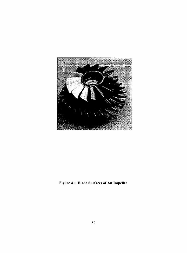
Figure 4.1 Bhde Surfaces of An Impeller

To detemine the cutter orientations for five-axis point milling, the cutter axis

Marginal Point Technique [6] can be utilized as shown in Fig.4.2. In this technique, the

normal plane of the surface tangent in the feed direction of the cutting point is used as the

cutter axis oscillating plane. In Fig. 4.2, the oscillating plane for the CC point is parallel to the

x-z plane and is perpendicular to the surface tangent of the CC point (the feed direction of the

rnachining). The cutter axis can Vary its orientation in the oscillating plane within a certain

limit. Using the cutter axis Marginal Point Technique. the steps for determininç the cutter

orientation are as follows:

1) Determine the marginal point:

In the cutter a i s oscillating plane. rotate the cutter a i s about the cutter position point

C, to the position at which the cutter contacts the surface at a marginal point Q;

2) Determine the projection point of the marginal point on the cutter mis:

Based on the cutter geometry data (cutter radius and conic angle) and the distance

between the cutter position point C, and the marginal point Q . a projection point Q'

of the marginal point Q on the cutter axis c m be determined usinç the cutter conic

angle. a. and the points of C, and Q throush a simple triangle geometq calculation;

3) Determine the cutter axis vector:

From the coordinates of the cutter position point Co and the projection point QI, the

cutter êuis vector, T, , is uniquely orientated.

Using wch a technique. a set of cutter orientation data can be generated with collision-free

conditions and maximum tilting angle. The generated cutter orientations Vary at each cutter

position.

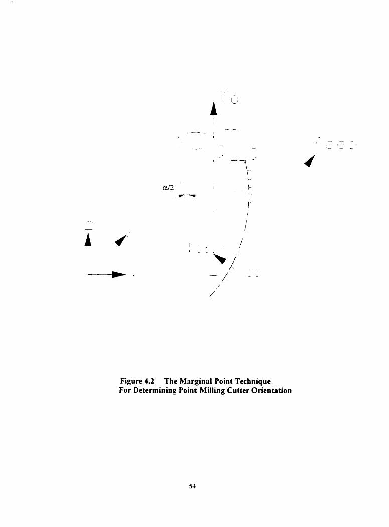
Figure 4.2 The Marginal Point Technique For Deterrnining Point Milling Cutter Orientation

For the machining of large sculptured surfaces. such as the machining of the blades

of a hydraulic turbine, five-axis CNC machining with flat-end mills is cornmonly used. The

cutter axis vector for end milling can be determined by estimating the cutter tilt angle from

the surface curvatures for different machining surfaces. and using the surface norrnals and

tangents in the feed direction [ 6 ] . Li and Jerard [20] and Choi, et al. [22] also discussed

techniques of generating cutter orientations for end millinç.

Flank rnillinç has wide applications for the rnillinç of small- and medium- dimensional

surfaces. such as the milling of the integral impellers. For rnachininç of impeller airfoi1

surfaces. point milling with conic shaped ball-rnills can be used. Althouçh the determination

of cutter orientations is more difficult in flank milling. this method is more favourable because

it does not require hand finishinp. The generation of the CLDATA for millinç the airfoils of

an impeller by flank rnillinç can be deterinined by applying the Bind Inclining Technique [6]

as shown in Fig.43 The Bind Inclining Technique uses the cutter calculation centre and the

equivalent cutter axis vector. The intersection point between the cutter axis of a cylindrical

shaped ball-end mil1 and the normal to the CC point is the cutter calculation centre. The C,

is the cutter calculation centre for the side CC point as shown in Fig.4.3. The cutter axis of

an equivalent cylindrical shaped ball-end miIl is the equivalent cutter axis vector, Ta*. to the

conical shaped ball-end mil1 as shown in Fiç.4.3. With a conical shaped ball-end mil1 (the ball-

end radius is r and the conic angle is a), the Bind Inclining Technique detemines the cutter

locations using the following steps:

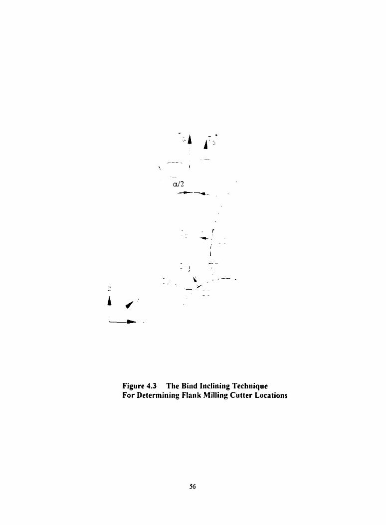
Figure 4.3 The Bind Inclining Technique For Determining Flnnk Milling Cutter Locations

1) Detemine the cutter calculation centre and the equivalent cutter avis vector:

Consider a cylindrical shaped ball-end cutter with the ball-end in contact with the hub

surface at the bottom CC point as s h o w in Fig.4.3. By inclining the cylindncal shaped

cutter on the bind surface (Le.. the airfoil surface). a side CC point can be determined.

The vector of the aiis of the cylindrical shaped cutter is the equivalent cutter axis

vector Ta*. The intersection point of the aidoil surface normal to the side CC point

and the equivalent cutter axis vector is the cutter calculation centre C,;

2) Detennine an offset surtàce of the hub:

Based on the cutter ball-end radius, r. and the surface normals from each of the

bottom CC points. an offset surface can be deterrnined by using mathematical spline

techniques as mentioned above:

3 ) Determine the cutter position data:

The intersection point ofthe offset surface with the equivalent cutter avis vector is the

cutter position C, as shown in Fiç.4.3.

4) Determine the cutter orientation data:

By rotatinç the equivalent cutter axis vector T, * about the cutter position Co by an

angle of a/2. the resuliing orientation of the vector T, * is the desired cutter axis

vector T, of the conical shaped ball-end milis.

Using this technique, under collision-free conditions. a set of CLDATA can be

çenerated with varying cutter orientations at each cutter position.

As rnentioned above, the cutter orientations are not only dependent upon the pure

geometry of the rnachined surface. but are also related to the machining kinematics. In fact,

the machine translational movements are functions of position and axis onentation of the

cutter, and the machine rotational rnovements are hnctions of the cutter onentation data.

Therefore, the detemination of cutter orientation data must also consider the machine

kinematics. Machine kinematic models describe the geornetric propenies of rnachining

kinematics, and reveal the relational functions between the cutter locations (CLDATA) and

the machining rnovement coordinates (NC-codes).

4.3 Development of Machine Kinematic Models

The cutter variables are the cutter's positions and axis orientations in reference to the

workpiece coordinate system. The machine variables are NC-codes which. for five-axis CNC

machining. consist of the translational axes motion parameters and the rotational axes motion

parameters. The functions that relate the cutter variables and the machine variables are the

kinematic rnodels. Machine kinematics describe the çeometrical and time-based properties of

multi-axis CNC machininç movements which include the fonvard and the inverse kinernatic

models. The fonvard kinernatics deals with the problem of determininç the cutter variables

by knowing the machine motion variables. The inverse kinematics is used to cornpute the

machine motion variables which are used to attain the given position and orientation of the

cutter. The functional relationship between the machine motion parameters and the cutter

variables ponrays the kinematic characteristics of a rnulti-ais CNC machine tool. This

functional relationship is dependent not only upon a multi-mis machine tool configuration,

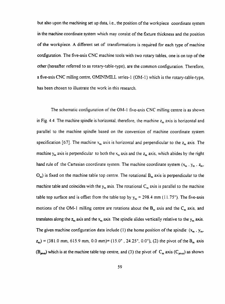
but aiso upon the machining set up data. Le.. the position of the workpiece coordinate system

in the machine coordinate system which may consist of the fixture thickness and the position

of the workpiece. A different set of transformations is required for each type of machine

configuration. The five-axis CNC machine tools with two rotary tables. one is on top of the

other (hereafter referred to as rotary-table-type), are the common configuration. Therefore.

a five-ais CNC rnilling centre. OMINIMILL senes- 1 (OM- 1 ) which is the rotary-table-type.

has been chosen to illustrate the work in this research.

The schematic configuration of the OM- 1 five-axis CNC rni!ling centre is as shown

in Fiç. 4.4. The machine spindle is horizontal. therefore. the machine zn, a i s is horizontal and

parallel to the machine spindle based on the convention of machine coordinate system

specification [67 ] . The machine \, asis is horizontal and perpendicular to the q,, axis The

machine y,, aus is perpendicular to both the q, avis and the z,,, axis. which abides by the riçht

hand rule of the Cartesian coordinate system. The machine coordinate system (q, . y,. z,,,,

O,) is fixed on the machine table top centre. The rotational B, axis is perpendicular to the

machine table and coincides with the y,,, a i s . The rotational C , axis is parallel to the machine

table top surface and is offset from the table top by y,, = 298.1 mm ( 1 1.75"). The five-axis

motions of the OM-1 milling centre are rotations about the B , axis and the Cm axis. and

translates dong the q,, axis and the x,,, mis. The spindle slides venically relative to the y, axis.

The given machine configuration data include ( 1 ) the home position of the spindle: (Y.,,, . y,. h) = (381.0 mm. 615.9 mm, 0.0 mm)= (15.0" , 24.25". 0.0"). (2) the pivot of the B, avis

( B A which is at the machine table top centre, and (3) the pivot of Cm mis (C,,,) as shown

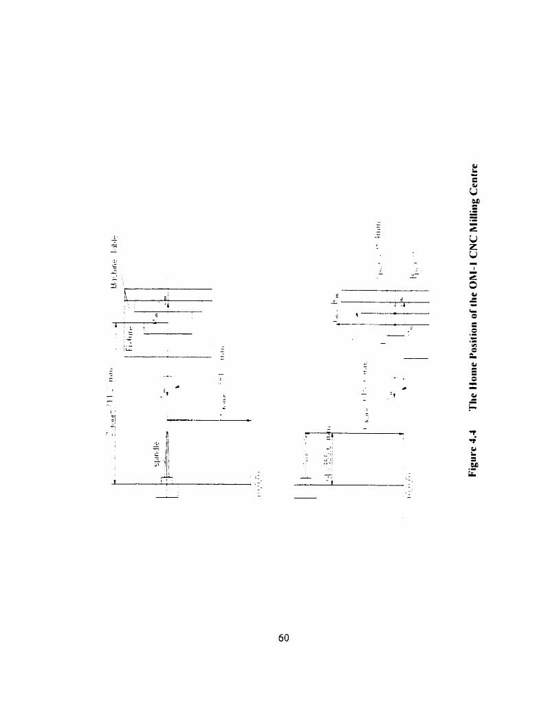
in Fig. 4.4. For the machine setup, the stack value is the distance of the workpiece coordinate

system origin to the face of the fixnire. The fixture thickness is set as F = 152.4 mm (6") and

the stack value, in this case. is G = 0.0. Therefore. the workpiece coordinate system position

in the machine coordinate system is known. The machine translational movements coordinates

are measured relative to the machine zeros (O. 0, O). The rotational angle about the B,, axis

is measured from the positive z,,, mis direction and the rotational angle about the Cm a~is is

measured 6om the positive y , axis direction. The points that represent the machine variables

coordinates usually are referred to as the Machine Control Point (MCP). In the case of the

OM-i millinç centre. since the machine tab!e and the spindle translate simultaneously durinç

the machininç process. the machine coordinate system origin and the spindle chuck are the

MCP. as MCP-O and MCP-s respectively.

Modelling machine kinematic models. geometrical approaches use the geometrical

configuration of individual machine tools and the geometrical intuition of the machininç

rnovements to determine the inverse and fonvard kinematic rnodels. In this research work,

based on the k n o w OM- 1 CNC milhiny centre configuration and the machininç set-up data,

a geomerric approach is applied to obtain the inverse kinematic model. The forward kinematic

mode1 is then developed on the basis of the inverse kinematic model.

The procedure for deriving the inverse kinematic model is approached in two steps.

In the first step, the machine rotationai variables are detemined by considering only the cutter

orientation change that cm be attained from the machine rotational movements. In the second

sep, the machine translational variables are deterrnined from the cutter position change that

can be attained fiom both machine rotational and translational movements.

A h e is a coordinate system. where in addition to the orientation of the coordinate

axes a position vector is given for locating the coordinate system origin to some other

embedding coordinate system [6S]. The machine coordinate system of the OM-1 milling

centre foms a moving h e (hereafter referred to as the machine coordinate frame) since the

machine coordinate system origin O, moves relative to the machine zeros. and the

orientations of the five axes Vary during the rnachininp process. The workpiece caordinate

system with its coordinate axes and the origin in reference to the machine coordinate frarne

f o n s a fiame (hereafter. referred to as the 'workpiece coordinate frame'). To formulate the

machine rotational movements as functions of cutter orientations in a çeneralized machine

setup, without loss of the çenerality, it is assumed that the workpiece coordinate frarne is set

at the position of the machine coordinate fiame as shown in Fig.4.5. and the cutter vector. Po,

is a free vector in reference to the workpiece coordinate frame. A free vector refers to a

vector which may be positioned anywhere in space without loss or change of rneaninç

provided that magnitude and direction are presenied [68]. For generating tool path, the cutter

vector is considered havinç unit magnitude and the direction cosines of the vector in the space

of the workpiece coordinate frame. Dunnç the rnachining process, the workpiece coordinate

frame translates and rotates sirnultaneously with the machine table. Hence. the cutter vector

with the workpiece coordinate frame can be considered as a solid part.

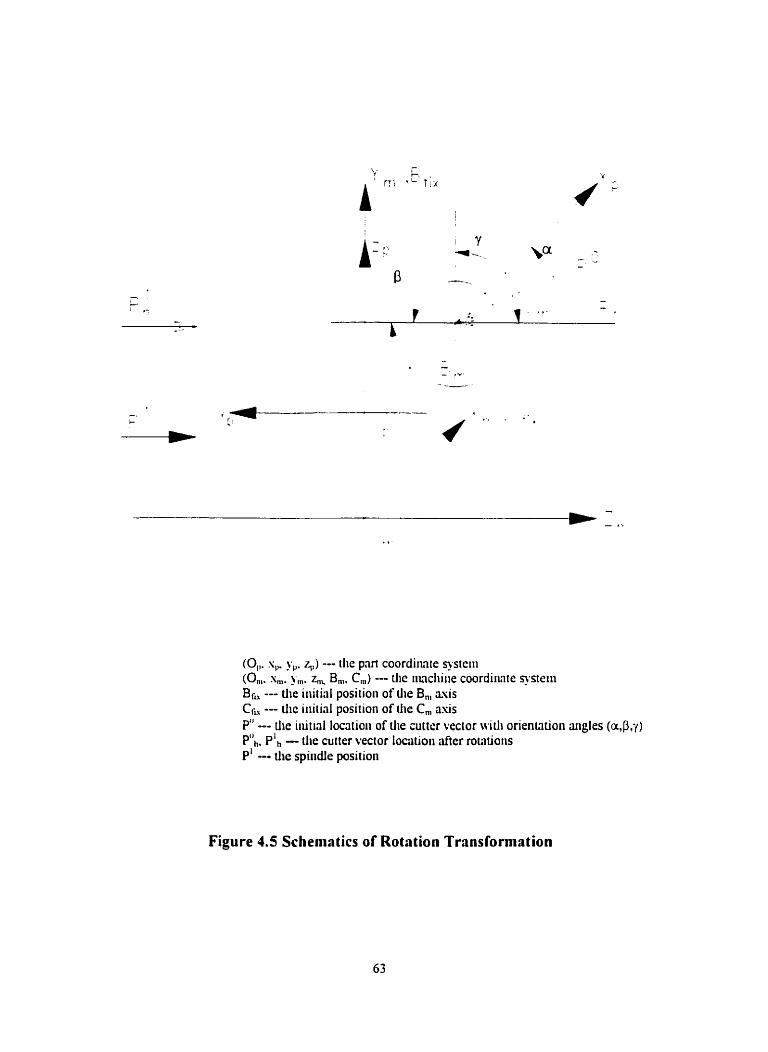
(O,,. s,. y,. q,) --- the p*m coordimte s y m n (Onl. Sm. ym. B,,. C,,,) -- tlic ti~icliirie coorditinte -stem Bfi, --- the initial position of die B,, mis CrLx --- die initial position of the Cm asis P" -- die iiitinl locritioii of the cuiter vecior witli orien~qtion aigles (a$,?)

PI,, - the cutter vector Iowtiori after rotatiatis P' - tlie spiildie position

Figure 4.5 Schematics o f Rotation Transformation

The machine rotational variables are the angles of the machine table together with the

workpiece coordinate frame rotated about the machine moving axes B,, and Cm,. To

determine the machine rotational variables, one can pursue the solution by using the method

of the spatial descriptions and transformations. Rotations can be defined as operators to

transform a frame or a vector from one location to another [68]. Hence, a rotation matnx that

represents the machine rotational movements can be used to operate on the workpiece

coordinate fiame d a n d the cutter vector from one location to another. Since rotations can

also be thought as descriptions of orientations. the rotational matrix can be detenined by

describing the orientation of the workpiece coordinate frame with the cutter vector In

representing the orientation of a frame. the angle sets convention includes fixed ançle sets and

Euler angle sets 1681. Fixed angle sets represent rotations specitïed bout the fixed reference

frame. while Euler angle sets describe the rotations relative to the axes of a movinç frame.

The duality of the fixed and Euler angle sets States that 'rotations taken about the fixed axes

yield the same final orientation as the same rotations taken in opposite order about the axes

of the rnoving frame' [6S]. Based on this theory. the rotations about the rnoving machine

coordinate frarne can be obtained from the rotations about a fixed frame. Usinç the initial

machining positions and orientations of the machine rotational axes as the fixed frame with

the axes, B, and Ch as show in Fiç.4.5, the rotational matrix can be determined as follows:

1) The machine Cm axis rotational movement rotates the workpiece coordinate frame

and the cutter vector P" about the C, axis to a new position which is on a horizontal

plane as shown in Fig.4.5. The mathematical expression is:

where, Po is the initial position of the cutter vector. P: is the position of the cutter

vector after the rotation. Rot (C, . C) means a rotation about the fixed C mis and

the rotation angle is C.

2) The machine table rotates the workpiece coordinate frame and the cutter vector Poh

about the B,, axis so that the cutter vector is transformed to a new position, Plh ,

which is parallel to the spindle vector P' (see Fiç. 1.5). one may obtain:

where. Ph0 is the cutter vector before the rotation. ph1 is the cutter vector afier the

rotation. Rot (B,, . 43) is the rotation about the fixed B axis. and the rotated angle

is B in counterclockwise direction. Therefore. the rotations of the workpiece

coordinate frame and the cutter vector from the initial position of Pu to the final

position of PhL is:

where, R is the rotation transformation matnx that is the product of the rotation

matrices in the order of first about the C, axis then about the B, axis. Based on the

theory of the angle sets duality mentioned above, the rotation matrix about the actual

machine moving axes B,,,, and C,,, can be determined. As shown in Fig.1.6, the

rotations taken about the moving axes of B,, and Cm, are equal to the rotations

taken about the fixed axes of C, and B, in opposite order as follows:

R = Rot(Cm,, , C ) Roi(B,,, , - B )

(4-4) = Rot (B f i , - B ) Rot (C,, , C )

The rotation matrix Rot (C,, . C) and Rot(B,, . -B) can be determined as given in

Appendix A. The mathematical representation of the rotation matrix R is:

cosB -sinB.sinC -sinB.coSr

- sid3 - cosB .siriC - cosB . cosC

O cosC - sin C

From Eq(4.3). the cutter vector initially is at Po with the orientation angle (a, P . y )

in reference to the workpiece coordinate frame and. after the rotations. the cutter vector is

at Ph1 which is parallel to the machine spindle. Since the machine spindle has orientation of

(cos90°, cosl8O0 . cos90°) in reference to the workpiece coordinate frame. using the

rotational matrix R as an operator. one may obtain:

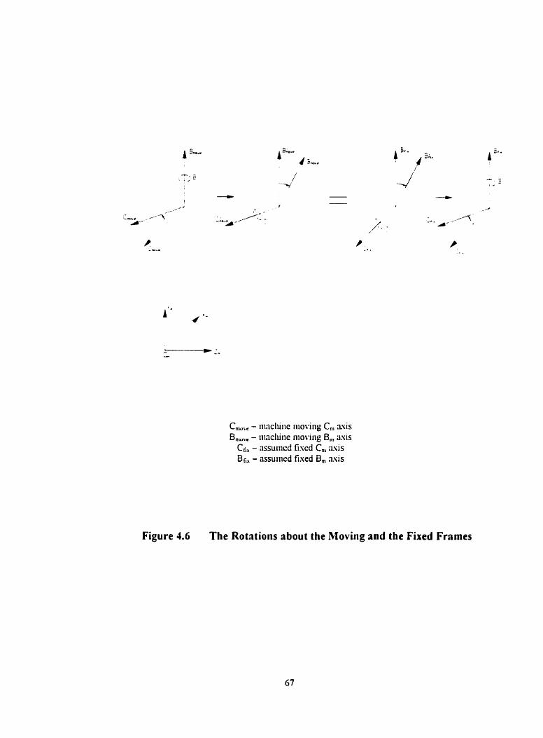
Cniobc - 1 1 1 3 ~ 1 ~ 1 1 ~ iiioving c,, a i s B,,,,, - ~iiacliine nioving B,, mis CL., - nssurncd fised Cm mis Bc, - assuiilcd fised B, nsis

Figure 4.6 The Rotations about the Moving and the Fixed Frrmes

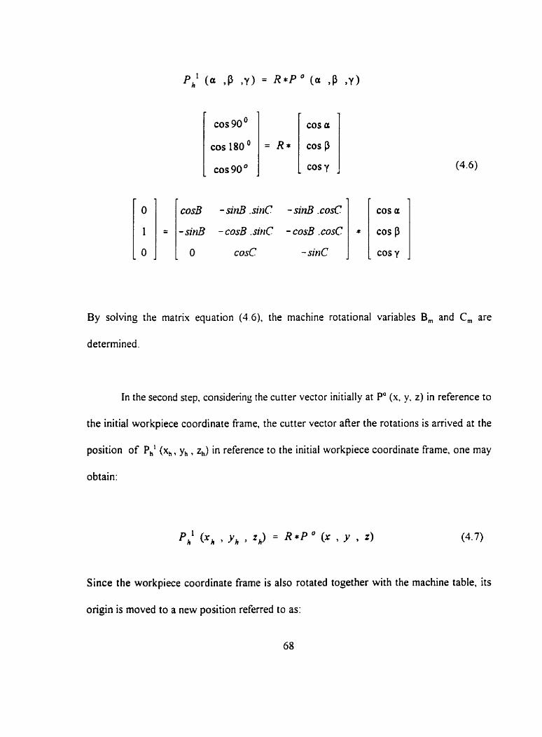
- cos 90 O

cos 180 O

COS 90 O

cosC -sinC ] [ cosy

A

By solving the matrix equation (1.6). the machine rotational variables B, and Cm are

determined.

In the second step. considerin3 the cutter vector initially at Po (x, y. z) in reference to

the initial workpiece coordinate frarne, the cutter vector after the rotations is arrived at the

position of Ph1 (x,, y, , 4) in reference to the initial workpiece coordinate frame. one may

obtain:

= R*

Since the workpiece coordinate frame is also rotated together with the machine table, its

origin is moved to a new position referred to as:

- 7

COS OC

cosP

- cos Y ,

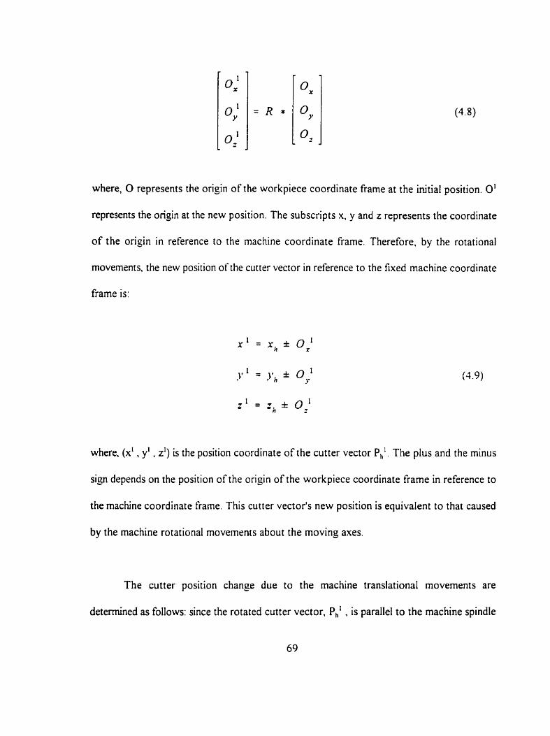
where, O represents the origin of the workpiece coordinate frame at the initial position. O'

represents the origin at the new position. The subscripts x, y and z represents the coordinate

of the origin in reference to the machine coordinate frame. Therefore, by the rotational

movernents. the new position of the cutter vector in reference to the fixed machine coordinate

frame is:

where. (x' , y' . zl) is the position coordinate of the cutter vector Ph1. The plus and the minus

siçn depends on the position of the origin of the workpiece coordinate frame in reference to

the machine coordinate frame. This cutter vector's new position is equivalent to that caused

by the machine rotational movements about the moving axes.

The cutter position change due to the machine translational movements are

determined as follows: since the rotated cutter vector, ph1 . is parallel to the machine spindle

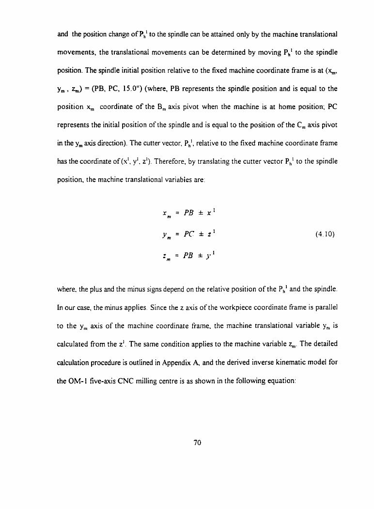
and the position change of PhL to the spindle c m be attained ody by the machine translational

movements, the translational movements can be detemined by moving Phi to the spindle

position. The spindle initial position relative to the fixed machine coordinate frame is at (h,

y,, z,,,) = (PB, PC, 15.0") (where, PB represents the spindle position and is equal to the

position x,,, coordinate of the B, axis pivot when the machine is at home position; PC

represents the initial position of the spindle and is equal to the position of the Cm a i s pivot

in the y, axis direction). The cutter vector, Ph1, reiative to the fixed machine coordinate frarne

has the coordinate of (xi, Y'. 2') . Therefore, by translatinç the cutter vector ph1 to the spindle

position, the machine translational variabies are:

where. the plus and the minus siçns depend on the relative position of the Ph1 and the spindle.

In our case, the minus applies. Since the z axis of the workpiece coordinate frame is parallel

to the y , axis of the machine coordinate frame, the machine translational variable y,, is

calculated from the 2'. The same condition applies to the machine variable q,. The detailed

calculation procedure is outlined in Appendix A, and the derived inverse kinematic rnodel for

the OM- l five-axis CNC rnilling centre is as shown in the following equation:

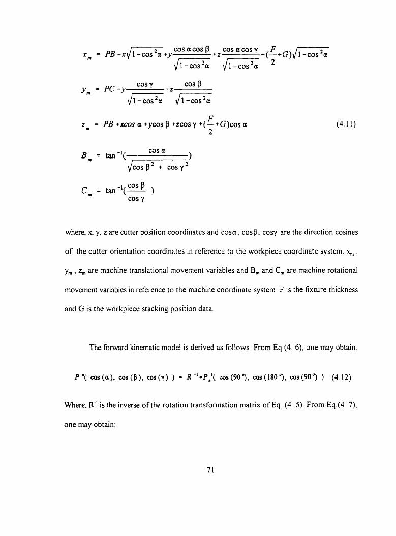
= PB-+J1-coç2cC+y cos acos p cos a cosy F -(-+cl Jx ~~-cos'cr+~ jl-coç20

cos y cos p y m = P r - y

/1-cor'.-=&X

COS a B = tan -'( m 1 -

+os p z + cosy'

where. x. y, z are cutter position coordinates and cosa. cosp. cosy are the direction cosines

of the cutter orientation coordinates in reference to the workpiece coordinate system. s, ,

y,, z, are machine translational movernent variables and Bm and Cm are machine rotational

movement variables in reference to the machine coordinate system. F is the fixture thickness

and G is the workpiece stacking position data.

The fonuard kinematic model is derived as follows. From Eq.(4. 6). one may obtain:

Where. R-' is the inverse of the rotation transformation matrix of Eq. (4. 5). From Eq.(4. 7).

one may obtain:

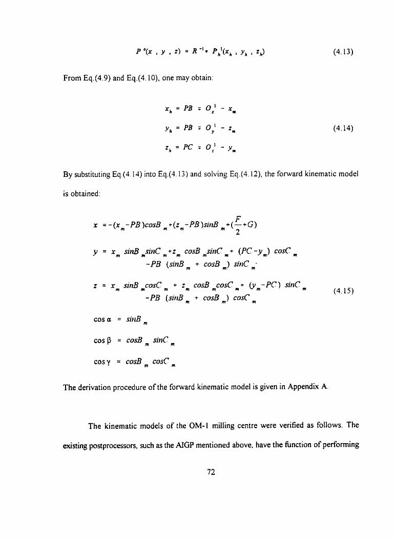
From Eq44.9) and Eq.(4.10), one may obiain:

By substituting Eq.(J. 14) into Eq.(l. 13) and soivinç Eq.(4.12). the fonvard kinematic model

is obtained:

y = x si& siîiC , +zm COSB _sine ,+ (PC -y,) cosC , m 111

-PB (sinB + COSB m ) I i C m.

cosa = siriB ,

cos p = c d ? sinC

cos y = cosB COSC ,

The derivation procedure of the fonvard kinematic model is given in Appendix A.

The kinematic models of the OM-1 milling centre were verified as follows. The

existing postprocessors, such as the AIGP mentioned above, have the function of performing

kinematic transformations between cutter variables and machine variables for a known

machine configuration. Using the AIGP. a set of CLDATA for machining the airfoi1 surfaces

of an impeller was transfonned to the corresponding NC-codes. Then, the set of CLDATA

was processed through the derived inverse kinematic model. The obtained machine variables

are then compared with the NC-codes obtained from the AiGP. A cornparison of results

showed that the calculated machine variables (q, . y, . z, . B,. Cm) are exactly the same (up

to five decimal digits) as the NC-codes computed by the AIGP. The result confirms the

correctness of the derived inverse kinematic model. Similarly. the foward kinematic mode1

is veritied by transforming the set of NC-codes for machining the airfoil surfaces of the

impeller into the correspondinç CLDATA. The resultant CLDATA were the sarne as the set

of data obtained from the NGP.

1.4 Development of Machining Motion Tr:ijectory Mode1

From the machine configuration shown in Fig.4.4 , the B,, axis coincides with the y, avis

which is perpendicular to the machine table. and the C,, axis is parallel to the z,,, axis during

machining process. Therefore, tlir B,, asis intersects the C,, âuis at a space point, P. Durinç

the machining process, the intersection point P moves translationally only in the x, axis and

the z,,, axis directions since the point is on both of the rotational axes. The point P also acts

as a pivot for the machininç spatial rotational movements. Thus. the CC point path is actually

the result of the superimposition of the rotational movements of the machine table about the

pivot P and the translational movements of the pivot P. which results in the combined 3D

circular interpolated and the 3D linear interpolated path. Frorn this geometncal perspective,

it is known that the CC point coordinate on the non-Iinear segment can be determined from

the pivot P translational coordinates and the machine table rotational movements coordinates.

Thus, the machining motion path can be formulated on the basis of the pivot translational

rnovements and the machine rotational movements.

The machine home position is defined by the machine table coordinates (q,, ym. zm,

B,. Cm) = (381.0 mm. 0.0 mm, 711.2 mm. O". 0") = (15.0". 0". 28.0". O". O") and by the

spindle coordinates (s,. y,, q,J = (381.0 mm. 6 15.95 mm. 0.0 mmj = (15.0", 24.25". 0.0").

The machining start point is chosen as the machine home position. Since the B,, mis coincides

with the y, a i s , the circular motion in the horizontal plane (the a,-%, plane) about the B,

axis changes the %, and the 4, coordinates as shown in Fig.4.7, one rnay obtain:

x_ = I sin (B, )

z = 1 cos ( B I ) SC

Similarly. because the C,, avis is parallel to the G~ auis. the circular motion in the vertical plane

(the %,-y,, plane) about the C , anis changes the s, and the y,, coordinates as shown in Fiç.

4.8. one rnay obtain:

xm = z sin(Cm)

y= = z cos (Cm)

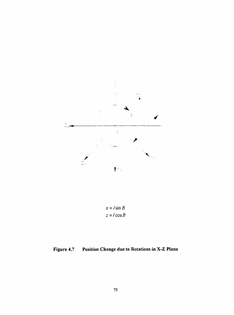
Figure 4.7 Position Change due to Rotations in X-Z Plane

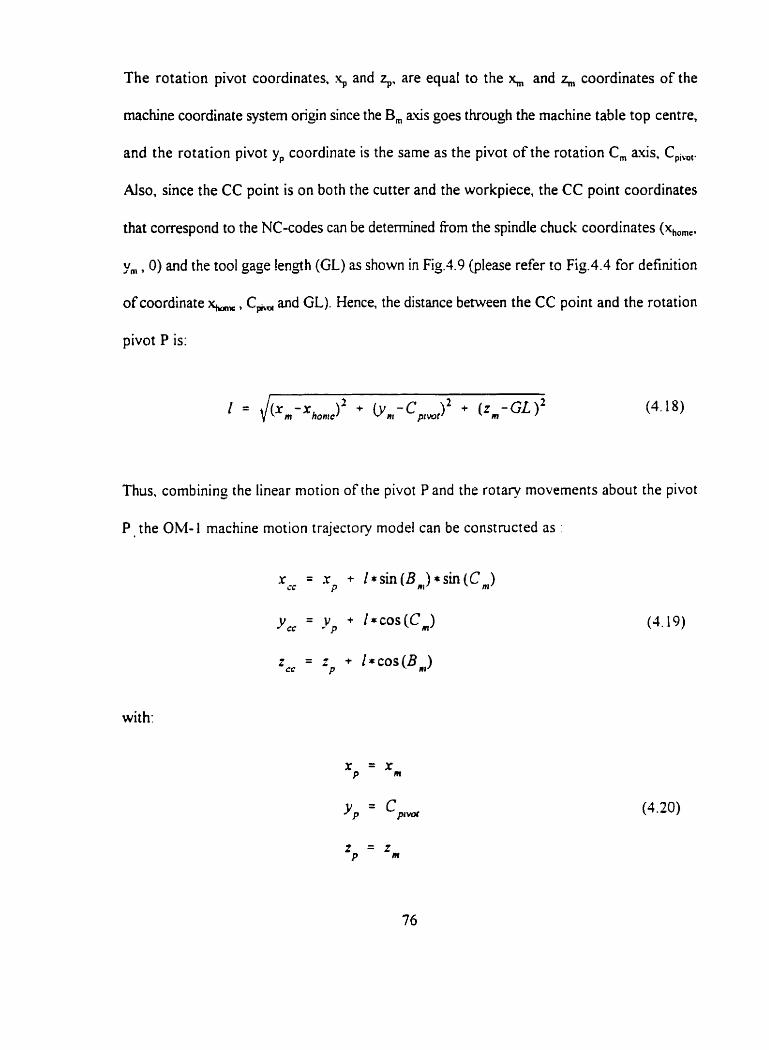
The rotation pivot coordinates. and 5. are equal to the >c, and z, coordinates of the

machine coordinate system ongin since the B, avis goes through the machine table top centre,

and the rotation pivot y, coordinate is the same as the pivot of the rotation Cm auis, C,i,ut.

Also, since the CC point is on both the cutter and the workpiece, the CC point coordinates

that correspond to the NC-codes can be determined f?om the spindle chuck coordinates (x,,,,.

v 0) and the tool gage iength (GL) as shown in Fig.1.9 (please refer to Fig.4.4 for definition ~ r n r

of coordinate x,,,,,,~, C, and GL). Hence, the distance between the CC point and the rotation

pivot P is:

Thus. combining the linear motion of the pivot P and the rotary rnovements about the pivot

P, the OM- 1 machine motion trajectory mode! can be constnicted as :

with:

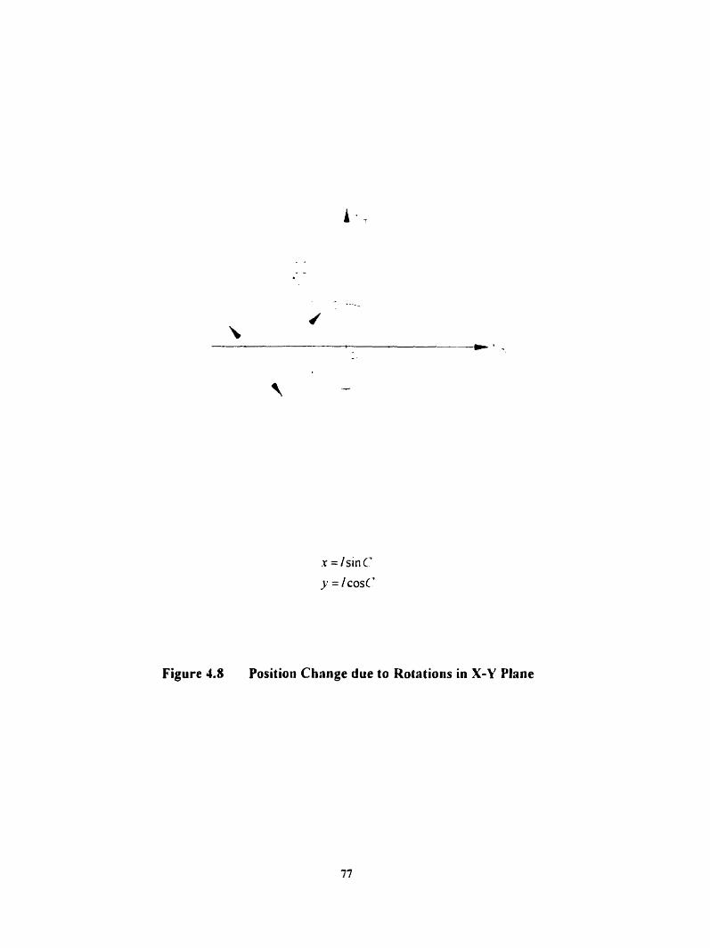
Figure 4.8 Position Change due to Rotations in X-Y Plane

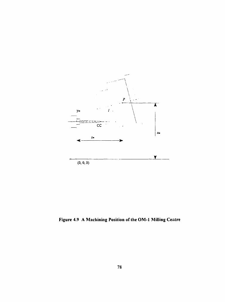
Figure 4.9 A Mnchining Position of the OM- 1 Milling Centre

where, (xc,, y,,, q,) are the coordinates of t he CC point, (x, , y, , 5) are the coordinates of

the rotation pivot P in reference to the machine coordinate system, I is the distance between

the CC point and the pivot P of Eq44.18). B, and Cm are the rotational rnovements of the

machine table, and C,,, is the C, avis pivot coordinate which is a constant.

4.5 Minimum Error Tool Path Generation Methodology

A methodology to determine the optimum CLDATA for minimum machining error based on

machine kinematics and machine motion trajectory analysis is explored. The machine

kinematic models of Eq.(4.11) and Eq(4.15) çive the OM- i rnachining geometrical relations

between the cutter orientations and the machine rotational variables. The machine rotational

movements are kinernatically related to the spatially chançed cutter orientations, and therefore

the non-linearity errors depend upon the cutter orientation changes. The OM- 1 machininç

motion trajectory model of Eq.(4.19) mathematically shows that the non-linear path curve

segments depend upon machine rotational variables for the determined translational steps.

Hence. non-linearity errors are a result of the machine 3D rotational movements. Also, by

using the motion trajectory model, the coordinates on each non-linear tool path segment can

be detemiined, which in turn. can be used with known lineanty errors to determine the non-

linearity mors. Particularly, the maximum non-linearity error on each segment can be

determined. In order to calculate the lineanty errors, the surface curvature at the machining

data points must be known. To detemine the geometrical properties, such as the local surface

curvature, the cutting curve mathematical function is required. The cubic spline curve function

is the minimum order function that can ensure the second order continuity [69]. Therefore,

the cutting curve can be closely approximated by the cubic spline of the known CLDATA.

The development of the cubic spline Functions to represent curting curves is presented in

Appendix B.

The proposed rnethodology reduces non-linearity errors by determining the acceptable

machining rotational variables usine the motion trajectory model, and also modifies the cutter

orientations through the kinematic relations wit h the machine rotational variables. For a

specified machining tolerance. the machine rotary movements which will result in an

acceptable machininç motion trajectory can therefore be drtermined. Then, the optimum

cutter orientations which correspond to the obtained rotational variables can be detennined.

The procedure stms with the transformation of the CLDATA to the machining NC-codes by

employi- the inverse kinematic model of Ec1.(1.1 1 ) The actual machining motion trajectory

is then determined by usin3 the OM- 1 motion trajectory model of Eq. (4.19). The local surface

curvature on the cutting curve and the step-fonuard distance. i.e.. the linear spacing between

a pair of the cutting points. determine the amount of linearity error. From the cubic spline

cutting curve fùnction, the local surface curvature can be determined (refer to Appendix B).

Thus, the linearity error for each move can be obtained from the adjacent CC point data and

the detennined curvature. The allowable non-linearity error can be computed by subtracting

the linearity error from the specified machining tolerance. The actual non-lineanty error for

each move is the deviation of the non-linear motion trajectory from the linear interpolated line

segment. Representing the linear segment using linear interpolation fùnction based on the CC

point coordinates determined fiom the OM- 1 motion trajectory model given in Eq.(4.19). the

maximum deviation between the non-linear motion trajectory and the linearly interpolated line

segment, Le., the maximum non-Iinearity error, for the step can be determined. In the steps

where the mavirnum non-linearity error exceed the allowable non-linearity error, the machine

rotational movements change will be modified. The new machine rotational movement

variables are determined based on the modified rotational movement change. These new

rotational movement variables are then used to calculate the resultant non-linearity error,

which in turn is compared again with the allowable non-linearity error. Thus, by using the

difference between the allowable non-linearity error and the rnodified non-linearity error as

the criterion. the acceptable machine rotational movements can be determined iteratively.

Finally, frorn the modified machine rotational movements. the corresponding cutter

orientations can be determined by performing the foward kinematic transformation using

Eq.(4.IS).

I t must be emphasized tliat the machining geometrical properties and the motion

trajectory are machine dependent. Hence. the modification of CLDATA has to be camed out

in terms of machining variables and subsequent use of the kinematic transformation to

determine the rnodified CLDATA. For a set of CLDATA* the modification procedure can

be performed by usinç the followinç algorithm.

Tool Path Modification Algorithrn:

1) Transform the initial CLDATA into its corresponding machininç NC-codes by using

the inverse kinematic mode1 for a particuiar CNC machine tool (for OM-1 see Eq.

(4.1 1));

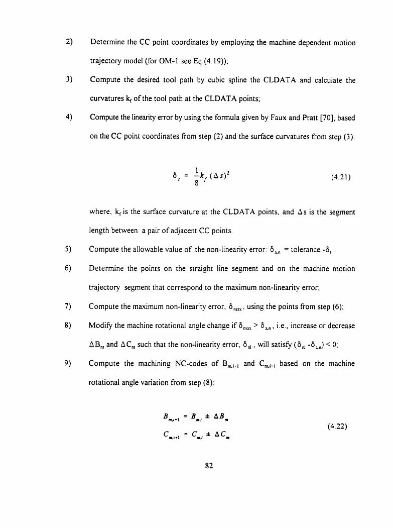
Determine the CC point coordinates by employing the machine dependent motion

trajectory mode1 (for OM- 1 see Eq.(4.19));

Compute the desired tool path by cubic spline the CLDATA and calculate the

curvatures k, of the tool path at the CLDATA points;

Compute the linearity error by using the formula given by Faux and Pratt [70], based

on the CC point coordinates from step (2) and the surface curvatures from step (3):

where. k, is the surface curvature at the CLDATA points. and As is the sesment

length between a pair of adjacent CC points.

Compute the allowable value of the non-linearity error: 6," = iolerance -6, ,

Determine the points on the straight line segment and on the machine motion

trajectory segment that correspond to the maximum non-lineanty error;

Compute the maximum non-linearity error. 6,, . usinç the points from step (6);

ModiQ the machine rotational angle change if 6,,, > 8,". Le.. increase or decrease

AB,,, and A C , such that the non-linearity error. 6, , will satisfy ( 6 , -6,3 < 0;

Compute the machininç NC-codes of Bmi., and Cm,-, based on the machine

rotational angle variation from step (8):

where. (Bmi , C,J are the i-th rotational variables, (B,,+, . Cmi+,) are the (i+l)-th

rotational vanables, and (AB, .ACn,) are the modified rotation angle change. The

' + ' and ' - ' sign depends on if the angles in step ( i+ l ) increases or decreases.

10) Determine the optimum cutter orientations by transforming the modified machining

NC-codes using the forward kinematic model (for OM- 1. use Eq.(4. ! 5)).

4.6 Software for Implenienting the Algorithm

A software program has been written to implement the proposed algorithm described above.

The computation procedure is shown in the program flow chan shown in Fig.J.lO. The

program stans by inputting the known CLDATA and machining parameters. which include

machining tolerance, fixture thickness and stack value. These machininç parameters can be

changed for different machining requireinents and machine setup. The program includes a

function for constructing the tool path cuwe based on the CLDATA by using the cubic spline

technique, so that the curvatures at the cutter positions can be calculated. The propram

consists of an inverse kinematic transformation function of the CLDATA generating the

machininç NC-codes. and a function of OM-1 motion trajectory determininç the CC point

coordinates. For each step. based on the determined curvature and the CC point coordinate.

the linearity error can be calculated. The allowable non-Iinearity error is deterrnined from the

iineanty error and the specified rnachininç tolerance. Considering that the maximum non-

linearity error usually occurs at the middle point of each linear line segment. the proçram

determines the points on the linear line seçment and on the motion trajectory segment. which

yields the maximum non-linearity error. By testing whether a non-linearity error exceeds the

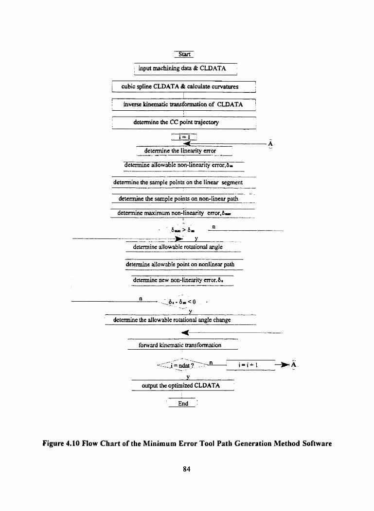
t input machining data & CLD.4TA

- -

determine the CC point trajectory I . * A -

detennine the linearity error

'detennine allowable n o n - h 4 t y error.6,

determine the sample points on the linear segment

determine the sample points on noa-finertr patb

detennine maximum non4 inearity error, 6 - t-- Y -

detamine ailowablc: rotational angle

dettminc al10w;ibIt point on nonlineu path

' determine the dlowable ro~&ond angle change

--

fonvard kinmafic. transformation

: output the optimized CLDATA '

I

' End

Figure 4.10 Flow Chnrt o f the Minimum Error Tool Pnth Generation Method Software

allowable non-linearity error determined previously. a procedure for determining the

acceptable rotational angle change is conducted iteratively as follows. Once the test of

whether the actual non-linearity error exceeds the allowable value is tme, the machine

rotationai angles' changes, AB, and A C , are adjusted in each iteration and the corresponding

machine rotational variables B,, and C , are calculated. The adjusted B, and Cm are then used

to determine the resultant non-lineanty error which in turn is compared with the allowable

value. The iteration is conducted untii the final non-linearity error is equal to or less than the

allowable value, and the corresponding B,, and C,, which are the desired machine rotational

variables can be determined. Repeatinç the computation for each step. the whole set of NC-

codes can be processed. For the steps. the non-linearity error is smaller than the allowable

value, the NC-codes remain unchançed. Finally. the NC-codes including the rnodified points

and the remaining points are transforrned into the CLDATA.

4.7 Summary

An off-line tool path generation methodolopy. which modifies the cutter orientations

to reduce the machininp errors. has been proposed. The rnethodology employs the machine

type-specific kinematic models and the machininç motion trajectory modei. The new method

reduces non-lineanty errors to be within the specified tolerance range by calcuiating the

allowable machine rotary angle changes. The optimum cutter orientations are then determined

based on these allowable machine rotary angle changes. The new method improves the

machining precision with srnoother machining data distribution because the modified

CLDATA contains the original cutter positions. Comparing with the existing methods, the

'Iinearization processes' insert cutter positions to reduce non-linearity errors which results in

the feedrate fideiity problem and increases rnachining time. Alternately. the new method

ensures the machining precision by tackling the cause of the non-linearity errors problem. the

cutter orientation changes, without undesired consequences.

As the result. the software for implementing the proposed methodology can be used

to process CLDATA specifically suitable to the OM-1 rnilling centre. and to çenerate NC-

codes for the rotary table type five-axis CNC machine tools by changing the configuration

data.

CHAPTER 5

AN APPLICATION OF THE

MINIMUM ERROR TOOL PATEI GENERATION METHOD

5.1 Introduction

The hiçhly twisted airfoil of a turbine irnpeller is a typical exnmple of scuiptured surfaces. For

machininç such complex surfaces. five-axis CNC machininç with conical shaped ball-mills is

usually used because of the highly twisted airfoil surfaces and the narrow passages beiween

the airfoils. The CLDATA çeneration technique for machininç of such impeller airfoil surfaces

was described in section 4.2. I t determines the cutter positions and its axis vector orientations

based solely on the çeometncal properties of the machined surfaces As an application of the

proposed 'minimum error tool path yeneration method'. a set of CLDATA for the rnachininç

of the impeller airfoi] surface is processed and the optimum CLDATA with minimum

machining errors is obtained. In the following. a simulation study for processing the set of

CLDATA by usinç rlie existing 'linearization process' is described in section 5.2. The

procedure and results for processing the CLDATA by using the proposed rnethodoloçy are

outlined in section 5 3.

5.2 Case Study Using the 'line:irizriion Process '

In order to compare the optimized results with those obtained throuçh the 'linearization

process' mentioned in section 2.2. the set of CLDATA is processed by the extensively used

postprocessor, the AIGP[3 l 1. The AiGP çenerates machininç NC-codes using the

'linearization process' as follows:

Tmnsfoms a pair of adjacent CLDATA points into corresponding machine NC-codes

coordinat es;

Constructs a straight line segment using the two NC-code position coordinates;

Divides the straight line segment and the conesponding rotational movements angle

change into two portions;

Calculates the middle point NC-code coordinate based on the result of step (3);

Transforms the calculated new NC-code into the corresponding new CLDATA;

Tests the deviation of the new CLDAT.4 point from the straight line constructed

between the two considered CLDATA;

Goes to step 8) if the considered CLDATA are the oriçinal data. otherwise. goes to

step 10).

Inserts a rniddle point between the two initial CLDATA if the deviation is geater

than the specified machining tolerance;

Repeats the process from step 1 ) to step 6) using the start CLDATA point and the

insened median point of CLDATA;

Inserts another intermediate point between the considered two CLDATA points if

the new deviat ion exceeds the specified tolerance:

Repeats the process from step 1) until either ail points are within the machining

tolerance range or a maximum of 63 points have been generated;

Repeats the steps I ) to I l ) to the next adjacent original CLDATA pairs until al1 data

points are processed.

The results for processing the CLDATA of machining the airfoil surfaces using

AIGP's 'linearization process' are as follows.

With the specified machining tolerance of 1 2 . 7 ~ 1 0 ~ ~ mm (o.S'X~O"), there was no

additional data inserted between any adjacent rnachining data points. However. the

'linearization process' inserted data points when the rnachining tolerance was reduced. With

the tolerance of 7 . 6 2 ~ lo5 mm (o.T"' 1 O-'). one data point was inserted in the first motion step

(between the first two original CLDATA). in the third motion step (between the third and the

fourth original CLDATA). and in the ninth motion step (between the ninth and the tenth

original CLDATA). Furthermore. by reducinç the tolerance to 5 0 8 x 1 O-' mm ( 0 . 2 " ~ 1 O"),

more data points were insened. Table 5. I shows 25 sets of inserted data (shown as underlined

points) among the complete set of 1 5 5 machining data points for the hiçhest attainable

machininç precision of 5 . 0 8 ~ 10-' mm (O 2" x 10*') The resultant tool path data are more

dense than the original data. Funherinore. the cutter position points are not equally spaced

and the cutter orientation varies incorrect ly .

5.3 Case Study Usiiig the 'hliniiiium Error Tool Pnth Ceneration Method'

Using the proposed methodoioçy, the set of CLDATA was also processed with the same

machining parameters as used for the AIGP. With the specified machining tolerance of

1 2 . 7 ~ 1 O" mm (0.5"~ 1 0"). the maximum non-linearity error calculated from the NC-codes

were al1 smailer than the ailowable non-linearity error. Hence. there was no need to conduct

the cutter orientation modifications. This result is the same as the one from the AIGP

'linearizatinn process' mentioned above. By specifying the tolerance = 7.62x10" mm

(0.3"xl O"), the prograrn processed the allowable machine rotational angle changes at some

steps and rnodified the corresponding cutter orientations. For instance. for the first step and

the third step, the non-linearity error exceeded the specified tolerance. Hence, the cutter

orientations in the second block of CLDATA and the fourth block of CLDATA were

modified. Furthemore. by tightening the machining tolerance to 5 .O8x 1 0-3 mm (O 2"x 1 05),

the allowable machine rotary angle changes were calculated iteratively at more motion steps.

The cutter orientation modification process was conducted up to nine iterations for the first

step until the non-linearity error was wit hin the allowable range. Three iterations were

performed for the third and the ninth steps. Similarly. the process was camed out for each

motion step of the whole set of CLDATA. The acceptable machine rotational movements B,

and C , were determined by adjusting the rotation angle changes: AB,, and AC,,. based on

Eq.(4.22). The corresponding CLDATA were rnodified by transforminç the processed NC-

codes using the fonvard kinematic model. For the data points where the maximum non-

linearity error calculated frorn the NC-codes were srnaller than the allowable non-linearity

error, the data remained unchanged.

Table 5.2 outlines some modified cutter orientation data and the corresponding NC-

codes. The set (i , j , k) = (cosa, cos p. cosy) are the direction cosines of the cutter axis

veaor relative to the workpiece coordinate system. For the first step (from point 1 to point

2). the adjusted rotary angle change AB,,, was increased, and the adjusted AC, was

decreased. The modified direction cosines (i, j, k) result in the rnodified cutter orientation

Table 5.2 Sample Modified Rotary Angle Changes & Cutter Orientations

point CLDATA cutter angle 1 angle change 1 Bm Cm 1 ABm ACm 1 modifirid original modifird original modüïcd original

a.P. y da dg da d(3 BmCm 8rn.Cm SBm

d~ dy ACm

83.571'. initial initial 353.571' 353.571' initial

90.723'. mgles mgls 359.271" 359.271" mgla

6.469.

84.383'. 0.724". 0.812", 354.295" 354.385' 0.724".

Y 1.338'. 0.609'. 0.6 15'. 358.660" 358.656' 4 .6 1 1'

5.774' -0.6 10' -0.695'

X4.608'. 354.610' 354.610'

9 1.327'. mchecd u n c h ~ d 35g.668' 3 5g.668. ~ ~ ~ 6 4

5.554"

X C . 1 16'. 0.480". 0.508". 355.088' 355.118' 0.478".

9 1.309'. -.ù204". -.O 17'. 358.688' 358.687' 0.020"

5.057' -.470° -.0436'

82.950". 0.462'. 0.404'. 352.972'. 352.853'. 0.424".

92.539". 0.460' . 0.462' . 357.443" 357.543' -.23J0

7.502' - 269' -.24?"

R5.227'. 0.2 1 Y. 0.223". 355270'. 355163'. U214*.

'2.4 1 0.052". 0.056". 357 037" 357.06U0 - 028'

5.6G3" - 157' - 086'

'lU.33Uu. 0.3U3". 0.287". 8.644'. 8.525' . 0.298".

70 ,609'. - 62 X'. - 623'. 20.173" 19 976' 0.651".

f l .U25' 0.71 1' 0.570"

101.29' 0.316'. 0.412'. 1 1.5 13". I 1.495". 0.3U9'.

65.943'. -3 10'. -.292'. 25.325' 25.152" U.sj5"

26.952' 0.622" 0.527'

108.3 1' 0.359'. 0.3 13'. 18.72 1'. 1 I4.665". 0.356'.

58.384". -.9 13'. -.303", 33.795" 33.692' 0.344'

37.643' 0.441a 0.437'

angle changes (da, dp , dy) which were çreater than the original cutter orientation angle

changes. For the second step, since the maximum non-linearity error was srnaller than the

allowable value. there was no need to perform the cutter orientation modification and the

direction cosines (i, j, k) at the third point of cutter onentation remained u~ichanged. For the

third step (tiom point 3 to point 4). the adjusted rotary angle change AB, was increased, and

the adjusted AC, was decreased. The cutter orientation (i. j. k) at the fonh point were

modified. The resultant cutter orientation angle changes of da and dy were increased

comparinç with the original cutter orientation changes. and the cutter orientation angle

change of dp was decreased compannç with the original value Similarly, the original and the

modified cutter orientations (i. j. k) ai points 10. 20. 74. 83. 104. 105 and 123 are shown in

the table. The increasesidecreasrs of the machine rotational movement angles of (AB,,, AC,,)

and the corresponding cutter orientation changes of (da. d p. dy ) are due to the fact that the

machining motion trajectory is constnicted by cornbininç the 3D circular and linear motions.

Although the cutter onentation changes either increased or decreased. the non-linearity errors

were reduced as shown in Table 5 . 3 . From Table 5.3 the original non-linearity error for the

step 1 was 8.788~ l O" mm (0.%6"'t 1 O-') . The non-linearity error afier cutter orientation

modification was reduced to 2 . 3 6 2 ~ 10" mm (0.093"xf O-' ) which was smaller than the

allowable non-lineari ty error of 2.5 14x 1 0" mm (0.099"~ 1 O"). The reduced total machining

error For this step was up to 56.5%. For step 3, with the modified cutter onentation data the

non-linearity error was reduced from 5.486~ 1 O" mm (0.2 16"x 10") to 3 . 4 0 3 ~ 1 O" mm

(O.l34"xl0~), which was smaller than the allowable value of 3 . 7 8 4 ~ 1 o5 mm (O. 149"x 10").

The reduced total machining for this step was up to 30.7%. Similarly, for steps at which

Table 5.3. Machining Errors rt Sarnple Moves (tolerance = 0.005mm=0.0002")

S tepError

1 1

3

9

19 1

73

82

103 I

104

122

130

original non-iineui ty (inch s 1 0-j)

0.346

0.2 16

0.2 10 - -

O. 197

0.200

0.2 10

0.230

0.195

0.205

0.2 10

I 1ineiu-i ty

(inch s IO-')

0.101

0.05 1

0.005

0.007

0.002

0.005

0.00 1

0.025

0.00 1

0.004

rnodifled non-Iinearity (inch s 1 O-3)

0.093

0.134

0. 185

O. 182

0.189

O. L 87

O. L 90

O. 172

O. 193

O. 193

133

13 9

reduced total (%)

56.5

30.7

11.6

7.4

5 3

10.7 1

17.3

10.5

5 . 8

7.0

O. 192

O. 196

7.6

3.4 *

0.003

0.002

0.208

0.203

AIGP1s 'linearization process' was inserted data points (see Table 5.1). the original non-

linearity erroo were reduced to the modified values which were within the allowable ranges.

For each step, the percentage of the reduced total machining error is also calculated as shown

in Table 5.3. It should be noted that the allowable non-linearity error changes depend on the

linearity error changes in each step. For example, in step 3. the lineanty error was reduced,

so the allowable non-linearity error was increased.

For the specified machining tolerance of 5 . 0 8 ~ 10" mm (0.2"' 10-~)). the MGP must

insert the additional cutter positions to meet the rnachining precision requirernents.

Altemately. the new method rnodibiny the cutter orientations of CLDAT.4 also ensures the

machining precision without data-point insertion. Specifically. the modified CLDATA has

fewer data points than the one processed by the 'linearization process'. The proposed

methodology improves the rnachining precision from 1 2 . 7 ~ 10" mm (0.5"~ 10") to 5.08~ 10.'

mm ( 0 . 2 " ~ 1 O-'.) wit hout reducing the cutter st ep-fonvard distance. This result overcomes the

drawbacks fi-orn the 'linearization process'. It illustrates that the proposed methodology results

in hiçher rnachining precision and reduced data storage space which in tum reduces machininç

time.

CHAPTER 6

A 3D COMBJNED LINEAR AND

CIRCULAR INTERPOLATOR DESIGN TECHNIQUE

6.1 Introduction

Continuous path contouring requires continuous control of spindle head movemeots with

respect to the machine table (or of the table relative to the spindle). not only of the start and

the end points of movements, but also al1 of the intermediate points as well. The process of

filling in data about curved surfaces. from a set of point data describing some points on the

curve, is termed interpolation. In conventional multi-asis CNC machininç of sculptured

surfaces. the 'position contouring' technique with linear interpolation rnethod are commonly

used to generate the required cornmands for driving the motion axes. In five-axis CNC

machining, the three translational axes movements are linearly interpolated alonç the straight

line segment and, simultaneously. the rotational movements are interpolated alonç space

circles, which have coupling effects on the linearly inrerpolated translational movement

positions. Consequently, the actual CC point moves along cuwe segments. which results in

the non-linearity error problem.

Many factors contribute to the CNC machining errors. One way solving the non-

linearity error problem in ultra-precision five-ais CNC machininç process is to modiS, off-

line the cutter orientation changes to reduce non-linearity errors within the rnachining

tolerance. This method has been explored as the 'minimum error tool path generation method'

in ultra-precision five-axis CNC machining as outlined in Chapter 4. Another route is to

pursue new interpolator designs, because one of the factors causing the non-linearity

machinhg errors is due to the machininç interpolation method. The five-axis CNC machining

motion trajectones are non-linear cuwe segments, therefore, it is desired to design new

interpolators which are capable of tracing non-linear curves and provide solutions to the non-

linearity error problem. This chapter presents a procedure for desiçning a new interpolator

for five-axis CNC machining systems. The proposed interpolator will coordinare the

translstional movements to move along a predesigned curve path. and conducts the CC point

to move along the straight line segment connecting each pair of adjacent machining data

points. Thus, non-linearity errors in five-axis CNC machininç are expected to be eliminated.

In the following, in section 6.2, the conventional interpolation methods in CNC systems are

discussed. In section 6.3, the ?D and 3D Digital Differential halyzer @DA) linear

interpolation principles in conventional linear interpolation methods are reviewed. Then. the

denving procedure of the 2D DDA circular interpolation principle is reviewed in section 6.4

since it forms a basis for the development of a new 3D circular interpolation principle

presented in section 6.5. This is followed by the developrnent of an innovative 3D combined

linear and circular interpolation principle in section 6.6. An algorithm for eliminatinç non-

linearity errors in five-axis CNC rnachininç by using the 3D combined linear and circular

interpolator is presented in section 6.6. Finally. a software interpolation routine for

implementing the proposed algorithm is developed and is outlined in section 6.7.

6.2 The Conventional Interpolation Methods

The function of an interpolator is to generate intermediate points lying between two

consecutive machining data points. Carefùl programming of cutter pat h motions allows the

point-to-point type of milling machine to follow almost any curve within reasonable

tolerances. In CNC machining, an interpolation method is the core of the CNC systern since

the accuracy of the calculated intermediate position directly affects the machining precision

of the whole CNC system and the time for cornputing the intermediate positions affects the

controlled axis velocity. which in turn. afTects the quality of the machined surface and the

macliining tirne. Basically, the conventional interpolation rnethods can be divided as the

reference-pulse methods and the reference-word method [4].

In the reference-pulse system. the interpolator routine in the MCU calculates the

intermediate positions and send reference pulse signais to each axis control loop. The

operation of the reference-pulse interpolators is based on an iterative technique controlled by

an intempt clock. At each intemipt. a single ireration of the routine is executed and produces

an output pulse. Each pulse generates a motion of one basic lençth-unit (BLU) for the

controlled axis. The accumulated nurnber of pulses represents the axis position and the pulse

(intempt) fiequency expresses the axis velocity. Since each pulse is equivalent to one BLU

and the pulse frequency proportional to the axis velocity. the maximum velocity is

proportional to the attainable interrupt frequency. While the pulse frequency depends upon

the interpolation execution time, the axis velocity (the feedrate) is inversely proportional to

the interpolation execution time of a single iteration. Thus. the maamum axis velocity is

proportional to the maximum attainable intempt frequency, which in tum, depends on the

execution tirne of the interpolator algorithm. For this reason, the reference-pulse interpolation

technique is unsuitable for manufactunng systems requiring high axis velocities. The common

reference-pulse interpolation techniques include the software DDA method, the stairs

approximation method and the direct search method [ E l .

With the reference-word technique in the sarnpled-data system. the control loop of

each axis is closed by the computer interpolation software itself. which generates reference

binary words of line incremeiits. rather than the pulses. In fact. the interpolator operates

iteratively at an interpolation period of T. At each iteration. with the desired feedrate F. the

interpolator cornputes the line increment of FT which is transmitted to the correspondinç

software loop comparators as the reference word. Then. the control proçram compares the

reference word with the feedback signal to determine the position error. The error is fed at

fixed time intervals to a digital-to-analog convener, whish in turn supplies a voltage

proportionai to the required ais velocity. The reference-word interpolation techniques adopt

the tirne-division idea to divide the curve segment into the line increments and function in an

on-line mode correspondinç to the data-samplinç of the control system. Thus, the maximum

velocity in the sampled-data system is not limited by the interpolation execution time. The

practical reference-word linear interpolation techniques include the feedrate number method

and the direction cosine method. The reference-word circular interpolation rnethods include

the linear tiinction method, the reference word DDA method, the extended DDA method and

the improved Tustin method [49, 711.

Conventional CNC machines support the hnctions of 3D linear and 2D circular

interpolations. With linear interpolation. the actual path formed consists of either the BLU

increments in the reference pulse system or a set of straight line increments in the reference-

word system. The BLU increments or line increments are used to approximate the line

segments. Using the BLU increments to coordinate the intermediate data points, the

intermediate positions either fall on the straight line segment or positioned within the band of

one BLU. In reference-word linear interpolation. the linearly interpolated line increments are

al1 on the line segment [49. 611. The circular interpolation uses the circular arc increments

to approximate the required contour path. Circular interpolated arcs actually are comprised

of either BLU increments in the reference pulse system or straight line increments in the

reference-word system. The basic idea of circular interpolations is to use straight line

increments either in the chord direction or the tangent direction to approximate the arc

increments. The number of the line incrernents determines the accuracy of the generated

circular arcs. The optimal number of increments is the smallest one which maintains the path

error within the band of BLU.

In selecting the interpolation method. one criterion is the uniformity of velocity along

the path, because variations in milling velocity cause feed variations which affect the surface

finish of the workpiece. It has been shown that the appropriate reference-pulse interpolation

technique for machine tool systems is the software DDA method [52], which provides a

uniform feedrate along the circular path. On the basis of the reference-pulse DDA

interpolation algorithm, the reference-word DDA interpolation method has been designed

[49] with a selected interpolation penod that replaces the differential time interval in the

reference-pulse method. The reference-word DDA method coordinates the intermediate

positions with the specified line increments and functions in an on-line mode. so that it

overcomes the drawback on the limitation of the maximum feedrate in the reference-pulse

DDA method. For this reason, a 3D circular software interpolator and a 3D combined linear

and circular software interpolator for five-ais CNC machining have bern designed based on

the reference-word DDA technique. To demonstrate the developments of the new 5D

interpolators, the basic 2D DDA interpolation principles, which are commonly used [19. 50.

5 I l , are first discussed in the Following sections.

6.3 The 2D and 3D DDA Linear Interpobtion Principles

6.3.1 The 2D DDA linear interpolation principle[48.49]

To drive the cuttinç tool moving along a srraight line segment as shown in Fig. 6.1, with the

start point of p, (q, y,,) and the end point of pl (x, , y,), the i-th increment from the i-th point

to the (i+l)-th point for each axis cm be determined from the stan and the end points:

where, AL represents the line increment lençth in the direction of the velocity. L represents

the length of the segment between the start point p,(x, , y,) and the end point p,(x, , y,). If

the specified feedrate for the segment is F and the interpolation period is T, the Iine increment

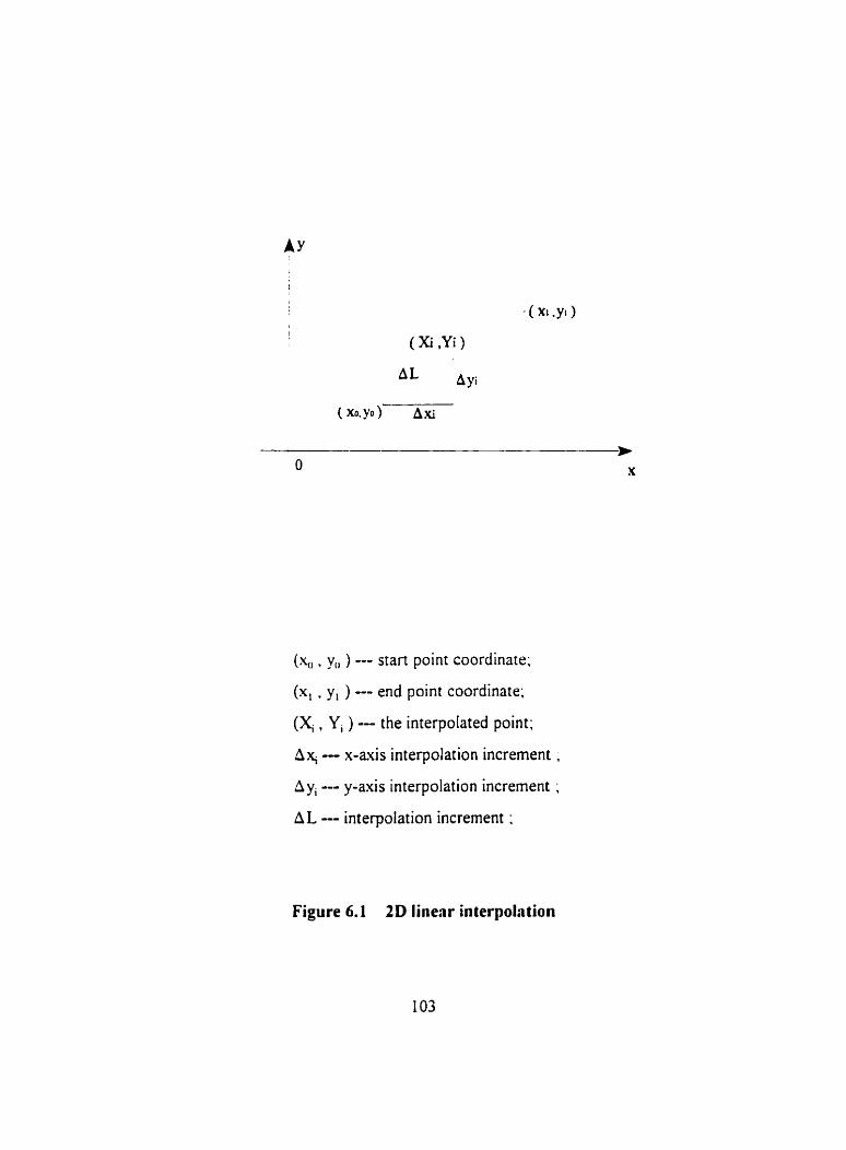
(x,, . y,, ) - - start point coordinare;

(x, . y, ) --- end point coordinate;

(X, , Y, ) --- the interpolated point;

P x , -- x-auis interpolation increment . Ay, -- y-axis interpolation increment ;

AL - interpolation increment ;

Figure 6.1 2D linerr interpolation

length is AL = FT and the increments of each axis are:

The 2D DDA linear interpolation can be operated as follows:

1) Preparatory calculation of the scale factor:

2) Cornputation of the segment length for each axis:

3) Computation of the (i+l)-th 2D linear interpolated point:

Xi+, = X I + AX,

Yi+l = Y, + A Yi

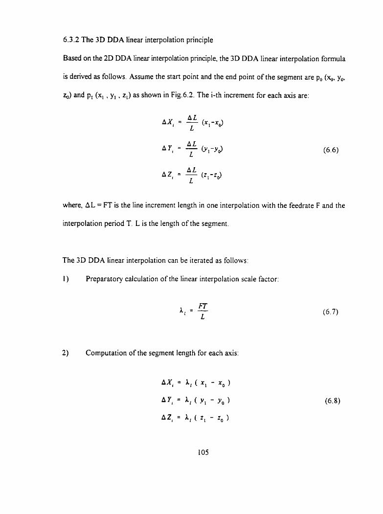
6.3.2 The 3D DDA linear interpolation pnnciple

Based on the 2D DDA linear interpolation pnnciple. the 3D DDA linear interpolation formula

is denved as follows. Assume the start point and the end point of the segment are p, (q, y,,,

zo) and p, (x, , y, , z,) as shown in Fig.6.2. The i-th increment for each axis are:

where. AL = FT is the line incrernent length in one interpolation with the feedrate F and the

interpolation period T. L is the length of the segment.

The 3D DDA linear interpolation c m be iterated as follows:

1 ) Preparatory calculation of the linear interpolation scale factor:

2) Computatlon of the segment lençth for each axis:

AX, = b , ( r, - x, )

q = L, ( Y , - Y,,

AZ, = k[ ( z1 - q, )

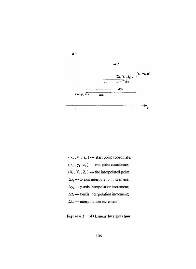
( . yu. q, ) --- stan point coordinate;

( s, . y,. z , ) --- end point coordinate;

(y. Y , , Z, ) --- the interpolated point;

Ax, - x-axis interpolation increment;

Ay, -- y-axis interpolation incrernent;

Az, -- z-axis interpolation increment;

AL - interpolation incrernent ;

Figure 6.2 3D Linenr Interpolation

3) Computation of the (i+l)-th 3D linear interpolated point:

6.4 The 2D DDA Circular Interpolation Principle [19]

The 2D DDA circular interpolation pnnciple is based on the solution of differential equations.

As shown in Fig.6.3, a partial circular arc in the x-y plane is:

where. X, = X(t) and Y, = Y(t) represent the interpolation position variable with parameter

t . (x y) represents the circle centre coordinate and R represents the radius of the circle. By

differentiating, it results in:

where, k represents a scale constant, and dt represents the differential time interval.

Figure 6.3 2D DDA Circulrr Interpolation

From E4.(6.12). it is known that each axis velocity depends on the cross-coupled i-th

interpolated point, i.e., the x-axis velocity v, depends on the value of the interpolated

coordinate Yi and v, depends on the interpolated coordinate X,. Thus, the i-th step increment

for each axis is:

where. the plus sign for AX, and the minus sign for AY, is for the case of the clockwise

circular interpolation. From Eq.(6.13), it can be seen that each avis increment is in the

direction of the axis velocity vector. Representinç the feedrate by F and replacing the

differential tirne interval At by the interpolation period T. and letting k = F/R the i-th

increment for each axis is:

Similarly. for the arc on the 2-x plane. the i-th step increment for each axis is:

FT AX, = V= A C = --(Zt-z) R

And, for the arc on the z-y plane. the i-th step increment for each a i s is:

FT AY, = y A t = -(Z,-2) R

The 2D DDA circular interpolation can be operated as follows:

1 ) Preparatory calculation of the circular interpolation scale factor:

2) Computation of the (i+ I )-th point of interpolation on the x-y plane if the interpolated

circle is on the plane:

3) Computation of the (i+I)-th point of interpolation on the x-z plane if the interpolated

circle is on the plane:

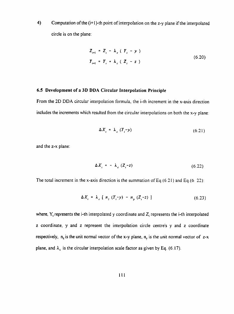
4) Computation of the (i+l)-th point of interpolation on the z-y plane if the interpolated

circle is on the plane:

6.5 Development of r 3 D DDA Circulrr Interpolation Principle

From the 2D DDA circular interpolation formula. the i-th increment in the x-axis direction

includes the increments which resulted from the circular interpolations on both the x-y plane:

AX, = Lc (Yi-y)

and the z-x plane:

AX, = - A c (2,-Z) (6.23)

The total increment in the x-axis direction is the summation of Eq(6 .2 1 ) and Eq.(6 2 2 ) :

where, Yi represents the i-th interpolated y coordinate and Zi represents the i-th interpolated

z coordinate, y and z represent the interpolation circle centre's y and z coordinate

respectively, R, is the unit normal vector of the x-y plane, n,. is the unit normal vector of z-x

plane. and A, is the circular interpolation scale factor as given by Eq. (6.17).

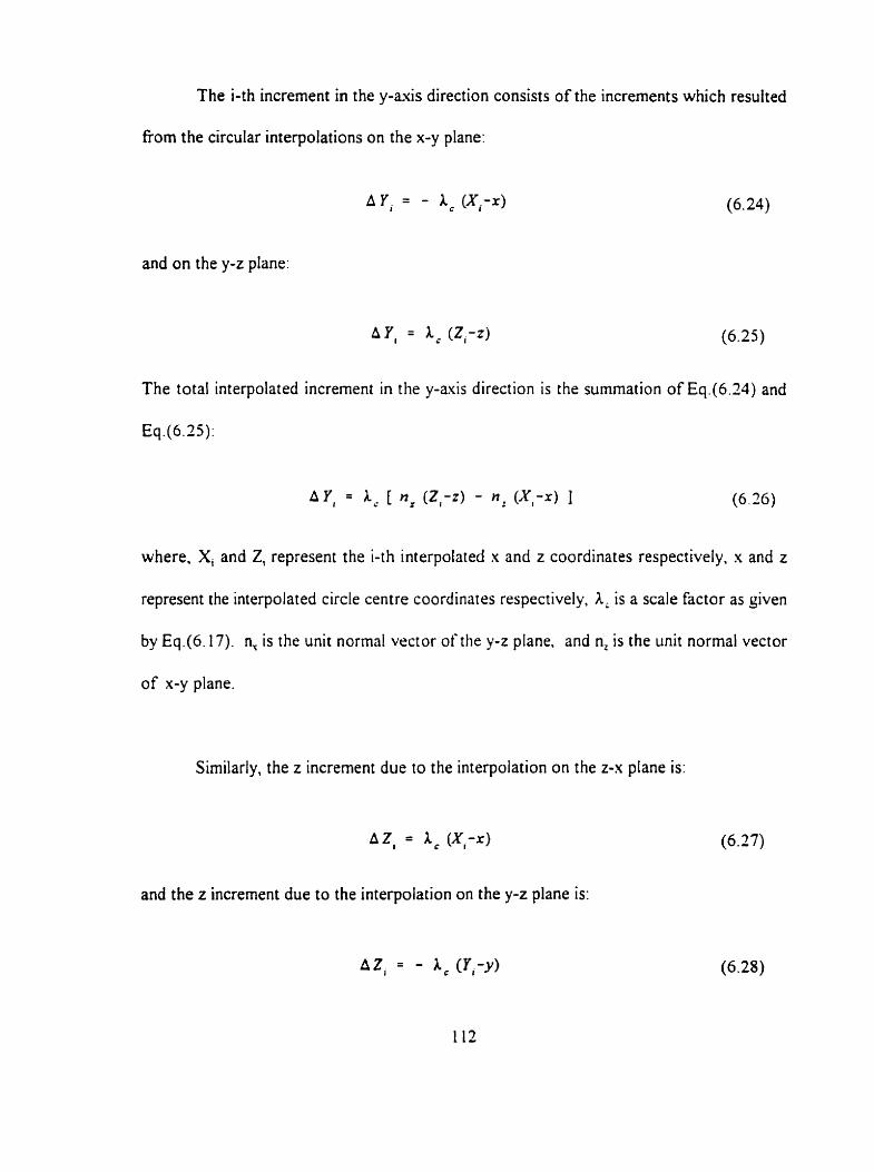
The i-th increment in the y-mis direction consists of the increments which resuited

fiom the circular interpolations on the x-y plane:

and on the y-z plane:

AY, = A c (2,-r) (6 .25)

The total interpolated incrernent in the y-axis direction is the summation of Eq.(6.?4) and

Eq.(6.25):

where, Xi and Z, represent the i-th interpolated x and z coordinates respectively, x and z

represent the interpolated circle centre coordinat es respectively. A, is a scale factor as given

by Eq.(6.17). n, is the unir normal vector of the y-z plane. and n, is the unit normal vector

of x-y plane.

Similarly, the z increment due to the interpolation on the z-x plane is:

A Z, = L (XI-x)

and the z increment due to the interpolation on the y-z plane is:

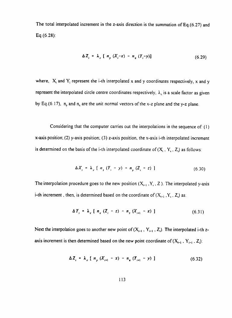
The total interpolated increment in the z-mis direction is the summation of Eq.(6.27) and

Eq.(6.28):

where. y and Yi represent the i-th interpolated x and y coordinates respectively. x and y

represent the interpolated circle centre coordinates respectively. 1, is a scale factor as given

by Eq.(6.17). n, and n, are the unit normal vectors of t he x-z plane and the y-z plane.

Considering that the computer carries out the interpolations in the sequence of ( 1 )

x-axis position; (2) y-axis position; (3) z-axis position. the x-axis i-th interpolated increment

is determined on the basis of the i-th interpolated coordinate of (X, . Y, . 23 as follows:

AX, = A [ t (Y, - y ) - ny (2, - ;) ] (6.30)

The interpolation procedure goes to the new position (X,., .Y, . Z ). The interpolated y-auis

i-th increment . then, is determined based on the coordinate of (Y-, .Yi. Zi) as:

Next the interpolation goes to another new point of (Y-, . Y,, . ZJ. The interpolated i-th 2-

axis increment is then determined based on the new point coordinate of (Y+, . Yi_, -23:

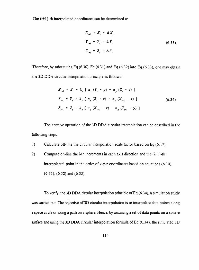
The (i+l)-th interpolated coordinates can be determined as:

XI., = XI + AX,

YJ., = Y, + A Y i

2 , = zi + AZI

Therefore. by substituting Eq.(6.30). Eq(6.3 I ) and Eq.16.32) into Eq . (6 .33) . one may obtain

the 3D DDA circular interpolation principle as follows:

The iterative operation of the 3D DDA circular interpolation can be described in the

followin~ steps:

1 ) Calculate off-line the circular interpolation scale factor based on Eq(6.17);

2) Compute on-line the i-th increments in each axis direction and the (i+l)-th

interpolated point in the order of x-y-z coordinates based on equations (6.30).

(6.3 1). (6.32) and (6.33).

To venQ the 3D DDA circular inierpolation principie of Eq.(6.34), a simulation study

was canied out. The objective of 3D circular interpolation is to interpolate data points along

a space circle or dong a path on a sphere. Hence. by assurning a set of data points on a sphere

surface and using the 3D DDA circular interpolation formula of Eq.(6.34). the simulated 3D

circular interpolated path was generated. A sphere centred at the origin of the coordinate

system and having the radius of 76.2 mm (3") was chosen for the simulation as shown in

Fig.6.4 . The assumed data points are on the space circle with the longitude angle 4 = 60" and

the latitude angle 8 varying from O" to 90" on the surface of the sphere. In order to investigate

the interpolation accuracy, the segment arc length between two consecutive assumed data

points was set to be varying. The segment arc lengths were assumed 10" latitude angle apan

for the region that the latitude ançle is between 60" and 90" of the sphere circle. The segment

arc lengths were assumed 15" latitude angle aput for the region that the latitude angle is from

30" tu 60°0f the sphere circle. and for the reçion that the latitude angle is between O" to 30"

of the sphere circle. the segment length was assumed corresponding to 3 0" latitude angle

apart. The interpolation feedrate was chosen as F=l524 mm/min. (60 ipm). and the

interpolation penod was chosen as T = 0.7 sec. Hence. the interpolation increment FT = 5.08

mm (0 .2") . A detailed discussion on how to select the interpolation parameters F and T is

given in Chapter 7.

The simulation was conducted as follows:

1) Based on the chosen interpolation feedrate, the interpolation period and the radius of

the sphere, the circular interpolation scale factor was calculated by usinç Eq.(b. 17).

This is an off-line calculation and the scale factor is a constant.

2) Based on the assumed data points on the sphere surface. the calculations of each

segment length on each axis was performed:

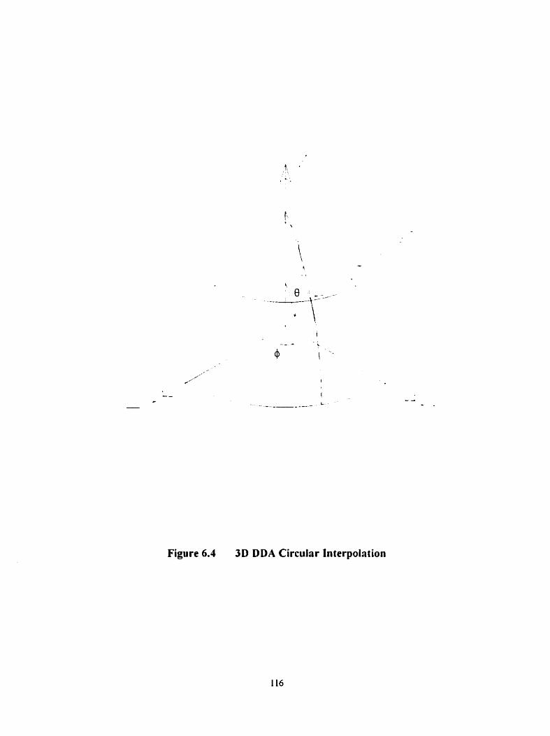
Figure 6.4 3D DDA Circular Interpolation

where, (x(k), y@), z(k)) and (x(k+ l ) , y(k+ 1), z(k+ 1)) represent the start and the

end points of the k-th segment, and L,(k). Ly(k) and L,(k) are the corresponding k-th

segment lengths along each mis direction.

3 ) The interpolation stan point (Xt, . Y,. 2, ) for each seçment was initialized:

4) The interpolation procedure was continued from step 5) when the interpolated

coordinates, X, ,Y, and 2, , had not arrived at the end point of the seçment, in which

case they would have satisfied the following condition:

when one or two of the conditions of Eq.(6.37) were not met, the interpolation

procedure in the axes directions would not be performed and the other axis direction

of interpolation continued from step 5). If al1 of the conditions were not met, the

interpolation procedures went on to the next segment.

5 ) The differences between the interpolated point (X, , Yi , ZJ and the end point

of the segment (X, , Y, , 2,) were calculated:

6) The interpolation procedure was continued from step 7) when the maximum ditference

among the D, , D, and D, calculated in step 5) satistied the followinç condition:

If the condition of Eq.( 6.39) was not met. the interpolation procedure repeated from

step 3). In fact, this happened when the interpolation procedure approached the end

point of the segent . Since the maximum difference was smaller than the interpolation

increment and usually was a very small value. it was then skipped and interpolation

went on to the next segment.

7) The interpolation increment in the x-axis direction was calculated based on Eq.(6.30);

8) The next interpolation point in the x-axis direction was calculated as fo1Iows:

where. the plus and the minus sign depended upon whether the interpolation increased

or decreased.

9) The interpolation increment in the y-auis direction was calculated based on Eq.(6.3 1);

10) The next interpolated point in the y-axis direction was calculated as follows:

where. the plus and the minus sign depended upon whether the interpolation increased

or decreased.

i l ) The interpolation increment in the z-ais direction was calculated based on Eq(6.32);

12) The next interpolated point in the z-asis direction was calculated as follows:

where. the plus and the minus sign depended upon whether the interpolation increased

or decreased.

The total number of interpolated points were 33 points among the assumed 7 data

points on the sphere surface. Since the segment arc lençths were purposely set varyinç alonç

the sphere circle path, the amount of interpolated points for each segment were different. The

shoner the segment arc length, the less points were interpolated. In fact, in the region when

the latitude angle was close to the equator. the amount of interpolated points were less than

that close to the pole. Fiç. 6.4 shows the interpolated path and the space curve on the sphere

surface. It is obvious that the interpolated path is aiong the space circle and the accuracy is

better at the region near to the equator, which is due to the fact that the shoner segment arc

length was assigned. The accuracy study results of the interpolation are outlined in Table 6.1.

The maximum interpolation error is 5.052 1mm (0.1989") which is smaller than the

interpolation increment: FT= 5.08 mm (0.2"). When the segment arc length is 10" apart. the

minimum interpolation error of 0.0203 mm (0.0008 ") resulted. The interpolation accuracy c m

also be improved by choosing a srnaller interpolation period. This simulated result verifies the

usefulness of the new 3D DDA circular interpolation principle.

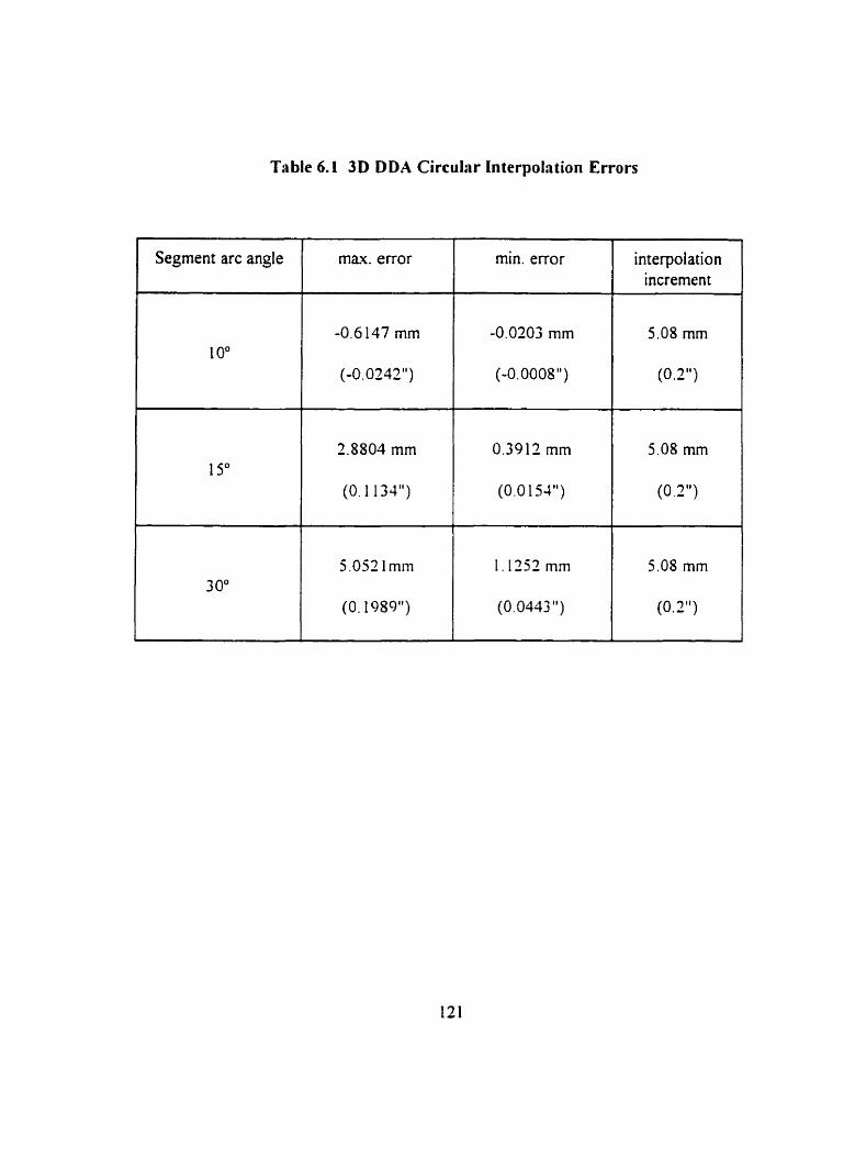
Table 6.1 3D DDA Circular Interpolation Errors

Segment arc angle max error min. error interpolation increment

6.6. A 3D Combined Linear and Circular Interpolation Principle

6.6.1 The Motion Trajectory of the OM-1 Milling Centre

The motion trajectory in five-axis CNC machining depends on different machine

configurations and rotational movements. The common configuration of five-axis CNC

machine tools include both the swivel-head and the rotary-table types. In the swivel-head

type, the spindlr chuck acts as the swivel (the rotational) movernents pivot. The 3D circular

swivel movements about the pivot superirnposed on the 3D linear motion of the pivot

constmct the combined 3D linear and circular motion trajectory. In the rotary-table type. the

intersection point of two axes acts as the pivot for the rotational movernents. The machine

table's 3D rotational movernents. superirnposed on the translational movements of the pivot.

form the 3D combined linear and circular motion trajectory. To analyze the 3D combined

motion trajectory, without loss ofçenerality. the OM- l millinç centre. which is the rotary-

table type, is considered in this work. From the OM- 1 confï~wration (see Fiç.4.4 ). it is known

that the rotational B,, axis and C,, axis are perpendicular and intersect at a space point. P, at

ail time during the machining processes while the machine table moves. Since the intersection

point P is on both the B, axis and the C,, axis, it rnoves translationally only. Thus, the

intersection point P acts as a pivot for the machining rotational rnovements, such that the pan

together with the machine table rotates about the moving pivot P tracing out a 3D non-linear

path. In other words, the actual CC point trajectory is constmcted by the 3D circular

movements (about the pivot P) which are supenmposed on the linearly interpolated

movements of the pivot P. Frorn this geometncal perspective. the CC point trajectory mode1

for the OM- 1 was determined as çiven by Eq.(4.19) and Eq.(4.20).

6.6.2 The Rotational Movements Interpolation Principle

In multi-axis CNC machining. the rotational movement increments are angles measured in

degrees. The common interpolation method for rotational movements is using the direct

function algonthm [7 11 as follows :

B, = B o + s ( B , - B o )

C l = C o + r ( C , - C o )

where, (Bi , CJ is the interpolated coordinate of the rotational movements in deçree units,

(l3, C,) and (B, , C,) represent the start and the end coordinates of the rotational movements

for the move respectively, r represents a parameter which is proponional to tirne and varies

intherangeof(0. 1). i.e.. r =Oat(B,, . C, ,)andt = 1 at ( B I , CI).

The direct function algorithm is designed for parametric space curves and is

particularly suitable to rotational movement angles. The 3D machine movements are

pararnetric functions of time. because each axis coordinate (linear position in length or

circular position in degree units) is a parametric function of time. Therefore. the direct

function algorithm is used to interpolate the rotaiional rnovements in five-axis machining.

6.6.3 A 3D Combined Linear and Circular Interpolation Principle

In conventional five-axis CNC machining. 3D Iinear interpolation principle is used to

coordinate the translational rnovements dong each 3D araight line segment and the rotational

movements are interpolated based on the direct function algorithm of Eq. (6 . 43). As a result,

the CC point trajectories are the 3D linear motions of the rotation pivot combined with the

3D circular motions about the rotation pivot as shown by the machining motion trajectory

model of Eq(4.19). The curved trajectories cause non-lineanty errors in multi-axis CNC

machining. To eliminate non-linearity errors. it is desired to conduct the CC point to move

along the 3D straieht line segment connecting the consecutive movement points. This can be

achieved if the rotational pivot (or the translational movements ) is interpolated along a

predesigned curve. say a 3 D combined linear and circular curve. Based on this geometrical

analysis. a cornbined 3D linear and circular interpolation principle is developed. The

corresponding 3D DDA linear and circular interpolation formula is:

The detailed denving procedure is provided in Appendix C.

Interpolating the rotational movements based on the direct function of Eq(6.43) and

interpolating the pivot P along the curve of Eq(6.44). i.e., coordinate the translational axes

based on Eq.(6. 44). the CC point is expected to move along the straight line segment with

constant feedrate at each move:

where. (x,(i), y,(i), q,(i))and (-Ji+ 1). y,,(i+ 1). q,(i+ 1 )) are the present and the next CC

point coordinates respectively. ( k ( 0 ) . y,@). &(O)) and (%( 1 ). ycc( 1 ), q,( 1)) are the start and

the end CC point coordinates of the segment. and A, is the linear interpolation scale factor.

6.6.4. Proposed Methodoloçy for Solving the Non-Linearity Error Problern

What follows is the proposa1 of a methodology which can be utilized to solve the multi-mis

CNC machininç precision problem. The method. applyinç the 3D cornbined linear and circular

interpolation principle, coordinates the translational axes. or the rotation pivot. alonç the

predesigned curve seçment and conducts the CC point to move along the 3D straight line

segment co~ect ing each two consecutive machiring data points. The rnethod interpolates the

CC point coordinates which are determined from the machine motion trajectory model. By

comparing the coordinates of the interpolated point and the end point of the seçment, the

iterative interpolation is performed. The procedure for perfonning the iterative interpolation

can be presented in the following algorithm.

3D Combined Linear & Circular Interpolation Alonthm

1) Compute off-Lne the stan and the ending CC point coordinates for each segment by

using the machine motion trajectory rnodel (for OM-1. usinç Eqs. (4.19) and ( 4. 20));

2) Calculate off-line the interpolation scale factors for each segment:

2.1) Calculate each segment lengt h:

where, the i n d e ~ e. represents t h e end point and the index, S. represenis the start

point.

2.2) Calculate the linear interpolation scale factor: A, = FTL;

2.3) Calculate the rotational (3D circular) movements radius. R. which equals

io the distance between the CC point and the rotation pivot. Hence. one may

have:

where. (x,,,. y, , q,,) are the NC-codes coordinates. x , , , is the spindle position x-

coordinate, C,i,m, is the C,, a i s pivot constant and GL is the cutter çafe iençth as

shown in Fiç.4.1.

2.4) Calculate the circular interpolation scale factor: h, = FTR;

3) On-line interpolation routine:

3.1) Interpolate the CC point coordinates based on the stan point

(xcc (s), y, (s), z&)) and the end point (x, (e). y,., (e) . q , ( e ) ) of the segment:

3.2) Interpolate the translational axes coordinates in the following order: x-axis- y-

âuis- z-ais. Thus, the 3D linear and circular interpolation of the pivot centre is:

3 . 3 ) Interpolate the rotational axes circular movements accordinç to the direct

fùnction alçori thm as foliows:

4) Calculate the lençth between the start point and the present interpolated CC point:

5 ) Compare the coordinates of the interpolated point with the end point of the segment

by performing the test:

If the test is tme, perform step 6) . othenvise go to step 7).

6) Repeat the interpolation routine on the present segment by performing the steps 3)

to 5).

7) Determine the modified feedrate if the test is false:

and modify the interpolation scale factors: k , = F' TIL and h, = F' Tm;

and repeat the step 3) to reach the end point of the segment.

8) Repeat the steps 3 ) to 7) on next segment until the machininç arrives at the end of the

6.7. The Software Interpolation Routine

The first step in the overall design of a CNC system involves the selection of an appropriate

control technique and the optimal settinç of the control loop parameters. Subsequently, an

appropriate interpolaior routine that generates the reference signals to the control system

mua be desiçned. The reference-word interpolation technique in the sampled-data system has

been comrnonly employed in current CNC systems. Therefore. the new 3D combined linear

and circular interpolation technique is designed as a reference-word type interpolator. In the

sampled-data system. the interpolation calculation is perfomed by the soflware interpolation

routine in the MCU. The tool path data input into the MCU must be pre-processed, which

includes decoding the tool path data into a set of cornputer system data, performing cutter

compensations if needed, and distributing feedrate to each axis of motion. M e r preparatory

processing, the data are inputted into the interpolation routine and the interpolator computes

the intermediate coordinates of positions based on the appropriate interpolation algorithm.

The proposed software interpolation routine computes the coordinates based on the algorithm

developed in section 6.6. The software interpolation routine includes the following functions:

I ) A function accepting the machining NC-codes and the machining parameters such

as the specified feedrate and the chosen interpolation period;

2) A hnction determininç the CC point coordinates that correspond to the end points

of each movement (the machine motion trajectory model is employed);

3 ) Three functions computiny the interpolated translational axes coordinates based on

the 3D combined linear and circular interpolation principlr cf E q (6. 49);

4) Two functions calculating the interpolated rotational rnovements coordinates based

on the direct function algorithm of Eq. ( 6 50).

A flow chan of the new interpolation software is shown in Fiç. 6.5. The program

starts by inputtinç the machining parameters: the specified feedrate F and the chosen

interpolation period T, and the machining NC-codes. Then, the CC point coordinates of the

end points of each segment is computed. Using the rnachining parameters and the NC-codes,

the Iinev and circuiar interpolation scale factors can be deiermined. These are constants for

each machining step move and are calculated off-line pior to the on-line execution of the

!

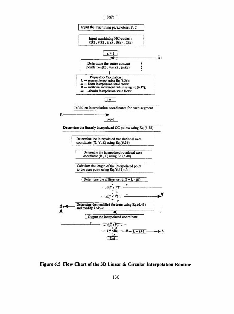
input the machining panimetcn: F, T 1 ,

1 Input machining NC-eodes : 1

1

1 a), Y&) 9 BOr) , W) 1

I

P~para ioy Caicuiation : L - q m a i t Icngth ushg Eq.(636);

J AI - liPtar inrcrpolatian scalc faw, R - rotational mavunent radius ushg Eq.(6.37); '

Ac - cllculaf inttrpohiion d c faftor . 1

initialize interpolation coordinates for each segment

i Determine the lincvly inkrpolaed CC points using Eq(6.38)

1 Determine the intcrpolated ~~islational axcs coordiaatt (X, Y, Z) using Eq(6.39)

Determine the interpolated romtiod axcs mtduiau (B , C) using Eq.(6.40)

Calculate the Ieugth of the interpolami point to the start point using Eq,(6.4 1 ): 1 ( i )

Determine the di ff&ence: diff = L - i(i)

Deknnioe the modided feednte using Eq.(6,43) and d i f y AI&AC 1 :

A , -

i : Output the intrrpolatcd coordinsttc ! 1

Figure 6.5 Flow Chnrt of the 3D Linerr & Circular Interpolrtion Routine

130

interpolation. Then, real-tirne interpolation begins by initializing each a i s coordinate for each

segment. The interpolated positions of the translational and rotational axes are then computed

successively. The iterative computation of the interpolated positions for each axis is

perfomed under the conditions that the total interpolation incremented length of I ( i ) is less

than the segment length of L, and the rernaining lençth of (L - I(i) ) is greater than the

interpolation increment as given in Eq. (6 .52) . In the case that the remaining length of (L -

I(i) ) is smaller than the interpolation incrernent, the remaining length is used to modify the

feedrate which. in tum. is used to command the axes to reach the end point of the segment.

This interpolation routine is repeated until al1 the NC-codes are completed. For the final

interpolation point. it should be noted that each axis may not arrive at the segment end at the

same time since each axis segment lençth is different. The interpolation process on next

segment. however, is started at the same tirne for each avis since the iterative interpolation

is pedomed under the condition of Eq.(6 5 2 ) and the feedrate adaptation procedure is used.

The new software interpolation routine is coded in the programrning langage C. in order to

adapt to general CNC machine tool control systems.

6.8 Summnry

In this chapter, a methodology for solving the non-linearity error problern in ultra-precision

five-auis CNC machining was proposed. Based on the 2D DDA circular interpolation

principle, the 3D DDA circular interpolation formula was developed and a simulation using

the proposed 3D circular interpolation principle was performed. The simulated result

demonstrated the validity and the precision achieved by the new 3D circular interpolation

principle. Then, a 3D cornbined linear and circular interpolator was designed based on the 3D

DDA linear and circular interpolation principles. A software interpolation routine based on

the 3D cornbined linear and circular interpolation algorithm was developed. The software is

capable of generating the reference-word signals to the machine axes control loops of the

sarnpled-data systems, such that the machine translational axes can be driven to move along

the predesigned curve and the machine rotational movements cm be driven tc move circularly

in space. The CC point thus cm be conducted to move along the straight line segment, so that

the non-linearity errors can be eliminated.

CHAPTER 7

AN APPLICATION OF

THE INTERPOLATOR DESIGN TECHNIQUE

7.1 Introduction

Applying the '3D cornbined linear and circular interpolation technique' proposed in Chapter

6, the process of machining the airfoil surfaces of an impeller is sirnulated and is presented in

this chapter. The simulated results demonstrate that the proposed 3D linear and circular

interpolator drives the translational axes dong the predesigned 3D c u v e and conducts the CC

point dong the straight line segment that connects each two consecutive machining data

points, so that eliminaiion of non-lineanty errors is achieved. In the following, the

interpolation preparatory data processing procedure is outlined in section 7.2. Based on the

data from the interpolation preparatory data processing. the conventional five-axis CNC

machininç process for machins the airfoi1 surfaces of an impeller is simulated and the result

is outlined in section 7 .3 . This simulation result is then compared with that from the

simulation of machininç the same airfoil surface usinç the proposed 3D linear and circular

interpolator (section 7.4).

7.2 Interpolation Prepnrntory Data Processiiig

An NC part program contains the data of the geometric information of the machined surfaces

(the coordinates of the tooi path) and the motion information of the rnachining (the feedrate

and the auxiliary fùnctions data). These data cannot be directly input into the interpolation

routine in the MCU of the control computer, and must be processed by the data processing

unit in the MCU before the interpolation is executed. This interpolation preparatory data

processing includes: (i) the decoding of the NC-codes into a set of computer systern data

based on standard format, (ii) the cutter compensations to obtain the cutter centre tool path

if the tool path is generated based on the contour of the machined surface, and (iii) the

feedrate caiculations for each avis of motion to generate cornmands to the control loops. The

procedure for interpolation preparatory data processing usually involves the following steps:

1) The NC-codes are input and stored in the NC-codes buffer;

2) The data decodinç routine in the MCU processes a block of NC-codes data and store

it in the decoded data buffer;

3 ) The cutter compensation routine in the MCU determines the cutter centre coordinate

based on the surface çeornetry and the cutter radius if the tool path is generated based

on the contour of the surface to be rnachined. and then stores the compensated data

in the cutter compensator data butrer;

4) The feedrate routine in the MCU calculates the feedrate for each axis of motion for

the machining movement and stores the data in the system workinç buffer;

5) The MCU transfers the data into the interpolation reçister and the interpolation

process can be staned.

The data decoding process is needed for different computer systems of CNC machine

tools in order to perforrn the other MCU tùnctions. In this study, however, for the purpose

of simulating the function of the new interpolator, the NC-codes for machining the airfoil

surfaces of an impeller are directly used in the interpolation calculation.

In machining simple or regular geometry surfaces, such as a plane or circular shaped

surface, the NC-codes are usually generated from the contour of the surface. Cutter

compensation is required to obtain the cutter centre coordinates of motion. This can be

accomplished by using the cutter compensation techniques as given by Liu and Lei [72] and

Li, et. al. [73]. For machining complex 3D surfaces ( Le. the sculptured surfaces), the tool

path is usually generated in terms of the cutter centre positions. Hence. there is no need to

perform the cutter radius compensation process. and cutter lençth compensation is usually

perfoned by compensating the spindle lençth. In this study. the available CLDATA for

machining the airfoil surfaces of an impeller were generated in terrns of the ball-end cutter

centre position coordinates. therefore, the cutter compensation process is not required in the

simulation study.

The feedrate calculation is closely related to the interpolation process of the machine

axes movements. The feedrate calculation determines the step increment in an interpolation

penod for each axes of motion based on the specified rnachining feedrate. Many factors affect

the rnachining feedrate, the specification of which m u a be based on the materials of the cutter

and the workpiece, cutter geometry data (cutter radius and length). depth of cut and cutting

velocity. In this study, assuming that the matenal of the workpiece is titanium and the material

of the cutter is carbide, and considering the depth of cut is for the tinish machininç and the

cutting velocity is that equivalents to the spindle speed of 1200 rpm. the feedrate is specified

as 25 mmlsec (60 ipm).

In conventional five-awis machining, the feedrate specified in tems of the inverse-time

feedrate word (inverse-tirne FRN) is recornmended. since the rotationai movements are

involved. The feedrate specified in trrms of the direct feedrate word (IengtWtime units) is

defined for linear movements. Changes in rotational movements are measured in degrees.

Therefore, the direct feedrate word is not suitable for anglehime units. The inversr-time FRN

is defined as the time required for the cutter moving in the angular/linear position chançe of

a machining step. By using the inverse-time FRN and the linear or angular position change

on each axis. the feedrate alonç each axis can be determined. The specified feedrate

represented as the inverse-time FRN in the NC-codes is by setting the G tiinction as G93. For

point milling, each seçment lençth can be calculated from the cutter position coordinates.

Using the seçment lençth for the k-th machining step move, L, . and the specified feedrate.

F, the inverse-time FRN can be determined as:

Using the inverse-tirne FRN, . the feedrate calculation routine in the MCU then

calculates each mis speed for the k-th segment movement as follows:

Based on these axis feedrates F, . F, . F, and the interpolation pet-iod T. the linear

interpolator generates the incrernents for each a4s of motion:

The determination of the interpolation period must consider interpolation accuracy.

which directly affects the rnachining precision of the whole CNC system. It should be greater

than the tirne required for perforininç the actual interpolation calculations since the MCU

performs not only the interpolations but also the other on-line tasks. The Pythagorean

theorem used by Huang [74] gives the relational function of the rnacliining precision measure,

Le.. the machining tolerance t , the machining feedrate F and the interpolation period, T . as

foi10 ws:

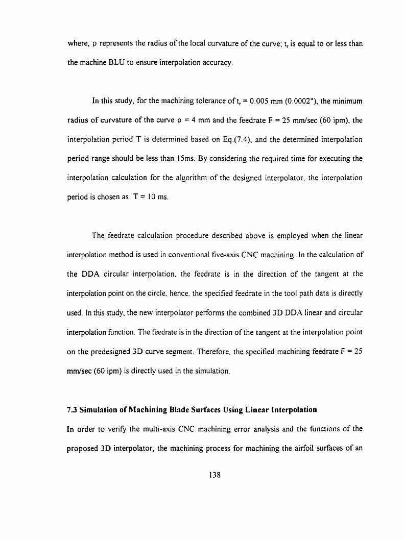
where, p represents the radius of the local curvature of the curve; t, is equal to or less than

the machine BLU to ensure interpolation accuracy.

In this study. for the machining tolerance of t, = 0.005 mm (0.0002"), the minimum

radius of curvature of the cuwe p = 4 mm and the feedrate F = 25 mdsec (60 ipm). the

interpolation period T is determined based on Eq.(7.4), and the determined interpolation

period range sliould be less than 15ms. By considering the required time for executing the

interpolation calculation for the algorithm of the designed interpolator, the interpolation

period is chosen as T = 10 ms.

The feedrate calculation procedure described above is employed when the linear

interpolation method is used in conventional five-axis CNC machining. In the calculation of

the DDA circular interpolation. the feedrate is in the direction of the tangent at the

interpolation point on the circle. hence. the specified feedrate in the tool path data is directly

used. In this study, the new interpolator performs the combined 3D DDA linear and circular

interpolation fùnction. The feedrate is in the direction of the tangent at the interpolation point

on the predesigned 3D curve segment. Therefore. the specified machins feedrate F = 25

mm/sec (60 ipm) is directly used in the simulation.

7.3 Simulation of Machining Blrde Surf;ices Using Linerr Interpolation

In order to veriS, the multi-axis CNC machining error anaiysis and the functions of the

proposed 3D interpolator. the machining process for machining the airfoil surfaces of an

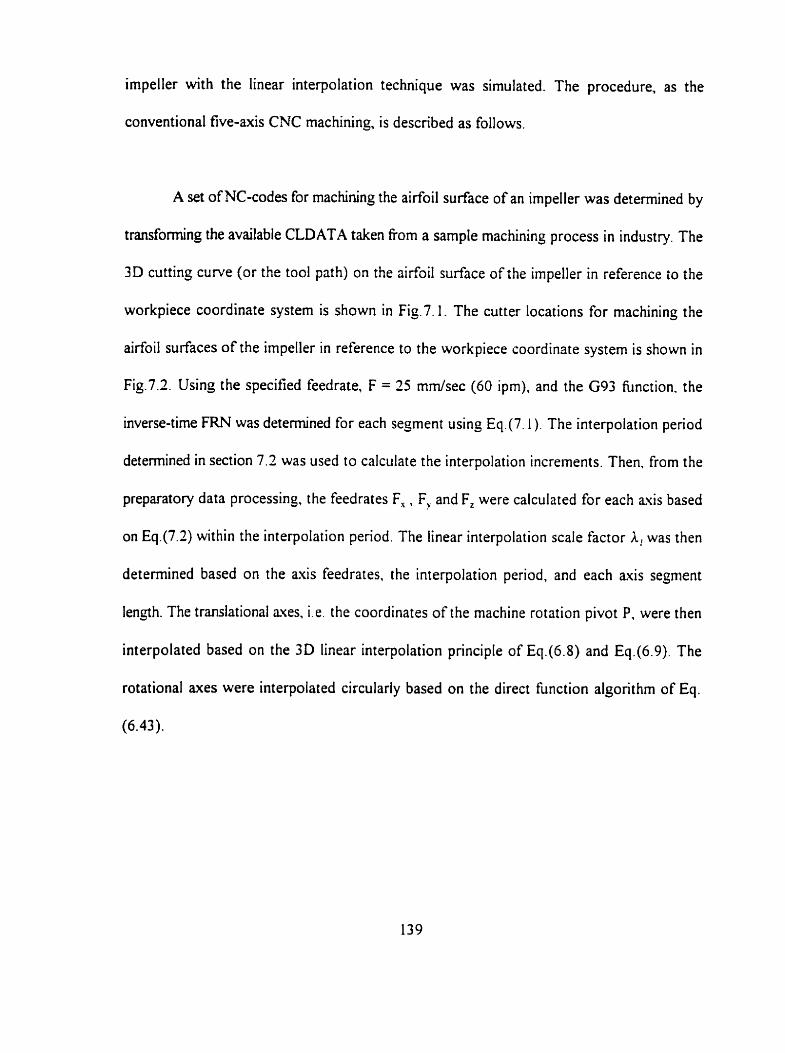
impelier with the linear interpolation technique was simulated. The procedure, as the

conventional five-axis CNC machining, is described as follows.

A set of NC-codes for machining the airfoil surface of an impeller was determined by

transforming the available CLDATA taken from a sample machining process in industry. The

3D cutting curve (or the tool path) on the airfoi1 surface of the impeller in reference ro the

workpiece coordinate system is shown in Fig.7.1. The cutter locations for machining the

airfoil surfaces of the impeller in reference to the workpiece coordinate systern is shown in

Fig.7.2. Using the specified feedrate. F = 25 rnrnhec (60 ipm). and the G93 function. the

inverse-time FRN was detemined for each segment using Eq47.1). The interpolation period

detemined in section 7.2 was used to calculate the interpolation increments. Then. from the

preparatory data processing, the feedrates F, , F, and F, were calculated for each axis based

on Eq.(7.2) within the interpolation period. The linear interpolation scale factor A , was then

determined based on the axis feedrates, the interpolation period, and each axis segment

length. The translational ayes, i.e. the coordinates of the machine rotation pivot P. were then

interpolated based on the 3D linear interpolation pnnciple of Eq. (6.8) and Eq.(6.9). The

rotational axes were interpolated circularly based on the direct function algorithm of Eq.

(6.43).

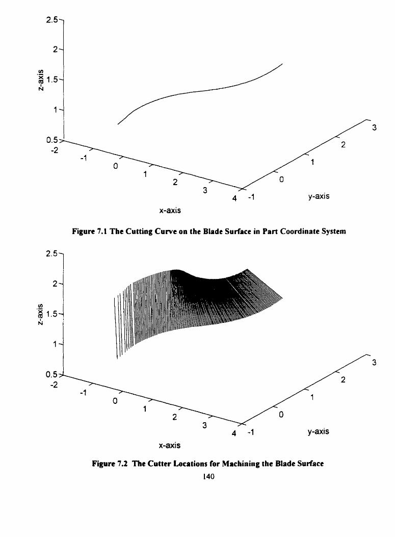
x-axis

Figure 7.1 The Cutting Cuwe on the Blade Surlace in Part Coordinate System

4 -1 x-axis

y-axi s

Figure 7.2 The Cutter Locations for Machining the Blade Surlace

140

The linear interpolation and the direct fùnction algonthrns interpolated the

translational and the rotational movement coordinates in each interpolation period as in the

real machining process. The corresponding cutting point (CC point) moved along the

machining motion trajectory. The CC point coordinates, for the OM-1 milling centre, was

then calculated based on the OM-1 machininç motion trajectory model of Eq44.19) and

Eq.(4.20).

The resulting CC point path in reference to the machine coordinate sysrem is plotted

as shown in Fiç.7.3. It can be seen that the CC point path is fonned by a series of space curve

segments. which is a fact that is obvious from the OM-1 non-linear machininç motion

trajectory model. The enlarged closer view of the CC point path between adjacent machininç

data points shows that the CC point moves alonç the non-linrar curve segments which

deviate from the straight line segments connecting each pair of the machining data points

when the rotation pivot (or the translational axes) was linearly interpolated. The machininç

errors. resulting from the simulation using the linear interpolation method. were determined

and a sample of the machining errors are shown in Table 7.1. It shows that the total

machining error for each move consists of both the linearity error and the non-linearity error.

The simulation results confirm the rnachining error analysis indicating that the non-

linear curve segments deviate from the linearly interpolated straight line segments. which

causes non-lineanty errors. The result also shows the inadequacy of the linear interpolation

method when applied to current multi-ais CNC rnachining of convex surfaces.

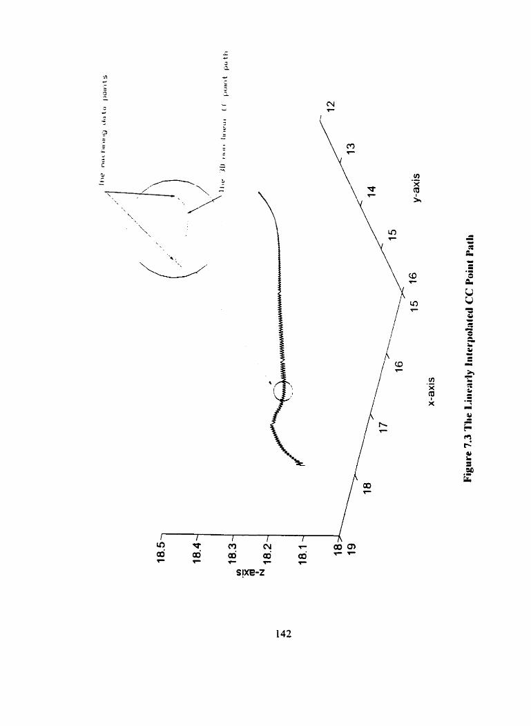
7.4 Simulation of Machining Blrde Surfaces Using the Proposed lnterpolator

Applying the proposed interpolator. the '3D combined linear and circular interpolation

technique,' to process the same set of NC-codes for machining the airfoil surface, a simulation

was perfomed. Using the OM-1 inverse kinematic mode!. a set of NC-codes was determined

by inverse transforming the available CLDATA as s h o w in Fig.7.Z. The procedure followed

the proposed algorithm in section 6.5 and is described next.

The 3D combined linear and circular interpolator is designed to interpolate the

machiiiing translational movements. i.e., the 3D coordinates of the rotational movements

pivot, such that the rotation pivot moves alonç the predesigned 3D linear and circular curve

segments and the CC point of the cutter moves a small straight line increment from one

cornmand to the next dong the 3D straight line segment connectinç the end CC points. In the

interpolation calculation. as a precalculation. the CC point coordinates which correspond to

the tool path data points were determined based on the already-known NC-codes and the

OM-1 motion trajectory model. Then, these CC point coordinates were linearly interpolated

and used in the calculation of interpolated positions of the rotation pivot. The specified

feedrate of F = 25 mdsec (60 ipm) and the interpolation period T=IO ms were used to

calculate the interpolation scale factor for each interpolation increment. The initial

interpolation coordinates of the rotation pivot P were assigned as the start point coordinates

of each segment. In the first interpolation period, based on the linearly interpolated CC point

coordinate, the first point of translational movernents was interpolated by using the 3D

combined linear and circular interpolation formula of Eq.(6.49). The rotational movements

were interpolated in the same way as in the Iinear interpolation simulation of section 7.3. The

interpolated position and rotation coordinates were sent to each machine avis control loop

as the reference-words. It should be clarified that the control Ioops were not sirnulated in this

interpolaior function simulation study. M e r sending the interpolated position coordinates,

the interpolated CC point increment was compared with the present segment length, L, which

was pre-determined using the CC point coordinates for the segment. Upon the companson

of the interpolation incremented length with the segment length. L. the interpolation was

continued since the first increment was shorter than the segment length. In the second

interpolation period. the second point of the translational axes and the rotational axes

incremented coordinates were interpolated on the basis of the first interpolated coordinates.

Next, the total length of the interpolated increments was compared with the present segment

length, L. Upon the cornparison, the interpolation was performed on the present segment or

continued on to the next seçment. This iterative interpolation procedure repeated until the

interpolated point reached the end point of the seçment. When the test showed the difference

between the total length of the interpolated increments and the seçment length was shoner

than one interpolation increment F*T. the feedrate was modified as in the algorithm presented

in section 6.5 and the interpolation scale factors were also re-calculated. The 3D linear and

circular interpolation was continued to calculate the new increment. Thus, the end point of

the segment was reached. The same procedure was perfcned on each consecutive segment

of the complete set of NC-codes.

The interpolated pivot point path in reference to the machine coordinate system is

143

ploned as shorvn in Fig. 7.4. It can be seen that the pivot point path is constnicted by a series

of 3D curved segments, and the eniarged closer view of the pivot point path between adjacent

rnachining data points shows that the pivot point moves along a 3D non-linear curve segment

which deviates from the straight line segment connecting the machining data points. The

corresponding interpolated CC point path in reference to the machine coordinate system is

ploned as shown in Fig. 7.5. It clearly show that the resulted CC point path is formed by a

series of smooth segments. In fact. the CC point path is connecred by a set-ies of line segments

when the rotation pivot was interpolated alonç the pre-desiçned 3D curve segments.

Obviousl y. the non-linearity error for each segment is eliminated. The machining errors

resulting from this simulation were also cornputed as shown in Table 7.1. The resulting

machining errors using the proposed interpolator consist solely of linearity error for each

rnove.

Compared with the result obtained from the linear interpolation simulation. the linear

interpolation method is simpler. but it results in both linearity errors and non-linearity errors

which cause dificulties for ensuring machining precision. Aternatively. the '3D combined

linear and circula. interpolator ' conducts the CC point to move along straight line segments.

so that the ody machining error for each segment is the linearity error. Although the proposed

interpolator needs more calculations to interpolate the position points as compared to the

linear interpolator, the non-linearity error for each segment is eliminated. The simulated

results show that the proposed interpolation technique is superior to the linear interpolation

method since the resulting motion trajectory causes only the linearity rnachining error.

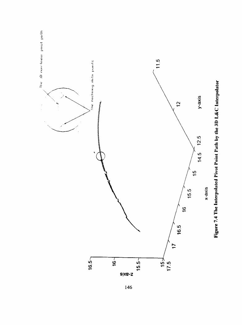
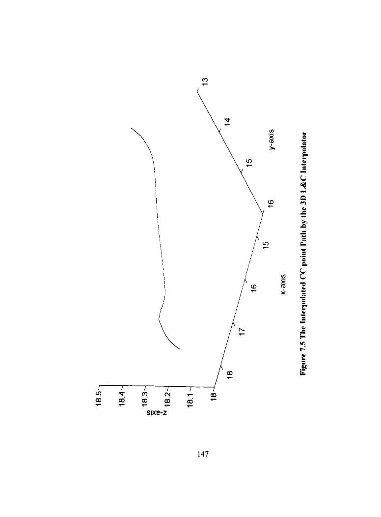
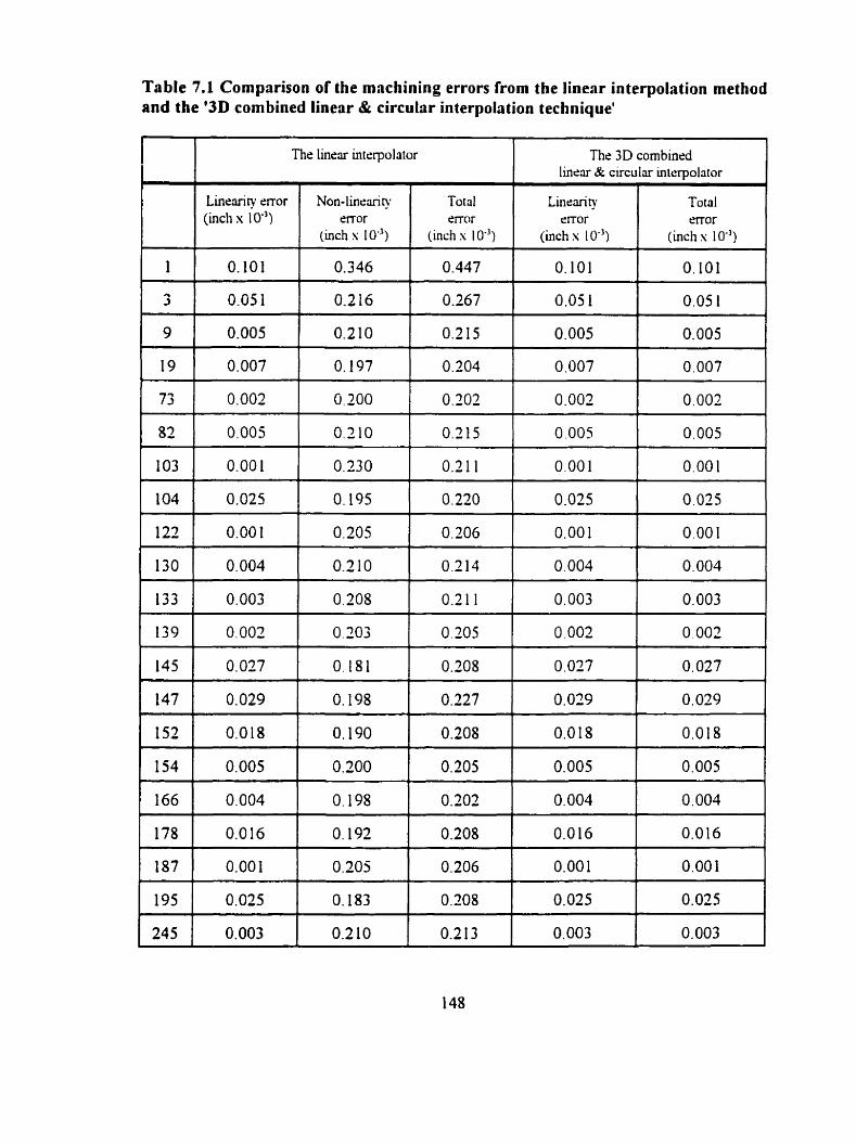
Table 7.1 Comprrison of the machining errors f'rom the linerr interpolation method and the '3D combined linerir & circuhr interpolation technique'

The Iinear intrrpolator -

The 3D combined linear & circular intemolator

Linerui ty error (inch x 1 (Y3)

Non-1inea-i ty enor

(inch s 1 O")

Total error

(inch s 1 0")

Lineaity mot-

(inch s 1 O-')

Total rrror

(inch s 1 O-')

CHAPTER 8

CONCLUSION

AND

RECOMMENDATION FOR FUTURE RESEARCH

8.1 Conclusion

The non-linearity error problem is the main obstacle to ensuring machining precision in multi-

axis CNC rnachining of sculptured surfaces. The nature of the problem is that superimposinç

rotational movements on translational movements yields non-linear machining motion

trajectories, which deviate from the lineariy interpolated straiçht line segments resulting in

non-lineanty errors. Five-axis rotational movements are kinematically related to cutter

orientations. therefore. one of the factors causinç non-lineanty errors is cutter orientation

changes. Another factor contributinç the non-linearity error problem is due to the linear

interpolation method which is not able to trace the non-linear motion trajectory in five-ais

machining. The objectives of this thesis work were to develop novel procedures to eliminate

the problem. The first objective was to develop an off-line tool path generation method which

tackles the problem from off-line cutter orientation generation. The second objective deals

with the development of an on-line 3 D interpolator design technique.

As the achievement of the first objective, an off-line tool path generation

methodology, the 'minimum error tool path seneration method', has been developed. This new

method is capable of reducing non-linearity errors to mect machining precision requirements

and has the following charactenstics:

Ability to obtain high machining precision is increased without undesired

consequences. compared to the existing off-line methods.

Generation of CLDATA is based on the geometnc properties of the machined

surfaces, the machining kinematics and motion trajectory;

Optimum machininç SC-codes cm be generated by rnodiQing off-line cutter

orientations without inserting extra machining position data;

Capacity for generatinç smoother tool path is irnproved. thus ensuring feedrate fidelity

and resulting in better machined surface finish;

Requirement for data storage memory size is reduced;

Machininç time cm be reduced.

A software package for implementing the proposed off-line 'minimum error tool path

generation method' has been developed. The software can be usrd (i) to directly generate NC-

codes specifically suitable for OM-1 millinç centre: (ii) to çenerate NC-codes for other OM-

series five-axis CNC machine tools by inputting different machine configuration data and

setup data. Case studies were performed by applying the proposed 'minimum error tool path

generation method'. It was verified through simulation that the new method increased

machining precision from 0.0 l27rnm (0.0005") to 0.005 mm (0.0002"). In other words, the

proposed method increased the machining precision by an amount of 30% without undesired

consequences such as the incorrect cutter orientation and the feedrate fidelity problems,

compared with the result of 'linearization process'.

An on-line 3D interpolator design technique for solvinç the multi-axis CNC machining

non-lineanty error problem has been proposed which fulfills the second objective of this

thesis. Conventional CNC machining systems support functions of 2D circular and 3D linear

interpolations, which are unfortunateiy inadequate for the machining of highly complex 3D

surfaces. A 3D software circular interpolation principle has been developed in this thesis,

which is capable of tracking sphencal curves with low position errors and uniform feedrate.

To veriS, this 3D software circular interpolation, a cornputer simulation of interpolating a 3D

curve has been performed. The interpolaied space path s h o w in Fig. 6.4 illustrates the new

interpolatots 3D circular interpolation capability. and the interpolation errors analysis results

given in Table 6.1 showed small curve tracking errors. On the basis of this software-based 3D

circular interpolator. a '3D combined linear and circular (L&C) interpolation technique' has

been proposed. which provides a solution to tlie m ~ l t i - ~ s CNC machining non-linearity error

problem and has the followinç characteristics:

1) Applicable to çeneratinç command signals for accurate position-trackinç of 3D non-

linear trajectones;

2) Applicable to eliminating non-linearity errors in five-ais CNC machining;

3) Applicable to machining 3D curves on five-axis machine tool systems of al1 types;

4) Uniforrn machininç feedrate for each rnove can be obtained;

5) Small data storage rnemory are required.

.A software interpolation routine which implements the '3D combined linear and

circular interpolation technique' has been developed. The software is applicable to the

machining on the rotaiy-table type five-auis CNC machine tools, and can be extended to other

types of five-axis CNC machine tools. Computer simulations have been performed to venS,

the proposed '3D combined linear and circular interpolation technique' and to compare it with

the Linear interpolation method. In the simulation of the machining process in section 7.3. the

elirnination of non-linearity errors were conducted successfùlly. Such capability is unattainable

using the existing linear interpolation method or using the 'linearization processes'.

The results of the research work in this thesis are innovative and contribute solutions

to present day concerns in the manufacturing industry. The 'minimum error tool path

generation rnethod' is readily applicable in off-line tool path generation for OM-series five-axis

CNC machine tools. and can be used to increase machininç precision considerably The off-

line method can be funher extended to a11 type five-axis machine tool configurations. The

proposed '3D combined linear and circular interpolation technique' can be used in tive-axis

CNC machine tool systerns once implemented and tested in the real-time machining

environment. The proposed technique possesses the ability of elirninating non-linearity errors.

and if the proposed technique is verified by successfùl experimental study and proves to be

effective in on-line application. the benefits to industry would not oniy include reduced

machining time and greater precision. but also reduced post-machininç processing time.

8.2 Recommendation of Future Research

The followinç topics are sugçested for further research to expand the present work:

1. Generalization of the 'minimum error tool path generation method' software:

The 'minimum error tool path generation method' is machine type-specific since it

uses the individual machine's kinematic models and motion trajectory model. The

software of implementing the off-line method developed in this thesis contains the

functions and machine configuration data which are specific for use with OM- 1 rnilling

centre. In order to adapt the off-line method to different machine tool configurations

and machining set-up. the software requires extension to different machine kinematic

rnodeis and machine motion trajectory rnodels. Therefore. for future work. it is

recommended that the software be extended into a general application which can

apply the proposed off-line method to all types of tive-axis CNC machine tool

configurations.

2. Experimental study of the 3D combined linear and circular interpolator:

The simulation of usinç the '3D combined linear and circular interpolation technique'

has been perforrned. which dernonstrated the ability of the interpolator to eliminate

non-linearity errors. To verify and evaiuate the whole performance of the proposed

interpolator not oniy from the machining errors issue but also from actual rnachininç

time concerns, experimental studies are required. Through expenments. the adaptation

of the proposed interpolation technique to CNC control systerns can be irnplemented,

and the required machininç tirne and position tracking accuracy can be verified using

the real-tirne feedrate and cuttinç force control. Experimental study can be performed

by modifjing the controllers of five-axis CNC machine tool systems.

3. Feedrate study of the 3D combined linear and circular interpolator:

The '3D combined linear and circular interpolator' is capable of driving the CC point

dong the space straight line segments with constant feedrate. but without considering

the feedrate continuity between segments. In addition. the feedrate adaptation

procedure in the proposed interpolator is not a best solution to ensure uniform

feedrate in each machining move. Therefore. it is recommended that research work

is continued on the subject of feedrate continuity and control in machine CNC

systems.

1. Choi, B. K., Lee. C. S., Hwang. J. S . and Jun, C. S.. 1988, " Compound Surface Modelling

and Machining", Compiîier Aided Desipi, Vol. 20, No.3, pp. 127- 136.

2. Wu , C. Y. , 1994, "" Arbitras, Surface Flank Milling of Fan. Cornpressor, and Impeller

Blades", AS2.E. ~ h e hi~enzcl~iomd Gus Twhi~w arid Arrorttgiiir, ~~o!rgress miJ Exposifion.

The Hapîc.. )rrtherlm& JIIIILJ 13- 16, pp. 1-7.

3. Bedi. S.. Gravelle, S. and Chen. Y. H.. 1997. " Principle Curvature Alignment Technique

for Machining Complex Surfaces". AShfE, Jortniol of ll./tritirjtrc~rrri~ig Sckcir,icr u~id

Ecir,ighrreri~g, Vol. 1 19. No. 4(8), pp. 756-765.

4. Vickers, G. W. and Quan, K. W., 1989, " Ball-mills Versus End-mills for Curved Surface

Machining", Tmisricfioii cf the .4ShlE, Jmr,nid rfl E~igicir,ic~.ri~~gfir bidirs~~v. Vol. 1 I 1 ,

pp. 22-26.

5. Renker. H. J.. 1993, "Collision-Free Five-PLUS Miliing of Twisted Ruled Surfaces". rl~rmls

ojthc /TZP. Vol. 42. No. 1.

6. Liu. X. W . , 1 994, "Niimericai ( ' o ~ r o i C I Theory uii J N( ' progrumm N I R

Trchnology", ((;hi?iese ), Manufacturinç Industrial Press.

7. Koren, Y ., 1995, " Five-axis Surface Interpolators ". A~i~ials of the ('IRP. Vol. 441 1, pp.

379-382

9. Chou, J. J and Yang. D. C. H.. 199 1 . " Command Generation for Three-Axis CNC

Machining", Joirmal of Eqitweri t~gfor hid~istry, Vol. 1 1 3 , pp. 3 05-3 10

10. "CA TM II User A4awol" , 1985. Version 2, Release 1, Dassault Systems.

1 1. "CA TIA IV User Mutitrai" , 1996, Version 4.1 .8 , Dassault Systems.

12. "SmurC4M ProgrammItig M a ~ ~ ~ i a i " . 1988. Point Control, Oreçan.

13. Elber. G. and Cohen. E. . 1993. " Toolpath Generation for Freeforrn Surface Models",

Con~p~irer Aided Desipr. Vol. 26, No. 6. pp. 490-496.

14. Wysocki, D. A.. 1987. " Generation. Verification. and Correction of Numerical Control

Tool Pat hs" , Master Thesis, illichigc;~ 1 Statr l Jirivrrsi~y.

15. Loney. G. C. and Ozsoy, T. M.. 1987. "NC Machininç of Free Form Surfaces".

Ci~n~pi i fc" .iliJec/ Desigt~. Vol. 19, No. 2. pp. 85-90.

16. " Utripraphicv II Ilxr hfmirrcil ", 1990. hlcDonnel Douglas Manufacturinç System.

17. Oliver. I. H., Wysocki. D. A. and Goodman, E . D. , 1993. " Gouge Detection Alçorithms

for Sculptured Surface NC Generation". Joiirmi ofEtrgïtwrriii,g for I d ~ i . ~ ~ r y , Vol. 1 1 5 .

pp. i 39-143.

18. Huang. Y. and Oliver, J. H., 1992. "Non-constant Parameter NC Tool Path Generation

on Scuiptured Surfaces ". ASME, ( ' o n ~ p ~ m - s hl Etigitreeri~~g, Vol. 1, pp. 4 1 1-4 19.

19. Marciniak, K., 1987. "Influence of Surface Shape on Admissible Tool Positions in 5-Axis

Face Milling". Coniprttrr Aidrd Design. Vol. 19, No. 5, pp. 233 -236.

20. Li, S. X. and Jerard, R B.. 1994, " 5 - k U s Machining of Sculptured Surfaces with a Flat-

End Cutter", Cornpiter Ai&J Desipi, Vol. 26, N o . 3, pp. 165-1 78.

21. Choi, B. K., Park, J. W. and Jun. C. S.. 1993, " Cutter Location Data Optimization in 5-

Axis Surface Machining". Compiiter A i J d DL'SZ~II , Vol. 25, N O . 6, pp. 377-386.

22. Cho, H. D., Jun, Y. T. and Yang. M. Y.. 1993, "Five-Axis Milling for Effective

Machining of Sculptureci Surfaces ", liri~.r>rcliiotiulJoi~ri~~~/ o j Pt.oJiiciion u i d Resetlrch,

Vol. 3 1, NO. 1 1, pp. 2559-2573.

23. Jensen, C. G. and Anderson, D. C., 1993, " Accurate Tool Placement and Orientation for

Finish Surface Machining". Joirnrul ofd~.sig~r atid rrtmrr~icriuii, Vol. 3, pp. 25 1-26 1 .

24. Lee. Y. S. and Chang, T. C.. 1996. "hlachined Surface Error halysis for 5-kuis

Machininç". Itrt~.r>iatioiro/ J O I W I I ~ of Pr(Id~icrioti B Rcsctrrd?, V o 1.3 4. no. 1 . p p 1 1 1 - 1 3 5 .

25. Kruth. J . P. and Klewais. P.. 1 993. "Optimization %Dynamic Adaptation of t he Cutter

Inclination During Five-Axis Millinç of Scul ptured Surfaces ". rliuruls (if the ('IRP. Vol.

13/1. pp. 443-448.

26. Lee, Y. S. and Chang, T. C., 1995, "2-Phase Approach to Global tool Interference

Avoidance in 5-ais Machining". Conpuret- Aided Des ip . Vo l 27. No. 10. pp. 7 1 5-729.

27. Rao, N., Ismail. F., and Bedi, S.. " 5-kuis Sculptured Surface Machining Usinç the

Principal Axis Method". 91hmitld tro brfmia~io~~al hiinroi ojAdva~icrJ Mumjiactt~ri~~g

Trch)lo@y.

28. Liu, X. W. . 1995, "Five-ais NC Cyiindncal Milling of Sculptured Surfaces", Comp~tcr

Aided Desigr. Vol. 27, No. 12, pp. 887-894.

29. Liu, X. W. , Yuan, 2. M. and Liu, H. M. . 1994, " Interpolating Surfaces in Practical

Engineering", ( in Chinese ), Mechanical utid Eletroriic EtiRi,irrrbig, Vol. 1. pp. 2 1-23.

30. Morishige, K., Takeuchi. Y. and Kase, K.. 1999, "Tool Path Generation Using Cspace

fro 5-Axis Control Machining". Tramacriotis of rhr ASME. Jotrrrial ojMar~i&crtiririg

Scie~~ce a d Ei,Ri,irrri~g Vol. 121, pp. 144 - 149.

3 1 . "Autornatiorr Ir~irlligerrcr Gewra/ ix J Posrprocessor Rrfrrrirce Mimitral " . 1 996 ,

Int elIiPost.

37. "Ica4 Posr: NC' Psrprocessnr G'~ .~r ro f t~ r ", 1996, ICAM Technologies Corporation.

38. Takeuchi, Y., Shimizu, H., Idemura, T., Watnabe, T. , and Ito,T.. 1990, "5-Axis

Controlled Machining Based on Solid Models ", Jo~inial of the Jupmz Society for

Precisio?~ Eirgiwcrit~g 56, 2063, pp. 1 1 1 - 1 16

39. Paul, R P., 198 1 ," Robot Maiiipirlarors: Ma~hrn~atics. Progaontmirig, ami Conrrol", The

MIT Press.

40. Lee, C.S.G., and Ziegler, M., 1984. "Geometric Approach in Solving Inverse Kinernatics

of PUMA Robots ", IEEE Trm~acfiom or> Aerospace Q Elrc~rot~iç Systms, Vol. aes-20.

4 1. Chou, J. J and Yang, D. C. H. , 1992, "On the Generation of Coordinated Motion of

Five-Ais CNC/CMM Machines", Jounral of Ettgimwri~ig fur Itrdusrt-y,Vol. 1 14, pp. 15-.

42. Lin, R S., and Koren, Y. . 1994, "Real-Time Five Axis Interpolator for Machining Ruled

Surfaces". ASME Wit~rrr rltrrrirul Merri~~g, DSC-Vol. 55-2, pp. 95 1-960.

43. Masory, 0. and Koren, Y. , 1982. " Reference-Word Circular Interpolatiors for CNC

Systems". Tramxtiot~ cflhe A S ~ ~ E , Jor~rrrol of Etgirierrt~~gfor Ittrl>lstq. Vol. 104. pp.

40 1-405.

44. Koren, Y., 1 983. "(ontprrrw ( 'mrfrol o/Mnritficttrril~g S J Y Z ~ S * " . McGraw-Hill. Inc. N. Y.

45. Mayorov, F. V., 1964, "L)ig;tol D,ffiret,riui A t i u ~ z e ~ ~ " . Iliffe Books. London, England.

46. Sizer, T. R. H.. 1968, " The Digird D~,@re?itiol A~~a!vxr". Chapman & Hall. London,

England.

47. Danielsson, P. E., 1970, "Incremental Curve Generation ", IEEE Pmsucriorr ( I I I

Comprtfcrs, Vol. c- 19, pp. 783-793.

48. Milner. D. A., 1976, "Some Aspects of Computer Numerical Control with Reference to

Interpolation" . ASME Jormal of Errgitieeriqq for bid~rsfry. pp. 883-889, Aug.

49. Bi, C. N. and Ding, N. J . . 1993. " Muder11 Nrrrncricol Ck~itrolledhfachi~ Tools",

(Chimse), Mechanical Ençineerinç Press, Beijing.

50- Li. C. R. and Wu, W. Q., 1 996. "Compiitcr Numerical Cotitrd of Machine Tools"

(Chinesr), North-West Poletechnic University Press. Xian.

5 1. Koren, Y., 1976, " Interpolator for A Computer Numencd Control System", IEEE Tratts.

on Cornputer, Vol. C-25, No. 1. pp. 32-37.

52. Koren, Y . and 0. Masory, 198 1. "Reference-Pulse Circular Interpolator for CNC

Systems", ASME. Jorrriiof of Etrpitie~riig for ItiJiistry, Vol. 1 03, pp. 1 3 1 - 1 3 6.

53. Gan. J. G. and Woo . T. C. . 1992. " Error-Free Interpolation of Parametric Surfaces".

ASME J o w ) / d o / E ~ ~ , g i ~ i ~ ' ~ ' r N ~ g f i w I ) ~ J I I s I ) ~ . Vol. 1 13, p p. 27 1 -276.

54. Sata, T., F. Kirnura, N. Okada and M. Hosaka, 198 1. " .A new Method of NC

Interpolation for Machining the Sculptured Surface". d r i ~ d s of fhe <ïW, Vol. ;O/ 1 .

55. Stadelmann, R. , 1989. " Computation of Nominal Path Values to Generate Various

Special Curves for Machine ". Atr t~a l s ojrhc. <'IICYt Vol. 3 S/1. pp. 3 73-376.

56. Makino. H. . 1988. " Clothoidal Interpolation - A New Tool for High-Speed Continuous

Path Control". Aliirols of the ('IRP. Vol. 37/ 1. pp. 25-28

57. Papaioannou, S. G. and D. Kiritsis, 1988, " Cornputer-Aided Manufacture of High

Precision Carns", Trmrs'c~ctioti of t h ASME. Jorrnral of E~igi~le>reerit~gfor Itidtrsiry, Vol.

1 10, pp. 352-358.

58. Huang. 1. T. and Yang, D. C. H., 1992, "A generalized interpolator for cornrnand

generation of parameiric curves in cornputer-controlled machinest'. Jop.. USA *mp.

Flexible Al<tornario~; Vol. 1, pp. 3 93-399.

59. Renner, G. and Pochop ,V. . 198 1, " A New Method for Local Smooth Interpolation".

Proc. Ezrrographics.

60. Renner. G. . 1982. " A Method of Shape Description for Mechanical Engineering

Practice". C o m p t e r I~~iizistry, Vol. 3 . pp. 13 7- 142.

6 1 .Wang, F. C. and Yang. D. C. H. . 1993. " Nearly Arc-Lençth Pararneterized Quintic-

Spline Interpolation for Precision Machining", Coniprrrrr AiddDe.s~gti , Vol. 25. no3

pp. 28 1-288.

62. Kiritsis. D., 1994, " Hiçh Precision Interpolation Algorithm for 3D Parametnc Curve

Generation", (onpr ie r A i ~ J i ' d D e s ~ ~ ~ l . Vol. 26. no. 1 1. pp. 850-856.

64. Lo, C. C. and Hsiao, C. Y.. 1998, "CNC machine tool interpoiator with path compensation

for repeated contour machininç". (on~~~i~trr -AideJD~.sigt~. Vol 30. No. 1, pp. 55 - 62.

65. Shpitalni. M., Koren. Y. and Lo. C. C. . 1994, " Realtime Curve Interpolators".

Comp»ter-Aidd Desipt, Vol. 7 6 , NO. 1 1. pp.832 - 838.

66. Lo. C. C.. 1998. "A new approach to CNC tool path generation". (<~mprcrrr-Aided

Desipi. Vol. 30, No. 8. pp. 649 - 655.

67. Lynch. M . " Compirter Niimrrical Corrtrol for Machitihg ", McGraw-Hill, Inc. 1992.

69. Zeid, L., 199 1, "CAD,lCAM nteory a d Prnctice", McGraw-Hill, Inc. N.Y. 10020.

70. Faux, 1. D., and Pratt, M. J., 1979. "Comprrtatioiiai Gronwtr), for Desipi ami

Mmtrjacttire", Halsted Press, A Division of John Wiley & Sons.

7 1. Wang, Y . 2. , 1 995, "NC T r c h n o l o ~ of Machitrr Tools" ( in Chinese), Harebin

Politenique University Press.

72. Liu, Y. U. and Lei, X. D.. 1998, "Machine Tooi Computer Numerical Control and

Applications" (in Chinese), Manufacturing Industrial Press.

73. Li, H. S.. Chou, X. R. and Guo, W. C.. 1997. "NC Principles and Systems" (in Chinese).

China Numencal Control Trainning Network, Manufactunng Industrial Press.

74. Huang, J. T. . 1992. " Design and application of a new CNC command generator for

CADKAM integraiion". Ph. L) I I I L J ~ S I ~ . U ~ I I V L J I W ~ of (iillfonutr [ I r Los A,I~LJ/LJS. i/,i'.4.

75. Rogers. D. F. and Mams, I. A.. 1976. "hf~ idwmt icd Ele:k.n~eilr.sfiw ('rmprrler Grnpkics".

McGraw-Hill, Inc. New York, 75-29930.

Appendix A

Development of Kinematic Models of OM-1 Milling Centre

1. Development of the rotation transformation matrix

In representing the orientation of a body with an attached coordinate system {B in reference to a

coordinate system {A} , a set of three vectors may be used to constmct a 3 x 3 matrk with the three

vectors as its columns [68]:

(A. 1)

where. "R, is called a rotation matnx which describes the orientation of { B } and the body relative

to { A ) . hX, . .5n . A ~ e denote the unit vectors giving the principle directions of coordinate system

{B } in terms of coordinate system { A i .

Since the rotation rnatrix has onhonomal columns. the inverse of the rotation rnatris is equal

to its transpose:

(A. 2)

where, !RA is the rotation matrix that describes the orientation of { A } relative to {B 1, hence, it is the

inverse of the rotation matrix 'RB .

A rotation matrix can be interpreted as a rotation operator which transforms a vector and

changes that vector to a new vector by means of a rotation:

163

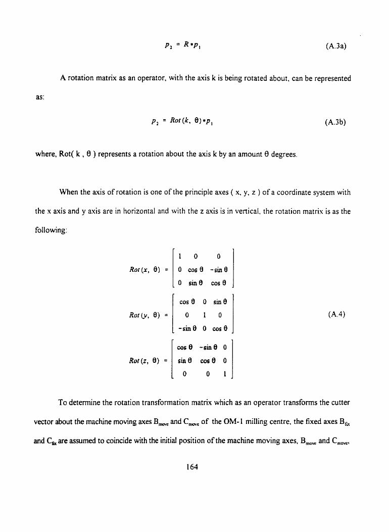
Pl = R r p l (A. 3 a)

A rotation matnx as an operator, with the avis k is being rotated about, can be represented

as:

pl = Rot(k. W p ,

where, Rot( k , 0 ) represents a rotation about the axis k by an amount 8 degrees.

When the axis of rotation is one of the principle axes ( rt. y. z ) of a coordinate system with

the x axis and y axis are in horizontal and with the z axis is in vertical. the rotation matris is as the

following:

Rot (x, 8) =

1 O O

O cos 0 -sin 0

O sin 0 cos 0

Rot&, 8) =

-sin 0 O cos 0

Rot (2, 0) = sin 0 cos 0 0 I

To determine the rotation transformation matnx which as an operator transfomis the cutter

vector about the machine moving axes B,, and C, , of the OM- 1 milling centre, the fixed axes B,

and C, are assurned to coincide with the initial position of the machine moving axes, B,, and Cm,,=,

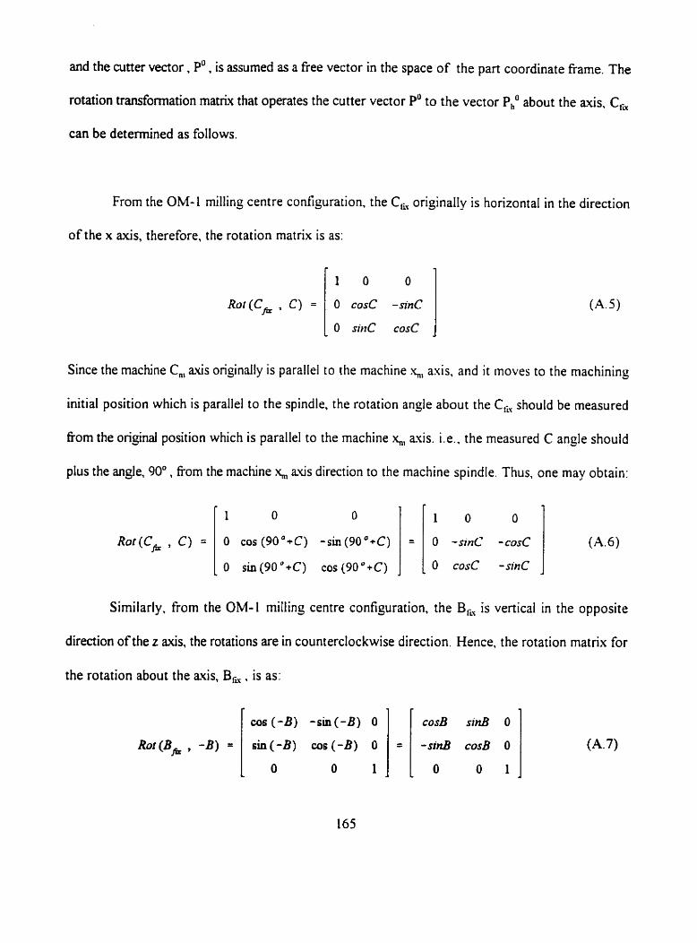
and the cutter vector , PO, is asnimed as a free vector in the space of the part coordinate fi-ame. The

rotation transformation rnatrix that operates the cutter vector PO to the vector P," about the mis, C,iw

can be determined as follows.

From the OM-l milling centre configuration. the C , onginally is horizontal in the direction

of the x a i s , therefore, the rotation matrix is as:

Rut (C,, , C) =

Since the machine C,, axis onginally is parallel to the machine x,,, axis, and it moves to the machining

initial position which is parallel to the spindle, the rotation angle about the C, should be measured

6om the original position which is parallel to the machine x,,, mis. Le.. the measured C angle should

plus the angle, 90" . from the machine x, a i s direction to the machine spindle. Thus, one rnay obtain:

Sirniiarly. from the OM-1 milling centre configuration. the B,, is vertical in the opposite

direction of the z axis, the rotations are in counterclockwise direction. Hence. the rotation rnatrix for

the rotation about the auis, B, . is as:

1 O O

O -sznC -cosC

O cosC -sine

= Rot (C& , C) =

1 O O

O cos (90 ' + C ) -sin (90 ' +C)

O sin(90°+C) cos(90°+C)

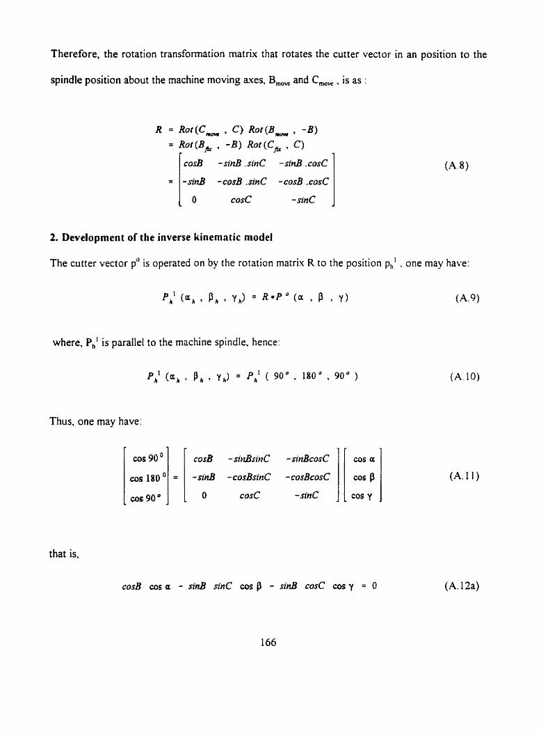
Therefore, the rotation transformation matnx that rotates the cutter vector in an position to the

spindle position about the machine moving aues, B,,, and Cm,, , is as :

R = Rot(CmM , C) Ror(Bm_ , - B ) = Rot@& . 4) Ror(C,, , C)

CO& -sinB .sinC -sinB .cosC

-sinB -cosB .sinC -cosB .CO&

O COSC -SM

2. Development of the inverse kinernatic mode1

The cutter vector p" is operated on by the rotation matrix R to the position ph1 . one may have:

ph1 ( a , , P h . Y,) = R * P O ( a 9 P 9 Y ) (A.9)

where, Ph' is parallel to the machine spindle. hence:

ph1 ( a h . P,, , y h ) = ph1 ( 9 0 ' . 1 8 0 ° . 90' )

Thus. one may have:

cos 90 O

cos 180

cos 90 O

that is,

cosB cos a - sinB sinC cos p - sini3 cosC cos y = O

cosB -si)zBsinC -sinBcosC

- s a - cosBsinC - cosBcosC

O cosc -sine

(A. 10)

cos a

cos P cos y -

(A. l2a)

and,

cosc cos p - sinc cos y = O

From (A. 12.b), one may have:

sin = * c o ~ cos y

cos y cos Cm =

JCM-

Substitute ( A. 12.c ) into (A. 12.a ). one rnay have:

COSB cos a = sinB (sine cos p + cosC cos y )

= sinB \/cos ?y + cos 'p

COS a tanB =

Jcos + cos p

(A. I2.b)

(A. 12.c)

(A. 13)

(A. 14)

The cutter vector position initially is pO ( x, y, z ). after rotated by the transformation matrix

R it is mived at ph1 ( , y,', zhl ) in reference to the initial pan coordinate frame. In matrix form,

it is:

cosC -sinC

Thus, one may have:

x,' = x cosB - y sid sinC -2 sinB cosC

yhl = -x s i n . -y cosB sinC -z cosB cosC

2,' = y cosC -r sine

(A. 15)

(A. 16)

Since the part coordinate frame is also rotated. the frarne origin is moved to a new position. one have:

cosB - sinBsinC - siriBcosC

-si& - cosBsinC - cosBcosC

O cosC -sine

(A. 17)

From the machine set up data, the fixture thickness. F . and the part stacking position data. G . the

initial position of the part coordinate frame origin is as:

(A. 18)

Hence, one may have:

(A. 19)

Therefore. after rotations. the cutter position in reference to the 'fixed' machine coordinate frarne is

as :

where, the plus sign and the minus sign depends on the position of the oriçin of the pan frame in

reference to the machine coordinate frame. In our case. the minus applirs.

The spindle MCP-s initial position in the 'fixed' machine coordinate frame is at:

( x m . Y m > z J = ( P B ,PC , P B )

where, PB represents the position of the B,, axis pivot in the >6, avis direction which is equal to the

spindle initial position in x, (see Fig. 4.4) and in q,, . PC represents the position of the Cm axis pivot

in the y, axis direction which is equal to the spindle initial position in y , as shown in Fig.4.4.

To rnove the cutter vector PhL from the position (xl . y' . zi) to the spindle position (PB, PC,

PB), the machine should translate the Ph1 to the spindle by the amount of:

where, the plus or the minus sign of (xl , y' , 2') depends on the relative position of the vector Ph1 to

the spindle, in our case, the minus siçn applies.

Substitute Eq(A.20) and using the rotational axes pivot constant. PB = 15.0" and PC =

1 1.75", the machine translational variables are obtained as:

y," = PC - lycosc -zs»lC ]

cos ' a + cos'p + = i

one may have:

COSB = 1

= sin a

Ji-Tz

sinB = r a d cosB = cos a

as P sinc = ranc cosc = -- J 1 - cos 'or

Substitute Eq.(A.25) into Eq. (A.23). one may obtain:

wsP ] = P C - [ y - 2 - Y cos y J1-ccs'rr

cos a = P B + x - F + y ( 4 + + 5 ) sina + (-4) C O S E

sin a Y sin a 2

Therefore, the inverse kinematic rnodel for the OM-1 5-axis CNC milling centre is obtained as the

following:

-1 P ) Cm = tan (- cos y

where, x, y. z are cutter position coordinates and cosa. cosp. cosy are the direction cosine of the

cutter orientation coordinates in reference to the part coordinate system. x,,, . y,, , z, are machine

translational movernent variables and B,, and C,, are machine rotational movement variables in

reference to the machine coordinate system.

3. Development o f the fonvnrd kinemntic mode1

The fonvard kinernatics deal with the problem of determining cutter variables from the machine

variables. From Eq.(A. 9):

one may have:

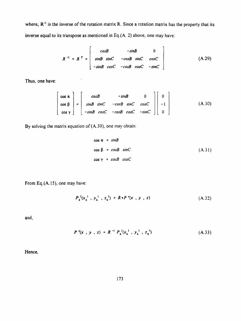
where, R-' is the inverse of the rotation matrix R. Since a rotation matrix has the property that its

inverse equal to its transpose as mentioned in Eq.(A. 2) above, one rnay have:

Thus, one have:

cos a

cos Q cos y

By solving the matrix equation of (A.30). one may obtain:

cos a = sinB

cos p = cosB sinC

cos y = cosB cosC

From Eq.(A. 15), one may have:

1 ~ ~ ' ( ~ j , ' y, ) = *' ' ( x 7 y > ')

and,

P '(x , y , z ) = R -' f,,'(xhl , yhl , zhl)

(A. 3 0)

Hence,

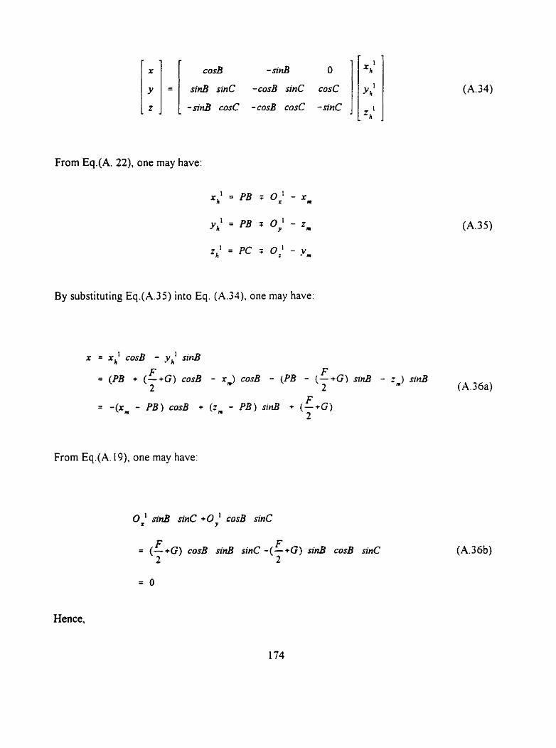
sinB sinC -cosB sinC cosC

-sinB cosC -cosB cosC -si&

From Eq.(A. 22). one may have:

(A. 3 5)

By substituting Eq.(A.3 5) into Eq. (A.34). one may have:

r = r,' cosB - y,' si&

F = (PB + ( - + G ) msB - xm) cosB - (PB - ( F + G ) sinB - 2,) sinB

2 2 (A. 36a) F

= - (xm - P B ) cosB + (rm - P B ) si& + (-+G) 2

From Eq.(A. 19), one may have:

F F = (- +G) cosB si& sinC - (- +G) s i d cosB sine

2 2 (A. 3 6b)

Hence,

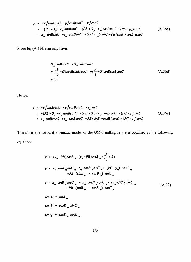
Frorn Eq. (A. 19). one may have:

Hence,

z = - x , ' s i n ~ c o s ~ - y , ' c o s ~ c o s ~ + z , ' s i n ~

= -(PB +O=' -rm)sinBcosC -(PB +O,,' -z,,)cosRcmC - (PC -ym)srK (A.36e)

= xm SjnBcosC +zm COSBCOSC -PB (sirzB +cosB )cosC - (PC -ym)sinC

Therefore, the fonvard kinematic mode1 of the OM-i millinç centre is obtained as the followinç

equation:

y = xm sinB , +zm cosB -sinC , + (PC -y,) cosC

-PB (sini3 + cosB J sinC

z = xm SM -cosC , + zm cosB mcosC + Cv,-PC) sine

-PB (sinB + c o d cosC (A. 3 7)

cos p = cosB sinCm

cos y = COSB cosc

where, x, y, z are cutter position coordinates and cosu, cos p. cosy are the direction cosine of the

cutter orientation coordinates in reference to the part coordinate system. h, , y , , are machine

translationai movement variables and B,, and Cm are machine rotational movement variables in

reference to the machine coordinate system-

Appendix B

Development of Cubic Spline Representation of Tool Path

A cornmon technique is to use a series of cubic spline segments with each seçment spanning only two

points. The cubic spline is advantaeeous since i t is the lowest degree curve which allows a point of

inflection and which has the ability to twist through space. To represent the desired cutting curve on

the machined surface and calculate the local surface geometrical pro perties. cubic spline technique

can be used to approximate the desired tool path. Thus, the cubic polynomial is developed. The

resultant fonnu!a are the same as that by Ragers and Adams[75].

The equation for a single parametric cubic spline seçment is given by:

where t is the parameter which varies between the two end-point values t , and t2 correspondinç to

the two end-points P, and P, of the cubic segment. By knowing the tangents at the two end-points

of the cubic segment, Pt, and Pl,, and considering the normalized parameters. i.e..

The cubic polynomial for each cubic segment can be determined as follows.

177

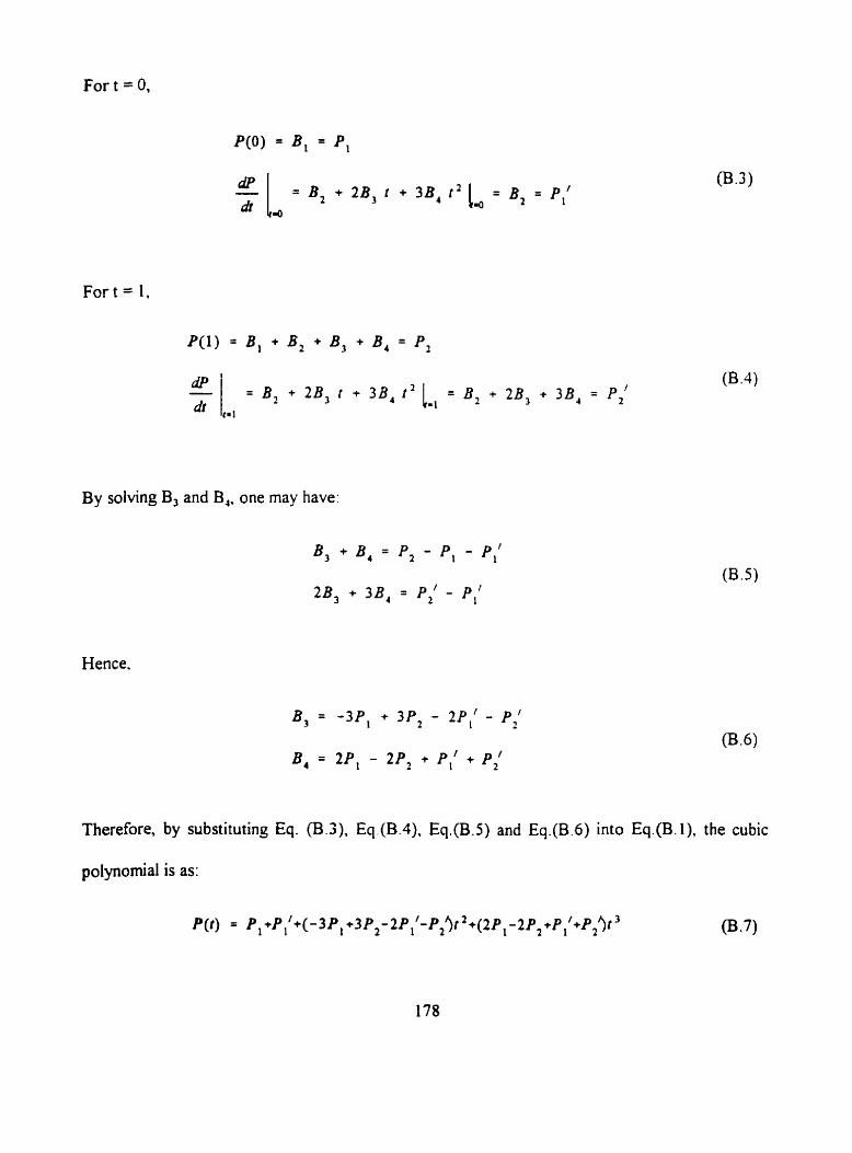
For t = 0,

Fort = 1,

By solving B, and B,, one may have:

Hence,

B, = - 3 P , + 3P2 - ZP,' - P,'

B, = 2P1 - 2P2 + PI' + P;

To ensure second-order continuity for a cubic spline, we impose the condition for constant

curvature at the interna1 joint between the two spans, namely:

where, k represents the curvature at a joint.

From Eq.(B. 1). one may have:

P "(1) = ZB, + 6 B , r

Since at the end of the first segment (s, ). t = t, = 1. one may have:

( f ) = ZB, + 6 4

and at the beginning of the second segment ( s2 ), t = t , = O. on may have:

P " ( r ) = 2 4

By equating Eq.(Bla) and Eq.(B.lb). one may have:

( 2 4 + 6q,, = 2 4 l2

Thus, From Eq.P.6) and Eq.CB.9). for joint between 5, 2nd %,,. one rnay have:

(B. Sa)

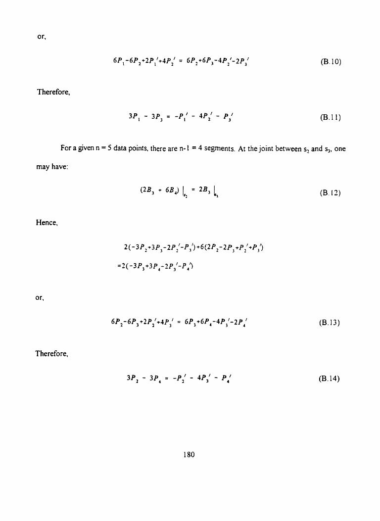
Therefore,

For a given n = 5 data points. there are n- l = 4 segments. At the joint between s2 and s,, one

may have:

Hence,

Therefore,

3 P 2 - 3P4 = -pi - 4P,/ - P,'

(B. 13)

(B. 13)

(B. 14)

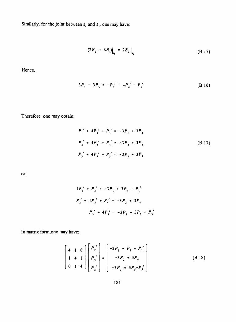
Similarly. for the joint between s, and s,, one rnay have:

Hence,

Therefore, one may obtain:

1p2/ + P,' = - 3 P , + 3P3 - P,'

P,' + 1P,' + P,' = - 3 P , + 3 P ,

P,/ + 1~, ' = -3P3 + 3P5 - Pi

In matrix fonn,one may have:

(B. i5)

(B. 16)

(B. 17)

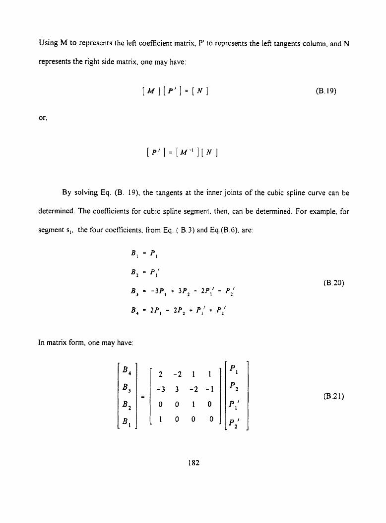
Using M to represents the left coefficient matrix, Pt to represents the left tangents column, and N

represents the right side matnx, one may have:

(B. 19)

By solving Eq. (B. 19). the tangents at the inner joints of the cubic spline curve can be

determined. The coefficients for cubic spline segment. then. c m be determined. For exarnple. for

segment s,. the four coeficients, frorn Eq. ( B.3) and Eq(B.6). are:

In matrix form, one may have:

(B. 20)

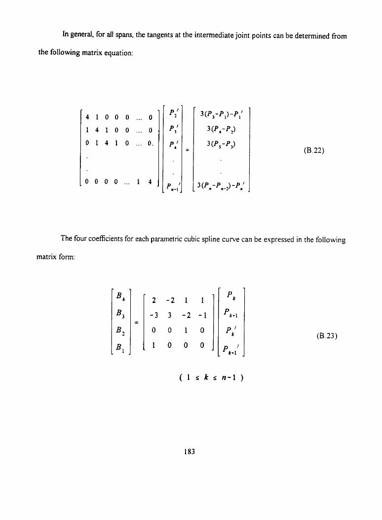
In general, for al! spans, the tangents at the intermediate joint points can be determined from

the following matrix equation:

The four coefficients for each parametric cubic spiine curve can be expresscd in the following

matrix fonn:

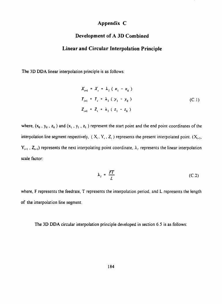
Appendix C

Development of A 3D Cornbined

Linear and Circular Interpolation Principle

The 3D DDA linear interpolation principle is as foilows:

where, (x, . y, . 4 ) and (x, . y, . z1 ) represent the stan point and the end point coordinates of the

interpolation line segment respectively. ( X, , Y, , 2, ) represents the present interpolated point. (X,.,.

Yi., , Zi+,) represents the next interpolating point coordinate, A, represents the linear interpolation

scale factor:

where, F represents the feedrate, T represents the interpolation period. and L represents the lençth

of the interpolation line segment.

The 3D DDA circular interpolation principle developed in section 6.5 is as foliows:

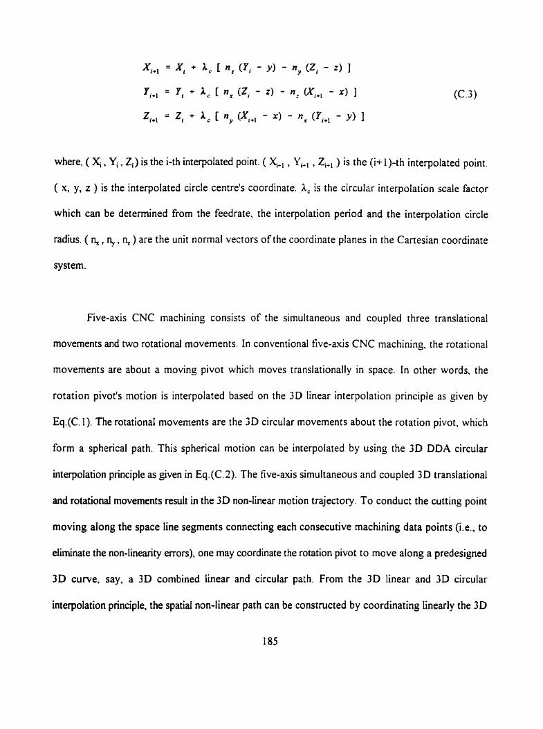
where, ( y, Yi, Zi) is the i-th interpolated point. ( Y+, , Yi+, , Zi,, ) is the (i+l)-th interpolated point.

( x, y, z ) is the interpolated circle centre's coordinate. A, is the circular interpolation scale factor

which can be detemined From the feedrate, the interpolation period and the interpolation circle

radius. ( R, , n, , n, ) are the unit normal vectors of the coordinate planes in the Cartesian coordinate

system.

Five-ais CNC machining consists of the simultaneous and coupled three translational

movements and two rotational movements. In conventional five-auis CNC machining, the rotational

movements are about a moving pivot which moves translationally in space. In other words. the

rotation pivot's motion is interpolated based on the 3D linear interpolation principle as given by

Eq.(C. 1). The rotational movements are the 3D circular movernents about the rotation pivot, which

form a spherical path. This spherical motion can be interpoiated by using the 3D DDA circular

interpolation principle as given in Eq.tC.2). The five-ais simultaneous and cou pied 3D translational

and rotational rnovements result in the 3D non-linear motion trajectory. To conduct the cutting point

moving along the space line segments connecting each consecutive machining data points (Le., to

eliminate the non-linearity errors), one may coordinate the rotation pivot to move along a predesigned

3D curve, Say, a 3D combined linear and circular path. From the 3D linear and 3D circular

interpolation principle, the spatial non-linear path can be constructed by coordinating linearly the 3D

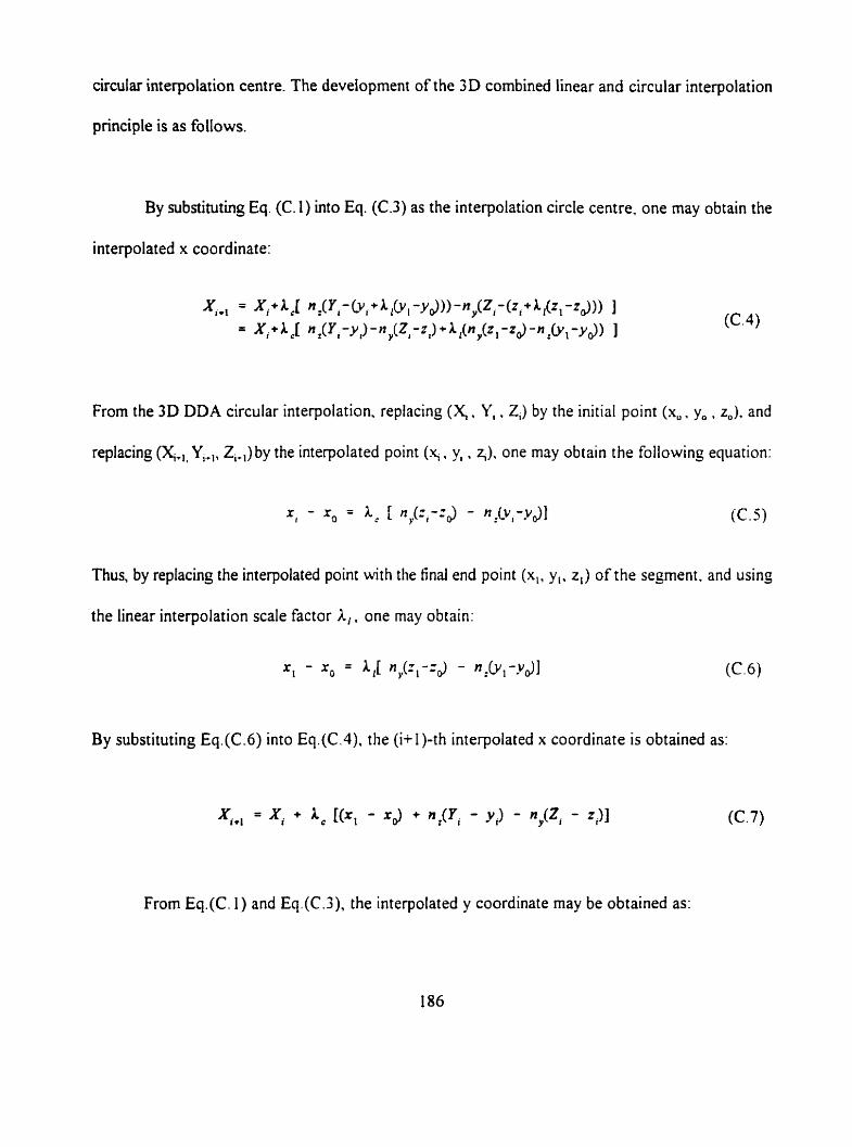
circular interpolation centre. The development of the 3D combined linear and circular interpolation

principle is as follows.

By substituthg Eq. (C. 1) into Eq. (C.3) as the interpolation circle centre, one may obtain the

interpolated x coordinate:

From the 3D DDA circular interpolation. replacing (Y. Y, . 2,) by the initial point (x, . y, , z,). and

replacing (Y,,, Y,,. Z,.,) by the interpolated point (5 . y, . z,). one m g obtain the followinç equation:

Thus, by replacing the interpolated point with the final end point ( x , . y,. z,) o f the segment. and usinç

the linear interpolation scale factor A,. one rnay obiain:

By substituting Eq(C.6) into Eq.(C.4). the ( i+ 1)-th interpolated x coordinate is obtained as:

xi, = xi + 1, rcx, - x j + q q - Y S - n p , - ZJI

From Eq.(C. 1 ) and Eq(C.3). the interpolated y coordinate may be obtained as:

From the 3D DDA circular interpolation. replacing (Y. Yi , 23 by the initial point (x,. y, , 2,) and

(X,+,. Y,,, Z,,,) by the interpolated point (5 . y, . z,). one may obtain the following equation:

By replacing the interpolated point with the final end point (x, . y, , z,) of the segment, and usinç the

linear interpolation scale factor A,. one may obtain:

Therefore. by substituting Eq.(C. 10) into Eq. (C.8). the ( i+ !)-th interpolated y coordinate is

Similarly. from Eq.(C. 1 ) and Eq.(C.3), one may obtain the interpolated z coordinate as:

From the 3D DDA circular interpolation, replacing (Y. Yi . 23 by the initial point (x,. y,, . zo) and

(YIl, Yi-,, Zi,,) by the interpolated point ( 5 , yi . z,), one may obtain the following equation:

By replacing the interpolated point with the final end point (x, , y, , z,) ofthe sesment, and using the

iinear interpolation scale factor A, . one may obtain:

Thus, by substituting Eq.(C. 14) into Eq.(C. 12). the (i+l)-th interpolated z coordinate is as:

= Zi + A c [(zl - ZJ + ny(Xi-! - xt*l? - nz(Yi+l - (C. I S )

Therefore. by cornbininç the Eq.(C.7). Eq. (C. 1 1 ) and Eq.(C. 15). a combined 3D DDA linear and

circular interpolation principle is obtained as follows: