Millennium-long summer temperature variations in the European Alps as reconstructed from tree rings

Clim. Past, 6, 379–400, 2010www.clim-past.net/6/379/2010/doi:10.5194/cp-6-379-2010© Author(s) 2010. CC Attribution 3.0 License.

Climateof the Past

Millennium-long summer temperature variations in the EuropeanAlps as reconstructed from tree rings

C. Corona1, J. Guiot1, J. L. Edouard2, F. Chalie1, U. Buntgen3, P. Nola4, and C. Urbinati5

1CEREGE, UMR 6635 CNRS/Aix-Marseille Universite, BP 80, 13545 Aix-en-provence cedex 4, France2IMEP, UMR 6116 CNRS/Aix-Marseille Universite, BP 80, 13545 Aix-en-provence cedex 4, France3Swiss Federal Research Institute WSL Zuercherstrasse 111 8903 Birmensdorf, Switzerland4Univ. degli Studi di Pavia, Dip. Ecologia del Territorio a degli Ambienti Terrestri, Via S. Epifanio, 14, 27100 Pavia, Italy5Univ. Politecnica delle Marche, Dip. SAPROV, Forest Ecology and Management, Via Brecce Bianche, 60131 Ancona, Italy

Received: 8 August 2008 – Published in Clim. Past Discuss.: 7 October 2008Revised: 3 June 2010 – Accepted: 9 June 2010 – Published: 25 June 2010

Abstract. This paper presents a reconstruction of the sum-mer temperatures over the Greater Alpine Region (44.05◦–47.41◦ N, 6.43◦–13◦ E) during the last millennium basedon a network of 38 multi-centennial larch and stone pinechronologies. Tree ring series are standardized using anAdaptative Regional Growth Curve, which attempts to re-move the age effect from the low frequency variations in theseries. The proxies are calibrated using the June to Augustmean temperatures from the HISTALP high-elevation tem-perature time series spanning the 1818–2003. The methodcombines an analogue technique, which is able to extendthe too short tree-ring series, an artificial neural networktechnique for an optimal non-linear calibration includinga bootstrap technique for calculating error assessment onthe reconstruction. About 50% of the temperature varianceis reconstructed. Low-elevation instrumental data back to1760 compared to their instrumental target data reveal diver-gence between (warmer) early instrumental measurementsand (colder) proxy estimates. The proxy record indicatescool conditions, from the mid-11th century to the mid-12thcentury, related to the Oort solar minimum followed by ashort Medieval Warm Period (1200–1420). The Little IceAge (1420–1830) appears particularly cold between 1420and 1820 with summers that are 0.8◦C cooler than the 1901–2000 period. The new record suggests that the persistency ofthe late 20th century warming trend is unprecedented. It alsoreveals significant similarities with other alpine reconstruc-tions.

Correspondence to:C. Corona([email protected])

1 Introduction

In the last decade, many studies concerned past temperaturevariations in the Greater Alpine Region (GAR). They arebased on long instrumental observations (Begert et al., 2005;Brunetti et al., 2006; Auer et al., 2007), written historicaldocuments (Pfister, 1999; LeRoy Ladurie 2004), glacier frontelevation (Holzhauser et al. 2005; Oerlemans 2005) or mul-tiproxy combinations (Casty et al., 2005, for example). Re-garding dendroclimatological studies, the Alps are favouredby several low-elevation instrumental series extending to themid-18th century and by some high-elevation ones to theearly 19th century (Auer et al., 2007). This enables calibra-tion and independent verification of tree-ring proxy to instru-mental target data over exceptionally long periods (Frank andEsper 2005; Buntgen et al., 2008). To date, numerous tem-perature reconstructions have been produced from local tree-ring chronologies and regional-scale network compilations(see references herein). However, most of them span thelast 300–500 years only. There are relatively few that extendback prior to 1000 (all dates in this paper are given in calen-dar years AD). To date and to our knowledge, there are onlytwo tree ring-based Alpine temperature reconstructions thatextend back prior to 1000 and forward into the 21st century(Buntgen et al., 2005, 2006a). This is because of the scarcityof wood material from the early part of the last millennium,necessary to assess climate variations during the putative Me-dieval Warm Period (MWP) (Lamb, 1976). In contrast, muchmore evidence of a Little Ice Age (LIA) cooling is reportedfrom various sites and archives (Grove, 1988). Buntgenet al. (2005, 2006a) published two mean summer (June–August and June–September) temperature reconstructions

Published by Copernicus Publications on behalf of the European Geosciences Union.

http://creativecommons.org/licenses/by/3.0/

380 C. Corona et al.: Millennium-long summer temperature variations in the European Alps

based on tree-ring width (TRW) and maximum latewooddensity (MXD) from tree-ring sites in Switzerland and Aus-tria. These reconstructions are the longest available for theAlps (951–2002 and 755–2004).

In this paper, we present a millennium-long summer tem-perature reconstruction covering most of the Alpine arc byvarious existing and newly updated composite dataset thatcombine living trees with dendroarchaeological material.Unlike previous reconstruction, our reconstruction is builtfrom series widely distributed in the Alpine arc, and, inparticular, series from Western Alps are incorporated in thedataset. In an effort to capture the natural range of high- tolow- frequency temperature variations and to provide a re-fined reconstruction of their amplitude over past millennium,we combined version of the well-established RCS techniquefor tree-ring detrending, an analog method for data aggrega-tion, and a neural network approach for reconstruction (Guiotet al., 2005). This approach has been applied successfully inpalaeoclimatology (Peyron et al., 1998; Guiot et al., 2005)and in dendroclimatology (Guiot and Tessier, 1997; Keller etal., 1997; Carrer and Urbinati, 2005). It differs from linearstatistical methods in that it introduces non-linearity to thesystem and appears particularly adapted to tree-ring basedreconstructions due to the complexity of tree growth, depen-dent on climate but also on time, tree geometry and otherfactors. Results are compared to existing alpine reconstruc-tions, and comparison with NH reconstructions is conductedto place our regional reconstruction in a larger-scale context.

2 Material

2.1 Tree-ring data

We have collected a large compilation of living and his-toric wood samples from numerous well-distributed, high-elevation wood samples in the European Alps. The dataextracted from the DENDRODB relational European tree-ring database (http://dendrodb.cerege.fr/) and the WDCtree-ring database (http://www.ncdc.noaa.gov/paleo/treering.html) have been supplemented with new and unpublishedmulti-centennial-long pine and larch chronologies (Edouard,unpublished chronologies). In total, 502 larch series (LarixdeciduaMill., 19 sites) and 463 stone pine series (Pinus cem-bra L., 17 sites) have been used (Table 1). For the larchcollection, the precise number of trees concerned by theseseries is, however, not clearly specified, as some of the his-torical timbers might originate from the same trees (Buntgenet al., 2006b). In contrast, each pine represents a singletree. Two composite chronologies (Swiss1 and Swiss2) arealso integrated. Swiss1 (TRW) is a Regional Curve Stan-dardized (RCS) chronology, including four larch compos-ite chronologies (1110 TRW series) from Switzerland andthe most recent part of a 7000-year pine TRW chronology(417 ring width series) from western Austria (Buntgen et

al., 2005). “Swiss 2” (MXD) is composed of 180 max-imum latewood density (MXD) larch measurement seriesfrom 86 living trees and 94 historic timbers deriving from el-evations>1600 m a.s.l. located in the sub-alpine Lotschental,Simplon and Aletsch regions (Buntgen et al., 2006a). Allthese chronologies are more than 400 years long. Threelarch chronologies (“Merveilles”, “Swiss1” and “Swiss2”)are covering the whole last millennium. The “NevacheGranges” larch chronology covers the last millennium with agap between AD 1255 and AD 1384. Characteristics of thesechronologies are detailed in Table 1.

2.2 Climatic data

Our aim is to provide reliable palaeoclimatic evidence for theperiod before AD 1818, when systematically homogenizedhigh-elevation instrumental station measurements startedrecording in the Greater Alpine Region (GAR) (HISTALP;Auer et al., 2007). The HISTALP high-elevation tem-perature data derive from 13 individual stations located>1500 m a.s.l. and cover the 45◦–47◦ N and 6◦–9◦ E areaalong the main Alpine crest-line. This compilation thus bestrepresents the spatial area and the elevation-zone of the tree-ring network.

The HISTALP low-elevation (<1500 m a.s.l.) tempera-ture time series (Auer et al., 2007) back to 1760 derivesfrom 118 stations across the GAR. It is herein used for ex-tra verification and to characterize potential limitations ofour reconstruction in preserving long-term trends as thosereported from the transition of the LIA cooling until themost recent warming. Correlation (1818–2003) between theJune–August (JJA) mean from high- and low-elevation is0.92, indicating that these two series display a similar his-tory. Temperatures are expressed as anomalies with respectto the 1901–2000 mean.

3 Methods

First, the tree-ring width series are detrended using an Adap-tive Regional Growth Curve (ARGC) (Nicault et al., 2008,2010), which preserves long-term trends in the resultingchronologies. Secondly, an analogue technique is used to ex-pand all series to the common 1000–2000 period. Thirdly, anArtificial Neural Network (ANN) technique (referred to hereas a transfer function) is calibrated on the 1818–2000 periodand then applied to the individual site chronologies back toAD 1000. Five calibration and validation tests are finally car-ried out to assess the reliability of the reconstruction.

3.1 Tree-ring data detrending and chronologydevelopment

Cook et al. (1995) demonstrated that methods of individualseries detrending result in a lose of potential longer-term cli-matic information above the segment length. Mean segment

Clim. Past, 6, 379–400, 2010 www.clim-past.net/6/379/2010/

http://dendrodb.cerege.fr/

http://www.ncdc.noaa.gov/paleo/treering.html


C. Corona et al.: Millennium-long summer temperature variations in the European Alps 381

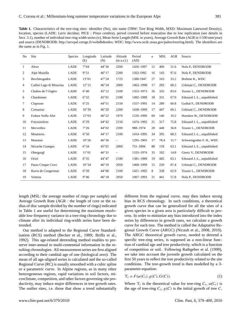
Table 1. Characteristics of the tree-ring sites: identifier (No), site name (TRW: Tree Ring Width, MXD: Maximum Latewood Density),location, species (LADE:Larix decidua; PICE : Pinus cembra), period covered before truncation due to low replication (see details inSect. 3.1), number of individual tree-ring width series (n), Mean Serie Length (MSL in years), Average Growth Rate (AGR in 1/100 mm/year)and source (DENDRODB:http://servpal.cerege.fr/webdbdendro; WDC: http://www.ncdc.noaa.gov/paleo/treering.html). The identifiers arethe same as in Fig. 1.

No Site Species Longitude Latitude Altitude Period n MSL AGR Source(E) (N) (m a.s.l.) (AD)

1 Aleve LADE 7◦04 44◦36 2200 1426–1997 12 400 51.6 Nola P., DENDRODB

2 Alpe Musella LADE 9◦51 46◦17 2200 1563-1992 16 143 97.6 Nola P., DENDRODB

3 Berchtesgaden LADE 13◦01 47◦24 1725 1380-1947 27 163 33.2 Brehme K., WDC

4 Cadini Lago di Misurina LADE 12◦15 46◦34 2000 1463–1998 17 283 68.3 Urbinati C., DENDRODB

5 Chalets de l’Orgere LADE 6◦40 45◦12 2100 1353–1973 26 335 83.6 Tessier L., DENDRODB

6 Chardonnet LADE 6◦32 45◦01 2180 1492–1989 18 331 67.9 Edouard J.-L., unpublished

7 Clapouse LADE 6◦25 44◦51 2150 1557–1995 14 289 60.8 Guibal F., DENDRODB

8 Comasine LADE 10◦39 46◦20 2200 1438–1999 17 447 69.1 Urbinati C., DENDRODB

9 Fodara Vedla Alm LADE 12◦03 46◦22 1970 1520–1990 69 140 10.2 Huesken W., DENDRODB

10 Freyssinieres LADE 6◦29 44◦42 2150 1474–1992 21 317 75.8 Edouard J.-L., unpublished

11 Merveilles LADE 7◦26 44◦02 2200 988–1974 28 448 36.8 Tessier L., DENDRODB

12 Moutieres LADE 6◦50 44◦17 2100 1414–1995 34 395 68.3 Edouard J.-L., unpublished

13 Muestair LADE 10◦26 46◦36 – 1295–1905 17 78.4 15.7 Schweingruber F. H., WDC

14 Nevache Granges LADE 6◦34 45◦01 2000 751–1894 88 159 63.1 Edouard J.-L., unpublished

15 Obergurgl LADE 11◦01 46◦31 – 1333–1974 35 182 14.8 Giertz V., DENDRODB

16 Oriol LADE 6◦35 44◦47 2180 1381–1989 19 445 63.1 Edouard J.-L., unpublished

17 Passo Cinque Croci LADE 10◦34 46◦10 2050 1468–1999 15 220 87.4 Urbinati C., DENDRODB

18 Ravin de Congerman LADE 6◦39 44◦06 2100 1421–1992 8 338 62.9 Tessier L., DENDRODB

19 Ventina LADE 9◦46 46◦18 2050 1007–1993 21 441 57.8 Nola P., DENDRODB

length (MSL: the average number of rings per sample) andAverage Growth Rate (AGR : the length of core or the ra-dius of disc sample divided by the number of rings) indicatedin Table 1 are useful for determining the maximum resolv-able low-frequency variance in a tree-ring chronology due toclimate after its individual ring-width series have been de-trended.

Our method is adapted to the Regional Curve Standard-isation (RCS) method (Becker et al., 1989; Briffa et al.,1992). This age-related detrending method enables to pre-serve inter-annual to multi-centennial information in the re-sulting chronologies. All measurement series are first alignedaccording to their cambial age of one (biological zero). Themean of all age-aligned series is calculated and the so-calledRegional Curve (RC) is usually smoothed with a cubic splineor a parametric curve. In Alpine regions, as in many otherheterogeneous regions, rapid variations in soil factors, mi-croclimate, competition, and other factors governing site pro-ductivity, may induce major differences in tree growth rates.The outlier sites, i.e. those that show a trend substantially

different from the regional curve, may then induce strongbias in RCS chronology. In such conditions, a theoreticalgrowth curve that can be generalized for all the sites of agiven species in a given area is particularly difficult to pro-cess. In order to minimize any bias introduced into the indexseries by differences in growth rates, we calculate a growthcurve for each tree. The method is called the Adaptative Re-gional Growth Curve (ARGC) (Nicault et al., 2008, 2010).The ARGC theoretical growth curve, needed to detrend aspecific tree-ring series, is supposed as a non-linear func-tion of cambial age and tree productivity, which is a functionof competition or soil. Following Rathgeber et al. (1999),we take into account the juvenile growth calculated on thefirst 50 years to reflect the tree productivity related to the siteconditions. The tree-growth trend is then modelled by a 3-parameter-equation:

ϒt = F(α(Ct ),g(C),G(C)). (1)

Whereϒt is the theoretical value for tree-ringCt , α(Ct ) isthe age of tree-ringCt , g(C) is the initial growth of treeC,

www.clim-past.net/6/379/2010/ Clim. Past, 6, 379–400, 2010

http://servpal.cerege.fr/webdbdendro



Table 1. Continued.

No Site Species Longitude Latitude Altitude Period n MSL AGR Source(E) (N) (m a.s.l.) (AD)

20 Swiss1 (TRW) LADE 7◦29-11◦03 46◦-47◦ 1900–2200 951–2002 Composite Buntgen U., Buntgen et al. 2005

20a Lotschental (TRW) LADE 7◦29 46◦25 – 1085–2002 330 201 86 Buntgen U., Schmidhalter M.

20b Simplon (TRW) LADE 8◦03 46◦12 – 685–2003 78 259 87 Schmidhalter M.

20c Engadine (TRW) LADE 9◦46 46◦27 – 800–1993 376 144 115 Seifert M. et al.

20d Goms (TRW) LADE 8◦10 46◦25 – 505–2003 326 129 104 Schmidhalter M.

20e Tyrol (TRW) PICE 11◦03 47◦00 – 645–1997 417 197 99 Nicolussi K.

21 Swiss2 (MXD) LADE 7◦29–11◦03 46◦12–47◦ 1900–2200 755–2004 Composite Buntgen U., Buntgen et al. (2006)

21a Aletsch (MXD) LADE 8◦01 46◦50 –1681–1986 31

– – Buntgen U.21b Simmental (MXD) LADE 6◦24 46◦25 – – – Buntgen U.

21c Lotschental (MXD) LADE 7◦29 46◦25 – 1258–2004 110 – – Buntgen U., Schmidhalter M.

21d Simplon (MXD) LADE 8◦03 46◦12 – 735–1510 39 – – Schmidhalter M.

22 Aleve PICE 7◦04 44◦36 2225 1453–1994 23 312 70.9 Nola P., DENDRODB

23 Ambrizzola PICE 12◦07 46◦06 2100 1425–1997 56 220 84.8 Urbinati C., DENDRODB

24 Bois des Ayes PICE 6◦40 44◦49 2000 1475–1998 26 361 68.8 Edouard J.-L., unpublished

25 Bufferes PICE 6◦34 45◦00 2100 1594–2000 39 243 92.4 Edouard J.-L., DENDRODB

26 Chaussettaz PICE 7◦07 45◦31 1820 1478–1994 25 274 85.4 Nola P., DENDRODB

27 Clavieres PICE 6◦40 44◦55 2200 1472–1995 24 308 74.2 Nola P., DENDRODB

28 Fodara Vedla Alm PICE 12◦03 46◦22 1970 1474–1990 93 164 91 Huesken W., DENDRODB

29 Formin PICE 12◦04 46◦29 2100 1493–1995 13 195 93.6 Urbinati C., DENDRODB

30 Isola PICE 7◦09 44◦10 2100 1637–2000 18 235 82.2 Edouard J.-L., DENDRODB

31 Jalavez PICE 6◦47 44◦39 2270 1575–1998 23 294 78.4 Edouard J.-L., DENDRODB

32 La Joux PICE 6◦57 45◦42 2200 1472–1997 17 376 67.9 Nola P., DENDRODB

33 Lac Miroir PICE 6◦28 44◦22 2300 1564–2000 11 327 60.6 Meijer F., DENDRODB

34 Manghen PICE 11.26 46◦10 2100 1488–1996 29 235 97.1 Urbinati C., DENDRODB

35 Obergurgl PICE 11◦01 46◦31 – 1544-1971 24 309 28.5 Giertz V., DENDRODB

36 Roubinettes PICE 7◦13 44◦07 2100 1540–2000 16 284 64.9 Edouard J.-L., DENDRODB

37 Val di Fumo PICE 10◦32 46◦02 2100 1584–1996 14 211 98.6 Nola P., DENDRODB

38 Vallee du Tronchet PICE 6◦30 44◦22 2350 1551–2000 12 280 77.1 Meijer F., DENDRODB

i.e. the average of the first 10 rings,G(C) is the maximaljuvenile growth of treeC, i.e. the maximum value reachedduring its juvenile stage (first 50 years) after smoothing usinga 10-yr window.

An ANN technique as introduced by Nicault et al. (2010)is used to estimate F for each tree (Eq. 1). The tree-ring seriesare indexed by dividing each measured ring by its expectedvalue estimated from this curve. Finally, the standardizedtree-ring indices are averaged on the site-level. As each treeis fitted by the ANN, the detrending is not sensitive to the oc-currence missing rings at the tree pith (Nicault et al., 2010).Resulting chronologies are truncated at a minimum replica-tion of three series. Due to a high degree of common variancebetween the larch and pine chronologies (see Sect. 4.1), these

data were simply merged yielding to increased sample sizeand thus more robust time-series allowing further analysis tobe applied.

3.2 The analogue technique

Considering the fact that the number of available proxiesdecreases back in time, several authors (Mann et al., 1999;Luterbacher et al., 2002; Xoplaki et al., 2005; Casty et al.,2005; Pauling et al., 2006) have used a number of regressionsbased on a decreasing number of proxies or nested compo-nent regression models (Cook et al., 2002). Resulting re-constructions are often still contaminated by artificial vari-ances changes through time (Frank et al., 2007b) which are



Table 2. Correlation matrix of the Adaptative Regional Growth Curve detrended chronologies (1637–1974 period).

31

Table 2. Correlation matrix of the Adaptative Regional Growth Curve detrended chronologies

(1637-1974 period).

31

Table 2. Correlation matrix of the Adaptative Regional Growth Curve detrended chronologies

(1637-1974 period).

an inverse function of the number of proxies used. Moreover,such methods do not account for missing values within proxyseries. A more and more frequently used alternative is theregularized expectation maximization (REGEM), which im-putes missing values on the basis of the regression betweenvariables (Schneider, 2001), in a manner that make optimaluse of spatial and temporal information in the dataset. Here,infilling of missing data is done using an analogue techniqueintroduced by Guiot et al. (2005). This technique has not thesame weakness as REGEM, as the number of predictors ismaintained constant in time. In order to replace a missingyear for any given tree ring series, we compared the existing

vector of data with all other series available during this timeon the basis of the Euclidian distance and not on the basis ofthe correlation between variables, as most of the methods do.The corresponding year from the eight nearest series (calledanalogues) are averaged with a weight inversely proportionalto the distance, providing the estimate of the missing tree-ring value. The number of analogues varies according to thedata available, but those are used with a distance lower than0.5. Note that some missing values may remain, if there arenot enough data for that period or if there are no close enoughanalogues. The quality of the fit is estimated with the cor-relation between observations and estimates on the common



98

7 5

5

4

1

38

37

36

35

34

33

32

31

30

2928

2

26

2

22

19

1513

1211

20a

20e

20d

20c

21b21c

21a

16

13°E12°E11°E10°E9°E8°E7°E47

°N46

°N45

°N44

°N

Tree ring sitesLarix decidua

Pinus cembra

FRANCE

ITALY

SWITZERLANDAUSTRIA

6

21d

72

42

25

0 12060 Km

10

14

3

3

2

17

18

20b

Fig. 1. Location map of the 38 tree-ring sites used for the Alpine temperature reconstruction. Sites are differentiated by species and whetherring-width and maximum latewood density parameters were both available for a site (grey symbol) or only ring-width (white symbol). Alltree-ring sites are above 1700 m a.s.l. The labelled numbers also refer to Table 1.

period. A good correlation proves that the hypothesis justify-ing the use of analogues is satisfied. Finally, if estimated se-ries have a standard deviation inferior by 20% to the originalseries, the estimates are rescaled to keep the same variance.This method allows us to expand all series to the same com-mon 1000–2000 period using only a single transfer function.Results will show below that the method has an interestingcharacteristic as compared with the regression based meth-ods: the correlations between estimated series are not betterthan those of the observed series as the estimation processis not based on the similarity between variables but betweenthe years. The method is then conservative for the observedspatial variability. Moreover, it has been demonstrated thatvariance is well maintained independent of the number ofpredictors (Nicault et al., 2008).

3.3 Calibration and verification

Standardized and completed tree-ring series were trans-formed into a smaller number of principal component analy-sis (PCA Richman, 1986) in order to remove the correlationbetween the regressors and to provide more robust estimates.We have successively tested the inclusion of 10 to 19 prin-cipal components to select principal component truncationcriteria. These principal components were then related toseveral combinations of regressors on the 1818–2000 periodusing the same ANN technique above mentioned. The bestcalibration was obtained when calibrating with JJA temper-

atures anomalies in accordance with the positive responsesof Pinus cembraandLarix deciduato summer temperaturesobserved, by several authors (e.g. Frank and Esper, 2005), athigh altitude in the Alps. The anomalies of the JJA temper-atures during the last 1000 years were estimated by apply-ing the ANN to the principal components. To avoid loss ofamplitude due to imperfect calibration, simple scaling of thereconstruction against instrumental targets, that is adjustingthe variance, was applied.

To assess the reliability of the ANN, a bootstrap method(Efron, 1979; Guiot, 1990) was used. A subset of the ob-served data (principal components and temperature) was ran-domly extracted with replacement. The ANN was then cali-brated on this data subset. This is iterated 50 times. At eachcalibration, a determination coefficient (R2) between esti-mated and observed values was calculated for the data ran-domly taken for the calibration (the calibrationR-squared,R2C), and another one was calculated for the remaining data(the verificationR-squared,R2V).

The reconstruction skill and robustness are assessed by theRoot Mean Squared Error of the calibration data (RMSE),the Root Mean Squared Error of Prediction of the verifica-tion data (RMSEP), the Reduction of Error statistic (RE) andthe Coefficient of Efficiency (CE), both on the verificationdata (Wigley et al., 1984). The RMSE statistic tests the qual-ity of fit on the calibration data, while the RMSEP test theprediction capacity of the transfer function by using inde-pendent data. The RE statistic ranges from minus infinity



2. Alpe Musella

3. Berchstesgaden

4. Cadini Lagodi Misurina

5. Chalets de l'Orgère

8. Comasine

9. Fodara Vedla Alm

6. Chardonnet

7. Clapouse

10. Freyssinières

13. Muestair

14. Névache Granges

11. Merveilles

12. Moutières

15. Obergurgl

18. Ravin de Congerman

19. Ventina

16. Oriol

20. Swiss1 (TRW)

21. Swiss2 (MXD)

1000 1100 1200 1300 1400 1500 1600 1700 1800 1900 2000

1. Aleve

17. Passo Cinque Croci

a

Year (AD)

0.5

1

1.5

Inde

x

Fig. 2a. Missing data estimation by the analogues method (thin line) and comparison with the original series (thick line).(a) Larch series;(b) Pine series. Original series are detrended using the Adaptative Regional Growth Curve (ARGC) method. All series are smoothed with a20-year lowpass filter. Dark-grey shading denotes a period of increasing growth, light-grey shading reveals period of growth reduction.



22. Aleve

25. Buffères

26. Chaussettaz

23. Ambrizzola

24. Bois des Ayes

27. Clavières

30. Isola

31. Jalavez

28. Fodara Vedla Alm

29. Formin

32. La Joux

35. Obergurgl

36. Roubinettes

33. Lac Miroir

34. Manghen

37. Val di Fumo

38. Vallée du Tronchet

1000 1100 1200 1300 1400 1500 1600 1700 1800 1900 2000

b

Year (AD)

0.5

1

1.5

Inde

x

Fig. 2b. Continued.

to one. If this statistic is greater than zero, the reconstruc-tion has greater skill than would be obtained by simply usingthe mean of the calibration period as the value for each yearof the reconstruction (Fritts, 1976). The CE compares esti-mates with the mean of the verification period. It providesthe more rigorous verification test, particularly when thereare low-frequency variations and substantial differences inthe means of the calibration and verification periods. The

confidence interval for all these statistics are obtained fromthe 5th and 95th percentiles of the 50 reconstructions. Boot-strap technique then provides a way to decide statistically ifthe reconstruction is robust or not.



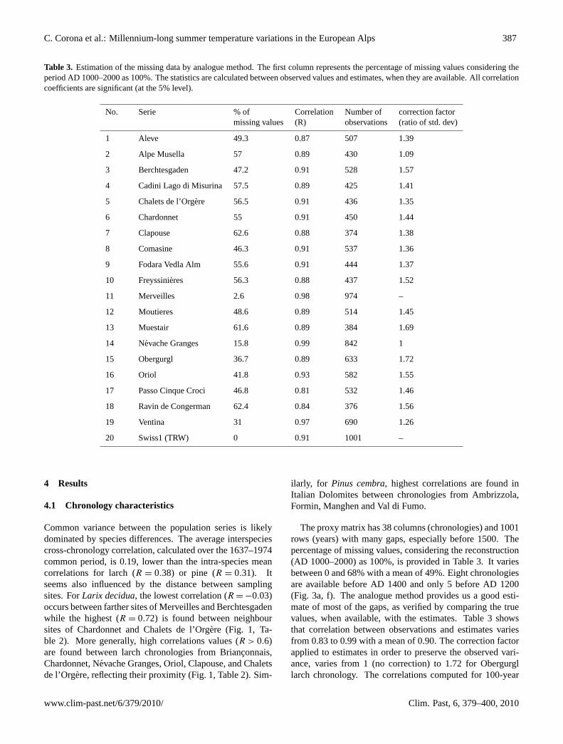
Table 3. Estimation of the missing data by analogue method. The first column represents the percentage of missing values considering theperiod AD 1000–2000 as 100%. The statistics are calculated between observed values and estimates, when they are available. All correlationcoefficients are significant (at the 5% level).

No. Serie % of Correlation Number of correction factormissing values (R) observations (ratio of std. dev)

1 Aleve 49.3 0.87 507 1.39

2 Alpe Musella 57 0.89 430 1.09

3 Berchtesgaden 47.2 0.91 528 1.57

4 Cadini Lago di Misurina 57.5 0.89 425 1.41

5 Chalets de l’Orgere 56.5 0.91 436 1.35

6 Chardonnet 55 0.91 450 1.44

7 Clapouse 62.6 0.88 374 1.38

8 Comasine 46.3 0.91 537 1.36

9 Fodara Vedla Alm 55.6 0.91 444 1.37

10 Freyssinieres 56.3 0.88 437 1.52

11 Merveilles 2.6 0.98 974 –

12 Moutieres 48.6 0.89 514 1.45

13 Muestair 61.6 0.89 384 1.69

14 Nevache Granges 15.8 0.99 842 1

15 Obergurgl 36.7 0.89 633 1.72

16 Oriol 41.8 0.93 582 1.55

17 Passo Cinque Croci 46.8 0.81 532 1.46

18 Ravin de Congerman 62.4 0.84 376 1.56

19 Ventina 31 0.97 690 1.26

20 Swiss1 (TRW) 0 0.91 1001 –

4 Results

4.1 Chronology characteristics

Common variance between the population series is likelydominated by species differences. The average interspeciescross-chronology correlation, calculated over the 1637–1974common period, is 0.19, lower than the intra-species meancorrelations for larch (R = 0.38) or pine (R = 0.31). Itseems also influenced by the distance between samplingsites. ForLarix decidua,the lowest correlation (R = −0.03)occurs between farther sites of Merveilles and Berchtesgadenwhile the highest (R = 0.72) is found between neighboursites of Chardonnet and Chalets de l’Orgere (Fig. 1, Ta-ble 2). More generally, high correlations values (R > 0.6)are found between larch chronologies from Brianconnais,Chardonnet, Nevache Granges, Oriol, Clapouse, and Chaletsde l’Orgere, reflecting their proximity (Fig. 1, Table 2). Sim-

ilarly, for Pinus cembra, highest correlations are found inItalian Dolomites between chronologies from Ambrizzola,Formin, Manghen and Val di Fumo.

The proxy matrix has 38 columns (chronologies) and 1001rows (years) with many gaps, especially before 1500. Thepercentage of missing values, considering the reconstruction(AD 1000–2000) as 100%, is provided in Table 3. It variesbetween 0 and 68% with a mean of 49%. Eight chronologiesare available before AD 1400 and only 5 before AD 1200(Fig. 3a, f). The analogue method provides us a good esti-mate of most of the gaps, as verified by comparing the truevalues, when available, with the estimates. Table 3 showsthat correlation between observations and estimates variesfrom 0.83 to 0.99 with a mean of 0.90. The correction factorapplied to estimates in order to preserve the observed vari-ance, varies from 1 (no correction) to 1.72 for Obergurgllarch chronology. The correlations computed for 100-year



Table 3. Continued.

No. Serie % of Correlation Number of correction factormissing values (R) observations (ratio of std. dev)

21 Swiss2 (MXD) 0 0.99 1001 –

22 Aleve 53.9 0.86 461 1.48

23 Ambrizzola 56 0.92 440 1.37

24 Bois des Ayes 51.6 0.88 484 1.47

25 Bufferes 68 0.83 313 1.53

26 Chaussettaz 53.2 0.87 468 1.59

27 Clavieres 51.2 0.90 488 1.38

28 Fodara Vedla Alm 51.2 0.90 488 1.46

29 Formin 68 0.87 320 1.36

30 Isola 66.5 0.86 335 1.36

31 Jalavez 60.1 0.87 399 1.54

32 La Joux 51.6 0.87 484 1.42

33 Lac Mirroir 59.2 0.84 408 1.46

34 Manghen 63.7 0.91 363 1.35

35 Obergurgl 58.4 0.87 416 1.43

36 Roubinettes 61.6 0.85 384 1.52

37 Val di Fumo 63.8 0.87 362 1.40

38 Vallee du Tronchet 62.8 0.88 372 1.41

Mean 49 0.90

segments in the original and in the infilled matrix are close(Fig. 3d, h). Interestingly, for larch chronologies (Fig. 3d),the intra-species correlations before 1200, between 0.38 and0.55, reveal a fairly robust signal in the four oldest popula-tions from Switzerland/Austria (Swiss 1, Swiss 2) and France(Merveilles, Nevache). Despite the distance and the com-posite nature of these populations, these correlations reveal acommon climate-related signal in the Alps during the earlypart of the millennium for which regional temperature recon-structions considerably differ at regional scale (Mann, 2007).For the infilled series, mean correlation between 1050 and1250 is 0.43. It decreases to 0.23 (at the same order of magni-tude than for the observed data) between 1400 and 1600. Forpine chronologies, correlations range between 0.14 and 0.45with a minimum between 1500 and 1700 (Fig. 3h). The peri-ods of decreasing correlation match with the beginning of themajority of the larch (pine) chronologies (Fig. 2). These pop-ulations are composed of juvenile trees that are less sensitive,especially forLarix decidua(Carrer and Urbinati 2004) to alesser extent forPinus cembra(Carrer and Urbinati, 2004) toclimate. This climate signal age effect (Esper et al., 2008)

might explain the low correlation. It appears to be related toan endogeneous parameter linked to hydraulic status that be-comes increasingly limiting as tree grow and age, inducingmore stressful conditions and a higher climate sensitivity inolder individuals (Carrer and Urbinati, 2004).

The ARGC detrended larch and pine chronologies revealinter-decadal scale growth variations over the past millen-nium. Visually, the original and infilled smoothed chronolo-gies (Fig. 3a, b, d, e) show periods of similar inter-decadalfluctuations, with low values at∼ 1585−1605 and∼ 1960−1980, and high values at∼ 1610−1620, and∼ 1860−1880,and during the last decades. Interestingly, after 1620, thetwo chronologies are out of phase, withPinuslagging behindLarix by 20 years. For example, during the Late MaunderMinimum 1675–1715, all larch chronologies show a promi-nent, multi-decadal growth reduction during the∼1680–1700 period, whereas pine chronologies indicate a later andless important reduction at∼ 1710− 1720. Between 1810and 1821, almost all chronologies indicate reduced growthrates and by the end of the 19th century, the chronologies areback in phase.



Table 4. Statistics of reconstructions of June to August temperature in the Alps functions of the number (10–18) of principal componentsused. Four neurons and a maximum of 5000 iterations were used in each reconstruction. Calibration statistics are computed on the randomlyselected observations within the 1818–2003 period. Validation statistics are based on not taken observation within the same period. TheRMSE and theR2 statistic tests the quality of fit on the calibration data, while the RMSEP, RE and CE test the prediction capacity of thetransfer function by using independent data.

Number of 10 11 12 13 14 15 16 17 18principal components

% of variance 0.81 0.83 0.85 0.86 0.88 0.89 0.90 0.91 0.92

RMSE 0.67 0.64 0.64 0.64 0.62 0.59 0.59 0.60 0.59

[0.61; 0.71] [0.59; 0.69] [0.59; 0.70] [0.57; 0.69] [0.55; 0.69] [0.54; 0.65] [0.54; 0.66] [0.56; 0.64] [0.54; 0.64]

RMSEP 0.73 0.72 0.71 0.71 0.70 0.71 0.69 0.69 0.69

[0.63; 0.83] [0.63; 0.84] [0.61; 0.82] [0.62; 0.82] [0.59 ; 0.81] [0.61; 0.80] [0.59; 0.78] [0.59; 0.76] [0.61; 0.80]

R2 (calibration) 0.43 0.46 0.47 0.49 0.51 0.55 0.54 0.55 0.55

[0.32; 0.53] [0.36; 0.56] [0.34; 0.56] [0.37; 0.59] [0.40 ; 0.61] [0.45; 0.66] [0.45; 0.64] [0.46; 0.64] [0.43; 0.65]

Reduction of 0.32 0.34 0.37 0.35 0.39 0.38 0.38 0.38 0.38error (RE)

[0.14; 0.45] [0.17; 0.46] [0.21; 0.46] [0.18; 0.48] [0.19; 0.50] [0.18; 0.51] [0.22; 0.49] [0.24; 0.48] [0.21; 0.49]

Coefficient of 0.31 0.33 0.35 0.32 0.37 0.37 0.37 0.37 0.37efficiency (CE)

[0.12; 0.43] [0.15; 0.46] [0.17; 0.45] [0.15; 0.47] [0.19 ;0.49] [0.15; 0.46] [0.17; 0.49] [0.22; 0.48] [0.13; 0.50]

4.2 Calibration and validation

The ANN was used with 4 neurons in the hidden layer, amaximum of 5000 iterations. The calibration is based on therandomly selected observations within the 1818–2003 periodand the verification is done on the non taken observations.We have successively tested the inclusion of 10 to 19 princi-pal components of the regressors, explaining from 81 to 92%of their variance. The optimal configuration seems to be 14principal components explaining 88% of the regressor’s vari-ance and 51% of the predictand’s variance (R2) with a 95%confidence interval of [40%, 60%]. It is considered as theoptimum configuration because it gives the best verificationstatistics, say RE=0.39 and CE=0.37. These values, basedon observations which were not taken into account withinthe 1818–2003 period, are largely significant with 95% con-fidence intervals of respectively [0.19, 0.50] and [0.19, 0.49].The mean discrepancy between reconstructed and instrumen-tal temperatures is−0.07◦C (Fig. 4a) for the 1818–2000 pe-riod. Discrepancies are maximal at 1823 (+2◦C) and 1976(−1.45◦C) (Fig. 4a). When the curves are smoothed witha 20-year low-pass filter (Fig. 4b), we see a maximum de-coupling between colder periods e.g. 1950–1970 (−0.6◦C),1819–1825 (−0.4◦C) and 1875–1900 (−0.25◦C) (Fig. 4b).

An extra verification of the results is provided by the com-parison between low-elevation instrumental data and our re-construction on the 1760–1818 independent period (Fig. 4c):we obtained aR2 of 0.40, which is highly significant (p <

0.001) and comparable to the CE of 0.37 obtained on in-

dependent observation randomly selected between 1819 and2000. The tree-ring-based reconstruction of 1760–1818 tem-perature variability indicates discrepancies between “cooler”proxy and “warmer” instrumental prior to 1840, similarly toBuntgen et al. (2005, 2006a) and Frank et al. (2007a). The re-construction substantially underestimates temperatures dur-ing all the overlap period with early instrumental data witha maximal gap in 1832 (−2.3◦C, Fig. 4c) and a mean di-vergence (1760–1818) of−0.75◦C. For the 20-yr low passcurves,R2 is 0.45 before 1819 and increases to 0.81 between1819 and 2000 (Fig. 4d). This statement proves that the re-construction is slightly better in the low frequency domainthan in the high frequency one.

5 Discussion

The discussion is lead by considering first methodologicalpoints and then by analysing the Alpine climate and by com-paring the reconstructed climatic variations at different geo-graphical scales (region, hemisphere).

5.1 Comparison of the reconstruction to the proxies

Several hypotheses concerning proxy and target have beeninvoked to explain this observed systematic tree-ring under-estimates of early instrumental temperature: (1) tree-ring de-trending, (2) biological persistence, (3) non linearity in theclimate/growth relationships and (4) instrumental data avail-ability (Frank et al., 2007a).



38

Figure 3. Adaptative Regional Growth Curve (ARGC) detrended alpine chronologies and

signal robustness. (a), (e), distribution of the chronologies with each bar representing a single

chronology. The alpine larch (b), (c) and pine (f), (g) ARGC detrended chronologies are

calculated for original ((b), (f), grey) and infilled ((c), (g), black) matrixes. The thick lines

derive from 20-years low-pass filtering. The box-plots (d), (h) display the mean correlations

computed for 100-years segments in each matrix

Fig. 3. Adaptative Regional Growth Curve (ARGC) detrended alpine chronologies and signal robustness.(a), (e), distribution of thechronologies with each bar representing a single chronology. The alpine larch(b), (c) and pine(f), (g) ARGC detrended chronologies arecalculated for original (b, f, grey) and infilled (c, g, black) matrixes. The thick lines derive from 20-years low-pass filtering. The box-plots(d), (h) display the mean correlations computed for 100-years segments in each matrix.

About the detrending methods, several reconstructions ofsummer temperatures using independent datasets and bothindividual spline fits and RCS techniques (Buntgen et al.,2005, 2006a; Casty et al., 2005; Frank and Esper, 2005)similarly underestimated the early instrumental data. Thisdiscrepancy also appears in this study even with the new de-trending ARGC technique. It is then not likely that these sys-tematic discrepancies can be explained by standardisation.

The divergence due to biological persistence is demon-strated to be maximal in alpine TRW reconstructions duringthe temperature minima around 1815 (Frank et al., 2007a).During this cold period, the tree growth reduction enduredduring several consecutive years likely because of detri-ments in mobilizing resources from root and needle follow-ing stressful years (Frank et al., 2007a), leading to an un-derestimation of the temperatures. This bias is absent in ourreconstruction (Fig. 4c) like in other TRW-MXD (Buntgen



39

Figure 4. Comparison of the bootstrap ANN reconstruction of the JJA temperatures against

the high-elevation (a, grey) JJA mean temperatures (1818-2000) and extra verification using

low-elevation data (c, grey) back to 1760. b, d : the 20-year low-pass filter of the bootstrap

ANN reconstruction (black) and JJA mean temperatures at high and low elevations (grey).

Temperatures are expressed as anomalies with regard to 1901-2000. Grey shadings denote the

offset between (warmer) early instrumental and (colder) proxy data.

Fig. 4. Comparison of the bootstrap ANN reconstruction of the JJA temperatures against the high-elevation (a, grey) JJA mean temperatures(1818–2000) and extra verification using low-elevation data (c, grey) back to 1760.(b), (d): the 20-year low-pass filter of the bootstrap ANNreconstruction (black) and JJA mean temperatures at high and low elevations (grey). Temperatures are expressed as anomalies with regard to1901–2000. Grey shadings denote the offset between (warmer) early instrumental and (colder) proxy data.

et al., 2006a) or MXD (Frank and Esper, 2005) reconstruc-tions thanks to the lower autocorrelation existing in MXDdata (Cook and Kairiukstis, 1990). This phenomenon seemsthen to have the largest consequences on the early wood.

Concerning the climate/tree-growth relationships, weknow that a large variety of environmental variables are in-tegrated by tree growth. Moreover, trees can carry moreof an annual signal in the lower frequency domain due tophysiological processes and feedbacks (for example, photo-synthesis occurring outside the growing season) (Frank andEsper, 2005). Thus, the selection of only one instrumentalparameter as a reconstruction target may be responsible foruncertainties in proxy/target relationships. Moreover, the rel-ative influence of environmental factors may shift over timeas shown in some studies demonstrating change in the sensi-tivity of hemispheric tree-growth to temperature forcing andpossible response shifts between temperatures and precipita-tion (Briffa et al., 1998).

The reduction of instrumental data coverage back in time(in the GAR, 36 temperatures series go back to 1850, 16

extend prior to 1800), particularly at higher elevations, in-creases the weight of single stations in explaining the sur-rounding climatic variations (Frank et al., 2007a). Thismakes also difficult the homogenization of instrumental data.The decoupling of target and proxy data is maximal be-fore 1818. It coincides with the use of the HISTALP low-elevation temperature time series doubtlessly highly corre-lated to the high-elevation time series but also less replicated,with more data gaps, a large amount of inhomogeneities andgenerally recorded by urban stations (Buntgen et al., 2006a).This decline in data quality and the elevational differencesbetween tree ring sites and meteorological stations might ex-plain a large part of the observed discrepancy (see Frank etal., 2007a for further discussion).

Some additional discussion can be done on the calibrationmethod. The ANN method is not linear and works as a blackbox. It does not give any indication such as which of the pre-dictors most influence the reconstruction (Guiot et al., 2005).Even if Ni et al. (2002) conclude that it is an intrinsic advan-tage of the ANN method to focus on the net effect of all the



40

Figure 5. Alpine summer temperatures reconstruction (a) with the white boxes denoting the

warmest and coldest years, and the smoothed black line (b) being a 20-year low pass filter

with 95% bootstrap confidence limits (gray). Temperatures are expressed as anomalies with

respect to 1901-2000.

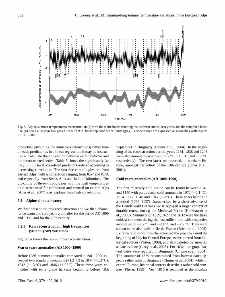
Fig. 5. Alpine summer temperatures reconstruction(a) with the white boxes denoting the warmest and coldest years, and the smoothed blackline (b) being a 20-year low pass filter with 95% bootstrap confidence limits (gray). Temperatures are expressed as anomalies with respectto 1901–2000.

predictors (including the numerous interactions) rather thanon each predictor as in a linear regression, it may be instruc-tive to calculate the correlation between each predictor andthe reconstructed series. Table 5 shows the significantly (atthep = 0.05 level) correlated predictors ordered according todecreasing correlation. The first five chronologies are fromeastern Alps, with a correlation ranging from 0.57 and 0.70,and especially from Swiss Alps and Italian Dolomites. Theproximity of these chronologies with the high temperaturestime series used for calibration and centred on central Alps(Auer et al., 2007) may explain these high correlations.

5.2 Alpine climate history

We first present the raw reconstruction and we then charac-terise warm and cold years anomalies for the period AD 1000and 1900, and for the 20th century.

5.2.1 Raw reconstruction: high frequencies(year-to-year) variations

Figure 5a shows the raw summer reconstruction.

Warm years anomalies (AD 1000–1900)

Before 1986, summer anomalies compared to 1901–2000 ex-ceeded two standard deviations (+1.2◦C) in 1834 (+1.3◦C),1842 (+1.3◦C) and 1846 (+1.9◦C). These three years co-incides with early grape harvests beginning before 18th

September in Burgundy (Chuine et al., 2004). In the begin-ning of the reconstruction period, years 1161, 1238 and 1246were also among the warmest (+1.2◦C, +1.1◦C, and +1.1◦Crespectively). The two latest are reported, in northern Eu-rope, amongst the hottest of the 13th century (Jones et al.,2001).

Cold years anomalies (AD 1000–1900)

The first relatively cold period can be found between 1040and 1140 with particularly cold summers in 1072 (−2.1◦C),1114, 1117, 1046 and 1047 (−2◦C). These years belong toa period (1088–1137) characterised by a short advance ofthe Grindelwald Glacier (Swiss Alps) in a larger context ofdurable retreat during the Medieval Period (Holzhauser etal., 2005). Summers of 1639, 1627 and 1632 were the threecoldest summers during the last millennium with respectiveanomalies of−2.2◦C and−2.1◦C and−2.2◦C. They wereshown to be also cold in Ile de France (Etien et al., 2008).Extreme cold conditions characterized the year 1627 until thebeginning of July for Central Europe, as deciphered from his-torical sources (Pfister, 1999), and also denoted by snowfallas late as June (Casty et al., 2005). For 1632, late grape har-vest dates were reported in Burgundy (Chuine et al., 2004).The summer of 1639 reconstructed from harvest dates ap-pears rather mild in Burgundy (Chuine et al., 2004), while incentral Europe, historical sources describe a rather cold sum-mer (Pfister, 1999). Year 1816 is recorded as the absolute



41

Figure 6. Comparison of regional and large-scale temperature reconstructions. All

reconstructions were 20-yr low-pass filtered. a. The solar irradiance variations (black)

reconstructed by Bard et al. (2007). Shadings denote the timing of great solar minima. b. The

average value of June to August graduated indices of Pfister et al. (1994). c. The speleothem

yearly temperature reconstruction (dark blue) of Mangini et al. (2005), the grape harvest

April-August temperature reconstruction of Meier et al. (2007) and the multi-proxy JJA

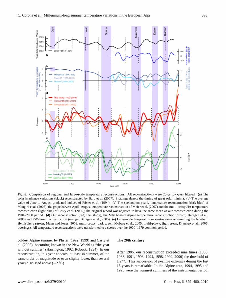
Fig. 6. Comparison of regional and large-scale temperature reconstructions. All reconstructions were 20-yr low-pass filtered.(a) Thesolar irradiance variations (black) reconstructed by Bard et al. (2007). Shadings denote the timing of great solar minima.(b) The averagevalue of June to August graduated indices of Pfister et al. (1994).(c) The speleothem yearly temperature reconstruction (dark blue) ofMangini et al. (2005), the grape harvest April–August temperature reconstruction of Meier et al. (2007) and the multi-proxy JJA temperaturereconstruction (light blue) of Casty et al. (2005); the original record was adjusted to have the same mean as our reconstruction during the1901–2000 period.(d) Our reconstruction (red; this study), the MXD-based Alpine temperature reconstruction (brown; Buntgen et al.,2006) and RW-based reconstruction (orange; Buntgen et al., 2005).(e) Large-scale temperature reconstructions representing the NorthernHemisphere (green, Mann and Jones, 2003, multi-proxy; dark green, Moberg et al., 2005, multi-proxy; light green, D’arrigo et al., 2006,treerings). All temperature reconstructions were transformed to z scores over the 1000–1979 common period.

coldest Alpine summer by Pfister (1992, 1999) and Casty etal. (2005), becoming known in the New World as “the yearwithout summer” (Harrington, 1992; Robock, 1994). In ourreconstruction, this year appears, at least in summer, of thesame order of magnitude or even slighty lower, than severalyears discussed above (−2◦C).

The 20th century

After 1986, our reconstruction exceeded nine times (1986,1988, 1991, 1993, 1994, 1998, 1999, 2000) the threshold of1.2◦C. This succession of positive extremes during the last15 years is remarkable. In the Alpine area, 1994, 1995 and1993 were the warmest summers of the instrumental period,



Table 5. Correlation coefficient between the reconstructed tempera-ture of Alps and the proxies used (after estimating the missing datawith the analogue method). Coefficients are calculated on the to-tal length of the period analysis, i.e., 1001 observations. Species:LADE: Larix decidua; PICE: Pinus cembra. The horizontal lineindicates significant correlation coefficients (at the 5% level).

No. Chronologies Species Correlation

21 Swiss2 (MXD) LADE 0.70

4 Cadini Lago di Misurina LADE 0.57

8 Comasine LADE 0.57

9 Fodara Vedla Alm LADE 0.57

20 Swiss1 (TRW) LADE, PICE 0.57

2 Alpe Musella LADE 0.51

25 Bufferes PICE 0.48

19 Ventina LADE 0.47

5 Chalets de l’Orgere LADE 0.46

17 Passo Cinque Croci LADE 0.45

6 Chardonnet LADE 0.44

14 Nevache Granges LADE 0.43

34 Manghen PICE 0.41

3 Berchtesgaden LADE 0.40

23 Ambrizzola PICE 0.40

13 Muestair LADE 0.39

22 Aleve LADE 0.39

1 Aleve LADE 0.35

with anomalies greater than +2◦C compared with the sum-mer mean temperature 1901–2000. The 95%-level error barscalculated by adding the bootstrap error (related to the qual-ity of the calibration sample) and the residual error (relatedto the quality of the model selected) is on average 0.57◦C.

5.2.2 Smoothed reconstruction: low-frequenciesclimatic variations and possible related forcing

Overview

Figure 5b shows the smoothed summer reconstruction. Werecontruct long cold periods from the second half of the11th and the first half of the 12th century (−0.5◦C be-low the 1901–2000 average) and between the late 16th cen-tury and the early 18th century (−0.8◦C). The culminationis achieved between 1685 and 1705 (−1.1◦C), which ap-pears to be the coldest decades of the millennium. By con-trast, a warm period is reconstructed between 1200 and 1420(+0.4◦C). The first decades of the 13th century (1300–1340)

Table 5. Continued.

No. Chronologies Species Correlation

12 Moutieres LADE 0.33

15 Obergurgl LADE 0.32

35 Obergurgl PICE 0.29

28 Fodara Vedla Alm PICE 0.27

32 La Joux PICE 0.27

7 Clapouse LADE 0.26

29 Formin PICE 0.26

30 Isola PICE 0.26

37 Val di Fumo PICE 0.26

26 Chaussettaz PICE 0.24

31 Jalavez PICE 0.22

24 Bois des Ayes PICE 0.20

16 Oriol LADE 0.19

10 Freyssinieres LADE 0.14

18 Ravin de Congerman LADE 0.12

27 Clavieres PICE 0.09

11 Merveilles LADE 0.06

38 Vallee du Tronchet PICE −0.13

33 Lac Miroir PICE −0.16

36 Roubinettes PICE −0.18

are clearly the warmest of the millennium (+0.7◦C) until1980–2000 (+1.8◦C). Warm summers were also recordedaround 1550 and during the second half of 18th century.

Solar activity

Correlations between the low-frequency solar activity andthe 20 year-smoothed temperature reconstruction are 0.21over their common period respectively. Even though, thecorrelation is not significant atp < 0.05 level, records sharehigh values (0.41) during the twelfth and thirteenth centuries(great solar maximum; Eddy, 1976) a prolonged depressionduring 1350–1600 (0.21) and an increasing values toward thetwentieth century (0.31). The prominent interdecadal solarminima, Oort, Wolf, Sporer, Maunder, Dalton, and Damonas well as the corresponding maxima are superimposed uponthis secular trend. The relatively cold conditions during themid-11th century to the mid-12th century with a minimumduring the decade 1045–1055 can be related to the Oort so-lar depression (Bard et al., 2007, Fig. 6a) with magnitudecomparable to that of the Late Maunder Minimum during



1675–1715 (Shindell et al., 2001). Warmer conditions dur-ing the end of the 12th and the 13th centuries of the mil-lennium are associated in Europe with the Medieval WarmPeriod (Hugues and Diaz, 1994) coinciding with the Me-dieval solar maximum (Eddy, 1976). It is characterized athigh altitude, in the French Alps by its shortness and by sig-nificant interdecadal variations. Warmer decades are cen-tered around 1160, 1240 and 1315. Summer temperaturessteadily decrease from mid-14th century. Between 1400 and1720, if we except decades centred on 1410 and 1560, the re-construction indicates below-average temperatures, accom-panied by significant inter-decadal variations. Key fluctua-tions are low temperatures in the 1460s, 1600s and around1700. These coldest periods of the LIA coincide with theSporer and Maunder solar minima (Fig. 6a). The cooling be-ginning in the mid-18th century is in phase with the decreaseof the solar irradiance.

Volcanic activity

The pronounced cooling of summer temperatures, duringthe period 1805-1820, recorded in Alpine glacier advances(Holzhauser et al., 2005; Zumbuhl et al., 2008), is char-acterized by a sequence of larger volcanic eruptions: in1808, with unknown location (Dai et al., 1991), in 1813 inAwu, Soufriere, St. Vincent, Suwanose-Jima (Buntgen et al.,2006a) and in 1815 in Tambora/Indonesia (Sigurdsson andCarey, 1989; Crowley, 2000; Oppenheimer, 2003). Happen-ing during the Dalton solar minimum, these eruptions mostlikely lead to an accumulated aerosol cooling effect (Esper etal., 2007).

Anthropogenic activity

During the industrial period, the proportion of man-madeforcing agents on the earth’s climate system increases com-paratively to natural forcing agents (Anderson et al., 2003;Crowley 2000; Meehl et al., 2003). Since the end of theLate Maunder Minimum, temperatures discontinuously in-creased until the end of the record in 2000. This trend andthe inter-decadal variations of the reconstructed temperaturesseen since the beginning of the 19th century are in line withJJA instrumental temperatures recorded in the Alps (Auer etal., 2007). The global and northern hemispheric warming ofthe 20th century (e.g. Folland et al., 2001) and in Europe (e.g.Luterbacher et al., 2004) is also prominent at high altitude inthe GAR (Casty et al. 2005; Buntgen et al., 2005, 2006a). Itoccurred in mainly two stages: between 1880 and 1945 andsince 1975. If we consider the last three centuries (1700–2000), the warming is higher than 2.5◦C (0.08◦C/decade),but it is mainly due to two important steps, the first one likelylinked with natural forcings (beginning of 18th century) andthe second being anthopogenic (end of 20th century). Never-theless, the anthopogenic step, compared to 1730–1980, re-mains as 1.3◦C.

5.3 Comparison with other reconstructions

5.3.1 Regional-scale comparisons

To further assess the reconstructed Alpine JJA temperaturehistory, we compare the new record with regional scale re-constructions by Pfister94 (Pfister et al., 1994), Meier07(Meier et al., 2007), Mangini05 (Mangini et al., 2005),Casty05 (Casty et al., 2005), Buntgen05 (Buntgen et al.,2005) and Buntgen06 (Buntgen et al., 2006a). The Pfis-ter94 graduated indices of summer temperatures (1525–1990) covers central Europe and are related to biologicalindicators such as dendro-climatic data, phenological obser-vations, para-phenological indicators such as grape or vineharvest dates. Monthly Graduated Indexes GI, range from−3 to +3 (from very cold to very warm anomalies), 0 be-ing ”average” months or data not available (according to the1901–1960 period). On a seasonal level the GI is definedas the average of the monthly GI, which yields gradationsof 0.3 between−3 and +3. The Meier07 April-August re-construction concerns specifically Switzerland. It is derivedback to 1480 from an annually resolved record of grape har-vest dates calibrated with monthly data from the Basel andGeneva stations (1928–1979) and verified over 1980–2006.The Mangini05 summer reconstruction is based on the pre-cisely dated isotopic composition of a stalagmite from Span-nagel Cave (2524 m a.s.l.) in the Central Alps of Austria. Thereconstruction covers the last millennium with a mean tem-poral resolution of three years. Despite it concerns the wholeyear, this reconstruction is used for comparison because itis fully independent from our dataset. The Casty05 grid-ded (0.5◦×0.5◦ lat/long) reconstruction covers the EuropeanAlpine region using long instrumental data in combinationwith documentary proxy evidence. Monthly (seasonal) gridsare reconstructed back to 1659 (1500–1658). The data de-tailed by Mitchell et al. (2005) comprising monthly globalland surface temperatures for the 1901–2000 period with0.5◦ resolution serve as predictands. Here, for purposesof comparison, a mean JJA series, representing the studiedzone, is calculated from 56 homogeneous grid-points. TheBuntgen05 reconstruction covers the Eastern Alps extendsback to 951. The dataset consists in 1527 subalpine larchand pine ring width series. For the calibration of proxy data,11 high-elevation meteorological station records are used(Bohm et al., 2001). Finally, Buntgen06 is also centeredon Swiss and Austrian Alps. It compiled 180 MXD larchseries dating from 735–2004. The HISTALP high tempera-tures time series of the GAR spanning the 1818–2003 periodare considered. Both reconstructions used the RCS methodto standardize dendrochronological series. Our dataset inte-grates Swiss1 and Swiss2 chronologies used as regressors inBuntgen05 and Buntgen06 reconstructions, respectively. Alldata have been smoothed with a 20 year low-pass filter.



According to the comparison provided in Fig. 6, thesmoothed Pfister94 reconstruction (Fig. 6b) correlates at 0.48(1525–2000) with our reconstruction, revealing similar inter-annual variations between indexes from historical documentsand our reconstruction. On low and medium frequency, bothsignals show the same trends during cool periods in 1590,1810 and 1910 and warm periods in 1550, 1850 and 1940.

The Mangini05 record (Fig. 6c) correlates at 0.30(p < 0.05) with our record. It reveals warm conditions dur-ing the putative Medieval Warm Period (1000–1300) early inthe last millennium, followed by cooler conditions during theLIA e.g. around 1600, 1700 and 1820, partly similar to thetrends displayed in our reconstruction. However, tempera-tures during the eleventh and twelfth centuries in Mangini05are higher than in our study (Fig. 6c, d). The four oldest pop-ulations used in our study shared a strong common signal be-tween 1000 and 1200. Thus, this discrepancy can hardly berelated to the decline of replication back in time. Moreover,cool summers around 1050 and 1120 are in phase with Oortsolar minimum and with the advance of the Great AletschGlacier around 1100. Finally, the Mangini05 curve ends atabout 1930, making difficult to evaluate the Medieval warmin the light of the 20th century. The filtered Meier07 recordhas lower amplitude than our reconstruction. The greater am-plitude of our reconstruction can be related to both scalinguncertainties/dependence upon particular statistical recon-struction approaches as well as amplitude dependence uponboth the spatial and temporal scales of interest (e.g., Esper etal., 2005). The courses of both curves are similar between1660–1710, 1800–1830 and 1950–2000. A divergence of thecurves is seen mainly between 1600–1660, 1730–1760 and1880–1950. Such discrepancies may be explained by chang-ing viticultural traditions (Lachiver, 1988), the varieties cul-tivated, the style of wine produced, the quality sought, theagricultural practices (Garcıa de Cortazar-Atauri et al., 2010)or other environmental influences than temperature. For ex-ample, anomalously high September precipitations fostersdiseases and irregular sugar assimilation and, thus, distortthe accuracy of the temperature signal recorded (Meier et al.,2007). These uncertainties on grape harvest dates and grapeharvest-based reconstructions are discussed extensively andquantified by Garcıa de Cortazar-Atauri et al. (2010).

Casty05 is calibrated against different instrumental targetrecords. Yet, the amplitude between the coldest and thewarmest year over the past 500 years are close, i.e. 4◦C(between 1807 and 1816) for Casty05 and 4.5◦C (between1639 and 1998) here. The smoothed Casty05 correlates at0.50 (p < 0.05) with our record over their 1500–2000 com-mon period and similar courses are observed during the peri-ods 1500–1620 and 1800–2000. A major discrepancy occursaround 1750. During this period, our reconstruction mightbe influenced by differences between larch and pine datasets(Fig. 3). Before 1800, Casty05 is systematically higher thanour reconstruction but also displays increasing uncertaintiesrelated to inhomogeneities in the instrumental data before the

mid-19th century as reported by Luterbacher et al. (2004). Abias as 0.7 to 0.8◦C (Moberg et al., 2003) and up to 1–2◦C(Etien et al., 2008) before 1860, could exist in temperatures,likely because of insufficient or inadequate shading appara-tus of the thermometers, and may explain the differences be-tween both reconstructions.

Unsurprisingly, our reconstruction, not fully independentof Buntgen05 and Buntgen06, shared a high common signalwith both alpine reconstructions. Buntgen05 and Buntgen06respectively correlate at 0.56 (p < 0.05) and 0.70 (p < 0.05)(0.57 (p <0.05) and 0.77 (p <0.05) after smoothing) withour record. The range of inter-annual variations of ourcurve is also quite similar to Buntgen05, i.e. 4.2◦C (be-tween 1821 and 2000) but slightly lower than Buntgen06(6.2◦C, between 1816 and 1928). This difference may bedue to enhanced interannual climate response of the MXDdata (Buntgen06) considered as having a lower biologicalmemory as compared to their RW counterparts (Frank et al.,2007). In details, between 1430 and 1700 our reconstructionremains in phase with Buntgen05 and Buntgen06, despite theintroduction of several populations from the western Alpsin the dataset, indicating a generalised cooling of the GARduring the LIA. Between1720 and 1920, our reconstructionslightly differs from Buntgen05 and Buntgen06. Higher tem-peratures are reconstructed at the end of the Maunder mini-mum (1720’s) and the Dalton solar minimum (1820’s) is lesspronounced (Fig. 6d). They are related with growth increasesin several of the most Western chronologies used for recon-struction, e.g. Chardonnet, Freyssinieres, Nevaches Grangesor Lac Miroir and absents in eastern populations. These pe-riods match with abnormal dry conditions in Europe (Paul-ing et al., 2006) and in the Alps (Casty et al., 2005) and alower drought sensitivity of Western populations exposed tooceanic conditions might explain the observed differences.This hypothesis is consistent with recent studies showing theexistence of longitudinal gradients of chronologies responsesfor coniferous species (Frank and Esper, 2005b; Carrer et al.2007).

5.3.2 Hemispheric-scale comparisons

Comparisons are carried out with the hemispheric tree-ring-based D’Arrigo06 (D’Arrigo et al., 2006), andthe multiproxy-based Mann03 (Mann et al., 2003) andMoberg05 (Moberg et al., 2005) reconstructions (Fig. 6e).Alpine like other regional temperature changes have, as ex-pected, larger amplitudes of variations than those averagedover large areas (e.g. Mann et al., 2000; Luterbacher et al.,2004; Jones and Mann, 2004; Brazdil et al., 2005; Xoplakiet al., 2005). Correlations between this study and Mann03,D’Arrigo06, and Moberg05, computed over the 1000–1979common period are 0.18, 0.18 and 0.19. They are 0.50(p < 0.05), 0.30 (p < 0.05), and 0.38 (p < 0.05) after 20-yrsmoothing indicating some similarities in the low frequencydomain. This reveals some common patterns in spite of



differences in spatial extension and detrending methods ap-plied in the large scale records. Key multi-centennial varia-tions common to all records are high values associated with alate Medieval Warm Period (1200–1420) a multi-centennialdepression between 1420 and 1830, attributed to the LIA,and a recent warming trend (from 1980 onwards). However,the reconstructed NH temperatures are not very high duringthe 10th and 11th centuries and are less sensitive to the Oortsolar minimum. At decadal scales, all records show low tem-peratures in the 1070s, 1300s, 1460s, around 1600, and 1820,and high temperatures in the 1420s and in the 1570s.

6 Conclusions

A new larch/pine composite chronology is presented, inte-grating populations from western Alps and providing ev-idence of Alpine summer temperature variations back to1000. The Adaptive Regional Growth Curve method is usedto preserve both low to high frequency information from thedata. Instrumental measurements from the HISTALP hightemperatures time series back to 1818 are used for calibra-tion and low-elevation series were used for verification. Thenew record correlates with high-elevation JJA temperaturesback to 1818, but indicates discrepancies between “cooler”proxy-inferred and “warmer” instrumental values prior to1850. The multidecadal to centennial variations properlymatch with solar forcings particularly during solar minimaand some annual to decadal coolings are related to volcaniceruptions especially at the beginning of the 19th century. Therecord indicates a short Medieval Warm Period with warmerconditions beginning as late as the early 13th. The LIA isparticularly cold between 1420 and 1720 with a mean sum-mer temperature of−0.80◦C compared to the 1901–2000reference period. After 1720, temperatures increase with dis-tinct depressions during the 1810–20s, the 1910s, and 1970s.According to this regional analysis, the last decade of the20th is the warmest period over the past millennium: +0.9◦C(compared to the 1901–2000 reference period). The ampli-tude of this warming compared to the previous period is evenhigher. It largely exceeds the warming reconstructed for theMedieval Warm Period in both its amplitude and abruptness.This particular feature (outstanding intense and rapid warm-ing) is consistent with the fact that it might be attributedto the contribution of anthropogenic greenhouse gases andaerosols. These periods are seen in Alpine, European orhemispheric reconstructions but also in independent proxies(historical archives, speleothems) indicating the relevance ofthis new record and the Alps to large-scale studies of globalclimate change.

Acknowledgements.This research has been supported by theprogram ESCARSEL (2007–2010), “Evolution Seculaire du Cli-mat dans les regions circum-Atlantiques et Reponse de SystemesEco-Lacustres” funded by the French ANR “Vulnerabilite: milieuxet climat”. We are grateful to 2 anonymous referees who provideddetailed comments and suggestions that greatly helped to clarifythe points discussed here.

Edited by: H. Goosse

The publication of this article is financed by CNRS-INSU.

References

Anderson, T. L., Charlson, R. J., Schwartz, S. E., Knutti, R.,Boucher, O., Rodhe, H., and Heintzenberg, J.: Climate forcingby aerosols – A hazy picture, Science, 302, 1679–1681, 2003.

Auer, I., Bohm, R., Jurkovi, A., Lipa, W., Orlik, A., Potzmann,R., Schoner, W., Ungersbock, M., Matulla, C., Briffa, K., Jones,P., Efthymiadis, D., Brunetti, M., Nanni, T., Maugeri, M., Mer-calli, L., Mestre, O., Moisselin, J.-M., Begert, M., Muller-Westermeier, G., Kveton, V., Bochnicek, O., Stastny, P., Lapin,M., Szalai, S., Szentimrey, T., Cegnar, T., Dolinar, M., Gajic-Capka, M., Zaninovic, K., Majstorovic, Z., and Nieplova, E.:HISTALP - historical instrumental climatological surface timeseries of the Greater Alpine Region, Int. J. Climatol., 27, 17–46,2007.

Bard, E., Raisbeck, G., Yiou, F., and Jouzel, J.: Comment on ”So-lar activity during the last 1000 yr inferred from radionucliderecords” by Muscheler et al. (2007), Quaternary Sci. Rev., 26,2301–2308, 2007.

Becker, M.: The role of climate on present and past vitality of silverfir in the Vosges mountains of northern France, Can. J. ForestRes., 19, 1110–1117, 1989.

Begert, M., Schlegel T., and Kirchhofer W.: Homogeneous temper-ature and precipitation series of Switzerland for 1864 to 2000,Int. J. Climatol., 25, 65–80, 2005.

Bohm, R., Auer, L., Brunetti, M., Maugeri, M., Nanni, D., andSchoner, W.: Regional temperature variability in the EuropeanAlps: 1760–1998 from homogenized instrumental time series,Int. J. Climatol., 21, 1779–1801, 2001.

Brazdil, R., Pfister, C., Wanner, H., Von Storch, H., and Luter-bacher, J.: Historical climatology in Europe—State of the art,Climate Change, 70, 363–430, 2005.

Briffa, K. R., Jones, P. D., Bartholin, T. S., Eckstein, D., Schwe-ingruber, F. H., Karlen, W., Zetterberg, P., and Eronen, M.:Fennoscandian summers from AD 500 – temperature-changes onshort and long timescales, Clim. Dynam., 7, 111–119, 1992.

Briffa, K. R., Schweingruber, F. H., Jones, P. D., Osborn, T. J.,Harris, I. C., Shiyatov, S. G., Vaganov, E. A., and Grudd, H.:



“Trees tell of past climates: but are they speaking less clearlytoday?”, Philos. T. Roy. Soc. B., 353, 65–73, 1998.

Briffa, K. R., Osborn, T. J., Schweingruber, F. H., Harris, I. C.,Jones, P. D., Shiyatov, S. G., and Vaganov, E. A.: Low-frequencytemperature variations from a northern tree-ring density network,J. Geophys. Res., 106, 2929–2941, 2001.

Brunetti, M., Maugeri, M., Monti, F., and Nanni, T.: Temperatureand precipitation variability in Italy in the last two centuries fromhomogenised instrumental time series, Int. J. Climatol., 26, 345–381, 2006.

Buntgen, U., Esper, J., Frank, D. C., Nicolussi, K., and Schmidhal-ter, M.: A 1052-year tree-ring proxy of Alpine summer tempera-tures, Clim. Dynam., 25, 141–153, 2005.

Buntgen, U., Frank, D. C., Nievergelt, D., and Esper, J.: Summertemperature variations in the European Alps, AD 755-2004, J.Climate, 19, 5606–5623, 2006a.

Buntgen, U., Bellwald, I., Kalbermatten, H., Schmidhalter, M., Fre-und, H., Frank, D.C., Bellwald, W., Neuwirth, B., Nusser, M.,and Esper, J.: 700 years of settlement and building history in theLotschental/Switzerland, Erdkunde, 60/2, 96–112, 2006b.

Buntgen, U., Frank, D., Wilson, R., and Esper, J.: A test for tree-ring divergence in the European Alps, Glob. Change Biol., 14,2443–2453, 2008.

Carrer, M. and Urbinati, C.: Age-dependent tree-ring growth re-sponses to climate in Larix decidua and Pinus cembra., Ecology,85, 730–740, 2004.

Carrer, M. and Urbinati, C.: Long-term change in the sensitivity oftreering growth to climate forcing in Larix decidua, New Phytol.,170, 861–872, 2006.

Casty, C., Wanner, H., Luterbacher, J., Esper, J., and Bohm, R.:Temperature and precipitation variability in the European Alpssince 1500, Int. J. Climatol., 25, 1855–1880, 2005.

Chuine, I., Yiou, P., Viovy, N., Seguin, B., Daux, V., and LeRoyLadurie, E.: Grape ripening as an indicator of past climate, Na-ture, 432, 289–290, 2004.

Cook, E. and Kairiukstis, L.: Methods of dendrochronology,Kluwer, Dordrecht, 1990.

Cook, E. R., Briffa, K. R., and Jones, P. D.: Spatial regression meth-ods in dendroclimatology: A review and comparison of two tech-niques, Int. J. Climatol., 14, 379–402, 1994.

Cook, E. R., D’Arrigo, R. D., and Mann, M. E.: A well-verified,multiproxy reconstruction of the Winter North Atlantic Oscilla-tion Index since AD 1400, J. Climate, 15, 1754–1764, 2002.

Crowley, T. J.: Causes of climate change over the past 1000 years,Science, 295, 270–277, 2000.

D’Arrigo, R., Wilson, R., and Jacoby, G.: On the long-term con-text for late twentieth century warming, J. Geophys. Res., 111,D03103, doi:10.1029/2005JD006352, 2006.

Dai, J., Mosley-Thompson, E., and Thompson, L. G.: Ice core evi-dence for an explosive tropical volcanic eruption 6 years preced-ing Tambora, J. Geophys. Res., 96, 17361–17366, 1991.

Eddy, J. A.: The maunder minimum, Science, 192, 1189–1202,1976.

Efron, B.: Bootstrap methods: another look at the jackknife, TheAnnals of Statistics, 7, 1–26, 1979.

Esper, J., Cook, E. R., and Schweingruber, F. H.: Low-frequencysignals in long tree-ring chronologies for reconstructing pasttemperature variability, Science, 295, 2250–2253, 2002.

Esper, J., Niederer, R., Bebi, P., and Frank, D: Climate signal age ef-

fects – Evidence from young and old trees in the Swiss Engadin,Forest Ecol. Manag., 255, 3783–3789, 2008.

Etien, N., Daux, V., Masson-Delmotte, V., Stievenard, M., Bernard,V., Durost, S., Guillemin, M. T., Mestre, O., and Pierre, M.: Abi-proxy reconstruction of Fontainebleau (France) growing sea-son temperature from AD 1596 to 2000, Clim. Past, 4, 91–106,doi:10.5194/cp-4-91-2008, 2008.

Folland, C. K., Rayner, N. A., Brown, S. J., Smith, T. M., Shen,S. S. P., Parker, D. E., Macadam, I., Jones, P. D., Jones, R. N.,Nicholls, N., and Sexton, D. M. H.: Global temperature changeand its uncertainties since 1861, J. Geophys. Res., 28, 2621–2624, 2001.

Frank, D. and Esper, J.: Temperature reconstructions and compar-isons with instrumental data from a tree-ring network for the Eu-ropean Alps, Int. J. Climatol., 25, 1437–1454, 2005.

Frank, D., Buntgen, U., Bohm, R., Maugeri, M., and Esper, J.:Warmer early instrumental measurements versus colder recon-structed temperatures: shooting at a moving target, QuaternarySci. Rev., 28, 3298–3310, 2007a.

Frank, D., Esper, J., and Cook, E. R.: Adjustment for proxy numberand coherence in a large-scale temperature reconstruction, Geo-phys. Res., 34, doi:10.1029/2007GL030571, 2007b.

Fritts, H. C.: Tree Rings and Climate, Academic Press, 1976.Garcıa de Cortazar-Atauri, I., Daux, V., Garnier, E., Yiou, P.,

Viovy, N., Seguin, B., Boursiquot, J.M., Parker, A.K., vanLeeuwen, C., and Chuine I.: Climate reconstructions from grapeharvest dates: Methodology and uncertainties, The Holocene,doi:10.1177/0959683609356585, 2010.

Grove, J. M.: The Little Ice Age, Methuen and Co., London, NewYork, 1988.

Guiot, J.: Methods of calibration, verification and reconstruction,in: Methods of denrochronology, application in the environmen-tal sciences, edited by: Cook, E. and Kairiukstis, L., Dordrecht,International Institute for Applied Systems Analysis, KluwerAcademy Publications, 163–217, 1990.

Guiot, J., Nicault, A., Rathgeber, C., Edouard, J.-L., Guibal, F.,Pichard, G., and Till, C.: Last-millennium summer-temperaturevariations in western Europe based on proxy data, The Holocene,15, 489–500, 2005.

Harrington, C. D.: The Year without a Summer? World Climate in1816, Canadian Museum of Nature, Ottawa, 1992.

Holzhauser, H., Magny, M., and Zumbuhl, H. J.: Glacier and lake-level variations in west-central Europe over the last 3500 years,The Holocene, 15, 789–801, 2005.

Hughes, M. K. and Diaz, H. F.: Was there a “Medieval Warm Pe-riod” and if so, where and when?, Climatic Change, 26, 109–142,1994.

Jones, P. D., Osborn, T. J., and Briffa, K. R.: The evolution of cli-mate over the last millennium, Science, 292, 662–666, 2001.

Jones, P. D. and Mann, M. E.: Climate over past millennia, Rev.Geophys., 42, RG2002, doi:10.1029/2003RG000143, 2004.

Lamb, H. H.: Climate: present, past and future, London: Methuen,1976.

Lachiver, M.: Vins, Vignes et Vignerons: Histoire du VignobleFrancais, Fayard, Paris, 1988.

LeRoy Ladurie, E.: Histoire humaine et comparee du climat, Vol 1:Canicules et glaciers XIII-XVIII siecles, Fayard, 740pp., Paris,2004.

Luterbacher, J., Rickli, R., Xoplaki, E., Tinguely, C., Beck, C., Pfis-



ter, C., and Wanner, H.: The Late Maunder Minimum (1675–1715) – A key period for studying decadal scale climate changein Europe, Climate Change, 49, 441–462, 2001.

Luterbacher, J., Xoplaki, E., Dietrich, D., Jones, P. D., Davies, T.D., Portis, D., Gonzalez- Rouco, J. F., von Storch, H., Gyalistras,D., Casty, C., and Wanner, H.: Extending North Atlantic Oscilla-tion reconstructions back to 1500, Atmos. Sci. Lett., 2, 114–124,2002.

Luterbacher, J., Dietrich, D., Xoplaki, E., Grosjean, M., and Wan-ner, H.: European seasonal and annual temperature variability,trends, and extremes since 1500, Science, 303, 1499–1504, 2004.

Luterbacher, J., Dietrich, D., Xoplaki, E., Grosjean, M., and Wan-ner, H.: European Seasonal Temperature Reconstructions. IGBPPAGES/World Data Center for Paleoclimatology Data Contri-bution Series # 2006-060. NOAA/NCDC Paleoclimatology Pro-gram, Boulder CO, USA, 2006.

Mangini, A., Spoetl, C., and Verdes, P.: Reconstruction of temper-ature in the Central Alps during the past 2000 year from a d18Ostalagmite record, Earth Planet. Sc. Lett., 235, 741–751, 2005.

Mann, M. E., Bradley, R. S., and Hughes, M. K.: Northern Hemi-sphere temperatures during the past millennium: inferences, un-certainties, and limitations, Geophys. Res. Lett., 26, 759–762,1999.

Mann, M. E., Gille, E., Bradley, R. S., Hughes, M. K., Overpeck, J.T., Keimig, F. T., and Gross, W.: Global temperature patterns inpast centuries: an interactive presentation, Earth Interactions, 4,1–29, 2000.

Mann, M. E. and Jones, P. D.: Global Surface Tempera-tures over the Past Two Millennia, Geophys. Res. Lett., 30,doi:10.1029/2003GL017814, 2003.

Mann, M. E.: Clmate over the Past two millennia, Annu. EarthPlanet. Sci., 35, 111–136, 2007.

Matulla, C., Auer, I., Bohm, R., Ungersbock, M., Schoner,W., Wagner, S., and Zorita, E.: Outstanding past decadal-scale climate events in the Greater Alpine region analysed by250 years data and model runs, GKSS-Report 2005/4, GKSSForschungszentrum in der Helmholtz Gemeinschaft, Geesthacht,2005.

Meehl, G. A., Washington, W. M., Wigley, T. M. L., Arblaster, J.M., and Dai, A.: Solar and greenhouse gas forcing and climateresponse in the twentieth century, J. Climate, 16, 426–444, 2003.

Meier, N., Rutishauser, T., Pfister, C., Wanner H., and Luterbacher,J.: Grape harvest dates as proxy for Swiss April to August tem-perature reconstructions back to AD 1480, Geophys. Res. Lett.,34, L20705, doi:10.1029/2007GL031381, 2007.

Moberg, A., Alexandersson, H., Bergstrom, H., and Jones, P. D.:Were Southern Swedish summer temperatures before 1860 aswarm as measured?, Int. J. Climatol., 23, 1495–1521, 2003.

Moberg, A. D., Sonechkin, M., Holmgren, K., Datsenko, N. M., andKarlen, W.: Highly variable Northern Hemisphere temperaturesreconstructed from low- and high-resolution proxy data, Nature,433, 613–617, 2005.

Mitchell, T. D., Hulme, M., and New, M.: Climate data for politicalareas, Area, 34, 109–112, 2002.

Mitchell, T. D. and Jones, P.: An improved method of constructinga database of monthly climate observations and associated high-resolution grids, Int. J. Climatol., 25, 693–712, 2005.

New, M., Hulme, M., and Jones, P. D.: Representing twentieth-century space – time climate variability. Part II: development of

1901–96 monthly grids of terrestrial surface climate, J. Climate,13, 2217–2238, 2000.

Ni, F., Cavazos, T., Hughes, M. K., Combrie, A., and Funkhouser,G.: Cool-season precipitation in the Southwestern USA sinceAD 1000: comparison of linear and non linear techniques forreconstruction, Int. J. Climatol., 22, 1645–1662, 2002.

Nicault, A., Alleaume, S., Brewer, S., Carrer, M., Nola, P., andGuiot, J.: Mediterranean drought fluctuation during the last 500years based on tree-ring data, Clim. Dynam., 31, 227–245, 2008.

Nicault, A., Guiot, J., Edouard, J.-L., and Brewer, S.: Preserv-ing long-term fluctuations in standardization of tree-ring se-ries by the Adaptative Regional Growth Curve (ARGC), Den-drochronologia, 28, 1–12, 2010.

Oerlemans, J.: Extracting a climate signal from 169 glacier records,Science, 308, 675–677, 2005.

Oppenheimer, C.: Climatic, environmental and human conse-quences of the largest known historic eruption: Tambora volcano(Indonesia) 1815, Prog. Phys. Geog., 27, 230–259, 2003.

Pauling, A., Luterbacher, J., Casty C., and Wanner, H.: Five hun-dred years of gridded high-resolution precipitation reconstruc-tions over Europe and the connection to large-scale circulation,Clim. Dynam., 26, 387–405, 2006.

Pfister, C.: Monthly temperature and precipitation patterns in Cen-tral Europe from 1525 to the present. A methodology for quan-tifying man made evidence on weather and climate, in: Climatesince 1500 AD, edited by: Bradley, R. S. and Jones, P. D., Lon-don, 118–143, 1992.

Pfister, C., Kington, J., Kleinlogel, G., Schuele, H., and Siffert,E.: The creation of highresolution spatio-temporal reconstruc-tions of past climate from direct meteorological observations andproxy data, Methodological considerations and results, in: Cli-mate in Europe 1675–1715, edited by: Frenzel, B., Pfister, C.,and Glaeser, B., 1994.

Pfister, C.: Wetternachhersage, 500 Jahre Klimavariationen undNaturkatastrophen 1496–1995, Haupt Verlag, 1999.

Rathgeber, C., Guiot, J., Roche, P., and Tessier, L.: Augmentationde productivite du chene pubescent en region mediterraneennefrancaise, Ann. Sci. Forest., 56, 201–209, 1999.

Richman, M. B.: Rotation of principal components, J. Climatol., 6,293–335, 1986.

Robock, A.: Review of year without a summer? World climate in1816, Climate Change, 26, 105–108, 1994.

Schneider, T.: Analysis of incomplete climate data: estimation ofmean values and covariance matrices and imputation of missingvalues, J. Climate, 14, 853–871, 2001.

Shindell, D. T., Schmidt, G. A., Mann, M. E., Rind, D., and Waple,A.: Solar forcing of regional climate change during the MaunderMinimum, Science, 294, 2149–2152, 2001.

Sigurdsson, H. and Carey, S.: Plinian and co-ignimbrite tephra fallfrom the 1815 eruption of Tambora volcano, B. Volcanol., 51,243–270, 1989.

Wanner, H., Pfister, C., Brazdil, R., Frich, P., and Frydendah, K.:Wintertime European circulation patterns during the late Maun-der minimum cooling period [1675-1704], Theor. Appl. Clima-tol., 51, 167–175, 1995.

Wigley, T. M. L., Briffa, K. R., and Jones, P. D.: On the averageof value of correlated time series, with applications in dendrocli-matology and hydrometeorology, J. Clim. Appl. Meteorol., 23,201–213, 1984.



Woodhouse, C. A.: Artificial neural networks and dendroclimaticreconstructions: an example from the Front Range, Colorado,USA, The Holocene, 9, 521–529, 1999.

Xoplaki, E., Luterbacher, J., Paeth, H., Dietrich, D., Steiner,N., Grosjean, M., and Wanner, H.: European spring andautumn temperature variability and change of extremes overthe last half millennium, Geophys. Res. Lett., 32, L15713,doi:10.1029/2005GL023424, 2005.

Zumbuhl, H. J., Steiner, D., and Nussbaumer, S. U.: 19th centuryglacier representations and fluctuations in the central and west-ern European Alps: an interdisciplinary approach, Global Planet.Change, 60, 42–57, 2008.


Millennium-long summer temperature variations in the European Alps as reconstructed from tree rings

Documents

Transcript of Millennium-long summer temperature variations in the European Alps as reconstructed from tree rings