Military Laser Technology for Defense
312
Military Laser Technology for Defense Technology for Revolutionizing 21st Century Warfare Alastair D. McAulay Lehigh University, Bethlehem, PA
-
Upload
khangminh22 -
Category
Documents
-
view
0 -
download
0
Transcript of Military Laser Technology for Defense

Military Laser Technologyfor DefenseTechnology for Revolutionizing 21stCentury Warfare
Alastair D. McAulayLehigh University, Bethlehem, PA

Copyright © 2011 by John Wiley & Sons, Inc. All rights reserved
Published by John Wiley & Sons, Inc., Hoboken, New JerseyPublished simultaneously in Canada
No part of this publication may be reproduced, stored in a retrieval system, or transmitted in any form orby any means, electronic, mechanical, photocopying, recording, scanning, or otherwise, except aspermitted under Section 107 or 108 of the 1976 United States Copyright Act, without either the priorwritten permission of the Publisher, or authorization through payment of the appropriate per-copy fee tothe Copyright Clearance Center, Inc., 222 Rosewood Drive, Danvers, MA 01923, (978) 750-8400, fax(978) 750-4470, or on the web at www.copyright.com. Requests to the Publisher for permission shouldbe addressed to the Permissions Department, John Wiley & Sons, Inc., 111 River Street, Hoboken, NJ07030, (201) 748-6011, fax (201) 748-6008, or online at http://www.wiley.com/go/permission.
Limit of Liability/Disclaimer of Warranty: While the publisher and author have used their best efforts inpreparing this book, they make no representations or warranties with respect to the accuracy orcompleteness of the contents of this book and specifically disclaim any implied warranties ofmerchantability or fitness for a particular purpose. No warranty may be created or extended by salesrepresentatives or written sales materials. The advice and strategies contained herein may not be suitablefor your situation. You should consult with a professional where appropriate. Neither the publisher norauthor shall be liable for any loss of profit or any other commercial damages, including but not limited tospecial, incidental, consequential, or other damages.
For general information on our other products and services or for technical support, please contact ourCustomer Care Department within the United States at (800) 762-2974, outside the United States at (317)572-3993 or fax (317) 572-4002.
Wiley also publishes its books in a variety of electronic formats. Some content that appears in print maynot be available in electronic formats. For more information about Wiley products, visit our web site atwww.wiley.com.
ISBN 978-0-470-25560-5
Library of Congress Cataloging-in-Publication Data is available.
Printed in Singapore
10 9 8 7 6 5 4 3 2 1

CONTENTS
PREFACE xiii
ACKNOWLEDGMENTS xv
ABOUT THE AUTHOR xvii
I OPTICS TECHNOLOGY FOR DEFENSE SYSTEMS 1
1 OPTICAL RAYS 3
1.1 Paraxial Optics / 4
1.2 Geometric or Ray Optics / 5
1.2.1 Fermat’s Principle / 51.2.2 Fermat’s Principle Proves Snell’s Law for Refraction / 51.2.3 Limits of Geometric Optics or Ray Theory / 61.2.4 Fermat’s Principle Derives Ray Equation / 61.2.5 Useful Applications of the Ray Equation / 81.2.6 Matrix Representation for Geometric Optics / 9
1.3 Optics for Launching and Receiving Beams / 10
1.3.1 Imaging with a Single Thin Lens / 101.3.2 Beam Expanders / 131.3.3 Beam Compressors / 141.3.4 Telescopes / 141.3.5 Microscopes / 171.3.6 Spatial Filters / 18
v
vi CONTENTS
2 GAUSSIAN BEAMS AND POLARIZATION 20
2.1 Gaussian Beams / 20
2.1.1 Description of Gaussian Beams / 212.1.2 Gaussian Beam with ABCD Law / 242.1.3 Forming and Receiving Gaussian Beams with Lenses / 26
2.2 Polarization / 29
2.2.1 Wave Plates or Phase Retarders / 312.2.2 Stokes Parameters / 332.2.3 Poincare Sphere / 342.2.4 Finding Point on Poincare Sphere and Elliptical Polarization
from Stokes Parameters / 352.2.5 Controlling Polarization / 36
3 OPTICAL DIFFRACTION 38
3.1 Introduction to Diffraction / 38
3.1.1 Description of Diffraction / 393.1.2 Review of Fourier Transforms / 40
3.2 Uncertainty Principle for Fourier Transforms / 42
3.2.1 Uncertainty Principle for Fourier Transforms in Time / 423.2.2 Uncertainty Principle for Fourier Transforms in Space / 45
3.3 Scalar Diffraction / 47
3.3.1 Preliminaries: Green’s Function and Theorem / 483.3.2 Field at a Point due to Field on a Boundary / 483.3.3 Diffraction from an Aperture / 503.3.4 Fresnel Approximation / 513.3.5 Fraunhofer Approximation / 543.3.6 Role of Numerical Computation / 56
3.4 Diffraction-Limited Imaging / 56
3.4.1 Intuitive Effect of Aperture in Imaging System / 563.4.2 Computing the Diffraction Effect of a Lens Aperture
on Imaging / 57
4 DIFFRACTIVE OPTICAL ELEMENTS 61
4.1 Applications of DOEs / 62
4.2 Diffraction Gratings / 62
4.2.1 Bending Light with Diffraction Gratings andGrating Equation / 63
4.2.2 Cosinusoidal Grating / 644.2.3 Performance of Grating / 66

CONTENTS vii
4.3 Zone Plate Design and Simulation / 67
4.3.1 Appearance and Focusing of Zone Plate / 674.3.2 Zone Plate Computation for Design and Simulation / 68
4.4 Gerchberg–Saxton Algorithm for Design of DOEs / 73
4.4.1 Goal of Gerchberg–Saxton Algorithm / 734.4.2 Inverse Problem for Diffractive Optical Elements / 734.4.3 Gerchberg–Saxton Algorithm for Forward Computation / 744.4.4 Gerchberg–Saxton Inverse Algorithm for Designing a
Phase-Only Filter or DOE / 74
5 PROPAGATION AND COMPENSATION FORATMOSPHERIC TURBULENCE 77
5.1 Statistics Involved / 78
5.1.1 Ergodicity / 795.1.2 Locally Homogeneous Random Field Structure Function / 805.1.3 Spatial Power Spectrum of Structure Function / 80
5.2 Optical Turbulence in the Atmosphere / 82
5.2.1 Kolmogorov’s Energy Cascade Theory / 835.2.2 Power Spectrum Models for Refractive Index in
Optical Turbulence / 855.2.3 Atmospheric Temporal Statistics / 865.2.4 Long-Distance Turbulence Models / 86
5.3 Adaptive Optics / 86
5.3.1 Devices and Systems for Adaptive Optics / 86
5.4 Computation of Laser Light Through Atmospheric Turbulence / 89
5.4.1 Layered Model of Propagation ThroughTurbulent Atmosphere / 90
5.4.2 Generation of Kolmogorov Phase Screens by theSpectral Method / 92
5.4.3 Generation of Kolmogorov Phase Screens from CovarianceUsing Structure Functions / 94
6 OPTICAL INTERFEROMETERS AND OSCILLATORS 99
6.1 Optical Interferometers / 100
6.1.1 Michelson Interferometer / 1016.1.2 Mach–Zehnder Interferometer / 1056.1.3 Optical Fiber Sagnac Interferometer / 108
6.2 Fabry–Perot Resonators / 109
6.2.1 Fabry–Perot Principles and Equations / 1106.2.2 Fabry–Perot Equations / 110

viii CONTENTS
6.2.3 Piezoelectric Tuning of Fabry–Perot Tuners / 116
6.3 Thin-Film Interferometric Filters and Dielectric Mirrors / 116
6.3.1 Applications for Thin Films / 1176.3.2 Forward Computation Through Thin-Film Layers
with Matrix Method / 1186.3.3 Inverse Problem of Computing Parameters for Layers / 122
II LASER TECHNOLOGY FOR DEFENSE SYSTEMS 125
7 PRINCIPLES FOR BOUND ELECTRON STATE LASERS 127
7.1 Laser Generation of Bound Electron State Coherent Radiation / 128
7.1.1 Advantages of Coherent Light from a Laser / 1287.1.2 Basic Light–Matter Interaction Theory for Generating
Coherent Light / 129
7.2 Semiconductor Laser Diodes / 133
7.2.1 p–n Junction / 1337.2.2 Semiconductor Laser Diode Gain / 1367.2.3 Semiconductor Laser Dynamics / 1397.2.4 Semiconductor Arrays for High Power / 140
7.3 Semiconductor Optical Amplifiers / 140
8 POWER LASERS 143
8.1 Characteristics / 144
8.1.1 Wavelength / 1448.1.2 Beam Quality / 1448.1.3 Power / 1458.1.4 Methods of Pumping / 1468.1.5 Materials for Use with High-Power Lasers / 147
8.2 Solid-State Lasers / 148
8.2.1 Principles of Solid-State Lasers / 1488.2.2 Frequency Doubling in Solid State Lasers / 150
8.3 Powerful Gas Lasers / 158
8.3.1 Gas Dynamic Carbon Dioxide Power Lasers / 1588.3.2 COIL System / 160
9 PULSED HIGH PEAK POWER LASERS 165
9.1 Situations in which Pulsed Lasers may be Preferable / 165
9.2 Mode-Locked Lasers / 167
CONTENTS ix
9.2.1 Mode-Locking Lasers / 1679.2.2 Methods of Implementing Mode Locking / 169
9.3 Q-Switched Lasers / 170
9.4 Space and Time Focusing of Laser Light / 171
9.4.1 Space Focusing with Arrays and Beamforming / 1719.4.2 Concentrating Light Simultaneously in Time
and Space / 173
10 ULTRAHIGH-POWER CYCLOTRON MASERS/LASERS 177
10.1 Introduction to Cyclotron or Gyro Lasersand Masers / 178
10.1.1 Stimulated Emission in an Electron Cyclotron / 178
10.2 Gyrotron-Type Lasers and Masers / 179
10.2.1 Principles of Electron Cyclotron Oscillatorsand Amplifiers / 180
10.2.2 Gyrotron Operating Point and Structure / 182
10.3 Vircator Impulse Source / 184
10.3.1 Rationale for Considering the Vircator / 18410.3.2 Structure and Operation of Vircator / 18410.3.3 Selecting Frequency of Microwave Emission from
a Vircator / 18610.3.4 Marx Generator / 18610.3.5 Demonstration Unit of Marx Generator Driving
a Vircator / 188
11 FREE-ELECTRON LASER/MASER 191
11.1 Significance and Principles of Free-ElectronLaser/Maser / 192
11.1.1 Significance of Free-Electron Laser/Maser / 19211.1.2 Principles of Free-Electron Laser/Maser / 192
11.2 Explanation of Free-Electron Laser Operation / 193
11.2.1 Wavelength Versatility for Free-Electron Laser / 19411.2.2 Electron Bunching for Stimulated Emission in
Free-Electron Laser / 197
11.3 Description of High- and Low-Power Demonstrations / 199
11.3.1 Proposed Airborne Free-Electron Laser / 19911.3.2 Demonstration of Low-Power System for
Free-Electron Maser at 8–12 GHz / 20011.3.3 Achieving Low Frequencies with FELs / 200

x CONTENTS
11.3.4 Range of Tuning / 20311.3.5 Design of Magnetic Wiggler / 203
III APPLICATIONS TO PROTECT AGAINSTMILITARY THREATS 205
12 LASER PROTECTION FROM MISSILES 207
12.1 Protecting from Missiles and Nuclear-Tipped ICBMs / 208
12.1.1 Introducing Lasers to Protect from Missiles / 20812.1.2 Protecting from Nuclear-Tipped ICBMs / 209
12.2 The Airborne Laser Program for Protecting from ICBMs / 212
12.2.1 Lasers in Airborne Laser / 21212.2.2 Incorporating Adaptive Optics for Main Beam Cleanup
into Airborne Laser / 21312.2.3 Incorporating Adaptive Optics to Compensate for
Atmospheric Turbulence in ABL / 21512.2.4 Illuminating Lasers for Selecting Target Aim Point / 21512.2.5 Nose Turret / 21712.2.6 Challenges Encountered in the ABL Program / 21712.2.7 Modeling Adaptive Optics and Tracking for
Airborne Laser / 219
12.3 Protecting from Homing Missiles / 223
12.3.1 Threat to Aircraft from Homing Missiles / 22312.3.2 Overview of On-Aircraft Laser Countermeasure System / 22412.3.3 Operation of Countermeasure Subsystems / 22712.3.4 Protecting Aircraft from Ground-Based Missiles / 228
12.4 Protecting Assets from Missiles / 228
13 LASER TO ADDRESS THREAT OF NEW NUCLEAR WEAPONS 231
13.1 Laser Solution to Nuclear Weapons Threat / 231
13.1.1 Main Purpose of U.S. and International Efforts / 23113.1.2 Benefits of Massive Laser Project / 23213.1.3 About the NIF Laser / 232
13.2 Description of National Infrastructure Laser / 233
13.2.1 Structure of the NIF Laser / 233
14 PROTECTING ASSETS FROM DIRECTED ENERGY LASERS 237
14.1 Laser Characteristics Estimated by Laser Warning Device / 238
14.2 Laser Warning Devices / 239
CONTENTS xi
14.2.1 Grating for Simultaneously Estimating Directionand Frequency / 240
14.2.2 Lens for Estimating Direction Only / 24214.2.3 Fizeau Interferometer / 24314.2.4 Integrated Array Waveguide Grating Optic Chip for
Spectrum Analysis / 24514.2.5 Design of AWG for Laser Weapons / 249
15 LIDAR PROTECTS FROM CHEMICAL/BIOLOGICALWEAPONS 251
15.1 Introduction to Lidar and Military Applications / 252
15.1.1 Other Military Applications for Lidar / 252
15.2 Description of Typical Lidar System / 253
15.2.1 Laser / 25315.2.2 Cassegrain Transmit/Receive Antennas / 25415.2.3 Receiver Optics and Detector / 25415.2.4 Lidar Equation / 255
15.3 Spectrometers / 257
15.3.1 Fabry–Perot-Based Laboratory Optical SpectrumAnalyzer / 258
15.3.2 Diffraction-Based Spectrometer / 25815.3.3 Grating Operation in Spectrometer / 26015.3.4 Grating Efficiency / 261
15.4 Spectroscopic Lidar Senses Chemical Weapons / 262
15.4.1 Transmission Detection of Chemical andBiological Materials / 262
15.4.2 Scattering Detection of Chemical and BacteriologicalWeapons Using Lidar / 263
16 94 GHz RADAR DETECTS/TRACKS/IDENTIFIES OBJECTSIN BAD WEATHER 265
16.1 Propagation of Electromagnetic Radiation Through Atmosphere / 266
16.2 High-Resolution Inclement Weather 94 GHz Radar / 267
16.2.1 94 GHz Radar System Description / 26716.2.2 Gyroklystron with Quasi-Optical Resonator / 26916.2.3 Overmoded Low 94 GHz Loss Transmission Line
from Gyroklystron to Antenna / 27116.2.4 Quasi-Optical Duplexer / 27216.2.5 Antenna / 27316.2.6 Data Processing and Performance / 273

xii CONTENTS
16.3 Applications, Monitoring Space, High Doppler, andLow Sea Elevation / 274
16.3.1 Monitoring Satellites in Low Earth Orbit / 27416.3.2 Problem of Detecting and Tracking Lower Earth
Orbit Debris / 27516.3.3 Doppler Detection and Identification / 27616.3.4 Low Elevation Radar at Sea / 276
17 PROTECTING FROM TERRORISTS WITH W-BAND 277
17.1 Nonlethal Crowd Control with Active Denial System / 278
17.2 Body Scanning for Hidden Weapons / 279
17.3 Inspecting Unopened Packages / 282
17.3.1 Principles for Proposed Unopened Package Inspection / 283
17.4 Destruction and Protection of Electronics / 284
17.4.1 Interfering or Destroying Enemy Electronics / 28517.4.2 Protecting Electronics from Electromagnetic
Destruction / 286
BIBLIOGRAPHY 289
INDEX 299

PREFACE
In 1832, Carl Von Clausewitz [22] wrote: “War is an extension of politics.” Histori-cally, war erupts when groups cannot resolve their conflicts politically. Consequently,every group must prepare to defend itself against reasonable future threats.
Laser technology is ideal for defense against modern weapons because laserbeams can project energy over kilometers in microseconds, fast enough to eliminatemost countermeasure responses. This book includes only unclassified or declassifiedinformation and focuses on military applications that involve propagation throughthe atmosphere. Chapters 1–6 provide background material on optical technolo-gies. Chapters 7–11 describe laser technologies including efficient ultrahigh-powerlasers such as the free-electron laser that will have a major impact on future warfare.Chapters 12–17 show how laser technologies can effectively mitigate six of the mostpressing military threats of the 21st century. This includes the use of lasers to protectagainst missiles, future nuclear weapons, directed beam weapons, chemical and bio-logical attacks, and terrorists and to overcome the difficulty of imaging in bad weatherconditions.
Understanding these threats and their associated laser protection systems is criticalfor allocating resources wisely because a balance is required between maintaining astrong economy, an effective infrastructure, and a capable military defense. A strongdefense discourages attackers and is often, in the long run, more cost-effective thanalternatives. I believe laser technology will revolutionize warfare in the 21st century.
Alastair D. McAulayLehigh University, Bethlehem, PA
xiii

ACKNOWLEDGMENTS
I thank my wife Carol-Julia, for her patience and help with this book. Also my thanksto my son Alexander and his wife Elizabeth. I wish to acknowledge the too-many-to-name researchers in this field whose publications I have referenced or with whomI have had discussions. This includes appreciation for the International Society forOptical Engineering (SPIE), the Optical Society of America (OSA), and IEEE. I alsothank Lehigh University for providing me with the environment to write this book.
xv
ABOUT THE AUTHOR
Alastair McAulay received a PhD in Electrical Engineering from Carnegie MellonUniversity, and an MA and BA in Mechanical Sciences from Cambridge University.Since 1992, he is a Professor in the Electrical and Computer Engineering Departmentat Lehigh University; he was Chandler-Weaver Professor and Chair of EECS at Lehighfrom 1992 to 1997 and NCR Distinguished Professor and Chair of CSE at Wright StateUniversity from 1987 to 1992. Prior to that, he was in the Corporate Laboratories ofTexas Instruments for 8 years, where he was program manager for a DARPA opticaldata flow computer described in his book “Optical Computer Architectures” thatwas published by Wiley in 1991. Prior to that, he worked in the defense indus-try on projects such as the Advanced Light Weight Torpedo that became the Mk.50 torpedo. Dr McAulay can be contacted via network Linked In.
xvii

PART I
OPTICS TECHNOLOGY FORDEFENSE SYSTEMS
CHAPTER 1
OPTICAL RAYS
Geometric or ray optics [16] is used to describe the path of light in free space in whichpropagation distance is much greater than the wavelength of the light—normally mi-crons (see Section 1.2.3 for more exact conditions). Note that we cannot apply raytheory if the media properties vary noticeably in distances comparable to wavelength;for such cases, we use more computationally demanding finite approximation tech-niques such as finite-difference time domain (FDTD) [154] or finite elements [78,79]. Ray theory postulates rays that are at right angles to wave fronts of constantphase. Such rays describe the path along which light emanates from a source and therays track the Poynting vector of power in the wave. Geometric or ray optics providesinsight into the distribution of energy in space with time. The spread of neighboringrays with time enables computation of attenuation, which provides information anal-ogous to that provided by diffraction equations but with less computation. Ray opticsis extensively used for the passage of light through optical elements, such as lenses,and inhomogeneous media for which refractive index (or dielectric constant) varieswith position in space.
In Section 1.1, we derive the paraxial equation that reduces dimensionality whenlight stays close to the axis. In Section 1.2, we study geometric or ray optics: Fermat’sprinciple, limits of ray theory, the ray equation, rays through quadratic media, and ma-trix representations. In Section 1.3, we consider thin lens optics for launching and/orreceiving beams: magnification, beam expanders, beam compressors, telescopes, mi-croscopes, and spatial filters.
Military Laser Technology for Defense: Technology for Revolutionizing 21st Century Warfare,First Edition. By Alastair D. McAulay.© 2011 John Wiley & Sons, Inc. Published 2011 by John Wiley & Sons, Inc.
3

4 OPTICAL RAYS
Parabola
Circle
1.0
0.5
−0.0
0.0 1.00.750.25 0.5
−0.5
−1.0
Axis
FIGURE 1.1 Illustrates the paraxial approximation.
1.1 PARAXIAL OPTICS
In 1840, Gauss proposed the paraxial approximation for propagation of beams thatstay close to the axis of an optical system. In this case, propagation is, say, in the z
direction and the light varies in transverse x and y directions over only a small distancerelative to the distance associated with the radius of curvature of a spherically curvedsurface in x and y (Figure 1.1). The region of the spherical surface near the axis canbe approximated by a parabola. The spherical surface of curvature R is
x2 + y2 + z2 = R2 or z = R
√(1 − x2 + y2
R2
)(1.1)
Using the binomial theorem to eliminate the square root,
z = R
(1 − x2 + y2
2R2
)or R − z = x2 + y2
2R(1.2)
which is the equation for a parabola.

GEOMETRIC OR RAY OPTICS 5
1.2 GEOMETRIC OR RAY OPTICS
1.2.1 Fermat’s Principle
In 1658, Fermat introduced one of the first variational principles in physics, the basicprinciple that governs geometrical optics [16]: A ray of light will travel between pointsP1 and P2 by the shortest optical path L = ∫ P2
P1n ds; no other path will have a shorter
optical path length. The optical path length is the equivalent path length in air fora path through a medium of refractive index n. Equivalently, because the refractiveindex is n = c/v (v is the phase velocity, and c is the velocity of light), n ds = c dt,this is also the shortest time path. As the optical path length or time differs for eachpath, our optimization to determine the shortest (a minimum extremum) is that of alength or time function among many path functions, that is a function of a function (afunctional), and this requires the use of calculus of variations [42]. Fermat’s principleis written for minimum optical path length or, equivalently, for minimum time:
δL = δ
∫ P2
P1
n ds = 0 or δL = δ
∫ P2
P1
c dt = 0 (1.3)
Fermat’s principle lends itself to geometric optics in which light is considered to berays that propagate at right angles to the phase front of a wave, normally in the directionof the Poynting power vector. Note that electromagnetic waves are transverse, and theelectric and magnetic fields in free space oscillate at right angles to the direction ofpropagation and hence to the ray path. When valid, a wave can be represented moresimply by a single ray.
1.2.2 Fermat’s Principle Proves Snell’s Law for Refraction
Fermat’s principle can be used to directly solve problems of geometric optics asillustrated by our proof of Snell’s law of refraction, the bending at an interface betweentwo media of different refractive indices n1 = √
μ1ε1 and n2 = √μ2ε2, where ε is
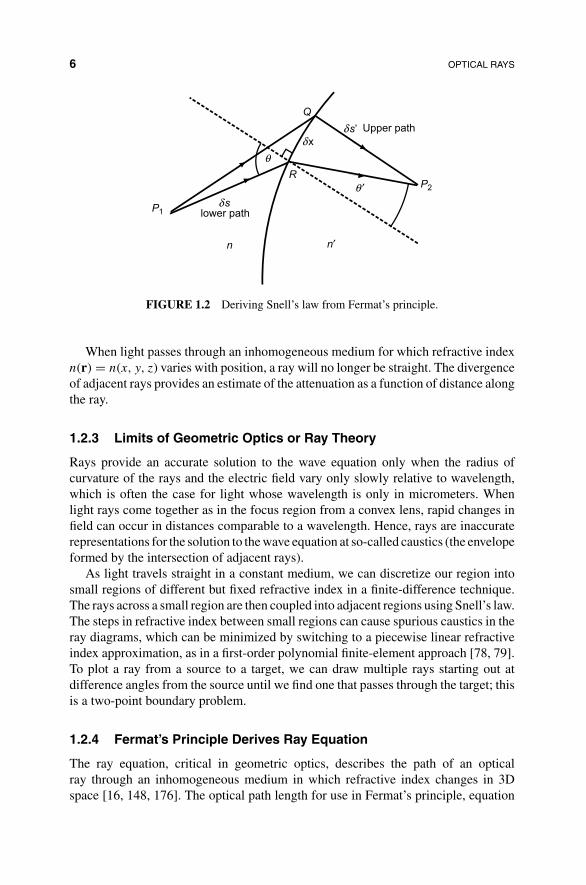
the dielectric constant and μ is the relative permeability (Figure 1.2). From Fermat’sprinciple, the optical path from P1 to P2 intercepts the dielectric interface at R so thatthe optical path length through R is the least for all possible intercepts at the interface.Because at an extremum the function in equation (1.3) has zero gradient, moving theintercept point a very small variational distance δx along the interface to Q will notchange the optical path length. From Figure 1.2, the change in optical path lengthwhen moving from the path through R to the path through Q is
δs − δs′ = nδx sin θ − n′δx sin θ′ = 0 (1.4)
which gives Snell’s law
n sin θ = n′ sin θ′ (1.5)
6 OPTICAL RAYS
P1
P2
Q
R
δs’ Upper path
δx
δslower path
n n′
θ
θ ′
FIGURE 1.2 Deriving Snell’s law from Fermat’s principle.
When light passes through an inhomogeneous medium for which refractive indexn(r) = n(x, y, z) varies with position, a ray will no longer be straight. The divergenceof adjacent rays provides an estimate of the attenuation as a function of distance alongthe ray.
1.2.3 Limits of Geometric Optics or Ray Theory
Rays provide an accurate solution to the wave equation only when the radius ofcurvature of the rays and the electric field vary only slowly relative to wavelength,which is often the case for light whose wavelength is only in micrometers. Whenlight rays come together as in the focus region from a convex lens, rapid changes infield can occur in distances comparable to a wavelength. Hence, rays are inaccuraterepresentations for the solution to the wave equation at so-called caustics (the envelopeformed by the intersection of adjacent rays).
As light travels straight in a constant medium, we can discretize our region intosmall regions of different but fixed refractive index in a finite-difference technique.The rays across a small region are then coupled into adjacent regions using Snell’s law.The steps in refractive index between small regions can cause spurious caustics in theray diagrams, which can be minimized by switching to a piecewise linear refractiveindex approximation, as in a first-order polynomial finite-element approach [78, 79].To plot a ray from a source to a target, we can draw multiple rays starting out atdifference angles from the source until we find one that passes through the target; thisis a two-point boundary problem.
1.2.4 Fermat’s Principle Derives Ray Equation
The ray equation, critical in geometric optics, describes the path of an opticalray through an inhomogeneous medium in which refractive index changes in 3Dspace [16, 148, 176]. The optical path length for use in Fermat’s principle, equation

GEOMETRIC OR RAY OPTICS 7
(1.3), may be written by factoring out dz from ds =√
dx2 + dy2 + dz2:
δ
∫ P2
P1
n ds = δ
∫ z2
z1
n(x, y, z)
√(dx
dz
)2
+(
dy
dz
)2
+ 1 dz
= δ
∫ z2
z1
n(x, y, z)√
x′2 + y′2 + 1 dz (1.6)
where prime indicates d/dz and ds =√
x′2 + y′2 + 1 dz. Equation (1.6) can be writ-ten as δ
∫ z2z1
F dz, where the integrand F has the form of a functional (function offunctions)
F (x′, y′, x, y, z) ≡ n(x, y, z)√
x′2 + y′2 + 1 (1.7)
From calculus of variations [16], the solutions for extrema (maximum or minimum)with integrand of the form of equation (1.7) are the Euler equations
Fx − d
dzFx′ = 0, Fy − d
dzFy′ = 0 (1.8)
where subscripts refer to partial derivatives. From equation (1.7) and x′ = dx/dz,
Fx = ∂n
∂xds = ∂n
∂x
√x′2 + y′2 + 1 = ∂n
∂x
ds
dz(1.9)
and
Fx′ = n1
2√
x′2 + y′2 + 12x′ = n
dx
dz
dz
ds= n
dx
ds(1.10)
Similar equations apply for Fy and Fy′ . Substituting equations (1.9) and (1.10) intoequation (1.8) gives
∂n
∂x
ds
dz− d
dz
(n
dx
ds
)= ∂n
∂x− dz
ds
d
dz
(n
dx
ds
)= 0 (1.11)
The resulting equations for the ray path are
d
ds
(n
dx
ds
)= ∂n
∂x,
d
ds
(n
dy
ds
)= ∂n
∂y,
d
ds
(n
dz
ds
)= ∂n
∂z(1.12)
where the last equation is obtained by reassigning coordinates, by analogy, or byadditional algebraic manipulation [16]. These equations can be written in vector form

8 OPTICAL RAYS
for the vector ray equation
d
ds
(n
drds
)= ∇n (1.13)
Another derivation [16] for the ray equation provides a different perspective. Thederivation generates, from Maxwell’s equations or from the wave equation, an equiv-alent to Fermat’s principle, the eikonal equation.
(∇S)2 = n2 or
(∂S
∂x
)2
+(
∂S
∂y
)2
+(
∂S
∂z
)2
= n2(x, y, z) (1.14)
The eikonal equation relates phase fronts S(r) = constant and refractive index n. Aray ns is in the direction at right angles to the phase front, that is, in the direction ofthe gradient of S(r), or
ns = ∇S or ndrds
= ∇S (1.15)
By taking the derivative of equation (1.15) with respect to s, we obtain the ray equa-tion (1.13).
1.2.5 Useful Applications of the Ray Equation
We illustrate the ray equation for rays propagating in a z–y plane of a slab, where z
is the propagation direction axis for the paraxial approximation and refractive indexvaries transversely in y. For a homogeneous medium, n is constant and ∇n = ∂n/∂y =0. Then the ray equation (1.13) becomes d2y/dz2 = 0. After integrating twice, y =az + b, a straight line in the z–y plane. Therefore, in a numerical computation, wediscretize the refractive index profile into piecewise constant segments in y and obtaina piecewise linear optical ray path in plane z–y.
For a linearly varying refractive index in y, n = n0 + ay with n ≈ n0, ∂n/∂y =a, the ray equation (1.13) becomes d2y/dz2 ≈ a/n0. After two integrations, y =(a/n0)z2 + (b/n0)z + d, which is a quadratic in the z–y plane and can be representedto first approximation by a spherical arc. Therefore, if we discretize the refractiveindex profile into piecewise linear segments, we obtain a ray path of joined arcsthat is smoother than the piecewise linear optical ray path for a piecewise constantrefractive index profile. The approach is extrapolatable to higher dimensions.
Another useful refractive index profile is that of a quadratic index medium, in whichthe refractive index smoothly decreases radially out from the axis of a cylindrical body(Figure 1.3a):
n2 = n20(1 − (gr)2) with r2 = (x2 + y2) (1.16)

GEOMETRIC OR RAY OPTICS 9
n
n0
r0
(a) (b)
z
FIGURE 1.3 Ray in quadratic index material: (a) refractive index profile and (b) ray path.
where g is the strength of the curvature and gr � 1. Material doping creates sucha profile in graded index fiber to replace step index fiber. In a cylindrical piece ofglass, such an index profile will act as a lens, called a GRIN lens [47]. A GRINlens can be attached to the end of an optical fiber and can match the fiber diameterto focus or otherwise image out of the fiber. In the ray equation, for the paraxialapproximation, d/ds = d/dz, and from equation (1.16), ∂n/∂r = −n0g
2r. So the rayequation reduces to
d2r
dz2 + g2r = 0 (1.17)
which has sin and cos solutions. A solution to equation (1.17) with initial conditions(r0)in and (dr0/dz)in = (r′
0)in is
r = (r0)in cos(gz) + (r′0)in
sin(gz)
g(1.18)
which can be verified by substituting into equation (1.17). A ray according to equa-tion (1.18) for a profile, equation (1.17), is shown in Figure 1.3b.
1.2.6 Matrix Representation for Geometric Optics
The ability to describe paraxial approximation propagation in the z direction throughcircularly symmetric optical components using a location and a slope in geometricoptics allows for a 2 × 2 matrix representation [44, 132, 176].
We consider a material of constant refractive index and width d. For this medium,light propagates in a straight line (Section 1.2.3), and a ray path does not change slope,r′
out = r′in. The ray location changes after passing through width d of this medium
according to
r(z)out = r(z)in + r′(z)ind (1.19)
where after traveling a distance d at slope r′, location has changed by r′(z)ind.Hence, we can write a matrix equation relating the output and the input for a
position and a slope vector [r(z), r′(z)]T:
[r(z)
r′(z)
]out
=[
1 d
0 1
] [r(z)
r′(z)
]in
(1.20)
10 OPTICAL RAYS
Similarly, the ray can be propagated through a change in refractive index from n1 ton2 with
[r(z)
r′(z)
]out
=[
1 0
0 n1n2
] [r(z)
r′(z)
]in
(1.21)
where position does not change and from Snell’s law for small angles, for which slopetan θ ≈ sin θ, the slope changes by n1/n2.
Another common matrix is that for passing through a lens of focal length f :
[r(z)
r′(z)
]out
=[
1 01
−f1
] [r(z)
r′(z)
]in
(1.22)
where a lens changes the slope of a ray by −r(z)/f .A useful case is the propagation of rays through a quadratic medium. From equa-
tion (1.18), a 2 × 2 matrix can be written and verified by substituting
[r(z)
r′(z)
]out
=[
cos(gz) sin(gz)g
−g sin (gz) cos(gz)
] [r(z)
r′(z)
]in
(1.23)
Other matrices are illustrated in Ref. [176]. The advantage of the 2 × 2 representa-tion is that for a string (or sequence) of circularly symmetric components, the matricescan be multiplied together to achieve a single 2 × 2 matrix for transmission throughthe complete string. The property is that the determinant of any matrix is zero. Wewill use in Section 2.1.2 the 2 × 2 notation with matrix elements labeled clockwisefrom top left as ABCD to compute the effect of propagating a Gaussian beam throughthe corresponding optical element.
1.3 OPTICS FOR LAUNCHING AND RECEIVING BEAMS
Ray tracing allows modeling of simple optics for launching and receiving beams.Beam expanders, beam compressors, telescopes, microscopes, and spatial filters arefrequently used in military optical systems to change the beam diameter, view anobject at different levels of magnification, or improve the beam spatial coherence.These systems can be constructed with two thin refractive lenses [61]. More complexlens designs can be performed with commercial software such as Code V. A singlethin lens system and a magnifier are discussed first.
1.3.1 Imaging with a Single Thin Lens
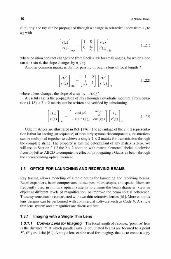
1.3.1.1 Convex Lens for Imaging The focal length of a convex (positive) lensis the distance f ′ at which parallel rays (a collimated beam) are focused to a pointF ′, (Figure 1.4a) [61]. A single lens can be used for imaging, that is, to create a copy
OPTICS FOR LAUNCHING AND RECEIVING BEAMS 11
FIGURE 1.4 Focusing a collimated parallel beam: (a) with a convex lens, (b) with a concavelens, (c) with a concave mirror, and (d) with a convex mirror.
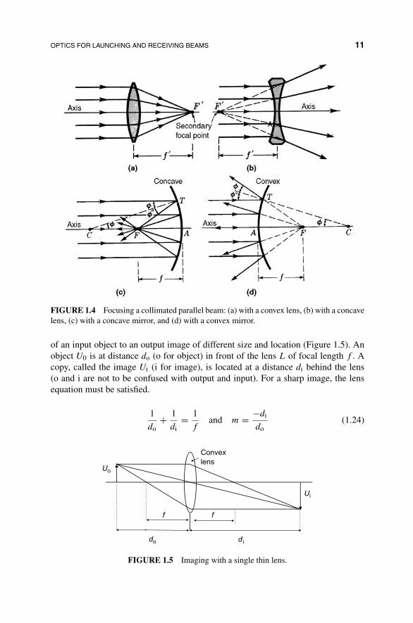
of an input object to an output image of different size and location (Figure 1.5). Anobject U0 is at distance do (o for object) in front of the lens L of focal length f . Acopy, called the image Ui (i for image), is located at a distance di behind the lens(o and i are not to be confused with output and input). For a sharp image, the lensequation must be satisfied.
1
do+ 1
di= 1
fand m = −di
do(1.24)
Uo
Ui
d ido
f f
Convex
lens
FIGURE 1.5 Imaging with a single thin lens.
12 OPTICAL RAYS
The negative sign in the image or lateral magnification m refers to the fact that theimage is inverted. By wearing inverting glasses, it was shown that the brain invertsthe image in the case of the human eye. Note that lens designers may use a differentconvention that changes the equations; for example, distances to the left of an elementare often considered negative.
Note that figures can be reversed as light can travel in the opposite directionsthrough lenses and mirrors. In a concave lens (Figure 1.4b), parallel rays are causedto diverge. A viewer at the right will think the light is emitted by a point sourceat F ′. This is a virtual point source as, unlike with a convex lens, a piece of papercannot be placed at F ′ to see a real image. When using the lens equation (1.24)for a concave lens, the focal length f for a convex lens is replaced by −f for aconcave lens.
A concave mirror (Figure 1.4c) performs a function similar to the convex lens infocusing parallel rays of light. But the light is folded back to focus on the left of themirror instead of passing through. Mirrors may be superior to lenses because of lessweight and small size owing to folding. Similarly, the convex mirror acts like a foldedconcave lens (Figure 1.4d).
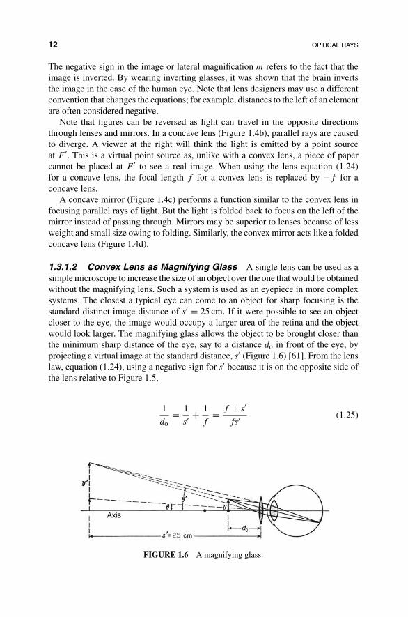
1.3.1.2 Convex Lens as Magnifying Glass A single lens can be used as asimple microscope to increase the size of an object over the one that would be obtainedwithout the magnifying lens. Such a system is used as an eyepiece in more complexsystems. The closest a typical eye can come to an object for sharp focusing is thestandard distinct image distance of s′ = 25 cm. If it were possible to see an objectcloser to the eye, the image would occupy a larger area of the retina and the objectwould look larger. The magnifying glass allows the object to be brought closer thanthe minimum sharp distance of the eye, say to a distance do in front of the eye, byprojecting a virtual image at the standard distance, s′ (Figure 1.6) [61]. From the lenslaw, equation (1.24), using a negative sign for s′ because it is on the opposite side ofthe lens relative to Figure 1.5,
1
do= 1
s′+ 1
f= f + s′
fs′(1.25)
FIGURE 1.6 A magnifying glass.
OPTICS FOR LAUNCHING AND RECEIVING BEAMS 13
The angle θ subtended by the object in the absence of a magnifying lens and the angleθ′ subtended with the magnifying glass are
tan θ = y
s′
tan θ′ = y
do= y
f + s′
fs′(1.26)
where the second equation used equation (1.25). Therefore, the angular or powermagnification may be written for small angles, using equation (1.25) for 1/do, as
M = θ′
θ= s′
do= s′
f+ 1 ≈ s′
f(1.27)
For f in centimeters, and minimum distinct distance of s′ = 25 cm, magnifyingpower is M = 25/f . An upper case M distinguishes from lateral magnification m inequation (1.24).
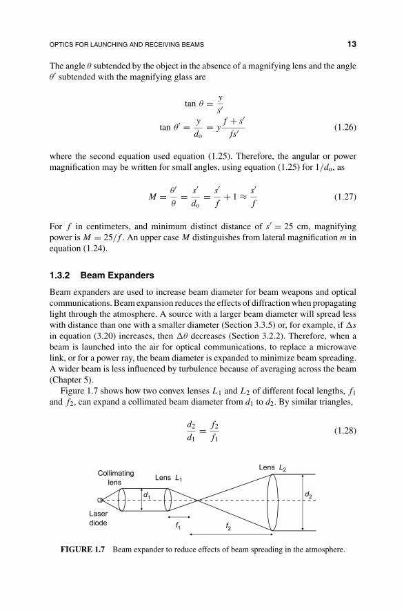
1.3.2 Beam Expanders
Beam expanders are used to increase beam diameter for beam weapons and opticalcommunications. Beam expansion reduces the effects of diffraction when propagatinglight through the atmosphere. A source with a larger beam diameter will spread lesswith distance than one with a smaller diameter (Section 3.3.5) or, for example, if �s
in equation (3.20) increases, then �θ decreases (Section 3.2.2). Therefore, when abeam is launched into the air for optical communications, to replace a microwavelink, or for a power ray, the beam diameter is expanded to minimize beam spreading.A wider beam is less influenced by turbulence because of averaging across the beam(Chapter 5).
Figure 1.7 shows how two convex lenses L1 and L2 of different focal lengths, f1and f2, can expand a collimated beam diameter from d1 to d2. By similar triangles,
d2
d1= f2
f1(1.28)
Laser
diode
Lens L1
Lens L2
f1
d1
f2
d2
Collimating
lens
FIGURE 1.7 Beam expander to reduce effects of beam spreading in the atmosphere.
14 OPTICAL RAYS
Laser
diode
Lens L1
Lens L2
f1
d1
f2
d2
Collimating
lens
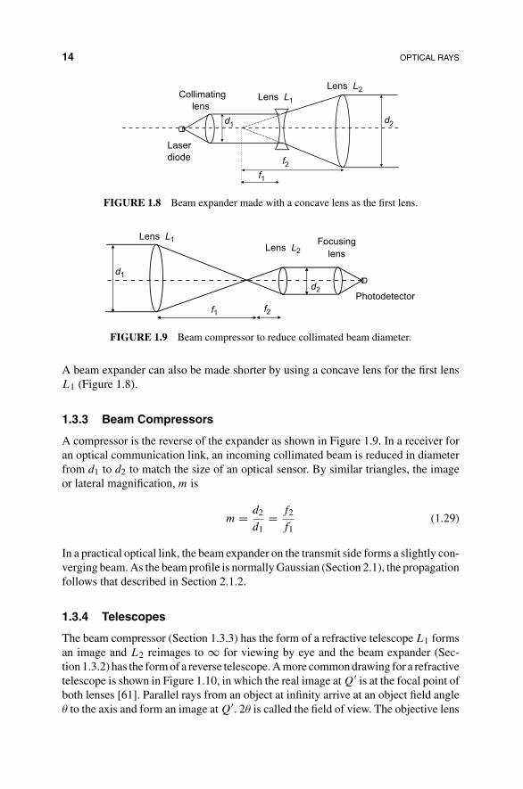
FIGURE 1.8 Beam expander made with a concave lens as the first lens.
Photodetector
Lens L1
Lens L2
f2f1
Focusing
lens
d1
d2
FIGURE 1.9 Beam compressor to reduce collimated beam diameter.
A beam expander can also be made shorter by using a concave lens for the first lensL1 (Figure 1.8).
1.3.3 Beam Compressors
A compressor is the reverse of the expander as shown in Figure 1.9. In a receiver foran optical communication link, an incoming collimated beam is reduced in diameterfrom d1 to d2 to match the size of an optical sensor. By similar triangles, the imageor lateral magnification, m is
m = d2
d1= f2
f1(1.29)
In a practical optical link, the beam expander on the transmit side forms a slightly con-verging beam. As the beam profile is normally Gaussian (Section 2.1), the propagationfollows that described in Section 2.1.2.
1.3.4 Telescopes
The beam compressor (Section 1.3.3) has the form of a refractive telescope L1 formsan image and L2 reimages to ∞ for viewing by eye and the beam expander (Sec-tion 1.3.2) has the form of a reverse telescope. A more common drawing for a refractivetelescope is shown in Figure 1.10, in which the real image at Q′ is at the focal point ofboth lenses [61]. Parallel rays from an object at infinity arrive at an object field angleθ to the axis and form an image at Q′. 2θ is called the field of view. The objective lens

OPTICS FOR LAUNCHING AND RECEIVING BEAMS 15
FIGURE 1.10 Telescope.
acts as the aperture stop or the entrance pupil in the absence of a separate stop [61].The second lens, usually called an eyepiece, magnifies the image at Q′ so that a largervirtual image Q′′ appears at infinity (Section 1.3.1.2). The virtual image subtendsan angle θ′ at the eye. Angular magnification or magnifying power M (reciprocal oflateral magnification) is
M = θ′
θ= fo
fe(1.30)
Large astronomical telescopes built with refractive lenses are limited to approximately1 m diameter because of the weight of the lenses. Higher resolution telescopes withlarger diameters use mirrors and are discussed next.
1.3.4.1 Cassegrain Telescope The Cassegrain telescope has a common dishappearance and is used in military systems to reduce weight and size relative to arefractive lens telescope for transmitting and receiving signals. (see Sections 16.2.5,15.1.1 and 12.2). Figure 1.11a shows the inverted telescope as a beam expander for
Concavemirror
Convexmirror
Input beamupper edge
Input beamlower edge
Outputbeam tosensor
Concavemirror
Convexmirror
Output beamlower edge
Output beamupper edge
Inputbeamfromlaser
(a) (b)
FIGURE 1.11 Cassegrain antenna as (a) beam expander or inverted telescope and (b) tele-scope.

16 OPTICAL RAYS
transmitting light beams. The input beam passes through a small hole in the largeconcave mirror to strike the small convex mirror. Comparing the Cassegrain invertedtelescope with the lens beam expander in Figure 1.8, the first small concave lens,L1, is replaced by a small convex mirror that spreads the light over a concave mirrorthat replaces the second lens L2. The output aperture size is close to that of the largemirror diameter.
The reverse structure acts as a telescope (Figure 1.11b). The large concave mirroraperture determines the resolution of images. Light reflecting from the concave mirrorfocuses on the small convex mirror and then through a hole in the concave mirror ontoa CCD image sensor. This configuration is used in the Geoeye imaging satellite 400miles up (Figure 1.12) [125]. Such imaging satellites are critical for providing intelli-gence information for the military and data for commercial ventures such as Google.A Geoeye satellite, launched in 2008, as shown in Figure 1.13 [125], involves manyother systems, solar panels, global positioning system (GPS), star tracker (togetherthe star tracker and the GPS can locate objects to within 3 m), image storage, and dataantenna for transmitting signals back to earth when over designated ground stations.In the open literature as of 2009, there are in orbit 51 imaging satellites with resolutionbetween 0.4 and 56 m launched by 31 countries and 10 radar satellites launched by 18countries [125]. The military and commercial sectors rely on these and classified satel-lites for intelligence relating to threat warnings of enemy activities and environmentalissues, on global positioning satellites for guiding missiles and locating U.S. and alliespersonnel and vehicles, on communication satellites for battlefield communications,
FIGURE 1.12 Optics inside Geoeye using a Cassegrain telescope.

OPTICS FOR LAUNCHING AND RECEIVING BEAMS 17
FIGURE 1.13 Geoeye imaging satellite.
and on classified antisatellite satellites aimed at interfering with other countries’ satel-lites. Hence, the control of satellite space will be critical in future wars, although inrecent wars control of air space was adequate. Most satellites are vulnerable to laserattack from the ground, aircraft, or other satellites. For example, imaging satellites canbe blinded by glare from lasers and for most satellites the solar cell arrays can be easilydamaged by lasers, which can disable their source of solar energy. Consequently, asdiscussed in Chapter 14, the military satellites should also have laser warning devicesand protection such as their own lasers and electronic countermeasures.
1.3.4.2 Nasmyth Telescope Sometimes for convenience of mounting subse-quent equipment, such as optical spectral analyzers, a variation of the Cassegraintelescope is used in which the light is brought out to one side using a third mirror,rather than through a hole in the primary mirror. This is referred to as a Nasmyth tele-scope (related to a Coude telescope). Such an arrangement is shown diagrammaticallyin Figure 15.1.
1.3.5 Microscopes
A typical two-lens microscope (Figure 1.14) has a form similar to the beam expander(Section 1.3.2). A tiny object, in this case an arrow, is placed just inside the focal
18 OPTICAL RAYS
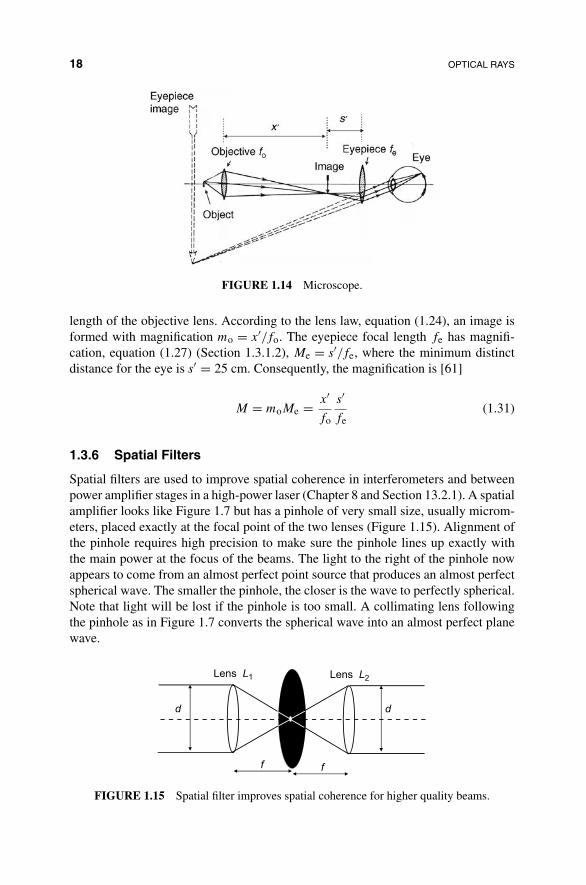
FIGURE 1.14 Microscope.
length of the objective lens. According to the lens law, equation (1.24), an image isformed with magnification mo = x′/fo. The eyepiece focal length fe has magnifi-cation, equation (1.27) (Section 1.3.1.2), Me = s′/fe, where the minimum distinctdistance for the eye is s′ = 25 cm. Consequently, the magnification is [61]
M = moMe = x′
fo
s′
fe(1.31)
1.3.6 Spatial Filters
Spatial filters are used to improve spatial coherence in interferometers and betweenpower amplifier stages in a high-power laser (Chapter 8 and Section 13.2.1). A spatialamplifier looks like Figure 1.7 but has a pinhole of very small size, usually microm-eters, placed exactly at the focal point of the two lenses (Figure 1.15). Alignment ofthe pinhole requires high precision to make sure the pinhole lines up exactly withthe main power at the focus of the beams. The light to the right of the pinhole nowappears to come from an almost perfect point source that produces an almost perfectspherical wave. The smaller the pinhole, the closer is the wave to perfectly spherical.Note that light will be lost if the pinhole is too small. A collimating lens followingthe pinhole as in Figure 1.7 converts the spherical wave into an almost perfect planewave.
Lens L1 Lens L2
d d
ff
FIGURE 1.15 Spatial filter improves spatial coherence for higher quality beams.

OPTICS FOR LAUNCHING AND RECEIVING BEAMS 19
Optical amplifiers cause distortion due to nonlinear effects at high power. Spatialcorrelation is degraded and the plane wave has regions pointing off axis. Hence, aspatial filter is often used to clean up the beam after amplification. In a series ofpower amplifiers (Section 13.2.1), a spatial filter after each amplifier will preventdistortion building up to unacceptable levels. The beam can even be passed back andforth through the same amplifier, as in the National Infrastructure Laser (Chapter 13),because the flash light duration is long enough for several passes of the beam to beamplified. An alternative method of improving beam quality by adaptive optics isdescribed in Section 5.3.2 and used in the airborne laser in Section 12.2.2 and 12.2.3.
CHAPTER 2
GAUSSIAN BEAMS ANDPOLARIZATION
Laser beams are generally brighter at the center and have a cross-sectional intensityclose to a Gaussian or a normal distribution. They also tend to have a defined polar-ization or direction of motion of the electric field. For example, in a laser diode witha rectangular waveguide, the polarization may be in the direction of the longer sideof the rectangle.
In Section 2.1, we analyze Gaussian beams, characterized by spot size and curva-ture, and their propagation through lens systems. In section 2.2, we describe how tocharacterize, analyze, and control polarization.
2.1 GAUSSIAN BEAMS
The output of a laser is generally brighter at the center than at the edges and the cross-sectional intensity profile can often be approximated with a Gaussian distribution.This forms a Gaussian beam [148, 176]. The type of laser influences how well thefar field from the laser satisfies the approximation. In a laser diode (Section 7.2), thebeam emits from a small waveguide, which by diffraction causes the beam to spreadwidely. Coherent light emitted from a smaller diameter source will spread more withdistance than light from a larger diameter source (Section 3.3.5) or, for example, if �s
in equation (3.20) decreases, then the spreading angle �θ increases (Section 3.2.2). Alens brings it back to a narrower beam pattern with a close approximation to Gaussian.
Military Laser Technology for Defense: Technology for Revolutionizing 21st Century Warfare,First Edition. By Alastair D. McAulay.© 2011 John Wiley & Sons, Inc. Published 2011 by John Wiley & Sons, Inc.
20

GAUSSIAN BEAMS 21
In other lasers, concave curved mirrors reinforce the formation of a Gaussianbeam [176].
Analogous to specifying Gaussian probability density functions with only twoparameters (mean and variance), Gaussian beams can also be specified with onlytwo parameters: in this case, radius of curvature R and spot radius W . By trackingthese two parameters, we can analyze propagation of Gaussian beams through opticalelements and turbulence.
2.1.1 Description of Gaussian Beams
The complex amplitude of a plane wave propagating in the z direction is modulatedwith a complex envelope A(r) that has a Gaussian shape transversely and varies withz as the beam expands and contracts:
U(r) = A(r, z) exp{−jkz} (2.1)
where we ignored polarization effects for simplicity.The modulated wave at a single laser frequency in air satisfies the time harmonic
or Helmholtz wave equation
∇2U + k2U = 0 (2.2)
We separate out the transverse component in r, where we assumed cylindrical sym-metry, and the component in the direction of propagation z to obtain
∂2
∂r2 U + ∂2
∂z2 U + k2U = 0 (2.3)
We now derive equation (2.7) for the envelope A (r, z) by substituting the fieldfrom equation (2.1) into equation (2.3)
∂2
∂r2 (A(r, z)) exp{−jkz}) + ∂2
∂z2 (A(r, z) exp{−jkz}) + k2A(r, z) exp{−jkz} = 0
(2.4)
Consider the second term in equation (2.4). As A(r, z) exp{−jkz} is a product of twofunctions in z, the second derivative with respect to z gives four terms. Taking thefirst derivative with respect to z gives
∂
∂z(A(r, z) exp{−jkz}) = A(r, z)(−jk) exp{−jkz} + exp{−jkz}∂A(r, z)
∂z(2.5)
22 GAUSSIAN BEAMS AND POLARIZATION
Taking the second derivative with respect to z, the derivative of equation (2.5),
∂2
∂z2 (A(r, z) exp{−jkz})
= A(r, z)(−k2) exp{−jkz} + (−jk) exp{−jkz}∂A(r, z)
∂z
+ exp{−jkz}∂2A(r, z)
∂2z+ ∂A(r, z)
∂z(−jk) exp{−jkz} (2.6)
At right side of equation (2.6) we neglect the third term by using the slowly vary-ing amplitude approximation ∂2A/∂z2 � ∂A/∂z, equation (8.13) [176], combine thesecond and fourth term and cancel the first term on substituting into equation (2.4),to get the paraxial Helmholtz equation (with ∇2
r = ∂2/∂x2 + ∂2/∂y2)
∇2r A(r, z) − 2jk
∂A(r, z)
∂z= 0 (2.7)
Equation (2.7) provides ∂A/∂z, which describes how the envelope A propagates in z.Integrating equation (2.7) gives a parabolic wave approximation (Section 1.1) to thespherical wave close to the axis:
A(r) = Az
exp
{−jk
ρ2
2z
}(2.8)
where ρ2 = x2 + y2. That equation (2.8) is the solution to equation (2.7) can beverified by substitution and appropriate differentiation [148].
The Gaussian beam is obtained from the parabolic wave by transforming z by apurely imaginary amount jz0, where z0 is called the Rayleigh range,
q(z) = z + jz0 (2.9)
Therefore, we replace z in equation (2.8) by q(z) defined in equation (2.9):
A(r) = A1
q(z)exp
{−jk
ρ2
2q(z)
}(2.10)
We now show that the complex term 1/q(z), arising twice in equation (2.10), fullydescribes the propagation of a Gaussian beam at z: its real part specifying the radiusof curvature R(z) of the phase front and the imaginary part specifying the spot sizeW(z), which is the radius of the spot at 1/e of the peak. Separating the reciprocal ofequation (2.9) into real and imaginary parts,
1
q(z)= 1
z + jz0= z − jz0
z2 + z20
= z
z2 + z20
− jz0
z2 + z20
(2.11)

GAUSSIAN BEAMS 23
FIGURE 2.1 Gaussian beam propagation.
The reciprocal of the real part, second to the last term in equation (2.11), defines theradius of curvature R(z):
R(z) = z
[1 +
(z0
z
)2]
(2.12)
This describes how the phase front associated with the radius of curvature R(z) ex-pands and contracts with distance (Figure 2.1). The imaginary part of the reciprocalof last term in equation (2.11) times λ/π defines the beam radius W(z) from
W2(z) = λ
πz0
[1 +
(z
z0
)2]
(2.13)
Using equations (2.12) and (2.13), we can rewrite equation (2.11) in terms of R
and W :
1
q(z)= 1
R(z)− j
λ
π
1
W2(z)(2.14)
Note that πW2 is the area of the beam falling inside amplitude 1/e of its peak. Fromequation (2.13), for z = 0, the waist of the beam, the narrowest part, is
W20 = λ
πz0 (2.15)
Substituting equation (2.15) into equation (2.13) gives the beam radius W(z) in termsof its waist W0 and distance z from the waist (Figure 2.1),
W2(z) = W20
[1 +
(z
z0
)2]
(2.16)

24 GAUSSIAN BEAMS AND POLARIZATION
From equations (2.11) and (2.16), the amplitude and the phase of 1/q(z) can bewritten as
1√z2 + z2
0
= 1
z0
W0
W(z) and ζ(z) = tan−1 z
z0(2.17)
where we used equations (2.13) and (2.15) for the first equality.Consider equation (2.10) for the envelope of the Gaussian beam. In the ampli-
tude part of equation (2.10), replace 1/q(z) with real and imaginary parts of 1/q(z)from equation (2.17). In the phase part of equation (2.10), replace the real and imag-inary parts of 1/q(z) from equation (2.14). The resulting expression for the complexenvelope of a Gaussian beam can be written as
A(r) = A1
z0
W0
W(z)exp{jζ(z)} exp
[−jk
ρ2
2
(1
R(z)− j
λ
π
1
W2(z)
)](2.18)
Hence, by using k = 2π/λ (in air) and substituting the complex envelope, A(r) inequation (2.18), into the complex amplitude of the Gaussian beam field, equation (2.1),
U(r) = A1
z0
W0
W(z)exp
[− ρ2
W2(z)
]exp
[−jkz − jk
ρ2
2R(z)+ jζ(z)
](2.19)
The properties of the Gaussian beam are apparent in Figure 2.1 and elaborated indetail elsewhere [148, 176].
2.1.2 Gaussian Beam with ABCD Law
Interestingly, knowledge of the 2 × 2 matrix for an optical element, labeled clockwisefrom top left element as ABCD (Section 1.2.6), is sufficient to determine the changefrom q1 to q2 describing a Gaussian beam [148, 176] propagating through the opticalelement, equation (2.14). For propagation through an optical element, converting raysto Gaussian beams is accomplished by the ABCD law
q2 = q1A + B
q1C + D(2.20)
For paraxial waves, equation (2.20) is proved analytically in Ref. [176] and byinduction in Ref. [148]. In induction, each element in the ray path, no matter howcomplex, may be discretized along the z axis into thin slivers that either shift theray position, matrix (1.20), or change the ray slope (1.21). Now we show that equa-tion (2.20) will give the correct change in Gaussian beam parameter q for both thesecases. So, by induction, for any optical element, equation (2.20) will provide theinformation on the propagation of a Gaussian beam.
For a Gaussian beam passing through a slab of constant refractive index, the slopeof the ray is constant, but the location of the ray changes with distance (the ray

GAUSSIAN BEAMS 25
can be considered to be along the 1/e amplitude edge of a Gaussian beam). Fromequation (2.9) with q1 at the input and q2 at the output,
q2 = z2 + jz0 and q1 = z1 + jz0 (2.21)
Subtracting one equation from the other in equation (2.21) for a thin sliver gives
q2 − q1 = z2 − z1 = d (2.22)
where d is the thickness of the slab.The matrix elements A = 1, B = d, C = 0, and D = 1 from equation (1.20) for
propagating across a slab of width d are inserted into the ABCD law, equation (2.20),to give
q2 = q11 + d
q10 + 1= q1 + d (2.23)
which is the same as equation (2.22), proving the ABCD law for propagation acrossa slab.
For a Gaussian beam passing through a dielectric interface with change in refractiveindex from n1 to n2, the beam radius W is the same on both sides of the interface, butthe ray slope changes at the interface due to refraction. From equation (2.14),
1
q2= 1
R2− j
λ2
π
1
W2 and1
q1= 1
R1− j
λ1
π
1
W2 (2.24)
Consider a ray along the edge of the Gaussian beam (1/e amplitude) (Figure 2.2)incident on the interface at angle θ1 with the axis and having radius of curvature R1and spot radius W at the interface. After refraction at the interface, while the beamradius W is unchanged, the angle with the horizontal becomes θ2 and the radius of
R1 R2
2
2
1
1
W
θ
Wave front
after refraction
Wave front
before refraction
Dielectric
interface
n1 n2
θ
θ
θ
FIGURE 2.2 Refraction of Gaussian beam at dielectric interface.

26 GAUSSIAN BEAMS AND POLARIZATION
curvature becomes R2. Then
W
R1= sin θ1 and
W
R2= sin θ2. (2.25)
Dividing one equation by the other and using Snell’s law gives
R2
R1= sin θ1
sin θ2= n2
n1or
1
R2= n1
n2
1
R1(2.26)
As wavelength is inversely proportional to refractive index (λ = c/(n(freq))), wecan write
λ2 = n1
n2λ1 (2.27)
SubstitutingR2 from equation (2.26) andλ2 from equation (2.27) into the first equationin equation (2.24) shows, in the first equation, the change in Gaussian beam parameterto q2,
1
q2= n1
n2
(1
R1− j
λ1
π
1
W2
)or
1
q2= n1
n2
1
q1(2.28)
The second equation in equation (2.24) is used to obtain the second equation inequation (2.28).
Inserting the matrix elements from equation (1.21) A = 1, B = 0, C = 0,D = n1/n2 and using the ABCD law, equation (2.20),
q2 = q11 + 0
q10 + n1/n2= q1
n2
n1or
1
q2= n1
n2
1
q1(2.29)
which is the same as equation (2.28), proving the ABCD law for crossing from onerefractive index to another.
Thus, by induction, as any optical element may be written in terms of thin sliversthat are either a constant refractive index or a dielectric interface between two differentmedia, we have proven the ABCD law, equation (2.20), for all cases.
2.1.3 Forming and Receiving Gaussian Beams with Lenses
Figure 2.3 shows a Gaussian beam with waist W01 at distance d1 in front of a convexlens that focuses light to waist W02 at distance d2 after the lens [176]. We label thecomplex Gaussian beam parameters as q1 at the input waist and q2 at the output waist.Then, from equation (2.14) at a waist, radius of curvature R1 = ∞, 1/R1 → 0,
1
q1= −j
λ
π
1
W201
= 1
jz1or q1 = jz1 (2.30)

GAUSSIAN BEAMS 27
FIGURE 2.3 Focusing a Gaussian beam.
where we used the confocal beam parameter z1 that describes the distance at whichthe waist expands by
√2, that is, z = z0 in equation (2.16). Similarly, for R2 = ∞,
1/R2 → 0,
1
q2= −j
λ
π
1
W202
= 1
jz2or q2 = jz2 (2.31)
For a medium of refractive index n, we can replace λ with λ/n.For a ray passing from input waist to output waist, in order to define A, B, C,
and D, we write the product in reverse order (the order of occurrence) of the threepropagation matrices: to the lens through distance d1, equation (1.20); through thelens, equation (1.22); and to the output waist through distance d2,
[A B
C D
]=
[1 d2
0 1
] [1 01
−f1
] [1 d1
0 1
]=
⎡⎣ 1 − d2
fd1 + d2 − d1d2
f
− 1f
1 − d1f
⎤⎦ (2.32)
We use A, B, C, and D from equation (2.32) with equations (2.30) and (2.31) toinsert into the ABCD law, equation (2.20). We include the unimodal property of thematrices, AD − BC = 1. The Gaussian beam complex propagation parameter q isupdated from q1 to q2 during propagation from the input to the output waists, asshown in Figure 2.3. q1 and q2 are represented by the respective confocal parametersz1 and z2 from equations (2.30) and (2.31),
jz2 = jz1A + B
jz1C + D= (jz1A + B)(−jz1C + D)
(z21C
2 + D2)= ACz2
1 + BD + jz1
C2z21 + D2
(2.33)
From equations (2.30) and (2.31), the confocal parameters z1 and z2 in terms of inputand output spot sizes W01 and W02 in air (n = 1) are, respectively,
z1 = πW201
λand z2 = πW2
02
λ(2.34)

28 GAUSSIAN BEAMS AND POLARIZATION
Equating real parts of either side of equation (2.33) gives
ACz21 + BD = 0 or z2
1 = −BD
AC(2.35)
and equating imaginary parts of either side of equation (2.33) gives
z2 = z1
C2z21 + D2
(2.36)
To find the relation between the output spot size W02 and the input spot size W01,eliminating z2
1 from equations (2.35) and (2.36), using the unimodal property of thematrices, AD − BC = 1, and assigning A = 1 − (d2/f ) and D = 1 − (d1/f ) fromequation (2.32) gives
z2 = A
Dz1 = d2 − f
d1 − fz1 or from equation (2.34) W2
02 = d2 − f
d1 − fW2
01 (2.37)
We would like the location and the spot size at the output as a function of onlyinput parameters, hence we need d2 as function of d1 from equation (2.37). Fromequation (2.35), inserting ABCD elements from equation (2.20),
z21 = −BD
AC= − (d1 + d2 − (d1d2)/f ) (1 − d1/f )
(1 − d2/f ) (−1/f )
= (d1f + d2f − d1d2)
(d1 − f
d2 − f
)(2.38)
(d2 − f )z21 = −(d1 − f )2(d2 − f ) + f 2(d1 − f ) (2.39)
Hence, the location d2 of the output waist is given by
(d2 − f ) =(
f 2
z21 + (d1 − f )2
)(d1 − f ) (2.40)
Substituting (d2 − f )/(d1 − f ) = W202/W2
01 from equation (2.37) into equa-tion (2.40), the waist radius W02 at the output is
W202 =
(f 2
z21 + (d1 − f )2
)W2
01 (2.41)
Some special cases of Figure 2.3 are summarized [176].

POLARIZATION 29
(a) A point source has input spot size W01 = 0 or z1 = 0 from equation (2.34).Then equation (2.40) with z1 = 0 gives (d2 − f ) (d1 − f ) = f 2 or the lenslaw 1/d1 + 1/d2 = 1/f .
(b) For a plane wave, z1 = ∞, from equation (2.40), d2 = f . The plane wave isfocused to a point in the back focal plane.
(c) For the input waist at the front focal plane d1 = f , from equation (2.40), theoutput waist is at the back focal plane.
(d) In a laser weapon (Section 12.2), the approximate plane wave at the sourcecorresponding to an infinite radius of curvature, d1 = 0, feeds directly into alens or mirror for which the focal length can be selected to focus the light ontoa waist on the target at distance d2. Focusing onto a waist of the Gaussianbeam can provide maximum intensity at the target spot. Similarly, in a laserwarning device (Section 14.2.2), mounted on most military vehicles, the lensfocuses a parallel threatening laser beam to a detector array at a distance d2for detection and direction estimation. For both cases, equation (2.40) withd1 = 0 gives the distance between lens and target or detector array d2:
(d2 − f ) = f 2
z21 + f 2
(−f ) or d2 = f
1 + (f/z1)2 (2.42)
where the confocal distance z1 may be obtained by using W01 and λ in equa-tion (2.34). From equation (2.41), the beam size at the array for d1 = 0 is
W02 = f√z2
1 + f 2W01 = f/z1√
1 + (f/z1)2W01 (2.43)
2.2 POLARIZATION
Polarization is concerned with the direction of motion of the electric field vector inthe transverse plane for electromagnetic wave propagation. The polarization angle ψ
is in a direction transverse to the direction of propagation for electromagnetic wavesand is measured with reference to the x axis. Its sign is defined while looking in thedirection of propagation. So for a conventional western right-hand coordinate system(for which the right-hand rule may be used), we draw the transverse x axis as verticaland the transverse y axis as horizontal when looking in the z propagation direction.Any polarization may be written as the sum of two orthogonal direction polarizations;for example, we write the waves for the orthogonal polarizations as [16, 83]
E′x = Ex cos(τ + φx) and E′
y = Ey cos(τ + φy) (2.44)
where τ = ωt − kzz, and φx and φy are the phase lags for E′x and E′
y, respectively.The phase φ is a function of time and should not be confused with ψ, the angle of

30 GAUSSIAN BEAMS AND POLARIZATION
polarization. By expanding the angle sums in equation (2.44),
E′x
Ex
= cos(τ) cos(φx) − sin(τ) sin(φx),E′
y
Ey
= cos(τ) cos(φy) − sin(τ) sin(φy)
(2.45)
Multiplying the first equation (2.45) by sin(φy) and the second equation by sin(φx)allows the last terms in the resulting equations to cancel on subtraction,
E′x
Ex
sin(φy) − E′y
Ey
sin(φx) = cos(τ) sin(�φ)
E′x
Ex
cos(φy) − E′y
Ey
cos(φx) = sin(τ) sin(�φ) (2.46)
where �φ = φy − φx. Squaring and adding gives
(E′
x
Ex
)2
+(
E′y
Ey
)2
− 2E′
x
Ex
E′y
Ey
cos(�φ) = sin2(�φ) (2.47)
This is an ellipse since the associated determinant is nonnegative; a typical polar-ization ellipse is shown in Figure 2.4a. If the ratio of Ex to Ey changes, the polarizationangle ψ changes. When the minor axis goes to zero, this reverts to linear polariza-tion (Figure 2.4b), and when Ex = Ey, the ellipse reverts to a circle for circularpolarization.
For linear polarization, the angle ψ, measured from direction x, is such that thetwo orthogonal polarizations in the transverse plane are �φ = φy − φx = 0 for linearpolarizations from 0 ≤ ψ < π/2 and �φ = π for linear polarizations from π/2 ≤ψ < π. Note that because E field oscillations range from one side of the origin to theother, polarization repeats after rotating by ψ = π, while, in contrast, regular anglessuch as phase φ repeat after 2π.
For circular polarization, �φ = φx − φy = ±π/2. When x direction peaks justbefore y direction peaks, the y direction phase lags that of the x direction by +π/2,
Ex
Ey
y axis
x axis
(a) (b) (c)
FIGURE 2.4 Polarization: (a) general polarization ellipse, (b) special linear case, and (c)special circular case.

POLARIZATION 31
resulting in right circular (clockwise) polarization (Figure 2.4a). When the x directionpeaks just after the y direction peaks, the y direction phase leads that of the x direction,or lags by −π/2, resulting in left circular (anticlockwise) polarization.
2.2.1 Wave Plates or Phase Retarders
Polarization may be changed with a slice of an anisotropic crystal called a waveplate or a phase retarder [83]. Typically, we use uniaxial crystals for which one ofthe three orthogonal axes has a different refractive index from the other two and thisdirection is lined up with the flat surface of the crystal slice. The single unique axisis referred to as extraordinary (subscript e), while the other two are referred to asordinary (subscript o). The extraordinary direction is known as the optic axis and ismarked with a dot labeled OA on the edge of a wave plate. The velocity of propagationof light v depends on the refractive index v = c/n, where c is the speed of light in avacuum. Therefore, waves with polarization (E field oscillation) in the direction of theoptic axis will see a refractive index ne, while waves with polarization at right anglesto the optic axis will see refractive index of no. For a fast crystal, the light polarizedin the direction of the optic axis will travel faster than that polarized in orthogonaldirections; this means ne < no. Consequently, at the crystal output, the phase of theextraordinary light will be ahead of that for an orthogonal direction. For a slow crystal,no < ne, the light with optic axis direction polarization will travel more slowly thanthat with the orthogonal polarizations and have a phase behind that of the orthogonalpolarizations.
2.2.1.1 Half-Wave Plate Consider a uniaxial crystal of depth d and optical axisOA on the surface in direction x as shown in Figure 2.5a. The refractive indices arenx ≡ ne, and ny = nz ≡ no.
When light travels through a material of width d and refractive index n, the pathlength, equivalent distance traveled through air, is nd. Consider that a linearly polar-ized wave strikes the crystal at normal incidence to the crystal and with a polarization
FIGURE 2.5 Half-wave plate: (a) operation, (b) input wave components, and (c) output wavecomponents.

32 GAUSSIAN BEAMS AND POLARIZATION
at ψ = 45◦ ≡ π/4 with respect to the optic axis. For a half-wave plate, the widthd of the crystal is such that the extraordinary ray is delayed or advanced by half awavelength with respect to the ordinary wave, |no − ne|d = λ/2. Then, there will bea phase difference between the orthogonal polarizations in x and y of �φ = π radiansat the crystal output, which leads to a change in polarization of ψ = π/2. As d maybe too thin for safe handling and because of the cyclic nature of waves, the length canbe increased by any integer multiple m of wavelengths,
|no − ne|d = λ/2 + mλ (2.48)
If the overall width of the plate d is to be greater than d′, the minimum width forhandling, d ≥ d′, we first solve for next highest integer m from m = ceiling (|no −ne|d′/λ) (see maple ceil() function) and then use equation (2.48) with this integervalue of m to find the correct width d. Figure 2.5b shows the components of the inputwave along x and y. The input waves are synchronized so that they both increasetogether to produce the vector Ein. The output waves are exactly π out of phase,so that when one increases, the other decreases as in Figure 2.5c. Together theyform the vector Eout, which represents polarization π/2 different from Ein. A linearpolarizer after the crystal is set to pass or block light polarized at π/4. A voltage intoan electro-optic crystal provides a mechanism for switching the output on and offfor displays.
2.2.1.2 Quarter-Wave Plate If the depth d of the crystal is such that the ex-traordinary ray is delayed or advanced by |no − ne|d = λ/4, relative to the ordinaryray, there will be a phase difference between them of �φ = π/2 and the crystal isknown as a quarter-wave plate as shown in Figure 2.6. The quarter-wave plate causesa �φ = π/2 phase shift of the phase φ of the x polarization relative to the y po-larization. If a plane monochromatic wave strikes the crystal in a normal incidence,
FIGURE 2.6 Quarter-wave plate: (a) operation, (b) Input wave components, and (c) outputwave components.
POLARIZATION 33
and it has a polarization at ψ = 45◦ ≡ π/4 with respect to the optic axis, then therewill be equal components as extraordinary and ordinary rays. If the crystal has a fastaxis such as calcite, the extraordinary wave will travel faster than the ordinary wave.The �φ = π/2 change in phase will cause a linearly polarized beam to be convertedinto a circularly polarized one, as shown in Figure 2.6b and at Eout (Figure 2.6a).The input components are shown in Figure 2.6b and the output components with thex component delayed by 90◦ relative to the y component in Figure 2.6c. With the x
component delayed relative to the y component, the rotation is left circular (anticlock-wise). In general, the direction of rotation of the circularly polarized beam dependson the direction of the linear polarization relative to the optical axis and on whetherthe crystal is fast or slow.
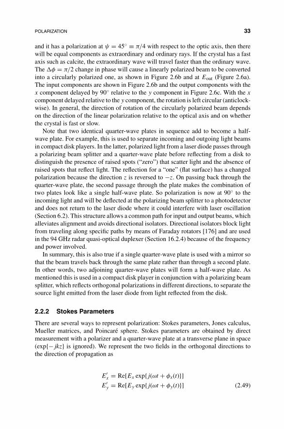
Note that two identical quarter-wave plates in sequence add to become a half-wave plate. For example, this is used to separate incoming and outgoing light beamsin compact disk players. In the latter, polarized light from a laser diode passes througha polarizing beam splitter and a quarter-wave plate before reflecting from a disk todistinguish the presence of raised spots (“zero”) that scatter light and the absence ofraised spots that reflect light. The reflection for a “one” (flat surface) has a changedpolarization because the direction z is reversed to −z. On passing back through thequarter-wave plate, the second passage through the plate makes the combination oftwo plates look like a single half-wave plate. So polarization is now at 90◦ to theincoming light and will be deflected at the polarizing beam splitter to a photodetectorand does not return to the laser diode where it could interfere with laser oscillation(Section 6.2). This structure allows a common path for input and output beams, whichalleviates alignment and avoids directional isolators. Directional isolators block lightfrom traveling along specific paths by means of Faraday rotators [176] and are usedin the 94 GHz radar quasi-optical duplexer (Section 16.2.4) because of the frequencyand power involved.
In summary, this is also true if a single quarter-wave plate is used with a mirror sothat the beam travels back through the same plate rather than through a second plate.In other words, two adjoining quarter-wave plates will form a half-wave plate. Asmentioned this is used in a compact disk player in conjunction with a polarizing beamsplitter, which reflects orthogonal polarizations in different directions, to separate thesource light emitted from the laser diode from light reflected from the disk.
2.2.2 Stokes Parameters
There are several ways to represent polarization: Stokes parameters, Jones calculus,Mueller matrices, and Poincare sphere. Stokes parameters are obtained by directmeasurement with a polarizer and a quarter-wave plate at a transverse plane in space(exp{−jkz} is ignored). We represent the two fields in the orthogonal directions tothe direction of propagation as
E′x = Re[Ex exp{j(ωt + φx(t)}]
E′y = Re[Ey exp{j(ωt + φy(t)}] (2.49)

34 GAUSSIAN BEAMS AND POLARIZATION
The four Stokes equations are (with �φ = φy − φx)
s0 = |Ex|2 + |Ey|2s1 = |Ex|2 − |Ey|2s2 = 2|Ex||Ey| cos(�φ)
s3 = 2|Ex||Ey| sin(�φ) (2.50)
These are measured as follows [16]. If I(θ) uses a linear polarizer at an angle θ tomeasure intensity at angle θ, and Q(θ) uses a quarter-wave plate followed by a linearpolarizer at angle θ, then the Stokes parameters are measured by
s0 = I(0) + I(π/2)
s1 = I(0) − I(π/2)
s2 = I(π/4) − I(3π/4)
s3 = Q(π/4) − Q(3π/4) (2.51)
In the Stokes parameters, s0 represents the total power where s20 = s2
1 + s22 + s2
3. Soonly three of the four Stokes parameters are independent and need be measured. s1represents excess power in x direction polarization over y direction polarization, s2represents the amount of π/4 polarized power over that in −π/4, and s3 representsthe amount of right circular polarized power over left circular polarized power.
2.2.3 Poincare Sphere
Polarimeters that measure polarization often display the polarization on a sphere [16].The sphere, introduced by Poincare, provides a convenient way of representing allpossible polarizations. It is interesting that for analysis to obtain simpler results andfor advanced research, Poincare used spherical geometry [16], in which, for example,the three angles of a triangle (placed on a sphere) no longer add to 180◦. Every possiblepolarization is represented by one point on the Poincare sphere and every point onthe sphere represents one polarization (a one-to-one mapping) (Figure 2.7a) [29].Points on sphere are marked with x, y, z coordinates. Polarimeters may show thewhole sphere or only one quadrant with a note to say which quadrant is displayed. ASiemens VPI simulator, popular for optical network design, allows the sphere to beturned with a mouse to view any quadrant.
Points P on the sphere along the equator represent linear polarizations at differ-ent angles ψ, at left linear horizontal polarization (LHP), and opposite at right onthe sphere linear vertical polarization (LVP). Note that opposite points on the sphereare uncorrelated. Twice the angle of the polarization, or 2ψ, is the azimuth of thepoint P (Figure 2.7b). As P moves up from the equator to elevation 2χ (Figure 2.7aand b), the minor axis of the right circular ellipse increases until the polarizationbecomes right circular at the north pole. If we return back to the equator, on pass-ing through the equator, the minor axis inverts to produce left circular elliptical

POLARIZATION 35
FIGURE 2.7 Poincare sphere: (a) polarizations and (b) Stokes parameters on Poincare sphereand polarization control.
polarization. The angle γ subtended at the center of the sphere between two differentpolarizations P1 and P2 gives the correlation between the two polarizations:
ρ = cos(γ
2
)(2.52)
For example, if points P1 and P2 are coincident, γ = 0 and correlation is ρ = cos(0) =1 or perfect correlation. As mentioned, if points P1 and P2 are on opposite sidesof the sphere, γ = π and correlation is ρ = cos(π/2) = 0 for uncorrelated points.Interference patterns improve as the correlation between interfering beams increases.If light loses polarization, it will move down the line toward the center of the sphere.The origin of the sphere has no distinct polarization (it has all polarizations equally).If the polarization drifts with time, it will create a time trajectory on the surface of thesphere. If many frequencies are present, the polarization will differ and there will bea point for each, so for a pulse with a continuum of frequencies, a trace will appear.Due to dispersion, the trace will change shape with propagation.
2.2.4 Finding Point on Poincare Sphere and Elliptical Polarizationfrom Stokes Parameters
A shown in Figure 2.7b, we plot the Stokes parameters s1, s2, and s3 on the x, y,and z axes, respectively, where these axes are drawn over the sphere. A polarizationpoint P on the sphere can now be described with rectangular coordinate (s1, s2, s3) orspherical coordinate (s0, 2χ, 2ψ), where the radius of the sphere is the total power s0,2χ is the elevation, and 2ψ is the azimuthal angle. Note that the spherical coordinatesystem is that used for the earth; electrical engineers typically use angle from northpole rather than elevation. By propagating the vector from origin to P down to the

36 GAUSSIAN BEAMS AND POLARIZATION
x, y, and z axes, we obtain the following equations:
s1 = s0 cos 2χ cos 2ψ
s2 = s0 cos 2χ sin 2ψ
s3 = s0 sin 2χ (2.53)
From equations (2.53), we can derive expressions for the spherical coordinates forthe point on the sphere in terms of the Stokes parameters, equation (2.50). From thefirst and second equations,
tan 2ψ = s2
s1(2.54)
From the third equation,
sin 2χ = s3
s0(2.55)
Hence, a point in spherical equations on the Poincare sphere can be equated to theone in rectangular coordinates from the Stokes parameters and vice versa.
We also know the difference in phase angle �φ between the x and y wave com-ponents from the Stokes parameters, equation (2.50),
tan(�φ) = s3
s2(2.56)
We can also draw the elliptical polarization plot like that in Figure 2.4a by com-puting the circumscribing rectangle of size 2Ex by 2Ey. From the first two Stokesequations (2.50),
|Ex|2 =(
s0 + s1
2
)1/2
|Ey|2 =(
s0 − s1
2
)1/2
(2.57)
The polarization angle ψ was computed in equation (2.54).
2.2.5 Controlling Polarization
A polarization controller is commonplace in optical fiber telecommunications. Fiberis birefringent because it is not perfectly circularly symmetric. Hence, fiber has dif-ferent refractive indices in two orthogonal cross-section directions; that is, verticalpolarized waves will travel at a different speed from horizontal polarized waves, orindeed any arbitrary polarized wave will travel at a different speed from its oppo-site polarization. Worse still, any movement in the fiber will change the polarization.
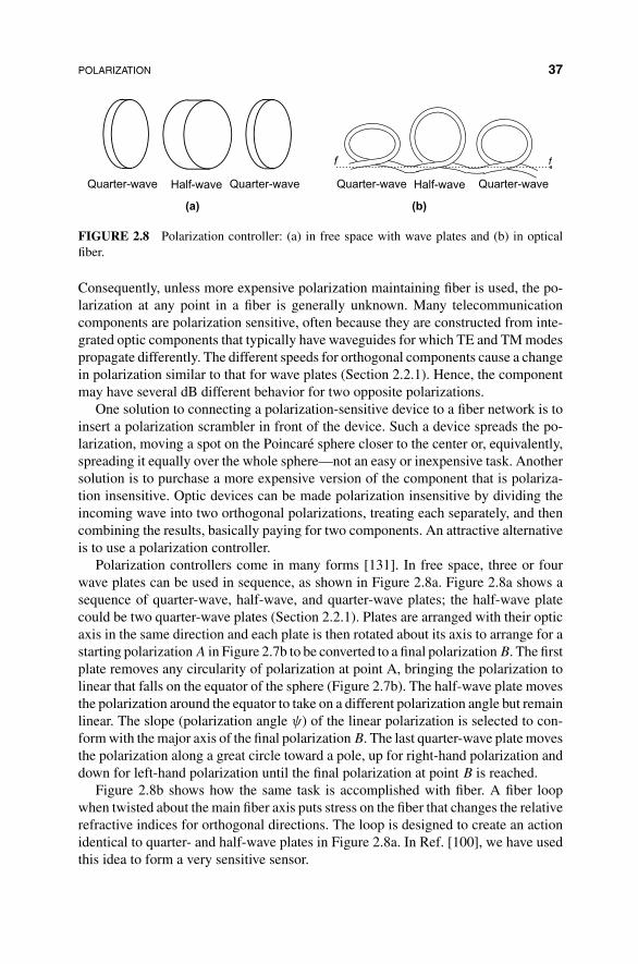
POLARIZATION 37
Quarter-waveQuarter-wave Half-wave
f f
Half-waveQuarter-wave Quarter-wave
(a) (b)
FIGURE 2.8 Polarization controller: (a) in free space with wave plates and (b) in opticalfiber.
Consequently, unless more expensive polarization maintaining fiber is used, the po-larization at any point in a fiber is generally unknown. Many telecommunicationcomponents are polarization sensitive, often because they are constructed from inte-grated optic components that typically have waveguides for which TE and TM modespropagate differently. The different speeds for orthogonal components cause a changein polarization similar to that for wave plates (Section 2.2.1). Hence, the componentmay have several dB different behavior for two opposite polarizations.
One solution to connecting a polarization-sensitive device to a fiber network is toinsert a polarization scrambler in front of the device. Such a device spreads the po-larization, moving a spot on the Poincare sphere closer to the center or, equivalently,spreading it equally over the whole sphere—not an easy or inexpensive task. Anothersolution is to purchase a more expensive version of the component that is polariza-tion insensitive. Optic devices can be made polarization insensitive by dividing theincoming wave into two orthogonal polarizations, treating each separately, and thencombining the results, basically paying for two components. An attractive alternativeis to use a polarization controller.
Polarization controllers come in many forms [131]. In free space, three or fourwave plates can be used in sequence, as shown in Figure 2.8a. Figure 2.8a shows asequence of quarter-wave, half-wave, and quarter-wave plates; the half-wave platecould be two quarter-wave plates (Section 2.2.1). Plates are arranged with their opticaxis in the same direction and each plate is then rotated about its axis to arrange for astarting polarization A in Figure 2.7b to be converted to a final polarization B. The firstplate removes any circularity of polarization at point A, bringing the polarization tolinear that falls on the equator of the sphere (Figure 2.7b). The half-wave plate movesthe polarization around the equator to take on a different polarization angle but remainlinear. The slope (polarization angle ψ) of the linear polarization is selected to con-form with the major axis of the final polarization B. The last quarter-wave plate movesthe polarization along a great circle toward a pole, up for right-hand polarization anddown for left-hand polarization until the final polarization at point B is reached.
Figure 2.8b shows how the same task is accomplished with fiber. A fiber loopwhen twisted about the main fiber axis puts stress on the fiber that changes the relativerefractive indices for orthogonal directions. The loop is designed to create an actionidentical to quarter- and half-wave plates in Figure 2.8a. In Ref. [100], we have usedthis idea to form a very sensitive sensor.
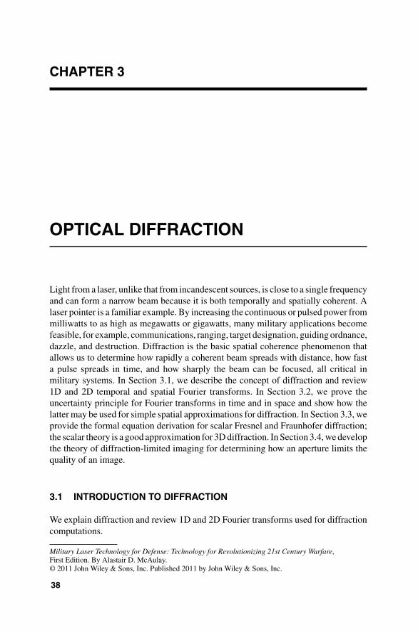
CHAPTER 3
OPTICAL DIFFRACTION
Light from a laser, unlike that from incandescent sources, is close to a single frequencyand can form a narrow beam because it is both temporally and spatially coherent. Alaser pointer is a familiar example. By increasing the continuous or pulsed power frommilliwatts to as high as megawatts or gigawatts, many military applications becomefeasible, for example, communications, ranging, target designation, guiding ordnance,dazzle, and destruction. Diffraction is the basic spatial coherence phenomenon thatallows us to determine how rapidly a coherent beam spreads with distance, how fasta pulse spreads in time, and how sharply the beam can be focused, all critical inmilitary systems. In Section 3.1, we describe the concept of diffraction and review1D and 2D temporal and spatial Fourier transforms. In Section 3.2, we prove theuncertainty principle for Fourier transforms in time and in space and show how thelatter may be used for simple spatial approximations for diffraction. In Section 3.3, weprovide the formal equation derivation for scalar Fresnel and Fraunhofer diffraction;the scalar theory is a good approximation for 3D diffraction. In Section 3.4, we developthe theory of diffraction-limited imaging for determining how an aperture limits thequality of an image.
3.1 INTRODUCTION TO DIFFRACTION
We explain diffraction and review 1D and 2D Fourier transforms used for diffractioncomputations.
Military Laser Technology for Defense: Technology for Revolutionizing 21st Century Warfare,First Edition. By Alastair D. McAulay.© 2011 John Wiley & Sons, Inc. Published 2011 by John Wiley & Sons, Inc.
38
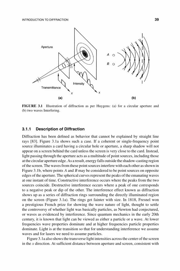
INTRODUCTION TO DIFFRACTION 39
FIGURE 3.1 Illustration of diffraction as per Huygens: (a) for a circular aperture and(b) two waves Interfering.
3.1.1 Description of Diffraction
Diffraction has been defined as behavior that cannot be explained by straight linerays [83]. Figure 3.1a shows such a case. If a coherent or single-frequency pointsource illuminates a card having a circular hole or aperture, a sharp shadow will notappear on a screen behind the card unless the screen is very close to the card. Instead,light passing through the aperture acts as a multitude of point sources, including thoseat the circular aperture edge. As a result, energy falls outside the shadow-casting regionof the screen. The waves from these point sources interfere with each other as shown inFigure 3.1b, where points A and B may be considered to be point sources on oppositeedges of the aperture. The spherical curves represent the peaks of the emanating wavesat one instant of time. Constructive interference occurs where the peaks from the twosources coincide. Destructive interference occurs where a peak of one correspondsto a negative peak or dip of the other. The interference effect known as diffractionshows up as a series of diffraction rings surrounding the directly illuminated regionon the screen (Figure 3.1a). The rings get fainter with size. In 1818, Fresnel wona prestigious French prize for showing the wave nature of light, thought to settlethe controversy of whether light was basically particles, as Newton had conjectured,or waves as evidenced by interference. Since quantum mechanics in the early 20thcentury, it is known that light can be viewed as either a particle or a wave. At lowerfrequencies wave properties dominate and at higher frequencies particle propertiesdominate. Light is at the transition so that for understanding interference we assumewaves and for lasers we need to assume particles.
Figure 3.1a also shows the transverse light intensities across the center of the screenin the x direction. At sufficient distance between aperture and screen, consistent with
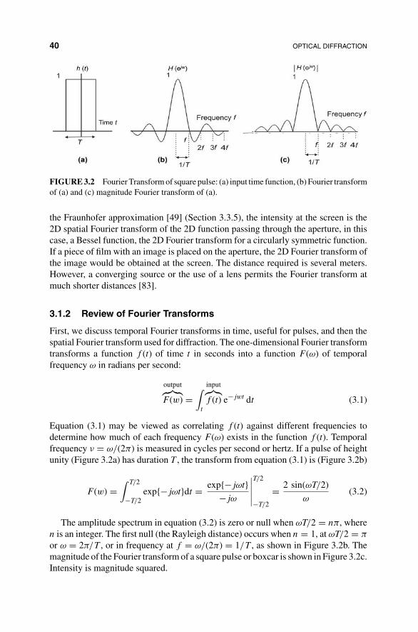
40 OPTICAL DIFFRACTION
FIGURE 3.2 Fourier Transform of square pulse: (a) input time function, (b) Fourier transformof (a) and (c) magnitude Fourier transform of (a).
the Fraunhofer approximation [49] (Section 3.3.5), the intensity at the screen is the2D spatial Fourier transform of the 2D function passing through the aperture, in thiscase, a Bessel function, the 2D Fourier transform for a circularly symmetric function.If a piece of film with an image is placed on the aperture, the 2D Fourier transform ofthe image would be obtained at the screen. The distance required is several meters.However, a converging source or the use of a lens permits the Fourier transform atmuch shorter distances [83].
3.1.2 Review of Fourier Transforms
First, we discuss temporal Fourier transforms in time, useful for pulses, and then thespatial Fourier transform used for diffraction. The one-dimensional Fourier transformtransforms a function f (t) of time t in seconds into a function F (ω) of temporalfrequency ω in radians per second:
output︷ ︸︸ ︷F (w) =
∫t
input︷︸︸︷f (t) e−jwt dt (3.1)
Equation (3.1) may be viewed as correlating f (t) against different frequencies todetermine how much of each frequency F (ω) exists in the function f (t). Temporalfrequency ν = ω/(2π) is measured in cycles per second or hertz. If a pulse of heightunity (Figure 3.2a) has duration T , the transform from equation (3.1) is (Figure 3.2b)
F (w) =∫ T/2
−T/2exp{−jωt}dt = exp{−jωt}
−jω
∣∣∣∣∣T/2
−T/2
= 2 sin(ωT/2)
ω(3.2)
The amplitude spectrum in equation (3.2) is zero or null when ωT/2 = nπ, wheren is an integer. The first null (the Rayleigh distance) occurs when n = 1, at ωT/2 = π
or ω = 2π/T , or in frequency at f = ω/(2π) = 1/T , as shown in Figure 3.2b. Themagnitude of the Fourier transform of a square pulse or boxcar is shown in Figure 3.2c.Intensity is magnitude squared.

INTRODUCTION TO DIFFRACTION 41
A 1D electromagnetic wave cos(ωt − kxx) oscillates in time with angular fre-quency ω radians per second and oscillates in 1D space x with spatial angularfrequency kx radians per meter. In an analogous transverse water wave, a cork floatingon a wave bobs up and down with frequency ω radians per second and a flash pho-tograph shows the spatial wave oscillating with kx radians per meter in x direction.So the 1D Fourier transform in the spatial domain may be written by analogy withequation (3.1) by replacing time t by space variable x and angular frequency in timeω radians per second by angular frequency in space kx radians per meter:
F (kx) =∫
x
f (x)e−jkxx dx (3.3)
where kx is the wave number in the x direction in radians per meter and x is distancein meters. Spatial frequency fx = 2πkx has units of cycles per meter (or lines permeter). Physical space has more than one dimension; consequently, higher dimensiontransforms are of interest.
In considering beams or propagation of images between planes, we will consider2D spatial Fourier transforms. A 1D spatial Fourier transform, equation (3.3), maybe extended to 2D as follows:
2D output︷ ︸︸ ︷F (kx, ky) =
∫x
∫y
2D input︷ ︸︸ ︷f (x, y)
plane wave︷ ︸︸ ︷e−j(kxx+kyy) dxdy (3.4)
where spatial frequencies kx and ky are in radians per meter in x and y directions,respectively. Note that the input wave pattern is decomposed into a set of plane waveswith different propagation directions (kx, ky) and amplitudes. The 2D input patternis correlated with each plane wave to give F (kx, ky), the amount of each plane wavepresent in the input. A square shaped beam or source of width and height S will havea transform similar to that shown in Figure 3.2 in x and y in the 2D spatial frequencydomain with null points at 1/S (S replaces T ).
There are many reasons for converting from the time or space domain into thetemporal or spatial frequency domain. Sometimes data are more meaningful in thefrequency domain. For example, in the temporal frequency domain ω, we can filter outspecific frequencies that we consider noise, such as a single-frequency jammer. In thespace domain, multiple plane waves from different directions (from distant sources)will strike a sensor array from different directions. The spatial Fourier transform willseparate the plane waves into multiple discrete points in the spatial frequency domain(Section 14.1). A single-direction jammer can be removed in adaptive beamformingto prevent it from masking target information from a different direction. If a 2Dtransform is used with time t on one axis and space x (or angle) on the other, sourceswith different frequencies and directions will show up as different points on the 2DFourier transform.
In image processing, we can remove spatially periodic background noise;for example, bars in front of a tiger in a cage can be filtered out in the spatial
42 OPTICAL DIFFRACTION
frequency domain. On taking the inverse transform, the tiger can be seen withoutthe bars. Targets with spatial periodicity can be recognized, and early submarinescould be identified by the periodic ribs in their structure.
Correlation and convolution are widely performed computations. The Fouriertransform is normally used to perform convolution or correlation on a computer or inoptics because convolution and correlation become multiplication in the frequencydomain and the low cost of the fast Fourier transform in computers or the opticalFourier transform in optics makes the computation faster than a straight convolutionor correlation computation [83]. Correlation is the basis for comparing images orsearching for patterns or words in huge databases. Convolution implements linearsystems such as smoothing, prediction, and many other signal processing functions.Chapter 14 of my previous book [83] describes an optical data flow computer thatI designed as a PI to DARPA and that was later partially constructed for NSA. Itperforms ultrafast correlation.
3.2 UNCERTAINTY PRINCIPLE FOR FOURIER TRANSFORMS
Instead of computing the diffraction fields exactly, we can use the uncertainty principlefor Fourier transforms to obtain a relation between the width of the field at the sourceand the smallest width of the information in the far field. The uncertainty principle forthe Fourier transform is related to the Heisenberg uncertainty principle in quantummechanics, �x�p ≥ �/2. This states that we cannot simultaneously determine theposition of a particle (�x → 0) and its momentum (�p → 0) to arbitrarily highaccuracy. We now show that a similar principle applies to Fourier transforms in timeor space and how this may be used for a first approximation in lieu of performing alengthy and detailed diffraction computation.
3.2.1 Uncertainty Principle for Fourier Transforms in Time
The uncertainty principle for Fourier transforms (or harmonics) in time specifies
�t�ω ≥ 1
2or �t�ν ≥ 1
2(3.5)
where �t is the width in time and �ν is the width in frequency, ω = 2πν.First, the reasonableness of the uncertainty principle, equation (3.5), can be seen
from the Fourier transform scaling property [49, 133]. Consider the scaling property,if F{g(t)} = G(ω), then
F {g(at)} = 1
|a|G(ω
a
)(3.6)
Or if a pulse is stretched by a in time to at, then the spectrum will become narrower by1/a in frequency to ω/a and vice versa: the inverted scaling property of the Fourier

UNCERTAINTY PRINCIPLE FOR FOURIER TRANSFORMS 43
transform. Consequently, we expect a limit to accurately predict both the locationof the pulse and its frequency simultaneously. In the limit, a delta function in time,representing exact knowledge of time (�t → 0), has all frequencies equally, whichprevents accurate determination of its frequency. Similarly, a single frequency, asinusoid, represented by a delta function in frequency, giving exact knowledge offrequency (�ω → 0), continues for all time, which prevents accurate measurementof its time of occurrence.
3.2.1.1 Proof of Uncertainty Principle for Fourier Transforms in TimeWe note that the constant on the right-hand side of the equation (3.5) may varydepending on the definitions of width used for �t and �ω: possibilities are width athalf maximum, root mean square, standard deviation, and Rayleigh width betweennulls.
We follow the approach for complex functions f used in Ref. [134]. A proof forreal functions f is given in Ref. [169].
E =∫ ∞
−∞|f (t)|2 dt, E = 1
2π
∫ ∞
−∞|F (ω)|2 dω (3.7)
Using Schwartz’s inequality [134],∣∣∫ p(t)q(t)dt
∣∣2 ≤ ∫ |p(t)|2 dt∫ |q(t)|2dt, with
p(t) = tf and q(t) = df ∗/dt, we can write, reversing the direction of the equation,
∫ ∞
−∞t2|f |2 dt
∫ ∞
−∞
∣∣∣∣df
dt
∣∣∣∣2
dt ≥∣∣∣∣∫ ∞
−∞(tf )
(df ∗
dt
)dt
∣∣∣∣2
(3.8)
We show that the square root of the right-hand side of equation (3.8) leads toE/2, which is E times the right-hand side of the uncertainty principle, equation (3.5);that is
∫ ∞−∞(tf )(df ∗/dt) dt = E/2. First, the square root of the right-hand side of
equation (3.8) may be written as
∣∣∣∣∫ ∞
−∞tf
df ∗
dtdt
∣∣∣∣ = 1
2
∣∣∣∣∫ ∞
−∞t
(f
df ∗
dt+ f ∗ df
dt
)dt
∣∣∣∣ (3.9)
= 1
2
∣∣∣∣∫ ∞
−∞td(ff ∗)
dtdt
∣∣∣∣ = 1
2
∣∣∣∣∫ ∞
−∞t
(d|f |2
dt
)dt
∣∣∣∣ = 1
2
∣∣∣∣∫ ∞
−∞td|f |2
∣∣∣∣= 1
2
(t|f |2
∣∣∣∞−∞−
∫ ∞
−∞|f |2 dt
)= −E
2(3.10)
where we used integration by parts and equation (3.7) for obtaining the last line.Also, as t → ∞,
√|t||f | → 0 ⇒ t|f |2 = 0, so the first term of the last line in equa-tion (3.10) is zero.
Now we show that the left-hand side of equation (3.8) leads to the product ofwidth squared in time and width squared in frequency for the square of the uncertaintyprinciple on the left-hand side of equation (3.5). Taking a derivative of a time functionis equivalent to multiplying by jω in the frequency domain and taking a second
44 OPTICAL DIFFRACTION
derivative is equivalent to multiplying by ω2 in the frequency domain. Therefore, ifF (ω) is the Fourier transform of f , then
∫ ∞
∞
∣∣∣∣df
dt
∣∣∣∣2
dt = 1
2π
∫ ∞
∞ω2 |F (ω)|2 dω (3.11)
Substituting equation (3.11) into the left-hand side of equation (3.8) and equa-tion (3.10) into the right-hand side of equation (3.8) gives
∫ ∞
−∞t2|f |2 dt
1
2π
∫ ∞
−∞ω2 |F (ω)|2 dω ≥ E2
4(3.12)
If we define
(�t)2 = 1
E
∫ ∞
−∞t2|f (t)|2 dt and (�ω)2 = 1
E
1
2π
∫ ∞
−∞ω2|F (ω)|2 dω (3.13)
then substituting equation (3.13) into equation (3.12) gives
(�t)2(�ω)2 ≥ 1
4(3.14)
The inequality holds after taking square roots of both sides, so we get
�t�ω ≥ 1
2(3.15)
which proves the uncertainty principle for Fourier transforms, equation (3.5).For equality to hold in equation (3.15), equality must also hold in equation (3.8) or
|df/dt| = |kft|. This occurs only for functions f with a Gaussian magnitude becausethe Fourier transform of a Gaussian function is also Gaussian, exp{−π(bt)2} ←→exp{−π(f/b)2}.
In an alternative form, we scale equation (3.12) by changing variables to frequencyν in place of angular frequency ω = 2πν (and dω = 2π dν).
∫ ∞
−∞t2|f |2 dt
∫ ∞
−∞ν2 |F (ν)|2 dν ≥ E2
4(3.16)
The uncertainty principle for Fourier transforms in time can then be written in termsof time and frequency widths as
�t�ν ≥ 1
2(3.17)

UNCERTAINTY PRINCIPLE FOR FOURIER TRANSFORMS 45
FIGURE 3.3 Relation between beam angle θ and spatial frequency λs: (a) wave strikingvertical screen and (b) triangle in (a).
3.2.2 Uncertainty Principle for Fourier Transforms in Space
Because of the interchangeability of space and time, we can derive an uncertainty prin-ciple for Fourier transforms in space in a similar manner. More simply, we replacetime t with space s and temporal angular frequency ω = 2πν with spatial angularfrequency kx = 2πfx to obtain the equivalent uncertainty principle for Fourier trans-forms in space, the one that arises in diffraction. Note that space has up to threedimensions, unlike time. For simplicity, we consider only 1D.
�s�kx ≥ 1
2or �s�fx ≥ 1
2(3.18)
The uncertainty principle may also be formulated in terms of emitted beam angleinstead of spatial frequency. We consider a wave of wavelength λ striking a plane at anangle θ with the normal (Figure 3.3a). The propagation vector k can be decomposedinto x and z components according to k2 = k2
x + k2z . A wave component propagates
down the screen in x direction with propagation constant kx corresponding to a spatialfrequency fx with wavelength λx = 1/fx. Figure 3.3b shows a right triangle, extractedfrom Figure 3.3a, from which
sin θ = λ
λx
= λfx for small angles �fx = �θ
λ(3.19)
where for small angles, θ → �θ and sin(�θ) → �θ. Substituting equation (3.19)into equation (3.18) gives an uncertainty principle for angle and distance:
�s�θ ≥ λ
2(3.20)

46 OPTICAL DIFFRACTION
(a)
2x
3x
4x
s s0
s1x = z
(b)
d1
d2
zL
s1x = zL
/2
/2Slit
Slit
s/2 /2sin
Intensity
FIGURE 3.4 Fraunhofer diffraction as an interference phenomenon: (a) finite width sourceand (b) two slits.
In this case, it is not possible to make both the source size �s and the beam angle �θ oflight emission arbitrarily small. In fact, arrays in radar and sonar and beam expandersin optics increase �s to reduce beam angle in order to channel electromagnetic energyinto a narrower beam for more accurate detection, imaging, or direction finding. Aphased array radar or sonar scans this more piercing narrow beam electronically orit can be rotated. In the limit, if the source becomes infinitely small, it radiates in alldirections and an angle cannot be distinguished. If, on the other hand, the beam angleis infinitely narrow, the source should be of infinite dimension.
3.2.2.1 Relation Between Diffraction and Interference It is instructive toview diffraction from an interference perspective. We consider a plane wave front ata source of width �s (Figure 3.4a). A similar problem is presented by the two slitsshown in Figure 3.4b. In either case, we consider two rays starting �s apart. At ascreen at the Fraunhofer distance, the two beams will interfere to produce a spatialFourier transform in x. A null occurs at point P on the screen when the two beamsarrive out of phase (π phase difference) with each other for destructive interference.This corresponds to the difference in distance traveled by the beams, d2 − d1 = λ/2.For interference, we add the two beams, E1 + E2, and then compute their combinedintensity, 〈(E1 + E2)〉〈(E1 + E2)∗〉. As discussed in Chapter 6, if we assume that thetwo beams arrive at the target with equal power A, one of the form exp{i(kd1 − ωt)}and the other exp{i(kd2 − ωt)}, the intensity of the field on the screen can be written as
I = 2A2(1 + cos(kx�d)) (3.21)
where �d = d2 − d1. From Figure 3.4b, �d = �s sin(�θ/2) ≈ �sx/zL, so thatequation (3.21) becomes, using kx = 2π/λ,
I = 2A2[
(1 + cos
(2π�sx
λzL
)](3.22)
SCALAR DIFFRACTION 47
where λzL is characteristic of shrinkage when optical diffraction is used to com-pute a Fourier transform. For example, when λ = 600 nm and distance to screenzL = 10 cm, the spatial Fourier transform at the screen is smaller than would becalculated by multiplying by λzL = 600 × 10−9 × 10−1 = 6 × 10⁻⁸. The shrinkageis the basis of holographic optical memory [83] and espionage in which a page ofdata is shrunk to the size of a period in a letter for covert communication.
From equation (3.22), peaks or fringes occur on the x axis at distances xf when(2π�sxf )/(λzL) = 2π or xf = (λzL)/(�s). As shown in time in Figure 3.4b, thedistance to the first null from the axis is proportional to 1/�s. However, for spacethere is reduction by multiplication by λzL.
3.3 SCALAR DIFFRACTION
Most of us are familiar with reflection and refraction from mirrors and the apparentbend of a straw in water. The third interaction between coherent light and boundariesis diffraction. We are concerned with a monochromatic wave passing through a 2Dmask and then propagating over a distance z to a target. Given the electromagneticwave field incident on the mask and the transmissive function U(x, y) of the mask, wedesire to know the electromagnetic field at the target. This will allow us to predict thefield after a laser beam has propagated through the atmosphere to project energy eitherfor a laser weapon (Section 12.2) or for transmitting or receiving signals in opticalcommunications. It also allows us to modify a beam’s wave front for adaptive optics(Sections 5.3 and 12.2) or determine the spot size for focused beams or Gaussianbeams (Section 2.1) in order to concentrate power to high intensities (Section 14.2.2).
We restrict our mathematical development to scalar diffraction for simplicity; thatis, we consider only one component of the electric field Ez [49]. For the vector deriva-tion, see Ref. [16]. Apparently, the scalar result provides satisfactory answers mostof the time. Following Fresnel’s award winning procedure, we break the derivationinto four stages:
1. Find an expression for the field at a point due to the field on a boundary sur-rounding the point (Section 3.3.2).
2. Find the field behind an aperture (Section 3.3.3).
3. Use the Fresnel approximation for a linear system relating the field at point P0in the output plane to the field at point P1 in the plane of the input mask for aplane wave incident on the mask and a distance limited to that involving spaceinvariant transformation allowing convolution (Section 3.3.4).
4. Use the Fraunhofer (far-field) approximation to show the 2D Fourier transformrelation between the field at P0 and the field at P1 (Section 3.3.5). A lens canbring the transform much closer [49, 83].
We note that the results may be useful after any step. We have used the result of item1 to improve the magnetic detection of nuclear missile carrying submarines hiding
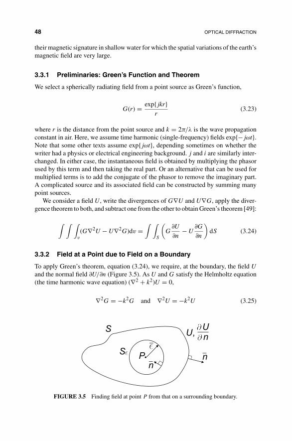
48 OPTICAL DIFFRACTION
their magnetic signature in shallow water for which the spatial variations of the earth’smagnetic field are very large.
3.3.1 Preliminaries: Green’s Function and Theorem
We select a spherically radiating field from a point source as Green’s function,
G(r) = exp{jkr}r
(3.23)
where r is the distance from the point source and k = 2π/λ is the wave propagationconstant in air. Here, we assume time harmonic (single-frequency) fields exp{−jωt}.Note that some other texts assume exp{jωt}, depending sometimes on whether thewriter had a physics or electrical engineering background. j and i are similarly inter-changed. In either case, the instantaneous field is obtained by multiplying the phasorused by this term and then taking the real part. Or an alternative that can be used formultiplied terms is to add the conjugate of the phasor to remove the imaginary part.A complicated source and its associated field can be constructed by summing manypoint sources.
We consider a field U, write the divergences of G∇U and U∇G, apply the diver-gence theorem to both, and subtract one from the other to obtain Green’s theorem [49]:
∫ ∫ ∫v
(G∇2U − U∇2G)dv =∫ ∫
S
(G
∂U
∂n− U
∂G
∂n
)dS (3.24)
3.3.2 Field at a Point due to Field on a Boundary
To apply Green’s theorem, equation (3.24), we require, at the boundary, the field U
and the normal field ∂U/∂n (Figure 3.5). As U and G satisfy the Helmholtz equation(the time harmonic wave equation) (∇2 + k2)U = 0,
∇2G = −k2G and ∇2U = −k2U (3.25)
S
S P nn
nU, U
FIGURE 3.5 Finding field at point P from that on a surrounding boundary.
SCALAR DIFFRACTION 49
By substituting equation (3.25), the left-hand side of equation (3.24) tends to zero.Furthermore, to avoid the difficulty of dealing with the field at a point (singularity),we draw a small sphere around the point P and consider the surface of this sphere tobe a second boundary Sε. ε will be allowed to shrink to zero later. Then,
0 =∫ ∫
Sε
(G
∂U
∂n− U
∂G
∂n
)dSε +
∫ ∫S
(G
∂U
∂n− U
∂G
∂n
)dS (3.26)
Now consider Green’s function G = exp{jkr}/r. For the small sphere around P ,r = ε, so G = exp{jkε}/ε and
∂G
∂ε= 1
εjk exp{jkε} + exp{jkε}
(− 1
ε2
)= exp{jkε}
ε
(jk − 1
ε
)(3.27)
This should be modified as ∂G/∂n for equation (3.24):
∂G
∂n= ∂ε
∂n
∂G
∂ε= cos(n, ε)
exp{jkε}ε
(jk − 1
ε
)(3.28)
where a refers to a unit direction vector of magnitude a. As n is toward the center ofsmall sphere and ε is outward, cos(n, ε) = −1. Now substituting equation (3.28) intoequation (3.26) gives
0 =∫ ∫
Sε
[exp{jkε}
ε
∂U
∂n− U
exp{jkε}ε
(1
ε− jk
)]dSε
+∫ ∫
S
(G
∂U
∂n− U
∂G
∂n
)dS (3.29)
For a point P , ε → 0, dSε → 4πε2, U → U(P0),
0 = 4πε2[
exp{jkε}ε
∂U(P0)
∂n− U(P0)
exp{jkε}ε
(1
ε− jk
)]
+∫ ∫
S
(G
∂U
∂n− U
∂G
∂n
)dS (3.30)
Consider the first term of equation (3.30), 4πε2 × terms in the square bracket.When ε → 0, the only term remaining in the first term of equation (3.30) is4πε2U(P0) exp{jkε}/ε2. So
0 = −4πU(P0) +∫ ∫
S
(G
∂U
∂n− U
∂G
∂n
)dS (3.31)

50 OPTICAL DIFFRACTION
From this equation, the field U(P0) at a point (P0) inside a closed region for whichthe field U and normal field ∂U/∂n are known along the boundary is
U(P0) = 1
4π
∫ ∫S
(G
∂U
∂n− U
∂G
∂n
)dS (3.32)
3.3.3 Diffraction from an Aperture
We assume that the aperture through which light passes is placed into the boundaryaround the point at which we seek the field (Figure 3.6). First, we form a moreconvenient Green’s function G2(P1) that has two point sources of opposite phase sothat for G2(P1), the field at point P1 cancels in the aperture:
G2(P1) = exp{jkr01}r01
− exp{jkr02}r02
(3.33)
We assume that the second point source is located at a mirror image of the first aroundthe plane of the aperture. Then, r01 = r02 and from equation (3.33),
G2(P1) = 0 (3.34)
Now using a similar process (using a bar over a variable to represent a unit vector) asfor equation (3.28), but with r01 replacing ε,
∂G2
∂n= cos(n, r01)
(jk − 1
r01
)exp{jkr01}
r01− cos(n, r02)
(jk − 1
r02
)exp{jkr02}
r02
(3.35)
As cos(n, r02) = − cos(n, r01), k = 2π/λ, and r01 = r02
∂G2
∂n= 2 cos(n, r01)
(jk − 1
r01
)exp{jkr01}
r01(3.36)
P0 P0
Point in
aperture P1
r01 = r02r01
Surface far
enough
to be ignoredPoint behind
aperture
n
FIGURE 3.6 Diagram for deriving light behind an aperture.

SCALAR DIFFRACTION 51
If we assume that r01 � λ, 1/r01 may be neglected in (jk − 1/r01), using k = 2π/λ,
∂G2
∂n= −4π
jλ
exp{jkr01}r01
cos(n, r01) (3.37)
For the field at point P0, substitute equations (3.37) and (3.34) into equation (3.32).Label the surrounding surface S1 and an arbitrary point in the aperture P1:
U(P0) = 1
4π
∫ ∫S1
−U(P1)∂G2
∂ndS
= 1
jλ
∫ ∫S1
U(P1)exp{jkr01}
r01cos(n, r01)dS (3.38)
This gives the Rayleigh–Sommerfeld equation for an aperture, relabeled ,
U(P0) =∫ ∫
h(P0, P1)U(P1)dS
with h(P0, P1) = 1
jλ
exp{jkr01}r01
cos(n, r01) (3.39)
where h(P0, P1) is the impulse response that describes a linear system representingdiffraction during propagation.
We see how close Huygens came to the general structure in 1687 by rewritingequation (3.39):
U(P0) =∫ ∫
spherical wave︷ ︸︸ ︷exp{jkr01}
r01
⎡⎢⎢⎢⎣
angle loss︷ ︸︸ ︷cos(n, r01)
jλ︸ ︷︷ ︸λ dependence
⎤⎥⎥⎥⎦U(P1)dS (3.40)
Huygens, lacking different single frequency sources, ignored the square bracket inequation (3.40) in explaining a diffraction of a plane wave striking an aperture asregenerating a set of point sources for which each of the spherical waves emanatedadds at a screen to produce an interference pattern (Figure 3.7).
3.3.4 Fresnel Approximation
We first assume that the distance z between input mask and screen is much greaterthan the transverse dimension at the diffraction plane so that the obliquity factorcos(n, r01) = 1. In this case, r01 ≈ z in the denominator of equation (3.40). This can-not be used in the exponential phase term in the numerator because of the smallsize of wavelength λ. Now equation (3.39) can be written for propagation from

52 OPTICAL DIFFRACTION
Constructive
interference
at overlaps
on screen
Screen
Aperture
Rays from
edges of
aperture
Plane
wave
(a) (b)
FIGURE 3.7 Interpretation of diffraction as sum of fields from new point sources at anaperture: (a) spherical waves and (b) view of intensity on screen.
input plane (x1, y1) to output plane (x0, y0) (Figure 3.8) as
U(x0, y0) =∫ ∫
h(x0, y0 : x1, y1)U(x1, y1)dx1 dy1
with h(x0, y0 : x1, y1) = 1
jλ
exp{jkr01}z
(3.41)
We now apply an approximation that will convert the linear system representing prop-agation with diffraction into a shift invariant system that is described by convolution.Convolution can be performed rapidly using the frequency domain and the convolu-tion theorem of Fourier transform theory [49]. The spherical wave fronts generatedby diffraction at the input mask, plane 1, are approximated by parabolas close to theaxis because a parabola approximates a sphere over a small region; this is called the
Plane 1 input Plane 0 output
x1
y1
x0
y0
z
r01
Input
plane
wave
FIGURE 3.8 Diffraction from plane 1 to plane 0.
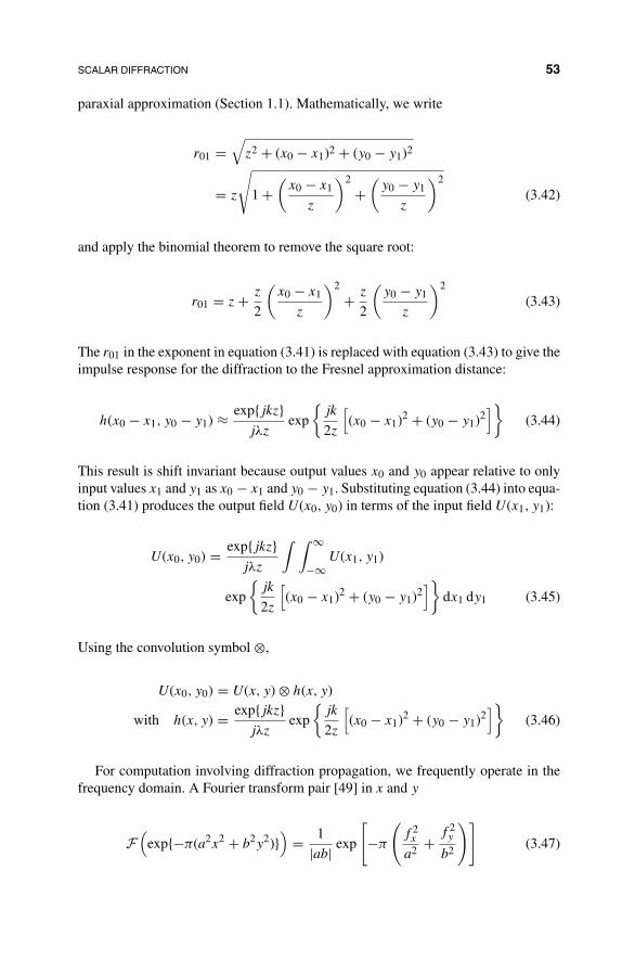
SCALAR DIFFRACTION 53
paraxial approximation (Section 1.1). Mathematically, we write
r01 =√
z2 + (x0 − x1)2 + (y0 − y1)2
= z
√1 +
(x0 − x1
z
)2
+(
y0 − y1
z
)2
(3.42)
and apply the binomial theorem to remove the square root:
r01 = z + z
2
(x0 − x1
z
)2
+ z
2
(y0 − y1
z
)2
(3.43)
The r01 in the exponent in equation (3.41) is replaced with equation (3.43) to give theimpulse response for the diffraction to the Fresnel approximation distance:
h(x0 − x1, y0 − y1) ≈ exp{jkz}jλz
exp
{jk
2z
[(x0 − x1)2 + (y0 − y1)2
]}(3.44)
This result is shift invariant because output values x0 and y0 appear relative to onlyinput values x1 and y1 as x0 − x1 and y0 − y1. Substituting equation (3.44) into equa-tion (3.41) produces the output field U(x0, y0) in terms of the input field U(x1, y1):
U(x0, y0) = exp{jkz}jλz
∫ ∫ ∞
−∞U(x1, y1)
exp
{jk
2z
[(x0 − x1)2 + (y0 − y1)2
]}dx1 dy1 (3.45)
Using the convolution symbol ⊗,
U(x0, y0) = U(x, y) ⊗ h(x, y)
with h(x, y) = exp{jkz}jλz
exp
{jk
2z
[(x0 − x1)2 + (y0 − y1)2
]}(3.46)
For computation involving diffraction propagation, we frequently operate in thefrequency domain. A Fourier transform pair [49] in x and y
F(
exp{−π(a2x2 + b2y2)})
= 1
|ab| exp
[−π
(f 2
x
a2 + f 2y
b2
)](3.47)
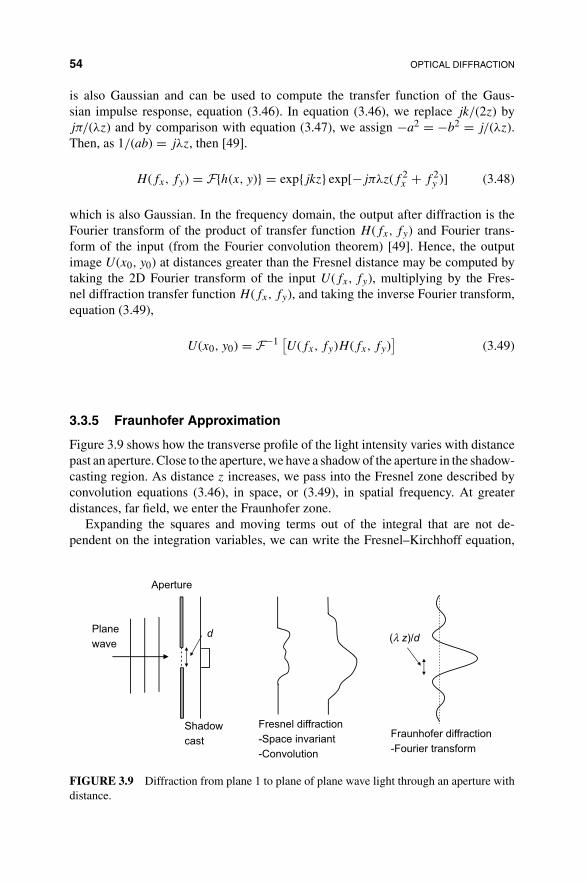
54 OPTICAL DIFFRACTION
is also Gaussian and can be used to compute the transfer function of the Gaus-sian impulse response, equation (3.46). In equation (3.46), we replace jk/(2z) byjπ/(λz) and by comparison with equation (3.47), we assign −a2 = −b2 = j/(λz).Then, as 1/(ab) = jλz, then [49].
H(fx, fy) = F{h(x, y)} = exp{jkz} exp[−jπλz(f 2x + f 2
y )] (3.48)
which is also Gaussian. In the frequency domain, the output after diffraction is theFourier transform of the product of transfer function H(fx, fy) and Fourier trans-form of the input (from the Fourier convolution theorem) [49]. Hence, the outputimage U(x0, y0) at distances greater than the Fresnel distance may be computed bytaking the 2D Fourier transform of the input U(fx, fy), multiplying by the Fres-nel diffraction transfer function H(fx, fy), and taking the inverse Fourier transform,equation (3.49),
U(x0, y0) = F−1 [U(fx, fy)H(fx, fy)
](3.49)
3.3.5 Fraunhofer Approximation
Figure 3.9 shows how the transverse profile of the light intensity varies with distancepast an aperture. Close to the aperture, we have a shadow of the aperture in the shadow-casting region. As distance z increases, we pass into the Fresnel zone described byconvolution equations (3.46), in space, or (3.49), in spatial frequency. At greaterdistances, far field, we enter the Fraunhofer zone.
Expanding the squares and moving terms out of the integral that are not de-pendent on the integration variables, we can write the Fresnel–Kirchhoff equation,
Aperture
Shadow
cast
Fresnel diffraction
-Space invariant
-Convolution
Fraunhofer diffraction
-Fourier transform
Plane
waved (λ z)/d
FIGURE 3.9 Diffraction from plane 1 to plane of plane wave light through an aperture withdistance.
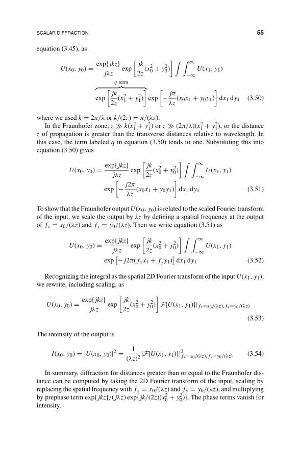
SCALAR DIFFRACTION 55
equation (3.45), as
U(x0, y0) = exp{jkz}jλz
exp
[jk
2z(x2
0 + y20)
] ∫ ∫ ∞
−∞U(x1, y1)
q term︷ ︸︸ ︷exp
[jk
2z(x2
1 + y21)
]exp
[−jπ
λz(x0x1 + y0y1)
]dx1 dy1 (3.50)
where we used k = 2π/λ or k/(2z) = π/(λz).In the Fraunhofer zone, z � k(x2
1 + y21) or z � (2π/λ)(x2
1 + y21), or the distance
z of propagation is greater than the transverse distances relative to wavelength. Inthis case, the term labeled q in equation (3.50) tends to one. Substituting this intoequation (3.50) gives
U(x0, y0) = exp{jkz}jλz
exp
[jk
2z(x2
0 + y20)
] ∫ ∫ ∞
−∞U(x1, y1)
exp
[−j2π
λz(x0x1 + y0y1)
]dx1 dy1 (3.51)
To show that the Fraunhofer output U(x0, y0) is related to the scaled Fourier transformof the input, we scale the output by λz by defining a spatial frequency at the outputof fx = x0/(λz) and fy = y0/(λz). Then we write equation (3.51) as
U(x0, y0) = exp{jkz}jλz
exp
[jk
2z(x2
0 + y20)
] ∫ ∫ ∞
−∞U(x1, y1)
exp[−j2π(fxx1 + fyy1)
]dx1 dy1 (3.52)
Recognizing the integral as the spatial 2D Fourier transform of the input U(x1, y1),we rewrite, including scaling, as
U(x0, y0) = exp{jkz}jλz
exp
[jk
2z(x2
0 + y20)
]F{U(x1, y1)}|fx=x0/(λz),fy=y0/(λz)
(3.53)
The intensity of the output is
I(x0, y0) = |U(x0, y0)|2 = 1
(λz)2 |F{U(x1, y1)}|2fx=x0/(λz),fy=y0/(λz) (3.54)
In summary, diffraction for distances greater than or equal to the Fraunhofer dis-tance can be computed by taking the 2D Fourier transform of the input, scaling byreplacing the spatial frequency with fx = x0/(λz) and fy = y0/(λz), and multiplyingby prephase term exp{jkz}/(jλz) exp{jk/(2z)(x2
0 + y20)}. The phase terms vanish for
intensity.

56 OPTICAL DIFFRACTION
3.3.6 Role of Numerical Computation
Propagation of physical waves, including optic waves, may be described mathemat-ically and numerically by solutions to the wave equations that satisfy the boundaryconditions and material properties. In normal mode theory, propagation is describedby the sum of resonant modes, each of which is a solution to the wave equation. Thecombination of modes satisfies the boundary and source conditions. Mode theoryis invaluable for analysis and when used in combination with algebraic computerprograms (work with algebraic symbols in place of numbers) such as Maple andMathematica. Mode theory can provide valuable information on relationships amongparameters.
However, because the real world often has varying refractive index in space andboundaries are often too complicated for mode theory, we frequently solve the dis-cretized wave equations directly with digital computers using finite approximationtechniques. Discretizing the wave equation in both space and time is accomplishedwith finite-difference time-domain (FTDT) techniques [154]. FTDT provides insightinto the distribution of energy in space and time as it propagates through inhomo-geneous media. Discretizing in space only is accomplished with finite difference orfinite elements [78, 79].
3.4 DIFFRACTION-LIMITED IMAGING
A circular lens captures light falling on the lens, so it not only performs a lens functionbut also acts as a circular aperture of diameter equal to that of the lens. In an imagingsystem, there will be a limiting aperture that limits the ability of the system to focusan input point source to an output point source. If the output is distorted only by thediffraction of the limiting aperture, the system is called a diffraction-limited system.A diffraction-limited system has no other aberrations and is therefore the best possibleimaging system [49].
3.4.1 Intuitive Effect of Aperture in Imaging System
Figure 3.10 shows that the aperture of a convex lens loses high spatial frequenciesin the focused output image of an input point source. Light from the input pointsource is expanded as a set of plane waves at different angles, the angular spectrum,as shown on the left-hand side of Figure 3.10. On striking a vertical plane at thelens, the source plane wave components at the widest angle from the axis correspondto those with the highest frequency at the plane of the lens. These fall outside thelens aperture so that they are lost in forming the output image. The loss of highspatial frequencies in passing through the aperture results in rings around the pointsource image and smoothing of the image. Smoothing arises because the high spatialfrequencies provide the fine detail in an image. A larger diameter lens will capturehigher spatial frequencies and the output image will appear closer to a point source,making the point sharper. This is the reason that a photographic camera will provide

DIFFRACTION-LIMITED IMAGING 57
Lowspatialfrequency
Highspatialfrequency
P(x,y)
Aperture
Image of point source
Pointsource
k yk = k sin θy
kz = k cos θ
y
θ
FIGURE 3.10 Diffraction through aperture loses high spatial frequencies, causing smoothingof an image.
less sharp pictures with small apertures: high f -numbers. The large apertures used indimmer light will also be less sharp but for a different reason: the edges of the lensare now used and these often have more aberrations than the center.
3.4.2 Computing the Diffraction Effect of a Lens Aperture onImaging
We now show how to compute the effects of the aperture on an output image. Theaperture is called a pupil function in the following. Figure 3.11 shows a simple imagingsystem with input object Uo with coordinates xo and yo at distance d0 from a lens. Thelens with coordinates x and y has an optical field labeled Ul in front of the lens andU ′
l after passing through the lens. An image Ui with coordinates xi and yi is formed
U0
Ui
x0
y0
x
y
xi
yi
d0 di
UlUl
′
FIGURE 3.11 Imaging a point source (at arrowhead) with a limited aperture lens.

58 OPTICAL DIFFRACTION
at distance di from the lens. Owing to linearity of wave propagation,
Ui(xi, yi) =∫ ∞
∞
∫ ∞
∞h(xi, yi, xo, yo)Uo(xo, yo)dxo dyo (3.55)
The effects of diffraction on imaging can be computed in three steps:
1. Compute the geometric image by ignoring the effects of diffraction(Section 3.4.2.1).
2. Compute the impulse response describing diffraction through the system(Section 3.4.2.2).
3. For output image, compute the convolution between the impulse response fromstep 2 and the geometric image from step 1 (Section 3.4.2.3).
We proceed with equations for the three steps to prove that this procedure computesthe correct image with diffraction effects.
3.4.2.1 Step 1: Compute the Geometric Image We would like the image tobe an identical copy of the input, except for scaling by M to allow for magnification.This requires the impulse response from input to output to be a delta function of theform (|M|2 is added to preserve total power)
h(xi, yi, xo, yo) = 1
|M|2 δ(xi − Mxo, yi − Myo) (3.56)
The negatives account for image inversion through M = −di/do = −xi/xo. Substi-tuting equation (3.56) into equation (3.55) shows that a scaled copy of the input isobtained:
Ui(xi, yi) =∫ ∞
∞
∫ ∞
∞1
|M|2 δ(xi − Mxo, yi − Myo)Uo(xo, yo)dxo dyo (3.57)
From the sampling theorem for delta functions, the δ means sample Uo at xi − Mx0 =0 or x0 = xi/M to give a geometric image that is a scaled version of the input:
Ug(xi, yi) = 1
|M|2 Uo
( xi
M,
yi
M
)(3.58)
3.4.2.2 Step 2: Compute the Impulse Response Describing DiffractionThrough the System The propagation impulse response from the output of thelens in Figure 3.11 to the output screen is adapted from Fresnel diffraction equa-tion (3.45) (Section 3.3.4),
h(xi, yi, x, y) = 1
jλdi
∫ ∫ ∞
−∞U ′
l (x, y) exp
{jk
2di
[(xi − x)2 + (yi − y)2
]}dx dy
(3.59)where we neglected the leading phase term that is independent of x and y.

DIFFRACTION-LIMITED IMAGING 59
Propagation through the lens with pupil P(x, y) is represented by
U ′l (x, y) = Ul(x, y)P(x, y) exp
{− jk
2f
(x2 + y2
)}(3.60)
Propagation from point source input object to the lens is represented by
Ul(x, y) = 1
jλdoexp
{jk
2do
[(x − xo)2 + (y − yo)2
]}(3.61)
Substituting equation (3.61) into equation (3.60) and the result into equation (3.59)gives the overall impulse response from the input point source to the output pointsource:
h(xi, yi, xo, yo)
= 1
λ2dido
(a)︷ ︸︸ ︷exp
{jk
2do
(x2
o + y2o
)} (b)︷ ︸︸ ︷exp
{jk
2do
(x2
i + y2i
)}
∫ ∫ ∞
−∞P(x, y) exp
⎧⎪⎪⎪⎨⎪⎪⎪⎩
jk
2
(c)︷ ︸︸ ︷(1
do+ 1
di− 1
f
)(x2 + y2
)⎫⎪⎪⎪⎬⎪⎪⎪⎭
exp
{−jk
[(xo
do+ xi
di
)x +
(yo
do+ yi
di
)y
]}dx dy (3.62)
For imaging, our interest is in magnitude; therefore, we ignore the phase terms(a) and (b). If we assume perfect imaging according to the lens law, equation (1.24),1/do + 1/di − 1/f = 0, term (c) is zero and as exp{0} = 1, the exponential contain-ing term (c) vanishes. We eliminate do using equation (1.24) or do = −di/M. Thenequation (3.62) becomes
h(xi, yi, xo, yo) = 1
λ2dido∫ ∫ ∞
−∞P(x, y) exp
{jk
di(xi − Mxo)x + (yi − Myo)y
}dx dy (3.63)
Equation (3.63) is not space invariant because of the magnification M. We force it tobe space invariant, that is, in convolution form, by redefining variables xo = |M|xoand yo = |M|yo. We also incorporate the scaling in new variables, x = x/(λdi) andy = y/(λdi) from which dx = λdi dx and dy = λdi dy. In addition, using k = 2π/λ,equation (3.63) becomes (cancel |M| from 1/(λ2d1do) and P)
h(xi − xo, yi − yo)
=∫ ∫ ∞
−∞P(λdix, λdiy) exp
{−j2π[(xi − xo)x + (yi − yo)y
]}dx dy (3.64)
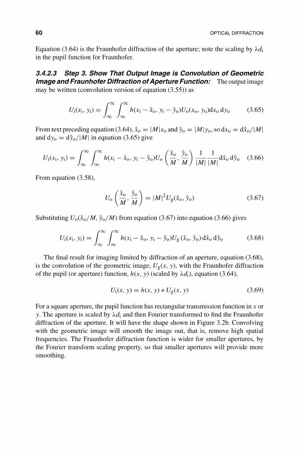
60 OPTICAL DIFFRACTION
Equation (3.64) is the Fraunhofer diffraction of the aperture; note the scaling by λdiin the pupil function for Fraunhofer.
3.4.2.3 Step 3. Show That Output Image is Convolution of GeometricImage and Fraunhofer Diffraction of Aperture Function: The output imagemay be written (convolution version of equation (3.55)) as
Ui(xi, yi) =∫ ∞
∞
∫ ∞
∞h(xi − xo, yi − yo)Uo(xo, yo)dxo dyo (3.65)
From text preceding equation (3.64), xo = |M|xo and yo = |M|yo, so dxo = dxo/|M|and dyo = dyo/|M| in equation (3.65) give
Ui(xi, yi) =∫ ∞
∞
∫ ∞
∞h(xi − xo, yi − yo)Uo
(xo
M,yo
M
)1
|M|1
|M|dxo dyo (3.66)
From equation (3.58),
Uo
(xo
M,yo
M
)= |M|2Ug(xo, yo) (3.67)
Substituting Uo(xo/M, yo/M) from equation (3.67) into equation (3.66) gives
Ui(xi, yi) =∫ ∞
∞
∫ ∞
∞h(xi − xo, yi − yo)Ug (xo, yo) dxo dyo (3.68)
The final result for imaging limited by diffraction of an aperture, equation (3.68),is the convolution of the geometric image, Ug(x, y), with the Fraunhofer diffractionof the pupil (or aperture) function, h(x, y) (scaled by λdi), equation (3.64),
Ui(x, y) = h(x, y) ∗ Ug(x, y) (3.69)
For a square aperture, the pupil function has rectangular transmission function in x ory. The aperture is scaled by λdi and then Fourier transformed to find the Fraunhoferdiffraction of the aperture. It will have the shape shown in Figure 3.2b. Convolvingwith the geometric image will smooth the image out, that is, remove high spatialfrequencies. The Fraunhofer diffraction function is wider for smaller apertures, bythe Fourier transform scaling property, so that smaller apertures will provide moresmoothing.

CHAPTER 4
DIFFRACTIVE OPTICAL ELEMENTS
Diffractive optical elements (DOEs) manipulate light by diffraction (Chapter 3),rather than by refraction with lenses or reflection with mirrors. DOEs often con-sist of a thin piece of transparent material with an opaque or etched pattern thatdiffracts light into the desired form. The different behavior and manufacturing ofDOEs relative to refractive elements has led to a significant diffractive optic elementindustry [69, 152] to complement the refractive lens industry (or mirror equivalents,Section 1.3).
The diffractive optical elements are based on the theory developed in Chapter 3,where we derived the equations for free-space Fresnel and Fraunhofer diffraction.For high-power optics (Section 12.2), light is manipulated with DOEs and dielectricmirrors (Section 6.3) to avoid conductors that overheat.
In Section 4.1, we briefly discuss some important applications of DOEs. In Sec-tion 4.2, we describe gratings for bending light and for separating colors or wave-lengths for spectrometry in chemical analysis (Chapter 15) and wavelength divisionmultiplexing (WDM). The grating equations are similar to those for an antenna array.Gratings can be created without lenses in the Talbot effect [85, 111]. In Section 4.3,we design a zone plate to replace a convex lens. In Section 4.4, we describe a widelyused algorithm, Gerchberg–Saxton algorithm, for computing a phase-only diffractiveelement to perform 2D filtering without loss.
Military Laser Technology for Defense: Technology for Revolutionizing 21st Century Warfare,First Edition. By Alastair D. McAulay.© 2011 John Wiley & Sons, Inc. Published 2011 by John Wiley & Sons, Inc.
61
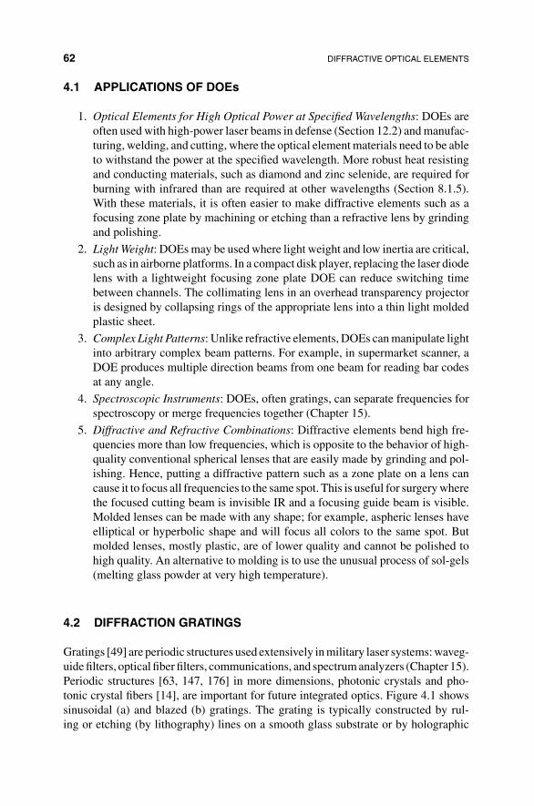
62 DIFFRACTIVE OPTICAL ELEMENTS
4.1 APPLICATIONS OF DOEs
1. Optical Elements for High Optical Power at Specified Wavelengths: DOEs areoften used with high-power laser beams in defense (Section 12.2) and manufac-turing, welding, and cutting, where the optical element materials need to be ableto withstand the power at the specified wavelength. More robust heat resistingand conducting materials, such as diamond and zinc selenide, are required forburning with infrared than are required at other wavelengths (Section 8.1.5).With these materials, it is often easier to make diffractive elements such as afocusing zone plate by machining or etching than a refractive lens by grindingand polishing.
2. Light Weight: DOEs may be used where light weight and low inertia are critical,such as in airborne platforms. In a compact disk player, replacing the laser diodelens with a lightweight focusing zone plate DOE can reduce switching timebetween channels. The collimating lens in an overhead transparency projectoris designed by collapsing rings of the appropriate lens into a thin light moldedplastic sheet.
3. Complex Light Patterns: Unlike refractive elements, DOEs can manipulate lightinto arbitrary complex beam patterns. For example, in supermarket scanner, aDOE produces multiple direction beams from one beam for reading bar codesat any angle.
4. Spectroscopic Instruments: DOEs, often gratings, can separate frequencies forspectroscopy or merge frequencies together (Chapter 15).
5. Diffractive and Refractive Combinations: Diffractive elements bend high fre-quencies more than low frequencies, which is opposite to the behavior of high-quality conventional spherical lenses that are easily made by grinding and pol-ishing. Hence, putting a diffractive pattern such as a zone plate on a lens cancause it to focus all frequencies to the same spot. This is useful for surgery wherethe focused cutting beam is invisible IR and a focusing guide beam is visible.Molded lenses can be made with any shape; for example, aspheric lenses haveelliptical or hyperbolic shape and will focus all colors to the same spot. Butmolded lenses, mostly plastic, are of lower quality and cannot be polished tohigh quality. An alternative to molding is to use the unusual process of sol-gels(melting glass powder at very high temperature).
4.2 DIFFRACTION GRATINGS
Gratings [49] are periodic structures used extensively in military laser systems: waveg-uide filters, optical fiber filters, communications, and spectrum analyzers (Chapter 15).Periodic structures [63, 147, 176] in more dimensions, photonic crystals and pho-tonic crystal fibers [14], are important for future integrated optics. Figure 4.1 showssinusoidal (a) and blazed (b) gratings. The grating is typically constructed by rul-ing or etching (by lithography) lines on a smooth glass substrate or by holographic
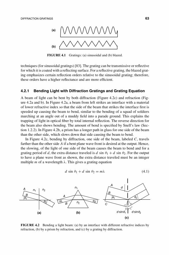
DIFFRACTION GRATINGS 63
(a)
(b)
FIGURE 4.1 Gratings: (a) sinusoidal and (b) blazed.
techniques (for sinusoidal gratings) [83]. The grating can be transmissive or reflectivefor which it is coated with a reflecting surface. For a reflective grating, the blazed grat-ing emphasizes certain reflection orders relative to the sinusoidal grating; therefore,these orders have a higher reflectance and are more efficient.
4.2.1 Bending Light with Diffraction Gratings and Grating Equation
A beam of light can be bent by both diffraction (Figure 4.2c) and refraction (Fig-ure 4.2a and b). In Figure 4.2a, a beam from left strikes an interface with a materialof lower refractive index so that the side of the beam that strikes the interface first isspeeded up causing the beam to bend, similar to the bending of a squad of soldiersmarching at an angle out of a muddy field into a parade ground. This explains thetrapping of light in optical fiber by total internal reflection. The reverse direction forthe beam also shows bending. The amount of bend is specified by Snell’s law (Sec-tion 1.2.2). In Figure 4.2b, a prism has a longer path in glass for one side of the beamthan the other side, which slows down that side causing the beam to bend.
In Figure 4.2c, bending by diffraction, one side of the beam, labeled C, travelsfarther than the other side A if a bent plane wave front is desired at the output. Hence,the slowing, of the light of one side of the beam causes the beam to bend and for agrating period of d, the extra distance traveled is d sin θ1 + d sin θ2. For the outputto have a plane wave front as shown, the extra distance traveled must be an integermultiple m of a wavelength λ. This gives a grating equation
d sin θ1 + d sin θ2 = mλ (4.1)
(a) (b)
(c)
d
d sinθ1 d sinθ2
A
A
AB
Bθ1
θ2 θ1 θ2
θ1 θ2
B C
n1
n1n2
n2
FIGURE 4.2 Bending a light beam: (a) by an interface with different refractive indices byrefraction, (b) by a prism by refraction, and (c) by a grating by diffraction.

64 DIFFRACTIVE OPTICAL ELEMENTS
0
0
2
12f0
12f0
2W
2W
Horizontalgrating
Mean
Intensity
1
x
Spatialfrequencyf0
x
y
(a) (b)
FIGURE 4.3 Cosinusoidal grating shape.
A major difference between diffractive and refractive bending (Figure 4.2c and aor b, is that in diffractive elements long wavelengths such as infrared make the gratinglook finer and are bent more than shorter wavelengths, while in refractive elementsthe reverse occurs; that is, the shorter wavelengths are bent more.
4.2.2 Cosinusoidal Grating
Figure 4.3a shows a cosinusoidal transmission grating of size 2W × 2W and gratingfrequency f0 for which the cross-sectional transmittance profile in x (Figure 4.3b)may be written as
Uin(x, y) =[
1
2+ 1
2cos(2πf0x1)
]rect
( x0
2W
)rect
( y0
2W
)(4.2)
A blazed grating is analyzed in Section 15.3.3. The first 12 in equation (4.2) arises
because intensity cannot be negative, so a zero spatial frequency or a DC componentexists to produce the zeroth-order component (Figure 4.4). The far-field diffraction(called Fraunhofer field) may be written using the Fourier transform of the intensityimmediately after the grating:
Uout(x0, y0) = F{Uin(x1, y1)}= F
[1
2+ 1
2cos(2πf0x1)
]∗ F
[rect
( x0
2W
)rect
( x0
2W
)]
=[
1
2δ(fxfy) + 1
4δ(fx + f0, fy) + 1
4δ(fx − f0, fy)
]∗ (2W)2sinc(2Wfx)sinc(2Wfy)
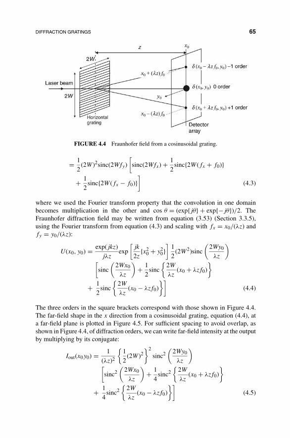
DIFFRACTION GRATINGS 65
FIGURE 4.4 Fraunhofer field from a cosinusoidal grating.
= 1
2(2W)2sinc(2Wfy)
[sinc(2Wfx) + 1
2sinc{2W(fx + f0)}
+ 1
2sinc{2W(fx − f0)}
](4.3)
where we used the Fourier transform property that the convolution in one domainbecomes multiplication in the other and cos θ = (exp{jθ} + exp{−jθ})/2. TheFraunhofer diffraction field may be written from equation (3.53) (Section 3.3.5),using the Fourier transform from equation (4.3) and scaling with fx = x0/(λz) andfy = y0/(λz):
U(x0, y0) = exp(jkz)
jλzexp
[jk
2z{x2
0 + y20}
]1
2(2W2)sinc
(2Wy0
λz
)[
sinc
(2Wx0
λz
)+ 1
2sinc
{2W
λz(x0 + λzf0)
}
+ 1
2sinc
{2W
λz(x0 − λzf0)
}](4.4)
The three orders in the square brackets correspond with those shown in Figure 4.4.The far-field shape in the x direction from a cosinusoidal grating, equation (4.4), ata far-field plane is plotted in Figure 4.5. For sufficient spacing to avoid overlap, asshown in Figure 4.4, of diffraction orders, we can write far-field intensity at the outputby multiplying by its conjugate:
Iout(x0y0) = 1
(λz)2
{1
2(2W)2
}2
sinc2(
2Wy0
λz
)[
sinc2(
2Wx0
λz
)+ 1
4sinc2
{2W
λz(x0 + λzf0)
}
+ 1
4sinc2
{2W
λz(x0 − λzf0)
}](4.5)
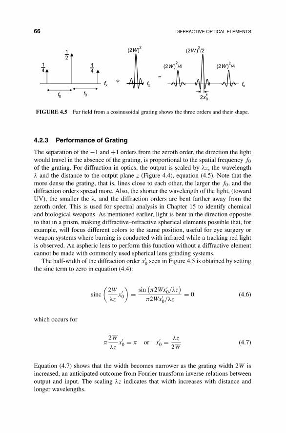
66 DIFFRACTIVE OPTICAL ELEMENTS
*=
14
14
12
f0 f0
(2W)2
(2W )2/4 (2W )
2/4
(2W )2/2
fx fx fx
2x0
FIGURE 4.5 Far field from a cosinusoidal grating shows the three orders and their shape.
4.2.3 Performance of Grating
The separation of the −1 and +1 orders from the zeroth order, the direction the lightwould travel in the absence of the grating, is proportional to the spatial frequency f0of the grating. For diffraction in optics, the output is scaled by λz, the wavelengthλ and the distance to the output plane z (Figure 4.4), equation (4.5). Note that themore dense the grating, that is, lines close to each other, the larger the f0, and thediffraction orders spread more. Also, the shorter the wavelength of the light, (towardUV), the smaller the λ, and the diffraction orders are bent farther away from thezeroth order. This is used for spectral analysis in Chapter 15 to identify chemicaland biological weapons. As mentioned earlier, light is bent in the direction oppositeto that in a prism, making diffractive–refractive spherical elements possible that, forexample, will focus different colors to the same position, useful for eye surgery orweapon systems where burning is conducted with infrared while a tracking red lightis observed. An aspheric lens to perform this function without a diffractive elementcannot be made with commonly used spherical lens grinding systems.
The half-width of the diffraction order x′0 seen in Figure 4.5 is obtained by setting
the sinc term to zero in equation (4.4):
sinc
(2W
λzx′
0
)= sin
(π2Wx′
0/λz)
π2Wx′0/λz
= 0 (4.6)
which occurs for
π2W
λzx′
0 = π or x′0 = λz
2W(4.7)
Equation (4.7) shows that the width becomes narrower as the grating width 2W isincreased, an anticipated outcome from Fourier transform inverse relations betweenoutput and input. The scaling λz indicates that width increases with distance andlonger wavelengths.

ZONE PLATE DESIGN AND SIMULATION 67
4.3 ZONE PLATE DESIGN AND SIMULATION
A zone plate is a widely used diffractive optical element that performs a functionsimilar to a refractive lens, except that it is manufactured differently and separatesdifferent wavelengths in opposite directions. It is used for light powers that woulddamage a normal refractive lens, or when a lens profile is required that is impossibleto make by grinding with a spherical tool, or where an especially light lens is required.The equations are derived for a zone plate and for the field profile at the focal planefor the first-order diffraction. For a selected focal length, the radii and the etch depth,in the case of a surface relief zone plate, are computed for the purpose of fabrication.The transverse intensity profile and the peak field value on axis are computed andcompared with a refractive lens.
4.3.1 Appearance and Focusing of Zone Plate
For a zone plate, we describe its appearance and how it focuses light.
4.3.1.1 Appearance of Zone Plate A zone plate is defined by concentricrings of increasing radii with decreasing separation between rings with radius [61, 86,134]. There are two types of zone plates: blocking and surface relief. In the blockingzone plate (Figure 4.6a), alternate rings are opaque to block light. This is also theappearance of the scaled mask for fabricating the surface relief type of zone plate.Note that most lithography machines reduce the mask size by 10 in printing the zoneplate. In the surface relief zone plate, the opaque regions, instead of being opaque,are raised or lowered by an integer multiple of half-wavelengths in the material. A3D view of the relief zone plate is shown in Figure 4.6b and a section through it isshown in Figure 4.7.
4.3.1.2 Focusing of Zone Plate A zone plate focuses light by diffractionrather than by refraction as in a lens. Figure 4.8 shows the cross section of a blockingzone plate and how the zone plate focuses a parallel beam of light onto a spot at the
FIGURE 4.6 View zone plates: (a) a blocking zone plate (and scaled mask for any zoneplate) (b) a 3D view of a surface relief zone plate.
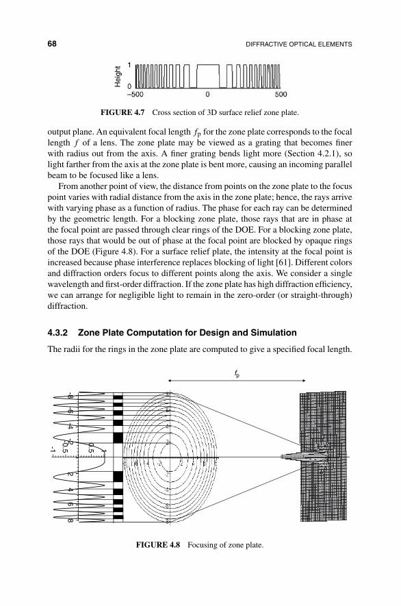
68 DIFFRACTIVE OPTICAL ELEMENTS
FIGURE 4.7 Cross section of 3D surface relief zone plate.
output plane. An equivalent focal length fp for the zone plate corresponds to the focallength f of a lens. The zone plate may be viewed as a grating that becomes finerwith radius out from the axis. A finer grating bends light more (Section 4.2.1), solight farther from the axis at the zone plate is bent more, causing an incoming parallelbeam to be focused like a lens.
From another point of view, the distance from points on the zone plate to the focuspoint varies with radial distance from the axis in the zone plate; hence, the rays arrivewith varying phase as a function of radius. The phase for each ray can be determinedby the geometric length. For a blocking zone plate, those rays that are in phase atthe focal point are passed through clear rings of the DOE. For a blocking zone plate,those rays that would be out of phase at the focal point are blocked by opaque ringsof the DOE (Figure 4.8). For a surface relief plate, the intensity at the focal point isincreased because phase interference replaces blocking of light [61]. Different colorsand diffraction orders focus to different points along the axis. We consider a singlewavelength and first-order diffraction. If the zone plate has high diffraction efficiency,we can arrange for negligible light to remain in the zero-order (or straight-through)diffraction.
4.3.2 Zone Plate Computation for Design and Simulation
The radii for the rings in the zone plate are computed to give a specified focal length.
-8-4
-2
1
0.5
-0.5
fp
-1
24
68
-6
FIGURE 4.8 Focusing of zone plate.
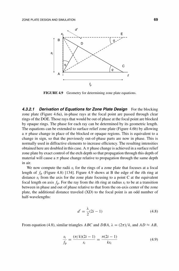
ZONE PLATE DESIGN AND SIMULATION 69
q
q
q
A
BD
C
fp
d ′
si
z
x E
FIGURE 4.9 Geometry for determining zone plate equations.
4.3.2.1 Derivation of Equations for Zone Plate Design For the blockingzone plate (Figure 4.6a), in-phase rays at the focal point are passed through clearrings of the DOE. Those rays that would be out of phase at the focal point are blockedby opaque rings. The phase for each ray can be determined by its geometric length.The equations can be extended to surface relief zone plate (Figure 4.6b) by allowinga π phase change in place of the blocked or opaque regions. This is equivalent to achange in sign, so that the previously out-of-phase parts are now in phase. This isnormally used in diffractive elements to increase efficiency. The resulting intensitiesobtained here are doubled in this case. A π phase change is achieved in a surface reliefzone plate by exact control of the etch depth so that propagation through this depth ofmaterial will cause a π phase change relative to propagation through the same depthin air.
We now compute the radii si for the rings of a zone plate that focuses at a focallength of fp (Figure 4.8) [134]. Figure 4.9 shows at B the edge of the ith ring atdistance si from the axis for the zone plate focusing to a point C at the equivalentfocal length on axis fp. For the ray from the ith ring at radius si to be at a transitionbetween in phase and out of phase relative to that from the on-axis center of the zoneplate, the additional distance traveled (XD) to the focal point is an odd number ofhalf-wavelengths:
d′ = λ
2(2i − 1) (4.8)
From equation (4.8), similar triangles ABC and DBA, λ = (2π)/k, and AD ≈ AB,
si
fp= (π/k)(2i − 1)
si= π(2i − 1)
ksi(4.9)

70 DIFFRACTIVE OPTICAL ELEMENTS
We select an equivalent focal length for the zone plate and define a parameter
σ2 = fp/k (4.10)
Substituting fp from equation (4.10) into equation (4.9),
s2i
σ2 = π(2i − 1) (4.11)
Therefore, opaque rings can be placed at intervals s2i ≤ ρ ≤ s2i+1, where the radiusis ρ, s0 = 0, and integers i > 0:
si = σ√
π(2i − 1) (4.12)
The opaque rings are marked black on the cross section at the left-hand side of Fig-ure 4.8. Because the zeros of U[cos{ρ2/(2σ2)}] occur when ρ = si in equation (4.12),the transmission function for the zone plate may be written as
T (ρ) = U
[cos
(ρ2
2σ2
)], U(x) =
{1 for x ≥ 0
0 for x < 0(4.13)
Equation (4.13) is used to compute the cross section for the zone plate.
4.3.2.2 Derivation of Equations for Transverse Field at Focal Plane To findthe intensity of the field at the output plane, we use scalar diffraction theory (Sec-tion 3.3). Fresnel diffraction can be written from equation (3.45) as
g(x0, y0, z0) = − j
λz0ejkz0
∫y
∫x
f (x, y) exp
{j
k
2z0
[(x − x0)2 + (y − y0)2
]}dx dy
(4.14)
For circular symmetry ρ =√
x2 + y2, equation (4.14) can be written using aFourier–Bessel transform [49, 134] as
g(ρ0, z0) = −j2π
λz0ejkr0
∫ b
0ρf (ρ) exp
{jkρ2
2z0
}J0
(kρρ0
z0
)dρ (4.15)
where r0 = z0 + (x20 + y2
0)/(2z0) and J0 is a Bessel function of first kind and zeroth
order.Inserting the zone plate design equations (4.13) and (4.10) into equation (4.15) in
place of f (ρ), B is the amplitude of the incoming wave, and by changing variables

ZONE PLATE DESIGN AND SIMULATION 71
using w = kρ2/(2z0) (dω = (kρ)/(z0)dρ) or ρ2 = (2z0ω)/k, we obtain [134]
g(ρ0, z0) = B
∫ kb2/(2z0)
0ejwU
[cos
(wz0
f
)]J0
[ρ0
(2kw
z0
)1/2]
dw (4.16)
where the phase term −jejkr0 is neglected. From equation (4.16), for the zone platewith n rings and transparent ring locations (left-hand side of Figure 4.8),
g(ρ0, z0) (4.17)
= B
∫ π/2
0ejwJ0
[ρ0
(2kw
z0
)1/2]
dw
+ B
∫ 5π/2
3π/2ejwJ0
[ρ0
(2kw
z0
)1/2]
d w + · · ·
+ B
∫ π(n−1/2)
π(n−3/2)ejwJ0
[ρ0
(2kw
z0
)1/2]
dw (4.18)
4.3.2.3 Performance of Zone Plate On the z axis, ρ0 = 0, and as J0 = 1, thefield at the focal point of the zone plate for n rings is from equation (4.18)
g(ρ0, z0) = B[[1 + j] + [1 + 1] + · · · + [1 + 1]
] = B[n + j]
Equation (4.18) shows that incoming light is focused to a higher intensity at the focalpoint.
The solid line in Figure 4.10 shows the normalized output intensity at the backfocal plane for the zone plate illuminated with collimated coherent light. Note that
0.8
0.6
0.4
0.2
0
10 20 30 40
Lens
Zone plate
Radius
Abs
olut
e am
plitu
de
50 60
FIGURE 4.10 Comparison of profile at focal plane with a lens.

72 DIFFRACTIVE OPTICAL ELEMENTS
the zone plate will divert light into many higher orders because it is binary. Therefore,there are other higher order focus points at greater distances than the first order. Lightin negative orders is spread around a circle and not focused at a point, so its peakintensity is significantly less than that at the focal point of a lens.
The field across the focal plane, z0 = f , for a lens can be obtained from equa-tion (4.15) by allowing the lens function to cancel the first exponent in the in-tegral and setting f (ρ) = 1. By changing variables to ρ′ = kρρ0/z0 and using∫ x
0 ρ′J0(ρ′)dρ′ = xJ1(x), this can be written as
g(ρ0, z0) = −j2π
λfejkr0b
J1(bkρ0/f )
kρ0/f(4.19)
As J1(bkρ0/fp) = 0, when bkρ0/fp = 1.22π, the distance 2ρs across the main lobe,or the spot size, is
2ρs = 2.44λf
2b(4.20)
We consider the surface relief zone plate. If the opaque blocking regions are re-placed by the material of the zone plate with additional height or depth such that180◦ (π) phase shift occurs in these regions, then we add the same intensity again forthese regions. The intensity at the peak for the surface relief zone plate is thereforetwice that for the blocking zone plate. The intensity of the spot at the focal lengthwill decrease if the etch depth deviates from that computed for 180◦ phase shift.Figure 4.11 shows the computed profile, rescaled, at the focal plane for a surfacerelief zone plate: This represents a significant improvement over the blocking zoneplate shown previously because the side lobes fall off faster.
16
14
12
10
8
6
4
100 20 30 40
Radius
Abs
olut
e am
plitu
de
50 60
FIGURE 4.11 Computed profile at the focal plane for a surface relief zone plate.
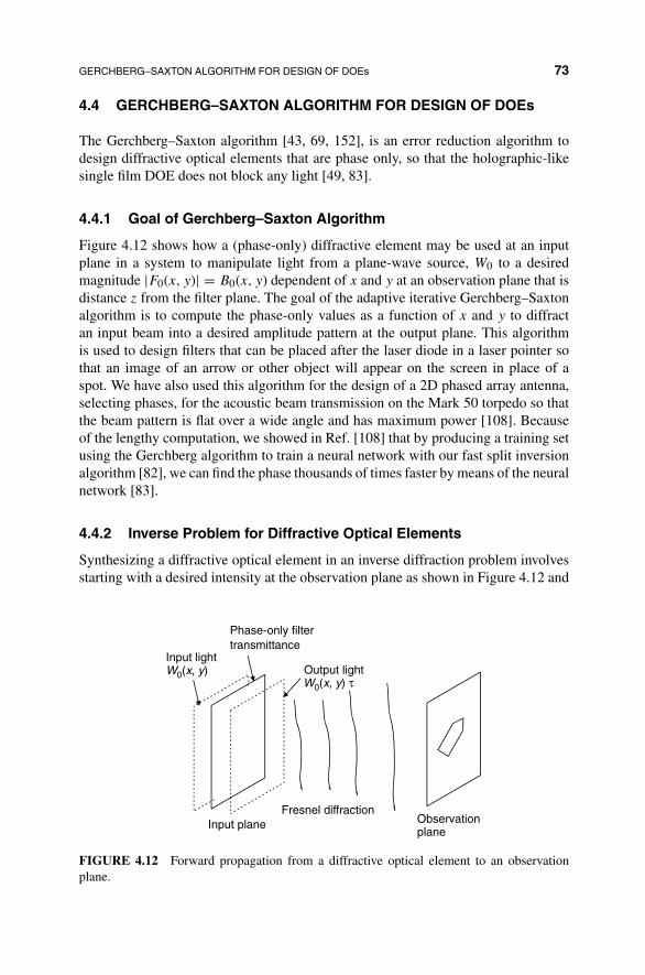
GERCHBERG–SAXTON ALGORITHM FOR DESIGN OF DOEs 73
4.4 GERCHBERG–SAXTON ALGORITHM FOR DESIGN OF DOEs
The Gerchberg–Saxton algorithm [43, 69, 152], is an error reduction algorithm todesign diffractive optical elements that are phase only, so that the holographic-likesingle film DOE does not block any light [49, 83].
4.4.1 Goal of Gerchberg–Saxton Algorithm
Figure 4.12 shows how a (phase-only) diffractive element may be used at an inputplane in a system to manipulate light from a plane-wave source, W0 to a desiredmagnitude |F0(x, y)| = B0(x, y) dependent of x and y at an observation plane that isdistance z from the filter plane. The goal of the adaptive iterative Gerchberg–Saxtonalgorithm is to compute the phase-only values as a function of x and y to diffractan input beam into a desired amplitude pattern at the output plane. This algorithmis used to design filters that can be placed after the laser diode in a laser pointer sothat an image of an arrow or other object will appear on the screen in place of aspot. We have also used this algorithm for the design of a 2D phased array antenna,selecting phases, for the acoustic beam transmission on the Mark 50 torpedo so thatthe beam pattern is flat over a wide angle and has maximum power [108]. Becauseof the lengthy computation, we showed in Ref. [108] that by producing a training setusing the Gerchberg algorithm to train a neural network with our fast split inversionalgorithm [82], we can find the phase thousands of times faster by means of the neuralnetwork [83].
4.4.2 Inverse Problem for Diffractive Optical Elements
Synthesizing a diffractive optical element in an inverse diffraction problem involvesstarting with a desired intensity at the observation plane as shown in Figure 4.12 and
Input plane Observationplane
Phase-only filtertransmittance
Input lightW (x, y)0 Output light
W (x, y) τ0
Fresnel diffraction
FIGURE 4.12 Forward propagation from a diffractive optical element to an observationplane.

74 DIFFRACTIVE OPTICAL ELEMENTS
iteratively update the phases for the phase-only filter at the input plane. Mathemat-ically, this involves solving the inverse nonlinear Fresnel diffraction integral equa-tion (4.21) or Fraunhofer equation, in which nonlinearity is due to taking the modulus.That is, we solve for the phase-only input U(x1, y1) = exp{jφk}, given the output|F0(x, y)|.
Note that because of the different nature of the nonlinearity here, this problemdiffers from the frequently arising conventional image processing problem of recon-structing an image from a distorted one in which a linear convolution-type problemwith additive noise must be solved.
Furthermore, because phase wraps around at 2π, there is significant ambiguity inthe solution process. We did not consider phase unwrapping [46] because iterativealgorithms converge to local minima and uniqueness of solution is not required. Atypical goal for minimization is the root mean square (RMS) deviation of the modulusof the output from the desired output.
4.4.3 Gerchberg–Saxton Algorithm for Forward Computation
For the Fresnel forward computation (Figure 4.12), from the Fresnel diffraction equa-tion (4.21), the magnitude of the output field |F (x0, y0)| involves the magnitude ofthe convolution between the input field U(x1, y1) and the Fresnel diffraction impulseresponse h(x, y) = ((jk)/(2z))
[(x0 − x1)2 + (y0 − y1)2
]:
|F (x0, y0)| =∣∣∣∣ 1
jλz
∫ ∫ ∞
−∞U(x1, y1)
jk
2z
[(x0 − x1)2 + (y0 − y1)2
]dx1 dy1
∣∣∣∣(4.21)
The observed intensity is |F (x0, y0|2.We write the filter phase-only transmittance function as τ = exp{iφ(x, y)} and the
input light field as W0. The field after the input light has passed through the filter isthen U(x1, y1) = W0τ = W0 exp{iφ0(x, y)}. Hence, the initial field at the input planeat the top left in Figure 4.13 is W0 exp{iφ0(x, y)}.
From equation (4.21), the expression for modulus of the output field at the obser-vation plane can be written as
|F (x0, y0|=
∣∣∣∣∫ ∫ ∞
−∞W0 exp{iφ0(x, y)} jk
2z
[(x0 − x1)2 + (y0 − y1)2
]∣∣∣∣ dx1 dy1
(4.22)
4.4.4 Gerchberg–Saxton Inverse Algorithm for Designing aPhase-Only Filter or DOE
Designing a diffractive optical element involves finding φ(x, y) from equation (4.22)when the desired intensity of the observation plane image is defined as I(y0, y0) =|F (x0, y0)|2.

GERCHBERG–SAXTON ALGORITHM FOR DESIGN OF DOEs 75
FIGURE 4.13 Diagram of Gerchberg–Saxton algorithm for DOE design.
The Gerchberg–Saxton algorithm uses an iterative successive approximation algo-rithm for solving this nonlinear integral equation, nonlinear because of the modulussign in equation (4.22). First, we note that in practice the distance from input plane toobservation plane is large compared to the transverse dimensions at the wavelengthof interest. Therefore, as is known from diffraction theory [49], for large distanceswe can use the Fraunhofer approximation (Section 3.3.5), which allows us to use asingle Fourier transform in place of the convolution with the Fresnel approximation(Section 3.3.4). The fast Fourier transform (FFT) is used to speed up the computa-tion [133]. Figure 4.13 shows a diagram of the algorithm.
Prepare the initial input to start the iterative algorithm by choosing an initial phaseφ0 (can be random) and compute W0 exp{iφ0(x, y)} for iteration k = 0. Steps for thekth repeated loop are as follows:
1. Transform Wk exp{iφk(x, y)} with an FFT to obtain Fk(x0, y0).
2. Compute the error function εk, the mean square error between the desiredoutput B(x0, y0) (which is real) and the amplitude of the output obtained at thisiteration |Fk(x0, y0)|,
εk =∫ ∫ ∞
−∞
[|Fk(x0, y0)| − B(x0, y0)]2 dx0 dy0 (4.23)
Check if error function is sufficiently small to stop the iterations. Otherwise,repeat the loop.
3. Remove the magnitude of Fk(x0, y0) by computing Fk(x0, y0)|Fk(x0, y0)|−1
and replace the magnitude with that for the desired function, B(x0, y0), that is,

76 DIFFRACTIVE OPTICAL ELEMENTS
compute
Fgk(x0, y0) = B(x0, y0)Fk(x0, y0)|Fk(x0, y0)|−1 (4.24)
4. Inverse Fourier transform Fgk(x0, y0) to get Wk(x0, y0).
5. Remove the magnitude of Wk(x0, y0) by computing Wk(x0, y0)|Wk(x0, y0)|−1
and replace the magnitude with that for the amplitude of the input wave, W0,that is, compute
Wgk(x0, y0) = W0Wk(x0, y0)|Wk(x0, y0)|−1 (4.25)

CHAPTER 5
PROPAGATION AND COMPENSATIONFOR ATMOSPHERIC TURBULENCE
Motion of air in the atmosphere is represented by active random fluctuations in velocityV (x, y, z). The random velocity fluctuations are accompanied by random variationsin temperature (x, y, z). Expansion and contraction of air with temperature causes thedensity of the air to vary randomly, leading to passive random variations in refractiveindex n(x, y, z). Here, passive means that variations in refractive index n do notchange the velocity of the air. Fluctuating changes in refractive index bend a beam oflight randomly as it propagates through the atmosphere. Therefore, the beam wandersaround and spreads out more than that for diffraction alone. When considering theeffects of index of refraction on light beams, we refer to the atmospheric turbulenceas optic turbulence.
There are two distinct situations of interest to the military: the effect on a coherentlaser beam and the effect on incoherent imaging. The effect of turbulence on imagingis observable by the shimmering of a scene viewed across a tarmac parking lot that hasbeen in the sun all day or by observing the twinkle of a star due to turbulence splittingthe light into one or more paths that interfere, first explained by Isaac Newton. We willfocus on the effects of spatially varying refractive index n(x, y, z) due to turbulenceon propagating laser beams. The resulting beams can be described by random fieldsU(x, y, z) (or possibly U(x, y, z, ct)). Random fields vary in space and are the spaceequivalent of random processes [135], which vary only in time. Stochastic is often
Military Laser Technology for Defense: Technology for Revolutionizing 21st Century Warfare,First Edition. By Alastair D. McAulay.© 2011 John Wiley & Sons, Inc. Published 2011 by John Wiley & Sons, Inc.
77
78 PROPAGATION AND COMPENSATION FOR ATMOSPHERIC TURBULENCE
used in place of random. Note that random fields are more complex than randomprocesses because space has three dimensions while time has only one.
In Section 5.1, we review the locally homogeneous random field structure functionand its power spectrum, following Ref. [4]. Those not needing to follow the detailedequations can skip this section. In Section 5.2, we describe optical turbulence: turbu-lence of refractive index that influences optical beams. Kolmogorov’s cascade theoryprovides physical insight. Those not needing to follow detailed equations can skipover to Section 5.2.2 and equation (5.32). In Section 5.3, we describe adaptive opticsdevices and systems for cleaning up power beams and for compensating for opticalturbulence, used in the airborne laser (Section 12.2) and homing missile protection(Section 12.3.3). In Section 5.4, we describe computational methods for modelingturbulence and our research on computation of phase screens widely used for lay-ers of a layered model. Such phase screens are used in the airborne laser testbed(Section 12.2.7.2). In particular, we studied and wrote the first paper that comparedtwo approaches, frequency and spatial, in modeling turbulence for phase screens [90].The first method takes a spatial Fourier transform (FT) of the Kolmogorov spec-trum [88] and the second one computes a covariance matrix from the Kolmogorovturbulence structure function. Both methods were shown to satisfy Kolmogorov’sspectrum, but they handle problems of uncertain large atmospheric eddies differentlyand have different capabilities for modeling wind.
5.1 STATISTICS INVOLVED
Owing to random fluctuations of refractive index in space, whenever a pulse of lightfrom a laser propagates through the atmosphere, it takes a slightly different physicalpath. The collection, called ensemble, of different paths in space composes a continu-ous random field [4]. Each path is considered to be a realization of the random field inspace. A random field for which realizations are in space contrasts a random processfor which realizations are in time. Because of randomness, the path for a realizationis unpredictable, so we use averages or expected values that we label with 〈a 〉 (insome texts E{} is used). For tractability, we initially focus on first- and second-orderstatistics: the mean and autocovariance. The mean for a random field m(R) is theensemble average at a point in space identified by its vector location R(x, y, z) overall realizations or paths:
m(R) = 〈u(R)〉 (5.1)
The spatial autocovariance function (second-order statistic) provides the expectedrelationship between the fields at two different locations R1 and R2:
Bu(R1, R2) = 〈[u(R1) − m(R1)][u∗(R2) − m∗(R2)]〉 (5.2)
When the mean is zero, m(R) = 0, Bu reduces to the autocorrelation function, aspecial case of the autocovariance function.

STATISTICS INVOLVED 79
If Bu does not depend on the absolute value of R(x, y, z) but only on the differenceR = R2 − R1 or R2 = R1 + R, we have a statistically homogeneous field in space.(This is the equivalent of a wide sense stationary process in random processes.)
Bu(R1, R2) = Bu(R1 − R2) = 〈u(R1)u∗(R1 + R)〉 − |m|2 (5.3)
Often fields are invariant under rotation or statistically isotropic: independent of di-rection of R, R = |R2 − R1|. This allows us to reduce the 3D vector location to a1D scalar, the distance R from the axis of a beam. Then,
Bu(R1, R2) = Bu(R) (5.4)
5.1.1 Ergodicity
In practice, when we shine a laser beam through the atmosphere, we have only asingle realization. Statistics for this one beam are easier to compute than those for anensemble of beams. For example, a 3D space average is
Bu(R) = limx→∞
1
L
∫ L
0u(R)dR (5.5)
where L is the path length. This is the 3D space equivalent of a time average in arandom process.
Similarly, for the space average for autocovariance,
Bu(R1, R2) = limx→∞
1
L
∫ L
0[u(R1) − m(R1)][u∗(R2) − m∗(R2)]dR (5.6)
Often we assume that the random field is ergodic, which means that the ensembleaverage at a point in space for a specific realization or path can be replaced by thespace average for a single path. Ergodicity is difficult to prove except for simple cases,but for optical turbulence most of the time, ergodicity turns out to be a reasonableassumption. For an ergodic random field, the space average u(R) is the same as theensemble average 〈u(R)〉:
u(R) = 〈u(R)〉 (5.7)
and the space average of autocovariance Bu(R1, R2) is the same as the ensembleaverage for the autocovariance 〈Bu(R1, R2)〉:
Bu(R1, R2) = 〈Bu(R1, R2)〉 (5.8)
Note that the space average for one realization is easier to measure than the ensembleaverage.
80 PROPAGATION AND COMPENSATION FOR ATMOSPHERIC TURBULENCE
5.1.2 Locally Homogeneous Random Field Structure Function
In practice, for atmospheric turbulence, the mean is not constant over all space: ve-locity, temperature, and refractive index vary because the wind blows harder in someplaces. However, the mean is constant in a local region. We write
u(R) = m(R) + u1(R) (5.9)
where m(R) is the local mean that depends on R and u1(R) represents the randomfluctuations about the mean. Locally homogeneous random fields are characterized bystructure functions [4]. Such behavior frequently arises in random processes where itis labeled a random process with stationary increments [135], for example, a Poissonrandom process. Stationary may be qualified by wide sense when only autocovarianceand mean are involved.
The structure function that characterizes locally homogeneous atmospheric turbu-lence is written as [4]
Du(R1, R2) = Du(R) = 〈[u1(R1) − u1(R1 + R)]2〉 (5.10)
where we set u(R1) ≈ u1(R1). Expanding equation (5.10) for a locally homogeneousrandom field gives
Du(R) = 〈u1(R1)u∗1(R1)〉 + 〈u1(R1 + R)u∗
1(R1 + R)〉− 2〈u1(R1 + R)u1(R1)〉 (5.11)
If the random field is also isotropic, R = |R|, Du(R) is related to Bu(R)
Du(R) = 2[Bu(0) − Bu(R)] (5.12)
5.1.3 Spatial Power Spectrum of Structure Function
For high-frequency microwaves and optics, we often measure power because sen-sors may not be fast enough to record phase information. Furthermore, for randomprocesses or fields, the phase may be of no consequence. Also, extracting signalsfrom noise is often accomplished by spectral filtering to remove noise frequencies.So we need to compute the power spectrum �u(κ) from the structure function Du(R)for locally homogeneous isotropic fields. Relation between a space function and itsspectrum is usually defined using Fourier transforms (Section 3.1.2). This requiresthat the space function be absolutely integrable [133]:
∫ ∞
−∞u(R)d(R) < ∞ (5.13)
STATISTICS INVOLVED 81
Unfortunately, equation (5.13) is not valid for a random field or process. The Fourier–Stieltjes (or Riemann–Stieltjes) transform solves this problem [4, 135] and producesthe well-known Wiener–Khintchine theorem.
For wide sense (mean and covariance) stationary random processes (in time), theautocovariance Bx(τ) and the power spectral density (or power spectrum) Sx(ω) area Fourier transform pair:
Sx(ω) = 1
2π
∫ ∞
−∞Bx(τ) exp{−iωτ}dτ = 1
π
∫ ∞
0Bx(τ) cos(ωτ)dτ
Bx(τ) =∫ ∞
−∞Sx(ω) exp{iωτ}dω = 2
∫ ∞
0Sx(ω) cos(ωτ)dω (5.14)
where the cosine equations arise in the second equalities because power and autoco-variance are real and even.
In space, for statistically homogeneous isotropic random fields, from equa-tions (5.14), the autocovariance Bu(R) and 1D spatial power spectrum Vu(κ) aresimilarly related by
Vu(κ) = 1
2π
∫ ∞
−∞Bu(R) exp{−iκR}dR = 1
π
∫ ∞
0Bu(R) cos(κR)dR
Bu(R) =∫ ∞
−∞Vu(κ) exp{iκR}dκ = 2
∫ ∞
0Vu(κ) cos(κR)dκ (5.15)
where κ is the spatial angular frequency, κ = 2πfs (space equivalent to ω = 2πf ).We now find the relationship between the 1D spatial power spectrum Vu in equa-
tion (5.15) and the spatial power spectrum for a 3D statistically homogeneous isotropicmedium (for which radius R = |R2 − R1|). Note that these are not the same. For astatistically homogeneous medium (not isotropic), the 3D autocovariance Bu(R) andthe 3D spatial power spectral density are related by the Wiener–Khintchine theorem:
�u(κ) =(
1
2π
)3 ∫∫∫ ∞
−∞exp{−iκ · R}Bu(R)d3R
Bu(R) =∫∫∫ ∞
−∞exp{iκ · R}�u(κ)d3κ (5.16)
If the medium is also isotropic, we set R = |R2 − R1| and κ = |κ| in equations (5.16)to get [4]
�u(κ) = 1
2π2κ
∫ ∞
0Bu(R) sin(κR)R dR
Bu(R) = 4π
R
∫ ∞
0�u(κ) sin(κR)κ dκ (5.17)
82 PROPAGATION AND COMPENSATION FOR ATMOSPHERIC TURBULENCE
Therefore, the 3D spatial power spectrum for a locally statistically homogeneousisotropic medium,�u(κ) in equation (5.17), is related to the 1D spatial power spectrumfor a locally statistically homogeneous medium, Vu(κ) in equation (5.15), by
�u(κ) = − 1
2πκ
dVu(κ)
dκ(5.18)
From equation (5.18), we see the origin of the −11/3 power rule that arises inmodels of turbulence: If 1D spectrum Vu ∝ κ−5/3, then the 3D spectrum �u ∝−(5/3)V−8/3/κ = −(5/3)V−11/3. Note that �u(κ) in equation (5.17) has a singu-larity at κ = 0, so the convergence of Bu(R) in equation (5.17) require restrictions inthe rate of increase of �u(κ) as κ → 0 [4].
In practice, we allow a beam to propagate from one plane to another at separationz so that we need the 2D spatial power spectrum Fu(κx, κy, 0, z) between two planesz apart [4]:
Fu(κx, κy, 0, z) =∫ ∞
−∞�u(κx, κy, κz) cos(κzz)dκz
�u(κx, κy, κz) = 1
2π
∫ ∞
−∞Fu(κx, κy, 0, z) cos(κzz)dκz (5.19)
The structure function for a 3D locally homogeneous random field, Du(R), equa-tion (5.11), is related to its 3D spatial power spectrum �u(κ), equation (5.16), by[4, 60, 155]
Du(R) = 2∫∫ ∞
−∞�u(κ)[1 − cos(κ · R)]d3κ (5.20)
If the field is also isotropic, we have the Wiener–Khintchine equation pair
�u(κ) = 1
4π2κ2
∫ ∞
0
sin(κR)
κR
d
dR
[R2 d
dRDu(R)
]dR
Du(R) = 8π
∫ ∞
0κ2�u(κ)
(1 − sin(κR)
κR
)dκ (5.21)
We note that some approaches to optical turbulence use the spatial power spectrumand some the structure function. We compare the two approaches in Refs. [88, 90].
5.2 OPTICAL TURBULENCE IN THE ATMOSPHERE
Turbulence in the atmosphere, or elsewhere, is considered to be due to statisticalvariations in velocity flow in a medium. The active variations in velocity cause pressureand temperature variations. Air expansion and contraction with temperature producespassive refractive index fluctuations: passive means these do not affect velocity. In a
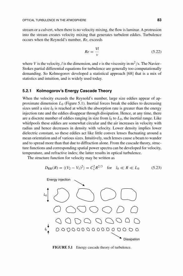
OPTICAL TURBULENCE IN THE ATMOSPHERE 83
stream or a culvert, when there is no velocity mixing, the flow is laminar. A protrusioninto the stream creates velocity mixing that generates turbulent eddies. Turbulenceoccurs when the Reynold’s number, Re, exceeds
Re = Vl
ν(5.22)
where V is the velocity, l is the dimension, and ν is the viscosity in m2/s. The Navier–Stokes partial differential equations for turbulence are generally too computationallydemanding. So Kolmogorov developed a statistical approach [68] that is a mix ofstatistics and intuition, and is widely used today.
5.2.1 Kolmogorov’s Energy Cascade Theory
When the velocity exceeds the Reynold’s number, large size eddies appear of ap-proximate dimension L0 (Figure 5.1). Inertial forces break the eddies to decreasingsizes until a size l0 is reached at which the absorption rate is greater than the energyinjection rate and the eddies disappear through dissipation. Hence, at any time, thereare a discrete number of eddies ranging in size from l0 to L0, the inertial range. Likewhirlpools these eddies are somewhat circular and the air increases in velocity withradius and hence decreases in density with velocity. Lower density implies lowerdielectric constant, so these eddies act like little convex lenses fluctuating around amean orientation and of various sizes. Intuitively, such lenses cause a beam to wanderand to spread more than that due to diffraction alone. From the cascade theory, struc-ture functions and corresponding spatial power spectra can be developed for velocity,temperature, and refractive index; the latter results in optical turbulence.
The structure function for velocity may be written as
DRR(R) = 〈(V2 − V1)2〉 = C2vR
2/3 for l0 R L0 (5.23)
L0
l0
Energy injection
Dissipation
FIGURE 5.1 Energy cascade theory of turbulence.
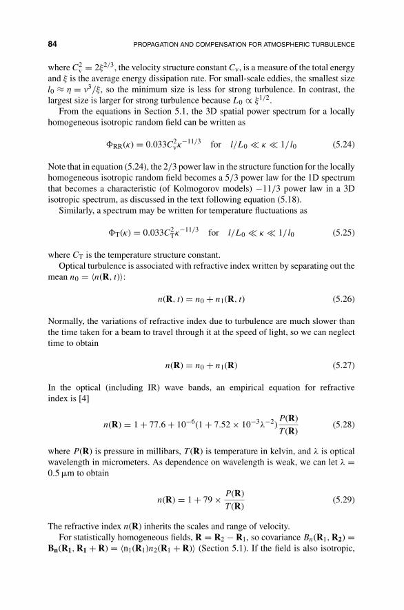
84 PROPAGATION AND COMPENSATION FOR ATMOSPHERIC TURBULENCE
where C2v = 2ξ2/3, the velocity structure constant Cv, is a measure of the total energy
and ξ is the average energy dissipation rate. For small-scale eddies, the smallest sizel0 ≈ η = ν3/ξ, so the minimum size is less for strong turbulence. In contrast, thelargest size is larger for strong turbulence because L0 ∝ ξ1/2.
From the equations in Section 5.1, the 3D spatial power spectrum for a locallyhomogeneous isotropic random field can be written as
�RR(κ) = 0.033C2vκ
−11/3 for l/L0 κ 1/l0 (5.24)
Note that in equation (5.24), the 2/3 power law in the structure function for the locallyhomogeneous isotropic random field becomes a 5/3 power law for the 1D spectrumthat becomes a characteristic (of Kolmogorov models) −11/3 power law in a 3Disotropic spectrum, as discussed in the text following equation (5.18).
Similarly, a spectrum may be written for temperature fluctuations as
�T(κ) = 0.033C2Tκ−11/3 for l/L0 κ 1/l0 (5.25)
where CT is the temperature structure constant.Optical turbulence is associated with refractive index written by separating out the
mean n0 = 〈n(R, t)〉:
n(R, t) = n0 + n1(R, t) (5.26)
Normally, the variations of refractive index due to turbulence are much slower thanthe time taken for a beam to travel through it at the speed of light, so we can neglecttime to obtain
n(R) = n0 + n1(R) (5.27)
In the optical (including IR) wave bands, an empirical equation for refractiveindex is [4]
n(R) = 1 + 77.6 + 10−6(1 + 7.52 × 10⁻³λ−2)P(R)
T (R)(5.28)
where P(R) is pressure in millibars, T (R) is temperature in kelvin, and λ is opticalwavelength in micrometers. As dependence on wavelength is weak, we can let λ =0.5 �m to obtain
n(R) = 1 + 79 × P(R)
T (R)(5.29)
The refractive index n(R) inherits the scales and range of velocity.For statistically homogeneous fields, R = R2 − R1, so covariance Bn(R1, R2) =
Bn(R1, R1 + R) = 〈n1(R1)n2(R1 + R)〉 (Section 5.1). If the field is also isotropic,
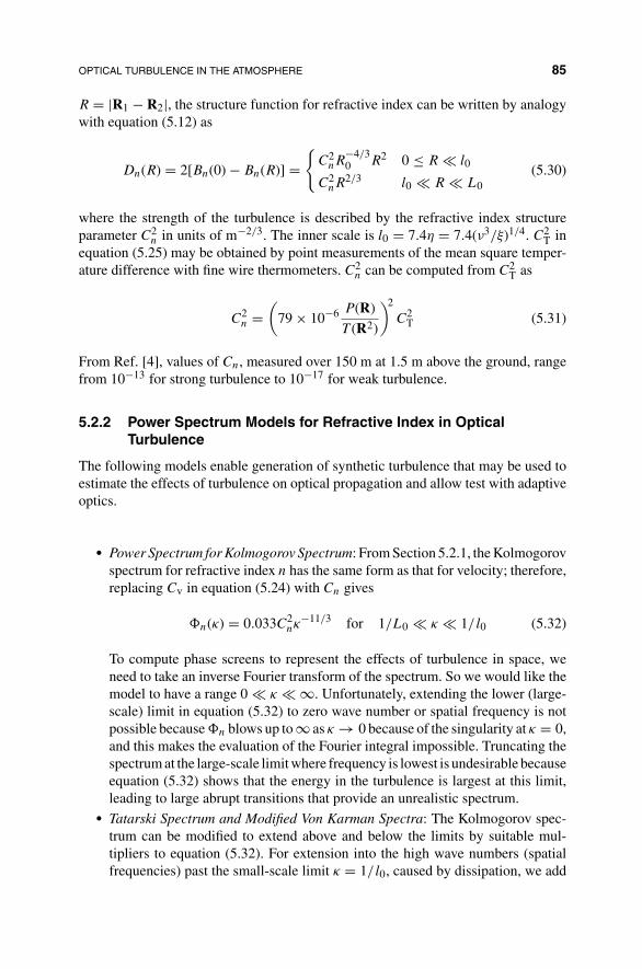
OPTICAL TURBULENCE IN THE ATMOSPHERE 85
R = |R1 − R2|, the structure function for refractive index can be written by analogywith equation (5.12) as
Dn(R) = 2[Bn(0) − Bn(R)] ={
C2nR
−4/30 R2 0 ≤ R l0
C2nR
2/3 l0 R L0(5.30)
where the strength of the turbulence is described by the refractive index structureparameter C2
n in units of m−2/3. The inner scale is l0 = 7.4η = 7.4(ν3/ξ)1/4. C2T in
equation (5.25) may be obtained by point measurements of the mean square temper-ature difference with fine wire thermometers. C2
n can be computed from C2T as
C2n =
(79 × 10−6 P(R)
T (R2)
)2
C2T (5.31)
From Ref. [4], values of Cn, measured over 150 m at 1.5 m above the ground, rangefrom 10−13 for strong turbulence to 10−17 for weak turbulence.
5.2.2 Power Spectrum Models for Refractive Index in OpticalTurbulence
The following models enable generation of synthetic turbulence that may be used toestimate the effects of turbulence on optical propagation and allow test with adaptiveoptics.
• Power Spectrum for Kolmogorov Spectrum: From Section 5.2.1, the Kolmogorovspectrum for refractive index n has the same form as that for velocity; therefore,replacing Cv in equation (5.24) with Cn gives
�n(κ) = 0.033C2nκ
−11/3 for 1/L0 κ 1/l0 (5.32)
To compute phase screens to represent the effects of turbulence in space, weneed to take an inverse Fourier transform of the spectrum. So we would like themodel to have a range 0 κ ∞. Unfortunately, extending the lower (large-scale) limit in equation (5.32) to zero wave number or spatial frequency is notpossible because �n blows up to ∞ as κ → 0 because of the singularity at κ = 0,and this makes the evaluation of the Fourier integral impossible. Truncating thespectrum at the large-scale limit where frequency is lowest is undesirable becauseequation (5.32) shows that the energy in the turbulence is largest at this limit,leading to large abrupt transitions that provide an unrealistic spectrum.
• Tatarski Spectrum and Modified Von Karman Spectra: The Kolmogorov spec-trum can be modified to extend above and below the limits by suitable mul-tipliers to equation (5.32). For extension into the high wave numbers (spatialfrequencies) past the small-scale limit κ = 1/l0, caused by dissipation, we add

86 PROPAGATION AND COMPENSATION FOR ATMOSPHERIC TURBULENCE
a Gaussian exponential proposed by Tatarski [155]. For extending into the lowerwave number (low spatial frequency) past the large-scale limit κ = 1/L0, we di-vide by a factor (κ2 + κ2
0), where κ0 = C0/L0 with C0 = 2π, 4π, or 8π depend-ing on the application [4]. The reason for the variety in selecting C0 is that abovethe large-scale limit L0, the field is no longer statistically homogeneous—theeddies may be distorted by atmospheric striations—so approximation is mainlyto make the equations more tractable. The resulting modified Von Karman spec-trum is
�n(κ) = 0.033C2n
(κ2 + κ20)11/6
exp
{−κ2
κ2m
}for κm = 5.92/l0, κ0 = 2π/L0
(5.33)
5.2.3 Atmospheric Temporal Statistics
When wind blows across the path of a laser beam in the atmosphere, the turbulencewill move at wind speed V⊥ across the beam. Because the eddy pattern takes manyseconds to change, the motion of noticeable wind L0/V⊥ is much faster. This isknown as the frozen turbulence hypothesis and is similar to cloud patterns caused byair turbulence passing across the sky. Therefore, we can convert spatial turbulencedue to eddy currents into temporal turbulence that incorporates the effects of thecomponent of wind at right angles to the path.
u(R, t + τ) = u(R − V⊥τ, t) (5.34)
5.2.4 Long-Distance Turbulence Models
For an optical beam traversing many miles, the strength of turbulence may varyover the path. For example, if a beam moves over the land past cliffs over sea, theturbulence strength will vary because the land and sea have different temperaturesand wind striking the cliff will generate strong turbulence. Such situations may behandled by partitioning the path into regions, each with its own constant turbulence.Further in numerical computations, the effect of turbulence in each region may beequated to a phase screen. Such phase screens were implemented around a sequenceof optical disks for a hybrid test facility for the airborne laser (Section 12.2.7.2).
5.3 ADAPTIVE OPTICS
Adaptive optics may be used to reduce the impact of turbulence and is used in theAirborne Laser program (Section 12.2).
5.3.1 Devices and Systems for Adaptive Optics
There are two principal devices: wave front sensor to measure the shape of the wavefront and deformable mirror to change the wave front.

ADAPTIVE OPTICS 87
A
B
C
D
DetectorarraysWave
front
Lenslet array
FIGURE 5.2 Hartmann wave front sensor.
5.3.1.1 Wave Front Sensor The wave front sensor measures the shape of thewave front [144, 160, 163]. Many approaches are possible. Figure 5.2 illustrates howwave front shape is measured with a popular Hartmann wave front sensor. At A inFigure 5.2, the wave front is tilted up substantially and the small lens will focus thelight into the upper row of the associated sensor array. At B the wave front is tiltedup less, causing light to be focused to the next from top row of the sensor array. Thelower half of the wave front focuses to the lower parts of the sensor array. The datafrom the wave front sensor arrays indicate the local direction in transverse x and y ofthe wave front.
The wave front shape is fed to a computer that calculates the settings for thedeformable mirror to give a desired correction to the wave front. The computationallows the discretization of the wave front sensor and the deformable array.
5.3.1.2 Deformable Mirror Device The deformable mirror consists of a flex-ible mirror supported by an array of pistons that can raise the mirror up locally undercomputer control. Moving the mirror up locally advances the phase of the reflectedlight at this point because the light travels less far than that at neighboring points.
The light emanating from most high-power lasers has poor spatial coherencebecause of nonlinear effects that are significant at high powers (Section 8.1.2).Figure 5.3a shows the distorting effect of a beam of poor spatial coherence. Someparts of the wave front, labeled A, B, C, D, and E, are in the direction of the beam.But other points on the wave front point out of the beam along F, G, H , and J anddegrade the quality of the beam with distance. In a beam cleanup, the wave front isflattened into a plane wave by setting the deformable mirror to the conjugate phaseof the wave front. For example, we can move to the right the mirror element of thedeformable mirror that lines up with the wave front in the direction along the beam atC (Figure 5.3a). This will retard the wave from C, so it has to travel farther than theone from B, which brings waves from B and C into line. Then waves propagating atan angle to the main beam (F, G, H, J) will be eliminated. In practice, adaptive optics

88 PROPAGATION AND COMPENSATION FOR ATMOSPHERIC TURBULENCE
A
B
C
D
E
F
G
H
J
Wave front Deformable mirror(a) (b)
Deformablemirror
Beam splitter
Wave front sensorComputer
Main beam
Cleaned upmain beam
FIGURE 5.3 (a) Poor spatial coherence of a beam and (b) beam cleanup adaptive opticssystem.
will shape the wave front into a desired smooth function in space while improvingbeam spatial coherence.
5.3.1.3 Adaptive Optics Cleanup System Figure 5.3b illustrates the prin-ciples of an adaptive optics beam cleanup system to improve spatial coherence andshape the wave front for a high-power laser. The adaptive optics beam cleanup systemhas an advantage over a spatial filter (Section 1.3.6), which cannot focus a poor qualitybeam (such as the one distorted by turbulence or from very high-power gas lasers)through a pinhole without losing considerable power. The spatial filter is adequatefor cleaning up distortion caused by a Nd:YAG power amplifier (Section 13.2.1). Themain beam to be cleaned up is deflected by a deformable mirror that will be set to per-form the cleanup [83, 163]. The deformable mirror sends some of the reflected wavesto the wave front sensor via a beam splitter so that the computer can determine howto set the deformable mirror to achieve beam cleanup and transform the wave frontto that desired, as specified in the computer. Note that the beam size can be modifiedto operate with deformable mirrors of different sizes. For example, the 1000 × 1000mirror array in the digital light projector (DLP) used in projectors, manufactured byTexas Instruments, is very small because it is a modified memory chip [83, 113]. Theadaptive beam cleanup system (Figure 5.3), is incorporated into the airborne laser(ABL) system in Section 12.2.2.
5.3.1.4 Principles of Adaptive Optics Compensation for TurbulenceThe main beam reflection from a missile cannot be relied on to provide adequateinformation for estimating turbulence. For this reason, a separate beacon laser is usedthat is coincident with the path of the main laser beam. The beacon laser light strikesthe target and, unlike the main beam, is reflected back to the aircraft for the pur-pose of estimating the turbulence (Section 5.2). The beacon laser is a 1.06 �m diodepulsed semiconductor pumped solid-state laser (Section 8.2). Beacon lasers are usedin adaptive optics for many astronomical telescopes. In this case, the beacon laser acts

COMPUTATION OF LASER LIGHT THROUGH ATMOSPHERIC TURBULENCE 89
Deformable mirrorcompensates foratmospheric turbulence
Beam splitterCleaned upmain beam
Wave frontsensor
Computer
Cassegraintelescope
To target - all beams
From target - beacon
Beaconlaser
Dichroicmirror
FIGURE 5.4 Principle of adaptive optics for compensating for turbulence.
like the orange ranging beam that measures distance to set focusing before taking aphotograph in many digital cameras.
The beacon laser is activated to allow compensating corrections to the wave frontwith a deformable mirror, DMturb in Figure 12.4, before shooting a pulse of the mainhigh-power beam. Figure 5.4 shows the principle of using a beacon laser to estimateturbulence and then precompensate the main beam wave front. In Figure 5.4, thebeacon laser light bounces off a dichroic mirror that reflects the Nd:YAG beaconbeam (Section 8.2), at 1.06 �m and passes the COIL laser main beam (Section 8.3.2)at 1.315 �m. The beacon beam now bounces off the deformable mirror before beingfocused onto a spot on the target with a Cassegrain telescope (Section 1.3.4.1). Thereflected beacon light returning from the target, distorted by two-way turbulence,bounces off the deformable and dichroic mirrors to pass through the beam splitter ontothe wave front sensor. A computer iteratively calculates the setting for the deformablemirror to remove the effects of turbulence on the beacon beam. After the deformablemirror for removing turbulence stabilizes, light passing to the target and back againwill be turned into a plane wave with turbulence effects removed. The main weaponbeam, after cleaning up as described in Section 5.3.1.3, emits a powerful pulse thatis merged into the same optical path as the beacon beam on passing through thedichroic mirror. Note that the pulsed beacon and main beams, although following thesame path, occur at different times. The adaptive compensation system for turbulence(Figure 5.4) is incorporated into the ABL system in Section 12.2.3.
5.4 COMPUTATION OF LASER LIGHT THROUGH ATMOSPHERICTURBULENCE
Temperature variations in the air over the earth generate convection currents thatcause turbulence in the velocity of the air. Turbulence results in eddies of varioussizes, typically from a few millimeters to an upper bound corresponding to tens to

90 PROPAGATION AND COMPENSATION FOR ATMOSPHERIC TURBULENCE
FIGURE 5.5 Layered propagation system for modeling propagation of light through turbu-lent atmosphere.
hundreds of meters. The latter corresponds to a low spatial frequency bound. Thesmallest eddy size decreases as the largest eddy size increases [155]. When smalleddy size decreases, more samples in the transverse direction may be needed foraccurate computation. The density variations of the air with velocity cause eddies inthe refractive index that in turn bend and disperse the light. Turbulence affects thespatial and temporal properties of the laser beam and interacts with the diffractionprocess [4, 60, 144, 155].
Design and analysis of laser weapons (Section 12.2), optical communications [87],and optical imaging [144] require accurate simulation for the propagation of lightthrough a turbulent atmosphere. Accurate modeling is required to develop and testadaptive optics systems (Section 5.3.1.4) necessary to compensate for turbulence withlaser beams traveling long distances or near the earth. A substantial testbed facilitywas required for the Airborne Laser program (Section 12.2.7). It would be impossibleto test and optimize such a system without a testbed with modeled turbulence becauseturbulence in the real world is extremely variable because of the variability due toweather conditions.
Computing turbulence with the Navier–Stokes equation is too computationallydemanding, although polynomial models, fitted to Navier–Stokes results, have beenattempted [84]. Therefore, statistical approaches and a layered model of the mediumare typically used (Figure 5.5) [4, 88, 90]. The model developed here is used in theairborne laser testbed for adaptive optics and tracking in Section 12.2.7.
5.4.1 Layered Model of Propagation Through Turbulent Atmosphere
In the layered model (Figure 5.5), the propagation distance is split into layers ofselected length. The atmospheric parameters are assumed to be constant in a layerand can differ between layers. Propagation across a layer is split into that due todiffraction in the absence of turbulence and that due to turbulence in the absence ofdiffraction. The two computations for each layer are performed in sequence. First,

COMPUTATION OF LASER LIGHT THROUGH ATMOSPHERIC TURBULENCE 91
1.5
1
0.5
0
24
68
10Wave number K
y Wave number Kx
1214
16 1614
1210
86
42
FIGURE 5.6 Kolmogorov spectrum in x direction spatial frequency domain.
the light is propagated across a layer. Then, it is propagated through a phase screenthat represents the effects of turbulence in traveling across the layer.
5.4.1.1 Bounds on Spatial Frequency for Kolmogorov Power SpectrumTurbulence Model The Kolmogorov spectrum, as a function of spatial frequencyin a transverse direction, is shown in Figure 5.6, equation (5.32). The Kolmogorovspectrum is specified only between limits specified by the curve shown. It is unspec-ified at spatial frequencies (or wavelengths) below or above this range. The lowestspatial frequencies correspond with the largest eddies determining the size of phasescreen and the highest spatial frequencies correspond with the smallest eddies af-fecting the sampling fineness or resolution. Note that the power in the Kolmogorovspectrum increases with decreasing spatial frequency, so more energy arises at lowspatial frequencies. Therefore, power below this lower bound can have a significantinfluence on the effect of turbulence. Unfortunately, the size of the largest eddies isnot easily determined and is very much influenced by the weather and the application.As the power falls with decreasing eddy size, a lower resolution in space than that atthe limit makes little difference.
5.4.1.2 Application Dependence of Bounds for Kolmogorov SpectrumFor beams interconnecting earth and satellites or high flying aircraft, the largest eddysize can reach a diameter of several hundred meters (Sections 12.2 and 12.2.7). Suchlarge eddies may no longer be stationary for the beam propagation and some of theanalysis may lose its validity.
For horizontal beams close to the earth, as for point to point optical wireless, theradius of the largest eddy size is limited by the distance of the beam from the earth.

92 PROPAGATION AND COMPENSATION FOR ATMOSPHERIC TURBULENCE
A rule of thumb is sometimes used for which the largest eddy is approximately 0.4times the height from the earth’s surface [4]. In this case, there can be an abrupt cutofffor the lower spatial frequencies.
For optical wireless among sky scrapers in a large city, the largest turbulence eddyvaries along the path, depending on the distance between buildings through whichthe beam passes and the height of buildings over which the beam passes. The fansin building air conditioners also generate eddies in the air. In the spectral method, asdiscussed in an earlier study [88], it was shown that an abrupt cutoff at low spatialfrequencies presents a ringing problem in the Fourier transform process.
For laser beams angled up into the sky, the shape of the spatial spectrum is oftennot known and hard to measure because it may change with the weather conditions.However, the more gradual change in the largest eddy size makes the Fourier transformcomputation more accurate.
We next investigate the generation of turbulence phase screens for layers of thelayer model (Figure 5.5) and compare two approaches: the first method is directlyfrom the Kolmogorov spectrum and the second method is from the covariance ofthe structure function. The Kolmogorov approach starts with the Kolmogorov powerspectrum and uses a Fourier transform to convert to a space screen, while the covari-ance approach starts in the space domain with the structure function for turbulenceand computes the covariance. We show that in both methods the phase screens havesimilar appearance and, that on averaging, satisfy the Kolmogorov turbulence spec-trum. However, they handle the limits in large eddies differently. We have limitedourselves to the case for which the phase screens in different layers are independent.In practice, if a wind is blowing approximately along the direction of beam propaga-tion, the phase screens are related to a time delay and sideways velocity. The windeffects can be incorporated into the covariance method.
5.4.2 Generation of Kolmogorov Phase Screens by the SpectralMethod
In this section, we generate phase screens directly from the Kolmogorov spectrumusing methods described in the literature [23, 48, 77]. Phase screens are generateddirectly by Fourier transforming the Kolmogorov spectrum. In the Airborne Laserprogram, phase screens are written around the edge of several compact disks so thata laser beam in the laboratory will experience turbulence effects that are reproduciblebut can be changed by rotating the disks (Section 12.2.7.2, Figure 12.9).
5.4.2.1 Equations for Generating Phase Screens by FT of SpectrumThe Kolmogorov spectral model for turbulence, equation (5.32), is [4, 144]
�(fx, fy) = 0.033C2n(2π)−11/3(f 2
x + f 2y )−11/6 for
1
L0≤ fx, fy ≤ 1
l0(5.35)
where fx = 2π/κx and fy = 2π/κy are the spatial frequencies in x and y transverseto the direction of propagation, C2
n is the strength of the turbulence, κ is the transverse
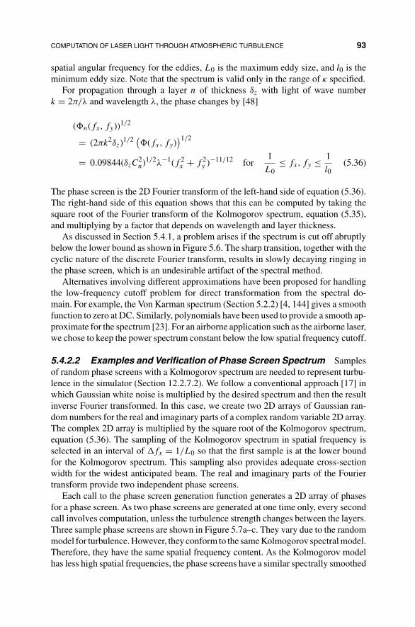
COMPUTATION OF LASER LIGHT THROUGH ATMOSPHERIC TURBULENCE 93
spatial angular frequency for the eddies, L0 is the maximum eddy size, and l0 is theminimum eddy size. Note that the spectrum is valid only in the range of κ specified.
For propagation through a layer n of thickness δz with light of wave numberk = 2π/λ and wavelength λ, the phase changes by [48]
(�n(fx, fy))1/2
= (2πk2δz)1/2 (�(fx, fy)
)1/2
= 0.09844(δzC2n)1/2λ−1(f 2
x + f 2y )−11/12 for
1
L0≤ fx, fy ≤ 1
l0(5.36)
The phase screen is the 2D Fourier transform of the left-hand side of equation (5.36).The right-hand side of this equation shows that this can be computed by taking thesquare root of the Fourier transform of the Kolmogorov spectrum, equation (5.35),and multiplying by a factor that depends on wavelength and layer thickness.
As discussed in Section 5.4.1, a problem arises if the spectrum is cut off abruptlybelow the lower bound as shown in Figure 5.6. The sharp transition, together with thecyclic nature of the discrete Fourier transform, results in slowly decaying ringing inthe phase screen, which is an undesirable artifact of the spectral method.
Alternatives involving different approximations have been proposed for handlingthe low-frequency cutoff problem for direct transformation from the spectral do-main. For example, the Von Karman spectrum (Section 5.2.2) [4, 144] gives a smoothfunction to zero at DC. Similarly, polynomials have been used to provide a smooth ap-proximate for the spectrum [23]. For an airborne application such as the airborne laser,we chose to keep the power spectrum constant below the low spatial frequency cutoff.
5.4.2.2 Examples and Verification of Phase Screen Spectrum Samplesof random phase screens with a Kolmogorov spectrum are needed to represent turbu-lence in the simulator (Section 12.2.7.2). We follow a conventional approach [17] inwhich Gaussian white noise is multiplied by the desired spectrum and then the resultinverse Fourier transformed. In this case, we create two 2D arrays of Gaussian ran-dom numbers for the real and imaginary parts of a complex random variable 2D array.The complex 2D array is multiplied by the square root of the Kolmogorov spectrum,equation (5.36). The sampling of the Kolmogorov spectrum in spatial frequency isselected in an interval of �fx = 1/L0 so that the first sample is at the lower boundfor the Kolmogorov spectrum. This sampling also provides adequate cross-sectionwidth for the widest anticipated beam. The real and imaginary parts of the Fouriertransform provide two independent phase screens.
Each call to the phase screen generation function generates a 2D array of phasesfor a phase screen. As two phase screens are generated at one time only, every secondcall involves computation, unless the turbulence strength changes between the layers.Three sample phase screens are shown in Figure 5.7a–c. They vary due to the randommodel for turbulence. However, they conform to the same Kolmogorov spectral model.Therefore, they have the same spatial frequency content. As the Kolmogorov modelhas less high spatial frequencies, the phase screens have a similar spectrally smoothed

94 PROPAGATION AND COMPENSATION FOR ATMOSPHERIC TURBULENCE
FIGURE 5.7 Sample phase screens using the spectral method for Kolmogorov turbulencemodel: (a) first, (b) second, and (c) third.
FIGURE 5.8 Average of absolute value of Fourier transform of 10 phase screens producedusing the spectral method.
appearance. A noticeable hill in the phase screen acts as a lens on the light beam. Asthe hills are off-center, they will bend the light in a random manner, causing the beamwander at the receiver.
Correct implementation of the equations is verified by averaging the |FT |2 for 100random phase screens. The result is identical to that shown in Figure 5.6 and is shownin a 3D plot in Figure 5.8. One quadrant of Figure 5.8 matches Figure 5.6.
5.4.3 Generation of Kolmogorov Phase Screens from CovarianceUsing Structure Functions
We consider a much slower method that avoids taking a Fourier transform by com-puting a covariance matrix directly using a structure function [144]. The method ismore versatile because it can include temporal dependencies between phase screens. A

COMPUTATION OF LASER LIGHT THROUGH ATMOSPHERIC TURBULENCE 95
method for speeding the algorithm has been proposed [54]. However, the Kolmogorovspectrum is no longer truncated at the lower spatial frequency bound, resulting in ex-cessive low spatial frequencies, unless a remedy is applied. We decided to truncatethe low spatial frequencies, which represent very large-scale turbulence, by excludingthe largest eigenvalues prior to computing the phase screens.
5.4.3.1 Equations for Computing the Phase Covariance for the Kol-mogorov Spectrum Structure functions are used to construct a covariance matrixfrom which phase screens are computed. The structure function for a homogeneous(spatially stationary) field f with zero mean, as in equation (5.10), is [155]
Df (r) = E[{f (r1 + r) − f (r1)}2
](5.37)
Df (r) is large for periodic oscillations with wavelength less than r, providing thestructure function with some spectral properties not present in a correlation function.Expanding equation (5.37) gives as in equation (5.12)
Df (r) = 2[Bf (0) − Bf (r)] (5.38)
where Bf (r) is the correlation function for f .The equations for a phase covariance matrix are derived by assuming a phase
across a transverse plane and subtracting the mean over the phase screen aperture. Thecovariance then has four correlation terms. The correlation terms of form Bf (r) arereplaced by structure functions Df (r) from equation (5.38). The Bf (0) terms cancel.Note that this approach can be readily extended to the case in which phase screensat different layers are dependent [144]. The structure function for the Kolmogorovturbulence model is then used: (Similar to equation (5.23) for velocity)
Dn(r) = C2nr
2/3 (5.39)
The resulting expression for the phase covariance for one layer is
γφ(n, m, n′, m′) (5.40)
= 6.88r−5/30
{−1
2
[{(m − m′)�x
}2 + {(n − n′)�y
}2]5/6
+1
2
NxNy∑u′,v′
1
Nx, Ny
[{(u′ − m′)�x
}2 + {(v′ − n′)�y
}2]5/6

96 PROPAGATION AND COMPENSATION FOR ATMOSPHERIC TURBULENCE
+1
2
NxNy∑u′′,v′′
1
Nx, Ny
[{(m − u′′)�x
}2 + {(n − v′′)�y
}2]5/6
−1
2
NxNy∑u′,v′
Nx,Ny∑u′′,v′′
(1
Nx, Ny
)2 [{(u′ − u′′)�x
}2 + {(v′ − v′′)�y
}2]5/6
⎫⎬⎭
(5.41)
where the atmospheric coherence length or the Fried parameter is
r0 = q
[4π2
k2C2n�zi
]3/5
(5.42)
The atmospheric coherence length r0 is used to determine the size of aperture atthe receiver and the maximum resolution when imaging through turbulence. Theparameter q is 0.185 for a plane wave and 3.69 for a spherical wave. The valuesfor the Gaussian beam at the distances of interest are close to those for a planewave. At �z = 1000 m, r0 = 0.185 m, which leads to an aperture of approximately0.2 m2. The propagation constant is k = 2π/λ and the strength of the turbulence istaken as C2
n = 10−13. There are many measurements and models for the strength ofturbulence [4]. The distance along the propagation path for a layer�zi ≥ Nx�xNy�y.We used Nx = Ny = 20 and �x = �y = 1 in the simulator.
5.4.3.2 Computing a Kolmogorov-Based Phase Screen Sample for aLayer from the Covariance The singular value decomposition (SVD) computesthe eigenvalues, diagonals of �, and eigenvectors, columns of U, of the covariancematrix:
� = U�UT (5.43)
We generate a vector b′ of uncorrelated Gaussian random variables with zero meanand variance � of length Nx × Ny. Then
E{
b′b′T}
= � (5.44)
where � is a matrix with eigenvalues on the diagonal and zero elsewhere. Randomphase screens are formed using
a = Ub′ (5.45)
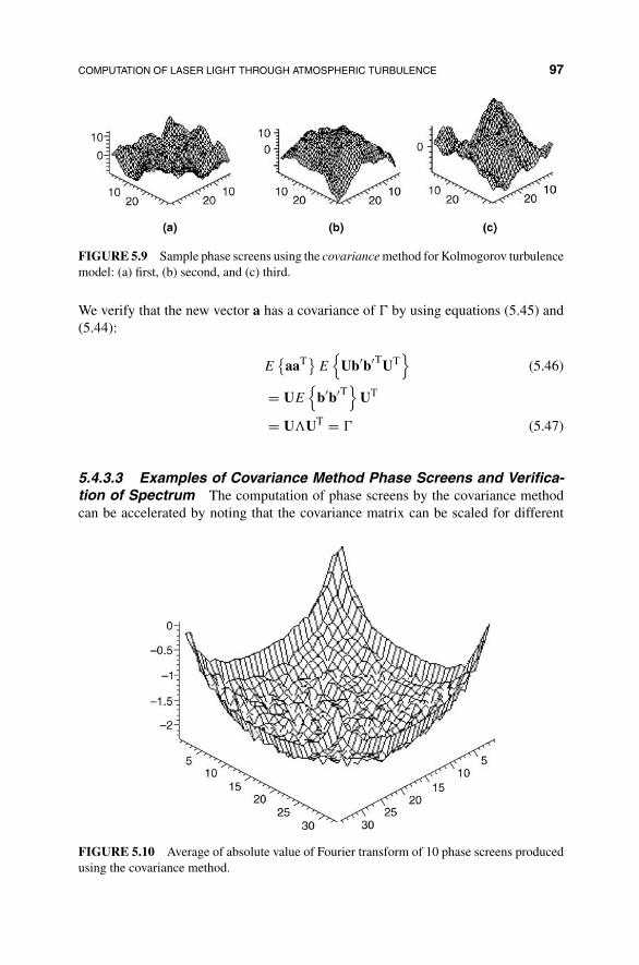
COMPUTATION OF LASER LIGHT THROUGH ATMOSPHERIC TURBULENCE 97
FIGURE 5.9 Sample phase screens using the covariance method for Kolmogorov turbulencemodel: (a) first, (b) second, and (c) third.
We verify that the new vector a has a covariance of � by using equations (5.45) and(5.44):
E{
aaT}E
{Ub′b′TUT
}(5.46)
= UE{
b′b′T}
UT
= U�UT = � (5.47)
5.4.3.3 Examples of Covariance Method Phase Screens and Verifica-tion of Spectrum The computation of phase screens by the covariance methodcan be accelerated by noting that the covariance matrix can be scaled for different
FIGURE 5.10 Average of absolute value of Fourier transform of 10 phase screens producedusing the covariance method.
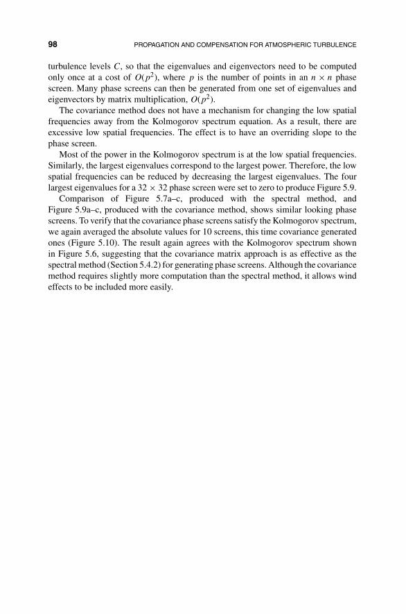
98 PROPAGATION AND COMPENSATION FOR ATMOSPHERIC TURBULENCE
turbulence levels C, so that the eigenvalues and eigenvectors need to be computedonly once at a cost of O(p2), where p is the number of points in an n × n phasescreen. Many phase screens can then be generated from one set of eigenvalues andeigenvectors by matrix multiplication, O(p2).
The covariance method does not have a mechanism for changing the low spatialfrequencies away from the Kolmogorov spectrum equation. As a result, there areexcessive low spatial frequencies. The effect is to have an overriding slope to thephase screen.
Most of the power in the Kolmogorov spectrum is at the low spatial frequencies.Similarly, the largest eigenvalues correspond to the largest power. Therefore, the lowspatial frequencies can be reduced by decreasing the largest eigenvalues. The fourlargest eigenvalues for a 32 × 32 phase screen were set to zero to produce Figure 5.9.
Comparison of Figure 5.7a–c, produced with the spectral method, andFigure 5.9a–c, produced with the covariance method, shows similar looking phasescreens. To verify that the covariance phase screens satisfy the Kolmogorov spectrum,we again averaged the absolute values for 10 screens, this time covariance generatedones (Figure 5.10). The result again agrees with the Kolmogorov spectrum shownin Figure 5.6, suggesting that the covariance matrix approach is as effective as thespectral method (Section 5.4.2) for generating phase screens. Although the covariancemethod requires slightly more computation than the spectral method, it allows windeffects to be included more easily.
CHAPTER 6
OPTICAL INTERFEROMETERSAND OSCILLATORS
Coherent light can be viewed as a wave or particle phenomenon. Waves can interferewith other waves because of their phase nature. If two waves with the same frequencyand polarization are in phase, they will interfere constructively. That is, the resultingintensity, the average of the square of the sum of the two waves, will show increasedintensity because of the wave overlap. In contrast, if the two waves are out of phase,the square of the sum of the waves will tend to zero intensity because of destructiveinterference. At phases between in-and out-of-phase, the average intensity will fallbetween that for in-phase and out-of-phase interference. Optical interference plays acritical role in military applications.
In Section 6.1, we describe the operation of interferometers, including three of themost common, Michelson, Mach–Zehnder, and Sagnac, for sensing a wide range ofphysical phenomena. In Section 6.2, we analyze the Fabry–Perot resonator, whichtraps light in a cavity between two parallel mirrors and resonates at frequenciesfor which reflection from the mirrors interferes constructively with waves trappedin the cavity. Fabry–Perot resonators are fundamental for many filters and lasers(Chapter 7) [83]. In Section 6.3, we consider multireflection interference filters madefrom thin layers of transparent dielectric materials of different media. Such layersare widely used for coating optical elements, for example, in eyeglasses, to avoidreflection. We describe the matrix method for design and analysis and an inversemethod to measure optical properties of individual layers [95, 97].
Military Laser Technology for Defense: Technology for Revolutionizing 21st Century Warfare,First Edition. By Alastair D. McAulay.© 2011 John Wiley & Sons, Inc. Published 2011 by John Wiley & Sons, Inc.
99

100 OPTICAL INTERFEROMETERS AND OSCILLATORS
6.1 OPTICAL INTERFEROMETERS
Interferometers provide sensing for measuring a variety of physical phenomena, suchas distance, pressure, temperature, rotation (gyroscopes), presence of chemical orbiological weapons, and perimeter protection sensors—all of which are important inmilitary applications [16, 55]. An interferometer splits coherent light from a laserinto two paths. In many applications, one path acts as a reference and the other expe-riences the phenomenon to be measured. The phenomenon to be measured changesthe velocity of the light in the measurement path, causing the phase of light to differfrom that in the reference path. Note that the output is influenced by both changes inabsorption between the two arms and changes in refractive index. On recombiningthe light paths in the interferometer and using a photodetector or CCD camera, thephase difference is converted to an intensity difference indicative of the strength ofthe phenomena.
Coherent light from a laser has temporal and spatial coherence that affect theperformance of an interferometer. Spatial coherence is a measure of how close awave is to a plane wave. High spatial coherence is achieved with a small source(Sections 1.3.6 and 3.2.2). Temporal coherence concerns how close light is to a singlefrequency, monochromatic, and is discussed here.
The bandwidth in wavelength �λ of the source laser limits the maximum differ-ence in distance, lc, the coherence length, at which combining the two paths of aninterferometer will produce a distinct interference pattern. At a difference in pathlengths of lc, the constructive interference from the center wavelength λ is canceledby the destructive interference from the wavelength λ + �λ/2 at the band edge. Forconstructive interference at a difference in distance of lc, and a wavelength of λ, thetwo paths must differ by a whole number m of wavelengths so as to be in phase.Therefore,
mλ = lc (6.1)
Destructive interference occurs at a whole number of wavelengths minus a half.Therefore, at a difference in distance of lc and a wavelength λ + �λ/2 at the edge ofthe frequency band,
(m − 1/2)(λ + �λ
2) = lc (6.2)
For the constructive interference at the nominal wavelength λ to be canceled out bythe destructive interference, we equate lc in equation (6.1) with lc in equation (6.2)and solve for integer m to get
m = λ
�λ+ 1
2≈ λ
�λ(6.3)

OPTICAL INTERFEROMETERS 101
Substituting equation (6.3) into equation (6.1) gives a coherence length in terms ofwavelength and bandwidth of the source:
lc = λ2
�λ(6.4)
Using equation (6.20) to convert from wavelength to a frequency source bandwidth�f ,
lc = c
�f(6.5)
From equation (6.5), a corresponding coherence time tc = lc/c, the maximum timedifference between two paths of an interferometer before the interference patterndisappears, is the reciprocal of the source frequency bandwidth (for a laser for which�f is small, the bandwidth is known as linewidth):
tc = 1
�f(6.6)
Interferometers may be implemented in free space on an optical bench. In thelaboratory, optical tables with air supported legs are required to maintain sta-bility. Often interferometers are implemented with optical fiber or in integratedoptics [57].
In Section 6.1.1, we describe the Michelson interferometer, commonly used foraccurate distance measurement among other things. In Section 6.1.2, we describethe Mach–Zehnder interferometer in free space, optical fiber, and integrated circuits.The Mach–Zehnder interferometer is used in integrated optics for sensing and on–off light switching, for example, for telecommunication modulators [102, 106]. InSection 6.1.3, we describe a stable optical fiber Sagnac interferometer, which is thebasis of modern gyroscopes and novel perimeter security systems [112].
6.1.1 Michelson Interferometer
Figure 6.1 shows a beam splitter at the center that splits light into two equal parts: onepassing to mirror M1 and the other to mirror M2. In this case, the Michelson inter-ferometer measures the displacement of mirror M2. Such interferometers are used inVLSI lithography machines and elsewhere for very accurate distance measurements.
Following reflection from the mirrors, the paths are combined at the screen afterpassing through the beam splitter again. Consequently, the field after combining thetwo paths at the screen may be written as
E(t) = E1(t) + E2(t) (6.7)

102 OPTICAL INTERFEROMETERS AND OSCILLATORS
for which intensity is
I = 〈EE∗〉 = 〈(E1 + E2)(E1 + E2)∗〉= 〈E1E
∗1〉 + 〈E2E
∗2〉 + 〈E1E
∗2〉 + 〈E2E
∗1〉
= I1 + I2 + 2Re{〈E∗
1E2〉}
(6.8)
If the intensities are equal for the fields, I1 = I2,
I = 2I1 + 2Re{〈E∗
1E2〉}
(6.9)
6.1.1.1 Autocorrelation Function in Michelson interferometer For aMichelson interferometer, if mirror M2 is moved to the right by distance d, as shownin Figure 6.1, the electric field E2 will be delayed by time τ = 2d/c relative tofield E1, where c is the speed of light in air. Therefore, as mirror M2 is moved,E2(t) = E1(t − τ), and the Michelson interferometer computes the autocorrelationof the input beam. The product E∗
1E2 in equation (6.8) can now be written with theautocorrelation function �(τ) for the Michelson interferometer. In optics, the auto-correlation function �(τ) is called the complex self-coherence function:
�(τ) = 〈E∗1(t)E1(t − τ)〉 (6.10)
So, substituting equation (6.10) into equation (6.9) allows the intensity on axis outof a Michelson interferometer to be written as
I = 2I1 + 2Re {�(τ)} (6.11)
M1
M2
d
E1E2
Laser
Beamexpander
Planewaves
Ray
Screen
Adjustableposition
FIGURE 6.1 Michelson interferometer for measuring distance.
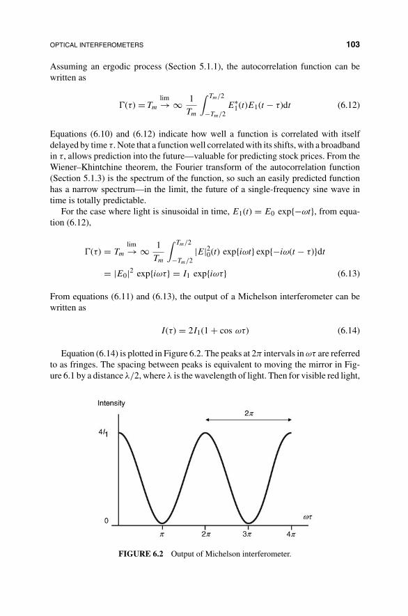
OPTICAL INTERFEROMETERS 103
Assuming an ergodic process (Section 5.1.1), the autocorrelation function can bewritten as
�(τ) = limTm → ∞ 1
Tm
∫ Tm/2
−Tm/2E∗
1(t)E1(t − τ)dt (6.12)
Equations (6.10) and (6.12) indicate how well a function is correlated with itselfdelayed by time τ. Note that a function well correlated with its shifts, with a broadbandin τ, allows prediction into the future—valuable for predicting stock prices. From theWiener–Khintchine theorem, the Fourier transform of the autocorrelation function(Section 5.1.3) is the spectrum of the function, so such an easily predicted functionhas a narrow spectrum—in the limit, the future of a single-frequency sine wave intime is totally predictable.
For the case where light is sinusoidal in time, E1(t) = E0 exp{−ωt}, from equa-tion (6.12),
�(τ) = limTm → ∞ 1
Tm
∫ Tm/2
−Tm/2|E|20(t) exp{iωt} exp{−iω(t − τ)}dt
= |E0|2 exp{iωτ} = I1 exp{iωτ} (6.13)
From equations (6.11) and (6.13), the output of a Michelson interferometer can bewritten as
I(τ) = 2I1(1 + cos ωτ) (6.14)
Equation (6.14) is plotted in Figure 6.2. The peaks at 2π intervals in ωτ are referredto as fringes. The spacing between peaks is equivalent to moving the mirror in Fig-ure 6.1 by a distance λ/2, where λ is the wavelength of light. Then for visible red light,
FIGURE 6.2 Output of Michelson interferometer.
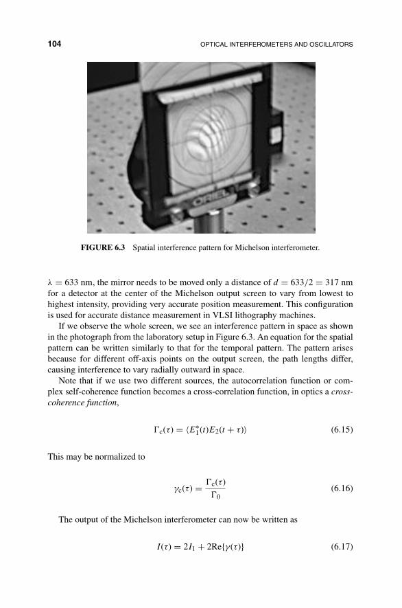
104 OPTICAL INTERFEROMETERS AND OSCILLATORS
FIGURE 6.3 Spatial interference pattern for Michelson interferometer.
λ = 633 nm, the mirror needs to be moved only a distance of d = 633/2 = 317 nmfor a detector at the center of the Michelson output screen to vary from lowest tohighest intensity, providing very accurate position measurement. This configurationis used for accurate distance measurement in VLSI lithography machines.
If we observe the whole screen, we see an interference pattern in space as shownin the photograph from the laboratory setup in Figure 6.3. An equation for the spatialpattern can be written similarly to that for the temporal pattern. The pattern arisesbecause for different off-axis points on the output screen, the path lengths differ,causing interference to vary radially outward in space.
Note that if we use two different sources, the autocorrelation function or com-plex self-coherence function becomes a cross-correlation function, in optics a cross-coherence function,
�c(τ) = 〈E∗1(t)E2(t + τ)〉 (6.15)
This may be normalized to
γc(τ) = �c(τ)
�0(6.16)
The output of the Michelson interferometer can now be written as
I(τ) = 2I1 + 2Re{γ(τ)} (6.17)

OPTICAL INTERFEROMETERS 105
FIGURE 6.4 Mach–Zehnder free-space interferometer.
6.1.2 Mach–Zehnder Interferometer
The Mach–Zehnder interferometer may be implemented in free space, optical fiber,or integrated optics, depending on the application and manufacturing volume. Theapplication is often first tested in free space but alignment and stability are detrimentalfor mass production. Optical fiber is used where distributed sensing is required. Inte-grated optics is used for point sensing when manufacturing volume is high becauseunit cost is reduced by volume and the initial design cost occurs only once.
6.1.2.1 Free-Space Mach–Zehnder Interferometer A free-space setup isshown in Figure 6.4, in which beam splitter BS1 is used to split light into two paths. Thetwo paths are recombined by beam splitter BS2. If the environment path is identical tothe reference path, the light will be in phase at beam splitter BS2 and constructivelyinterfere to give back the original light intensity of the source at the center of thescreen (minus reflective losses). If the environment changes the propagation time inone arm of the interferometer, there will be a phase difference at the screen. If phasedifference is 180◦ (π), the beams at the center of the screen will combine destructively(destructive interference) and there will be no light at the center of the screen. Notethat power is not destroyed—it just no longer illuminates the center of the screen.
A setup in our laboratory is shown in Figure 6.5. The two paths through theinterferometer cannot differ by more than the coherence length (Section 6.1) of thelaser, at which distance the fringes in time and space will vanish. In the case of the fiberoptic and integrated optic versions following, the light is dispersed into the claddingon destructive interference.
6.1.2.2 Optical Fiber Mach–Zehnder Interferometer Mach–Zehnder in-terferometers are often implemented in fiber [164]. Components may now be pluggedinto one another and optical alignment avoided, reducing assembly cost relative tofree space. Figure 6.6 shows such a fiber Mach–Zehnder interferometer. A directionalcoupler has no back reflections and splits the light into two equal intensities alongtwo fibers, one acting as reference and the other for sensing. When light crosses fromone side to the other while propagating through a directional coupler, it experiences a90◦ phase lag [176]. A second 50/50 coupler, acting as a combiner, merges the pathstogether. Therefore, the top path from input to output experiences no crossovers inthe sensing path while the lower path has experienced two. The 180◦ phase difference

106 OPTICAL INTERFEROMETERS AND OSCILLATORS
FIGURE 6.5 Photograph of Mach–Zehnder free-space interferometer in laboratory.
between top and lower paths results in zero output because of destructive interference.A photograph of a prototype of such a fiber interferometer is shown in Figure 6.7.
For maximum optical interference, light from the two paths must have the samefrequency and polarization. Ordinary optical fiber does not maintain polarization, soa polarization controller (Section 2.2.5) is included in Figure 6.6. The optical fiberMach–Zehnder interferometer often measures strain caused by stress in mechanicaland structural systems. In columns and struts of bridges, strain due to excessiveloads, such as tanks or heavily loaded trucks, or subsidence with age can be instantlyspotted, and if excessive, a wireless signal is sent back to a highway monitoringoffice. In military applications, the Mach–Zehnder fiber interferometer may be usedin the wings of military aircraft. Excessive strain to wings can be monitored to avoidexceeding damage limits while maneuvering abruptly. The strain sensor is particularlyvaluable if a wing is damaged and the pilot has to maneuver within a strain limit.
Optical sensors are advantageous in hazardous environments because there are nosparks when a fiber breaks or its cover is worn. This allows hot switching in opticaltelecommunication circuits. An aircraft on an international flight crashed a few yearsago because of frayed wires inside the wing where fuel is stored. Optical fiber with
Inputlight
Splitter(coupler)
Polarizationcontrol
Fiberpath 1
Fiberpath 2
Combiner(coupler)
Outputintensity
Photo detectoror screen
FIGURE 6.6 Optical fiber Mach–Zehnder interferometer.
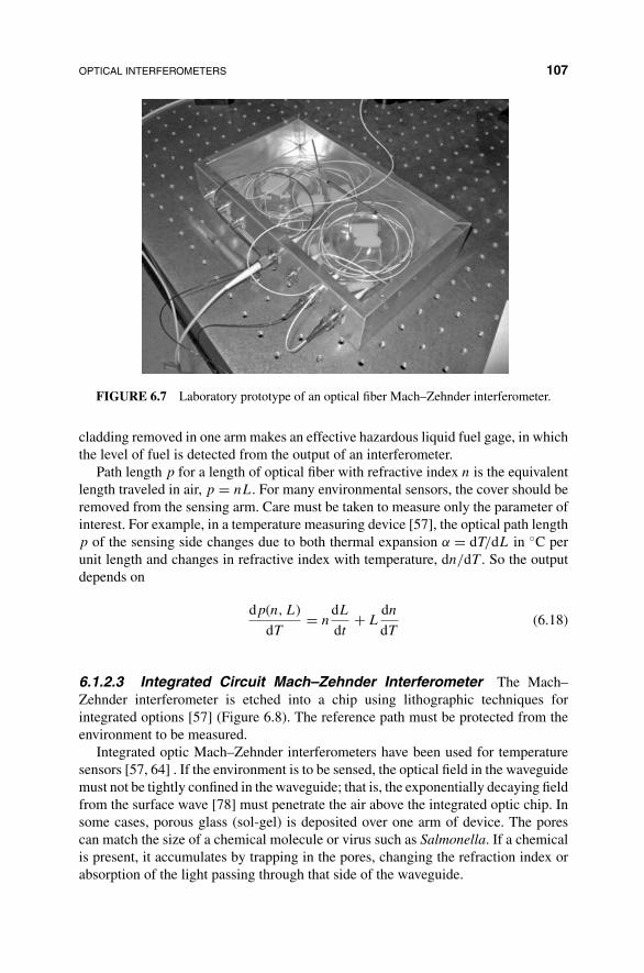
OPTICAL INTERFEROMETERS 107
FIGURE 6.7 Laboratory prototype of an optical fiber Mach–Zehnder interferometer.
cladding removed in one arm makes an effective hazardous liquid fuel gage, in whichthe level of fuel is detected from the output of an interferometer.
Path length p for a length of optical fiber with refractive index n is the equivalentlength traveled in air, p = nL. For many environmental sensors, the cover should beremoved from the sensing arm. Care must be taken to measure only the parameter ofinterest. For example, in a temperature measuring device [57], the optical path lengthp of the sensing side changes due to both thermal expansion α = dT/dL in ◦C perunit length and changes in refractive index with temperature, dn/dT . So the outputdepends on
dp(n, L)
dT= n
dL
dt+ L
dn
dT(6.18)
6.1.2.3 Integrated Circuit Mach–Zehnder Interferometer The Mach–Zehnder interferometer is etched into a chip using lithographic techniques forintegrated options [57] (Figure 6.8). The reference path must be protected from theenvironment to be measured.
Integrated optic Mach–Zehnder interferometers have been used for temperaturesensors [57, 64] . If the environment is to be sensed, the optical field in the waveguidemust not be tightly confined in the waveguide; that is, the exponentially decaying fieldfrom the surface wave [78] must penetrate the air above the integrated optic chip. Insome cases, porous glass (sol-gel) is deposited over one arm of device. The porescan match the size of a chemical molecule or virus such as Salmonella. If a chemicalis present, it accumulates by trapping in the pores, changing the refraction index orabsorption of the light passing through that side of the waveguide.
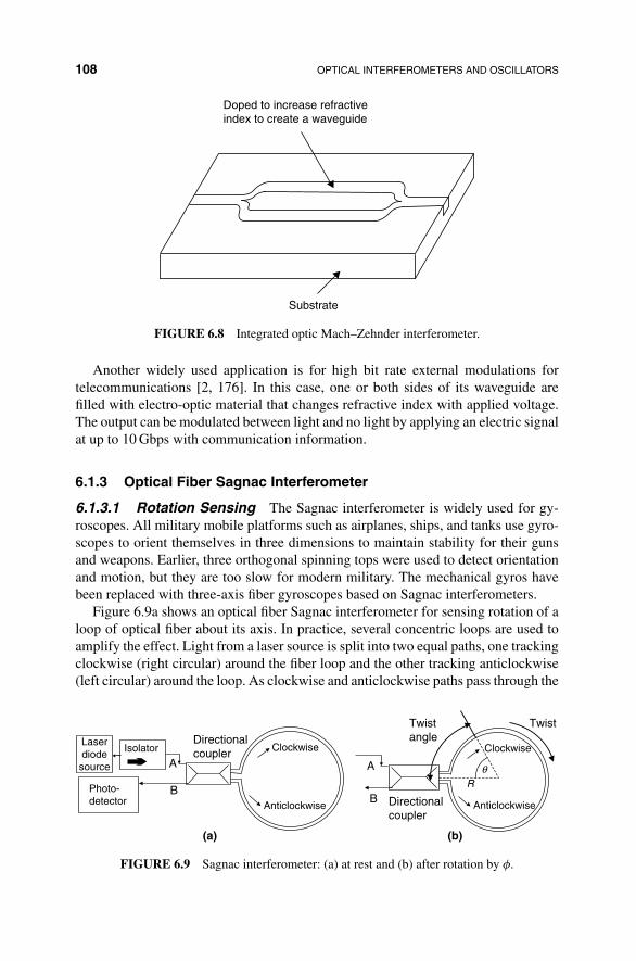
108 OPTICAL INTERFEROMETERS AND OSCILLATORS
Substrate
Doped to increase refractiveindex to create a waveguide
FIGURE 6.8 Integrated optic Mach–Zehnder interferometer.
Another widely used application is for high bit rate external modulations fortelecommunications [2, 176]. In this case, one or both sides of its waveguide arefilled with electro-optic material that changes refractive index with applied voltage.The output can be modulated between light and no light by applying an electric signalat up to 10 Gbps with communication information.
6.1.3 Optical Fiber Sagnac Interferometer
6.1.3.1 Rotation Sensing The Sagnac interferometer is widely used for gy-roscopes. All military mobile platforms such as airplanes, ships, and tanks use gyro-scopes to orient themselves in three dimensions to maintain stability for their gunsand weapons. Earlier, three orthogonal spinning tops were used to detect orientationand motion, but they are too slow for modern military. The mechanical gyros havebeen replaced with three-axis fiber gyroscopes based on Sagnac interferometers.
Figure 6.9a shows an optical fiber Sagnac interferometer for sensing rotation of aloop of optical fiber about its axis. In practice, several concentric loops are used toamplify the effect. Light from a laser source is split into two equal paths, one trackingclockwise (right circular) around the fiber loop and the other tracking anticlockwise(left circular) around the loop. As clockwise and anticlockwise paths pass through the
Photo-detector
DirectionalcouplerIsolator
Laserdiodesource A
B
Clockwise
Anticlockwise
(a)
Directionalcoupler
A
B
Clockwise
Anticlockwise
Twistangle
Twist
(b)
Rθ
FIGURE 6.9 Sagnac interferometer: (a) at rest and (b) after rotation by φ.
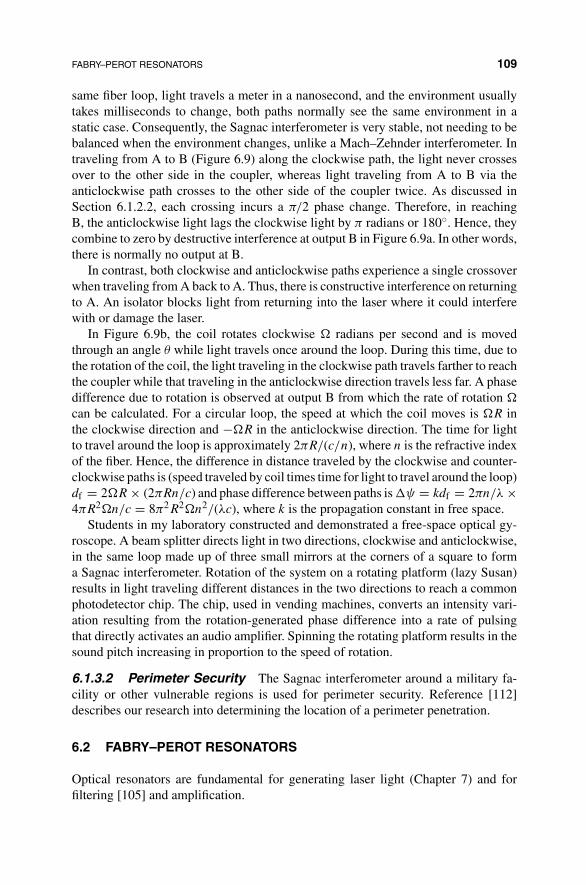
FABRY–PEROT RESONATORS 109
same fiber loop, light travels a meter in a nanosecond, and the environment usuallytakes milliseconds to change, both paths normally see the same environment in astatic case. Consequently, the Sagnac interferometer is very stable, not needing to bebalanced when the environment changes, unlike a Mach–Zehnder interferometer. Intraveling from A to B (Figure 6.9) along the clockwise path, the light never crossesover to the other side in the coupler, whereas light traveling from A to B via theanticlockwise path crosses to the other side of the coupler twice. As discussed inSection 6.1.2.2, each crossing incurs a π/2 phase change. Therefore, in reachingB, the anticlockwise light lags the clockwise light by π radians or 180◦. Hence, theycombine to zero by destructive interference at output B in Figure 6.9a. In other words,there is normally no output at B.
In contrast, both clockwise and anticlockwise paths experience a single crossoverwhen traveling from A back to A. Thus, there is constructive interference on returningto A. An isolator blocks light from returning into the laser where it could interferewith or damage the laser.
In Figure 6.9b, the coil rotates clockwise � radians per second and is movedthrough an angle θ while light travels once around the loop. During this time, due tothe rotation of the coil, the light traveling in the clockwise path travels farther to reachthe coupler while that traveling in the anticlockwise direction travels less far. A phasedifference due to rotation is observed at output B from which the rate of rotation �
can be calculated. For a circular loop, the speed at which the coil moves is �R inthe clockwise direction and −�R in the anticlockwise direction. The time for lightto travel around the loop is approximately 2πR/(c/n), where n is the refractive indexof the fiber. Hence, the difference in distance traveled by the clockwise and counter-clockwise paths is (speed traveled by coil times time for light to travel around the loop)df = 2�R × (2πRn/c) and phase difference between paths is �ψ = kdf = 2πn/λ ×4πR2�n/c = 8π2R2�n2/(λc), where k is the propagation constant in free space.
Students in my laboratory constructed and demonstrated a free-space optical gy-roscope. A beam splitter directs light in two directions, clockwise and anticlockwise,in the same loop made up of three small mirrors at the corners of a square to forma Sagnac interferometer. Rotation of the system on a rotating platform (lazy Susan)results in light traveling different distances in the two directions to reach a commonphotodetector chip. The chip, used in vending machines, converts an intensity vari-ation resulting from the rotation-generated phase difference into a rate of pulsingthat directly activates an audio amplifier. Spinning the rotating platform results in thesound pitch increasing in proportion to the speed of rotation.
6.1.3.2 Perimeter Security The Sagnac interferometer around a military fa-cility or other vulnerable regions is used for perimeter security. Reference [112]describes our research into determining the location of a perimeter penetration.
6.2 FABRY–PEROT RESONATORS
Optical resonators are fundamental for generating laser light (Chapter 7) and forfiltering [105] and amplification.

110 OPTICAL INTERFEROMETERS AND OSCILLATORS
6.2.1 Fabry–Perot Principles and Equations
An optical resonator is formed by trapping light between two parallel vertical mirrorsthat form a cavity or an etalon; this type of resonator is known as a Fabry–Perotresonator [53, 176]. If we stand inside a pair of Fabry–Perot mirrors in a fairgroundhall of mirrors, we can see an infinite number of reflections. A different resonator,a ring resonator, is often used in integrated optics [96, 102, 105, 106]. In a Fabry–Perot resonator, photons bounce back and forth between the mirrors and at certainresonant wavelengths they coherently add inside the cavity to increase the powertrapped in the resonator to a high level. This is like pushing a child’s swing at thecorrect intervals for resonance to slowly increase the energy contained in the swing.The Fabry–Perot resonator can also enhance images and many fish and animals thatlive in dark environments, such as deep sea fish, have reflecting surfaces at the frontand rear of their eyes to trap photons so that the intensity in the etalon is sufficient toexcite neurons in the retina.
6.2.2 Fabry–Perot Equations
The equations for a Fabry–Perot resonator are derived by considering reflection andtransmission at a single mirror. Partially reflecting mirrors allow input to and outputfrom the cavity between them. Figure 6.10a and b shows for an incident field fromthe left the reflection and transmission at a mirror interface without attenuation andwith power attenuation A, respectively. A negative power attenuation can be used torepresent power gain. Note that the reflected power is R times the input power. Topreserve power, the output power must then be 1 − R times the input power. Hence,from Figure 6.10b, for an incoming field Ei,
√R is reflected and
√1 − A − R is
transmitted by the mirror.From Figure 6.10, we can hypothesize light bouncing back and forth be-
tween the mirrors, as shown in Figure 6.11. We assume a phase change in cross-ing the etalon of βx, where β in radians per second is the propagation con-stant and x is the etalon width. Hence, on reaching the right-hand side mirror inFigure 6.11, the field is
√1 − R − AEi exp{jβz} and on reflection from the mirror,√
R√
1 − R − AEi exp{jβz}. With perfect mirror alignment, the light reflects backand forth along the same path. For clarity in Figure 6.11, we shifted the beams downon reflection.
E i1 − R − A Ei
E iR
√
√
E iE i1−R
E iR
√
√
(a) (b)
FIGURE 6.10 Reflection and transmission at a mirror: (a) without attenuation and (b) withattenuation.

FABRY–PEROT RESONATORS 111
Ei exp{jβ x}
exp{jβ x}R exp{j2β x}
exp{j2β x}R R exp{j3β x}
exp{jβ x}E i(1 − R − A)
Right mirrorLeft mirror
Inputfield
Outputfield
x
(1 − R − A)R exp{j3 x}E i β
1− R − A Ei√
1− R − A Ei√
1− R − A Ei√ 1− R − A Ei√
1− R − A Ei√
1− R − A Ei√√ R√
FIGURE 6.11 Illustration for deriving Fabry–Perot transfer function equations.
From Figure 6.11, the output at the right of the etalon is the infinite sum of theoutputs transmitted through the output mirror on each bounce of the light:
Eo = (1 − A − R)Ei exp{jβx}∞∑
m=0
[R exp{j2βx}]m (6.19)
where for each cycle of the light, we add in the sum R for two reflections and exp{j2βx}for two propagations across the cavity. Similarly, we could determine the reflectionfrom the resonator by summing the infinite reflections to the left.
If incoming broadband light has an electric field Ei only those wavelengths willresonate for which a whole number of half-wavelengths fit between the mirrors(Figure 6.12).
/21
/266 ×
5 ×
/244 ×
/233 ×
/222 ×
Mirror 1 Mirror 2
Number of half-wavelengthsthat fit betweenmirrors providesmode number
λ
/25λ
λ
λ
λ
λ
FIGURE 6.12 Electric fields for modes in Fabry–Perot resonator.
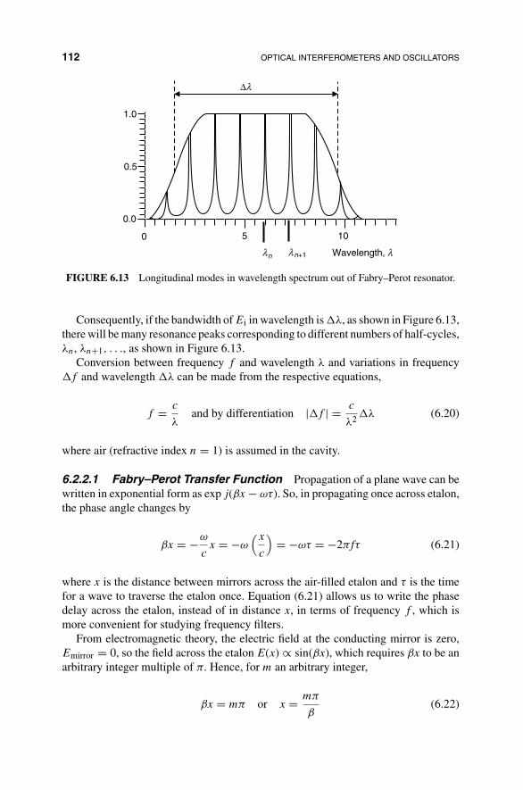
112 OPTICAL INTERFEROMETERS AND OSCILLATORS
Wavelength, λn n+1
Δλ
1.0
0.5
0.0
0 5 10
λ λ
FIGURE 6.13 Longitudinal modes in wavelength spectrum out of Fabry–Perot resonator.
Consequently, if the bandwidth of Ei in wavelength is �λ, as shown in Figure 6.13,there will be many resonance peaks corresponding to different numbers of half-cycles,λn, λn+1, . . ., as shown in Figure 6.13.
Conversion between frequency f and wavelength λ and variations in frequency�f and wavelength �λ can be made from the respective equations,
f = c
λand by differentiation |�f | = c
λ2 �λ (6.20)
where air (refractive index n = 1) is assumed in the cavity.
6.2.2.1 Fabry–Perot Transfer Function Propagation of a plane wave can bewritten in exponential form as exp j(βx − ωτ). So, in propagating once across etalon,the phase angle changes by
βx = −ω
cx = −ω
(x
c
)= −ωτ = −2πfτ (6.21)
where x is the distance between mirrors across the air-filled etalon and τ is the timefor a wave to traverse the etalon once. Equation (6.21) allows us to write the phasedelay across the etalon, instead of in distance x, in terms of frequency f , which ismore convenient for studying frequency filters.
From electromagnetic theory, the electric field at the conducting mirror is zero,Emirror = 0, so the field across the etalon E(x) ∝ sin(βx), which requires βx to be anarbitrary integer multiple of π. Hence, for m an arbitrary integer,
βx = mπ or x = mπ
β(6.22)
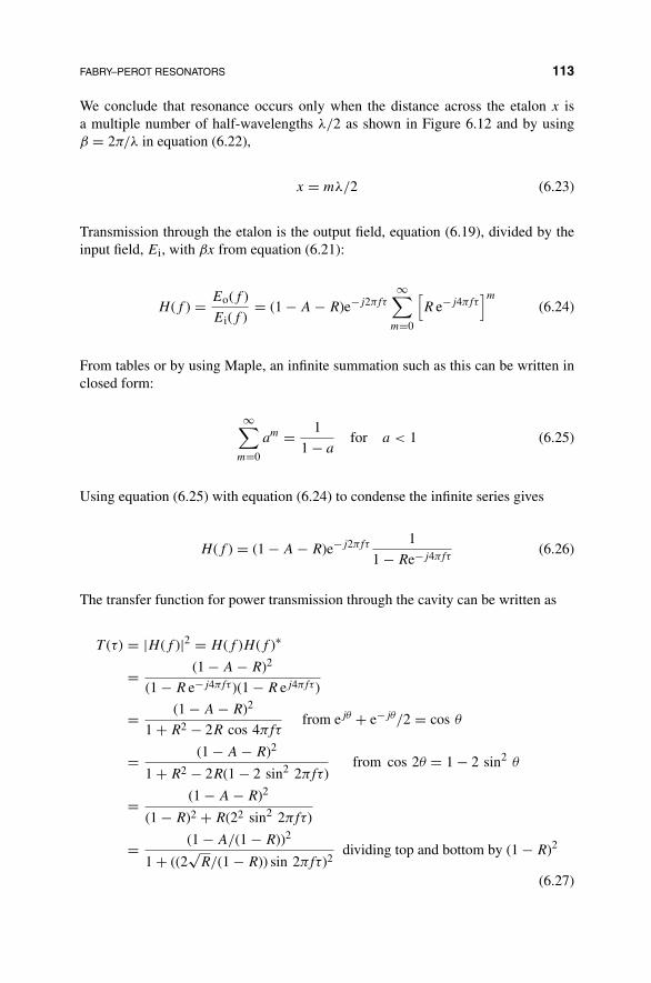
FABRY–PEROT RESONATORS 113
We conclude that resonance occurs only when the distance across the etalon x isa multiple number of half-wavelengths λ/2 as shown in Figure 6.12 and by usingβ = 2π/λ in equation (6.22),
x = mλ/2 (6.23)
Transmission through the etalon is the output field, equation (6.19), divided by theinput field, Ei, with βx from equation (6.21):
H(f ) = Eo(f )
Ei(f )= (1 − A − R)e−j2πfτ
∞∑m=0
[R e−j4πfτ
]m
(6.24)
From tables or by using Maple, an infinite summation such as this can be written inclosed form:
∞∑m=0
am = 1
1 − afor a < 1 (6.25)
Using equation (6.25) with equation (6.24) to condense the infinite series gives
H(f ) = (1 − A − R)e−j2πfτ 1
1 − Re−j4πfτ(6.26)
The transfer function for power transmission through the cavity can be written as
T (τ) = |H(f )|2 = H(f )H(f )∗
= (1 − A − R)2
(1 − R e−j4πfτ)(1 − R ej4πfτ)
= (1 − A − R)2
1 + R2 − 2R cos 4πfτfrom ejθ + e−jθ/2 = cos θ
= (1 − A − R)2
1 + R2 − 2R(1 − 2 sin2 2πfτ)from cos 2θ = 1 − 2 sin2 θ
= (1 − A − R)2
(1 − R)2 + R(22 sin2 2πfτ)
= (1 − A/(1 − R))2
1 + ((2√
R/(1 − R)) sin 2πfτ)2dividing top and bottom by (1 − R)2
(6.27)
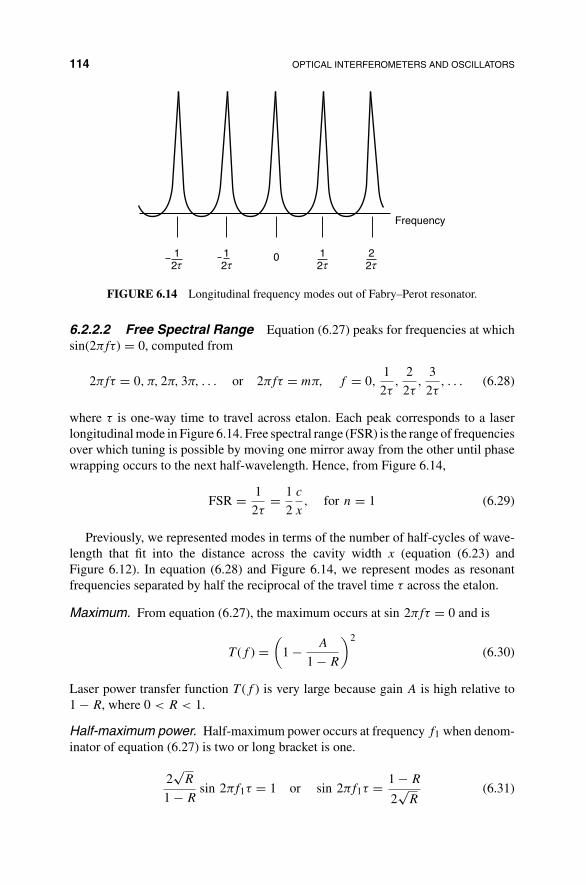
114 OPTICAL INTERFEROMETERS AND OSCILLATORS
21
220
21
21
Frequency
τ τ τ τ
FIGURE 6.14 Longitudinal frequency modes out of Fabry–Perot resonator.
6.2.2.2 Free Spectral Range Equation (6.27) peaks for frequencies at whichsin(2πfτ) = 0, computed from
2πfτ = 0, π, 2π, 3π, . . . or 2πfτ = mπ, f = 0,1
2τ,
2
2τ,
3
2τ, . . . (6.28)
where τ is one-way time to travel across etalon. Each peak corresponds to a laserlongitudinal mode in Figure 6.14. Free spectral range (FSR) is the range of frequenciesover which tuning is possible by moving one mirror away from the other until phasewrapping occurs to the next half-wavelength. Hence, from Figure 6.14,
FSR = 1
2τ= 1
2
c
x, for n = 1 (6.29)
Previously, we represented modes in terms of the number of half-cycles of wave-length that fit into the distance across the cavity width x (equation (6.23) andFigure 6.12). In equation (6.28) and Figure 6.14, we represent modes as resonantfrequencies separated by half the reciprocal of the travel time τ across the etalon.
Maximum. From equation (6.27), the maximum occurs at sin 2πfτ = 0 and is
T (f ) =(
1 − A
1 − R
)2
(6.30)
Laser power transfer function T (f ) is very large because gain A is high relative to1 − R, where 0 < R < 1.
Half-maximum power. Half-maximum power occurs at frequency f1 when denom-inator of equation (6.27) is two or long bracket is one.
2√
R
1 − Rsin 2πf1τ = 1 or sin 2πf1τ = 1 − R
2√
R(6.31)
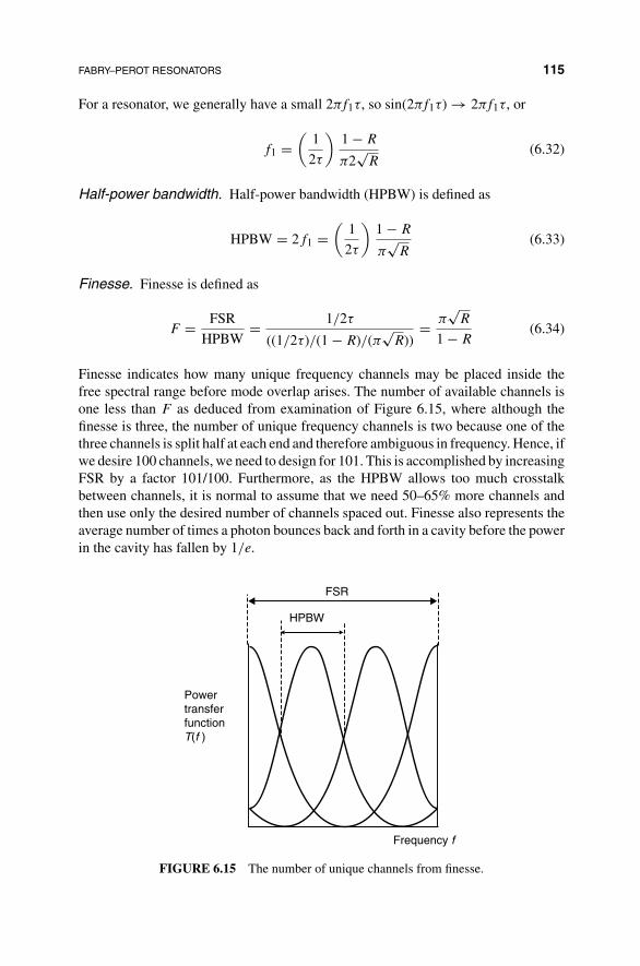
FABRY–PEROT RESONATORS 115
For a resonator, we generally have a small 2πf1τ, so sin(2πf1τ) → 2πf1τ, or
f1 =(
1
2τ
)1 − R
π2√
R(6.32)
Half-power bandwidth. Half-power bandwidth (HPBW) is defined as
HPBW = 2f1 =(
1
2τ
)1 − R
π√
R(6.33)
Finesse. Finesse is defined as
F = FSR
HPBW= 1/2τ
((1/2τ)/(1 − R)/(π√
R))= π
√R
1 − R(6.34)
Finesse indicates how many unique frequency channels may be placed inside thefree spectral range before mode overlap arises. The number of available channels isone less than F as deduced from examination of Figure 6.15, where although thefinesse is three, the number of unique frequency channels is two because one of thethree channels is split half at each end and therefore ambiguous in frequency. Hence, ifwe desire 100 channels, we need to design for 101. This is accomplished by increasingFSR by a factor 101/100. Furthermore, as the HPBW allows too much crosstalkbetween channels, it is normal to assume that we need 50–65% more channels andthen use only the desired number of channels spaced out. Finesse also represents theaverage number of times a photon bounces back and forth in a cavity before the powerin the cavity has fallen by 1/e.
HPBW
FSR
Frequency f
PowertransferfunctionT(f )
FIGURE 6.15 The number of unique channels from finesse.

116 OPTICAL INTERFEROMETERS AND OSCILLATORS
(a) (b)
Distance x
Leftmirror
Rightmirror
Distance x
Mirrors
FIGURE 6.16 Tuning a Fabry–Perot filter with piezoelectric material: (a) piezoelectric ma-terial inside etalon and (b) with mechanical gain.
Contrast. Contrast may be defined as max / min for the Fabry–Perot resonator out-put. From equation (6.27), the maximum and minimum values are
Max =(
1 − A
1 − R
)2
Min = (1 − (A/(1 − R)))2
1 + (4R/(1 − R)2), where sin(2πfτ) = 1
Contrast = Max
Min= 1 +
(2√
R
1 − R
)2
Using equation (6.34),
Contrast = 1 +(
2F
π
)2
(6.35)
6.2.3 Piezoelectric Tuning of Fabry–Perot Tuners
Piezoelectric material is convenient because it expands slowly with increasing volt-age across its ends [53]. Figure 6.16a shows a tube of piezoelectric material placedbetween the two mirrors of a Fabry–Perot etalon so that the beam in the cavity passesthrough the hole in the tube. If piezoelectric material has length X and the extensionfor a full range of voltage is �X, the ratio of extension to length is �X/X = r. Typ-ically, r = 0.05. When this expansion is inadequate for providing a desired tuningrange R, we use a mechanical gain of G = R/r by making the piezoelectric materialG times longer than the Fabry–Perot cavity, as shown in Figure 6.16b.
6.3 THIN-FILM INTERFEROMETRIC FILTERS AND DIELECTRICMIRRORS
Thin-film layered coatings are widely used for optical elements, especially with high-power lasers to minimize losses. Even small reflections from high-power laser beams

THIN-FILM INTERFEROMETRIC FILTERS AND DIELECTRIC MIRRORS 117
can have enough power to damage eyes during testing. A stack of thin-film interfer-ometric layers can filter a light beam.
6.3.1 Applications for Thin Films
6.3.1.1 Dielectric Mirrors for a Single Frequency High-power lasers candamage mirrors through I2R0 loss in metal conducting surfaces, where for the con-ductor, I is the induced current and R0 is the resistance. Consequently, layers ofdielectric material with no conducting materials, hence with no I2R loss, are used inplace of metal mirrors in high-power applications, such as the Airborne Laser pro-gram (Section 12.2). If the thickness of a layer is half the wavelength, d = λ/2, thereflection from the front side of the layer will be in phase with that from the rear side,which has traveled an extra distance of 2d = λ. The amplitude of the reflectance willalso depend on the refractive indices across the interfaces, equation (6.36).
As discussed in Section 6.2, for incident light of field Ei, if the power reflectivityis R, the reflected field will be
√REi and the transmitted field
√1 − REi because of
conservation of power. If there are N identical layers, the transmission through thestack of N layers will be approximately (
√1 − R)NEi, which can be extremely small
for large N. For infrared frequencies, the thickness of a layer is d = λ/2 ≈ 500 nmso the thickness of 100 layers is still only 0.05 �m. The light that is not transmittedis reflected, showing that extremely high reflectivities are possible, much higher thanthat for a metal mirror. When almost the entire high-power beam is reflected, thereis little heating effect from residual resistance and the mirror remains undamaged. Amore exact computation can be made with the matrix method of Section 6.3.2.
Students in my laboratory designed and constructed an interferometer used forremote listening. The system involves shining a laser beam across a street onto awindow of a conference room in another building. They used a small square panelof glass to represent the window. The reflections from the front and back sides of thewindow glass interfere. Conversation in the conference room vibrates the glass panelat audio rates. The bending of the glass changes the angle of incidence, so the thicknessof the glass along the beam changes, causing the back reflected beam to change phaserelative to the front reflected beam. The thickness has only to vary nanometers foradequate phase difference. The phase difference modulates the intensity of the lightreflected back to a photodetector next to the laser. The detector cannot respond to thefrequency of light and sees only the modulation. The output of the detector is fedto an audio amplifier from which conversation in the room across the street can beheard. Military and commercial secure rooms that have windows often have whitenoise generators in their windows to reduce the effectiveness of such a spy system.
Dielectric periodic structures in thin film or etched in relief into semiconductormaterials, to act as a dielectric mirror, are used in distributed feedback lasers to reflectonly a very narrow band of frequencies. This allows selection of a single longitudinalmode in a Fabry–Perot laser or resonator (Figure 6.13) for wavelength division multi-plexing. The narrow laser frequency linewidth allows hundreds of channels of varyingwavelength to be simultaneously amplified through a band-limited optical ampli-fier. Periodic structures are also etched into fiber for filtering in telecommunications,
118 OPTICAL INTERFEROMETERS AND OSCILLATORS
for example, for dispersion compensation or equalization every 40 km in optical fibernetworks.
6.3.1.2 Dielectric Mirrors and Filters for Multiple Frequencies To pro-tect eyes, military goggles and windshields highly reflect light at the major laserweapon frequencies (Section 8.1.3). In this case, a stack of thin films is used for eachfrequency. The resulting thin-film filters have such narrow bandwidth that the overalllight intensity is not noticeably impacted (Chapter 14).
In another student project, a small low-cost portable system was developed formeasuring the accumulated UV-A and UV-B that cause skin damage. A UV detectorand integrator indicates when safe levels of sun exposure are exceeded. Phosphor thinfilms were used to convert the UV to visible light for low-cost silicon sensing [83,99].
6.3.1.3 Antireflection Coatings In high-power laser systems, optical ele-ments are coated with antireflection coating to minimize losses in the system. If athin-film layer has thickness d = λ/4, light reflecting from the front of the layeris exactly 180◦ out of phase with light reflecting from the back that has traveled2d = λ/2 farther. Thus, the reflected wave cancels by destructive interference. Manylayers can provide extremely low reflectance, in a manner similar to obtaining highreflectivity for dielectric mirrors. Layers of different widths can optically filter lightcoming in; for example, optical antireflection coatings on eyeglasses cover the visiblespectrum with several layers. Layered media [18] arise in many fields, for example,by deposition in nature [80, 81], in integrated circuits in lithography [95, 97], andin thin-film filters for telecommunication coarse wavelength division multiplexing(CWDM).
Stealth vehicles are designed to give low radar or sonar signatures. This impliesreducing diffraction (Chapter 3) which includes reflection. It also means removingsharp metal objects that diffract in all directions, making detection possible from anyangle. Aerodynamic shapes, such as a sharp wing edge, can be achieved by moldingcomposite materials around smooth metal shapes. Absorption is also used to suppressreflection. Recently, there has been increased interest in making objects invisible foroptical or radar wavelengths. Metamaterials of periodic structures allow negative re-fractive index materials to bend light in the opposite direction to normal refractiveindex materials. Layered coatings on an object can now cause monochromatic elec-tromagnetic waves to bend around an object and return to the path along which itoriginally came, so the object appears to have vanished. It is more difficult to makethis work at optical frequencies for a broader band.
6.3.2 Forward Computation Through Thin-Film Layers with MatrixMethod
We use the matrix method [45, 56, 156]. We have used it previously in geophysics[80, 81], for leaking fields in integrated optics [95], and for curved dielectric layeredfields [97]. We have also used it for determining the values of refractive index in a

THIN-FILM INTERFEROMETRIC FILTERS AND DIELECTRIC MIRRORS 119
FIGURE 6.17 Reflection and transmission of TE mode at an interface: (a) entering from leftand (b) entering from right.
few layers when illuminating the waveguide at an angle and observing the angle ofoutput beams for each mode (method of lines) as used in the prism coupling methodin optical integrated circuits.
Figure 6.17 shows the reflection r and transmission t for a wave of unity ampli-tude entering from the left side of an interface (Figure 6.17a) and reflection r′ andtransmission t′ for a unity amplitude wave entering from the right side of the interface(Figure 6.17b). We assume normal rays, so that reflection and transmission do notchange the angles of the waves. Angles and absorption are included in Ref. [81].
Figure 6.18 shows propagation of right and left fields across a single layer, the kthlayer. Superscript “+” refers to right moving fields, “−” to left side of an interface,and k to the layer number. The reflection coefficients for the TE waveguide mode,having the electric field E perpendicular to the plane of incidence, entering from theleft and right sides of the kth interface are, respectively, given by
rk = nk − nk−1
nk + nk−1and r′
k = −rk (6.36)
The transmission coefficients for the TE waveguide mode from the left and right sidesof the kth interface are, respectively, given by
tk = 2nk
nk + nk−1and t′k = 2nk−1
nk + nk−1(6.37)
FIGURE 6.18 Propagation across a single layer.

120 OPTICAL INTERFEROMETERS AND OSCILLATORS
We derive an equation for the right and left fields entering the kth interface inFigure 6.18 in terms of those entering the (k + 1)th interface—in other words, thefield E′+
k , E′−k just to the left of the kth interface to the field E′+
k+1, E′−k+1 just to the
left of the following k + 1th interface. Figures 6.17 and 6.18 show that
E+k = tkE
′+k + r′
kE−k
E′−k = t′kE
−k + rkE
′+k (6.38)
or
−tkE′+k = −E+
k + r′kE
−k
−rkE′+k +E′−
k = t′kE−k
Therefore, in matrix form,
[ −tk 0
−rk 1
] [E′+
k
E′−k
]=
[−1 r′k
0 t′k
] [E+
k
E−k
](6.39)
By inverting the matrix on the left-hand side, this gives
[E′+
k
E′−k
]= 1
−tk
[1 0
rk −tk
] [−1 r′k
0 t′k
] [E+
k
E−k
]
= 1
−tk
[ −1 −rk
−rk rkr′k − tkt
′k
] [E+
k
E−k
](6.40)
where we used equation (6.36), rkr′k − tkt
′k = 1 from power conservation. So,
[E′+
k
E′−k
]= 1
tk
[1 rk
rk 1
] [E+
k
E−k
](6.41)
From Figure 6.18, in passing from kth layer to the (k + 1)th layer or from (k + 1)thlayer to the kth layer, there is a unit delay represented by the
√Z transform operator
(time to cross layer) [133]:
E′+k+1 =
√ZE+
k
E−k =
√ZE′−
k+1 (6.42)
or [E+
k
E−k
]=
[1/
√Z 0
0√
Z
] [E′+
k+1
E′−k+1
](6.43)

THIN-FILM INTERFEROMETRIC FILTERS AND DIELECTRIC MIRRORS 121
Substituting equation (6.43) into equation (6.41) gives the relation sought betweenjust left of the kth interface to just left of the (k + 1)th interface.
[E′+
k
E′−k
]= 1
tk
[1 rk
rk 1
] [1/
√Z 0
0√
Z
] [E′+
k+1
E′−k+1
]
= 1
tk
[1/
√Z rk
√Z
rk/√
Z√
Z
] [E′+
k+1
E′−k+1
](6.44)
From equation (6.44), we name the matrix for propagating through the kth layerfrom right to left as
Sk = 1
tk
[1/
√Z rk
√Z
rk/√
Z√
Z
]= 1√
Ztk
[1 rkZ
rk Z
](6.45)
Figure 6.19 shows a horizontal stack of layers. Using equations (6.45) and (6.43),the field at left top is related to field at left bottom by
[E+′
1
E−′1
]= �K
k=1Sk
[E+′
K+1
E−′K+1
](6.46)
where �Kk=1 is the product of 2 × 2 matrices from k = 1 to k = K. There is a final
interface, the (K + 1)th interface at the right, that can be accounted for by assuming anadditional (K + 1)th layer with zero width dK+1 = 0 for which the scattering matrix,equation (6.45) or equation (6.41), reduces to
SK+1 = 1
tK+1
[1 rK+1
rK+1 1
](6.47)
FIGURE 6.19 Horizontal layer stack.

122 OPTICAL INTERFEROMETERS AND OSCILLATORS
Then
[E+′
K+1
E−′K+1
]= 1
tK+1
[1 rK+1
rK+1 1
] [E+
K+1
E−K+1
]= SK+1
[E+
K+1
E−K+1
](6.48)
We can define the product result for 2 × 2 matrices for the whole plane layer stack ina matrix M with elements M11, M12, M21, and M22:
[E+′
1
E−′1
]= SK+1�
Kk=1Sk
[E+
K+1
E−K+1
]=
[M11 M12
M21 M22
] [E+
K+1
E−K+1
](6.49)
In equation (6.49), there are four unknowns, the right and left fields at the top ofthe stack of layers and the right and left fields at the output at the right of the stack, butonly two equations. The specific problem determines which of these four unknownscan be assumed to be known or zero. For example, if we assume that there are nofurther reflections after the (K + 1)th one at the right, then no field couples back intothe right side of the layer stack and E−
K+1 = 0. Then equation (6.49) can be writtenas
[E+′
1
E−′1
]=
[M11 M12
M21 M22
] [E+
K+1
0
](6.50)
We can now compute transmittance Q for the stack E+K+1 relative to the input E+′
1by dividing one by the other:
Q = E+K+1
E+′1
= M−111 (6.51)
where the series M11 is a single term of matrix M, defined in equation (6.49).We can also compute reflection from the stack E−′
1 in terms of the input E+′1
[80, 81]:
P = E−′1
E+′1
= M22M−111 (6.52)
6.3.3 Inverse Problem of Computing Parameters for Layers
Following the generalized linear inverse approach [80] of Figure 6.20, we computea Jacobian (or sensitivity) matrix that shows the sensitivity of the output, that is, the
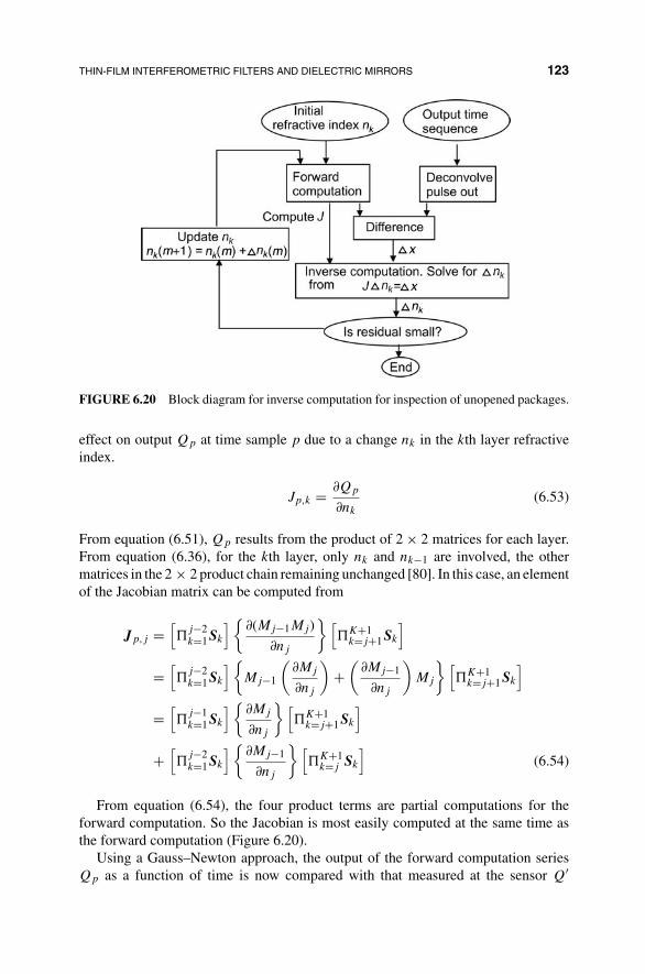
THIN-FILM INTERFEROMETRIC FILTERS AND DIELECTRIC MIRRORS 123
FIGURE 6.20 Block diagram for inverse computation for inspection of unopened packages.
effect on output Qp at time sample p due to a change nk in the kth layer refractiveindex.
Jp,k = ∂Qp
∂nk
(6.53)
From equation (6.51), Qp results from the product of 2 × 2 matrices for each layer.From equation (6.36), for the kth layer, only nk and nk−1 are involved, the othermatrices in the 2 × 2 product chain remaining unchanged [80]. In this case, an elementof the Jacobian matrix can be computed from
Jp,j =[�
j−2k=1Sk
] {∂(Mj−1Mj)
∂nj
} [�K+1
k=j+1Sk
]
=[�
j−2k=1Sk
] {Mj−1
(∂Mj
∂nj
)+
(∂Mj−1
∂nj
)Mj
} [�K+1
k=j+1Sk
]
=[�
j−1k=1Sk
] {∂Mj
∂nj
} [�K+1
k=j+1Sk
]
+[�
j−2k=1Sk
] {∂Mj−1
∂nj
} [�K+1
k=j Sk
](6.54)
From equation (6.54), the four product terms are partial computations for theforward computation. So the Jacobian is most easily computed at the same time asthe forward computation (Figure 6.20).
Using a Gauss–Newton approach, the output of the forward computation seriesQp as a function of time is now compared with that measured at the sensor Q′

124 OPTICAL INTERFEROMETERS AND OSCILLATORS
after deconvolving the pulse out if necessary. Hence, the difference vector �yp =Qp − Q′
p is computed. The difference vector �y is now used with the Jacobianmatrix Jp,j to compute an update vector �n for the refractive indices for the layersby solving the linear equation
�y = J�n (6.55)
The refractive indices are now updated for the next (m + 1)th iteration of the gener-alized inverse algorithm (Figure 6.20) using
nm+1 = nm + �nk(m) (6.56)
We repeat loops of forward and inverse computations until the RMS of the updatevector converges to a lower limit. When the Jacobian is sparse, we use a conjugategradient algorithm [83]. The method was successfully applied and adopted in studiesin geophysics [80, 81].

PART II
LASER TECHNOLOGY FORDEFENSE SYSTEMS

CHAPTER 7
PRINCIPLES FOR BOUND ELECTRONSTATE LASERS
The word laser is derived from the acronym light amplification by stimulated emis-sion of radiation and the name maser from the acronym microwave amplification bystimulated emission of radiation. Stimulated emission refers to Bremsstrahlung radi-ation, converting energy produced from showing down of electrons into microwaveor light radiation.
For coherent electromagnetic radiation, below 1 GHz we have radio frequenciesthat are lower than microwaves and for which masers are not generally used. From1 to 100 GHz, we have microwaves that can be generated with masers (some use300 GHz as the upper limit). Between 100 and 300 GHz, radiation is sometimes calledmillimeter waves and falls between masers and lasers. Above 300 GHz, we have lightthat can be generated with lasers. Higher frequencies with more energy per photoninvolve X-rays, gamma rays, nuclear rays, and cosmic rays. X-ray lasers have alsobeen demonstrated and applied to high-resolution VLSI lithography.
Bremsstrahlung means slowing down of electrons in an electron beam to convertenergy to electromagnetic radiation. There are two types of bremsstrahlung stimulatedemission. This chapter discusses the first type, that is, lasers that generate coherentphotons from electrons jumping from a higher energy to a lower energy bound electronstate. Frequency is determined by the material energy levels. The second type ofbremsstrahlung stimulated emission is the cyclotron maser or laser (free-electron
Military Laser Technology for Defense: Technology for Revolutionizing 21st Century Warfare,First Edition. By Alastair D. McAulay.© 2011 John Wiley & Sons, Inc. Published 2011 by John Wiley & Sons, Inc.
127

128 PRINCIPLES FOR BOUND ELECTRON STATE LASERS
laser), described in Chapter 10 and 11, which is used for ultrahigh-power masers andlasers at any frequency.In Section 7.1, we list some of the significant advantages of coherent light that helprevolutionize warfare and the basic light–matter interaction process for generatinglaser light in bound electron state lasers. In Section 7.2, we describe the basic semi-conductor laser diode widely used for low-power applications, such as pumps formore powerful lasers and in arrays. In section 7.3, we discuss semiconductor opticalamplifiers.
7.1 LASER GENERATION OF BOUND ELECTRON STATE COHERENTRADIATION
We discuss the advantages of coherent radiation and then the basic light–matter in-teraction for bound electron state lasers.
7.1.1 Advantages of Coherent Light from a Laser
Coherent light has temporal coherence (Section 6.1), and spatial coherence (Sec-tions 1.3.6 and 3.2.2). Some advantages of coherent light radiation are discussed inthis section from the system point of view.
1. Coherent light has the ability to project energy over a distance, such as for alaser pointer, a laser designator, a range finder, or a laser weapon (Chapter 12).
2. Coherent light can be focused to a small region for a weapon or for densecompact optical disk storage.
3. Coherent light can detect chemical and biological weapons because the wave-length is comparable to the size of molecules and bacteria.
4. Frequencies of around 1014 Hz provide the potential to send 1014 bit/s, onecycle is on or off, which corresponds to a hundred thousand billion bits persecond through air or in fiber. This is important for optical communicationsand the optical fiber-connected Internet.
5. The short wavelength allows high-resolution imaging for satellites and opera-tion with day or night vision cameras.
A significant advantage of coherent radiation is that the energy is close to a singlefrequency that produces an entropy (or uncertainty) approaching zero: there is nouncertainty in a sine wave. In contrast, thermal energy from burning coal, or to someextent from the sun, is disordered with high entropy. When coherent light enters asystem, it lowers the system entropy, whereas when a system is heated, it increases theentropy. Higher entropy lowers efficiency. In a chemical laser, the heat generated in achemical reaction is used to pump a laser directly to create coherent electromagneticwaves. Direct generation of high-power coherent light can be efficient in generation(Chapter 10) and distribution, especially in future, as some predict that energy will
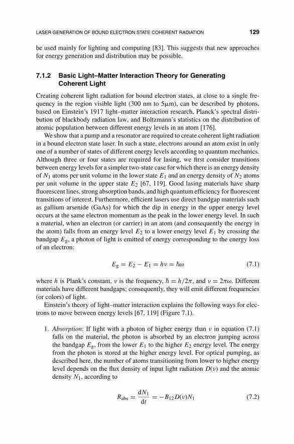
LASER GENERATION OF BOUND ELECTRON STATE COHERENT RADIATION 129
be used mainly for lighting and computing [83]. This suggests that new approachesfor energy generation and distribution may be possible.
7.1.2 Basic Light–Matter Interaction Theory for GeneratingCoherent Light
Creating coherent light radiation for bound electron states, at close to a single fre-quency in the region visible light (300 nm to 5�m), can be described by photons,based on Einstein’s 1917 light–matter interaction research, Planck’s spectral distri-bution of blackbody radiation law, and Boltzmann’s statistics on the distribution ofatomic population between different energy levels in an atom [176].
We show that a pump and a resonator are required to create coherent light radiationin a bound electron state laser. In such a state, electrons around an atom exist in onlyone of a number of states of different energy levels according to quantum mechanics.Although three or four states are required for lasing, we first consider transitionsbetween energy levels for a simpler two-state case for which there is an energy densityof N1 atoms per unit volume in the lower state E1 and an energy density of N2 atomsper unit volume in the upper state E2 [67, 119]. Good lasing materials have sharpfluorescent lines, strong absorption bands, and high quantum efficiency for fluorescenttransitions of interest. Furthermore, efficient lasers use direct bandgap materials suchas gallium arsenide (GaAs) for which the dip in energy in the upper energy leveloccurs at the same electron momentum as the peak in the lower energy level. In sucha material, when an electron (or carrier) in an atom (and consequently the energy inthe atom) falls from an energy level E2 to a lower energy level E1 by crossing thebandgap Eg, a photon of light is emitted of energy corresponding to the energy lossof an electron:
Eg = E2 − E1 = hν = �ω (7.1)
where h is Plank’s constant, ν is the frequency, � = h/2π, and ν = 2πω. Differentmaterials have different bandgaps; consequently, they will emit different frequencies(or colors) of light.
Einstein’s theory of light–matter interaction explains the following ways for elec-trons to move between energy levels [67, 119] (Figure 7.1).
1. Absorption: If light with a photon of higher energy than ν in equation (7.1)falls on the material, the photon is absorbed by an electron jumping acrossthe bandgap Eg, from the lower E1 to the higher E2 energy level. The energyfrom the photon is stored at the higher energy level. For optical pumping, asdescribed here, the number of atoms transitioning from lower to higher energylevel depends on the flux density of input light radiation D(ν) and the atomicdensity N1, according to
Rabs = dN1
dt= −B12D(ν)N1 (7.2)
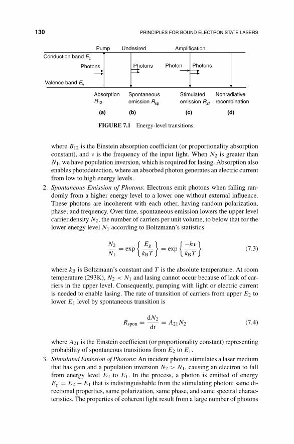
130 PRINCIPLES FOR BOUND ELECTRON STATE LASERS
Amplification
Photons PhotonsPhoton
Undesired
AbsorptionR12
Spontaneousemission Rsp
Stimulatedemission R21
Nonradiativerecombination
Conduction band Ec
Valence band Ev
Photons
Pump
(a) (b) (c) (d)
FIGURE 7.1 Energy-level transitions.
where B12 is the Einstein absorption coefficient (or proportionality absorptionconstant), and ν is the frequency of the input light. When N2 is greater thanN1, we have population inversion, which is required for lasing. Absorption alsoenables photodetection, where an absorbed photon generates an electric currentfrom low to high energy levels.
2. Spontaneous Emission of Photons: Electrons emit photons when falling ran-domly from a higher energy level to a lower one without external influence.These photons are incoherent with each other, having random polarization,phase, and frequency. Over time, spontaneous emission lowers the upper levelcarrier density N2, the number of carriers per unit volume, to below that for thelower energy level N1 according to Boltzmann’s statistics
N2
N1= exp
{Eg
kBT
}= exp
{−hν
kBT
}(7.3)
where kB is Boltzmann’s constant and T is the absolute temperature. At roomtemperature (293K), N2 < N1 and lasing cannot occur because of lack of car-riers in the upper level. Consequently, pumping with light or electric currentis needed to enable lasing. The rate of transition of carriers from upper E2 tolower E1 level by spontaneous transition is
Rspon = dN2
dt= A21N2 (7.4)
where A21 is the Einstein coefficient (or proportionality constant) representingprobability of spontaneous transitions from E2 to E1.
3. Stimulated Emission of Photons: An incident photon stimulates a laser mediumthat has gain and a population inversion N2 > N1, causing an electron to fallfrom energy level E2 to E1. In the process, a photon is emitted of energyEg = E2 − E1 that is indistinguishable from the stimulating photon: same di-rectional properties, same polarization, same phase, and same spectral charac-teristics. The properties of coherent light result from a large number of photons

LASER GENERATION OF BOUND ELECTRON STATE COHERENT RADIATION 131
in coherent lockstep. The rate of stimulated emissions is
Rstim = dN2
dt= B21N2D(ν) (7.5)
where B21 is the Einstein coefficient for stimulated emission and D(ν) is theflux density of light in the cavity at frequency ν.
4. Nonradiative Deexcitation: An electron can fall from a higher to a lower energylevel without generating a photon. The energy lost by the carrier appears in otherforms, such as translational, vibrational, or rotational.
Assuming that N1 and N2 are the electron densities in lower and upper energystates, from equations (7.2), (7.4) and (7.5), the up and down rates between the twostates must be equal at thermal equilibrium:
Spontaneous emission︷ ︸︸ ︷A21N2 +
Stimulated emission︷ ︸︸ ︷B21N2D(ν) =
Absorption︷ ︸︸ ︷B12D(ν)N1 (7.6)
Using Boltzmann’s equation, equation (7.3), to replace N2/N1 in equation (7.6) andwith the blackbody radiation law from [176]
D(ν) = 8πn3hν3
c3(exp{hν/(kBT ) − 1}) (7.7)
gives Einstein’s relation between A’s and B’s [176]:
Spontaneous coefficient︷︸︸︷A21 = 8πn3hν3
c3
Stimulated coefficient︷︸︸︷B21 (7.8)
and
Absorption coefficient︷︸︸︷B21 =
Stimulated coefficient︷︸︸︷B12 (7.9)
where the speed of light in material of refractive index n is c = c0/n, with c0 thespeed of light in vacuum or air. Equation (7.8) shows that the Einstein coefficient forthe rate of spontaneous emission, causing the incoherent noise, is proportional to theEinstein coefficient for the rate of stimulated emission, the desired coherent light. Sowe cannot eliminate noise from the laser with useful output. Equation (7.9) showsthat the Einstein coefficient for the rate of stimulated emission and that for the rateof absorption (or pumping) are equal. Consequently, two properties are required forlasing in a suitable material.
The first criterion for lasing is that the rate of stimulated emission generating laserlight must be greater than the rate of absorption (otherwise all the light generated is
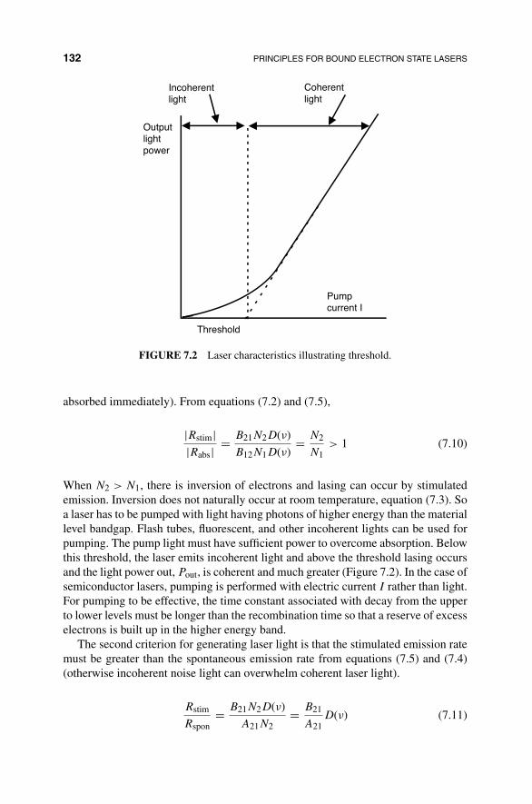
132 PRINCIPLES FOR BOUND ELECTRON STATE LASERS
Pumpcurrent I
Outputlightpower
Threshold
Coherentlight
Incoherentlight
FIGURE 7.2 Laser characteristics illustrating threshold.
absorbed immediately). From equations (7.2) and (7.5),
|Rstim||Rabs| = B21N2D(ν)
B12N1D(ν)= N2
N1> 1 (7.10)
When N2 > N1, there is inversion of electrons and lasing can occur by stimulatedemission. Inversion does not naturally occur at room temperature, equation (7.3). Soa laser has to be pumped with light having photons of higher energy than the materiallevel bandgap. Flash tubes, fluorescent, and other incoherent lights can be used forpumping. The pump light must have sufficient power to overcome absorption. Belowthis threshold, the laser emits incoherent light and above the threshold lasing occursand the light power out, Pout, is coherent and much greater (Figure 7.2). In the case ofsemiconductor lasers, pumping is performed with electric current I rather than light.For pumping to be effective, the time constant associated with decay from the upperto lower levels must be longer than the recombination time so that a reserve of excesselectrons is built up in the higher energy band.
The second criterion for generating laser light is that the stimulated emission ratemust be greater than the spontaneous emission rate from equations (7.5) and (7.4)(otherwise incoherent noise light can overwhelm coherent laser light).
Rstim
Rspon= B21N2D(ν)
A21N2= B21
A21D(ν) (7.11)

SEMICONDUCTOR LASER DIODES 133
+V
0LW
Lightout
Lightout
Current I
(a) (b)
FIGURE 7.3 Laser diode: (a) structure and (b) symbol.
For equation (7.11), we need a high concentration of photons D(ν) in the laser. This isachieved with a resonant cavity that may be formed by means of two parallel mirrorsor reflectors (Section 6.2), or an integrated optic ring resonator [96, 102, 105, 106]. Insummary, we need a pump to provide carrier inversion, equation (7.10), and a resonantcavity to make sure that coherent light surpasses incoherent light, equation (7.11).
7.2 SEMICONDUCTOR LASER DIODES
Semiconductor laser diodes convert electric current into a beam of coherent light.They are efficient (over 50%), small (0.5 mm), and robust and are used as sources inlong-haul telecommunication, compact disk players, laser pointers, and integrated andfiber-optic sensors, as well as for pumping solid-state lasers in military designator andrange finding systems. Groups of laser diodes may be used for laser weapon systems(Section 7.2.4). Figure 7.3a shows a simple structure. A thin undoped intrinsic layerof a direct bandgap material such as GaAs is sandwiched between n-doped (excesselectrons) and p-doped (reduced electrons) layers to form a p–n junction that acts asa diode. The sandwiched active layer is made from a slice of an approximately 30 cmdiameter GaAs crystal which has been diced into thousands of small millimeter-sizerectangular pieces, one for each laser diode. The cleaved faces at left and right sidesof a piece reflect sufficient light to act as mirrors that form a cavity to bounce photonsback and forth inside the laser diode. An electric current flows down through thejunction to pump electrons in the intrinsic layer to a higher energy level for inversion.Light is emitted at the right as shown in Figure 7.3a. Figure 7.3b shows the symbolfor a laser diode. Coherent light is emitted when forward current exceeds the valueneeded to overcome absorption.
7.2.1 p–n Junction
Figure 7.4 shows the energy level versus the momentum k (wave vector for elec-tron). The upper energy level (conductance level c), the n-doped level, holds excesselectrons. The Fermi level Efc is the level below which the probability of findingan electron is greater than a half. Increasing the doping level will raise Efc. Thelower energy level (valence level v), the p-doped level, holds excess holes (absence of
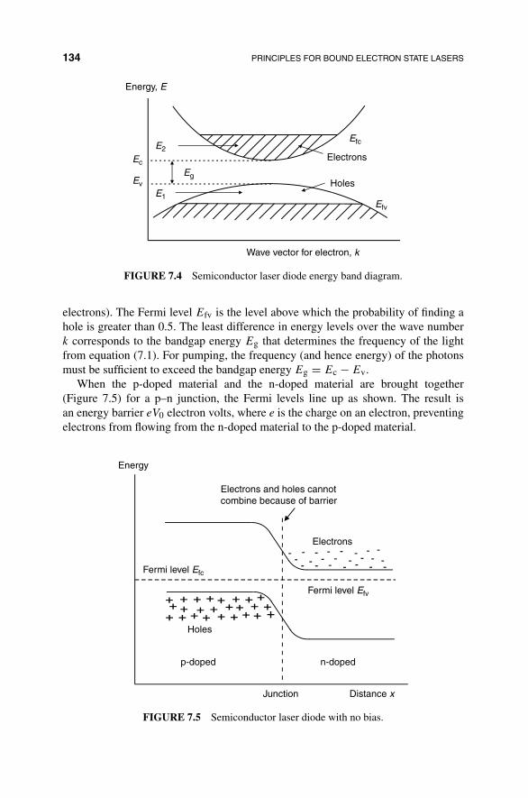
134 PRINCIPLES FOR BOUND ELECTRON STATE LASERS
Energy, E
Wave vector for electron, k
Ec
Ev
Eg
Efc
Efv
Electrons
Holes
E2
E1
FIGURE 7.4 Semiconductor laser diode energy band diagram.
electrons). The Fermi level Efv is the level above which the probability of finding ahole is greater than 0.5. The least difference in energy levels over the wave numberk corresponds to the bandgap energy Eg that determines the frequency of the lightfrom equation (7.1). For pumping, the frequency (and hence energy) of the photonsmust be sufficient to exceed the bandgap energy Eg = Ec − Ev.
When the p-doped material and the n-doped material are brought together(Figure 7.5) for a p–n junction, the Fermi levels line up as shown. The result isan energy barrier eV0 electron volts, where e is the charge on an electron, preventingelectrons from flowing from the n-doped material to the p-doped material.
Distance x
Energy
p-doped n-doped
-- --- -
---- --
---
- --
--- -
-
Electrons
Holes
Electrons and holes cannotcombine because of barrier
Junction
Fermi level Efv
Fermi level Efc
FIGURE 7.5 Semiconductor laser diode with no bias.

SEMICONDUCTOR LASER DIODES 135
Distance x
Energy
p-doped n-doped
-- -- - --- -
- --- -- -
- -- - -- -
-- --- - Electrons
Holes
Electrons and holes overlap in junction
Junction
eV0Fermi level EfcFermi level Efv
FIGURE 7.6 Forward-biased semiconductor laser diode.
By applying a forward voltage bias Vf across the diode from a battery or a source(Figure 7.6), the barrier is reduced from e(V0) to e(V0 − Vf ) and electrons in then-doped material now orient directly above the holes in the so-called depletion width.Electrons can now readily transfer from higher to lower energy levels.
Figure 7.7 shows how activity is encouraged to focus at the junction in a doubleheterostructure laser diode. Figure 7.7a shows the schematic symbol for a laser diode.To confine carriers (electrons and holes) in the vicinity of the junction we sandwicha thin layer, called the active or intrinsic “i” layer, between the n- and p-doped mate-rials to form a heterojunction or double heterostructure (Figure 7.7b). This improvesperformance by confining transfers between layers and by trapping light in the active
Current I
Light out
p ni
Reduced bandgapin intrinsic layer
Ec
Ev
Waveguide formedby intrinsic layer
Optical mode field for waveguide confinement
Refractiveindex
Optical field
(a)
(b)
(c)
(d)
(e)
FIGURE 7.7 Double heterostructure laser diode: (a) symbol, (b) structure, (c) confinementwith reduced bandgap, (d) refractive index for waveguide confinement, and (e) optical modefield for waveguide confinement.

136 PRINCIPLES FOR BOUND ELECTRON STATE LASERS
L
E0
Cleaved facetreflectance isR1 = 0.3
Cleaved facetreflectance isR2 = 0.3
Power gain gAbsorption α
FIGURE 7.8 Steady-state condition in laser diode cavity at threshold.
layer. First, the active layer has a smaller bandgap than elsewhere (Figure 7.7c), whichallows transfer between layers to be confined to the active layer. Second, by makingthe refractive index in the active layer larger than the surrounding n- and p-doped layerrefractive indices, the light generated is trapped in an index guiding waveguide [130],as shown in Figure 7.7d. The lowest order mode field for the generated light showsthat light is trapped in the active layer shown in Figure 7.7e.
7.2.2 Semiconductor Laser Diode Gain
The cleaved facets of the semiconductor laser diode act as reflectors for a Fabry–Perotresonator (Section 6.2), having a power reflectivity of
Rm =(
n − 1
n + 1
)2
(7.12)
where we assumed refractive index n = 1 for air. For n = 3.5, a typical value ofrefractive index for GaAs, power reflectivity is Rm = 30%. The gain of the lasingmaterial is sufficient to overcome the cavity loss at the imperfect mirrors. The re-flectivity of the rear facet is often enhanced with optical reflective coating leavingonly sufficient light for a photodetector to provide amplitude feedback control. Thepump must provide sufficient current I to overcome losses at the threshold for lasing,(Figures 7.2).
We now develop the equations for gain and resonance by taking an approachdifferent from that used in Section 6.2, achieving results in a more illustrative formfor our purpose [176]. If g is the power gain per unit length in the active material andα is the internal absorption per unit length, we can write for a round-trip betweenfacets in the cavity of length L [176] (Figure 7.8) the amplitude gain (factor 2 fortwo-way and square root for amplitude) as [eg2L]1/2 = egL and the absorption as[e−α2L]1/2 = e−αL. The light bounces off the two facets with power reflectivities R1and R2 so that the amplitude loss for a round-trip is
√R1R2. The phase change during
a round-trip is 2kL. Therefore, for a steady state, the field E0 after a round-trip equalsthat at the start:
E0 = E0√
R1R2egLe−αLej2kL (7.13)
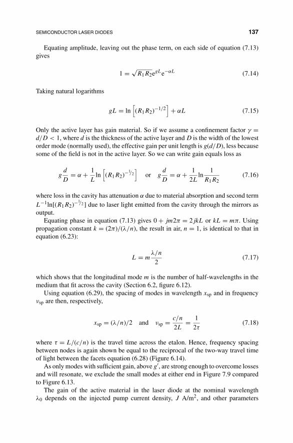
SEMICONDUCTOR LASER DIODES 137
Equating amplitude, leaving out the phase term, on each side of equation (7.13)gives
1 = √R1R2egLe−αL (7.14)
Taking natural logarithms
gL = ln[(R1R2)−1/2
]+ αL (7.15)
Only the active layer has gain material. So if we assume a confinement factor γ =d/D < 1, where d is the thickness of the active layer and D is the width of the lowestorder mode (normally used), the effective gain per unit length is g(d/D), less becausesome of the field is not in the active layer. So we can write gain equals loss as
gd
D= α + 1
Lln
[(R1R2)−
1/2]
or gd
D= α + 1
2Lln
1
R1R2(7.16)
where loss in the cavity has attenuation α due to material absorption and second termL−1ln[(R1R2)−1/2 ] due to laser light emitted from the cavity through the mirrors asoutput.
Equating phase in equation (7.13) gives 0 + jm2π = 2jkL or kL = mπ. Usingpropagation constant k = (2π)/(λ/n), the result in air, n = 1, is identical to that inequation (6.23):
L = mλ/n
2(7.17)
which shows that the longitudinal mode m is the number of half-wavelengths in themedium that fit across the cavity (Section 6.2, figure 6.12).
Using equation (6.29), the spacing of modes in wavelength xsp and in frequencyνsp are then, respectively,
xsp = (λ/n)/2 and νsp = c/n
2L= 1
2τ(7.18)
where τ = L/(c/n) is the travel time across the etalon. Hence, frequency spacingbetween nodes is again shown be equal to the reciprocal of the two-way travel timeof light between the facets equation (6.28) (Figure 6.14).
As only modes with sufficient gain, above g′, are strong enough to overcome lossesand will resonate, we exclude the small modes at either end in Figure 7.9 comparedto Figure 6.13.
The gain of the active material in the laser diode at the nominal wavelengthλ0 depends on the injected pump current density, J A/m2, and other parameters

138 PRINCIPLES FOR BOUND ELECTRON STATE LASERS
FIGURE 7.9 Longitudinal modes of frequency in a laser diode.
according to [57, 176]
g = ηqλ20J
8πen2dν(7.19)
where ηq is the internal quantum efficiency for converting electrons to photons, e ischarge of an electron, n is the refractive index of active layer, d is the active layerthickness and ν is the linewidth of the laser output. The current needed to initiatelasing in the steady state, the threshold current density, Jth, occurs when gain equalsloss. So substituting g from equation (7.19) into equation (7.16) and solving for Jthgives (J > Jth for lasing)
Jth = 8πen2νD
ηqλ20
(α + 1
Lln
1
R1R2
)(7.20)
Across the active layer in the diode, absorption loss can be written as Ploss = αPz
and gain can be written as Pgain = gPz. Therefore, an internal efficiency can be written(with g modified for confinement) as
η = Pgain − Ploss
Pgain= g(d/D) − α
g(d/D)(7.21)
or using equation (7.16) as
η = (1/2L)ln (1/R1R2)
α + (1/2L)ln (1/R1R2)(7.22)

SEMICONDUCTOR LASER DIODES 139
The optical power into the laser diode is
Popt−in = J
e(L × W)ηqhν (7.23)
where J is the current density, J/e is the number of electrons per second per area,L × W is area of active layer of length L and width W , ηq is the number of photonsproduced per electron, and hν is the energy per photon. The optical power out of thelaser diode is, using efficiency η from equation (7.22),
Popt−out = ηPopt−in = (1/2L)ln(1/R1R2)
α + (1/2L)ln(1/R1R2)
(J
eηq(L × W)hν
)(7.24)
The electrical input power Pelec−in differs from the optical input power Popt−in byincluding I2R loss to get current onto the chip, in place of ηq in equation (7.23):
Pelec−in = J
e(L × W) hν + [J(L × W)]2Rseries (7.25)
So the total so-called wall plug efficiency is obtained from equations (7.24) and(7.25) by
ηwall = Popt−out
Pelec−in(7.26)
7.2.3 Semiconductor Laser Dynamics
The simplest dynamic model of a bound electron state laser involves two first-orderdifferential equations, called rate equations, that describe the interaction betweentwo reservoirs: one for the electronic carrier density, N carriers or electrons percubic meter, and the other for the photon density, Nph photons per cubic meter. Theinteraction is complicated because the two reservoirs have different time constants.
For a laser diode, the level in the carrier density reservoir increases in time withthe number of carriers per cubic meter J/qd injected by the pump current density J
A/m2, where q is the charge on an electron and d is the thickness of the active layer.The level in the carrier density reservoir lowers in time due to recombination for
stimulated emission that creates photons (Section 7.1.2). The stimulated emission rate�vgg(N)Nph depends on the confinement factor �, (Section 7.2.2) group velocity vg,the gain g(N) = a(N − N0), which is proportional to the excess carriers N − N0 inthe reservoir, where N0 is that needed at threshold (transparency), and the number ofphotons in the photon reservoir Nph. There is also a loss due to recombination thatdoes not contribute to the generation of photons, N/τe, where 1/τe is the effective

140 PRINCIPLES FOR BOUND ELECTRON STATE LASERS
recombination rate. This can be written [75] as
∂N
∂t= J(t)
qd− �vgg(N)Nph − N
τe(N)(7.27)
The level in the photon density reservoir increases in time by the amount of themodified stimulated emission reduction �vgg(N)Nph from the carrier density reser-voir and decreases due to a photon decay time constant τph that represents the time aphoton stays in the cavity (longer for high-reflectivity mirrors). It also increases be-cause a percentage βsp of the modified spontaneous emission rate BN2, equation (7.4),is coherent with the stimulated emission. This can be written as
∂Nph
∂t= �vgg(N)Nph − Nph
τph+ βspBN2 (7.28)
In Refs [98, 109], we show that the laser diode rate equations for a single opticallyinjected laser diode, modeled by two coupled first-order equations as above, giverise to supercritical Hopf bifurcations that exactly mimic the popular Wilson–Cowanmathematical model for representing a neuron in the brain. The Wilson–Cowan modelmay be viewed as two cross-coupled dynamical nonlinear neural networks, one exci-tatory and the other inhibitory. Varying an input parameter, the sum of input intensitiesfrom all other incoming neurons, causes the Wilson-Cowan neural oscillator to movethrough a supercritical Hopf bifurcation so as to switch its output from a stable offstate when the input is below a firing threshold to a stable oscillation state (limit cycle)for signals above the threshold, the frequency of which depends on the level of inputstimulation. We note that a single optically injected laser diode was shown in Ref.[171] to be able to represent any form of nonlinear dynamics and chaos [153].
7.2.4 Semiconductor Arrays for High Power
Because of robustness, small size, and high efficiency, laser diodes are pervasive inthe military for low-power applications. Higher power can be achieved by combiningseveral broad-area laser diode emitters in a row on one substrate, called a bar. For stillhigher power, twenty 50 W laser bars of size 10 mm ×1 mm are arranged to form a1 kW laser shown in Figure 7.10 [6]. Combining requires skill to cost effectively mergethe beams to produce a single spatially coherent beam, and methods of maintainingbeam quality and performance characteristics are discussed in Ref. [6].
7.3 SEMICONDUCTOR OPTICAL AMPLIFIERS
For any laser that generates coherent light, a variation can be made that amplifieslight of the same wavelength. We illustrate this with a semiconductor optical amplifier(SOA) that is a variation of a laser diode. Normally, for high-power lasers (Section 8.2and Chapter 13), optical amplifiers are used to boost power in several stages. For

SEMICONDUCTOR OPTICAL AMPLIFIERS 141
FIGURE 7.10 Ray trace for 1 kW laser diode array.
light detection and ranging (lidar), (Chapter 15), and radio frequency detection andranging (radar), including millimeter radar, (Chapter 16), complex signals are neededfor optimal signal processing performance, so such signals are created electronically.They are then converted to optics when appropriate, for example, with a laser diode,and then amplified to high power with optical amplifiers.
A semiconductor optical amplifier (SOA) differs from a laser diode in that itavoids resonance. The reflecting facets of the semiconductor laser chip are coatedwith antireflection coatings (Section 6.3.1.3). If remnants of the resonance still showup noticeably, the SOA is known as a Fabry–Perot SOA. If the resonances are virtuallyeliminated, the SOA is known as a traveling-wave SOA. To further reduce resonancebetween front and rear facets, the waveguide is angled as shown in Figure 7.11.
FIGURE 7.11 Photograph of semiconductor optical amplifier.

142 PRINCIPLES FOR BOUND ELECTRON STATE LASERS
FIGURE 7.12 Photograph showing fiber coupling into a semiconductor optical amplifier.
Wires coming up in the center provide electric current for the power required foramplification. The current spreads across the chip into the waveguide. Light passingthrough the gain material in the waveguide is amplified, generally by as much as 1000times. Thus, 1 �W in becomes 1 mW out. If too much power is entered, it will damagethe output side of the waveguide, unless specifically designed with tapers.
In the case of an SOA, laser light must be channeled into and out of the active layerwaveguide as input and output, respectively, to the amplifier. This can be accomplishedwith a lens or by machining a fiber to the small size of the waveguide, small because therefractive index of III–V materials is around 3.5. Figure 7.12 shows the coupling withfiber. The fiber core, although only 8 �m in diameter, should be pointed and finishedwith an antireflection coating. Because of the high amplification and nonlinear natureof saturation, many nonlinear processes can be performed with low-power inputs,clipping, frequency changing, and cleaning up pulses [93]. Analysis and modeling ofsemiconductor optical amplifiers is described in Ref. [25] and some of our researchin Refs [91, 92, 94].

CHAPTER 8
POWER LASERS
Powerful laser light from 1 W to many gigawatts can be obtained from solids(Nd:YAG-doped glass), liquids (dye lasers) or gases (carbon dioxide, oxygen–iodine).Semiconductor lasers (Chapter 7), can be used for a 1 kW laser (or higher power) bymerging outputs for an array of laser diode bars in a way that preserves beam quality(Figure 7.10). A high-power solid-state laser is described in Chapter 13 for allowingnuclear weapon development in an age of test-ban treaties. The free-electron laser,rapidly maturing for very high power from kilowatts to gigawatts, does not dependon bound electron states and is described in Section 11.1.
In discussing power, we must separate continuous wave lasers that remain onfor over a second from pulse lasers that are on for only a small part of a second.Pulsed lasers are characterized by pulse energy: peak power times pulse duration.Both energy and duration affect the nature of the impact on the target, the averagepower for driving the laser, the weight, and the cost. Methods of creating pulsedlasers from continuous ones are described in Chapter 9. High power is often attainedby following the laser with a series of optical amplifiers, which are often identical tothe initiating laser except for the absence of a resonating cavity (mirrors removed).In this case, a pulse shaper ensures high temporal coherence and spatial filters (apinhole) after each amplifier ensure high spatial coherence for good beam quality atthe final output (Chapter 3). In Section 12.2.2, we describe adaptive optics methodsfor improving spatial coherence.
In Section 8.1 of this book, we discuss characteristics of high-power lasers. InSection 8.2, we consider solid-state lasers and frequency doubling of solid-state lasers
Military Laser Technology for Defense: Technology for Revolutionizing 21st Century Warfare,First Edition. By Alastair D. McAulay.© 2011 John Wiley & Sons, Inc. Published 2011 by John Wiley & Sons, Inc.
143

144 POWER LASERS
for visible green light. In Section 8.3, we describe gas dynamic principles, gas dynamiccarbon dioxide power lasers used for shooting down cruise and sidewinder missiles in1983, and chemical oxygen–iodine lasers (COIL) used in the Airborne Laser (ABL)to target intercontinental ballistic missiles (ICBMs) and in the Advanced TacticalLaser (ATL) to target armored vehicles.
8.1 CHARACTERISTICS
Power lasers can be categorized by wavelength, power, type, material (gas, solid state,liquid), fiber, semiconductor, pumping technology, continuous wave, or pulse length.Selecting a laser for an application must also include weight, cost, beam quality, andefficiency.
8.1.1 Wavelength
Wavelength is one of the most important characteristics. For bound electron lasers,wavelength depends on the material bandgap; only a few easy-to-work-with materialswill produce high power economically. According to diffraction (Chapter 3), light ofa certain wavelength is relatively unaffected by nonabsorbing particles having a sizeless than the wavelength while objects larger than the wavelength will be scattered orabsorbed. This effect can be observed when waves strike large versus small rocks closeto a beach. For some substances where the wavelength is similar to the molecule size,the particle will resonate and absorb the wave energy, for example, water vapor in theatmosphere (Chapter 15). Some applications require visible light, target designators,and spotter lasers, while others prefer invisible infrared (IR) light, range finders, andheat damage lasers.
Sometimes we prefer an eye-safe laser to protect our troops: lasers with emissionwavelengths longer than 1.4 �m are often called eye safe because light in this wave-length range is strongly absorbed in the eye’s cornea and lens and therefore cannotreach the significantly more sensitive retina. This makes erbium lasers and erbium-doped fiber amplifiers used in 1.5 �m telecommunication systems less dangerous thanNd:YAG 1 �m lasers with similar output powers. At longer wavelengths, a CO2 laserat 10.4 �m, the cornea absorption depth is small, energy is concentrated in a smallvolume along the surface, and the cornea surface is damaged, apparently a painfulinjury. Of course, the peak power and energy in a light pulse reaching the eye are alsocritical. Extensive safety documents and regulations apply to lasers.
8.1.2 Beam quality
For a laser beam to deliver energy efficiently to a distant target it must have goodbeam quality, which means high temporal and spatial coherence and suitable beamconvergence (depends on geometry) (Chapter 3). Damaging vehicles with lasers re-quires high-power lasers similar to those used in manufacturing, where the ability tofocus a Gaussian beam to a small spot for cutting and welding has led to a specificquality measurement, spot size times convergence angle (see left side of Figure 8).
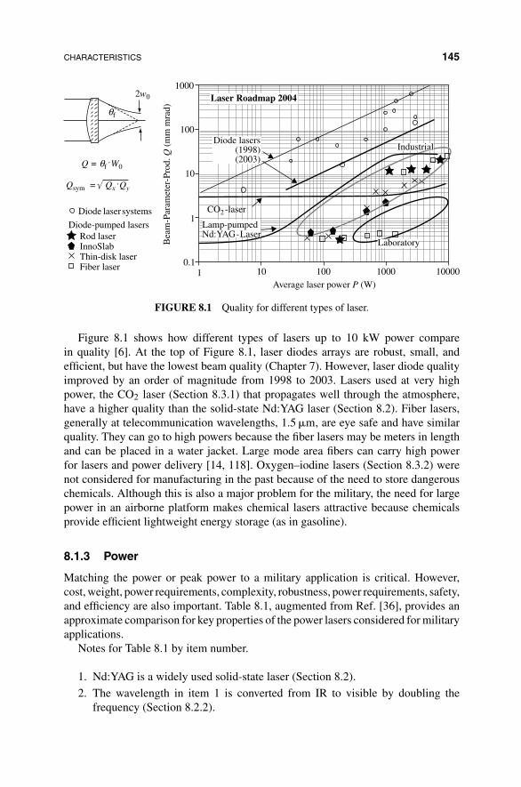
CHARACTERISTICS 145
Rod laserInnoSlabThin-disk laserFiber laser
Diode laser systems
Diode-pumped lasers
1 10 100 1000 10000Average laser power P (W)
Laboratory
1000
100
10
1
0.1
Laser Roadmap 2004
Diode lasers(1998)(2003)
Industrial
Lamp-pumpedNd:YAG-Laser
CO2-laser
Bea
m-P
aram
eter
-Pro
d. Q
(m
m m
rad)
2w0
θf
Q = θf .W0
Qsym = Qx .Qy√
FIGURE 8.1 Quality for different types of laser.
Figure 8.1 shows how different types of lasers up to 10 kW power comparein quality [6]. At the top of Figure 8.1, laser diodes arrays are robust, small, andefficient, but have the lowest beam quality (Chapter 7). However, laser diode qualityimproved by an order of magnitude from 1998 to 2003. Lasers used at very highpower, the CO2 laser (Section 8.3.1) that propagates well through the atmosphere,have a higher quality than the solid-state Nd:YAG laser (Section 8.2). Fiber lasers,generally at telecommunication wavelengths, 1.5 �m, are eye safe and have similarquality. They can go to high powers because the fiber lasers may be meters in lengthand can be placed in a water jacket. Large mode area fibers can carry high powerfor lasers and power delivery [14, 118]. Oxygen–iodine lasers (Section 8.3.2) werenot considered for manufacturing in the past because of the need to store dangerouschemicals. Although this is also a major problem for the military, the need for largepower in an airborne platform makes chemical lasers attractive because chemicalsprovide efficient lightweight energy storage (as in gasoline).
8.1.3 Power
Matching the power or peak power to a military application is critical. However,cost, weight, power requirements, complexity, robustness, power requirements, safety,and efficiency are also important. Table 8.1, augmented from Ref. [36], provides anapproximate comparison for key properties of the power lasers considered for militaryapplications.
Notes for Table 8.1 by item number.
1. Nd:YAG is a widely used solid-state laser (Section 8.2).
2. The wavelength in item 1 is converted from IR to visible by doubling thefrequency (Section 8.2.2).

146 POWER LASERS
TABLE 8.1 Power Lasers Approximate Properties
Peak Pulse RepetitionType Wavelength Power (W) Length Rate Efficiency
1. Nd:YAG 1.064 �m 106–1012 10 ps–100 ns 1–100 Hz 10−3
2. Doubled 532 �m 106–1012 10 ps–100 ns 1–100 Hz < 10−3
3. Extreme 351 �m 0.5 × 10¹⁵ ps–ns 0.001 Hz < 10−3
4. CO2 10.4 �m 108 10 ns–1�s 100–500 Hz 10−1
5. Iodine 1.315 �m 109–1012 160 ps–50 ns 0.014 Hz 10−2
6. KrF 249 nm 106–1010 30 ns–100 ns 1–100 Hz 10−2
7. LD array 0.475–1.6 �m 108 105 ps 105 0.58. FEL 10−6–2 mm 105 10–30 ns 0.1–1 Hz 10−2
9. Fiber 1.018, 1.5 �m 104 10−15–10−8 1011 0.03
3. Extreme refers to the most powerful lasers in development in the world, theprodigious National Ignition Facility (NIF) in the United States (Chapter 13)and the competitive Megajoule Laser in France. The NIF, currently in testphase, focuses 192 powerful Nd:YAG-doped glass lasers, each with 16 ampli-fiers, onto a single target with wavelength conversion from 1.064 �m (IR) to351 nm (UV).
4. The CO2 laser in gas dynamic form was used to disable sidewinder and cruisemissiles in the Airborne Laser Lab in 1985 (Sections 8.3.1 and 12.1.2).
5. The COIL in gas dynamic form was used in the current ABL program to shootdown nuclear-armed ICBMs entering the atmosphere (Sections 8.3.2 and 12.2).
6. A Krypton fluoride (UV) laser is included in the table because its ability togenerate high power has been demonstrated in military applications.
7. LD array refers to laser diode arrays composed of a large number of laser diodesworking together while preserving beam quality (Section 7.2.4).
8. The free-electron laser (FEL), an example of a cyclotron-based laser, is mostpromising for future destructive beams because almost any wavelength can begenerated at very high power (Section 11.1).
9. Optical fiber lasers [32] are evolving from optical fiber amplifiers [30]. Theycan replaces item 1 in some cases and can be frequency doubled as in item2. Multiple water-cooled fiber lasers may be combined. The power and effi-ciency refer to the 1.018 �m wavelength. The second wavelength, 1.5 �m, isless efficient but is eye safe.
8.1.4 Methods of Pumping
Energy is provided for population inversion for lasers and optical amplifiers (Chap-ter 7). Population inversion is achieved by several means or their combinations, suchas electrical, optical, thermal, and particle acceleration.

CHARACTERISTICS 147
8.1.4.1 Electrical Pumping Semiconductor lasers are pumped with electricalcurrent (Chapter 7). The electrons from the electric current jump to a higher energylevel to produce population inversion. Laser diodes convert electrons to photons veryefficiently. High power is achieved by combining hundreds of laser diodes to producea single beam, but maintaining quality in the beam severely limits total power. PulsedCO2 lasers may be pumped with electrical discharge (Section 8.3.1).
8.1.4.2 Optical Pumping Incoherent light such as from a flashtube can be usedto pump a pulsed laser or an optical amplifier. In this case, incoherent light is convertedto coherent light for which all the photons are in lockstep. Often lasers are pumpedwith many lower powered lasers in a cascade to provide very high power.
8.1.4.3 Chemical Pumping Heat is a product of many chemical reactions andthe thermal energy can be used to excite particles to a higher energy level (Sec-tion 8.3.2).
8.1.4.4 Gas dynamic Pumping For gas lasers, power can be substantiallyreduced by flowing the incoming cold gases or gaseous chemicals through the laserand exhausting the hot gases to prevent overheating of the active medium. Populationinversion is achieved by heating the gases to high temperature and pressure andallowing them to escape through nozzles at supersonic speeds, low temperature, andlow pressure. In this case, thermal energy causes population inversion. This form ofenergy conversion from thermal is more like the process in a steam engine.
8.1.4.5 Particle Acceleration Cyclotron (or synchrotron) pumping passes astream of electrons at relativistic speed through an evacuated tube with a periodicfield in a free-electron laser (Section 11.1). The flow of relativistic electrons, whosemass and speed depend on each other, causes oscillations with density periodicitythat provide high and low energy levels. The externally generated periodic field andthe energy of the electron gun select frequency.
8.1.5 Materials for Use with High-Power Lasers
High-power lasers described in this chapter and Chapters 9 and 10 are powerful enoughto damage optical components used at lower power levels. Consequently, special ma-terial should be used that can withstand the high-power levels without damage. Mate-rials for high-power lasers in the 1–3 �m range include fusion-cast calcium fluoride(CaF2), multispectral zinc sulfide (ZnS-MS), zinc selenide (ZnSe), sapphire (Al2O3),and fused silica (SiO2) [35]. All these materials can be obtained in blanks larger than175 mm diameter. Sapphire and calcium fluoride require more experience to fabricatethan other materials, but all these materials can be polished to the minimal beam de-viations required. The final choice of material is made based on the requirements ofa system and varies based on maximum laser power, operating environment, durabil-ity requirements, wavelength range, size required, and budget. In Section 12.2.2, we
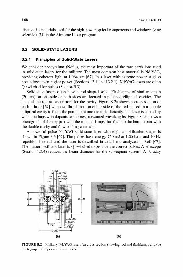
148 POWER LASERS
discuss the materials used for the high-power optical components and windows (zincselenide) [34] in the Airborne Laser program.
8.2 SOLID-STATE LASERS
8.2.1 Principles of Solid-State Lasers
We consider neodymium (Nd3+), the most important of the rare earth ions usedin solid-state lasers for the military. The most common host material is Nd:YAG,providing coherent light at 1.064 �m [67]. In a laser with extreme power, a glasshost allows even higher power (Sections 13.1 and 13.2.1). Nd:YAG lasers are oftenQ-switched for pulses (Section 9.3).
Solid-state lasers often have a rod-shaped solid. Flashlamps of similar length(20 cm) on one side or both sides are located in polished elliptical cavities. Theends of the rod act as mirrors for the cavity. Figure 8.2a shows a cross section ofsuch a laser [67] with two flashlamps on either side of the rod placed in a doubleelliptical cavity to focus the pump light into the rod efficiently. The laser is cooled bywater, perhaps with dopants to suppress unwanted wavelengths. Figure 8.2b shows aphotograph of the top part with the rod and lamps that fits into the bottom part withthe double cavity and flow cooling channels.
A powerful pulse Nd:YAG solid-state laser with eight amplification stages isshown in Figure 8.3 [67]. The pulses have energy 750 mJ at 1.064 �m and 40 Hzrepetition interval, and the laser is described in detail and analyzed in Ref. [67].The master oscillator laser is Q-switched to provide the correct pulses. A telescope(Section 1.3.4) reduces the beam diameter for the subsequent system. A Faraday
FIGURE 8.2 Military Nd:YAG laser: (a) cross section showing rod and flashlamps and (b)photograph of upper and lower parts.

SOLID-STATE LASERS 149
Masteroscillator
FaradayIsolator
KTPSHG90°
Rotator Polarizer Telescope(M = 1.2)
Output =0.5 Jat 532 nm
λ /2 Plate
λ /2 Plate
Telescope(M = 1.5)
Input =68 mJ, IR
Amphead
Amphead
Amphead
Amphead
FIGURE 8.3 Powerful Nd:YAG laser with eight amplification stages.
isolator and a half-wave plate prevent reflections from the subsequent stages fromreturning to interfere with the master oscillator. The Faraday isolator rotates thepolarization clockwise by π/4 in one direction and anticlockwise by π/4 on return,resulting in a π/2 change, so returning light is blocked by a π/2 polarizer. Thelight passes through two Nd:YAG amplifiers for which the rods have antireflectioncoatings to prevent oscillations. Then it passes through a quarter-wave plate (90◦phase angle rotator) and two more amplifiers and reflects from a mirror at left.After passing back through the quarter-wave plate, it returns to the polarizingbeam splitter with a phase change of 180◦ and the polarization is rotated by 90◦(Section 2.2.1.2). The polarizing beam splitter deflects the new polarization downto the output. A further telescope compresses the beam for high intensity intothe nonlinear KTP crystal to double the frequency from 1.064 �m to 532 nm(doubling frequency is equivalent to halving wavelength). Doubling is considered inSection 8.2.2.
Side pumping in this system is performed with laser diode arrays (Section 7.2.4)placed along the rod in place of flashtubes. The efficiency of this system is reportedas follows:
1. Laser diode efficiency is 0.35.
2. Conversion of optical pump energy to upper state population is 0.51.
3. Conversion of upper state population is 0.38.
4. Overall efficiency is 0.35 × 0.51 × 0.38 = 0.068 (7%).
In Section 13.2.1, an ultra high-power solid-state laser at the National Ignition Facilityis described.

150 POWER LASERS
8.2.2 Frequency Doubling in Solid State Lasers
High-power (upto 8 kW) infrared light is easily generated with a solid-state Nd:YAG.More than a few milliwatts of infrared laser light is dangerous to the eyes because ofthe heat it can generate on a very small spot and failure to blink as the eye does notsee infrared. Some military applications, such as range finding, target designators,countermeasures, and lidar, use a second harmonic generator to convert the IR to visi-ble green light. Nonmilitary applications include industrial, medical prostate surgery,and replacement of traffic police radar with lidar to reduce incidence of police cancer.
We derive equations for second harmonic generation (SHG) that doubles the laserfrequency f , or equivalently, as λ = c/f , halves the wavelength λ. In this case, for asolid-state Nd:YAG laser, the IR wavelength λ = 1.064 �m is converted to green atλ = 0.5 �m [67, 176]. A nonlinear crystal performs SHG.
8.2.2.1 Nonlinear Crystal for SHG Doubling is accomplished by passing theIR light into a nonlinear crystal [176]. In elastic media, the electrons are pulled backand forth by the alternating electric field of the IR light. The polarization of thecrystal medium represents an induced electric field that opposes the IR field influenceand can be detected by suitably arranging a system. Centrosymmetric crystals [176]such as sodium chloride (common salt), NaCl, cannot be used for SHG because theyhave structural symmetry about a sodium ion (Na+), shown as dots in Figure 8.4a,which causes them to polarize linearly and equally for plus and minus electric fields(Figure 8.4b). Hence, there is no change in frequency between incident light andinduced polarization.
In noncentrosymmetric crystals, such as potassium dihydrogen phosphate (KDP),or zinc sulfide (Figure 8.5a), the central sulfur ion does not see symmetry betweenNE and SW zinc ions because the zinc in this case is at different depths in these twoplaces. Consequently, there is a nonlinear relation between incident electric field andpolarization (Figure 8.5b). Electrons are more easily pulled to one side than the other.An incident field is suppressed more in the positive polarization in the crystal than inthe negative polarization. When decomposed into Fourier components, the distortedpolarization sine wave shows presence of double frequencies. Nonlinear polarization
FIGURE 8.4 Symmetric crystal: (a) structure and (b) optical polarization.

SOLID-STATE LASERS 151
Opticalpolarization
Incidentfield
(a) (b)
Positive fieldsuppressedmore than negative
Input
O O
OO
O
½
½½
½
11
3/43/4
Depth
Sulfur Zinc
+
-
FIGURE 8.5 Noncentrosymmetric crystal: (a) structure and (b) optical polarization.
(Pi) can be described by a Taylor series
Pi = E0χijEj + 2dijkEjEk + 4χijklEjEkEl + · · · (8.1)
where χij is the first-order or linear susceptibility, dijk is the second-order nonlinearsusceptibility (allows SHG), and χijkl is the third-order nonlinear susceptibility (fordifferent nonlinear effects). We are interested in the second-order nonlinear effectsfor SHG for which the polarization depends on the product of two electric fields thatcan be in different directions (j and k). In particular, from the second term on theright-hand side of equation (8.1), we desire the polarization P2ω
i , in the ith direction atdouble frequency 2ω, resulting from the interaction of two incident IR electric fields,Eω
j and Eωk , in the j and k orthogonal directions to be
Pi = 2dijkEjEk (8.2)
We convert terms P and E to exponentials using
E = Re {E0} = 1
2
{E0eiωt + E0e−iωt
} = 1
2
{E0eiωt + c.c.
}(8.3)
where c.c. is complex conjugate and subscript 0 denotes a phasor. (Note that here weused the physics nomenclature time harmonic exp{iωt} and elsewhere we have usedthe Re exp{−jωt}.) Using equation (8.3), we have several ways to produce secondharmonic (2ω) frequencies described in equation (8.2). Two ways are representative:select the two E0 fields so that their frequencies ω1 and ω2 during nonlinear mixingwill produce terms in 2ω1 or select the two E0 fields with the same frequency ω,which is half the final double frequency 2ω.
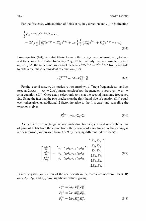
152 POWER LASERS
For the first case, with addition of fields at ω1 in j direction and ω2 in k direction
1
2P0i
ω1+ω2 ei(ω1+ω2)t + c.c.
= 2dijk
1
2
{E
ω10j eiω1t + E
ω20j eiω2t + c.c.
} 1
2
{E
ω10k eiω1t + E
ω20k eiω2t + c.c.
}(8.4)
From equation (8.4), we extract those terms of the mixing that contain ω1 + ω2 (whichadd to become the double frequency 2ω1). Note that only the two cross terms giveω1 + ω2. At the same time, we cancel the term eiω1teiω2t = ei(ω1+ω2)t from each sideto obtain the phasor equivalent of equation (8.2):
Pω1+ω20i = 2dijkE
ω10j E
ω20k (8.5)
For the second case, we do not desire the sum of two different frequencies ω1 and ω2to equal 2ω, (ω1 + ω2 = 2ω1), but rather select both frequencies to be ω or ω1 = ω2 =ω in equation (8.4). Once again select only terms at the second harmonic frequency2ω. Using the fact that the two brackets on the right-hand side of equation (8.4) equaleach other gives us additional 2 factor (relative to the first case) and canceling theexponents gives
P2ω0i = dijkE
ω0jE
ω0k (8.6)
As there are three rectangular coordinate directions (x, y, z) and six combinationsof pairs of fields from three directions, the second-order nonlinear coefficient dijh isa 3 × 6 tensor (compressed from 3 × 9 by merging different index orders):
⎡⎢⎣
P2ω0x
P2ω0y
P2ω0z
⎤⎥⎦ =
⎡⎢⎣
d11d12d13d14d15d16
d21d22d23d24d25d26
d31d32d33d34d35d36
⎤⎥⎦
⎡⎢⎢⎢⎢⎢⎢⎢⎢⎣
E0xE0x
E0yE0y
E0zE0z
2E0yE0z
2E0zE0x
2E0xE0y
⎤⎥⎥⎥⎥⎥⎥⎥⎥⎦
(8.7)
In most crystals, only a few of the coefficients in the matrix are nonzero. For KDP,only d14, d25, and d36 have significant values, giving
P2ωx = 2d14E
ω0yE
ω0z
P2ωy = 2d25E
ω0xE
ω0z
P2ωz = 2d36E
ω0xE
ω0y (8.8)
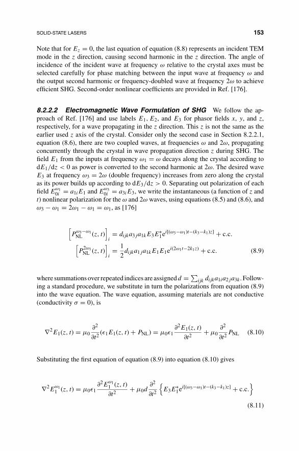
SOLID-STATE LASERS 153
Note that for Ez = 0, the last equation of equation (8.8) represents an incident TEMmode in the z direction, causing second harmonic in the z direction. The angle ofincidence of the incident wave at frequency ω relative to the crystal axes must beselected carefully for phase matching between the input wave at frequency ω andthe output second harmonic or frequency-doubled wave at frequency 2ω to achieveefficient SHG. Second-order nonlinear coefficients are provided in Ref. [176].
8.2.2.2 Electromagnetic Wave Formulation of SHG We follow the ap-proach of Ref. [176] and use labels E1, E2, and E3 for phasor fields x, y, and z,respectively, for a wave propagating in the z direction. This z is not the same as theearlier used z axis of the crystal. Consider only the second case in Section 8.2.2.1,equation (8.6), there are two coupled waves, at frequencies ω and 2ω, propagatingconcurrently through the crystal in wave propagation direction z during SHG. Thefield E1 from the inputs at frequency ω1 = ω decays along the crystal according todE1/dz < 0 as power is converted to the second harmonic at 2ω. The desired waveE3 at frequency ω3 = 2ω (double frequency) increases from zero along the crystalas its power builds up according to dE3/dz > 0. Separating out polarization of eachfield E
ω10i = a1iE1 and E
ω30i = a3iE3, we write the instantaneous (a function of z and
t) nonlinear polarization for the ω and 2ω waves, using equations (8.5) and (8.6), andω3 − ω1 = 2ω1 − ω1 = ω1, as [176]
[P
ω3−ω1NL (z, t)
]i= dijka3ja1kE3E
∗1ei[(ω3−ω1)t−(k3−k1)z] + c.c.[
P2ω1NL (z, t)
]i= 1
2dijka1ja1kE1E1ei(2ω1t−2k1z) + c.c. (8.9)
where summations over repeated indices are assignedd = ∑ijk dijka1ia2ja3k. Follow-
ing a standard procedure, we substitute in turn the polarizations from equation (8.9)into the wave equation. The wave equation, assuming materials are not conductive(conductivity σ = 0), is
∇2E1(z, t) = μ0∂2
∂t2 (ε1E1(z, t) + PNL) = μ0ε1∂2E1(z, t)
∂t2 + μ0∂2
∂t2 PNL (8.10)
Substituting the first equation of equation (8.9) into equation (8.10) gives
∇2Eω11 (z, t) = μ0ε1
∂2Eω11 (z, t)
∂t2 + μ0d∂2
∂t2
{E3E
∗1ei[(ω3−ω1)t−(k3−k1)z] + c.c.
}(8.11)

154 POWER LASERS
As E1 in equation (8.11) is dependent on the product of z-dependent terms, the left-hand side can be written in terms of phasor E1 as
∇2E(ω1)1 (z, t) = 1
2
∂2
∂z2
[E1(z)ei(ω1t−k1z) + c.c.
]
= −1
2
[k2
1E1(z) + 2ik1dE1
dz(z)
]ei(ω1t−k1z) + c.c. (8.12)
where we assumed the slowly varying amplitude approximation to eliminated2E1(z)/(dz2) with (see Section 2.1.1)
d2E1(z)
dz2 ≤ k1∂E1
∂z(z) (8.13)
Substituting equation (8.12) for the left-hand side of equation (8.11) and using∂2/∂t2 ≡ −ω2
1,
−1
2
[k2
1E1(z) + 2ik1dE1
dz(z)
]ei(ω1t−k1z) + c.c.
= −μ0ε1ω21
[E1(z)
2ei(ω1t−k1z)
]+ c.c.
−μ0dω21
[E3E
∗1ei{(ω3−ω1)t−(k3−k1)z}
]+ c.c. (8.14)
As k21 = μ0ε1ω
21, the terms like this on both sides cancel. Also, as ω3 = 2ω and
ω1 = ω, ω3 − ω1 = ω, the term ei(ω1t) at left cancels with ei(ω3−ω1)t at right:
−ikdE1
dze−i(k1z) + c.c. = −μ0dω2
1
[E3E
∗1e−i(k3−k1)z + c.c.
](8.15)
or the rate of decay of the incident field at frequency ω with distance z along thecrystal
dE1
dz= −iω1
√μ0
ε1dE3E
∗1e−i(k3−2k1)z (8.16)
where we used (μ0ω21)/(ik) ≡ −iω1
√μ0/ε1 with k = ω
√μ0ε1.
Similarly, substituting the second equation of equation (8.9) into the wave equa-tion (8.10) gives the rate of increase of the second harmonic at 2ω with distance z
along the crystal: (ω3 = 2ω)
dE3
dz= − iω3
2
√μ0
ε3dE1E
∗1ei(k3−2k1)z (8.17)
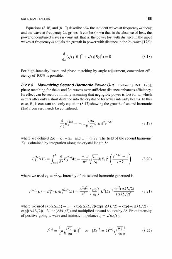
SOLID-STATE LASERS 155
Equations (8.16) and (8.17) describe how the incident waves at frequency ω decayand the wave at frequency 2ω grows. It can be shown that in the absence of loss, thepower of combined waves is constant; that is, the power lost with distance in the inputwaves at frequency ω equals the growth in power with distance in the 2ω wave [176]:
d
dz(√
ε1|E1|2 + √ε3|E3|2) = 0 (8.18)
For high-intensity lasers and phase matching by angle adjustment, conversion effi-ciency of 100% is possible.
8.2.2.3 Maximizing Second Harmonic Power Out Following Ref. [176],phase matching for the ω and 2ω waves over sufficient distance enhances efficiency.Its effect can be seen by initially assuming that negligible power is lost for ω, whichoccurs after only a short distance into the crystal or for lower intensity beams. In thiscase, E1 is constant and only equation (8.17) showing the growth of second harmonic(2ω) from zero needs be considered:
d
dzE
(2ω)3 = −iω
√μ0
ε3d|E1|2eikz (8.19)
where we defined k = k3 − 2k1 and ω = ω3/2. The field of the second harmonicE3 is obtained by integration along the crystal length L:
E(2ω)3 (L) ≡
∫ L
z=0
d
dzE
(2ω)3 dz = −iω
n2
√μ0
ε0d|E1|2
(eikL − 1
ik
)(8.20)
where we used ε3 = n2ε0. Intensity of the second harmonic generated is
I(2ω)(L) = E2ω3 (L)E∗(2ω)
3 (L) = ω2d2
n2
(μ0
ε0
)L2|E1|2 sin2(kL/2)
(kL/2)2 (8.21)
where we used exp{ikL} − 1 = exp{ikL/2}(exp{ikL/2} − exp{−ikL/2}) =exp{ikL/2}(−2i sin(kL/2)) and multiplied top and bottom by L2. From intensityof positive-going ω wave and intrinsic impedance η = √
μ0/ε0,
I(ω) = 1
2n
√ε0
μ0|E1|2 or |E1|2 = 2I(ω)
√μ0
ε0
1
n(8.22)

156 POWER LASERS
Dividing equation (8.21) by equation (8.22) gives the efficiency of second harmonicgeneration:
ηSHG = I(2ω)
I(ω) = w2d2
n2
μ0
ε0L2
(2I(ω)
√μ0
ε0
1
n
)sin2 kL/2
(kL/2)2
= 2ω2d2
n3
(μ0
ε0
)3/2
L2 sin2 kL/2
(kL/2)2 Iω (8.23)
Thus, the efficiency of second harmonic generation is proportional to the intensity ofthe input beam. So for maximizing the intensity of the second harmonic, we shouldselect material with a high value for d (KDP is good), use a longer length L, use alarge intensity input, and have the ω wave propagate at the same propagation constant(wave number) k as the 2ω wave. The last condition gives k = k(2ω) − k(ω) = 0 forwhich the phases of the two waves are matched. Unfortunately, waves copropagatingthrough a crystal at frequencies ω and 2ω do not have the same propagation constant,so k cannot equal zero. The next section addresses this issue.
8.2.2.4 Phase Matching for SHG Phase matching to achieve k = 0 isaccomplished by selecting the angle at which the incident wave at frequency ω strikesthe crystal. A uniaxial anisotropic crystal such as KDP exhibits birefringence as shownin its index ellipsoid (Figure 8.6). The equation for the index ellipsoid is
x2
no+ y2
no+ z2
ne= 1 (8.24)
x
yne
z
Ellipse withaxes 2nand 2n
o
e
x
y
no
n0
zEllipse withaxes 2noand 2ne(θ)
ne(θ)
Incomingwave
Incomingwave
(a) (b)
θ
FIGURE 8.6 Process for phase matching for SHG: (a) index ellipsoid and (b) finding angleθ for phase matching.

SOLID-STATE LASERS 157
An incoming wave sees refractive indices no for its x and y polarized components andne for its z polarized one. In a uniaxial crystal, subscripts no and ne refer to ordinaryand extraordinary directions, respectively, the latter being extraordinary because itsrefractive index differs from the other two orthogonal directions that have the ordinaryrefractive index no. If the incoming wave propagating in the z–y plane is tilted at anangle θ with respect to the z axis (Figure 8.6b), the wave strikes an elongated ellipse(marked by dashes) at normal incidence. The refractive index no is unchanged forthe perpendicular component of the incoming wave, while the refractive index for theparallel component is stretched from ne to ne(θ). The stretch is computed as follows.For the ellipse including the z, y, and incident wave directions,
y2
n2o
+ z2
n2e
= 1 (8.25)
Dropping a perpendicular from ne(θ) to the y axis gives
y = ne(θ) cos θ (8.26)
and to the z axis gives
z = ne(θ) sin θ (8.27)
Substituting equations (8.26) and (8.27) into equation (8.25) gives an equation fordetermining ne(θ) in order to achieve phase matching with a specific crystal:
1
n2e(θ)
= cos2 θ
n2o
+ sin2 θ
n2e
(8.28)
We write equation (8.28) for the second harmonic wave at frequency 2ω as
1[n
(2ω)e
]2 = cos2 θ[n
(2ω)o
]2 + sin2 θ[n
(2ω)e
]2 (8.29)
For phase matching of ω and 2ω waves, we require
n2ωe (θ) = n(ω)
o (8.30)
so that velocities and propagation constants for the two waves are equal, velocity =c/n
(2ω)e (θ) = c/n
(ω)o . Substituting equation (8.30) into the left-hand side of equa-
tion (8.29) gives an equation for which the optimum angle θ for phase matching can
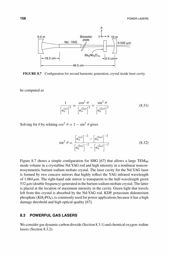
158 POWER LASERS
Brewsterplate
0.5 m
Nd : YAG
18.5 cm 2.5 cm
0.532 µm
10 mac
b
Ba2Nb5O15
46.5 cm
FIGURE 8.7 Configuration for second harmonic generation, crystal inside laser cavity.
be computed as
1[n
(ω)o
]2 = cos2 θ[n
(2ω)o
]2 + sin2 θ[n
(2ω)e
]2 (8.31)
Solving for θ by relating cos2 θ = 1 − sin2 θ gives
sin2 θ =[n
(ω)o
]−2 −[n
(2ω)o
]−2
[n
(2ω)e
]−2 −[n
(2ω)o
]−2 (8.32)
Figure 8.7 shows a simple configuration for SHG [67] that allows a large TEM00mode volume in a crystalline Nd:YAG rod and high intensity in a nonlinear noncen-trosymmetric barium sodium niobate crystal. The laser cavity for the Nd:YAG laseris formed by two concave mirrors that highly reflect the YAG infrared wavelengthof 1.064 �m. The right-hand side mirror is transparent to the half-wavelength green532 �m (double frequency) generated in the barium sodium niobate crystal. The latteris placed at the location of maximum intensity in the cavity. Green light that travelsleft from this crystal is absorbed by the Nd:YAG rod. KDP, potassium dideuteriumphosphate (KH2PO4), is commonly used for power applications because it has a highdamage threshold and high optical quality [67].
8.3 POWERFUL GAS LASERS
We consider gas dynamic carbon dioxide (Section 8.3.1) and chemical oxygen–iodinelasers (Section 8.3.2).
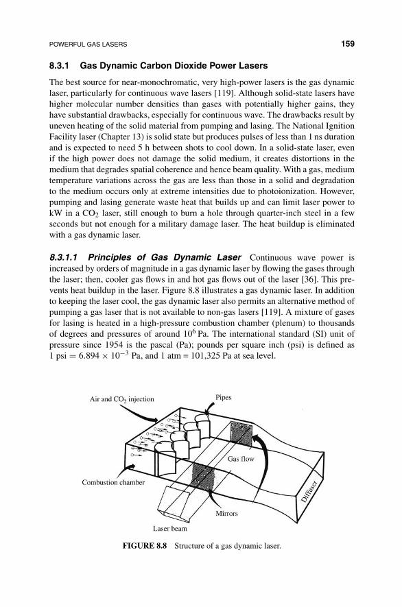
POWERFUL GAS LASERS 159
8.3.1 Gas Dynamic Carbon Dioxide Power Lasers
The best source for near-monochromatic, very high-power lasers is the gas dynamiclaser, particularly for continuous wave lasers [119]. Although solid-state lasers havehigher molecular number densities than gases with potentially higher gains, theyhave substantial drawbacks, especially for continuous wave. The drawbacks result byuneven heating of the solid material from pumping and lasing. The National IgnitionFacility laser (Chapter 13) is solid state but produces pulses of less than 1 ns durationand is expected to need 5 h between shots to cool down. In a solid-state laser, evenif the high power does not damage the solid medium, it creates distortions in themedium that degrades spatial coherence and hence beam quality. With a gas, mediumtemperature variations across the gas are less than those in a solid and degradationto the medium occurs only at extreme intensities due to photoionization. However,pumping and lasing generate waste heat that builds up and can limit laser power tokW in a CO2 laser, still enough to burn a hole through quarter-inch steel in a fewseconds but not enough for a military damage laser. The heat buildup is eliminatedwith a gas dynamic laser.
8.3.1.1 Principles of Gas Dynamic Laser Continuous wave power isincreased by orders of magnitude in a gas dynamic laser by flowing the gases throughthe laser; then, cooler gas flows in and hot gas flows out of the laser [36]. This pre-vents heat buildup in the laser. Figure 8.8 illustrates a gas dynamic laser. In additionto keeping the laser cool, the gas dynamic laser also permits an alternative method ofpumping a gas laser that is not available to non-gas lasers [119]. A mixture of gasesfor lasing is heated in a high-pressure combustion chamber (plenum) to thousandsof degrees and pressures of around 106 Pa. The international standard (SI) unit ofpressure since 1954 is the pascal (Pa); pounds per square inch (psi) is defined as1 psi = 6.894 × 10⁻³ Pa, and 1 atm = 101,325 Pa at sea level.
FIGURE 8.8 Structure of a gas dynamic laser.
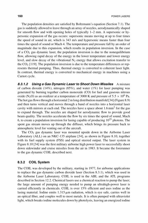
160 POWER LASERS
The population densities are satisfied by Boltzmann’s equation (Section 7.1). Thegas is suddenly allowed to leave through an array of nozzles, aerodynamically shapedfor smooth flow and with opening holes of typically 1–2 mm. A supersonic or hy-personic expansion of the gas occurs: supersonic means moving at up to four timesthe speed of sound in air, which is 343 m/s and hypersonic means faster than fourtimes the speed of sound or Mach 4. The temperature and pressure fall by an order ofmagnitude due to this expansion, which results in population inversion. In the caseof a CO2 gas dynamic laser, the population inversion is due to the nonequilibriumflow, allowing rapid decay of the energy in the lower temperature and lower energylevel, and slow decay of the vibrational N2 energy that allows excitation transfer tothe CO2 [119]. The population inversion is due to the temperature differences or rep-resents thermal pumping. Thus, thermal energy is converted to coherent laser light.In contrast, thermal energy is converted to mechanical energy in machines using aCarnot cycle.
8.3.1.2 Using a Gas Dynamic Laser to Shoot Down Missiles A mixtureof carbon dioxide (14%), nitrogen (85%), and water (1%) for laser pumping wasgenerated by burning together carbon monoxide (CO) for fuel and gaseous nitrousoxide (N2O) as an oxidizer at a temperature of 3000 K and pressure of 5.5 × 10⁶ Pa.The hot gas flows through a horizontal 2 m long distribution manifold [34] (Figure 8.9)and then turns vertical and moves through a band of nozzles into a horizontal lasercavity with mirrors at each end. The nozzles have a space about 1.6 mm2 for the gasto expand through. The nozzles are shaped for aerodynamic flow to provide goodbeam quality. The nozzles accelerate the flow by six times the speed of sound, Mach6, to create a population inversion for lasing capable of producing 1025 photons. Thespent gas stream moves up through the diffuser, which brings its pressure back toatmospheric level for venting out of the aircraft.
The CO2 gas dynamic laser was mounted upside down in the Airborne LaserLaboratory (ALL) on an NKC-135 airplane [34], as shown in Figure 8.10, togetherwith its fuel supply system (FSS) and optical steered output. The laser system inFigure 8.10 [34] was the first military airborne high power laser to successfully shootdown sidewinder and cruise missiles from the air in 1983. It became the forerunnerto the gas dynamic COIL described next.
8.3.2 COIL System
The COIL was developed by the military, starting in 1977, for airborne applicationsto replace the gas dynamic carbon dioxide laser (Section 8.3.1), which was used inthe Airborne Laser Laboratory. COIL is used in the ABL and the ATL programsdescribed in Section 12.2. Chemical lasers use a chemical reaction to pump the laser;the large amount of pumping energy needed to pump an ultrahigh-power laser iscarried efficiently in chemicals. COIL is over 15% efficient and uses iodine as thelasing material. Iodine emits 1.315 �m radiation, which is eye safe, carries well inan optical fiber, and couples well to most metals. It is often pumped with ultravioletlight, which breaks iodine molecules down by photolysis, leaving an energized iodine

POWERFUL GAS LASERS 161
FIGURE 8.9 Physical structure of the ALL gas dynamic CO2 laser that shot down a missilein 1983.
atom for population inversion. In the case of COIL, chemically pumping iodine to anexcited state is performed by excitation transfer pumping that involves two stages. Inthe first stage, oxygen is excited to a metastable state known as singlet delta oxygen,O∗
2(1):.
O2 −→ O∗2(1) (8.33)
Then, in the second stage, the singlet delta oxygen is merged with iodine to transferthe excitation from the oxygen to the iodine molecule for population inversion of theiodine:.
O∗2 + I −→ O2 + I∗ (8.34)

162 POWER LASERS
FIGURE 8.10 ALL gas dynamic CO2 laser with fuel system and optics.
After pumping, lasing causes iodine to move from the excited stage to emit photonsat 1.315 �m:
I2P1/2 −→ I2P3/2 (8.35)
We consider the two pumping stages separately: singlet delta oxygen production,equation (8.33), and excited iodine production, equation (8.34).
8.3.2.1 Singlet Delta Oxygen Production A lot of methods have been pro-posed for generation of singlet delta oxygen and many have been tested. The mostconvenient method for an airborne application, at left-hand side of Figure 8.11 [31], isto mix basic hydrogen peroxide (BHP) with chlorine, in which the word basic refersto the addition of a base such as KOH (or NaOH). The liquid BHP passes throughas many as 12,000 orifices to create drops for a high surface area contact with thegas. The chlorine gas passes through an array of orifices and most of the chlorineis used up in the chemical reaction. The chemical reaction produces heat, potassiumchloride, and oxygen in an excited state (singlet delta oxygen) with a spontaneouslifetime of 45 min. This operation occurs at left-hand side in the reactor as shown inFigure 8.11 [31] (from U.S. patent 6,072,820). Other methods for exciting (pump-ing) the oxygen are often simpler or faster but may be less efficient. For example,electric discharge, such as used for a CO2 electric discharge laser EDL, is used inRef. [146]. Another example claims to provide a laser pulse more quickly, useful in
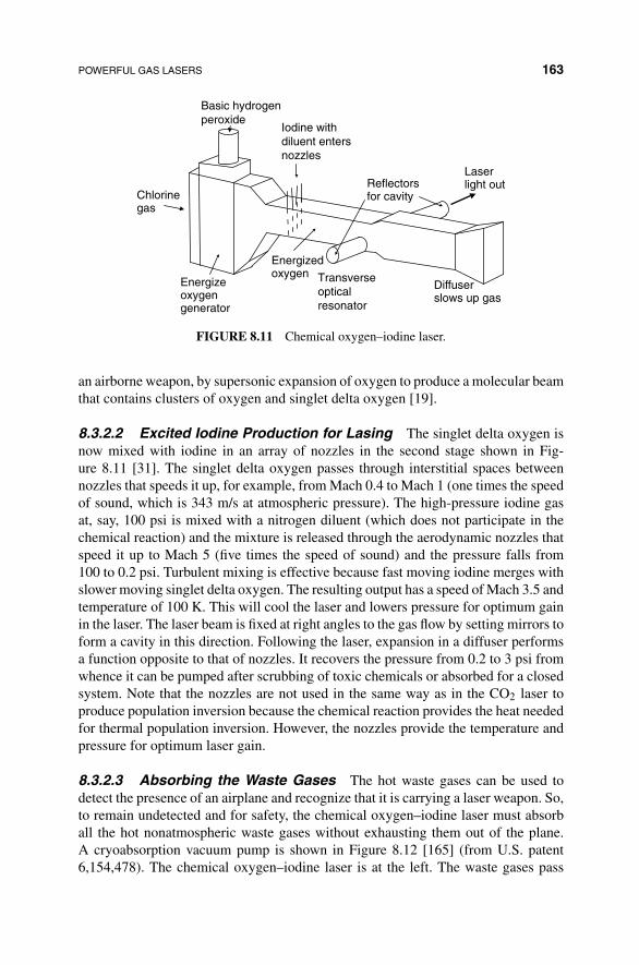
POWERFUL GAS LASERS 163
Chlorinegas
Basic hydrogenperoxide
Energizedoxygen
Iodine withdiluent entersnozzles
Energizeoxygengenerator
Laserlight out
Transverseopticalresonator
Diffuserslows up gas
Reflectorsfor cavity
FIGURE 8.11 Chemical oxygen–iodine laser.
an airborne weapon, by supersonic expansion of oxygen to produce a molecular beamthat contains clusters of oxygen and singlet delta oxygen [19].
8.3.2.2 Excited Iodine Production for Lasing The singlet delta oxygen isnow mixed with iodine in an array of nozzles in the second stage shown in Fig-ure 8.11 [31]. The singlet delta oxygen passes through interstitial spaces betweennozzles that speeds it up, for example, from Mach 0.4 to Mach 1 (one times the speedof sound, which is 343 m/s at atmospheric pressure). The high-pressure iodine gasat, say, 100 psi is mixed with a nitrogen diluent (which does not participate in thechemical reaction) and the mixture is released through the aerodynamic nozzles thatspeed it up to Mach 5 (five times the speed of sound) and the pressure falls from100 to 0.2 psi. Turbulent mixing is effective because fast moving iodine merges withslower moving singlet delta oxygen. The resulting output has a speed of Mach 3.5 andtemperature of 100 K. This will cool the laser and lowers pressure for optimum gainin the laser. The laser beam is fixed at right angles to the gas flow by setting mirrors toform a cavity in this direction. Following the laser, expansion in a diffuser performsa function opposite to that of nozzles. It recovers the pressure from 0.2 to 3 psi fromwhence it can be pumped after scrubbing of toxic chemicals or absorbed for a closedsystem. Note that the nozzles are not used in the same way as in the CO2 laser toproduce population inversion because the chemical reaction provides the heat neededfor thermal population inversion. However, the nozzles provide the temperature andpressure for optimum laser gain.
8.3.2.3 Absorbing the Waste Gases The hot waste gases can be used todetect the presence of an airplane and recognize that it is carrying a laser weapon. So,to remain undetected and for safety, the chemical oxygen–iodine laser must absorball the hot nonatmospheric waste gases without exhausting them out of the plane.A cryoabsorption vacuum pump is shown in Figure 8.12 [165] (from U.S. patent6,154,478). The chemical oxygen–iodine laser is at the left. The waste gases pass
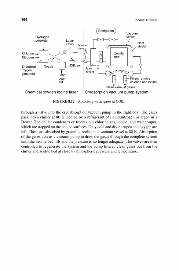
164 POWER LASERS
Nozzle Diffuser
Lasercavity
Hydrogenperoxide
ChlorineNitrogen
Energizedoxygengenerator Laser
beamout
Chemical oxygen iodine laser
RefrigerantVacuumvessel
Heatshield
Gaschiller
Zeolitebed
Clean exhaust gases
Cryosorption vacuum pump system
Filters removechlorine and iodine
Pumps
Isolationvalve
FIGURE 8.12 Absorbing waste gases in COIL.
through a valve into the cryoabsorption vacuum pump in the right box. The gasespass into a chiller at 80 K, cooled by a refrigerant of liquid nitrogen or argon in aDewar. The chiller condenses or freezes out chlorine gas, iodine, and water vapor,which are trapped on the cooled surfaces. Only cold and dry nitrogen and oxygen areleft. These are absorbed by granulite zeolite in a vacuum vessel at 80 K. Absorptionof the gases acts as a vacuum pump to draw the gases through the complete systemuntil the zeolite bed fills and the pressure is no longer adequate. The valves are thencontrolled to regenerate the system and the pump filtered clean gases out from thechiller and zeolite bed at close to atmospheric pressure and temperature.
CHAPTER 9
PULSED HIGH PEAK POWER LASERS
Continuous wave lasers can be modified to provide pulsed lasers that are preferable inmany situations. A pulse shaping network can be used to form pulses from the outputof a continuous wave laser, often used for very high laser powers. In Section 9.1 wediscuss situations in which a pulsed laser may be advantageous over a continuousone. The use of two gratings to change pulse duration is discussed. In Section 9.2, wedescribe how a laser may be mode locked to become a pulsed laser. In Section 9.3,we describe Q-switching to generate pulses. In contrast to mode locking, the laserdoes not need many modes. In Section 9.4.1, we describe how arrays of lasers can besynchronized to simultaneously focus beams in space and time.
9.1 SITUATIONS IN WHICH PULSED LASERS MAY BE PREFERABLE
A pulsed laser is preferable to a continuous wave laser in many applications.
1. Fast Changing Environments: Pulsed lasers are effective when the environmentand/or geometry is changing rapidly.
2. Lidar and Ladar: The time between sending a pulse and receiving its reflectionor scattering allows distance estimation or surface profiling for target identifi-cation and ground maps. Scanning a pulsed system detects chemical weaponsand dangerous weather patterns.
Military Laser Technology for Defense: Technology for Revolutionizing 21st Century Warfare,First Edition. By Alastair D. McAulay.© 2011 John Wiley & Sons, Inc. Published 2011 by John Wiley & Sons, Inc.
165

166 PULSED HIGH PEAK POWER LASERS
3. Low Power for Mobile Applications: For aircraft, mobile vehicles, and person-nel, pulse lasers reduce average power, resulting in smaller size and less weightfor batteries and generators. For the same peak power, a pulse with 1% dutycycle or a fixed pulse at 1/100 the repetition rate lowers average power by 100.Other possible ways of reducing power include generating it from solar energyor from the recoil when firing conventional weapons.
4. Adjusting Pulse Length: Pulse length can be adjusted with pulse shaping net-works to match an application. For example, a pair of parallel gratings cannarrow a pulse that has frequencies spread out in time: one spreads the differ-ent frequencies that are then delayed differently while the other brings themback together, having moved the energy for the frequencies closer together intime [72]. For amplifying high-power pulses, it is common to broaden the pulsebefore amplification to minimize amplifier damage and shorten it again afteramplification.
5. Energy: The energy in a pulse is its peak power times its duration. Energy, pulseduration, and wavelength must match the application. With usual power lasersfor heat damage, longer than nanosecond pulses are used.
6. Selecting Pulse Length: For very long pulses, heat damage can spread toneighboring regions, which may match a target application but could alsobe detrimental, for example, in surgery. Very short pulses (picoseconds) canvaporize materials, bypassing the liquid phase, in laser-induced breakdownspectroscopy [120]. Also, they can produce shock waves that result in metalfailure and the plasma is thought to interfere with jet engine intake. Such pulsescan break down air like lightning, creating a conducting path through whichhigh-power dangerous microwaves, not normally focusable, can travel.
7. Light Bullets: The light from a pulsed laser can look like a light bullet.For example, if the pulse length �t is 1 ns (10−9), 1 ps (10−12), and 1 fs(10−15), the length of the light bullet is �l = c�t = 3 × 10⁸�t or 0.3 m,0.3 mm, and 0.3 �m, respectively. The bullet for the modern AK74 of caliber5.45 × 39 mm has muzzle velocity 900 m/s and muzzle energy 1.39 kJ. Fora light bullet of comparable length and energy, we require a pulse length of�t = distance/speed = 39 × 10−3/(3 × 108) = 0.13 ns or 130 ps with peakpower Ppeak = energy/time = 139 × 103/(0.13 × 10−9) = 1013 W, which iswithin the reach of a Q-switched Nd:YAG laser described in this chapter.
8. Differences Between Light Bullet and Actual Bullet: There are significant dif-ferences between a light and an actual bullet. The light bullet has a Gaussianprofile, that is, higher intensity at the center. Depending on the wavelength,the light bullet may perform poorly in bad weather (Section 16.1), but in goodweather, it may lose less power during propagation than an actual bullet andbe so fast (3 × 10⁸ m/s) that movement of the target is immaterial. The laserhas a faster firing repetition rate because it can operate 100 times per second.Light power can be adjusted for range to save power. In fact, to meet the Genevaconvention of not blinding with a laser in battle, dazzle lasers must have theirpower controlled based on a range finder. The light bullet will interact with

MODE-LOCKED LASERS 167
bulletproof vests differently from a real bullet. Lasers are used to drill holesin ceramics, but reflective surfaces reduce effectiveness. Dragon plate armor,which spreads the bullet force over a wider area, is not likely to be effectiveagainst laser bullets. Explosive charges can be used to produce a light pulse inplace of firing a bullet.
9.2 MODE-LOCKED LASERS
Lasers are generally longer than half the wavelength of the light they generate. Conse-quently, there are many longitudinal modes resulting from the Fabry–Perot resonancesbetween the reflectors (Section 6.2 and Figure 6.13). The resonances in frequency areshown in Figure 6.14. The mode is determined by the number of half-cycles resonat-ing, (Figure 6.12).
The frequency spacing �ω between modes, (Figure 6.14), can be determined usingequation (6.23) by writing angular frequency at two adjacent modes, with n the modenumber, η the refractive index, and d = nλ/2 the length of the laser cavity: (usingfn = c/λn)
ωn = 2πfn = 2πc/η
λn
= −2πcn
2dη= πcn
ηd
ωn−1 = πc(n − 1)
ηd(9.1)
Subtracting the equations in equation (9.1),
�ω = ωn − ωn−1 = πc
ηd(9.2)
Hence, the frequency separation between modes is for air η = 1
�f = fn − fn−1 = �ω
2π= c
2d= 1
2τ(9.3)
where τ = d/c is the one-way travel time across the cavity (also called etalon).
9.2.1 Mode-Locking Lasers
Using exponential representation (the real part of which provides instantaneous time-dependent field), the electric field for N modes can be represented by
E(t) = A
N−1∑n=0
exp{−j(ωnt + δn)} (9.4)
where for the nth mode, wn is angular frequency and δn is its phase, and we assumeda flat gain curve over the modes for simplicity.
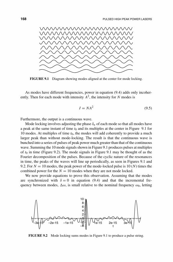
168 PULSED HIGH PEAK POWER LASERS
FIGURE 9.1 Diagram showing modes aligned at the center for mode locking.
As modes have different frequencies, power in equation (9.4) adds only incoher-ently. Then for each mode with intensity A2, the intensity for N modes is
I = NA2 (9.5)
Furthermore, the output is a continuous wave.Mode locking involves adjusting the phase δn of each mode so that all modes have
a peak at the same instant of time t0 and its multiples at the center in Figure 9.1 for10 modes. At multiples of time t0, the modes will add coherently to provide a muchlarger peak than without mode-locking. The result is that the continuous wave isbunched into a series of pulses of peak power much greater than that of the continuouswave. Summing the 10 mode signals shown in Figure 9.1 produces pulses at multiplesof t0 in time (Figure 9.2). The mode signals in Figure 9.1 may be thought of as theFourier decomposition of the pulses. Because of the cyclic nature of the resonancesin time, the peaks of the waves will line up periodically, as seen in Figures 9.1 and9.2. For N = 10 modes, the peak power of the mode-locked pulse is 10 (N) times thecombined power for the N = 10 modes when they are not mode locked.
We now provide equations to prove this observation. Assuming that the modesare synchronized with δ = 0 in equation (9.4) and that the incremental fre-quency between modes, �ω, is small relative to the nominal frequency ω0, letting
–3e-15 –2e-15 –1e-15–4–2
02468
10
1e-15 2e-15t
3e-15
FIGURE 9.2 Mode locking sums modes in Figure 9.1 to produce a pulse string.

MODE-LOCKED LASERS 169
ωn = ω0 + n�ω, and neglecting e−jω0t ,
E(t) = A
n=N−1∑n=0
e−jn �ω t (9.6)
From equation (6.23), for the nth mode having frequency fn = ωn/(2π) and refractiveindex in the cavity η,
d = nλn
2= n
2
c/η
fn
= nπc
ηωn
or ωn = nπc
ηd(9.7)
which is identical to the first equation in equation (9.1).The spacing between mode frequencies (from mode n to mode n + 1) is from
equation (9.2), �ω = πc/(ηd). For equation (9.6), there is a closed-form solution fora < 1:
N−1∑n=0
an = 1 − aN
1 − a(9.8)
Applying equation (9.8) to equation (9.6),
E(t) = A
(1 − e−jN �ω t
1 − ej �ω t
), (9.9)
Using (1 − exp{j � ω t}) = exp{j� ωt/2} (exp{−j� ωt/2} − exp{j� ωt/2}) =exp{j�ωt/2}(−j2 sin(�ωt/2)), the power from equation (9.9) is
Pt = E(t)E∗(t) = A2 sin2(N �ω t/2)
sin2(�ω t/2)(9.10)
For small deviations in times away from the peak at t = 0, sin θ → θ, and the peakintensity can be approximated from equation (9.10):
A2 (N�ωt/2)2
(�ωt/2)2 = A2N2 (9.11)
Equation (9.11) shows a peak power A2N2 that is N times greater than the powerA2N for the nonmode-locked laser with N modes from equation (9.5).
9.2.2 Methods of Implementing Mode Locking
Mode locking has the effect of bunching the output of a continuous wave laser into astring of pulses. When modes are locked, a pulse moves back and forward between

170 PULSED HIGH PEAK POWER LASERS
FIGURE 9.3 Implementing mode locking: (a) shutter in cavity and (b) shutter timing.
mirrors in the laser cavity. Mode locking can be accomplished by opening a shutterin the cavity long enough to allow the mode-locked pulse to pass through each timeit crosses the cavity (Figure 9.3a). The pulses that open the shutter are periodic ata period of twice the travel time of the pulse across the cavity between the mirrors(Figure 9.3b). Only the locked pulse will resonate and build up energy in the cavityresonator, and any nonlocked arrangement of modes will be blocked by the shutter.
9.3 Q-SWITCHED LASERS
As an alternative to mode locking and not requiring many modes, a string of pulsesof high peak power may be obtained from a laser by Q-switching. In Q-switching,propagation across the cavity is blocked while laser pumping continues to invertcarriers to the upper level. Then, when the shutter releases the excess carriers in theupper level, they drop abruptly to generate an excessive number of photons in a veryshort time, creating a very powerful pulse. Figure 9.4 shows, as a function of time,the shutter opening, the fraction of excited atoms at the upper level, and the outputpulse. While the shutter is closed, the laser pump continues to move atoms to theexcited upper state, as seen in Figure 9.4b, way past the steady state that would havebeen reached without the shutter. As the shutter opens (Figure 9.4a), excess excitedatoms rapidly drop to the ground state, generating many more photons than wouldhave been generated in the steady state without the shutter. As a result, the excited
FIGURE 9.4 Timing for Q-switched laser: (a) shutter, (b) fraction of excited atoms at theupper level and (c) output pulse.
SPACE AND TIME FOCUSING OF LASER LIGHT 171
atoms in the upper level overshoot to a much lower number. Figure 9.4c shows thelarge output pulse generated.
The shutter can be implemented with an electro-optic switch, controlled by avoltage pulse. More commonly, a saturable absorber is placed in the cavity. A sat-urable absorber blocks light transmission until the light power exceeds a threshold.This avoids the need for timing. Note that saturable absorbers perform opposite toblockers in shields or goggles that block light that is too intense and could cause eyedamage.
If ni and nt are the percentage of carriers per unit volume, initial and final, respec-tively, N0 is the total number of energized atoms, V is the volume of the cavity, h isPlank’s constant, and ν is the frequency associated with the bandgap of the material,then the total energy in a Q-switched laser pulse may be written as
E = 1
2(ni − nt)N0Vhν (9.12)
If t1 = 2d/c is the round-trip time and R is the mirror reflectivity, then 1 − R
of the light passes out of the cavity and the cavity lifetime for a photon may bewritten as
tc = t1
1 − R(9.13)
As a result, peak power can be computed from equations (9.12) and (9.13) as
Pm ≈ E
2tc(9.14)
9.4 SPACE AND TIME FOCUSING OF LASER LIGHT
Continuous wave light from a laser can be concentrated into a sequence of pulses intime by mode locking [176] (Section 9.2).
9.4.1 Space Focusing with Arrays and Beamforming
Coherent light from a group of lasers can be concentrated in space by synchronizingan array of lasers or splitting a source into many copies. In Figure 9.5, a linear 1Darray of lasers is shown steered to a point Q for illustrative purposes [162]. For M
lasers, if they are not synchronized, the average power at point Q is M times that ofa single laser. The power at point Q can be increased a further M times by arrangingthe peaks from each laser to arrive at point Q at the same time. This is accomplishedby delaying or advancing the phases from the lasers so that the phase front points inthe direction of Q as shown. From Figure 9.5, to focus at Q, the extra distance that

172 PULSED HIGH PEAK POWER LASERS
FIGURE 9.5 Diagram showing how array processing produces a pulse at a specific angle inspace.
the mth laser beam must travel relative to the zeroth laser is approximately
xm = mh sin α (9.15)
where h is the distance between lasers in the linear array and α is the pointing angle.Therefore, the additional time advance for successive lasers is
�t(α) = xm+1
c/ηp
− xm
c/ηp
= h sin(α)
c/ηp
(9.16)
where, if a fiber delay line is used, ηp is the refractive index of the material forthe delay line. For narrow frequency band ω0, the delay corresponds to a phase of�t(α)ω0, which provides the correct delay in time for nominal wavelength ω0: thephase may be adjusted to steer the beam.
The field at Q, synchronized from all M lasers, is then
E(α) = A
m=M−1∑m=0
e−jm �t(α) ω0 (9.17)
By analogy with equation (9.6) and its closed-form equation (9.9) for mode lockingin time, we can write the field for the spatial beam in closed form as
E(α) = A
(1 − e−jM �t(α) ω0
1 − ej�t(α)ω0
)(9.18)
By analogy with the intensity from equation (9.10) for mode locking in time, we canwrite the intensity for the beam pattern in space from equation (9.18) as
Pα = E(α)E∗(α) = A2 sin2(M �t(α) ω0/2)
sin2(�t(α) ω0/2)(9.19)

SPACE AND TIME FOCUSING OF LASER LIGHT 173
–15 –10 –5 0
α × 10–4 (degrees)
α
r
(a) (b)
0.25
0.5
0.75
1.0
0.05 10 15 10–45 0
00.
250.
50.
751.
0
–5
FIGURE 9.6 Plots of intensity versus beam angle for a 1D array: (a) rectangular coordinatesand (b) polar coordinates.
with �t(α) given by equation (9.16). The power versus beam steering angle is shownin rectangular coordinates in Figure 9.6a and in polar coordinates in Figure 9.6b. Thelatter is referred to as the array beam pattern.
Note that in a similar manner as for time in equation (9.11), for small spacing h
between array elements, sin θ → θ. This approximates a peak power
P(α)peak = A2 (M�t(α)ω0/2)2
(�t(α)ω0/2)2 = A2M2 (9.20)
which is M times larger (due to focusing an array) than the nonsynchronized casefor which the intensity is A2M. The analogy between time and space follows be-cause both may be regarded as dimensions in a four-dimensional space (x, y, z, ct).In practice, we use a 2D array with M lasers for which a similar computation maybe used.
9.4.2 Concentrating Light Simultaneously in Time and Space
In order for the light to arrive and add coherently at the same point in time and spaceat an angle α, we synchronize both the mode-locked pulses from different lasers toarrive together at a point Q in direction α and the light carrier frequencies betweendifferent lasers to be in phase at point Q.
9.4.2.1 Arranging Mode-Locked Pulses to Arrive Simultaneously at theSame Point The mode-locked pulses can be controlled in time by adjusting thetiming for the mode-locked shutters (Figure 9.3). Figure 9.7 shows a computer con-trolling the m�T time delay for the mth mode-locked laser.

174 PULSED HIGH PEAK POWER LASERS
FIGURE 9.7 Array and mode-locked space and time focusing with steering.
9.4.2.2 Synchronizing the Light Carrier Frequency In Figure 9.7, fiberpigtailed laser diodes couple directly into the first column of fiber-connected opticaldirectional couplers, C11 to CM1. For the couplers, the first subscript denotes the lasernumber from m = 1, . . . , M and the second subscript the coupler column number, 1or 2, as shown in Figure 9.7 [57, 89, 106].
The synchronization of lasers at light frequencies in an array to perform beam-forming for focusing is achieved by splitting a small percent p of the light emittedby the mth coupler in column 2 into the output of a successive (m + 1)th laser incolumn 1. An isolator is placed in this feedback path to ensure that the (m + 1)thlaser is synchronized to follow the frequency and phase of the mth laser [110]. Thepercentage of light not coupled back (1 − p) passes to a phase controller (or fiberdelay line). The phases are set according to �t(α)ω0, where �t(α) is determined byequation (9.16) to steer the beam in a fixed direction α from the normal to the array.
A beam expander (reverse telescope) (Section 1.3.4) provides a collimated beamthat allows beams from all lasers to overlap at the array focus point. As the outputbeam from a single laser tends to be Gaussian shaped in space with a small radius ofcurvature, the optics is designed to focus the beam to its minimum waist (Section 2.1).For a broader frequency band, we should replace the phase controller with a time delay,such as a fiber delay, line with delays �t(α).

SPACE AND TIME FOCUSING OF LASER LIGHT 175
FIGURE 9.8 Combining mode-locked lasers in an array.
9.4.2.3 Equations and Simulation for Concentrating Laser Light inTime and Space Using the results of concentrating light in time and 1D spaceseparately from Sections 9.2.1 and 9.4.1, respectively, we now combine these tosynchronize M mode-locked lasers, each having N modes as shown in Figure 9.8.The field at a point Q in space is obtained by combining the time and space fieldequations (9.6) and (9.17), respectively.
E(α, t) = A
n=N−1∑n=0
m=M−1∑m=0
e−j(m �t(α) ω0−n �ω t) (9.21)
The power P(α, t) at point P for a given angle α and a specific time t is computedfrom
P(α, t) = E(α, t)E∗(α, t) (9.22)
FIGURE 9.9 Field concentrated in space and time.

176 PULSED HIGH PEAK POWER LASERS
Power at point Q in Figure 9.8 from equations (9.21) and (9.22), for a 1D array,is plotted versus beam angle α and time in Figure 9.9 for a semiconductor laser ofcavity length d = 0.5 cm, laser waveguide refractive index η = 3.5, N = 10 modes,M = 5 lasers in a linear array, a separation between lasers h = 3 cm, and a nominalwavelength λ = 1.04 �m. The half-power widths of the pulse in time and space arethose for combining laser pulses at the array focus point Q.
For M lasers, each having N modes, the peak power at the target is MN timesgreater than that for M nonbeamformed nonmode-locked lasers with N modes each.For N = 50 and a 10 × 10 array of lasers for which M = 100 lasers, the peak is 5000times greater than that for the nonbeamformed array of nonmode-locked lasers. In thecase of 2 W laser diodes in an array, this would provide 5000 × 2 W or 10 kW peakpower. It is possible to increase the peak power further by using a longer laser, suchas a water jacket cooled fiber laser, that exhibits more longitudinal modes. Becauseof beamforming from an array of lasers, the light intensity at less than or more thanthe range to point Q is less for the laser array than for a single laser of identicalpower to the total array. This avoids collateral damage of a weapon system, reducesenemy ability to compromise a communication system, and provides better regionalselection for spectrometry.
9.4.2.4 Impact of Atmospheric Turbulence The pulse at Q can be severelydistorted in both space and time by atmospheric turbulence: the extent of distortionand subsequent peak power reduction depends on the strength of atmospheric tur-bulence [4, 155] (Section 5.4). For a single laser path, turbulence will spread thepulse in time [87] and generate multipaths for which the varying path lengths causeconstructive and destructive interference with time—the reason a star twinkles. Thebeam expanders in Figure 9.7 expand the diameters of the laser beams, which alsoreduces the effects of turbulence by averaging over a larger cross section [4, 49, 155].The optimum beam size and target area are application dependent, for example, ina laser weapon, a larger beam diameter will reduce the influence of turbulence butdecrease the intensity at the target and accordingly the damage.
An array of lasers provides a more robust system than a single laser against mul-tipath fading because each laser beam sees different turbulence. Owing to diffractionand turbulence [4, 48], the pulse at the focus point Q will also wander around andexpand in space. This effect may be computed by approximating the output beamwith a Gaussian function of standard deviation determined by the optical output aper-ture and the radius of curvature determined to place the beam waist between laserand target. Turbulence is accounted for by computing phase masks as described inRefs [48, 88, 90, 144] and diffraction by propagating between phase masks using aFourier transform formulation for diffraction (Section 5.4).

CHAPTER 10
ULTRAHIGH-POWER CYCLOTRONMASERS/LASERS
In Chapter 7, we described stimulated emission by bremsstrahlung for lasers hav-ing conventional bound state electrons. In this chapter, we consider higher powergeneration of stimulated emission by using cyclotron (or gyrodevice) concepts. Weinclude cyclotron microwave masers with cyclotron optical lasers because of the over-lap in technologies, for example, the similarity of the cyclotron lasers and masers,and because significant new applications fall between microwaves and optical fre-quencies. Note that the most promising of the cyclotron lasers and masers is the free-electron laser. Because of its importance, we dedicated Chapter 11 to the free-electronlaser.
In Section 10.1, we discuss the relationship between conventional microwave de-vices and the much more powerful cyclotron devices that use bremsstrahlung to emithigh-frequency electromagnetic radiation. In Section 10.2, we describe the principlesand operation of the basic continuous wave gyrotron, normally operating at high-frequency microwaves. In Section 10.3, we describe the operation and a tabletoplaboratory demonstration of a vircator that uses the cyclotron effect for robust simplegeneration of high-power pulses on a high-frequency carrier, usually microwaves, forpulsed applications (Chapter 9).
Military Laser Technology for Defense: Technology for Revolutionizing 21st Century Warfare,First Edition. By Alastair D. McAulay.© 2011 John Wiley & Sons, Inc. Published 2011 by John Wiley & Sons, Inc.
177
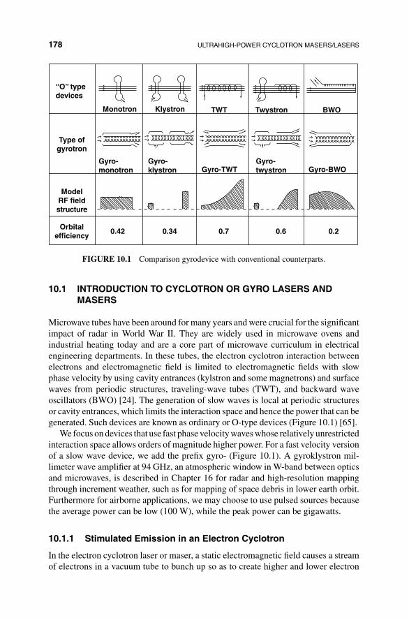
178 ULTRAHIGH-POWER CYCLOTRON MASERS/LASERS
“O” typedevices
Monotron Klystron TWT Twystron BWO
Type ofgyrotron
Gyro-monotron
Gyro-klystron Gyro-TWT
Gyro-twystron Gyro-BWO
ModelRF fieldstructure
Orbitalefficiency
0.42 0.34 0.7 0.6 0.2
FIGURE 10.1 Comparison gyrodevice with conventional counterparts.
10.1 INTRODUCTION TO CYCLOTRON OR GYRO LASERS ANDMASERS
Microwave tubes have been around for many years and were crucial for the significantimpact of radar in World War II. They are widely used in microwave ovens andindustrial heating today and are a core part of microwave curriculum in electricalengineering departments. In these tubes, the electron cyclotron interaction betweenelectrons and electromagnetic field is limited to electromagnetic fields with slowphase velocity by using cavity entrances (kylstron and some magnetrons) and surfacewaves from periodic structures, traveling-wave tubes (TWT), and backward waveoscillators (BWO) [24]. The generation of slow waves is local at periodic structuresor cavity entrances, which limits the interaction space and hence the power that can begenerated. Such devices are known as ordinary or O-type devices (Figure 10.1) [65].
We focus on devices that use fast phase velocity waves whose relatively unrestrictedinteraction space allows orders of magnitude higher power. For a fast velocity versionof a slow wave device, we add the prefix gyro- (Figure 10.1). A gyroklystron mil-limeter wave amplifier at 94 GHz, an atmospheric window in W-band between opticsand microwaves, is described in Chapter 16 for radar and high-resolution mappingthrough increment weather, such as for mapping of space debris in lower earth orbit.Furthermore for airborne applications, we may choose to use pulsed sources becausethe average power can be low (100 W), while the peak power can be gigawatts.
10.1.1 Stimulated Emission in an Electron Cyclotron
In the electron cyclotron laser or maser, a static electromagnetic field causes a streamof electrons in a vacuum tube to bunch up so as to create higher and lower electron
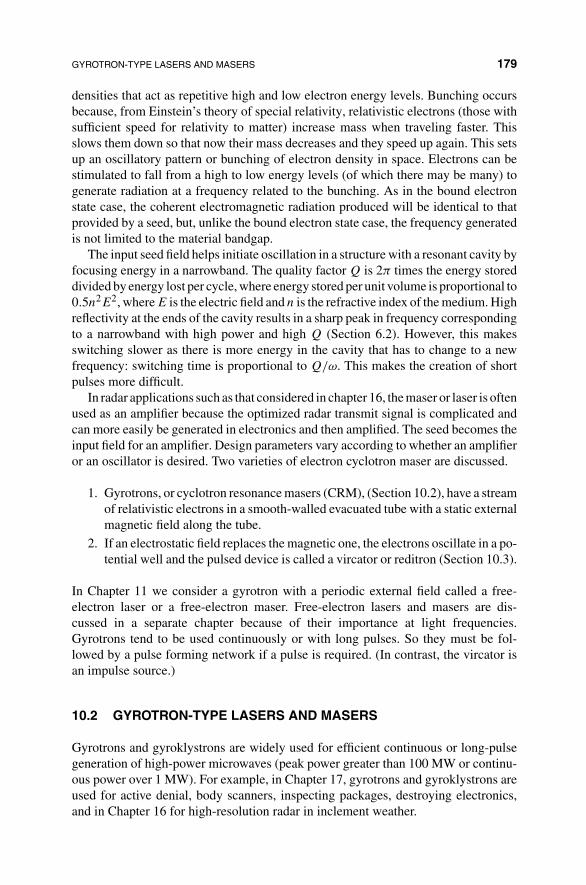
GYROTRON-TYPE LASERS AND MASERS 179
densities that act as repetitive high and low electron energy levels. Bunching occursbecause, from Einstein’s theory of special relativity, relativistic electrons (those withsufficient speed for relativity to matter) increase mass when traveling faster. Thisslows them down so that now their mass decreases and they speed up again. This setsup an oscillatory pattern or bunching of electron density in space. Electrons can bestimulated to fall from a high to low energy levels (of which there may be many) togenerate radiation at a frequency related to the bunching. As in the bound electronstate case, the coherent electromagnetic radiation produced will be identical to thatprovided by a seed, but, unlike the bound electron state case, the frequency generatedis not limited to the material bandgap.
The input seed field helps initiate oscillation in a structure with a resonant cavity byfocusing energy in a narrowband. The quality factor Q is 2π times the energy storeddivided by energy lost per cycle, where energy stored per unit volume is proportional to0.5n2E2, where E is the electric field and n is the refractive index of the medium. Highreflectivity at the ends of the cavity results in a sharp peak in frequency correspondingto a narrowband with high power and high Q (Section 6.2). However, this makesswitching slower as there is more energy in the cavity that has to change to a newfrequency: switching time is proportional to Q/ω. This makes the creation of shortpulses more difficult.
In radar applications such as that considered in chapter 16, the maser or laser is oftenused as an amplifier because the optimized radar transmit signal is complicated andcan more easily be generated in electronics and then amplified. The seed becomes theinput field for an amplifier. Design parameters vary according to whether an amplifieror an oscillator is desired. Two varieties of electron cyclotron maser are discussed.
1. Gyrotrons, or cyclotron resonance masers (CRM), (Section 10.2), have a streamof relativistic electrons in a smooth-walled evacuated tube with a static externalmagnetic field along the tube.
2. If an electrostatic field replaces the magnetic one, the electrons oscillate in a po-tential well and the pulsed device is called a vircator or reditron (Section 10.3).
In Chapter 11 we consider a gyrotron with a periodic external field called a free-electron laser or a free-electron maser. Free-electron lasers and masers are dis-cussed in a separate chapter because of their importance at light frequencies.Gyrotrons tend to be used continuously or with long pulses. So they must be fol-lowed by a pulse forming network if a pulse is required. (In contrast, the vircator isan impulse source.)
10.2 GYROTRON-TYPE LASERS AND MASERS
Gyrotrons and gyroklystrons are widely used for efficient continuous or long-pulsegeneration of high-power microwaves (peak power greater than 100 MW or continu-ous power over 1 MW). For example, in Chapter 17, gyrotrons and gyroklystrons areused for active denial, body scanners, inspecting packages, destroying electronics,and in Chapter 16 for high-resolution radar in inclement weather.

180 ULTRAHIGH-POWER CYCLOTRON MASERS/LASERS
10.2.1 Principles of Electron Cyclotron Oscillators and Amplifiers
In electron cyclotron maser stimulated emission [129], the interaction is betweenrelativistic electrons (close to the speed of light c) and an electromagnetic field withfast phase velocity (exceeding the speed of light). The stream of electrons is at a slightangle to the axis of the magnetic field. We now show that this causes the electronsto gyrate in a helical path around the axis. First, we neglect the relativistic nature ofelectrons. For motion of a charged particle in a constant and uniform magnetostaticfield, from Newton’s law, mass times acceleration equals force [13]:
mdvdt
= q(v × B) (10.1)
where B is the magnetic field flux density, and a particle has rest mass m, velocityv, and charge q. Splitting v into components v‖ that is parallel to B and v⊥ that isperpendicular to B,
v = v‖ + v⊥ (10.2)
Figure 10.2b shows the case with axes rotated so that v is in the x–z plane ofFigure 10.2a. In the cross product in equation (10.1), only v components at rightangles to B are nonzero. So equation (10.1) becomes
dv⊥dt
= q
m(v⊥ × B) (10.3)
If we define a vector
�c = −qBm
(10.4)
FIGURE 10.2 Splitting velocity v into parallel and perpendicular components: (a) coordinatesystem and (b) components of velocity.
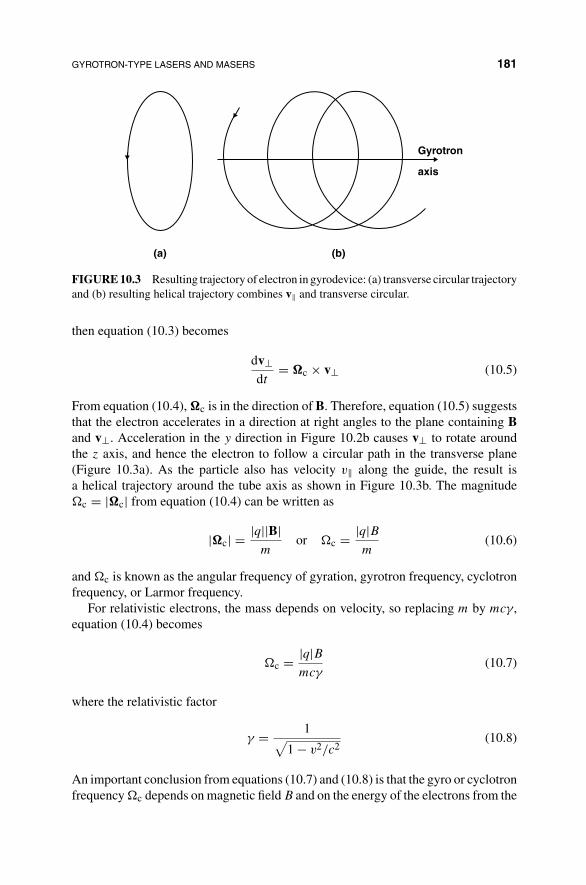
GYROTRON-TYPE LASERS AND MASERS 181
(a) (b)
Gyrotron
axis
FIGURE 10.3 Resulting trajectory of electron in gyrodevice: (a) transverse circular trajectoryand (b) resulting helical trajectory combines v‖ and transverse circular.
then equation (10.3) becomes
dv⊥dt
= �c × v⊥ (10.5)
From equation (10.4), �c is in the direction of B. Therefore, equation (10.5) suggeststhat the electron accelerates in a direction at right angles to the plane containing Band v⊥. Acceleration in the y direction in Figure 10.2b causes v⊥ to rotate aroundthe z axis, and hence the electron to follow a circular path in the transverse plane(Figure 10.3a). As the particle also has velocity v‖ along the guide, the result isa helical trajectory around the tube axis as shown in Figure 10.3b. The magnitude�c = |�c| from equation (10.4) can be written as
|�c| = |q||B|m
or �c = |q|Bm
(10.6)
and �c is known as the angular frequency of gyration, gyrotron frequency, cyclotronfrequency, or Larmor frequency.
For relativistic electrons, the mass depends on velocity, so replacing m by mcγ ,equation (10.4) becomes
�c = |q|Bmcγ
(10.7)
where the relativistic factor
γ = 1√1 − v2/c2
(10.8)
An important conclusion from equations (10.7) and (10.8) is that the gyro or cyclotronfrequency �c depends on magnetic field B and on the energy of the electrons from the

182 ULTRAHIGH-POWER CYCLOTRON MASERS/LASERS
accelerator (electron gun) through γ and hence v and also influences the frequencyof the electromagnetic oscillation (laser light) produced by electrons moving at rela-tivistic velocity v in a constant uniform magnetic field. Therefore, the frequency of agyrodevice can be tuned by changing the voltage on the electron gun, hence changingthe electron velocity v; this allows a large range of frequencies �c. This contrasts thebound electron state case for conventional lasers (such as laser diodes) and masers forwhich the frequency is determined by the material bandgap that is extremely limiting.
A second effect, bunching of relativistic electrons, produces repetitive high–lowenergy levels that support stimulated emission. For a TEM mode propagating downthe waveguide, the electric field (E) is transverse. Therefore, at one side of the circularelectron path, the E field contributes a force qE to accelerate the electrons, while onthe other side of the circular path, the E field decelerates the electron. The combinationof acceleration and deceleration results in bunching of electrons to produce higherdensity and lower density periodicity. This periodicity of electron bunching enablesstimulated emission. Very large power is possible because of absence of a nonlinearmaterial and opportunity for large interaction volume when using a large diametersmooth vacuum tube. The result is orders of magnitude higher power than that fornonrelativistic electrons or slow phase microwave tubes. In addition, the high poweris produced very efficiently and can be used to generate coherent microwaves over alarge range of frequencies. The upper end of the range approaches optical frequencies.
10.2.2 Gyrotron Operating Point and Structure
The gyrating electrons not only acquire an orbital velocity but also change theirspeed vz in the axial direction to produce a Doppler effect [129]. Therefore, thegyration frequency � differs from the angular frequency ω of the electromagneticwave according to
ω − kzv(z) ≈ s� (10.9)
where s allows harmonics of �.The gyrotron operates by interaction between the gyrating electrons and the elec-
tromagnetic wave. Figure 10.4 [9] shows a dispersion diagram, angular frequency ω
versus propagation constant kz. For the cyclotron wave from gyrating electrons, thegraph of equation (10.9) is a straight line as shown in the figure. The microwave fieldin the waveguide is represented by a parabola for the normal TE waveguide mode:
ω2 = ω2co + c2kz (10.10)
where ωco is the cutoff angular frequency. The intersection of the two curves, equa-tions (10.9) and (10.10), provides the operating point for the gyrotron resulting fromthe interaction of the gyrating electrons and the microwave field and gives the fre-quency of oscillation that will be observed. Two different variations of gyrotron areshown with different operating points. A gyrotron traveling-wave tube (gyro-TWT)provides forward velocity of the electromagnetic wave. Traveling wave means that
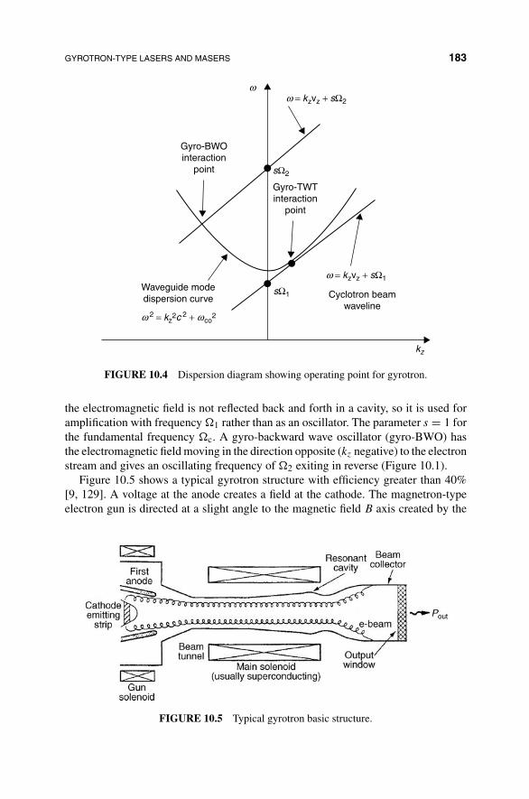
GYROTRON-TYPE LASERS AND MASERS 183
ωω = kzvz + sΩ2
ω = kzvz + sΩ1
ω 2 = kz2c 2 + ωco
2
sΩ1
sΩ2
kz
Gyro-BWOinteraction
point
Gyro-TWTinteraction
point
Waveguide modedispersion curve Cyclotron beam
waveline
FIGURE 10.4 Dispersion diagram showing operating point for gyrotron.
the electromagnetic field is not reflected back and forth in a cavity, so it is used foramplification with frequency �1 rather than as an oscillator. The parameter s = 1 forthe fundamental frequency �c. A gyro-backward wave oscillator (gyro-BWO) hasthe electromagnetic field moving in the direction opposite (kz negative) to the electronstream and gives an oscillating frequency of �2 exiting in reverse (Figure 10.1).
Figure 10.5 shows a typical gyrotron structure with efficiency greater than 40%[9, 129]. A voltage at the anode creates a field at the cathode. The magnetron-typeelectron gun is directed at a slight angle to the magnetic field B axis created by the
FIGURE 10.5 Typical gyrotron basic structure.
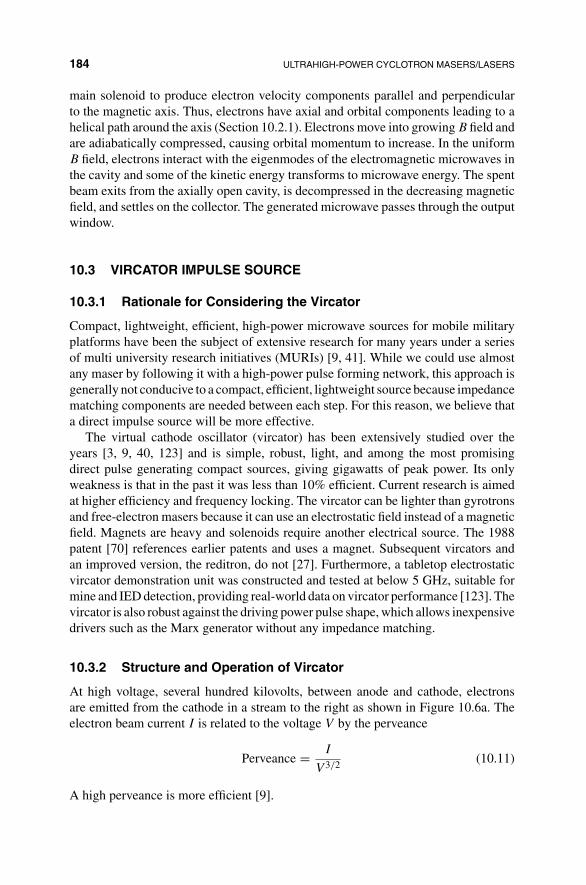
184 ULTRAHIGH-POWER CYCLOTRON MASERS/LASERS
main solenoid to produce electron velocity components parallel and perpendicularto the magnetic axis. Thus, electrons have axial and orbital components leading to ahelical path around the axis (Section 10.2.1). Electrons move into growing B field andare adiabatically compressed, causing orbital momentum to increase. In the uniformB field, electrons interact with the eigenmodes of the electromagnetic microwaves inthe cavity and some of the kinetic energy transforms to microwave energy. The spentbeam exits from the axially open cavity, is decompressed in the decreasing magneticfield, and settles on the collector. The generated microwave passes through the outputwindow.
10.3 VIRCATOR IMPULSE SOURCE
10.3.1 Rationale for Considering the Vircator
Compact, lightweight, efficient, high-power microwave sources for mobile militaryplatforms have been the subject of extensive research for many years under a seriesof multi university research initiatives (MURIs) [9, 41]. While we could use almostany maser by following it with a high-power pulse forming network, this approach isgenerally not conducive to a compact, efficient, lightweight source because impedancematching components are needed between each step. For this reason, we believe thata direct impulse source will be more effective.
The virtual cathode oscillator (vircator) has been extensively studied over theyears [3, 9, 40, 123] and is simple, robust, light, and among the most promisingdirect pulse generating compact sources, giving gigawatts of peak power. Its onlyweakness is that in the past it was less than 10% efficient. Current research is aimedat higher efficiency and frequency locking. The vircator can be lighter than gyrotronsand free-electron masers because it can use an electrostatic field instead of a magneticfield. Magnets are heavy and solenoids require another electrical source. The 1988patent [70] references earlier patents and uses a magnet. Subsequent vircators andan improved version, the reditron, do not [27]. Furthermore, a tabletop electrostaticvircator demonstration unit was constructed and tested at below 5 GHz, suitable formine and IED detection, providing real-world data on vircator performance [123]. Thevircator is also robust against the driving power pulse shape, which allows inexpensivedrivers such as the Marx generator without any impedance matching.
10.3.2 Structure and Operation of Vircator
At high voltage, several hundred kilovolts, between anode and cathode, electronsare emitted from the cathode in a stream to the right as shown in Figure 10.6a. Theelectron beam current I is related to the voltage V by the perveance
Perveance = I
V 3/2 (10.11)
A high perveance is more efficient [9].

VIRCATOR IMPULSE SOURCE 185
(a) (b)
(c) (d)
Insulator Anode
Window
Cathode Virtual cathodeWindow
Insulator Anode
Cathode
Virtual cathode
Window
Insulator
Anode
Cathode
Virtual cathodeInsulator Anode
Window
Cathode Virtual cathode
FIGURE 10.6 Virtual cathode oscillator: (a) basic vircator, (b) transverse extracted, (c) red-itron, and (d) reflex triode removes chirp.
The vircator operates by forming a virtual cathode, hence name virtual cathodeoscillator (vircator). The virtual cathode arises when the cathode generated currentexceeds the maximum current that can pass through the drift space of the tube. Thiscurrent is called the space charge current and is of the order of 10 kA. If the injectedbeam current is greater than the space charge current and the radius of the drift spaceregion is sufficient, the excess space charge forms a strong potential barrier at the headof the beam. This is the virtual cathode that reflects electrons to form an oscillatingcavity. The cavity reinforces microwave radiation by bremsstrahlung radiation. Thecavity can be designed to radiate at a frequency suitable for airborne mine detection(say less than 10 GHz). In the structures shown in Figure 10.6a and b [9], the virtualcathode oscillates axially, but in Figure 10.6b the direction of the microwave outputbeam is transverse to the axis.
When the drive voltage is switched off at the end of a pulse, the amplitude of thevirtual cathode oscillation decays and the frequency increases as the cavity lengthreduces. This chirp significantly increases bandwidth that may be useful in someapplications.
Some variations of the vircator are aimed at removing the chirp to maintain aconstant frequency (narrowband), in order to maximize peak power. Figure 10.6cshows a reditron [27] that uses a thick anode plate with holes to remove virtualcathode oscillation and hence the chirp. The peak power of an experimental unit was1.6 GW. Figure 10.6d shows a reflex triode that also eliminates the oscillation of the
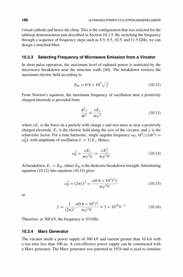
186 ULTRAHIGH-POWER CYCLOTRON MASERS/LASERS
virtual cathode and hence the chirp. This is the configuration that was selected for thetabletop demonstration unit described in Section 10.3.5. By switching the frequencythrough a sequence of frequency steps such as 8.5, 9.5, 10.5, and 11.5 GHz, we candesign a matched filter.
10.3.3 Selecting Frequency of Microwave Emission from a Vircator
In short pulse operation, the maximum level of radiated power is restricted by themicrowave breakdown near the structure walls [40]. The breakdown restricts themaximum electric field according to
Ebr = 0.8 × 10³√
f (10.12)
From Newton’s equation, the maximum frequency of oscillation near a positivelycharged electrode is provided from
d2z
dt2 = eEz
mγ3 (10.13)
where eEz is the force on a particle with charge e and rest mass m near a positivelycharged electrode, Ez is the electric field along the axis of the vircator, and γ is therelativistic factor. For a time harmonic, single angular frequency ω0, (d2z)/(dt2) =ω2
0L with amplitude of oscillation L = V/Ez. Hence,
ω20 = eEz
mγ3L= eE2
z
mγ3V(10.14)
At breakdown, Ez = Ebr, where Ebr is the dielectric breakdown strength. Substitutingequation (10.12) into equation (10.14) gives
ω20 = (2πf )2 = e(0.8 × 10³)2f
mγ3V(10.15)
or
f = 1
(2π)2
e(0.8 × 10³)2
mγ3V≈ 3 × 10¹⁵V−1 (10.16)
Therefore, at 300 kV, the frequency is 10 GHz.
10.3.4 Marx Generator
The vircator needs a power supply of 300 kV and current greater than 10 kA witha rise time less than 100 ns. A cost-effective power supply can be constructed witha Marx generator. The Marx generator was patented in 1924 and is used to simulate

VIRCATOR IMPULSE SOURCE 187
0 V
0 V
(a) (b)
30 kV 120 kV
C4
G3
C3
C2
G1
C130 kV
G2
C4
G3
C3
C2
G1
C1
G2
FIGURE 10.7 Marx generator structure: (a) showing charging and (b) discharge.
lightning, generate X-rays, and ignite a thermonuclear device. It charges a number ofcapacitors in parallel and then discharges them in series. We would like the outputimpedance of the Marx generator to match the input impedance of the vircator formaximum transfer of energy to the vircator load. This avoids large and expensiveimpedance matching components.
Figure 10.7a shows the structure of a four-stage Marx generator in which a 30 kVDC source charges four capacitors in parallel. For a system with N stages, theVcharge = 30 kV power supply source charges all N capacitors of value Cstage, C1to CN , in parallel up to 30 kV through boxes containing resistors. The N capacitors inparallel give an equivalent capacitance for charging of Cset = NCstage (Figure 10.7a).Inductors may be used in place of charging resistors for more efficiency and speed.
To generate a high-voltage pulse at the right-hand side of Figure 10.7b, a spark gapG1 is triggered to form a short circuit between the two dark circles at G1. This nowdoubles the voltage across G2, causing it to trigger into a short circuit. This repeatsrapidly until all the capacitors are discharged in series as shown in Figure 10.7b, wherethe peak voltage is 4 × 30 kV = 120 kV. In general, on discharge, a pulse is generatedat the right-hand side of Figure 10.7b of peak approximately Vpeak = NVcharge. Fordischarging, the N capacitors in series have a capacitance of Cset = Cstage/N andinductance Lset = NLstage. Therefore, the Marx output impedance may be written as
ZMarx =√
Lset
Cset= N
√Lstage
Cstage(10.17)

188 ULTRAHIGH-POWER CYCLOTRON MASERS/LASERS
FIGURE 10.8 Photograph of combined Marx generator with vircator demonstration.
10.3.5 Demonstration Unit of Marx Generator Driving a Vircator
A vircator driven by a Marx generator appears to be capable of producing 200 MWimpulses suitable for airborne applications such as ground penetration radar [123].Figure 10.8 [123] shows a photograph of a tabletop demonstration unit in which a 25-stage Marx generator drives a reflex triode vircator to provide a high-power microwaveimpulse source suitable for airborne mine detection. The 18 � output impedance ofthe Marx generator is similar to the input impedance of the vircator, so large andlossy impedance matching components such as transmission lines, transformers, ortapered waveguides are avoided. This simplifies the system, reducing cost and weightand improving reliability. The maximum voltage that can be delivered to the matchedload is (1/2)N × Vcharge. So for a charging voltage of Vcharge = 20 kV and 25 stages,the maximum voltage is 250 kV.
FIGURE 10.9 Photograph of Marx generator used in demonstration.

VIRCATOR IMPULSE SOURCE 189
(a) (b)
1.0
0.5
0.0
0 1 2
Time (µS)
Cur
rent
(kA
)
–0.5
–1.0
–1.5
IC = 30 kV
5 nF
1.1 µHL1
C1
IC = 0A
4 Ω
R1
FIGURE 10.10 20-stage Marx generator test: (a) output pulse and (b) equivalent circuit.
A second advantage for the vircator is that it is forgiving with respect to drivervoltage fluctuations compared to other masers and gyrodevices; most of these requirea flattop pulse. Furthermore, no other power supply is needed because the vircatoruses the electrostatic field and does not require a magnetic field. This further simplifiesthe system and reduces weight and cost and increases reliability.
FIGURE 10.11 Vircator in demonstration unit: (a) reflex triode-type vircator and (b) anodestalk.

190 ULTRAHIGH-POWER CYCLOTRON MASERS/LASERS
10.3.5.1 Marx Generator in Demonstration Unit Figure 10.9 shows a pho-tograph [123] of the N = 25-stage Marx generator used in the demonstration with-out its steel cover: the cover is part of the coaxial construction. Each stage ofthe Marx generator has four mica capacitors of 25 nF in parallel, giving a stagecapacitance of Cstage = 100 nF. The inductance of connections, spark gap, andcapacitors add to give an inductance per stage of Lstage = 55 nH. From equa-tion (10.17), these values give an output impedance of 18.5 � for 25 stages, whichapproximately matches the impedance of the vircator. The total energy stored be-fore discharge is E = (1/2)CsetV
2peak where Vpeak = N × Vcharge ≈ 500 kV and
Cset(series) = Cstage/N ≈ 4 nF, giving E = 0.5 × 4 × 10−9 × (5 × 105)2 ≈ 500 J.In an earlier test of the Marx generator with N = 20 stages and a low charging
voltage of Vcharge = 1.5 kV, the pulse out is shown in Figure 10.10a and the equivalentLCR circuit in Figure 10.10b [123].
10.3.5.2 Vircator in Demonstration Unit A velvet cathode with approxi-mately 6 cm diameter and a 10 mm gap between anode and cathode is shown inFigure 10.11a [71] for the reflex triode vircator [123]. The anode stalk is shown inFigure 10.11b [123]. This vircator, charged with 20 kV, gave 50 MW with a 220 kVpeak voltage. The input impedance fluctuates starting around 18 � and dropping to-ward the end of the pulse; 5 GHz was generated. Researchers expect to get 200 MWwith this design. The charging time of approximately 100 ms limits the repetitionrate. Cooling will allow faster charging.
CHAPTER 11
FREE-ELECTRON LASER/MASER
We describe the free-electron laser in this chapter because it is the most promisingof the ultrahigh-power cyclotron lasers. Chapter 10 provides the background for thischapter.
We expect the free-electron laser to revolutionize high-power generation of coher-ent light radiation for lasers that will in turn revolutionize the use of lasers in militaryapplications including manufacturing, which is critical for military buildup in a crisis.The development of free-electron lasers is progressing steadily. In 1994, the Navyfunded Jefferson Laboratory demonstrated 10 MW at 6 �m and in 2005 plans wereunderway for 10 MW at 1 and 3 �m, 1 MW at UV, and 100 W in terahertz range [170].Since then, several large contracts have been awarded to construct large free-electronlasers. For example, a press announcement in June 2009 [126] indicated that Raytheonwas awarded a 12-month contract with ONR to perform the preliminary design of a100 kW experimental free-electron laser. The free-electron laser is considered for usewith future millimeter radar (radio frequency detection and ranging) in Chapter 16and lidar (light detection and ranging) in Chapter 15.
In Section 11.1, we describe the significance and principles of the free-electronlaser/maser (FEL/FEM) that is distinguished from other cyclotron lasers by theaddition of a wiggler whose spatially oscillating field enables the range of frequenciesof the gyrotron to be extended through light up to X-rays. With variation it can alsoextend the range down to 0.28 GHz [33]. The frequency of the generated microwavesnow depends on both the periodicity of this structure and the oscillating energy ofthe electrons. In Section 11.2, we explain the theory of free-electron operation to
Military Laser Technology for Defense: Technology for Revolutionizing 21st Century Warfare,First Edition. By Alastair D. McAulay.© 2011 John Wiley & Sons, Inc. Published 2011 by John Wiley & Sons, Inc.
191

192 FREE-ELECTRON LASER/MASER
show that electron bunching produces stimulated laser emission by bremsstrahlungand why any wavelength can be generated. In Section 11.3, we describe a proposedairborne free-electron laser [170] at high multimegawatt power and an inexpensivelaboratory tabletop free-electron X-band laser [173, 175], with low multikilowattpower.
11.1 SIGNIFICANCE AND PRINCIPLES OF FREE-ELECTRONLASER/MASER
11.1.1 Significance of Free-Electron Laser/Maser
The reasons why free-electron lasers show the most promise for high-power lasersand masers are as follows [170]:
1. The wavelength of free-electron laser light can be chosen for a specific appli-cation from an impressive range from radio frequencies through IR and UV toX-rays. This contrasts bound electron state lasers covered in Chapters 7 to 9for which the wavelength depends on the specific bandgap of the material. Itcontrasts gyrotrons that do not extend up through light frequencies.
2. Because of the free-electron laser flexibility in wavelength and tunability, thesame design can match and cover diverse applications at significant cost savings.
3. With a free-electron laser, megawatts of light can be available at any time andwithin seconds in contrast to other high-power laser systems that generally havesignificant warm-up and/or recovery time when fired.
4. The free-electron laser light can be modulated so that matched filtering may beused with return signals in radar to enhance signal to noise ratio.
5. The free-electron laser is efficient—approximately 30% of the electronic powersupplied is converted into light at megawatt power.
6. The free-electron laser is powered by electricity that can be generated from anaircraft engine and does not require storage of toxic chemicals or batteries. Amultimegawatt laser on a 747 is expected to need less than 7% of the enginecapacity.
11.1.2 Principles of Free-Electron Laser/Maser
As described in Chapter 10, the FEL/FEM generates or amplifies electromagneticradiation in light or microwaves by converting energy in a stream of electrons intohigh-power (many megawatts) coherent continuous or pulsed electromagnetic energyat any frequency in microwaves (1–300 GHz) or light (300 GHz–UV).
In addition to the elements used in all high-power gyrodevices, electron accelerator(gun) generating relativistic electrons (close to the speed of light), fast phase veloc-ity electromagnetic field, and absence of nonlinearity to limit power, the FEL has a
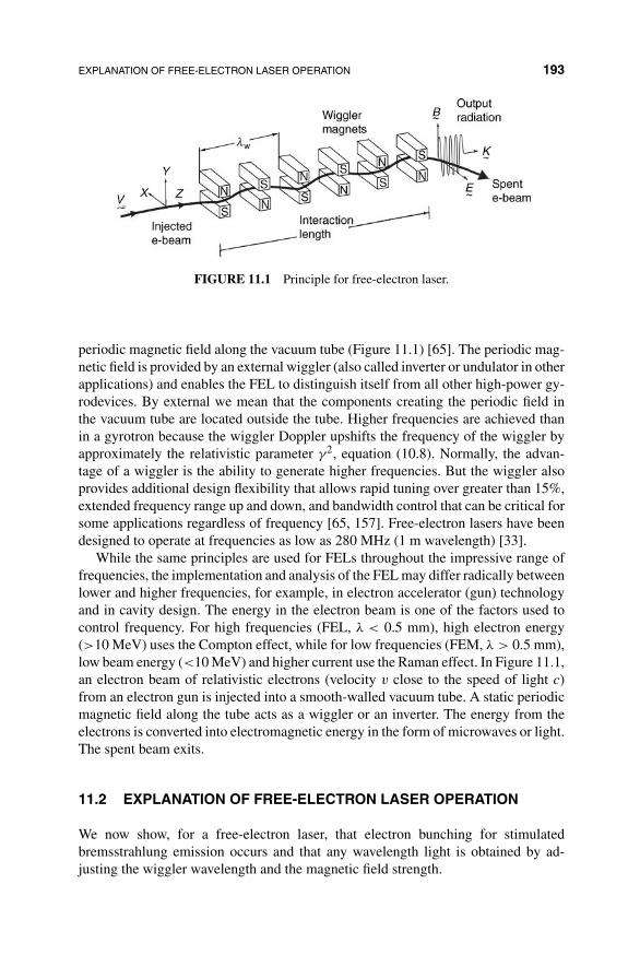
EXPLANATION OF FREE-ELECTRON LASER OPERATION 193
FIGURE 11.1 Principle for free-electron laser.
periodic magnetic field along the vacuum tube (Figure 11.1) [65]. The periodic mag-netic field is provided by an external wiggler (also called inverter or undulator in otherapplications) and enables the FEL to distinguish itself from all other high-power gy-rodevices. By external we mean that the components creating the periodic field inthe vacuum tube are located outside the tube. Higher frequencies are achieved thanin a gyrotron because the wiggler Doppler upshifts the frequency of the wiggler byapproximately the relativistic parameter γ2, equation (10.8). Normally, the advan-tage of a wiggler is the ability to generate higher frequencies. But the wiggler alsoprovides additional design flexibility that allows rapid tuning over greater than 15%,extended frequency range up and down, and bandwidth control that can be critical forsome applications regardless of frequency [65, 157]. Free-electron lasers have beendesigned to operate at frequencies as low as 280 MHz (1 m wavelength) [33].
While the same principles are used for FELs throughout the impressive range offrequencies, the implementation and analysis of the FEL may differ radically betweenlower and higher frequencies, for example, in electron accelerator (gun) technologyand in cavity design. The energy in the electron beam is one of the factors used tocontrol frequency. For high frequencies (FEL, λ < 0.5 mm), high electron energy(>10 MeV) uses the Compton effect, while for low frequencies (FEM, λ > 0.5 mm),low beam energy (<10 MeV) and higher current use the Raman effect. In Figure 11.1,an electron beam of relativistic electrons (velocity v close to the speed of light c)from an electron gun is injected into a smooth-walled vacuum tube. A static periodicmagnetic field along the tube acts as a wiggler or an inverter. The energy from theelectrons is converted into electromagnetic energy in the form of microwaves or light.The spent beam exits.
11.2 EXPLANATION OF FREE-ELECTRON LASER OPERATION
We now show, for a free-electron laser, that electron bunching for stimulatedbremsstrahlung emission occurs and that any wavelength light is obtained by ad-justing the wiggler wavelength and the magnetic field strength.

194 FREE-ELECTRON LASER/MASER
11.2.1 Wavelength Versatility for Free-Electron Laser
We assume that the electron density is small enough during the exchange of energyfrom electron beam to radiation that many-electron collective effects are negligible.This is the Compton regime of operation for the FEL. This is easier to explain than themany-electron Raman case while still illustrating the general principles. We followthe approach in Ref. [119]. A linear wiggler produces an alternating magnetic fieldalong the tube (Figure 11.1):
Bw = xBw cos2πz
λw(11.1)
For a linear wiggler, the output electromagnetic wave is linearly polarized in the x
direction. The spatial frequency of wiggler field is fw = 1/λw. Or we can use a helicalwiggler
Bw = Bw
(x cos
2πz
λw+ y sin
2πz
λw
)(11.2)
For a helical wiggler, the output field is circularly polarized. On electrons at velocityv, the magnetic wiggler exerts a force
Fw = ev × Bw (11.3)
where e is charge of an electron. From equation (11.3), the force is transverse tothe plane containing velocity v and magnetic field Bw and there is no force on theelectron traveling in direction v, or Fwv = 0. But the magnetic field exerts a transverse(sideways) force on the electron, causing it to wiggle back and forth as it passes throughthe periodic magnetic field (Figure 11.1).
The electromagnetic wave generated (or provided at input for an amplifier) has atransverse electric field E, which can interact with the transverse oscillating electronsthrough a force eE. The transfer of energy is used to amplify the electromagneticwave.
The electron velocity is written as
v = vxx + vyy + vzz (11.4)
where vz along the tube is close to the speed of light c for relativistic electrons andthe distance along the tube is z = vzt ≈ ct. Then, from Newton’s equation for anelectron, static mass m times acceleration v equals force using equation (11.2) and(11.3)
mv = ecBw or m(vxx + vyy) = ecBw
(−x sin
2πct
λw+ y cos
2πct
λw
)(11.5)

EXPLANATION OF FREE-ELECTRON LASER OPERATION 195
So
vx = − e
mBwc sin
2πct
λwand vy = e
mBwc cos
2πct
λw(11.6)
Integrating equation (11.6) over time,
vx = Kc cos2πz
λwand vy = Kc sin
2πz
λw(11.7)
As the integral yields an additional factor λw/(2πc), the wiggler parameter
K = e
mBw
(λw
2πc
)= eBwλw
2πmc(11.8)
As electron velocity is close to the speed of light for our relativistic electrons (FELworks only with relativistic electrons), we must include the effect of relativity definedby Einstein that mass increases with velocity (neglected in Newton’s laws). We writefor a relativistic electron mass, using equation (10.8),
M = m√1 − v2/c2
≡ γm (11.9)
From equation (11.9), the mass for a relativistic electron is γ times that for a nonrela-tivistic one. So energy from E = mc2 is also higher by γ , which from equation (10.8)means that the velocity v for the electron accelerator gun determines the energy ofthe electrons. Thus, from equation (11.8), K changes to K/γ for the relativistic caseto give a modified equation (11.7).
vx = Kc
γcos
2πz
λwand vy = Kc
γsin
2πz
λw(11.10)
Note that vx and vy are small when vz in equation (11.4) approaches c. Using thedefinition of γ from equation (10.8) to compute v and v2
x + v2y = (Kc)2/γ2 from
equation (11.10), we write
v2z = v2 − v2
x − v2y = c2
(γ2 − 1
γ2
)− v2
x − v2y
= c2(
γ2 − 1
γ2
)− K2c2
γ2 = c2(
1 − 1 + K2
γ2
)(11.11)

196 FREE-ELECTRON LASER/MASER
For v ≈ c, γ is very large (and K assumed not large), we use the binomial approxi-mation on equation (11.11) to remove the square root for vz:
vz = c
(1 − 1 + K2
γ2
)1/2
= c
(1 − 1 + K2
2γ2
)(11.12)
The wiggler field B is strong enough relative to the electromagnetic field to controlthe electron trajectory. In some FELs, cryogenic magnets are used. The wiggler fielddoes not exchange energy with the electrons but determines their trajectory.
We write the electron field of the plane wave as
E = E0
[x sin
(2πz
λ− wt + φ0
)+ y cos
(2πz
λ− wt + φ0
)](11.13)
As the electron has a transverse velocity component and the E field is transverse to v,the field will exert a force on the electron. As work (energy) W is force times distance,work per second W is force eE times speed v (times involves dot product for vectors),using equations (11.13) and (11.10) and sin(A + B) = sin A cos B + cos A sin B,
W = eE · v
= eE0Kc
γ
[cos
2πz
λwsin
(2πz
λ− ωt + φ0
)+ sin
2πz
λwcos
(2πz
λ− ωt + φ0
)]
= eE0Kc
γsin
[2π
(1
λ+ 1
λw
)z − ωt + φ0
]
≡ eE0Kc
γsin φ (11.14)
where φ is defined in equation (11.14) as
φ ≡ 2π
(1
λ+ 1
λw
)z − ωt + φ0 (11.15)
Here, φ relates to phase between generated optical or microwave field E of wavelengthλ and electron velocity v that depends on wiggler wavelength λw. Note that φ = π/2for in phase and φ = 0 for out of phase.
From Einstein’s mass–energy formula,
E = Mc2 = γmc2 (11.16)
where m is the static mass. Therefore, γ that depends on v ≈ c according to equa-tion (10.8) is proportional to energy. Then, using equation (11.16), we can writeequation (11.14) as
W = γmc2 = eK0Kc
γsin φ or γ = eK0K
γmcsin φ (11.17)

EXPLANATION OF FREE-ELECTRON LASER OPERATION 197
As transverse electron velocity oscillates, see equation (11.10), so does φ from right-hand side of equation (11.14), which used equation (11.10) in the second line of itsdevelopment. Hence, from equation (11.17), the rate of change of energy W and γ
both oscillate. Using z = vz and equation (11.12) for vz allows us to write the timederivative of equation (11.15):
φ = 2π
(1
λ+ 1
λw
)vz − w = 2πc
(1
λ+ 1
λw
) (1 − 1 + K2
2γ2
)− 2πc
λ
= 2πc
λw
[1 −
(1 + λw
λ
)1 + K2
2γ2
](11.18)
The Compton effect applies to high frequency where the laser wavelength is muchshorter than the wiggler wavelength, λw/λ >> 1. So
φ ≈ 2πc
λw
(1 − λw
λ
1 + K2
2γ2
)(11.19)
In a steady resonant state, the rate of phase change φ = 0, which means that thephase difference is constant between the emitted light or microwave electromagneticradiation and the electron velocity v that depends on wiggler wavelength λw. Fromequation (11.16), the resonant electron energy depends on γ . In the steady stateγ → γR, so setting equation (11.19) to zero, the bracket goes to zero and the resonanceelectron energy γR (that defines electron velocity for resonance) is
γ2R ≡ λw
2λ(1 + K2) (11.20)
From equation (11.20), the resonant energy depends on the wiggler magnetic fieldstrength Bw and the wiggler wavelength λw through K, equation (11.8). Furthermore,by making λ the subject of equation (11.20), we see that the free-electron laser canbe made to work at any wavelength λ by adjusting γ2
R (the voltage of the electrongun) or by changing the wiggler magnetic strength field Bw or wiggler wavelengthλw. This explains the range of frequencies and versatility of the free-electron laser.
11.2.2 Electron Bunching for Stimulated Emission in Free-ElectronLaser
We observe that the change in phase of the field in traveling a distance equal to thewavelength of the wiggler at resonance can be shown to be 2π [119]. By substitut-ing λw/(2λ)(1 + K2) = 2γ2
R from equation (11.20) into equation (11.19) and usingequation (11.17) for the first equation, we now have coupled first-order differential
198 FREE-ELECTRON LASER/MASER
equations linking energy and phase:
γ = eK0K
γmcsin φ
φ = 2πc
λw
(1 − γ2
R
γ2
)(11.21)
These equations describe a single electron in a wiggler field. The electrons gain energyγ > 0 or lose energy γ > 0 depending on the phase φ. Energy gain implies absorptionand energy loss stimulated emission. The average value of sin θ is zero, so there wouldbe no net gain without some other activity, as discussed in Section 10.2. Substitutingfor (1 + K2) in equation (11.20) into equation (11.12) and using equation (10.8) gives
vz = c
(1 − λγ2
R
λwγ2
)or vz = dvz
dγγ ≈ 2cλγ2
R
λwγ3 γ (11.22)
which means electrons are accelerated or decelerated longitudinally depending onwhether they are gaining (γ > 0) or losing (γ < 0) energy to the plane wave. Thebunching of electrons can lead to a net gain rather than absorption. Bunching canbe anticipated because when electrons speed up, their mass increases from relativis-tic considerations, causing them to slow down. The levels of high- and low-energyelectrons allow electrons to be stimulated to fall to a lower level for stimulated emis-sion similar to bremsstrahlung in conventional lasers. Gain can be shown to oc-cur when γ > γR and loss if γ < γR [119]. The maximum gain occurs at electronenergy [119]:
γ =(
1 + 0.2
Nw
)γR (11.23)
where Nw is the number of wiggler periods. For substantial gain, we need a narrowdistribution of electron energies:
�γ ≤ γR/2Nw (11.24)
Electron beam sources must deliver a few amperes for substantial gains. Bandwidth ofa FEL is estimated from bunch length le. Laser radiation must be produced in pulsesof length lc. So bandwidth δν ≈ c/le or relative bandwidth is
δν
ν= λ
le(11.25)
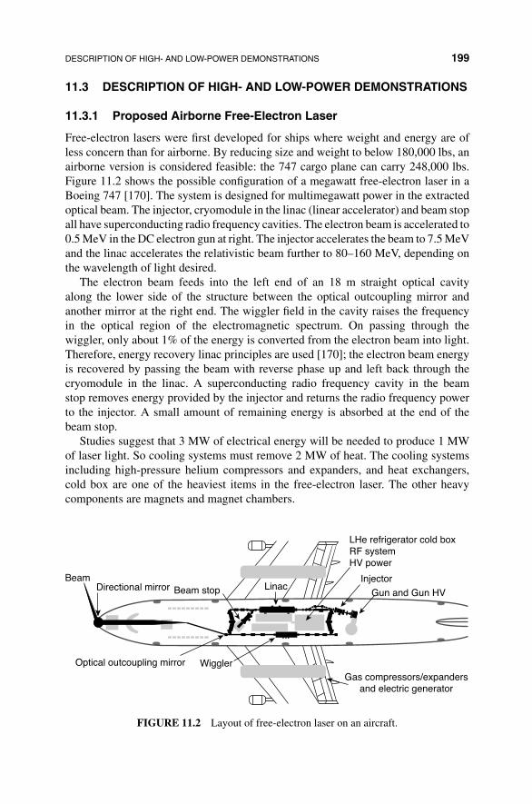
DESCRIPTION OF HIGH- AND LOW-POWER DEMONSTRATIONS 199
11.3 DESCRIPTION OF HIGH- AND LOW-POWER DEMONSTRATIONS
11.3.1 Proposed Airborne Free-Electron Laser
Free-electron lasers were first developed for ships where weight and energy are ofless concern than for airborne. By reducing size and weight to below 180,000 lbs, anairborne version is considered feasible: the 747 cargo plane can carry 248,000 lbs.Figure 11.2 shows the possible configuration of a megawatt free-electron laser in aBoeing 747 [170]. The system is designed for multimegawatt power in the extractedoptical beam. The injector, cryomodule in the linac (linear accelerator) and beam stopall have superconducting radio frequency cavities. The electron beam is accelerated to0.5 MeV in the DC electron gun at right. The injector accelerates the beam to 7.5 MeVand the linac accelerates the relativistic beam further to 80–160 MeV, depending onthe wavelength of light desired.
The electron beam feeds into the left end of an 18 m straight optical cavityalong the lower side of the structure between the optical outcoupling mirror andanother mirror at the right end. The wiggler field in the cavity raises the frequencyin the optical region of the electromagnetic spectrum. On passing through thewiggler, only about 1% of the energy is converted from the electron beam into light.Therefore, energy recovery linac principles are used [170]; the electron beam energyis recovered by passing the beam with reverse phase up and left back through thecryomodule in the linac. A superconducting radio frequency cavity in the beamstop removes energy provided by the injector and returns the radio frequency powerto the injector. A small amount of remaining energy is absorbed at the end of thebeam stop.
Studies suggest that 3 MW of electrical energy will be needed to produce 1 MWof laser light. So cooling systems must remove 2 MW of heat. The cooling systemsincluding high-pressure helium compressors and expanders, and heat exchangers,cold box are one of the heaviest items in the free-electron laser. The other heavycomponents are magnets and magnet chambers.
BeamDirectional mirror Linac
WigglerGas compressors/expanders
and electric generator
Gun and Gun HV
Injector
LHe refrigerator cold boxRF systemHV power
Beam stop
Optical outcoupling mirror
FIGURE 11.2 Layout of free-electron laser on an aircraft.

200 FREE-ELECTRON LASER/MASER
11.3.2 Demonstration of Low-Power System for Free-Electron Maserat 8–12 GHz
We describe a laboratory tabletop X-band, 10 GHz free-electron maser [173, 175]for the purpose of illustrating the possibility and complexity of constructing smallfree-electron lasers and masers. The experimental arrangement (Figure 11.3) showsan electron beam entering a vacuum cavity through a small hole at the left. At thesame time, an oscillator seed for generating microwave power is entered through awaveguide at top right. The waveguide ends are blocked, except for the small endholes for electron injection and exit. So the waveguide acts as a cavity that allows adiscrete set of microwave resonating frequency oscillation longitudinal modes. Themicrowave power passes in the backward direction (relative to electron motion),to form a backward wave oscillator (BWO Section 10.1), and interacts with theelectron beam in the wiggler to convert energy from the electron beam into mi-crowave energy by stimulated emission (bremsstrahlung). In a backward wave os-cillator (BWO) gyrotron [65], the dispersion diagram for the waveguide intersectsthe fast cyclotron mode for negative propagation constant. The BWO FEM oper-ates in a manner similar to a BWO gyrotron (Figure 10.4) but has the additionalwiggler. A coupler at the microwave frequency passes the microwaves to the outputat left.
The experimental system (Figure 11.4) [173] is approximately 2 m long and sim-ple to construct and relatively inexpensive (Table 11.1). However, a pulse formingnetwork might be needed to reduce the pulse length and increase the peak power,which is not too high at this time. Reduction of pulse length from microseconds tonanoseconds could possibly result in a peak to 1 MW.
11.3.3 Achieving Low Frequencies with FELs
Free-electron lasers have been explored mainly because of their ability to reach muchhigher frequencies (up to soft X-rays). Extending the free-electron maser frequency
Microwavepowermeter
Microwavepowersource
Microwavecoupler
Microwavecoupler
Electron beam Electron beam
Beam entranceaperture Microwave power
Wiggler
Beam exitaperture
Resonantcavity
FIGURE 11.3 Arrangement for 10 GHz free-electron maser experiment.
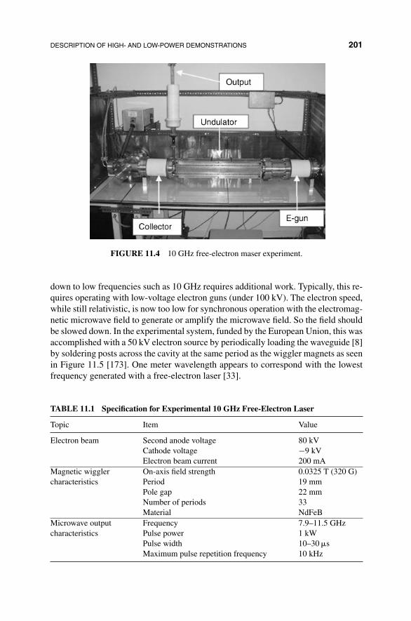
DESCRIPTION OF HIGH- AND LOW-POWER DEMONSTRATIONS 201
FIGURE 11.4 10 GHz free-electron maser experiment.
down to low frequencies such as 10 GHz requires additional work. Typically, this re-quires operating with low-voltage electron guns (under 100 kV). The electron speed,while still relativistic, is now too low for synchronous operation with the electromag-netic microwave field to generate or amplify the microwave field. So the field shouldbe slowed down. In the experimental system, funded by the European Union, this wasaccomplished with a 50 kV electron source by periodically loading the waveguide [8]by soldering posts across the cavity at the same period as the wiggler magnets as seenin Figure 11.5 [173]. One meter wavelength appears to correspond with the lowestfrequency generated with a free-electron laser [33].
TABLE 11.1 Specification for Experimental 10 GHz Free-Electron Laser
Topic Item Value
Electron beam Second anode voltage 80 kVCathode voltage −9 kVElectron beam current 200 mA
Magnetic wiggler On-axis field strength 0.0325 T (320 G)characteristics Period 19 mm
Pole gap 22 mmNumber of periods 33Material NdFeB
Microwave output Frequency 7.9–11.5 GHzcharacteristics Pulse power 1 kW
Pulse width 10–30 �sMaximum pulse repetition frequency 10 kHz
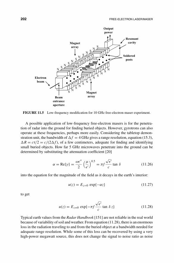
202 FREE-ELECTRON LASER/MASER
NN
NN
NN
SS
SS
SS
NN
NN
NN
SS
SS
SS Magnet
array
Magnetarray
Outputpower
Resonantcavity
Solderedposts
Beamentranceaperture
Electronbeam
FIGURE 11.5 Low-frequency modification for 10 GHz free-electron maser experiment.
A possible application of low-frequency free-electron masers is for the penetra-tion of radar into the ground for finding buried objects. However, gyrotrons can alsooperate at these frequencies, perhaps more easily. Considering the tabletop demon-stration unit, the bandwidth of �f = 4 GHz gives a range resolution, equation (15.3),�R = cτ/2 = c/(2�f ), of a few centimeters, adequate for finding and identifyingsmall buried objects. How far 5 GHz microwaves penetrate into the ground can bedetermined by substituting the attenuation coefficient [20]
α = Re{γ} = ωε′′
2
(μ
ε′)0.5 = πf
√ε′
ctan δ (11.26)
into the equation for the magnitude of the field as it decays in the earth’s interior:
u(z) = Ez=0 exp{−αz} (11.27)
to get
u(z) = Ez=0 exp{−πf
√ε′
ctan δ z} (11.28)
Typical earth values from the Radar Handbook [151] are not reliable in the real worldbecause of variability of soil and weather. From equation (11.28), there is an enormousloss in the radiation traveling to and from the buried object at a bandwidth needed foradequate range resolution. While some of this loss can be recovered by using a veryhigh-power megawatt source, this does not change the signal to noise ratio as noise

DESCRIPTION OF HIGH- AND LOW-POWER DEMONSTRATIONS 203
10.5
10
9.5
9
8.5
860 61 62 63 64 65
Accelerating voltage (kV)
Fre
quen
cy (
GH
z)
66 67 68 69 70
Observed LF modes
Synch (theory)
We gain range
Observed HF modes
FIGURE 11.6 Tuning range for operating frequencies of experimental 10 GHz free-electronmaser experiment.
is mostly clutter. A synthetic aperture antenna can reduce the noise somewhat bynarrowing the beam pattern. Mach–Zehnder interferometric methods (Section 6.1.2)such as the laser Doppler vibrometer will probably work better.
11.3.4 Range of Tuning
The output frequency for the experimental unit can be continuously tuned from ap-proximately 8 to 12 GHz, which is a bandwidth of 4 GHz. Figure 11.6 [173] showshow the accelerator (electron gun) voltage (x axis in kV) of the electron gun deter-mines the operating frequency (y axis in GHz). A range is shown for each operatingfrequency with a line terminated in black triangles. The position on the line is de-termined by using a seed into the output to select one dominant mode (right-handcontinuous curve) or the other (left-hand continuous curve). We note that only onefrequency in the range 8–10 GHz is obtained at a time, so we do not have the fullbandwidth simultaneously as we might in a band-limited carrier frequency.
11.3.5 Design of Magnetic Wiggler
The design of a low-cost (<$2,000) permanent magnet wiggler is described inRef. [174]. It uses only two orientations of magnets rather than the Halbach four-orientation wiggler that performs better but is more expensive. The material used isNdFeB. The end magnets were half the size and overlapped to avoid electrons hit-ting the walls of the waveguide, a less expensive approach than the normal tapering.Analysis for design and adjustment is discussed in Ref. [174].

PART III
APPLICATIONS TO PROTECT AGAINSTMILITARY THREATS

CHAPTER 12
LASER PROTECTION FROM MISSILES
In 1942, the first ballistic missile was launched by Germany that went into the fringesof space at an altitude of 100 km, had a thrust of 56,000 lbs (alcohol and liquidoxygen), a velocity of 3500 mile/h, and a payload of 2200 lbs [124]. Since WorldWar II, the missile has become a dominant weapon of war [140]. A laser beam travelsfast enough in air, kilometers in a few microseconds, to track, disable, or destroy anincoming missile before it has time to perform significant evasive maneuvers or tolaunch countermeasures. The threat of missile attack is increasing with time becausemore sophisticated platforms for launching missiles are in continuous development:land robot vehicles and unmanned aircraft and submersibles. We note that GPS orradio-controlled vehicles, and to a lesser extent autonomous vehicles, can also becountered by interfering with their free-space communication channels.
In Section 12.1, we introduce the protection from missiles and discuss ways tocombat the threat of attack on cities with nuclear multiple warhead intercontinentalballistic missiles (ICBMs). In Section 12.2, we describe the airborne laser programto combat the ICBM threat. In Section 12.3, we discuss protection against attacks byhoming missiles on aircraft and moving assets. In Section 12.4, we address targetedattacks by missiles on stationary or slow-moving targets such as ships.
Military Laser Technology for Defense: Technology for Revolutionizing 21st Century Warfare,First Edition. By Alastair D. McAulay.© 2011 John Wiley & Sons, Inc. Published 2011 by John Wiley & Sons, Inc.
207

208 LASER PROTECTION FROM MISSILES
12.1 PROTECTING FROM MISSILES AND NUCLEAR-TIPPED ICBMs
12.1.1 Introducing Lasers to Protect from Missiles
12.1.1.1 Laser Requirements and Selection The cost of firing a powerlaser is much less than that for firing an antimissile missile. There is no recoil orafter effect. The amount of energy that must be delivered depends on the type oftarget. In addition, the power and expense per shot may be reduced for trainingpurposes, allowing operators more practice in acquisition, tracking, and firing.Sensors on dummy targets enable computation of accuracy, propagation loss andefficiency.
Lasers in development (Chapters 8 through 11) can produce pulses of sufficientenergy to damage soft and hard targets. The energy per unit area, F , required todamage a hard target made of metal or steel is on the order of 100,000 J/cm2, whiledamage to a soft target: flesh, fabrics, plastics, and homing missile sensors needs onlyon the order of 1000 J/cm2. The energy per unit area, F , delivered by a laser to a spotof area A at a target depends on the laser power P , the laser pulse length �t, and theratio L of power remaining after propagating to the target:
F = P�tL
A(12.1)
Requirements for a laser system vary depending on the range to the target, so weseparate the discussion into long and short ranges.
12.1.1.2 Long Range Because the missile plume is highly visible on launch,long-range acquisition from an aircraft is feasible during the launch phase. The launchphase is also the best for destroying a missile because while the missile acceleratesup through the atmosphere after launch, the missile skin is under maximum stress, atwhich time the energy required to break or pierce the skin is least. A high-quality laserbeam can project energy in milliseconds over distances of tens of kilometers in spaceor upper atmosphere. Diffraction, causing beam spreading, is reduced by expandingthe diameter of the Gaussian beam at its waist to several tens of centimeters using abeam expander (Sections 1.3.2 and 2.1).
It is difficult to destroy missiles or other military targets at long range in theatmosphere because in addition to diffraction, atmospheric turbulent causes the beamto spread and wander (Section 5.2). Spreading and wandering due to atmosphericturbulence can be reduced by adaptive optics in which the anticipated distortionof the beam is measured and a precomputed wave front set adaptively with mirrorarrays at the source (Section 5.3). But adaptive optics incurs significant complexityand additional cost. Even with adaptive optics, the loss at long range, hundreds ofkilometers, is large. The weakened intensity arriving at the target means that we mayhave to track a spot on the target for several seconds to provide the required energyfor destruction. This allows time for a missile to engage in simple countermeasuremaneuvers such as rotation.

PROTECTING FROM MISSILES AND NUCLEAR-TIPPED ICBMs 209
At long range, high-power beams can heat the air through which they pass, espe-cially a problem when there is no wind. Heating the path expands the air more towardthe center of the path than at the edges because beams are approximately Gaussian(Section 2.1). The expansion on heating reduces the density of the air toward the beamcenter and hence decreases its density there. The resulting cross sectional refractiveindex profile for the path is then similar to that for a concave lens that spreads thebeam out, reducing efficiency of delivering energy to a small area. The bloomingeffect is reduced by dithering or spiraling the beam in small circles to avoid heatingthe same path for too long.
12.1.1.3 Short Range At short range, compared to long range, the fast speedof light (c = 3 × 10⁸ m/s) gives the missile insufficient time to maneuver, perhapsonly microseconds. Atmospheric turbulence and path heating are less significant. Atshort range, a pulsed laser with short duration, �t, may be used (Chapter 9) becausegeometry is changing fast and less average power is needed. With a pulsed laser, pulsecompression can reduce the pulse length while maintaining the energy (Chapter 9).Other effects can occur with very short pulses. For example, with nanosecond lasers,vaporization or ablation can occur in which material bypasses the usual solid to liquidphase and moves directly to a vapor phase. This is used in laser-induced breakdownspectroscopy [120]. The shock waves generated can cause other types of materialfailures at the atomic level. The plasma generated can reportedly interfere with jetengine intakes. The breakdown of air into a plasma by a laser beam, similar to light-ning, produces a conductive path of ions through which microwave frequencies canbe focused more finely.
12.1.2 Protecting from Nuclear-Tipped ICBMs
The practice of multiple nuclear warheads on a single ICBM [140] makes annihilationof a country feasible. The theory and construction of both nuclear bombs and ICBMs,though difficult, are fairly widely available and efforts can, to some extent, be dis-guised as activities for developing commercial nuclear power. By the year 2015, weexpect more than 10 countries to have multiple nuclear warhead tipped ICBMs thatcan reach the United States and many other countries. This represents a significantthreat.
12.1.2.1 Historical Background The philosophy of Mutually AssuredDestruction (MAD) was used in the Cold War to protect against nuclear attack.In 1960, the United States stockpiled approximately 19,000 nuclear missilesand warheads [140], more than all known targets and equivalent to 1.4 millionHiroshimas. Delivery was also varied and sophisticated: nuclear tipped missilescould be launched by the Navy from hard-to-detect ballistic missile submarines(Figure 12.1a) [140], nuclear bombs could be dropped with Air Force bombers,and intercontinental ballistic missiles with multiple warheads (Figure 12.1b) [140]could be launched from land-based silos. The USSR was estimated to have had
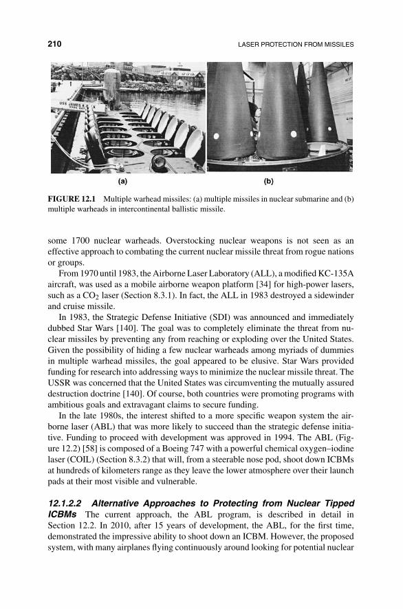
210 LASER PROTECTION FROM MISSILES
FIGURE 12.1 Multiple warhead missiles: (a) multiple missiles in nuclear submarine and (b)multiple warheads in intercontinental ballistic missile.
some 1700 nuclear warheads. Overstocking nuclear weapons is not seen as aneffective approach to combating the current nuclear missile threat from rogue nationsor groups.
From 1970 until 1983, the Airborne Laser Laboratory (ALL), a modified KC-135Aaircraft, was used as a mobile airborne weapon platform [34] for high-power lasers,such as a CO2 laser (Section 8.3.1). In fact, the ALL in 1983 destroyed a sidewinderand cruise missile.
In 1983, the Strategic Defense Initiative (SDI) was announced and immediatelydubbed Star Wars [140]. The goal was to completely eliminate the threat from nu-clear missiles by preventing any from reaching or exploding over the United States.Given the possibility of hiding a few nuclear warheads among myriads of dummiesin multiple warhead missiles, the goal appeared to be elusive. Star Wars providedfunding for research into addressing ways to minimize the nuclear missile threat. TheUSSR was concerned that the United States was circumventing the mutually assureddestruction doctrine [140]. Of course, both countries were promoting programs withambitious goals and extravagant claims to secure funding.
In the late 1980s, the interest shifted to a more specific weapon system the air-borne laser (ABL) that was more likely to succeed than the strategic defense initia-tive. Funding to proceed with development was approved in 1994. The ABL (Fig-ure 12.2) [58] is composed of a Boeing 747 with a powerful chemical oxygen–iodinelaser (COIL) (Section 8.3.2) that will, from a steerable nose pod, shoot down ICBMsat hundreds of kilometers range as they leave the lower atmosphere over their launchpads at their most visible and vulnerable.
12.1.2.2 Alternative Approaches to Protecting from Nuclear TippedICBMs The current approach, the ABL program, is described in detail inSection 12.2. In 2010, after 15 years of development, the ABL, for the first time,demonstrated the impressive ability to shoot down an ICBM. However, the proposedsystem, with many airplanes flying continuously around looking for potential nuclear

PROTECTING FROM MISSILES AND NUCLEAR-TIPPED ICBMs 211
FIGURE 12.2 Airborne laser to protect from ICBMs.
missile launches, is too complex and costly to handle the geographically spreadingthreat since the program was started (Section 12.2.6).
One approach is to make a simpler, less costly version. For long ranges, amore powerful laser that avoids toxic chemicals would help. For example, asmentioned in the previous chapters, more powerful free-electron lasers are beingdeveloped (Section 11.1) that avoid the storing of dangerous liquid oxygen andiodine for a COIL laser. The current designs of high-power free-electron lasersare large and heavy, making them more useful for shipboard lasers (Section 12.4).Lightweight free-electron lasers are being developed for airborne platforms(Figure 11.2).
A second approach is to ban nuclear testing to curtail future development of moreadvanced nuclear weapons. At this time, 151 countries have signed and ratified theComprehensive International Nuclear-Test-Ban Treaty, but nine significant countrieshave not yet ratified it (Chapter 13). Even if such a treaty is ratified, there is noguarantee that some group will not perform surreptitious testing to develop smallerand more powerful, improved thermonuclear bombs.
In the absence of a viable ICBM missile shield and lacking confidence in an ef-fective comprehensive international test ban (Chapter 13), the ability to continue de-signing thermonuclear bombs without testing is considered an important deterrent towould-be nuclear assailants. Therefore, several countries, including the United States,are developing extremely powerful inertial confinement lasers that can emulate thetemperatures and pressures inside a thermonuclear reaction (Chapter 13). The UnitedStates is the leader in this potential new arms race, expecting to demonstrate fusion innext few years. An attractive possibility is that such extremely high-power picosecondinertial confinement lasers will help us understand nuclear fusion sufficiently to pro-duce continuous cost-effective energy by fusion (like the sun) in the next 50 years.Fusion, unlike fission in current nuclear plants, is not expected to pollute futureenvironments with long-lifetime radioactive residual materials and is expected to re-duce the possibility of serious accidents from nuclear plants. However, alternativeapproaches to inertial confinement, such as magnetic confinement, look equally ormore promising at this time.

212 LASER PROTECTION FROM MISSILES
12.2 THE AIRBORNE LASER PROGRAM FOR PROTECTING FROMICBMs
The airborne laser program that started in 1994 involves a Boeing 747 carrying a high-power COIL (Section 8.3.2) that aims to shoot down ICBMs that may be carryingnuclear warheads. The ABL is alerted to a missile launch by a reconnaissance system,such as a satellite, an AWACS airplane, or an advanced radar warning system. TheABL has a suite of infrared (IR) wide-field telescopes and video cameras to detectthe plume from a missile launch. A pointing and tracking system tracks the missileand computes an optimum intercept path for the main light beam to destroy themissile while the missile is still under launch stress. The ABL nose turret has a1.5 m telescope through which it tracks the missile until activating the main beam todestroy the missile. As seen in the airplane (Figure 12.3) [58], six modules of a COIL(Section 8.3.2) are at the rear of the plane, in front of the fuel service system containingstored hydrogen peroxide, chlorine, and oxygen. The beam from the main COIL lasertravels in a pipe through a hole in the bulkhead and the crew battle management areato the nose-mounted turret that directs the beam to the target. The bulkhead separatesthe laser and dangerous chemicals from the crew and optical alignment system.
12.2.1 Lasers in Airborne Laser
There are three laser systems in ABL [39] (Figure 12.4). First, the main beam is froma chemical oxygen–iodine laser at wavelength 1.3 �m with megawatts of power,sustainable for several seconds (Section 8.3.2). The 1.5 m diameter mirror in therotatable turret focuses the light in a Gaussian beam (Section 2.1) onto the target inthe lower atmosphere several hundred kilometers away.
FIGURE 12.3 Inside configuration of airborne laser.
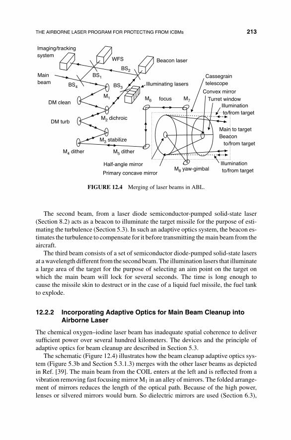
THE AIRBORNE LASER PROGRAM FOR PROTECTING FROM ICBMs 213
Imaging/trackingsystem
WFS Beacon laser
Illuminating lasers
Cassegraintelescope
Mainbeam
DM clean
DM turb
M1
M3 stabilize
M4 dither M5 dither
M8 yaw-gimbal
M2 dichroic
BS1
BS2
BS3BS4
M6 M7focus
Primary concave mirror
Half-angle mirror
Convex mirrorTurret window
Main to targetBeacon to/from target
Illumination to/from target
Illumination to/from target
FIGURE 12.4 Merging of laser beams in ABL.
The second beam, from a laser diode semiconductor-pumped solid-state laser(Section 8.2) acts as a beacon to illuminate the target missile for the purpose of esti-mating the turbulence (Section 5.3). In such an adaptive optics system, the beacon es-timates the turbulence to compensate for it before transmitting the main beam from theaircraft.
The third beam consists of a set of semiconductor diode-pumped solid-state lasersat a wavelength different from the second beam. The illumination lasers that illuminatea large area of the target for the purpose of selecting an aim point on the target onwhich the main beam will lock for several seconds. The time is long enough tocause the missile skin to destruct or in the case of a liquid fuel missile, the fuel tankto explode.
12.2.2 Incorporating Adaptive Optics for Main Beam Cleanup intoAirborne Laser
The chemical oxygen–iodine laser beam has inadequate spatial coherence to deliversufficient power over several hundred kilometers. The devices and the principle ofadaptive optics for beam cleanup are described in Section 5.3.
The schematic (Figure 12.4) illustrates how the beam cleanup adaptive optics sys-tem (Figure 5.3b and Section 5.3.1.3) merges with the other laser beams as depictedin Ref. [39]. The main beam from the COIL enters at the left and is reflected from avibration removing fast focusing mirror M1 in an alley of mirrors. The folded arrange-ment of mirrors reduces the length of the optical path. Because of the high power,lenses or silvered mirrors would burn. So dielectric mirrors are used (Section 6.3),

214 LASER PROTECTION FROM MISSILES
which have alternating high and low dielectric coefficients repeating at period �. Thisreflects when � = λ/2 (Section 6.3.1). The dielectric is made from materials that canwithstand the high power, such as a II–VI semiconductor zinc selenide crystal usedfor the airborne laser window [34]. Materials for high-power lasers are discussed inSection 8.1.5.
The main beam then reflects from the beam cleanup deformable mirror, DM clean(Section 5.3.1.3 and Figure 5.3b), onto a dichroic mirror M2 (Figure 5.4) for mergingwith the beacon light at a different wavelength. Some light also reflects back into awave front sensor (WFS) via two beam splitters BS2 and BS1. The measurementsfrom the wave front sensor are used in a computer to set the pistons in the beamcleanup deformable mirror (DM clean) to improve the wave front as described inSection 5.3.1.3. The spatial coherence of the main beam is improved by DM clean onits way to DM turb via mirror M2 dichroic. The cleaned up beam propagates betterfor focusing to long distances. The optics shown in Figure 12.4 were tested in thelaboratory as shown in Figure 12.5 [58].
FIGURE 12.5 Demonstrating ABL optic’s functionality in laboratory.
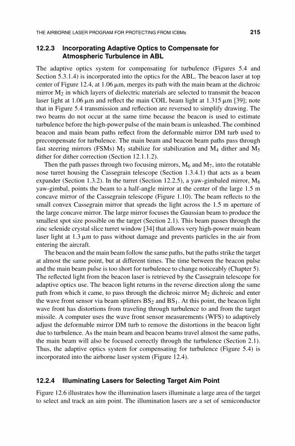
THE AIRBORNE LASER PROGRAM FOR PROTECTING FROM ICBMs 215
12.2.3 Incorporating Adaptive Optics to Compensate forAtmospheric Turbulence in ABL
The adaptive optics system for compensating for turbulence (Figures 5.4 andSection 5.3.1.4) is incorporated into the optics for the ABL. The beacon laser at topcenter of Figure 12.4, at 1.06 �m, merges its path with the main beam at the dichroicmirror M2 in which layers of dielectric materials are selected to transmit the beaconlaser light at 1.06 �m and reflect the main COIL beam light at 1.315 �m [39]; notethat in Figure 5.4 transmission and reflection are reversed to simplify drawing. Thetwo beams do not occur at the same time because the beacon is used to estimateturbulence before the high-power pulse of the main beam is unleashed. The combinedbeacon and main beam paths reflect from the deformable mirror DM turb used toprecompensate for turbulence. The main beam and beacon beam paths pass throughfast steering mirrors (FSMs) M3 stabilize for stabilization and M4 dither and M5dither for dither correction (Section 12.1.1.2).
Then the path passes through two focusing mirrors, M6 and M7, into the rotatablenose turret housing the Cassegrain telescope (Section 1.3.4.1) that acts as a beamexpander (Section 1.3.2). In the turret (Section 12.2.5), a yaw-gimbaled mirror, M8yaw-gimbal, points the beam to a half-angle mirror at the center of the large 1.5 mconcave mirror of the Cassegrain telescope (Figure 1.10). The beam reflects to thesmall convex Cassegrain mirror that spreads the light across the 1.5 m aperture ofthe large concave mirror. The large mirror focuses the Gaussian beam to produce thesmallest spot size possible on the target (Section 2.1). This beam passes through thezinc selenide crystal slice turret window [34] that allows very high-power main beamlaser light at 1.3 �m to pass without damage and prevents particles in the air fromentering the aircraft.
The beacon and the main beam follow the same paths, but the paths strike the targetat almost the same point, but at different times. The time between the beacon pulseand the main beam pulse is too short for turbulence to change noticeably (Chapter 5).The reflected light from the beacon laser is retrieved by the Cassegrain telescope foradaptive optics use. The beacon light returns in the reverse direction along the samepath from which it came, to pass through the dichroic mirror M2 dichroic and enterthe wave front sensor via beam splitters BS2 and BS1. At this point, the beacon lightwave front has distortions from traveling through turbulence to and from the targetmissile. A computer uses the wave front sensor measurements (WFS) to adaptivelyadjust the deformable mirror DM turb to remove the distortions in the beacon lightdue to turbulence. As the main beam and beacon beams travel almost the same paths,the main beam will also be focused correctly through the turbulence (Section 2.1).Thus, the adaptive optics system for compensating for turbulence (Figure 5.4) isincorporated into the airborne laser system (Figure 12.4).
12.2.4 Illuminating Lasers for Selecting Target Aim Point
Figure 12.6 illustrates how the illumination lasers illuminate a large area of the targetto select and track an aim point. The illumination lasers are a set of semiconductor
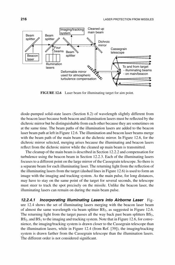
216 LASER PROTECTION FROM MISSILES
Cleaned upmain beam
Cassegraintelescope
To and from target - illuminating beams - on main/beacon
Dichroicmirror
Beaconlaser
Illuminationlasers
Imaging/trackingsystem
Beamsplitter
Beamsplitter
Beamsplitter
Deformable mirrorused for atmospheric turbulence compensation
Fourbeams
FIGURE 12.6 Laser beam for illuminating target for aim point.
diode-pumped solid-state lasers (Section 8.2) of wavelength slightly different fromthe beacon laser because both beacon and illumination lasers must be reflected by thedichroic mirror but be distinguishable from each other because they are sometimes onat the same time. The beam paths of the illumination lasers are added to the beaconlaser beam path at left in Figure 12.6. The illumination and beacon laser beams mergewith the beam path of the main beam at the dichroic mirror. In Figure 12.6, for thedichroic mirror selected, merging arises because the illuminating and beacon lasersreflect from the dichroic mirror while the cleaned up main beam is transmitted.
The cleanup of the main beam is described in Section 12.2.2 and compensation forturbulence using the beacon beam in Section 12.2.3. Each of the illuminating lasersfocuses to a different point on the large mirror of the Cassegrain telescope. So there isa separate beam for each illuminating laser. The returning light from the reflection ofthe illuminating lasers from the target (dashed lines in Figure 12.6) is used to form animage with the imaging and tracking system. As the main pulse, for long distances,may have to stay on the same point of the target for several seconds, the telescopemust steer to track the spot precisely on the missile. Unlike the beacon laser, theilluminating lasers can remain on during the main beam pulse.
12.2.4.1 Incorporating Illuminating Lasers into Airborne Laser Fig-ure 12.4 shows the set of illuminating lasers merging with the beacon laser beamof almost the same wavelength via beam splitter BS3, as suggested in Figure 12.6.The returning light from the target passes all the way back past beam splitters BS3,BS2, and BS1 to the imaging and tracking system. Note that in Figure 12.6, for conve-nience, the imaging/tracking system is drawn closer to the Cassegrain telescope thanthe illumination lasers, while in Figure 12.4 (from Ref. [39]), the imaging/trackingsystem is drawn farther from the Cassegrain telescope than the illumination lasers.The different order is not considered significant.

THE AIRBORNE LASER PROGRAM FOR PROTECTING FROM ICBMs 217
FIGURE 12.7 Rotating turret of airborne laser: (a) mechanism for pointing and tracking and(b) looking sideways.
12.2.5 Nose Turret
The mechanism for rotating the nose for the airborne laser in azimuth and elevationis shown in Figure 12.7a [34]. In Figure 12.7b [58], the nose turret in the airbornelaser plane is looking sideways toward the photographer. A block diagram showinglayout of the optics in the pointing and tracking system is shown in Figure 12.8 (seeRef. [34] for details).
12.2.6 Challenges Encountered in the ABL Program
Tests to shoot down intercontinental ballistic missiles have recently succeeded. Suc-cessfully completing such a complicated system with so many diverse systems thathave to be developed [34] is an extraordinary accomplishment that will be immenselyvaluable in future laser weapon systems. For this application, several potential prob-lems were identified.
1. Coverage Requires Fast Long-Distance Acquisition: To detect launches of mis-siles from all potentially dangerous areas of the world with a limited number ofplanes places an extraordinary requirement on the airplane acquisition systemin terms of speed and distance.
2. Turbulence Compensation Requires Complicated and Expensive AdaptiveOptics: In the upper atmosphere, turbulence and air path heating cause the maindestruction beam to spread and wander, necessitating a complicated system ofcompensating adaptive optics that is expensive and reduces performance.
3. Maintaining Beam on Target Spot Requires Accurate Long-Distance Tracking:The weakened and wandering laser spot at the target, which is at some distance
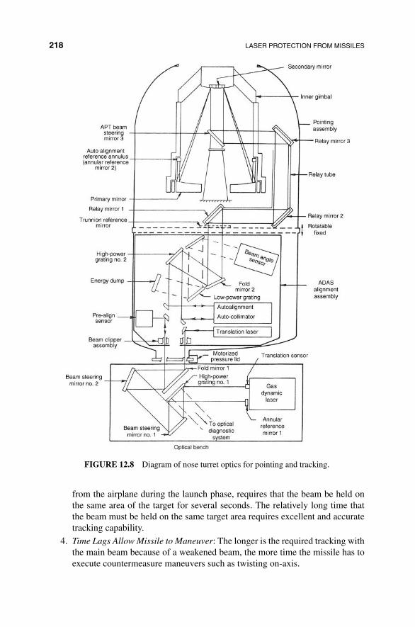
218 LASER PROTECTION FROM MISSILES
FIGURE 12.8 Diagram of nose turret optics for pointing and tracking.
from the airplane during the launch phase, requires that the beam be held onthe same area of the target for several seconds. The relatively long time thatthe beam must be held on the same target area requires excellent and accuratetracking capability.
4. Time Lags Allow Missile to Maneuver: The longer is the required tracking withthe main beam because of a weakened beam, the more time the missile has toexecute countermeasure maneuvers such as twisting on-axis.

THE AIRBORNE LASER PROGRAM FOR PROTECTING FROM ICBMs 219
5. Sensitivity to Bad Weather: Bad weather leading to excessive turbulence andbeam attenuation can further reduce the performance of the system.
6. Missile Coating: The missile can be coated with mirror or dielectric mirrors toreflect frequencies of interest to reduce the ABL performance.
7. Carrying Dangerous Chemicals on the Plane: Toxic and dangerous chemicalssuch as basic hydrogen peroxide, chlorine, and iodine create a hazard for thecrew, especially in a battle situation.
8. Optical System Sensitivity: The 1.5 m diameter mirror that points the beamat the target requires pointing accuracy and accurate alignment, making theoptical system highly sensitive to airplane maneuvers or vibration.
9. Speed Vulnerability of ABL: The airplane is large and slow. It presents an easytarget to enemy weapons.
10. Reload Time Vulnerability of ABL: The heat generated by firing the laser mustbe dissipated before another shot is taken. This causes the plane to remain inthe same location for a noticeable time.
11. Eliminating Laser Exhaust Signature Requires Expensive CryoabsorptionSystem: In order not to provide a large infrared signature and announce thepresence of a high-power COIL laser (Section 8.3.2), ABL needs to have acomplicated expensive cryoabsorption vacuum pump to absorb waste gases(Section 8.3.2.3).
12. New More Powerful Lasers May Make the System Obsolete Before It Can BeDeployed: Nonchemical lasers such as the free-electron laser are being devel-oped (Section 11.1). These avoid the storing of dangerous chemicals, such ashydrogen peroxide, liquid oxygen, and iodine, used with the current COIL laser.They are also tunable and can operate at almost any frequency.
The ABL program showed that each of the above problems could be addressed.However, continuously flying such a complex system around an increasing number ofnuclear missile threat areas of the world is unlikely to prove sufficiently cost-effectiveand reliable. While the future of this 15 year-old program seems to be uncertain, theresults with be of immense value for future military laser systems.
12.2.7 Modeling Adaptive Optics and Tracking for Airborne Laser
In Section 5.4.1, we described a numerical approach to modeling turbulence in prop-agating a beam through atmospheric turbulence over distance. As turbulence variesover the path from start to end, the method uses a layered model. Fresnel diffractionis used to propagate from one layer to the next while ignoring turbulence. At eachlayer interface, a phase screen changes the phase to account for the turbulence encoun-tered since the last phase screen. The computation for the computationally demandingphase screen uses a Kolmogorov statistical model and is described in Section 5.4.2and 5.4.3. Such phase screens are used in an adaptive optics and tracking testbed inthe Advanced Concepts Laboratory (ACL) at MIT Lincoln Laboratories [37].

220 LASER PROTECTION FROM MISSILES
12.2.7.1 Reason for Airborne Laser Testbed To design such a complexdynamic system as ABL, a testbed was needed.
1. The testbed provides records of time history of intensities and gradients,reconstructed phases, tracker tilts, main beam pointing, jitter, and beam in-tensity at target. Not only do these records enable system optimization but theyare also available for comparison with the measurements for a physical systemto ensure everything is operating as planned.
2. The testbed results can be cross-checked with wave optics simulations and witha physical system.
3. Many test scenarios may be tested with reproducible turbulence for selecting thebest approach and optimizing the configuration. In the real world, turbulencechanges from one flight to another reducing the validity of comparisons, not tomention the longer time required to perform test flights. Anticipated effects ofwind and turbulence levels are more easily determined with a simulator.
12.2.7.2 Description of ABL Adaptive Optics and Tracking TestbedFigure 12.9 shows the three sections of the testbed [37]: a transmit/receive bench foradaptive optics to compensate for turbulence (sections 5.3 and 12.2.3), beam prop-agation through the atmosphere with layered rotating phase screens (Section 5.4.2)and target bench with model missile. The transmit/receive bench and the target benchcan be moved in 3D by actuators for tracking and pointing, in the same manner asseats in flight simulators and video games. Wavelengths are scaled down by abouthalf relative to actual wavelengths to reduce size as explained next.
The transmit/receive bench includes a wave front sensor (Section 5.3.1.1), a 241actuator deformable mirror (Section 5.3.1.2), image tracker and fast steering mirror,adaptive optics and tracking illuminators (Section 12.2.4), and a scoring beam. Thescoring beam is a surrogate for the main beam from a high-energy laser (HEL), inthis case a COIL (Section 8.3.2) at 1.315 �m. The scoring beam is powered by ahelium–neon (HeNe) laser at 0.6328 �m, approximately half of the wavelength of theCOIL.
Transmit / receive bench
AO Illuminator(2-beamlet BILL)
Surrogate HEL
Point-aheadmirror
FSM
DM
Tracker Wave frontsensor
Track illuminator(4-beamlet TILL)
10–28 m propagation pathScoring
diagnostics
Modelmissile
CCD
Beaconsources
Target bench
AtmosphereRotating phase screensreplicate ABL turbulence
FIGURE 12.9 Diagram of adaptive optics and tracking testbed.

THE AIRBORNE LASER PROGRAM FOR PROTECTING FROM ICBMs 221
The adaptive optic (Figure 12.9) AO illuminator performs the role of the beaconilluminator (BILL) described in Section 12.2.3 for adaptively compensating for turbu-lence. In the testbed, the lines of an argon-ion laser provide the BILL for compensatingfor turbulence at 0.514 �m and the tracking illuminator (TILL) at 0.488 �m. The ac-tual BILL and TILL are generated by Nd:YAG lasers (Section 8.2) of slightly differentwavelengths around 1.06 �m. The TILL has four beams as shown in Figure 12.9 thatare each slightly divergent to flood the target model missile with light.
The BILL or beacon laser spot on the target returns light to the transmit/receivebench where the WFS measures the wave front over the cross section to set theactuators in the DM adaptively so that the aberrations due to turbulence are removed.The wave front is shaped so that the Gaussian main beam and beacon beams arefocused by the Cassegrain telescope (Section 1.3.4) to a tiny spot on the target modelmissile. The return light from the TILL provides the tilt of the beam that is used tocontrol the fast steering mirror (FSM).
The propagation path L can be varied from 10 to 28 m for the specific applicationscenario to meet the Fresnel index [163] F = D2/(λL), that is, brightness at theGaussian image point in the absence of aberrations. F is dependent on aperture D
and inversely dependent on distance L and wavelength λ. Seven stations along thepath (Figure 12.9) allow two phase screens at each station. Each phase screen modelsthe effects of turbulence over the distance from the last phase screen. Because of thelengthy computation for phase screens, phase screens are precomputed as describedin Section 5.4.2 and 5.4.3. Each phase screen is etched finely around a 6 in. diameterfused silica disk to provide phase inhomogeneities to model accumulated turbulenceeffects since the last phase screen. At the altitude of the airborne laser, atmosphericturbulence is weak, so 14 phase screens are adequate for modeling over the distance tothe target. The strength of the turbulence is determined by the depth of the etch. Eachdisk has 1 in. wide annular rings of varying turbulence strength. The scoring beam,representing the main beam, passes through the center of an annulus ring. Rotatingthe disk causes the phase screen to shift, simulating wind across the beam path. Astrong single direction wind will reduce blooming due to heating of the air and willhave consistent effect on the adaptive optics system.
For a specific engagement scenario, the phase screens are selected to match anumber of parameters [4, 37, 144, 163].
1. The turbulence profile C2n(z), equation (5.31), is a function of strength of tur-
bulence along the path.
2. The parameter r0 is the atmospheric coherence length or seeing eye size abovewhich diameter no further resolution is obtained with a telescope because ofturbulence. Adaptive optics is used with new terrestrial telescopes to increaseresolution beyond this limit in an effort to compete with space telescopes.
3. The Rytov variance σ2R is a measure of the strength of scintillation that de-
scribes fluctuations in received irradiance resulting from propagation throughturbulence; for example, stars twinkle for temporal variation and specklefor spatial variation. The Rytov approximation for weak turbulence involves
222 LASER PROTECTION FROM MISSILES
multiplication of perturbation terms [4]. Phase screens developed for the air-borne laser simulation cover the range of atmospheres 0 < σ2
R < 0.7.
4. In adaptive optics, to remove turbulence with a beacon beam, the wave frontfrom the beacon beam is used to set the deformable mirror so as to removeeffects of turbulence from the main beam prior to launching it. Therefore,the effectiveness of the adaptive optics turbulence compensation depends onstaying within the isoplanatic angle, θ0/(λ/D), which is the largest angle at thewave front sensor for which the main beam and the beacon beam are reasonablysimilar. In this case, the difference in frequency between main beam and BILL,or chromatic isoplanatic angle, matters.
5. The adaptive optic electronic or computer controller controls the feedback loopin an adaptive optics system [144]. The controllers task is to take a vector ms ofreadings from the wavefront sensor WFS and compute a vector of settings c forthe actuators in the deformable mirror DM. Note that both WFS and DM are2D and we simplify the explanation by assuming a linear relation and enteringthe 2D values into 1D vectors. The controller performs the computation
c = Mms (12.2)
where matrix M is computed to minimize the difference between slopes in thewave front sensor and deformable mirror using commonly used maximum aposterior and least squares estimation [161]. An alternative more complicatedapproach minimizes the aperture average mean square residual phase errorusing wave front statistics and WFS noise statistics. The feedback loops havebandwidth fB for compensating for turbulence and fT, the Tyler frequency,for compensating for tilt due to delays in the loops. A characteristic frequencyfor atmospheric turbulence is the Greenwood frequency fG. The orientationand the velocity of each screen are selected to reproduce the ratios fB/fG andfB/fT.
The target bench carries a centroid monitor for estimating far-field jitter and a CCDcamera to measure the intensity profile of the scoring beam across the target. The Strehlratio relates intensity on-axis for the turbulent aberrated beam to the intensity on-axisof an unaberrated beam. The Strehl ratio is measured by taking short and long exposurereadings of the scoring beam, peak to total integrated intensity compared to that fora diffraction-limited beam. Illumination back from the target is obtained in the targetbench by reflection from a model missile or with a beacon point source illuminatoror an extended width beacon at wavelengths 0.488 and 0.514 �m. The latter BILLand TILL sources are passed through a cut out of the model missile and then reflectedfrom a rotating retroreflective disk to remove scintillation before returning light tothe transmit/receive bench through the propagation phase screen path.
12.2.7.3 Experimental Testbed Simulation Results One of the com-plications in the ABL is that the optical tracking system and the adaptive optics

PROTECTING FROM HOMING MISSILES 223
turbulence compensation share the same optical paths at the same time. Three setsof experiments of increasing difficulty with both systems in operation were designedto allow separate assessment and optimization of each system while both arepresent.
The first set of experiments used a point source for both tracking and adaptive opticsfor turbulence. In the second set, a point source was used for tracking, but a morerealistic extended source over an adjustable area to represent reflection from a missilewas used for adaptive optics turbulence compensation. In the third set of experiments,the model missile was used to provide still more accurate modeling. The resultsshow reproducibility of experiments, critical for comparing different configurationsto optimize the overall system. Each system performance was assessed independently.The results agreed with lengthy computer computations. The results are presented indetail in Ref. [37]. The simulation clearly played a significant role in designing thefinal optical tracking and adaptive optics turbulence compensation systems.
12.3 PROTECTING FROM HOMING MISSILES
12.3.1 Threat to Aircraft from Homing Missiles
Single person shoulder fired missile launchers were introduced in the 1950s and arenow produced in 25 countries. They sell for around $10,000 but can be purchasedbetween $100, for old models, and $250,000, for the latest models. They are extremelyeffective against slow targets with limited maneuverability, including helicopters,transport planes, and almost any aircraft during take-off and landing. A modern IRseeking missile may sense more than one wavelength, for example 3–5 and 8–13 �m.The missile performs image processing such as contour imaging that makes commonlyused flares and point countermeasures ineffective. More recently, the advent of lasersin the countermeasure systems has allowed aircraft to be reliably protected. However,the countermeasures should continue to evolve with the missiles to maintain this levelof protection. The cost of protection is orders of magnitude less than the value of amilitary plane, including its value by remaining in service. For a civilian plane flyingin nondangerous places, the risk of downing by a missile is so small that it makes itdifficult to justify up to $1 million per plane for protection from missiles. However,the public fear of flying can be escalated for commercial purposes as people mightpay more to fly on a protected plane and costs will decrease with volume.
12.3.1.1 Missile Guidance Mechanisms The closed-loop guidance systemis the most vulnerable part of the missile guidance because a small error in steering cancause the missile to miss the target. Steering involves an antenna array: for infraredoptics, this may be a CCD. Missile guidance has been well studied as a time-varyingproblem of nonlinear parameter estimation of the direction of arrival (DOA) of a planewave incident at an angle θ with the normal on the array (Chapter 14). Reference [162]derives optimum processors. As indicated in Chapters 1 and 14, finding the directionof arrival of a plane wave source with an array is equivalent to finding the component
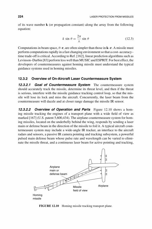
224 LASER PROTECTION FROM MISSILES
of its wave number k (or propagation constant) along the array from the followingequation:
k sin θ = 2π
λsin θ (12.3)
Computations in beam space, θ–r, are often simpler than those in k–r. A missile mustperform computations rapidly in a fast changing environment so that a cost–accuracy–time trade-off is critical. According to Ref. [162], linear prediction algorithms such asLevinson–Durbin [83] perform less well than MUSIC and ESPRIT. For best effect, thedevelopers of countermeasures against homing missile must understand the typicalguidance systems used in homing missiles.
12.3.2 Overview of On-Aircraft Laser Countermeasure System
12.3.2.1 Goal of Countermeasure System The countermeasure systemshould accurately track the missile, determine its threat level, and then if the threatis serious, interfere with the missile guidance tracking control loop, so that the mis-sile will lose its lock and miss the aircraft. Concurrently, the laser beam from thecountermeasure will dazzle and at closer range damage the missile IR sensor.
12.3.2.2 Overview of Operation and Parts Figure 12.10 shows a hom-ing missile tracking the engines of a transport plane with a wide field of view asmarked [167] (U.S. patent 5,600,434). The airplane countermeasure system for hom-ing missiles, located on the underbelly behind the wing, responds by sending a lasermain or defense beam in the direction of the missile to foil it. A typical aircraft coun-termeasure system may include a wide-angle IR tracker, an interface to the aircraftradars and sensors, a passive IR camera pointing and tracking subsystem, a powerfulpulsed main defense beam whose pulse rate and wavelength can be varied to elimi-nate the missile threat, and a continuous laser beam for active pointing and tracking,
Homingmissile
AirplaneMissilefield of view
Airplanemain ordefense beam
FIGURE 12.10 Homing missile tracking transport plane.

PROTECTING FROM HOMING MISSILES 225
vibration elimination, adaptive turbulence compensation, and selection of main beamaim point. A shutter allows the reflection from the missile for the continuous wave tobe viewed only while the main beam pulse is off. This shutter provides a time gate tosignificantly reduce clutter.
12.3.2.3 Description of Countermeasure Pods The man portable air de-fense system program (MANPADS) was completed for the Department of HomelandSecurity (DHS) in 2010. In this program [62], countermeasure homing pods on an air-plane protect the airplane from homing missiles such as those fired from the shoulder.The pods may be streamlined units that are built into the plane with a turret stickingout, such as the BAE Jeteye pod [59] (Figure 12.11). Figure 12.12 shows such a BAE
FIGURE 12.11 Turret of built-in BAE Jeteye countermeasure system.
FIGURE 12.12 Testing BAE Jeteye countermeasure system on an American Airlines jet.
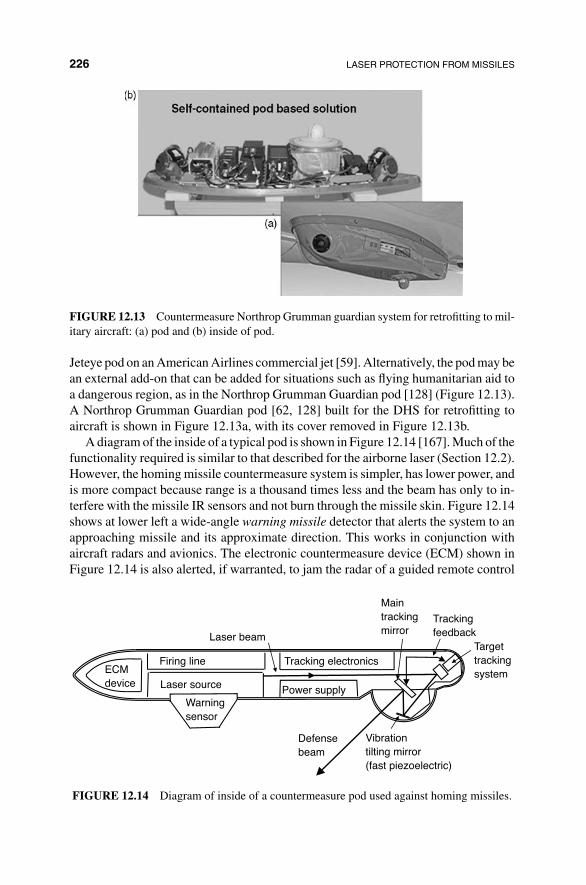
226 LASER PROTECTION FROM MISSILES
FIGURE 12.13 Countermeasure Northrop Grumman guardian system for retrofitting to mil-itary aircraft: (a) pod and (b) inside of pod.
Jeteye pod on an American Airlines commercial jet [59]. Alternatively, the pod may bean external add-on that can be added for situations such as flying humanitarian aid toa dangerous region, as in the Northrop Grumman Guardian pod [128] (Figure 12.13).A Northrop Grumman Guardian pod [62, 128] built for the DHS for retrofitting toaircraft is shown in Figure 12.13a, with its cover removed in Figure 12.13b.
A diagram of the inside of a typical pod is shown in Figure 12.14 [167]. Much of thefunctionality required is similar to that described for the airborne laser (Section 12.2).However, the homing missile countermeasure system is simpler, has lower power, andis more compact because range is a thousand times less and the beam has only to in-terfere with the missile IR sensors and not burn through the missile skin. Figure 12.14shows at lower left a wide-angle warning missile detector that alerts the system to anapproaching missile and its approximate direction. This works in conjunction withaircraft radars and avionics. The electronic countermeasure device (ECM) shown inFigure 12.14 is also alerted, if warranted, to jam the radar of a guided remote control
ECMdevice
Firing line
Laser source
Warningsensor
Tracking electronics
Power supply
Targettrackingsystem
Defensebeam
Laser beam
Maintrackingmirror
Trackingfeedback
Vibrationtilting mirror(fast piezoelectric)
FIGURE 12.14 Diagram of inside of a countermeasure pod used against homing missiles.

PROTECTING FROM HOMING MISSILES 227
missile. If the missile is deemed a threat, the passive and active tracking systems areactivated. For an underbody system, the transparent dome at right sees a completehemisphere below. More pods may be required for protection of large planes fromseveral directions.
12.3.3 Operation of Countermeasure Subsystems
12.3.3.1 Passive Missile Tracker Because of its high speed, a homing missilegets hot in front of the dome of its homing head and at its wing tips. An IR camerain the aircraft pod optical tracking head observes these hot spots and tilts the maintracking mirrors to lock onto these with a feedback loop (Figure 12.14) [167]. Oncea lock is achieved, the firing line is tripped to activate the power lasers. The lockedtracking directs all laser beams from tracker to missile.
12.3.3.2 Pulsed Main Power Beam A laser diode-pumped Nd:YAG solid-state laser in the aircraft pod (Section 8.2) is pulsed at the reticule rate used by theelectronics in the missile to read the missile CCD. This will cause incorrect estimatesof the aircraft direction and interfere with the guidance control so as to break its lock.Even without this effect, the laser from the aircraft will cause dazzle and glare in themissiles sensors and at close range can damage the sensors. The pulsed power laseris not pointed at a hot spot used for tracking because it has high reflectivity. Instead,a camera and electronics select an aim point on the missile head that is less reflectiveand hence more prone to absorbing the laser energy, as well as more critical to thecorrect functioning of the missile, for example, the sensor area. Several lasers ofdifferent wavelengths may be used as shown in Figure 12.15 [167], which includes
CO2 pulsed doubled laser
Nd:YAG resonator
Nd:YAG resonator
Beam expander
Trackingopticalsystem
Wave frontdetector Adaptive
optical system
Camera
Shutter
Tilting mirror
Illumination beam
Defensebeam
Illuminationbeam reflection
FIGURE 12.15 Lasers and adaptive optics system to compensate for turbulence.

228 LASER PROTECTION FROM MISSILES
a doubled carbon dioxide laser (Section 8.3.1) at a missile light wavelength of5 �m (a frequency that has low attenuation through the atmosphere, Figure 16.1), aND:YAG laser (Section 8.2) at 1.06 �m doubled to 0.53 (Section 8.2.2), and a secondNd:YAG frequency tripled to 0.25 �m for ultraviolet. A countermeasure system canalso include an optical parametric amplifier (OPO) consisting of a nonlinear crystalto tune a laser over a wider range for countering more sophisticated missiles.
12.3.3.3 Low-Power Laser for Adaptive Optics Atmospheric turbulencecauses the relatively narrow beams to diverge and wander around because of rotatingeddies in the air due to atmospheric turbulence, to which the motions of the missileand aircraft contribute. These eddies have less density at the edges and act as lensesof varying diameter and orientation (Chapter 5). The system is greatly enhanced byusing a continuous wave beam with an adaptive optics system shown in the lowerpart of Figure 12.15. The returning illumination beam reflection at lower right fromthe missile into the tracking optical system, is directed by the tracking optical systemmirror to a wave front detector (Section 5.3.1.1). A shutter is used to allow light topass to a CCD camera only when the main power light is zero between pulses. Thelocation of the returned light on the camera is used to move the adaptive optics systemmirror to keep the focus on the aim spot of the array.
The shutter also provides a time window that significantly reduces clutter. As themissile target starts at a point at far distance, light reflecting from other places willproduce clutter that is difficult to distinguish from the target. The shutter time windowblocks those reflections that are not in the same time window.
12.3.4 Protecting Aircraft from Ground-Based Missiles
The airborne laser was designed for destruction of intercontinental ballistic missiles.However, the COIL (Section 8.3.2), can be mounted in other aircraft to remove mis-sile carrying assets on the ground that might endanger the aircraft. For this purpose,a downward looking COIL was mounted by Boeing in a C-130 aircraft to demon-strate the ability to damage a Humvee on the ground that could be carrying a missilelauncher [1] (Figure 12.16). The main components of the system are shown in thefigure and described in Section 12.2. The system is simpler than the airborne laser forshooting down missiles because it does not have to operate over hundreds of kilome-ters from the target and the target moves relatively slowly. This avoids compensationfor turbulence and provides higher power at the target than is possible with the nose-mounted airborne laser. This system is less expensive and removes some of the riskfactors associated with the airborne laser program.
12.4 PROTECTING ASSETS FROM MISSILES
Figure 12.17 shows a Zumwalt class destroyer, which is stealth because it has a com-posite topside structure and a steel hull. Lasers are planned as shown in Figure 12.17to shoot down aircraft, missiles, other ships, and shore targets. Ships may have both
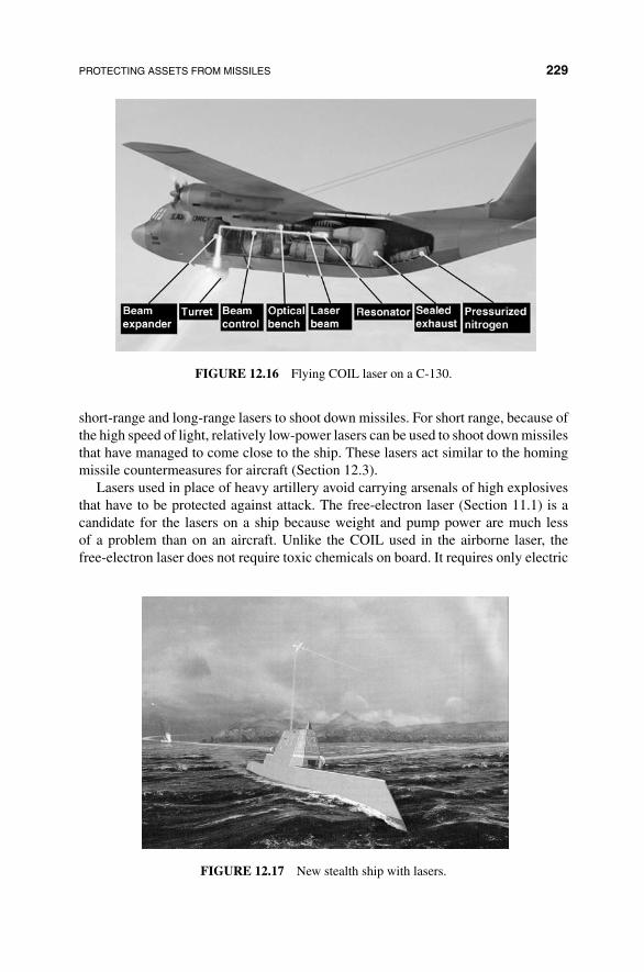
PROTECTING ASSETS FROM MISSILES 229
FIGURE 12.16 Flying COIL laser on a C-130.
short-range and long-range lasers to shoot down missiles. For short range, because ofthe high speed of light, relatively low-power lasers can be used to shoot down missilesthat have managed to come close to the ship. These lasers act similar to the homingmissile countermeasures for aircraft (Section 12.3).
Lasers used in place of heavy artillery avoid carrying arsenals of high explosivesthat have to be protected against attack. The free-electron laser (Section 11.1) is acandidate for the lasers on a ship because weight and pump power are much lessof a problem than on an aircraft. Unlike the COIL used in the airborne laser, thefree-electron laser does not require toxic chemicals on board. It requires only electric
FIGURE 12.17 New stealth ship with lasers.

230 LASER PROTECTION FROM MISSILES
generators for powering the lasers. Pulsing the lasers reduces the average power(Chapter 9). The free-electron laser is tunable over more than a 15% range and canbe built for a much wider range of frequencies. This allows the frequency to bechosen for good atmospheric propagation. For example, 3 mm electromagnetic waves,between optics and microwaves, pass through fog, mild rain, drizzle, and sea haze(Figure 16.1) and are also hazardous to electronic systems on missiles and satellites(Section 17.4). The problem of sea haze is discussed in the introduction to Chapter 14and (Section 16.3.4) [145]. Laser beams travel straight and cannot shoot over thehorizon as conventional artillery or missiles, but high-energy lasers have the powerto shoot satellites in earth orbit or destroy them by punching holes in their solar cellsand map satellites and debris in lower earth orbit (Section 16.3.1).

CHAPTER 13
LASER TO ADDRESS THREAT OF NEWNUCLEAR WEAPONS
Testing thermonuclear weapons for the military is harmful for the environment. So in1996, 151 countries signed and ratified the Comprehensive Nuclear-Test-Ban Treaty.Subsequently, international pressure is on the significant countries who signed thetreaty but have not ratified it, for example, China, Egypt, Indonesia, Iran, Israel, and theUnited States, and those who have not yet signed the treaty, for example, India, NorthKorea, and Pakistan. Without the ability to perform nuclear tests, the legal design anddevelopment of novel thermonuclear (fusion) bombs would languish. Unfortunately, arogue country or group might continue surreptitious testing to develop nuclear bombsto everyone’s disadvantage.
In Section 13.1, we discuss the justification to construct a super laser that cangenerate the conditions inside a thermonuclear bomb in the coming age of testbantreaties. In Section 13.2, we describe the structure and operation of the NationalInfrastructure laser.
13.1 LASER SOLUTION TO NUCLEAR WEAPONS THREAT
13.1.1 Main Purpose of U.S. and International Efforts
A solution to this threat for the United States was proposed: create an extreme laser thatcan emulate the temperature and pressure conditions at the center of a thermonuclear
Military Laser Technology for Defense: Technology for Revolutionizing 21st Century Warfare,First Edition. By Alastair D. McAulay.© 2011 John Wiley & Sons, Inc. Published 2011 by John Wiley & Sons, Inc.
231
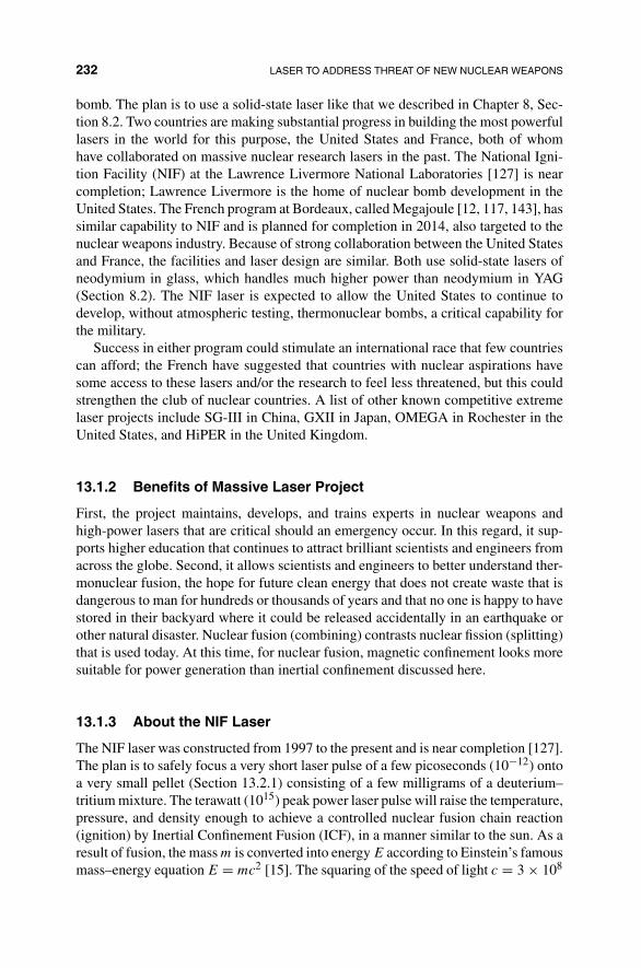
232 LASER TO ADDRESS THREAT OF NEW NUCLEAR WEAPONS
bomb. The plan is to use a solid-state laser like that we described in Chapter 8, Sec-tion 8.2. Two countries are making substantial progress in building the most powerfullasers in the world for this purpose, the United States and France, both of whomhave collaborated on massive nuclear research lasers in the past. The National Igni-tion Facility (NIF) at the Lawrence Livermore National Laboratories [127] is nearcompletion; Lawrence Livermore is the home of nuclear bomb development in theUnited States. The French program at Bordeaux, called Megajoule [12, 117, 143], hassimilar capability to NIF and is planned for completion in 2014, also targeted to thenuclear weapons industry. Because of strong collaboration between the United Statesand France, the facilities and laser design are similar. Both use solid-state lasers ofneodymium in glass, which handles much higher power than neodymium in YAG(Section 8.2). The NIF laser is expected to allow the United States to continue todevelop, without atmospheric testing, thermonuclear bombs, a critical capability forthe military.
Success in either program could stimulate an international race that few countriescan afford; the French have suggested that countries with nuclear aspirations havesome access to these lasers and/or the research to feel less threatened, but this couldstrengthen the club of nuclear countries. A list of other known competitive extremelaser projects include SG-III in China, GXII in Japan, OMEGA in Rochester in theUnited States, and HiPER in the United Kingdom.
13.1.2 Benefits of Massive Laser Project
First, the project maintains, develops, and trains experts in nuclear weapons andhigh-power lasers that are critical should an emergency occur. In this regard, it sup-ports higher education that continues to attract brilliant scientists and engineers fromacross the globe. Second, it allows scientists and engineers to better understand ther-monuclear fusion, the hope for future clean energy that does not create waste that isdangerous to man for hundreds or thousands of years and that no one is happy to havestored in their backyard where it could be released accidentally in an earthquake orother natural disaster. Nuclear fusion (combining) contrasts nuclear fission (splitting)that is used today. At this time, for nuclear fusion, magnetic confinement looks moresuitable for power generation than inertial confinement discussed here.
13.1.3 About the NIF Laser
The NIF laser was constructed from 1997 to the present and is near completion [127].The plan is to safely focus a very short laser pulse of a few picoseconds (10−12) ontoa very small pellet (Section 13.2.1) consisting of a few milligrams of a deuterium–tritium mixture. The terawatt (1015) peak power laser pulse will raise the temperature,pressure, and density enough to achieve a controlled nuclear fusion chain reaction(ignition) by Inertial Confinement Fusion (ICF), in a manner similar to the sun. As aresult of fusion, the mass m is converted into energy E according to Einstein’s famousmass–energy equation E = mc2 [15]. The squaring of the speed of light c = 3 × 10⁸

DESCRIPTION OF NATIONAL INFRASTRUCTURE LASER 233
Deformablemirror (LM1)
Mainamplifier
Cavity spatialfilter (CSF)
PolarizerLM2
LM3
Poweramplifier
Transportspatial
filter (TSF)
Transportoptics Final
opticsassembly
Fiber
Master oscillator
Preamp
Polarizationswitch
FIGURE 13.1 One of the 48 similar beamlines in the NIF.
means that a great deal of energy is obtained from a very small mass, which is whythermonuclear bombs are so powerful and the sun lasts so long.
13.2 DESCRIPTION OF NATIONAL INFRASTRUCTURE LASER
13.2.1 Structure of the NIF Laser
The NIF laser starts by generating a short pulse with a master ytterbium-doped(1053 nm) fiber laser oscillator. This signal is distributed to 48 identical beamlinesvia an optical fiber; a typical beamline [127] is shown in Figure 13.1. The pulse fromthe master oscillator at lower center enters a preamplifier.
All the preamplifiers and amplifiers use flashlamp-driven Nd:glass disks, a mate-rial that withstands higher powers than Nd:YAG. Rods similar to much larger ver-sions of those used in solid-state Nd:YAG (Section 8.2) were used in earlier inertialconfinement lasers: an example is shown of a Nd:glass rod used in France in 1970(Figure 13.2) [143]. The maximum power is limited by that for which the glass rodfractures or the beam becomes overly distorted. The power of an amplifier can beincreased 10 times by replacing a rod by a series of disks, angled alternately for-ward and backward at the Brewster angle, to eliminate reflections from their surfaces(Figure 13.3) [36]. Disks are thin, avoiding the uneven heating due to different flash-lamp penetration distances into the rod that causes rods to fracture. As a result, diskscan be pumped with up to nine times the power of rods [36]. The expanded beamdiameter also causes much less glass deterioration at high intensities. The zigzag linesin the amplifiers in Figure 13.1 represent angled disks. One of the disks that replacedthe rod in Figure 13.2 in the French laser is shown in Figure 13.4 [143].
The light entering the center of Figure 13.1 is reflected to the left into a poweramplifier and then down by mirror LM3 through a polarization switch that directsit into a spatial filter to restore spatial coherence (Section 1.3.6). After passing themain amplifier, the light is reflected by mirror LM1 that is deformable to correct foraberrations. Because the flashlamp incoherent light duration is longer than the mainlaser beam pulse duration, the amount of light coupling from flashlamp to pulse isenhanced by allowing light to bounce back and forth between LM2 and LM1 until the

234 LASER TO ADDRESS THREAT OF NEW NUCLEAR WEAPONS
FIGURE 13.2 Nd:glass rod in 1970 French inertial confinement laser and amplifier.
FIGURE 13.3 Illustration of a Nd:glass disk amplifier with many disks.

DESCRIPTION OF NATIONAL INFRASTRUCTURE LASER 235
FIGURE 13.4 Nd:glass disk in 1974 French inertial confinement laser and amplifier.
flash light subsides. This means allowing the light to pass through the main amplifierfour times before setting the polarization to switch the light out of the cavity throughmirror LM3. A total of 7680 flashlamps are used in the 48 beamlines throughout thesystem, using a total electrical energy of 400 MJ from capacitor banks. As a result,even if nuclear fusion occurs, there is unlikely to be net energy produced.
The beam travels back to the right through the power amplifier and the centraltransport spatial filter. The spatial filters and deformable mirrors are critical to recov-ering the spatial coherence lost in distortion by the amplifiers. Figure 13.5 [127] shows24 beamlines on one of the two parallel identical laser bays of the NIF facility; thepeople in the left foreground give a sense of the immensity of the laser.
FIGURE 13.5 One of the two laser bays showing 24 beamlines in NIF.

236 LASER TO ADDRESS THREAT OF NEW NUCLEAR WEAPONS
FIGURE 13.6 Target of the beams during assembly.
Transport optics in Figure 13.1 now move the 48 beams to their positions arounda 10 m diameter spherical target chamber to place more than a megajoule of energyon a single centimeter-size spot at the center of the sphere at precisely the same timewithin picoseconds (10−12 s) (Figure 13.6) [127]. This explains the enormity of thedifficulty involved.
In a final step (not shown in Figure 13.6) before merging beams, because ultravioletpenetrates the plasma better than infrared, the wavelength is halved from 1053 nm(infrared) to 527 nm (green) (Section 8.2.2) and then converted to 351 nm (ultraviolet)using thin sheets cut from a single crystal of potassium dihydrogen phosphate. Therecovery time to cool down after firing the laser is expected to be around 5 hours.

CHAPTER 14
PROTECTING ASSETS FROMDIRECTED ENERGY LASERS
Military targets must be protected from high-energy light pulses that propagate effi-ciently across space at high speed and have potential to cause damage [103]. Coatingtargets can reduce the damage for some combinations of weak laser source and robusttarget but in general we need laser warning devices (LWD). A laser warning systemwas built into the system to protect aircraft from homing missiles in Section 12.3.The problem is somewhat similar to avoiding a speeding ticket in your car by using alaser warning detector, except perhaps that the military target may be worth hundredsof millions of dollars and many lives may be involved. The challenge is to detectthe threat laser light fast enough for the target to evade the threat beam or launchcountermeasures to save the target.
Almost every scenario is unique because targets include personnel, vehicles, mis-siles, aircraft, or satellites, while the threat could be from a variety of lasers: powerlasers (Chapter 8), pulsed lasers (Chapter 9) and, ultrahigh-power lasers (Chapter 10).Sometimes the target is large relative to the threat laser beam diameter, a ship forexample, and many coordinated sensors are required on the target. In ocean en-vironments, the threat laser can scatter to form haze and fewer sensors may suf-fice. The laser threat beam may be modulated to provide unique identification forthat beam.
Military Laser Technology for Defense: Technology for Revolutionizing 21st Century Warfare,First Edition. By Alastair D. McAulay.© 2011 John Wiley & Sons, Inc. Published 2011 by John Wiley & Sons, Inc.
237

238 PROTECTING ASSETS FROM DIRECTED ENERGY LASERS
Detecting laser threats in the future may become more difficult because newcyclotron-based lasers such as the free-electron laser (Chapter 10) [126] aretunable, orders of magnitude more powerful, and can be used at any microwaveor light frequency.
In Section 14.1, we discuss the characteristics of lasers, some of which are mea-sured by the laser warning device. In Section 14.2, we describe four basic approachesfor laser warning devices from which systems may be tailored for specific applica-tions.
14.1 LASER CHARACTERISTICS ESTIMATED BY LASER WARNINGDEVICE
The main types of threat laser for military applications include laser diodes, diode-pumped solid-state lasers, fiber lasers, chemical lasers, and free-electron lasers (Sec-tion 8.1.3). A laser warning system is designed to detect one or more of the followingrelevant laser characteristics:
• Frequency and Power of Light: Fortunately, with the exception of the free-electron laser, there are a finite number of frequencies that can be easily generatedwith a laser because frequency is determined by the energy of the photon result-ing when an electron falls across a bandgap from a higher energy level to a lowerone in a lasing material. The number of low-cost easy-to-process lasing materialscapable of generating high power is limited. Consequently, in detecting currenthigh-power lasers we have only a few frequencies to consider.
The application also influences the choice of laser frequency; for example,target designators where an operator points a beam at a target to relay its GPScoordinates require visible light. In contrast, an infrared (IR) range finder, notvisible to the eye, is less likely to alert the target. In some cases, eye-safe lasers aredesirable, similar to those operating around 1550 nm used in optical telecommu-nications. Minimizing the affects of the atmosphere can also influence frequencyselection (Section 16.1).
• Bandwidth or Temporal Coherence: The bandwidth of the light, linewidth for alaser, indicates how close the light is to a single frequency. A narrow linewidthor equivalently a high temporal coherence (Section 6.1) defines the presenceof a laser and may provide insight into the laser and its application. Commu-nication lasers may have narrow linewidth so that many wavelength divisionmultiplexed signals can pass through an optical amplifier. Detecting laser lightis more difficult in high ambient light such as sunshine [26].
• Direction of Laser and Spatial Coherence: Spatial coherence is related to therate at which a laser beam spreads with diffraction (Sections 3.2.2 and 1.3.6) anddepends on the size of the emitting surface of the laser. Direction of the beamcan be determined more precisely for a beam that is spreading more slowly.Beam direction systems are related to wave front detectors used in adaptiveoptics (Section 5.3.1). The direction of the source can indicate whether the laser

LASER WARNING DEVICES 239
is from an airborne vehicle such as a drone or airplane, from a satellite, or from aground vehicle. Identifying the direction aids the threat assessment and permitsimmediate retaliation.
• Pulse and Modulation: Pulses are commonplace for laser weapons because forthe same average laser power, greater damage may be inflicted by the higher peakpower. A laser warning detector must respond faster to detect shorter pulses.Unfortunately, fast response conflicts with high sensitivity, which requires longintegration times. The platform and application often dictate which is more crit-ical, nevertheless both types of system may be required in the same installation.Many laser beams are modulated in the battlefield to avoid confusion with otherbeams, for example, target designators and for communications.
14.2 LASER WARNING DEVICES
In order to identify a laser threat and select an appropriate response, we simultane-ously estimate several parameters for the light impinging on a laser weapon warningsystem. First, accurately estimating the direction of the source allows opportunityfor an immediate response to neutralize the source. Second, estimating power andfrequency enables us to assess the goal of the laser source and its damage potentialfrom which we can decide on the threat level and corresponding evasion or retaliationresponse. Third, the bandwidth in frequency of the source �f indicates the level oftemporal coherence tc = 1/�f and can provide data on the modulation and pulsewidth. Indeed, laser light is distinguished from ambient light by its high temporaland spatial coherence [26]. The subject of spectrum analysis was discussed in severalplaces in the book (Sections 4.2 and 15.3) and many of the techniques presented therecan be used. The array waveguide structure in Section 14.2.4 provides a compactintegrated optic spectrum analyzer.
We describe four approaches that can be used in different circumstances. The si-multaneous estimation of direction and frequency with a grating (Section 14.2.1) isfast but has limited sensitivity to low light levels. Performance may be improved byseparating the tasks of estimating direction and frequency. A single lens can replacethe grating to provide direction only (Section 14.2.2), as in wave front detection inadaptive optics (Section 5.3.1). This is more sensitive to low light level because allthe light is used purely for direction estimation. An interferometer (Chapter 6) [16]provides more accurate measurement of frequency only [28] but measures a singlefrequency unambiguously only within a spectral range. In Section 14.2.3, we selecta Fizeau interferometer, because it can simultaneously estimate multiple frequenciesunambiguously without mechanical motion. This allows bandwidth measurement andwill operate on very short pulses, assuming fast detectors. However, now a curvedmirror is needed to direct the beam into the interferometer. In Section 14.2.4, wedescribe an integrated optic spectrometer that is more robust, accurate, and less ex-pensive. Such spectrometers will be required for new cyclotron-based lasers such asthe free-electron laser that can operate at any frequency and are typically tunable overapproximately 20% range.
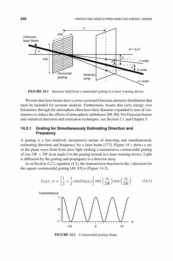
240 PROTECTING ASSETS FROM DIRECTED ENERGY LASERS
Unknownlaser beam
2W
2W
Horizontalgrating
0 order
−1 order
+1 order
Z
d
p = f0λz
p
p
Detectorarray
θ
FIGURE 14.1 Intensity field from a sinusoidal grating in a laser warning device.
We note that laser beams have a cross-sectional Gaussian intensity distribution thatmust be included for accurate analysis. Furthermore, beams that carry energy overkilometers through the atmosphere often have their diameter expanded to tens of cen-timeters to reduce the effects of atmospheric turbulence [88, 90]. For Gaussian beamsand statistical detection and estimation techniques, see Section 2.1 and Chapter 5.
14.2.1 Grating for Simultaneously Estimating Direction andFrequency
A grating is a fast relatively inexpensive means of detecting and simultaneouslyestimating direction and frequency for a laser beam [177]. Figure 14.1 shows a rayof the plane wave front from laser light striking a transmissive cosinusoidal gratingof size 2W × 2W at an angle θ to the grating normal in a laser warning device. Lightis diffracted by the grating and propagates to a detector array.
As in Section 4.2.2, equation (4.2), the transmission function in the z direction forthe square cosinusoidal grating [49, 83] is (Figure 14.2).
Uin(x, y) =[
1
2+ 1
2cos(2πf0x1)
]rect
( x0
2W
)rect
( y0
2W
)(14.1)
Transmittance1
0
–1
–10 0 10X
FIGURE 14.2 Cosinusoidal grating shape.

LASER WARNING DEVICES 241
The square bracket represents the sinusoidal grating pattern of spatial frequency f0in the x direction. The first 1
2 in equation (14.1) provides the mean or zero-orderdiffraction (straight through) in Figure 14.1, which arises because intensity cannot benegative. The rectangular functions represent the finite 2W × 2W square aperture ofthe grating.
Incident light with propagation constant k at an angle θ with the horizon-tal has a downward propagating component at the grating of exp {jk sin θ x1} =exp {j2πx1 sin θ/λ}. The normal incidence case, θ = 0, was analyzed in Sec-tion 4.2.2. So in a similar manner to Section 4.2.2, the Fourier transform in thex–y plane of the intensity immediately after the grating is, from equation (14.1),
Uout(x0, y0) = F[Uin(x1, y1) exp
{j2πx1 sin θ
λ
}]
= F[
1
2+ 1
2cos 2πf0x1
]∗ F
[rect
(x0
2W
)rect
(x0
2W
)]∗ F
[exp
{j2π sin θ x1
λ
}]
=[
1
2δ(fxfy) + 1
4δ(fx + f0, fy) + 1
4δ(fx − f0, fy)
]
∗ (2W)2sinc(2Wfx)sinc(2Wfy) ∗ δ
(fx + sin θ
λ
)
=(
2W
2
)2
sinc(2Wfy)
[sinc
{2W
(fx + sin θ
λ
)}
+ 1
2sinc
{2W
(fx + sin θ
λ+ f0
)}+ 1
2sinc
{2W
(fx + sin θ
λ− f0
)}](14.2)
If a front-end telescope is used or the beam from the laser is less than the gratingaperture size, the Gaussian nature of the laser beam should be included as discussedin Section 14.2.2.
The three orders in the square bracket in the last line of equation (14.2) correspondto those in Figure 14.1 (0, −1, 1). Assuming sufficient spacing to avoid overlap ofdiffraction orders, we can write the Fraunhofer diffraction far-field intensity at theoutput by introducing scaling for optics, fx = x0/(λz) and fy = y0/(λz), and thenmultiplying by its conjugate,
Iout(x0y0) = 1
(λz)2
{1
2(2W)2
}2
sinc2(
2Wy0
λz
)[
sinc2(
2W
λz(x0 + z sin θ)
)+ 1
4sinc2
{2W
λz(x0 + z sin θ + f0λz)
}
+ 1
4sinc2
{2W
λz(x0 + z sin θ − f0λz)
}](14.3)
The intensity of the far field from a cosinusoidal grating, equation (14.3), at a far-fieldplane, is illustrated in Figure 14.1. Comparison of equation (14.3) with the normalincidence case, equation (4.5), shows that the output orders are shifted down by d in

242 PROTECTING ASSETS FROM DIRECTED ENERGY LASERS
Figure 14.1 compared to the normal incident case (Figure 4.4). Information about thewavelength λ of the unknown laser is obtained from the distance p on the detectorarray in Figure 14.1.
λ = p
f0z(14.4)
The distance between grating and detector array, z, is known for the system. Informa-tion about the unknown laser direction θ is obtained from the distance d in the outputdetector array:
tan θ = d
z(14.5)
Due to atmospheric turbulence, the image at the detector will wander around and thefocus regions fluctuate in size with time. In this case, the equation approximates thecentroid of the pattern on the image plane. The turbulence effect is in addition to thatcaused by relative motion of the target and beam source.
14.2.2 Lens for Estimating Direction Only
A lens can be used in place of a grating to avoid the inefficiencies of the sinusoidalgrating due to dispersion into three orders. Hence, the lens direction finding systemis more sensitive than a grating for finding the direction of low light level lasersources such as those arising in munitions guiding lasers or due to scattering fromthe atmosphere. This is similar to a Hartmann wave front sensing in adaptive optics(Section 5.3.1) [144, 163]. Figure 14.3 shows a Gaussian beam of laser light withspot size Wlens striking a lens at an angle θ with the horizontal in a laser warningdevice.
UnknownGaussianlaser beam
Detectorarray
x
2W0
2W lens
f
θ
FIGURE 14.3 A lens-based direction finding system in a laser warning device.
LASER WARNING DEVICES 243
A Gaussian beam is fully defined by its spot size W(z) (radius of 1/e amplitudespot) and the radius of curvature of the phase frontR(z) (Section 2.1.1, equation (2.18))times exp{−jkz}, equivalent to Equation (2.19).
U(x, y, z) = A1
ω
W0
W(z)exp
{−j[kz − ζ(z)] − ρ2
[1
W(z)2 + jk
2R(z)
]}(14.6)
where k = 2π/λ is the propagation phase constant, W0 is the beam spot size at thewaist (narrowest point), ζ is the beam divergence angle, and ρ is the radial directionin the transverse plane. In Figure 14.3, a lens is used to focus a Gaussian beam ofspot size Wlens to its narrowest spot size (waist) W0 at the detector (Figure 14.3) [148,176].
On passing a Gaussian beam through a lens of focal length f , the spot size Wlensremains the same but the slope is reduced by 1/f , equation (1.22). As slope equalsthe reciprocal of radius of curvature R, the radius of curvature of the Gaussian beamexiting the convex lens is given by
1
R= 1
Rin− 1
f(14.7)
Assuming the incoming beam approximates a plane wave because of its great distancefrom the source, Rin = ∞, then from equation (14.7) the radius of curvature of theGaussian beam leaving the lens is R = −f : the negative sign represents a convergingbeam. The Gaussian beam parameters for the beam exiting the lens are W = Wlens andR = −f . The Gaussian beam parameters at the detector array are radius of curvatureR = ∞ and the waist size W0 that can be derived from the equations in Section 2.1.3item (d). Substituting for z, from equation (2.34) into equation (2.43) and using thebinomial approximation gives the beam size W0 on the detector.
In the same manner as for the grating (Section 14.2.1), the image on the detectorarray moves around and the spot size varies because of atmospheric turbulence. Con-sequently, the centroid of the spot must be computed to determine the direction of thelaser source.
14.2.3 Fizeau Interferometer
A Fizeau interferometer [28] has two off-parallel planar reflecting surfaces separatedby a small angle φ (Figure 14.4). At any point along z, the plates approximate aparallel plate because φ is small. So we first consider the parallel plate interferometerin Figure 14.5 in which an unknown laser beam in air impinges at an angle α andis reflected from the top and bottom surfaces. We can determine the increased pathlength �s of the bottom surface reflection relative to the top surface reflection in twoparts: the part in the glass dg and the part dp required to bring the phases together for

244 PROTECTING ASSETS FROM DIRECTED ENERGY LASERS
FIGURE 14.4 Fizeau interferometer.
the output beam.
�s = dg − dp = 2nd
cos β− 2d tan β sin α = 2nd
cos β− 2d tan β n sin β = 2nd cos β
(14.8)where we used Snell’s law sin α = n sin β and 1 − sin2 θ = cos2 θ. When the dif-ference in path lengths �s = mλ (m an integer), light from the two paths is in phaseand combines constructively for a maximum intensity, while when the difference inpath lengths is �s = λ/2 + mλ, light from the two paths is out of phase and combinesdestructively for a minimum intensity. Setting �s = mλ in equation (14.8) gives
mλ = 2nd cos β (14.9)
Shortpath
Longpath
dp
dg/2dg/2
d β
α
α
Phase frontof reflectedbeam
FIGURE 14.5 Parallel plate interferometer.

LASER WARNING DEVICES 245
In the Fizeau interferometer, the spacing between the surfaces d(z) changes withdistance z along the wedge formed and this changes the resonant wavelength λ withdistance. By detecting wavelengths of interest in parallel, the Fizeau is more suitablefor rapid detection of pulsed laser sources than a resonator that detects only a singlefrequency. From equation (14.9) we can write for adjacent peaks,
2n[d(z2) − d(z1)] cos β = λ or d(z2) − d(z1) = λ
2n cos β(14.10)
The distance � along z between two fringe maxima may be written from Figure 14.4and equation (14.10):
� = z2 − z1 = d(z2) − d(z1)
tan φ= λ
2n cos β tan φ(14.11)
Equation (14.11) shows that � varies with wavelength λ. Further as φ is small, theresonant wavelength continues to behave locally at location z like a parallel plate forwhich λ depends on plate separation d(z). Consequently, changing λ will both movethe fringes and change the separation of their maxima.
For parallel plate resonators, λ can be determined within only one spectral rangebecause of higher order integers m in equation (14.10) give the same output. The freespectral range, the frequency range between two maxima, is δν = c/�s. Insertingfor δν from the second equation (6.20) that converts from frequency range δν towavelength range δλ gives
c
λ2 δλ = c/�s (14.12)
or, replacing �s using equation (14.8),
δλ = λ2
�s= λ2
2nd cos β(14.13)
Compared to a parallel plate interferometer, the Fizeau interferometer is better forhandling pulsed lasers because it measures many wavelengths simultaneously as afunction of distance z along the interferometer. Hence we can also estimate absolutewavelength over a wide range of wavelengths and avoid the ambiguity inherent in theperiodicity of the parallel plate interferometers [28].
14.2.4 Integrated Array Waveguide Grating Optic Chip for SpectrumAnalysis
The laser threat detector must operate with current laser weapon designs as well asfuture cyclotron-based lasers that we expect will initially use the same wavelengthsas current laser weapons because of availability of components and instrumentation.The wavelengths of current and anticipated laser weapons are listed in Table 8.1. Forlaser threat detection, we propose a robust inexpensive integrated optic spectrometer

246 PROTECTING ASSETS FROM DIRECTED ENERGY LASERS
p
s sFirst starcoupler Second star
coupler
q
λ1.λ2.λn...λNλN
Waveguides
Length L
Length L + sΔL(a)
(b) λ1λn
FIGURE 14.6 Photonic integrated circuit layout for array waveguide grating.
to determine the laser wavelength [103]. The array waveguide grating (AWG) is anintegrated optic version of the grating (Section 14.2.1) as a spectrometer for estimatingwavelength. The spectrometer consists of an array waveguide grating similar to thoseused in telecommunications (Figure 14.6) [2, 53, 75].
The array waveguide grating is used for wavelength division multiplexing intelecommunications. Prior to the invention of the AWG, a separate filter was usedfor each wavelength, typically 128 per band. The AWG handles all 128 differentfrequency channels at once. We propose an AWG as a spectrum analyzer for de-tecting laser threats such as those from new tunable high-power free-electron lasers(Section 11.1) [103] or other cyclotron-based lasers (Chapter 10).
Figure 14.6a shows an integrated optic AWG chip and Figure 14.6b showsthe circuit layout for the AWG chip. As a spectrometer, the input with multiplewavelengths is entered at one of the input ports at lower left, for example, the pth
input port. The wavelengths are spread to separate ports at the output at the right-side.There are three parts: a first star coupler, a waveguide part, and a second starcoupler.
In the first star coupler, the input enters the coupler and spreads out due to diffrac-tion; thus, the input is broadcast to all the outputs of the first star coupler. The circularcurvature of the first star coupler ensures that all the outputs from the first star couplerenter the waveguides in the waveguide section with the same phase. The waveguidesection has waveguides of increasing lengths. The difference in length between awaveguide and its neighbor is �L. In the second star coupler, the light at wavelengthλ1 is focused to the first output waveguide, λ2 to the second, and so on.
The operation can be understood by examining phase delays throughout the sys-tem. As the upper waveguides are longer than those below, light is delayed in theupper guides relative to the lower ones. The amount of delay depends on wavelength.Therefore, at the entrance to the second star coupler, the wave front defined by thephase peaks has a tilt depending on wavelength. Similar to steering with a phasedarray antenna, the tilt causes beams of different wavelengths to focus to different out-puts. We derive two design equations for the AWG: the first computes the relationshipbetween the incremental length �L and the nominal wavelength λ0, and the secondcomputes the relationship between the coupler geometry and the resolution betweenwavelengths at the output �λ.

LASER WARNING DEVICES 247
R RR sin pα RpαR sin sα ′Rsα ′
pth
portsth
portdps
sα ′ pαα ′ α
R
R−R(1− cos pα)−R(1− cos sα ′)R(1− cos pα )
R cos pα
R cos sα ′
R(1− cos sα ′)
FIGURE 14.7 First star coupler geometry.
Figure 14.7 defines the star coupler geometry. The circular boundaries in the starcoupler have radius R and the distance separating the two arcs on the axis is also R.The angles subtended by the first ports above the axis at the opposite faces are α andα′ for the two directions, respectively, as shown. The angle subtended at the outputaxis by the arc to the pth input port is pα and that subtended by the sth output portat the input axis is sα′. In order to compute the phase lag from the pth input port tothe sth output port, we first compute the distance dps using Pythagoras theorem withhorizontal and vertical distances. The horizontal distance is computed by dropping aperpendicular from the input pth port and output sth port to the axis. The horizontaldistance between the ports is the distance between these lines R [1 − (1 − cos (pα)) −(1 − cos(sα′))]. We drop perpendiculars from the pth port and sth port to the verticalline through the intersections of curved surface and axis to obtain the vertical distanceR (sin (pα) − R sin(sα′)). Hence, by Pythagoras theorem
d2ps = R2(−1 + cos (pα) + cos (sα′))2 + R2(sin (pα) − sin (sα′))2 (14.14)
For small angles pα and sα′, cos (pα) → 1, cos (sα′) → 1, sin (pα) → pα, andsin(sα′) → sα′ and neglecting second-order terms (pα)2 and (sα′)2, and using thebinomial theorem to remove the square root, equation (14.14) becomes
dps = R(1 − psαα′) (14.15)
For the three parts of the AWG, we write the following:
1. Phase Delay Across First Star Coupler. From equation (14.15), using phaseφ = kd = 2πncoupler/λ, the phase delay from input port p to output ports is,
φps = 2π
λ/ncouplerR(1 − psαα′) (14.16)

248 PROTECTING ASSETS FROM DIRECTED ENERGY LASERS
2. Phase Delay in Waveguide Part. From Figure 14.6, the phase delay along thesth waveguide is
φs = 2π
λ/nwg(s�L + L) (14.17)
3. Phase Delay Across Second Star Coupler. Analogous to equation (14.16), thephase delay for the input s port to the output q port is
φsq = 2π
λ/ncouplerR(1 − sqαα′) (14.18)
The total phase from the AWG input port p to the AWG output port q is written byadding phase from equations (14.16)–(14.18):
φp,s,q = φps + φs + φsq
= 4π
λ/ncouplerR + 2π
λ/nwg(s�L + L)
− 2π
λ/ncouplerRαα′s(p + q) (14.19)
where the first term of the last equation sums the first and constant terms from equa-tions (14.16) and (14.18) and the last term sums the second terms of these equationsfor which there is port number dependence.
The phase difference between two waveguide paths, s and s − 1, from equa-tion (14.19) removes constant terms:
�φpq = φp,s,q − φp,s−1,q
= 2π
λ/nwg�L − 2π
λ/ncouplerRαα′(p + q) (14.20)
The power at the output port q results from summing signals with phase �φpq for allM waveguides (s from 0 to M − 1), (see Section 9.2.1)
Ppq = Pin
M2
∣∣∣∣∣s=M−1∑
s=0
exp{js�pq}∣∣∣∣∣2
= Pin
M2
∣∣∣∣1 − exp{jM�φpq}1 − exp{j�φpq}
∣∣∣∣2
= Pin
M2
sin2(M�φpq/2)
sin2(�φpq/2)(14.21)

LASER WARNING DEVICES 249
When �φpq → 2π, all paths are in phase at the output, the angles are small andsin θ → θ, so the maximum power approaches
Ppq(�φpq) → Pin
M2
(M�φpq/2)2
(�φpq/2)2 = Pin (14.22)
Substituting �φpq = 2π into the left-hand side of equation (14.20), canceling 2π,and setting λ = λpq,
λpq = nwg�L − ncouplerRαα′(p + q) (14.23)
λpq is the wavelength for which all paths through different waveguides combine atthe output port q. We can write equation (14.23) by separating out and defining aconstant term λ0 from a term �λ that depends on the input port p and output port q:
λpq = λ0 − (p + q)�λ (14.24)
where the newly defined terms provide the two design equations for an AWG. The firstdesign equation for an AWG relates the operating wavelength λ0 to the incrementallength �L of the waveguides:
λ0 = nwg�L (14.25)
and the second design equation for an AWG relates the wavelength resolution, spacingbetween wavelengths, �λ, and the geometric values for the layout, α and α′:
�λ = ncouplerRαα′ (14.26)
14.2.5 Design of AWG for Laser Weapons
Assuming refractive index of both star coupler and waveguides is n, from equa-tion (14.25), we write the first design equation, the difference in length between twoadjacent central waveguides, as
�L = λ0
n(14.27)
From equation (14.26) for the second design equation, we assume that the angleα = α′ for a given device of radius R and spacing between wavelengths �λ:
α =√
�λ
nR(14.28)
For illustration and to show feasibility with modern lithography machines, wedesign a device with a center wavelength at a laser weapon wavelength around

250 PROTECTING ASSETS FROM DIRECTED ENERGY LASERS
λ0 = 1.5 �m and a range of ±15%, comparable to that of a cyclotron-based laser, suchas a free-electron laser. The±15% is an estimate for the tunable range of a specific free-electron or other cyclotron laser. For reference, the airborne laser uses a wavelength of1.315 �m. For the laser weapon at a wavelength λ0 = 1.5 �m, from equation (14.27)the distance in length between adjacent waveguides is �L = 1.5 × 10⁻⁶/1.5 = 10−6
or 1 �m for waveguide refractive index n = 1.5. Current lithographic machines fortelecommunication AWGs have the capability to provide 1 �m resolution in waveg-uide length.
For ±15% tuning around λ0 = 1.5 �m, the wavelength range of operation isfrom 1.275 to 1.725 �m or 450 nm. If 200 wavelength bin slots are selected forthe array waveguide spectrometer, each slot is �λ = 450/200 = 2.25 nm wide.For a radius of R = 5 cm, using equation (14.28), the angle α in Figure 14.7 isα =
√2.25 × 10⁻⁹/(1.5 × 5 × 10−2) = 1.7 × 10⁻⁴ or 0.17 mrad. This is a rea-
sonable angle for current lithography because it is larger than that used in currenttelecommunication array waveguides [2, 75].
CHAPTER 15
LIDAR PROTECTS FROM CHEMICAL/BIOLOGICAL WEAPONS
Lidar stands for light detection and ranging and refers to systems in which a beamof laser light shines into the atmosphere and is scattered or reflected from an objector from a cloud [168]. Light wavelengths are short enough to interact with chemi-cal and biological elements in the air, so the backscatter from an aerosol cloud maybe analyzed for the presence of chemical and biological weapons. This chapter fo-cuses on lidar for detecting the presence of chemical and biological weapons in theatmosphere.
Other military applications involve scanning a pulsed laser beam to produce 3Dimages of a target. The depth is obtained by measuring the time between the emissionof a pulse and receiving the backscattered pulse. When scanning the earth from anaircraft or a satellite, 3D remote sensing surveillance maps are obtained.
In Section 15.1, we introduce lidar for detecting and assessing threats from chem-ical and biological weapons and briefly mention other military applications. In Sec-tion 15.2, we describe a typical lidar system. In Section 15.3, we describe optical spec-trum analyzers for identifying chemicals from lidar return signals. In Section 15.4, weconsider a lidar system with spectrum analyzer to determine the presence of chemicalor biological weapons and the associated threat assessment.
Military Laser Technology for Defense: Technology for Revolutionizing 21st Century Warfare,First Edition. By Alastair D. McAulay.© 2011 John Wiley & Sons, Inc. Published 2011 by John Wiley & Sons, Inc.
251

252 LIDAR PROTECTS FROM CHEMICAL/BIOLOGICAL WEAPONS
15.1 INTRODUCTION TO LIDAR AND MILITARY APPLICATIONS
Lidar is developing fast to become one of the more important technologies for militaryapplications. Lidar, which operates at light frequencies, is similar in concept to radar(radio detection and ranging) that operates at radio frequencies or microwaves. Lidar,in addition to 3D image scanning capabilities, has a significant additional capabilitycompared to radar: it can identify chemicals. The shorter light wavelengths that rangefrom infrared through visible to ultraviolet can match the size of chemical or biologicalmolecules and particles in an aerosol. Both absorption and scattering depend onparticle size and concentration. For absorption, when a match occurs the molecule orparticle resonates, absorbing energy and causing a dip in intensity in the backscatteredsignal at the resonant frequency for that molecule or particle. Sweeping the lightthrough a range of wavelengths allows spectral identification and concentration ofthe chemicals present in the air or in a cloud. This chapter focuses on the ability oflidar to remotely measure chemicals in the atmosphere.
Lidar can profile the atmosphere up to over 100 km from the ground and higher fromaircraft or satellites. Lidar atmospheric measurements include wind, temperature,humidity, trace gases, clouds, and aerosols. These parameters can drastically affectperformance of military systems including missiles, artillery, lasers, communications,imaging, visible range, and aircraft motion. Lidar is used to estimate turbulence foradaptive optics (Section 5.3.1.4) and for optimizing windmill location and bladedirection. Ladar can detect the presence of an aerosol cloud in the sky.
Once an aerosol is detected, lidar can be used to estimate the extent, motion,concentration, and composition of an aerosol cloud: an aerosol is a system of col-loidal particles in a gas, smoke, or fog. Colloidal particles have a diameter of 10−7
to 10−5 cm, larger than that of most inorganic molecules, and remain suspended in-definitely, due to the motion and associated electrostatic charges in the surroundingmedia. Detection of trace gases, toxic chemicals, and biological agents and their con-centrations from the lidar enables a military threat assessment. The responses mustthen be evaluated: for example, is contamination equipment needed? Can we avoidthe cloud? Is the aerosol hiding something? Do we need to use radar such as W-bandradar or 94 GHz radar in Chapter 16 to see into it? Can we operate through it? Arecent startling example of our unpreparedness for unpredicted aerosol events is il-lustrated by the dilemma regarding whether jet aircraft can safely fly through airbornevolcanic ash and where and how long the ash will interfere with international travel.The molten iron, the crust of which we live on, is in turmoil, indicated by the recentbeginning of reversal of the earth’s magnetic field; we can expect a great deal moreproblems of penetration of the crust leading to earthquakes and volcanoes.
15.1.1 Other Military Applications for Lidar
Lidar can be used like radar but the shorter relative wavelength on a visually clear day(Section 16.1) provides narrower beams, higher space and time resolution, and, bytiming pulse response, the ability to perform 3D profiling of targets for identification
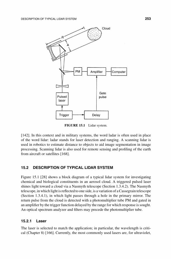
DESCRIPTION OF TYPICAL LIDAR SYSTEM 253
FIGURE 15.1 Lidar system.
[142]. In this context and in military systems, the word ladar is often used in placeof the word lidar: ladar stands for laser detection and ranging. A scanning lidar isused in robotics to estimate distance to objects to aid image segmentation in imageprocessing. Scanning lidar is also used for remote sensing and profiling of the earthfrom aircraft or satellites [168].
15.2 DESCRIPTION OF TYPICAL LIDAR SYSTEM
Figure 15.1 [28] shows a block diagram of a typical lidar system for investigatingchemical and biological constituents in an aerosol cloud. A triggered pulsed lasershines light toward a cloud via a Nasmyth telescope (Section 1.3.4.2). The Nasmythtelescope, in which light is reflected to one side, is a variation of a Cassegrain telescope(Section 1.3.4.1), in which light passes through a hole in the primary mirror. Thereturn pulse from the cloud is detected with a photomultiplier tube PM and gated inan amplifier by the trigger function delayed by the range for which response is sought.An optical spectrum analyzer and filters may precede the photomultiplier tube.
15.2.1 Laser
The laser is selected to match the application; in particular, the wavelength is criti-cal (Chapter 8) [166]. Currently, the most commonly used lasers are, for ultraviolet,
254 LIDAR PROTECTS FROM CHEMICAL/BIOLOGICAL WEAPONS
excimer and, for infrared, Nd:YAG (Section 8.2) at 1064 nm. Nd:YAG can be doubledto 532 nm (Section 8.2.2), tripled to 355 nm, and quadrupled to 266 nm. Longer wave-lengths are obtained by stimulated Raman scattering in hydrogen and deuterium thatwhen applied to an excimer laser provides ozone differential absorption lidar and solar-blind lidar. In solar-blind lidar, superior performance is achieved in bright sunshineby using ultraviolet wavelengths not emitted by the sun and filtering the sunlight out.For sweeping through wavelengths for chemical analysis with differential absorptionand resonance fluorescence lidars, dye lasers pumped with excimer or Nd:YAG arebeing replaced with tunable solid-state lasers such as titanium:sapphire with opticalparametric amplifiers [176]. Infrared lidars suitable for Doppler lidar involve dopingof crystalline lattices YAG, YLF or LuAG with active dopants such as Nd, Ho, Tm,Cr, Er, or Yb. New lasers are routinely considered for lidar as they are developed; forexample, fiber lasers emitting eye-safe 1500 nm are valuable for some high-powerapplications and free-electron lasers allow tuning over limited ranges (Section 11.1).
15.2.2 Cassegrain Transmit/Receive Antennas
A Cassegrain or Nasmyth mirror telescope up to a few meters in diameter is typ-ically used to launch the lidar beam and receive the backscatter (Section 1.3.4.1,Figure 1.11). For chemical/biological lidar, the sensitivity required is such that sep-arate antennas in a biaxial system are normally used for transmit and receive. Thebeam expansion (Section 1.3.2) of the inverted telescope reduces the divergence dueto diffraction to 100 � rad. A field stop (Section 1.3.4) in the receiver telescope focalplane reduces the field of view to a few hundred � rad. The narrow transmit and receivebeams reduce the interfering background light and the effects of multiple scattering.The small field of view improves selectivity in spectrum analyzers. For a ground lidarinvestigating far distance targets, the upper atmosphere, such as a radar for mappingdebris and objects in satellite space (Section 16.3.2), a chopper, timed by the emitpulse repetition rate, can eliminate interference from scatterers at close distances.
In a biaxial system, the launch beam expander (inverse telescope) and the receivingtelescope are separated by half the antenna width or more to reduce inadvertentcoupling of powerful transmit signals directly into the receiver system. In this case,there is a receiver field-of-view overlap functionO(R) that may require a few kilometerrange to the target area before overlap reaches 100%, depending on field of view andseparation.
15.2.3 Receiver Optics and Detector
An optical filter at the passband of the laser can filter out interference from unwantedwavelengths. Other filters, such as polarization filters, can be used in conjunctionwith a spectrum analyzer (Section 15.3). A photomultiplier tube or avalanche pho-todiode converts light to an electronic signal. Both photomultiplier tube and lesssensitive avalanche photodiode have sufficient sensitivity to provide Geiger counteroperation for which a count of individual photons measures very weak backscatterlight intensities.
DESCRIPTION OF TYPICAL LIDAR SYSTEM 255
15.2.4 Lidar Equation
We derive the lidar equation for the received lidar signal [168]. The lidar equationcan be used for many applications but the backscatter and absorption equations mustbe modified for the different applications, remote chemical sensing, target mapping,and ground mapping.
15.2.4.1 Range Bin The lidar sends a pulse of duration τ into the atmosphere.If P0 is the average power in the pulse, the energy in a pulse is E = P0τ and theilluminated length of a pulse in space is cτ, where c is the velocity of light. For apulse repetition rate of frep, the average power emitted is P = Efrep.
Because the pulse has duration, each point in the received time trace shows theresponse from a range bin �R that we now compute. At a time t after sending thepulse, we observe the return signal. The front edge of the pulse returns from a scattererat a distance from the lidar of
R1 = ct
2(15.1)
where the factor 2 accounts for the two-way travel distance 2R1. The rear edge of thepulse leaves the emitter at τ after the front edge and returns from a distance
R2 = c(t − τ)
2(15.2)
The range bin �R from which return signals are obtained for pulse duration τ is then
�R = R1 − R2 = cτ
2(15.3)
The system performance characteristic K is written as
K = P0cτ
2Aη (15.4)
where the strength of the return signal is proportional to the area of the telescopeA = π(D/2)2 with D the diameter of the telescope main mirror, η is the overallsystem efficiency, P0 is the average power in the pulse, and the range bin �R = cτ/2.
15.2.4.2 Antenna Gain and R2 Fall Off with Distance For isotropic scat-terers, the radiated scattered intensity Is lies on the surface of a sphere of radiusR according to 4πR2. The collected light Ic for an antenna of area A as a ratio ofscattered light is
Ic
Is= A
4πR2 (15.5)
256 LIDAR PROTECTS FROM CHEMICAL/BIOLOGICAL WEAPONS
The collected intensity falls off with distance as R2 and A/R2 is known as the per-ception angle for the light scattered at distance R. For bistatic lidar, we combine theoverlap function O(R), defined in Section 15.2.2, and the R2 fall off into
G(R) = O(R)
R2 (15.6)
15.2.4.3 Backscatter Coefficient The backscatter coefficient, β(R, λ), at dis-tance R and wavelength λ, represents the ability of the atmosphere to scatter lightback into the direction from which it came (π radians from the forward direction). Forthe jth particle in a collection of varying particles, with concentration of Nj particlesper unit volume, and particle cross section per unit solid angle [dσj,scat/d()](π, λ),the backscatter coefficient is written as
β(R, λ) =∑
j
Nj
[dσj,scat
d
](π, λ) (15.7)
If the N scatterers per unit volume are identical and isotropic (radiating over solidangle d → 4π) with cross section σscat, from equation (15.7)
4πβ = Nσscat (15.8)
If the cross-sectional area of the lidar beam at the scattering volume is AL, from equa-tion (15.3), the scattering volume is V = AL�R = ALcτ/2. From equation (15.8),the intensity of scattered light is proportional to
As = NσscatV = NσscatALcτ
2(15.9)
Using As from equation (15.9) andNσscat from (15.8), the ratio of intensity of scatteredlight Is to emitted light I0 is
Is
I0= As
AL= Nσscat
cτ
2= 4πβcτ
2(15.10)
Substituting Is from equation (15.5) into equation (15.10) gives the ratio of collectedlight in the receiver Ic to the emitted light I0 by the transmitter:
Ic
I0= Is
I0
Ic
Is=
(βcτ
2
) (A
R2
)=
(Aβcτ
2R2
)(15.11)
in terms of the perception angle A/R2, backscatter coefficient β, and pulse length τ.We note that the backscatter coefficient can be considered in two parts, that due to
molecules and that due to particulate matter in aerosols:
β(R, λ) = βmol(R, λ) + βaer(R, λ) (15.12)
SPECTROMETERS 257
βmol, mainly from oxygen and nitrogen, decreases with height above ground becauseof decreasing density. βaer varies in time and space and includes liquid and solid airpollution particles such as sulfates, soot, organic compounds, mineral dust, sea salt,pollen, rain drops, ice crystals, and hail [166].
15.2.4.4 Transmission Loss Transmission loss T (R, λ) is the fraction of lightthat is lost in two-way travel
T (R, λ) = exp
{−2
∫ R
0α(r, λ)
}dr (15.13)
The sum is extinction loss and α(r, λ) is the extinction coefficient. Similar to back-scatter, equation (15.7), the extinction coefficient depends on the number concentra-tion Nj and the extinction cross section σj of the jth scatterer:
α(R, λ) =∑
j
Nj(R)σj,ext(λ) (15.14)
The extinction cross section σj,ext(λ) can be partitioned into that due to scatteringand that due to absorption and the extinction coefficient α(r, λ) can be additionallydivided into that due to molecules and that due to aerosols.
15.2.4.5 Lidar Equation From, these equations, we can write the lidar equationfor the received signal power P(R) in a lidar from a distance R as
P(R) = KG(R)β(R)T (R)
= P0cτ
2Aη
O(R)
R2 β(R, λ) exp
{−2
∫ R
0α(r, λ)
}dr (15.15)
where we used equation (15.4) for the system function K, equation (15.6) for thegeometric R dependence, β(R, λ) for the unknown scattering coefficient, and equa-tion (15.13) for the transmission loss. In addition to the lidar power in equation (15.15),there will be a background power that can be due to sun, stars, moon, and detectornoise. The background power can be measured before emitting a pulse or at distanceswhere no scatterers are expected. Background power is subtracted from the receivedlidar power before passing it to an optical spectrum analyzer for chemical analysis.The optical spectrum analyzer is described in Section 15.3 and its use in a lidar inSection 15.4.
15.3 SPECTROMETERS
Spectrometers or optical spectrum analyzers measure optical power as a functionof wavelength [28, 29]. For absorption measurements, the molecular size of a par-ticular chemical (such as CO2) or bacteria (such as Salmonella) matches a specificwavelength of light, so that light at this wavelength is absorbed in causing resonance.

258 LIDAR PROTECTS FROM CHEMICAL/BIOLOGICAL WEAPONS
FIGURE 15.2 Generic laboratory optical spectrum analyzer.
15.3.1 Fabry–Perot-Based Laboratory Optical Spectrum Analyzer
Laboratory optical spectrum analyzers (OSAs) are used to view signals such as thespectrum of laser diodes and output of filters, but are not generally sensitive enoughfor determining chemical elements in a material or vapor. Fabry–Perot resonators(Section 6.2) may be used for spectrum analyzers by varying the spacing between twoparallel mirrors. As one mirror moves with respect to the other, the half-wavelengththat satisfies the boundary condition to fit between two mirrors determines the resonantwavelength. Such a tunable optical filter may be placed in Figure 15.2, a typicallaboratory optical spectrum analyzer [29].
A sweep frequency causes the filter acting on the input light signal whose spec-trum is sought to sweep linearly through wavelength. In a spectrum analyzer, eachwavelength segment of the input is measured separately. As shown in Figure 15.2,an electric signal in the form of a sawtooth or ramp is used to move one mirror ofa Fabry–Perot filter with a piezoelectric device to extract a wavelength band. Thedistance between mirrors determines the band center frequency and the reflectivity ofthe mirrors determines the bandwidth (Section 6.2). The electric signal for the sweepfrequency is used to drive the horizontal axis of an oscilloscope as shown. The filteredlight is detected by a reverse-biased photodetector and transimpedance amplifier [52]and the electric output fed to the vertical axis of the oscilloscope. On the screen wesee the power spectrum of the input light, which is the intensity (W/m2) as a functionof wavelength (λ).
15.3.2 Diffraction-Based Spectrometer
15.3.2.1 System for Diffraction-Based Spectrometer A glass prism (Fig-ure 4.2b) will separate incoming light into its constituent colors but does not work at
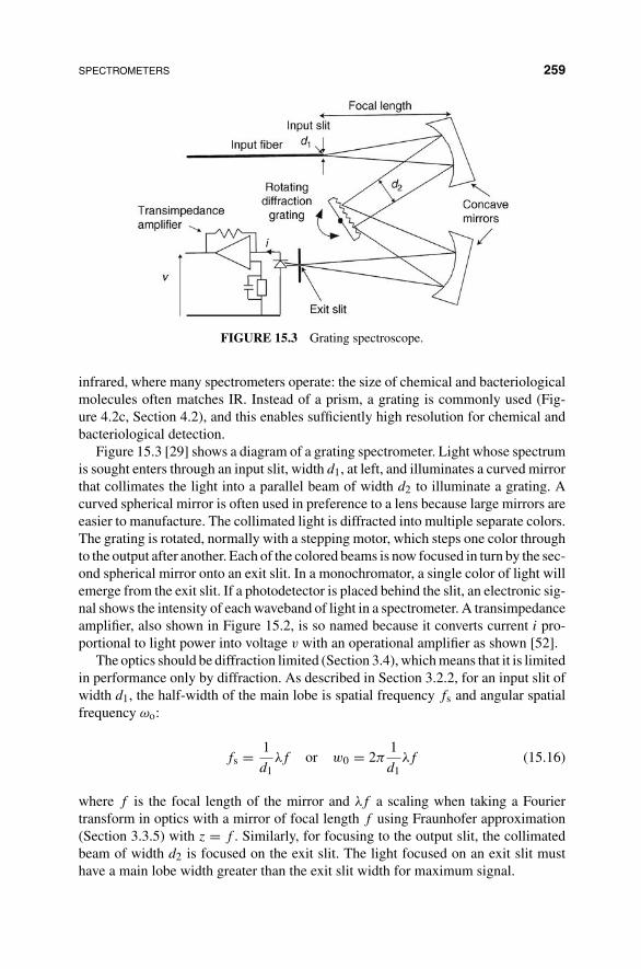
SPECTROMETERS 259
FIGURE 15.3 Grating spectroscope.
infrared, where many spectrometers operate: the size of chemical and bacteriologicalmolecules often matches IR. Instead of a prism, a grating is commonly used (Fig-ure 4.2c, Section 4.2), and this enables sufficiently high resolution for chemical andbacteriological detection.
Figure 15.3 [29] shows a diagram of a grating spectrometer. Light whose spectrumis sought enters through an input slit, width d1, at left, and illuminates a curved mirrorthat collimates the light into a parallel beam of width d2 to illuminate a grating. Acurved spherical mirror is often used in preference to a lens because large mirrors areeasier to manufacture. The collimated light is diffracted into multiple separate colors.The grating is rotated, normally with a stepping motor, which steps one color throughto the output after another. Each of the colored beams is now focused in turn by the sec-ond spherical mirror onto an exit slit. In a monochromator, a single color of light willemerge from the exit slit. If a photodetector is placed behind the slit, an electronic sig-nal shows the intensity of each waveband of light in a spectrometer. A transimpedanceamplifier, also shown in Figure 15.2, is so named because it converts current i pro-portional to light power into voltage v with an operational amplifier as shown [52].
The optics should be diffraction limited (Section 3.4), which means that it is limitedin performance only by diffraction. As described in Section 3.2.2, for an input slit ofwidth d1, the half-width of the main lobe is spatial frequency fs and angular spatialfrequency ωo:
fs = 1
d1λf or w0 = 2π
1
d1λf (15.16)
where f is the focal length of the mirror and λf a scaling when taking a Fouriertransform in optics with a mirror of focal length f using Fraunhofer approximation(Section 3.3.5) with z = f . Similarly, for focusing to the output slit, the collimatedbeam of width d2 is focused on the exit slit. The light focused on an exit slit musthave a main lobe width greater than the exit slit width for maximum signal.
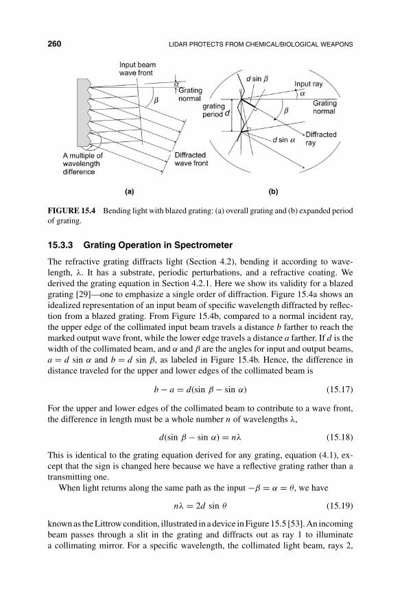
260 LIDAR PROTECTS FROM CHEMICAL/BIOLOGICAL WEAPONS
FIGURE 15.4 Bending light with blazed grating: (a) overall grating and (b) expanded periodof grating.
15.3.3 Grating Operation in Spectrometer
The refractive grating diffracts light (Section 4.2), bending it according to wave-length, λ. It has a substrate, periodic perturbations, and a refractive coating. Wederived the grating equation in Section 4.2.1. Here we show its validity for a blazedgrating [29]—one to emphasize a single order of diffraction. Figure 15.4a shows anidealized representation of an input beam of specific wavelength diffracted by reflec-tion from a blazed grating. From Figure 15.4b, compared to a normal incident ray,the upper edge of the collimated input beam travels a distance b farther to reach themarked output wave front, while the lower edge travels a distance a farther. If d is thewidth of the collimated beam, and α and β are the angles for input and output beams,a = d sin α and b = d sin β, as labeled in Figure 15.4b. Hence, the difference indistance traveled for the upper and lower edges of the collimated beam is
b − a = d(sin β − sin α) (15.17)
For the upper and lower edges of the collimated beam to contribute to a wave front,the difference in length must be a whole number n of wavelengths λ,
d(sin β − sin α) = nλ (15.18)
This is identical to the grating equation derived for any grating, equation (4.1), ex-cept that the sign is changed here because we have a reflective grating rather than atransmitting one.
When light returns along the same path as the input −β = α = θ, we have
nλ = 2d sin θ (15.19)
known as the Littrow condition, illustrated in a device in Figure 15.5 [53]. An incomingbeam passes through a slit in the grating and diffracts out as ray 1 to illuminatea collimating mirror. For a specific wavelength, the collimated light beam, rays 2,

SPECTROMETERS 261
3
3
2
123
K
2
4
4
1
1
FIGURE 15.5 Device using Littrow condition grating.
returns to the grating and the beam is diffracted by the grating along rays 3 andreturns to the collimating mirror that now focuses the light to a spot on the grating viarays 4. Each color focuses to a different position as shown at the different λ valuesout at left.
15.3.3.1 Limits to Grating Resolution The grating imposes a limit to thewavelength resolution, how finely colors may be separated. The blazed grating (Fig-ure 15.4) has length Nd, where N is the number of grating periods and d is thegrating period. Like an antenna, a longer grating produces a narrower beam pattern.For exit angle β, the 3 dB width at which power emitted is half the peak is (equation(3.20), [29])
�βm = λ
Nd cos β(15.20)
Wavelength resolution is further limited by the dispersion equation (15.18). Taking aderivative dβ/�λ of equation (15.18), we can write
�β = n
d cos β�λ (15.21)
where n is the order of the grating.For minimum wavelength resolution, �λmin, equating (15.21) and (15.20) to eli-
minate �βS and solving for �λmin shows resolution depends only on grating lengthand λ
�λmin = λ
Nn(15.22)
Note that using a different focal length lens or mirror for focusing to the output affectsmagnification but not the resolution.
15.3.4 Grating Efficiency
The efficiency with which input light is used for producing output depends on thequality of the grating, both the quality of the coating and the quality of the blaze,

262 LIDAR PROTECTS FROM CHEMICAL/BIOLOGICAL WEAPONS
FIGURE 15.6 Detecting chemical and biological weapons by transmission.
which emphasizes order n at the expense of other orders. As reflection is polarizationsensitive, a less preferable polarization direction will reduce efficiency.
The output is focused on an exit slit; the narrower the slit, the smaller the part ofthe spectrum selected, and therefore the higher the spectral resolution. But the highestresolution remains limited by the grating resolution (15.22). A spectrum analyzer hasa photodetector after the exit slit. The type of photodetector depends on wavelengthand sensitivity. For high-resolution spectroscopy, a photomultiplier is used. If highresolution is not required, a photodiode is adequate.
15.4 SPECTROSCOPIC LIDAR SENSES CHEMICAL WEAPONS
Two approaches to sensing chemical and bacteriological elements in the battlefieldor terrorist environments are by direct transmission or backscatter [28].
15.4.1 Transmission Detection of Chemical and Biological Materials
Direct transmission is normally performed close to the ground. Figure 15.6 [28] showsa transmission optical spectrometer in which laser light from a tunable laser diode orother fixed laser that covers several molecular sizes of interest is passed to a beamsplitter BS. One output of the beam splitter feeds a beam expander BE, or invertingtelescope (Section 1.3.2), to produce a collimated beam passing through the medium(shaded) in which chemical or biological weapons material may exist. The otheroutput from the beam splitter is reflected by a mirror at top into the polychromatoras a reference for the power of the laser P0. A polychromator is a spectrum analyzerthat separates the light into constituent wavelengths.
SPECTROSCOPIC LIDAR SENSES CHEMICAL WEAPONS 263
A retroreflector reflects the light reduced by absorption of power P back to thebeam splitter BS that passes it to the polychromator. Each wavelength passes to adifferent channel of an optical multichannel analyzer (OMA). A plot of power ver-sus wavelength is obtained from the computer. If a specific molecule from a weaponschemical or bacteria is present, the wavelength matching the molecular size will expe-rience attenuation due to the power absorbed by resonance. Several different moleculetypes are detected simultaneously. The fraction of the input power P0 received for agiven frequency after traveling a distance L is
P(L) = P0 exp{−a(ω)L} (15.23)
where the attenuation coefficient α(ω) = Niσi,abs depends on the concentration Ni ofabsorbing molecules with absorption cross section σi,abs. An attenuation coefficienta(ω) may be written as
a(ω) = α(ω) + S (15.24)
where the sum of absorption from all particles is
α(ω) = Nkσk,abs (15.25)
and the sum of the scattering from all particles S is
S =∑
Nkσk,scat (15.26)
S is mainly Mie scattering from particles, dust, and water drops. A small part isfrom Rayleigh scattering from molecules and atoms for which the wavelength isgreater than the molecule size. S has a broad spectrum while α(ω) has a very narrowlinewidth (a few GHz) matching a specific molecule. Consequently, sensitive detectionis obtained by comparing the input power at the exact frequency for the peak powerfor a specific chemical molecule P(ω1, L) with the output power for neighboringfrequencies that change little with frequency P(ω2, L). The difference values aresimultaneously computed for a number of known chemical and biological agents.Detection depends on the ratio
P(ω1, L)
P(ω2, L)≈ exp{−Ni[σi,abs(ω1) − σi,abs(ω2)]L} (15.27)
15.4.2 Scattering Detection of Chemical and BacteriologicalWeapons Using Lidar
As described in Figure 15.1 (Section 15.2), pulsed laser light moves through a tele-scope (Section 1.3.4) to form a wide beam that is projected toward a questionablecloud in the sky to determine its chemical composition. The light scattered from thecloud S(λ, t) returns to a photomultiplier tube (PM) and is measured in wavelength

264 LIDAR PROTECTS FROM CHEMICAL/BIOLOGICAL WEAPONS
and in time [28]. The scattered light is gated during the time interval t1 ± �t todetermine the time signal at t1 = 2R/c (equation (15.1), Section 15.2.4.1).
S(λ, t1) =∫ t1+ 1
2 �t
t1− 12 �t
S(λ, t)dt (15.28)
The magnitude of S(λ, t) depends on the solid angle d = D2/R2 covered by thetelescope, diameter D, and aperture A = π(D/2)2; the concentration of the moleculessignal N; and backscattering cross section σscat. We can write
S(λ, t) = P0(λ) exp
{−2
∫ R
0α(r, λ)
}dr Nσscat(λ)D2/R2 (15.29)
This is similar to the lidar equation (15.15) with 100% overlap, O(R) = 1, efficiencyη = 1, signal for a range bin cτ/2, antenna perception A/R2 ≈ D2/R2, and scatteringcoefficient β = Nσscat.
Similar to the transmission approach (Section 15.4.1), we consider a wavelength λ1at an absorption line (the resonance peak) of a molecule and a wavelength λ2 whereabsorption is negligible. For small �λ = λ1 − λ2, the variation in scattering crosssection may be neglected. Then, ratio of scattering for λ1 and λ2 is
S(λ1, t)
S(λ2, t)= exp
{2
∫ R
0[α(λ2) − α(λ1)]dR
}
≈ exp
{2
∫ R
0Ni(R)σ(λ1)dR
}(15.30)
Equation (15.30) provides the concentration of molecules sought Ni(R) integratedover the complete path to cloud and back.
The variation in concentration of molecules with distance is obtained by samplingalternate λ values at successive intervals of �t. Then absorption for a range bin atdistance R is obtained (using a series expansion for the exponential) by
S(λ1, t)/S(λ2, t + �t)
S(λ1, t)/S(λ2, t)= exp{−[α(λ2) − α(λ1)]�R}≈ 1 − [α(λ2) − α(λ1)]�R (15.31)
According to equation (15.25), the concentration of molecules, Ni for the ith chemicalelement, can be obtained from the absorption coefficients in equation (15.31). Theconcentration of a toxic chemical or bacteria is used to assess the nature of a threat.
CHAPTER 16
94 GHz RADAR DETECTS/TRACKS/IDENTIFIES OBJECTS INBAD WEATHER
At 94 GHz the radar uses many of the light technologies described in Part I becausethe frequency falls between light and microwaves. For example, the gyroklystronused (Section 10.1) has a quasi-optical mirror resonator and the 94 GHz radar usesa quasi-optical duplexer to separate transmit and receive waves. This frequency isconsidered the upper part of the millimeter band of frequencies and has distinctadvantages over light or microwaves in several applications. The frequencies classifiedas W-band, 75–110 GHz, have wavelengths of a few millimeters (4–2.7 mm), whichallows them to pass through particles of smaller size. Of particular interest is f =94 GHz that falls in an atmospheric window and has a wavelength in air of λ = c/f =3.2 mm, where c = 3 × 10⁸. We include consideration of W-band in this book becauseelectromagnetic waves between light and microwaves can be generated efficientlyat high power using free electron lasers or other cyclotron resonators or amplifiers(Chapter 10) and because resolution and visibility are better than conventional radar,especially at 94 GHz, the atmospheric window.
In Section16.1, we discuss propagation of electromagnetic radiation through theatmosphere and show the window at 94 GHz. In Section 16.2, we describe the designof the high-resolution, high-power 94 GHz W-band radar developed at Navy ResearchLaboratories. In Section 16.3, we describe four applications: monitoring satellites in
Military Laser Technology for Defense: Technology for Revolutionizing 21st Century Warfare,First Edition. By Alastair D. McAulay.© 2011 John Wiley & Sons, Inc. Published 2011 by John Wiley & Sons, Inc.
265
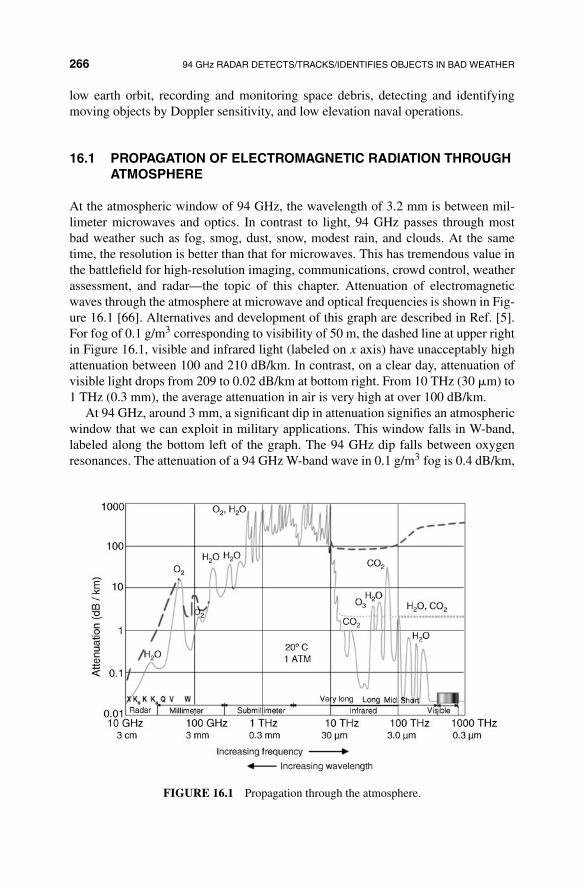
266 94 GHz RADAR DETECTS/TRACKS/IDENTIFIES OBJECTS IN BAD WEATHER
low earth orbit, recording and monitoring space debris, detecting and identifyingmoving objects by Doppler sensitivity, and low elevation naval operations.
16.1 PROPAGATION OF ELECTROMAGNETIC RADIATION THROUGHATMOSPHERE
At the atmospheric window of 94 GHz, the wavelength of 3.2 mm is between mil-limeter microwaves and optics. In contrast to light, 94 GHz passes through mostbad weather such as fog, smog, dust, snow, modest rain, and clouds. At the sametime, the resolution is better than that for microwaves. This has tremendous value inthe battlefield for high-resolution imaging, communications, crowd control, weatherassessment, and radar—the topic of this chapter. Attenuation of electromagneticwaves through the atmosphere at microwave and optical frequencies is shown in Fig-ure 16.1 [66]. Alternatives and development of this graph are described in Ref. [5].For fog of 0.1 g/m3 corresponding to visibility of 50 m, the dashed line at upper rightin Figure 16.1, visible and infrared light (labeled on x axis) have unacceptably highattenuation between 100 and 210 dB/km. In contrast, on a clear day, attenuation ofvisible light drops from 209 to 0.02 dB/km at bottom right. From 10 THz (30 �m) to1 THz (0.3 mm), the average attenuation in air is very high at over 100 dB/km.
At 94 GHz, around 3 mm, a significant dip in attenuation signifies an atmosphericwindow that we can exploit in military applications. This window falls in W-band,labeled along the bottom left of the graph. The 94 GHz dip falls between oxygenresonances. The attenuation of a 94 GHz W-band wave in 0.1 g/m3 fog is 0.4 dB/km,
FIGURE 16.1 Propagation through the atmosphere.
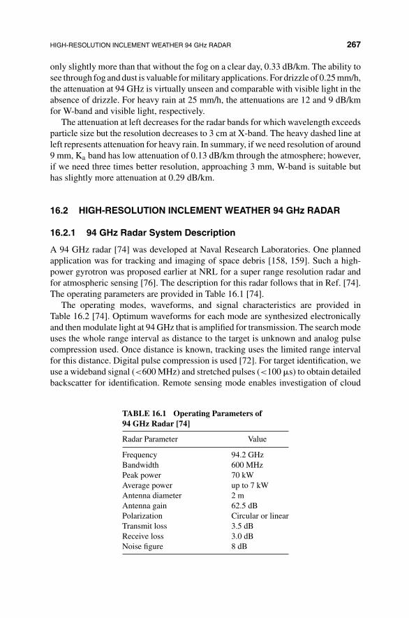
HIGH-RESOLUTION INCLEMENT WEATHER 94 GHz RADAR 267
only slightly more than that without the fog on a clear day, 0.33 dB/km. The ability tosee through fog and dust is valuable for military applications. For drizzle of 0.25 mm/h,the attenuation at 94 GHz is virtually unseen and comparable with visible light in theabsence of drizzle. For heavy rain at 25 mm/h, the attenuations are 12 and 9 dB/kmfor W-band and visible light, respectively.
The attenuation at left decreases for the radar bands for which wavelength exceedsparticle size but the resolution decreases to 3 cm at X-band. The heavy dashed line atleft represents attenuation for heavy rain. In summary, if we need resolution of around9 mm, Ka band has low attenuation of 0.13 dB/km through the atmosphere; however,if we need three times better resolution, approaching 3 mm, W-band is suitable buthas slightly more attenuation at 0.29 dB/km.
16.2 HIGH-RESOLUTION INCLEMENT WEATHER 94 GHz RADAR
16.2.1 94 GHz Radar System Description
A 94 GHz radar [74] was developed at Naval Research Laboratories. One plannedapplication was for tracking and imaging of space debris [158, 159]. Such a high-power gyrotron was proposed earlier at NRL for a super range resolution radar andfor atmospheric sensing [76]. The description for this radar follows that in Ref. [74].The operating parameters are provided in Table 16.1 [74].
The operating modes, waveforms, and signal characteristics are provided inTable 16.2 [74]. Optimum waveforms for each mode are synthesized electronicallyand then modulate light at 94 GHz that is amplified for transmission. The search modeuses the whole range interval as distance to the target is unknown and analog pulsecompression used. Once distance is known, tracking uses the limited range intervalfor this distance. Digital pulse compression is used [72]. For target identification, weuse a wideband signal (<600 MHz) and stretched pulses (<100 �s) to obtain detailedbackscatter for identification. Remote sensing mode enables investigation of cloud
TABLE 16.1 Operating Parameters of94 GHz Radar [74]
Radar Parameter Value
Frequency 94.2 GHzBandwidth 600 MHzPeak power 70 kWAverage power up to 7 kWAntenna diameter 2 mAntenna gain 62.5 dBPolarization Circular or linearTransmit loss 3.5 dBReceive loss 3.0 dBNoise figure 8 dB

268 94 GHz RADAR DETECTS/TRACKS/IDENTIFIES OBJECTS IN BAD WEATHER
TABLE 16.2 Operating Modes for 94 GHz Radar
Pulse Band PRF Burst lengthMode Width (�s) width (MHz) (kHz) (No. of Pulses)
Search/acquisition 17 14 5 64Track 20 18 5 128Stretch 20–100 ≤600 1–5 100–1000Remote sensing 0.1–1 1–10 5 1–100
physics for weather assessment. More pulses in the burst length increase the timelength of the signal for better frequency resolution.
A block diagram of the 94 GHz radar system (Figure 16.2) [74] has transmit,antenna, and receive parts. Waveforms for transmission are developed in electronicwaveform synthesizers at 60 MHz and upconverted through 1.8 and 10–94 GHz. Thewideband signal is generated at 255 MHz and upconverted appropriately. The finalconversion to 94 GHz is performed with a 94 GHz local oscillator and mixer at upperleft. The operating mode is selected at the mixer that converts to 94 GHz. The signalfeeds to a commercially available ordinary (O-type) traveling-wave tube (TWT) [24]that amplifies the signal to 50 W (Section 10.1, Figure 10.1). The output of the TWTfeeds into a 100 kW gyroklystron amplifier built at Naval Research Laboratories(Section 10.1, Figure 10.1) [65], described next.
FIGURE 16.2 Block diagram of 94 GHz radar system.
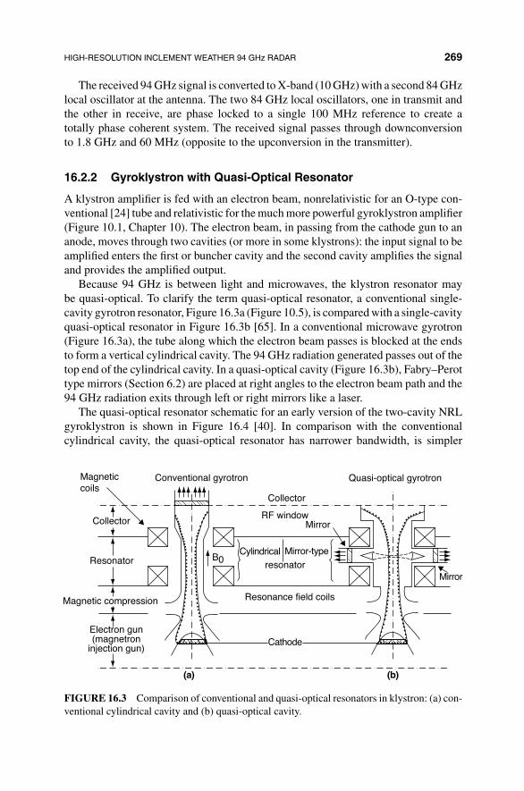
HIGH-RESOLUTION INCLEMENT WEATHER 94 GHz RADAR 269
The received 94 GHz signal is converted to X-band (10 GHz) with a second 84 GHzlocal oscillator at the antenna. The two 84 GHz local oscillators, one in transmit andthe other in receive, are phase locked to a single 100 MHz reference to create atotally phase coherent system. The received signal passes through downconversionto 1.8 GHz and 60 MHz (opposite to the upconversion in the transmitter).
16.2.2 Gyroklystron with Quasi-Optical Resonator
A klystron amplifier is fed with an electron beam, nonrelativistic for an O-type con-ventional [24] tube and relativistic for the much more powerful gyroklystron amplifier(Figure 10.1, Chapter 10). The electron beam, in passing from the cathode gun to ananode, moves through two cavities (or more in some klystrons): the input signal to beamplified enters the first or buncher cavity and the second cavity amplifies the signaland provides the amplified output.
Because 94 GHz is between light and microwaves, the klystron resonator maybe quasi-optical. To clarify the term quasi-optical resonator, a conventional single-cavity gyrotron resonator, Figure 16.3a (Figure 10.5), is compared with a single-cavityquasi-optical resonator in Figure 16.3b [65]. In a conventional microwave gyrotron(Figure 16.3a), the tube along which the electron beam passes is blocked at the endsto form a vertical cylindrical cavity. The 94 GHz radiation generated passes out of thetop end of the cylindrical cavity. In a quasi-optical cavity (Figure 16.3b), Fabry–Perottype mirrors (Section 6.2) are placed at right angles to the electron beam path and the94 GHz radiation exits through left or right mirrors like a laser.
The quasi-optical resonator schematic for an early version of the two-cavity NRLgyroklystron is shown in Figure 16.4 [40]. In comparison with the conventionalcylindrical cavity, the quasi-optical resonator has narrower bandwidth, is simpler
Magneticcoils
Collector
Resonator
Magnetic compression
Electron gun(magnetron
injection gun)
Conventional gyrotron
Collector
RF windowMirror
Mirror-typeresonator
Resonance field coils
Cathode
Mirror
(b)(a)
CylindricalB0
Quasi-optical gyrotron
FIGURE 16.3 Comparison of conventional and quasi-optical resonators in klystron: (a) con-ventional cylindrical cavity and (b) quasi-optical cavity.
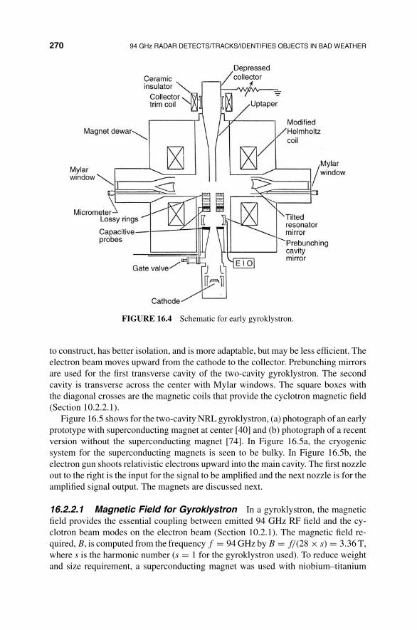
270 94 GHz RADAR DETECTS/TRACKS/IDENTIFIES OBJECTS IN BAD WEATHER
FIGURE 16.4 Schematic for early gyroklystron.
to construct, has better isolation, and is more adaptable, but may be less efficient. Theelectron beam moves upward from the cathode to the collector. Prebunching mirrorsare used for the first transverse cavity of the two-cavity gyroklystron. The secondcavity is transverse across the center with Mylar windows. The square boxes withthe diagonal crosses are the magnetic coils that provide the cyclotron magnetic field(Section 10.2.2.1).
Figure 16.5 shows for the two-cavity NRL gyroklystron, (a) photograph of an earlyprototype with superconducting magnet at center [40] and (b) photograph of a recentversion without the superconducting magnet [74]. In Figure 16.5a, the cryogenicsystem for the superconducting magnets is seen to be bulky. In Figure 16.5b, theelectron gun shoots relativistic electrons upward into the main cavity. The first nozzleout to the right is the input for the signal to be amplified and the next nozzle is for theamplified signal output. The magnets are discussed next.
16.2.2.1 Magnetic Field for Gyroklystron In a gyroklystron, the magneticfield provides the essential coupling between emitted 94 GHz RF field and the cy-clotron beam modes on the electron beam (Section 10.2.1). The magnetic field re-quired, B, is computed from the frequency f = 94 GHz by B = f/(28 × s) = 3.36 T,where s is the harmonic number (s = 1 for the gyroklystron used). To reduce weightand size requirement, a superconducting magnet was used with niobium–titanium

HIGH-RESOLUTION INCLEMENT WEATHER 94 GHz RADAR 271
FIGURE 16.5 Photographs of NRL gyroklystron: (a) prototype with cryogenic supercon-ducting magnet and (b) that without superconducting magnet.
wire at 9 K. A closed-cycle cryocooling system provides 1 W cooling at 4 K. Themagnet takes 20 min to reach its full field after which it takes relatively little powerbecause of the low superconductor resistance.
16.2.2.2 Modulator The anode of the electron gun of the gyroklystron is mod-ulated at a maximum peak repetition frequency of 5 kHz with an 18 kV switch. Thepulse width is 100 �s and maximum duty cycle is 10%. The cathode voltage of thegun is < 70 kV and cathode reference is 30 kV.
16.2.3 Overmoded Low 94 GHz Loss Transmission Line fromGyroklystron to Antenna
Because of the high multi-kW power at 94 GHz and the duplex nature of radar, thetransmitter equipment cannot be mounted directly on the antenna as in Section 17.1,where no return signal is received. Therefore, we require a low-loss transmissionline and rotary joint to carry transmitted power from the final power amplifier tothe antenna-mounted duplexer. A conventional 94 GHz waveguide suffers 3 dB/mloss at these high peak and average powers. A circular overmoded waveguide isused in which the waveguide transverse dimension, diameter 32 mm, is many times

272 94 GHz RADAR DETECTS/TRACKS/IDENTIFIES OBJECTS IN BAD WEATHER
the wavelength, for excess modes (Figure 16.2). Then losses for a smooth-walledwaveguide are below 0.01 dB/m for the TE01 mode and less for the HE11 mode [7].The gyroklystron emits a TE01 mode into the circular waveguide, which is thenconverted with a curved corrugated waveguide into an HE11 mode for coupling tothe rotating antenna (Figure 16.2). The HE11 mode emits a Gaussian beam into freespace as is required for input to the quasi-optical duplexer attached to the antenna.The HE11 mode is converted to circular polarization with a grating polarizer built intoa high-power miter [73, 149, 172] (angled) bend. Circular polarization is required sothat polarization will remain unchanged as the antenna rotates. After passing throughthe rotary joint, the polarization is converted back to linear for the duplexer.
16.2.4 Quasi-Optical Duplexer
The goal of the quasi-optical duplexer is to separate the transmit and receive beams.The advantage of the quasi-optical duplexer is low loss, high power handling, andbroad bandwidth [38, 74]. The linear polarized HE11 mode from the transmission linein Section 16.2.3 launches a linear polarized TEM00 mode into the input port of theduplexer at the right-side of Figure 16.6 [74]. Clamshell reflectors direct the beamonto the first wire grid polarizer, where parallel wires allow a polarized signal, withE field oriented along spaces, to pass. For light propagating from right to left, thewires are at −45◦ as shown; that is, the field to the left of the wire polarizer is linearlypolarized at −45◦. The Faraday rotator rotates the polarization clockwise through45◦ to become vertically or zero polarized and passes it on to the second wire gridpolarizer through which it passes because the second wire polarizer is also orientedvertically, at 45◦ to the first wire grid polarizer. The Faraday rotator is commonly usedfor isolators [176]. For the high power and frequency involved, isolators are preferableto quarter-wave plates (Section 2.2.1.2). In Figure 16.6, the signal passing throughthe vertical wire polarizer couples to the Cassegrain antenna (Section 1.3.4.1).
45ºFaradayrotatorFilter Filter
Transmission lineconnectiong to
transmitter
To co-polreceiver
To x-polreceiver
Clamshellmirrors
Sub-reflector
Antenna
Transmit pathReceiver path
FIGURE 16.6 Quasi-optical duplexer.

HIGH-RESOLUTION INCLEMENT WEATHER 94 GHz RADAR 273
On return from the target, at the output of the Cassegrain antenna, the cross-polarized component relative to that transmitted from the Cassegrain reflects off thevertical wire grid polarizer (as if a polarized beam splitter) and feeds to the cross-polarization receiver, the lowest receiver in the control van in Figure 16.2. In contrast,the copolarized signal, polarized at right angles to the cross-polarized signal, passesthrough the vertical wire grid polarizer. The zero polarized signal receives another45◦ clockwise rotation while traveling left to right through the Faraday rotator so thatit is polarized at right angles to the right side or −45◦ wire polarizer and bouncesoff it and is directed to the input of the copolarization receiver, the uppermost of thereceivers in the control van in Figure 16.2. Separating the polarizations into cross- andcopolarizations at the receiver provides additional information relating to propagationand the nature of the target. The cooling system for the Faraday rotator had to beredesigned to handle 100 kW power.
Measurements from testing are described in Ref. [74]. By reflecting all the radi-ation back into the duplexer with an aluminum plate, a two-way loss of 4.8 dB wasmeasured for the duplexer. By replacing the aluminum sheet reflector with absorbingmaterial, the amount reflected back inside the transmitter was −17 dB. The leakage orloss in passing through the antenna was measured as −30 dB. Frequency response forcombined gyroklystron amplifier, overmoded transmission line, quasi-optical multi-plexer, and antenna was measured in a field test over 700 m. For a linear frequencymodulation [141] and a 50 �s chirp pulse of bandwidth 400 MHz centered at 94 GHz,the resulting pulse was flat, within 1.5 dB, over the 400 MHz bandwidth of the chirpbandwidth.
16.2.5 Antenna
A symmetric Cassegrain antenna was used (Section 1.3.4.1) for which the feed is linedup with the axis of the antenna. This provides a stiff structure because the receiverand duplexer, which feeds the antenna, are mounted directly on the antenna. Thisminimizes losses and reduces aperture losses compared to placing a deflecting mirrorin the antenna output path, the Nasmyth telescope (Section 1.3.4.2, Figure 15.1). Theovermoded waveguides and miter bends can be seen in the photograph of the back ofthe antenna (Figure 16.7) [74]. Two further miter bends are used to align the waveguidewith the elevation axis of rotation before the elevation rotary coupler and a miter benddirects power to the duplexer box. The duplexer box emits at the center of the antennato illuminate the subreflector of the 1.8 m Cassegrain bidirectional antenna, machinedto high precision for operation in a variable environment. Measurements showed abeamwidth of 0.11◦ and an antenna gain (peak over omnidirectional response) of62.7 dB.
16.2.6 Data Processing and Performance
The data processing setup is described in Ref. [74]. The performance of the com-plete system was measured in terms of range in the earth’s atmosphere. The range issubstantially larger with altitude because turbulence decreases. Using the parametersin Table 16.2 and a 100 �s pulse, the signal to noise ratio on a 1 m2 target at 1000 km

274 94 GHz RADAR DETECTS/TRACKS/IDENTIFIES OBJECTS IN BAD WEATHER
FIGURE 16.7 Back of antenna showing overmoded waveguides and miter bends.
was −1 dB. For imaging with a 100 ms dwell, 30◦ elevation, and 20 dB signal tonoise ratio, the range was 680 km. For tracking with 60 ms dwell, 30◦ elevation, and20 dB signal to noise ratio, the range was 570 km. Low elevations are worse becausethe beam spends more time close to the earth, where turbulence is highest. Calibra-tion measurements are described in Ref. [74] and depend on water content in the air(1.4 dB/km at 9 g/m3).
16.3 APPLICATIONS, MONITORING SPACE, HIGH DOPPLER, ANDLOW SEA ELEVATION
Four applications for the 94 GHz radar are discussed.
16.3.1 Monitoring Satellites in Low Earth Orbit
Since World War II, the advantage is with the side that controls the air space above theconflict area. In future conflicts, the satellite space (lower earth orbit) will be equallyif not more critical because we rely on many different types of satellites both forcommercial activity and in a conflict. We rely on GPS satellites to keep track of ourforces and those of our allies and to steer our missiles; FedEx would be lost withoutit, not to mention many vehicle drivers. We also rely on communication satellites tocommunicate across the battlefield, not to mention their use in credit card and ATM pinverification. Our imaging satellites keep surveillance (every 90 min) around most ofthe critical areas of the globe and have sufficient resolution to see humans and addressenvironmental issues. One country has reportedly used dazzle lasers to blind a U.S.
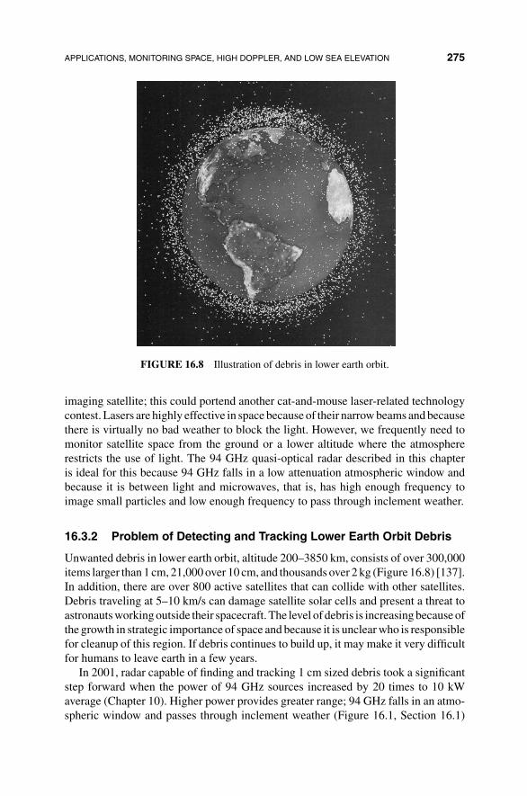
APPLICATIONS, MONITORING SPACE, HIGH DOPPLER, AND LOW SEA ELEVATION 275
FIGURE 16.8 Illustration of debris in lower earth orbit.
imaging satellite; this could portend another cat-and-mouse laser-related technologycontest. Lasers are highly effective in space because of their narrow beams and becausethere is virtually no bad weather to block the light. However, we frequently need tomonitor satellite space from the ground or a lower altitude where the atmosphererestricts the use of light. The 94 GHz quasi-optical radar described in this chapteris ideal for this because 94 GHz falls in a low attenuation atmospheric window andbecause it is between light and microwaves, that is, has high enough frequency toimage small particles and low enough frequency to pass through inclement weather.
16.3.2 Problem of Detecting and Tracking Lower Earth Orbit Debris
Unwanted debris in lower earth orbit, altitude 200–3850 km, consists of over 300,000items larger than 1 cm, 21,000 over 10 cm, and thousands over 2 kg (Figure 16.8) [137].In addition, there are over 800 active satellites that can collide with other satellites.Debris traveling at 5–10 km/s can damage satellite solar cells and present a threat toastronauts working outside their spacecraft. The level of debris is increasing because ofthe growth in strategic importance of space and because it is unclear who is responsiblefor cleanup of this region. If debris continues to build up, it may make it very difficultfor humans to leave earth in a few years.
In 2001, radar capable of finding and tracking 1 cm sized debris took a significantstep forward when the power of 94 GHz sources increased by 20 times to 10 kWaverage (Chapter 10). Higher power provides greater range; 94 GHz falls in an atmo-spheric window and passes through inclement weather (Figure 16.1, Section 16.1)
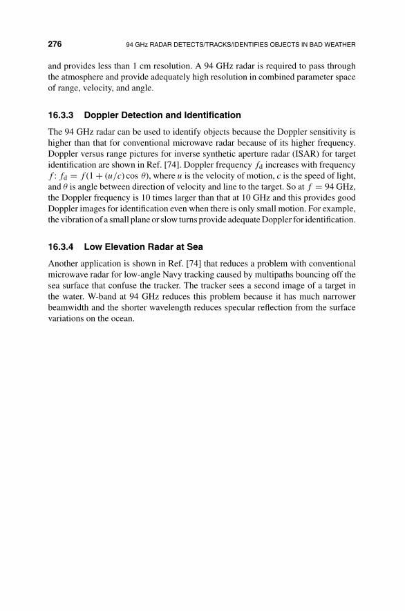
276 94 GHz RADAR DETECTS/TRACKS/IDENTIFIES OBJECTS IN BAD WEATHER
and provides less than 1 cm resolution. A 94 GHz radar is required to pass throughthe atmosphere and provide adequately high resolution in combined parameter spaceof range, velocity, and angle.
16.3.3 Doppler Detection and Identification
The 94 GHz radar can be used to identify objects because the Doppler sensitivity ishigher than that for conventional microwave radar because of its higher frequency.Doppler versus range pictures for inverse synthetic aperture radar (ISAR) for targetidentification are shown in Ref. [74]. Doppler frequency fd increases with frequencyf : fd = f (1 + (u/c) cos θ), where u is the velocity of motion, c is the speed of light,and θ is angle between direction of velocity and line to the target. So at f = 94 GHz,the Doppler frequency is 10 times larger than that at 10 GHz and this provides goodDoppler images for identification even when there is only small motion. For example,the vibration of a small plane or slow turns provide adequate Doppler for identification.
16.3.4 Low Elevation Radar at Sea
Another application is shown in Ref. [74] that reduces a problem with conventionalmicrowave radar for low-angle Navy tracking caused by multipaths bouncing off thesea surface that confuse the tracker. The tracker sees a second image of a target inthe water. W-band at 94 GHz reduces this problem because it has much narrowerbeamwidth and the shorter wavelength reduces specular reflection from the surfacevariations on the ocean.

CHAPTER 17
PROTECTING FROM TERRORISTSWITH W-BAND
Several useful applications are discussed in which W-band electromagnetic radiationis used to protect from terrorists. W-band covers the frequencies from 75 to 110 GHzwith corresponding wavelengths of a few millimeters (4–2.7 mm) (Section 16.1) [5].The higher frequency end of W-band is approaching optics so that some quasi-opticaltechniques may be used, such as mirror resonators (Section 16.2.2, Figure 16.3) andquasi-optical duplexer (Section 16.2.4). Moreover, in Section 16.1, Figure 16.1 [5],W-band provides an application trade-off between attenuation through the atmosphereand resolution. For example, at higher frequencies than W band, left side of Figure16.1, wavelength and resolution decrease but attenuation increases. As discussed inChapter 10, W-band frequencies can be generated efficiently at very high power usingfree electron lasers or other cyclotron resonators or amplifiers. We can also generatehigh peak power in this frequency range with explosives (Section 17.4.1.1) [3, 123].
In Section 17.1, we discuss a system, called Active Denial, that uses W-bandto break up crowds in which terrorists may be hiding with concealed weapons. Thetechnology is similar to the transmit side of the 94 GHz radar described in Chapter 16,so the details are not repeated in this chapter. In Section 17.2, we discuss nonionizingairport body scanners that are safer than X-rays for uncovering concealed weapons.In Section 17.3, we inspect unopened packages with W-band radiation that passesthrough Styrofoam and cardboard but reflects or scatters from the package contents.In Section 17.4, we discuss the use of W-band to interfere with or destroy enemy
Military Laser Technology for Defense: Technology for Revolutionizing 21st Century Warfare,First Edition. By Alastair D. McAulay.© 2011 John Wiley & Sons, Inc. Published 2011 by John Wiley & Sons, Inc.
277

278 PROTECTING FROM TERRORISTS WITH W-BAND
electronics. We also discuss methods of protecting our electronic equipment fromelectromagnetic radiation used by enemy.
17.1 NONLETHAL CROWD CONTROL WITH ACTIVEDENIAL SYSTEM
Terrorists carrying concealed weapons can hide in a crowd. As most of the peoplein a crowd are likely to be innocent civilians, it is better to disperse the crowd thanattack it or threaten it by shooting live or rubber bullets at them or over their heads. Acrowd may be dispersed rapidly with electromagnetic radiation at W-band in systemssuch as Active Denial (Figure 17.1) [10, 139].
94 GHz, at the high end of W-band, falls in a dip in Figure 16.1 (Section 16.1),which is in an atmospheric window. Because it passes through dielectric particlessmaller than its wavelength (3.2 mm), 94 GHz will pass through varied weather, fog,smog, dust, snow, modest rain, and clouds. On reaching a person, it passes throughclothes, but reflects from skin. Conducting clothes can be worn to block it. In theprocess, with adequate power, the 94 GHz electromagnetic wave heats up water and
FIGURE 17.1 Active denial system on a Humvee.

BODY SCANNING FOR HIDDEN WEAPONS 279
fat molecules near or on the surface of the skin, causing perspiration to boil. Atthe higher W-band frequency of 94 GHz, the wave penetrates less than 0.04 mminto the skin, thus avoiding nerve endings and blood vessels that could otherwiseproduce permanent damage. A microwave oven at 2.45 GHz penetrates deeper and ismore dangerous. The rising temperature creates intense pain causing those exposedto instantly flee from the radiation. Eyelids are most vulnerable because they haveonly a thin top layer of skin, but people naturally protect their eyelids by turning theirheads away at the first sign of pain.
With typical power of 2.5 MW, the beam can be used at distances up to 700 mand penetrates thick clothes. The beam is narrow at 94 GHz. The tests suggest thatthere is only 0.1% chance of injury. Eye glasses and body piercings are not affectedbut tattoos can release toxins that make people feel sick. The system was not used inIraq, perhaps because of operational constraints regarding overuse or critical intensitysetting. Raytheon has developed a commercial system.
The generation of 94 GHz at high power is described in Chapters 10 and 16.Because active denial involves only transmit and not receive part, the active denialsystem differs from the 94 GHz radar in Chapter 16 by omitting the receive part of thesystem. Because of reduced size and weight, the transmitter is now mounted directlyon the Cassegrain antenna (Section 1.3.4.1) and the system is small enough to fit on aHumvee (Figure 17.1). The large dish on the roof is the main mirror of the Cassegraintelescope, used as a beam expander or inverse telescope, and the small convex mirrorof the Cassegrain telescope sticks out over the windshield.
17.2 BODY SCANNING FOR HIDDEN WEAPONS
As mentioned in Section 17.1, because millimeter waves pass through dielectric par-ticles smaller than their wavelength, they pass through most clothes and reflect orscatter from skin. This is used in full body scanners to disclose concealed weaponsat a standoff distance of up to 100 m [5]. Less power is needed for body scanningthan for active denial (Section 17.1). An existing 35 GHz Ka band radar was adaptedfor demonstration in early scanners. An example of an image produced at 33 GHzis shown in Figure 17.2a [150] in which a concealed handgun shows up tucked intoa waist band. Concealed plastic explosives such as C4 also show up on 33 GHzscans [5].
Frequencies higher than 94 GHz have been used in experiments. The shorter wave-length gives higher resolution but is attenuated more, which reduces the standoff dis-tance for detection of concealed weapons (Section 16.1) [5]. Many researchers arealso experimenting with passive millimeter wave body scanning, for which there isno source but a 94 GHz filter is placed in front of the receiver. The body naturallyemits electromagnetic radiation and there is a difference in emissivity and reflectancebetween skin and explosives or metal. However, results vary with environmental fac-tors such as temperature. Figure 17.2b [5] shows a 94 GHz passive image of a man inthe open carrying a knife hidden in a newspaper. The newspaper appears transparentat 94 GHz.
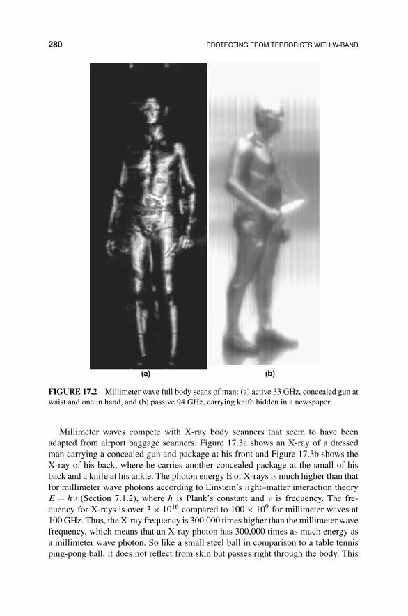
280 PROTECTING FROM TERRORISTS WITH W-BAND
FIGURE 17.2 Millimeter wave full body scans of man: (a) active 33 GHz, concealed gun atwaist and one in hand, and (b) passive 94 GHz, carrying knife hidden in a newspaper.
Millimeter waves compete with X-ray body scanners that seem to have beenadapted from airport baggage scanners. Figure 17.3a shows an X-ray of a dressedman carrying a concealed gun and package at his front and Figure 17.3b shows theX-ray of his back, where he carries another concealed package at the small of hisback and a knife at his ankle. The photon energy E of X-rays is much higher than thatfor millimeter wave photons according to Einstein’s light–matter interaction theoryE = hν (Section 7.1.2), where h is Plank’s constant and ν is frequency. The fre-quency for X-rays is over 3 × 10¹⁶ compared to 100 × 109 for millimeter waves at100 GHz. Thus, the X-ray frequency is 300,000 times higher than the millimeter wavefrequency, which means that an X-ray photon has 300,000 times as much energy asa millimeter wave photon. So like a small steel ball in comparison to a table tennisping-pong ball, it does not reflect from skin but passes right through the body. This

BODY SCANNING FOR HIDDEN WEAPONS 281
FIGURE 17.3 Examples of X-ray of man carrying a concealed gun and packages at his frontand back: (a) front view and (b) rear view.
has a slight possibility of internal damage, hence X-ray exposure is considered life-time accumulative. So unlike millimeter waves, the X-rays cannot be used so easilyin backscatter mode. The X-ray dose is very small, so it will take an extremely largenumber of airport inspections before any problem could be observed for a correctlyset up scanner. However, the effects will be added to whatever medical CT and X-rayscans a person has previously been exposed to.
One of the problems with body scanners that see through clothes is public concernabout being seen or photographed naked. Some specific concerns are illustrated inthe photograph of people protesting in Germany [138] regarding the issue of bodypiercing and artificial limbs (Figure 17.4). On the girl’s chest is written “piercing”and on her right leg “prosthesis.”

282 PROTECTING FROM TERRORISTS WITH W-BAND
FIGURE 17.4 Protest against full body scanners regarding body piercing and prosthetics.
17.3 INSPECTING UNOPENED PACKAGES
Concern has increased in recent years over the shipment of packages with dangerouscontents such as bombs, pistols, chemical explosives, and hazardous chemicals. It isgenerally too expensive to open all packages at sources and destinations. In currentX-ray machines for checking contents without opening packages, X-ray particlestravel through the package onto a phosphor screen [99]. For a 3D view, the systemwould require rotation and images would have to be processed with computer tomog-raphy (CT). Such machines would be expensive and/or may not provide adequate 3Dview of the contents.

INSPECTING UNOPENED PACKAGES 283
We describe a novel millimeter wave approach that has the capability to provide 3Dscans cost effectively without opening packages [101]. The approach uses a 94 GHzsource that has 3.2 mm wavelength. Previously, we discussed more powerful sourcesat this frequency (Chapters 10 and 16), but low-power sources for this frequencyare also in development [11]. A wavelength of 3.2 mm passes through cardboardand Styrofoam materials, the usual materials for packages. Conducting and otherobjects in the package will reflect or scatter the radiation. Observation of the scatteredradiation in transmission, or backscatter in reflection (Chapter 15), can be analyzedto determine the contents of the package [101]. By tuning the source, it is possible touse a set of images at different frequencies to construct a 3D image of the contentsof the package. Ka band radar at 35 GHz can also be used but with a degradation ofresolution.
An iterative computation, similar to Gauss–Newton, is described in Section 6.3and is split into forward and inverse computations.
17.3.1 Principles for Proposed Unopened Package Inspection
A handheld scanner passes a short pulse from a collimated beam at 94 GHz through orreflected from the package to be inspected onto a sensor detector array (Figure 17.5).This is somewhat similar to a transmissive or reflective lidar (Chapter 15) and tothe W-band radar (Chapter 16). By moving the handheld device across the package,cross-sectional shapes of objects inside the package may be observed. Further, thehandheld device can be used from the sides or back of the package to further ascertainthe contents. A fixed configuration rather than a handheld device can also be used.The sensor is connected to a laptop computer for displaying the properties of thematerial along the path of the beam through the package.
17.3.1.1 Forward Computation We use a layered model for propagating thefield through the package. The region through which the beam passes in the package issliced into vertical homogeneous slices (Figure 17.5), each considered to have differ-ent homogeneous refractive index and absorption. In layered models, the thicknesses
FIGURE 17.5 Proposed system for inspection of unopened packages.

284 PROTECTING FROM TERRORISTS WITH W-BAND
of the slices dk are selected for constant travel time T to simplify the computations [21,50, 83].
dk = cT
nk
(17.1)
Such models are widely used in other field propagation problems for the purposeof computation; geophysics [80, 81] (the latter includes absorption); thin film filterdesign and testing (Section 6.3); the method of lines in integrated optics; and propa-gation of light through turbulence (Section 5.4.1). After passing through the package,the light pulse is diffracted through air onto a detector. A matrix method computeralgorithm is described in Section 6.3 that estimates the field in each of the verticalslices through which the beam passed. This method was extended to include absorp-tion in Ref. [81]. An output display shows images of the field that passes through or isreflected from the package. Because of multiple scattering between layers, the imagewill be unclear [104] and further processing will be needed.
17.3.1.2 Inverse Computation for Package Inspection Because the es-timation of parameters for layers is nonlinear, we use the Gauss–Newton iterativemethod described in Section 6.3.3 to determine the refractive index and absorp-tion [81] of each layer. Starting with a random set of refractive indices in a model,the values are updated iteratively until the output image agrees with that of the modelas shown in Figure 6.20. The refractive index and absorption for the layers throughwhich the beam passes or is reflected show the contents of the package. We note thatif a short enough source pulse is used so that multiple scattering between layers canbe neglected, we can use a faster inverse approach of deconvolution [104].
17.4 DESTRUCTION AND PROTECTION OF ELECTRONICS
Because of increasing dependence on electronics in the military, electromagnetic war-fare is one of the most critical technologies in the military. We rely on electronicsfor fire control and on satellites for communications, global positioning (for knowingwhere everything is), and surveillance imaging to detect conflict preparations (Sec-tion 1.3.4.1). Electromagnetic warfare includes both protecting electronics from harmby the enemy and being able to inflict harm on the enemy’s electronic systems, includ-ing interfering with their electromagnetic communications such as remote control ofimprovised explosive devices (IEDs). The reason this is so important is that militaryactivities have become increasingly dependent on electronics.
One of the most respected admirals of the Soviet Navy build up in the Cold War,Admiral Sergei Gorshkov, said many years ago, “The next war will be won by theside that best exploits the electromagnetic spectrum.” More recently, the Gulf Wardemonstrated the significant advantages in a war of negating the use of the electro-magnetic spectrum by the other side [122]. Electromagnetic warfare is more relevanttoday than ever before.

DESTRUCTION AND PROTECTION OF ELECTRONICS 285
FIGURE 17.6 W-band tabletop prototype for frying electronics.
17.4.1 Interfering or Destroying Enemy Electronics
17.4.1.1 Generating Short Pulses to Destroy Electronics Pulses frompowerful 94 GHz sources around W-band, described in Section 10.3 and elsewherein Chapter 10, can be used to interfere with or destroy electronics. For example, aprototype table top system (Figure 17.6) [121] is said to be able to stop an automobileat 100 m. A more powerful system could destroy the electronics at a missile launchsite before the missile can take off.
An alternative is the electromagnetic bomb [3, 123] in which an explosive is usedto generate an intense electromagnetic field pulse. The electromagnetic bomb usesexplosives to move a short circuit into a coil generating a magnetic field so as to com-press the B field in microseconds [3, 123]. From Maxwell’s equation, equation (17.2),this generates a very high electric field pulse E around the coil, proportional to therate of change of the magnetic flux ∂B/∂t passing through the coil:
∇ × E = −∂B∂t
(17.2)
The coil acts as an antenna that radiates the high-intensity electrical field pulse throughthe air and the pulse induces high voltage and current spikes in electronic circuits todamage them. The waveform, propagating at the speed of light, from a high-altitudesource of electromagnetic pulse (EMP) can reach several million square miles of earth.
17.4.1.2 Methods by Which High Peak Power Electromagnetic PulseInterferes with Electronics If the EMP is designed to disrupt communicationflow or push a resonator out of synchronization, such as an electronic clock or timing

286 PROTECTING FROM TERRORISTS WITH W-BAND
on a vehicle, a lower power may suffice and the coupling into the system becomes crit-ical. In general, the high peak power field will couple into wires in a similar manner tothe way lightning couples into electronics by causing a large voltage spike, especiallybad for high-speed low-power electronics, the sort found in military applicationswhere long battery life and fast response matter. The voltage spike finds its way intothe electronics. The field can also find its way through gaps in the packaging [136].
17.4.2 Protecting Electronics from Electromagnetic Destruction
17.4.2.1 Nature of Threat The increasing dependence of the military on elec-tronics and electrical power connections creates a serious vulnerability to EMP fromhigh-altitude nuclear explosion, an electromagnetic bomb, or an electromagnetic raygun such as that in Figure 17.6. A crop duster plane flying over a battlefield could dropan electromagnetic bomb to explode in the air above the battlefield to destroy most ofthe computers, handheld electronic devices, and weapon’s electronics within a largearea. Hence, in the battlefield, communications, global positioning systems, imagingsystems, drones, and weapons electronics such as fire control can fail with disastrousconsequences. This is not just a military threat. In assessing the threat of EMP toU.S. electronics, a recent U.S. Government report states, “The damage level couldbe sufficient to be catastrophic to the Nation, and our current vulnerability invitesattack.” [51]. In addition to applying all the best practices used in electromagneticcompatibility (EMC) [136], we consider two future approaches.
17.4.2.2 Replacing Wires with Optical Fibers Electromagnetic fields can-not couple into an optical fiber because there are no electrical conductors in a fiber. Infact, during the 1950s, the missile silos constructed in the United States as part of themutually assured destruction philosophy (MAD) (Chapter 13) for nuclear retaliationin the event of a nuclear attack were reportedly connected to the outside world withoptical fiber. This includes electronic and electrical power to electronics. The rea-son was that a nuclear explosion produces a sequence of high-power electromagneticpulses that would otherwise couple into electrical wires in the silos and prevent themfrom functioning. Moreover today, optical fiber technology is more highly developedfor the Internet backbone and power fiber has improved to the point where it canreplace wire in most electronic and many electrical power applications.
17.4.2.3 Replacing Electronics with Photons Electronic integrated cir-cuits can be replaced with optical integrated circuits [57]. Connections in opticalintegrated circuits are with optical waveguides and optical fiber is used betweenchips. Such optical guides have no metal or electronic parts and convey informationand power with photons instead of electrons. Photons are uncharged particles, unlikeelectrons, and are immune to electromagnetic interference.
Over the past 30 years, $300 billion has been spent on electronic very large-scaleintegration (VLSI), currently approximately $50 billion per year. We can now place 1.9billion transistors (switching and amplifying elements) on a single half-inch chip. Incontrast, today, only a few components are integrated into an optical integrated circuit

DESTRUCTION AND PROTECTION OF ELECTRONICS 287
because integrated optics development started only a few years ago as a result of theoptical telecommunications thrust for the Internet. There is currently rapid progressin integrated optics that can be applied to the optics in many military systems.
All-optical computers are immune to EMP and are becoming feasible because ofrecent developments in the computing and telecommunication industries where opticsprovides high bit rate for dense communications. Many approaches to constructingan optical computer are described in my book, “Optical Computer Architectures,”Wiley, 1991 [83]. However, the technology at that time made all-optical computersexpensive, so, as PI, my group in Texas Instruments Central Research Laboratories,designed a hybrid (not all-optical) optical crossbar data flow computer for DARPA[107, 114–116] that was subsequently constructed by Texas Instruments for DoD andis described in Chapter 14 of my book [83]. My recent research on optical computersuses integrated optics for a crossbar switch [102] for a military all-optical computerthat is immune to electromagnetic radiation including nuclear blasts and electro-magnetic bombs. We need all-optical computers for immunity to electromagneticattack, to reduce transitions between electronics and optics in telecommunications, tocombine optics and electronics on the same silicon chip in large telecommunicationrouters, to connect more processors on a single chip, and to interface with future fastermicroprocessors to reduce heat.

BIBLIOGRAPHY
[1] E. Adams. Flying laser gun. Popular Science, 2008.[2] G. P. Agrawal. Fiber-Optic Communication Systems, 3rd edition. Wiley Interscience,
New York, 2002.[3] L. L. Altgilbers, M. D. J. Brown, I. Grishnaev, B. M. Novac, I. R. Smith, I. Tkach, and
Y. Tkach. Magnetocumulative Generators. Springer, New York, 2000.[4] L. C. Andrews and R. L. Phillips. Laser Beam Propagation Through Random Media,
2nd edition. SPIE Press, Bellingham, WA, 2005.[5] R. Appleby, H. B. Wallace, and B. Wallace. Standoff detection of weapons and contra-
band in the 100 GHz to 1 THz region. IEEE Transactions on Antennas and Propagation,55(11):2944–2956, 2007.
[6] F. Bachman, P. Loosen, and R. Proprawe, editors. High Power Diode Lasers. Springer,New York, 2007.
[7] C. A. Balanis. Advanced Engineering Electromagnetics. Wiley, New York, 1989.[8] C. Balfour, R. A. Stuart, and A. I. Al-Shamma’a. Experimental studies of backward
waves in an industrial free electron laser system. Optics Communications, 236:403–410,2004.
[9] R. J. Barker and E. Schamiloglu, editors. High-Power Microwave Sources and Tech-nologies. IEEE Press, New York, 2001.
[10] D. Beason. The E-Bomb: How America’s New Directed Energy Weapons Will Changethe Way Future Wars Will Be Fought. Da Capo Press, Cambridge, MA, 2005.
[11] M. A. Belkin, F. Capasso, F. Xie, A. Belyanin, M. Fischer, A. Wittmann, andJ. Faist. Room temperature terahertz quantum cascade laser source based on intracavitydifference-frequency generation. Physics Letters, 92(20), 2008.
Military Laser Technology for Defense: Technology for Revolutionizing 21st Century Warfare,First Edition. By Alastair D. McAulay.© 2011 John Wiley & Sons, Inc. Published 2011 by John Wiley & Sons, Inc.
289
290 BIBLIOGRAPHY
[12] D. Besnard. The megajoule laser program, ignition at hand. The European Phys-ical Journal D: Atomic, Molecular, Optical and Plasma Physics, 44(2):207–213,2007.
[13] J. A. Bittencourt. Fundamentals of Plasma Physics, 3rd edition. Springer, New York,2004.
[14] A. Bjarklev, J. Broeng, and A. Sanchez Bjarklev. Photonic Crystal Fibres. Kluwer Aca-demic Publishers, Boston, MA, 2003.
[15] D. Bodanis. E = mc2. Walker Publishing Company, New York, 2000.[16] M. Born and E. Wolf. Principles of Optics, 7th edition. Cambridge University Press,
Cambridge, UK, 1999.[17] G. E. Box and G. Jenkins. Time-Series Analysis. Elsevier, 1976.[18] L. Brekhovskikh. Waves in Layered Media. Academic Press, New York, 1980.[19] T. I. Bunn. Method and system for producing singlet delta oxygen (SDO) and laser
system incorporating an SDO generator. U.S. Patent 7,512,169, 2009.[20] D. K. Cheng. Fundamentals of Engineering Electromagnetics. Prentice-Hall, Upper
Saddle River, NJ, 1993.[21] J. F. Claerbout. Fundamentals of Geophysical Data Processing. McGraw-Hill,
New York, 1976.[22] C. Von Clausewitz. On War. Oxford University Press, New York, 1976. Translated from
original 1832.[23] W. A. Coles, J. P. Filice, R. G. Frehlich, and M. Yadlowsky. Simulation of wave
propagation in three-dimensional random media. Applied Optics, 34(12):2089–2101,1995.
[24] R. E. Collin. Foundations for Microwave Engineering. McGraw-Hill, New York, 1966.[25] M. J. Connelly. Semiconductor Optical Amplifiers. Kluwer Academic Publishers,
Boston, MA, 2002.[26] R. C. Coutinho, D. R. Selviah, and H. D. Griffiths. High-sensitivity detection of nar-
rowband light in a more intense broadband background using coherence interferogramphase. Journal of Lightwave Technology, 24(10), 2006.
[27] H. A. Davis, R. D. Fulton, E. G. Sherwood, and T. J. T. Kwan. Enhanced-efficiency,narrow-band gigawatt microwave output of the reditron oscillator. IEEE Transactionson Plasma Science, 18(3):611–617, 1990.
[28] W. Demtroder. Laser Spectroscopy, 2nd edition. Springer, New York, 1996.[29] D. Derickson, editor. Fiber Optic Test and Measurement. Prentice-Hall, Upper Saddle
River, NJ, 1998.[30] E. Desurvire. Erbium-Doped Fiber Amplifiers. Wiley, New York, 1994.[31] R. A. Dickerson. Chemical oxygen iodine laser gain generator system. U.S. Patent
6,072,820, 2000.[32] M. J. F. Digonnet, editor. Rare-Earth-Doped Fiber Lasers and Amplifiers. Marcel Dekker,
New York, 2001.[33] R. Drori and E. Jerby. Free-electron-laser-type interaction at 1 meter wavelength range.
Nuclear Instruments and Methods in Physics Research A, 393:284–288, 1997.[34] R. W. Duffner. Airborne Laser: Bullets of Light. Plenum Press, New York, 1997.[35] Exotic Electro-Optics. Materials for high-power lasers. Private communication, Exotic
Electro-Optics is a subsidiary of II-VI Incorporated, San Diego, CA, August 2010.[36] J.-F. Eloy. Power Lasers. Wiley, New York, 1987. Translated from French original 1985
to English in 1987 by H. Beedie.[37] M. H. Fields, J. E. Kansky, R. D. Stock, D. S. Powers, P. J. Berger, and
C. Higgs. Initial results from the advanced-concepts laboratory for adaptive optics and
BIBLIOGRAPHY 291
tracking. In Proceedings of SPIE, Laser Weapons Technology, Vol. 4034, April 2000,pp. 116–127.
[38] W. Fitzgerald. A 35 GHz beam waveguide system for millimeter-wave radar. LincolnLaboratory Journal, 5(2):245–272, 1992.
[39] G. E. Forden. The airborne laser. IEEE Spectrum, 34(9), pp. 40–49, 1997.[40] A. V. Gaponov-Grekhov and V. L. Granatstein, editors. Applications of High-Power
Microwaves. Artech House, Boston, 1994.[41] J. A. Gaudet, R. J. Barker, C. J. Buchenauer, C. Christodoulou, J. Dickens, M. A. Gun-
dersen, R. P. Joshi, H. G. Krompholz, J. F. Kolb, A. Kuthi, M. Laroussi, A. Neuber,W. Nunnally, E. Schamiloglu, K. H. Schoenbach, J. S. Tyo, and R. J. Vidmar. Researchissues in developing compact pulsed power for high peak power applications on mobileplatforms. Proceedings of the IEEE, 92(7):1144–1165, 2004.
[42] I. M. Gelfand and S. V. Fomin. Calculus of Variations. Prentice-Hall, Englewood Cliffs,NJ, 1963.
[43] R. W. Gerchberg and W. O. Saxton. A practical algorithm for the determination of phasefrom image and diffraction plane pictures. Optik, 35(2):237–246, 1972.
[44] A. Gerrard and J. M. Burch. Introduction to Matrix Methods in Optics. Dover Publica-tions, New York, 1975.
[45] A. K. Ghatak, K. Thyagarajan, and M. R. Shenoi. Numerical analysis of planar opticalwaveguides using matrix approach. Journal of Lightwave Technology, 5(5):660–667,1987.
[46] D. C. Ghiglia and M. D. Pritt. Two-Dimensional Phase Unwrapping. Wiley, New York,1998.
[47] C. Gomez-Reino, M. V. Perez, C. Bao, and V. Perez. Gradient-Index Optics. Springer,New York, 2002.
[48] J. W. Goodman. Statistical Optics. Wiley, New York, 1985.[49] J. W. Goodman. Introduction to Fourier Optics, 3rd edition. Roberts and Com-
pany Publishers, Englewood, CO, 2005. Previously McGraw-Hill, New York,1996.
[50] P. Goupillaud. An approach to inverse filtering of near surface layer effects from seismicrecords. Geophysics, 26(6):754–760, 1961.
[51] U.S. Government. Report of the Commission to Assess the Threat to the UnitedStates from Electromagnetic Pulse (EMP) Attack. http://www.globalsecurity.org/wmd/library/congress/2004 r/04-07-22emp.pdf, 2004.
[52] J. G. Graeme. Photodiode Amplifiers. McGraw-Hill, New York, 1996.[53] P. E. Green. Fiber Optic Networks. Prentice-Hall, Englewood Cliffs, NJ, 1993.[54] C. M. Harding, R. A. Johnston, and R. G. Lane. Fast simulation of a Kolmogorov phase
screen. Applied Optics, 38(11):2161–2170, 1999.[55] P. Harihanran. Basics of Interferometry. Academic Press, San Diego, CA, 1992.[56] O. S. Heavens. Optical Properties of Thin Solid Films. Dover Publications, 1991. Original
publication 1955.[57] R. G. Hunsperger. Integrated Optics, 5th edition. Springer, New York, 2002.[58] Google images of ABL. Images of ABL. http://www.google.com/images?rlz=1T4ACAW
enUS341US346&q=airborne+laser+photograph&um=1&ie=UTF-8&source=univ&ei=WwpoTKncOYP7lweV OmgBQ&sa=X&oi=image result group&ct=title&resnum=1&ved=0CCYQsAQwAA, 2010.
[59] Google images of BAE Jeteye. Images of BAE JetEye program. http://www.baesystems.com/BAEProd/groups/public/documents/bae publication/bae pdf eisjeteye.pdf, 2010.

292 BIBLIOGRAPHY
[60] A. Ishimaru. Wave Propagation and Scattering in Random Media. IEEE Press, Piscat-away, NJ, 1997. Previously published by Academic Press in Vols. 1 and 2 in 1978.
[61] F. A. Jenkins and H. E. White. Fundamentals of Optics, 4th edition. McGraw-Hill,New York, 1976.
[62] D. Jensen. Missile defense: post DHS. http://www.militaryaerospace.com/index/display/avi-article-display.372267.articles.avionics-intelligence.news.2010.01.missile-defense-post-dhs.html, 2010.
[63] J. D. Joannopoulos, R. D. Meade, and J. N. Winn. Photonic Crystals: Molding the Flowof Light. Princeton University Press, Princeton, NJ, 1995.
[64] L. Johnson, F. Leonberger, and G. Pratt. Integrated-optic temperature sensor. AppliedPhysics Letters, 41(2):134–136, 1982.
[65] M. V. Kartikeyan, E. Borie, and M. K. A. Thumm, Gyrotrons. Springer, New York, 2004.[66] L. A. Klein. Millimeter-Wave and Infrared Multisensor Design and Signal Processing.
Artech House, Boston, MA, 1997.[67] W. Koechner. Solid-State Laser Engineering, 3rd edition. Springer, New York, 1992.[68] A. N. Kolmogorov. The local structure of turbulence in an incompressible viscous fluid
for very large Reynolds numbers. Comptes Rendus (Doklady) Academy of Sciences,USSR, 30:301–305, 1941.
[69] B. Kress and P. Meyrueis. Digital Diffractive Optics. Wiley, New York, 2000.[70] T. J. T. Kwan and C. M. Snell. Virtual cathode microwave generator having annular
anode slit. U.S. Patent 4,730,170, March 1988. Assigned to U.S. Department of Energy.[71] M. B. Lara, J. Mankowski, J. Dickens, and M. Kristiansen. Reflex-triode geometry of
the virtual-cathode oscillator. In Digest of Technical Papers, 14th IEEE InternationalPulsed Power Conference, Vol. 2, June 2003, pp. 1161–1164.
[72] W. Lauterborn and T. Kurz. Coherent Optics, 2nd edition. Springer, New York, 2003.[73] S. Liao. Miter bend design for corrugated waveguides. Progress in Electromagnetics Re-
search Letters, 10:157–162, 2009. http://ceta.mit.edu/PIERL/pierl10/17.09062103.pdf.[74] G. J. Linde, M. T. Ngo, B. G. Danly, W. J. Cheung, and V. Gregers-Hansen. WARLOC:
a high-power coherent 94 GHz radar. IEEE Transactions on Aerospace and ElectronicSystems, 44(3):1102–1107, 2008.
[75] M. M.-K. Liu. Principles and Applications of Optical Communications. Irwin, Boston,1996.
[76] W. M. Manheimer. On the possibility of high power gyrotrons for super range resolutionradar and atmospheric sensing. International Journal of Electronics, 72(6):1165–1189,1992.
[77] J. M. Martin and S. M. Flatte. Intensity images and statistics from numerical simu-lation of wave propagation in 3-D random media. Applied Optics, 27(11):2111–2126,1988.
[78] A. D. McAulay. The finite element solution of dissipative electromagnetic surfacewaveguides. International Journal for Numerical Methods in Engineering, 11(1):11–27,1977.
[79] A. D. McAulay. Variational finite element solution of dissipative waveguides andtransportation application. IEEE Transactions on Microwave Theory and Techniques,25(5):382–392, 1977.
[80] A. D. McAulay. Prestack inversion with plane-layer point source modeling. Geophysics,50(1):77–89, 1985.
[81] A. D. McAulay. Plane-layer prestack inversion in the presence of surface reverberation.Geophysics, 51(9):1789–1800, 1986.

BIBLIOGRAPHY 293
[82] A. D. McAulay. Engineering design neural networks using split inversion learning. InProceedings of the IEEE First International Conference on Neural Networks, Vol. IV,June 1987, pp. 635–641.
[83] A. D. McAulay. Optical Computer Architectures. Wiley, New York, 1991.[84] A. D. McAulay. Modeling of deterministic chaotic noise to improve target recognition.
In Proceedings of SPIE, Signal Processing, Sensor Fusion, and Target RecognitionConference, Vol. 1955-17, April 1993, pp. 50–57.
[85] A. D. McAulay. Optical recognition of defective pins on VLSI chips using electrontrapping material. In Proceedings of SPIE, Optical Implementation of Information Pro-cessing Conference, July 1995.
[86] A. D. McAulay. Diffractive optical element for multiresolution preprocessing for com-puter vision. In Proceedings of SPIE, Signal Processing, Sensor Fusion, and TargetRecognition Conference VIII, Vol. 3720-43, April 1999.
[87] A. D. McAulay. Improving bandwidth for line-of-sight optical wireless in turbulent airby using phase conjugation. In Proceedings of SPIE, Optical Wireless CommunicationsII, Vol. 3850-5, September 1999.
[88] A. D. McAulay. Generating Kolmogorov phase screens for modeling optical turbulence.In Proceedings of SPIE, Laser Weapons Technology, Vol. 4034-7, April 2000.
[89] A. D. McAulay. Optical arithmetic unit using bit-WDM. Optics and Laser Technology,32:421–427, 2000.
[90] A. D. McAulay. Artificial turbulence generation alternatives for use in computer andlaboratory experiments. In Proceedings of SPIE, High Resolution Wavefront Con-trol: Methods, Devices, and Applications III, Vol. 4493, August 2001, pp. 141–149.
[91] A. D. McAulay. All-optical SOA latch fail-safe alarm system. In Proceedings of SPIE,Photonic Devices and Algorithms for Computing VI, Vol. 5556-7, August 2004, pp. 68–72.
[92] A. D. McAulay. Novel all-optical flip-flop using semiconductor optical amplifiers ininnovative frequency-shifting inverse-threshold pairs. Optical Engineering, 45(5):1115–1120, 2004.
[93] A. D. McAulay. Optical bit-serial computing. Encyclopedia of Modern Optics, 2004.[94] A. D. McAulay. Optimizing SOA frequency conversion with discriminant filter. In Pro-
ceedings of SPIE, Active and Passive Optical Components for WDM CommunicationsIV, Vol. 5595, October 2004, pp. 323–327.
[95] A. D. McAulay. Leaky wave interconnections between integrated optic waveguides. InProceedings of SPIE, Active and Passive Optical Components for WDM CommunicationsV, Vol. 6014-17, October 2005, pp. OC-1–OC-8.
[96] A. D. McAulay. Nonlinear microring resonators forge all-optical switch. Laser FocusWorld, November 2005, pp. 127–130.
[97] A. D. McAulay. Computing fields in a cylindrically curved dielectric layered media.In Proceedings of SPIE, Enabling Photonic Technologies for Defense, Security andAerospace Applications VII, Vol. 6243-18, April 2006, pp. 1–8.
[98] A. D. McAulay. Modeling the brain with laser diodes. In Proceedings of SPIE, Ac-tive and Passive Optical Components for Communications VII, Vol. 6775-10, October2007.
[99] A. D. McAulay. Novel lock-in amplifier for identification of luminescent materials forauthentication. In Proceedings of SPIE, Signal Processing, Sensor Fusion, and TargetRecognition XVI, Vol. 6567-48, April 2007.

294 BIBLIOGRAPHY
[100] A. D. McAulay. Frustrated polarization fiber Sagnac interferometer displacement sensor.In Proceedings of SPIE, Signal Processing, Sensor Fusion, and Target Recognition XVII,Vol. 6969-50, March 2008.
[101] A. D. McAulay. Package inspection using inverse diffraction. In SPIE Optics and Pho-tonics for Information Processing II, Vol. 7072-16, August 2008.
[102] A. D. McAulay. Digital crossbar switch using nonlinear optical ring resonator. In Pro-ceedings of SPIE, Optics and Photonics for Information Processing III, Vol. 7442-2,August 2009.
[103] A. D. McAulay. Integrated optic chip for laser threat identification. In Proceedings ofSPIE, Signal Processing, Sensor Fusion, and Target Recognition XIX, Vol. 7697-48,April 2010.
[104] A. D. McAulay. Optical deconvolution for multilayer reflected data. In Proceedingsof SPIE, Optics and Photonics for Information Processing IV, Vol. 7797-8, August2010.
[105] A. D. McAulay, M. R. Corcoran, C. J. Florio, and I. B. Murray. Optical micro-ring res-onator filter trade-offs. In Proceedings of SPIE, Active and Passive Optical Componentsfor WDM Communications IV, Vol. 5595-48, October 2004, pp. 359–364.
[106] A. D. McAulay, M. R. Corcoran, C. J. Florio, and I. B. Murray. All optical switching andlogic with an integrated optic microring resonator. In Proceedings of SPIE, EnablingPhotonic Technologies for Defense, Security and Aerospace Applications VI, Vol. 5814-3, March 2005, pp. 16–22.
[107] A. D. McAulay, D. W. Oxley, R. W. Cohn, J. D. Provence, E. Parsons, and D. Casasent.Optical crossbar interconnected signal processor. Report, DARPA/ONR N00014-85-C-0755, 1991.
[108] A. D. McAulay, K. Saruhan, and A. Coker. Real-time computation for absorption freebeamforming using neural networks. In Proceedings of the IEEE International Confer-ence on Systems Engineering, August 1990.
[109] A. D. McAulay and H. Tong. Modeling neural networks with active optical devices. InProceedings of SPIE, Optical Information Systems III, Vol. 5908-15, August 2005.
[110] A. D. McAulay and H. Tong. Optical clustering for unsupervised learning using coupledmicroring resonators. In Proceedings of SPIE, Signal Processing, Sensor Fusion, andTarget Recognition XIV, Vol. 5809-49, April 2005, pp. 402–408.
[111] A. D. McAulay and J. Wang. Optical diffraction inspection of periodic structures usingneural networks. Optical Engineering, 37(3):884–888, 1998.
[112] A. D. McAulay and J. Wang. A Sagnac interferometer sensor system for intrusion de-tection and localization. In Proceedings of SPIE, Enabling Photonic Technologies forAerospace Applications V, Vol. 5435-16, April 2004, pp. 114–119.
[113] A. D. McAulay. Deformable mirror nearest neighbor optical computer. Optical Engi-neering, 25(1):76–81, January 1986.
[114] A. D. McAulay. Optical crossbar interconnected signal processor with basic algorithms.Optical Engineering, 25(1):82–90, 1986.
[115] A. D. McAulay. Spatial light modulator interconnected computers. Computer,20(10):45–57, 1987.
[116] A. D. McAulay. Conjugate gradients on optical crossbar interconnected multiprocessor.Journal of Parallel and Distributed Processing, 6:136–150, 1989.
[117] Megajoule. French Megajoule Laser Facility. http://en.wikipedia.org/wiki/Laser M%C3%A9gajoule, 2009.
[118] A. Mendez and T. F. Morse. Specialty Optical Fibers Handbook. Elsevier/AcademicPress, Boston, MA, 2007.

BIBLIOGRAPHY 295
[119] P. W. Milonni and J. H. Eberly. Lasers. Wiley, New York, 1988.[120] A. W. Miziolek, V. Palleschi, and I. Schecter, editors. Laser-Induced Breakdown Spec-
troscopy. Cambridge University Press, Cambridge, UK, 2006.[121] G. Murdoch. Blackout bomb: Air Force’s high-powered microwave weapons fry enemy
equipment. Popular Science, 2009.[122] V. K. Nair. War in the Gulf: Lessons for the Third World. Lancer International, New Delhi,
1991.[123] A. A. Neuber, editor. Explosively Driven Pulse Power: Helical Magnetic Flux Compres-
sion Generators. Springer, New York, 2005.[124] M. J. Neufeld. Von Braun. A. A. Knopf, New York, 2007.[125] PR News. American Society for Photogrammetry and Remote Sensing web
site, guide to land imaging satellites. http://www.asprs.org/news/satellites/,2009.
[126] PR News. Raytheon awarded contract for Office of Naval Research’s free electron laserprogram. PR News, June 9, 2009. http://www.prnewswire.com/comp/149999.htm, 2009.
[127] NIF. National Ignition Facility, or NIF. http://en.wikipedia.org/wiki/National IgnitionFacility, 2009.
[128] Northrop-Grumman. Northrop-Grumman Guardian images. http://www.es.northropgrumman.com/countermanpads/media gallery/photos.html, 2010.
[129] G. S. Nusinovich. Introduction to the Physics of Gyrotrons. Johns Hopkins UniversityPress, Baltimore, MD, 2004.
[130] K. Okamoto. Fundamentals of Optical Waveguides. Academic Press, New York, 2000.[131] T. Okoshi and K. Kikuchi. Coherent Optical Fiber Communications. KTK Scientific
Publishers/Kluwer Academic Publishers, Tokyo/Boston, MA, 1988.[132] E. L. O’Neill. Introduction to Statistical Optics. Dover Publications, New York,
1991.[133] A. V. Oppenheim and R. W. Schafer. Discrete-Time Signal Processing, 2nd edition.
Prentice-Hall, Upper Saddle River, New Jersey, 1999.[134] A. Papoulis. Systems and Transforms with Applications in Optics. R. E. Krieger Pub-
lishing Company, 1981. Original printing 1968.[135] A. Papoulis. Probability, Random Variables, and Stochastic Processes, 3rd edition.
McGraw-Hill, New York, 1991.[136] C. R. Paul. Introduction to Electromagnetic Compatibility. Wiley, New York, 1992.[137] J. Pearson. The Electrodynamic Debris Eliminator (EDDE): removing debris from space.
The Bent of Tau Beta Pi, C1(2), 2010.[138] M. Phillips. From granny to nearly nude germans, Everyone’s raising cane at the airport.
Wall Street Journal, January 11, 2010.[139] Active Denial Program. Active Denial System on Humvee. http://en.wikipedia.org/
wiki/File:Active Denial System Humvee.jpg, 2010.[140] R. Rhodes. Arsenals of Folly. A. A. Knopf, New York, 2007.[141] M. A. Richards. Fundamentals of Radar Signal Processing. McGraw-Hill, New York,
2005.[142] R. D. Richmond and S. C. Cain. Direct-Detection LADAR Systems. SPIE Publications,
Bellingham, WA, 2010.[143] J. Robieux. High Power Laser Interactions. Lavoisier Publishing, Secaucus, NJ, 2000.[144] M. C. Roggemann and B. Welsh. Imaging Through Turbulence. CRC Press, New York,
1996.[145] N. Roy and F. Reid. Off-axis laser detection model in coastal areas. Optical Engineering,
47(8), 2008.
296 BIBLIOGRAPHY
[146] B. S. Woodard, J. W. Zimmerman, G. F. Benavides, D. L. Carroll, J. T. Verdeyen,A. D. Palla, T. H. Field, W. C. Solomon, S. J. Davis, W. T. Rawlins, and S. Lee.Gain and continuous-wave laser oscillation on the 1315 nm atomic iodine transi-tion pumped by an air–helium electric discharge. Applied Physics Letters, 93:021104,2008.
[147] K. Sakoda. Optical Properties of Photonic Crystals. Springer, New York, 2001.[148] B. E. A. Saleh and M. C. Teich. Fundamentals of Photonics. Wiley, 1991.[149] M. A. Shapiro and R. J. Temkin. High power miter-bend for the next linear collider. In
Proceedings of the 1999 Particle Accelerator Conference, 1999.[150] D. M. Sheen, D. L. McMakin, H. D. Collins, T. E. Hall, and R. H. Stevertson. Con-
cealed explosive detection on personnel using a wideband holographic millimeter-waveimaging system. In Proceedings of SPIE, Signal Processing, Sensor Fusion, and TargetRecognition V, Vol. 2755, 1996.
[151] M. Skolnik. Radar Handbook, 3rd edition. McGraw-Hill, New York, 2008.[152] V. A. Soifer, editor. Methods for Computer Design of Diffractive Optical Elements. Wiley
Interscience, 2002.[153] S. H. Strogatz. Nonlinear Dynamics and Chaos. Addison-Wesley, Reading, MA, 1994.[154] A. Taflove and S. C. Hagness. Computational Electrodynamics: The Finite Difference
Time-Domain Method, 2nd edition. Artech House, Boston, MA, 2000.[155] V. I. Tatarski. Wave Propagation in a Turbulent Medium. McGraw-Hill, New York, 1961.
Translated from Russian by R. A. Silverman.[156] K. Thayagaran, M. R. Shenoi, and A. K. Ghatak. Accurate method for the calculation of
bending loss in optical waveguides using a matrix approach. Optics Letters, 12(4):296–298, 1987.
[157] M. K. A. Thumm. State of the art of high power gyro devices and free electron masers.Technical Report FZKA 7198, Institute fur Hochleistungsimplus- und Mikrowellen-technik, Karlsruhe FZKA, 2008.
[158] A. Tolkachev. Gyroklystron-based 35 GHz radar for observation of space objects. InProceedings of the 22nd International Conference on Infrared and Millimeter Waves,Vol. 5595-48, October 1997, pp. 359–364.
[159] A. Tolkachev, V. Trushin, and V. Veitsel. On the possibility of using powerful millimeterwave band radars for tracking objects in circumterrestrial space. In Proceedings of the1996 CIE International Conference of Radar, 1996.
[160] H. Tong and A. D. McAulay. Wavefront measurement by using photonic crystals. InProceedings of SPIE, Enabling Photonic Technologies for Aerospace Applications VI,Vol. 5435-13, April 2004.
[161] H. L. Van Trees. Detection, Estimation and Modulation Theory, Part I. Wiley, 2001.Originally published in 1968.
[162] H. L. Van Trees. Detection, Estimation and Modulation Theory, Part IV. Optimum ArrayProcessing. Wiley Interscience, 2002.
[163] R. K. Tyson. Principles of Adaptive Optics, 2nd edition. Academic Press, New York,1998.
[164] E. Udd, editor. Fiber Optic Sensors. Wiley, New York, 1991.[165] J. Vetrovec. Chemical oxygen–iodine laser (coil)/cryosorption vacuum pump system,
2000.[166] U. Wandinger. Introduction to lidar. In C. Weitkamp, editor, Lidar Range-Resolved Op-
tical Remote Sensing of the Atmosphere. Springer, New York, 2005, Chapter 1.[167] B. Warm, D. Wittner, and M. Noll. Apparatus for defending against an attacking missile.
U.S. Patent 5,600,434, 1997.

BIBLIOGRAPHY 297
[168] C. Weitkamp, editor. Lidar Range-Resolved Optical Remote Sensing of the Atmosphere.Springer, New York, 2005.
[169] H. Weyl. Theory of Groups and Quantum Mechanics. Dover Publications, 1950.[170] R. Whitney, D. Douglas, and G. Neil. Airborne megawatt class free-electron laser for
defense and security. In 2005 Conference: Laser Source and System Technology forDefense and Security, Jefferson Laboratory, 2008.
[171] S. Wieczorek, B. Krauskopf, and D. Lenstra. A unifying view of bifurcations in a semi-conductor laser subject to optical injection. Optics Communications, 172.1:279–295,1999.
[172] P. P. Woskov, V. S. Bajaj, M. K. Hornstein, R. J. Temkin, and R. G. Griffin. Cor-rugated waveguide and directional coupler for CW 250-GHz gyrotron DNP experi-ments. IEEE Transactions on Microwave Theory and Techniques, 53(6):1863–1869,2005.
[173] C. C. Wright, R. A. Stuart, A. Al-Shamma’a, and A. Shaw. Free electron maser as afrequency agile microwave source. In Loughborough Antennas and Propagation Con-ference, April 2007, pp. 325–328.
[174] C. C. Wright, R. A. Stuart, J. Lucas, and A. Al-Shamma’a. Low cost undulator magnetsfor industrial free electron masers. Optics Communications, 185:387–391, 2000.
[175] C. C. Wright, R. A. Stuart, J. Lucas, A. Al-Shamma’a, and C. Petichakis. Design andconstruction of a table top microwave free electron maser for industrial applications.Vacuum, 77:527–531, 2005.
[176] A. Yariv and P. Yeh. Photonics: Optical Electronics in Modern Communications,6th edition. Oxford University Press, Oxford UK, 2007.
[177] J. L. Zhang, E. M. Tian, and Z. B. Wang. Research on coherent laser warning receiverbased on sinusoidal transmission grating diffraction. Journal of Physics: ConferenceSeries, 48, 2006.

INDEX
3-D viewing of inside of package, 28294GHz 3cm resolution, 26794GHz advantages
between light and microwaves, 26594GHz attenuation with weather, 26694GHz interaction clothes, skin, water, 27894GHz radar, 265–276
block diagram, 268quasi-optical duplexer and cavity, 265system description, 267–268
ABCD law, 24–26ABL—Airborne Laser, 211absorption, 129active denial
abuse, 279on humvee photo, 279
active denial system, 278–279adaptive optics, 86–89, 208
beam clean up, 88devices, 86for cleaning up main beam, 213for cleaning up main beam in ABL, 214
turbulence compensation, 88turbulence compensation, ABL, 214–215
Advanced-Concepts-Laboratory (ACL), 219aerosol, 252Airborne Laser, 210–223
goal, plane, lasers, 211Airborne Laser (ABL), 146, 160–164Airborne Laser Laboratory (ALL), 160, 210airborne laser tank buster, 228Airborne Laser testbed rationale, 219airborne pulsed lasers, 178all-optical computers feasibility, 286amplification stages example, 148amplified power Nd:YAG laser efficiency,
149antenna for 94GHz radar, back view, 273antisatellite satellites use EM
radiation, 286array waveguide grating (AWG), 245–250atmospheric window at 94GHz, 278atmospheric turbulence explanation, 82atmospheric window, 265atmospheric window at 94GHz, 266
Military Laser Technology for Defense: Technology for Revolutionizing 21st Century Warfare,First Edition. By Alastair D. McAulay.© 2011 John Wiley & Sons, Inc. Published 2011 by John Wiley & Sons, Inc.
299

300 INDEX
attenuation at 94GHz in drizzle, fog, rain,266
autocorrelation function, 104AWG—array waveguide grating
operation, 246design, 249output power, 248
backscatter coefficient, 256beacon illuminator (BILL), 220beacon laser in adaptive optics, 212beam compressors, 14beam diffraction, 208beam expander, 13beam expander reduces turbulence, 176beam splitter, 105beamforming with laser array, 171beamlines in NIF, 235bending light beams, 63blackbody radiation, 129blooming, 208body scanners
35GHz, 94GHz radar, passive, X-Ray, 279protest over naked pictures, 281
body scanning for hidden weapons, 279–282Boeing 747, 211Boltzman’s statistics, 129boxcar, 40Bremsstrahlung, 127, 177Brewster angle, 233
C-130 carried COIL, 228carbon-dioxide laser, 158Cassegrain, 15Cassegrain antenna, 273, 279Cassegrain telescope, 253
in ABL, 215cavity, 110centroid monitor, 222characteristics of high power lasers, 144chemical oxygen-iodine laser
absorbing waste gases, 163–164cryoabsorption pump, 163exciting oxygen, 160–162nozzles mix oxygen and iodine, 163transfering oxygen excitation to iodine,
161–163chemical oxygen-iodine laser (COIL), 146,
160–164, 211, 220
chemical pumping, 147coherence length, 100, 105coherence time, 101coherent radiation
advantage, 128importance, 129
complex self-coherence function, 104Comprehensive Nuclear-Test-Ban Treaty,
231constructive interference, 38controlled nuclear fusion chain reaction,
232conversion to UV in NIF, 236countermeasure pods against missiles,
225–226coupling to rotating antenna at 94 GHz, 271cross coherence function, 104cross-correlation function, 104crowd control, 278cyclotron, 177, 191cyclotron based laser, 146cyclotron resonance masers
see gyrotrons, 179
danger from explosive EM bombs, 285danger from nuclear explosion EMP, 284debris in lower earth orbit problem, 275deformable mirror device, 87, 214, 220design for array waveguide grating, 249design of diffractive element
inverse problem, 73designing nuclear bombs after
test-ban, 211destroying electronics with EMP, 285destructive interference, 38, 105
π phase difference, 105detecting chemical concentration, 264detecting concealed plastic explosives, 279detecting future electron-cyclotron lasers,
238detecting laser beams, 237deuterium-tritium mixture, 232dielectric and dichroic mirrors, 213diffraction, 38
relation interference, 46scalar, 47–55
field at point, 48field from aperture, 50
spectrum analyzer, 258

INDEX 301
diffraction limited imaging, 56–60aperture, 56
diffractive optical element, 61–76direct bandgap, 129direction finding for Gaussian beam, 242directional-coupler, 105discs with turbulence phase screens, 221dither mirror in adaptive optics, 214DOE, see diffractive optical elementDoppler imaging at 94GHz, 276double heterostructure, 135
eddies from air conditioners, 92Einstein coefficient, 130–131Einstein’s energy-mass equation, 232Einstein’s light-matter interaction, 129, 279Einstein’s theory of special relativity, 178electrical pumping, 146electromagnetic spectrum, 129electron gun, 178electron gun modulation for gyroklystron,
271electron-cyclotron
amplifier, 179principles, 179–183
electron-cyclotron lasers/masers, 177–190,203
electronic warfare importance, 284EM wave attenutation in atmosphere,
266–267EMP—electromagnetic pulse, 284entropy, 128ergodicity, 79etalon, 110extreme power lasers
for thermonuclear fusion, 211extreme world lasers: NIF, MegaJoule,
SG-III, GXII, OMEGA, HiPER, 232eye-safe lasers, 144, 238
Fabry–Perot resonator, 109–116Fabry–Perot spectrum analyzer, 257fast steering mirrors in adaptive optics, 214fast velocity waves, 178Fermat’s Principle, 4Fermi level, 133fiber gyroscope, 108fiber laser, 146finding buried object from air, 201
Fizeau interferometer, 243–245flashlamp pumping, 233focusing 48 beams in space and time in NIF,
235focusing light in space and time, 176focusing mirror in adaptive optics, 215forward computation through layers, 122forward propagation for inspection, 284Fourier transforms, 40–45
uncertainty principle, 42–45in space, 45in time, 42–44
Fraunhofer appoximation, 54Fraunhofer diffraction for sin grating, 241free-electron laser, 146, 229
at low frequencies, 200Compton and Raman regions, 193frequency range, 191principles, 192–198
free-electron laser and maser, 191–203free-spectral range, 114frequency doubling, 148, 149frequency doubling for eye-safety, 149Fresnel approximation, 51–54frozen turbulence hypothesis, 86future lasers to protect from ICBMS, 210
gas-dynamic laser, 146, 159–160pumping, 147
Gauss-Newton method, 122, 123, 283Gaussian beams, 20–29
equations, 21lens optics, 26–29
Geiger counter mode, 254generating EMP to destroy electronics, 285geometric optics, 3, see ray theoryGerchberg-Saxton algorithm, 72–76German V2 in 1942, 207good lasing materials, 129grating, 62–66
bending rays, 63cosinusoidal, 64efficiency, 261performance, 66resolution, 261spectrometer, 258, 259
grating estimates direction and frequency,242
grating for direction and frequency, 240

302 INDEX
Green’s theorem, 48Gulf war electronic warfare lesson, 284gyrodevices, 177–190, 203gyroklystron with quasi-optic resonator,
269–270gyrokylstron, 178gyrotron, 179–183
operating point, 182–183
half wave plate, 31Harman wave front sensing, 242helical wiggler, 194high light intensity blockers, 171high power semiconductor arrays, 140homing missile countermeasure system
operation, 227–228overview, 224–226
homing missile hot spots, 227Huygens, 38, 51
IED—improvised explosive device, 284illumination aim point lasers, 213
in ABL, 215–216image intensifier, 110Inertial Confinement Fusion (ICF), 232inspecting unopened packages, 282–284inspection by transmission or reflection, 282integrated optics, 245interference, 46interferometer, 99–109International Nuclear-Test-Ban Treaty, 211inverse computation for package content,
284inverse problem for layer identification, 122
Jacobian matrix, 122jitter measurement, 222
K-band attenuation in atmosphere, 267Kolmogorov spectrum, 85
covariance method, 95spectral method, 92
Kolmogorov statistic turbulence model, 219Kolmogorov’s theory of turbulence, 83krypton fluoride laser, 146kylstrons, 177
laser, 127laser armed destroyer in development, 228
laser array beamformingequation, 172
laser beam direction finding with grating,240
laser beam direction finding with lens, 242laser beam quality, 144laser diode, see semiconductor laser diodelaser diode pumped solid state lasers
for ABL illumination aim point, 215laser for lidar, 253laser modes
frequency separation, 167laser principles, 127–139laser pumping and resonance, 131–132laser warning device characteristics, 238laser warning devices, 239–250
types, 239lasers protect from missiles, 207–230
advantages, requirements, range, 208launch beams, 10layer matrix, 121layered model for package inspection, 283layered model for turbulence, 90layout for array waveguide grating, 246lenses and imaging, 10LIDAR, see lidarlidar, 251–257
3D imaging, 252system description, 253–257transmission loss, 257
lidar antenna, 254lidar antenna gain, 255lidar equation derivation, 254–257light propagation through turbulence,
77–98light waves, 127Littrow condition, 260
Mach–Zehnder interferometer, 105–107free-space, 105integrated optics, 107optical fiber, 105–107
magnetic wiggler, 194design, 203
magnetrons, 177magnifying glass, 12Marx generator, 186
demonstration, 187maser, 127

INDEX 303
materials for high power lasers, 147matrix-method, 118–124Megajoule laser, 145Megajoule laser, France, 231Michelson interferometer, 101–104microscope, 17microwave tubes, 177microwaves, 127military applications for lidar, 252millimeter waves, 127, 265millimeter waves release tatoo toxins, 279missile guidance, 223missiles, 207–230miter bends at high power 94GHz, 271mode locked laser, 169
methods of implementing, 169mode locked laser derive equation, 167–169modeling and tracking for ABL, 219–223modeling turbulence
bounds on spatial frequency, 91monitoring satellite space from ground, 274multiple warhead intercontinental missiles,
209
Nasmyth telescope, 253National Ignition Facility laser, 145, 211national threat from EMP, 286NdGlass disk amplfiers, 233NdGlass laser with extreme power, 231NdYAG laser, 145, 148
Q-switched, 148NdYAG laser pumping, 148–149NIF, National Ignition Facility, 231nose turret rotates in ABL, 215, 216nuclear ICBM shield, 211nuclear tipped ICBM threat, 209–211
historical approach, 209–210nuclear weapon threat, 231–236numerical computation of turbulence, 89numerical computing, 55
operation of sun, 232optical
chemical detection, 107virus detection, 107
optical fiber less vulnerable than wire, 286optical gyroscope, 108optical pumping, 129, 147overmoded transmission line in 94GHz radar
rationale and losses, 271oxygen resonance in atmosphere, 266
p-n junction, 133–135particle acceleration pumping, 147peak power
for beamformed laser array, 171–173for mode locked laser array, 176in Q-switched laser, 171
performance of 94GHz radar system, 273phase retarders, 31phase screens
covariance method, 94, 96examples, 97
spectral method, 92examples, 93
phase-only filter design, 73phases through AWG, 247piezo electric
tuning, 116plane wave decomposition, 41Plank’s law, 129platform dependence for laser, 238Poincare sphere, 34polarization, 29–38
controller, 36relation Stokes and Poincare, 35
population inversion, 129potassium dihydrogen phosphate for UV,
236power lasers, 143–164
methods of pumping, 146power lasers table
wavelength, power, efficiency, 145prediction, 103problem list for Airborne Laser, 217–219propagation through thin layers, 118protect aircraft from homing missiles,
223–228protecting from terrorists, 277–287pulsed beam breaks missile lock, 227pulsed high-power lasers, 165–176
advantages, 165
Q-factor versus switching for resonator, 179Q-switch laser energy and lifetime, 171Q-switched laser, 170–171
delayed cavity energy release, 170quality factor for resonator, 179

304 INDEX
quantum mechanics, 129quarter wave plate, 32quasi-optical duplexer, 272–273quasi-optical source at 94GHz, 269
radar, 252random
fields, 78processes, 78
range bin, 255range resolution of free-electron laser, 203ray theory, 3–18
limits to ray theory, 6matrix representation, 9paraxial optics, 3ray equation, 6
applications, 8Rayleigh-Summerfield equation, 51recovery time for NIF, 236reduced low angle multipath at 94GHz, 276reducing EMP threat with optics, 286relativistic electrons, 178remote biological material detection, 252remote chemical weapon detection, 252removing scintillation, 222resonance and child’s swing, 110resonant frequencies for Fabry–Perot, 110resonator
Fabry–Perot, 110–116ring, 110
safety of active denial system, 279Sagnac interferometer, 108–109saturable absorber, 171scalar diffraction, 47–55scattering detection with lidar, 263second harmonic generation
for frequency doubling, 150maximizing output power, 155non-centrosymmetric crystals, 150phase matching by angle, 155–158potassium dihydrogen phosphate (KDP),
150wave formulation, 153
second order nonlinearsusceptibility for SHG, 150
semiconducor laser diode, 133–140semiconductor laser diode
dynamics, 139
efficiency, 138, 139gain, 136–137modes, 137threshold current, 138
sensing chemicals with lidar, 262–264shooting missiles with CO2 laser, 160slowly varying amplitude approximation,
154Snell’s law, 5solgel, 107solid-state lasers, 148–158spatial coherence, 100, 213
improve with adaptive optics, 213spatial concentration of laser light
beamforming, 171spatial filter, 18spatial filters improve spatial coheence,
235spectrometer, 257–262
Fabry-Perot, 257grating, 258
spectrum, 103spectrum analysis with AWG, 245spontaneous emission, 130star coupler integrated optic design, 246star wars, 210stimulated emission, 127, 130
bunching of electrons in static field,178
by bound electron states, 128–136Stokes parameters, 33stopping cars with W-band beam, 285strain measurement
aircraft wings, 106bridges, 106
Strehl ratio, 222structure function, 79, 94
power spectrum, 80Styrofoam, cardboard transmit 94 GHz, 282superconducting magnet for gyroklystron,
270
table top free-electron demonstration,199–203
table-top source destroys electronics, 285target designators, 238Tatarski spectrum, 85telescopes, 14–16
Cassegrain, 15

INDEX 305
temperature sensingfiber, 107integrated optics, 107
TeraWatt peak picosecond pulse laser, 232testbed experimental results for ABL, 222testbed for ABL adaptive optics, 220–223thermal laser pumping, 159thermonuclear bomb, 232thermonuclear bomb design, 231thin-film filter, 118threat to aircraft from shoulder
missiles, 223tracking illuminator (TILL), 220tracking lock on homing missile, 227tracking lower earth orbit debris, 275transmission detection with lidar, 262transmission through layer stack, 122triggering of IEDs from cell phones, 284turbulence
degrade missile performance, 208statistics, 78–82
temporal, 86turbulence effects in beam direction, 242turbulence light propagation, 77turbulence over long distances, 86turbulence parameters for phase screens, 221two cavity gyroklystron, 269
Van Karmen spectrum, 85vircator high power pulsed source,
184–190advantages, structure, operation, 184demonstration unit, 190selecting output frequency, 186
visible electromagnetic spectrum, 129
W-band, 266, 277clothes transparent, skin reflects,
279wave front sensor, 220wave plates, 31wavefront sensor, 87, 214wavelength estimation with grating, 241Wiener-Khintchine theorem, 80, 103wiggler, 192
X-Ray life-time accumulation danger, 279X-Rays, 127
yaw gimballed mirror in ABL, 215
zinc selenide, 213zone plate, 66–72
design and computation, 68–76focusing, 67