Practical Metagenomics: Microbiome tutorial with QIIME 2

Randall R. Jiménez, Ph.D.1,2

1Institute of Evolutionary Ecology and Conservation Genomics, University of Ulm, Ulm, Germany2Center for Conservation Genomics, Smithsonian National Zoological Park and Conservation BiologyInstitute, Washington, DC; randall87@gmail.com

This course will guide you through microbiome data analysis in a practical way using thecommand line.

Key words: microbiome, bacterial communities, 16S rRNA, amplicon sequencing,bioinformatics

Learning objectives:

- Describe the steps to analyze metagenomic data for microbiome data analysis usingnext-generation microbiome bioinformatics platform QIIME2 that is extensible, opensource, and community developed.

- Execute a microbiome data analysis pipeline with QIIME2 using as an example datafrom the amphibian skin microbiome.

Target audience:This course is aimed at researchers or students who seek to learn how to perform metagenomicdata analysis. It will provide an overview and exercises to analyze 16S rRNA data, as well asbasic biostatistical analysis.

This course is considered medium level due to the complexity involved in using the commandline and R statistical packages.

Previous knowledgeAlthough this tutorial includes every command required to analyze the data using the commandline, a basic knowledge of UNIX is needed. That is why we suggest studying the followingtutorials ahead of time:

UNIX: www.ee.surrey.ac.uk/Teaching/Unix

Resources needed:To complete the tutorial you need 6GB RAM memory and ~10GB free hard disk memory in yourcomputer and have administrator permissions.

This part of the tutorial is currently written only for Linux users.

1. Introduction

In this tutorial we will use Quantitative Insights Into Microbial Ecology version 2 (QIIME 2) software toperform the bioinformatic and biostatistical analysis to study the skin bacterial community of tadpoles,juveniles and adults of the amphibian Lithobates vibicarius. The frog L. vibicarius is a semi-aquaticmontane frog from Costa Rica and western Panama. After the disappearance of their known populationsin the late 90s, the species was presumed to be extinct, surprisingly, some have been found years later insmall and isolated populations. A study based on these samples was published in Jimenez et al. (2019).The data used in this tutorial was sequenced on an Illumina MiSeq at the Institute of Evolutionary Ecologyand Conservation Genomics, Ulm University, Germany. The samples were sequenced using thehypervariable region V4 region of the 16S rRNA gene.

This tutorial follows the same line of commands from the QIIME2 website (tutorial link) with someadditional commands.

2. Materials

a. Software

For this tutorial we will be using the 2021.2 distribution of the QIIME 2 software suite. Installationinstructions are explained in https://docs.qiime2.org/2020.2/install/.

Once installed, the QIIME 2 environment must be activated in the terminal with command conda activateqiime2-2021.2

Note: Changes in the command line interface may occur between versions of QIIME 2 and with pluginupdates. Updates of QIIME2 might cause problems in the current code of this tutorial, so you might needto adapt the code to the new version of QIIME2.

This tutorial assumes you have installed QIIME 2 using one of the procedures from the link above.

b. Sequence data

Here we will use sequence data with sequence quality information (i.e. FASTQ) and Casava 1.8demultiplexed (paired-end) format. This format has two fastq.gz files for each sample, each containing the

forward or reverse reads for that sample. The file name includes the sample identifier and all of theFASTQ files should be placed into the same directory.

Sequence data should be in FASTQ format and must be named using the Illumina naming convention.For example, the forward and reverse read file names for a single sample look like thisSampleName_S1_L001_R1_001.fastq.gz and SampleName_S1_L001_R2_001.fastq.gz, respectively.

The underscore-separated fields in this file name are:1. Sample identifier2. Barcode identifier3. Lane number4. Direction of the read (i.e. R1 or R2)5. Set number

c. Sample metadata

Sample metadata is stored in a tab-separated text file (.tsv). Each row represents a sample, and eachcolumn represents a metadata category. The first line is a header that contains the metadata categorynames. The first column is used for sample names and must use the same names as in the Sampleidentifier of the fasta files.

Note: the first three headers should be named as SampleID, BarcodeSequence,

LinkerPrimerSequence. The columns of the last two can remain blank. Other columns can includeinformation relevant to the project. In this case, we include the life stage of the frogs, sampling locationand year which we will be analysing later on.

Please explore the sample metadata to become familiar with the samples used in the study.

3. Methods Before starting with the tutorial, in your homespace or other desired location please create a directory andset to that directory. Take note of this directory! mkdir qiime2-amphibian-tutorialcd qiime2-amphibian-tutorial

a. Understanding QIIME 2 files

All data that is used as input/output to QIIME 2 is in the form of QIIME 2 artifacts (.qza file extension) andQIIME 2 visualizations (.qzv file extension). QIIME 2 artifacts are objects that contain data and metadatathat results from a given step in the pipeline. You can observe what type of data is contained in an artifactwith the command qiime tools peek filename.qza. QIIME 2 visualization file contains the data to bevisualized. All QIIME 2 files can be viewed using a web browser with the qiime tools view command. Inthis browser, there are many interactive elements that facilitate data exploration. The online browser isalso available at https://view.qiime2.org. The raw data in these files can be accessed using the commandqiime tools export.

Now, let’s start!

b. Get the data and first evaluations

Get the sample metadataThe sample metadata is a tab-separated text (.tsv) and will be used throughout the rest of the tutorial. Download the sample-metadata.tsv directly to the directory qiime2-amphibian-tutorial

cd qiime2-amphibian-tutorial

wget --ftp-user=CABANA --ftp-password=archivos.2021ftp://163.178.89.70/metagenomics_frogs/sample-metadata.tsv

Get the sequence data

We will work with a subset of the complete sequence data from Jiménez et al. (2019) so that thecommands will run fast. Our subset data contains demultiplexed paired-end sequences. Create a new directory to save the sequence files: mkdir frog-paired-end-sequences Download the sequence data that will be used in this analysis.

cd frog-paired-end-sequences

wget --ftp-user=CABANA --ftp-password=archivos.2021ftp://163.178.89.70/metagenomics_frogs/frog-paired-end-sequences.zip Then, we need to extract all of the FASTQ files from the frog-paired-end-sequences.zip: unzip frog-paired-end-sequences.zip

Create an additional folder with the name “filtered-sequences” that we will use later in the tutorial to savesome files.

mkdir filtered-sequences

Import the sequence data to QIIME2 We need to import the sequences data files into a QIIME 2 artifact using the qiime tools import plugin. qiime tools import \ --type 'SampleData[PairedEndSequencesWithQuality]' \ --input-path frog-paired-end-sequences \ --input-format CasavaOneEightSingleLanePerSampleDirFmt \ --output-path demux-paired-end.qza Output artifact

● demux-paired-end.qza

Generate a visualization file to examine the sequence quality After importing the demultiplex sequence data into an artifact, we will generate a summary with the pluginqiime demux summarize. This summary provides us with visual information of the distribution of sequencequalities at each position in the sequence data for the next step of the pipeline. The sequence qualitiesinform the choices for some of the sequence-processing parameters, such as the truncation parametersof the DADA2 denoising step. This summary also tells us about how many sequences were obtained persample. qiime demux summarize \ --i-data demux-paired-end.qza \

--o-visualization demux-paired-end.qzv Output visualization

● demux-paired-end.qzv Visualize results

● qiime tools view demux-paired-end.qzv Note: We can also upload .qzv files at view.qiime2.org to view this file. We will explain how to use the information from this visualization file in the following step..

Denoise sequences, selecting sequence variants and feature table construction QIIME 2 offers Illumina sequence denoising via DADA2 among others (e.g., deblur). For this procedurewe will use the dada2 denoise-paired method, which will both merge and denoise paired-end reads. This method will allow us to remove the low-quality regions of the sequences. It also allows us to removeour primers in the sequences before denoising. DADA2 requires the primers to be removed to preventfalse positive detection of chimeras as a result of degeneracy in the primers. Sequence variant selectionthrough DADA2 is the slowest step in the tutorial. The dada2 denoise-paired method requires four parameters: --p-trunc-len-f n truncates each forward read sequence at position n--p-trunc-len-r n truncates each reverse read sequence at position n--p-trim-left-f m trims off the first m bases of each forward read sequence--p-trim-left-r m trims off the first m bases of each reverse read sequence To determine what values to use for these parameters, we need to look at the Interactive Quality Plot tabin the demux-paired-end.qzv file that was generated by qiime demux summarize Let’s observe the Interactive Quality Plot Visualize results

● qiime tools view demux-paired-end.qzv When viewing the quality plot look for the point in the forward and reverse reads where quality scoresdecline below 25-30. We will need to trim reads around this point to create high quality sequence variants. In the quality plot, we see that the quality scores of the initial bases appear to be slightly lower, which isexpected from the bases that belong to the primer sequences. So, we will be removing the primersequences. We will set the optional --p-trim-left-f and --p-trim-left-r parameters to the length of the primersequences to remove them before denoising. We also see that the quality seems to drop off aroundposition 200, so we’ll truncate our sequences at 200 bases.

qiime dada2 denoise-paired \ --i-demultiplexed-seqs demux-paired-end.qza \

--p-trunc-len-f 200 \ --p-trim-left-f 23 \ --p-trunc-len-r 200 \ --p-trim-left-r 20 \ --o-representative-sequences rep-seqs.qza \ --o-table table.qza \ --o-denoising-stats stats.qza Output artifacts

● stats.qza● table.qza● rep-seqs.qza

Note: The qiime dada2 denoise-paired plugin will both merge and denoise paired-end reads. The table.qza is a FeatureTable[Frequency]QIIME 2 artifact that contains counts (frequencies) of eachunique sequence in each sample in the dataset. The rep-seqs.qza is a FeatureData[Sequence] QIIME 2 artifact, which maps feature identifiers in theFeatureTable to the sequences they represent.

c. Generate FeatureTable and FeatureData summaries After the previous step, we will create visual summaries of the data to start exploring the data by usingtwo commands: · feature-table summarize: Provides information on how many sequences are associated with eachsample and with each feature, histograms of those distributions, and some related summary statistics.· feature-table tabulate-seqs: Provides a mapping of feature IDs to sequences, and links to BLASTeach sequence against the NCBI database. qiime feature-table summarize \ --i-table table.qza \ --o-visualization table.qzv \ --m-sample-metadata-file sample-metadata.tsv

qiime feature-table tabulate-seqs \ --i-data rep-seqs.qza \ --o-visualization rep-seqs.qzv Output visualizations

● table.qzv● rep-seqs.qzv

Filter feature table (Total-frequency-based filtering)

After denoising with DADA2, many reads may have been excluded since they could not be merged orwere rejected during chimera detection. In many 16S surveys, only a few (perhaps tens) of sequences willbe obtained for some samples, possibly due to low biomass of the sample resulting in low DNA extractionyield. Therefore, we need to exclude samples that have significantly fewer sequences than the majority.Let’s take a look! We will use the visualization file table.qzv to identify a lower bound on the sequence depth and evaluate ifit is necessary to filter out low sequence depth samples with the qiime feature-table filter-samplescommand with the --pmin-frequency parameter. qiime tools view table.qzv Here, we will remove from the sequence table table.qza any samples with lower sequencing depth thanall of the other samples (lower than 14000 sequences). qiime feature-table filter-samples \ --i-table table.qza \ --p-min-frequency 14000 \ --o-filtered-table filtered-sequences/filtered-table.qza

Output artifact

● filtered-table.qza

Filter features with very low abundance

Additionally, we will remove features with low abundance, such as singletons, from our feature table. Wewill filter all features with a total abundance (summed across all samples) of less than 10. qiime feature-table filter-features \ --i-table filtered-sequences/filtered-table.qza \ --p-min-frequency 10 \ --o-filtered-table filtered-sequences/feature-frequency-filtered-table.qza Output artifact

● feature-frequency-filtered-table.qza

d. Assign taxonomy ASVs are of limited usefulness by themselves. We are often more interested in what type of bacterialstrains are present in our samples, not just the diversity of the samples. So, to identify these sequencevariants, we require (1) a reference database (2) an algorithm for identifying the sequence using thedatabase.

In the following sections of the tutorial we begin exploring the bacterial taxonomic composition of thesamples and relate that to our sample metadata. We will now start to assign the taxonomy to the sequences in our FeatureData[Sequence] QIIME 2artifact. We will use a pre-trained Naive Bayes classifier already provided by QIIME 2 project and theq2-feature-classifier plugin. The pre-trained Naive Bayes classifier that we will use in this tutorial was trained on the Greengenes(13_8 revision), where the sequences have been trimmed to only include 250 bases from the V4hypervariable region of the 16S and pre-clustered at 99% sequence identity. Note: You can train a naive Bayes classifier on a different set of reference sequences, use the qiimefeature-classifier fit-classifier-naive-bayes command. Other pre-trained artifacts are available on theQIIME 2 website. Click here for more information about classifiers. Before starting the assignment, we must download the pre-trained Naive Bayes classifier artifact:gg-13-8-99-515-806-nb-classifier.qza. We will obtain this from the QIIME 2 website with the commandwget. wget https://data.qiime2.org/2021.2/common/gg-13-8-99-515-806-nb-classifier.qza We are now ready to perform the taxonomic classification!

Perform taxonomy assignment

qiime feature-classifier classify-sklearn \ --i-classifier gg-13-8-99-515-806-nb-classifier.qza \ --i-reads rep-seqs.qza \ --o-classification taxonomy.qza Output artifact

● taxonomy.qza Then we will create a taxonomy table for visualization.

Create taxonomic tableqiime metadata tabulate \ --m-input-file taxonomy.qza \ --o-visualization taxonomy.qzv Output visualization

● taxonomy.qzv Visualize results

● qiime tools view taxonomy.qzv

Remove unwanted taxa from tables and sequences Filter from tables We will retain all features that contain a phylum-level annotation but exclude all features that containeither mitochondria or chloroplast in their taxonomic annotation. We will also exclude sequences thatbelong to Archaea and Eukaryota. Remove features that contain mitochondria or chloroplast qiime taxa filter-table \ --i-table filtered-sequences/feature-frequency-filtered-table.qza \ --i-taxonomy taxonomy.qza \ --p-include p__ \ --p-exclude mitochondria,chloroplast \ --o-filtered-table filtered-sequences/table-with-phyla-no-mitochondria-chloroplast.qza Remove Archaea qiime taxa filter-table \ --i-table filtered-sequences/table-with-phyla-no-mitochondria-chloroplast.qza \ --i-taxonomy taxonomy.qza \ --p-exclude "k__Archaea" \ --o-filtered-table filtered-sequences/table-with-phyla-no-mitochondria-chloroplasts-archaea.qza Filter Eukaryota qiime taxa filter-table \ --i-table filtered-sequences/table-with-phyla-no-mitochondria-chloroplasts-archaea.qza \ --i-taxonomy taxonomy.qza \ --p-exclude "k__Eukaryota" \ --o-filtered-tablefiltered-sequences/table-with-phyla-no-mitochondria-chloroplasts-archaea-eukaryota.qza Filter from sequences Remove features that contain mitochondria or chloroplast qiime taxa filter-seqs \ --i-sequences rep-seqs.qza \ --i-taxonomy taxonomy.qza \ --p-include p__ \ --p-exclude mitochondria,chloroplast \ --o-filtered-sequences filtered-sequences/rep-seqs-with-phyla-no-mitochondria-chloroplast.qza Remove Archaea qiime taxa filter-seqs \

--i-sequences filtered-sequences/rep-seqs-with-phyla-no-mitochondria-chloroplast.qza \ --i-taxonomy taxonomy.qza \ --p-exclude "k__Archaea" \ --o-filtered-sequences filtered-sequences/rep-seqs-with-phyla-no-mitochondria-chloroplasts-archaea.qza Remove Eukaryota qiime taxa filter-seqs \--i-sequences filtered-sequences/rep-seqs-with-phyla-no-mitochondria-chloroplasts-archaea.qza \--i-taxonomy taxonomy.qza \--p-exclude "k__Eukaryota" \--o-filtered-sequencesfiltered-sequences/rep-seqs-with-phyla-no-mitochondria-chloroplasts-archaea-eukaryota.qza Let’s rename the final filtered file to proceed mv filtered-sequences/table-with-phyla-no-mitochondria-chloroplasts-archaea-eukaryota.qzafiltered-sequences/filtered-table2.qza mv filtered-sequences/rep-seqs-with-phyla-no-mitochondria-chloroplasts-archaea-eukaryota.qzafiltered-sequences/filtered-rep-seqs.qza

Visualize taxonomic classifications Now, we will visualize the taxonomic profiles of each sample using the qiime taxa barplot. This creates aninteractive bar plot of the taxa present in the samples, as determined by the taxonomic classificationperformed above using the reference sequence set. qiime taxa barplot \ --i-table filtered-sequences/filtered-table2.qza \ --i-taxonomy taxonomy.qza \ --m-metadata-file sample-metadata.tsv \ --o-visualization taxa-bar-plots.qzv Output visualization

● taxa-bar-plots.qzv The bars can be aggregated at a desired taxonomic level and sorted by abundance of a specifictaxonomic group or by metadata groupings. Visualize results

● qiime tools view taxa-bar-plots.qzv

e. Build phylogenetic tree for phylogenetic diversity analyses

A phylogenetic tree must be created in order to generate phylogenetic diversity metrics such as Faith’sPhylogenetic Diversity and weighted and unweighted UniFrac. QIIME 2 is able to create a phylogenetictree that these metrics require, which is a rooted phylogenetic tree that relates the features to oneanother. Note: These phylogenetic diversity metrics can be generated within QIIME 2 or using other programsoutside QIIME 2 environment (e.g., phyloseq within R). QIIME 2 will store the phylogenetic information in a Phylogeny[Rooted] QIIME 2 artifact. To generate aphylogenetic tree, we will use align-to-tree-mafft-fasttree pipeline from the q2-phylogeny plugin. Create phylogenetic tree qiime phylogeny align-to-tree-mafft-fasttree \ --i-sequences filtered-sequences/filtered-rep-seqs.qza \ --o-alignment aligned-rep-seqs.qza \ --o-masked-alignment masked-aligned-rep-seqs.qza \ --o-tree unrooted-tree.qza \ --o-rooted-tree rooted-tree.qza Output artifacts

● aligned-rep-seqs.qza● masked-aligned-rep-seqs.qza● rooted-tree.qza● unrooted-tree.qza

Note: For more information about the process used by QIIME 2 to create phylogenetic tree see Hall andBaiko (2018) (3.7 Build Phylogeny) At this point of the tutorial you can decide if you want to continue doing the statistical analysis on QIIME 2or other software like R. Here we will only conduct some statistical analysis using QIIME 2. However, ifyou want to proceed your analysis on R using packages such as Phyloseq you can access the followinglink for instructions: https://github.com/jbisanz/qiime2R

f. Alpha and beta diversity analysis using QIIME 2 We will generate different phylogenetic and non-phylogenetic diversity measures using the q2-diversityplugin. This plugin creates an artifact that contains alpha and beta diversity metrics. For alpha and beta diversity analyses, we will normalize read counts across samples by rarefying thesequences according to the sample with the lowest read number. This is performed in order to comparesamples with uneven sequencing depth. To look at this value we will need to create a summary of thetable.qza file that was created above. qiime feature-table summarize \ --i-table filtered-sequences/filtered-table2.qza \ --o-visualization filtered-sequences/filtered-table2.qzv \ --m-sample-metadata-file sample-metadata.tsv

qiime tools view filtered-sequences/filtered-table2.qzv We observe that the lowest read number from our samples is 13108 sequences. So, we will set the–p-sampling-depth parameter to 13108. This step will sub-sample the counts in each sample withoutreplacement so that each sample in the resulting table has a total count of 13108. Generate alpha and beta diversity metricsqiime diversity core-metrics-phylogenetic \ --i-phylogeny rooted-tree.qza \ --i-table filtered-sequences/filtered-table2.qza \ --p-sampling-depth 13108 \ --m-metadata-file sample-metadata.tsv \ --output-dir diversity-metrics-results We are ready to start exploring the microbial composition of the samples in the context of the samplemetadata.

Alpha diversity analysis We will test for associations between categorical metadata columns and alpha diversity data. We’ll do thathere for the Faith Phylogenetic Diversity (a measure of community richness) and Shannon diversity. The following commands will test for significant differences in the alpha diversity measures of samples ofthe life stages of the frog L. vibicarius. qiime diversity alpha-group-significance \ --i-alpha-diversity diversity-metrics-results/faith_pd_vector.qza \ --m-metadata-file sample-metadata.tsv \ --o-visualization diversity-metrics-results/faith-pd-group-significance.qzv qiime diversity alpha-group-significance \ --i-alpha-diversity diversity-metrics-results/shannon_vector.qza \ --m-metadata-file sample-metadata.tsv \ --o-visualization diversity-metrics-results/shannon-group-significance.qzv Output visualizations

● faith-pd-group-significance.qzv● shannon-group-significance.qzv

These commands will run all-group and pairwise Kruskal-Wallis tests (non-parametric analysis ofvariance). The visualization files show boxplots and test statistics for each metadata grouping. Visualize resultsqiime tools view diversity-metrics-results/faith-pd-group-significance.qzv qiime tools view diversity-metrics-results/shannon-group-significance.qzv

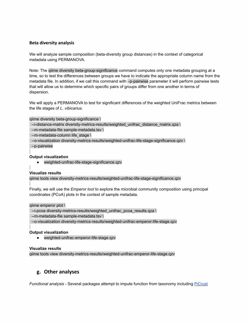
Beta diversity analysis We will analyze sample composition (beta-diversity group distances) in the context of categoricalmetadata using PERMANOVA. Note: The qiime diversity beta-group-significance command computes only one metadata grouping at atime, so to test the differences between groups we have to indicate the appropriate column name from themetadata file. In addition, if we call this command with –p-pairwise parameter it will perform pairwise teststhat will allow us to determine which specific pairs of groups differ from one another in terms ofdispersion. We will apply a PERMANOVA to test for significant differences of the weighted UniFrac metrics betweenthe life stages of L. vibicarius. qiime diversity beta-group-significance \ --i-distance-matrix diversity-metrics-results/weighted_unifrac_distance_matrix.qza \ --m-metadata-file sample-metadata.tsv \ --m-metadata-column life_stage \ --o-visualization diversity-metrics-results/weighted-unifrac-life-stage-significance.qzv \ --p-pairwise Output visualization

● weighted-unifrac-life-stage-significance.qzv Visualize resultsqiime tools view diversity-metrics-results/weighted-unifrac-life-stage-significance.qzv Finally, we will use the Emperor tool to explore the microbial community composition using principalcoordinates (PCoA) plots in the context of sample metadata. qiime emperor plot \ --i-pcoa diversity-metrics-results/weighted_unifrac_pcoa_results.qza \ --m-metadata-file sample-metadata.tsv \ --o-visualization diversity-metrics-results/weighted-unifrac-emperor-life-stage.qzv Output visualization

● weighted-unifrac-emperor-life-stage.qzv

Visualize resultsqiime tools view diversity-metrics-results/weighted-unifrac-emperor-life-stage.qzv

g. Other analyses Functional analysis - Several packages attempt to impute function from taxonomy including PiCrust

Other general analysis tools - R-based Phyloseq

4. Conclusions

In this tutorial we explained how to process short-sequencing reads with the open-source QIIME2 (Boylenet al. 2018). We used amplicon sequence data from the V4 region of the 16S rRNA to characterize andanalyze the bacterial communities of the frog Lithobates vibicarius. We showed the basic commands toprocess amplicon sequences for data analyses (e.g., denoise sequences and select sequence variants).This initial process allowed us to assign taxonomy to bacterial sequences using the Greengenesdatabase (version 13_8) (http://greengenes.lbl.gov) and perform diversity analysis with our samples. Weused plugins of QIIME2 to calculate alpha and beta diversity of three developmental stages (tadpoles,juveniles and adults) of L. vibicarius, and to perform statistical analysis to detect significant differencesbetween developmental stages. We were also able to visualize the differences of the skin bacterialcommunity composition among the developmental stages using principal coordinates (PCoA) plots withthe Emperor tool.

Author Contributions

RRJ developed the idea for this tutorial and wrote the content. The Institute of Evolutionary

Ecology and Conservation Genomics of Ulm University focusses at the interface of Evolutionary

Ecology, Genetics and Functional Biodiversity research. The Center for Conservation Genomics

at Smithsonian National Zoological Park and Conservation Biology Institute works to understand

and conserve biodiversity through the application of genomics and genetics approaches.

EMBL-European Bioinformatics Institute makes the world’s public biological data freely available

to the scientific community via a range of services and tools, performs basic research and

provides professional training in bioinformatics.

The CABANA Project aims to strengthen capacity for bioinformatics research and training in

Latin America, with the goal of addressing three challenges - management of communicable

disease, protection of biodiversity, and improving food security. It is funded by the Global

Challenges Research Fund, part of the UK AID budget.

Competing Interests or Disclaimer

The author declares no conflict of interest.

5. References

Bolyen, E., Rideout, J. R., Dillon, M. R., Bokulich , N. A., Abnet, C., Al-Ghalith, G. A., et al. (2018). QIIME2: reproducible, interactive, scalable, and extensible microbiome data science. PeerJ Inc 6:e27295v2.

Jiménez RR, Alvarado G, Estrella J, Sommer S. Moving beyond the host: unraveling the skin microbiomeof endangered Costa Rican amphibians. (2019). Front Microbiol 10:2060.

McMurdie PJ, Holmes S. phyloseq: an R package for reproducible interactive analysis and graphics ofmicrobiome census data. (2013). Plos One 8:e61217.