Micro-level Estimation of Prevalence of Child

Malnutrition In Cambodia

Tomoki Fujii1 Peter Lanjouw2 Silvia Alayon3

Livia Montana4

February 1, 2004

1University of California, Berkeley email:fujii@are.berkeley.edu2The World Bank email:planjouw@worldbank.org3ORC Macro email:silvia.alayon@orcmacro.com4ORC Macro email:Livia.S.Montana@orcmacro.com

Contents

1 Introduction 8

1.1 Malnutrition: Causes and Effects . . . . . . . . . . . . . . . . 8

1.2 Objective and Structure . . . . . . . . . . . . . . . . . . . . . 11

2 Child Malnutrition and Public Health Policy in Cambodia 15

2.1 Child Malnutrition in Cambodia . . . . . . . . . . . . . . . . . 15

2.2 Public Health Policy in Cambodia . . . . . . . . . . . . . . . . 16

3 Malnutrition and Anthropometric Indicators 18

3.1 Use of Anthropometry as a Malnutrition Indicator . . . . . . . 18

3.2 Explaining Anthropometric Indicators . . . . . . . . . . . . . 24

4 Methodology 28

4.1 Two Rounds of Estimates . . . . . . . . . . . . . . . . . . . . 28

4.2 Various Small Area Estimation Techniques . . . . . . . . . . . 30

4.3 Small Area Estimation for Nutrition Maps . . . . . . . . . . . 32

4.4 Theory of Small Area Estimation . . . . . . . . . . . . . . . . 35

2

5 Data 39

5.1 CDHS data . . . . . . . . . . . . . . . . . . . . . . . . . . . . 39

5.2 Cambodian National Population Census . . . . . . . . . . . . 41

5.3 Geographic data . . . . . . . . . . . . . . . . . . . . . . . . . . 41

6 Results 43

6.1 Putting the Estimates on the Maps . . . . . . . . . . . . . . . 43

6.2 Evaluating the Estimates . . . . . . . . . . . . . . . . . . . . . 49

6.3 Comparison of the First-Round and Second-Round Estimates 50

6.4 Interpreting the Maps . . . . . . . . . . . . . . . . . . . . . . 55

7 Conclusion 58

A Econometric Specification and Implementation 62

A.1 Introduction . . . . . . . . . . . . . . . . . . . . . . . . . . . . 62

A.2 Assumptions . . . . . . . . . . . . . . . . . . . . . . . . . . . . 66

A.3 Formula for the variance of different components of residuals . 69

A.4 Implementation . . . . . . . . . . . . . . . . . . . . . . . . . . 76

B Regression Results 83

B.1 Definition of Variables . . . . . . . . . . . . . . . . . . . . . . 83

B.2 Estimated Coefficients . . . . . . . . . . . . . . . . . . . . . . 87

B.3 Summary Statistics . . . . . . . . . . . . . . . . . . . . . . . . 107

C Summary of the First-Round Results 110

3

C.1 Tables . . . . . . . . . . . . . . . . . . . . . . . . . . . . . . . 111

C.2 Maps . . . . . . . . . . . . . . . . . . . . . . . . . . . . . . . . 113

References 118

4

List of Tables

3.1 Summary of Inforamtion on Anthropometric Indices . . . . . . 20

3.2 Pairwise Correlation Between Malnutrition Indicators. . . . . . 20

3.3 Comparison of Explanatory Power of Regression Models. . . . 22

6.1 Statistics on the Commune-Level Estimates. . . . . . . . . . . 50

6.2 Comparison of the Stratum-Level Estimates. . . . . . . . . . . 51

6.3 Comparison of the Small-Area and DHS Estimates. . . . . . . 55

B.1 List of Variables Used. . . . . . . . . . . . . . . . . . . . . . . 84

B.2 OLS and GLS Results for Urban Height Model. . . . . . . . . 88

B.3 Heteroskedastic Regression Results for Urban Height Model . 89

B.4 OLS and GLS Results for Urban Weight Model. . . . . . . . . 89

B.5 Heteroskedastic Regression Results for Urban Weight Model . 91

B.6 OLS and GLS Results for Plain Height Model. . . . . . . . . . 91

B.7 Heteroskedastic Regression Results for Plain Height Model . . 93

B.8 OLS and GLS Results for Plain Weight Model. . . . . . . . . . 94

B.9 Heteroskedastic Regression Results for Plain Weight Model . . 95

5

B.10 OLS and GLS Results for Tonlesap Height Model. . . . . . . . 95

B.11 Heteroskedastic Regression Results for Tonlesap Height Model 98

B.12 OLS and GLS Results for Tonlesap Weight Model. . . . . . . . 99

B.13 Heteroskedastic Regression Results for Tonlesap Weight Model 100

B.14 OLS and GLS Results for Coastal Height Model. . . . . . . . . 101

B.15 Heteroskedastic Regression Results for Coastal Height Model . 101

B.16 OLS and GLS Results for Coastal Weight Model. . . . . . . . 102

B.17 Heteroskedastic Regression Results for Coastal Weight Model . 103

B.18 OLS and GLS Results for Plateau Height Model. . . . . . . . 104

B.19 Heteroskedastic Regression Results for Plateau Height Model . 105

B.20 OLS and GLS Results for Plateau Weight Model. . . . . . . . 106

B.21 Heteroskedastic Regression Results for Plateau Weight Model 107

B.22 Regression Summary From Round Two . . . . . . . . . . . . . 109

C.1 Regression Summary Results from Round One . . . . . . . . . 112

C.2 Statistics on First-Round Commune Estimates . . . . . . . . . 112

C.3 First-Round Stratum-Level Estimates . . . . . . . . . . . . . . 113

6

List of Figures

6.1 Prevalence of Stunting in Cambodia. . . . . . . . . . . . . . . 44

6.2 Prevalence of Underweight in Cambodia. . . . . . . . . . . . . 45

6.3 Stunting Compared with National Average . . . . . . . . . . . 47

6.4 Underweight Compared with National Average . . . . . . . . . 48

C.1 Prevalence of Stunting in Cambodia (R1) . . . . . . . . . . . . 114

C.2 Prevalence of Underweight in Cambodia (R1) . . . . . . . . . 115

C.3 Stunting Compared with National Average (R1) . . . . . . . . 116

C.4 Underweight Compared with National Average (R1) . . . . . . 117

7

Chapter 1

Introduction

1.1 Malnutrition: Causes and Effects

Malnutrition remains a major public health concern in most developing coun-

tries. The serious impact of malnutrition on the life and health of chil-

dren is well documented. For example, malnourished children are more sus-

ceptible to some infectious diseases, such as diarrhea, malaria and measles

(Tomkins and Watson, 1989; Rice et al., 2000). For many children, the cost

of malnutrition is much higher; a recent report published by the World Health

Organization estimated that in 2000, about 3.7 million deaths among young

children worldwide were related to malnutrition (World Health Organization,

2002). Other studies estimate that about one half of childhood deaths in

developing countries are caused by undernutrition (Pelletier et al., 1994).

Malnutrition has also been associated with mortality and morbidity in later

8

life, delayed mental development and reduced intellectual performance (See,

de Onis et al. (2000)).

The immediate causes of malnutrition are considered to be a combination

of inadequate dietary intake and infection, which in turn are caused by food

insecurity, inadequate child care and inadequate health services. In children,

malnutrition is synonymous with growth failure. Though many people still

refer to growth failure as ‘protein-energy’ malnutrition, it is now recognized

that poor growth in children results not only from a deficiency of protein and

energy but also from an inadequate intake of vital minerals and vitamines,

and often essential fatty acids as well (UNICEF, 1998). These nutrients

required in tiny quantities for good functioning of human body are often

referred to as micronutrients.

To address micronutrient malnutrition, World Bank (1994) argues that

developing countries must carry out consumer education, aggressive distri-

bution of pharmaceutical supplements and the fortification of common food-

stuffs or water. All of these options are inexpensive and cost-effective. Be-

sides these actions geared to micronutrient malnutrition, Mason et al. (2001)

recommend a number of other components for nutrition strategies in Cam-

bodia, including women’s health and nutrition, antenatal care, breast feed-

ing, complementary feeding and food security. Behrman (1999) provides

economic considerations for analysis of early childhood development pro-

grammes, including child nutrition programmes. Using the human capital

approach, the theoretical framework to consider early childhood development

9

program is presented. He then argues that the two standard economic ratio-

nales for policy, efficiency and distribution, hold for early childhood develop-

ment program and also gives some policy options for childhood development.

Readers should bear in mind that the underlying causes of malnutrition may

be different from one place to another.

Therefore, just looking at the prevalence of malnutrition may not be

enough for formulating appropriate policies as the underlying causes may be

different even when the prevalence is the same. For example, a high level of

malnutrition in a relatively wealthy area may be more relevant to care prac-

tices in comparison with more remote and poorer areas with the same level of

malnutrition, where high prevalence of malnutrition may stem primarily from

insufficient food intake. In this case, parental education program for child

care would be appropriate in the former areas, but food aid may be more

appropriate in the latter. Though policy-specific issues are beyond the scope

of this study, one should note that the adequate policy may depend on the

local conditions that do not appear in the prevalence of malnutrition. Hence,

the decision-makers must exercise caution when formulating the policies.

Galler and Barrett (2001) reviewed the current and long-term effects of

and malnutrition on cognitive and behavioral development and showed that

malnutrition has a negative impact on cognitive and behavioral functioning

throughout childhood and adolescence, even after controlling for socioeco-

nomic conditions and other factors in the home environment. Shariff et al.

(2000) also found that, even after controlling for household socioeconomic

10

status, significant association between children’s total test score and height-

for-age persisted. They argue that height-for-age reflects the accumulation

of nutritional deprivation throughout the years, which may consequently af-

fect the cognitive development of children. Similar findings are also found

in Glewwe et al. (2001). They found that better nourished children perform

significantly better in school mostly because of greater learning productiv-

ity per year of schooling. Their cost-benefit analysis suggests that a dollar

invested in an early childhood nutrition program in a developing country

could potentially return at least three dollars worth of gains in academic

achievement, and perhaps much more.

1.2 Objective and Structure

With almost half the Cambodian children under five malnourished as mea-

sured by the height-for-age or weight-for-age indicator, malnutrition is one

of the direst public health problems in Cambodia. Given the grave conse-

quences of malnutrition, it is beyond question that the issue of malnutrition

must be tackled seriously. However, the resources to address malnutrition

is severely limited. Thus efforts must be made to allocate the available re-

sources in an efficient manner. In particular, analysis of current health data

is indispensable for that end.

Demographic and Health Surveys (DHS) have been widely used to analyze

public health issues in developing countries. In Cambodia, the Cambodian

11

Demographic and Health Survey (CDHS) was carried out in 2000 by the Na-

tional Institute of Statistics, Directorate General for Health and ORC Macro,

which have provided valuable information for those who are concerned with

health and nutrition issues in Cambodia (See, National Institute of Statistics et al.

(2001)). However, the sampling design of the DHS poses severe limitation

on the level of disaggregation at which one can estimate the prevalence of

malnutrition indicators; It allows one to estimate only at the stratum level,

which is more aggregated than the provincial level.

It is often the case, however, that what policy-makers really need is infor-

mation that is geographically disaggregated. They may want the estimates

of the prevalence of malnutrition at the district or even commune-level. If

policy-makers want to deliver food aid or nutrition supplements to malnour-

ished children, stratum-level estimates of the prevalence of malnutrition may

not be of great use since too many well-nourished children may benefit due

to the error of inclusion. If the coverage of food aid is limited due to the lack

of available resources, the error of exclusion is likely to be large unless the

locations of malnourished children are known.

To utilize available resources in a more efficient and effective manner,

targeting is often useful. Whether fine targeting is possible depends on the

information available to policy-makers. The objective of this study is to

provide the estimates of the prevalence of stunting and underweight among

children under five for small geographic areas in Cambodia, which are then

mapped out. Nutrition maps allow reducing informational constraints, which

12

are one of the central issues concerning the formulation of targeting policies

(Ravallion and Chao, 1989; Kanbur, 1987). They help policy-makers to iden-

tify the areas in which the prevalence of malnutrition is high, which cannot

be identified from DHS alone. Hence, nutrition maps are useful for formu-

lating geographic targeting policies to move assistance to the neediest people

in a more efficient and transparent manner.

To create the nutrition maps, a modified version of the small area estima-

tion technique developed by Elbers et al. (2003) was employed in this study.

While the small are estimation technique has already been used successfully

in over 10 countries to estimate poverty, this study is the first application of

the small area estimation technique to estimate nutritional outcomes.

As noted above, the estimates of the prevalence of malnutrition in them-

selves cannot tell the decision-makers what policy mix would be desirable to

address child malnutrition. In the Cambodian context, it is important that

the Council for Nutrition chaired by Ministry of Planning appreciates the

different underlying causes of malnutrition, and lets the relevant decision-

makers decide on the use of the information on malnutrition. Though we

do not have a suitable indicator that allows us to distinguish the underlying

causes of malnutrition, information on poverty and maternal education may

be reasonably good proxies for food intake and child care respectively.

There are a number of governmental agencies, non-governmental organi-

zations and international organizations that are expected to benefit from this

study. One of the Millennium Development Goals (MDGs) is the eradication

13

of extreme poverty and hunger, and the prevalence of underweight in children

under five is used as the indicator to gauge the achievement of the target of

halving, between 1990 and 2015, the proportion of people who suffer from

hunger. The nutrition maps resulting from this study, if used appropriately,

can contribute to the achievement of the MDGs. The maps are also use-

ful for the implementation of the Cambodian Nutrition Investment Plan, a

comprehensive plan developed by the Ministry of Planning with other line

ministries. Moreover, the maps are also has relevance to the National Poverty

Reduction Strategy and the second Socio-Economic Development Plan.

This paper is structured as follows: Child malnutrition and public health

policy in Cambodia will be discussed in Chapter 2. Chapter 3 provides

a brief overview of malnutrition and anthropometric indicators relevant to

this study. Chapter 4 provides the outline of the methodology, followed by

Chapter 5, which discusses the data used in this study. Chapter 6 summarizes

the results and Chapter 7 concludes.

14

Chapter 2

Child Malnutrition and Public

Health Policy in Cambodia

2.1 Child Malnutrition in Cambodia

There have been a relatively few studies done on child malnutrition and public

health policy in Cambodia. The most comprehensive study on child malnutri-

tion along with other public health issues is National Institute of Statistics et al.

(2001). They estimated the prevalence of stunting1 at 44.6 percent, which

means that nearly half of the Cambodian children under five are short com-

pared with a healthy population.

Hardy and Health Unlimited Ratanakiri Team (2001) analyzed health sit-

uation in Ratanakiri province, focusing on three ethnic groups of Jarai, Kru-

1More precise definition of this term will be given later.

15

eng and Tampoeun. They surveyed five villages of each ethnic group, to-

talling fifteen villages. They conclude food security is the major nutrition

issue for those people, but they also note there are other specific nutrition is-

sues to be addressed at the community level. Among these are infant feeding

practices, the diet of pregnant and lactating women and the heavy infestation

of intestinal parasites in children. Although their study is location-specific

and cannot be readily extrapolated to the rest of Cambodia especially be-

cause the Khmer people tend to have a quite different life-style, they are

suggestive.

2.2 Public Health Policy in Cambodia

There are a few studies that have relevance to Cambodian public health pol-

icy. Using data from health cards for mothers and their children and history

data, Main et al. (2001) evaluated a training intervention program aimed at

enhancing the roles of health centre stuff in the district of Krakor. They

found statistically significant change over the two-year period for tetanus,

BCG, polio and DTP, supporting the positive impact the intervention had

on immunization coverage in the district.

Gollogly (2002) illustrates the difficulties of medical aid using several

episodes. He reports the cases of medical aid in which the supposed benefi-

ciaries are excluded or the aid is diverted to the hands of a few people. He

states that it might be time for the parallel supply of services, which has al-

16

lowed the government to concentrate on military spending and personal gain

to an unconscionable degree, to become convergent, and for the international

community to reconsider its role in Cambodia’s reconstruction.

Hill (2000) points out the three conceptual fallacies when strategic plan-

ning fails, using as an example the Cambodian-German Health Project which

was disrupted by the military action on 5-6 July, 1997. Firstly, the fallacy

of predeterminism refers to the assumption that goals, results, appropriate

activities and required inputs can confidently be predicted based on past

and current experience, while they may not be predictable in reality. Sec-

ondly, the fallacy of detachments suggests that the functions of planning and

implementation are discrete management functions, and that objective, ra-

tional decisions in determining activities and inputs are sufficient to achieve

project goals and results. Thirdly, the fallacy of formalization is the essential

premise of planning that the creative insight required for successful strategic

development can be captured.

Although none of the above-mentioned studies are directly related to the

mapping of nutrition indicators in Cambodia, they seem to be consistent

with the motivation of this study when taken together; there is a dire child

health situation in Cambodia, and more transparent and effective policies

are called for. The nutrition maps are expected to help formulating such

policies.

17

Chapter 3

Malnutrition and

Anthropometric Indicators

3.1 Use of Anthropometry as a Malnutrition

Indicator

Thus far, we have not been specific what we mean by malnutrition. To mea-

sure malnutrition in a non-invasive and inexpensive manner, anthropometry

has been widely used among nutritionists and epidemiologists. Waterlow et al.

(1977) recommended that the basic indices recommended for the analysis of

data collected on a cross-sectional basis are height-for-age and weight-for-

height. The terms “wasting” and “stunting” are now used to refer to the

deficits of those indicators respectively.

Wasting indicates a deficit in tissue and fat mass compared with the

18

amount expected in a child of the same height or length, and may result

either from failure to gain weight or from actual weight loss. On the other

hand, stunting signifies slowing in skeletal growth (WHO Working Group,

1986). Wasting reflects ‘acute’ malnutrition whereas ‘chronic’ malnutrition.

Weight-for-age is also a commonly reported indicator and one is called under-

weight when deficit in the weight-for-age indicator exists. Though the use of

weight-for-age has decreased, partly because it is viewed as being unable to

distinguish between chronic and acute malnutrition, it may, however, regain

some favor with wider use of accurate solar powered digital scales (Alderman,

2000).

As WHO Working Group (1986) points out, there are several obvious

differences between wasting and stunting. Firstly, one can lose weight but

not height. Secondly, linear growth is a slower process than growth in body

mass. Thirdly, catch-up in height is possible, but takes a relatively long time

even with a favorable environment. Hence, wasting and stunting are quite

different processes with underweight somewhere in between. Gorstein et al.

(1994) summarized the usefulness of these anthropometric indicators as in

Table 3.1.

In fact, Victora (1992) finds no apparent pattern between levels of stunt-

ing in a population and levels of wasting. Stratum level comparison of various

malnutrition indicators derived from the CDHS data is consistent with this

observation. Table 3.2 shows that the pairwise correlation between stunt-

1Depends to some extent on the prevalence of wasting and stunting in the population

19

Table 3.1: Summary of information on anthropometric indices (AfterGorstein et al. (1994)).

Weight- Height- Weight-for-height for-age for-age

Usefulness in populations whereage is unknown or inaccurate

Excellent Poor Poor

Usefulness in identifying wastedchildren

Excellent Poor Moderate

Sensitivity to weight change over ashort time period

Excellent Poor Good

Usefulness in identifying stuntedchildren1

Poor Excellent Good

Table 3.2: Pairwise correlation between stunting, wasting and underweight.Correlation was taken at the stratum level without weights and its standarderrors were calculated by bootstrapping. N=17.

Correlation S.E.Stunting vs Wasting -0.434 0.177Stunting vs Underweight 0.763 0.115Wasting vs Underweight -0.250 0.240

ing, wasting and underweight. Significantly positive correlation between the

prevalence of stunting and underweight was observed while significantly neg-

ative correlation between stunting and wasting existed. No significant rela-

tionship was found between wasting and underweight.

Although the fact that the prevalence of stunting and underweight are

negatively correlated is puzzling, it is clear that we need to distinguish these

concepts. In this study, we report the prevalence of stunting and underweight,

20

but we do not report the prevalence of wasting. The primary reason is that

we were unable to construct a regression model for weight-for-height with

sufficient explanatory power for the small area estimation to work.2

Interestingly, this seems to be the case in other countries. Alderman

(2000) created regression models of various anthropometric indicators for

Viet Nam, South Africa, Pakistan and Morocco. As Table 3.3 shows, the vari-

ability of weight-for-height was least captured among all the indicators. This

may be because of the fact that all of the regressors used in this Alderman

(2000) reflect the welfare in a relatively long run. Hence, it is not surpris-

ing that the variation of the weight-for-height, a very short-term measure, is

least captured of all the three anthropometric indicator. Another thing to

note in Table 3.3 is that the community level effects are of great importance.

This observation has led us to include a number of commune or village level

variables in our regression model.

Admitting that it is more desirable to be able to estimate the preva-

lence of wasting, given the use of nutrition map, the prevalence of stunting

and underweight are more important indicator to look at. Since the map

reflects acute malnutrition as of 1998, the prevalence of wasting may well

have changed quite substantially by now. Hence, inability to estimate the

prevalence of wasting at a small geographic level should not undermine the

usefulness of this exercise.

2It is in theory possible to estimate weight-for-height from weight-for-age, height-for-age and age. This is one of the possible extensions of this research.

21

Table 3.3: Comparison of explanatory power of regression models. (Basedon Alderman (2000)).

Height- Weight- Weightfor-age for-height -for-age

With Viet Nam 0.283 0.128 0.412Community South Africa 0.239 0.250 0.277

Fixed Pakistan 0.304 0.256 0.347Effects Morocco 0.338 0.267 0.346

Without Viet Nam 0.225 0.080 0.251Fixed South Africa 0.125 0.053 0.128Effects Pakistan 0.142 0.025 0.146

Morocco 0.192 0.018 0.180Regressors include age, gender, interaction of those, parental education and

logarithmic income. Parental heights are modeled where available. Regressions

for South Africa and Viet Nam also include variables for race.

The anthropometric indices such as height-for-age and weight-for-age can

be described in terms of z-scores, percentile, and percent-of-median. But

Gorstein et al. (1994) supports the use of z-scores because their interpre-

tation is straightforward and they also consider the distribution of the an-

thropometric measure around the median. In this study, we shall use the

standardized height and weight, which are the z-scores converted back to the

corresponding height and weight of the reference age-sex group of 24-month-

old girls. The standardized height and weight are an affine transformation of

z-scores and preserve all of the desirable properties that the original z-score

possesses. The additional merit of the standardized height and weight is

that they are always positive for practically possible values of z-scores. This

22

allows us to compute inequality measures in terms of height or weight, which

can be compared with the international cross-sectional study carried out by

Pradhan et al. (2003). The choice of the reference group of 24-month-old

girls is to make this study comparable with Pradhan et al. (2003). It should

also be noted that standardized height and weight can be transformed to

z-scores easily.

Though height-for-age and weight-for-age z-scores have been widely used

and accepted, they are not the perfect measure. For example, Dibley et al.

(1987) note the discontinuity around the age of two that stems from the mea-

surement of recumbent length and height. Warner (2000) recommend that

more direct measurements such as skinfold thickness, mid-arm circumfer-

ences, or impedance measurements, be made for cross-validation with height

and weight data, which in turn leads to an improvement in the reliability

of the assessment of nutritional status in children. Forcheh (2002) notes

the law-like relationship between weight and height of children found by

Ehrenberg (1968) can be extended to include children under five and it can

be used to assess nutritional status. Though we do not discuss any further

the limitations of standardized height and weight we use in this study, read-

ers are reminded that the validity of this study is naturally restricted by the

limitations of the height-for-age and weight-for-age measures.

23

3.2 Explaining Anthropometric Indicators

The approach used in this study is built on the association between anthro-

pometric indicators and other socio-economic and geographic indicators. It

is, therefore, instructive to overview the previous international studies on the

relationship between anthropometric indicators and other indicators. While

experiences from other countries do not necessarily apply to Cambodia and

thus do not justify a specific choice of model in this study, it makes sense

to try models that have proved to be useful in explaining the variation of

anthropometric indicators in other countries.

Curtis and Hossain (1998) have explored the effect of aridity zone on child

nutritional status with data from 11 DHS surveys conducted in West Africa

between 1988 and 1996. They have constructed three different logistic models

for two malnutrition indicators, stunting and wasting, to see if there exists a

significant association between malnutrition indicators and aridity zone. In

particular, their study illustrates the use of geographic data in explaining

malnutrition. Though their results are preliminary, their results indicate

that aridity zone is genuinely associated with wasting, while it is not with

stunting once controlled for other variables.

Surprisingly, their socio-economic index did not have significant relation-

ship with neither of the malnutrition indicators. 3 On the other hand, age,

3The socioeconomic index is defined as the sum of four indicator functions, which donot seem to have a clear theoretical foundation. It would have been easier to understandthe underlying association if four indicators were entered as separate regressors in themodel.

24

schooling of the mother and breast-feeding indicators as well as the inter-

action between age and breast-feeding indicators generally had a significant

relationship with a malnutrition indicator.

Li et al. (1999) investigated the issue of malnutrition with various an-

thropometric indices and examined its correlates in a large sample of poor

rural minority children in China. In this study, age, maternal height, water

sources, maternal education and very low income were significant correlates.

In the case of Vietnam, the similar factors are relevant. The height-for-age

Z-score was significantly correlated with the age of the child, maternal weight

and height, parental education and some indicator variables on water sources

Haughton and Haughton (1997).

On a slightly different front, James et al. (1999) have looked at the cor-

relations between the maternal BMI and child anthropometric indicators,

using data taken from five communities in India, Ethiopia and Zimbabwe.

The correlations were low or not significant. In particular, the correlations

of the maternal BMI with the height-for-age Z-score are not significant in all

locations. Schmidt et al. (2002) have investigated the determinants and the

relative contribution of prenatal and postnatal factors to growth and nutri-

tional status of infants in West Java, Indonesia. Using multiple regression

models, which captured 19 to 41 percent of the variation in growth and nu-

tritional status of infants, they argue that the neonatal weight and length,

reflecting the prenatal environment, are the most important predictors of

infant nutritional status.

25

From an international perspective, Frongillo et al. (1997) have estimated

the variability among nations in the prevalence of stunting and wasting with

the October 1993 version of the WHO Global Database on Child Growth,

which covers 90 percent of the total population of children under five in

developing countries. They found that higher energy availability, female

literacy and gross product were the most important factors associated with

lower prevalence of stunting. In Asia, higher immunization rate and energy

availability were the most important factors associated with lower prevalence

of wasting. Other international studies include Victora (1992); De Onis et al.

(1993)

Monteiro et al. (1997) have investigated the patterns of intra-familiar dis-

tributions of undernutrition in Brazil. They analyzed the data for four income

strata separately and found that undernutrition was significantly associated

among household members only for the 25 percent poorest families. Sastry

(1997) have investigated the correlation of childhood morality risk in the

household in Northeast Brazil, and once community level effects are incor-

porated, family-level variance of was not significant. These studies seem to

suggest that the intra-familiar correlation may not be as important as one

may think, while efforts should be made to capture intra-familiar correlations

in modelling malnutrition.

Khorshed Alam Mozumder et al. (2000) has investigated the effects of

the length of birth interval on malnutrition. Using the data taken from

two districts in Bangladesh, they found that children were at higher risk of

26

malnutrition if they were female, their mothers were less educated, they had

several siblings, and either previous or subsequent siblings were born within

24 month. They conclude that the results indicate the potential importance

of longer birth intervals in reducing child malnutrition.

Zeini and Casterline (2002) have explored different levels of clustering,

including the regional level, governorate-level, local level, household level and

individual level, using the 2000 Egypt Demographic and Health Survey. They

have found that spatial clustering does seem to exist. They also found that,

even after controlling for socioeconomic factors, significant household-level

clustering remained. Another interesting point to note from their study is

the individual clustering. They found a little evidence that children suffering

from the nutritional problems revealed by the anthropometric measures are

more likely to suffer from anemia. While association between the various

nutritional risks may not exist in general, underweight was correlated with

stunting and/or wasting in some, but not all, governorates.

27

Chapter 4

Methodology

4.1 Two Rounds of Estimates

Before moving on to the details of the methodology, it should be noted that

this research was carried out in two rounds. In the first round conducted in

2002, we wanted to create something that can be readily used by the World

Food Programme. Since malnourished children would not like to wait until

the best possible estimates are derived, our approach in the first round was

minimalistic. Our primary goal in the first round was to produce within the

timeline of the World Food Programme a map that would reflect the spatial

distribution of malnourished children with a reasonable accuracy.

To the best of our knowledge, no nutrition map has been created prior

to this study by the small area estimation technique. Hence, our initial step

in the first round was to modify the technique and see if it works. The

28

answer was positive, and, in fact, the map has been used to select the WFP’s

target communes. As we shall argue later in Chapter 6, the first-round map

seems to have been appropriate for the use of WFP, given that there was no

alternative map. However, it was also clear to us that some modifications

would be needed to make the estimation model more realistic.

In the second round conducted in 2003, we have further studied literatures

on nutrition and taken more complex correlational structure into consider-

ation, namely the possibilities of the correlation of error terms within the

household and across two nutrition indicators. While there is no reason to

believe a priori that the second-round estimates are necessarily better than

the first round estimates, we believe that the second round estimates are

more realistic and recommend the second-round estimates if one would like

to use the estimates for policy analysis. This point will be visited in Chapter

6.

This Chapter aims at providing the readers with the basic framework of

the methodology. Section 4.2 first discusses various methodologies that are

relevant to this study. In Section 4.3 discusses the features of the method-

ology. Finally, 4.4 provides a short summary of the theory as to why the

methodology works. The technical explanation of the details of the method-

ology is delegated to the Appendix A.

29

4.2 Various Small Area Estimation Techniques

The small area estimation we use in this study has been used to create

poverty maps. This study is the first application of small area estimation to

the prevalence of malnutrition. To make it clear how this study relates to

other applications of small area estimation, let us briefly look at the typology

of poverty maps in this section.

Poverty maps can be created by a number of methodologies including the

small area estimation, multivariate weighted basic needs index, combination

of qualitative information and secondary data, and extrapolation of partic-

ipatory approaches. Davis (2002) overviews these various poverty mapping

methods and their applications, and discusses their merits and limitations.

Small area estimation is a statistical technique that combines survey and cen-

sus data to derive statistics for geographically small areas such as communes

and districts. Earlier application of small area estimation was mainly on

population estimates in post-censual years in the United States. As the de-

mand for small area statistics increases, various statistical models have been

developed and small area estimation has found a variety of applications. For

example, it was applied to estimate for small areas per capita income, areas

under corn and soybeans, adjustment for population undercount, and mean

wages and salaries in a given industry for each census division in a province

(Ghosh and Rao, 1994).

Application of small area estimation to poverty in developing countries

30

is relatively recent. There are two variants called the household unit level

method and the community level data method, depending on the level at

which the census records are available. The basic idea for these methods is

that the welfare measure at the household level or community level is re-

gressed on a set of variables that are common between the census and the

socio-economic survey. Then the welfare measure is imputed in each record

in the census. The advantage of running regression at the household level

is that the standard errors associated with poverty estimates can be eval-

uated through regression, while it is often easier to access the community

level census data and computational burden is substantially lower. Viet-

nam has a poverty map based on the community level data method (Minot,

2000). Other examples include Bigman et al. (2000) for Burkina Faso, and

Bigman and Fofack (2000) for India.

The household unit level method was first applied to Ecuador (Hentschel et al.,

2000). Its statistical properties were rigorously studied and various estima-

tion strategies were discussed by Elbers et al. (2003). The ELL approach has

been applied to a number of countries. Alderman et al. (2002) study the case

in South Africa and find that the income from the census data provides only

a weak proxy for the average income or poverty rates at either the provincial

level or at lower levels of aggregation. Demombynes et al. (2002) compared

the experience of poverty mapping from Ecuador, Madagascar and South

Africa. As discussed above, Cambodia witnessed the first application of the

ELL technique in Asia.

31

The ELL approach can be applied to estimate inequality. Elbers et al.

(2002) decompose inequality estimates in Ecuador, Madagascar and Mozam-

bique into progressively more disaggregated spatial units. The results in

all three countries are suggestive that even at a very high level of spatial

disaggregation, the contribution to overall inequality of within-community

inequality remain very high. Elbers et al. (2001b) use a large sample data

instead of the census. The methodology used in this study basically follows

the ELL approach, but there are some differences. In the next section, we

shall turn to the features of our methodology.

4.3 Small Area Estimation for Nutrition Maps

As noted above, the methodology used in this study is similar to the ELL

approach. This section is intended to provide the readers with the features

of the methodology, especially in constrast with the ELL approach, and the

readers are referred to Appendix A for technical details.

Like the ELL approach, we combine a census data and a survey data.

However, we used the Demographic and Health Survey (DHS) instead of a

socio-economic survey. This is precisely because we would like to predict

the nutrition indicators instead of consumption indicators. The Cambodian

Demographic and Health Survey (CDHS) contains the outcome variables of

interest, or the height and weight measurements for children under five. As

discussed earlier in Section 3.1, the height and weight measures were stan-

32

dardized respectively by taking the corresponding height and weight of the

24-month-old girl with the same height-for-age and weight-for-age z-scores.

As with the ELL approach, we then regress the left-hand-side variables on

the explanatory variables in common with the census, along with geographic

indicators available for the entire country at the village or commune level.

The geographic indicators include the remotely-sensed data as well as the

village-level statistics derived from the census data, both of which can be

joined with both the survey and the census data. More detailed accounts of

the data set we used will be given in Chapter 5.

It should be reminded here that the unit record is taken at the individ-

ual level in both survey and census data, or the level of each child. Our

methodology may be called the individual unit level method as opposed to

the household unit level method. This gives rise to the another difference. In

poverty mapping, the standard assumption is that each person in the house-

hold gets the same per capita consumption and that there may be unobserved

location-specific (i.e. village-specific in the Case of Cambodia) shocks. In

nutrition mapping, we do not, of course, assume that the standard height or

weight is the same across all the children within the same household. But it

would be reasonable to consider unobserved household-specific shocks. Hence

there may be two layers of shocks, both the location-specific and household-

specific shocks.1 In the first round, we only took into account the location

1It is possible to consider a variety of other structures for the unobserved shocks. Itwould be possible, for example, to shocks that go only to boys or girls in the same village,due to, perhaps, unobserved child-care practices that differ between the gender of the

33

effect, but in the second round, we also took into account the household

effect.

The third difference is the number of left-hand-side variables used in this

study. In ELL paper, they considered only the consumption measure whereas

we consider two indicators, standardized height and weight. If the unobserved

parts of the different indicators are correlated, they should be taken account

when computing the parameter estimates. In the first round, we separately

run the models, but we took into account this individual-clustering in the

second round.

Once we obtain the regression parameter estimates, we apply them to the

census data to make the predictions of the standardized height and weight

indicators. We can then aggregate them up to the lowest geographic unit

possible with acceptable standard errors. Separate models were calculated

for the following five ecozones: Urban, Plain, Tonlesap, Coastal, and Plateau.

The important feature of the ELL approach and this methodology is that

they allows for the estimation of standard errors associated with the predic-

tions of underweight and stunting prevalence. The calculation of standard

errors is necessary to evaluate the reliability of the estimates. When the

standard errors are too large, the estimates are not useful as it is impos-

sible to rank communes accurately. While the method allows us to derive

estimates at any level of aggregation, the standard errors tend to be larger

child, even though we are not aware of such practices. While we chose a structure thatseems reasonable and relevant to other studies, the choice is admittedly arbitrary.

34

at lower levels of aggregation, where population size may be small. Hence,

there is a trade-off between the level of disaggregation and the precision of

the estimates.

As briefly noted at the beginning of this Chapter, this study was carried

out in two rounds and, the details of the implementation differ between the

two rounds. There are two main differences. First is the choice of regres-

sors. We spent more time on modelling in the second rounds to improve

the explanatory power of the models. Second is the structure we impose on

the error terms. As we noted above, we took into consideration not only

the location effect, but also household effect and individual-clustering in the

second round. More detailed accounts for the estimation models are given in

Appendix A.

4.4 Theory of Small Area Estimation

The theoretical underpinnings of this methodology are given in detail in a

series of papers by Elbers et al. (2000, 2001a, 2003). In what follows, we shall

present a brief summary of the theory. We shall use a standardized anthropo-

metric indicator, yi as our left-hand-side variable. This may be standardized

height or standardized weight. The subscript i denotes the individual. yi is

related to a k-vector of observable characteristics, xh, through the following

35

anthropometric model.

yi = xTi β + ui (4.1)

where β is a k-vector of parameters and ui is a disturbance term. ui satisfies

E[ui|xi] = 0. The disturbance term is decomposed into the location, or

cluster-specific, effect and the household-specific effect and individual-specific

effect in application. Some or all of them may be heteroskedastic. Though we

have assumed here yi is a scalar for simplicity, there may be more than one

anthropometric indicators to estimate, in which case we may need to take

into account the correlation of ui across different indicators. The parameter

β is estimated through regression using the CDHS data. This regression will

be referred to as the first-stage regression.

For the purposes of the nutrition maps, what is of interest is not the

anthropometric measure of each individual in the census but various mea-

sures of nutritional status at a certain level of aggregation. In this paper,

commune-level aggregation was chosen because such a level of aggregation is

useful and the estimate at that level is acceptable. Estimates of nutritional

status at a more aggregated level such as the district or provincial level are

more accurate. Hereafter, the nutrition measure for the commune c with

Mc households is denoted as W (mc,Xc, β,uc), where mc is a Mc-vector of

household size. Xc and uc are a matrix Mc × k of observable characteristics,

and a Mc-vector of disturbances respectively.

36

Because the vector of disturbances for the target population, uc, is always

unknown, the expected value µc = E[W |mc,Xc, ζc] of the nutrition measure

W given the observable characteristics in the commune is estimated. ζc is the

vector of model parameters, including those which describe the disturbances.

To construct an estimator of µc, ζc is replaced by its consistent estimator ζc.

This yields an estimator of the form µc = E[W |mc,Xc, ζc]. This expectation

is often analytically intractable, so computer simulation is used to arrive at

the estimator µc presented in this paper.

The difference between µ,2 the estimator of the expected value of W in

this paper, and the actual level of welfare W can be written as:

W − µ = (W − µ) + (µ − µ) + (µ − µ) (4.2)

The first term on the right-hand-side of the equation is called the id-

iosyncratic error, which is due to the presence of a disturbance term in the

anthropometric model. The second term, the model error, is due to variance

in the first-stage estimates of the parameters of the anthropometric model.

The last term, the computation error, is due to using an inexact method to

compute µ.

The variance in µ due to idiosyncratic error falls approximately propor-

tionately with the size of the population of households in the commune. In

other words, since the component of the prediction error grows as the target

population becomes smaller, there is a practical limit to the degree of disag-

2For the sake of notational simplicity, the subscript c will be dropped.

37

gregation possible. This is precisely the reason village-level estimates were

not produced.

The model error is determined by the properties of ζc and hence it does not

increase or fall systematically as the size of the target population changes. Its

magnitude depends, in general, only on the standard errors of the first-stage

coefficients and the sensitivity of the indicators to deviations in household

consumption. For a given commune, its magnitude will also depend on the

distance of the explanatory variables for households in that commune from

the level of those variables in the sample data.

The computation error depends upon the computational method used.

Using simulation methods with sufficient computational resources and time,

this error can be made arbitrarily small. When the distribution of is known

or can be estimated, a Monte-Carlo simulation can be designed to capture

both the idiosyncratic error and the model error. The simulated disturbance

term uRc and the simulated consistent estimator ζR

c are drawn for the R-th

simulation to generate the R-th welfare estimate WR. The estimator µ is

found by taking the mean of WR over R and the associated standard error

can also derived by taking the standard deviation of WR. Once µ is found

for each cluster, it is straightforward to map out the results.

38

Chapter 5

Data

5.1 CDHS data

The CDHS was designed to collect health and demographic information

for the Cambodian population, with a particular focus on women of child-

bearing age and young children. The cluster sample covered 12,236 house-

holds across the country. Survey estimates were produced for 12 individual

provinces, (Banteay Mean Chey, Kampong Cham, Kampong Chhnang, Kam-

pong Spueu, Kampong Thom, Kandal, Koh Kong, Phnom Penh, Prey Veng,

Pursat, Svay Rieng and Takeo) and for the following 5 groups of provinces:

i) Bat Dambang and Krong Pailing, ii) Kampot, Krong Preah Sihanouk and

In addition to detailed information about each household, its members,

and housing characteristics, one half of these households were systematically

selected to participate in the anthropometric data collection. All children

39

under 60 months of age in the sub-sampled households were weighed and

measured. After excluding children for which information on height or weight

is missing or implausible, 3,596 observations were used for this analysis.

Since height and weight increase as the child gets older, the measure-

ments must be standardized so that they can be compared across different

ages. The z-score is a conventional measure for this purpose. However, be-

cause of the technical requirements in the methodology, the outcome variable

had to be non-negative and continuous. Consumption measures always take

on non-negative values, therefore a transformation of z-scores was needed

that would produce non-negative measures of height and weight. The z-

scores were standardized using the distribution of height and weight of 24

month-old females in a healthy population as the reference. Each childfs

original height-for-age z-score was converted to the height of a 24 month old

girl with the same z-score. Weight-for-age z-scores were treated in the same

manner. This allowed the outcome variables to remain positive as they rep-

resented height in centimeters or weight in kilograms. This approach avoids

the methodological problems arising from the use of the original z-scores,

which have both positive and negative values. This transformation has been

previously applied to z-scores to measure health inequality (Pradhan, Sahn

and Younger, 2002).

40

5.2 Cambodian National Population Census

The second data source was the Cambodian National Population Census,

the first population census to be conducted in Cambodia since 1962. The

census covered all persons staying in Cambodia, including foreigners, at the

reference time of midnight of March 3, 1998. The 1998 census in Cambodia

gathered information to allow a count of the population, as well as detailed

information on housing characteristics. Additionally, the census included

detailed information on each usual household member and visitors present

on the reference night, including the relationship to the head of household,

sex, age, marital status, migration, literacy, education and employment. The

census also contained questions on fertility of females aged 15 and over, and

infant mortality.

5.3 Geographic data

A set of geographic indicators was also used in this analysis. Although

geographic data has been used in a few applications prior to this study

(Mistiaen et al., 2001; Benson et al., 2002), this study is characterized by

extensive use of the geographic data. Because Cambodia has a rich collec-

tion of geographic data, indicators on a range of characteristics could be

generated. These indicators included distance calculations, land use and

land cover information, climate indicators, vegetation, agricultural produc-

tion and flooding. A number of data sets from various sources were compiled

41

into a GIS and these indicators were generated for all villages and com-

munes in Cambodia. Very coarse resolution data was summarized at the

commune-level, while high resolution data was attributed to individual vil-

lages. Distances from villages to roads, other towns, health facilities, and

major rivers were calculated from the center of the villages. Indicators based

on satellite data with varying temporal resolutions included land use within

the commune (agricultural, urban, forested, etc.), a vegetation greenness in-

dicator to proxy agricultural productivity, and the degree to which the area

was lit by nighttime lights as a proxy of urbanization. Relatively stable in-

dicators including soil quality, elevation, and various 30-year average climate

variables were derived from other composite data sets.

We have also used the village-level means from the census data. It should

be noted that the village-level means do not have to be taken from the

variables that also exist in the CDHS data set. This is because the village-

level means, as with other geographic variables, can be linked to both the

census and the survey data sets. Inclusion of these geographic variables

and their cross terms with other individual-level and household-level have

improved substantially the ability to fit the data.

42

Chapter 6

Results

6.1 Putting the Estimates on the Maps

After the predictions for the standardized height and weight for each child in

the census were made, they were aggregated to the commune level in Cambo-

dia. Due to missing data in the census data for a small number of communes,

we obtained commune-level estimates for a total of 1,594 communes out of

the 1,616 communes in Cambodia. Using these estimates, we can then cre-

ate the maps for the prevalence of stunting and underweight. Figure 6.1 and

Figure 6.2 show the estimated prevalence of stunting and underweight as of

the census year 1998.1 The darker areas represent worse situation.

1In this chapter, we shall present the results from the second round. Maps and tablesfrom the first round can be found in Appendix C

43

epsfiles/st_r2.eps

Figure 6.1: Commune-Level Prevalence of Stunting for the Children Under Five in Cambodia.

44

epsfiles/uw_r2.eps

Figure 6.2: Commune-Level Prevalence of Underweight for the Children Under Five in Cambodia.

45

These maps are presented in a very user-friendly format. They can be

easily understood. But we should also note that maps like these may be

misleading as such presentation does not take into account the fact that

these numbers are estimates and subject to statistical errors. One possible

way to avoid this is to compare the numbers with a fixed reference level.

For example, we can compare the estimated prevalence of underweight and

stunting with the national average. In Figure 6.3 and Figure 6.4, the darkest

areas represent the communes in which the estimated commune-level preva-

lence of malnutrition is more than two standard deviations higher than the

national average. Likewise, the lightest areas represent the communes with

significantly lower prevalence of malnutrition than the national average.

While this presentation takes into account the standard errors, it would

be less intuitive. One should note that the darkest areas do not necessarily

have higher estimated the second darkest areas, and that a similar thing

goes to the areas with lighter colors. It is essential that the decision makers

understand the meaning of the estimates.

46

epsfiles/stz_r2.eps

Figure 6.3: Commune-Level Prevalence of Stunting in Comparison With the National Average.

47

epsfiles/uwz_r2.eps

Figure 6.4: Commune-Level Prevalence of Underweight in Comparison With the National Average.

48

6.2 Evaluating the Estimates

The key statistics on the commune level estimates are given in Table 6.1. The

first column is the nutrition indicator for which the statistics are derived. The

second column is the mean standard error for the commune level estimates.

The third and fourth column are the minimum and maximum standard error

of commune level estimates. The fifth column is the mean coefficient of vari-

ation, which is the ratio of standard error to the point estimate averaged over

the communes. As one can see from the table, the commune-level estimates

are more accurate for underweight measures. It is more desirable to have a

smaller number for each column. Hence, the estimates for underweight are

more accurate than those for stunting.

Since the mean standard error is reasonably low, the commune level esti-

mates are useful for policy formulation. However, it must be reiterated that

the point estimates are subject to statistical errors, and they could be as high

as 20.7 percent for stunting and 17.4 percent for underweight. The standard

errors are particularly important when only a limited number of communes

are targeted.

To evaluate the reliability of the estimates, the stratum level CDHS preva-

lence of stunting and underweight were compared with the estimated stratum

level estimates using the census, DHS and GIS variables. Table 6.2 summa-

rizes these results. The differences are within two standard errors of the

CDHS estimates except for the underweight model for urban stratum , sug-

49

Table 6.1: Statistics on the commune-level estimates. The statistics arederived from the second round estimates. Each commune is given the sameweight. All the numbers are in percentage. The number of communes is1594.

Indicator Mean SE Min SE Max SE Mean CVStunting 4.0 1.4 20.7 9.0Underweight 2.7 1.3 17.4 5.8

gesting that the predicted estimates are consistent with the observation from

the DHS data. It should also be noted from 6.2 that the standard errors from

DHS only are higher than the DHS+CENSUS. In particular, the standard

errors from Coastal stratum is quite high.

6.3 Comparison of the First-Round and Second-

Round Estimates

As mentioned in Section 4.1, we have carried out this study in two rounds.

Since the first-round estimates have already been used by the World Food

Programme, it is necessary to consider the validity of the first-round esti-

mates in the light of the second-round estimates. One should note, however,

that the comparison per se does not tell us whether the first-round estimates

are any better or worse than the second-round estimates. Our goal here is

to give the readers ideas about the magnititude of the difference of the two

rounds and how they shold interpret it. Readers are referred to Appendix B

50

Table 6.2: Comparison of the stratum-level estimates. B. Mean and B. SEstand for the mean and standard error calculated by 100-time two-stagebootstrapping.

DHS Only DHS+CENSUSIndicator Stratum Mean B. Mean B. SE Mean SE

Urban 37.89 37.89 3.30 40.91 1.75Plain 47.58 48.00 2.49 50.61 1.92

Stunting Tonlsap 42.87 43.23 2.09 44.86 1.84Coastal 47.21 46.68 5.52 49.65 2.27Plateau 47.10 47.57 2.99 47.28 1.64Urban 39.58 39.37 2.93 45.55 0.95Plain 47.80 47.55 2.44 47.87 0.80

Underweight Tonlsap 45.84 45.88 1.95 46.33 1.10Coastal 38.95 38.80 5.28 45.32 1.20Plateau 46.37 46.72 3.87 48.26 0.75

for the relevant statistics.

Since we used two different models in the two rounds, neither of which

is a subset of the other, at least one of the models must be wrong, logically

speaking. In reality, both of the two models are wrong. This would be

inevitable as we would neither know the true model nor observe the every

single variable in the true model. Had there been data taken at the time of

census that allow us to calculate the prevalence of underweight and stunting

at the commune-level, we could have gauged which model performs better.

Unfortunately, though, there do not exist such data, and we are unable to

validate or invalidate our results.

Yet, we can still look at some of the key statistics and get some ideas

on how reliable the estimates are. First, we would like the both rounds

51

of estimates to be reasonably close. This is because at least one of the two

models has a large model error if the two models yielded very different results.

The mean absolute differences in the two rounds of point estimate made at the

commune level are 6.5 percent for stunting and 8.7 percent for underweight.

It should be noted that both rounds of estimates have statistical errors and

the mean absolute difference does not take the errors into account.

To fathom the magnitude of the difference between the two rounds in

comparison with the standard errors, we employed the following criteria.

We regarded the two rounds of estimates as if the two rounds of estimates

were a statistically independent trial, and checked whether the difference

is more than twice the standard errors. 346 communes out of 1596 were

significantly different for stunting and 303 communes for underweight. This

is obviously invalid as a statistical test because the underlying stochastic

process is unclear, but it gives us a useful summary statistics.

We can also look at the correlation between the two rounds. The corre-

lations at the commune level are 43.2 percent for stunting and 47.9 percent

for underweight. All of the above-mentioned statistics seem to suggest that

the two rounds of estimates give us somewhat close estimates. Given that

these two rounds of estimates are based on different models with different

assumptions, the small-area estimation seem to perform well enough to be

useful. This also reassures us that it was a reasonable choice to use the first

round estimates, given there was no alternative information at that time.

Yet, the estimates from the two rounds are not as close as one would like

52

them to be. For example, if the two estimates were two independent trials

and did follow the normal distribution, we would expect only around 170

communes. Readers should bear in mind that the model errors at least in

one of the two rounds are not negligible.

Now, let us look at the consequences of the assumptions made in different

rounds. First, the location effect was not found in each of the two rounds.

The absence of the location effect is presumably as a result of the inclusion of

the geogrpahic indicators, which are not often omitted other studies. Hence

in Cambodian case, the remaining location effects indeed seemed to be small.

Second, as shown in Table B.22 in Appendix B, high levels of correla-

tion exist in the estimated individual effects for the standardized height and

weight indicators. This supoorts the inclusion of the correlation between the

two indicators.

Third, whether we should need to include the household effects is some-

what arguable for the height indicator. Because the household effect takes

account of only less than five percent of σu, it may not affect the final re-

sults much. We should note, however, that the bootstraping simulation of

the residuals suggest that σδ is significantly less than unity, which in turn

suggests that the proportion of the residual explained by the household effect

is on average significantly greater than zero. The importance of the inclusion

of household effects would be less arguable for the weight indicator.

Fourth, in most of the models, the small-area estimates at the stratum

level have improved from the first round to the second round. In Table 6.3,

53

Column (A) is the stratum-level estimate of the prevalence of stunting and

underweight derived only from the DHS data. Column (B) is the small-area

estimates from the second round. These two columns also appear in Ta-

ble 6.2. Column (C) is the small-area estimates form the first round. The

two columns next to Column (C) are the different between the small-area

estimates and the DHS-only estiates respectively. If the absolute value of

the difference is smaller in the second round, we deemed that the small-area

estimates at the stratum level had improved. The last column of Table 6.3

shows if the estimates at the stratum level have improved. Under this cri-

teria, all the models except for the Plain stratum for the stunting indicator

and the Urban and Coastal strata for the underweight indicator have im-

proved./footnoteOne should note that, in the second round, the prevalence

of stunting and underweight was esimated jointly. This made it difficult to

find models that are better for both indicators. In particular, one should note

that, in the second round, the prevalence of underweight in Urban strata was

overestimated.

While none of the above observations logically concludes that the second

round estimates are necessarily better than the first round estimates, we

recommend, from the balance of aforementioned evidence, that the readers

use the second round estimates. Yet, the second round estimates are far

from perfect, and the users of the estimates should be fully aware of their

limitations. In the next section, we shall note some points that would be

directly relevant to the policy formulation. We shall also point out the overall

54

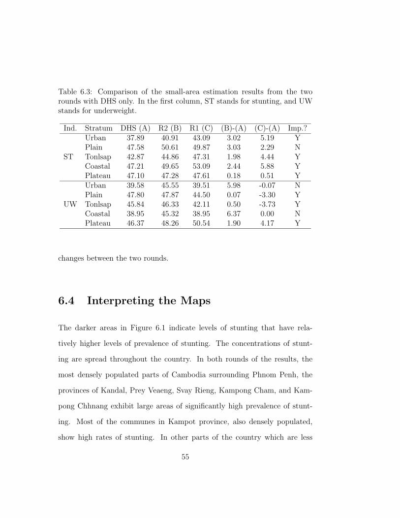
Table 6.3: Comparison of the small-area estimation results from the tworounds with DHS only. In the first column, ST stands for stunting, and UWstands for underweight.

Ind. Stratum DHS (A) R2 (B) R1 (C) (B)-(A) (C)-(A) Imp.?Urban 37.89 40.91 43.09 3.02 5.19 YPlain 47.58 50.61 49.87 3.03 2.29 N

ST Tonlsap 42.87 44.86 47.31 1.98 4.44 YCoastal 47.21 49.65 53.09 2.44 5.88 YPlateau 47.10 47.28 47.61 0.18 0.51 YUrban 39.58 45.55 39.51 5.98 -0.07 NPlain 47.80 47.87 44.50 0.07 -3.30 Y

UW Tonlsap 45.84 46.33 42.11 0.50 -3.73 YCoastal 38.95 45.32 38.95 6.37 0.00 NPlateau 46.37 48.26 50.54 1.90 4.17 Y

changes between the two rounds.

6.4 Interpreting the Maps

The darker areas in Figure 6.1 indicate levels of stunting that have rela-

tively higher levels of prevalence of stunting. The concentrations of stunt-

ing are spread throughout the country. In both rounds of the results, the

most densely populated parts of Cambodia surrounding Phnom Penh, the

provinces of Kandal, Prey Veaeng, Svay Rieng, Kampong Cham, and Kam-

pong Chhnang exhibit large areas of significantly high prevalence of stunt-

ing. Most of the communes in Kampot province, also densely populated,

show high rates of stunting. In other parts of the country which are less

55

populated and generally more forested such as Preah Vihear, Stueng Traeng,

and Rotanak Kiri in the north, and Kaoh Kong on the Gulf of Thailand,

there are also concentrations of high rates of stunting. Areas that have lower

prevalence of stunting include Phnom Penh, Mondol Kiri, and Eastern Bat

Dambang. Many communes around Lake Tonle Sap in Pousat and Kampong

Thum provinces also have relatively low stunting rates. There appears to be

an East-West band across the middle of the country where children are less

stunted.

The darker areas in Figure 6.2 represent the communes where the preva-

lence of underweight children is relatively high. While the two rounds of

results share some important characteristics of the results, there appear to

exist some differences. In the first round, we have seen that the underweight

children is concerntrated in the northeastern part of the country. Though it

is still the case in the second round, the magnitude seems less. Lower levels

of prevalence of underweight are seen in both rounds in the south, including

some parts of Kampong Cham, Kandal and Kaoh Kong. Communes around

Lake Tonle Sap in Bat Dambang and Siem Reab have lower prevalence of

stunting. Northern Siem Reap, Otdar Mean Chey and Bantay Mean Chey in

the north had relatively low prevalence in the first round, but not so in the

second round. While we generally recommend the use of the second round

for reasons discussed in the next section, the estimates in above-mentioned

areas where two rounds of estimates differ substantially should be taken par-

ticularly carefully, because the estimates in these areas may be more likely

56

to be influenced by the model error.

57

Chapter 7

Conclusion

We have shown that the small-area estimation technique can be applied to the

mapping of the prevalence of stunting and underweight. We have extended

the small area estimation technique to include the household effect, along

with the location and individual effects, and the individual clustering. We

argued that the results from the second round, which take care of these

elements should be more appropriate for application than those from the

first round. While the standard errors are quite high for some communes,

the magnitude of the standard errors for the estimated prevalence of stunting

and underweight at the commune level is, on average, acceptable.

An obvious extension to this research is to include wasting. One way to

do this is to use weight-for-height instead of weight-for-age in the simulta-

neous estimation. Our exploratory work seems to suggest, thought that this

approach is not promising as it is difficult to construct a good explanatory

58

model of the weight-for-height indicator. Another possibility is to use the

estimated height and weight to derive the weight-for-height measure. The

inclusion of the individual-clustering would make the latter approach more

meaningful.

There are a number of directions for further research. With the nutrition

maps, we can answer a number of research questions that we could not answer

before. For example, we can look at the relationship between the inequality

in the height or inequality measures, and other commune-level indicators. It

is also possible to see the relationship between the poverty inequality and

nutrition inequality.

The results brought about by this study have a number of applications.

Previously, estimates of the prevalence of child malnutrition from the CDHS

were only available at the province level. These estimates are useful to target

interventions in areas with a high prevalence of malnutrition throughout the

province, such as the northeastern provinces. However, provincial estimates

often mask great disparities in the prevalence of malnutrition within the

province. Targeting based on such estimates will likely fail to capture many

malnourished children.

Further, understanding the determinants of malnutrition to better in-

form program planners. The power of these maps can be multiplied when

they are combined with others to explain relationships among outcomes. It

might be assumed that there is insufficient access to food where high rates of

malnutrition overlap with high poverty rates. An overlay of stunting preva-

59

lence with women’s education as a proxy for child care may be a first step

towards understanding and distinguishing areas of high malnutrition along

with their causes. Such exploratory maps may be followed with a multivari-

ate analysis of the underlying and immediate causes of malnutrition. The

conclusions drawn from such integration of maps and follow-on analysis can

inform program planners so that interventions can be designed, targeted

and coordinated across different institutions in a more efficient, effective and

transparent manner. Such interventions, in turn, would help to achieve the

goals and aims that are set in important policy-related documents, includ-

ing the Millenium Development Goals, Poverty Reduction Strategy Papers

(PRSPs), Socio Economic Development Plan and Cambodian Nutrition In-

vestment Plan.

Another direction of the research is the validation of the results. It should

be reminded that the small area estimation is predicated on a number of

assumptions. This means that the results we obtained may be completely

wrong if one or more of the assumptions do not hold. While we believe we

have made reasonable assumptions, the results should be taken with sound

criticism. Hence, it would be valuable to try to validate these estimates

from external data sources. Since we do not have an external data on the

nutritional status of children taken at the time of census, we would not be

able to validate the map in a statistical sense. Yet, it would be useful for

practical purposes to look at relevant data sources or collect, as such an

exercise may identify those areas for which the nutrition maps created in

60

this study are accurate and those ares for which they are misleading. One

example of such validation exercise carried out in Cambodia is

It is also useful to develop methods of updating these maps when new

survey data becomes available. Such updating would be desirable for the

nutrition estimates in the near future as it ensures the policy makers to

target resources more timely. Updating is relatively starightforward, if the

survey is taken as a panel data. This is because we can use the new height

and weight indicators as the new left-hand-side variable, while keeping the

household characteristics in the previous survey as the regressors. Another

possibility is to do an exercise similiar to this study, if a new survey and a

large sample data become available. Otherwise, it may be possible to update

by some sort of matching.

As we have discussed, this study opens doors to different directions. Yet,

one should be aware of the limitations it entails. While the maps can be

a powerful tool, it may be misleading. The estimates have errors and are

derived on the basis of a number of assumptions. It should also be emphasized

that the map reflects the situation as of the census year of 1998, and the

current situation may have changed. The maps presented in this study should

be used in combination with other data sources whenever possible. This is

especial so when important programmatic decisions are at stake.

61

Appendix A

Econometric Specification and

Implementation

A.1 Introduction

In this Appendix, we present the estimation models for both rounds and we

shall also discuss their implementation. While our presentation will be based

on the second-round estimation model, we shall point out the difference from

the first-round estimation model.

In the first round, we almost directly applied the small area estimation

technique developed by Elbers et al. (2001a, 2003). The main difference was

the nature of the left-hand-side variable. Instead of the logarithmic con-

sumption, we used the standardized height and weight. Also, we used the

62

logarithmic model for the heteroskedastic model in round 1.1

In the second-round, we wanted to construct a model which incorporates

location effects, heteroskedastic household effects and individual effects. We

also wanted to allow for the possibility of the unobserved individual effects

correlated across the indicators, which we shall call the individual-clustering.

This Appendix develops an estimation model meeting these requirements

and its implementation.

Before moving on, let us provide the rationale for the particular specifi-

cation used in the estimation. Firstly, we assumed the hierarchical structure

of the error terms, which are, as mentioned above, comprised of the location

effect, household effect and individual effect. We wanted to allow for the

heteroskedasticity of some of these effects. As noted in footnote 1, the choice

of such structure is arbitrary. Our choice is determined by the limitation of

the data, but also it is influenced by other studies mentioned in Chapter 3

and our field observation.

We first decided to allow for heteroskedasticity at one level only. This

is because, if we allow for heteroskedasticity at more than one levels, it

becomes increasingly difficult to separate out the each heteroskedastic com-

ponent. Also, we preferred to keep the individual effect homoskedastic for

three reasons. First, the individual effect is difficult to separate from the

1It seemed that the logarithmic model may be better in the sense that we do not haveto make an arguably arbitrary choice of upper and lower bounds. However, after a reviewof the round 1 results, this point seems to be offset by the lack of robustness of the results,which have led us to use the logistic model in the round 2. It should be pointed out thatdeveloping more appropriate heteroskedastic models is a matter of future research.

63

household effect, if the household effect is allowed for. This is because there

are many household for which there is only one child under the age of five

in Cambodia.2 Since we decided to allow for the household effect in the sec-

ond round, it was almost necessary to assume the heteroskedasticity at the

household level in the second round. Second, even if there were many kids

under five in each household, it would have been still very difficult to run the

heteroskedastic regression, if the individual-clustering exists. Third, there

are very limited number of variables observe at the individual level. Hence,

it would not practically matter much whether we run the heteroskedastic re-

gression at the individual level or the household level. Because the household

effect seems to be important than the location effect, which turns out to be

correct in all the strata in Cambodia, we chose to allow for heteroskedasticity

at the household level.

The location effect is assumed to take place at the village level. This

would be reasonable, given the relatively homogeneous lifestyle in the village.

On the other hand, other effect may remain at higher levels of aggregation

such as the levels of commune, district and province. We also assumed the

homogeneity of the location effect, but the location effect may interact with

the individual or household characteristics. For example, the mineral content

of the ground water, which would be reasonably approximated by the village-

level random effect, could influence the growth of children, but its magnitude

may vary according to the age and sex of the child. Readers are reminded that

2In the CDHS survey, the (unweighted) average number of children under five is 1.33.

64

heterogeneity of this sort, while we have no evidence that such heterogeneity

exists or otherwise, is not captured in our model.

We also take into consideration the household effects. Since a household

is the group of people who usually share the food, among other things, with

each other, it would be reasonable to consider that there may be unobserved

household-specific shocks. Furthermore, one may suspect that the genetic

factor may determine the growth of children. Unfortunately, we were unable

to identify the mother of the child in the census data. Hence, all the variables

included in the regression models were in one way or another aggregated over

the women in the household. And unexplained part should be captured as

the household effect in our model.

We also allowed for the unobserved individual effects correlated across

the indicators, or the individual-clustering. This would be reasonable as the

height and weight indicator are closely related, and there may be a number

of factors that do not appear in the data. Our regression results suggest that

individual-clustering do in fact exist.

This Appendix is organized as follows. In Section A.2, we present the

assumptions. In Section A.3, we present some useful equations to determine

the distribution of location effect and individual effect. In Section A.4, we

present the estimation equations used in this study.

65

A.2 Assumptions

In this section, we present the assumptions of the econometric model used

in the second round. At the end of this section, we shall point out what

was different in the first round. In the second round, we are interested in K

real-valued nutrition indicators. Our particular interest is the case where the

indicators are the standardized height and weight so that K = 2. However,

we shall treat more general case here. For k-th (1 ≤ k ≤ K) indicator, we

assume the following model:

y(k) = x(k)β(k) + u(k)

where y(k) and u(k) are a scalar, x(k) a 1×d(k) vector, β(k) a d(k)×1 vector.

d(k) is the number of the variables used to explain y(k). The superscripts in

the bracket are used to denote the variables related to the k-th indicator.

Now let us denote

�u =

u(1)

...

u(K)

and similar notations will be used hereafter.

Let us further assume that u(k) can be decomposed into the location effect

η(k), household effect ε(k) and individual effect δ(k). We denote the set of all

clusters by C, the set of all households in cluster c(∈ C) by Hc and the set

66

of all individuals in household h(∈ Hc) by Ich. We shall denote the counting

measure by #(·), and let C ≡ #(C), Hc ≡ #(Hc), and Ich ≡ #(Ich). Let the

total number of observations N ≡∑c∈C∑

h∈HcIch. Also, we assume that Ich

is small and takes 1 for some households. We also assume that each cluster

has a weight wc which is normalized so that∑

c wc = 1. Using the subscripts

cluster c, household h and individual i, we assume uchi can be written as

follows:

u(k)chi = η(k)

c + ε(k)ch + δ

(k)chi

We also assume that η(k)c , ε

(k)ch and δ

(k)chi are a random variable, and for

∀c, h, i and k , they satisfy

E[u(k)chi] = E[η(k)

c ] = E[ε(k)ch ] = E[δ

(k)chi] = 0

�ηc,�εch and �δchi are uncorrelated. We also assume that the matrices V ar[�ηc]

and V ar[�εch] are diagonal for all c and h, while V ar[�δchi] may not be diagonal.

In other words, the unsystematic part of the model across different indicators

are correlated through individual effects. We also assume that �εch may be

heteroskedastic and thus V ar[�εch] is dependent on the household h. Since

K × K matrix V ar[�εch] is assumed to be diagonal, we can write it as

67

V ar[�εch] =

(σ

(1)ε,ch)

2 0

. . .

0 (σ(K)ε,ch)2

Likewise, K × K matrix V ar[�ηc] is also assumed to be diagonal, we can

write it as

V ar[�ηc] =

(σ

(1)η )2 0

. . .

0 (σ(K)η )2

The individual component of different indicators may be correlated. We

shall write

V ar[�δchi] =

σ

(1,1)δ . . . σ

(1,K)δ

.... . .

...

σ(K,1)δ . . . σ

(K,K)δ

,

and we define (σ(k)δ )2 ≡ σ

(k,k)δ . Obviously, we must have σ

(j,k)δ = σ

(k,j)δ for

∀j, k(∈ {1, K}).

Now, let us briefly turn to the difference between the first-round and

second-round specification. Since we did not consider the household effect in

the first round, we in effect set ε(k)ch ≡ 0. We considered the heteroskedasticity

at the individual. Thus, the appropriate notation for the variance of the

68

individual effect is σ2δ,chi. Finally, since the individual-clustering was not

taken into account, we assumed σ(k,j)δ ≡ 0 in the first round.

Under the first-round specification, the results given in Elbers et al. (2001a)

are directly applicable by regarding as if each individual consisted a house-

hold and we do not reproduce the results here. The only remaining differ-

ence is the heteroskedastic model. In the first round, we had the form of

log σ2chi = zT

chiα + τchi. Also, the heteroskedasticity was modeled only when

the white’s test of heteroskedasticity suggests the existence of heteroskedas-

ticity. In the second round, we chose to keep variables that has significant

explanatory power of the variation of the household effect.

A.3 Formula for the variance of different com-

ponents of residuals

In this section we present several formula needed to derive the estimates of

V ar[�ηc], V ar[�εch] and V ar[�δchi] from �u, and these formula primarily relevant

to the second-round specification. The results presented in this section will

be used in the next section.

Let us define

u(k)ch· ≡

1

Ich

∑i∈Ich

u(k)chi = η(k)

c + ε(k)ch + δ

(k)ch·

69

u(k)c·· ≡ 1

Hc

∑h∈Hc

u(k)ch· = η(k)

c + ε(k)c· + δ(k)

c··

where

δ(k)ch· ≡

1

Ich

∑i∈Ich

δ(k)chi

ε(k)c· ≡ 1

Hc

∑h∈Hc

ε(k)ch

δ(k)c·· ≡ 1

Hc

∑h∈Hc

δ(k)ch·

A.3.1 Finding σ2δ

. Since the following argument holds for all the nutrition indicator, we shall

drop for now the superscript (k) for simplicity. Let us denote the sampling

weight by wc. We assume∑

c∈C wc ≡ 1. Now let us define Hc ≡ {h ∈Hc|Ich > 1}, Hc ≡ #{Hc}, C ≡ {c ∈ C|Hc > 0}, and wc ≡ wcP

c′∈C wc′.

Then we have the following:

E

∑c∈C

wc

Hc

∑h∈Hc

∑i∈Ich

(uchi − uch·)2

Ich − 1

= σ2δ (A.1)

Proof

70

E[(uchi − uch·)2] = E[(δchi − δch·)2]

=Ich − 1

Ichσ2

δ

Hence,

E

∑c∈C

wc

Hc

∑h∈Hc

∑i∈Ich

(uchi − uch·)2

Ich − 1

=∑c∈C

wc

Hc

∑h∈Hc

∑i∈Ich

E[(uchi − uch·)2]

Ich − 1

=∑c∈C

wc

Hc

∑h∈Hc

∑i∈Ich

σ2δ

Ich

=∑c∈C

wc

Hc

∑h∈Hc

σ2δ

= σ2δ

A.3.2 Finding σ2ε,ch

Now, let us turn to the household effects. We can derive the following for-

mula, but, unfortunately, for reasons I shall mention later, this is not very

useful.

71

σ2ε,ch =

Hc · E[(uch· − uc··)2]

Hc − 2− E[

∑h′∈Hc

(uch′· − uc··)2]

(Hc − 1)(Hc − 2)− σ2

δ

Ich(A.2)

Proof

By straightforward calculations, we have

E[(εch − εc·)2] =Hc − 2

Hc

σ2ε,ch +

1

H2c

∑h′∈Hc

σ2ε,ch′

and

E[(δch· − δc··)2] =Hc − 2

Hc

E[δ2ch·] +

1

H2c

∑h′∈Hc

E[δ2ch′·]

=Hc − 2

Hc

· σ2δ

Ich+

1

H2c

(∑h′∈Hc

1

Ich′

)σ2

δ

Let vch ≡ uch· − uc··. Then, we have

E[v2ch] = E[(εch − εc·)2 + (δch· − δc··)2]

=Hc − 2

Hc

{σ2

δ

Ich+ σ2

ε,ch

}+

1

H2c

{∑h′∈Hc

(σδ

Ich′+ σ2

ε,ch′

)}

By summing over the households in each cluster, we have

72

E[∑

h′∈Hc

v2ch′ ] =

Hc − 1

Hc

{∑h′∈Hc

(σ2

δ

Ich′+ σ2

ε,ch′

)}

Therefore, for all the households in C∗∗(≡ {c ∈ C|Hc > 2})

σ2ε,ch =

Hc

Hc − 2E[v2

ch] −1

Hc(Hc − 2)

{∑h′∈Hc

(σ2

δ

Ich′+ σ2

ε,ch′

)}− σ2

δ

Ich

=Hc

Hc − 2E[v2

ch] −1

(Hc − 1)(Hc − 2)E[∑

h′∈Hc

v2ch′ ] − σ2

δ

Ich

A.3.3 Finding σ2η

. Let us now derive the following formula for σ2η.

σ2η =

∑c∈C wcHcE[(uc··)2] −∑c∈C

wc

Hc

∑h∈Hc

E[(uch·)2]∑c∈C wc(Hc − 1)

(A.3)

Proof

First, note

E[(uch·)2] = E[(ηc)2 + (εch)

2 + (δch·)2]

= σ2η + σ2

ε,ch + E

( 1

Ich

∑i∈Ich

δchi

)2

= σ2η + σ2

ε,ch +1

Ichσ2

δ

73

Clearly,

E[(uc··)2] = σ2η + E[(εc·)2] + E[(δc··)2] (A.4)

The second term can be expressed as follows:

E[(εc·)2] = E

( 1

Hc

∑h∈Hc

εch

)2

=1

H2c

E[∑h∈Hc

ε2ch]

=1

H2c

∑h∈Hc

σ2ε,ch

The third term can be expressed as follows:

E[(δc··)2] = E

( 1

Hc

∑h∈Hc

δch·

)2

=1

H2c

E

(∑h∈Hc

δch·

)2

=1

H2c

∑h∈Hc

E[δ2ch·]

=1

H2c

∑h∈Hc

E

( 1

Ich

∑i∈Ich

δchi

)2

=1

H2c

(∑h∈Hc

1

Ich

)σ2

δ

74

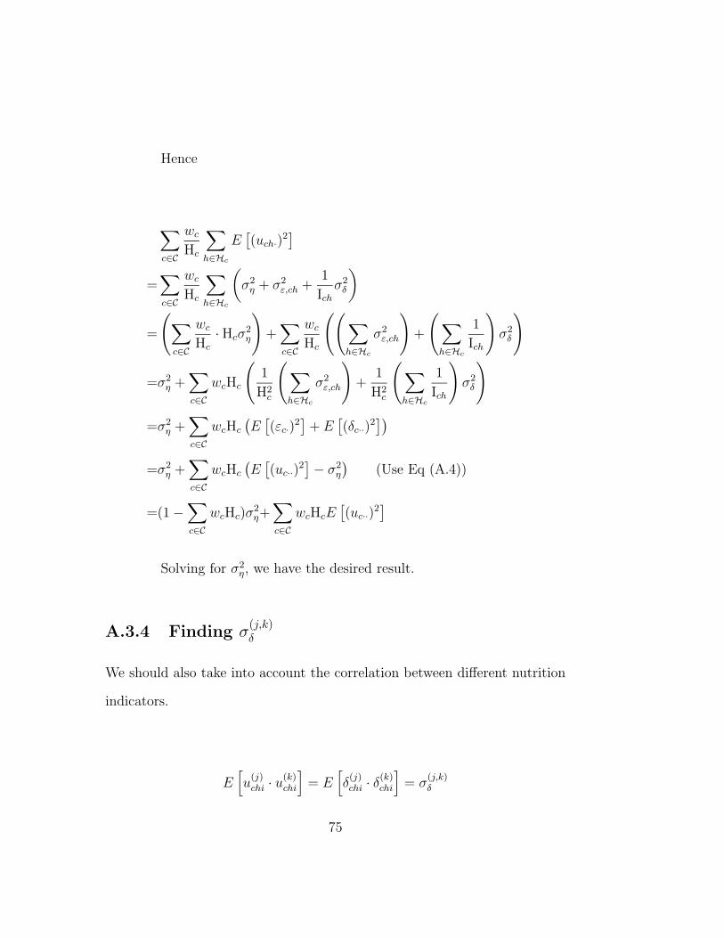
Hence

∑c∈C

wc

Hc

∑h∈Hc

E[(uch·)2

]=∑c∈C

wc

Hc

∑h∈Hc

(σ2

η + σ2ε,ch +

1

Ichσ2

δ

)

=

(∑c∈C

wc

Hc

· Hcσ2η

)+∑c∈C

wc

Hc

((∑h∈Hc

σ2ε,ch

)+

(∑h∈Hc

1

Ich

)σ2

δ

)

=σ2η +∑c∈C

wcHc

(1

H2c

(∑h∈Hc

σ2ε,ch

)+

1

H2c

(∑h∈Hc

1

Ich

)σ2

δ

)

=σ2η +∑c∈C

wcHc

(E[(εc·)2

]+ E[(δc··)2

])=σ2

η +∑c∈C

wcHc

(E[(uc··)2

]− σ2η

)(Use Eq (A.4))

=(1 −∑c∈C

wcHc)σ2η+∑c∈C

wcHcE[(uc··)2

]

Solving for σ2η, we have the desired result.

A.3.4 Finding σ(j,k)δ

We should also take into account the correlation between different nutrition

indicators.

E[u

(j)chi · u(k)

chi

]= E[δ

(j)chi · δ(k)

chi

]= σ

(j,k)δ

75

Therefore,

σ(j,k)δ =

∑c∈C

wc

Hc

∑h∈Hc

∑i∈Ich

E[u

(j)chi · u(k)

chi

]Ich

Another useful result is that

E[(u

(j)chi − u

(j)ch·)(u

(k)chi − u

(k)ch·)]

=Ich − 1

Ichσ

(j,k)δ

This implies that

σ(j,k)δ =

∑c∈C

wc

Hc

∑h∈Hc

∑i∈Ich

E[(u

(j)chi − u

(j)ch·) · (u(k)

chi − u(k)ch·)]

Ich − 1

A.4 Implementation

A.4.1 Finding the variances of the residual compo-

nents.

To estimate the distribution of u, we first run an OLS for each indicator and

obtain β(k)OLS. Let us denote the regression residual by u

(k)chi(≡ y

(k)chi−x

(k)chiβ

(k)OLS).

By replacing u by u, we define u(k)ch· and u

(k)c·· . A consistent estimate of (σ

(k)δ )2

is:

76

(σ(k)δ )2 =

∑c∈C

wc

Hc

∑h∈Hc

∑i∈Ich

(u

(k)chi − u

(k)ch·)2

Ich − 1

and a consistent estimate of (σ(k)η )2 is

(σ(k)η )2 =

∑c∈C wcHc(u

(k)c·· )2 −∑c∈C

wc

Hc

∑h∈Hc

(u(k)ch·)

2∑c∈C wc(Hc − 1)

If (σ(k)η )2 turns out to be negative, we do not model the location effect

and assume uchi = εch + δchi.

A consistent estimate of (σ(j,k)δ ) is3

σ(j,k)δ =

∑c∈C

wc

Hc

∑h∈Hc

∑i∈Ich

(u(j)chi − u

(j)ch·) · (u(k)

chi − u(k)ch·)

Ich − 1(A.5)

Now let us turn to the heteroskedasticity of the model. Let us first define

s2ε,ch ≡ σ2

ε,ch + σ2δ , which is the sum of the household effect and individual

effect. It is useful to work with s2ε,ch as there are number of households for

which Ich = 1 so that the individual and household effects are not easily

separated. It should also be noted that the heteroskedasticity of s2ε,ch comes

only from the household effect part. Now notice that, for c ∈ C∗∗,

3We could instead use the weighted average of u(j)chi · u(k)

chi. However, numerical experi-ments seem to suggest this perform worse as it is susceptible to the cluster and householdeffects.

77

s2ε,ch = σ2

ε,ch + σ2δ

=Hc · E[v2

ch]

Hc − 2− E[

∑h′∈Hc

v2ch′ ]

(Hc − 1)(Hc − 2)+

Ich − 1

Ichσ2

δ

Now, letting v2ch ≡ (uch· − uc··)2, we can find s2

ch as follows:

s2ε,ch =

Hc · v2ch

Hc − 2−

∑h′∈Hc

v2ch′

(Hc − 1)(Hc − 2)+

Ich − 1

Ichσ2

δ

If the location effect is not modelled, we have

E[(uch·)2] = σ2ε,ch +

σ2δ

Ich

Thus, we can use the following formula to find s when the location effect

is not modelled.

s2ε,ch = u2

ch· +Ich − 1

Ichσ2

δ

As with Elbers et al. (2003), we propose the following logistic heteroskedas-

tic model.

s2ε,ch =

[AezT

chα + B

1 + ezTchα

](A.6)

78

A few cautions are in order. First, we use B∗ be five percent below the

minimum value of s2ch, and A∗ = 1.05 ·(maxch s2

ch−B∗)+B∗ and for practical

purposes.4 This allows us to use the following OLS model to estimate α.

lns2

ch − B∗

A∗ + B∗ − s2ch

= zTchα + τch (A.7)

,where τch is the residual term. The use of delta method suggests the

following estimate of σ2ε,ch.

σ2ε,ch = max

{(E

1 + E+

E(1 − E)V ar[τch]

2(1 + E)3

)A∗ + B∗ − σ2

δ , 0

}(A.8)

,where E ≡ exp(zTchα). The max{·, ·} function is introduced to ensure the

non-negativity of σ2ε,ch. The consequence of this is that σ2

ε,ch may be upward-

biased. Hence, the standard errors for the estimates of nutrition measures

at the level of small geographic areas are conservative. We can now estimate

the Omega matrix and carry out a (feasible) GLS regression to obtain βGLS

and V ar[βGLS].

4We could also use the constrained non-linear least squares. However, numerical ex-periments show the difficulty in obtaining convergence.

79

A.4.2 Finding the distribution of the residual compo-

nents.

Once we find the regression coefficients, we then impute the standardized

height and weight indicators for each of the census record. To eliminate

the extreme values, we dropped observations. When the point estimate for

the child (i.e. XβGLS) is outside the range of the observed values in the

survey. When we impute the nutrition indicators for the census record in

each simulation, we draw the each of the error components. Hence, we need

their distributions. Let us define the following:

e2ch =

Hc − 2

Hc

(σ2

δ

Ich+ σ2

ε,ch

)+

1

H2c

(∑h′∈Hc

(σ2

δ

Ich′+ σ2

ε,ch′

))

e2ch may be considered as an estimate of E[v2

ch]. Now, let C∗ ≡ {c ∈C|Hc > 1}. Then, we have

E[u2c··] = σ2

η +1

Hc(Hc − 1)E[∑h∈Hc

v2ch] for c ∈ C∗

, let us define the following

V ar[uc··] ≡ σ2η +

1

Hc(Hc − 1)

∑h∈Hc

e2ch

80

w∗c ≡ wc ·

Pc∈C HcP

c∈C∗ Hc. We approximate the distributions of ηc, εch and δchi

as follows:

ηc ≡ uc··√V ar[uc··]

−∑c′∈C∗

w∗c′uc′··√

V ar[uc′··](c ∈ C∗)

εch ≡ uch· − uc··√e2

ch

−∑c′∈C∗

w∗c′

Hc′

∑h′∈Hc′

uc′h′· − uc′··√e2

c′h′(c ∈ C∗)

δchi ≡ uchi − uch·√Ich−1Ich

σ2δ

(h ∈ Hc)

We need to normalize the first two as there is no guarantee that they have

the mean 0.5

When the location effect is not modelled, we have V ar[uch·] = E[(uch·)2] =

σ2ε,ch +

σ2δ

Ich. Thus, we can approximate the distributions of εch and δchi as

follows:

5As is obvious from the construction, the distributions of ηc, εch, δchi are reproducedonly asymptotically. However, since the number of children under five seldom exceedstwo, and thus the asymptotic theory does not apply here. It may be more reasonable toassume that ηc, εch and δchi come from the same family of additively-closed distribution.Normal distribution is an obvious example.

81

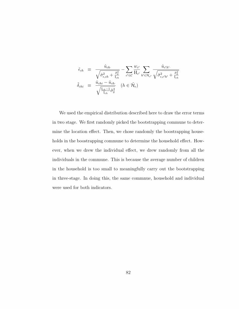
εch ≡ uch·√σ2

ε,ch +σ2

δ

Ich

−∑c′∈C

wc′

Hc′

∑h′∈Hc′

uc′h′·√σ2

ε,c′h′ +σ2

δ

Ich

δchi ≡ uchi − uch·√Ich−1Ich

σ2δ

(h ∈ Hc)

We used the empirical distribution described here to draw the error terms

in two stage. We first randomly picked the bootstrapping commune to deter-

mine the location effect. Then, we chose randomly the boostrapping house-

holds in the boostrapping commune to determine the household effect. How-

ever, when we drew the individual effect, we drew randomly from all the

individuals in the commune. This is because the average number of children

in the household is too small to meaningfully carry out the bootstrapping

in three-stage. In doing this, the same commnue, household and individual

were used for both indicators.

82

Appendix B

Regression Results

In this appendix, the relevant regression results from the second round are

presented.1 Since the results are long, the tables are presented in the follow-

ing way. In Section B.1, the definition of each variable used in the regressions

is given. Section B, the regression results are presented. In Section B.3, some

summary statistics relevant to regressions are presented.

B.1 Definition of Variables

Table B.1 explains the list of variables used in this study. The variables listed

here appear at least in one of the regression models presented in Section B.2,

but not necessarily all. It should be noted that many of the variables listed

in the table enter in the form of a cross term in the regression.

1Summary statistics similar to those presented in Section B.3 from the round one arepresented in Appendix C.

83

Table B.1: List of Variables Used in the Analysis.

Variable Explanation

Variable Explanation

age age of the child

amigra any women in household who have been in HH less then five years

awrk any women in HH worked last 12 months

awrkag any women in HH worked in agriculture last 12 months

awrksr any women in HH worked in services last 12 months

births total births to women aged between 15 and 49

cafem the number of those girls born to a woman in the village who are still alive

costkhum distance to commune center

costsrok distance to district center

deaths total deaths of children of women aged between 15 and 49 in the household

dec1996 drought prone areas derived from normalized differential vegetation index (NDVI)

derived

dec ave NDVI indicator (Dec)

distmnrd distance to main road

doverb child deaths over births

elec0 Electricity Not Available

elec1 Electricity Available

flood00 Flood prone communes

floor1 floor material in earth/sand/clay

floor2 floor material in wood/plywood

floor3 floor material in cement/brick/stone

floor 2p ratio of households with wood/plywood floor in village

fmls number of female household members aged 15+

fuel1 main cooking fuel is LPG/Electricity/Kerosene

fuel2 main cooking fuel is charcoal

fuel3 main cooking fuel is firewood

hdage age of household head

hded0 education of the HH head is ’no education’

hded1 education of the HH head is ’incomplete primary’

hded2 education of the HH head is ’complete primary’

hded3 education of the HH head is ’incomplete secondary’

84

Table B.1: (Continued)

Variable Explanation

hded4 education of the HH head is ’complete secondary’

hdey education of the HH head in years

hdsex1 Household head is male

hdspage Age of spouse

hesta 1p the percentage of HH in the village where the HH head is an employer

hhedu 4p the percentage of HH in the village where the HH’s education is lower secondary

school

hhprim Fraction of household head in the village completed primary education

hhsize household size

max rad Maximum radiation

maxed 9p the percentage of HH in the village where the HH’s education is none of the

following: no education, primary not completed, primary completed, lower sec-

ondary, secondary school/diploma, undergraduate, graduate/degree holder, post

graduate

mb0 number of household members aged 0

mb0 4 number of household members aged 0-4

mb1 4 number of household members aged 1-4

mb5 14 number of household members aged 5-14

mb65ov number of household members aged 65+

min dtr minimum diurnal temperature change

min tmn Minimum temperature min

mort f the proportion of those girls born to the women in the village who have died

mort m the proportion of those boys born to the women in the village who have died

mxedhh0 highest education attained by a HH member is ’no education’

mxedhh1 highest education attained by a HH member is ’incomplete primary’

mxedhh2 highest education attained by a HH member is ’complete primary’

mxedhh3 highest education attained by a HH member is ’incomplete secondary’

mxedhh4 highest education attained by a HH member is ’complete secondary’

mxeyhh maximum education attained by a HH member in years

mxfmed0 highest education attained by a female HH member is ’no education’

mxfmed1 highest education attained by a female HH member is ’incomplete primary’

mxfmed2 highest education attained by a female HH member is ’complete primary’

85

Table B.1: (Continued)

Variable Explanation

mxfmed3 highest education attained by a female HH member is ’incomplete secondary’

mxfmey highest education attained by a female HH member is ’complete secondary’

nov1996 maximum education attained in HH in years

occup 3p Percentage of HH in the village who do not own the residence but can use it for

free.

othnf ch change between 1993 and 1997 in the area of other forest in the commune

pcnted percentage of HH members who ever attended school

pcntfm percentage of HH members who are female

pop65ov Population of people aged 65 and over

prerng precipitation range

roof1 roof is made of wood/plastic

roof2 roof is made of metal

roof3 roof is made of rock

sesta 1p the percentage of HH in the village where the spouse is an employer

sesta 5p the percentage of HH in the village where the spouse’s employment status is none

of the following: employer, paid employee, own account or family worker.

sex1 the child is a boy

sex2 the child is a girl

soils soil quality indicator in the commune

spage av average age of spouse in the village

spedu 3p the percentage of households in the village where the spouse’s education is pri-

mary school

spin 16p the percentage of households in the village where the spouse’s work is related to

education

spin 17p the percentage of households in the village where the spouse’s work is related to

health and social work

stdnts number of students in HH

tmigra total number of women in HH who lived in HH less than five years

toilet0 toilet not available on premises

toilet1 toilet available on premises

twrk total number of women in HH worked last 12 months

twrkag total number of women in HH worked in agriculture last 12 months

86

Table B.1: (Continued)

Variable Explanation

twrkpr total number of women in HH worked as a professional last 12 months

twrksr total number of women in HH worked in service last 12 months

v81 ch change between 1993 and 1997 in coverage of cropping mosaic with cropping area

less than 30 percent

v82 97 coverage of cropping mosaic with cropping area over 30 percent in commune in

1997

v94 97 coverage of urban areas in commune in 1997

water2 water source is tube/pipe well

water3 water source is dug water

water4 water source is surface water or rainwater

water5 water is bought

water6 other water source (water source is not any of above or piped water)

wetrng the rage of wet day frequency

wndrng the range of wind

yrkids number of younger children in HH

B.2 Estimated Coefficients

This section presents the regression results. We present the results stratum

by stratum. In each stratum, the OLS and GLS results for the standardized

height are first presented, followed by the relevant heteroskedastic regres-

sion. Then, the results for the standardized weight is presented. One should

note that the interaction of the error term across the left-hand-side variables

are taken into consideration when the GLS is run. The relevant summary

statistics are found in Section B.3.

87

B.2.1 Urban Stratum

Table B.2: OLS and GLS Results for Urban stratum. The left hand side

variable is standardized height.

OLS Results GLS Results

Var No. Variable Coef. Std. E t P-value Coef. Std. E

Var1 Intercept 97.001 2.870 33.79 0.000 97.589 4.260

Var2 hded4*age1 17.083 2.440 7.00 0.000 13.169 3.244

Var3 hdey*floor3 0.312 0.053 5.86 0.000 0.271 0.082

Var4 roof1*water2 -5.292 1.083 -4.89 0.000 -4.598 1.760

Var5 water3*age1 6.759 1.230 5.49 0.000 5.893 1.516

Var6 mxedhh2*age2 -5.728 1.215 -4.71 0.000 -6.124 1.678

Var7 mxedhh4*age1 -9.032 1.709 -5.29 0.000 -8.199 2.361

Var8 fmls*age1 4.678 0.598 7.82 0.000 4.062 0.786

Var9 mb5 14*water3 -1.074 0.180 -5.98 0.000 -1.082 0.274

Var10 mb0*toilet1 -2.197 0.557 -3.95 0.000 -2.015 0.906

Var11 hdage*floor1 0.088 0.017 5.32 0.000 0.094 0.031

Var12 fmls*min cld -0.034 0.005 -6.53 0.000 -0.033 0.008

Var13 spage av -0.375 0.099 -3.80 0.000 -0.406 0.148

Var14 fmls*hded2 1.877 0.403 4.65 0.000 1.700 0.593

Var15 pcntfm*roof3 0.051 0.015 3.47 0.001 0.046 0.022

Var16 age*hded2 -1.232 0.345 -3.57 0.000 -0.974 0.453

Var17 fuel2*hded4 7.429 1.944 3.82 0.000 7.944 2.783

Var18 water2*mxfmed3 -2.576 0.944 -2.73 0.007 -3.049 1.353

Var19 water2*hded2 -5.962 1.352 -4.41 0.000 -5.577 2.053

Var20 water4*mxfmed4 16.420 2.885 5.69 0.000 15.672 3.387

Var21 hded4*hdsex1 -6.167 1.061 -5.81 0.000 -5.202 1.646

Var22 sex1*age4 3.260 0.653 4.99 0.000 2.560 0.882

Var23 age*max wnd -0.068 0.007 -9.28 0.000 -0.061 0.010

Var24 wetrng*age1 -0.068 0.007 -9.28 0.000 -0.061 0.010

Var25 water4*age1 -3.074 1.116 -2.76 0.006 -2.880 1.390

Var26 mb65ov*age2 -3.243 1.228 -2.64 0.009 -3.019 1.475

Var27 mb1 4*age2 -2.773 0.685 -4.05 0.000 -2.545 0.825

Var28 hdage*age2 0.094 0.025 3.69 0.000 0.082 0.032

88

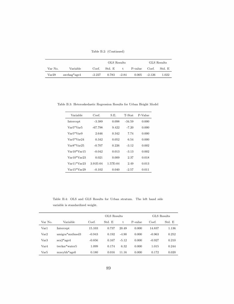
Table B.2: (Continued)

OLS Results GLS Results

Var No. Variable Coef. Std. E t P-value Coef. Std. E

Var29 awrkag*age4 -2.227 0.783 -2.84 0.005 -2.126 1.022

Table B.3: Heteroskedastic Regression Results for Urban Height Model

Variable Coef. S.E. T-Stat P-Value

Intercept -3.389 0.098 -34.59 0.000

Var5*Var5 -67.798 9.422 -7.20 0.000

Var5*Var9 2.646 0.342 7.74 0.000

Var5*Var24 0.342 0.052 6.54 0.000

Var8*Var25 -0.707 0.226 -3.12 0.002

Var10*Var15 -0.042 0.013 -3.13 0.002

Var10*Var23 0.021 0.009 2.37 0.018

Var11*Var23 3.91E-04 1.57E-04 2.49 0.013

Var15*Var29 -0.102 0.040 -2.57 0.011

Table B.4: OLS and GLS Results for Urban stratum. The left hand side

variable is standardized weight.

OLS Results GLS Results

Var No. Variable Coef. Std. E t P-value Coef. Std. E

Var1 Intercept 15.103 0.737 20.49 0.000 14.837 1.136

Var2 amigra*mxfmed3 -0.943 0.192 -4.90 0.000 -0.963 0.252

Var3 sex2*age4 -0.856 0.167 -5.12 0.000 -0.927 0.210

Var4 twrksr*water5 1.099 0.174 6.32 0.000 1.015 0.244

Var5 mxeyhh*age0 0.180 0.016 11.16 0.000 0.172 0.020

89

Table B.4: (Continued)

OLS Results GLS Results

Var No. Variable Coef. Std. E t P-value Coef. Std. E

Var6 water2*mxfmed2 2.124 0.428 4.96 0.000 1.976 0.712

Var7 doverb*flood00 2.755 0.525 5.25 0.000 2.061 0.775

Var8 floor 2p -0.826 0.177 -4.67 0.000 -0.743 0.274

Var9 fuel1*water2 -1.537 0.349 -4.40 0.000 -1.274 0.697

Var10 hdey*sex2 0.086 0.014 6.09 0.000 0.074 0.018

Var11 yrkids*toilet0 0.774 0.143 5.42 0.000 0.752 0.164

Var12 deaths*sex2 -0.349 0.092 -3.77 0.000 -0.320 0.122

Var13 awrkag*roof1 -0.873 0.163 -5.34 0.000 -0.904 0.264

Var14 elec0*water2 -0.754 0.192 -3.92 0.000 -0.660 0.305

Var15 toilet0*age0 0.924 0.190 4.87 0.000 0.976 0.229

Var16 water5*age1 -1.011 0.283 -3.57 0.000 -0.714 0.386

Var17 mxedhh2*age2 -0.984 0.273 -3.60 0.000 -0.915 0.382

Var18 mb5 14*wndrng -0.015 0.006 -2.53 0.012 -0.019 0.009

Var19 mb1 4*dec1996 2.238 0.558 4.01 0.000 2.314 0.878

Var20 pcnted*v81 97 1.74E-09 3.41E-10 5.10 0.000 1.81E-09 4.88E-10

Var21 mb0*roof2 -1.034 0.148 -7.00 0.000 -0.928 0.213

Var22 mxeyhh*toilet0 -0.083 0.016 -5.25 0.000 -0.085 0.024

Var23 hdage*hdsex1 -0.010 0.003 -3.96 0.000 -0.008 0.004

Var24 awrk*hded5 -0.960 0.312 -3.07 0.002 -0.861 0.465

Var25 hdspage*elec0 0.013 0.003 3.83 0.000 0.012 0.005

Var26 spage av -0.144 0.025 -5.72 0.000 -0.136 0.039

Var27 maxed 9p 77.583 15.884 4.88 0.000 66.321 24.795

Var28 spin 17p -10.175 2.115 -4.81 0.000 -8.163 2.892

Var29 water4*hded1 -0.469 0.171 -2.74 0.006 -0.448 0.215

90

Table B.5: Heteroskedastic Regression Results for Urban Weight Model

Variable Coef. S.E. T-Stat P-Value

Intercept -4.163 0.110 -37.86 0.000

Var2*Var28 -26.040 8.089 -3.22 0.001

Var7*Var16 -19.693 5.421 -3.63 0.000

Var8*Var9 4.561 1.818 2.51 0.013

Var8*Var13 0.859 0.357 2.4 0.017

Var9*Var18 -0.270 0.050 -5.44 0.000

Var11*Var22 0.142 0.052 2.73 0.007

Var15*Var18 -0.128 0.027 -4.67 0.000

Var15*Var28 39.092 14.730 2.65 0.008

Var18*Var29 -0.077 0.024 -3.18 0.002

B.2.2 Plain Stratum

Table B.6: OLS and GLS Results for Plain stratum. The left hand side variable

is standardized height.

OLS Results GLS Results

Var No. Variable Coef. Std. E t P-value Coef. Std. E

Var1 Intercept 137.539 14.078 9.77 0.000 119.967 17.937

Var2 mb1 4*sex1 1.058 0.238 4.44 0.000 0.922 0.276

Var3 mb0*floor2 -2.498 0.508 -4.91 0.000 -1.857 0.697

Var4 fmls*floor3 4.620 0.851 5.43 0.000 4.334 1.403

Var5 stdnts*fuel2 5.175 1.027 5.04 0.000 5.585 1.169

Var6 yrkids*water6 5.955 1.786 3.34 0.001 3.675 1.727

Var7 mb1 4*twrkag -1.531 0.276 -5.55 0.000 -1.657 0.437

Var8 pcnted*age 0.018 0.003 5.40 0.000 0.017 0.004

Var9 roof3*mxedhh0 4.819 1.691 2.85 0.005 4.798 3.932

Var10 water3*hded2 -3.434 1.072 -3.20 0.001 -2.250 1.412

91

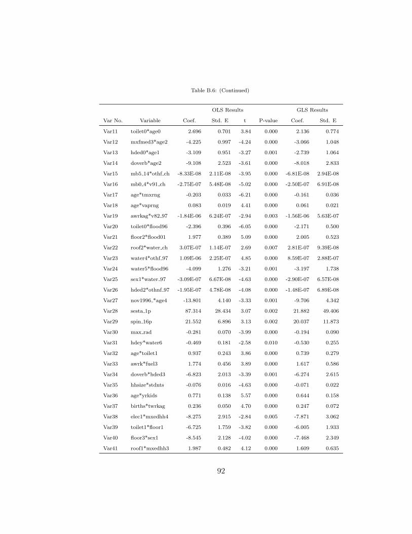
Table B.6: (Continued)

OLS Results GLS Results

Var No. Variable Coef. Std. E t P-value Coef. Std. E

Var11 toilet0*age0 2.696 0.701 3.84 0.000 2.136 0.774

Var12 mxfmed3*age2 -4.225 0.997 -4.24 0.000 -3.066 1.048

Var13 hded0*age1 -3.109 0.951 -3.27 0.001 -2.739 1.064

Var14 doverb*age2 -9.108 2.523 -3.61 0.000 -8.018 2.833

Var15 mb5 14*othf ch -8.33E-08 2.11E-08 -3.95 0.000 -6.81E-08 2.94E-08

Var16 mb0 4*v91 ch -2.75E-07 5.48E-08 -5.02 0.000 -2.50E-07 6.91E-08

Var17 age*tmxrng -0.203 0.033 -6.21 0.000 -0.161 0.036

Var18 age*vaprng 0.083 0.019 4.41 0.000 0.061 0.021

Var19 awrkag*v82 97 -1.84E-06 6.24E-07 -2.94 0.003 -1.56E-06 5.63E-07

Var20 toilet0*flood96 -2.396 0.396 -6.05 0.000 -2.171 0.500

Var21 floor2*flood01 1.977 0.389 5.09 0.000 2.005 0.523

Var22 roof2*water ch 3.07E-07 1.14E-07 2.69 0.007 2.81E-07 9.39E-08

Var23 water4*othf 97 1.09E-06 2.25E-07 4.85 0.000 8.59E-07 2.88E-07

Var24 water5*flood96 -4.099 1.276 -3.21 0.001 -3.197 1.738

Var25 sex1*water 97 -3.09E-07 6.67E-08 -4.63 0.000 -2.90E-07 6.57E-08

Var26 hded2*othnf 97 -1.95E-07 4.78E-08 -4.08 0.000 -1.48E-07 6.89E-08

Var27 nov1996 *age4 -13.801 4.140 -3.33 0.001 -9.706 4.342

Var28 sesta 1p 87.314 28.434 3.07 0.002 21.882 49.406

Var29 spin 16p 21.552 6.896 3.13 0.002 20.037 11.873

Var30 max rad -0.281 0.070 -3.99 0.000 -0.194 0.090

Var31 hdey*water6 -0.469 0.181 -2.58 0.010 -0.530 0.255

Var32 age*toilet1 0.937 0.243 3.86 0.000 0.739 0.279

Var33 awrk*fuel3 1.774 0.456 3.89 0.000 1.617 0.586

Var34 doverb*hded3 -6.823 2.013 -3.39 0.001 -6.274 2.615

Var35 hhsize*stdnts -0.076 0.016 -4.63 0.000 -0.071 0.022

Var36 age*yrkids 0.771 0.138 5.57 0.000 0.644 0.158

Var37 births*twrkag 0.236 0.050 4.70 0.000 0.247 0.072

Var38 elec1*mxedhh4 -8.275 2.915 -2.84 0.005 -7.871 3.062

Var39 toilet1*floor1 -6.725 1.759 -3.82 0.000 -6.005 1.933

Var40 floor3*sex1 -8.545 2.128 -4.02 0.000 -7.468 2.349

Var41 roof1*mxedhh3 1.987 0.482 4.12 0.000 1.609 0.635

92

Table B.6: (Continued)

OLS Results GLS Results

Var No. Variable Coef. Std. E t P-value Coef. Std. E

Var42 roof3*age3 1.612 0.649 2.48 0.013 1.046 0.828

Var43 mxedhh4*age0 6.269 1.857 3.38 0.001 5.165 1.910

Var44 mxeyhh*age2 0.309 0.085 3.64 0.000 0.208 0.095

Table B.7: Heteroskedastic Regression Results for Plain Height Model

Variable Coef. S.E. T-Stat P-Value

Intercept -4.604 0.115 -40.09 0.000

Var2*Var11 1.190 0.542 2.19 0.029

Var2*Var16 -1.13E-07 3.09E-08 -3.65 0.000

Var7*Var40 -4.982 2.246 -2.22 0.027

Var8*Var42 0.006 0.002 3.68 0.000

Var10*Var42 -7.817 2.242 -3.49 0.001

Var11*Var41 -1.662 0.599 -2.77 0.006

Var12*Var20 -3.116 0.616 -5.06 0.000

Var15*Var22 1.61E-14 5.65E-15 2.86 0.004

Var18*Var37 -3.11E-04 1.27E-04 -2.44 0.015

Var20*Var28 238.978 42.474 5.63 0.000

Var20*Var41 1.118 0.320 3.50 0.001

Var21*Var28 -194.833 41.169 -4.73 0.000

Var21*Var29 23.235 6.628 3.51 0.001

Var21*Var35 -0.030 0.009 -3.24 0.001

Var23*Var42 -6.03E-07 2.41E-07 -2.51 0.012

Var26*Var39 -1.08E-06 4.33E-07 -2.49 0.013

Var28*Var36 -112.032 28.144 -3.98 0.000

Var30*Var36 0.002 4.14E-04 3.71 0.000

Var32*Var34 -5.103 2.174 -2.35 0.019

Var33*Var37 0.095 0.028 3.43 0.001

93

Table B.8: OLS and GLS Results for Plain stratum. The left hand side variable

is standardized weight.

OLS Results GLS Results

Var No. Variable Coef. Std. E t P-value Coef. Std. E

Var1 Intercept 9.426 0.262 35.98 0.000 9.406 0.345

Var2 mb0 4*stdnts -0.134 0.027 -4.96 0.000 -0.148 0.040

Var3 pcnted*age 0.003 0.001 4.05 0.000 0.003 0.001

Var4 births*awrkag 0.074 0.020 3.66 0.000 0.085 0.028

Var5 mb1 4*costkhet 1.18E-05 2.57E-06 4.59 0.000 7.92E-06 4.21E-06

Var6 elec0*othnf ch 1.37E-07 3.03E-08 4.53 0.000 1.21E-07 4.33E-08

Var7 floor2*flood01 0.322 0.091 3.54 0.000 0.362 0.127

Var8 floor3*ldf ch -5.42E-06 9.30E-07 -5.83 0.000 -5.13E-06 9.94E-07

Var9 soils*age0 -0.286 0.071 -4.02 0.000 -0.165 0.080

Var10 prerng*age0 0.053 0.007 7.49 0.000 0.040 0.008

Var11 spedu 3p 3.501 0.892 3.93 0.000 3.385 1.209

Var12 cafem -0.001 0.000 -4.98 0.000 -0.001 0.000

Var13 mort m -3.047 0.829 -3.68 0.000 -2.483 1.112

Var14 mb5 14*fuel2 1.243 0.311 4 0.000 1.231 0.442

Var15 mb0*mxedhh0 1.647 0.400 4.12 0.000 1.177 0.590

Var16 stdnts*toilet1 0.370 0.091 4.06 0.000 0.295 0.129

Var17 mxeyhh*sex1 0.070 0.016 4.44 0.000 0.068 0.019

Var18 mxeyhh*mxfmed0 0.126 0.035 3.64 0.000 0.119 0.046

Var19 awrksr*mxedhh3 -1.779 0.503 -3.54 0.000 -1.136 0.532

Var20 awrksr*hded3 2.543 0.557 4.57 0.000 1.860 0.631

Var21 twrksr*water6 -3.833 1.351 -2.84 0.005 -3.422 1.849

Var22 age*twrkag -0.120 0.033 -3.65 0.000 -0.131 0.039

Var23 fuel2*mxfmed0 -3.489 0.642 -5.44 0.000 -3.448 0.892

Var24 elec1*mxedhh4 -3.650 0.853 -4.28 0.000 -3.467 0.883

Var25 toilet1*floor1 -1.276 0.492 -2.59 0.010 -1.157 0.520

Var26 roof3*water3 0.606 0.157 3.87 0.000 0.677 0.223

Var27 roof3*water6 -1.237 0.408 -3.03 0.003 -1.302 0.537

Var28 roof3*sex2 0.652 0.148 4.41 0.000 0.575 0.179

94

Table B.8: (Continued)

OLS Results GLS Results

Var No. Variable Coef. Std. E t P-value Coef. Std. E

Var29 roof3*mxedhh3 -0.791 0.149 -5.31 0.000 -0.693 0.195

Var30 water2*mxfmed0 -0.933 0.260 -3.59 0.000 -0.862 0.342

Var31 water3*mxedhh2 -0.820 0.251 -3.26 0.001 -0.784 0.353

Var32 mxedhh4*hded1 1.612 0.573 2.81 0.005 1.497 0.654

Var33 elec1*age1 2.365 0.927 2.55 0.011 1.703 1.026

Var34 sex1*age0 -0.662 0.208 -3.18 0.002 -0.700 0.238

Var35 mb65ov*age0 -0.868 0.267 -3.25 0.001 -0.632 0.308

Table B.9: Heteroskedastic Regression Results for Plain Weight Model

Variable Coef. S.E. T-Stat P-Value

Intercept -4.217 0.094 -44.81 0.000

Var4*Var11 0.619 0.261 2.38 0.018

Var5*Var10 4.94E-07 1.90E-07 2.60 0.010

Var5*Var25 -7.11E-05 3.16E-05 -2.25 0.025

Var8*Var12 2.68E-07 5.86E-09 45.71 0.000

B.2.3 Tonlesap Stratum

Table B.10: OLS and GLS Results for Tonlesap stratum. The left hand side

variable is standardized height.

OLS Results GLS Results

Var No. Variable Coef. Std. E t P-value Coef. Std. E

Var1 Intercept 81.096 0.400 202.52 0.000 80.935 0.563

95

Table B.10: (Continued)

OLS Results GLS Results

Var No. Variable Coef. Std. E t P-value Coef. Std. E

Var2 fmls*hded3 1.291 0.260 4.96 0.000 1.244 0.359

Var3 mxfmey*mxfmed1 0.445 0.102 4.37 0.000 0.371 0.147

Var4 age*toilet0 -1.282 0.112 -11.48 0.000 -1.189 0.140

Var5 deaths*roof2 2.174 0.334 6.51 0.000 2.269 0.462

Var6 awrk*floor1 9.483 1.706 5.56 0.000 7.759 2.618

Var7 awrkag*hded1 2.042 0.357 5.71 0.000 1.929 0.513

Var8 mb0 4*twrkag -0.744 0.135 -5.50 0.000 -0.576 0.220

Var9 pcntfm*yrkids 0.092 0.016 5.88 0.000 0.077 0.019

Var10 toilet1*mxfmed0 -5.915 1.934 -3.06 0.002 -6.141 3.405

Var11 roof3*mxedhh0 7.341 1.534 4.79 0.000 6.537 2.586

Var12 water2*mxfmed0 4.783 1.445 3.31 0.001 4.369 2.095

Var13 roof2*age3 2.714 0.749 3.62 0.000 2.162 0.889

Var14 mb65ov*ldf 97 -2.68E-07 5.62E-08 -4.77 0.000 -2.44E-07 7.81E-08

Var15 mb65ov*othf ch -3.33E-06 4.46E-07 -7.47 0.000 -2.91E-06 6.57E-07

Var16 mb1 4*dist hf -1.84E-04 3.89E-05 -4.74 0.000 -1.88E-04 5.64E-05

Var17 mb0*v94 97 1.65E-06 3.53E-07 4.67 0.000 2.26E-06 6.49E-07

Var18 mb0*mdf 97 -2.11E-08 6.90E-09 -3.06 0.002 -1.77E-08 9.38E-09

Var19 mb0*othnf 97 4.43E-08 7.01E-09 6.31 0.000 4.41E-08 9.80E-09

Var20 mb0*othf ch 8.39E-07 2.18E-07 3.85 0.000 7.21E-07 3.00E-07

Var21 mxeyhh*v81 ch 8.46E-08 2.26E-08 3.74 0.000 6.64E-08 2.88E-08

Var22 hdage*distmnrd 3.65E-06 5.26E-07 6.94 0.000 3.11E-06 7.17E-07

Var23 twrk*dist hf 1.19E-04 3.96E-05 3.01 0.003 8.60E-05 5.70E-05

Var24 awrksr*dist riv -6.30E-05 2.26E-05 -2.79 0.005 -5.01E-05 2.86E-05

Var25 elec1*othnf 97 -6.17E-08 1.31E-08 -4.72 0.000 -5.14E-08 1.74E-08

Var26 toilet1*mdf 97 -5.88E-08 2.13E-08 -2.76 0.006 -5.35E-08 2.64E-08

Var27 roof2*costkhet -9.55E-05 2.33E-05 -4.10 0.000 -7.81E-05 3.08E-05

Var28 roof3*othf ch 1.82E-06 2.99E-07 6.10 0.000 1.66E-06 5.09E-07

Var29 water2*ldf 97 -2.51E-07 5.42E-08 -4.63 0.000 -2.75E-07 8.89E-08

Var30 water2*othf 97 1.46E-07 4.60E-08 3.18 0.002 1.41E-07 6.66E-08

Var31 water4*mdf ch 4.39E-06 1.52E-06 2.89 0.004 4.20E-06 2.07E-06

Var32 mxedhh0*min pre -1.421 0.532 -2.67 0.008 -1.436 0.657

96

Table B.10: (Continued)

OLS Results GLS Results

Var No. Variable Coef. Std. E t P-value Coef. Std. E

Var33 mxedhh1*othnf 97 1.41E-08 4.63E-09 3.04 0.002 1.16E-08 6.64E-09

Var34 mxedhh2*mdf ch 5.03E-06 1.40E-06 3.58 0.000 4.36E-06 1.94E-06

Var35 mxedhh3*v91 ch 2.11E-07 5.27E-08 4.00 0.000 2.29E-07 6.54E-08

Var36 mxfmed2*mdf 97 1.05E-07 1.76E-08 5.98 0.000 9.41E-08 3.65E-08

Var37 hded0*nov1996 -17.544 4.331 -4.05 0.000 -15.318 6.234

Var38 hded0*mdf ch -1.27E-05 1.81E-06 -7.00 0.000 -1.28E-05 2.62E-06

Var39 hded4*min wet 0.476 0.128 3.71 0.000 0.442 0.154

Var40 distmnrd*age1 -1.70E-04 3.41E-05 -4.98 0.000 -1.31E-04 3.94E-05

Var41 costsrok*age3 -1.20E-04 3.31E-05 -3.61 0.000 -7.47E-05 3.81E-05

Var42 dec1996 *age2 20.124 3.847 5.23 0.000 16.824 4.877

Var43 v81 ch*age1 -5.58E-07 1.43E-07 -3.91 0.000 -4.22E-07 1.59E-07

Var44 othnf ch*age2 2.04E-07 5.92E-08 3.44 0.001 1.52E-07 6.39E-08

Var45 occup 3p 17.436 4.598 3.79 0.000 14.593 6.027

Var46 hhsize*floor1 -1.079 0.267 -4.04 0.000 -0.591 0.408

Var47 mb65ov*sex2 -1.721 0.449 -3.84 0.000 -1.647 0.581

Var48 awrk*mxfmed1 -1.310 0.386 -3.40 0.001 -1.254 0.537

Var49 awrkag*water2 -2.265 0.667 -3.39 0.001 -2.258 1.008

Var50 twrkag*floor1 -2.706 0.974 -2.78 0.006 -3.196 2.029

Var51 mb0*age -0.641 0.160 -4.01 0.000 -0.582 0.196

Var52 stdnts*births -0.093 0.031 -3.01 0.003 -0.102 0.039

Var53 stdnts*hdspage 0.026 0.006 4.29 0.000 0.026 0.008

Var54 mxfmey*doverb -1.158 0.258 -4.49 0.000 -1.083 0.354

Var55 twrkag*twrkpr -5.616 1.216 -4.62 0.000 -5.688 2.396

Var56 floor1*water4 4.183 1.423 2.94 0.003 1.963 2.257

97

Table B.11: Heteroskedastic Regression Results for Tonlesap Height Model

Variable Coef. S.E. T-Stat P-Value

Intercept -4.222 0.097 -43.31 0.000

Var9 0.091 0.019 4.80 0.000

Var4*Var42 -3.069 1.225 -2.51 0.012

Var7*Var13 3.403 0.725 4.69 0.000

Var7*Var20 -1.12E-06 2.73E-07 -4.09 0.000

Var7*Var24 -3.45E-04 7.26E-05 -4.75 0.000

Var7*Var35 -4.39E-07 1.18E-07 -3.73 0.000

Var8*Var26 5.72E-08 2.55E-08 2.24 0.025

Var9*Var9 -0.002 0.001 -2.74 0.006

Var9*Var13 -0.332 0.043 -7.75 0.000

Var13*Var51 2.645 1.087 2.43 0.015

Var13*Var54 -1.866 0.391 -4.78 0.000

Var15*Var27 -5.52E-08 2.18E-08 -2.54 0.011

Var16*Var20 -2.29E-10 6.66E-11 -3.44 0.001

Var18*Var33 -1.82E-16 5.20E-17 -3.50 0.001

Var18*Var40 1.07E-11 4.72E-12 2.27 0.024

Var19*Var20 2.69E-14 6.14E-15 4.38 0.000

Var20*Var27 5.37E-08 2.18E-08 2.47 0.014

Var20*Var45 -4.76E-05 1.64E-05 -2.90 0.004

Var20*Var54 3.42E-06 6.27E-07 5.46 0.000

Var22*Var33 1.77E-14 7.33E-15 2.41 0.016

Var22*Var45 -1.87E-05 6.91E-06 -2.71 0.007

Var24*Var47 -1.35E-04 4.10E-05 -3.29 0.001

Var25*Var56 -2.78E-07 6.30E-08 -4.42 0.000

Var26*Var48 -1.09E-07 2.82E-08 -3.86 0.000

Var27*Var37 8.70E-04 3.49E-04 2.49 0.013

Var30*Var35 4.84E-14 1.55E-14 3.13 0.002

Var33*Var50 5.14E-08 1.83E-08 2.80 0.005

Var39*Var41 -1.21E-04 5.46E-05 -2.21 0.028

Var40*Var51 -4.78E-04 1.16E-04 -4.11 0.000

Var42*Var52 0.676 0.207 3.27 0.001

Var45*Var54 10.176 3.719 2.74 0.006

98

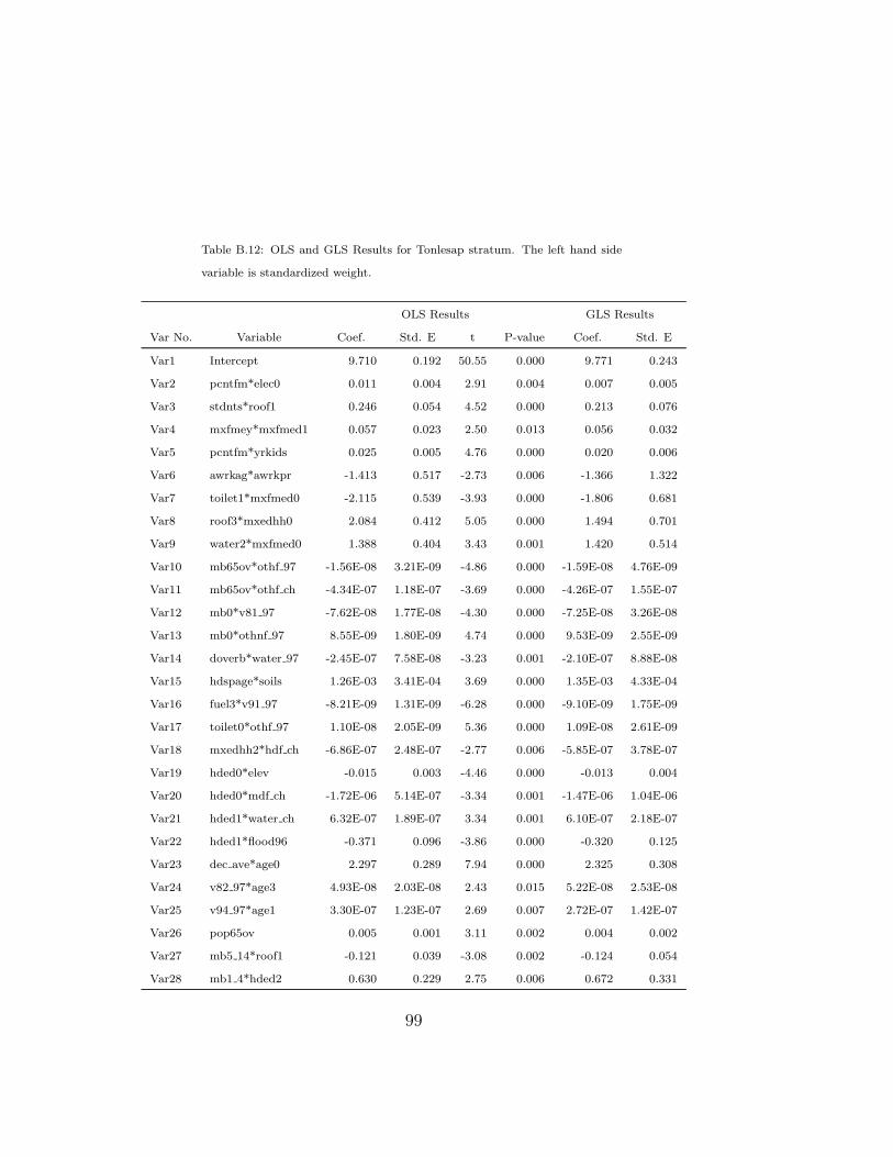
Table B.12: OLS and GLS Results for Tonlesap stratum. The left hand side

variable is standardized weight.

OLS Results GLS Results

Var No. Variable Coef. Std. E t P-value Coef. Std. E

Var1 Intercept 9.710 0.192 50.55 0.000 9.771 0.243

Var2 pcntfm*elec0 0.011 0.004 2.91 0.004 0.007 0.005

Var3 stdnts*roof1 0.246 0.054 4.52 0.000 0.213 0.076

Var4 mxfmey*mxfmed1 0.057 0.023 2.50 0.013 0.056 0.032

Var5 pcntfm*yrkids 0.025 0.005 4.76 0.000 0.020 0.006

Var6 awrkag*awrkpr -1.413 0.517 -2.73 0.006 -1.366 1.322

Var7 toilet1*mxfmed0 -2.115 0.539 -3.93 0.000 -1.806 0.681

Var8 roof3*mxedhh0 2.084 0.412 5.05 0.000 1.494 0.701

Var9 water2*mxfmed0 1.388 0.404 3.43 0.001 1.420 0.514

Var10 mb65ov*othf 97 -1.56E-08 3.21E-09 -4.86 0.000 -1.59E-08 4.76E-09

Var11 mb65ov*othf ch -4.34E-07 1.18E-07 -3.69 0.000 -4.26E-07 1.55E-07

Var12 mb0*v81 97 -7.62E-08 1.77E-08 -4.30 0.000 -7.25E-08 3.26E-08

Var13 mb0*othnf 97 8.55E-09 1.80E-09 4.74 0.000 9.53E-09 2.55E-09

Var14 doverb*water 97 -2.45E-07 7.58E-08 -3.23 0.001 -2.10E-07 8.88E-08

Var15 hdspage*soils 1.26E-03 3.41E-04 3.69 0.000 1.35E-03 4.33E-04

Var16 fuel3*v91 97 -8.21E-09 1.31E-09 -6.28 0.000 -9.10E-09 1.75E-09

Var17 toilet0*othf 97 1.10E-08 2.05E-09 5.36 0.000 1.09E-08 2.61E-09

Var18 mxedhh2*hdf ch -6.86E-07 2.48E-07 -2.77 0.006 -5.85E-07 3.78E-07

Var19 hded0*elev -0.015 0.003 -4.46 0.000 -0.013 0.004

Var20 hded0*mdf ch -1.72E-06 5.14E-07 -3.34 0.001 -1.47E-06 1.04E-06

Var21 hded1*water ch 6.32E-07 1.89E-07 3.34 0.001 6.10E-07 2.18E-07

Var22 hded1*flood96 -0.371 0.096 -3.86 0.000 -0.320 0.125

Var23 dec ave*age0 2.297 0.289 7.94 0.000 2.325 0.308

Var24 v82 97*age3 4.93E-08 2.03E-08 2.43 0.015 5.22E-08 2.53E-08

Var25 v94 97*age1 3.30E-07 1.23E-07 2.69 0.007 2.72E-07 1.42E-07

Var26 pop65ov 0.005 0.001 3.11 0.002 0.004 0.002

Var27 mb5 14*roof1 -0.121 0.039 -3.08 0.002 -0.124 0.054

Var28 mb1 4*hded2 0.630 0.229 2.75 0.006 0.672 0.331

99

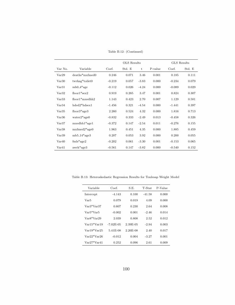
Table B.12: (Continued)

OLS Results GLS Results

Var No. Variable Coef. Std. E t P-value Coef. Std. E

Var29 deaths*mxfmed0 0.246 0.071 3.46 0.001 0.185 0.111

Var30 twrkag*toilet0 -0.219 0.057 -3.83 0.000 -0.234 0.079

Var31 mb0 4*age -0.112 0.026 -4.24 0.000 -0.089 0.029

Var32 floor1*sex2 0.919 0.265 3.47 0.001 0.824 0.307

Var33 floor1*mxedhh2 1.143 0.423 2.70 0.007 1.129 0.581

Var34 hded2*hdsex1 -1.456 0.321 -4.54 0.000 -1.441 0.397

Var35 floor3*age3 2.260 0.524 4.32 0.000 1.816 0.713

Var36 water2*age0 -0.832 0.333 -2.49 0.013 -0.458 0.326

Var37 mxedhh1*age1 -0.372 0.147 -2.54 0.011 -0.276 0.155

Var38 mxfmed2*age0 1.963 0.451 4.35 0.000 1.885 0.459

Var39 mb5 14*age3 0.207 0.053 3.92 0.000 0.200 0.055

Var40 fmls*age2 -0.202 0.061 -3.30 0.001 -0.153 0.065

Var41 awrk*age3 -0.561 0.147 -3.82 0.000 -0.540 0.152

Table B.13: Heteroskedastic Regression Results for Tonlesap Weight Model

Variable Coef. S.E. T-Stat P-Value

Intercept -4.143 0.100 -41.58 0.000

Var5 0.079 0.019 4.09 0.000

Var3*Var37 0.607 0.230 2.64 0.008

Var5*Var5 -0.002 0.001 -2.46 0.014

Var8*Var29 2.039 0.808 2.52 0.012

Var15*Var19 -7.02E-05 2.39E-05 -2.94 0.003

Var19*Var25 5.41E-08 2.26E-08 2.40 0.017

Var22*Var26 -0.012 0.004 -3.27 0.001

Var27*Var41 0.252 0.096 2.61 0.009

100

B.2.4 Coastal Stratum

Table B.14: OLS and GLS Results for Coastal stratum. The left hand side

variable is standardized height.

OLS Results GLS Results

Var No. Variable Coef. Std. E t P-value Coef. Std. E

Var1 Intercept 76.858 0.733 104.86 0.000 77.487 1.125

Var2 mxeyhh*hded0 1.087 0.157 6.92 0.000 1.061 0.250

Var3 hdey*water3 0.462 0.111 4.17 0.000 0.498 0.199

Var4 twrkpr*hded3 -17.279 2.849 -6.06 0.000 -16.455 4.871

Var5 mb0*amigra -7.312 1.534 -4.77 0.000 -8.684 2.854

Var6 hdey*deaths -0.612 0.102 -6.02 0.000 -0.671 0.162

Var7 doverb*hdspage 0.355 0.070 5.07 0.000 0.355 0.100

Var8 water4*hded2 10.869 1.685 6.45 0.000 10.839 2.356

Var9 sex2*hded3 5.614 1.010 5.56 0.000 5.981 1.524

Var10 roof3*age4 -7.805 0.906 -8.62 0.000 -8.913 1.489

Var11 water4*age3 -6.449 1.210 -5.33 0.000 -6.460 1.745

Var12 water6*age0 9.137 2.319 3.94 0.000 11.998 3.544

Var13 pcntfm*age3 -0.165 0.029 -5.73 0.000 -0.163 0.041

Var14 awrk*nov cov 13.291 3.147 4.22 0.000 12.391 4.436

Var15 toilet1*dist riv 2.95E-04 6.18E-05 4.78 0.000 0.000 0.000

Var16 hhedu 4p 25.574 4.453 5.74 0.000 21.946 7.419

Var17 hdage*water3 -0.078 0.015 -5.19 0.000 -0.086 0.025

Var18 twrksr*doverb -19.973 4.942 -4.04 0.000 -22.729 7.393

Var19 mxfmed0*hded3 -6.332 1.908 -3.32 0.001 -5.654 3.575

Var20 hdsex1*age0 3.104 0.665 4.67 0.000 3.038 0.992

Table B.15: Heteroskedastic Regression Results for Coastal Height Model

Variable Coef. S.E. T-Stat P-Value

Intercept -3.784 0.183 -20.70 0.000

101

Table B.15: (Continued)

Variable Coef. S.E. T-Stat P-Value

Var3*Var8 1.83E-04 3.29E-05 5.55 0.000

Var5*Var12 -5.69E-05 1.60E-05 -3.56 0.001

Var6*Var9 -7.26E-07 1.49E-07 -4.87 0.000

Var6*Var15 2.237 0.625 3.58 0.000

Var8*Var8 -4.40E-07 5.35E-08 -8.23 0.000

Var8*Var9 2.41E-10 3.51E-11 6.86 0.000

Var9*Var14 -8.38E-07 1.53E-07 -5.48 0.000

Var9*Var15 -2.30E-07 4.34E-08 -5.30 0.000

Var11*Var14 1.780 0.555 3.21 0.002

Var11*Var16 -1.303 0.463 -2.81 0.005

Var14*Var18 -8.539 2.451 -3.48 0.001

Table B.16: OLS and GLS Results for Coastal stratum. The left hand side

variable is standardized weight.

OLS Results GLS Results

Var No. Variable Coef. Std. E t P-value Coef. Std. E

Var1 Intercept 10.066 0.209 48.13 0.000 10.211 0.325

Var2 mxeyhh*hded0 0.207 0.040 5.23 0.000 0.205 0.057

Var3 hdey*water3 0.120 0.030 4.00 0.000 0.108 0.047

Var4 mb0*amigra -1.993 0.381 -5.23 0.000 -2.069 0.546

Var5 pcnted*mxfmey 0.002 0.000 4.38 0.000 0.002 0.001

Var6 roof3*age4 -1.268 0.254 -4.99 0.000 -1.349 0.370

Var7 mb0 4*age0 0.823 0.101 8.14 0.000 0.851 0.127

Var8 floor2*area ric 4.90E-04 7.21E-05 6.80 0.000 4.00E-04 1.02E-04

Var9 mxfmed1*v91 ch -6.95E-08 1.72E-08 -4.04 0.000 -7.14E-08 2.08E-08

Var10 flood00*age4 1.612 0.345 4.68 0.000 1.886 0.498

Var11 mb0 4*water3 -0.376 0.101 -3.72 0.000 -0.436 0.152

Var12 hdage*toilet0 -0.024 0.004 -6.27 0.000 -0.022 0.006

Var13 yrkids*roof1 1.266 0.233 5.44 0.000 1.141 0.282

102

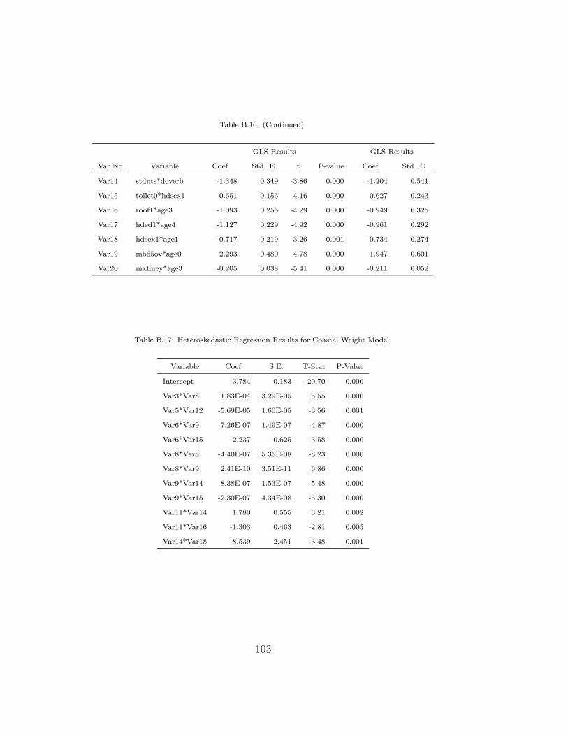
Table B.16: (Continued)

OLS Results GLS Results

Var No. Variable Coef. Std. E t P-value Coef. Std. E

Var14 stdnts*doverb -1.348 0.349 -3.86 0.000 -1.204 0.541

Var15 toilet0*hdsex1 0.651 0.156 4.16 0.000 0.627 0.243

Var16 roof1*age3 -1.093 0.255 -4.29 0.000 -0.949 0.325

Var17 hded1*age4 -1.127 0.229 -4.92 0.000 -0.961 0.292

Var18 hdsex1*age1 -0.717 0.219 -3.26 0.001 -0.734 0.274

Var19 mb65ov*age0 2.293 0.480 4.78 0.000 1.947 0.601

Var20 mxfmey*age3 -0.205 0.038 -5.41 0.000 -0.211 0.052

Table B.17: Heteroskedastic Regression Results for Coastal Weight Model

Variable Coef. S.E. T-Stat P-Value

Intercept -3.784 0.183 -20.70 0.000

Var3*Var8 1.83E-04 3.29E-05 5.55 0.000

Var5*Var12 -5.69E-05 1.60E-05 -3.56 0.001

Var6*Var9 -7.26E-07 1.49E-07 -4.87 0.000

Var6*Var15 2.237 0.625 3.58 0.000

Var8*Var8 -4.40E-07 5.35E-08 -8.23 0.000

Var8*Var9 2.41E-10 3.51E-11 6.86 0.000

Var9*Var14 -8.38E-07 1.53E-07 -5.48 0.000

Var9*Var15 -2.30E-07 4.34E-08 -5.30 0.000

Var11*Var14 1.780 0.555 3.21 0.002

Var11*Var16 -1.303 0.463 -2.81 0.005

Var14*Var18 -8.539 2.451 -3.48 0.001

103

B.2.5 Plateau Stratum

Table B.18: OLS and GLS Results for Plateau stratum. The left hand side

variable is standardized height.

OLS Results GLS Results

Var No. Variable Coef. Std. E t P-value Coef. Std. E

Var1 Intercept 88.568 1.849 47.91 0.000 87.968 2.049

Var2 mb65ov*water2 5.303 1.346 3.94 0.000 7.089 2.245

Var3 stdnts*floor1 -1.611 0.398 -4.04 0.000 -1.409 0.623

Var4 yrkids*mxedhh1 2.809 0.444 6.33 0.000 2.680 0.561

Var5 births*floor1 0.590 0.127 4.64 0.000 0.493 0.217

Var6 deaths*roof2 -1.377 0.396 -3.48 0.001 -1.265 0.553

Var7 deaths*water2 1.306 0.363 3.60 0.000 1.274 0.504

Var8 amigra*hded0 -3.957 0.981 -4.03 0.000 -3.810 1.599

Var9 water4*hded0 2.540 0.489 5.19 0.000 2.213 0.676

Var10 fuel3*age0 45.287 9.469 4.78 0.000 44.189 10.719

Var11 mxedhh0*age2 -2.788 1.033 -2.70 0.007 -2.856 1.180

Var12 age*tmnrng -0.038 0.004 -9.36 0.000 -0.036 0.005

Var13 doverb*dist riv 2.03E-04 5.23E-05 3.87 0.000 1.92E-04 6.87E-05

Var14 fuel3*min cld -0.145 0.040 -3.60 0.000 -0.137 0.044

Var15 roof3*elev -0.063 0.011 -5.63 0.000 -0.061 0.018

Var16 roof3*dist hf 7.22E-04 1.14E-04 6.31 0.000 7.06E-04 1.72E-04

Var17 mxfmed2*flood01 -7.467 1.556 -4.80 0.000 -6.992 1.788

Var18 hded3*othnf 97 9.29E-08 2.17E-08 4.27 0.000 8.59E-08 2.55E-08

Var19 costkhum*age3 -0.001 0.000 -5.20 0.000 -4.61E-04 1.18E-04

Var20 min tmn*age0 -0.306 0.057 -5.32 0.000 -0.291 0.065

Var21 wndrng*age0 3.160 0.468 6.75 0.000 2.836 0.515

Var22 hesta 1p -210.393 50.945 -4.13 0.000 -203.006 75.054

Var23 sesta 5p 1077.568 228.715 4.71 0.000 1110.839 236.301

Var24 hhsize*mxedhh2 1.128 0.177 6.37 0.000 1.065 0.235

Var25 mb0 4*mxedhh2 -3.569 0.712 -5.01 0.000 -3.275 1.054

Var26 stdnts*hded2 -3.103 0.667 -4.65 0.000 -3.070 0.922

Var27 hhsize*mb0 -0.330 0.062 -5.34 0.000 -0.283 0.088

Var28 roof1*sex1 -1.034 0.359 -2.88 0.004 -0.993 0.469

104

Table B.18: (Continued)

OLS Results GLS Results

Var No. Variable Coef. Std. E t P-value Coef. Std. E

Var29 toilet1*age3 -5.700 1.722 -3.31 0.001 -5.127 1.718

Var30 roof2*age3 3.673 0.855 4.30 0.000 2.626 1.029

Var31 mxedhh0*age3 4.501 1.115 4.04 0.000 4.241 1.165

Var32 mb0*age1 7.306 1.882 3.88 0.000 6.013 2.142

Var33 pcntfm*age1 -0.072 0.020 -3.58 0.000 -0.060 0.025

Table B.19: Heteroskedastic Regression Results for Plateau Height Model

Variable Coef. S.E. T-Stat P-Value

Intercept -4.223 0.089 -47.48 0.000

Var2*Var28 2.897 1.211 2.39 0.017

Var3*Var9 -1.556 0.364 -4.27 0.000

Var4*Var14 0.026 0.007 3.51 0.001

Var5*Var11 -6.107 1.298 -4.70 0.000

Var5*Var12 -1.53E-03 3.58E-04 -4.28 0.000

Var5*Var28 0.201 0.075 2.68 0.008

Var6*Var19 5.93E-04 2.17E-04 2.74 0.006

Var6*Var23 -2604.527 937.770 -2.78 0.006

Var6*Var24 -0.270 0.068 -3.96 0.000

Var9*Var13 -1.36E-04 5.27E-05 -2.58 0.010

Var9*Var16 -2.37E-04 7.64E-05 -3.10 0.002

Var13*Var23 0.796 0.323 2.46 0.014

Var16*Var24 -1.24E-04 2.12E-05 -5.87 0.000

Var17*Var28 -2.944 1.116 -2.64 0.009

Var18*Var19 1.43E-10 4.70E-11 3.03 0.003

Var18*Var28 -5.58E-08 2.07E-08 -2.70 0.007

Var18*Var33 -1.18E-08 2.60E-09 -4.53 0.000

Var22*Var28 -253.246 61.042 -4.15 0.000

Var22*Var30 -214.626 93.031 -2.31 0.022

105

Table B.20: OLS and GLS Results for Plateau stratum. The left hand side

variable is standardized weight.

OLS Results GLS Results

Var No. Variable Coef. Std. E t P-value Coef. Std. E

Var1 Intercept 9.284 0.211 43.98 0.000 9.278 0.287

Var2 stdnts*floor1 -0.480 0.116 -4.14 0.000 -0.384 0.215

Var3 births*floor1 0.305 0.050 6.06 0.000 0.242 0.100

Var4 amigra*hded0 -0.868 0.275 -3.16 0.002 -0.830 0.505

Var5 water4*hded0 0.732 0.163 4.50 0.000 0.659 0.242

Var6 fuel3*age0 -19.800 4.376 -4.52 0.000 -17.856 5.306

Var7 mxedhh0*age2 -0.996 0.300 -3.32 0.001 -0.999 0.334

Var8 mb0*age0 -2.680 0.328 -8.17 0.000 -2.373 0.384

Var9 hhsize*soils -0.010 0.003 -3.42 0.001 -0.010 0.004

Var10 mb65ov*v91 ch -8.40E-08 1.70E-08 -4.94 0.000 -8.04E-08 2.08E-08

Var11 mb65ov*radrng 0.017 0.003 6.57 0.000 0.016 0.004

Var12 tmigra*hdf ch -4.63E-07 1.19E-07 -3.90 0.000 -4.63E-07 2.34E-07

Var13 twrk*othnf ch -6.61E-08 1.35E-08 -4.91 0.000 -6.41E-08 1.83E-08

Var14 doverb*dist riv 8.68E-05 2.02E-05 4.30 0.000 7.98E-05 2.57E-05

Var15 doverb*dist hf -8.98E-05 3.14E-05 -2.86 0.004 -6.60E-05 3.51E-05

Var16 elec0*v81 ch -7.14E-08 2.20E-08 -3.24 0.001 -8.21E-08 2.70E-08

Var17 floor1*dist riv -5.57E-05 1.22E-05 -4.55 0.000 -4.72E-05 1.95E-05

Var18 min dtr*age0 0.372 0.063 5.88 0.000 0.336 0.077

Var19 hhprim 3.423 0.693 4.94 0.000 3.161 0.988

Var20 mort f 2.467 0.696 3.54 0.000 2.295 0.942

Var21 mb0 4*water4 0.426 0.091 4.67 0.000 0.433 0.152

Var22 mb1 4*water2 -0.379 0.107 -3.54 0.000 -0.350 0.177

Var23 mb0*mxedhh0 -1.331 0.258 -5.16 0.000 -1.048 0.359

Var24 pcnted*water2 0.013 0.003 4.20 0.000 0.013 0.004

Var25 hdage*water4 -0.015 0.004 -3.75 0.000 -0.013 0.006

Var26 yrkids*roof1 0.353 0.119 2.96 0.003 0.283 0.138

Var27 awrksr*hded0 -1.580 0.444 -3.56 0.000 -1.420 0.666

Var28 twrksr*sex1 1.352 0.346 3.91 0.000 1.228 0.407

106

Table B.20: (Continued)

OLS Results GLS Results

Var No. Variable Coef. Std. E t P-value Coef. Std. E

Var29 hdspage*mxedhh0 0.019 0.006 3.27 0.001 0.015 0.007

Var30 elec0*sex1 -0.426 0.092 -4.61 0.000 -0.359 0.116

Var31 floor2*roof1 -0.447 0.110 -4.05 0.000 -0.394 0.147

Var32 roof3*sex2 -0.745 0.165 -4.50 0.000 -0.816 0.244

Var33 hhsize*age0 -0.199 0.053 -3.73 0.000 -0.174 0.058

Table B.21: Heteroskedastic Regression Results for Plateau Weight Model

Variable Coef. S.E. T-Stat P-Value

Intercept -4.691 0.126 -37.34 0.000

Var26 1.994 0.417 4.78 0.000

Var3*Var7 -9.904 1.782 -5.56 0.000

Var9*Var32 0.018 0.006 2.77 0.006

Var11*Var22 0.087 0.025 3.42 0.001

Var11*Var24 -1.11E-03 4.95E-04 -2.24 0.026

Var11*Var25 -2.95E-04 9.86E-05 -2.99 0.003

Var16*Var19 -2.93E-06 1.16E-06 -2.52 0.012

B.3 Summary Statistics

In this section, we present some summary statistics. The rows A1, A2 and

A3 respectively provide the number of children, households and clusters in

the data set. A4 is the estimated correlation of the unobserved individual

107

effect.

B1 thourgh B4 are the OLS regression regression results for the height

model. In each stratum, over fourty percent of the total variation of the

standardized height in CDHS data set were explained. B7 is the estimated

sum of the variance of the error terms. B8 and B9 comes from the estima-

tion equation presented in Section A.4. Hence the ratio of σ2δ and σ2

η to σ2u

respectively gives us the magnitude of individual and location effect. The

location effects did not exist in any stratum. It also turned out that the

individual effect is predominantly important and the household effect makes

up less than only five percent except for the Plain stratum.

C1 through C4 are the statistics for the heteroskedastic regression for the

height indicator. D1 through D9 are similar to B1 thorugh B9, but the stan-

dardized weight is the left-hand-side variable in this case. E1 through E4 are

the associated heteroskedastic regression. The magnitude of the household

effect is higher for the standardized weight for each stratum but the Plain

stratum. The location effect also did exist in any stratum.

108

Table B.22: Regression Summary From Round Two

Item Urban Plain Tonlesap Coastal Plateau

A1 # Obs (# Kids) 585 847 1136 328 700A2 # Household 436 672 831 247 506A3 # Cluster 104 126 130 38 67A4 ρ 0.46 0.49 0.53 0.44 0.48

B1 OLS Var # 28 43 55 19 32B2 R2 0.47 0.44 0.45 0.63 0.47B3 Adj R2 0.44 0.41 0.42 0.61 0.45B4 Height F 17.71 14.81 16.04 27.98 18.83B5 OLS σ2

δ/σ2u 0.99 0.81 0.96 0.98 0.97

B6 Model σ2η/σ

2u 0.00 0.00 0.00 0.00 0.00

B7 σ2u 18.95 19.24 17.81 18.18 16.32

B8 σ2δ 18.70 15.67 17.10 17.80 15.87

B9 σ2η 0.00 0.00 0.00 0.00 0.00

C1 Hetero Var # 8 20 31 9 19C2 Hetero R2 0.22 0.21 0.31 0.26 0.31C3 Reg Adj R2 0.21 0.18 0.28 0.23 0.29C4 F 15.14 8.58 11.51 9.13 11.64

D1 OLS Var # 28 34 40 19 32D2 R2 0.53 0.41 0.40 0.61 0.49D3 Adj R2 0.51 0.39 0.38 0.59 0.46D4 Weight F 22.70 16.62 18.49 25.27 19.65D5 OLS σ2

δ/σ2u 0.92 0.85 0.66 0.71 0.90

D6 Model σ2η/σ

2u 0.00 0.00 0.00 0.00 0.00

D7 σ2u 1.19 1.56 1.46 1.17 1.23

D8 σ2δ 1.09 1.33 0.97 0.83 1.11

D9 σ2η 0.00 0.00 0.00 0.00 0.00

E1 Hetero Var # 9 4 8 11 7E2 Hetero R2 0.19 0.76 0.07 0.38 0.14E3 Reg Adj R2 0.17 0.76 0.06 0.35 0.13E4 F 10.96 529.95 7.40 13.20 11.82

109

Appendix C

Summary of the First-Round

Results

In this Appendix, we first present the tables and maps that summarizes the

results from the first round. We indended that the first-round results were

preliminary and we recommend that the readers use the second-round. The

tables are provided for those readers who are interested in how the results

differ between the two rounds. The tables from different rounds may not

be directly comparable because they are created on the basis of different

assumptions. Section C.1 presents tables and C.2 presents maps.

110

C.1 Tables

In Table C.1, the summary statics from the first-round regressions are pre-

sented in a slightly more compact form. The Item number corresponds to

Table B.22. It should be noted that Items A1 through A3 are the same in

the first round and A4 is irrelevant in the first round. Table C.2 corresponds

to Table 6.1. In Table C.3, the stratum-level estimates from the first round

is given. This table may be compared with 6.2.

111

Table C.1: Regression Summary Results from Round One

Item Urban Plain Tonlesap Coastal Plateau

B1 OLS Var # 28 43 55 19 32B2 R2 0.46 0.45 0.43 0.65 0.47B3 Height Adj R2 0.43 0.42 0.40 0.63 0.44B4 OLS F 16.89 15.01 14.69 30.31 18.37B6 σ2

η/σ2u 0.00 0.00 0.00 0.00 0.00

B7 σ2u 19.37 19.19 18.51 17.25 16.58

C1 Hetero Var #C2 Hetero R2

C3 Reg Adj R2

C4 F

D1 OLS Var # 28 34 40 19 32D2 R2 0.53 0.40 0.40 0.63 0.47D3 Weight Adj R2 0.51 0.37 0.38 0.60 0.45D4 OLS F 22.70 16.62 18.49 25.27 19.65D6 σ2

η/σ2u 0.00 0.00 0.00 0.00 0.00

D7 σ2u 1.20 1.60 1.46 1.13 1.26

E1 Hetero Var # 8 6 7E2 Hetero R2 0.12 0.09 0.08E3 Reg Adj R2 0.11 0.09 0.07E4 F 13.79 19.52 8.93

Note: The blank cells for heteroskedasticity means that the White’s testrejected heteroskedasticity for that stratum and indicator.

Table C.2: Statistics on First-Round Commune Estimates. All the numbersare in percentage.

Indicator Mean SE Min SE Max SE Mean CVStunting 2.7 1.2 36.6 5.7Underweight 7.3 1.7 29.6 18.8

112

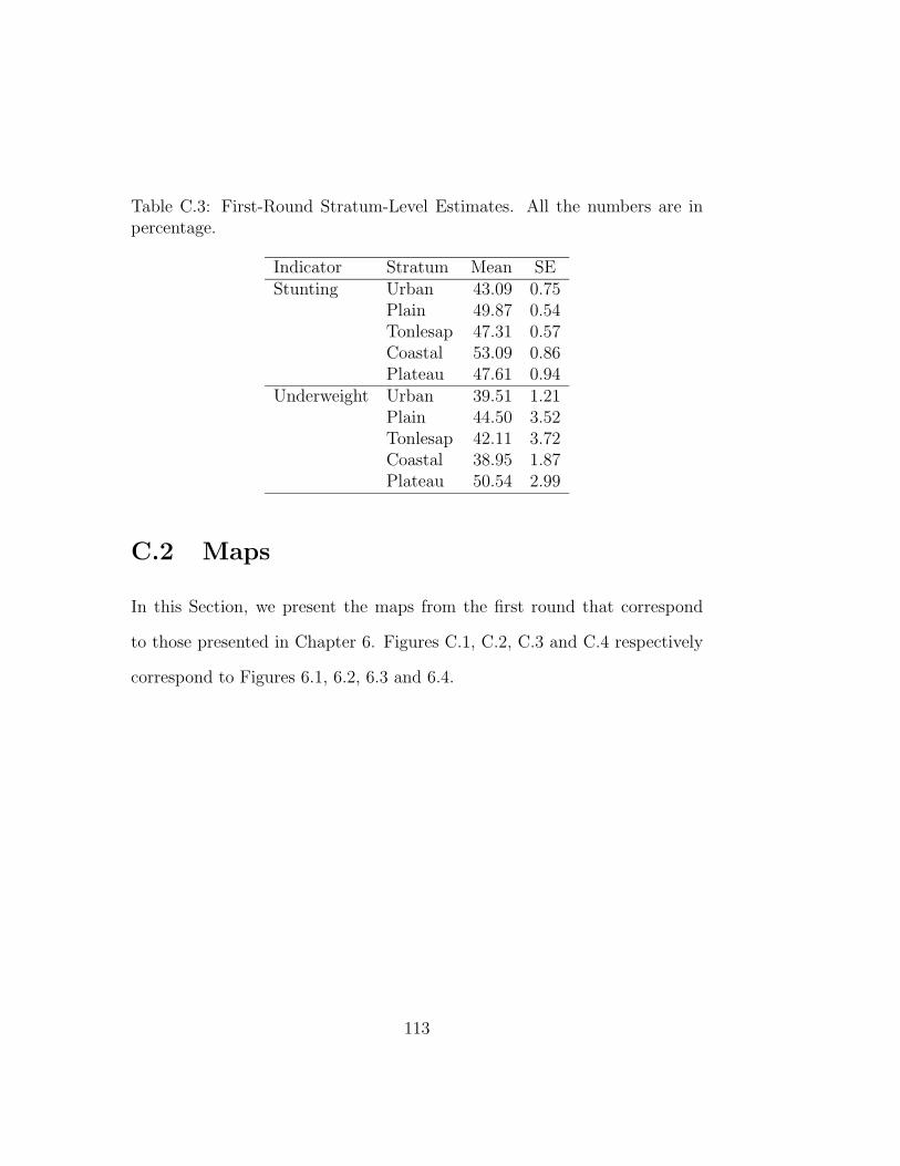
Table C.3: First-Round Stratum-Level Estimates. All the numbers are inpercentage.

Indicator Stratum Mean SEStunting Urban 43.09 0.75

Plain 49.87 0.54Tonlesap 47.31 0.57Coastal 53.09 0.86Plateau 47.61 0.94

Underweight Urban 39.51 1.21Plain 44.50 3.52Tonlesap 42.11 3.72Coastal 38.95 1.87Plateau 50.54 2.99

C.2 Maps

In this Section, we present the maps from the first round that correspond

to those presented in Chapter 6. Figures C.1, C.2, C.3 and C.4 respectively

correspond to Figures 6.1, 6.2, 6.3 and 6.4.

113

epsfiles/st_r1.eps

Figure C.1: Commune-Level Prevalence of Stunting for the Children Under Five in Cambodia. This mapis created from the round-one estimates and Figure 6.1 should be used for application.

114

epsfiles/uw_r1.eps

Figure C.2: Commune-Level Prevalence of Underweight for the Children Under Five in Cambodia. Thismap is created from the round-one estimates and Figure 6.2 should be used for application.

115

epsfiles/stz_r1.eps

Figure C.3: Commune-Level Prevalence of Stunting in Comparison With the National Average. This mapis created from the round-one estimates and Figure C.3 should be used for application.

116

epsfiles/uwz_r1.eps

Figure C.4: Commune-Level Prevalence of Underweight in Comparison With the National Average. Thismap is created from the round-one estimates and Figure 6.4 should be used for application.

117

References

Alderman, H. (2000) ‘Anthropometry.’ In Designing Household Survey Ques-

tionnaires for Developing Countries: Lessons from Ten Years of LSMS Ex-

perience, ed. M. Grosh and P. Glewwe (Oxford University Press) pp. 251–

272

Alderman, H., M. Babita, G. Demombynes, N. Makhatha, and B. Ozler

(2002) ‘How small can you go? combining census and survey data for

mapping poverty in South Africa.’ Journal of African Economies 11, 169–

200

Behrman, J.R. (1999) ‘Economic considerations for analysis of early child-

hood development programmes.’ Food and Nutrition Bulletin 20(1), 146–

170

Benson, T., S. Kanyanda, and R. Chinula (2002) ‘Poverty mapping in malawi

- results of the fourth iteration of the analysis.’ Report to the National Eco-

nomic Council and the National Statistical Office, Government of Malawi

Bigman, D., and H. Fofack (2000) ‘Geographical targeting of poverty allevi-

118

ation programs: Methodology and applications in rural India.’ Journal of

Policy Modeling 24(3), 237–255

Bigman, D., S. Dercon, D. Guillaume, and M. Lambotte (2000) ‘Commu-

nity targeting for poverty reduction in Burkina Faso.’ The World Bank

Economic Review 14(1), 167–194

Curtis, S.L., and M. Hossain (1998) ‘West africa spatial analysis prototype

explanatory analysis: The effects of aridity zone on child nutritional sta-

tus.’ Technical Report, Demographic and Health Survey, Macro Interna-

tional

Davis, B. (2002) ‘Is it possible to avoid a lemon?: Reflections on choosing a

poverty mapping method.’ mimeo, Agriculture in Economic Development

Service, Food and Agricultural Organization of the United Nations

de Onis, M., C. Monteiro, J. Akre, and G. Clugston (1993) ‘The worldwide

magnitude of protein-energy malnutrition: an overview from the WHO

global database on child growth.’ Bulletin of the World Health Organiza-

tion 71(6), 703–712

de Onis, M., E.A. Frongillo, and M. Blossner (2000) ‘Is malnutrition de-

clining? an analysis of changes in levels of child malnutrition since 1980.’

Bulletin of the World Health Organization 78, 1222–1233

Demombynes, G., C. Elbers, J. Lanjouw, J. Lanjouw, J. Mistiaen, and

B. Ozler (2002) ‘Producing an improved geographic profile of poverty:

119

Methodology and evidence from three developing countries.’ WIDER Dis-

cussion Paper 2002/39, United Nations University

Dibley, M.J., N. Staehling, P. Nieburg, and F.L. Trowbridge (1987) ‘Interpre-

tation of Z-score anthropometric indicators derived from the international

growth refrence.’ Am. J. Clin. Nutr. 46, 749–762

Ehrenberg, A.S.C. (1968) ‘The elements of lawlike relationships.’ Journal of

Royal Statistical Society A 131, 280–302

Elbers, C., J.O. Lanjouw, and P. Lanjouw (2000) ‘Welfare in villages and

towns.’ Timbergen Institute Discussion Paper TI 2000-029/2, Timbergen

Institute

(2001a) ‘Welfare in villages and towns: Micro-level estimation of poverty

and inequality.’ mimeo, World Bank

(2003) ‘Micro-level estimation of poverty and inequality.’ Econometrica

71(1), 355–364

Elbers, C., J.O. Lanjouw, P. Lanjouw, and Leite (2001b) ‘Poverty and in-

equality in Brazil’ new estimates from combined PPV-PNAD data.’ mimeo,

World Bank

Elbers, C., P. Lanjouw, J. Mistiaen, B. Ozler, and K. Simler (2002) ‘Are

neighbours equal? estimating local inequality in three developing coun-

tries.’ Paper presented at the Cornell/LSE/WIDER Conference on Spa-

120

tial Ineqality and Development, The World Bank. Downloadable from

http://www.unu.wider.edu

Forcheh, N. (2002) ‘Ehrenberg law-like relationship and anthropometry.’

Journal of Royal Statistical Society A 165(Part 1), 155–172

Frongillo, E.A., M. de Onis, and K.M.P. Hanson (1997) ‘Socioeconomic and

demographic factors are associated with worldwide patterns of stunting

and wasting of children.’ Journal of Nutrition 127(12), 2302–2309

Galler, J.R., and L.R. Barrett (2001) ‘Children and famine: Long-term im-

pact on development.’ Ambulatory Child Health 7, 85–95

Ghosh, M., and J.N.K. Rao (1994) ‘Small area estimation: An appraisal.’

Statistical Science 9(1), 55–76

Glewwe, P., H.G. Jacoby, and E.M. King (2001) ‘Early childhood nutrition

and academic achievement: a longitudinal analysis.’ Journal of Public Eco-

nomics 81, 345–368

Gollogly, L. (2002) ‘The dillemmas of aid: Cambodia 1992-2002.’ Lancet

360, 793–798

Gorstein, J., K. Sullivan, R. Yip, M. de Onis, F. Trowbridge, P. Fajans, and

G. Clugston (1994) ‘Issues in the assessment of nutritional status using

anthropometry.’ Bulletin fo the World Health Organization 72(2), 273–282

121

Hardy, F., and Health Unlimited Ratanakiri Team (2001) ‘Health situation

analysis ratanakiri cambodia.’ Technical Report, Health Unlimited

Haughton, D., and J. Haughton (1997) ‘Explaining child nutrition in viet-

nam.’ Economic Development and Cultural Change 45(3), 541–556

Hentschel, J., J.O. Lanjouw, P. Lanjouw, and J. Poggi (2000) ‘Combining

census and survey data to study spatial dimensions of poverty: A case

study of ecuador.’ The World Bank Economic Review 14(1), 147–166

Hill, P.S. (2000) ‘Planning and change: a Cambodian public health case

study.’ Social Science & Medicine 51, 1711–1722

James, W.P.T., A. Ferro-Luzzi, S. Sette, and C.G.N. Mascie-Taylor (1999)

‘The potential use of maternal size in priority setting when combating

childhood malnutrition.’ European Journal of Clinical Nutrition 53, 112–

119

Kanbur, R. (1987) ‘Transfers, targeting and poverty.’ Economic Policy

4(1), 112–147

Khorshed Alam Mozumder, A.B.M., T.T. Kane, A. Levin, and S. Ahmed

(2000) ‘The effect of birth interval on malnutrition in bangladeshi infants

and young children.’ Journal of Biosocial Science 32, 289–300

Li, Y., G. Guo, A. Shi, Y. Li, T. Anme, and H. Ushijima (1999) ‘Prevalence

and correlates of malnutrition among children in rural minority areas of

China.’ Pediatrics International 41, 549–556

122

Main, B., T. Lower, R. James, and I. Rouse (2001) ‘Changes in expanded pro-

gram for immunization coverage for mother and child in Krakor, Cambodia

1996-1998.’ Tropical Medicine and International Health 6(7), 526–528

Mason, J.B., J. Hunt, Parker D., and U. Jonsson (2001) ‘Improving child

nutrition in asia.’ Food and Nutrition Bulletin

Minot, N. (2000) ‘Generating disaggregated poverty maps: An application

to Vietnam.’ World Development 28(2), 319–331

Mistiaen, J., B. Ozler, T. Razafimanantena, and J. Razafindravonona (2001)

‘Disaggregated maps of estimated poverty and inequality for madagascar

in 1993.’ mimeo, DECRG, The World Bank

Monteiro, C.A., L. Mondini, A.M. Torres, and I.M. dos Reis (1997) ‘Patterns

of intra-familiar distribution of undernutrition: Methods and applicatins

for developing societites.’ European Journal of Clinical Nutrition 51, 800–

803

National Institute of Statistics, Directorate General for Health, and ORC

Macro (2001) Cambodia Demographic and Health Survey 2000 (National

Institute of Statistics, Directorate General for Health and ORC Macro)

Pelletier, D.L., E.A. Frongillo Jr., D.G. Schroeder, and J-P. Habicht (1994)

‘A methodology for estimating the contribution of malnutrition to child

mortality in developing countries.’ Journal of Nutrition 124, 2106S–2122S

123

Pradhan, M., D.E. Sahn, and S.D. Younger (2003) ‘Decomposing world

health inequality.’ Journal of Health Economics 22(2), 271–293

Ravallion, M., and K. Chao (1989) ‘Targeting policies for poverty allevia-

tion under imperfect information: Algorithms and applications.’ Journal

of Policy Modeling 11(2), 213–224

Rice, A.L., L. Sacco, A. Hyder, and R.E. Black (2000) ‘Malnutrition as

an underlying cause of childhood deaths associated with infectious dis-

eases in developing countries.’ Bulletin of the World Health Organization

78(10), 1207–1217

Sastry, N. (1997) ‘Family-level clustering of childhood mortality risk in north-

east Brazil.’ Population Studies 51(3), 245–261

Schmidt, M.K., S. Muslimatun, C.E. West, W. Schultink, R. Gross, and

J.G.A.J. Hautvast (2002) ‘Nutritional status and linear growth of indone-

sian infants in west java are determined more by prenatal environment

than by postnatal factors.’ Journal of Nutrition pp. 2202–2207

Shariff, Z.M., J.T. Bond, and N.E. Johnson (2000) ‘Nutrition and educational

achievement of urban primary schoolchildren in Malaysia.’ Asia Pacific

Journal of Clinical Nutrition 4(9), 264–273

Tomkins, A., and F. Watson (1989) ‘Malnutrition and infection: a re-

view.’ ACC/SCN State-of-the-art Series, Nutrition Policy Discussion Pa-

124

per No. 5, United Nations Administrative Committee on Coordina-

tion/Subcommittee on Nutrition

UNICEF (1998) The State of the World’s Children 1998 (Oxford University

Press)

Victora, C. (1992) ‘The association between wasting and stunting: An inter-

national perspective.’ Journal of Nutrition 122(5), 1105–1110

Warner, J.T. (2000) ‘Reliability of indices of weight and height in assessment

of nutritional state in children.’ The Lancet 356, 1073–1074

Waterlow, J.C., R. Buzina, W. Keller, J.M. Lane, M.Z. Nichaman, and J.M.

Tanner (1977) ‘The presentation and use of height and weight data for

comparing the nutritional status of groups of children under the age of 10

years.’ Bulletin of the World Health Organization 55(4), 489–498

WHO Working Group (1986) ‘Use and interpretation of anthropometric in-

dicators of nutritional status.’ Bulletin of the World Health Organization

64(6), 929–941

World Bank (1994) Enriching Lives: Overcoming Vitamin and Mineral Mal-

nutrition in Developing Countries

World Health Organization (2002) World Health Report 2002: Reducing risks

and promoting healthy life (Geneva: World Health Organization)

125

Zeini, L.O., and J.B. Casterline (2002) ‘Clustering of malnutrition among

egyptian children.’ mimeo, Cairo University and Population Council

126