Methods For Evaluation Of The Alberta Hail Suppression ...
72
University of North Dakota University of North Dakota UND Scholarly Commons UND Scholarly Commons Theses and Dissertations Theses, Dissertations, and Senior Projects January 2021 Methods For Evaluation Of The Alberta Hail Suppression Project Methods For Evaluation Of The Alberta Hail Suppression Project Using Radar Observations Using Radar Observations Sankha Subhra Maitra Follow this and additional works at: https://commons.und.edu/theses Recommended Citation Recommended Citation Maitra, Sankha Subhra, "Methods For Evaluation Of The Alberta Hail Suppression Project Using Radar Observations" (2021). Theses and Dissertations. 4173. https://commons.und.edu/theses/4173 This Thesis is brought to you for free and open access by the Theses, Dissertations, and Senior Projects at UND Scholarly Commons. It has been accepted for inclusion in Theses and Dissertations by an authorized administrator of UND Scholarly Commons. For more information, please contact [email protected].
-
Upload
khangminh22 -
Category
Documents
-
view
0 -
download
0
Transcript of Methods For Evaluation Of The Alberta Hail Suppression ...

University of North Dakota University of North Dakota
UND Scholarly Commons UND Scholarly Commons
Theses and Dissertations Theses, Dissertations, and Senior Projects
January 2021
Methods For Evaluation Of The Alberta Hail Suppression Project Methods For Evaluation Of The Alberta Hail Suppression Project
Using Radar Observations Using Radar Observations
Sankha Subhra Maitra
Follow this and additional works at: https://commons.und.edu/theses
Recommended Citation Recommended Citation Maitra, Sankha Subhra, "Methods For Evaluation Of The Alberta Hail Suppression Project Using Radar Observations" (2021). Theses and Dissertations. 4173. https://commons.und.edu/theses/4173
This Thesis is brought to you for free and open access by the Theses, Dissertations, and Senior Projects at UND Scholarly Commons. It has been accepted for inclusion in Theses and Dissertations by an authorized administrator of UND Scholarly Commons. For more information, please contact [email protected].

METHODS FOR EVALUATION OF THE ALBERTA HAILSUPPRESSION PROJECT USING RADAR OBSERVATIONS
by
Sankha Subhra Maitra
Bachelor of Technology, West Bengal University of Technology, 2013
Diploma in Meteorology, Dalhousie University, 2017
A Thesis
Submitted to the Graduate Faculty
of the
University of North Dakota
in partial fulfillment of the requirements
for the degree of
Master of Science
Grand Forks, North Dakota
December
2021

Copyright 2021 Sankha Subhra Maitra
ii

iii
This document, submitted in partial fulfillment of the requirements for the degree from
the University of North Dakota, has been read by the Faculty Advisory Committee under whom
the work has been done and is hereby approved.
____________________________________
____________________________________
____________________________________
____________________________________
____________________________________
____________________________________
This document is being submitted by the appointed advisory committee as having met all
the requirements of the School of Graduate Studies at the University of North Dakota and is
hereby approved.
____________________________________
Chris Nelson
Dean of the School of Graduate Studies
____________________________________
Date
Name:
Degree:
DocuSign Envelope ID: 4523B8B9-64EC-42BD-B527-2B505318369A
Sankha Subhra Maitra
David Delene
Andrew Detwiler
Master of Science
Michael Poellot
12/9/2021
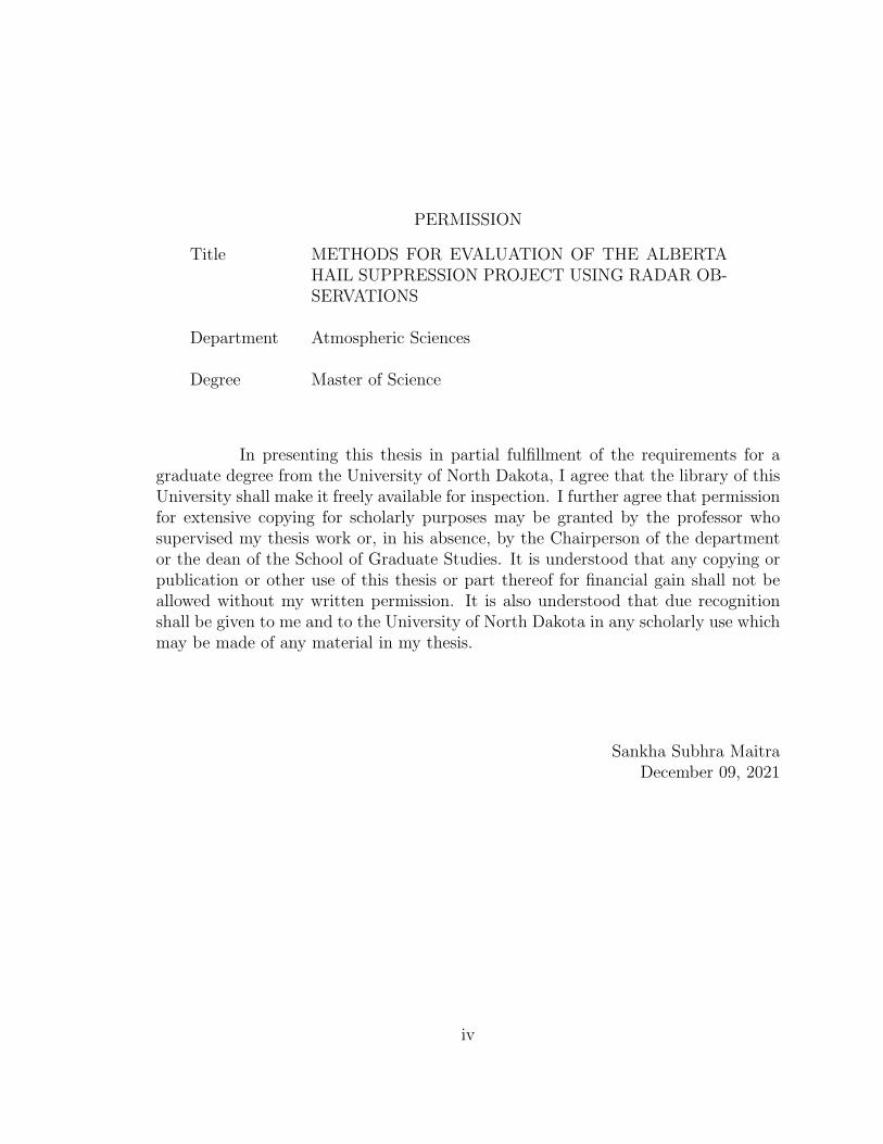
PERMISSION
Title METHODS FOR EVALUATION OF THE ALBERTA
HAIL SUPPRESSION PROJECT USING RADAR OB-
SERVATIONS
Department Atmospheric Sciences
Degree Master of Science
In presenting this thesis in partial fulfillment of the requirements for a
graduate degree from the University of North Dakota, I agree that the library of this
University shall make it freely available for inspection. I further agree that permission
for extensive copying for scholarly purposes may be granted by the professor who
supervised my thesis work or, in his absence, by the Chairperson of the department
or the dean of the School of Graduate Studies. It is understood that any copying or
publication or other use of this thesis or part thereof for financial gain shall not be
allowed without my written permission. It is also understood that due recognition
shall be given to me and to the University of North Dakota in any scholarly use which
may be made of any material in my thesis.
Sankha Subhra Maitra
December 09, 2021
iv
TABLE OF CONTENTS
LIST OF FIGURES................................................................................................vii
LIST OF TABLES....................................................................................................x
ACKNOWLEDGMENTS.......................................................................................xi
ABSTRACT...........................................................................................................xii
1. INTRODUCTION................................................................................................1
1.1 History and Background.................................................................................2
2. THE ALBERTA HAIL SUPPRESSION PROJECT.............................................9
3. DATA SET..........................................................................................................15
4. METHODOLOGY.............................................................................................17
4.1 Case Classification.......................................................................................18
4.2 Indicators Used.............................................................................................18
4.3 Case Periods.................................................................................................21
4.4 Case Selection Using LROSE TITAN..........................................................21
4.5 Hailstorm Case Example..............................................................................22
4.6 Data from 2017.............................................................................................30
4.7 Metrics Used to Calculate Seeding Effectiveness........................................35
v

4.7.1 Average Hail Indicator (AHI)................................................................36
4.7.2 Hail Occurrence Ratio (HOR)...............................................................38
4.7.3 Increasing Hail Ratio (IHR)..................................................................40
4.8 Interpretation of Seeding Effectiveness Metrics...........................................42
5. RESULTS...........................................................................................................43
5.1 Average Hail Indicator (AHI) Metric...........................................................43
5.2 Hail Occurrence Ratio (HOR) Metric..........................................................43
5.3 Increasing Hail Ratio (IHR) Metric..............................................................44
6. DISCUSSION.....................................................................................................49
7. CONCLUSIONS AND BROADER IMPACTS.................................................51
APPENDIX A: DEFINITION OF TERMS............................................................53
REFERENCES.......................................................................................................55
vi
LIST OF FIGURES
Figure 1: Figure illustrating the size and shape of the project area for the Alberta Hail
Suppression Project. The protected area is shown in green and the buffer zone in yellow. The
protected area extending from Ponoka in the north to High River in the south measures about
23,474 km2 and measures approximately 242 km along the North South direction and 97 km
along the East-West direction. The buffer area measuring approximately 20,787 km2 surrounds
the protected area and indicates the boundaries of the cloud seeding operations. Grey circles
indicate two of the biggest cities (by population) inside the project area. The project radar
location is indicated by the star symbol........................................................................................10
Figure 2: Image showing maximum occurrence of composite radar reflectivity for the storm
occurring on the 13th July 2017 between 00:20 UTC and 01:58 UTC, north of Calgary. The thin,
colour lines south of the storm denote seeding aircraft flight tracks. The white lines delineate
different sections of the storm based on the cloud seeding operations.........................................17
Figure 3: Plot showing the average annual freezing level heights computed between June 1 st and
September 15th of every year during a twenty-year period from 1999 to 2019. The daily freezing
level heights are obtained from historical records of the soundings at the AHSP project area. The
twenty year mean is 3.39 km and the standard deviation is 0.58 km...........................................20
Figure 4: LROSE-TITAN images showing the Olds radar at 19:44:11 UTC and 19:48:04 UTC
on the 16th July 2017. The scan times represent time instants immediately after the completion of
the respective volume scans. Different distance labels give the approximate distance from the
project radar site. At 19:44:11 UTC, two of the three storms on the North-Western corner are
identified as TITAN Cells and have track numbers (numbers within the black box). The
Southernmost of the three storms (encircled in orange) does not have a track number because it
is yet to become a TITAN Cell. All three storms are more than 100 km from the project radar. At
19:48:04 UTC on the 16th July 2017, the Southernmost of the three storms on the North-Western
corner has just become a TITAN Cell (highlighted in cyan and encircled in orange) and is
assigned a track number 57. The thin pink lines East of TITAN Cell 57 is the seeding aircraft
flight track, which is patrolling the area and are yet to start seeding...........................................23
Figure 5: Figure showing the evolution of a TITAN Cell on the LROSE-TITAN display of the
Olds radar reflectivity from 20:15:10 UTC and till 20:46:09 UTC on the 16th July 2017. The
TITAN Cell with track number 57whose evolution is being tracked is highlighted in cyan.
Distance labels show the approximate distance from the project radar placed at the Olds-
Didsbury airport, which is located between the towns of Olds and Didsbury. Thin pink and
vii
yellow lines indicate flight tracks and thick yellow lines indicate the tracks of the seeding flares.
At 20:30:40 UTC the seeding aircraft are flying towards case 57/72 but have not started seeding
the case yet. At 20:46:09 UTC the location of the thick yellow lines suggests that the seeding
aircraft have just started seeding case 57/80.................................................................................26
Figure 6: Figure showing the evolution of a TITAN Cell on the LROSE-TITAN display of the
Olds radar reflectivity from 21:17:08 UTC and till 22:22:58 UTC on the 16th July 2017. The
case 57/89 whose evolution is being tracked is highlighted in cyan. Thin pink, cyan and yellow
lines indicate flight tracks and thick yellow lines indicate the tracks of the seeding flares.
Distance labels show the approximate distance from the project radar placed at the Olds-
Didsbury airport, which is located between the towns of Olds and Didsbury. By 22:22:58 UTC
the case previously with the track number 57/89 (encircled in orange) is no longer a TITAN Cell
and is hence not assigned a track number. Meanwhile, a new cell about 40 km North of Olds
(highlighted in cyan) now satisfies the criteria for a TITAN Cell and is assigned a track number
93 by LROSE-TITAN...................................................................................................................29
Figure 7: Histogram showing Convective Available Potential Energy (CAPE) of all the analyzed
seed cases. The CAPE values are obtained from the NAM-WRF model’s forecast sounding for
the time and city (either Calgary or Red Deer) closest to the occurrence of a case.....................32
Figure 8: Histogram showing the Convective Available Potential Energy (CAPE) of all the non-
seed cases. The CAPE values are obtained from the NAM-WRF model’s forecast sounding for
the time and city (either Calgary or Red Deer) closest to the occurrence of a case.....................33
Figure 9: Bar graph showing the variability in the Bulk Richardson Number (BRN) shear of the
21 analyzed seed cases used in the analysis. The BRN shear values are obtained from the NAM-
WRF model’s forecast sounding for the time and city (either Calgary or Red Deer) closest to the
occurrence of a case......................................................................................................................33
Figure 10: The Bulk Richardson Number (BRN) shear of the non-seed cases used in the
analysis. The BRN shear values are obtained from the NAM-WRF model’s forecast sounding
for the time and city (either Calgary or Red Deer) closest to the occurrence of a case................34
Figure 11: Illustration of the different periods used in the radar data analysis of cases. The time-
height image uses synthetic reflectivity (dBZ) that is based on the review of 2017 Alberta Hail
Suppression Project storms. The Active Storm Period (ASP) is the period of potential hail and
starts when the composite reflectivity is first greater than 45 dBZ and ends when the composite
reflectivity is below 25 dBZ. The Active Storm Period can contain one or more TITAN storm
cells. The Hail Likelihood Period is the time within the ASP when moderate or large hail is
viii
present. The Before Seeding Period (BSP), Effective Seeding Period (ESP), and Post Seeding
Period (PSP) are periods within the ASP related to the start of seeding.......................................35
Figure 12: A plot showing a hypothetical storm’s MaxVIL at each volume scan in its Active
Storm Period (ASP). The red, green and blue correspond to the storm’s Before Seeding Period
(BSP), Effective Seeding Period (ESP) and the Post Seeding Period (PSP), respectively.
MaxVILs are given above each circle and used in the example calculations given in the text....38
Figure 13: Plot showing the Increasing Hail Ratio (IHR - Equation 10) seeding effectiveness for
the 2017 season seed-cases of the Calgary Hail Suppression project calculated using the change
of MaxVIL hail indicator..............................................................................................................46
Figure 14: Figure showing the individual seeding effectiveness (SE) of the seed cases calculated
using the six different metrics; Average Hail Indicator (AHI), Hail Occurrence Ration (HOR)
and Increasing Hail Ratio (IHR) for both Maximum Vertically Integrated Liquid (MaxVIL) and
storm area greater than or equal to 60 dBZ (Ar60). Figures 14A and 14E have the seeding
effectiveness (SE) of all 21 seed cases. However, the before seeding and effective seeding
metric values for case # 13 in Figure 14B, case #s 13, 14 and 15 in Figure 14C, case # 13 in
Figure 14D and case #s 11, 13, 15, 16, 17, and 20 in Figure 14F are zero. Therefore, the SE for
such cases could not be computed and plotted.............................................................................47
Figure 15: Box and whisker plots of the seeding effectiveness values for all analyzed seed cases
are shown in the figure. Seeding effectiveness is calculated for six metrics; Average Hail
Indicator (AHI), Hail Occurrence Ratio (HOR) and Increasing Hail Ratio (IHR) for both
MaxVIL and area greater than or equal to 60 dBZ indicators. The boxes show the interquartile
range (middle fifty percent of the values) and the red lines indicate the median of the seeding
effectiveness values. The diamonds show the outlier points, which are points having values
either 1.5 times greater or less than the width of the boxes (interquartile range); and her hence
deemed to be too far from the middle fifty-percent values...........................................................48
ix

LIST OF TABLES
Table 1: List of analyzed seed cases from 2017 with date and time of cells. Also included are the
track numbers based on the 45 dBZ TITAN Cells. The TITAN date and time is 1200 UTC of a
day until 1200 UTC the following day. The sounding location of the city geographically closest
to the seed case is used to derive thermodynamic properties.......................................................30
Table 2: List of non-seed cases from 2017 with the date and time of cells. Also included are the
track numbers based on the 45 dBZ TITAN Cells. The TITAN date and time is 1200 UTC of a
day until 1200 UTC the following day. The sounding location of the city geographically closest
to a non-seed case is used to derive thermodynamic properties...................................................30
Table 3: List showing seeding effectiveness (SE) calculated for the seed cases from 2017 using
indicators for the radar detection of hail.......................................................................................45
Table 4: Important terms and their definitions..............................................................................53
x

ACKNOWLEDGMENTS
I would like to thank my advisor, Dr. David Delene, for his support and guidance
throughout the course of this project; and especially for helping me out with Python
programming, an area in which he has an exceptional level of expertise. I am also very grateful
to my committee members, Dr. Andrew Detwiler and Mr. Michael Poellot for their helpful
inputs and timely feedback during the project.
I extend my heartiest thankfulness to Mr. Bruce Boe (Vice President of Meteorology,
Weather Modification International), Mr. Dan Gilbert (Chief Meteorologist, Weather
Modification International) and Dr. Terry Krauss (Project Director, Alberta Severe Weather
Management Society) for taking time out of their busy schedule to help us with the analysis. A
very big “THANK YOU” to The Weather Modification International, Fargo for funding the
project.
I thank my parents for letting me resign from my IT job and follow my dreams. No part of
this project would have been complete without their constant support and encouragement.
Lastly, I would like to thank the fantastic “gang” of graduate students at University of North
Dakota’s Department of Atmospheric Sciences, for putting up with my eccentricities and
making my time here in Grand Forks, a wonderful and memorable one!!
xi

To the ones who have felt the rain..

ABSTRACT
The Alberta Hail Suppression Project is an operational weather modification program
designed to reduce hailstone induced property damage that has been conducted in the area
around Calgary and Red Deer since 1996. Evaluation of the project is done using the project’s
C-band radar located at Olds and an Environment Canada operated C-band radar at Strathmore.
An in-depth, manual review of radar data from the 2017 seeding operations has identified 21
seed cases and 15 non-seed cases. The effectiveness of seeding is determined using hail
indicators of Maximum Vertically Integrated Liquid (MaxVIL) and storm area greater than or
equal to 60 dBZ (Ar60) by comparing before and during seeding observations for the 21 seed
cases. Several different seeding effectiveness metrics are evaluated with the Increasing Hail
Ratio metric having the highest value of 0.12 for both MaxVIL and Ar60 indicators. A positive
metric indicates a reduction in damaging hail, with 1 being the highest possible value. The
metrics are based on the 2017 season where there are only 21 cases; however, the data set could
be expanded by incorporating 2014 to 2020 years of observations since the radar configuration
is similar.
xii

1. INTRODUCTION
Alberta, Canada regularly receives hailstorms that cause major property damage. Property
damage is especially severe in the Calgary metropolitan area, which receives over fifty percent
of Canada’s severe weather related insurance claims. Along with property damage, hailstorms
have also caused a significant amount of damage to crops over the years. Historically, claims for
crop hail damage in Alberta have been received on an average of 50 days each year between 1
June and 10 September (Summers and Wojtiw 1971). Average crop loss due to hail has risen
steadily since the mid 70s. Average annual crop loss amount due to hail was estimated to be
about $50 million in 1975 (Renick 1975). For the 1980 - 1985 period the annual crop loss had
increased to more than $150 million (Alberta Research Council 1986). However, over the last
three decades property damage has far exceeded crop hail damage. Thirteen separate storms
between 1981 and 1998 caused property damages worth $600 million in Calgary. Two Alberta
hailstorms in 1996 resulted in a combined loss of $103 million due in part to one-third of the
cars damaged being irreparable. In 2010, a storm with golfball sized hailstones ravaged Calgary
causing property damages of over $400 million. In 2012, Calgary received golf ball size
hailstones that resulted in a staggering $552 million worth of damage, which accounted for
almost half of the $1.2 billion worth of claims across Canada (Desjardins Insurance 2017).
To reduce hailstorm property damage, the Alberta Hail Suppression Project sponsors
weather modification operations in the area around Calgary and Red Deer. The project uses
cloud seeding that is based on the principle of beneficial competition (Iribarne and de Pena
1962). Beneficial competition assumes a lack of natural ice nuclei in the environment at
temperatures warmer than -20 °C and that the injection of ice-nuclei active at warmer
1

temperatures by cloud seeding produces a significant number of ice particles. In beneficial
competition, both natural and artificial ice nuclei compete for the available supercooled liquid
water within the clouds. Having the same amount of supercooled liquid water distributed among
a greater number of ice nuclei results in more hailstones but of smaller size. As a result, the
hailstones that are formed within the seeded storms are smaller and produce less damage to
property. The smaller hail stones may even melt completely before reaching the ground.
Evidence suggests that hail embryos grow in the main updraft of single cell storms and in
the updrafts of developing “feeder clouds” or cumulus towers that flank the mature “multi-cell”
and “super-cell” storms (Browning 1977; Foote 1984; Krauss and Marwitz 1984). The growth
of large hail is hypothesized to occur along the edges of the main storm updraft where the
merging feeder clouds interact with the main storm updraft (Marwitz 1972a,b,c; Foote 1984).
Seeding operations target the feeder cloud updraft regions associated with the production of hail
(Foote 1984; Krauss and Marwitz 1984). Regions of the storm that are associated with only rain
are left unseeded, which makes efficient use of the seeding material and reduces the risk of over
seeding the rain clouds.
1.1 History and Background
The history of hail suppression can be traced back to 1951 when, after positive field
research results of working with cumulus and cumulus clouds in Canada, Irving P Crick
Associates of Canada Ltd started a hail suppression field research project in the Logan and
Washington counties of Colorado, which receive lots of hailstorms (Krick and Stone 1975).
While the project area received only light hail, areas upwind of the project area had some heavy
2
hailstorms. With the positive indication of hail damage reduction in Colorado, hail suppression
field operations were started in California and Oregon.
The Alberta hail suppression research program was started in Alberta in 1956 under the
guidance of the Alberta Research Council with the purpose of developing and evaluating the
effectiveness of aircraft based cloud seeding to mitigate the hail damage done to crops (Krick
and Stone 1975). During the first seeding season, only ground generators were used; however,
while the main project area received little damage, the non-project areas of Carstairs-Cremona
and Wimborne received heavy hail damage. As a result of the somewhat successful first season,
the program continued the following year. Throughout the 1960s, primary focus of the hail
suppression projects was to minimize hail-crop damage and enhance rainfall to improve crop
yield. From 1961 to 1968, commercial hail suppression operations in Alberta showed a benefit
to cost ratio of 47 to 1 and indicated some level of success (Krick and Stone 1975). A series of
hail suppression projects suggested that projects reduced the economic impact of hail damage by
20 to 50 % (Changnon 1977). However, project insurance data used in some studies was
questionable (NCAR 1976).
In the North Dakota Pilot Project, a seeded and non-seeded area comparison was done
using hailpad data, crop hail insurance losses, hail-rain relations and radar echo characteristics
(Miller et al. 1975). The hailpad data indicated a 21% non-significant reduction in hail energy
on seeded days and a 4% reduction in hail volume. The insurance loss data that covered
approximately 10% of the project area showed a 60% reduction on seeded days. The ratio of
hail (representative of the energy) and rain (representative of the quantity) for the seeded days
showed a 40% decrease in hail energy compared to no-seed days. Analysis of various seeding
3

rates show that heavier rates (>400 g/hr) were more effective in reducing hail than light rates
(<200 g/hr). The rainfall results revealed an average increase of approximately 23% on seeded
days. Insured crop-hail damage ratio suggested a 50-75% reduction in damage costs. Overall,
the results suggested that hail suppression might be effective (Simpson 1975).
A commercial hail-suppression project carried out in west Texas showed potential for
successful hail suppression (Changnon Jr 1975). Aircraft were used to carry out cloud base
seeding and the project analyzed using Weather Bureau hail day data and crop hail insurance
data. The hail reduction rates varied from 5% to 94% for different time and space comparisons.
The single best estimate of a meaningful hail reduction was 48% decrease in the insurance loss
cost value. The calculations for percentage reduction in hail was based on four different
parameters – hail days, liability, losses and loss costs. Most of the examined data suggested that
the hail suppression process was successful (Schickedanz 1975).
A three year project in South Africa showed a decrease in the large daily damage values but
an increase in days with small damage values (Schickedanz 1975; Changnon Jr. and Morgan Jr.
1976). Overall, there was 20% reduction in hail damage severity (Simpson 1975). However,
since the experiment was not randomized, the decrease in hail insured damages may not be due
to cloud seeding. A similar project, referred to as the National Hail Research Experiment
(NHRE) was carried out in north-east Colorado from 1972 to 1974 using the injection of silver-
iodide in supercooled clouds based on the principle of beneficial competition. Analysis of the
1972-73 period showed a 30% reduction in the hail mass on seeded days, which was not
statistically significant. Rainfall increased by 25% on the seeded days but was also not
significant statistically (NCAR 1974). However, the 1972-74 period has a complete reversal
4

with hail mass increasing by 41% (Long 1975). Changes in the seeding criteria, delivery
techniques and the surface networks made the results questionable. Analysis of three years of
data were inconclusive with no appreciable effect (NCAR 1976). Cloud base seeding with silver
iodide was used to suppress hail in South Dakota. Evaluations were carried out using rainfall
and the loss cost data from the seeded and non-seeded counties. The results showed a reduction
in hail related losses ranging from 18% to 40%.
The projects carried out in west Texas, Colorado, North Dakota, South Dakota and South
Africa all attempted to alter hail formation using the beneficial competition approach. While a
substantial number of hail suppression operations were carried out through the mid 70s, a
consensus was achieved as to what the most effective methodology for hail suppression was. All
the projects carried out during this time used the crop-hail damage metric as the parameter to
evaluate hail suppression effectiveness. While the crop-hail damage metric has direct
application to cost-benefit analysis, an analysis based on physical processes seemed elusive. A
metric directly relating the reduction in damage potential of hailstorms to the seeding was not
used. In many of the projects, storm cells were chosen randomly for seeding without identifying
the ones with a greater damage potential. As a result, many of the storm cells with lesser damage
potential ended up getting seeded while cells producing large and damaging hailstones were
often left unseeded. Methods like the paired storm design was suggested, in which one member
of a pair of storms with similar characteristics is seeded (Schickedanz and Changnon 1970). It
was believed that such the paired storm design approach would help make a more rigorous
evaluation of the effects of seeding.
5
The World Meteorological Organization’s recommendation that a physical parameter be
used instead of crop hail insurance data led to a large scale hailstorm seeding project using silver
iodide ground generators by the Association Nationale d’Etude et de Lutte contre le Fleaux
Atmospheriques (ANELFA) in South Western France (World Meteorological Organization
1996). Data collected from 1988 to 1995 was based on 630 point hailfalls that occurred on 43
seeded days. A network of hailpads were used to count the number of hailstones larger than 0.7
cm. The results showed a negative correlation between the number of hailstones larger than 0.7
cm and the mass of silver iodide released 80 minutes beforehand. A 15.6 % decrease in hailfall
number was observed with a seeding amount of 23.2 g h-1 of silver iodide per 531 km2 area. For
the heavily seeded storms, hailfall reduced by approximately 42 % (Dessens 1998).
Along with glaciogenic seeding, hygroscopic seeding was also carried out in some parts of
the world. In hygroscopic seeding, hygroscopic particles are introduced in supersaturated warm
cloud environments. The hygroscopic particles take in water and grow by vapour deposition.
When they grow large enough, the serve as “coalescence embryos” and keep growing larger
through collision and coalescence with other supercooled liquid water droplets to initiate
precipitation (Cooper et al. 1997). The initial results of a hygroscopic seeding program in South
Western France showed that out of the 95 storms seeded over the network: 55 storms did not
produce hail before, during or after the treatment; 27 storms stopped producing hail after the
seeding; 13 storms continued to produce hail during and after the treatment. Additionally, no
non-hailing storms started to produce hail during or after the initiation of seeding. A storm was
successfully seeded if 8 to 10 minutes after seeding, the following changes were observed: a
substantial fall in the average altitude of the maximum echo zone, an increase in the volume of
6
the maximum reflectivity (>50 dBz), the altitude of the max echo top increased or stayed at the
same level, and only rain was observed on the ground. However, the number of hailstorms
analyzed in the project was too low for significant statistical results. For example, in 2001 and
2003 only 12 hailstorms were treated (Berthoumieu 2003).
Hail suppression projects did not try to reduce non-agricultural property (housing,
automobiles and other outdoor equipment) damage until the early 90s. On 7 September 1991 a
severe hailstorm striking Calgary caused extensive property damage. Insurance costs associated
with this hailstorm were estimated to be approximately $ 400 million (Charlton et al. 1995). Due
to the large property damage cost, a new Alberta Hail Suppression Project was created with the
aim of reducing hail induced property damage. The program used the techniques and results of
the long term hail research project conducted by the Alberta Research Council from the 1960s to
1985 and prioritized to minimize property damage. An improved and fast-acting formulation of
the silver iodide flares having the capability of producing 100 times more ice nuclei per gram of
seeding material were used. The flares made it possible to nucleate ice that were as warm as 4
°Celsius. The response of the 1996 Alberta Hail Suppression was quite encouraging. Sixty five
cloud seeding operations were carried out on thirty storm days. The project area received hail on
22 days. However, walnut or larger sized hail was reported only on five occasions (Krauss and
Renick 1997). Insurance information were used by the ASWMS to assess the benefits and
usefulness of the project.
In spite of the initiation of the Alberta Hail Suppression Project, there was a serious lack of
property-hail loss data in the late 90s (Changnon 1999). Only a few studies were conducted on
the subject of property hail loss data. On behalf of the property insurance industry conducted, a
7

study to find ways of assessing the risks associated with property-hail damage and reducing
them was conducted by Cook 1995. Since most of the property hail damage occurred to roofs,
studies on the roofing materials and ways to mitigate future hail losses were also conducted
(Devlin 1996, 1997). Property insurance claims data from the Dallas-Fort Worth metroplex area
were used to evaluate hail damage by Brown et al. 2015. The study made use of the insurance
claims and policy data to evaluate roofing material type with regard to resiliency to hailstone
impacts. Such works, along with a series of hailstorms between 1996 and 2012, gradually turned
the attention of the scientific community towards the assessment of property-hail damage.
Property damage is related to the size of hailstone that impact the surface. To obtain a
relationship between hailstone size and radar observations, hail reports can be related to
Maximum Vertically Integrated Liquid (MaxVIL) (Krauss et al. 1998). VIL is a non-linear
function of radar reflectivity that represents equivalent liquid water content using an empirical
relationship, which is calculated as,
VIL=∑i=1
n
(3.44∗10−6[(Z i+Z i+1)/2]4 /7 Δ h) ,
(1)
where, VIL has units kilograms per square meter (kg m-2), Zi and Zi+1 are the radar reflectivity
values (mm6m-3) for two consecutive scan angles and Δh is the vertical thickness between
centres of the areas sampled by the two consecutive scan angles in meters (US Department of
Commerce 1991). The radar continues scanning the storm through its entire height at all scan
angles to generate the VIL. VIL is related to the mass of hydrometers in a height interval, over
which it is calculated. Hail present within that height interval has high reflectivity, which
increases the VIL. Greene and Clark 1972 were the first to show that VIL derived from radar
data could be used to predict the occurrence of hail. Billet et al. 1997 demonstrated that VIL can
8

be utilized to determine the occurrence and size of hailstones in potentially severe
thunderstorms.
The MaxVIL to hail size relationship has been used by the Alberta Hail Suppression Project
for forecast verification of hail sizes in the absence of ground hail reports since 1998. Gilbert et
al. 2016 analyzed two seeded storms and one non-seeded storm occurring very close in space
and time and found the seeded storms to have a substantially lesser area greater than or equal to
60 dBZ and MaxVIL than the neighbouring non-seeded storm. Such results indicate that
MaxVIL and storm area greater than or equal to 60 dBZ can be used to analyze the effect of
cloud seeding on hailstone size and the areal extent of hailstones respectively.
The objective is to analyze radar data to quantify the project’s operational effectiveness
using seeding effectiveness metrics based on the concept of beneficial competition. The 2017
radar data is analyzed to determine if cloud seeding reduces MaxVIL and the storm area greater
than or equal to 60 dBZ reflectivity in storms. Changes in these hail indicators provide a
quantification of the seeding effectiveness.
2. THE ALBERTA HAIL SUPPRESSION PROJECT
The aim of the Alberta Hail Suppression Project since its inception in 1996 has been the
protection of urban property from severe hailstorm damage to the maximum extent that
technology and safety allows. Storms threatening the protected area (Figure 1) are seeded with
priority assigned based on population. Calgary and Red Deer are the two largest cities inside the
protected area and receive the maximum priority. Storms that are moving to threaten the
protected area are typically seeded while still in the buffer area. However, storms are never
9

seeded outside the buffer area. The purpose of the buffer area is to make sure that the seeding
becomes effective by the time a storm moves into the protected area.
Figure 1: Figure illustrating the size and shape of the project area for the Alberta Hail
Suppression Project. The protected area is shown in green and the buffer zone in yellow. The
protected area extending from Ponoka in the north to High River in the south measures about
23,474 km2 and measures approximately 242 km along the North South direction and 97 km
along the East-West direction. The buffer area measuring approximately 20,787 km2 surrounds
the protected area and indicates the boundaries of the cloud seeding operations. Grey circles
indicate two of the biggest cities (by population) inside the project area. The project radar
location is indicated by the star symbol.
The daily forecasts are valid for a 24 hour period from 12 UTC of one day to 12 UTC of the
following day. The period is referred to as the “official storm day”. The forecast also includes a
brief “day 2” outlook for planning purposes. A modified WRF model sounding indicating the
10

probable extent and time of maximum hail threat is also included. A surface depiction map from
Nav Canada, an 850 hPa Theta-E chart, a 500 hPa chart with heights and vorticity and a 250 hPa
jet level chart are also included. Model sounding files are analyzed with the Universal
RAwinsonde OBservation program (RAOB) to create a skewT/logP thermodynamic diagram.
Model soundings are available for both Calgary and Red Deer and either can be used depending
where the more significant hail threat is expected. If conditions indicate a possibility of
hailstorms, the model sounding data are sometimes analyzed with the HAILCAST, which is a
2D model predicting hail size. After analyzing all the data, the weather forecast for a particular
day is synthesized into a single number called the Convective Day Category (CDC), which
ranges from -3 to +5. The CDC summarizes the threat of hail for the day. A value of -3 means no
deep convection whereas a +5 value indicates a larger than golf ball size hail (>5.2 cm diameter)
(Weather Modification International 2017).
The project’s radar is a C-band radar located at the Olds-Didsbury airport. All convective
storms having more than 10 km3 of 45 dBz reflectivity above 4 km altitude (MSL) and moving
towards the protected area may be seeded. Radar observers and aircraft controllers are
responsible for making the seeding decision and directing the cloud seeding missions. Patrol
flights are launched before clouds within the protected areas or buffer zones meet the radar
reflectivity seeding criteria. These patrol flights are meant to provide immediate response to
developing cells. In general, a patrol flight is launched in the event of visual reports of towering
cumulus clouds or when radar cells exceed 20,000 ft height over the higher terrain along the
western border on days with forecast for thunderstorms with hail potential. Extensive aircraft
patrolling based upon forecasts and radar observations are used to initiate seeding as soon as
11

appropriate conditions develop. Twin engine high performance aircraft are used for prompt
response and timely seeding. Seeding aircraft position is downlink in real-time and overlaid on
radar displays to direct aircraft to the most critical regions of the storms.
Launches of more than one aircraft are determined by the number of storms in each area,
the lead time required for a seeder aircraft to reach the proper location and altitude and projected
overlap of coverage and on-station time for multiple aircraft missions. In general, only one
aircraft can work safely at cloud top and one aircraft at cloud base for a single storm. If required,
at least three aircraft operate to provide uninterrupted seeding coverage at either cloud-base or
cloud-top and to seed three storms simultaneously.
The program is designed to deliver seeding material to regions where supercooled liquid
water exists. Cloud seeding involves the release of ice nucleating agents into either the cloud
base or the cloud tops or both. Factors, which determine if the seeding should be a cloud base or
cloud top seeding include storm structure, visibility, cloud base height and time available to
reach seeding altitude. Cloud base seeding is conducted by flying at cloud base within the main
inflow of single cell storms, or the inflow associated with the new growth zones located on the
upshear side of multi-cell storms. With cloud base seeding, the seeding material moves upwards
into the storm core where it encounters an area with supercooled liquid water droplets. Cloud
top seeding is conducted between -8 °C and -15 °C altitudes. With cloud top seeding, the
seeding material is released at or above an area of supercooled liquid water droplets. The
seeding agents are injected at least 20 minutes before a storm moves over a city within the
protected zone to enable the seeding agent to distribute throughout the volume of the storm and
grow to sufficiently large ice crystals to compete for the available supercooled liquid water
12

(Hsie et al. 1980). Generally, 30 minute or greater amount of time is advised to stay on the safe
side.
Storms are seeded by aircraft using either droppable silver iodide (AgI) pyrotechnics or by
burning AgI-Acetone solutions attached to burners on the aircraft. The seeding agent is
dispensed in three ways: (1) the silver-iodide acetone seeding solution is burned from wing-tip
borne ice nucleus generators, (2) pyrotechnics can be burned “in-place”, while held to special
racks affixed to the trailing edges of the aircraft wings, and (3) small pyrotechnics can be ignited
and ejected into cloud tops from racks mounted on the belly of the aircraft fuselage. The total
amount of seeding material used depends upon the lifetime and size of the storm. Larger storms
require more seeding material; however the amount of seeding material is the same per unit area
of the storm. Seeding is focused on the feeder clouds of the storm’s new growth zone and is
conducted either at the cloud base or the cloud top or both. Seeding materials are injected
directly into the developing cloud turrets to facilitate the seeding process.
The ejected pencil seeding flares fall approximately 1.5 km during their 40 s burn time. The
seeding aircraft penetrates the edges of single convective cells meeting the seeding criteria. For
multicell storms, or storms with feeder clouds, the seeding aircraft penetrates the tops of the
developing cumulus towers on the downdraft side of convective cells, as they grow up through
the aircraft’s altitude. Occasionally, with embedded cells or convective complexes, there are no
clearly defined feeder turrets visible to the flight crews or on radar. In these instances, seeding
aircraft penetrate the storm edge at an altitude between -5 °C and -10 °C on the downdraft side
and burn an end burner flare and inject droppable pencil flares when updrafts are encountered.
The storm edge is chosen because that is the region having a tight radar reflectivity gradient.
13
Technically seeding should continue as long as the seeding criteria are satisfied. However,
seeding is effective only within cloud updrafts and in the presence of supercooled liquid water,
i.e. the developing and mature stages in the evolution of the classic thunderstorm conceptual
model. The dissipative stages of the storm are seeded only if the maximum reflectivity is
particularly severe and there are evidences like visual cloud growth or tight reflectivity gradients
indicating the possible presence of embedded updrafts. Additional cloud seeding flights are sent
if there are visual signs of new cloud growth or radar reflectivity gradients remain tight, which
is an indication of persistent updrafts.
A seeding rate of one 20 g flare for every 5 s is used during cloud penetration. A slightly
higher rate of one flare every 2 s is used if updrafts are very strong (10 m/s or 2000 ft/min) and
the storms are particularly intense. Calculations have shown that such a seeding rate produces
over 1300 ice crystals per litre, which is more than sufficient to deplete the liquid water content
produced by updrafts greater than 10 m/s, thereby preventing the growth of hailstones within the
seeded cloud volumes (Cooper and Marwitz 1980). A 5 to 10 minute waiting period is used to
allow for the seeding material to take effect and the storm to dissipate, if visual signs of
glaciation appear or radar reflectivity values decrease and gradients weaken. This waiting
periods makes sure that the seeding materials are not wasted.
The silver-iodide (AgI) flares used produce more than 1011 nuclei per g of AgI at -4 C as
determined by independent cloud chamber tests at Colorado State University (CSU). Rates of
ice-crystal formation in the CSU isothermal cloud chamber was quite rapid with 63% of the
nuclei becoming active within one to two minutes and 90% of the nuclei becoming active within
4 minutes (DeMott 1999) . Sufficient dispersion of the seeding particles is required for AgI
14

plume overlap from consecutive flares by the time the cloud particles reach hail size for
effective hail suppression. Previous works based on turbulence measurements within the Alberta
feeder clouds have shown that the time for the diameter of the diffusing line of AgI to reach the
integral length scale of 200 m in the inertial sub range size scales of mixing is 140 s. This time
is insufficient for ice particles to grow to hail size. Therefore, dropping flares at 5 s intervals
should effectively deplete the supercooled liquid water and prevent the growth of hail particles.
The use of the 20 gm flares and a frequent drop rate provides better seeding coverage than using
larger flares with a greater time/distance spacing between flare drops. In fact, the stated
calculations work only under the assumption that the centre of the ice crystal plume centre
contains a higher concentration of ice crystals (Grandia et al. 1979).
3. DATA SET
The analysis builds on previous research on the Alberta Hail Suppression Project where
radar observations are used to evaluate seeding effects (Krauss and Santos 2004). The Alberta
Hail Suppression Project initially began with a WR-100 weather radar, which was replaced with
a C-band Doppler radar in 2011. The new C-band Doppler radar could detect clouds while still
in their developmental stage. In 2014 the project’s radar was replaced with a more sensitive
5.975 GHz C-band radar, which had a minimum detectable signal of slightly less than 10 dBZ.
The radar upgrade enabled deployment of the latest version of the TITAN radar software, state-
of-the-science radar antenna control and improved data processing capabilities. As a result,
volume scans could be completed in less than 4 minutes, which provided 15 scans every hour
(Weather Modification International 2017). Data from an Environment Canada operated C-band
Doppler radar placed at Strathmore is also used for the analysis. The Strathmore radar has a new
15

volume scan every 10 minutes. For both radars, volume scans consist of 18 elevations angles.
The lowest and the highest elevation scans occur at heights of 2 km (MSL) and 14.75 km (MSL)
respectively with 0.75 km being the height difference between two consecutive elevation scans.
A dedicated computer system is used to store all radar data, along with seeding operation
documentation. The Lidar Radar Open Software Environment-Thunderstorm Identification,
Tracking, Analysis and Nowcasting (LROSE-TITAN) software package is used to analyze data
from the two radars (Dixon and Wiener 1993). The raw data obtained in IRIS format is
converted to the NetCdf (cfRadial) format using the LROSE-TITAN application RadxConvert.
The data in NetCdf format (polar coordinates) is converted to the meteorological data volume
(mdv) format (cartesian coordinates) using the Radx2Grid application. It is the data in mdv
format that is ultimately analyzed. The data in mdv format is used to obtain the MaxVIL (also in
mdv format) using the application Mdv2Vil.
Seeding aircraft flight tracks are superimposed on radar displays and individual storms
identified to create a record of each storm in relation to when seeding started and concluded
(Figure 2). Sometimes a reduction in high reflectivity is clearly evident for storms after seeding
becomes effective, which is evident in Figure 2 where the reflectivity in the storm core changed
from above 57 dBZ to below 57 dBZ. However, not all storms show such obvious effects, so it
is necessary to investigate many storms using high quality observations and well thought out
methodology to see the effect of seeding on radar reflectivity in hailstorms. Furthermore, as
evident in Figure 2, some time is required before seeding effects are evident in radar
observations.
16
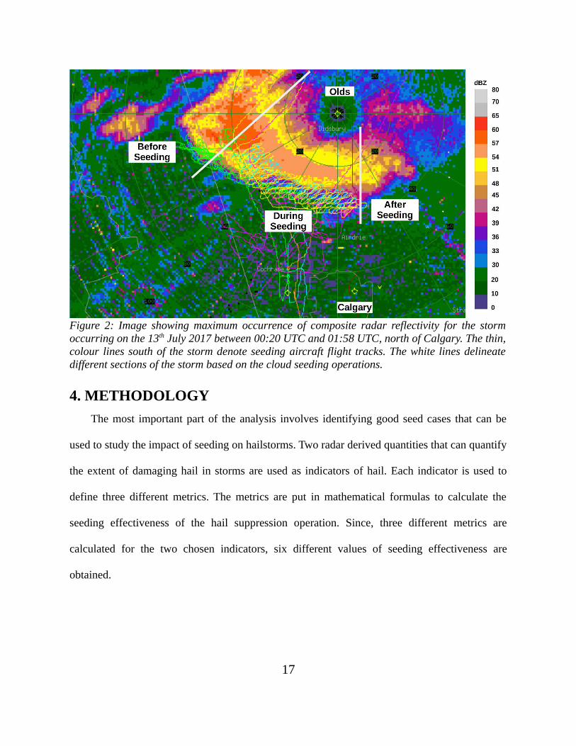
Figure 2: Image showing maximum occurrence of composite radar reflectivity for the storm
occurring on the 13th July 2017 between 00:20 UTC and 01:58 UTC, north of Calgary. The thin,
colour lines south of the storm denote seeding aircraft flight tracks. The white lines delineate
different sections of the storm based on the cloud seeding operations.
4. METHODOLOGY
The most important part of the analysis involves identifying good seed cases that can be
used to study the impact of seeding on hailstorms. Two radar derived quantities that can quantify
the extent of damaging hail in storms are used as indicators of hail. Each indicator is used to
define three different metrics. The metrics are put in mathematical formulas to calculate the
seeding effectiveness of the hail suppression operation. Since, three different metrics are
calculated for the two chosen indicators, six different values of seeding effectiveness are
obtained.
17
4.1 Case Classification
The analysis builds on a 2015 case study of three Alberta hailstorms (Gilbert et al. 2016) by
analysing all 2017 storms. The LROSE-TITAN software package has been configured to define
a “TITAN cell” a storms having a composite reflectivity greater than 45 dBZ and a volume
greater than 10 km3. A storm with a TITAN cell within 100 km radius of the radar and staying
within 100 km radius of the radar for at least three volume scans defines a case. Cases are
restricted to a 100 km radius to ensure high quality radar observations. Cases are classified into
three different categories; seeded, non-seeded, and non-analyzed. Seed cases must be treated
with at least 2 kg of seeding material. Non-seed cases must be free of seeding material for the
preceding 20 minutes. Seed cases 20 minutes after the end of seeding are also considered as
non-seed cases. Non-analyzed cases have TITAN cells but do not meet the seeded or non-seeded
criteria. Additionally, cases are restricted to west to east moving cells; hence, TITAN cells tracks
that move in the North-South direction along the Rocky Mountains are placed into the non-
analyzed category. The removal of these TITAN cell tracks is done so that the storms analyzed
have similar morphology. All cases moving over the radar cone of silence are also not analyzed.
Cases whose radar return signals are attenuated by other cases situated in front of them are also
not analyzed.
4.2 Indicators Used
All storms satisfying the definition of a seed case are analyzed to evaluate different seeding
effectiveness (SE) methodologies using a custom built python program. The python program
analyzes ASCII data files extracted using the LROSE-TITAN software and calculates the
metrics. The metrics are used to calculate the seeding effectiveness. For calculating the metrics,
18
two radar derived indicators are used to quantitatively represent damaging hail in storms are
used. Based on the conceptual model of how seeding should reduce the quantity of damaging
hail in a storm, observations of the two indicators allow the analysis of hail suppression
effectiveness. One indicator is storm area with radar reflectivity greater than or equal to 60 dBZ
(Ar60). A reflectivity of 60 dBZ represents the minimum reflectivity when damaging hailstones
are present in storms (Ward et al. 1965). Previous work carried out by Donaldson 1961 and Wilk
1961 showed that hail is often associated with a reflectivity greater than or equal to 60 dBZ aloft
for a 3 cm wavelength radar. Auer 1972 plotted radar reflectivity factor as a function of
hydrometeor diameter and showed that a reflectivity of 60 dBZ might be associated with
damaging hailstones. The other indicator used is Maximum Vertically Integrated Liquid
(MaxVIL), which is a radar derived quantity correlated with severe weather potential of
thunderstorms (Greene and Clark 1972). The VIL is restricted to being above the freezing level
(4 km) to eliminate contamination by the bright band caused by the melting of ice particles,
which can overestimate hail’s impact on VIL (Austin and Bemis 1950). A height of 4 km is used
since the twenty year average of the daily freezing level heights for the AHSP project area is 3.4
km (Figure 3) and 0.6 is added to account for days above the average. The freezing levels during
the 1999 and 2000 operational period are relatively low at around 3 km (MSL). However, for
the later years they show an increase and stay close to a height of 3.5 km (MSL). The maximum
value of VIL within the area of a TITAN cell is referred to as MaxVIL.
19
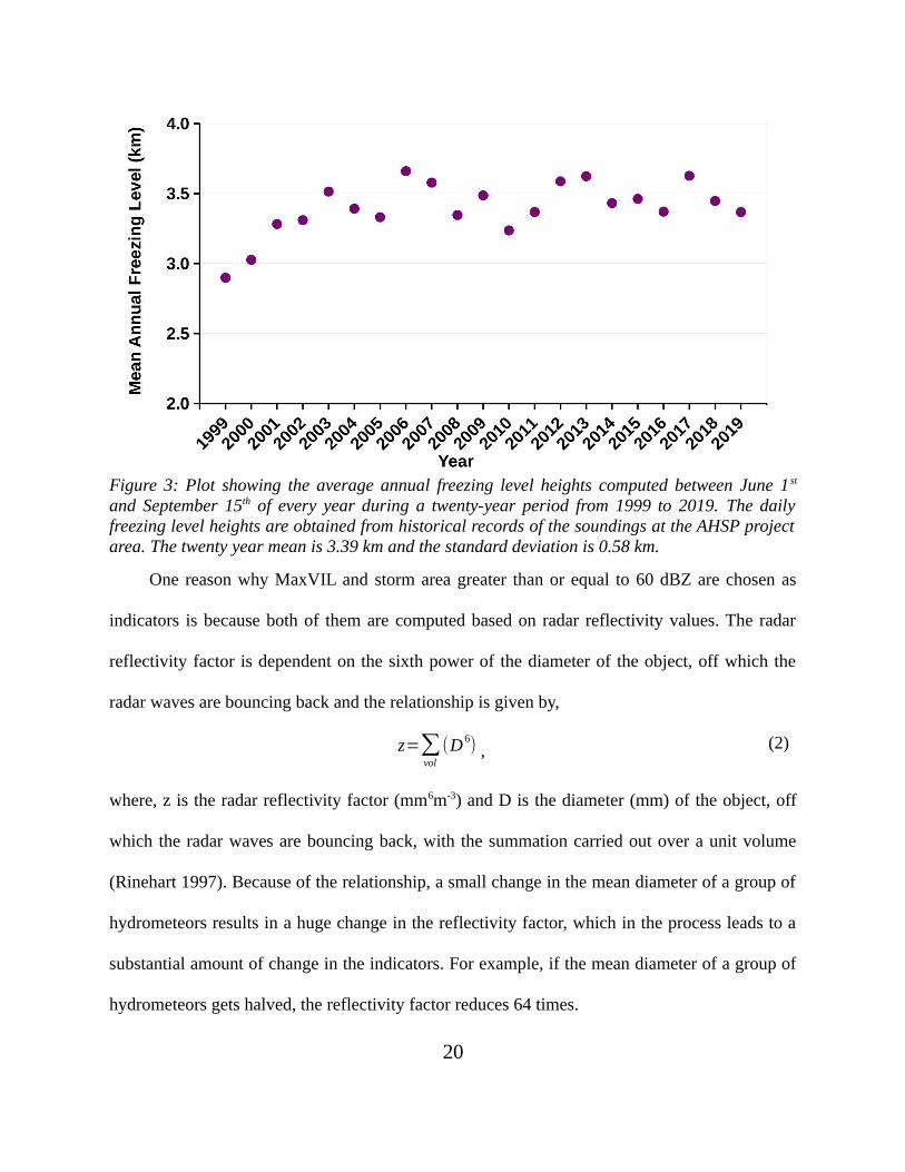
Figure 3: Plot showing the average annual freezing level heights computed between June 1 st
and September 15th of every year during a twenty-year period from 1999 to 2019. The daily
freezing level heights are obtained from historical records of the soundings at the AHSP project
area. The twenty year mean is 3.39 km and the standard deviation is 0.58 km.
One reason why MaxVIL and storm area greater than or equal to 60 dBZ are chosen as
indicators is because both of them are computed based on radar reflectivity values. The radar
reflectivity factor is dependent on the sixth power of the diameter of the object, off which the
radar waves are bouncing back and the relationship is given by,
z=∑vol
(D6) , (2)
where, z is the radar reflectivity factor (mm6m-3) and D is the diameter (mm) of the object, off
which the radar waves are bouncing back, with the summation carried out over a unit volume
(Rinehart 1997). Because of the relationship, a small change in the mean diameter of a group of
hydrometeors results in a huge change in the reflectivity factor, which in the process leads to a
substantial amount of change in the indicators. For example, if the mean diameter of a group of
hydrometeors gets halved, the reflectivity factor reduces 64 times.
20

4.3 Case Periods
Several different periods are defined for each case. The Active Storm Period (ASP) is the
period, during which a case has the potential of producing hail and starts when a case’s
composite reflectivity is first greater than 45 dBZ and ends either with the composite reflectivity
falling below 25 dBZ or when the TITAN cell moves more than 100 km of the radar. The ASP
can contain one or more TITAN cells since a storm’s reflectivity may fall below 45 dBZ and
increase above 45 dBZ.
The MaxVIL and storm area greater than or equal to 60 dBZ ( ≥ 60 dBZ) hail indicators are
used to define a Hail Likelihood Period (HLP). Within an Active Storm Period, there can be one
or more HLPs when moderate or large hail is likely present. A MaxVIL greater than or equal to
30 kg/m2 is used to define moderate hail that is capable of causing property damage (Krauss et
al. 1998). A HLP starts when the MaxVIL is greater than 30 kg/m2 and ends when MaxVIL falls
below 30 kg/m2. HLPs are also defined using the storm area greater than or equal to 60 dBZ
indicator. HLP starts when the composite reflectivity is greater than or equal to 60 dBZ and ends
when the composite reflectivity falls below 60 dBZ.
4.4 Case Selection Using LROSE TITAN
The annual Alberta Hail Suppression Project report is used to obtain an initial list of
seeding days during the 2017 season, which includes their approximate locations, times of
occurrence and the seeding duration. The LROSE-TITAN software is used to extract and view
storm information such as MaxVIL and storm area greater than equal to 60 dBZ. The report’s
seeding start and end times are also verified using LROSE-TITAN. The LROSE-TITAN Rview
window is used to review radar observations on cloud seeding operation days. Typically there
21

are a number of storms occurring simultaneously, many of which have areas of weak convection
and light rain. Some storms have areas of strong and intense convection, which may have hail
(Figures 4 - 6). Not every radar observed potential hailstorm is seeded since the project only
targets the storms threatening the project’s protected area.
LROSE-TITAN uses a complicated algorithm to identify and track storms that assigns
unique simple and composite track numbers to TITAN Cells. A TITAN Cell is defined using a
threshold of 45 dBZ composite reflectivity above a height of 4 km (MSL) that has a volume of
at least 10 km3. If a TITAN Cell does not merge or split with another TITAN Cell during its
trackable lifetime, the simple and complex track numbers are the same. However, most TITAN
Cells exhibit a much more complex behavioural pattern that includes merging or splitting, which
results in different simple and complex track numbers. For example, having a TITAN Cell with
Track 100 or Track 100/100 indicates that both the simple and complex track number is 100;
while, a TITAN Cell with track 100/105 indicates the complex track is 100 and the simple track
105. The complex track number is for the original TITAN Cells while the simple track number
is for the current segment. TITAN Cells may have more than one track number label as the
storm evolves. The TITAN Cell numbers are used to obtain text files (using the application
Tracks2Ascii) with calculated radar parameters, which are read by a Python program (script
name AHSPSE2017.py) to calculate metrics and create plots for the 2017 season.
4.5 Hailstorm Case Example
The 16th July 2017 seed case (Figure 4) is used as an example of how LROSE-TITAN
identifies different seeding periods. The project’s annual report identified the 16th July 2017
storm as a hailstorm that threatened the project area. The storm is first detected by radar at the
22
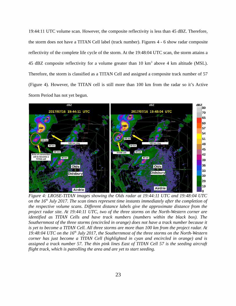
19:44:11 UTC volume scan. However, the composite reflectivity is less than 45 dBZ. Therefore,
the storm does not have a TITAN Cell label (track number). Figures 4 - 6 show radar composite
reflectivity of the complete life cycle of the storm. At the 19:48:04 UTC scan, the storm attains a
45 dBZ composite reflectivity for a volume greater than 10 km3 above 4 km altitude (MSL).
Therefore, the storm is classified as a TITAN Cell and assigned a composite track number of 57
(Figure 4). However, the TITAN cell is still more than 100 km from the radar so it’s Active
Storm Period has not yet begun.
Figure 4: LROSE-TITAN images showing the Olds radar at 19:44:11 UTC and 19:48:04 UTC
on the 16th July 2017. The scan times represent time instants immediately after the completion of
the respective volume scans. Different distance labels give the approximate distance from the
project radar site. At 19:44:11 UTC, two of the three storms on the North-Western corner are
identified as TITAN Cells and have track numbers (numbers within the black box). The
Southernmost of the three storms (encircled in orange) does not have a track number because it
is yet to become a TITAN Cell. All three storms are more than 100 km from the project radar. At
19:48:04 UTC on the 16th July 2017, the Southernmost of the three storms on the North-Western
corner has just become a TITAN Cell (highlighted in cyan and encircled in orange) and is
assigned a track number 57. The thin pink lines East of TITAN Cell 57 is the seeding aircraft
flight track, which is patrolling the area and are yet to start seeding.
23

At the 20:15:10 UTC scan, the TITAN Cell with track number 57 moves within 100 km
from the project radar (Figure 5), which marks the beginning of the TITAN Cell’s ASP. Since,
the TITAN Cell is yet to have three volume scans within 100 km of the radar, it is classified as a
TITAN Cell and not as a case. Since no merge or split of the TITAN Cell has taken place, it only
has a composite track number of 57. At 20:15:10 UTC time the TITAN Cell 48/54 immediately
North-East of TITAN Cell 57 is being seeded. About four minutes later, the TITAN Cell merges
with another cell just north of it. As a result, a simple track number 66 is assigned to the TITAN
Cell. The previously assigned complex track number is also present. At 20:19:03 UTC the
TITAN Cell has a track number 57/66. At the exact moment the TITAN cell immediately North-
East of cell 57/66 is still getting seeded. Seeding aircraft are flying towards TITAN Cell 57/66
but have not started seeding it yet. The track number assigned to the TITAN Cell is later used to
extract the MaxVIL and storm area greater than 60 dBZ data using a LROSE-TITAN
application. At the 20:30:40 UTC scan, the TITAN Cell with track number 57/66 has spend
three volume scans within 100 km of the radar radius. Therefore, the TITAN Cell is now
classified as a case. At the 20:30:40 UTC scan, the case 57/66 merges with another cell just
south of it. As a result, the case gets a new simple track number 72. The case now has a track
number 57/72, which is the third track number assigned to the case after 57 and 57/66. At this
point, the cell immediately North-East of it is getting seeded. The case being tracked (case
57/72) is yet to get seeded. At the 20:46:09 UTC scan, the first split occurs. The case 57/72
splits into two TITAN Cells. The larger of the two is assigned a new simple track number 80 and
is indicated by the TITAN Cell with the track number 57/80. The smaller of the two TITAN
Cells stays South-West of the case 57/80 and has the track number 57/79. Later, while extracting
24

storm data, the track number of the larger case (57/80) is used, since it stays active for a longer
period of time and over a greater area. Also, seeding of the case 57/80 starts at this point.
Therefore, the time 20:46 UTC marks the beginning of the seeding operational period (SOP).
The instant twenty minutes later is the beginning of the effective seeding period (ESP). The
seeding start time is most likely mentioned in the annual AHSP report. But the seeding start
times in the report are always verified with the seeding start times of the cases ascertained using
the position of the seeding aircraft tracks on the Rview screen. For inconsistencies occurring
between the two times, the seeding time available via the Rview display is used as the start of
the SOP.
25
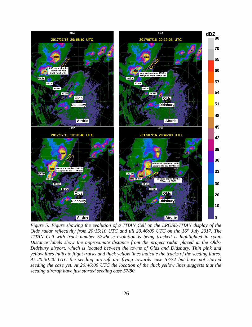
Figure 5: Figure showing the evolution of a TITAN Cell on the LROSE-TITAN display of the
Olds radar reflectivity from 20:15:10 UTC and till 20:46:09 UTC on the 16th July 2017. The
TITAN Cell with track number 57whose evolution is being tracked is highlighted in cyan.
Distance labels show the approximate distance from the project radar placed at the Olds-
Didsbury airport, which is located between the towns of Olds and Didsbury. Thin pink and
yellow lines indicate flight tracks and thick yellow lines indicate the tracks of the seeding flares.
At 20:30:40 UTC the seeding aircraft are flying towards case 57/72 but have not started
seeding the case yet. At 20:46:09 UTC the location of the thick yellow lines suggests that the
seeding aircraft have just started seeding case 57/80.
26
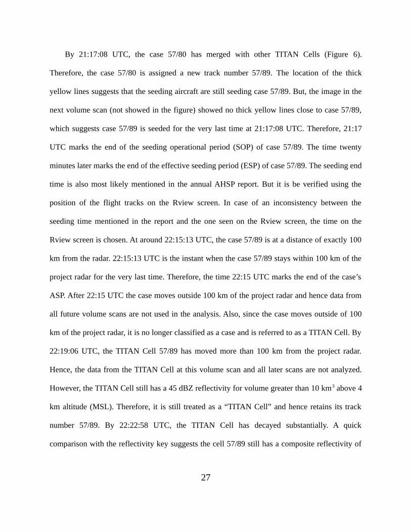
By 21:17:08 UTC, the case 57/80 has merged with other TITAN Cells (Figure 6).
Therefore, the case 57/80 is assigned a new track number 57/89. The location of the thick
yellow lines suggests that the seeding aircraft are still seeding case 57/89. But, the image in the
next volume scan (not showed in the figure) showed no thick yellow lines close to case 57/89,
which suggests case 57/89 is seeded for the very last time at 21:17:08 UTC. Therefore, 21:17
UTC marks the end of the seeding operational period (SOP) of case 57/89. The time twenty
minutes later marks the end of the effective seeding period (ESP) of case 57/89. The seeding end
time is also most likely mentioned in the annual AHSP report. But it is be verified using the
position of the flight tracks on the Rview screen. In case of an inconsistency between the
seeding time mentioned in the report and the one seen on the Rview screen, the time on the
Rview screen is chosen. At around 22:15:13 UTC, the case 57/89 is at a distance of exactly 100
km from the radar. 22:15:13 UTC is the instant when the case 57/89 stays within 100 km of the
project radar for the very last time. Therefore, the time 22:15 UTC marks the end of the case’s
ASP. After 22:15 UTC the case moves outside 100 km of the project radar and hence data from
all future volume scans are not used in the analysis. Also, since the case moves outside of 100
km of the project radar, it is no longer classified as a case and is referred to as a TITAN Cell. By
22:19:06 UTC, the TITAN Cell 57/89 has moved more than 100 km from the project radar.
Hence, the data from the TITAN Cell at this volume scan and all later scans are not analyzed.
However, the TITAN Cell still has a 45 dBZ reflectivity for volume greater than 10 km3 above 4
km altitude (MSL). Therefore, it is still treated as a “TITAN Cell” and hence retains its track
number 57/89. By 22:22:58 UTC, the TITAN Cell has decayed substantially. A quick
comparison with the reflectivity key suggests the cell 57/89 still has a composite reflectivity of
27
45 dBZ but the volume occupied by the 45 dBZ is less than 10 km3. Therefore, at this point and
beyond the TITAN Cell 57/89 is no longer treated as a “TITAN Cell” and is referred to as just a
storm. Since, it is no longer a TITAN Cell, it does not have a track number. The track numbers
assigned to the case tracked in the example are 57, 57/66, 57/72, 57/80 and 57/89. A LROSE-
TITAN application (Tracks2Ascii) is used to extract the storm data corresponding to these track
numbers. The storm data are obtained in text files, which are used as input to the custom built
Python program (AHSPSE2017.py) for generating plots and calculating the metrics during
different periods of a hailstorm. The process is repeated for all 21 seed cases.
28

Figure 6: Figure showing the evolution of a TITAN Cell on the LROSE-TITAN display of the
Olds radar reflectivity from 21:17:08 UTC and till 22:22:58 UTC on the 16th July 2017. The
case 57/89 whose evolution is being tracked is highlighted in cyan. Thin pink, cyan and yellow
lines indicate flight tracks and thick yellow lines indicate the tracks of the seeding flares.
Distance labels show the approximate distance from the project radar placed at the Olds-
Didsbury airport, which is located between the towns of Olds and Didsbury. By 22:22:58 UTC
the case previously with the track number 57/89 (encircled in orange) is no longer a TITAN Cell
and is hence not assigned a track number. Meanwhile, a new cell about 40 km North of Olds
(highlighted in cyan) now satisfies the criteria for a TITAN Cell and is assigned a track number
93 by LROSE-TITAN.
29
4.6 Data from 2017
Review of the 2017 data set identified 21 seed cases, 15 non-seed cases and 17 non-
analyzed cases. Details of the seed and non-seed cases are provided in Table 1 and Table 2
respectively. The given details ensure the reproducibility of the case identification procedure
should the need for such a process arise in future.
Table 1: List of analyzed seed cases from 2017 with date and time of cells. Also included are the
track numbers based on the 45 dBZ TITAN Cells. The TITAN date and time is 1200 UTC of a
day until 1200 UTC the following day. The sounding location of the city geographically closest
to the seed case is used to derive thermodynamic properties.
Case Number
Complex TrackNumber
Simple TrackNumber
TITAN Date (mm/dd)
TITAN Time(UTC)
SoundingLocation
1 11 11 07/03 0011 Red Deer
2 17 17 07/03 2155 Red Deer
3 22 22 07/03 2238 Red Deer4 30 30 07/09 2226 Red Deer
5 31 32 07/09 0007 Red Deer6 09 09 07/12 2030 Calgary
7 25 25 07/12 2149 Red Deer8 40 52 07/12 2341 Calgary
9 04 04 07/23 2027 Red Deer10 06 06 07/23 2136 Red Deer
11 72 72 07/27 0238 Red Deer12 159 159 06/08 0115 Red Deer
13 09 14 06/16 0001 Calgary14 03 03 06/27 2242 Calgary
15 13 13 06/27 0215 Calgary16 06 22 07/01 1950 Red Deer
17 12 12 07/01 1836 Calgary18 16 16 07/01 1919 Calgary
19 57 57 07/16 1948 Red Deer20 07 07 07/28 2343 Red Deer
21 05 05 07/31 0101 Calgary
Table 2: List of non-seed cases from 2017 with the date and time of cells. Also included are the
track numbers based on the 45 dBZ TITAN Cells. The TITAN date and time is 1200 UTC of a
day until 1200 UTC the following day. The sounding location of the city geographically closest
to a non-seed case is used to derive thermodynamic properties.
30

Case Number
Complex TrackNumber
Simple TrackNumber
TITAN Date(mm/dd)
TITAN Time(UTC)
SoundingLocation
1 99 99 06/02 2101 Red Deer
2 130 130 06/02 2215 Red Deer
3 06 06 07/01 1750 Red Deer
4 78 78 07/01 0120 Calgary5 80 80 07/08 2135 Red Deer
6 136 136 07/10 1330 Calgary7 213 213 07/10 1936 Calgary
8 213 238 07/10 2038 Calgary9 08 08 07/12 2020 Calgary
10 16 16 07/12 2150 Calgary11 07 28 07/28 0214 Calgary
12 141 147 08/05 2325 Red Deer13 20 20 08/10 0450 Calgary
14 22 22 08/10 0450 Calgary15 24 24 08/10 0500 Calgary
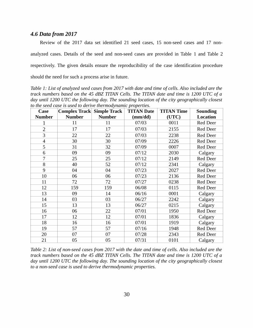
A comparison of the Convective Available Potential Energy (CAPE) of the seeded (Figure
7) and the non-seed cases (Figure 8) show that for both the types, most of the cases have CAPE
less than 1000 J/kg. The remaining cases have CAPE between 1000 J/kg and 2500 J/kg. None of
the seeded or non-seed cases have CAPE greater than 2500 J/kg. Therefore, the seeded and non-
seed cases show some similarity. However, a comparison of the Bulk Richardson Number
(BRN) shear of the seed cases (Figure 9) to those of the non-seed cases (Figure 10) reveal that
on average the non-seed cases are substantially weakly sheared compared to the seed cases.
31
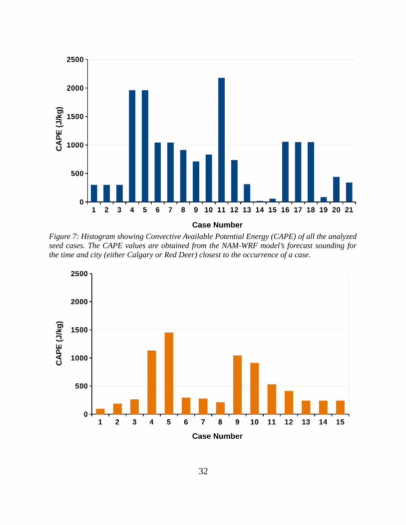
Figure 7: Histogram showing Convective Available Potential Energy (CAPE) of all the analyzed
seed cases. The CAPE values are obtained from the NAM-WRF model’s forecast sounding for
the time and city (either Calgary or Red Deer) closest to the occurrence of a case.
32
Figure 8: Histogram showing the Convective Available Potential Energy (CAPE) of all the non-
seed cases. The CAPE values are obtained from the NAM-WRF model’s forecast sounding for
the time and city (either Calgary or Red Deer) closest to the occurrence of a case.
Figure 9: Bar graph showing the variability in the Bulk Richardson Number (BRN) shear of the
21 analyzed seed cases used in the analysis. The BRN shear values are obtained from the NAM-
WRF model’s forecast sounding for the time and city (either Calgary or Red Deer) closest to the
occurrence of a case.
33

Figure 10: The Bulk Richardson Number (BRN) shear of the non-seed cases used in the
analysis. The BRN shear values are obtained from the NAM-WRF model’s forecast sounding for
the time and city (either Calgary or Red Deer) closest to the occurrence of a case.
The weak shear of the non seed cases makes them meteorologically different from the seed
cases. Since the seeded and non-seed cases are meteorologically different from one another, it is
not useful to carry out a seeding effectiveness analysis based on a statistical comparison of
seeded and non-seed cases. This is because, the meteorological properties of the
meteorologically dissimilar storms are different owing to natural reasons. The dissimilarities in
the properties are not a result of seeding’s impact on the storms. The difference in the storm
properties can be wrongly attributed to seeding. Therefore, instead of carrying out a seed case
versus non-seed case comparison, the analysis is kept confined to the seed cases. The ASP
(Figure 11) of the seed cases are split into three distinct periods – : 1.) the before seeding period
(BSP), 2.) the effective seeding period (ESP) and 3.) the post seeding periods (PSP). The
analysis compares the seeding effectiveness during these periods instead of comparing the seed
cases to the non-seed cases. The MaxVIL and the storm area greater than or equal to 60 dBZ
hail indicators are used to evaluate the seeding effectiveness by comparing the BSP and ESP.
The tracks of the seeding aircraft and the seeding flares are carefully reviewed using LROSE-
TITAN’s Rview software to check the seeding start and end times of all the seed cases within
the Active Storm Periods (ASP). The BSP is the beginning of the ASP until 20 minutes after the
seeding start time. The ESP is 20 minutes after seeding starts until 20 minutes after the seeding
ends. The PSP is 20 minutes after seeding ends until the end of the ASP. The 20 minutes
duration is used since this is the maximum time that seeding materials take to affect a TITAN
cell (Hsie et al. 1980). Only 2 seed cases have PSP, while all 21 seed cases have BSP and ESP.
34
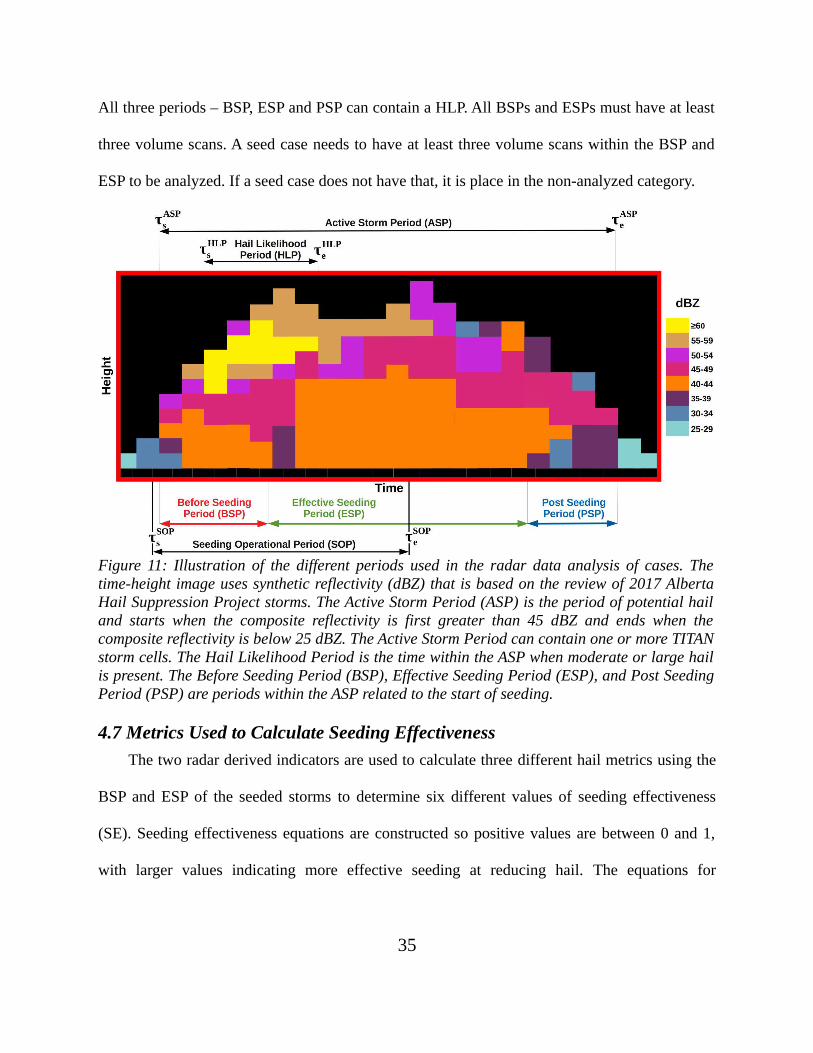
All three periods – BSP, ESP and PSP can contain a HLP. All BSPs and ESPs must have at least
three volume scans. A seed case needs to have at least three volume scans within the BSP and
ESP to be analyzed. If a seed case does not have that, it is place in the non-analyzed category.
Figure 11: Illustration of the different periods used in the radar data analysis of cases. The
time-height image uses synthetic reflectivity (dBZ) that is based on the review of 2017 Alberta
Hail Suppression Project storms. The Active Storm Period (ASP) is the period of potential hail
and starts when the composite reflectivity is first greater than 45 dBZ and ends when the
composite reflectivity is below 25 dBZ. The Active Storm Period can contain one or more TITAN
storm cells. The Hail Likelihood Period is the time within the ASP when moderate or large hail
is present. The Before Seeding Period (BSP), Effective Seeding Period (ESP), and Post Seeding
Period (PSP) are periods within the ASP related to the start of seeding.
4.7 Metrics Used to Calculate Seeding Effectiveness
The two radar derived indicators are used to calculate three different hail metrics using the
BSP and ESP of the seeded storms to determine six different values of seeding effectiveness
(SE). Seeding effectiveness equations are constructed so positive values are between 0 and 1,
with larger values indicating more effective seeding at reducing hail. The equations for
35

calculating all each seeding effectiveness using each hail metric are given in the following
sections.
4.7.1 Average Hail Indicator (AHI)
The MaxVIL is averaged over the BSP and the ESP for all cases in the data set. The
Average Hail Indicator metric is calculated using the equation,
AHI x
MaxVIL=∑
1
N
MaxVILx
N
, (3)
where N is the number of volume scans within all cases, for either the BSP or ESP as denoted by
the subscript x. The seeding effectiveness is calculated using,
SE AHI
MaxVIL=AHI BSP
MaxVIL−AHI ESP
MaxVIL
AHI BSP
MaxVIL+ AHI ESP
MaxVIL , (4)
Similar to the MaxVIL indicator, the Ar60 average hail indicator seeding effectiveness is,
SE AHI
Ar 60=AHI BSP
Ar 60−AHIESPAr 60
AHI BSP
Ar 60+ AHIESP
Ar 60 , (5)
The SE calculated using the Average Hail Indicator (AHI) metric measures the average
change across all cases in the hail indicator value from the BSP to the ESP. The SE gives a
measure of the change in the indicator value (from the BSP to the ESP) relative to the indicator
value during the BSP. If seeding reduces the size of a hailstone, the MaxVIL decreases. If the
average MaxVIL during the ESP stays lower than the average MaxVIL during the BSP, the SE is
positive. A positive SE indicates a reduction in the size of hailstones. A higher SE indicates a
greater degree of reduction in the hailstone size. Similarly, if seeding reduces the size of
hailstones the number of damaging hailstones in the storm should reduce. Hence, the number of
36
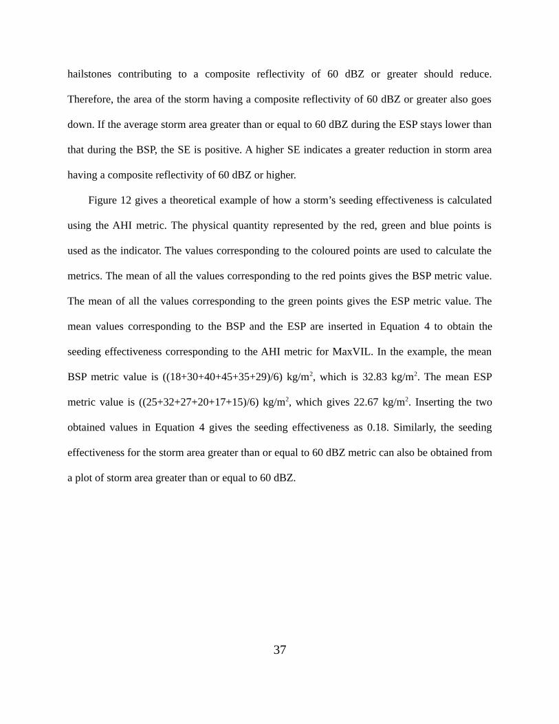
hailstones contributing to a composite reflectivity of 60 dBZ or greater should reduce.
Therefore, the area of the storm having a composite reflectivity of 60 dBZ or greater also goes
down. If the average storm area greater than or equal to 60 dBZ during the ESP stays lower than
that during the BSP, the SE is positive. A higher SE indicates a greater reduction in storm area
having a composite reflectivity of 60 dBZ or higher.
Figure 12 gives a theoretical example of how a storm’s seeding effectiveness is calculated
using the AHI metric. The physical quantity represented by the red, green and blue points is
used as the indicator. The values corresponding to the coloured points are used to calculate the
metrics. The mean of all the values corresponding to the red points gives the BSP metric value.
The mean of all the values corresponding to the green points gives the ESP metric value. The
mean values corresponding to the BSP and the ESP are inserted in Equation 4 to obtain the
seeding effectiveness corresponding to the AHI metric for MaxVIL. In the example, the mean
BSP metric value is ((18+30+40+45+35+29)/6) kg/m2, which is 32.83 kg/m2. The mean ESP
metric value is ((25+32+27+20+17+15)/6) kg/m2, which gives 22.67 kg/m2. Inserting the two
obtained values in Equation 4 gives the seeding effectiveness as 0.18. Similarly, the seeding
effectiveness for the storm area greater than or equal to 60 dBZ metric can also be obtained from
a plot of storm area greater than or equal to 60 dBZ.
37
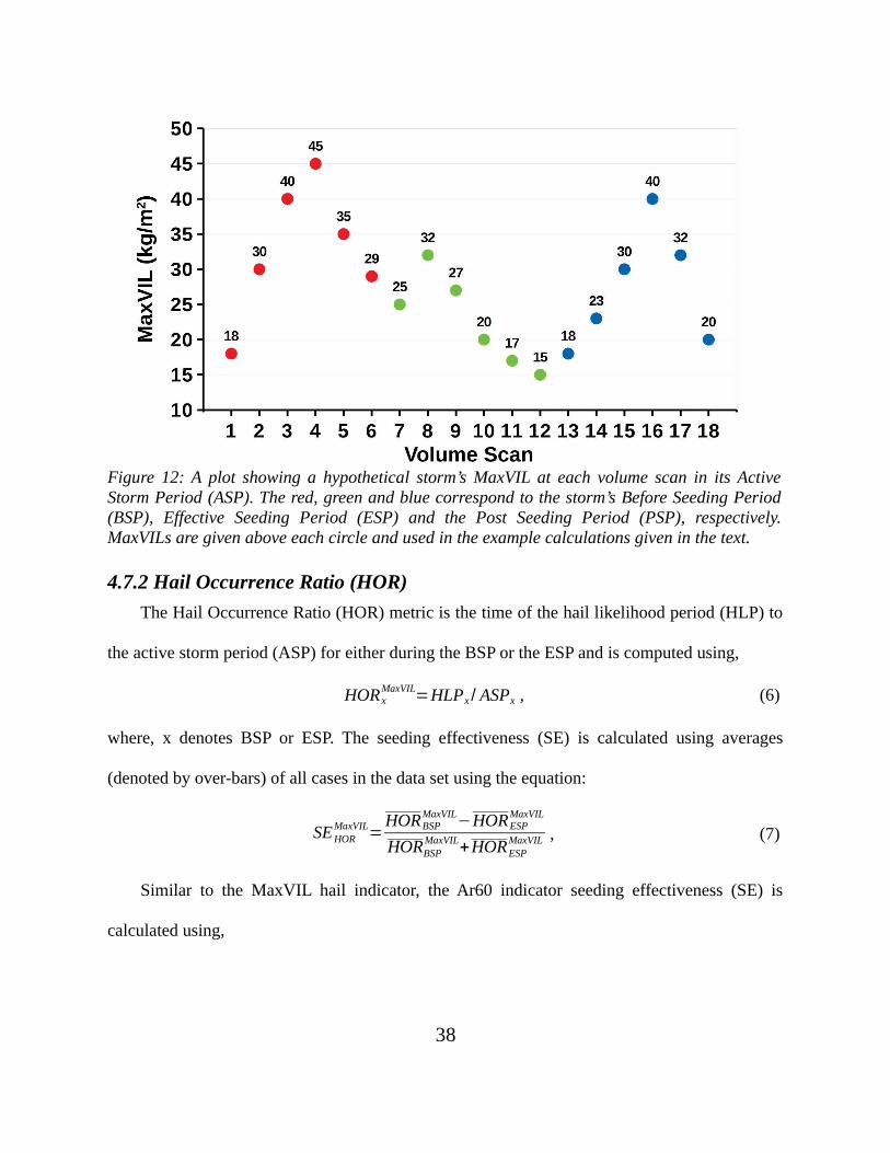
Figure 12: A plot showing a hypothetical storm’s MaxVIL at each volume scan in its Active
Storm Period (ASP). The red, green and blue correspond to the storm’s Before Seeding Period
(BSP), Effective Seeding Period (ESP) and the Post Seeding Period (PSP), respectively.
MaxVILs are given above each circle and used in the example calculations given in the text.
4.7.2 Hail Occurrence Ratio (HOR)
The Hail Occurrence Ratio (HOR) metric is the time of the hail likelihood period (HLP) to
the active storm period (ASP) for either during the BSP or the ESP and is computed using,
HORx
MaxVIL=HLPx / ASPx , (6)
where, x denotes BSP or ESP. The seeding effectiveness (SE) is calculated using averages
(denoted by over-bars) of all cases in the data set using the equation:
SEHOR
MaxVIL=HORBSP
MaxVIL−HORESPMaxVIL
HORBSP
MaxVIL+HORESP
MaxVIL , (7)
Similar to the MaxVIL hail indicator, the Ar60 indicator seeding effectiveness (SE) is
calculated using,
38

SEHOR
Ar 60=HORBSP
Ar 60−HORESP
Ar 60
HORBSP
Ar 60+HORESP
Ar 60 , (8)
The seeding effectiveness calculated using the Hail Occurrence Ratio (HOR) metric
measures the average change across all seed cases in the time fraction, for which damaging hail
is present from the BSP to the ESP. The seeding effectiveness gives a measure of the change in
time fraction, for which hail is present relative to the time fraction, for which hail is present
during the BSP. If seeding reduces the size of a hailstone sufficiently, the MaxVIL decreases
below the damage threshold. Hence, the MaxVIL stays above the damage threshold for a lesser
time. If the average time, for which the MaxVIL stays above the damage threshold during the
ESP is lesser than the average time, for which MaxVIL stays above the damage threshold during
the BSP, the SE is positive. A higher SE indicates a greater degree of reduction in the time, for
which the MaxVIL stays above the damage threshold. Similarly, if seeding reduces the size of
hailstones the number of damaging hailstones in the storm should reduce. Hence, the number of
hailstones contributing to a composite reflectivity of 60 dBZ or greater should reduce.
Consequently, the area of the storm having a composite reflectivity of 60 dBZ or higher also
goes down. Therefore, the time, for which the storm has an area with a composite reflectivity of
60 dBZ or higher also goes down. If the average time, for which the storm has an area greater
than or equal to 60 dBZ during the ESP is lesser than that during the BSP, the SE is positive. A
higher SE indicates a greater reduction in the time, for which the storm has an area with a
composite reflectivity of 60 dBZ or higher.
Figure 12 gives a theoretical example of how a storm’s seeding effectiveness is calculated
using the HOR metric. The physical quantity represented by the red, green and blue points is
39
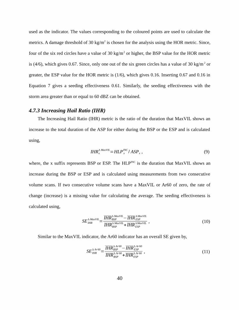
used as the indicator. The values corresponding to the coloured points are used to calculate the
metrics. A damage threshold of 30 kg/m2 is chosen for the analysis using the HOR metric. Since,
four of the six red circles have a value of 30 kg/m2 or higher, the BSP value for the HOR metric
is (4/6), which gives 0.67. Since, only one out of the six green circles has a value of 30 kg/m 2 or
greater, the ESP value for the HOR metric is (1/6), which gives 0.16. Inserting 0.67 and 0.16 in
Equation 7 gives a seeding effectiveness 0.61. Similarly, the seeding effectiveness with the
storm area greater than or equal to 60 dBZ can be obtained.
4.7.3 Increasing Hail Ratio (IHR)
The Increasing Hail Ratio (IHR) metric is the ratio of the duration that MaxVIL shows an
increase to the total duration of the ASP for either during the BSP or the ESP and is calculated
using,
IHRx
Δ MaxVIL=HLP x
INC / ASPx , (9)
where, the x suffix represents BSP or ESP. The HLPINC is the duration that MaxVIL shows an
increase during the BSP or ESP and is calculated using measurements from two consecutive
volume scans. If two consecutive volume scans have a MaxVIL or Ar60 of zero, the rate of
change (increase) is a missing value for calculating the average. The seeding effectiveness is
calculated using,
SE IHR
Δ MaxVIL=IHRBSP
Δ MaxVIL−IHRESPΔMaxVIL
IHRBSP
Δ MaxVIL+ IHRESP
ΔMaxVIL , (10)
Similar to the MaxVIL indicator, the Ar60 indicator has an overall SE given by,
SE IHR
Δ Ar 60=IHRBSP
Δ Ar 60−IHRESP
Δ Ar 60
IHRBSP
Δ Ar 60+IHRESP
Δ Ar 60 , (11)
40
The seeding effectiveness using the Increasing Hail Ratio (IHR) metric measures the
average change in the duration ratio of increasing hail indicator values between the BSP and the
ESP. The seeding effectiveness gives a measure of the change in the time fraction of increasing
indicator behaviour relative to the time fraction of increasing indicator behaviour during the
BSP. If seeding keeps on reducing the size of hailstones, the MaxVIL should keep on
decreasing. But, the seeding effectiveness is influenced by the opposing trends of natural
hailstone growth – which leads to MaxVIL increase and seeding – which leads to MaxVIL
decrease. Therefore, the MaxVIL can potentially show both an increase and decrease. But, if
seeding dominates the natural growth process, the duration for which the MaxVIL increases,
goes down. If the reduction in the duration of MaxVIL increase is more during the ESP than
during the BSP, the seeding effectiveness is positive. Similarly, if seeding reduces the size of
damaging hailstones, the storm area having a reflectivity of 60 dBZ or higher also reduces.
Therefore, the duration for which the storm area having a reflectivity of 60 dBZ or higher
increases also goes down. If the reduction is more during the ESP than during the BSP, the
seeding effectiveness is positive. A higher seeding effectiveness indicates a greater degree of
reduction.
Figure 12 gives a theoretical example of how a storm’s seeding effectiveness is calculated
using the IHR metric. The physical quantity represented by the red, green and blue points is
used as the indicator. The values corresponding to the coloured points are used to calculate the
metrics. Since, the values of the red circles increase thrice and there are six red circles, the
metric value corresponding to the BSP is (3/6), which gives 0.50. The values of the green circles
increase only once and there are six green circles. Therefore, the metric value corresponding to
41
the ESP is (1/6), which gives 0.16. Inserting, the values 0.50 and 0.16 in Equation 10 gives a
seeding effectiveness 0.51. Similarly, the seeding effectiveness corresponding to the storm area
greater than or equal to 60 dBZ can be obtained.
4.8 Interpretation of Seeding Effectiveness Metrics
A positive seeding effectiveness indicates a reduction in damaging hail while a negative
seeding effectiveness indicates an increase in damaging hail. Metrics generating a positive value
of seeding effectiveness indicate that those metrics may be effective at showing a seeding
response; with higher values of seeding effectiveness indicating a better seeding response.
Metrics giving a negative value of seeding effectiveness do not show a clear seeding response.
The inability to show a clear seeding response arises due to the individual cases having random
noisy results. The randomness appears because, the indicator values increase during the ESP in
some cases while decrease in the others. No consistent increase or decrease in the indicator
values is seen.
For a particular seed case, the seeding effectiveness calculated using one metric may come
out as positive; however a different metric may give a negative value. The results may reverse
for a different seed case. Such scenarios indicate that both the metrics are capable of showing a
seeding response but calculating seeding effectiveness value calculated using the metric values
of just a few cases likely does not provide an accurate result. Therefore, the seeding
effectiveness values are calculated using the average metric values of all 21 seed cases from the
2017 season.
42
5. RESULTS
5.1 Average Hail Indicator (AHI) Metric
The Average Hail Indicator seeding effectiveness using the MaxVIL and Ar60 indicators
are -0.03 and -0.11 respectively (Table 3). The seeding effectiveness for both the indicators are
negative, which indicates an increase in the indicator values during the ESP. Storms typically
develop following a basic life-cycle pattern of initialization, rapid intensification, and slow
decay. The Alberta Hail Suppression Project, almost always starts seeding storms during the
initialization phase, which results in storms naturally strengthening during seeding. Hence, the
hail indicator values can increase greatly during the ESP due to the natural life cycle of storms,
which can make many metrics poor at determining seeding effectiveness. Since, only 21 seed
cases are analyzed, the seeding effectiveness calculated using the AHI metric does not say much
about the effectiveness of cloud seeding towards hail suppression.
5.2 Hail Occurrence Ratio (HOR) Metric
The Hail Occurrence Ratio seeding effectiveness using the MaxVIL and the Ar60 indicators
are -0.09 and -0.02 respectively (Table 3). The seeding effectiveness for both the indicators are
negative. The negative SE indicates an increase in indicator values during the ESP. Since, the
Alberta Hail Suppression Project almost always starts seeding storms during the initialization
phase, the hail indicator values can increase greatly during the ESP and stay above the damage
threshold for a greater length of time than the BSP, thus making the seeding effectiveness
negative. The natural storm cycle likely affects this seeding effectiveness metric too.
43

5.3 Increasing Hail Ratio (IHR) Metric
The Increasing Hail Ratio seeding effectiveness using both the MaxVIL and the Ar60
indicators for the 21 storms is 0.12 (Table 3). The seeding effectiveness for both the indicators
are positive. Many times storms are seeded during their initial explosive-growth stages, and
seeding doesn’t “turn off” growing storms. Therefore, the hail indicator values increase greatly
during the ESP and stay above the damage threshold for a greater length of time. However,
seeding can slow this growth and sometimes the indicator values might even start to decrease
while still staying above the damage threshold. Such scenarios indicate a seeding response and
are captured through a positive seeding effectiveness calculated using the IHR Metric. It should
be noted that 21 is not a large number of cases; however, it is larger than looking at the post-
seeded changes, which had only 4 cases in 2017.
The magnitudes of the seeding effectiveness also give an interesting insight into the hail
suppression process. For the MaxVIL indicator, the magnitude of seeding effectiveness
calculated using the HOR metric is greater than that calculated using the AHI metric. This fact
indicates that the MaxVIL stays above the damage threshold for a greater length of time during
the ESP compared to the BSP. But, the mean MaxVIL during the ESP is only slightly larger
compared to the mean MaxVIL during the BSP. However, for the Ar60 indicator the magnitude
of seeding effectiveness calculated using the AHI metric is a lot larger compared to that
calculated using the HOR metric. The difference indicates that on an average the area greater
than or equal to 60 dBZ is substantially greater during the ESP compared to the BSP. But, the
ratio of time, for which the hailstorms have area greater than or equal to 60 dBZ reduces greatly
during the ESP compared to BSP. In a way, about 30 minutes after the start of seeding, the
44
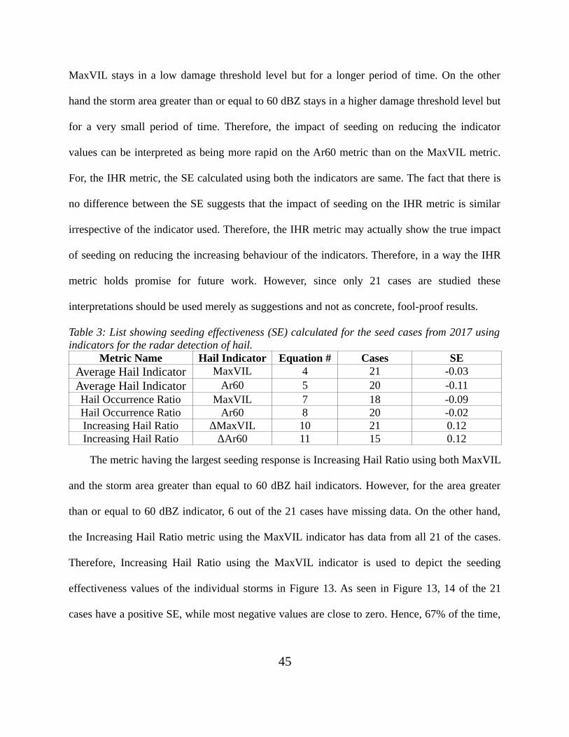
MaxVIL stays in a low damage threshold level but for a longer period of time. On the other
hand the storm area greater than or equal to 60 dBZ stays in a higher damage threshold level but
for a very small period of time. Therefore, the impact of seeding on reducing the indicator
values can be interpreted as being more rapid on the Ar60 metric than on the MaxVIL metric.
For, the IHR metric, the SE calculated using both the indicators are same. The fact that there is
no difference between the SE suggests that the impact of seeding on the IHR metric is similar
irrespective of the indicator used. Therefore, the IHR metric may actually show the true impact
of seeding on reducing the increasing behaviour of the indicators. Therefore, in a way the IHR
metric holds promise for future work. However, since only 21 cases are studied these
interpretations should be used merely as suggestions and not as concrete, fool-proof results.
Table 3: List showing seeding effectiveness (SE) calculated for the seed cases from 2017 using
indicators for the radar detection of hail.
Metric Name Hail Indicator Equation # Cases SE
Average Hail Indicator MaxVIL 4 21 -0.03
Average Hail Indicator Ar60 5 20 -0.11
Hail Occurrence Ratio MaxVIL 7 18 -0.09
Hail Occurrence Ratio Ar60 8 20 -0.02Increasing Hail Ratio ΔMaxVIL 10 21 0.12
Increasing Hail Ratio ΔAr60 11 15 0.12
The metric having the largest seeding response is Increasing Hail Ratio using both MaxVIL
and the storm area greater than equal to 60 dBZ hail indicators. However, for the area greater
than or equal to 60 dBZ indicator, 6 out of the 21 cases have missing data. On the other hand,
the Increasing Hail Ratio metric using the MaxVIL indicator has data from all 21 of the cases.
Therefore, Increasing Hail Ratio using the MaxVIL indicator is used to depict the seeding
effectiveness values of the individual storms in Figure 13. As seen in Figure 13, 14 of the 21
cases have a positive SE, while most negative values are close to zero. Hence, 67% of the time,
45
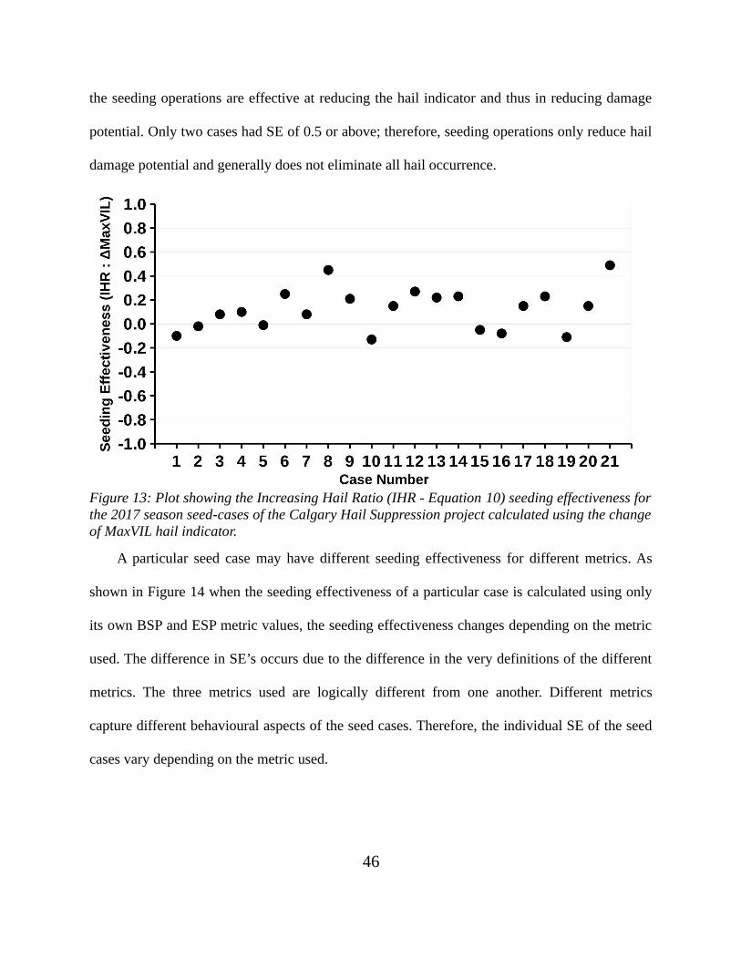
the seeding operations are effective at reducing the hail indicator and thus in reducing damage
potential. Only two cases had SE of 0.5 or above; therefore, seeding operations only reduce hail
damage potential and generally does not eliminate all hail occurrence.
Figure 13: Plot showing the Increasing Hail Ratio (IHR - Equation 10) seeding effectiveness for
the 2017 season seed-cases of the Calgary Hail Suppression project calculated using the change
of MaxVIL hail indicator.
A particular seed case may have different seeding effectiveness for different metrics. As
shown in Figure 14 when the seeding effectiveness of a particular case is calculated using only
its own BSP and ESP metric values, the seeding effectiveness changes depending on the metric
used. The difference in SE’s occurs due to the difference in the very definitions of the different
metrics. The three metrics used are logically different from one another. Different metrics
capture different behavioural aspects of the seed cases. Therefore, the individual SE of the seed
cases vary depending on the metric used.
46

Figure 14: Figure showing the individual seeding effectiveness (SE) of the seed cases calculated
using the six different metrics; Average Hail Indicator (AHI), Hail Occurrence Ration (HOR)
and Increasing Hail Ratio (IHR) for both Maximum Vertically Integrated Liquid (MaxVIL) and
storm area greater than or equal to 60 dBZ (Ar60). Figures 14A and 14E have the seeding
effectiveness (SE) of all 21 seed cases. However, the before seeding and effective seeding metric
values for case # 13 in Figure 14B, case #s 13, 14 and 15 in Figure 14C, case # 13 in Figure
14D and case #s 11, 13, 15, 16, 17, and 20 in Figure 14F are zero. Therefore, the SE for such
cases could not be computed and plotted.
As seen in the Figure 15 , the box plots for the six metrics all look very different from one
another. The interquartile ranges of the AHI metric for MaxVIL and both the IHR metrics are
quite low indicating the seeding effectiveness calculated using these metrics do not vary much
47
across the 21 seed cases. Therefore, these metrics show potential for future analysis and may be
used to carry out a seeded versus non-seeded analysis provided a sufficient number of
meteorologically similar seeded and non-seeded storms are obtained. On the other hand, the
interquartile ranges of the AHI metric for storm area greater than or equal to 60 dBZ and both
the HOR metrics are quite large indicating a lot of variation in the seeding effectiveness values
of the individual 21 seed cases. The high variation in the seeding effectiveness values indicate
these metrics may not be very useful tools in assessing the effectiveness of a cloud seeding
operation.
Figure 15: Box and whisker plots of the seeding effectiveness values for all analyzed seed cases
are shown in the figure. Seeding effectiveness is calculated for six metrics; Average Hail
Indicator (AHI), Hail Occurrence Ratio (HOR) and Increasing Hail Ratio (IHR) for both
MaxVIL and area greater than or equal to 60 dBZ indicators. The boxes show the interquartile
range (middle fifty percent of the values) and the red lines indicate the median of the seeding
effectiveness values. The diamonds show the outlier points, which are points having values
48

either 1.5 times greater or less than the width of the boxes (interquartile range); and her hence
deemed to be too far from the middle fifty-percent values.
6. DISCUSSION
None of the previous hail suppression programs specified any evaluation method in
particular. Therefore, any reasonable approach can be chosen to measure the effectiveness of a
seeding operation. Each approach implies the acceptance of a corresponding theory of how
seeding impacts the precipitation. Failure to detect a seeding effect using one particular
approach does not prove that no seeding effect exists. So, the same data can be analyzed using
different approaches. Each of the metrics used in the analysis of the Alberta Hail Suppression
Project has its own set of advantages and weaknesses. Logically, all three metrics can be used to
analyze seeding effectiveness but the lack of adequate number of cases – both seeded and non-
seeded makes it challenging to bring out their best features. To obtain a more convincing
statistically significant result using the methods discussed in this analysis, a greater number of
seed cases should be used. Using a greater number of seed cases will either add to the existing
randomness in the seeding effectiveness and strengthen the hailstorms’ lack of seeding response
or it will show a clear signal of a seeding response and offset the effects of the existing
randomness. Either way, the result would be statistically significant.
Throughout its life period a hailstorm is subjected to two contrasting processes – cloud
seeding and the natural growth process. According to our hypothesis, cloud seeding reduces
hailstone size. The reduction in hailstone size reduces the indicator values during the ESP than
during the BSP. But the storms’ natural variability along with the commencement of seeding
during the storm initialization phase causes the storms’ natural growth phase to fall in the ESP,
which results in the indicator values being higher during the ESP than during the BSP. When the
49

ESP metric values are higher than the BSP metric values, the SE is negative as seen in most of
the seed cases. But the SE calculated using IHR is positive, which creates a discrepancy
between the SE calculated using different metrics. In order to correct the discrepancy different
approaches can be taken. For all three of the metrics and especially the AHI and the HOR
metrics, the metric values during the PSP of seeded storms should be compared with those
during the BSP and the ESP. For the current analysis, only 4 out of the 21 cases had a PSP. For
all of those cases, a major portion of the PSP lay outside 100 km of the radar. Therefore, a
comparison of PSP with the BSP and ESP is not done. But, with sufficient data, such a
comparison should be possible. A comparison of the metrics during the BSP and ESP with the
PSP should give better insight into how the metrics change 20 minutes after the end of seeding.
For storms moving in a West-East direction seeding is stopped when storms cross the QE 2
highway because beyond that point the storms are not considered as a threat to the project area.
Such storms continue to grow before eventually decaying out naturally. Comparison of metric
values during the BSP, ESP and PSP of such storms is expected to give a clearer signal of the
hailstorms’ seeding response – especially 20 minutes after the end of seeding. But, not too many
hailstorms occur east or south of Calgary. So, data spanning over the 2014-2020 period should
be obtained in order to get a substantial number of hailstorms with a PSP.
Another approach that can be taken is a simple seeded versus non-seeded storm comparison
for all three of the metrics. Since the AHSP seeds all high-sheared storms threatening the project
area, it is almost impossible to get a non-seeded storm having a shear as high as a seeded storm
from the AHSP project area and the area south of it. So, a seeded versus non-seeded comparison
could not be done in this analysis. But, a significant number of hailstorms moving north of the
50
AHSP project area are left unseeded and some of those storms may have a shear comparable to
those of the seed cases. Data from such hailstorms can be captured using the Environment
Canada radar at Carvel. All three metrics should be calculated during the ASP of both non-
seeded and seeded hailstorms and compared to one another. Such a comparison could paint a
better picture as to whether hailstorms respond to seeding and if so, how well.
7. CONCLUSIONS AND BROADER IMPACTS
Several different methods of analysing seeding effectiveness have been investigated, with
the Increasing Hail Ratio metric for both MaxVIL and storm area greater than or equal to 60
dBZ indicators having the largest response to seeding based on the 21 cases from 2017. The
MaxVIL indicator is more sensitive to the size of large hail, while the Ar60 indicator is more
sensitive to the area of hail. Therefore, the Increasing Hail Ratio seeding effectiveness indicates
a reduction for both hail size and area. Examination of additional seasons’ data should increase
the statistical significance of the calculated seeding effectiveness.
Automated data-processing scripts have been developed; therefore, it will be
straightforward to analyze additional storms once they have been reviewed to determine the start
and end times of the pre-seeding, seeding, and post-seeding periods. Additionally, with more
seasons, statistical comparison between the seed cases and the non-seed cases may make more
sense since there will be a lot more storms available if the ratio (2 to 1) between the seed and
non-seed cases is maintained. The additional non-seed cases may make it possible to obtain
cases that are meteorologically similar to the seed cases; however, this may not be the case since
operations try to seed all storms that are likely to produce hail.
51

The SE are of interest to insurance companies that insure properties in hail likely locations.
An effective hail suppression operation would lead to lesser hail related property damage and
reduce the cost of premiums charged by the companies. If there are fewer hail related property
damages, the insurance companies would have to pay fewer hail related claims, which would
result in them being able to charge low insurance premiums. Lower premiums would make
insurance services affordable to a greater number of people. An increase in the number of clients
would generate more revenue for the insurance companies. More revenue might lead to the
insurance companies investing more in projects related to hail suppression. More investment in
hail suppression operations can lead to seeding missions over smaller towns that do not
currently receive the benefits of currently conducted hail suppression projects.
52

APPENDIX A: DEFINITION OF TERMS
The appendix gives a general but more fundamental definition of some of the terms that
have been used in the analysis of the hail suppression operation in Alberta. The appendix
intends to provide only a very simple and basic understanding of the terms. The terms have
specific definitions for the Alberta Hail Suppression Project. However, they can be defined
differently to suit the requirements of some other project. The conceptual idea of those terms
and the purpose of their use would still stay the same. Terms used in the definitions are given in
parenthesis.
Table 4: Important terms and their definitions.
Terms Definitions
Active Storm Period (ASP) Duration for which a “Case” stays within a pre-defineddistance (eg. 100 km) from a radar site
Analyzed Seed Case A “Seed Case” whose ASP has at least twelve minutes ofboth BSP and ESP.
Before Seeding Period (BSP) The difference between a “Case’s” start of SOP and 20minutes after the start of SOP.
Case A “TITAN Cell” spending twelve minutes or more whilebeing within a pre-defined distance or less from a radar site.
Cell A region in a storm characterized by very strong convectionand intense precipitation.
Effective Seeding Period (ESP) The difference between 20 minutes after the start of SOP and20 minutes after the end of SOP of a “Case”.
Hail Likelihood Period (HLP) Segment of the ASP during which a “Case” has indicator/sexceeding a certain value/s. The indicator values suggest the
presence of damaging hailstones in the “Case”.
Non-Analyzed Case A “Case” satisfying one or more of the following conditions:1. Treated with less than the minimum prescribed
quantity of seeding material.2. A “Seed Case” either (or both) of whose BSP or ESP
is shorter than twelve minutes.3. “Cases” passing over the radar cone of silence. 4. “Cases” moving along the foothills of the Rockies in
a North-South direction.5. “Cases” that do not receive radar waves because of
being obstructed by another “Cell”.
53
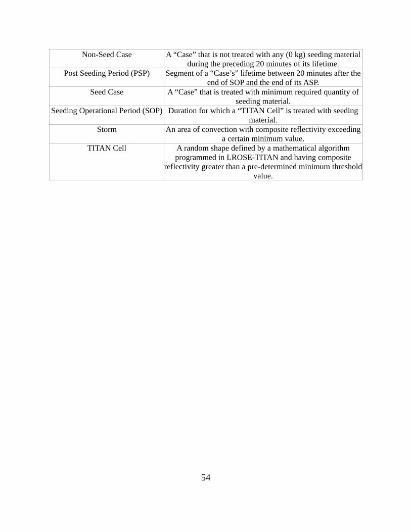
Non-Seed Case A “Case” that is not treated with any (0 kg) seeding materialduring the preceding 20 minutes of its lifetime.
Post Seeding Period (PSP) Segment of a “Case’s” lifetime between 20 minutes after theend of SOP and the end of its ASP.
Seed Case A “Case” that is treated with minimum required quantity ofseeding material.
Seeding Operational Period (SOP) Duration for which a “TITAN Cell” is treated with seedingmaterial.
Storm An area of convection with composite reflectivity exceedinga certain minimum value.
TITAN Cell A random shape defined by a mathematical algorithmprogrammed in LROSE-TITAN and having composite
reflectivity greater than a pre-determined minimum thresholdvalue.
54
REFERENCES
Alberta Research Council, 1986: Weather Modification in Alberta: Research and Operations 1980-85.
Alberta Research Council, Atmospheric Sciences Dept., Edmonton, AB,.
Auer, A. H., 1972: Distribution of Graupel and Hail With Size. Monthly Weather Review, 100, 325–328,
https://doi.org/10.1175/1520-0493-100-05-0325.
Austin, P. M., and A. C. Bemis, 1950: A Quantitative Study of the “Bright Band” in Radar Precipitation
Echoes. J. Meteor., 7, 145–151, https://doi.org/10.1175/1520-
0469(1950)007<0145:AQSOTB>2.0.CO;2.
Berthoumieu, J.-F., 2003: The Concept of Cloud Base Seeding With Hygroscopic Salts Flares for Hail
Prevention and Rain Precipitation. An Actualisation. Eighth WMO Scientific Conference on
Weather Modification, Casablanca, Morocco.
Billet, J., M. DeLisi, B. G. Smith, and C. Gates, 1997: Use of Regression Techniques to Predict Hail Size
and the Probability of Large Hail. Weather and Forecasting, 12, 154–164,
https://doi.org/10.1175/1520-0434(1997)012<0154:UORTTP>2.0.CO;2.
Brown, T. M., W. H. Pogorzelski, and I. M. Giammanco, 2015: Evaluating Hail Damage Using Property
Insurance Claims Data. Weather, Climate, and Society, 7, 197–210,
https://doi.org/10.1175/WCAS-D-15-0011.1.
Browning, K. A., 1977: The Structure and Mechanisms of Hailstorms. Hail: A Review of Hail Science and
Hail Suppression, S.W. Borland et al., Eds., Meteorological Monographs, American
Meteorological Society, 1–47.
Changnon Jr., S. A., and G. M. Morgan Jr., 1976: Design of an Experiment to Suppress Hail in Illinois.
Illinois State Water Survey, Urbana,.
Changnon Jr, S. C., 1975: Evaluation of an Operational Hail Suppression Project in Texas.
JournalWeaMod, 7, 88–100.
Changnon, S. A., 1977: On the Status of Hail Suppression. Bull. Amer. Meteor. Soc., 58, 20–28,
https://doi.org/10.1175/1520-0477(1977)058<0020:OTSOHS>2.0.CO;2.
——, 1999: Data and Approaches for Determining Hail Risk in the Contiguous United States. Journal of
Applied Meteorology and Climatology, 38, 1730–1739, https://doi.org/10.1175/1520-
0450(1999)038<1730:DAAFDH>2.0.CO;2.
Charlton, R. B., B. M. Kachman, and L. Wojtiw, 1995: Urban Hailstorms: A View From Alberta. Nat
Hazards, 12, 29–75, https://doi.org/10.1007/BF00605280.
55

Cook, G. R., 1995: Hail Loss Potential in the US. Boston, MA, 6 pp. [Available from Institute for Business
and Home Safety, 175 Federal St.,Suite 500, Boston, MA 02110-2222]., Insurance Institute of
Property Loss Reduction, 6 pp.
Cooper, W. A., and J. D. Marwitz, 1980: Winter Storms over the San Juan Mountains. Part III: Seeding
Potential. Journal of Applied Meteorology and Climatology, 19, 942–949,
https://doi.org/10.1175/1520-0450(1980)019<0942:WSOTSJ>2.0.CO;2.
——, R. T. Bruintjes, and G. K. Mather, 1997: Calculations Pertaining to Hygroscopic Seeding with Flares.
Journal of Applied Meteorology and Climatology, 36, 1449–1469, https://doi.org/10.1175/1520-
0450(1997)036<1449:CPTHSW>2.0.CO;2.
DeMott, P. J., 1999: Report to the Weather Modification, Incorporated on Tests of the Ice Nucleating
Ability of Aerosols Produced by New Formulation Pyrotechnics. Department of Atmospheric
Sciences, Colorado State University, Fort Collins, CO,.
Desjardins Insurance, 2017: Expensive and Deadly Hailstorm in Alberta I Desjardins Insurance.
desjardinsgeneralinsurance.com,. https://www.desjardinsgeneralinsurance.com/blog/-/the-
most-expensive-and-deadly-hailstorms-in-alberta-s-history (Accessed June 14, 2021).
Dessens, J., 1998: A Physical Evaluation of a Hail Suppression Project With Silver Iodide Ground Burners
in Southwestern France. Journal of Applied Meteorology and Climatology, 37, 1588–1599,
https://doi.org/10.1175/1520-0450(1998)037<1588:APEOAH>2.0.CO;2.
Devlin, P., 1996: Hail Property Damage in the US.: Development of Hail Resistant Shingles. Proc. Conf. on
Hail Damage Mitigation and Hail Science,. Bismarck, ND, North Dakota Atmospheric Resources
Board, 32–33.
——, 1997: Insurance Industry Strategies and Efforts in Mitigating Hail Loss. Proc. Conf. on Hail, The
Damage is Here, Overland Park, KS, Employers Reinsurance Corp., 33–40.
Dixon, M., and G. Wiener, 1993: TITAN: Thunderstorm Identification, Tracking, Analysis, and Nowcasting
—A Radar-based Methodology. J. Atmos. Oceanic Technol., 10, 785–797,
https://doi.org/10.1175/1520-0426(1993)010<0785:TTITAA>2.0.CO;2.
Donaldson, R. J., 1961: Radar Reflectivity Profiles in Thunderstorms. Journal of the Atmospheric
Sciences, 18, 292–305, https://doi.org/10.1175/1520-0469(1961)018<0292:RRPIT>2.0.CO;2.
Foote, G. B., 1984: A Study of Hail Growth Utilizing Observed Storm Conditions. Journal of Applied
Meteorology and Climatology, 23, 84–101, https://doi.org/10.1175/1520-
0450(1984)023<0084:ASOHGU>2.0.CO;2.
Gilbert, D. B., B. A. Boe, and T. W. Krauss, 2016: Twenty Seasons of Airborne Hail Suppression In Alberta,
Canada. The Journal of Weather Modification, 48, 68–92.
56

Grandia, K. L., D. S. Davison, and J. H. Renick, 1979: On the Dispersion of Silver Iodide in Alberta
Hailstorms. 7th Conference on Planned and Inadvertent Weather Modification, Banff, Alberta,
Canada, American Meteorological Society, Boston, MA, 56–57.
Greene, D. R., and R. A. Clark, 1972: Vertically Integrated Liquid Water—A New Analysis Tool. Monthly
Weather Review, 100, 548–552, https://doi.org/10.1175/1520-
0493(1972)100<0548:VILWNA>2.3.CO;2.
Hsie, E.-Y., R. D. Farley, and H. D. Orville, 1980: Numerical Simulation of Ice-Phase Convective Cloud
Seeding. J. Appl. Meteor., 19, 950–977, https://doi.org/10.1175/1520-
0450(1980)019<0950:NSOIPC>2.0.CO;2.
Iribarne, J. V., and R. G. de Pena, 1962: The Influence of Particle Concentration on the Evolution of
Hailstones. Nubila, 5, 7–30.
Krauss, T. W., and J. D. Marwitz, 1984: Precipitation Processes within an Alberta Supercell Hailstorm. J.
Atmos. Sci., 41, 1025–1035, https://doi.org/10.1175/1520-
0469(1984)041<1025:PPWAAS>2.0.CO;2.
Krauss, T. W., and J. Renick, 1997: The New Alberta Hail Suppression Project. The Journal of Weather
Modification, 29, 100–105.
Krauss, T. W., and J. R. Santos, 2004: Exploratory Analysis Of The Effect Of Hail Suppression Operations
On Precipitation In Alberta. Atmospheric Research, 71, 35–50,
https://doi.org/10.1016/j.atmosres.2004.03.004.
Krauss, T. W., R. E. Rinehart, J. L. Kollegger, and S. A. Kozak, 1998: VIL As A Predictor of Hail in Alberta.
Amer. Meteor. Soc., 14th Conf. on Planned and Inadvertent Weather Modification,.
Krick, I., and N. Stone, 1975: Hail suppression in Alberta 1956-1968. The Journal of Weather
Modification, 7, 101–115.
Long, A., 1975: Hail Suppression Analyses in NHRE, Paper Presented to NSF Advisory Panel for Weather
Modification Meeting. NSF, Washington, D.C., 1 p.
Marwitz, J. D., 1972a: The Structure and Motion of Severe Hailstorms. Part I: Supercell Storms. Journal
of Applied Meteorology and Climatology, 11, 166–179, https://doi.org/10.1175/1520-
0450(1972)011<0166:TSAMOS>2.0.CO;2.
——, 1972b: The Structure and Motion of Severe Hailstorms. Part II: Multi-Cell Storms. Journal of
Applied Meteorology and Climatology, 11, 180–188, https://doi.org/10.1175/1520-
0450(1972)011<0180:TSAMOS>2.0.CO;2.
——, 1972c: The Structure and Motion of Severe Hailstorms. Part III: Severely Sheared Storms. Journal
of Applied Meteorology and Climatology, 11, 189–201, https://doi.org/10.1175/1520-
0450(1972)011<0189:TSAMOS>2.0.CO;2.
57

Miller, J. R., E. I. Boyd, R. A. Schleusener, and A. S. Dennis, 1975: Hail Suppression Data from Western
North Dakota, 1969–1972. Journal of Applied Meteorology and Climatology, 14, 755–762,
https://doi.org/10.1175/1520-0450(1975)014<0755:HSDFWN>2.0.CO;2.
NCAR, 1974: National Hail Research Experiment Project Plan, 1975-1980. Boulder, Colorado, 286 pp.
——, 1976: The Status of NHRE. Staff Notes. Boulder, Colorado, 3–4.
Renick, J., 1975: The Alberta Hail Project: Update 1975. The Journal of Weather Modification, 7, 1–6.
Rinehart, R. E., 1997: Radar for Meteorologists. Third Edition. 428 pp.
Schickedanz, P. T., 1975: Evaluation of Hail Suppression. NCAR,.
Schickedanz, P. T., and S. A. Changnon, 1970: The Design and Evaluation of Hail Suppression
Experiments. Mon. Wea. Rev., 98, 242–251, https://doi.org/10.1175/1520-
0493(1970)098<0242:TDAEOH>2.3.CO;2.
Simpson, J., 1975: Assessments of Results of Hail Suppression Experiments Around the World. NCAR,.
Summers, P. W., and L. Wojtiw, 1971: The Economic Impact of Hail Damage in Alberta, Canada and its
Dependence on Various Hailfall Parameters. Seventh Conf. of Severe Local Storms, Kansas City,
Amer. Meteor. Soc., 158–163.
US Department of Commerce, 1991: Doppler Radar Meteorological Observations Part c. Federal
Meteorological Handbook 1 11, p. 105.
Ward, N. B., K. E. Wilk, and W. C. Hermann, 1965: WSR-57 Reflectivity Measurements and Hail
Observations. U.S. Weather Bureau, Environmental Science Services Administration,.
Weather Modification International, 2017: The Alberta Hail Suppression Project Executive Summary
2017, Final Operations Report. Alberta Severe Weather Management Society,.
Wilk, K. E., 1961: Radar Reflectivity Observations of Illinois Thunderstorms. Proceedings of the Ninth
Weather Radar Conference, Kansas City, Missouri, October 23-26, 1961, American
Meteorological Society, Boston, Mass., 127–132.
World Meteorological Organization, 1996: Meeting of Experts to Review The Present Status of Hail
Suppression.
58