Memory and attention in deep learning - arXiv
212
arXiv:2107.01390v1 [cs.LG] 3 Jul 2021 Memory and attention in deep learning by Hung Thai Le BSc. (Honours) Submitted in fulfilment of the requirements for the degree of Doctor of Philosophy Deakin University August 2019
-
Upload
khangminh22 -
Category
Documents
-
view
2 -
download
0
Transcript of Memory and attention in deep learning - arXiv
arX
iv:2
107.
0139
0v1
[cs
.LG
] 3
Jul
202
1
Memory and attention
in deep learning
by
Hung Thai Le
BSc. (Honours)
Submitted in fulfilment of the requirements for the degree of
Doctor of Philosophy
Deakin UniversityAugust 2019
Acknowledgements
I would like to thank my principal supervisor A/Prof. Truyen Tran for his continual
guidance and support. I have been lucky to have an outstanding supervisor with
deep insight and great vision, who has taught me valuable lessons for both my work
and personal life. I would also like to express my appreciation to my co-supervisor
Prof. Svetha Venkatesh for giving me the opportunity to undertake research at
PRaDA and for her valuable advice and inspirational talks. Thanks to my friends
Kien Do, Tung Hoang, Phuoc Nguyen, Vuong Le, Romelo, Tin Pham, Dung Nguyen,
Thao Le, Duc Nguyen and everyone else at PRaDA for making it an original and
interesting place to do research. Most of all, I would like to thank my parents, my
sister and my wife for their encouragement, love and support.
ii
Contents
Acknowledgements ii
Abstract xx
Relevant Publications xxiii
Notation 1
1 Introduction 1
1.1 Motivations . . . . . . . . . . . . . . . . . . . . . . . . . . . . . . . . 1
1.2 Aims and Scope . . . . . . . . . . . . . . . . . . . . . . . . . . . . . 3
1.3 Significance and Contribution . . . . . . . . . . . . . . . . . . . . . . 5
1.4 Thesis Structure . . . . . . . . . . . . . . . . . . . . . . . . . . . . . . 6
2 Taxonomy for Memory in RNNs 9
2.1 Memory in Brain . . . . . . . . . . . . . . . . . . . . . . . . . . . . . 9
2.1.1 Short-term Memory . . . . . . . . . . . . . . . . . . . . . . . . 9
2.1.2 Long-term Memory . . . . . . . . . . . . . . . . . . . . . . . . 10
2.2 Neural Networks and Memory . . . . . . . . . . . . . . . . . . . . . . 11
iii

Contents iv
2.2.1 Introduction to Neural Networks . . . . . . . . . . . . . . . . 11
2.2.2 Semantic Memory in Neural Networks . . . . . . . . . . . . . 15
2.2.3 Associative Neural Networks . . . . . . . . . . . . . . . . . . . 17
2.3 The Constructions of Memory in RNNs . . . . . . . . . . . . . . . . . 18
2.3.1 Attractor dynamics . . . . . . . . . . . . . . . . . . . . . . . 18
2.3.2 Transient Dynamics . . . . . . . . . . . . . . . . . . . . . . . 20
2.4 External Memory for RNNs . . . . . . . . . . . . . . . . . . . . . . . 22
2.4.1 Cell Memory . . . . . . . . . . . . . . . . . . . . . . . . . . . 23
2.4.2 Holographic Associative Memory . . . . . . . . . . . . . . . . 29
2.4.3 Matrix Memory . . . . . . . . . . . . . . . . . . . . . . . . . . 31
2.4.4 Sparse Distributed Memory . . . . . . . . . . . . . . . . . . . 33
2.5 Relation to Computational Models . . . . . . . . . . . . . . . . . . . 37
2.6 Closing Remarks . . . . . . . . . . . . . . . . . . . . . . . . . . . . . 39
3 Memory-augmented Neural Networks 40
3.1 Gated RNNs . . . . . . . . . . . . . . . . . . . . . . . . . . . . . . . . 40
3.1.1 Long Short-Term Memory . . . . . . . . . . . . . . . . . . . . 40
3.1.2 Gated Recurrent Unit . . . . . . . . . . . . . . . . . . . . . . 42
3.2 Attentional RNNs . . . . . . . . . . . . . . . . . . . . . . . . . . . . . 43
3.2.1 Encoder-Decoder Architecture . . . . . . . . . . . . . . . . . . 43
3.2.2 Attention Mechanism . . . . . . . . . . . . . . . . . . . . . . . 44
3.2.3 Multi-Head Attention . . . . . . . . . . . . . . . . . . . . . . 45
Contents v
3.3 Slot-Based Memory Networks . . . . . . . . . . . . . . . . . . . . . . 46
3.3.1 Neural Stack . . . . . . . . . . . . . . . . . . . . . . . . . . . 46
3.3.2 Memory Networks . . . . . . . . . . . . . . . . . . . . . . . . 49
3.3.3 Neural Turing Machine . . . . . . . . . . . . . . . . . . . . . . 50
3.3.4 Differentiable Neural Computer . . . . . . . . . . . . . . . . . 53
3.3.5 Memory-augmented Encoder-Decoder Architecture . . . . . . 54
3.4 Closing Remarks . . . . . . . . . . . . . . . . . . . . . . . . . . . . . 55
4 Memory Models for Multiple Processes 57
4.1 Introduction . . . . . . . . . . . . . . . . . . . . . . . . . . . . . . . . 57
4.1.1 Multi-Process Learning . . . . . . . . . . . . . . . . . . . . . . 57
4.1.2 Real-World Motivation . . . . . . . . . . . . . . . . . . . . . . 58
4.2 Background . . . . . . . . . . . . . . . . . . . . . . . . . . . . . . . . 62
4.2.1 Multi-View Learning . . . . . . . . . . . . . . . . . . . . . . . 62
4.2.2 Existing Approaches . . . . . . . . . . . . . . . . . . . . . . . 64
4.3 Dual Control Architecture . . . . . . . . . . . . . . . . . . . . . . . . 66
4.4 Dual Memory Architecture . . . . . . . . . . . . . . . . . . . . . . . . 68
4.4.1 Dual Memory Neural Computer . . . . . . . . . . . . . . . . . 68
4.4.2 Inference in DMNC . . . . . . . . . . . . . . . . . . . . . . . . 72
4.4.3 Persistent Memory for Multiple Admissions . . . . . . . . . . 73
4.5 Applications . . . . . . . . . . . . . . . . . . . . . . . . . . . . . . . . 74
4.5.1 Synthetic Task: Odd-Even Sequence Prediction . . . . . . . . 74
Contents vi
4.5.2 Treatment Recommendation Tasks . . . . . . . . . . . . . . . 77
4.5.3 Synthetic Task: Sum of Two Sequences . . . . . . . . . . . . . 79
4.5.4 Drug Prescription Task . . . . . . . . . . . . . . . . . . . . . . 82
4.5.5 Disease Progression Task . . . . . . . . . . . . . . . . . . . . . 84
4.6 Closing Remarks . . . . . . . . . . . . . . . . . . . . . . . . . . . . . 87
5 Variational Memory in Generative Models 89
5.1 Introduction . . . . . . . . . . . . . . . . . . . . . . . . . . . . . . . . 89
5.2 Preliminaries . . . . . . . . . . . . . . . . . . . . . . . . . . . . . . . 91
5.2.1 Conditional Variational Autoencoder (CVAE) for Conversa-
tion Generation . . . . . . . . . . . . . . . . . . . . . . . . . . 91
5.2.2 Related Works . . . . . . . . . . . . . . . . . . . . . . . . . . 92
5.3 Variational Memory Encoder-Decoder . . . . . . . . . . . . . . . . . 93
5.3.1 Generative Process . . . . . . . . . . . . . . . . . . . . . . . . 94
5.3.2 Neural Posterior Approximation . . . . . . . . . . . . . . . . . 95
5.3.3 Learning . . . . . . . . . . . . . . . . . . . . . . . . . . . . . . 96
5.3.4 Theoretical Analysis . . . . . . . . . . . . . . . . . . . . . . . 96
5.4 Experiments and Results . . . . . . . . . . . . . . . . . . . . . . . . . 98
5.4.1 Quantitative Results . . . . . . . . . . . . . . . . . . . . . . . 98
5.4.2 Qualitative Analysis . . . . . . . . . . . . . . . . . . . . . . . 100
5.5 Closing Remarks . . . . . . . . . . . . . . . . . . . . . . . . . . . . . 102
6 Optimal Writing Memory 103
Contents vii
6.1 Introduction . . . . . . . . . . . . . . . . . . . . . . . . . . . . . . . 103
6.2 Related Backgrounds . . . . . . . . . . . . . . . . . . . . . . . . . . . 104
6.3 Theoretical Analysis on Memorisation . . . . . . . . . . . . . . . . . 106
6.3.1 Generic Memory Operations . . . . . . . . . . . . . . . . . . . 106
6.3.2 Memory Analysis of RNNs . . . . . . . . . . . . . . . . . . . . 107
6.3.3 Memory Analysis of MANNs . . . . . . . . . . . . . . . . . . . 107
6.4 Optimal Writing for Slot-based Memory Models . . . . . . . . . . . . 109
6.4.1 Uniform Writing . . . . . . . . . . . . . . . . . . . . . . . . . 109
6.4.2 Local Optimal Design . . . . . . . . . . . . . . . . . . . . . . 110
6.4.3 Local Memory-Augmented Attention Unit . . . . . . . . . . . 111
6.5 Experiments and Results . . . . . . . . . . . . . . . . . . . . . . . . . 111
6.5.1 An Ablation Study: Memory-Augmented Neural Networks
with and without Uniform Writing . . . . . . . . . . . . . . . 111
6.5.2 Synthetic Memorisation . . . . . . . . . . . . . . . . . . . . . 113
6.5.3 Synthetic Reasoning . . . . . . . . . . . . . . . . . . . . . . . 114
6.5.4 Synthetic Sinusoidal Regression . . . . . . . . . . . . . . . . . 115
6.5.5 Flatten Image Recognition . . . . . . . . . . . . . . . . . . . . 116
6.5.6 Document Classification . . . . . . . . . . . . . . . . . . . . . 117
6.6 Closing Remarks . . . . . . . . . . . . . . . . . . . . . . . . . . . . . 118
7 Neural Stored-Program Memory 120
7.1 Introduction . . . . . . . . . . . . . . . . . . . . . . . . . . . . . . . . 120
Contents viii
7.2 Backgrounds . . . . . . . . . . . . . . . . . . . . . . . . . . . . . . . . 121
7.2.1 Turing Machines and MANNs . . . . . . . . . . . . . . . . . . 121
7.2.2 Related Approaches . . . . . . . . . . . . . . . . . . . . . . . . 123
7.3 Neural Stored-Program Memory and Neural Universal Turing Machine124
7.3.1 Neural Stored-Program Memory . . . . . . . . . . . . . . . . . 124
7.3.2 Neural Universal Turing Machine . . . . . . . . . . . . . . . . 125
7.3.3 On the Benefit of NSM to MANN: An Explanation from Mul-
tilevel Modeling . . . . . . . . . . . . . . . . . . . . . . . . . . 126
7.4 Applications . . . . . . . . . . . . . . . . . . . . . . . . . . . . . . . . 127
7.4.1 NTM Single Tasks . . . . . . . . . . . . . . . . . . . . . . . . 127
7.4.2 NTM Sequencing Tasks . . . . . . . . . . . . . . . . . . . . . 129
7.4.3 Continual Procedure Learning . . . . . . . . . . . . . . . . . . 130
7.4.4 Few-Shot Learning . . . . . . . . . . . . . . . . . . . . . . . . 131
7.4.5 Text Question Answering . . . . . . . . . . . . . . . . . . . . 132
7.5 Closing Remarks . . . . . . . . . . . . . . . . . . . . . . . . . . . . . 133
8 Conclusions 134
8.1 Summary . . . . . . . . . . . . . . . . . . . . . . . . . . . . . . . . . 134
8.2 Future Directions . . . . . . . . . . . . . . . . . . . . . . . . . . . . . 135
Appendix 137
C Supplementary for Chapter 5 . . . . . . . . . . . . . . . . . . . . . . 137
C.1 Proof of Theorem 5.1 . . . . . . . . . . . . . . . . . . . . . . . 137
Contents ix
C.2 Derivation of the Upper Bound on the Total Timestep-Wise
KL Divergence . . . . . . . . . . . . . . . . . . . . . . . . . . 138
C.3 ProofT∏
t=1gt (x) =
T∏t=1
K∑i=1
πitg
it (x) Is a Scaled MoG . . . . . . . . 140
C.4 Details of Data Descriptions and Model Implementations . . . 141
C.5 Full Reports on Model Performance . . . . . . . . . . . . . . . 143
D Supplementary for Chapter 6 . . . . . . . . . . . . . . . . . . . . . . 144
D.1 Derivation on the Bound Inequality in Linear Dynamic System 144
D.2 Derivation on the Bound Inequality in Standard RNN . . . . . 145
D.3 Derivation on the Bound Inequality in LSTM . . . . . . . . . 146
D.4 Proof of Theorem 6.1 . . . . . . . . . . . . . . . . . . . . . . . 147
D.5 Proof of Theorem 6.2 . . . . . . . . . . . . . . . . . . . . . . . 148
D.6 Proof of Theorem 6.3 . . . . . . . . . . . . . . . . . . . . . . . 148
D.7 Summary of Synthetic Discrete Task Format . . . . . . . . . . 149
D.8 UW Performance on Bigger Memory . . . . . . . . . . . . . . 149
D.9 Memory Operating Behaviors on Synthetic Tasks . . . . . . . 150
D.10 Visualisations of Model Performance on Sinusoidal Regression
Tasks . . . . . . . . . . . . . . . . . . . . . . . . . . . . . . . . 151
D.11 Comparison with Non-Recurrent Methods in Flatten Image
Classification Task . . . . . . . . . . . . . . . . . . . . . . . . 152
D.12 Details on Document Classification Datasets . . . . . . . . . . 153
D.13 Document Classification Detailed Records . . . . . . . . . . . 154
E Supplementary for Chapter 7 . . . . . . . . . . . . . . . . . . . . . . 155
Contents x
E.1 Full Learning Curves on Single NTM Tasks . . . . . . . . . . 155
E.2 Clustering on The Latent Space . . . . . . . . . . . . . . . . . 155
E.3 Program Usage Visualisations . . . . . . . . . . . . . . . . . . 156
E.3.1 Visualisation on Program Distribution across Timesteps
(Single Tasks) . . . . . . . . . . . . . . . . . . . . . . 157
E.3.2 Visualisation on Program Distribution across Timesteps
(Sequencing Tasks) . . . . . . . . . . . . . . . . . . . 160
E.3.3 Perseveration Phenomenon in NTM (Sequencing Tasks)162
E.4 Details on Synthetic Tasks . . . . . . . . . . . . . . . . . . . . 164
E.4.1 NTM Single Tasks . . . . . . . . . . . . . . . . . . . 164
E.4.2 NTM Sequencing Tasks . . . . . . . . . . . . . . . . 164
E.4.3 Continual Procedure Learning Tasks . . . . . . . . . 165
E.5 Details on Few-Shot Learning Task . . . . . . . . . . . . . . . 165
E.6 Details on bAbI Task . . . . . . . . . . . . . . . . . . . . . . . 168
E.7 Others . . . . . . . . . . . . . . . . . . . . . . . . . . . . . . . 169
Bibliography 170
List of Figures
2.1 Types of memory in cognitive models . . . . . . . . . . . . . . . . . . 11
2.2 A multilayer perceptron with a single hidden-layer. . . . . . . . . . . 12
2.3 A typical Recurrent Neural Network (Left) and its unfolded repre-
sentation (Right). Each neuron at timestep t takes into consideration
the current input xt and previous hidden state ht−1 to generate the
t-th output ot. W , U and V are learnable weight matrices of the model. 14
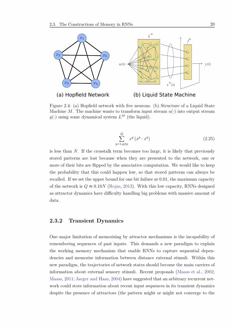
2.4 (a) Hopfield network with five neurons. (b) Structure of a Liquid
State Machine M . The machine wants to transform input stream
u(·) into output stream y(·) using some dynamical system LM (the
liquid). . . . . . . . . . . . . . . . . . . . . . . . . . . . . . . . . . . 20
2.5 Error back flow from ϑu (t) to ϑv (t− q) in the computation graph.
Each computation node has n children. Each product term corre-
sponds to a computation path of depth q from node u to v. The sum
of nq−1 products is the total error. . . . . . . . . . . . . . . . . . . . 24
2.6 (a) Example of a tree encoded by TPR. (b) SDM’s memory write
(red) and read (blue) access. The read and write involve all memory
locations around the queried points. . . . . . . . . . . . . . . . . . . . 34
2.7 Relation between external memory and computational models . . . . 39
3.1 Block diagram of a modern LSTM unit. × and + are element-wise
product and add operators, respectively. σ and tanh are sigmoid and
tanh functions, respectively. . . . . . . . . . . . . . . . . . . . . . . . 41
xi
List of Figures xii
3.2 (a) Seq2Seq Model. Gray and green denote the LSTM encoder and
decoder, respectively. In this architecture, the output at each decod-
ing step can be fed as input for the next decoding step. (b) Seq2Seq
Model with attention mechanism. The attention computation is re-
peated across decoding steps. . . . . . . . . . . . . . . . . . . . . . . 44
3.3 Computation stages of the encoding using self-attention (a) and encoding-
decoding architecture–The Transformer (b). Embedding layers con-
vert input/output tokens to vectors of fix dimension, followed by Posi-
tional Encoding layers that add temporal information to each vector.
The main block of computation combines multi-head attention, resid-
ual connection, layer normalisation and Feed-forward layers, which
can be repeated multiple times. . . . . . . . . . . . . . . . . . . . . . 47
3.4 (a) Architecture of NTM. Circles denote intermediate variables com-
puted by the controller. The controller takes the current timestep
data xt and the previous read value rt−1 as the input and produces
rt, updates memory Mt and predict output ot. (b) Architecture of
DNC. The operation is similar to NTM’s with extra modules to keep
track of memory usage ut, precedence pt and link matrix Lt. . . . . . 51
4.1 Dual Controller Write-Protected Memory Augmented Neural Net-
work. LSTME is the encoding controller. LSTMD is the decoding
controller. Both are implemented as LSTMs. . . . . . . . . . . . . . 66
4.2 Dual Memory Neural Computer. LSTM i1 , LSTM i2 are the two en-
coding controllers implemented as LSTMs. LSTMd is the decod-
ing controller. The dash arrows represent cross-memory accessing in
early-fusion mode. . . . . . . . . . . . . . . . . . . . . . . . . . . . . 68
4.3 Training Loss of Odd-Even Task . . . . . . . . . . . . . . . . . . . . . 75
4.4 Training NLD of Odd-Even Task . . . . . . . . . . . . . . . . . . . . 75
4.5 Read Modes of MANNs on Odd-Even Task . . . . . . . . . . . . . . . 76
4.6 Training Loss of Drug Prescription Task . . . . . . . . . . . . . . . . 79
4.7 Testing Loss of Drug Prescription Task . . . . . . . . . . . . . . . . . 79
List of Figures xiii
4.8 Training loss of sum of two sequences task. The training error curves
have similar patterns. . . . . . . . . . . . . . . . . . . . . . . . . . . . 80
4.9 M1’s gwt over diagnoses. Diagnosis codes of a MIMIC-III patient is
listed along the x-axis (ordered by priority) with the y-axis indicating
how much the write gate allows a diagnosis to be written to the
memory M1. . . . . . . . . . . . . . . . . . . . . . . . . . . . . . . . . 86
4.10 M2’s gwt over procedures. Medical procedure codes of a MIMIC-III
patient is listed along the x-axis (in the order of executions) with the
y-axis indicating how much the write gate allows a procedure to be
written to the memory M2. . . . . . . . . . . . . . . . . . . . . . . . 87
5.1 Graphical Models of the vanilla CVAE (a) and our proposed VMED
(b) . . . . . . . . . . . . . . . . . . . . . . . . . . . . . . . . . . . . . 93
5.2 Training and testing of VMED . . . . . . . . . . . . . . . . . . . . . . 97
6.1 Writing mechanism in Cached Uniform Writing. During non-writing
intervals, the controller hidden states are pushed into the cache.
When the writing time comes, the controller attends to the cache,
chooses suitable states and accesses the memory. The cache is then
emptied. . . . . . . . . . . . . . . . . . . . . . . . . . . . . . . . . . 108
6.2 The accuracy (%) and computation time reduction (%) with different
memory types and number of memory slots. The controllers/sequence
lengths/memory sizes are chosen as LSTM/50/{2, 4, 9, 24} (a&b) and
RNN/30/{2, 4, 9, 14} (c&d), respectively. . . . . . . . . . . . . . . . 112
6.3 Learning curves of models in clean (a) and noisy (b) sinusoid regres-
sion experiment. . . . . . . . . . . . . . . . . . . . . . . . . . . . . . . 116
7.1 Introducing NSM into MANN. At each timestep, the program inter-
face network (PI) receives input from the state network and queries
the program memory Mp, acquiring the working weight for the inter-
face network (W ct ). The interface network then operates on the data
memory M. . . . . . . . . . . . . . . . . . . . . . . . . . . . . . . . 126
List of Figures xiv
7.2 Learning curves on NTM tasks. . . . . . . . . . . . . . . . . . . . . . 127
7.3 (a,b,c) visualises NUTM’s executions in synthetic tasks: the upper
rows are memory read (left)/write (right) locations; the lower rows
are program distributions over timesteps. The green line indicates
the start of the decoding phase. (d) visualises perservation in NTM:
the upper row are input, output, predicted output with errors (orange
bits); the lower row is reading location. . . . . . . . . . . . . . . . . 129
7.4 Learning curves on sequencing NTM tasks. . . . . . . . . . . . . . . . 130
7.5 Mean bit accuracy for the continual algorithmic tasks. Each of the
first four panels show bit accuracy on four tasks after finishing a task.
The rightmost shows the average accuracy. . . . . . . . . . . . . . . . 131
D.1 Memory operations on copy task in DNC (a), DNC+UW (b) and
DNC+CUW(c). Each row is a timestep and each column is a memory
slot. . . . . . . . . . . . . . . . . . . . . . . . . . . . . . . . . . . . . 151
D.2 Memory operations on max task in DNC (a), DNC+UW (b) and
DNC+CUW(c). Each row is a timestep and each column is a memory
slot. . . . . . . . . . . . . . . . . . . . . . . . . . . . . . . . . . . . . 151
D.3 Sinusoidal generation with clean input sequence for DNC, UW and
CUW in top-down order. . . . . . . . . . . . . . . . . . . . . . . . . 152
D.4 Sinusoidal generation with noisy input sequence for DNC, UW and
CUW in top-down order. . . . . . . . . . . . . . . . . . . . . . . . . 153
E.1 Learning curves on NTM tasks. . . . . . . . . . . . . . . . . . . . . . 155
E.2 Visualisation of the first two principal components of ct space in NTM
(a,c) and NUTM (b,d) for Copy (red) and Repeat Copy (blue). Fader
color denotes lower timestep in a sequence. Both can learn clusters
of hidden states yet NUTM exhibits clearer partition. . . . . . . . . 156
E.3 Copy (p=2). . . . . . . . . . . . . . . . . . . . . . . . . . . . . . . . . 157
E.4 Repeat Copy (p=2). . . . . . . . . . . . . . . . . . . . . . . . . . . . 157
List of Figures xv
E.5 Associative Recall (p=2). . . . . . . . . . . . . . . . . . . . . . . . . . 158
E.6 Dynamic N-grams (p=2). . . . . . . . . . . . . . . . . . . . . . . . . . 158
E.7 Priority Sort (p=2). . . . . . . . . . . . . . . . . . . . . . . . . . . . . 159
E.8 Long Copy (p=2). . . . . . . . . . . . . . . . . . . . . . . . . . . . . . 159
E.9 Copy+Repeat Copy (p=3). . . . . . . . . . . . . . . . . . . . . . . . 160
E.10 Copy+Associative Recall (p=3). . . . . . . . . . . . . . . . . . . . . . 160
E.11 Copy+Priority Sort (p=3). . . . . . . . . . . . . . . . . . . . . . . . . 161
E.12 Copy+Repeat Copy+Associative Recall+Priority Sort (p=4). . . . . 161
E.13 Copy+Repeat Copy perseveration (only Repeat Copy). . . . . . . . . 162
E.14 Copy+Associative Recall perseveration (only Copy). . . . . . . . . . . 162
E.15 Copy+Priority Sort perseveration (only Copy). . . . . . . . . . . . . . 163
E.16 Copy+Repeat Copy+Associative Recall+Priority Sort perseveration
(only Repeat Copy). . . . . . . . . . . . . . . . . . . . . . . . . . . . 163
E.17 Testing accuracy during training (five random classes/episode, one-
hot vector labels, of length 50). . . . . . . . . . . . . . . . . . . . . . 166
E.18 Testing accuracy during training (ten random classes/episode, one-
hot vector labels, of length 75). . . . . . . . . . . . . . . . . . . . . . 167
List of Tables
4.1 Test Results on Odd-Even Task (lower is better) . . . . . . . . . . . . 76
4.2 Statistics of MIMIC-III sub-datasets . . . . . . . . . . . . . . . . . . 77
4.3 Results on MIMIC-III dataset for procedure prediction and drug pre-
scription (higher is better). . . . . . . . . . . . . . . . . . . . . . . . . 78
4.4 Sum of two sequences task test results. Max train sequence length is
10. . . . . . . . . . . . . . . . . . . . . . . . . . . . . . . . . . . . . . 79
4.5 MIMIC-III data statistics. . . . . . . . . . . . . . . . . . . . . . . . . 82
4.6 Mimic-III drug prescription test results. . . . . . . . . . . . . . . . . . 82
4.7 Example Recommended Medications by DMNCs on MIMIC-III dataset.
Bold denotes matching against ground-truth. . . . . . . . . . . . . . . 85
4.8 Regional hospital test results. P@K is precision at top K predictions
in %. . . . . . . . . . . . . . . . . . . . . . . . . . . . . . . . . . . . . 86
5.1 BLEU-1, 4 and A-Glove on testing datasets. B1, B4, AG are acronyms
for BLEU-1, BLEU-4, A-Glove metrics, respectively (higher is bet-
ter). . . . . . . . . . . . . . . . . . . . . . . . . . . . . . . . . . . . . 98
5.2 Examples of context-response pairs. /*/ denotes separations between
stochastic responses. . . . . . . . . . . . . . . . . . . . . . . . . . . . 101
6.1 Test accuracy (%) on synthetic memorisation tasks. MANNs have 4
memory slots. . . . . . . . . . . . . . . . . . . . . . . . . . . . . . . . 114
xvi
List of Tables xvii
6.2 Test accuracy (%) on synthetic reasoning tasks. MANNs have 4 mem-
ory slots. . . . . . . . . . . . . . . . . . . . . . . . . . . . . . . . . . . 115
6.3 Test accuracy (%) on MNIST, pMNIST. Previously reported results
are from the literature (Le et al., 2015)†, (Arjovsky et al., 2016)◦,
(Trinh et al., 2018)⋆, and (Chang et al., 2017)�. . . . . . . . . . . . . 117
6.4 Document classification accuracy (%) on several datasets. Previ-
ously reported results are from the literature (Conneau et al., 2016)•,
(Yogatama et al., 2017)∗, (Seo et al., 2018)‡ and (Qui et al., 2018)N.
We use italics to denote the best published and bold the best records. 118
7.1 Generalisation performance of best models measured in average bit
error per sequence (lower is better). For each task, we pick a set of
1,000 unseen sequences as test data. . . . . . . . . . . . . . . . . . . 128
7.2 Test-set classification accuracy (%) on the Omniglot dataset after
100,000 episodes of training. * denotes available results from Santoro
et al., (2016). See Appendix E.5 for more details. . . . . . . . . . . . 132
7.3 Mean and s.d. for bAbI error (%). . . . . . . . . . . . . . . . . . . . . 133
C.1 Results on Cornell Movies . . . . . . . . . . . . . . . . . . . . . . . . 143
C.2 Results on OpenSubtitles . . . . . . . . . . . . . . . . . . . . . . . . . 143
C.3 Results on LJ users question-answering . . . . . . . . . . . . . . . . . 143
C.4 Results on Reddit comments . . . . . . . . . . . . . . . . . . . . . . . 144
D.1 Synthetic discrete task’s input-output formats. T is the sequence
length. . . . . . . . . . . . . . . . . . . . . . . . . . . . . . . . . . . . 149
D.2 Test accuracy (%) on synthetic copy task. MANNs have 50 memory
slots. Both models are trained with 100,000 mini-batches of size 32. . 149
D.3 Test accuracy (%) on MNIST, pMNIST. Previously reported results
are from Vaswani et al., (2017)⋆ and Chang et al., (2017)�. . . . . . 152
List of Tables xviii
D.4 Statistics on several big document classification datasets . . . . . . . 153
D.5 Document classification accuracy (%) on several datasets reported for
3 different runs. Bold denotes the best records. . . . . . . . . . . . . 154
E.1 Model hyper-parameters (single tasks). . . . . . . . . . . . . . . . . . 164
E.2 Task settings (single tasks). . . . . . . . . . . . . . . . . . . . . . . . 164
E.3 Model hyper-parameters (sequencing tasks). . . . . . . . . . . . . . . 164
E.4 Task settings (sequencing tasks). . . . . . . . . . . . . . . . . . . . . 165
E.5 Task settings (continual procedure learning tasks). . . . . . . . . . . . 165
E.6 Hyper-parameters for few-shot learning. . . . . . . . . . . . . . . . . . 166
E.7 Test-set classification accuracy (%) on the Omniglot dataset after
100,000 episodes of training. * denotes available results from Santoro
et al., (2016) (some are estimated from plotted figures). . . . . . . . . 167
E.8 NUTM hyper-parameters for bAbI. . . . . . . . . . . . . . . . . . . . 168
E.9 NUTM (p = 4) bAbI best and mean errors (%). . . . . . . . . . . . . 168
List of Algorithms
2.1 Memory writing in SDM . . . . . . . . . . . . . . . . . . . . . . . . . 35
4.1 Training algorithm for healthcare data (set output) . . . . . . . . . . 70
5.1 VMED Generation . . . . . . . . . . . . . . . . . . . . . . . . . . . . 95
6.1 Cached Uniform Writing . . . . . . . . . . . . . . . . . . . . . . . . . 110
7.1 Neural Universal Turing Machine . . . . . . . . . . . . . . . . . . . . 127
xix
Abstract
Intelligence necessitates memory. Without memory, humans fail to perform various
nontrivial tasks such as reading novels, playing games or solving maths. As the
ultimate goal of machine learning is to derive intelligent systems that learn and act
automatically just like human, memory construction for machine is inevitable.
Artificial neural networks model neurons and synapses in the brain by interconnect-
ing computational units via weights, which is a typical class of machine learning
algorithms that resembles memory structure. Their descendants with more com-
plicated modeling techniques (a.k.a deep learning) have been successfully applied
to many practical problems and demonstrated the importance of memory in the
learning process of machinery systems.
Recent progresses on modeling memory in deep learning have revolved around ex-
ternal memory constructions, which are highly inspired by computational Turing
models and biological neuronal systems. Attention mechanisms are derived to sup-
port acquisition and retention operations on the external memory. Despite the lack
of theoretical foundations, these approaches have shown promises to help machinery
systems reach a higher level of intelligence. The aim of this thesis is to advance the
understanding on memory and attention in deep learning. Its contributions include:
(i) presenting a collection of taxonomies for memory, (ii) constructing new memory-
augmented neural networks (MANNs) that support multiple control and memory
units, (iii) introducing variability via memory in sequential generative models, (iv)
searching for optimal writing operations to maximise the memorisation capacity in
slot-based memory networks, and (v) simulating the Universal Turing Machine via
Neural Stored-program Memory–a new kind of external memory for neural networks.
The simplest form of MANNs consists of a neural controller operating on an ex-
ternal memory, which can encode/decode one stream of sequential data at a time.
Our proposed model called Dual Controller Write-Protected Memory Augmented
xx
Abstract xxi
Neural Network extends MANNs to using dual controllers executing the encoding
and decoding process separately, which is essential in some healthcare applications.
One notable feature of our model is the write-protected decoding for maintaining
the stored information for long inference. To handle two streams of inputs, we
propose a model named Dual Memory Neural Computer that consists of three con-
trollers working with two external memory modules. These designs provide MANNs
with more flexibility to process structural data types and thus expand the range of
application for MANNs. In particular, we demonstrate that our architectures are
effective for various healthcare tasks such as treatment recommendation and disease
progression.
Learning generative models for sequential discrete data such as utterances in con-
versation is a challenging problem. Standard neural variational encoder-decoder
networks often result in either trivial or digressive conversational responses. To
tackle this problem, our second work presents a novel approach that models vari-
ability in stochastic sequential processes via external memory, namely Variational
Memory Encoder-Decoder. By associating each read head of the memory with a
mode in the mixture distribution governing the latent space, our model can capture
the variability observed in natural conversations.
The third work aims to give a theoretical explanation on optimal memory operations.
We realise that the scheme of regular writing in current MANN is suboptimal in
memory utilisation and introduces computational redundancy. A theoretical bound
on the amount of information stored in slot-based memory models is formulated
and our goal is to search for optimal writing schemes that maximise the bound.
The proposed solution named Uniform Writing is proved to be optimal under the
assumption of equal contribution amongst timesteps. To balance between max-
imising memorisation and overwriting forgetting, we modify the original solution,
resulting in a solution dubbed Cached Uniform Writing. The proposed solutions are
empirically demonstrated to outperform other recurrent architectures, claiming the
state-of-the-arts in various sequential tasks.
MANNs can be viewed as a neural realisation of Turing Machines and thus, can
learn algorithms and other complex tasks. By leveraging neural network simulation
of Turing Machines to neural architecture for Universal Turing Machines, we develop
a new class of MANNs that uses Neural Stored-program Memory to store the weights
of the controller, thereby following the stored-program principle in modern computer
architectures. By validating the computational universality of the approach through
Abstract xxii
an extensive set of experiments, we have demonstrated that our models not only
excel in classical algorithmic problems, but also have potential for compositional,
continual, few-shot learning and question-answering tasks.
Relevant Publications
Part of this thesis has been published or documented elsewhere. The details of these
publications are as follows:
Chapter 4:
• Le, H., Tran, T., & Venkatesh, S. (2018). Dual control memory augmented
neural networks for treatment recommendations. In Pacific-Asia Conference
on Knowledge Discovery and Data Mining (pp. 273-284). Springer, Cham.
• Le, H., Tran, T., & Venkatesh, S. (2018). Dual memory neural computer for
asynchronous two-view sequential learning. In Proceedings of the 24th ACM
SIGKDD International Conference on Knowledge Discovery & Data Mining
(pp. 1637-1645). ACM.
Chapter 5:
• Le, H., Tran, T., Nguyen, T., & Venkatesh, S. (2018). Variational memory
encoder-decoder. In Advances in Neural Information Processing Systems (pp.
1508-1518).
Chapter 6:
• Le, H., Tran, T., & Venkatesh, S. (2019). Learning to Remember More with
Less Memorization. In International Conference on Learning Representations.
2019.
Chapter 7:
xxiii
Relevant Publications xxiv
• Le, H., Tran, T., & Venkatesh, S. (2019). Neural Stored-program Memory. In
International Conference on Learning Representations. 2020.
Although not the main contributions, the following collaborative work is the appli-
cation of some work in the thesis:
• Khan, A., Le, H., Do, K., Tran, T., Ghose, A., Dam, H., & Sindhgatta, R.
(2018). Memory-augmented neural networks for predictive process analytics.
arXiv preprint arXiv:1802.00938.
Chapter 1
Introduction
1.1 Motivations
In a broad sense, memory is the ability to store, retain and then retrieve infor-
mation on request. In human brain, memory is involved in not just remembering
and forgetting but also reasoning, attention, insight, abstract thinking, appreciation
and imagination. Modern machine learning models find and transfer patterns from
training data into some form of memory that will be utilised during inference. In the
case of neural networks, long-term memories on output-input associations are stored
in the weights on the connections between processing units. These connections are
a simple analogy of synapses between neurons and this form of memory simulates
the brain’s neocortex responsible for gradual acquisition of data patterns. Learning
in such scenario is slow since the signal from the output indicating how to adjust
the connecting weights will be both noisy and weak (Kumaran et al., 2016). While
receiving training data samples, the learning algorithm performs small update per
sample to reach a global optimisation for the whole set of data.
It is crucial to keep in mind that memory in neural networks does not limit to
the concept of storing associations in the observed data. For example, in sequential
processes, where the individual data points are no longer independent and identically
distributed (i.i.d.), some form of short-term memory must be constructed across
sequence before the output is given to the network for weight updating. Otherwise,
the long-term memory on associations between the output and inputs, which are
given at different timestamps, will never be achieved. Interestingly, both forms of
1
1.1. Motivations 2
memory are found in Recurrent Neural Networks (RNNs) (Elman, 1990; Jordan,
1997; Rumelhart et al., 1988)– a special type of neural network capable of modeling
sequences. The featured short-term memory, also referred to as working memory,
has been known to relate with locally stable points (Hopfield, 1982; Sussillo, 2014) or
transient dynamics (Maass et al., 2002; Jaeger and Haas, 2004) of RNNs. Although
these findings shed light into the formation of the working memory, the beneath
memory mechanisms and how they affect the learning process remain unclear. With
the rise of deep learning, more layers with complicated interconnections between
neurons have been added to neural networks. These complications make it harder
to understand and exploit the working memory mechanisms. Worse still, due to
its short-term capacity, the working memory in RNNs struggles to cope with long
sequences. These challenges require new interpretations and designs of memory for
deep learning in general and RNNs in particular.
In recent years, memory-augmented neural networks (MANNs) emerge as a new
form of memory construction for RNNs. They model external memories explic-
itly and thus, overcome the short-term limitation of the working memory. Known
as one of the first attempts at representing explicit memory for RNNs, the Long
Short-Term Memory (LSTM) (Hochreiter and Schmidhuber, 1997) stores the “world
states” in a cell memory vector, which is determined after a single exposure of input
at each timestep. By referring to the cell memory, LSTM can bridge longer time
lags between relevant input and output events, extending the range of RNN’s work-
ing memory. Recent advances have proposed new external memory modules with
multiple memory vectors (slots) supporting attentional retrieval and fast-update
(Graves et al., 2014; Graves et al., 2016; Weston et al., 2014). The memory slots
are accessed and computed fast by a separated controller whose parameters are
slowly learnt weights. Because these memories are external and separated, it is con-
venient to derive theoretical explanations on memorisation capacity (Gulcehre et al.,
2017; Le et al., 2019). Nonetheless, with bigger memory and flexible read/write op-
erators, these models significantly outperform other recurrent counterparts in var-
ious long-term sequential testbeds such as algorithmic tasks (Graves et al., 2014;
Graves et al., 2016), reasoning over graphs (Graves et al., 2016), continual learning
(Lopez-Paz et al., 2017), few-shot learning (Santoro et al., 2016; Le et al., 2020a),
healthcare (Le et al., 2018c; Prakash et al., 2017; Le et al., 2018b), process analyt-
ics (Khan et al., 2018), natural language understanding (Le et al., 2018a, 2019) and
video question-answering (Gao et al., 2018).
In this thesis, we focus on external memory of MANNs by explaining and promoting
1.2. Aims and Scope 3
its influence on deep neural architectures. In the original formulation of MANNs, one
controller is allowed to operate on one external memory. This simple architecture is
suitable for supervised sequence labeling tasks where a sequence of inputs with tar-
get labels are provided for supervised training. However, single controller/memory
design is limited for tasks involving sequence-to-sequence and especially, multi-view
sequential mappings. For example, an electronic medical record (EMR) contains
information on patient’s admissions, each of which consists of various views such
as diagnosis, medical procedure, and medicine. The complexity of view interac-
tions, together with the unalignment and long-term dependencies amongst views
poses a great challenge for classical MANNs. One important aspect of external
memory is its role in imagination or generative models. Sequence generation can
be supported by RNNs (Graves, 2013; Chung et al., 2015), yet how different kinds
of memory in RNNs or MANNs cooperate in this process has not been adequately
addressed. Another underexplored problem is to measure memorisation capacity of
MANNs. There is no theoretical analysis or clear understanding on optimal oper-
ations that a memory should have to maximise its capacity. Finally, the current
form of external memory is definitely not the ultimate memory mechanism for deep
learning. Current MANNs are equivalent to neural simulations of Turing Machines
(Graves et al., 2014). Hence, in terms of computational capacity, MANNs are not
superior to RNNs, which are known to be Turing-complete (Siegelmann and Sontag,
1995). This urges new designs of external memory for MANNs that express higher
computational power and more importantly, reach the capacity of human memory.
1.2 Aims and Scope
This thesis focuses on expanding the capacity of MANNs. Our objectives are:
• To construct a taxonomy for memory in RNNs.
• To design novel MANN architectures for modeling different aspects of mem-
ory in solving complicated tasks, which include multiple processes, generative
memory, optimal operation, and universality.
• To apply such architectures to a wide range of sequential problems, especially
those require memory to remember long-term contexts.
We study several practical problems that require memory:
1.2. Aims and Scope 4
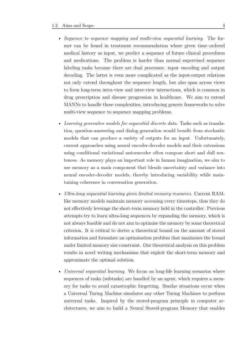
• Sequence to sequence mapping and multi-view sequential learning. The for-
mer can be found in treatment recommendation where given time–ordered
medical history as input, we predict a sequence of future clinical procedures
and medications. The problem is harder than normal supervised sequence
labeling tasks because there are dual processes: input encoding and output
decoding. The latter is even more complicated as the input-output relations
not only extend throughout the sequence length, but also span across views
to form long-term intra-view and inter-view interactions, which is common in
drug prescription and disease progression in healthcare. We aim to extend
MANNs to handle these complexities, introducing generic frameworks to solve
multi-view sequence to sequence mapping problems.
• Learning generative models for sequential discrete data. Tasks such as transla-
tion, question-answering and dialog generation would benefit from stochastic
models that can produce a variety of outputs for an input. Unfortunately,
current approaches using neural encoder-decoder models and their extensions
using conditional variational autoencoder often compose short and dull sen-
tences. As memory plays an important role in human imagination, we aim to
use memory as a main component that blends uncertainty and variance into
neural encoder-decoder models, thereby introducing variability while main-
taining coherence in conversation generation.
• Ultra-long sequential learning given limited memory resources. Current RAM-
like memory models maintain memory accessing every timesteps, thus they do
not effectively leverage the short-term memory held in the controller. Previous
attempts try to learn ultra-long sequences by expanding the memory, which is
not always feasible and do not aim to optimise the memory by some theoretical
criterion. It is critical to derive a theoretical bound on the amount of stored
information and formulate an optimisation problem that maximises the bound
under limited memory size constraint. Our theoretical analysis on this problem
results in novel writing mechanisms that exploit the short-term memory and
approximate the optimal solution.
• Universal sequential learning. We focus on long-life learning scenarios where
sequences of tasks (subtasks) are handled by an agent, which requires a mem-
ory for tasks to avoid catastrophic forgetting. Similar situations occur when
a Universal Turing Machine simulates any other Turing Machines to perform
universal tasks. Inspired by the stored-program principle in computer ar-
chitectures, we aim to build a Neural Stored-program Memory that enables
1.3. Significance and Contribution 5
MANNs to switch tasks through time, adapt to variable contexts and thus
fully resemble the Universal Turing Machine or Von Neumann Architecture.
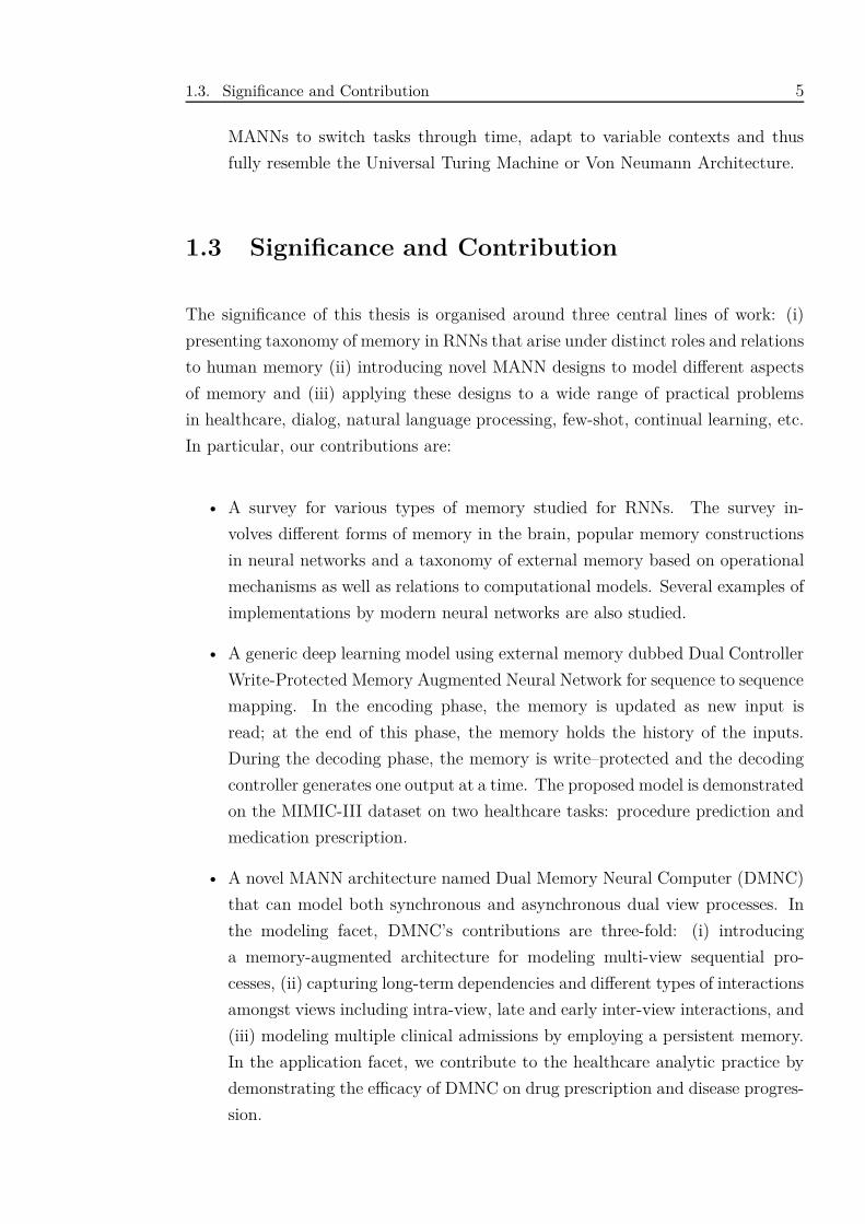
1.3 Significance and Contribution
The significance of this thesis is organised around three central lines of work: (i)
presenting taxonomy of memory in RNNs that arise under distinct roles and relations
to human memory (ii) introducing novel MANN designs to model different aspects
of memory and (iii) applying these designs to a wide range of practical problems
in healthcare, dialog, natural language processing, few-shot, continual learning, etc.
In particular, our contributions are:
• A survey for various types of memory studied for RNNs. The survey in-
volves different forms of memory in the brain, popular memory constructions
in neural networks and a taxonomy of external memory based on operational
mechanisms as well as relations to computational models. Several examples of
implementations by modern neural networks are also studied.
• A generic deep learning model using external memory dubbed Dual Controller
Write-Protected Memory Augmented Neural Network for sequence to sequence
mapping. In the encoding phase, the memory is updated as new input is
read; at the end of this phase, the memory holds the history of the inputs.
During the decoding phase, the memory is write–protected and the decoding
controller generates one output at a time. The proposed model is demonstrated
on the MIMIC-III dataset on two healthcare tasks: procedure prediction and
medication prescription.
• A novel MANN architecture named Dual Memory Neural Computer (DMNC)
that can model both synchronous and asynchronous dual view processes. In
the modeling facet, DMNC’s contributions are three-fold: (i) introducing
a memory-augmented architecture for modeling multi-view sequential pro-
cesses, (ii) capturing long-term dependencies and different types of interactions
amongst views including intra-view, late and early inter-view interactions, and
(iii) modeling multiple clinical admissions by employing a persistent memory.
In the application facet, we contribute to the healthcare analytic practice by
demonstrating the efficacy of DMNC on drug prescription and disease progres-
sion.
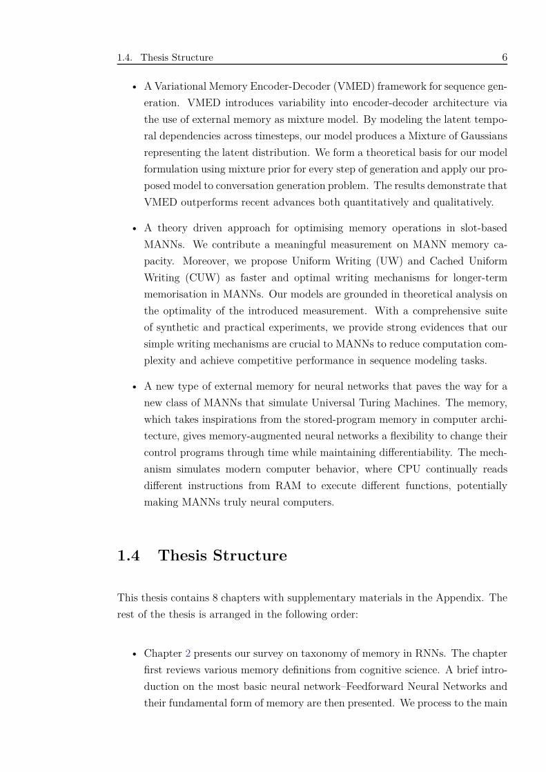
1.4. Thesis Structure 6
• A Variational Memory Encoder-Decoder (VMED) framework for sequence gen-
eration. VMED introduces variability into encoder-decoder architecture via
the use of external memory as mixture model. By modeling the latent tempo-
ral dependencies across timesteps, our model produces a Mixture of Gaussians
representing the latent distribution. We form a theoretical basis for our model
formulation using mixture prior for every step of generation and apply our pro-
posed model to conversation generation problem. The results demonstrate that
VMED outperforms recent advances both quantitatively and qualitatively.
• A theory driven approach for optimising memory operations in slot-based
MANNs. We contribute a meaningful measurement on MANN memory ca-
pacity. Moreover, we propose Uniform Writing (UW) and Cached Uniform
Writing (CUW) as faster and optimal writing mechanisms for longer-term
memorisation in MANNs. Our models are grounded in theoretical analysis on
the optimality of the introduced measurement. With a comprehensive suite
of synthetic and practical experiments, we provide strong evidences that our
simple writing mechanisms are crucial to MANNs to reduce computation com-
plexity and achieve competitive performance in sequence modeling tasks.
• A new type of external memory for neural networks that paves the way for a
new class of MANNs that simulate Universal Turing Machines. The memory,
which takes inspirations from the stored-program memory in computer archi-
tecture, gives memory-augmented neural networks a flexibility to change their
control programs through time while maintaining differentiability. The mech-
anism simulates modern computer behavior, where CPU continually reads
different instructions from RAM to execute different functions, potentially
making MANNs truly neural computers.
1.4 Thesis Structure
This thesis contains 8 chapters with supplementary materials in the Appendix. The
rest of the thesis is arranged in the following order:
• Chapter 2 presents our survey on taxonomy of memory in RNNs. The chapter
first reviews various memory definitions from cognitive science. A brief intro-
duction on the most basic neural network–Feedforward Neural Networks and
their fundamental form of memory are then presented. We process to the main
1.4. Thesis Structure 7
part that covers Recurrent Neural Networks (RNNs) and memory categories
for RNNs based on their formations. Further interpretations on memory tax-
onomy based on operational mechanisms and automata simulations are also
investigated.
• Chapter 3 reviews a special branch of memory in RNNs and also the main
focus of this thesis: memory-augmented neural networks (MANNs). We first
describe the Long Short-term Memory (LSTM) and its variants. Next, we
also spend a section for attention mechanism–a featured operation commonly
exploited in accessing external memory in MANNs. We then introduce several
advanced developments that empower RNNs with multiple memory slots, espe-
cially generic slot-based memory architectures such as Neural Turing Machine
and Differentiable Neural Computer.
• Chapter 4 introduces Dual Control Memory-augmented Neural Network (DC-
MANN), an extension of MANN to model sequence to sequence mapping. Our
model supports write-protected decoding (DCw-MANN), which is empirically
proved suitable for sequence-to-sequence task. We further extend our DC-
MANN to a broader range of problems where the input can come from multiple
channels. To be specific, we propose a general structure Dual Memory Neural
Computer (DMNC) that can capture the correlations between two views by
exploiting two external memory units. We conduct the experiments to validate
the performance of these models on applications in healthcare.
• Chapter 5 presents a novel memory-augmented generation framework called
Variational Memory Encoder-Decoder. Our external memory plays a role as
a mixture model distribution generating the latent variables to produce the
output and take part in updating the memory for future generation steps. We
adapt Stochastic Gradient Variational Bayes framework to train our model by
minimising variational approximation of KL divergence to accommodate the
Mixture of Gaussians in the latent space. We derive theoretical analysis to
backup our training protocol and evaluate our model on two open-domain and
two closed-domain conversational datasets.
• Chapter 6 suggests a meaningful measurement on MANN’s memory capacity.
We then formulate an optimisation problem that maximises the bound on the
proposed measurement. The proposed solution dubbed Uniform Writing is
optimal under the assumption of equal timestep contributions. To relax this
assumption, we introduce modifications to the original solution, resulting in a
new solution termed Cached Uniform Writing. This method aims to balance
1.4. Thesis Structure 8
between memorising and forgetting via allowing overwriting mechanism. To
validate the effectiveness of our solutions, we conduct experiments on six ultra-
long sequential learning problems given a limited number of memory slots.
• Chapter 7 interprets MANNs as neural realisations of Turing Machines. The
chapter points out a missing component–the stored-program memory, that is
potential for making current MANNs truly neural computers. Then, a design
of Neural Stored-program Memory (NSM) is proposed to implement stored-
program principle, together with new MANN architectures that materialise
Universal Turing Machines. The significance of NSM lies in its formulation
as a new form of memory, standing in between slow-weight and fast-weight
concepts. NSM not only induces Universal Turing Machine realisations, which
imply universal artificial intelligence, but also defines another type of adaptive
weights, from which other neural networks can also reap benefits.
• Chapter 8 summarises the main content of the thesis and outlines future di-
rections.
Chapter 2
Taxonomy for Memory in RNNs
2.1 Memory in Brain
Memory is a crucial part of any cognitive model studying the human mind. This sec-
tion briefly reviews memory types studied throughout the cognitive and neuroscience
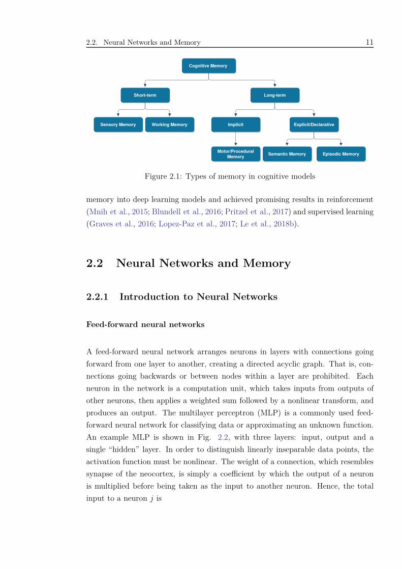
literature. Fig. 2.1 shows a taxonomy of cognitive memory (Kotseruba and Tsotsos,
2018).
2.1.1 Short-term Memory
Sensory memory Sensory memory caches impressions of sensory information af-
ter the original stimuli have ended. It can also preprocess the information before
transmitting it to other cognitive processes. For example, echoic memory keeps
acoustic stimulus long enough for perceptual binding and feature extraction pro-
cesses. Sensory memory is known to associate with temporal lope in the brain. In
the neural network literature, sensory memory can be designed as neural networks
without synaptic learning (Johnson et al., 2013).
Working memory Working memory holds temporary storage of information re-
lated to the current task such as language comprehension, learning, and reasoning
(Baddeley, 1992). Just like computer that uses RAM for its computations, the brain
needs working memory as a mechanism to store and update information to perform
9
2.1. Memory in Brain 10
cognitive tasks such as attention, reasoning and learning. Human neuroimaging
studies show that when people perform tasks requiring them to hold short-term
memory, such as the location of a flash of light, the prefrontal cortex becomes ac-
tive (Curtis and D’Esposito, 2003). As we shall see later, recurrent neural networks
must construct some form of working memory to help the networks learn the task
at hand. As working memory is short-term (Goldman-Rakic, 1995), the working
memory in RNNs also tends to vanish quickly and needs the support from other
memory mechanisms to learn complex tasks that require long-term dependencies.
2.1.2 Long-term Memory
Motor/procedural memory The procedural memory, which is known to link
to basal ganglia in the brain, contains knowledge about how to get things done in
motor task domain. The knowledge may involve co-coordinating sequences of motor
activity, as would be needed when dancing, playing sports or musical instruments.
This procedural knowledge can be implemented by a set of if-then rules learnt for
a particular domain or a neural network representing perceptual-motor associations
(Salgado et al., 2012).
Semantic memory Semantic memory contains knowledge about facts, concepts,
and ideas. It allows us to identify objects and relationships between them. Semantic
memory is a highly structured system of information learnt gradually from the world.
The brain’s neocortex is responsible for semantic memory and its processing is seen
as the propagation of activation amongst neurons via weighted connections that
slowly change (Kumaran et al., 2016).
Episodic memory Episodic memory stores specific instances of past experience.
Different from semantic memory, which does not require temporal and spatial in-
formation, episodic remembering restores past experiences indexed by event time
or context (Tulving et al., 1972). Episodic memory is widely acknowledged to
depend on the hippocampus, acting like an autoassociate memory that binds di-
verse inputs from different brain areas that represent the constituents of an event
(Kumaran et al., 2016). It is conjectured that the experiences stored in hippocam-
pus transfer to neocortex to form semantic knowledge as we sleep via consoli-
dation process. Recently, many attempts have been made to integrate episodic
2.2. Neural Networks and Memory 11
Cognitive Memory
Short-term Long-term
Sensory Memory Working Memory Implicit
Motor/Procedural
Memory
Explicit/Declarative
Episodic MemorySemantic Memory
Figure 2.1: Types of memory in cognitive models
memory into deep learning models and achieved promising results in reinforcement
(Mnih et al., 2015; Blundell et al., 2016; Pritzel et al., 2017) and supervised learning
(Graves et al., 2016; Lopez-Paz et al., 2017; Le et al., 2018b).
2.2 Neural Networks and Memory
2.2.1 Introduction to Neural Networks
Feed-forward neural networks
A feed-forward neural network arranges neurons in layers with connections going
forward from one layer to another, creating a directed acyclic graph. That is, con-
nections going backwards or between nodes within a layer are prohibited. Each
neuron in the network is a computation unit, which takes inputs from outputs of
other neurons, then applies a weighted sum followed by a nonlinear transform, and
produces an output. The multilayer perceptron (MLP) is a commonly used feed-
forward neural network for classifying data or approximating an unknown function.
An example MLP is shown in Fig. 2.2, with three layers: input, output and a
single “hidden” layer. In order to distinguish linearly inseparable data points, the
activation function must be nonlinear. The weight of a connection, which resembles
synapse of the neocortex, is simply a coefficient by which the output of a neuron
is multiplied before being taken as the input to another neuron. Hence, the total
input to a neuron j is
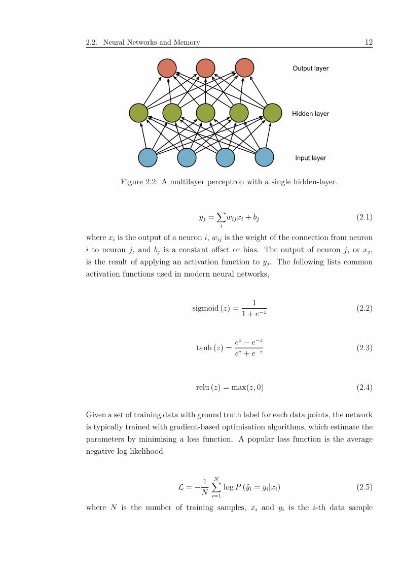
2.2. Neural Networks and Memory 12
Figure 2.2: A multilayer perceptron with a single hidden-layer.
yj =∑
i
wijxi + bj (2.1)
where xi is the output of a neuron i, wij is the weight of the connection from neuron
i to neuron j, and bj is a constant offset or bias. The output of neuron j, or xj ,
is the result of applying an activation function to yj. The following lists common
activation functions used in modern neural networks,
sigmoid (z) =1
1 + e−z(2.2)
tanh (z) =ez − e−z
ez + e−z(2.3)
relu (z) = max(z, 0) (2.4)
Given a set of training data with ground truth label for each data points, the network
is typically trained with gradient-based optimisation algorithms, which estimate the
parameters by minimising a loss function. A popular loss function is the average
negative log likelihood
L = − 1N
N∑
i=1
log P (yi = yi|xi) (2.5)
where N is the number of training samples, xi and yi is the i-th data sample
2.2. Neural Networks and Memory 13
and its label, respectively, and yi is the predicted label. During training, forward
propagation outputs yi and calculates the loss function. An algorithm called back-
propagation, which was first introduced in (Rumelhart et al., 1988), computes the
gradients of the loss function L with respect to (w.r.t) the parameters θ = {wij , bj}.Then, an optimisation algorithm such as stochastic gradient descent updates the
parameters based on their gradients{
∂L∂wij
, ∂L∂bj
}as follows,
wij := wij − λ∂L
∂wij(2.6)
bj := bj − λ∂L∂bj
(2.7)
where λ is a small learning rate.
Recurrent neural networks
A recurrent neural network (RNN) is an artificial neural network where connections
between nodes form a directed graph with self-looped feedback. This allows the
network to capture the hidden states calculated so far when activation functions of
neurons in the hidden layer are fed back to the input layer at every time step in con-
junction with other input features. The ability to maintain the state of the system
makes RNN especially useful for processing sequential data such as sound, natural
language or time series signals. So far, many varieties of RNN have been proposed
such as Hopfield Network (Hopfield, 1982), Echo State Network (Jaeger and Haas,
2004) and Jordan Network (Jordan, 1997). Here, for the ease of analysis, we only
discuss Elman’s RNN model (Elman, 1990) with single hidden layer as shown in
Fig. 2.3.
An Elman RNN consists of three layers, which are input (x ∈ RN), hidden (h ∈ RD)
and output (o ∈ RM) layer. At each timestep, the feedback connection forwards the
previous hidden state ht−1 to the current hidden unit, together with the values from
input layer xt, to compute the current state ht and output value ot. The forward
pass begins with a specification of the initial state h0, then we apply the following
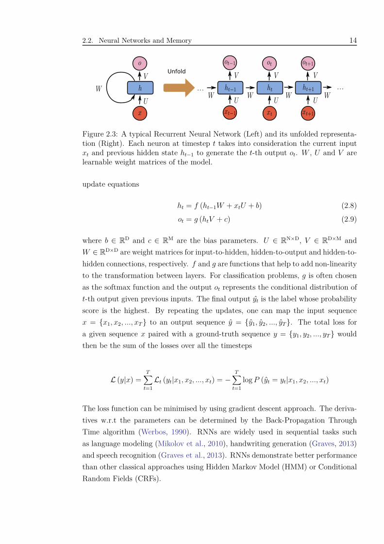
2.2. Neural Networks and Memory 14
Unfold
... . . .
Figure 2.3: A typical Recurrent Neural Network (Left) and its unfolded representa-tion (Right). Each neuron at timestep t takes into consideration the current inputxt and previous hidden state ht−1 to generate the t-th output ot. W , U and V arelearnable weight matrices of the model.
update equations
ht = f (ht−1W + xtU + b) (2.8)
ot = g (htV + c) (2.9)
where b ∈ RD and c ∈ RM are the bias parameters. U ∈ RN×D, V ∈ RD×M and
W ∈ RD×D are weight matrices for input-to-hidden, hidden-to-output and hidden-to-
hidden connections, respectively. f and g are functions that help to add non-linearity
to the transformation between layers. For classification problems, g is often chosen
as the softmax function and the output ot represents the conditional distribution of
t-th output given previous inputs. The final output yt is the label whose probability
score is the highest. By repeating the updates, one can map the input sequence
x = {x1, x2, ..., xT} to an output sequence y = {y1, y2, ..., yT}. The total loss for
a given sequence x paired with a ground-truth sequence y = {y1, y2, ..., yT} would
then be the sum of the losses over all the timesteps
L (y|x) =T∑
t=1
Lt (yt|x1, x2, ..., xt) = −T∑
t=1
log P (yt = yt|x1, x2, ..., xt)
The loss function can be minimised by using gradient descent approach. The deriva-
tives w.r.t the parameters can be determined by the Back-Propagation Through
Time algorithm (Werbos, 1990). RNNs are widely used in sequential tasks such
as language modeling (Mikolov et al., 2010), handwriting generation (Graves, 2013)
and speech recognition (Graves et al., 2013). RNNs demonstrate better performance
than other classical approaches using Hidden Markov Model (HMM) or Conditional
Random Fields (CRFs).
2.2. Neural Networks and Memory 15
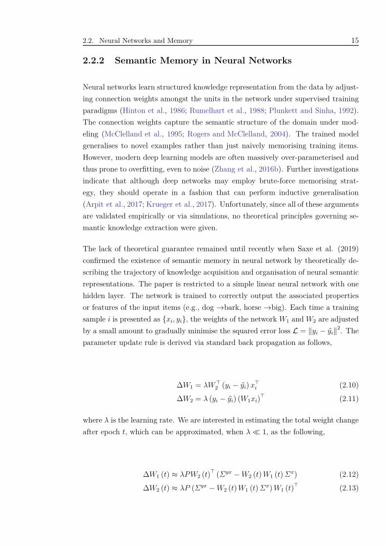
2.2.2 Semantic Memory in Neural Networks
Neural networks learn structured knowledge representation from the data by adjust-
ing connection weights amongst the units in the network under supervised training
paradigms (Hinton et al., 1986; Rumelhart et al., 1988; Plunkett and Sinha, 1992).
The connection weights capture the semantic structure of the domain under mod-
eling (McClelland et al., 1995; Rogers and McClelland, 2004). The trained model
generalises to novel examples rather than just naively memorising training items.
However, modern deep learning models are often massively over-parameterised and
thus prone to overfitting, even to noise (Zhang et al., 2016b). Further investigations
indicate that although deep networks may employ brute-force memorising strat-
egy, they should operate in a fashion that can perform inductive generalisation
(Arpit et al., 2017; Krueger et al., 2017). Unfortunately, since all of these arguments
are validated empirically or via simulations, no theoretical principles governing se-
mantic knowledge extraction were given.
The lack of theoretical guarantee remained until recently when Saxe et al. (2019)
confirmed the existence of semantic memory in neural network by theoretically de-
scribing the trajectory of knowledge acquisition and organisation of neural semantic
representations. The paper is restricted to a simple linear neural network with one
hidden layer. The network is trained to correctly output the associated properties
or features of the input items (e.g., dog →bark, horse →big). Each time a training
sample i is presented as {xi, yi}, the weights of the network W1 and W2 are adjusted
by a small amount to gradually minimise the squared error loss L = ‖yi − yi‖2. The
parameter update rule is derived via standard back propagation as follows,
∆W1 = λW ⊤2 (yi − yi) x⊤
i (2.10)
∆W2 = λ (yi − yi) (W1xi)⊤ (2.11)
where λ is the learning rate. We are interested in estimating the total weight change
after epoch t, which can be approximated, when λ≪ 1, as the following,
∆W1 (t) ≈ λP W2 (t)⊤ (Σyx −W2 (t) W1 (t) Σx) (2.12)
∆W2 (t) ≈ λP (Σyx −W2 (t) W1 (t) Σx) W1 (t)⊤ (2.13)
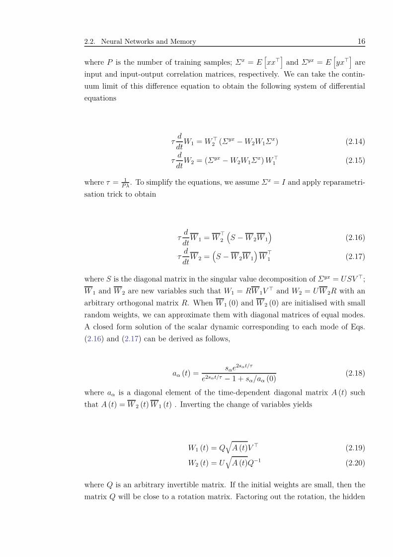
2.2. Neural Networks and Memory 16
where P is the number of training samples; Σx = E[xx⊤
]and Σyx = E
[yx⊤
]are
input and input-output correlation matrices, respectively. We can take the contin-
uum limit of this difference equation to obtain the following system of differential
equations
τd
dtW1 = W ⊤
2 (Σyx −W2W1Σx) (2.14)
τd
dtW2 = (Σyx −W2W1Σ
x) W ⊤1 (2.15)
where τ = 1P λ
. To simplify the equations, we assume Σx = I and apply reparametri-
sation trick to obtain
τd
dtW 1 = W
⊤2
(S −W 2W 1
)(2.16)
τd
dtW 2 =
(S −W 2W 1
)W
⊤1 (2.17)
where S is the diagonal matrix in the singular value decomposition of Σyx = USV ⊤;
W 1 and W 2 are new variables such that W1 = RW 1V ⊤ and W2 = UW 2R with an
arbitrary orthogonal matrix R. When W 1 (0) and W 2 (0) are initialised with small
random weights, we can approximate them with diagonal matrices of equal modes.
A closed form solution of the scalar dynamic corresponding to each mode of Eqs.
(2.16) and (2.17) can be derived as follows,
aα (t) =sαe2sαt/τ
e2sαt/τ − 1 + sα/aα (0)(2.18)
where aα is a diagonal element of the time-dependent diagonal matrix A (t) such
that A (t) = W 2 (t) W 1 (t) . Inverting the change of variables yields
W1 (t) = Q√
A (t)V ⊤ (2.19)
W2 (t) = U√
A (t)Q−1 (2.20)
where Q is an arbitrary invertible matrix. If the initial weights are small, then the
matrix Q will be close to a rotation matrix. Factoring out the rotation, the hidden
2.2. Neural Networks and Memory 17
representation of item i is
hαi (t) =
√aα (t)vα
i (2.21)
where vαi = V ⊤ [α, i]. Hence, we obtain a temporal evolution of internal represen-
tations h of the deep network. By using multi-dimensional scaling (MDS) visual-
isation of the evolution of internal representations over developmental time, Saxe
et al. (2019) demonstrated a progressive differentiation of hierarchy in the evolu-
tion, which matched the data’s underlying hierarchical structure. When we have
the explicit form of the evolution (Eq. (2.21)), this matching can be proved as an
inevitable consequence of deep learning dynamics when exposed to hierarchically
structured data (Saxe et al., 2019).
2.2.3 Associative Neural Networks
Associative memory is used to store associations between items. It is a general
concept of memory that spans across episodic, semantic and motor memory in the
brain. We can use neural networks (either feed-forward or recurrent) to implement
associative memory. There are three kinds of associative networks:
• Heteroassociative networks store Q pair of vectors {x1 ∈ X , y1 ∈ Y}, ...,{xQ ∈
X , yQ ∈ Y}
such that given some key xk, they return value yk.
• Autoassociative networks are a special type of the heteroassociative networks,
in which yk = xk (each item is associated with itself).
• Pattern recognition networks are also a special case where xk is associated
with a scalar k representing the item’s category.
Basically, these networks are used to represent associations between two vectors.
After two vectors are associated, one can be used as a cue to retrieve the other. In
principle, there are three functions governing an associative memory:
• Encoding function ⊗ : X × Y →M associates input items into some form of
memory traceM.
• Trace composition function ⊕ :M×M → M combines memory traces to
form the final representation for the whole dataset.
2.3. The Constructions of Memory in RNNs 18
• Decoding function • : X ×M → Y produces a (noisy) version of the item
given its associated.
Different models employ different kinds of functions (linear, non-linear, dot product,
outer product, tensor product, convolution, etc.). Associative memory concept is
potential to model memory in the brain (Marr and Thach, 1991). We will come
across some embodiment of associative memory in the form of neural networks in
the next sections.
2.3 The Constructions of Memory in RNNs
2.3.1 Attractor dynamics
Attractor dynamics denotes neuronal network dynamics which is dominated by
groups of persistently active neurons. In general, such a persistent activation asso-
ciates with an attractor state of the dynamics, which for simplicity, can take the
form of fixed-point (Amit, 1992). This kind of network can be used to implement
associative memory by allowing the network’s attractors to be exactly those vectors
we would like to store (Rojas, 2013). The approach supports memory for the items
per se, and thus differs from semantic memory in the sense that the items are often
stored quickly and what being stored cannot represent the semantic structure of
the data. Rather, attractor dynamics resembles working and episodic memory. Like
episodic memory, it acts as an associative memory, returning stored value when trig-
gered with the right clues. The capacity of attractor dynamics is low, which reflects
the short-term property of working memory. In the next part of the sub-section, we
will study these characteristics through one embodiment of attractor dynamics.
Hopfield network
The Hopfield network, originally proposed in 1982 (Hopfield, 1982), is a recurrent
neural network that implements associative memory using fix-points as attractors.
The function of the associative memory is to recognise previously learnt input vec-
tors, even in the case where some noise has been added. To achieve this function,
every neuron in the network is connected to all of the others (see Fig. 2.4 (a)).
2.3. The Constructions of Memory in RNNs 19
Each neuron outputs discrete values, normally 1 or −1, according to the following
equation
xi (t + 1) = sign
N∑
j=1
wijxj (t)
(2.22)
where xi (t) is the state of i-th neuron at time t and N is the number of neurons.
Hopfield network has a scalar value associated with the state of all neurons x, referred
to as the "energy" or Lyapunov function,
E (x) = −12
N∑
i=1
N∑
j=1
wijxixj (2.23)
If we want to store Q patterns xp, p = 1, 2, ..., Q, we can use the Hebbian learning
rule (Hebb, 1962) to assign the values of the weights as follows,
wij =Q∑
p=1
xpi xp
j (2.24)
which is equivalent to setting the weights to the elements of the correlation matrix
of the patterns1.
Upon presentation of an input to the network, the activity of the neurons can be
updated (asynchronously) according to Eq. (2.22) until the energy function has
been minimised (Hopfield, 1982). Hence, repeated updates would eventually lead
to convergence to one of the stored patterns. However, the network will possibly
converge to spurious patterns (different from the stored patterns) as the energy in
these spurious patterns is also a local minimum.
The capacity problem
The memorisation of some pattern can be retrieved when the network produces the
desired vector xp such that x (t + 1) = x (t) = xp. This happens when the crosstalk
computed by
1As an associative memory, Hopfield network implements ⊗, ⊕, • by outer product, additionand nonlinear recurrent function, respectively.
2.3. The Constructions of Memory in RNNs 20
(a) Hop eld Network (b) Liquid State Machine
Figure 2.4: (a) Hopfield network with five neurons. (b) Structure of a Liquid StateMachine M . The machine wants to transform input stream u(·) into output streamy(·) using some dynamical system LM (the liquid).
Q∑
q=1,q 6=p
xq (xp · xq) (2.25)
is less than N . If the crosstalk term becomes too large, it is likely that previously
stored patterns are lost because when they are presented to the network, one or
more of their bits are flipped by the associative computation. We would like to keep
the probability that this could happen low, so that stored patterns can always be
recalled. If we set the upper bound for one bit failure at 0.01, the maximum capacity
of the network is Q ≈ 0.18N (Rojas, 2013). With this low capacity, RNNs designed
as attractor dynamics have difficulty handling big problems with massive amount of
data.
2.3.2 Transient Dynamics
One major limitation of memorising by attractor mechanisms is the incapability of
remembering sequences of past inputs. This demands a new paradigm to explain
the working memory mechanism that enable RNNs to capture sequential depen-
dencies and memorise information between distance external stimuli. Within this
new paradigm, the trajectories of network states should become the main carriers of
information about external sensory stimuli. Recent proposals (Maass et al., 2002;
Maass, 2011; Jaeger and Haas, 2004) have suggested that an arbitrary recurrent net-
work could store information about recent input sequences in its transient dynamics
despite the presence of attractors (the pattern might or might not converge to the
2.3. The Constructions of Memory in RNNs 21
attractors). A useful analogy is the surface of a liquid. Transient ripples on the
surface can encode information about past objects that were thrown in even though
the water surface has no attractors (Ganguli et al., 2008). In the light of transient
dynamics, RNNs carry past information to serve a given task as a working memory.
Liquid State Machines
Liquid State Machines (LSMs) (Maass et al., 2002) use a dynamic reservoir/liquid
(LM), which consists of nodes randomly connected to each other, to handle time-
series data. The purpose is to map an input function of time u (t)–a continuous
sequence of disturbances, to an output function y (t) that provides a real-time anal-
ysis of the input sequence. In order to achieve that, we assume that at every time t,
LM generates an internal “liquid state” xM (t), which constitutes its current response
to preceding perturbations u(s) for s ≤ t. After a certain time-period, the state of
the liquid xM (t) is read as input for a readout network fM , which by assumption,
has no temporal integration capability of its own. This readout network learns to
map the states of the liquid to the target outputs as illustrated in Fig. 2.4 (b).
All information about the input u(s) from preceding time points s ≤ t that is needed
to produce a target output y(t) at time t has to be contained in the current liquid
state xM (t). LSMs allow realisation of large computational power on functions of
time even if all memory traces are continuously decaying. Instead of worrying about
the code and location where information about past inputs is stored, the approach
focuses on addressing the separation question: for which later time point t will any
two significantly different input functions of time u (t) and v (t) cause significantly
different liquid states xMu (t) and xM
v (t) (Maass, 2011).
Most implementations of LSMs use the reservoir of untrained neurons. In other
words, there is no need to train the weights of the RNN. The recurrent nature of
the connections fuses the input sequence into a spatio-temporal pattern of neuronal
activation in the liquid and computes a large variety of nonlinear functions on the
input. This mechanism is theoretically possible to perform universal continuous
computations. However, separation and approximation properties must be fulfilled
for the system to work well. Similar neural network design can be found in Echo
state networks (Jaeger and Haas, 2004). A Liquid State Machine is a particular
kind of spiking neural networks that more closely mimics biological neural networks
(Maass, 1997).
2.4. External Memory for RNNs 22
Memory trace of recurrent networks
When viewing recurrent networks as transient dynamics, one may want to measure
the lifetimes of transient memory traces in the networks. Ganguli et al. (2018)
studied a discrete time network whose dynamics is given by
xi (n) = f ([Wx (n− 1)]i + vis (n) + zi (n)) , i = 1, ..., N (2.26)
Here, a scalar time-varying signal s(n) drives an RNN of N neurons. x(n) is the
network state at n-th timestep, f(·) is a general sigmoidal function, W is an N ×N
recurrent connectivity matrix, and v is a vector of feed-forward connections encoding
the signal into the network. z(n) denotes a zero mean Gaussian white noise with
covariance 〈zi(k1), zj(k2)〉 = εδk1,k2δi,j.
The authors built upon Fisher information to construct useful measures of the ef-
ficiency with which the network state x(n) encodes the history of the signal s (n),
which can be derived as
J (k) = v⊤W k⊤
(ε
∞∑
k=0
W kW k⊤
)−1
W kv (2.27)
where J (k) measures the Fisher information that x(n) retains about a signal entering
the network at k time steps in the past. For a special case of normal networks having
a normal connectivity matrix W , Eq. (2.27) simplifies to
J (k) =N∑
i=1
v2i |λi|2k
(1− |λi|2
)(2.28)
where λi is the i-th eigenvalue of W . For large k, the decay of the Fisher information
is determined by the magnitudes of the largest eigenvalues and it decays exponen-
tially. Similar findings with different measurements on the memory trace in modern
recurrent networks are also found in a more recent work (Le et al., 2019).
2.4 External Memory for RNNs
Recurrent networks can in principle use their feedback connections to store repre-
sentations of recent input events in the form of implicit memory (either attractor
2.4. External Memory for RNNs 23
or transient dynamics). Unfortunately, from transient dynamics perspective, the
implicit memory tends to decay quickly (Ganguli et al., 2008; Le et al., 2019). This
phenomenon is closely related to gradient vanishing/exploding problems (Bengio et al.,
1994; Hochreiter and Schmidhuber, 1997; Pascanu et al., 2013) which often occur
when training RNNs with gradient-based algorithms such as Back-Propagation Through
Time (Williams and Zipser, 1989; Werbos, 1990). A solution is to equip RNNs with
external memory to cope with exponential decay of the implicit short-term memory.
The external memory enhances RNNs with stronger working (Hochreiter and Schmidhuber,
1997; Cho et al., 2014b; Graves et al., 2014, 2016) or even episodic-like memory
(Graves et al., 2014; Santoro et al., 2016). We will spend the next sections to anal-
yse different types of external memory and their memory operation mechanisms.
Examples of modern recurrent neural networks that utilise external memory are
also discussed.
2.4.1 Cell Memory
Despite the fact that RNNs offer working memory mechanisms to handle sequential
inputs, learning what to put in and how to utilise the memory is challenging. Back-
Propagation Through Time (Williams and Zipser, 1989; Werbos, 1990) is the most
common learning algorithm for RNNs, yet it is inefficient in training long sequences
mainly due to insufficient or decaying backward error signals. This section will re-
view the analysis of this problem and study a group of methodologies that overcome
the problem through the use of cell memory and gated operation.
Hochreiter’s analysis on gradient vanishing/exploding problems
Let us assume that the hidden layer of an RNN has n neurons. With differen-
tiable activation function fi, the activation of a neuron i at step t of the recurrent
computation is as follow,
yi (t) = fi
∑
j
wijyj (t− 1)
(2.29)
= fi (neti (t)) (2.30)
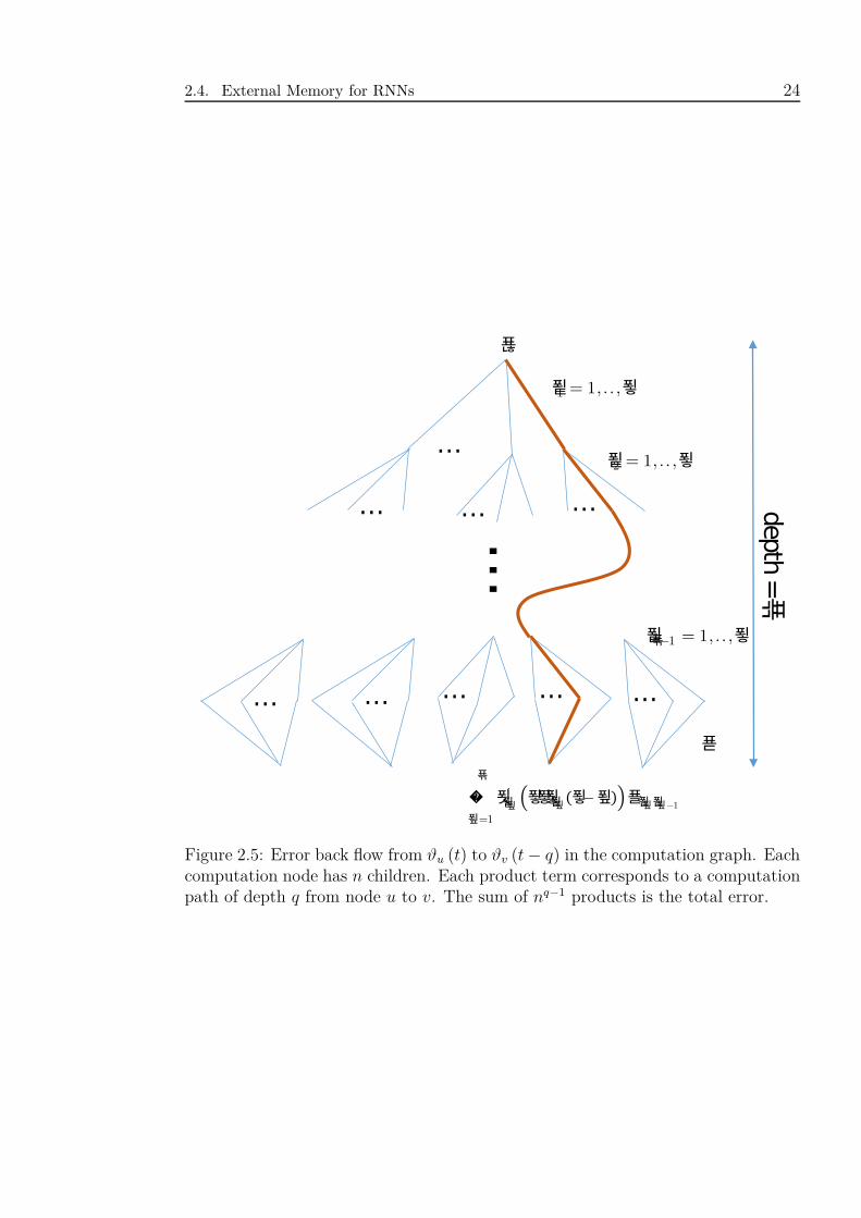
2.4. External Memory for RNNs 24
……
…
…
…
… …… … …
depth
= 푞
�
푚=1
푞
푓푙푚′ 푛푛푛푙푚 푛−푚 푤푙푚푙푚−1
푙1 = 1,.. ,푛
푙2 = 1,.. ,푛
푙푞−1 = 1,.. ,푛
푢
푣
Figure 2.5: Error back flow from ϑu (t) to ϑv (t− q) in the computation graph. Eachcomputation node has n children. Each product term corresponds to a computationpath of depth q from node u to v. The sum of nq−1 products is the total error.
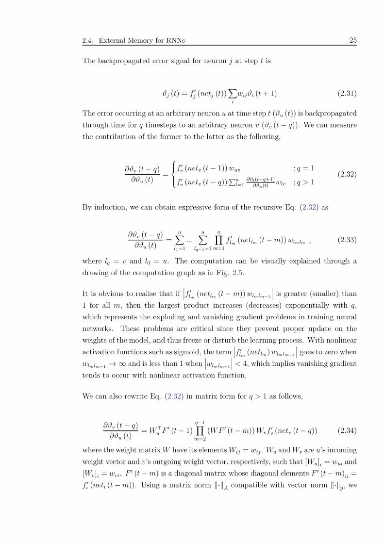
2.4. External Memory for RNNs 25
The backpropagated error signal for neuron j at step t is
ϑj (t) = f ′j (netj (t))
∑
i
wijϑi (t + 1) (2.31)
The error occurring at an arbitrary neuron u at time step t (ϑu (t)) is backpropagated
through time for q timesteps to an arbitrary neuron v (ϑv (t− q)). We can measure
the contribution of the former to the latter as the following,
∂ϑv (t− q)∂ϑu (t)
=
f ′v (netv (t− 1)) wuv ; q = 1
f ′v (netv (t− q))
∑nl=1
∂ϑl(t−q+1)∂ϑu(t)
wlv ; q > 1(2.32)
By induction, we can obtain expressive form of the recursive Eq. (2.32) as
∂ϑv (t− q)∂ϑu (t)
=n∑
l1=1
...n∑
lq−1=1
q∏
m=1
f ′lm (netlm (t−m)) wlmlm−1
(2.33)
where lq = v and l0 = u. The computation can be visually explained through a
drawing of the computation graph as in Fig. 2.5.
It is obvious to realise that if∣∣∣f ′
lm (netlm (t−m)) wlmlm−1
∣∣∣ is greater (smaller) than
1 for all m, then the largest product increases (decreases) exponentially with q,
which represents the exploding and vanishing gradient problems in training neural
networks. These problems are critical since they prevent proper update on the
weights of the model, and thus freeze or disturb the learning process. With nonlinear
activation functions such as sigmoid, the term∣∣∣f ′
lm (netlm) wlmlm−1
∣∣∣ goes to zero when
wlmlm−1→∞ and is less than 1 when
∣∣∣wlmlm−1
∣∣∣ < 4, which implies vanishing gradient
tends to occur with nonlinear activation function.
We can also rewrite Eq. (2.32) in matrix form for q > 1 as follows,
∂ϑv (t− q)∂ϑu (t)
= W ⊤u F ′ (t− 1)
q−1∏
m=2
(WF ′ (t−m)) Wvf ′v (netv (t− q)) (2.34)
where the weight matrix W have its elements Wij = wij. Wu and Wv are u’s incoming
weight vector and v’s outgoing weight vector, respectively, such that [Wu]i = wui and
[Wv]i = wvi. F ′ (t−m) is a diagonal matrix whose diagonal elements F ′ (t−m)ii =
f ′i (neti (t−m)). Using a matrix norm ‖·‖A compatible with vector norm ‖·‖p, we
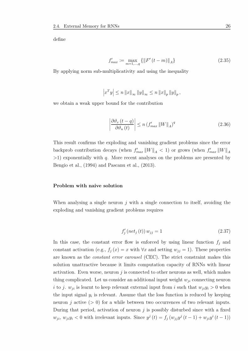
2.4. External Memory for RNNs 26
define
f ′max := max
m=1,...,q{‖F ′ (t−m)‖A} (2.35)
By applying norm sub-multiplicativity and using the inequality
∣∣∣xT y∣∣∣ ≤ n ‖x‖∞ ‖y‖∞ ≤ n ‖x‖p ‖y‖p ,
we obtain a weak upper bound for the contribution
∣∣∣∣∣∂ϑv (t− q)
∂ϑu (t)
∣∣∣∣∣ ≤ n (f ′max ‖W‖A)q (2.36)
This result confirms the exploding and vanishing gradient problems since the error
backprob contribution decays (when f ′max ‖W‖A < 1) or grows (when f ′
max ‖W‖A
>1) exponentially with q. More recent analyses on the problems are presented by
Bengio et al., (1994) and Pascanu et al., (2013).
Problem with naive solution
When analysing a single neuron j with a single connection to itself, avoiding the
exploding and vanishing gradient problems requires
f ′j (netj (t)) wjj = 1 (2.37)
In this case, the constant error flow is enforced by using linear function fj and
constant activation (e.g., fj (x) = x with ∀x and setting wjj = 1). These properties
are known as the constant error carousel (CEC). The strict constraint makes this
solution unattractive because it limits computation capacity of RNNs with linear
activation. Even worse, neuron j is connected to other neurons as well, which makes
thing complicated. Let us consider an additional input weight wji connecting neuron
i to j. wji is learnt to keep relevant external input from i such that wjiyi > 0 when
the input signal yi is relevant. Assume that the loss function is reduced by keeping
neuron j active (> 0) for a while between two occurrences of two relevant inputs.
During that period, activation of neuron j is possibly disturbed since with a fixed
wji, wjiyi < 0 with irrelevant inputs. Since yj (t) = fj (wjjyj (t− 1) + wjiy
i (t− 1))
2.4. External Memory for RNNs 27
where fj is linear, yj (t− 1) is kept constant and yi (t− 1) scales with the external
input, it is likely to deactivate neuron j. Hence, if naively following CEC, learning
a wji to capture relevant inputs while protecting neuron j from disturbances of
irrelevant inputs is challenging (input weight conflict (Hochreiter and Schmidhuber,
1997)). Similar problem happens with the output weight (output weight conflict).
These conflicts make the learning hard, and require a more flexible mechanism for
controlling input/output weight impact conditioned on the input signal.
The original Long Short-Term Memory (LSTM)
Hochreiter and Schmidhuber (1997) originally proposed LSTM using multiplicative
gate units and a memory cell unit to overcome the weight conflicts while following
CEC. The idea is to apply CEC to neurons specialised for memorisation, each of
which has an internal state independent from the activation function. This sep-
aration between memorisation and computation is essential for external memory
concept. Besides, to control input/output weight impact, gate units conditioned on
the inputs are multiplied with the incoming/outgoing connections, modifying the
connection value through time. In particular, if a neuron cj becomes cell memory,
its output is computed as
ycj (t) = youtj (t) h(scj
(t))
(2.38)
where youtj (t) is the output gate, h is a differentiable function for scaling down the
neuron’s output, and scjcaptures past information by using the dynamics
scj(0) = 0 (2.39)
scj(t) = yfgj (t) scj
(t− 1) + yinj (t) f(netcj
(t))
for t > 0 (2.40)
where yinj (t) is the input gate, yfgj (t) is the (optional) forget gate and f is the
activation function, which can be nonlinear. Without forget gate, cj can be viewed
as a neuron with an additional fixed self-connection. The computation paths that
mainly pass through this special neuron preserve the backward error. The remaining
problem is to protect this error from disturbance from other paths. The gates are
calculated as
2.4. External Memory for RNNs 28
ygj (t) = fgj
(∑
u
wgjuyu (t− 1)
)(2.41)
where g can represent input, output and forget gate. The gates are adaptive accord-
ing to the input from other neurons, hence, it is possible to learn{wgju
}to resolve
the input/output weight conflict problem.
Although the cell memory provides a potential solution to cope with training RNN
over long time lag, unfortunately, in practice, the multiplicative gates are not good
enough to overcome a fundamental challenge of LSTM: the gates are not coordinated
at the start of training, which can cause scjto explode quickly (internal state drift).
Various variants of LSTM have been proposed to tackle the problem (Greff et al.,
2016). We will review some of them in Chapter 3.
Cell memory as external memory
From Eq. (2.40), we can see the internal state of the cell memory holds two types
of information: (i) the previous cell state and (ii) the normal state of RNN, which
is the activation of current computation. Therefore, the cell state contains a new
form of external memory for RNNs. The size of the memory is often equal the
number of hidden neurons in RNNs and thus, cell memory is also known as vector
memory. The memory supports writing and reading mechanisms implemented as
gated operations in yinj (t) and youtj , respectively. They control how much to write
to and read from the cell state. With the cell state, which is designed to keep
information across timesteps, the working memory capacity of LSTM should be
greater than that of RNNs. The memory reading and writing are also important
to determine the memory capacity. For instance, if writing irrelevant information
too often, the content in the cell state will saturate and the memory fails to hold
much information. Later works make use of the gating mechanism to build skip-
connections between inputs (a source of raw memory) and neurons in higher layers
(Srivastava et al., 2015; He et al., 2016), opening chance to ease the training of very
deep networks.
2.4. External Memory for RNNs 29
2.4.2 Holographic Associative Memory
The holographic associative memory (HAM) roots its operation on the principle of
optical holography, where two beams of light are associated with one another in a
holograms such that reconstruction of one original beam can be made by present-
ing another beam. Recall that the capacity of associative memory using attractor
dynamics is low. To maintain Q pairs of key-value (in Hopfield network, value is
also key), it requires N2 weight storage where Q ≈ 0.18N . HAM presents a solution
to compress the key-values into a fixed size vector via Holographic Reduced Repre-
sentation (HRR) without substantial loss of information (Plate, 1995). This can be
done in real or complex domain using circular convolution or element-wise complex
multiplication for the encoding function (⊗), respectively. The compressed vector
(M), as we shall see, can be used as external memory for RNNs.
Holographic Reduced Representation
Consider a complex-valued vector key x ∈ CN ,
x =[xa [1] eixφ[1], ..., xa [N ] eixφ[N ]
](2.42)
The association encoding is computed by
m = x ⊛ y (2.43)
=[xa [1] ya [1] ei(xφ[1]+yφ[1]), ..., xa [N ] ya [N ] ei(xφ[N ]+yφ[N ])
](2.44)
where ⊛ is element-wise complex multiplication, which multiplies the moduli and
adds the phases of the elements. Trace composition function is simply addition
m = x1 ⊛ y1 + x2 ⊛ y2 + ... + xQ ⊛ yQ (2.45)
Although the memory m is a vector with the same dimension as that of stored
items, it can store many pairs of items since we only need to store the information
that discriminates them. The decoding function is multiplying an inverse key x−1 =[xa [1]−1 e−ixφ[1], ..., xa [N ]−1 e−ixφ[N ]
]with the memory as follows,
2.4. External Memory for RNNs 30
y = x−1 ⊛ m (2.46)
= x−1 ⊛
(∑
∀k
xk ⊛ yk
)(2.47)
= y + x−1 ⊛
∑
∀k:xk 6=x
xk ⊛ yk
(2.48)
The second term in Eq. (2.48) is noise and should be minimised. Under certain
conditions, the noise term has zero mean (Plate, 1995). One way to reconstruct
better is to pass the retrieved vector through an auto-associative memory to correct
any errors.
Redundant Associative Long Short-Term Memory
One recent attempt to apply HRR to LSTM is the work by Danihelka et al. (2016).
The authors first propose Redundant Associative Memory, an extension of HRR
with multiple memory traces for multiple transformed copies of each key vector. In
particular, each key vector will be transformed S times using S constant random
permutation matrix Ps. Hence, we obtain the memory trace cs for the s-th copy
cs =∑
∀k
(Psx
k)⊛ yk (2.49)
The k-th value is retrieved as follows,
yk =1S
S∑
s=1
(Psxk
)⊛ cs (2.50)
= yk +∑
k′ 6=k
yk′
⊛1S
S∑
s=1
Ps
[xk ⊛ xk′
](2.51)
where Psxk and xk are the complex conjugates of Psxk and xk, respectively, which
are equal to the inverses if the modulus xka = 1. Since permuting the key decorrelates
the retrieval noise, the noise term has variance O(
QS
)and increase the number of
copies will enhance retrieval quality.
Applying the idea to LSTM, we can turn the cell memory to a holographic memory
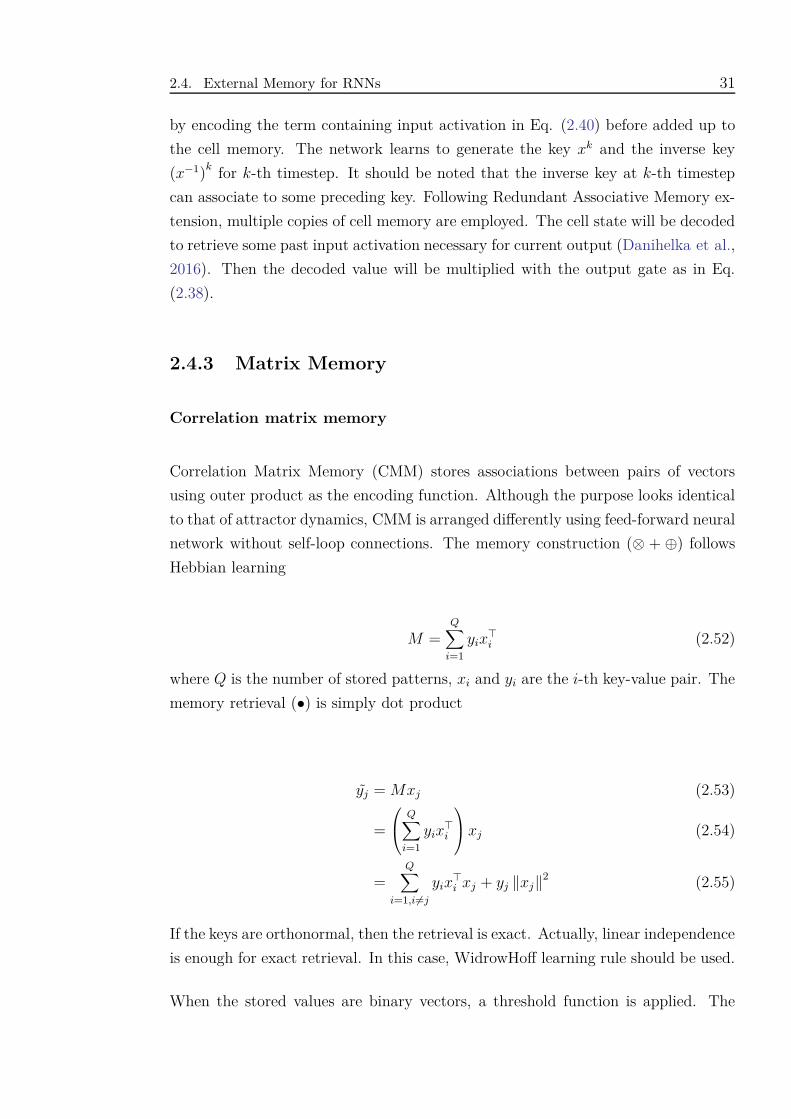
2.4. External Memory for RNNs 31
by encoding the term containing input activation in Eq. (2.40) before added up to
the cell memory. The network learns to generate the key xk and the inverse key
(x−1)k for k-th timestep. It should be noted that the inverse key at k-th timestep
can associate to some preceding key. Following Redundant Associative Memory ex-
tension, multiple copies of cell memory are employed. The cell state will be decoded
to retrieve some past input activation necessary for current output (Danihelka et al.,
2016). Then the decoded value will be multiplied with the output gate as in Eq.
(2.38).
2.4.3 Matrix Memory
Correlation matrix memory
Correlation Matrix Memory (CMM) stores associations between pairs of vectors
using outer product as the encoding function. Although the purpose looks identical
to that of attractor dynamics, CMM is arranged differently using feed-forward neural
network without self-loop connections. The memory construction (⊗ + ⊕) follows
Hebbian learning
M =Q∑
i=1
yix⊤i (2.52)
where Q is the number of stored patterns, xi and yi are the i-th key-value pair. The
memory retrieval (•) is simply dot product
yj = Mxj (2.53)
=
Q∑
i=1
yix⊤i
xj (2.54)
=Q∑
i=1,i6=j
yix⊤i xj + yj ‖xj‖2 (2.55)
If the keys are orthonormal, then the retrieval is exact. Actually, linear independence
is enough for exact retrieval. In this case, WidrowHoff learning rule should be used.
When the stored values are binary vectors, a threshold function is applied. The
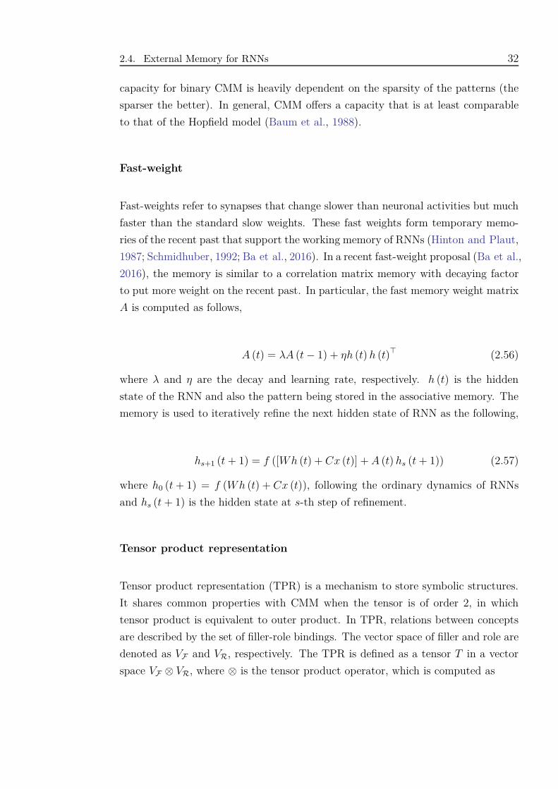
2.4. External Memory for RNNs 32
capacity for binary CMM is heavily dependent on the sparsity of the patterns (the
sparser the better). In general, CMM offers a capacity that is at least comparable
to that of the Hopfield model (Baum et al., 1988).
Fast-weight
Fast-weights refer to synapses that change slower than neuronal activities but much
faster than the standard slow weights. These fast weights form temporary memo-
ries of the recent past that support the working memory of RNNs (Hinton and Plaut,
1987; Schmidhuber, 1992; Ba et al., 2016). In a recent fast-weight proposal (Ba et al.,
2016), the memory is similar to a correlation matrix memory with decaying factor
to put more weight on the recent past. In particular, the fast memory weight matrix
A is computed as follows,
A (t) = λA (t− 1) + ηh (t) h (t)⊤ (2.56)
where λ and η are the decay and learning rate, respectively. h (t) is the hidden
state of the RNN and also the pattern being stored in the associative memory. The
memory is used to iteratively refine the next hidden state of RNN as the following,
hs+1 (t + 1) = f ([Wh (t) + Cx (t)] + A (t) hs (t + 1)) (2.57)
where h0 (t + 1) = f (Wh (t) + Cx (t)), following the ordinary dynamics of RNNs
and hs (t + 1) is the hidden state at s-th step of refinement.
Tensor product representation
Tensor product representation (TPR) is a mechanism to store symbolic structures.
It shares common properties with CMM when the tensor is of order 2, in which
tensor product is equivalent to outer product. In TPR, relations between concepts
are described by the set of filler-role bindings. The vector space of filler and role are
denoted as VF and VR, respectively. The TPR is defined as a tensor T in a vector
space VF ⊗ VR, where ⊗ is the tensor product operator, which is computed as
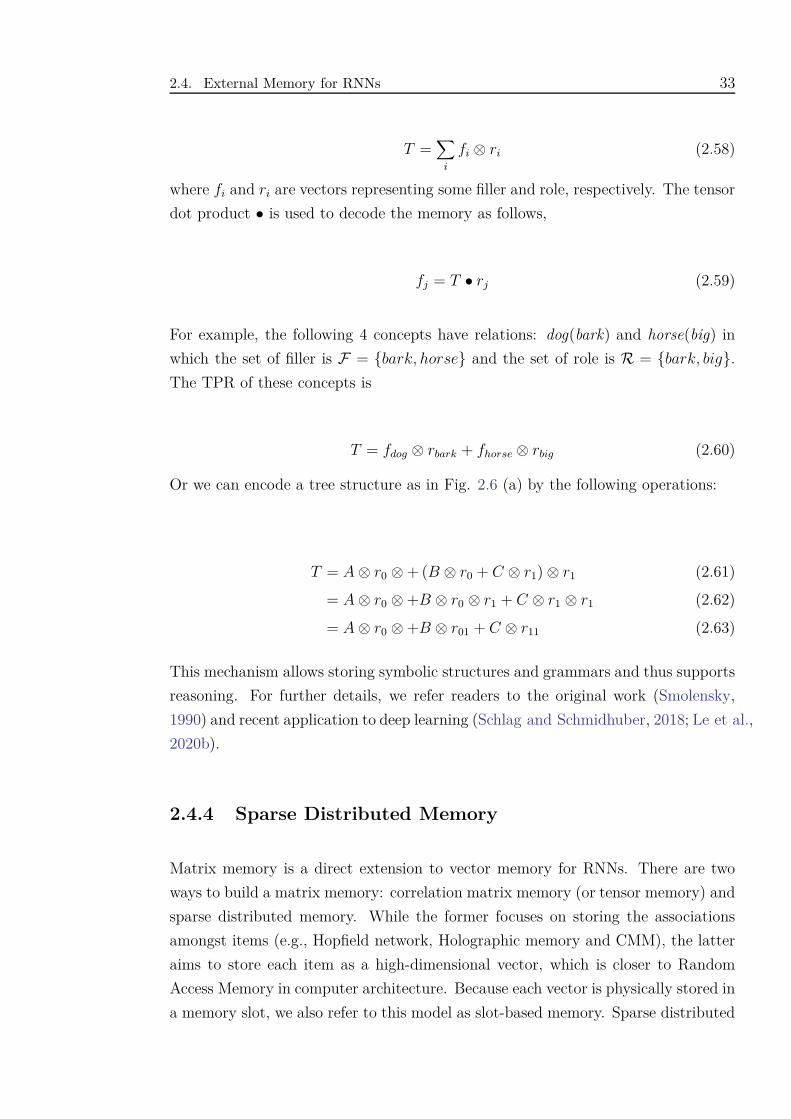
2.4. External Memory for RNNs 33
T =∑
i
fi ⊗ ri (2.58)
where fi and ri are vectors representing some filler and role, respectively. The tensor
dot product • is used to decode the memory as follows,
fj = T • rj (2.59)
For example, the following 4 concepts have relations: dog(bark) and horse(big) in
which the set of filler is F = {bark, horse} and the set of role is R = {bark, big}.The TPR of these concepts is
T = fdog ⊗ rbark + fhorse ⊗ rbig (2.60)
Or we can encode a tree structure as in Fig. 2.6 (a) by the following operations:
T = A⊗ r0 ⊗+ (B ⊗ r0 + C ⊗ r1)⊗ r1 (2.61)
= A⊗ r0 ⊗+B ⊗ r0 ⊗ r1 + C ⊗ r1 ⊗ r1 (2.62)
= A⊗ r0 ⊗+B ⊗ r01 + C ⊗ r11 (2.63)
This mechanism allows storing symbolic structures and grammars and thus supports
reasoning. For further details, we refer readers to the original work (Smolensky,
1990) and recent application to deep learning (Schlag and Schmidhuber, 2018; Le et al.,
2020b).
2.4.4 Sparse Distributed Memory
Matrix memory is a direct extension to vector memory for RNNs. There are two
ways to build a matrix memory: correlation matrix memory (or tensor memory) and
sparse distributed memory. While the former focuses on storing the associations
amongst items (e.g., Hopfield network, Holographic memory and CMM), the latter
aims to store each item as a high-dimensional vector, which is closer to Random
Access Memory in computer architecture. Because each vector is physically stored in
a memory slot, we also refer to this model as slot-based memory. Sparse distributed
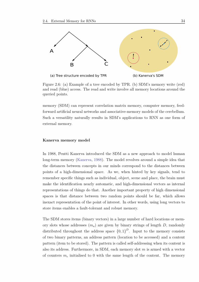
2.4. External Memory for RNNs 34
A
B C
(a) Tree structure encoded by TPR (b) Kanerva's SDM
Figure 2.6: (a) Example of a tree encoded by TPR. (b) SDM’s memory write (red)and read (blue) access. The read and write involve all memory locations around thequeried points.
memory (SDM) can represent correlation matrix memory, computer memory, feed-
forward artificial neural networks and associative-memory models of the cerebellum.
Such a versatility naturally results in SDM’s applications to RNN as one form of
external memory.
Kanerva memory model
In 1988, Pentti Kanerva introduced the SDM as a new approach to model human
long-term memory (Kanerva, 1988). The model revolves around a simple idea that
the distances between concepts in our minds correspond to the distances between
points of a high-dimensional space. As we, when hinted by key signals, tend to
remember specific things such as individual, object, scene and place, the brain must
make the identification nearly automatic, and high-dimensional vectors as internal
representations of things do that. Another important property of high dimensional
spaces is that distance between two random points should be far, which allows
inexact representation of the point of interest. In other words, using long vectors to
store items enables a fault-tolerant and robust memory.
The SDM stores items (binary vectors) in a large number of hard locations or mem-
ory slots whose addresses (ma) are given by binary strings of length D, randomly
distributed throughout the address space {0, 1}D. Input to the memory consists
of two binary patterns, an address pattern (location to be accessed) and a content
pattern (item to be stored). The pattern is called self-addressing when its content is
also its address. Furthermore, in SDM, each memory slot m is armed with a vector
of counters mc initialised to 0 with the same length of the content. The memory
2.4. External Memory for RNNs 35
Algorithm 2.1 Memory writing in SDMRequire: input x and SDM
1: Find a set of chosen locations M(x) using Eq. (2.64)2: for each m in M(x) do3: for i = 1, D do4: if xc[i] == 1 then5: mc[i] += 16: else7: mc[i] −= 18: end if9: end for
10: end for
operations are based on similarity between the addresses.
Memory writing When storing input item x = (xa, xc) to the SDM, the address
pattern xa is compared against all memory location addresses. Relevant physical
locations to consider are those which lie within a hypersphere of radius r centered
on the address pattern point
M (x) = {m : d (ma, xa) < r} (2.64)
where d is some similarity measure between 2 vectors. In the original model, Kanerva
used Hamming distance. The content is distributed in the set of locations M (x) as
in Algo. 2.1.
Memory reading Basically, reading from any point in the memory space pools
the data of all nearby locations. Given a cue address x′a, contents of the counters at
locations near x′a are summed and thresholded at zero to return the binary content.
The proximity criteria still follows Eq. (2.64). The reading mechanism allows SDM
to retrieve data from imprecise or noisy cues. Fig. 2.6 (b) visualises the memory
access behaviors.
The assumption underlying the original SDM are: (i) the location addresses are
fixed, and only the contents of the locations are modifiable, (ii) the locations are
sparse and distributed across the address space {0, 1}D (e.g., randomly sample 106
addresses from an address space of 1000 dimensions ). These assumptions make the
model perform well on storing random input data.
2.4. External Memory for RNNs 36
SDM as an associative matrix memory We can implement SDM by using
three operations of associative memory. The minimum setting for this implementa-
tion includes:
• A hard-address matrix A ∈ BN×D where N and D are the numbers of memory
locations and the dimension of the address space, respectively.
• A counter (content) matrix C ∈ BN×D.
• Cosine similarity is used to measure proximity.
• Threshold function y that maps distances to binary values:y (d) = 1 if d ≥ r
and vice versa.
• Threshold function z that converts a vector to binary vector: z (x) = 1 if
x ≥ 0 and vice versa.
Then, the memory writing (⊗+⊕) and reading (•) become
C := C + y (Axa) x⊤c (2.65)
x′c = z
(C⊤
y (Ax′a))
(2.66)
These expressions are closely related to attention mechanisms commonly used nowa-
days (Sec. 3.2.2).
In general, SDM overcomes limitations of correlation matrix memory such as Hop-
field network since the number of stored items in SDM is not limited by the number
of processing elements. Moreover, one can design SDM to store a sequence of pat-
terns. Readers are referred to Keeler (1988) for a detailed comparison between SDM
and Hopfield network (Keeler, 1988).
Memory-augmented neural networks and attention mechanisms
The current wave of deep learning has leveraged the concept of SDM to external
neural memory capable of supporting the working memory of RNNs (Weston et al.,
2014; Graves et al., 2014, 2016; Miller et al., 2016). These models enhance the SDM
with real-valued vectors and learnable parameters. For example, the matrices A and
2.5. Relation to Computational Models 37
C can be automatically generated by a learnable neural network. To make whole
architecture learnable, differentiable functions and flexible memory operations must
be used. Attention mechanisms are the most common operations used in MANNs
to facilitate the similarity-based memory access of SDM. Through various ways of
employing attentions, RNNs can access the external memory in the same manner as
one accesses SDM. Details on neural distributed (slot-based) memory and attention
mechanisms will be provided in Chapter 3.
2.5 Relation to Computational Models
Automatons are abstract models of machines that perform computations on an input
by moving through a series of states (Sipser et al., 2006). Once the computation
reaches a finish state, it accepts and possibly produces the output of that input. In
terms of computational capacity, there are three major classes of automaton:
• Finite-state machine
• Pushdown automata
• Turing machine
Pushdown automata and Turing machine can be thought of as extensions of finite-
state machines (FSMs) when equipped with an external storage in the form of stack
and memory tape, respectively. With stored-program memory, an even more pow-
erful class of machines, which simulates any other Turing machines, can be built as
universal Turing machine (Turing, 1936). As some Turing machines are also uni-
versal, they are usually regarded as one of the most general and powerful automata
besides universal Turing machines.
One major objective of automata theory is to understand how machines compute
functions and measure computation power of models. For example, RNNs, if prop-
erly wired, are Turing-complete (Siegelmann and Sontag, 1995), which means they
can compute arbitrary sequences if they have unlimited memory. Nevertheless, in
practice, RNNs struggle to learn from the data to predict output correctly given
simple input sequence (Bengio et al., 1994). This poses a question on the effective
computation power of RNNs.
2.5. Relation to Computational Models 38
Another way to measure the capacity of RNNs is via simulations of operations that
they are capable of doing. The relationship between RNNs and FSMs has been dis-
covered by many (Giles et al., 1992; Casey, 1996; Omlin and Giles, 1996; Tiňo et al.,
1998), which suggest that RNNs can mimic FSMs by training with data. The states
of an RNN must be grouped into partitions representing the states of the generating
automation. Following this line of thinking, we can come up with neural architec-
tures that can simulate pushdown automata, Turing machine and universal Turing
machine. Neural stack is an example which arms RNN with a stack as its exter-
nal memory (Mozer and Das, 1993; Joulin and Mikolov, 2015; Grefenstette et al.,
2015). By simulating push and pop operations, which are controlled by the RNN,
neural stack mimics the working mechanism of pushdown automata. Neural Tur-
ing Machine and its extension Differentiable Neural Computer (Graves et al., 2014,
2016) are prominent neural realisations of Turing machine. They use an RNN con-
troller to read from and write to an external memory in a manner resembling Turing
machine’s operations on its memory tape. Since the memory access is not limited to
the top element as in neural stack, these models have more computational flexibil-
ity. Until recently, Le et al. (2020) extended the simulation to the level of universal
Turing machine (Le et al., 2020a; Le and Venkatesh, 2020) by employing the stored-
program principle (Turing, 1936; von Neumann, 1993). We save a thorough analysis
on the correspondence between these MANNs and Turing machines for Chapter 7.
Here, we briefly draw a correlation between models of recurrent neural networks and
automata (see Fig. 2.7 ).
It should be noted that the illustration is found on the organisation of memory
in the models rather than the computational capacity. For example, some Turing
machines are equivalent to universal Turing machine in terms of capacity; RNNs are
on par with other MANNs because they are all Turing-complete. Having said that,
when neural networks are organised in a way that simulates powerful automata,
their effective capacity is often greater and thus, they tend to perform better in
complicated sequential learning tasks (Graves et al., 2014, 2016; Le et al., 2020a).
A similar taxonomy with proof of inclusion relation amongst models can be found
in the literature (Ma and Principe, 2018).
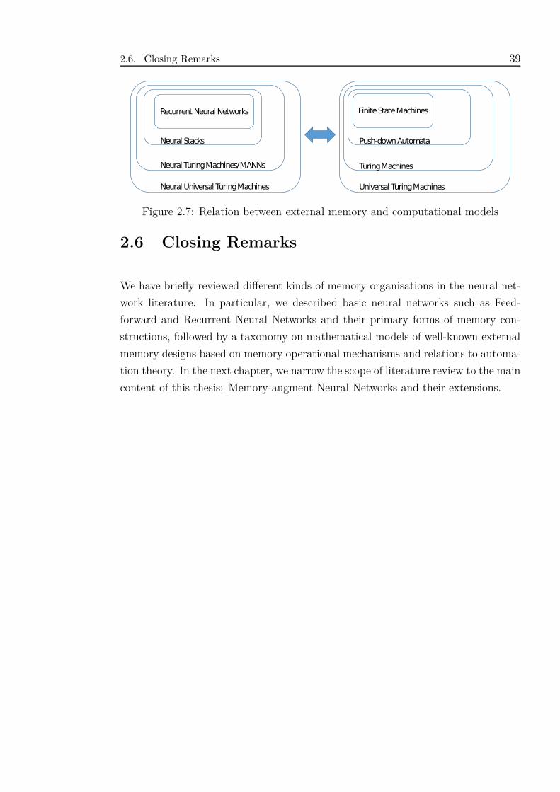
2.6. Closing Remarks 39
Neural Stacks
Neural Turing Machines/MANNs
Neural Universal Turing Machines
Finite State Machines
Push-down Automata
Turing Machines
Universal Turing Machines
Recurrent Neural Networks
Figure 2.7: Relation between external memory and computational models
2.6 Closing Remarks
We have briefly reviewed different kinds of memory organisations in the neural net-
work literature. In particular, we described basic neural networks such as Feed-
forward and Recurrent Neural Networks and their primary forms of memory con-
structions, followed by a taxonomy on mathematical models of well-known external
memory designs based on memory operational mechanisms and relations to automa-
tion theory. In the next chapter, we narrow the scope of literature review to the main
content of this thesis: Memory-augment Neural Networks and their extensions.
Chapter 3
Memory-augmented Neural
Networks
3.1 Gated RNNs
3.1.1 Long Short-Term Memory
Despite its ability to model temporal dependencies in sequential data, RNNs face a
big mathematical challenge of learning long sequences. The basic problem is that
gradients propagated over many steps tend to either vanish or explode. Although
the explosion can be prevented with the use of activation functions (i.e., tanh or
sigmoid) that restrict the range of update values, the vanishing problem remains
with these nonlinear activation functions (Sec. 2.4.1). The difficulty with long-
term dependencies arises from the exponentially smaller weights given to long-term
interactions compared to short-term ones. In practice, experiments have shown that
RNNs might find it hard to learn sequences of only length 10 or 20 (Bengio et al.,
1994).
Long Short-Term Memory (LSTM) (Hochreiter and Schmidhuber, 1997) is intro-
duced as a simple yet clever way to alleviate the problem. The core idea is to
produce paths where the gradient can flow for long duration by adding a linear
self-loop memory cell to the computation of the hidden unit. Notably, the weight
of the linear self-loop is gated (controlled by another hidden unit) and dependent
on the input. This enables the network to dynamically moderate the amount of
40
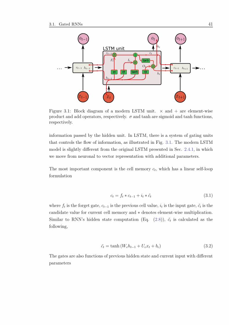
3.1. Gated RNNs 41
LSTM unit
� � tanh �
tanh
. . . . . .
Figure 3.1: Block diagram of a modern LSTM unit. × and + are element-wiseproduct and add operators, respectively. σ and tanh are sigmoid and tanh functions,respectively.
information passed by the hidden unit. In LSTM, there is a system of gating units
that controls the flow of information, as illustrated in Fig. 3.1. The modern LSTM
model is slightly different from the original LSTM presented in Sec. 2.4.1, in which
we move from neuronal to vector representation with additional parameters.
The most important component is the cell memory ct, which has a linear self-loop
formulation
ct = ft ∗ ct−1 + it ∗ ct (3.1)
where ft is the forget gate, ct−1 is the previous cell value, it is the input gate, ct is the
candidate value for current cell memory and ∗ denotes element-wise multiplication.
Similar to RNN’s hidden state computation (Eq. (2.8)), ct is calculated as the
following,
ct = tanh (Wcht−1 + Ucxt + bc) (3.2)
The gates are also functions of previous hidden state and current input with different
parameters
3.1. Gated RNNs 42
ft = σ (Wf ht−1 + Ufxt + bf ) (3.3)
it = σ (Wiht−1 + Uixt + bi) (3.4)
ot = σ (Woht−1 + Uoxt + bo) (3.5)
where σ is the sigmoid function that keeps the gate values in range [0, 1]. The final
hidden state ht is computed based on the cell memory ct, gated by the output gate
ot as follows,
ht = ot ∗ tanh (ct) (3.6)
Given the hidden state ht, other computations for the output ot are the same as in
Elman’s RNN (Eq. (2.9)).
In LSTM, the forget gate ft plays a crucial role in enabling the network to capture
long-term dependencies. If ft → 1, the previous memory will be preserved and
thus, the product of derivatives associated with a distant input is close to one. This
allows a distant input to take part in the backpropagation update and slow down
the gradient vanishing process. If ft → 0, the path to previous cells is disconnected
and the model tends to remember only short-term events.
Empirical results have shown that LSTM networks learn long-term dependencies
more easily than the simple RNNs. State-of-the-art performances were obtained
in various challenging sequence processing tasks (Graves and Schmidhuber, 2005;
Vinyals and Le, 2015). Other simpler alternatives to LSTM have been studied in-
cluding Highway Networks (Srivastava et al., 2015) and GRUs (Cho et al., 2014b).
3.1.2 Gated Recurrent Unit
One simplified variant of LSTM is Gated Recurrent Unit (GRU) (Cho et al., 2014b),
which uses two multiplicative gates to harness the vanishing gradients problem and
capture longer dependencies in the sequence. Unlike LSTM, GRU does not require
a separate memory cell. At each timestep, using a reset gate rt, the model computes
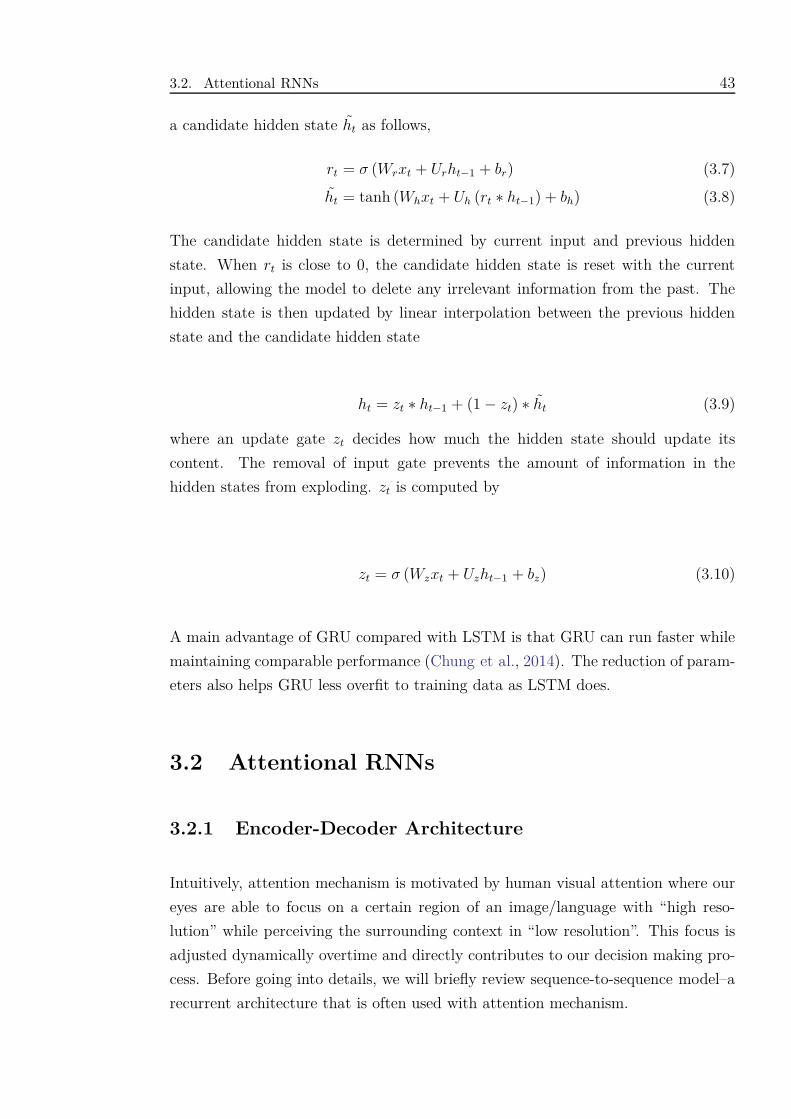
3.2. Attentional RNNs 43
a candidate hidden state ht as follows,
rt = σ (Wrxt + Urht−1 + br) (3.7)
ht = tanh (Whxt + Uh (rt ∗ ht−1) + bh) (3.8)
The candidate hidden state is determined by current input and previous hidden
state. When rt is close to 0, the candidate hidden state is reset with the current
input, allowing the model to delete any irrelevant information from the past. The
hidden state is then updated by linear interpolation between the previous hidden
state and the candidate hidden state
ht = zt ∗ ht−1 + (1− zt) ∗ ht (3.9)
where an update gate zt decides how much the hidden state should update its
content. The removal of input gate prevents the amount of information in the
hidden states from exploding. zt is computed by
zt = σ (Wzxt + Uzht−1 + bz) (3.10)
A main advantage of GRU compared with LSTM is that GRU can run faster while
maintaining comparable performance (Chung et al., 2014). The reduction of param-
eters also helps GRU less overfit to training data as LSTM does.
3.2 Attentional RNNs
3.2.1 Encoder-Decoder Architecture
Intuitively, attention mechanism is motivated by human visual attention where our
eyes are able to focus on a certain region of an image/language with “high reso-
lution” while perceiving the surrounding context in “low resolution”. This focus is
adjusted dynamically overtime and directly contributes to our decision making pro-
cess. Before going into details, we will briefly review sequence-to-sequence model–a
recurrent architecture that is often used with attention mechanism.
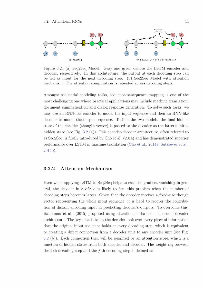
3.2. Attentional RNNs 44
Figure 3.2: (a) Seq2Seq Model. Gray and green denote the LSTM encoder anddecoder, respectively. In this architecture, the output at each decoding step canbe fed as input for the next decoding step. (b) Seq2Seq Model with attentionmechanism. The attention computation is repeated across decoding steps.
Amongst sequential modeling tasks, sequence-to-sequence mapping is one of the
most challenging one whose practical applications may include machine translation,
document summarisation and dialog response generation. To solve such tasks, we
may use an RNN-like encoder to model the input sequence and then an RNN-like
decoder to model the output sequence. To link the two models, the final hidden
state of the encoder (thought vector) is passed to the decoder as the latter’s initial
hidden state (see Fig. 3.2 (a)). This encoder-decoder architecture, often referred to
as Seq2Seq, is firstly introduced by Cho et al. (2014) and has demonstrated superior
performance over LSTM in machine translation (Cho et al., 2014a; Sutskever et al.,
2014b).
3.2.2 Attention Mechanism
Even when applying LSTM to Seq2Seq helps to ease the gradient vanishing in gen-
eral, the decoder in Seq2Seq is likely to face this problem when the number of
decoding steps becomes larger. Given that the decoder receives a fixed-size though
vector representing the whole input sequence, it is hard to recover the contribu-
tion of distant encoding input in predicting decoder’s outputs. To overcome this,
Bahdanau et al. (2015) proposed using attention mechanism in encoder-decoder
architecture. The key idea is to let the decoder look over every piece of information
that the original input sequence holds at every decoding step, which is equivalent
to creating a direct connection from a decoder unit to any encoder unit (see Fig.
3.2 (b)). Each connection then will be weighted by an attention score, which is a
function of hidden states from both encoder and decoder. The weight αij between
the i-th decoding step and the j-th encoding step is defined as
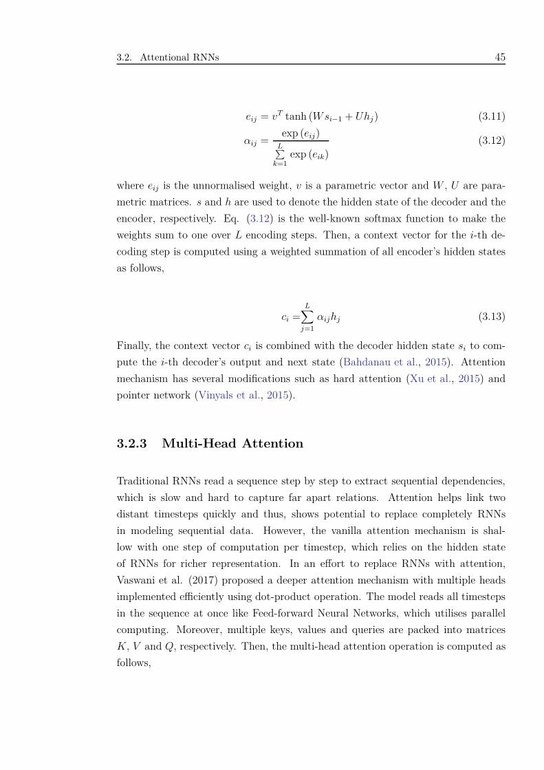
3.2. Attentional RNNs 45
eij = vT tanh (Wsi−1 + Uhj) (3.11)
αij =exp (eij)
L∑k=1
exp (eik)(3.12)
where eij is the unnormalised weight, v is a parametric vector and W , U are para-
metric matrices. s and h are used to denote the hidden state of the decoder and the
encoder, respectively. Eq. (3.12) is the well-known softmax function to make the
weights sum to one over L encoding steps. Then, a context vector for the i-th de-
coding step is computed using a weighted summation of all encoder’s hidden states
as follows,
ci =L∑
j=1
αijhj (3.13)
Finally, the context vector ci is combined with the decoder hidden state si to com-
pute the i-th decoder’s output and next state (Bahdanau et al., 2015). Attention
mechanism has several modifications such as hard attention (Xu et al., 2015) and
pointer network (Vinyals et al., 2015).
3.2.3 Multi-Head Attention
Traditional RNNs read a sequence step by step to extract sequential dependencies,
which is slow and hard to capture far apart relations. Attention helps link two
distant timesteps quickly and thus, shows potential to replace completely RNNs
in modeling sequential data. However, the vanilla attention mechanism is shal-
low with one step of computation per timestep, which relies on the hidden state
of RNNs for richer representation. In an effort to replace RNNs with attention,
Vaswani et al. (2017) proposed a deeper attention mechanism with multiple heads
implemented efficiently using dot-product operation. The model reads all timesteps
in the sequence at once like Feed-forward Neural Networks, which utilises parallel
computing. Moreover, multiple keys, values and queries are packed into matrices
K, V and Q, respectively. Then, the multi-head attention operation is computed as
follows,
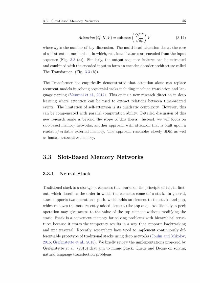
3.3. Slot-Based Memory Networks 46
Attention (Q, K, V ) = softmax
(QKT
√dk
)V (3.14)
where dk is the number of key dimension. The multi-head attention lies at the core
of self-attention mechanism, in which, relational features are encoded from the input
sequence (Fig. 3.3 (a)). Similarly, the output sequence features can be extracted
and combined with the encoded input to form an encoder-decoder architecture called
The Transformer. (Fig. 3.3 (b)).
The Transformer has empirically demonstrated that attention alone can replace
recurrent models in solving sequential tasks including machine translation and lan-
guage parsing (Vaswani et al., 2017). This opens a new research direction in deep
learning where attention can be used to extract relations between time-ordered
events. The limitation of self-attention is its quadratic complexity. However, this
can be compensated with parallel computation ability. Detailed discussion of this
new research angle is beyond the scope of this thesis. Instead, we will focus on
slot-based memory networks, another approach with attention that is built upon a
readable/writable external memory. The approach resembles closely SDM as well
as human associative memory.
3.3 Slot-Based Memory Networks
3.3.1 Neural Stack
Traditional stack is a storage of elements that works on the principle of last-in-first-
out, which describes the order in which the elements come off a stack. In general,
stack supports two operations: push, which adds an element to the stack, and pop,
which removes the most recently added element (the top one). Additionally, a peek
operation may give access to the value of the top element without modifying the
stack. Stack is a convenient memory for solving problems with hierarchical struc-
tures because it stores the temporary results in a way that supports backtracking
and tree traversal. Recently, researchers have tried to implement continuously dif-
ferentiable prototype of traditional stacks using deep networks (Joulin and Mikolov,
2015; Grefenstette et al., 2015). We briefly review the implementations proposed by
Grefenstette et al. (2015) that aim to mimic Stack, Queue and Deque on solving
natural language transduction problems.
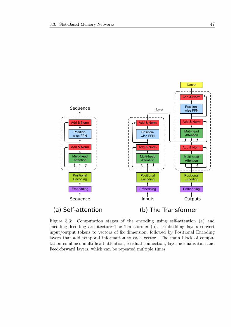
3.3. Slot-Based Memory Networks 47
Inputs OutputsSequence
Sequence
(a) Self-attention (b) The Transformer
Figure 3.3: Computation stages of the encoding using self-attention (a) andencoding-decoding architecture–The Transformer (b). Embedding layers convertinput/output tokens to vectors of fix dimension, followed by Positional Encodinglayers that add temporal information to each vector. The main block of compu-tation combines multi-head attention, residual connection, layer normalisation andFeed-forward layers, which can be repeated multiple times.
3.3. Slot-Based Memory Networks 48
In the implementations, a row-expandable matrix V is used to store the data. The
i-th row V [i] is associated with a strength scalar s [i]. When vt–the item at timestep
t– is presented, its value is added to the matrix V and never be modified, which
yields,
Vt [i] =
Vt−1 [i] = vi if 1 ≤ i < t
vt if i = t(3.15)
To modify the stack content under push and pop operations, we modify the strength
vector instead as the following,
st [i] =
max(0, st−1 [i]−max
(0, ut −
∑t−1j=i+1 st−1 [j]
))if 1 ≤ i < t
dt if i = t(3.16)
where ut and dt are the pop and push signals generated by a neural network, re-
spectively. Basically, the strength for the top item is set to the push signal. Then,
we want to subtract the strength of stored items (st [i]) by an amount of the pop
signal (ut) from the top (highest index) to the bottom (lowest index) of the stack.
If the pop signal is greater than the strength, the strength of the item is set to 0
(totally popped out of the stack) and the remainder of the pop signal is passed to
lower items until we run out of pop signal. The peek or read operation is carried
out by
rt =t∑
i=1
min
st [i] , max
0, 1−
t∑
j=i+1
st [j]
Vt [i] (3.17)
The output rt of the read operation is the weighted sum of the rows of Vt, scaled by
the temporary strength values created during the traversal. Intuitively, items with
zero strength do not contribute to read value and items on the bottom contribute
less than those near the top. Neural Queue and DeQue can be implemented in
similar manners by modifying Eqs. (3.15)-(3.17).
A controller implemented as RNN is employed to control stack operations. The cur-
rent input it from the sequence and the previous read-out rt−1 will be concatenated
as input for the RNN to produce the current hidden state ht and the controller
output o′t. The controller output will be used to generate the item, control signals
and final output of the whole network as follows,
3.3. Slot-Based Memory Networks 49
dt = σ (Wdo′t + bd) (3.18)
ut = σ (Wuo′t + bu) (3.19)
vt = tanh (Wvo′t + bv) (3.20)
ot = tanh (Woo′t + bo) (3.21)
Experiments have demonstrated that the proposed models are capable of solving
transduction tasks for which LSTM-based models falter (Grefenstette et al., 2015).
3.3.2 Memory Networks
One solution to ensure a model will not forget is to create a slot-based memory
module and store every piece of information into the memory slots. The memory
can be implemented as a matrix M ∈ RN×D whose rows contain vectors representing
the considering piece of information. Here, N is the number of slots and D is the
dimension of the representation vector (word size). Following this principle, Memory
Network (MemNN) (Weston et al., 2014) stores all information (e.g., knowledge base
or background context) into an external memory. When there is a retrieval request,
it assigns a relevance probability to each memory slot using content-based attention
scheme, and reads contents from each memory slot by taking their weighted sum.
Since the model is designed for language understanding, each slot of the memory
often associates with a document or a sentence. When a query/question about facts
related to the stored documents is presented, MemNN will perform content-based
attention as follows,
pi = softmax(uT mi
)(3.22)
where u is the feature and mi is the memory’s i-th row vector, which represent the
query and the stored document, respectively. pi is the attention score to the i-th
memory slot, normalised by softmax function.
The output of the memory, given query u, is the read vector
r =N∑
i=1
pici (3.23)
3.3. Slot-Based Memory Networks 50
where ci is the output vector corresponding to the i-th slot. In MemNN, it is train-
able parameter while in key-value memory network (Miller et al., 2016), it comes
from the data. Then, the model can make prediction by feeding the read values to
another feed-forward neural network.
A multi-hop version MemN2N has also been studied and outperforms LSTM and
MemNN in question-answering tasks (Sukhbaatar et al., 2015). MemN2N extends
MemNN by adding refinement updates on the query and the read-out. The refine-
ment reads
uk+1 = Huk + rk (3.24)
where H is a parametric matrix and k is the refinement step.
Although memory networks have big advantages over LSTM due to the use of ex-
ternal matrix memory, it is hard to scale to big dataset since the number of memory
slots grows linearly with the number of data. Some tricks such as hashing have been
proposed but they have a trade-off between capacity and accuracy. More impor-
tantly, it is unlikely that we tend to store everything in our brain. We have the
ability to forget the old memory and update with new knowledge, which is ignored
by memory network designs.
3.3.3 Neural Turing Machine
In contrast to MemNN, Neural Turing Machine (NTM) (Graves et al., 2014) intro-
duces a slot-based read/write mechanism to the memory module. The memory size
does not need to equal the number of considering pieces of information. The model
learns to overwrite obsolete or unimportant memory slots with recent and useful
information to optimise a final goal. This writing scheme fits with sequential task
where the prediction goal can be achieved without paying attention to all timestep
inputs. To control the memory operations, NTM uses a neural controller network
whose parameters are slow-learning weights. The controller is responsible for deter-
mining instantly after each timestep the content to be read from and written to the
memory. An illustration of NTM components is described in Fig. 3.4 (a).
In NTM, both reading and writing locations are determined by the address, which
is a weight over the memory slots. The weight is initially computed by the content-
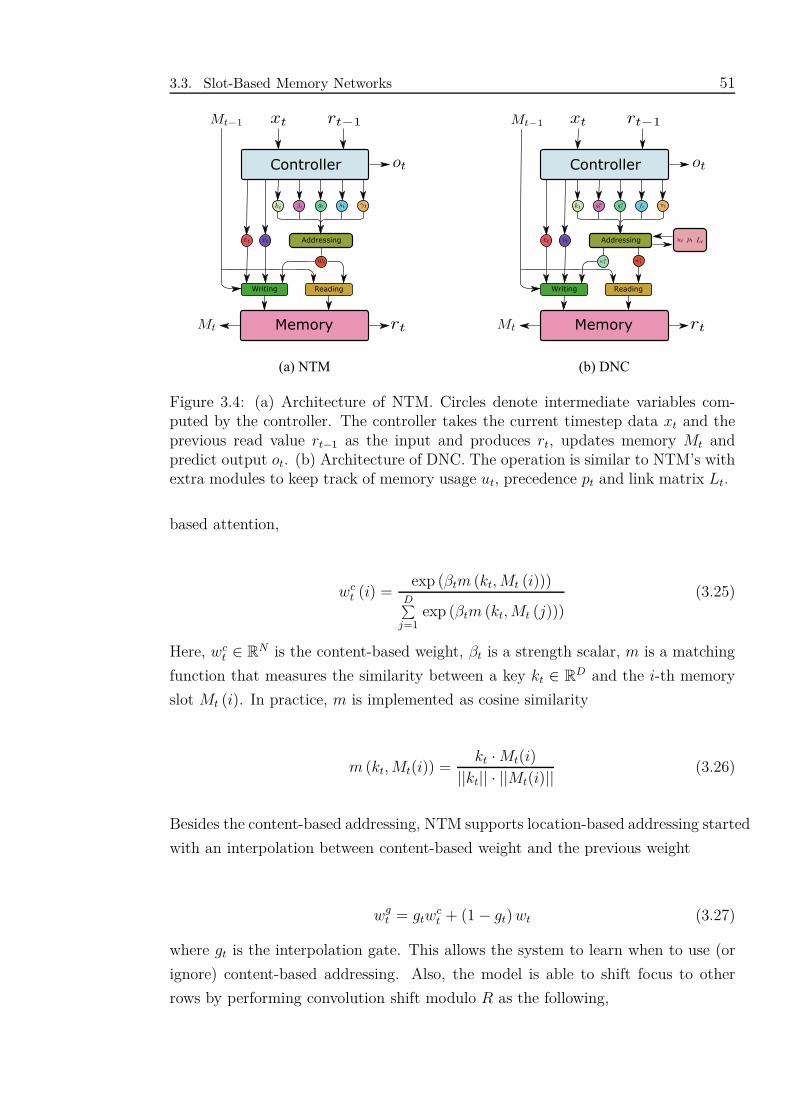
3.3. Slot-Based Memory Networks 51
Figure 3.4: (a) Architecture of NTM. Circles denote intermediate variables com-puted by the controller. The controller takes the current timestep data xt and theprevious read value rt−1 as the input and produces rt, updates memory Mt andpredict output ot. (b) Architecture of DNC. The operation is similar to NTM’s withextra modules to keep track of memory usage ut, precedence pt and link matrix Lt.
based attention,
wct (i) =
exp (βtm (kt, Mt (i)))D∑
j=1exp (βtm (kt, Mt (j)))
(3.25)
Here, wct ∈ RN is the content-based weight, βt is a strength scalar, m is a matching
function that measures the similarity between a key kt ∈ RD and the i-th memory
slot Mt (i). In practice, m is implemented as cosine similarity
m (kt, Mt(i)) =kt ·Mt(i)
||kt|| · ||Mt(i)||(3.26)
Besides the content-based addressing, NTM supports location-based addressing started
with an interpolation between content-based weight and the previous weight
wgt = gtw
ct + (1− gt) wt (3.27)
where gt is the interpolation gate. This allows the system to learn when to use (or
ignore) content-based addressing. Also, the model is able to shift focus to other
rows by performing convolution shift modulo R as the following,
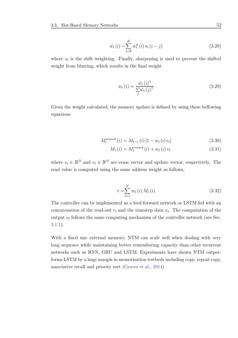
3.3. Slot-Based Memory Networks 52
wt (i) =R∑
j=0
wgt (i) st (i− j) (3.28)
where st is the shift weighting. Finally, sharpening is used to prevent the shifted
weight from blurring, which results in the final weight
wt (i) =wt (i)γ
∑j
wt (j)γ (3.29)
Given the weight calculated, the memory update is defined by using these bellowing
equations
Merasedt (i) = Mt−1 (i) [1− wt (i) et] (3.30)
Mt (i) = Merasedt (i) + wt (i) vt (3.31)
where et ∈ RD and vt ∈ R
D are erase vector and update vector, respectively. The
read value is computed using the same address weight as follows,
r =N∑
i=1
wt (i) Mt (i) (3.32)
The controller can be implemented as a feed-forward network or LSTM fed with an
concatenation of the read-out rt and the timestep data xt. The computation of the
output ot follows the same computing mechanism of the controller network (see Sec.
3.1.1).
With a fixed size external memory, NTM can scale well when dealing with very
long sequence while maintaining better remembering capacity than other recurrent
networks such as RNN, GRU and LSTM. Experiments have shown NTM outper-
forms LSTM by a huge margin in memorisation testbeds including copy, repeat copy,
associative recall and priority sort (Graves et al., 2014).
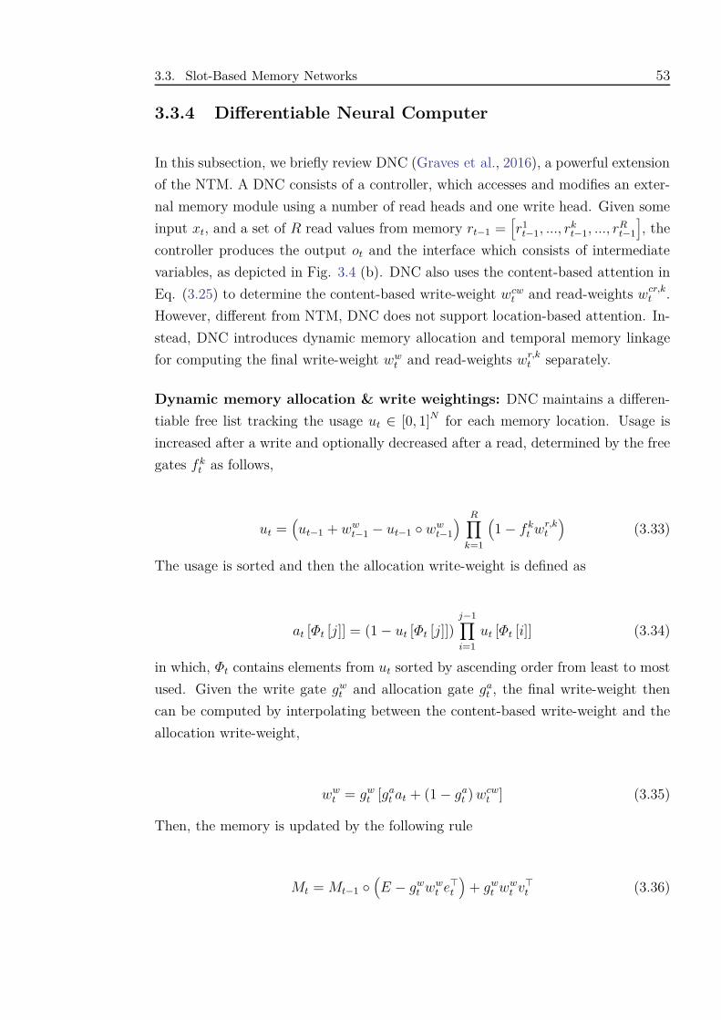
3.3. Slot-Based Memory Networks 53
3.3.4 Differentiable Neural Computer
In this subsection, we briefly review DNC (Graves et al., 2016), a powerful extension
of the NTM. A DNC consists of a controller, which accesses and modifies an exter-
nal memory module using a number of read heads and one write head. Given some
input xt, and a set of R read values from memory rt−1 =[r1
t−1, ..., rkt−1, ..., rR
t−1
], the
controller produces the output ot and the interface which consists of intermediate
variables, as depicted in Fig. 3.4 (b). DNC also uses the content-based attention in
Eq. (3.25) to determine the content-based write-weight wcwt and read-weights wcr,k
t .
However, different from NTM, DNC does not support location-based attention. In-
stead, DNC introduces dynamic memory allocation and temporal memory linkage
for computing the final write-weight wwt and read-weights wr,k
t separately.
Dynamic memory allocation & write weightings: DNC maintains a differen-
tiable free list tracking the usage ut ∈ [0, 1]N for each memory location. Usage is
increased after a write and optionally decreased after a read, determined by the free
gates fkt as follows,
ut =(ut−1 + ww
t−1 − ut−1 ◦ wwt−1
) R∏
k=1
(1− fk
t wr,kt
)(3.33)
The usage is sorted and then the allocation write-weight is defined as
at [Φt [j]] = (1− ut [Φt [j]])j−1∏
i=1
ut [Φt [i]] (3.34)
in which, Φt contains elements from ut sorted by ascending order from least to most
used. Given the write gate gwt and allocation gate ga
t , the final write-weight then
can be computed by interpolating between the content-based write-weight and the
allocation write-weight,
wwt = gw
t [gat at + (1− ga
t ) wcwt ] (3.35)
Then, the memory is updated by the following rule
Mt = Mt−1 ◦(E − gw
t wwt e⊤
t
)+ gw
t wwt v⊤
t (3.36)
3.3. Slot-Based Memory Networks 54
Temporal memory linkage & read weightings: DNC uses a temporal link
matrix Lt ∈ [0, 1] N×N to keep track of consecutively modified memory locations,
and Lt [i, j] represents the degree to which location i was the location written to after
location j. Each time a memory location is modified, the link matrix is updated to
remove old links to and from that location, and add new links from the last-written
location. To compute the link matrix, DNC maintains a precedence weighting to
keep track of which locations were most recently written by using the following
equation
pt =
(1−
N∑
i
wwt (i)
)pt−1 + ww
t (3.37)
Then pt is used to update the link matrix as follows,
Lt (i, j) = (1− wwt (i)− ww
t (j)) Lt−1 (i, j) + wwt (i) pt−1 (j) (3.38)
Given the link matrix, the final read-weight is given as follow,
wr,kt = πk
t (1) L⊤t wr,k
t−1 + πkt (2) wcr,k
t + πkt (3) Ltw
r,kt−1 (3.39)
The read mode weight πkt is used to balance between the content-based read-weight
and the forward Ltwr,kt−1 and backward L⊤
t wr,kt−1 of the previous read. Then, the k-th
read value rkt is retrieved using the final read-weight vector
rkt =
N∑
i
wr,kt (i)Mt(i) (3.40)
The performance of DNC is better than that of NTM, LSTM and other variants
of memory networks. It achieves state-of-the-art results under various experimental
settings such as copy/recall, question-answering and graph reasoning (Graves et al.,
2016).
3.3.5 Memory-augmented Encoder-Decoder Architecture
A memory-augmented encoder-decoder (MAED) consists of two neural controllers
linked via external memory. This is a natural extension to read-write MANNs
3.4. Closing Remarks 55
to handle sequence-to-sequence problems, which has been investigated in Sec. 3.2.
MAED has recently demonstrated promising results in machine translation (Britz et al.,
2017; Wang et al., 2016), OCR (Nguyen et al., 2019) and healthcare (Le et al., 2018c,b;
Prakash et al., 2017). In this thesis, MAED is the basic framework on which some
of our proposed architectures are built upon. Here, we briefly analyse the operations
of MAED. More details can be found in Chapter 4.
As mentioned in Sec. 3.2.1, Seq2Seq only allows information transfer from the en-
coder to the decoder via “thought vector”. Attention mechanism creates shortcut
connections via directly attending to other timesteps (see Sec. 3.2.2 and 3.2.3). Un-
like these approaches, MAED uses an external memory as a reservoir containing past
information to which the controllers attend. That is, instead of directly attending
to other timesteps, the controllers (both encoder and decoder) attend to the mem-
ory to store and retrieve relevant information The information then participates in
other decision-making processes such as output predictions, feature extractions and
memory operations. If the number of memory slots is finite, the method keeps the
computation resource linear to the length of the sequence, which is feasible for life-
long learning. Furthermore, selectively attending to a fixed number of memory slots
requires the model to learn to compress the information to the external memory. On
one hand, it may make the learning harder since the controllers must learn to write
timestep information to the memory efficiently. On the other hand, attending to
all timesteps is biologically implausible and information compression is a powerful
skill that mimics the capacity of memory in the brain. Hence, this thesis has chosen
MAED as the key framework to study and develop several memory and attention
techniques for neural networks (Chapter 4 and 5).
3.4 Closing Remarks
We have reviewed MANNs, a family of recurrent neural networks with external
memory, which is useful for a wide range of sequential learning tasks. Armed with
operations such as gating and attention mechanisms, MANNs are able to control and
update external vector or matrix memory module. The power of MANNs has been
verified in learning long sequential data, in which their performances are superior
to that of vanilla RNNs.
We hypothesise that MANNs are also effective in open challenges in multi-process/multi-
view data, data with uncertainty, ultra-long sequences and problems required univer-
3.4. Closing Remarks 56
sal computation. We address these challenges in Chapters 4, 5, 6 and 7, respectively.
A recurring theme across all of our proposed MANNs is found on slot-based memory
architecture.
Chapter 4
Memory Models for Multiple
Processes
4.1 Introduction
4.1.1 Multi-Process Learning
Traditional sequential learning focuses on modeling single processes, in which the
sequence of outputs shares the same domain with the input sequence. We can
extend the problem to broader scenarios where input and output sequences are from
different processes (sequence to sequence) or there are multiple sequences acting as
inputs and outputs (multi-view sequential mapping). For example, in healthcare
setting, there are at least three processes that are executed: the disease progression,
the treatment protocols, and the recording rules.
Let us start with a generic formulation of the multi-process learning. Let Si1 , ...,SiM
and So1, ...,SoN denote M input and N output view spaces, respectively. Each sam-
ple of the multi-process problem({X ik}M
k=1 , {Y ok}Nk=1
)consists of M input views:
X i1 ={xi1
1 , ..., xi1
t1, ..., xi1
Li1
}, ..., X iM =
{xiM
1 , ..., xiMtM
, ..., xiM
LiM
}and N output views
Y o1 = {yo1
1 , ..., yo1
t1, ..., yo1
Lo1} , ..., Y oN ={yoN
1 , ..., yoNtN
, ..., yoNLoN
}. Each view has a par-
ticular length (Li1 , ..., LiM and Lo1 , ..., LoN ) and can be treated as a set/sequence
of events that belongs to different spaces (xi1
t1∈ Si1 , ..., xiM
tM∈ SiM , yo1
t1∈ So1 , ...,
yoNtN∈ SoN ). Each event then can be represented by an one-hot vector v ∈ [0, 1]‖C‖,
where C can be Si1 , ..., SiM or So1, ..., SoN . In single process, M = N = 1 and
57
4.1. Introduction 58
Si1 = So1. Practical problems belonging to this setting can be solved efficiently using
RNNs or LSTM as in language modeling (Mikolov et al., 2010), speech and optical
character recognition (Graves et al., 2013; Graves, 2013; Graves and Schmidhuber,
2005). We focus more on other complicated cases, which are dual processes (se-
quence to sequence) and dual-view mapping, where M = N = 1, Si1 6= So1 and
M = 2, N = 1, Si1 6= Si2 6= So1 , respectively. These cases represent two classes of
problems that traditional RNNs may struggle to deal with. Thus, we aim to solve
them using MAED (Sec. 3.3.5) by proposing: (i) separate controls for two separate
sub-processes (encoding, decoding) and (ii) multiple memories for multiple paral-
lel, asynchronous processes. To account for these settings, we need more powerful
MAEDs to handle the complexity of long-term dependencies and view interactions,
which will be presented in the next sections using healthcare as a practical domain.
4.1.2 Real-World Motivation
A main motivation for our work in this chapter is modeling healthcare processes.
In healthcare, a hospital visit is documented as one admission record consisting of
diagnosis and treatment codes for the admission. The collection of these records
are electronic medical records (EMRs) of a patient. Recently, using EMRs as the
data for scientists to analyse and make treatment predictions has become the key for
improving healthcare (Williams, 2008). A typical EMR contains information about a
sequence of admissions for a patient and a wide range of information can be stored
in each admission, such as detailed records of symptoms, data from monitoring
devices, clinicians’ observations. Diagnoses, procedures or drug prescriptions are the
most important information stored in EMRs and are typically coded in standardised
formats, each of which represents a medical process in EMR data.
In particular, diagnoses are coded using WHO’s ICD (International Classification
of Diseases) coding schemes. For example, in the ICD10 scheme, E10 encodes Type
1 diabetes mellitus, E11 encodes Type 2 diabetes mellitus and F32 indicates de-
pressive episode. The treatment can be procedure or drug. The procedures are
typically coded in CPT (Current Procedural Terminology) or ICHI (International
Classification of Health Interventions) schemes. The drugs are often coded in ATC
(Anatomical Therapeutic Chemical) or NDC (National Drug Code).
It is important to note that there are order dependencies amongst medical processes
such as the diagnosis codes as well as procedure or drug codes. For example, diag-
4.1. Introduction 59
nosis codes are often sequenced under some strict rules such as: (i) condition codes
must be sequenced first, followed by the manifestation codes, (ii) primary diagnosis
that describe the nature of the sequela must be coded before the secondary diagno-
sis that describes the original injury, (iii) single conditions that require more than
one code have clear instructions that indicate which must be coded first. Similarly,
procedure or drug codes often follow specific order, often corresponding to the order
of diagnosis codes or the order of prescriptions. Moreover, the dependency in EMR
clinical codes can be very long-term. Due to the fact that EMR data is temporally
sequenced by patient medical visits, clinical codes at current admission may be re-
lated to other codes appearing in previous admissions. Since it is normal for patients
to periodically visit hospital for regular health check, the number of admissions for
some person should be very large and thus the dependency amongst clinical codes
should be very long. Another characteristic of EMR data is its rarity. Although the
number of EMR records are increasing day by day, it cannot cover many rarely-seen
symptoms and treatments which appear sparsely throughout the history of EMR
documentation. More seriously, rare diseases are deadly and rare treatments are
expensive, so it is compulsory to make use of these rare information in order to
make significant predictions.
Unfortunately, it is not easy for prediction models to capture the long-term depen-
dencies and rarity of EMR data. Recent researches dealing with medical prediction
have largely focused on modeling the admission’s diagnosis and treatments as two
set of codes and only capture sequential dependencies from one admission to another
(Nguyen et al., 2017; Pham et al., 2017). Also, most of these methods avoid using
rare data by only keeping codes that appear frequently. This approach exposes three
limitations. First, using set representation ignores the internal internal sequential
dependencies and thus fail to discover sequential relations amongst codes from the
same admission. Second, refusing to use rare clinical events makes the contribu-
tion less significant because in healthcare, rare events are the more important ones.
Third, outputs of this approach are often set of codes, which again detaches from
realistic need where treatments and diagnoses have to follow strict orders. These
challenges motivate new approaches that treat EMR history as sequences of corre-
lated processes.
4.1. Introduction 60
Sequence to sequence mapping
Treatment recommendation can be cast as sequence to sequence problem. Once
diagnoses are confirmed, we want to predict the output sequence (treatment codes
of the current visit) given the input sequence (all diagnoses followed by treatments
from the first visit to the previous visit plus the diagnoses of the current visit). More
formally, we denote all the unique medical codes (diagnosis, procedures and drugs)
from the EMR data as c1, c2, ..c|C| ∈ C, where |C| is the number of unique medical
codes. A patient’s n-th admission’s input is represented by a sequence of codes:
[c1
d1, c1
d2, ...,h, c1
p1, c1
p2...,�, ..., cn−1
d1, cn−1
d2, ...,h, cn−1
p1, , cn−1p2
, ....,�, cnd1
, cnd2
, ...,h]
(4.1)
Here, ckdj
and ckpj
are the j-th diagnosis and treatment code of the k-th admission,
respectively. h , � are special characters that informs the model about the change
from diagnosis to treatment codes and the end of an admission, respectively. This re-
flects the natural structure of a medical history, which is a sequence of clinical visits,
each of which typically includes a subsequence of diagnoses, and a subset of treat-
ments. A diagnosis subsequence usually starts with the primary condition followed
by secondary conditions. In a subset of treatments, the order is not strictly enforced,
but it may reflect the coding practice. The output of the patient’s n-th admission is :[cn
p1, cn
p2, ..., cn
pLout,�], in which Lout is the length of the treatment sequence we want
to predict and � is used to inform the model to stop predicting. Finally, each code
is represented by one-hot vector vc ∈ [0, 1]‖C‖, where vc = [0, ..., 0, 1, 0.., 0] (vc[i] = 1
if and only if vc represents ci). Unlike set encoding of each admission, representing
the data in this way preserves the admission’s internal order information allowing
sequence-based methods to demonstrate their power of capturing sequential events.
In Sec. 4.3, we present a novel treatment recommendation model using memory net-
work to remember long-term dependencies and rare events from EMR data. This
model is built upon Differential Neural Computer (DNC) (Graves et al., 2016), a
fully differentiable implementation of memory-augmented neural network (MANN)
(see Sec. 3.3.4). In question-answer bAbI task (Weston et al., 2015), DNC treats
the story, question as sequences of words and perform well on the task of predicting
sequence of answers, which suggests the power of DNC in handling sequence input
and solving sequence prediction task. Despite of its successes, DNC have never been
applied to realistic domain such as healthcare, especially in clinical treatment se-
quence prediction. This realisation motivates us to design a DNC-based architecture
that fits and works well with healthcare domain. In our design, we make use of two
4.1. Introduction 61
controllers instead of one to handle dual processes: diagnoses and treatments. Each
controller will employ different remembering strategies for each process and thus
increase the robustness of prediction and the speed of learning. Besides, we apply
a write-protected policy for our controller to direct the model toward reasonable
remember strategies.
Two-view sequential learning
For two-view problems, the generic notations simplify to Si1 , Si2 denoting input
view spaces and S the output view space. Each sample of the two-view prob-
lem (X i1, X i2 , Y ) consists of two input views: X i1 ={
xi1
1 , ..., xi1
t1, ..., xi1
Lii
}, X i2 ={
xi2
1 , ..., xi2
t2, ..., xi2
Li2
}and one output view Y = {y1, ..., yt, ..., yL}. Each view has a
particular length (Li1 , Li2 or L), each of which is a set/sequence of events that be-
longs to different spaces (xi1
t1∈ Si1 , xi2
t2∈ Si2, yt ∈ S). It should be noted that this
formulation can be applied to many situations including video-audio understanding,
image-captioning and other two-channel time-series signals. Here we focus effort on
solving the two-view problems in healthcare.
For example, in drug prescription, doctors prescribe drugs after considering diag-
noses and procedures administered to patients. In modeling disease progression,
doctor may refer to patient’s history of admissions to help diagnoses the current
diseases or to predict the future disease occurrences of the patient. There are clin-
ical recording rules applying to EMR codes such that diagnoses are “ordered by
priority” or procedures follow the order that “the procedures were performed”1. Be-
sides, although medical codes from different views are highly correlated, they are
not aligned. For instances, some diagnoses may correspond to one procedure or one
diagnosis may result in multiple medicines. Hence, these problems can be treated
as asynchronous two-view sequential learning.
In the drug prescription context, Si1 and Si2 represent the diagnosis and procedure
spaces, respectively and S corresponds to the medicine space. The drug prescription
objective is to select an optimal subset of medications from S based on diagnosis and
procedure codes. Similarly, we can formulate the disease progression problem as two
input sequences (diagnoses and interventions) and one output set (next diagnoses).
Although our architecture can model sequential output, the choice of representing
output as set is to follow a common practice in healthcare where the order of medical
1https://mimic.physionet.org/mimictables/
4.2. Background 62
suggestions is specified. Because a patient may have multiple admission records for
different hospital visits, a patient record can be represented as {(X i1
a , X i2
a , Ya)}Aa=1,
where A is the number of admissions this patient commits. In order to predict Ya, we
may need to exploit not only (X i1
a , X i2
a ) but also{(
X i1
pa, X i2
pa
)}a−1
pa=1. More details on
how our work makes use of previous admissions and handles long-term dependencies
will be given in Sec. 4.4.3.
In Sec. 4.4, we propose a novel memory augmented neural network model solving
the problem of asynchronous interactions and long-term dependencies at the same
time. Our model makes use of three neural controllers and two external memories
constituting a dual memory neural computer. In our architecture, each input view is
assigned to a controller and a memory to model the intra-view interactions in that
particular view. At each time step, the controller reads an input event, updates
the memory, and generates an output based on its current hidden state and read
vectors from the memory. Corresponding to the two types of inter-view interactions,
there are two modes in our architecture: late-fusion and early-fusion memories. In
the late-fusion mode, the memory space for each view is separated and indepen-
dent, that is, there is no information exchange between the two memories during
the encoding process. The memories’ read values are only synthesised to generate
inter-view knowledge in the decoding phase. Contrast to the late-fusion mode, the
memory addressing space in the early-fusion mode is shared amongst views. That
is, the encoder from one view can access and modify the contents of the other view’s
memory. This design ensures the information is shared across views via memories
accessing. In order to facilitate this asynchronous sharing, we design novel cache
components that temporarily hold the write values of every timestep. This enables
related information at different time steps to be written to the memories together.
Finally, we apply memory write-protected mechanism in the decoding process to
make the inference of our model more efficient.
4.2 Background
4.2.1 Multi-View Learning
In multi-view learning, data can be naturally partitioned into channels presenting
different views of the same data. Multi-view sequential learning is a sub-class of
multi-view learning where each view data is in the form of sequential events, which
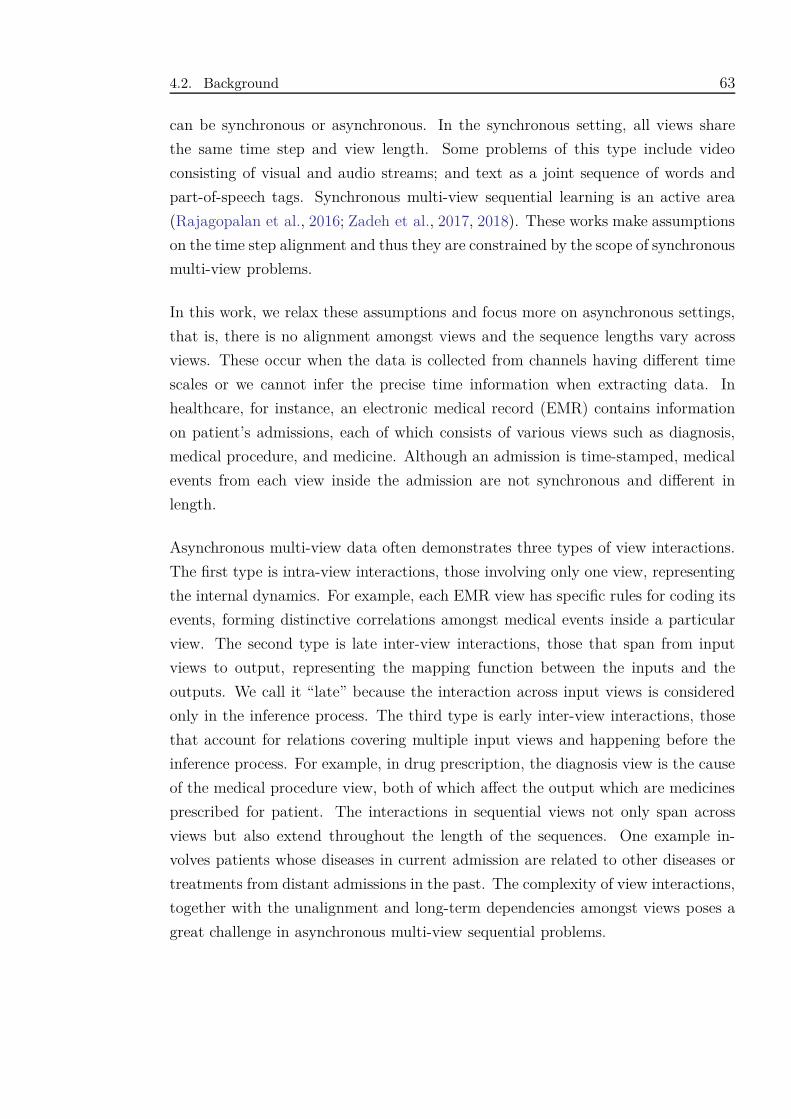
4.2. Background 63
can be synchronous or asynchronous. In the synchronous setting, all views share
the same time step and view length. Some problems of this type include video
consisting of visual and audio streams; and text as a joint sequence of words and
part-of-speech tags. Synchronous multi-view sequential learning is an active area
(Rajagopalan et al., 2016; Zadeh et al., 2017, 2018). These works make assumptions
on the time step alignment and thus they are constrained by the scope of synchronous
multi-view problems.
In this work, we relax these assumptions and focus more on asynchronous settings,
that is, there is no alignment amongst views and the sequence lengths vary across
views. These occur when the data is collected from channels having different time
scales or we cannot infer the precise time information when extracting data. In
healthcare, for instance, an electronic medical record (EMR) contains information
on patient’s admissions, each of which consists of various views such as diagnosis,
medical procedure, and medicine. Although an admission is time-stamped, medical
events from each view inside the admission are not synchronous and different in
length.
Asynchronous multi-view data often demonstrates three types of view interactions.
The first type is intra-view interactions, those involving only one view, representing
the internal dynamics. For example, each EMR view has specific rules for coding its
events, forming distinctive correlations amongst medical events inside a particular
view. The second type is late inter-view interactions, those that span from input
views to output, representing the mapping function between the inputs and the
outputs. We call it “late” because the interaction across input views is considered
only in the inference process. The third type is early inter-view interactions, those
that account for relations covering multiple input views and happening before the
inference process. For example, in drug prescription, the diagnosis view is the cause
of the medical procedure view, both of which affect the output which are medicines
prescribed for patient. The interactions in sequential views not only span across
views but also extend throughout the length of the sequences. One example in-
volves patients whose diseases in current admission are related to other diseases or
treatments from distant admissions in the past. The complexity of view interactions,
together with the unalignment and long-term dependencies amongst views poses a
great challenge in asynchronous multi-view sequential problems.
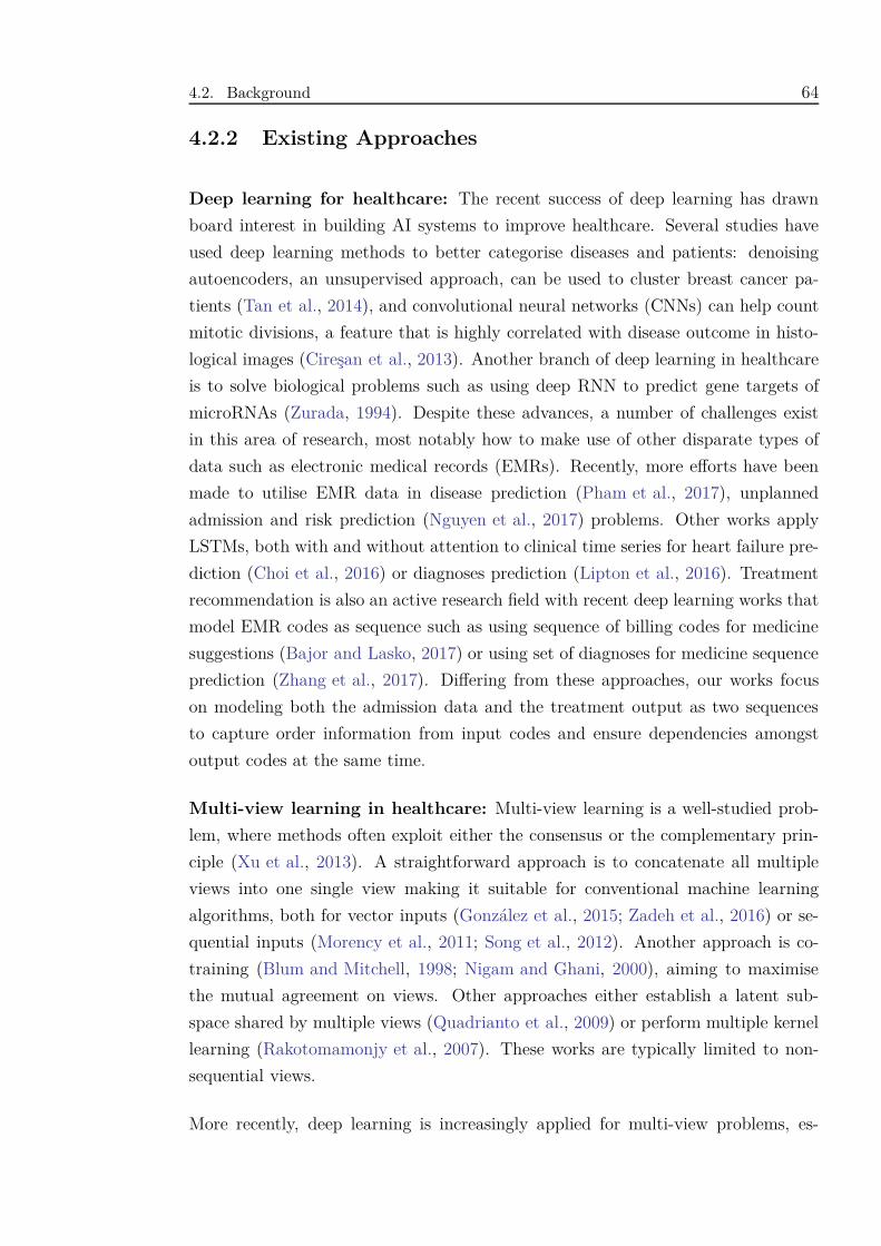
4.2. Background 64
4.2.2 Existing Approaches
Deep learning for healthcare: The recent success of deep learning has drawn
board interest in building AI systems to improve healthcare. Several studies have
used deep learning methods to better categorise diseases and patients: denoising
autoencoders, an unsupervised approach, can be used to cluster breast cancer pa-
tients (Tan et al., 2014), and convolutional neural networks (CNNs) can help count
mitotic divisions, a feature that is highly correlated with disease outcome in histo-
logical images (Cireşan et al., 2013). Another branch of deep learning in healthcare
is to solve biological problems such as using deep RNN to predict gene targets of
microRNAs (Zurada, 1994). Despite these advances, a number of challenges exist
in this area of research, most notably how to make use of other disparate types of
data such as electronic medical records (EMRs). Recently, more efforts have been
made to utilise EMR data in disease prediction (Pham et al., 2017), unplanned
admission and risk prediction (Nguyen et al., 2017) problems. Other works apply
LSTMs, both with and without attention to clinical time series for heart failure pre-
diction (Choi et al., 2016) or diagnoses prediction (Lipton et al., 2016). Treatment
recommendation is also an active research field with recent deep learning works that
model EMR codes as sequence such as using sequence of billing codes for medicine
suggestions (Bajor and Lasko, 2017) or using set of diagnoses for medicine sequence
prediction (Zhang et al., 2017). Differing from these approaches, our works focus
on modeling both the admission data and the treatment output as two sequences
to capture order information from input codes and ensure dependencies amongst
output codes at the same time.
Multi-view learning in healthcare: Multi-view learning is a well-studied prob-
lem, where methods often exploit either the consensus or the complementary prin-
ciple (Xu et al., 2013). A straightforward approach is to concatenate all multiple
views into one single view making it suitable for conventional machine learning
algorithms, both for vector inputs (González et al., 2015; Zadeh et al., 2016) or se-
quential inputs (Morency et al., 2011; Song et al., 2012). Another approach is co-
training (Blum and Mitchell, 1998; Nigam and Ghani, 2000), aiming to maximise
the mutual agreement on views. Other approaches either establish a latent sub-
space shared by multiple views (Quadrianto et al., 2009) or perform multiple kernel
learning (Rakotomamonjy et al., 2007). These works are typically limited to non-
sequential views.
More recently, deep learning is increasingly applied for multi-view problems, es-
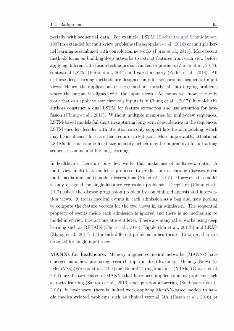
4.2. Background 65
pecially with sequential data. For example, LSTM (Hochreiter and Schmidhuber,
1997) is extended for multi-view problems (Rajagopalan et al., 2016) or multiple ker-
nel learning is combined with convolution networks (Poria et al., 2015). More recent
methods focus on building deep networks to extract features from each view before
applying different late-fusion techniques such as tensor products (Zadeh et al., 2017),
contextual LSTM (Poria et al., 2017) and gated memory (Zadeh et al., 2018). All
of these deep learning methods are designed only for synchronous sequential input
views. Hence, the applications of these methods mostly fall into tagging problems
where the output is aligned with the input views. As far as we know, the only
work that can apply to asynchronous inputs is in Chung et al., (2017), in which the
authors construct a dual LSTM for feature extraction and use attention for late-
fusion (Chung et al., 2017). Without multiple memories for multi-view sequences,
LSTM-based models fail short in capturing long-term dependencies in the sequences.
LSTM encoder-decoder with attention can only support late-fusion modeling, which
may be insufficient for cases that require early-fusion. More importantly, attentional
LSTMs do not assume fixed size memory, which may be impractical for ultra-long
sequences, online and life-long learning.
In healthcare, there are only few works that make use of multi-view data. A
multi-view multi-task model is proposed to predict future chronic diseases given
multi-media and multi-model observations (Nie et al., 2015). However, this model
is only designed for single-instance regression problems. DeepCare (Pham et al.,
2017) solves the disease progression problem by combining diagnosis and interven-
tion views. It treats medical events in each admission as a bag and uses pooling
to compute the feature vectors for the two views in an admission. The sequential
property of events inside each admission is ignored and there is no mechanism to
model inter-view interactions at event level. There are many other works using deep
learning such as RETAIN (Choi et al., 2016), Dipole (Ma et al., 2017b) and LEAP
(Zhang et al., 2017) that attack different problems in healthcare. However, they are
designed for single input view.
MANNs for healthcare: Memory augmented neural networks (MANNs) have
emerged as a new promising research topic in deep learning. Memory Networks
(MemNNs) (Weston et al., 2014) and Neural Turing Machines (NTMs) (Graves et al.,
2014) are the two classes of MANNs that have been applied to many problems such
as meta learning (Santoro et al., 2016) and question answering (Sukhbaatar et al.,
2015). In healthcare, there is limited work applying MemNN-based models to han-
dle medical-related problems such as clinical textual QA (Hasan et al., 2016) or
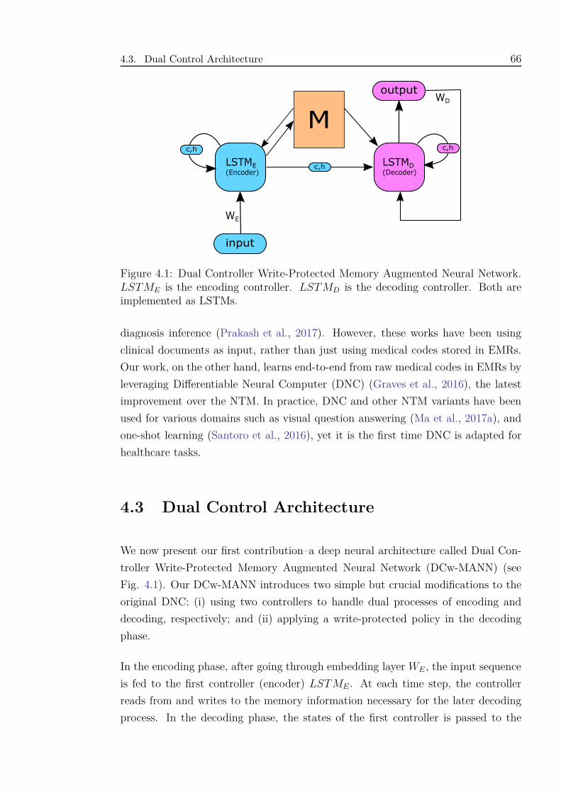
4.3. Dual Control Architecture 66
Figure 4.1: Dual Controller Write-Protected Memory Augmented Neural Network.LSTME is the encoding controller. LSTMD is the decoding controller. Both areimplemented as LSTMs.
diagnosis inference (Prakash et al., 2017). However, these works have been using
clinical documents as input, rather than just using medical codes stored in EMRs.
Our work, on the other hand, learns end-to-end from raw medical codes in EMRs by
leveraging Differentiable Neural Computer (DNC) (Graves et al., 2016), the latest
improvement over the NTM. In practice, DNC and other NTM variants have been
used for various domains such as visual question answering (Ma et al., 2017a), and
one-shot learning (Santoro et al., 2016), yet it is the first time DNC is adapted for
healthcare tasks.
4.3 Dual Control Architecture
We now present our first contribution–a deep neural architecture called Dual Con-
troller Write-Protected Memory Augmented Neural Network (DCw-MANN) (see
Fig. 4.1). Our DCw-MANN introduces two simple but crucial modifications to the
original DNC: (i) using two controllers to handle dual processes of encoding and
decoding, respectively; and (ii) applying a write-protected policy in the decoding
phase.
In the encoding phase, after going through embedding layer WE , the input sequence
is fed to the first controller (encoder) LSTME . At each time step, the controller
reads from and writes to the memory information necessary for the later decoding
process. In the decoding phase, the states of the first controller is passed to the
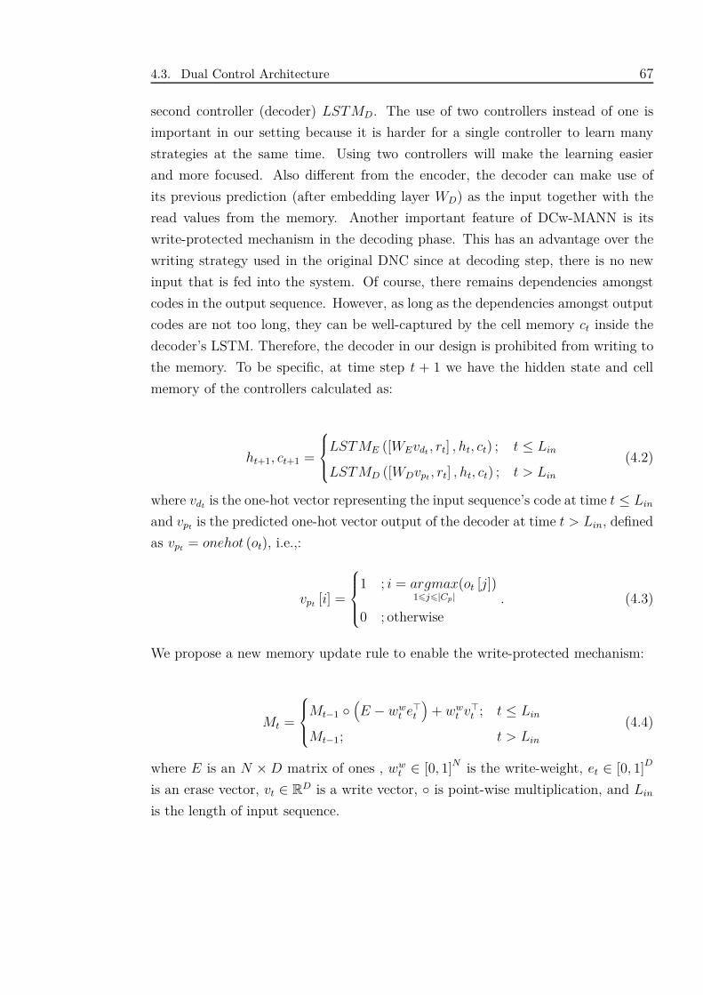
4.3. Dual Control Architecture 67
second controller (decoder) LSTMD. The use of two controllers instead of one is
important in our setting because it is harder for a single controller to learn many
strategies at the same time. Using two controllers will make the learning easier
and more focused. Also different from the encoder, the decoder can make use of
its previous prediction (after embedding layer WD) as the input together with the
read values from the memory. Another important feature of DCw-MANN is its
write-protected mechanism in the decoding phase. This has an advantage over the
writing strategy used in the original DNC since at decoding step, there is no new
input that is fed into the system. Of course, there remains dependencies amongst
codes in the output sequence. However, as long as the dependencies amongst output
codes are not too long, they can be well-captured by the cell memory ct inside the
decoder’s LSTM. Therefore, the decoder in our design is prohibited from writing to
the memory. To be specific, at time step t + 1 we have the hidden state and cell
memory of the controllers calculated as:
ht+1, ct+1 =
LSTME ([WEvdt , rt] , ht, ct) ; t ≤ Lin
LSTMD ([WDvpt , rt] , ht, ct) ; t > Lin
(4.2)
where vdt is the one-hot vector representing the input sequence’s code at time t ≤ Lin
and vpt is the predicted one-hot vector output of the decoder at time t > Lin, defined
as vpt = onehot (ot), i.e.,:
vpt [i] =
1 ; i = argmax16j6|Cp|
(ot [j])
0 ; otherwise. (4.3)
We propose a new memory update rule to enable the write-protected mechanism:
Mt =
Mt−1 ◦(E − ww
t e⊤t
)+ ww
t v⊤t ; t ≤ Lin
Mt−1; t > Lin
(4.4)
where E is an N ×D matrix of ones , wwt ∈ [0, 1]N is the write-weight, et ∈ [0, 1]D
is an erase vector, vt ∈ RD is a write vector, ◦ is point-wise multiplication, and Lin
is the length of input sequence.
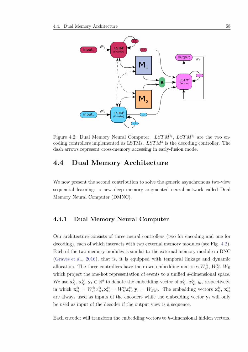
4.4. Dual Memory Architecture 68
Figure 4.2: Dual Memory Neural Computer. LSTM i1 , LSTM i2 are the two en-coding controllers implemented as LSTMs. LSTMd is the decoding controller. Thedash arrows represent cross-memory accessing in early-fusion mode.
4.4 Dual Memory Architecture
We now present the second contribution to solve the generic asynchronous two-view
sequential learning: a new deep memory augmented neural network called Dual
Memory Neural Computer (DMNC).
4.4.1 Dual Memory Neural Computer
Our architecture consists of three neural controllers (two for encoding and one for
decoding), each of which interacts with two external memory modules (see Fig. 4.2).
Each of the two memory modules is similar to the external memory module in DNC
(Graves et al., 2016), that is, it is equipped with temporal linkage and dynamic
allocation. The three controllers have their own embedding matrices W i1
E , W i2
E , WE
which project the one-hot representation of events to a unified d-dimensional space.
We use xi1
t1, xi2
t2, yt ∈ Rd to denote the embedding vector of xi1
t1, xi2
t2, yt, respectively,
in which xi1
t1= W i1
E xi1
t1, xi2
t2= W i2
E xi2
t2, yt = WEyt. The embedding vectors xi1
t1, xi2
t2
are always used as inputs of the encoders while the embedding vector yt will only
be used as input of the decoder if the output view is a sequence.
Each encoder will transform the embedding vectors to h-dimensional hidden vectors.
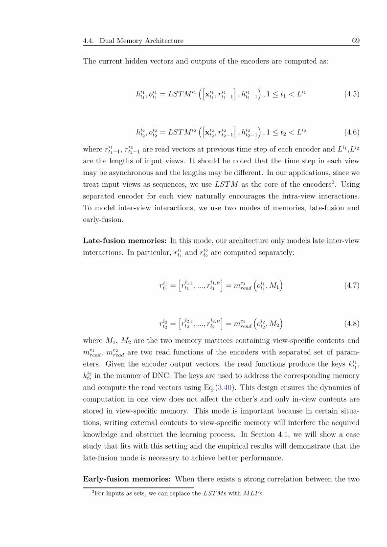
4.4. Dual Memory Architecture 69
The current hidden vectors and outputs of the encoders are computed as:
hi1
t1, oi1
t1= LSTM i1
([xi1
t1, ri1
t1−1
], hi1
t1−1
), 1 ≤ t1 < Li1 (4.5)
hi2
t2, oi2
t2= LSTM i2
([xi2
t2, ri2
t2−1
], hi2
t2−1
), 1 ≤ t2 < Li2 (4.6)
where ri1
t1−1, ri2
t2−1 are read vectors at previous time step of each encoder and Li1 ,Li2
are the lengths of input views. It should be noted that the time step in each view
may be asynchronous and the lengths may be different. In our applications, since we
treat input views as sequences, we use LSTM as the core of the encoders2. Using
separated encoder for each view naturally encourages the intra-view interactions.
To model inter-view interactions, we use two modes of memories, late-fusion and
early-fusion.
Late-fusion memories: In this mode, our architecture only models late inter-view
interactions. In particular, ri1
t1and ri2
t2are computed separately:
ri1
t1=[r
i1,1
t1, ..., r
i1,R
t1
]= me1
read
(oi1
t1, M1
)(4.7)
ri2
t2=[r
i2,1
t2, ..., r
i2,R
t2
]= me2
read
(oi2
t2, M2
)(4.8)
where M1, M2 are the two memory matrices containing view-specific contents and
me1
read, me2
read are two read functions of the encoders with separated set of param-
eters. Given the encoder output vectors, the read functions produce the keys ki1
t1,
ki2
t2in the manner of DNC. The keys are used to address the corresponding memory
and compute the read vectors using Eq.(3.40). This design ensures the dynamics of
computation in one view does not affect the other’s and only in-view contents are
stored in view-specific memory. This mode is important because in certain situa-
tions, writing external contents to view-specific memory will interfere the acquired
knowledge and obstruct the learning process. In Section 4.1, we will show a case
study that fits with this setting and the empirical results will demonstrate that the
late-fusion mode is necessary to achieve better performance.
Early-fusion memories: When there exists a strong correlation between the two
2For inputs as sets, we can replace the LST Ms with MLP s
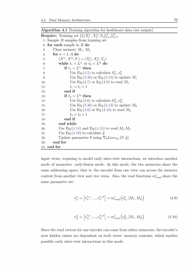
4.4. Dual Memory Architecture 70
Algorithm 4.1 Training algorithm for healthcare data (set output)
Require: Training set {{(X i1
a , X i2
a , Ya}Aa=1}N
n=1
1: Sample B samples from training set2: for each sample in B do3: Clear memory M1, M2
4: for a = 1, A do5: (X i1 , X i2, Y ) = (X i1
a , X i2
a , Ya)6: while t1 < Li1 or t2 < Li2 do7: if t1 < Li1 then8: Use Eq.(4.5) to calculate hi1
t1, oi1
t1
9: Use Eq.(3.36) or Eq.(4.13) to update M1
10: Use Eq.(4.7) or Eq.(4.9) to read M1
11: t1 = t1 + 112: end if13: if t2 < Li2 then14: Use Eq.(4.6) to calculate hi2
t2, oi2
t2
15: Use Eq.(3.36) or Eq.(4.13) to update M2
16: Use Eq.(4.8) or Eq.(4.10) to read M2
17: t2 = t2 + 118: end if19: end while20: Use Eq.(4.14) and Eq.(4.15) to read M1,M2
21: Use Eq.(4.18) to calculate y22: Update parameter θ using ∇θLossset (Y, y)23: end for24: end for
input views, requiring to model early inter-view interactions, we introduce another
mode of memories: early-fusion mode. In this mode, the two memories share the
same addressing space, that is, the encoder from one view can access the memory
content from another view and vice versa. Also, the read functions meread share the
same parameter set:
ri1
t1=[r
i1,1
t1, ..., r
i1,R
t1
]= me
read
(oi1
t1, [M1, M2]
)(4.9)
ri2
t2=[r
i2,1
t2, ..., r
i2,R
t2
]= me
read
(oi2
t2, [M1, M2]
)(4.10)
Since the read vectors for one encoder can come from either memories, the encoder’s
next hidden values are dependent on both views’ memory contents, which enables
possible early inter-view interactions in this mode.
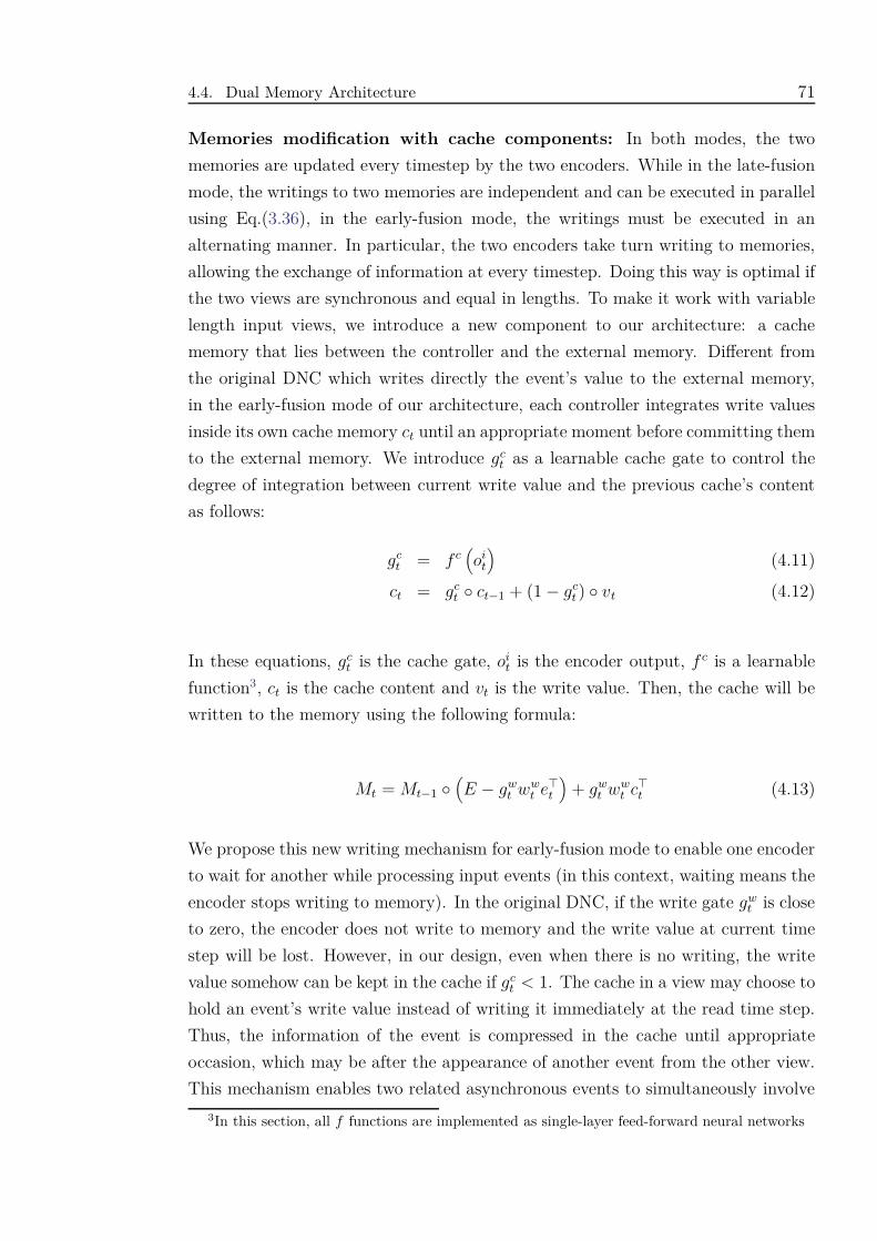
4.4. Dual Memory Architecture 71
Memories modification with cache components: In both modes, the two
memories are updated every timestep by the two encoders. While in the late-fusion
mode, the writings to two memories are independent and can be executed in parallel
using Eq.(3.36), in the early-fusion mode, the writings must be executed in an
alternating manner. In particular, the two encoders take turn writing to memories,
allowing the exchange of information at every timestep. Doing this way is optimal if
the two views are synchronous and equal in lengths. To make it work with variable
length input views, we introduce a new component to our architecture: a cache
memory that lies between the controller and the external memory. Different from
the original DNC which writes directly the event’s value to the external memory,
in the early-fusion mode of our architecture, each controller integrates write values
inside its own cache memory ct until an appropriate moment before committing them
to the external memory. We introduce gct as a learnable cache gate to control the
degree of integration between current write value and the previous cache’s content
as follows:
gct = f c
(oi
t
)(4.11)
ct = gct ◦ ct−1 + (1− gc
t ) ◦ vt (4.12)
In these equations, gct is the cache gate, oi
t is the encoder output, f c is a learnable
function3, ct is the cache content and vt is the write value. Then, the cache will be
written to the memory using the following formula:
Mt = Mt−1 ◦(E − gw
t wwt e⊤
t
)+ gw
t wwt c⊤
t (4.13)
We propose this new writing mechanism for early-fusion mode to enable one encoder
to wait for another while processing input events (in this context, waiting means the
encoder stops writing to memory). In the original DNC, if the write gate gwt is close
to zero, the encoder does not write to memory and the write value at current time
step will be lost. However, in our design, even when there is no writing, the write
value somehow can be kept in the cache if gct < 1. The cache in a view may choose to
hold an event’s write value instead of writing it immediately at the read time step.
Thus, the information of the event is compressed in the cache until appropriate
occasion, which may be after the appearance of another event from the other view.
This mechanism enables two related asynchronous events to simultaneously involve
3In this section, all f functions are implemented as single-layer feed-forward neural networks
4.4. Dual Memory Architecture 72
in building up the memories.
Write-protected memories: In our architecture, during the inference process, the
decoder stops writing to memories. We add this feature to our design because the
decoder does not receive any new input when producing output. Writing to memo-
ries in this phase may deteriorate the memory contents, hampering the efficiency of
the model.
4.4.2 Inference in DMNC
In this section, we give more details on the operation of the decoder. Because the
decoder works differently for different output types (set or sequence), we will present
two versions of decoder implementation.
Output as sequence: In this setting, the decoder ingests the encoders’ final states
as its initial hidden state h0 =[hi1
Li1, hi2
Li2
]. The decoder’s hidden and output
vectors are given as: ht, [o1t , o2
t ] = LSTMd([
y∗t−1, ri1
t−1, ri2
t−1
], ht−1
). Here, y∗
t−1 is
the embedding of the previous prediction y∗t−1. The decoder combines the read
vectors from both memories to produce a probability distribution over the output:
ri1
t =[r
i1,1
t , ..., ri1,R
t
]= md
read
(o1
t , M1
)(4.14)
ri2
t =[r
i2,1
t , ..., ri2,R
t
]= md
read
(o2
t , M2
)(4.15)
P(yt|X i1, X i2
)= π
([o1
t , o2t
]+ fd
([ri1
t , ri2
t
]))(4.16)
where ri1
t , ri2
t are read vector from M1, M2, respectively, provided by the read func-
tion mdread, fd is a learnable function and π is softmax function. The current predic-
tion is y∗t = argmax
y∈SP (yt = y|X i1, X i2) and the loss function is the cross entropy:
Lossseq (Y, P ) = −L∑
t=1
log P(yt|X i1 , X i2
)(4.17)
Output as set: In this setting, the decoder uses mdread to read from the memories
4.4. Dual Memory Architecture 73
once to get the read vectors ri1, ri2 . The decoder combines these vectors with the
encoders’ final hidden values to produce the output vector y ∈ R|S|:
y = σ(fd(W1r
i1 + W2ri2 + W3
[hi1
Li1, hi2
Li2
]))
(4.18)
Here, the combination is simply the linear weighted summation with parameter
matrices W1, W2, W3. fd is a learnable function and σ is the sigmoid function. For
set output, the loss function is multi-label loss defined as:
Lossset (Y, y) = −∑
yl∈Y
log yl +∑
yl /∈Y
log (1− yl)
(4.19)
For both settings, the decoder makes use of both memories’ contents and encoders’
final hidden values to produce the output. While memory contents represent the
long-term knowledge, the encoder’s hidden values represent the short-term informa-
tion stored inside the controllers. Both are crucial to model inter-view interactions
and necessary for the decoder to predict the correct outputs.
4.4.3 Persistent Memory for Multiple Admissions
As mentioned earlier in Sec. 4.1.2, one unique property of healthcare is the long-term
dependencies amongst admissions. Therefore, the output at the current admission
Ya is dependent on the current and all previous admission’s inputs{(
X i1
pa, X i1
pa
)}a
pa=1.
There are several ways to model this property. The simplest solution is to concate-
nate the current admission with previous ones to make up single sequence input for
the model. This method causes data replication and preprocessing overhead. An-
other solution is to use recurrent neural network to model the dependencies. Some
papers use GRU and LSTM where each time step is fed with an admission. The
admission is treated as a set of medical events and represented by a feature vector
(Choi et al., 2015; Pham et al., 2017).
In our memory-augmented architecture, we can model this dependencies by using the
memories to store information from previous admissions. In the original DNC, the
memory content is flushed every time new data sample (i.e. new admission) is fed –
this certainly loses the information of admission history. We modify this mechanism
by keeping the memories persistent during a patient’s admissions processing. That
is, the content of memories is built up and modified during the whole history of a
4.5. Applications 74
patient’s admissions. The memories are only cleared prior to reading a new patient’s
record.
Persistent memories in our architecture play two important roles. First, because
the number of events across admissions are large while memory sizes are moderate,
the memory modules learn to compress efficiently the input views, keeping only
essential information. This makes memory look-ups in the decoding process only
limited to a fixed size of chosen knowledge. This is more compact and focused than
attention mechanisms, in which the decoder has to attend to all events in the input.
Second, each memory slot can store information of any event in the input views,
which enables skip-connection reference in the decoding process, i.e., the decoder can
jump to any input event, even the one in the farthest admission, to look for relevant
information. The whole process of training our dual memory neural computer for
healthcare data is summarised in Algorithm 4.1.
4.5 Applications
In this section, we perform experiments both on real-world data and synthetic
tasks. The purpose of the synthetic task is to study the incremental impact of
dual control modifications we propose. Moreover, we demonstrate the effective-
ness of our proposed dual memory model DMNC. We use DMNCl and DMNCe
to denote the late-fusion and early-fusion mode of our model, respectively. The
data for real-world problems are real EMR data sets, some are public accessi-
ble. We make the source code of DCw-MANN and DMNC publicly available at
https://github.com/thaihungle/MAED and https://github.com/thaihungle/DMNC,
respectively.
4.5.1 Synthetic Task: Odd-Even Sequence Prediction
In this task, the input is sequence of random odd numbers chosen without replace-
ment from the set So = {1, 3, 5, ..., 49} and the output is sequence of even numbers
from the set Se = {2, 4, 6, ..98} . The n-th number yn in the output sequence is
computed as:
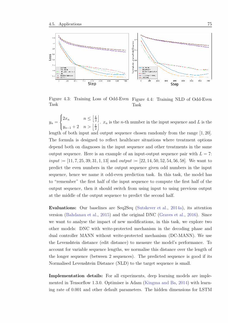
4.5. Applications 75
Figure 4.3: Training Loss of Odd-EvenTask
Figure 4.4: Training NLD of Odd-EvenTask
yn =
2xn n ≤⌊
L2
⌋
yn−1 + 2 n >⌊
L2
⌋ . xn is the n-th number in the input sequence and L is the
length of both input and output sequence chosen randomly from the range [1, 20].
The formula is designed to reflect healthcare situations where treatment options
depend both on diagnoses in the input sequence and other treatments in the same
output sequence. Here is an example of an input-output sequence pair with L = 7:
input := [11, 7, 25, 39, 31, 1, 13] and output := [22, 14, 50, 52, 54, 56, 58]. We want to
predict the even numbers in the output sequence given odd numbers in the input
sequence, hence we name it odd-even prediction task. In this task, the model has
to “remember” the first half of the input sequence to compute the first half of the
output sequence, then it should switch from using input to using previous output
at the middle of the output sequence to predict the second half.
Evaluations: Our baselines are Seq2Seq (Sutskever et al., 2014a), its attention
version (Bahdanau et al., 2015) and the original DNC (Graves et al., 2016). Since
we want to analyse the impact of new modifications, in this task, we explore two
other models: DNC with write-protected mechanism in the decoding phase and
dual controller MANN without write-protected mechanism (DC-MANN). We use
the Levenshtein distance (edit distance) to measure the model’s performance. To
account for variable sequence lengths, we normalise this distance over the length of
the longer sequence (between 2 sequences). The predicted sequence is good if its
Normalised Levenshtein Distance (NLD) to the target sequence is small.
Implementation details: For all experiments, deep learning models are imple-
mented in Tensorflow 1.3.0. Optimiser is Adam (Kingma and Ba, 2014) with learn-
ing rate of 0.001 and other default parameters. The hidden dimensions for LSTM
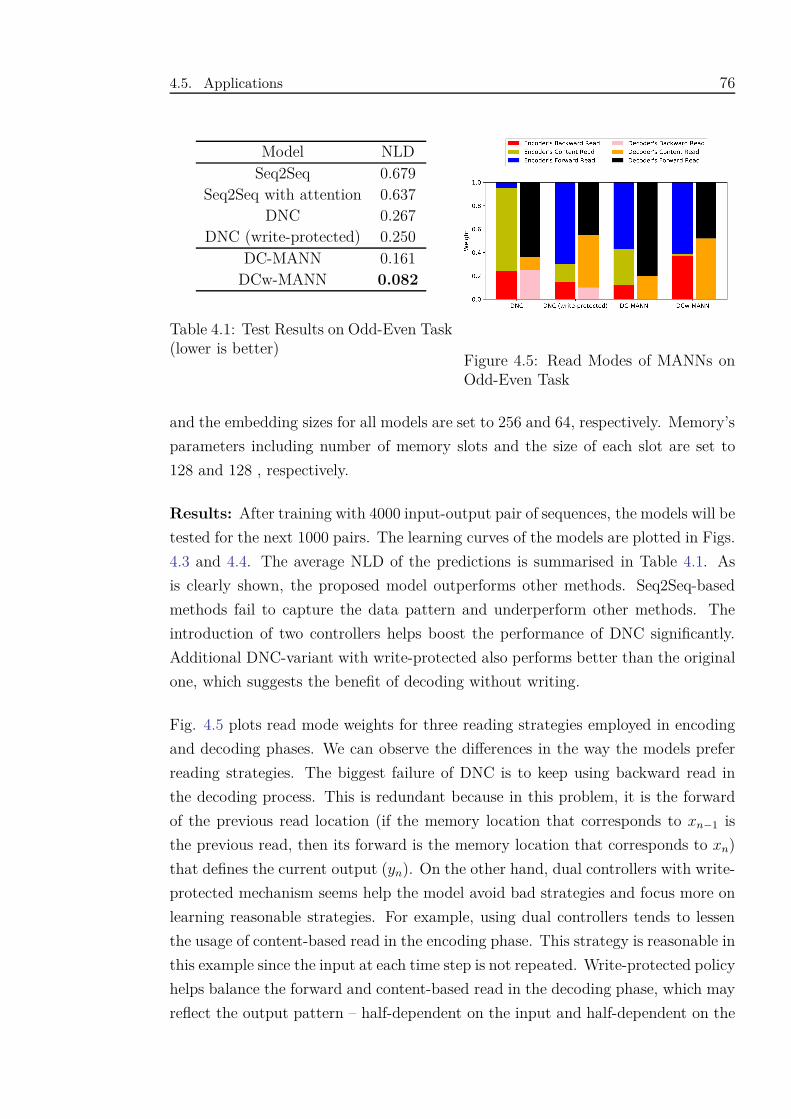
4.5. Applications 76
Model NLDSeq2Seq 0.679
Seq2Seq with attention 0.637DNC 0.267
DNC (write-protected) 0.250DC-MANN 0.161
DCw-MANN 0.082
Table 4.1: Test Results on Odd-Even Task(lower is better)
Figure 4.5: Read Modes of MANNs onOdd-Even Task
and the embedding sizes for all models are set to 256 and 64, respectively. Memory’s
parameters including number of memory slots and the size of each slot are set to
128 and 128 , respectively.
Results: After training with 4000 input-output pair of sequences, the models will be
tested for the next 1000 pairs. The learning curves of the models are plotted in Figs.
4.3 and 4.4. The average NLD of the predictions is summarised in Table 4.1. As
is clearly shown, the proposed model outperforms other methods. Seq2Seq-based
methods fail to capture the data pattern and underperform other methods. The
introduction of two controllers helps boost the performance of DNC significantly.
Additional DNC-variant with write-protected also performs better than the original
one, which suggests the benefit of decoding without writing.
Fig. 4.5 plots read mode weights for three reading strategies employed in encoding
and decoding phases. We can observe the differences in the way the models prefer
reading strategies. The biggest failure of DNC is to keep using backward read in
the decoding process. This is redundant because in this problem, it is the forward
of the previous read location (if the memory location that corresponds to xn−1 is
the previous read, then its forward is the memory location that corresponds to xn)
that defines the current output (yn). On the other hand, dual controllers with write-
protected mechanism seems help the model avoid bad strategies and focus more on
learning reasonable strategies. For example, using dual controllers tends to lessen
the usage of content-based read in the encoding phase. This strategy is reasonable in
this example since the input at each time step is not repeated. Write-protected policy
helps balance the forward and content-based read in the decoding phase, which may
reflect the output pattern – half-dependent on the input and half-dependent on the
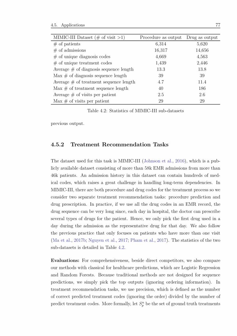
4.5. Applications 77
MIMIC-III Dataset (# of visit >1) Procedure as output Drug as output# of patients 6,314 5,620# of admissions 16,317 14,656# of unique diagnosis codes 4,669 4,563# of unique treatment codes 1,439 2,446Average # of diagnosis sequence length 13.3 13.8Max # of diagnosis sequence length 39 39Average # of treatment sequence length 4.7 11.4Max # of treatment sequence length 40 186Average # of visits per patient 2.5 2.6Max # of visits per patient 29 29
Table 4.2: Statistics of MIMIC-III sub-datasets
previous output.
4.5.2 Treatment Recommendation Tasks
The dataset used for this task is MIMIC-III (Johnson et al., 2016), which is a pub-
licly available dataset consisting of more than 58k EMR admissions from more than
46k patients. An admission history in this dataset can contain hundreds of med-
ical codes, which raises a great challenge in handling long-term dependencies. In
MIMIC-III, there are both procedure and drug codes for the treatment process so we
consider two separate treatment recommendation tasks: procedure prediction and
drug prescription. In practice, if we use all the drug codes in an EMR record, the
drug sequence can be very long since, each day in hospital, the doctor can prescribe
several types of drugs for the patient. Hence, we only pick the first drug used in a
day during the admission as the representative drug for that day. We also follow
the previous practice that only focuses on patients who have more than one visit
(Ma et al., 2017b; Nguyen et al., 2017; Pham et al., 2017). The statistics of the two
sub-datasets is detailed in Table 4.2.
Evaluations: For comprehensiveness, beside direct competitors, we also compare
our methods with classical for healthcare predictions, which are Logistic Regression
and Random Forests. Because traditional methods are not designed for sequence
predictions, we simply pick the top outputs (ignoring ordering information). In
treatment recommendation tasks, we use precision, which is defined as the number
of correct predicted treatment codes (ignoring the order) divided by the number of
predict treatment codes. More formally, let Snp be the set of ground truth treatments
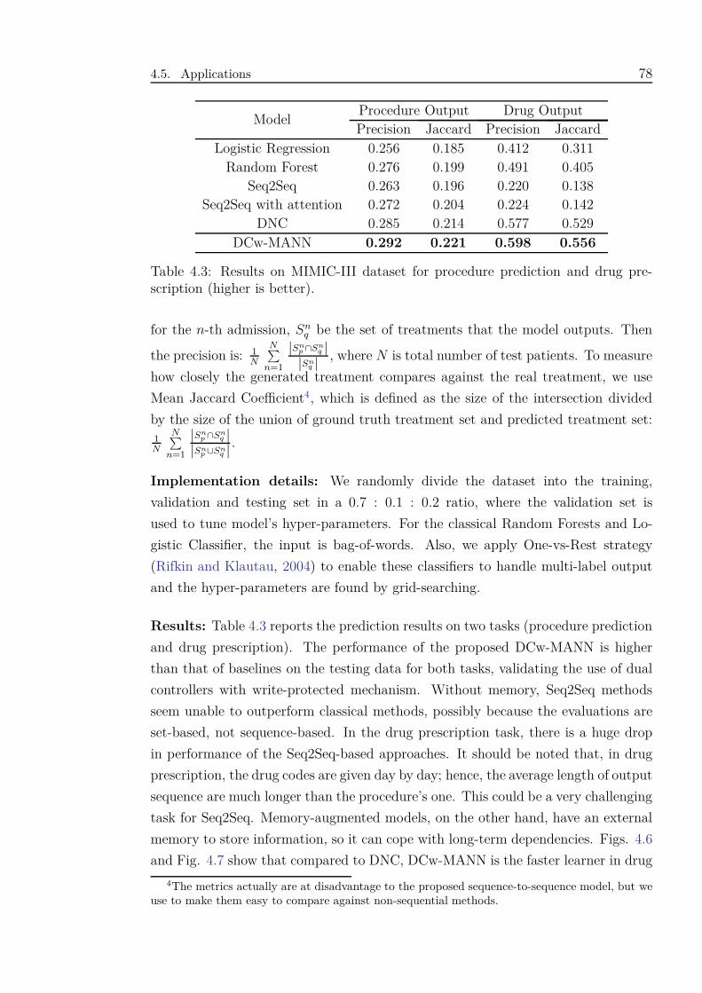
4.5. Applications 78
ModelProcedure Output Drug OutputPrecision Jaccard Precision Jaccard
Logistic Regression 0.256 0.185 0.412 0.311Random Forest 0.276 0.199 0.491 0.405
Seq2Seq 0.263 0.196 0.220 0.138Seq2Seq with attention 0.272 0.204 0.224 0.142
DNC 0.285 0.214 0.577 0.529DCw-MANN 0.292 0.221 0.598 0.556
Table 4.3: Results on MIMIC-III dataset for procedure prediction and drug pre-scription (higher is better).
for the n-th admission, Snq be the set of treatments that the model outputs. Then
the precision is: 1N
N∑n=1
|Snp ∩Sn
q ||Sn
q | , where N is total number of test patients. To measure
how closely the generated treatment compares against the real treatment, we use
Mean Jaccard Coefficient4, which is defined as the size of the intersection divided
by the size of the union of ground truth treatment set and predicted treatment set:1N
N∑n=1
|Snp ∩Sn
q ||Sn
p ∪Snq | .
Implementation details: We randomly divide the dataset into the training,
validation and testing set in a 0.7 : 0.1 : 0.2 ratio, where the validation set is
used to tune model’s hyper-parameters. For the classical Random Forests and Lo-
gistic Classifier, the input is bag-of-words. Also, we apply One-vs-Rest strategy
(Rifkin and Klautau, 2004) to enable these classifiers to handle multi-label output
and the hyper-parameters are found by grid-searching.
Results: Table 4.3 reports the prediction results on two tasks (procedure prediction
and drug prescription). The performance of the proposed DCw-MANN is higher
than that of baselines on the testing data for both tasks, validating the use of dual
controllers with write-protected mechanism. Without memory, Seq2Seq methods
seem unable to outperform classical methods, possibly because the evaluations are
set-based, not sequence-based. In the drug prescription task, there is a huge drop
in performance of the Seq2Seq-based approaches. It should be noted that, in drug
prescription, the drug codes are given day by day; hence, the average length of output
sequence are much longer than the procedure’s one. This could be a very challenging
task for Seq2Seq. Memory-augmented models, on the other hand, have an external
memory to store information, so it can cope with long-term dependencies. Figs. 4.6
and Fig. 4.7 show that compared to DNC, DCw-MANN is the faster learner in drug
4The metrics actually are at disadvantage to the proposed sequence-to-sequence model, but weuse to make them easy to compare against non-sequential methods.
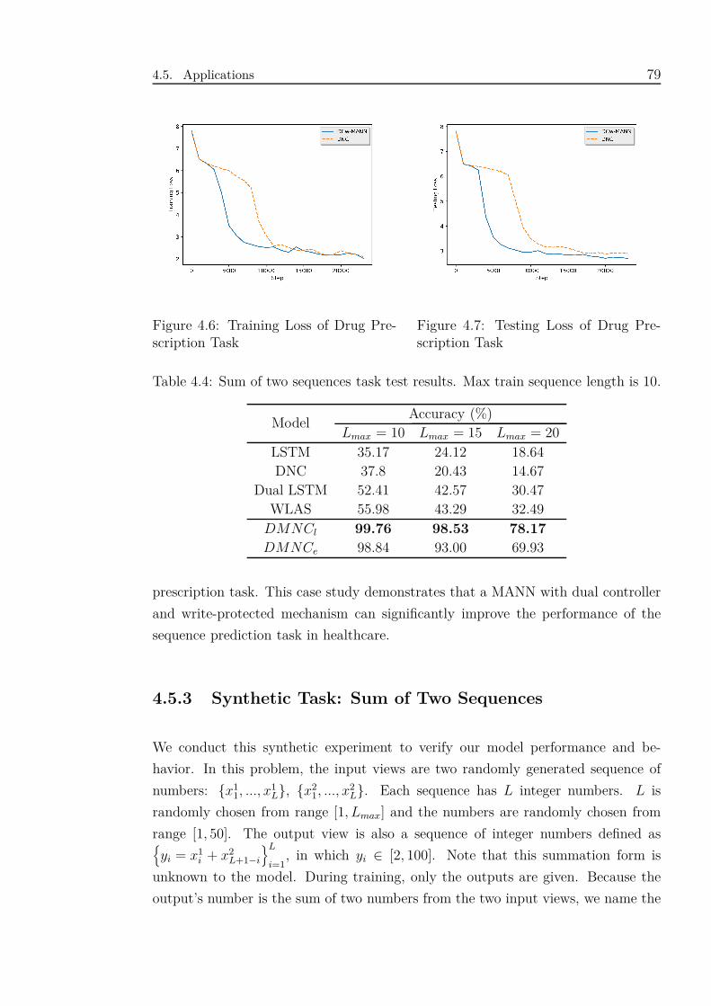
4.5. Applications 79
Figure 4.6: Training Loss of Drug Pre-scription Task
Figure 4.7: Testing Loss of Drug Pre-scription Task
Table 4.4: Sum of two sequences task test results. Max train sequence length is 10.
ModelAccuracy (%)
Lmax = 10 Lmax = 15 Lmax = 20LSTM 35.17 24.12 18.64DNC 37.8 20.43 14.67
Dual LSTM 52.41 42.57 30.47WLAS 55.98 43.29 32.49
DMNCl 99.76 98.53 78.17
DMNCe 98.84 93.00 69.93
prescription task. This case study demonstrates that a MANN with dual controller
and write-protected mechanism can significantly improve the performance of the
sequence prediction task in healthcare.
4.5.3 Synthetic Task: Sum of Two Sequences
We conduct this synthetic experiment to verify our model performance and be-
havior. In this problem, the input views are two randomly generated sequence of
numbers: {x11, ..., x1
L}, {x21, ..., x2
L}. Each sequence has L integer numbers. L is
randomly chosen from range [1, Lmax] and the numbers are randomly chosen from
range [1, 50]. The output view is also a sequence of integer numbers defined as{yi = x1
i + x2L+1−i
}L
i=1, in which yi ∈ [2, 100]. Note that this summation form is
unknown to the model. During training, only the outputs are given. Because the
output’s number is the sum of two numbers from the two input views, we name the
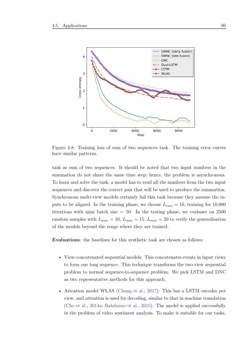
4.5. Applications 80
0 2000 4000 6000 8000
Step
0
1
2
3
4
Cro
ss e
ntr
opy
Figure 4.8: Training loss of sum of two sequences task. The training error curveshave similar patterns.
task as sum of two sequences. It should be noted that two input numbers in the
summation do not share the same time step; hence, the problem is asynchronous.
To learn and solve the task, a model has to read all the numbers from the two input
sequences and discover the correct pair that will be used to produce the summation.
Synchronous multi-view models certainly fail this task because they assume the in-
puts to be aligned. In the training phase, we choose Lmax = 10, training for 10,000
iterations with mini batch size = 50. In the testing phase, we evaluate on 2500
random samples with Lmax = 10, Lmax = 15, Lmax = 20 to verify the generalisation
of the models beyond the range where they are trained.
Evaluations: the baselines for this synthetic task are chosen as follows:
• View-concatenated sequential models: This concatenates events in input views
to form one long sequence. This technique transforms the two-view sequential
problem to normal sequence-to-sequence problem. We pick LSTM and DNC
as two representative methods for this approach.
• Attention model WLAS (Chung et al., 2017): This has a LSTM encoder per
view, and attention is used for decoding, similar to that in machine translation
(Cho et al., 2014a; Bahdanau et al., 2015). The model is applied successfully
in the problem of video sentiment analysis. To make it suitable for our tasks,
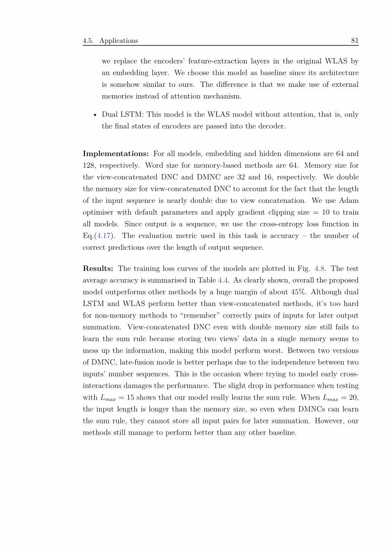
4.5. Applications 81
we replace the encoders’ feature-extraction layers in the original WLAS by
an embedding layer. We choose this model as baseline since its architecture
is somehow similar to ours. The difference is that we make use of external
memories instead of attention mechanism.
• Dual LSTM: This model is the WLAS model without attention, that is, only
the final states of encoders are passed into the decoder.
Implementations: For all models, embedding and hidden dimensions are 64 and
128, respectively. Word size for memory-based methods are 64. Memory size for
the view-concatenated DNC and DMNC are 32 and 16, respectively. We double
the memory size for view-concatenated DNC to account for the fact that the length
of the input sequence is nearly double due to view concatenation. We use Adam
optimiser with default parameters and apply gradient clipping size = 10 to train
all models. Since output is a sequence, we use the cross-entropy loss function in
Eq.(4.17). The evaluation metric used in this task is accuracy – the number of
correct predictions over the length of output sequence.
Results: The training loss curves of the models are plotted in Fig. 4.8. The test
average accuracy is summarised in Table 4.4. As clearly shown, overall the proposed
model outperforms other methods by a huge margin of about 45%. Although dual
LSTM and WLAS perform better than view-concatenated methods, it’s too hard
for non-memory methods to “remember” correctly pairs of inputs for later output
summation. View-concatenated DNC even with double memory size still fails to
learn the sum rule because storing two views’ data in a single memory seems to
mess up the information, making this model perform worst. Between two versions
of DMNC, late-fusion mode is better perhaps due to the independence between two
inputs’ number sequences. This is the occasion where trying to model early cross-
interactions damages the performance. The slight drop in performance when testing
with Lmax = 15 shows that our model really learns the sum rule. When Lmax = 20,
the input length is longer than the memory size, so even when DMNCs can learn
the sum rule, they cannot store all input pairs for later summation. However, our
methods still manage to perform better than any other baseline.
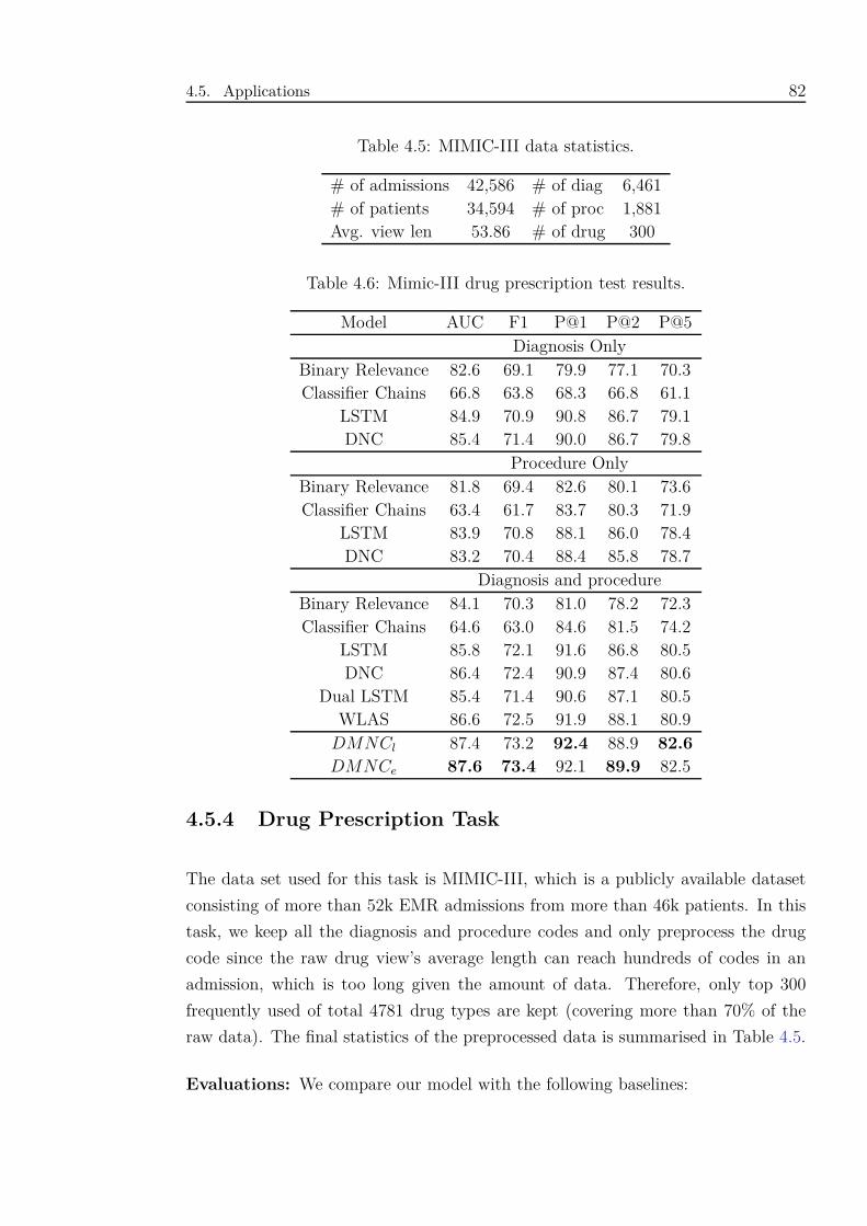
4.5. Applications 82
Table 4.5: MIMIC-III data statistics.
# of admissions 42,586 # of diag 6,461# of patients 34,594 # of proc 1,881Avg. view len 53.86 # of drug 300
Table 4.6: Mimic-III drug prescription test results.
Model AUC F1 P@1 P@2 P@5Diagnosis Only
Binary Relevance 82.6 69.1 79.9 77.1 70.3Classifier Chains 66.8 63.8 68.3 66.8 61.1
LSTM 84.9 70.9 90.8 86.7 79.1DNC 85.4 71.4 90.0 86.7 79.8
Procedure OnlyBinary Relevance 81.8 69.4 82.6 80.1 73.6Classifier Chains 63.4 61.7 83.7 80.3 71.9
LSTM 83.9 70.8 88.1 86.0 78.4DNC 83.2 70.4 88.4 85.8 78.7
Diagnosis and procedureBinary Relevance 84.1 70.3 81.0 78.2 72.3Classifier Chains 64.6 63.0 84.6 81.5 74.2
LSTM 85.8 72.1 91.6 86.8 80.5DNC 86.4 72.4 90.9 87.4 80.6
Dual LSTM 85.4 71.4 90.6 87.1 80.5WLAS 86.6 72.5 91.9 88.1 80.9
DMNCl 87.4 73.2 92.4 88.9 82.6
DMNCe 87.6 73.4 92.1 89.9 82.5
4.5.4 Drug Prescription Task
The data set used for this task is MIMIC-III, which is a publicly available dataset
consisting of more than 52k EMR admissions from more than 46k patients. In this
task, we keep all the diagnosis and procedure codes and only preprocess the drug
code since the raw drug view’s average length can reach hundreds of codes in an
admission, which is too long given the amount of data. Therefore, only top 300
frequently used of total 4781 drug types are kept (covering more than 70% of the
raw data). The final statistics of the preprocessed data is summarised in Table 4.5.
Evaluations: We compare our model with the following baselines:
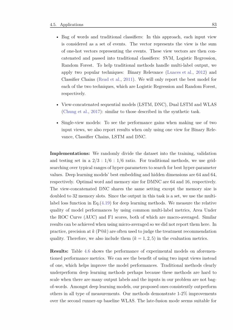
4.5. Applications 83
• Bag of words and traditional classifiers: In this approach, each input view
is considered as a set of events. The vector represents the view is the sum
of one-hot vectors representing the events. These view vectors are then con-
catenated and passed into traditional classifiers: SVM, Logistic Regression,
Random Forest. To help traditional methods handle multi-label output, we
apply two popular techniques: Binary Relevance (Luaces et al., 2012) and
Classifier Chains (Read et al., 2011). We will only report the best model for
each of the two techniques, which are Logistic Regression and Random Forest,
respectively.
• View-concatenated sequential models (LSTM, DNC), Dual LSTM and WLAS
(Chung et al., 2017): similar to those described in the synthetic task.
• Single-view models: To see the performance gains when making use of two
input views, we also report results when only using one view for Binary Rele-
vance, Classifier Chains, LSTM and DNC.
Implementations: We randomly divide the dataset into the training, validation
and testing set in a 2/3 : 1/6 : 1/6 ratio. For traditional methods, we use grid-
searching over typical ranges of hyper-parameters to search for best hyper-parameter
values. Deep learning models’ best embedding and hidden dimensions are 64 and 64,
respectively. Optimal word and memory size for DMNC are 64 and 16, respectively.
The view-concatenated DNC shares the same setting except the memory size is
doubled to 32 memory slots. Since the output in this task is a set, we use the multi-
label loss function in Eq.(4.19) for deep learning methods. We measure the relative
quality of model performances by using common multi-label metrics, Area Under
the ROC Curve (AUC) and F1 scores, both of which are macro-averaged. Similar
results can be achieved when using micro-averaged so we did not report them here. In
practice, precision at k (P@k) are often used to judge the treatment recommendation
quality. Therefore, we also include them (k = 1, 2, 5) in the evaluation metrics.
Results: Table 4.6 shows the performance of experimental models on aforemen-
tioned performance metrics. We can see the benefit of using two input views instead
of one, which helps improve the model performances. Traditional methods clearly
underperform deep learning methods perhaps because these methods are hard to
scale when there are many output labels and the inputs in our problem are not bag-
of-words. Amongst deep learning models, our proposed ones consistently outperform
others in all type of measurements. Our methods demonstrate 1-2% improvements
over the second runner-up baseline WLAS. The late-fusion mode seems suitable for
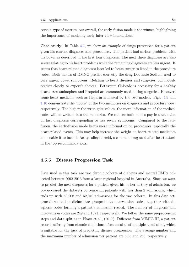
4.5. Applications 84
certain type of metrics, but overall, the early-fusion mode is the winner, highlighting
the importance of modeling early inter-view interactions.
Case study: In Table 4.7, we show an example of drugs prescribed for a patient
given his current diagnoses and procedures. The patient had serious problems with
his bowel as described in the first four diagnoses. The next three diagnoses are also
severe relating to his heart problems while the remaining diagnoses are less urgent. It
seems that heart-related diagnoses later led to heart surgeries listed in the procedure
codes. Both modes of DMNC predict correctly the drug Docusate Sodium used to
cure urgent bowel symptoms. Relating to heart diseases and surgeries, our models
predict closely to expert’s choices. Potassium Chloride is necessary for a healthy
heart. Acetaminophen and Propofol are commonly used during surgeries. However,
some heart medicine such as Heparin is missed by the two models. Figs. 4.9 and
4.10 demonstrate the “focus” of the two memories on diagnosis and procedure view,
respectively. The higher the write gate values, the more information of the medical
codes will be written into the memories. We can see both modes pay less attention
on last diagnoses corresponding to less severe symptoms. Compared to the late-
fusion, the early-fusion mode keeps more information on procedures, especially the
heart-related events. This may help increase the weight on heart-related medicines
and enable it to include Acetylsalicylic Acid, a common drug used after heart attack
in the top recommendations.
4.5.5 Disease Progression Task
Data used in this task are two chronic cohorts of diabetes and mental EMRs col-
lected between 2002-2013 from a large regional hospital in Australia. Since we want
to predict the next diagnoses for a patient given his or her history of admission, we
preprocessed the datasets by removing patients with less than 2 admissions, which
ends up with 53,208 and 52,049 admissions for the two cohorts. In this data set,
procedures and medicines are grouped into intervention codes, together with di-
agnosis codes forming a patient’s admission record. The number of diagnosis and
intervention codes are 249 and 1071, respectively. We follow the same preprocessing
steps and data split as in Pham et al., (2017). Different from MIMIC-III, a patient
record suffering from chronic conditions often consists of multiple admissions, which
is suitable for the task of predicting disease progression. The average number and
the maximum number of admission per patient are 5.35 and 253, respectively.

4.5. Applications 85
Table 4.7: Example Recommended Medications by DMNCs on MIMIC-III dataset.Bold denotes matching against ground-truth.
Diagnoses Calculus Of Gallbladder (57411),Vascular disorders ofmale genital organs (60883), Abdominal Pain (78901),Poisoning By Other Tranquilizers (9695), AcuteMyocardial Infarction Of Other Inferior Wall (41042),Hematoma Complicating (99812), Malignant hypertensiveheart disease 40200), Dizziness and giddiness (7804),Venous (Peripheral) Insufficiency, Unspecified (45981),Hemorrhage Of Gastrointestinal Tract (5789)
Procedures Coronary Bypass Of Three Coronary Arteries (3613),Single Internal Mammary Artery Bypass (3615),Extracorporeal circulation auxiliary to open heart surgery(3961), Insertion Of Intercostal Catheter For Drainage(3404), Operations on cornea(114)
Top 5 Ground-truthdrugs (manuallypicked by experts)
Docusate Sodium (DOCU100L), Acetylsalicylic Acid(ASA81), Heparin (HEPA5I), Acetaminophen(ACET325), Potassium Chloride (KCLBASE2)
Top 5 Late-fusionRecommendations
Docusate Sodium (DOCU100L), Neostigmine(NEOSI), Acetaminophen (ACET325), Propofol(PROP100IG), Potassium Chloride (KCLBASE2)
Top 5 Early-fusionRecommendations
Docusate Sodium (DOCU100L), Acetaminophen(ACET325), Potassium Chloride (KCLBASE2),Dextrose (DEX50SY), Acetylsalicylic Acid (ASA81)
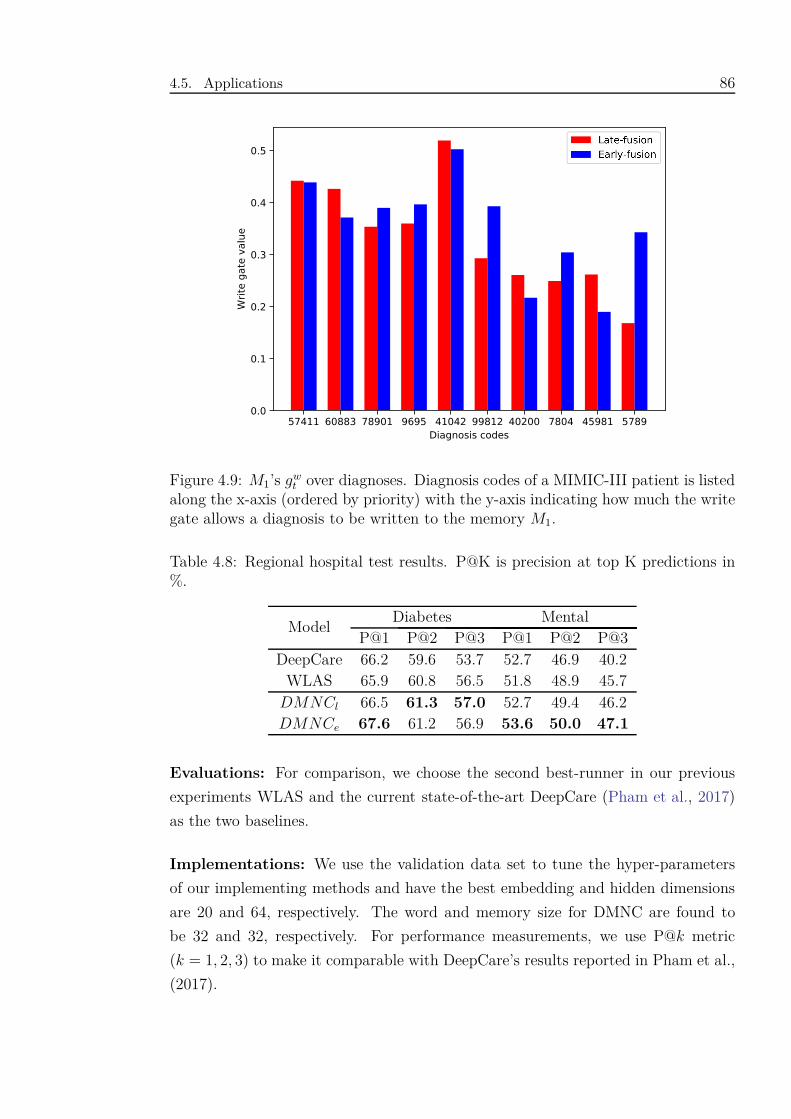
4.5. Applications 86
57411 60883 78901 9695 41042 99812 40200 7804 45981 5789
Diagnosis codes
0.0
0.1
0.2
0.3
0.4
0.5
Wri
te g
ate
valu
e
Figure 4.9: M1’s gwt over diagnoses. Diagnosis codes of a MIMIC-III patient is listed
along the x-axis (ordered by priority) with the y-axis indicating how much the writegate allows a diagnosis to be written to the memory M1.
Table 4.8: Regional hospital test results. P@K is precision at top K predictions in%.
ModelDiabetes Mental
P@1 P@2 P@3 P@1 P@2 P@3DeepCare 66.2 59.6 53.7 52.7 46.9 40.2
WLAS 65.9 60.8 56.5 51.8 48.9 45.7DMNCl 66.5 61.3 57.0 52.7 49.4 46.2DMNCe 67.6 61.2 56.9 53.6 50.0 47.1
Evaluations: For comparison, we choose the second best-runner in our previous
experiments WLAS and the current state-of-the-art DeepCare (Pham et al., 2017)
as the two baselines.
Implementations: We use the validation data set to tune the hyper-parameters
of our implementing methods and have the best embedding and hidden dimensions
are 20 and 64, respectively. The word and memory size for DMNC are found to
be 32 and 32, respectively. For performance measurements, we use P@k metric
(k = 1, 2, 3) to make it comparable with DeepCare’s results reported in Pham et al.,
(2017).
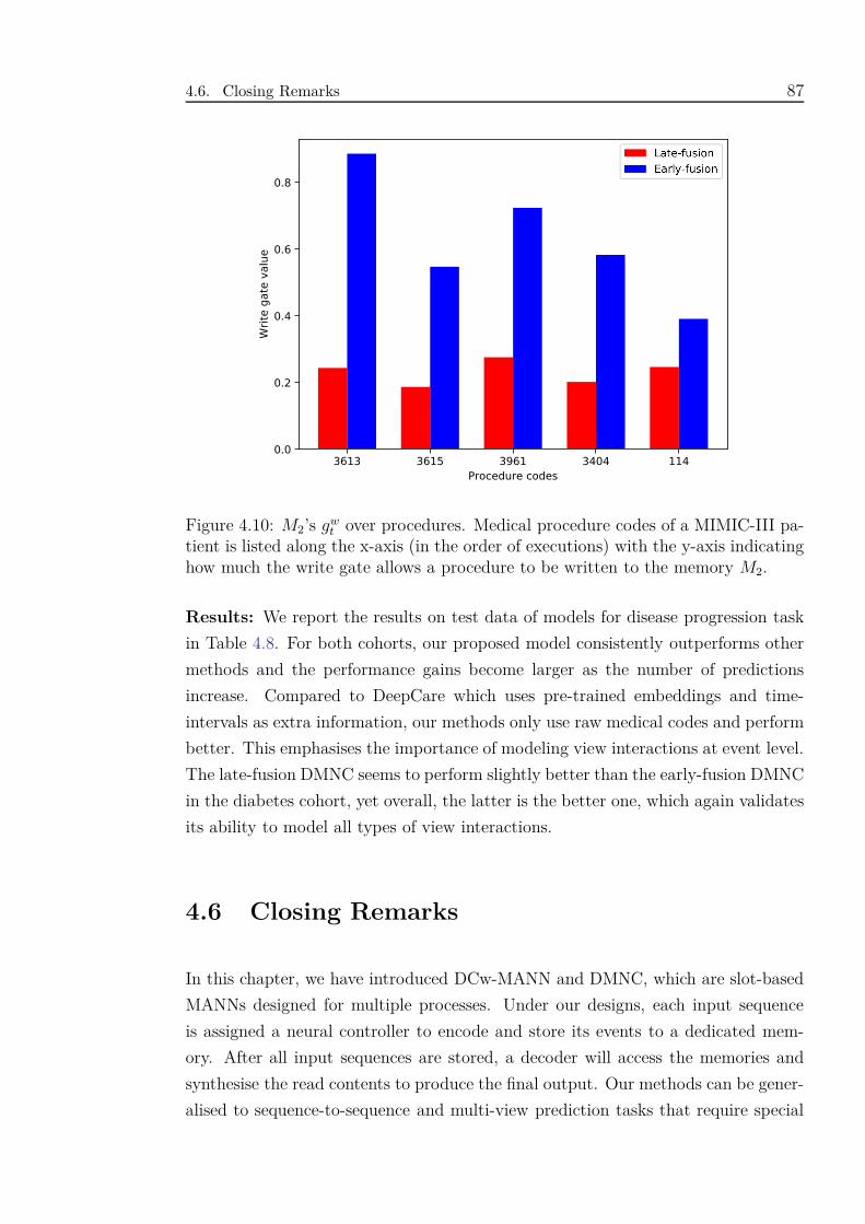
4.6. Closing Remarks 87
3613 3615 3961 3404 114
Procedure codes
0.0
0.2
0.4
0.6
0.8
Wri
te g
ate
valu
e
Figure 4.10: M2’s gwt over procedures. Medical procedure codes of a MIMIC-III pa-
tient is listed along the x-axis (in the order of executions) with the y-axis indicatinghow much the write gate allows a procedure to be written to the memory M2.
Results: We report the results on test data of models for disease progression task
in Table 4.8. For both cohorts, our proposed model consistently outperforms other
methods and the performance gains become larger as the number of predictions
increase. Compared to DeepCare which uses pre-trained embeddings and time-
intervals as extra information, our methods only use raw medical codes and perform
better. This emphasises the importance of modeling view interactions at event level.
The late-fusion DMNC seems to perform slightly better than the early-fusion DMNC
in the diabetes cohort, yet overall, the latter is the better one, which again validates
its ability to model all types of view interactions.
4.6 Closing Remarks
In this chapter, we have introduced DCw-MANN and DMNC, which are slot-based
MANNs designed for multiple processes. Under our designs, each input sequence
is assigned a neural controller to encode and store its events to a dedicated mem-
ory. After all input sequences are stored, a decoder will access the memories and
synthesise the read contents to produce the final output. Our methods can be gener-
alised to sequence-to-sequence and multi-view prediction tasks that require special

4.6. Closing Remarks 88
handling of long-term dependencies and view interactions.
In summary, our main contributions are: (i) handling very long-term dependen-
cies and rare events in healthcare data by solving the sequence prediction prob-
lem, (ii) proposing a novel memory-augmented architecture that uses dual controller
and write-protected mechanism (DCw-MANN) to fit with sequence-in-sequence-out
(SISO) task, (iii) proposing a novel dual memory neural computer (DMNC) to solve
the asynchronous multi-view sequential problem and designing our architecture to
model view interactions and long-term dependencies, (iv) demonstrating the efficacy
of our proposed model on real-world medical data sets for the problems of treatment
recommendation, drug prescription and disease progression. In particular, our mod-
els outperform other baselines by 1-2% across various metrics, which is significant
in the domain. More importantly, explainability is critical in healthcare and we
can somehow explain the behavior of our models by analysing the write gate of the
memory.
We wish to emphasise that although our models are designed as predictive model
targeted to healthcare, they can be applied to other sequential domains with sim-
ilar data characteristics (i.e., sequential, long-term, rare and multi-view) such as
video understanding. Also, the current work is limited to generating simple and
deterministic output sequences. In the next chapter, we will focus on another im-
portant problem, in which, an external memory is necessary for holding temporal
information and composing mixture distributions in the latent space of generative
models.
Chapter 5
Variational Memory in Generative
Models
5.1 Introduction
In the previous chapter, we have addressed the problem of encoder-decoder architec-
ture with long-term dependencies. However, the decoding is an ill-posed problem,
where there are many possible decoded sequences given an input sequence. To ac-
count for such variation, we need a method to model latent variables underlying
these uncertainty. This lends naturally to generative model of sequences.
Recent advances in generative modeling have led to exploration of generative tasks.
While generative models such as GAN (Goodfellow et al., 2014) and VAE (Kingma and Welling,
2014; Rezende et al., 2014) have been applied successfully for image generation,
learning generative models for sequential discrete data is a long-standing prob-
lem. Early attempts to generate sequences using RNNs (Graves, 2013) and neural
encoder-decoder models (Kalchbrenner and Blunsom, 2013; Vinyals and Le, 2015)
gave promising results, but the deterministic nature of these models proves to be
inadequate in many realistic settings. Tasks such as translation, question-answering
and dialog generation would benefit from stochastic models that can produce a va-
riety of outputs for an input. For example, there are several ways to translate a
sentence from one language to another, multiple answers to a question and multiple
responses for an utterance in conversation.
For tasks involving language understanding and production, handling intrinsic un-
89
5.1. Introduction 90
certainty and latent variations is necessary. The choice of words and grammars may
change erratically depending on speaker intentions, moods and previous languages
used. The underlying RNNs in neural sequential models find it hard to capture the
dynamics and their outputs are often trivial or too generic (Li et al., 2016). One
way to overcome these problems is to introduce variability into these models. Un-
fortunately, sequential data such as speech and natural language is a hard place to
inject variability (Serban et al., 2017) since they require a coherence of grammars
and semantics yet allow freedom of word choice.
We propose a novel hybrid approach that integrates MAED (Sec. 3.3.5) and VAE,
called Variational Memory Encoder-Decoder (VMED), to model the sequential prop-
erties and inject variability in sequence generation tasks. In this proposal, we utilise
DC-MANN described in Sec. 4.3 where the powerful DNC (Graves et al., 2016) is
chosen as the external memory. We prefer to allow writing to the memory during in-
ference because in this work, we focus on generating diverse output sequences, which
requires a dynamic memory for both encoding and decoding process. Furthermore,
we introduce latent random variables to model the variability observed in the data
and capture dependencies between the latent variables across timesteps. Our as-
sumption is that there are latent variables governing an output at each timestep. In
the conversation context, for instance, the latent space may represent the speaker’s
hidden intention and mood that dictate word choice and grammars. For a rich latent
multimodal space, we use a Mixture of Gaussians (MoG) because a spoken word’s
latent intention and mood can come from different modes, e.g., whether the speaker
is asking or answering, or she/he is happy or sad. By modeling the latent space
as an MoG where each mode associates with some memory slot, we aim to capture
multiple modes of the speaker’s intention and mood when producing a word in the
response. Since the decoder in our model has multiple read heads, the MoG can be
computed directly from the content of chosen memory slots. Our external memory
plays a role as a mixture model distribution generating the latent variables that
are used to produce the output and take part in updating the memory for future
generative steps.
To train our model, we adapt Stochastic Gradient Variational Bayes (SGVB) frame-
work (Kingma and Welling, 2014). Instead of minimising the KL divergence di-
rectly, we resort to using its variational approximation (Hershey and Olsen, 2007)
to accommodate the MoG in the latent space. We show that minimising the ap-
proximation results in KL divergence minimisation. We further derive an upper
bound on our total timestep-wise KL divergence and demonstrate that minimising
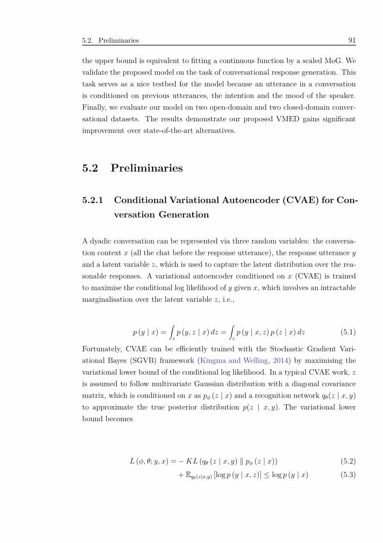
5.2. Preliminaries 91
the upper bound is equivalent to fitting a continuous function by a scaled MoG. We
validate the proposed model on the task of conversational response generation. This
task serves as a nice testbed for the model because an utterance in a conversation
is conditioned on previous utterances, the intention and the mood of the speaker.
Finally, we evaluate our model on two open-domain and two closed-domain conver-
sational datasets. The results demonstrate our proposed VMED gains significant
improvement over state-of-the-art alternatives.
5.2 Preliminaries
5.2.1 Conditional Variational Autoencoder (CVAE) for Con-
versation Generation
A dyadic conversation can be represented via three random variables: the conversa-
tion context x (all the chat before the response utterance), the response utterance y
and a latent variable z, which is used to capture the latent distribution over the rea-
sonable responses. A variational autoencoder conditioned on x (CVAE) is trained
to maximise the conditional log likelihood of y given x, which involves an intractable
marginalisation over the latent variable z, i.e.,
p (y | x) =∫
zp (y, z | x) dz =
∫
zp (y | x, z) p (z | x) dz (5.1)
Fortunately, CVAE can be efficiently trained with the Stochastic Gradient Vari-
ational Bayes (SGVB) framework (Kingma and Welling, 2014) by maximising the
variational lower bound of the conditional log likelihood. In a typical CVAE work, z
is assumed to follow multivariate Gaussian distribution with a diagonal covariance
matrix, which is conditioned on x as pφ (z | x) and a recognition network qθ(z | x, y)
to approximate the true posterior distribution p(z | x, y). The variational lower
bound becomes
L (φ, θ; y, x) =−KL (qθ (z | x, y) ‖ pφ (z | x)) (5.2)
+ Eqθ(z|x,y) [log p (y | x, z)] ≤ log p (y | x) (5.3)
5.2. Preliminaries 92
where KL is the Kullback–Leibler divergence. With the introduction of the neural
approximator qθ(z | x, y) and the reparameterisation trick (Kingma et al., 2014), we
can apply the standard back-propagation to compute the gradient of the variational
lower bound. Fig. 5.1(a) depicts elements of the graphical model for this approach
in the case of using CVAE.
5.2.2 Related Works
With the recent revival of recurrent neural networks (RNNs), there has been much
effort spent on learning generative models of sequences. Early attempts include
training RNN to generate the next output given previous sequence, demonstrat-
ing RNNs’ ability to generate text and handwriting images (Graves, 2013). Later,
encoder-decoder architecture (Sutskever et al., 2014b) enables generating a whole
sequence in machine translation (Kalchbrenner and Blunsom, 2013), text summa-
tion (Nallapati et al., 2016) and conversation generation (Vinyals and Le, 2015).
Although these models have achieved significant empirical successes, they fall short
to capture the complexity and variability of sequential processes.
These limitations have recently triggered a considerable effort on introducing vari-
ability into the encoder-decoder architecture. Most of the methods focus on condi-
tional VAE (CVAE) by constructing a variational lower bound conditioned on the
context. The setting can be found in many applications including machine transla-
tion (Zhang et al., 2016a) and dialog generation (Bowman et al., 2016; Serban et al.,
2017; Shen et al., 2017; Zhao et al., 2017). A common trick is to place a neural net
between the encoder and the decoder to compute the Gaussian prior and poste-
rior of the CVAE. This design is further enhanced by the use of external memory
(Chen et al., 2018) and reinforcement learning (Wen et al., 2017). In contrast to this
design, our VMED uses recurrent latent variable approach (Chung et al., 2015), that
is, our model requires a CVAE for each step of generation. Besides, our external
memory is used for producing the latent distribution, which is different from the
one proposed in (Chen et al., 2018) where the memory is used only for holding long-
term dependencies at sentence level. Compared to variational addressing scheme
mentioned in (Bornschein et al., 2017), our memory uses deterministic addressing
scheme, yet the memory content itself is used to introduce randomness to the archi-
tecture. More relevant to our work is GTMM (Gemici et al., 2017) where memory
read-outs involve in constructing the prior and posterior at every timestep. However,
this approach uses Gaussian prior without conditional context.

5.3. Variational Memory Encoder-Decoder 93
Figure 5.1: Graphical Models of the vanilla CVAE (a) and our proposed VMED (b)
Using mixture of models instead of single Gaussian in VAE framework is not a new
concept. Several works proposed replacing the Gaussian prior and posterior in VAE
by MoGs for clustering and generating image problems (Dilokthanakul et al., 2016;
Jiang et al., 2017; Nalisnick et al., 2016). Others applied MoG prior to model tran-
sitions between video frames and caption generation (Shu et al., 2016; Wang et al.,
2017). These methods use simple feed forward network to produce Gaussian sub-
distributions independently. In our model, on the contrary, memory slots are strongly
correlated with each others, and thus modes in our MoG work together to define the
shape of the latent distributions at specific timestep. To the best of our knowledge,
our work is the first attempt to use an external memory to induce mixture models
for sequence generation problems.
5.3 Variational Memory Encoder-Decoder
Built upon CVAE and partly inspired by VRNN (Chung et al., 2015), we intro-
duce a novel memory-augmented variational recurrent network dubbed Variational
Memory Encoder-Decoder (VMED). With an external memory module, VMED ex-
plicitly models the dependencies between latent random variables across subsequent
timesteps. However, unlike the VRNN which uses hidden values of RNN to model
the latent distribution as a Gaussian, our VMED uses read values r from an exter-
nal memory M as a Mixture of Gaussians (MoG) to model the latent space. This
choice of MoG also leads to new formulation for the prior pφ and the posterior qθ
mentioned in Eq. (5.2). The graphical representation of our model is shown in Fig.
5.1(b).
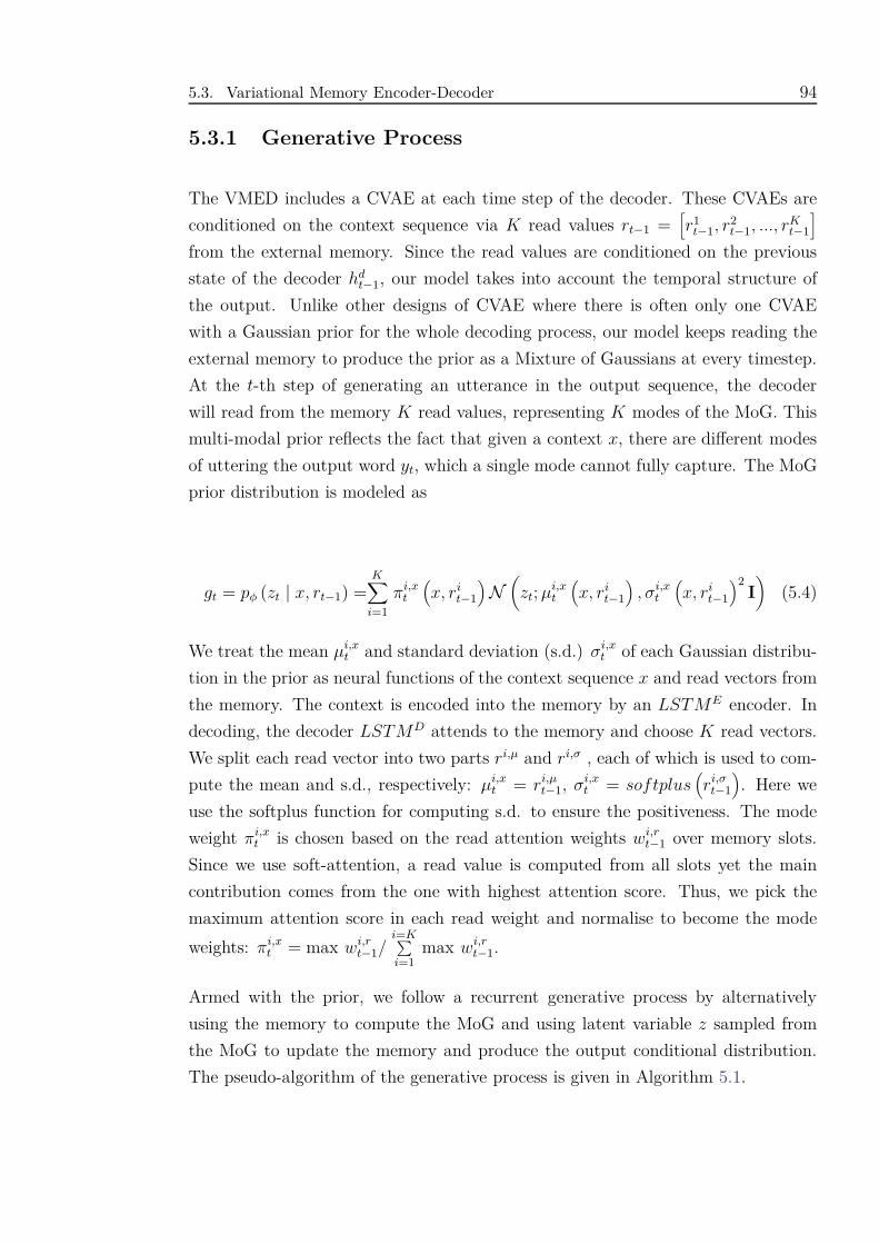
5.3. Variational Memory Encoder-Decoder 94
5.3.1 Generative Process
The VMED includes a CVAE at each time step of the decoder. These CVAEs are
conditioned on the context sequence via K read values rt−1 =[r1
t−1, r2t−1, ..., rK
t−1
]
from the external memory. Since the read values are conditioned on the previous
state of the decoder hdt−1, our model takes into account the temporal structure of
the output. Unlike other designs of CVAE where there is often only one CVAE
with a Gaussian prior for the whole decoding process, our model keeps reading the
external memory to produce the prior as a Mixture of Gaussians at every timestep.
At the t-th step of generating an utterance in the output sequence, the decoder
will read from the memory K read values, representing K modes of the MoG. This
multi-modal prior reflects the fact that given a context x, there are different modes
of uttering the output word yt, which a single mode cannot fully capture. The MoG
prior distribution is modeled as
gt = pφ (zt | x, rt−1) =K∑
i=1
πi,xt
(x, ri
t−1
)N(
zt; µi,xt
(x, ri
t−1
), σi,x
t
(x, ri
t−1
)2I)
(5.4)
We treat the mean µi,xt and standard deviation (s.d.) σi,x
t of each Gaussian distribu-
tion in the prior as neural functions of the context sequence x and read vectors from
the memory. The context is encoded into the memory by an LSTME encoder. In
decoding, the decoder LSTMD attends to the memory and choose K read vectors.
We split each read vector into two parts ri,µ and ri,σ , each of which is used to com-
pute the mean and s.d., respectively: µi,xt = ri,µ
t−1, σi,xt = softplus
(ri,σ
t−1
). Here we
use the softplus function for computing s.d. to ensure the positiveness. The mode
weight πi,xt is chosen based on the read attention weights wi,r
t−1 over memory slots.
Since we use soft-attention, a read value is computed from all slots yet the main
contribution comes from the one with highest attention score. Thus, we pick the
maximum attention score in each read weight and normalise to become the mode
weights: πi,xt = max wi,r
t−1/i=K∑i=1
max wi,rt−1.
Armed with the prior, we follow a recurrent generative process by alternatively
using the memory to compute the MoG and using latent variable z sampled from
the MoG to update the memory and produce the output conditional distribution.
The pseudo-algorithm of the generative process is given in Algorithm 5.1.
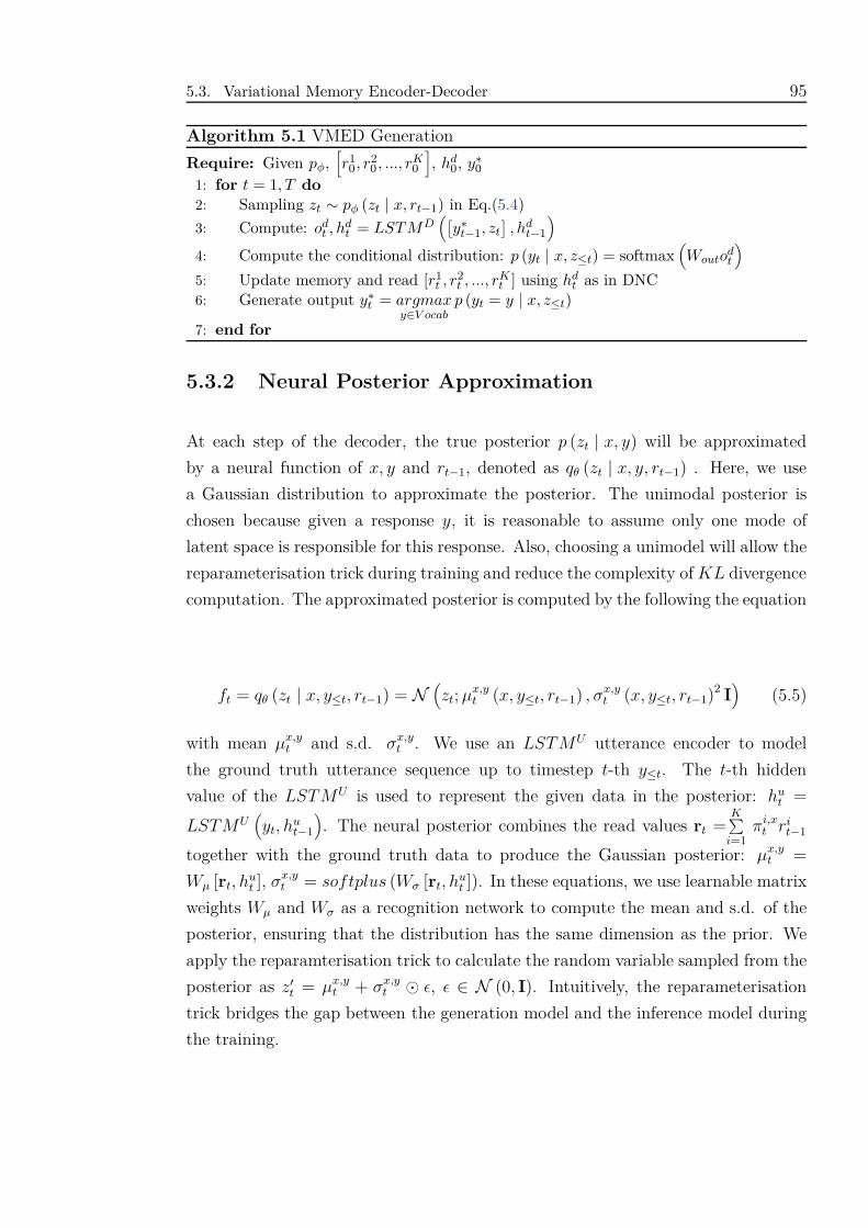
5.3. Variational Memory Encoder-Decoder 95
Algorithm 5.1 VMED Generation
Require: Given pφ,[r1
0, r20 , ..., rK
0
], hd
0, y∗0
1: for t = 1, T do2: Sampling zt ∼ pφ (zt | x, rt−1) in Eq.(5.4)
3: Compute: odt , hd
t = LST MD([
y∗t−1, zt
], hd
t−1
)
4: Compute the conditional distribution: p (yt | x, z≤t) = softmax(Wouto
dt
)
5: Update memory and read [r1t , r2
t , ..., rKt ] using hd
t as in DNC6: Generate output y∗
t = argmaxy∈V ocab
p (yt = y | x, z≤t)
7: end for
5.3.2 Neural Posterior Approximation
At each step of the decoder, the true posterior p (zt | x, y) will be approximated
by a neural function of x, y and rt−1, denoted as qθ (zt | x, y, rt−1) . Here, we use
a Gaussian distribution to approximate the posterior. The unimodal posterior is
chosen because given a response y, it is reasonable to assume only one mode of
latent space is responsible for this response. Also, choosing a unimodel will allow the
reparameterisation trick during training and reduce the complexity of KL divergence
computation. The approximated posterior is computed by the following the equation
ft = qθ (zt | x, y≤t, rt−1) = N(zt; µx,y
t (x, y≤t, rt−1) , σx,yt (x, y≤t, rt−1)
2 I)
(5.5)
with mean µx,yt and s.d. σx,y
t . We use an LSTMU utterance encoder to model
the ground truth utterance sequence up to timestep t-th y≤t. The t-th hidden
value of the LSTMU is used to represent the given data in the posterior: hut =
LSTMU(yt, hu
t−1
). The neural posterior combines the read values rt =
K∑i=1
πi,xt ri
t−1
together with the ground truth data to produce the Gaussian posterior: µx,yt =
Wµ [rt, hut ], σx,y
t = softplus (Wσ [rt, hut ]). In these equations, we use learnable matrix
weights Wµ and Wσ as a recognition network to compute the mean and s.d. of the
posterior, ensuring that the distribution has the same dimension as the prior. We
apply the reparamterisation trick to calculate the random variable sampled from the
posterior as z′t = µx,y
t + σx,yt ⊙ ǫ, ǫ ∈ N (0, I). Intuitively, the reparameterisation
trick bridges the gap between the generation model and the inference model during
the training.
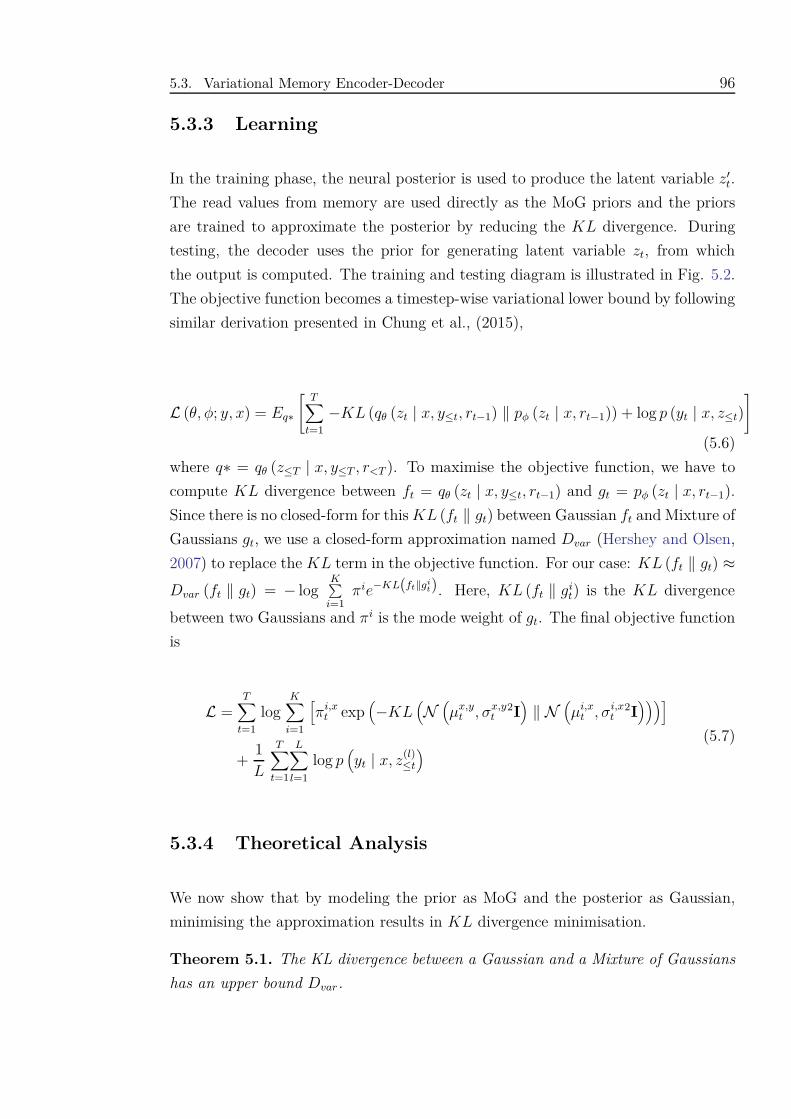
5.3. Variational Memory Encoder-Decoder 96
5.3.3 Learning
In the training phase, the neural posterior is used to produce the latent variable z′t.
The read values from memory are used directly as the MoG priors and the priors
are trained to approximate the posterior by reducing the KL divergence. During
testing, the decoder uses the prior for generating latent variable zt, from which
the output is computed. The training and testing diagram is illustrated in Fig. 5.2.
The objective function becomes a timestep-wise variational lower bound by following
similar derivation presented in Chung et al., (2015),
L (θ, φ; y, x) = Eq∗
[T∑
t=1
−KL (qθ (zt | x, y≤t, rt−1) ‖ pφ (zt | x, rt−1)) + log p (yt | x, z≤t)
]
(5.6)
where q∗ = qθ (z≤T | x, y≤T , r<T ). To maximise the objective function, we have to
compute KL divergence between ft = qθ (zt | x, y≤t, rt−1) and gt = pφ (zt | x, rt−1).
Since there is no closed-form for this KL (ft ‖ gt) between Gaussian ft and Mixture of
Gaussians gt, we use a closed-form approximation named Dvar (Hershey and Olsen,
2007) to replace the KL term in the objective function. For our case: KL (ft ‖ gt) ≈Dvar (ft ‖ gt) = − log
K∑i=1
πie−KL(ft‖git). Here, KL (ft ‖ gi
t) is the KL divergence
between two Gaussians and πi is the mode weight of gt. The final objective function
is
L =T∑
t=1
logK∑
i=1
[πi,x
t exp(−KL
(N(µx,y
t , σx,yt
2I)‖ N
(µi,x
t , σi,xt
2I)))]
+1L
T∑
t=1
L∑
l=1
log p(yt | x, z
(l)≤t
) (5.7)
5.3.4 Theoretical Analysis
We now show that by modeling the prior as MoG and the posterior as Gaussian,
minimising the approximation results in KL divergence minimisation.
Theorem 5.1. The KL divergence between a Gaussian and a Mixture of Gaussians
has an upper bound Dvar.
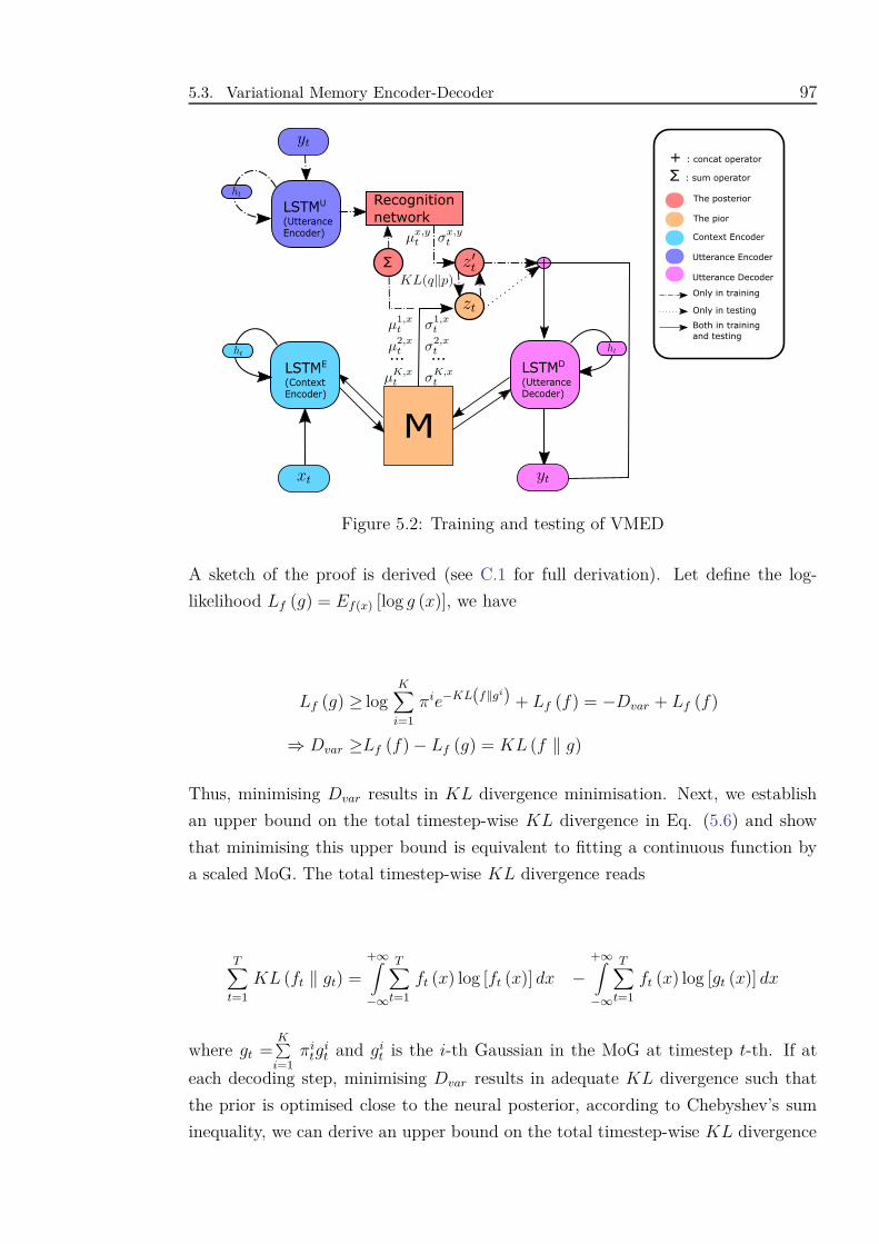
5.3. Variational Memory Encoder-Decoder 97
Figure 5.2: Training and testing of VMED
A sketch of the proof is derived (see C.1 for full derivation). Let define the log-
likelihood Lf (g) = Ef(x) [log g (x)], we have
Lf (g) ≥ logK∑
i=1
πie−KL(f‖gi) + Lf (f) = −Dvar + Lf (f)
⇒ Dvar ≥Lf (f)− Lf (g) = KL (f ‖ g)
Thus, minimising Dvar results in KL divergence minimisation. Next, we establish
an upper bound on the total timestep-wise KL divergence in Eq. (5.6) and show
that minimising this upper bound is equivalent to fitting a continuous function by
a scaled MoG. The total timestep-wise KL divergence reads
T∑
t=1
KL (ft ‖ gt) =+∞∫
−∞
T∑
t=1
ft (x) log [ft (x)] dx −+∞∫
−∞
T∑
t=1
ft (x) log [gt (x)] dx
where gt =K∑
i=1πi
tgit and gi
t is the i-th Gaussian in the MoG at timestep t-th. If at
each decoding step, minimising Dvar results in adequate KL divergence such that
the prior is optimised close to the neural posterior, according to Chebyshev’s sum
inequality, we can derive an upper bound on the total timestep-wise KL divergence
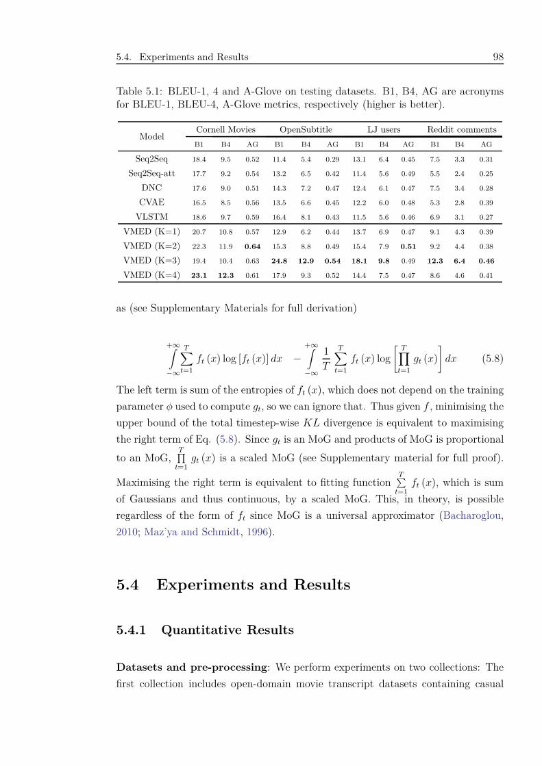
5.4. Experiments and Results 98
Table 5.1: BLEU-1, 4 and A-Glove on testing datasets. B1, B4, AG are acronymsfor BLEU-1, BLEU-4, A-Glove metrics, respectively (higher is better).
ModelCornell Movies OpenSubtitle LJ users Reddit comments
B1 B4 AG B1 B4 AG B1 B4 AG B1 B4 AG
Seq2Seq 18.4 9.5 0.52 11.4 5.4 0.29 13.1 6.4 0.45 7.5 3.3 0.31
Seq2Seq-att 17.7 9.2 0.54 13.2 6.5 0.42 11.4 5.6 0.49 5.5 2.4 0.25
DNC 17.6 9.0 0.51 14.3 7.2 0.47 12.4 6.1 0.47 7.5 3.4 0.28
CVAE 16.5 8.5 0.56 13.5 6.6 0.45 12.2 6.0 0.48 5.3 2.8 0.39
VLSTM 18.6 9.7 0.59 16.4 8.1 0.43 11.5 5.6 0.46 6.9 3.1 0.27
VMED (K=1) 20.7 10.8 0.57 12.9 6.2 0.44 13.7 6.9 0.47 9.1 4.3 0.39
VMED (K=2) 22.3 11.9 0.64 15.3 8.8 0.49 15.4 7.9 0.51 9.2 4.4 0.38
VMED (K=3) 19.4 10.4 0.63 24.8 12.9 0.54 18.1 9.8 0.49 12.3 6.4 0.46
VMED (K=4) 23.1 12.3 0.61 17.9 9.3 0.52 14.4 7.5 0.47 8.6 4.6 0.41
as (see Supplementary Materials for full derivation)
+∞∫
−∞
T∑
t=1
ft (x) log [ft (x)] dx −+∞∫
−∞
1T
T∑
t=1
ft (x) log
[T∏
t=1
gt (x)
]dx (5.8)
The left term is sum of the entropies of ft (x), which does not depend on the training
parameter φ used to compute gt, so we can ignore that. Thus given f , minimising the
upper bound of the total timestep-wise KL divergence is equivalent to maximising
the right term of Eq. (5.8). Since gt is an MoG and products of MoG is proportional
to an MoG,T∏
t=1gt (x) is a scaled MoG (see Supplementary material for full proof).
Maximising the right term is equivalent to fitting functionT∑
t=1ft (x), which is sum
of Gaussians and thus continuous, by a scaled MoG. This, in theory, is possible
regardless of the form of ft since MoG is a universal approximator (Bacharoglou,
2010; Maz’ya and Schmidt, 1996).
5.4 Experiments and Results
5.4.1 Quantitative Results
Datasets and pre-processing: We perform experiments on two collections: The
first collection includes open-domain movie transcript datasets containing casual
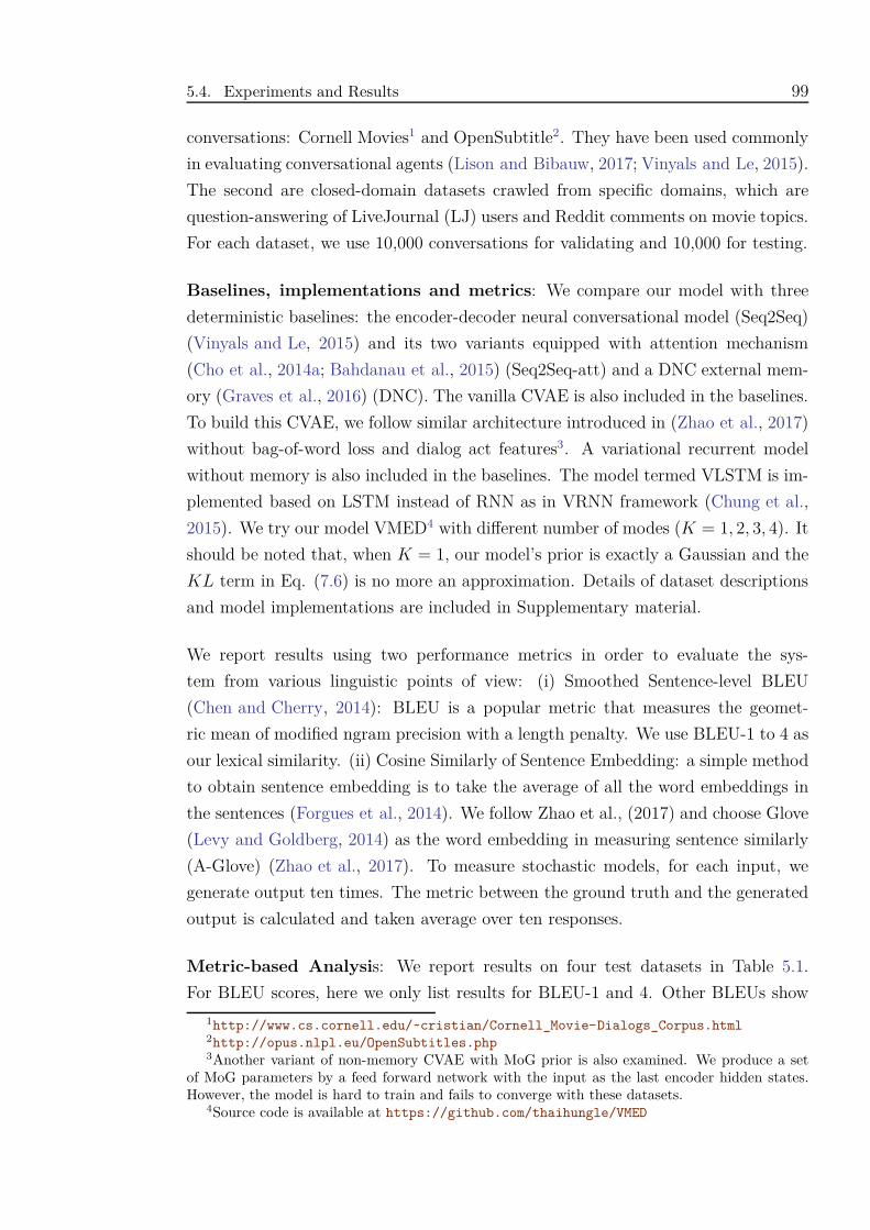
5.4. Experiments and Results 99
conversations: Cornell Movies1 and OpenSubtitle2. They have been used commonly
in evaluating conversational agents (Lison and Bibauw, 2017; Vinyals and Le, 2015).
The second are closed-domain datasets crawled from specific domains, which are
question-answering of LiveJournal (LJ) users and Reddit comments on movie topics.
For each dataset, we use 10,000 conversations for validating and 10,000 for testing.
Baselines, implementations and metrics: We compare our model with three
deterministic baselines: the encoder-decoder neural conversational model (Seq2Seq)
(Vinyals and Le, 2015) and its two variants equipped with attention mechanism
(Cho et al., 2014a; Bahdanau et al., 2015) (Seq2Seq-att) and a DNC external mem-
ory (Graves et al., 2016) (DNC). The vanilla CVAE is also included in the baselines.
To build this CVAE, we follow similar architecture introduced in (Zhao et al., 2017)
without bag-of-word loss and dialog act features3. A variational recurrent model
without memory is also included in the baselines. The model termed VLSTM is im-
plemented based on LSTM instead of RNN as in VRNN framework (Chung et al.,
2015). We try our model VMED4 with different number of modes (K = 1, 2, 3, 4). It
should be noted that, when K = 1, our model’s prior is exactly a Gaussian and the
KL term in Eq. (7.6) is no more an approximation. Details of dataset descriptions
and model implementations are included in Supplementary material.
We report results using two performance metrics in order to evaluate the sys-
tem from various linguistic points of view: (i) Smoothed Sentence-level BLEU
(Chen and Cherry, 2014): BLEU is a popular metric that measures the geomet-
ric mean of modified ngram precision with a length penalty. We use BLEU-1 to 4 as
our lexical similarity. (ii) Cosine Similarly of Sentence Embedding: a simple method
to obtain sentence embedding is to take the average of all the word embeddings in
the sentences (Forgues et al., 2014). We follow Zhao et al., (2017) and choose Glove
(Levy and Goldberg, 2014) as the word embedding in measuring sentence similarly
(A-Glove) (Zhao et al., 2017). To measure stochastic models, for each input, we
generate output ten times. The metric between the ground truth and the generated
output is calculated and taken average over ten responses.
Metric-based Analysis: We report results on four test datasets in Table 5.1.
For BLEU scores, here we only list results for BLEU-1 and 4. Other BLEUs show
1http://www.cs.cornell.edu/~cristian/Cornell_Movie-Dialogs_Corpus.html2http://opus.nlpl.eu/OpenSubtitles.php3Another variant of non-memory CVAE with MoG prior is also examined. We produce a set
of MoG parameters by a feed forward network with the input as the last encoder hidden states.However, the model is hard to train and fails to converge with these datasets.
4Source code is available at https://github.com/thaihungle/VMED
5.4. Experiments and Results 100
similar pattern and will be listed in Supplementary material. As clearly seen, VMED
models outperform other baselines over all metrics across four datasets. In general,
the performance of Seq2Seq is comparable with other deterministic methods despite
its simplicity. Surprisingly, CVAE or VLSTM does not show much advantage over
deterministic models. As we shall see, although CVAE and VLSTM responses are
diverse, they are often out of context. Amongst different modes of VMED, there is
often one best fit with the data and thus shows superior performance. The optimal
number of modes in our experiments often falls to K = 3, indicating that increasing
modes does not mean to improve accuracy.
It should be noted that there is inconsistency between BLEU scores and A-Glove
metrics. This is because BLEU measures lexicon matching while A-Glove evaluates
semantic similarly in the embedding space. For example, two sentences having dif-
ferent words may share the same meaning and lie close in the embedding space. In
either case, compared to others, our optimal VMED always achieves better perfor-
mance.
5.4.2 Qualitative Analysis
Table 5.2 represents responses generated by experimental models in reply to different
input sentences. The replies listed are chosen randomly from 50 generated responses
whose average of metric scores over all models are highest. For stochastic models,
we generate three times for each input, resulting in three different responses. In
general, the stochastic models often yield longer and diverse sequences as expected.
For closed-domain cases, all models responses are fairly acceptable. Compared to
the rest, our VMED’s responds seem to relate more to the context and contain
meaningful information. In this experiment, the open-domain input seems nosier
and harder than the closed-domain ones, thus create a big challenge for all models.
Despite that, the quality of VMED’s responses is superior to others. Amongst deter-
ministic models, DNC’s generated responses look more reasonable than Seq2Seq’s
even though its BLEU scores are not always higher. Perhaps, the reference to ex-
ternal memory at every timestep enhances the coherence between output and input,
making the response more related to the context. VMED may inherit this feature
from its external memory and thus tends to produce reasonable responses. By con-
trast, although responses from CVAE and VLSTM are not trivial, they have more
grammatical errors and sometimes unrelated to the topic.
5.4. Experiments and Results 101
Table 5.2: Examples of context-response pairs. /*/ denotes separations betweenstochastic responses.
Input context Response
comment: What
is your favorite
scene in film
history ? Mine is
the restaurant
scene in the
Godfather.
Seq2Seq: The scene in
Seq2Seq-att: The final
DNC: The scene in
CVAE: Inception god! Not by a shark /*/ Amour great /*/ Pro thing
you know 3 dead
VLSTM: The scene in /*/ The of a dead /*/ The sky in scene
VMED (K=3): The opening scene from history movie /*/ The scene
in a shot nights! Robin movie /*/ The psycho scene in fight from
comment: What
actor will win an
Oscar in the next
10 years ?
Seq2Seq: Colin
Seq2Seq-att: Liam Neeson
DNC: Tom Gyllenhaal
CVAE: Daryl and Aaron /*/ Carefully count Alfred Deniro /*/
Ponyo Joker possible
VLSTM: Michael Bullock /*/ Michael /*/ Michael De
VMED (K=3): Edward or Leo Dicaprio goes on /*/ Dicaprio will
/*/ Dicaprio Tom has actually in jack on road
LJ user: Your
very pretty and
your is very cute.
May i add ya to
my friends list ?
Seq2Seq: I! Add and too you back
Seq2Seq-att: I did may! Away back
DNC: Sure you added
CVAE: Sure ! I can add you /*/ Thank cool of surely /*/ Thank hi of
sure!
VLSTM: Haha of do go /*/ Haha of sure! Yes lol /*/ Haha sure! Go
VMED (K=3): Thank cool for sure /*/ Add definitely! Sure surely
friends /*/ Thank girl go ahead
Cornell movies:
Nobody can
murder someone
with their feelings .
I mean that is
crazy ?
Seq2Seq: Yes you are
Seq2Seq-att: Really not is it
DNC: Managing the truth
CVAE: Sure not to be in here /*/ Oh yes but i know! /*/ That to
doing with here and
VLSTM: I am dead . ! That is ... /*/ I did not what way . /*/ I am
not . But his things with ...
VMED (K=4): You are right! /*/ That is crazy /*/ You can’t know
Jimmy
OpenSubtitle:
I’m obliged for
your hospitality. I
appreciate it and
your husband too.
Seq2Seq: That is have got coming about these
Seq2Seq-att: May you not what nothing nobody
DNC: Yes i am taking this
CVAE: No . that for good! And okay /*/ All in the of two thing /*/
Sure. Is this!
VLSTM: I ... /*/ I understand /*/ I ! . ...
VMED (K=3): I know. I can afford /*/ I know nothing to store for
you pass /*/ I know. Doing anymore you father
5.5. Closing Remarks 102
5.5 Closing Remarks
In this chapter, we propose a novel approach to sequence generation called Varia-
tional Memory Encoder-Decoder (VMED) that introduces variability into encoder-
decoder architecture via the use of external memory as mixture model. By modeling
the latent temporal dependencies across timesteps, our VMED produces a MoG rep-
resenting the latent distribution. Each mode of the MoG associates with some mem-
ory slot and thus captures some aspect of context supporting generation process. To
accommodate the MoG, we employ a KL approximation and we demonstrate that
minimising this approximation is equivalent to minimising the KL divergence. We
derive an upper bound on our total timestep-wise KL divergence and indicate that
the optimisation of this upper bound is equivalent to fitting a continuous function
by an scaled MoG, which is in theory possible regardless of the function form. This
forms a theoretical basis for our model formulation using MoG prior for every step of
generation. We apply our proposed model to conversation generation problem. The
results demonstrate that VMED outperforms recent advances both quantitatively
and qualitatively.
So far we have designed and applied MANNs to long-term sequential modeling
problems without considering the memorisation ability of these models. Besides, we
have followed common memory access patterns without judging the effectiveness of
these accesses. We will tackle these issues in the next chapter.
Chapter 6
Optimal Writing Memory
6.1 Introduction
Recall that a core task in sequence learning is to capture long-term dependencies
amongst timesteps which demands memorisation of distant inputs (Sec. 2.4). In
recurrent neural networks (RNNs), the memorisation is implicitly executed via in-
tegrating the input history into the state of the networks. However, learning vanilla
RNNs over long distance proves to be difficult due to the vanishing gradient problem
(Sec. 2.4.1). One alleviation is to introduce skip-connections along the execution
path, in the form of dilated layers (Van Den Oord et al., 2016; Chang et al., 2017),
which is not our main focus. Other solutions have been mentioned in Chapter 3 in-
cluding attention mechanisms (Cho et al., 2014a; Vaswani et al., 2017; Bahdanau et al.,
2015) and external slot-based memory (Graves et al., 2014, 2016).
Amongst all, using external memory most resembles human cognitive architecture
where we perceive the world sequentially and make decision by consulting our mem-
ory. Recent attempts have simulated this process by using RAM-like memory archi-
tectures that store information into memory slots. Reading and writing are governed
by neural controllers using attention mechanisms (Sec. 3.3).
Despite the promising empirical results, there is no theoretical analysis or clear
understanding on optimal operations that a memory should have to maximise its
performance. To the best of our knowledge, no solution has been proposed to help
MANNs handle ultra-long sequences given limited memory. This scenario is practical
because (i) sequences in the real-world can be very long while the computer resources
103
6.2. Related Backgrounds 104
are limited and (ii) it reflects the ability to compress in human brain to perform life-
long learning. Previous attempts (Rae et al., 2016) try to learn ultra-long sequences
by expanding the memory, which is not always feasible and do not aim to optimise
the memory by some theoretical criterion. This chapter presents a new approach
towards finding optimal operations for MANNs that serve the purpose of learning
longer sequences with finite memory.
More specifically, upon analysing RNN and MANN operations we first introduce a
measurement on the amount of information that a MANN holds after encoding a
sequence. This metric reflects the quality of memorisation under the assumption
that contributions from timesteps are equally important. We then derive a generic
solution to optimise the measurement. We term this optimal solution as Uniform
Writing (UW), and it is applicable for any MANN due to its generality. Crucially,
UW helps reduce significantly the computation time of MANN. Third, to relax the
assumption and enable the method to work in realistic settings, we further pro-
pose Cached Uniform Writing (CUW) as an improvement over the Uniform Writing
scheme. By combining uniform writing with local attention, CUW can learn to dis-
criminate timesteps while maximising local memorisation. Finally we demonstrate
that our proposed models outperform several MANNs and other state-of-the-art
methods in various synthetic and practical sequence modeling tasks.
6.2 Related Backgrounds
Traditional recurrent models such as RNN/LSTM (Elman, 1990; Hochreiter and Schmidhuber,
1997) exhibit some weakness that prevents them from learning really long sequences.
The reason is mainly due to the vanishing gradient problem or to be more specific,
the exponential decay of input value over time, which is analysed in Sec. 2.4.1.
It should be noted that although LSTM is designed to diminish the problem, it is
limited to the capacity of cell memory. In other words, if the amount of relevant
information exceeds the capacity, LSTM will forget distant inputs since exponen-
tial decay still exists outside the cell memory. One different approach to overcome
this problem is enforcing the exponential decay factor close to one by putting a
unitary constraint on the recurrent weight (Arjovsky et al., 2016; Wisdom et al.,
2016). Although this approach is theoretically motivated, it restricts the space of
learnt parameters.
More relevant to our work, the idea of using less or adaptive computation has been
6.2. Related Backgrounds 105
proposed by many (Graves, 2016; Yu et al., 2017, 2018; Seo et al., 2018). Most of
these works are based on the assumption that some of timesteps in a sequence are
unimportant and thus can be ignored to reduce the cost of computation and increase
the performance of recurrent networks. Different form our approach, these methods
lack theoretical supports and do not directly aim to solve the problem of memorising
long-term dependencies.
Dilated RNN (Chang et al., 2017) is another RNN-based proposal which improves
long-term learning by stacking multiple dilated recurrent layers with hierarchical
skip-connections. This theoretically guarantees the mean recurrent length and
shares with our method the idea to construct a measurement on memorisation ca-
pacity of the system and propose solutions to optimise it. The difference is that
our system is memory-augmented neural networks while theirs is multi-layer RNNs,
which leads to totally different optimisation problems.
Recent researches recommend to replace traditional recurrent models by other neu-
ral architectures to overcome the vanishing gradient problem. The Transformer
(Vaswani et al., 2017) attends to all timesteps at once, which ensures instant ac-
cess to distant timestep yet requires quadratic computation and physical memory
proportional to the sequence length (see Sec. 3.2.3). Memory-augmented neural
networks (MANNs), on the other hand, learn to establish a limited-size memory
and attend to the memory only, which is scalable to any-length sequence (see Sec.
3.3). Compared to others, MANNs resemble both computer architecture design and
human working memory (Logie, 2014). However, the current understanding of the
underlying mechanisms and theoretical foundations for MANNs are still limited.
Recent works on MANNs rely almost on reasonable intuitions. Some introduce
new addressing mechanisms such as location-based (Graves et al., 2014), least-used
(Santoro et al., 2016) and order-based (Graves et al., 2016). Others focus on the
scalability of MANN by using sparse memory access to avoid attending to a large
number of memory slots (Rae et al., 2016). These problems are different from ours
which involves MANN memorisation capacity optimisation.
Our local optimal solution to this problem is related to some known neural caching
(Grave et al., 2017b,a; Yogatama et al., 2018) in terms of storing recent hidden
states for later encoding uses. These methods either aim to create structural bias
to ease the learning process (Yogatama et al., 2018) or support large scale retrieval
(Grave et al., 2017a). These are different from our caching purpose, which encour-
ages overwriting and relaxes the equal contribution assumption of the optimal so-
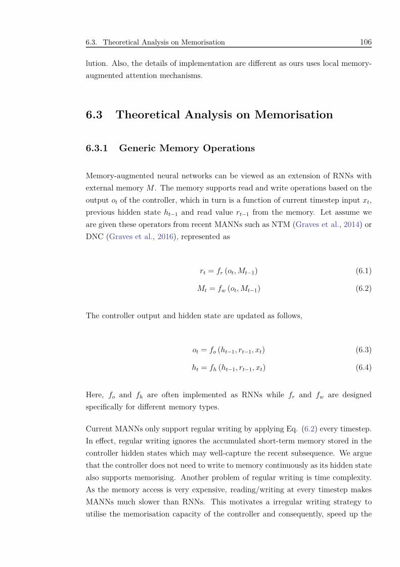
6.3. Theoretical Analysis on Memorisation 106
lution. Also, the details of implementation are different as ours uses local memory-
augmented attention mechanisms.
6.3 Theoretical Analysis on Memorisation
6.3.1 Generic Memory Operations
Memory-augmented neural networks can be viewed as an extension of RNNs with
external memory M . The memory supports read and write operations based on the
output ot of the controller, which in turn is a function of current timestep input xt,
previous hidden state ht−1 and read value rt−1 from the memory. Let assume we
are given these operators from recent MANNs such as NTM (Graves et al., 2014) or
DNC (Graves et al., 2016), represented as
rt = fr (ot, Mt−1) (6.1)
Mt = fw (ot, Mt−1) (6.2)
The controller output and hidden state are updated as follows,
ot = fo (ht−1, rt−1, xt) (6.3)
ht = fh (ht−1, rt−1, xt) (6.4)
Here, fo and fh are often implemented as RNNs while fr and fw are designed
specifically for different memory types.
Current MANNs only support regular writing by applying Eq. (6.2) every timestep.
In effect, regular writing ignores the accumulated short-term memory stored in the
controller hidden states which may well-capture the recent subsequence. We argue
that the controller does not need to write to memory continuously as its hidden state
also supports memorising. Another problem of regular writing is time complexity.
As the memory access is very expensive, reading/writing at every timestep makes
MANNs much slower than RNNs. This motivates a irregular writing strategy to
utilise the memorisation capacity of the controller and consequently, speed up the
6.3. Theoretical Analysis on Memorisation 107
model. In the next sections, we first define a metric to measure the memorisation
performance of RNNs, as well as MANNs. Then, we solve the problem of finding
the best irregular writing that optimises the metric.
6.3.2 Memory Analysis of RNNs
We first define the ability to “remember” of recurrent neural networks, which is
closely related to the vanishing/exploding gradient problem (Pascanu et al., 2013).
In RNNs, the state transition ht = φ (ht−1, xt) contains contributions from not only
xt, but also previous timesteps xi<t embedded in ht−1. Thus, ht can be considered
as a function of timestep inputs, i.e, ht = f (x1, x2, ..., xt). One way to measure
how much an input xi contributes to the value of ht is to calculate the norm of
the gradient∥∥∥∂ht
∂xi
∥∥∥. If the norm equals zero, ht is constant w.r.t xi, that is, ht
does not “remember” xi. As a bigger∥∥∥∂ht
∂xi
∥∥∥ implies more influence of xi on ht, we
propose using∥∥∥∂ht
∂xi
∥∥∥ to measure the contribution of the i-th input to the t-th hidden
state. Let ci,t denotes this term, we can show that in the case of common RNNs,
λcci,t ≥ ci−1,t with some λc ∈ R+(see Appendix D.1 - D.3 for proof). This means
further to the past, the contribution decays (when λc < 1) or grows (when λc > 1)
with the rate of at least λc .We can measure the average amount of contributions
across T timesteps as follows (see Appendix D.4 for proof):
Theorem 6.1. There exists λ ∈ R+such that the average contribution of a sequence
of length T with respect to a RNN can be quantified as the following,
Iλ =
T∑t=1
ct,T
T= cT,T
T∑t=1
λT −t
T(6.5)
If λ < 1, λT −t → 0 as T − t → ∞. This is closely related to vanishing gradient
problem. LSTM is known to “remember” long sequences better than RNN by using
extra memory gating mechanisms, which help λ to get closer to 1. If λ > 1, the
system may be unstable and suffer from the exploding gradient problem.
6.3.3 Memory Analysis of MANNs
In slot-based MANNs, memory M is a set of D memory slots. A write at step t
can be represented by the controller’s hidden state ht, which accumulates inputs
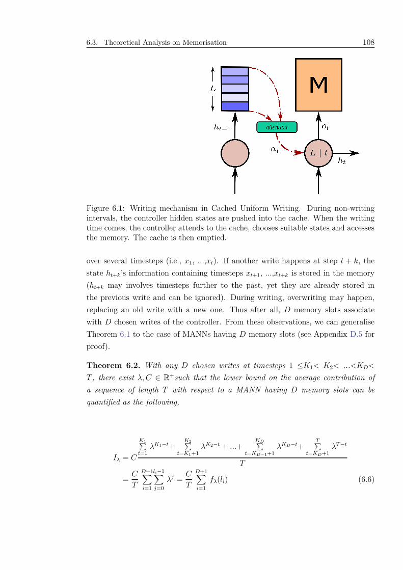
6.3. Theoretical Analysis on Memorisation 108
Figure 6.1: Writing mechanism in Cached Uniform Writing. During non-writingintervals, the controller hidden states are pushed into the cache. When the writingtime comes, the controller attends to the cache, chooses suitable states and accessesthe memory. The cache is then emptied.
over several timesteps (i.e., x1, ...,xt). If another write happens at step t + k, the
state ht+k’s information containing timesteps xt+1, ...,xt+k is stored in the memory
(ht+k may involves timesteps further to the past, yet they are already stored in
the previous write and can be ignored). During writing, overwriting may happen,
replacing an old write with a new one. Thus after all, D memory slots associate
with D chosen writes of the controller. From these observations, we can generalise
Theorem 6.1 to the case of MANNs having D memory slots (see Appendix D.5 for
proof).
Theorem 6.2. With any D chosen writes at timesteps 1 ≤K1< K2< ...<KD<
T , there exist λ, C ∈ R+such that the lower bound on the average contribution of
a sequence of length T with respect to a MANN having D memory slots can be
quantified as the following,
Iλ = C
K1∑t=1
λK1−t+K2∑
t=K1+1λK2−t + ...+
KD∑t=KD−1+1
λKD−t+T∑
t=KD+1λT −t
T
=C
T
D+1∑
i=1
li−1∑
j=0
λj =C
T
D+1∑
i=1
fλ(li) (6.6)
6.4. Optimal Writing for Slot-based Memory Models 109
where li =
K1 ; i = 1
Ki −Ki−1 ; D ≥ i > 1
T −KD ; i = D + 1
, fλ (x) =
1−λx
1−λλ 6= 1
x λ = 1, ∀x ∈ R+.
If λ ≤ 1, we want to maximise Iλ to keep the information from vanishing. On
the contrary, if λ > 1, we may want to minimise Iλ to prevent the information
explosion. As both scenarios share the same solution (see Appendix D.6), thereafter
we assume that λ ≤ 1 holds for other analyses. By taking average over T , we are
making an assumption that all timesteps are equally important. This helps simplify
the measurement as Iλ is independent of the specific position of writing. Rather,
it is a function of the interval lengths between the writes. This turns out to be an
optimisation problem whose solution is stated in the following theorem.
Theorem 6.3. Given D memory slots, a sequence with length T , a decay rate
0 < λ ≤ 1, then the optimal intervals {li ∈ R+}D+1i=1 satisfying T =
D+1∑i=1
li such that
the lower bound on the average contribution Iλ = CT
D+1∑i=1
fλ(li) is maximised are
l1 = l2 = ... = lD+1 =T
D + 1(6.7)
We name the optimal solution as Uniform Writing (UW) and refer to the term TD+1
and D+1T
as the optimal interval and the compression ratio, respectively. The proof
is given in Appendix D.6.
6.4 Optimal Writing for Slot-based Memory Mod-
els
6.4.1 Uniform Writing
Uniform writing can apply to any MANNs that support writing operations. Since
the writing intervals are discrete, i.e., li ∈ N+, UW is implemented as the following,
Mt =
fw (ot, Mt−1) if t =⌊
TD+1
⌋k, k ∈ N
+
Mt−1 otherwise(6.8)
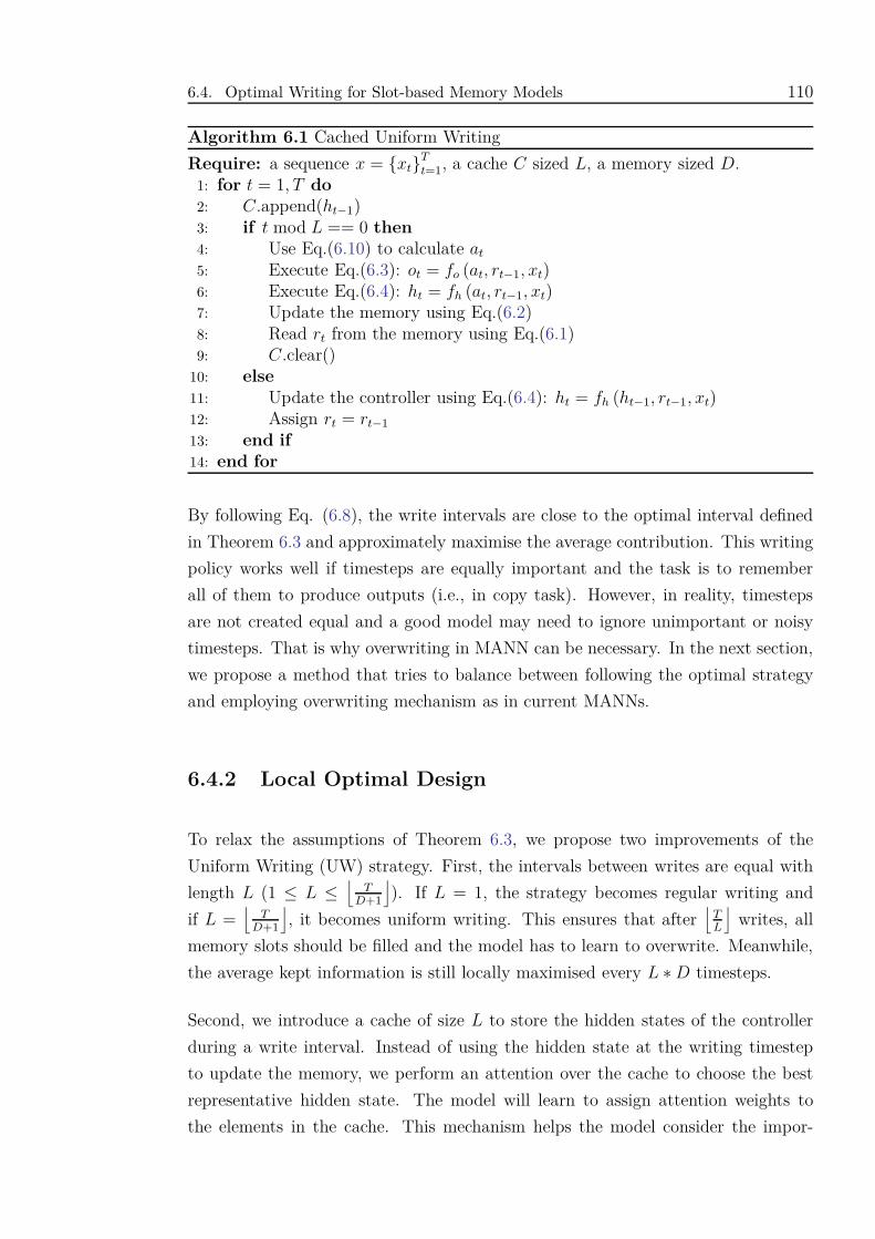
6.4. Optimal Writing for Slot-based Memory Models 110
Algorithm 6.1 Cached Uniform Writing
Require: a sequence x = {xt}Tt=1, a cache C sized L, a memory sized D.
1: for t = 1, T do2: C.append(ht−1)3: if t mod L == 0 then4: Use Eq.(6.10) to calculate at
5: Execute Eq.(6.3): ot = fo (at, rt−1, xt)6: Execute Eq.(6.4): ht = fh (at, rt−1, xt)7: Update the memory using Eq.(6.2)8: Read rt from the memory using Eq.(6.1)9: C.clear()
10: else11: Update the controller using Eq.(6.4): ht = fh (ht−1, rt−1, xt)12: Assign rt = rt−1
13: end if14: end for
By following Eq. (6.8), the write intervals are close to the optimal interval defined
in Theorem 6.3 and approximately maximise the average contribution. This writing
policy works well if timesteps are equally important and the task is to remember
all of them to produce outputs (i.e., in copy task). However, in reality, timesteps
are not created equal and a good model may need to ignore unimportant or noisy
timesteps. That is why overwriting in MANN can be necessary. In the next section,
we propose a method that tries to balance between following the optimal strategy
and employing overwriting mechanism as in current MANNs.
6.4.2 Local Optimal Design
To relax the assumptions of Theorem 6.3, we propose two improvements of the
Uniform Writing (UW) strategy. First, the intervals between writes are equal with
length L (1 ≤ L ≤⌊
TD+1
⌋). If L = 1, the strategy becomes regular writing and
if L =⌊
TD+1
⌋, it becomes uniform writing. This ensures that after
⌊TL
⌋writes, all
memory slots should be filled and the model has to learn to overwrite. Meanwhile,
the average kept information is still locally maximised every L ∗D timesteps.
Second, we introduce a cache of size L to store the hidden states of the controller
during a write interval. Instead of using the hidden state at the writing timestep
to update the memory, we perform an attention over the cache to choose the best
representative hidden state. The model will learn to assign attention weights to
the elements in the cache. This mechanism helps the model consider the impor-
6.5. Experiments and Results 111
tance of each timestep input in the local interval and thus relax the equal contribu-
tion assumption of Theorem 6.3. We name the writing strategy that uses the two
mentioned-above improvements as Cached Uniform Writing (CUW). An illustration
of the writing mechanism is depicted in Fig. 6.1.
6.4.3 Local Memory-Augmented Attention Unit
In this subsection, we provide details of the attention mechanism used in our CUW.
To be specific, the best representative hidden state at is computed as follows,
αtj = softmax(vT tanh (Wht−1 + Udj + V rt−1)
)(6.9)
at =L∑
j=1
αtjdj (6.10)
where αtj is the attention score between the t-th writing step and the j-th element
in the cache; W , U , V and v are parameters; h and r are the hidden state of the
controller and the read-out (Eq. (6.1)), respectively; dj is the cache element and
can be implemented as the controller’s hidden state (dj = ht−1−L+j).
The vector at will be used to replace the previous hidden state in updating the
controller and memory. The whole process of performing CUW is summarised in
Algo. 6.11.
6.5 Experiments and Results
6.5.1 An Ablation Study: Memory-Augmented Neural Net-
works with and without Uniform Writing
In this section, we study the impact of uniform writing on MANNs under various cir-
cumstances (different controller types, memory types and number of memory slots).
1Source code is available at https://github.com/thaihungle/UW-DNC
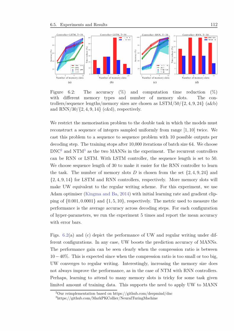
6.5. Experiments and Results 112
Figure 6.2: The accuracy (%) and computation time reduction (%)with different memory types and number of memory slots. The con-trollers/sequence lengths/memory sizes are chosen as LSTM/50/{2, 4, 9, 24} (a&b)and RNN/30/{2, 4, 9, 14} (c&d), respectively.
We restrict the memorisation problem to the double task in which the models must
reconstruct a sequence of integers sampled uniformly from range [1, 10] twice. We
cast this problem to a sequence to sequence problem with 10 possible outputs per
decoding step. The training stops after 10,000 iterations of batch size 64. We choose
DNC2 and NTM3 as the two MANNs in the experiment. The recurrent controllers
can be RNN or LSTM. With LSTM controller, the sequence length is set to 50.
We choose sequence length of 30 to make it easier for the RNN controller to learn
the task. The number of memory slots D is chosen from the set {2, 4, 9, 24} and
{2, 4, 9, 14} for LSTM and RNN controllers, respectively. More memory slots will
make UW equivalent to the regular writing scheme. For this experiment, we use
Adam optimiser (Kingma and Ba, 2014) with initial learning rate and gradient clip-
ping of {0.001, 0.0001} and {1, 5, 10}, respectively. The metric used to measure the
performance is the average accuracy across decoding steps. For each configuration
of hyper-parameters, we run the experiment 5 times and report the mean accuracy
with error bars.
Figs. 6.2(a) and (c) depict the performance of UW and regular writing under dif-
ferent configurations. In any case, UW boosts the prediction accuracy of MANNs.
The performance gain can be seen clearly when the compression ratio is between
10−40%. This is expected since when the compression ratio is too small or too big,
UW converges to regular writing. Interestingly, increasing the memory size does
not always improve the performance, as in the case of NTM with RNN controllers.
Perhaps, learning to attend to many memory slots is tricky for some task given
limited amount of training data. This supports the need to apply UW to MANN
2Our reimplementation based on https://github.com/deepmind/dnc3https://github.com/MarkPKCollier/NeuralTuringMachine
6.5. Experiments and Results 113
with moderate memory size. We also conduct experiments to verify the benefit of
using UW for bigger memory. The results can be found in Appendix D.8.
We also measure the speed-up of training time when applying UW on DNC and
NTM, which is illustrated in Figs. 6.2(b) and (d). The result shows that with UW,
the training time can drop up to 60% for DNC and 28% for NTM, respectively. As
DNC is more complicated than NTM, using UW to reduce memory access demon-
strates clearer speed-up in training (similar behavior can be found for testing time).
6.5.2 Synthetic Memorisation
Here we address a broader range of baselines on two synthetic memorisation tasks,
which are the sequence copy and reverse. In these tasks, there is no discrimination
amongst timesteps so the model’s goal is to learn to compress the input efficiently
for later retrieval. We experiment with different sequence lengths of 50 and 100
timesteps. Other details are the same as the previous double task except that we fix
the learning rate and gradient clipping to 0.001 and 10, respectively. The standard
baselines include LSTM, NTM and DNC. All memory-augmented models have the
same memory size of 4 slots, corresponding to compression ratio of 10% and 5%,
respectively. We aim at this range of compression ratio to match harsh practical
requirements. UW and CUW (cache size L = 5) are built upon the DNC, which
from our previous observations, works best for given compression ratios. We choose
different dimensions Nh for the hidden vector of the controllers to ensure the model
sizes are approximately equivalent. To further verify that our UW is actually the
optimal writing strategy, we design a new baseline, which is DNC with random
irregular writing strategy (RW). The write is sampled from a binomial distribution
with p = (D + 1) /T (equivalent to compression ratio). After sampling, we conduct
the training for that policy. The final performances of RW are taken average from
3 different random policies’ results.
The performance of the models is listed in Table 6.1. As clearly seen, UW is the
best performer for the pure memorisation tests. This is expected from the theory
as all timesteps are importantly equivalent. Local attention mechanism in CUW
does not help much in this scenario and thus CUW finishes the task as the runner-
up. Reverse seems to be easier than copy as the models tend to “remember” more
the last-seen timesteps whose contributions λT −t remains significant. In both cases,
other baselines including random irregular and regular writing underperform our
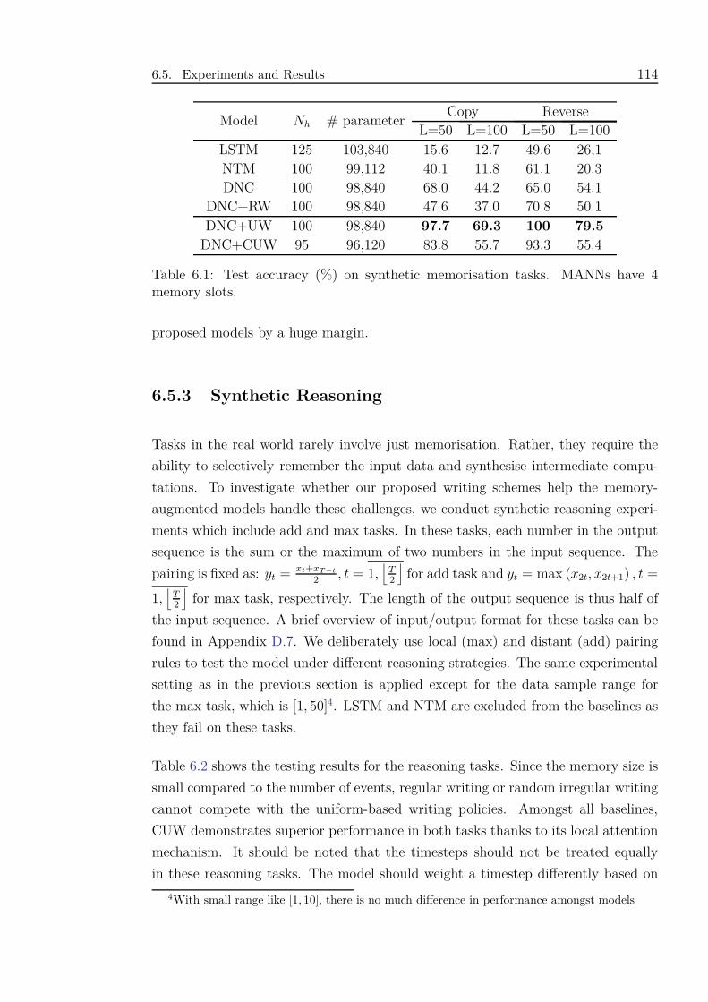
6.5. Experiments and Results 114
Model Nh # parameterCopy Reverse
L=50 L=100 L=50 L=100LSTM 125 103,840 15.6 12.7 49.6 26,1NTM 100 99,112 40.1 11.8 61.1 20.3DNC 100 98,840 68.0 44.2 65.0 54.1
DNC+RW 100 98,840 47.6 37.0 70.8 50.1DNC+UW 100 98,840 97.7 69.3 100 79.5
DNC+CUW 95 96,120 83.8 55.7 93.3 55.4
Table 6.1: Test accuracy (%) on synthetic memorisation tasks. MANNs have 4memory slots.
proposed models by a huge margin.
6.5.3 Synthetic Reasoning
Tasks in the real world rarely involve just memorisation. Rather, they require the
ability to selectively remember the input data and synthesise intermediate compu-
tations. To investigate whether our proposed writing schemes help the memory-
augmented models handle these challenges, we conduct synthetic reasoning experi-
ments which include add and max tasks. In these tasks, each number in the output
sequence is the sum or the maximum of two numbers in the input sequence. The
pairing is fixed as: yt = xt+xT −t
2, t = 1,
⌊T2
⌋for add task and yt = max (x2t, x2t+1) , t =
1,⌊
T2
⌋for max task, respectively. The length of the output sequence is thus half of
the input sequence. A brief overview of input/output format for these tasks can be
found in Appendix D.7. We deliberately use local (max) and distant (add) pairing
rules to test the model under different reasoning strategies. The same experimental
setting as in the previous section is applied except for the data sample range for
the max task, which is [1, 50]4. LSTM and NTM are excluded from the baselines as
they fail on these tasks.
Table 6.2 shows the testing results for the reasoning tasks. Since the memory size is
small compared to the number of events, regular writing or random irregular writing
cannot compete with the uniform-based writing policies. Amongst all baselines,
CUW demonstrates superior performance in both tasks thanks to its local attention
mechanism. It should be noted that the timesteps should not be treated equally
in these reasoning tasks. The model should weight a timestep differently based on
4With small range like [1, 10], there is no much difference in performance amongst models
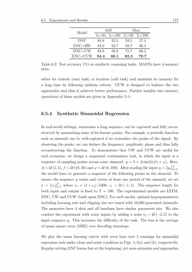
6.5. Experiments and Results 115
ModelAdd Max
L=50 L=100 L=50 L=100DNC 83.8 22.3 59.5 27.4
DNC+RW 83.0 22.7 59.7 36.5DNC+UW 84.8 50.9 71.7 66.2
DNC+CUW 94.4 60.1 82.3 70.7
Table 6.2: Test accuracy (%) on synthetic reasoning tasks. MANNs have 4 memoryslots.
either its content (max task) or location (add task) and maintain its memory for
a long time by following uniform criteria. CUW is designed to balance the two
approaches and thus it achieves better performance. Further insights into memory
operations of these models are given in Appendix D.9.
6.5.4 Synthetic Sinusoidal Regression
In real-world settings, sometimes a long sequence can be captured and fully recon-
structed by memorising some of its feature points. For example, a periodic function
such as sinusoid can be well-captured if we remember the peaks of the signal. By
observing the peaks, we can deduce the frequency, amplitude, phase and thus fully
reconstructing the function. To demonstrate that UW and CUW are useful for
such scenarios, we design a sequential continuation task, in which the input is a
sequence of sampling points across some sinusoid: y = 5 + A sin(2πfx + ϕ). Here,
A ∼ U (1, 5), f ∼ U (10, 30) and ϕ ∼ U (0, 100). After reading the input y = {yt}Tt=1,
the model have to generate a sequence of the following points in the sinusoid. To
ensure the sequence y varies and covers at least one period of the sinusoid, we set
x = {xt}Tt=1 where xi = (t + ǫ1) /1000, ǫ1 ∼ U (−1, 1). The sequence length for
both input and output is fixed to T = 100. The experimental models are LSTM,
DNC, UW and CUW (built upon DNC). For each model, optimal hyperparameters
including learning rate and clipping size are tuned with 10,000 generated sinusoids.
The memories have 4 slots and all baselines have similar parameter size. We also
conduct the experiment with noisy inputs by adding a noise ǫ2 ∼ U (−2, 2) to the
input sequence y. This increases the difficulty of the task. The loss is the average
of mean square error (MSE) over decoding timesteps.
We plot the mean learning curves with error bars over 5 runnings for sinusoidal
regression task under clean and noisy condition in Figs. 6.3(a) and (b), respectively.
Regular writing DNC learns fast at the beginning, yet soon saturates and approaches
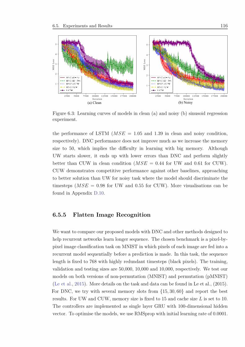
6.5. Experiments and Results 116
Figure 6.3: Learning curves of models in clean (a) and noisy (b) sinusoid regressionexperiment.
the performance of LSTM (MSE = 1.05 and 1.39 in clean and noisy condition,
respectively). DNC performance does not improve much as we increase the memory
size to 50, which implies the difficulty in learning with big memory. Although
UW starts slower, it ends up with lower errors than DNC and perform slightly
better than CUW in clean condition (MSE = 0.44 for UW and 0.61 for CUW).
CUW demonstrates competitive performance against other baselines, approaching
to better solution than UW for noisy task where the model should discriminate the
timesteps (MSE = 0.98 for UW and 0.55 for CUW). More visualisations can be
found in Appendix D.10.
6.5.5 Flatten Image Recognition
We want to compare our proposed models with DNC and other methods designed to
help recurrent networks learn longer sequence. The chosen benchmark is a pixel-by-
pixel image classification task on MNIST in which pixels of each image are fed into a
recurrent model sequentially before a prediction is made. In this task, the sequence
length is fixed to 768 with highly redundant timesteps (black pixels). The training,
validation and testing sizes are 50,000, 10,000 and 10,000, respectively. We test our
models on both versions of non-permutation (MNIST) and permutation (pMNIST)
(Le et al., 2015). More details on the task and data can be found in Le et al., (2015).
For DNC, we try with several memory slots from {15, 30, 60} and report the best
results. For UW and CUW, memory size is fixed to 15 and cache size L is set to 10.
The controllers are implemented as single layer GRU with 100-dimensional hidden
vector. To optimise the models, we use RMSprop with initial learning rate of 0.0001.
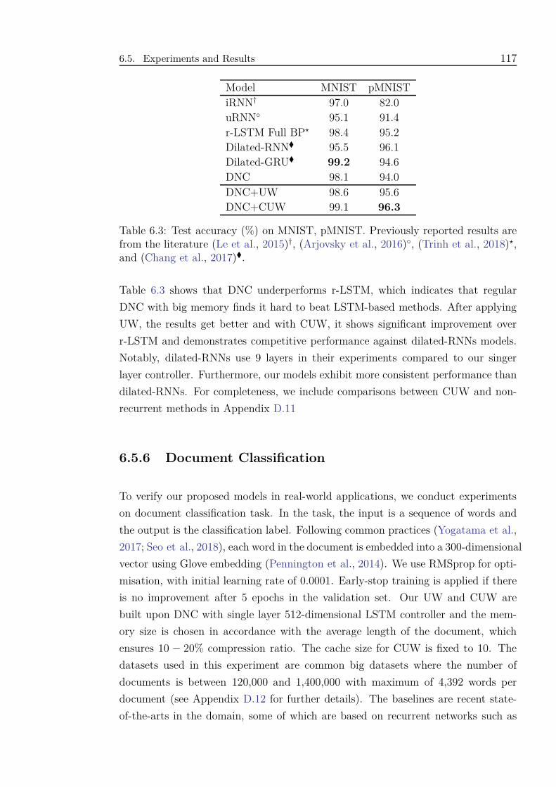
6.5. Experiments and Results 117
Model MNIST pMNISTiRNN† 97.0 82.0uRNN◦ 95.1 91.4r-LSTM Full BP⋆ 98.4 95.2Dilated-RNN� 95.5 96.1Dilated-GRU� 99.2 94.6DNC 98.1 94.0DNC+UW 98.6 95.6DNC+CUW 99.1 96.3
Table 6.3: Test accuracy (%) on MNIST, pMNIST. Previously reported results arefrom the literature (Le et al., 2015)†, (Arjovsky et al., 2016)◦, (Trinh et al., 2018)⋆,and (Chang et al., 2017)�.
Table 6.3 shows that DNC underperforms r-LSTM, which indicates that regular
DNC with big memory finds it hard to beat LSTM-based methods. After applying
UW, the results get better and with CUW, it shows significant improvement over
r-LSTM and demonstrates competitive performance against dilated-RNNs models.
Notably, dilated-RNNs use 9 layers in their experiments compared to our singer
layer controller. Furthermore, our models exhibit more consistent performance than
dilated-RNNs. For completeness, we include comparisons between CUW and non-
recurrent methods in Appendix D.11
6.5.6 Document Classification
To verify our proposed models in real-world applications, we conduct experiments
on document classification task. In the task, the input is a sequence of words and
the output is the classification label. Following common practices (Yogatama et al.,
2017; Seo et al., 2018), each word in the document is embedded into a 300-dimensional
vector using Glove embedding (Pennington et al., 2014). We use RMSprop for opti-
misation, with initial learning rate of 0.0001. Early-stop training is applied if there
is no improvement after 5 epochs in the validation set. Our UW and CUW are
built upon DNC with single layer 512-dimensional LSTM controller and the mem-
ory size is chosen in accordance with the average length of the document, which
ensures 10 − 20% compression ratio. The cache size for CUW is fixed to 10. The
datasets used in this experiment are common big datasets where the number of
documents is between 120,000 and 1,400,000 with maximum of 4,392 words per
document (see Appendix D.12 for further details). The baselines are recent state-
of-the-arts in the domain, some of which are based on recurrent networks such as
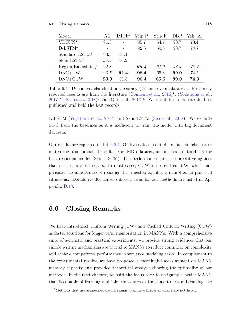
6.6. Closing Remarks 118
Model AG IMDb5 Yelp P. Yelp F. DBP Yah. A.VDCNN• 91.3 - 95.7 64.7 98.7 73.4D-LSTM∗ - - 92.6 59.6 98.7 73.7
Standard LSTM‡ 93.5 91.1 - - - -Skim-LSTM‡ 93.6 91.2 - - - -Region EmbeddingN 92.8 - 96.4 64.9 98.9 73.7
DNC+UW 93.7 91.4 96.4 65.3 99.0 74.2DNC+CUW 93.9 91.3 96.4 65.6 99.0 74.3
Table 6.4: Document classification accuracy (%) on several datasets. Previouslyreported results are from the literature (Conneau et al., 2016)•, (Yogatama et al.,2017)∗, (Seo et al., 2018)‡ and (Qui et al., 2018)N. We use italics to denote the bestpublished and bold the best records.
D-LSTM (Yogatama et al., 2017) and Skim-LSTM (Seo et al., 2018). We exclude
DNC from the baselines as it is inefficient to train the model with big document
datasets.
Our results are reported in Table 6.4. On five datasets out of six, our models beat or
match the best published results. For IMDb dataset, our methods outperform the
best recurrent model (Skim-LSTM). The performance gain is competitive against
that of the state-of-the-arts. In most cases, CUW is better than UW, which em-
phasises the importance of relaxing the timestep equality assumption in practical
situations. Details results across different runs for our methods are listed in Ap-
pendix D.13.
6.6 Closing Remarks
We have introduced Uniform Writing (UW) and Cached Uniform Writing (CUW)
as faster solutions for longer-term memorisation in MANNs. With a comprehensive
suite of synthetic and practical experiments, we provide strong evidences that our
simple writing mechanisms are crucial to MANNs to reduce computation complexity
and achieve competitive performance in sequence modeling tasks. In complement to
the experimental results, we have proposed a meaningful measurement on MANN
memory capacity and provided theoretical analysis showing the optimality of our
methods. In the next chapter, we shift the focus back to designing a better MANN
that is capable of learning multiple procedures at the same time and behaving like
5Methods that use semi-supervised training to achieve higher accuracy are not listed.
6.6. Closing Remarks 119
a universal Turing machine rather than a Turing machine.

Chapter 7
Neural Stored-Program Memory
7.1 Introduction
Recurrent Neural Networks (RNNs) are Turing-complete, that is, we can theoreti-
cally construct a Turing machine by using RNN elements (Siegelmann and Sontag,
1995). However, in practice RNNs struggle to learn simple procedures as they lack
explicit memory (Graves et al., 2014; Mozer and Das, 1993) . Memory Augmented
Neural Networks (MANNs) as analysed in Chapter 3, lift these limitations as they
are capable of emulating modern computer behavior by detaching memorisation from
computation via memory and controller network, respectively. In previous chapters,
we have also demonstrated that MANNs are powerful in many settings, ranging from
encoding multi-processes, generating complex sequences, to skip-readings. Nonethe-
less, MANNs have barely simulated general-purpose computers as they miss a key
concept in computer design: stored-program memory.
The concept of stored-program has emerged from the idea of Universal Turing
Machine (UTM) (Turing, 1936) and developed in the Von Neumann Architecture
(VNA) (von Neumann, 1993). In UTM/VNA, both data and programs that manip-
ulate the data are stored in memory. A control unit then reads the programs from the
memory and executes them with the data. This mechanism allows flexibility to per-
form universal computations. Unfortunately, current MANNs such as Neural Tur-
ing Machine (NTM) (Graves et al., 2014), Differentiable Neural Computer (DNC)
(Graves et al., 2016) and Least Recently Used Access (LRUA) (Santoro et al., 2016)
only support memory for data and embed a single program into the controller net-
120
7.2. Backgrounds 121
work, which goes against the stored-program memory principle.
Our goal is to advance a step further towards UTM/VNA by coupling a MANN with
an external program memory. The program memory co-exists with the data mem-
ory in the MANN, providing more flexibility, reuseability and modularity in learning
complicated tasks. The program memory stores the weights of the MANN’s con-
troller network, which are retrieved quickly via a key-value attention mechanism
across timesteps yet updated slowly via backpropagation. By introducing a meta
network to moderate the operations of the program memory, our model, hence-
forth referred to as Neural Stored-program Memory (NSM), can learn to switch
the programs/weights in the controller network appropriately, adapting to different
functionalities aligning with different parts of a sequential task, or different tasks in
continual and few-shot learning.
To validate our proposal, the NTM armed with NSM, namely Neural Universal Tur-
ing Machine (NUTM), is tested on a variety of synthetic tasks including algorithmic
tasks (Graves et al., 2014), composition of algorithmic tasks and continual proce-
dure learning. For these algorithmic problems, we demonstrate clear improvements
of NUTM over NTM. Further, we investigate NUTM in few-shot learning by using
LRUA as the MANN and achieve notably better results. Finally, we expand NUTM
application to linguistic problems by equipping NUTM with DNC core and achieve
competitive performances against state-of-the-arts in the bAbI task (Weston et al.,
2015).
Taken together, our study advances neural network simulation of Turing Machines
to neural architecture for Universal Turing Machines. This develops a new class of
MANNs that can store and query both the weights and data of their own controllers,
thereby following the stored-program principle. A set of five diverse experiments
demonstrate the computational universality of the approach.
7.2 Backgrounds
7.2.1 Turing Machines and MANNs
In this section, we briefly review MANN and its relations to Turing Machines. A
MANN consists of a controller network and an external memory M ∈ RN×M , which
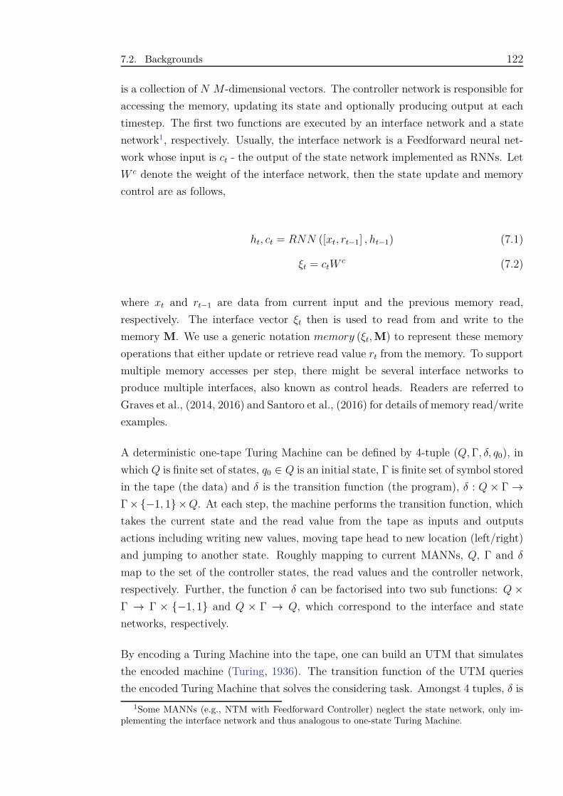
7.2. Backgrounds 122
is a collection of N M-dimensional vectors. The controller network is responsible for
accessing the memory, updating its state and optionally producing output at each
timestep. The first two functions are executed by an interface network and a state
network1, respectively. Usually, the interface network is a Feedforward neural net-
work whose input is ct - the output of the state network implemented as RNNs. Let
W c denote the weight of the interface network, then the state update and memory
control are as follows,
ht, ct = RNN ([xt, rt−1] , ht−1) (7.1)
ξt = ctWc (7.2)
where xt and rt−1 are data from current input and the previous memory read,
respectively. The interface vector ξt then is used to read from and write to the
memory M. We use a generic notation memory (ξt, M) to represent these memory
operations that either update or retrieve read value rt from the memory. To support
multiple memory accesses per step, there might be several interface networks to
produce multiple interfaces, also known as control heads. Readers are referred to
Graves et al., (2014, 2016) and Santoro et al., (2016) for details of memory read/write
examples.
A deterministic one-tape Turing Machine can be defined by 4-tuple (Q, Γ, δ, q0), in
which Q is finite set of states, q0 ∈ Q is an initial state, Γ is finite set of symbol stored
in the tape (the data) and δ is the transition function (the program), δ : Q × Γ →Γ×{−1, 1}×Q. At each step, the machine performs the transition function, which
takes the current state and the read value from the tape as inputs and outputs
actions including writing new values, moving tape head to new location (left/right)
and jumping to another state. Roughly mapping to current MANNs, Q, Γ and δ
map to the set of the controller states, the read values and the controller network,
respectively. Further, the function δ can be factorised into two sub functions: Q×Γ → Γ × {−1, 1} and Q × Γ → Q, which correspond to the interface and state
networks, respectively.
By encoding a Turing Machine into the tape, one can build an UTM that simulates
the encoded machine (Turing, 1936). The transition function of the UTM queries
the encoded Turing Machine that solves the considering task. Amongst 4 tuples, δ is
1Some MANNs (e.g., NTM with Feedforward Controller) neglect the state network, only im-plementing the interface network and thus analogous to one-state Turing Machine.

7.2. Backgrounds 123
the most important and hence uses most of the encoding bits. In other words, if we
assume that the space of Q, Γ and q0 are shared amongst Turing Machines, we can
simulate any Turing Machine by encoding only its transition function δ. Translating
to neural language, if we can store the controller network into a queriable memory
and make use of it, we can build a Neural Universal Turing Machine. Using NSM
is a simple way to achieve this goal, which we introduce in the subsequent section.
7.2.2 Related Approaches
Previous investigations into MANNs mostly revolve around memory access mecha-
nisms. The works in Graves et al., (2014, 2016) introduce content-based, location-
based and dynamic memory reading/writing. Further, Rae et al., (2016) scales to
bigger memory by sparse access while Le et al., (2019a) optimises memory opera-
tions with uniform writing. These works keep using memory for storing data rather
than the weights of the network and thus parallel to our approach. Other DNC mod-
ifications (Csordas and Schmidhuber, 2019; Franke et al., 2018) are also orthogonal
to our work.
Another line of related work involves modularisation of neural networks, which is de-
signed for visual question answering. In module networks (Andreas et al., 2016b,a),
the modules are manually aligned with predefined concepts and the order of execu-
tion is decided by the question. Although the module in these works resembles the
program in NSM, our model is more generic and flexible with soft-attention over pro-
grams and thus fully differentiable. Further, the motivation of NSM does not limit
to a specific application. Rather, NSM aims to help MANN reach general-purpose
computability.
Finally, if we view NSM network as a dynamic weight generator, the program
in NSM can be linked to fast weight (Hinton and Plaut, 1987; Ba et al., 2016;
Munkhdalai and Yu, 2017). These papers share the idea of using different weights
across timesteps to enable dynamic adaptation. However, fast weights are directly
generated while our programs are interpolated from a set of slow weights.
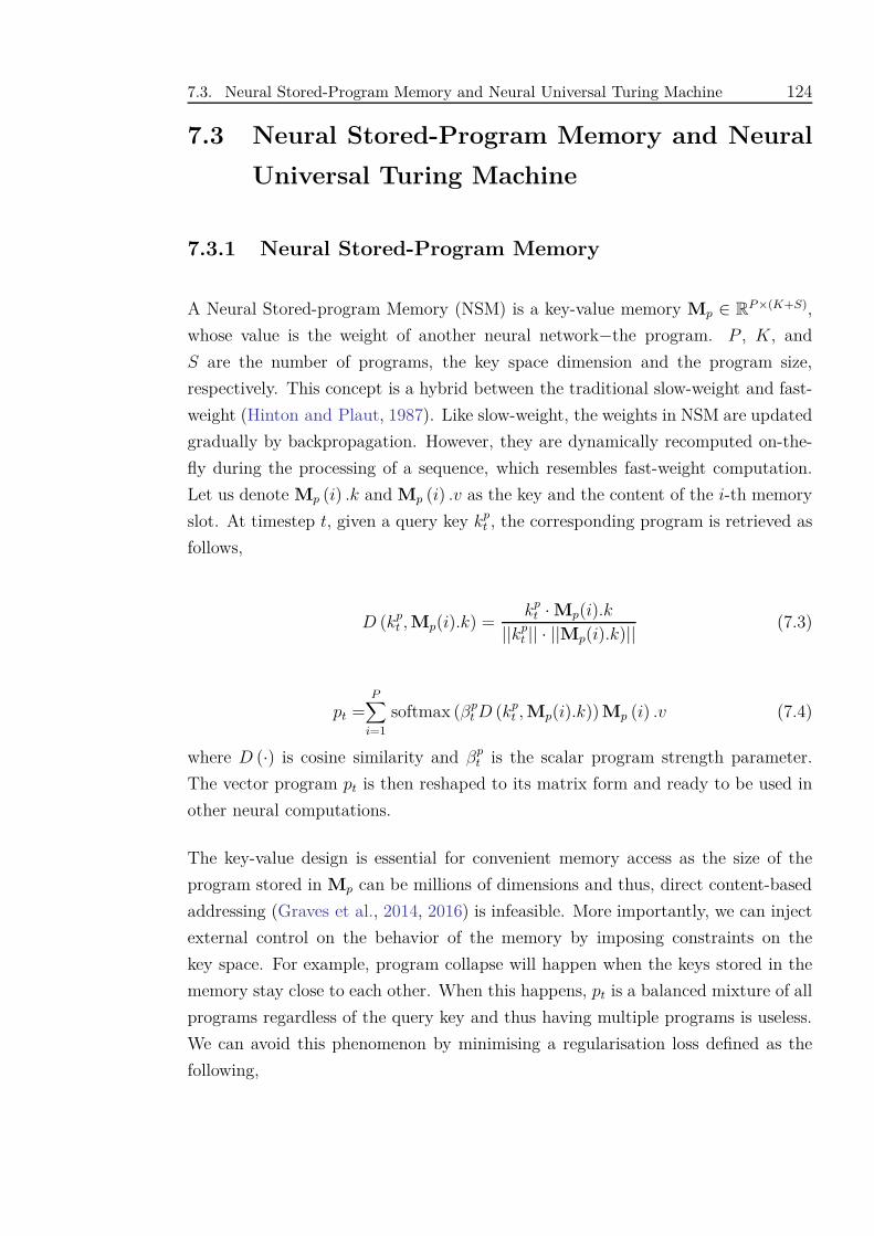
7.3. Neural Stored-Program Memory and Neural Universal Turing Machine 124
7.3 Neural Stored-Program Memory and Neural
Universal Turing Machine
7.3.1 Neural Stored-Program Memory
A Neural Stored-program Memory (NSM) is a key-value memory Mp ∈ RP ×(K+S),
whose value is the weight of another neural network−the program. P , K, and
S are the number of programs, the key space dimension and the program size,
respectively. This concept is a hybrid between the traditional slow-weight and fast-
weight (Hinton and Plaut, 1987). Like slow-weight, the weights in NSM are updated
gradually by backpropagation. However, they are dynamically recomputed on-the-
fly during the processing of a sequence, which resembles fast-weight computation.
Let us denote Mp (i) .k and Mp (i) .v as the key and the content of the i-th memory
slot. At timestep t, given a query key kpt , the corresponding program is retrieved as
follows,
D (kpt , Mp(i).k) =
kpt ·Mp(i).k
||kpt || · ||Mp(i).k)|| (7.3)
pt =P∑
i=1
softmax (βpt D (kp
t , Mp(i).k)) Mp (i) .v (7.4)
where D (·) is cosine similarity and βpt is the scalar program strength parameter.
The vector program pt is then reshaped to its matrix form and ready to be used in
other neural computations.
The key-value design is essential for convenient memory access as the size of the
program stored in Mp can be millions of dimensions and thus, direct content-based
addressing (Graves et al., 2014, 2016) is infeasible. More importantly, we can inject
external control on the behavior of the memory by imposing constraints on the
key space. For example, program collapse will happen when the keys stored in the
memory stay close to each other. When this happens, pt is a balanced mixture of all
programs regardless of the query key and thus having multiple programs is useless.
We can avoid this phenomenon by minimising a regularisation loss defined as the
following,
7.3. Neural Stored-Program Memory and Neural Universal Turing Machine 125
lp =P∑
i=1
P∑
j=i+1
D (Mp(i).k, Mp(j).k) (7.5)
7.3.2 Neural Universal Turing Machine
It turns out that the combination of MANN and NSM approximates an Universal
Turing Machine (Sec. 7.2). At each timestep, the controller in MANN reads its state
and memory to generate control signal to the memory via the interface network W c,
then updates its state using the state network RNN . Since the parameters of RNN
and W c represent the encoding of δ, we store both into NSM to completely encode
an MANN. For simplicity, in this proposal, we only use NSM to store W c, which is
equivalent to the Universal Turing Machine that can simulate any one-state Turing
Machine.
In traditional MANN, W c is constant across timesteps and only updated slowly
during training, typically through backpropagation. In our design, we compute W ct
from NSM for every timestep and thus, we need a program interface network−the
meta network PI−that generates an interface vector for the program memory: ξpt =
PI (ct), where ξpt = [kp
t , βpt ] and PI is implemented as a Feedforward neural network.
The procedure for computing W ct is executed by following Eqs. (7.3)-(7.4), hereafter
referred to as NSM (ξpt , Mp). Figure 7.1 depicts the integration of NSM into MANN.
For the case of multi-head NTM, we implement one NSM per control head and
name this model Neural Universal Turing Machine (NUTM). Each control head will
read from (for read head) or write to (for write head) the data memory M via
memory (ξt, M) as described in Graves et al., (2014). Other MANNs such as DNC
(Graves et al., 2016) and LRUA (Santoro et al., 2016) can be armed with NSM in
this manner. We also employ the regularisation loss lp to prevent the programs from
collapsing, resulting in a final loss as follows,
Loss = Losspred + ηtlp (7.6)
where Losspred is the prediction loss and ηt is annealing factor, reducing as the
training step increases. The details of NUTM operations are presented in Algorithm
7.1.
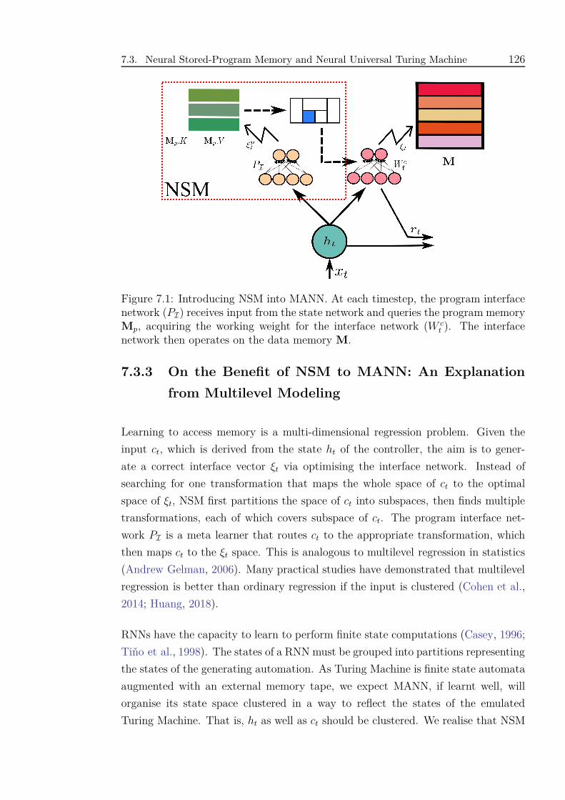
7.3. Neural Stored-Program Memory and Neural Universal Turing Machine 126
Figure 7.1: Introducing NSM into MANN. At each timestep, the program interfacenetwork (PI) receives input from the state network and queries the program memoryMp, acquiring the working weight for the interface network (W c
t ). The interfacenetwork then operates on the data memory M.
7.3.3 On the Benefit of NSM to MANN: An Explanation
from Multilevel Modeling
Learning to access memory is a multi-dimensional regression problem. Given the
input ct, which is derived from the state ht of the controller, the aim is to gener-
ate a correct interface vector ξt via optimising the interface network. Instead of
searching for one transformation that maps the whole space of ct to the optimal
space of ξt, NSM first partitions the space of ct into subspaces, then finds multiple
transformations, each of which covers subspace of ct. The program interface net-
work PI is a meta learner that routes ct to the appropriate transformation, which
then maps ct to the ξt space. This is analogous to multilevel regression in statistics
(Andrew Gelman, 2006). Many practical studies have demonstrated that multilevel
regression is better than ordinary regression if the input is clustered (Cohen et al.,
2014; Huang, 2018).
RNNs have the capacity to learn to perform finite state computations (Casey, 1996;
Tiňo et al., 1998). The states of a RNN must be grouped into partitions representing
the states of the generating automation. As Turing Machine is finite state automata
augmented with an external memory tape, we expect MANN, if learnt well, will
organise its state space clustered in a way to reflect the states of the emulated
Turing Machine. That is, ht as well as ct should be clustered. We realise that NSM
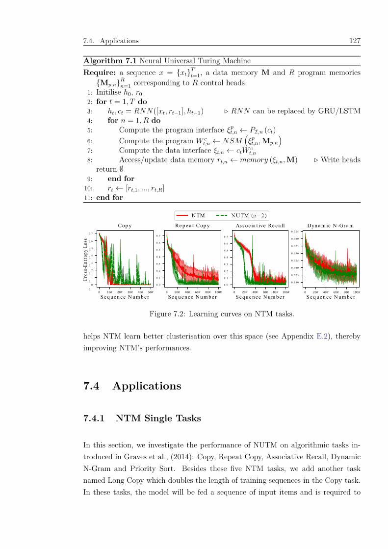
7.4. Applications 127
Algorithm 7.1 Neural Universal Turing Machine
Require: a sequence x = {xt}Tt=1, a data memory M and R program memories
{Mp,n}Rn=1 corresponding to R control heads
1: Initilise h0, r0
2: for t = 1, T do3: ht, ct = RNN([xt, rt−1], ht−1) ⊲ RNN can be replaced by GRU/LSTM4: for n = 1, R do5: Compute the program interface ξp
t,n ← PI,n (ct)
6: Compute the program W ct,n ← NSM
(ξp
t,n, Mp,n
)
7: Compute the data interface ξt,n ← ctWct,n
8: Access/update data memory rt,n ← memory (ξt,n, M) ⊲ Write headsreturn ∅
9: end for10: rt ← [rt,1, ..., rt,R]11: end for
Figure 7.2: Learning curves on NTM tasks.
helps NTM learn better clusterisation over this space (see Appendix E.2), thereby
improving NTM’s performances.
7.4 Applications
7.4.1 NTM Single Tasks
In this section, we investigate the performance of NUTM on algorithmic tasks in-
troduced in Graves et al., (2014): Copy, Repeat Copy, Associative Recall, Dynamic
N-Gram and Priority Sort. Besides these five NTM tasks, we add another task
named Long Copy which doubles the length of training sequences in the Copy task.
In these tasks, the model will be fed a sequence of input items and is required to

7.4. Applications 128
Task Copy Repeat Copy A. Recall D. N-grams Priority Sort Long Copy
NTM 0.00 405.10 7.66 132.59 24.41 16.04
NUTM (p=2) 0.00 366.69 1.35 127.68 20.00 0.02
Table 7.1: Generalisation performance of best models measured in average bit errorper sequence (lower is better). For each task, we pick a set of 1,000 unseen sequencesas test data.
infer a sequence of output items. Each item is represented by a binary vector.
In the experiment, we compare two models: NTM2 and NUTM with two programs.
Although the tasks are atomic, we argue that there should be at least two memory
manipulation schemes across timesteps, one for encoding the inputs to the memory
and another for decoding the output from the memory. The two models are trained
with cross-entropy objective function under the same setting as in Graves et al.,
(2014). For fair comparison, the controller hidden dimension of NUTM is set smaller
to make the total number of parameters of NUTM equivalent to that of NTM (details
in Appendix E.4).
We run each experiments five times and report the mean with error bars of training
losses for the first 4 tasks in Fig. E.1. Except for the Copy task, which is too
simple, other tasks observe convergence speed improvement of NUTM over that of
NTM, thereby validating the benefit of using two programs across timesteps even
for the single task setting. Full report is listed in Appendix E.1. As NUTM requires
fewer training samples to converge, it generalises better to unseen sequences that
are longer than training sequences. Table 7.1 reports the test results of the best
models chosen after five runs and confirms the outperformance of NUTM over NTM
for generalisation.
To illustrate the program usage, we plot NUTM’s program distributions across
timesteps for Repeat Copy and Priority Sort in Fig. 7.3 (a) and (b), respectively.
We observe two program usage patterns corresponding to the encoding and decoding
phases. For Repeat Copy, there is no reading in encoding and thus, NUTM assigns
the “no-read” strategy mainly to the “orange program”. In decoding, the sequential
reading is mostly done by the “blue program” with some contributions from the “or-
ange program” when resetting reading head. For Priority Sort, while the encoding
“fitting writing” (see Graves et al., (2014) for explanation on the strategy) is often
2For algorithmic tasks, we choose NTM as the only baseline as NTM is known to perform andgeneralise well on these tasks. If NSM can help NTM in these tasks, it will probably help otherMANNs as well.
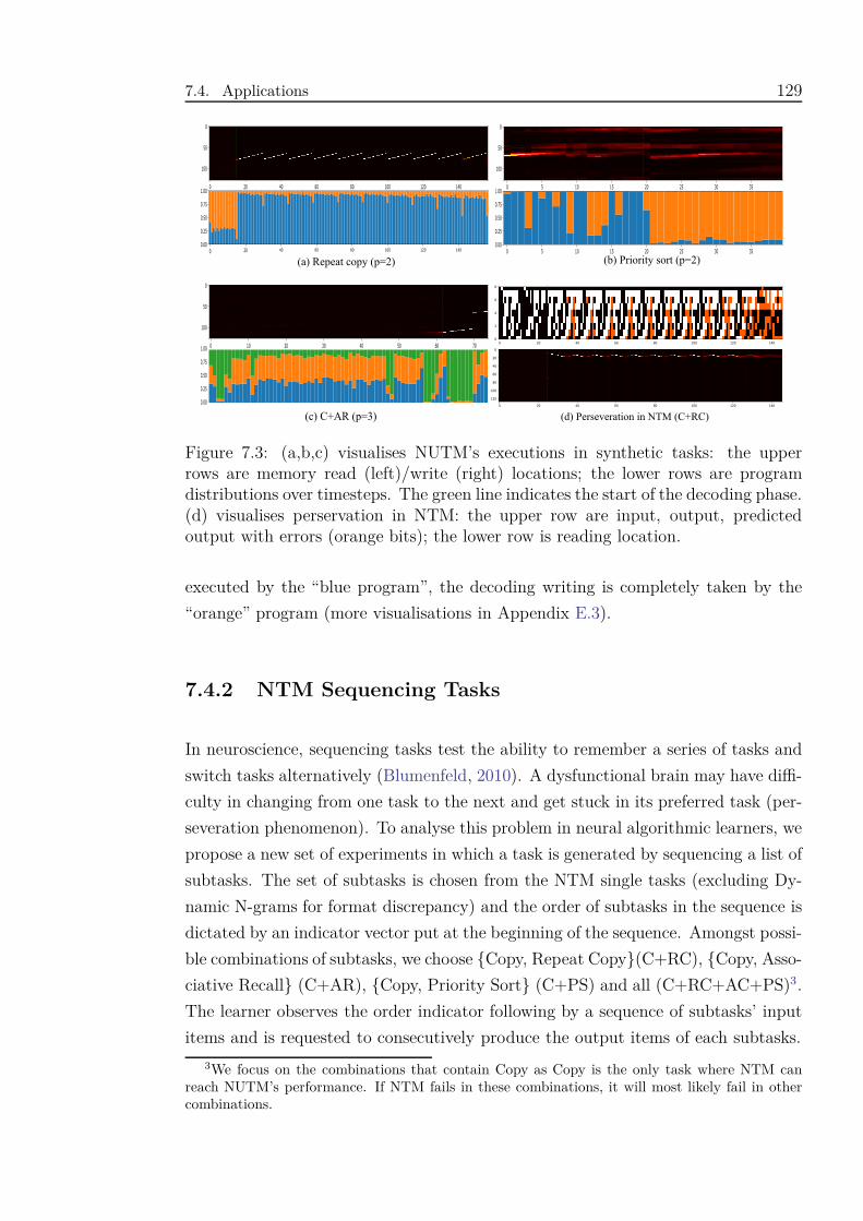
7.4. Applications 129
Figure 7.3: (a,b,c) visualises NUTM’s executions in synthetic tasks: the upperrows are memory read (left)/write (right) locations; the lower rows are programdistributions over timesteps. The green line indicates the start of the decoding phase.(d) visualises perservation in NTM: the upper row are input, output, predictedoutput with errors (orange bits); the lower row is reading location.
executed by the “blue program”, the decoding writing is completely taken by the
“orange” program (more visualisations in Appendix E.3).
7.4.2 NTM Sequencing Tasks
In neuroscience, sequencing tasks test the ability to remember a series of tasks and
switch tasks alternatively (Blumenfeld, 2010). A dysfunctional brain may have diffi-
culty in changing from one task to the next and get stuck in its preferred task (per-
severation phenomenon). To analyse this problem in neural algorithmic learners, we
propose a new set of experiments in which a task is generated by sequencing a list of
subtasks. The set of subtasks is chosen from the NTM single tasks (excluding Dy-
namic N-grams for format discrepancy) and the order of subtasks in the sequence is
dictated by an indicator vector put at the beginning of the sequence. Amongst possi-
ble combinations of subtasks, we choose {Copy, Repeat Copy}(C+RC), {Copy, Asso-
ciative Recall} (C+AR), {Copy, Priority Sort} (C+PS) and all (C+RC+AC+PS)3.
The learner observes the order indicator following by a sequence of subtasks’ input
items and is requested to consecutively produce the output items of each subtasks.
3We focus on the combinations that contain Copy as Copy is the only task where NTM canreach NUTM’s performance. If NTM fails in these combinations, it will most likely fail in othercombinations.
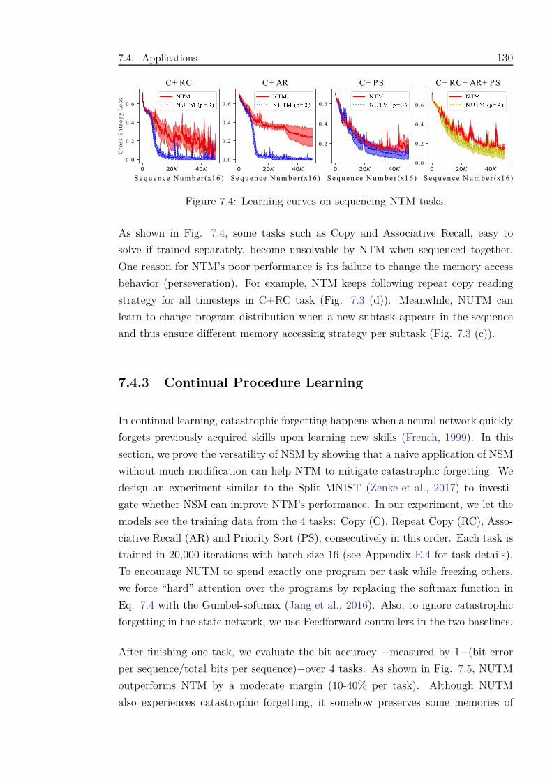
7.4. Applications 130
Figure 7.4: Learning curves on sequencing NTM tasks.
As shown in Fig. 7.4, some tasks such as Copy and Associative Recall, easy to
solve if trained separately, become unsolvable by NTM when sequenced together.
One reason for NTM’s poor performance is its failure to change the memory access
behavior (perseveration). For example, NTM keeps following repeat copy reading
strategy for all timesteps in C+RC task (Fig. 7.3 (d)). Meanwhile, NUTM can
learn to change program distribution when a new subtask appears in the sequence
and thus ensure different memory accessing strategy per subtask (Fig. 7.3 (c)).
7.4.3 Continual Procedure Learning
In continual learning, catastrophic forgetting happens when a neural network quickly
forgets previously acquired skills upon learning new skills (French, 1999). In this
section, we prove the versatility of NSM by showing that a naive application of NSM
without much modification can help NTM to mitigate catastrophic forgetting. We
design an experiment similar to the Split MNIST (Zenke et al., 2017) to investi-
gate whether NSM can improve NTM’s performance. In our experiment, we let the
models see the training data from the 4 tasks: Copy (C), Repeat Copy (RC), Asso-
ciative Recall (AR) and Priority Sort (PS), consecutively in this order. Each task is
trained in 20,000 iterations with batch size 16 (see Appendix E.4 for task details).
To encourage NUTM to spend exactly one program per task while freezing others,
we force “hard” attention over the programs by replacing the softmax function in
Eq. 7.4 with the Gumbel-softmax (Jang et al., 2016). Also, to ignore catastrophic
forgetting in the state network, we use Feedforward controllers in the two baselines.
After finishing one task, we evaluate the bit accuracy −measured by 1−(bit error
per sequence/total bits per sequence)−over 4 tasks. As shown in Fig. 7.5, NUTM
outperforms NTM by a moderate margin (10-40% per task). Although NUTM
also experiences catastrophic forgetting, it somehow preserves some memories of
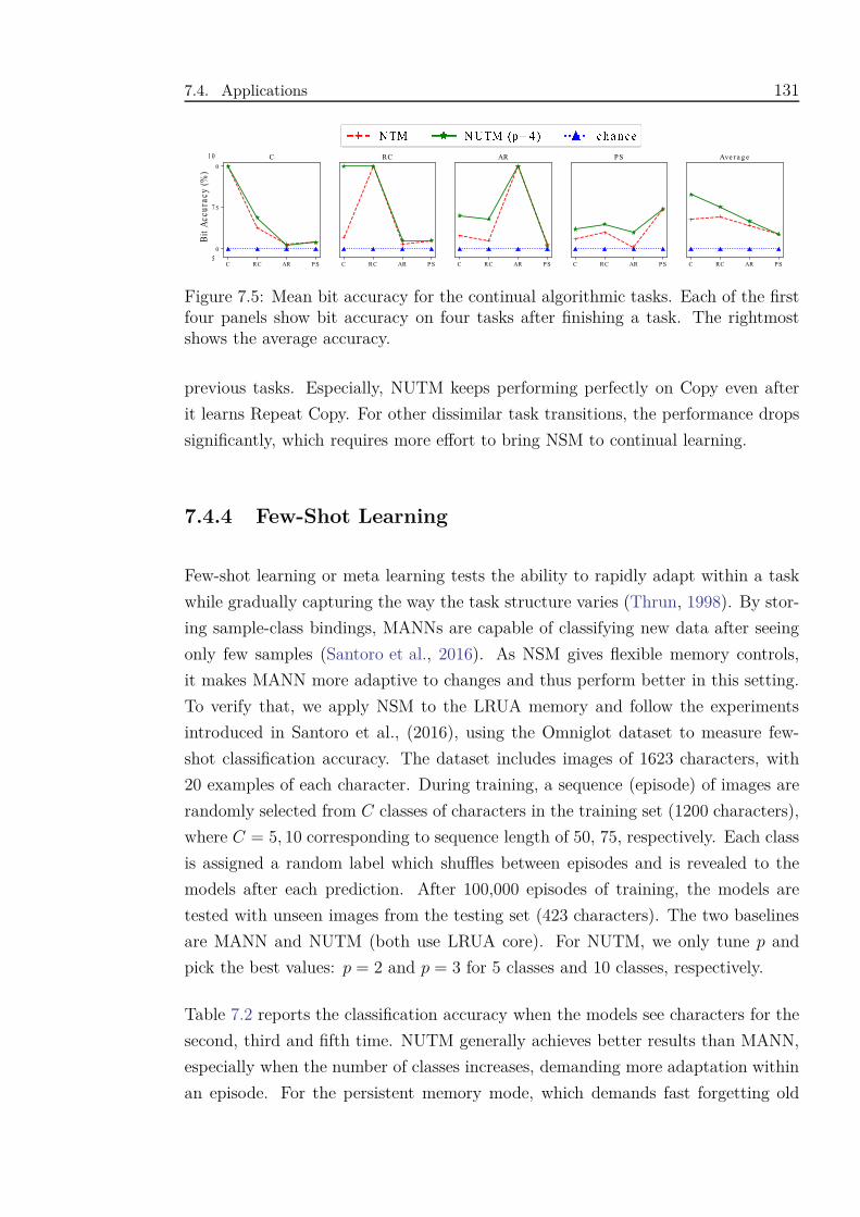
7.4. Applications 131
Figure 7.5: Mean bit accuracy for the continual algorithmic tasks. Each of the firstfour panels show bit accuracy on four tasks after finishing a task. The rightmostshows the average accuracy.
previous tasks. Especially, NUTM keeps performing perfectly on Copy even after
it learns Repeat Copy. For other dissimilar task transitions, the performance drops
significantly, which requires more effort to bring NSM to continual learning.
7.4.4 Few-Shot Learning
Few-shot learning or meta learning tests the ability to rapidly adapt within a task
while gradually capturing the way the task structure varies (Thrun, 1998). By stor-
ing sample-class bindings, MANNs are capable of classifying new data after seeing
only few samples (Santoro et al., 2016). As NSM gives flexible memory controls,
it makes MANN more adaptive to changes and thus perform better in this setting.
To verify that, we apply NSM to the LRUA memory and follow the experiments
introduced in Santoro et al., (2016), using the Omniglot dataset to measure few-
shot classification accuracy. The dataset includes images of 1623 characters, with
20 examples of each character. During training, a sequence (episode) of images are
randomly selected from C classes of characters in the training set (1200 characters),
where C = 5, 10 corresponding to sequence length of 50, 75, respectively. Each class
is assigned a random label which shuffles between episodes and is revealed to the
models after each prediction. After 100,000 episodes of training, the models are
tested with unseen images from the testing set (423 characters). The two baselines
are MANN and NUTM (both use LRUA core). For NUTM, we only tune p and
pick the best values: p = 2 and p = 3 for 5 classes and 10 classes, respectively.
Table 7.2 reports the classification accuracy when the models see characters for the
second, third and fifth time. NUTM generally achieves better results than MANN,
especially when the number of classes increases, demanding more adaptation within
an episode. For the persistent memory mode, which demands fast forgetting old
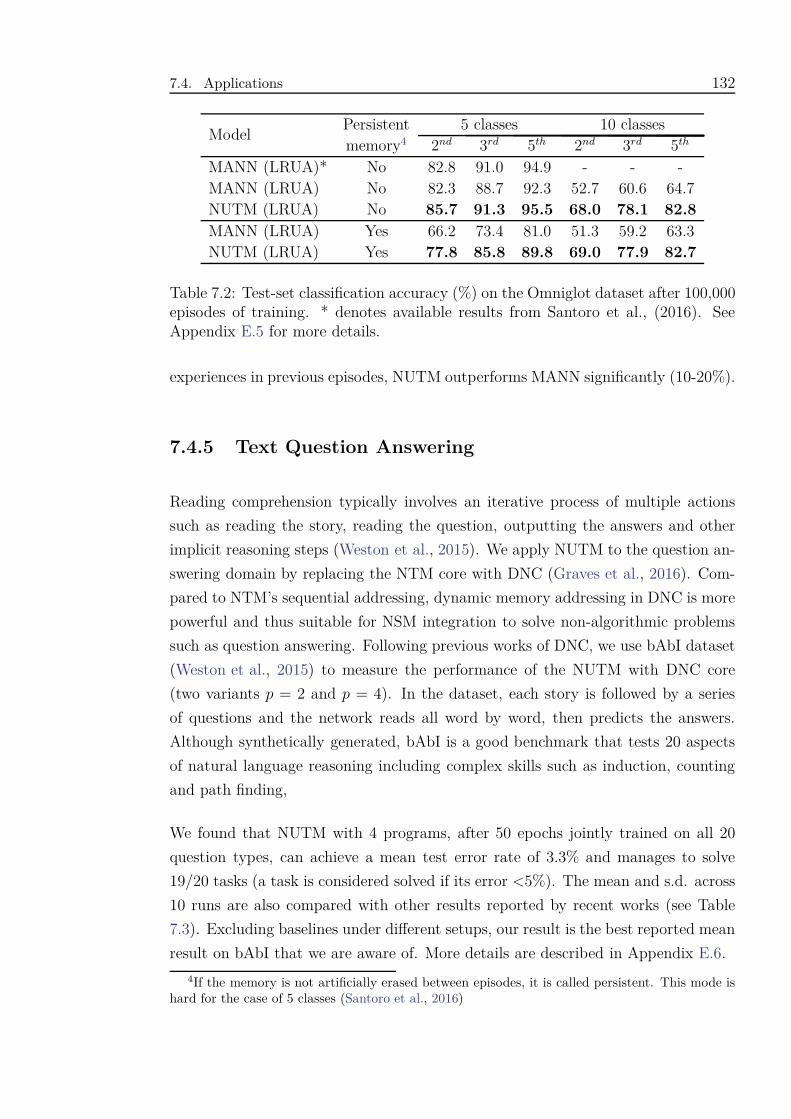
7.4. Applications 132
ModelPersistent 5 classes 10 classesmemory4 2nd 3rd 5th 2nd 3rd 5th
MANN (LRUA)* No 82.8 91.0 94.9 - - -MANN (LRUA) No 82.3 88.7 92.3 52.7 60.6 64.7NUTM (LRUA) No 85.7 91.3 95.5 68.0 78.1 82.8
MANN (LRUA) Yes 66.2 73.4 81.0 51.3 59.2 63.3NUTM (LRUA) Yes 77.8 85.8 89.8 69.0 77.9 82.7
Table 7.2: Test-set classification accuracy (%) on the Omniglot dataset after 100,000episodes of training. * denotes available results from Santoro et al., (2016). SeeAppendix E.5 for more details.
experiences in previous episodes, NUTM outperforms MANN significantly (10-20%).
7.4.5 Text Question Answering
Reading comprehension typically involves an iterative process of multiple actions
such as reading the story, reading the question, outputting the answers and other
implicit reasoning steps (Weston et al., 2015). We apply NUTM to the question an-
swering domain by replacing the NTM core with DNC (Graves et al., 2016). Com-
pared to NTM’s sequential addressing, dynamic memory addressing in DNC is more
powerful and thus suitable for NSM integration to solve non-algorithmic problems
such as question answering. Following previous works of DNC, we use bAbI dataset
(Weston et al., 2015) to measure the performance of the NUTM with DNC core
(two variants p = 2 and p = 4). In the dataset, each story is followed by a series
of questions and the network reads all word by word, then predicts the answers.
Although synthetically generated, bAbI is a good benchmark that tests 20 aspects
of natural language reasoning including complex skills such as induction, counting
and path finding,
We found that NUTM with 4 programs, after 50 epochs jointly trained on all 20
question types, can achieve a mean test error rate of 3.3% and manages to solve
19/20 tasks (a task is considered solved if its error <5%). The mean and s.d. across
10 runs are also compared with other results reported by recent works (see Table
7.3). Excluding baselines under different setups, our result is the best reported mean
result on bAbI that we are aware of. More details are described in Appendix E.6.
4If the memory is not artificially erased between episodes, it is called persistent. This mode ishard for the case of 5 classes (Santoro et al., 2016)
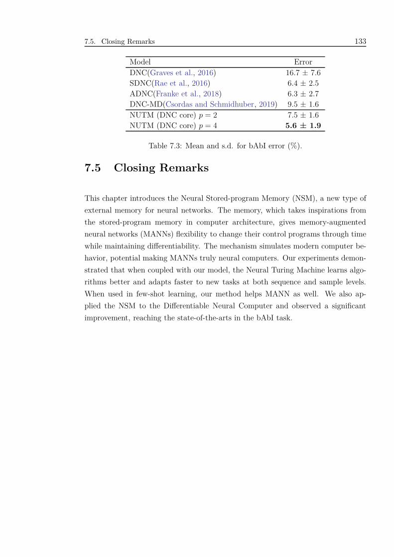
7.5. Closing Remarks 133
Model ErrorDNC(Graves et al., 2016) 16.7 ± 7.6SDNC(Rae et al., 2016) 6.4 ± 2.5ADNC(Franke et al., 2018) 6.3 ± 2.7DNC-MD(Csordas and Schmidhuber, 2019) 9.5 ± 1.6NUTM (DNC core) p = 2 7.5 ± 1.6NUTM (DNC core) p = 4 5.6 ± 1.9
Table 7.3: Mean and s.d. for bAbI error (%).
7.5 Closing Remarks
This chapter introduces the Neural Stored-program Memory (NSM), a new type of
external memory for neural networks. The memory, which takes inspirations from
the stored-program memory in computer architecture, gives memory-augmented
neural networks (MANNs) flexibility to change their control programs through time
while maintaining differentiability. The mechanism simulates modern computer be-
havior, potential making MANNs truly neural computers. Our experiments demon-
strated that when coupled with our model, the Neural Turing Machine learns algo-
rithms better and adapts faster to new tasks at both sequence and sample levels.
When used in few-shot learning, our method helps MANN as well. We also ap-
plied the NSM to the Differentiable Neural Computer and observed a significant
improvement, reaching the state-of-the-arts in the bAbI task.
Chapter 8
Conclusions
8.1 Summary
In this thesis, we have presented several types of memory for neural networks in gen-
eral and Recurrent Neural Networks (RNNs) in particular. We emphasise the notion
of the memory as an external storage for RNNs in which, RNNs can learn to read
from and write to the external memory to support their working memory (Chapter
2). We reviewed advancements to solve the difficulties in training RNNs such as
gating and attention mechanisms and especially we focused on slot-based MANNs,
which is based on sparse distributed memory model–the main theme of new models
we propose in the thesis (Chapter 3). Our main contributions are four-fold. First, we
extended MANNs as a multi-process multi-view model to handle complex problems
such as sequence-to-sequence mapping and multi-view sequential learning (Chapter
4). We further extended MANNs as a model for discrete sequence generation on
conversational data where variability and coherence are required (Chapter 5). We
also shed light into memory operations to estimate MANN capacity and proposed
new writing schemes to maximise the capacity (Chapter 6). Finally, we introduced a
new class of MANNs that follows stored-program memory principle and can switch
the controller’s programs to execute different functionalities through time.
In Chapter 4, we presented our first contributions: Dual Controller Write-Protected
Memory Augmented Neural Network (DCw-MANN), an extension of MANN to
model sequence to sequence mapping, and Dual Memory Neural Computer (DMNC)
that can capture the correlations between two views by exploiting two external
134

8.2. Future Directions 135
memory units. We demonstrated these models on predicting next disease stages
and recommending medicines in healthcare. The results are competitive against
contemporary state-of-the-arts.
Chapter 5 presented Variational Memory Encoder-Decoder, a novel memory-augmented
generation framework. Our external memory not only holds long-term context but
also constructs mixture model distribution generating the latent variables. We de-
rived theoretical analysis to validate our training protocol using Stochastic Gradi-
ent Variational Bayes framework by minimising variational approximation of KL
divergence. We evaluated our model on two open-domain and two closed-domain
conversational datasets and outperformed other baselines by a large margin.
Chapter 6 focused more on theoretical analysis of a meaningful measurement on
MANN’s memory capacity. We proposed solution dubbed Uniform Writing is op-
timal in terms of maximising the memory capacity. To encourage forgetting when
necessary, we introduce modifications to the original solution, resulting in a new
solution termed Cached Uniform Writing. This method aims to balance between
memorising and forgetting via allowing overwriting mechanism. We conducted a set
of diverse experiments on six ultra-long sequential learning problems given a limited
number of memory slots to demonstrate the superiority of our methods.
Chapter 7 addressed the simulation capacity of MANNs. To make current MANNs
truly simulate modern computers, a design of Neural Stored-program Memory (NSM)
was proposed to implement stored-program principle, which resulted in new MANN
architectures that materialise Universal Turing Machines.
8.2 Future Directions
There are possible extensions of the work proposed in this thesis for further inves-
tigations. First, in Chapter 4, we can extend the DCw-MANN to handle multi-
ple healthcare tasks by developing new capabilities for medical question answering,
which can be cast to a sequence-to-sequence mapping problem. Moreover, DMNC
can be generalised to multi-input multi-output settings and extending the range of
applications to bigger problems such as multi-media and multi-agent systems. For
VMED (Chapter 5), future explorations may involve implementing a dynamic num-
ber of modes that enable learning of the optimal K for each timestep. Another
aspect would be multi-person dialog setting, where our memory as mixture model
8.2. Future Directions 136
may be useful to capture more complex modes of speaking in the dialog. Future
investigations for Chapter 6 will focus on tightening the measurement bound. Last
but not least, we emphasise that apart from MANNs, other neural networks can
also reap benefits from the NSM proposed in Chapter 7. More effort will be spent
on integrating NSM into different neural networks to make them more flexible and
modular.
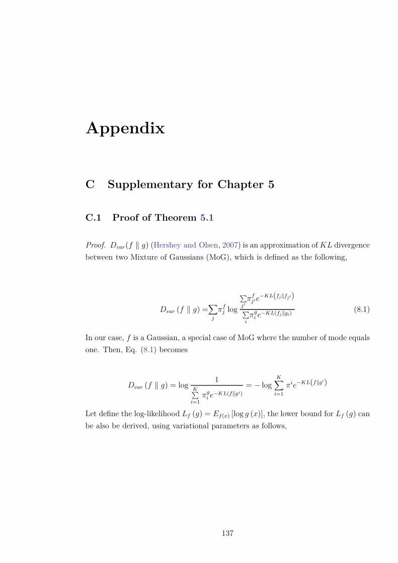
Appendix
C Supplementary for Chapter 5
C.1 Proof of Theorem 5.1
Proof. Dvar(f ‖ g) (Hershey and Olsen, 2007) is an approximation of KL divergence
between two Mixture of Gaussians (MoG), which is defined as the following,
Dvar (f ‖ g) =∑
j
πfj log
∑j′
πfj′e
−KL(fj‖fj′)
∑i
πgi e−KL(fj‖gi)
(8.1)
In our case, f is a Gaussian, a special case of MoG where the number of mode equals
one. Then, Eq. (8.1) becomes
Dvar (f ‖ g) = log1
K∑i=1
πgi e−KL(f‖gi)
= − logK∑
i=1
πie−KL(f‖gi)
Let define the log-likelihood Lf (g) = Ef(x) [log g (x)], the lower bound for Lf (g) can
be also be derived, using variational parameters as follows,
137
C. Supplementary for Chapter 5 138
Lf (g) =Ef
[log
(K∑
i=1
πigi (x)
)]
=+∞∫
−∞
f (x) log
(K∑
i=1
βiπi gi (x)βi
)dx
≥K∑
i=1
βi
+∞∫
−∞
f (x) log
(πi g
i (x)βi
)dx
where βi ≥ 0 andK∑
i=1βi = 1. According to Durrieu et al., (2012), maximising the
RHS of the above inequality with respect to βi provides a lower bound for Lf (g)
(Durrieu et al., 2012),
Lf (g) ≥ logK∑
i=1
πie−KL(f‖gi) + Lf (f)
=−Dvar + Lf (f)
⇒ Dvar ≥Lf (f)− Lf (g)
=KL (f ‖ g)
Therefore, the KL divergence has an upper bound: Dvar.
C.2 Derivation of the Upper Bound on the Total Timestep-
Wise KL Divergence
Lemma C.1. Chebyshev’s sum inequality:
if
a1 ≥ a2 ≥ ... ≥ an
and
b1 ≥ b2 ≥ ... ≥ bn
C. Supplementary for Chapter 5 139
then
1n
n∑
k=1
akbk ≥(
1n
n∑
k=1
ak
)(1n
n∑
k=1
bk
)
Proof. Consider the sum
S =n∑
j=1
n∑
k=1
(aj − ak) (bj − bk)
The two sequences are non-increasing, therefore aj − ak and bj − bk have the same
sign for any j, k. Hence S ≥ 0. Opening the brackets, we deduce
0 ≤ 2nn∑
j=1
ajbj − 2n∑
j=1
aj
n∑
k=1
bk
whence
1n
n∑
j=1
ajbj ≥1
n
n∑
j=1
aj
(
1n
n∑
k=1
bk
)
In our problem, ai = fi (x) and bi = log [gi (x)], i = 1, T . Under the assumption that
at each step, thanks to minimising Dvar, the approximation between the MoG and
the Gaussian is adequate to preserve the order of these values, that is, if fi (x) ≤fj (x), then gi (x) ≤ gj (x) and log [gi (x)] ≤ log [gj (x)]. Without loss of generality,
we hypothesise that f1 (x) ≤ f2 (x) ≤ ... ≤ fT (x), then we have log [g1 (x)] ≤log [g2 (x)] ≤ ... ≤ log [gT (x)]. Thus, applying Lemma C.1, we have
1T
T∑
t=1
ft (x) log [gt (x)] dx ≥ 1T
T∑
t=1
ft (x)1T
T∑
t=1
log [gt (x)] dx
⇒+∞∫
−∞
T∑
t=1
ft (x) log [gt (x)] dx ≥+∞∫
−∞
1T
T∑
t=1
ft (x)T∑
t=1
log [gt (x)] dx
⇒+∞∫
−∞
T∑
t=1
ft (x) log [gt (x)] dx ≥+∞∫
−∞
1T
T∑
t=1
ft (x) log
[T∏
t=1
gt (x)
]dx
Thus, the upper bound on the total timestep-wise KL divergence reads
C. Supplementary for Chapter 5 140
+∞∫
−∞
T∑
t=1
ft (x) log [ft (x)] dx −+∞∫
−∞
1T
T∑
t=1
ft (x) log
[T∏
t=1
gt (x)
]dx
C.3 ProofT∏
t=1gt (x) =
T∏t=1
K∑i=1
πitg
it (x) Is a Scaled MoG
Lemma C.2. Product of two Gaussians is a scaled Gaussian.
Proof. Let Nx (µ, Σ) denote a density of x, then
Nx (µ1, Σ1) · Nx (µ2, Σ2) = ccNx (µc, Σc)
where
cc =1√
det (2π (Σ1 + Σ2))exp
(−1
2(m1 −m2)
T (Σ1 + Σ2)−1 (m1 −m2))
mc =(Σ−1
1 + Σ−12
)−1 (Σ−1
1 m1 + Σ−12 m2
)
Σc =(Σ−1
1 + Σ−12
)
Lemma C.3. Product of two MoGs is proportional to an MoG.
Proof. Let g1 (x) =K1∑i=1
π1,iNx (µ1,i, Σ1,i) and g2 (x) =K2∑j=1
π2,jNx (µ2,j, Σ2,j) are two
Mixtures of Gaussians. We have
g1 (x) · g2 (x) =K1∑
i=1
π1,iNx (µ1,i, Σ1,i) ·K2∑
j=1
π2,jNx (µ2,j, Σ2,j)
=K1∑
i=1
K2∑
,j=1
π1,iπ2,jNx (µ1,i, Σ1,i) · Nx (µ2,j , Σ2,j) (8.2)
By applying Lemma C.2 to Eq. (8.2), we have
C. Supplementary for Chapter 5 141
g1 (x) · g2 (x) =K1∑
i=1
K2∑
,j=1
π1,iπ2,jcijNx (µij, Σij)
= CK1∑
i=1
K2∑
,j=1
π1,iπ2,jcij
CNx (µij, Σij) (8.3)
where C =K1∑i=1
K2∑,j=1
π1,iπ2,jcij. Clearly, Eq. (8.3) is proportional to an MoG with
K1 ·K2 modes
Theorem C.1.T∏
t=1gt (x) =
T∏t=1
K∑i=1
πitg
it (x) is a scaled MoG.
Proof. By induction from Lemma C.3, we can easily show that product of T MoGs
is also proportional to an MoG. That meansT∏
t=1gt (x) equals to a scaled MoG.
C.4 Details of Data Descriptions and Model Implementa-
tions
Here we list all datasets used in our experiments:
• Open-domain datasets:
– Cornell movie dialog: This corpus contains a large metadata-rich collec-
tion of fictional conversations extracted from 617 raw movies with 220,579
conversational exchanges between 10,292 pairs of movie characters. For
each dialog, we preprocess the data by limiting the context length and
the utterance output length to 20 and 10, respectively. The vocabulary
is kept to top 20,000 frequently-used words in the dataset.
– OpenSubtitles: This dataset consists of movie conversations in XML for-
mat. It also contains sentences uttered by characters in movies, yet it
is much bigger and noisier than Cornell dataset. After preprocessing as
above, there are more than 1.6 million pairs of contexts and utterance
with chosen vocabulary of 40,000 words.
• Closed-domain datasets::
– Live Journal (LJ) user question-answering dataset: question-answer dia-
log by LJ users who are members of anxiety, arthritis, asthma, autism,

C. Supplementary for Chapter 5 142
depression, diabetes, and obesity LJ communities1. After preprocessing
as above, we get a dataset of more than 112,000 conversations. We limit
the vocabulary size to 20,000 most common words.
– Reddit comments dataset: This dataset consists of posts and comments
about movies in Reddit website2. A single post may have multiple com-
ments constituting a multi-people dialog amongst the poster and com-
mentors, which makes this dataset the most challenging one. We crawl
over four millions posts from Reddit website and after preprocessing by
retaining conversations whose utterance’s length are less than 20, we have
a dataset of nearly 200 thousand conversations with a vocabulary of more
than 16 thousand words.
We trained with the following hyperparameters (according to the performance on
the validate dataset): word embedding has size 96 and is shared across everywhere.
We initialise the word embedding from Google’s Word2Vec (Mikolov et al., 2013)
pretrained word vectors. The hidden dimension of LSTM in all controllers is set to
768 for all datasets except the big OpenSubtitles whose LSTM dimension is 1024.
The number of LSTM layers for every controller is set to 3. All the initial weights
are sampled from a normal distribution with mean 0, standard deviation 0.1. The
mini-batch size is chosen as 256. The models are trained end-to-end using the Adam
optimiser (Kingma and Ba, 2014) with a learning rate of 0.001 and gradient clipping
at 10. For models using memory, we set the number and the size of memory slots
to 16 and 64, respectively. As indicated previously, it is not trivial to optimise VAE
with RNN-like decoder due to the vanishing latent variable problem (Bowman et al.,
2016). Hence, to make the variational models in our experiments converge we have
to use the KL annealing trick by adding to the KL loss term an annealing coefficient
α starts with a very small value and gradually increase up to 1.
1https://www.livejournal.com/2https://www.reddit.com/r/movies/
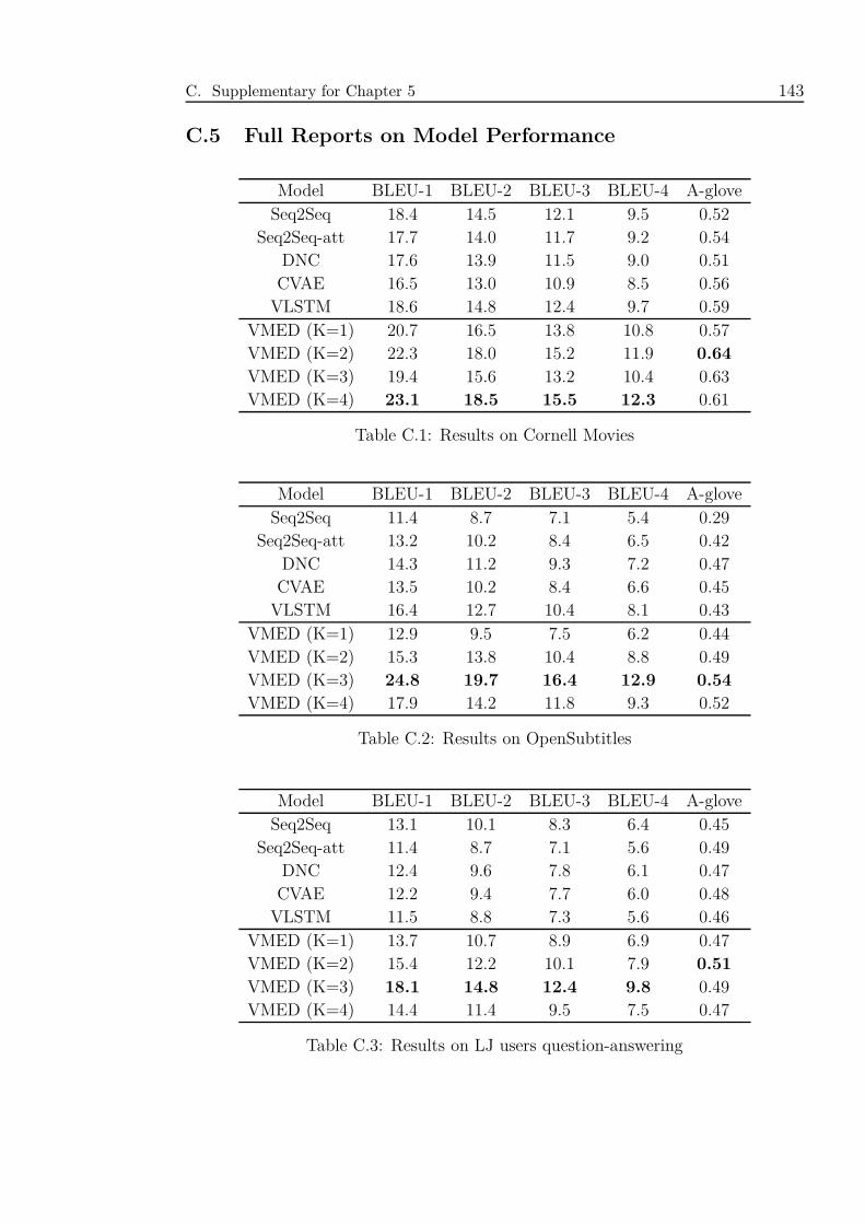
C. Supplementary for Chapter 5 143
C.5 Full Reports on Model Performance
Model BLEU-1 BLEU-2 BLEU-3 BLEU-4 A-gloveSeq2Seq 18.4 14.5 12.1 9.5 0.52
Seq2Seq-att 17.7 14.0 11.7 9.2 0.54DNC 17.6 13.9 11.5 9.0 0.51CVAE 16.5 13.0 10.9 8.5 0.56
VLSTM 18.6 14.8 12.4 9.7 0.59VMED (K=1) 20.7 16.5 13.8 10.8 0.57VMED (K=2) 22.3 18.0 15.2 11.9 0.64
VMED (K=3) 19.4 15.6 13.2 10.4 0.63VMED (K=4) 23.1 18.5 15.5 12.3 0.61
Table C.1: Results on Cornell Movies
Model BLEU-1 BLEU-2 BLEU-3 BLEU-4 A-gloveSeq2Seq 11.4 8.7 7.1 5.4 0.29
Seq2Seq-att 13.2 10.2 8.4 6.5 0.42DNC 14.3 11.2 9.3 7.2 0.47CVAE 13.5 10.2 8.4 6.6 0.45
VLSTM 16.4 12.7 10.4 8.1 0.43VMED (K=1) 12.9 9.5 7.5 6.2 0.44VMED (K=2) 15.3 13.8 10.4 8.8 0.49VMED (K=3) 24.8 19.7 16.4 12.9 0.54
VMED (K=4) 17.9 14.2 11.8 9.3 0.52
Table C.2: Results on OpenSubtitles
Model BLEU-1 BLEU-2 BLEU-3 BLEU-4 A-gloveSeq2Seq 13.1 10.1 8.3 6.4 0.45
Seq2Seq-att 11.4 8.7 7.1 5.6 0.49DNC 12.4 9.6 7.8 6.1 0.47CVAE 12.2 9.4 7.7 6.0 0.48
VLSTM 11.5 8.8 7.3 5.6 0.46VMED (K=1) 13.7 10.7 8.9 6.9 0.47VMED (K=2) 15.4 12.2 10.1 7.9 0.51
VMED (K=3) 18.1 14.8 12.4 9.8 0.49VMED (K=4) 14.4 11.4 9.5 7.5 0.47
Table C.3: Results on LJ users question-answering
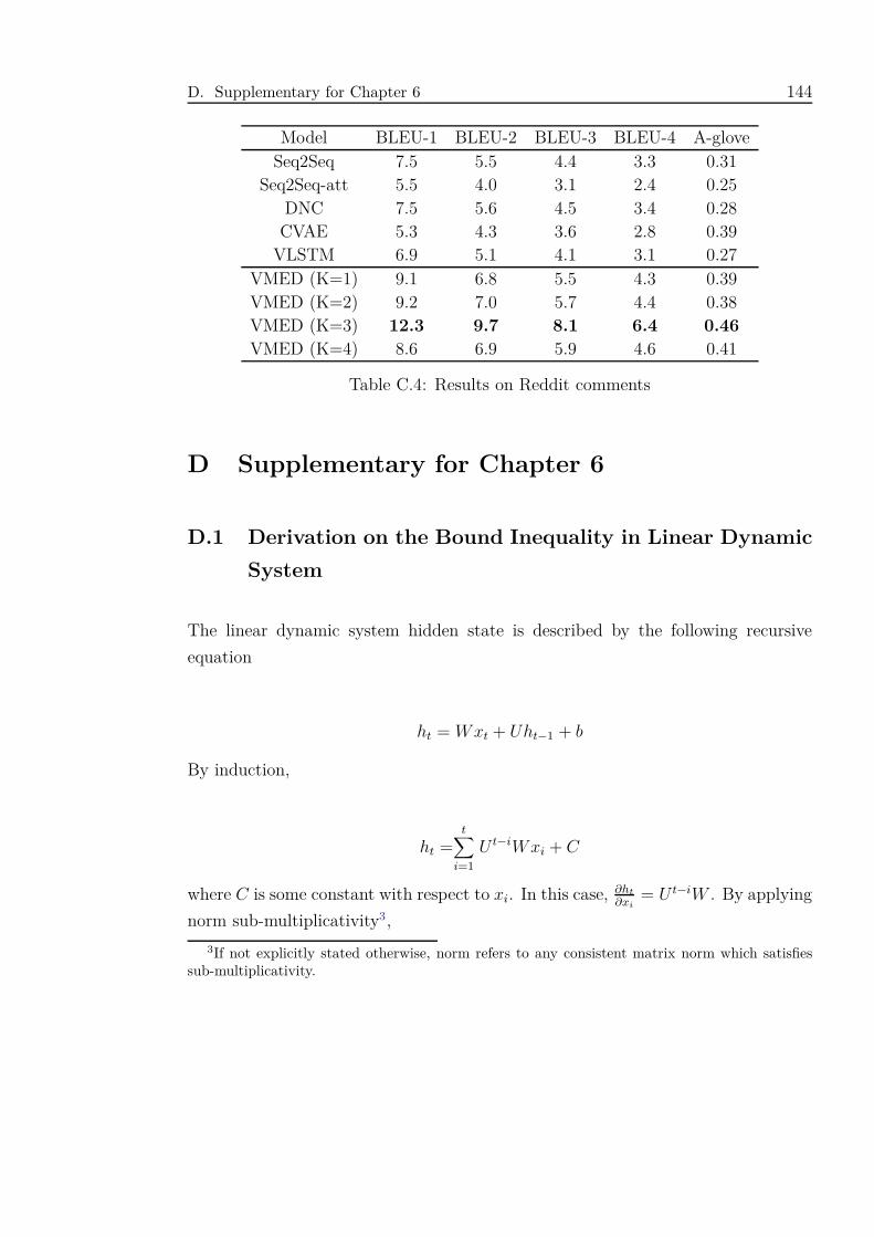
D. Supplementary for Chapter 6 144
Model BLEU-1 BLEU-2 BLEU-3 BLEU-4 A-gloveSeq2Seq 7.5 5.5 4.4 3.3 0.31
Seq2Seq-att 5.5 4.0 3.1 2.4 0.25DNC 7.5 5.6 4.5 3.4 0.28CVAE 5.3 4.3 3.6 2.8 0.39
VLSTM 6.9 5.1 4.1 3.1 0.27VMED (K=1) 9.1 6.8 5.5 4.3 0.39VMED (K=2) 9.2 7.0 5.7 4.4 0.38VMED (K=3) 12.3 9.7 8.1 6.4 0.46
VMED (K=4) 8.6 6.9 5.9 4.6 0.41
Table C.4: Results on Reddit comments
D Supplementary for Chapter 6
D.1 Derivation on the Bound Inequality in Linear Dynamic
System
The linear dynamic system hidden state is described by the following recursive
equation
ht = Wxt + Uht−1 + b
By induction,
ht =t∑
i=1
U t−iWxi + C
where C is some constant with respect to xi. In this case, ∂ht
∂xi= U t−iW . By applying
norm sub-multiplicativity3,
3If not explicitly stated otherwise, norm refers to any consistent matrix norm which satisfiessub-multiplicativity.

D. Supplementary for Chapter 6 145
ci−1,t =∥∥∥U t−i+1W
∥∥∥
≤ ‖U‖∥∥∥U t−iW
∥∥∥
= ‖U‖ ci,t
That is, λc = ‖U‖.
D.2 Derivation on the Bound Inequality in Standard RNN
The standard RNN hidden state is described by the following recursive equation
ht = tanh (Wxt + Uht−1 + b)
From ∂ht
∂xi= ∂ht
∂ht−1
∂ht−1
∂xi, by induction,
∂ht
∂xi=
t∏
j=i+1
∂hj
∂hj−1
∂hi
∂xi=
t∏
j=i
diag(tanh′ (aj)
)U t−iW
where aj = Wxj + Uhj−1 + b and diag (·) converts a vector into a diagonal matrix.
As 0 ≤ tanh′ (x) = 1− tanh (x)2 ≤ 1,∥∥∥diag
(tanh′ (X)
)∥∥∥ is bounded by some value
B. By applying norm sub-multiplicativity,
ci−1,t =
∥∥∥∥∥∥
t∏
j=i
diag(tanh′ (aj)
) diag
(tanh′ (ai−1)
)U t−i+1W
∥∥∥∥∥∥
≤ ‖U‖∥∥∥∥∥∥
t∏
j=i
diag(tanh′ (aj)
)U t−iW
∥∥∥∥∥∥
∥∥∥diag(tanh′ (ai−1)
)∥∥∥
= B ‖U‖ ci,t
That is, λc = B ‖U‖.
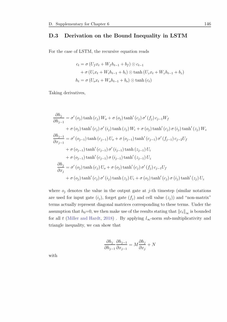
D. Supplementary for Chapter 6 146
D.3 Derivation on the Bound Inequality in LSTM
For the case of LSTM, the recursive equation reads
ct = σ (Uf xt + Wf ht−1 + bf )⊙ ct−1
+ σ (Uixt + Wiht−1 + bi)⊙ tanh (Uzxt + Wzht−1 + bz)
ht = σ (Uoxt + Woht−1 + bo)⊙ tanh (ct)
Taking derivatives,
∂hj
∂hj−1
= σ′ (oj) tanh (cj) Wo + σ (oj) tanh′ (cj) σ′ (fj) cj−1Wf
+ σ (oj) tanh′ (cj) σ′ (ij) tanh (zj) Wi + σ (oj) tanh′ (cj) σ (ij) tanh′ (zj) Wz
∂hj−1
∂xj−1= σ′ (oj−1) tanh (cj−1) Uo + σ (oj−1) tanh′ (cj−1) σ′ (fj−1) cj−2Uf
+ σ (oj−1) tanh′ (cj−1) σ′ (ij−1) tanh (zj−1) Ui
+ σ (oj−1) tanh′ (cj−1) σ (ij−1) tanh′ (zj−1) Uz
∂hj
∂xj
= σ′ (oj) tanh (cj) Uo + σ (oj) tanh′ (cj) σ′ (fj) cj−1Uf
+ σ (oj) tanh′ (cj) σ′ (ij) tanh (zj) Ui + σ (oj) tanh′ (cj) σ (ij) tanh′ (zj) Uz
where oj denotes the value in the output gate at j-th timestep (similar notations
are used for input gate (ij), forget gate (fj) and cell value (zj)) and “non-matrix”
terms actually represent diagonal matrices corresponding to these terms. Under the
assumption that h0=0, we then make use of the results stating that ‖ct‖∞ is bounded
for all t (Miller and Hardt, 2018) . By applying l∞-norm sub-multiplicativity and
triangle inequality, we can show that
∂hj
∂hj−1
∂hj−1
∂xj−1= M
∂hj
∂xj+ N
with
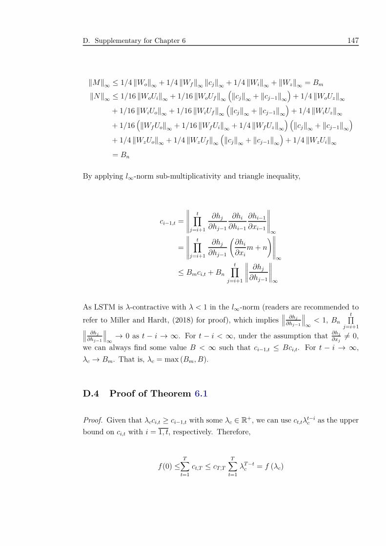
D. Supplementary for Chapter 6 147
‖M‖∞ ≤ 1/4 ‖Wo‖∞ + 1/4 ‖Wf‖∞ ‖cj‖∞ + 1/4 ‖Wi‖∞ + ‖Wz‖∞ = Bm
‖N‖∞ ≤ 1/16 ‖WoUi‖∞ + 1/16 ‖WoUf‖∞
(‖cj‖∞ + ‖cj−1‖∞
)+ 1/4 ‖WoUz‖∞
+ 1/16 ‖WiUo‖∞ + 1/16 ‖WiUf‖∞
(‖cj‖∞ + ‖cj−1‖∞
)+ 1/4 ‖WiUz‖∞
+ 1/16(‖Wf Uo‖∞ + 1/16 ‖WfUi‖∞ + 1/4 ‖WfUz‖∞
) (‖cj‖∞ + ‖cj−1‖∞
)
+ 1/4 ‖WzUo‖∞ + 1/4 ‖WzUf‖∞
(‖cj‖∞ + ‖cj−1‖∞
)+ 1/4 ‖WzUi‖∞
= Bn
By applying l∞-norm sub-multiplicativity and triangle inequality,
ci−1,t =
∥∥∥∥∥∥
t∏
j=i+1
∂hj
∂hj−1
∂hi
∂hi−1
∂hi−1
∂xi−1
∥∥∥∥∥∥∞
=
∥∥∥∥∥∥
t∏
j=i+1
∂hj
∂hj−1
(∂hi
∂xim + n
)∥∥∥∥∥∥∞
≤ Bmci,t + Bn
t∏
j=i+1
∥∥∥∥∥∂hj
∂hj−1
∥∥∥∥∥∞
As LSTM is λ-contractive with λ < 1 in the l∞-norm (readers are recommended to
refer to Miller and Hardt, (2018) for proof), which implies∥∥∥ ∂hj
∂hj−1
∥∥∥∞
< 1, Bn
t∏j=i+1∥∥∥ ∂hj
∂hj−1
∥∥∥∞→ 0 as t − i → ∞. For t − i < ∞, under the assumption that ∂hj
∂xj6= 0,
we can always find some value B < ∞ such that ci−1,t ≤ Bci,t. For t − i → ∞,
λc → Bm. That is, λc = max (Bm, B).
D.4 Proof of Theorem 6.1
Proof. Given that λcci,t ≥ ci−1,t with some λc ∈ R+, we can use ct,tλt−ic as the upper
bound on ci,t with i = 1, t, respectively. Therefore,
f(0) ≤T∑
t=1
ct,T ≤ cT,T
T∑
t=1
λT −tc = f (λc)
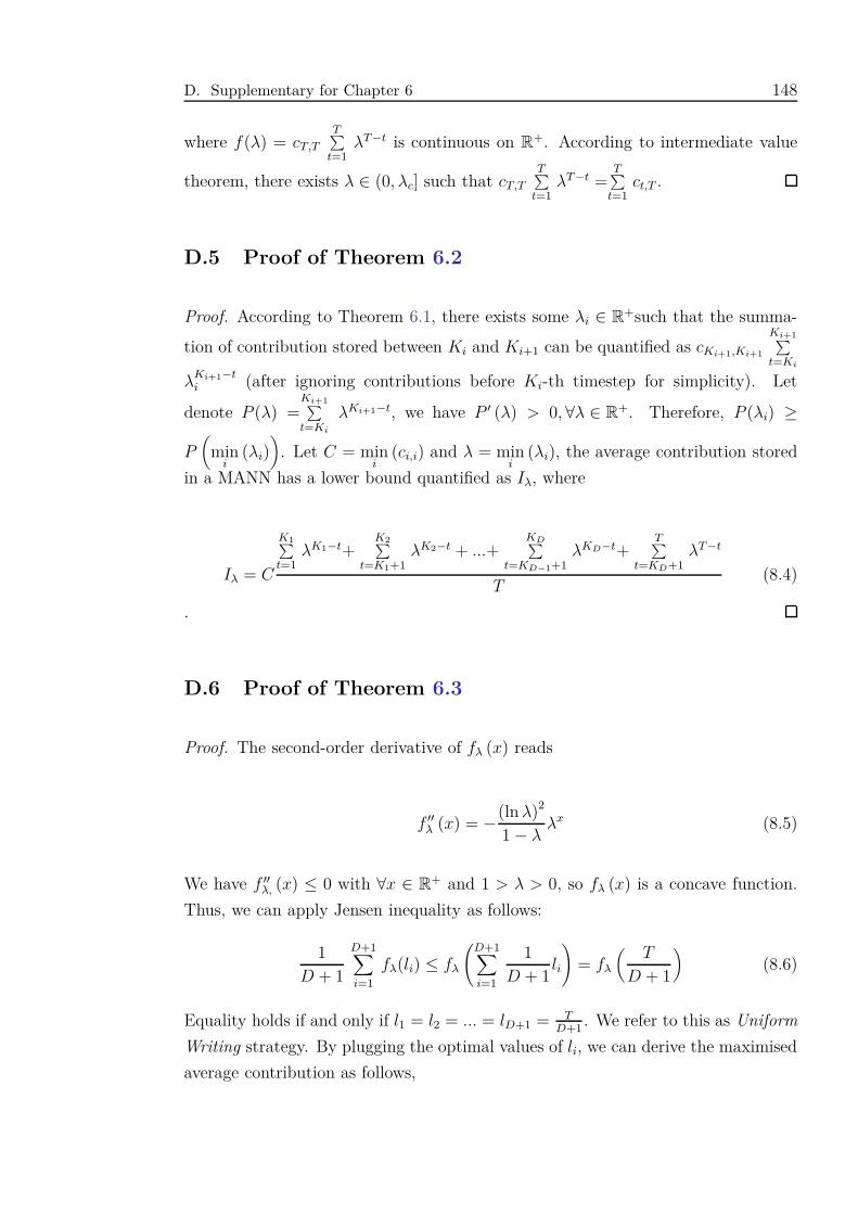
D. Supplementary for Chapter 6 148
where f(λ) = cT,T
T∑t=1
λT −t is continuous on R+. According to intermediate value
theorem, there exists λ ∈ (0, λc] such that cT,T
T∑t=1
λT −t =T∑
t=1ct,T .
D.5 Proof of Theorem 6.2
Proof. According to Theorem 6.1, there exists some λi ∈ R+such that the summa-
tion of contribution stored between Ki and Ki+1 can be quantified as cKi+1,Ki+1
Ki+1∑t=Ki
λKi+1−ti (after ignoring contributions before Ki-th timestep for simplicity). Let
denote P (λ) =Ki+1∑t=Ki
λKi+1−t, we have P ′ (λ) > 0, ∀λ ∈ R+. Therefore, P (λi) ≥
P(
mini
(λi))
. Let C = mini
(ci,i) and λ = mini
(λi), the average contribution stored
in a MANN has a lower bound quantified as Iλ, where
Iλ = C
K1∑t=1
λK1−t+K2∑
t=K1+1λK2−t + ...+
KD∑t=KD−1+1
λKD−t+T∑
t=KD+1λT −t
T(8.4)
.
D.6 Proof of Theorem 6.3
Proof. The second-order derivative of fλ (x) reads
f ′′λ (x) = −(ln λ)2
1− λλx (8.5)
We have f ′′λ, (x) ≤ 0 with ∀x ∈ R+ and 1 > λ > 0, so fλ (x) is a concave function.
Thus, we can apply Jensen inequality as follows:
1D + 1
D+1∑
i=1
fλ(li) ≤ fλ
(D+1∑
i=1
1D + 1
li
)= fλ
(T
D + 1
)(8.6)
Equality holds if and only if l1 = l2 = ... = lD+1 = TD+1
. We refer to this as Uniform
Writing strategy. By plugging the optimal values of li, we can derive the maximised
average contribution as follows,
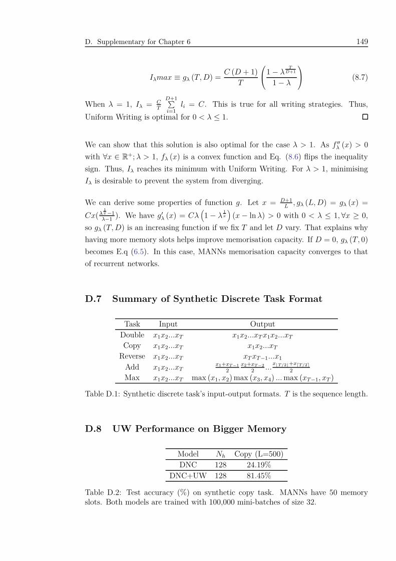
D. Supplementary for Chapter 6 149
Iλmax ≡ gλ (T, D) =C (D + 1)
T
1− λ
TD+1
1− λ
(8.7)
When λ = 1, Iλ = CT
D+1∑i=1
li = C. This is true for all writing strategies. Thus,
Uniform Writing is optimal for 0 < λ ≤ 1.
We can show that this solution is also optimal for the case λ > 1. As f ′′λ (x) > 0
with ∀x ∈ R+; λ > 1, fλ (x) is a convex function and Eq. (8.6) flips the inequality
sign. Thus, Iλ reaches its minimum with Uniform Writing. For λ > 1, minimising
Iλ is desirable to prevent the system from diverging.
We can derive some properties of function g. Let x = D+1L
, gλ (L, D) = gλ (x) =
Cx(λ1x −1
λ−1). We have g′
λ (x) = Cλ(1− λ
1
x
)(x− ln λ) > 0 with 0 < λ ≤ 1, ∀x ≥ 0,
so gλ (T, D) is an increasing function if we fix T and let D vary. That explains why
having more memory slots helps improve memorisation capacity. If D = 0, gλ (T, 0)
becomes E.q (6.5). In this case, MANNs memorisation capacity converges to that
of recurrent networks.
D.7 Summary of Synthetic Discrete Task Format
Task Input OutputDouble x1x2...xT x1x2...xT x1x2...xT
Copy x1x2...xT x1x2...xT
Reverse x1x2...xT xT xT −1...x1
Add x1x2...xTx1+xT −1
2x2+xT −2
2...
x⌊T/2⌋+x⌈T/2⌉
2
Max x1x2...xT max (x1, x2) max (x3, x4) ... max (xT −1, xT )
Table D.1: Synthetic discrete task’s input-output formats. T is the sequence length.
D.8 UW Performance on Bigger Memory
Model Nh Copy (L=500)DNC 128 24.19%
DNC+UW 128 81.45%
Table D.2: Test accuracy (%) on synthetic copy task. MANNs have 50 memoryslots. Both models are trained with 100,000 mini-batches of size 32.
D. Supplementary for Chapter 6 150
D.9 Memory Operating Behaviors on Synthetic Tasks
In this section, we pick three models (DNC, DNC+UW and DNC+CUW) to anal-
yse their memory operating behaviors. Fig. D.1 visualises the values of the write
weights and read weights for the copy task during encoding input and decoding
output sequence, respectively. In the copy task, as the sequence length is 50 while
the memory size is 4, one memory slot should contain the accumulation of multiple
timesteps. This principle is reflected in the decoding process in three models, in
which one memory slot is read repeatedly across several timesteps. Notably, the
number of timesteps consecutively spent for one slot is close to 10-the optimal in-
terval, even for DNC ( Fig. D.1(a)), which implies that the ultimate rule would
be the uniform rule. As UW and CUW are equipped with uniform writing, their
writing patterns follow the rule perfectly. Interestingly, UW chooses the first writ-
ten location for the final write (corresponding to the <eos> token) while CUW
picks the last written location. As indicated in Figs. D.1(b) and (c), both of them
can learn the corresponding reading pattern for decoding process, which leads to
good performances. On the other hand, regular DNC fails to learn a perfect writing
strategy. Except for the timesteps at the end of the sequence, the timesteps are
distributed to several memory slots while the reading phase attends to one memory
slot repeatedly. This explains why regular DNC cannot compete with the other two
proposed methods in this task.
For the max task, Fig. D.2 displays similar visualisation with an addition of write
gate during encoding phase. The write gate indicates how much the model should
write the input at some timestep to the memory. A zero write gate means there
is no writing. For this task, a good model should discriminate between timesteps
and prefer writing the greater ones. As clearly seen in Fig. D.2(a), DNC suffers the
same problem as in copy task, unable to synchronise encoding writing with decoding
reading. Also, DNC’s write gate pattern does not show reasonable discrimination.
For UW (Fig. D.2(b)), it tends to write every timestep and relies on uniform
writing principle to achieve write/read accordance and thus better results than DNC.
Amongst all, CUW is able to ignore irrelevant timesteps and follows uniform writing
at the same time (see Fig. D.2(c)).
D. Supplementary for Chapter 6 151
0 1 2 3
0
10
20
30
40
50
0 1 2 3
0
10
20
30
40
50
0 1 2 3
0
10
20
30
40
50
0 1 2 3
0
10
20
30
40
50
0 1 2 3
0
10
20
30
40
500 1 2 3
0
10
20
30
40
50
a) DNC b) DNC+UW c) DNC+CUW
Encoding Write Weight Decoding Read Weight Encoding Write Weight Decoding Read Weight Encoding Write Weight Decoding Read Weight
Figure D.1: Memory operations on copy task in DNC (a), DNC+UW (b) andDNC+CUW(c). Each row is a timestep and each column is a memory slot.
Encoding Write Weight Decoding Read Weight
Enco
din
g W
rite
Gat
e
Encoding Write Weight Decoding Read Weight
Enco
din
g W
rite
Gat
e
a) DNC b) DNC+UW c) DNC+CUW
Encoding Write Weight Decoding Read Weight
Enco
din
g W
rite
Gat
e
Figure D.2: Memory operations on max task in DNC (a), DNC+UW (b) andDNC+CUW(c). Each row is a timestep and each column is a memory slot.
D.10 Visualisations of Model Performance on Sinusoidal Re-
gression Tasks
We pick randomly 3 input sequences and plot the output sequences produced by
DNC, UW and CUW in Figs. D.3 (clean) and D.4 (noisy). In each plot, the
first and last 100 timesteps correspond to the given input and generated output,
respectively. The ground truth sequence is plotted in red while the predicted in
blue. We also visualise the values of MANN write gates through time in the bottom
of each plots. In irregular writing encoding phase, the write gate is computed even
when there is no write as it reflects how much weight the controller puts on the
timesteps. In decoding, we let MANNs write to memory at every timestep to allow
instant update of memory during inference.
Under clean condition, all models seem to attend more to late timesteps during
encoding, which makes sense as focusing on late periods of sine wave is enough for
later reconstruction. However, this pattern is not clear in DNC and UW as in CUW.
During decoding, the write gates tend to oscillate in the shape of sine wave, which
is also a good strategy as this directly reflects the amplitude of generation target.
In this case, both UW and CUW demonstrate this behavior clearer than DNC.
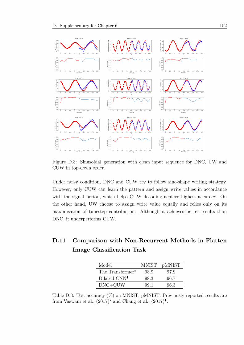
D. Supplementary for Chapter 6 152
0 25 50 75 100 125 150 175 200
x
2
4
6
8
y
=5
+
A sin(2
fx+
)
MSE = 1.09
0 25 50 75 100 125 150 175 200
timestep
0.0
0.2
0.4
0.6
0.8
1.0
wri
te g
ate
0 25 50 75 100 125 150 175 200
x
2
4
6
8
y=
5+
Asin(2
fx+
)
MSE = 0.60
0 25 50 75 100 125 150 175 200
timestep
0.0
0.2
0.4
0.6
0.8
1.0
wri
te g
ate
0 25 50 75 100 125 150 175 200
x
2
4
6
8
y=
5+
Asin(2
fx+
)
MSE = 0.52
0 25 50 75 100 125 150 175 200
timestep
0.0
0.2
0.4
0.6
0.8
1.0
wri
te g
ate
0 25 50 75 100 125 150 175 200
x
3
4
5
6
7
y=
5+
Asin(2
fx+
)
MSE = 0.12
0 25 50 75 100 125 150 175 200
timestep
0.0
0.2
0.4
0.6
0.8
1.0
wri
te g
ate
0 25 50 75 100 125 150 175 200
x
2
4
6
8
y=
5+
Asin(2
fx+
)
MSE = 0.71
0 25 50 75 100 125 150 175 200
timestep
0.0
0.2
0.4
0.6
0.8
1.0
wri
te g
ate
0 25 50 75 100 125 150 175 200
x
2
4
6
8
y=
5+
Asin(2
fx+
)
MSE = 0.13
0 25 50 75 100 125 150 175 200
timestep
0.0
0.2
0.4
0.6
0.8
1.0
wri
te g
ate
0 25 50 75 100 125 150 175 200
x
2
4
6
y=
5+
Asin(2
fx+
)
MSE = 0.65
0 25 50 75 100 125 150 175 200
timestep
0.0
0.2
0.4
0.6
0.8
1.0
wri
te g
ate
0 25 50 75 100 125 150 175 200
x
2
4
6
8
y=
5+
Asin(2
fx+
)
MSE = 0.37
0 25 50 75 100 125 150 175 200
timestep
0.0
0.2
0.4
0.6
0.8
1.0
wri
te g
ate
0 25 50 75 100 125 150 175 200
x
2
4
6
8
y=
5+
Asin(2
fx+
)
MSE = 0.16
0 25 50 75 100 125 150 175 200
timestep
0.0
0.2
0.4
0.6
0.8
1.0
wri
te g
ate
Figure D.3: Sinusoidal generation with clean input sequence for DNC, UW andCUW in top-down order.
Under noisy condition, DNC and CUW try to follow sine-shape writing strategy.
However, only CUW can learn the pattern and assign write values in accordance
with the signal period, which helps CUW decoding achieve highest accuracy. On
the other hand, UW choose to assign write value equally and relies only on its
maximisation of timestep contribution. Although it achieves better results than
DNC, it underperforms CUW.
D.11 Comparison with Non-Recurrent Methods in Flatten
Image Classification Task
Model MNIST pMNISTThe Transformer⋆ 98.9 97.9Dilated CNN� 98.3 96.7DNC+CUW 99.1 96.3
Table D.3: Test accuracy (%) on MNIST, pMNIST. Previously reported results arefrom Vaswani et al., (2017)⋆ and Chang et al., (2017)�.
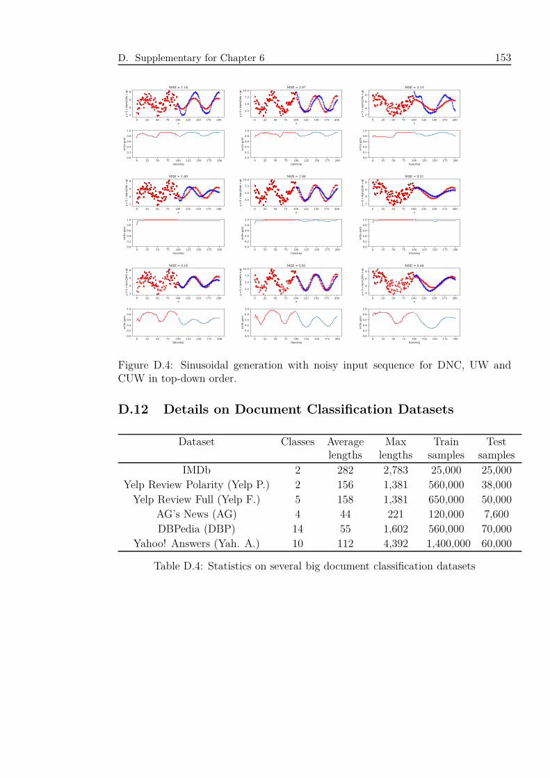
D. Supplementary for Chapter 6 153
0 25 50 75 100 125 150 175 200
x
2
4
6
8
y=
5+
Asin(2
fx+
)
MSE = 1.14
0 25 50 75 100 125 150 175 200
timestep
0.0
0.2
0.4
0.6
0.8
1.0
wri
te g
ate
0 25 50 75 100 125 150 175 200
x
2.5
5.0
7.5
10.0
y=
5+
Asin(2
fx+
)
MSE = 2.97
0 25 50 75 100 125 150 175 200
timestep
0.0
0.2
0.4
0.6
0.8
1.0
wri
te g
ate
0 25 50 75 100 125 150 175 200
x
2
4
6
8
y=
5+
Asin(2
fx+
)
MSE = 2.13
0 25 50 75 100 125 150 175 200
timestep
0.0
0.2
0.4
0.6
0.8
1.0
wri
te g
ate
0 25 50 75 100 125 150 175 200
x
2
4
6
8
y=
5+
Asin(2
fx+
)
MSE = 1.00
0 25 50 75 100 125 150 175 200
timestep
0.0
0.2
0.4
0.6
0.8
1.0
wri
te g
ate
0 25 50 75 100 125 150 175 200
x
2.5
5.0
7.5
10.0
y=
5+
Asin(2
fx+
)
MSE = 1.46
0 25 50 75 100 125 150 175 200
timestep
0.0
0.2
0.4
0.6
0.8
1.0
wri
te g
ate
0 25 50 75 100 125 150 175 200
x
2
4
6
8
y=
5+
Asin(2
fx+
)
MSE = 0.31
0 25 50 75 100 125 150 175 200
timestep
0.0
0.2
0.4
0.6
0.8
1.0
wri
te g
ate
0 25 50 75 100 125 150 175 200
x
2
4
6
8
y=
5+
Asin(2
fx+
)
MSE = 0.16
0 25 50 75 100 125 150 175 200
timestep
0.0
0.2
0.4
0.6
0.8
1.0
wri
te g
ate
0 25 50 75 100 125 150 175 200
x
2.5
5.0
7.5
10.0
y=
5+
Asin(2
fx+
)
MSE = 0.81
0 25 50 75 100 125 150 175 200
timestep
0.0
0.2
0.4
0.6
0.8
1.0
wri
te g
ate
0 25 50 75 100 125 150 175 200
x
2
4
6
8
y=
5+
Asin(2
fx+
)
MSE = 0.44
0 25 50 75 100 125 150 175 200
timestep
0.0
0.2
0.4
0.6
0.8
1.0
wri
te g
ate
Figure D.4: Sinusoidal generation with noisy input sequence for DNC, UW andCUW in top-down order.
D.12 Details on Document Classification Datasets
Dataset Classes Averagelengths
Maxlengths
Trainsamples
Testsamples
IMDb 2 282 2,783 25,000 25,000Yelp Review Polarity (Yelp P.) 2 156 1,381 560,000 38,000
Yelp Review Full (Yelp F.) 5 158 1,381 650,000 50,000AG’s News (AG) 4 44 221 120,000 7,600DBPedia (DBP) 14 55 1,602 560,000 70,000
Yahoo! Answers (Yah. A.) 10 112 4,392 1,400,000 60,000
Table D.4: Statistics on several big document classification datasets
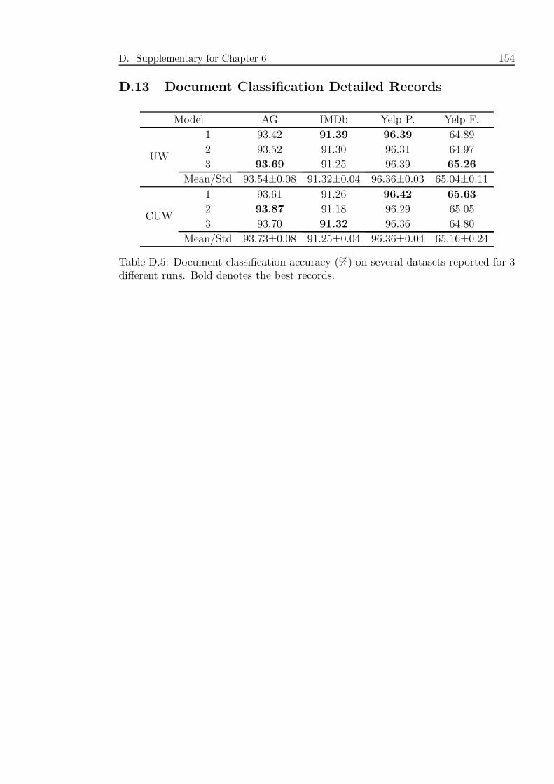
D. Supplementary for Chapter 6 154
D.13 Document Classification Detailed Records
Model AG IMDb Yelp P. Yelp F.
UW
1 93.42 91.39 96.39 64.892 93.52 91.30 96.31 64.973 93.69 91.25 96.39 65.26
Mean/Std 93.54±0.08 91.32±0.04 96.36±0.03 65.04±0.11
CUW
1 93.61 91.26 96.42 65.63
2 93.87 91.18 96.29 65.053 93.70 91.32 96.36 64.80
Mean/Std 93.73±0.08 91.25±0.04 96.36±0.04 65.16±0.24
Table D.5: Document classification accuracy (%) on several datasets reported for 3different runs. Bold denotes the best records.
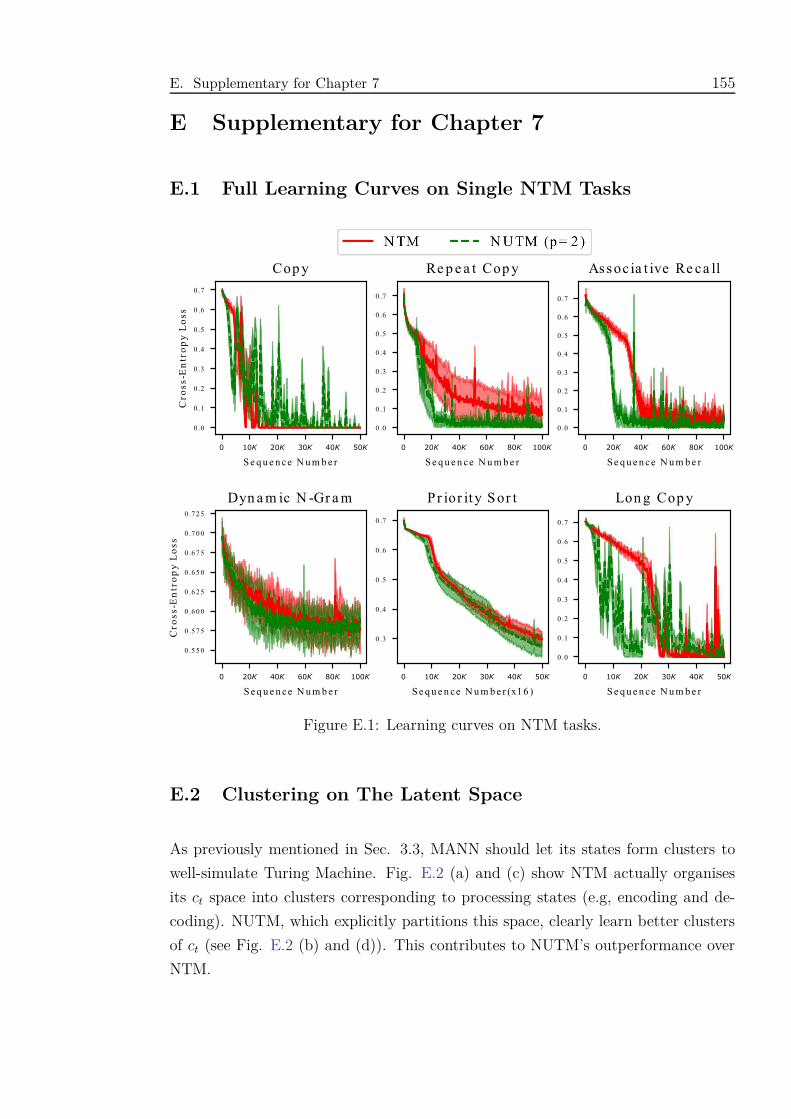
E. Supplementary for Chapter 7 155
E Supplementary for Chapter 7
E.1 Full Learning Curves on Single NTM Tasks
Figure E.1: Learning curves on NTM tasks.
E.2 Clustering on The Latent Space
As previously mentioned in Sec. 3.3, MANN should let its states form clusters to
well-simulate Turing Machine. Fig. E.2 (a) and (c) show NTM actually organises
its ct space into clusters corresponding to processing states (e.g, encoding and de-
coding). NUTM, which explicitly partitions this space, clearly learn better clusters
of ct (see Fig. E.2 (b) and (d)). This contributes to NUTM’s outperformance over
NTM.
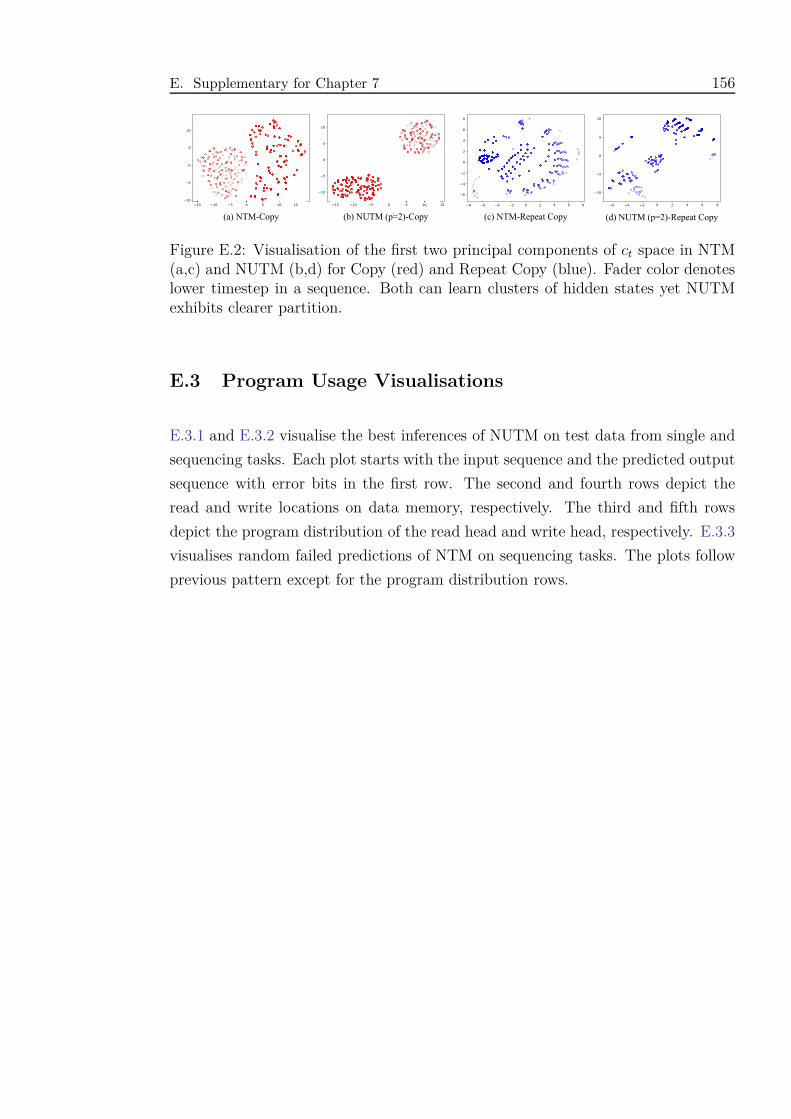
E. Supplementary for Chapter 7 156
Figure E.2: Visualisation of the first two principal components of ct space in NTM(a,c) and NUTM (b,d) for Copy (red) and Repeat Copy (blue). Fader color denoteslower timestep in a sequence. Both can learn clusters of hidden states yet NUTMexhibits clearer partition.
E.3 Program Usage Visualisations
E.3.1 and E.3.2 visualise the best inferences of NUTM on test data from single and
sequencing tasks. Each plot starts with the input sequence and the predicted output
sequence with error bits in the first row. The second and fourth rows depict the
read and write locations on data memory, respectively. The third and fifth rows
depict the program distribution of the read head and write head, respectively. E.3.3
visualises random failed predictions of NTM on sequencing tasks. The plots follow
previous pattern except for the program distribution rows.
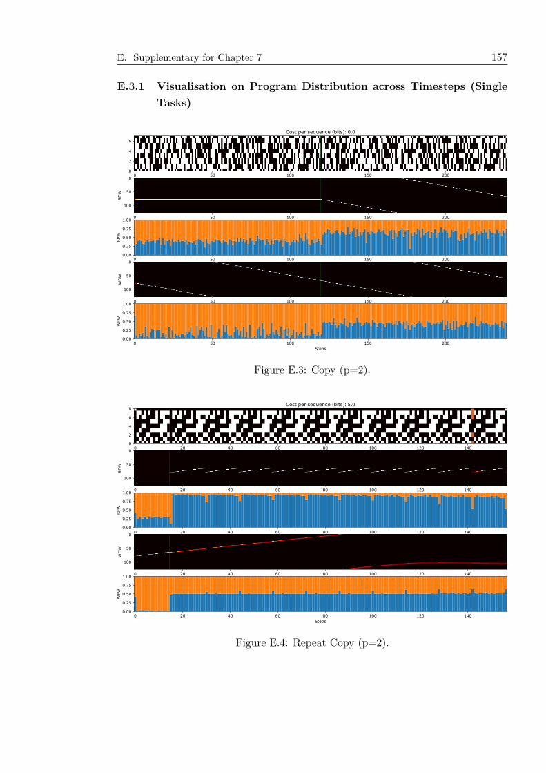
E. Supplementary for Chapter 7 157
E.3.1 Visualisation on Program Distribution across Timesteps (Single
Tasks)
Figure E.3: Copy (p=2).
Figure E.4: Repeat Copy (p=2).
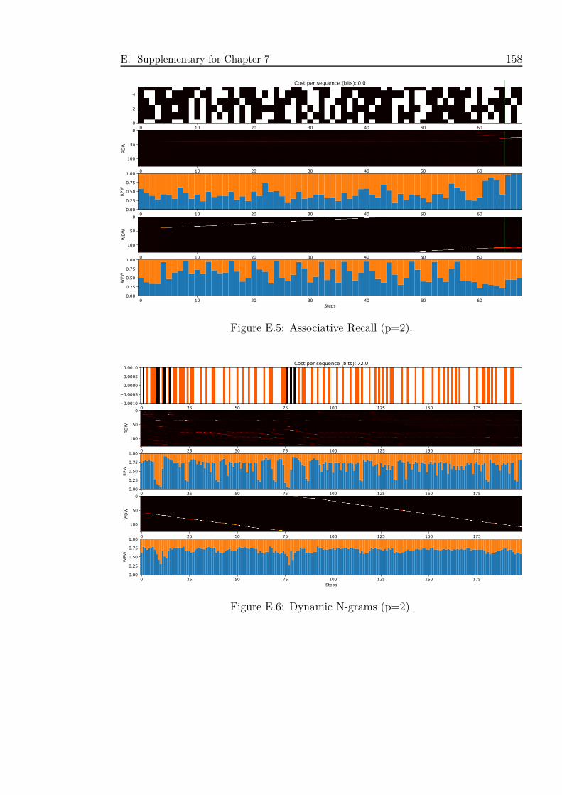
E. Supplementary for Chapter 7 158
Figure E.5: Associative Recall (p=2).
Figure E.6: Dynamic N-grams (p=2).
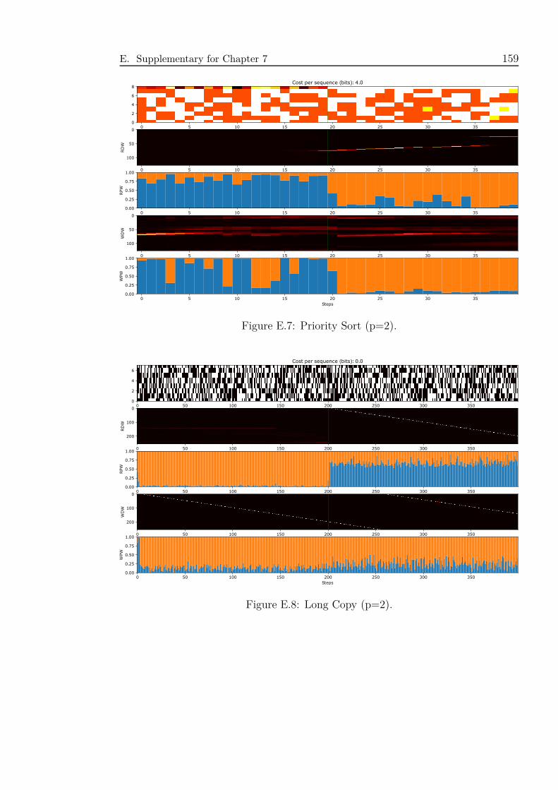
E. Supplementary for Chapter 7 159
Figure E.7: Priority Sort (p=2).
Figure E.8: Long Copy (p=2).
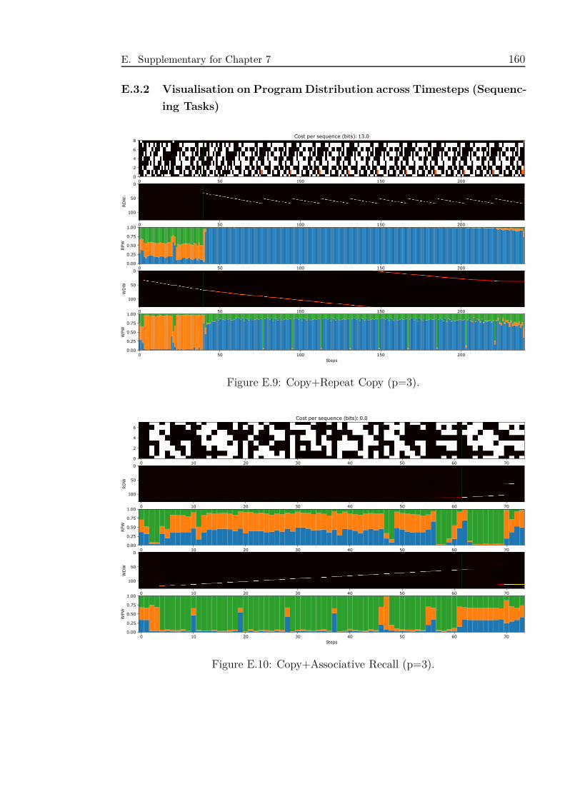
E. Supplementary for Chapter 7 160
E.3.2 Visualisation on Program Distribution across Timesteps (Sequenc-
ing Tasks)
Figure E.9: Copy+Repeat Copy (p=3).
Figure E.10: Copy+Associative Recall (p=3).
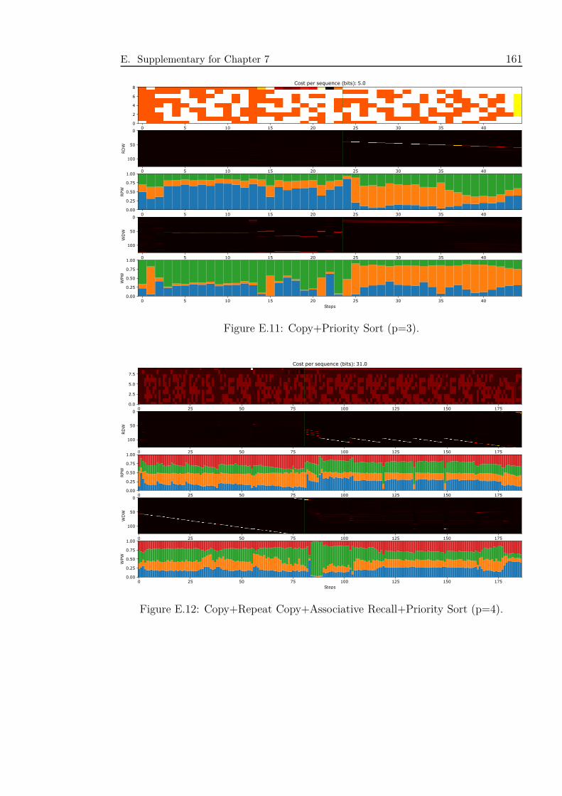
E. Supplementary for Chapter 7 161
Figure E.11: Copy+Priority Sort (p=3).
Figure E.12: Copy+Repeat Copy+Associative Recall+Priority Sort (p=4).
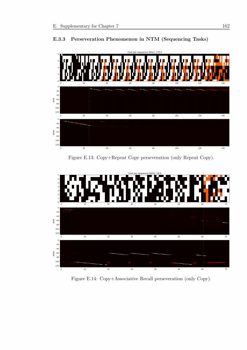
E. Supplementary for Chapter 7 162
E.3.3 Perseveration Phenomenon in NTM (Sequencing Tasks)
Figure E.13: Copy+Repeat Copy perseveration (only Repeat Copy).
Figure E.14: Copy+Associative Recall perseveration (only Copy).
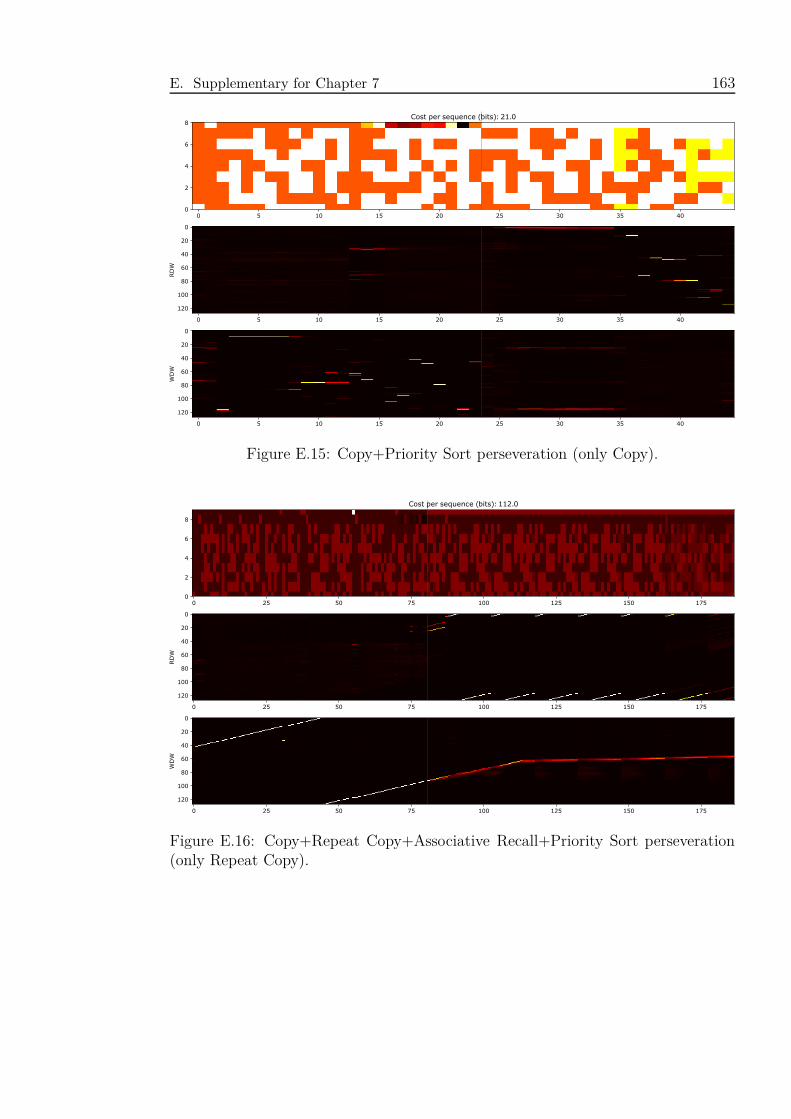
E. Supplementary for Chapter 7 163
Figure E.15: Copy+Priority Sort perseveration (only Copy).
Figure E.16: Copy+Repeat Copy+Associative Recall+Priority Sort perseveration(only Repeat Copy).
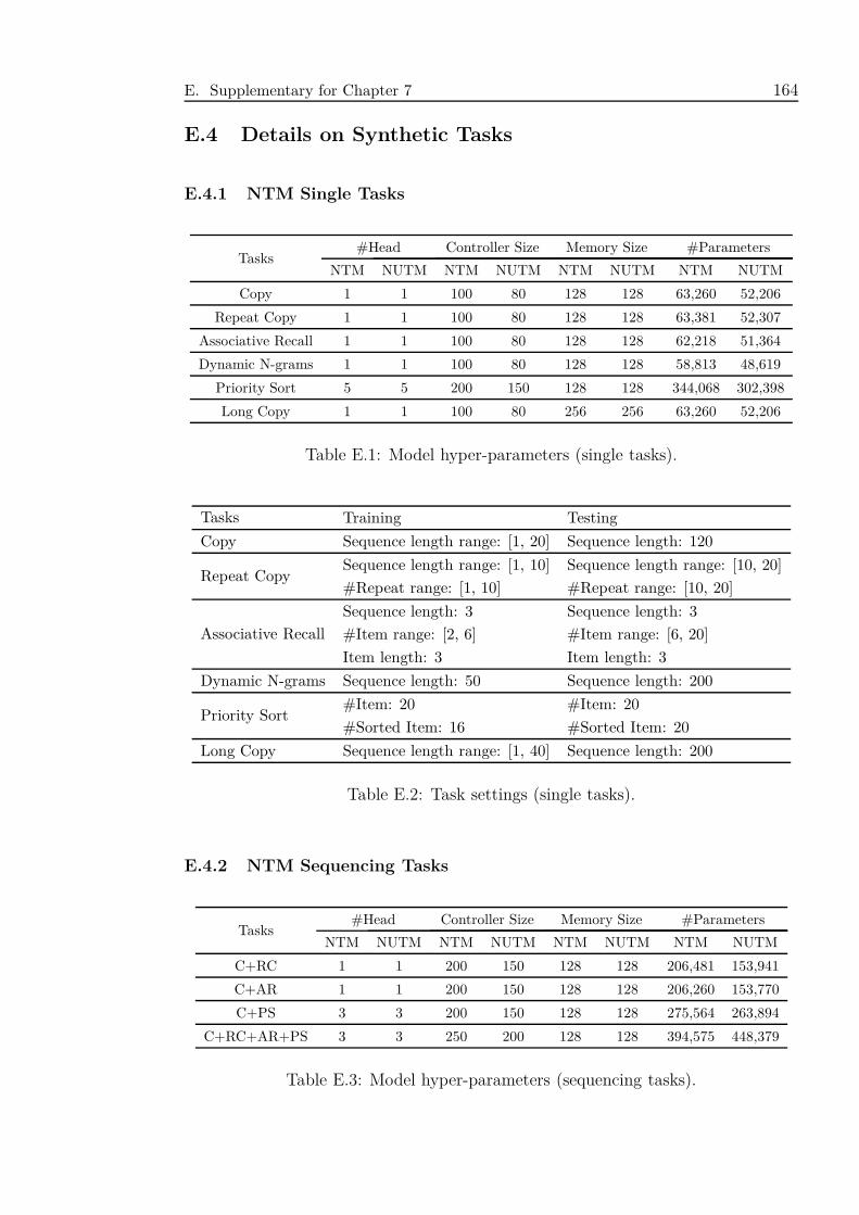
E. Supplementary for Chapter 7 164
E.4 Details on Synthetic Tasks
E.4.1 NTM Single Tasks
Tasks#Head Controller Size Memory Size #Parameters
NTM NUTM NTM NUTM NTM NUTM NTM NUTM
Copy 1 1 100 80 128 128 63,260 52,206
Repeat Copy 1 1 100 80 128 128 63,381 52,307
Associative Recall 1 1 100 80 128 128 62,218 51,364
Dynamic N-grams 1 1 100 80 128 128 58,813 48,619
Priority Sort 5 5 200 150 128 128 344,068 302,398
Long Copy 1 1 100 80 256 256 63,260 52,206
Table E.1: Model hyper-parameters (single tasks).
Tasks Training Testing
Copy Sequence length range: [1, 20] Sequence length: 120
Repeat CopySequence length range: [1, 10] Sequence length range: [10, 20]
#Repeat range: [1, 10] #Repeat range: [10, 20]
Associative Recall
Sequence length: 3 Sequence length: 3
#Item range: [2, 6] #Item range: [6, 20]
Item length: 3 Item length: 3
Dynamic N-grams Sequence length: 50 Sequence length: 200
Priority Sort#Item: 20 #Item: 20
#Sorted Item: 16 #Sorted Item: 20
Long Copy Sequence length range: [1, 40] Sequence length: 200
Table E.2: Task settings (single tasks).
E.4.2 NTM Sequencing Tasks
Tasks#Head Controller Size Memory Size #Parameters
NTM NUTM NTM NUTM NTM NUTM NTM NUTM
C+RC 1 1 200 150 128 128 206,481 153,941
C+AR 1 1 200 150 128 128 206,260 153,770
C+PS 3 3 200 150 128 128 275,564 263,894
C+RC+AR+PS 3 3 250 200 128 128 394,575 448,379
Table E.3: Model hyper-parameters (sequencing tasks).
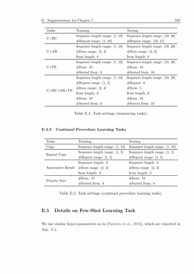
E. Supplementary for Chapter 7 165
Tasks Training Testing
C+RCSequence length range: [1, 10] Sequence length range: [10, 20]
#Repeat range: [1, 10] #Repeat range: [10, 15]
C+AR
Sequence length range: [1, 10] Sequence length range: [10, 20]
#Item range: [2, 4] #Item range: [4, 6]
Item length: 8 Item length: 8
C+PS
Sequence length range: [1, 10] Sequence length range: [10, 20]
#Item: 10 #Item: 10
#Sorted Item: 8 #Sorted Item: 10
C+RC+AR+PS
Sequence length range: [1, 10] Sequence length range: [10, 20]
#Repeat range: [1, 5] #Repeat: 6
#Item range: [2, 4] #Item: 5
Item length: 6 Item length: 6
#Item: 10 #Item: 10
#Sorted Item: 8 #Sorted Item: 10
Table E.4: Task settings (sequencing tasks).
E.4.3 Continual Procedure Learning Tasks
Tasks Training Testing
Copy Sequence length range: [1, 10] Sequence length range: [1, 10]
Repeat CopySequence length range: [1, 5] Sequence length range: [1, 5]
#Repeat range: [1, 5] #Repeat range: [1, 5]
Associative Recall
Sequence length: 3 Sequence length: 3
#Item range: [2, 3] #Item range: [2, 3]
Item length: 3 Item length: 3
Priority Sort#Item: 10 #Item: 10
#Sorted Item: 8 #Sorted Item: 8
Table E.5: Task settings (continual procedure learning tasks).
E.5 Details on Few-Shot Learning Task
We use similar hyper-parameters as in (Santoro et al., 2016), which are reported in
Tab. E.6.
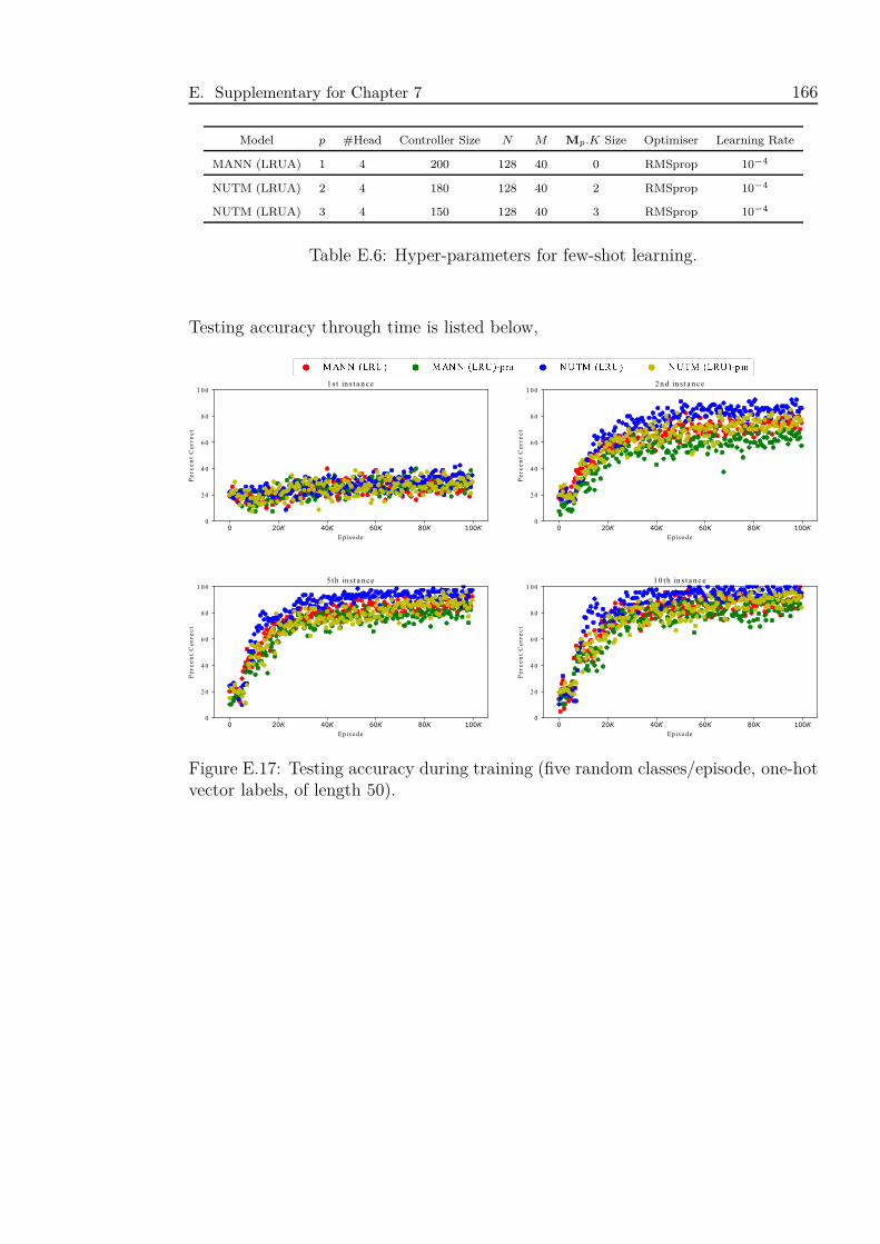
E. Supplementary for Chapter 7 166
Model p #Head Controller Size N M Mp.K Size Optimiser Learning Rate
MANN (LRUA) 1 4 200 128 40 0 RMSprop 10−4
NUTM (LRUA) 2 4 180 128 40 2 RMSprop 10−4
NUTM (LRUA) 3 4 150 128 40 3 RMSprop 10−4
Table E.6: Hyper-parameters for few-shot learning.
Testing accuracy through time is listed below,
Figure E.17: Testing accuracy during training (five random classes/episode, one-hotvector labels, of length 50).
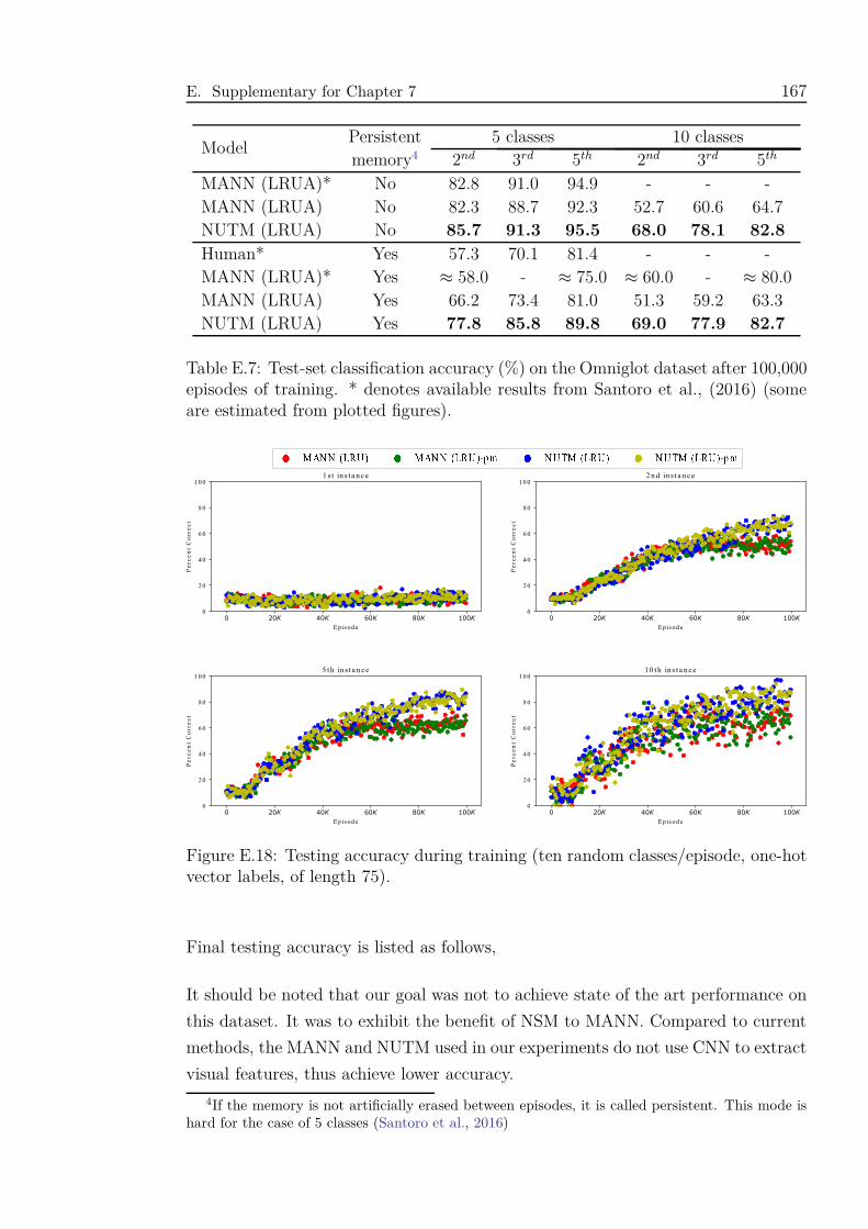
E. Supplementary for Chapter 7 167
ModelPersistent 5 classes 10 classesmemory4 2nd 3rd 5th 2nd 3rd 5th
MANN (LRUA)* No 82.8 91.0 94.9 - - -MANN (LRUA) No 82.3 88.7 92.3 52.7 60.6 64.7NUTM (LRUA) No 85.7 91.3 95.5 68.0 78.1 82.8
Human* Yes 57.3 70.1 81.4 - - -MANN (LRUA)* Yes ≈ 58.0 - ≈ 75.0 ≈ 60.0 - ≈ 80.0MANN (LRUA) Yes 66.2 73.4 81.0 51.3 59.2 63.3NUTM (LRUA) Yes 77.8 85.8 89.8 69.0 77.9 82.7
Table E.7: Test-set classification accuracy (%) on the Omniglot dataset after 100,000episodes of training. * denotes available results from Santoro et al., (2016) (someare estimated from plotted figures).
Figure E.18: Testing accuracy during training (ten random classes/episode, one-hotvector labels, of length 75).
Final testing accuracy is listed as follows,
It should be noted that our goal was not to achieve state of the art performance on
this dataset. It was to exhibit the benefit of NSM to MANN. Compared to current
methods, the MANN and NUTM used in our experiments do not use CNN to extract
visual features, thus achieve lower accuracy.
4If the memory is not artificially erased between episodes, it is called persistent. This mode ishard for the case of 5 classes (Santoro et al., 2016)
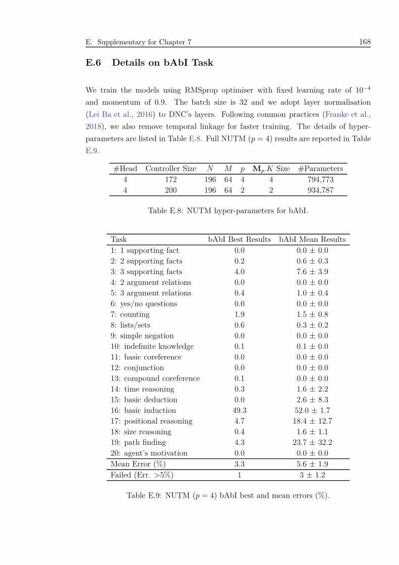
E. Supplementary for Chapter 7 168
E.6 Details on bAbI Task
We train the models using RMSprop optimiser with fixed learning rate of 10−4
and momentum of 0.9. The batch size is 32 and we adopt layer normalisation
(Lei Ba et al., 2016) to DNC’s layers. Following common practices (Franke et al.,
2018), we also remove temporal linkage for faster training. The details of hyper-
parameters are listed in Table E.8. Full NUTM (p = 4) results are reported in Table
E.9.
#Head Controller Size N M p Mp.K Size #Parameters4 172 196 64 4 4 794,7734 200 196 64 2 2 934,787
Table E.8: NUTM hyper-parameters for bAbI.
Task bAbI Best Results bAbI Mean Results1: 1 supporting fact 0.0 0.0 ± 0.02: 2 supporting facts 0.2 0.6 ± 0.33: 3 supporting facts 4.0 7.6 ± 3.94: 2 argument relations 0.0 0.0 ± 0.05: 3 argument relations 0.4 1.0 ± 0.46: yes/no questions 0.0 0.0 ± 0.07: counting 1.9 1.5 ± 0.88: lists/sets 0.6 0.3 ± 0.29: simple negation 0.0 0.0 ± 0.010: indefinite knowledge 0.1 0.1 ± 0.011: basic coreference 0.0 0.0 ± 0.012: conjunction 0.0 0.0 ± 0.013: compound coreference 0.1 0.0 ± 0.014: time reasoning 0.3 1.6 ± 2.215: basic deduction 0.0 2.6 ± 8.316: basic induction 49.3 52.0 ± 1.717: positional reasoning 4.7 18.4 ± 12.718: size reasoning 0.4 1.6 ± 1.119: path finding 4.3 23.7 ± 32.220: agent’s motivation 0.0 0.0 ± 0.0Mean Error (%) 3.3 5.6 ± 1.9Failed (Err. >5%) 1 3 ± 1.2
Table E.9: NUTM (p = 4) bAbI best and mean errors (%).
E. Supplementary for Chapter 7 169
E.7 Others
If we deliberately set the key dimension equal to the number of programs, we can
even place an orthogonal basis constraint on the key space of NSM by minimising
the following loss,
lp2=∥∥∥Mp.KMp.KT − I
∥∥∥ (8.8)
where Mp.K and I denote the key part in NSM and the identity matrix, respectively.
For all tasks, ηt is fixed to 0.1, reducing with decay rate of 0.9.
Bibliography
Daniel J Amit. Modeling brain function: The world of attractor neural networks.
Cambridge university press, 1992.
Jacob Andreas, Marcus Rohrbach, Trevor Darrell, and Dan Klein. Learning to
compose neural networks for question answering. In Proceedings of the 2016
Conference of the North American Chapter of the Association for Computa-
tional Linguistics: Human Language Technologies, pages 1545–1554, 2016a. doi:
10.18653/v1/N16-1181. URL https://www.aclweb.org/anthology/N16-1181.
Jacob Andreas, Marcus Rohrbach, Trevor Darrell, and Dan Klein. Neural module
networks. In Proceedings of the IEEE Conference on Computer Vision and Pattern
Recognition, pages 39–48, 2016b.
Jennifer Hill Andrew Gelman. Data Analysis Using Regression and Multi-
level/Hierarchical Models. Cambridge University Press, 2006.
Martin Arjovsky, Amar Shah, and Yoshua Bengio. Unitary evolution recurrent
neural networks. In International Conference on Machine Learning, pages 1120–
1128, 2016.
Devansh Arpit, Stanisław Jastrzębski, Nicolas Ballas, David Krueger, Emmanuel
Bengio, Maxinder S Kanwal, Tegan Maharaj, Asja Fischer, Aaron Courville,
Yoshua Bengio, et al. A closer look at memorization in deep networks. In Pro-
ceedings of the 34th International Conference on Machine Learning-Volume 70,
pages 233–242. JMLR. org, 2017.
Jimmy Ba, Geoffrey E Hinton, Volodymyr Mnih, Joel Z Leibo, and Catalin Ionescu.
Using fast weights to attend to the recent past. In Advances in Neural Information
Processing Systems, pages 4331–4339, 2016.
Athanassia Bacharoglou. Approximation of probability distributions by convex mix-
tures of gaussian measures. Proceedings of the American Mathematical Society,
138(7):2619–2628, 2010.
170
Bibliography 171
Alan Baddeley. Working memory. Science, 255(5044):556–559, 1992.
Dzmitry Bahdanau, Kyunghyun Cho, and Yoshua Bengio. Neural machine trans-
lation by jointly learning to align and translate. Proceedings of the International
Conference on Learning Representations, 2015.
Jacek M Bajor and Thomas A Lasko. Predicting medications from diagnostic codes
with recurrent neural networks. In International Conference on Learning Repres-
entations, 2017.
Eric B Baum, John Moody, and Frank Wilczek. Internal representations for associ-
ative memory. Biological Cybernetics, 59(4-5):217–228, 1988.
Yoshua Bengio, Patrice Simard, and Paolo Frasconi. Learning long-term dependen-
cies with gradient descent is difficult. IEEE transactions on neural networks, 5
(2):157–166, 1994.
Avrim Blum and Tom Mitchell. Combining labeled and unlabeled data with co-
training. In Proceedings of the eleventh annual conference on Computational
learning theory, pages 92–100. ACM, 1998.
Hal Blumenfeld. Neuroanatomy through Clinical Cases. Oxford University Press,
2010.
Charles Blundell, Benigno Uria, Alexander Pritzel, Yazhe Li, Avraham Ruderman,
Joel Z Leibo, Jack Rae, Daan Wierstra, and Demis Hassabis. Model-free episodic
control. arXiv preprint arXiv:1606.04460, 2016.
Jörg Bornschein, Andriy Mnih, Daniel Zoran, and Danilo Jimenez Rezende. Vari-
ational memory addressing in generative models. In Advances in Neural Inform-
ation Processing Systems, pages 3923–3932, 2017.
Samuel R Bowman, Luke Vilnis, Oriol Vinyals, Andrew Dai, Rafal Jozefowicz, and
Samy Bengio. Generating sentences from a continuous space. In Proceedings of
The SIGNLL Conference on Computational Natural Language Learning, pages
10–21, 2016.
Denny Britz, Melody Guan, and Minh-Thang Luong. Efficient attention using a
fixed-size memory representation. In Proceedings of the Conference on Empirical
Methods in Natural Language Processing, pages 392–400, 2017.
Mike Casey. The dynamics of discrete-time computation, with application to recur-
rent neural networks and finite state machine extraction. Neural computation, 8
(6):1135–1178, 1996.
Bibliography 172
Shiyu Chang, Yang Zhang, Wei Han, Mo Yu, Xiaoxiao Guo, Wei Tan, Xiaodong Cui,
Michael Witbrock, Mark A Hasegawa-Johnson, and Thomas S Huang. Dilated
recurrent neural networks. In Advances in Neural Information Processing Systems,
pages 77–87, 2017.
Boxing Chen and Colin Cherry. A systematic comparison of smoothing techniques
for sentence-level bleu. In Proceedings of the Ninth Workshop on Statistical Ma-
chine Translation, pages 362–367, 2014.
Hongshen Chen, Zhaochun Ren, Jiliang Tang, Yihong Eric Zhao, and Dawei Yin.
Hierarchical variational memory network for dialogue generation. In Proceedings
of the World Wide Web Conference on World Wide Web, pages 1653–1662. Inter-
national World Wide Web Conferences Steering Committee, 2018.
Kyunghyun Cho, Bart Van Merriënboer, Dzmitry Bahdanau, and Yoshua Bengio.
On the properties of neural machine translation: Encoder-decoder approaches.
arXiv preprint arXiv:1409.1259, 2014a.
Kyunghyun Cho, Bart Van Merriënboer, Caglar Gulcehre, Dzmitry Bahdanau, Fethi
Bougares, Holger Schwenk, and Yoshua Bengio. Learning phrase representations
using rnn encoder–decoder for statistical machine translation. In Proceedings
of the 2014 Conference on Empirical Methods in Natural Language Processing
(EMNLP), pages 1724–1734, Doha, Qatar, October 2014b. Association for Com-
putational Linguistics. URL http://www.aclweb.org/anthology/D14-1179.
Edward Choi, Mohammad Taha Bahadori, and Jimeng Sun. Doctor AI: Predicting
Clinical Events via Recurrent Neural Networks. arXiv preprint arXiv:1511.05942,
2015.
Edward Choi, Mohammad Taha Bahadori, Jimeng Sun, Joshua Kulas, Andy
Schuetz, and Walter Stewart. RETAIN: An Interpretable Predictive Model for
Healthcare using Reverse Time Attention Mechanism. In Advances in Neural
Information Processing Systems, pages 3504–3512, 2016.
J. S. Chung, A. Senior, O. Vinyals, and A. Zisserman. Lip reading sentences in the
wild. In IEEE Conference on Computer Vision and Pattern Recognition, 2017.
Junyoung Chung, Caglar Gulcehre, KyungHyun Cho, and Yoshua Bengio. Empir-
ical evaluation of gated recurrent neural networks on sequence modeling. arXiv
preprint arXiv:1412.3555, 2014.
Bibliography 173
Junyoung Chung, Kyle Kastner, Laurent Dinh, Kratarth Goel, Aaron C Courville,
and Yoshua Bengio. A recurrent latent variable model for sequential data. In
Advances in Neural Information Processing Systems, pages 2980–2988, 2015.
Dan C Cireşan, Alessandro Giusti, Luca M Gambardella, and Jürgen Schmidhuber.
Mitosis detection in breast cancer histology images with deep neural networks.
In International Conference on Medical Image Computing and Computer-assisted
Intervention, pages 411–418. Springer, 2013.
Patricia Cohen, Stephen G West, and Leona S Aiken. Applied multiple regres-
sion/correlation analysis for the behavioral sciences. Psychology Press, 2014.
Alexis Conneau, Holger Schwenk, Loıc Barrault, and Yann Lecun. Very deep con-
volutional networks for natural language processing. In Proceedings of the 15th
Conference of the European Chapter of the Association for Computational Lin-
guistics, 2016.
Robert Csordas and Juergen Schmidhuber. Improving differentiable neural com-
puters through memory masking, de-allocation, and link distribution sharpness
control. In International Conference on Learning Representations, 2019. URL
https://openreview.net/forum?id=HyGEM3C9KQ.
Clayton E Curtis and Mark D’Esposito. Persistent activity in the prefrontal cortex
during working memory. Trends in cognitive sciences, 7(9):415–423, 2003.
Ivo Danihelka, Greg Wayne, Benigno Uria, Nal Kalchbrenner, and Alex Graves.
Associative long short-term memory. In International Conference on Machine
Learning, pages 1986–1994, 2016.
Nat Dilokthanakul, Pedro AM Mediano, Marta Garnelo, Matthew CH Lee,
Hugh Salimbeni, Kai Arulkumaran, and Murray Shanahan. Deep unsuper-
vised clustering with gaussian mixture variational autoencoders. arXiv preprint
arXiv:1611.02648, 2016.
J-L Durrieu, J-Ph Thiran, and Finnian Kelly. Lower and upper bounds for ap-
proximation of the kullback-leibler divergence between gaussian mixture models.
In IEEE International Conference on Acoustics, Speech and Signal Processing.,
2012.
Jeffrey L Elman. Finding structure in time. Cognitive science, 14(2):179–211, 1990.
Bibliography 174
Gabriel Forgues, Joelle Pineau, Jean-Marie Larchevêque, and Réal Tremblay. Boot-
strapping dialog systems with word embeddings. In Nips, Modern Machine Learn-
ing and Natural Language Processing Workshop, volume 2, 2014.
Jörg Franke, Jan Niehues, and Alex Waibel. Robust and scalable differentiable
neural computer for question answering. In Proceedings of the Workshop on Ma-
chine Reading for Question Answering, pages 47–59. Association for Computa-
tional Linguistics, 2018. URL http://aclweb.org/anthology/W18-2606.
Robert M French. Catastrophic forgetting in connectionist networks. Trends in
cognitive sciences, 3(4):128–135, 1999.
Surya Ganguli, Dongsung Huh, and Haim Sompolinsky. Memory traces in dynamical
systems. Proceedings of the National Academy of Sciences, 105(48):18970–18975,
2008.
Jiyang Gao, Runzhou Ge, Kan Chen, and Ram Nevatia. Motion-appearance co-
memory networks for video question answering. arXiv preprint arXiv:1803.10906,
2018.
Mevlana Gemici, Chia-Chun Hung, Adam Santoro, Greg Wayne, Shakir Mohamed,
Danilo J Rezende, David Amos, and Timothy Lillicrap. Generative temporal
models with memory. arXiv preprint arXiv:1702.04649, 2017.
C Lee Giles, Clifford B Miller, Dong Chen, Hsing-Hen Chen, Guo-Zheng Sun, and
Yee-Chun Lee. Learning and extracting finite state automata with second-order
recurrent neural networks. Neural Computation, 4(3):393–405, 1992.
Patricia S Goldman-Rakic. Cellular basis of working memory. Neuron, 14(3):477–
485, 1995.
Alejandro González, Gabriel Villalonga, Jiaolong Xu, David Vázquez, Jaume
Amores, and Antonio M López. Multiview random forest of local experts combin-
ing rgb and lidar data for pedestrian detection. In Intelligent Vehicles Symposium
(IV), 2015 IEEE, pages 356–361. IEEE, 2015.
Ian Goodfellow, Jean Pouget-Abadie, Mehdi Mirza, Bing Xu, David Warde-Farley,
Sherjil Ozair, Aaron Courville, and Yoshua Bengio. Generative adversarial nets.
In Advances in Neural Information Processing Systems, pages 2672–2680, 2014.
Edouard Grave, Moustapha M Cisse, and Armand Joulin. Unbounded cache model
for online language modeling with open vocabulary. In Advances in Neural In-
formation Processing Systems, pages 6042–6052, 2017a.

Bibliography 175
Edouard Grave, Armand Joulin, and Nicolas Usunier. Improving neural language
models with a continuous cache. In International Conference on Learning Rep-
resentations, 2017b.
A. Graves, G. Wayne, and I. Danihelka. Neural Turing Machines. ArXiv e-prints,
October 2014.
Alex Graves. Generating sequences with recurrent neural networks. arXiv preprint
arXiv:1308.0850, 2013.
Alex Graves. Adaptive computation time for recurrent neural networks. arXiv
preprint arXiv:1603.08983, 2016.
Alex Graves and Jürgen Schmidhuber. Framewise phoneme classification with bid-
irectional lstm and other neural network architectures. Neural Networks, 18(5-6):
602–610, 2005.
Alex Graves, Abdel-rahman Mohamed, and Geoffrey Hinton. Speech recognition
with deep recurrent neural networks. In Acoustics, speech and signal processing
(icassp), 2013 ieee international conference on, pages 6645–6649. IEEE, 2013.
Alex Graves, Greg Wayne, and Ivo Danihelka. Neural turing machines. arXiv
preprint arXiv:1410.5401, 2014.
Alex Graves, Greg Wayne, Malcolm Reynolds, Tim Harley, Ivo Danihelka, Ag-
nieszka Grabska-Barwińska, Sergio Gómez Colmenarejo, Edward Grefenstette,
Tiago Ramalho, John Agapiou, et al. Hybrid computing using a neural network
with dynamic external memory. Nature, 538(7626):471–476, 2016.
Edward Grefenstette, Karl Moritz Hermann, Mustafa Suleyman, and Phil Blun-
som. Learning to transduce with unbounded memory. In Advances in Neural
Information Processing Systems, pages 1828–1836, 2015.
Klaus Greff, Rupesh K Srivastava, Jan Koutník, Bas R Steunebrink, and Jürgen
Schmidhuber. Lstm: A search space odyssey. IEEE transactions on neural net-
works and learning systems, 28(10):2222–2232, 2016.
Caglar Gulcehre, Sarath Chandar, and Yoshua Bengio. Memory augmented neural
networks with wormhole connections. arXiv preprint arXiv:1701.08718, 2017.
Sadid A Hasan, Siyuan Zhao, Vivek V Datla, Joey Liu, Kathy Lee, Ashequl Qadir,
Aaditya Prakash, and Oladimeji Farri. Clinical question answering using key-value
memory networks and knowledge graph. In TREC, 2016.
Bibliography 176
Kaiming He, Xiangyu Zhang, Shaoqing Ren, and Jian Sun. Deep residual learning
for image recognition. In Proceedings of the IEEE conference on computer vision
and pattern recognition, pages 770–778, 2016.
Donald Olding Hebb. The organization of behavior: a neuropsychological theory.
Science Editions, 1962.
John R Hershey and Peder A Olsen. Approximating the kullback leibler divergence
between gaussian mixture models. In IEEE International Conference on Acous-
tics, Speech and Signal Processing., 2007.
Geoffrey E Hinton and David C Plaut. Using fast weights to deblur old memories.
In Proceedings of the ninth annual conference of the Cognitive Science Society,
pages 177–186, 1987.
Geoffrey E Hinton et al. Learning distributed representations of concepts. In Pro-
ceedings of the eighth annual conference of the cognitive science society, volume 1,
page 12. Amherst, MA, 1986.
Sepp Hochreiter and Jürgen Schmidhuber. Long short-term memory. Neural com-
putation, 9(8):1735–1780, 1997.
John J Hopfield. Neural networks and physical systems with emergent collective
computational abilities. Proceedings of the national academy of sciences, 79(8):
2554–2558, 1982.
Francis L Huang. Multilevel modeling and ordinary least squares regression: how
comparable are they? The Journal of Experimental Education, 86(2):265–281,
2018.
Herbert Jaeger and Harald Haas. Harnessing nonlinearity: Predicting chaotic sys-
tems and saving energy in wireless communication. science, 304(5667):78–80,
2004.
Eric Jang, Shixiang Gu, and Ben Poole. Categorical reparameterization with
gumbel-softmax. arXiv preprint arXiv:1611.01144, 2016.
Zhuxi Jiang, Yin Zheng, Huachun Tan, Bangsheng Tang, and Hanning Zhou. Vari-
ational deep embedding: An unsupervised and generative approach to clustering.
In Proceedings of the International Joint Conference on Artificial Intelligence,
pages 1965–1972. International Joint Conference on Artificial Intelligence, 2017.
Bibliography 177
Alistair EW Johnson, Tom J Pollard, Lu Shen, Li-wei H Lehman, Mengling Feng,
Mohammad Ghassemi, Benjamin Moody, Peter Szolovits, Leo Anthony Celi, and
Roger G Mark. MIMIC-III, a freely accessible critical care database. Scientific
data, 3, 2016.
Samuel Johnson, J Marro, and Joaquín J Torres. Robust short-term memory without
synaptic learning. PloS one, 8(1):e50276, 2013.
Michael I Jordan. Serial order: A parallel distributed processing approach. In
Advances in psychology, volume 121, pages 471–495. Elsevier, 1997.
Armand Joulin and Tomas Mikolov. Inferring algorithmic patterns with stack-
augmented recurrent nets. In Advances in Neural Information Processing Systems,
pages 190–198, 2015.
Nal Kalchbrenner and Phil Blunsom. Recurrent continuous translation models. In
Proceedings of the Conference on Empirical Methods in Natural Language Pro-
cessing, pages 1700–1709, 2013.
Pentti Kanerva. Sparse distributed memory. MIT press, 1988.
James D Keeler. Comparison between kanerva’s sdm and hopfield-type neural net-
works. Cognitive Science, 12(3):299–329, 1988.
Asjad Khan, Hung Le, Kien Do, Truyen Tran, Aditya Ghose, Hoa Dam, and Renuka
Sindhgatta. Memory-augmented neural networks for predictive process analytics.
arXiv preprint arXiv:1802.00938, 2018.
Diederik P Kingma and Jimmy Ba. Adam: A method for stochastic optimization.
arXiv preprint arXiv:1412.6980, 2014.
Diederik P Kingma and Max Welling. Auto-encoding variational bayes. In Proceed-
ings of the International Conference on Learning Representations, 2014.
Diederik P Kingma, Shakir Mohamed, Danilo Jimenez Rezende, and Max Welling.
Semi-supervised learning with deep generative models. In Advances in Neural
Information Processing Systems, pages 3581–3589, 2014.
Iuliia Kotseruba and John K Tsotsos. 40 years of cognitive architectures: core
cognitive abilities and practical applications. Artificial Intelligence Review, pages
1–78, 2018.
Bibliography 178
David Krueger, Nicolas Ballas, Stanislaw Jastrzebski, Devansh Arpit, Maxinder S
Kanwal, Tegan Maharaj, Emmanuel Bengio, Asja Fischer, and Aaron Courville.
Deep nets don’t learn via memorization. 2017.
Dharshan Kumaran, Demis Hassabis, and James L McClelland. What learning sys-
tems do intelligent agents need? complementary learning systems theory updated.
Trends in cognitive sciences, 20(7):512–534, 2016.
Hung Le and Svetha Venkatesh. Neurocoder: Learning general-purpose computation
using stored neural programs. arXiv preprint arXiv:2009.11443, 2020.
Hung Le, Truyen Tran, Thin Nguyen, and Svetha Venkatesh. Variational memory
encoder-decoder. In Advances in Neural Information Processing Systems, pages
1508–1518, 2018a.
Hung Le, Truyen Tran, and Svetha Venkatesh. Dual memory neural com-
puter for asynchronous two-view sequential learning. In Proceedings of
the 24th ACM SIGKDD International Conference on Knowledge Discovery;
Data Mining, KDD ’18, pages 1637–1645, New York, NY, USA, 2018b.
ACM. ISBN 978-1-4503-5552-0. doi: 10.1145/3219819.3219981. URL
http://doi.acm.org/10.1145/3219819.3219981.
Hung Le, Truyen Tran, and Svetha Venkatesh. Dual control memory augmented
neural networks for treatment recommendations. In Pacific-Asia Conference on
Knowledge Discovery and Data Mining, pages 273–284. Springer, 2018c.
Hung Le, Truyen Tran, and Svetha Venkatesh. Learning to remember more with less
memorization. In International Conference on Learning Representations, 2019.
URL https://openreview.net/forum?id=r1xlvi0qYm.
Hung Le, Truyen Tran, and Svetha Venkatesh. Neural stored-program memory.
In International Conference on Learning Representations, 2020a. URL
https://openreview.net/forum?id=rkxxA24FDr.
Hung Le, Truyen Tran, and Svetha Venkatesh. Self-attentive associative memory. In
International Conference on Machine Learning, pages 5682–5691. PMLR, 2020b.
Quoc V Le, Navdeep Jaitly, and Geoffrey E Hinton. A simple way to initialize
recurrent networks of rectified linear units. arXiv preprint arXiv:1504.00941,
2015.
Jimmy Lei Ba, Jamie Ryan Kiros, and Geoffrey E Hinton. Layer normalization.
arXiv preprint arXiv:1607.06450, 2016.
Bibliography 179
Omer Levy and Yoav Goldberg. Neural word embedding as implicit matrix factor-
ization. In Advances in Neural Information Processing Systems, pages 2177–2185,
2014.
Jiwei Li, Michel Galley, Chris Brockett, Jianfeng Gao, and Bill Dolan. A diversity-
promoting objective function for neural conversation models. In Proceedings of the
Conference of the North American Chapter of the Association for Computational
Linguistics: Human Language Technologies, pages 110–119, 2016.
Zachary C Lipton, David C Kale, Charles Elkan, and Randall Wetzel. Learning to
Diagnose with LSTM Recurrent Neural Networks. In International Conference
on Learning Representations, 2016.
Pierre Lison and Serge Bibauw. Not all dialogues are created equal: Instance weight-
ing for neural conversational models. In Proceedings of the Annual SIGdial Meeting
on Discourse and Dialogue, pages 384–394, 2017.
Robert H Logie. Visuo-spatial working memory. Psychology Press, 2014.
David Lopez-Paz et al. Gradient episodic memory for continual learning. In Advances
in Neural Information Processing Systems, pages 6467–6476, 2017.
Oscar Luaces, Jorge Díez, José Barranquero, Juan José del Coz, and Antonio Ba-
hamonde. Binary relevance efficacy for multilabel classification. Progress in Arti-
ficial Intelligence, 1(4):303–313, 2012.
Chao Ma, Chunhua Shen, Anthony Dick, and Anton van den Hengel. Visual question
answering with memory-augmented networks. arXiv preprint arXiv:1707.04968,
2017a.
Fenglong Ma, Radha Chitta, Jing Zhou, Quanzeng You, Tong Sun, and Jing Gao.
Dipole: Diagnosis prediction in healthcare via attention-based bidirectional re-
current neural networks. In Proceedings of the 23rd ACM SIGKDD International
Conference on Knowledge Discovery and Data Mining, pages 1903–1911. ACM,
2017b.
Ying Ma and Jose Principe. A taxonomy for neural memory networks. arXiv preprint
arXiv:1805.00327, 2018.
Wolfgang Maass. Networks of spiking neurons: the third generation of neural net-
work models. Neural networks, 10(9):1659–1671, 1997.
Bibliography 180
Wolfgang Maass. Liquid state machines: motivation, theory, and applications. In
Computability in context: computation and logic in the real world, pages 275–296.
World Scientific, 2011.
Wolfgang Maass, Thomas Natschläger, and Henry Markram. Real-time comput-
ing without stable states: A new framework for neural computation based on
perturbations. Neural computation, 14(11):2531–2560, 2002.
David Marr and W Thomas Thach. A theory of cerebellar cortex. In From the
Retina to the Neocortex, pages 11–50. Springer, 1991.
Vladimir Maz’ya and Gunther Schmidt. On approximate approximations using
gaussian kernels. IMA Journal of Numerical Analysis, 16(1):13–29, 1996.
James L McClelland, Bruce L McNaughton, and Randall C O’Reilly. Why there
are complementary learning systems in the hippocampus and neocortex: insights
from the successes and failures of connectionist models of learning and memory.
Psychological review, 102(3):419, 1995.
Tomáš Mikolov, Martin Karafiát, Lukáš Burget, Jan Černocky, and Sanjeev
Khudanpur. Recurrent neural network based language model. In Eleventh Annual
Conference of the International Speech Communication Association, 2010.
Tomas Mikolov, Ilya Sutskever, Kai Chen, Greg S Corrado, and Jeff Dean. Distrib-
uted representations of words and phrases and their compositionality. In Advances
in Neural Information Processing Systems, pages 3111–3119, 2013.
Alexander Miller, Adam Fisch, Jesse Dodge, Amir-Hossein Karimi, Antoine Bordes,
and Jason Weston. Key-value memory networks for directly reading documents.
In Proceedings of the 2016 Conference on Empirical Methods in Natural Language
Processing, pages 1400–1409, 2016.
John Miller and Moritz Hardt. When recurrent models don’t need to be recurrent.
arXiv preprint arXiv:1805.10369, 2018.
Volodymyr Mnih, Koray Kavukcuoglu, David Silver, Andrei A Rusu, Joel Veness,
Marc G Bellemare, Alex Graves, Martin Riedmiller, Andreas K Fidjeland, Georg
Ostrovski, et al. Human-level control through deep reinforcement learning. Nature,
518(7540):529, 2015.
Louis-Philippe Morency, Rada Mihalcea, and Payal Doshi. Towards multimodal
sentiment analysis: Harvesting opinions from the web. In Proceedings of the 13th
international conference on multimodal interfaces, pages 169–176. ACM, 2011.
Bibliography 181
Michael C Mozer and Sreerupa Das. A connectionist symbol manipulator that dis-
covers the structure of context-free languages. In Advances in Neural Information
Processing Systems, pages 863–870, 1993.
Tsendsuren Munkhdalai and Hong Yu. Meta networks. In Proceedings of the 34th In-
ternational Conference on Machine Learning-Volume 70, pages 2554–2563. JMLR.
org, 2017.
Eric Nalisnick, Lars Hertel, and Padhraic Smyth. Approximate inference for deep lat-
ent gaussian mixtures. In NIPS Workshop on Bayesian Deep Learning, volume 2,
2016.
Ramesh Nallapati, Bowen Zhou, Cicero dos Santos, Caglar Gulcehre, and Bing Xi-
ang. Abstractive text summarization using sequence-to-sequence rnns and beyond.
In Proceedings of the SIGNLL Conference on Computational Natural Language
Learning, pages 280–290, 2016.
Duc Nguyen, Nhan Tran, and Hung Le. Improving long handwritten text line
recognition with convolutional multi-way associative memory. arXiv preprint
arXiv:1911.01577, 2019.
Phuoc Nguyen, Truyen Tran, Nilmini Wickramasinghe, and Svetha Venkatesh.
Deepr: A Convolutional Net for Medical Records. Journal of Biomedical and
Health Informatics, 21(1), 2017.
Liqiang Nie, Luming Zhang, Yi Yang, Meng Wang, Richang Hong, and Tat-Seng
Chua. Beyond doctors: future health prediction from multimedia and multimodal
observations. In Proceedings of the 23rd ACM international conference on Multi-
media, pages 591–600. ACM, 2015.
Kamal Nigam and Rayid Ghani. Analyzing the effectiveness and applicability of
co-training. In Proceedings of the ninth international conference on Information
and knowledge management, pages 86–93. ACM, 2000.
Christian W Omlin and C Lee Giles. Constructing deterministic finite-state auto-
mata in recurrent neural networks. Journal of the ACM (JACM), 43(6):937–972,
1996.
Razvan Pascanu, Tomas Mikolov, and Yoshua Bengio. On the difficulty of training
recurrent neural networks. In International Conference on Machine Learning,
pages 1310–1318, 2013.
Bibliography 182
Jeffrey Pennington, Richard Socher, and Christopher D Manning. Glove: Global
vectors for word representation. In EMNLP, volume 14, pages 1532–1543, 2014.
Trang Pham, Truyen Tran, Dinh Phung, and Svetha Venkatesh. Predicting health-
care trajectories from medical records: A deep learning approach. Journal of
Biomedical Informatics, 69:218–229, May 2017.
Tony A Plate. Holographic reduced representations. IEEE Transactions on Neural
networks, 6(3):623–641, 1995.
Kim Plunkett and Chris Sinha. Connectionism and developmental theory. British
Journal of Developmental Psychology, 10(3):209–254, 1992.
Soujanya Poria, Erik Cambria, and Alexander Gelbukh. Deep convolutional neural
network textual features and multiple kernel learning for utterance-level mul-
timodal sentiment analysis. In Proceedings of the 2015 conference on empirical
methods in natural language processing, pages 2539–2544, 2015.
Soujanya Poria, Erik Cambria, Devamanyu Hazarika, Navonil Majumder, Amir Za-
deh, and Louis-Philippe Morency. Context-dependent sentiment analysis in user-
generated videos. In Proceedings of the 55th Annual Meeting of the Association for
Computational Linguistics (Volume 1: Long Papers), volume 1, pages 873–883,
2017.
Aaditya Prakash, Siyuan Zhao, Sadid A Hasan, Vivek V Datla, Kathy Lee, Ashequl
Qadir, Joey Liu, and Oladimeji Farri. Condensed memory networks for clinical
diagnostic inferencing. In Proceedings of the AAAI Conference on Artificial In-
telligence, pages 3274–3280, 2017.
Alexander Pritzel, Benigno Uria, Sriram Srinivasan, Adrià Puigdomènech, Oriol
Vinyals, Demis Hassabis, Daan Wierstra, and Charles Blundell. Neural episodic
control. arXiv preprint arXiv:1703.01988, 2017.
N. Quadrianto, A.J. Smola, T.S. Caetano, and Q.V. Le. Estimating labels from label
proportions. The Journal of Machine Learning Research, 10:2349–2374, 2009.
Chao Qui, Bo Huang, Guocheng Niu, Daren Li, Daxiang Dong, Wei He, Dian-
hai Yu, and Hua Wu. A new method of region embedding for text classific-
ation. In International Conference on Learning Representations, 2018. URL
https://openreview.net/forum?id=BkSDMA36Z.
Jack Rae, Jonathan J Hunt, Ivo Danihelka, Timothy Harley, Andrew W Senior,
Gregory Wayne, Alex Graves, and Tim Lillicrap. Scaling memory-augmented
Bibliography 183
neural networks with sparse reads and writes. In Advances in Neural Information
Processing Systems, pages 3621–3629, 2016.
Shyam Sundar Rajagopalan, Louis-Philippe Morency, Tadas Baltrusaitis, and Ro-
land Goecke. Extending long short-term memory for multi-view structured learn-
ing. In European Conference on Computer Vision, pages 338–353. Springer, 2016.
Alain Rakotomamonjy, Francis Bach, Stéphane Canu, and Yves Grandvalet. More
efficiency in multiple kernel learning. In Proceedings of the 24th international
conference on Machine learning, pages 775–782. ACM, 2007.
Jesse Read, Bernhard Pfahringer, Geoff Holmes, and Eibe Frank. Classifier chains
for multi-label classification. Machine learning, 85(3):333–359, 2011.
Danilo Jimenez Rezende, Shakir Mohamed, and Daan Wierstra. Stochastic back-
propagation and approximate inference in deep generative models. In Proceedings
of the International Conference on International Conference on Machine Learn-
ing, pages II–1278. JMLR. org, 2014.
Ryan Rifkin and Aldebaro Klautau. In defense of one-vs-all classification. Journal
of machine learning research, 5(Jan):101–141, 2004.
Timothy T Rogers and James L McClelland. Semantic cognition: A parallel distrib-
uted processing approach. MIT press, 2004.
Raúl Rojas. Neural networks: a systematic introduction. Springer Science & Business
Media, 2013.
David E Rumelhart, Geoffrey E Hinton, Ronald J Williams, et al. Learning repres-
entations by back-propagating errors. Cognitive modeling, 5(3):1, 1988.
Rodrigo Salgado, Francisco Bellas, Pilar Caamaño, Borja Santos-Diez, and Richard J
Duro. A procedural long term memory for cognitive robotics. In 2012 IEEE
Conference on Evolving and Adaptive Intelligent Systems, pages 57–62. IEEE,
2012.
Adam Santoro, Sergey Bartunov, Matthew Botvinick, Daan Wierstra, and Timothy
Lillicrap. Meta-learning with memory-augmented neural networks. In Interna-
tional conference on machine learning, pages 1842–1850, 2016.
Andrew M Saxe, James L McClelland, and Surya Ganguli. A mathematical theory
of semantic development in deep neural networks. Proceedings of the National
Academy of Sciences, 116(23):11537–11546, 2019.
Bibliography 184
Imanol Schlag and Jürgen Schmidhuber. Learning to reason with third order tensor
products. In Advances in Neural Information Processing Systems, pages 9981–
9993, 2018.
Jürgen Schmidhuber. Learning to control fast-weight memories: An alternative to
dynamic recurrent networks. Neural Computation, 4(1):131–139, 1992.
Minjoon Seo, Sewon Min, Ali Farhadi, and Hannaneh Hajishirzi. Neural Speed
Reading via Skim-RNN. In International Conference on Learning Representa-
tions, 2018.
Iulian Vlad Serban, Alessandro Sordoni, Ryan Lowe, Laurent Charlin, Joelle Pineau,
Aaron C Courville, and Yoshua Bengio. A hierarchical latent variable encoder-
decoder model for generating dialogues. In Proceedings of the AAAI Conference
on Artificial Intelligence, pages 3295–3301, 2017.
Xiaoyu Shen, Hui Su, Yanran Li, Wenjie Li, Shuzi Niu, Yang Zhao, Akiko Aizawa,
and Guoping Long. A conditional variational framework for dialog generation. In
Proceedings of the Annual Meeting of the Association for Computational Linguist-
ics (Volume 2: Short Papers), volume 2, pages 504–509, 2017.
Rui Shu, James Brofos, Frank Zhang, Hung Hai Bui, Mohammad Ghavamzadeh,
and Mykel Kochenderfer. Stochastic video prediction with conditional density
estimation. In ECCV Workshop on Action and Anticipation for Visual Learning,
volume 2, 2016.
Hava T Siegelmann and Eduardo D Sontag. On the computational power of neural
nets. Journal of computer and system sciences, 50(1):132–150, 1995.
Michael Sipser et al. Introduction to the Theory of Computation, volume 2. Thomson
Course Technology Boston, 2006.
Paul Smolensky. Tensor product variable binding and the representation of symbolic
structures in connectionist systems. Artificial intelligence, 46(1-2):159–216, 1990.
Yale Song, Louis-Philippe Morency, and Randall Davis. Multi-view latent variable
discriminative models for action recognition. In Computer Vision and Pattern
Recognition (CVPR), 2012 IEEE Conference on, pages 2120–2127. IEEE, 2012.
Rupesh K Srivastava, Klaus Greff, and Jürgen Schmidhuber. Training very deep
networks. In Advances in Neural Information Processing Systems, pages 2377–
2385, 2015.
Bibliography 185
Sainbayar Sukhbaatar, Jason Weston, Rob Fergus, et al. End-to-end memory net-
works. In Advances in Neural Information Processing Systems, pages 2440–2448,
2015.
David Sussillo. Neural circuits as computational dynamical systems. Current opinion
in neurobiology, 25:156–163, 2014.
Ilya Sutskever, Oriol Vinyals, and Quoc V. Le. Sequence to sequence learning with
neural networks. International Conference on Machine Learning, 2014a. URL
http://arxiv.org/abs/1409.3215.
Ilya Sutskever, Oriol Vinyals, and Quoc VV Le. Sequence to sequence learning with
neural networks. In Advances in Neural Information Processing Systems, pages
3104–3112, 2014b.
Jie Tan, Matthew Ung, Chao Cheng, and Casey S Greene. Unsupervised feature
construction and knowledge extraction from genome-wide assays of breast cancer
with denoising autoencoders. In Pacific Symposium on Biocomputing Co-Chairs,
pages 132–143. World Scientific, 2014.
Sebastian Thrun. Lifelong learning algorithms. In Learning to learn, pages 181–209.
Springer, 1998.
Peter Tiňo, Bill G Horne, C Lee Giles, and Pete C Collingwood. Finite state
machines and recurrent neural networks–automata and dynamical systems ap-
proaches. In Neural networks and pattern recognition, pages 171–219. Elsevier,
1998.
Trieu H Trinh, Andrew M Dai, Thang Luong, and Quoc V Le. Learning longer-term
dependencies in rnns with auxiliary losses. In Proceedings of the 35 th Interna-
tional Conference on Machine Learning, Stockholm, Sweden, PMLR 80, 2018.
Endel Tulving et al. Episodic and semantic memory. Organization of memory, 1:
381–403, 1972.
Alan Mathison Turing. On computable numbers, with an application to the
entscheidungsproblem. In Proceedings of the London Mathematical Society, 1936.
Aäron Van Den Oord, Sander Dieleman, Heiga Zen, Karen Simonyan, Oriol Vinyals,
Alex Graves, Nal Kalchbrenner, Andrew W Senior, and Koray Kavukcuoglu.
Wavenet: A generative model for raw audio. In SSW, page 125, 2016.
Bibliography 186
Ashish Vaswani, Noam Shazeer, Niki Parmar, Jakob Uszkoreit, Llion Jones, Aidan N
Gomez, Łukasz Kaiser, and Illia Polosukhin. Attention is all you need. In Advances
in Neural Information Processing Systems, pages 5998–6008, 2017.
Oriol Vinyals and Quoc Le. A neural conversational model. arXiv preprint
arXiv:1506.05869, 2015.
Oriol Vinyals, Meire Fortunato, and Navdeep Jaitly. Pointer networks. In Advances
in Neural Information Processing Systems, pages 2692–2700, 2015.
John von Neumann. First draft of a report on the edvac. IEEE Ann. Hist. Com-
put., 15(4):27–75, October 1993. ISSN 1058-6180. doi: 10.1109/85.238389. URL
https://doi.org/10.1109/85.238389.
Liwei Wang, Alexander Schwing, and Svetlana Lazebnik. Diverse and accurate image
description using a variational auto-encoder with an additive gaussian encoding
space. In Advances in Neural Information Processing Systems, pages 5756–5766,
2017.
Mingxuan Wang, Zhengdong Lu, Hang Li, and Qun Liu. Memory-enhanced decoder
for neural machine translation. In Proceedings of the Conference on Empirical
Methods in Natural Language Processing, pages 278–286, 2016.
Tsung-Hsien Wen, Yishu Miao, Phil Blunsom, and Steve Young. Latent inten-
tion dialogue models. In Proceedings of the International Conference on Machine
Learning, pages 3732–3741, 2017.
Paul J Werbos. Backpropagation through time: what it does and how to do it.
Proceedings of the IEEE, 78(10):1550–1560, 1990.
Jason Weston, Sumit Chopra, and Antoine Bordes. Memory networks. arXiv pre-
print arXiv:1410.3916, 2014.
Jason Weston, Antoine Bordes, Sumit Chopra, Alexander M Rush, Bart van Mer-
riënboer, Armand Joulin, and Tomas Mikolov. Towards ai-complete question
answering: A set of prerequisite toy tasks. arXiv preprint arXiv:1502.05698,
2015.
Faustine Williams. The role of the electronic medical record (emr) in care delivery
development in developing countries: a systematic review. Informatics in Primary
Care Journal, 2008.
Ronald J Williams and David Zipser. A learning algorithm for continually running
fully recurrent neural networks. Neural computation, 1(2):270–280, 1989.
Bibliography 187
Scott Wisdom, Thomas Powers, John Hershey, Jonathan Le Roux, and Les Atlas.
Full-capacity unitary recurrent neural networks. In Advances in Neural Informa-
tion Processing Systems, pages 4880–4888, 2016.
Chang Xu, Dacheng Tao, and Chao Xu. A survey on multi-view learning. arXiv
preprint arXiv:1304.5634, 2013.
Kelvin Xu, Jimmy Ba, Ryan Kiros, Kyunghyun Cho, Aaron Courville, Ruslan
Salakhudinov, Rich Zemel, and Yoshua Bengio. Show, attend and tell: Neural
image caption generation with visual attention. In International conference on
machine learning, pages 2048–2057, 2015.
Dani Yogatama, Chris Dyer, Wang Ling, and Phil Blunsom. Generative and dis-
criminative text classification with recurrent neural networks. arXiv preprint
arXiv:1703.01898, 2017.
Dani Yogatama, Yishu Miao, Gabor Melis, Wang Ling, Adhiguna Kuncoro, Chris
Dyer, and Phil Blunsom. Memory architectures in recurrent neural network lan-
guage models. In International Conference on Learning Representations, 2018.
URL https://openreview.net/forum?id=SkFqf0lAZ.
Adams Wei Yu, Hongrae Lee, and Quoc Le. Learning to skim text. In Proceed-
ings of the 55th Annual Meeting of the Association for Computational Linguistics
(Volume 1: Long Papers), volume 1, pages 1880–1890, 2017.
Keyi Yu, Yang Liu, Alexander G Schwing, and Jian Peng. Fast and accurate text
classification: Skimming, rereading and early stopping. ICLR Workshop Track,
2018.
Amir Zadeh, Rowan Zellers, Eli Pincus, and Louis-Philippe Morency. Multimodal
sentiment intensity analysis in videos: Facial gestures and verbal messages. IEEE
Intelligent Systems, 31(6):82–88, 2016.
Amir Zadeh, Minghai Chen, Soujanya Poria, Erik Cambria, and Louis-Philippe
Morency. Tensor fusion network for multimodal sentiment analysis. arXiv preprint
arXiv:1707.07250, 2017.
Amir Zadeh, Paul Pu Liang, Navonil Mazumder, Soujanya Poria, Erik Cambria,
and Louis-Philippe Morency. Memory fusion network for multi-view sequential
learning. In Thirty-Second AAAI Conference on Artificial Intelligence, 2018.
Bibliography 188
Friedemann Zenke, Ben Poole, and Surya Ganguli. Continual learning through syn-
aptic intelligence. In Proceedings of the 34th International Conference on Machine
Learning-Volume 70, pages 3987–3995. JMLR. org, 2017.
Biao Zhang, Deyi Xiong, Hong Duan, Min Zhang, et al. Variational neural machine
translation. In Proceedings of the Conference on Empirical Methods in Natural
Language Processing, pages 521–530, 2016a.
Chiyuan Zhang, Samy Bengio, Moritz Hardt, Benjamin Recht, and Oriol Vinyals.
Understanding deep learning requires rethinking generalization. arXiv preprint
arXiv:1611.03530, 2016b.
Yutao Zhang, Robert Chen, Jie Tang, Walter F Stewart, and Jimeng Sun. Leap:
Learning to prescribe effective and safe treatment combinations for multimor-
bidity. In Proceedings of the 23rd ACM SIGKDD International Conference on
Knowledge Discovery and Data Mining, pages 1315–1324. ACM, 2017.
Tiancheng Zhao, Ran Zhao, and Maxine Eskenazi. Learning discourse-level diversity
for neural dialog models using conditional variational autoencoders. In Proceedings
of the Annual Meeting of the Association for Computational Linguistics (Volume
1: Long Papers), volume 1, pages 654–664, 2017.
Jozef Zurada. End effector target position learning using feedforward with error
back-propagation and recurrent neural networks. In Neural Networks, 1994. IEEE
World Congress on Computational Intelligence., 1994 IEEE International Con-
ference on, volume 4, pages 2633–2638. IEEE, 1994.
—————————–
Every reasonable effort has been made to acknowledge the owners of
copyright material. I would be pleased to hear from any copyright owner
who has been omitted or incorrectly acknowledged.