
MEErP 2011 - European Commission
201
Final Report Methodology for Ecodesign of Energy‐related Products MEErP 2011 Methodology Report Part 2: Environmental policies & data Contractor: COWI Belgium sprl ‐in association with‐ Van Holsteijn en Kemna B.V. (VHK) Prepared for the European Commission, DG Enterprise and Industry Unit B1 Sustainable Industrial Policy under specific contract SI2.581529, Technical Assistance for the update of the Methodology for the Ecodesign of Energy‐using products (MEEuP), within the framework service contract TREN/R1/350‐2008 Lot 3 René Kemna Brussels/ Delft, 28 November 2011 This report is subject to a disclaimer Ref. Ares(2017)5679959 - 21/11/2017
-
Upload
khangminh22 -
Category
Documents
-
view
2 -
download
0
Transcript of MEErP 2011 - European Commission

Final Report
Methodology for Ecodesign of Energy‐related Products
MEErP 2011
Methodology Report Part 2: Environmental policies & data
Contractor:
COWI Belgium sprl ‐in association with‐ Van Holsteijn en Kemna B.V. (VHK)
Prepared for the European Commission, DG Enterprise and Industry
Unit B1 Sustainable Industrial Policy
under specific contract SI2.581529, Technical Assistance for the update of the Methodology for the Ecodesign of Energy‐using products (MEEuP),
within the framework service contract TREN/R1/350‐2008 Lot 3
René Kemna
Brussels/ Delft, 28 November 2011
This report is subject to a disclaimer
Ref. Ares(2017)5679959 - 21/11/2017

MEErP 2011 METHODOLOGY PART 2 FINAL
2
page intentionally left blank (optimized for double‐sided printing) m²
MEErP 2011 METHODOLOGY PART 2 FINAL
3
COWI Belgium sprl Avenue de Tervuren COWI Belgium sprl, Av. Tervuren 13, B1040 Brussels, Belgium E‐mail: [email protected] www.cowi‐belgium.be Tel.: +32 (0) 2 511 23 83
Van Holsteijn en Kemna B.V. (VHK) Elektronicaweg 14 2628 XG Delft The Netherlands Branche: Av. Albert 126, B 1190 Brussels E‐mail: [email protected] www.vhk.nl Tel.: +31 (0) 2 755 755
Lead author:
René Kemna (VHK)
in collaboration with:
Nelly Azaïs (COWI Belgium), quality control Martijn van Elburg (VHK), review Maaike van der Voort (VHK), questionnaire & assistance software tool William Li (VHK), webmaster www.meerp.eu
Bibliography:
200 pages, 228 references, 102 figures, 50 tables.
DISCLAIMER:
The sole responsibility for the content of this report lies with the authors. It does not necessarily reflect the opinion of the European Communities. The European Commission is not responsible for any use that may be made of the information contained therein.
The authors have produced this report to their best ability and knowledge, nevertheless they assume no liability for any damages, material or immaterial, that may arise from the use of the report or its content.

MEErP 2011 METHODOLOGY PART 2 FINAL
4
MEErP 2011 METHODOLOGY PART 2 FINAL
5
PREFACE
The present report has been prepared by COWI Belgium in association with Van Holsteijn en Kemna (VHK), as member of the COWI Consortium, under the Multiple Framework Contract for Technical Assistance Activities in the field of energy and transport policy (TREN/R1/350‐2008 lot 3), and in response to the Terms of Reference included in the Contract No. SI2.581529 "Technical assistance for an update of the Methodology for the Ecodesign of Energy‐using Products (MEEuP)".
Sustainable industrial policy aims in particular at developing a policy to foster environmental and energy efficient products in the internal market. The Ecodesign Directive 2009/125/EC is the cornerstone of this approach. It establishes a framework for the setting of ecodesign requirements for energy‐related products with the aim of ensuring the free movement of those products within the internal market. Directive 2009/125/EC repealed the original Directive 2005/32/EC for the setting of ecodesign requirements for energy‐using products.
The Methodology for the Ecodesign of Energy‐using Products (MEEuP)1 was developed in 2005 to contribute to the creation of a methodology allowing evaluating whether and to which extent various energy‐using products fulfil certain criteria that make them eligible for implementing measures under the Ecodesign Directive 2005/32/EC.
Against this background the objective of the underlying study is twofold:
1.) To review the effectiveness and update, whenever necessary, the Ecodesign Methodology after having been applied for 5 years in ecodesign studies and contributed to the evaluation of implementing measures on energy‐using products.
2.) To extend the Ecodesign Methodology to Energy‐related Products to evaluate whether and to which extent new energy‐related products fulfil certain criteria for implementing measures under the Ecodesign Directive 2009/125/EC.
The study is conducted according to the four tasks specified in the tender specifications, including public stakeholder involvement:
1. Information sourcing and publicity
2. Extension of the Methodology to Energy‐related Products
3. Update of the Methodology Report
4. Update of the EcoReport Tool
The present MEErP 2011 Methodology Report covers Task 3 (excluding procedural part). The updated EcoReport tool is contained in a separate spreadsheet file.
A separate MEErP 2011 Project Report covers the reports on Task 1 and 2, including procedural paragraphs of Tasks 3 and 4.
1 http://ec.europa.eu/enterprise/policies/sustainable‐business/ecodesign/methodology/index_en.htm: VHK BV, Netherlands: Methodology Study Ecodesign of Energy‐using Products, MEEuP Methodology Report, Tender No.: ENTR/03/96, Final Report: 28/11/2005
MEErP 2011 METHODOLOGY PART 2 FINAL
6
CONTENTS
PREFACE...................................................................................................................... 5
ACRONYMNS ................................................................................................................ 9
1 INTRODUCTION ................................................................................................. 11
2 RESOURCES ..................................................................................................... 12
2.1 Materials 12 2.1.1 Steel 13 2.1.2 Plastics 15 2.1.3 Aluminium 16 2.2 Recycling 23 2.3 Energy 31 2.3.1 Energy policy 31 2.3.2 Energy statistics 37 2.3.3 Energy trends 46 2.3.4 Consumption by application 47 2.3.5 Efficiency of power generation and distribution 53 2.3.6 Security of energy supply 55 2.3.7 Accounting units 55 2.4 Water 57 2.5 Waste 59
3 EMISSIONS ...................................................................................................... 70
3.1 Greenhouse gases (GHGs) 70 3.2 Air pollution in general 81 3.3 Acidification 82 3.4 Non‐Methane Volatile Organic Compounds (NMVOCs) 86 3.5 Persistent Organic Pollutants (POPs), including PAHs 89 3.6 Heavy Metals to air (HM air) 92 3.7 PAHs 97 3.8 Particulate Matter 97 3.9 Heavy Metals to Water (HMwater) 99 3.10 Eutrophication 103
4 OTHER IMPACTS ............................................................................................. 106
4.1.1 Noise 106 4.1.2 Other health‐related impacts 108
5 ECOREPORT 2011 LCA UNIT INDICATORS ............................................................. 116
5.1 Introduction 116 5.2 Table Unit Indicator 116 5.3 Notes per Policy Area 119 5.4 Notes per Unit Indicator 121 5.4.1 Plastics 121 5.4.2 Metals 121
MEErP 2011 METHODOLOGY PART 2 FINAL
7
5.4.3 Coating/plating 122 5.4.4 Electronics 123 5.4.5 Miscellaneous 124 5.4.6 Final Assembly 124 5.4.7 Distribution & Retail 125 5.4.8 Energy use during product life 125 5.4.9 Consumables during product life 127 5.4.10 Maintenance, Repairs 127 5.4.11 Disposal: Environmental costs 127 5.4.12 Disposal: Environmental Benefit 128
6 CLIMATE, ENERGY & BUILDINGS .......................................................................... 129
6.1 Introduction 129 6.2 Climate 129 6.3 Domestic water consumption (cold and hot) 134 6.4 Lighting 137 6.5 Residential buildings 138 6.5.1 Single family/duplex dwellings 139 6.5.2 Multi‐family dwellings 140 6.5.3 Miscellaneous residential building‐related characteristics (tables) 142 6.6 Commercial buildings 153 6.6.1 Distributive trade and personal services 155 6.6.2 Hotels & Restaurants 157 6.6.3 Business services, real estate and rental companies 158 6.6.4 Transportation and communication 159 6.6.5 Communication 160 6.6.6 Financial institutions 160 6.7 Public sector and community sector buildings 161 6.7.1 Health care 162 6.7.2 Education 163 6.7.3 Justice 164 6.7.4 Defence 166 6.7.5 Home office and municipalities 167 6.7.6 Other public buildings 168 6.7.7 Political and religious organizations 168 6.7.8 Entertainment and news 169 6.7.9 Other cultural/ educational activities 170 6.7.10 Sports facilities 170 6.8 Primary & secondary sector buildings 172 6.8.1 Primary sector 173 6.8.2 Secondary sector 174
7 PEOPLE ......................................................................................................... 176
7.1 Introduction 176 7.2 Occupancy rate residential buildings 176 7.3 Occupancy rates tertiary sector buildings 177
REFERENCES ............................................................................................................. 185
LIST OF FIGURES ........................................................................................................ 194

MEErP 2011 METHODOLOGY PART 2 FINAL
8
LIST OF TABLES ......................................................................................................... 199
MEErP 2011 METHODOLOGY PART 2 FINAL
9
ACRONYMNSAcronym Description
AA Annual Average (concentration)
AAQ Ambient Air Quality (Directive)
ANSI American National Standards Institute
AOT40 derived parameter for the protection of vegetation from the effect of ground‐level ozone
AP Acidification Potential
As Arsenic (HM)
ASHRAE American Standards
B2B Business‐to‐Business (market, product)
B2C Business‐to‐Consumer (market, product)
BaP Benzo(a)pyrene (in PAH group)
BAT Best Available Technology
BaU Business‐as‐Usual (scenario for the baseline)
BC Base Case (average EU product defined for analysis)
BNAT Best Not (yet) Available Technology
BOM Bill‐of‐Materials
CAP Common Agricultural Policy
Cd Cadmium (HM)
CH Central Heating
CH4 methane (gas)
CLRTAP Convention on Long‐Range Transboundary Air Pollution (a.k.a. LRTAP)
CO2 eq. carbon dioxide equivalent (GWP)
COWI COWI Belgium (contractor of the study)
Cr Chrome (HM, when used without Roman figure suffix relates to Cr‐III or Cr‐IV, not Cr VI)
Cu Copper (HM)
dB(A) decibel A‐rated (noise power)
DLS Directional Light Sources
DMC Domestic Material Consumption
DoE US Department of Energy
EAA European Aluminium Association
EAP (EU) Environmental Action Plan
EC European Commission
ECB European Central Bank
ECCP The European Commission's European Climate Change Programme
EEA European Environmental Agency
EEB European Environmental Bureau
EIA Environmental Impact Assessment (cf. Directive 85/337/EEC & 97/11/EC)
ELCD European Life Cycle Database (EC JRC‐Ispra)
ELV Emission Limit Value
ENER European Commission, DG Energy
ENTR European Commission, DG Enterprise
EoL End‐of‐Life
EP Eutrophication Potential
EPBD Energy Performance of Buildings Directive (cf. recast 2010/31/EU)
EPER European Pollutant Emission Register (predecessor of E‐PRTR)
E‐PRTR European Pollutant Release and Transfer Register
EQS Environmental Quality Standards
ErP Energy‐related Product(s)
ESD Energy Services Directive
ESO European Standardisation Organisation (CEN, CENELEC, ETSI)
ETC/SCP The European Topic Centre on Sustainable Consumption and Production
ETS Emission Trading System (a.k.a. EU‐ETS)
EU‐27 European Union of 27 Member States (for statistical data, as opposed to EU‐25, EU‐15, EU‐32)
EuP Energy‐using Product(s)
Eurelectric Association of EU electric utility companies
Eurofer Industry association of EU iron & steel producers
Eurostat EU statistics office
F‐gas regulation on fluorinated greenhouse gases
GCV Gross Calorifc Value (of fuels, a.k.a. upper heating value Hs)
GDP Gross Domestic Product (in Euro)
GHG GreenHouse Gas
GPP Green Public Procurement
GWP Global Warming Potential
HCH hexachlorocyclohexane (in the POP group)
HFCs Hydrofluorocarbons
Hg Mercury (HM)
HM Heavy Metals
HS8 product classification for Eurostat trade statistics
HVAC Heating, Ventilation and Air Conditioning
IA Impact Assessment (usually relates to the Commission's IA study following Ecodesign preparatory study)
IAQ Indoor Air Quality
IEA International Energy Agency
IIASA International Institute for Advanced Systems Analysis (work on acidification, e.g. RAINS model)
ILCD International Reference Life Cycle Data System (EC JRC Ispra)
IPCC Intergovernmental Panel on Climate Change
IPPC Integrated Pollution Prevention and Control
ISO International Standardisation Organisation
JIS Japanese Institute for Standards
JRC Joint Research Centre (of European Commission)
kt kilo tonne (1000 metric tonnes, 106 kg)
Lbl Label (short for energy label scenario)
LBNL Lawrence Berkely National Laboratories
LCA (environmental) Life Cycle Assessment
LCC Life Cycle Costs
LCD Liquid Cristal Display
MEErP 2011 METHODOLOGY PART 2 FINAL
10
LCI (environmental) Life Cycle Inventory
LCIA (environmental) Life Cycle Impact Assessment
LCP Large Combustion Plants (directive, now incorporated in the recast Industrial Emissions directive 2010/75/EC)
LED Light Emitting Diode
LFS Eurostat Labour Force Survey
LLCC Least Life Cycle Costs (lowest point on an LCC curve)
MAC Maximum Allowable Concentration
Marcogaz Association of gas utilities
MEErP Methodology for Ecodesign of Energy‐related Products (methodology for Directive 2009/125/EC)
MEEuP Methodology for Ecodesign of Energy‐using Products (methodology for repealed Directive 2005/32/EC)
MEPS Minimum Energy/Efficiency Performance Standard
Mt Mega tonnes (106 metric tonnes; 109 kg)
NACE Nomenclature statistique des activités économiques dans la Communauté européenne. Data in this report relate to version 1.1 for data 2002‐2007 or version 2 from 2008 onwards.
NCV Net Calorific Value (of fuels, a.k.a. lower heating value Hi)
NDLS Non‐Directional Light Sources
NEC National Emission Ceilings (directive, a.k.a. NECD)
Ni Nickel (HM)
NMVOC Non Methane VOC
NPV Net Present Value (in economic calculations)
ODP Ozone Depletion Potential
ODS Ozone Depleting Substances
OEM Original Equipment Manufacturer (supplier)
PAH Polycyclic Aromatic Hydrocarbons
Pb Lead (HM)
PBD polybrominated biphenyls
PBDE polybrominated diphenyl ethers
PCB polychlorinated biphenyls (in the POP group)
PFCs Perfluorocarbons
PJ Peta Joule (1015 Joule)
PM Particulate Matter
PM10 Particulate Matter with particle size <= 10 μm
PM2.5 Particulate Matter with particle size <= 2.5 μm
POP Persistent Organic Pollutants
PRIMES Energy forecast model, developed by ICCS‐NTUA for EC, DG ENER
PRODCOM Eurostat production statistics of EU‐27 (including classification)
PWF Present Worth Factor (in economic calculations)
RoHS Restriction of Hazardous Substances (directive)
SF6 sulphur hexafluoride
SIP/SCP Sustainable Industrial Policy/Sustainable Consumption and Production (action plan)
SME Small‐ or Medium Enterprise
SO2 eq. sulphur dioxide equivalent (acidification)
TCDD tetrachlorodibenzodioxin (in the POP group; dioxin)
TEC Treaty on the European Communities (until 1.12.2009)
Teq Total equivalent (unit used for POPs)
TFEU Treaty on the Functioning of the European Union (since 1.12.2009)
TWh Tera Watt hour (1012 Watt hour)
TWhe Tera Watt hour electric
UNECE United Nations Economic Commission for Europe (Gothenburg and Århus Protocol)
UNFCCC United Nations Framework Convention on Climate Change (under which the Kyoto protocol resides)
VHK Van Holsteijn en Kemna (author of the study, in association with COWI Belgium)
VOC Volatile Organic Compounds
WEEE Waste of Electrical and Electronic Equipment
WFD Water Framework Directive
WTO World Trade Organisation (treaty)
Zn Zinc (HM)
Country denominators AT Austria
BE Belgium
BU Bulgaria
CY Cyprus
CZ Czech Republic
DE Germany
DK Denmark
EE Estonia
ES Spain
FI Finland
FR France
EL Greece
HU Hungary
IE Ireland
IT Italy
LT Lithuania
LU Luxembourg
LV Latvia
MT Malta
NL Netherlands
PL Poland
PT Portugal
RO Romania
SE Sweden
SI Slovenia
SK Slovakia
UK United Kingdom

MEErP 2011 METHODOLOGY PART 2 FINAL
11
1 INTRODUCTIONOver the past 5 years MEEuP has proven to be an effective methodology for Ecodesign preparatory studies. The new MEErP can and should now focus more on the ‘how’ instead of the ‘why’.
This is the key message from stakeholders following a questionnaire reported in the MEErP 2011 Project Report
The underlying MEErP 2011 Methodology Report is thus on maintaining the qualities of the former MEEuP methodology, extending the scope also to energy‐related products and providing more guidance to persons in charge and stakeholders involved in the Ecodesign preparatory studies.
To this end, the MEErP 2011 Methodology Report is divided into two parts:
Part 1 has a focus on the methods and contains (socio)economic data, the essential environmental characterisation factors and the description of the EcoReport 2011 tool (added as separate .xls file);
Part 2 deals with the background EU environmental policies, LCIA data and other reference data from past and ongoing preparatory studies.
For policy makers and stakeholders that have concerns over the validity of the MEErP for other impacts besides energy consumption during the use phase, the new MEErP expands the sections on the environmental indicators, providing key numbers, trends, main sources of the impacts and how the parameter was included in Ecodesign studies so far. This can be found in this Part 2.
In this Part 2 first gives the EU policies and overall data for Resouces (Chapter 2), Emissions (Chapter 3) and other impacts (Chapter 4). The policy descriptions aim to give guidance on possible Ecodesign requirements in general; for data retrieval the many reference data are useful, because they provide a reality check on the findings from e.g. MEErP Task 7 scenario studies. They provide the overall picture of EU resources and emissions as well as their applications in a ‘top‐down’ approach, which must be consistent with the ‘bottom‐up’ claims from other sources.
Chapter 5 gives the background to the look‐up table of environmental unit indicators in the EcoReport 2011 tool.
Chapters 6 (Climate, Building and Energy) and 7 (People) are meant to help persons in charge and stakeholders on their way with an assessment of the indirect effect of many ErP, which are often related to climates and building characteristics, as well as human behaviour. The data‐sets in these Chapters, although not complete, can streamline the data retrieval and discussions with stakeholders. And they induce consistency between the preparatory studies.

MEErP 2011 METHODOLOGY PART 2 FINAL
12
2 RESOURCES
2.1 MaterialsThe importance of resource efficiency has been identified in several EU policies according to the EEA’s State of the Environment 2010 report2. It is one of the seven flagship initiatives within the European Commission's Europe 2020 strategy. Its challenge is recognized in the revised EU Sustainable Development Strategy (EC, 2006) and it is mentioned in the 6tht Environmental Action Plan (EAP). In absolute terms, Europe is using more and more materials, and this trend has run for several
decades (Figure 1). Of the 8.2 billion tonnes of Domestic Material Consumption (DMC) in the EU‑27 in 2007, minerals (mainly for the construction industry) accounted for 52 %, fossil fuels for 23 %, biomass for 21 % and metals for 4 %. The most popular ErP materials are ferrous (206 Mt) and non‐ferrous (20 Mt) metals, glass (10 Mt) and paper/cardboard (88 Mt). Total DMC in the EU‐27 grew by 7.9 % in the period 2000–2007, and the material streams that increased the most were minerals for construction and industrial use (+ 13.8 %) and metals (+ 9.8 %). Average resource consumption in the EU‐27 in 2007 was 16.5 tonnes per person, a 5 % increase on the 2000 figure. However, while the EU‐15 actually experienced a small decline in per person use of materials between 2000 and 2007, in the EU‐12 it grew by 34 %, mostly as a result of construction activities. In 2008 the EU‐27 imported almost 1.8 billion tonnes and exported 0.53 billion tonnes DMC to the rest of the world. The trade deficit of 1.37 billion tonnes was almost wholly caused by fuels and mining resources. Figure 1 shows some resources for which the EU has a particularly high import dependency.
Figure 1: Share of imports in EU‑27 consumption of selected materials (2000–2007) (source: left Eurostat, 2009c. Right: Raw materials initiative annex, EU 2008)
2 European Environmental Agency (EEA), Material resources and waste — SOER 2010 thematic assessment,State of the envrionment report No. 5/2010. This European Commission source is used for the introductory paragraph and may contain literal citations, especially where value statements are involved.
MEErP 2011 METHODOLOGY PART 2 FINAL
13
In comparison to the rest of the world the EU growth trend in resources use at <1% per annum (2000‐2007) is modest. According to a business‐as‐usual scenario prepared in 20093, global extraction of resources is expected to increase from 58 billion tonnes in 2005, to more than 100 billion tonnes in 2030, a 75 % increase over 25 years. This is an annual growth rate of 2.2%/a. For comparison, resource extraction between 1980 and 2005 grew by about 50 % (growth rate 1.6%/a).
The EU strategy in materials resources efficiency is probably best characterised by the ‘5R’ priorities in the 2008 Waste Framework Directive:
1. Reduce (Design for Dematerialisation)
2. Re‐use (Design for Re‐use)
3. Recycle (Design for Recycling)
4. Recover (Design for energy recovery)
5. Remove (Design for best disposal)
Note that Design for Dematerialisation, i.e. using as little material as possible, is given as the highest priority. When considering the other design strategies, they should not (overly) compromise the higher ranking priorities.
In the following subparagraphs some important material resources for ErP will be discussed.
2.1.1 Steel
The diagrams below show production and materials flows in the iron and steel industry.
202 195207 210
198
139
172
111 106115 117 111
81
0
50
100
150
200
250
2004 2005 2006 2007 2008 2009 2010
Mt
EU 27 crude steel production and scrap
consumption 2004‐2010 (source: Eurofer)
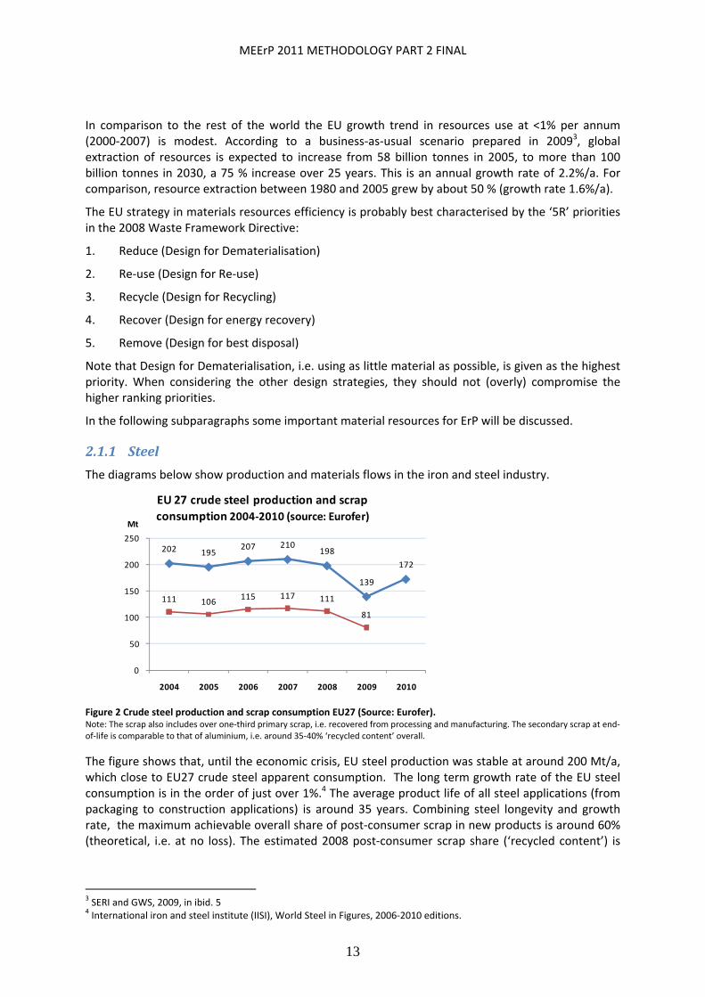
Figure 2 Crude steel production and scrap consumption EU27 (Source: Eurofer). Note: The scrap also includes over one‐third primary scrap, i.e. recovered from processing and manufacturing. The secondary scrap at end‐of‐life is comparable to that of aluminium, i.e. around 35‐40% ‘recycled content’ overall.
The figure shows that, until the economic crisis, EU steel production was stable at around 200 Mt/a, which close to EU27 crude steel apparent consumption. The long term growth rate of the EU steel consumption is in the order of just over 1%.4 The average product life of all steel applications (from packaging to construction applications) is around 35 years. Combining steel longevity and growth rate, the maximum achievable overall share of post‐consumer scrap in new products is around 60% (theoretical, i.e. at no loss). The estimated 2008 post‐consumer scrap share (‘recycled content’) is
3 SERI and GWS, 2009, in ibid. 5 4 International iron and steel institute (IISI), World Steel in Figures, 2006‐2010 editions.
MEErP 2011 METHODOLOGY PART 2 FINAL
14
around 40%, with the highest recycled content in iron castings, hot rolled and long products. Overall collection and recycling yield rates are relatively high (e.g. 70‐80% for end‐of‐life vehicles).
The figure 2 shows the use of recycled materials in steel production, including traded new scrap (production waste), which was 56% of production input in 2008. The EU27 is a net exporter (5 Mt/a) of steel scrap.
The overall EU‐27 steel trade is fairly balanced, with the EU producing and consuming around 15% of world steel (2008). With the rise of especially China this figure is diminishing; 10 years ago it was around 23%.
Raw materials for steel production (iron ore, coal, etc.) are not scarce. Import dependence for iron ore is 80% but not seen as critical, but some (micro‐) alloying elements like Cobalt, Nobium and Tungsten are part of the EU’s Critical Raw Materials list. Energy intensity per mass unit is moderate compared to its main competing materials in ErP (aluminium, plastics), but specific weight (in kg/dm³) is almost 3 times higher than aluminium and 7 times higher than plastics.
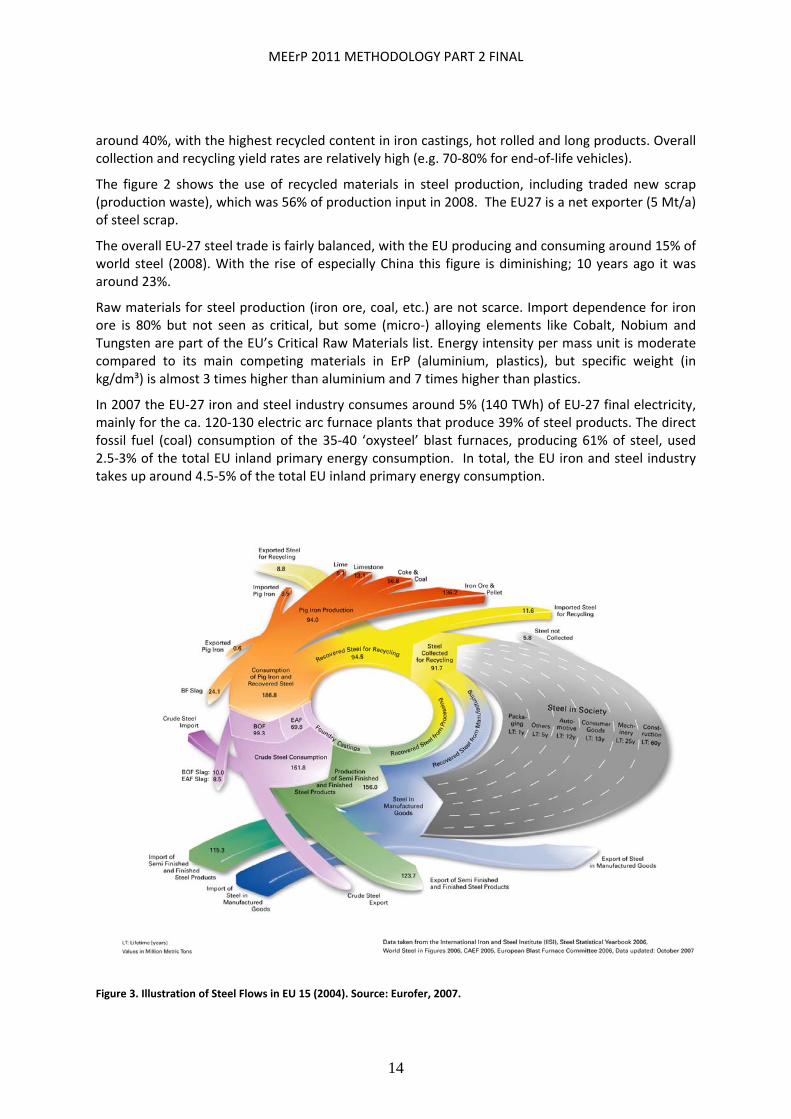
In 2007 the EU‐27 iron and steel industry consumes around 5% (140 TWh) of EU‐27 final electricity, mainly for the ca. 120‐130 electric arc furnace plants that produce 39% of steel products. The direct fossil fuel (coal) consumption of the 35‐40 ‘oxysteel’ blast furnaces, producing 61% of steel, used 2.5‐3% of the total EU inland primary energy consumption. In total, the EU iron and steel industry takes up around 4.5‐5% of the total EU inland primary energy consumption.
Figure 3. Illustration of Steel Flows in EU 15 (2004). Source: Eurofer, 2007.

MEErP 2011 METHODOLOGY PART 2 FINAL
15
2.1.2 Plastics
EU27 plastics demand in 2009 was 45 million tonnes (Mt), a drop of 7.2% with respect of 2008. The EU plastics industry is a net exporter of plastics at <1 Mt trade surplus. Important plastics applications are in short‐lived products like plastics. Post consumer waste was 24.3 Mt. Of this, 11.2 Mt were disposed of and 13.1 Mt recovered. Overall recovered quantity increased by 2.5% in 2009 over 2008. Mechanical recycling (grinding and re‐use in other products of e.g. PET bottles) increased by 3.1% because of stronger activities of some packaging collecting and recycling systems as well as through stronger exports outside of Europe for recycling purposes. Energy recovery (thermal recycling) increased 2.2% mainly because of stronger usage of post consumer plastic waste as alternative fuel in special power plants and cement kilns.
Figure 4 EU27 plastics use and end‐of‐life 2009 (source: PlasticsEurope, Plastics‐The Facts, 2010)
Figure 5. Europe Plastics Demand by Resin Types 2009 (Source: PlasticsEurope Market Research Group (PEMRG))
The main feedstock for plastics (oil) is relatively scarce, but feedstock applications are probably the last to survive because of the higher added value. Also, as practice shows in other continents (e.g. US) it is substitutable –at a price‐‐ by just about any hydrocarbon input. Energy‐intensity per mass unit is high, mainly (80‐90% with most bulkplastics) because of the calorific value of the feedstock,
PE‐LD: low density polyethylene PE‐LLD: linear low density PE‐HD: high density PP: polypropylene PVC: polyvinyl chloride PS: polystyrene (solid) PS‐E: polystyrene expandable (also EPS) PET: polyethylene terephthalate PUR: polyurethane
MEErP 2011 METHODOLOGY PART 2 FINAL
16
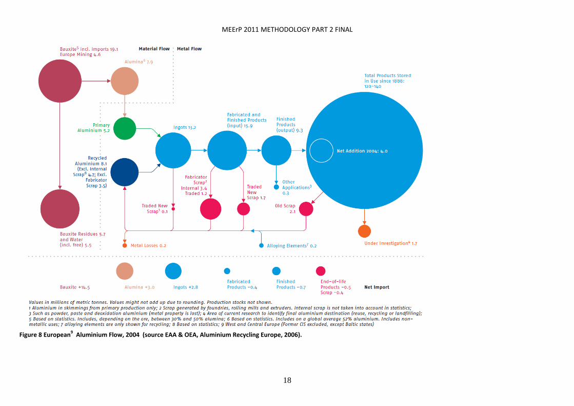
which in principle can be recovered. At a rough estimate of 50‐55 Mtoe net ‘energy’ use5 the 45 Mt plastics produced cost around 2% of EU inland primary energy consumption. At an overall average product life of 9‐10 years and a long term volume growth of over 4%/a, the annually disposed volume is 55% of produced input and thereby the –theoretical‐‐ maximum achievable post‐consumer recycling/recovery rate. As figure 8 shows, at the moment 13.1 Mt, i.e. 30% of consumption, is recycled or used for energy recovery. this means there is still a sizeable potential, but especially in non‐ErP (e.g. packaging and disposables).
2.1.3 Aluminium
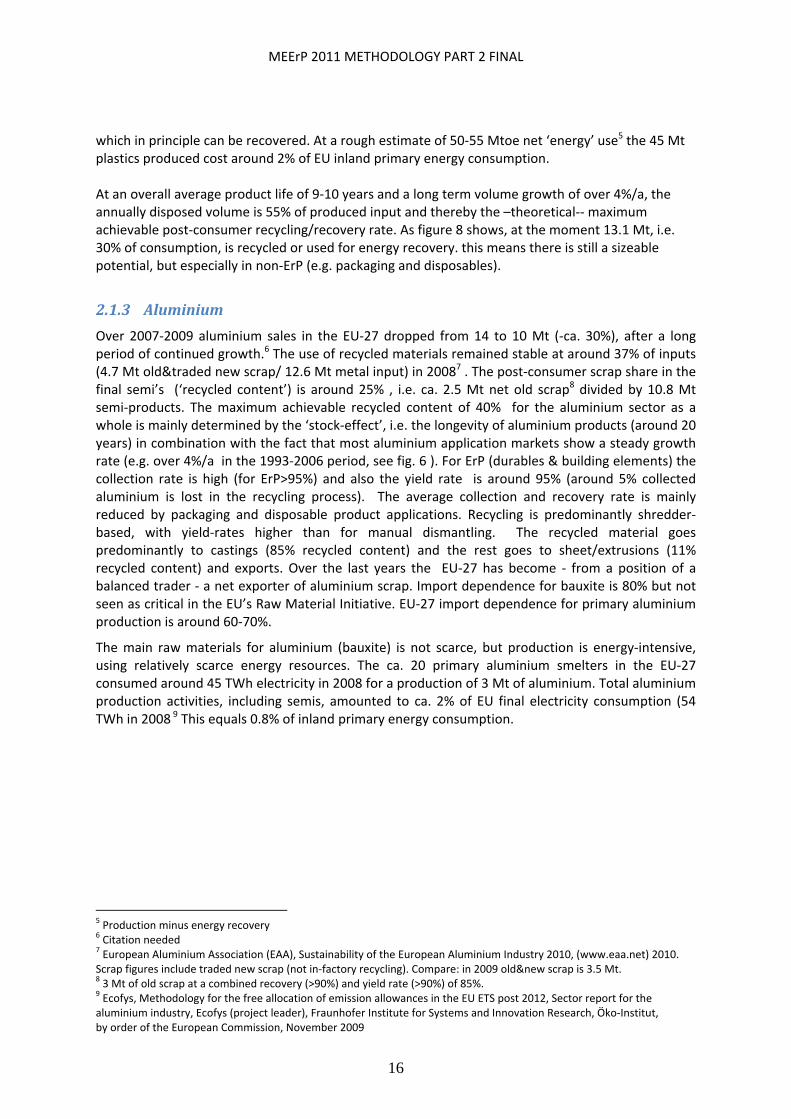
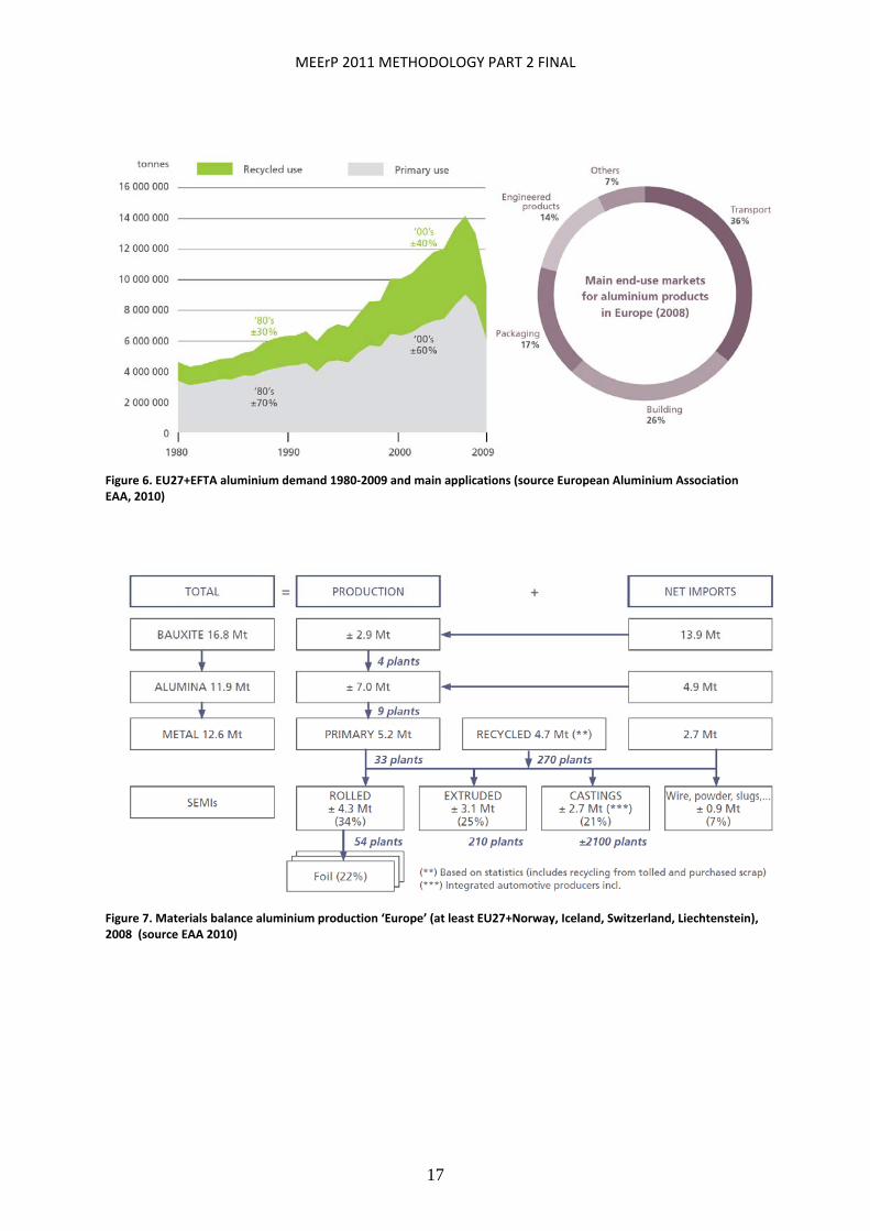
Over 2007‐2009 aluminium sales in the EU‐27 dropped from 14 to 10 Mt (‐ca. 30%), after a long period of continued growth.6 The use of recycled materials remained stable at around 37% of inputs (4.7 Mt old&traded new scrap/ 12.6 Mt metal input) in 20087 . The post‐consumer scrap share in the final semi’s (‘recycled content’) is around 25% , i.e. ca. 2.5 Mt net old scrap8 divided by 10.8 Mt semi‐products. The maximum achievable recycled content of 40% for the aluminium sector as a whole is mainly determined by the ‘stock‐effect’, i.e. the longevity of aluminium products (around 20 years) in combination with the fact that most aluminium application markets show a steady growth rate (e.g. over 4%/a in the 1993‐2006 period, see fig. 6 ). For ErP (durables & building elements) the collection rate is high (for ErP>95%) and also the yield rate is around 95% (around 5% collected aluminium is lost in the recycling process). The average collection and recovery rate is mainly reduced by packaging and disposable product applications. Recycling is predominantly shredder‐based, with yield‐rates higher than for manual dismantling. The recycled material goes predominantly to castings (85% recycled content) and the rest goes to sheet/extrusions (11% recycled content) and exports. Over the last years the EU‐27 has become ‐ from a position of a balanced trader ‐ a net exporter of aluminium scrap. Import dependence for bauxite is 80% but not seen as critical in the EU’s Raw Material Initiative. EU‐27 import dependence for primary aluminium production is around 60‐70%.
The main raw materials for aluminium (bauxite) is not scarce, but production is energy‐intensive, using relatively scarce energy resources. The ca. 20 primary aluminium smelters in the EU‐27 consumed around 45 TWh electricity in 2008 for a production of 3 Mt of aluminium. Total aluminium production activities, including semis, amounted to ca. 2% of EU final electricity consumption (54 TWh in 2008 9 This equals 0.8% of inland primary energy consumption.
5 Production minus energy recovery 6 Citation needed 7 European Aluminium Association (EAA), Sustainability of the European Aluminium Industry 2010, (www.eaa.net) 2010. Scrap figures include traded new scrap (not in‐factory recycling). Compare: in 2009 old&new scrap is 3.5 Mt. 8 3 Mt of old scrap at a combined recovery (>90%) and yield rate (>90%) of 85%. 9 Ecofys, Methodology for the free allocation of emission allowances in the EU ETS post 2012, Sector report for the aluminium industry, Ecofys (project leader), Fraunhofer Institute for Systems and Innovation Research, Öko‐Institut, by order of the European Commission, November 2009
MEErP 2011 METHODOLOGY PART 2 FINAL
17
Figure 6. EU27+EFTA aluminium demand 1980‐2009 and main applications (source European Aluminium Association EAA, 2010)
Figure 7. Materials balance aluminium production ‘Europe’ (at least EU27+Norway, Iceland, Switzerland, Liechtenstein), 2008 (source EAA 2010)
MEErP 2011 METHODOLOGY PART 2 FINAL
18
Figure 8 European9 Aluminium Flow, 2004 (source EAA & OEA, Aluminium Recycling Europe, 2006).
MEErP 2011 METHODOLOGY PART 2 FINAL
19
4.3.1CriticalRawMaterials
In February 2011 the European Commission published its communication on Critical Raw Materials.10 This communication proposed a list of 14 raw materials that are critical to the EU‐27 in the sense of
high import dependency (ratio of EU imports vs. consumption)
limited possibilities to find substitutes for the same or similar performance (“substitutability”)
no or very limited recycling rate (ratio of recycled old scrap vs. production)
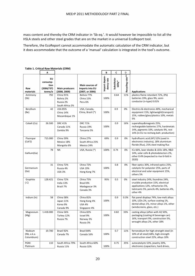
The table 1 below gives the list of 14 materials which are subject to a higher risk of supply interruption, the EU consumption (in metric tonne/a), the main global producing countries, the main sources of EU imports, the import dependency rate, the substitutability rate (0=easy substitution at no extra cost; 1=no of very difficult substitution possible), the ‘old scrap ‘recycling rate and finally the main (global) applications.
The strategy proposed in the aforementioned Commission communication rests on three pillars:
Fair and sustainable supply of raw materials from global markets,
Fostering sustainable supply within the EU and
Boost resources efficiency and recycling
For the latter two pillars the MEErP proposes an easy to use quantitative indicator that uses the multiplication of EU consumption (Table 1, column [A]), import dependency (column [B]), substitutability (column [C]) and the complement of the recycling rate (1 – [D]).
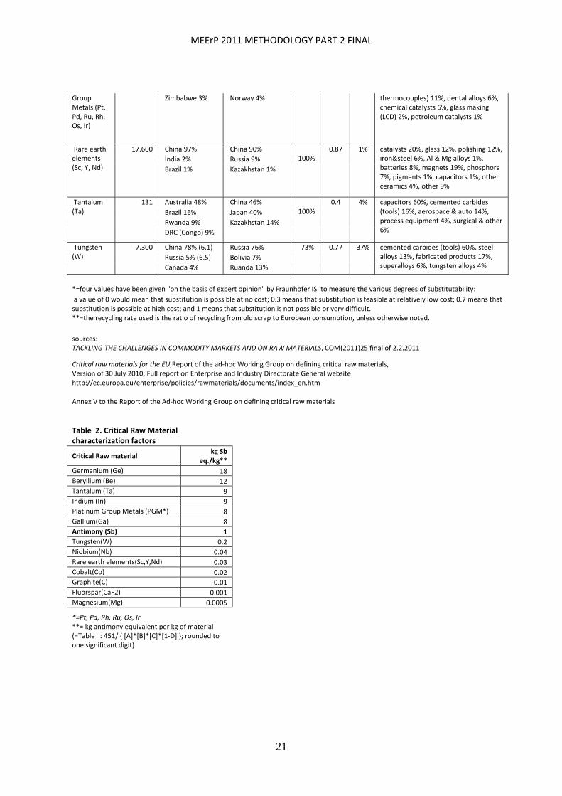
The outcome is then set against the outcome of this multiplication for one reference material, i.e. antimony (Sb), which is de number 792*100%*0.64*(1‐11%)= 451 t. The accounting unit is ‘kg Sb equivalent’ per kg CRM (cf. ‘CO2 equivalent’ for GHG emissions). The formula is
kg Sb equivalent per kg CRM = 451 / {[A]*[B]*[C]*(1‐[D])}
where [A], {B], [C], [D] refer to the numbers in columns A, B, C, D in Table 1.
For instance, for Germanium the CRM characterization factor is 18 kg Sb equivalent per kg of Germanium. The total EU‐27 consumption of CRMs is 3.450 t Sb eq..
A full overview of the CRM characterization factors is given in Table 2.
Every material or process can be characterized by their CRM indicator. In theory, it could be used directly in the EcoReport tool (presented in Chapter 5), but a closer study of the application shows that there are some practical problems in doing that at this moment. Most CRM, except perhaps Magnesium, are used not as single construction materials to build parts and components, but they are alloying elements, additives, coatings, agents, etc. used in miniscule fractions of (or for the production of) the main materials like steel, aluminium and plastics. Hence, a very comprehensive large list of variations (over 100 steel grades, alloys, plastic mixes) of these main materials would be required to capture the CRM indicator.
To realize this on a structural and universal basis is not (yet) possible. However, it should be possible to do this ‘manually’ on an ad‐hoc basis, i.e. once a product group is known and once the specific alloys in a Bill‐of‐Materials have been identified. For instance, once it is known that a specific grade of HSLA11 steel is used in a product’s Bill of Materials it is relatively easy to establish the Niobium‐
10 TACKLING THE CHALLENGES IN COMMODITY MARKETS AND ON RAW MATERIALS, COM(2011)25 final of 2.2.2011 11 HSLA= High Strength – Low Alloy steel. Niobium mass is usually in the range of 0‐2 mg per kg HSLA steel.
MEErP 2011 METHODOLOGY PART 2 FINAL
20
mass content and thereby the CRM indicator in ‘Sb eq.’. It would however be impossible to list all the HSLA steels and other steel grades that are on the market in a universal EcoReport tool.
Therefore, the EcoReport cannot accommodate the automatic calculation of the CRM indicator, but it does accommodate that the outcome of a ‘manual’ calculation is integrated in the tool’s outcome.
Table 1. Critical Raw Materials (CRM)
A B C D
Raw materials
EU consump‐
tion (2006/'07) tonne/a
Main producers (2008, 2009)
Main sources of imports into EU (2007, or 2006) Im
port depen‐
dency rate
Substituta‐
bility*
Recycling rate**
Applications
Antimony (Sb)
792 China 91% Bolivia 77% 100%
0.64 11% plastics flame retardant 72%, (Pb) batteries 19%, glass 9%, semi‐conductor (n‐type) 0.01%
Bolivia 2% China 15%
Russia 2% Peru 6%
South Africa 2%
Beryllium (Be)
42 USA 85% USA, Canada, China, Brazil (*) 100%
0.9 0% Electrics & electronics 40%, mechanical equipment 15%, lightweight(transport) 15%, rubber/glass/plastics 10%, metals 5%
China 14%
Mozambique 1%
Cobalt (Co) 26.500 DRC 41% DRC 71% 100%
0.9 16% superalloys&magnets 25%, rechargeable batteries 27%, hardmetals 14%, pigments 10%, catalysts 9%, rest 14% (in EU no recharg.batt. production)
Canada 11% Russia 19%
Zambia 9% Tanzania 5%
Fluorspar (CaF2)
715.000 China 59% China 27% 69% 0.9 0% hydrofluoric acid (HF) 52% (used in electronics industry), 18% aluminium floride (flux), 25% steel making flux
Mexico 18% South Africa 25%
Mongolia 6% Mexico 24%
Gallium(Ga)
78 NA USA, Russia (*) 100% 0.74 0% ICs 66%, laser diodes & LEDs 18%, R&D 14%, solar cells & photodetectors 2%, other 0.4% (expected to rise 6‐fold in 2020)
Germanium (Ge)
31 China 72% China 72% 100%
0.8 0% fiber optics 30%, infrared optics 25%, catalysts for polyester 25%, parts of electrical and solar equipment 15%, others 5%
Russia 4% USA 19%
USA 3% Hong Kong 7%
Graphite ( C)
128.421 China 72% China 75% 95% 0.5 0% steel industry 24%, foundries 24%, crucible production 15%, electrical applications 12%, refractories 5%, lubricants 5%, pencils 4%, batteries 4%, other 4%
India 13% Brazil 8%
Brazil 7% Madagascar 3%
Canada 3%
Indium (In) 58 China 58% China 81% 100%
0.9 0.3% flat panel displays 74%, low‐melt alloys 10%, LEDs 2%, surface coating 1%, dental alloys 1%, minor alloys 1%, other (windscreens, glass, etc.)
Japan 11% Hong Kong 4%
Korea 9% USA 4%
Canada 9% Singapore 4%
Magnesium (Mg)
1.418.000 China 56% China 82% 100%
0.82 33% casting alloys (often with Al) 50%, packaging (coating Al beverage can) 16%, transport 9%, construction 5%, wrought alloys 2%, other 18%
Turkey 12% Israel 9%
Russia 7% Norway 3%
Russia 3%
Niobium (Nb, a.k.a. Columbium)
19.700 Brazil 92% Brazil 84% 100%
0.7 11% ferronobium for high‐strength steel (in 10% of all steel) 68%, high‐strength construction steel 22%, alloys 10%
Canada 7% Canada 16%
PGM: Platinum
110 South Africa 79% South Africa 60% 100%
0.75 35% autocatalysts 53%, jewelry 20%, electronics (capacitors, hard drives, Russia 11% Russia 32%
MEErP 2011 METHODOLOGY PART 2 FINAL
21
Group Metals (Pt, Pd, Ru, Rh, Os, Ir)
Zimbabwe 3% Norway 4% thermocouples) 11%, dental alloys 6%, chemical catalysts 6%, glass making (LCD) 2%, petroleum catalysts 1%
Rare earth elements (Sc, Y, Nd)
17.600 China 97% China 90% 100%
0.87 1% catalysts 20%, glass 12%, polishing 12%, iron&steel 6%, Al & Mg alloys 1%, batteries 8%, magnets 19%, phosphors 7%, pigments 1%, capacitors 1%, other ceramics 4%, other 9%
India 2% Russia 9%
Brazil 1% Kazakhstan 1%
Tantalum (Ta)
131 Australia 48% China 46% 100%
0.4 4% capacitors 60%, cemented carbides (tools) 16%, aerospace & auto 14%, process equipment 4%, surgical & other 6%
Brazil 16% Japan 40%
Rwanda 9% Kazakhstan 14%
DRC (Congo) 9%
Tungsten (W)
7.300 China 78% (6.1) Russia 76% 73% 0.77 37% cemented carbides (tools) 60%, steel alloys 13%, fabricated products 17%, superalloys 6%, tungsten alloys 4%
Russia 5% (6.5) Bolivia 7%
Canada 4% Ruanda 13%
*=four values have been given "on the basis of expert opinion" by Fraunhofer ISI to measure the various degrees of substitutability:
a value of 0 would mean that substitution is possible at no cost; 0.3 means that substitution is feasible at relatively low cost; 0.7 means that substitution is possible at high cost; and 1 means that substitution is not possible or very difficult. **=the recycling rate used is the ratio of recycling from old scrap to European consumption, unless otherwise noted.
sources: TACKLING THE CHALLENGES IN COMMODITY MARKETS AND ON RAW MATERIALS, COM(2011)25 final of 2.2.2011
Critical raw materials for the EU,Report of the ad‐hoc Working Group on defining critical raw materials, Version of 30 July 2010; Full report on Enterprise and Industry Directorate General websitehttp://ec.europa.eu/enterprise/policies/rawmaterials/documents/index_en.htm
Annex V to the Report of the Ad‐hoc Working Group on defining critical raw materials
Table 2. Critical Raw Material characterization factors
Critical Raw material kg Sb
eq./kg**
Germanium (Ge) 18
Beryllium (Be) 12
Tantalum (Ta) 9
Indium (In) 9
Platinum Group Metals (PGM*) 8
Gallium(Ga) 8
Antimony (Sb) 1
Tungsten(W) 0.2
Niobium(Nb) 0.04
Rare earth elements(Sc,Y,Nd) 0.03
Cobalt(Co) 0.02
Graphite(C) 0.01
Fluorspar(CaF2) 0.001
Magnesium(Mg) 0.0005
*=Pt, Pd, Rh, Ru, Os, Ir **= kg antimony equivalent per kg of material (=Table : 451/ { [A]*[B]*[C]*[1‐D] }; rounded to one significant digit)

MEErP 2011 METHODOLOGY PART 2 FINAL
22
Figure 9. Production concentration of the ‘critical’ raw materials by source country (source: EC, DG ENTR)
Material flow indicators have been assessed in all Ecodesign studies, but have so far not been found significant enough, in terms of potential, to be singled out for Ecodesign studies.

MEErP 2011 METHODOLOGY PART 2 FINAL
23
2.2 RecyclingThe accounting of recycling and of the end‐of‐life (EoL) stage in general, can be very complex. There are several specific ‘mechanisms’ that play a role, which are not always self‐evident and there are several possible routes to arrive at quantitative data, often poorly documented. This paragraph, which is an extension of the ‘Materials’ and ‘Waste’ paragraph, tries to shed some light on the situation. The final part will re‐iterate some of the methodological aspects that, although unproblematic during the preparatory studies in the last 6 years, have proven to be controversial with stakeholders reacting to the questionnaire (see MEErP 2011 Project Report).
Q1: Why is there a theoretical maximum recycling percentage for materials/products?
A1: Because, at any time, you cannot recycle more than is discarded. And how much is discarded depends on the variation in the “stock” of products that are in use. In principle, there are three situations:
the demand for a product is stable over time. In that case people throw away roughly the same quantity that they buy. The post‐consumer recycling rate can be (close to) 100%.
the demand for a product is decreasing over time. In that case, people throw away more than they buy. The post‐consumer recycling rate can be 100% and some products will have to be disposed off. There is still a large stock of products in use, but when people throw it away to buy a replacement, an increasing share of people does not buy that product anymore presumably because there is a better alternative or (e.g. example of lead) it is forbidden in new products.
the demand for a product is increasing over time. In that case people throw away less than they buy. Or rather, at any point in time, there will be more people buying a product than people, who bought the product years ago, throwing it away.
When talking about materials, e.g. metals, 90% of the products ‐ except those heavy metals that are forbidden ‐ will be in the last category. Population is growing, building stock is growing, economies are usually growing and therefore also the demand/consumption of steel, plastics and aluminium is growing.
In that case there are more new products than products thrown away, i.e. there is less material to recycle than there is material sold. How much this is depends on a) the product life L and b) the growth rate of the consumption r, in a correlation
Maximum post‐consumer recycling rate= 1 / (1+r)L
The longer the product life and/or the higher the annual growth rate, the lower will be the abovementioned maximum recycling rate. E.g. for food packaging and disposables, the maximum recycling rate will be close to 100% because the product‐life is a matter of a few weeks. For building elements that are in use 40‐60 years, the maximum possible post‐consumer recycling rate will be very low, even if the annual growth rate is low. E.g. at a 1% growth rate, the maximum recycling rate at any time is 60%; at 4% it will only be 15%.

MEErP 2011 METHODOLOGY PART 2 FINAL
24
The table below gives a first estimate of maximum recycling percentages of all steel, aluminium and plastics application based on historical growth rates.12 Figure 10 is a reality check, showing the distribution of post‐consumer plastics waste.
At this point it is important to make a distinction between an analytical context and a regulatory context. In the analytical context, the stock effect is a real effect and should therefore be taken into account in determining how much the recycling of a material could contribute to realizing a quantitative policy goal (e.g. meet ‘2020’/Kyoto/Stockholm/Gothenburg etc. targets). In a regulatory context it may be decided, because the absolute amount of the discarded material is interesting enough to take into account, that specific Ecodesign measures promoting recycling are worthwhile to be implemented. These are two different things.
Figure 10. Generation of post‐consumer plastics waste by application, EU‐27, 2008
Source: European Plastics Recyclers Association (EuPR), How to increase the mechanical recycling of post‐consumer plastics, strategy paper, Feb. 2010.
Note: Comparing this End‐of‐Life output with the converter input (Figure 6) clearly shows the influence of the stock‐effect on the waste streams. E.g. packaging is 40% of input, but 63% of post consumer waste. Building & Construction products (B&C) are 20% of input and 6% of waste output. Overall, ErP can mainly be found in E&E (5%) and part of B&C. In total, ErP will represent <10% of the plastics waste stream. Total waste in 2008 was 24.9 Mt.
12 The analysis is illustrative. In a more refined analysis growth rates can be differentiatet per market segment and projected future growth rates play a role.

MEErP 2011 METHODOLOGY PART 2 FINAL
25
Table 3 . Stock effect: Calculated post‐consumer waste for steel, plastics, aluminium (2005‐2007, EU27)
STEEL annual growth rate r=1.3%, product life 34.4 years
life L in years
crude steel production
post consumer
waste*
scrap pro‐duc‐
tion**
scrap purchased by steel‐works***
export balance
avg. 34.4 yr 100% 66% 45% 42% 3%
Mt 210 132 93.5 88 5.5
construction 60 38% 26%
shipyards 40 1% 1%
tubes 30 12% 12%
machinery 25 14% 15%
consumer goods 13 4% 5%
metal goods 13 12% 15%
automotive 12 16% 21%
others 5 2% 3%
packaging 1 1% 1%
*=calculated with waste=1/(r^L), where r is annual growth rate and L is product life in years
**=steel purchase steelworks (incl. imports) 88 minus 5.1 import plus 10.6 Mt export
*= incl. imports
PLASTICS annual growth rate r=4.5%, product life 9.5 years
life L in years
plastics production
post consumer
waste* recyc‐ling
energy recovery disposal
avg. 9.5 yr 100% 54% 12% 17% 25%
Mt (weight) 45 24.3 5.5 7.6 11.2
construction 30 20% 6%
transport 12 7% 5%
engineered products 13 6% 5%
others 5 22‐27% 21‐26%
packaging 1 40‐50% 58‐63%
*=calculated with waste=1/(r^L), where r is annual growth rate and L is product life in years
but also checked against EuPR post consumer waste data 2010. Where there is a difference
data and calculation this is indicated by a range
ALUMINIUM annual growth rate r=4.2%, product life 19.7 years
life L in years
aluminium semi
production
post consumer
waste* recyc‐ling
export balance disposal
avg. 19.7 yr 100% 44% 28% 16%
Mt (weight) 11 4.8 3.1 0.7 1.7
construction 50 26% 6%
transport 12 36% 40%
engineered products 13 14% 15%
others 5 7% 10%
packaging 1 17% 29%
*=calculated with waste=1/(r^L), where r is annual growth rate and L is product life in years
Sources: EFR (org. sources: IISI, Eurofer, Statistics Bureau Germany), PlasticsEurope, EuPR, EAA.
MEErP 2011 METHODOLOGY PART 2 FINAL
26
Q2: What is the difference between ‘recycled content’ and ‘recyclability’ and what are the results of using one or the other as a basis for the analysis of resources use and emissions?
A2: ‘Recycled content’ is the materials fraction of a product or component that is produced from recycled material. It is based on the actual physical resources flows (materials, energy) taking place in society and thus is bound by the condition that ‐ at any moment in time ‐ a large amount of that material is in use, with a stock increasing in time. As such it is limited by the boundaries sketched above (e.g. max. 40% recycled content for aluminium).
‘Recyclability’ is the materials fraction of a product or component that potentially –from a technical viewpoint‐‐ could be recycled. For most metals, after deduction of alimited fraction that is unavoidably discarded, this fraction will be around 70‐90% because technically recycling will always be possible, i.e. without specific design measures. The ‘recyclability’ approach does no take into account the stock‐effect.
‘Recyclability’ places the recycling credit with the product that can be recycled, not with the product that actually uses the recycled material as an input. Within the ‘recyclability‐accounting’ there are two ‘schools’: Some actors take into account both the recycled content and recyclability credit. The World Business Council for Sustainable Development (WBCSD), laying down accounting rules for environmental business reports, excludes this practice and proposes to use ‘recycled content’ (a.k.a. ‘100/0 Input Method’) as a default method for product LCAs but allows ‘recyclability’ (a.k.a. ‘0/100 Output Method’) under certain conditions. But in case of the latter, the accounting of the production phase starts from the impacts of the virgin material (i.e. without recycled content), to avoid double counting.
Note that, if the WBSCD approach would also include the stock‐effect, the outcomes could be comparable to those of the strict ‘recycled content’ approach.
The LCA standard ISO 14040 allows all methods, depending on the application.Note that the ‘recyclability’ approach goes by many names: ‘substitution method’, ‘expansion method’ and ‐ in the variation of the WBCSD ‐ the ‘0/100 Output Method’.
The results of a ‘recyclability’ approach would be, for example that aluminium or copper electric wire, which for functional reasons have to be 99.9999% pure, will have 80% recyclability with almost 0% recycled content. Following this reasoning, the energy impacts of this wire should also calculate 20% of the impacts based on virgin materials and 80% from recycling processes.
Castings, using alloys and being very tolerant to impurities (helps with casting process) will have a lower recyclability score, but are made from 80% recycled material.
Likewise with plastics: Products made from recycled plastics will have a lower ‘recyclability’ percentage than products made from virgin material, because the latter will be better to recycle. So instead of having a better environmental impact score, the ‘recyclability criterion’ will cause recycled products to have a worse environmental score.
Although the ‘recyclability’ approach or similar may have merits in a regulatory context, in an analytical context like MEErP 2011 ‐ looking at the possible contribution of recycling to quantitative policy goals ‐ it is not deemed suitable. MEErP does however, in order to promote the chances of post‐consumer waste to be recycled for more upmarket applications, give a credit to the ease of pre‐ disassembly (expressed in product‐specific disassembly time) of critical parts and/or larger metal parts before they enter shredder‐based recycling process.

MEErP 2011 METHODOLOGY PART 2 FINAL
27
Q3: What is the difference between old and new scrap, and how does it affect the recycling percentage?
A3: When the industry publishes recycling figures they usually relate to the amount of ‘old scrap’ plus ‘new scrap’13 divided by the amount of new products sold. As figure 12 shows, the new scrap is approximately over 35‐40%14 of the total scrap being recycled. If the recycling percentage relates only to old scrap then it is more like 25%, so there is still some (small) margin for improvement.
‘New scrap’ (a.k.a. ‘primary scrap’) is material that is lost during the fabrication of semi‐finished products (rolled sheet, extrusions, castings, etc.) and finished products (e.g. metalwork products). It is brought to the internal furnace (fabricator scrap) or to an external smelter (traded scrap) and recycled within a matter of minutes/hours (when inside the same factory; the so‐called ‘run‐around‐scrap’) or at the most weeks (when collected and transported to the smelting plant). It is relatively uncontaminated and pure material that can be re‐used with little or no pre‐treatment.
Although it boosts the recycling figure, having a lot of ‘new scrap’ is ecologically and economically ‘Not A Good Thing’. It indicates an inefficient production and/or product design that causes a large amount of avoidable waste. It may be relatively low‐cost , also in terms of energy, to recycle that waste (around 5% of energy when compared to the virgin material) but still it is better avoided.
Q4: Does the MEErP discriminate metals against plastics in terms of recycling credits?
A4: In principle, it does not. Both plastics and metals get the recycling credit that fits the actual materials flows (the ‘recycled content’, see above). For aluminium it is assumed that 85‐90% of scrap is recycled, independently of how it is designed. Taking into account the stock‐effect (see earlier) this then results in an overall share of 30% recycled post‐consumer scrap material in aluminium products. This credit is taken into account in the production impacts of the aluminium half‐products (sheet, extrusion profiles, diecasts) in accordance with the current routes. In the case of aluminium, the partitioning between the half‐products is not evenly distributed (not every half‐product gets 30% recycled content), because it is economically most advantageous to use more recycled material in the half‐product that is the least critical for contamination, i.e. the diecasts. For instance, as can be seen in Figure 7, the total mass of aluminium halfproducts sold is ca. 10.2 Mt, of which 2.7 Mt diecasts, 7.4 Mt extrusion+ sheet and 0.9 Mt of other applications. In MEErP we assume that the recycled content of the diecasts is 85%, which comes down to 2.3 Mt. For extrusion+sheet this is 11% and thus 0.8 Mt. In total the recycled mass is thus 3.1 Mt or around 30% of all aluminium sold.The fact that there is no ‘closed loop’ but that the recycled material goes to the application which is economically the most advantageous can be interpreted as ‘downcycling’ (degradation), but it should be seen not as a technical degradation, but the causes are economical. For plastics, it is assumed that the production impacts are based on virgin material (no recycling credit up front), but the person in charge of the preparatory study is required to assess which fractions go to re‐use, recycling, energy recovery, incineration of hazardous substances (no recovery) and landfill.
On this basis, and unit indicators for each route, the recycling credits will have to be ‘earned’ for the plastics fraction. The unit indicators give e.g. a credit of 75% of the feedstock energy & GWP value for energy recovery. For re‐use the credit is 75% of all the plastics production impacts, because it is assumed that collection and cleaning will take its toll. For materials recycling there is a fixed credit of
13 Terminology: Old scrap, secondary scrap and End‐of‐Life scrap all refer to the same thing. New scrap, primary scrap and production scrap are also synonymous. 14 As mentioned in figure 12, the internal and fabricator scrap are usually not taken into account in the statistics. The amount of ‘new scrap’ relates to the ‘Traded New Scrap’ from ingots (0.1 Mt) and Fabricated and Finished Products (Input) (1.7 Mt). The Old Scrap is at least 2.1 Mt but if half of the scrap ‘Under Investigation’ turns out to be recycled this would add an extra 0.8 Mt.

MEErP 2011 METHODOLOGY PART 2 FINAL
28
27 MJ (displaces wood) + 50% of feedstock energy & GWP of plastics (for energy recovery after re‐use). Note that also here there is a –both technically and economically determined—‘downcycling’, i.e. the plastics are not used to produce the same type of product, but in fact are used in applications where they displace wood (e.g. in park benches).
As mentioned in Q1 and Q5, with the extension to ErP and especially the building products the maximum recycle/re‐use/recovery percentage will now also be limited by the stock‐effect.
What has been signalled in former MEEuP 2005 report as a subject for further investigation is the high percentage of thermal heat recovery for plastic assumed in former MEEuP.15 In the EuP studied this far it would not have made a noticeable difference, but with the extension to ErP and especially the building products (e.g. plastic window frames) this subject should be re‐visited (see next Q&A).
Q5: What lessons are learned and what improvements can be made in the EcoReport tool for recycling and End‐of‐Life?
A5: From the past Ecodesign studies it is learned that very few new, product‐specific data are introduced in the EcoReport 2005 tool for the EoL phase. And in the absence of real data, the default values ‐ i.e. the values given at the opening of the spreadsheet file ‐ are not changed, despite the fact that persons in charge of the preparatory studies would have the option to do so. These default values are based primarily on the use of plastics in the product packaging (e.g. EPS), consumables (e.g. cartridges) and components of products with a relatively short product‐life (e.g. casings of computer equipment with life <6 years) and show 1% for re‐use, 9% for materials recycling and 90% for thermal heat recovery. These values16 do not assume any noticeable stock‐effect.
In the EuP preparatory studies so far, with a low fraction plastics in the bill‐of‐materials and a dominance of the use phase, the lack of a stock effect would hardly have been noticeable in the analysis and most certainly not in the design of subsequent measures.
However, with the addition of ErP, the stock effect ‐ i.e. a permanent fraction of products in use and thus not available for any sort of re‐use, recycling or heat recovery ‐ should be taken into account. To accommodate this, a new line with a 40% percentage for the stock effect is introduced. In principle, as with metals, this percentage should not be changed. The maximum possible thermal recovery will be calculated as the remainder of 100% minus re‐use minus materials recycling minus the stock effect.
Q6: When is re‐use important?
A6: Special attention should be given to re‐use/ re‐manufacturing of consumables (filters, bags, ink cartridges, disposable or non‐disposable cups, medical disposables when related to ErP, etc.) Projects with ink cartridges and medical instruments show a high potential of both monetary and ecological savings of up to 50%.17
Having said that, for the energy‐related products –especially those with long product life—the same caution applies for a design strategy of re‐use as applies for a design‐strategy of prolonging the product life (see MEErP Methodology Report, Part 1). In fact, re‐use is a way of prolonging product service life and thus it causes a larger inertia which could be disadvantageous when the resources efficiency or emissions during the use phase of new products on the market improves rapidly.
Q7: What is the role of ‘Design for Disassembly’ (DfDis)?
15 VHK MEEuP 2005 (pp. 41): “…Rolf Frischknecht, mentions that the energy recovery of plastics is much lower than the MEEuP estimate of 75% of the combustion value. Allegedly no more 25‐30% of the combustion value is recovered (data CH). This subject needs further investigation.” 16 This was already signaled in the MEEuP 2005 report by one of the reviewer but left for a review, e.g. now. 17 Pers. comm.. Michael Gell, May 2011.
MEErP 2011 METHODOLOGY PART 2 FINAL
29
A7: This aspect has been extensively discussed in the former MEEuP 2005 report. Basically, after separation of the electronics and hazardous substances (e.g. refrigerants), for which an extra DfDis credit is given in the EcoReport tool, it is assumed that the rest of the recycling is shredder‐based. This is also in line with the findings of JRC‐IPTS on End of Life Materials18. With this route, there is limited merit in the ‘classic’ DfDis actions that were relevant to the manual dismantling in the 1980’s. What is included in MEErP 2011 is a test (yes/no) whether the pre‐shredder disassembly time of refrigerants, electronics board, batteries and LCD screens and possibly other large components of interest (e.g. glass shelves in a fridge, stainless steel drum, copper tank, etc.) meets a minimum target that is found appropriate in the preparatory study.
Note that technical design measures for ‘Design for Disassembly” or ‘Design for Recycling’, like extra knock‐outs, mono‐materials, are often in contrast with ‘Design for Dematerialisation’, i.e. lightweight through integrated constructions, composite and sandwhich materials, etc.. In the MEErP 2011 analysis, applying the correct inputs, this effect is calculated and ‐ from experience ‐ most often the ‘Design for Dematerialisation’ strategy will be found to be dominant.
Q8: What is the difference between ‘closed loop’ and ‘open loop’ recycling and how is it relevant in the recycling discussion?
A8: ‘Closed loop’ recycling relates to the concept that the discarded material of a product can be used to make exactly that same product, i.e. that no degeneration of the material’s characteristics takes place. ‘Open loop’ recycling relates to the concept that degeneration of the material does take place and therefore the recycled material cannot be used to produce exactly the same product, but instead is used in products that are less critical to the degeneration that took place.
Both concepts are theoretical and stem from the very beginning of LCA analysis in the 1970’s. They are still being cited in LCA‐standards like ISO 14040, which takes a neutral stand as regards which concept should be used and when (it depends.). The relevance of the closed or open loop concept is limited, because basically it refers to the technical feasibility of full recycling or not. Today, it is widely recognized that the technical feasibility is not really the limiting factor, but economical considerations dominate the choice in which products the recycled scrap will be used. And from that perspective it is usually easy to see that e.g. secondary scrap will be used in the applications that are least critical to contamination in terms of material characteristics and production. In that sense it is irrelevant whether it is technically possible to remove all contamination from the use phase, because that is only going to happen if the market for this least critical application ‐ for metals these are usually castings ‐ is too small to receive all the available scrap.
Note that in some LCA literature, ‘closed loop (recycling)’ is also used to indicate the recycled content and ‘open loop (recycling)’ is used to indicate a fraction that is not recycled but also not disposed off (e.g. fraction used for energy recovery). In the EcoReport 2011, the term is ‘closed loop recycling’ is used in that sense for end‐of‐life plastics.
Q9: Why does the EcoReport table provide the impacts (energy, GWP, etc.) of metal production at the level of half‐products (‘semis’) and not as the raw material?
A9: The EcoReport was conceived to show designers and policy makers in the simplest possible way the impacts of parameters that they can hope to influence through product design. The selection, not only of a metal but also of a specific half‐product, is such a choice. But the percentage of ‘recycled content’ of that half‐product is typically not such a choice. The designer determines the geometry, the
18 JRC‐IPTS, End of Waste criteria, Ispra, 2008. http://susproc.jrc.ec.europa.eu/activities/waste/documents/Endofwastecriteriafinal.pdf
MEErP 2011 METHODOLOGY PART 2 FINAL
30
chemical‐physical properties of the product, the production technology and the way a product is used. He or she does not determine how a supplier gets there. It would add unnecessary complexity to the tool and possibly open discussions on items that anyway could not be translated in Ecodesign measures.
The added advantage of taken ‘semis’ as the basis for the LCIA table in Chapter 5 is that it keeps the EoL analysis of metals simple and makes sure that, in spite of the fact that each of the studies treat individual products, the correct overall accounting stays valid. When summing all use of metals in individual products the total amounts of virgin and secondary materials are still in the domain of what is physically possible.
Recycling and recovery indicators have been assessed in all Ecodesign studies, but have so far not been found significant enough, in terms of potential, to be singled out for Ecodesign studies.

MEErP 2011 METHODOLOGY PART 2 FINAL
31
2.3 Energy
2.3.1 Energypolicy
The Energy Policy for Europe, agreed by the European Council in March 2007119, establishes the
Union’s core energy policy objectives of competitiveness, sustainability and security of supply. The internal energy market has to be completed in the coming years and by 2020 renewable sources have to contribute 20% to our gross final energy consumption, greenhouse gas emissions have to fall by 20%2 and energy efficiency gains have to deliver 20% savings in energy consumption with respect of 1990.
This has recently been confirmed by the Commission, embedding these medium‐term targets in the
communication on the Resource‐efficient Europe – Flagship initiative20. Furthermore, the
communication mentions 2050 carbon targets of 80‐95% reduction on carbon emissions with respect of 2005. This should take care of the EU‐share in keeping global warming below 2°C, whereas with current policy science predicts that the average temperature might rise by as much as 4°C by 2100.
Figure 11. Temperature deviation, compared to the 1850‐1899 average (source: EEA 2010)
19 Presidency conclusions, European Council, March 2007 20 A resource‐efficient Europe – Flagship initiative under the Europe 2020 Strategy, EC, 26.1.2011, COM(2011) 21
MEErP 2011 METHODOLOGY PART 2 FINAL
32
The Energy 2020 strategy paper calls for a step change in order to reach these objectives. On the basis of the National Renewable Energy Action Plans (NREAPs) of the Member States the paper is optimistic that the renewable target will be achieved, but calls the quality of the National Energy Efficiency Action Plans (NEEAPs) ‘disappointing’ and is not confident that the 20% energy efficiency improvement target will be met in 2020. 21
At the end of 2010 and at the beginning of 2011 the Commission published a number of operational papers with measures that should contribute to achieving the objectives:
Energy efficiency
The Energy Efficiency Plan 201122 lists recent and imminent legislative measures, such as the (recasts of) directives for ecodesign of energy‐related products (‘Ecodesign’)23, energy labeling24, energy performance of buildings (EPBD)25, energy services (ESD)26. At Member State level the plan announces an extended set‐up ‐ under the ESD ‐ of the national energy efficiency action plans NEEAPs, including also non end‐use sectors. Public authorities will be required to refurbish at least 3% of their buildings (by floor area) each year –about twice the going rate for the building stock. Each refurbishment should bring the building up to the level of the best 10% of the national building stock.27 Public services should only buy or rent buildings with best available energy performance. Under the European Energy Star Programme, central government authorities of Member States and EU institutions are obliged to procure equipment not less efficient than Energy Star. 28 Member States are obliged to roll out smart electricity meters for at least 80% of their final consumers by 2020 provided this is supported by a favourable national cost‐benefit analysis. The Commission is launching the 'BUILD UP Skills: Sustainable Building Workforce Initiative' to support Member States in providing appropriate training of building professionals, especially installers. It mentions that today (2011) about 1.1 million qualified workers are available, while it is estimated that 2.5 million will be needed by 2015. The ICT sector has been invited to contribute to the efficiency improvement and carbon reduction effort in the context of the Digital Agenda.29 Other upcoming actions include the launch of the Smart Cities and Smart Communities initiative as well as EU‐support for the Covenant of Mayors.30 Emissions Trading31 , the Energy Taxation Directive32, the CHP directive33, as well as the new Industrial Emissions Directive34 are seen as catalysts for the realization of new power capacity with
21 A Roadmap for moving to a competitive low carbon economy in 2050, EC, 8.3.2011, COM(2011) 112 final
22 Energy Efficiency Plan 2011, EC, 8.3.2011, COM(2011) 109 final 23 Directive 2009/125/EC OF THE EUROPEAN PARLIAMENT AND OF THE COUNCIL of 21 October 2009 establishing a framework for the setting of ecodesign requirements for energy‐related products 24 Directive 2010/30/EC OF THE EUROPEAN PARLIAMENT AND OF THE COUNCIL of 19 May 2010 on the indication by labelling and standard product information of the consumption of energy and other resources by energy‐related products 25 Directive 2010/31/EC OF THE EUROPEAN PARLIAMENT AND OF THE COUNCIL of 19 May 2010 on the energy performance of buildings 26 Directive 2006/32/EC OF THE EUROPEAN PARLIAMENT AND OF THE COUNCIL of 5 April 2006 on energy end‐use efficiency and energy services and repealing Council Directive 93/76/EEC 27 COM(2008) 400: Communication from the Commission: Public procurement for a better environment. 28 EC No 106/2008 of the European Parliament and of the Council of 15 January 2008 on a Community energy‐efficiency labelling programme for office equipment. Also see website www.eu‐energystar.org with database on office equipment. 29A Digital Agenda for Europe, COM (2010) 245 30 http://www.eumayors.eu/home_en.htm 31 Emissions Trading Scheme (ETS), Directive 2003/87/EC OF THE EUROPEAN PARLIAMENT AND OF THE COUNCIL of 13 October 2003 establishing a scheme for greenhouse gas emission allowance trading within the Community and amending Council Directive 96/61/EC 32 Directive 2003/96/EC of 27 October 2003 restructuring the Community framework for the taxation of energy products and electricity (including its planned reform)
MEErP 2011 METHODOLOGY PART 2 FINAL
33
Best Available Technology (BAT). Sources for funding of energy efficiency related projects are the Strategic Energy Technology (SET) plan, Cohesion Policy, the Intelligent Energy Europe Programme, the European Economic Recovery Programme and the Framework Programme for research, technological development and demonstration (2007‐2013, so far € 1 bln. spent on 200 projects).
Product‐related legislation under Ecodesign, approved thus far, is expected to reduce power consumption by some 340 TWh by 2020. The EPBD is expected to deliver a 5% final energy consumption reduction by 2020. Reportedly, estimates show that smart electricity grids should reduce CO2 emissions in the EU by 9% and the annual household energy consumption by 10%.35 Other efficiency‐related papers and measures are the European Climate Change Programme (ECCP)36, the Industrial Pollution Prevention and Control Directive (IPPC) looking –amongst others‐‐ at the energy efficiency of industrial installations37, Green Public Procurement (GPP)38, the EU Ecolabel39, Integrated Product Policy (IPP)40, the 6tht Environmental Action Plan (EAP)41. Furthermore, the voluntary industry agreements –under Ecodesign—should be mentioned, e.g. (possibly) in the fields of complex set top boxes, machine tools, medical equipment and imaging equipment. Finally, the EC mandates to European Standardisation Bodies to (re)design energy efficiency harmonized test standards are important42.
Renewable energy sources In January 2011 the Commission published its paper on Renewable Energy: Progressing towards the 2020 target. 43 After failure to reach indicative targets for 201044, the Renewable Energy Directive (recast) 45 has now introduced new NREAPs with binding national targets for 2020 and ‘joint mechanisms’ that should ensure that Member States work together through statistical transfers, joint projects and joint
33 Directive 2004/8/EC on the promotion of cogeneration based on a useful heat demand in the internal energy market and amending Directive 92/42/EEC 34 Directive 2010/75/EU OF THE EUROPEAN PARLIAMENT AND OF THE COUNCIL of 24 November 2010 on industrial emissions (integrated pollution prevention and control) 35 http://ec.europa.eu/energy/gas_electricity/smartgrids/smartgrids_en.htm 36 EC, Second ECCP Progress Report: Can we meet our Kyoto targets?, April 2003. See http://ec.europa.eu/clima/documentation/eccp/index_en.htm 37 http://eippcb.jrc.es/reference/ene.html . IPPC BREF on energy efficiency, Feb. 2009. 38 Directives 2004/17/EC OF THE EUROPEAN PARLIAMENT AND OF THE COUNCIL of 31 March 2004 coordinating the procurement procedures of entities operating in the water, energy, transport and postal services sectors and 2004/18/EC OF THE EUROPEAN PARLIAMENT AND OF THE COUNCIL of 31 March 2004 on the coordination of procedures for the award of public works contracts, public supply contracts and public service contracts. see also http://ec.europa.eu/internal_market/publicprocurement/other_aspects/index_en.htm 39 REGULATION (EC) No 66/2010 OF THE EUROPEAN PARLIAMENT AND OF THE COUNCILof 25 November 2009 on the EU Ecolabel 40 REPORT, On the State of Implementation of Integrated Product Policy, COM(2009)693 final of 21.12.2009. 41 Decision No 1600/2002/EC of the European Parliament and of the Council of 22 July 2002 laying down the Sixth
Community Environment Action Programme of 10 September 2002 42 See also the New Legislative Framework website http://ec.europa.eu/enterprise/policies/single‐market‐goods/regulatory‐policies‐common‐rules‐for‐products/new‐legislative‐framework/ 43 Renewable Energy: Progressing towards the 2020 target, EC, 31.1.2011, COM(2011) 31 final 44 The 2001 RES directive (Directive 2001/77/EC of 27 September 2001 on the promotion of electricity produced from renewable energy sources) had a target of 21% electricity from renewable energy sources in 2010. The 2003 Biofuels (directive 2003/30/EC of 8 May 2003 on the promotion of the use of biofuels or other renewable fuels) aimed at 5.75% renewable energy share in transportation by 2010. 45 Directive 2009/28/EC of 23 April 2009 on the promotion of the use of energy from renewable sources
MEErP 2011 METHODOLOGY PART 2 FINAL
34
support schemes in meeting the goal of 20% renewable energy share in the gross final consumption. The directive includes rules for building regulations or codes to include minimum levels of renewable energy in buildings. Funding, harmonized promotion and removal of administrative barriers are key instruments of EU policy. For the period 2007‐2009, funds spent on renewable energy amounted to roughly €9.8bn, (€3.26bn/a), the bulk of which in the form of loans from the European Investment Bank. The "NER 300 programme", established under the Emissions Trading Directive 2003/87/EC, will support the demonstration of CCS (Carbon Capture and Storage) and innovative renewables at commercial scale and provide around €4.5 billion of co‐funding.
Combined Member States expect to more than double their total renewable energy consumption from 103 Mtoe in 2005 to 217 Mtoe in 2020 (gross final energy consumption). The electricity sector is expected to account for 45% of the increase, heating 37% and transport 18%. Based on Member States' plans, renewable energy should constitute 37% of Europe's electricity mix by 2020. The plans also indicate how Member States expect to meet their 10% renewable energy in transport target.
Low‐carbon energy
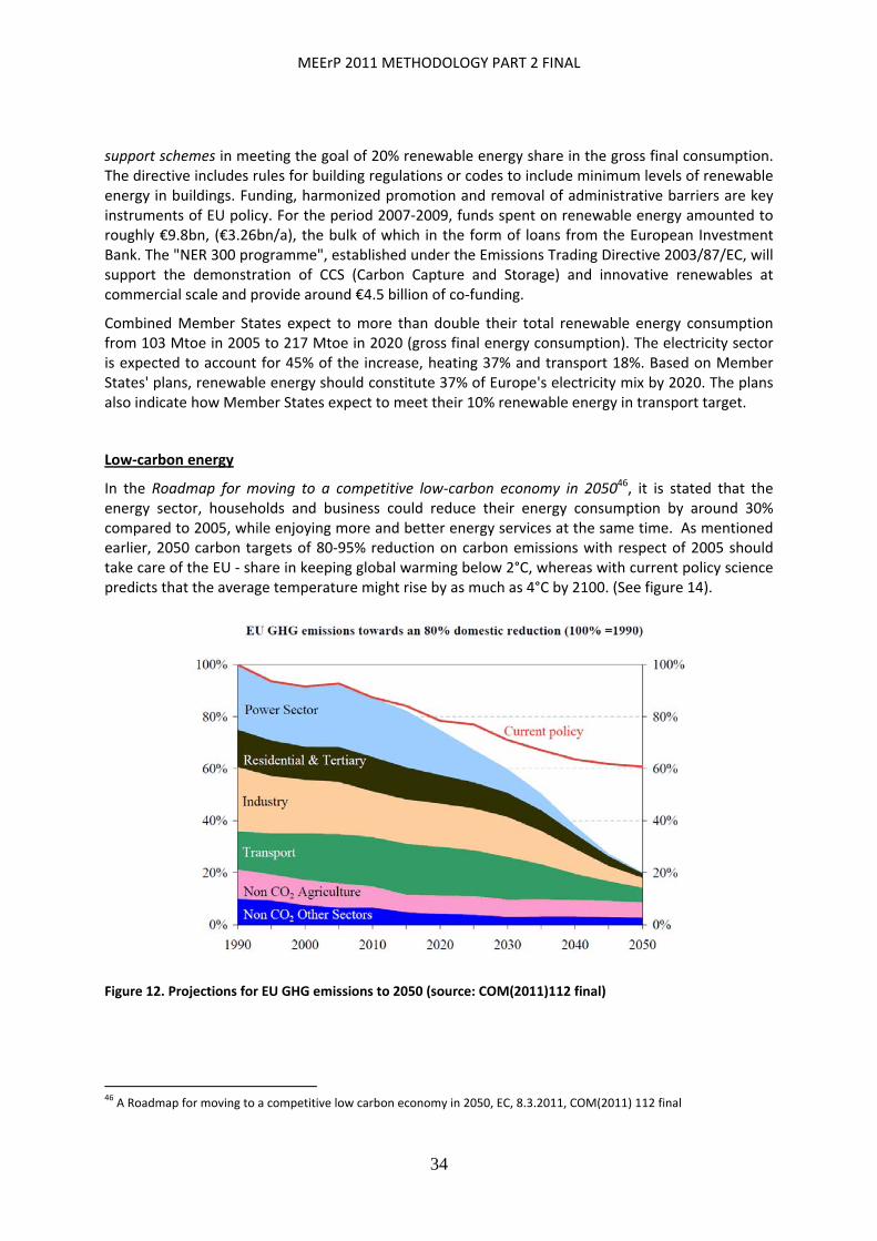
In the Roadmap for moving to a competitive low‐carbon economy in 205046, it is stated that the energy sector, households and business could reduce their energy consumption by around 30% compared to 2005, while enjoying more and better energy services at the same time. As mentioned earlier, 2050 carbon targets of 80‐95% reduction on carbon emissions with respect of 2005 should take care of the EU ‐ share in keeping global warming below 2°C, whereas with current policy science predicts that the average temperature might rise by as much as 4°C by 2100. (See figure 14).
Figure 12. Projections for EU GHG emissions to 2050 (source: COM(2011)112 final)
46 A Roadmap for moving to a competitive low carbon economy in 2050, EC, 8.3.2011, COM(2011) 112 final
MEErP 2011 METHODOLOGY PART 2 FINAL
35
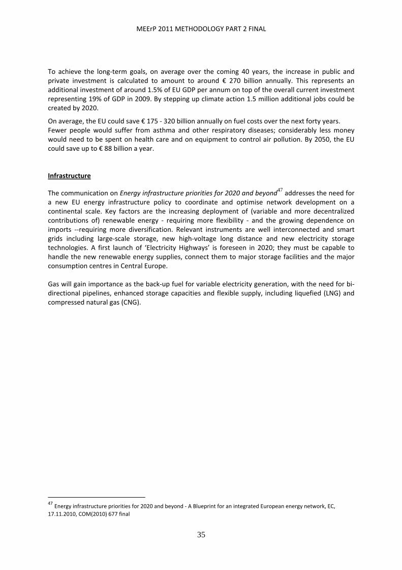
To achieve the long‐term goals, on average over the coming 40 years, the increase in public and private investment is calculated to amount to around € 270 billion annually. This represents an additional investment of around 1.5% of EU GDP per annum on top of the overall current investment representing 19% of GDP in 2009. By stepping up climate action 1.5 million additional jobs could be created by 2020.
On average, the EU could save € 175 ‐ 320 billion annually on fuel costs over the next forty years. Fewer people would suffer from asthma and other respiratory diseases; considerably less money would need to be spent on health care and on equipment to control air pollution. By 2050, the EU could save up to € 88 billion a year. Infrastructure The communication on Energy infrastructure priorities for 2020 and beyond
47 addresses the need for
a new EU energy infrastructure policy to coordinate and optimise network development on a continental scale. Key factors are the increasing deployment of (variable and more decentralized contributions of) renewable energy ‐ requiring more flexibility ‐ and the growing dependence on imports ‐‐requiring more diversification. Relevant instruments are well interconnected and smart grids including large‐scale storage, new high‐voltage long distance and new electricity storage technologies. A first launch of ‘Electricity Highways’ is foreseen in 2020; they must be capable to handle the new renewable energy supplies, connect them to major storage facilities and the major consumption centres in Central Europe. Gas will gain importance as the back‐up fuel for variable electricity generation, with the need for bi‐directional pipelines, enhanced storage capacities and flexible supply, including liquefied (LNG) and compressed natural gas (CNG).
47 Energy infrastructure priorities for 2020 and beyond ‐ A Blueprint for an integrated European energy network, EC, 17.11.2010, COM(2010) 677 final
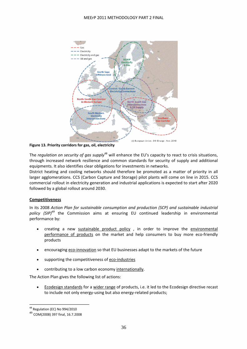
MEErP 2011 METHODOLOGY PART 2 FINAL
36
Figure 13. Priority corridors for gas, oil, electricity
The regulation on security of gas supply48 will enhance the EU's capacity to react to crisis situations, through increased network resilience and common standards for security of supply and additional equipments. It also identifies clear obligations for investments in networks. District heating and cooling networks should therefore be promoted as a matter of priority in all larger agglomerations. CCS (Carbon Capture and Storage) pilot plants will come on line in 2015. CCS commercial rollout in electricity generation and industrial applications is expected to start after 2020 followed by a global rollout around 2030. Competitiveness
In its 2008 Action Plan for sustainable consumption and production (SCP) and sustainable industrial policy (SIP)49 the Commission aims at ensuring EU continued leadership in environmental performance by:
creating a new sustainable product policy , in order to improve the environmental performance of products on the market and help consumers to buy more eco‐friendly products
encouraging eco‐innovation so that EU businesses adapt to the markets of the future
supporting the competitiveness of eco‐industries
contributing to a low carbon economy internationally.
The Action Plan gives the following list of actions:
Ecodesign standards for a wider range of products, i.e. it led to the Ecodesign directive recast to include not only energy‐using but also energy‐related products;
48 Regulation (EC) No 994/2010 49 COM(2008) 397 final, 16.7.2008
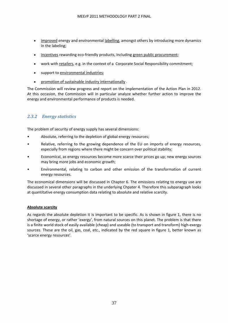
MEErP 2011 METHODOLOGY PART 2 FINAL
37
improved energy and environmental labelling, amongst others by introducing more dynamics in the labeling;
incentives rewarding eco‐friendly products, including green public procurement;
work with retailers, e.g. in the context of a Corporate Social Responsibility commitment;
support to environmental industries;
promotion of sustainable industry internationally .
The Commission will review progress and report on the implementation of the Action Plan in 2012. At this occasion, the Commission will in particular analyze whether further action to improve the energy and environmental performance of products is needed.
2.3.2 Energystatistics
The problem of security of energy supply has several dimensions:
• Absolute, referring to the depletion of global energy resources;
• Relative, referring to the growing dependence of the EU on imports of energy resources, especially from regions where there might be concern over political stability;
• Economical, as energy resources become more scarce their prices go up; new energy sources may bring more jobs and economic growth;
• Environmental, relating to carbon and other emission of the transformation of current energy resources.
The economical dimensions will be discussed in Chapter 6. The emissions relating to energy use are discussed in several other paragraphs in the underlying Chpater 4. Therefore this subparagraph looks at quantitative energy consumption data relating to absolute and relative scarcity.
Absolute scarcity
As regards the absolute depletion it is important to be specific. As is shown in figure 1, there is no shortage of energy, or rather ‘exergy’, from natural sources on this planet. The problem is that there is a finite world stock of easily available (cheap) and useable (to transport and transform) high‐exergy sources. These are the oil, gas, coal, etc., indicated by the red square in figure 1, better known as ‘scarce energy resources’.

MEErP 2011 METHODOLOGY PART 2 FINAL
38
Figure 14 EARTH’S ENERGY RESOURCES: Exergy flux, accumulation, destruction, and use (Source: W. Hermann. Quantifying Global Exergy Resources. Energy 2006;31(12):1349‐1366.)
Main drivers for the rapid depletion of the scarce resources are the continuing growth of world population ‐ from 7 billion today to around 9 billion in 2050 according to latest UNSTAT projections ‐ and the increase in per capita energy consumption in the developing economies like China and India (see figures 1 and 2).
Figure 15 Projected population growth per region (UNSTAT 2006)
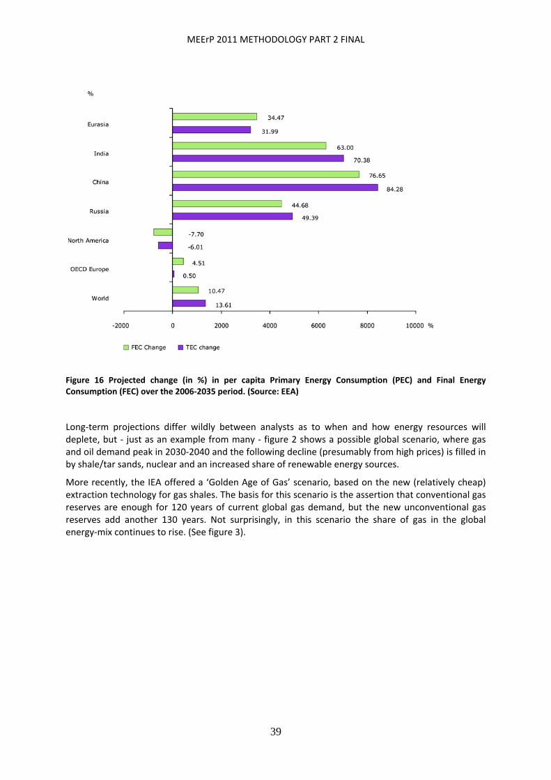
MEErP 2011 METHODOLOGY PART 2 FINAL
39
Figure 16 Projected change (in %) in per capita Primary Energy Consumption (PEC) and Final Energy Consumption (FEC) over the 2006‐2035 period. (Source: EEA)
Long‐term projections differ wildly between analysts as to when and how energy resources will deplete, but ‐ just as an example from many ‐ figure 2 shows a possible global scenario, where gas and oil demand peak in 2030‐2040 and the following decline (presumably from high prices) is filled in by shale/tar sands, nuclear and an increased share of renewable energy sources.
More recently, the IEA offered a ‘Golden Age of Gas’ scenario, based on the new (relatively cheap) extraction technology for gas shales. The basis for this scenario is the assertion that conventional gas reserves are enough for 120 years of current global gas demand, but the new unconventional gas reserves add another 130 years. Not surprisingly, in this scenario the share of gas in the global energy‐mix continues to rise. (See figure 3).
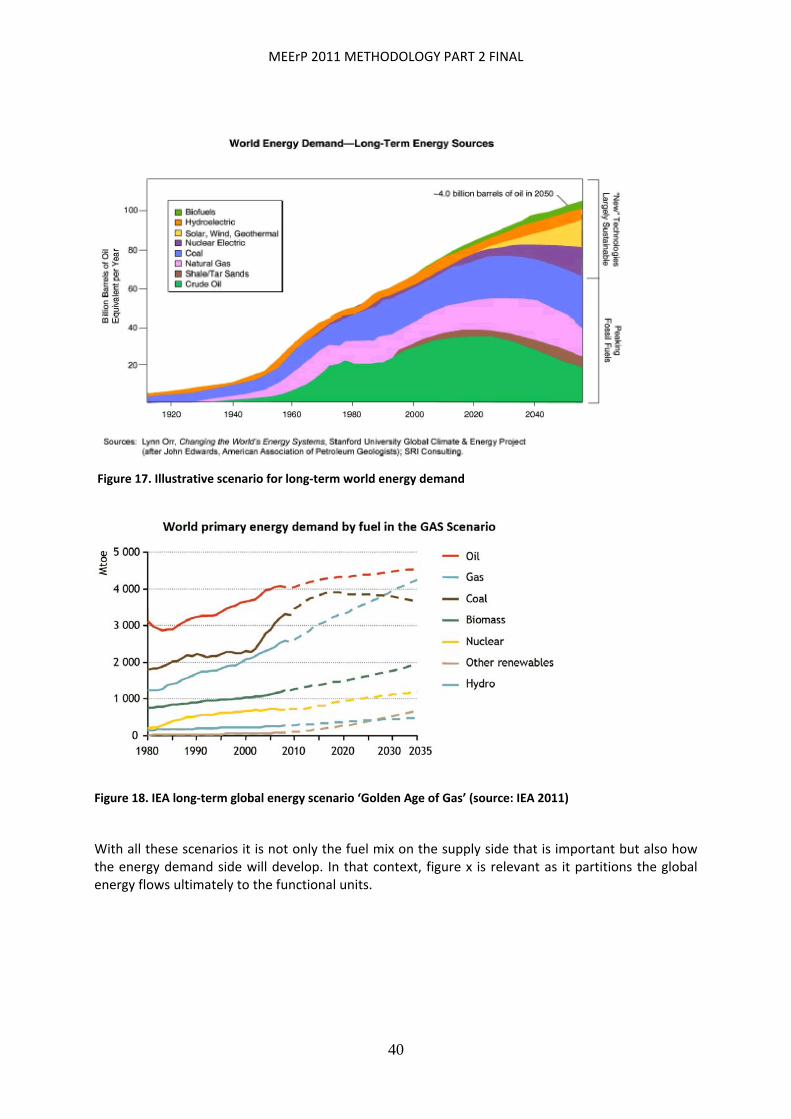
MEErP 2011 METHODOLOGY PART 2 FINAL
40
Figure 17. Illustrative scenario for long‐term world energy demand
Figure 18. IEA long‐term global energy scenario ‘Golden Age of Gas’ (source: IEA 2011)
With all these scenarios it is not only the fuel mix on the supply side that is important but also how the energy demand side will develop. In that context, figure x is relevant as it partitions the global energy flows ultimately to the functional units.
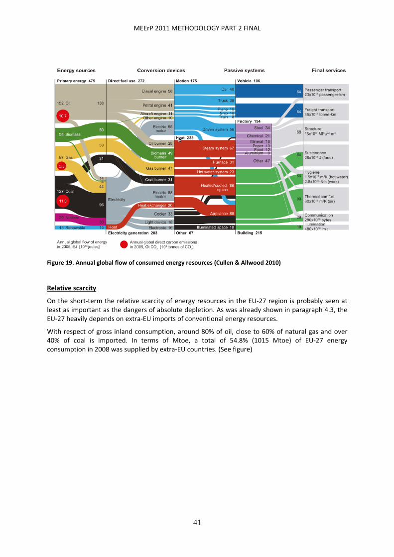
MEErP 2011 METHODOLOGY PART 2 FINAL
41
Figure 19. Annual global flow of consumed energy resources (Cullen & Allwood 2010)
Relative scarcity
On the short‐term the relative scarcity of energy resources in the EU‐27 region is probably seen at least as important as the dangers of absolute depletion. As was already shown in paragraph 4.3, the EU‐27 heavily depends on extra‐EU imports of conventional energy resources.
With respect of gross inland consumption, around 80% of oil, close to 60% of natural gas and over 40% of coal is imported. In terms of Mtoe, a total of 54.8% (1015 Mtoe) of EU‐27 energy consumption in 2008 was supplied by extra‐EU countries. (See figure)
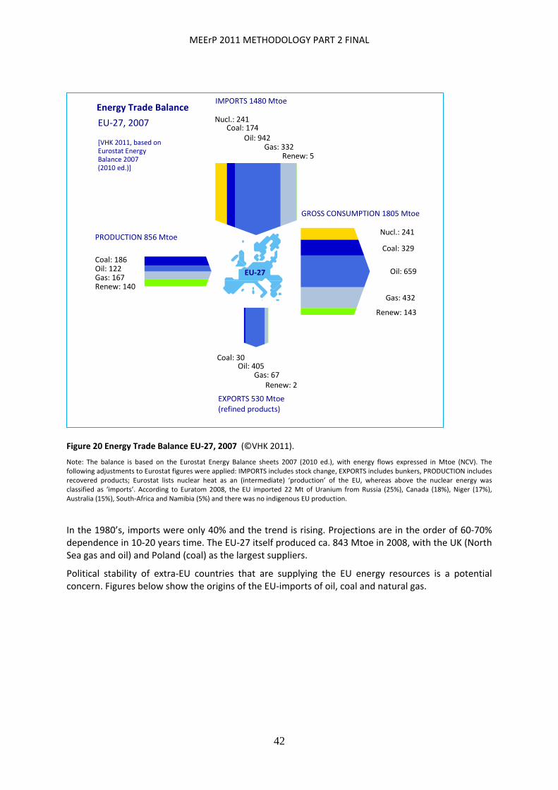
MEErP 2011 METHODOLOGY PART 2 FINAL
42
EU‐27
IMPORTS 1480 Mtoe
EXPORTS 530 Mtoe(refined products)
Nucl.: 241Coal: 174
Oil: 942Gas: 332
Renew: 5
PRODUCTION 856 Mtoe
Renew: 140 Gas: 167Oil: 122 Coal: 186
Coal: 30Oil: 405
Gas: 67Renew: 2
GROSS CONSUMPTION 1805 Mtoe
Renew: 143
Gas: 432
Oil: 659
Coal: 329
Nucl.: 241
EU‐27, 2007
[VHK 2011, based on Eurostat Energy Balance 2007 (2010 ed.)]
Figure 20 Energy Trade Balance EU‐27, 2007 (©VHK 2011).
Note: The balance is based on the Eurostat Energy Balance sheets 2007 (2010 ed.), with energy flows expressed in Mtoe (NCV). The following adjustments to Eurostat figures were applied: IMPORTS includes stock change, EXPORTS includes bunkers, PRODUCTION includes recovered products; Eurostat lists nuclear heat as an (intermediate) ‘production’ of the EU, whereas above the nuclear energy was classified as ‘imports’. According to Euratom 2008, the EU imported 22 Mt of Uranium from Russia (25%), Canada (18%), Niger (17%), Australia (15%), South‐Africa and Namibia (5%) and there was no indigenous EU production.
In the 1980’s, imports were only 40% and the trend is rising. Projections are in the order of 60‐70% dependence in 10‐20 years time. The EU‐27 itself produced ca. 843 Mtoe in 2008, with the UK (North Sea gas and oil) and Poland (coal) as the largest suppliers.
Political stability of extra‐EU countries that are supplying the EU energy resources is a potential concern. Figures below show the origins of the EU‐imports of oil, coal and natural gas.
Energy Trade Balance
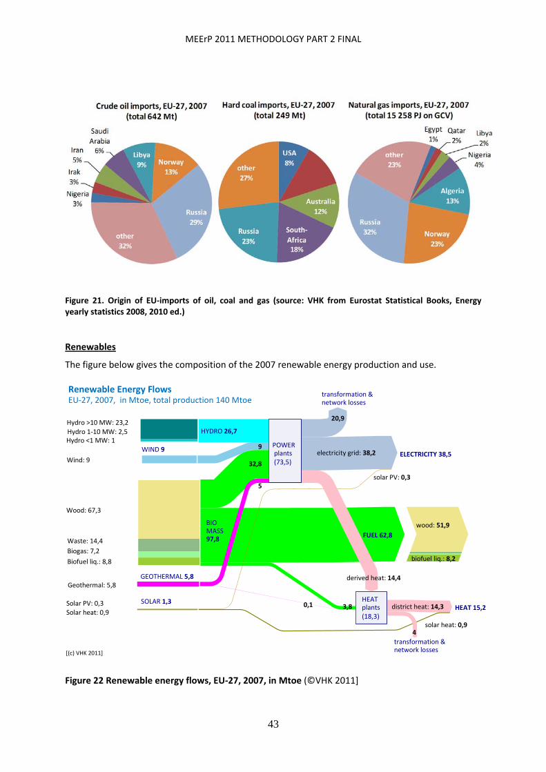
MEErP 2011 METHODOLOGY PART 2 FINAL
43
Figure 21. Origin of EU‐imports of oil, coal and gas (source: VHK from Eurostat Statistical Books, Energy yearly statistics 2008, 2010 ed.)
Renewables
The figure below gives the composition of the 2007 renewable energy production and use.
WIND 9
SOLAR 1,3
Hydro <1 MW: 1 Hydro 1‐10 MW: 2,5
Hydro >10 MW: 23,2
Wind: 9
Biofuel liq.: 8,8
Biogas: 7,2
Waste: 14,4
Wood: 67,3
Solar PV: 0,3Solar heat: 0,9
GEOTHERMAL 5,8 Geothermal: 5,8
POWERplants(73,5)
9
32,8
HEAT plants(18,3)
3,80,1
ELECTRICITY 38,5
transformation & network losses
transformation & network losses
HEAT 15,2
BIOMASS 97,8
5
HYDRO 26,7
20,9
electricity grid: 38,2
district heat: 14,3
FUEL 62,8
solar heat: 0,9
solar PV: 0,3
derived heat: 14,4
4
biofuel liq.: 8,2
wood: 51,9
Renewable Energy FlowsEU‐27, 2007, in Mtoe, total production 140 Mtoe
[(c) VHK 2011]
Figure 22 Renewable energy flows, EU‐27, 2007, in Mtoe (©VHK 2011]
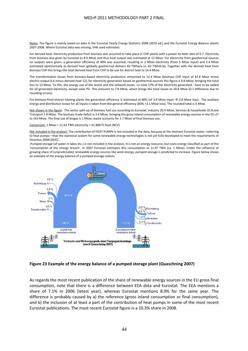
MEErP 2011 METHODOLOGY PART 2 FINAL
44
Notes: The figure is mainly based on data in the Eurostat Yearly Energy Statistics 2008 (2010 ed.) and the Eurostat Energy Balance sheets 2007‐2008. Where Eurostat data was missing, VHK used estimates:
For derived heat: Electricity production from biomass was assumed to take place in CHP‐plants with a power‐to‐heat ratio of 0.7. Electricity from biomass was given by Eurostat as 8.9 Mtoe and thus heat output was estimated at 12 Mtoe. For electricity from geothermal sources no outputs were given; a generation efficiency of 40% was assumed, resulting in 2 Mtoe electricity (from 5 Mtoe input) and 2.4 Mtoe estimated optimistically as derived heat (globally geothermal delivers 60 TWhe/a vs. 63 TWhth/a). Together with the derived heat from biomass CHP this brings the total derived heat from CHP to be use for district heat to 14.4 Mtoe.
The transformation losses from biomass‐based electricity production amounted to 12.4 Mtoe (biomass CHP input of 32.8 Mtoe minus electric output 8.4 minus derived heat 12); for electricity generation based on geothermal sources this figure is 0.6 Mtoe, bringing the total loss to 13 Mtoe. To this, the energy use of the sector and the network losses –in total 17% of the electricity generated‐‐ have to be added for all generated electricity, except solar PV. This amounts to 7.8 Mtoe, which brings the total losses to 20.8 Mtoe (0.1 difference due to rounding errors).
For biomass‐fired district heating plants the generation efficiency is estimated at 80% (of 3.9 Mtoe input 0.8 Mtoe loss). The auxiliary energy and distribution losses for all inputs is taken from the general efficiency (83% =3.1 Mtoe loss). The rounded total is 4 Mtoe.
Not shown in the figure: The sector split‐up of biomass fuel use according to Eurostat: Industry 20.9 Mtoe, Services & households 35.8 and Transport 7.8 Mtoe. The biomass trade deficit is 2.6 Mtoe, bringing the gross inland consumption of renewable energy sources in the EU‐27 to 143 Mtoe. The final use of biogas is 1 Mtoe; waste accounts for 1.7 Mtoe of final biomass use.
Conversion: 1 Mtoe = 11.63 TWh electricity = 41.868 PJ heat (NCV)
Not included in the analysis: The contribution of HEAT PUMPS is not included in the data, because at the moment Eurostat states –referring to heat pumps—that the statistical system for some renewable energy technologies is not yet fully developed to meet the requirements of Directive 2009/28/EC. .Pumped storage (of water in lakes etc.) is not included in the analysis. It is not an energy resource, but costs energy classified as part of the ‘consumption of the energy branch’. In 2007 Eurostat estimates this consumption at 11.97 TWh (ca. 1 Mtoe). Under the influence of growing share of (unpredictable) renewable energy sources like wind energy, pumped storage is predicted to increase. Figure below shows an example of the energy balance of a pumped storage station.
Figure 23 Example of the energy balance of a pumped storage plant (Quaschning 2007)
As regards the most recent publication of the share of renewable energy sources in the EU gross final consumption, note that there is a difference between EEA data and Eurostat. The EEA mentions a share of 7.1% in 2006 (latest year), whereas Eurostat mentions 8.9% for the same year. The difference is probably caused by a) the reference (gross inland consumption or final consumption), and b) the inclusion of at least a part of the contribution of heat pumps in some of the most recent Eurostat publications. The most recent Eurostat figure is a 10.3% share in 2008.
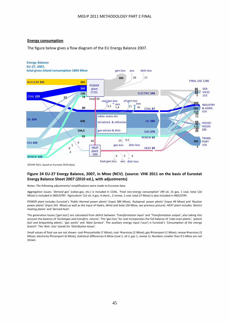
MEErP 2011 METHODOLOGY PART 2 FINAL
45
Energy consumption
The figure below gives a flow diagram of the EU Energy Balance 2007.
IEA/OECD
Figure 24 EU‐27 Energy Balance, 2007, in Mtoe (NCV). (source: VHK 2011 on the basis of Eurostat Energy Balance Sheet 2007 (2010 ed.), with adjustments)
Notes: The following adjustments/ simplifications were made to Eurostat data:
Aggregation issues: ‘Derived gas’ (cokes‐gas, etc.) is included in COAL. ‘Final non‐energy consumption’ (99 oil, 15 gas, 1 coal, total 116 Mtoe) is included in INDUSTRY. ‘Agriculture’ (15 oil, 4 gas, 4 electr., 2 renew, 1 coal, total 27 Mtoe) is also included in INDUSTRY.
POWER plant includes Eurostat’s ‘Public thermal power plants’ (input 386 Mtoe), ‘Autoprod. power plants’ (input 49 Mtoe) and ‘Nuclear power plants’ (input 241 Mtoe) as well as the input of Hydro, Wind and Solar (36 Mtoe, see previous picture). HEAT plant includes ‘district heating plants’ and ‘derived heat’.
The generation losses (‘gen.loss’) are calculated from deficit between ‘Transformation input’ and ‘Transformation output’, also taking into account the balance of ‘Exchanges and transfers, returns’. The ‘gen.loss’ for coal incorporates the full balance of ‘coke‐oven plants’, ‘patent fuel and briquetting plants’, ‘gas works’ and ‘blast furnace’. The auxiliary energy input (‘aux’) is Eurostat’s ‘Consumption of the energy branch’. The ‘distr. loss’ stands for ‘Distribution losses’.
Small values of final use are not shown: coalhouseholds (7 Mtoe); coal services (2 Mtoe); gastransport (1 Mtoe); renewservices (3 Mtoe); electricitytransport (6 Mtoe); statistical differences 6 Mtoe (coal 2, oil 2, gas 1, renew 1). Numbers smaller than 0.5 Mtoe are not shown.
69
distr.loss
HEAT plant(58)
POWER plant(712)
HEAT 45
241
245
80
22 130
9 4
65
74
gen.loss aux. distr.loss
heat gen.loss aux.
1 4
385 26 17
coal gen.lossaux.
distr.lossgas aux.
5,5 1,4
15 3,5
COAL 67
RENEW 65
oil gen.lossaux.
11 41
4 5 4
Energy Balance EU‐27, 2007, total gross inland consumption 1804 Mtoe
[©VHK 2011, based on Eurostat 2010 data]
RENEW 143
GAS 432
OIL 659
COAL 329
NUCLEAR 241
GAS 276
OIL 584
ELECTRIC 244
SER‐VICES153
INDUSTRY& AGRIC.474
HOUSE‐HOLDS285
TRANS‐PORT376
66
103
361
113
113161
8
9
16
20
cokes ovens etc.
oil extract. & refineries
gas extract.& distr.
heat: 40
50
56
23
42
32
23
294,5
636
40
FINAL USE 1286

MEErP 2011 METHODOLOGY PART 2 FINAL
46
2.3.3 Energytrends
The graph shows the trends in gross electricity consumption and primary energy consumption. In 2008, the EU‐27 was consuming around 1800 Mtoe (ca. 75 000 PJ) of energy per year. Of this, 78% was fossil fuel (oil 36%, gas 24% and solid fuel 18%), nuclear energy accounted for 13‐14% and renewable energy sources for 8‐9%. The absolute energy consumption, in Mtoe, is still slowly rising but currently at a lower rate than GDP (Gross Domestic Product).
Figure 25. Gross electricity (left) and primary energy (right) consumption by main fuel in EU 27, 1990–2008 Source: EEA, 2010a, Eurostat 2010
Between 1990 and 2007, economic growth in Europe required increasing but less and less energy inputs. Total energy consumption increased until 2004 and stabilized all the way through 2006. In 2007 there was an absolute decoupling of economic growth and energy consumption, with the latter decreasing by 1.1% compared to 2006 while GDP continued to grow. Over the period 1990‐2007, GDP grew at an annual average rate of 2.2% and total energy consumption at an annual average rate of 0.5%. As a result, total energy intensity in the EU fell at an annual average rate of 1.7%.
Figure 26. Index (1990=100) of GDP, energy consumption and energy intensity EU‐27, 1990‐2007
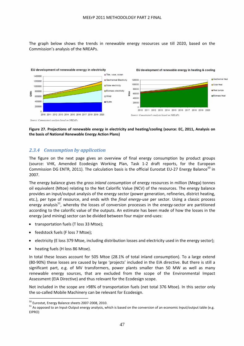
MEErP 2011 METHODOLOGY PART 2 FINAL
47
The graph below shows the trends in renewable energy resources use till 2020, based on the Commission’s analysis of the NREAPs.
Figure 27. Projections of renewable energy in electricity and heating/cooling (source: EC, 2011, Analysis on the basis of National Renewable Energy Action Plans)
2.3.4 Consumptionbyapplication
The figure on the next page gives an overview of final energy consumption by product groups (source: VHK, Amended Ecodesign Working Plan, Task 1‐2 draft reports, for the European Commission DG ENTR, 2011). The calculation basis is the official Eurostat EU‐27 Energy Balance50 in 2007.
The energy balance gives the gross inland consumption of energy resources in million (Mega) tonnes oil equivalent (Mtoe) relating to the Net Calorific Value (NCV) of the resources. The energy balance provides an input/output analysis of the energy sector (power generation, refineries, district heating, etc.), per type of resource, and ends with the final energy‐use per sector. Using a classic process energy analysis51, whereby the losses of conversion processes in the energy‐sector are partitioned according to the calorific value of the outputs. An estimate has been made of how the losses in the energy (and mining) sector can be divided between four major end‐uses:
transportation fuels (T loss 33 Mtoe);
feedstock fuels (F loss 7 Mtoe);
electricity (E loss 379 Mtoe, including distribution losses and electricity used in the energy sector);
heating fuels (H loss 86 Mtoe).
In total these losses account for 505 Mtoe (28.1% of total inland consumption). To a large extend (80‐90%) these losses are caused by large ‘projects’ included in the EIA directive. But there is still a significant part, e.g. of MV transformers, power plants smaller than 50 MW as well as many renewable energy sources, that are excluded from the scope of the Environmental Impact Assessment (EIA Directive) and thus relevant for the Ecodesign scope.
Not included in the scope are >98% of transportation fuels (net total 376 Mtoe). In this sector only the so‐called Mobile Machinery can be relevant for Ecodesign. 50 Eurostat, Energy Balance sheets 2007‐2008, 2010. 51 As opposed to an Input‐Output energy analysis, which is based on the conversion of an economic Input/output table (e.g. EIPRO)
MEErP 2011 METHODOLOGY PART 2 FINAL
48
Included in Ecodesign, but usually not as a ‘product’ but as a part of the production stage is the ‘feedstock’ (net total 115 Mtoe).
Without the items mentioned above, a final end‐use remains of 239 Mtoe of electricity (2780 TWh) and 555 Mtoe of the heating fuels account for approximately 24.720 PJ (GCV)52 53
The final end‐use is further split up in Figure 28Error! Reference source not found., where the Mtoe units are converted to the units that are commonly used in the preparatory studies, i.e. TWh electricity and PJ (petaJoules) of heating fuels related to the Gross Calorific Value (GCV) of the fuels.
In order to make the partitioning to products, the sources were Ecodesign regulations, public impact assessment studies accompanying the measures, preparatory studies (ENER Lots 1‐31, ENTR Lots 1‐6), European Climate Change Program (ECCP) figures, additional literature search, SAVE studies for labeling, VHK engineering estimates and past product studies
Furthermore, especially useful for the industrial sector, the estimates were guided by the boundaries set in the Eurostat energy balance for the consumption of heating fuels and electricity per sector. Thus the sum of individual energy‐users per sector and energy type cannot exceed the Eurostat totals.
End‐use electricity
For electricity, the 2780 TWh/a end‐use is first split between 5 major conversion categories. This is the first outer ring in Figure 28:
motors (1360 TWh, 49%): applications for internal transport or power transmission;
heat (680 TWh, 24%): applications depending on direct or indirect Joule effect;
electro‐magnetic applications (340 TWh, 12%): applications that emit electro‐magnetic waves of any frequency and amplitude as their main function (note: infrared radiation is covered by 'Heat');
electronics (100 TWh, 3.5%), i.e. relating only to end‐uses in signal processing, storage, local open or closed loop control;
electrolysis (100 TWh, 3.5%), i.e. relating to various electro‐chemical processes.
In a second outer ring, the 1360 TWh motor applications are split between
‘movers’ (270 TWh, 20%);
compressors (510 TWh, 37%), of which cooling compressors 375 TWh (27%);
pumps (300 TWh, 22%);
fan applications (280 TWh, 21%).
52 Gross Calorific Value takes into account the latent heat from water vapour that results from the combustion process (compare: ‘condensing’ boiler). It depends on the fuel mix: For natural gas 1 PJ NCV (net calorific value)= 1.11 PJ GCV. For oil products 1 PJ NCV=1.06 PJ GCV. For solids and heat NCV=GCV. The value of 24.720 PJ is a value weighted by the share of the fuel (44.5 PJMtoe). The equivalent in NCV is 23.237 PJ (41.868 PJ/Mtoe). 53 The energy analysis to arrive at these numbers is for the most part not controversial. But disputes may arise over not
including a part of the mining and transportation effort of imported fuels from outside the EU (error maximum 1‐2%) and over the way that the complex exchanges and transfers in the oil refineries were accounted (which led to using 1792 Mtoe as inland production instead of the official 1808 Mtoe figure for 2007). Another choice is the way the fuel input for the joint generation of derived heat and electricity is partitioned on the basis of Mtoe useful output of both items. In an alternative approach where all losses are partitioned to the main product ‘electricity’ the E‐losses would be 48 Mtoe more (resulting in 427 Mtoe ‘E loss’, i.e. power generation efficiency 35.9% instead of 38.7%). More details can be found in the VHK draft study report on the Working Plan, 2011, see www.ecodesign‐wp2.eu .
MEErP 2011 METHODOLOGY PART 2 FINAL
49
With this, it has to be noted that a part of the ‘cooling compressor’ applications are in fact reversible and could also be partitioned to 'heat'.
The electromagnetic applications are split between light sources (340 TWh) and other applications (200 TWh), such as displays (incl. TVs) and communication equipment (incl. wireless).
The third ring of Figure 28 contains the energy‐using product groups. Most of these, some 80% in terms of electricity consumption, are dealt with by measures or preparatory studies. Around 5‐10% of consumption is by e.g. aluminium or chemicals electrolysis plants, arc‐furnaces for steel making etc. and may be adequately covered by existing policies. The remaining 5‐10% of consumption can be linked to product groups that are not yet covered. What the picture doesn’t show are the energy‐related products (non EuP, discussed later in this paragraph) and ‘gaps’ or exceptions in the product scope of the individual measures and preparatory studies. More information can be found in the ongoing update of the Ecodesign Working Plan.54
End‐use heating fuels
For heating fuels, Figure 28 first divides the 555 Mtoe (23.237 PJ on NCV, 24.720 PJ, on NCV) end‐use of heating (fuel) energy in 3 exergy levels55: Low (<100 °C, LT), Medium (100‐600 °C, MT) and High (>600 °C, HT) temperature applications. Low temperature applications (space and water heating) represent over 60% of heating fuel use, whereas Medium and High Temperature applications represent around 20% of the total.
The next ring shows the end‐results of the heat conversion process. For LT applications the end‐product is non‐electric space heat (86%)56, hot water and cooking (14%). For the MT and HT applications the end‐result are raw materials, components, products (incl. construction and food) and waste disposal.57
Energy‐related products
The outer ring of Figure 28 gives a snapshot of the actual energy consumption by energy using products (EuP). It does not question whether the actual energy consumption is justified from the point of view of user demand. This is the domain of the energy‐related products (ErP). The ErP plus the theoretical minimum user demand determine the (energy) performance that the EuP have to deliver.
For instance, from the EuP‐perspective Figure 28 shows that the gas‐fired CH boiler consumes around 7000 PJ of fuel. From the ErP‐perspective, it could be concluded that the transmission and the ventilation/infiltration losses of the buildings heated by those boilers require 7.000 PJ of fuel. And these losses depend on ErP like insulation materials, windows, ventilation systems, etc.. If all these losses were (close to58) zero and full heat recovery ventilation is realized, those buildings would
54 Study on Amended Ecodesign Working Plan under the Ecodesign Directive. www.ecodesign‐wp2.eu 55 Exergy is the capacity of an energy(heat) source to perform labour: the higher the temperature level of the energy, the more it is useful to perform labour. Exergy is an important concept in heating cascades . 56 Note that the item ‘district heating’ was not further split‐up for lack of information. 57 Total HT and MT applications is 9.345 PJ= ca. 210 Mtoe excl. loss 242 Mtoe incl. loss. Together with the feedstock from the general energy balance (122 Mtoe incl. loss), ca. 10% of the manufacturing electricity use (ca. 62 Mtoe incl. loss) and around 30% of the transportation energy for the transport of goods (123 Mtoe incl. loss) this represents the total gross inland consumption for the production, distribution and end‐of‐life phase of products. The sum is 549 Mtoe, or ca. 30% of the total EU‐27 gross inland consumption; the remaining 70% of energy is spent in the use‐phase of the products. Note that this includes all products, also the means of transport and the products that are not ‘energy‐related’ during their use phase 58 Zero loss and 100% heat recovery are theoretically impossible, but theoretically it is possible to come very close and use <10% of current building losses. Also note that this is a simplification to illustrate a point. In reality buildings have also to deal [incomplete sentence]
MEErP 2011 METHODOLOGY PART 2 FINAL
50
hardly require any energy input for heating at all. And at that stage the efficiency of the EuP (the boiler) would be irrelevant.
In the intermediate, until the ‘nearly zero loss’ point is reached (if ever), there are several other ErPs that play a role. Heating controls in combination of a good controllability of the heating system components, can play an important role in ensuring that buildings or rather building and dwelling zones are only heated when occupied and ‐ when they are occupied ‐ the heat is delivered effectively (no ‘overshoot’) and at the right thermal comfort, i.e. that there is no overheating to compensate for indoor temperature stratification or fluctuation. Occupancy data for commercial buildings in Chapter 7 show that for zone‐ and occupancy rate controlled ventilation saving potentials of up to 70‐80% with respect to the design flow rate are possible. Shading products can be instrumental in optimizing solar gain in the heating season without negative repercussions (e.g. need for active cooling) in summer. Daylight systems minimize the need for artificial lighting. Products using renewable energy sources like solar thermal collectors or heat pumps (using ambient heat) can provide active space heating (and, if needed, space cooling) without having to use scarce conventional energy sources. Likewise, photovoltaic (PV) solar collectors in combination with the previous products can turn the home into a so‐called ‘Passive House’, ‘Zero Energy Building’ (ZEB) or ‘nearly Zero Energy Building’ (nZEB).
A consequence of the reduction of energy in the use phase of the building is that the ‘embodied energy’ needed for the buildings construction, currently on average less than 20%, will become more and more important in the coming decades.
Outside the world of building space heating there are also several other ErP that are not shown in Figure 28. For instance for the energy use of (circulator and other) pumps, compressors and fans the controls and the end‐use equipment (e.g. heat exchangers, expanders, valves, ducts, piping). Not so long ago and thus still widely popular in existing installations, the pump flow was regulated by letting the pump run at full load but squeezing the flow by valves. Using variable speed drives and appropriate flow controls has largely put an end to that but there is still scope for improvement in more conservative sectors. Another ErP that reduces the energy consumption of fluid‐dynamic products like pumps is in a reduction of demand. For water and sewage pumps this includes plumbing appliances such as toilets, shower heads and taps, which have the added advantage of tackling water saving. In HT and MT products, like furnaces and ovens, a significant part of the heating needs stem from transmission and convection losses. Like with buildings, insulation materials and oven fans optimized for optimization (re‐use) of convection heat flows play a role. Difficult to grasp with such a generic instrument as the Ecodesign directive, but certainly very effective are ErP contributing to process‐innovation, i.e. that can eliminate whole process steps or drastically lower the exergy (temperature) level by optimising the other parts of the transformation processes like ‘pressure’, ‘time’, ‘mechanical action’, etc.. These are ‘products’ like catalysts, heat recovery heat exchangers, ultra‐high pressure compressors for the (petro)chemical industry, etc. which may well be energy‐consuming themselves but with a huge saving potential vis‐à‐vis the alternative.
Looking more at component level, there are several energy flows that are not related to the main function but only necessary to eliminate undesirable side‐effects of the main performance technology. In ICT (computers, switches, data centers) a significant energy amount goes into active cooling (fans, air conditioning), where ErP like passive cooling devices (heat sinks, heat pipes, etc.) 59 are relevant. In electric motors, the windings and ball‐bearings are important ErP, with a significant potential in helping to fight electric, magnetic and friction losses.
59 Apart of course from process innovation like more efficient ICs, which is more difficult to grasp.

MEErP 2011 METHODOLOGY PART 2 FINAL
51
The study contractor estimates that the energy‐use that indirectly is affected by ErP is slightly less than that connected to EuP, because there is a minimum component of inevitable energy use needed to fulfill the user demand even under the best circumstances. At the moment there is not enough information to sketch an equally comprehensive quantitative picture for ErP as for EuP.

MEErP 2011 METHODOLOGY PART 2 FINAL
52
Figure 28. EU‐27, 2007
Energy consumption by origin
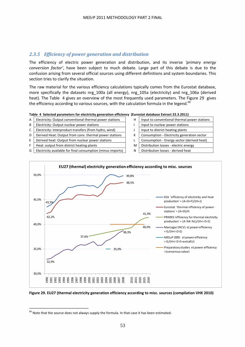
MEErP 2011 METHODOLOGY PART 2 FINAL
53
2.3.5 Efficiencyofpowergenerationanddistribution
The efficiency of electric power generation and distribution, and its inverse ‘primary energy conversion factor’, have been subject to much debate. Large part of this debate is due to the confusion arising from several official sources using different definitions and system boundaries. This section tries to clarify the situation.
The raw material for the various efficiency calculations typically comes from the Eurostat database, more specifically the datasets nrg_100a (all energy), nrg_105a (electricity) and nrg_106a (derived heat). The Table 4 gives an overview of the most frequently used parameters. The Figure 29 gives the efficiency according to various sources, with the calculation formula in the legend.60
43,5%
49,8%
42,2%
48,5%
37,6%
41,4%
32,9%
38,3%
35,0%
40,0%
30,0%
35,0%
40,0%
45,0%
50,0%
1990
1991
1992
1993
1994
1995
1996
1997
1998
1999
2000
2001
2002
2003
2004
2005
2006
2007
2008
2010
2015
2020
2025
2030
EU27 (thermal) electricity generation efficiency according to misc. sources
EEA 'efficiency of electricity and heat
production' = (A+D+F)/(H+J)
Eurostat 'thermal efficiency of power
stations' = (A+D)/H
PRIMES 'efficiency for thermal electricity
production' = (A‐%K‐%L)/(H+I‐D‐E)
Marcogaz (NCV) el.power efficiency
= G/(H+I‐D‐E)
MEEuP 2005 el.power efficiency
= G/(H+I‐D‐E+extraEU)
Preparatory studies el.power efficiency
=(consensus value)
Figure 29. EU27 (thermal electricity generation efficiency according to misc. sources (compilation VHK 2010)
60 Note that the source does not always supply the formula. In that case it has been estimated.
Table 4 Selected parameters for electricity generation efficiency (Eurostat database Extract 22.3.2011)
A Electricity: Output conventional thermal power stations H Input to conventional thermal power stations
B Electricity: Output nuclear power stations I Input to nuclear power stations
C Electricity: Interproduct transfers (from hydro, wind) J Input to district heating plants
D Derived Heat: Output from conv. thermal power stations K Consumption ‐ Electricity generation sector
E Derived heat: Output from nuclear power stations L Consumption ‐ Energy sector (derived heat)
F Heat: output from district heating plants M Distribution losses ‐ electric energy
G Electricity available for final consumption (minus imports) N Distribution losses ‐ derived heat
MEErP 2011 METHODOLOGY PART 2 FINAL
54
The efficiency indicators from EEA61, Eurostat62 and PRIMES63 all relate to conventional fossil fuel fired power plants (excl. nuclear and renewable energy sources) and only relate to the strict ‘generation efficiency’ (excluding distribution losses) on Net Calorific Value of the fuel
The figures from Marcogaz64, MEEuP (LCI value)65 and the consensus value used in the preparatory studies relate to all power plants (including nuclear and renewable) and includes the distribution.
The difference between EEA and Eurostat is caused by the fact that the EEA gives credits not only to the derived heat from the power plants, but includes also the public district heating where heat is generated by other means.
The difference between EEA/Eurostat on one hand and PRIMES derives from the fact that PRIMES does take into account not only the strict transformation energy, but also the energy consumption of the energy sector partitioned to the electricity generation, e.g. to produce the fuel (mining, refineries, gasworks, etc.). PRIMES uses 5‐year steps and aims primarily at long‐term forecasts (note that the right hand side of the Figure 29 also uses 5 year steps).
The difference between PRIMES and Marcogaz figures is mainly caused by the fact that Marcogaz also includes distribution losses and PRIMES does not and that PRIMES only looks at conventional thermal power plants and Marcogaz includes all power plants.
The MEEuP 2005 efficiency was calculated using non‐Eurostat data (e.g. from Eurelectric and the GEMIS database), because Eurostat data were not available at the time. In contrast to the Marcogaz data, the MEErP LCI data also take into account the energy losses of mining, fuel production and fuel transport outside the EU.
Following initial debates, the fixed efficiency value of 40% actually used in the preparatory studies was a long term average over the product life of most products (i.e. over the period 2005‐2025). The primary energy factor pertaining to this efficiency is 2.5 (1 kWh electric = 2.5 kWh primary energy).
For the period up to 2030, i.e. when analyzing products with a life less than 20 years, the factor 2.5 still seems a robust fixed value to be used in preparatory studies. According to PRIMES, the average efficiency of conventional thermal power plants is progressing only slowly. The share of renewable energy sources and natural gas will increase, but the increased use of biomass, coal and nuclear energy will reduce this positive effect.
For building components with a product life of 40‐50 years, like window frames, insulation panels, etc., the primary energy conversion factor of 2.4 (efficiency 41.7%) can be assumed.
Note that the calculation methodology for the primary energy requirement of power generation and distribution ‐‐e.g. partitioning of heat recovery flows, system boundaries, etc.‐‐ may be subject to change following imminent new legislation.
61 www.eea.europa.eu The European Environmental Agency is an EU agency that, based on (candidate‐) Member State and/or Eurostat data inputs, monitors the progress in achieving several environmental policy goals 62 Eurostat, Pocketbook of Energy indicators (ed. 2009), 2010.
63 Capros, P. et al., EU Energy Trends To 2030, Update 2009, [PRIMES model], ICCS‐NTUA (E3M Lab) for EUROPEAN COMMISSION Directorate‐General for Energy in collaboration with Climate Action DG and Mobility and Transport DG, European Union, 2010. 64 European gas industry association Marcogaz, Note 13.10.2010 to the Commission, regarding primary energy conversion factor. Note that Marcogaz gives lower efficiency values, because they are corrected for Gross Calorific Value. However, for reasons of coherence with the other sources, the data are recalculated to NCV. 65 Kemna et al., MEEuP report, VHK for the European Commission DG ENTR with DG ENER, Nov. 2005

MEErP 2011 METHODOLOGY PART 2 FINAL
55
2.3.6 Securityofenergysupply
Ensuring security of energy supply is one of the priorities of EU energy policy. As was already shown in Figure 1 of paragraph 2.1 on Materials, the EU‐27 heavily depends on extra‐EU imports of conventional energy resources. Around 80% of oil, close to 60% of natural gas and over 40% of coal is imported. In terms of Mtoe, a total of 54.8% (1015 Mtoe) of EU‐27 energy consumption in 2008 was supplied by extra‐EU countries, amongst which not the politically most stable regions. In the 1980’s this was only 40% and the trend is rising. The EU‐27 itself produced ca. 843 Mtoe in 200866, with the UK (North Sea gas and oil) and Poland (coal) as the largest suppliers.
2.3.7 Accountingunits
Following conventions in statistics the preferred accounting unit for energy is primary energy, Net Calorific Value, in Joules (MJ, PJ). This is applied all through the unit indicator table in Chapter 5.
The following tables give conversion factors for the various fuels.
For use phase analysis of fossil fuel consuming products, however, it is recommended to use the Gross Calorific Value of fossil energy resources as an accounting unit all through the preparatory study. For electricity consuming products, accounting in kWh electricity makes more sense (TWh for totals).
Table 5 Energy units conversion for statistics (source: Eurostat, Energy Balance 2007‐2008, 2010)
From | /To TJ Gcal Mtoe GWh
TJ 1 238.8 2.388 x 10 ‐5 0.2778
Gcal 4.1868 x 10 ‐3 1 1 x 10 ‐7 1.163 x 10 ‐3
Mtoe 4.1868 x 10 4 1 x 10 7 1 11630
GWh 3.6 860 8.6 x 10 ‐5 1
66 Source Eurostat. http://epp.eurostat.ec.europa.eu/statistics_explained/index.php/Energy_production_and_imports
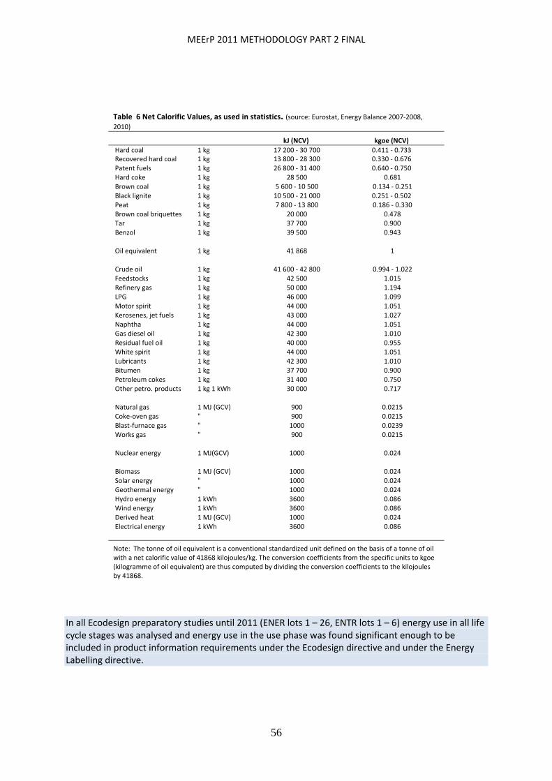
MEErP 2011 METHODOLOGY PART 2 FINAL
56
Table 6 Net Calorific Values, as used in statistics. (source: Eurostat, Energy Balance 2007‐2008, 2010)
kJ (NCV) kgoe (NCV)
Hard coal 1 kg 17 200 ‐ 30 700 0.411 ‐ 0.733 Recovered hard coal 1 kg 13 800 ‐ 28 300 0.330 ‐ 0.676 Patent fuels 1 kg 26 800 ‐ 31 400 0.640 ‐ 0.750 Hard coke 1 kg 28 500 0.681 Brown coal 1 kg 5 600 ‐ 10 500 0.134 ‐ 0.251 Black lignite 1 kg 10 500 ‐ 21 000 0.251 ‐ 0.502 Peat 1 kg 7 800 ‐ 13 800 0.186 ‐ 0.330 Brown coal briquettes 1 kg 20 000 0.478 Tar 1 kg 37 700 0.900 Benzol 1 kg 39 500 0.943 Oil equivalent 1 kg 41 868 1 Crude oil 1 kg 41 600 ‐ 42 800 0.994 ‐ 1.022 Feedstocks 1 kg 42 500 1.015 Refinery gas 1 kg 50 000 1.194 LPG 1 kg 46 000 1.099 Motor spirit 1 kg 44 000 1.051 Kerosenes, jet fuels 1 kg 43 000 1.027 Naphtha 1 kg 44 000 1.051 Gas diesel oil 1 kg 42 300 1.010 Residual fuel oil 1 kg 40 000 0.955 White spirit 1 kg 44 000 1.051 Lubricants 1 kg 42 300 1.010 Bitumen 1 kg 37 700 0.900 Petroleum cokes 1 kg 31 400 0.750 Other petro. products 1 kg 1 kWh 30 000 0.717 Natural gas 1 MJ (GCV) 900 0.0215 Coke‐oven gas " 900 0.0215 Blast‐furnace gas " 1000 0.0239 Works gas " 900 0.0215 Nuclear energy 1 MJ(GCV) 1000 0.024 Biomass 1 MJ (GCV) 1000 0.024 Solar energy " 1000 0.024 Geothermal energy " 1000 0.024 Hydro energy 1 kWh 3600 0.086 Wind energy 1 kWh 3600 0.086 Derived heat 1 MJ (GCV) 1000 0.024 Electrical energy 1 kWh 3600 0.086
Note: The tonne of oil equivalent is a conventional standardized unit defined on the basis of a tonne of oil with a net calorific value of 41868 kilojoules/kg. The conversion coefficients from the specific units to kgoe (kilogramme of oil equivalent) are thus computed by dividing the conversion coefficients to the kilojoules by 41868.
In all Ecodesign preparatory studies until 2011 (ENER lots 1 – 26, ENTR lots 1 – 6) energy use in all life cycle stages was analysed and energy use in the use phase was found significant enough to be included in product information requirements under the Ecodesign directive and under the Energy Labelling directive.
MEErP 2011 METHODOLOGY PART 2 FINAL
57
2.4 WaterWater use is monitored in the context of the Water Framework Directive (WFD) and related EU‐legislation. In 2007 the EU‐27 was using around 247 000 million m³ of water. According to the EEA67 in Europe as a whole, 45 % of freshwater abstraction is for cooling in energy production, followed by agriculture, 22 %; public water supply, 21 %; and industry, 12 %. This includes some candidate countries like Turkey. In southern Europe agriculture accounts for more than half of total national abstraction, rising to more than 80 % in some countries, while in Western Europe more than half of water abstracted is used for cooling in energy production (see Figure 30).
These sectors differ significantly in their consumptive use of water. Almost all water used as cooling water in energy production is returned. In contrast, the consumption of water through crop growth and evaporation typically means that only about 30 % of the amount abstracted for agriculture is returned.
Since the early 1990s there has been an 88 % decrease in water abstraction for irrigation in Eastern Europe. This was driven mainly by the decline of agriculture in Bulgaria and Romania during the period of economic transition, with poor maintenance and abandonment of irrigation systems. In the remaining eastern EU countries, the total irrigable area has declined by about 20 %. Water abstraction for irrigation in Western Europe is very low compared with southern countries but rises in years with dry summers.
According to the EEA, water abstraction for irrigation decreased by about 2 % in Southern Europe other than Turkey, where it increased by up to 36 % from the 1990 level. In Southern Europe there is a tendency to use irrigation water more efficiently with a higher proportion of the area using drip irrigation. Also, the use of recycled water in these areas has increased. Although the main source of irrigation water is surface water, unregulated/ illegal water abstraction, mainly from groundwater, need to be added to the high figures for water abstraction for irrigation in many Southern European countries.
A range of factors influence public water demand, including population and household size, tourism, income, technology, and lifestyle. Public water demand in Eastern Europe has declined by 40 % since the early 1990s, according to the EEA as a result of higher water prices and the economic downturn. A similar but less marked reduction in demand is apparent in Western Europe over recent years, driven by changes in awareness and behaviour and increases in water prices.
The abstraction of water for industrial use has decreased over the past 20 years, partly because of the general decline in water‐intensive heavy industry (textiles, leather, etc.) but also because of increases in the efficiency of water use. Abstraction for cooling water has also decreased, due mainly to the implementation of advanced cooling technologies that require less water.
67 European Environmental Agency (EEA), Water resources: quantity and flows — SOER 2010 thematic assessment, The European Environment ‐ State and Outlook 2010, Nov. 2010. Note that this introductory section contains direct citations from this official European Commission source, especially where value statements are involved.

MEErP 2011 METHODOLOGY PART 2 FINAL
58
Figure 30 . Water abstraction for irrigation, manufacturing industry, energy cooling and public water supply (million m3/year) EU‐27, 2008 (source: ©VHK 2011)
Note with figure 30: The figures are a VHK estimate based on Eurostat 2011 (extract Oct. 2011) Tables ten00002‐ten00010. If 2008 country data were not available, figures were taken from the latest previous year or –if no specific country data were found at all—they were estimated from a population weighted share of the EU‐average or other sources. Accuracy is estimated at ±10%. Note that ‘irrigation’ in figure 30 does not include rainwater.
The EEA mentions a 2009 report by the 2030 Water Resource Group68 estimating that in just 20 years global demand for water will be 40 % higher than it is today, and more than 50 % higher in the most rapidly developing countries. By 2030, under an average economic growth scenario and assuming no efficiency gains, annual global water requirement increases from 4.500 billion m3 to 6.900 billion m³, more than 40 % above current accessible reliable supply ‐ including return flows, and taking into account that a portion of supply should be reserved for environmental requirements.
The drivers of this resource challenge are fundamentally tied to economic growth and development. According to the Water Resource Group agriculture currently accounts for about 3.100 billion m³ of global water abstraction per year, and without efficiency gains this will increase to 4.500 billion m³ by 2030. Industrial abstraction will nearly double, and domestic abstraction will increase by 50 % over the next 20 years.
The historic rate of efficiency improvement in agricultural and industrial water use is approximately 1 % per year. Were agriculture and industry to sustain this rate to 2030, improvements in water efficiency would meet only 20 % of the supply‐demand gap. Similarly, historic rates of increase of supply will only meet a further 20 % of the gap, resulting in a remaining gap of 60 %.
68 2030 Water Resource Group: Members include McKinsey & Company, the World Bank Group, and a consortium of business partners: The Barilla Group, The Coca Cola Company, Nestlé SA, New Holland Agriculture, SAB Miller PLC, Standard Chartered and Syngenta AG.. In ibid. 2.
MEErP 2011 METHODOLOGY PART 2 FINAL
59
Note that anecdotal data suggests that the EU‐27 ‘water footprint’ mostly depends on the ‘external footprint’, i.e. the water use to produce foodstuffs and industrial products imported into the the EU‐27.69
Recent studies for the European Commission70 found that
Europe could cut its overall consumption by some 40%. A lot of water is wasted.
New technologies, improved irrigation management, droughtresistant crops and water recycling in factories could save up to 40% in the agricultural and industrial sectors.
Some cities could save 50% of their water by repairing leaks in public supply networks.
In the home, water‐saving devices and more efficient household appliances could make a big difference, coupled with a more careful approach by consumers.
Applying the Ecodesign Directive to domestic water‐saving devices could reduce total EU public water consumption by 19.6%.
In all Ecodesign preparatory studies until 2011 (cooling, process and use) water use was analysed. In studies on washing machines and dishwashers water use in the use phase was found significant enough to be included in product information requirements under the Ecodesign directive and under the Energy Labelling directive.
2.5 WasteThe EU‑27 Member States plus Croatia, Iceland, Norway and Turkey in total generated some 3 billion tonnes of waste in 2006, or roughly 6 tonnes per person, of which around 3 % is hazardous (Eurostat data centre on waste, 2010; data reported according to the Waste Statistics Regulation71). The data situation has improved with the new Waste Statistics Regulation (Regulation (EC) No 2150/2002). As longer time‐series are not yet available, no trend on generation of total waste can be derived. Data that is available, covering 15 European countries, however, show an increase of 2 % over the period 1996–2004 (EEA, 2007).
In general, 32 % of the waste generated in the EEA countries is from construction and demolition activities, 25 % from mining and quarrying, and the rest from manufacturing, households and other activities (Figure 31). About two thirds of the total is mineral waste, mainly from mining, quarrying, construction and demolition (Figure 32). Muncipal waste in the EU‐27 amounted to 258 Mt in 2007 (Eurostat data centre on waste, 2010). This is on average 524 kg per capita/a, ranging from 800 (Denmark) to 300 (Czech Republic) kg per capita per annum.
69 Hoekstra, A.Y. and Chapagain, A.K. (2005) ''De water‐voetafdruk van de Nederlanders en de wereldbevolking', H2O, 38
(4): 37‐41. Note that the subject of ‘external water footprint’, especially for foodstuffs, is a new and vast subject currently outside the scope of EU policy and thus not further pursued in the underlying study. 70 Water Scarcity and Drought in the European Union, EC DG ENV, August 2010. (http://ec.europa.eu/environment/water/quantity/pdf/brochure.pdf) 71 European Environmental Agency (EEA), Material resources and waste — SOER 2010 thematic assessment,State of the envrionment report No. 5/2010. Note that this introductory paragraph contains direct citations from this official European Commission source.
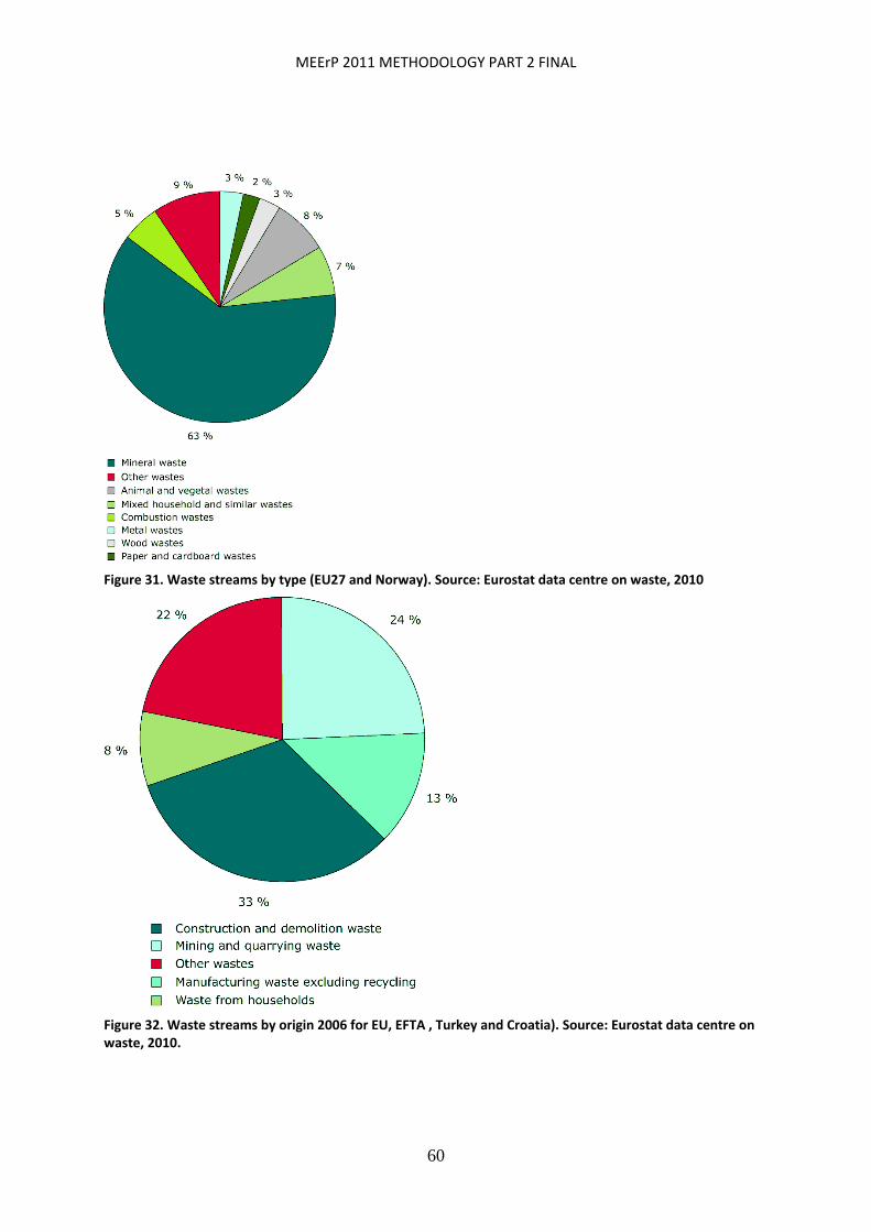
MEErP 2011 METHODOLOGY PART 2 FINAL
60
Figure 31. Waste streams by type (EU27 and Norway). Source: Eurostat data centre on waste, 2010
Figure 32. Waste streams by origin 2006 for EU, EFTA , Turkey and Croatia). Source: Eurostat data centre on waste, 2010.
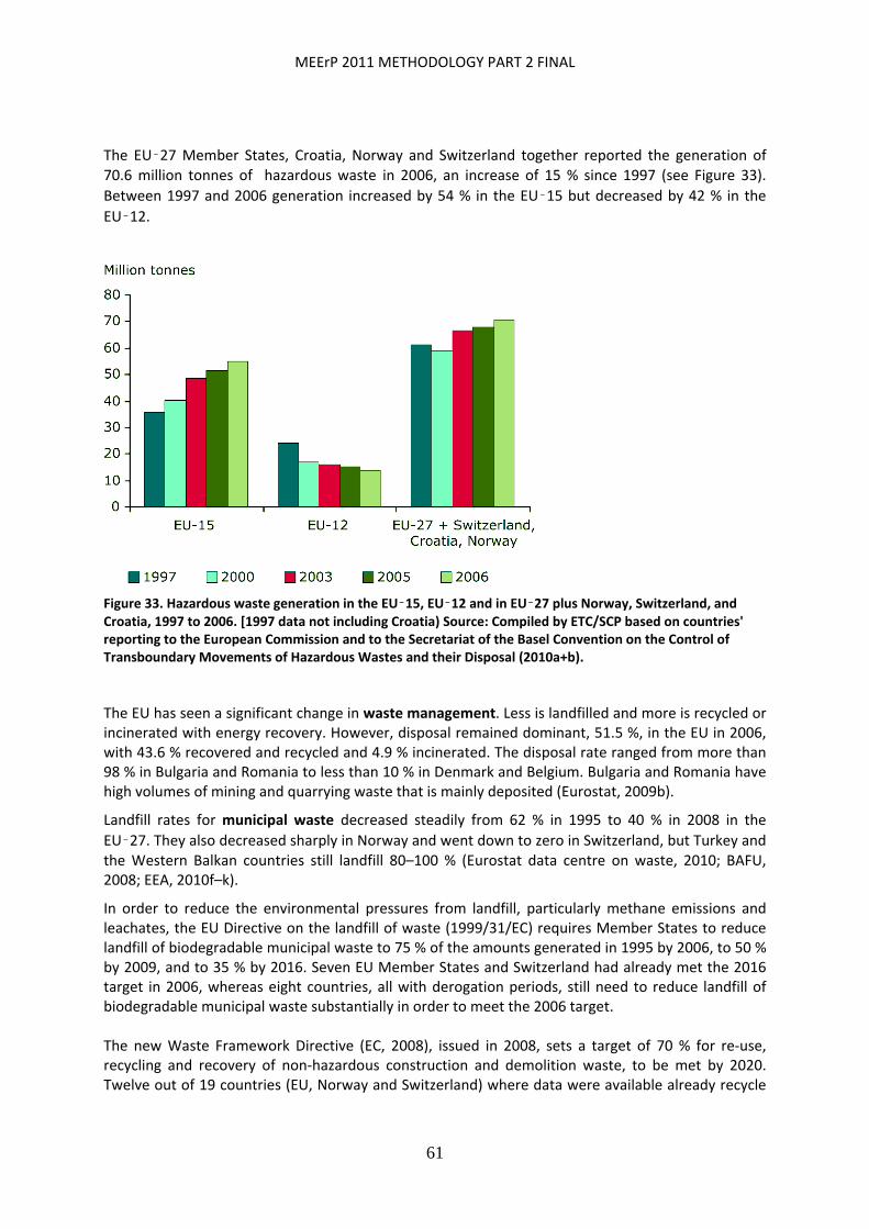
MEErP 2011 METHODOLOGY PART 2 FINAL
61
The EU‑27 Member States, Croatia, Norway and Switzerland together reported the generation of 70.6 million tonnes of hazardous waste in 2006, an increase of 15 % since 1997 (see Figure 33). Between 1997 and 2006 generation increased by 54 % in the EU‑15 but decreased by 42 % in the
EU‑12.
Figure 33. Hazardous waste generation in the EU‑15, EU‑12 and in EU‑27 plus Norway, Switzerland, and Croatia, 1997 to 2006. [1997 data not including Croatia) Source: Compiled by ETC/SCP based on countries' reporting to the European Commission and to the Secretariat of the Basel Convention on the Control of Transboundary Movements of Hazardous Wastes and their Disposal (2010a+b).
The EU has seen a significant change in waste management. Less is landfilled and more is recycled or incinerated with energy recovery. However, disposal remained dominant, 51.5 %, in the EU in 2006, with 43.6 % recovered and recycled and 4.9 % incinerated. The disposal rate ranged from more than 98 % in Bulgaria and Romania to less than 10 % in Denmark and Belgium. Bulgaria and Romania have high volumes of mining and quarrying waste that is mainly deposited (Eurostat, 2009b).
Landfill rates for municipal waste decreased steadily from 62 % in 1995 to 40 % in 2008 in the
EU‑27. They also decreased sharply in Norway and went down to zero in Switzerland, but Turkey and the Western Balkan countries still landfill 80–100 % (Eurostat data centre on waste, 2010; BAFU, 2008; EEA, 2010f–k).
In order to reduce the environmental pressures from landfill, particularly methane emissions and leachates, the EU Directive on the landfill of waste (1999/31/EC) requires Member States to reduce landfill of biodegradable municipal waste to 75 % of the amounts generated in 1995 by 2006, to 50 % by 2009, and to 35 % by 2016. Seven EU Member States and Switzerland had already met the 2016 target in 2006, whereas eight countries, all with derogation periods, still need to reduce landfill of biodegradable municipal waste substantially in order to meet the 2006 target. The new Waste Framework Directive (EC, 2008), issued in 2008, sets a target of 70 % for re‐use, recycling and recovery of non‐hazardous construction and demolition waste, to be met by 2020. Twelve out of 19 countries (EU, Norway and Switzerland) where data were available already recycle
MEErP 2011 METHODOLOGY PART 2 FINAL
62
or recover more than 50 % of their construction and demolition waste, totaling an estimated 300 million tonnes. As regards building materials the European Aluminium Association EAA commissioned Delft University of Technology to conduct a scientific study investigating aluminium content and collection rates in European buildings. The demolition of a significant number of buildings in six European countries was closely monitored and comprehensive data were gathered. The collection rates of aluminium in this sector were found to vary between 92 and 98% (on average 96%). Aluminium metal losses incurred during separation treatment range from 0% (no treatment necessary) to 10%. Melting oxidation losses are on average 2%.72
Packaging waste is an example where EU and national legislation has successfully increased recycling
across the EU. In 2007, 59 % of all packaging waste in the EU‑27 was recycled and 14 % energy‐recovered (EEA, 2010b). In 2007, 18 of the EEA countries had met the 2008 target of the Packaging Waste Directive (2004/12/EC) to recycle at least 55 % of the packaging waste generated. Recycling rates differ considerably according to packaging material, with highest rates for paper and cardboard and lowest for plastics. At the same time, the use of plastics as packaging material is increasing most rapidly ‐ 40 % between 1997 and 2006 in the EU‐15 compared to a 24 % increase of paper and cardboard and 0‐2 % for glass and metals packaging (calculated using data from Eurostat data centre on waste, 2010).
EU‑wide information on the management of hazardous waste is sparse. In 2006, 33.6 % of the hazardous waste generated was disposed of, 34.0 % was recovered, and no information about the management of the remaining 32.4 % is available (calculations based on data from Eurostat data centre on waste, 2010).
The EC Directive 2002/96/EC on waste of electrical and electronic equipment (WEEE Directive) sets a collection target of 4 kg of WEEE per person and per year from private households. In addition, by 31 December 2006, manufacturers and importers were to achieve, for treated WEEE, recovery targets of 70–80 % differentiated for the respective categories, as well as material and substance reuse and recycling targets of 50–75 %. However, as the amount of electrical and electronic equipment (EEE) put on the market in many countries is far above 4 kg per person/year, the targets are currently under revision. Only 11 countries out of 23 have met the 4 kg per person/year collection target, the remaining countries have either not met the target or not reported (see Figure 34).
Member States are currently still building or expanding systems for collecting WEEE. The collection rate achieved so far is only 23 % by weight of amounts put on the market in 2006 — the average of 18 European countries for which data are available. There is evidence that considerably more than 23
% of WEEE is collected but not reported, and that a substantial part of this undergoes sub‑standard treatment in the EU or is illegally exported. This non‐reported collection and trade is driven by the material value of some WEEE fractions (EC, 2008b). However, where WEEE is collected separately, it is widely recycled: for 17 countries where recycling rates can be calculated, the average recycling rate was 79 % (Figure 34)
72 European Aluminium Association (EAA) and Organisation of European Aluminium Refiners and Remelters (OEA),
Aluminium Recycling in Europe, The Road to High Quality Products, ca. 2006

MEErP 2011 METHODOLOGY PART 2 FINAL
63
Figure 34 WEEE put on the market, collected and recycled/recovered/reused in 23 European countries (kg/person), all figures relate to 2006. Source: Compiled by ETC/SCP based data from Eurostat data centre on waste, 2010a,b
Figure 35 below gives the expected trends in the management of municipal waste in a Business‐as Usual scenario, i.e. not taking into account measures.
Figure 35. Trends and outlook for management
of municipal waste in the EU‑27 (excluding Cyprus) plus Norway and Switzerland, baseline scenario. Source: ETC/SCP, 2010a.73
Note
1) In case of a difference between generated municipal waste and amounts reported as landfilled, incinerated, recycled/ composted, the difference has been distributed proportionally to the three management options;
2) The projection of municipal waste generation assumes a fall in GDP in 2008–2010, and a gradual recovery to 2 % annual growth until 2020.
73 In ibid 1
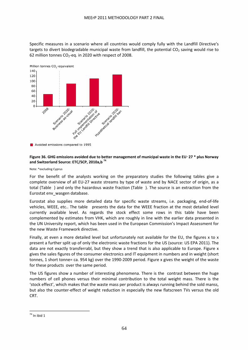
MEErP 2011 METHODOLOGY PART 2 FINAL
64
Specific measures in a scenario where all countries would comply fully with the Landfill Directive's targets to divert biodegradable municipal waste from landfill, the potential CO2 saving would rise to 62 million tonnes CO2‐eq. in 2020 with respect of 2008.
Figure 36. GHG emissions avoided due to better management of municipal waste in the EU‑27 * plus Norway and Switzerland Source: ETC/SCP, 2010a,b 74
Note: *excluding Cyprus
For the benefit of the analysts working on the preparatory studies the following tables give a complete overview of all EU‐27 waste streams by type of waste and by NACE sector of origin, as a total (Table ) and only the hazardous waste fraction (Table ). The source is an extraction from the Eurostat env_wasgen database.
Eurostat also supplies more detailed data for specific waste streams, i.e. packaging, end‐of‐life vehicles, WEEE, etc.. The table presents the data for the WEEE fraction at the most detailed level currently available level. As regards the stock effect some rows in this table have been complemented by estimates from VHK, which are roughly in line with the earlier data presented in the UN University report, which has been used in the European Commission’s Impact Assessment for the new Waste Framework directive.
Finally, at even a more detailed level but unfortunately not available for the EU, the figures x to x present a further split up of only the electronic waste fractions for the US (source: US EPA 2011). The data are not exactly transferrabl, but they show a trend that is also applicable to Europe. Figure x gives the sales figures of the consumer electronics and IT equipment in numbers and in weight (short tonnes, 1 short tonne= ca. 954 kg) over the 1990‐2009 period. Figure x gives the weight of the waste for these products over the same period.
The US figures show a number of interesting phenomena. There is the contrast between the huge numbers of cell phones versus their minimal contribution to the total weight mass. There is the ‘stock effect’, which makes that the waste mass per product is always running behind the sold manss, but also the counter‐effect of weight reduction in especially the new flatscreen TVs versus the old CRT.
74 In ibid 1
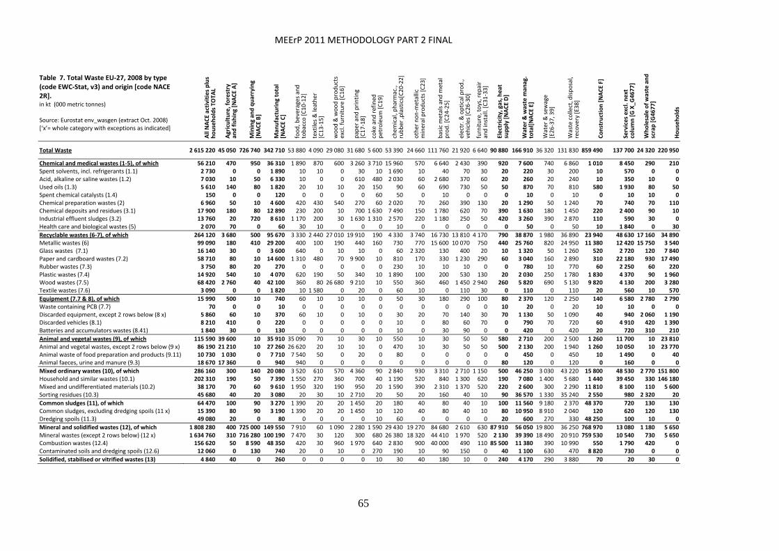
MEErP 2011 METHODOLOGY PART 2 FINAL
65
Table 7. Total Waste EU‐27, 2008 by type (code EWC‐Stat, v3) and origin [code NACE 2R]. in kt (000 metric tonnes) Source: Eurostat env_wasgen (extract Oct. 2008) [‘x’= whole category with exceptions as indicated]
All NACE activities plus
households TO
TAL
Agriculture, forestry
and fishing [NACE A]
Mining an
d quarrying
[NACE B]
Man
ufacturing total
[NACE C]
food, beverages and
tobacco [C10‐12]
textiles & leather
[C13‐15]
wood & wood products
excl. furniture [C16]
paper and printing
[C17‐18]
coke and refined
petroleum [C19]
chem
ical, pharmac.,
rubber ,plastics[C20‐22]
other non‐m
etallic
mineral products [C23]
basic m
etals and m
etal
prod. [C24‐25]
electr. &
optical prod.,
vehicles [C26‐30]
furniture, toys, rep
air
and install. [C31‐33]
Electricity, gas, h
eat
supply [NACE D]
Water & waste m
anag.
total[NACE E]
Water & sew
age
[E26‐37, 39]
Waste collect, disposal,
recovery [E38]
Construction [NACE F]
Services excl. next
column [G X_G
4677]
Wholesale of waste and
scrap [G4677]
Households
Total Waste 2 615 220 45 050 726 740 342 710 53 880 4 090 29 080 31 680 5 600 53 390 24 660 111 760 21 920 6 640 90 880 166 910 36 320 131 830 859 490 137 700 24 320 220 950
Chemical and medical wastes (1‐5), of which 56 210 470 950 36 310 1 890 870 600 3 260 3 710 15 960 570 6 640 2 430 390 920 7 600 740 6 860 1 010 8 450 290 210Spent solvents, incl. refrigerants (1.1) 2 730 0 0 1 890 10 10 0 30 10 1 690 10 40 70 30 20 220 30 200 10 570 0 0Acid, alkaline or saline wastes (1.2) 7 030 10 50 6 330 10 0 0 610 480 2 030 60 2 680 370 60 20 260 20 240 10 350 10 0Used oils (1.3) 5 610 140 80 1 820 20 10 10 20 150 90 60 690 730 50 50 870 70 810 580 1 930 80 50Spent chemical catalysts (1.4) 150 0 0 120 0 0 0 0 60 50 0 10 0 0 0 10 0 10 0 10 10 0Chemical preparation wastes (2) 6 960 50 10 4 600 420 430 540 270 60 2 020 70 260 390 130 20 1 290 50 1 240 70 740 70 110Chemical deposits and residues (3.1) 17 900 180 80 12 890 230 200 10 700 1 630 7 490 150 1 780 620 70 390 1 630 180 1 450 220 2 400 90 10Industrial effluent sludges (3.2) 13 760 20 720 8 610 1 170 200 30 1 630 1 310 2 570 220 1 180 250 50 420 3 260 390 2 870 110 590 30 0Health care and biological wastes (5) 2 070 70 0 60 30 10 0 0 0 10 0 0 0 0 0 50 0 50 10 1 840 0 30
Recyclable wastes (6‐7), of which 264 120 3 680 500 95 670 3 330 2 440 27 010 19 910 190 4 330 3 740 16 730 13 810 4 170 790 38 870 1 980 36 890 23 940 48 630 17 160 34 890Metallic wastes (6) 99 090 180 410 29 200 400 100 190 440 160 730 770 15 600 10 070 750 440 25 760 820 24 950 11 380 12 420 15 750 3 540Glass wastes (7.1) 16 140 30 0 3 600 640 0 10 10 0 60 2 320 130 400 20 10 1 320 50 1 260 520 2 720 120 7 840Paper and cardboard wastes (7.2) 58 710 80 10 14 600 1 310 480 70 9 900 10 810 170 330 1 230 290 60 3 040 160 2 890 310 22 180 930 17 490Rubber wastes (7.3) 3 750 80 20 270 0 0 0 0 0 230 10 10 10 0 0 780 10 770 60 2 250 60 220Plastic wastes (7.4) 14 920 540 10 4 070 620 190 50 340 10 1 890 100 200 530 130 20 2 030 250 1 780 1 830 4 370 90 1 960Wood wastes (7.5) 68 420 2 760 40 42 100 360 80 26 680 9 210 10 550 360 460 1 450 2 940 260 5 820 690 5 130 9 820 4 130 200 3 280Textile wastes (7.6) 3 090 0 0 1 820 10 1 580 0 20 0 60 10 0 110 30 0 110 0 110 20 560 10 570
Equipment (7.7 & 8), of which 15 990 500 10 740 60 10 10 10 0 50 30 180 290 100 80 2 370 120 2 250 140 6 580 2 780 2 790Waste containing PCB (7.7) 70 0 0 10 0 0 0 0 0 0 0 0 0 0 10 20 0 20 10 10 0 0Discarded equipment, except 2 rows below (8 x) 5 860 60 10 370 60 10 0 10 0 30 20 70 140 30 70 1 130 50 1 090 40 940 2 060 1 190Discarded vehicles (8.1) 8 210 410 0 220 0 0 0 0 0 10 0 80 60 70 0 790 70 720 60 4 910 420 1 390Batteries and accumulators wastes (8.41) 1 840 30 0 130 0 0 0 0 0 10 0 30 90 0 0 420 0 420 20 720 310 210
Animal and vegetal wastes (9), of which 115 590 39 600 10 35 910 35 090 70 10 30 10 550 10 30 50 50 580 2 710 200 2 500 1 260 11 700 10 23 810Animal and vegetal wastes, except 2 rows below (9 x) 86 190 21 210 10 27 260 26 620 20 10 10 0 470 10 30 50 50 500 2 130 200 1 940 1 260 10 050 10 23 770Animal waste of food preparation and products (9.11) 10 730 1 030 0 7 710 7 540 50 0 20 0 80 0 0 0 0 0 450 0 450 10 1 490 0 40Animal faeces, urine and manure (9.3) 18 670 17 360 0 940 940 0 0 0 0 0 0 0 0 0 80 120 0 120 0 160 0 0
Mixed ordinary wastes (10), of which 286 160 300 140 20 080 3 520 610 570 4 360 90 2 840 930 3 310 2 710 1 150 500 46 250 3 030 43 220 15 800 48 530 2 770 151 800Household and similar wastes (10.1) 202 310 190 50 7 390 1 550 270 360 700 40 1 190 520 840 1 300 620 190 7 080 1 400 5 680 1 440 39 450 330 146 180Mixed and undifferentiated materials (10.2) 38 170 70 60 9 610 1 950 320 190 950 20 1 590 390 2 310 1 370 520 220 2 600 300 2 290 11 810 8 100 110 5 600Sorting residues (10.3) 45 680 40 20 3 080 20 30 10 2 710 20 50 20 160 40 10 90 36 570 1 330 35 240 2 550 980 2 320 20
Common sludges (11), of which 64 470 100 90 3 270 1 390 20 20 1 450 20 180 40 80 40 10 100 11 560 9 180 2 370 48 370 720 130 130Common sludges, excluding dredging spoils (11 x) 15 390 80 90 3 190 1 390 20 20 1 450 10 120 40 80 40 10 80 10 950 8 910 2 040 120 620 120 130Dredging spoils (11.3) 49 080 20 0 80 0 0 0 0 10 60 0 0 0 0 20 600 270 330 48 250 100 10 0
Mineral and solidified wastes (12), of which 1 808 280 400 725 000 149 550 7 910 60 1 090 2 280 1 590 29 430 19 270 84 680 2 610 630 87 910 56 050 19 800 36 250 768 970 13 080 1 180 5 650Mineral wastes (except 2 rows below) (12 x) 1 634 760 310 716 280 100 190 7 470 30 120 300 680 26 380 18 320 44 410 1 970 520 2 130 39 390 18 490 20 910 759 530 10 540 730 5 650Combustion wastes (12.4) 156 620 50 8 590 48 350 420 30 960 1 970 640 2 830 900 40 000 490 110 85 500 11 380 390 10 990 550 1 790 420 0Contaminated soils and dredging spoils (12.6) 12 060 0 130 740 20 0 10 0 270 190 10 90 150 0 40 1 100 630 470 8 820 730 0 0
Solidified, stabilised or vitrified wastes (13) 4 840 40 0 260 0 0 0 0 10 30 40 180 10 0 240 4 170 290 3 880 70 20 30 0
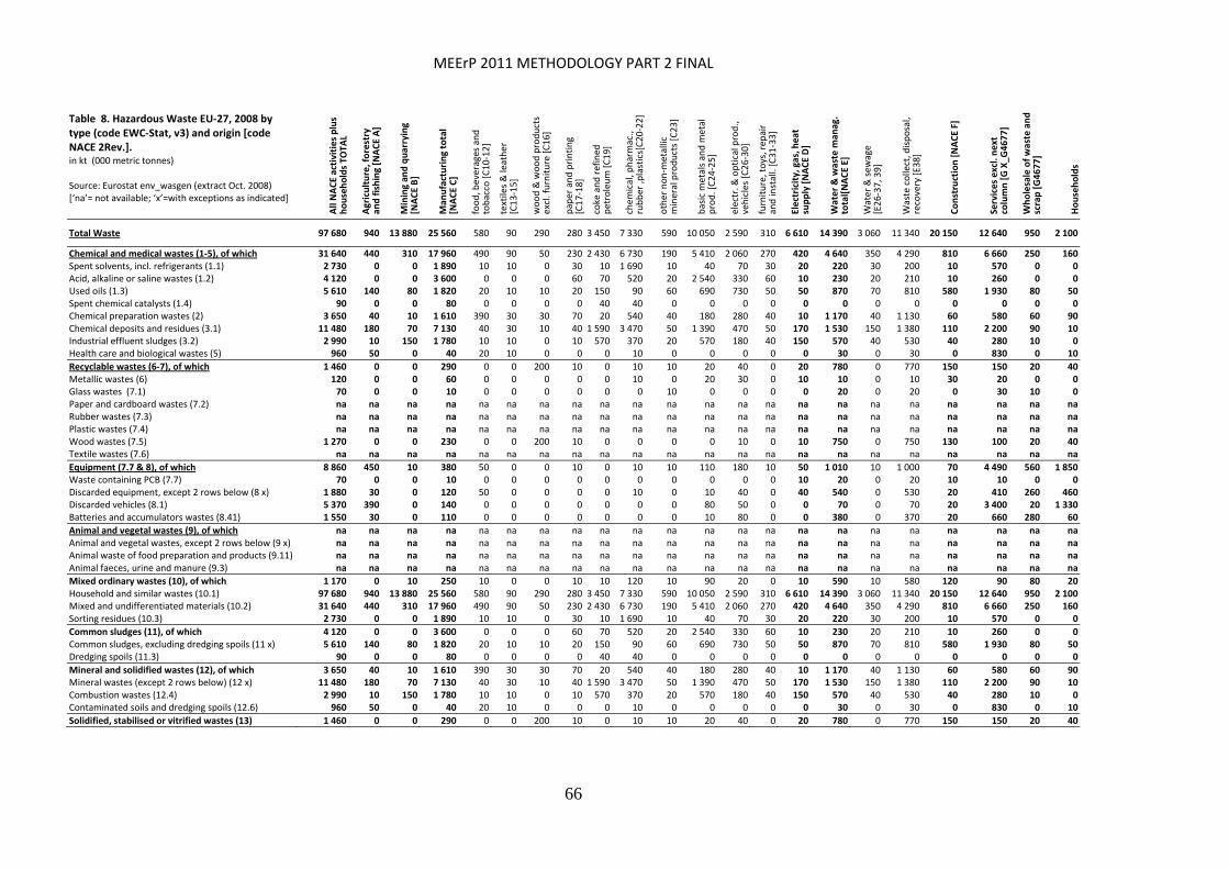
MEErP 2011 METHODOLOGY PART 2 FINAL
66
Table 8. Hazardous Waste EU‐27, 2008 by type (code EWC‐Stat, v3) and origin [code NACE 2Rev.]. in kt (000 metric tonnes) Source: Eurostat env_wasgen (extract Oct. 2008) [‘na’= not available; ‘x’=with exceptions as indicated]
All NACE activities plus
households TO
TAL
Agriculture, forestry
and fishing [NACE A]
Mining an
d quarrying
[NACE B]
Man
ufacturing total
[NACE C]
food, beverages and
tobacco [C10‐12]
textiles & leather
[C13‐15]
wood & wood products
excl. furniture [C16]
paper and printing
[C17‐18]
coke and refined
petroleum [C19]
chem
ical, pharmac.,
rubber ,plastics[C20‐22]
other non‐m
etallic
mineral products [C23]
basic m
etals and m
etal
prod. [C24‐25]
electr. &
optical prod.,
vehicles [C26‐30]
furniture, toys, rep
air
and install. [C31‐33]
Electricity, gas, h
eat
supply [NACE D]
Water & waste m
anag.
total[NACE E]
Water & sew
age
[E26‐37, 39]
Waste collect, disposal,
recovery [E38]
Construction [NACE F]
Services excl. next
column [G X_G
4677]
Wholesale of waste and
scrap [G4677]
Households
Total Waste 97 680 940 13 880 25 560 580 90 290 280 3 450 7 330 590 10 050 2 590 310 6 610 14 390 3 060 11 340 20 150 12 640 950 2 100
Chemical and medical wastes (1‐5), of which 31 640 440 310 17 960 490 90 50 230 2 430 6 730 190 5 410 2 060 270 420 4 640 350 4 290 810 6 660 250 160 Spent solvents, incl. refrigerants (1.1) 2 730 0 0 1 890 10 10 0 30 10 1 690 10 40 70 30 20 220 30 200 10 570 0 0 Acid, alkaline or saline wastes (1.2) 4 120 0 0 3 600 0 0 0 60 70 520 20 2 540 330 60 10 230 20 210 10 260 0 0 Used oils (1.3) 5 610 140 80 1 820 20 10 10 20 150 90 60 690 730 50 50 870 70 810 580 1 930 80 50 Spent chemical catalysts (1.4) 90 0 0 80 0 0 0 0 40 40 0 0 0 0 0 0 0 0 0 0 0 0 Chemical preparation wastes (2) 3 650 40 10 1 610 390 30 30 70 20 540 40 180 280 40 10 1 170 40 1 130 60 580 60 90 Chemical deposits and residues (3.1) 11 480 180 70 7 130 40 30 10 40 1 590 3 470 50 1 390 470 50 170 1 530 150 1 380 110 2 200 90 10 Industrial effluent sludges (3.2) 2 990 10 150 1 780 10 10 0 10 570 370 20 570 180 40 150 570 40 530 40 280 10 0 Health care and biological wastes (5) 960 50 0 40 20 10 0 0 0 10 0 0 0 0 0 30 0 30 0 830 0 10
Recyclable wastes (6‐7), of which 1 460 0 0 290 0 0 200 10 0 10 10 20 40 0 20 780 0 770 150 150 20 40 Metallic wastes (6) 120 0 0 60 0 0 0 0 0 10 0 20 30 0 10 10 0 10 30 20 0 0 Glass wastes (7.1) 70 0 0 10 0 0 0 0 0 0 10 0 0 0 0 20 0 20 0 30 10 0 Paper and cardboard wastes (7.2) na na na na na na na na na na na na na na na na na na na na na na Rubber wastes (7.3) na na na na na na na na na na na na na na na na na na na na na na Plastic wastes (7.4) na na na na na na na na na na na na na na na na na na na na na na Wood wastes (7.5) 1 270 0 0 230 0 0 200 10 0 0 0 0 10 0 10 750 0 750 130 100 20 40 Textile wastes (7.6) na na na na na na na na na na na na na na na na na na na na na na
Equipment (7.7 & 8), of which 8 860 450 10 380 50 0 0 10 0 10 10 110 180 10 50 1 010 10 1 000 70 4 490 560 1 850 Waste containing PCB (7.7) 70 0 0 10 0 0 0 0 0 0 0 0 0 0 10 20 0 20 10 10 0 0 Discarded equipment, except 2 rows below (8 x) 1 880 30 0 120 50 0 0 0 0 10 0 10 40 0 40 540 0 530 20 410 260 460 Discarded vehicles (8.1) 5 370 390 0 140 0 0 0 0 0 0 0 80 50 0 0 70 0 70 20 3 400 20 1 330 Batteries and accumulators wastes (8.41) 1 550 30 0 110 0 0 0 0 0 0 0 10 80 0 0 380 0 370 20 660 280 60
Animal and vegetal wastes (9), of which na na na na na na na na na na na na na na na na na na na na na na Animal and vegetal wastes, except 2 rows below (9 x) na na na na na na na na na na na na na na na na na na na na na na Animal waste of food preparation and products (9.11) na na na na na na na na na na na na na na na na na na na na na na Animal faeces, urine and manure (9.3) na na na na na na na na na na na na na na na na na na na na na na
Mixed ordinary wastes (10), of which 1 170 0 10 250 10 0 0 10 10 120 10 90 20 0 10 590 10 580 120 90 80 20 Household and similar wastes (10.1) 97 680 940 13 880 25 560 580 90 290 280 3 450 7 330 590 10 050 2 590 310 6 610 14 390 3 060 11 340 20 150 12 640 950 2 100 Mixed and undifferentiated materials (10.2) 31 640 440 310 17 960 490 90 50 230 2 430 6 730 190 5 410 2 060 270 420 4 640 350 4 290 810 6 660 250 160 Sorting residues (10.3) 2 730 0 0 1 890 10 10 0 30 10 1 690 10 40 70 30 20 220 30 200 10 570 0 0
Common sludges (11), of which 4 120 0 0 3 600 0 0 0 60 70 520 20 2 540 330 60 10 230 20 210 10 260 0 0 Common sludges, excluding dredging spoils (11 x) 5 610 140 80 1 820 20 10 10 20 150 90 60 690 730 50 50 870 70 810 580 1 930 80 50 Dredging spoils (11.3) 90 0 0 80 0 0 0 0 40 40 0 0 0 0 0 0 0 0 0 0 0 0
Mineral and solidified wastes (12), of which 3 650 40 10 1 610 390 30 30 70 20 540 40 180 280 40 10 1 170 40 1 130 60 580 60 90 Mineral wastes (except 2 rows below) (12 x) 11 480 180 70 7 130 40 30 10 40 1 590 3 470 50 1 390 470 50 170 1 530 150 1 380 110 2 200 90 10 Combustion wastes (12.4) 2 990 10 150 1 780 10 10 0 10 570 370 20 570 180 40 150 570 40 530 40 280 10 0 Contaminated soils and dredging spoils (12.6) 960 50 0 40 20 10 0 0 0 10 0 0 0 0 0 30 0 30 0 830 0 10
Solidified, stabilised or vitrified wastes (13) 1 460 0 0 290 0 0 200 10 0 10 10 20 40 0 20 780 0 770 150 150 20 40
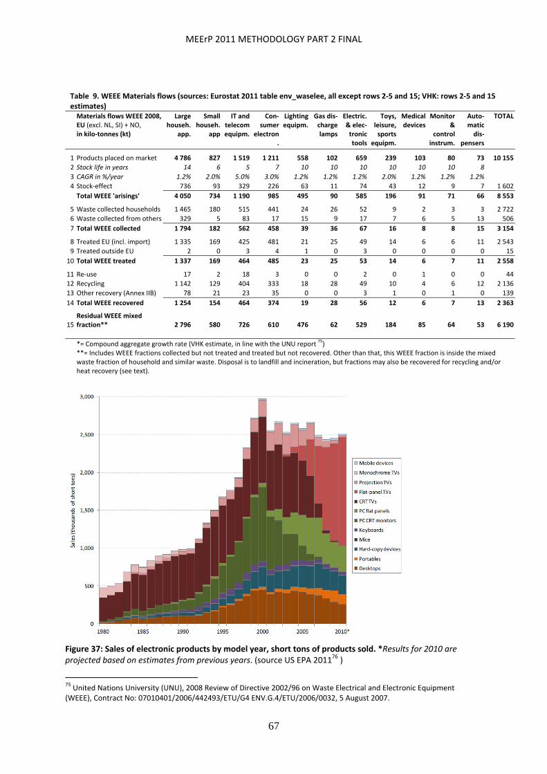
MEErP 2011 METHODOLOGY PART 2 FINAL
67
Table 9. WEEE Materials flows (sources: Eurostat 2011 table env_waselee, all except rows 2‐5 and 15; VHK: rows 2‐5 and 15 estimates)
Materials flows WEEE 2008, EU (excl. NL, SI) + NO, in kilo‐tonnes (kt)
Large househ.
app.
Small househ.
app
IT and telecomequipm.
Con‐sumer
electron.
Lighting equipm.
Gas dis‐charge lamps
Electric. & elec‐tronic tools
Toys, leisure, sports
equipm.
Medical devices
Monitor &
control instrum.
Auto‐matic dis‐
pensers
TOTAL
1 Products placed on market 4 786 827 1 519 1 211 558 102 659 239 103 80 73 10 155
2 Stock life in years 14 6 5 7 10 10 10 10 10 10 8
3 CAGR in %/year 1.2% 2.0% 5.0% 3.0% 1.2% 1.2% 1.2% 2.0% 1.2% 1.2% 1.2%
4 Stock‐effect 736 93 329 226 63 11 74 43 12 9 7 1 602
Total WEEE 'arisings' 4 050 734 1 190 985 495 90 585 196 91 71 66 8 553
5 Waste collected households 1 465 180 515 441 24 26 52 9 2 3 3 2 722
6 Waste collected from others 329 5 83 17 15 9 17 7 6 5 13 506
7 Total WEEE collected 1 794 182 562 458 39 36 67 16 8 8 15 3 154
8 Treated EU (incl. import) 1 335 169 425 481 21 25 49 14 6 6 11 2 543
9 Treated outside EU 2 0 3 4 1 0 3 0 0 0 0 15
10 Total WEEE treated 1 337 169 464 485 23 25 53 14 6 7 11 2 558
11 Re‐use 17 2 18 3 0 0 2 0 1 0 0 44
12 Recycling 1 142 129 404 333 18 28 49 10 4 6 12 2 136
13 Other recovery (Annex IIB) 78 21 23 35 0 0 3 1 0 1 0 139
14 Total WEEE recovered 1 254 154 464 374 19 28 56 12 6 7 13 2 363
15 Residual WEEE mixed fraction** 2 796 580 726 610 476 62 529 184 85 64 53 6 190
*= Compound aggregate growth rate (VHK estimate, in line with the UNU report 75)
**= Includes WEEE fractions collected but not treated and treated but not recovered. Other than that, this WEEE fraction is inside the mixed waste fraction of household and similar waste. Disposal is to landfill and incineration, but fractions may also be recovered for recycling and/or heat recovery (see text).
Figure 37: Sales of electronic products by model year, short tons of products sold. *Results for 2010 are projected based on estimates from previous years. (source US EPA 201176 )
75 United Nations University (UNU), 2008 Review of Directive 2002/96 on Waste Electrical and Electronic Equipment (WEEE), Contract No: 07010401/2006/442493/ETU/G4 ENV.G.4/ETU/2006/0032, 5 August 2007.
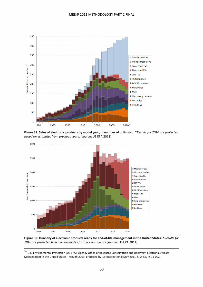
MEErP 2011 METHODOLOGY PART 2 FINAL
68
Figure 38: Sales of electronic products by model year, in number of units sold. *Results for 2010 are projected based on estimates from previous years. (source: US EPA 2011)
Figure 39: Quantity of electronic products ready for end‐of‐life management in the United States. *Results for 2010 are projected based on estimates from previous years.(source: US EPA 2011)
76 U.S. Environmental Protection (US EPA), Agency Office of Resource Conservation and Recovery, Electronics Waste
Management in the United States Through 2009, prepared by ICF International May 2011, EPA 530‐R‐11‐002.

MEErP 2011 METHODOLOGY PART 2 FINAL
69
Figure 40: Quantity of electronic products collected for recycling or disposed, by year. *Results for 2010 are projected based on estimates from previous years. (source: US EPA).
In all Ecodesign preparatory studies until 2011, waste disposal was studied. Thus far, for none of the studied ErP it was found significant enough to be included in Ecodesign or labelling measures.
MEErP 2011 METHODOLOGY PART 2 FINAL
70
3 EMISSIONS
3.1 Greenhousegases(GHGs)Emissions of the six Kyoto GHGs77 from anthropogenic sources in the EU have fallen each year since 2003 (EEA, 2010a)78. In the past 18 years, GHG emissions have declined in both the EU‐15, as party to the Kyoto Protocol, and in the EU‐27. The EU‐15 stood 6.9 % below its base‐year emissions under the Kyoto Protocol in 2008 (6) [Please check footnote.] ‐ a net reduction of 295 million tonnes of CO2‐equivalent. Total emissions in the EU‐27 were 11.3 % below 1990 in 2008 (7) [Please check footnote.], ‐ equivalent to a net reduction of 627 million tonnes of CO2‐equivalent (see section 3).
On a longer time perspective, EU emissions have been decreasing since the mid to late 1980s and the downward trend is expected to continue at least until 2009 (Figure 41). Early 2009 greenhouse gas estimates published by the EEA during 2010 showed EU emissions decreased by 6.9 % in 2009 compared to 2008. Based on these estimates, the EU‐27's 2009 emissions stand approximately 17.3 % below the 1990 level. The EU‐15 stands 12.9 % below the base‐year level, achieving its Kyoto commitment to an 8 % reduction for the first time.
The strength of the 2009 recession affected all economic sectors in the EU. Consumption of fossil fuels (coal, oil and natural gas) fell compared to the previous year, mainly for coal. The decreased demand for energy linked to the economic recession was accompanied by cheaper natural gas and increased renewable energy use, which together contributed to lower emissions (see footnote 10). The relatively colder winter of 2009 increased the residential sector's heating needs, partly offsetting the total reduction in greenhouse gas emissions. In relative terms, the largest emission reductions occurred in industrial processes reflecting lower activity levels in the cement, chemical and iron and steel industries. The 2009 verified emissions from the sectors covered by the EU Emission Trading Scheme (EU‐ETS) decreased by 11.6 % compared to 2008 (EEA, 2010b). The recession in 2009 accelerated, temporarily, the downward trend in total greenhouse gas emissions. Of the estimated 1 billion tonnes of CO2‐equivalent reduced between 1990 and 2009, one third would have been accounted for by the 2009 economic recession (EEA, 2010c).
77 CO2, methane (CH4), nitrous oxide (N2O), hydrofluorocarbons (HFCs), perfluorocarbons (PFCs) and sulphur hexafluoride (SF6). 78 Information in this section based on EEA, THE EUROPEAN ENVIRONMENT, STATE AND OUTLOOK 2010, MITIGATING CLIMATE CHANGE, Copenhagen, 2010. Note that especially where value statements are involved the text may contain literal citations from this official EU source.
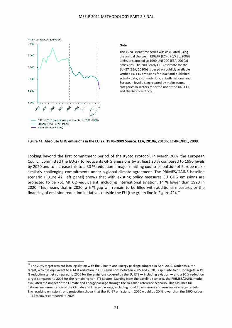
MEErP 2011 METHODOLOGY PART 2 FINAL
71
Figure 41. Absolute GHG emissions in the EU 27, 1970–2009 Source: EEA, 2010a, 2010b; EC‐JRC/PBL, 2009.
Looking beyond the first commitment period of the Kyoto Protocol, in March 2007 the European Council committed the EU‐27 to reduce its GHG emissions by at least 20 % compared to 1990 levels by 2020 and to increase this to a 30 % reduction if major emitting countries outside of Europe make similarly challenging commitments under a global climate agreement. The PRIMES/GAINS baseline scenario (Figure 42, left panel) shows that with existing policy measures EU GHG emissions are projected to be 761 Mt CO2‐equivalent, including international aviation, 14 % lower than 1990 in 2020. This means that in 2020, a 6 % gap will remain to be filled with additional measures or the financing of emission reduction initiatives outside the EU (the green line in Figure 42). 79
79 The 20 % target was put into legislation with the Climate and Energy package adopted in April 2009. Under this, the
target, which is equivalent to a 14 % reduction in GHG emissions between 2005 and 2020, is split into two sub‐targets: a 19 % reduction target compared to 2005 for the emissions covered by the EU ETS — including aviation — and a 10 % reduction target compared to 2005 for the remaining non‐ETS sectors. Starting from the baseline scenario, the PRIMES/GAINS model evaluated the impact of the Climate and Energy package through the so‐called reference scenario. This assumes full national implementation of the Climate and Energy package, including non‐ETS emissions and renewable energy targets. The resulting emission trend projection shows that the EU‐27 emissions in 2020 would be 20 % lower than the 1990 values — 14 % lower compared to 2005
Note
The 1970–1990 time series was calculated using
the annual change in EDGAR (EC‐・JRC/PBL, 2009) emissions applied to 1990 UNFCCC (EEA, 2010a) emissions. The 2009 early GHG estimate for the
EU・27 (EEA, 2010b) is based on publicly available
verified EU ETS emissions for 2009 and published
activity data, as of mid‐・July, at both national and European level disaggregated by major source categories in sectors reported under the UNFCCC and the Kyoto Protocol.
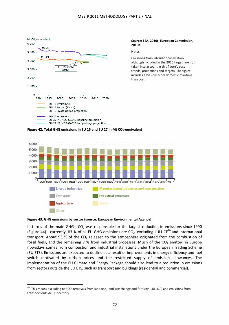
MEErP 2011 METHODOLOGY PART 2 FINAL
72
Figure 42. Total GHG emissions in EU 15 and EU 27 in Mt CO2‐equivalent
Figure 43. GHG emissions by sector (source: European Environmental Agency)
In terms of the main GHGs, CO2 was responsible for the largest reduction in emissions since 1990 (Figure 44) ‐ currently, 83 % of all EU GHG emissions are CO2, excluding LULUCF
80 and international transport. About 93 % of the CO2 released to the atmosphere originated from the combustion of fossil fuels, and the remaining 7 % from industrial processes. Much of the CO2 emitted in Europe nowadays comes from combustion and industrial installations under the European Trading Scheme (EU ETS). Emissions are expected to decline as a result of improvements in energy efficiency and fuel switch motivated by carbon prices and the restricted supply of emission allowances. The implementation of the EU Climate and Energy Package should also lead to a reduction in emissions from sectors outside the EU ETS, such as transport and buildings (residential and commercial).
80 This means excluding net CO2 removals from land use, land‐use change and forestry (LULUCF) and emissions from transport outside EU territory.
Source: EEA, 2010c, European Commission, 2010b.
Notes:
Emissions from international aviation, although included in the 2020 target, are not taken into account in this figure's past trends, projections and targets. The figure includes emissions from domestic maritime transport.

MEErP 2011 METHODOLOGY PART 2 FINAL
73
Emissions of CH4 and N2O also fell between 1990 and 2008 — CH4 represented 8.3 % of total GHG emissions in 2008 ‐ and N2O ‐ 7.3 % of the total. The reduction in CH4 emissions reflects lower levels of coal mining and post‐mining activities as well as lower emissions from managed waste disposal on land. There has also been a significant reduction in CH4 emissions from agricultural livestock, due to a reduction in numbers but also to changes in the agricultural management of organic manures. N2O emissions fell because of lower emissions from agricultural soils.
Key EU policies such as the Nitrates Directive, the Common Agriculture Policy (CAP) and the Landfill Waste Directive have been successful in reducing greenhouse gas emissions from methane and nitrous oxides. The Nitrates Directive (EC, 1991) which aims at reducing and preventing water pollution caused by nitrates from agricultural sources has had a significant impact on greenhouse emissions. The so‐called first pillar of the CAP (dealing with market support) also had a strong impact through the milk quota system by reducing animal numbers in the dairy sector to compensate for increasing animal productivity. The Landfill Waste Directive (EC, 1999) which requires Member States to reduce the amount of biodegradable waste landfilled has also contributed to an increase in the amounts of waste recycled, composted and an increase in the recovery of landfill gas.
One of the key EU emission sources is the consumption of hydrofluorocarbons (HFCs) used in industrial processes. HFCs were the only group of gases for which emissions increased between 1990 and 2008. HFCs are used in the production of cooling devices such as air conditioning systems and refrigerators and the increase is consistent with both warmer climatic conditions in Europe and higher standards of comfort demanded by citizens. HFC emissions from air‐conditioning systems in motor vehicles are of concern because HFC‐134a is the largest contributor to total HFCs emissions and has a global warming potential (GWP) about 1 400 times stronger than CO2. In Europe, however, the use of HFC‐134a for mobile air‐conditioning in new cars will be phased out between 2011 and 2017 (EC, 2006). From January 2011, EU Member States will no longer grant EC type‐approval or national type‐approval for a type of vehicle fitted with an air conditioning system designed to contain fluorinated GHGs with a GWP higher than 150, and from January 2017, Member States will have to refuse registration and prohibit the sale of such new vehicles.
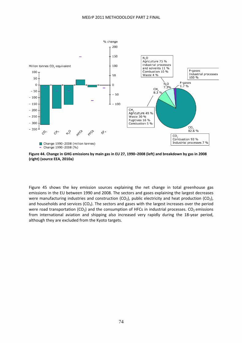
MEErP 2011 METHODOLOGY PART 2 FINAL
74
Figure 44. Change in GHG emissions by main gas in EU 27, 1990–2008 (left) and breakdown by gas in 2008 (right) (source EEA, 2010a)
Figure 45 shows the key emission sources explaining the net change in total greenhouse gas emissions in the EU between 1990 and 2008. The sectors and gases explaining the largest decreases were manufacturing industries and construction (CO2), public electricity and heat production (CO2), and households and services (CO2). The sectors and gases with the largest increases over the period were road transportation (CO2) and the consumption of HFCs in industrial processes. CO2 emissions from international aviation and shipping also increased very rapidly during the 18‐year period, although they are excluded from the Kyoto targets.
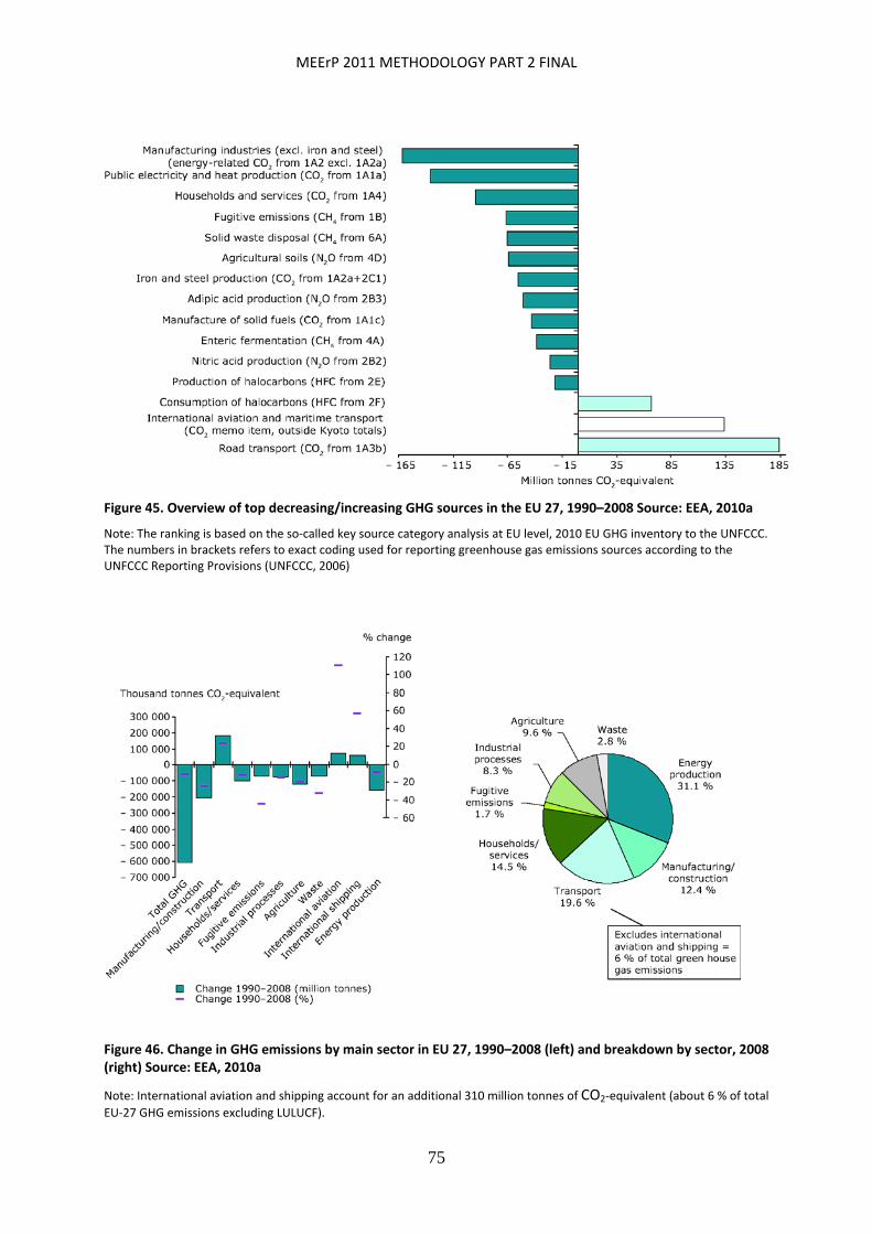
MEErP 2011 METHODOLOGY PART 2 FINAL
75
Figure 45. Overview of top decreasing/increasing GHG sources in the EU 27, 1990–2008 Source: EEA, 2010a
Note: The ranking is based on the so‐called key source category analysis at EU level, 2010 EU GHG inventory to the UNFCCC. The numbers in brackets refers to exact coding used for reporting greenhouse gas emissions sources according to the UNFCCC Reporting Provisions (UNFCCC, 2006)
Figure 46. Change in GHG emissions by main sector in EU 27, 1990–2008 (left) and breakdown by sector, 2008 (right) Source: EEA, 2010a
Note: International aviation and shipping account for an additional 310 million tonnes of CO2‐equivalent (about 6 % of total
EU‐27 GHG emissions excluding LULUCF).

MEErP 2011 METHODOLOGY PART 2 FINAL
76
Energy combustion (i.e. the production and consumption of energy by all sectors, including transport) accounts for 92 % of the reduction in EU‐27 greenhouse gas emissions between 1990 and 2008. Figure 46 shows a breakdown of the factors that help explain or illustrate year‐on‐year changes in CO2 emissions from the combustion of fossil fuels.
CO2 emissions from energy combustion (EEA, 2010a) fell by 7.1 % (288 million tonnes) in the EU‐27 between 1990 and 2008, while real GDP increased by 46 % and population grew by almost 6 % (27 million people, Eurostat, 2010) over the 18‐year period (EC, 2010a). A growing population and GDP generally contribute to higher CO2 emissions. A faster growth in GDP relative to population has led to significant increases in GDP per capita, particularly in the mid‐to‐late 1990s.
The remaining two factors, i.e. the energy intensity and carbon intensity of the economy are key for understanding the evolution of CO2 emissions from energy‐related sources. Energy intensity has fallen almost every year since 1990, partly due to a contraction in primary energy consumption, partly due to a more rapid increase in real GDP. Carbon intensity has also declined and this is mainly due to the switch to less polluting fuels.
Figure 47. Change in GDP, population, primary energy and emissions, 1990–2010 Source: EEA, 2010a; Eurostat, 2010; European Commission, 2010a.
Note: The chart to the left shows the estimated contributions of the various factors that have affected CO2 emissions from
energy production and consumption in the EU‐27. This approach is often used to portray the primary forces driving emissions. The explanatory factors should not be seen as fundamental factors in themselves nor should they be seen as independent of each other. The chart to the right shows the increase in GDP, population, primary energy and total greenhouse gas emissions in the EU‐27 compared to 1990.
Carbon intensity can be defined as the amount of CO2 released to the atmosphere per unit of primary energy consumed (relatively small amounts of methane are also emitted). At EU level, one of the sectors contributing most to the net emission reduction between 1990 and 2008 was the production of heat and electricity. Less coal and oil, more gas and more combustible renewables (i.e. biomass) explain why this sector emitted 136 million tonnes of CO2 less than in 2007.
MEErP 2011 METHODOLOGY PART 2 FINAL
77
The change in the fuel mix in the production of heat and electricity in thermal stations has led to important savings in CO2 emissions. The average 2008 implied emission factor (i.e. carbon dioxide emitted per unit energy released) for coal was 100 t CO2/TJ, compared to 76 t CO2/TJ for liquid fuels and 57 t CO2/TJ for gas. Therefore, the reduced contribution of both coal and liquid fuels in the average household fuel mix, together with the increased contribution from gas and biomass, have led to a better CO2 emission intensity per unit of energy generated (see also earlier discussion on the sectors achieving the largest emission reductions and Figure 45). Other factors clearly contributed to the decline in greenhouse gas emissions in the EU‐27. Eurostat 2008 energy balances confirm the decline of primary consumption of solid fuels and the increase in natural gas. The energy balances also show a strong increase in the amount of renewable energy, particularly from biomass, wind and hydro for electricity generation.
The UNFCCC and Kyoto Protocol do not cover all GHGs (10). The Montreal Protocol was agreed by countries in 1987 in order to phase out the production of a number of substances that deplete the ozone layer ‐ it has since been widely recognised as one of the most successful multilateral environmental agreements to date. Implementation of the Montreal protocol has led to a very significant decrease in the atmospheric burden of ozone‐depleting substances (ODSs) in the lower atmosphere and in the stratosphere. Importantly however, many of the substances addressed in the Montreal protocol such as chlorofluorocarbons (CFCs) are also potent GHGs in their own right but are not addressed under the Kyoto Protocol. Thus the direct effects of the Montreal Protocol in reducing emissions of ODS have also indirectly contributed to a very significant reduction in emissions of some potent greenhouse gases.
Consumption and production of ozone‐depleting substances has gone down markedly in EEA member countries, particularly in the first half of the 1990s. Before the Montreal Protocol was signed in 1987, EEA ODS production exceeded half a million ODP (ozone depletion potential) tonnes. ODS production was negative (see note to Figure 48) in 2007 and 2008, although it increased again in 2009 to reach 747 ODP tonnes. ODS consumption in EEA member countries fell from about 80 thousand ODP tonnes in 1986 to almost zero in 2009 (see Figure 48).

MEErP 2011 METHODOLOGY PART 2 FINAL
78
Figure 48. Production and consumption of ozone depleting substances in EEA member countries, 1986–2009 Source: EEA, 2010e.
Note: Production is defined under Article 1(5) of the Montreal Protocol as production minus the amount destroyed minus the amount entirely used as feedstock in the manufacture of other chemicals. Since the figures are for each calendar year, it is quite possible that in some years the destroyed amounts and/or the feedstock figure may exceed the production figure of that year, if they include ODS from a carry‐over stock. The calculated production could be negative in such cases. Consumption is defined as production plus imports minus exports of controlled substances under the Montreal Protocol. As with calculated production, the consumption of ODS can be negative, also because exports in any one year can exceed production and imports if they include ODS from carry‐over stocks.
Characterisation Factors
The Kyoto protocol under the UNFCCC81, implemented in the EU through the Council Decision 2002/358/CE, and the so called ‘F‐gas’ Regulation82 provide the legal basis for the characterisation of Green House Gases under the MEErP. In turn, both pieces of legislation recognize the authority of the Intergovernmental Panel on Climate Change (IPPC) to supply characterisation factors for GHGs.
Table 10 below list Global Warming Potential (GWP100) characterisation factors from IPCC Fourth Assessment Report on Climate Change 2007. The unit is the weight of CO2 equivalent (‘CO2 eq.’).
81 United Nations Framework Convention on Climate Change 82 Regulation (EC) No 842/2006 of the European Parliament and of the Council of 17 May 2006 on certain fluorinated greenhouse gases.
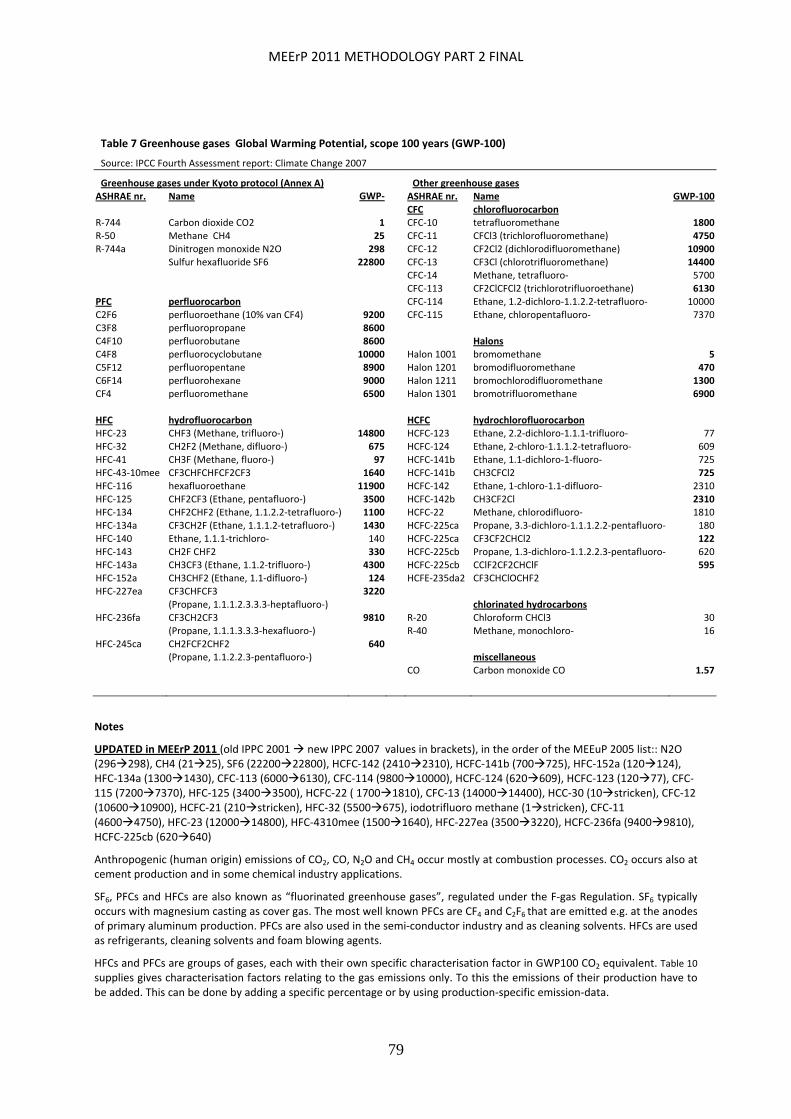
MEErP 2011 METHODOLOGY PART 2 FINAL
79
Table 7 Greenhouse gases Global Warming Potential, scope 100 years (GWP‐100)
Source: IPCC Fourth Assessment report: Climate Change 2007
Greenhouse gases under Kyoto protocol (Annex A) Other greenhouse gases ASHRAE nr. Name GWP‐ ASHRAE nr. Name GWP‐100 CFC chlorofluorocarbon R‐744 Carbon dioxide CO2 1 CFC‐10 tetrafluoromethane 1800R‐50 Methane CH4 25 CFC‐11 CFCl3 (trichlorofluoromethane) 4750R‐744a Dinitrogen monoxide N2O 298 CFC‐12 CF2Cl2 (dichlorodifluoromethane) 10900 Sulfur hexafluoride SF6 22800 CFC‐13 CF3Cl (chlorotrifluoromethane) 14400 CFC‐14 Methane, tetrafluoro‐ 5700
CFC‐113 CF2ClCFCl2 (trichlorotrifluoroethane) 6130PFC perfluorocarbon CFC‐114 Ethane, 1.2‐dichloro‐1.1.2.2‐tetrafluoro‐ 10000C2F6 perfluoroethane (10% van CF4) 9200 CFC‐115 Ethane, chloropentafluoro‐ 7370C3F8 perfluoropropane 8600 C4F10 perfluorobutane 8600 Halons C4F8 perfluorocyclobutane 10000 Halon 1001 bromomethane 5C5F12 perfluoropentane 8900 Halon 1201 bromodifluoromethane 470C6F14 perfluorohexane 9000 Halon 1211 bromochlorodifluoromethane 1300CF4 perfluoromethane 6500 Halon 1301 bromotrifluoromethane 6900 HFC hydrofluorocarbon HCFC hydrochlorofluorocarbon HFC‐23 CHF3 (Methane, trifluoro‐) 14800 HCFC‐123 Ethane, 2.2‐dichloro‐1.1.1‐trifluoro‐ 77HFC‐32 CH2F2 (Methane, difluoro‐) 675 HCFC‐124 Ethane, 2‐chloro‐1.1.1.2‐tetrafluoro‐ 609HFC‐41 CH3F (Methane, fluoro‐) 97 HCFC‐141b Ethane, 1.1‐dichloro‐1‐fluoro‐ 725HFC‐43‐10mee CF3CHFCHFCF2CF3 1640 HCFC‐141b CH3CFCl2 725HFC‐116 hexafluoroethane 11900 HCFC‐142 Ethane, 1‐chloro‐1.1‐difluoro‐ 2310HFC‐125 CHF2CF3 (Ethane, pentafluoro‐) 3500 HCFC‐142b CH3CF2Cl 2310HFC‐134 CHF2CHF2 (Ethane, 1.1.2.2‐tetrafluoro‐) 1100 HCFC‐22 Methane, chlorodifluoro‐ 1810HFC‐134a CF3CH2F (Ethane, 1.1.1.2‐tetrafluoro‐) 1430 HCFC‐225ca Propane, 3.3‐dichloro‐1.1.1.2.2‐pentafluoro‐ 180HFC‐140 Ethane, 1.1.1‐trichloro‐ 140 HCFC‐225ca CF3CF2CHCl2 122HFC‐143 CH2F CHF2 330 HCFC‐225cb Propane, 1.3‐dichloro‐1.1.2.2.3‐pentafluoro‐ 620HFC‐143a CH3CF3 (Ethane, 1.1.2‐trifluoro‐) 4300 HCFC‐225cb CClF2CF2CHClF 595HFC‐152a CH3CHF2 (Ethane, 1.1‐difluoro‐) 124 HCFE‐235da2 CF3CHClOCHF2 HFC‐227ea CF3CHFCF3 3220
(Propane, 1.1.1.2.3.3.3‐heptafluoro‐) chlorinated hydrocarbons HFC‐236fa CF3CH2CF3 9810 R‐20 Chloroform CHCl3 30
(Propane, 1.1.1.3.3.3‐hexafluoro‐) R‐40 Methane, monochloro‐ 16HFC‐245ca CH2FCF2CHF2 640
(Propane, 1.1.2.2.3‐pentafluoro‐) miscellaneous CO Carbon monoxide CO 1.57
Notes
UPDATED in MEErP 2011 (old IPPC 2001 new IPPC 2007 values in brackets), in the order of the MEEuP 2005 list:: N2O (296298), CH4 (2125), SF6 (2220022800), HCFC‐142 (24102310), HCFC‐141b (700725), HFC‐152a (120124), HFC‐134a (13001430), CFC‐113 (60006130), CFC‐114 (980010000), HCFC‐124 (620609), HCFC‐123 (12077), CFC‐115 (72007370), HFC‐125 (34003500), HCFC‐22 ( 17001810), CFC‐13 (1400014400), HCC‐30 (10stricken), CFC‐12 (1060010900), HCFC‐21 (210stricken), HFC‐32 (5500675), iodotrifluoro methane (1stricken), CFC‐11 (46004750), HFC‐23 (1200014800), HFC‐4310mee (15001640), HFC‐227ea (35003220), HCFC‐236fa (94009810), HCFC‐225cb (620640)
Anthropogenic (human origin) emissions of CO2, CO, N2O and CH4 occur mostly at combustion processes. CO2 occurs also at cement production and in some chemical industry applications.
SF6, PFCs and HFCs are also known as “fluorinated greenhouse gases”, regulated under the F‐gas Regulation. SF6 typically occurs with magnesium casting as cover gas. The most well known PFCs are CF4 and C2F6 that are emitted e.g. at the anodes of primary aluminum production. PFCs are also used in the semi‐conductor industry and as cleaning solvents. HFCs are used as refrigerants, cleaning solvents and foam blowing agents.
HFCs and PFCs are groups of gases, each with their own specific characterisation factor in GWP100 CO2 equivalent. Table 10 supplies gives characterisation factors relating to the gas emissions only. To this the emissions of their production have to be added. This can be done by adding a specific percentage or by using production‐specific emission‐data.
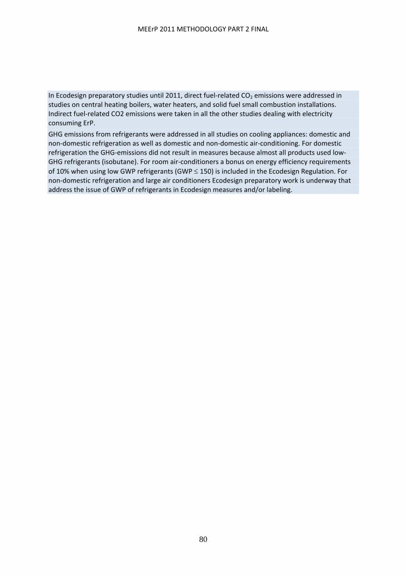
MEErP 2011 METHODOLOGY PART 2 FINAL
80
In Ecodesign preparatory studies until 2011, direct fuel‐related CO2 emissions were addressed in studies on central heating boilers, water heaters, and solid fuel small combustion installations. Indirect fuel‐related CO2 emissions were taken in all the other studies dealing with electricity consuming ErP.
GHG emissions from refrigerants were addressed in all studies on cooling appliances: domestic and non‐domestic refrigeration as well as domestic and non‐domestic air‐conditioning. For domestic refrigeration the GHG‐emissions did not result in measures because almost all products used low‐GHG refrigerants (isobutane). For room air‐conditioners a bonus on energy efficiency requirements
of 10% when using low GWP refrigerants (GWP 150) is included in the Ecodesign Regulation. For non‐domestic refrigeration and large air conditioners Ecodesign preparatory work is underway that address the issue of GWP of refrigerants in Ecodesign measures and/or labeling.
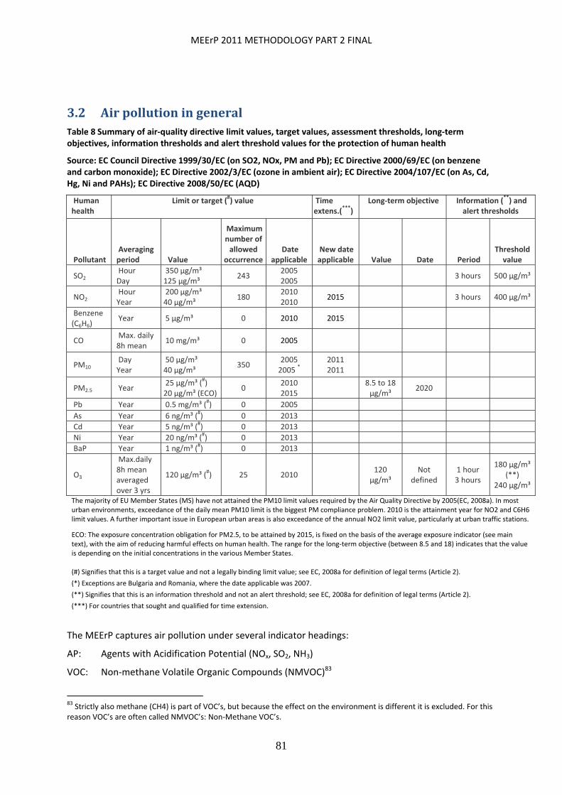
MEErP 2011 METHODOLOGY PART 2 FINAL
81
3.2 AirpollutioningeneralTable 8 Summary of air‐quality directive limit values, target values, assessment thresholds, long‐term objectives, information thresholds and alert threshold values for the protection of human health
Source: EC Council Directive 1999/30/EC (on SO2, NOx, PM and Pb); EC Directive 2000/69/EC (on benzene and carbon monoxide); EC Directive 2002/3/EC (ozone in ambient air); EC Directive 2004/107/EC (on As, Cd, Hg, Ni and PAHs); EC Directive 2008/50/EC (AQD)
Human health
Limit or target (#) value Time extens.(***)
Long‐term objective Information (**) and alert thresholds
Pollutant Averaging period Value
Maximum number of allowed
occurrence Date
applicable New date applicable Value Date Period
Threshold value
SO2 Hour Day
350 μg/m³
125 μg/m³ 243
2005 2005
3 hours 500 μg/m³
NO2 Hour Year
200 μg/m³
40 μg/m³ 180
2010 2010
2015 3 hours 400 μg/m³
Benzene (C6H6)
Year 5 μg/m³ 0 2010 2015
CO Max. daily 8h mean
10 mg/m³ 0 2005
PM10 Day Year
50 μg/m³
40 μg/m³ 350
2005 2005 *
2011 2011
PM2.5 Year 25 μg/m³ (#) 20 μg/m³ (ECO)
0 2010 2015
8.5 to 18 μg/m³
2020
Pb Year 0.5 mg/m³ (#) 0 2005
As Year 6 ng/m³ (#) 0 2013
Cd Year 5 ng/m³ (#) 0 2013
Ni Year 20 ng/m³ (#) 0 2013
BaP Year 1 ng/m³ (#) 0 2013
O3
Max.daily 8h mean averaged over 3 yrs
120 μg/m³ (#) 25 2010
120 μg/m³
Not defined
1 hour 3 hours
180 μg/m³ (**)
240 μg/m³
The majority of EU Member States (MS) have not attained the PM10 limit values required by the Air Quality Directive by 2005(EC, 2008a). In most urban environments, exceedance of the daily mean PM10 limit is the biggest PM compliance problem. 2010 is the attainment year for NO2 and C6H6 limit values. A further important issue in European urban areas is also exceedance of the annual NO2 limit value, particularly at urban traffic stations.
ECO: The exposure concentration obligation for PM2.5, to be attained by 2015, is fixed on the basis of the average exposure indicator (see main text), with the aim of reducing harmful effects on human health. The range for the long‐term objective (between 8.5 and 18) indicates that the value is depending on the initial concentrations in the various Member States.
(#) Signifies that this is a target value and not a legally binding limit value; see EC, 2008a for definition of legal terms (Article 2).
(*) Exceptions are Bulgaria and Romania, where the date applicable was 2007.
(**) Signifies that this is an information threshold and not an alert threshold; see EC, 2008a for definition of legal terms (Article 2).
(***) For countries that sought and qualified for time extension.
The MEErP captures air pollution under several indicator headings:
AP: Agents with Acidification Potential (NOx, SO2, NH3)
VOC: Non‐methane Volatile Organic Compounds (NMVOC)83
83 Strictly also methane (CH4) is part of VOC’s, but because the effect on the environment is different it is excluded. For this reason VOC’s are often called NMVOC’s: Non‐Methane VOC’s.
MEErP 2011 METHODOLOGY PART 2 FINAL
82
POP: Persistent Organic Pollutants (dioxins and furans)
HM: Heavy Metals (As, Cd, Ni, Zn, Pb)
PAH: Polycyclic Aromatic Hydrocarbons (Benzo(a)pyrene: BaP)
PM: Particulate Matter (PM10, PM2.5)
3.3 AcidificationThis section deals with emissions that have acidifying potential (AP), which includes substances with multiple environmental impacts:
The unit for the AP indicator is kg SO2 equivalent, with values –amongst others‐‐ of 0.7 kg SO2 eq./kg NOx and 1.88 kg SO2 eq./kg NH3.
National emissions are reported to the Convention on Long‐Range Transboundary Air Pollution (LRTAP) and published by EEA.
Acidification (‘acid rain’) occurs as a result of a cycle of air pollution, precipitation and water pollution Figure 49 gives an example of nitrogen.
According to the EEA, various European policies have successfully targeted air pollution in recent years.84 For example, local and regional administrations must now develop and implement air quality management plans in areas of high air pollution, including initiatives such as low emission zones. Such actions complement national or regional measures, including the EU's National Emission Ceilings Directive and the UNECE Gothenburg Protocol, which set national emission limits for SO2, NOX, NMVOCs and NH3. Likewise, the Euro vehicle emission standards and EU directives on large combustion plants have greatly reduced emissions of PM, NMVOCs, NOX and SO2.
84 European Environmental Agency (EEA), Air pollution — SOER 2010 thematic assessment, The European Environment ‐ State and Outlook 2010, 30 Nov. 2010. Note that this official European Commission publication is the main source used in this section. The text may contain literal citations, especially where value statements are involved.
Nitrogen oxides (NOx)
Nitrogen oxides (NOx) are emitted during fuel combustion, such as by industrial facilities and the road transport sector. As with SO2, NOx contributes to acid deposition but also to eutrophication. Of the chemical species that comprise NOx, it is NO2 that is associated with adverse affects on health, as high concentrations cause inflammation of the airways and reduced lung function. NOx also contributes to the formation of secondary inorganic particulate matter and tropospheric O3 (see below).
Ammonia (NH3)
Ammonia (NH3), like NOx, contributes to both eutrophication and acidification. The vast majority of NH3 emissions — around 94 % in Europe — come from the agricultural sector, from activities such as manure storage, slurry spreading and the use of synthetic nitrogenous fertilisers.
Sulphur dioxide (SO2)
Sulphur dioxide (SO2) is emitted when fuels containing sulphur are burned. It contributes to acid deposition, the impacts of which can be significant, including adverse effects on aquatic ecosystems in rivers and lakes, and damage to forests.

MEErP 2011 METHODOLOGY PART 2 FINAL
83
Figure 49. Past and projected emissions of the acidifying pollutants. EEA‐32 + Western Balkan countries (Source: IIASA, 2010a.)
Notes with Figure 49:
1) The 2010 projections for the EU‐27 are the aggregated projections reported by Member States in 2009 (EEA, 2010g) under the EU NECD (EC, 2001a). The horizontal red line indicates the aggregated sum of individual EU Member State emission ceilings to be attained by 2010 under the NECD.
2) The 2020 baseline scenario (based on the PRIMES 2010 energy reference scenario) and maximum emission reductions (MRR) projections are from IIASA (2010). The assumptions in the PRIMES 2010 energy reference include the effects of economic crisis in 2008 and 2009, as well as assuming the objectives of the EU Climate and Energy (C&E) package will be met, as well as the target for renewable energy. 3) 2020 projections data for Iceland and Liechtenstein are not available. 4) Excludes emissions from international shipping, and emissions from aviation not associated with flight landing and take‐off movements.
Figure 50 below shows the emission sources.
Figure 50. NOx, SOx, NH3 emission sources EU, 2007 (source EEA, 2010 air pollution)
SOx NH3 NOx
MEErP 2011 METHODOLOGY PART 2 FINAL
84
Indirect emission with relevance for ErP are emissions of NOx and SO2 from electricity production and public heat. The trend for these emissions, constituting 21% and 70% of the totals for NOx and SO2, is given in Figure 51 below. The causes for the decrease over the last decades are mainly abatement (purification of flue gases), efficiency improvements (less fuel overall) and fuel switch (less heavy oil, more natural gas).Increased use of biomass had a negative effect counterbalancing positive effects from other renewable sources.
In Ecodesign preparatory studies until 2011, direct AP emissions were addressed in studies on central heating boilers, water heaters, and solid fuel small combustion installations. Appropriate target values for NOx, SO2 were developed. Indirect AP emissions were taken in all the other studies dealing with electricity consuming ErP.
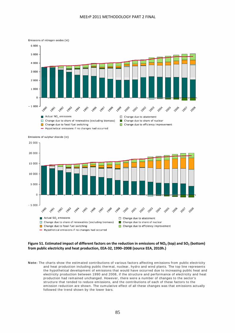
MEErP 2011 METHODOLOGY PART 2 FINAL
85
Figure 51. Estimated impact of different factors on the reduction in emissions of NOX (top) and SO2 (bottom) from public electricity and heat production, EEA‐32, 1990–2008 (source EEA, 2010h.)
Note: The charts show the estimated contributions of various factors affecting emissions from public electricity and heat production including public thermal, nuclear, hydro and wind plants. The top line represents the hypothetical development of emissions that would have occurred due to increasing public heat and electricity production between 1990 and 2008, if the structure and performance of electricity and heat production had remained unchanged. However, there were a number of changes to the sector's structure that tended to reduce emissions, and the contributions of each of these factors to the emission reduction are shown. The cumulative effect of all these changes was that emissions actually followed the trend shown by the lower bars.
MEErP 2011 METHODOLOGY PART 2 FINAL
86
Characterisation of Acidifying emissions
The legal basis for the characterisation of the acid potential is the The United Nations Economic Commission for Europe (UNECE) Convention on Long‐Range Transboundary Air Pollution (CLRTAP), also known as the Gothenburg Protocol. The protocol is signed by 31 countries, incl. the Russian Federation and the USA.85 Key element in the EU strategy to fulfill the Gothenburg obligations is the national emissions ceiling directive (NECD, European Community, 2001a), which sets emission ceilings for the acidifying agents sulphur dioxide (SO2), nitrogen oxides (NOx) and ammonia (NH3).
The Gothenburg factors are also used in the Regional Air Pollution Information and Simulation (RAINS) model (Amann et al., 1999b) developed at the International Institute for Applied Systems Analysis (IIASA) in Laxenburg, Austria. And the MEEuP 2005 study looked also at the 9 LCA sources, which seemed to be fairly in agreement on the factors to be used.
Apart from –or rather within‐‐ the overarching Gothenburg emission ceilings, there are a number of EU directives controlling emissions from point sources like vehicles (EC 1998), large combustion plants (LCP) waste incineration and large industrial installations (IPPC)86. Furthermore, there is a daughter directive of the Ambient Air Quality directive (AAQ) dealing with SO2, NOx and other non‐acidifying substances.87 The AAQ directive does not refer to point sources but to local air quality measurements in a national grid of measurement points. These are the same measurement points that are used to assess conformity to the Gothenburg protocol.
The limit values in the above directives, especially the AAQ directive, mirror the characterisation factors of the Gothenburg protocol, but mostly they are rounded. For instance, the AAQ daughter directive specifies an eco‐toxicity limit value of 20 µg/m³ for SO2 and 30 µg/m³ for NOx. This reflects the characterisation factor of 1 (SO2) versus 0.7 (NOx). Directive 2008/50/EC confirms these limit values for the protection of vegetation; this directive repeals and replaces Directive 1999/30/EC from 11 June 2010.
The legislation for emissions from point sources is different and only partially related to acidification; human toxicity also plays a role. This explains for instance the much more stringent emission limit values (ELVs) of HCl and HF in the waste incineration directive than would be justified from the acidification perspective only. Also the ELVs in e.g. the LCP directive 2001/80/EC88 and amending act regulation 1137/2008, do not reflect the acidification effect only, but e.g. the best available technology given the type of fuel involved.
The characterisation factors for the AP category, expressed in SO2 equivalent, are given in MEErP Methodology Report, Part 1.
3.4 Non‐MethaneVolatileOrganicCompounds(NMVOCs)NMVOCs, important O3 precursors, are emitted from a large number of sources including paint application, road transport, oil heating (CxHy), dry‐cleaning and other solvent uses. Certain NMVOC species, such as benzene (C6H6) and 1.3‐butadiene, are directly hazardous to human health. Biogenic NMVOCs are emitted by vegetation, with amounts dependent on the species and on temperature.
85 For status of ratification see http://www.unece.org/env/lrtap/status/99multi_st.htm 86 LCP and IPPC directives are repealed and replaced by the Industrial Emissions directive 2010/75/EU 87 Lead, VOCs 88 Note that the LCP directive 2001/80/EC is repealed with effect of 1 Jan. 2016 and replaced by provisions in the Industrial Emissions directive 2010/75/EC.
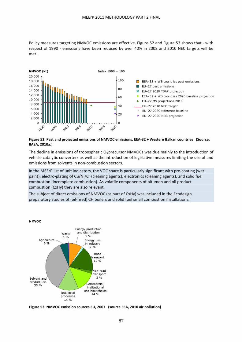
MEErP 2011 METHODOLOGY PART 2 FINAL
87
Policy measures targeting NMVOC emissions are effective. Figure 52 and Figure 53 shows that ‐ with respect of 1990 ‐ emissions have been reduced by over 40% in 2008 and 2010 NEC targets will be met.
Figure 52. Past and projected emissions of NMVOC emissions. EEA‐32 + Western Balkan countries (Source: IIASA, 2010a.)
The decline in emissions of tropospheric O3 precursor NMVOCs was due mainly to the introduction of vehicle catalytic converters as well as the introduction of legislative measures limiting the use of and emissions from solvents in non‐combustion sectors.
In the MEErP list of unit indicators, the VOC share is particularly significant with pre‐coating (wet paint), electro‐plating of Cu/Ni/Cr (cleaning agents), electronics (cleaning agents), and solid fuel combustion (incomplete combustion). As volatile components of bitumen and oil product combustion (CxHy) they are also relevant.
The subject of direct emissions of NMVOC (as part of CxHy) was included in the Ecodesign preparatory studies of (oil‐fired) CH boilers and solid fuel small combustion installations.
Figure 53. NMVOC emission sources EU, 2007 (source EEA, 2010 air pollution)
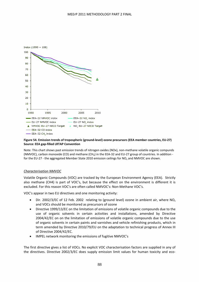
MEErP 2011 METHODOLOGY PART 2 FINAL
88
Figure 54. Emission trends of tropospheric (ground‐level) ozone precursors (EEA member countries, EU‐27) Source: EEA gap‐filled LRTAP Convention
Note: This chart shows past emission trends of nitrogen oxides (NOx), non‐methane volatile organic compunds (NMVOC), carbon monoxide (CO) and methane (CH4) in the EEA‐32 and EU‐27 group of countries. In addition ‐ for the EU‐27 ‐ the aggregated Member State 2010 emission ceilings for NOx and NMVOC are shown.
Characterisation NMVOC
Volatile Organic Compounds (VOC) are tracked by the European Environment Agency (EEA). Strictly also methane (CH4) is part of VOC’s, but because the effect on the environment is different it is excluded. For this reason VOC’s are often called NMVOC’s: Non‐Methane VOC’s.
VOC’s appear in two EU directives and one monitoring activity:
Dir. 2002/3/EC of 12 Feb. 2002 relating to (ground level) ozone in ambient air, where NOx and VOCs should be monitored as precursors of ozone
Directive 1999/13/EC on the limitation of emissions of volatile organic compounds due to the use of organic solvents in certain activities and installations, amended by Directive 2004/42/EC on on the limitation of emissions of volatile organic compounds due to the use of organic solvents in certain paints and varnishes and vehicle refinishing products, which in term amended by Directive 2010/79/EU on the adaptation to technical progress of Annex III of Directive 2004/42/EC.
IMPEL network monitoring the emissions of fugitive NMVOC’s
The first directive gives a list of VOCs. No explicit VOC characterisation factors are supplied in any of the directives. Directive 2002/3/EC does supply emission limit values for human toxicity and eco‐
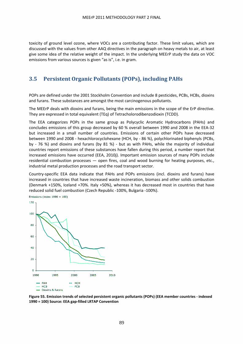
MEErP 2011 METHODOLOGY PART 2 FINAL
89
toxicity of ground level ozone, where VOCs are a contributing factor. These limit values, which are discussed with the values from other AAQ directives in the paragraph on heavy metals to air, at least give some idea of the relative weight of the impact. In the underlying MEErP study the data on VOC emissions from various sources is given “as is”, i.e. in gram.
3.5 PersistentOrganicPollutants(POPs),includingPAHs
POPs are defined under the 2001 Stockholm Convention and include 8 pesticides, PCBs, HCBs, dioxins and furans. These substances are amongst the most carcinogenous pollutants.
The MEErP deals with dioxins and furans, being the main emissions in the scope of the ErP directive. They are expressed in total equivalent (TEq) of Tetracholorodibenzodioxin (TCDD).
The EEA categorizes POPs in the same group as Polycyclic Aromatic Hydrocarbons (PAHs) and concludes emissions of this group decreased by 60 % overall between 1990 and 2008 in the EEA‐32 but increased in a small number of countries. Emissions of certain other POPs have decreased between 1990 and 2008 ‐ hexachlorocyclohexane (HCH, by ‐ 86 %), polychlorinated biphenyls (PCBs, by ‐ 76 %) and dioxins and furans (by 81 %) ‐ but as with PAHs, while the majority of individual countries report emissions of these substances have fallen during this period, a number report that increased emissions have occurred (EEA, 2010j). Important emission sources of many POPs include residential combustion processes — open fires, coal and wood burning for heating purposes, etc., industrial metal production processes and the road transport sector.
Country‐specific EEA data indicate that PAHs and POPs emissions (incl. dioxins and furans) have increased in countries that have increased waste incineration, biomass and other solids combustion (Denmark +150%, Iceland +70%. Italy +50%), whereas it has decreased most in countries that have reduced solid fuel combustion (Czech Republic ‐100%, Bulgaria ‐100%).
Figure 55. Emission trends of selected persistent organic pollutants (POPs) (EEA member countries ‐ indexed 1990 = 100) Source: EEA gap‐filled LRTAP Convention

MEErP 2011 METHODOLOGY PART 2 FINAL
90
Note: Emission trends 1990‐2008 for the persistent organic pollutants: HCB ‐ hexachlorobenzene, HCH ‐ hexachlorocyclohexane, PCBs ‐ polychlorinated biphenyls; dioxins & furans; and PAHs ‐ polyaromatic hydrocarbons.
Figure 56 Emissions by sector of selected persistent organic pollutants ‐ 2008 (EEA member countries) Source: EEA gap‐filled LRTAP Convention
Figure 56 shows the contribution made by different sectors to emissions of: HCB ‐ hexachlorobenzene, HCH ‐ hexachlorocyclohexane, PCBs ‐ polychlorinated biphenyls; dioxins & furans; and PAHs ‐ polyaromatic hydrocarbons.

MEErP 2011 METHODOLOGY PART 2 FINAL
91
Figure 57. Past and projected emissions of the main air pollutants and primary particulate matter.. EEA‐32 + Western Balkan countries Source: IIASA, 2010a
Characterisation factors
The POP’s (Persistent Organic Pollutants) are defined under the Stockholm Convention89 and include mainly pesticides (not relevant for ErP) and some other chemicals/emissions. The latter include PCB’s, dioxins and furans. PCB’s are relatively seldom with ErP, because they mainly occur with some specific products like large medium‐voltage transformers. In some EU Member States there are initiatives to phase out PCB’s. It is proposed to deal with PCBs on an ad‐hoc basis for these very specific products. The same goes for bio‐plastics and biofuels, where pesticides (and land‐use) might come into the equation: They have a low market share and their application might occur only with very specific ErPs.
This leaves dioxins and furans, which typically occur at the (incomplete) combustion of solids. They are usually expressed as the total concentration equivalent (Teq) of Tetrachlorodibenzodioxin (TCDD). The Waste Incineration directive 2000/76/EC Annex I gives the equivalence factors.
In some countries, like the UK, also PAHs (Polycyclic Aromatic Hydrocarbons) are included in the POP‐category because of their persistent and damaging nature. Also, there has been a study by Sara Eklund90, investigating whether PAHs could be included in the Stockholm Convention and she found several disadvantages in using this approach.
The characterisation factors for the POP category, expressed in Teq, are given in MEErP Methodology Report, Part 1.
In Ecodesign preparatory studies until 2011, direct emissions of dioxins and furans were addressed in the study on solid fuel small combustion installations. PCB’s are addressed in the study on distribution transformers. Legislation for this product group is being prepared. One of the main problems is the absence of accurate test methods.
89 The Stockholm Convention is ratified in Regulation (EC) No 850/2004 of the European Parliament and of the Council of 29 April 2004 on persistent organic pollutants and amending Directive 79/117/EEC. The Industrial Emissions directive 2010/75/EU also contains limit values for dioxins and furans from waste incineration (Annex VI). 90 Sara Eklund, PAH as a POP: possibilities, implications and appropriateness of regulating global emissions of poylcyclic aromatic hydrocarbons through the Stockholm Convention on Persistent Organic Pollutants, IIIEE, Lund, 2001
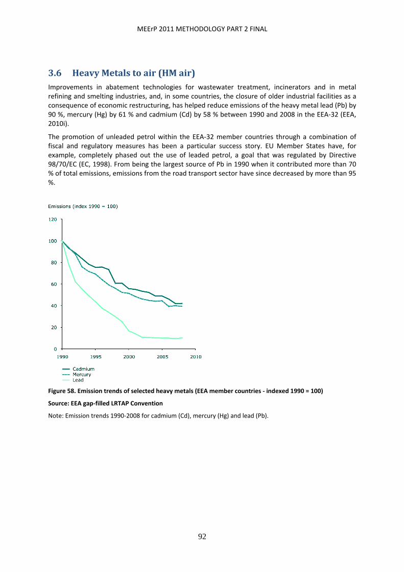
MEErP 2011 METHODOLOGY PART 2 FINAL
92
3.6 HeavyMetalstoair(HMair)Improvements in abatement technologies for wastewater treatment, incinerators and in metal refining and smelting industries, and, in some countries, the closure of older industrial facilities as a consequence of economic restructuring, has helped reduce emissions of the heavy metal lead (Pb) by 90 %, mercury (Hg) by 61 % and cadmium (Cd) by 58 % between 1990 and 2008 in the EEA‐32 (EEA, 2010i).
The promotion of unleaded petrol within the EEA‐32 member countries through a combination of fiscal and regulatory measures has been a particular success story. EU Member States have, for example, completely phased out the use of leaded petrol, a goal that was regulated by Directive 98/70/EC (EC, 1998). From being the largest source of Pb in 1990 when it contributed more than 70 % of total emissions, emissions from the road transport sector have since decreased by more than 95 %.
Figure 58. Emission trends of selected heavy metals (EEA member countries ‐ indexed 1990 = 100)
Source: EEA gap‐filled LRTAP Convention
Note: Emission trends 1990‐2008 for cadmium (Cd), mercury (Hg) and lead (Pb).
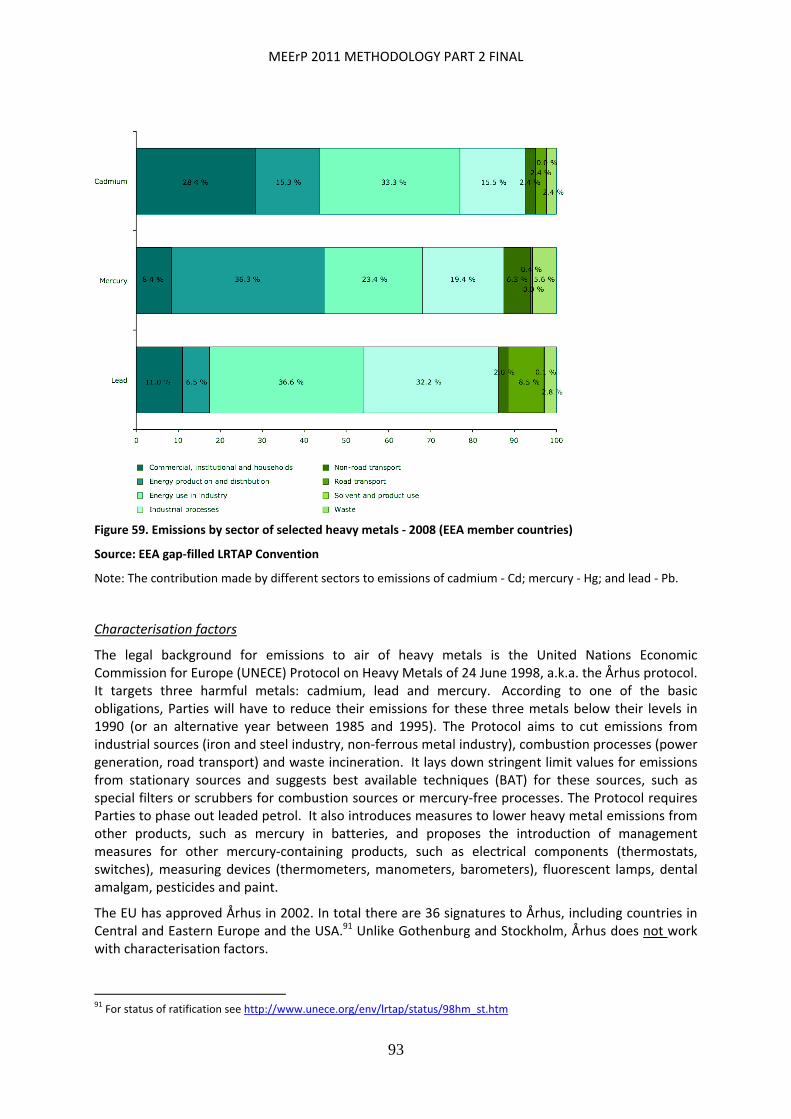
MEErP 2011 METHODOLOGY PART 2 FINAL
93
Figure 59. Emissions by sector of selected heavy metals ‐ 2008 (EEA member countries)
Source: EEA gap‐filled LRTAP Convention
Note: The contribution made by different sectors to emissions of cadmium ‐ Cd; mercury ‐ Hg; and lead ‐ Pb.
Characterisation factors
The legal background for emissions to air of heavy metals is the United Nations Economic Commission for Europe (UNECE) Protocol on Heavy Metals of 24 June 1998, a.k.a. the Århus protocol. It targets three harmful metals: cadmium, lead and mercury. According to one of the basic obligations, Parties will have to reduce their emissions for these three metals below their levels in 1990 (or an alternative year between 1985 and 1995). The Protocol aims to cut emissions from industrial sources (iron and steel industry, non‐ferrous metal industry), combustion processes (power generation, road transport) and waste incineration. It lays down stringent limit values for emissions from stationary sources and suggests best available techniques (BAT) for these sources, such as special filters or scrubbers for combustion sources or mercury‐free processes. The Protocol requires Parties to phase out leaded petrol. It also introduces measures to lower heavy metal emissions from other products, such as mercury in batteries, and proposes the introduction of management measures for other mercury‐containing products, such as electrical components (thermostats, switches), measuring devices (thermometers, manometers, barometers), fluorescent lamps, dental amalgam, pesticides and paint.
The EU has approved Århus in 2002. In total there are 36 signatures to Århus, including countries in Central and Eastern Europe and the USA.91 Unlike Gothenburg and Stockholm, Århus does not work with characterisation factors.
91 For status of ratification see http://www.unece.org/env/lrtap/status/98hm_st.htm
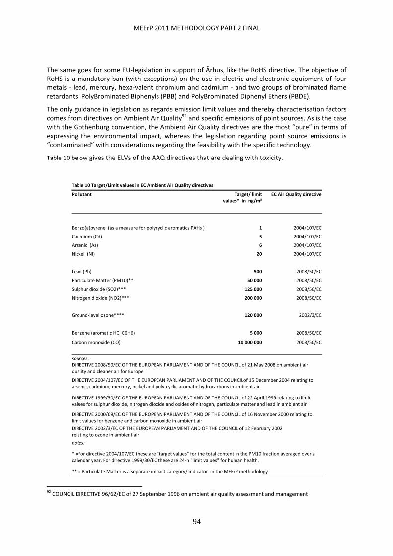
MEErP 2011 METHODOLOGY PART 2 FINAL
94
The same goes for some EU‐legislation in support of Århus, like the RoHS directive. The objective of RoHS is a mandatory ban (with exceptions) on the use in electric and electronic equipment of four metals ‐ lead, mercury, hexa‐valent chromium and cadmium ‐ and two groups of brominated flame retardants: PolyBrominated Biphenyls (PBB) and PolyBrominated Diphenyl Ethers (PBDE).
The only guidance in legislation as regards emission limit values and thereby characterisation factors comes from directives on Ambient Air Quality92 and specific emissions of point sources. As is the case with the Gothenburg convention, the Ambient Air Quality directives are the most “pure” in terms of expressing the environmental impact, whereas the legislation regarding point source emissions is “contaminated” with considerations regarding the feasibility with the specific technology.
Table 10 below gives the ELVs of the AAQ directives that are dealing with toxicity.
Table 10 Target/Limit values in EC Ambient Air Quality directives
Pollutant Target/ limit values* in ng/m³
EC Air Quality directive
Benzo(a)pyrene (as a measure for polycyclic aromatics PAHs ) 1 2004/107/EC
Cadmium (Cd) 5 2004/107/EC
Arsenic (As) 6 2004/107/EC
Nickel (Ni) 20 2004/107/EC
Lead (Pb) 500 2008/50/EC
Particulate Matter (PM10)** 50 000 2008/50/EC
Sulphur dioxide (SO2)*** 125 000 2008/50/EC
Nitrogen dioxide (NO2)*** 200 000 2008/50/EC
Ground‐level ozone**** 120 000 2002/3/EC
Benzene (aromatic HC, C6H6) 5 000 2008/50/EC
Carbon monoxide (CO) 10 000 000 2008/50/EC
sources: DIRECTIVE 2008/50/EC OF THE EUROPEAN PARLIAMENT AND OF THE COUNCIL of 21 May 2008 on ambient air quality and cleaner air for Europe
DIRECTIVE 2004/107/EC OF THE EUROPEAN PARLIAMENT AND OF THE COUNCILof 15 December 2004 relating to arsenic, cadmium, mercury, nickel and poly‐cyclic aromatic hydrocarbons in ambient air
DIRECTIVE 1999/30/EC OF THE EUROPEAN PARLIAMENT AND OF THE COUNCIL of 22 April 1999 relating to limit values for sulphur dioxide, nitrogen dioxide and oxides of nitrogen, particulate matter and lead in ambient air
DIRECTIVE 2000/69/EC OF THE EUROPEAN PARLIAMENT AND OF THE COUNCIL of 16 November 2000 relating to limit values for benzene and carbon monoxide in ambient air
DIRECTIVE 2002/3/EC OF THE EUROPEAN PARLIAMENT AND OF THE COUNCIL of 12 February 2002 relating to ozone in ambient air
notes:
* =For directive 2004/107/EC these are "target values" for the total content in the PM10 fraction averaged over a calendar year. For directive 1999/30/EC these are 24‐h "limit values" for human health.
** = Particulate Matter is a separate impact category/ indicator in the MEErP methodology
92 COUNCIL DIRECTIVE 96/62/EC of 27 September 1996 on ambient air quality assessment and management
MEErP 2011 METHODOLOGY PART 2 FINAL
95
***= SO2 and NO2 are included in the separate category of acidifying agents with more or less the same relative characterisation factor ( 1 vs. 0.7 for eco‐toxicity, 1 vs. 0.62 here)
****= Ground‐level ozone is not a direct anthropogenic emission but the result of a photochemical reaction (see text)
The target value for the protection of vegetation from the effect of ground‐level ozone is not an emission limit value, but a derived parameter called AOT40. AOT40 (expressed in (µg/m³)∙hours) means the sum of the difference between hourly concentrations greater than 80 µg/m³ (= 40 parts per billion) and 80 µg/m³ over a given period using only the 1‐hour values measured between 8:00 and 20:00. Central European Time each day (1). These measurements have to take place over period May to July. In other words, the target value relate to the sum of around 1000 hourly samples. The target value for 2010 is 18 000 µg/m³∙h (annual averaged over five years). In average, this means 18 µg/m³ plus the base level of 80 µg/m³ results in 96 µg/m³ (96.000 ng/ m³). The long‐term target is 6 000 µg/m³∙h, resulting similarly in 86 µg/m³ annually.
These eco‐toxicity values are not relevant here, but they at least provide some sort of indication of the relative importance of ground‐level ozone versus the other Gothenburg substances and could be helpful in case of normalization exercise or similar at the end of the study. As mentioned in directive 2008/50/EC the annual eco‐toxicity limit values are 20 µg/m³ for SO2 and 30 µg/m³ for NOx.
The list of heavy metals in the above Table 10 is relatively short and contains EU legislation on point sources to make the list more robust. As a characterisation factor the most generic (least technology‐specific) point‐source legislation is taken into account, which in this case were the threshold values for reporting under EPER.
Table 11 EPER (European Pollutant Emission Register) Reporting Threshold Values
Pollutants / Substances Identification Thresholds Air in kg/yr Thresholds water in kg/yr
Metals and compounds
As and compounds total, as As 20 5
Cd and compounds total, as Cd 10 5
Cr and compounds total, as Cr 100 50
Cu and compounds total, as Cu 100 50
Hg and compounds total, as Hg 10 1
Ni and compounds total, as Ni 50 20
Pb and compounds total, as Pb 200 20
Zn and compounds total, as Zn 200 100
source: ANNEX A1 LIST OF POLLUTANTS TO BE REPORTED IF THRESHOLD VALUE IS
EXCEEDED, Guidance Document for EPER implementation ‐ Part III, European Commission, 2000
Table 11 above suggests that Zinc (Zn) is in the same league as Lead (Pb). Chromium (Cr) and Copper (Cu) threshold values are half of that, suggesting that their impact is twice as serious as that of Pb/Zn, but half that of Nickel (Ni). Finally, Mercury (Hg) has the same threshold value as Cadmium (Cd). Using this outcome the MEErP characterisation factors shown in Table 12 were constructed and compared to the human toxicity and eco‐toxicity factors given by Huppes, CML. All values were normalized to index Nickel (Ni) = 1.

MEErP 2011 METHODOLOGY PART 2 FINAL
96
Table 12 MEERP characterisation factors compared to human and eco‐toxicity factors CML
MEErP (VHK) CML(adapted from Huppes comments 2005)
air pollutant ranked by factor from EU legislation
characterisation factor
air pollutant ranked by eco‐ toxicity (FAETP+FSETP +TETP)
Eco‐toxicity
air pollutant ranked by human toxicity (HTP)
Humantoxicity
carbon monoxide 0.000002 benzene 0 zinc 0.00
benzene 0.004 lead 0.01 lead 0.01
zinc* 0.04 zinc 0.03 chromium III 0.02
lead 0.04 Carc. PAHs 0.31 Benzene 0.05
chromium (III)* 0.50 copper 0.33 copper 0.12
copper* 0.50 cadmium 0.47 mercury 0.17
nickel 1.00 arsenic 0.76 nickel 1.00
arsenic 3.33 nickel 1.00 cadmium 4.29
cadmium 5.00 chromium III 1.28 arsenic 10.00
mercury* 5.00 chromium VI 1.29 Carcinogenic PAHs 16.29
Carc. PAHs 20.00 mercury 12.40 chromium VI 97.14
2.3.7.8‐TCDD 3792.34 2.3.7.8‐TCDD 54285.71
*= from EPER, rest AAQD; all values normalised to index Nickel=1
Table 12 shows that the proposed MEErP characterisation factors are a mix of the human toxicity and eco‐toxicity factors proposed by CML. Note that CML has specified Cr VI and Cr III. The first will be banned by RoHS Directive in 2006 and there are very little emissions of Cr VI if it is not actually used in a product. Therefore the characterisation factor for Cr is satisfactory, which will be essentially Cr III, as is. CML has also added the toxicity factors for the dioxin 2.3.7.8‐TCDD, thereby providing the link with characterisation factors in the separate POP category.
The characterisation factors for the Heavy Metals category, expressed in Ni equivalent and based on the values in Tables 10 and 11, are given in MEErP Methodology Report, Part 1.
In Ecodesign preparatory studies until 2011, direct emissions of heavy metals were addressed in the study on lighting, especially analysing the trade off between emissions of mercury (Hg) from compact fluorescent lamps versus the Hg emissions from (coal‐based) power generation in the EU. Product information requirements for this issue was being incorporated in the domestic lighting and television measure.
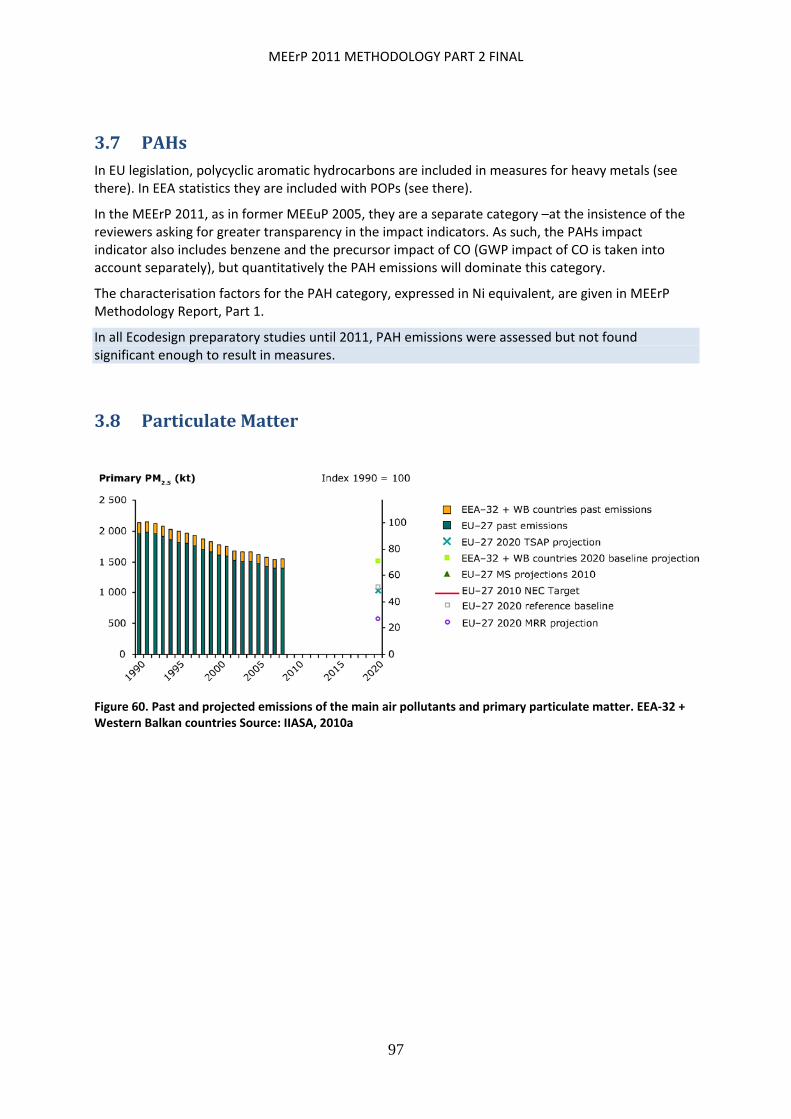
MEErP 2011 METHODOLOGY PART 2 FINAL
97
3.7 PAHsIn EU legislation, polycyclic aromatic hydrocarbons are included in measures for heavy metals (see there). In EEA statistics they are included with POPs (see there).
In the MEErP 2011, as in former MEEuP 2005, they are a separate category –at the insistence of the reviewers asking for greater transparency in the impact indicators. As such, the PAHs impact indicator also includes benzene and the precursor impact of CO (GWP impact of CO is taken into account separately), but quantitatively the PAH emissions will dominate this category.
The characterisation factors for the PAH category, expressed in Ni equivalent, are given in MEErP Methodology Report, Part 1.
In all Ecodesign preparatory studies until 2011, PAH emissions were assessed but not found significant enough to result in measures.
3.8 ParticulateMatter
Figure 60. Past and projected emissions of the main air pollutants and primary particulate matter. EEA‐32 + Western Balkan countries Source: IIASA, 2010a
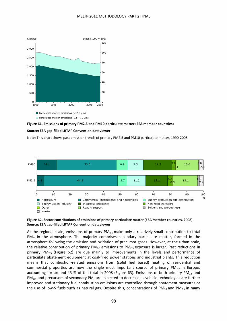
MEErP 2011 METHODOLOGY PART 2 FINAL
98
Figure 61. Emissions of primary PM2.5 and PM10 particulate matter (EEA member countries)
Source: EEA gap‐filled LRTAP Convention dataviewer
Note: This chart shows past emission trends of primary PM2.5 and PM10 particulate matter, 1990‐2008.
Figure 62. Sector contributions of emissions of primary particulate matter (EEA member countries, 2008). Source: EEA gap‐filled LRTAP Convention dataviewer
At the regional scale, emissions of primary PM2.5 make only a relatively small contribution to total PM2.5 in the atmosphere. The majority comprises secondary particulate matter, formed in the atmosphere following the emission and oxidation of precursor gases. However, at the urban scale, the relative contribution of primary PM2.5 emissions to PM2.5 exposure is larger. Past reductions in primary PM2.5 (Figure 62) are due mainly to improvements in the levels and performance of particulate abatement equipment at coal‐fired power stations and industrial plants. This reduction means that combustion‐related emissions from (solid fuel based) heating of residential and commercial properties are now the single most important source of primary PM2.5 in Europe, accounting for around 43 % of the total in 2008 (Figure 63). Emissions of both primary PM2.5 and PM10, and precursors of secondary PM, are expected to decrease as vehicle technologies are further improved and stationary fuel combustion emissions are controlled through abatement measures or the use of low‐S fuels such as natural gas. Despite this, concentrations of PM10 and PM2.5 in many
MEErP 2011 METHODOLOGY PART 2 FINAL
99
urban areas across the EU are expected to remain above EU air‐ quality limit values in the next decade.
Characterisation factors
Particulate Matter PM or dust is an important indicator for Human Toxicity (respiratory problems). AAQ Directive 2008/50/EC sets a one day emission limit value of 50 μg/m³ PM10, not to be exceeded more than 35 times a calendar year, starting 1 Jan. 2005. The annual average emission limit should not exceed 40 μg/m³
For PM2.5 there is a one day emission limit value of 25 μg/m³ ,not to be exceeded, starting 1 Jan. 2005. The annual average emission limit should not exceed 20 μg/m³
This results in a weighting of PM10:PM2.5 = 1:2 with a unit indicator in kg PM10 emissions . However, at the moment, assessment of particulate matter mass from available LCA‐data sources in the unit indicator list does not allow for this differentiation. Most LCA sources just specify ‘dust’ or PM.
The characterisation factors for the PM category, expressed in PM10 equivalent, are given in MEErP Methodology Report, Part 1.
In Ecodesign preparatory studies until 2011, direct emissions of particulate matter were addressed in the study on solid fuel small combustion installations. Legislation is currently under preparation. Indirectly, abatements of particulate matter emissions follows from Ecodesign measures aimed at reduction of electricity consumption.
3.9 HeavyMetalstoWater(HMwater)While landfills, forestry, mining, aquaculture and dwellings un‐connected to a municipal sewage treatment works, for example, can all be of great importance locally, two broad sources alone contribute most to the freshwater pollution observed across Europe: agriculture and the urban environment. For ErP the latter is the most relevant.
A range of pollutants is generated within the wider urban environment, including industrial and household chemicals, metals, pharmaceutical products, nutrients, pesticides and pathogenic micro‐organisms. These pollutants come from various sources including domestic premises, transport networks, industrial plants and atmospheric deposition within urban areas. Domestic premises discharge sewage, personal care products, household chemicals and medicines to sewer networks while hydrocarbons and heavy metals such as zinc from the wear of vehicle tyres arise from the transport sector. Industrial wastewaters are treated either on‐site or by their transfer to a municipal wastewater treatment works. The treatment process can, however, be incomplete resulting in industrial pollutants being discharged to surface waters. Pesticide release to the wider urban environment arises from their use in controlling unwanted plant growth on sports grounds, public parks and buildings, private gardens, roads and railways.
Figure 63 shows the regional variation in wastewater treatment between 1990 and 2007. The map in Figure 64 shows the emissions of mercury to water based on E‐PRTR reporting of 2007 data.
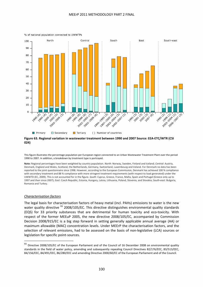
MEErP 2011 METHODOLOGY PART 2 FINAL
100
Figure 63. Regional variation in wastewater treatment between 1990 and 2007 Source: EEA‐ETC/WTR (CSI 024)
This figure illustrates the percentage population per European region connected to an Urban Wastewater Treatment Plant over the period 1990 to 2007. In addition, a breakdown by treatment type is portrayed.
Note: Regional percentages have been weighted by country population. North: Norway, Sweden, Finland and Iceland; Central: Austria, Denmark, England and Wales, Scotland, the Netherlands, Germany, Switzerland, Luxembourg and Ireland. For Denmark no data has been reported to the joint questionnaire since 1998. However, according to the European Commission, Denmark has achieved 100 % compliance with secondary treatment and 88 % compliance with more stringent treatment requirements (with respect to load generated) under the UWWTD (EC, 2009). This is not accounted for in the figure. South: Cyprus, Greece, France, Malta, Spain and Portugal (Greece only up to 1997 and then since 2007); East: Czech Republic, Estonia, Hungary, Latvia, Lithuania, Poland, Slovenia, and Slovakia; South‐east: Bulgaria, Romania and Turkey.
Characterisation factors
The legal basis for characterisation factors of heavy metal (incl. PAHs) emissions to water is the new water quality directive 93 2008/105/EC. This directive distinguishes environmental quality standards (EQS) for 33 priority substances that are detrimental for human toxicity and eco‐toxicity. With respect of the former MEEuP 2005, the new directive 2008/105/EC, accompanied by Commission Decision 2008/915/EC is a big step forward in setting generally applicable annual average (AA) or maximum allowable (MAC) concentration levels. Under MEErP the characterisation factors, and the selection of relevant emissions, had to be assessed on the basis of non‐legislative (LCA) sources or legislation for specific point‐sources.
93 Directive 2008/105/EC of the European Parliament and of the Council of 16 December 2008 on environmental quality
standards in the field of water policy, amending and subsequently repealing Council Directives 82/176/EEC, 83/513/EEC, 84/156/EEC, 84/491/EEC, 86/280/EEC and amending Directive 2000/60/EC of the European Parliament and of the Council.

MEErP 2011 METHODOLOGY PART 2 FINAL
101
Table 13 Directive 2008/105/EC, Annex I, annual average (AA) and maximum allowable (MAC) concentration levels in μg/l
No Name of substance CAS
number(1)
AA‐EQS(2) Inland surface waters(3)
AA‐EQS(2) Other surface waters
MAC‐QS(4) Inland surface
waters (3)
MAC‐EQS(4) Other surface waters
(1) Alachlor 15972‐60‐8 0.3 0.3 0.7 0.7
(2) Anthracene 120‐12‐7 0.1 0.1 0.4 0.4
(3) Atrazine 1912‐24‐9 0.6 0.6 2.0 2.0
(4) Benzene 71‐43‐2 10 8 50 50
(5) Brominated diphenylether(5) 32534‐81‐9 0.0005 0.0002 n.a. n.a.
(6) Cadmium and its compounds (depending on waterhardness classes)(6)
7440‐43‐9
≤0.08(Class1)0.08(Class2) 0.09(Class3) 0.15(Class4) 0.25(Class5)
0.2
≤0.45(Class1) 0.45(Class2) 0.6(Class3) 0.9(Class4) 1.5(Class5)
≤0.45(Class1)0.45(Class2) 0.6(Class3) 0.9(Class4) 1.5(Class5)
(6a) Carbon‐tetrachloride(7) 56‐23‐5 12 12 n.a. n.a.
(7) C10‐13Chloroalkanes 85535‐84‐8 0.4 0.4 1.4 1.4
(8) Chlorfenvinphos 470‐90‐6 0.1 0.1 0.3 0.3
(9) Chlorpyrifos(Chlorpyrifos‐ethyl) 2921‐88‐2 0.03 0.03 0.1 0.1
(9a)
Cyclodienepesticides: Aldrin(7) Dieldrin(7) Endrin(7) Isodrin(7)
309‐00‐2 60‐57‐1 72‐20‐8 465‐73‐6
Σ=0.01 Σ=0.005 n.a. n.a.
(9b) DDT total(7)(8) n.a. 0.025 0.025 n.a. n.a.
para‐para‐DDT(7) 50‐29‐3 0.01 0.01 n.a. n.a.
(10) 1.2‐Dichloroethane 107‐06‐2 10 10 n.a. n.a.
(11) Dichloromethane 75‐09‐2 20 20 n.a. n.a.
(12) Di(2‐ethylhexyl)‐phthalate(DEHP) 117‐81‐7 1.3 1.3 n.a. n.a.
(13) Diuron 330‐54‐1 0.2 0.2 1.8 1.8
(14) Endosulfan 115‐29‐7 0.005 0.0005 0.01 0.004
(15) Fluoranthene 206‐44‐0 0.1 0.1 1 1
(16) Hexachloro‐benzene 118‐74‐1 0.01(9) 0.01(9) 0.05 0.05
(17) Hexachloro‐butadiene 87‐68‐3 0.1(9) 0.1(9) 0.6 0.6
(18) Hexachloro‐cyclohexane 608‐73‐1 0.02 0.002 0.04 0.02
(19) Isoproturon 34123‐59‐6 0.3 0.3 1.0 1.0
(20) Lead and its compounds 7439‐92‐1 7.2 7.2 n.a. n.a.
(21) Mercury and its compounds 7439‐97‐6 0.05(9) 0.05(9) 0.07 0.07
(22) Naphthalene 91‐20‐3 2.4 1.2 n.a. n.a.
(23) Nickel and its compounds 7440‐02‐0 20 20 n.a. n.a.
(24) Nonylphenol(4‐Nonylphenol) 104‐40‐5 0.3 0.3 2.0 2.0
(25) Octylphenol((4‐(1.1′.3.3′‐tetramethylbutyl)‐phenol))
140‐66‐9 0.1 0.01 n.a. n.a.
(26) Pentachloro‐benzene 608‐93‐5 0.007 0.0007 n.a. n.a.
(27) Pentachloro‐phenol 87‐86‐5 0.4 0.4 1 1
(28) lyaromatichydrocarbons(PAH)(10) n.a. n.a. n.a. n.a. n.a.
Benzo(a)pyrene (BaP) 50‐32‐8 0.05 0.05 0.1 0.1
Benzo(b)fluor‐anthene 205‐99‐2 Σ=0.03 Σ=0.03 n.a. n.a.
Benzo(k)fluor‐anthene 207‐08‐9
Benzo(g,h,i)‐perylene 191‐24‐2 Σ=0.002 Σ=0.002 n.a. n.a.
Indeno(1.2.3‐cd)‐pyrene 193‐39‐5
(29) Simazine 122‐34‐9 1 1 4 4
Tetrachloro‐ethylene(7) 127‐18‐4 10 10 n.a. n.a.
Trichloro‐ethylene(7) 79‐01‐6 10 10 n.a. n.a.
(30) Tributyltincompounds(Tributhyltin‐cation)
36643‐28‐4 0.0002 0.0002 0.0015 0.0015
(31) Trichloro‐benzenes 12002‐48‐1 0.4 0.4 n.a. n.a.
(32) Trichloro‐methane 67‐66‐3 2.5 2.5 n.a. n.a.
(33) Trifluralin 1582‐09‐8 0.03 0.03 n.a. n.a.
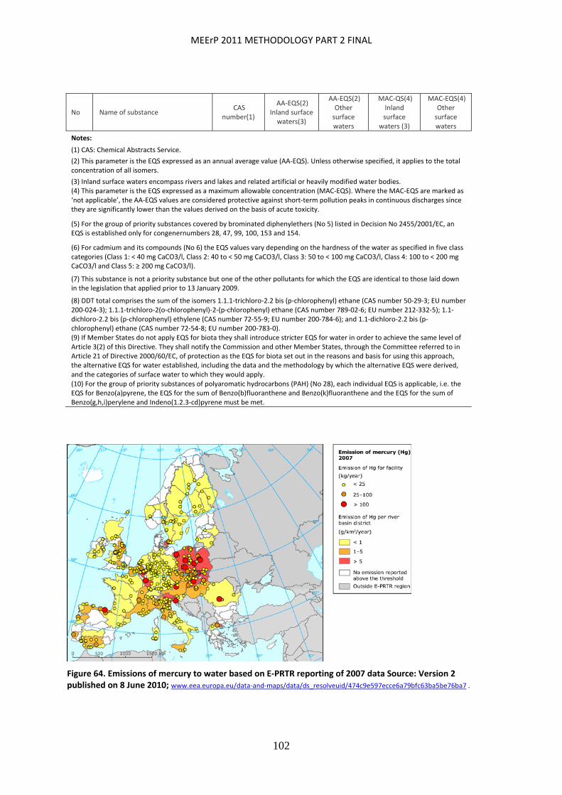
MEErP 2011 METHODOLOGY PART 2 FINAL
102
No Name of substance CAS
number(1)
AA‐EQS(2) Inland surface waters(3)
AA‐EQS(2) Other surface waters
MAC‐QS(4) Inland surface
waters (3)
MAC‐EQS(4) Other surface waters
Notes:
(1) CAS: Chemical Abstracts Service.
(2) This parameter is the EQS expressed as an annual average value (AA‐EQS). Unless otherwise specified, it applies to the total concentration of all isomers.
(3) Inland surface waters encompass rivers and lakes and related artificial or heavily modified water bodies. (4) This parameter is the EQS expressed as a maximum allowable concentration (MAC‐EQS). Where the MAC‐EQS are marked as ‘not applicable’, the AA‐EQS values are considered protective against short‐term pollution peaks in continuous discharges since they are significantly lower than the values derived on the basis of acute toxicity.
(5) For the group of priority substances covered by brominated diphenylethers (No 5) listed in Decision No 2455/2001/EC, an EQS is established only for congenernumbers 28, 47, 99, 100, 153 and 154.
(6) For cadmium and its compounds (No 6) the EQS values vary depending on the hardness of the water as specified in five class categories (Class 1: < 40 mg CaCO3/l, Class 2: 40 to < 50 mg CaCO3/l, Class 3: 50 to < 100 mg CaCO3/l, Class 4: 100 to < 200 mg CaCO3/l and Class 5: ≥ 200 mg CaCO3/l).
(7) This substance is not a priority substance but one of the other pollutants for which the EQS are identical to those laid down in the legislation that applied prior to 13 January 2009.
(8) DDT total comprises the sum of the isomers 1.1.1‐trichloro‐2.2 bis (p‐chlorophenyl) ethane (CAS number 50‐29‐3; EU number 200‐024‐3); 1.1.1‐trichloro‐2(o‐chlorophenyl)‐2‐(p‐chlorophenyl) ethane (CAS number 789‐02‐6; EU number 212‐332‐5); 1.1‐dichloro‐2.2 bis (p‐chlorophenyl) ethylene (CAS number 72‐55‐9; EU number 200‐784‐6); and 1.1‐dichloro‐2.2 bis (p‐chlorophenyl) ethane (CAS number 72‐54‐8; EU number 200‐783‐0). (9) If Member States do not apply EQS for biota they shall introduce stricter EQS for water in order to achieve the same level of Article 3(2) of this Directive. They shall notify the Commission and other Member States, through the Committee referred to in Article 21 of Directive 2000/60/EC, of protection as the EQS for biota set out in the reasons and basis for using this approach, the alternative EQS for water established, including the data and the methodology by which the alternative EQS were derived, and the categories of surface water to which they would apply. (10) For the group of priority substances of polyaromatic hydrocarbons (PAH) (No 28), each individual EQS is applicable, i.e. the EQS for Benzo(a)pyrene, the EQS for the sum of Benzo(b)fluoranthene and Benzo(k)fluoranthene and the EQS for the sum of Benzo(g,h,i)perylene and Indeno(1.2.3‐cd)pyrene must be met.
Figure 64. Emissions of mercury to water based on E‐PRTR reporting of 2007 data Source: Version 2 published on 8 June 2010; www.eea.europa.eu/data‐and‐maps/data/ds_resolveuid/474c9e597ecce6a79bfc63ba5be76ba7 .
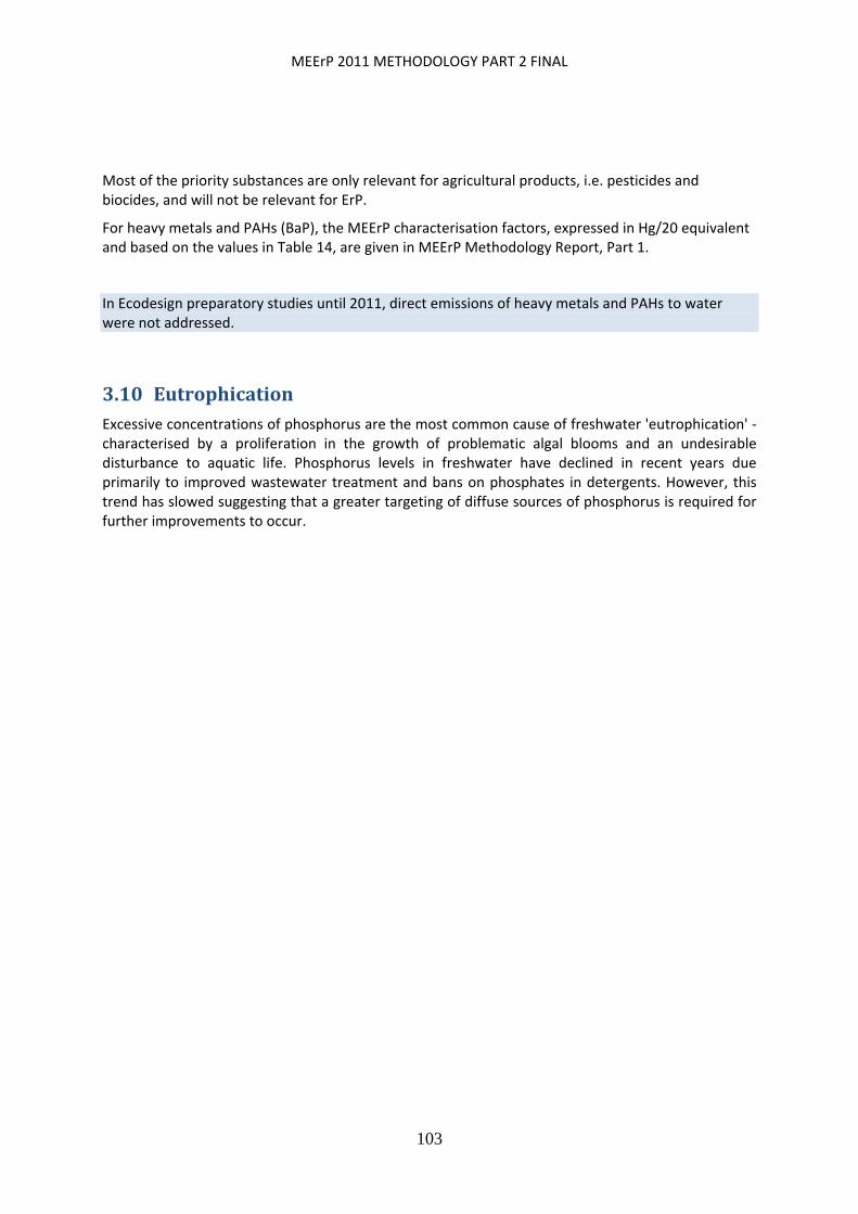
MEErP 2011 METHODOLOGY PART 2 FINAL
103
Most of the priority substances are only relevant for agricultural products, i.e. pesticides and biocides, and will not be relevant for ErP.
For heavy metals and PAHs (BaP), the MEErP characterisation factors, expressed in Hg/20 equivalent and based on the values in Table 14, are given in MEErP Methodology Report, Part 1.
In Ecodesign preparatory studies until 2011, direct emissions of heavy metals and PAHs to water were not addressed.
3.10 EutrophicationExcessive concentrations of phosphorus are the most common cause of freshwater 'eutrophication' ‐ characterised by a proliferation in the growth of problematic algal blooms and an undesirable disturbance to aquatic life. Phosphorus levels in freshwater have declined in recent years due primarily to improved wastewater treatment and bans on phosphates in detergents. However, this trend has slowed suggesting that a greater targeting of diffuse sources of phosphorus is required for further improvements to occur.
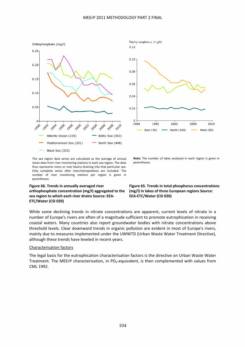
MEErP 2011 METHODOLOGY PART 2 FINAL
104
While some declining trends in nitrate concentrations are apparent, current levels of nitrate in a number of Europe's rivers are often of a magnitude sufficient to promote eutrophication in receiving coastal waters. Many countries also report groundwater bodies with nitrate concentrations above threshold levels. Clear downward trends in organic pollution are evident in most of Europe's rivers, mainly due to measures implemented under the UWWTD (Urban Waste Water Treatment Directive), although these trends have leveled in recent years.
Characterisation factors
The legal basis for the eutrophication characterisation factors is the directive on Urban Waste Water Treatment. The MEErP characterisation, in PO4‐equivalent, is then complemented with values from CML 1992.
The sea region data series are calculated as the average of annual mean data from river monitoring stations in each sea region. The data thus represents rivers or river basins draining into that particular sea. Only complete series after inter/extrapolation are included. The number of river monitoring stations per region is given in parentheses.
Note: The number of lakes analysed in each region is given in parentheses.
Figure 66. Trends in annually averaged river orthophosphate concentration (mg/l) aggregated to the sea region to which each river drains Source: EEA‐ETC/Water (CSI 020)
Figure 65. Trends in total phosphorus concentrations (mg/l) in lakes of three European regions Source: EEA‐ETC/Water (CSI 020)
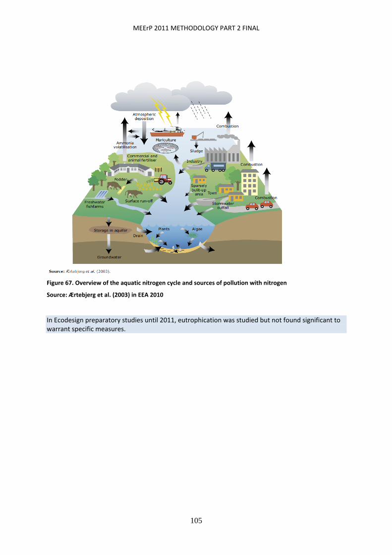
MEErP 2011 METHODOLOGY PART 2 FINAL
105
Figure 67. Overview of the aquatic nitrogen cycle and sources of pollution with nitrogen
Source: Ærtebjerg et al. (2003) in EEA 2010
In Ecodesign preparatory studies until 2011, eutrophication was studied but not found significant to warrant specific measures.

MEErP 2011 METHODOLOGY PART 2 FINAL
106
4 OTHERIMPACTS
4.1.1 Noise
Exposure to noise can have several adverse non‐auditory effects. It disturbs and interferes with concentration and activities such as communication, relaxation and sleep. In addition, there are concerns about the health impacts of transport noise including effects on the cognitive development of children, sleep disturbance, endocrine balance, and cardiovascular disorders (Babisch, 2002). The Aircraft and road traffic noise and children's cognition and health (RANCH) study in the Netherlands, Spain and the United Kingdom found that chronic aircraft noise exposure impaired the reading comprehension and recognition memory of 9–10‐year‐old children by up to 2 months, after taking a range of socio‐economic and confounding factors into account (Stansfeld et al., 2005). In the long run, chronic noise stress may affect homeostasis and metabolism due to disregulation, incomplete adaptation and/or the physiological costs of adaptation (Babisch, 2006).
Figure 68 Reported noise exposure of more than 55 dB Lden in European agglomerations with more than 250 000 inhabitants based on the results of strategic noise mapping Source: Noise 2010
The figure shows the reported long‐term (yearly) average exposure to day‐evening‐night noise of more than 55 dB in EU‐27 agglomerations with more than 250 000 inhabitants
The WHO Night Noise Guidelines for Europe (WHO, 2009a) describe levels above 55 dB Lnight as 'increasingly dangerous to public health'. Figure 68 and Figure 69 show the situation in selected European agglomerations over more than 250 000 people.
In some cities, close to half the population is exposed to 55 dB Lnight or more (see Figure 2.2). However, for the primary prevention of sub‐clinical adverse health effects related to night noise in
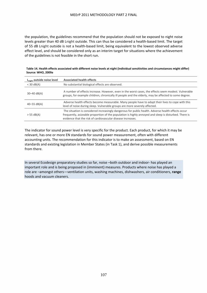
MEErP 2011 METHODOLOGY PART 2 FINAL
107
the population, the guidelines recommend that the population should not be exposed to night noise levels greater than 40 dB Lnight outside. This can thus be considered a health‐based limit. The target of 55 dB Lnight outside is not a health‐based limit, being equivalent to the lowest observed adverse effect level, and should be considered only as an interim target for situations where the achievement of the guidelines is not feasible in the short run.
Table 14. Health effects associated with different noise levels at night (individual sensitivities and circumstances might differ) Source: WHO, 2009a
Lnight outside noise level Associated health effects
< 30 dB(A) No substantial biological effects are observed.
30–40 dB(A) A number of effects increase. However, even in the worst cases, the effects seem modest. Vulnerable groups, for example children, chronically ill people and the elderly, may be affected to some degree.
40–55 dB(A) Adverse health effects become measurable. Many people have to adapt their lives to cope with this level of noise during sleep. Vulnerable groups are more severely affected.
> 55 dB(A) The situation is considered increasingly dangerous for public health. Adverse health effects occur frequently, asizeable proportion of the population is highly annoyed and sleep is disturbed. There is evidence that the risk of cardiovascular disease increases.
The indicator for sound power level is very specific for the product. Each product, for which it may be relevant, has one or more EN standards for sound power measurement, often with different accounting units. The recommendation for this indicator is to make an assessment, based on EN standards and existing legislation in Member States (in Task 1), and derive possible measurements from there.
In several Ecodesign preparatory studies so far, noise –both outdoor and indoor‐ has played an important role and is being proposed in (imminent) measures. Products where noise has played a role are –amongst others—ventilation units, washing machines, dishwashers, air conditioners, range hoods and vacuum cleaners.

MEErP 2011 METHODOLOGY PART 2 FINAL
108
Figure 69. Perception of noise (all sources) as a problem in European cities compared to road noise (major source of environmental noise) levels reported in the urban agglomerations correlated to processes of centralisation (c), decentralisation (d) and no change (n) in the density gradient of populations
Source: EC 2005; Urban Audit database (Eurostat, 2010) – population trends between 2001 and 2004 ; NOISE 2010.
Note: * no noise data available.
4.1.2 Otherhealth‐relatedimpacts
Health related impacts were discussed in Part 1 (Methods). Below only some details as regards RoHs and REACH are given.
The table below gives the exemptions to the RoHS legislation.

MEErP 2011 METHODOLOGY PART 2 FINAL
109
Table 15. Exemptions, according to Commission Decision 2010/571/EU of 24 September 2010 amending, for the purposes of adapting to scientific and technical progress, the Annex to Directive 2002/95/EC of the European Parliament and of the Council as regards exemptions for applications containing lead, mercury, cadmium, hexavalent chromium, polybrominated biphenyls or polybrominated diphenyl ethers
5(a) Lead in glass of cathode ray tubes
5(b) Lead in glass of fluorescent tubes not exceeding 0.2 % by weight
6(a) Lead as an alloying element in steel for machining purposes and in galvanized steel containing up to 0.35 % lead by weight
6(b) Lead as an alloying element in aluminium containing up to 0.4 % lead by weight
6(c) Copper alloy containing up to 4 % lead by weight
7(a) Lead in high melting temperature type solders (i.e. lead‐based alloys containing 85 % by weight or more lead)
7(b) Lead in solders for servers, storage and storage array systems, network infrastructure equipment for switching, signalling, transmission, and network management for telecommunications
7(c)‐I Electrical and electronic components containing lead in a glass or ceramic other than dielectric ceramic in capacitors, e.g. piezoelectronic devices, or in a glass or ceramic matrix compound
7(c)‐II
Lead in dielectric ceramic in capacitors for a rated voltage of 125 V AC or 250 V DC or higher
7(c)‐III
Lead in dielectric ceramic in capacitors for a rated voltage of less than 125 V AC or 250 V DC [expires on 1 January 2013 and after that date may be used in spare parts for EEE placed on the market before 1 January 2013]
8(a) Cadmium and its compounds in one shot pellet type thermal cut‐offs [expires on 1 January 2012 and after that date may be used in spare parts for EEE placed on the market before 1 January 2012]
8(b) Cadmium and its compounds in electrical contacts
9 Hexavalent chromium as an anticorrosion agent of the carbon steel cooling system in absorption refrigerators up to 0.75 % by weight in the cooling solution
9(b) Lead in bearing shells and bushes for refrigerant‐containing compressors for heating, ventilation, air conditioning and refrigeration (HVACR) applications
11(a) Lead used in C‐press compliant pin connector systems [allowed in spare parts for EEE placed on the market before 24.9.2010]
11(b) Lead used in other than C‐press compliant pin connector systems [expires 1.1.2013 and then allowed in spare parts for EEE placed on the market before 1.1.2013]
12 Lead as a coating material for the thermal conduction module C‐ring [allowed in spare parts for EEE placed on the market before 24.9.2010]
13(a) Lead in white glasses used for optical applications
13(b) Cadmium and lead in filter glasses and glasses used for reflectance standards
14 Lead in solders consisting of more than two elements for the connection between the pins and the package of microprocessors with a lead content of more than 80 % and less than 85 % by weight [expires 1.1.2011and then allowed in spare parts for EEE placed on the market before 1.1.2011]
15 Lead in solders to complete a viable electrical connection between semiconductor die and carrier within integrated circuit flip chip packages
16 Lead in linear incandescent lamps with silicate coated tubes [expires 1.9.2013]
17 Lead halide as radiant agent in high intensity discharge (HID) lamps used for professional reprography applications
1
Mercury in single capped (compact) fluorescent lamps not exceeding (per burner): For general lighting purposes
1(a) < 30 W: 5 mg [expires 31.12.2011; 2012: 3.5 mg; after 31.12.2012: 2.5 mg]
1(b) ≥ 30 W and < 50 W: 5 mg [expires 31.12.2011; after that: 3.5 mg]
1(c) ≥ 50 W and ≤ 150 W: 5 mg
1(d) ≥ 150 W: 15 mg
1(e) with circular or square structural shape and tube diameter < 17 mm, no limit [after 31.12.2011: 7 mg]
For special purposes:
1(f) 5 mg
2(a)
Mercury in double‐capped linear fluorescent lamps for general lighting purposes not exceeding (per lamp): Tri‐band phosphor with normal lifetime and a tube diameter
2(a)(1) < 9 mm* (e.g. T2): 5 mg [expires 31.12.2011; after that: 4 mg]
2(a)(2) ≥ 9 mm and ≥ 17 mm (e.g. T5): 5 mg [expires 31.12.2011; after that: 3 mg]
2(a)(3) ≥ 17 mm and ≤ 28 mm (e.g. T8): 5 mg [expires 31.12.2011; after that: 3.5 mg]
2(a)(4) > 28 mm (e.g. T12): 5 mg [expires 31.12.2011; after that: 3.5 mg]
Tri‐band phosphor with long lifetime (≥ 25 000 h):
2(a)(5) 8 mg [expires 31.12.2011; after that: 5 mg]
2(b)
Mercury in other fluorescent lamps not exceeding (per lamp):
2(b)(1) Linear halophosphate lamps with tube > 28 mm (e.g. T10 and T12): 10 mg [expires 13 April 2012]
2(b)(2) Non‐linear halophosphate lamps (all diameters): 15 mg [expires 13 April 2016]
2(b)(3) Non‐linear tri‐band phosphor lamps with tube diameter > 17 mm (e.g. T9), no limit
2(b)(4) Lamps for other general lighting and special purposes (e.g. induction lamps) [after 31.12.2011: 15 mg]
3
Mercury in cold cathode fluorescent lamps and external electrode fluorescent lamps (CCFL and EEFL) for special purposes not exceeding (per lamp): 3(a) Short length (≥ 500 mm), no limit [after 31.12.2011: 3.5
mg]
3(b) Medium length (> 500 mm and < 1 500 mm), no limit [after 31.12.2011: 5 mg]
3(c) Long length (> 1 500 mm), no limit [after 31.12.2011: 13 mg]
4(a) Mercury in other low pressure discharge lamps (per lamp) [after 31.12.2011: 15 mg]
4(b)
Mercury in High Pressure Sodium (vapour) lamps for general lighting purposes not exceeding (per burner) in lamps with improved colour rendering index Ra > 60: 4(b)‐I P < 155 W, no limit [after 31.12.2011: 30 mg]
4(b)‐II 155 W < P < 405 W, no limit [after 31.12.2011: 40 mg]
4(b)‐III P>405 W, no limit [after 31.12.2011: 40 mg]
4(c)
Mercury in other High Pressure Sodium (vapour) lamps for general lighting purposes not exceeding (per burner): 4(c)‐I P < 155 W, no limit [after 31.12.2011: 25 mg]
4(c)‐II 155 W < P < 405 W [after 31.12.2011: 30 mg]
4(c)‐III P > 405 W [after 31.12.2011: 40 mg]
4(d) Mercury in High Pressure Mercury (vapour) lamps (HPMV) [expires 15.4.2015]
4(e) Mercury in metal halide lamps (MH)
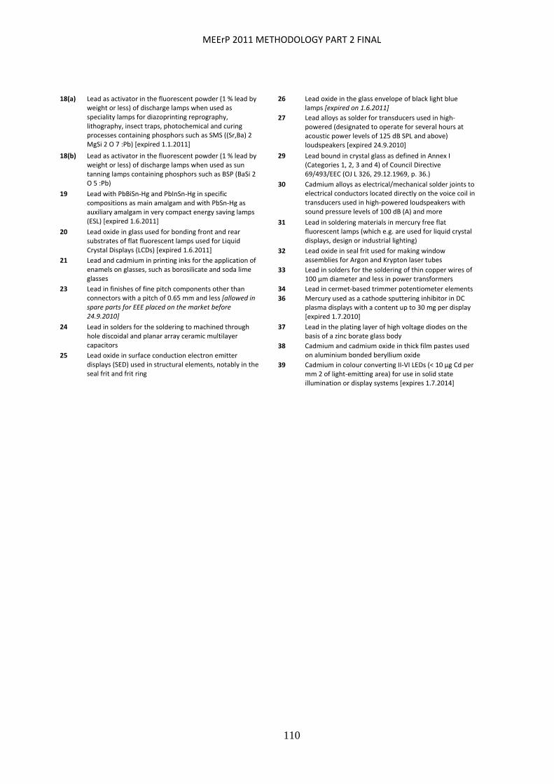
MEErP 2011 METHODOLOGY PART 2 FINAL
110
26 Lead oxide in the glass envelope of black light blue lamps [expired on 1.6.2011]
27 Lead alloys as solder for transducers used in high‐powered (designated to operate for several hours at acoustic power levels of 125 dB SPL and above) loudspeakers [expired 24.9.2010]
29 Lead bound in crystal glass as defined in Annex I (Categories 1, 2, 3 and 4) of Council Directive 69/493/EEC (OJ L 326, 29.12.1969, p. 36.)
30 Cadmium alloys as electrical/mechanical solder joints to electrical conductors located directly on the voice coil in transducers used in high‐powered loudspeakers with sound pressure levels of 100 dB (A) and more
31 Lead in soldering materials in mercury free flat fluorescent lamps (which e.g. are used for liquid crystal displays, design or industrial lighting)
32 Lead oxide in seal frit used for making window assemblies for Argon and Krypton laser tubes
33 Lead in solders for the soldering of thin copper wires of 100 μm diameter and less in power transformers
34 Lead in cermet‐based trimmer potentiometer elements
36 Mercury used as a cathode sputtering inhibitor in DC plasma displays with a content up to 30 mg per display [expired 1.7.2010]
37 Lead in the plating layer of high voltage diodes on the basis of a zinc borate glass body
38 Cadmium and cadmium oxide in thick film pastes used on aluminium bonded beryllium oxide
39 Cadmium in colour converting II‐VI LEDs (< 10 μg Cd per mm 2 of light‐emitting area) for use in solid state illumination or display systems [expires 1.7.2014]
18(a) Lead as activator in the fluorescent powder (1 % lead by weight or less) of discharge lamps when used as speciality lamps for diazoprinting reprography, lithography, insect traps, photochemical and curing processes containing phosphors such as SMS ((Sr,Ba) 2 MgSi 2 O 7 :Pb) [expired 1.1.2011]
18(b) Lead as activator in the fluorescent powder (1 % lead by weight or less) of discharge lamps when used as sun tanning lamps containing phosphors such as BSP (BaSi 2 O 5 :Pb)
19 Lead with PbBiSn‐Hg and PbInSn‐Hg in specific compositions as main amalgam and with PbSn‐Hg as auxiliary amalgam in very compact energy saving lamps (ESL) [expired 1.6.2011]
20 Lead oxide in glass used for bonding front and rear substrates of flat fluorescent lamps used for Liquid Crystal Displays (LCDs) [expired 1.6.2011]
21 Lead and cadmium in printing inks for the application of enamels on glasses, such as borosilicate and soda lime glasses
23 Lead in finishes of fine pitch components other than connectors with a pitch of 0.65 mm and less [allowed in spare parts for EEE placed on the market before 24.9.2010]
24 Lead in solders for the soldering to machined through hole discoidal and planar array ceramic multilayer capacitors
25 Lead oxide in surface conduction electron emitter displays (SED) used in structural elements, notably in the seal frit and frit ring
MEErP 2011 METHODOLOGY PART 2 FINAL
111
REACH
REACH is the European Community Regulation on chemicals and their safe use (EC 1907/2006)94. It deals with the Registration, Evaluation, Authorisation and Restriction of Chemical substances. The law entered into force on 1 June 2007. The REACH system is introduced gradually ‐ up till 2019 ‐ as more and more substances are phased into REACH.
The aim of REACH is to improve the protection of human health and the environment through the better and earlier identification of the intrinsic properties of chemical substances.
REACH ultimately entails an authorization procedure for Substances of Very High Concern (SVHC), a.k.a. as Annex XIV substances. The status of SVHC is confirmed when a substance is in the Candidate List, published on the homepage of the European Chemical Agency (ECHA) in Helsinki. In October 2011 there were 53 substances in the Candidate List, shown in Table 16. These substances are not (yet) subject to the authorization procedure, but there are information requirements in the supply chain. Starting 1st of June 2011 manufacturers and importers, annually producing or importing more than a certain quantity of the substance, are required to report to their clients if their products contain more than 0.1% mass of the SVHC.
For 6 out of 53 substances on the Candidate list, indicated in red italic font in the table, dates for the start of the authorization procedure is set (‘sunset date’). For the 6 substances these dates are in the 2014‐2015 period. In the coming years ‘sunset dates’ for more substances of the Candidate list will follow. Also, more substances are expected to be added to the Candidate List. They will be selected from a list of currently over 3500 pre‐registered substances for which dossiers are being developed.
The authorization procedure entails that –from the sunset date onwards‐ SVHC are banned unless the manufacturer or importer can supply arguments against a ban, i.e. that they are indispensable (not substitutable) in certain applications, that they will be handled and applied in a safe way, etc..
MEErP proposes to use a general indicator from a simple total mass‐count of SVHC on the Candidate list (possibly with underlying mass‐specification per specific SVHC95) in the Ecodesign preparatory studies. The European Commission has identified the type of environmental/health impacts per SVHC (carcinogenic, mutagenic, toxic for reproduction, (very) persistent, (very) bio‐accumulative, toxic in general96), but has not given quantitative characterization factors that would allow a more specific evaluation.
The reasons why the SVHC‐mass is included as an indicator in MEErP is not to possibly duplicate REACH requirements, but prepare industry and –as with RoHS— make sure that the number of special authorisations for SVHC is reduced to a minimum.
Having said that, for this new indicator, preparatory studies will have to deal with a number of practical issues:
94 REGULATION (EC) No 1907/2006 OF THE EUROPEAN PARLIAMENT AND OF THE COUNCIL of 18 December 2006
concerning the Registration, Evaluation, Authorisation and Restriction of Chemicals (REACH), establishing a European Chemicals Agency, amending Directive 1999/45/EC and repealing Council Regulation (EEC) No 793/93 and Commission Regulation (EC) No 1488/94 as well as Council Directive 76/769/EEC and Commission Directives 91/155/EEC, 93/67/EEC, 93/105/EC and 2000/21/EC, OJ L 396, 30.12.2006, p. 1. 95 A specified mass count per SVHC is ideal, but if such information is not available (e.g. for confidentiality reasons) a total mass count is acceptable. 96 PBT= Persistent, Bio‐accumulative and Toxic substances; vPvB=very Persistent and very Bio‐accumulative.
MEErP 2011 METHODOLOGY PART 2 FINAL
112
As mentioned, the Candidate list is expected to change frequently and thus in the preparatory study first the latest status of the Candidate list will have to be checked before an assessment is undertaken. This is also one of the reasons why the assessment of an SVHC‐indicator is not included in the EcoReport tool, but has to be performed manually.
The inclusion of SVHC relates to the concentration in the product, not to resources or emissions during the use phase. Hence, in all cases the SVHC in Affected Energy System (for indirect ErP) should not be taken into account.
The implementation of the REACH directive is new. This means that actors have to gain experience with the reporting mechanism and compliance rate will presumably not be 100% immediately. In this case, the persons responsible for the preparatory study, if they are not able to retrieve information on SVHC‐concentrations from industry reports, are not required to perform their own assessment at laboratory level and have to assume that there are no mass concentrations of SVHC larger than 0.1 mass % in the ErP.
REACH specifies a reporting requirement at a 0.1% minimum mass concentration ‘per product’. It is not clear if ‘product’ relates to the total mass of the ErP, components of the ErP or monolitic parts of the (components of) ErP. This is expected to become clear when the first substance concentrations in ErP (products, components, parts) are actually reported, i.e. at the earliest after 1st December 2011. This problem is aggravated by the fact that most of the substances on the lists are additives or plating agents, like PVC plasticers, fragrances, chroming agents, flame retardants, etc. which are usually applied in ErP‐components, if any, at very low mass fractions. In other words, it may take a while before the problem actually becomes apparent. Untill that time, the persons responsible for the preparatory study are not required to perform research at laboratory level to analyse mass fractions of SVHC but can assume that SVHC‐concentrations larger than 0.1 weight % do not occur in (parts of) the product.
In many cases the use of SVHCs may differ between various products that are chosen as a base‐case. In that case, the preparatory study will have to try to make a sales‐weighted assessment of the average SVHC‐content of the base‐case.
From a practical standpoint, the SVHC‐indicator is most critical for the (currently 6) products where already a ‘sunset date’ is set. Here it is most likely that at a central level, e.g. an industry association, there is representative data on the industry‐average concentrations. For that reason, these substances are mentioned explicitly in MEErP Report Part 1 and the persons responsible for the preparatory study should actively approach industry associations and/or other centralized sources of information regarding concentration levels of these substances.
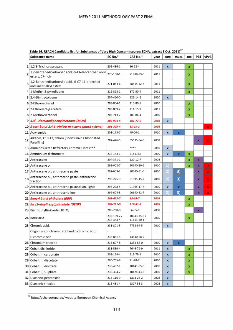
MEErP 2011 METHODOLOGY PART 2 FINAL
113
Table 16. REACH Candidate list for Substances of Very High Concern (source: ECHA, extract 5 Oct. 2011)97
Substance name EC No.* CAS No.* year carc muta tox PBT vPvB
1 1.2.3‐Trichloropropane 202‐486‐1 96‐18‐4 2011 x x
2 1.2‐Benzenedicarboxylic acid, di‐C6‐8‐branched alkyl esters, C7‐rich
276‐158‐1 71888‐89‐6 2011 x
3 1.2‐Benzenedicarboxylic acid, di‐C7‐11‐branched and linear alkyl esters
271‐084‐6 68515‐42‐4 2011 x
4 1‐Methyl‐2‐pyrrolidone 212‐828‐1 872‐50‐4 2011 x
5 2.4‐Dinitrotoluene 204‐450‐0 121‐14‐2 2010 x
6 2‐Ethoxyethanol 203‐804‐1 110‐80‐5 2010 x
7 2‐Ethoxyethyl acetate 203‐839‐2 111‐15‐9 2011 x
8 2‐Methoxyethanol 203‐713‐7 109‐86‐4 2010 x
9 4.4'‐ Diaminodiphenylmethane (MDA) 202‐974‐4 101‐77‐9 2008 x
10 5‐tert‐butyl‐2.4.6‐trinitro‐m‐xylene (musk xylene) 201‐329‐4 81‐15‐2 2008 x
11 Acrylamide 201‐173‐7 79‐06‐1 2010 x x
12 Alkanes, C10‐13, chloro (Short Chain Chlorinated Paraffins)
287‐476‐5 85535‐84‐8 2008 x x
13 Aluminosilicate Refractory Ceramic Fibres*** ‐ **** 2010 x
14 Ammonium dichromate 232‐143‐1 2151163 2010 x x x
15 Anthracene 204‐371‐1 120‐12‐7 2008 x x
16 Anthracene oil 292‐602‐7 90640‐80‐5 2010 1) x x x
17 Anthracene oil, anthracene paste 292‐603‐2 90640‐81‐6 2010 2) 3) x x
18 Anthracene oil, anthracene paste, anthracene fraction
295‐275‐9 91995‐15‐2 2010 2) 3) x x
19 Anthracene oil, anthracene paste,distn. lights 295‐278‐5 91995‐17‐4 2010 x x x x
20 Anthracene oil, anthracene‐low 292‐604‐8 90640‐82‐7 2010 2) 3) x x
21 Benzyl butyl phthalate (BBP) 201‐622‐7 85‐68‐7 2008 x
22 Bis (2‐ethylhexyl)phthalate (DEHP) 204‐211‐0 117‐81‐7 2008 x
23 Bis(tributyltin)oxide (TBTO) 200‐268‐0 56‐35‐9 2008 x
24 Boric acid 233‐139‐2 / 234‐343‐4
10043‐35‐3 / 11113‐50‐1
2010 x
25 Chromic acid, 231‐801‐5 7738‐94‐5 2010 x
Oligomers of chromic acid and dichromic acid, ‐ ‐ ..
Dichromic acid 236‐881‐5 13530‐68‐2
26 Chromium trioxide 215‐607‐8 1333‐82‐0 2010 x x
27 Cobalt dichloride 231‐589‐4 7646‐79‐9 2011 x x
28 Cobalt(II) carbonate 208‐169‐4 513‐79‐1 2010 x x
29 Cobalt(II) diacetate 200‐755‐8 71‐48‐7 2010 x x
30 Cobalt(II) dinitrate 233‐402‐1 10141‐05‐6 2010 x x
31 Cobalt(II) sulphate 233‐334‐2 10124‐43‐3 2010 x x
32 Diarsenic pentaoxide 215‐116‐9 1303‐28‐2 2008 x
33 Diarsenic trioxide 215‐481‐4 1327‐53‐3 2008 x
97 http://echa.europa.eu/ website European Chemical Agency
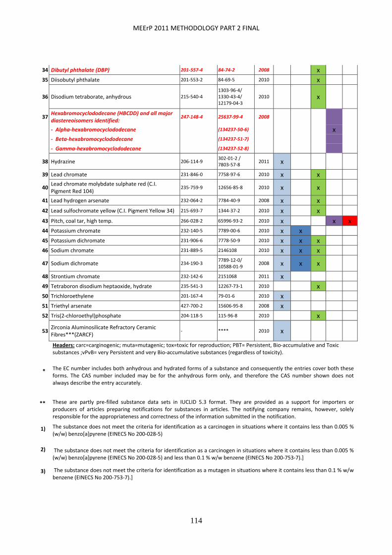
MEErP 2011 METHODOLOGY PART 2 FINAL
114
34 Dibutyl phthalate (DBP) 201‐557‐4 84‐74‐2 2008 x
35 Diisobutyl phthalate 201‐553‐2 84‐69‐5 2010 x
36 Disodium tetraborate, anhydrous 215‐540‐4 1303‐96‐4/ 1330‐43‐4/ 12179‐04‐3
2010 x
37 Hexabromocyclododecane (HBCDD) and all major diastereoisomers identified:
247‐148‐4 25637‐99‐4 2008
‐ Alpha‐hexabromocyclododecane (134237‐50‐6) x
‐ Beta‐hexabromocyclododecane (134237‐51‐7)
‐ Gamma‐hexabromocyclododecane (134237‐52‐8)
38 Hydrazine 206‐114‐9 302‐01‐2 / 7803‐57‐8
2011 x
39 Lead chromate 231‐846‐0 7758‐97‐6 2010 x x
40 Lead chromate molybdate sulphate red (C.I. Pigment Red 104)
235‐759‐9 12656‐85‐8 2010 x x
41 Lead hydrogen arsenate 232‐064‐2 7784‐40‐9 2008 x x
42 Lead sulfochromate yellow (C.I. Pigment Yellow 34) 215‐693‐7 1344‐37‐2 2010 x x
43 Pitch, coal tar, high temp. 266‐028‐2 65996‐93‐2 2010 x x x
44 Potassium chromate 232‐140‐5 7789‐00‐6 2010 x x
45 Potassium dichromate 231‐906‐6 7778‐50‐9 2010 x x x
46 Sodium chromate 231‐889‐5 2146108 2010 x x x
47 Sodium dichromate 234‐190‐3 7789‐12‐0/ 10588‐01‐9
2008 x x x
48 Strontium chromate 232‐142‐6 2151068 2011 x
49 Tetraboron disodium heptaoxide, hydrate 235‐541‐3 12267‐73‐1 2010 x
50 Trichloroethylene 201‐167‐4 79‐01‐6 2010 x
51 Triethyl arsenate 427‐700‐2 15606‐95‐8 2008 x
52 Tris(2‐chloroethyl)phosphate 204‐118‐5 115‐96‐8 2010 x
53 Zirconia Aluminosilicate Refractory Ceramic Fibres***(ZARCF)
‐ **** 2010 x
Headers: carc=carginogenic; muta=mutagenic; tox=toxic for reproduction; PBT= Persistent, Bio‐accumulative and Toxic substances ;vPvB= very Persistent and very Bio‐accumulative substances (regardless of toxicity).
* The EC number includes both anhydrous and hydrated forms of a substance and consequently the entries cover both these forms. The CAS number included may be for the anhydrous form only, and therefore the CAS number shown does not always describe the entry accurately.
** These are partly pre‐filled substance data sets in IUCLID 5.3 format. They are provided as a support for importers or producers of articles preparing notifications for substances in articles. The notifying company remains, however, solely responsible for the appropriateness and correctness of the information submitted in the notification.
1) The substance does not meet the criteria for identification as a carcinogen in situations where it contains less than 0.005 % (w/w) benzo[a]pyrene (EINECS No 200‐028‐5)
2) The substance does not meet the criteria for identification as a carcinogen in situations where it contains less than 0.005 % (w/w) benzo[a]pyrene (EINECS No 200‐028‐5) and less than 0.1 % w/w benzene (EINECS No 200‐753‐7).]
3) The substance does not meet the criteria for identification as a mutagen in situations where it contains less than 0.1 % w/w benzene (EINECS No 200‐753‐7).]

MEErP 2011 METHODOLOGY PART 2 FINAL
115
***
***=are fibres covered by index number 650‐017‐00‐8 in Annex VI, part 3, table 3.2 of Regulation (EC) No 1272/2008 of the European Parliament and of the Council of 16 December 2008 on classification, labelling and packaging of substances and mixtures, and fulfil the two following conditions:
a) for ZARCF: Al2O3, SiO2 and ZrO2 are present within the following concentration ranges: Al2O3: 35 – 36 % w/w, and SiO2: 47.5 – 50 % w/w, and ZrO2: 15 ‐ 17 % w/w |||
for ARCF: Al2O3 and SiO2 are present within the following concentration ranges: Al2O3: 43.5 – 47 % w/w, and SiO2: 49.5 – 53.5 % w/w, or Al2O3: 45.5 – 50.5 % w/w, and SiO2: 48.5 – 54 % w/w,
b) fibres have a length weighted geometric mean diameter less two standard geometric errors of 6 or less micrometres (µm).
****=Extracted from Index no.: 650‐017‐00‐8
MEErP 2011 METHODOLOGY PART 2 FINAL
116
5 ECOREPORT2011LCAUNITINDICATORS
5.1 IntroductionBuilding on Chapter 4, this chapter describes the Life Cycle Analysis method as used in the EcoReport tool for Ecodesign preparatory studies. The Eco Report tool was specifically developed to provide persons in charge for the study with a compact, easy‐to‐use instrument in the public domain.
The tool contains the compact database of Unit (Inpact) Indicators for close to 100 materials and processes most commonly used in the LCA of ErP. It is tuned to the use in product design, e.g. at the aggregation level of half‐products for materials, simple parameters to give a quick impression of the distribution and EoL‐effort and finally a section on the use phase that has been expanded to accommodate ErP.
Using the tool these data can be transformed into the environmental profile per BaseCase, as a mandatory part of Task 5. In addition, there is a separate section on basic economics which –once the right data are known—will help contractorspersons in charge underway also in that field, although in the final analysis the person in charge may decide to use a more comprehensive set‐up.
The EcoReport tool is accompanied by a MEErP Excel file for use with direct and indirect ErPs. The fileis offered both in Excel ’99‐2003 format (.xls) and in Excel 2010 format (.xlsx). The latter has the advantage of being less than 50% in size (0.5 Mb instead of 1 Mb).
5.2 TableUnitIndicatorUsing the methodology in Chapter 4 the following table with so‐called Unit Indicators was generated. The Unit Indicators constitute the non‐product specific part of the EuP EcoReport that leads to the impact analysis as defined in the table of the tender document. The table below gives the Unit Indicators.
But on some points the LCIA multipliers, following the latest developments in legislation, were adjusted as described in the previous chapters. This may lead to minor deviations from the EcoReport 2005 data.
Please note that, should an expansion of the list be needed in a specific case, the persons in charge can use a new facility in the EcoReport 2011 tool to introduce up to 20 new materials/processes based on their own LCA data.

MEErP 2011 METHODOLOGY PART 2 FINAL
117
Table 17. ECOREPORT Unit indicators, Part 1 (VHK)
MATERIALS & PROCESSES
unit indicators
re‐ ENERGY WATER WASTE EMISSIONS: TO AIR TO WATER
cycle prim electr fd proc cool haz non GWP AD VOC POP HMa PAH PM HMw EP
% MJ MJ MJ ltr ltr g g kg g g ng mg mg g mg mg
PLASTICS (in kg)
1 LDPE 78 13 52 3 45 4 44 1.9 7 0.5 ‐ ‐ 0 1 ‐ 272 HDPE 77 10 54 3 31 5 38 1.8 6 0.2 ‐ ‐ 0 1 ‐ 303 LLDPE 74 10 47 2 116 3 31 1.9 6 0.1 ‐ ‐ 0 1 ‐ 394 PP 73 7 53 5 40 4 28 2.0 6 0.0 ‐ ‐ 0 1 ‐ 1655 PS 87 4 48 5 177 1 22 2.8 17 0.0 ‐ ‐ 121 2 ‐ 55
6 EPS 84 3 48 6 176 1 38 2.7 18 0.0 ‐ ‐ 61 2 ‐ 1257 HI‐PS 92 5 49 6 186 1 30 2.9 19 0.0 ‐ ‐ 61 2 ‐ 608 PVC 57 11 23 11 62 5 67 2.2 15 0.0 ‐ ‐ 0 3 3 3149 SAN 89 4 47 6 163 4 32 3.0 14 0.0 ‐ ‐ 0 2 ‐ 28110 PET 79 13 39 7 36 2 92 3.1 34 1.3 ‐ ‐ 1 5 ‐ 380
11 ABS 95 7 46 9 165 10 92 3.3 18 0.0 ‐ ‐ 2 3 2 63012 PA 6 120 15 39 16 219 19 176 8.6 39 0.0 ‐ ‐ 0 5 49 187213 PC 117 15 38 14 114 10 177 5.4 25 0.0 ‐ ‐ 0 7 ‐ 50414 PMMA 110 13 42 10 26 1 105 6.0 44 0.0 ‐ ‐ 0 5 3 206815 Epoxy 141 25 43 19 384 19 407 6.6 44 0.0 ‐ ‐ 0 15 ‐ 9650
16 Rigid PUR 104 17 39 60 301 20 427 4.2 31 0.0 ‐ ‐ 20 7 43 318617 Flex PUR 104 19 40 70 298 32 549 4.5 32 0.0 ‐ ‐ 20 8 3 5686 Plastics fillers, reinforcements, additives (in kg)
18 Talcum filler 10 ‐ 0 ‐ ‐ ‐ 6 0.6 3 ‐ ‐ ‐ 1 ‐ ‐ ‐19 E‐glass fibre 66 21 11 54 271 7 311 3.4 29 0.0 ‐ ‐ ‐ 8 47 3.15120 Aramid fibre 257 82 42 212 1058 28 1214 13 114 0.0 ‐ ‐ ‐ 32 185 12290 Plastics OEM Manufacturing
21 all plastic parts 41 25 1 ‐ 12 0 128 2.3 10 0.0 ‐ ‐ ‐ 2 ‐ 24 METALS (in kg)
22 St sheet galv. 5 34 2 ‐ ‐ ‐ ‐ 1722 2.8 7 0.1 26 4 ‐ 3 4 6523 St tube/profile 50 17 5 ‐ ‐ ‐ ‐ 801 1.4 4 0.1 12 3 ‐ 1 2 3824 Cast iron 85 10 ‐ ‐ 1 4 ‐ 315 1.1 3 0.1 6 2 ‐ 14 1 2625 Ferrite 0 51 3 0 39 0 ‐ 2582 4.2 11 0.2 39 36 ‐ 4 2 7926 Stainless 18/8 coil 63 62 10 4 76 8 ‐ 1000 6.2 56 0.1 8 36 ‐ 8 86 2328
27 Al sheet/extrusion 11 193 ‐ 0 ‐ ‐ ‐ 360 10 67 0.1 5 4 97 17 35 528 Al diecast 85 55 ‐ 0 ‐ ‐ ‐ 150 3.5 16 0.1 33 1 18 4 6 129 Cu winding wire 0 143 ‐ 0 ‐ ‐ 1 40 7.4 304 0.0 4 57 6 3 6 15830 Cu wire 0 117 ‐ 0 ‐ ‐ ‐ 12 6.2 292 0.0 4 55 5 3 94 15531 Cu tube/sheet 60 51 ‐ 0 ‐ ‐ ‐ 14 2.7 63 0.0 10 33 5 1 38 62
32 CuZn38 cast 85 38 ‐ 0 ‐ ‐ ‐ 43 1.8 35 0.0 25 57 3 1 9 1533 ZnAl4 cast 85 28 ‐ 0 2 ‐ 1 33 1.1 6 0.0 60 2 1 1 ‐ 134 MgZn5 cast 50 162 ‐ 0 119 13 6 286 18 45 0.1 27 3 49 9 18 4 Metals OEM Manufacturing 35 foundries Fe/Cu/Zn 2 1 0 ‐ 1 ‐ 7 0.1 1 0.0 ‐ ‐ ‐ ‐ ‐ 136 foundries Al 7 4 0 ‐ 2 ‐ 20 0.4 2 0.0 ‐ ‐ ‐ ‐ ‐ 437 sheetmetal plant 15 9 1 ‐ 4 ‐ 47 0.8 4 0.0 ‐ ‐ ‐ 1 ‐ 638 sheetmetal scrap 12 5 0 ‐ 0 ‐ 180 0.8 4 0.1 11 25 ‐ 1 ‐ ‐ Coating/plating kg (Au/Pt/Pd in g) 39 pre‐coating coil 0 314 83 43 19 384 19 407 16 59 0.8 ‐ 1 ‐ 15 ‐ 965240 powder coating 0 357 61 43 19 384 21 492 18 63 0.0 ‐ 1 ‐ 15 1 965241 Cu/Ni/Cr plating 0 2759 2584 0 187 1742 58 20000 125 1676 3.1 397 1935 5 53 153 9500442 Au/Pt/Pd per g 25 225 203 0 ‐ ‐ 26 187500 18 344 ‐ ‐ 128 ‐ 13 ‐ ‐ ELECTRONICS (in kg, unless indicated otherwise)
43 LCD per m² scrn 3564 2270 0 45 670 1 52 184 59 0 0 1 0 0 0 244 CRT per m² scrn 3169 2131 0 290 ‐ 49 2468 171 1077 1 14 933 0 2828 14 72345 big caps & coils 383 0 0 35 55 20 601 22 142 0 2 8 205 36 74 746 slots / ext. ports 187 59 0 75 255 17 308 10 184 0 1 38 2 13 32 647047 large IC 8022 7951 0 ‐ ‐ 237 8789 505 2787 69 49 447 15 73 3740 21481
48 small IC 1787 1744 0 ‐ ‐ 67 1807 115 816 14 10 185 3 24 10 429649 SMD/ LED's avg. 2969 2886 0 925 ‐ 131 2831 167 1620 7 15 422 5 51 15 219550 PWB 1/2 lay 3.75kg/m² 281 151 9 170 77 1733 2625 11 214 2 3 36 4 5 85 368651 PWB 6 lay 4.5 kg/m² 367 146 9 485 77 1892 4073 16 396 1 5 70 7 37 125 244352 PWB 6 lay 2 kg/m² 488 333 12 403 104 4256 2335 20 219 0 3 33 3 6 326 2845
53 Solder SnAg4Cu0.5 234 194 0 70 0 5 228 12 65 0 1 3 2 1 ‐ 654 PWB assembly 128 3 5 12 36 4 107 9 49 2 ‐ 1 3 15 ‐ 70998 Controller board (aggreg.) 2240 1814 0 422 34 97 2084 125 994 5 11 427 51 821 106 2040
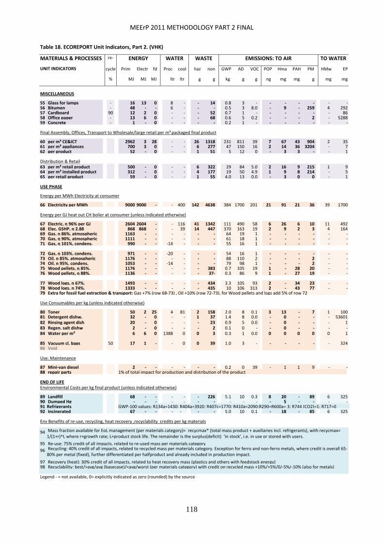
MEErP 2011 METHODOLOGY PART 2 FINAL
118
Table 18. ECOREPORT Unit Indicators, Part 2. (VHK)
MATERIALS & PROCESSES
UNIT INDICATORS
re‐ ENERGY WATER WASTE EMISSIONS: TO AIR TO WATER
cycle Prim Electr fd Proc cool haz non GWP AD VOC POP Hma PAH PM HMw EP
% MJ MJ MJ ltr ltr g g kg g g ng mg mg g mg mg
MISCELLANEOUS
55 Glass for lamps ‐ 16 13 0 8 ‐ ‐ 14 0.8 3 ‐ ‐ ‐ ‐ ‐ ‐ ‐56 Bitumen ‐ 48 ‐ ‐ 6 ‐ ‐ ‐ 0.5 3 8.0 ‐ 9 ‐ 259 4 29257 Cardboard 90 12 2 0 ‐ ‐ ‐ 52 0.7 1 ‐ ‐ ‐ ‐ ‐ ‐ 8658 Office paper ‐ 13 6 0 ‐ ‐ ‐ 68 0.6 5 0.2 ‐ ‐ ‐ 2 ‐ 528859 Concrete ‐ 1 ‐ 0 ‐ ‐ ‐ ‐ 0.2 1 ‐ ‐ ‐ ‐ ‐ ‐ ‐ Final Assembly, Offices, Transport to Wholesale/large retail per m³packaged final product
60 per m³ CE&ICT 2962 3 28 ‐ ‐ 26 1318 231 811 39 7 67 43 904 2 3561 per m³ appliances 700 3 0 ‐ ‐ 6 277 47 150 16 2 14 36 3204 ‐ 762 per product 52 ‐ 0 ‐ ‐ 1 51 5 12 0 ‐ 3 3 ‐ ‐ 1 Distribution & Retail 63 per m³ retail product 500 ‐ 0 ‐ ‐ 6 322 29 84 5.0 2 16 9 215 1 964 per m³ installed product 312 ‐ 0 ‐ ‐ 4 177 19 50 4.9 1 9 8 214 ‐ 565 per retail product 59 ‐ 0 ‐ ‐ 1 55 4.0 13 0.0 ‐ 3 0 0 ‐ 1 USE PHASE
Energy per MWh Electricity at consumer
66 Electricity per MWh 9000 9000 ‐ ‐ 400 142 4638 384 1700 201 21 91 21 36 39 1700
Energy per GJ heat out CH boiler at consumer (unless indicated otherwise)
67 Electric, η 96% per GJ 2604 2604 ‐ ‐ 116 41 1342 111 490 58 6 26 6 10 11 49268 Elec. GSHP, η 2.88 868 868 ‐ ‐ 39 14 447 370 163 19 2 9 2 3 4 16469 Gas, η 86%, atmospheric 1163 ‐ ‐ ‐ ‐ ‐ ‐ 64 19 1 ‐ ‐ ‐ ‐ ‐ ‐70 Gas, η 90%, atmospheric 1111 ‐ ‐ ‐ ‐ ‐ ‐ 61 18 1 ‐ ‐ ‐ ‐ ‐ ‐71 Gas, η 101%, condens. 990 ‐ ‐ ‐14 ‐ ‐ ‐ 55 16 1 ‐ ‐ ‐ ‐ ‐ ‐ 72 Gas, η 103%, condens. 971 ‐ ‐ ‐20 ‐ ‐ ‐ 54 16 1 ‐ ‐ ‐ ‐ ‐ ‐73 Oil, η 85%, atmospheric 1176 ‐ ‐ ‐ ‐ ‐ ‐ 88 110 2 ‐ ‐ ‐ 2 ‐ ‐74 Oil, η 95%, condens. 1053 ‐ ‐ ‐14 ‐ ‐ ‐ 79 98 1 ‐ ‐ ‐ 2 ‐ ‐75 Wood pellets, η 85%. 1176 ‐ ‐ ‐ ‐ ‐ 383 0.7 105 19 1 ‐ 28 20 ‐ ‐76 Wood pellets, η 88%. 1136 ‐ ‐ ‐ ‐ ‐ 37‐ 0.3 86 9 1 ‐ 27 19 ‐ ‐ 77 Wood logs, η 67%. 1493 ‐ ‐ ‐ ‐ ‐ 434 3.3 105 93 2 ‐ 34 23 ‐ ‐78 Wood logs, η 74%. 1333 ‐ ‐ ‐ ‐ ‐ 435 10 106 313 2 ‐ 43 77 ‐ ‐79 Extra for fossil fuel extraction & transport: Gas +7% (row 68‐73) , Oil +10% (row 72‐73), for Wood pellets and logs add 5% of row 72 Use Consumables per kg (unless indicated otherwise)
80 Toner 50 2 25 4 81 2 158 2.0 8 0.1 3 13 ‐ 7 1 10081 Detergent dishw. 32 ‐ 0 ‐ ‐ 1 37 1.4 8 0.0 ‐ 0 ‐ ‐ ‐ 5360182 Rinsing agent dish 20 ‐ 0 ‐ ‐ ‐ 23 0.9 5 0.0 ‐ 0 ‐ ‐ ‐ 183 Regen. salt dishw 2 ‐ 0 ‐ ‐ ‐ 2 0.1 0 ‐ ‐ 0 ‐ ‐ ‐ ‐84 Water per m³ 6 6 0 1388 0 0 3 0.3 1 0.0 0 0 0 0 0 1 85 Vacuum cl. bags 50 17 1 ‐ ‐ 0 0 39 1.0 3 ‐ ‐ ‐ ‐ ‐ ‐ 32486 Void Use: Maintenance
87 Mini‐van diesel 2 ‐ ‐ ‐ ‐ ‐ ‐ 0.2 0 39 ‐ 1 1 9 ‐ ‐88 repair parts 1% of total impact for production and distribution of the product END OF LIFE Environmental Costs per kg final product (unless indicated otherwise)
89 Landfill 68 ‐ ‐ ‐ ‐ ‐ 226 5.1 10 0.3 8 20 ‐ 89 6 32590 Dumped Hg ‐ ‐ ‐ ‐ ‐ ‐ ‐ ‐ ‐ ‐ ‐ 5 ‐ ‐ ‐ ‐91 Refrigerants GWP‐100 values: R134a=1430; R404a=3920; R407c=1770; R410a=2090;R290=R600a= 3; R744 (CO2)=1; R717=092 Incinerated 67 ‐ ‐ ‐ ‐ ‐ ‐ 5.0 10 0.1 ‐ 18 ‐ 85 6 325 Env Benefits of re‐use, recycling, heat recovery ,recyclability credits per kg materials
94 Mass fraction available for EoL management (per materials category)= recycmax* (total mass product + auxiliaries incl. refrigerants), with recycmax= 1/(1+r)^L where r=growth rate; L=product stock life. The remainder is the surplus(deficit) ‘in stock’, i.e. in use or stored with users.
95 Re‐use: 75% credit of all impacts, related to re‐used mass per materials category
96 Recycling: 40% credit of all impacts, related to recycled mass per materials category. Exception for ferro and non‐ferro metals, where credit is overall 65‐80% per metal (fixed), further differentiated per halfproduct and already included in production impact.
97 Recovery (heat): 30% credit of all impacts, related to heat recovery mass (plastics and others with feedstock energy) 98 Recyclability: best/>avg/avg (basecase)/<avg/worst (per materials category) with credit on recycled mass +10%/+5%/0/‐5%/‐10% (also for metals) Legend ‐ = not available, 0= explicitly indicated as zero (rounded) by the source
MEErP 2011 METHODOLOGY PART 2 FINAL
119
Explanatory Notes to tables 20 and 21
Scope
The main table gives environmental indicators of almost 100 materials and unit processes relevant to the Eco‐design of Energy‐related Products (ErP). Each row in the table represents a material or energy conversion process, characterized by 15 numerical Environmental Indicators (EI). The EIs are aggregated data derived from emissions and resources‐use of the processes involved. Characterisation factors for some EIs are given in the former MEEuP 2005 report. Following the principles of the ISO 14040 series for emissions and IFIAS for energy, emissions and resources were traced back to the 2nd or 3rd level. Indicators are given per unit (kg, GJ, etc.) of materials and process‐outputs and allow the conversion of product‐specific data from the production (Bill‐of‐Materials, BOM), distribution, use and disposal into environmental impacts.
The totals of the 15 different EIs per product will be called the Product Environmental Indicators (PEIs). Together with the Functional Unit (FU) ‐ the product’s performance over product life ‐ the PEI’s make up the Eco‐design Product‐indicator (PI=PEI/ FU). The PI is the starting point for assessing the environmental improvement potential. An improvement can be quantified in % reduction of PI new versus PI old (per EI).
For policy purposes the PEI’s ‐ multiplied by product‐specific EU market data ‐ can also be used to assess the total environmental impact (per EI) of the product category in the EU. This allows to prioritize one product category versus another (per EI) or to compare the product impact with EU targets (per EI). A prioritization between different EI’s (e.g. Global Warming versus Acidification) is outside the scope of the underlying Methodology.
DATA.
These refer to the average EU/ global technology 2005/ 2006. Great care was taken to create a robust data‐set, yet the figures will be subject to change as more and better data become available and the underlying technologies change. Important selection criteria for source material were horizontal quality ‐ i.e. finding the most informed, recent and transparent public source per material or process ‐ and vertical consistency – i.e. allowing a fair comparison on every aspect between potentially ‘competing’ materials and processes.
Sources
Sources for emission data are amongst others: APME (plastics), AKZO (aramid fibres), IISI, Eurofer (St), IPAI, Aluminium Institute (Al), ETH‐1996 (preliminary data on Cu pending Eurocopper input), The Nickel Institute (Ni), IPPC BREF on VOC’s (Cu filaments, pre‐coat, powder coat), The European Dioxin Inventory (secondary metals, solids combustion), Frauenhofer Institute and SemaTech 2002 (electronics), IPPC BREF’s on Paper, Glass (misc.), NTM (transport), ANEC, Öko‐institut GEMIS 4.2 (Fossil fuel heat), EPER 2001, Eurelectric (electricity), IPPC BREF on Waste Incineration (disposal), Ecolabel‐studies (dishwasher detergents, paper/cardboard, CRT), USGS and US DoE EER (mining), US EPA (some Hg emissions), SAVE studies (Heating & hot water appliances, Lithuanian Cleaner Production programme and individual manufacturer’s environmental reports. Data were checked against public VHK studies in the past (downloads from www.vhk.nl), databases in SIMAPRO 6 and a host of other literature. The largest part of the emission data refers to 2000‐2005. For electronics only more recent (2003‐2004) information was used.
UPDATE ELECTRICITY
Following the findings of the feasibility study as reported in the MEErP 2011 Project Report, the list of Unit Indicators contains no new LCA data.. This is not an ideal situation, but for most materials and processes the error is contained and should not stand in the way of using the EcoReport tool for ErP.
The only exception to this rule is the impact of electricity, where larger changes have occurred. VHK has made an effort, despite the lack of budgetary means, to at least make a ‘quick fix’ that would align the values with the latest data and insights.
5.3 NotesperPolicyAreaThe columns in the table refer to the following POLICY AREAs:
Energy: The total Gross Energy Requirement GER [column 1] and – as a part of the GER ‐ the energy requirement (in MJ primary) of electricity [col. 2] and the net calorific value of feedstock [col. 3].
MEErP 2011 METHODOLOGY PART 2 FINAL
120
Please note that electricity and feedstock are auxiliary parameters and not as such indicators of environmental impact. Apart from being an indicator of energy resources depletion, the GER allegedly are covering 90% of the Materials Depletion aspect.
Water: Process water [col. 4] and cooling water volume [col. 5]. The water data of metals should be treated with caution because they may be incomplete. Cooling water is not always considered by all sources; process water use, especially for mining/ benefication is often underestimated
Waste, subdivided in hazardous [col. 6] and not hazardous [col. 7]. LCA sources on metals tend to underestimate the waste from mining operations. The non‐hazardous waste quantities for metals production from the various sources were therefore replaced by an independent set of waste data that allows a fairer comparison. See paragraph 3.5 for more information.
Global Warming Potential GWP [col. 8] includes the weighted emissions of greenhouse gases (GHG’s), including fluorinated GHG’s, with GWP‐100 factors given by the Intergovernmental Panel for Climate Change (IPCC), in order to attain the CO2 equivalent.
Acidification Potential AD [col. 9] in SO2 characterisation factors for acidifying agents, derived from EU legislation, are given in Part 1 report.
Volatile Organic Compounds VOC [col. 10] are indicators (precursors) for smog and ground‐level ozone. NOx (part of AD) is another important parameter. Furthermore VOCs, esp. in higher concentrations can cause neurological health problems (Human Toxicity indicator).
Persistent Organic Compounds POP [col. 11] : Mainly dioxins and furans into air are relevant to ErP’s, expressed in ng I‐TEQ (2.3.7.8‐TCDD equivalent). Conversion factors are part of EU‐legislation, values taken from the European Dioxin Inventory. PCBs in medium/high voltage transformers should be treated on an ad‐hoc basis and are not included in the table. There are no POP emissions to water with EuP.
Heavy Metals [col. 12] relates to emissions of regulated heavy metals, weighted according to their emission limit values as specified in current legislation under the Ambient Air Quality Framework Directive.
Polycyclic Aromatic Hydrocarbons PAH [col. 13] relates to emissions of regulated organic compounds (incl. CO and benzene) of which PAHs are the most prominent, weighted according to their emission limit values as specified in current legislation under the Ambient Air Quality Framework Directive. Original accounting unit in legislation is ng/m³ Benzo(a)pyrene equivalent (for PAHs), CO and benzene, but it was converted to Nickel‐equivalent (1 ng/m³ Benzo(a)pyrene equals 20 ng/m³ Nickel as in directive 2004/107/EC) to keep the link with the previous column on Heavy Metals.
Particulate Matter PM [col. 13] or dust is an important indicator (precursors) for smog and ground‐level ozone. Furthermore PM are indicators for Human Toxicity (respiratory problems). For a subdivision between PM10 and PM2.5 not enough data were available.
Heavy Metals (Water) [col. 14] relates to emissions of regulated heavy metals, weighted according to their emission limit values as specified in current legislation under the Water Quality Framework Directive.
Eutrophication [col. 15] refers to substances that influence the oxygen balance of the water. Individual emissions are weighted according to threshold values in the Water Quality directive to attain the aggregated EI value.
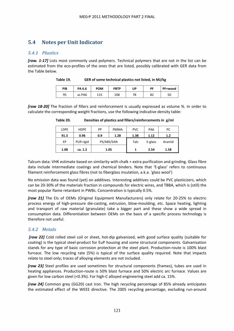
MEErP 2011 METHODOLOGY PART 2 FINAL
121
5.4 NotesperUnitIndicator
5.4.1 Plastics
[row. 1‐17] Lists most commonly used polymers. Technical polymers that are not in the list can be estimated from the eco‐profiles of the ones that are listed, possibly calibrated with GER data from the Table below.
Table 19. GER of some technical plastics not listed, in MJ/kg
PIB PA 6.6 POM PBTP UP PF PF+wood
95 as PA6 115 108 78 82 50
[row 18‐20] The fraction of fillers and reinforcement is usually expressed as volume %. In order to calculate the corresponding weight fractions, use the following indicative density table:
Table 20. Densities of plastics and fillers/reinforcements in g/ml
LDPE HDPE PP PMMA PVC PA6 PC
91.3 0.96 0.9 1.28 1.38 1.12 1.2
EP PUR rigid PS/ABS/SAN Talc E‐glass Aramid
1.08 ca. 1.2 1.05 1 2.54 1.58
Talcum data: VHK estimate based on similarity with chalk + extra purification and grinding. Glass fibre data include intermediate coatings and chemical binders. Note that ‘E‐glass’ refers to continuous filament reinforcement glass fibres (not to fiberglass insulation, a.k.a. ‘glass wool’)
No emission data was found (yet) on additives. Interesting additives could be PVC plasticizers, which can be 20‐30% of the materials fraction in compounds for electric wires, and TBBA, which is (still) the most popular flame retardant in PWBs. Concentration is typically 0.5%.
[row 21] The EIs of OEMs (Original Equipment Manufacturers) only relate for 20‐25% to electric process energy of high‐pressure die‐casting, extrusion, blow‐moulding, etc. Space heating, lighting and transport of raw material (granulate) take a bigger part and these show a wide spread in consumption data. Differentiation between OEMs on the basis of a specific process technology is therefore not useful.
5.4.2 Metals
[row 22] Cold rolled steel coil or sheet, hot‐dip galvanized, with good surface quality (suitable for coating) is the typical steel‐product for EuP housing and some structural components. Galvanisation stands for any type of basic corrosion protection at the steel plant. Production‐route is 100% blast furnace. The low recycling rate (5%) is typical of the surface quality required. Note that impacts relate to steel only; traces of alloying elements are not included.
[row 23] Steel profiles are used sometimes for structural components (frames), tubes are used in heating appliances. Production‐route is 50% blast furnace and 50% electric arc furnace. Values are given for low carbon steel (<0.3%). For high‐C alloyed engineering steel add ca. 15%.
[row 24] Common grey (GG20) cast iron. The high recycling percentage of 85% already anticipates the estimated effect of the WEEE directive. The 2005 recycling percentage, excluding run‐around
MEErP 2011 METHODOLOGY PART 2 FINAL
122
scrap is estimated to be around 65%. The same goes for other die‐/sand‐casts metals in the list, i.e. Al, CuZn38, MgZn5, ZnAl4
[row 25] High‐purity ferrite for application in transformers, electric motors, etc. , preliminary VHK estimate.
[row 26] Austenitic Stainless Steel (FeCr18Ni8), type 304,Surface quality 2B, on coil.
[row 27] Differences between extruded and cold rolled Al sheet are small enough to fall within a 5% range, which is smaller than the overall error margin. Therefore they fall under the same indicators. High PAHs because of carbon anode. High GHG because of fluorinated GHG.
[row 28]Aluminium die‐casts, e.g. AlSi1 and AlMg5. High dioxins due to secondary Aluminium smelters.
[row 29] Winding wires e.g. for el. Motors, coated (IPPC BREF VOCs 2004)
[row 30] Based on ETH 1996 data for virgin Cu. Typical of el. wire.
[row 31] Cu tube (heating/ hot water appliances) and sheet (hot water tanks).
[row 32] Cu with 38% Zn, general purpose brass, die‐cast. High dioxins because of secondary Cu smelting, as with al cast‐products; also ZnAl4 and MgZn5.
[row 33] Zn with 4% Al, general purpose “Zamac”, die‐cast.
[row 34] Magnesium with 5% Zn. High GWP is due to SF6 as cover gas.
[row 35‐36] For Fe/Zn/Cu the process energy was already included in the material. Only comprises space heating, lighting, transport, etc. As space requirements depend mostly on volume and not weight Fe/Zn/Cu (ca. 8‐9 kg/l) and Al/Mg (ca. 2‐3 kg/l) are distinguished in terms of impact.
[row 37‐38] For sheet‐metal and similar OEMs, there is an impact for the space heating, lighting, process energy, raw material transport, etc., expressed per kg final component/ product. And there is a second UI, which takes into account the waste and recycling of primary scrap. As a default, if no specific values are used, one can assume25‐30% cutting losses for average deep‐drawing, cutting and stamping. For folded sheet in e.g. fridge housings, losses are much less (default 10%).
5.4.3 Coating/plating
[row 39] Pre‐coated Steel or Al sheet with a 55 μm layer of epoxy or PUR is one of the few wet‐paint process left in EuP. High VOCs.
[row 40] Powder coating with epoxy. Default layer thickness 35 μm/side.
[row 41] There are differences between Cu (GER 101 MJ/kg virgin), Ni (240 MJ/kg) and Cr (>400 MJ/kg) but the differences fall within the margins of error with electroplating. Default layer thickness for thin‐layer Cu 12 μm (under‐layer for Ni), Ni 20 μm, decorative Cr (on Ni) 2 μm. [sources: Clean Production projects Lithuania and manufacturer reports]. High N to water from Ni beneficiation to be discussed (225 g N/kg Ni?)
[row 42] Typical impact and recycling rate for decorative plating with Au. For high purity “Five‐Nine” (99.999%) applications in electronics the EI values should be increased by 25%. Default layer thickness for Pt (HDD application) and Pd (capacitors) is 1 μm. For gold plating default is 3 μm on Cu‐Ni (8+8 μm) under‐layer.
MEErP 2011 METHODOLOGY PART 2 FINAL
123
5.4.4 Electronics
[row 43] An LCD is mainly a semi‐conductor (8‐9 layers, 4‐5 masks) on glass substrate (0.7mm), covered by another glass 0.7 mm panel with colour filters. The energy consumption data relate to state‐of‐the‐art 6G plant 2005 (source Sharp Corp., Japan), using a cogeneration power plant and extensive recycling (100% water and waste recycling) and scrubbing facilities. As a consequence Sharp Corp. data for GWP from PFCs are a fraction of what was previously indicated for 4G and 5G fabs in 2003 and should be robust for the immediate future. The data are including glass production (IPPC BREF source) and include an indicative figure (0.12 GJ oil, emissions and resources according to row 72) for extraction & transportation of fuels for the cogeneration plant. Data are in m² viewable screen size. Conversion with density 2.76 g/ml (BSi glass) 1 m² = 3.86 kg.
[row 44] Data in m² nominal screen size. Conversion 1 m² = 120 kg for CRTs >13” diagonal. Data refer to glass and Pb fractions (source IPPC, BREF) plus manufacturing based on US EPA 2001 minus 30% improvement.
[row 45] Refers to large capacitors (Al) and coils (Cu, Fe) components on a PWB. No doped silicon, no precious metals. Components are typical for power conversion functions. VHK estimate based on materials composition.
[row 46] PWB‐mounted slots for RAM‐chips, PCI cards + external ports. VHK estimate based on materials fractions. Per 1.000 g: Cu alloy pins 330 g+5 g Cu/Ni plated + 635 g polymer+0.15 g Au.
[row 47 & 48] Based on Si wafer 200 mm diameter, 20 layer complexity. Following ESIA‐indications (European Semi‐conductor Industry Ass.) we used SemaTech 2002 data of 499 kWh electricity use per wafer and a yield of 44 g of core material per wafer ( 11.34 kWh/g). At 5% core material per IC this results in 567 kWh per kg of IC. Back‐end production is adding 25%, leading to 709 kWh electricity per kg of IC. To this a gold content of 0.2 % is added (avg. for larger IC, incl. memory), see row 41 +25%. For small SMD‐type ICs we assume 1 wt. % core material and 0.1 wt. % gold content. For non‐electricity related emissions sustainability reports of individual manufacturers were used. More in general, the two indicated data‐sets for 1% and 5% core‐material (=actual die, silicon, without lid) roughly represent extremes of the current range of ICs.
[row 49] SMD (Surface Mounted Devices) 50 g/m² PWB in a desktop PC main‐board (1.2% of standard PWB weight, 3% of microvia PWB), est. 15 wt. % capacitors (of which estimated one third Pd based, rest Ta and ceramic). E.g. Pd= 300 layers of 1 um x 2 x 3 mm Pd 20 mg Pd/50 mg capacitor overall 3% Pd (at 225000 MJ/kg).
Diodes, thyristors, RF, etc. (estimated 35 wt. % of total) are treated as ICs with oversized packaging (0.5% doped silicon instead of 5%) without gold. The ecoprofile of resistors (estimated 50% of total) will be close to Cu/Ni plating+glass. In terms of energy there is not much difference with diodes etc., therefore no distinction is made.
[row 50] Standard FR4 (density 1.9) board with 1 or 2 Cu foils 35 µm thick. Overall board thickness 1.5 mm, assumed density 2.5 g/ml. 1 m² = 3.75 kg. Manufacturing energy 440 MJ + materials energy 490 MJ = 930 MJ/m². 248 MJ/kg. Typical PWB for appliances and motor controllers. [data: AT&S + standard Unit Indicator values for Cu, E‐glass, epoxy, etc. for materials inputs].
[row 51] Multilayer standard FR4 (density 1.9) board resin (EP 30%‐GF, 125 MJ/kg) with 2 external Cu foils 35 µg thick and 4 internal Cu layers of 18 µg. Overall board thickness 1.5 mm and assumed density 3 g/ml. 1 m² = 4.5 kg. Manufacturing energy 540 MJ/m² + materials energy 4.5*130=585 MJ/m². Total 1125 MJ/m² 250 MJ/kg. Typical PWB (also in 3‐4 layer version) for PC Desktop mainboards, TVs, etc. [source as row 49]
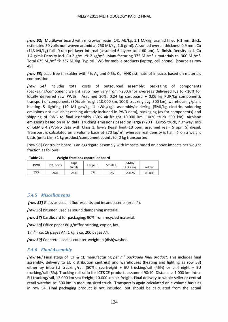
MEErP 2011 METHODOLOGY PART 2 FINAL
124
[row 52] Multilayer board with microvias, resin (141 MJ/kg, 1.1 MJ/kg) aramid filled (<1 mm thick, estimated 30 vol% non‐woven aramid at 250 MJ/kg, 1.6 g/ml). Assumed overall thickness 0.9 mm. Cu (143 MJ/kg) foils 9 um per layer internal (assumed 6 layer= total 60 um). Ni finish. Density excl. Cu 1.4 g/ml; Density incl. Cu 2 g/ml 2 kg/m². Manufacturing 375 MJ/m² + materials ca. 300 MJ/m². Total 675 MJ/m² 337 MJ/kg. Typical PWB for mobile products (laptop, cell phone). [source as row 49]
[row 53] Lead‐free tin solder with 4% Ag and 0.5% Cu. VHK estimate of impacts based on materials composition.
[row 54] Includes total costs of outsourced assembly: packaging of components (packaging/component weight ratio may vary from >200% for overseas delivered ICs to <10% for locally delivered raw PWBs. Assumed 30%: 0.24 kg cardboard + 0.06 kg PUR/kg component), transport of components (30% air‐freight 10.000 km, 100% trucking avg. 500 km), warehousing/plant heating & lighting (10 MJ gas/kg, 1 kWhe/kg), assembly/soldering (5MJ/kg electric, soldering emissions not available; etching already included in PWB data), packaging (as for components) and shipping of PWB to final assembly (30% air‐freight 10.000 km, 100% truck 500 km). Airplane emissions based on NTM data. Trucking emissions based on large (>20 t) Euro5 truck, highway, mix of GEMIS 4.2/Volvo data with Class 1, low‐S (legal limit=10 ppm, assumed real= 5 ppm S) diesel. Transport is calculated on a volume basis at 270 kg/m³, whereas real density is half on a weight basis (unit: t.km) 1 kg product/component counts for 2 kg transported.
[row 98] Controller board is an aggregate assembly with impacts based on above impacts per weight fraction as follows:
Table 21. Weight fractions controller board
PWB ext. ports caps &coils
Large IC Small IC SMD/
LED's avg. solder
35% 24% 28% 8% 2% 2.40% 0.60%
5.4.5 Miscellaneous
[row 55] Glass as used in fluorescents and incandescents (excl. P).
[row 56] Bitumen used as sound dampening material
[row 57] Cardboard for packaging, 90% from recycled material.
[row 58] Office paper 80 g/m²for printing, copier, fax.
1 m² = ca. 16 pages A4. 1 kg is ca. 200 pages A4.
[row 59] Concrete used as counter‐weight in (dish)washer.
5.4.6 FinalAssembly
[row 60] Final stage of ICT & CE manufacturing per m³ packaged final product. This includes final assembly, delivery to EU distribution centre(s) and warehouses (heating and lighting as row 53) either by intra‐EU trucking/rail (50%), sea‐freight + EU trucking/rail (45%) or air‐freight + EU trucking/rail (5%). Trucking‐rail ratio for ICT&CE products assumed 90:10. Distances: 1.000 km intra‐EU trucking/rail, 12.000 km sea‐freight, 10.000 km air‐freight. Final delivery to whole‐seller or central retail warehouse: 500 km in medium‐sized truck. Transport is again calculated on a volume basis as in row 54. Final packaging product is not included, but should be calculated from the actual

MEErP 2011 METHODOLOGY PART 2 FINAL
125
packaging of the final product. [Assume 5 kg cardboard + 1 kg EPS + 1.5 kg paper manual per m³ packaged product if packaging is unknown].
[row 61] Final stage of heating/domestic appliance manufacturing per m³. Differences with row 59: Only 10% imports (instead of 50%) and no air‐freight ( sea‐freight). EU trucking/rail ratio 70:30. Packaging not included [Assume 1 kg LDPE + 0.5 kg EPS + 1 kg paper manual per m³ (straps counted as EPS) if packaging unknown].
[row 62] Space heating and lighting of offices, executive travels, etc. are independent of the size or weight of the product. It cannot be influenced by product‐design but is added to complete the picture.
5.4.7 Distribution&Retail
[row 63] Shop heating and lighting (0.5 GJ gas+90 kWhe per m² shop) is calculated from NL data (source ECN/EIM), assuming 20 units sold per m² and >3.5 m ceiling height. Half of this is assumed to be fixed (counter +traffic space), half linked to the size of the product. Heating and electricity of the wholesale/central retail warehouse is ~60% of shop. Goods are transported from the retailer’s central warehouse to the shop by medium‐sized truck 200 km (Euro 5). From the shop, products go to the customer’s home either by delivery van or customer’s car 20 km (Euro 5, diesel, city‐traffic). The part of shop heating and lighting that is depending on the size of the product is attributed here. The rest is taken into account under row 64.
[row 64] Wholesale & transport; no shop stock assumed.
[row 65] Fixed part of space heating and lighting requirements of EuP‐retailer and wholesaler (also see row 62) per product. Overall, data in rows 54 and 59‐64 are rough estimates for the sole purpose of giving the eco‐designer an idea of the impact of product‐size and weight on the general logistics effort.
5.4.8 Energyuseduringproductlife
[row 66] Electricity from public grid 230V AC. See table below.
MEErP 2011 aligns the electricity data with the latest data and insights. These latest insights include that, while the former MEEuP 2005 data were originally designed to assess instantaneous impacts, they were also used for the scenario analysis e.g. over the period 2010‐2020. In the latter application they proved to be more critical and subject to debate. For that reason, MEErP uses average projected values for the 2010‐2020 period (ca. 2015) instead of the former MEEuP‐approach referring to 2001‐2002. In other words, there is a ‘jump’ of 13‐14 years between the former MEEuP 2005 data and the data in the underlying MEErP study.
The table hereafter shows the differences:
Table 22. Comparison electricity impacts former MEEuP 2005 – MEErP 2011
1 MWh electricity Energy Water Waste Emissions: To Air To Water
at consumer prim el. fd proc cool haz non GWP AP VOC POP HM PAH PM HM EP
MJ MJ MJ ltr ltr g g kg g g ng mg mg g mg mg
MEEuP (2001‐'02) 10500 10500 ‐ ‐ 242 12174 458 2704 4 69 180 21 58 68 323
MEErP (2010‐'20) 9000 9000 ‐ 400 142 4638 384 1700 201 21 91 21 36 39 1700
Notes:
The efficiency of power generation and distribution has been discussed in paragraph 4.3. On this basis an average energy efficiency of 40% (primary energy factor 2.5) is assumed for the period 2010‐
MEErP 2011 METHODOLOGY PART 2 FINAL
126
2020. For products with a product life of 15‐20 years or more, an efficiency of 42% or more may be assumed but this correction should be made manually and not in the tool.
For waste, the E‐PRTR data show that currently 51% (hazardous) and 64% (non‐hazardous) of waste from power stations is recovered. The values show the part that is disposed. It has to be considered that this only relates to waste from the energy sector and does not include coal mining and other fuel extraction. For water use still no data are readily available.
For carbon emissions former MEEuP 2005 used a value of 0.458 kg CO2 equivalent per kWh electricity at the consumer, which is representative for 2001‐2002. This figure does not only take into account strict generation (at ca. 0.43 kg CO2 eq./kWh), but also the extraction, preparation and transport of fuels; credit to derived heat and distribution losses. In line with PRIMES projections, but taking into account the extra elements mentioned above, the carbon intensity will drop to around 0.394 kg CO2 eq./kWh in 2010 and 0.374 kg CO2 eq./kWh in 2020. This means that the average intensity over that period is 0.384 CO2 eq./kWh.
For the emissions to air, the values were taken from EEA data as reported in the various tables and graphs in Chapter 4, whereby it was assumed that 70% of emissions to the energy sector are partitioned to 2800 TWh electricity98. Outcomes were briefly checked against data from official data bases (E‐PRTR, CLRTAP) and EEA data were found to be plausible, but a full comparative analysis is outside the scope of the current study.99 With respect to former MEEuP data, the new values showed a considerable decline of 15‐30%, which is in line with projections in Chapter. The only exceptions are VOC and EP, where new data became available showing a much higher impact than previously known.
[row 67] Heat from electric resistance CH boiler 96% efficiency. 1 GJ electric CH heat = 290 kWh. Electric water storage CH boilers are not listed because they are rare and data is lacking. Emissions are expected to be higher because of standby losses.
[row 68] Electric Ground Source Heat Pump (GSHP) with an assumed COP (Coefficient Of Performance) of 300% and 4% heat losses.
[rows 69‐78] Data from GEMIS 4.2 for fossil fuel powered 10 kW Central heating (CH) boilers in GJ heat produced at the boiler exit in the form of hot CH water. Intermediate emission values can be extrapolated from the ones given. Efficiency values relate to net calorific value (lower heating value) of the fuel. Electricity (pump, fan, control) is not included. Please note, that direct CO2 emissions from wood log and wood pellet boilers are zero by political default (renewable fuel). Dioxin emissions (POP) are taken from EU Dioxin Inventory. Operating time is 1.600h during 15 years. The table below gives some more details on specific operating conditions of the boilers.
98 The other 30% are emissions in the production and distribution of fuels plus emissions partitioned to derived heat. 99 To get an impression of what such an analysis would entail (in this case: of 2 sources), see EEA Technical report No 4/2008, Air pollution from electricity‐generating large combustion plants, http://www.eea.europa.eu/publications/technical_report_2008_4

MEErP 2011 METHODOLOGY PART 2 FINAL
127
Table 23. Details of boiler operation
Gas CH Oil CH Wood CH
Row nr. 68 69 70 71 72 73 74 75 76 77
% O2 3% 3% 13%
% CO2 in flue 9.96% 13.11% 7.69%
Nm³/h flue 11.7 11.2 10.0 9.8 12.2 10.9 27.9 27.0 32.3 36.2
[row 79] For the sake of transparency, emissions from fossil fuel powered CH boilers in rows 64‐75 are only direct emissions and energy. To take into account fuel extraction and refining add 7% for gas (pipeline, North Sea, compressors, gas‐grid), 10% for oil (refinery, transport), 15% for coal (mining, sea‐freight, etc.) and 5% of oil emissions (incl. CO2) for wood logs and wood pellets (collection, transport, treatment).
5.4.9 Consumablesduringproductlife
[rows 80‐85] Emissions and resources for the production of a number of consumables during product life. Office paper [row 54] is also part of this (for copiers, printers, etc.). Note that emissions that are not part of EU legislation (yet) are not mentioned, e.g. ozone‐emissions from copiers, electro‐magnetic radiation, etc. Noise should be dealt with on an ad‐hoc basis if EU legislation exists.
[row 80] Toner based on 48% SAN, 45% iron oxide, 4% PP, 3% silica.
[row 81‐83] Dishwasher detergent, rinsing agent and salt based on EU Ecolabel studies (avg. EU phosphate) and CECED data (energy). Phosphate emissions are considered after Urban Waste Water Treatment (80% removal efficiency).
[row 84] Emissions and resources consumed per m³ (1000 kg) water, from mainly 0.7 kWh electricity per m³ for pumps extraction, production, distribution and sewage. Excludes direct emissions and possible energy credits (biogas) from waste water treatment, because these should be partitioned to the waste source.
[row 85] Vacuum cleaner bags, high quality thick paper, 50% recycled.
[row 86] Void, used as default if no consumable is selected in the EcoReport tool.
5.4.10 Maintenance,Repairs
[row 87] Given is a Euro5 mini‐van/diesel car in city traffic per km.
[row 88] VHK estimate (based on wall‐hung CH boiler).
5.4.11 Disposal:Environmentalcosts
[row 89] Emissions from landfill. In post‐WEEE directive era for EuP this is assumed to be 50% illegal dumping and 50% inert fractions. For illegal dumping emissions based on the equivalent of 1 MJ (Euro 5, city traffic combusted) diesel for transport, cleaning+ landfill emissions (no data available, assume impact as the equivalent of all galvanic protection leaching to groundwater before site is cleaned: 20 mg Zn equivalent per kg product at 0.1 characterisation factor= PAH & HM +2) + normal landfill emissions (ecl. CH4) according to EPER 2001 (counting 115.000 kt municipal waste to landfill in EU‐15) before eventually it will have to be treated anyway as most EuP‐fractions are not biodegradable (assume equivalent of full incineration and no credits for recycling of metals because of cleaning effort).
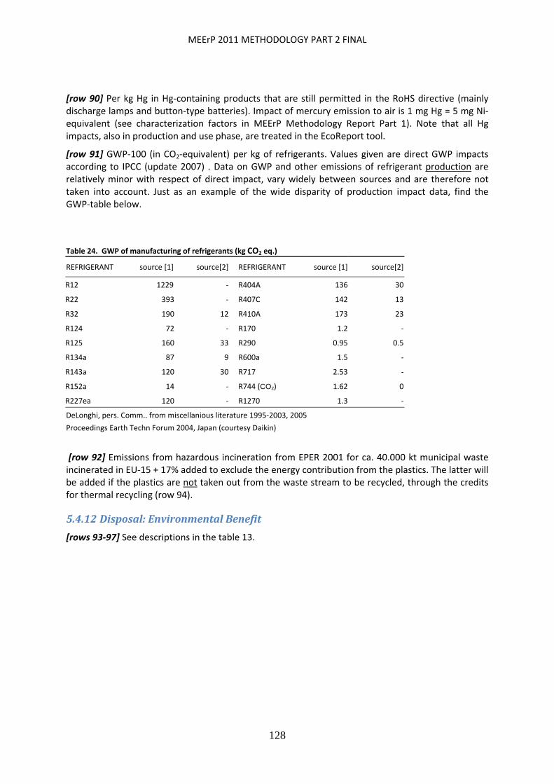
MEErP 2011 METHODOLOGY PART 2 FINAL
128
[row 90] Per kg Hg in Hg‐containing products that are still permitted in the RoHS directive (mainly discharge lamps and button‐type batteries). Impact of mercury emission to air is 1 mg Hg = 5 mg Ni‐equivalent (see characterization factors in MEErP Methodology Report Part 1). Note that all Hg impacts, also in production and use phase, are treated in the EcoReport tool.
[row 91] GWP‐100 (in CO2‐equivalent) per kg of refrigerants. Values given are direct GWP impacts according to IPCC (update 2007) . Data on GWP and other emissions of refrigerant production are relatively minor with respect of direct impact, vary widely between sources and are therefore not taken into account. Just as an example of the wide disparity of production impact data, find the GWP‐table below.
Table 24. GWP of manufacturing of refrigerants (kg CO2 eq.)
REFRIGERANT source [1] source[2] REFRIGERANT source [1] source[2]
R12 1229 ‐ R404A 136 30
R22 393 ‐ R407C 142 13
R32 190 12 R410A 173 23
R124 72 ‐ R170 1.2 ‐
R125 160 33 R290 0.95 0.5
R134a 87 9 R600a 1.5 ‐
R143a 120 30 R717 2.53 ‐
R152a 14 ‐ R744 (CO2) 1.62 0
R227ea 120 ‐ R1270 1.3 ‐
DeLonghi, pers. Comm.. from miscellanious literature 1995‐2003, 2005
Proceedings Earth Techn Forum 2004, Japan (courtesy Daikin)
[row 92] Emissions from hazardous incineration from EPER 2001 for ca. 40.000 kt municipal waste incinerated in EU‐15 + 17% added to exclude the energy contribution from the plastics. The latter will be added if the plastics are not taken out from the waste stream to be recycled, through the credits for thermal recycling (row 94).
5.4.12 Disposal:EnvironmentalBenefit
[rows 93‐97] See descriptions in the table 13.
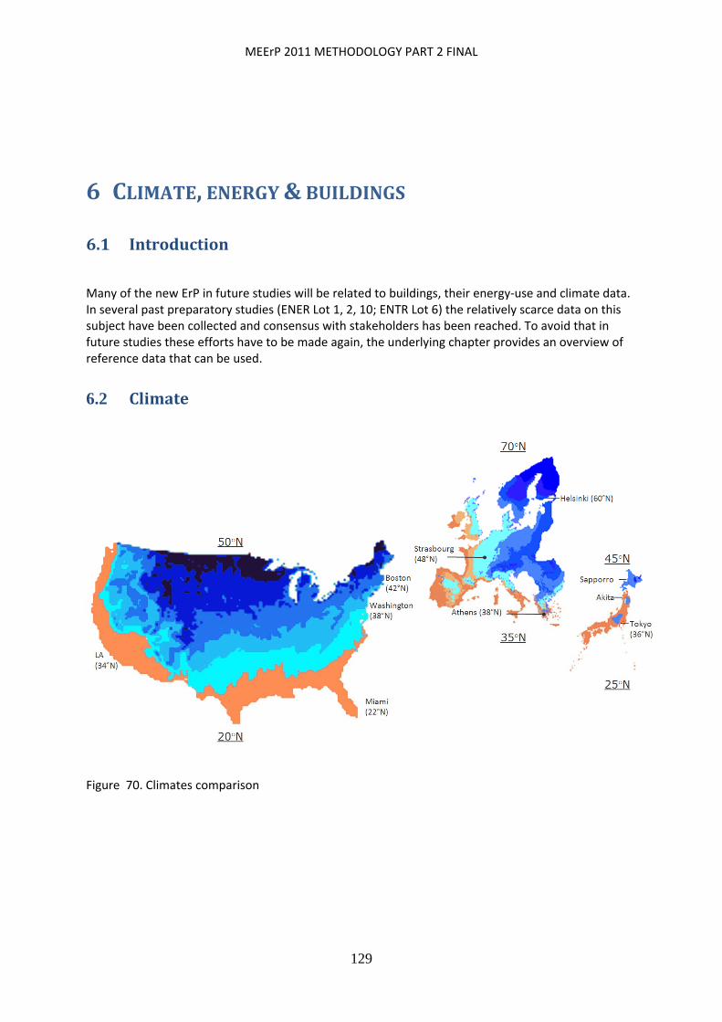
MEErP 2011 METHODOLOGY PART 2 FINAL
129
6 CLIMATE,ENERGY&BUILDINGS
6.1 Introduction
Many of the new ErP in future studies will be related to buildings, their energy‐use and climate data. In several past preparatory studies (ENER Lot 1, 2, 10; ENTR Lot 6) the relatively scarce data on this subject have been collected and consensus with stakeholders has been reached. To avoid that in future studies these efforts have to be made again, the underlying chapter provides an overview of reference data that can be used.
6.2 Climate
Figure 70. Climates comparison
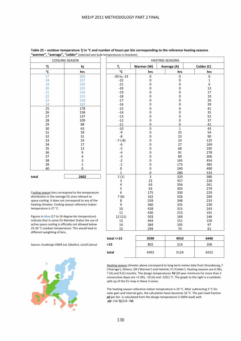
MEErP 2011 METHODOLOGY PART 2 FINAL
130
Table 25 – outdoor temperature Tj in °C and number of hours per bin corresponding to the reference heating seasons “warmer”, “average”, “colder” (selected wet bulb temperatures in brackets)
COOLING SEASON HEATING SEASONS
Tj hj Tj Warmer (W) Average (A) Colder (C)
°C hrs °C hrs hrs hrs
17 205 ‐30 to ‐23 0 0 018 227 ‐22 0 0 119 225 ‐21 0 0 620 225 ‐20 0 0 1321 216 ‐19 0 0 1722 215 ‐18 0 0 1923 218 ‐17 0 0 2624 197 ‐16 0 0 3925 178 ‐15 0 0 4126 158 ‐14 0 0 3527 137 ‐13 0 0 5228 109 ‐12 0 0 3729 88 ‐11 0 0 4130 63 ‐10 0 1 4331 39 ‐9 0 25 5432 31 ‐8 0 23 9033 24 ‐7 (‐8) 0 24 12534 17 ‐6 0 27 16935 13 ‐5 0 68 19536 9 ‐4 0 91 27837 4 ‐3 0 89 30638 3 ‐2 0 165 45439 1 ‐1 0 173 38540 0 0 0 240 490
1 0 280 533total 2602 2 (1) 3 320 380 3 22 357 228
Cooling season bins correspond to the temperature distribution in the average EU area relevant to space cooling. It does not correspond to any of the heating climates. Cooling season reference indoor temperature is 27 °C.
4 63 356 2615 63 303 2796 175 330 229
7 (6) 162 326 2698 259 348 2339 360 335 23010 428 315 24311 430 215 191
Figures in blue (17 to 24 degree bin temperature) indicate that in some EU Member States the use of active space cooling is officially not allowed below 25‐26 °C outdoor temperature. This would lead to different weighting of bins.
12 (11) 503 169 14613 444 151 15014 384 105 9715 294 74 61
total <=15 3590 4910 6446
Source: Ecodesign ENER Lot 1(boiler), Lot10 (airco) >15 802 214 106
total 4392 5124 6552
Heating season climates above correspond to long‐term meteo data from Strassbourg, F ('Average'), Athens, GR ('Warmer') and Helsinki, FI ('Colder'). Heating seasons are 6 (W), 7 (A) and 9 (C) months. The design temperatures Td (20 year minimum for more than 3 consecutive days) are +2 (W), ‐10 (A) and ‐22(C) °C. The graph to the right is a symbolic split up of the EU map in these 3 zones. The heating season reference indoor temperature is 19 °C. After subtracting 3 °C for solar gain and internal gain, the calculation basis becomes 16 °C. The part load fraction plj per bin is calculated from the design temperature (=100% load) with plj= (16‐Tj)/(16 ‐Td)

MEErP 2011 METHODOLOGY PART 2 FINAL
131
Table 26 . Heating energy demand distribution per reference climate (approximation used in solar assisted heating calculations). Source: VHK, Ecodesign preparatory study, for EC DG ENER, Lot 1, Sept. 2007
Jan. Feb. Mar. April May June July Aug. Sept. Oct. Nov. Dec.
Average climate 0.20 0.20 0.13 0.06 0 0 0 0 0 0.06 0.16 0.19
Warmer climate 0.26 0.24 0.18 0.03 0 0 0 0 0 0 0.06 0.23
Colder climate 0.17 0.17 0.14 0.09 0.04 0 0 0 0.03 0.08 0.12 0.16
Td= IF(Lat<40;1;
CHOOSE(TRUNC(1+(Lat‐40)/5);
‐(Lat‐40)*0.2*0.4*Long‐2;
‐(Lat‐45)*0.2*4‐0.4*Long‐2;
‐(Lat‐50)*0.2*2‐4‐0.4*Long‐2;
‐(Lat‐55)*0.2*3‐6‐0.4*Long‐2;
‐(Lat‐60)*0.2*5‐9‐0.4*Long‐2;
‐(Lat‐65)*0.2*6‐14‐0.4*Long‐2))
- 0.01*Alt*1 +G*6 + S*2
where
Td is design temperature;
Lat is latitude in ºN
Long is longitude in ºE
Alt is altitude in m
S is (Y/N=1/0) close to sea (<30 km)
G is (Y/N=1/0) Gulf stream country , i.e. EI, PO, UK
Source: VHK, ABC Method, for EC DG ENER, 2009‐2010. The formula is part of the ABC Method (Assessment Boiler Capacity) and is derived from the building design temperatures in national building codes in several EU Member States (NL, BE, AT, DE, FR, FI, SE, UK, ES, IT, DK).
Note: The calculated design temperature for a specific location can be used as a weighting parameter for the efficiencies calculated for the 3 heating season reference climates: Average (Td=‐10), Warmer (Td=2), Colder (Td=‐22).
The empirical formula covers most of the EU‐27 but accuracy may be diminished for extremes (e.g. above 65 o Latitude and below 40 o Lat.)
The notation follows spreadsheet conventions. The function CHOOSE (TRUNC (1+ (Lat‐40)/5) means that one of the following 6 formulas is selected depending on the truncated value (function TRUNC) of (1+ (Lat‐40)/5).
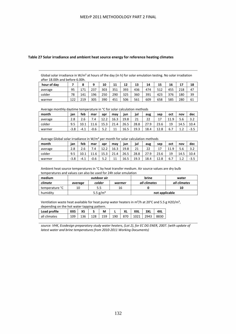
MEErP 2011 METHODOLOGY PART 2 FINAL
132
Table 27 Solar irradiance and ambient heat source energy for reference heating climates
Global solar irradiance in W/m² at hours of the day (in h) for solar emulation testing. No solar irradiation after 18.00h and before 6.00h.
hour of day 7 8 9 10 11 12 13 14 15 16 17 18
average 95 171 237 303 351 393 436 474 512 455 218 47
colder 78 141 196 250 290 325 360 391 423 376 180 39
warmer 122 219 305 390 451 506 561 609 658 585 280 61
Average monthly daytime temperature in °C for solar calculation methods
month jan feb mar apr may jun jul aug sep oct nov dec
average 2.8 2.6 7.4 12.2 16.3 19.8 21 22 17 11.9 5.6 3.2
colder 9.5 10.1 11.6 15.3 21.4 26.5 28.8 27.9 23.6 19 14.5 10.4
warmer ‐3.8 ‐4.1 ‐0.6 5.2 11 16.5 19.3 18.4 12.8 6.7 1.2 ‐3.5
Average Global solar irradiance in W/m² per month for solar calculation methods
month jan feb mar apr may jun jul aug sep oct nov dec
average 2.8 2.6 7.4 12.2 16.3 19.8 21 22 17 11.9 5.6 3.2
colder 9.5 10.1 11.6 15.3 21.4 26.5 28.8 27.9 23.6 19 14.5 10.4
warmer ‐3.8 ‐4.1 ‐0.6 5.2 11 16.5 19.3 18.4 12.8 6.7 1.2 ‐3.5
Ambient heat source temperatures in °C by heat transfer medium. Air source values are dry bulb temperatures and values can also be used for 24h solar emulation
medium outdoor air brine water
climate average colder warmer all climates all climates
temperature °C 10 5.5 16 0 10
humidity 5.5 g/m³ not applicable
Ventilation waste heat available for heat pump water heaters in m³/h at 20°C and 5.5 g H2O/m³, depending on the hot water tapping pattern.
Load profile XXS XS S M L XL XXL 3XL 4XL
all climates 109 136 128 159 190 870 1021 2943 8830
source: VHK, Ecodesign preparatory study water heaters, (Lot 2), for EC DG ENER, 2007. (with update of latest water and brine temperatures from 2010‐2011 Working Documents)

MEErP 2011 METHODOLOGY PART 2 FINAL
133
Notes:
[1] Test periods >48 h may apply to appliances to test cycles where a thermal equilibrium and/or repetability must be reached. Test periods <48 h apply to space heating applications of all products and water heating applications of conventional products. Test period <1 h applies to the simplified test procedures for appliances
[2] Test gases as in the essential requirements of the Gas Appliances Directive 90/396/EEC with amendments as in 93/68/EC
[3] A factor K has to be applied to correct the calorific value for the actual average atmospheric absolute pressure pa and gas gauge pressure pg as well as the average gas temperature Tg over the test period. K = (pa + pg)/1013.25 x 288.15/(273.15+Tg)
[4] In case of low Sulfur test fuels, N‐fractions lower than 70 mg/kg and lower S fractions are allowed. Note that Sulfur content should be updated. Currently <0.1 %.
[5] Default value, if value is not determined calorimetrically. Also other values are defaults. Alternatively, if volumetric mass and sulphur content are known (e.g. by basic analysis) the net heating value (Hi) may be determined with Hi =
52.92 ‐ (11.93 ρ15 )‐ (0.3 ‐ S) in MJ/kg
[6] Calculated from net calorific value with multiplier GCV=1.067 NCV
Table 28 . Electricity and Fossil Fuels
Measured quantity Unit Value Permissible deviation (average over test period)
Uncertainty of measurement (accuracy)
Notes
Electricity
power W ± 1 %
energy kWh ± 1 %
voltage, test‐period > 48 h V 230/ 400 ± 4 % ± 0.5 % [1]
voltage, test‐period < 48h V 230/ 400 ± 2 %
voltage, test‐period < 1 h V 230/ 400 ± 1 % ± 0.2 %
electric current A ± 0.5 %
frequency Hz 50 ± 1 %
Gas
types ‐ Test gases GAD [2]
net calorific value (NCV) MJ/ m³ Test gases GAD ± 1 % [3]
temperature K 288.15 ± 0.5 [3]
pressure mbar 1013.25 ± 1 % [3]
density dm³/kg ± 0.5 %
flow rate m³/s or l/min
± 1 %
Oil
Heating gas oil
composition, Carbon/ Hydrogen/ Sulfur kg/kg 86/13.6/ 0.2 %
N‐fraction mg/kg 140 ± 70 [4]
net calorific value (NCV, Hi) MJ/kg 42.689 [5]
gross calorific value (GCV, Hs) MJ/kg 45.55 [6]
density ρ15 at 15 °C: kg/dm³ 0.85
Kerosene
composition, Carbon/ Hydrogen/ Sulfur kg/kg 85/ 14.1/ 0.4 %
N‐fraction mg/kg 140 ± 70 [4]
net calorific value (NCV, Hi) MJ/kg 43.3 [5]
gross calorific value (CGV, Hs) MJ/kg 46.2 [6]
density ρ15 at 15 °C: kg/dm³ 0.79
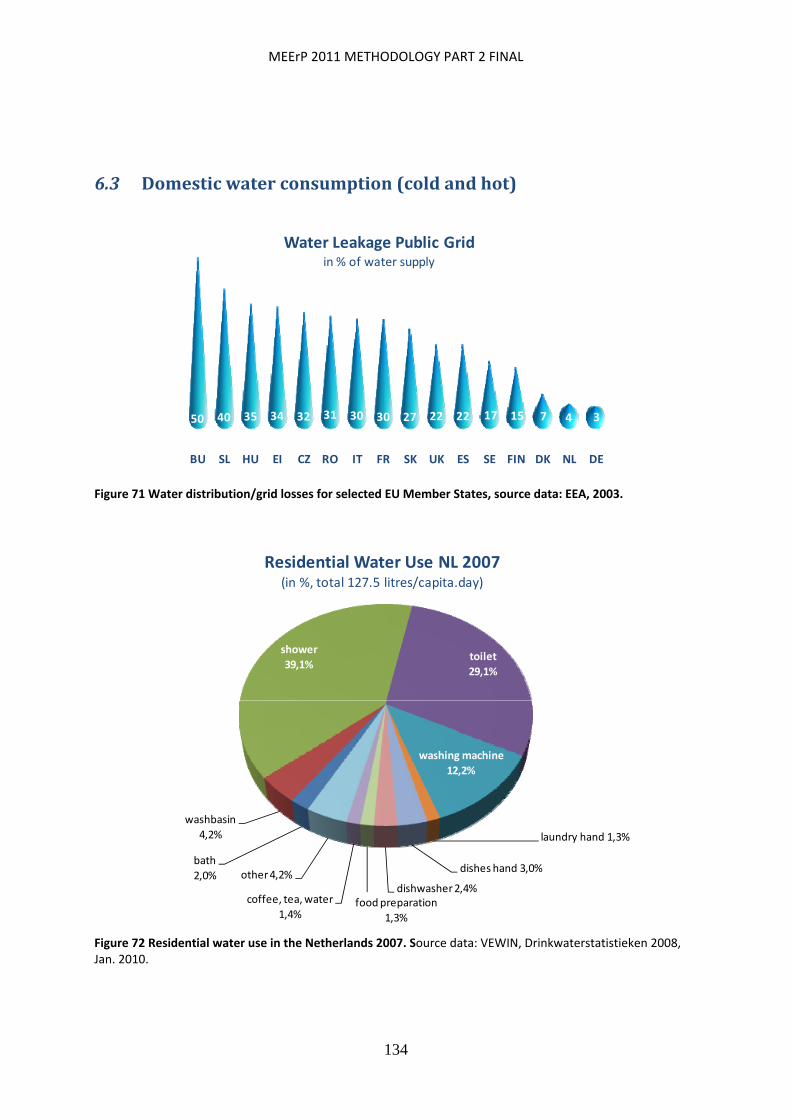
MEErP 2011 METHODOLOGY PART 2 FINAL
134
6.3 Domesticwaterconsumption(coldandhot)
BU SL HU EI CZ RO IT FR SK UK ES SE FIN DK NL DE
50 40 35 34 32 31 30 30 27 22 22 17 15 7 4 3
Water Leakage Public Gridin % of water supply
Figure 71 Water distribution/grid losses for selected EU Member States, source data: EEA, 2003.
bath
2,0%
washbasin
4,2%
shower
39,1%toilet
29,1%
washing machine
12,2%
laundry hand 1,3%
dishes hand 3,0%
dishwasher 2,4%food preparation
1,3%
coffee, tea, water
1,4%
other 4,2%
Residential Water Use NL 2007 (in %, total 127.5 litres/capita.day)
Figure 72 Residential water use in the Netherlands 2007. Source data: VEWIN, Drinkwaterstatistieken 2008, Jan. 2010.
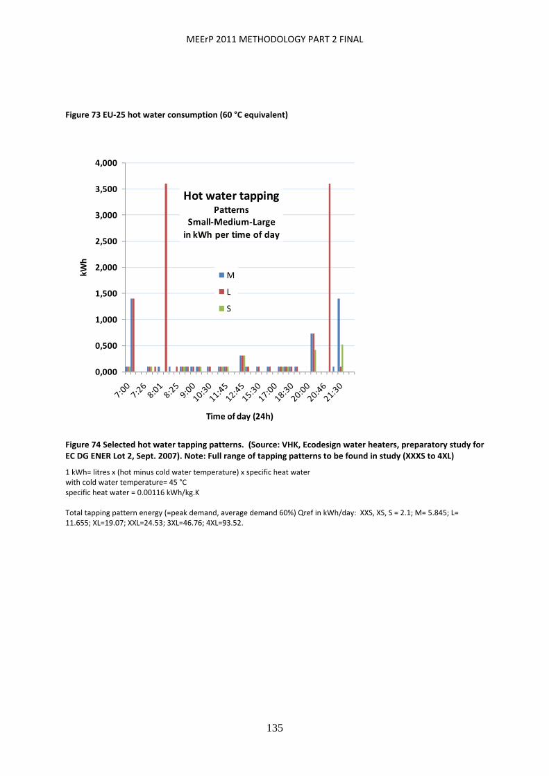
MEErP 2011 METHODOLOGY PART 2 FINAL
135
Figure 73 EU‐25 hot water consumption (60 °C equivalent)
0,000
0,500
1,000
1,500
2,000
2,500
3,000
3,500
4,000
kWh
Time of day (24h)
Hot water tappingPatterns
Small‐Medium‐Large
in kWh per time of day
M
L
S
Figure 74 Selected hot water tapping patterns. (Source: VHK, Ecodesign water heaters, preparatory study for EC DG ENER Lot 2, Sept. 2007). Note: Full range of tapping patterns to be found in study (XXXS to 4XL)
1 kWh= litres x (hot minus cold water temperature) x specific heat water with cold water temperature= 45 °C specific heat water = 0.00116 kWh/kg.K Total tapping pattern energy (=peak demand, average demand 60%) Qref in kWh/day: XXS, XS, S = 2.1; M= 5.845; L= 11.655; XL=19.07; XXL=24.53; 3XL=46.76; 4XL=93.52.
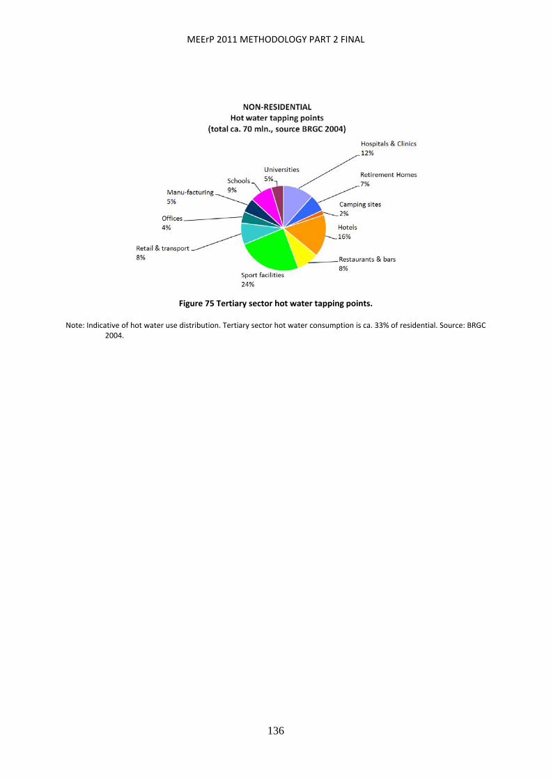
MEErP 2011 METHODOLOGY PART 2 FINAL
136
Figure 75 Tertiary sector hot water tapping points.
Note: Indicative of hot water use distribution. Tertiary sector hot water consumption is ca. 33% of residential. Source: BRGC 2004.
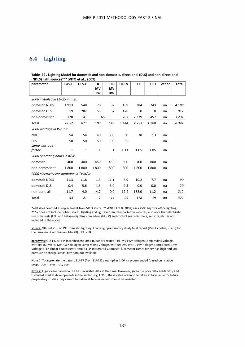
MEErP 2011 METHODOLOGY PART 2 FINAL
137
6.4 Lighting
Table 29 . Lighting Model for domestic and non‐domestic, directional (DLS) and non‐directional (NDLS) light sources***(VITO et al., 2009)
parameter GLS‐F GLS‐C HL‐MV LW
HL‐MV HW
HL‐LV LFL CFLi other Total
2006 installed in EU‐25 in mln.
domestic NDLS 1 913 548 70 82 459 384 743 na 4 199
domestic DLS 19 282 58 67 478 0 8 na 912
non‐domestic* 120 41 65 207 2 339 457 na 3 231
Total 2 052 871 193 149 1 144 2 723 1 208 na 8 342
2006 wattage in W/unit
NDLS 54 54 40 300 30 38 13 na
DLS 50 50 50 100 35 na Lamp wattage factor 1 1 1 1 1.11 1.05 1.05 na
2006 operating hours in h/yr
domestic 400 400 450 450 500 700 800 na
non‐domestic** 1 800 1 800 1 800 1 800 1 800 1 800 1 800 na
2006 electricity consumption in TWh/yr
domestic NDLS 41.3 11.8 1.3 11.1 6.9 10.2 7.7 na 90
domestic DLS 0.4 5.6 1.3 3.0 9.3 0.0 0.0 na 20
non‐dom. all 11.7 4.0 4.7 0.0 12.4 168.0 11.2 na 212
Total 53 21 7 14 29 178 19 na 322
*=all sales counted as replacement from VITO study.; **=ENER Lot 8 (2007) uses 2500 h/yr for office lighting; ***= does not include public (street) lighting and light bulbs in transportation vehicles; also note that electricity use of ballasts (LFL) and halogen lighting converters (HL‐LV) and control gear (dimmers, sensors, etc.) is not included in the above.
source: VITO et al., Lot 19: Domestic Lighting, Ecodesign preparatory study final report (Van Tichelen, P. ed.) for the European Commission, Mol (B), Oct. 2009.
acronyms: GLS (‐C or ‐F)= incandescent lamp (Clear or Frosted); HL‐MV LW= Halogen Lamp Mains Voltage, wattage<80 W; HL‐MV HW= Halogen Lamp Mains Voltage, wattage ≥80 W; HL‐LV= Halogen Lamps extra Low Voltage; LFL= Linear Fluorescent Lamp; CFLi= integrated Compact Fluorescent Lamp; other= e.g. high and low pressure discharge lamps; na= data not available
Note 1: To aggregate the data to EU‐27 (from EU‐25) a multiplier 1.06 is recommended (based on relative proportion in electricity use)
Note 2: Figures are based on the best available data at the time. However, given the poor data availability and turbulent market developments in the sector (e.g. LEDs), these values cannot be taken at face value for future preparatory studies they cannot be taken at face value and should be revisited.
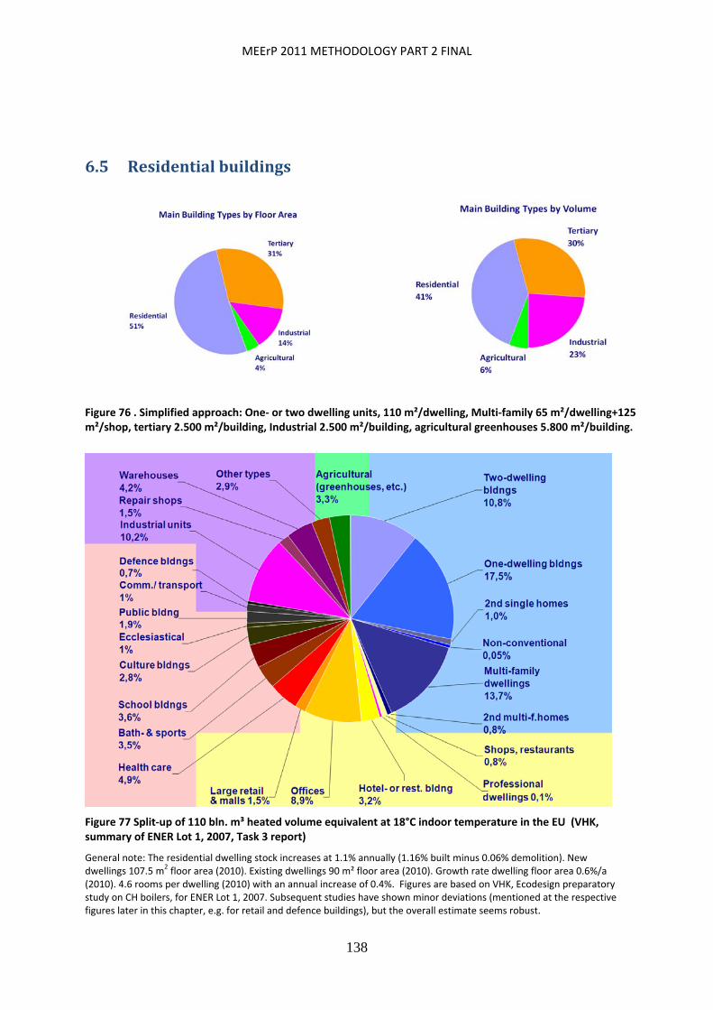
MEErP 2011 METHODOLOGY PART 2 FINAL
138
6.5 Residentialbuildings
Figure 77 Split‐up of 110 bln. m³ heated volume equivalent at 18°C indoor temperature in the EU (VHK, summary of ENER Lot 1, 2007, Task 3 report)
General note: The residential dwelling stock increases at 1.1% annually (1.16% built minus 0.06% demolition). New dwellings 107.5 m2 floor area (2010). Existing dwellings 90 m² floor area (2010). Growth rate dwelling floor area 0.6%/a (2010). 4.6 rooms per dwelling (2010) with an annual increase of 0.4%. Figures are based on VHK, Ecodesign preparatory study on CH boilers, for ENER Lot 1, 2007. Subsequent studies have shown minor deviations (mentioned at the respective figures later in this chapter, e.g. for retail and defence buildings), but the overall estimate seems robust.
Figure 76 . Simplified approach: One‐ or two dwelling units, 110 m²/dwelling, Multi‐family 65 m²/dwelling+125 m²/shop, tertiary 2.500 m²/building, Industrial 2.500 m²/building, agricultural greenhouses 5.800 m²/building.
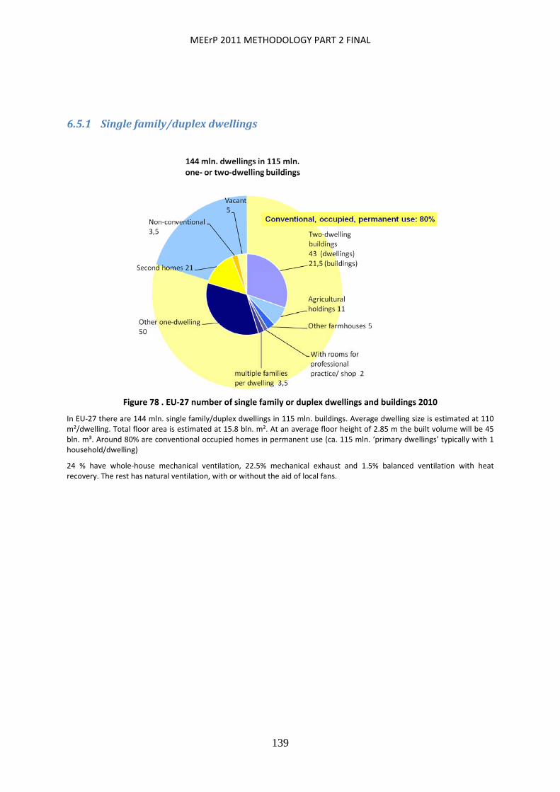
MEErP 2011 METHODOLOGY PART 2 FINAL
139
6.5.1 Singlefamily/duplexdwellings
Figure 78 . EU‐27 number of single family or duplex dwellings and buildings 2010
In EU‐27 there are 144 mln. single family/duplex dwellings in 115 mln. buildings. Average dwelling size is estimated at 110 m²/dwelling. Total floor area is estimated at 15.8 bln. m². At an average floor height of 2.85 m the built volume will be 45 bln. m³. Around 80% are conventional occupied homes in permanent use (ca. 115 mln. ‘primary dwellings’ typically with 1 household/dwelling)
24 % have whole‐house mechanical ventilation, 22.5% mechanical exhaust and 1.5% balanced ventilation with heat recovery. The rest has natural ventilation, with or without the aid of local fans.
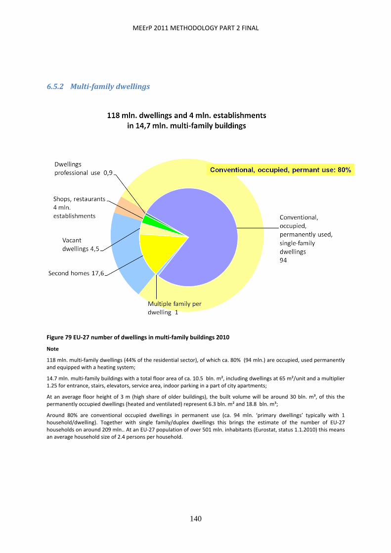
MEErP 2011 METHODOLOGY PART 2 FINAL
140
6.5.2 Multi‐familydwellings
Figure 79 EU‐27 number of dwellings in multi‐family buildings 2010
Note
118 mln. multi‐family dwellings (44% of the residential sector), of which ca. 80% (94 mln.) are occupied, used permanently and equipped with a heating system;
14.7 mln. multi‐family buildings with a total floor area of ca. 10.5 bln. m², including dwellings at 65 m²/unit and a multiplier 1.25 for entrance, stairs, elevators, service area, indoor parking in a part of city apartments;
At an average floor height of 3 m (high share of older buildings), the built volume will be around 30 bln. m³, of this the permanently occupied dwellings (heated and ventilated) represent 6.3 bln. m² and 18.8 bln. m³;
Around 80% are conventional occupied dwellings in permanent use (ca. 94 mln. ‘primary dwellings’ typically with 1 household/dwelling). Together with single family/duplex dwellings this brings the estimate of the number of EU‐27 households on around 209 mln.. At an EU‐27 population of over 501 mln. inhabitants (Eurostat, status 1.1.2010) this means an average household size of 2.4 persons per household.
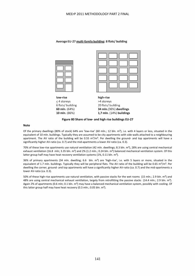
MEErP 2011 METHODOLOGY PART 2 FINAL
141
Figure 80 Share of low‐ and high rise buildings EU‐27
Note
Of the primary dwellings (80% of stock) 64% are ‘low‐rise’ (60 mln.; 12 bln. m³), i.e. with 4 layers or less, situated in the equivalent of 10 mln. buildings. Typically they are assumed to be city apartments with side‐walls attached to a neighbouring apartment. The AV ratio of the building will be 0.55 m²/m³. Per dwelling the ground‐ and top apartments will have a significantly higher AV‐ratio (ca. 0.7) and the mid‐apartments a lower AV‐ratio (ca. 0.3).
70% of these low‐rise apartments use natural ventilation (42 mln. dwellings; 8.3 bln. m³), 28% are using central mechanical exhaust ventilation (16.8 mln; 3.35 bln. m³) and 2% (1.2 mln.; 0.24 bln. m³) balanced mechanical ventilation system. Of this latter group half may have heat recovery ventilation systems (1%, 0.11 bln. m³).
36% of primary apartments (34 mln. dwelling; 6.6 bln. m³) are ‘high‐rise’, i.e. with 5 layers or more, situated in the equivalent of 1.7 mln. buildings. Typically they will be peripheral flats. The AV ratio of the building will be 0.65 m²/m³. Per dwelling the corner, ground‐ and top apartments will have a significantly higher AV‐ratio (ca. 0.7) and the mid‐apartments a lower AV‐ratio (ca. 0.3).
50% of these high‐rise apartments use natural ventilation, with passive stacks for the wet rooms (15 mln.; 2.9 bln. m³) and 48% are using central mechanical exhaust ventilation, largely from retrofitting the passive stacks (14.4 mln.; 2.9 bln. m³). Again 2% of apartments (0.6 mln; 0.1 bln. m³) may have a balanced mechanical ventilation system, possibly with cooling. Of this latter group half may have heat recovery (0.3 mln.; 0.05 bln. m³).
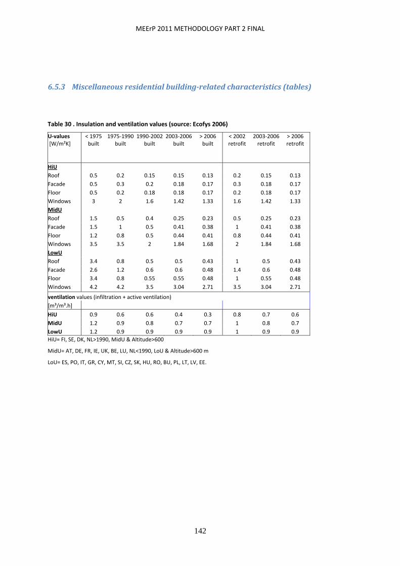
MEErP 2011 METHODOLOGY PART 2 FINAL
142
6.5.3 Miscellaneousresidentialbuilding‐relatedcharacteristics(tables)
Table 30 . Insulation and ventilation values (source: Ecofys 2006)
U‐values [W/m²K]
< 1975 built
1975‐1990 built
1990‐2002 built
2003‐2006built
> 2006 built
< 2002 retrofit
2003‐2006retrofit
> 2006 retrofit
HiU
Roof 0.5 0.2 0.15 0.15 0.13 0.2 0.15 0.13
Facade 0.5 0.3 0.2 0.18 0.17 0.3 0.18 0.17
Floor 0.5 0.2 0.18 0.18 0.17 0.2 0.18 0.17
Windows 3 2 1.6 1.42 1.33 1.6 1.42 1.33
MidU
Roof 1.5 0.5 0.4 0.25 0.23 0.5 0.25 0.23
Facade 1.5 1 0.5 0.41 0.38 1 0.41 0.38
Floor 1.2 0.8 0.5 0.44 0.41 0.8 0.44 0.41
Windows 3.5 3.5 2 1.84 1.68 2 1.84 1.68
LowU
Roof 3.4 0.8 0.5 0.5 0.43 1 0.5 0.43
Facade 2.6 1.2 0.6 0.6 0.48 1.4 0.6 0.48
Floor 3.4 0.8 0.55 0.55 0.48 1 0.55 0.48
Windows 4.2 4.2 3.5 3.04 2.71 3.5 3.04 2.71
ventilation values (infiltration + active ventilation)
[m³/m³.h]
HiU 0.9 0.6 0.6 0.4 0.3 0.8 0.7 0.6
MidU 1.2 0.9 0.8 0.7 0.7 1 0.8 0.7
LowU 1.2 0.9 0.9 0.9 0.9 1 0.9 0.9
HiU= FI, SE, DK, NL>1990, MidU & Altitude>600
MidU= AT, DE, FR, IE, UK, BE, LU, NL<1990, LoU & Altitude>600 m
LoU= ES, PO, IT, GR, CY, MT, SI, CZ, SK, HU, RO, BU, PL, LT, LV, EE.
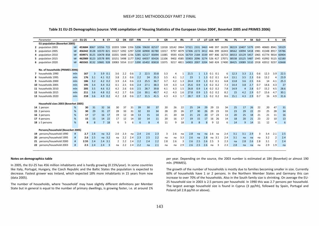
MEErP 2011 METHODOLOGY PART 2 FINAL
143
Table 31 EU‐25 Demographics (source: VHK compilation of 'Housing Statistics of the European Union 2004', Boverket 2005 and PRIMES 2006)
Parameter unit EU‐25 A B CY CZ DK EST FIN F D GR H IRL IT LT LIT LUX MT NL PL P SK SLO E S UK
EU population (Boverket 2005)
2 population 2003 k# 453684 8067 10356 715 10203 5384 1356 5206 59630 82537 11018 10142 3964 57321 2331 3463 448 397 16193 38219 10407 5379 1995 40683 8941 59329
3 population 2005 k# 456342 8128 10370 821 10227 5392 1297 5230 60900 82780 11017 9797 4079 57306 2272 3412 466 399 16343 38562 10094 5418 1981 41348 8917 59786
4 population 2010 k# 459971 8125 10478 858 10201 5449 1236 5285 62527 83094 11085 9593 4326 56759 2184 3339 497 406 16733 38553 10129 5457 1965 41774 9014 60904
5 population 2015 k# 462989 8123 10578 895 10151 5498 1177 5342 64037 83426 11106 9402 4585 55903 2096 3274 526 417 17071 38538 10125 5487 1945 41992 9115 62180
6 population 2020 k# 465565 8132 10681 928 10083 5554 1117 5390 65402 83818 11075 9217 4811 54903 2007 3204 560 424 17400 38425 10089 5510 1918 42012 9237 63668
No. of households (PRIMES 2006)
7 households 1990 mln 167 3 3.9 0.1 3.6 2.2 0.6 2 22.5 33.8 3.3 4 1 21.5 1 1.3 0.1 0.1 6 12.3 3.3 2.1 0.6 12.3 3.9 22.5
8 households 1995 mln 176 3.1 4.1 0.2 3.8 2.3 0.6 2.2 24 35.3 3.5 4.1 1.2 23 1 1.3 0.2 0.1 6.4 13.1 3.5 2.3 0.6 13.2 4 23.9
9 households 2000 mln 186 3.2 4.2 0.2 3.9 2.4 0.6 2.3 25.5 36.7 3.7 4.2 1.3 24.4 0.9 1.3 0.2 0.1 6.8 13.8 3.6 2.5 0.6 14 4.1 25.3
10 households 2005 mln 195 3.4 4.4 0.2 4.1 2.5 0.6 2.4 27.1 38.3 3.9 4.3 1.4 25.6 0.9 1.4 0.2 0.2 7.3 14.4 3.8 2.7 0.7 14.6 4.3 27
11 households 2010 mln 205 3.5 4.6 0.2 4.2 2.6 0.6 2.5 28.7 39.8 4.1 4.3 1.5 26.8 0.9 1.4 0.2 0.2 7.8 14.9 4 2.8 0.7 15.2 4.5 28.6
12 households 2015 mln 211 3.6 4.8 0.2 4.2 2.7 0.6 2.6 30.1 40.7 4.2 4.3 1.6 27.8 0.9 1.5 0.2 0.2 8.2 15 4.2 2.9 0.7 15.6 4.7 30.1
13 households 2020 mln 218 3.6 4.9 0.2 4.2 2.8 0.6 2.7 31.5 41.5 4.3 4.3 1.7 28.7 0.9 1.5 0.2 0.2 8.6 15.1 4.3 2.9 0.7 16 4.9 31.6
Household sizes 2003 (Boverket 2005)
14 1 person % 30 31 32 16 30 37 31 39 30 37 20 26 22 25 24 29 29 15 34 25 17 26 22 20 47 31
15 2 persons % 30 29 31 27 28 33 31 32 33 34 28 29 26 27 30 26 29 23 33 23 29 22 23 25 28 34
16 3 persons % 17 17 16 17 19 12 18 13 15 14 21 20 18 21 23 20 17 23 13 20 25 18 21 21 11 16
17 4 persons % 15 15 14 22 17 12 14 10 14 11 20 16 17 19 15 17 16 26 14 18 20 21 23 22 10 13
18 ≥ 5 persons % 8 8 7 18 6 5 6 6 8 4 11 9 18 8 8 8 9 12 6 14 9 14 11 12 4 6
Persons/household (Boverket 2005)
19 persons/household 1990 # 2.7 2.6 na 3.2 2.6 2.3 na 2.4 2.6 2.3 3 2.6 na 2.8 na na 2.6 na 2.4 3.1 3.1 2.9 3 3.4 2.1 2.5
20 persons/household 1995 # 2.6 2.5 na 3.2 na 2.2 2.4 2.3 2.5 2.2 na na 3.3 2.6 na 2.8 na 3.1 2.4 3.1 na na na 3.2 2 2.4
21 persons/household 2000 # 2.55 2.4 2.4 3.1 2 2.2 2.4 2.2 2.4 2.2 2.8 2.6 3 2.6 2.5 2.6 2.5 3 2.3 na 2.8 2.6 2.8 3.1 2 2.4
22 persons/household 2003 # 2.5 2.4 2.4 3 na 2.2 2.4 2.2 na 2.1 na na 2.9 2.6 2.5 2.6 na 3 2.3 2.8 na na na 2.9 1.9 na
Notes on demographics table
In 2005, the EU‐25 has 456 million inhabitants and is hardly growing (0.15%/year). In some countries like Italy, Portugal, Hungary, the Czech Republic and the Baltic States the population is expected to decrease. Fastest grower was Ireland, which expected 18% more inhabitants in 15 years from now (data 2005).
The number of households, where ‘household’ may have slightly different definitions per Member State but in general is equal to the number of primary dwellings, is growing faster, i.e. at around 1%
per year. Depending on the source, the 2003 number is estimated at 184 (Boverket) or almost 190 mln. (PRIMES).
The growth of the number of households is mostly due to families becoming smaller in size. Currently 60% of households have 1 or 2 persons. In the Northern Member States and Germany this can increase to over 70% of the households. Also in the South family size is shrinking. On average the EU‐25 household size in 2003 is 2.5 persons per household. In 1990 this was 2.7 persons per household. The largest average household size is found in Cyprus (3 pp/hh), followed by Spain, Portugal and Poland (all 2.8 pp/hh or above).
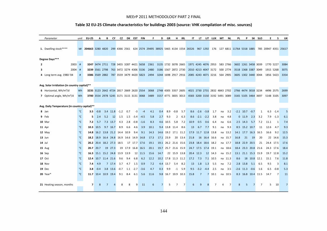
MEErP 2011 METHODOLOGY PART 2 FINAL
144
Table 32 EU‐25 Climate characteristics for buildings 2003 (source: VHK compilation of misc. sources)
Parameter unit EU‐25 A B CY CZ DK EST FIN F D GR H IRL IT LT LIT LUX MT NL PL P SK SLO E S UK
1. Dwelling stock**** k# 204663 3280 4820 299 4366 2561 624 2574 29495 38925 5465 4134 1554 26526 967 1292 176 127 6811 11764 5318 1885 785 20947 4351 25617
Degree Days***
2 2003 # 3247 3474 2711 728 3455 3287 4421 5658 2361 3135 1732 3078 2665 1971 4245 4076 2953 583 2766 3602 1261 3458 3039 1770 5227 3084
3 2004 # 3239 3561 2798 763 3472 3274 4306 5536 2480 3186 1567 2872 2730 2010 4213 4047 3172 500 2774 3518 1368 3387 3049 1915 5268 3075
4 Long term avg. 1980‐'04 # 3386 3569 2882 787 3559 3479 4420 5823 2494 3244 1698 2917 2916 2085 4243 4071 3216 564 2905 3605 1302 3440 3044 1856 5423 3354
Avg. Solar Irridiation (in country capital)**
6 Horizontal, Wh/m²/d Wh 3235 3123 2642 4724 2817 2669 2620 2554 3068 2748 4305 3357 2605 4021 2730 2731 2832 4843 2702 2766 4474 3018 3234 4496 2575 2699
7 Optimal angle, Wh/m²/d Wh 3700 3554 2978 5245 3171 3115 3131 3068 3489 3157 4771 3835 3013 4583 3200 3150 3192 5491 3089 3165 5105 3464 3697 5148 3105 3097
Avg. Daily Temperature (in country capital)**
8 Jan °C 3.5 ‐0.8 3.4 11.8 ‐1.2 0.7 ‐3 ‐4 4.1 0.4 8.9 ‐0.8 5.7 8.6 ‐2.6 ‐3.8 1.7 na 3.2 ‐2.1 10.7 ‐0.7 1 6.3 ‐1.4 5
9 Feb °C 5 2.4 5.2 12 1.5 1.5 ‐3.4 ‐4.5 5.8 2.7 9.3 2 6.3 8.6 ‐2.1 ‐2.2 3.8 na 4.8 0 11.9 2.3 3.2 7.9 ‐1.3 6.1
10 Mar °C 7.2 5.7 7.3 13.7 4.3 2.8 ‐0.8 ‐1.6 8.3 4.6 10.5 5.8 7.2 10.9 0.5 0.6 6.4 na 6.6 2.5 14.3 5.7 7.2 11.1 1 7.4
11 Apr °C 10.3 10.5 9.7 16.7 8.9 6.6 4.6 3.9 10.1 9.4 13.8 11.4 8.6 13 6.7 7.7 9.1 na 9.3 8.5 15.2 10.7 11 12.6 4.7 9.3
12 May °C 14.8 16.2 13.8 21.2 14.4 10.9 9.4 9.1 14.3 14.6 19.2 17.1 11.2 17.9 11.7 12.8 13.8 na 13.2 14.1 17.7 16.3 16.5 16.6 9.2 12.5
13 Jun °C 18.2 18.9 16.4 24.8 16.9 14.6 14.9 14.8 17.3 17.1 23.9 20 13.4 21.8 16 16.4 16.6 na 15.7 16.8 21 19 20 22 14.6 15.3
14 Jul °C 20.2 20.4 18.2 27.3 18.5 17 17.7 17.6 19.1 19.1 26.2 21.6 15.6 23.8 18.4 18.6 18.2 na 17.7 18.8 22.9 20.5 21 24.4 17.5 17.6
15 Aug °C 20.7 20.7 19 27.3 19 17.9 16.8 16.5 20.1 19.7 25.7 21.6 15.9 24.7 17.5 17.4 19.1 na 18.6 18.4 23.3 20.8 21.6 24.3 17.6 18.4
16 Sep °C 16.3 15.1 15.2 24.8 13.9 13.9 12 11.5 15.6 14.7 22 15.9 13.8 20.4 12.3 12 14.3 na 15.2 13.1 21.1 15.3 15.9 19.7 12.8 15.2
17 Oct °C 12.4 10.7 11.4 21.6 9.6 9.4 6.8 6.2 12.2 10.2 17.8 11.3 11.2 17.2 7.3 7.1 10.5 na 11.3 8.6 18 10.8 12.1 15.1 7.6 11.8
18 Nov °C 7.4 4.9 7 17.4 3.7 4.7 1.5 0.9 7.2 4.4 13.7 5.4 8.2 13 1.8 1.3 5.5 na 7.2 2.8 13.8 5.1 6.5 9.5 3 8.1
19 Dec °C 3.8 ‐0.4 3.8 13.6 ‐0.7 1.1 ‐2.7 ‐3.6 4.7 0.3 9.9 ‐1 5.9 9.5 ‐3.2 ‐4.4 2.5 na 3.5 ‐2.6 11.3 ‐0.6 1.6 6.5 ‐0.8 5.3
20 Year* °C 11.7 10.4 10.9 19.4 9.1 8.4 6.1 5.6 11.6 9.8 16.7 10.9 10.3 15.8 7 7 10.1 na 10.5 8.3 16.8 10.4 11.5 14.7 7 11
21 Heating season, months 7 8 7 4 8 8 9 11 6 7 5 7 7 6 9 8 7 4 7 8 5 7 7 5 10 7
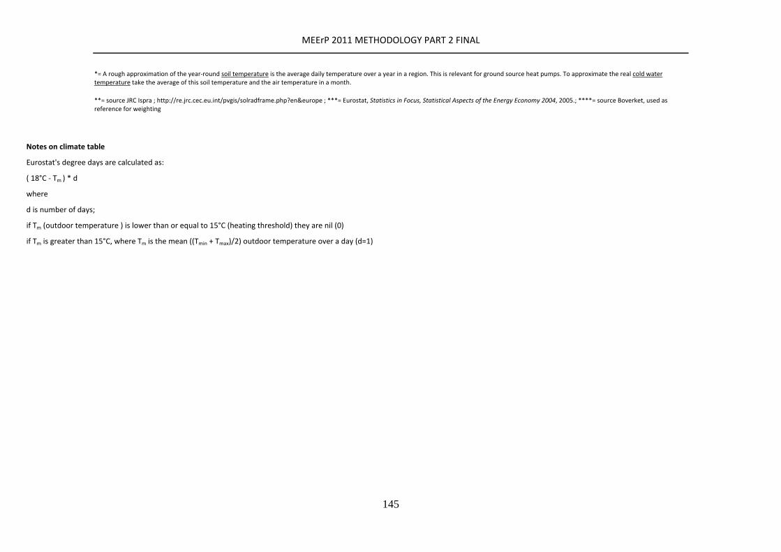
MEErP 2011 METHODOLOGY PART 2 FINAL
145
*= A rough approximation of the year‐round soil temperature is the average daily temperature over a year in a region. This is relevant for ground source heat pumps. To approximate the real cold water temperature take the average of this soil temperature and the air temperature in a month.
**= source JRC Ispra ; http://re.jrc.cec.eu.int/pvgis/solradframe.php?en&europe ; ***= Eurostat, Statistics in Focus, Statistical Aspects of the Energy Economy 2004, 2005.; ****= source Boverket, used as reference for weighting
Notes on climate table
Eurostat's degree days are calculated as:
( 18°C ‐ Tm ) * d
where
d is number of days;
if Tm (outdoor temperature ) is lower than or equal to 15°C (heating threshold) they are nil (0)
if Tm is greater than 15°C, where Tm is the mean ((Tmin + Tmax)/2) outdoor temperature over a day (d=1)

MEErP 2011 METHODOLOGY PART 2 FINAL
146
Table 33 EU‐25 Housing Characteristics 2003 (source: VHK compilation of 'Housing Statistics of the European Union 2004', Boverket 2005)
Parameter unit EU‐25 A B CY CZ DK EST FIN F D GR H IRL IT LT LIT LUX MT NL PL P SK SLO E S UK
1. Dwelling stock** k# 204663 3280 4820 299 4366 2561 624 2574 29495 38925 5465 4134 1554 26526 967 1292 176 127 6811 11764 5318 1885 785 20947 4351 25617
2 Primary (= ca. # households) k# 184166 3280 4325 239 4216 2481 566 2378 24525 38944 3674 3863 1382 22004 915 1346 171 129 6996 13337 3651 2072 685 14187 4454 24346
3 Secondary k# 20497 0 495 60 150 80 58 196 4970 ‐19 1791 271 172 4522 52 ‐54 5 ‐2 ‐185 ‐1573 1667 ‐187 100 6760 ‐103 1271
4 Secondary types, included in dwelling stock*
WSV WSC WS SVN V na SVN WSH S WSV WSV WSm WSV WV CN CHM WSN V‐ SCH WS V WSV WS CV WSV
VN CV MV VN MVN VN VN
5 Vacant dwellings k# 18083 na 72 537 128 68 237 2006 3192 514 347 182 5199 58 48 4 na 150 623 564 219 79 2912 74 871
6 One/two family dwellings % 54 48 75 na 44 61 32 42 57 46 59 66 91 25 29 39 71 na 69 37 77 49 72 53 48 81
7 Multi‐family dwellings % 46 52 25 na 57 39 68 58 43 54 41 34 9 75 71 61 29 na 31 63 23 52 28 48 52 19
8 of which high‐rise (> 4 % 16 na 4 na 34 10 na na 16 6 na 23 na 23 na na 16 na 7 39 22 38 12 31 na 2
9 New built 2003 (completed) k# 2174 42 41 6 27 24 2 28 334 268 128 22 69 178 1 5 2 na 60 163 82 14 7 459 24 190
10 New built 1990 (completed) k# 2169 42 43 8 45 27 8 65 336 319 120 44 20 176 13 22 3 na 101 134 66 25 8 281 58 205
11 Demolished/removed k# 133 16 2 0 2 8 1 3 21 22 na 5 11 na 3 0 na na 18 5 1 1 0 16 2 15
12 Year of built <1919 [VHK 1880] % 15 19 15 na 11 20 9 2 20 15 3 14 10 19 11 6 12 15 7 10 6 3 15 9 12 21
13 Year of built 1919–1945 % 12 8 17 7 15 17 14 9 13 13 7 13 8 11 14 23 15 11 13 13 9 7 8 4 20 18
14 Year of built 1946–1970 % 32 27 29 17 26 28 30 31 18 47 32 26 16 41 28 33 27 29 31 27 23 35 28 34 33 21
15 Year of built 1971–1980 % 20 16 15 21 23 18 22 23 26 11 25 22 18 20 23 18 15 17 19 18 18 26 24 24 17 22
16 Year of built >1980 % 22 12 9 27 16 10 20 20 10 15 19 18 16 10 21 14 12 16 30 19 44 21 16 14 10 19
17 of which, year of built >1990 % 13 18 15 | 8 7 5 14 12 | 14 7 32 | 4 6 17 12 | 13 | 7 9 16 7 |
18 Avg. age dwellings [VHK est.] yr 49 49 50 28 46 57 45 33 52 53 35 48 35 56 46 47 45 48 40 43 33 36 47 39 52 56
19 Floor area/dwelling (stock) m² 87 94 86 145 76 109 60 77 90 90 83 75 104 90 55 61 125 106 98 68 83 56 75 90 92 87
20 Floor area/dwelling (new m² 103 101 119 198 105 112 89 90 113 114 125 94 105 82 194 106 120 106 116 99 89 118 114 96 128 83
21 Floor area/person (stock) m² 35 38 36 48 29 51 28 36 38 40 30 28 35 35 24 23 50 34 41 22 30 26 30 31 44 44
22 Number of rooms (stock) # 4 4.1 4.3 5.4 2.9 3.8 3.6 3.6 4 4.4 3.8 na 5.6 4.1 2.4 2.5 5.5 na 4.2 3.7 4.3 3.2 2.8 5 4.2 4.7
23 Number of rooms (new built) # 4.5 3.5 5.8 6.1 3.9 3.4 4 3.8 3.9 5.1 3.1 4 5.6 3.8 4.3 3.5 5.2 na 3.9 4.2 4.9 3.1 3.4 5.4 4.2 4.5
24 persons/household (stock) # 2.5 2.4 2.4 3 2.4 2.2 2.4 2.2 2.4 2.1 2.8 2.6 2.9 2.6 2.5 2.6 2.5 3 2.3 2.8 2.8 2.6 2.8 2.9 1.9 2.4
25 Central heating (wet & dry) % 79 90 73 27 82 92 59 92 91 91 64 53 59 79 65 72 92 3 90 78 4 74 79 42 100 94
26 Bath/shower (hot water) % 78 98 96 99 96 95 67 99 98 98 87 94 99 67 70 94 100 100 87 66 93 92 99 100 99
* = W=Winter or summer habitation; S=Second homes; C=Collective homes; H=Hotels; M=Trailers & ships; m=Trailers; V=Vacant homes; N=Non‐permanent habitation; na= no data available; | = data included in line above; **= dwelling stock data year CY: 2002; FI: 2001; FR: 2002; GR:2001; HU: 2001; LU: 2002; MT: 1983; PL: 2002. PT: 1999 most recent, 2003 is estimate; In other lines, italic font indicate older reference years
MEErP 2011 METHODOLOGY PART 2 FINAL
147
Notes on table physical characteristics
(next table)
Main findings are:
Boverket reports an EU‐25 stock of 205 million dwellings in 2003, of which 19% in Germany, 14% in France, 13% in Italy, 12% in the UK and 10% in Spain. If we also include Poland (6%), there are 6 countries that make up three quarters of the EU‐25 dwelling stock. The other countries each make up 3.3% (NL) or less of the total.
Primary dwellings, the principle dwellings where families live, are around 184 million. Around 20.5 secondary dwellings are reported which represent a heterogenous mix of second homes, vacant homes, etc..
Remarkable in this context is e.g. that
Germany does not include vacant homes in its dwelling stock, whereas most countries do.
France100 includes hotels in its dwelling stock figure.
Ireland, France and Poland also include mobile dwellings such as ships and/or permanent caravans (US. ‘trailers’).
Collective homes are reportedly included in the dwelling stock statistics of Belgium, Cyprus, Lithuania, Luxembourg, Poland and Sweden. This could have a negative effect on the primary dwelling stock, because these dwellings house multiple households.
With the possible exception of Spain, the reported figures on the stock of second homes, winter and summer habitations, etc. after subtraction of the vacant homes are very unlikely. Despite the efforts of Boverket this will probably remain a grey area.
Vacant homes, waiting to be sold, renovated or demolished, are the most substantial part of what is reported as ‘secondary homes’. In 2003 some 18 million homes were identified as such. If we exclude the German vacant homes, we find that almost 15 out of the 20 million ‘secondary homes’ are in fact ‘vacant homes’. The remainder are mostly second homes reported by Spain, whereas of course also in many other countries there is a vast –but not reported—stock of weekend/winter/summer cottages.
Single‐ and two family homes account for 54% of the dwelling stock and multi‐family homes for 46%, of which some 16% are high rise buildings with more than 4 storeys. In some countries, notably Germany, a distinction is made in the statistics between single‐family and two‐family houses, where the latter are slightly less than half of the total. But some countries just count two‐family dwellings as
100
and in principle also Poland, but the figure presented in the table only includes primary dwellings.
(semi‐detached) single family homes. Please note that the figures represent the number of dwellings (not the number of buildings).
Every year the EU‐25 builds some 2.2 million new dwellings, this is true in 1990 and in 2003. Effectively, given the rise in population and the smaller household size this means that there has been a negative growth rate in many countries, notably in Germany (‐16% ), Baltics (around ‐75%), Scandinavia (>‐50%), whereas also in Slovakia, Czech Republic and Hungary the new 2003 dwellings are only half of what they were in 1990. The most dramatic increases took place in Ireland (+245%) and in Spain (+63%).
Reporting on demolished dwellings is incomplete, so the figure of 133000 dwellings removed from the 2003 stock is a minimum figure.
The largest fraction of older buildings in the EU‐25 can be found in the UK, Denmark, France and Italy, where buildings from before 1919 make up 19‐21% of the total stock.
These countries also have the highest average dwelling age of 56‐57 years. The youngest building stock can be found in Portugal and Finland (33 years), followed by Ireland, Spain and Greece (35 years). The Netherlands has relatively built the most new dwellings (30% of total) in the period since 1981.
The average EU floor area for existing dwellings is 87 m² or 35 m²/person. For new dwellings this is 103 m² per dwelling. The largest existing houses can be found in Cyprus (145 m²), Luxembourg (125), Denmark (109) and Ireland (106). The smallest existing dwellings (avg. 55‐60 m²) can be found in the Baltic States and some countries in Central Europe. However, new dwellings in the Baltics and Central Europe are on or above the EU‐average.
Existing dwellings have approx. 4 rooms per dwelling, wheres new dwellings have 4.5. This excludes the hall(s), cellars, etc.. Whether the kitchen is counted as a ‘room’ depends on the country. Many countries use a definition with a minimum number of square meters. Austria, Denmark, France and Lithuania do not usually count the kitchen as a room. From the number of rooms the number of heat emitters can be estimated to be 6‐7 heat emitters per dwelling (including the hall and 2‐3 radiators in living room + kitchen).
Around 78‐79% of the dwelling stock –or some 160 million dwellings—are reported to have some form of central heating (wet/dry/district) and running hot water for showers or baths. In friendly climates like Malta (3%), Portugal (4%), Cyprus (27%) the occasional stove is probably enough for space heating. For hot water we find the lowest penetration (60‐70%) in the Baltic States and Portugal. In general, the reliability of these figures should not be overrated because it is usually left to the imagination of the people filling in a questionnaire to determine whether they have ‘central heating’ or not.
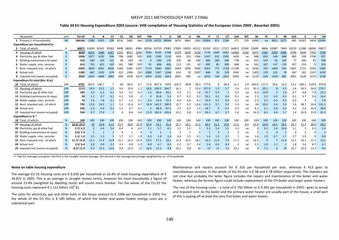
MEErP 2011 METHODOLOGY PART 2 FINAL
148
Table 34 EU Housing Expenditure 2003 (source: VHK compilation of 'Housing Statistics of the European Union 2004', Boverket 2005)
Parameter unit EU‐25 A B CY CZ DK EST FIN F D GR H IRL IT LT LIT LUX MT NL PL P SK SLO E S UK
1 Primary (= # households) k# 184166 3280 4325 239 4216 2481 566 2378 24525 38944 3674 3863 1382 22004 915 1346 171 129 6996 na 3651 2072 685 14187 4454 24346
Expenditure per household €/yr
2 Total, of which € 36872 31690 32542 29285 9498 28031 8384 30256 33759 27082 27893 10055 42211 35350 6512 27317 64815 22340 23699 8806 20987 7849 19259 11286 26856 39877
3 Housing, of which € 6039 6053 7680 6267 2232 8017 1920 7836 8136 6798 4379 1820 9118 7176 1400 4261 14000 2100 5072 2184 2204 2080 3794 3544 7762 7258
4 Electricity, gas & other fuel € 1006 1077 1432 996 798 1682 520 635 1249 1110 614 553 1266 1167 352 1502 1426 na 948 810 546 848 982 339 1746 957
5 Building maintenance & repair € 316 349 163 322 28 364 34 0 439 135 195 60 169 460 189 300 778 na 355 414 42 165 77 260 81 598
6 Water supply, misc. services € 413 792 423 293 161 589 159 91 608 650 112 151 42 495 85 300 648 na 332 167 147 133 327 214 0 319
7 Rent, Imputed rent , of which € 4303 3834 5662 4656 1244 5382 1207 7110 5840 4902 3459 1056 7640 5055 775 2158 11148 na 3436 793 1469 934 2407 2731 5935 5383
8 Actual rent € 1282 887 1595 674 313 1906 193 2088 1587 2248 614 70 1097 848 26 109 1944 na 1303 159 231 78 347 181 2337 1635
9 Imputed rent (owner‐occupied) € 3020 2947 4068 3983 940 3476 1014 5023 4220 2654 2845 985 na 4242 749 2021 9204 na 2133 634 1259 801 2061 2528 3572 3748
Expenditure EU total (bln. €/yr)
10 Total, of which 109 6791 103.9 140.7 7 40 69.5 4.7 71.9 827.9 1055 102.5 38.8 58.3 777.8 6 36.8 11.1 2.9 165.8 117.5 76.6 16.3 13.2 160.1 119.6 970.8
11 Housing, of which 109 1112 19.9 33.2 1.5 9.4 19.9 1.1 18.6 199.5 264.7 16.1 7 12.6 157.9 1.3 5.7 2.4 0.3 35.5 29.1 8 4.3 2.6 50.3 34.6 176.7
12 Electricity, gas & other fuel 109 185 3.5 6.2 0.2 3.4 4.2 0.3 1.5 30.6 43.2 2.3 2.1 1.8 25.7 0.3 2 0.2 na 6.6 10.8 2 1.8 0.7 4.8 7.8 23.3
13 Building maintenance & repair 109 58 1.1 0.7 0.1 0.1 0.9 0 0 10.8 5.3 0.7 0.2 0.2 10.1 0.2 0.4 0.1 na 2.5 5.5 0.2 0.3 0.1 3.7 0.4 14.6
14 Water supply, misc. services 109 76 2.6 1.8 0.1 0.7 1.5 0.1 0.2 14.9 25.3 0.4 0.6 0.1 10.9 0.1 0.4 0.1 na 2.3 2.2 0.5 0.3 0.2 3 0 7.8
15 Rent, Imputed rent , of which 109 792 12.6 24.5 1.1 5.2 13.4 0.7 16.9 143.2 190.9 12.7 4.1 10.6 111.2 0.7 2.9 1.9 na 24 10.6 5.4 1.9 1.6 38.7 26.4 131.1
16 Actual rent 109 236 2.9 6.9 0.2 1.3 4.7 0.1 5 38.9 87.5 2.3 0.3 1.5 18.7 0 0.1 0.3 na 9.1 2.1 0.8 0.2 0.2 2.6 10.4 39.8
17 Imputed rent (owner‐occupied) 109 556 9.7 17.6 1 4 8.6 0.6 11.9 103.5 103.4 10.5 3.8 9.3 93.3 0.7 2.7 1.6 na 14.9 8.5 4.6 1.7 1.4 35.9 15.9 91.3
Expenditure in % *
18 Total, of which % 100 100 100 100 100 100 100 100 100 100 100 100 100 100 100 100 100 100 100 100 100 100 100 100 100 100
19 Housing, of which % 16.4/ 23.0 19 23.6 21.4 23.5 28.6 22.9 25.9 24.1 25.1 15.7 18.1 21.6 20.3 21.5 15.6 21.6 9.4 21.4 24.8 10.5 26.5 19.7 31.4 28.9 18.2
20 Electricity, gas & other fuel % 2.7/ 4.2 3 4.4 3.4 8.4 6 6.2 2.1 3.7 4.1 2.2 5.5 3 3.3 5.4 5.5 2.2 na 4 9.2 2.6 10.8 5.1 3 6.5 2.4
21 Building maintenance & repair % 0.9/ 1.4 1 1 1 0 1 0 0 1 1 1 1 0 1 3 1 1 na 2 5 0 2 0 2 0 2
22 Water supply, misc. services % 1.1/ 1.6 2.5 1.3 1 1.7 2.1 1.9 0.3 1.8 2.4 0.4 1.5 0.1 1.4 1.3 1.1 1 na 1.4 1.9 0.7 1.7 1.7 1.9 0 0.8
23 Rent, Imputed rent , of which % 11.7/ 15.8 12.1 17.4 15.9 13.1 19.2 14.4 23.5 17.3 18.1 12.4 10.5 18.1 14.3 11.9 7.9 17.2 na 14.5 9 7 11.9 12.5 24.2 22.1 13.5
24 Actual rent % 3.5/ 4.4 2.8 4.9 2.3 3.3 6.8 2.3 6.9 4.7 8.3 2.2 0.7 2.6 2.4 0.4 0.4 3 na 5.5 1.8 1.1 1 1.8 1.6 8.7 4.1
25 Imputed rent (owner‐occupied) % 8.2/ 11.4 9.3 12.5 13.6 9.9 12.4 12 16.6 12.5 9.8 10.2 9.8 16 12 12 7.4 14.2 na 9 7.2 6 10 10.7 22.4 13.3 9.4
*= Two EU averages are given: the first is the straight money average, the second is the average percentage weighted by no. of households
Notes on table housing expenditure
The average EU‐25 housing costs are € 6.039 per household or 16.4% of total housing expenditure of € 36.872 in 2003. This is an average in straight money terms, however for most households a figure of around 23.4% (weighted by dwelling stock) will sound more familiar. For the whole of the EU‐25 the housing costs represent € 1.112 billion (109 €).
The costs for electricity, gas and other fuels in the house amount to € 1006 per household in 2003. For the whole of the EU this is € 185 billion, of which the boiler and water heater energy costs are a substantial part.
Maintenance and repairs account for € 316 per household per year, whereas € 413 goes to miscellaneous services. In the whole of the EU this is € 58 and € 78 billion respectively. The statistics are not clear but probably the latter figure includes the repairs and maintenance of the boiler and water heater, whereas the former figure could include replacement of the CH‐boiler and larger water heaters.
The rest of the housing costs – a total of € 792 billion or € 4.303 per household in 2003—goes to actual and imputed rent. As the boiler and the primary water heater are usually part of the house, a small part of this is paying off at least the very first boiler and water heater.
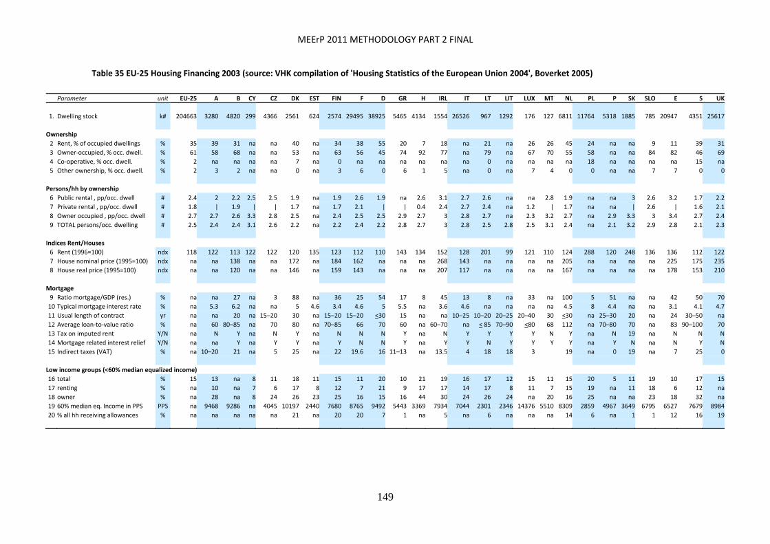
MEErP 2011 METHODOLOGY PART 2 FINAL
149
Table 35 EU‐25 Housing Financing 2003 (source: VHK compilation of 'Housing Statistics of the European Union 2004', Boverket 2005)
Parameter unit EU‐25 A B CY CZ DK EST FIN F D GR H IRL IT LT LIT LUX MT NL PL P SK SLO E S UK
1. Dwelling stock k# 204663 3280 4820 299 4366 2561 624 2574 29495 38925 5465 4134 1554 26526 967 1292 176 127 6811 11764 5318 1885 785 20947 4351 25617
Ownership
2 Rent, % of occupied dwellings % 35 39 31 na na 40 na 34 38 55 20 7 18 na 21 na 26 26 45 24 na na 9 11 39 31
3 Owner‐occupied, % occ. dwell. % 61 58 68 na na 53 na 63 56 45 74 92 77 na 79 na 67 70 55 58 na na 84 82 46 69
4 Co‐operative, % occ. dwell. % 2 na na na na 7 na 0 na na na na na na 0 na na na na 18 na na na na 15 na
5 Other ownership, % occ. dwell. % 2 3 2 na na 0 na 3 6 0 6 1 5 na 0 na 7 4 0 0 na na 7 7 0 0
Persons/hh by ownership
6 Public rental , pp/occ. dwell # 2.4 2 2.2 2.5 2.5 1.9 na 1.9 2.6 1.9 na 2.6 3.1 2.7 2.6 na na 2.8 1.9 na na 3 2.6 3.2 1.7 2.2
7 Private rental , pp/occ. dwell # 1.8 | 1.9 | | 1.7 na 1.7 2.1 | | 0.4 2.4 2.7 2.4 na 1.2 | 1.7 na na | 2.6 | 1.6 2.1
8 Owner occupied , pp/occ. dwell # 2.7 2.7 2.6 3.3 2.8 2.5 na 2.4 2.5 2.5 2.9 2.7 3 2.8 2.7 na 2.3 3.2 2.7 na 2.9 3.3 3 3.4 2.7 2.4
9 TOTAL persons/occ. dwelling # 2.5 2.4 2.4 3.1 2.6 2.2 na 2.2 2.4 2.2 2.8 2.7 3 2.8 2.5 2.8 2.5 3.1 2.4 na 2.1 3.2 2.9 2.8 2.1 2.3
Indices Rent/Houses
6 Rent (1996=100) ndx 118 122 113 122 122 120 135 123 112 110 143 134 152 128 201 99 121 110 124 288 120 248 136 136 112 122
7 House nominal price (1995=100) ndx na na 138 na na 172 na 184 162 na na na 268 143 na na na na 205 na na na na 225 175 235
8 House real price (1995=100) ndx na na 120 na na 146 na 159 143 na na na 207 117 na na na na 167 na na na na 178 153 210
Mortgage
9 Ratio mortgage/GDP (res.) % na na 27 na 3 88 na 36 25 54 17 8 45 13 8 na 33 na 100 5 51 na na 42 50 70
10 Typical mortgage interest rate % na 5.3 6.2 na na 5 4.6 3.4 4.6 5 5.5 na 3.6 4.6 na na na na 4.5 8 4.4 na na 3.1 4.1 4.7
11 Usual length of contract yr na na 20 na 15–20 30 na 15–20 15–20 <30 15 na na 10–25 10–20 20–25 20–40 30 <30 na 25–30 20 na 24 30–50 na
12 Average loan‐to‐value ratio % na 60 80–85 na 70 80 na 70–85 66 70 60 na 60–70 na < 85 70–90 <80 68 112 na 70–80 70 na 83 90–100 70
13 Tax on imputed rent Y/N na N Y na N Y na N N N Y na N Y Y Y Y N Y na N 19 na N N N
14 Mortgage related interest relief Y/N na na Y na Y Y na Y N N Y na Y Y N Y Y Y Y na Y N na N Y N
15 Indirect taxes (VAT) % na 10–20 21 na 5 25 na 22 19.6 16 11–13 na 13.5 4 18 18 3 19 na 0 19 na 7 25 0
Low income groups (<60% median equalized income)
16 total % 15 13 na 8 11 18 11 15 11 20 10 21 19 16 17 12 15 11 15 20 5 11 19 10 17 15
17 renting % na 10 na 7 6 17 8 12 7 21 9 17 17 14 17 8 11 7 15 19 na 11 18 6 12 na
18 owner % na 28 na 8 24 26 23 25 16 15 16 44 30 24 26 24 na 20 16 25 na na 23 18 32 na
19 60% median eq. Income in PPS PPS na 9468 9286 na 4045 10197 2440 7680 8765 9492 5443 3369 7934 7044 2301 2346 14376 5510 8309 2859 4967 3649 6795 6527 7679 8984
20 % all hh receiving allowances % na na na na na 21 na 20 20 7 1 na 5 na 6 na na na 14 6 na 1 1 12 16 19
MEErP 2011 METHODOLOGY PART 2 FINAL
150
Notes on table housing financing
Around 61% of the dwelling stock is owner‐occupied and 35% is rental. The 4% remainder is owned by a co‐operation or there is another ownership situation. The information is not complete, but assuming that these percentages are valid throughout, it means that 124 million dwellings are owner‐occupied and 72 million are rental.
The household size varies with the ownership situation. In public rental dwellings the household size is 2.4 persons per household, in private rental it is only 1.8 persons and in owner‐occupied houses it is 2.7 persons per household. The average—as mentioned before—is 2.5 persons per household.
The rent index (not corrected for inflation) has risen to 122 in 2003 (1996=100). Roughly over the same period the index of the single family house –also not corrected for inflation— has gone up to around 190 (1995=100). The real price index of the house prices—corrected for inflation (PPS)— went to 178 over the same period. This is a very rough estimate. The EU‐25 data are not complete and that is why no estimate is given in the table.
From the ratio of the outstanding residential mortgage to GDP (Gross Domestic Product) it is clear that the Dutch are the biggest lenders and that the houses are in fact fully mortgaged and the loan‐against‐value ratio is on average 112%. The reason is a tax regime which favours maximum
mortgaging, as can be see from the line ‘Mortgage related interest relief’ and banks that have very few reservations. On the other side of the spectrum we find Italy, Greece and Central European countries where mortgages are (far) lower than 20% of GDP.
The typical length of the mortgage contract is 20 years with some countries going upo to 30 years. The typical mortgage rate in the EU‐25 in 2003 was around 5%.
Around 15% of the households can be classified as ‘low income’ according to the definition mentioned earlier. For most EU‐15 Member States this means an income of less than 6.000‐9.000 PPS per household/year. For some new Member States, especially the Baltic States, this can be as low as around 2.400 PPS per household/year.
Nonetheless, the ownership situation amongst the low income groups is not very different from the rest: in most countries one third is paying rent and two thirds owns the house.
In most countries that are reporting on the issue there is a state subsidy for the low income groups. In Denmark, Finland, France, Sweden, the Netherlands and the UK this subsidy covers more than 14‐20% of the total population, i.e. the whole of the low income group. The statistics do not reveal the level of support.
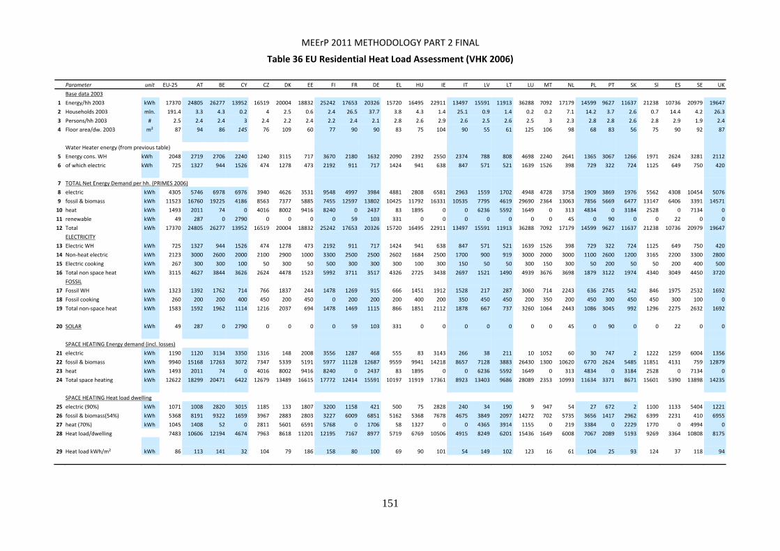
MEErP 2011 METHODOLOGY PART 2 FINAL
151
Table 36 EU Residential Heat Load Assessment (VHK 2006)
Parameter unit EU‐25 AT BE CY CZ DK EE FI FR DE EL HU IE IT LV LT LU MT NL PL PT SK Sl ES SE UK
Base data 2003
1 Energy/hh 2003 kWh 17370 24805 26277 13952 16519 20004 18832 25242 17653 20326 15720 16495 22911 13497 15591 11913 36288 7092 17179 14599 9627 11637 21238 10736 20979 19647
2 Households 2003 mln. 191.4 3.3 4.3 0.2 4 2.5 0.6 2.4 26.5 37.7 3.8 4.3 1.4 25.1 0.9 1.4 0.2 0.2 7.1 14.2 3.7 2.6 0.7 14.4 4.2 26.3
3 Persons/hh 2003 # 2.5 2.4 2.4 3 2.4 2.2 2.4 2.2 2.4 2.1 2.8 2.6 2.9 2.6 2.5 2.6 2.5 3 2.3 2.8 2.8 2.6 2.8 2.9 1.9 2.4
4 Floor area/dw. 2003 m² 87 94 86 145 76 109 60 77 90 90 83 75 104 90 55 61 125 106 98 68 83 56 75 90 92 87
Water Heater energy (from previous table)
5 Energy cons. WH kWh 2048 2719 2706 2240 1240 3115 717 3670 2180 1632 2090 2392 2550 2374 788 808 4698 2240 2641 1365 3067 1266 1971 2624 3281 2112
6 of which electric kWh 725 1327 944 1526 474 1278 473 2192 911 717 1424 941 638 847 571 521 1639 1526 398 729 322 724 1125 649 750 420
7 TOTAL Net Energy Demand per hh. (PRIMES 2006)
8 electric kWh 4305 5746 6978 6976 3940 4626 3531 9548 4997 3984 4881 2808 6581 2963 1559 1702 4948 4728 3758 1909 3869 1976 5562 4308 10454 5076
9 fossil & biomass kWh 11523 16760 19225 4186 8563 7377 5885 7455 12597 13802 10425 11792 16331 10535 7795 4619 29690 2364 13063 7856 5669 6477 13147 6406 3391 14571
10 heat kWh 1493 2011 74 0 4016 8002 9416 8240 0 2437 83 1895 0 0 6236 5592 1649 0 313 4834 0 3184 2528 0 7134 0
11 renewable kWh 49 287 0 2790 0 0 0 0 59 103 331 0 0 0 0 0 0 0 45 0 90 0 0 22 0 0
12 Total kWh 17370 24805 26277 13952 16519 20004 18832 25242 17653 20326 15720 16495 22911 13497 15591 11913 36288 7092 17179 14599 9627 11637 21238 10736 20979 19647
ELECTRICITY
13 Electric WH kWh 725 1327 944 1526 474 1278 473 2192 911 717 1424 941 638 847 571 521 1639 1526 398 729 322 724 1125 649 750 420
14 Non‐heat electric kWh 2123 3000 2600 2000 2100 2900 1000 3300 2500 2500 2602 1684 2500 1700 900 919 3000 2000 3000 1100 2600 1200 3165 2200 3300 2800
15 Electric cooking kWh 267 300 300 100 50 300 50 500 300 300 300 100 300 150 50 50 300 150 300 50 200 50 50 200 400 500
16 Total non space heat kWh 3115 4627 3844 3626 2624 4478 1523 5992 3711 3517 4326 2725 3438 2697 1521 1490 4939 3676 3698 1879 3122 1974 4340 3049 4450 3720
FOSSIL
17 Fossil WH kWh 1323 1392 1762 714 766 1837 244 1478 1269 915 666 1451 1912 1528 217 287 3060 714 2243 636 2745 542 846 1975 2532 1692
18 Fossil cooking kWh 260 200 200 400 450 200 450 0 200 200 200 400 200 350 450 450 200 350 200 450 300 450 450 300 100 0
19 Total non‐space heat kWh 1583 1592 1962 1114 1216 2037 694 1478 1469 1115 866 1851 2112 1878 667 737 3260 1064 2443 1086 3045 992 1296 2275 2632 1692
20 SOLAR kWh 49 287 0 2790 0 0 0 0 59 103 331 0 0 0 0 0 0 0 45 0 90 0 0 22 0 0
SPACE HEATING Energy demand (incl. losses)
21 electric kWh 1190 1120 3134 3350 1316 148 2008 3556 1287 468 555 83 3143 266 38 211 10 1052 60 30 747 2 1222 1259 6004 1356
22 fossil & biomass kWh 9940 15168 17263 3072 7347 5339 5191 5977 11128 12687 9559 9941 14218 8657 7128 3883 26430 1300 10620 6770 2624 5485 11851 4131 759 12879
23 heat kWh 1493 2011 74 0 4016 8002 9416 8240 0 2437 83 1895 0 0 6236 5592 1649 0 313 4834 0 3184 2528 0 7134 0
24 Total space heating kWh 12622 18299 20471 6422 12679 13489 16615 17772 12414 15591 10197 11919 17361 8923 13403 9686 28089 2353 10993 11634 3371 8671 15601 5390 13898 14235
SPACE HEATING Heat load dwelling
25 electric (90%) kWh 1071 1008 2820 3015 1185 133 1807 3200 1158 421 500 75 2828 240 34 190 9 947 54 27 672 2 1100 1133 5404 1221
26 fossil & biomass(54%) kWh 5368 8191 9322 1659 3967 2883 2803 3227 6009 6851 5162 5368 7678 4675 3849 2097 14272 702 5735 3656 1417 2962 6399 2231 410 6955
27 heat (70%) kWh 1045 1408 52 0 2811 5601 6591 5768 0 1706 58 1327 0 0 4365 3914 1155 0 219 3384 0 2229 1770 0 4994 0
28 Heat load/dwelling 7483 10606 12194 4674 7963 8618 11201 12195 7167 8977 5719 6769 10506 4915 8249 6201 15436 1649 6008 7067 2089 5193 9269 3364 10808 8175
29 Heat load kWh/m² kWh 86 113 141 32 104 79 186 158 80 100 69 90 101 54 149 102 123 16 61 104 25 93 124 37 118 94
MEErP 2011 METHODOLOGY PART 2 FINAL
152
Notes on table heat loads:
The table is based on outcomes of more recent studies in 2005 on the subject of the average heat load per dwelling and revisiting every aspect of earlier studies (PRIMES ‘Shared Analysis’ 1999, SAVE 2002, ECCP 2003). It tries to reconcile a ‘bottom‐up’and ‘top‐down’ approach in not only correcting the EU‐average, but also making an estimate per Member State.
The average EU‐25 space heating/cooling energy demand is currently around 12.600 kWh/dwelling. This is 72.5% of the total average net energy demand (excl. power generation losses) of 17370 kWh/dwelling.
Of this, the effective heating/cooling load of the dwelling (transmission, ventilation, internal gains at current comfort level) is 7.400 kWh/dwelling.
Both of the above points combined imply that around 40% of the space heating demand is due to heating system losses (generator, distribution and control losses).
Per unit of floor area the 7.400 kWh/hh.a. heat load equals around 85 kWh/m² or a little over 300 MJ/m². In Southern Europe this is half (Italy 54, Spain 37, Greece 69 kWh/m², etc. ) and in Northern Europe this is double that value (Estonia 186, Finland 158, Sweden 118, etc.). But the climate certainly doesn’t explain all differences, e.g. the highest calculated heat loads per dwelling can be found in the middle of the EU, i.e. in Luxemburg (15.400 kWh/hh.a) and Belgium (12.200 kWh/hh.a).
On the long run (2020‐2025) the data suggest
The heat load will increase by 7‐8% because of a bigger average floor area (from 87 m² today to 94‐95 m²/dwelling in 2020)
The heat load will decrease because of better insulation and less ventilation heat losses. Even taking into account the continuously growing floor area per dwelling the SAVE study –building on a 1960‐2005 historical data—predicted a decrease of 900 kWh (12%). Given the negative effect of the enlargement of the floor area this means that insulation and ventilation measures would yield a 20% improvement.
The effective heat load will increase by 8% because the comfort level (the average indoor temperatures) in Southern and Eastern EU Member States will increase.
Combining the three points above VHK expects a decrease in the effective space heat load of the average existing dwelling by 4‐5% in 2020‐2025.
Statistical information on housing characteristics has improved, but we are still a long way from being able to monitor efficiency improvements in the housing stock.
The figures in the table per individual Member State should be understood as an attempt to test the average EU heat load data for consistency, not as the best possible estimate of the residential energy balance for each individual Member State. This would require a higher level of differentiation between e.g. generator, distribution and control losses in each country and a more extensive study. Having said that, the accuracy of the EU average heat load is estimated at within ± 10%, which is sufficient for our purpose.

MEErP 2011 METHODOLOGY PART 2 FINAL
153
6.6 Commercialbuildings
(semi ‐) public 3.1
commercial 1.65
tertiary sector UNITS
(figures in mln.units, total 4.74 mln. ‐residential buildings)
Hotel ‐ or restaurant building of which hotels 0.17 (10 beds), other short ‐ stay lodgings 0.07 (e.g. campings, hostels), ca. 0.1 restaurants
Offices incl 0.1 offices on industrial sites
Retail large scale & malls
Bath ‐ & sports of which 0.05 public pools
Health care of which 0.011 hospitals mln. beds)0.05 (3.6 mln. places)
Defence buildings 0.0
Communication (post, train, airport, etc.)
Public building (town hall, etc.)
Ecclesiastical building of which 50% unheated
Culture building
School building
Figure 81 Tertiary sector building units, EU‐25, 2005.
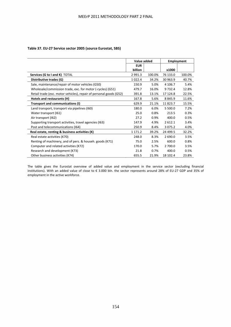
MEErP 2011 METHODOLOGY PART 2 FINAL
154
Table 37. EU‐27 Service sector 2005 (source Eurostat, SBS)
Value added Employment
EUR
billion x1000
Services (G to I and K) TOTAL 2 991.3 100.0% 76 133.0 100.0%
Distributive trades (G) 1 022.4 34.2% 30 963.9 40.7%
Sale, maintenance/repair of motor vehicles (G50) 150.9 5.0% 4 106.7 5.4%
Wholesale/commission trade, exc. for motor (‐cycles) (G51) 479.7 16.0% 9 732.4 12.8%
Retail trade (exc. motor vehicles), repair of personal goods (G52) 391.8 13.1% 17 124.8 22.5%
Hotels and restaurants (H) 167.8 5.6% 8 845.9 11.6%
Transport and communications (I) 629.9 21.1% 11 823.7 15.5%
Land transport, transport via pipelines (I60) 180.0 6.0% 5 500.0 7.2%
Water transport (I61) 25.0 0.8% 213.5 0.3%
Air transport (I62) 27.2 0.9% 400.0 0.5%
Supporting transport activities, travel agencies (I63) 147.9 4.9% 2 612.1 3.4%
Post and telecommunications (I64) 250.9 8.4% 3 075.2 4.0%
Real estate, renting & business activities (K) 1 171.2 39.2% 24 499.5 32.2%
Real estate activities (K70) 248.0 8.3% 2 690.0 3.5%
Renting of machinery, and of pers. & househ. goods (K71) 75.0 2.5% 600.0 0.8%
Computer and related activities (K72) 170.0 5.7% 2 700.0 3.5%
Research and development (K73) 21.8 0.7% 400.0 0.5%
Other business activities (K74) 655.5 21.9% 18 102.4 23.8%
The table gives the Eurostat overview of added value and employment in the service sector (excluding financial institutions). With an added value of close to € 3.000 bln. the sector represents around 28% of EU‐27 GDP and 35% of employment in the active workforce.
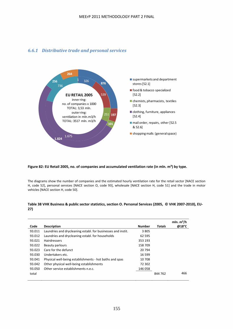
MEErP 2011 METHODOLOGY PART 2 FINAL
155
6.6.1 Distributivetradeandpersonalservices
326
539
251
1.675
736
1876
197
101
1.824
256
264
EU RETAIL 2005inner ring:
no. of companies x 1000TOTAL: 3,53 mln.
outer ring: ventilation in mln.m3/hTOTAL: 3517 mln. m3/h
supermarkets and department
stores [52.1]
food & tobacco specialized
[52.2]
chemists, pharmacists, textiles
[52.3]
clothing, furniture, appliances
[52.4]
mail order, repairs, other [52.5
& 52.6]
shopping malls (general space)
Figure 82: EU Retail 2005, no. of companies and accumulated ventilation rate (in mln. m³) by type.
The diagrams show the number of companies and the estimated hourly ventilation rate for the retail sector [NACE section H, code 52], personal services [NACE section O, code 93], wholesale [NACE section H, code 51] and the trade in motor vehicles [NACE section H, code 50].
Table 38 VHK Business & public sector statistics, section O. Personal Services (2005, © VHK 2007‐2010), EU‐27)
Code Description Number Totals mln. m³/h
@18°C
93.011 Laundries and drycleaning establ. for businesses and instit. 3 805
93.012 Laundries and drycleaning establ. for households 62 595
93.021 Hairdressers 353 193
93.022 Beauty parlours 158 709
93.023 Care for the defunct 20 794
93.030 Undertakers etc. 16 599
93.041 Physical well‐being establishments ‐ hot baths and spas 10 708
93.042 Other physical well‐being establishments 72 302
93.050 Other service establishments n.e.c. 146 058
total 844 762 466
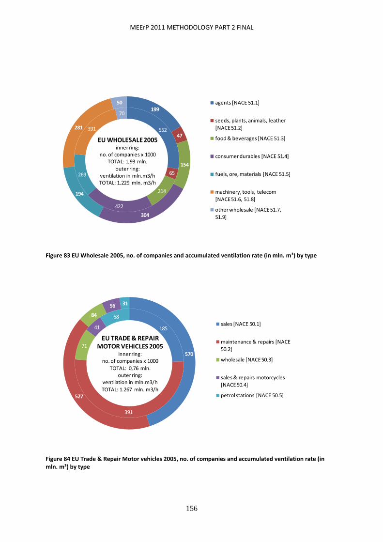
MEErP 2011 METHODOLOGY PART 2 FINAL
156
552
65
214
422
269
391
70199
47
154
304
194
281
50
EU WHOLESALE 2005inner ring:
no. of companies x 1000TOTAL: 1,93 mln.
outer ring: ventilation in mln.m3/hTOTAL: 1.229 mln. m3/h
agents [NACE 51.1]
seeds, plants, animals, leather
[NACE 51.2]
food & beverages [NACE 51.3]
consumer durables [NACE 51.4]
fuels, ore, materials [NACE 51.5]
machinery, tools, telecom
[NACE 51.6, 51.8]
other wholesale [NACE 51.7,
51.9]
Figure 83 EU Wholesale 2005, no. of companies and accumulated ventilation rate (in mln. m³) by type
185
391
71
41
68
570
527
84
56 31
EU TRADE & REPAIR MOTOR VEHICLES 2005
inner ring: no. of companies x 1000
TOTAL: 0,76 mln.outer ring:
ventilation in mln.m3/h
TOTAL: 1.267 mln. m3/h
sales [NACE 50.1]
maintenance & repairs [NACE
50.2]
wholesale [NACE 50.3]
sales & repairs motorcycles
[NACE 50.4]
petrol stations [NACE 50.5]
Figure 84 EU Trade & Repair Motor vehicles 2005, no. of companies and accumulated ventilation rate (in mln. m³) by type
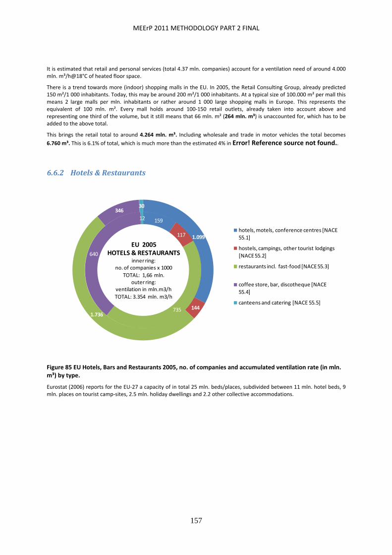
MEErP 2011 METHODOLOGY PART 2 FINAL
157
It is estimated that retail and personal services (total 4.37 mln. companies) account for a ventilation need of around 4.000 mln. m³/h@18°C of heated floor space.
There is a trend towards more (indoor) shopping malls in the EU. In 2005, the Retail Consulting Group, already predicted 150 m²/1 000 inhabitants. Today, this may be around 200 m²/1 000 inhabitants. At a typical size of 100.000 m² per mall this means 2 large malls per mln. inhabitants or rather around 1 000 large shopping malls in Europe. This represents the equivalent of 100 mln. m². Every mall holds around 100‐150 retail outlets, already taken into account above and representing one third of the volume, but it still means that 66 mln. m² (264 mln. m³) is unaccounted for, which has to be added to the above total.
This brings the retail total to around 4.264 mln. m³. Including wholesale and trade in motor vehicles the total becomes
6.760 m³. This is 6.1% of total, which is much more than the estimated 4% in Error! Reference source not found..
6.6.2 Hotels&Restaurants
159
117
735
640
12
1.099
1441.736
34630
EU 2005HOTELS & RESTAURANTS
inner ring: no. of companies x 1000
TOTAL: 1,66 mln.outer ring:
ventilation in mln.m3/h
TOTAL: 3.354 mln. m3/h
hotels, motels, conference centres [NACE
55.1]
hostels, campings, other tourist lodgings
[NACE 55.2]
restaurants incl. fast‐food [NACE 55.3]
coffee store, bar, discotheque [NACE
55.4]
canteens and catering [NACE 55.5]
Figure 85 EU Hotels, Bars and Restaurants 2005, no. of companies and accumulated ventilation rate (in mln. m³) by type.
Eurostat (2006) reports for the EU‐27 a capacity of in total 25 mln. beds/places, subdivided between 11 mln. hotel beds, 9 mln. places on tourist camp‐sites, 2.5 mln. holiday dwellings and 2.2 other collective accommodations.
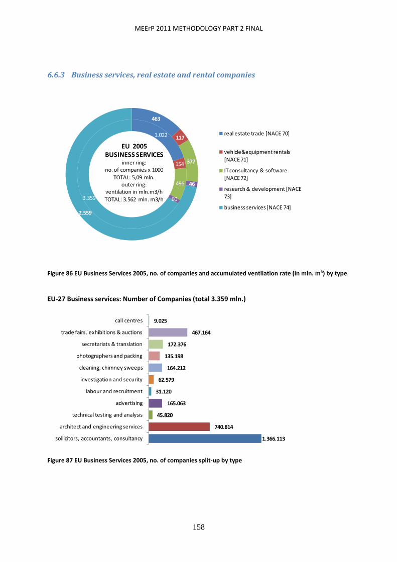
MEErP 2011 METHODOLOGY PART 2 FINAL
158
6.6.3 Businessservices,realestateandrentalcompanies
1.022
154
496
603.359
463
117
377
46
2.559
EU 2005BUSINESS SERVICES
inner ring: no. of companies x 1000
TOTAL: 5,09 mln.outer ring:
ventilation in mln.m3/h
TOTAL: 3.562 mln. m3/h
real estate trade [NACE 70]
vehicle&equipment rentals
[NACE 71]
IT consultancy & software
[NACE 72]
research & development [NACE
73]
business services [NACE 74]
Figure 86 EU Business Services 2005, no. of companies and accumulated ventilation rate (in mln. m³) by type
EU‐27 Business services: Number of Companies (total 3.359 mln.)
1.366.113
740.814
45.820
165.063
31.120
62.579
164.212
135.198
172.376
467.164
9.025
sollicitors, accountants, consultancy
architect and engineering services
technical testing and analysis
advertising
labour and recruitment
investigation and security
cleaning, chimney sweeps
photographers and packing
secretariats & translation
trade fairs, exhibitions & auctions
call centres
Figure 87 EU Business Services 2005, no. of companies split‐up by type

MEErP 2011 METHODOLOGY PART 2 FINAL
159
Trade Fairs
In terms of the size of the buildings, the trade fair exhibition halls are an interesting subsection at NEC 5‐digit level. Germany alone boosts 2.7 mln. m² of trade fair exhibition hall floor area. In total EU‐27 is estimated to have ca. 10 mln. m² of trade fair exhibition area. At a ceiling height of 8 m this comes down to ca. 80 mln. m³. Largest 5 fairs in EU: Hannover, Milano Fiera, Frankfurt, Cologne, Dusseldorf.
101
6.6.4 Transportationandcommunication
It is estimated that the EU has around 10.000 manned train stations, i.e. featuring at least one heated area. The size of the heated area may range from a one‐man ticket counter to the arrivals & departures hall of an international high speed rail station. As a first guess, the heated area is estimated at 200 m², including the company head‐offices. This brings the total to 2 mln. m² and around 8 mln. m³.
There are around 25 large cities in the EU that feature a subway‐network. Per network, around 100 underground stations are estimated, which require ventilation. In total, these 2.500 underground stations will have a floor area of 2.5 mln. m² and a total ventilated volume of 5 mln. m³.
The CIA World Factbook reports 3.376 airfields in the EU (2009), of which 1.981 with a paved runway and presumably some heated area. Of the latter it is estimated that around 200‐300 airports host commercial flights, of which again around 30 large airports. Estimating the latter at 200.000 m² (2 mln. m³, excluding shops) a piece, 250 other commercial airports at 2 000 m² (10 000 m³) and 1600 small airports at 200 m² (1000 m³) per unit, the total is around 64 mln. m³.
For harbour buildings (port authorities, waiting hall ferry’s etc.) , in as much as they are not already taken into account under the heading ‘wholesale’, it is difficult to make an accurate estimate. A figure of 3 mln. m³ is given.
For the whole transport sector, excluding the building area already taken into account under other headings (retail, petrol stations, motels, restaurants, etc.), the total is estimated at around 80 mln. m³ considerably less than 1% of total mentioned in figure 1.
101 AUMA report 2009. Note that in Belgium, the Brussels Exhibition Park (114.000 m² hall area) is the largest. In NL this is Jaarbeurs (100.000 m²).
paved1995
un‐paved1396
>3km
115 2,4‐3 km
341
1,5‐2,4 km
543
0,9‐1,5 km
421
<0,9 km
575
>0,9 km
286
<0,9 km
1110
3.396 airfields (2009), by runway type and length (graph)
100 heliports (2007)
5.454.446 km roadways (2008)
229.450 km railways (2008)
52.332 km waterways (2006)
Figure 88 EU Transport key figures
MEErP 2011 METHODOLOGY PART 2 FINAL
160
6.6.5 CommunicationStatistics on post offices are extremely volatile, given the trends of privatisation, internet and mix of mail services with other activities (banking, shops). A very rough estimate is that typical mail activities of larger mail‐offices can be partitioned to around 20 mln. m³ gross floor area in the EU. 102
Computer and telephone data centres (a.k.a. ‘server farms’) accounted for 61.4 TWh of electricity consumption in the US in 2006.
103 At the same time, the energy use in the EU‐27 was lagging some 20% behind104, but it is assumed that today the EU‐27 will have the same 10‐11 mln. servers installed as the US and will also be spending some 60 TWh/a on data centres. Of this, 22% (13.2 TWh/a) is attributed to air‐conditioning and ventilation. In principle, this type of air‐conditioning and cooling is outside the scope of the study, because it concerns process‐cooling and not comfort cooling (no people). But the figure is important enough to mention here, because it can explain 1‐2% of total HVAC stock of chillers or AHU’s. At an ICT heat dissipation of 1 kW/m² floor area, 45 TWh/a ICT electricity use, 8.000 h operation, a ceiling height of 3.5 m, the data centres represent around 6 mln. m² of gross floor area and 20 mln. m³, but the cooling performance is of course much higher than for comfort cooling.
Note that the ventilation of tunnels and parking garages105, as well as the ventilation and conditioning of motor vehicles,
trains, ships and aircraft can constitute considerable energy consumption.
6.6.6 FinancialinstitutionsBelga (2007) reports an average density of 1 EU bank branch office per 2.230 inhabitants. At 500 mln. inhabitants this means 220.000 bank branch offices in the EU. At an estimated average of 200 m² (800 m³) per office (including ATM area, including head‐office) this comes down to a heated volume of 180 mln. m³.
102 Basis of estimate: NL still has 250 ‘larger’ main‐offices. EU=30xNL. At 1000 m²/building for specific mail‐linked activities this gives 7.5 mln. m² (20 mln. m³). Note that NL has around 1.850 mail‐offices mixed with shops (headcount is under ‘retail’). 103 Report to Congress on Server and Data Center Energy Efficiency Public Law 109‐431 U.S. Environmental Protection
Agency ENERGY STAR Program, August 2, 2007. 104 ECN, Data hotels, report 2008 with data 2007 on the Netherlands (average EU internet density): 1.6 TWh. EU=30xNl 48 TWh. Of this 22% went into HVAC 105 The EU‐27 has 5860 km of tunnels (CIA World Factbook data 1.1. 2009), including railroad (ca. 23%), subway(28%), road tunnels (49% of safety regulated km capacity). Regulated tunnels (>300 m) are on average ca. 1.2 km/tunnel long and account for ¾ of the total km. This means around 3660 tunnels with sufficient ventilation capacity to evacuate toxic fumes. Typical fan‐values found are 2 supply fans (90 m3/s) and 2 exhaust fans (70 m3/s) per tunnel, amounting to a total of capacity of 320 m3/s or 1.15 mln. m3/h per tunnel. No data on part load operation are available.

MEErP 2011 METHODOLOGY PART 2 FINAL
161
6.7 Publicsectorandcommunitysectorbuildings
Home office & municipalities 600
Justice 444
Defense 168
Finance 132
Social affairs 84
Transport 67
Agriculture 60
Foreign affairs 48
Industry dept. 29Int. & advisory 28
Housing/ Env. 24PM & repres. 20
PUBLIC SECTOR
(excl. health care and schools)
1700 mln. m³/m³Health
Care 5400
Education
4000
Other
1700
Public sector, health care & education:ventilation in m³/m³.h
Figure 89 Public sector summary, heated building volume by department (11 100 m³/m³.h)

MEErP 2011 METHODOLOGY PART 2 FINAL
162
6.7.1 Healthcare
Table 39 Health and social work, NACE section N, 2005, EU‐25 (© VHK 2007‐2010)
Code Description Number Totals mln.
85.111 Hospital primary health activities 5 949 85.112 Hospitals for specialized somatic health activities 2 732
85.113 Hospitals for specialized psychiatric health activities 833
85.114 Rehabilitation centres 13
85.115 Other specialized health activities 2 250
11 777 993 85.121 Medical practices, at hospitals 161 804
85.122 Medical practices, not at hospitals 139 813
85.123 Somatic polyclinics 506 534
85.124 Psychiatric healing centre 19 333
85.125 Adult psychiatric polyclinic 10
85.127 Children’s and adolescents psychiatric polyclinic 11 314
838 808 815 85.130 Dental practices 156 840
156 840 189 85.141 Medical laboratories etc. 13 535
85.142 Ambulance transports and ambulance health activities 6 045
85.143 Medical nursing homes 45 341
85.144 Other health establishments n.e.c. 272 001
85.145 Organ collection centres and banks 6
336 928 2 028 85.200 Veterinary clinics 45 754
45 754 55 85.311 Service homes and homes for the aged 6 128
85.312 Homes for disabled persons 5 807
85.313 Homes for children and young people 13 776
85.315 Homes for adult substance misusers 2 786
85.316 Hostels etc. 489
85.322 Child day‐care establishments 15 927
85.323 Social work establishments for children and young people 1 533
85.324 Welfare and counselling centres 10 097
85.325 Humanitarian relief organisations 1 439
85.327 Day‐care establishments for the aged 3 836
85.328 Day‐care establishments for disabled persons 9 297
85.329 Day‐care establishments for adult substance misusers 1 998
73 112 1 320
TOTAL 1 463 219 5 400
The total ventilation is set at 5 400 mln. m³/h, not only due to the actual heated floor area, but also influenced by certain specific activities like laboratories, operating theatre and treatment areas that require up >10 times the usual ventilation fold.
In the EU‐27 (2006) there are 200 000 curative beds in hospitals (406.3 per 100 000 inhabitants) and 29 700 psychiatric care beds (60.4 per 100 000 inhabitants).106
106 Eurostat Yearbook 2009.
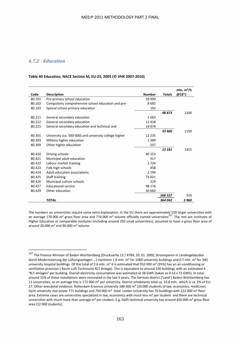
MEErP 2011 METHODOLOGY PART 2 FINAL
163
6.7.2 Education
Table 40 Education, NACE Section M, EU‐25, 2005 (© VHK 2007‐2010)
Code Description Number Totals mln. m³/h @18°C
80.101 Pre‐primary school education 39 999 80.102 Compulsory comprehensive school education and pre‐ 8 682 80.103 Special school primary education 192
48 873 1100 80.211 General secondary education 1 063
80.212 General secondary education 12 418 80.221‐ General secondary education and technical and 19 979
33 460 1150 80.301 University (ca. 500‐600) and university college higher 11 235
80.303 Military higher education 1 389
80.309 Other higher education 557
13 181 1415 80.410 Driving schools 40 153
80.421 Municipal adult education 917
80.422 Labour market training 2 724
80.423 Folk high schools 458
80.424 Adult education associations 2 190
80.425 Staff training 73 021
80.426 Municipal culture schools 229
80.427 Educational service 98 176
80.429 Other education 50 660
268 527 310
TOTAL 364 042 3 960
The numbers on universities require some extra explanation. In the EU there are approximately 550 larger universities with an average 170.000 m² gross floor area and 774.000 m³ volume officially named universities107. The rest are institutes of Higher Education or comparable institutes (including around 250 small universities), assumed to have a gross floor area of around 20.000 m² and 90.000 m³ volume.
107 The Finance Minister of Baden‐Württemberg (Drucksache 12 / 4784, 20. 01. 2000, Stromsparen in Landesgebäuden
durch Modernisierung der Lüftungsanlagen …) mentions 1.9 mln. m² for 1060 university buildings and 0.7 mln. m² for 340 university hospital buildings. Of this total of 2.6 mln. m² it is estimated that 910 000 m² (35%) has an air‐conditioning or ventilation provision ( Raum Luft Technische RLT Anlage). This is equivalent to around 530 buildings with an estimated 4 ‘RLT‐Anlagen’ per building. Overall electricity consumption was estimated at 38 GWh (taken as 0.53 x 72 GWh). In total around 15% of these installations were renovated in the last 5 years. The German district (‘Land’) Baden‐Württemberg has 11 universities, so on average this is 172 000 m² per university. District inhabitants total ca. 10.8 mln., which is ca. 2% of EU‐27. Other anecdotal evidence: Rotterdam Erasmus university 180 000 m² (20.000 students of law, economics, medicine). Gent university real estate 771 buildings and 750 000 m² total. Leiden University has 70 buildings with 222 000 m² floor area. Extreme cases are universities specialized in law, economics with much less m² per student and there are technical universities with much more than average m² per student. E.g. Delft technical university has around 450 000 m² gross floor area (12 000 students).
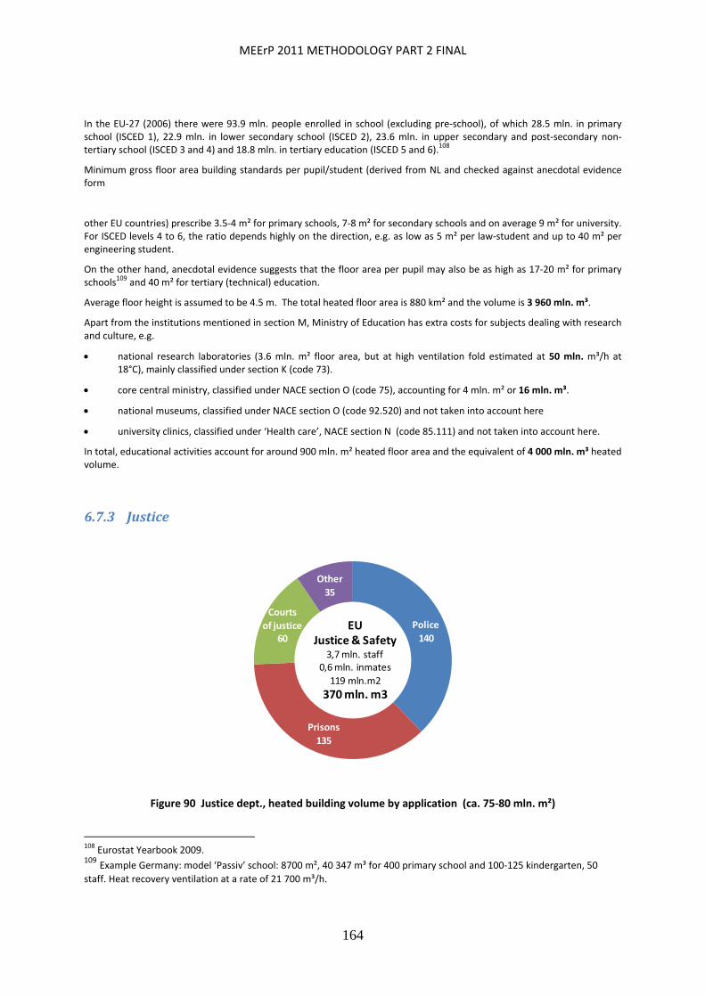
MEErP 2011 METHODOLOGY PART 2 FINAL
164
In the EU‐27 (2006) there were 93.9 mln. people enrolled in school (excluding pre‐school), of which 28.5 mln. in primary school (ISCED 1), 22.9 mln. in lower secondary school (ISCED 2), 23.6 mln. in upper secondary and post‐secondary non‐tertiary school (ISCED 3 and 4) and 18.8 mln. in tertiary education (ISCED 5 and 6).108
Minimum gross floor area building standards per pupil/student (derived from NL and checked against anecdotal evidence form
other EU countries) prescribe 3.5‐4 m² for primary schools, 7‐8 m² for secondary schools and on average 9 m² for university. For ISCED levels 4 to 6, the ratio depends highly on the direction, e.g. as low as 5 m² per law‐student and up to 40 m² per engineering student.
On the other hand, anecdotal evidence suggests that the floor area per pupil may also be as high as 17‐20 m² for primary schools
109 and 40 m² for tertiary (technical) education.
Average floor height is assumed to be 4.5 m. The total heated floor area is 880 km² and the volume is 3 960 mln. m³.
Apart from the institutions mentioned in section M, Ministry of Education has extra costs for subjects dealing with research and culture, e.g.
national research laboratories (3.6 mln. m² floor area, but at high ventilation fold estimated at 50 mln. m³/h at 18°C), mainly classified under section K (code 73).
core central ministry, classified under NACE section O (code 75), accounting for 4 mln. m² or 16 mln. m³.
national museums, classified under NACE section O (code 92.520) and not taken into account here
university clinics, classified under ‘Health care’, NACE section N (code 85.111) and not taken into account here.
In total, educational activities account for around 900 mln. m² heated floor area and the equivalent of 4 000 mln. m³ heated volume.
6.7.3 Justice
Police
140
Prisons
135
Courts
of justice60
Other
35
EUJustice & Safety
3,7 mln. staff0,6 mln. inmates
119 mln.m2
370 mln. m3
Figure 90 Justice dept., heated building volume by application (ca. 75‐80 mln. m²)
108 Eurostat Yearbook 2009. 109 Example Germany: model ‘Passiv’ school: 8700 m², 40 347 m³ for 400 primary school and 100‐125 kindergarten, 50
staff. Heat recovery ventilation at a rate of 21 700 m³/h.
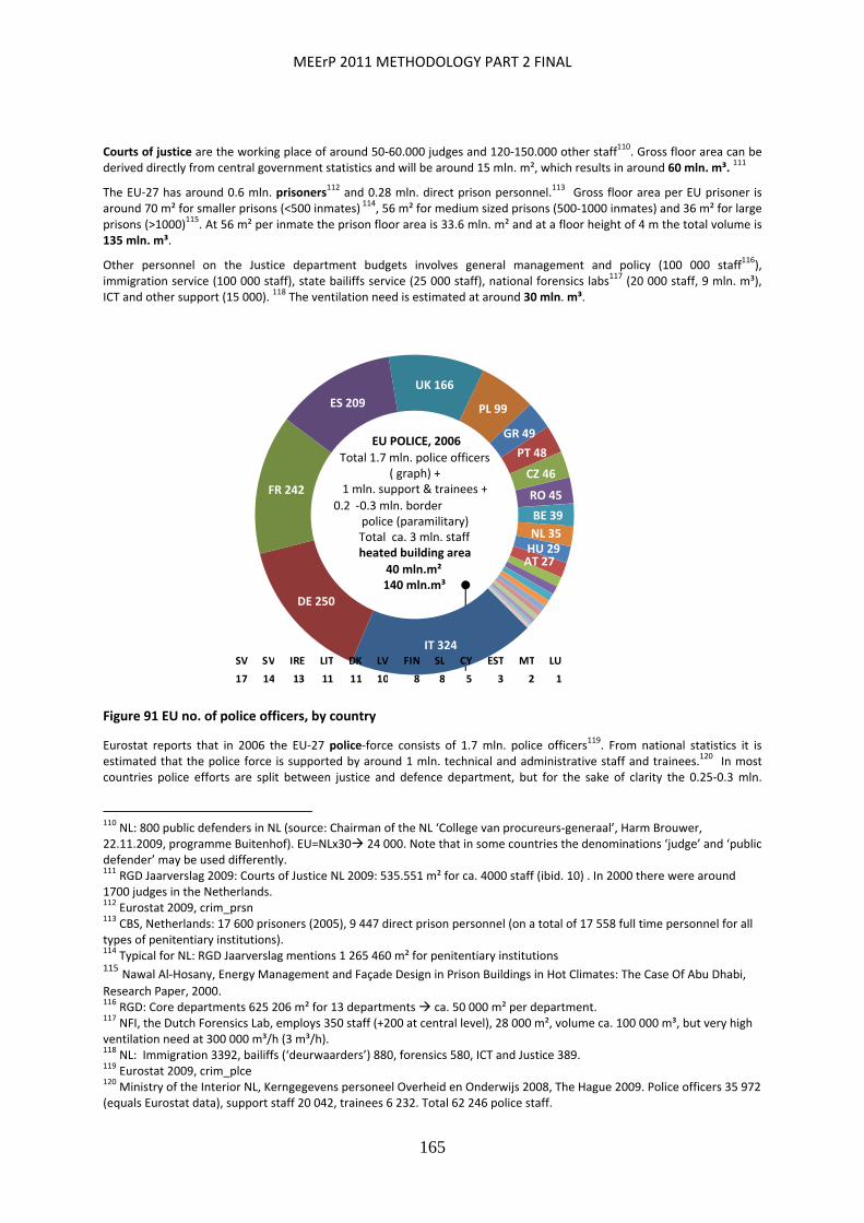
MEErP 2011 METHODOLOGY PART 2 FINAL
165
Courts of justice are the working place of around 50‐60.000 judges and 120‐150.000 other staff110. Gross floor area can be derived directly from central government statistics and will be around 15 mln. m², which results in around 60 mln. m³. 111
The EU‐27 has around 0.6 mln. prisoners112 and 0.28 mln. direct prison personnel.113 Gross floor area per EU prisoner is
around 70 m² for smaller prisons (<500 inmates) 114, 56 m² for medium sized prisons (500‐1000 inmates) and 36 m² for large prisons (>1000)
115. At 56 m² per inmate the prison floor area is 33.6 mln. m² and at a floor height of 4 m the total volume is 135 mln. m³.
Other personnel on the Justice department budgets involves general management and policy (100 000 staff116),
immigration service (100 000 staff), state bailiffs service (25 000 staff), national forensics labs117 (20 000 staff, 9 mln. m³), ICT and other support (15 000). 118 The ventilation need is estimated at around 30 mln. m³.
Eurostat reports that in 2006 the EU‐27 police‐force consists of 1.7 mln. police officers119. From national statistics it is estimated that the police force is supported by around 1 mln. technical and administrative staff and trainees.120 In most countries police efforts are split between justice and defence department, but for the sake of clarity the 0.25‐0.3 mln.
110 NL: 800 public defenders in NL (source: Chairman of the NL ‘College van procureurs‐generaal’, Harm Brouwer, 22.11.2009, programme Buitenhof). EU=NLx30 24 000. Note that in some countries the denominations ‘judge’ and ‘public defender’ may be used differently. 111 RGD Jaarverslag 2009: Courts of Justice NL 2009: 535.551 m² for ca. 4000 staff (ibid. 10) . In 2000 there were around 1700 judges in the Netherlands. 112 Eurostat 2009, crim_prsn 113 CBS, Netherlands: 17 600 prisoners (2005), 9 447 direct prison personnel (on a total of 17 558 full time personnel for all types of penitentiary institutions). 114 Typical for NL: RGD Jaarverslag mentions 1 265 460 m² for penitentiary institutions 115 Nawal Al‐Hosany, Energy Management and Façade Design in Prison Buildings in Hot Climates: The Case Of Abu Dhabi,
Research Paper, 2000. 116 RGD: Core departments 625 206 m² for 13 departments ca. 50 000 m² per department. 117 NFI, the Dutch Forensics Lab, employs 350 staff (+200 at central level), 28 000 m², volume ca. 100 000 m³, but very high ventilation need at 300 000 m³/h (3 m³/h). 118 NL: Immigration 3392, bailiffs (‘deurwaarders’) 880, forensics 580, ICT and Justice 389. 119 Eurostat 2009, crim_plce 120 Ministry of the Interior NL, Kerngegevens personeel Overheid en Onderwijs 2008, The Hague 2009. Police officers 35 972 (equals Eurostat data), support staff 20 042, trainees 6 232. Total 62 246 police staff.
Figure 91 EU no. of police officers, by country
IT 324
DE 250
FR 242
ES 209
UK 166
PL 99
GR 49
PT 48
CZ 46
RO 45
BE 39
NL 35HU 29AT 27
EU POLICE, 2006
Total 1.7 mln. police officers ( graph) +
1 mln. support & trainees +
0.2 ‐0.3 mln. border police (paramilitary)Total ca. 3 mln. staffheated building area
40 mln.m²140 mln.m³
SV SV IRE LIT DK LV FIN SL CY EST MT LU 17 14 13 11 11 10 8 8 5 3 2 1

MEErP 2011 METHODOLOGY PART 2 FINAL
166
paramilitary forces working as border police, coast guard and customs guards are classified as ‘police’ and have to be added to the 1.7 mln. staff reported by Eurostat. Statistics on heated gross floor area of buildings are scarce, but from anecdotal evidence a figure of 10 m² per person is estimated.121 At around 3 mln. personnel this brings the total heated floor area to approximately 30 mln. m² and a volume of around 110 mln. m³. An archetype police station (small city) has around 800‐1000 m² heated floor area. Building sizes ranges from <100 m² (small village) to >25.000 m² (regional head office or larger city).
6.7.4 Defence
The EU Defence departments employs around 2.1 mln. active military staff 122 (2004), with around 15% (300.000) civilian support staff. The number of reservists varies widely per country, but they are not estimated to take up heated floor area (training facilities partitioned to active military staff). Para‐military forces are not included under this heading, but included under the heading ‘police’. Total headcount of employees under the heading ‘Defence’ is thus estimated at 2.4 mln. For the heated gross floor area only anecdotal were found, but is estimated at around 15 m² per person.123 This results in 40 mln. m² floor area and an estimated 140 mln. m³ of heated volume.
124 Note that this is 0.15% of the EU total, i.e. considerably
less than the 0.7% estimated in the diagram
121 Netherlands has 15% state police (military police (6800 staff), national police force KLPD (5000 staff) ) and 85% regional police. State police (RGD 2009) takes up 85.959 m² (ca. 5400 officers). 122 Active military staff: Wikipedia.nl. Ratio civilians/military taken from ibid. 11. 123 Netherlands (53.150 military) occupies 47 army bases (Wikipedia). Gross floor area of buildings is around 25.000‐40.000 m². Part of this will be unheated. Estimated is 15.000 m² of heated floor area for around 1000 personnel. 124 Netherlands (professional army only): 67.000 personnel, 85.496 m² gross floor area. In countries with drafted personnel specific floor area is believed to be factor 2 higher.
DE 284FR 259
IT 230
UK 188
ES 178
GR 178 PL 164
RO 94
BU 68
CZ 57
NL 53
PT 45BE 41
EU MILITARY, 2004
Total 2,1 mln. activemilitary ( graph) +0,3 mln. support
Total ca. 2,4 mln. staffca. 50.000 heated buildings
40 mln.m2140 mln.m3
FIN AT SV HU SK DK LIT IRE SL EST LV MT LU
37 35 34 33 26 23 14 11 7 6 5 2 1
Figure 92 Defence dept., EU military personell by country
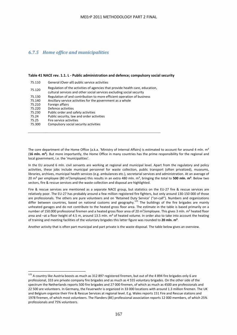
MEErP 2011 METHODOLOGY PART 2 FINAL
167
6.7.5 Homeofficeandmunicipalities
Table 41 NACE rev. 1.1. L ‐ Public administration and defence; compulsory social security
75.110 General (Over‐all) public service activities
75.120 Regulation of the activities of agencies that provide health care, education, cultural services and other social services excluding social security
75.130 Regulation of and contribution to more efficient operation of business75.140 Ancillary service activities for the government as a whole75.210 Foreign affairs 75.220 Defence activities 75.230 Public order and safety activities 75.24 Public security, law and order activities75.25 Fire service activities 75.300 Compulsory social security activities
The core department of the Home Office (a.k.a. ‘Ministry of Internal Affairs) is estimated to account for around 4 mln. m² (16 mln. m³). But more importantly, the Home Office in many countries has the prime responsibility for the regional and local government, i.e. the ‘municipalities’.
In the EU around 6 mln. civil servants are working at regional and municipal level. Apart from the regulatory and policy activities, these jobs include municipal personnel for waste collection, public transport (often privatized), museums, libraries, archives, municipal health services (e.g. ambulances etc.), secretarial services and administration. At an average of 20 m² per employee (80 m³/employee) this results in an extra 480 mln. m³, bringing the total to 500 mln. m³. Below two sectors, fire & rescue services and the waste collection and disposal are highlighted.
Fire & rescue services are mentioned as a separate NACE group, but statistics on the EU‐27 fire & rescue services are relatively poor. The EU‐27 has probably around a few million registered fire fighters, but only around 130‐150 000 of those are professionals. The others are pure volunteers and on ‘Retained Duty Service’ (“on‐call”). Numbers and organizations differ between countries, based on national customs and geography.125 The buildings of the fire brigades are mainly unheated garages and do not contribute to the heated gross floor area. The estimate in the table is based primarily on a number of 150.000 professional firemen and a heated gross floor area of 20 m²/employee. This gives 3 mln. m² heated floor area and –at a floor height of 4.5 m, around 13.5 mln. m³ of heated volume. In order also to take into account the heating of training and meeting facilities of the voluntary brigades this latter figure was rounded to 20 mln. m³.
Another activity that is often part municipal and part private is the waste disposal. The table below gives an overview.
125 A country like Austria boosts as much as 312 897 registered firemen, but out of the 4 894 fire brigades only 6 are professional, 333 are private company fire brigades and as much as 4 555 voluntary brigades. On the other side of the spectrum the Netherlands reports 500 fire brigades and 27 000 firemen, of which as much as 4500 are professionals and 22 500 are volunteers. In Germany, the Feuerwehr is organized in 33 000 locations with around 1.3 million firemen. The UK and Belgium organize their Fire & Rescue Services at regional level. E.g. Wales reports 151 Fire and Rescue stations and 1978 firemen, of which most volunteers. The Flanders (BE) professional association reports 12 000 members, of which 25% professionals and 75% volunteers.
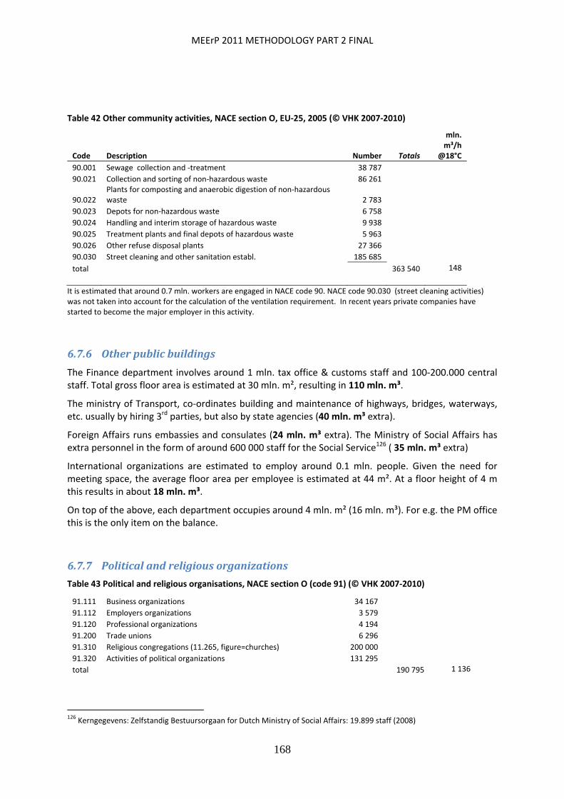
MEErP 2011 METHODOLOGY PART 2 FINAL
168
Table 42 Other community activities, NACE section O, EU‐25, 2005 (© VHK 2007‐2010)
Code Description Number Totals
mln. m³/h
@18°C
90.001 Sewage collection and ‐treatment 38 787
90.021 Collection and sorting of non‐hazardous waste 86 261
90.022 Plants for composting and anaerobic digestion of non‐hazardous waste 2 783
90.023 Depots for non‐hazardous waste 6 758
90.024 Handling and interim storage of hazardous waste 9 938
90.025 Treatment plants and final depots of hazardous waste 5 963
90.026 Other refuse disposal plants 27 366
90.030 Street cleaning and other sanitation establ. 185 685
total 363 540 148
It is estimated that around 0.7 mln. workers are engaged in NACE code 90. NACE code 90.030 (street cleaning activities) was not taken into account for the calculation of the ventilation requirement. In recent years private companies have started to become the major employer in this activity.
6.7.6 Otherpublicbuildings
The Finance department involves around 1 mln. tax office & customs staff and 100‐200.000 central staff. Total gross floor area is estimated at 30 mln. m², resulting in 110 mln. m³.
The ministry of Transport, co‐ordinates building and maintenance of highways, bridges, waterways, etc. usually by hiring 3rd parties, but also by state agencies (40 mln. m³ extra).
Foreign Affairs runs embassies and consulates (24 mln. m³ extra). The Ministry of Social Affairs has extra personnel in the form of around 600 000 staff for the Social Service126 ( 35 mln. m³ extra)
International organizations are estimated to employ around 0.1 mln. people. Given the need for meeting space, the average floor area per employee is estimated at 44 m². At a floor height of 4 m this results in about 18 mln. m³.
On top of the above, each department occupies around 4 mln. m² (16 mln. m³). For e.g. the PM office this is the only item on the balance.
6.7.7 Politicalandreligiousorganizations
Table 43 Political and religious organisations, NACE section O (code 91) (© VHK 2007‐2010)
91.111 Business organizations 34 167
91.112 Employers organizations 3 579
91.120 Professional organizations 4 194
91.200 Trade unions 6 296
91.310 Religious congregations (11.265, figure=churches) 200 000
91.320 Activities of political organizations 131 295
total 190 795 1 136
126 Kerngegevens: Zelfstandig Bestuursorgaan for Dutch Ministry of Social Affairs: 19.899 staff (2008)
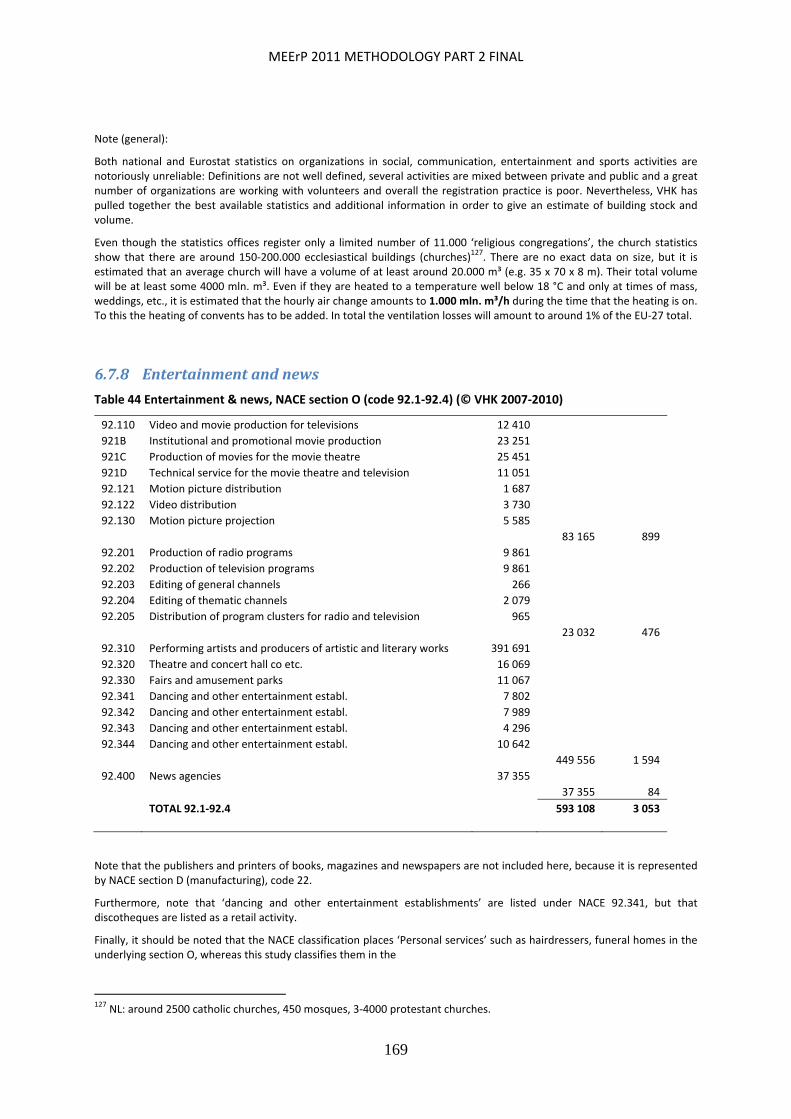
MEErP 2011 METHODOLOGY PART 2 FINAL
169
Note (general):
Both national and Eurostat statistics on organizations in social, communication, entertainment and sports activities are notoriously unreliable: Definitions are not well defined, several activities are mixed between private and public and a great number of organizations are working with volunteers and overall the registration practice is poor. Nevertheless, VHK has pulled together the best available statistics and additional information in order to give an estimate of building stock and volume.
Even though the statistics offices register only a limited number of 11.000 ‘religious congregations’, the church statistics show that there are around 150‐200.000 ecclesiastical buildings (churches)
127. There are no exact data on size, but it is estimated that an average church will have a volume of at least around 20.000 m³ (e.g. 35 x 70 x 8 m). Their total volume will be at least some 4000 mln. m³. Even if they are heated to a temperature well below 18 °C and only at times of mass, weddings, etc., it is estimated that the hourly air change amounts to 1.000 mln. m³/h during the time that the heating is on. To this the heating of convents has to be added. In total the ventilation losses will amount to around 1% of the EU‐27 total.
6.7.8 Entertainmentandnews
Table 44 Entertainment & news, NACE section O (code 92.1‐92.4) (© VHK 2007‐2010)
92.110 Video and movie production for televisions 12 410
921B Institutional and promotional movie production 23 251
921C Production of movies for the movie theatre 25 451
921D Technical service for the movie theatre and television 11 051
92.121 Motion picture distribution 1 687
92.122 Video distribution 3 730
92.130 Motion picture projection 5 585
83 165 899
92.201 Production of radio programs 9 861
92.202 Production of television programs 9 861
92.203 Editing of general channels 266
92.204 Editing of thematic channels 2 079
92.205 Distribution of program clusters for radio and television 965
23 032 476
92.310 Performing artists and producers of artistic and literary works 391 691
92.320 Theatre and concert hall co etc. 16 069
92.330 Fairs and amusement parks 11 067
92.341 Dancing and other entertainment establ. 7 802
92.342 Dancing and other entertainment establ. 7 989
92.343 Dancing and other entertainment establ. 4 296
92.344 Dancing and other entertainment establ. 10 642
449 556 1 594
92.400 News agencies 37 355
37 355 84
TOTAL 92.1‐92.4 593 108 3 053
Note that the publishers and printers of books, magazines and newspapers are not included here, because it is represented by NACE section D (manufacturing), code 22.
Furthermore, note that ‘dancing and other entertainment establishments’ are listed under NACE 92.341, but that discotheques are listed as a retail activity.
Finally, it should be noted that the NACE classification places ‘Personal services’ such as hairdressers, funeral homes in the underlying section O, whereas this study classifies them in the
127 NL: around 2500 catholic churches, 450 mosques, 3‐4000 protestant churches.
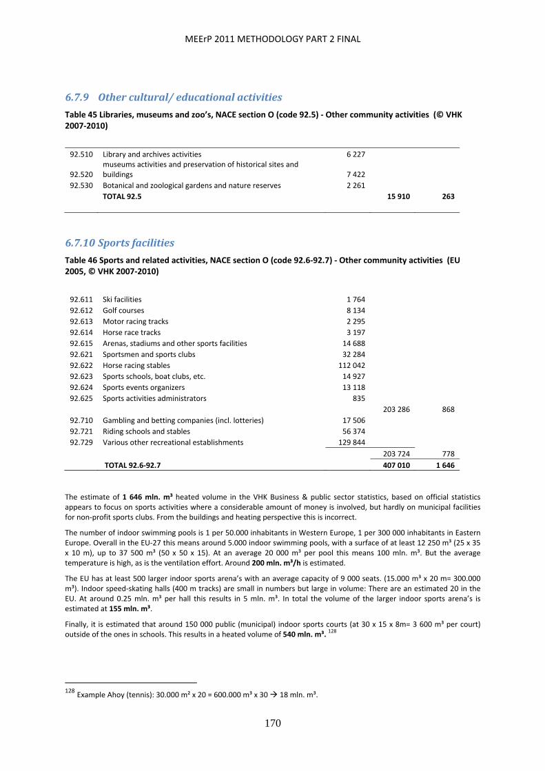
MEErP 2011 METHODOLOGY PART 2 FINAL
170
6.7.9 Othercultural/educationalactivities
Table 45 Libraries, museums and zoo’s, NACE section O (code 92.5) ‐ Other community activities (© VHK 2007‐2010)
92.510 Library and archives activities 6 227
92.520 museums activities and preservation of historical sites and buildings 7 422
92.530 Botanical and zoological gardens and nature reserves 2 261
TOTAL 92.5 15 910 263
6.7.10 Sportsfacilities
Table 46 Sports and related activities, NACE section O (code 92.6‐92.7) ‐ Other community activities (EU 2005, © VHK 2007‐2010)
92.611 Ski facilities 1 764
92.612 Golf courses 8 134
92.613 Motor racing tracks 2 295
92.614 Horse race tracks 3 197
92.615 Arenas, stadiums and other sports facilities 14 688
92.621 Sportsmen and sports clubs 32 284
92.622 Horse racing stables 112 042
92.623 Sports schools, boat clubs, etc. 14 927
92.624 Sports events organizers 13 118
92.625 Sports activities administrators 835
203 286 868
92.710 Gambling and betting companies (incl. lotteries) 17 506
92.721 Riding schools and stables 56 374
92.729 Various other recreational establishments 129 844
203 724 778
TOTAL 92.6‐92.7 407 010 1 646
The estimate of 1 646 mln. m³ heated volume in the VHK Business & public sector statistics, based on official statistics appears to focus on sports activities where a considerable amount of money is involved, but hardly on municipal facilities for non‐profit sports clubs. From the buildings and heating perspective this is incorrect.
The number of indoor swimming pools is 1 per 50.000 inhabitants in Western Europe, 1 per 300 000 inhabitants in Eastern Europe. Overall in the EU‐27 this means around 5.000 indoor swimming pools, with a surface of at least 12 250 m³ (25 x 35 x 10 m), up to 37 500 m³ (50 x 50 x 15). At an average 20 000 m³ per pool this means 100 mln. m³. But the average temperature is high, as is the ventilation effort. Around 200 mln. m³/h is estimated.
The EU has at least 500 larger indoor sports arena’s with an average capacity of 9 000 seats. (15.000 m³ x 20 m= 300.000 m³). Indoor speed‐skating halls (400 m tracks) are small in numbers but large in volume: There are an estimated 20 in the EU. At around 0.25 mln. m³ per hall this results in 5 mln. m³. In total the volume of the larger indoor sports arena’s is estimated at 155 mln. m³.
Finally, it is estimated that around 150 000 public (municipal) indoor sports courts (at 30 x 15 x 8m= 3 600 m³ per court) outside of the ones in schools. This results in a heated volume of 540 mln. m³. 128
128 Example Ahoy (tennis): 30.000 m² x 20 = 600.000 m³ x 30 18 mln. m³.

MEErP 2011 METHODOLOGY PART 2 FINAL
171
In total, excluding the facilities in educational institutions, the ventilation need in sports facilities is estimated at 2 541 mln.
m³. Note that this is considerably less than the 3.2 % (3 520 mln. m³) estimated in Error! Reference source not found..
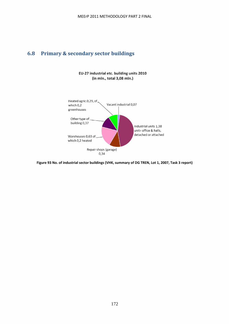
MEErP 2011 METHODOLOGY PART 2 FINAL
172
6.8 Primary&secondarysectorbuildings
Figure 93 No. of industrial sector buildings (VHK, summary of DG TREN, Lot 1, 2007, Task 3 report)
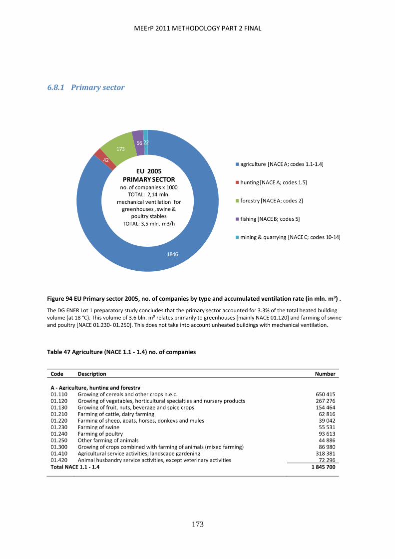
MEErP 2011 METHODOLOGY PART 2 FINAL
173
6.8.1 Primarysector
1846
42
17356 22
EU 2005PRIMARY SECTORno. of companies x 1000
TOTAL: 2,14 mln.
mechanical ventilation forgreenhouses , swine &
poultry stables
TOTAL: 3,5 mln. m3/h
agriculture [NACE A; codes 1.1‐1.4]
hunting [NACE A; codes 1.5]
forestry [NACE A; codes 2]
fishing [NACE B; codes 5]
mining & quarrying [NACE C; codes 10‐14]
Figure 94 EU Primary sector 2005, no. of companies by type and accumulated ventilation rate (in mln. m³) . The DG ENER Lot 1 preparatory study concludes that the primary sector accounted for 3.3% of the total heated building volume (at 18 °C). This volume of 3.6 bln. m³ relates primarily to greenhouses [mainly NACE 01.120] and farming of swine and poultry [NACE 01.230‐ 01.250]. This does not take into account unheated buildings with mechanical ventilation.
Table 47 Agriculture (NACE 1.1 ‐ 1.4) no. of companies
Code Description Number
A ‐ Agriculture, hunting and forestry 01.110 Growing of cereals and other crops n.e.c. 650 41501.120 Growing of vegetables, horticultural specialties and nursery products 267 27601.130 Growing of fruit, nuts, beverage and spice crops 154 46401.210 Farming of cattle, dairy farming 62 81601.220 Farming of sheep, goats, horses, donkeys and mules 39 04201.230 Farming of swine 55 53101.240 Farming of poultry 93 61301.250 Other farming of animals 44 88601.300 Growing of crops combined with farming of animals (mixed farming) 86 98001.410 Agricultural service activities; landscape gardening 318 38101.420 Animal husbandry service activities, except veterinary activities 72 296Total NACE 1.1 ‐ 1.4 1 845 700
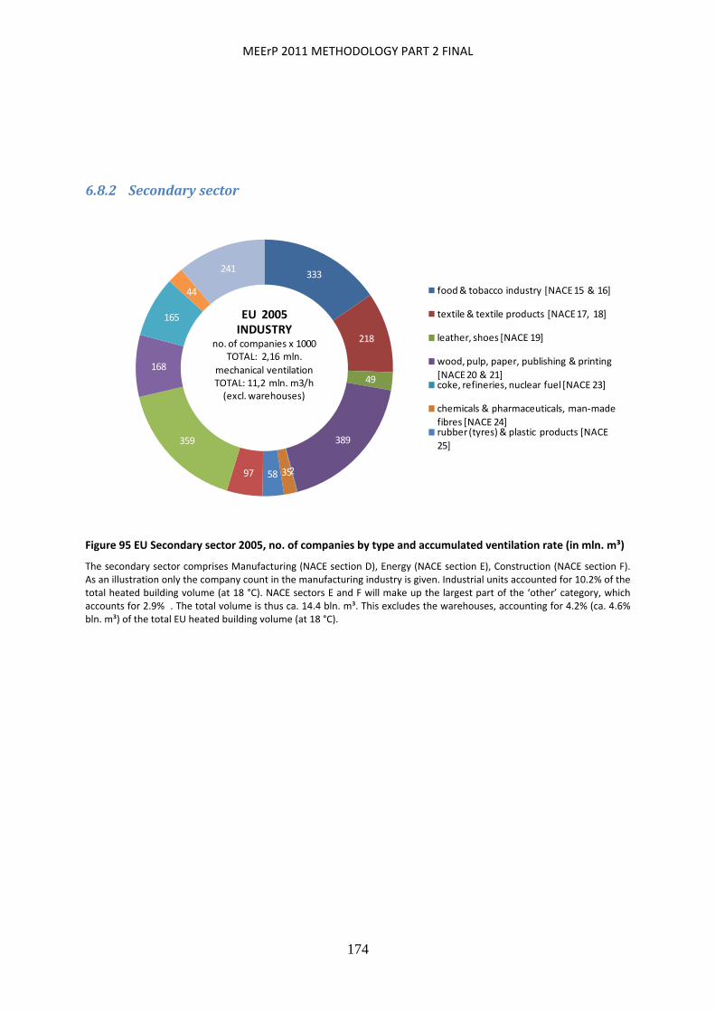
MEErP 2011 METHODOLOGY PART 2 FINAL
174
6.8.2 Secondarysector
333
218
49
389
2355897
359
168
165
44
241
EU 2005INDUSTRY
no. of companies x 1000TOTAL: 2,16 mln.
mechanical ventilation TOTAL: 11,2 mln. m3/h (excl. warehouses)
food & tobacco industry [NACE 15 & 16]
textile & textile products [NACE 17, 18]
leather, shoes [NACE 19]
wood, pulp, paper, publishing & printing
[NACE 20 & 21]coke, refineries, nuclear fuel [NACE 23]
chemicals & pharmaceuticals, man‐made
fibres [NACE 24]rubber (tyres) & plastic products [NACE
25]
Figure 95 EU Secondary sector 2005, no. of companies by type and accumulated ventilation rate (in mln. m³)
The secondary sector comprises Manufacturing (NACE section D), Energy (NACE section E), Construction (NACE section F). As an illustration only the company count in the manufacturing industry is given. Industrial units accounted for 10.2% of the total heated building volume (at 18 °C). NACE sectors E and F will make up the largest part of the ‘other’ category, which accounts for 2.9% . The total volume is thus ca. 14.4 bln. m³. This excludes the warehouses, accounting for 4.2% (ca. 4.6% bln. m³) of the total EU heated building volume (at 18 °C).

MEErP 2011 METHODOLOGY PART 2 FINAL
175
Table 48 EU‐27 Manufacturing industry 2005, NACE Section D (Eurostat, 2009)
Value added Employment
EUR billion % x1000 %
Manufacturing (NACE Section D) 1 629.9 100.0% 34 644 99.8%
Food products; beverages and tobacco (DA) 199.1 12.2% 4 700 13.6%
Textiles and textile products (DB) 53.3 3.3% 2 614 7.5%
Leather and leather products (DC) 11.4 0.7% 564 1.6%
Wood and wood products (DD) 35.1 2.2% 1 280 3.7%
Pulp, paper and paper products; publishing and printing (DE) 134.7 8.3% 2 562 7.4%
Coke, refined petroleum products and nuclear fuel (DF) 38.5 2.4% 170 0.5%
Chemicals, chemical products and man‐made fibres (DG) 178.5 10.9% 1 888 5.5%
Rubber and plastic products (DH) 76.1 4.7% 1 700 4.9%
Other non‐metallic mineral products (DI) 73.5 4.5% 1 596 4.6%
Basic metals and fabricated metal products (DJ) 221.9 13.6% 5 045 14.6%
Machinery and equipment n.e.c. (DK) 178.4 10.9% 3 636 10.5%
Electrical and optical equipment (DL) 189.8 11.6% 3 664 10.6%
Transport equipment (DM) 181.9 11.2% 3 152 9.1%
Manufacturing n.e.c. (DN) 57.7 3.5% 1 988 5.7%
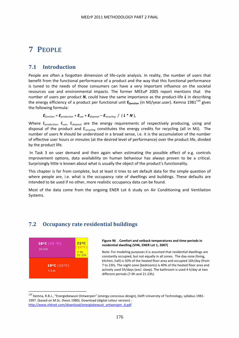
MEErP 2011 METHODOLOGY PART 2 FINAL
176
7 PEOPLE
7.1 IntroductionPeople are often a forgotten dimension of life‐cycle analysis. In reality, the number of users that benefit from the functional performance of a product and the way that this functional performance is tuned to the needs of those consumers can have a very important influence on the societal resources use and environmental impacts. The former MEEuP 2005 report mentions that the number of users per product N, could have the same importance as the product‐life L in describing the energy efficiency of a product per functional unit Efunction (in MJ/year.user). Kemna 1981129 gives the following formula:
Efunction = Eproduction + Euse + Edisposal – Erecycling / ( L * N ),
Where Eproduction, Euse, Edisposal are the energy requirements of respectively producing, using and disposal of the product and Erecycling constitutes the energy credits for recycling (all in MJ). The number of users N should be understood in a broad sense, i.e. it is the accumulation of the number of effective user hours or minutes (at the desired level of performance) over the product life, divided by the product life.
In Task 3 on user demand and then again when estimating the possible effect of e.g. controls improvement options, data availability on human behaviour has always proven to be a critical. Surprisingly little is known about what is usually the object of the product’s functionality.
This chapter is far from complete, but at least it tries to set default data for the simple question of where people are, i.e. what is the occupancy rate of dwellings and buildings. These defaults are intended to be used if no other, more realistic occupancy data can be found.
Most of the data come from the ongoing ENER Lot 6 study on Air Conditioning and Ventilation Systems.
7.2 Occupancyrateresidentialbuildings
129 Kemna, R.B.J., “Energiebewust Ontwerpen” (energy‐conscious design), Delft University of Technology, syllabus 1981‐1997. (based on M.Sc. thesis 1980). Download (digital colour version) : http://www.vhknet.com/download/energiebewust_ontwerpen_d.pdf
Figure 96 . Comfort and setback temperatures and time‐periods in residential dwelling (VHK, ENER Lot 1, 2007)
Note: For modeling purposes it is assumed that residential dwellings are constantly occupied, but not equally in all zones. The day‐zone (living, kitchen, hall) is 50% of the heated floor area and occupied 16h/day (from 7 to 23h). The night‐zone (bedrooms) is 40% of the heated floor area and actively used 5h/days (excl. sleep). The bathroom is used 4 h/day at two different periods (7‐9h and 21‐23h).
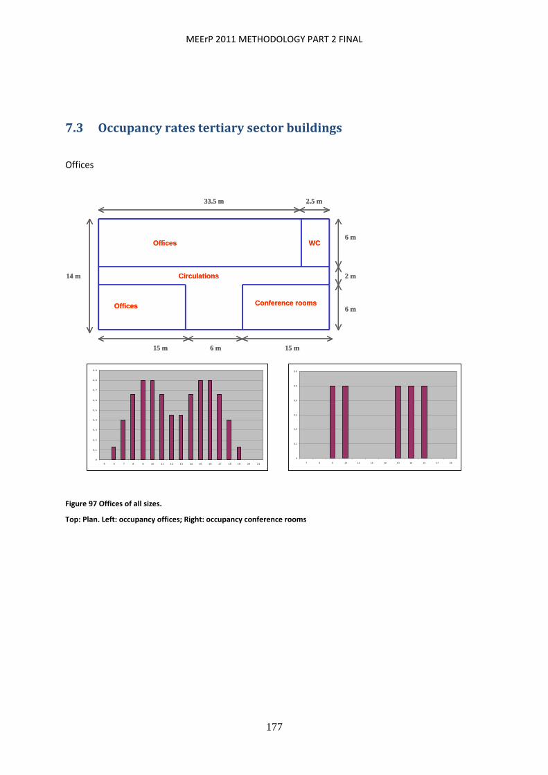
MEErP 2011 METHODOLOGY PART 2 FINAL
177
7.3 Occupancyratestertiarysectorbuildings
Offices
Figure 97 Offices of all sizes.
Top: Plan. Left: occupancy offices; Right: occupancy conference rooms
0
0,1
0,2
0,3
0,4
0,5
0,6
0,7
0,8
0,9
5 6 7 8 9 10 11 12 13 14 15 16 17 18 19 20 21
0
0,1
0,2
0,3
0,4
0,5
0,6
7 8 9 10 11 12 13 14 15 16 17 18
Offices
Offices Conference rooms
Circulations
WC
33.5 m
15 m
14 m 2 m
6 m
6 m
6 m 15 m
2.5 m
Offices
Offices Conference rooms
Circulations
WC
33.5 m
15 m
14 m 2 m
6 m
6 m
6 m 15 m
2.5 m
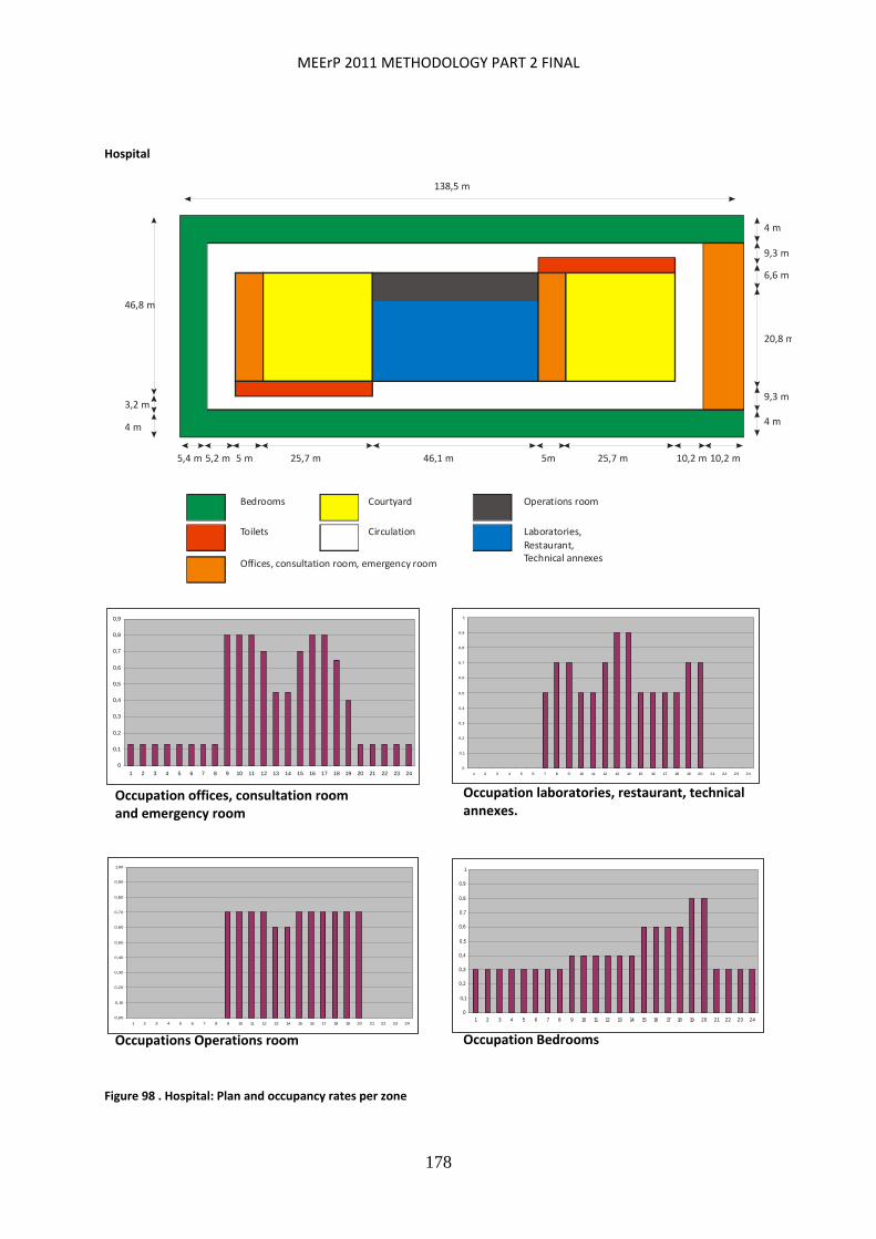
MEErP 2011 METHODOLOGY PART 2 FINAL
178
Hospital
Figure 98 . Hospital: Plan and occupancy rates per zone
Occupation laboratories, restaurant, technical annexes.
Occupation offices, consultation room and emergency room
Occupations Operations room Occupation Bedrooms
0
0,1
0,2
0,3
0,4
0,5
0,6
0,7
0,8
0,9
1 2 3 4 5 6 7 8 9 10 11 12 13 14 15 16 17 18 19 20 21 22 23 240
0,1
0,2
0,3
0,4
0,5
0,6
0,7
0,8
0,9
1
1 2 3 4 5 6 7 8 9 10 11 12 13 14 15 16 17 18 19 20 21 22 23 24
0,00
0,10
0,20
0,30
0,40
0,50
0,60
0,70
0,80
0,90
1,00
1 2 3 4 5 6 7 8 9 10 11 12 13 14 15 16 17 18 19 20 21 22 23 24
0
0,1
0,2
0,3
0,4
0,5
0,6
0,7
0,8
0,9
1
1 2 3 4 5 6 7 8 9 10 11 12 13 14 15 16 17 18 19 20 21 22 23 24
Operations roomBedrooms
Circulation
Courtyard
Toilets
Offices, consultation room, emergency room
Laboratories,
Restaurant, Technical annexes
138,5 m
46,8 m
3,2 m
4 m
5,4 m 5,2 m 5 m 25,7 m 46,1 m 5m 25,7 m 10,2 m 10,2 m
4 m
9,3 m
20,8 m
6,6 m
9,3 m
4 m
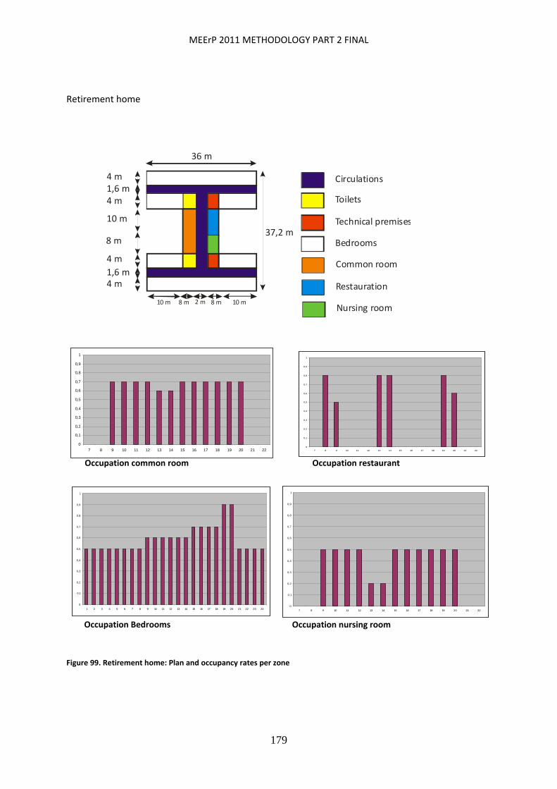
MEErP 2011 METHODOLOGY PART 2 FINAL
179
Retirement home
Figure 99. Retirement home: Plan and occupancy rates per zone
Circulations
Toilets
Bedrooms
Restauration
Nursing room
Common room
Technical premises
4 m
36 m
37,2 m
4 m
4 m
10 m 8 m 2 m 8 m 10 m
1,6 m
10 m
8 m
1,6 m4 m
Occupation Bedrooms Occupation nursing room
0
0,1
0,2
0,3
0,4
0,5
0,6
0,7
0,8
0,9
1
1 2 3 4 5 6 7 8 9 10 11 12 13 14 15 16 17 18 19 20 21 22 23 240
0,1
0,2
0,3
0,4
0,5
0,6
0,7
0,8
0,9
1
7 8 9 10 11 12 13 14 15 16 17 18 19 20 21 22
Occupation common room Occupation restaurant
0
0,1
0,2
0,3
0,4
0,5
0,6
0,7
0,8
0,9
1
7 8 9 10 11 12 13 14 15 16 17 18 19 20 21 220
0,1
0,2
0,3
0,4
0,5
0,6
0,7
0,8
0,9
1
7 8 9 10 11 12 13 14 15 16 17 18 19 20 21 22

MEErP 2011 METHODOLOGY PART 2 FINAL
180
Hotel
Figure 100 Hotel: Plan and occupancy rates per zone
Offices Hall and utilities
Kitchen
Passages
Restau
rant
GROUND FLOOR
10 m 13,6 m
6,2 m
29,7 m
21,7 m
14,2m
15,5 m 21,6 m
37 m 8,2 mSTOREY
Bedrooms BedroomsWC
Passages
Bedrooms
Bedrooms
6,2 m
2,1 m
5,1 m
5,4 m
12,6 m
60,7 m
6,2 m
Monday Tuesday Wednesday Thursday Friday Saturday Sunday
40
0
Monday Thursday Saturday SundayFridayTuesday Wednesday
Monday Tuesday Wednesday Thursday Friday Saturday Sunday
100
0
Monday Tuesday Wednesday Thursday Friday Saturday Sunday
90
0
Monday Tuesday Wednesday Thursday Friday Saturday Sunday
100
0
OCCUPANCY KITCHEN
OCCUPANCY OFFICES
OCCUPANCY ROOMS
OCCUPANCY ROOMS
OCCUPANCY PASSAGEWAYS (FLOORS)
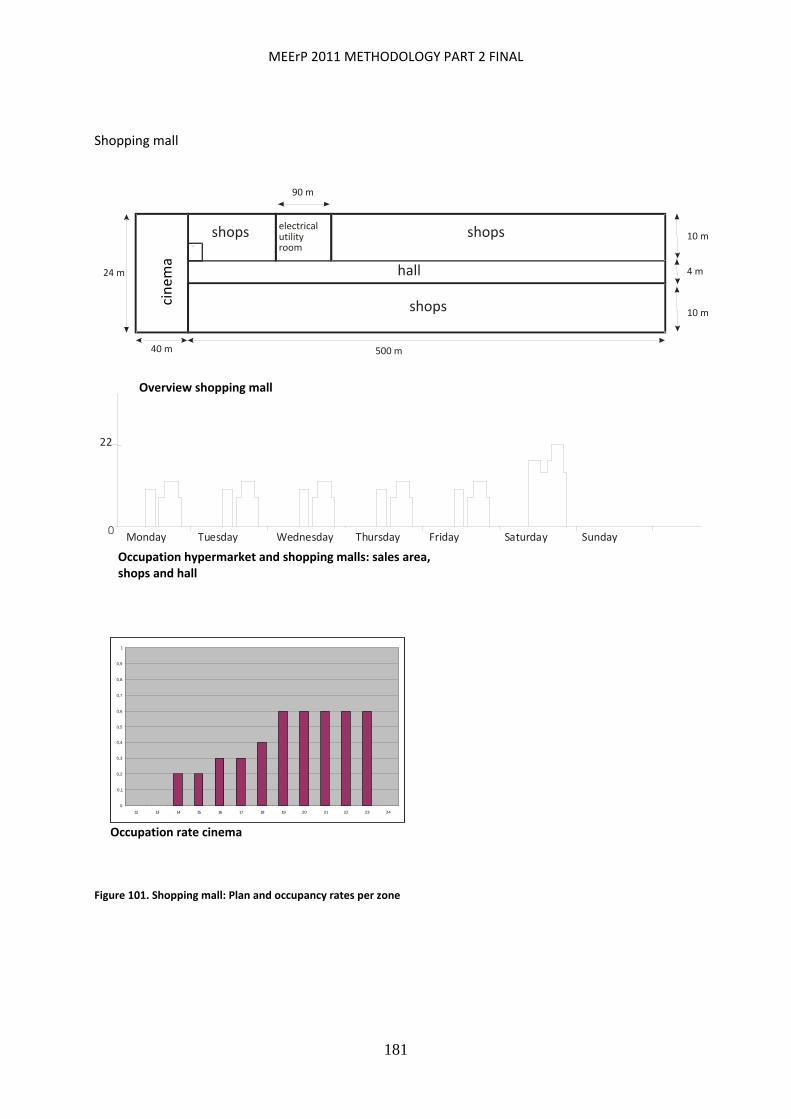
MEErP 2011 METHODOLOGY PART 2 FINAL
181
Shopping mall
Figure 101. Shopping mall: Plan and occupancy rates per zone
Overview shopping mall
shops
shops shopsWC
hall
cinem
a
electrical utility 10 m
10 m
90 m
500 m
24 m
40 m
4 m
room
Occupation hypermarket and shopping malls: sales area, shops and hall
22
0 Monday Tuesday ThursdayWednesday Friday Sunday Saturday
0
0,1
0,2
0,3
0,4
0,5
0,6
0,7
0,8
0,9
1
12 13 14 15 16 17 18 19 20 21 22 23 24
Occupation rate cinema
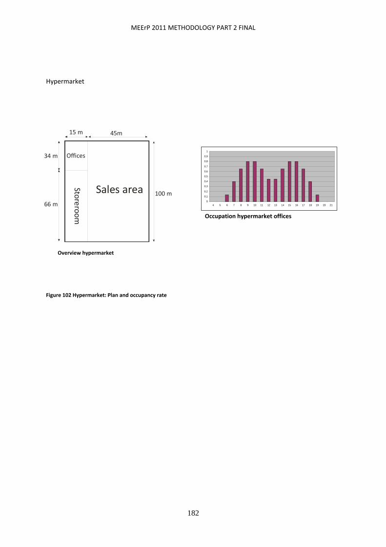
MEErP 2011 METHODOLOGY PART 2 FINAL
182
Hypermarket
Figure 102 Hypermarket: Plan and occupancy rate
Overview hypermarket
Sales areaStoreroom
Offices34 m
15 m 45m
100 m
66 m0
0,1
0,2
0,3
0,4
0,5
0,6
0,7
0,8
0,9
1
4 5 6 7 8 9 10 11 12 13 14 15 16 17 18 19 20 21
Occupation hypermarket offices
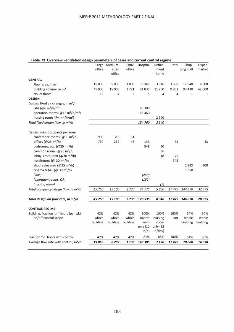
MEErP 2011 METHODOLOGY PART 2 FINAL
183
Table 49 Overview ventilation design parameters of cases and current control regime
Large office
Medium‐sized office
Small office
Hospital Retire‐ment home
Hotel Shop‐ping mall
Hyper‐market
GENERAL
Floor area, in m² 15 000 5 000 1 008 30 345 3 916 3 668 12 940 6.000
Building volume, in m³ 45 000 15 000 2 721 91 035 11 750 9 832 93 430 42.000
No. of floors 12 4 2 5 4 4 1 1
DESIGN
Design: fixed air changes, in m³/h
labs (@6 m³/h/m³) 86 300
operation rooms (@15 m³/h/m³) 68 460
nursing room (@4 m³/h/m³) 2 340
Total fixed design flow, in m³/h 154 760 2 340
Design: max. occupants per zone
conference rooms (@30 m³/h) 900 310 51
offices (@25 m³/h) 750 232 48 143 75 43
bedrooms, etc. (@25 m³/h) 848 90
common room (@25 m³/h) 96
lobby, restaurant (@30 m³/h) 48 175
hotelrooms (@ 30 m³/h) 345
shop, sales area (@35 m³/h) 2 982 900
cinema & hall (@ 30 m³/h) 1 350
(labs) (240)
(operation rooms, OR) (152)
(nursing room) (7)
Total occupancy design flow, in m³/h 45.750 15 100 2 730 24 775 5 850 17 475 144 870 32 575
Total design air flow rate, in m³/h 45.750 15 100 2 730 179 535 8 340 17 475 146 870 28 075
CONTROL REGIME
Building, fraction 'on' hours (per wk) 42% 42% 42% 100% 100% 100% 54% 50%
on/off control scope whole building
whole building
whole building
operatroom
only (12 h/d)
nursing room
only (12 h/day)
not whole building
whole building
Fraction 'on' hours with control 42% 42% 42% 81% 86% 100% 54% 50%
Average flow rate with control, m³/h 19.063 6 292 1 138 145 305 7 170 17 475 78 680 14 038
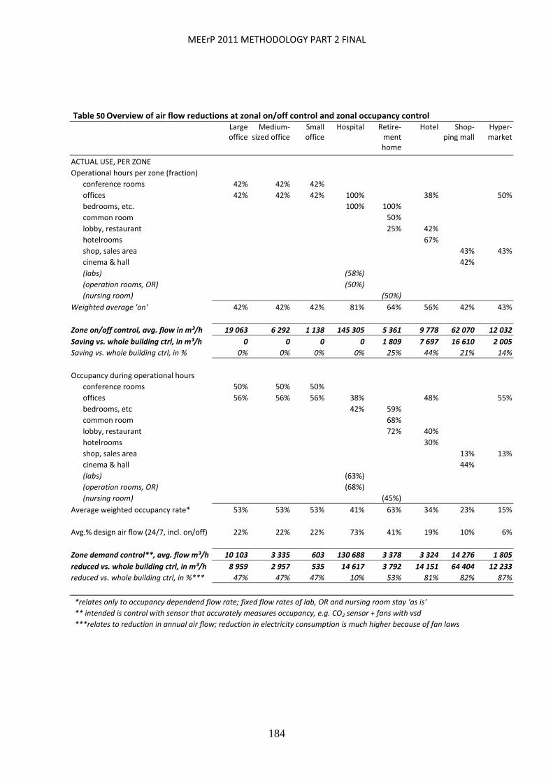
MEErP 2011 METHODOLOGY PART 2 FINAL
184
Table 50 Overview of air flow reductions at zonal on/off control and zonal occupancy control
Large office
Medium‐sized office
Small office
Hospital Retire‐ment home
Hotel Shop‐ping mall
Hyper‐market
ACTUAL USE, PER ZONE
Operational hours per zone (fraction)
conference rooms 42% 42% 42%
offices 42% 42% 42% 100% 38% 50%
bedrooms, etc. 100% 100%
common room 50%
lobby, restaurant 25% 42%
hotelrooms 67%
shop, sales area 43% 43%
cinema & hall 42%
(labs) (58%)
(operation rooms, OR) (50%)
(nursing room) (50%)
Weighted average 'on' 42% 42% 42% 81% 64% 56% 42% 43%
Zone on/off control, avg. flow in m³/h 19 063 6 292 1 138 145 305 5 361 9 778 62 070 12 032
Saving vs. whole building ctrl, in m³/h 0 0 0 0 1 809 7 697 16 610 2 005
Saving vs. whole building ctrl, in % 0% 0% 0% 0% 25% 44% 21% 14%
Occupancy during operational hours
conference rooms 50% 50% 50%
offices 56% 56% 56% 38% 48% 55%
bedrooms, etc 42% 59%
common room 68%
lobby, restaurant 72% 40%
hotelrooms 30%
shop, sales area 13% 13%
cinema & hall 44%
(labs) (63%)
(operation rooms, OR) (68%)
(nursing room) (45%)
Average weighted occupancy rate* 53% 53% 53% 41% 63% 34% 23% 15%
Avg.% design air flow (24/7, incl. on/off) 22% 22% 22% 73% 41% 19% 10% 6%
Zone demand control**, avg. flow m³/h 10 103 3 335 603 130 688 3 378 3 324 14 276 1 805
reduced vs. whole building ctrl, in m³/h 8 959 2 957 535 14 617 3 792 14 151 64 404 12 233
reduced vs. whole building ctrl, in %*** 47% 47% 47% 10% 53% 81% 82% 87%
*relates only to occupancy dependend flow rate; fixed flow rates of lab, OR and nursing room stay 'as is'
** intended is control with sensor that accurately measures occupancy, e.g. CO2 sensor + fans with vsd
***relates to reduction in annual air flow; reduction in electricity consumption is much higher because of fan laws

MEErP 2011 METHODOLOGY PART 2 FINAL
185
REFERENCES 2030 Water Resource Group: Members include McKinsey & Company, the World Bank Group, and a consortium of business partners: The Barilla Group, The Coca Cola Company, Nestlé SA, New Holland Agriculture, SAB Miller PLC, Standard Chartered and Syngenta AG..
Ærtebjerg et al. (2003) in EEA 2010.
Annual Reports misc. aluminium companies (most recent available June 2011), www.riotintoalcan.com; www.alcoa.com; www.rusal.com.
Babisch, W., Road Traffic Noise and Health Effects, Workshop Copenhagen, Nov. 9‐10, 2006.
BAFU, Bundesamt fuer Umwelt, Switzerland, 2008. ( www.bafu.admin.ch ).
Capros, P. et al., EU Energy Trends To 2030, Update 2009, [PRIMES model], ICCS‐NTUA (E3M Lab) for EUROPEAN COMMISSION Directorate‐General for Energy in collaboration with Climate Action DG and Mobility and Transport DG, European Union, 2010.
COM (2010) 245 final, A Digital Agenda for Europe,
COM(2008) 397 final, Action Plan for sustainable consumption and production (SCP) and sustainable industrial policy (SIP) , 16.7.2008
COM(2008) 400: Communication from the Commission: Public procurement for a better environment.
COM(2009) 693 final, Report On the State of Implementation of Integrated Product Policy, 21.12.2009.
COM(2010) 677 final, Energy infrastructure priorities for 2020 and beyond ‐ A Blueprint for an integrated European energy network, EC, 17.11.2010.
COM (2011) 25 final, Tackling the challenges in commodity markets and on raw materials, 2.2.2011.
COM(2011) 109 final, Energy Efficiency Plan 2011, EC, 8.3.2011.
COM(2011) 112 final, A Roadmap for moving to a competitive low carbon economy in 2050, EC, 8.3.2011.
COM(2011) 21 final, A resource‐efficient Europe – Flagship initiative under the Europe 2020 Strategy, EC, 26.1.2011.
COM(2011) 31 final, Renewable Energy: Progressing towards the 2020 target, EC, 31.1.2011.
Commission Decision 2000/532/EC of 3 May 2000 replacing Decision 94/3/EC establishing a list of wastes pursuant to Article 1(a) of Council Directive 75/442/EEC on waste and Council Decision 94/904/EC establishing a list of hazardous waste pursuant to Article 1(4) of Council Directive 91/689/EEC on hazardous waste.
Commission Decision 2010/571/EU of 24 September 2010 amending, for the purposes of adapting to scientific and technical progress, the Annex to Directive 2002/95/EC of the European Parliament and of the Council as regards exemptions for applications containing lead, mercury, cadmium, hexavalent chromium, polybrominated biphenyls or polybrominated diphenyl ethers.
Convention on Long‐Range Transboundary Air Pollution (LRTAP), published by EEA.
MEErP 2011 METHODOLOGY PART 2 FINAL
186
Critical raw materials (CRM) for the EU, Report of the ad‐hoc Working Group on defining critical raw materials, Version of 30 July 2010; Full report on Enterprise and Industry Directorate General website. Specific source Annex V to this report. http://ec.europa.eu/enterprise/policies/rawmaterials/documents/index_en.htm.
Cullen, J.M., Allwood, J.M., Energy & Materials Efficiency in a Nutshell, presentation, University of Cambridge, Cambridge (UK), 2010.
Decision No 1600/2002/EC of the European Parliament and of the Council of 22 July 2002 laying down the Sixth Community Environment Action Programme of 10 September 2002.
Directive (2004/12/EC) of 11 February 2004 amending Directive 94/62/EC on packaging and packaging waste.
Directive 1999/13/EC on the limitation of emissions of volatile organic compounds due to the use of organic solvents in certain activities and installations, amended by Directive 2004/42/EC on on the limitation of emissions of volatile organic compounds due to the use of organic solvents in certain paints and varnishes and vehicle refinishing products, which in term amended by Directive 2010/79/EU on the adaptation to technical progress of Annex III of Directive 2004/42/EC.
Directive 1999/30/EC of 22 april 1999 relating to limit values for sulphur dioxide, nitrogen dioxide and oxides of nitrogen, particulate matter and lead in ambient air.
Directive 2000/69/EC of 16 november 2000 relating to limit values for benzene and carbon monoxide in ambient air.
Directive 2000/69/EC of 16 November 2000 relating to limit values for benzene and carbon monoxide in ambient air.
Directive 2001/77/EC of 27 September 2001 on the promotion of electricity produced from renewable energy sourcesThe 2003 Biofuels () aimed at 5.75% renewable energy share in transportation by 2010.
Directive 2001/80/EC on Large Comunstion Plants (repealed with effect of 1 Jan. 2016 and replaced by provisions in the Industrial Emissions directive 2010/75/EC).
Directive 2002/3/EC of 12 Feb. 2002 relating to (ground level) ozone in ambient air, where NOx and VOCs should be monitored as precursors of ozone.
Directive 2002/96/EC on waste of electrical and electronic equipment (WEEE).
Directive 2003/30/EC of 8 May 2003 on the promotion of the use of biofuels or other renewable fuels.
Directive 2003/87/EC of 13 October 2003 establishing a scheme for greenhouse gas emission allowance trading within the Community and amending Council Directive 96/61/EC (Emissions Trading Scheme ETS).
Directive 2003/96/EC of 27 October 2003 restructuring the Community framework for the taxation of energy products and electricity (including its planned reform) .
Directive 2004/107/EC of 15 December 2004 relating to arsenic, cadmium, mercury, nickel and polycyclic aromatic hydrocarbons in ambient air.
Directive 2004/17/EC of 31 march 2004 coordinating the procurement procedures of entities operating in the water, energy, transport and postal services sectors and 2004/18/EC of 31 march 2004 on the coordination of procedures for the award of public works contracts, public supply
MEErP 2011 METHODOLOGY PART 2 FINAL
187
contracts and public service contracts. see also http://EC.europa.eu/internal_market/publicprocurement/other_aspects/index_en.htm .
Directive 2004/8/EC on the promotion of cogeneration based on a useful heat demand in the internal energy market and amending Directive 92/42/EEC.
Directive 2006/32/EC of 5 april 2006 on energy end‐use efficiency and energy services and repealing council directive 93/76/EEC.
Directive 2008/105/EC of 16 December 2008 on environmental quality standards in the field of water policy, amending and subsequently repealing Council Directives 82/176/EEC, 83/513/EEC, 84/156/EEC, 84/491/EEC, 86/280/EEC and amending Directive 2000/60/EC of the European Parliament and of the Council.
Directive 2008/50/EC of 21 May 2008 on ambient air quality and cleaner air for Europe.
Directive 2008/98/EC of 19 November 2008 on waste and repealing certain Directives (Waste Framework Directive WFD) repealing 75/439/EEC (Waste Oils Directive), 91/689/EEC (Hazardous Waste Directive) and 2006/12/EC (Waste Directive) with effect from 12 December 2010.
Directive 2009/125/EC of 21 october 2009 establishing a framework for the setting of ecodesign requirements for energy‐related products (Ecodesign directive recast).
Directive 2009/28/EC of 23 April 2009 on the promotion of the use of energy from renewable sources (RES recast).
Directive 2010/30/EC of 19 may 2010 on the indication by labelling and standard product information of the consumption of energy and other resources by energy‐related products (Energy Labelling directive).
Directive 2010/31/EC of 19 may 2010 on the energy performance of buildings (EPBD recast).
Directive 2010/75/EU of 24 november 2010 on industrial emissions (integrated pollution prevention and control).
Directive 91/271/EEC of 21 May 1991 concerning urban waste‐water treatment. UWWTD (Urban Waste Water Treatment Directive)
Directive 96/62/EC of 27 september 1996 on ambient air quality assessment and management
Ecodesign preparatory studies until 2011 (ENER lots 1 – 26, ENTR lots 1 – 6)
Ecofys, Methodology for the free allocation of emission allowances in the EU ETS post 2012, Sector report for the aluminium industry, Ecofys (project leader), Fraunhofer Institute for Systems and Innovation Research, Öko‐Institut,
EEA 2010, Air pollution misc. pub.
EEA CSI 018 — Figure 2 Sectoral water use www.eea.europa.eu/data‐and‐maps/figures/water‐abstractions‐for‐irrigation‐manufacturing‐industry‐energy‐cooling‐and‐public‐water‐supply‐million‐m³‐year‐in‐early‐1990s‐and‐the‐period‐1997‐2005
EEA gap‐filled LRTAP Convention. EEA gap‐filled LRTAP Convention dataviewer based on 2010 officially reported national total and sectoral emissions to UNECE LRTAP Convention, the EU NEC Directive and EU‐MM/UNFCCC. http://dataservice.eea.europa.eu/PivotApp/pivot.aspx?pivotid=478.
EEA Technical report No 4/2008, Air pollution from electricity‐generating large combustion plants, http://www.eea.europa.eu/publications/technical_report_2008_4
MEErP 2011 METHODOLOGY PART 2 FINAL
188
EEA, 2010a. AirBase — The European air quality database, European Environment Agency. www.eea.europa.eu/data‐and‐maps/data/airbase‐the‐european‐air‐quality‐database‐2 .
EEA, 2010a. Annual European Union greenhouse gas inventory 1990–2008 and inventory report 2010. EEA Technical report No 6/2010. European Environment Agency.
EEA, 2010b. EU ETS data viewer. http://dataservice.eea.europa.eu/PivotApp/pivot.aspx?pivotid=473
EEA, 2010b. Exceedance of air quality limit values in urban areas (Indicator CSI 004), European Environment Agency. www.eea.europa.eu/data‐and‐maps/indicators/exceedance‐of‐air‐quality‐limit‐1/exceedance‐of‐air‐quality‐limit‐2 .
EEA, 2010c. Air pollution by ozone across Europe during summer 2009. EEA Technical report No 2/2010, European Environment Agency. www.eea.europa.eu/publications/air‐pollution‐by‐ozone‐across‐europe‐during‐summer‐2009 .
EEA, 2010c. Recession accelerates the decline in EU greenhouse gas emissions. European Environment Agency, Copenhagen. www.eea.europa.eu/highlights/recession‐accelerates‐the‐decline‐in
EEA, 2010d. Core set indicator Global and European temperature (CSI 012) — Assessment published June 2010. www.eea.europa.eu/data‐and‐maps/indicators/global‐and‐european‐temperature/global‐and‐european‐temperature‐assessment‐3
EEA, 2010d. Exposure of ecosystems to acidification, eutrophication and ozone (Version 2, Indicator CSI 005), European Environment Agency. www.eea.europa.eu/themes/air/indicators#c7=all&c5=all&c10=&c13=20&b_start=0&c6=CSI005 .
EEA, 2010e. Core set indicator, Production and consumption of ozone depleting substances (CSI 006) — Assessment published January 2009. www.eea.europa.eu/data‐and‐maps/indicators/production‐and‐consumption‐of‐ozone/production‐and‐consumption‐of‐ozone‐1
EEA, 2010g. NEC Directive status report 2009. EEA Technical Report No 10/2010, European Environment Agency. www.eea.europa.eu/publications/nec‐directive‐status‐report‐2009 .
EEA, 2010h. Emissions (CO2, SO2 and NOx) from public electricity and heat production — explanatory indicators (indicator ENER 009). European Environment Agency. EEA, 2010i. EEA‐32 Heavy metal (HM) emissions (Indicator APE 005), European Environmental Agency. www.eea.europa.eu/data‐and‐maps/indicators/eea32‐heavy‐metal‐hm‐emissions‐1
EEA, 2010j. EEA‐32 Persistent organic pollutant (POP) emissions (Indicator APE 006), European Environment Agency. www.eea.europa.eu/data‐and‐maps/indicators/eea32‐persistent‐organic‐pollutant‐pop‐emissions‐1.
EEA, 2010k. Effectiveness of European air emission reduction measures. EEA Technical report No 8/2010. The European environment | State and outlook 2010 40 Thematic assessment | Air pollution.
EEA, 2010l. The European environment — state and outlook 2010: freshwater quality. European Environment Agency, Copenhagen.
EEA, 2010m. The European environment — state and outlook 2010: marine and coastal environment. European Environment Agency, Copenhagen.
EEA, 2010n. The European environment — state and outlook 2010: urban environment. European Environment Agency, Copenhagen.
MEErP 2011 METHODOLOGY PART 2 FINAL
189
EEA, 2010o. The European environment — state and outlook 2010: land use. European Environment Agency, Copenhagen.
EEA, 2010p. The European environment — state and outlook 2010: mitigating climate change. European Environment Agency, Copenhagen.
EEA, European Environmental Agency, www.eea.europa.eu.
EEA, The European environment ‐‐ State and outlook 2010, mitigating climate change, Copenhagen, 2010.
EEA: CH4 data from EEA greenhouse gas dataviewer. http://dataservice.eea.europa.eu/PivotApp/pivot.aspx?pivotid=475
EEA‐‑ETC/Water (CSI 020) based on data reported to Eionet. www.eea.europa.eu/data‐and‐maps/indicators/nutrients‐in‐freshwater/nutrients‐in‐freshwater‐assessment‐published‐1 .
EEA‐ETC/WTR (CSI 024) based on data reported to OECD/EUROSTAT Joint Questionnaire 2008. www.eea.europa.eu/data‐and‐maps/indicators/urban‐waste‐water‐treatment/urban‐waste‐water‐treatment‐assessment‐1 .
ETC European Topic Centre on Sustainable Consumption and Production.
ETC/SCP, 2010a. 'Updated ETC/SCP working paper GHG emissions from municipal waste management'.
ETC/SCP, 2010b. Country fact sheets on waste policies — 2009 edition. European Topic Centre on Sustainable Consumption and Production. http://scp.eionet.europa.eu/facts/factsheets_waste/2009_edition.
ETC/SCP, compilation based on data from Eurostat data centre on waste, 2010a,b
EU energy trends to 2030 update 2009; EUROPEAN COMMISSION Directorate‐General for Energy ;
Eurofer, European Steel Association, 2007. http://www.eurofer.org/
European Aluminium Association (EAA) and Organisation of European Aluminium Refiners and Remelters (OEA), Aluminium Recycling in Europe, The Road to High Quality Products, 2006.
European Aluminium Association (EAA), Environmental Profile Report for the European Aluminium Industry, Life Cycle Inventory data for aluminium production and transformation processes in Europe, April 2008.
European Aluminium Association (EAA), Sustainability of the European Aluminium Industry 2010, (www.eaa.net) 2010.
European Chemical Agency (ECHA) http://echa.europa.eu/.
European Commission DG JRC‐IPTS and ETSO, Environmental Impact of Products (EIPRO), Analysis of the life cycle environmental impacts related to the final consumption of the EU‐25, study by TNO/CML/VITO/DTU, May 2006.
European Commission, 2010a. Annual macro‐‑economic database (AMECO). http://ec.europa.eu/economy_finance/db_indicators/ameco/index_en.htm .
European Commission, 2010b. COM(2010) 265 final. Commission staff working document accompanying the Communication from the Commission to the European Parliament, The Council, The European Economic and Social Committee and The Committee of the Regions. Analysis of
MEErP 2011 METHODOLOGY PART 2 FINAL
190
options to move beyond 20% greenhouse gas emission reductions and assessing the risks of carbon leakage. Background Information and analysis. Part II.
European Commission, 2011, Analysis on the basis of National Renewable Energy Action Plans.
European Commission, DG ENER, smartgrids. http://ec.europa.eu/energy/gas_electricity/smartgrids/smartgrids_en.htm.
European Commission, DG JRC‐IPTS, End of Waste criteria, Ispra, 2008. http://susproc.jrc.ec.europa.eu/activities/waste/documents/Endofwastecriteriafinal.pdf.
European Commission, European Climate Change Program (ECCP), The Way to Kyoto, 2003.
European Commission, Second ECCP Progress Report: Can we meet our Kyoto targets?, April 2003. See http://ec.europa.eu/clima/documentation/eccp/index_en.htm.
European Commission, Water Scarcity and Drought in the European Union, EC DG ENV, August 2010. (http://ec.europa.eu/environment/water/quantity/pdf/brochure.pdf).
European Commission: Joint Research Centre (JRC)/Netherlands Environmental Assessment Agency (PBL), 2009. Emission Database for Global Atmospheric Research (EDGAR), release version 4.0. http://edgar.jrc.ec.europa.eu.
European Environmental Agency (EEA), Material resources and waste — SOER 2010 thematic assessment,State of the environment report No. 5/2010.
European Environmental Agency (EEA), Water resources: quantity and flows — SOER 2010 thematic assessment, The European Environment ‐ State and Outlook 2010, Nov. 2010.
European gas industry association Marcogaz, Note 13.10.2010 to the Commission, regarding primary energy conversion factor.
European Plastics Recyclers Association (EuPR), How to increase the mechanical recycling of post‐consumer plastics, strategy paper, Feb. 2010.
European Presidency conclusions, European Council, March 2007.
European Topic Centre on Waste (ETC) and European Environment Agency (EEA), Review of selected waste streams: Sewage sludge, construction and demolition waste, waste oils, waste from coal‐fired power plants and biodegradable municipal waste, Technical Report 69, Prepared by: Jens Brodersen, Jacob Juul and Henrik Jacobsen (ETC); Dimitrios Tsotsos, January 2002.
Eurostat data centre on waste, 2010. http://epp.eurostat.ec.europa.eu/portal/page/portal/waste/introduction.
Eurostat data centre on waste, 2010.
Eurostat Energy Balance sheets 2007‐2008 (2010 ed.)
Eurostat Statistical Books, Energy yearly statistics 2008, 2010 ed. .
Eurostat Waste portal: http://epp.eurostat.ec.europa.eu/statistics_explained/index.php/Waste_statistics ; databases env_wasgen; env_ten000x; env_waselee.
Eurostat Yearly Energy Statistics 2008 (2010 ed.)
Eurostat, 2009c. Consumers in Europe. 2009 Edition. Eurostat Statistical Books. http://epp.eurostat.ec.europa.eu/cache/ITY_OFFPUB/KSDY09001/EN/KSDY09001EN.PDF.
MEErP 2011 METHODOLOGY PART 2 FINAL
191
Eurostat, 2010. Online statistical database. http://epp.eurostat.ec.europa.eu/portal/page/portal/statistics/themes.
Eurostat, 2010. Urban Audit database. http://epp.eurostat.ec.europa.eu/portal/page/portal/region_cities/city_urban.
Eurostat, Energy Balance sheets 2007 (2010 ed.)
Eurostat, Pocketbook of Energy indicators (ed. 2009), 2010.
Eurostat. http://epp.eurostat.ec.europa.eu/statistics_explained/index.php/Energy_production_and_imports.
Global Resources Initiative (GRI), Guidelines 3.1 (source: www.globalreporting.com) .
Guidance Document for EPER implementation ‐ Part III, European Commission, 2000. ANNEX A1 LIST OF POLLUTANTS TO BE REPORTED IF THRESHOLD VALUE IS EXCEEDED.
Hermann, W., Quantifying Global Exergy Resources. Energy 2006;31(12):1349‐1366.
Hoekstra, A.Y. and Chapagain, A.K. ''De water‐voetafdruk van de Nederlanders en de wereldbevolking', H2O, 38 (4): 37‐41, 2005.
IEA International Energy Agency, Golden Age of Gas, 2011.
IIASA, 2010a. Baseline Emission Projections and Further Cost‐effective Reductions of Air Pollution Impacts in Europe ‐ A 2010 Perspective, NEC Scenario Analysis Report Nr. 7. International Institute for Applied Systems Analysis, Laxenburg, Austria. http://gains.iiasa.ac.at/images/stories/reports/NEC7_Interim_report_20100827.pdf (accessed 20 September 2010).
IMPEL network monitoring the emissions of fugitive NMVOC’s.
International Aluminium Institute, Primary Aluminium Smelters, Currently Included in IAI Production and Capacity Statistics, www.world‐aluminium.org (pdf 2011).
International iron and steel institute (IISI), World Steel in Figures, 2006‐2010 editions.
IPCC Fourth Assessment report: Climate Change 2007.
IPPC BREF on energy efficiency, Feb. 2009. http://eippcb.jrc.es/reference/ene.html .
National Renewable Energy Laboratory (NREL), U.S. LCI Database Project Development Guidelines, NREL/SR‐33806, Report by Athena™ Sustainable Materials Institute for NREL, Colorado (US), Feb. 2004.
New Legislative Framework website http://ec.europa.eu/enterprise/policies/single‐market‐goods/regulatory‐policies‐common‐rules‐for‐products/new‐legislative‐framework..
NOISE, 2010. Noise Observation and Information Service for Europe. http://noise.eionet.europa.eu .
OECD global forum on environment focusing on sustainable materials management 25‐27 october 2010, mechelen, belgium, materials case study 2: aluminium, working document, oecd environment directorate, OECD, 2010.
Or, Lynn, Changing the world's energy systems, Stanford University Global Climate & Energy Project.
Pers. comm.. Michael Gell, May 2011.
PlasticsEurope Market Research Group (PEMRG).
MEErP 2011 METHODOLOGY PART 2 FINAL
192
PlasticsEurope, Plastics: Too valuable to be thrown away, Recovery, recycling and resource conservation, brochure.
PlasticsEurope, Plastics‐The Facts, 2010.
RANCH, aircraft and road traffic noise and children's cognition and health study .
Regional Air Pollution Information and Simulation (RAINS) model (Amann et al., 1999b).
Regulation (EC) No 106/2008 of the European Parliament and of the Council of 15 January 2008 on a Community energy‐efficiency labelling programme for office equipment. Also see website www.eu‐energystar.org with database on office equipment.
Regulation (EC) No 1907/2006 of the European Parliament and of the Council of 18 december 2006 concerning the registration, evaluation, authorisation and restriction of chemicals (REACH), establishing a european chemicals agency, amending directive 1999/45/EC and repealing council regulation (EEC) no 793/93 and commission regulation (EC) no 1488/94 as well as council directive 76/769/EEC and commission directives 91/155/EEC, 93/67/EEC, 93/105/EC and 2000/21/EC, OJ L 396, 30.12.2006, p. 1.
Regulation (EC) No 66/2010 of 25 november 2009 on the EU ecolabel.
Regulation (EC) No 842/2006 of the European Parliament and of the Council of 17 May 2006 on certain fluorinated greenhouse gases.
Regulation (EC) No 850/2004 of the European Parliament and of the Council of 29 April 2004 on persistent organic pollutants and amending Directive 79/117/EEC (Stockholm Convention).
Regulation (EC) No 994/2010 on security of gas supply.
Sara Eklund, PAH as a POP: possibilities, implications and appropriateness of regulating global emissions of poylcyclic aromatic hydrocarbons through the Stockholm Convention on Persistent Organic Pollutants, IIIEE, Lund, 2001.
The United Nations Economic Commission for Europe (UNECE) Convention on Long‐Range Transboundary Air Pollution (CLRTAP), also known as the Gothenburg Protocol.status of ratification see http://www.unece.org/env/lrtap/status/99multi_st.htm .
U.S. Environmental Protection Agency (US EPA), Office of Resource Conservation and Recovery, Electronics Waste Management in the United States Through 2009, prepared by ICF International May 2011, EPA 530‐R‐11‐002.
United Nations Framework Convention on Climate Change, UNFCCC Reporting Provisions (UNFCCC, 2006).
United Nations University (UNU), 2008 Review of Directive 2002/96 on Waste Electrical and Electronic Equipment (WEEE), Contract No: 07010401/2006/442493/ETU/G4. also ENV.G.4/ETU/2006/0032, 5 August 2007.
UNSTAT 2006, United Nations statistics office, population statistics.
VHK Van Holsteijn en Kemna, ABC Method, presentation ENER Lot 1 Consultation Forum, June 2009.
VHK Van Holsteijn en Kemna, Amended Ecodesign Working Plan, Draft task reports, for the European Commission DG ENTR, 2011. www.ecodesign‐wp2.eu.
VHK Van Holsteijn en Kemna, Ecodesign preparatory study on CH Boilers Lot 1, for EC DG ENER, Lot 1, Final Report, Sept. 2007.

MEErP 2011 METHODOLOGY PART 2 FINAL
193
VHK Van Holsteijn en Kemna, Ecodesign preparatory study on Water Heaters Lot 2, for EC DG ENER, Final Report, Sept. 2007.
VHK Van Holsteijn en Kemna, Methodology for the Ecodesign of Energy‐using Products, VHK for the European Commission DG ENTR with DG ENER, Nov. 2005.
VHK Van Holsteijn en Kemna, proprietary research projects (copyright 2005‐2011).
WHO, 2009a. Night Noise Guidelines for Europe. WHO Regional Office for Europe, Copenhagen. www.euro.who.int/__data/assets/pdf_file/0017/43316/E92845.pdf.

MEErP 2011 METHODOLOGY PART 2 FINAL
194
LISTOFFIGURES
Figure 1: Share of imports in EU‑27 consumption of selected materials (2000–2007) (source: left Eurostat, 2009c. Right: Raw materials initiative annex, EU 2008) ........................................................ 12
Figure 2 Crude steel production and scrap consumption EU27 (Source: Eurofer). .............................. 13
Figure 3. Illustration of Steel Flows in EU 15 (2004). Source: Eurofer, 2007. ....................................... 14
Figure 4 EU27 plastics use and end‐of‐life 2009 (source: PlasticsEurope, Plastics‐The Facts, 2010) .. 15
Figure 5. Europe Plastics Demand by Resin Types 2009 ....................................................................... 15
Figure 6. EU27+EFTA aluminium demand 1980‐2009 and main applications (source European Aluminium Association EAA, 2010) ....................................................................................................... 17
Figure 7. Materials balance aluminium production ‘Europe’ (at least EU27+Norway, Iceland, Switzerland, Liechtenstein), 2008 (source EAA 2010) .......................................................................... 17
Figure 8 European9 Aluminium Flow, 2004 (source EAA & OEA, Aluminium Recycling Europe, 2006). ............................................................................................................................................................... 18
Figure 9. Production concentration of the ‘critical’ raw materials by source country (source: EC, DG ENTR) ..................................................................................................................................................... 22
Figure 10. Generation of post‐consumer plastics waste by application, EU‐27, 2008 ......................... 24
Figure 11. Temperature deviation, compared to the 1850‐1899 average (source: EEA 2010) ............ 31
Figure 12. Projections for EU GHG emissions to 2050 (source: COM(2011)112 final) ......................... 34
Figure 13. Priority corridors for gas, oil, electricity ............................................................................... 36
Figure 14 EARTH’S ENERGY RESOURCES: Exergy flux, accumulation, destruction, and use (Source: W. Hermann. Quantifying Global Exergy Resources. Energy 2006;31(12):1349‐1366.) ............................ 38
Figure 15 Projected population growth per region (UNSTAT 2006) ..................................................... 38
Figure 16 Projected change (in %) in per capita Primary Energy Consumption (PEC) and Final Energy Consumption (FEC) over the 2006‐2035 period. (Source: EEA) ............................................................ 39
Figure 17. Illustrative scenario for long‐term world energy demand ................................................... 40
Figure 18. IEA long‐term global energy scenario ‘Golden Age of Gas’ (source: IEA 2011) ................... 40
Figure 19. Annual global flow of consumed energy resources (Cullen & Allwood 2010) ..................... 41
Figure 20 Energy Trade Balance EU‐27, 2007 (©VHK 2011). ............................................................... 42
Figure 21. Origin of EU‐imports of oil, coal and gas (source: VHK from Eurostat Statistical Books, Energy yearly statistics 2008, 2010 ed.) ................................................................................................ 43
Figure 22 Renewable energy flows, EU‐27, 2007, in Mtoe (©VHK 2011] ............................................. 43
Figure 23 Example of the energy balance of a pumped storage plant (Quaschning 2007) .................. 44
Figure 24 EU‐27 Energy Balance, 2007, in Mtoe (NCV). (source: VHK 2011 on the basis of Eurostat Energy Balance Sheet 2007 (2010 ed.), with adjustments) .................................................................. 45

MEErP 2011 METHODOLOGY PART 2 FINAL
195
Figure 25. Gross electricity (left) and primary energy (right) consumption by main fuel in EU 27, 1990–2008 Source: EEA, 2010a, Eurostat 2010 ................................................................................... 46
Figure 26. Index (1990=100) of GDP, energy consumption and energy intensity EU‐27, 1990‐2007 .. 46
Figure 27. Projections of renewable energy in electricity and heating/cooling (source: EC, 2011, Analysis on the basis of National Renewable Energy Action Plans) ...................................................... 47
Figure 28. EU‐27, 2007 .......................................................................................................................... 52
Figure 29. EU27 (thermal electricity generation efficiency according to misc. sources (compilation VHK 2010) .............................................................................................................................................. 53
Figure 30 . Water abstraction for irrigation, manufacturing industry, energy cooling and public water supply (million m3/year) EU‐27, 2008 (source: ©VHK 2011) ................................................................ 58
Figure 31. Waste streams by type (EU27 and Norway). Source: Eurostat data centre on waste, 201060
Figure 32. Waste streams by origin 2006 for EU, EFTA , Turkey and Croatia). Source: Eurostat data centre on waste, 2010. .......................................................................................................................... 60
Figure 33. Hazardous waste generation in the EU‑15, EU‑12 and in EU‑27 plus Norway, Switzerland, and Croatia, 1997 to 2006. [1997 data not including Croatia) Source: Compiled by ETC/SCP based on countries' reporting to the European Commission and to the Secretariat of the Basel Convention on the Control of Transboundary Movements of Hazardous Wastes and their Disposal (2010a+b). ....... 61
Figure 34 WEEE put on the market, collected and recycled/recovered/reused in 23 European countries (kg/person), all figures relate to 2006. Source: Compiled by ETC/SCP based data from Eurostat data centre on waste, 2010a,b ............................................................................................... 63
Figure 35. Trends and outlook for management of municipal waste in the EU‑27 (excluding Cyprus) plus Norway and Switzerland, baseline scenario. Source: ETC/SCP, 2010a. ......................................... 63
Figure 36. GHG emissions avoided due to better management of municipal waste in the EU‑27 * plus Norway and Switzerland Source: ETC/SCP, 2010a,b ............................................................................ 64
Figure 37: Sales of electronic products by model year, short tons of products sold. *Results for 2010 are projected based on estimates from previous years. (source US EPA 2011 ) ................................... 67
Figure 38: Sales of electronic products by model year, in number of units sold. *Results for 2010 are projected based on estimates from previous years. (source: US EPA 2011) ......................................... 68
Figure 39: Quantity of electronic products ready for end‐of‐life management in the United States. *Results for 2010 are projected based on estimates from previous years.(source: US EPA 2011) ....... 68
Figure 40: Quantity of electronic products collected for recycling or disposed, by year. *Results for 2010 are projected based on estimates from previous years. (source: US EPA). .................................. 69
Figure 41. Absolute GHG emissions in the EU 27, 1970–2009 Source: EEA, 2010a, 2010b; EC‐JRC/PBL, 2009. ...................................................................................................................................................... 71
Figure 42. Total GHG emissions in EU 15 and EU 27 in Mt CO2‐equivalent .......................................... 72
Figure 43. GHG emissions by sector (source: European Environmental Agency) ................................. 72
Figure 44. Change in GHG emissions by main gas in EU 27, 1990–2008 (left) and breakdown by gas in 2008 (right) (source EEA, 2010a) ........................................................................................................... 74
Figure 45. Overview of top decreasing/increasing GHG sources in the EU 27, 1990–2008 Source: EEA, 2010a ..................................................................................................................................................... 75
MEErP 2011 METHODOLOGY PART 2 FINAL
196
Figure 46. Change in GHG emissions by main sector in EU 27, 1990–2008 (left) and breakdown by sector, 2008 (right) Source: EEA, 2010a ................................................................................................ 75
Figure 47. Change in GDP, population, primary energy and emissions, 1990–2010 Source: EEA, 2010a; Eurostat, 2010; European Commission, 2010a. .................................................................................... 76
Figure 48. Production and consumption of ozone depleting substances in EEA member countries, 1986–2009 Source: EEA, 2010e. ............................................................................................................ 78
Figure 49. Past and projected emissions of the acidifying pollutants. EEA‐32 + Western Balkan countries (Source: IIASA, 2010a.) ........................................................................................................ 83
Figure 50. NOx, SOx, NH3 emission sources EU, 2007 (source EEA, 2010 air pollution) ...................... 83
Figure 51. Estimated impact of different factors on the reduction in emissions of NOX (top) and SO2 (bottom) from public electricity and heat production, EEA‐32, 1990–2008 (source EEA, 2010h.) ...... 85
Figure 52. Past and projected emissions of NMVOC emissions. EEA‐32 + Western Balkan countries (Source: IIASA, 2010a.) .......................................................................................................................... 87
Figure 53. NMVOC emission sources EU, 2007 (source EEA, 2010 air pollution) ............................... 87
Figure 54. Emission trends of tropospheric (ground‐level) ozone precursors (EEA member countries, EU‐27) Source: EEA gap‐filled LRTAP Convention ................................................................................. 88
Figure 55. Emission trends of selected persistent organic pollutants (POPs) (EEA member countries ‐ indexed 1990 = 100) Source: EEA gap‐filled LRTAP Convention ........................................................... 89
Figure 56 Emissions by sector of selected persistent organic pollutants ‐ 2008 (EEA member countries) .............................................................................................................................................. 90
Figure 57. Past and projected emissions of the main air pollutants and primary particulate matter.. EEA‐32 + Western Balkan countries Source: IIASA, 2010a .................................................................... 91
Figure 58. Emission trends of selected heavy metals (EEA member countries ‐ indexed 1990 = 100) 92
Figure 59. Emissions by sector of selected heavy metals ‐ 2008 (EEA member countries) .................. 93
Figure 60. Past and projected emissions of the main air pollutants and primary particulate matter. EEA‐32 + Western Balkan countries Source: IIASA, 2010a .................................................................... 97
Figure 61. Emissions of primary PM2.5 and PM10 particulate matter (EEA member countries) ......... 98
Figure 62. Sector contributions of emissions of primary particulate matter (EEA member countries, 2008). Source: EEA gap‐filled LRTAP Convention dataviewer ............................................................... 98
Figure 63. Regional variation in wastewater treatment between 1990 and 2007 Source: EEA‐ETC/WTR (CSI 024) .............................................................................................................................................. 100
Figure 64. Emissions of mercury to water based on E‐PRTR reporting of 2007 data Source: Version 2 published on 8 June 2010; www.eea.europa.eu/data‐and‐maps/data/ds_resolveuid/474c9e597ecce6a79bfc63ba5be76ba7 ................................................... 102
Figure 65. Trends in total phosphorus concentrations (mg/l) in lakes of three European regions Source: EEA‐ETC/Water (CSI 020) ....................................................................................................... 104
Figure 66. Trends in annually averaged river orthophosphate concentration (mg/l) aggregated to the sea region to which each river drains Source: EEA‐ETC/Water (CSI 020) ........................................... 104
Figure 67. Overview of the aquatic nitrogen cycle and sources of pollution with nitrogen ............... 105
MEErP 2011 METHODOLOGY PART 2 FINAL
197
Figure 68 Reported noise exposure of more than 55 dB Lden in European agglomerations with more than 250 000 inhabitants based on the results of strategic noise mapping Source: Noise 2010 ....... 106
Figure 69. Perception of noise (all sources) as a problem in European cities compared to road noise (major source of environmental noise) levels reported in the urban agglomerations correlated to processes of centralisation (c), decentralisation (d) and no change (n) in the density gradient of populations .......................................................................................................................................... 108
Figure 70. Climates comparison ......................................................................................................... 129
Figure 71 Water distribution/grid losses for selected EU Member States, source: EEA, 2003. ......... 134
Figure 72 Water use in the Netherlands, source: RIVM, Milieucompendium, 1999. ......................... 134
Figure 73 EU‐25 hot water consumption (60 °C equivalent) .............................................................. 135
Figure 74 Selected hot water tapping patterns. (Source: VHK, Ecodesign water heaters, preparatory study for EC DG ENER Lot 2, Sept. 2007). Note: Full range of tapping patterns to be found in study (XXXS to 4XL) ....................................................................................................................................... 135
Figure 75 Tertiary sector hot water tapping points. ........................................................................... 136
Figure 77 Split‐up of 110 bln. m³ heated volume equivalent at 18°C indoor temperature in the EU (VHK, summary of ENER Lot 1, 2007, Task 3 report) ........................................................................... 138
Figure 76 . Simplified approach: One‐ or two dwelling units, 110 m²/dwelling, Multi‐family 65 m²/dwelling+125 m²/shop, tertiary 2.500 m²/building, Industrial 2.500 m²/building, agricultural greenhouses 5.800 m²/building. ......................................................................................................... 138
Figure 78 . EU‐27 number of single family or duplex dwellings and buildings 2010 .......................... 139
Figure 79 EU‐27 number of dwellings in multi‐family buildings 2010 ................................................ 140
Figure 80 Share of low‐ and high rise buildings EU‐27 ........................................................................ 141
Figure 81 Tertiary sector building units, EU‐25, 2005. ........................................................................ 153
Figure 82: EU Retail 2005, no. of companies and accumulated ventilation rate (in mln. m³) by type. ............................................................................................................................................................. 155
Figure 83 EU Wholesale 2005, no. of companies and accumulated ventilation rate (in mln. m³) by type ...................................................................................................................................................... 156
Figure 84 EU Trade & Repair Motor vehicles 2005, no. of companies and accumulated ventilation rate (in mln. m³) by type ............................................................................................................................. 156
Figure 85 EU Hotels, Bars and Restaurants 2005, no. of companies and accumulated ventilation rate (in mln. m³) by type. ............................................................................................................................ 157
Figure 86 EU Business Services 2005, no. of companies and accumulated ventilation rate (in mln. m³) by type ................................................................................................................................................. 158
Figure 87 EU Business Services 2005, no. of companies split‐up by type ........................................... 158
Figure 88 EU Transport key figures ..................................................................................................... 159
Figure 89 Public sector summary, heated building volume by department (11 100 m³/m³.h) .......... 161
Figure 90 Justice dept., heated building volume by application (ca. 75‐80 mln. m²) ....................... 164
Figure 91 EU no. of police officers, by country ................................................................................... 165
MEErP 2011 METHODOLOGY PART 2 FINAL
198
Figure 92 Defence dept., EU military personell by country ................................................................ 166
Figure 93 No. of industrial sector buildings (VHK, summary of DG TREN, Lot 1, 2007, Task 3 report)172
Figure 94 EU Primary sector 2005, no. of companies by type and accumulated ventilation rate (in mln. m³) . ............................................................................................................................................. 173
Figure 95 EU Secondary sector 2005, no. of companies by type and accumulated ventilation rate (in mln. m³) ............................................................................................................................................... 174
Figure 96 . Comfort and setback temperatures and time‐periods in residential dwelling (VHK, ENER Lot 1, 2007) .......................................................................................................................................... 176
Figure 97 Offices of all sizes. ............................................................................................................... 177
Figure 98 . Hospital: Plan and occupancy rates per zone .................................................................... 178
Figure 99. Retirement home: Plan and occupancy rates per zone ..................................................... 179
Figure 100 Hotel: Plan and occupancy rates per zone ...................................................................... 180
Figure 101. Shopping mall: Plan and occupancy rates per zone ......................................................... 181
Figure 102 Hypermarket: Plan and occupancy rate ............................................................................ 182
MEErP 2011 METHODOLOGY PART 2 FINAL
199
LISTOFTABLESTable 1 Critical Raw Materials (CRM) ................................................................................................... 20
Table 2. Critical Raw Material characterization factors ....................................................................... 21
Table 3 . Stock effect: Calculated post‐consumer waste for steel, plastics, aluminium (2005‐2007, EU27) ..................................................................................................................................................... 25
Table 4 Selected parameters for electricity generation efficiency (Eurostat database Extract 22.3.2011) ............................................................................................................................................. 53
Table 5 Energy units conversion for statistics (source: Eurostat, Energy Balance 2007‐2008, 2010) .. 55
Table 6 Net Calorific Values, as used in statistics. (source: Eurostat, Energy Balance 2007‐2008, 2010) ............................................................................................................................................................... 56
Table 7. Total Waste EU‐27, 2008 by type (code EWC‐Stat, v3) and origin [code NACE 2R]. .............. 65
Table 8. Hazardous Waste EU‐27, 2008 by type (code EWC‐Stat, v3) and origin [code NACE 2Rev.]. 66
Table 9. WEEE Materials flows (sources: Eurostat 2011 table env_waselee, all except rows 2‐5 and 15; VHK: rows 2‐5 and 15 estimates) .................................................................................................... 67
Table 10 Target/Limit values in EC Ambient Air Quality directives ....................................................... 94
Table 11 EPER (European Pollutant Emission Register) Reporting Threshold Values ........................... 95
Table 12 MEERP characterisation factors compared to human and eco‐toxicity factors CML ............. 96
Table 13 Directive 2008/105/EC, Annex I, annual average (AA) and maximum allowable (MAC) concentration levels in μg/l ................................................................................................................. 101
Table 14. Health effects associated with different noise levels at night (individual sensitivities and circumstances might differ) Source: WHO, 2009a .............................................................................. 107
Table 15. Exemptions, according to Commission Decision 2010/571/EU of 24 September 2010 amending, for the purposes of adapting to scientific and technical progress, the Annex to Directive 2002/95/EC of the European Parliament and of the Council as regards exemptions for applications containing lead, mercury, cadmium, hexavalent chromium, polybrominated biphenyls or polybrominated diphenyl ethers ......................................................................................................... 109
Table 16. REACH Candidate list for Substances of Very High Concern (source: ECHA, extract 5 Oct. 2011) .................................................................................................................................................... 113
Table 17. ECOREPORT Unit indicators, Part 1 (VHK) ........................................................................... 117
Table 18. ECOREPORT Unit Indicators, Part 2. (VHK) .......................................................................... 118
Table 19. GER of some technical plastics not listed, in MJ/kg ........................................................ 121
Table 20. Densities of plastics and fillers/reinforcements in g/ml ................................................. 121
Table 21. Weight fractions controller board ................................................................................... 124
Table 22. Comparison electricity impacts former MEEuP 2005 – MEErP 2011 .................................. 125
Table 23. Details of boiler operation ................................................................................................... 127
Table 24. GWP of manufacturing of refrigerants (kg CO2 eq.) .......................................................... 128
MEErP 2011 METHODOLOGY PART 2 FINAL
200
Table 25 – outdoor temperature Tj in °C and number of hours per bin corresponding to the reference heating seasons “warmer”, “average”, “colder” (selected wet bulb temperatures in brackets) ....... 130
Table 26 . Heating energy demand distribution per reference climate (approximation used in solar assisted heating calculations). Source: VHK, Ecodesign preparatory study, for EC DG ENER, Lot 1, Sept. 2007 ..................................................................................................................................................... 131
Table 27 Solar irradiance and ambient heat source energy for reference heating climates .............. 132
Table 28 . Electricity and Fossil Fuels ................................................................................................ 133
Table 29 . Lighting Model for domestic and non‐domestic, directional (DLS) and non‐directional (NDLS) light sources***(VITO et al., 2009) ......................................................................................... 137
Table 30 . Insulation and ventilation values (source: Ecofys 2006) .................................................... 142
Table 31 EU‐25 Demographics (source: VHK compilation of 'Housing Statistics of the European Union 2004', Boverket 2005 and PRIMES 2006) ............................................................................................ 143
Table 32 EU‐25 Climate characteristics for buildings 2003 (source: VHK compilation of misc. sources) ............................................................................................................................................................. 144
Table 33 EU‐25 Housing Characteristics 2003 (source: VHK compilation of 'Housing Statistics of the European Union 2004', Boverket 2005) .............................................................................................. 146
Table 34 EU Housing Expenditure 2003 (source: VHK compilation of 'Housing Statistics of the European Union 2004', Boverket 2005) .............................................................................................. 148
Table 35 EU‐25 Housing Financing 2003 (source: VHK compilation of 'Housing Statistics of the European Union 2004', Boverket 2005) .............................................................................................. 149
Table 36 EU Residential Heat Load Assessment (VHK 2006) .............................................................. 151
Table 37. EU‐27 Service sector 2005 (source Eurostat, SBS)............................................................... 154
Table 38 VHK Business & public sector statistics, section O. Personal Services (2005, © VHK 2007‐2010), EU‐27) ....................................................................................................................................... 155
Table 39 Health and social work, NACE section N, 2005, EU‐25 (© VHK 2007‐2010) ........................ 162
Table 40 Education, NACE Section M, EU‐25, 2005 (© VHK 2007‐2010) ............................................ 163
Table 41 NACE rev. 1.1. L ‐ Public administration and defence; compulsory social security .............. 167
Table 42 Other community activities, NACE section O, EU‐25, 2005 (© VHK 2007‐2010) ................. 168
Table 43 Political and religious organisations, NACE section O (code 91) (© VHK 2007‐2010) ......... 168
Table 44 Entertainment & news, NACE section O (code 92.1‐92.4) (© VHK 2007‐2010)................... 169
Table 45 Libraries, museums and zoo’s, NACE section O (code 92.5) ‐ Other community activities (© VHK 2007‐2010)................................................................................................................................... 170
Table 46 Sports and related activities, NACE section O (code 92.6‐92.7) ‐ Other community activities (EU 2005, © VHK 2007‐2010) .............................................................................................................. 170
Table 47 Agriculture (NACE 1.1 ‐ 1.4) no. of companies ..................................................................... 173
Table 48 EU‐27 Manufacturing industry 2005, NACE Section D (Eurostat, 2009) .............................. 175
Table 49 Overview ventilation design parameters of cases and current control regime ................. 183
Table 50 Overview of air flow reductions at zonal on/off control and zonal occupancy control ....... 184

MEErP 2011 METHODOLOGY PART 2 FINAL
201