www.elsevier.com/locate/rse

Remote Sensing of Environment 88 (2003) 351–362

Mediterranean Balloon Experiment: ocean wind speed sensing from the

stratosphere, using GPS reflections

Estel Cardellacha,*, Giulio Ruffinib, David Pinoa, Antonio Riusa,Attila Komjathyc,1, James L. Garrisond

a Institut d’Estudis Espacials de Catalunya (IEEC/CSIC), Ed. Nexus, Gran Capita 2-4, 08034 Barcelona, SpainbStarlab, Ed. Observatori Fabra, Muntanya del Tibidabo, Cami de l’Observatori s/n, 08035 Barcelona, Spain

cCCAR/University of Colorado at Boulder, Boulder, CO 80309, USAdPurdue University, West Lafayette, IN 47907, USA

Received 21 September 2001; received in revised form 6 September 2002; accepted 27 May 2003

Abstract

The MEditerranean Balloon EXperiment (MEBEX), conducted in August 99 from the middle–up stratosphere, was designed to assess the

wind retrieval sensitivity of Global Navigation Satellite Systems Reflections (GNSSR) technology from high altitudes. Global Positioning

System reflected signals (GPSR) collected at altitudes around 37 km with a dedicated receiver have been inverted to mean square slopes

(MSS) of the sea surface and wind speeds. The theoretical tool to interpret the geophysical parameters was a bistatic model, which also

depends on geometrical parameters. The results have been analyzed in terms of internal consistency, repeatability and geometry-dependent

performance. In addition, wind velocities have been compared to independent measurements by QuikSCAT, TOPEX, ERS/RA and a Radio

Sonde, with an agreement better than 2 m/s. A Numerical Weather Prediction Model (NWPM, the MM5 mesoscale forecast model) has also

been used for comparison with varying results during the experiment. The conclusion of this study confirms the capability of high altitude

GPSR/Delay-map receivers with low gain antennas to infer surface winds.

D 2003 Elsevier Inc. All rights reserved.

Keywords: Global Positioning System (GPS); Scatterometry; Oceanography; Bistatic radar

1. Introduction

The Global Navigation Satellite Systems Reflections

(GNSSR) technology, an implementation of the PAssive

Reflectometry and Interferometry System (PARIS) concept,

has emerged as a remote sensing tool of great potential,

offering a wide range of applications. It is now thought that

the bistatic scattering of reflected GNSS signals can provide

measurements for the study of the ocean surface (altimetry,

sea state, sea winds), the cryosphere, land dielectric prop-

0034-4257/$ - see front matter D 2003 Elsevier Inc. All rights reserved.

doi:10.1016/S0034-4257(03)00176-7

* Corresponding author. Present address: NASA/Jet Propulsion Labo-

ratory 238-600, 4800 Oak Grove Drive, Pasadena, CA 91109, USA. Tel.:

+1-818-393-9008; fax: +1-818-393-4965.

E-mail addresses: Estel.Cardellach@jpl.nasa.gov (E. Cardellach),

giulio.ruffini@starlab.es (G. Ruffini), pino@ieec.fcr.es (D. Pino),

rius@ieec.fcr.es (A. Rius), Attila.Komjathy@jpl.nasa.gov (A. Komjathy),

jgarriso@ecn.purdue.edu (J.L. Garrison).1 Present address: NASA/Jet Propulsion Laboratory 238-600, 4800 Oak

Grove Drive, Pasadena, CA 91109, USA.

erties (soil moisture) and the atmosphere. This concept was

originally developed by Martin-Neira (1993) (the PARIS

concept), focusing on altimetric applications. PARIS aims to

take advantage of available simultaneous observations from

multiple footprints where geophysical parameters can be

obtained. The multi-static character of PARIS exploiting

GNSS signal of opportunity improves the coverage of

measurements with respect to the monostatic instruments.

Moreover, it does not require an on board emitter system

(already operational) but only the receiving equipment,

which can be continuously ‘‘listening’’. Scatterometric

GPSR observations for sea roughness and wind retrieval

were proposed by Garrison and Katzberg (1998), based on

the relationship between the degradation of the reflected

signal and the sea roughness state. Several experiments have

been conducted to demonstrate the concept (Garrison &

Katzberg, 1998; Komjathy, Zavorotny, Axelrad, Born, &

Garrison, 2000; Martin-Neira, Caparrini, Font-Rossello,

Lannelongue, & Serra, 2001; Rius, Aparicio, Cardellach,

E. Cardellach et al. / Remote Sensing of Environment 88 (2003) 351–362352

Martin-Neira, & Chapron, 2002). In the work of Lowe et al.

(2002), we find a description of how the first Global

Positioning System (GPS) reflections from space were

detected in (very limited) historical Shuttle SIR-C data sets,

a finding contributing to the validation of fundamental

aspects of reflection models. Even so, more detailed analysis

of experimental data obtained at higher altitudes is still

needed to prepare future space-borne GNSS bistatic scat-

terometric systems. We present here the analysis of an

experimental campaign using a low gain GPS receiver

system at 37 km of altitude (higher than any previous

dedicated experiment) to study the potential of the technique

to infer ocean surface wind speeds—an important test for

future space use of the GNSSR concept.

2. Experiment and data set

MEBEX was the result of a IEEC/CSIC-NASA collab-

oration. The GPSR instrument, a receiver developed at

NASA Goddard Space Flight Center (GSFC) (Garrison et

al., 2000) was placed as a secondary payload in a ASI/INTA

Transmediterranean Balloon Campaign. The scientific ob-

jective of GPSR–MEBEX was to measure sea surface

characteristics through the analysis of GPS signals scattered

from the surface of the Mediterranean Sea. The NASA GPS

receiver recorded the GPS signal reflected from the ocean

surface using a low gain (6 dB) nadir-oriented LHCP

antenna, and it used a RCHP up-looking antenna to track

the direct signal. This receiver was a delay mapping

receiver, i.e., it outputs the power associated to the correla-

tion function between the signal and its PRN replica at

delays around those corresponding to the specular point.

The shape of this power-delay function shall be called a

waveform from here on.

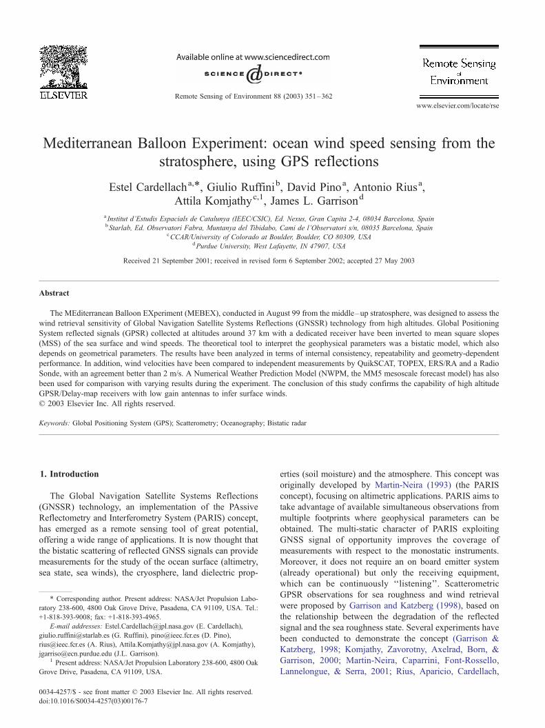
The MEBEX launch took place at 20:22 UTC August

1999. Stratospheric winds drove the balloon westward,

Fig. 1. MEditerranean Balloon EXperiment crossing from Sicily to Spain. Trac

locations. Areas of GPSR measurements: L, O, R, U, and X. For MM5 comparis

4j:30V.

crossing the Mediterranean from Sicily to Southern Spain

bordering the African Coast. The flight maintained an

altitude of 37–38 km approximately for 14 h, and entered

Spanish mainland airspace on August 3rd at noon. The

tracks defined by the locations of the reflections on the

Earth surface and collected by the receiver are shown in

Fig. 1.

The Delay Mapping receiver was programmed to se-

quentially operate in different modes, but the present paper

focuses on the data acquired by the Serial Delay Mapping

Receiver mode (SDMR). In this mode, the receiver collected

waveforms from up to six satellites at a time, for both direct

and reflected channels. Once four or more satellites were

tracked through the direct part of the receiver, the receiver

was able to predict their specular point positions (and thus

their delay and frequency offsets) and automatically search

for them in the reflected signal. The observables detected

by the receiver, the waveforms, were 32-bin long, cor-

responding to 32 half-chip sampling, performed every 100

ms (we refer to chip as the unit of the PRN code unit, as

explained in Section 3.1). SDMR data has a somewhat

reduced signal to noise ratio because of the sequencing

acquisition limitations on the number of power measure-

ments available to average within a fixed output sample

interval. The raw 10-Hz waveforms were passed through a

running window average filter to be written on disk at 1 Hz.

Garrison et al. (2000) provided a detailed description of the

receiver.

3. Data processing

3.1. Expected performance

In the frame of the ESA contract Utilization of Scatter-

ometry Using Sources of Opportunity, OPPSCAT, a wave-

form simulator has been implemented and the feasibility of

ks of the GPSR, QuikSCAT, ERS, TOPEX and Radio Sonde observation

ons, the data has been divided in two regions, East and West of longitude

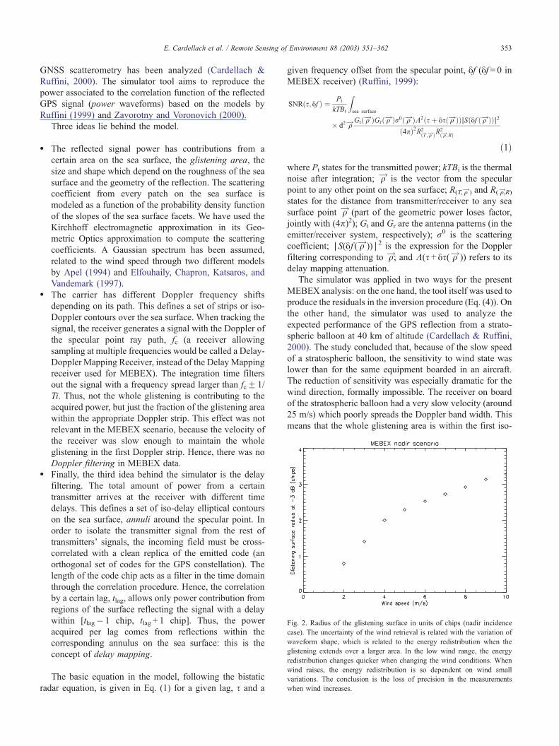
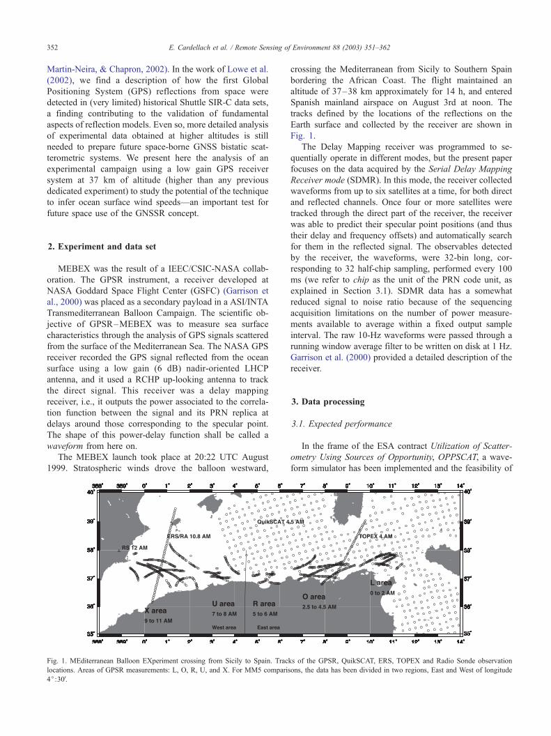
Fig. 2. Radius of the glistening surface in units of chips (nadir incidence

case). The uncertainty of the wind retrieval is related with the variation of

waveform shape, which is related to the energy redistribution when the

glistening extends over a larger area. In the low wind range, the energy

redistribution changes quicker when changing the wind conditions. When

wind raises, the energy redistribution is so dependent on wind small

variations. The conclusion is the loss of precision in the measurements

when wind increases.

E. Cardellach et al. / Remote Sensing of Environment 88 (2003) 351–362 353

GNSS scatterometry has been analyzed (Cardellach &

Ruffini, 2000). The simulator tool aims to reproduce the

power associated to the correlation function of the reflected

GPS signal (power waveforms) based on the models by

Ruffini (1999) and Zavorotny and Voronovich (2000).

Three ideas lie behind the model.

� The reflected signal power has contributions from a

certain area on the sea surface, the glistening area, the

size and shape which depend on the roughness of the sea

surface and the geometry of the reflection. The scattering

coefficient from every patch on the sea surface is

modeled as a function of the probability density function

of the slopes of the sea surface facets. We have used the

Kirchhoff electromagnetic approximation in its Geo-

metric Optics approximation to compute the scattering

coefficients. A Gaussian spectrum has been assumed,

related to the wind speed through two different models

by Apel (1994) and Elfouhaily, Chapron, Katsaros, and

Vandemark (1997).� The carrier has different Doppler frequency shifts

depending on its path. This defines a set of strips or iso-

Doppler contours over the sea surface. When tracking the

signal, the receiver generates a signal with the Doppler of

the specular point ray path, fc (a receiver allowing

sampling at multiple frequencies would be called a Delay-

Doppler Mapping Receiver, instead of the Delay Mapping

receiver used for MEBEX). The integration time filters

out the signal with a frequency spread larger than fcF 1/

Ti. Thus, not the whole glistening is contributing to the

acquired power, but just the fraction of the glistening area

within the appropriate Doppler strip. This effect was not

relevant in the MEBEX scenario, because the velocity of

the receiver was slow enough to maintain the whole

glistening in the first Doppler strip. Hence, there was no

Doppler filtering in MEBEX data.� Finally, the third idea behind the simulator is the delay

filtering. The total amount of power from a certain

transmitter arrives at the receiver with different time

delays. This defines a set of iso-delay elliptical contours

on the sea surface, annuli around the specular point. In

order to isolate the transmitter signal from the rest of

transmitters’ signals, the incoming field must be cross-

correlated with a clean replica of the emitted code (an

orthogonal set of codes for the GPS constellation). The

length of the code chip acts as a filter in the time domain

through the correlation procedure. Hence, the correlation

by a certain lag, tlag, allows only power contribution from

regions of the surface reflecting the signal with a delay

within [tlag� 1 chip, tlag + 1 chip]. Thus, the power

acquired per lag comes from reflections within the

corresponding annulus on the sea surface: this is the

concept of delay mapping.

The basic equation in the model, following the bistatic

radar equation, is given in Eq. (1) for a given lag, s and a

given frequency offset from the specular point, yf (yf = 0 in

MEBEX receiver) (Ruffini, 1999):

SNRðs; yf Þ ¼ Pt

kTBi

Zsea surface

� d2!q Gtð!q ÞGrð!q Þr0ð!q ÞK2ðs þ ysð!q ÞÞASðyf ð!q ÞÞA2

ð4pÞ2R2ðT ;!q ÞR

2ð!q;RÞ

ð1Þ

where Pt states for the transmitted power; kTBi is the thermal

noise after integration; !q is the vector from the specular

point to any other point on the sea surface; R(T,!q ) and R(!q,R)states for the distance from transmitter/receiver to any sea

surface point !q (part of the geometric power loses factor,

jointly with (4p)2); Gt and Gr are the antenna patterns (in the

emitter/receiver system, respectively); r0 is the scattering

coefficient; AS(yf (!q ))A2 is the expression for the Doppler

filtering corresponding to !q; and K(s + ys(!q )) refers to its

delay mapping attenuation.

The simulator was applied in two ways for the present

MEBEX analysis: on the one hand, the tool itself was used to

produce the residuals in the inversion procedure (Eq. (4)). On

the other hand, the simulator was used to analyze the

expected performance of the GPS reflection from a strato-

spheric balloon at 40 km of altitude (Cardellach & Ruffini,

2000). The study concluded that, because of the slow speed

of a stratospheric balloon, the sensitivity to wind state was

lower than for the same equipment boarded in an aircraft.

The reduction of sensitivity was especially dramatic for the

wind direction, formally impossible. The receiver on board

of the stratospheric balloon had a very slow velocity (around

25 m/s) which poorly spreads the Doppler band width. This

means that the whole glistening area is within the first iso-

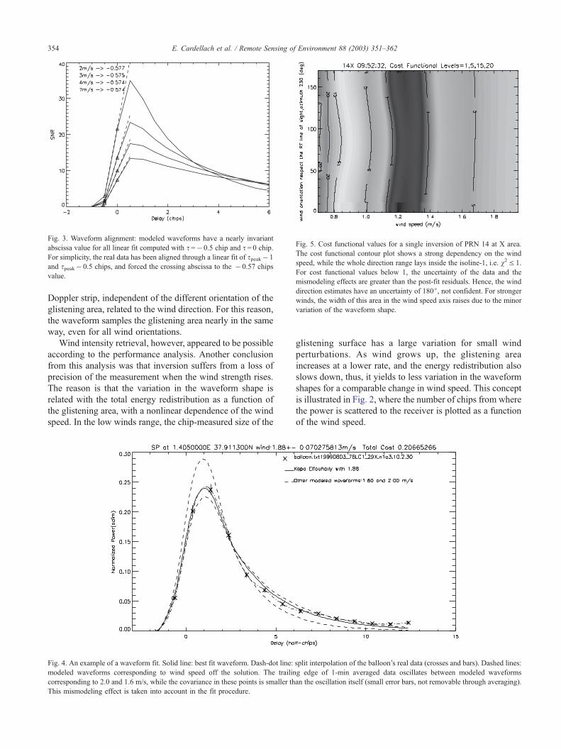
Fig. 5. Cost functional values for a single inversion of PRN 14 at X area.

The cost functional contour plot shows a strong dependency on the wind

speed, while the whole direction range lays inside the isoline-1, i.e. v2V 1.

For cost functional values below 1, the uncertainty of the data and the

mismodeling effects are greater than the post-fit residuals. Hence, the wind

direction estimates have an uncertainty of 180j, not confident. For strongerwinds, the width of this area in the wind speed axis raises due to the minor

variation of the waveform shape.

Fig. 3. Waveform alignment: modeled waveforms have a nearly invariant

abscissa value for all linear fit computed with s=� 0.5 chip and s = 0 chip.

For simplicity, the real data has been aligned through a linear fit of speak� 1

and speak� 0.5 chips, and forced the crossing abscissa to the � 0.57 chips

value.

E. Cardellach et al. / Remote Sensing of Environment 88 (2003) 351–362354

Doppler strip, independent of the different orientation of the

glistening area, related to the wind direction. For this reason,

the waveform samples the glistening area nearly in the same

way, even for all wind orientations.

Wind intensity retrieval, however, appeared to be possible

according to the performance analysis. Another conclusion

from this analysis was that inversion suffers from a loss of

precision of the measurement when the wind strength rises.

The reason is that the variation in the waveform shape is

related with the total energy redistribution as a function of

the glistening area, with a nonlinear dependence of the wind

speed. In the low winds range, the chip-measured size of the

Fig. 4. An example of a waveform fit. Solid line: best fit waveform. Dash-dot line:

modeled waveforms corresponding to wind speed off the solution. The trailin

corresponding to 2.0 and 1.6 m/s, while the covariance in these points is smaller th

This mismodeling effect is taken into account in the fit procedure.

glistening surface has a large variation for small wind

perturbations. As wind grows up, the glistening area

increases at a lower rate, and the energy redistribution also

slows down, thus, it yields to less variation in the waveform

shapes for a comparable change in wind speed. This concept

is illustrated in Fig. 2, where the number of chips from where

the power is scattered to the receiver is plotted as a function

of the wind speed.

split interpolation of the balloon’s real data (crosses and bars). Dashed lines:

g edge of 1-min averaged data oscillates between modeled waveforms

an the oscillation itself (small error bars, not removable through averaging).

ing of Environment 88 (2003) 351–362 355

3.2. Pre-processing

Before inversion, the waveform data was pre-processed

in order to (a) reduce the noise, (b) align the delay offset and

(c) remove uncalibrated power scaling factor effects.

3.2.1. Smoothing

The raw data at 1 Hz is too noisy to retrieve reliable wind

estimates. Instead, 1-min averaging produced stable wave-

E. Cardellach et al. / Remote Sens

Fig. 6. (top) Map of the sea surface mean square slopes (MSS) obtained through the

translate it to wind speed values (Figs. 10 and 12 show part of such models). (m

MEBEX specular points’ trajectories (color scale in m/s). (bottom) Independent ob

MEBEX arcs and Radio Sonde measurement (color scale in m/s).

forms. The implemented smoothing procedure reduces each

set of 61 raw waveforms to a single observation. In the

MEBEX case, 1-min (or longer) incoherent averaging was

permissible, given the very low speed of the balloon: spatial

resolution was not affected (the receiver moved about 1.5 km

during this time).

Another goal of pre-processing was to constrain the

system to reduce the degrees of freedom in the inversion:

the geophysical and instrumental parameters affecting the

GPSR inversion. The Elfouhaily and Apel ocean models have been used to

iddle) MM5 sea wind simulation interpolated, both in time and space, to

servations: TOPEX and ERS/RAwind products, QuikSCAT interpolated to

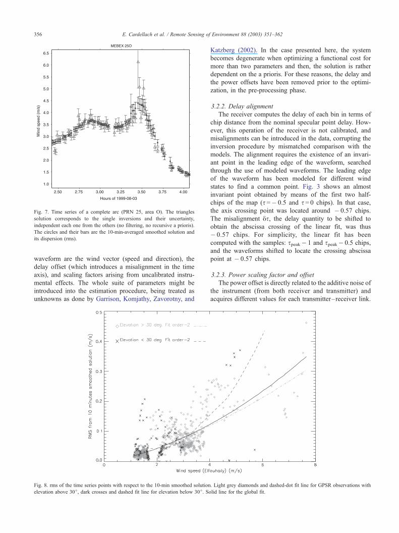
Fig. 7. Time series of a complete arc (PRN 25, area O). The triangles

solution corresponds to the single inversions and their uncertainty,

independent each one from the others (no filtering, no recursive a prioris).

The circles and their bars are the 10-min-averaged smoothed solution and

its dispersion (rms).

E. Cardellach et al. / Remote Sensing of Environment 88 (2003) 351–362356

waveform are the wind vector (speed and direction), the

delay offset (which introduces a misalignment in the time

axis), and scaling factors arising from uncalibrated instru-

mental effects. The whole suite of parameters might be

introduced into the estimation procedure, being treated as

unknowns as done by Garrison, Komjathy, Zavorotny, and

Fig. 8. rms of the time series points with respect to the 10-min smoothed solution

elevation above 30j, dark crosses and dashed fit line for elevation below 30j. So

Katzberg (2002). In the case presented here, the system

becomes degenerate when optimizing a functional cost for

more than two parameters and then, the solution is rather

dependent on the a prioris. For these reasons, the delay and

the power offsets have been removed prior to the optimi-

zation, in the pre-processing phase.

3.2.2. Delay alignment

The receiver computes the delay of each bin in terms of

chip distance from the nominal specular point delay. How-

ever, this operation of the receiver is not calibrated, and

misalignments can be introduced in the data, corrupting the

inversion procedure by mismatched comparison with the

models. The alignment requires the existence of an invari-

ant point in the leading edge of the waveform, searched

through the use of modeled waveforms. The leading edge

of the waveform has been modeled for different wind

states to find a common point. Fig. 3 shows an almost

invariant point obtained by means of the first two half-

chips of the map (s =� 0.5 and s = 0 chips). In that case,

the axis crossing point was located around � 0.57 chips.

The misalignment ys, the delay quantity to be shifted to

obtain the abscissa crossing of the linear fit, was thus

� 0.57 chips. For simplicity, the linear fit has been

computed with the samples: speak� 1 and speak� 0.5 chips,

and the waveforms shifted to locate the crossing abscissa

point at � 0.57 chips.

3.2.3. Power scaling factor and offset

The power offset is directly related to the additive noise of

the instrument (from both receiver and transmitter) and

acquires different values for each transmitter–receiver link.

. Light grey diamonds and dashed-dot fit line for GPSR observations with

lid line for the global fit.

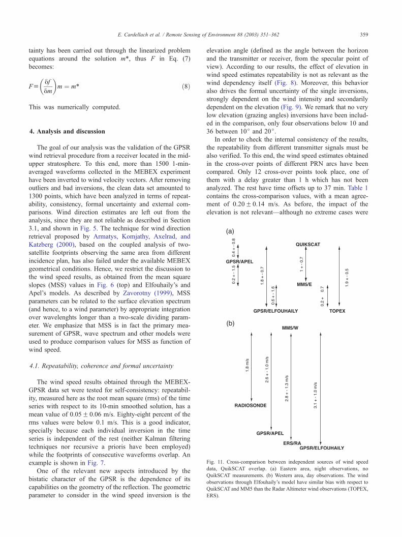
Table 1

Cross-over points analysis

SVs and

area

Dt

min

Delev.

(j)w mean

speed (m/s)

Dw

(m/s)

05 24 L 23 25 1.42 0.11

06 08 L 20 13 1.21 0.01

29 30 L 37 34 1.36 0.39

06 25 O 22 14 3.24 0.49

17 30 O 24 15 3.13 0.26

17 25 O 19 20 2.27 0.28

03 21 U 8 13 2.51 0.07

21 31 U 26 9 2.99 0.20

01 03 X 5 2 1.59 0.20

01 31 X 14 15 1.46 0.14

14 31 X 26 4 1.32 0.09

Linear regression coefficient

0.006

(m/s)/min

0.005

(m/s)/deg

0.14

(m/s)/(m/s)

The first column contains the Space Vehicle numbers which generated the

cross-over point and the area of observation (see Fig. 1 to locate the areas).

Columns 2 and 3 contain the delay and elevation difference between both

observations. Column 4 is the mean of the inverted wind speed (using

Elfouhaily’s model) and the last one contains the comparison offset. The

mean agreement between cross-observations from different emitters of the

same spot on the sea surface is 0.20 m/s. The regression coefficient from

linear fits shows that the disagreement depends more strongly on wind

speed than on Dt or Delev.

E. Cardellach et al. / Remote Sensing of Environment 88 (2003) 351–362 357

The approach we use treats all data before s =� 0.57 chips as

noise floor, and substracts the mean power of all those data

from the waveforms. On the other hand, the uncalibrated

scaling factor effect is removed through a re-normalization of

the waveform by its total energy (as described by Garrison et

al., 2002; Komjathy et al., 2000).

3.3. From waveforms to wind speed: inversion procedure

The MEBEX waveforms were compared to modeled

waveforms to obtain sea state information. The modeled

waveform was a function of a model state!m, containing the

model parameters such as wind stress and direction:

!Pmod ¼

!f ð!m Þ ð2Þ

To invert the power observations into wind/sea estimates,

a nonlinear cost functional v has been minimized:

v2ð!m Þ ¼ !r T ð!m Þ W !r ð!m Þ ð3Þ

where the residual !r is:

!r ð!m Þ ¼ !Pobs �

!Pmodð!m Þ ð4Þ

being!P 1-min-averaged power-delay map, normalized by

its total energy. The subindices obs and mod stand for

balloon’s pre-processed data and modeled waveform,

respectively.

The weighting coefficients given by theW matrix contain

the inverse of the data covariance, Cd� 1 and other factor

Fig. 9. Formal uncertainty of single inversions. It is related to the width of the ar

variation around the solution drives to a fit where the post-fit residuals are of

diamonds and dashed-dot fit line for GPSR observations with elevation above 30

for the global fit.

derived from mismodeling. In a great part of the data set, the

model had trouble to fit the trailing edge of the waveform,

where systematic low variance oscillations are not remov-

able through averaging (Fig. 4). This unmodeled effect has

ea within the cost functional below 1 (Fig. 5), meaning that a wind speed

the same order than the data uncertainty and mismodeling. Light grey

j, dark grey crosses and dashed fit line for elevation below 30j. Solid line

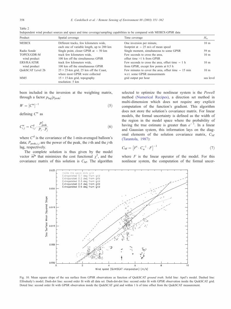
Table 2

Independent wind product sources and space and time coverage/sampling capabilities to be compared with MEBEX-GPSR data

Product Spatial coverage Time coverage Hw

MEBEX Different tracks, few kilometers wide,

each one of variable length, up to 200 km

One inversion per minute,

footprint at f 25 m/s of mean speed

10 m

Radio Sonde Single point, closer GPSR at f 50 km Single moment, simultaneous to some GPSR 59 m

TOPEX/GDR-M

wind product

track few kilometers wide,

100 km off the simultaneous GPSR

Few seconds to cross the area,

offset time >1 h from GPSR

10 m

ERS/RA/ATSR

wind product

track few kilometers wide,

100 km off the simultaneous GPSR

Few seconds to cross the area, offset time f 1 h

from GPSR, except few points at 0.5 h

10 m

QuikSCAT Level 2b 25� 25-km grid, 25 km off the Coast,

where most GPSR were collected

Few minutes to cover the area, offset time f 15 min

w.r.t. some GPSR measurements

10 m

MM5 15� 15-km grid, topography

resolution: 5 km

grid output per hour sea level

E. Cardellach et al. / Remote Sensing of Environment 88 (2003) 351–362358

been included in the inversion at the weighting matrix,

through a factor plag/ppeak:

W ¼ ½Cw��1 ð5Þ

defining Cw as

Cwi; j ¼ Cd

i; j P2peak

Pi Pj

ð6Þ

where Cd is the covariance of the 1-min-averaged balloon’s

data; Ppeak,i, j are the power of the peak, the i-th and the j-th

lag, respectively.

The complete solution is thus given by the model

vector!m* that minimizes the cost functional v2, and the

covariance matrix of this solution is CMV. The algorithm

Fig. 10. Mean square slope of the sea surface from GPSR observations as fun

Elfouhaily’s model. Dash-dot line: second order fit with all data set. Dash-dot-do

Doted line: second order fit with GPSR observation inside the QuikSCAT grid a

selected to optimize the nonlinear system is the Powell

method (Numerical Recipes), a direction set method in

multi-dimension which does not require any explicit

computation of the function’s gradient. This algorithm

does not store the solution’s covariance matrix. For linear

models, the formal uncertainty is defined as the width of

the region in the model space where the probability of

having the true estimate is greater than e� 1. In a linear

and Gaussian system, this information lays on the diag-

onal elements of the solution covariance matrix, CMV

(Tarantola, 1987):

CMV¼�F t C�1

w F��1 ð7Þ

where F is the linear operator of the model. For this

nonlinear system, the computation of the formal uncer-

ction of QuikSCAT ground truth. Solid line: Apel’s model. Dashed line:

t line: second order fit with GPSR observation inside the QuikSCAT grid.

nd within 1 h of time offset from the QuikSCAT measurement.

E. Cardellach et al. / Remote Sensing of Environment 88 (2003) 351–362 359

tainty has been carried out through the linearized problem

equations around the solution m*, thus F in Eq. (7)

becomes:

Fuyf

ym

� �m ¼ m* ð8Þ

This was numerically computed.

Fig. 11. Cross-comparison between independent sources of wind speed

data, QuikSCAT overlap. (a) Eastern area, night observations, no

QuikSCAT measurements. (b) Western area, day observations. The wind

observations through Elfouhaily’s model have similar bias with respect to

QuikSCAT and MM5 than the Radar Altimeter wind observations (TOPEX,

ERS).

4. Analysis and discussion

The goal of our analysis was the validation of the GPSR

wind retrieval procedure from a receiver located in the mid-

upper stratosphere. To this end, more than 1500 1-min-

averaged waveforms collected in the MEBEX experiment

have been inverted to wind velocity vectors. After removing

outliers and bad inversions, the clean data set amounted to

1300 points, which have been analyzed in terms of repeat-

ability, consistency, formal uncertainty and external com-

parisons. Wind direction estimates are left out from the

analysis, since they are not reliable as described in Section

3.1, and shown in Fig. 5. The technique for wind direction

retrieval proposed by Armatys, Komjathy, Axelrad, and

Katzberg (2000), based on the coupled analysis of two-

satellite footprints observing the same area from different

incidence plan, has also failed under the available MEBEX

geometrical conditions. Hence, we restrict the discussion to

the wind speed results, as obtained from the mean square

slopes (MSS) values in Fig. 6 (top) and Elfouhaily’s and

Apel’s models. As described by Zavorotny (1999), MSS

parameters can be related to the surface elevation spectrum

(and hence, to a wind parameter) by appropriate integration

over wavelenghts longer than a two-scale dividing param-

eter. We emphasize that MSS is in fact the primary mea-

surement of GPSR, wave spectrum and other models were

used to produce comparison values for MSS as function of

wind speed.

4.1. Repeatability, coherence and formal uncertainty

The wind speed results obtained through the MEBEX-

GPSR data set were tested for self-consistency: repeatabil-

ity, measured here as the root mean square (rms) of the time

series with respect to its 10-min smoothed solution, has a

mean value of 0.05F 0.06 m/s. Eighty-eight percent of the

rms values were below 0.1 m/s. This is a good indicator,

specially because each individual inversion in the time

series is independent of the rest (neither Kalman filtering

techniques nor recursive a prioris have been employed)

while the footprints of consecutive waveforms overlap. An

example is shown in Fig. 7.

One of the relevant new aspects introduced by the

bistatic character of the GPSR is the dependence of its

capabilities on the geometry of the reflection. The geometric

parameter to consider in the wind speed inversion is the

elevation angle (defined as the angle between the horizon

and the transmitter or receiver, from the specular point of

view). According to our results, the effect of elevation in

wind speed estimates repeatability is not as relevant as the

wind dependency itself (Fig. 8). Moreover, this behavior

also drives the formal uncertainty of the single inversions,

strongly dependent on the wind intensity and secondarily

dependent on the elevation (Fig. 9). We remark that no very

low elevation (grazing angles) inversions have been includ-

ed in the comparison, only four observations below 10 and

36 between 10j and 20j.In order to check the internal consistency of the results,

the repeatability from different transmitter signals must be

also verified. To this end, the wind speed estimates obtained

in the cross-over points of different PRN arcs have been

compared. Only 12 cross-over points took place, one of

them with a delay greater than 1 h which has not been

analyzed. The rest have time offsets up to 37 min. Table 1

contains the cross-comparison values, with a mean agree-

ment of 0.20F 0.14 m/s. As before, the impact of the

elevation is not relevant—although no extreme cases were

E. Cardellach et al. / Remote Sensing of Environment 88 (2003) 351–362360

present—compared to the wind strength itself. The conclu-

sion from the cross-over analysis corroborates the self-

coherence of the estimates. However, repeatability and

consistency would probably suffer under windier meteoro-

logical conditions, since these parameters seem to be driven

by the wind speed.

4.2. External analysis: comparison with independent

sources

A difficult aspect of comparing MEBEX results to

other sources is the different space and time sampling

(Fig. 1). Different remote sensing instruments provided

comparison data in the region near the MEBEX trajec-

tory during the mission. We had access to data coming

from a Radio Sonde, QuikSCAT satellite scatterometer,

TOPEX and ERS satellite Radar Altimeters (RA).

Space–Time sampling comparison limitations are sum-

marized in Table 2. In addition to observational data

from these independent sources, comparisons have ex-

tended to the Pennsylvania State National Center for

Atmospheric Research (PSU-NCAR) fifth generation Me-

soscale Model (MM5) outputs.

QuikSCAT Level 2b wind products [QuickSCAT User’s

Manual] (Weiss, 2000) have been interpolated/extrapolated

to the eastern MEBEX tracks’ positions (Fig. 6, bottom).

However, most of the GPSR observations have a large

time offset with respect to the QuikSCAT over-pass (up to

4 h). The comparison yields different values when con-

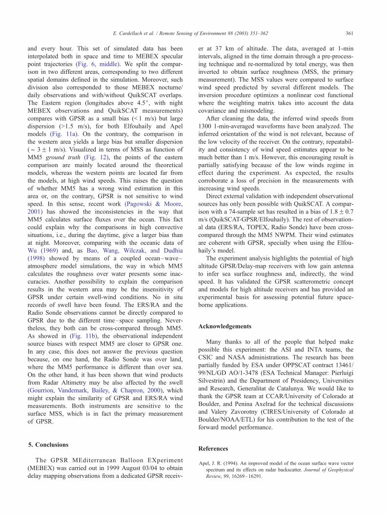
Fig. 12. Mean square slopes from GPSR observations as function of the MM5 gro

Solid line: Apel’s model. Dashed line: Elfouhaily’s model. Upper doted line: secon

using measurements from the Western area.

sidering all the data set, when rejecting QuikSCAT grid

outliers, or when selecting points according to a time

offset criteria. Moreover, the choice in the ocean surface

models (Apel, Elfouhaily) also had an impact on the

comparisons. Restricting the comparison to GPSR obser-

vations located inside the QuikSCAT grid and within 1 h

time offset yields a bias of 1.8 m/s (QuikSCAT higher

winds) and a rms of 0.7 m/s (Elfouhaily’s model). Using

Apel’s model, the bias reduces to 0.4 m/s with a bit more

dispersion: 0.8 m/s of rms. Another way to visualize these

discrepancies is through the plot in Fig. 10, which shows

MEBEX MSS against QuikSCAT winds. The points far

away from the ocean models are off the QuikSCAT grid,

closer to the coast. On the other hand, the points selected

for the comparison have a second order fit parallel to

Elfouhaily’s model and biased f + 2 m/s, while the fit

crosses Apel’s function. The TOPEX GDR-M wind prod-

uct (AVISO/Altimetry, 1996) from track 161 has been

used for comparison with QuikSCAT wind velocities.

TOPEX crossed the QuikSCAT area 30 min before, and

the direct comparison gives an offset of 1.9 m/s, similar to

QuikSCAT vs. GPSR with Elfouhaily mean value.

The other gridded data source available for interpola-

tion to a great number of MEBEX locations is the MM5

Numerical Weather Prediction Model (NWPM) (Dudhia,

1993), whose initial and boundary conditions are updated

every 6 h with information obtained from the 0.5j� 0.5jECMWF model. The MM5 simulation provides the sea

surface wind at each point of the grid (15 km resolution)

und truth. Grey scale corresponds to the time evolution of the experiment.

d order fit using East area measurements. Lower doted line: second order fit

E. Cardellach et al. / Remote Sensing of Environment 88 (2003) 351–362 361

and every hour. This set of simulated data has been

interpolated both in space and time to MEBEX specular

point trajectories (Fig. 6, middle). We split the compar-

ison in two different areas, corresponding to two different

spatial domains defined in the simulation. Moreover, such

division also corresponded to those MEBEX nocturne/

daily observations and with/without QuikSCAT overlaps.

The Eastern region (longitudes above 4.5j, with night

MEBEX observations and QuikSCAT measurements)

compares with GPSR as a small bias (< 1 m/s) but large

dispersion (>1.5 m/s), for both Elfouhaily and Apel

models (Fig. 11a). On the contrary, the comparison in

the western area yields a large bias but smaller dispersion

(f 3F 1 m/s). Visualized in terms of MSS as function of

MM5 ground truth (Fig. 12), the points of the eastern

comparison are mainly located around the theoretical

models, whereas the western points are located far from

the models, at high wind speeds. This raises the question

of whether MM5 has a wrong wind estimation in this

area or, on the contrary, GPSR is not sensitive to wind

speed. In this sense, recent work (Pagowski & Moore,

2001) has showed the inconsistencies in the way that

MM5 calculates surface fluxes over the ocean. This fact

could explain why the comparisons in high convective

situations, i.e., during the daytime, give a larger bias than

at night. Moreover, comparing with the oceanic data of

Wu (1969) and, as Bao, Wang, Wilczak, and Dudhia

(1998) showed by means of a coupled ocean–wave–

atmosphere model simulations, the way in which MM5

calculates the roughness over water presents some inac-

curacies. Another possibility to explain the comparison

results in the western area may be the insensitivity of

GPSR under certain swell-wind conditions. No in situ

records of swell have been found. The ERS/RA and the

Radio Sonde observations cannot be directly compared to

GPSR due to the different time–space sampling. Never-

theless, they both can be cross-compared through MM5.

As showed in (Fig. 11b), the observational independent

source biases with respect MM5 are closer to GPSR one.

In any case, this does not answer the previous question

because, on one hand, the Radio Sonde was over land,

where the MM5 performance is different than over sea.

On the other hand, it has been shown that wind products

from Radar Altimetry may be also affected by the swell

(Gourrion, Vandemark, Bailey, & Chapron, 2000), which

might explain the similarity of GPSR and ERS/RA wind

measurements. Both instruments are sensitive to the

surface MSS, which is in fact the primary measurement

of GPSR.

5. Conclusions

The GPSR MEditerranean Balloon EXperiment

(MEBEX) was carried out in 1999 August 03/04 to obtain

delay mapping observations from a dedicated GPSR receiv-

er at 37 km of altitude. The data, averaged at 1-min

intervals, aligned in the time domain through a pre-process-

ing technique and re-normalized by total energy, was then

inverted to obtain surface roughness (MSS, the primary

measurement). The MSS values were compared to surface

wind speed predicted by several different models. The

inversion procedure optimizes a nonlinear cost functional

where the weighting matrix takes into account the data

covariance and mismodeling.

After cleaning the data, the inferred wind speeds from

1300 1-min-averaged waveforms have been analyzed. The

inferred orientation of the wind is not relevant, because of

the low velocity of the receiver. On the contrary, repeatabil-

ity and consistency of wind speed estimates appear to be

much better than 1 m/s. However, this encouraging result is

partially satisfying because of the low winds regime in

effect during the experiment. As expected, the results

corroborate a loss of precision in the measurements with

increasing wind speeds.

Direct external validation with independent observational

sources has only been possible with QuikSCAT. A compar-

ison with a 74-sample set has resulted in a bias of 1.8F 0.7

m/s (QuikSCAT-GPSR/Elfouhaily). The rest of observation-

al data (ERS/RA, TOPEX, Radio Sonde) have been cross-

compared through the MM5 NWPM. Their wind estimates

are coherent with GPSR, specially when using the Elfou-

haily’s model.

The experiment analysis highlights the potential of high

altitude GPSR/Delay-map receivers with low gain antenna

to infer sea surface roughness and, indirectly, the wind

speed. It has validated the GPSR scatterometric concept

and models for high altitude receivers and has provided an

experimental basis for assessing potential future space-

borne applications.

Acknowledgements

Many thanks to all of the people that helped make

possible this experiment: the ASI and INTA teams, the

CSIC and NASA administrations. The research has been

partially funded by ESA under OPPSCAT contract 13461/

99/NL/GD AO/1-3478 (ESA Technical Manager: Pierluigi

Silvestrin) and the Department of Presidency, Universities

and Research, Generalitat de Catalunya. We would like to

thank the GPSR team at CCAR/University of Colorado at

Boulder, and Penina Axelrad for the technical discussions

and Valery Zavorotny (CIRES/University of Colorado at

Boulder/NOAA/ETL) for his contribution to the test of the

forward model performance.

References

Apel, J. R. (1994). An improved model of the ocean surface wave vector

spectrum and its effects on radar backscatter. Journal of Geophysical

Review, 99, 16269–16291.

E. Cardellach et al. / Remote Sensing of Environment 88 (2003) 351–362362

Armatys, M., Komjathy, A., Axelrad, P., & Katzberg, S. J. (2000, July). A

comparison of GPS and scatterometer sensing of ocean wind speed and

direction. Proceedings of IGARSS 2000.

AVISO/Altimetry (1996). AVISO User Handbook for Merged TOPEX/

POSEIDON products, AVI-NT-02-101, Edition 3.0.

Bao, J. -W., Wang, W., Wilczak, J., & Dudhia, J. (1998). Numerical sim-

ulation of air– sea interaction under high wind conditions: A case study.

Preprints, 8th. PSU/NCAR Mesoscale Modeling System Users’ Work-

shop ( pp. 22–26). Boulder, CO: NCAR.

Cardellach, E., & Ruffini, G. (2000). OPPSCAT WP3400: End-to-End

Performance, Final Report ESA Contract 13461/99/NL/GD.

Dudhia, J. (1993). A nonhydrostatic version of the Penn-State-Ncar meso-

scale model: Validation tests and simulation of an atlantic cyclone and

cold front. Monthly Weather Review, 121, 1493–1513.

Elfouhaily, T., Chapron, B., Katsaros, K., & Vandemark, D. (1997). A

unified directional spectrum for long and short wind-driven waves.

Journal of Geophysical Research, 102, 15781–15796.

Garrison, J. L., Katzberg, S. J., & Hill, M. I. (1998). Effects of sea rough-

ness on bistatically scattered range coded signals from the Global Posi-

tioning System. Geophysical Research Letter, 25(13), 2257–2260.

Garrison, J. L., Komjathy, A., Zavorotny, V., & Katzberg, S. (2002,

January). Wind speed measurement using forward scattered GPS sig-

nals. IEEE Transactions on Geoscience and Remote Sensing, 40(1),

50–65.

Garrison, J. L., Ruffini, G., Rius, A., Cardellach, E., Masters, D., Armatys,

M., & Zavorotny, V. U. (2000). Preliminary results from the GPSR

mediterranean balloon experiment (GPSR–MEBEX). Proceedings of

ERIM 2000, Remote Sensing for Marine and Coastal Environments,

Charleston, South Carolina, USA, 1–3 May.

Gourrion, J., Vandemark, D., Bailey, S., & Chapron, B. (2000, May).

Satellite altimeter models for surface wind speed developed using ocean

satellite crossovers, IFREMER-DROOS-2000-02.

Komjathy, A., Zavorotny, V. U., Axelrad, P., Born, G. H., & Garrison, J. L.

(2000). GPS signal scattering from sea surface: Comparison between

experimental data and theoretical model. Remote Sensing of Environ-

ment, 73, 162–174.

Lowe, S. T., LaBrecque, J. L., Zuffada, C., Romans, L. J., Young, L. E., &

Hajj, G. A. (2002). First spaceborne observation of Earth-reflected GPS

signal. Radio Science, 37, 1.

Martin-Neira, M. (1993). A passive reflectometry and interferometry

system (PARIS): Application to ocean altimetry. ESA Journal, 17,

331–355.

Martin-Neira, M., Caparrini, M., Font-Rossello, J., Lannelongue, S., &

Serra, C. (2001, January). The PARIS concept: An experimental dem-

onstration of sea surface altimetry using GPS reflected signals. IEEE

Transactions on Geoscience and Remote Sensing, 39(1), 142–150.

Numerical Recipes in C: The Art of Scientific Computing. Cambridge Univ.

Press.

Pagowski, M., & Moore, W. K. (2001, January). A numerical study of an

extreme cold-air outbreak over the Labrador Sea: Sea ice, air– sea in-

teraction, and development of polar lows. Monthly Weather Review,

129, 47–72.

Rius, A., Aparicio, J. M., Cardellach, E., Martı́n-Neira, M., & Chapron, B.

(2002). Sea surface statemeasurements usingGPS reflected signals.Geo-

physical Research Letters, 29(23,2122) (doi 10.1029/2002GL015524).

Ruffini, G. (1999). OPPSCAT WP1000: Remote sensing of the ocean by

bistatic radar observations: A review. Final Report ESA Contract

13461/99/NL/GD.

Tarantola, A. (1987). Inverse Problem Theory. Amsterdam, The Nether-

lands: Elsevier.

Weiss, B. (2000, April). Level 2B Data Software Interface Specification.

SeaPAC, JPL/NASA, D-16079.

Wu, J. (1969). Froude number scaling of wind-stress coefficients. Journal

of the Atmospheric Sciences, 26, 408–413.

Zavorotny, V. U. (1999, July 6). Bistatic GPS Signal Scattering from an

Ocean Surface: Theoretical Modeling and Wind Speed Retrieval from

Aircraft Measurements, talk given at the ESA Workshop on Meteoro-

logical and Oceanographic Applications of GNSS Surface Reflections:

from Modeling to User Requirements, De Bilt, The Netherlands,

http://www.etl.noaa.gov/~vzavorotny/.

Zavorotny, V. U., & Voronovich, A. (2000). Scattering of GPS signals from

the ocean with wind remote sensing application. IEEE Transactions on

Geoscience and Remote Sensing, 38(2), 951–964.