Second Chambers: Bicameralism Today, 2002 edition - Rajya ...
Upload
khangminh22Category
view
1download
0
6 254Mechanics of Materials: Symmetric Bending of BeamsM. VablePr
inte
d fr
om: h
ttp://
ww
w.m
e.m
tu.e
du/~
mav
able
/MoM
2nd.
htm
CHAPTER SIX
SYMMETRIC BENDING OF BEAMS
Learning objectives1. Understand the theory of symmetric bending of beams, its limitations, and its applications for a strength-based design
and analysis.2. Visualize the direction of normal and shear stresses and the surfaces on which they act in the symmetric bending of beams.
_______________________________________________
On April 29th, 2007 at 3:45 AM, a tanker truck crashed into a pylon on interstate 80 near Oakland, California, spilling 8600gallons of fuel that ignited. Fortunately no one died. But the heat generated from the ignited fuel, severely reduced thestrength and stiffness of the steel beams of the interchange, causing it to collapse under its own weight (Figure 6.1a). In thischapter we will study the stresses, hence strength of beams. In Chapter 7 we will discuss deflection, hence stiffness of thebeams.
Which structural member can be called a beam? Figure 6.1b shows a bookshelf whose length is much greater than its width or thickness, and the weight of the books is perpendicular to its length. Girders, the long horizontal members in bridges and highways transmit the weight of the pavement and traffic to the columns anchored to the ground, and again the weight is perpendicular to the member. Bookshelves and girders can be modeled as beams—long structural member on which loads act perpendicular to the longitudinal axis. The mast of a ship, the pole of a sign post, the frame of a car, the bulkheads in an air-craft, and the plank of a seesaw are among countless examples of beams.
The simplest theory for symmetric bending of beams will be developed rigorously, following the logic described in Figure 3.15, but subject to the limitations described in Section 3.13.
6.1 PRELUDE TO THEORY
As a prelude to theory, we consider several examples, all solved using the logic discussed in Section 3.2. They highlightobservations and conclusions that will be formalized in Section 6.2.
• Example 6.1, discrete bars welded to a rigid plate, illustrates how to calculate the bending normal strains from geometry.• Example 6.2 shows the similarity of Example 6.1 to the calculation of normal strains for a continuous beam.• Example 6.3 applies the logic described in Figure 3.15 to beam bending.• Example 6.4 shows how the choice of a material model alters the calculation of the internal bending moment. As we saw
in Chapter 5 for shafts, the material model affects only the stress distribution, leaving all other equations unaffected.Thus, the kinematic equation describing strain distribution is not affected. Neither are the static equivalency equations
Figure 6.1 (a) I-80 interchange collapse. (b) Beam example.
(b)(a)
August 2012

6 255Mechanics of Materials: Symmetric Bending of BeamsM. VablePr
inte
d fr
om: h
ttp://
ww
w.m
e.m
tu.e
du/~
mav
able
/MoM
2nd.
htm
between stress and internal moment and the equilibrium equations relating internal forces and moments. Although weshall develop the simplest theory using Hooke’s law, most of the equations will apply to complex material models aswell.
EXAMPLE 6.1
The left ends of three bars are built into a rigid wall, and the right ends are welded to a rigid plate, as shown in Figure 6.2. The unde-formed bars are straight and perpendicular to the wall and the rigid plate. The rigid plate is observed to rotate due to the applied momentby an angle of 3.5° from the vertical plane. If the normal strain in bar 2 is zero, determine the normal strains in bars 1 and 3.
METHOD 1: PLANThe tangent to a circular arc is perpendicular to the radial line. If the bars are approximated as circular arcs and the wall and the rigidplate are in the radial direction, then the kinematic restriction of bars remaining perpendicular to the wall and plate is satisfied by thedeformed shape. We can relate the angle subtended by the arc to the length of arc formed by CD, as we did in Example 2.3. From thedeformed geometry, the strains of the remaining bars can be found.
SOLUTIONFigure 6.3 shows the deformed bars as circular arcs with the wall and the rigid plate in the radial direction. We know that the length of arcCD1 is still 30 in., since it does not undergo any strain. We can relate the angle subtended by the arc to the length of arc formed by CD andcalculate the radius of the arc R as
(E1)
The arc length AB1 and EF1 can be found using Figure 6.3 and the strains in bars 1 and 3 calculated.
(E2)
ANS.
(E3)
ANS.
COMMENT1. In developing the theory for beam bending, we will view the cross section as a rigid plate that rotates about the z axis but stays per-
pendicular to the longitudinal lines. The longitudinal lines will be analogous to the bars, and bending strains can be calculated as inthis example.
30 in
2 in
2 inBar 1
Bar 3
Bar 2
A
E
C
B
F
D
MextMM
x
y
z
Figure 6.2 Geometry in Example 6.1.
E
C
A
R � 2
R � 2
R
B1
D1
F1
O
�
� � 3.5�
Figure 6.3 Normal strain calculations in Example 6.1.
ψ 3.5°180°-----------⎝ ⎠
⎛ ⎞ 3.142 rad( ) 0.0611 rad= = CD1 Rψ 30 in.= = or R 491.1 in.=
AB1 R 2–( )ψ 29.8778 in.= = ε1AB1 AB–
AB----------------------- 0.1222 in.–
30 in.-------------------------- 0.004073 in./in.–= = =
ε1 4073– μin./in.=
EF1 R 2+( )ψ 30.1222 in.= = ε3EF1 EF–
EF----------------------- 0.1222 in.
30 in.------------------------ =0.004073 in./in.= =
ε3 4073 μin./in.=
August 2012

6 256Mechanics of Materials: Symmetric Bending of BeamsM. VablePr
inte
d fr
om: h
ttp://
ww
w.m
e.m
tu.e
du/~
mav
able
/MoM
2nd.
htm
METHOD 2: PLANWe can use small-strain approximation and find the deformation component in the horizontal (original) direction for bars 1 and 3. Thenormal strains can then be found.
SOLUTIONFigure 6.4 shows the rigid plate in the deformed position. The horizontal displacement of point D is zero as the strain in bar 2 is zero.Points B, D, and F move to B1, D1, and F1 as shown. We can use point D1 to find the relative displacements of points B and F as shownin Equations (E4) and (E5). We make use of small strain approximation to the sine function by its argument:
(E4)
(E5)
The normal strains in the bars can be found as
(E6)
ANS.
COMMENTS1. Method 1 is intuitive and easier to visualize than method 2. But method 2 is computationally simpler. We will use both methods when
we develop the kinematics in beam bending in Section 6.2. 2. Suppose that the normal strain of bar 2 was not zero but ε2 = 800 μin/in. What would be the normal strains in bars 1 and 3? We could
solve this new problem as in this example and obtain R = 491.5 in., ε1 = −3272 μin./in, and ε3 = 4872 μin./in. Alternatively, we viewthe assembly was subjected to axial strain before the bending took place. We could then superpose the axial strain and bending strainto obtain ε1 = −4073 + 800 = −3273 μin./in. and ε3 = 4073 + 800 = 4873 μin./in. The superposition principle can be used only for lin-ear systems, which is a consequence of small strain approximation, as observed in Chapter 2.
EXAMPLE 6.2
A beam made from hard rubber is built into a rigid wall at the left end and attached to a rigid plate at the right end, as shown in Figure 6.5.After rotation of the rigid plate the strain in line CD at y = 0 is zero. Determine the strain in line AB in terms of y and R, where y is the dis-tance of line AB from line CD, and R is the radius of curvature of line CD.
PLANWe visualize the beam as made up of bars, as in Example 6.1, but of infinitesimal thickness. We consider two such bars, AB and CD, andanalyze the deformations of these two bars as we did in Example 6.1.
SOLUTIONBecause of deformation, point B moves to point B1 and point D moves to point D1, as shown in Figure 6.6. We calculate the strain in AB:
(E1)
Δu3 DF2 D2F1 D1F1 ψ 2ψ≈sin 0.1222 in.= = = =
Δu1 B2D D3D1 B1D1 ψ 2ψ≈sin 0.1222 in.= = = =
2 in
2 in
u3u1
B2
B1
D1D3
D2
F2
F1
D
�
�
�
Figure 6.4 Alternate method for normal strain calculations in Example 6.1.
ε1Δu1
30 in.-------------- 0.1222 in.–
30 in.--------------------------- 0.004073 in./in.–= = = ε3
Δu3
30 in.-------------- 0.1222 in.
30 in.------------------------ 0.004073 in./in.= = =
ε1 4073– μin./in.= ε3 4073 μin./in.=
Figure 6.5 Beam geometry in Example 6.2. ψ
L
C DyA B
εCDCD1 CD–
CD------------------------- 0= = or CD1 CD Rψ L ψ L
R---== = =
August 2012

6 257Mechanics of Materials: Symmetric Bending of BeamsM. VablePr
inte
d fr
om: h
ttp://
ww
w.m
e.m
tu.e
du/~
mav
able
/MoM
2nd.
htm
(E2)
ANS.
COMMENTS1. In Example 6.1, R = 491.1 and y = +2 for bar 3, and y = −2 for bar 1. On substituting these values into the preceding results, we obtain
the results of Example 6.1.2. Suppose the strain in CD were εCD. Then the strain in AB can be calculated as in comment 2 of Method 2 in Example 6.1 to obtain εAB
= εCD − y/R. The strain εCD is the axial strain, and the remaining component is the normal strain due to bending.
EXAMPLE 6.3
The modulus of elasticity of the bars in Example 6.1 is 30,000 ksi. Each bar has a cross-sectional area A = in.2. Determine the external
moment Mext that caused the strains in the bars in Example 6.1.
PLANUsing Hooke’s law, determine the stresses from the strains calculated in Example 6.1. Replace the stresses by equivalent internal axialforces. Draw the free-body diagram of the rigid plate and determine the moment Mext.
SOLUTION1. Strain calculations: The strains in the three bars as calculated in Example 6.1 are
(E1)2. Stress calculations: From Hooke’s law we obtain the stresses
(E2)
(E3)
(E4)3. Internal forces calculations: The internal normal forces in each bar can be found as
(E5)4. External moment calculations: Figure 6.7 is the free body diagram of the rigid plate. By equilibrium of moment about point O we can
find Mz:
(E6)
ANS.
AB1 R y–( )ψ R y–( )LR
--------------------= = εABAB1 AB–
AB----------------------- R y–( )L R⁄ L–
L-------------------------------------- L yL R⁄– L–
L--------------------------------= = =
εABy–
R-----=
C
A
B1
D1
O
�
�
R � y
R
Figure 6.6 Exaggerated deformed geometry in Example 6.2.C
A
BD
12---
ε1 4073– μin./in. ε2 0 ε3 4073 μin./in.===
σ1 Eε1 30,000 ksi( ) 4073–( ) 10 6–( ) 122.19= ksi C( )= =
σ2 Eε2 0==
σ3 Eε3 30,000 ksi( ) 4073( ) 10 6–( ) 122.19= ksi T( )= =
N1 σ1A 61.095 kips= = C( ) N3 σ3A 61.095 kips T( )= =
Mz N1 y( ) N3 y( )+ 61.095 kips( ) 2 in.( ) 61.095 kips( ) 2 in.( )+= =
Mz 244.4 in.· kips=
y � 2
y � 2
N3
MzMN1
O
Figure 6.7 Free-body diagram in Example 6.3.
August 2012

6 258Mechanics of Materials: Symmetric Bending of BeamsM. VablePr
inte
d fr
om: h
ttp://
ww
w.m
e.m
tu.e
du/~
mav
able
/MoM
2nd.
htm
COMMENTS
1. The sum in Equation (E6) can be rewritten where σ is the normal stress acting at a distance y from the zero strain bar,
and ΔAi is the cross-sectional area of the ith bar. If we had n bars attached to the rigid plate, then the moment would be given by
As we increase the number of bars n to infinity, the cross-sectional area ΔAi tends to zero, becoming the infinitesimal
area dA and the summation is replaced by an integral. In effect, we are fitting an infinite number of bars to the plate, resulting in acontinuous body.
2. The total axial force in this example is zero because of symmetry. If this were not the case, then the axial force would be given by the
summation As in comment 1, this summation would be replaced by an integral as n tends to infinity, as will be shown in
Section 6.1.1.
6.1.1 Internal Bending Moment
In this section we formalize the observation made in Example 6.3: that is, the normal stress σxx can be replaced by an equiva-lent bending moment using an integral over the cross-sectional area. Figure 6.8 shows the normal stress distribution σxx to bereplaced by an equivalent internal bending moment Mz. Let y represent the coordinate at which the normal stress acts. Staticequivalency in Figure 6.8 results in
(6.1)
Figure 6.8a suggests that for static equivalency there should be an axial force N and a bending moment about the y axis My. However, the requirement of symmetric bending implies that the normal stress σxx is symmetric about the axis of symme-try—that is, the y axis. Thus My is implicitly zero owing to the limitation of symmetric bending. Our desire to study bending independent of axial loading requires that the stress distribution be such that the internal axial force N should be zero. Thus we must explicitly satisfy the condition
(6.2)
Equation (6.2) implies that the stress distribution across the cross section must be such that there is no net axial force. That is,the compressive force must equal the tensile force on a cross section in bending. If stress is to change from compression totension, then there must be a location of zero normal stress in bending. The line on the cross section where the bending normalstress is zero is called neutral axis.
Equations (6.1) and (6.2) are independent of the material model. That is because they represent static equivalency between the normal stress on the entire cross section and the internal moment. If we were to consider a composite beam cross section or a nonlinear material model, then the value and distribution of σxx would change across the cross section yet Equa-tion (6.1) relating σxx to Mz would remain unchanged. Example 6.4 elaborates on this idea. The origin of the y coordinate is located at the neutral axis irrespective of the material model. Hence, determining the location of the neutral axis is critical in all bending problems. The location of the origin will be discussed in greater detail for a homogeneous, linearly elastic, isotro-pic material in Section 6.2.4.
yσΔAi ,i=1
2∑
yσΔAi .i=1
n∑
σΔAi .i=1
n∑
Mz yσxx AdA
∫–=
x
y
y
dN � �xx dA
z
z
Mz
x
y
z
(a) (b) Figure 6.8 Statically equivalent internal moment.
σxx AdA
∫ 0=
August 2012

6 259Mechanics of Materials: Symmetric Bending of BeamsM. VablePr
inte
d fr
om: h
ttp://
ww
w.m
e.m
tu.e
du/~
mav
able
/MoM
2nd.
htm
EXAMPLE 6.4
Figure 6.9 shows a homogeneous wooden cross section and a cross section in which the wood is reinforced with steel. The normal strainfor both cross sections is found to vary as εxx = −200y μ. The moduli of elasticity for steel and wood are Esteel = 30,000 ksi and Ewood =8000 ksi. (a) Write expressions for normal stress σxx as a function of y, and plot the σxx distribution for each of the two cross sections shown. (b)Calculate the equivalent internal moment Mz for each cross section.
PLAN(a) From the given strain distribution we can find the stress distribution by Hooke’s law. We note that the problem is symmetric andstresses in each region will be linear in y. (b) The integral in Equation (6.1) can be written as twice the integral for the top half since the stressdistribution is symmetric about the center. After substituting the stress as a function of y in the integral, we can perform the integration toobtain the equivalent internal moment.
SOLUTION(a) From Hooke’s law we can write the stress in each material as
(E1)
(E2)For the homogeneous cross section the stress distribution is given in Equation (E1), but for the laminated case it switches from Equation(E1) to Equation (E2), depending on the value of y. We can write the stress distribution for both cross sections as a function of y. Homogeneous cross section:
(E3)Laminated cross section:
(E4)
Using Equations (E3) and (E4) the strains and stresses can be plotted as a function of y, as shown in Figure 6.10.
(b) The thickness (dimension in the z direction) is 2 in. Hence we can write dA = 2dy. Noting that the stress distribution is symmetric, wecan write the integral in Equation (6.1) as
(E5)
Homogeneous cross section: Substituting Equation (E3) into Equation (E5) and integrating, we obtain the equivalent internal moment.
y
z
2 in.
112--- in.Wood Steel
Wood
2 in.
Wood
Steel
Steel
y
z1 in.
1/4 in.
1/4 in.
(a) (b)
Figure 6.9 Cross sections in Example 6.4. (a) Homogeneous. (b) Laminated.
σxx( )wood 8000 ksi( ) 200y–( )10 6– 1.6y ksi–= =
σxx( )steel 30000 ksi( ) 200– y( )10 6– 6y ksi–= =
σxx 1.6y ksi– 0.75 in.– y 0.75 in.<≤=
σxx
6y ksi 0.5 in. y 0.75 in.≤<–1.6y ksi 0.5 in. y 0.5 in.< <––6y ksi 0.75 in. y 0.5 in.–<≤––⎩
⎪⎨⎪⎧
=
y (in)
0.50.75
100O 150�xx (�)
100150
(a)
O
y (in)
0.5
0.75
0.8 1.2�xx (ksi)
0.81.2
(b)
O
y (in)
0.50.75
0.8 3.0 4.5�xx (ksi)
0.83.04.5
(c)
σxx
y (in.)
0.8 4.50.83.04.5
0.50.75
O (ksi)3.0
Figure 6.10 Strain and stress distributions in Example 6.4: (a) strain distribution; (b) stress distribution in homogeneous cross section;(c) stress distribution in laminated cross section.
Mz yσxx 2 yd( )0.75–
0.75
∫– 2 yσxx 2 yd( )0
0.75
∫–= =
August 2012

6 260Mechanics of Materials: Symmetric Bending of BeamsM. VablePr
inte
d fr
om: h
ttp://
ww
w.m
e.m
tu.e
du/~
mav
able
/MoM
2nd.
htm
(E6)
ANS.Laminated cross section: Substituting Equation (E4) into Equation (E5) and integrating, we obtain the equivalent internal moment.
(E7)
ANS.
COMMENTS1. As this example demonstrates, although the strain varies linearly across the cross section, the stress may not. In this example we con-
sidered material nonhomogeneity. In a similar manner we can consider other models, such as elastic–perfectly plastic model, or mate-rial models that have nonlinear stress–strain curves.
2. Figure 6.11 shows the stress distribution on the surface. The symmetry of stresses about the center results in a zero axial force.
3. We can obtain the equivalent internal moment for a homogeneous cross section by replacing the triangular load by an equivalent loadat the centroid of each triangle. We then find the equivalent moment, as shown in Figure 6.12. This approach is very intuitive. How-ever, as the stress distribution becomes more complex, such as in a laminated cross section, or for more complex cross-sectionalshapes, this intuitive approach becomes very tedious. The generalization represented by Equation (6.1) and the resulting formula canthen simplify the calculations.
4. The relationship between the internal moment and the external loads can be established by drawing the appropriate free-body diagramfor a particular problem. The relationship between internal and external moments depends on the free-body diagram and is indepen-dent of the material homogeneity.
PROBLEM SET 6.1
6.1 The rigid plate that is welded to the two bars in Figure P6.1 is rotated about the z axis, causing the two bars to bend. The normal strains inbars 1 and 2 were found to be ε1 = 2000 μin./in. and ε2 = −1500 μin./in. Determine the angle of rotation ψ .
Mz 2 y 1.6y ksi–( ) 2 yd( )0
0.75
∫ 6.4y3
3----
0
0.75
6.40.753
3------------==–=
Mz 0.9 in.· kips=
Mz 2 y 1.6y–( ) 2 yd( )0
0.5
∫ y 6y–( ) 2 yd( )0.5
0.75
∫+– 4 1.6 y3
3----
0
0.5
6 y3
3----
0.5
0.75
+⎝ ⎠⎜ ⎟⎛ ⎞
= =
Mz 2.64 in.· kips=
1.2 ksi
1.2 ksi
(a)
4.5 ksi
(a)
0.8 ksi
4.5 ksi
3 ksi
(b) Figure 6.11 Surface stress distributions in Example 6.4 for (a) homogeneous cross section; (b) laminated cross section.
2 in
0.75 in
0.75 in
(a)
0.5 in
0.5 in
y
N
Nz
(b)
N � � 1.2 � 2 � 0.75 � 0.912
y
z
Mz
(c)
Mz � 2 � 0.5 � N � 0.9 in�kips1.2 ksi
1.2 ksi
Figure 6.12 Statically equivalent internal moment in Example 6.4.
48 in
Bar 2
Bar 1
4 inx
�
y
z
Figure P6.1
August 2012

6 261Mechanics of Materials: Symmetric Bending of BeamsM. VablePr
inte
d fr
om: h
ttp://
ww
w.m
e.m
tu.e
du/~
mav
able
/MoM
2nd.
htm
6.2 Determine the location h in Figure P6.2 at which a third bar in Problem 6.1 must be placed so that there is no normal strain in the thirdbar.
6.3 The two rigid plates that are welded to six bars in Figure P6.3 are rotated about the z axis, causing the six bars to bend. The normal strains in bars2 and 5 were found to be zero. What are the strains in the remaining bars?
6.4 The strains in bars 1 and 3 in Figure P6.4 were found to be ε1 = 800 μ and ε3 = 500 μ. Determine the strains in the remaining bars.
6.5 The rigid plate shown in Figure P6.5 was observed to rotate by 2° from the vertical plane due to the action of the external moment Mext
and force P, and the normal strain in bar 1 was found to be ε1 = 2000 μin./in. Both bars have a cross-sectional area in.2 and a modulus
of elasticity E = 30,000 ksi. Determine the applied moment Mext and force P.
6.6 The rigid plate shown in Figure P6.6 was observed to rotate 1.25° from the vertical plane due to the action of the external moment Mext andthe force P. All three bars have a cross-sectional area A = 100 mm2 and a modulus of elasticity E = 200 GPa. If the strain in bar 2 was measured aszero, determine the external moment Mext and the force P.
6.7 The rigid plates BD and EF in Figure P6.7 were observed to rotate by 2° and 3.5° from the vertical plane in the direction of appliedmoments. All bars have a cross-sectional area of A = 125 mm2. Bars 1 and 3 are made of steel ES = 200 GPa, and bars 2 and 4 are made of alu-minum Eal = 70 GPa. If the strains in bars 1 and 3 were found to be ε1 = 800 μ and ε3 = 500 μ determine the applied moment M1 and M2 and theforces P1 and P2 that act at the center of the rigid plates.
48 in
Bar 2
Bar 1
4 inhx
y
z� Figure P6.2
Figure P6.33.0 m 2.5 m
25 mm
15 mm
Bar 1
Bar 3
Bar 4
Bar 2 Bar 5
1.25� 2.5�
Bar 6
x
y
z
Figure P6.4 3.0 m
25 mm
2.5 m
Bar 2
Bar 1A B
C D
E
FBar 4
2.0� 3.5�
Bar 3
A 12---=
Figure P6.5 48 in
Bar 2
Bar 1
MzM
4 in2 in
P
x
y
zext
Figure P6.6Bar 1
Bar 3
Bar 2
3.0 m
P
MzM
x
y
z
ext
Figure P6.7
P2 P1
A B
C
E
F
3.0 m 2.5 m
Bar 2 Bar 4
Bar 1 Bar 3
M2MM M1
25 mm
August 2012

6 262Mechanics of Materials: Symmetric Bending of BeamsM. VablePr
inte
d fr
om: h
ttp://
ww
w.m
e.m
tu.e
du/~
mav
able
/MoM
2nd.
htm
6.8 Three wooden beams are glued to form a beam with the cross-section shown in Figure 6.8. The normal strain due to bending about the zaxis is εxx = -0.012y, where y is measured in meters. The modulus of elasticity of wood is 10 GPa. Determine the equivalent internal momentacting at the cross-section. Use tW =20 mm, h =250 mm, tF = 20 mm, and d= 125 mm.
6.9 Three wooden beams are glued to form a beam with the cross-section shown in Figure 6.8. The normal strain at the cross due to bendingabout the z axis is εxx = -0.015y, where y is measured in meters. The modulus of elasticity of wood is 10 GPa. Determine the equivalent inter-nal moment acting at the cross-section. Use tW =10 mm, h =50 mm, tF = 10 mm, and d= 25 mm.
6.10 Three wooden beams are glued to form a beam with the cross-section shown in Figure 6.8. The normal strain at the cross due to bend-ing about the z axis is εxx = 0.02y, where y is measured in meters. The modulus of elasticity of wood is 10 GPa. Determine the equivalent inter-nal moment acting at the cross-section. Use tW =15 mm, h =200 mm, tF = 20 mm, and d= 150 mm.
6.11 Steel strips (ES = 30,000 ksi) are securely attached to wood (EW = 2000 ksi) to form a beam with the cross section shown in FigureP6.11. The normal strain at the cross section due to bending about the z axis is εxx = −100y μ, where y is measured in inches. Determine the
equivalent internal moment Mz.. Use d = 2 in., hW = 4 in., and in.
6.12 Steel strips (ES = 30,000 ksi) are securely attached to wood (EW = 2000 ksi) to form a beam with the cross section shown in FigureP6.11 . The normal strain at the cross section due to bending about the z axis is εxx = −50y μ, where y is measured in inches. Determine the
equivalent internal moment Mz. Use d = 1 in., hW = 6 in., and in.
6.13 Steel strips (ES = 30,000 ksi) are securely attached to wood (EW = 2000 ksi) to form a beam with the cross section shown in FigureP6.11 . The normal strain at the cross section due to bending about the z axis is εxx = 200y μ, where y is measured in inches. Determine the equiva-
lent internal moment Mz. Use d = 1 in., hW = 2 in., and in.
Figure P6.8
d
tW
h
tF
h
tF
d
y
z
hS18---=
Figure P6.11
Steel
Wood
d
Wood
Steel
Steel
y
zhw
hs
hs
hS14---=
hS116------=
August 2012

6 263Mechanics of Materials: Symmetric Bending of BeamsM. VablePr
inte
d fr
om: h
ttp://
ww
w.m
e.m
tu.e
du/~
mav
able
/MoM
2nd.
htm
6.14 Steel strips (ES = 200 GPa) are securely attached to wood (EW = 10 GPa) to form a beam with the cross section shown in Figure P6.14.The normal strain at the cross section due to bending about the z axis is εxx = 0.02y, where y is measured in meters. Determine the equivalentinternal moment Mz .Use tW = 15 mm, hW = 200 mm, tF = 20 mm, and dF = 150 mm.
Stretch Yourself6.15 A beam of rectangular cross section shown in Figure 6.15 is made from elastic-perfectly plastic material. If the stress distribution acrossthe cross section is as shown determine the equivalent internal bending moment.
6.16 A rectangular beam cross section has the dimensions shown in Figure 6.16. The normal strain due to bending about the z axis wasfound to vary as , with y measured in meters. Determine the equivalent internal moment that produced the given state of strain.
The beam is made from elastic-perfectly plastic material that has a yield stress of σyield= 250 MPa and a modulus of elasticity E = 200 GPa.Assume material that the behaves in a similar manner in tension and compression (see Problem 3.152)
6.17 A rectangular beam cross section has the dimensions shown in Figure 6.16. The normal strain due to bending about the z axis wasfound to vary as , with y measured in meters. Determine the equivalent internal moment that would produce the given strain.
The beam is made from a bi-linear material that has a yield stress of σyield= 200 MPa, modulus of elasticity E1 = 250 GPa, and E2= 80 GPa.Assume that the material behaves in a similar manner in tension and compression (see Problem 3.153).
6.18 A rectangular beam cross section has the dimensions shown in Figure 6.16. The normal strain due to bending about the z axis wasfound to vary as , with y measured in meters. Determine the equivalent internal moment that would produce the given strain.
The beam material has a stress strain relationship given by . Assume that the material behaves in a similar manner in tensionand compression (see Problem 3.154).
Figure P6.14
dF
tW
hW
tF
hW
tF
dF
y
z
4 in
0.5 in30 ksi
30 ksiy
z σxx
Figure P6.15
εxx 0.01y–=
Figure P6.16150 mm
150 mm
100 mm
z
y
100 mm
εxx 0.01y–=
εxx 0.01y–=
σ 952ε0.2= MPa
August 2012

6 264Mechanics of Materials: Symmetric Bending of BeamsM. VablePr
inte
d fr
om: h
ttp://
ww
w.m
e.m
tu.e
du/~
mav
able
/MoM
2nd.
htm
6.2 THEORY OF SYMMETRIC BEAM BENDING
In this section we develop formulas for beam deformation and stress. We follow the procedure in Section 6.1 with variables inplace of numbers. The theory will be subject to the following limitations:
1. The length of the member is significantly greater than the greatest dimension in the cross section. 2. We are away from the regions of stress concentration; 3. The variation of external loads or changes in the cross-sectional areas are gradual except in regions of stress concen-
tration.4. The cross section has a plane of symmetry. This limitation separates bending about the z axis from bending about the
y axis. (See Problem 6.135 for unsymmetric bending.)5. The loads are in the plane of symmetry. Load P1 in Figure 6.13 would bend the beam as well as twist (rotate) the cross sec-
tion. Load P2, which lies in the plane of symmetry, will cause only bending. Thus, this limitation decouples the bending prob-lem from the torsion problem1.
6. The load direction does not change with deformation. This limitation is required to obtain a linear theory and works wellas long as the deformations are small.
7. The external loads are not functions of time; that is, we have a static problem. (See Problems 7.50 and 7.51 fordynamic problems.)
Figure 6.14 shows a segment of a beam with the x–y plane as the plane of symmetry. The beam is loaded by transverse forces P1 and P2 in the y direction, moments M1 and M2 about the z axis, and a transverse distributed force py(x). The distrib-uted force py(x) has units of force per unit length and is considered positive in the positive y direction. Because of external loads, a line on the beam deflects by v in the y direction.
The objectives of the derivation are:
1. To obtain a formula for bending normal stress σxx and bending shear stress τxy in terms of the internal moment Mz andthe internal shear force Vy.
2. To obtain a formula for calculating the beam deflection v(x).
1The separation of torsion from bending requires that the load pass through the shear center, which always lies on the axis of symmetry.
Figure 6.13 Loading in plane of symmetry.
y
P2 P1Bending and torsionBending only
x
z
�1
�1
�2
�2 �dvdx
x
y
z
x1
P1 p(x)
AC
By D
M2M1
x2
v(x2)P2
y Figure 6.14 Beam segment.
ψ2 xddv=
v(x)
August 2012

6 265Mechanics of Materials: Symmetric Bending of BeamsM. VablePr
inte
d fr
om: h
ttp://
ww
w.m
e.m
tu.e
du/~
mav
able
/MoM
2nd.
htm
To account for the gradual variation of py(x) and the cross-sectional dimensions, we will take Δx = x2 − x1 as infinitesimal distance in which these quantities can be treated as constants. The logic shown in Figure 6.15 and discussed in Section 3.2 will be used to develop the simplest theory for the bending of beams. Assumptions will be identified as we move from one step to the next. The assumptions identified as we move from each step are also points at which complexities can later be added, as discussed in examples and Stretch Yourself problems.
6.2.1 Kinematics
In Example 6.1 we found the normal strains in bars welded to rigid plates rotating about the z axis. Here we state assumptionsthat will let us simulate the behavior of a cross section like that of the rigid plate. We will consider the experimental evidencejustifying our assumptions and the impact of these assumptions on the theory.
Assumption 1: Squashing—that is, dimensional changes in the y direction—is significantly smaller than bending.Assumption 2: Plane sections before deformation remain planes after deformation.Assumption 3: Plane sections perpendicular to the beam axis remain nearly perpendicular after deformation.
Figure 6.16 shows a rubber beam with a grid on its surface that is bent by hand. Notice that the dimensional changes in the y direction are significantly smaller than those in the x direction, the basis of Assumption 1. The longer the beam, the bet-ter is the validity of Assumption 1. Neglecting dimensional changes in the y direction implies that the normal strain in the y direction is small2 and can be neglected in the kinematic calculations; that is, εyy = ∂v/∂y ≈ 0. This implies that deflection of the beam v cannot be a function of y:
(6.3)Equation (6.3) implies that if we know the curve of one longitudinal line on the beam, then we know how all other longi-
tudinal lines on the beam bend. The curve described by v(x), called the elastic curve, will be discussed in detail in the next chapter.
2It is accounted for as the Poisson effect. However the normal strain in the y direction is not an independent variable and hence is negligible in kinematics.
Figure 6.15 Logic in mechanics of materials.
v v x( )=
August 2012

6 266Mechanics of Materials: Symmetric Bending of BeamsM. VablePr
inte
d fr
om: h
ttp://
ww
w.m
e.m
tu.e
du/~
mav
able
/MoM
2nd.
htm
Figure 6.16 shows that lines initially in the y direction continue to remain straight but rotate about the z axis, validating Assumption 2. This implies that the displacement u varies linearly, as shown in Figure 6.17. In other words, the equation for u is
(6.4)
where u0 is the axial displacement at y = 0 and ψ is the slope of the plane. (We accounted for uniform axial displacement u0 in
Chapter 4.) In order to study each problem independently, we will assume u0 = 0. (See Problem 6.133 for .)
Figure 6.16 also shows that the right angle between the x and y directions is nearly preserved during bending, validating Assumption 3. This implies that the shear strain γxy is nearly zero. We cannot use this assumption in building theoretical mod-els of beam bending if shear is important, such as in sandwich beams (see comment 3 in Example 6.7) and Timoshenko beams (see Problem 7.49). But Assumption 3 helps simplify the theory as it eliminates the variable ψ by imposing the constraint that the angle between the longitudinal direction and the cross section be always 90°. This is accomplished by relating ψ to v as described next.
6.2.2 Strain Distribution
Assumption 4: Strains are small.
The bending curve is defined by v(x). As shown in Figure 6.14, the angle of the tangent to the curve v(x) is equal to the rotation of the cross section when Assumption 3 is valid. For small strains, the tangent of an angle can be replaced by the angle itself, that is, tanψ ≈ ψ = dv/dx. Substituting ψ and u0 = 0 in Equation (6.4), we obtain
(6.5)
Figure 6.18 shows the exaggerated deformed shape of a segment of the beam. The rotation of the right cross section is taken relative to the left. Thus, the left cross section is viewed as a fixed wall, as in Examples 6.1 and 6.2. We assume that line CD representing y = 0 has zero bending normal strain. The calculations of Example 6.2 show that the bending normal strain for line AB is given by
Original Grid
xy
z
Deformed Grid
Figure 6.16 Deformation in bending. (Courtesy Professor J. B. Ligon.)
z
xy
u u0 ψ– y=
u0 0≠
yx
u0
�
Figure 6.17 Linear variation of axial displacement u.
u yxd
dv x( )–=
August 2012

6 267Mechanics of Materials: Symmetric Bending of BeamsM. VablePr
inte
d fr
om: h
ttp://
ww
w.m
e.m
tu.e
du/~
mav
able
/MoM
2nd.
htm
(6.6a)
We can also obtain the equation of bending normal strain by substituting Equation (6.5) into Equation (2.12a) to obtain
or
(6.6b)
Equations 6.6a and 6.6b show that the bending normal strain εxx varies linearly with y and has a maximum value at either the
top or the bottom of the beam. d2v/dx2 is the curvature of the beam, and its magnitude is equal to 1/R, where R is the radiusof curvature.
6.2.3 Material Model
In order to develop a simple theory for the bending of symmetric beams, we shall use the material model given by Hooke’slaw. We therefore make the following assumptions regarding the material behavior.
Assumption 5: The material is isotropic.Assumption 6: The material is linearly elastic.3 Assumption 7: There are no inelastic strains.4
Substituting Equation (6.6b) into Hooke’s law σxx = Eεxx, we obtain
(6.7)
Though the strain is a linear function of y, we cannot say the same for stress. The modulus of elasticity E could change acrossthe cross section, as in laminated structures.
6.2.4 Location of Neutral Axis
Equation (6.7) shows that the stress σxx is a function of y, and its value must be zero at y = 0. That is, the origin of y must be atthe neutral axis. But where is the neutral axis on the cross section? Section 6.1.1 noted that the distribution of σxx is such that
the total tensile force equals the total compressive force on a cross section, given by Equation (6.2). d2v/dx2 is a function of xonly, whereas the integration is with respect to y and z (dA = dy dz). Substituting Equation (6.7) into Equation (6.2), we obtain
3See Problems 6.57 and 6.58 for nonlinear material behavior.4Inelastic strains could be due to temperature, humidity, plasticity, viscoelasticity, etc. See Problem 6.134 for including thermal strains.
εxxyR---–=
CA
yB1
D1
O
��
��
R � y
R
Figure 6.18 Normal strain calculations in symmetric bending.
εxxu∂x∂
-----x∂
∂ yxd
dv x( )–⎝ ⎠⎛ ⎞= =
εxx yd2vdx2-------- x( )–=
σxx Eyd2vdx2--------–=
August 2012

6 268Mechanics of Materials: Symmetric Bending of BeamsM. VablePr
inte
d fr
om: h
ttp://
ww
w.m
e.m
tu.e
du/~
mav
able
/MoM
2nd.
htm
(6.8a)
The integral in Equation (6.8a) must be zero as shown in Equation (6.8b), because a zero value of d2v/dx2 would imply thatthere is no bending.
(6.8b)
Equation (6.8b) is used for determining the origin (and thus the neutral axis) in composite beams. Consistent with the motiva-tion of developing the simplest possible formulas, we would like to take E outside the integral. In other words, E should notchange across the cross section, as implied in Assumption 8:
Assumption 8: The material is homogeneous across the cross section5 of a beam.
Equation (6.8b) can be written as
(6.8c)
In Equation (6.8c) either E or must be zero. As E cannot be zero, we obtain
(6.9)
Equation (6.9) is satisfied if y is measured from the centroid of the cross section. That is, the origin must be at the centroid of the cross section of a linear, elastic, isotropic, and homogeneous material. Equation (6.9) is the same as Equation (4.12a) in axial members. However, in axial problems we required that the internal bending moment that generated Equation (4.12a) be zero. Here it is zero axial force that generates Equation (6.9). Thus by choosing the origin to be the centroid, we decouple the axial problem from the bending problem.
From Equations (6.7) and (6.9) two conclusion follow for cross sections constructed from linear, elastic, isotropic, and homogeneous material:
• The bending normal stress σxx varies linearly with y.• The bending normal stress σxx has maximum value at the point farthest from the centroid of the cross section.
The point farthest from the centroid is the top surface or the bottom surface of the beam. Example 6.5 demonstrates the use ofour observations.
EXAMPLE 6.5
The maximum bending normal strain on a homogeneous steel (E = 30,000 ksi) cross section shown in Figure 6.19 was found to be εxx =+1000 μ. Determine the bending normal stress at point A.
5See Problems 6.55 and 6.56 on composite beams for nonhomogeneous cross sections.
Eyd2vdx2-------- x( ) dA d2v
dx2--------– x( ) Ey dA 0=
A∫=
A∫–
yE AdA
∫ 0=
E y AdA
∫ 0=
y AdA
∫
y AdA
∫ 0=
Figure 6.19 T cross section in Example 6.5.
1 in.
10 in.
16 in.
1.5 in.
y
z CA
August 2012

6 269Mechanics of Materials: Symmetric Bending of BeamsM. VablePr
inte
d fr
om: h
ttp://
ww
w.m
e.m
tu.e
du/~
mav
able
/MoM
2nd.
htm
PLANThe centroid C of the cross section can be found where the bending normal stress is zero. The maximum bending normal stress will be atthe point farthest from the centroid. Its value can be found from the given strain and Hooke’s law. Knowing the normal stress at twopoints of a linear distribution, we can find the normal stress at point A.
SOLUTIONFigure 6.20a can be used to find the centroid ηc of the cross section.
(E1)
The maximum bending normal stress will be at point B, which is farthest from centroid, and its value can be found as
(E2)
The linear distribution of bending normal stress across the cross section can be drawn as shown in Figure 6.20b. By similar triangles weobtain
(E3)
ANS.
COMMENT1. The stress distribution in Figure 6.20b can be represented as σxx = −3.82y ksi. The equivalent internal moment can be found using
Equation (6.1).
6.2.5 Flexure Formulas
Note that d2v/dx2 is a function of x only, while integration is with respect to y and z (dA = dy dz). Substituting σxx from Equa-tion (6.8b) into Equation (6.1), we therefore obtain
(6.10)
With material homogeneity (Assumption 8), we can take E outside the integral in Equation (6.10) to obtain
or
(6.11)
where is the second area moment of inertia about the z axis passing through the centroid of the cross section.
The quantity EIzz is called the bending rigidity of a beam cross section. The higher the value of EIzz, the smaller will be thedeformation (curvature) of the beam; that is, the beam rigidity increase. A beam can be made more rigid either by choosing astiffer material (a higher value of E ) or by choosing a cross sectional shape that has a large area moment of inertia (see Exam-ple 6.7).
ηc
ηiAii
∑Ai
i∑
------------------- 5 in.( ) 10 in.( ) 1.5 in.( ) 10.5 in.( ) 16 in.( ) 1 in.( )+10 in.( ) 1.5 in.( ) 16 in.( ) 1 in.( )+
-------------------------------------------------------------------------------------------------------------------------- 7.84 in.= = =
Figure 6.20 (a) Centroid location (b) Linear stress distribution.
y
z CA
ηc
B
σx
y
σB
σA
7.84 in.
2.16 in.
(a) (b)
σB Eεmax 30,000 ksi( ) 1000( ) 10 6–( ) = 30 ksi= =
σA
2.16 in.------------------ 30 ksi
7.84 in.------------------=
σA 8.27 ksi C( )=
Mz Ey2 d2v
dx2-------- Ad
A∫
d2vdx2-------- Ey2 Ad
A∫= =
Mz Ed2vdx2-------- y2 Ad
A∫=
Mz EIzz d2vdx2--------=
Izz y2 AdA∫=
August 2012

6 270Mechanics of Materials: Symmetric Bending of BeamsM. VablePr
inte
d fr
om: h
ttp://
ww
w.m
e.m
tu.e
du/~
mav
able
/MoM
2nd.
htm
Solving for d2v/dx2 in Equation (6.11) and substituting into Equation (6.7), we obtain the bending stress formula or flex-ure stress formula:
(6.12)
The subscript z emphasizes that the bending occurs about the z axis. If bending occurs about the y axis, then y and z in Equation (6.12) are interchanged, as elaborated in Section 10.1 on combined loading.
6.2.6 Sign Conventions for Internal Moment and Shear Force
Equation (6.1) allowed us to replace the normal stress σxx by a statically equivalent internal bending moment. The normalstress σxx is positive on two surfaces; hence the equivalent internal bending moment is positive on two surfaces, as shown inFigure 6.21. If we want the formulas to give the correct signs, then we must follow a sign convention for the internal momentwhen we draw a free body diagram: At the imaginary cut the internal bending moment must be drawn in the positive direc-tion.
Sign Convention: The direction of positive internal moment Mz on a free-body diagram must be such that it puts a point in the positive y direction into compression.
Mz may be found in either of two possible ways as described next (see also Example 6.8).
1. In one method, on a free-body diagram Mz is always drawn according to the sign convention. The equilibrium equa-tion is then used to get a positive or negative value for Mz. Positive values of stress σxx from Equation (6.12) are ten-sile, and negative values of σxx are compressive.
2. Alternatively, Mz is drawn at the imaginary cut in a direction that equilibrates the external loads. Since inspection isbeing used in determining the direction of Mz, Equation (6.12) can determine only the magnitude. The tensile andcompressive nature of σxx must be determined by inspection.
Figure 6.22 shows a cantilever beam loaded with a transverse force P. An imaginary cut is made at section AA, and a free-body diagram is drawn. For equilibrium it is clear that we need an internal shear force Vy, which is possible only if there is a nonzero shear stress τxy. By Hooke’s law this implies that the shear strain γxy cannot be zero. Assumption 3 implied that shear strain was small but not zero. In beam bending, a check on the validity of the analysis is to compare the maximum shear stress τxy to the maximum normal stress σxx for the entire beam. If the two stress components are comparable, then the shear strain cannot be neglected in kinematic considerations, and our theory is not valid.
• The maximum normal stress σxx in the beam should be nearly an order of magnitude greater than the maximum shear stressτxy.
σxxMzyIzz
----------–=
y
z
Tensile �xx
Compressive �xx
Mz
y
z
y
z
Mz
y
z
(a) (b)
�Mz
y
x
Figure 6.21 Sign convention for internal bending moment Mz.
Figure 6.22 Internal forces and moment necessary for equilibrium.
A
AP
x
PMz
Vy A
A
August 2012

6 271Mechanics of Materials: Symmetric Bending of BeamsM. VablePr
inte
d fr
om: h
ttp://
ww
w.m
e.m
tu.e
du/~
mav
able
/MoM
2nd.
htm
The internal shear force is defined as
(6.13)
In Section 1.3 we studied the use of subscripts to determine the direction of a stress component, which we can now use to determine the positive direction of τxy. According to this second sign convention, the equivalent shear force Vy is in the same direction as the shear stress τxy.
Sign Convention: The direction of positive internal shear force Vy on a free-body diagram is in the direction of the pos-itive shear stress on the surface.6
Figure 6.23 shows the positive direction for the internal shear force Vy. The sign conventions for the internal bending momentand the internal shear force are tied to the coordinate system because the sign convention for stresses is tied to the coordinatesystem. But we are free to choose the directions for our coordinate system. Example 6.6 elaborates this comment further.
EXAMPLE 6.6
Figure 6.24 shows a beam and loading in three different coordinate systems. Determine for the three cases the internal shear force andbending moment at a section 36 in. from the free end using the sign conventions described in Figures 6.21 and 6.23.
PLANWe make an imaginary cut at 36 in. from the free end and take the right-hand part in drawing the free-body diagram. We draw the shearforce and bending moment for each of the three cases as per our sign convention. By writing equilibrium equations we obtain the valuesof the shear force and the bending moment.
SOLUTIONWe draw three rectangles and the coordinate axes corresponding to each of the three cases, as shown in Figure 6.25. Point A is on the sur-face that has an outward normal in the positive x direction, and hence the force will be in the positive y direction to produce a positiveshear stress. Point B is on the surface that has an outward normal in the negative x direction, and hence the force will be in the negative ydirection to produce a positive shear stress. Point C is on the surface where the y coordinate is positive. The moment direction is shownto put this surface into compression.
6Some mechanics of materials books use an opposite direction for a positive shear force. This is possible because Equation (6.13) is a definition, and a minussign can be incorporated into the definition. Unfortunately positive shear force and positive shear stress are then opposite in direction, causing problems withintuitive understanding.
Vy τxy AdA
∫=
Figure 6.23 Sign convention for internal shear force Vy.
y
z
Positive �xy
y
z
Vy
y
z
(a) (b)
��xy
�Vy
y
x
Vy
z x
y
Case 1 Case 2 Case 3
36 in
10 kips
x
y
36 in
10 kips
x
y
36 in
10 kips
x
y
Figure 6.24 Example 6.6 on sign convention.
August 2012

6 272Mechanics of Materials: Symmetric Bending of BeamsM. VablePr
inte
d fr
om: h
ttp://
ww
w.m
e.m
tu.e
du/~
mav
able
/MoM
2nd.
htm
Figure 6.26 shows the free body diagram for the three cases with the shear forces and bending moments drawn on the imaginary cut asshown in Figure 6.25. By equilibrium of forces in the y direction we obtain the shear force values. By equilibrium of moment about point Owe obtain the bending moments for each of the three cases as shown in Table 6.1.
COMMENTS1. In Figure 6.26 we drew the shear force and bending moment directions without consideration of the external force of 10 kips. The
equilibrium equations then gave us the correct signs. When we substitute these internal quantities, with the proper signs, into therespective stress formulas, we will obtain the correct signs for the stresses.
2. Suppose we draw the shear force and the bending moment in a direction such that it satisfies equilibrium. Then we shall always obtainpositive values for the shear force and the bending moment, irrespective of the coordinate system. In such cases the sign for thestresses will have to be determined intuitively, and the stress formulas should be used only for the magnitude. To reap the benefit ofboth approaches, the internal quantities should be drawn using the sign convention, and the answers should be checked intuitively.
3. All three cases show that the shear force acts upward and the bending moment is counterclockwise, which are the directions for equilibrium.
EXAMPLE 6.7
The two square beam cross sections shown in Figure 6.27 have the same material cross-sectional area A. Show that the hollow cross sec-tion has a higher area moment of inertia about the z axis than the solid cross section.
PLANWe can find dimensions aS and aH in terms of the cross-sectional area A. Then we can find the area moments of inertia in terms of A and compare.
SOLUTIONThe dimensions aS and aH in terms of area can be found as
(E1)Let IS and IH represent the area moments of inertia about the z axis for the solid cross section and the hollow cross section, respectively.We can find IS and IH in terms of area A as
(E2)
Dividing IH by IS we obtain
(E3)
ANS. As the area moment of inertia for the hollow beam is greater than that of the solid beam for the same amount of material.
Vy
y
x
Vy
Case 1
Mz Mz Mz Mz Mz MzB AC
Vy
yx
Vy
Case 2
B ACVy
yx
Vy
Case 3
A BC
Figure 6.25 Positive shear forces and bending moments in Example 6.6.
Case 1
Vy
O
10 kips
36 in
Case 2
Vy
O
10 kips
36 in
Case 3
Vy
MzMzMz O
10 kips
36 in
Figure 6.26 Free-body diagrams in Example 6.6.
TABLE 6.1 Results for Example 6.6.
Case 1 Case 2 Case 3
Vy = −10 kips Vy = 10 kips Vy = −10 kipsMz = −360 in.·kips Mz = 360 in.· kips Mz = 360 in.·kips
z
y
z
y
aS 2aH
aS 2aH
aH
aH
Figure 6.27 Cross sections in Example 6.7.
AS aS2 A= = or aS A= and AH 2aH( )2 aH
2– 3aH2 A= = = or aH A 3⁄=
IS1
12------aSaS
3 112------A2= = and IH
112------ 2aH( ) 2aH( )3 1
12------aHaH
3– 1512------aH
4 1512------ A
3---⎝ ⎠
⎛ ⎞2 5
36------A2= = = =
IH
IS----- 5
3--- 1.677= =
IH IS>
Au
gust 2012
6 273Mechanics of Materials: Symmetric Bending of BeamsM. VablePr
inte
d fr
om: h
ttp://
ww
w.m
e.m
tu.e
du/~
mav
able
/MoM
2nd.
htm
COMMENTS1. The hollow cross section has a higher area moment of inertia for the same cross-sectional area. From Equations (6.11) and (6.12) this
implies that the hollow cross section will have lower stresses and deformation. Alternatively, a hollow cross section will require lessmaterial (and be lighter in weight) giving the same area moment of inertia. This observation plays a major role in the design of beamshapes. Figure 6.28 shows some typical steel beam cross sections used in structures. Notice that in each case material from the regionnear the centroid is removed. Cross sections so created are thin near the centroid. This thin region near the centroid is called the web,while the wide material near the top or bottom is referred to as the flange. Section C.6 in Appendix has tables showing the geometricproperties of some structural steel members.
2. We know that the bending normal stress is zero at the centroid and maximum at the top or bottom surfaces. We take material near thecentroid, where it is not severely stressed, and move it to the top or bottom surface, where stress is maximum. In this way, we usematerial where it does the most good in terms of carrying load. This phenomenological explanation is an alternative explanation forthe design of the cross sections shown in Figure 6.28. It is also the motivation in design of sandwich beams, in which two stiff panelsare separated by softer and lighter core material. Sandwich beams are common in the design of lightweight structures such as aircraftsand boats.
3. Wooden beams are usually rectangular as machining costs do not offset the saving in weight.
EXAMPLE 6.8
An S180 × 30 steel beam is loaded and supported as shown in Figure 6.29. Determine: (a) The bending normal stress at a point A thatis 20 mm above the bottom of the beam. (b) The maximum compressive bending normal stress in a section 0.5 m from the left end.
PLANFrom Section C.6 we can find the cross section, the centroid, and the moment of inertia. Using free body diagram for the entire beam, wecan find the reaction force at B. Making an imaginary cut through A and drawing the free body diagram, we can determine the internalmoment. Using Equation (6.12) we determine the bending normal stress at point A and the maximum bending normal stress in the sec-tion.
SOLUTIONFrom Section C.6 we obtain the cross section of S180 × 30 shown in Figure 6.30a and the area moment of inertia:
(E1)The coordinates of point A can be found from Figure 6.30a, as shown in Equation (E2). The maximum bending normal stress will occurat the top or at the bottom of the cross section.The y coordinates are
(E2)
We draw the free-body diagram of the entire beam with distributed load replaced by a statically equivalent load placed at the centroid ofthe load as shown in Figure 6.31a. By equilibrium of moment about point D we obtain RB
(E3)
Figure 6.28 Metal beam cross sections.
Web
Flange Flange Flange
Web
Web
Web
Flange
1 m 1 m2.0 m 2.5 m
20 kN/m
A C DBx
y
27 kN�m
Figure 6.29 Beam in Example 6.8.
20 mmA
z
y
178
2mm
178
2mm
Figure 6.30 (a) S180 x 30 cross section in Example 6.8. (b) Intensity of distributed force at point A in Example 6.8
pA20 kN/m
AB C2 m
4.5 m
(a) (b)
Izz 17.65 106( ) mm4=
yA178 mm
2-------------------- 20 mm–⎝ ⎠
⎛ ⎞– 69 mm–= = ymax178 mm
2--------------------± 89± mm= =
RB 5.5 m( ) 27 kN m⋅( )– 45 kN( ) 2.5 m( )– 0 = or RB 25.36 kN=
August 2012

6 274Mechanics of Materials: Symmetric Bending of BeamsM. VablePr
inte
d fr
om: h
ttp://
ww
w.m
e.m
tu.e
du/~
mav
able
/MoM
2nd.
htm
Figure 6.30b shows the variation of distributed load. The intensity of the distributed load acting on the beam at point A can be foundfrom similar triangles,
(E4)
We make an imaginary cut through point A in Figure 6.29 and draw the internal bending moment and the shear force using our sign con-vention. We also replace that portion of the distributed load acting at left of A by an equivalent force to obtain the free-body diagramshown in Figure 6.31b. By equilibrium of moment at point A we obtain the internal moment.
(E5)
(a) Using Equations (6.12) we obtain the bending normal stress at point A.
(E6)
ANS.(b) We make an imaginary cut at 0.5 m from the left, draw the internal bending moment and the shear force using our sign convention toobtain the free body diagram shown in Figure 6.30c. By equilibrium of moment we obtain
(E7)
The maximum compressive bending normal stress will be at the bottom of the beam, where y = –88.9 (10−3) m. Its value can be calcu-lated as
(E8)
ANS.
COMMENT1. For an intuitive check on the answer, we can draw an approximate deformed shape of the beam, as shown in Figure 6.32. We start by
drawing the approximate shape of the bottom surface (or the top surface). At the left end the beam deflects downward owing to theapplied moment. At the support point B the deflection must be zero. Since the slope of the beam must be continuous (otherwise a cor-ner will be formed), the beam has to deflect upward as one crosses B. Now the externally distributed load pushes the beam downward.Eventually the beam will deflect downward, and finally it must have zero deflection at the support point D. The top surface is drawnparallel the bottom surface.
2. By inspection of Figure 6.32 we see that point A is in the region where the bottom surface is in tension and the top surface in compres-sion. If point A were closer to the inflection point, then we would have greater difficulty in assessing the situation. This once moreemphasizes that intuitive checks are valuable but their conclusions must be viewed with caution.
RD
B D
RB
27 kN�m
F � � 20 � 4.5 � 45 kN12
3.0 m 2.5 m
Figure 6.31 Free-body diagrams in Example 6.8 for (a) entire beam (b) calculation of MA (c) calculation of M0.5.
(a)
VA
MA23
m
B A
RB � 25.36 kN
27 kN�m
F � � pA � 2 � 8.89 kN12
2 m
(b) (c)
V0.5
M0.5
0.5 m
27 kN�m
pA
2 m--------- 20 kN/m
4.5 m-----------------------= or pA 8.89 kN/m=
MA 27 kN m⋅( ) 25.36 kN( ) 2 m( )– 8.89 kN( ) 23--- m⎝ ⎠
⎛ ⎞+ + 0= or MA 17.8 kN m⋅=
σAMAyA
Izz-------------– 17.8 103( ) N m⋅[ ] 69– 10 3–( ) m[ ]
17.65 10 6–( ) m4---------------------------------------------------------------------------------– 69.6 106( ) N/m2= = =
σA 69.6 MPa T( )=
M0.5 27 kN m⋅–=
σ0.527 103( ) N m⋅[ ]– 89– 10 3–( ) m[ ]
17.65 10 6–( ) m4--------------------------------------------------------------------------------–=
σ0.5 136.1 MPa C( )=
BA
D
Tension
Compression
Tension
Compression
Figure 6.32 Approximate deformed shape of beam in Example 6.8.
Consolidate your knowledge1. Identity five examples of beams from your daily life.2. With the book closed, derive Equations (6.11) and (6.12), listing all the assumptions as you go along.
August 2012

6 275Mechanics of Materials: Symmetric Bending of BeamsM. VablePr
inte
d fr
om: h
ttp://
ww
w.m
e.m
tu.e
du/~
mav
able
/MoM
2nd.
htm
MoM in Action: Suspension BridgesThe Golden Gate Bridge (Figure 6.33a) opened May 27, 1937, spanning the opening of San Francisco Bay. More
than 100,000 vehicles cross it every day, and more than 9 million visitors come to see it each year. The first bridge to span the Tacoma Narrows, between the Olympic peninsula and the Washington State mainland, opened just three years later, on July 1, 1940. It quickly acquired the name Galloping Gertie (Figure 6.33b) for its vertical undulations and twisting of the bridge deck in even moderate winds. Four months later, on November 7, it fell. The two suspension bridges, one famous, the other infamous, are a story of pushing design limits to cut cost.
Bridges today frequently have spans of up to 7000 ft and high clearances, for large ships to pass through. But sus-pension bridges are as old as the vine and rope bridges (Figure 6.33c) used across the world to ford rivers and canyons. Simply walking on rope bridges can cause them to sway, which can be fun for a child on a playground but can make a traveler very uncomfortable crossing a deep canyon. In India in the 4th century C.E., cables were introduced – first of plaited bamboo and later iron chains – to increase rigidity and decrease swaying. But the modern form, in which a road-way is suspended by cables, came about in the early nineteenth century in England, France, and America to bridge naviga-ble streams. Still, early bridges were susceptible to stability and strength failures from wind, snow, and droves of cattle. John Augustus Roebling solved the problem, first in bridging Niagara Falls Gorge and again with his masterpiece—the Brooklyn Bridge, completed in 1883. Roebling increased rigidity and strength by adding on either side, a truss underneath the roadway.
Clearly engineers have long been aware of the impact of wind and traffic loads on the strength and motion of suspension bridges. Galloping Gertie was strong enough to withstanding bending stresses from winds of 120 mph. However, the cost of public works is always a serious consideration, and in case of Galloping Gertie it led to design decisions with disastrous consequences. The six-lane Golden Gate Bridge is 90 feet wide, has a bridge-deck depth of 25 feet and a center-span length to width ratio of 47:1. Galloping Gertie’s two lanes were only 27 feet wide, a bridge-deck depth of only 8 feet, and center-span length to width ratio of 72:1. Thus, the bending rigidity (EI) and torsional rigidity (GJ) per unit length of Galloping Gertie were significantly less than the Golden Gate bridge. To further save on construction costs, the roadway was supported by solid I-beam girders, which unlike the open lattice of Golden Gate did not allow wind to pass through it but rather over and under it— that is, the roadway behaved like a wing of a plane. The bridge collapsed in a wind of 42 mph, and torsional and bending rigidity played a critical role.
There are two kinds of aerodynamic forces: lift, which makes planes rise into air, and drag, a dissipative force that helps bring the plane back to the ground. Drag and lift forces depend strongly on the wind direction relative to the structure. If the structure twists, then the relative angle of the wind changes. The structure’s rigidity resists further deformation due to changes in torsional and bending loads. However, when winds reach the flutter speed, torsional and bending deformation couple, with forces and deformations feeding each other till the structure breaks. This aerodynamic instability, known as flutter, was not understood in bridge design in 1940.
Today, wind-tunnel tests of bridge design are mandatory. A Tacoma Narrows Bridge with higher bending and tor-sional rigidity and an open lattice roadway support was built in 1950. Suspension bridges are as popular as ever. The Pearl Bridge built in 1998, linking Kobe, Japan, with Awaji-shima island has the world’s longest center span at 6532 ft. Its mass dampers swing to counter earthquakes and wind. Galloping Gertie, however, will be remembered for the lesson it taught in design decisions that are penny wise but pound foolish.
(a) (b) (c)
Figure 6.33 Suspension bridges: (a) Golden Gate (Courtesy Mr. Rich Niewiroski Jr.); (b) Galloping Gertie collapse; (c) Inca’s ropebridge
August 2012

6 276Mechanics of Materials: Symmetric Bending of BeamsM. VablePr
inte
d fr
om: h
ttp://
ww
w.m
e.m
tu.e
du/~
mav
able
/MoM
2nd.
htm
PROBLEM SET 6.2
Second area moments of inertia6.19 A solid and a hollow square beam have the same cross-sectional area A, as shown in Figure P6.19. Show that the ratio of the secondarea moment of inertia for the hollow beam IH to that of the solid beam IS is given by the equation below.
6.20 Figure P6.20a shows four separate wooden strips that bend independently about the neutral axis passing through the centroid of eachstrip. Figure 6.15b shows the four strips glued together and bending as a unit about the centroid of the glued cross section. (a) Show that IG =16IS, where IG is the area moment of inertia for the glued cross section and IS is the total area moment of inertia of the four separate beams. (b)Also show that σG = σS /4, where σG and σS are the maximum bending normal stresses at any cross section for the glued and separate beams,respectively.
6.21 The cross sections of the beams shown in Figure P6.21 is constructed from thin sheet metal of thickness t. Assume that the thickness. Determine the second area moments of inertia about an axis passing through the centroid in terms of a and t.
6.22 The cross sections of the beams shown in Figure P6.22 is constructed from thin sheet metal of thickness t. Assume that the thickness. Determine the second area moments of inertia about an axis passing through the centroid in terms of a and t.
6.23 The cross sections of the beams shown in Figure P6.23 is constructed from thin sheet metal of thickness t. Assume that the thickness. Determine the second area moments of inertia about an axis passing through the centroid in terms of a and t.
z
y
aS
aS z
y�aH aH
aH
�aH
IH
IS----- α2 1+
α2 1–---------------=
Figure P6.19
Separate beams
b
P
a
(a)
Neutral axes
(b)
Glued beams
2b
2b
P
a
Neutral axis
Figure P6.20
t a«
60�60�
a Figure P6.21
t a«
a
a Figure P6.22
t a«
a
Figure P6.23
August 2012

6 277Mechanics of Materials: Symmetric Bending of BeamsM. VablePr
inte
d fr
om: h
ttp://
ww
w.m
e.m
tu.e
du/~
mav
able
/MoM
2nd.
htm
6.24 The same amount of material is used for constructing the cross sections shown in Figures P6.21, P6.22, and P6.23. Let the maximumbending normal stresses be σT, σS, and σC for the triangular, square, and circular cross sections, respectively. For the same moment-carryingcapability determine the proportional ratio of the maximum bending normal stresses; that is, σT : σS : σC . What is the proportional ratio of thesection moduli?
Normal stress and strain variations across a cross section6.25 Due to bending about the z axis the normal strain at point A on the cross section shown in Figures P6.25 is εxx = 200 μ. The modulus ofelasticity of the beam material is E = 8000 ksi. Determine the maximum tensile and compressive normal stress on the cross-section.
6.26 Due to bending about the z axis the maximum bending normal stress on the cross section shown in Figures P6.26 was found to be 40 ksi(C). The modulus of elasticity of the beam material is E = 30,000 ksi. Determine (a) the bending normal strain at point A. (b) the maximumbending tensile stress.
6.27 A composite beam cross section is shown in Figure 6.27. The bending normal strain at point A due to bending about the z axis wasfound to be εxx = −200 μ. The modulus of elasticity of the two materials are E1 = 200 GPa, E2 = 70 GPa. Determine the maximum bending stressin each of the two materials.
6.28 A composite beam cross section is shown in Figure 6.28. The bending normal strain at point A due to bending about the z axis wasfound to be εxx = 300 μ. The modulus of elasticity of the two materials are E1 = 30,000 ksi, E2 = 20,000 ksi. Determine the maximum bendingstress in each of the two materials.
1 in
4 in
1 in
z C
A
y4 in
Figure P6.25
z
A
y
2 inC
4 in
1
2in 1
2in
1
2in2
Figure P6.26
z
10 mm
50 mm
10 mm
10 mm
50 mm
Figure P6.27
AC
E2E2
E1
z
y4 in
2 in1.75 inin1
2
12
in 12
in Figure P6.28
August 2012

6 278Mechanics of Materials: Symmetric Bending of BeamsM. VablePr
inte
d fr
om: h
ttp://
ww
w.m
e.m
tu.e
du/~
mav
able
/MoM
2nd.
htm
6.29 The internal moment due to bending about the z axis, at a beam cross section shown in Figures P6.29 is Mz = 20 in.·kips. Determine thebending normal stresses at points A, B, and D.
6.30 The internal moment due to bending about the z axis, at a beam cross section shown in Figures P6.30 is Mz = 10 kN·m. Determine thebending normal stresses at points A, B, and D.
6.31 The internal moment due to bending about the z axis, at a beam cross section shown in Figures P6.31 is Mz = –12 kN·m. Determine thebending normal stresses at points A, B, and D.
Sign convention6.32 A beam and loading in three different coordinate systems is shown in Figures P6.32. Determine the internal shear force and bendingmoment at the section containing point A for the three cases shown using the sign convention described in Section 6.2.6.
6.33 A beam and loading in three different coordinate systems is shown in Figures P6.33. Determine the internal shear force and bendingmoment at the section containing point A for the three cases shown using the sign convention described in Section 6.2.6.
1 in
1.5 in
1 in
1 in2.5 in
2 in
z C
B
y4 in
D
A
Figure P6.29
10 mm
10 mm
50 mm10 mm
z
C
A
y50 mm
B
D Figure P6.30
Figure P6.31D
10 mm 10 mm
10 mm
100 mm70.6 mm
z C
A y
100 mm
B
0.5 m 0.5 mAx
y
Case 1
5 kN/m
0.5 m 0.5 m
A x
y
Case 2
5 kN/m
0.5 m 0.5 mA x
y
Case 3
5 kN/m
Figure P6.32
Figure P6.330.5 m 0.5 m
Ax
y
Case 1
20 kN�m
0.5 m 0.5 m
Ax
y
Case 2
0.5 m 0.5 m
Ax
y
Case 3
20 kN�m 20 kN�m
August 2012

6 279Mechanics of Materials: Symmetric Bending of BeamsM. VablePr
inte
d fr
om: h
ttp://
ww
w.m
e.m
tu.e
du/~
mav
able
/MoM
2nd.
htm
6.34 A beam and loading in three different coordinate systems is shown in Figures P6.34. Determine the internal shear force and bendingmoment at the section containing point A for the three cases shown using the sign convention described in Section 6.2.6.
Sign of stress by inspection
6.35 Draw an approximate deformed shape of the beam for the beam and loading shown in Figure P6.35. By inspection determine whetherthe bending normal stress is tensile or compressive at points A and B.
6.36 Draw an approximate deformed shape of the beam for the beam and loading shown in Figure P6.36. By inspection determine whetherthe bending normal stress is tensile or compressive at points A and B.
6.37 Draw an approximate deformed shape of the beam for the beam and loading shown in Figure P6.37. By inspection determine whetherthe bending normal stress is tensile or compressive at points A and B.
6.38 Draw an approximate deformed shape of the beam for the beam and loading shown in Figure P6.38. By inspection determine whetherthe bending normal stress is tensile or compressive at points A and B.
6.39 Draw an approximate deformed shape of the beam for the beam and loading shown in Figure P6.39. By inspection determine whetherthe bending normal stress is tensile or compressive at points A and B.
6.40 Draw an approximate deformed shape of the beam for the beam and loading shown in Figure P6.40. By inspection determine whetherthe bending normal stress is tensile or compressive at points A and B.
Bending normal stress and strain calculations6.41 A W150 × 24 steel beam is simply supported over a length of 4 m and supports a distributed load of 2 kN/m. At the midsection of thebeam, determine (a) the bending normal stress at a point 40 mm above the bottom surface; (b) the maximum bending normal stress.
6.42 A W10 × 30 steel beam is simply supported over a length of 10 ft and supports a distributed load of 1.5 kips/ft. At the midsection of thebeam, determine (a) the bending normal stress at a point 3 in below the top surface; (b) the maximum bending normal stress.
Figure P6.340.5 m 0.5 m 0.5 m
A x
y
Case 1
10 kN 0.5 m 0.5 m 0.5 m
A x
y
Case 2
10 kN 0.5 m 0.5 m 0.5 m
A
Case 3
1
x
y
A
p
B
Figure P6.35
A BM
Figure P6.36
A B
p
Figure P6.37
AB
Figure P6.38
AB
Figure P6.39
AB
Figure P6.40
August 2012

6 280Mechanics of Materials: Symmetric Bending of BeamsM. VablePr
inte
d fr
om: h
ttp://
ww
w.m
e.m
tu.e
du/~
mav
able
/MoM
2nd.
htm
6.43 An S12 × 35 steel cantilever beam has a length of 20 ft. At the free end a force of 3 kips acts downward. At the section near the built-inend, determine (a) the bending normal stress at a point 2 in above the bottom surface; (b) the maximum bending normal stress.
6.44 An S250 × 52 steel cantilever beam has a length of 5 m. At the free end a force of 15 kN acts downward. At the section near the built-in end, determine (a) the bending normal stress at a point 30 mm below the top surface; (b) the maximum bending normal stress.
6.45 Determine the bending normal stress at point A and the maximum bending normal stress in the section containing point A for the beamand loading shown in Figure P6.45.
6.46 Determine the bending normal stress at point A and the maximum bending normal stress in the section containing point A for the beamand loading shown in Figure P6.46.
6.47 Determine the bending normal stress at point A and the maximum bending normal stress in the section containing point A for the beamand loading shown in Figure P6.47.
6.48 A simply supported beam with its cross section is shown in Figure P6.48. The intensity of distributed load reaches a maximum value of5 kN/m. Determine the bending normal stress at point A and the maximum bending normal stress in the section containing point A.
6.49 A cantilever beam with cross section is shown in Figure P6.49. The distributed load reaches its maximum intensity of 300 lb/in. Deter-mine the bending normal stress at point A and the maximum bending normal stress in the section containing point A for the beam and loading
10 ft
500 lb/ft
10 ft
A
2 in
Figure P6.45
6 in
2 in
2 in
A
0.5 m 0.5 m
A
5 mm
5 mm5 mm
20 kN�m
100 mm
20 mm5 mm
5 mm
5 mm5 mm
60 mm
A Figure P6.46
3 m
5 kN/m
3 m
A
80 mm100 mm
A
Figure P6.47
50 mm
10 mm
y
0.5 m 0.5 m
Ax
y5 kN/m
z
50 mm
10 mm
10 mm
50 mm10 mm
z
A
y
Izz � 1.01(106) mm4 Figure P6.48
36 in 36 in
zx
y
300 lb/in
A
Ay
4 in
1 in
4 in3.25 in
1 in
z
Ay
4 in
1 in
Izz � 18.2 in4 Figure P6.49
August 2012

6 281Mechanics of Materials: Symmetric Bending of BeamsM. VablePr
inte
d fr
om: h
ttp://
ww
w.m
e.m
tu.e
du/~
mav
able
/MoM
2nd.
htm
6.50 Determine the bending normal stress at point A and the maximum bending normal stress in the section containing point A for the beamand loading shown in Figure P6.50.
6.51 A wooden rectangular beam (E = 10 GPa), its loading, and its cross section are as shown in Figure P6.51. If the distributed forcew = 5 kN/m, determine the normal strain εxx at point A on the bottom of the beam.
6.52 A wooden rectangular beam (E = 10 GPa), its loading, and its cross section are as shown in Figure P6.51. The normal strain at point Awas measured as εxx = −600 μ. Determine the distributed force w that is acting on the beam.
6.53 A wooden beam (E = 8000 ksi), its loading, and its cross section are as shown in Figure P6.53. If the applied load P = 6 kips, determinethe normal strain εxx at point A.
6.54 A wooden beam (E = 8000 ksi), its loading, and its cross section are as shown in Figure P6.53. The normal strain at point A was mea-sured as εxx = −250 μ. Determine the load P.
Stretch Yourself6.55 A composite beam made from n materials is shown in Figure 6.55. If Assumptions 1 through 7 are valid, show that the location of neu-tral axis ηc is given by Equation (6.14), where ηj, Ej, and Aj are location of the centroid, the modulus of elasticity, and cross sectional area of thejth material.
4 in
24 in 24 in
A10 in�kips
2 kips
zx
y
2.5 in2 in1.625 in
z A
y4 in
0.5 in 0.5 in
Izz � 2.27 in4
Figure P6.50
0.5 m 0.5 m
w kN/m
Ax
Figure P6.51
100 mm
25 mm
y
1 in 1 in
4 ft4 ft2 ft
A
p
z
x
y
Figure P6.53
7 in6 in
2.6 in
z
y
8 in
Izz � 95.47 in4
1 in 1 in
1
x
y
z
y
z
ηcFigure P6.55
(6.14)ηc
ηjEjAj
j 1=
n
∑
EjAj
j 1=
n
∑------------------------=
August 2012

6 282Mechanics of Materials: Symmetric Bending of BeamsM. VablePr
inte
d fr
om: h
ttp://
ww
w.m
e.m
tu.e
du/~
mav
able
/MoM
2nd.
htm
6.56 A composite beam made from n materials is shown in Figure 6.55. If Assumptions 1 through 7 are valid, show that the moment curva-ture relationship and the equation for bending normal stress in the ith material are as given by
where Ej and (Izz)j are the modulus of elasticity and cross sectional area, and second area moment of inertia of the jth material. Show that ifE1=E2=...=En=E then Equations (6.15) and (6.16) reduce to Equations (6.11) and (6.12).
6.57 The stress–strain curve in tension for a material is given by σ = Kε0.5. For the rectangular cross section shown in Figure P6.57, showthat the bending normal stress is given by the equations below.
6.58 The hollow square beam shown in Figure P6.58 is made from a material that has a stress–strain relation given by σ = Kε0.4. Assume thesame behavior in tension and in compression. In terms of K, L, a, and Mext determine the bending normal strain and stress at point A.
6.3 SHEAR AND MOMENT BY EQUILIBRIUM
Equilibrium equations at a point on the beam are differential equations relating the distributed force py, the shear force Vy, andthe bending moment Mz. The differential equations can be integrated analytically or graphically to obtain Vy and Mz as a func-tion of x. These in turn can be used to determine the maximum values of Vy and Mz, and hence the maximum values of thebending normal stress from Equation (6.12) and the maximum bending shear stress, as discussed in Section 6.6. Mz as a func-tion of x is also needed when integrating Equation (6.11) to find the deflection of the beam, as we will discuss in Chapter 7.
Consider a differential element Δx of the beam shown at left in Figure 6.34. Recall that a positive distributed force py acts in the positive y direction, as shown in Figure 6.14. Internal shear forces and the internal moment change as one moves across the element, as shown in Figure 6.34. By replacing the distributed force by an equivalent force, we obtain the diagram on the right of Figure 6.34.
By equilibrium of forces in the y direction, we obtain
or
As we obtain
(6.17)
By equilibrium of moment in the z direction about an axis passing through the right side, we obtain
σxx( )i
(6.15)Mzx2
2
dd v Ej Izz( )j
j 1=
n
∑=(6.16)σxx( )i E– iy
Mz
Ej Izz( )j
j 1=
n
∑
-------------------------------=
h
b
y
z
Figure P6.57
σxx
5 2–bh2
------------- yh---⎝ ⎠
⎛ ⎞ 0.5Mz y 0>
5 2bh2---------- y
h---–⎝ ⎠
⎛ ⎞0.5
Mz y 0<,⎩⎪⎪⎨⎪⎪⎧
=
a
x
z
y
L
Mext
Figure P6.58
y
z
a
2 a a
2 a
A
Vy
Mz Mz � �Mz
Vy � �Vy�x
p
Vy
Mz Mz � �Mz
Vy � �Vy�x
p�xy y
Figure 6.34 Differential beam element.
V– y Vy ΔVy+( ) pyΔx+ + 0=ΔVy
Δx--------- py–=
Δx 0,→
dVy
dx--------- py–=
August 2012

6 283Mechanics of Materials: Symmetric Bending of BeamsM. VablePr
inte
d fr
om: h
ttp://
ww
w.m
e.m
tu.e
du/~
mav
able
/MoM
2nd.
htm
or
As we obtain
(6.18)
Equations (6.17) and (6.18) are differential equilibrium equations that are applicable at every point on the beam, except whereVy and Mz are discontinuous. In Example 6.10 we shall see that Vy and Mz are discontinuous at the points where concentrated(point) external forces or moments are applied. We shall consider two methods for finding Vy and Mz as a function of x:
1. We can integrate Equation (6.17) to obtain Vy and then integrate Equation (6.18) to obtain Mz. The integration constants canbe found from the values of Vy and Mz at the end of the beam, as illustrated in Example 6.9.
2. Alternatively, we can make an imaginary cut at some location defined by the variable x and draw the free-body dia-gram. We then determine Vy and Mz in terms of x by writing equilibrium equations. We can check our results by substi-tuting the expressions of Vy and Mz in Equations (6.17) and (6.18), respectively.
The first approach, by integration, is a general approach. This is particularly useful if py is represented by a complicated func-tion. But for uniform and linear variations of py the free-body diagram method is simpler. Example 6.9 compares the twomethods, and Example 6.10 elaborates the use of the free-body diagram approach further.
EXAMPLE 6.9
Figure 6.35 shows two models of wind pressure on a light pole. Find Vy and Mz as a function of x for the two distributions shown.Neglect the weights of the light and the pole.
PLANFor uniform distribution we can find Vy and Mz as a function of x by making an imaginary cut at a distance x from the bottom and draw-ing the free-body diagram of the top part. For the quadratic distribution we can first integrate Equation (6.17) to find Vy and then inte-grate Equation (6.18) to find Mz. To find the integration constants, we can construct a free-body diagram of infinitesimal length at the top(x = L) and obtain the boundary conditions on Vy and Mz. Using boundary conditions and integrated expressions, we can obtain Vy andMz as a function of x for the quadratic distribution.
SOLUTION
M– z Mz ΔMz+( ) VyΔx pyΔx( )Δx2
------++ + 0=ΔMz
Δx----------- pΔx
2----------+ Vy–=
Δx 0,→
dMz
dx---------- Vy–=
L
p0 p0
pox2
L2-----⎝ ⎠
⎛ ⎞
x
y
(a) (b)
Figure 6.35 Light pole in Example 6.9. (a) Uniform distribution. (b) Quadratic distribution.
(L � x)p0(L � x)
L � x 2
p0
Mz
Vy
Mz
Vy
Figure 6.36 Shear force and bending moment by free-body diagram.
August 2012

6 284Mechanics of Materials: Symmetric Bending of BeamsM. VablePr
inte
d fr
om: h
ttp://
ww
w.m
e.m
tu.e
du/~
mav
able
/MoM
2nd.
htm
Uniform distribution: We can make an imaginary cut at location x and draw the free-body diagram of the top part, as shown in Figure6.36.We then replace the distributed load by an equivalent force and write the equilibrium equations.
(E1)
Check: Differentiating Equation (E1), we obtain
(E2)
Equation (E2) shows that the equilibrium Equations (6.17) and (6.18) are satisfied.
Quadratic distribution: Substituting into Equation (6.17) and integrating, we obtain
(E3)
Substituting Equation (E3) into Equation (6.18) and integrating, we obtain
(E4)
We make an imaginary cut at a distance Δx from the top and draw the free-body diagram shown in Figure 6.37.By equilibrium of forces inthe y direction and equilibrium of moment about point O and letting Δx tend to zero we obtain the boundary conditions:
(E5)
(E6)
Substituting x = L into Equation (E3) and using the condition Equation (E5), we obtain
(E7)
Substituting Equation (E7) into Equation (E3), we obtain the shear force,
(E8)
ANS.
Substituting x = L into Equation (E4), and using Equations (E6) and (E7), we obtain
(E9)
From Equation (E4) we obtain the moment
(E10)
ANS.
COMMENTS1. Suppose that for the uniform distribution we integrate Equation (6.17) after substituting py = p0. We would obtain . On
substituting this into Equation (6.18) and integrating, we would obtain Substituting x = L in the expres-
sions of Vy and Mz and equating the results to zero, we obtain and . Substituting these in the expressions ofVy and Mz, we obtain Equation (E1).
2. The free-body diagram approach is simpler than the integration approach for uniform distribution for two reasons. First, we did nothave to perform any integration to obtain the equivalent load p0L or to determine its location when we constructed the free-body dia-gram in Figure 6.36. Second, we do not have to impose zero boundary conditions on the shear force and bending moments at x = L,because these conditions are implicitly included in the free-body diagram in Figure 6.36.
Vy p0 L x–( )= Mz p0 L x–( ) L x–2
------------⎝ ⎠⎛ ⎞ p0
2----- x2 2xL– L2+( )= =
dVy
dx--------- p0– py–= =
dMz
dx---------- p0 L x–( )– Vy–= =
py p0 x2 L2⁄( )=
Vyp0
3L2---------⎝ ⎠
⎛ ⎞ x3 C1+–=
Mzp0
3L2--------- x4
4----⎝ ⎠
⎛ ⎞ C1– x C2+=
Vy x L=( ) pΔx+[ ]Δx 0→lim 0 or Vy x L=( ) 0==
Mz x L=( ) pΔx2
2------------+
Δx 0→lim 0 or Mz x L=( ) 0==
p� � x
O
Mz(x � L)
Vy(x � L) Figure 6.37 Boundary conditions on shear force and bending moments.
p0
3L2---------⎝ ⎠
⎛ ⎞ L3 C1+– 0= or C1p0L
3---------=
Vyp0
3L2--------- x3 p0L
3---------+–=
Vyp0
3L2--------- L3 x3–( )=
p0
3L2--------- L4
4-----⎝ ⎠
⎛ ⎞ p0L
3---------– L( ) C2+ 0 or C2
p0L2
4-----------==
Mzp0x4
12L2------------
p0
3-----xL–
p0L2
4-----------+=
Mzp0
12L2------------ x4 4xL3– 3L4+( )=
Vy p0x– C3+=
Mz p0 x2 2⁄( ) C3x– C4.+=
C3 p0L= C4 p0L2 2⁄=
August 2012

6 285Mechanics of Materials: Symmetric Bending of BeamsM. VablePr
inte
d fr
om: h
ttp://
ww
w.m
e.m
tu.e
du/~
mav
able
/MoM
2nd.
htm
3. The free-body diagram approach would present difficulties for the quadratic distribution, as we would need to find the equivalent loadand its location. Both involve the same integrals as obtained from Equations (6.17) and (6.18). Thus for simple distributions the free-body diagram approach is preferred, whereas the integration approach is better for more complex loading.
EXAMPLE 6.10
(a) Write the equations for the internal shear force Vy and the internal bending moments Mz as a function of x for the entire beam shownin Figure 6.38. (b) Determine the values of Vy and Mz just before and after point B.
PLANBy considering the free-body diagram of the entire beam we can determine the reactions at supports A and D. (a) The loading changes atpoints B and C. Thus shear force and bending moment will be represented by different functions in AB, BC, and CD. We draw free bodydiagrams after making imaginary cuts in AB, BC, and CD and determine shear force and bending moment by equilibrium. We can useEquations (6.17) and (6.18) to check our answers. (b) By substituting x = 2 m in the expressions for Vy and Mz in segment AB we canfind the values just before B, and by substituting x = 2 in segment BC we find the values just after B.
SOLUTION(a) We replace the distributed loads by equivalent forces and draw the free-body diagram of the entire beam as shown in Figure 6.39.Byequilibrium of moment about point D and equilibrium of forces in the y direction we obtain the reaction forces.
(E1)
(E2)
Segment AB, 0 ≤ x < 2: We make an imaginary cut at some location x in segment AB. We take the left part of the cut and draw the free-body diagram after replacing the distributed force over the distance x by a statically equivalent force, as shown in Figure 6.40a. We writethe equilibrium equations to obtain Vy and Mz as a function of x.
(E3)
(E4)
ANS.
Check: Differentiating the shear force and bending moment, we obtain
(E5)
Equation (E5) shows that Equations (6.17) and (6.18) are satisfied. Segment BC, 2 < x < 3: We make an imaginary cut at some location x in segment BC. We take the left part of the cut and draw the free-body diagram after replacing the distributed force by a statically equivalent force, as shown in Figure 6.40b. We write the equilibriumequations to obtain Vy and Mz as a function of x.
(E6)
12 kN�m 4 kN/m5 kN
5 kN/m
xA C DB
y
2.0 m 1.0 m 3.0 m Figure 6.38 Beam in Example 6.10.
RA 6 m( ) 10 kN( ) 5 m( ) 12 kN m⋅( )+– 5 kN( ) 4 m( ) 12 kN( ) 1.5 m( )+ + 0= or RA 0=
Figure 6.39 Free-body diagram of entire beam in Example 6.10.
5 kN 12 kNRA
RD
10 kN
12 kN�m DCA B
1.5 m4 m
5 m
RA 10 kN 5 kN– 12 kN– RD+ +– 0= or RD 7 kN=
Vy 5x+ 0= or Vy 5x kN–=
Mz 5– x x2---⎝ ⎠
⎛ ⎞ 0= or Mz52---x2 kN·m=
Vy 5x kN–= Mz52---x2 kN·m=
RA � 0
Vy
MzA O1
5xx m
x2
m
Figure 6.40 Free body diagrams in Example 6.10 after imaginary cut in (a) AB (b) BC (c) CD.
RA � 0
Vy
Mz
A B O2
x m
12 kN�m
5 kN
10 kN1.0 m1.0 m
O3
RD � 7 kN
Vy
Mz
(6 � x)�2 m
4(6 � x) kN
(6 � x) m
(a) (b) (c)
dVy
dx--------- 5 – py ,–==
dMz
dx---------- 5x Vy–= =
Vy 10 kN 5 kN–+ 0= or Vy 5 kN–=
August 2012

6 286Mechanics of Materials: Symmetric Bending of BeamsM. VablePr
inte
d fr
om: h
ttp://
ww
w.m
e.m
tu.e
du/~
mav
able
/MoM
2nd.
htm
(E7)
ANS.Check: Differentiating shear force and bending moment, we obtain
(E8)
Equation (E8) shows that Equations (6.17) and (6.18) are satisfied.Segment CD, 3 < x < 6: We make an imaginary cut at some location x in segment CD. We take the right part of the cut and note that leftpart is x m long and the right part hence is 6 − x m long. We draw the free-body diagram after replacing the distributed force by a stati-cally equivalent force, as shown in Figure 6.40c.We write the equilibrium equations to obtain Vy and Mz as a function of x,
(E9)
(E10)
ANS.Check: Differentiating shear force and bending moment, we obtain
(E11)
Equation (E11) shows that Equations (6.17) and (6.18) are satisfied.(b) Substituting x = 2 m into Equations (E3) and (E6) we obtain the values of Vy and Mz just before point B,
ANS.where the superscripts − refer to just before x = 2 m. Substituting x = 2 m into Equations (E4) and (E7) we obtain the values of Vy and Mz
just after point B,
ANS.where the superscripts + refer to just after x = 2m.
COMMENTS1. In Figures 6.40a and 6.40b the left part after the imaginary cut was taken and the distance from A was labeled x. In Figure 6.40c the
right part of the imaginary cut was taken, and the distance from the right end was labeled (6 – x). These free-body diagrams empha-size that x defines the location of the imaginary cut, irrespective of the part used in drawing the free-body diagram. Furthermore, thedistance (coordinate) x is always measured from the same point in all free-body diagrams, which in this problem is point A.
2. We note that Vy(2+) – Vy(2–) = 5 kN, which is the magnitude of the applied external force at point B. Similarly, Mz(2+) – Mz(2–) =–12 kN·m, which is the magnitude of the applied external moment at point B. This emphasizes that the external point force causes a jumpin internal shear force, and the external point moment causes a jump in the internal bending moment. We will make use of these observa-tions in the next section in plotting the shear force—bending moment diagrams.
3. We can obtain Vy and Mz in each segment by integrating Equations (6.17) and (6.18). Observe that the shear force and bending momentjump by the value of applied force and moment, respectively causing additional difficulties in determining integration constants. Thus, thefree-body approach is easier then the method of integration in this case.
4. For beam deflection, Section 7.4* introduces a method based on the integration approach, that eliminates drawing free-body diagramsfor each segment to account for jumps in the loading. But that method requires an additional concept—discontinuity functions (alsocalled singularity functions).
6.4 SHEAR AND MOMENT DIAGRAMS
Shear and moment diagrams are plots of internal shear force and internal bending moment as a function of x. By looking atthese plots, we can immediately see the maximum values of the shear force and the bending moment, as well as the location ofthese maximum values. One way of making these plots is to determine the shear force and bending moment as a function of x,as in Section 6.3, and plot the results. However, for simple loadings there exists an easier alternative. We first discuss how thedistributed forces are accounted, then how to account for the point forces and moments.
6.4.1 Distributed Force
The graphical technique described in this section is based on the interpretation of an integral as the area under a curve. Theminus signs7 in Equations (6.17) and (6.18) lead to positive areas being subtracted and negative areas being added. To over-
Mz 10 kN( ) x 1–( ) 12 kN m⋅( ) 5 kN( )+ +– x 2–( ) 0= or Mz 5x 12–( ) kN m⋅=
Vy 5 kN–= Mz 5x 12–( ) kN m⋅=
dVy
dx--------- 0 py–= =
dMz
dx---------- 5 Vy–= =
Vy 4( ) 6 x–( ) kN 7 kN( )–+ 0= or Vy 4x 17–( ) kN=
Mz 4 6 x–( ) kN[ ] 6 x–2
-----------⎝ ⎠⎛ ⎞ 7 kN( ) 6 x–( )–+ 0= or Mz 2x2– 17x 30–+( ) kN m⋅=
Vy 4x 17–( ) kN= Mz 2x2– 17x 30–+( ) kN m⋅=
dVy
dx--------- 4 py
dMz
dx---------- 4– x 17+ Vy–= =,–= =
Vy 2-( ) 10 kN Mz 2-( ),–= +10 kN·m=
Vy 2+( ) 5 kN Mz 2+( ) 2 kN·m–=,–=
August 2012

6 287Mechanics of Materials: Symmetric Bending of BeamsM. VablePr
inte
d fr
om: h
ttp://
ww
w.m
e.m
tu.e
du/~
mav
able
/MoM
2nd.
htm
come this problem of flip-flop of sign in the graphical procedure, we introduce V = −Vy. Let V1 and V2 be the values of V at x1
and x2, respectively. Let M1 and M2 be the of values of Mz at x1 and x2, respectively. Equations (6.17) and (6.18) can be writtenin terms of V as dV/dx = py and dMz /dx = V. Integration then yields
(6.19)
(6.20)
The key idea is to recognize that the values of the integrals in Equations (6.19) and (6.20) are the areas under the load curve py
and the curve defining V, respectively. If we know V1 and M1, then by adding or subtracting the areas under the respectivecurves, we can find V2 and M2. We then move to point 2, where we now know the shear force and bending moment, and con-sider it as point 1 for the next segment of the beam. Moving in this bootstrap manner, we go across the beam accounting forthe distributed forces.
Shear force curve Recall that py is positive in the positive y direction. Thus in Figure 6.41a and b, py = +w, and from Equation (6.19) we obtainV2 = V1 + w(x2 - x1 ). Similarly, in Figure 6.46c and d, py = -w, and from Equation (6.19) we obtain V2 = V1 - w(x2 - x1 ). Theterm w(x2 - x1 ) is the area of the rectangle and represents the magnitude of the integral in Equation (6.19).The line joining thevalues of V1 and V2 is a straight line because the integral of a constant function will result in a linear function.
Bending moment curveThe integral in Equation (6.20) represents the area under the curve defining V, that is, the areas of the trapezoids shown bythe shaded regions in Figure 6.41. In Figure 6.41a and c, V is positive and we add the area to M1 to get M2. In Figure6.41b and d, V is negative and we subtract the area from M1 to get M2. As V is linear between x1 and x2, the integral inEquation (6.20) will generate a quadratic function. But what would be the curvature of the moment curve, concave orconvex? To answer this question, we note that the derivative of the moment curve—that is, the slope of the tangent—isequal to the value on the shear force diagram. To avoid some ambiguities associated with the sign8 of a slope, we considerthe inclination of the tangent to the moment curve, . If the magnitude of V is increasing, the inclinationof the tangent to the moment curve must increase, as shown in Figure 6.41a and d. If the magnitude of V is decreasing,the inclination of the tangent to the moment curve must decrease, as shown in Figure 6.41b and c.
7This is a consequence of trying to stay mathematically consistent while keeping the directions of shear force and shear stress the same. See footnote 6.8We avoid statements such as “increasing negative slope,” which could mean more negative or less negative. “Decreasing negative slope.” is similarly ambiguous.
V2 V1 py xdx1
x2
∫+=
M2 M1 V xdx1
x2
∫+=
Figure 6.41 Shear and moment diagrams for uniformly distributed load.
Increasing incline of tangente
V1
Increasing incline of tangent
V1V
Decreasing incline of tangent
(a) (b) (c) (d)
w
V � �VyVV
MzMM1
V1
M2MM
1
V1
M1
M1
M2MM
M2MM
M2MM
V ��VyVV
V2VV
V2VV
V2VV
V2VV
MzM
V ��VyVV
MzM
V ��VyVV
MzM
x
y
x1
x1
x1
x2
x2
x2
x1
x1
x1
x2
x2
x1 x2
x1
x1
x2
x1 x2
x2
w
x1 x2
x1 x2
x1 x2
dMz dx⁄ V=
August 2012

6 288Mechanics of Materials: Symmetric Bending of BeamsM. VablePr
inte
d fr
om: h
ttp://
ww
w.m
e.m
tu.e
du/~
mav
able
/MoM
2nd.
htm
An alternative approach to getting the curvature of the moment curve is to note that if we substitute Equation (6.18) into Equation (6.17), we obtain . If py is positive, then the curvature of the moment curve is positive, and hence the curve is concave, as shown in Figure 6.41a and b. If py is negative, then the curvature of the moment curve is negative, and the curve is convex, as shown in Figure 6.41c and d.
We call our conclusions the curvature rule for quadratic Mz curves:
6.4.2 Point Force and Moments
It was noted in Comment 2 of Example 6.10 that the values of the internal shear force and the bending moment jump as onecrosses an applied point force and moment, respectively. In Section 4.2.8 on axial force diagrams and in Section 5.2.6 ontorque diagrams we used a template to give us the correct direction of the jump. We use the same idea here.
A template is a small segment (Δx tends to zero in Figure 6.42) of a beam on which the external moment Mext and an external force Fext are drawn. The directions of Fext and Mext are arbitrary. The ends at +Δx and –Δx from the applied external force and moment represent the imaginary cut just to the left and just to the right of the applied external forces and moments. On these cuts the internal shear force and the internal bending moment are drawn. Equilibrium equations are written for this 2Δx segment of the beam to obtain the template equations.
Shear force template Notice that the internal forces V1 and V2 are drawn opposite to the direction of positive internal shear forces, as per the defini-tion V = −Vy , which is an additional artifact of the procedure to remember. To avoid this, we note that the sign of Fext is thesame as the direction in which V2 will move relative to V1. In the future we will not draw the shear force template but use thefollowing observation:
• V will jump in the direction of the external point force.
Moment template On the moment template, the internal moments are drawn according to our sign convention, discussed in Section 6.2.6. Unlikethe observation about the jump in V, there is no single observation that is valid for all coordinate systems. Thus the momenttemplate must be drawn and the corresponding template equation used as follows.
If the external moment on the beam is in the direction of the assumed moment Mext on the template, then the value of M2 is calculated according to the template equation. If the external moment on the beam is opposite to the direction of Mext on the template, then M2 is calculated by changing the sign of Mext in the template equation.
6.4.3 Construction of Shear and Moment Diagrams
Figure 6.43 is used to elaborate the procedure for constructing shear and moment diagrams as we outline it next.
d2Mz dx2⁄ py=
The curvature of the Mz curve must be such that the incline of the tangent to the Mz curve must increase (or decrease) as the magnitude of V increases (or decreases).
or (6.21)The curvature of the moment curve is concave if py is positive, and convex if py is negative.
V1 V2
Fext
�x �x
M2M1 Mext
� �
(a)M2 M1 Mext+=Template Equations
M2M1 Mext
�x �x
(b)
V2 V1 Fext+=
(a) (b)
Figure 6.42 Beam templates and equations for (a) Shear force (b) Moment.
August 2012
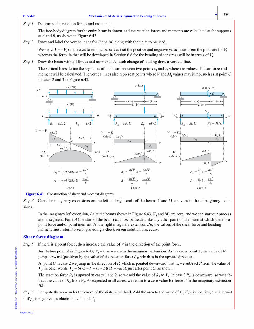
6 289Mechanics of Materials: Symmetric Bending of BeamsM. VablePr
inte
d fr
om: h
ttp://
ww
w.m
e.m
tu.e
du/~
mav
able
/MoM
2nd.
htm
Step 1 Determine the reaction forces and moments.
The free-body diagram for the entire beam is drawn, and the reaction forces and moments are calculated at the supports at A and B, as shown in Figure 6.43.
Step 2 Draw and label the vertical axes for V and Mz along with the units to be used.
We show V = −Vy on the axis to remind ourselves that the positive and negative values read from the plots are for V, whereas the formula that will be developed in Section 6.6 for the bending shear stress will be in terms of Vy .
Step 3 Draw the beam with all forces and moments. At each change of loading draw a vertical line.
The vertical lines define the segments of the beam between two points x1 and x2 where the values of shear force and moment will be calculated. The vertical lines also represent points where V and Mz values may jump, such as at point C in cases 2 and 3 in Figure 6.43.
Step 4 Consider imaginary extensions on the left and right ends of the beam. V and Mz are zero in these imaginary exten-sions.
In the imaginary left extension, LA at the beams shown in Figure 6.43, V1 and M1 are zero, and we can start our process at this segment. Point A (the start of the beam) can now be treated like any other point on the beam at which there is a point force and/or point moment. At the right imaginary extension BR, the values of the shear force and bending moment must return to zero, providing a check on our solution procedure.
Shear force diagramStep 5 If there is a point force, then increase the value of V in the direction of the point force.
Just before point A in Figure 6.43, V1 = 0 as we are in the imaginary extension. As we cross point A, the value of V jumps upward (positive) by the value of the reaction force RA, which is in the upward direction.
At point C in case 2 we jump in the direction of P, which is pointed downward; that is, we subtract P from the value of V1. In other words, V2 = bP/L – P = (b – L)P/L = –aP/L just after point C, as shown.
The reaction force RB is upward in cases 1 and 2, so we add the value of RB to V1. In case 3 RB is downward, so we sub-tract the value of RB from V1. As expected in all cases, we return to a zero value for force V in the imaginary extension BR.
Step 6 Compute the area under the curve of the distributed load. Add the area to the value of V1 if py is positive, and subtractit if py is negative, to obtain the value of V2.
L (ft)
L R L R
w (lb/ft)
CC C
L (in)a (in) b (in)
P kips
RA � wL�2 RA � bP�LRB � wL�2 RB � aP�L
C
A B L R
M
L (m)a (m) b (m)
M (kN�m)
RA � M�L RB � M�L
C
A B
V � �Vy V � �Vy(kips)
V � �Vy(kN)
Mz(ft�lb)
Mz(in�kips)
Mz(kN�m)
wL�2
wL�2wL2�8
L�2
L�2
A1 A1A1
A2 A2
A2
aP�LabP�L
bP�L M�L
bM�L
aM�L
M�L
A B
x
y
A1 � wL�2(L�2) � 1
2
wL2
8
A2 � wL�2(L�2) � 1
2
wL2
8
Case 1
A1 � a � bFP
LabFP
L
A2 � b � aFP
LabFP
L
Case 2
A1 � a � M
L
aML
A2 � b � M
L
bML
Case 3
Figure 6.43 Construction of shear and moment diagrams.
August 2012

6 290Mechanics of Materials: Symmetric Bending of BeamsM. VablePr
inte
d fr
om: h
ttp://
ww
w.m
e.m
tu.e
du/~
mav
able
/MoM
2nd.
htm
In case 1 the area under the distributed force is wL and py is negative. Therefore we subtract wL from the value of V just after A (+wL/2) to get the value of V just before B (–wL /2).
Step 7 Repeat Steps 5 and 6 until the imaginary extension at the right of the beam is reached. If the value of V is not zero inthe imaginary extension, then check Steps 5 and 6 for each segment of the beam.
For the three simple cases considered in Figure 6.43, this step is not required.Step 8 Draw additional vertical lines at any point where the value V is zero. Determine the location of these points by usinggeometry.
The points where V is zero represent the location of the maximum or minimum values of the bending moment because at these points. In case 1 V = 0 at point C. The location can be found by using similar triangles.
Step 9 Calculate the areas under the V curve and between two adjacent vertical lines.
Areas A1 and A2 can be found and recorded as shown in Figure 6.48.
Moment diagramStep 10 If there is a point moment, then use the moment template and the template equation to determine the direction of thejump.
In case 3 there is a point moment at point C. Comparing the direction of the moment at C to that in the template in Fig-ure 6.42, we conclude that Mext = – M. Just before C, M1 = aM /L. As per the template equation, M2 = aM /L – M = (a – L)M /L = –bM /L, which is the value just after C.In all three cases there is no point moment at A, hence our starting value is zero. If there were a point moment at A, we would use the moment template and the template equation to determine the starting value as we move from the imagi-nary segment to just right of A.
Step 11 To move from the right of one vertical line to the left of the next vertical line, add the areas under the V curve if V ispositive, and subtract the areas if V is negative. Draw the curve according to the curvature rule in Equation (6.21).
In all three cases the area A1 is positive and we add the value of the area to the value of the moment at point A to obtain the moment just before C. In cases 1 and 2 the area A2 is negative. Hence we subtract the value of A2 from the moment value just after C to get a zero value just before B. In case 3 A2 is positive and we add the value of A2 to the moment value just after C. In cases 2 and 3 the V curve is constant in each segment, and hence the Mz curve is linear in each segment. In case 1 the V curve is linear. Hence the Mz curve is quadratic and we need to determine the curvature of the curve. The inclination of the tangent to the Mz curve at A is nonzero, and it decreases to zero at C. Thus the inclination of the tangent decreases as the magnitude of V decreases. Similarly, as we move from C to B, the inclination of the tangent increases from zero to a nonzero value, consistent with the increasing magnitude of V.Alternatively, in case 1 py = −w, and hence the curvature of the moment curve is convex.
Step 12 Repeat Steps 10 and 11 until you reach the imaginary extension on the right of the beam. If the value of Mz is notzero in the imaginary extension, then check Steps 10 and 11 for each segment of the beam.
This procedure is applied and elaborated in Examples 6.11 and 6.12.
6.5 STRENGTH BEAM DESIGN
This section addresses two issues. The first relates to choosing a standard, commonly manufactured beam cross section thatwill be cheapest to use. The second issue relates to determining the maximum tensile or compressive bending normal stress.
6.5.1 Section Modulus
In the design of steel beams, the tensile and compressive strength are usually assumed to be equal. We calculate the magnitudeof the maximum bending normal stress using Equation (6.12), which can be written as , where Mmax is the
magnitude of the maximum internal bending moment, and ymax the distance of the point farthest from the neutral axis. Themoment of inertia Izz and ymax depend on the geometry of the cross section. Thus, Equation (6.12) requires two variables to
dMz dx⁄ = 0
σmax = Mmaxymax Izz⁄
August 2012

6 291Mechanics of Materials: Symmetric Bending of BeamsM. VablePr
inte
d fr
om: h
ttp://
ww
w.m
e.m
tu.e
du/~
mav
able
/MoM
2nd.
htm
determine the best geometric shape in a particular design. A variable called section modulus S, simplifies the equation for themaximum bending normal stress
(6.22)
Section C.6 give the section modulus S for steel beams of standard shapes and Example 6.12 shows its use in design.
6.5.2 Maximum Tensile and Compressive Bending Normal Stresses
Section 3.1 observed that a brittle material usually ruptures when the maximum tensile normal stress exceeds the ultimate ten-sile stress of the material. Cracks in materials propagate due to tensile stress. Adhesively bonded material debonds from ten-sile normal stress called peel stress. Thus a structure designed for maximum normal stress may fail when the maximum tensilestress is less in magnitude than the maximum compressive stress. Similarly, failure may occur when the maximum compres-sive normal stress is less than the maximum tensile normal stress. This may happen because buckling, which is discussed inChapter 11. Proper beam design must take into account failure due to tensile or compressive normal stresses.
To account for these stresses, it may be necessary to determine two stress values—the maximum tensile and compressive bending normal stress. These may differ when the top and the bottom of the beam are at different distances from the neutral axis of the cross section. Since both Mz and y affect the sign of the bending normal stress in Equation (6.12), stresses must be checked at four points:
• On the top and bottom surfaces on the cross-section location where Mz is a maximum positive value. • On the top and bottom surfaces on the cross-section location where Mz is a maximum negative value.
Example 6.11 elaborates this issue.
EXAMPLE 6.11
Figure 6.44 shows a loaded beam and cross section. (a) Draw the shear force and bending moment diagrams for the beam, and determinethe maximum shear force and bending moment. (b) Determine the maximum tensile and compressive bending normal stress in the beam.
PLAN(a) We can determine the reaction force and moment at wall C and follow the procedure for drawing shear and moment diagramsdescribed in Section 6.4.3. (b) We can find σxx from Equation (6.12) at points E and F at those cross sections where the Mz value is max-imum positive and maximum negative. From these four values we can find the maximum tensile and compressive bending normalstresses.
SOLUTION(a) We draw the shear force and bending moment diagram as per the procedure outlined in Section 6.4.3.Step 1: From the free-body diagram shown in Figure 6.45 we can determine the value of the reaction force Rw by equilibrium of forcesin the y direction. By equilibrium of moment about point C, we can determine the reaction moment Mw. The values of these reactions are
Rw = 10 kips (E1)Mw 3 ft ⋅kips (E2)
SIzz
ymax---------= σmax
Mmax
S------------=
3 ft 3 ft
M � 18 ft�kips x BA C
y
1 in
1 in
4 in
6 in4.
4 in
Izz � 47.7 in4
z
y
F
E
8 kips
6 kips/ft
Figure 6.44 Beam and loading in Example 6.11.
August 2012
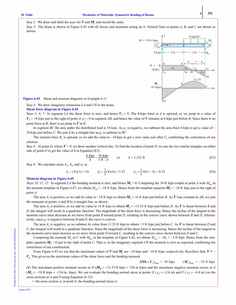
6 292Mechanics of Materials: Symmetric Bending of BeamsM. VablePr
inte
d fr
om: h
ttp://
ww
w.m
e.m
tu.e
du/~
mav
able
/MoM
2nd.
htm
Step 2: We draw and label the axes for V and Mz and record the units.Step 3: The beam is shown in Figure 6.45 with all forces and moments acting on it. Vertical lines at points A, B, and C are drawn asshown.
Step 4: We draw imaginary extensions LA and CR to the beam.Shear force diagram in Figure 6.45Steps 5, 6, 7: In segment LA the shear force is zero, and hence V1 = 0. The 8-kips force at A is upward, so we jump to a value ofV2 = +8 kips just to the right of point A. py = 0 in segment AB, and hence the value of V remains at 8 kips just before B. Since there is nopoint force at B, there is no jump in V at B.
In segment BC the area under the distributed load is 18 kips. As py is negative, we subtract the area from 8 kips to get a value of −10 kips just before C. We join it by a straight line as py is uniform in BC.
The reaction force Rw is upward, so we add the value to −10 kips to get a zero value just after C, confirming the correctness of oursolution. Step 8: At point D, where V = 0, we draw another vertical line. To find the location of point D, we use the two similar triangles on eitherside of point D to get the value of h in Equation (E3).
(E3)
Step 9: We calculate areas A1, A2, and A3 as
(E4)
Moment diagram in Figure 6.45Steps 10, 11, 12: In segment LA the bending moment is zero, and hence M1 = 0. Comparing the 18-ft·kips couple at point A with Mext inthe moment template in Figure 6.47, we obtain Mext = –18 ft·kips. Hence from the template equation M2 = –18 ft·kips just to the right ofpoint A.
The area A1 is positive, so we add its value to −18 ft·kips to obtain M2 = +6 ft·kips just before B. As V was constant in AB, we jointhe moments at points A and B by a straight line, as shown.
The area A2 is positive, so we add its value to +6 ft·kips to obtain M2 = +11.33 ft·kips just before D. As V is linear between B andD, the integral will result in a quadratic function. The magnitude of the shear force is decreasing. Hence the incline of the tangent to themoment curve must decrease as we move from point B toward point D, resulting in the convex curve shown between B and D. Alterna-tively, since py is negative between B and D, the curve is convex.
The area A3 is negative, so we subtract its value from 11.33 ft·kips to obtain +3 ft·kips just before C. As V is linear between D andC, the integral will result in a quadratic function. Since the magnitude of the shear force is increasing. Hence the incline of the tangent tothe moment curve must increase as we move from point D toward C, resulting in the convex curve shown between D and C.
Comparing the moment Mw at C with Mext in the template in Figure 6.42, we obtain Mext = –Mw = –3 ft·kips. Hence from the tem-plate equation M2 = 0 just to the right of point C. That is, in the imaginary segment CR the moment is zero as expected, confirming thecorrectness of our construction.
From Figure 6.45 we see that the maximum values of V and Mz are –10 kips and –18 ft ·kips, respectively. Recollect that, V = –Vy. This gives us the maximum values of the shear force and the bending moment.
ANS.
(b) The maximum positive moment occurs at D (MD = +11.33 ft·kips = 136 in·kips) and the maximum negative moment occurs at A(MA = −18 ft·kips = −216 in.·kips). We can evaluate the bending normal stress at points E ( yE = +2.6 in) and F ( yF = −4.4 in.) on thecross sections at A and D using Equation (6.12):
• On cross section A, at point E, the bending normal stress is
3 ft 3 ft
M � 18 ft�kips
x BA C
y
8 kips
6 kips/ft
h 3 � hV � �Vy
(kips)
Mz(ft�kips)
10
A1 A2DxBxA
xC
Mw
Rw
xDA3
18
11.33
3
88
6
L R
Figure 6.45 Shear and moment diagrams in Example 6.11.
8 kipsh
-------------- = 10 kips3 ft h–----------------- or h = 1.333 ft
A1 = 8( ) 3( ) = 24 A2 = 12--- 8( ) h( ) = 5.33 A3 = 1
2---10 3 h–( ) = 8.33
Vy( )max 10 kips= Mz( )max 18– ft ·kips=
August 2012

6 293Mechanics of Materials: Symmetric Bending of BeamsM. VablePr
inte
d fr
om: h
ttp://
ww
w.m
e.m
tu.e
du/~
mav
able
/MoM
2nd.
htm
(E5)
• On cross section A, at point F, the bending normal stress is
(E6)
• On cross section D, at point E, the bending normal stress is
(E7)
• On cross section D, at point F, the bending normal stress is
(E8)
From the results in Equations (E5), (E6), (E7), and (E8), it is clear that the maximum tensile bending normal stress occurs at point F onthe cross section at D. The maximum compressive bending normal stress occurs instead at point F on the cross section at A.
ANS.
COMMENTS1. In practice we need not write each step. Equations (E3) through (E4) suffice for drawing the shear and moment diagrams.2. In Figure 6.45 we see that at point D, where shear force is zero, there is a local maximum in the bending moment. But the maximum
moment in the beam is at point A, where a point moment is applied.3. If we were determining the magnitude of the maximum bending normal stress, then we need to evaluate stress one point only—where
the moment is a maximum (cross section A) and where y is also a maximum (point F). 4. We could use the template shown in Figure 6.46 to determine the direction of the jump in the moment. It can be verified that the
moment jumps at A and C will be as before. This shows that the direction of Mext on the template is immaterial. Thus there is no needto memorize the template, which can be drawn before starting on the shear and moment diagrams.
EXAMPLE 6.12
Consider the beam shown in Figure 6.38. Select the lightest W- or S-shaped beams from these given in Appendix E if the allowablebending normal stress is 53 MPa in tension or compression.
PLANWe can draw the shear and moment diagrams using the procedure described in Section 6.4.3. From the moment diagram we can find themaximum moment. Using the allowable bending normal stress of 53 MPa and Equation (6.22), we can find the minimum sectional mod-ulus. Using Section C.6, we can make a list of the beams for which the sectional modulus is just above the one we determined andchoose the lightest beam we can use.
SOLUTIONStep 1: The reaction forces at points A and D were determined in Example 6.10.Step 2: The beam with all forces and moments acting on it is shown in Figure 6.47. Vertical lines at points A, B, C, and D are shown as drawn.
Step 3: We draw imaginary extensions LA and DR to the beam.
σAE216 in.· kips–( ) 2.6 in.( )
47.7 in.4-----------------------------------------------------------– +11.8 ksi= =
σAF216 in.· kips–( ) 4.4 in.–( )
47.7 in.4--------------------------------------------------------------– 19.9 ksi–= =
σDE136 in.· kips( ) 2.6 in.( )
47.7 in.4--------------------------------------------------------– 7.4 ksi–= =
σDF136 in.· kips( ) 4.4 in.–( )
47.7 in.4-----------------------------------------------------------– +12.6 ksi= =
σDF = 12.6 ksi T( ) σAF = 19.9 ksi C( )
M1 M2
Mext
�x �x Figure 6.46 Alternative template and equation.
M2 = M1 Mext–Template Equation:
12 kN�m 4 kN/m5 kN
5 kN/m
xA C DB
2.0 m 1.0 m 3.0 m
RA � 0
RD � 7 kN
E
10
5 5
7
10
2
3
6.125
h 3 � h
Vy � �V(kN)
Mz(kN�m)
xDxExCxBxA
A1 A2 A3
A4
L R
Figure 6.47 Shear and moment diagrams in Example 6.12.
August 2012

6 294Mechanics of Materials: Symmetric Bending of BeamsM. VablePr
inte
d fr
om: h
ttp://
ww
w.m
e.m
tu.e
du/~
mav
able
/MoM
2nd.
htm
Step 4: We label the axes for V and Mz and record the units. Shear force diagram in Figure 6.47Steps 5, 6, 7: In segment LA, V1 = 0. Since RA is zero, there is no jump at A and we start our diagram at zero.
In segment AB, py = +5 kN/m. Hence we add the area of 5 × 2 = 10 kN to obtain V2 = 10 kN just before point B and draw a straightline between the values of V at A and B, as shown in Figure 6.47. At B the point force of 5 kN is downward. Thus we jump downward by5 kN to obtain V2 = 5 kN just after point B.
In segment BC, py= 0; hence the value of V does not change until point C.In segment CD, py = −4 kN/m. Hence we subtract the area of 4 × 3 = 12 kN to obtain V2 = −7 kN just before point D and draw a
straight line between the values of V at C and D, as shown in Figure 6.47. The reaction force at D is upward, so we jump upward by 7 kNto obtain V2 = 0 kN just after point D. That is, in the imaginary segment DR the shear force is zero as expected, confirming the correctnessof our construction.Step 8: At point E, where Vy = 0, we draw another vertical line. To find the location of point E, we use the two similar triangles on eitherside of point E to obtain h:
(E1)
Step 9: We calculate the areas A1 through A4
(E2)
Bending moment diagram in Figure 6.47Steps 10, 11, 12: In segment LA the bending moment is zero, and hence M1 = 0. As there is no point moment at A, we start our momentdiagram at zero.
As V is positive in segment AB, we add the area A1 to obtain M2 = +10 kN·m just before B. As V is linear in AB, the integral willresult in a quadratic function between A and B. As the magnitude of the shear force is increasing, the incline of the tangent to the momentcurve must increase as we move from point A toward point B, resulting in the concave curve shown between A and B. Alternatively,since py is positive in AB, the moment curve is concave.
Comparing the moment 12 kN·m at B with Mext in the template in Figure 6.42, we obtain Mext = –12 kN·m. Hence from the tem-plate equation M2 = 10 – 12 = –2 kN·m just to the right of point B.
As V is positive in segment BC, we add the area A2 to obtain the value of M2 = +3 kN·m just before C. As V is constant between Band C, the integral will result in a linear function, so we draw a straight line between B and C.
As V is positive in segment CE, we add the area A3 to obtain the value of M2 = +6.125 kN·m just before E. As V is linear betweenC and E, the integral will result in a quadratic function. As the magnitude of the shear force is decreasing, the incline of the tangent to themoment curve must also decrease as we move from point C toward E, resulting in the convex curve between C and E, as shown. Alter-natively, since py is negative in CE, the moment curve is convex.
As V is positive in ED, we add the area A4 to obtain the value of M2 = 0 just before D. As V is linear between E and D, the integralwill result in a quadratic function. As the magnitude of the shear force is increasing, the incline of the tangent to the moment curve mustalso increase as we move from point E toward D, resulting in the convex curve between E and D, as shown. Alternatively, since py isnegative in ED, the moment curve is convex.
As there is no point moment at D, there will be no jump in the moment at D. Hence we obtain a zero value for the moment in the imag-inary segment DR as expected, confirming the correctness of our construction.
From the moment diagram in Figure 6.47 the maximum moment is Mmax = 10 kN·m. Noting that the allowable bending normalstress is 53 MPa, Equation (6.22) yields
(E3)
From Section C.6 we obtain the following list of W- and S-shaped beams that have a section modulus close to that given in Equation (E3):
The lightest beam is W200 × 22.5 as it has a mass of only 22.5 kg/m. ANS.
COMMENTS1. This example demonstrate the use of the section modulus in selecting the beam cross section from a set of standard shapes. But the
section modulus can also be used with nonstandard shapes. 2. The alternative template shown in Figure 6.46 could have been used in this example. It would result in the same jumps as shown in
Figure 6.47.3. Again, only Equations (E1) through (E2) are needed to obtain the shear and moment diagrams. From here on, the shear and moment
diagrams will be drawn without additional explanations.
5 mh
--------- 7 m3 m h–------------------= or h 1.25 m=
A112---10 2× 10= = A2 5 1× 5= = A3
12---5h 3.125= = A4
12---7 3 h–( ) 6.125= =
σmax10 103( ) N
S------------------------- 53 106( ) N/m2 or S 188.7 103( ) mm3≥≤=
W150 29.8×W200 22.5×
S 219 103× mm3=
S 194.2 103× mm3=and
S200 27.4×S180 30×
S 236 103× mm3=
S 198.3 103× mm3=
W200 22.5×
August 2012

6 295Mechanics of Materials: Symmetric Bending of BeamsM. VablePr
inte
d fr
om: h
ttp://
ww
w.m
e.m
tu.e
du/~
mav
able
/MoM
2nd.
htm
PROBLEM SET 6.3
Equilibrium of shear force and bending moment 6.59 (a) Write the equations for shear force and bending moments as a function of x for the entire beam shown in Figure P6.59; (b) show thatyour results satisfy Equations (6.17) and (6.18).
6.60 (a) Write the equations for shear force and bending moments as a function of x for the entire beam shown in Figure P6.60; (b) show thatyour results satisfy Equations (6.17) and (6.18).
QUICK TEST 6.1 Time: 20 minutes/Total: 20 points
Answer true or false and justify each answer in one sentence. Grade yourself with the answers given in Appendix E.
Assume linear elastic, homogeneous material unless stated otherwise.
1. If you know the geometry of the cross section and the bending normal strain at one point on a cross section,
then the bending normal strain can be found at any point on the cross section.
2. If you know the geometry of the cross section and the maximum bending normal stress on a cross section, then
the bending normal stress at any point on the cross section can be found.
3. A rectangular beam with a 2-in. × 4-in. cross section should be used with the 2-in. side parallel to the bending
(transverse) forces.
4. The best place to drill a hole in a beam is through the centroid.
5. In the formula , y is measured from the bottom of the beam.
6. The formula can be used to find the normal stress on a cross section of a tapered beam.
7. The equations and cannot be used for nonlinear materials.
8. The equation can be used for nonhomogeneous cross sections.
9. The internal shear force jumps by the value of the applied transverse force as one crosses it from left to right.
10. The internal bending moment jumps by the value of the applied concentrated moment as one crosses it from
left to right.
σxx Mzy Izz⁄–=
σxx Mzy Izz⁄–=
σxx Ad 0=A
∫ Mz yσxx AdA
∫–=
Mz yσxx AdA
∫–=
Figure P6.59
x
5 kN/my
3 m
Figure P6.60
x
y
3 kips/in
72 in
August 2012

6 296Mechanics of Materials: Symmetric Bending of BeamsM. VablePr
inte
d fr
om: h
ttp://
ww
w.m
e.m
tu.e
du/~
mav
able
/MoM
2nd.
htm
6.61 (a) Write the equations for shear force and bending moments as a function of x for the entire beam shown in Figure P6.61; (b) show thatyour results satisfy Equations (6.17) and (6.18).
6.62 (a) Write the equations for shear force and bending moments as a function of x for the entire beam shown in Figure P6.62; (b) show thatyour results satisfy Equations (6.17) and (6.18).
6.63 (a) Write the equations for shear force and bending moments as a function of x for the entire beam shown in Figure P6.63; (b) show thatyour results satisfy Equations (6.17) and (6.18).
6.64 (a) Write the equations for shear force and bending moments as a function of x for the entire beam shown in Figure P6.64; (b) show thatyour results satisfy Equations (6.17) and (6.18).
6.65 (a) Write the equations for shear force and bending moments as a function of x for the entire beam shown in Figure P6.65; (b) show thatyour results satisfy Equations (6.17) and (6.18).
6.66 (a) Write the equations for shear force and bending moments as a function of x for the entire beam shown in Figure P6.66; (b) show thatyour results satisfy Equations (6.17) and (6.18).
6.67 Consider the beam shown in Figure P6.67. (a) Write the shear force and moment equations as a function of x in segments AB and BC.(b) Show that your results satisfy Equations (6.17) and (6.18). (c) What are the shear force and bending moment values just before and just afterpoint B?
Figure P6.61
x
5 kN/my
3 m
5 kN/m
Figure P6.62x
y
72 in
3 kips/in3 kips/in.
Figure P6.63
x
y
0.5 m 0.5 m
5 kN/m
Figure P6.64
x
y
wL2 (in�kips)
L (in)L (in)
w(kips/in.)
x
y
L (in)L L (in)L
w (kips/in)
Figure P6.65
x
y
L (in) L (in)
w (kips/in)
Figure P6.66
12 kN/m 12 kN10 kN�m
16 kN�m
12 kN/mB E
CA Dx
y
3 m 2 m 4 m 3 m Figure P6.67
August 2012

6 297Mechanics of Materials: Symmetric Bending of BeamsM. VablePr
inte
d fr
om: h
ttp://
ww
w.m
e.m
tu.e
du/~
mav
able
/MoM
2nd.
htm
6.68 Consider the beam shown in Figure P6.67. (a) Write the shear force and moment equations as a function of x in segments CD and DE.(b) Show that your results satisfy Equations (6.17) and (6.18). (c) What are the shear force and bending moment values just before and just afterpoint D?
6.69 Consider the beam shown in Figure P6.69. (a) Write the shear force and moment equations as a function of x in segments AB and BC.(b) Show that your results satisfy Equations (6.17) and (6.18). (c) What are the shear force and bending moment values just before and just afterpoint B?
6.70 Consider the beam shown in Figure P6.69. (a) Write the shear force and moment equations as a function of x in segments CD and DE.(b) Show that your results satisfy Equations (6.17) and (6.18). (c) What are the shear force and bending moment values just before and just afterpoint D?
6.71 During skiing, the weight of a person is often all on one ski. The ground reaction is modeled as a distributed force p(x) and a concen-trated fore P is modeled as shown in Figure P6.71. (a) Find shear force and bending moment as a function of x across the ski. (b) The ski is50 mm wide and the thickness of the ski varies as shown. Determine the maximum bending normal stress. Use of spread sheet recommended.
Shear and moment diagrams6.72 Draw the shear and moment diagrams for the beam and loading shown in Figure P6.72.
6.73 Draw the shear and moment diagrams for the beam and loading shown in Figure P6.73.
6.74 For the beam shown in Figure P6.59, draw the shear force bending moment diagram. Determine the maximum values of shear forceand bending moment.
6.75 For the beam shown in Figure P6.60, draw the shear force bending moment diagram. Determine the maximum values of shear forceand bending moment.
6.76 A man whose mass is 80 kg is sitting in the middle of a flat bottom boat, as shown in Figure 6.76. The weight of the boat per unit lengthbetween A and B is 130 N/m. To a first approximation assume the resisting water pressure acts between A and B and is uniform. Draw the shearforce and bending moment diagram between A and B.
6 kN6 kN/m
10 kN
10 kN�m6 kN/m
B CA D Ex
3 m 2 m 4 m 3 m Figure P6.69
Figure P6.71
x
Thickness
792 N
25 mm7 mm 7 mm
p
0.9 m P1.5 m
x
y P P
L L L Figure P6.72
x
yM M
L L L Figure P6.73
4.5 m Figure P6.76
A B
August 2012

6 298Mechanics of Materials: Symmetric Bending of BeamsM. VablePr
inte
d fr
om: h
ttp://
ww
w.m
e.m
tu.e
du/~
mav
able
/MoM
2nd.
htm
6.77 Draw the shear and moment diagrams for the beam and loading shown in Figure P6.77. Determine the maximum values of shear forceand bending moment.
6.78 Draw the shear and moment diagrams for the beam and loading shown in Figure P6.78. Determine the maximum values of shear forceand bending moment.
6.79 Determine the maximum values of shear force and bending moment for the beam shown in Figure P6.67.
6.80 Determine the maximum values of shear force and bending moment for the beam shown in Figure P6.69.
6.81 Determine the maximum values of shear force and bending moment for the beam shown in Figure P6.81.
6.82 Determine the maximum values of shear force and bending moment for the beam shown in Figure P6.82.
6.83 Determine the maximum values of shear force and bending moment. for the beam shown in Figure P6.83.
6.84 Determine the maximum values of shear force and bending moment for the beam shown in Figure P6.84.
6.85 Determine the maximum value of the shear force and bending moment for the beam shown in Figure 6.85.
x
y
L L L
w
Figure P6.77
x
y
L L L
w w
Figure P6.78
3 kN/m16 kN�m
8 kN�m
2 kN/m4 kN
x
4 m4 m3 m Figure P6.81
Figure P6.82
5 ft�kips
2 ft�kips
2 kips4 kips
2 kips/ft
4 ft3 ft2 ft
Figure P6.83
3 kN/m4.5 kN�m
4 kN/m
3 kN
x
4 m4 m3 m
75 kN�m
45 kN�m
90 kN40 kN
150 kN100 kN
20 kN/m40 kN/m
2 m2 m 1 m1 m1 m
Figure P6.84
2 kips/ft
1 ft 1 ft 1 ft1 ft 1 ft1 ft
4 kips
4 kips
Figure P6.85
A B C D E
August 2012

6 299Mechanics of Materials: Symmetric Bending of BeamsM. VablePr
inte
d fr
om: h
ttp://
ww
w.m
e.m
tu.e
du/~
mav
able
/MoM
2nd.
htm
6.86 Determine the maximum values of shear force and bending moment for the beam shown in Figure P6.86.
Maximum bending normal stress6.87 A diver weighing 200 lb stands at the edge of the diving board, as shown in Figure 6.87. The diving board cross section is 16 in. x 1 in.Determine the maximum bending normal stress in the diving board.
6.88 A diver weighing 200 lb stands at the edge of the diving board, as shown in Figure 6.87. The diving board cross section is 16 in. x 1 in.and has a weight of 60 lb. Model the weight of the diving board as a uniform distributed load of 0.5 lb/in. along the length. Determine the max-imum bending normal stress in the diving board.
6.89 The diving board shown in Figure 6.87 has a cross section of 18 in. x 1 in. The allowable bending normal stress 10 ksi. What is themaximum force to the nearest pound that the board can sustain when the diver jumps on it before a dive. Neglect the weight of the diving board.
6.90 A father and his son are playing on a seesaw, as shown in Figure 6.90. The wooden plank of the see saw is 12 ft x 10 in. x 1.5 in. and ishinged in the middle. The weights of the father and son are 225 lb and 80 lb, respectively. The mass of the father mF and mass of the son ms
times the acceleration a are the inertial forces acting on them at the time the plank is horizontal. Neglecting the weight of the plank, determinethe maximum bending normal stress.
6.91 A mother and her daughter are on either side of the seesaw with the teenager son standing in the middle as shown in Figure 6.91. Thewooden plank of the seesaw is 3.5 m x 250 mm x 40 mm and is hinged in the middle. The mass of the mother, son, and daughter aremm= 70 kg, ms= 80 kg, and md= 40 kg, respectively. At the time the plank is horizontal, inertial forces of mass times the acceleration a acts onthe mother and daughter. Neglecting the weight of the plank, determine the maximum bending normal stress.
Design problems6.92 A beam, its loading, and its cross section are as shown Figure P6.92. Determine the intensity w of the distributed load if the maximumbending normal stress is limited to 10 ksi (C) and 6 ksi (T). The second area moment of inertia is Izz = 47.73 in.4.
Figure P6.86 3 ft
2 ft�kips2 kips/ft2 kips4 kips
5 ft�kips
6 ft
2 kips/ft
3 ft
Figure P6.87
64 in.A
B C56 in.
Figure P6.90 Father Son
ms amF a
Figure P6.91Mother Daughter
md amm a Son
Figure P6.92
w (lb/in)
50 in50 in 50 in50 in
1 in
6 in
4 in
1 in
1 in
2.6 in
y
z
August 2012

6 300Mechanics of Materials: Symmetric Bending of BeamsM. VablePr
inte
d fr
om: h
ttp://
ww
w.m
e.m
tu.e
du/~
mav
able
/MoM
2nd.
htm
6.93 Two pieces of lumber are glued together to form the beam shown in Figure P6.93. Determine the intensity w of the distributed load if themaximum tensile bending normal stress in the glue is limited to 800 psi (T) and the maximum bending normal stress in wood is limited to 1200 psi.
6.94 The beam shown in Figure P6.64 has a load w = 25 lb/in. and L = 72 in. Select the lightest W- or S-shaped beam from Section C.6 if theallowable bending normal stress is 21 ksi in tension and compression.
6.95 The beam shown in Figure P6.65 has a load w = 0.4 kips/in. and L = 48 in. Select the lightest W- or S-shaped beam from Section C.6 ifthe allowable bending normal stress is 16 ksi in tension and compression.
6.96 The beam shown in Figure P6.66 has a load w = 0.15 kips/in. and L = 48 in. Select the lightest W- or S-shaped beams from Section C.6if the allowable bending normal stress is 21 ksi in tension and compression.
6.97 Consider the beam shown in Figure P6.67. Select the lightest W- or S-shaped beam from Section C.6 if the allowable bending normalstress is 180 MPa in tension and compression.
6.98 Consider the beam shown in Figure P6.69. Select the lightest W- or S-shaped beam from Section C.6 if the allowable bending normalstress is 225 MPa in tension and compression.
6.99 The wind pressure on a signpost is approximated as a uniform pressure, as shown Figure P6.99. A similar signpost is to be designedusing a hollow square steel beam for the post. The outer dimension of the square is to be 12 in. If the allowable bending normal stress is 24 ksi
and the pressure p = 33 lb/ft2, determine the inner dimension of the lightest hollow beam to the nearest in.
Stress concentration6.100 The allowable bending normal stress in the stepped circular beam shown in Figure P6.100 is 200 MPa and P = 200 N. Determine the smallestfillet radius that can be used at section B. Use stress concentration graphs given in Section C.4.
6.101 The allowable bending normal stress in the stepped circular beam shown in Figure P6.101 is 48 ksi. Determine the maximum intensity ofthe distributed load w assuming the fillet radius is: (a) 0.3 in.; (b) 0.5 in. Use stress concentration graphs given in Section C.4.
Figure P6.93 1 in
2 inw (lb/in)
30 in 70 in
18---
p
HollowSquare Post
5 ft.
8.5 ft.
7 ft
Figure P6.99
B
P50 mm
1.5 m 1 m
25 mm
Figure P6.100
C
Bw
A
4 in
2 ft 6 ft
2 in
Figure P6.101
August 2012

6 301Mechanics of Materials: Symmetric Bending of BeamsM. VablePr
inte
d fr
om: h
ttp://
ww
w.m
e.m
tu.e
du/~
mav
able
/MoM
2nd.
htm
Fatigue 6.102 The fillet radius is 5 mm in the stepped aluminum circular beam shown in Figure P6.100. What should be the peak value of the cyclicload P to ensure a service life of one-half million cycles? Use the S–N curve shown in Figure 3.36.
6.103 The beam in Figure P6.101 is made from a steel alloy that has the S–N curve shown in Figure 3.36. The peak intensity of the cyclic dis-tributed load is w = 80 lbs/in. and the fillet radius is 0.36 in. What is the predicted service life of the beam?
Stretch Yourself6.104 A simply supported 3-m-long beam has a uniformly distributed load of 10 kN/m over the entire length of the beam. If the beam has the com-posite cross section shown in Figure P6.104, determine the maximum bending normal stress in each of the three materials. Use Eal = 70 GPa,Ew = 10 GPa, and Es = 200 GPa. [Hint: Use Equations (6.14) and (6.16)].
6.105 A steel (Esteel = 200 GPa) tube of outside diameter of 240 mm is attached to a brass (Ebrass = 100 GPa) tube to form the cross sectionshown in Figure P6.105. Determine the maximum bending normal stress in steel and brass. [Hint: Use Equation (6.16)]
6.6 SHEAR STRESS IN THIN SYMMETRIC BEAMS
In Section 6.2.6 we observed that the maximum bending shear stress has to be nearly an order of magnitude less than the max-imum bending normal stress for our theory to be valid. But shear stress plays an important role in bending, particularly whenbeams are constructed by joining a number of beams together to increase stiffness. In this section we develop a theory that canbe used for calculating the bending shear stress.
Figure 6.48a and b shows the bending of four wooden strips that are separate and glued together, respectively. In Figure 6.48a each wooden strip slides relative to the other in the longitudinal direction. But in Figure 6.48b the relative sliding is pre-vented by the shear resistance of the glue—that is, the shear stress in the glue. One may thus hypothesize that in any beam there will be shear stresses on imaginary surfaces parallel to the axis of the beam.
Notice that the beam in Figure 6.48a has significantly more curvature (it bends more) than that in Figure 6.48b, even though the forces exerted in both cases are approximately the same. This phenomenon of increasing stiffness (see Problem
Figure P6.104
80 mm
100 mm
10 mmAluminum
10 mmSteel
Woodz
x
y
2 kN/m
3 kN/m
3 m 4 m 4 m
8 kN�m
160 mm Figure P6.105
Brass
Steel
240 mm200 mm
160 mm
Relative sliding No relative sliding
(a) (b)
Figure 6.48 Effect of shear stress in bending. (a) Separate beams. (b) Glued beams.
August 2012

6 302Mechanics of Materials: Symmetric Bending of BeamsM. VablePr
inte
d fr
om: h
ttp://
ww
w.m
e.m
tu.e
du/~
mav
able
/MoM
2nd.
htm
6.20) at the expense of introducing shear stress is exploited in the design of lightweight structures. In metal beams, the flanges are designed for carrying most of the normal stress in bending, and the webs are designed for carrying most of the shear stress (see Figure 6.28). In sandwich beams two stiff panels are separated by a soft core material. The stiff panels are designed to carry the normal stress and the soft core is designed to carry the shear stress.
6.6.1 Shear Stress Direction
Before developing formulas, it is worthwhile to understand the character of the shear stresses in bending and to determinetheir direction by inspection.
Consider the beam in Figure 6.49a. The beam is constructed by gluing five pieces of wood together. From the evidence of the photographs in Figure 6.48, we know that shear stress will exist at each glued surface to resist the relative sliding of the wood strips. If we take a small element Δx of strips 3 and 5, we obtain Figure 6.49c and d. On the glued surface between wooden strips 2 and 3 there will be a shear stress τzx as the outward normal of the surface is in the z direction and the internal shear force is in the x direction. On the glued surface between wooden strips 4 and 5 there will be a shear stress τyx, as the out-ward normal of the surface is in the y direction and the internal shear force is in the x direction.
Because of the bending load P, a normal stress distribution across the cross section will develop as shown in Figure 6.49b. From Equation (6.12), we know the bending normal stress σxx will vary along the length of the beam as the moment Mz varies. The bending normal stress distribution is such that there is no resultant axial force over the entire cross section. But if we only take a part of the cross section, as in Figure 6.49b and c, then there will be an axial force generated that varies along the length as shown in Figure 6.49c and d.
On the small element Δx, the equivalent shear force from the bending shear stresses must balance the change in the equiv-alent normal axial force, as shown Figure 6.54e and f. Thus in bending, the shear stress must balance the variations in the nor-mal stress σxx along the length of the beam.9
The preceding shows that shear stress develops on surfaces cut parallel to the axis of the beam. But from the symmetry of shear stresses τxy = τyx and τxz = τzx. These stresses, τxy and τxz, are on the cross sections perpendicular to the axis of the beam.
9From the field of elasticity it is known that in the absence of body forces, the equilibrium at a point requires (seeProblem 1.105). Thus if σxx varies with x, then τyx (or τxy) must vary with y, and τzx (or τxz) must vary with z. See Problem 6.136 for additional details.
(a)
P
H 3
1 G
F
I
5
4
2
DC
z
x
A
E
y
B
Normal stress distribution
(b)
�xx � d�xx
(d)
�xx
5
�yx
(c)
�xx � d�xx�xx
3
�zx
(f)
N5
V5 � �yx(tz) �x
N5 � dN55
�xt z
(e)
N3 � dN3
V3 � �zx(ty) �x
N3 3
�x
ty
1
2
3
4
5
d d
d
d
d d
Figure 6.49 Shear stress on different surfaces in bending.
∂σxx ∂x ∂τyx ∂y ∂τzx ∂z⁄+⁄+⁄ 0=
August 2012

6 303Mechanics of Materials: Symmetric Bending of BeamsM. VablePr
inte
d fr
om: h
ttp://
ww
w.m
e.m
tu.e
du/~
mav
able
/MoM
2nd.
htm
We know from Equation (6.10) that on the cross section of the beam the resultant of the shear stress τxy distribution is the shear force Vy. Thus the direction (sign) of τxy should be the same as that of Vy. But the shear force Vz that would be statically equiva-lent to τxz must be zero, as there is no external force in the z direction. This means that τxz must reverse sign (and direction) on the cross section if the net force from it is zero. We also know that the y axis is the axis of symmetry, and the loading is in the plane of symmetry. Therefore all stresses including τxz must be symmetric about the y axis. In other words, the shear stress τxz will reverse its direction as one crosses the y axis on the cross section. This sometimes implies that the shear stress τxz will be zero at the y axis.
Consider now a circular cross section that is glued together from nine wooden strips, as shown in Figure 6.50a. Once more shear stresses will develop along each glued surface, to resist relative sliding between two adjoining wooden strips, and the shear stress value must balance the change in axial force due to the variation in σxx. The outward normal of the surface will be in a different direction for each glued surface on which we consider the shear stress. If we define a tangential coordinate s that is in the direction of the tangent to the center line of the cross section, then the outward normal to the glued surface will be in the s direction and the shear stress will be τsx. Once more by the symmetry of shear stresses, τxs = τsx. At a point if the s direction and the y direction are the same, then τxs will equal ±τxy. If the s direction and the z direction are the same at a point, then τxs will equal ±τxz.
It should be noted that in Figure 6.49e and f and in Figure 6.50b the shear force that balances the change in the axial force N is shown on only one surface. The surface on the other end of the free-body diagram is always assumed to be a free surface. That is, the shear stress is zero on these other surfaces. The origin of the s coordinate is chosen to be one of the free surfaces and will be used in the next section in developing shear stress formulas. In a beam cross section the top and bottom and the side surfaces are always assumed to be surfaces on which shear stress is zero.
In Figure 6.49e and f and in Figure 6.50b we notice that the shear force expression contains the product of the shear stress and the thickness t of the cross section at that point. This product is the shear flow q.
(6.23)
The units of the shear flow are force per unit length. The terminology is from fluid flow in channels, but it is used extensivelyto discuss shear stresses in thin cross sections, probably because of the image of an actual flow helps in discussing shear stressdirections, as elaborated further in the next section and Example 6.13.
6.6.2 Shear Flow Direction by Inspection
The shear flow and shear stress along the center line of the cross section are drawn in a direction that satisfies the followingrules:
1. The resultant force in the y direction is in the same direction as Vy.2. The resultant force in the z direction is zero.3. It is symmetric about the y axis. This requires that shear flow change direction as one crosses the y axis on the center
line. Sometimes this will imply that shear stress is zero at the point(s) where the center line intersects the y axis.
q = τxst
(a)
P
y
x
s
Free surface
1
2
3456
7
8
9z
Free surface
(b)
N
V � �xs(t)�xt
�x
Free surface
1
23
N �
Figure 6.50 Shear stress in circular cross section.
August 2012
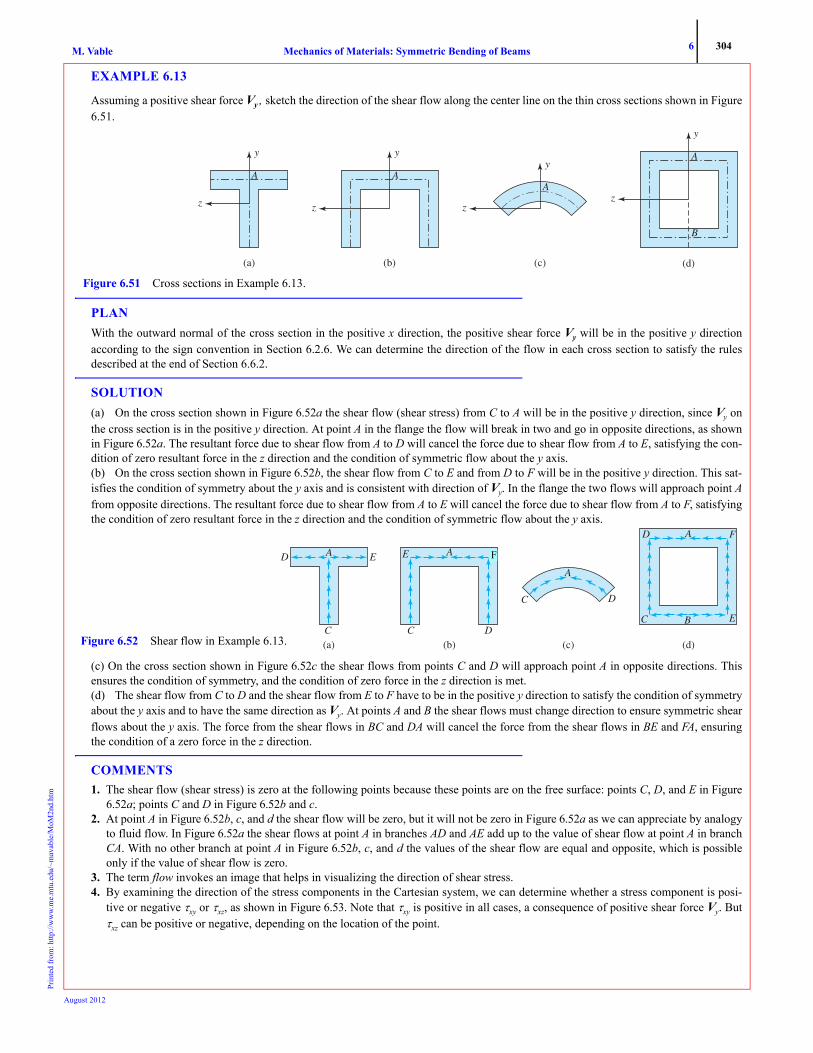
6 304Mechanics of Materials: Symmetric Bending of BeamsM. VablePr
inte
d fr
om: h
ttp://
ww
w.m
e.m
tu.e
du/~
mav
able
/MoM
2nd.
htm
EXAMPLE 6.13
Assuming a positive shear force Vy , sketch the direction of the shear flow along the center line on the thin cross sections shown in Figure6.51.
PLANWith the outward normal of the cross section in the positive x direction, the positive shear force Vy will be in the positive y directionaccording to the sign convention in Section 6.2.6. We can determine the direction of the flow in each cross section to satisfy the rulesdescribed at the end of Section 6.6.2.
SOLUTION(a) On the cross section shown in Figure 6.52a the shear flow (shear stress) from C to A will be in the positive y direction, since Vy onthe cross section is in the positive y direction. At point A in the flange the flow will break in two and go in opposite directions, as shownin Figure 6.52a. The resultant force due to shear flow from A to D will cancel the force due to shear flow from A to E, satisfying the con-dition of zero resultant force in the z direction and the condition of symmetric flow about the y axis.(b) On the cross section shown in Figure 6.52b, the shear flow from C to E and from D to F will be in the positive y direction. This sat-isfies the condition of symmetry about the y axis and is consistent with direction of Vy. In the flange the two flows will approach point Afrom opposite directions. The resultant force due to shear flow from A to E will cancel the force due to shear flow from A to F, satisfyingthe condition of zero resultant force in the z direction and the condition of symmetric flow about the y axis.
(c) On the cross section shown in Figure 6.52c the shear flows from points C and D will approach point A in opposite directions. Thisensures the condition of symmetry, and the condition of zero force in the z direction is met. (d) The shear flow from C to D and the shear flow from E to F have to be in the positive y direction to satisfy the condition of symmetryabout the y axis and to have the same direction as Vy. At points A and B the shear flows must change direction to ensure symmetric shearflows about the y axis. The force from the shear flows in BC and DA will cancel the force from the shear flows in BE and FA, ensuringthe condition of a zero force in the z direction.
COMMENTS1. The shear flow (shear stress) is zero at the following points because these points are on the free surface: points C, D, and E in Figure
6.52a; points C and D in Figure 6.52b and c. 2. At point A in Figure 6.52b, c, and d the shear flow will be zero, but it will not be zero in Figure 6.52a as we can appreciate by analogy
to fluid flow. In Figure 6.52a the shear flows at point A in branches AD and AE add up to the value of shear flow at point A in branchCA. With no other branch at point A in Figure 6.52b, c, and d the values of the shear flow are equal and opposite, which is possibleonly if the value of shear flow is zero.
3. The term flow invokes an image that helps in visualizing the direction of shear stress.4. By examining the direction of the stress components in the Cartesian system, we can determine whether a stress component is posi-
tive or negative τxy or τxz, as shown in Figure 6.53. Note that τxy is positive in all cases, a consequence of positive shear force Vy. Butτxz can be positive or negative, depending on the location of the point.
z
A
(a)
yy
z
A
(b) (c)
y
z
A
B
(d)
y
z
AA
Figure 6.51 Cross sections in Example 6.13.
A ED
C(a)
A F
E
D
BC
(d)
AE E
DC(b) (c)
AA
C D
Figure 6.52 Shear flow in Example 6.13.
F
August 2012

6 305Mechanics of Materials: Symmetric Bending of BeamsM. VablePr
inte
d fr
om: h
ttp://
ww
w.m
e.m
tu.e
du/~
mav
able
/MoM
2nd.
htm
6.6.3 Bending Shear Stress Formula
The previous section and Example 6.13 highlight that the bending shear stress is τxy in the web and τxz in the flange, whereasfor symmetric curvilinear cross sections it depends on the location of the point. To develop a single formula applicable to allsituations, we define a tangential coordinate s in the direction of the tangent to the center line of the cross section, startingfrom a free surface. In this section we derive the formula for bending shear stress τxs.
Consider a differential element of a wooden beam with circular cross section, as shown in Figure 6.54a. Consider the shear stress acting on the surface between wooden pieces 3 and 4. We can consider two possible free-body diagrams, shown in Figure 6.54b and c. The axial force Ns (or Ns*) acting on the part of cross section As (or As*) varies because of the variation of the bending stress σxx along the length of the beam. If the shear stress does not change across the thickness, the shear force V (or V*) is equal to the product of the shear stress multiplied by the area t dx, as shown. The assumption of constant shear stress in the thickness direction is a good approximation if the thickness is small.
Assumption 9: The beam is thin perpendicular to the center line of the cross section.
By equilibrium of forces in Figure 6.54c, we obtain or
(6.24)
Figure 6.53 Directions and signs of stress components in Example 6.13.
A F
E
D
BC
z
y
x
(a) (b)
Negative �xzPositive �xz
Positive �xz
Positive �xy
Negative �xz
(c)
A ED
C
AE F
DC
Positive �xyPositive �xy
Positive �xz Negative �xz Positive �xzNegative �xz
(b)
(c)
V � �sx t dx
t
dx1
23
Ns � dNs
Ns � � �xx dAAs
s*
Free surfaceFree surface
4567
8
9dxNs* � dNs*
Ns* � � �xx dAAs*
V* � �s*x t dx
(a)
y
x
s
s
s*
Free surface
1
2
3456
7
8
9 z
Free surface
dxAs*As
Figure 6.54 Differential element of beam for shear stress calculations.
Ns dNs+ Ns– τsxt xd+ 0=
τsxtdNs
dx---------– d
dx------– σxx Ad
As∫= =
August 2012

6 306Mechanics of Materials: Symmetric Bending of BeamsM. VablePr
inte
d fr
om: h
ttp://
ww
w.m
e.m
tu.e
du/~
mav
able
/MoM
2nd.
htm
Substituting Equation (6.12) into Equation (6.24) and noting that the moment Mz and the area moment of inertia Izz do not vary over the cross section, we obtain
(6.25)
where Qz is referred to as the first moment of the area As and is defined as
(6.26)
Assumption 10: The beam is not tapered.
Assumption 10 implies that Izz and Qz are not a function of x, and these quantities can be taken outside the derivative sign. We obtain
Substituting Equation (6.18), we obtain the formula for bending shear stress:
(6.27)
In Equation (6.27) the shear force Vy can be found either by equilibrium or by drawing the shear force diagram. Also, t is thethickness at the point where the shear stress is being found, and Izz is known from the geometry of the cross section. The direc-tion of s, identification of the area As, and the calculation of Qz are the critical new elements. We record the following observa-tions before discussing in detail the calculation of Qz.
• Area As is the area between the free surface and the point where the shear stress is being evaluated.• s is the direction from the free surface in the area As used in the calculation of Qz.
6.6.4 Calculating Qz
Figure 6.55 shows the area As between the top free surface and the point at which the shear stress is being found (line s–s).From Equation (6.26) we note that Qz is the first moment of the area As about the z axis. The integral in Equation (6.26) is thenumerator in the definition of the centroid of the area As. Analogous to the moment due to a force, the first moment of an areacan be found by placing the area As at its centroid and finding the moment about the neutral axis. That is, Qz is the product ofarea As and the distance of the centroid of the area As from the neutral axis, as shown in Figure 6.55. Alternatively, Qz can befound by using the bottom surface as the free surface, shown as Qz* in Figure 6.55.
At the top surface, which is a free surface, the value of Qz is zero, as the area As is zero. When we reach the bottom sur-face after starting from the top, the value of Qz is once more zero because As = A, and from Equation (6.9), . If Qz
starts with a zero value at the top and ends with a zero value at the bottom, then it must reach a maximum value somewhere on the cross section.
To see where Qz reaches a maximum value, consider the change in Qz as the line s–s moves downward in Figure 6.55. Toward the neutral axis, the moment of the area Qz increases as we add the moments from the additional areas. When the line s–s crosses the neutral axis, then the new additional area below the axis produces a negative moment because the centroid of
τsxt xdd Mz
Izz------- y Ad
As∫⎝ ⎠
⎛ ⎞xd
d MzQz
Izz-------------⎝ ⎠
⎛ ⎞= =
Qz y AdAs
∫=
τsxt Qz Izz⁄( )dMz dx⁄=
τsx τxs=VyQz
Izzt------------⎝ ⎠
⎛ ⎞–=
Qz � Asys
Qz* � As*ys*
Centroid of As
Neutralaxis
As
Centroid of As*
ys
ys*
As*
y
z
Line alongwhich shearstress isbeing found
ss
Figure 6.55 Calculation of Qz.
y AdA∫ 0=
August 2012

6 307Mechanics of Materials: Symmetric Bending of BeamsM. VablePr
inte
d fr
om: h
ttp://
ww
w.m
e.m
tu.e
du/~
mav
able
/MoM
2nd.
htm
this area is in the negative y direction. In other words, Qz increases up to the neutral axis and then starts decreasing. Thus Qz is maximum at the neutral axis. From Equation (6.27), it follows that bending shear stress is maximum at the neutral axis of a cross section. In summary
• Qz is zero at the top and bottom surface.• Qz is maximum at the neutral axis.• The maximum bending shear stress on a cross section is at the neutral axis.• The maximum bending shear stress in the beam will be at the neutral axis on a cross section where Vy is maximum.
We can write A = As + As* in Equation (6.9) and write the integral as to obtain . This
implies that Qz and Qz* will have the same magnitude but opposite signs. Thus, if we used Qz or Qz* in Equation (6.27), we
would get the same magnitude of the shear stress, but which would give the correct sign (or direction)?10 The answer is thatboth will give the correct sign, provided the s direction in Equation (6.27) is measured from the free surface used in the calcu-lation of Qz.
We can find the magnitude and the direction of the bending shear stress in two ways:
1. Use Equation (6.27) to find the magnitude of the shear stress. Use the rules described in Section 6.6.2 to determine thedirection of the shear stress.
2. Alternatively, follow the sign convention described in Section 6.2.6 to determine the shear force Vy . The shear stress isfound from Equation (6.27), and the direction of the shear stress is determined using the subscripts, as elaborated inSection 1.3.
6.6.5 Shear Flow Formula
The formula for shear flow can be obtained by substituting Equation (6.27) into Equation (6.23) to get
(6.28)
Equation (6.28) can be used in two ways. It can be used for finding the magnitude of the shear flow at a point, and the direc-tion of shear flow can then be found by inspection following the rules described in Section 6.6.2. Alternatively, the sign con-vention for the shear force Vy is followed and the shear flow is determined from Equation (6.28). A positive value of shearflow implies that the flow is in the positive s direction, where s is measured from the free surface used in the calculation of Qz.
One application of Equation (6.28) is the determination of the spacing between mechanical fasteners holding strips of beams together. Nails or screws are examples of mechanical fasteners used in wooden beams. Bolts or rivets are examples of mechanical fasteners used in metal beams. Figure 6.56 shows two strips of beams held together by a row of mechanical fasten-ers. Suppose the fasteners are spaced at intervals Δs, and each fastener can support a shear force VF. Then the row of fasteners can support an average shear force per unit length of VF/Δs, which can be approximated as the shear flow in the beam, or,
.
10In many textbooks the bending shear stress formula gives only the correct magnitude. The correct sign (or direction) has to be found by inspection. In thisbook inspection as well as subscripts in the formulas will be used in determining the direction of shear stress.
y A +dAs∫ y AdAs∗∫ 0= Qz Qz∗+ 0=
qVyQz
Izz------------–=
q VF Δs⁄≈
�s
P
VF
q � VF ��s
�s
q � 2VF ��s
�s
VF
Figure 6.56 Spacing in mechanically fastened beams.
August 2012

6 308Mechanics of Materials: Symmetric Bending of BeamsM. VablePr
inte
d fr
om: h
ttp://
ww
w.m
e.m
tu.e
du/~
mav
able
/MoM
2nd.
htm
Thus once we know the shear flow from Equation (6.28), we can find the spacing in a row of fasteners as . If there is more than one row of fasteners holding two pieces of wood together, then each row of fasteners can carry an average shear flow of VF/Δs. Thus the total shear flow carried by two rows is 2VF /Δs, which is then approximated by the shear flow in the beam, . Thus once we know the shear flow from Equation (6.28), we can use it to determine the spacing between the fasteners, once the shear force that the fasteners can support is known. Alternatively, if the spacing is known, then we can find the shear force carried by each fastener. Example 6.18 further elaborates on this discussion.
6.6.6 Bending Stresses and Strains
In symmetric bending about the z axis, the significant stress components in Cartesian coordinates are σxx and τxy in the web andσxx and τxz in the flange. We can find σxx from Equation (6.12), but from Equation (6.27) we get τxs. How do we get τxy or τxz
from τxs? There are two alternatives.
1. Follow the sign convention for the shear force to determine Vy. Using Equation (6.27), get τxs. Note that the positive sdirection is from the free surface to the point where the shear stress is found. Draw the stress cube using the argumentof subscripts as described in Section 1.3. Now look at the shear stress in the Cartesian coordinates and determine thedirection and sign of the stress component (τxy or τxz).
2. Alternatively, use Equation (6.27) to find the magnitude of τxs, and determine the direction of the shear stress byinspection, as described in Section 6.6.1. Draw the stress cube. Now look at the shear stress in the Cartesian coordi-nates and determine the direction and sign of the stress component (τxy or τxz).
In beam bending problems there are four possible stress elements, as shown in Figure 6.57. At the top and bottom sur-faces of the beam the bending shear stress τxy is zero, and the bending normal stress σxx is maximum at a cross section. The state of stress at the top and bottom is shown on in Figure 6.57a. No arrows are shown in the figures, as the normal stress could be tensile or compressive. At the neutral axis σxx is zero and τxy is maximum in a cross section, as shown by the stress element in Figure 6.57b. At any point on the web σxx and τxy are nonzero, whereas at any point in the flange σxx and τxz are non-zero, as shown in Figure 6.57c and d.
From the generalized Hooke’s law given by Equations (3.12a) through (3.12f), we obtain the strains
(6.29)
The normal strains in the y and z directions are due to the Poisson effect.
Δs VF q⁄≈
q = 2VF Δs⁄
Figure 6.57 Stress elements in symmetric bending of beams: (a) top or bottom; (b) neutral axis; (c) any point on web. (d) any point onflange.
y
x
z
�xx� �xx� �xx� �xx� �xx� �xx�
(a)
y
z
x x
z z
�yx��
�xy�
(b)
y
(c)
y
x
�xz�
�zx�
(d)
�yx��
�xy�
εxxσxx
E-------= εyy
νσxx
E-----------– νεxx–= = εzz
νσxx
E-----------– νεxx–= = γxy
τxy
G------ γxz
τxz
G------==
Consolidate your knowledge1. With the book closed, derive Equation (6.27).
August 2012

6 309Mechanics of Materials: Symmetric Bending of BeamsM. VablePr
inte
d fr
om: h
ttp://
ww
w.m
e.m
tu.e
du/~
mav
able
/MoM
2nd.
htm
EXAMPLE 6.14
A positive shear force V acts on the thin rectangular cross section shown in Figure 6.58. Determine the shear stress τxs due to bendingabout the z axis as a function of s and sketch it.
PLANWe can find Qz by taking the first moment of the area between the top surface and the surface located at an arbitrary point s. By substitut-ing Qz as a function of s in Equation (6.27), we can obtain τxs as a function of s.
SOLUTIONWe can draw the area As between the top surface and some arbitrary location s in Figure 6.59a and determine the first moment about thez axis to find Qz.
(E1)
Substituting Equation (E1) and the area moment of inertia into Equation (6.27), we obtain
(E2)
ANS.
Suppose we take the positive x direction normal to this page. Since we obtain a negative sign for the shear stress, the direction of theshear stress has to be in the negative s direction, as shown in Figure 6.59b.
COMMENTS1. Figure 6.59b shows that the shear stress is zero at the top (s = 0) and the bottom (s = b) and is maximum at the neutral axis, as
expected. The maximum bending shear stress at a cross section can be written τmax = 1.5V/A, where A is the cross-sectional area.2. The shear force is in the positive y direction. Hence the shear stress on the cross section should be in the positive direction, as shown
in Figure 6.59b.3. Note that the s direction is in the negative y direction. Hence , which is confirmed by the direction of shear stress in Fig-
ure 6.59b.
4. Substituting into Equation (6.13) and noting that dA = t ds, we obtain by integration
which once more confirms our results.
t
z
s
y
b
Figure 6.58 Cross section in Example 6.14.
Qz st b2--- s
2---–⎝ ⎠
⎛ ⎞ st b s–( )2
---------------------= =
Izz tb3/12=
τxsVst b s–( ) 2⁄
tb3 12⁄( ) t--------------------------------–=
τxs6Vs b s–( )–
b3t------------------------------=
z
s b2
� b2
s2
Figure 6.59 (a) Calculation of Qz in Example 6.14. (b) Shear stress distribution in Example 6.14
s
�
3V2bt
(a) (b)
τxy τxs–=
τxy τxs– 6Vs b s–( ) b3t⁄= =
Vy6Vs b s–( )
b3t-------------------------- t sd
0
b
∫6Vb3------- bs2
2-------- s3
3----–⎝ ⎠
⎛ ⎞0
b
V= = =
August 2012

6 310Mechanics of Materials: Symmetric Bending of BeamsM. VablePr
inte
d fr
om: h
ttp://
ww
w.m
e.m
tu.e
du/~
mav
able
/MoM
2nd.
htm
EXAMPLE 6.15
A positive shear force Vy = 30 kN acts on the thin cross sections shown in Figure 6.60 (not drawn to scale). Determine the shear stress atpoints B, C, D, and E. Report the answers as τxy or τxz.
PLANVy, Izz and t in Equation (6.27) are known. Hence the shear stress will be determined if Qz is determined at the given points. We make animaginary cut perpendicular to the center line, and we draw the area As between the bottom and the imaginary cut and calculate Qz.
SOLUTIONFigure 6.61 shows the areas As that can be used for finding Qz at points B, C, D, and E. The distance from the centroid of the areas As tothe z axis can be found and multiplied by the area As to obtain Qz at each point:
(E1)
(E2)
(E3)
(E4)
The shear stress at the points can be found from Equation (6.27):
(E5)
(E6)
(E7)
(E8)
In Figure 6.61, the s direction is in the positive y direction at points B, C, and D and negative z direction at point E. Thus, the stressresults are
ANS.
y
z
Izz � 2.35 � 106 mm4 Izz � 6.8 � 106 mm4
A E
O
C
D
( )
100 mm
100
mm
77.5
mm
70.6
mm
10 mm
10 mm 10 mm
(b)
10 mm
y
z
AF
O
DC
E
100 mm
100
mm
10 mm
B
C
D E
50 mm
50 mm
Figure 6.60 Cross sections in Example 6.15.
Qz( )B 0.05 m( ) 0.01 m( ) 0.0706 m 0.025 m–( )–[ ] 22.8 10 6–( ) m3–= =
Qz( )C 0.0706 m( ) 0.01 m( ) 0.0706 2⁄ m–[ ] 24.92 10 6–( ) m3–= =
Qz( )D 0.10 m( ) 0.01 m( ) 0.0706 m 0.05 m–( )–[ ] 20.6 10 6–( ) m3–= =
y
(a) (b) (c) (d)
Figure 6.61 Area As for calculations of Qz in Example 6.15.
s50 mm
y
z
70.6 mmBs
z
70.6 mm
C
s
y
z
70.6 mm100 mm
D
y
z
70.6 mm
50 mm
E
s
100 mm
Qz( )E 0.10 m( ) 0.01 m( ) 0.0706 m 0.05 m–( )–[ ] 0.05 m( ) 0.01 m( ) 0.105 m 0.0706 m–( )+= or Qz( )E 3.4 10 6–( ) m3–=
τxs( )B
Vy Qz( )B
IzztB--------------------–= 30 103( ) N[ ] 22.8– 10 6–( ) m3[ ]
6.8 10 6–( ) m4[ ] 0.01 m( )--------------------------------------------------------------------------– 10.5 106( ) N/m2= =
τxs( )C
Vy Qz( )C
IzztC--------------------–= 30 103( ) N[ ] 24.92– 10 6–( ) m3[ ]
6.8 10 6–( ) m4[ ] 0.01 m( )-----------------------------------------------------------------------------– 10.99 106( ) N/m2= =
τxs( )D
Vy Qz( )D
IzztD--------------------–= 30 103( ) N[ ] 20.6– 10 6–( ) m3[ ]
6.8 10 6–( ) m4[ ] 0.01 m( )--------------------------------------------------------------------------– 9.09 106( ) N/m2= =
τxs( )E
Vy Qz( )E
IzztE--------------------–= 30 103( ) N[ ] 3.4– 10 6–( ) m3[ ]
6.8 10 6–( ) m4[ ] 0.01 m( )-----------------------------------------------------------------------– 1.5 106( ) N/m2= =
τxy( )B 10.5 MPa= τxy( )C 11.0 MPa= τxy( )D 9.1 MPa= τxy( )B 1.5– MPa=
August 2012
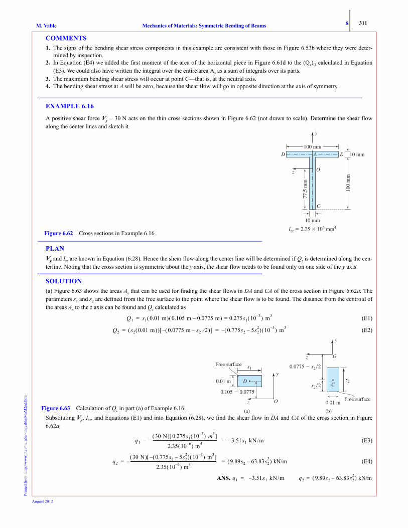
6 311Mechanics of Materials: Symmetric Bending of BeamsM. VablePr
inte
d fr
om: h
ttp://
ww
w.m
e.m
tu.e
du/~
mav
able
/MoM
2nd.
htm
COMMENTS1. The signs of the bending shear stress components in this example are consistent with those in Figure 6.53b where they were deter-
mined by inspection. 2. In Equation (E4) we added the first moment of the area of the horizontal piece in Figure 6.61d to the (Qz)D calculated in Equation
(E3). We could also have written the integral over the entire area As as a sum of integrals over its parts. 3. The maximum bending shear stress will occur at point C—that is, at the neutral axis.4. The bending shear stress at A will be zero, because the shear flow will go in opposite direction at the axis of symmetry.
EXAMPLE 6.16
A positive shear force Vy = 30 N acts on the thin cross sections shown in Figure 6.62 (not drawn to scale). Determine the shear flowalong the center lines and sketch it.
PLANVy and Izz are known in Equation (6.28). Hence the shear flow along the center line will be determined if Qz is determined along the cen-terline. Noting that the cross section is symmetric about the y axis, the shear flow needs to be found only on one side of the y axis.
SOLUTION(a) Figure 6.63 shows the areas As that can be used for finding the shear flows in DA and CA of the cross section in Figure 6.62a. Theparameters s1 and s2 are defined from the free surface to the point where the shear flow is to be found. The distance from the centroid ofthe areas As to the z axis can be found and Qz calculated as
(E1)
(E2)
Substituting Vy, Izz, and Equations (E1) and into Equation (6.28), we find the shear flow in DA and CA of the cross section in Figure6.62a:
(E3)
(E4)
ANS.
y
z
Izz � 2.35 � 106 mm4
A E
O
C
D
(a)
100 mm
100
mm
77.5
mm
10 mm
10 mm
Figure 6.62 Cross sections in Example 6.16.
Q1 s1 0.01 m( ) 0.105 m 0.0775 m–( ) 0.275s1 10 3–( ) m3==
y
z
0.105 � 0.0775
D
Free surface
O
0.01 m
s1
0.01 m
y
z
0.0775 � s2�2
Cs2�2s2
Free surface
O
(a) (b) Figure 6.63 Calculation of Qz in part (a) of Example 6.16.
Q2 s2 0.01 m( )( ) 0.0775 m s2 2⁄–( )–[ ] 0.775s2 5s22–( ) 10 3–( )– m3= =
q130 N( ) 0.275s1 10 3–( ) m3[ ]
2.35 10 6–( ) m4----------------------------------------------------------------- – 3.51– s1 kN/m= =
q230 N( ) 0.775s2 5s2
2–( ) 10 3–( )– m3[ ]
2.35 10 6–( ) m4---------------------------------------------------------------------------------------- – 9.89s2 63.83s2
2–( ) kN/m= =
q1 3.51– s1 kN/m= q2 9.89s2 63.83s22–( ) kN/m=
August 2012

6 312Mechanics of Materials: Symmetric Bending of BeamsM. VablePr
inte
d fr
om: h
ttp://
ww
w.m
e.m
tu.e
du/~
mav
able
/MoM
2nd.
htm
The shear flow q1 is negative, implying that the direction of the flow is opposite to the direction of s1. The values of q1 can be calculatedand plotted as shown in Figure 6.64a. By symmetry the flow in AE can also be plotted. The values of q2 are positive between C and A,implying the flow is in the direction of s2. The values of q2 can be calculated from and plotted as shown in Figure 6.64a.
COMMENTS1. In Example 6.13 the direction of flow was determined by inspection, whereas in this example it was determined using formulas. A
comparison of Figures 6.64 and 6.52a shows the same results. Thus, inspection can be used to check our results. Alternatively, wecould calculate the magnitude of the shear flow (or stress) from formulas and then determine the direction of the shear flow byinspection.
2. In Figure 6.64 the flow value at point A in CA is 351 N/m, which is the sum of the flows in AD and AE. Thus the behavior of shearflow is similar to that of fluid flow in a channel.
3. Figure 6.64 shows that the shear flow in the flanges varies linearly. The shear flow in the web varies quadratically, and its maximumvalue is at the neutral axis.
EXAMPLE 6.17
A beam is loaded as shown in Figure 6.65. The cross section of the beam is shown on the right and has an area moment of inertiaIzz = 40.83 in.4 (a) Determine the maximum bending normal and shear stresses. (b) Determine the bending normal and shear stresses atpoint D on a section just to the right of support A. Point D is just below the flange. (c) Show the results of parts (a) and (b) on stress cubes.
PLANWe can draw the shear force and bending moment diagrams and determine the maximum bending moment Mmax, the maximum shearforce (Vy)max, and the value of the bending moment MA and the shear force (Vy)A just to the right of support A. Using Equations (6.12)and (6.27), we can determine the required stresses and show the results on a stress cube.
SOLUTIONBy considering the free-body diagram of the entire beam, we can find the reaction forces at A and B and draw the shear force and bend-ing moment diagrams in Figure 6.66. The areas under the shear force curve are
(E1)From Figure 6.66 we can find the maximum shear force and moment, as well as the values of shear force and moment just to the right ofsupport A:
(E2)
(a)
Intensity ofshear flow
A
C
ED
O
Intensity ofshear flow
351 N/m
175.5 N/m
383.4N
/m
Figure 6.64 Shear flows on cross sections in Example 6.16.
500 lb 2200 lb
800 ft�lb800 ft�lb
2100 ft�lbA B
z
x
y
(a) (b)
3 ft 3 ft 3 ft
y
z
E
DD
C
F
4 in
1 in
1 in
2 in
1 in
1.5 in
2.5 in
Figure 6.65 Beam and loading in Example 6.17.
A1 500 3× 1500= = A2 1000 3× 3000= = A3 1200 3× 3600= =
Vy( )max 1200 lbs= Mmax 2300 ft· lbs= Vy( )A 1000– lbs= MA 700– ft· lbs=
August 2012

6 313Mechanics of Materials: Symmetric Bending of BeamsM. VablePr
inte
d fr
om: h
ttp://
ww
w.m
e.m
tu.e
du/~
mav
able
/MoM
2nd.
htm
(a) Point F is the point farthest away from the neutral axis. Hence the maximum bending normal stress will occur at point F. SubstitutingyF = –3.5 and Mmax into Equation (6.12), we obtain
(E3)
ANS.The maximum bending shear stress will occur at the neutral axis in the section where Vy is maximum. We can draw the area As between thetop surface and the neutral axis (NA) as shown in Figure 6.67 and determine the first moment about the z axis to find Qz, in Equation (E4)
(E4)Substituting Vmax and Equation (E4) into Equation (6.27), we obtain
(E5)
ANS.(b) Substituting yD = 1.5 in.and MA into Equation (6.12), we obtain the value of the normal stress at point D on a section just right of A as
(E6)
ANS.We can draw the area As between the free surface at the top and point D as shown in Figure 6.67b and find Qz at D.
(E7)
Substituting and Equation (E7) into Equation (6.27), we obtain the value of the shear stress at point D on a section just right of A as
(E8)
ANS.
V � �Vy(lb)
Mz(ft�lb) 800
700
23001500
2100
A2
x
x
A3A1
500
1000
1200
500 lb 2200 lb
RA � 1500 RB � 1200
800 ft�lb
800 ft�lb
2100 ft�lbA B
3 ft 3 ft 3 ft
Figure 6.66 Shear force and bending moment diagrams in Example 6.17.
σmax2300( ) 12( ) in.· lbs[ ] 3.5 in.–( )
40.83 in.4---------------------------------------------------------------------------– 2365.7 lbs/in.2= =
σmax 2366 psi T( )=
y
s
z
E
C
1 in
1 in
4 in
1.5 in2 in
NA Figure 6.67 Calculation of Qz in Example 6.17 (a) at neutral axis(b) at D.
y
s
z
D
C
1 in
4 in
1.5 in2 in
NA
(a) (b)
QNA 4 in.( ) 1 in.( ) 2 in.( ) 1.5 in.( ) 1 in.( ) 0.75 in.( )+ 9.125 in.3= =
τxs( )max1200 lbs( ) 9.125 in.3( )
40.83 in.4( ) 1 in.( )-------------------------------------------------------– 268.2 lbs/in.2–= =
τxs( )max 268– psi=
σxx( )D700–( ) 12( ) in.· lbs[ ] 1.5 in.( )
40.83 in.4( )------------------------------------------------------------------------– 308.6 lbs/in.2= =
σxx( )D 309 psi (T)=
QD 4 in.( ) 1 in.( ) 2 in.( ) 8 in.3= =
Vy( )A
τxs( )D1000 lbs–( ) 8 in.3( )
40.83 in.4( ) 1 in.( )-----------------------------------------------– 196 lbs/in.2= =
τxs( )D 196 psi=
2366 psi
x
y
(a)
268 psi
x
y
(b)
196 psi
309 psi
x
y
(c)
Figure 6.68 Stress elements in Example 6.17. (a) Maximum bending normal stress. (b) Maximum bending shear stress. (c) Bendingand normal shear stresses at point D just to the right of A.
August 2012

6 314Mechanics of Materials: Symmetric Bending of BeamsM. VablePr
inte
d fr
om: h
ttp://
ww
w.m
e.m
tu.e
du/~
mav
able
/MoM
2nd.
htm
(c) In Figures 6.67a and b the coordinate s is in the opposite direction to y at points D and the neutral axis. Hence at both these points, and from Equations (E5) and (E8) we obtain
ANS.We can show these results along with the normal stress values on the stress elements in Figure 6.68.
COMMENTS1. The maximum value of V is −1200 lbs but V = -Vy. Hence the maximum value of Vy is a positive value, as given in Equation (E2).2. Vy is positive in Equation (E2), thus we expect (τxy)max to be positive. Just after support A the shear force Vy is negative, thus we expect
that (τxy)D will be negative, as shown in Figure 6.68. 3. Note that the maximum bending shear stress in the beam given by Equation (E5) is nearly an order of magnitude smaller than the
maximum bending normal stress given by Equation (E3). This is consistent with the requirement for validity of our beam theory, aswas remarked in Section 6.2.6. If in some problem the maximum bending shear stress were nearly the same as the maximum bendingnormal stress, then that would indicate that the assumptions of beam theory are not valid and the theory needs to be modified toaccount for shear stress.
EXAMPLE 6.18
A wooden cantilever box beam is to be constructed by nailing four pieces of lumber in one of the two ways shown in Figure 6.69. Theallowable bending normal and shear stresses in the wood are 750 psi and 150 psi, respectively. The maximum force that the nails cansupport is 100 lb. Determine the maximum value of load P to the nearest pound, the spacing of the nails to the nearest half inch, and thepreferred nailing method.
Figure 6.69 Wooden beams in Example 6.18.
PLANThe maximum bending normal and shear stresses for both beams can be found in terms of P. These maximum values can be compared tothe allowable stress values, and the limiting value on force P can be found. The shear flow at the junction of the wood pieces can befound using Equation (6.28). The spacing of the nails for each joining method can be found by dividing the allowable force in the nail bythe shear flow. The method that gives the greater spacing between the nails is better as fewer nails will be needed.
SOLUTIONWe can draw the shear force and bending moment diagrams for the beams as shown in Figure 6.70a and calculate the maximum shearforce and moment
(E1)
The area moment of inertia about the z axis can be found as
(E2)
Substituting Equations (E1) and (E2) and ymax = ±3 in, we can find the magnitude of the maximum bending normal stress from Equation(6.12) in terms of P. Using the allowable normal stress as 750 psi, we can obtain one limiting value on P,
(E3)
τxy τxs–=
τxy( )max 268 psi= τxy( )D 196 psi–=
Joining method 1
8 ft
y Ps
6 in
4 in
1 in
1 in
y
z
y
8 ft
y P
4 in
6 in
1 in1 in
y
zs
Joining Method 1 Joining Method 2
Vy( )max P– lb= Mmax 8– P ft lb⋅ 96– P in lb⋅= =
V � �VyVV(lb)
MzMM(ft�lb)
20P
x
x
P
Figure 6.70 (a) Shear and moment diagrams. (b) Qz at neutral axis. (c) Qz at nails in joining method 1. (d) Qz at nails in joining method2
8P
1 in
1 in
4 in1 in 1 in
z
y
1 in2 in2.5 in
(a)
1 in
4 in
y
2 in
(c)
z
2.5 in
1 in
6 in
z
y
2 in2.5 in
(b)(a) (b) (c) (d)
Izz112------ 6 in.( ) 6 in.( )3 1
12------ 4 in.( ) 4 in.( )3– 86.67 in.4= =
σmaxMmaxymax
Izz----------------------
96P( ) 3 in.( )
86.67 in.4------------------------------- 750 lbs/in.2≤= = or P 225.7 lbs≤
August 2012

6 315Mechanics of Materials: Symmetric Bending of BeamsM. VablePr
inte
d fr
om: h
ttp://
ww
w.m
e.m
tu.e
du/~
mav
able
/MoM
2nd.
htm
Figure 6.70b shows the area As for the calculation of Qz at the neutral axis:
(E4)We also note that at the neutral axis, the thickness perpendicular to the center line is t = 1 in. + 1 in. = 2 in. Substituting Equations (E1),(E2), and (E4) and t = 2 in. into Equation (6.27), we can obtain the magnitude of the bending shear stress in terms of P. Using the allow-able shear stress as 150 psi, we can obtain another limiting value on P.
(E5)
If the maximum value of P is determined from Equation (E3), then Equation (E5) will be satisfied. Rounding downward we determine themaximum value of force P to the nearest pound.
ANS. Pmax = 225 lbsTo find the shear flow on the surface joined by the nails, we make imaginary cuts through the nails and draw the area As, as shown in Fig-ure 6.70c and d. We can then find Qz for each joining method:
(E6)From Equations (E1) and (E3) we obtain the shear force as Vy = –225 lb. Substituting this value along with Equations (E2) and (E6)into Equation (6.28), we obtain the magnitude of the shear flow for each joining method,
(E7)
(E8)
This shear flow is to be carried by two rows of nails for each of the joining methods. Thus each row resists half of the flow. Using thisfact, we can find the spacing between the nails,
(E9)
(E10)
As Δs2 > Δs1, fewer nails will be used in joining method 2. Rounding downward to the nearest half inch, we obtain the nail spacing. ANS. Use joining method 2 with a nail spacing of 7.5 in.
COMMENTS1. In this particular example only, the magnitudes of the stresses were important; the sign did not play any role. This will not always be
the case, particularly in later chapters when we consider combined loading and stresses on different planes.2. From visualizing the imaginary cut surface of the nails, we observe that the shear stress component in the nails is τyx in joining
method 1 and τzx in joining method 2.3. In Section 6.6.1 we observed that the shear stresses in bending balance the changes in axial force due to σxx. The shear stresses in the
nails balance σxx, which acts on a greater area in joining method 1 (6 in. wide) than in joining method 2 (4 in. wide). This is reflectedin the higher value of Qz, which led to a higher value of shear flow for joining method 1 than for joining method 2, as shown by Equa-tions (E7) and (E8).
4. The observations in comment 3 are valid as long as σxx is the same for both joining methods at any location. If Izz and ymax were different,then it is possible to arrive at a different answer. See Problem 6.126
PROBLEM SET 6.4Bending normal and shear stresses
6.106 For a positive shear force Vy, (a) sketch the direction of the shear flow along the center line on the thin cross sections shown in FigureP6.106. (b) At points A, B, C, and D, determine whether the stress component is τxy or τxz and whether it is positive or negative.
QNA 6 in.( ) 1 in.( ) 2.5 in.( ) 2 2 in.( ) 1 in.( ) 1 in.( ) 19 in.3=+=
τmaxP 19 in.3( )
86.67 in.4( ) 2 in.( )--------------------------------------------- 150 lbs/in.2 or P 1368 lbs≤≤=
Q1 6 in.( ) 1 in.( ) 2.5 in.( ) 15 in.3== Q2 4 in.( ) 1 in.( ) 2.5 in.( ) 10 in.3==
q1VyQ1
Izz------------- 225 lbs( ) 15 in.3( )
86.67 in.4--------------------------------------------- 39.94 lbs/in.= = =
q2VyQ2
Izz------------- 225 lbs( ) 10 in.3( )
86.67 in.4-------------------------------------------- 26.96 lbs/in.= = =
100 lbsΔs1
-----------------q1
2----- or Δs1
2 100 lbs( )39.94 lbs/in.------------------------------- 5.1 in.= ==
100Δs2---------
q2
2----- or Δs2
2 100 lbs( )26.96 lbs/in.------------------------------ 7.7 in.= ==
Figure P6.106
z
y
B
A
D
C
August 2012

6 316Mechanics of Materials: Symmetric Bending of BeamsM. VablePr
inte
d fr
om: h
ttp://
ww
w.m
e.m
tu.e
du/~
mav
able
/MoM
2nd.
htm
6.107 For a positive shear force Vy, (a) sketch the direction of the shear flow along the center line on the thin cross sections shown in FigureP6.107. (b) At points A, B, C, and D, determine whether the stress component is τxy or τxz and whether it is positive or negative
6.108 For a positive shear force Vy , (a) sketch the direction of the shear flow along the center line on the thin cross sections shown in FigureP6.108. (b) At points A, B, C, and D, determine whether the stress component is τxy or τxz and whether it is positive or negative.
6.109 For a positive shear force Vy , (a) sketch the direction of the shear flow along the center line on the thin cross sections shown in FigureP6.109. (b) At points A, B, C, and D, determine whether the stress component is τxy or τxz and whether it is positive or negative.
6.110 For a positive shear force Vy , (a) sketch the direction of the shear flow along the center line on the thin cross sections shown in FigureP6.109. (b) At points A, B, C, and D, determine whether the stress component is τxy or τxz and whether it is positive or negative.
6.111 For a positive shear force Vy , (a) sketch the direction of the shear flow along the center line on the thin cross sections shown in FigureP6.111. (b) At points A, B, C, and D, determine whether the stress component is τxy or τxz and whether it is positive or negative.
6.112 For a positive shear force Vy , (a) sketch the direction of the shear flow along the center line on the thin cross sections shown in FigureP6.112. (b) At points A, B, C, and D, determine whether the stress component is τxy or τxz and whether it is positive or negative.
Figure P6.107
z
y
A
C D
B
y
A DB
zC
Figure P6.108
z
y
B C
DA
Figure P6.109
z
y
B
D
A C
Figure P6.110
z
y
C
B A D Figure P6.111
z
y
CB
A
D
Figure P6.112
August 2012

6 317Mechanics of Materials: Symmetric Bending of BeamsM. VablePr
inte
d fr
om: h
ttp://
ww
w.m
e.m
tu.e
du/~
mav
able
/MoM
2nd.
htm
6.113 A cross section (not drawn to scale) of a beam that bends about the z axis is shown in Figure 6.113. The shear force acting at the crosssection is 5 kips. Determine the bending shear stress at points A, B, C, and D. Report your answers as positive or negative τxy or τxz. Point B isjust below the flange.
6.114 A cross section (not drawn to scale) of a beam that bends about the z axis is shown in Figure 6.71. The shear force acting at the crosssection is -10 kN. Determine the bending shear stress at points A, B, C, and D Report your answers as positive or negative τxy or τxz. Point B isjust below the flange.
6.115 A cross section of a beam that bends about the z axis is shown in Figure 6.115. The internal bending moment and shear force acting atthe cross section are Mz = 50 in.-kips and Vy = 10 kips, respectively. Determine the bending normal and shear stress at points A, B, and C andshow it on stress cubes.Point B is just below the flange.
6.116 Determine the magnitude of the maximum bending normal stress and bending shear stress in the beam shown in Figure P6.116.
6.117 For the beam, loading, and cross section shown in Figure P6.117, determine (a) the magnitude of the maximum bending normal stress,and shear stress; (b) the bending normal stress and the bending shear stress at point A. Point A is just below the flange on the cross section justright of the 4 kN force. Show your result on a stress cube. The area moment of inertia for the beam was calculated to be Izz = 3.6 × 106 mm4.
Figure P6.113
1 in.
1 in.
2 in.
1 in.
y
zC
D
B
A
2.5 in.
4 in.
1 in.
1 in. 1.5 in.
Figure 6.71
A10 mm
10 mm
50 mm10 mm
y
zC
B
50 mm
D
10 mm
10 mm
0.5 in
0.5 in
0.5 in
4 in
8 in
7 in
A
y
z
3.158 in.
C
B
Figure P6.115
5 ft�kips
2 ft�kips
2 kips4 kips
2 in
2 ft 3 ft 4 ft
6 in
Cross section
2 kips/ft Figure P6.116
August 2012

6 318Mechanics of Materials: Symmetric Bending of BeamsM. VablePr
inte
d fr
om: h
ttp://
ww
w.m
e.m
tu.e
du/~
mav
able
/MoM
2nd.
htm
6.118 For the beam, loading, and cross section shown in Figure P6.118, determine (a) the magnitude of the maximum bending normal stressand shear stress; (b) the bending normal stress and the bending shear stress at point A. Point A is on the cross section 2 m from the right end.Show your result on a stress cube. The area moment of inertia for the beam was calculated to be Izz = 453 (106) mm4.
6.119 Determine the maximum bending normal and shear stress in the beam shown in Figure 6.119a. The beam cross section is shown inFigure 6.119b.
6.120 Two pieces of lumber are nailed together as shown in Figure P6.120. The nails are uniformly spaced 10 in apart along the length.Determine the average shear force in each nail in segments AB and BC.
6.121 A cantilever beam is constructed by nailing three pieces of lumber, as shown in Figure P6.121. The nails are uniformly spaced at inter-vals of 75 mm. Determine the average shear force in each nail.
6.122 A cantilever beam is constructed by nailing three pieces of lumber, as shown in Figure P6.122. The nails are uniformly spaced at inter-vals of 75 mm. (a) Determine the shear force in each nail. (b) Which is the better nailing method, the one shown in Problem 6.99 or the one inthis problem?
Figure P6.117
16 kN�m8 kN�m
y
x A
3 m4 m
4 kN 2 kN/m
3 kN/m
4 m
y
10 mm
100 mm78.4 mm
160 mm
15 mm
Az
y
11 kN�my
x
3 m4 m
20 kN
8 kN30 kN
6 kN/m
4 m Figure P6.118
25 mm
25 mm
25 mm
300 mm120 mm
300 mm
Az
y
17 in
6 in1 in
4.5 in 4.5 in
6 in
y
z17
in
1 in
Figure P6.119
6 ft�kips
3 ft�kips
3 ft�kips
6 kips3 kips
3 kips6 kips
x
y
1.5 ft1.5 ft 1 ft 2 ft
(a) (b)
Figure P6.120
800 lb
6 ft 4 ft
4 in
2 in
1 in10 in
B CA
Figure P6.121x
y1.5 kN
2.5 m
200 mm25 mm
25 mm25 mm
200
mm
Figure P6.1222.5 m
25 mm
25 mm25 mm
200
mm
August 2012

6 319Mechanics of Materials: Symmetric Bending of BeamsM. VablePr
inte
d fr
om: h
ttp://
ww
w.m
e.m
tu.e
du/~
mav
able
/MoM
2nd.
htm
Design problems6.123 The planks in a park bench are made from recycled plastic and are bolted to concrete supports, as shown in Figure P6.123. For thepurpose of design the front plank is modeled as a simply supported beam that carries all the weight of two individuals. Assume that each personhas a mass 100 kg and the weight acts at one-third the length of the plank, as shown. The allowable bending normal stress for the recycled plas-tic is 10 MPa and allowable bending shear stress is 2 MPa. The width d of the planks that can be manufactured is in increments of 2 cm, from12 to 20 cm. To design the lightest bench, determine the corresponding values of the thickness t to the closest centimeter for the various valuesof d.
6.124 Two pieces of wood are glued together to form a beam, as shown in Figure P6.124. The allowable bending normal and shearstresses in wood are 3 ksi and 1 ksi, respectively. The allowable bending normal and shear stresses in the glue are 600 psi (T) and250 psi, respectively. Determine the maximum moment Mext that can be applied to the beam.
6.125 A wooden cantilever beam is to be constructed by nailing two pieces of lumber together, as shown in Figure P6.125. The allowablebending normal and shear stresses in the wood are 7 MPa and 1.5 MPa, respectively. The maximum force that the nail can support is 300 N.Determine the maximum value of load P to the nearest Newton and the spacing of the nails to the nearest centimeter.
6.126 A wooden cantilever box beam is to be constructed by nailing four 1-in.× 6-in. pieces of lumber in one of the two ways shown in FigureP6.126. The allowable bending normal and shear stresses in the wood are 750 psi and 150 psi, respectively. The maximum force that a nail cansupport is 100 lb. Determine the maximum value of load P to the nearest pound, the spacing of the nails to the nearest half inch, and the preferrednailing method
Historical problems6.127 Leonardo da Vinci conducted experiments on simply supported beams and drew the following conclusion: “If a beam 2 braccia long(L) supports 100 libbre (W), a beam 1 braccia long (L /2) will support 200 libbre (2W). As many times as the shorter length is contained in the
Figure P6.123
120 cm
W W
40 cm
10 cm 10 cm
td
Figure P6.124
100 in 40 in
1 in
Mext 1 in
2 in
4 in
yP
3 m
s
80 mm20 mm Figure P6.125
80 mm20 mm
20 mm
120 mm
Figure P6.126
Joining method 1
y
Joining m
20 ft
y P
6 in
1 in 1 in
August 2012

6 320Mechanics of Materials: Symmetric Bending of BeamsM. VablePr
inte
d fr
om: h
ttp://
ww
w.m
e.m
tu.e
du/~
mav
able
/MoM
2nd.
htm
longer (L /α), so many times more weight (αW) will it support than the longer one.” Prove this statement to be true by considering the two sim-ply supported beams in Figure P6.127 and showing that W2 = αW for the same allowable bending normal stress.
6.128 Galileo believed that the cantilever beam shown in Figure P6.128a would break at point B, which he considered to be a fulcrum pointof a lever, with AB and BC as the two arms. He believed that the material resistance (stress) was uniform across the cross section. Show that thestress value σ that Galileo obtained from Figure P6.128b is three times smaller than the bending normal stress predicted by Equation (6.12).
6.129 Galileo concluded that the bending moment due to the beam’s weight increases as the square of the length at the built-in end of a canti-lever beam. Show that Galileo’s statement is correct by deriving the bending moment at the built-in end in the cantilever beam in terms of specificweight γ, cross-sectional area A, and beam length L.
6.130 In the simply supported beam shown in Figure P6.130. Galileo determined that the bending moment is maximum at the applied loadand its value is proportional to the product ab. He then concluded that to break the beam with the smallest load P, the load should be placed inthe middle. Prove Galileo’s conclusions by drawing the shear force and bending moment diagrams and finding the value of the maximum bend-ing moment in terms of P, a, and b. Then show that this value is largest when a = b.
6.131 Mariotte, in an attempt to correct Galileo’s strength prediction, hypothesized that the stress varied in proportion to the distance from thefulcrum, point B in Figure P6.128. That is, it varied linearly from point B. Show that the maximum bending stress value obtained by Mariotte istwice that predicted by Equation (6.12).
Stretch Yourself6.132 A beam is acted upon by a distributed load p(x). Let MA and VA represent the internal bending moment and the shear force at A. Showthat the internal moment at B is given by
(6.30)
6.133 The displacement in the x direction in a beam cross section is given by u = u0(x) − y(dv/dx)(x). Assuming small strains and lin-ear, elastic, isotropic, homogeneous material with no inelastic strains, show that
where yc is the y coordinate of the centroid of the cross section measured from some arbitrary origin, A is the cross-sectional area, Izz is the areamoment of inertia about the z axis, and N and Mz are the internal axial force and the internal bending moment. Note that if y is measured fromthe centroid of the cross section, that is, if yc = 0, then the axial and bending problems decouple. In such a case show that σxx = N/A − Mzy/Izz.
6.134 Show that the bending normal stresses in a homogeneous, linearly elastic, isotropic symmetric beam subject to a temperature changeΔT(x, y) is given by
W
L
(a) Figure P6.127
W2
L��
(b)
L
A�
BC
(a)
Fulcrum P
Figure P6.128 Galileo’s beam experiment.
(a) (b)
ba
P
Figure P6.130
MB MA VA xB xA–( )–= xB x–( )p x( ) dxxA
xB
∫+
N EAdu0
dx-------- EAyc
d2vdx2--------–= Mz E– Ayc
du0
dx-------- EIzz
d2vdx2--------+=
August 2012

6 321Mechanics of Materials: Symmetric Bending of BeamsM. VablePr
inte
d fr
om: h
ttp://
ww
w.m
e.m
tu.e
du/~
mav
able
/MoM
2nd.
htm
(6.31)
where α is the coefficient of thermal expansion, and E is the modulus of elasticity.
6.135 In unsymmetrical bending of beams, under the assumption of plane sections remaining plane and perpendicular to the beam axis, the dis-placement u in the x direction can be shown to be u = − y dv/dx − z dw/dx, where y and z are measured from the centroid of the cross section, and v andw are the deflections of the beam in the y and z directions, respectively. Assume small strain, a linear, elastic, isotropic, homogeneous material, and noinelastic strain. Using Equations (1.8b) and (1.8c), show that
(6.32)
Note that if either y or z is a plane of symmetry, then Iyz = 0. From Equation (6.32), this implies that the moment about the z axis causes defor-mation in the y direction only and the moment about the y axis causes deformation in the z direction only. In other words, the bending problemsabout the y and z axes are decoupled.
6.136 The equation ∂σxx/∂x + ∂τyx/∂y = 0 was derived in Problem 1.105. Into this equation, substitute Equations (6.12) and (6.18) and inte-grate with y for beam cross section in Figure P6.136 and obtain the equation below.
Computer problems6.137 A cantilever, hollow circular aluminum beam of 5-ft length is to support a load of 1200 lb. The inner radius of the beam is 1 in. If the
maximum bending normal stress is to be limited to 10 ksi, determine the minimum outer radius of the beam to nearest in.
6.138 Table P6.138 shows the values of the distributed loads at several points along the axis of the rectangular beam shown in FigureP6.138. Determine the maximum bending normal and shear stresses in the beam.
6.139 Let the distributed load p(x) in Problem 6.138 be represented by p(x) = a + bx + cx 2. Using the data in Table P6.138, determine theconstants a, b, and c by the least-squares method. Then find the maximum bending moment and the maximum shear force by analyticalintegration and determine the maximum bending normal and shear stresses.
6.7* CONCEPT CONNECTOR
Historically, an understanding of the strength of materials began with the study of beams. It did not, however, follow a simplecourse. Instead, much early work addressed mistakes, regarding the location of the neutral axis and the stress distributionacross the cross section. The predicted values for the fracture loads on a beam did not correlate well with experiment. Tomake the pioneers’ struggle in the dark more difficult, near fracture the stress–strain relationship is nonlinear, which alters thestress distribution and the location of the neutral axis.
σxxMzyIzz
----------–MTyIzz
---------- EαΔT x y,( )–+=
MT Eα yΔT x y,( ) A ,dA∫=
My EIyzd2vdx2-------- EIyy
d2wdx2---------+= Mz EIzz
d2vdx2-------- EIyz
d2wdx2---------+= σxx
IyyMz IyzMy–
IyyIzz Iyz2–
---------------------------------⎝ ⎠⎜ ⎟⎛ ⎞
yIzzMy IyzMz–
IyyIzz Iyz2–
---------------------------------⎝ ⎠⎜ ⎟⎛ ⎞
z––=
t
b
z
y
Figure P6.136
τyx6Vy b2 4⁄ y2–( )
b3t--------------------------------------=
116------
2 in
8 in
Cross sectiony
px
10 ft
Figure P6.138
Table P6.138 Data for Problem 6.138
x (ft)
p(x) (lb/ft)
0 2751 3482 3983 4264 4325 416
6 3777 3168 2339 12810 0
Table P6.138 Data for Problem 6.138
x (ft)
p(x) (lb/ft)
August 2012

6 322Mechanics of Materials: Symmetric Bending of BeamsM. VablePr
inte
d fr
om: h
ttp://
ww
w.m
e.m
tu.e
du/~
mav
able
/MoM
2nd.
htm
6.7.1 History: Stresses in Beam Bending
The earliest known work on beams was by Leonardo da Vinci (1452–1519). In addition to his statements on simply sup-ported beams, which are described in Problem 6.127, he correctly concluded that in a cantilevered, untapered beam the crosssection farthest from the built-in end deflects the most. But it was Galileo’s work that had the greatest early influence.
Galileo Galilei (1564–1642) (Figure 6.72) was born in Pisa. In 1581 he enrolled at the University of Pisa to study medi-cine, but the work of Euclid, Archimedes, and Leonardo attracted him to mathematics and mechanics. In 1589 he became pro-fessor of mathematics at the university, where he conducted his famous experiments on falling bodies, and the field of dynamics was born. He concluded that a heavier object takes the same time as a lighter object to fall through the same height, in complete disagreement with the popular Aristotelian mechanics. He paid the price for his views, for the proponents of Aris-totelian mechanics made his stay at the university untenable, and he left in early 1592.
Fortunately, by the end of 1592 he was appointed professor of mathematics at the University of Padua. During this period he discovered his interest in astronomy. Based on sketchy reports, he built himself a telescope. On seeing moons in orbit around Jupiter in 1610, he found evidence for the Copernican theory, which held that the Earth is not the center of the uni-verse. In 1616 Copernicus was condemned by the Church, and the Inquisition warned Galileo to leave theology to the Church. In 1632, however, he published his views, under the mistaken belief that the new pope, Maffeo Barberini, who was Galileo’s admirer, would be more tolerant. Galileo was now condemned by the Inquisition and put under house arrest for the last eight years of his life. During this period he wrote Two New Sciences, in which he describes his work in mechanics, including the mechanics of materials. We have seen his contribution toward a concept of stress in Section 1.6. Here we discuss briefly his contributions on the bending of beams.
Figure P6.128 shows Galileo’s illustration of the bending test. We described two of his insights in Problems 6.129 and 6.130. Three other conclusions of his, too, have influenced the design of beams ever since. First, a beam whose width is greater than its thickness offers greater resistance standing on its edge than lying flat, because the area moment of inertia is then greater. Second, the resisting moment—and thus the strength of the beam—increases as the cube of the radius for circular beams. Thus, the section modulus increases as the cube of the radius. Finally, the cross-sectional dimensions must increase at a greater rate than the length for constant strength cantilever beam bending due to its own weight. However, as we saw in Problem 6.128, Galileo incorrectly predicted the load-carrying capacity of beams, because he misjudged the stress distribution and the location of the neutral axis.
Credit for an important correction to the stress distribution goes to Edme Mariotte (1620–1684), who also discovered the eye’s blind spot. Mariotte became interested in the strength of beams while trying to design pipes for supplying water to the palace of Versailles. His experiments with wooden and glass beams convinced him that Galileo’s load predictions were greatly exaggerated. His own theory incorporated linear elasticity, and he concluded that the stress distribution is linear, with a zero stress value at the bottom of the beam. Mariotte’s predicted values did not correlate well with experiment either, how-ever. To explain why, he argued that beams loaded over a long time would have failure loads closer to his predicted values. While true, this is not the correct explanation for the discrepancy.
As we saw in Problem 6.131, the cause lay instead in an incorrect assumption about the location of the neutral axis. This incorrect location hindered many pioneers, including Claude-Louis Navier (1785-1836), who also helped develop the formulas
Figure 6.72 Galileo Galilei.
August 2012

6 323Mechanics of Materials: Symmetric Bending of BeamsM. VablePr
inte
d fr
om: h
ttp://
ww
w.m
e.m
tu.e
du/~
mav
able
/MoM
2nd.
htm
for fluid flow, and the mathematician Jacob Bernoulli (1654-1705). (We saw some of Navier’s contribution in Section 1.6 and will discuss Bernoulli’s in Chapter 7 on beam deflection.) As a result, engineers used Galileo’s theory in designing beams of brittle material such as stone, but Mariotte’s theory for wooden beams.
Antoine Parent (1666–1716) was the first to show that Mariotte’s stress formula does not apply to beams with circular cross section. Born in Paris, Parent studied law on the insistence of his parents, but he never practiced it, because he wanted to do mathematics. He also proved that, for a linear stress distribution across a rectangular cross section, the zero stress point is at the center, provided the material behavior is elastic. Unfortunately Parent published his work in a journal that he himself edited and published, not in the journal by the French Academy, and it was not widely read. More than half a century later, Charles Augustin Coulomb, whose contributions we saw in Section 5.5, independently deduced the correct location of the neutral axis. Coulomb showed that the stress distribution is such that the net axial force is zero (Equation (6.2)), independent of the material.
Jean Claude Saint-Venant (see Chapter 5) rigorously examined kinematic Assumptions 1 through 3. He demonstrated that these are met exactly only for zero shear force: the beam must be subject to couples only, with no transverse force. However, the shear stresses in beams had still not received much attention.
As mentioned in Section 1.6, the concept of shear stress was developed in 1781, by Coulomb, who believed that shear was only important in short beams. Louis Vicat’s experiment in 1833 with short beams gave ample evidence of the importance of shear. Vicat (1786-1861), a French engineer, had earlier invented artificial cement. D. J. Jourawaski (1821-1891), a Russian railroad engineer, was working in 1844 on building a railroad between St. Petersburg and Moscow. A 180-ft-long bridge had to be built over the river Werebia, and Jourawaski had to use thick wooden beams. These thick beams were failing along the length of the fibers, which were in the longitudinal direction. Jourawaski realized the importance of shear in long beams and developed the theory that we studied in Section 6.6.
In sum, starting with Galileo, it took nearly 250 years to understand the nature of stresses in beam bending. Other histori-cal developments related to beam theory will appear in Section 7.6.
6.8 CHAPTER CONNECTOR
In this chapter we established formulas for calculating normal and shear stresses in beams under symmetric bending. We sawthat the calculation of bending stresses requires the internal bending moment and the shear force at a section. We consideredonly statically determinate beams. For these, the internal shear force and bending moment diagrams can be found by makingan imaginary cut and drawing an appropriate free-body diagram. Alternatively, we can draw a shear force–bending momentdiagram. The free-body diagram is preferred if stresses are to be found at a specified cross section. However, shear force–moment diagrams are the better choice if maximum bending normal or shear stress is to be found in the beam.
The shear force–bending moment diagrams can be drawn by using the graphical interpretation of the integral, as the area under a curve. Alternatively, internal shear force and bending moments can be found as a function of the x coordinate along the beam and plotted. Finding the bending moment as a function of x is important in the next chapter, where we integrate the moment–curvature relationship. Once we know how to find the deflection in a beam, we can solve problems of statically inde-terminate beams.
We also saw that, to understand the character of bending stresses, we can draw the bending normal and shear stresses on a stress element. In many cases, the correct direction of the stresses can be obtained by inspection. Alternatively, we can fol-low the sign convention for drawing the internal shear force and bending moment on free-body diagrams, determine the direc-tion using the subscripts in the formula. It is important to understand both methods for determining the direction of stresses. Shear–moment diagrams yield the shear force and the bending moment, following our sign convention. Drawing the bending stresses on a stress element is also important in stress or strain transformation, as described later.
In Chapter 8, on stress transformation, we will consider problems in which we first find bending stresses, using the stress formulas in this chapter. We then find stresses on inclined planes, including planes with maximum normal and shear stress. In Chapter 9, on strain transformation, we will find the bending strains and then consider strains in different coordinate systems, including coordinate systems in which the normal and shear strains are maximum. In Section 10.1 we will consider the com-bined loading problems of axial, torsion, and bending and the design of simple structures that may be determinate or indeter-minate.
August 2012

6 324Mechanics of Materials: Symmetric Bending of BeamsM. VablePr
inte
d fr
om: h
ttp://
ww
w.m
e.m
tu.e
du/~
mav
able
/MoM
2nd.
htm
POINTS AND FORMULAS TO REMEMBER
• Our Theory is limited to (1) slender beams; (2) regions away from the neighborhood of stress concentration; (3) gradualvariation in cross section and external loads; (4) loads acting in the plane of symmetry in the cross section; and (5) nochange in direction of loading during bending.
• (6.1) (6.5)
• small strain, (6.6a, b)
• where Mz is the internal bending moment that is drawn on the free-body diagram to put a point with positive y coordinatein compression; u and v are the displacements in the x and y directions, respectively; σxx and εxx are the bending (flexure)normal stress and strain; y is the coordinate measured from the neutral axis to the point where normal stress and normalstrain are defined, and d2v/dx2 is the curvature of the beam.
• The normal bending strain εxx is a linear function of y.• The normal bending strain εxx will be maximum at either the top or the bottom of the beam.• Equations (6.1), (6.6a), and (6.6b) are independent of the material model. • The following formulas are valid for material that is linear, elastic, and isotropic, with no inelastic strains. • For homogeneous cross section:
• (6.11) (6.12)
• where y is measured from the centroid of the cross section, and Izz is the second area moment about the z axis passingthrough the centroid.
• EIzz is the bending rigidity of a beam cross section.• Normal stress σxx in bending varies linearly with y on a homogeneous cross section.• Normal stress σxx is zero at the centroid (y = 0) and maximum at the point farthest from the centroid for a homogeneous
cross section.• The shear force Vy will jump by the value of the applied external force as one crosses it from left to right.• Mz will jump by the value of the applied external moment as one crosses it from left to right.
• (6.13) (6.27)
• where Qz is the first moment of the area As about the z axis passing through the centroid, t is the thickness perpendicularto the centerline, As is the area between the free surface and the line at which the shear stress is being found, and the coor-dinate s is measured from the free surface used in computing Qz.
• The direction of shear flow on a cross section must be such that (1) the resultant force in the y direction is in the samedirection as Vy; (2) the resultant force in the z direction is zero; and (3) it is symmetric about the y axis.
• Qz is zero at the top and bottom surfaces and is maximum at the neutral axis.• Shear stress is maximum at the neutral axis of a cross section in symmetric bending of beams.• The bending strains are
• (6.29)
Mz yσxx AdA∫–= u y
xddv ,–= v v x( )=
εxxyR---– yd2v
dx2--------–= =
Mz EIzzd2vdx2--------= σxx
MzyIzz
----------–=
Vy τxy AdA
∫= τxsVyQz
Izzt------------–=
εxxσxx
E------- εyy
νσxx
E-----------–= ν– εxx= = εzz
νσxx
E-----------– νεxx–= = γxy
τxy
G------= γxz
τxz
G------=
August 2012

325 2 SYMMETRIC BENDING OF

326
6.8 CHAPTERCONNECTOR
Copyright © 2022 FDOKUMEN