
PRINCIPLES OF SOIL DYNAMICS Second Edition
575
-
Upload
khangminh22 -
Category
Documents
-
view
1 -
download
0
Transcript of PRINCIPLES OF SOIL DYNAMICS Second Edition


PRINCIPLES OF SOIL DYNAMICS Second Edition Braja M. Das Dean Emeritus, California State University, Sacramento, USA G. V. Ramana Associate Professor, Indian Institute of Technology Delhi, India

This page intentionally left blank

To Elizabeth Madison,
Pratyusha and Sudiksha

© 2011, 1993 Cengage Learning
ALL RIGHTS RESERVED. No part of this work covered by the copyright herein may be reproduced, transmitted, stored, or used in any form or by any means graphic, electronic, or mechanical, including but not limited to photocopying, recording, scanning, digitizing, taping, web distribution, information networks, or information storage and retrieval systems, except as permitted under Section 107 or 108 of the 1976 United States Copyright Act, without the prior written permission of the publisher.
Library of Congress Control Number: 2009936680
ISBN-13: 978-0-495-41134-5
ISBN-10: 0-495-41134-5
Cengage Learning200 First Stamford Place, Suite 400Stamford, CT 06902USA
Cengage Learning is a leading provider of customized learning solu-tions with offi ce locations around the globe, including Singapore, the United Kingdom, Australia, Mexico, Brazil, and Japan. Locate your local offi ce at: international.cengage.com/region.
Cengage Learning products are represented in Canada by Nelson Education, Ltd.
For your course and learning solutions, visit www.cengage.com/ engineering.
Principles of Soil Dynamics, Second Edition,
Braja M. Das, G.V. Ramana
Director, Global Engineering Program:
Christopher M. Shortt
Senior Developmental Editor: Hilda Gowans
Editorial Assistant: Tanya Altieri
Associate Marketing Manager: Lauren Betsos
Content Project Manager: Jennifer Ziegler
Production Service: Integra
Compositor: Integra
Senior Art Director: Michelle Kunkler
Cover Designer: Andrew Adams
Permissions Account Manager, Text: Katie Huha
Text and Image Permissions Researcher:
Kristiina Paul
Senior First Print Buyer: Doug Wilke
Printed in the United States of America
1 2 3 4 5 6 7 13 12 11 10 09
For product information and technology assistance, contact us at Cengage Learning Customer & Sales Support, 1-800-354-9706.
For permission to use material from this text or product, submit all requests online at cengage.com/permissions .
Further permissions questions can be emailed [email protected].
Purchase any of our products at your local college store or at ourt preferred online store www.ichapters.com.

CONTENTS
PREFACE 1 INTRODUCTION 1 1.1 General 1 1.2 Nature and Type of Dynamic Loading on Soils 1 1.3 Importance of Soil Dynamics 4 References 6 2 FUNDAMENTALS OF VIBRATION 7 2.1 Introduction 7 2.2 Fundamentals of Vibration 8 System with Single Degree of Freedom 10 2.3 Free Vibration of a Spring-Mass System 10 2.4 Forced Vibration of a Spring-Mass System 16 2.5 Free Vibration with Viscous Damping 23 2.6 Steady-State Forced Vibration with Viscous Damping 30 2.7 Rotating-Mass-Type Excitation 35 2.8 Determination of Damping Ratio 37 2.9 Vibration-Measuring Instrument 40 System with Two Degrees of Freedom 42 2.10 Vibration of a Mass-Spring System 42 2.11 Coupled Translation and Rotation of a Mass-Spring System (Free Vibration) 48 Problems 51 Reference 55 3 WAVES IN ELASTIC MEDIUM 56 3.1 Introduction 56 3.2 Stress and Strain 56 3.3 Hooke's Law 58 Elastic Stress Waves in a Bar 60 3.4 Longitudinal Elastic Waves in a Bar 60 3.5 Velocity of Particles in the Stressed Zone 63 3.6 Reflections of Elastic Stress Waves at the End of a Bar 65 3.7 Torsional Waves in a Bar 67 3.8 Longitudinal Vibration of Short Bars 68 3.9 Torsional Vibration of Short Bars 73 Stress Waves in an Infinite Elastic Medium 74 3.10 Equation of Motion in an Elastic Medium 74 3.11 Equations for Stress Waves 75 3.12 General Comments 78

Stress Waves in Elastic Half-Space 82 3.13 Rayleigh Waves 82 3.14 Displacement of Rayleigh Waves 88 3.15 Attenuation of the Amplitude of Elastic Waves with Distance 90 References 94 4 PROPERTIES OF DYNAMICALLY LOADED SOILS 96 4.1 Introduction 96 Laboratory Tests and Results 4.2 Shear Strength of Soils under Rapid Loading Condition 97 4.3 Strength and Deformation Characteristics of Soils under Transient Load 101 4.4 Travel−Time Test for Determination of Longitudinal and Shear Wave Velocities
(vc and vs) 104 4.5 Resonant Column Test 106 4.6 Cyclic Simple Shear Test 121 4.7 Cyclic Torsional Simple Shear Test 125 4.8 Cyclic Triaxial Test 128 4.9 Summary of Cyclic Tests 133 Field Test Measurements 135 4.10 Reflection and Refraction of Elastic Body Waves—Fundamental Concepts 135 4.11 Seismic Refraction Survey (Horizontal Layering) 137 4.12 Refraction Survey in Soils with Inclined Layering 145 4.13 Reflection Survey in Soil (Horizontal Layering) 151 4.14 Reflection Survey in Soil (Inclined Layering) 154 4.15 Subsoil Exploration by Steady-State Vibration 158 4.16 Soil Exploration by "Shooting Up the Hole," "Shooting Down the Hole," and
"Cross-Hole Shooting" 160 4.17 Cyclic Plate Load Test 164 Correlations for Shear Modulus and Damping Ratio 169 4.18 Test Procedures for Measurement of Moduli and Damping Characteristics 169 4.19 Shear Modulus and Damping Ratio in Sand 171 4.20 Correlation of Gmax of Sand with Standard Penetration Resistance 176 4.21 Shear Modulus and Damping Ratio for Gravels 176 4.22 Shear Modulus and Damping Ratio for Clays 178 4.23 Shear Modulus and Damping Ratio for Lightly Cemented Sand 186 Problems 188 References 192 5 FOUNDATION VIBRATION 196 5.1 Introduction 196 5.2 Vertical Vibration of Circular Foundations Resting on Elastic Half-Space— Historical Development 196 5.3 Analog Solutions for Vertical Vibration of Foundations 205 5.4 Calculation Procedure for Foundation Response⎯Vertical Vibration 209 5.5 Rocking Vibration of Foundations 219

5.6 Sliding Vibration of Foundations 226 5.7 Torsional Vibration of Foundations 229 5.8 Comparison of Footing Vibration Tests with Theory 235 5.9 Comments on the Mass-Spring-Dashpot Analog Used for Solving Foundation
Vibration Problems 239 5.10 Coupled Rocking and Sliding Vibration of Rigid Circular Foundations 244 5.11 Vibration of Foundations for Impact Machines 248 Vibration of Embedded Foundations 251 5.12 Vertical Vibration of Rigid Cylindrical Foundations 251 5.13 Sliding Vibration of Rigid Cylindrical Foundations 256 5.14 Rocking Vibration of Rigid Cylindrical Foundations 257 5.15 Torsional Vibration of Rigid Cylindrical Foundations 259 Vibration Screening 261 5.16 Active and Passive Isolation: Definition 261 5.17 Active Isolation by Use of Open Trenches 261 5.18 Passive Isolation by Use of Open Trenches 264 5.19 Passive Isolation by Use of Piles 266 Problems 269 References 273 6 DYNAMIC BEARING CAPACITY OF SHALLOW FOUNDATIONS 276 6.1 Introduction 276 Ultimate Dynamic Bearing Capacity 277 6.2 Bearing Capacity in Sand 277 6.3 Bearing Capacity in Clay 283 6.4 Behavior of Foundations under Transient Loads 285 6.5 Experimental Observation of Load-Settlement Relationship for Vertical Transient Loading 285 6.6 Seismic Bearing Capacity and Settlement in Granular Soil 291 Problems 297 References 298 7 EARTHQUAKE AND GROUND VIBRATION 300 7.1 Introduction 300 7.2 Definition of Some Earthquake-Related Terms 300 7.3 Earthquake Magnitude 303 7.4 Characteristics of Rock Motion during an Earthquake 305 7.5 Vibration of Horizontal Soil Layers with Linearly Elastic Properties 308 7.6 Other Studies for Vibration of Soil Layers Due to Earthquakes 319 7.7 Equivalent Number of Significant Uniform Stress Cycles for Earthquakes 320 References 324 8 LATERAL EARTH PRESSURE ON RETAINING WALLS 327 8.1 Introduction 327 8.2 Mononobe−Okabe Active Earth Pressure Theory 328

8.3 Some Comments on the Active Force Equation 335 8.4 Procedure for Obtaining PAE Using Standard Charts of KA 335 8.5 Effect of Various Parameters on the Value of the Active Earth Pressure Coefficient 340 8.6 Graphical Construction for Determination of Active Force, PAE 342 8.7 Laboratory Model Test Results for Active Earth Pressure Coefficient, KAE 345 8.8 Point of Application of the Resultant Active Force, PAE 350 8.9 Design of Gravity Retaining Walls Based on Limited Displacement 353 8.10 Hydrodynamic Effects of Pore Water 361 8.11 Mononobe−Okabe Active Earth Pressure Theory for c − φ Backfill 363 8.12 Dynamic Passive Force on Retaining Wall 368 Problems 370 References 371 9 COMPRESSIBILITY OF SOILS UNDER DYNAMIC LOADS 374 9.1 Introduction 374 9.2 Compaction of Granular Soils: Effect of Vertical Stress and Vertical Acceleration 374 9.3 Settlement of Strip Foundation on Granular Soil under the Effect of Controlled
Cyclic Vertical Stress 380 9.4 Settlement of Machine Foundation on Granular Soils Subjected to Vertical
Vibration 384 9.5 Settlement of Sand Due to Cyclic Shear Strain 389 9.6 Calculation of Settlement of Dry Sand Layers Subjected to Seismic Effect 391 9.7 Settlement of a Dry Sand Layer Due to Multidirectional Shaking 394 Problems 396 References 397 10 LIQUEFACTION OF SOIL 398 10.1 Introduction 398 10.2 Fundamental Concept of Liquefaction 399 10.3 Laboratory Studies to Simulate Field Conditions for Soil Liquefaction 401 Dynamic Triaxial Test 402 10.4 General Concepts and Test Procedures 402 10.5 Typical Results from Cyclic Triaxial Test 405 10.6 Influence of Various Parameters on Soil Liquefaction Potential 410 10.7 Development of Standard Curves for Initial Liquefaction 414 Cyclic Simple Shear Test 415 10.8 General Concepts 415 10.9 Typical Test Results 416 10.10 Rate of Excess Pore Water Pressure Increase 418 10.11 Large-Scale Simple Shear Tests 420 Development of a Procedure for Determination of Field Liquefaction 426 10.12 Correlation of the Liquefaction Results from Simple Shear and Triaxial Tests 426

10.13 Correlation of the Liquefaction Results from Triaxial Tests to Field Conditions 430 10.14 Zone of Initial Liquefaction in the Field 432 10.15 Relation between Maximum Ground Acceleration and the Relative Density of Sand for Soil Liquefaction 433 10.16 Liquefaction Analysis from Standard Penetration Resistance 438 10.17 Other Correlations for Field Liquefaction Analysis 444 10.18 Remedial Action to Mitigate Liquefaction 447 Problems 454 References 455 11 MACHINE FOUNDATIONS ON PILES 459 11.1 Introduction 459 Piles Subjected to Vertical Vibration 460 11.2 End-Bearing Piles 460 11.3 Friction Piles 465 Sliding, Rocking, and Torsional Vibration 478 11.4 Sliding and Rocking Vibration 478 11.5 Torsional Vibration of Embedded Piles 492 Problems 501 References 504 12 SEISMIC STABILITY OF EARTH EMBANKMENTS 505 12.1 Introduction 505 12.2 Free Vibration of Earth Embankments 505 12.3 Forced Vibration of an Earth Embankment 509 12.4 Velocity and Acceleration Spectra 511 12.5 Approximate Method for Evaluation of Maximum Crest Acceleration and Natural Period of Embankments 513 12.6 Fundamental Concepts of Stability Analysis 521 Pseudostatic Analysis 527 12.7 Clay Slopes (φ = 0 Condition)—Koppula's Analysis 527 12.8 Slopes with c − φ Soil—Majumdar's Analysis 532 12.9 Slopes with c − φ Soil—Prater's Analysis 540 12.10 Slopes with c − φ Soil—Conventional Method of Slices 543 Deformation of Slopes 546 12.11 Simplified Procedure for Estimation of Earthquake-Induced Deformation 546 Problems 549 References 551 APPENDIX A—PRIMARY AND SECONDARY FORCES OF SINGLE-CYLINDER ENGINES 553 INDEX 556

PREFACE This text was originally published as Fundamentals of Soil Dynamics with a 1983 copyright by
Elsevier Science Publishing Company, New York. The first edition of Principles of Soil
Dynamics was published by PWS-Kent Publishing Company, Boston, with a 1993 copyright.
The present text is a revised version of Principles of Soil Dynamics with the addition of a co-
author, Professor G. V. Ramana.
During the past four decades, considerable progress has been made in the area of soil
dynamics. Soil dynamics courses have been added or expanded for graduate-level study in many
universities. The knowledge gained from the intensive research conducted all over the world has
gradually filtered into the actual planning, design, and construction process of various types of
earth-supported and earth-retaining structures. Based on the findings of those research initiatives,
this text is prepared for an introductory course in soil dynamics. While writing a textbook, all
authors are tempted to include research of advanced studies to some degree. However, since the
text is intended for an introductory course, it stresses the fundamental principles without
becoming cluttered with too many details and alternatives.
The text is divided into twelve chapters and an appendix. SI units are used throughout the
text. A new section on seismic bearing capacity and settlement of shallow foundations has been
added in Chapter 6. Also, in Chapter 8, a new section on the Mononobe-Okabe active earth
pressure theory for c−φ backfill has been introduced. A number of worked-out example problems
are included, which are essential for the students. Practice problems are given at the end of most
chapters, and a list of references is included at the end of each chapter. We also believe the text
will be of interest to researchers and practitioners.

The authors are indebted to their wives, Janice and Vijaylaxmi, for their help and
understanding during the revision of the text. Professor Jean-Pierre Bardet of the University of
Southern California was kind enough to provide the cover page pictures taken after the January
2001 Bhuj Earthquake in India.
Thanks are due to Chris Carson, Executive Director of Global Publishing Program, and
Hilda Gowans, Senior Developmental Editor of Engineering, at Cengage for their interest and
patience during the revision and production of the manuscript.
B. M. Das
G. V. Ramana

This page intentionally left blank

1
1 Introduction
1.1 General Information Soil mechanics is the branch of civil engineering that deals with the engineering properties and behavior of soil under stress. Since the publication of the book Erdbaumechanik aur Bodenphysikalischer Grundlage by Karl Terzaghi (1925), theoretical and experimental studies in the area of soil mechanics have progressed at a very rapid pace. Most of these studies have been devoted to the determination of soil behavior under static load conditions, in a broader sense, although the term load includes both static and dynamic loads. Dynamic loads are imposed on soils and geotechnical structures by several sources, such as earthquakes, bomb blasts, operation of machinery, construction operations, mining, traffic, wind, and wave actions. It is well known that the stress-strain properties of a soil and its behavior depend upon several factors and can be different in many ways under dynamic loading conditions as compared to the case of static loading. Soil dynamics is the branch of soil mechanics that deals with the behavior of soil under dynamic load, including the analysis of the stability of earth-supported and earth-retaining structures.
During the last 50 years, several factors, such as damage due to liquefaction of soil during earthquakes, stringent safety requirements for nuclear power plants, industrial advancements (for example, design of foundations for power generation equipment and other machinery), design and construction of offshore structures, and defense requirements, have resulted in a rapid growth in the area of soil dynamics.
1.2 Nature and Type of Dynamic Loading on Soils The type of dynamic loading in soil or the foundation of a structure depends on the nature of the source producing it. Dynamic loads vary in their magnitude, direction, or position with time. More than one type of variation of forces may

2 Chapter 1
coexist. Periodic load is a special type of load that varies in magnitude with time and repeats itself at regular intervals, for example, operation of a reciprocating or a rotary machine. Nonperiodic loads are those loads that do not show any periodicity, for example, wind loading on a building. Deterministic loads are those loads that can be specified as definite functions of time, irrespective of whether the time variation is regular or irregular, for example, the harmonic load imposed by unbalanced rotating machinery. Nondeterministic loads are those loads that can not be described as definite functions of time because of their inherent uncertainty in their magnitude and form of variation with time, for example, earthquake loads (Humar 2001). Cyclic loads are those loads which exhibit a degree of regularity both in its magnitude and frequency. Static loads are those loads that build up gradually over time, or with negligible dynamic effects. They are also known as monotonic loads. Stress reversals, rate effects and dynamic effects are the important factors which distinguishes cyclic loads from static loads (Reilly and Brown 1991).
The operation of a reciprocating or a rotary machine typically produces a dynamic load pattern, as shown in Figure 1.1a. This dynamic load is more or less sinusoidal in nature and may be idealized, as shown in Figure 1.1b.
The impact of a hammer on a foundation produces a transient loading condition in soil, as shown in Figure 1.2a. The load typically increases with time up to a maximum value at time t = t1 and drops to zero after that. The case shown in Figure 1.2a is a single-pulse load. A typical loading pattern (vertical acceleration) due to a pile-driving operation is shown in Figure 1.2b.
Dynamic loading associated with an earthquake is random in nature. A load that varies in a highly irregular fashion with time is sometimes referred to as a random load. Figure 1.3 shows the accelerogram of the E1 Centro, California, earthquake of May 18, 1940 (north-south component).
Figure 1.1 (a) Typical load versus record for a low-speed rotary machine;
(b) Sinusoidal idealization for (a)

Introduction 3
Figure 1.2 Typical loading diagrams: (a) transient loading due to single impact of a hammer; (b) vertical component of ground acceleration due to pile driving
Figure 1.3 Accelerogram of E1 Centro, California, earthquake of May 18, 1940 (N-S component)
For consideration of land-based structures, earthquakes are the important source of dynamic loading on soils. This is due to the damage-causing potential of strong motion earthquakes and the fact that they represent an unpredictable and uncontrolled phenomenon in nature. The ground motion due to an earthquake may lead to permanent settlement and tilting of footings and, thus, the structures supported by them. Soils may liquify, leading to buildings sinking and lighter structures such as septic tanks floating up (Prakash, 1981). The damage caused by an earthquake depends on the energy released at its source, as discussed in Chapter 7.

4 Chapter 1
Figure 1.4 Schematic diagram showing loading on the soil below the foundation during machine operation
For offshore structures, the dynamic load due to storm waves generally represents the significant load. However, in some situations the most severe loading conditions may occur due to the combined action of storm waves and earthquakes loading. In some cases the offshore structure must be analyzed for the waves and earthquake load acting independently of each other (Puri and Das, 1989; Puri, 1990).
The loadings represented in Figures 1.1, 1.2 and 1.3 are rather simplified presentations of the actual loading conditions. For example, it is well known that earthquakes cause random motion in every direction. Also, pure dynamic loads do not occur in nature and are always a combination of static and dynamic loads. For example, in the case of a well-designed foundation supporting a machine, the dynamic load due to machine operation is a small fraction of the static weight of the foundation (Barkan, 1962). The loading conditions may be represented schematically by Figure 1.4. Thus in a real situation the loading conditions are complex. Most experimental studies have been conducted using simplified loading conditions.
1.3 Importance of Soil Dynamics The problems related to the dynamic loading of soils and earth structures frequently encountered by a geotechnical engineer include, but are not limited to the following: 1. Earthquake, ground vibration, and wave propagation through soils 2. Dynamic stress, deformation, and strength properties of soils 3. Dynamic earth pressure problem 4. Dynamic bearing capacity problems and design of shallow foundations

Introduction 5
5. Problems related to soil liquefaction 6. Design of foundations for machinery and vibrating equipment 7. Design of embedded foundations and piles under dynamic loads 8. Stability of embankments under earthquake loading.
In order to arrive at rational analyses and design procedures for these problems, one must have an insight into the behavior of soil under both static and dynamic loading conditions. For example, in designing a foundation to resist dynamic loading imposed by the operation of machinery or an external source, the engineer has to arrive at a special solution dictated by the local soil conditions and environmental factors. The foundation must be designed to satisfy the criteria for static loading and, in addition, must be safe for resisting the dynamic load. When designing for dynamic loading conditions, the geotechnical engineer requires answers to questions such as the following:
1. How should failure be defined and what should be the failure criteria? 2. What is the relationship between applied loads and the significant parameters
used in defining the failure criteria? 3. How can the significant parameters be identified and evaluated? 4. What will be an acceptable factor of safety, and will the factor of safety as
used for static design condition be enough to ensure satisfactory performance or will some additional conditions need to be satisfied?
The problems relating to the vibration of soil and earth-supported and earth-retaining structures have received increased attention of geotechnical engineers in recent years, and significant advances have been made in this direction. New theoretical procedures have been developed for computing the response of foundations, analysis of liquefaction potential of soils, and design of retaining walls and embankments. Improved field and laboratory methods for determining dynamic behavior of soils and field measurements to evaluate the performance of prototypes deserve a special mention. In this text an attempt has been made to present the information available on some of the important problems in the field of soil dynamics. Gaps in the existing literature, if any, have also been pointed out. The importance of soil dynamics lies in providing safe, acceptable, and time-tested solutions to the problem of dynamic loading in soil, in spite of the fact that the information in some areas may be lacking and the actual loading condition may not be predictable, as in the case of the earthquake phenomenon.
From the above, it can be seen that soil dynamics is an interdisciplinary area and in addition to traditional soil mechanics, requires a knowledge of theory of vibrations, principles of wave propagation, soil behavior under dynamic/cyclic conditions, numerical methods such as finite element methods etc., in finding appropriate solutions for problems of practical interest.

6 Chapter 1
References Barkan, D. D. (1962). Dynamics of Bases and Foundations. McGraw-Hill Book
Company, New York. Humar, J. L. (2001). Dynamics of Structures. Balkema, Tokyo. Prakash, S. (1981). Soil Dynamics. McGraw-Hill Book Company, New York. Puri, V. K. (1990). “Dynamic Loading of Marine Soils,” Proceedings, 9th
International Conference on Offshore Mechanics in Arctic Engineering, ASME, Vol. 1, pp. 421–426.
Puri, V. K., and Das, B. M. (1989). “Some Considerations in the Design of Offshore Structures: Role of Soil Dynamics,” Proceedings, Oceans ’89, Vol. 5, Seattle, Washington, pp. 1544-1551.
Reilly, M. P., and Brown, S. F. (1991). Cyclic Loading of Soils: from theory to design, Blackie and Son Ltd, London
Terzaghi, K. (1925). Erdbaumechanik aur Bodenphysikalischer Grundlage, Deuticke, Vienna.

7
2 Fundamentals of Vibration
2.1 Introduction Satisfactory design of foundations for vibrating equipments is mostly based on displacement considerations. Displacement due to vibratory loading can be classified under two major divisions: 1. Cyclic displacement due to the elastic response of the soil-foundation system
to the vibrating loading 2. Permanent displacement due to compaction of soil below the foundation
In order to estimate the displacement due to the first loading condition listed above, it is essential to know the nature of the unbalanced forces (usually supplied by the manufacturer of the machine) in a foundation such as shown in Figure 2.1.
Figure 2.1 Six modes of vibration for foundation
8 Chapter 2
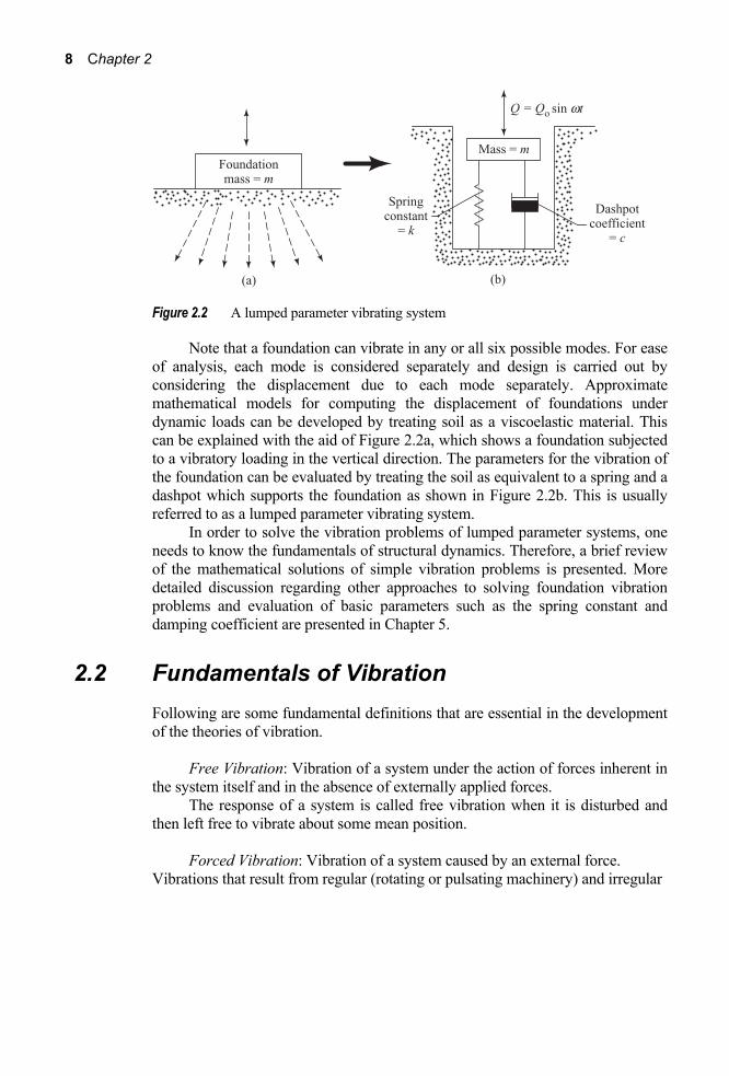
Figure 2.2 A lumped parameter vibrating system
Note that a foundation can vibrate in any or all six possible modes. For ease of analysis, each mode is considered separately and design is carried out by considering the displacement due to each mode separately. Approximate mathematical models for computing the displacement of foundations under dynamic loads can be developed by treating soil as a viscoelastic material. This can be explained with the aid of Figure 2.2a, which shows a foundation subjected to a vibratory loading in the vertical direction. The parameters for the vibration of the foundation can be evaluated by treating the soil as equivalent to a spring and a dashpot which supports the foundation as shown in Figure 2.2b. This is usually referred to as a lumped parameter vibrating system.
In order to solve the vibration problems of lumped parameter systems, one needs to know the fundamentals of structural dynamics. Therefore, a brief review of the mathematical solutions of simple vibration problems is presented. More detailed discussion regarding other approaches to solving foundation vibration problems and evaluation of basic parameters such as the spring constant and damping coefficient are presented in Chapter 5.
2.2 Fundamentals of Vibration Following are some fundamental definitions that are essential in the development of the theories of vibration.
Free Vibration: Vibration of a system under the action of forces inherent in the system itself and in the absence of externally applied forces.
The response of a system is called free vibration when it is disturbed and then left free to vibrate about some mean position.
Forced Vibration: Vibration of a system caused by an external force.
Vibrations that result from regular (rotating or pulsating machinery) and irregular

Fundamentals of Vibration 9
(chemical process plant) exciting agencies are also called as forced vibrations.
Degree of Freedom: The number of independent coordinates required to describe the solution of a vibrating system.
For example, the position of the mass m in Figure 2.3a can be described by
a single coordinate z, so it is a single degree of freedom system. In Figure 2.3b, two coordinates (z1 and z2) are necessary to describe the motion of the system; hence this system has two degree of freedom. Similarly, in Figure 2.3c, two coordinates (z and θ) are necessary, and the number of degrees of freedom is two. A rigid body has total six degrees of freedom: three rotational and three translational.
To understand the mathematical models that will be frequently used in analysis of machine foundations, a thorough understanding of physics as well as mathematics of a single degree of freedom system is required and is explained in the following sections. Once the mathematics as well as physics of a single degree of freedom system is clear, it is easy to extend this to multi-degree of freedom systems as well as modal analysis of complicated physical systems. In addition, the concept of response spectrum, often used by structural engineers is also based on a single degree of freedom system. A proper selection of vibration measuring instruments, design of vibration isolation as well as force isolation also require a good understanding of concepts such as natural frequency, damping ratio etc., that can be easily understood from one degree of freedoms systems.
Figure 2.3 Degree of freedom for vibrating system
10 Chapter 2
System with Single Degree of Freedom
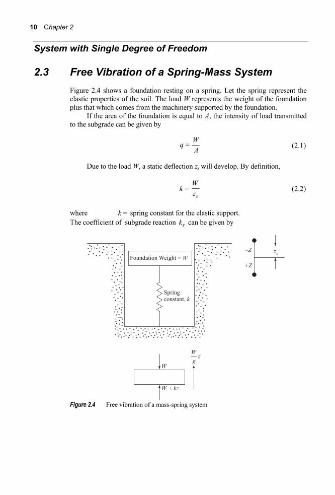
2.3 Free Vibration of a Spring-Mass System Figure 2.4 shows a foundation resting on a spring. Let the spring represent the elastic properties of the soil. The load W represents the weight of the foundation plus that which comes from the machinery supported by the foundation.
If the area of the foundation is equal to A, the intensity of load transmitted to the subgrade can be given by
q = WA
(2.1)
Due to the load W, a static deflection zs will develop. By definition,
k = s
Wz
(2.2)
where k = spring constant for the elastic support. The coefficient of subgrade reaction sk can be given by
Figure 2.4 Free vibration of a mass-spring system
Fundamentals of Vibration 11
ks = s
qz
(2.3)
If the foundation is disturbed from its static equilibrium position, the system will vibrate. The equation of motion of the foundation when it has been disturbed through a distance z can be written from Newton’s second law of motion as
W z k zg
⎛ ⎞+⎜ ⎟
⎝ ⎠ = 0
or
0kz zm
⎛ ⎞+ =⎜ ⎟⎝ ⎠
(2.4)
where g = acceleration due to gravity z = 2 2/d z dt t = time m = mass = W/g
In order to solve Eq. (2.4), let
1 2cos sinn nz A t A tw w= + (2.5)
where A1 and A2 = constants nw = undamped natural circular frequency
Substitution of Eq. (2.5) into Eq. (2.4) yields
21 2 1 2( cos sin ) ( cos sin ) 0n n n n n
kA t A t A t A tm
⎛ ⎞− + + + =⎜ ⎟⎝ ⎠
w w w w w
or
nkm
=w (2.6)
The unit of nw is in radians per second (rad/s). Hence,
1 2cos sink kz A t A tm m
⎛ ⎞ ⎛ ⎞= +⎜ ⎟ ⎜ ⎟⎜ ⎟ ⎜ ⎟
⎝ ⎠ ⎝ ⎠ (2.7)

12 Chapter 2
In order to determine the values of A1 and A2, one must substitute the proper boundary conditions. At time t = 0, let
Displacement z = z0
and
Velocity = dz zdt
= = 0u
Substituting the first boundary condition in Eq. (2.7),
z0 = A1 (2.8)
Again, from Eq. (2.7)
1 2– sin cosk k k kz A t A tm m m m
⎛ ⎞ ⎛ ⎞= +⎜ ⎟ ⎜ ⎟⎜ ⎟ ⎜ ⎟
⎝ ⎠ ⎝ ⎠ (2.9)
Substituting the second boundary condition in Eq. (2.9)
z = 0u = A2km
or
02 /
Ak mu
= (2.10)
Combination of Eqs. (2.7), (2.8), and (2.10) gives
z = z0 0cos sin/
k kt tm mk m
⎛ ⎞ ⎛ ⎞+⎜ ⎟ ⎜ ⎟⎜ ⎟ ⎜ ⎟
⎝ ⎠ ⎝ ⎠
u (2.11)
Now let
z0 = Z cos α (2.12)
and
0
/k mu = Z sin α (2.13)
Substitution of Eqs. (2.12) and (2.13) into Eq. (2.11) yields

Fundamentals of Vibration 13
cos( )nz Z tw a= − (2.14)
where
1 0
0
tanz k mua − ⎛ ⎞
= ⎜ ⎟⎜ ⎟⎝ ⎠
(2.15)
2
2 2 200 0 0/
mZ z zkk m
u u⎛ ⎞ ⎛ ⎞= + = +⎜ ⎟ ⎜ ⎟⎜ ⎟ ⎝ ⎠⎝ ⎠
(2.16)
The relation for the displacement of the foundation given by Eq. (2.14) can be represented graphically as shown in Figure 2.5.
At time t = 0, z = Z cos (− α) = Z cos α
t = ,n
aw
z = Z cos nn
⎛ ⎞−⎜ ⎟
⎝ ⎠
aw aw
= Z
Figure 2.5 Plot of displacement, velocity, and acceleration for the free vibration of a
mass-spring system (Note: Velocity leads displacement by π/2 rad: acceleration leads velocity by π/2 rad.)

14 Chapter 2
t =
12
n
a
w
p +, z = Z cos
12
nn
aw a
w
Ê ˆp +Á ˜-Á ˜Ë ¯ = 0
t = n
awp +
, z = Z cos nn
aw aa
⎛ ⎞+ −⎜ ⎟⎝ ⎠
p = − Z
t =
32
n
a
w
p +, z = Z cos
32
nn
aw a
w
Ê ˆp +Á ˜-Á ˜Ë ¯ = 0
t = 2
n
awp +
, z = Z cos 2
nn
aw aw
Ê ˆp + -Á ˜Ë ¯ = Z
. . . From Figure 2.5, it can be seen that the nature of displacement of the
foundation is sinusoidal. The magnitude of maximum displacement is equal to Z. This is usually referred to as the single amplitude. The peak-to-peak displacement amplitude is equal to 2Z, which is sometimes referred to as the double amplitude. The time required for the motion to repeat itself is called the period of the vibration. Note that in Figure 2.5 the motion is repeating itself at points A, B, and C. The period T of this motion can therefore be given by
2
n
Tw
= p (2.17)
The frequency of oscillation f is defined as the number of cycles in unit time, or
12
nfT
w= =p
(2.18)
It has been shown in Eq. (2.6) that, for this system, nw = k m/ . Thus,
12n
kf fm
⎛ ⎞= =⎜ ⎟⎝ ⎠p
(2.19)
The term fn is generally referred to as the undamped natural frequency. Since sk W z= , and m = W/g, Eq. (2.19) can also be expressed as

Fundamentals of Vibration 15
fn = 12 s
gz
⎛ ⎞⎜ ⎟π⎝ ⎠
(2.20)
Table 2.1 gives values of fn for various values of zs The variation of the velocity and acceleration of the motion with time can
also be represented graphically. From Eq.(2.14), the expressions for the velocity and the acceleration can be obtained as
1( )sin( ) cos2n n n nz Z t Z tw w a w w a⎛ ⎞= − − = − +⎜ ⎟
⎝ ⎠p (2.21)
and
2 2cos( ) cos( )n n n nz Z t Z tw w a w w a= − − = − + p (2.22)
The variation of the velocity and acceleration of the foundations is also shown in Figure 2.5.
Table 2.1 Undamped natural frequencies zs Undamped natural frequency (mm) (Hz) 0.02 111 0.05 71 0.10 50 0.20 35 0.50 22 1.0 16 2 11 5 7 10 5
Example 2.1
A mass is supported by a spring. The static deflection of the spring due to the mass is 0.381mm. Find the natural frequency vibration. Solution
From Eq. (2.20),
fn = 12 s
gz
Ê ˆÁ ˜Ë ¯p

16 Chapter 2
g = 9.81 m/s2, zs = 0.381 mm = 0.000381 m. So,
fn = 1 9.812 0.000381
⎛ ⎞⎜ ⎟π⎝ ⎠
= 25.54 Hz
Example 2.2
For a machine foundation, given weight of the foundation = 45 kN and spring constant = 104 kN/m, determine a) natural frequency of vibration, and b) period of oscillation
Solution
a) ( )41 1 10
2 2 45/9.81nkfm
= = =p p
7.43Hz
b) From Eq. (2.18),
T = 1 17fn
=.43
= 0.135 s
2.4 Forced Vibration of a Spring-Mass System Figure 2.6 shows a foundation that has been idealized to a simple spring-mass system. Weight W is equal to the weight of the foundation itself and that supported by it; the spring constant is k. This foundation is being subjected to an alternating force 0 sin( )Q Q tw b= + .This type of problem is generally encountered with foundations supporting reciprocating engines, and so on.
The equation of motion for this problem can be given by
0 sin( )m z kz Q t+ = +w b (2.23)
Let z = A1 sin( )tw b+ be a particular solution to Eq. (2.23) (A1 = const). Substitution of this into Eq. (2.23) gives
2
1 1 0sin( ) sin( ) sin( )mA t kA t Q tw w b w b w b− + + + = + ( )
01 2
//Q mA
k m w=
− (2.24)

Fundamentals of Vibration 17
Figure 2.6 Forced vibration of mass-spring system title
Hence the particular solution to Eq. (2.23) is of the form
01 2
/sin( ) sin( )( / )
Q mz A t tk m
w b w bw
= + = +−
(2.25)
The complementary solution of Eq. (2.23) must satisfy
m z + kz = 0
As shown in the preceding section, the solution to this equation may be given as
2 3= cos sinn nz A t A tw w+ (2.26)
where =nkm
w
A2, A3 = const
Hence, the general solution of Eq. (2.23) is obtained by adding Eqs. (2.25) and (2.26), or

18 Chapter 2
1 2 3= sin( ) + cos + sinn nz A t A t A tw b w w+ (2.27)
Now, let the boundary conditions be as follows: At time t = 0,
z = z0 = 0 (2.28)
dzdt
= velocity = 0u = 0 (2.29)
From Eqs. (2.27) and (2.28),
A1 sin β + A2 = 0 or A2 = −A1 sin β (2.30)
Again, from Eq. (2.27),
dzdt
= A1 w cos( tw + β) – A2 nw sin nw t + A3 nw cos nw t
Substituting the boundary condition given by Eq. (2.29) in the preceding equation gives
A1 w cos β + A3 nw = 0 or
A3 = − 1
n
A ww
⎛ ⎞⎜ ⎟⎝ ⎠
cos β (2.31)
Combining Eqs. (2.27), (2.30), and (2.31),
z = A1[sin( tw + β) – cos( tw ) . sin β – n
⎛ ⎞⎜ ⎟⎝ ⎠
ww
sin( nw t) . cos β ] (2.32)
For a real system, the last two terms inside the brackets in Eq. (2.32) will vanish due to damping, leaving the only term for steady-state solution.
If the forcing function is in phase with the vibratory system (i.e., β = 0), then
1(sin sin )nn
z A t tww ww
⎛ ⎞= − ⎜ ⎟
⎝ ⎠
02
/ sin sin( / ) n
n
Q m t tk m
ww ww w
⎛ ⎞= −⎜ ⎟− ⎝ ⎠

Fundamentals of Vibration 19
or
02 2
/ sin sin1 ( / ) n
n n
Q kz t tww ww w w
⎛ ⎞= −⎜ ⎟− ⎝ ⎠
(2.33)
However Q0/k = zs = static deflection. If one lets 2 21 (1 )nw w− be equal to M [equal to the magnification factor or 1 0( / )A Q k ], Eq. (2.33) reads as
z = zs M sin sin nn
t tww ww
⎡ ⎤⎛ ⎞−⎢ ⎥⎜ ⎟
⎢ ⎥⎝ ⎠⎣ ⎦ (2.34)
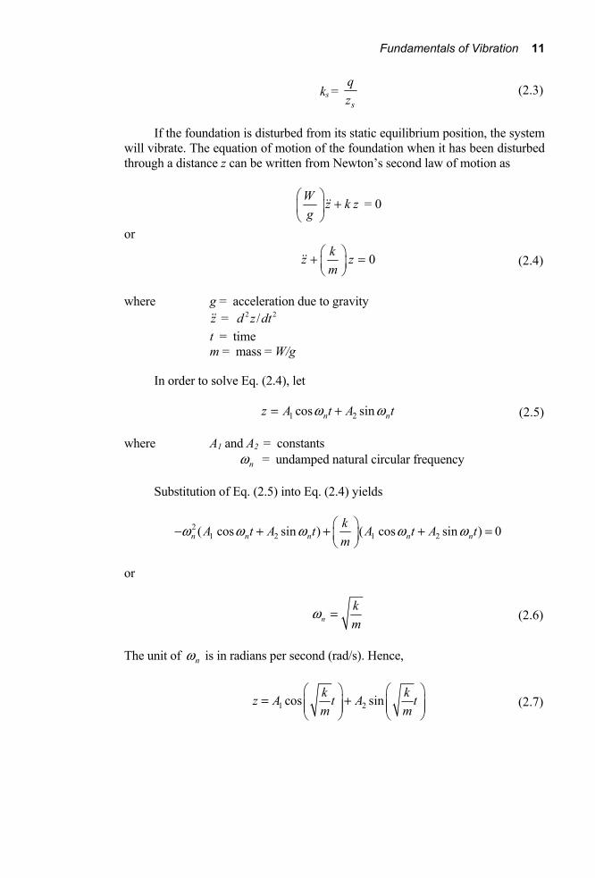
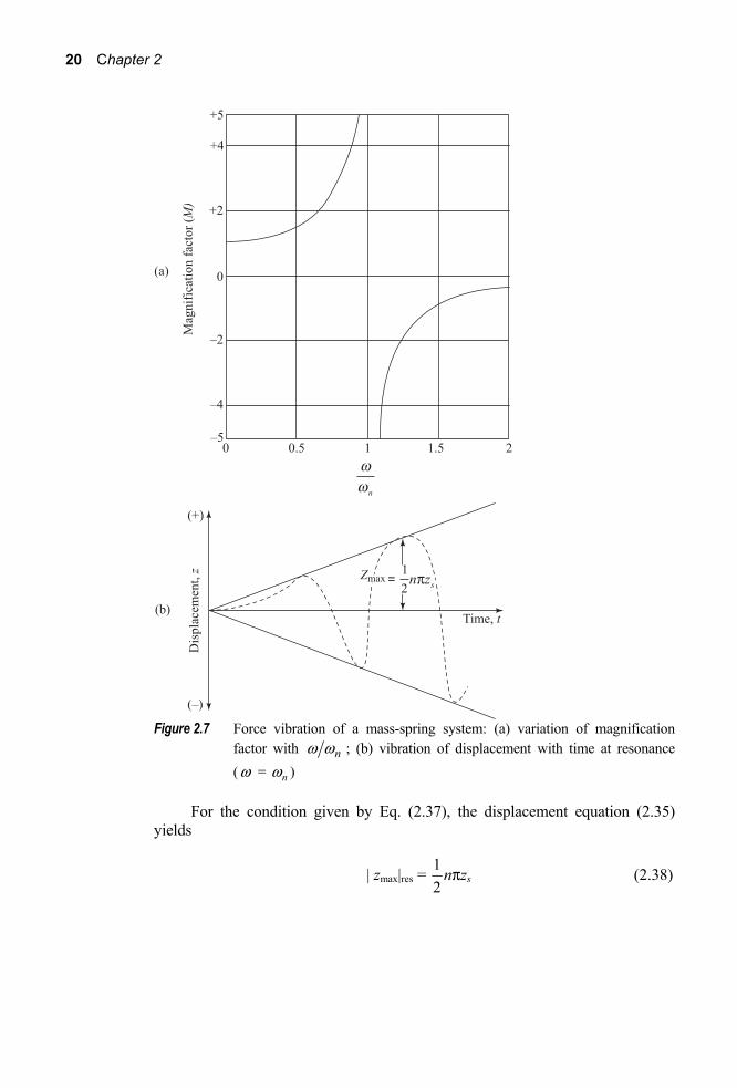
The nature of variation of the magnification factor M with nw w is shown in Figure 2.7a. Note that the magnification factor goes to infinity when nw w = 1. This is called the resonance condition. For resonance condition, the right-hand side of Eq. (2.34) yields 0/0.
Thus, applying L’Hopital’s rule,
lim( )n
zw w→
= zs( ) ( )
( ) ( )2 2
/ sin / sin
/ 1 /n n
n
d d t t
d d
w w w w ww w w
⎡ ⎤⎡ ⎤−⎣ ⎦⎢ ⎥−⎢ ⎥⎣ ⎦
or
z = 12
zs(sin n tw – n tw cos n tw ) (2.35)
The velocity at resonance condition can be obtained from Eq. (2.35) as
21 ( cos cos sin )2 s n n n n n nz z t t t tw w w w w w= − +
= 21 ( ) sin2 s n nz t tw w (2.36)
Since the velocity is equal to zero at the point where the displacement is at maximum, for maximum displacement
210 ( )sin2 s n nz z t tw w= =
or sin nw t = 0, i.e., nw t = nπ (2.37)
where n is an integer.
20 Chapter 2
Figure 2.7 Force vibration of a mass-spring system: (a) variation of magnification
factor with w wn ; (b) vibration of displacement with time at resonance (w = wn )
For the condition given by Eq. (2.37), the displacement equation (2.35) yields
| zmax|res = 12
nπzs (2.38)
Fundamentals of Vibration 21
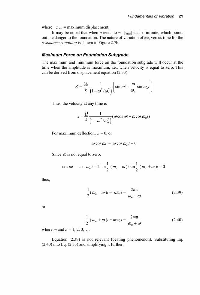
where zmax = maximum displacement. It may be noted that when n tends to ∞, |zmax| is also infinite, which points
out the danger to the foundation. The nature of variation of z/zs versus time for the resonance condition is shown in Figure 2.7b.
Maximum Force on Foundation Subgrade The maximum and minimum force on the foundation subgrade will occur at the time when the amplitude is maximum, i.e., when velocity is equal to zero. This can be derived from displacement equation (2.33):
( )0
2 21 sin sin
1 /n
nn
QZ t tk
ww www w
⎛ ⎞= −⎜ ⎟
− ⎝ ⎠
Thus, the velocity at any time is
( )2 21 ( cos cos )
1 /n
n
Qz t tk
w w w ww w
= −−
For maximum deflection, z = 0, or
w cos tw – w cos nw t = 0
Since w is not equal to zero,
cos tw – cos nw t = 2 sin 12
( nw –w )t sin 12
( nw +w )t = 0
thus,
12
( nw –w )t = nπ; t = 2
n
nw w−
p (2.39)
or
12
( nw +w )t = mπ; t = 2
n
mw w+
p (2.40)
where m and n = 1, 2, 3,….
Equation (2.39) is not relevant (beating phenomenon). Substituting Eq. (2.40) into Eq. (2.33) and simplifying it further,

22 Chapter 2
( )0
max1 2. . sin
1 / n n
Q mz zk
ww w w w
⎛ ⎞= = ⎜ ⎟− +⎝ ⎠
p (2.41)
In order to determine the maximum dynamic force, the maximum value of zmax given in Eq. (2.41) is required:
( )0
max(max)/
1 / n
Q kz
w w=
− (2.42)
Hence,
( )0 0
dynam(max) max(max)/
[ ]1 / 1 /n n
k Q k QF k zw w w w
= = =− −
(2.43)
Hence, the total force on the subgrade will very between the limits
W − 01 / n
Qw w−
and W + 01 / n
Qw w−
Example 2.3
A machine foundation can be idealized as a mass-spring system. This foundation can be subjected to a force that can be given as Q (kN) = 35.6 sin tw . Given f = 13.33 Hz
Weight of the machine + foundation = 178 kN Spring constant = 70,000 kN/m Determine the maximum and minimum force transmitted to the subgrade. Solution
Natural angular frequency = nw = 3
370000 10
178 10 9.81km
×=×
= 62.11 rad/s
0dynam 1 / n
QFw w
=−
But w = 2πf = 2π 13.33× = 83.75 rad/s

Fundamentals of Vibration 23
Thus
| dynamF | = 35.61 (83.75/62.11)−
= 102.18 kN
Maximum force on the subgrade = 178 + 102.18 = 280.18 kN Minimum force on the subgrade = 178 – 102.18 = 75.82 kN
2.5 Free Vibration with Viscous Damping In the case of undamped free vibration as explained in Section 2.3, vibration would continue once the system has been set in motion. However, in practical cases, all vibrations undergo a gradual decrease of amplitude with time. This characteristic of vibration is referred to as damping. Figure 2.2b shows a foundation supported by a spring and a dashpot. The dashpot represents the damping characteristic of the soil. The dashpot coefficient is equal to c. For free vibration of the foundation (i.e., the force Q = Q0 sin tw on the foundation is zero), the differential equation of motion can be given by
0mz cz kz+ + = (2.44)
Let z = Aert be a solution to Eq. (2.44), where A is a constant. Substitution of this into Eq. (2.44) yields
mAr2ert + cArert + kAert = 0 or
r2 + cmFHIK r + k
m = 0 (2.45)
The solutions to Eq. (2.45) can be given as
r = − 2
22 4c c km mm
± − (2.46)
There are three general conditions that may be developed from Eq. (2.46): 1. If c/2m > k m/ , both roots of Eq. (2.45) are real and negative. This is
referred to as an overdamped case. 2. If c/2m = k m/ , r = − c/2m. This is called the critical damping case.
Thus, for this case,
2cc c km= = (2.47a)

24 Chapter 2
3. If c/2m < k m/ , the roots of Eq. (2.45) are complex :
r = - ± -cm
i km
cm2 4
2
2
This is referred to as a case of underdamping. It is possible now to define a damping ratio D, which can be expressed as
2c
c cDc km
= = (2.47b)
Using the damping ratio, Eq. (2.46) can be rewritten as
r = ( )22 1
2 4 nc c k D Dm mm
w− ± − = − ± − (2.48)
where nw = k m/
For the overdamped condition (D > 1),
( )2 1nr D Dw= − ± −
For this condition, the equation for displacement (i.e., z = Aert) may be written as
( ) ( )2 21 2exp 1 exp 1n nZ A t D D A t D Dw w⎡ ⎤ ⎡ ⎤= − + − + − − −⎢ ⎥ ⎢ ⎥⎣ ⎦ ⎣ ⎦
(2.49)
where A1 and A2 are two constants. Now, let
A1 = 12 3 4A A+b g (2.50)
and
A2 = 12
(A3 – A4) (2.51)
Substitution of Eqs. (2.50) and (2.51) into Eq. (2.49) and rearrangement gives
Fundamentals of Vibration 25
( ) ( )2 23
1 exp 1 exp 12
nD tn nz e A D t D tw w w− ⎧ ⎡ ⎤= − + − −⎨ ⎢ ⎥⎣ ⎦⎩
( ) ( )2 24
1 exp 1 exp 12 n nA D t D tw w ⎫⎡ ⎤+ − − − − ⎬⎢ ⎥⎣ ⎦⎭
or
( ) ( )2 23 4cosh 1 sinh 1nD t
n nz e A D t A D tw w w− ⎡ ⎤= − + −⎢ ⎥⎣ ⎦ (2.52)
Equation (2.52) shows that the system which is overdamped will not oscillate at all. The variation of z with time will take the form shown in Figure 2.8a.
The constants A3 and A4 in Eq. (2.52) can be evaluated by knowing the initial conditions. Let, at time t = 0, displacement = z = z0 and velocity = dz/dt = 0u . From Eq. (2.52) and the first boundary condition,
z = z0 = A3 (2.53)
Again, from Eq. (2.52) and the second boundary condition,
dzdt
= ( )20 41n D Au w= − − D nw A3
or
A4 = 0 3 0 02 21 1
n n
n n
D A D z
D D
u w u w
w w
+ +=
− − (2.54)
Substituting Eqs. (2.53) and (2.54) into Eq. (2.52)
( ) ( )2 20 00 2
cosh 1 sinh 11
nD t nn
n
D zz e z D t D tD
w u www
−⎡ ⎤+⎢ ⎥= − + −⎢ ⎥−⎣ ⎦
(2.55)
*For a critically damped condition (D = 1), from Eq. (2.48),
r = − nw (2.56)
Given this condition, the equation for displacement (z = Aert) may be written as
5 6( ) ntz A A t e w−= + (2.57)

26 Chapter 2
Figure 2.8 Free vibration of a mass-spring-dashpot system: (a) overdamped case;
(b) critically damped case; (c) underdamped case
where A5 and A6 are two constants. This is similar to the case of the overdamped system except for the fact that the sign of z changes only once. This is shown in Figure 2.8b.
The values of A5 and A6 in Eq. (2.57) can be determined by using the initial conditions of vibration. Let, at time t = 0,
z = z0, 0dzdt
u=

Fundamentals of Vibration 27
From the first of the preceding two conditions and Eq. (2.57),
z = z0 = A5 (2.58)
Similarly, from the second condition and Eq. (2.57)
dzdt
= 0u = − nw A5 + A6 = − nw z0 + A6
or A6 = 0u + nw z0 (2.59)
A combination of Eqs. (2.57) – (2.59) yields
0 0 0[ ( ) ] ntnz z z t e wu w −= + + (2.60)
Lastly, for the underdamped condition (D < 1),
r = nw - ± -D i D1 2e j
Thus, the general form of the equation for the displacement (z = Aert) can be expressed as
( ) ( )2 27 8exp 1 exp 1nD t
n nz e A i D t A i D tw w w− ⎡ ⎤= − + − −⎢ ⎥⎣ ⎦ (2.61)
where A7 and A8 are two constants.
Equation (2.61) can be simplified to the form
( ) ( )2 29 10cos 1 sin 1nD t
n nz e A D t A D tw w w− ⎡ ⎤= − + −⎢ ⎥⎣ ⎦ (2.62)
where A9 and A10 are two constants.
The values of the constants A9 and A10 in Eq. (2.62) can be determined by using the following initial conditions of vibration. Let, at time t = 0,
z = z0 and 0dtdz
u=

28 Chapter 2
The final equation with theses boundary conditions will be of the form
( ) ( )2 20 00 2
cos 1 .sin 11
nD t nn n
n
D zz e z D t D tD
w u ww ww
−⎡ ⎤+⎢ ⎥= − + −⎢ ⎥−⎣ ⎦
(2.63)
Equation (2.63) can further be simplified as
z = Zcos( dw t – α) (2.64)
where
2
2 0 00 21
nD t n
n
D zZ e zD
w u w
w−
⎛ ⎞+⎜ ⎟= +⎜ ⎟−⎝ ⎠
(2.65)
1 0 02
0
tan1
n
n
D z
z D
u waw
−⎛ ⎞+⎜ ⎟=⎜ ⎟−⎝ ⎠
(2.66)
2damped natural circular frequency 1d n Dw w= = − (2.67)
The effect of damping is to decrease gradually the amplitude of vibration with time. In order to evaluate the magnitude of decrease of the amplitude of vibration with time, let Zn and Zn+1 be the two successive positive or negative maximum values of displacement at times tn and tn+1 from the start of the vibration as shown in Figure 2.8c. From Eq. (2.65),
ZZn
n
+ 1 = ( )( )
1exp
expn n
n n
D t
D t
ww
+−
− = exp ( )1n n nD t tw +⎡ ⎤− −⎣ ⎦ (2.68)
However, tn+1 − tn is the period of vibration T,
2
2 2
1d n
TDw w
= =−
p p (2.69)
Thus, combining Eqs. (2.68) and (2.69),
21
2ln1
n
n
Z DZ D+
⎛ ⎞ π= =⎜ ⎟⎜ ⎟ −⎝ ⎠δ (2.70)
The term δ is called the logarithmic decrement. If the damping ratio D is small, Eq. (2.70) can be approximated as

Fundamentals of Vibration 29
1
ln 2n
n
Z DZ +
⎛ ⎞= = π⎜ ⎟⎜ ⎟
⎝ ⎠δ (2.71)
Example 2.4
For a machine foundation, given weight = 60 kN, spring constant = 11,000 kN/m, and c = 200 kN-s/m, determine (a) whether the system is overdamped, underdamped, or critically damped, (b) the logarithmic decrement, and (c) the ratio of two successive amplitudes.
Solution
1. From Eq. (2.47),
cc = 602 2 11,0009.81
km Ê ˆ= Á ˜Ë ¯ = 518.76 kN-s/m
ccc
= D = 200518 76.
= 0.386 < 1
Hence, the system is underdamped.
2. From Eq. (2.70),
δ = ( )( )2 2
2 0.3862
1 1 0.386
D
D
pp =- -
= 2.63
3. Again, from Eq. (2.70),
ZZ
n
n +1 = eδ = e2.63 = 13.87
Example 2.5
For Example 2.4, determine the damped natural frequency. Solution
From Eq. (2.67),
fd = 21 nD f−

30 Chapter 2
where fd = damped natural frequency.
fn = 1 1 11,000 9.812 2 60
km
¥=p p
= 6.75 Hz
Thus, fd = 1 0 386 2-FH IK.a f (6.75) = 6.23 Hz
2.6 Steady-State Forced Vibration with Viscous Damping Figure 2.2b shows the case of a foundation resting on a soil that can be approximated to an equivalent spring and dashpot. This foundation is being subjected to a sinusoidally varying force Q = Q0 sin tw . The differential equation of motion for this system can be given be
m z + kz + cz = Q0 sin tw (2.72)
The transient part of the vibration is damped out quickly; so, considering the particular solution for Eq. (2.72) for the steady-state motion, let
z = A1 sin tw + A2 cos tw (2.73)
where A1 and A2 are two constants.
Substituting Eq. (2.73) into Eq. (2.72),
2 21 2 1 2( sin – cos ) ( sin cos )m A t A t k A t A tw w w w w w− + +
1 2 0( cos – sin ) sinc A t A t Q tw w w w w+ = (2.74)
Collecting sine and cosine functions in Eq. (2.74) separately,
1 2 1 2 0( – )sin sinmA kA cA t Q tw w w w− + = (2.75a) 2 2 2 1( ) cos 0mA A k cA tw w w− + + = (2.75b)
From Eq. (2.75a),
2 01 2
Qk cA Am m m
w w⎛ ⎞ ⎛ ⎞− − =⎜ ⎟ ⎜ ⎟⎝ ⎠ ⎝ ⎠
(2.76)

Fundamentals of Vibration 31
And from Eq. (2.75b),
1cAmw⎛ ⎞
⎜ ⎟⎝ ⎠
+ A22k
mw⎛ ⎞−⎜ ⎟
⎝ ⎠ = 0 (2.77)
Solution of Eqs. (2.76) and (2.77) will give the following relations for the constants A1 and A2 :
( )
20
1 22 2 2
( )k m QAk m c
w
w w
−=
− + (2.78)
and
( )
02 22 2 2
c QAk m c
w
w w
−=
− + (2.79)
By substituting Eqs. (2.78) and (2.79) into Eq. (2.73) and simplifying, one can obtain
cos( )z Z tw a= + (2.80) where
α = tan−1 -FHGIKJ
AA
1
2 = tan−1
2k mcw
w⎛ ⎞−⎜ ⎟⎝ ⎠
= tan−1 ( )( )
2 21 /
2 /n
nD
w ww w
⎡ ⎤−⎢ ⎥⎢ ⎥⎣ ⎦
(2.81)
and
( )
( ) ( )02 2
1 2 22 2 2 2 2
/
1 / 4 /n n
Q kZ A A
Dw w w w= + =
⎡ ⎤− +⎣ ⎦
(2.82)
where nw = k m/ is the undamped natural frequency and D is the damping ratio. Equation (2.82) can be plotted in a nondimensional form as 0( / )Z Q k
against nw w . This is shown if Figure 2.9. In this figure, note that the maximum values of 0( / )Z Q k do not occur at nw w= , as occurs in the case of forced vibration of a spring-mass system (Section 2.4). Mathematically, this can be shown as follows: From Eq. (2.82),

32 Chapter 2
Figure 2.9 Plot of Z/(Q0/k) against nw w
ZQ k0 /b g = ( ) ( )2
2 2 2 2 2
1
1 / 4 /n nDw w w w⎡ ⎤− +⎣ ⎦
(2.83)
For maximum value of 0( / )Z Q k ,
( )
( )0/ /
/ n
Z Q kw w
⎡ ⎤∂ ⎣ ⎦∂
= 0 (2.84)
From Eqs. (2.83) and (2.84),
2
221 2
n nn
Dw w ww ww
⎛ ⎞ ⎛ ⎞− −⎜ ⎟ ⎜ ⎟⎜ ⎟ ⎝ ⎠⎝ ⎠
= 0

Fundamentals of Vibration 33
or
21 2n Dw w= − (2.85) Hence, fm = fn 1 2 2- D (2.86)
where fm is the frequency at maximum amplitude (the resonant frequency for vibration with damping) and fn is the natural frequency = ( )1/2 /k mp . Hence, the amplitude of vibration at resonance can be obtained by substituting Eq. (2.85) into Eq. (2.82):
( ) ( )0
res 22 2 2
02
1
1 1 2 4 1 2
1
2 1
QZk
D D D
Qk D D
=⎡ ⎤− − + −⎣ ⎦
=−
(2.87)
Maximum Dynamic Force Transmitted to the Subgrade For vibrating foundations, it is sometimes necessary to determine the dynamic force transmitted to the foundation. This can be given by summing the spring force and the damping force caused by relative motion between mass and dashpot; that is,
dynamF k z c z= + (2.88a)
From Eq. (2.80),
cos( )z Z tw a= +
therefore,
( )sinz Z tw w a= − + and dynam cos( ) – sin( )F kZ t c Zw a w w a= + + (2.88b)
If one lets
kZ = A cos φ and cw Z = A sin φ,
34 Chapter 2
Then Eq. (2.88) can be written as
dynam cos ( )F A tw f a= + + (2.89)
where
A = ( ) ( ) ( )2 2 22cos sinA A Z k cf f w+ = + (2.90)
Hence, the magnitude of maximum dynamic force will be equal to
( )22Z k cw+ . Example 2.6
A machine and its foundation weigh 140 kN. The spring constant and the damping ratio of the soil supporting the soil may be taken as 12 × 104 kN/m and 0.2, respectively. Forced vibration of the foundation is caused by a force that can be expressed as
Q (kN) = Q0 sin tw Q0 = 46 kN,w = 157 rad/s
Determine (a) the undamped natural frequency of the foundation, (b) amplitude of motion, and (c) maximum dynamic force transmitted to the subgrade.
Solution
(a) fn = 41 1 12 10
2 2 140/9.81km
×= =p
14.59
(b) From Eq. (2.82),
Z = ( ) ( )
022 2 2 2 2
/
1 / 4 /n n
Q k
Dw w w w− +
nw = 2πfn = 2π(14.59) = 91.67 rad/s
Z = 46 12 10
1 157 91 67 4 0 2 157 91 67
4
2 2 2 2
/( )
/ . . / .
¥
- + ¥a f a f a f
= 3 833 103 737 0
4.. .469
¥+
-
= 0.000187 m = 0.187 mm
Fundamentals of Vibration 35
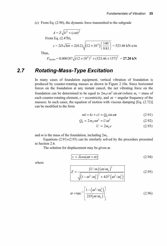
(c) From Eq. (2.90), the dynamic force transmitted to the subgrade
A = Z 2 2( )k cw+ From Eq. (2.47b),
c = 2D km = ¥ FHIK2 0 2 12 10 140
9 814( . )
.c h = 523.46 kN-s/m
Thus, Fdynam = 0.000187 ( ) ( .4612 10 523 157)4 2 2¥ + ¥ = 27.20 kN
2.7 Rotating-Mass-Type Excitation In many cases of foundation equipment, vertical vibration of foundation is produced by counter-rotating masses as shown in Figure 2.10a. Since horizontal forces on the foundation at any instant cancel, the net vibrating force on the foundation can be determined to be equal to 2mee 2w sin tw (where me = mass of each counter-rotating element, e = eccentricity, and w = angular frequency of the masses). In such cases, the equation of motion with viscous damping [Eq. (2.72)] can be modified to the form
0 sinmz kz cz Q tw+ + = (2.91) 2 2
0 2 eQ m e Uw w= = (2.92) 2 eU m e= (2.93)
and m is the mass of the foundation, including 2me. Equations (2.91)-(2.93) can be similarly solved by the procedure presented
in Section 2.6. The solution for displacement may be given as
cos( )z Z tw a= + (2.94) where
( ) ( )
( ) ( )
2
22 2 2 2 2
/ /
1 / 4 /
n
n n
U mZ
D
w w
w w w w=
− + (2.95)
( )( )
2 21
1 /tan
2 /n
nD
w wa
w w−⎡ ⎤−⎢ ⎥=⎢ ⎥⎣ ⎦
(2.96)

36 Chapter 2
Figure 2.10 (a) Rotating mass-type excitation; (b) plot of Z/(U/m) against nw w

Fundamentals of Vibration 37
In Section 2.6a, a nondimensional plot for the amplitude of vibration was given in Figure 2.9 [i.e., Z(Q0/k) versus nw w ]. This was for a vibration produced by a sinusoidal forcing function (Q0 = const). For a rotating-mass type of excitation, a similar type of non dimensional plot for the amplitude of vibration can also be prepared. This is shown in Figure 2.10b, which is a plot of Z/(U/m) versus nw w . Also proceeding in the same manner [as in Eq. (2.86) for the case where Q = const], the angular resonant frequency for rotating-mass-type excitation can be obtained as
21 2
n
D
ww =−
(2.97)
or
2
damped resonant frequency1 2
nm
ffD
= =−
(2.98)
The amplitude at damped resonant frequency can be given [similar to Eq. (2.87)] as
Zres = U mD D
/2 1 2-
(2.99)
2.8 Determination of Damping Ratio The damping ratio D can be determined from free and forced vibration tests on a system. In a free vibration test, the system is displaced from its equilibrium position, after which the amplitudes of displacement are recorded with time. Now, from Eq. (2.70)
21
2ln1
n
n
Z DZ D+
⎛ ⎞ π= =⎜ ⎟⎜ ⎟ −⎝ ⎠δ
If D is small, then
1
ln 2n
n
Z DZ +
⎛ ⎞= = π⎜ ⎟⎜ ⎟
⎝ ⎠δ (2.100)
It can also be shown that

38 Chapter 2
nδ = ln ZZn
0 = 2πnD (2.101)
where Zn = the peak amplitude of the nth cycle. Thus,
01 ln2 n
ZDn Z
=π
(2.102)
In a forced vibration test, the following procedure can be used to determine the damping ratio.
1. Vibrate the system with a constant force type of excitation and obtain a plot of amplitude (Z) with frequency (f), as shown in Figure 2.11.
2. Determine Zres from Figure 2.11. 3. Calculate 0.707Zres. Obtain the frequencies f1 and f2 that correspond to
0.707Zres. 4. From Eq. (2.87)
Zres = Qk D D
02
12 1
FHIK -
FHG
IKJ
However, if D is small,
Figure 2.11 Bandwidth method of determination of damping ratio from forced vibration test

Fundamentals of Vibration 39
0res
12
QZk D
⎛ ⎞ ⎛ ⎞= ⎜ ⎟⎜ ⎟ ⎝ ⎠⎝ ⎠ (2.103)
Again, from Eq. (2.83)
Z = 0.707 Zres =
( ) ( )022 2
/
1 4 /n n
Q k
f f D f f⎡ ⎤− +⎢ ⎥⎣ ⎦
(2.104)
Combining Eqs. (2.103) and (2.104),
0.7072D
= 1
1 42 2 2 2- +f f D f fn n/ /b g b g
ff
ff
D Dn n
FHGIKJ -FHGIKJ - + -
2 22 22 1 2 1 8c h c h = 0
2
1,2n
ff
⎛ ⎞⎜ ⎟⎝ ⎠
= 1 2 2 12 2- ± +D D Dc h
ff
ffn n
22
12F
HGIKJ -FHGIKJ = 4 1 42D D D+ ª (2.105)
However,
ff
ffn n
22
12F
HGIKJ -FHGIKJ = f f
ff f
fn n
2 1 2 1-FHG
IKJ
+FHG
IKJ
But
f ffn
2 1+ ≈ 2
So
ff
ffn n
22
12F
HGIKJ -FHGIKJ ≈ 2 2 1f f
fn
-FHG
IKJ (2.106)
Now, combining Eqs. (2.105) and (2.106)
4D = 2 f ffn
2 1-FHG
IKJ
or

40 Chapter 2
2 112 n
f fDf
⎛ ⎞−= ⎜ ⎟⎝ ⎠
(2.107)
Knowing the resonant frequency to be approximately equal to fn, the magnitude of D can be calculated. This is referred to as the bandwidth method.
2.9 Vibration-Measuring Instrument Based on the theories of vibration presented in the preceding sections, it is now possible to study the principles of a vibration-measuring instrument, as shown in Figure 2.12. The instrument consists of a spring-mass-dashpot system. It is mounted on a vibrating base. The relative motion of the mass m with respect to the vibrating base is monitored.
Let the motion of the base be given as
sinz Z tw′ ′= (2.108) Neglecting the transients let the absolute motion of the mass be given as sinz Z tw′′ ′′= (2.109) So, the equation of motion for the mass can be written as ( ) ( ) 0′′ ′′ ′ ′′ ′+ − + − =mz k z z c z z
By letting z z z′′ ′− = and z z z′′′ − = , the equation of motion can be rewritten as:
2 sin tmz kz c z m Zw w′+ + = (2.110) The solution to the Eq. (2.110) can be given as [similar to Eqs. (2.80), (2.81), and (2.82)]
Figure 2.12 Principles of vibration-measuring instrument

Fundamentals of Vibration 41
cos( )z Z tw a= + (2.111) where
( ) ( )
2
2 22
m ZZk m c
w
w w
′=− +
(2.112)
2
1tan k mcwa
w− ⎛ ⎞−= ⎜ ⎟⎝ ⎠
(2.113)
Again, from Eq. (2.112),
( )
( ) ( )
2
22 22
/
1 / 4 /
n
n n
ZZ
D
w w
w w w w=
′ ⎡ ⎤− +⎣ ⎦
(2.114)
If the natural frequency of the instrument nw is small and nw w is large, then for practically all values of D, the magnitude of Z/Z′ is about 1. Hence the instrument works as a velocity pickup.
Also, from Eq. (2.114) one can write that
( ) ( )2 22 22 2
1
1 / 4 /n n n
ZZ
Dw
w w w w w=
′ ⎡ ⎤− +⎢ ⎥⎣ ⎦
(2.115)
If D = 0.69 and nw w is varied from zero to 0.4 (Prakash, 1981), then Eq. (2.115) will result in
2 21
n
ZZw w
≈′
= const
So
Z ∝ 2w Z’
However, 2w Z′ is the absolute acceleration of the vibrating base. For this condition, the instrument works as an acceleration pickup. Note that, for this case, the natural frequency of the instrument and, thus, nw are large, and hence the ratio nw w is small.

42 Chapter 2
System with Two Degrees of Freedom
2.10 Vibration of a Mass-Spring System A mass-spring system with two degrees of freedom is shown in Figure 2.13a. The system may be excited into vibration in several ways. Two cases of practical interest are (a) sinusoidal force applied on mass m1 resulting in forced vibration of the
system, and (b) the vibration of the system triggered by an impact on mass m2.
The procedure for calculating the natural frequencies of the system shown in Figure 2.13 is described first, followed by a method for calculating amplitudes of masses m1 and m2 for the two cases of excitation mentioned here.
A. Calculation of Natural Frequency The free body diagrams for the vibration of the masses m1 and m2 are shown in Figure 2.13b. The equations of motion may be written as
Figure 2.13 Mass-spring system with two degrees of freedom

Fundamentals of Vibration 43
1 1 1 1 2 1 2( ) 0m z k z k z z+ + - = (2.116) 2 2 2 2 1( ) 0m z k z z+ - = (2.117)
where k1, k2 = spring constants
z1, z2 = displacement of masses m1 and m2, respectively
Now, let 1 sin nz A tw= (2.118a) 2 sin nz B tw= (2.118b)
where nw = natural frequency of the system.
Substitution of Eqs. (2.118a) and (2.118b) into Eqs. (2116) and (2.117) yields
21 2 1 2( ) 0nA k k m k Bw+ − − = (2.119a)
and 2
2 2 2( ) 0nAk k m Bw− + − = (2.119b)
For the nontrivial solution
2
1 2 1 22
2 2 2
0n
n
k k m k
k k m
ww
+ − −=
− −
or 2 2 2
1 2 1 2 2 2( )( )n nk k m k m kw w+ − − =
4 21 2 2 2 2 1 1 2
1 2 1 20n n
k m k m k m k km m m m
w w⎛ ⎞+ +− + =⎜ ⎟⎝ ⎠
(2.120)
Let
2
1
mm
h = (2.121a)
1
1
1 2nl
km m
w =+
(2.121b)
2
2
1nl
kk
w = (2.121c)
Substituting Eqs. (2.121a), (2.121b), and (2.121c) into Eq. (2.120) and simplifying one obtains

44 Chapter 2
1 2 1 2
4 2 2 2 2 2(1 )( ) (1 )( )( ) 0n nl nl n nl nlw h w w w h w w− + + + + = (2.122)
Equation (2.122) represents the frequency equation for a two-degree system.
B. Amplitude of Vibration of Masses m1 and m2 Vibration Induced by a Force Acting on Mass m1: Figure 2.14 shows the case where a force Q = Q0 sin ωt is acting on a mass m1. The equations of motion may be written as
1 1 1 1 2 1 2 0( ) sinm z k z k z z Q tw+ + - = (2.123a) 2 2 2 2 1( ) 0m z k z z+ - = (2.123b) Let z1 = A1 sin tw (2.124a) z2 = A2 sin tw (2.124b)
Substitution of Eqs. (2.124a) and (2.124b) into Eqs. (2.123a) and (2.123b) yields
Figure 2.14 Vibration induced by a force on a mass-spring system with two degrees of
freedom

Fundamentals of Vibration 45
A1(− m12w + k1 + k2) – A2k2 = Q0 (2.125a)
A2(k2 – m22w ) – A1k2 = 0 (2.125b)
From Eq. (2.125b)
( )1 2
2 22 2
A kAk m w
=−
(2.126)
Combining Eqs. (2.125a) and (2.126),
( )2
2 1 21 1 1 2 2
2 2
( ) A kA m k kk m
ww
− + + −−
= Q0
or
A1 = ( )
( )2
2 20
21
nlQ
m
w w
w
−
Δ (2.127)
where
1 2 1 2
2 4 2 2 2 2( ) (1 )( ) (1 )( )( )nl nl nl nlw w h w w h w w= − + + + +D (2.128)
Similarly, it can be shown that
( )2
20
2 21
nlQA
m
w
w=
Δ (2.129)
It may be observed from Eq. (2.127) that A1 = 0 if
2nlw w= (2.130)
Equations (2.127) and (2.130) illustrate the principle of vibration absorber. In a practical situation, the system k1, m1 represents a main system, and the system k2, m2 represent an auxiliary system. The vibration of the main system can, in principle, be reduced or even totally eliminated by attaching an auxiliary system to the main mass, designed in such a way that its natural frequency
2nlw is equal to the operating frequencyw .
Vibration Induced by an Impact on Mass m2: A practical solution to this
case is obtained by assuming that the vibration is being induced by an initial velocity 0u to mass m2. For this case, let

46 Chapter 2
z1 = C1sin 1n tw + C2 sin 2n tw (2.131a) z2 = D1sin
1n tw + D2 sin2n tw (2.131b)
The initial conditions of vibration are defined as follows. At time t = 0:
z1 = z2 = 0 (2.132a) z1 = 0 and z2 = 0u (2.132b)
Substituting Eqs. (2.131a) and (2.131b) into Eqs. (2.116) and (2.117), applying the initial conditions as defined in Eqs. (2.132a) and (2.132b), and simplifying, one obtains
( ) ( )
( )2 1 2 2 1 2
1 22 1 2
2 2 2 2
1 02 2 2
sin sinnl n nl n n n
n nnl n n
t tz
w w w w w wu
w ww w w=
− − ⎛ ⎞⎜ ⎟−⎜ ⎟− ⎝ ⎠
(2.133a)
and
( )( ) ( )2 1 1 2 2 2
211 2
2 2 2 2
2 02 2
sin sin1 nl n n nl n n
nnn n
t tz
w w w w w wu
www w
⎡ ⎤− −⎢ ⎥= −⎢ ⎥− ⎣ ⎦
(2.133b)
The preceding relationships can be further simplified to determine the amplitudes Z1 and Z2 of masses m1 and m2, respectively:
( ) ( )
( )2 1 2 2
2 1 2 2
2 2 2 2
1 02 2 2
nl n nl n
nl n n n
Zw w w w
uw w w w
− −=
− (2.134a)
and
( )( )
2 1
1 2 2
2 20
2 2 2
nl n
n n n
Zw w u
w w w
−=
− (2.134b)
Example 2.7
Refer to Figure 2.13a. Calculate the natural frequencies of the system. Given: Weight: W1 = 111.20 N; W2 = 22.24 N
Spring constant: k1 = 17.5 kN/m; k2 = 8.75 kN/m Solution
From Eqs. (2.121a), (2.121b), and (2.121c)

Fundamentals of Vibration 47
2 2
1 1
22.24 0.2111.20
m Wm W
η = = = =
1nlw = ( )3
1
1 2
17.5 10 9.81111.2 22.24
km m
× ×=+ +
= 35.86 rad/s
2nlw = 3
2
2
8.75 10 9.8122.24
km
¥ ¥= = 62.12 rad/s
From Eq. (2.122)
1 2 1 24 2 2 2 2 2(1 )( ) (1 )( )( ) 0n nl nl n nl nlw h w w w h w w− + + + + = 4 2 2 2 2 2(1 0.2) (35.86 62.12 ) (1 0.2) (35.86 ) (62.12 ) 0n nω ω− + + + + =4 26173.8 5954766.15 0n nω ω− + =
( ) ( ) ( )1,2
22 6173.1 6173.1 4 5954766.15
2nω± −
=
12nw = 1190.35;
22nw = 4977.45
So
1nw = 34.60 rad/s; 2nw = 70.55 rad/s
Example 2.8
Refer to Example 2.7. If a sinusoidally varying force Q = 44.5 sin tw N is applied to the mass m1 (Figure 2.13a), what would be the amplitudes of vibration given w = 78.54 rad/s?
Solution
From Eq. (2.128)
1 2 1 2
2 4 2 2 2 2 2( ) (1 )( ) (1 )( )( ) 0n nl nl n nl nlw w h w w w h w w= − + + + + =D
= (78.54)4 – (1 + 0.2)[(35.86)2 + (62.12)2](78.54)2 + (1 +0.2)(35.86) 2 (62.12)2
= 5922262.92 Again, using Eqs. (2.127) and (2.129),
( )( )
( ) ( ) ( )
( )2
2 22 20
1 21
44.5 62.12 78.54
111.2 5922262.929.81
nlQA
m
w w
w
⎡ ⎤−− ⎣ ⎦= =⎛ ⎞⎜ ⎟⎝ ⎠
D
= − 0.00153 m = −15.3 mm So, the magnitude of A1 is 15.3 mm.

48 Chapter 2
( )( )( )
( )2
220
2 21
44.5 62.12111.2 5922262.929.81
nlQA
m
w
w= =
⎛ ⎞Δ⎜ ⎟⎝ ⎠
= 0.0026 m = 2.6 mm.
2.11 Coupled Translation and Rotation of a Mass-Spring System (Free Vibration) Figure 2.15 shows a mass-spring system that will undergo translation and rotation. The equation of motion of the mass m can be given as
1 1 2 2( ) ( ) 0mz k z l k z l+ − + + =θ θ (2.135)
21 1 1 2 2 2( ) ( ) 0mr l k z l l k z l− − + + =θ θ θ (2.136)
where θ = angle of rotation of the mass m
θ2
2= ddt
θ
r = radius of gyration of the body about the center of gravity (Note: mr2 = J = mass moment of inertia about the center
of gravity) k1, k2 = spring constants z = distance of translation of the center of gravity of the body
Figure 2.15 Coupled translation and rotation of a mass-spring system

Fundamentals of Vibration 49
Now, let
k1 + k2 = kz (2.137) and 2 2
1 1 2 2l k l k k+ = θ (2.138)
So, the equations of motion can be written as
2 2 1 1( ) = 0zmz k z l k l k θ+ + − (2.139) 2
2 2 1 1( ) = 0mr k l k l k zθθ θ+ + − (2.140)
If l1k1 = l2k2, Eq. (2.139) is independent of θ and Eq. (2.140) is independent of z. This means that the two motions (i.e., translation and rotation) can exist independently of each one another (uncoupled motion); that is,
= 0zmz k z+ (2.141) and 2 = 0mr k+ θθ θ (2.142)
The natural circular frequency nzw of translation can be obtained by
= znz
km
w (2.143)
Similarly, the natural circular frequency of rotation nqw can be given by
2=nk
mrq
qw (2.144)
However, if l1k1 is not equal to l2k2, the equations of motion (coupled motion) can be solved as follows: Let
1=zk Em
(2.145)
2 2 1 22=l k l k E
m− (2.146)
3=k Emθ (2.147)
Combining Eqs. (2.139), (2.140), (2.145)-(2.147),
50 Chapter 2
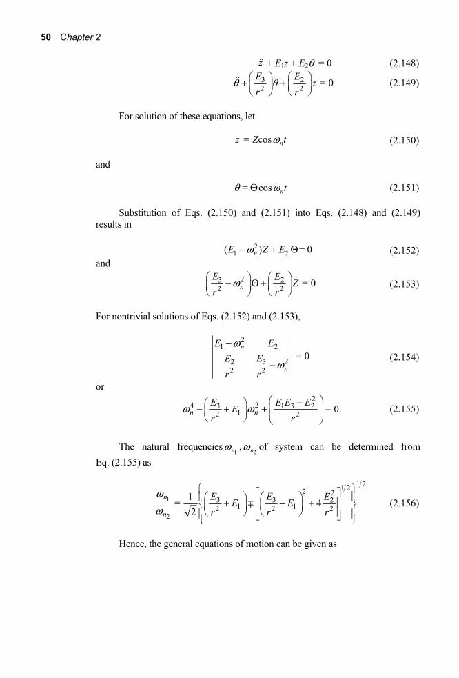
z + E1z + E2θ = 0 (2.148)
3 22 2 = 0
E E zr r
⎛ ⎞ ⎛ ⎞+ + ⎜ ⎟⎜ ⎟⎝ ⎠⎝ ⎠
θ θ (2.149)
For solution of these equations, let
= cos nz Z tw (2.150)
and
= cos ntq wQ (2.151)
Substitution of Eqs. (2.150) and (2.151) into Eqs. (2.148) and (2.149) results in
21 2( – ) = 0nE Z Ew Q+ (2.152)
and
23 22 2 = 0n
E E Zr r
w⎛ ⎞ ⎛ ⎞− Θ + ⎜ ⎟⎜ ⎟⎝ ⎠⎝ ⎠
(2.153)
For nontrivial solutions of Eqs. (2.152) and (2.153),
21 2
2322 2
= 0n
n
E EEE
r r
w
w
−
− (2.154)
or
2
4 23 1 3 212 2 = 0n n
E E E EEr r
w w⎛ ⎞−⎛ ⎞− + + ⎜ ⎟⎜ ⎟ ⎜ ⎟⎝ ⎠ ⎝ ⎠
(2.155)
The natural frequencies1nw ,
2nw of system can be determined from Eq. (2.155) as
1
2
1 21 22 23 3 2
1 12 2 21= 42
n
n
E E EE Er r r
ww
∓⎧ ⎫⎡ ⎤⎛ ⎞ ⎛ ⎞⎪ ⎪⎢ ⎥+ − +⎨ ⎬⎜ ⎟ ⎜ ⎟⎝ ⎠ ⎝ ⎠⎢ ⎥⎪ ⎪⎣ ⎦⎩ ⎭
(2.156)
Hence, the general equations of motion can be given as

Fundamentals of Vibration 51
z = Z1cos 1n tw + Z2 cos
2n tw (2.157) and 1 21 2= cos cosn nt tq w wΘ + Θ (2.158)
The amplitude ratios can also be obtained from Eqs. (2.152) and (2.153)
as
1
1
2 23
1 22 2
1 1 2
( )=
cos
n
n
E rZ EE E r
w
w
− −− =
Θ − (2.159)
and
2
2
2 23
2 22 2
2 1 2
( )=
cos
n
n
E rZ EE E r
w
w
− −− =
Θ − (2.160)
Problems 2.1 Define the following terms:
a. Spring constant b. Coefficient of subgrade reaction c. Undamped natural circular frequency d. Undamped natural frequency e. Period f. Resonance g. Critical damping coefficient h. Damping ratio i. Damped natural frequency
2.2 A machine foundation can be idealized to a mass-spring system, as shown in Figure 2.4.
Given Weight of machine + foundation = 400 kN Spring constant = 100,000 kN/m Determine the natural frequency of undamped free vibration of this
foundation and the natural period. 2.3 Refer to Problem 2.2, What would be the static deflection zs of this
foundation? 2.4 Refer to Example 2.3. For this foundation let time t = 0, z = z0 = 0.
z = 0u = 0.

52 Chapter 2
a. Determine the natural period T of the foundation. b. Plot the dynamic force on the subgrade of the foundation due to
the forced part of the response for time t =0 to t = 2T. c. Plot the dynamic force on the subgrade of the foundation due to
the free part of the response for t = 0 to 2T. d. Plot the total dynamic force on the subgrade [that is, the
algebraic sum of (b) and (c)]. Hint: Refer to Eq. (2.33)
Force due to forced part = 02 2 sin
1 n
Q kk tww w
⎛ ⎞⎜ ⎟⎜ ⎟−⎝ ⎠
Force due to free part = 02 2 sin
1 nnn
Q kk tw www w
⎛ ⎞⎛ ⎞−⎜ ⎟⎜ ⎟⎜ ⎟− ⎝ ⎠⎝ ⎠
2.5 A foundation of mass m is supported by two springs attached in series. (See Figure P2.5). Determine the natural frequency of the undamped free vibration.
Figure P2.5
2.6 A foundation of mass m is supported by two springs attached in parallel (Figure P2.6). Determine the natural frequency of the undamped free vibration.
2.7 For the system shown in Figure P2.7, calculate the natural frequency and period given k1 =100 N/mm, k2 = 200 N/mm, k3 = 150 N/mm, k4 = 100 N/mm, k5 = 150 N/mm, and m = 100 kg.

Fundamentals of Vibration 53
Figure P2.6
Figure P2.7
2.8 Refer to Problem 2.7. If a sinusoidally varying force Q = 50 sin tw (N) is applied to the mass as shown, what would be the amplitude of vibration given w = 47 rad/s?
2.9 A body weighs 135 N. A spring and a dashpot are attached to the body in the manner shown in Figure 2.2b. The spring constant is 2600 N/m. The dashpot has a resistance of 0.7 N at a velocity of 60 mm/s. Determine the following for free vibration: a. Damped natural frequency of the system b. Damping ratio c. Ratio of successive amplitudes of the body (Zn/Zn + 1)
54 Chapter 2
d. Amplitude of the body 5 cycles after it is disturbed, assuming that at time t = 0, z = 25 mm.
2.10 A machine foundation can be identified as a mass-spring system. This is subjected to a forced vibration. The vibrating force is expressed as
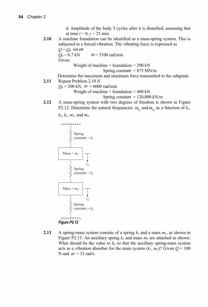
Q = Q0 sin tw Q0 = 6.7 kN w = 3100 rad/min Given Weight of machine + foundation = 290 kN Spring constant = 875 MN/m Determine the maximum and minimum force transmitted to the subgrade. 2.11 Repeat Problem 2.10 if Q0 = 200 kN, w = 6000 rad/min Weight of machine + foundation = 400 kN Spring constant = 120,000 kN/m 2.12 A mass-spring system with two degrees of freedom is shown in Figure
P2.12. Determine the natural frequencies 1nw and
2nw as a function of k1, k2, k3, m1, and m2.
Figure P2.12 2.13 A spring-mass system consists of a spring k1 and a mass m1, as shown in
Figure P2.13. An auxiliary spring k2 and mass m2 are attached as shown. What should be the value to k2 so that the auxiliary spring-mass system acts as a vibration absorber for the main system (k1, m1)? Given Q = 100 N and w = 31 rad/s.

Fundamentals of Vibration 55
Figure P2.13
2.14 A foundation weighs 800 kN. The foundation and the soil can be approximated as a mass-spring-dashpot system as shown in Figure 2.2b. Given
Spring constant = 200,000 kN/m Dashpot coefficient = 2340 kN-s/m Determine the following:
a. Critical damping coefficient cc. b. Damping ratio c. Logarithmic decrement d. Damped natural frequency
2.15 The foundation given in Problem 2.12 is subjected to a vertical force Q = Q0 sin tw in which Q0 = 25 kN w = 100 rad/s Determine
a. the amplitude of the vertical vibration of the foundation, and b. the maximum dynamic force transmitted to the subgrade.
References Prakash, S. (1981). Soil Dynamics. McGraw-Hill Book Company, New York.

56
3 Waves in Elastic Medium
3.1 Introduction If a stress is suddenly applied to a body, the part of the body closest to the source of disturbance will be affected first. The deformation of the body due to the load will gradually spread throughout the body via stress waves. The nature of propagation of stress waves in an elastic medium is the subject of discussion in this chapter. Stress wave propagation is of extreme importance in geotechnical engineering, since it allows determination of soil properties such as modulus of elasticity, shear wave velocity, shear modulus; interpretation of test results of geophysical investigation, numerical formulation of ground response analysis and also helps in the development of the design parameters for earthquake-resistant structures. The problem of stress wave propagation can be divided into three major categories: a) Elastic stress waves in a bar b) Stress waves in an infinite elastic medium c) Stress waves in an elastic half-space
However, before the relationships for the stress waves can be developed, it is essential to have some knowledge of the fundamental definitions of stress, strain, and other related parameters that are generally encountered in an elastic medium. These definitions are given in Sections 3.2 and 3.3.
3.2 Stress and Strain
Nations for Stress Figure 3.1 shows an element in an elastic medium whose sides measure dx, dy and dz. The normal stresses acting on the plane normal to the x, y, and z axes are

Waves in Elastic Medium 57
Figure 3.1 Notations for normal and shear stresses
,x ys s and zs , respectively. The shear stresses are xyt , yxt , yzt , zyt , xzt and zxt . The nations for the shear stresses are as follows.
If τij is a shear stress, it means that it is acting on a plane normal to the i axis, and its direction is parallel to the j axis. For equilibrium purposes, by taking moments, it may be seen that
xy yxt t= (3.1)
xz zxt t= (3.2) yz zyt t= (3.3)
Strain Due to a given stress condition, let the displacements in the x, y, and z directions (Figure 3.1) be, respectively, u,u and w. Then the equations for strains and rotations of elastic and isotropic materials in terms of displacements are as follows:
xux
e ∂=∂
(3.4)

58 Chapter 3
y yue ∂=
∂ (3.5)
zwz
e ∂=∂
(3.6)
xyu
x yug ∂ ∂′ = +
∂ ∂ (3.7)
yzwy z
ug ∂ ∂′ = +∂ ∂
(3.8)
zxu wz x
g ∂ ∂′ = +∂ ∂
(3.9)
12x
wy z
uw ⎛ ⎞∂ ∂= −⎜ ⎟∂ ∂⎝ ⎠ (3.10)
12y
u wz x
w ∂ ∂⎛ ⎞= −⎜ ⎟∂ ∂⎝ ⎠ (3.11)
12z
ux yuw ⎛ ⎞∂ ∂= −⎜ ⎟∂ ∂⎝ ⎠
(3.12)
where xe , ye and ze = normal strains in the direction of x, y and z, respectively xyg ′ = sheering strain between the planes xz and yz yzg ′ = shearing strain between the planes yx and zx zxγ ′ = shearing strain between the planes zy and xy ,x yw w and zw = the components of rotation about the x, y, and z axes.
These derivations are given in most of the textbooks on the theory of elasticity (e.g., Timoshenko and Goodier, 1970). The interested reader may consult these books and are not covered here in detail.
3.3 Hooke’s Law For an elastic, isotropic material, the normal strains and normal stresses can be related by the following equations:
1 )x x y zEe s m s s(È ˘= - +Î ˚ (3.13)
1= )y y x zEe s m s s⎡ ⎤− ( +⎣ ⎦ (3.14)

Waves in Elastic Medium 59
1= )z z x yEe s m s s⎡ ⎤− ( +⎣ ⎦ (3.15)
where xe , ye and ze are the respective normal strains in the directions of x, y, and z, E is Young’s modulus, andm is Poisson’s ratio.
The shear stresses and the shear strains can be related by the following equations:
xy xyGt g ′= (3.16)
yz yzGt g ′= (3.17)
zx zxGt g= ¢ (3.18)
where the Shear modulus (G) is
2(1 )
EGm
=+
(3.19)
and xyg ′ , yzg ′ , and zxg ′ are the shear strains.
Equations (3.13) – (3.15) can be solved to express normal stresses in terms of normal strains as
2x xGs le e= + (3.20) 2y yGs le e= + (3.21) 2z zGs le e= + (3.22)
where
(1 )(1 2 )
mElm m
=+ −
(3.23)
x y ze e e e= + + (3.24)
λ is known as the Lame’s constant and can easily estimated by a relatively easy measurement of E and μ of any material and thus can be used for describing the velocity of waves through the material. From Eqs (3.19) and (3.23), it is easy to see that
2( )G
lml
=+
(3.25)

60 Chapter 3
Elastic Stress Waves in a Bar
3.4 Longitudinal Elastic Waves in a Bar Figure 3.2 shows a rod, the cross-sectional area of which is equal to A. Let the Young’s modulus and the unit weight of the material that constitutes the rod be equal to E and γ, respectively. Now, let the stress along section a – a of the rod increase bys . The stress increase along the section b – b can then be given by ( )x xs s+ ∂ ∂ Δ . Based on Newton’s second law,
force = (mass) (acceleration) Thus, summing the forces in the x direction,
2
2( )A x uA x A
x g ts gs s DD∂ ∂⎛ ⎞− + + =⎜ ⎟∂ ∂⎝ ⎠
(3.26)
where A xΔ γ = weight of the rod of length xΔ , g is the acceleration due to gravity, u is displacement in the x direction, and t is time.
Equation (3.26) is based on the assumptions that (1) the stress is uniform over the entire cross-sectional area and (2) the cross section remains plane during the motion. Simplification of Eqs. (3.26) gives
2
2u
x ts r
⎛ ⎞∂ ∂= ⎜ ⎟⎜ ⎟∂ ∂⎝ ⎠ (3.27)
where gr g= is the density of the material of the bar. However,
s = (strain) (Young’s modulus) = ux
∂⎛ ⎞⎜ ⎟∂⎝ ⎠
E (3.28)
Substitution of Eq. (3.28) into (3.27) yields
2 2
2 2u E u
t xr⎛ ⎞⎛ ⎞∂ ∂= ⎜ ⎟⎜ ⎟ ⎜ ⎟∂ ∂⎝ ⎠ ⎝ ⎠
or
2 2
22 2cu u
t xu∂ ∂=
∂ ∂ (3.29)
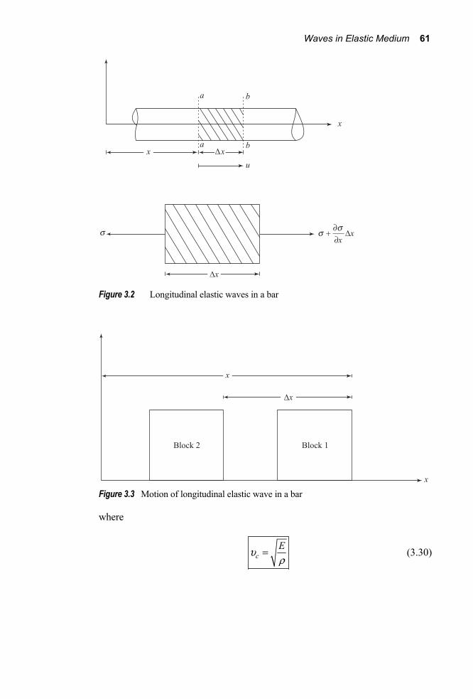
Waves in Elastic Medium 61
Figure 3.2 Longitudinal elastic waves in a bar
Figure 3.3 Motion of longitudinal elastic wave in a bar
where
cEu =ρ
(3.30)

62 Chapter 3
The term cu is the velocity of the longitudinal stress wave propagation. This fact can be demonstrated as follows. The solution to Eq. (3.29) can be written in the form
( ) ( )c cu = F t x +G t xu u+ − (3.31)
where ( )cF t xu + and ( )cG t xu − represent some functions of ( )ct xu + and
( )ct xu − , respectively. At a given time t, let the function ( )cF t xu + be represented by block 1 in Figure 3.3, and
ut = F( cu t + x)
At time t + Δt, the function will be represented by block 2 in Figure 3.3. Thus,
ut + Δt = F[ cu (t + Δt) + (x - Δx)] (3.32)
If the block moves unchanged in shaped from position 1 to position 2,
ut = ut + Δt or F( cu t + x) = F[ cu (t + Δt) + (x – Δx)] or cu Δt = Δx (3.33)
Thus the velocity of the longitudinal stress wave propagation is equal to cx t u=D D . In a similar manner, it can be shown that the function G( cu t – x)
represents a wave traveling in the positive direction of x. If the bar described above is confined, so that no lateral expansion is
possible, then the above equation can be modified as
2 2
22 2cu u
t xu∂ ∂′=
∂ ∂ (3.34)
where
cMur
′ = (3.35)
M = constrained modulus = (1 )(1 2 ) (1 )
E mm m
−− +
; μ = Poisson’s ratio

Waves in Elastic Medium 63
3.5 Velocity of Particles in the Stressed Zone It is important for readers to appreciate the difference between the velocity of the longitudinal wave propagation ( cu ) and the velocity of the particles in the stressed zone. In order to distinguish them, consider a compressive stress pulse of intensity σx and duration t’ (Figure 3.4a) be applied to the end of a rod (shown in Figure 3.4b). When this stress pulse is applied initially, a small zone of the rod will undergo compression. With time this compression will be transmitted to successive zones. During a time interval Δt the stress will travel through a distance
Δx = cu Δt
At any time t > t′, a segment of the rod of length x will constitute the compressed zone. Note that
x = cu t′
The elastic shortening of the rod then is
( ) ( )x xcu x t
E Es s u⎛ ⎞ ⎛ ⎞ ′= =⎜ ⎟ ⎜ ⎟⎝ ⎠ ⎝ ⎠
Note that u is the displacement of the end of the rod. Now, the velocity of the end of the rod and, thus, the particle velocity is
x cuut E
s u= =
′
Also, it is important to note the following: 1. Particle velocity u is a function of the intensity of stress σx. Higher the
amplitude of the intensity of stress, higher is the particle velocity for the same medium.
2. However, the longitudinal wave propagation velocity is a function of material property only. It is independent of the amplitude of stress applied.
3. The wave propagation velocity and the particle velocity are in the same direction when a compressive stress is applied. However when a tensile stress is applied, the wave propagation and the particle velocity are in opposite directions.
The above concepts are used in non-destructive testing apparatus such as pile integrity testing (PIT).
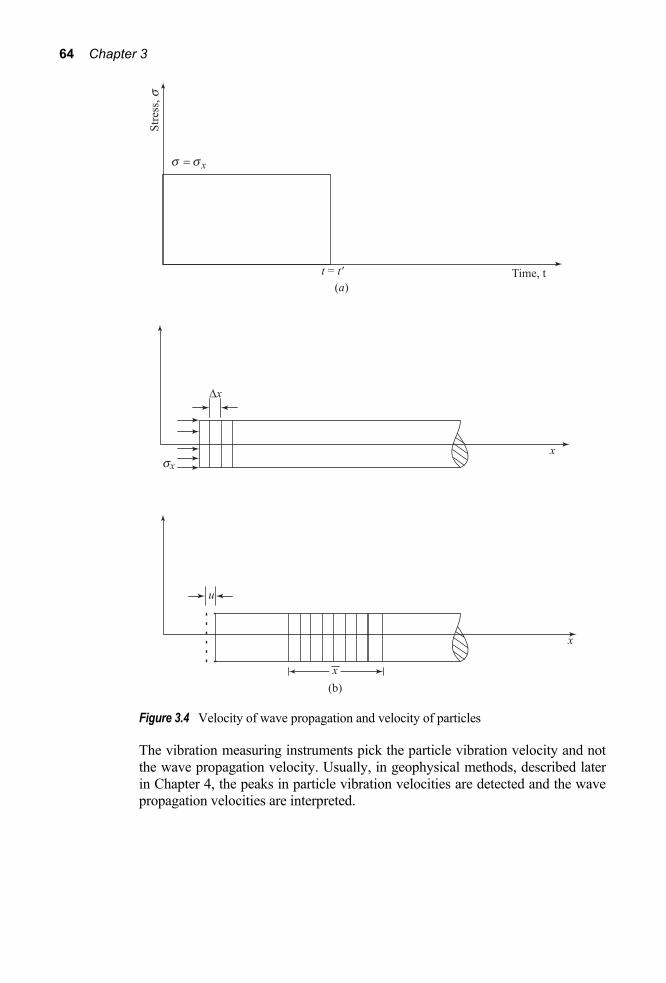
64 Chapter 3
Figure 3.4 Velocity of wave propagation and velocity of particles
The vibration measuring instruments pick the particle vibration velocity and not the wave propagation velocity. Usually, in geophysical methods, described later in Chapter 4, the peaks in particle vibration velocities are detected and the wave propagation velocities are interpreted.

Waves in Elastic Medium 65
3.6 Reflections of Elastic Stress Waves at the End of a Bar Bars must terminate at some point. One needs to consider the case of what happens when one of these disturbances, F( cu t + x) or G( cu t x- ) [Eq. (3.31)], meets the end of the bar.
Figure 3.5a shows a compression wave moving along a bar in the positive x direction. Additionally, a tension wave of the same length is moving along the negative direction of x. When the two waves meets each other (at section a–a), the compression and tension cancel each other, resulting in zero stress; however,
Figure 3.5 Reflection of stress waves at a free end of a bar

66 Chapter 3
the particle velocity is double (Figure 3.5b). This is because the particle velocity for a compression wave is in direction of the motion, and in the tension wave, the particle velocity is opposed to the direction of motion. After the two waves pass each other, the stress and the particle velocity again return to zero at section a–a (Figure 3.5c). The section a–a corresponds to having the stress condition that a free end of a bar would have. Figure 3.5d shows the portion of the rod located to the left of section a–a, and the section can be considered as a free end. By observation it can be seen that, at the free end of a bar, a compression wave is reflected back as a tension wave having the same magnitude and shape. In a similar manner, a tension wave is reflected back as a compression wave at the free end of a bar.
Figure 3.6 Reflection of stress waves at a fixed end of a bar

Waves in Elastic Medium 67
Figure 3.6a shows a bar in which two identical compression waves are traveling in opposite directions. When the two waves cross each other at section a–a, the magnitude of the stress will be doubled. However, the particle velocity u will be equal to zero (Figure 3.6b). After the two waves pass each other, the stress and the particle velocity return to zero at section a–a (Figure 3.6c). Section a–a remains stationary and behaves as a fixed end of a rod. By observation it can be seen (Figure 3.6d) that a compression wave is reflected back as a compression wave of the same magnitude and shape, but the stress is doubled at the fixed end. In a similar manner, a tension wave is reflected back as a tension wave at the fixed end of a bar.
3.7 Torsional Waves in a Bar Figure 3.7 shows a rod to which a torque T is applied at a distance x, and the end at x will be rotated through an angle θ. The torque at the section located at a distance x + Δx can be given by T + (∂T/∂x)Δx and the corresponding rotation by θ + (∂θ/∂x)Δx. Applying Newton’s second law of motion,
2
2TT T x J xx t
qr∂ ∂⎛ ⎞− + + Δ = Δ⎜ ⎟∂ ∂⎝ ⎠ (3.36)
where J is the polar moment of inertia of the cross section of the bar.
Figure 3.7 Torsional waves in a bar

68 Chapter 3
However, torque T can be expressed by the relation
T JGxq∂=
∂ (3.37)
Substitution of Eq. (3.37) into Eq. (3.36) results in
2 2
2 2G
t xq q
r∂ ∂=∂ ∂
(3.38)
or
2 2
22 2st xq qu∂ ∂=
∂ ∂ (3.39)
where
sGu =ρ
(3.40)
is the velocity of torsional waves.
Note that Eqs. (3.39) and (3.29) are of similar form.
3.8 Longitudinal Vibration of Short Bars The solution to the wave equations for short bars vibrating in a natural mode can be written in the general form as
1 2( , ) ( )( sin cos )n nu x t U x A t A tw w= + (3.41)
where A1 and A2 are constants, nw is the natural circular frequency of vibration, and U(x) is the amplitude of displacement along the length of the rod and is independent of time.
For longitudinal vibration of uniform bars, if Eq. (3.41) is substituted into Eq. (3.29), it yields
2 2
2 2( , ) ( , ) 0u x t u x t
Ex tρ∂ ∂− =
∂ ∂
or
2
22( ) ( ) ( ) 0n
U x U xExr w∂ + =
∂⋅ (3.42)
The solution to Eq. (3.42) may be expressed in the form

Waves in Elastic Medium 69
1 2( ) sin cosn n
c c
x xU x B Bw wu u
⎛ ⎞ ⎛ ⎞= +⎜ ⎟ ⎜ ⎟
⎝ ⎠ ⎝ ⎠ (3.43)
where B1 and B2 are constants. These constants may be determined by the end condition to which a rod may be subjected.
A. End Condition: Free-Free For the free-free condition, the stress and thus the strain at the ends are zero. So at x = 0, ( ) 0dU x dx = ; and at x = L, ( ) 0dU x dx = , where L is the length of the bar. Differentiating Eq. (3.43) with respect to x.
1 2( ) cos sinn n n n
c c c c
B x B xdU xdx
w w w wu u u u
⎛ ⎞ ⎛ ⎞= −⎜ ⎟ ⎜ ⎟
⎝ ⎠ ⎝ ⎠ (3.44)
Substitution of the first boundary condition into Eq. (3.44) results in
0 = 1 n
c
Bwu
; i.e., B1 = 0 (3.45)
Again, from the second boundary condition and Eq. (3.44),
20 sinn n
c c
B Lw wu u
⎛ ⎞ ⎛ ⎞= − ⎜ ⎟ ⎜ ⎟
⎝ ⎠ ⎝ ⎠
Since B2 is not equal to zero,
n
c
L nwu
p= (3.46)
or
cn
nLuw p= (3.47)
where n = 1, 2, 3,….. Thus,
nc
Lnwup
= (3.48)
The equation for the amplitude of displacement for this case can be given by combining Eqs. (3.43), (3.45), and (3.48), or
2( ) cos n xU x BLπ⎛ ⎞= ⎜ ⎟
⎝ ⎠ (3.49)

70 Chapter 3
Figure 3.8 Longitudinal vibration of a short bar: free-free end condition
The variation of the nature of U(x) for the first two harmonics (i.e., n = 1 and 2) is shown in Figure 3.8. The equation for u(x, t) for all modes of vibration can also be given by combining Eqs. (3.49) and (3.41).
B. End Condition: Fixed–Fixed For a fixed–fixed end condition, at x = 0, U(x) = 0 (i.e., displacement is zero); and at x = L, U(x) = 0
Substituting the first boundary condition into Eq. (3.43) results in
0 = B2 (3.50)
Again, combining the second boundary condition and Eq. (3.43),

Waves in Elastic Medium 71
10 sin n
c
LB wu
⎛ ⎞= ⎜ ⎟
⎝ ⎠
Since B1 ≠ 0,
n
c
L nwu
p⎛ ⎞
=⎜ ⎟⎝ ⎠
(3.51)
where n = 1, 2, 3,…; or
cn
nLuw p= (3.52)
or
nc
Lnwup
= (3.53)
The displacement amplitude equation can now be given be combining Eqs. (3.43), (3.50), and (3.52) ad
1( ) sin n xU x BLπ⎛ ⎞= ⎜ ⎟
⎝ ⎠ (3.54)
Figure 3.9 shows the variation of U(x) for the first two harmonics (n = 1 and 2)
C. End Condition: Fixed–Free The boundary conditions for the fixed – free case can be given as follows:
At x = 0 (fixed end), U(x) = 0
At x = L (free end), ( )dU xdx
= 0
From the first boundary condition and Eq. (3.43),
U(x) = 0 = B2 (3.55)
Again, from the second boundary condition and Eq. (3.43)
( )dU xdx
= 0 = 1 cosn n
c c
B Lw wu u
⎛ ⎞⎜ ⎟⎝ ⎠
(3.56)
or
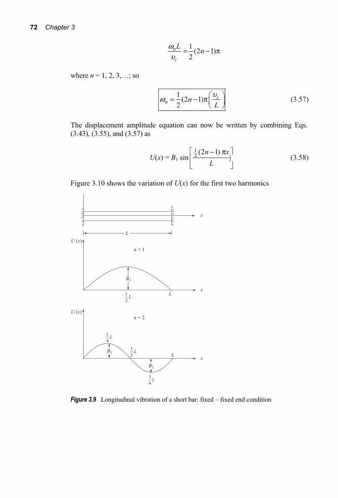
72 Chapter 3
1 (2 1)2
n
c
L nωυ
= − π
where n = 1, 2, 3,…; so
1 (2 1)2
cn n
Luw p⎛ ⎞= − ⎜ ⎟⎝ ⎠
(3.57)
The displacement amplitude equation can now be written by combining Eqs. (3.43), (3.55), and (3.57) as
U(x) = B1 sin12 (2 1)n x
L⎡ ⎤− π⎢ ⎥⎣ ⎦
(3.58)
Figure 3.10 shows the variation of U(x) for the first two harmonics
Figure 3.9 Longitudinal vibration of a short bar: fixed – fixed end condition
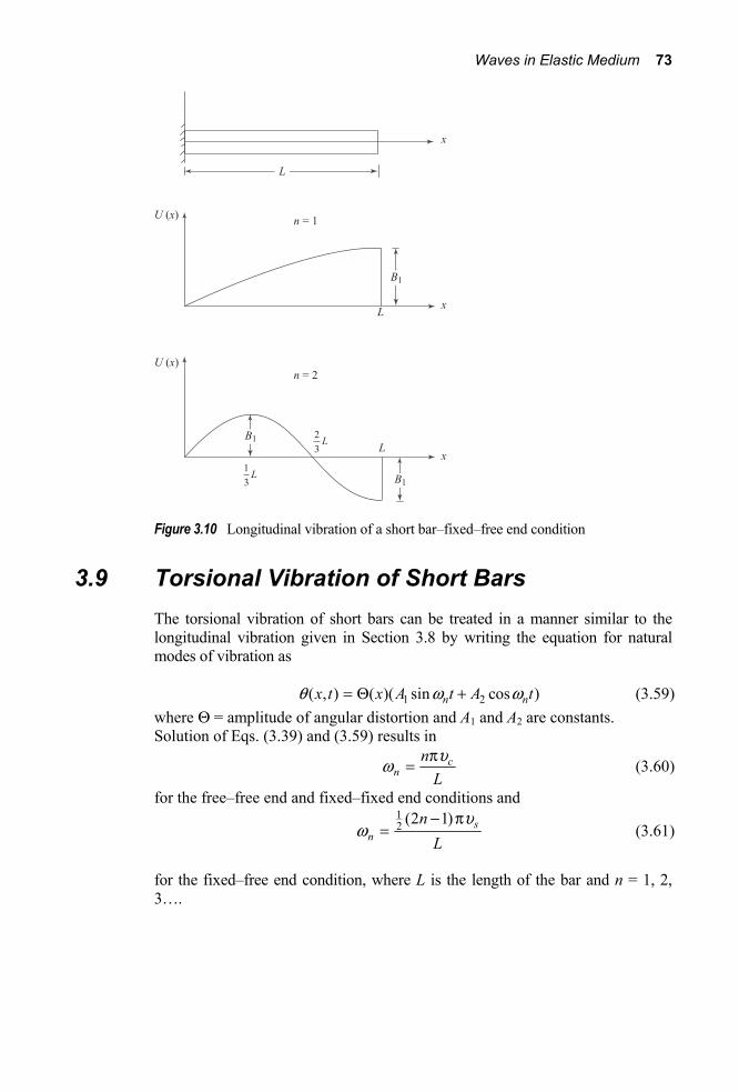
Waves in Elastic Medium 73
Figure 3.10 Longitudinal vibration of a short bar–fixed–free end condition
3.9 Torsional Vibration of Short Bars The torsional vibration of short bars can be treated in a manner similar to the longitudinal vibration given in Section 3.8 by writing the equation for natural modes of vibration as
1 2( , ) ( )( sin cos )n nx t x A t A tθ ω ω= Θ + (3.59) where Θ = amplitude of angular distortion and A1 and A2 are constants. Solution of Eqs. (3.39) and (3.59) results in
cn
nLuw p
= (3.60)
for the free–free end and fixed–fixed end conditions and
12 (2 1) s
nn
Lu
wp−
= (3.61)
for the fixed–free end condition, where L is the length of the bar and n = 1, 2, 3….

74 Chapter 3
Stress Waves in an Infinite Elastic Medium
3.10 Equation of Motion in an Elastic Medium Figure 3.11 shows the stresses acting on an element of elastic medium with sides measuring dx, dy and dz. For obtaining the differential equations of motion, one needs to sum the forces in the x, y, and z directions. Along the x direction,
xx xdx
xss s⎡ ⎤∂⎛ ⎞+ −⎜ ⎟⎢ ⎥∂⎝ ⎠⎣ ⎦
(dy)(dz) + zxzx zxdz
ztt t⎡ ⎤∂⎛ ⎞+ −⎜ ⎟⎢ ⎥∂⎝ ⎠⎣ ⎦
(dx)(dy)
+ yxyx yxdy
yt
t t⎡ ⎤∂⎛ ⎞
+ −⎢ ⎥⎜ ⎟∂⎢ ⎥⎝ ⎠⎣ ⎦(dx)(dz) = ρ(dx)(dy)(dz)
2
2u
t∂∂
where ρ is the density of the medium and u is the displacement component along the x direction. Alternatively,
2
2yxx zx u
x y z t
ts t r∂∂ ∂ ∂+ + =
∂ ∂ ∂ ∂ (3.62)
Figure 3.11 Derivation of the equation of motion in an elastic medium

Waves in Elastic Medium 75
Similarly, summing forces on the element in the y and z directions
2
2y xy zy
y x z t
s t t ur∂ ∂ ∂ ∂+ + =∂ ∂ ∂ ∂
(3.63)
and
2
2yzxzz w
z x y t
tts r∂∂∂ ∂+ + =
∂ ∂ ∂ ∂ (3.64)
whereu and w are the components of displacement in the y and z directions, respectively.
3.11 Equations for Stress Waves
A. Compression Waves Equations (3.62)–(3.64) give the equations of motion in terms of stresses. Now, considering Eq. (3.62) and noting that τxy = τyx and τxz = τzx,
2
2xyx xzu
x y zt
ts tr∂∂ ∂∂ = + +
∂ ∂ ∂∂
Substitution of Eqs. (3.16), (3.18), and (3.20) into the preceding equation yields
2
2 ( 2 ) ( ) ( )x xy xzu G G G
x y ztr le e g g∂ ∂ ∂ ∂′ ′= + + +
∂ ∂ ∂∂
Again, substitution of Eqs. (3.7) and (3.9) into the last expression will yield
2
2 ( 2 )xu u u wG G G
x y x y z z xtur le e ⎛ ⎞∂ ∂ ∂ ∂ ∂ ∂ ∂ ∂⎛ ⎞= + + + + +⎜ ⎟ ⎜ ⎟∂ ∂ ∂ ∂ ∂ ∂ ∂∂ ⎝ ⎠⎝ ⎠
or
2 2 2 2 2 2 2
2 2 2 2 2u u w u u uG
x x y x yt x x y ze ur l
⎛ ⎞∂ ∂ ∂ ∂ ∂ ∂ ∂ ∂= + + + + + +⎜ ⎟⎜ ⎟∂ ∂ ∂ ∂ ∂∂ ∂ ∂ ∂ ∂⎝ ⎠ (3.65)
But
2 2 2
2u w
x y x z xxu e∂ ∂ ∂ ∂+ + =
∂ ∂ ∂ ∂ ∂∂ (3.66)

76 Chapter 3
So
ρ 2
2u
t∂∂
= (λ + G) xe∂
∂ + G 2∇ u (3.67)
where
2∇ = 2 2 2
2 2 2x y z∂ ∂ ∂+ +∂ ∂ ∂
(3.68)
Similarly, by proper substitution in Eqs. (3.63) and (3.64), the following relations can be obtained:
ρ 2
2tu∂
∂ = (λ + G)
ye∂
∂ + G 2u∇ (3.69)
and
ρ 2
2w
t∂∂
= (λ + G) ze∂
∂ + G 2∇ w (3.70)
Now, differentiating Eqs. (3.67), (3.69), and (3.70) with respect to x, y, and z, respectively, and adding
ρ 2
2u wx y zt
u⎛ ⎞∂ ∂ ∂ ∂+ +⎜ ⎟∂ ∂ ∂∂ ⎝ ⎠ = (λ + G)
2 2 2
2 2 2x y ze e e⎛ ⎞∂ ∂ ∂+ +⎜ ⎟⎜ ⎟∂ ∂ ∂⎝ ⎠
+ G 2 u wx y z
u⎛ ⎞∂ ∂ ∂∇ + +⎜ ⎟∂ ∂ ∂⎝ ⎠
or
ρ 2
2te∂
∂ = (λ + G) 2 2( ) ( )Ge e∇ + ∇ = (λ + 2G) 2e∇ (3.71)
Therefore,
2
2 22
2 2p
Gte l e u e
r∂ += ∇ = ∇∂
(3.72)

Waves in Elastic Medium 77
where
2p
Glur
+= (3.73)
Equation (3.73) is in the same form as the wave equation given in Eq. (3.29). Also note that ε is the volumetric strain and pu is the velocity of the dilatational waves. This is also referred to as the primary wave, P-wave, or compression wave. Also another fact that needs to be pointed out here is that the expression for cu was given as cu = /E r . Comparing the expressions for cu and pu , one can
see that the velocity of compression waves is faster than cu .
B. Distortional Waves or Shear Waves Differentiating Eq. (3.69) with respect to z and Eq. (3.70) with respect to y,
ρ 2
2 ztu∂ ∂⎛ ⎞
⎜ ⎟∂∂ ⎝ ⎠ = (λ + G)
22
( )( )G
y z ze u∂ ∂+ ∇
∂ ∂ ∂ (3.74)
and
ρ 2
2wyt
⎛ ⎞∂ ∂⎜ ⎟∂∂ ⎝ ⎠
= (λ + G) 2
2
( ) ( )wG
y z ye∂ ∂+ ∇
∂ ∂ ∂ (3.75)
Substracting Eq. (3.74) from (3.75) yields
ρ 2wy zt
u⎛ ⎞∂ ∂ ∂−⎜ ⎟∂ ∂∂ ⎝ ⎠ = 2 wG
y zu⎛ ⎞∂ ∂∇ −⎜ ⎟∂ ∂⎝ ⎠
However, 2 xw y zu w∂ ∂ −∂ ∂ = [Eq. (3.10)]; thus,
ρ 2
2x
tw∂
∂ = G 2
xw∇ (3.76)
or
2
2 2 22
xx s x
Gtw w u w
r∂ = ∇ = ∇∂
(3.77)
where /s Gu = ρ .

78 Chapter 3
Equation (3.77) represents the equation for distortional waves and the velocity of propagation is su .This is also referred to as the shear wave, or S-wave. Comparison of the shear wave velocity given above with that in a rod [Eq. (3.40)] shows that they are the same. Using the process of similar manipulation, one can also obtain two more equations similar to Eq. (3.77):
2
2 22
ys yt
wu w
∂= ∇
∂ (3.78)
and
2
2 22
zs zt
w u w∂ = ∇∂
(3.79)
3.12 General Comments Based on the derivations for the velocities of comparison waves and shear waves as derived in the preceding section, the following general observations can be made. 1. There are two types of stress waves that can propagate through an infinite
elastic medium; however, they travel at different velocities. 2. From Eq. (3.73),
2p
Glur
+=
However
(1 ) (1 )
Eμλμ μ
=+ −
and
G = 2(1 )
Eμ+
Substitution of the preceding two relationships into the expression of pu yields
(1 )(1 ) (1 2 )p
E mur m m
−=+ −
(3.80)

Waves in Elastic Medium 79
Figure 3.12 Variation of pu / su with μ [Eq. (3.82)]
Similarly,
su = 2(1 )
G Er m r
=+
(3.81)
Combining Eqs. (3.80) and (3.81),
2(1 )(1 2 )
p
s
u mu m
−=−
(3.82)
Figure 3.12 shows a plot of pu / su versus μ based on Eq. (3.82). It can be
seen from the plot that for all values of μ, pu / su is greater than 1.
3. Table 3.1 gives some typical values of pu and su encountered through various types of soils and rocks. Techniques for field determination of the velocities of compression waves and shear waves traveling through various soil media are described in Chapter 4.
4. The more rigid the materials, the higher the shear and compressional wave velocities.

80 Chapter 3
5. If μ is 0.5, the velocity of compressional wave becomes unbounded.
Wave propagation through saturated soils involves the soil skeleton and water in the void spaces. A comprehensive theoretical study of this problem is given by Biot (1956). This study shows that there are two compressive waves and one shear wave through the saturated medium. Some investigators have referred to the two compressive waves as the fluid wave (transmitted through the fluid) and the frame wave (transmitted through the soil structure), although there is coupled motion of the fluid and the frame waves. As far as the shear wave is concerned, the pore water has no rigidity to shear. Hence, the shear wave in the soil is dependent only on the properties of the soil skeleton.
Table 3.1 Typical values of pu and su
Soil type Compressive wave Shear wave velocity, velocity, pu (m/s) su (m/s)
Fine sand 300 90 -150 Dense sand 460 230 Gravel 762 180 – 215 Moist clay 1220 – 1370 150 Granite 3960 – 5490 2130 – 3350 Sandstone 1370 – 3960 610 – 2130
Figure 3.13 Comparison of experimental and theoretical results for compressive frame
wave velocities in dry and saturated Ottawa sand (after Hardin and Richart, 1963)
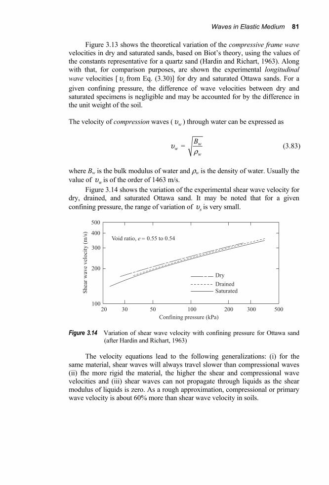
Waves in Elastic Medium 81
Figure 3.13 shows the theoretical variation of the compressive frame wave velocities in dry and saturated sands, based on Biot’s theory, using the values of the constants representative for a quartz sand (Hardin and Richart, 1963). Along with that, for comparison purposes, are shown the experimental longitudinal wave velocities [ cu from Eq. (3.30)] for dry and saturated Ottawa sands. For a given confining pressure, the difference of wave velocities between dry and saturated specimens is negligible and may be accounted for by the difference in the unit weight of the soil.
The velocity of compression waves ( wu ) through water can be expressed as
wu = w
w
Br
(3.83)
where Bw is the bulk modulus of water and ρw is the density of water. Usually the value of wu is of the order of 1463 m/s.
Figure 3.14 shows the variation of the experimental shear wave velocity for dry, drained, and saturated Ottawa sand. It may be noted that for a given confining pressure, the range of variation of su is very small.
Figure 3.14 Variation of shear wave velocity with confining pressure for Ottawa sand
(after Hardin and Richart, 1963)
The velocity equations lead to the following generalizations: (i) for the same material, shear waves will always travel slower than compressional waves (ii) fhe more rigid the material, the higher the shear and compressional wave velocities and (iii) shear waves can not propagate through liquids as the shear modulus of liquids is zero. As a rough approximation, compressional or primary wave velocity is about 60% more than shear wave velocity in soils.

82 Chapter 3
Stress Waves in Elastic Half-Space
3.13 Rayleigh Waves Equations derived in Section 3.11 are for stress waves in the body of an infinite, elastic, and isotropic medium. Another type of wave, called a Rayleigh wave, also exists near the boundary of an elastic half-space. This type of wave was first investigated by Lord Rayleigh (1885). In order to study this, consider a plane wave through an elastic medium with a plane boundary as shown in Figure 3.15. Note that the plane x – y is the boundary of the elastic half-space and z is positive downward. Let u and w represent the displacements in the directions x and z, respectively, and be independent of y. Therefore,
ux zφ ψ∂ ∂= +
∂ ∂ (3.84)
and
wz xφ ψ∂ ∂= −
∂ ∂ (3.85)
where φ and ψ are two potential functions. The dilation e can be defined as
Figure 3.15 Plane wave through an elastic medium with a plane boundary

Waves in Elastic Medium 83
x y ze e e e= + + = u wx y z
u∂ ∂ ∂+ +∂ ∂ ∂
=2 2 2 2 2 2
22 2 2 2(0)
x z x zx z x zf y f y f f f
⎛ ⎞ ⎛ ⎞∂ ∂ ∂ ∂ ∂ ∂+ + + − = + = ∇⎜ ⎟ ⎜ ⎟⎜ ⎟ ⎜ ⎟∂ ∂ ∂ ∂∂ ∂ ∂ ∂⎝ ⎠ ⎝ ⎠ (3.86)
Similarly, the rotation in the x – z plane can be given by
2 yw =2 2
22 2
u wz x x z
y y y∂ ∂ ∂ ∂− = + = ∇∂ ∂ ∂ ∂
(3.87)
Substituting Eqs. (3.84) and (3.86) into Eq. (3.67) yields
2
2 22 ( ) ( )G G
x z x x ztf y f yr l f∂ ∂ ∂ ∂ ∂ ∂⎛ ⎞ ⎛ ⎞+ = + ∇ + ∇ +⎜ ⎟ ⎜ ⎟∂ ∂ ∂ ∂ ∂∂ ⎝ ⎠ ⎝ ⎠
or
2 2
2 22 2 ( 2 ) ( ) ( )G G
x z x zt tf yr r l f y
⎛ ⎞ ⎛ ⎞∂ ∂ ∂ ∂ ∂ ∂+ = + ∇ + ∇⎜ ⎟ ⎜ ⎟⎜ ⎟ ⎜ ⎟∂ ∂ ∂ ∂∂ ∂⎝ ⎠ ⎝ ⎠ (3.88)
In a similar manner, substituting Eqs. (3.85) and (3.86) into Eqs. (3.70), we get
2 2
2 22 2 ( 2 ) ( ) ( )G G
z x z zt tφ ψρ ρ λ φ ψ
⎛ ⎞ ⎛ ⎞∂ ∂ ∂ ∂ ∂ ∂− = + ∇ − ∇⎜ ⎟ ⎜ ⎟⎜ ⎟ ⎜ ⎟∂ ∂ ∂ ∂∂ ∂⎝ ⎠ ⎝ ⎠ (3.89)
Equations (3.88) and (3.89) will be satisfied if (1) 2 2 2( ) ( 2 )t Gr f l f∂ ∂ = + ∇
or
2
2 2 22
2p
Gtf l f u f
r⎛ ⎞∂ += ∇ = ∇⎜ ⎟∂ ⎝ ⎠
(3.90)
and (2) 2 2 2( )t Gr y y∂ ∂ = ∇ or
2
2 2 22 s
Gty y u y
r⎛ ⎞∂ = ∇ = ∇⎜ ⎟∂ ⎝ ⎠
(3.91)
84 Chapter 3
Now, consider a sinusoidal wave traveling in the positive x direction. Let the solution of φ and ψ be expressed as
φ = F(z) exp[i( tw – fx)] (3.92) and ψ = G(z) exp[i( tw – fx)] (3.93)
where F(z) and G(z) are functions of depth
f = 2wavelength
π (3.94)
i = 1− (3.95)
Substituting Eq. (3.92) into Eq. (3.90), we get
2
2t⎛ ⎞∂⎜ ⎟⎜ ⎟∂⎝ ⎠
{F(z)exp[i( tw – fx)]} = 2 2pu ∇ {F(z)exp[i( tw – fx)]}
or 2 2 2( ) [ ( ) ( )]pF z F z f F zw u ′′− = − (3.96)
Similarly, substituting Eq. (3.93) into Eq. (3.91) results in
2 2 2( ) [ ( ) ( )]sG z G z f G zw u ′′− = − (3.97) where
F′′ (z) = 2
2( )F z
z∂
∂ (3.98)
G′′ (z) = 2
2( )G z
z∂
∂ (3.99)
Equations (3.96) and (3.97) can be rearranged to the form
F′′ (z) – q2F(z) = 0 (3.100) and G′′ (z) – s2G(z) = 0 (3.101)
where
q2 = 2
22p
f ωυ
− (3.102)

Waves in Elastic Medium 85
s2 = 2
22s
f ωυ
− (3.103)
Solutions to Eqs. (3.100) and (3.101) can be given as
1 2( ) qz qzF z A e A e−= + (3.104) and 1 2( ) sz szG z B e B e−= + (3.105)
where A1, A2, B1, and B2 are constants.
From Eqs. (3.104) and (3.105), it can be seen that A2 and B2 must equal zero; otherwise F(z) and G(z) will approach infinity with depth, which is not the type of wave that is considered here. With A2 and B2 equal zero,
F(z) = A1e–qz (3.106) G(z) = B1e–sz (3.107)
Combining Eqs. (3.92) and (3.106) and Eqs. (3.93) and (3.107),
( )1( )[ ]qz i t fxA e e ωφ − −= (3.108)
or ( )
1( )[ ]sz i t fxB e e ωψ − −= (3.109)
The boundary conditions for the two preceding equations are at z = 0, σz = 0, τzx = 0, and τzy = 0. From Eq. (3.22),
σz (z = 0) = λε + 2Gεz = le + 2G wz
∂⎛ ⎞⎜ ⎟∂⎝ ⎠
= 0 (3.110)
Combining Eqs. (3.85), (3.86), and (3.108)–(3.110), one obtains
A1[(λ + 2G)q2 – λ 2f ] – 2iB1Gfs = 0 (3.111) or
12 2
1
2( 2 )
A iGfsB G q fl l
=+ −
(3.112)
Similarly,

86 Chapter 3
τzx(z = 0) = Gγzx = G w ux z
∂ ∂⎛ ⎞+⎜ ⎟∂ ∂⎝ ⎠ = 0 (3.113)
Again, combining Eqs. (3.84), (3.85), (3.108), (3.109), and (3.113),
2iA1fq + (s2 + 2f ) B1 = 0 or
2 2
1
1
( )2
A s fB ifq
+=− (3.114)
Equating the right-hand sides of Eqs. (3.112) and (3.114),
2 2
2 22 ( )
2( 2 )iGfs s f
ifqG q f+=−
+ −λ λ
4Gf 2sq = (s2 + f 2)[(λ + 2G)q2 – λf 2] or 16G2f 4s2q2 = (s2 + f2)2 [(λ + 2G)q2 – λf2]2 (3.115)
Substituting for q and s and then dividing both sides of Eq. (3.115) by G2f 8, we get
2 22 2 2 2
2 2 2 2 2 2 2 2216 1 1 2 2
p s p s
GGf f f f
w w l w wu u u u
⎛ ⎞ ⎡ ⎤⎛ ⎞ ⎛ ⎞+⎛ ⎞⎜ ⎟− − = − −⎢ ⎥⎜ ⎟ ⎜ ⎟⎜ ⎟⎜ ⎟ ⎜ ⎟⎜ ⎟ ⎝ ⎠⎢ ⎥⎝ ⎠ ⎝ ⎠⎝ ⎠ ⎣ ⎦ (3.116)
From Eq. (3.94)
Wavelength = 2fπ (3.117)
However,
Wavelength = velocity of wave( /2 ) ( /2 )
ruw wp p
= (3.118)
where u r is the Rayleigh wave velocity. Thus, from Eqs. (3.117) and (3.118), 2 2 rf u wp p= , or

Waves in Elastic Medium 87
f =r
wu
(3.119)
So,
22 2
2 22 2 2 2 2 2( / )
r
p p r pV
fυω ω α
υ υ ω υ υ= = = (3.120)
Similarly,
22 2
22 2 2 2 2 2( / )
r
s s r sV
fυω ω
υ υ ω υ υ= = = (3.121)
where
2
22s
p
uau
= (3.122)
However 2 ( 2 )p Gu l r= + and 2s Gu r= Thus
2
22 2s
p
GG
ualu
= =+
(3.123)
Table 3.2 Values of V [Eq. (3.126)] m = υ υr sV 0.25 0.919 0.29 0.926 0.33 0.933 0.4 0.943 0.5 0.955
The term α2 can also be expressed in terms of Poisson’s ratio. From the
relations given in Eq. (3.25),
21 2
Gμλμ
=−
(3.124)
Substitution of this relation in Eq. (3.123) yields
2 (1 2 ) (1 2 )2 /(1 2 ) 2 2 2 4 (2 2 )
G GG G G G G
m mam m m m m
− −= = =− + + − −
(3.125)

88 Chapter 3
Again, substituting Eqs. (3.120), (3.121), and (3.123) into Eq. (3.116),
16(1 – α2V 2)(1 – V 2) = (2 – V 2)(2 – V 2)2
or
6 4 2 2 28 (16 24) 16(1 ) 0V V Va a− − − − − = (3.126)
Equation (3.126) is a cubic equation in V 2. For a given value of Poisson’s ratio, the proper value of V 2 can be found and, hence, so can the value of ru in terms of pu or su . An example of this is shown in Example 3.1. Table 3.2 gives some values of r su u (= V) for various values of Poisson’s ratio.
3.14 Displacement of Rayleigh Waves From Eqs. (3.84) and (3.85),
ux zφ ψ∂ ∂= +
∂ ∂ (3.84)
and
wz xφ ψ∂ ∂= −
∂ ∂ (3.85)
Substituting the relations developed for φ and ψ [Eqs. (3.108), (3.109)] in these equations, one obtains
u = – (if A1e-qz + B1se–sz) ( )[ ]i t fxe −ω (3.127) w = –(A1qe–qz – B1ife–sz) ( )[ ]i t fxe −ω (3.128)
However, from Eq. (3.114), 2 21 12 ( )B iA fq s f= − + . Substituting this relation in
Eqs. (3.127) and (3.128) gives
( )1 2 2
2 [ ]qz sz i t fxqsu A fi e e es f
− − −⎛ ⎞= − +⎜ ⎟
+⎝ ⎠
ω (3.129)
and
2
( )1 2 2
2 [ ]qz sz i t fxfw A q e e es f
− − −⎛ ⎞= − +⎜ ⎟⎜ ⎟+⎝ ⎠
ω (3.130)
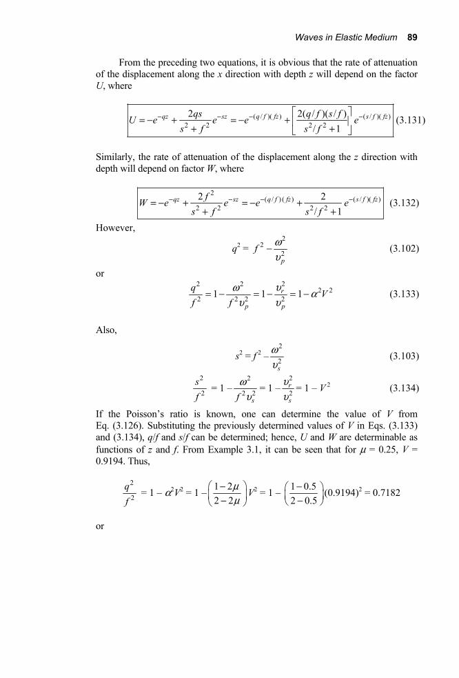
Waves in Elastic Medium 89
From the preceding two equations, it is obvious that the rate of attenuation of the displacement along the x direction with depth z will depend on the factor U, where
( / )( ) ( / )( )2 2 2 22 2( / )( / )
/ 1qz sz q f fz s f fzqs q f s fU e e e e
s f s f− − − −⎡ ⎤
= − + = − + ⎢ ⎥+ +⎣ ⎦
(3.131)
Similarly, the rate of attenuation of the displacement along the z direction with depth will depend on factor W, where
2
( / ) ( ) ( / )( )2 2 2 22 2
/ 1qz sz q f fz s f fzfW e e e e
s f s f− − − −= − + = − +
+ + (3.132)
However,
q2 = 2
22p
f ωυ
− (3.102)
or
22 2
2 22 2 2 21 1 1r
p p
q Vf f
uw au u
= − = − = − (3.133)
Also,
s2 = f 2 –2
2s
wu
(3.103)
2
2sf
= 1 –2
2 2sf
wu
= 1 –2
2r
s
uu
= 1 – V 2 (3.134)
If the Poisson’s ratio is known, one can determine the value of V from Eq. (3.126). Substituting the previously determined values of V in Eqs. (3.133) and (3.134), q/f and s/f can be determined; hence, U and W are determinable as functions of z and f. From Example 3.1, it can be seen that for μ = 0.25, V = 0.9194. Thus,
2
2qf
= 1 – α2V2 = 1 – 1 22 2
μμ
⎛ ⎞−⎜ ⎟−⎝ ⎠
V2 = 1 – 1 0.52 0.5
−⎛ ⎞⎜ ⎟−⎝ ⎠
(0.9194)2 = 0.7182
or
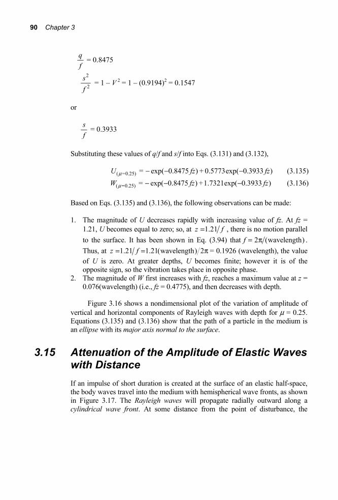
90 Chapter 3
qf
= 0.8475
2
2sf
= 1 – V 2 = 1 – (0.9194)2 = 0.1547
or
sf
= 0.3933
Substituting these values of q/f and s/f into Eqs. (3.131) and (3.132),
( =0.25) = exp( 0.8475 ) + 0.5773exp( 0.3933 )U fz fzμ − − − (3.135) ( =0.25) = exp( 0.8475 ) +1.7321exp( 0.3933 )W fz fzμ − − − (3.136)
Based on Eqs. (3.135) and (3.136), the following observations can be made: 1. The magnitude of U decreases rapidly with increasing value of fz. At fz =
1.21, U becomes equal to zero; so, at 1.21z f= , there is no motion parallel to the surface. It has been shown in Eq. (3.94) that 2 (wavelength)f = π . Thus, at 1.21 1.21(wavelength) 2z f= = π = 0.1926 (wavelength), the value of U is zero. At greater depths, U becomes finite; however it is of the opposite sign, so the vibration takes place in opposite phase.
2. The magnitude of W first increases with fz, reaches a maximum value at z = 0.076(wavelength) (i.e., fz = 0.4775), and then decreases with depth.
Figure 3.16 shows a nondimensional plot of the variation of amplitude of vertical and horizontal components of Rayleigh waves with depth for μ = 0.25. Equations (3.135) and (3.136) show that the path of a particle in the medium is an ellipse with its major axis normal to the surface.
3.15 Attenuation of the Amplitude of Elastic Waves with Distance If an impulse of short duration is created at the surface of an elastic half-space, the body waves travel into the medium with hemispherical wave fronts, as shown in Figure 3.17. The Rayleigh waves will propagate radially outward along a cylindrical wave front. At some distance from the point of disturbance, the
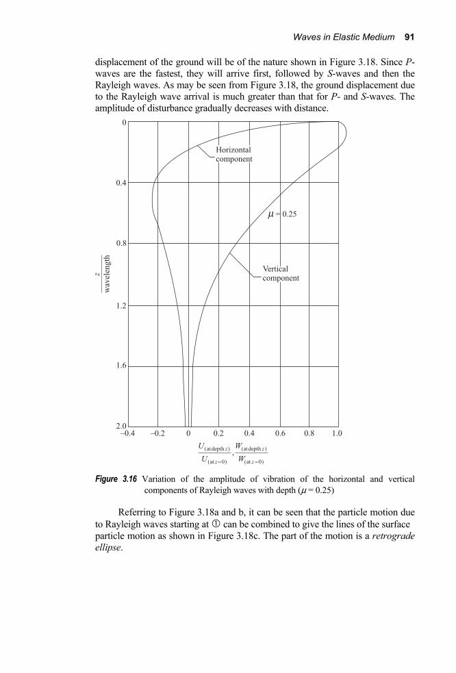
Waves in Elastic Medium 91
displacement of the ground will be of the nature shown in Figure 3.18. Since P-waves are the fastest, they will arrive first, followed by S-waves and then the Rayleigh waves. As may be seen from Figure 3.18, the ground displacement due to the Rayleigh wave arrival is much greater than that for P- and S-waves. The amplitude of disturbance gradually decreases with distance.
Figure 3.16 Variation of the amplitude of vibration of the horizontal and vertical
components of Rayleigh waves with depth (μ = 0.25)
Referring to Figure 3.18a and b, it can be seen that the particle motion due to Rayleigh waves starting at can be combined to give the lines of the surface particle motion as shown in Figure 3.18c. The part of the motion is a retrograde ellipse.

92 Chapter 3
Figure 3.17 Propagation of body waves and Rayleigh waves
When body waves spread out along a hemispherical wave front, the energy is distributed over an area that increases with the square of the radius:
E′ ∝ 21r
(3.137)
where E′ is the energy per unit area and r is the radius. However, the amplitude is proportional to the square root of the energy per unit area:
Amplitude 21Er
∝ ′ ∝
or
Amplitude 1r
∝ (3.138)
Along the surface of the half-space only, the amplitude of the body waves is proportional to 1/r2
Similarly, the amplitude of the Rayleigh waves, which spread out in a cylindrical wave front, is proportional to1 r . Thus the attention of the amplitude of the Rayleigh waves is slower than that for the body waves.
The loss of the amplitude of waves due to spreading out is called geometrical damping. In addition to the above damping, there is another type of loss — that from absorption in real earth material. This is called material damping. Thus, accounting for both types of damping, the vertical amplitude of Rayleigh waves can be given by the relation
nw = 1w 1
n
rr
exp [–β (rn – r1)] (3.139)

Waves in Elastic Medium 93
Figure 3.18 Wave systems from surface point source in ideal medium (after Richart,
Hall, and Woods, 1970)
where nw and 1w are vertical amplitudes at distance rn and r1, and β is the absorption coefficient.
Equation (3.139) is given by Bornitz (1931). (See also Hall and Richart, 1963.) The magnitude of β depends on the type of soil.
Example 3.1
Given μ = 0.25, determined the value of the Rayleigh wave velocity in terms of su .
Solution
From Eq. (3.126),

94 Chapter 3
V6 – 8V4 – (16α2 – 24)V2 – 16(1 – α2) = 0
For μ = 0.25,
2 1 2 1 0.52 2 2 0.5
μαμ
− −= =− −
= 13
V 6 – 8V 4 – ( )163 24− V2 – 16 ( )1
31− = 0
3V 6 – 24V 4 + 56V 2 – 32 = 0 (V 2 – 4)(3V 4 – 12V 2 + 8) = 0
Therefore,
V 2 = 4, 2 + 23
, 2 – 23
If V 2 = 4,
2
2sf
= 1 – V2 = 1 – 4 = –3
and s/f is imaginary. This is also the case for V 2 = 2 + 2/ 3 . Keeping Eqs. (3.129), (3.131), and (3.130), (3.132) in mind, one can see that
when q/f and s/f are imaginary, it does not yield the type of wave that is being discussed here. Thus,
V2 = 2 – 23
V = r
s
uu
= 0.9194
or ru = 0.9194 su
References Biot, M.A (1956). “Theory of Propagation of Elastic Waves in a Fluid Saturated
Soil.” Journal of the Acoustical Society of America. Vol. 28, pp. 168–178. Bornitz, G.(1931). Über die Ausbreitung der von Graszkolbenmaschinen
erzeugten Bodenschwingungen in die Tiefe, J. Springer, Berlin. Duffy, J., and Mindlin, R.D (1957). “Stress-Strain Relations of a Granular
Medium,” Transactions, ASME, pp. 585–593. Hall, J. R., Jr., and Richart, F. E., Jr. (1963). “Dissipation of Elastic Wave
Energy in Granular Soils,” Journal of the Soil Mechanics and Foundations Division, ASCE, Vol. 89. No. SM6, PP. 27–56.
Hardin, B. O., and Richard, F. E., Jr. (1963). “Elastic Wave Velocity in Granular Soils.” Journal of the Soil Mechanics and Foundations Division, ASCE, Vol. 89, No. SM1, pp. 33–65. ith permission from ASCEW .

Waves in Elastic Medium 95
Rayleigh, Lord (1885). “On Wave Propagated Along the Plane Surface of Elastic Solid,” Proceedings, London Mathematical Society, Vol. 17, pp. 4–11.
Richart, F. E., Jr., Hall, J. R., Jr., and Woods, R. D. (1970). Vibrations of Soils and Foundations, Prentice Hall, Inc., Englewood Cliffs, New Jersey.
Timoshenko, S.P., and Goodier, J. N. (1970). Theory of Elasticity, McGraw-Hill, New York.

96
4 Properties of Dynamically Loaded Soils
4.1 Introduction It is a well known fact that earthquake damage is strongly influenced by the dynamic properties of local soil deposits. In addition, many problems in civil engineering practice require the knowledge of the properties of soils subjected to dynamic loading. These problems include the dynamic bearing capacity of foundations, response of machine foundations subjected to cyclic loading, soil-structure interaction during the propagation of stress waves generated due to an earthquake, and earthquake resistance of dams and embankments.
A variety of laboratory tests as well as field techniques are available, each having its own limitations as well as advantages. Some of these tests are specifically developed for measuring properties of dynamically loaded soils whereas some are modified versions of tests used in the domain of traditional soil mechanics. Some of these methods are suitable for small strain range whereas some are suitable for large strain range. The range of strain of interest usually dictates the type of equipment/method to be used which in turn depends on the problem to be analyzed at hand. Some of these equipments are very specialized, expensive and require special training to use and interpret the results. It is worth noting that soil behavior over a wide range of strains is nonlinear and on unloading follows a different stress-strain path forming a hysteresis loop.
This chapter is devoted primarily to describing various laboratory and field test procedures available to measure as well as estimate the soil properties using empirical correlations subjected to dynamic loading. This chapter is divided into three major parts:
a) Laboratory tests and results b) Field tests and measurements c) Empirical correlations for the shear modulus and damping ratio obtained
from field and laboratory tests. These are the two most important parameters needed for most design work.
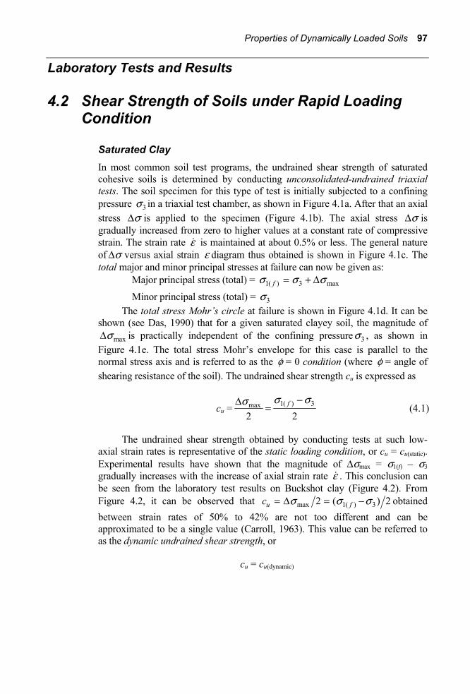
Properties of Dynamically Loaded Soils 97
Laboratory Tests and Results
4.2 Shear Strength of Soils under Rapid Loading Condition
Saturated Clay In most common soil test programs, the undrained shear strength of saturated cohesive soils is determined by conducting unconsolidated-undrained triaxial tests. The soil specimen for this type of test is initially subjected to a confining pressure 3s in a triaxial test chamber, as shown in Figure 4.1a. After that an axial stress sD is applied to the specimen (Figure 4.1b). The axial stress sD is gradually increased from zero to higher values at a constant rate of compressive strain. The strain rate e is maintained at about 0.5% or less. The general nature of sD versus axial strain e diagram thus obtained is shown in Figure 4.1c. The total major and minor principal stresses at failure can now be given as:
Major principal stress (total) = 1( ) 3 maxfs s s= + D
Minor principal stress (total) = 3s The total stress Mohr’s circle at failure is shown in Figure 4.1d. It can be
shown (see Das, 1990) that for a given saturated clayey soil, the magnitude of maxsD is practically independent of the confining pressure 3s , as shown in
Figure 4.1e. The total stress Mohr’s envelope for this case is parallel to the normal stress axis and is referred to as the f = 0 condition (where f = angle of shearing resistance of the soil). The undrained shear strength cu is expressed as
cu =1( ) 3max
2 2fs ss -D
= (4.1)
The undrained shear strength obtained by conducting tests at such low-axial strain rates is representative of the static loading condition, or cu = cu(static). Experimental results have shown that the magnitude of Δσmax = σ1(f) – σ3 gradually increases with the increase of axial strain rate e . This conclusion can be seen from the laboratory test results on Buckshot clay (Figure 4.2). From Figure 4.2, it can be observed that max 1( ) 32 ( ) 2u fc s s s= D = - obtained between strain rates of 50% to 42% are not too different and can be approximated to be a single value (Carroll, 1963). This value can be referred to as the dynamic undrained shear strength, or
cu = cu(dynamic)
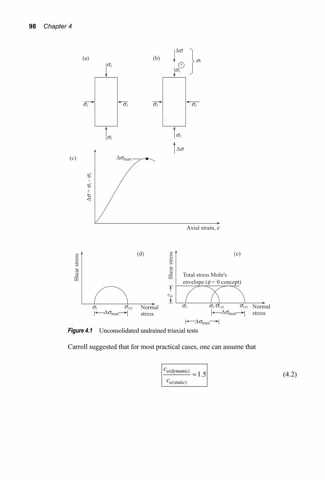
98 Chapter 4
Figure 4.1 Unconsolidated undrained triaxial tests Carroll suggested that for most practical cases, one can assume that
(dynamic)
(static)1.5u
u
cc
ª (4.2)

Properties of Dynamically Loaded Soils 99
Figure 4.2 Unconsolidated-undrained triaxial test results on Buckshot clay (after
Carroll, 1963)
Sand
Several vacuum triaxial test results on different dry sands (that is, standard Ottawa sand, Fort Peck sand, and Camp Cooke sand) were reported by Whitman and Healy (1963). These tests were conducted with various effective confining pressures ( 3s ) and axial strain rates. The compressive strength maxsD determined from these tests can be given as
max 1( ) 3fs s sD = - (4.3)
where 3s = effective minor principle stress 1( )fs = effective major principal stress at failure

100 Chapter 4
An example of the effect of axial strain rate on dry Ottawa sand is shown in Figure 4.3. It can be seen that for a given 3s the magnitude of maxsD decreases initially with the increase of the strain rate to a minimum value and increases thereafter. From fundamentals of soil mechanics it is known that
1( ) 31
1( ) 3sin f
f
s sf
s s- Ê ˆ-
= Á ˜+Ë ¯ (4.4)
where f = drained soil friction angle
Based on Figure 4.3 and Eq. (4.4) it is obvious that the initial increase of the strain rate results in a decrease of the soil friction angle. The minimum dynamic friction angle may be given as (Vesic, 1973)
φdynamic ≈ φ – 2° (4.5)
(obtained from static tests — that is, small strain rate of loading)
Figure 4.3 Strain-rate effect for dry Ottawa sand (after Whitman and Healy, 1963)
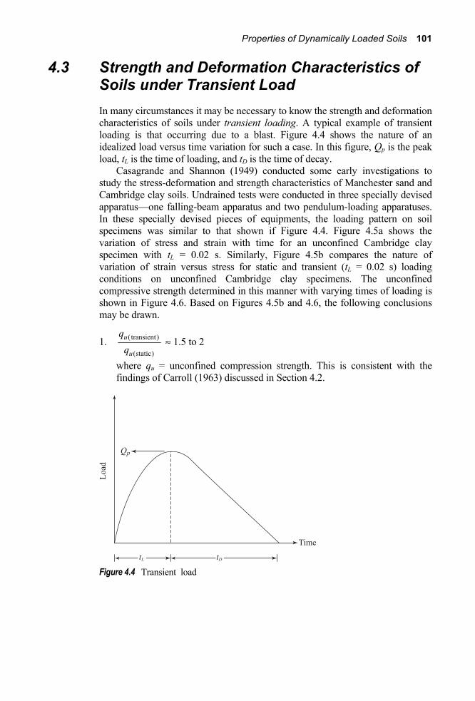
Properties of Dynamically Loaded Soils 101
4.3 Strength and Deformation Characteristics of Soils under Transient Load In many circumstances it may be necessary to know the strength and deformation characteristics of soils under transient loading. A typical example of transient loading is that occurring due to a blast. Figure 4.4 shows the nature of an idealized load versus time variation for such a case. In this figure, Qp is the peak load, tL is the time of loading, and tD is the time of decay.
Casagrande and Shannon (1949) conducted some early investigations to study the stress-deformation and strength characteristics of Manchester sand and Cambridge clay soils. Undrained tests were conducted in three specially devised apparatus—one falling-beam apparatus and two pendulum-loading apparatuses. In these specially devised pieces of equipments, the loading pattern on soil specimens was similar to that shown if Figure 4.4. Figure 4.5a shows the variation of stress and strain with time for an unconfined Cambridge clay specimen with tL = 0.02 s. Similarly, Figure 4.5b compares the nature of variation of strain versus stress for static and transient (tL = 0.02 s) loading conditions on unconfined Cambridge clay specimens. The unconfined compressive strength determined in this manner with varying times of loading is shown in Figure 4.6. Based on Figures 4.5b and 4.6, the following conclusions may be drawn.
1. (transient)
(static)
u
u
≈ 1.5 to 2
where qu = unconfined compression strength. This is consistent with the findings of Carroll (1963) discussed in Section 4.2.
Figure 4.4 Transient load

102 Chapter 4
Figure 4.5 Unconfined compressive strength of Cambridge clay for varying time of
loading (after Casagrande and Shannon, 1949) 2. The modulus of deformation E as defined in Figure 4.7 is about two times as
great for transient loading as compared to that for static loading.
The nature of the stress-versus-strain plot for confined compression tests on Manchester sand conducted by Casagrande and Shannon (1949) is as shown in Figure 4.8. From this study it was concluded that
1. 1( ) 3 transient
1( ) 3 static
]]
f
f
s ss s
[ -[ -
≈ 1.1 and
2. The modulus of deformation as defined by Figure 4.7 is approximately the same for transient and static loading conditions.

Properties of Dynamically Loaded Soils 103
Figure 4.6 Unconfined compressive strength of Cambridge clay for varying time of loading (after Casagrande and Shannon, 1949)
Figure 4.7 Definition of modulus of deformation, E

104 Chapter 4
Figure 4.8 Confined-compression test on sand — stress-versus-strain behavior under
static and transient loading
4.4 Travel-Time Test for Determination of Longitudinal and Shear Wave Velocities ( cu and su )
Using electronic equipment, the time tc requirement for travel of elastic waves through a soil specimen of length L can be measured in the laboratory. For longitudinal waves
cc
Lt
u = (4.6)
The modulus of elasticity E can then be calculated from Eq. (3.30) as
cEur
=
or
2
22cc
LEt
ru r= = (4.7)

Properties of Dynamically Loaded Soils 105
Figure 4.9 Travel-time method: (a) schematic diagram of the laboratory setup for
measuring cu¢ ; (b) details of the soil specimen and container for the laboratory setup (after Whitman and Lawrence, 1963)
If the soil specimen is confined laterally, then the travel time will give the
value of cu¢ as shown in Eq. (3.35). Thus c cL tu = ¢ , and
M = 2
2c
Lt
r¢
(4.8)
where ct ¢ = time of travel of longitudinal waves in a laterally confined specimen.
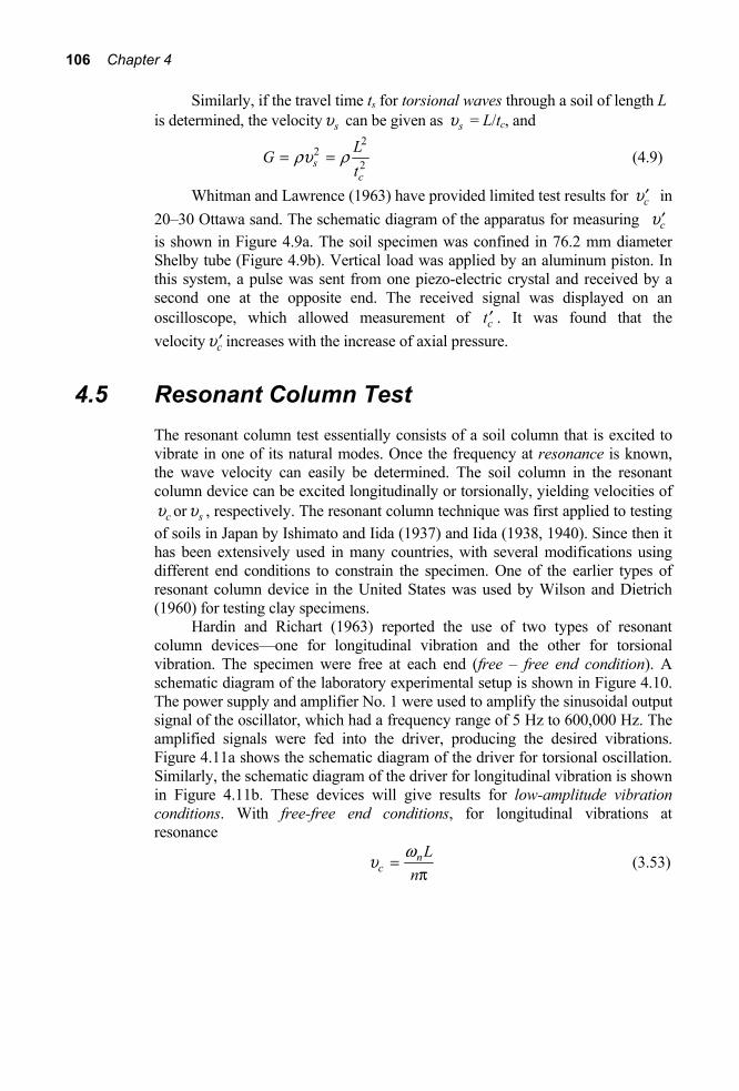
106 Chapter 4
Similarly, if the travel time ts for torsional waves through a soil of length L is determined, the velocity su can be given as su = L/tc, and
2
22sc
LGt
ru r= = (4.9)
Whitman and Lawrence (1963) have provided limited test results for cu¢ in 20–30 Ottawa sand. The schematic diagram of the apparatus for measuring cu¢ is shown in Figure 4.9a. The soil specimen was confined in 76.2 mm diameter Shelby tube (Figure 4.9b). Vertical load was applied by an aluminum piston. In this system, a pulse was sent from one piezo-electric crystal and received by a second one at the opposite end. The received signal was displayed on an oscilloscope, which allowed measurement of ct ¢ . It was found that the velocity cu ¢ increases with the increase of axial pressure.
4.5 Resonant Column Test The resonant column test essentially consists of a soil column that is excited to vibrate in one of its natural modes. Once the frequency at resonance is known, the wave velocity can easily be determined. The soil column in the resonant column device can be excited longitudinally or torsionally, yielding velocities of
cu or su , respectively. The resonant column technique was first applied to testing of soils in Japan by Ishimato and Iida (1937) and Iida (1938, 1940). Since then it has been extensively used in many countries, with several modifications using different end conditions to constrain the specimen. One of the earlier types of resonant column device in the United States was used by Wilson and Dietrich (1960) for testing clay specimens.
Hardin and Richart (1963) reported the use of two types of resonant column devices—one for longitudinal vibration and the other for torsional vibration. The specimen were free at each end (free – free end condition). A schematic diagram of the laboratory experimental setup is shown in Figure 4.10. The power supply and amplifier No. 1 were used to amplify the sinusoidal output signal of the oscillator, which had a frequency range of 5 Hz to 600,000 Hz. The amplified signals were fed into the driver, producing the desired vibrations. Figure 4.11a shows the schematic diagram of the driver for torsional oscillation. Similarly, the schematic diagram of the driver for longitudinal vibration is shown in Figure 4.11b. These devices will give results for low-amplitude vibration conditions. With free-free end conditions, for longitudinal vibrations at resonance
nc
Lnwu =p
(3.53)

Properties of Dynamically Loaded Soils 107
Figure 4.10 Schematic diagram of experimental setup for resonant column test of Hardin
and Richart — free–free end condition
For n = 1 (that is, normal mode of vibration),
2n n
cL f Lwu p
= =p p
= 2fnL
or
cEur
= = 2fnL
or
2 24 nE f Lr= (4.10)
Similarly, for torsional vibration, at resonance (with n =1)
su = 2fnL or
su = Gr
= 2fnL
or
2 24 nG f Lr= (4.11)
Once the magnitudes of E and G are known, the value of the Poisson’s ratio can be obtained as
12EG
m = - (4.12)

108 Chapter 4
Figure 4.11 Drawings for steady-system vibration drivers in the resonant column devices
with free-free end conditions: (a) for torsional vibration: (b) for longitudinal vibration (after Hardin and Richart, 1963)
Hall and Richart (1963) also used two other types of resonant column devices (one for longitudinal vibration and the other for torsional vibration). The end conditions for these two types of devices were fixed-free–fixed at the bottom and free at the top of the specimen. The general layouts of the laboratory setup for this equipment were almost the same as shown in Figure 4.10, except for the fact that the driver and the pickup were located at the top of the specimen. This is shown in Figure 4.12. Since the driver and the pickup were located close together, a correction circuit was introduced to correct the inductive coupling between the driver and the pickup. The driver and pickup were attached to a common frame. The differences in construction and arrangement of the driver and the pickup produce either longitudinal or torsional vibration of the specimen.
A. Derivation of Expressions for cu and E for Use in the Fixed-Free –Type Resonant Column Test An equation for the circular natural frequency for the longitudinal vibration of short rods with fixed-free end conditions was derived in Eq. (3.57) as
(2 1)2
cn
nLuw - p=
However, in a fixed–free–type resonant column test, the driving mechanism and also the motion-monitoring device have to be attached to the top of the specimen
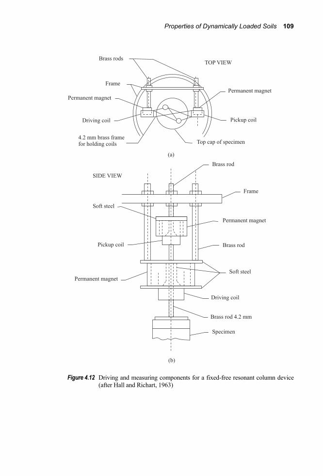
Properties of Dynamically Loaded Soils 109
Figure 4.12 Driving and measuring components for a fixed-free resonant column device
(after Hall and Richart, 1963)

110 Chapter 4
(Figure 4.13), in effect changing the boundary conditions assumed in deriving Eq. (3.57). So a modified equation for the circular natural frequency needs to be derived. This can be done as follows.
Let the mass of the attachments placed on the specimen be equal to m. For the vibration of the soil column in a natural mode,
u(x, t) = U(x)(A1 sin ntw + A2 cos ntw ) (3.41) and
U(x) = B1 sin n
c
xwu
Ê ˆÁ ˜Ë ¯
+ B2 cos n
c
xwu
Ê ˆÁ ˜Ë ¯
(3.43)
At x = 0, U(x) = 0. So B2 in Eq. (3.43) is zero. Thus
U(x) = B1sin n
c
xwu
Ê ˆÁ ˜Ë ¯
(4.13)
At x = L, the inertia force of mass m is acting on the soil column, and this can be expressed as
F = –m2
2u
t∂∂
(4.14)
where F = inertia force. Also, the strain
u Fx AE
∂ =∂
(4.15)
where A = cross-sectional area of specimen E = modulus of elasticity.
Combining Eqs. (3.41), (4.13), and (4.15) we get
FAE
= u Ux x
∂ ∂⎛ ⎞= ⎜ ⎟∂ ∂⎝ ⎠ (A1 sin ntw + A2 cos ntw )
= 1 sin n
c
xBx u
ω⎡ ⎤⎛ ⎞∂⎢ ⎥⎜ ⎟∂ ⎢ ⎥⎝ ⎠⎣ ⎦
(A1 sin ntw + A2 cos ntw )
1 cosn n
c c
B xw wu u
È ˘Ê ˆ Ê ˆ= Í ˙Á ˜ Á ˜Ë ¯ Ë ¯Í ˙Î ˚
(A1 sin ntw + A2 cos ntw ) (4.16)

Properties of Dynamically Loaded Soils 111
Figure 4.13 Derivation of Eq. (4.20)
Again, combining Eqs. (3.41), (4.13), and (4.14),
F = – m2
2u
t∂∂
= – m2
1 2sin n
c
xBt
wu
È ˘ Ê ˆÊ ˆ ∂Í ˙ Á ˜Á ˜Ë ¯ ∂Ë ¯Í ˙Î ˚
(A1 sin ntw + A2 cos ntw )
= m 2nw B1 sin n
c
xwu
Ê ˆÁ ˜Ë ¯
(A1sin ntw + A2 cos ntw ) (4.17)
Now, from Eqs. (4.16) and (4.17),
c
AEu
cos n
c
xwu
Ê ˆÁ ˜Ë ¯
= m nw sin n
c
xwu
Ê ˆÁ ˜Ë ¯
(4.18)
At x = L
tan nn c
c
LAE m ww uu
Ê ˆ= Á ˜Ë ¯
(4.19)
However /c Eu r= ; or 2cE u r= . Substitution of this in Eq. (4.19) gives
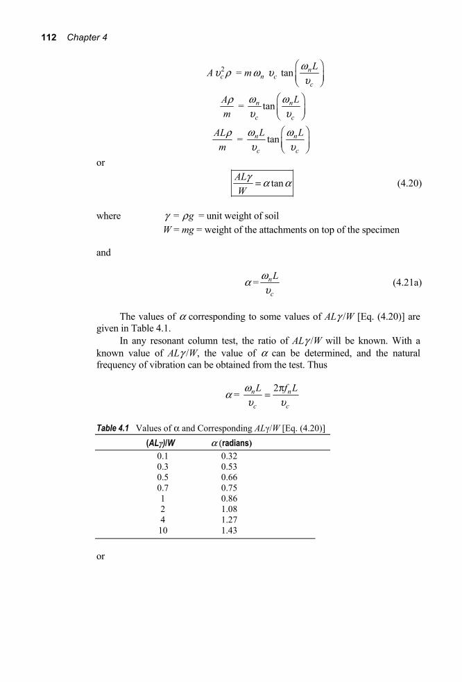
112 Chapter 4
A 2cu r = m nw cu tan n
c
Lwu
Ê ˆÁ ˜Ë ¯
Amr = tann n
c c
Lw wu u
Ê ˆÁ ˜Ë ¯
ALmr = tann n
c c
L Lw wu u
Ê ˆÁ ˜Ë ¯
or
tanALWg a a= (4.20)
where = gg r = unit weight of soil W = mg = weight of the attachments on top of the specimen
and
α = n
c
Lwu
(4.21a)
The values of α corresponding to some values of ALγ /W [Eq. (4.20)] are given in Table 4.1.
In any resonant column test, the ratio of ALγ /W will be known. With a known value of ALγ /W, the value of α can be determined, and the natural frequency of vibration can be obtained from the test. Thus
α = 2n n
c c
L f Lwu u
p=
Table 4.1 Values of α and Corresponding ALγ/W [Eq. (4.20)] (ALγ)/W α (radians)
0.1 0.32 0.3 0.53 0.5 0.66 0.7 0.75 1 0.86 2 1.08 4 1.27 10 1.43
or

Properties of Dynamically Loaded Soils 113
2 n
cf L
uap
= (4.21b)
The modulus of elasticity of the soil can then be obtained as
2 2 2
22
239.48n n
cf L f LE ru r ra a
Ê ˆpÊ ˆ= = =Á ˜ Á ˜Ë ¯ Ë ¯ (4.22)
B. Derivation of Expressions for su and G for Use in the Fixed-Free –Type Resonant Column Test In the resonant column tests where soil specimens are subjected to torsional vibration with fixed – free end conditions, the mass of the driving and motion-monitoring devices (Figure 4.14) can also be taken into account. For this condition, an equation similar to Eq. (4.20) can be derived that is of the form
tans n n
m s s
J L LJ
w wu u
Ê ˆ= Á ˜Ë ¯
= α tan α (4.23)
where Js = mass polar moment of inertia of the soil specimen and Jm = mass polar moment of inertia of the attachments with mass m.
Figure 4.14 Derivation of Eq. (4.23)

114 Chapter 4
Thus
2n ns
L f Lwua a
p= = (4.24)
and 2 2
2239.48 n
sf LG ru ra
Ê ˆ= = Á ˜Ë ¯
(4.25)
C. Typical Laboratory Test Results from Resonant Column Tests Most of the laboratory test results obtained from resonant column tests are for low amplitudes of vibration. By low amplitudes of vibration is meant strain amplitudes of the order of 10– 4 or less.
Typical values of cu andus with low amplitudes of vibration for No. 20–30 Ottawa sand compacted at a void ratio of about 0.55 are shown in Figures 3.13 and 3.14. These were conducted using the free – free and fixed – free types of resonant column device developed by Hardin and Richart (1963) and Hall and Richart (1963). Based on the results given in Figures 3.13 and 3.14, the following general conclusions can be drawn:
1. The values of cu and su in soils increase with the increase of the effective average confining pressure 0s .
2. The values of cu and su for saturated soils are slightly lower than those for dry soils. This can be accounted for by the increase of the unit weight of soil due to the presence of water in the void spaces.
Hardin and Richart (1963) also reported the results of several resonant column tests conducted in dry Ottawa sand. The shear wave velocities determined from these tests are shown in Figure 4.15. The peak-to-peak shear strain amplitude for these tests was 10–3 rad. From Figure 4.15, it may be seen that the values of su are independent of the gradation, grain-size distribution, and also the relative density of compaction. However, su is dependent on the void ratio and the effective confining pressure.
D. Shear Modulus for Large Strain Amplitudes For solid cylindrical specimens torsionally excited by resonant column devices, the shear strain varies from zero at the center to a maximum at the periphery, and it is difficult to evaluate a representative strain. For that reason, hollow cylindrical soil specimens in a resonant column device (Drnevich, Hall, and Richart, 1966, 1967) may be used to determine the shear modulus and damping at large strain amplitudes. Figure 4.16 shows a schematic diagram of this type of

Properties of Dynamically Loaded Soils 115
Figure 4.15 Variation of shear wave velocity with effective confining pressure 0s for
round-grained dry Ottawa sand (after Hardin and Richart, 1963) apparatus, in which the average shearing strain in the soil specimen is not greatly different from the maximum to the minimum. The variation of the shear modulus of dense C–190 Ottawa sand with the shear strain amplitude γ ′ is shown in Figure 4.17. Note that the value of G decreases with γ ′, but it decreases more rapidly for γ ′ > 10–4. This is true for all soils. The reason for this can be explained by the used of Figure 4.18, which is shear-stress-versus-strain diagram for a soil. The stress-strain relationships of soils are curvilinear. The shear modulus that is experimentally determined is the secant modulus obtained by joining the extreme points on the hysteresis loop. Note that when the amplitude of strain is small (that is, 1g ¢ g= ¢ ; Figure 4.18), the value of G is larger compared to that for the larger strain level (that is, 2g ¢ g= ¢ ).

116 Chapter 4
Figure 4.16 Schematic diagram of hollow-specimen resonant column device (after
Drnevich, 1972).
Text not available due to copyright restrictions

Properties of Dynamically Loaded Soils 117
Figure 4.18 Nature of variation of shear stress versus shear strain
E. Effect on Prestraining on the Shear Modulus of Soils The effect of shear modulus of soils due to prestraining was reported by Drnevich, Hall, and Richart (1967). These tests were conducted using C – 190 Ottawa sand specimens. The specimens were first vibrated at a large amplitude for a certain number of cycles under a constant effective confining pressure
0( )s . After that the shear modulii were determined by torsionally vibrating the specimens at small amplitudes (shearing strain < 10–5). Figure 4.19 shows the results of six series of this type of test for dense sand (void ratio = 0.46). In general, the value of G increases with increase of prestrain cycles.
F. Determination of Internal Damping In Section 3.15, a distinction was made between internal damping and material damping. The internal damping of a soil specimen can be determined by resonant column tests.
In Chapter 2, the derivation of the expression for the logarithmic decrement was given as
δ = ln 21
21
n
n
X DX D+
p=-
(2.70)

118 Chapter 4
where δ = logarithmic decrement D = damping ratio.
The preceding equation is for the case of free vibration of a mass-spring-dashpot system. The damping ratio is given by the expression
D =2cr s
c cc km
= (1.47b)
where ms = mass of the soil specimen (in this case).
For soils, the value of D is small and Eq. (2.70) can be approximated as
1
ln 2n
n
X DX
d+
= = p (4.26)
Now, combining Eqs. (1.47b) and (4.26)
δ =s
ckmp (4.27)
Text not available due to copyright restrictions
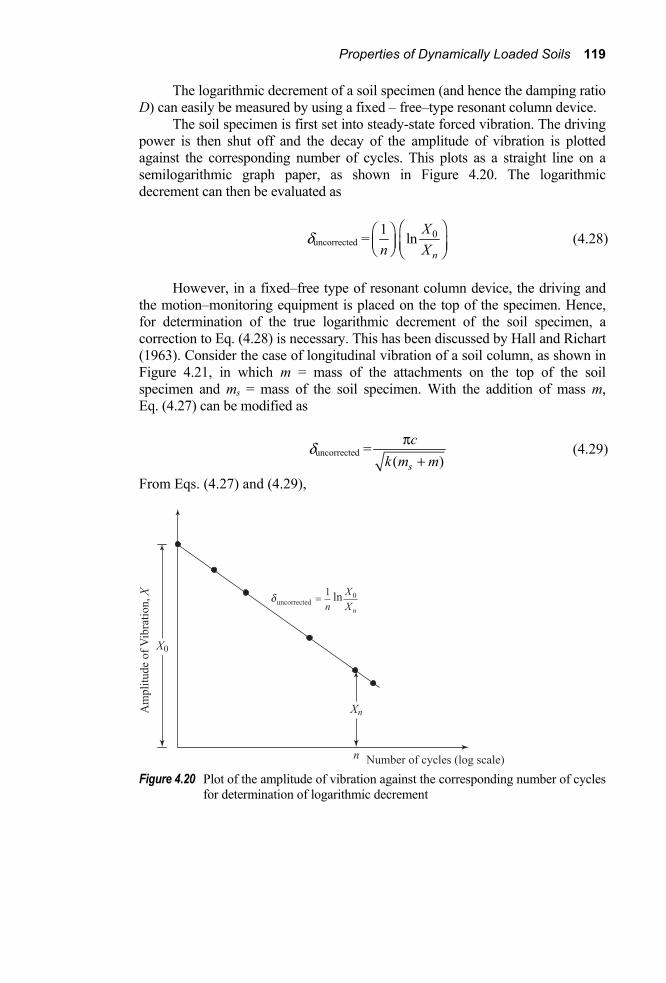
Properties of Dynamically Loaded Soils 119
The logarithmic decrement of a soil specimen (and hence the damping ratio D) can easily be measured by using a fixed – free–type resonant column device.
The soil specimen is first set into steady-state forced vibration. The driving power is then shut off and the decay of the amplitude of vibration is plotted against the corresponding number of cycles. This plots as a straight line on a semilogarithmic graph paper, as shown in Figure 4.20. The logarithmic decrement can then be evaluated as
δuncorrected = 01 lnn
Xn X
Ê ˆÊ ˆÁ ˜ Á ˜Ë ¯ Ë ¯
(4.28)
However, in a fixed–free type of resonant column device, the driving and the motion–monitoring equipment is placed on the top of the specimen. Hence, for determination of the true logarithmic decrement of the soil specimen, a correction to Eq. (4.28) is necessary. This has been discussed by Hall and Richart (1963). Consider the case of longitudinal vibration of a soil column, as shown in Figure 4.21, in which m = mass of the attachments on the top of the soil specimen and ms = mass of the soil specimen. With the addition of mass m, Eq. (4.27) can be modified as
δuncorrected =( )s
ck m m
p+
(4.29)
From Eqs. (4.27) and (4.29),
Figure 4.20 Plot of the amplitude of vibration against the corresponding number of cycles
for determination of logarithmic decrement

120 Chapter 4
Figure 4.21 Fixed – free soil column
uncorrected
1s
s s
m m mm m
dd
+= = + (4.30)
In order to use Eq. (4.30), it will be required to convert the mass ms into an equivalent concentrated mass. The equivalent concentrated mass can be shown to be equal to 0.405ms. Thus, replacing ms in Equation (4.30) by 0.405ms,
δ = δuncorrected 10.405 s
mm
+ (4.31)
A similar correction may be used for specimens subjected to torsional vibration, which will be of the form
δ = δuncorrected 10.405
m
s
JJ
+
Hardin (1965) suggested a relation for δ of dry sand in low amplitude torsional vibration as

Properties of Dynamically Loaded Soils 121
δ = 9π(γ ′)0.2 0.50( )s - (4.32)
Equation (4.32) is valid for γ ′ = 10–6 to 10–4 and 0s = 24 kPa to 144 kPa.
4.6 Cyclic Simple Shear Test A cyclic simple shear test is a convenient method for determining the shear modulus and damping ratio of soils. It is also a convenient device for studying the liquefaction parameters of saturated cohesionless soils (Chapter 10). In cyclic simple shear tests a soil specimen, usually 20 – 30 mm high with a side length (or diameter) of 60–80 mm, is subjected to a vertical effective stress us and a cyclic shear stress τ, as shown in Figure 4.22. The horizontal load necessary to deform the specimen is measured by a load cell, and the shear deformation of the specimen is measured by a linear variable differential transformer.
The shear modulus of a soil in the cyclic simple shear test can be determined as
G = amplitude of cyclic shear stress,amplitude of cyclic shear strain,
tg ¢
(4.33)
The damping ratio at a given shear strain amplitude can be obtained from the hysteretic stress-strain properties. Referring to Figure 4.23 (also see Figure 4.18), the damping ratio can be given as
D = 1 area of the hysteresis loop2 area of triangle andOAB OA Bp ¢ ¢
(4.34)
Figure 4.24 shows a plot of shear modulus G with cyclic shear strain γ ′ for two values of us (Silver and Seed, 1971) obtained from cyclic simple shear tests
Figure 4.22 Cyclic simple shear test

122 Chapter 4
Figure 4.23 Determination of damping ratio from hysteresis loop [Eq. (4.34)] on a medium dense sand (relative density, RD = 60%). From the results of this study, the following can be stated:
1. For a given value of γ ′ and us , the shear modulus increases with the number of cycles of shear stress application. Most of the increase in G takes place in the first ten cycles, after which the rate of increase is relatively small.
2. For a given value of us and number of cycles of stress application, the magnitude of G decreases with the amplitude of shear strain γ ′. (Note: Similar results are shown in Figure 4.17.)
3. For a given value of γ ′ and number of cycles, the magnitude of G increases with the increases of us .
The nature of the shear-stress-versus-shear-strain behavior of a dense sand under cyclic loading is shown in Figure 4.25. Using the hysteresis loops of this type and Eq. (4.34), the damping ratios obtained from a cyclic simple shear test for a medium dense sand are shown in Figure 4.26. Note the following:
1. For a given value of us and amplitude of shear strain γ ′, the damping ratio decreases with the number of cycles. Since, in most seismic events, the number of significant cycles is likely to be less than 20 (Chapter 7), the

Properties of Dynamically Loaded Soils 123
values determined at 5 cycles are likely to provide reasonable values for all practical purposes.
2. For a given number of cycles and us , the magnitude of D decreases with the decrease of γ ′.
Figure 4.24 Shear modulus–shear strain relationship for medium dense sand (after Silver
and Seed, 1971)
Figure 4.25 Stress-strain behaviour of dense sand under cyclic shear (after Silver and
Seed, 1971)

124 Chapter 4
Figure 4.26 Effect of number of stress cycles on hysteretic damping for medium dense
sand (after Silver and Seed, 1971)
Figure 4.27 Bilinear idealization of shear-stress-versus-shear-strain plots

Properties of Dynamically Loaded Soils 125
Other parameters remaining the same (that is, RD, number of cycles, and amplitude of shear strain), a vertical stress increase will decrease the damping ratio. In many seismic analysis studies, it is convenient to represent the nonlinear shear-stress-versus-shear-strain relationship in the form of a bilinear model (also see Figure 7.10), as shown in Figure 4.27 (Thiers and Seed, 1968). In this figure G1 is shear modulus up to a limiting strain of rg ¢ and G2 is the modulus for strain beyond rg ¢ .
Advantages of the Cyclic Simple Shear Test There are several advantages in conducting cyclic simple shear tests. They are more representative of the field conditions, since the specimens can be consolidated in K0 state. Solid soil specimens used in resonant column tests can provide good results up to a shear strain amplitude of about 310 %- . Similarly, the hollow samples used in resonant column studies provide results within a strain amplitude range of 310 %- to about 1%. However, cyclic simple shear tests can be conducted for a wider range of strain amplitude (that is, 210 %- to about 5%. This range is the general range of strain encountered in the ground motion during seismic activities.
The pore water pressure developed during the vibration of saturated soil specimens by a resonant column device is not usually measured. However, in cyclic simple shear tests, the pore water pressure can be measured at the boundary (see Section 10.10 and Figure 10.20).
4.7 Cyclic Torsional Simple Shear Test Another technique used to study the behavior of soils subjected to cyclic loading involves a torsional simple shear device. The torsional simple shear device accommodates a “doughnutlike” speciemen, as shown in Figure 4.28 (Ishibashi and Sherif, 1974). The specimen has inside and outside radii of r1 = 50.8 mm and r2 = 25.4 mm. The inside and outside heights of the specimen are h1 = 25.4 mm and h2 = 12.7 mm. The soil is initially subjected to a vertical effective stress us , an outside and inside horizontal effective stress of hs , and a cyclic shear stress of τ (Figure 4.29). When a shear stress τ is applied, line AB moves to the position of A′B′ (Figure 4.29). So, the shearing strain is
1
1A
rhqg =¢ and γ ′B = 2
2
rhq
For uniform shear strain throughout the sample,

126 Chapter 4
Figure 4.28 Soil specimen for torsional simple shear test
A Bg g=¢ ¢
or
1 2
1 2
r rh hq q=
So
1 1
2 2
r hr h= (4.35)
The following can be calculated after application of the horizontal shear stress on the specimen.
Major effective principal stress:
2
21 2 2
h hh
u us s s ss t+ -Ê ˆ= + + Á ˜Ë ¯ (4.36a)
Intermediate effective principle stress:
2 hs s= (4.36b)

Properties of Dynamically Loaded Soils 127
Figure 4.29 Applied stresses on a torsional simple shear test specimen Minor principal effective stress:
2
23 2 2
h hh
u us s s ss t+ -Ê ˆ= - + Á ˜Ë ¯ (4.36c)
With proper design [Eq. (4.35)], a cyclic torsional shear device can apply near uniform shear strain on the specimen. It can apply shear strains up to about 1%. It also eliminates any sidewall frictional stresses that are encountered in cyclic simple shear tests.
The shear modulus of a specimen tested can be determined as

128 Chapter 4
G = amplitude of shear stress,amplitude of shear stress,
tg ¢
The damping ratio corresponding to a given shear strain amplitude can be determined by using Figure 4.18 and Eq. (4.34).
Liquefaction studies on saturated granular soils can also be conducted by this device along with pore water pressure measurement.
4.8 Cyclic Triaxial Test Cyclic triaxial tests can be performed to determine the modulus of elasticity E and the damping ratio D of soils. In these tests, in most cases, the soil specimen is subjected to a confining pressure σ0 = σ3. After that, an axial cyclic stress Δσd is applied to the specimen, as shown in Figure 4.30. The tests conducted for the evaluation of the modulus of elasticity and damping ratio are strain-controlled tests. A servo-system is used to apply cycles of controlled deformation.
Figure 4.31 shows the nature of a hysteresis loop obtained from a dynamic triaxial test. From this,
E = dse
D
Figure 4.30 Cyclic triaxial test

Properties of Dynamically Loaded Soils 129
Once the magnitude of E is determined, the value of shear modulus can be calculated by assuming a representative value of Poisson’s ration, or
G = 2(1 )
Em+
Again referring to Figure 4.31, the damping ratio can be calculated as
D = 1 area of the hysteresis loop2 area of triangle andOAB OA Bp ¢ ¢
Stress-controlled dynamic triaxial tests are used for liquefaction studies on saturated granular soils (see Chapter 10).
A more elaborate type of dynamic test device has also been used by several
investigators to study the cyclic stress-strain history and shear characteristics of soils. Matsui, O-Hara, and Ito (1980) used a dynamic triaxial system that could generate sinusoidally varying axial and radial stresses.
Figure 4.31 Determination of damping ratio from cyclic triaxial test

130 Chapter 4
A. Cyclic Strength of Clay During earthquakes, the soil underlying building foundations and in structures such as earth embankments, is subjected to a series of vibratory stress applications. These vibratory stresses may induce large deformation in soil and thus failure. In order to evaluate the strength of clay under earthquake loading conditions, Seed and Chan (1966) conducted a number of dynamic triaxial tests. Figure 4.32 shows the nature of some of the stress conditions imposed on the soil specimens during those tests. The results of this study are very instructive and are described in some detail in this section.
Figure 4.33 shows the results of a laboratory test on a specimen of Vicksburg silty clay subjected to sustained and pulsating stresses. The specimen with a degree of saturation of 93% was initially subjected to a confining pressure of σ3 = 100 kPa and then to a conventional axial loading in undrained conditions up to 66% of its static strength. This implies that the sustained stress σ1 – σ3 was
Figure 4.32 Stress conditions on a soil specimen [Note: (b) One-directional loading with
symmetrical stress pulses; (c) and (d) one-directional loading with nonsymmetrical stress pulses]

Properties of Dynamically Loaded Soils 131
Figure 4.33 Stress-versus-strain relationship for Vicksburg silty clay under sustained and axial pulsating stress (after Seed and Chan, 1966)
equal to 0.66 [σ1(f) – σ3], which corresponds to a factor of safety of 1.5. At this time the axial deformation of the specimen was about 5%. After that, 100 transient stress pulses were applied to the specimen. (Note: Loading type is similar to that shown in Figure 4.32b). These stress pulses induced an additional axial stress of about 11%, although the static strength was never exceeded.
Figure 4.34 shows the nature of soil deformation on three soil specimens of San Francisco Bay mud subjected to pulsating stress levels to 100%, 80%, and 60% of normal strength (that is, static strength). For these tests, no sustained stress was applied. (Note: Loading type is similar to that shown in Figure 4.32d.) It is worth noting that, for each level of pulsating stress, the specimen ultimately failed.
Figure 4.35 is a plot of the pulsating stress level (as a percent of normal strength) versus sustained stress level (as a percent of normal strength) causing failure of San Francisco Bay mud at various numbers of transient stress pulses. As the number of stress pulses are increasing at the same pulsating stress level, the sustained stress level inducing failure is decreasing. The interested readers should refer to the original paper by Seed and Chan (1966). Similar plots could be developed for various soils to help in the design procedure of various structures.

132 Chapter 4
Figure 4.34 Deformation of San Francisco Bay mud specimens subjected to pulsating
stress (after Seed and Chan, 1966)
Figure 4.35 Combinations of sustained and pulsating stress intensities causing failure —
San Francisco Bay mud (after Seed and Chan, 1966)
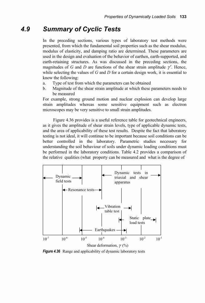
Properties of Dynamically Loaded Soils 133
4.9 Summary of Cyclic Tests In the preceding sections, various types of laboratory test methods were presented, from which the fundamental soil properties such as the shear modulus, modulus of elasticity, and damping ratio are determined. These parameters are used in the design and evaluation of the behavior of earthen, earth-supported, and earth-retaining structures. As was discussed in the preceding sections, the magnitudes of G and D are functions of the shear strain amplitude γ ′. Hence, while selecting the values of G and D for a certain design work, it is essential to know the following: a. Type of test from which the parameters can be obtained b. Magnitude of the shear strain amplitude at which these parameters needs to
be measured For example, strong ground motion and nuclear explosion can develop large strain amplitudes whereas some sensitive equipment such as electron microscopes may be very sensitive to small strain amplitudes.
Figure 4.36 provides is a useful reference table for geotechnical engineers, as it gives the amplitude of shear strain levels, type of applicable dynamic tests, and the area of applicability of these test results. Despite the fact that laboratory testing is not ideal, it will continue to be important because soil conditions can be better controlled in the laboratory. Parametric studies necessary for understanding the soil behaviour of soils under dynamic loading conditions must be performed in the laboratory conditions. Table 4.2 provides a comparison of the relative qualities (what property can be measured and what is the degree of
10-7 10-6 10-5 10-4 10-3 10-2 10-1
Shear deformation, γ (%)
Figure 4.36 Range and applicability of dynamic laboratory tests
Dynamic field tests
Resonance tests
Dynamic tests in triaxial and shear apparatus
Vibration table test
Earthquakes
Static plate load tests

134 Chapter 4
quality of the measured property) of various laboratory techniques for measuring dynamic soil properties. Similarly, Table 4.3 gives a summary of the different engineering parameters that can be measured in different dynamic or cyclic laboratory tests.
Table 4.2 Relative Quality of Laboratory Techniques for Measuring Dynamic Soil Propertiesa
Relative Quality of Test Results Effect of Shear Young’s Material number Attenuation modulus modulus damping of cycles Resonant column Good Good Good Good - with application - - - - Fair Ultrasonic pulse Fair Fair - - Poor Cyclic triaxial - Good Good Good - Cyclic simple shear Good - Good Good - Cyclic torsional shear Good - Good Good -
a After Silver (1981)
Table 4.3 Parameters Measured in Dynamic or Cyclic Laboratory Testsa Cyclic simple Resonant column Cyclic triaxial shear Torsional shear Resonant Horizontal Load frequency Axial force force Torque Deformation Axial Vertical Vertical Vertical Vertical displacement displacement displacement displacement
Shear Acceleration Not measured Horizontal Rotation displacement
Lateral Not usually Not usually Often Not usually measured measured controlled measured Volumetric None for undrained tests Volume of fluid moving into or out of the sample for drained tests
Pore water Not usually Measured at Measured at Measured at pressure measured boundary boundary boundary aAfter Silver (1981)

Properties of Dynamically Loaded Soils 135
Field Test Measurements
4.10 Reflection and Refraction of Elastic Body Waves —Fundamental Concepts When an elastic stress wave impinges on the boundary of two layers, the wave is reflected and refracted. As has already been discussed in Chapter 3, there are two types of body waves — that is, compression waves (or P–waves) and shear waves (or S–waves). In the case of P–waves, the direction of the movements of the particles coincides with the direction of propagation. This is shown by the arrows in Figure 4.37a. The shear waves can be separated into two components: a. SV-waves, in which the motion of the particles is in the plane of
propagation as shown by the arrows in Figure 4.37b b. SH-waves, in which the motion of the particles is perpendicular to the plane
of propagation, as shown by a dark dot in Figure 4.37c
If a P-wave impinges on the boundary between two layers, as shown in Figure 4.38a, there will be two reflected waves and two refracted waves. The reflected waves consist of (1) a P-wave shown as P1 in layer 1 and (2) an SV-wave shown as SV1 in layer 1.
Figure 4.37 P-wave, SV-wave, and SH-wave

136 Chapter 4
Figure 4.38 Reflection and refraction for (a) an incident P-ray; (b) an incident SH-ray;
and (c) an incident SV-ray
The refracted waves will consist of (1) a P-wave, shown as P2 in layer 2, and (2) an SV-wave, shown as SV2 in layer 2. Referring to the angles in Figure 4.38a, it can be shown that
α1 = α2 (4.37) and
1 1 1 2 2
3 31 2 2 sin sinsin sin sin
p p s p s
a ba a bu u u u u
= = = = (4.38)
where

Properties of Dynamically Loaded Soils 137
1pu and 2pu = the velocities of the P-wave front in layers 1 and 2, respectively
1su and 2su = the velocities of the S-wave front in layers 1 and 2, respectively
If an SH-wave impinges the boundary between two layers, as shown in Figure 4.38b, there will be one reflected SH-wave (shown as SH1) and one refracted SH-wave (shown as SH2). For this case
β1 = β2 (4.39)
and
1 2
31 sinsin
s s
bbu u
= (4.40)
Lastly, if an SV-wave impinges the boundary between two layers, as shown in Figure 4.38c, there will be two reflected waves and two refracted waves. The reflected waves are (1) a P-wave, shown as P1 in layer 1 and (2) an SV-wave, shown as SV1 in layer 1. The refracted waves are (a) a P-wave, shown as P2 in layer 2, and (b) an SV-wave, shown as SV2 in layer 2. For this case, β1 = β2:
1 1 1 2 2
3 31 2 2 sin sinsin sin sin
s p s s p
b ab a bu u u u u
= = = = (4.41)
The mathematical derivations of these facts will not be shown here. For further details the reader is referred to Kolsky (1963, pp. 24–38).
4.11 Seismic Refraction Survey (Horizontal Layering) Seismic refraction surveys are sometimes used to determine the wave propagation velocities through various soil layers in the field and to obtain thicknesses of each layer. Consider the case where there are two layers of soil, as shown in Figure 4.39a. Let the velocities of P-waves in layers 1 and 2 be
1pu and
2pu , respectively, and let 1pu <
2pu . A is a source of impulsive energy. If seismic waves are generated at A, the energy from the point will travel in hemispherical wave fronts. Consider the case of P-waves, since they are the fastest. If a detecting device is placed at point B, which is located at a small distance x from A, the P-wave that travels through the upper medium will reach it first before any other wave. The travel time for this first arrival may be given as

138 Chapter 4
Figure 4.39 Seismic refraction survey — horizontal layering
t = 1p
xu
(4.42)
where AB = x. Again, consider the first arrival time of a P-wave at a point G, which is
located at a greater distance from A. In order to understand this, one considers a spherical P-wave front that originates at A striking the interface of the two layers. At some point C, the refracted P-wave front in the lower medium will be such that the tangent to the sphere will be perpendicular to the interface. In that case, the refracted P-ray (shown as P2 in Figure 4.39a) will be parallel to the boundary

Properties of Dynamically Loaded Soils 139
and will travel with a velocity2pu . Note that because
1pu <2pu , this wave front
will travel faster than those described previously. From Eq. (4.38)
1 2
31 sinsin
p p
aau u
=
Since 3a = 90°, sin 3a = 1, and
α1 = sin–1 1
2
p
p
uuÊ ˆÁ ˜Ë ¯
= αc (4.43)
where αc = critical angle of incidence.
The wave front just described traveling with a velocity2pu will create
vibrating stresses at the interface, and this will generate wave fronts that will spread out into the upper medium. These P-waves will spread with a velocity of
1pu . The spherical wave front traveling downward from D in layer 2 will have a radius equal to DE after a time Δt. At the same time Δt, the spherical wave front traveling upward from point D will have a radius equal to DF. The resultant wave front in the upper layer will follow a line EF. It can be seen from the diagram that
1
2
sinpc
p
t DF it DE
uu
D= =
D (4.44)
So ray DFG will make an angle ic with the vertical. It can be mathematically shown that for x greater than a critical value xc, the P-wave that travels the path ACDG will be the first to arrive at point G. Let the time of travel for the P-wave along the path ACDG be equal to t. Thus, t = tAC + tCD + tDG, or
T = 1 2 1
2 tan1 1cos cos
c
c p p c p
x z iz zi iu u u
Ê ˆ Ê ˆÊ ˆ Ê ˆ-+ +Á ˜ Á ˜Á ˜ Á ˜Ë ¯ Ë ¯Ë ¯ Ë ¯
= 2 2 1
2 sin 2cos cos
c
p p c p c
z ix zi iu u u
- +
where x = AG . But 2pu =
1pu /sin ic [from Eq. (4.44)]; thus
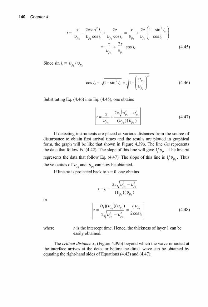
140 Chapter 4
t = 2 1 1 2 1
2 22 sin 1 sin2 2cos cos cos
c c
p p c p c p p c
z i ix z x zi i iu u u u u
Ê ˆ-- + = + Á ˜Ë ¯
= 2 1
2
p p
x zu u
+ cos ic (4.45)
Since sin ic = 1pu /
2pu
cos ic = 1
2
221 sin 1 p
cp
iuuÊ ˆ
- = - Á ˜Ë ¯
(4.46)
Substituting Eq. (4.46) into Eq. (4.45), one obtains
2 1
2 1 2
2 22
( ) ( )p p
p p p
zxtu u
u u u-
= + (4.47)
If detecting instruments are placed at various distances from the source of disturbance to obtain first arrival times and the results are plotted in graphical form, the graph will be like that shown in Figure 4.39b. The line Oa represents the data that follow Eq.(4.42). The slope of this line will give
11 .pu The line ab
represents the data that follow Eq. (4.47). The slope of this line is 2
1 .pu Thus the velocities of
1pu and 2pu can now be obtained.
If line ab is projected back to x = 0, one obtains
t = ti = 2 1
1 2
2 22
( )( )p p
p p
z u uu u
-
or
1 2 1
2 1
2 2
( )( )( )2cos2
i p p i p
cp p
t tz
iu u u
u u= =
- (4.48)
where ti is the intercept time. Hence, the thickness of layer 1 can be easily obtained.
The critical distance xc (Figure 4.39b) beyond which the wave refracted at the interface arrives at the detector before the direct wave can be obtained by equating the right-hand sides of Equations (4.42) and (4.47):
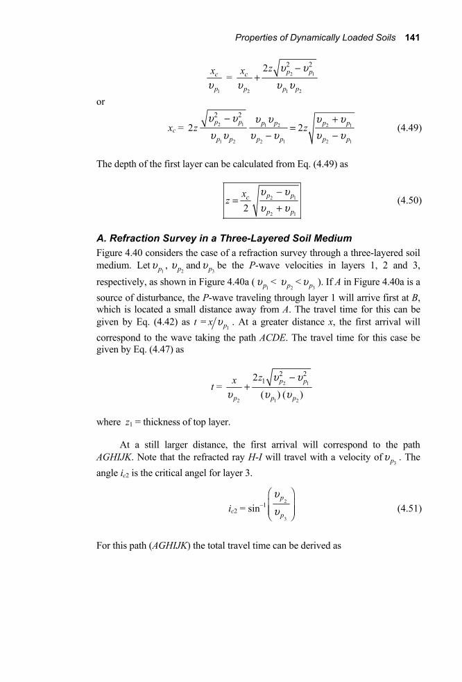
Properties of Dynamically Loaded Soils 141
1
c
p
xu
= 2 1
2 1 2
2 22 p pc
p p p
zx u uu u u
-+
or
xc = 2 1 1 2 2 1
1 2 2 1 2 1
2 2
2 2p p p p p p
p p p p p pz z
u u u u u uu u u u u u
- +=
- - (4.49)
The depth of the first layer can be calculated from Eq. (4.49) as
2 1
2 12
p pc
p p
xz
u uu u
-=
+ (4.50)
A. Refraction Survey in a Three-Layered Soil Medium Figure 4.40 considers the case of a refraction survey through a three-layered soil medium. Let
1,pu 2pu and
3pu be the P-wave velocities in layers 1, 2 and 3, respectively, as shown in Figure 4.40a (
1pu < 2pu <
3pu ). If A in Figure 4.40a is a source of disturbance, the P-wave traveling through layer 1 will arrive first at B, which is located a small distance away from A. The travel time for this can be given by Eq. (4.42) as t =
1px u . At a greater distance x, the first arrival will correspond to the wave taking the path ACDE. The travel time for this case be given by Eq. (4.47) as
t = 2 1
2 1 2
2 212
( ) ( )p p
p p p
zx u uu u u
-+
where z1 = thickness of top layer.
At a still larger distance, the first arrival will correspond to the path AGHIJK. Note that the refracted ray H-I will travel with a velocity of
3pu . The angle ic2 is the critical angel for layer 3.
ic2 = sin–1 2
3
p
p
u
u
Ê ˆÁ ˜Á ˜Ë ¯
(4.51)
For this path (AGHIJK) the total travel time can be derived as

142 Chapter 4
Figure 4.40 Refraction survey in a three-layer soil
3 1 3 2
3 3 1 3 2
2 2 2 21 22 2
( )( ) ( ) ( )p p p p
p p p p p
z zxtu u u u
u u u u u- -
= + + (4.52)
where z2 = thickness of layer 2. So, if detecting instruments are placed at various distances from the source
of disturbance to obtain first arrival times, they can be plotted in a t-versus-x graph. This graph will appear as shown in Figure 4.40b. The line Oa corresponds to Eq. (4.42), ab corresponds to Eq. (4.47), and bc corresponds to Eq. (4.52). The slopes of Oa, ab, and bc will be
11 ,pu 2
1 pu and3
1 pu , respectively. The thickness of the first layer z1 can be determined from the intercept time ti1 in a similar manner, as shown in Eq. (4.48), or
z1 = 1 2
2 1
1
2 2
( ) ( ) ( )
2
i p p
p p
t u u
u u-

Properties of Dynamically Loaded Soils 143
The thickness of the second layer can be obtained from Eq. (4.52). Referring to Figure 4.40b, the expression for the intercept time ti2 can be evaluated by substituting x = 0 into Eq. (4.52):
t = ti2 = 3 1 3 2
3 1 3 2
2 2 2 21 22 2
( )( ) ( )( )p p p p
p p p p
z zu u u uu u u u
- -+
or
3 1 3 2
3 1 3 2
2 21
2 2 2 2
2 ( )( )12 ( )( )
p p p pi
p p p p
zz t
u u u uu u u u
È ˘-Í ˙= -Í ˙ -Í ˙Î ˚ (4.53)
B. Refraction Survey for Multilayer Soil In general, if there are n layers, the first arrival time at various distances from the source of disturbance will plot as shown in Figure 4.41. There will be n segments in the t-versus-x plot. The slope of the nth segment will give the value 1
npu (n = 1, 2,…). More details on advanced test methods (detecting inclination of the bedrock is briefly described later) and interpretation could be found in several geophysics books.
The value of P-wave velocity in a natural deposit of soil will depend on several factors, such as confining pressure, moisture content, and void ratio. Some typical values of pu are given in Table 3.1. It is worth noting that P-wave velocity through saturated soils will be approximately 1500 m/sec. However, as P-wave velocity value could reach the order of few kilometres per second in case of rocks.
Figure 4.41 Refraction survey for multilayer soil

144 Chapter 4
Example 4.1
Following are the results of a refraction survey (horizontal layering of soil). Determine the P-wave velocities of the soil layers and their thicknesses.
Distance (m) Time of first arrival (ms) 2.5 5.5 5.0 11.1 7.5 16.1 15.0 24.0 25.0 30.8 35.0 38.2 45.0 46.1 55.0 51.3
60.0 52.8
Solution
The time-distance plot is given in Figure 4.42. From the plot,
1pu = 35
10.6 10-¥ = 472 m/s
2pu = 310
7.2 10-¥ = 1389 m/s
3pu = 310
3 10-¥ = 3333 m/s
Figure 4.42

Properties of Dynamically Loaded Soils 145
ti1 = 13.3 × 10⁻³ s; ti2 = 35.6 × 10⁻³ s. From Eq. (4.48)
z1 = 1 2
2 1
31
2 2 2 2
( ) ( ) ( ) (13.3 10 )(472)(1389)
2 2 (1389) (472)
i p p
p p
t u u
u u
-¥=- -
= 3.39 m From Eq. (4.53)
z2 = 3 1 3 2
3 1 3 2
2 21
2 2 2
2 ( ) ( )12 ( )( )
p p p pi
p p p p
zt
u u u uu u u u
È ˘-Í ˙-Í ˙ -Í ˙Î ˚
= 2 2
3 (2)(3.39) (3333) (472)1 35.6 102 (3333)(472)
-È ˘-Í ˙¥ -Í ˙Î ˚
2 2
(3333)(1389)
(3333) (1389)¥
-
= 12
(0.02138) (1528) = 16.33 m
4.12 Refraction Survey in Soils with Inclined Layering Figure 4.43a shows two soils layers. The interface of soil layers 1 and 2 is inclined at an angle β with respect to the horizontal. Let the P-wave velocities in layers 1 and 2 be
1pu and2pu , respectively (
1pu <2pu ).
If a disturbance is created at A and a detector is placed at B, which is small distance away from A, the detector will first receive the P-wave traveling through layer 1. The time for its arrival may be given by
td = 1p
xu
However, at a larger distance the first arrival will be for the P-wave following the path ACDE — which consists of three parts. The time taken can be written as td = tAC + tCD + tDE (4.54)
Referring to Figure 4.43a,
tAC = 1cosp c
ziu
¢ (4.55)

146 Chapter 4
tCD = 2 2
4 1 2 3 3 4
p p
AA AA A A A ACDu u
- - -=
= 2
cos tan tan sin tanc c c
p
x z i z i x ib bu
- - -¢ ¢ (4.56)
tDE = 1 1
3 3
sincos cosc c
p p
z xDA A E i i
b
u u
¢ ++
= (4.57)
Substitution of Eqs. (4.55), (4.46), and (4.57) into Eq. (4.54) and simplification yields
Figure 4.43 Refraction survey in soils with inclined layering

Properties of Dynamically Loaded Soils 147
td = 1 1
2 cos c
p p
z i xu u¢
+ sin (ic + β) (4.58)
Now, if the source of disturbance is E and the detector is placed at A, the first arrival time along the refracted ray path may be given by
tu = 1 1
2 cossin ( )c
cp p
z i x i bu u¢¢
+ - (4.59)
In the actual survey, one can have a source of disturbance such as A and observe the first arrival time at several points to the right of A and have a source of disturbance such as E and observe the first arrival time at several points to the left of E. These results can be plotted in a graphical form, as shown in Figure 4.43b (time-versus-x plot). From Figure 4.43b note that the slopes of Oa and O′a′ are both 1/
1pu . The slope of the branch ab will be [sin(ic + β)]/1pu , as can be
seen from Eq. (4.58). Similarly, the slope of the branch of a′b′ will be [sin (ic – β]/
1pu [see Eq. (4.59)]. Let
md = 1
sin ( )c
p
i bu
+ (4.60)
and
mu =1
sin ( )c
p
i bu
- (4.61)
From Eq. (4.60),
ic = sin–1(md 1pu ) – β (4.62)
Again, from Eq. (4.61)
ic = sin–1(mu 1pu ) + β (4.63)
Solving the two preceding equations,
1 1
1 112 [sin ( ) sin ( )]c p d p ui m mu u- -= + (4.64)
and
1 1
1 112 [sin ( ) sin ( )]p d p um mb u u- -= - (4.65)

148 Chapter 4
Once ic is determined, the value of 2pu can be obtained as
1
2 sinp
pci
uu = (4.66)
Again referring to Figure 4.43b, if the ab and a′b′ branches are projected back, they will intercept the time axes at tid and tiu, respectively. From Eqs. (4.58) and (4.59), it can be seen that
tid = 1
2 cos c
p
z iu¢
or
1( )2 cos
id p
c
tz
iu
=¢ (4.67)
and
tiu =1
2 cos c
p
z iu¢¢
or
1( )2 cos
iu p
c
tz
iu
=¢¢ (4.68)
Since ic and 1pu are known and tid and tiu can be determined from a graph, one
can obtain the values of z ¢ and z ¢¢ .
Example 4.2
Referring to Figure 4.43a, the results of a refraction survey are as follows. The distance between A and E is 60 m. Point of disturbance A Point of disturbance E Distance Time of first Distance Time of first from A (m) arrival (ms) from E (m) arrival (ms) 5 12.1 5 11.5 10 25.2 10 22.8 15 35.3 15 34.5 20 48.0 20 44.8 30 60.2 30 69.1 40 68.5 40 78.1 50 76.8 50 82.8 60 85.1 60 87.7

Properties of Dynamically Loaded Soils 149
Determine a.
1pu and 2pu ,
b. z′ and z′′, and c. β
Solution
The time-distance records have been plotted in Figure 4.44. a. From branch oa,
1 3
1025 10pu -=
¥ = 400 m/s
From branch O′a′
1pu = 310
22 10-¥ = 454 m/s
The average value of 1pu is 427 m/s.
From the slope of branch ab,
Figure 4.44
150 Chapter 4
md = 38.8 10
10
-¥ = 0.88 × 10⁻³
Again, from the slope of branch a′b′,
mu = 35 10
10
-¥ = 0.5 × 10⁻³
From Eq. (4.64),
ic = 1 1
1 112 [sin ( ) sin ( )]p d p um mu u- -+
sin–1 (1pu md) = sin–1 [(427)(0.88 × 10⁻³)] = 22.07°
sin–1(1pu mu) = sin–1[(427)(0.5 × 10⁻³] = 12.33°
Hence
ic = 12 (22.07° + 12.33°) = 17.2°
Using Eq. (4.66),
2pu = 1 427
sin sin (17.2)p
ciu
= = 1444 m/s
b. From Eq. (4.67)
z′ = 1( ) ( )2cosid p
c
tiu
tid = 35.9 × 10⁻³ s (from Figure 4.44). So
z′ = 3(35.9 10 )(427)
2 cos(17.2)
-¥ = 8.03 m
Again, from Eq. (4.68),
z′′ = 1( )( )2 cosiu p
c
ti
u
From Figure 4.44, tiu = 59.8 × 10⁻³ s.
z′′ = 3(59.8 10 )(427)
2cos (17.2)
-¥ = 13.37 m
c. From Eq. (4.65),
β = 12 [sin–1 (
1pu md) – sin–1 (1pu mu)] = 1
2 (22.07° – 12.33°) = 4.87°

Properties of Dynamically Loaded Soils 151
4.13 Reflection Survey in Soil (Horizontal Layering) Reflection surveys can also be conducted to obtain information about the soil layers. Figure 4.45a shows a two-layered soil system. A is the point of disturbance. If a recorder is placed at C at a distance x away from A, the travel time for the reflected P-wave can be given as
t =1 1
222
2p p
AB BC xzu u+ Ê ˆ= + Á ˜Ë ¯
(4.69)
where t = total travel time for the ray path ABC.
From Eq. (4.69), the thickness of layer 1 can be obtained as
1
2 212 ( )pz t xu= - (4.70)
If the travel times t for the reflected P-waves at various distances x are obtained, they can be plotted in a graphical form, as shown in Figure 4.45b. Note that the time-distance curve obtained form Eq. (4.69) will be a hyperbola. The line Oa shown in Figure 4.45b is the time-distance plot for the direct P-waves traveling through layer 1 (compare line Oa in Figure 4.45b to the line Oa in Figure 4.39b). The slope of this line will give
11 pu .
If the time-distance curve obtained from the reflection data is extended back, it will intersect the time axis at t0. From Eq. (4.69) it can be seen that at x = 0,
t0 = 1
2
p
zu
or
10
2pt
zu
= (4.71)
With 1pu and t0 known, the thickness of the top layer z can be calculated.
Another convenient way to interpret the reflection survey record is to plot a graph of t2 versus x2. From Eq. (4.69),
t2 = 1 1
22
2 24 1
2p p
xzu u
È ˘Ê ˆ+ =Í ˙Á ˜Ë ¯Í ˙Î ˚ (4z2 + x2) (4.72)

152 Chapter 4
Figure 4.45 Reflection survey in soil — horizontal layering

Properties of Dynamically Loaded Soils 153
This relation indicates that the plot of t2 versus x2 will be a straight line, as shown in Figure 4.45c. The slope of this line give
1
21 pu and the intercept on the
t2 axis will be equal to 20t . Substituting t = t0 and x = 0 into Eq. (4.72),
1
220 2
4
p
ztu
=
or
1
2 202
4pt
zu
= (4.73)
With 20t and
1
2pu known, the thickness of the top layer can now be
calculated.
Example 4.3
The results of a reflection survey on a relatively flat area (shale underlain by granite) are given here. Determine the velocity of P-waves in the shale.
Distance from point Time for first of disturbance (m) reflection (s)
30 1.000 90 1.002 150 1.003 210 1.007 270 1.011 330 1.017
390 1.023 Solution
Using the time-distance records, the following table can be prepared.
x x2 t t 2 (m) (m2) (s) (s2) 30 900 1.000 1.000 90 8,100 1.002 1.004 150 22,500 1.003 1.006 210 44,100 1.007 1.014 270 72,900 1.011 1.022 330 108,900 1.017 1.034 390 152,100 1.023 1.046

154 Chapter 4
Figure 4.46 A plot of t2 versus x2 is shown in Figure 4.46. From the plot,
1pu = 2
2( ) 79200
0.024( )xt
Δ =Δ
= 1816.6 m/s
4.14 Reflection Survey in Soil (Inclined Layering) Figure 4.47 considers the case of a reflection survey where the reflecting boundary is inclined at an angle β with respect to the horizontal. A is the point for the source of disturbance. The reflected P-ray reaching point C will take the path ABC. Referring to Figure 4.47, AB + BC = A′B + BC = A′C But (A′C)2 = (A′A2)2 + (A2C)2 (4.74)
A′A2 = AA′ cos β = 2z′ cos β (4.75) A2C = A2A + AC = 2z′ sin β + xC (4.76)
Substituting Eqs. (4.75) and (4.76) into Eq. (4.74),
A′C = 2 2(2 cos ) (2 sin )Cz z xb b+ +¢ ¢
= 2 24 4 sinC Cz x z x b+ +¢ ¢

Properties of Dynamically Loaded Soils 155
Figure 4.47 Reflection survey in soil — inclined layering Thus, the travel time for the reflected P-wave along the path ABC will be
tC = 1p
A Cu¢
So
tC = 1
2 21 4 4 sinC Cp
z x z x bu
+ +¢ ¢ (4.77)
In a similar manner, the time of arrival for the reflected P-waves received at point E can be given as
tE = 1
2 21 4 4 sinE Ep
z x z x bu
+ +¢ ¢ (4.78)
Combining Eqs. (4.77) and (4.78),
sin β = 1
2 2 2( )4 ( ) 4
p E C E C
E C
t t x xz x x zu - +
--¢ ¢
(4.79)
Now, let t = (tE + tC)/2 and Δt = tE – tC

156 Chapter 4
Substitution of the preceding relations in Eq. (4.79) gives
sin β = 1
2 ( )2 ( ) 4
p E C
E C
t t x xz x x zu D +
--¢ ¢
(4.80)
If xC is equal to zero, Eq. (4.80) will transform to
sin β = 1
2 ( )2 4p E
E
t t xz x z
u D-
¢ ¢ (4.81)
If xC = 0 and β = 0 (that is, the reflecting layer is horizontal) then, from Eq. (4.81),
Δt = 1
2
22E
p
xtu
(4.82)
If xC = 0 and Δt > 2Ex /
1
22 p tu , the reflecting layer is sloping down in the
direction of positive x, as shown in Figure 4.47. If xC = 0 and Δt < 2Ex /
1
22 p tu , the reflecting layer is sloping down in the direction of negative x (that is, opposite to that shown in Figure 4.47).
In actual practice, that point of disturbance A (Figure 4.48) is generally placed midway between the two detectors, so xE = –xC = x. So, from Eq. (4.80)
Figure 4.48

Properties of Dynamically Loaded Soils 157
sin β = 1
2 ( )4
p t tz x
u D¢
(4.83)
Referring to Figure 4.48, AA′ = 2z′ = (A′C + A′E)/2. So
1 1 1
2 1 1 ( )2 2 C E
p p p
z A C A E t t tu u u
Ê ˆ¢ ¢ ¢= + = + =Á ˜Ë ¯
(4.84)
Combining Eqs. (4.83) and (4.84),
sin β = 1( )
2p t
xu D
(4.85)
Example 4.4
Refer to Figure 4.48. Given: x = 85.5 m, tC = 0.026 s, and tE = 0.038 s. Determine β and z′. The value of
1pu i.e., the velocity of the primary wave through the top layer has been previously determined to be 410 m/s.
Solution
t = 0.026 0.0382 2
C Et t+ += = 0.032 s
Δt = tE – tC = 0.038 – 0.026 = 0.012 s From Eq. (4.85)
β = sin–1 1 1( ) (410)(0.012)sin2 (2)(85.5)
p tx
u −Δ⎡ ⎤ ⎡ ⎤=⎢ ⎥ ⎢ ⎥
⎣ ⎦⎣ ⎦ = 1.65°
From Eq. (4.84)
1
2
p
z tu
¢ =
or
z′ = 1 (0.032)(410)2 2
pt u= = 6.56 m

158 Chapter 4
4.15 Subsoil Exploration by Steady-State Vibration In steady-state vibration, a circular plate placed on the ground surface is vibrated vertically by a sinusoidal loading (Figure 4.49a). This vibration will send out Rayleigh waves (Section 3.13) and the vertical motion of the ground surface will predominantly be due to these waves. This can be picked up by motion transducers. The velocity of the Rayleigh waves can be given as
ru = fL (4.86)
where f = frequency of vibration of the plane and L = wavelength.
If the wavelength L can be measured, the velocity of Rayleigh waves can easily be calculated. The wavelength is generally determined by the number of waves
Figure 4.49 Subsoil exploration by steady-state vibration
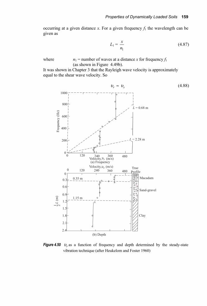
Properties of Dynamically Loaded Soils 159
occurring at a given distance x. For a given frequency f1 the wavelength can be given as
L1 = 1
xn
(4.87)
where n1 = number of waves at a distance x for frequency f1 (as shown in Figure 4.49b). It was shown in Chapter 3 that the Rayleigh wave velocity is approximately equal to the shear wave velocity. So
ru ≈ su (4.88)
Figure 4.50 ru as a function of frequency and depth determined by the steady-state vibration technique (after Heukelom and Foster 1960)

160 Chapter 4
It was also discussed in Chapter 3 that, for all practical purposes, the Rayleigh wave travels through the soil within a depth of one wavelength. Hence for a given frequency f, if the wavelength L is known, the value of su determined by the preceding technique will represent the soil conditions at an average depth of L/2. Thus for a large value of f, the value of su is representative of soil conditions at a smaller depth; and, for a small value of f, the value of su obtained is representative of the soil conditions at a larger depth. Figure 4.50 shows the results of wave propagation on a stratified pavement system obtained using this technique.
4.16 Soil Exploration by “Shooting Up the Hole,” “Shooting Down the Hole,” and “Cross-Hole Shooting”
Shooting Up the Hole In the technique of shooting up the hole, a hole is drilled into the ground and a detector is placed at the ground surface. Charges are exploded at various depths in the hole and the direct travel time of body waves (P or S) along the boundary of the hole is measured. Thus the values of pu and su of various soil layers can be easily obtained. There is a definite advantage in this technique, since it determines the shear wave velocities of various soil layers. The refraction and reflection techniques give only the P-wave velocity. However, below the groundwater table the compression waves will travel through water. The first arrival for points below the water table will usually be for this type, and the wave velocity will generally be higher than the compression wave velocity in soils. On the other hand, shear waves cannot travel through water, and the shear wave velocity measure above or below the water table will be the same.
Shooting Down the Hole Shear wave velocity determination of various soil layers by shooting down the hole has been described by Schwarz and Musser (1972), Beeston and McEvilly (1977), and Larkin and Taylor (1979). Figure 4.51 shows a schematic diagram for the down-hole method of seismic waves testing as presented by Larkin and Taylor, which relies on measuring the time interval for SH-waves to travel between the ground surface and the subsurface points. A bidirectional impulsive source for the propagation of SH-waves is placed on the surface adjacent to a borehole. A horizontal sensitive transducer is located at a depth in the borehole. The depth of the transducer in varied throughout the length of the borehole. The shear wave velocity can then be obtained as

Properties of Dynamically Loaded Soils 161
Figure 4.51 The down-hole method of seismic wave testing
szt
u D=D
(4.89)
where z = depth below the ground surface t = time of travel of the shear wave from the surface impulsive source to the transducer.
During the process of field investigation, Larkin and Taylor (1979) determined that the shear strains at depths of 3 m and 50 m were about 1 × 10⁻⁶ and 0.3 × 10⁻⁶, respectively. In order to compare the field and laboratory values of su , some undisturbed samples from various depths were collected. The shear wave velocity of various specimens at a shear strain level of 1 × 10⁻⁶ was determined. A comparison of the laboratory and field test results showed that, for similar soils, the value of (lab)su is considerably lower than that obtained in the field. For the range of soil tested,
(lab)su ≈ 0.25 (field)su + 83 where
162 Chapter 4
(lab)su and (field)su are in meters per second.
Larkin and Taylor also defined a quantity called the sample disturbance factor SD:
SD =2
(field) field
(lab) lab
s
s
GG
uu
È ˘=Í ˙
Í ˙Î ˚ (4.90)
The average value of SD in Larkin and Taylor’s investigation varied from about 1 for (field)su = 140 m/s to about 4 for (field)su = 400 m/s. This shows that small disturbances in the sampling could introduce large errors in the evaluation of representative shear moduli of soils.
Cross-Hole Shooting The seismic cross-hole survey is considered by many engineers to be the most reliable method of determining the dynamic shear modulus of soil. The technique of cross-hole shooting relies on the measurement of SV-wave velocity. In this procedure of seismic surveying, two vertical boreholes at a given distance apart are advanced into the ground (Figure 4.52). Shear waves are generated by a vertical impact at the bottom of one borehole. The arrival of the body wave is recorded by a vertically sensitive transducer placed at the bottom of another borehole at the same depth. Thus
sLt
u = (4.91)
where t = travel time for the shear wave L = length between the two boreholes.
The smallest possible borehole diameter should be used as small uncased boreholes are more stable than larger diameter holes. Even if casing is required, a small diameter borehole will cause less soil disturbance. Usually aluminium or PVC casing is used instead of steel casing. Void spaces around the casing must be filled with weak cement slurry grout. Spacing between the boreholes can be 2 to 3 meters. The borehole spacing at the surface cannot be used as L and for deeper boreholes (say more than 10 m in depth), inclinometers must be used to calculate L accurately as small error in L can lead to large differences in estimated shear wave velocity. Figure 4.53 shows the plot of the shear wave velocity against depth for a test site obtained from the cross-hole shooting technique of seismic surveying.

Properties of Dynamically Loaded Soils 163
Figure 4.52 Schematic diagram of cross-hole seismic survey technique
Figure 4.53 Shear wave velocity versus depth from cross-hole seismic survey (redrawn
after Stokoe and Woods. 1972)

164 Chapter 4
4.17 Cyclic Plate Load Test The cyclic field plate load test is similar to the plate bearing test conducted in the field for evaluation of the allowable bearing capacity of soil for foundation design purposes. The plates used for tests in the field are usually made of steel and are 25 mm thick and 150 mm to 762 mm in diameter.
To conduct a test, a hole is excavated to the desired depth. The plate is placed at the center of the hole, and load is applied to the plate in steps—about one-fourth to one-fifth of estimated ultimate load—by a jack. Each step load is kept constant until the settlement becomes negligible. The final settlement is recorded by dial gauges. Then the load is removed and the plate is allowed to rebound. At the end of the rebounding period, the settlement of the plate is recorded. Following that, the load on the plate is increases to reach a magnitude of the next proposed stage of loading. The process of settlement recording is then repeated.
Figure 4.54 shows the nature of the plot of q versus settlement (s) obtained from a cyclic plate load test. Note that
q = load on the plate,area of the plate,
QA
Based on field test results, the magnitude of the spring constant k [See Chapter 2, Eq. (2.3)] and the shear modulus G of the soil can be calculated in the following manner. It is worth noting that in order to accurately reflect the nonlinear response of the soil, it would be necessary to establish the similar strains between the small scale footing and prototype footing. A number of cycles of loading of the plate may be needed to replicate the elastic condition in the soil under footing.
Spring Constant k 1. Referring to Figure 4.54, calculate the elastic settlement [se(1), se(2),…] for
each loading stage. 2. Plot a graph of q versus se, as shown in Figure 4.55. 3. Calculate the spring constant of the plate as
platee
qAks
= (4.92)
4. The spring constant for vertical loading for a proposed foundation can then be extrapolated as follows (Terzaghi, 1955).

Properties of Dynamically Loaded Soils 165
Cohesive soil:
kfoundation = kplate foundation width
plate widthÊ ˆÁ ˜Ë ¯
(4.93)
Cohesionless soil:
kfoundation = kplate
2foundation width + plate width
2 plate widthÊ ˆÁ ˜¥Ë ¯
(4.94)
Shear Modulus, G It can be shown theoretically (Barkan, 1962) that
Cz = 211.13
1e
q Es Am
=-
(4.95)
where Cz = subgrade modulus E = modulus of elasticity μ = Poisson’s ratio A = area of the plate
However,
G = 2(1 )
Em+
So
Cz = 22.26 (1 ) 1
1G
Am
m+
-
or
(1 )2.26
zC AG m-= (4.96)
The magnitude of Cz can be obtained from the plot of q versus se (Figure 4.55). With the known value of A and a representative value of μ, the shear modulus can be calculated from Eq. (4.96). In nonhomogenous soils, it may be desirable to conduct the test at different depths or one may use different plate sizes to reflect the change in soil stiffness with depth. Again, it should be noted that this test suffers from the same limitations as reported in traditional geotechnical engineering practice for the design of foundations.

166 Chapter 4
Figure 4.54 Nature of load-settlement diagram for a cyclic plate load test
Figure 4.55
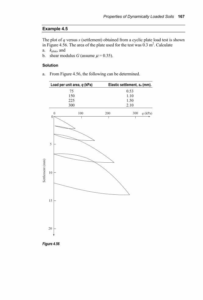
Properties of Dynamically Loaded Soils 167
Example 4.5
The plot of q versus s (settlement) obtained from a cyclic plate load test is shown in Figure 4.56. The area of the plate used for the test was 0.3 m2. Calculate a. kplate, and b. shear modulus G (assume μ = 0.35).
Solution
a. From Figure 4.56, the following can be determined.
Load per unit area, q (kPa) Elastic settlement, se (mm). 75 0.53 150 1.10 225 1.50
300 2.10
Figure 4.56

168 Chapter 4
Figure 4.57
Figure 4.57 shows a plot of q versus se. From the average plot,
Cz = 3000.0021e
qs
= = 142.86 MN/m3
From Eq. (4.92)
kplate = e
qAs
= (142.86)(0.3) = 42.86 MN/m.
b. From Eq. (4.96)
G = (1 ) (1 0.35)(142.86 ) ( 0.3)2.26 2.26
zC Aμ− −=
≈ 22.5 MPa This method can be extremely useful in sandy soils, provided it is being preceded by a boring program. But this test may not give good results if a weak stratum lies below the significant depth of test plate, but within the significant depth of the foundation. The procedure is costly, particularly if the ground water level is near the foundation and ground water lowering becomes necessary.

Properties of Dynamically Loaded Soils 169
Correlations for Shear Modulus and Damping Ratio
4.18 Test Procedures for Measurement of Moduli and Damping Characteristics For design of machine foundations subjected to vibration, calculation of ground response during an earthquake, analysis of the stability of slopes during an earthquake, and other dynamic analysis of soil, it is required that the shear modulus and the damping ratio of the soil be known. The shear modulus G and the damping ratio D of soils are dependent on several factors, such as type of soil, confining pressure, level of dynamic strain, degree of saturation, frequency, and number of cycles of dynamic load application, magnitude of dynamic stress, and dynamic prestrain (Hardin and Black, 1968).
From the preceding discussions in this chapter, it is obvious that a wide variety of procedures, including laboratory and field tests, can be used to obtain the shear moduli and damping characteristics of soils. A summary of those test conditions, range of applicability, and the parameters obtained are given in Table 4.4. Based on these studies several correlations for estimation of G and D have evolved during the last 25 to 30 years. Some of these correlations are summarized in the following sections.
Table 4.4 Test Procedures for Measuring Moduli and Damping Characteristics (after Seed and Idriss, 1970)
General Approximate Properties procedure Test condition strain range determined Determination of Triaxial compression 10–2 to 5% Modulus; damping hysteretic stress- Simple shear 10–2 to 5% Modulus; damping strain relationships Torsional shear 10–2 to 5% Modulus; damping Forced vibration Longitudinal vibrations 10–4 to 10–2% Modulus; damping Torsional vibrations 10–4 to 10–2% Modulus; damping Shear vibrations—lab 10–4 to 10–2% Modulus; damping Shear vibration—field 10–4 to 10–2 % Modulus Free vibration tests Longitudinal vibrations 10–3 to 1% Modulus; damping Torsional vibrations 10–3 to 1% Modulus; damping Shear vibration—lab 10–3 to 1% Modulus; damping Shear vibration—field 10–3 to 1% Modulus Field wave velocity Comparison waves ≈ 5 × 10⁻⁴% Modulus measurements Shear waves ≈ 5 × 10⁻⁴% Modulus Rayleigh waves ≈ 5 × 10⁻⁴% Modulus Field seismic Measurement of motions Modulus; damping response at different levels in deposit

170 Chapter 4
In general, the shear-stress-versus-strain relationship for soils will be of the nature as shown in Figure 4.58. The following can be seen from this figure:
1. The shear modulus G decreases with the increased level of shear strain. 2. At a very low strain level, the magnitude of the shear modulus is maximum
(that is, G = Gmax). 3. The shear stress-versus-shear-strain relationship shown in Figure 4.58 can be
approximated as (Hardin and Drnevich, 1972)
max max1/ /G
gtg t¢=+ ¢
(4.97)
where τ = shear stress and γ ′ = shear strain.
Figure 4.58 Nature of variation of shear modulus with strain
Properties of Dynamically Loaded Soils 171
4.19 Shear Modulus and Damping Ratio in Sand Hardin and Richart (1963) reported the results of several resonant column tests conducted in dry Ottawa sand. The shear wave velocities su determined from some of these tests are shown in Figure 4.15. The peak-to-peak shear strain amplitude for these tests was 10–3 rad. From Figure 4.15 it may be seen that the values of su are independent of the gradation, grain-size distribution, and also the relative density of compaction. However, su is dependent on the void ratio e and the effective confining 0s and can be expressed by the following empirical relations:
su = (19.7 – 9.06 e) 1/ 40s for 0s ≥ 95.8 kPa (4.98)
and
su = (11.36 – 5.35 e) 0.30s for 0s < 95.8 kPa (4.99)
In Equations (4.98) and (4.99), the units of su and 0s are meters per second and newtons per square meter, respectively.
Several experimental results for shear wave velocity in extremely angular crushed quartz sands were also reported by Hardin and Richart (1963). Based on these results, the value of su for angular sands can be expressed by the empirical relation
1/40
2
(18.43 6.2 )
(m/s) (N/m )
s eu s= -
≠ ≠ (4.100)
Based on the shear wave velocity relations presented here, the shear modulus of sands for low amplitudes of vibration can be given by the following relations (Hardin and Black, 1968):
2
1/ 2max 0
6908 (2.17 )= (round-grained)1
eGe
s-+
(4.101)
and
2
1/ 2max 0
3230 (2.97 )= (angular-grained)1
eGe
s-+
(4.102)
172 Chapter 4
where Gmax and 0s are in kPa.
For a soil specimen subjected to a stress condition such that 1 2 3s s sπ π (where 1 2,s s and 3s are the major, intermediate, and minor effective principal stresses, respectively), note that the average effective confining pressure is
10 1 2 32 ( )s s s s= + + = effective octahedral stress
This value of 0s can be used in Eqs. (4.98) – (4.102). For field conditions at any given depth,
1s = effective vertical stress = us 2s = 3 0K us s=
where K0 = at-rest earth pressure coefficient ≈ 1 – sin φ (where φ = drained friction angle).
So
0s = 13[ 2 (1 sin )]u us s f+ -
= 3us (3 – 2sin φ) (4.103)
Several investigators (e.g, Weissman and Hart, 1961; Richart, Hall, and Lysmer (1962); Drnevich, Hall, and Richart, 1966; Silver and Seed, 1969; Hardin and Drnevich, 1972; Seed and Idriss, 1970; Shibata and Soelarno, 1975; and Iwasaki, Tatsuoka, and Takagi, 1976), have reported the results of shear modulus and damping ratio measurements using various types of test techniques. From these test results it appears that the shear modulus at a given strain level can be expressed as (Seed and Idriss, 1970)
0.52 0218.82 ( )G K s= (4.104)
where G and 0s are in kPa. For low strain amplitudes (γ ′ ≤ 10–4%), the preceding equation will be
0.5max 2(max) 0218.82 ( )G K s= (4.105)

Properties of Dynamically Loaded Soils 173
The magnitudes of K2(max) vary from about 30 for loose sands to about 75 for dense sands. Seed and Idriss (1970) recommended the following values of K2(max).
Relative density, RD (%) K2(max) 30 34 40 40 45 43 60 52 75 61 90 70
Hence,
2
max 2(max)
KG FG K
= ¢ (4.106)
Figure 4.59 shows the variation of F′ with shear strain γ ′(%) obtained from several studies. These values fall in a rather narrow band and, for all practical purposes, the average plot can be used for design and estimation purposes. Thus Eqs. (4.101), (4.102), (4.104), (4.105), and (4.106) can be combined to estimate the shear modulus at any required shear strain level.
Studies by Hardin and Drnevich (1972) and Seed and Idriss (1970) show that the damping ratios for sands are affected by factors such as (a) grain-size characteristics, (b) degree of saturation, (c) void ratio, (d) earth pressure coefficient at rest (K0), (e) angle of internal friction (φ), (f) number of stress cycles (N), (g) level of strain, and (h) effective confining pressure. The last two factors, however, have the major effect on the magnitude of the damping ratio. Figure 4.60 shows a compilation of past studies (Seed et al. 1986) to determine D. For most practical cases the average plot of the variation of D versus γ ′ can be used for most calculation purposes.
Based on tests on dry sands using a torsional simple shear device, Sherif, Ishibashi, Gaddah (1977) proposed the following relationship for damping ratio.
D = 050 0.08738
s- (73.3F – 53.3)(γ ′)0.3 (1.01 – 0.046 logN) (4.107)
where D = damping ratio (%) 0s = effective confining pressure (kPa) γ ′ = shear strain (%) F = sphericity factor of the soil grains N = number of cycles of strain application
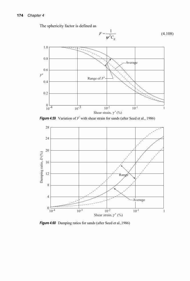
174 Chapter 4
The sphericity factor is defined as
F = 21
gCy (4.108)
Figure 4.59 Variation of F’ with shear strain for sands (after Seed et al., 1986)
Figure 4.60 Damping ratios for sands (after Seed et al.,1986)

Properties of Dynamically Loaded Soils 175
where
Cg = 230
10 60( )( )D
D D (4.109)
D10, D30, D60 = diameters, respectively, through which 10%, 30%, and 60% of the soil will pass
ψ = SS¢
where S′ and S are, respectively, the surface area of a sphere of the same volume as the soil particle and the actual surface area of the soil. Example 4.6
The ground water table in a normally consolidated sand layer is located at a depth of 3 m below the ground surface. The unit weight of sand above the groundwater table is 15.5 kN/m3. Below the groundwater table, the saturated unit weight of sand is 18.5 kN/m3. Assuming that the void ratio and effective angle of friction of sand below the groundwater table are 0.6 and 36°, respectively, determine the damping ratio and the shear modulus of this sand at a depth of 7.5 m below the ground surface if the strain is expected to be about 0.12%. Solution
From Eq. (4.103)
0s = 3υσ (3 – 2 sin φ)
us = 3(15.5) + 4.5(18.5 – 9.81) = 85.61 kPa
0s = 85.61 3
[3 – (2)(sin 36)] = 52.06 kPa
When φ is equal to 36°, RD is about 40 to 50%. Assuming RD ≈ 45%, K2(max) ≈ 43. So, from Eq. (4.105)
Gmax = 218.82 K2(max)( 0s )0.5 or Gmax = (218.82)(43)( 52.06)0.5
= 67,890 kPa ≈ 67.9 MPa
Referring to Figure 4.59, for γ ′ = 0.12%, the value of F′ is about 0.28. So

176 Chapter 4
G = F′Gmax = (0.28)( 67.9) ≈ 19 MPa
Referring to the average curve in Figure 4.60, for g ¢ = 0.12% D ≈ 17%
4.20 Correlation of Gmax of Sand with Standard Penetration Resistance The standard penetration test is used in soil-exploration programs in the United States and other countries. In granular soils the standard penetration numbers (N in blows/0.3 m) are widely used for the design of foundation. The standard penetration number can be correlated (Seed et al., 1986) in the following form to predict the maximum shear modulus:
0.34 0.4max 60 035 161.5 ( )
(kPa) (kPa)
G N s≈ ×
↑ ↑ (4.110)
where 0s = effective confining pressure (kPa) N60 = N-value measured in SPT test delivering 60% of the
theoretical free-fall energy to the drill rod
Equation (4.110) is very useful in predicting the variation of the maximum shear modulus with depth for a granular soil deposit.
4.21 Shear Modulus and Damping Ratio for Gravels Seed et al. (1986) provided the experimental results of several well-graded gravels. An example of such a study on well-graded Oroville material is shown in Figure 4.61. Based on several studies of this type, Seeds et al. concluded that Eqs. (4.105) and (4.106) can also be used to predict the variation of shear modulus with shear strain. However, the magnitude of K2(max) for gravels ranges between 80 to 180 (as compared to a range of 30 to 75 for sand). Thus,
0.5max 2(max) 0218.82 ( )
(kPa) (kPa)
G G F F K s= =¢ ¢
≠ ≠ (4.111)
The variation of F′ with the level of shear strain is shown in Figure 4.62.

Properties of Dynamically Loaded Soils 177
The equivalent damping ratio of gravelly soils determined in the laboratory from the hysteresis loops at the fifth cycle of each strain amplitude is shown in Figure 4.63. It can be seen that, for a given value of γ ′, the equivalent damping ratio increases with the increase of the relative density RD of the gravel. Seed et al. (1986) also observed that
a. there is not significant effect of gradation on the equivalent damping ratios of gravelly soil, and
b. the damping ratio is not significantly affected by the number of cycles at very small strain amplitudes. However it decreases to approximately three-fourths of its original value after 60 cycles at any axial strain amplitude of ± 0.2%.
Seed et al. showed that the range and the average plot of the damping ratio D with strain amplitude γ ′ for gravelly soils is approximately the same as that for sands (Figure 4.60).
Figure 4.61 Shear moduli of well-graded Oroville material (after Seed et al., 1986)

178 Chapter 4
Figure 4.62 Variation of F ¢ with shear strain for gravelly soils (after Seed et al., 1986)
Figure 4.63 Effect of relative density on damping ratio of gravelly soils (after Seeds et
al., 1986)
4.22 Shear Modulus and Damping Ratio for Clays For low amplitudes of strain, the shear modulus G = Gmax for clays of moderate sensitivity can be expressed in a modified form of Eq. (4.102) (Hardin and Drnevich, 1972):
21/2
max 03230(2.97 ) (OCR)
1
(kPa) (kPa)
KeGe
s-=+
≠ ≠ (4.112)

Properties of Dynamically Loaded Soils 179
where OCR = overconsolidation ratio and K = a constant = f(plasticity index, PI). Following are the recommended values of K for use in the preceding
equation.
Plasticity index, PI (%) K 0 0 20 0.18 40 0.30 60 0.41 80 0.48 ≥100 0.5
For field conditions
0s = 103 ( 2 )Ks s+v v (4.113)
where sv = effective vertical stress K0 = at-rest earth pressure coefficient
For normally consolidated clays (Booker and Ireland, 1965)
K0 = 0.4 + 0.007 (PI) (for 0 ≤ PI ≤ 40%) (4.114)
and
K0 = 0.68 + 0.001 (PI – 40) (for 40% ≤ PI ≤ 80%) (4.115)
In order to estimate the shear modulus at larger shear strain levels, Hardin and Drnevich (1972) suggested the following procedure. Referring to Figure 4.58,
G = tg ¢
and
Gmax = max
r
tg ¢
where rg ¢ = reference strain.

180 Chapter 4
Substituting the preceding relationship into Eq. (4.97), one obtains
G = max
1 / r
Gg g+ ¢ ¢
(4.116)
For real soils, the stress-strain relationship deviates somewhat from Eq. (4.116), and it can be modified as
max
1 h
GG
g=
+ ¢ (4.117)
where hg ¢ = hyperbolic strain
= ( )1 rb
rae g gg
g- ¢ ¢Ê ˆ¢ È ˘+Á ˜ Î ˚¢Ë ¯
(4.118)
where, for saturated cohesive soils,
a = 1 + 0.25 log N (4.119)
b = 1.3 (4.120)
N = number of cycles of loading
Figure 4.64 gives the variation of 1 2(0.145 kPa)r ug s¢ with the plasticity index for saturated cohesive soils. Once the magnitudes of hg ¢ and Gmax are calculated from Eqs. (4.118) and (4.112), they can be substituted in Eq. (4.117) to obtain G (at a strain level γ ′).
Hardin and Drnevich (1972) presented the relationship between the damping ratio and the shear modulus as
D = Dmaxmax
1 GG
Ê ˆ-Á ˜Ë ¯
(4.121)
where Dmax is the maximum damping ratio, which occurs when G = 0.
For saturated cohesive soils,
1/ 2 1/ 2max 0(%) 31 (0.3 0.003 ) 1.5 1.5(log )D f f Ns= - + + - (4.122)

Properties of Dynamically Loaded Soils 181
Figure 4.64 Reference strain for geostatic stress condition (after Hardin and Drnevich,
1972)
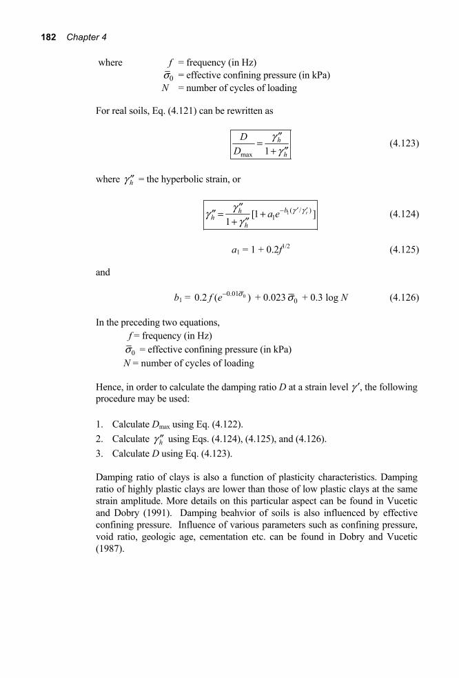
182 Chapter 4
where f = frequency (in Hz) 0s = effective confining pressure (in kPa) N = number of cycles of loading
For real soils, Eq. (4.121) can be rewritten as
max 1
h
h
DD
gg¢¢
=+ ¢¢
(4.123)
where hg ¢¢ = the hyperbolic strain, or
1( / )1[1 ]
1rbh
hh
a e g gggg
- ¢ ¢¢¢= +¢¢
+ ¢¢ (4.124)
a1 = 1 + 0.2f1/2 (4.125)
and
b1 = 00.010.2 ( )f e s- + 0.023 0s + 0.3 log N (4.126)
In the preceding two equations, f = frequency (in Hz) 0s = effective confining pressure (in kPa)
N = number of cycles of loading
Hence, in order to calculate the damping ratio D at a strain level γ ′, the following procedure may be used: 1. Calculate Dmax using Eq. (4.122). 2. Calculate hg ¢¢ using Eqs. (4.124), (4.125), and (4.126). 3. Calculate D using Eq. (4.123).
Damping ratio of clays is also a function of plasticity characteristics. Damping ratio of highly plastic clays are lower than those of low plastic clays at the same strain amplitude. More details on this particular aspect can be found in Vucetic and Dobry (1991). Damping beahvior of soils is also influenced by effective confining pressure. Influence of various parameters such as confining pressure, void ratio, geologic age, cementation etc. can be found in Dobry and Vucetic (1987).

Properties of Dynamically Loaded Soils 183
Correlation of Seed and Idriss Seed and Idriss (1970) collected the experimental results for shear modulus and damping ratio from various sources for saturated cohesive soils. Based on these results the variation of G/cu (where cu = undrained cohesion) with shear strain is shown in Figure 4.65. Also, Figure 4.66 shows the upper limit, average, and lower limit for the damping ratio at various strain levels.
Figure 4.65 In situ shear modulus for saturated clays (after Seed and Idriss, 1970)
Figure 4.66 Damping ratio for saturated clays (after Seed and Idriss, 1970)

184 Chapter 4
Example 4.7
A soil profile is shown in Figure 4.67a. Calculate and plot the variation of shear modulus with depth (for low amplitude of vibration).
Figure 4.67a
Solution
At any depth z 1
0 1 2 3 2 3 0 13 ( ) Ks s s s s s s= + + = =
where K0 is the coefficient of earth pressure at rest and 1s is the vertical effective pressure. For sands,
K0 = 1 – sin φ = 1 – sin 30° = 0.5 In layer II,
K0 = 1 – sin φ = 1 – sin 33° = 0.455 For normally consolidated clays,
K0 = 0.4 + 0.007(PI) for 0 ≤ PI ≤ 40 % = 0.4 + 0.007(48 – 23) = 0.575
Calculation of Effective Unit Weights z = 0 – 3.0 m:
dryg = effg = (2.65)(9.81)1 1 0.7
s wGe
γ=
+ + = 15.29 kN/m3
z = 3.0 – 4.5 m:
γeff = γsat – γw = ( )
1s wG e
eg+
+ – γw = 1
1sG
e−⎛ ⎞
⎜ ⎟+⎝ ⎠γw

Properties of Dynamically Loaded Soils 185
= (2.65 1) (9.81)1 0.6
−+
= 10.12 kN/m3
z = 4.5 – 6.0 m:
γeff = ( 1) (2.78 1) (9.81)1 1 1.22s wG
eγ− −
+ + = 7.87 kN/m3
The following table can now be prepared.
Depth z 1s 2 3 0 1= K=s s s 0s e G = Gmax (m) (kPa) (kPa) (kPa) (MPa) 0 0 0 0 0.7 0 1.5 15.29 x 1.5 11.47 15.29 0.7 34.34a = 22.94 3.0 15.29 x 3 22.94 30.58 0.7 48.56a (in layer I) = 45.87 3.0 45.87 20.87 29.20 0.6 57.51a (in layer II) 4.5 45.87 + 10.12 x 1.5 27.78 38.87 0.6 66.35a (in layer II) = 61.05 4.5 61.05 35.10 43.75 1.22 29.47b (in layer III) 6.0 61.05 + 7.87 x 1.5 41.89 52.21 1.22 32.20b
= 72.86 aEq. (4.101) bEq. (4.112)
The variation of G = Gmax with depth is plotted in Figure (4.67b).
Figure 4.67b

186 Chapter 4
4.23 Shear Modulus and Damping Ratio for Lightly Cemented Sand Lightly cemented sand deposits are encountered in many parts of the world. The cementing material in the sand deposits is primarily calcium carbonate. More recently, the results of several research projects relating to the properties of lightly cemented sands have been published. From these studies it appears that the behavior of lightly cemented sands can be duplicated in the laboratory by mixing sand and Portland cement in required properties. The maximum sheer modulus can be expressed as (Saxena, Avramidis, and Reddy, 1988)
Gmax(CS) = Gmax(S) + ΔGmax(C) (4.127)
where Gmax(CS) = maximum shear modulus of lightly cemented sand Gmax(S) = maximum shear modulus of sand alone
ΔGmax(C) = increase of maximum shear modulus due to cementation effect
According to Saxena, Avramidis, and Reddy, the magnitudes of Gmax(S) and ΔGmax(C) can be obtained from the following empirical relationships.
0.426 0.574max( ) 02
428.2 ( ) ( )0.3 0.7
(kPa) (kPa) (kPa)
S aG Pe
s=+
≠ ≠ ≠ (4.128)
where Pa = atmospheric pressure in the same units as Gmax(S).
max( )C
a
GP
D = 172
( 0.5168)e - (CC)0.88
0.515 0.13 0.2850
e CC
aPs
- +Ê ˆÁ ˜Ë ¯
(for CC < 2%) (4.129)
max( )C
a
GP
D=
0.698 0.04 0.21.2 0773 ( )
e CC
aCC
e Ps
- -Ê ˆÁ ˜Ë ¯
(for 2% ≤ CC ≤ 8%) (4.130)
where CC = cement content (in percent) and e = void ratio.
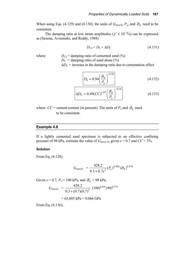
Properties of Dynamically Loaded Soils 187
When using Eqs. (4.129) and (4.130), the units of Gmax(S), Pa, and 0s need to be consistent.
The damping ratio at low strain amplitudes (γ ′ ≤ 10–3%) can be expressed as (Saxena, Avramidis, and Reddy, 1988)
DCS = DS + ΔDC (4.131)
where DCS = damping ratio of cemented sand (%) DS = damping ratio of sand alone (%) ΔDC = increase in the damping ratio due to cementation effect
0.38
00.94Sa
DPs
-Ê ˆ= Á ˜Ë ¯
(4.132)
0.36
1.07 00.49( )Ca
D CCPs
-Ê ˆD = Á ˜Ë ¯
(4.133)
where CC = cement content (in percent). The units of Pa and 0s need to be consistent.
Example 4.8
If a lightly cemented sand specimen is subjected to an effective confining pressure of 98 kPa, estimate the value of Gmax(CS), given e = 0.7 and CC = 3%.
Solution
From Eq. (4.128),
Gmax(S) = 0.426 0.57402
428.2 ( ) ( )0.3 0.7 aP
es
+
Given e = 0.7, Pa = 100 kPa, and 0s = 98 kPa,
Gmax(S) = 2428.2
0.3 (0.7)(0.7)+ (100)0.426 (98)0.574
= 65,805 kPa = 0.066 GPa
From Eq. (4.136),
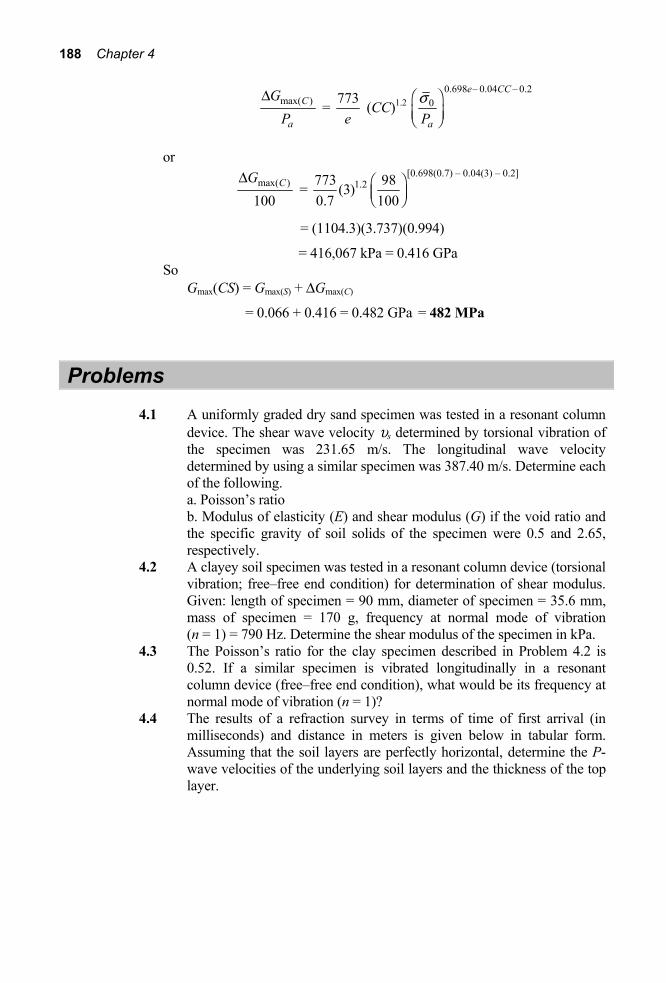
188 Chapter 4
max( )C
a
GP
D = 773
e (CC)1.2
0.698 – 0.04 – 0.20
e CC
aPsÊ ˆÁ ˜Ë ¯
or
max( )
100CGD
= [0.698(0.7) – 0.04(3) – 0.2]
1.2773 98(3)0.7 100
Ê ˆÁ ˜Ë ¯
= (1104.3)(3.737)(0.994)
= 416,067 kPa = 0.416 GPa So Gmax(CS) = Gmax(S) + ΔGmax(C)
= 0.066 + 0.416 = 0.482 GPa = 482 MPa
Problems 4.1 A uniformly graded dry sand specimen was tested in a resonant column
device. The shear wave velocity υs determined by torsional vibration of the specimen was 231.65 m/s. The longitudinal wave velocity determined by using a similar specimen was 387.40 m/s. Determine each of the following.
a. Poisson’s ratio b. Modulus of elasticity (E) and shear modulus (G) if the void ratio and
the specific gravity of soil solids of the specimen were 0.5 and 2.65, respectively.
4.2 A clayey soil specimen was tested in a resonant column device (torsional vibration; free–free end condition) for determination of shear modulus. Given: length of specimen = 90 mm, diameter of specimen = 35.6 mm, mass of specimen = 170 g, frequency at normal mode of vibration (n = 1) = 790 Hz. Determine the shear modulus of the specimen in kPa.
4.3 The Poisson’s ratio for the clay specimen described in Problem 4.2 is 0.52. If a similar specimen is vibrated longitudinally in a resonant column device (free–free end condition), what would be its frequency at normal mode of vibration (n = 1)?
4.4 The results of a refraction survey in terms of time of first arrival (in milliseconds) and distance in meters is given below in tabular form. Assuming that the soil layers are perfectly horizontal, determine the P-wave velocities of the underlying soil layers and the thickness of the top layer.

Properties of Dynamically Loaded Soils 189
Distance Time of first (m) arrival (ms)
7.5 49.08 15.0 81.96 23.0 122.8 30.5 148.2 45.5 174.2 61.0 202.8 76.0 228.6
91.5 256.7
4.5 Repeat Problem 4.4 for the following Comment regarding the material encountered in the second layer.
Distance Time of first Distance Time of first (m) arrival (ms) (m) arrival (ms)
10 19.23 100 125.82 20 38.40 150 138.72 30 57.71 200 152.61 40 76.90 250 166.81 60 115.40 300 178.31
80 120.71
4.6 Repeat Problem 4.4 with the following results. Also determine the thickness of the second layer of soil encountered.
Distance Time of first Distance Time of first (m) arrival (ms) (m) arrival (ms)
10 41.66 60 119.21 15 62.51 70 128.11 20 83.37 80 136.22 30 91.82 90 141.00 40 101.22 100 143.81
50 110.16 120 152.00
4.7 The results of a reflection survey are given here. Determine the velocity of P-waves in the top layer and its thickness.
Distance from Time for first arrival shot point (m) of reflected wave (ms)
10 32.5 20 39.05 30 48.02 40 58.3 60 80.78
100 128.55

190 Chapter 4
4.8 Refer to Figure 4.43 for the results of the following refraction survey:
Distance from Time of Distance from Time of point of first point of first disturbance, arrival disturbance, arrival
A (m) (ms) E (m) (ms) 0 0 0 0 6.0 20 6.0 20 12.0 40 12.0 40.1 18.0 60 18.0 59.8 24.5 78.2 24.5 79.7 36.5 92.8 36.5 121.0 61.0 122.2 61.0 167.2 85.5 149.8 85.5 175.1 Point E 110.0 177.9 Point A 110.0 180.2
Determine: a. the P-wave velocities in the two layers, b. z′ and z′′, and c. the angle β. 4.9 For a reflection survey refer to Figure 4.48, in which A is the shot point.
Distance AC = AE = 180 m. The times for arrival of the first reflected wave at points C and E are 45.0 ms and 64.1 ms, respectively. If the P-wave velocity in layer 1 is 280 m/s, determined β and z′.
4.10 The results of a subsoil exploration by steady-state vibration technique are given here (Section 4.15)
Distance from Number of Frequency of the plate waves vibration of vibrated x (m) per second the plate (Hz) 10 41.00 900 10 18.00 400 10 9.00 200 10 4.55 100 10 2.65 90 10 2.30 75 10 1.77 60 10 1.47 50
Make necessary calculations and plot the variation of the wave velocity with depth.
4.11 An angular-grained sand has maximum and minimum void ratios of 1.1 and 0.55, respectively. Using Eq. (4.102), determine and plot the variation of maximum shear modulus Gmax versus relative density

Properties of Dynamically Loaded Soils 191
(RD = 0 – 100%) for mean confining pressures of 50, 100, 150, 200 and 300 kPa.
4.12 A 20-m-thick sand layer in the field is underlain by rock. The groundwater table is located at a depth of 5 m measured from the ground surface. Determine the maximum shear modulus of this sand at a depth of 10 m below the ground surface. Given: void ratio = 0.6, specific gravity of soil solids = 2.68, angle of friction of sand = 36°. Assume the sand to be round-grained.
4.13 For a deposit of sand, at a certain depth in the field the effective vertical pressure is 120 kPa. The void ratio and the relative density are 0.72 and 30° respectively. Determine the shear modulus and damping ratio for a shear strain levels of 5 × 10⁻²%.
4.14 A remolded clay specimen was consolidated by a hydrostatic pressure of 205 kPa. The specimen was then allowed to swell under a hydrostatic pressure of 105 kPa. The void ratio at the end of swelling was 0.8. If this clay is subjected to a torsional vibration in a resonant column test, what would be its maximum shear modulus (Gmax)? These liquid and plastic limits of the clay are 58 and 28, respectively.
4.15 Refer to Figure P4.15. Given: H1 = 2 m Gs(1) = 2.68 H2 = 8 m Gs(2) = 2.65 H3 = 3 m φ1 = 35° e1 = 0.6 φ2 = 30° e2 = 0.7 PI of clay = 32 Estimate and plot the variation of the maximum shear modulus (Gmax)
with depth for the soil profile
Figure P4.15

192 Chapter 4
4.16 Repeat Problem 4.15 given H1 = H2 = H3 = 6 m Gs(1) = Gs(2) = 2.66 e1 = 0.88 φ1 = 28° e2 = 0.68 φ2 = 32° PI of clay = 20 4.17 A layer of clay deposit extends to a depth of 15.0 m below the ground
surface. The groundwater table coincides with the ground surface. Given, for the clay: void ratio = 1.0, specific gravity of soil solids = 2.78, plasticity index = 25%, over consolidation ratio = 2. Determine the shear modulus and damping ratio of this clay at a depth of 7.5 m for the fifth cycle at a strain level 0.1%, assuming that the frequency (f) is about 1 Hz. (Note: Use Figure 4.64) Given:
K0(overconsol.) ≈ K0(norm consol) ( OCR )
4.18 The unit weight of a sand deposit is 16.98 kN/m3 at a relative density of 60%. Assume that, for this sand
φ = 30 + 0.15RD where φ is the drained friction angle and RD is the relative density (in
percent). At a depth of 6.09 m below the ground surface, estimate its shear modulus and damping ratio at a shear strain level of 0.01%. Use the equation proposed by Seed and Idriss (1970).
4.19 The results of a standard unconsolidated drained triaxial test on a undisturbed saturated clay specimen are as follows:
Confining pressure = 70 kPa Total axial stress at failure = 166.6 kPa Using the method proposed by Seed the Idriss (1970), determine and
plot the variation of shear modulus and damping ratio with shear strain (strain range 10–3% to 1%).
4.20 For example 4.8, determine the damping ratio of the cemented sand.
References Barkan, D. D. (1962), Dynamics of Bases and Foundations, McGraw-Hill Book
Company, New York. Beston, H. E., and McEvilly, T. V. (1977). “Shear Wave Velocities from Down
Hole Measurements,” Journal of the International Association for Earthquake Engineering, Vol. 5, No. 2, pp. 181–190.
Booker, E. W., and Ireland, H. O. (1965). “Earth Pressure at Rest Related to Stress History,” Canadian Geotechnical Journal, Vol. 2, No. 1, pp. 1–15.

Properties of Dynamically Loaded Soils 193
Carroll, W. F. (1963), “Dynamic Bearing Capacity of Soils. Vertical Displacements of Spread Footing on Clay: Static and Impulsive Loadings,” Technical Report No. 3–599, Report 5, U.S. Army Corps of Engineers, Waterways Experiment Station, Vicksburg, Mississippi.
Casagrande, A., and Shannon, W. L. (1949). “Strength of Soils under Dynamic Loads,” Transactions, ASCE, Vol. 114, pp. 755–772.
Das, B. M. (1990). Principles of Geotechnical Engineering, 2nd ed., PWS-KENT, Boston.
Dobry, R., and Vucetic, M. (1987). “Dynamic Properties and Seismic Response of Soft Clay Deposits,”, Proceedings, International Symposium on Geotechnical Engineering of Soft Clays, Mexico City, Vol. 2, pp. 51 – 87.
Drnevich, V. P. (1972). “Undrained Cyclic Shear of Saturated Sand,” Journal of the Soil Mechanics and Foundations Division, ASCE, Vol. 98, No. SM8,
807–825. Drnevich, V. P., Hall, J. R., Jr., and Richart F. E., Jr. (1966). “Large Amplitude
Vibration Effects on the Shear Modulus of Sand,” University of Michigan Report to Waterways Experiment Station, Corps of Engineers, U.S. Army Contact DA-22-079-Eng-340, October 1966.
Drnevich, V. P., Hall, J.R., Jr., and RicharAmplitude of Vibration on the Shear Modulus of Sand,” Proceedings of the International Symposium on Wave Propagation and Dynamic Properties of Earth Materials, Ed. G. E. Triandafilidis, University of New Mexico Press, pp. 189–199.
Hall, J. R., Jr., and Richard, F. E., Jr. (1963). “Discussion of Elastic Wave Energy in Granular Soils,” Journal of the Soil Mechanics and Foundations Division, ASCE, Vol. 89, No. SM6, pp. 27–56.
Hardin, B. O. (1965). “The Nature of Damping of Sands,” Journal of the Soil Mechanics and Foundations Division, ASCE, Vol. 91, No. SM1, pp. 63–97.
Hardin, B. O., and Black, W. L. (1968). “Vibration Modulus of Normally Consolidated Clays,” Journal of the Soil Mechanics and Foundations Division, ASCE, Vol. 94, No. SM2, pp. 353-369.
Hardin, B. O., and Drnevich, V. P.(1972). “Shear Modulus and Damping in Soils: Design Equations and Curves,” Journal of Soil Mechanics and Foundations Division, ASCE, Vol. 98, No. SM7, pp. 667–692.
Hardin, B. O., and Richard, F. E., Jr. (1963). “Elastic Wave Velocity in Granular Soils,” Journal of the Soil Mechanics and Foundations Division, ASCE, Vol. 89, No. SM1, pp. 33-65.
Heukelom, W., and Foster, C. R. (1960). “Dynamic Testing of Pavements,” Journal of the Soil Mechanics and Foundation Division, ASCE, Vol. 86,
SM1, Part 1, pp. 1–28. Iida, K. (1938). “The Velocity of Elastic Waves in Sand,” Bulletin of the
Earthquake Research Institute, Tokyo Imperial University, Vol. 16, pp. 131–144.
With permission from ASCE.
With permission from ASCE.
With permission from ASCE.
With permission from ASCE.
With permission from ASCE.
With permission from ASCE.
pp.
No.
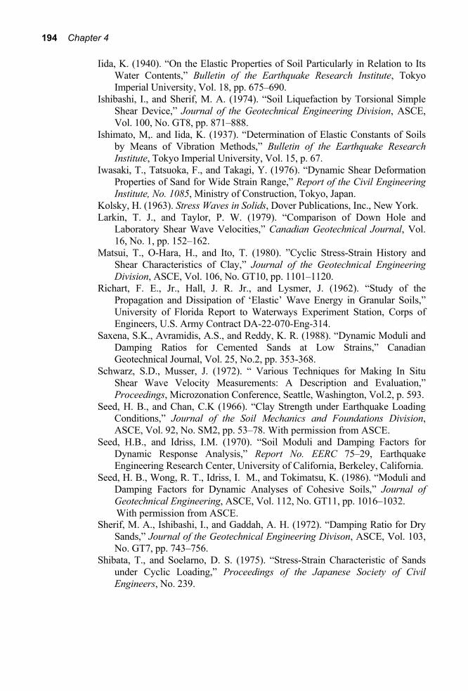
194 Chapter 4
Iida, K. (1940). “On the Elastic Properties of Soil Particularly in Relation to Its Water Contents,” Bulletin of the Earthquake Research Institute, Tokyo Imperial University, Vol. 18, pp. 675–690.
Ishibashi, I., and Sherif, M. A. (1974). “Soil Liquefaction by Torsional Simple Shear Device,” Journal of the Geotechnical Engineering Division, ASCE, Vol. 100, No. GT8, pp. 871–888.
Ishimato, M,. and Iida, K. (1937). “Determination of Elastic Constants of Soils by Means of Vibration Methods,” Bulletin of the Earthquake Research Institute, Tokyo Imperial University, Vol. 15, p. 67.
Iwasaki, T., Tatsuoka, F., and Takagi, Y. (1976). “Dynamic Shear Deformation Properties of Sand for Wide Strain Range,” Report of the Civil Engineering Institute, No. 1085, Ministry of Construction, Tokyo, Japan.
Kolsky, H. (1963). Stress Waves in Solids, Dover Publications, Inc., New York. Larkin, T. J., and Taylor, P. W. (1979). “Comparison of Down Hole and
Laboratory Shear Wave Velocities,” Canadian Geotechnical Journal, Vol. 16, No. 1, pp. 152–162.
Matsui, T., O-Hara, H., and Ito, T. (1980). ”Cyclic Stress-Strain History and Shear Characteristics of Clay,” Journal of the Geotechnical Engineering Division, ASCE, Vol. 106, No. GT10, pp. 1101–1120.
Richart, F. E., Jr., Hall, J. R. Jr., and Lysmer, J. (1962). “Study of the Propagation and Dissipation of ‘Elastic’ Wave Energy in Granular Soils,” University of Florida Report to Waterways Experiment Station, Corps of Engineers, U.S. Army Contract DA-22-070-Eng-314.
Saxena, S.K., Avramidis, A.S., and Reddy, K. R. (1988). “Dynamic Moduli and Damping Ratios for Cemented Sands at Low Strains,” Canadian Geotechnical Journal, Vol. 25, No.2, pp. 353-368.
Schwarz, S.D., Musser, J. (1972). “ Various Techniques for Making In Situ Shear Wave Velocity Measurements: A Description and Evaluation,” Proceedings, Microzonation Conference, Seattle, Washington, Vol.2, p. 593.
Seed, H. B., and Chan, C.K (1966). “Clay Strength under Earthquake Loading Conditions,” Journal of the Soil Mechanics and Foundations Division, ASCE, Vol. 92, No. SM2, pp. 53–78.
Seed, H.B., and Idriss, I.M. (1970). “Soil Moduli and Damping Factors for Dynamic Response Analysis,” Report No. EERC 75–29, Earthquake Engineering Research Center, University of California, Berkeley, California.
Seed, H. B., Wong, R. T., Idriss, I. M., and Tokimatsu, K. (1986). “Moduli and Damping Factors for Dynamic Analyses of Cohesive Soils,” Journal of Geotechnical Engineering, ASCE, Vol. 112, No. GT11, pp. 1016–1032.
Sherif, M. A., Ishibashi, I., and Gaddah, A. H. (1972). “Damping Ratio for Dry Sands,” Journal of the Geotechnical Engineering Divison, ASCE, Vol. 103, No. GT7, pp. 743–756.
Shibata, T., and Soelarno, D. S. (1975). “Stress-Strain Characteristic of Sands under Cyclic Loading,” Proceedings of the Japanese Society of Civil Engineers, No. 239.
With permission from ASCE.
With permission from ASCE.

Properties of Dynamically Loaded Soils 195
Silver, M. L. (1981), “Load Deformation and Strength Behavior of Soils Under Loading,” State-of-the-Art-Paper, Proceedings of the International Conference on Recent Advances in Geotechnical Earthquake Engineering and Soil Dynamics, Vol. 3, pp. 873–896.
Silver, M. L., and Seed, H. B.(1969). “The Behavior of Sands under Seismic Loading Conditions,” Report No. EERC 69–16, Earthquake Engineering Research Center, University of California, Berkeley, California.
Silver, M. L., and Seed, H. B (1971). “Deformation Characteristics of Sands under Cyclic Loading,” Journal of the Soil Mechanics and Foundation Division, ASCE, Vol. 94, No. SM8, pp. 1081–1098.
Stokoe, K. H., and Woods, R. D. (1972), “In Situ Shear Wave Velocity by Cross-Hole Method,” Journal of Soil Mechanics and Foundations Division, ASCE, Vol. 98, No. SM5, pp. 443–460.
Terzaghi, K. (1955). “Evaluation of Coefficient of Subgrade Reaction,” Geotechnique, No. 5, pp. 297-326.
Thiers, G, R., and Seed, H. B. (1968). “Cyclic Stress-Strain Characteristics of Clay,” Journal of the Soil Mechanics and Foundations Division, ASCE, Vol. 94, No. SM6, pp. 555–569.
Vesic, A. S. (1973). “Analysis of Ultimate Loads of Shallow Foundations,” Journal of the Soil Mechanics and Foundations Division, ASCE, Vol. 99, No. SM1, pp. 45–73.
Vucetic, M., and Dobry, R. (1991). “Effect of Soil Plasticity on Cyclic Response”, Journal of Geotechnical Engineering, ASCE, Vol. 117, No. 1, pp. 89–107.
Weissman, G. F., and Hart, R. R. (1961). “The Damping Capacity of Some Granular Soils,” ASTM Special Technical Publication No. 305, Symposium of Soil dynamics, pp. 45–54.
Whitman, R. V. and Healy, K. A. (1963). “Shear Strength of Sands During Rapid Loadings,” Transactions, ASCE, Vol. 128, Part 1, pp. 1553–1594.
Whitman, R. V. and Lawrence, F. V. (1963). “Discussion on Elastic Wave Velocities in Granular Soils,” Journal of the Soil Mechanics and Foundations Division, ASCE, Vol. 89, No. SM5, pp. 112–118.
Wilson, S. D. and Dietrich, R. J. (1960). “Effect of Consolidation Pressure on Elastic and Strength Properties of Clay,” Proceedings of the Research Conference on Shear Strength of Cohesive Soils, ASCE, pp. 419-435.
With
rom ASCE. fmission
With permission from ASCE.
With permission from ASCE.
With permission from ASCE.
,
,per

196
5 Foundation Vibration
5.1 Introduction In Chapter 2 (Figure 2.1), it was briefly mentioned that foundations supporting vibrating equipment do experience rigid body displacements. The cyclic displacement of a foundation can have six possible modes. They are
1. translation in the vertical direction, 2. translation in the longitudinal direction, 3. translation in the lateral direction, 4. rotation about the vertical axis (that is, yawing), 5. rotation about the longitudinal axis (that is, rocking), and 6. rotation about the lateral axis (that is, pitching).
In this chapter, the fundamentals of the vibration of foundations, in various modes, supported on an elastic medium will be developed. The elastic medium that supports the foundation will be considered to be homogeneous and isotropic. In general, the behaviour of soils departs considerably from that of an elastic material; only at low strain levels may it be considered as a reasonable approximation to an elastic material. Hence, the theories developed here should be considered as applicable only to the cases where foundations undergo low amplitudes of vibration.
5.2 Vertical Vibration of Circular Foundations Resting on Elastic Half-Space—Historical Development In 1904, Lamb studied the problem of vibration of a single vibrating force acting at a point on the surface of an elastic half-space. This study included cases in which the oscillating force R acts in the vertical direction and in the horizontal
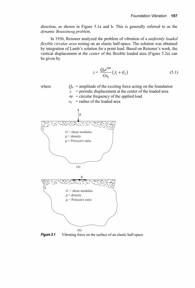
Foundation Vibration 197
direction, as shown in Figure 5.1a and b. This is generally referred to as the dynamic Boussinesq problem.
In 1936, Reissner analyzed the problem of vibration of a uniformly loaded flexible circular area resting on an elastic half-space. The solution was obtained by integration of Lamb’s solution for a point load. Based on Reissner’s work, the vertical displacement at the center of the flexible loaded area (Figure 5.2a) can be given by
z = ( )01 2
0
i tQ ef if
Gr
w+ (5.1)
where Q0 = amplitude of the exciting force acting on the foundation z = periodic displacement at the center of the loaded area w = circular frequency of the applied load r0 = radius of the loaded area
Figure 5.1 Vibrating force on the surface of an elastic half-space

198 Chapter 5
Figure 5.2 (a) Vibration of a uniformly loaded circular flexible area; (b) flexible circular foundation subjected to forced vibration
G = shear modulus of the soil Q = exciting force, which has an amplitude of Q0 f1, f2 = Reissner’s displacement functions
The displacement functions f1 and f2 are related to the Poisson’s ratio of the medium and the frequency of the exciting force.
Now, consider a flexible circular foundation of weight W (mass = m = W/g) resting on an elastic half-space and subjected to an exciting force of magnitude of ( )
0i tQ e w a+ , as shown in Figure 5.2b. (Note: α is the phase difference between
the exciting force and the displacement of the foundation.)
Using the displacement relation given in Eq. (5.1) and solving the equation of equilibrium of force, Reissner obtained the following relationships:
Az = QGr
0
0Z (5.2)
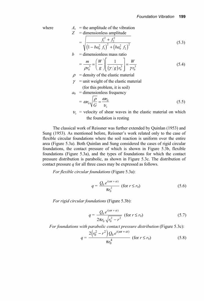
Foundation Vibration 199
where Az = the amplitude of the vibration Z = dimensionless amplitude
= f f
ba f ba f12
22
02
12
02
22
1
+
- +c h c h (5.3)
b = dimensionless mass ratio
= ( )3 3 3
0 0 0
1m W Wgr g r rr g g
È ˘Ê ˆ= =Í ˙Á ˜Ë ¯ Í ˙Î ˚
(5.4)
r = density of the elastic material g = unit weight of the elastic material (for this problem, it is soil) a0 = dimensionless frequency
= 00
s
rr
Gwrwu
= (5.5)
su = velocity of shear waves in the elastic material on which the foundation is resting
The classical work of Reissner was further extended by Quinlan (1953) and Sung (1953). As mentioned before, Reissner’s work related only to the case of flexible circular foundations where the soil reaction is uniform over the entire area (Figure 5.3a). Both Quinlan and Sung considered the cases of rigid circular foundations, the contact pressure of which is shown in Figure 5.3b, flexible foundations (Figure 5.3a), and the types of foundations for which the contact pressure distribution is parabolic, as shown in Figure 5.3c. The distribution of contact pressure q for all three cases may be expressed as follows.
For flexible circular foundations (Figure 5.3a):
q = ( )
02
0
i tQ er
w α+
π (for r ≤ r0) (5.6)
For rigid circular foundations (Figure 5.3b):
q = ( )
02 2
0 02
i tQ e
r r r
w a+
p - (for r ≤ r0) (5.7)
For foundations with parabolic contact pressure distribution (Figure 5.3c):
q = ( )2 2 ( )
0 04
0
2 i tr r Q e
r
w a+-
p (for r ≤ r0) (5.8)
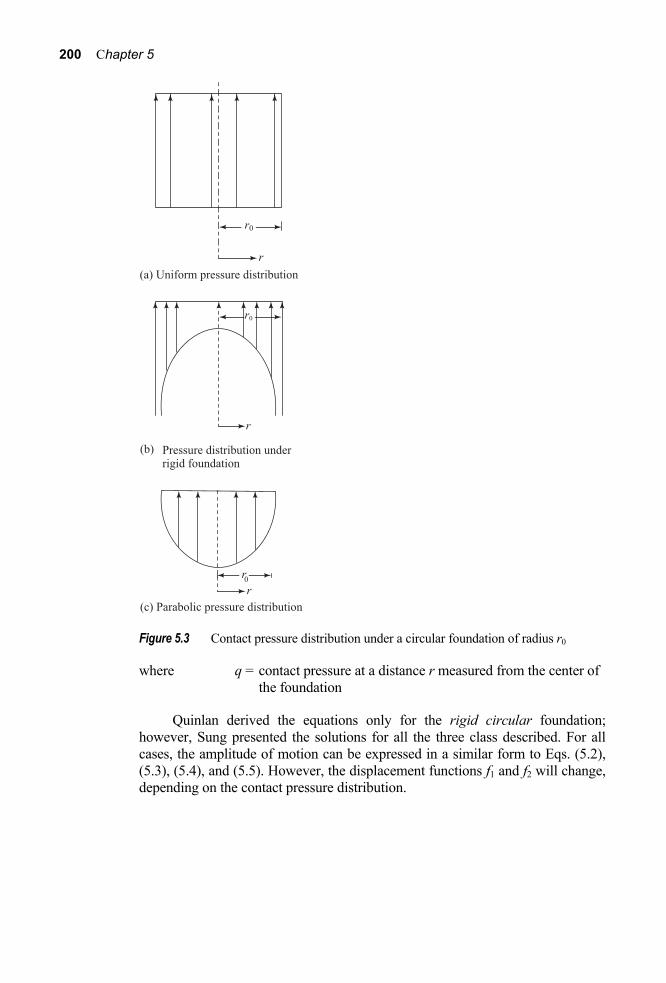
200 Chapter 5
Figure 5.3 Contact pressure distribution under a circular foundation of radius r0
where q = contact pressure at a distance r measured from the center of the foundation
Quinlan derived the equations only for the rigid circular foundation; however, Sung presented the solutions for all the three class described. For all cases, the amplitude of motion can be expressed in a similar form to Eqs. (5.2), (5.3), (5.4), and (5.5). However, the displacement functions f1 and f2 will change, depending on the contact pressure distribution.

Foundation Vibration 201
Foundations, on some occasions, may be subjected to a frequency-dependent excitation, in contrast to the constant-force type of excitation just discussed. Figure 5.4 shows a foundation excited by two rotating masses. The amplitude of the exciting force can be given as
2 212 eQ m e m ew w= = (5.9)
where m1 = total of the rotating masses w = circular frequency of the rotating masses
For this condition, the amplitude of vibration Az may be given by the relation
Az = ( ) ( )
2 2 21 1 2
2 22 20 0 1 0 21
m e f fGr ba f ba f
w +
- + (5.10)
From Eq. (5.5)
0 0a rGrw=
or
2
2 02
0
a Gr
wr
= (5.11)
Figure 5.4 Foundation vibration by a frequency-dependent exciting force

202 Chapter 5
Substituting Eq. (5.11) into (5.10), one obtains
Az = ( ) ( )
2 2 21 0 1 2 1
3 2 2 32 20 00 1 0 21
m ea f f m e Zr rba f ba fr r
+= ¢
- + (5.12)
where Z ¢ = dimensionless amplitude
= a f fba f ba f
02 1
222
02
12
02
22
1
+
- +c h c h (5.13)
Figures 5.5 and 5.6 show the plots of the variation of the dimensionless amplitude with a0 (Richart, 1962) for rigid circular foundations (for μ = Poisson’s ratio = 0.25 and b = 5, 10, 20, and 40).
Figure 5.5 Plot of Z versus a0 for rigid circular foundation (after Richart, 1962)

Foundation Vibration 203
Figure 5.6 Variation of Z′ with a0 for rigid circular foundation (redrawn after Richart,
1962)
Effect of Contact Pressure Distribution and Poisson’s Ratio The effect of the contact pressure distribution on the nature of variation of the nondimensional amplitude Z′ with a0 is shown in Figure 5.7 (for b = 5 and μ = 0.25). As can be seen, for a given value of a0, the magnitude of the amplitude is highest for the case of parabolic pressure distribution and lowest for rigid bases.

204 Chapter 5
For a given type of pressure distribution and mass ratio (b), the magnitude of Z′ also greatly depends on the assumption of the Poisson’s ratio μ. This is shown in Figure 5.8.
Figure 5.7 Effect of contact pressure distribution variation of Z ¢ with a0 (redrawn after
Richart and Whitman, 1967)
Figure 5.8 Effect of Poisson’s ratio on the variation of Z ¢ with a0 (redrawn after
Richart and Whitman, 1967)

Foundation Vibration 205
Figure 5.9 Variation of the displacement functions with a0 and μ
Variation of Displacement Functions f1 and f2 As mentioned before, the displacement functions are related to the dimensionless frequency a0 and Poisson’s ratio μ. In Sung’s original study, it was assumed that the contact pressure distribution remains the same throughout the range of frequency considered; however, for dynamic loading conditions, the rigid-base pressure distribution does not produce uniform displacement under the foundation. For that reason, Bycroft (1956) determined the weighted average of the displacements under a foundation. The variation of the displacement functions determined by the study is shown in Figure 5.9.
5.3 Analog Solutions for Vertical Vibration of Foundations
Hsieh’s Analog Hsieh (1962) attempted to modify the original solution of Reissner in order to develop an equation similar to that for damped vibrations of single-degree free

206 Chapter 5
system [Eq. (2.72)]. Hsieh’s analog can be explained with reference to Figure 5.10. Consider a rigid circular weightless disc on the surface of an elastic half-space. The disc is subjected to a vertical vibration by a force
P = 0i tP e w (5.14)
The vertical displacement of the disk can be given by Eq. (5.1) as
z = 0
0
i tP eGr
w
(f1 + if2)
Now,
dzdt
= 0
0
i tP eGr
ww (if1 − f2) (5.15)
or
1f zw − f2 dzdt
= 2 201 2
0( ) i tP
f f eGr
ww+
Since P = 0i tP e w , the preceding relationship can be written as
1f zw − f2 dzdt
= 2 21 2
0( )P f f
Grw +
or
P = 10 2 2
1 2
( )
zk
fGrf f
È ˘Ê ˆÍ ˙Á ˜+Ë ¯Í ˙Î ˚
z + 0 22 2
1 2
z
Gr f dzdtf f
cw
È ˘Ê ˆ-Ê ˆÍ ˙Á ˜ Á ˜Ë ¯ +Ë ¯Í ˙Î ˚
So z zP k z c z= + (5.16)
Now consider a rigid circular foundation having a mass m and radius r0 placed on the surface of the elastic half-space (Figure 5.10b). The foundation undergoes vibration by a periodic force
Q = 0i tQ e w (5.17)
For dynamic equilibrium mz Q P= - (5.18)
Combining Equations (5.16), (5.17) and (5.18)
0i t
z zmz c z k z Q e w+ + = (5.19)
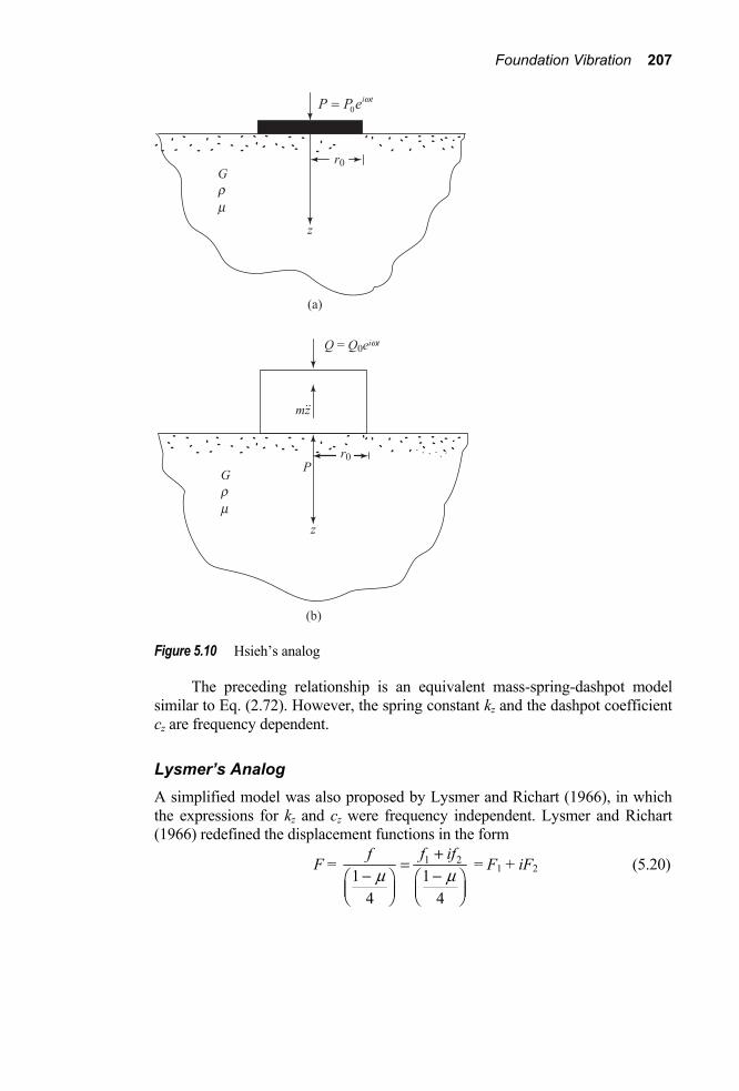
Foundation Vibration 207
Figure 5.10 Hsieh’s analog
The preceding relationship is an equivalent mass-spring-dashpot model similar to Eq. (2.72). However, the spring constant kz and the dashpot coefficient cz are frequency dependent.
Lysmer’s Analog A simplified model was also proposed by Lysmer and Richart (1966), in which the expressions for kz and cz were frequency independent. Lysmer and Richart (1966) redefined the displacement functions in the form
F = 1 2
1 14 4
f iffm m
+=
- -Ê ˆ Ê ˆÁ ˜ Á ˜Ë ¯ Ë ¯
= F1 + iF2 (5.20)
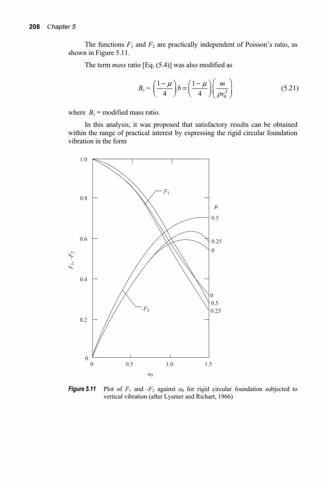
208 Chapter 5
The functions F1 and F2 are practically independent of Poisson’s ratio, as shown in Figure 5.11.
The term mass ratio [Eq. (5.4)] was also modified as
Bz = 30
1 14 4
mbr
m mr
Ê ˆ- -Ê ˆ Ê ˆ=Á ˜ Á ˜ Á ˜Ë ¯ Ë ¯ Ë ¯ (5.21)
where Bz = modified mass ratio.
In this analysis, it was proposed that satisfactory results can be obtained within the range of practical interest by expressing the rigid circular foundation vibration in the form
Figure 5.11 Plot of F1 and -F2 against a0 for rigid circular foundation subjected to
vertical vibration (after Lysmer and Richart, 1966)

Foundation Vibration 209
0i t
z zmz c z k z Q e w+ + = (5.22)
where
0
static spring constant for rigid circular foundation4
=1
zkGrm
=
- (5.23)
2
03.41z
rc Grm
=-
(5.24)
In Eqs. (5.23) and (5.24) the relationships for kz and cz are frequency independent. Equations (5.22), (5.23), and (5.24) are referred to as Lysmer’s analog.
5.4 Calculation Procedure for Foundation Response—Vertical Vibration Once the equation of motion of a rigid circular foundation is expressed in the form given in Equation (5.22), it is easy to obtain the resonant frequency and amplitude of vibration based on the mathematical expressions presented in Chapter 2. The general procedure is outlined next.
A. Resonant Frequency 1. Calculation of natural frequency. From Eqs. (2.6) and (2.18),
fn = 041 1 12 2 1
z Grkm mm
Ê ˆ= Á ˜p p -Ë ¯
(5.25)
2. Calculation of damping ratio Dz. From Eq. (2.47a),
ccz = 042 2 ( )
1zGr
k m mm
Ê ˆ= Á ˜-Ë ¯
= 3 2
0 0 04 88
1 1 1z
zGr B r r
GBr r
m m mÊ ˆÊ ˆ
=Á ˜Á ˜- - -Ë ¯ Ë ¯ (5.26)

210 Chapter 5
From Eq. (2.47b)
Dz =
20
20
3.40.4251
81
cz zz
r Gc
c r BGB
rm
rm
-= =
-
(5.27)
3. Calculation of the resonance frequency (that is, frequency at maximum displacement). From Eq. (2.86), for constant force-type excitation,
2
2 041 1 0.4251 2 1 22 1m n z
z
Grf f D
m Bm
È ˘ Ê ˆÊ ˆÍ ˙= - = - Á ˜Á ˜p -Ë ¯Í ˙ Ë ¯Î ˚
(5.28)
It has also been shown by Lysmer that, for Bz ≥ 0.3, the following approximate relationship can be established:
0
0.361 12
zm
z
BGfr Br
Ê ˆ Ê ˆ -Ê ˆ= Á ˜ Á ˜ Á ˜Ë ¯p Ë ¯Ë ¯ (5.29)
For rotating mass-type excitation [Eq. (2.98)]
0
2 2
41 12 1
1 2 0.4251 2
nm
z
z
Grmf
fD
B
mÊ ˆ Ê ˆ
Á ˜Á ˜ Ë ¯p -Ë ¯= =
- Ê ˆ- Á ˜
Ë ¯
(5.30)
Lysmer’s corresponding approximate relationship for fm is as follows:
0
1 1 0.92 0.45m
z
Gfr Br
Ê ˆ Ê ˆÊ ˆ= Á ˜ Á ˜ Á ˜Ë ¯p -Ë ¯Ë ¯ (5.31)
B. Amplitude of Vibration at Resonance The amplitude of vibration Az at resonance for constant force-type excitation can be determined from Eq. (2.87) as

Foundation Vibration 211
0(resonance) 2
1
2 1z
z z z
QAk D D
Ê ˆÊ ˆ= Á ˜Á ˜ Á ˜Ë ¯ -Ë ¯
(5.32)
where kz = 041
Grm-
and
Dz = 0.425Bz
Substitution of the relationships for kz and Dz in Eq. (5.32) yields
0(resonance)
0
(1 )4 0.85 0.18
zz
z
Q BAGr B
m-=
- (5.33)
The amplitude of vibration for rotating mass-type vertical excitation can be given as [see Eq. (2.99)]
(resonance) 2
1
2 1z
z z
UAm D D
=-
where U = m1e (m1 = total rotating mass causing excitation), or
1(resonance) 0.85 0.18
zz
z
m e BAm B
=-
(5.34)
C. Amplitude of Vibration at Frequencies Other Than Resonance For constant force-type excitation, Eq. (2.82) can be used for estimation of the amplitude of vibration, or
0
22 2 2 2 21 ( ) 4 ( )
zz
n z n
QkA
Dw w w w=
È ˘- +Î ˚
(5.35)
The relationships for kz and Dz are given by Eqs. (5.23) and (5.27) and

212 Chapter 5
zn
km
w = (5.36)
Figure 5.12 shows the plot of 0( )z zA Q k versus ( )nw w . So, with known values of Dz and ( )nw w , one can determine the value of 0( )z zA Q k and, from that, Az can be obtained.
In a similar manner, for rotating mass-type excitation, Eq. (2.95) can be used to determine the amplitude of vibration, or
2
122 2 2 2 2
( ) ( )
1 ( ) 4 ( )
nz
n z n
Am e m
D
w w
w w w w=
È ˘- +Î ˚
(5.37)
Figure 5.12 Plot of 0( )z zA Q k , ( )yM kqq , 0( )x xA Q k , and 0( )T kaa against ( )nw w
for constant force-type vibrator (Note: D = Dz for vertical vibration, D = Dθ for rocking, D = Dx for sliding; D = Dα for torsional vibration.)

Foundation Vibration 213
Figure 5.13 Plot of Az/(U/m), θ/(m1ez′/I0), Ax/(m1e/m), 12
[ ]1 xm e J zza Ê ˆÁ ˜Ë ¯ against ( )nw w
for rotating mass-type excitation (Note: D = Dz for vertical vibration, D = Dθ for rocking, D = Dx for sliding; D = Dα for torsional vibration.)
Figure 5.13 shows a plot of Az/(m1e/m) versus nw w , from which the magnitude of Az can also be determined.
The procedure just described relates to a rigid circular foundation having a radius of r0. If a foundation is rectangular in shape with length L and width B, it is conventional to obtain an equivalent radius, which can then be used in the preceding relationships. This can be done by equating the area of the given foundation to the area of an equivalent circle. Thus
πr02 = BL
or

214 Chapter 5
r0 = BLp
(5.38)
where r0 = radius of the equivalent circle.
The procedure for transforming areas of any shape to an equivalent circle of the same area gives good results in the evaluation of foundation response. Dobry and Gazetas (1986) demonstrated that any shape can be transformed to an equivalent circle and demonstrated the validity of this method through comparison with experimental results.
It is obviously impossible to eliminate vibration near a foundation. However, an attempt can be made to reduce the vibration problem as much as
Figure 5.14 Allowable vertical vibration amplitudes (after Richart, 1962)

Foundation Vibration 215
possible. Richart (1962) compiled guidelines for allowable vertical vibration amplitude for a particular frequency of vibration, and this is given in Figure 5.14. The data presented in Figure 5.14 refer to the maximum allowable amplitudes of vibration. These can be converted to maximum allowable accelerations by
Maximum acceleration = (maximum displacement) 2w
For example, in Figure 5.14, the limiting amplitude of displacement at an operating frequency of 2000 cpm is about 0.127 mm. So the maximum operating acceleration for a frequency of 2000 cpm is
(0.127 mm) ( ) ( ) 22 200060
È ˘pÍ ˙Î ˚
= 5570 mm/s2
In the design of machine foundations, the following general rules may be kept in mind to avoid possible resonance conditions:
1. The resonant frequency of foundation-soil system should be less than half the operating frequency for high-speed machines (that is operating frequency ≥ 1000 cpm). For this case, during starting or stopping the machine will briefly vibrate at resonant frequency.
2. For low-speed machineries (speed less than about 350-400 cpm), the resonant frequency of the foundation-soil system should be at least two times the operating frequency.
3. In all types of foundations, the increase of weight will decrease the resonant frequency.
4. An increase of r0 will increase the resonant frequency of the foundation.
5. An increase of shear modulus of soil (for example, by grouting) will increase the resonant frequency of the foundation.
Example 5.1
A foundation is subjected to a constant force-type vertical vibration. Given the total weight of the machinery and foundation block, W = 680 kN; unit weight of soil, γ = 18.5 kN/m3; μ = 0.4; G = 20700 kPa; the amplitude of the vibrating force, Q0 = 7 kN; the operating frequency, f = 180 cpm; and that the foundation is 6 m long and 2 m wide: a. Determine the resonant frequency. Check if
ffresonance
operating > 2
b. Determine the amplitude of vibration at resonance.
Solution

216 Chapter 5
a. This is a rectangular foundation, so the equivalent radius [Eq. (5.38)] is
r0 = ( )( )2 6BL =p p
= 1.954 m
The mass ratio [Eq. (5.21)]
Bz = 30
14
mr
mr
Ê ˆ-Ê ˆÁ ˜ Á ˜Ë ¯ Ë ¯
= 30
14
Wr
mgÊ ˆ-Ê ˆ
Á ˜ Á ˜Ë ¯ Ë ¯
= 31 0.4 680
4 18.5 1.954-Ê ˆ È ˘
Á ˜ Í ˙Ë ¯ ¥Î ˚
= 0.739 From Eq. (5.29), the resonant frequency is
fm = 0
0.361 12
z
z
BGr Br
Ê ˆ Ê ˆ -Ê ˆÁ ˜ Á ˜ Á ˜Ë ¯p Ë ¯Ë ¯
= 1 20700 1 0.739 0.36
2 18.5 / 9.81 1.954 0.739È ˘ -Ê ˆ Ê ˆÍ ˙Á ˜ Á ˜Ë ¯ Ë ¯p Î ˚
= 6.11 Hz ≈ 366.6 cpm
Hence
ffresonance
operating = 366.6
180 = 2.04 > 2
b. From Eq. (5.33)
0(resonance)
0
(1 )=
4 0.85 0.18z
zz
Q BAGr B
m--
= 0.00003 m = 0.03 mm Example 5.2
Figure 5.15a shows a single-cylinder reciprocating engine. The data for the engine are as follows: operating speed = 1500 cpm; connecting rod (r2) = 0.3 m; crank (r1) = 75 mm; total reciprocating weight = 54 N; total engine weight = 14 kN. Figure 5.15b shows the dimensions of the concrete foundation for the engine. The properties of the soil are as follows: γ = 18.5 kN/m3; G = 18,000 kPa; and μ = 0.5. Calculate:

Foundation Vibration 217
a. primary and secondary unbalanced forces at operating frequency (refer to Appendix A),
b. the resonance frequency, and c. the vertical vibration amplitude at resonance.
Figure 5.15

218 Chapter 5
Solution
a. The equations for obtaining the maximum primary and secondary unbalanced forces for a single cylinder reciprocating engine are given in Appendix A. From Eqs. (A.9) and (A.10)
Primary unbalanced force = 2rec 1m rw
= ( ) ( )254 75 2 1500
1000 9.81 1000 60p¥Ê ˆ Ê ˆ
Á ˜ Á ˜Ë ¯ Ë ¯
= 10.19 kN
Secondary unbalanced force = 2 2
rec 1
2
m rrw
rr1
2 =
0 0750 3.
. = 0.25
So
Secondary force = (primary force) rr1
2
FHGIKJ = (10.19) (0.25)
= 2.55 kN b. From Eq. (5.38),
r0 = BLp p
=1 5 2 5. .a f a f
= 1.093 m
The mass ratio is
Bz = 30
14
Wr
mg
Ê ˆ-Ê ˆÁ ˜ Á ˜Ë ¯ Ë ¯
Total weight is W = weight of foundation + engine. Assume the unit weight of concrete is 23.58 kN/m3. So W = (1.5 × 2.5 × 1.5) (23.58) + 14 = 146.64 kN
Bz = 1 0 5
4146 64
18 5 1 093 3-FH
IKLNM
OQP
. .. .a f a f = 0.759
The resonant frequency [Eq. (5.31)] is
fm = 0
1 1 0.92 0.45z
Gr Br
Ê ˆ Ê ˆÊ ˆÁ ˜ Á ˜ Á ˜Ë ¯p -Ë ¯Ë ¯

Foundation Vibration 219
= 1
218 000 9 81
18 51
1 0930 9
0 759 0pFHIKLNMM
OQPPFHIK -
, .. .
.. .45
a f a f
= 24.28 cps ≈ 1457 cpm c. From Eq. (5.34),
Az(resonance) = m em
BB
z
z
1
0 85 0 18. .-
At 1500 cpm, the total unbalanced force = primary force + secondary force = 10.19 + 2.55 = 12.74 kN.
Q0 (1457 cpm) = Q0 (1500 cpm) 14571500
2FHIK = (12.74) 1457
1500
2FHIK
= 12.02 kN Q0 (1457 cpm) = 2
1m ew = 12.02 kN
Therefore,
m1e = 212.02w
; w = 2 1457
60pa f
= 152.58 rad/s; m1e = 12 02
152 58 2..a f
Hence
Az (resonance) = 12 02 152 58146 64 9 81
0 7590 85 0 759 0 18
2. .. .
.. . .
a fLNM
OQP -FHG
IKJ
= 0.0000405 m = 0.0405 mm
5.5 Rocking Vibration of Foundations Theoretical solutions for foundations subjected to rocking vibration have been presented by Arnold, Bycroft, and Wartburton (1955) and Bycroft (1956). For rigid circular foundations (Figure 5.16), the contact pressure can be described by the equation
q = 3 2 20 0
3 cos
2
y i tM re
r r rwa
p -
where q = pressure at any point defined by point a on the plan

220 Chapter 5
Figure 5.16 Rocking vibration of rigid circular foundation
My = the exciting moment about the y axis = i tyM e w
Hall (1967) developed a mass-spring-dashpot model for rigid circular foundations in the same manner as Lysmer and Richart (1966) developed for vertical vibration. According to Hall, the equation of motion for a rocking vibration can be given as
0i t
yI c k M e wq qq q q+ + = (5.39)
where θ = rotation of the vertical axis of the foundation at any time t I0 = mass moment of inertia about the y axis (through its base)

Foundation Vibration 221
= Wg
r h0 02 2
4 3+
FHG
IKJ (5.40)
where W0 = weight of the foundation g = acceleration due to gravity h = height of the foundation
308
staticspringconstant3(1 )
Grkq m
= =-
(5.41)
4
00.8= dashpot coefficient =
(1 ) (1 )r G
cBqqm- +
(5.42)
where 050
3(1 )= inertia ratio =8
IB
rqm
r- (5.43)
The calculation procedure for foundation response using Eq. (5.39) is as follows.
A. Resonant Frequency 1. Calculate the natural frequency:
fn = 12 0p
qkI
(5.44)
2. Calculate the damping ratio Dθ:
02cC k Iq q=
Dθ = ( )
0.151c
cc B Bq
q q q=
+ (5.45)
3. Calculate the resonant frequency:
fm = fn 1 2 2- Dq (for constant force excitation)
fm = fD
n
1 2 2- q
(for rotating mass-type excitation)
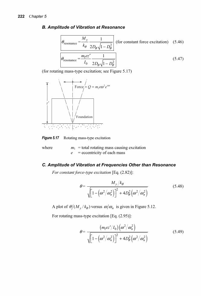
222 Chapter 5
B. Amplitude of Vibration at Resonance
resonance 2
1=2 1
yMk D Dq q q
q-
(for constant force excitation) (5.46)
1resonance 20
1=2 1
m ezI D Dq q
q ¢
- (5.47)
(for rotating mass-type excitation; see Figure 5.17)
Figure 5.17 Rotating mass-type excitation
where m1 = total rotating mass causing excitation e = eccentricity of each mass
C. Amplitude of Vibration at Frequencies Other than Resonance For constant force-type excitation [Eq. (2.82)]:
θ =
( ) ( )22 2 2 2 21 4
y
n n
M k
D
q
qw w w wÈ ˘- +Î ˚
(5.48)
A plot of ( / )yM kqq versus nw w is given in Figure 5.12.
For rotating mass-type excitation [Eq. (2.95)]:
θ = ( ) ( )( ) ( )
2 21 0
22 2 2 2 21 4
n
n n
m ez I
Dq
w w
w w w w
¢
È ˘- +Î ˚
(5.49)

Foundation Vibration 223
Figure 5.18 Equivalent radius of rectangular rigid foundation—rocking motion
Figure 5.13 shows a plot of θ/(m1ez′/I0) versus nw w .
In the case of rectangular foundation, the preceding relationships can be used by determining the equivalent radius as
r0 = BL34
3p (5.50)
The definitions of B and L are shown in Figure 5.18.
Example 5.3
A horizontal piston-type compressor is shown in Figure 5.19. The operating frequency is 600 cpm. The amplitude of the horizontal unbalanced force of the compressor is 30 kN, and it creates a rocking motion of the foundation about point O (see Figure 5.19b). The mass moment of inertia of the compressor assembly about the axis b′Ob′ is 16 × 105 kg-m2 (see Figure 5.19c). Determine
a. the resonant frequency, and b. the amplitude of rocking vibration at resonance.
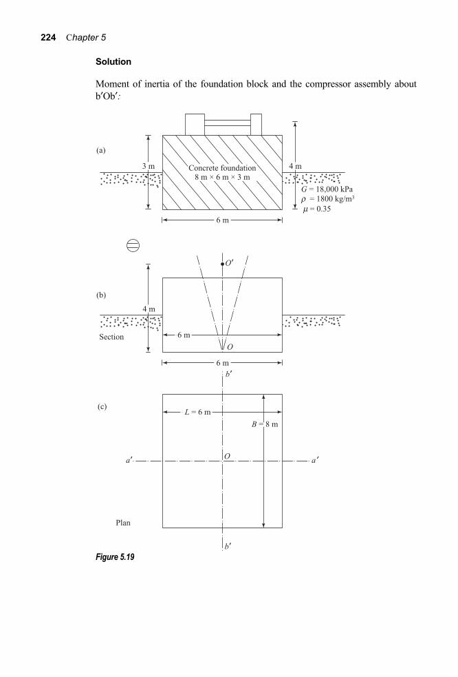
224 Chapter 5
Solution
Moment of inertia of the foundation block and the compressor assembly about b′Ob′:
Figure 5.19

Foundation Vibration 225
I0 = 2
foundation block 2 516 103 2
W L hg
È ˘Ê ˆ Ê ˆ + + ¥Í ˙Á ˜Á ˜ Ë ¯Ë ¯ Í ˙Î ˚ kg-m2
Assume the unit weight of concrete is 23.58 kN/m3.
Wfoundation block= (8 × 6 × 3)(23.58) = 3395.52 kN = 3395.52 × 103 N
I0 = 3395 52 10
3 9 81
3..¥
a fa f (32 + 32) + 16 × 105
= 36.768 × 10⁵ kg-m2
Calculation of equivalent radius of the foundation: From Eq. (5.50), the equivalent radius is
r0 = BL34
34
38 6
3p p= ¥ = 3.67 m
a. Determination of resonant frequency:
kθ = ( )( )( )( )
( )( )33
0 8 18,000 3.6783 1 3 1 0.35
Grm
=- -
= 3650279 kN-m/rad
fn = 3
50
1 1 3650279 10 N-m/rad2 2 36.768 10
kIq ¥=
p p ¥ = 5.01 Hz
= 300 cpm
Bθ = ( ) ( )
( )
505 50
3 1 3 1 0.35 36.768 108 (8)(1800) 3.67
Ir
mr
- - ¥= = 0.748
Dθ = ( ) ( )0.15 0.15
1 0.748 1 0.748B Bq q=
+ + = 0.099
fm = ( )2 2 2
300 300
1 2 1 2 1 2 0.099nf
D Dq q
= =- - -
= 303 cpm
b. Calculation of amplitude of vibration at resonance: My(operating frequency) = unbalanced force × 4 = 30 × 4 = 120 kN-m
My(at resonance) = 120f
fm
operation
FHG
IKJ
= 1202303
600Ê ˆÁ ˜Ë ¯ = 30.6 kN-m

226 Chapter 5
21( ) ym e z Mw =¢
( )( )
resonance
2 30360
wp
= = 31.73 rad/s
m1ez' = ( )
3
2 330.6 10 N-m
31.73yM
w¥= = 0.0304 × 10³
From Eq. (5.47)
θresonance = m ez
I D D1
02
12 1
¢
-q q
= 0 0304 1036 768 10
1
2 0 099 1 0 099
3
5 2
.. . .
¥¥
FHG
IKJ -
LNMM
OQPPa f a f a f
= 4.2 × 10⁻⁵ rad
5.6 Sliding Vibration of Foundations Arnold, Bycroft, and Wartburton (1955) have provided theoretical solutions for sliding vibration of rigid circular foundation (Figure 5.20) acted on by a force
0i tQ Q e w= . Hall (1967) developed the mass-spring-dashpot analog for this type
of vibration. According to this analog, the equation of motion of the foundation can be given in the form
0i t
x xmx c x k x Q e w+ + = (5.51)
where m= mass of the foundation
Figure 5.20 Sliding vibration of rigid circular foundation

Foundation Vibration 227
( ) 0
= static spring constant for sliding32 1
7 8
xkGrm
m-
=-
(5.52)
( ) 20
= dashpot coefficient for sliding18.4 1
7 8
xc
r Gm
rm-
=-
(5.53)
Based on Eqs. (5.51), (5.52), and (5.53), the natural frequency of the foundation for sliding can be calculated as
fn = ( )( )
032 11 12 2 7 8
x Grkm m
mm
-=
p p - (5.54)
The critical damping and damping ratio in sliding can be evaluated as
ccx = critical damping in sliding
= 2 ( )( )
032 12
7 8xGr m
k mmm
-=
- (5.55)
Dx = damping ratio in sliding
= cc B
x
cx x= 0 288. (5.56)
where the dimensionless mass ratio
( ) 30
7 832 1x
mBr
mm r
-=-
(5.57)
For rectangular foundation, the preceding relationships can be used by obtaining the equivalent radius r0, or
r0 = BLp
where B and L are the length and width of the foundation, respectively.
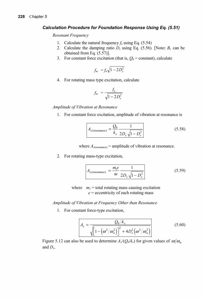
228 Chapter 5
Calculation Procedure for Foundation Response Using Eq. (5.51) Resonant Frequency
1. Calculate the natural frequency fn using Eq. (5.54) 2. Calculate the damping ratio Dx using Eq. (5.56). [Note: Bx can be
obtained from Eq. (5.57)]. 3. For constant force excitation (that is, Q0 = constant), calculate
fm = fn 1 2 2- Dx
4. For rotating mass type excitation, calculate
fm = f
Dn
x1 2 2-
Amplitude of Vibration at Resonance
1. For constant force excitation, amplitude of vibration at resonance is
0(resonance) 2
1
2 1x
x x x
QA
k D D=
- (5.58)
where Ax(resonance) = amplitude of vibration at resonance.
2. For rotating mass-type excitation,
1(resonance) 2
1
2 1x
x x
m eAm D D
=-
(5.59)
where m1 = total rotating mass causing excitation e = eccentricity of each rotating mass
Amplitude of Vibration at Frequency Other than Resonance
1. For constant force-type excitation,
( ) ( )022 2 2 2 21 4
xx
n x n
Q kA
Dw w w w=
È ˘- +Î ˚
(5.60)
Figure 5.12 can also be used to determine Ax/(Q0/kx) for given values of nw w and Dx.

Foundation Vibration 229
2. For rotating mass-type excitation,
( ) ( )
( ) ( )2
122 2 2 2 21 4
nx
n x n
m e mA
D
w w
w w w w=
È ˘- +Î ˚
(5.61)
Figure 5.13 provides a plot of Ax/(m1e/m) versus nw w for various values of Dx.
5.7 Torsional Vibration of Foundations Figure 5.21a shows a circular foundation of radius r0 subjected to a torque
0i tT T wq= about an axis z-z. Reissner (1937) solved the vibration problem of this
type considering a linear distribution of shear stress τzθ (shear stress zero at center and maximum at the periphery of the foundation), as shown in Figure 5.21b. This represents the case of a flexible foundation. In 1944 Reissner and Sagoli solved the same problem for the case of a rigid foundation considering a linear variation of displacement from the center to the periphery of the foundation. For this case, the shear stress can be given by (Figure 5.21c)
τzθ = 34
03
02 2p
Trr r r-
for 0 < r < r0 (5.62)
Similar to the cases of vertical, rocking, and sliding modes of vibration, the equation for the torsional vibration of a rigid circular foundation can be written as
0i t
zzJ c k T e wa aa a a+ + = (5.63)
where Jzz = mass moment of inertia of the foundation about the axis z-z cα = dashpot coefficient for torsional vibration
kα = static spring constant for torsional vibration = 163 0
3Gr (5.64)
α = rotation of the foundation at any time due to the application of a torque 0
i tT T wq=
The damping ratio Dα for this mode of vibration has been determined as (Richart, Hall, and Wood, 1970)
Dα = 0.51 2Ba+
(5.65)

230 Chapter 5
Figure 5.21 Torsional vibration of rigid circular foundation

Foundation Vibration 231
where Bα = the dimensionless mass ratio for torsion at vibration
= 50
zzJrr
(5.66)
Calculation Procedure for Foundation Response Using Eq. (5.63) Resonant Frequency
1. Calculate the natural frequency of the foundation as
fn = 12p
akJzz
(5.67)
2. Calculate Bα using Eq. (5.66) and then Dα using Eq. (5.65). 3. For constant force excitation (that is, T0 = constant)
fm = fn 1 2 2- Da
For rotating mass-type excitation
fm = 21 2
nf
Da-
Amplitude of Vibration at Resonance: For constant force excitation, the amplitude of vibration at resonance is
0resonance 2
1
2 1
Tk D Da a a
a =-
(5.68)
For rotating mass-type excitation
1
resonance 2
12
2 1zz
xm e
J D Da a
a
Ê ˆÁ ˜Ë ¯
=-
(5.69)
where m1 = total rotating mass causing the excitation e = eccentricity of each rotating mass
For the definition of x in Eq, (5.69), see, Figure 5.22.

232 Chapter 5
Figure 5.22
Amplitude of Vibration at Frequency Other than Resonance: For constant force excitation, calculate nw w and then refer to Figure 5.12 to obtain α/(T0/kα). For rotating mass-type excitation, calculate ω/ωn and then refer to Figure 5.13 to obtain α/[m1e(x/2)/Jzz].
For a rectangular foundation with dimensions B × L, the equivalent radius may be given by
r0 = BL B L2 2
4
6+c hp
(5.70)
The torsional vibration of foundations is uncoupled motion and hence can be treated independently of any vertical motion. Also, Poisson’s ratio does not influence the torsional vibration of foundations.
Example 5.4
A radar antenna foundation is shown in Figure 5.23. For torsional vibration of the foundation, given
T0 = 250 kN-m (due to inertia) T0 = 83 kN-m (due to wind)
mass moment of inertia of the tower about the axis z-z = 13 × 106 kg·m2, and the unit weight of concrete used in the foundation = 24 kN/m3. Calculate

Foundation Vibration 233
a. the resonant frequency for torsional mode of vibration; and b. angular deflection at resonance.
Figure 5.23
Solution
a.
Jzz = Jzz(tower) + Jzz(foundation)
= 13 × 106 + 2 20 0
1 24 10002 9.81
r h rÈ ˘¥Ê ˆp Á ˜Í ˙Ë ¯Î ˚
= 13 × 106 + 2 21 24 1000(7.6) (2.5) (7.6)2 9.81È ˘¥Ê ˆp Á ˜Í ˙Ë ¯Î ˚
= 13 × 106 + 32.05 × 106 = 45.05 × 10⁶ kg·m2
From Eq. (5.66)

234 Chapter 5
Bα = ( )( )6
5 530
45.05 1017.6 10 9.81 7.6
zzJrr
¥=¥
= 0.99
Again from Eq. (5.65),
Dα = ( ) ( )0.5 0.5
1 2 1 2 0.99Ba=
+ + = 0.168
Also, kα [Eq. (5.64)] is
kα = 3 6 3 110
16 16 135 10 (7.6) 3.16 103 3
Gr Ê ˆ= ¥ ¥ ¥ = ¥Á ˜Ë ¯ N-m
fn = 11
61 1 3.16 10
2 2 45.05 10zz
kJa ¥=
p p ¥
= 13.33 Hz Thus, the damped natural frequency
fm = fn ( ) ( )( )221 2 13.33 1 2 0.168Da- = -
= 12.92 Hz
b. Angular deflection at resonant frequency:
If the torque due to wind (T0) is to be treated as a static torque, then
0
static
Ta
= kα
or
αstatic = 0Tka
So
αstatic = 3
0(static)3 110
3 83 1016 3.16 10
TGr
È ˘¥= Í ˙¥Í ˙Î ˚
= 0.0263 × 10⁻⁵ rad Using Eq. (5.68), for the torque due to inertia
αresonance = 02
1
2 1
Tk D Da a a-

Foundation Vibration 235
= ( ) ( ) ( )
3
11 2
250 10 13.16 10 2 0.168 1 0.168
È ˘È ˘¥ Í ˙Í ˙ Í ˙¥Í ˙Î ˚ -Í ˙Î ˚
= 0.24 × 10⁻⁵ rad
At resonance, the total angular deflection is α = αinertia + αstatic = (0.24 + 0.0263) × 10−5 = 0.2663 × 10⁻⁵ rad
5.8 Comparison of Footing Vibration Tests with Theory Richart and Whitman (1967) conducted a comprehensive study to evaluate the applicability of the preceding theoretical findings to actual field problems. Ninety-four large-scale field test results for large footings 1.52 m to 4.88 m in diameter subjected to vertical vibration were reported by Fry (1963). Of these 94 test results, 55 were conducted at the U.S. Army Waterways Experiment Station, Vicksburg, Mississippi. The remaining 39 were conducted at Eglin Field, Florida. The classification of the soils for the Vicksburg site and Eglin site were CL and SP, respectively (unified soil classification system). For these tests, the vertical dynamic force on footings was generated by rotating mass vibrators.
Figure 5.24 shows a comparison of the theoretical amplitudes of vibration Az as determined from elastic half-space theory with the experimental results obtained for two bases at the Vicksburg site. The nondimensional mass ratios b [Eq. (5.4)] of these two bases were 5.2 and 3.8. For the base with b = 5.2, the experimental results fall between the theoretical curves, with μ = 0.5 and μ = 0.25. However, for the base with b = 3.8, the experimental curve is nearly identical to the theoretical curve with μ = 0.5. Figure 5.25 shows a comparison of the theory and experimental values reported by Fry in a nondimensional plot of Azm/m1e at resonance versus b. Similarly, a comparison of these test results with theory in a nondimensional plot of a0 [Eq. (5.5)] at resonance versus b is shown in Figure 5.26.
From these two plots it may be seen that the results of the Vicksburg site follow the general trends indicated by the theoretical curve obtained from the elastic half-space theory for a rigid base. A considerable scatter, however, exists for the tests conducted at Eglin Field. This may be due to the clean fine sand found at that site, for which the shear modulus will change with depth. The fundamental assumption of the theoretical derivation of a homogeneous, elastic, isotropic body is very much different than the actual field conditions.
Figure 5.27 shows a summary of all vertical vibration tests, which is plot of

236 Chapter 5
Figure 5.24 Vertical vibration of foundation—comparison of test results with theory
(after Richart and Whitman, 1967)
Figure 5.25 Motion at resonance for vertical excitation – comparison between theory
and experiment (after Richart and Whitman, 1967)
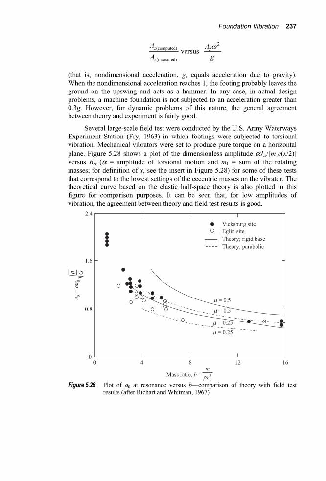
Foundation Vibration 237
AA
z
z
(computed)
(measured) versus
2zAgw
(that is, nondimensional acceleration, g, equals acceleration due to gravity). When the nondimensional acceleration reaches 1, the footing probably leaves the ground on the upswing and acts as a hammer. In any case, in actual design problems, a machine foundation is not subjected to an acceleration greater than 0.3g. However, for dynamic problems of this nature, the general agreement between theory and experiment is fairly good.
Several large-scale field test were conducted by the U.S. Army Waterways Experiment Station (Fry, 1963) in which footings were subjected to torsional vibration. Mechanical vibrators were set to produce pure torque on a horizontal plane. Figure 5.28 shows a plot of the dimensionless amplitude αJzz/[m1e(x/2)] versus Bα (α = amplitude of torsional motion and m1 = sum of the rotating masses; for definition of x, see the insert in Figure 5.28) for some of these tests that correspond to the lowest settings of the eccentric masses on the vibrator. The theoretical curve based on the elastic half-space theory is also plotted in this figure for comparison purposes. It can be seen that, for low amplitudes of vibration, the agreement between theory and field test results is good.
Figure 5.26 Plot of a0 at resonance versus b—comparison of theory with field test
results (after Richart and Whitman, 1967)

238 Chapter 5
The limiting torsional motion in most practical cases is about 2.5 × 10⁻³ mm (0.1 mil). So the half-space theory generally serves well for most practical design considerations. Comparisons between the elastic half-space theory and experimental results for footing vibration tests in rocking and sliding modes were also presented by Richart and Whitman (1967). The agreement seemed fairly good.
Figure 5.27 Summary of vertical vibration tests (after Richart and Whitman, 1967)
Figure 5.28 Comparison of amplitudes for torsional vibration (redrawn after Richart
and Whitman, 1967)

Foundation Vibration 239
5.9 Comments on the Mass-Spring-Dashpot Analog Used for Solving Foundation Vibration Problems The equations for the mass-spring-dashpot analog for various modes of vibration of rigid circular foundations developed in the preceding sections may be summarized as follows:
For vertical vibration,
0i t
z zmz c z k z Q e w+ + = (5.22)
For rocking vibration,
0i t
yI c k M e wq qq q q+ + = (5.39)
For sliding vibration,
0i t
x xmx c x k x Q e w+ + = (5.51)
For torsional vibration
0i t
zzJ c k T o wa aa a a+ + = (5.63)
The mathematical approach for solution of the preceding equations is similar for determination of the natural frequency, resonant frequency, critical damping, damping ratio, and the amplitudes of vibration at various frequencies. The agreement of these solutions with field conditions will depend on proper choice of the parameters (that is, m, I0, Jzz, cz, cθ, cx, cα, kz, kθ, kx, and kα). In this section, we will make a critical evaluation of these parameters.
Choice of Mass and Mass Moments of Inertia The mass terms m used in Eqs. (5.22) and (5.51) are actually the sum of
1. mass of structure foundation block mf, and 2. mass of all the machineries mounted on the block mm.
During the vibration of foundations, there is a mass of soil under the foundation that vibrates along with the foundation. Thus, it would be reasonable to consider the term m in Eqs. (5.22) and (5.51) to be the sum of m = mf + mm + ms (5.71)

240 Chapter 5
where ms = effective mass of soil vibrating with foundation.
In a similar manner, the mass moment of inertia terms I0 and Jzz included in Eqs (5.39) and (5.63) include the contributions of the mass of the foundation and that of the machine mounted on the block. It appears reasonable also to add the contribution of the effective mass of the vibrating soil (ms), that is, the effective soil mass moment of inertia. Thus
I0 = I0(foundation) + I0(machine) + I0(effective soil mass) (5.72) and Jzz = Jzz(foundation) + Jzz(machine) + Jzz(effective soil mass) (5.73)
Theoretically, calculated values of ms, I0(effective soil mass), and Jzz(effective soil mass) are given by Hsieh (1962). They are as follows:
1. Values of ms for vertical vibration:
Poisson’s ratio, μ ms
0.00 300.5 rr
0.25 300.5 rr
0.50 302.0 rr
2. Values of ms for horizontal vibration:
Poisson’s ratio, μ ms
0.0 300.2 rr
0.25 300.2 rr
0.50 300.1 rr
3. Values of I0(effective soil mass) for rocking vibration: Poisson’s ratio μ = 0; I0 (effective soil mass) = 5
00.4 rr
4. Values of Jzz(effective soil mass) for torsional vibration:
Poisson’s ratio, μ ms
0.00 500.3 rr
0.25 500.3 rr
0.50 500.3 rr

Foundation Vibration 241
In most cases, for design purposes the contribution of the effective soil mass is neglected. This will, in general, lead to answers that are within 30% accuracy.
Choice of Spring Constants In Equations (5.23), (5.41), (5.52), and (5.64), the spring constants defined were for the cases of rigid circular foundations. In examples where rigid rectangular foundations were encountered, the equivalent radii r0 were first determined. These values of r0 were then used to determine the value of the spring constants. However, more exact solutions for spring constants for rectangular foundations derived from the theory of elasticity can be used. These are given in Table 5.1 along with those for circular foundations. Dobry and Gazetas (1986) have developed more realistic values of spring constants and demonstrated their use through a design exercise.
Table 5.1 Values of Spring Constants for Rigid Foundations (after Whitman and Richart, 1967)
Motion Spring constant Reference Circular foundations
Vertical kz = 041
Grm-
Timoshenko and Goodier (1951)
Horizontal (sliding) kx = ( ) 3
032 17 8
Grmm
--
Bycroft (1956)
Rocking kθ = ( )308
3 1Gr
m- Borowicka (1943)
Torsion kα = 163 0
3Gr Reissner and Sagoci (1944)
Rectangular foundation
Verticala kz = 1 z
G F BLm-
Barkan (1962)
Horizontala (sliding) kx = 2(1 + μ) GFx BL Barkan (1962)
Rockingb kθ = 21
G F BLqm- Gorbunov-Possadov and
Serebrajanyi(1961) a B = width of foundation; L = length of foundation. b For definition of B and L, refer to Figure 5.18. Refer to Figure 5.29 for values of Fz, Fx, and Fθ.

242 Chapter 5
Figure 5.29 Plot of Fz, Fx, and Fq against L/B (after Whitman and Richart, 1967)
Another fact that needs to be kept in mind is that the foundation blocks are never placed at the surface. If the bottom of the foundation block is placed at a depth z measured from the ground surface, the spring constants will be higher than that calculated by theory. This fact is demonstrated in Figure 5.30 for the case of vertical motion of rigid foundations. This could possibly due to the frictional resistance of the sides of the foundations. The behavior of embedded foundations subjected to various types of vibration is presented in Sections 5.12 through 5.15.
Choice of Poisson’s Ratio Whitman and Richart (1967) recommended the following values of Poisson’s ratio for different types of soils:

Foundation Vibration 243
Spri
ng
const
ant,
kz
Depth of foundation from the ground surface Figure 5.30 Nature of variation of kz with the depth of the foundation
Sand (dry, moist, partially saturated) μ = 0.35 to 0.4
Clay (saturated) μ = 0.5
A good value for most partially saturated soils is about 0.4
Choice of Damping Ratio In soils there are two types of damping, geometric damping (also known as radiation damping) and internal damping (also known as material damping or hysteretic damping). The radiation damping (defined as loss of energy over one wave length) depends on parameters such as Poisson’s ratio, mass of the foundation, equivalent radius, and the density of the soil. The relations for the damping ratio given in Eqs. (5.27), (5.45), (5.56), and (5.65) are for radiation damping only.
The internal damping Di varies over a wide range, depending on the type of soil and the strains generated in the soil. Generally the values of Di are the range of 0.01 to 0.1. Thus an average value of Di would be a good estimate to be used in foundation design (Whitman and Richart, 1967). The damping ratio can then be approximated as
radiation 0.05D D= + (5.74)
For vertical and sliding motions, the contribution of internal damping can be somewhat neglected. However, for torsional and rocking modes of vibration, the contribution of the internal damping may be too large to be ignored.

244 Chapter 5
5.10 Coupled Rocking and Sliding Vibration of Rigid Circular Foundations In several cases of machine foundations, the rocking and sliding vibrations are coupled. This is because the center of gravity of the footing and vibrations are not coincident with the center of sliding resistance, as can be seen from Figure 5.31a. This is a case of vibration of a foundation with two degrees of freedom. The derivation given next for the coupled motion for rocking and sliding is based on the analysis of Richart and Whitman (1967). From Figure 5.31, it can be seen that the nature of foundation motion shown in Figure 5.31a is equal to sum of the sliding motion shown in Figure 5.31b and the rocking motion shown in Figure 5.31c. Note that
xb = xg – h′θ (5.75)
For the sliding motion,
gmx P= (5.76)
where P = horizontal resistance to sliding
= − cxdxdt
b − kxxb (5.77)
Substitution of Eq. (5.75) into (5.77) yields
P = −cxddt
(xg – h′θ) – kx(xg – h′θ)
= − cx x g + cxh′q – kxxg + kxh′θ (5.78)
Now, combining Eqs. (5.76) and (5.78)
0g x g x g x xmx c x k x c h k hq q+ + - - =¢ ¢ (5.79)
For rocking motion about the center of gravity,
Igq = M + Mr – h′P (5.80)
where Ig = mass moment of inertia about the horizontal axis passing through the center of gravity (at right angles to the cross section shown) Mr = the soil resistance to rotational motion

Foundation Vibration 245
Figure 5.31 Coupled rocking and sliding vibration
But
Mr = − cθq − kθθ (5.81)
Substitution of Eqs. (5.78) and (5.81) into Eq. (5.80) gives

246 Chapter 5
( ) ( )g x g x x g xI M c k h c x c h k x k hq qq q q q q= - + - - + - +¢ ¢ ¢ or
2 2( ) ( ) ( ) i tg x x x g x g yI c c h k k h h c x k x M M e w
q qq q q+ + + + - + = =¢ ¢ ¢ (5.82)
For a foundation resting on an elastic half-space, the spring and dashpot coefficients are frequency dependent. They need to be calculated first for a given frequency before Eqs. (5.79) and (5.82) can be solved. However, if they are assumed to be frequency independent, as in the case of analog solutions, Eqs. (5.79) and (5.82) can be easily solved. For that case, for determination of the damped natural frequency, one can make M in Eq. (5.82) equal zero. So
2 2( ) ( ) ( ) 0g x x x g x gI c c h k k h h c x k xq qq q q+ + + + - + =¢ ¢ ¢ (5.83)
For solving Eqs. (5.79) and (5.83), let
1mi t
gx A e w= (5.84)
and
2mi tA e wq = (5.85)
where mw = damped natural frequency.
Substituting Eqs. (5.84) and (5.85) into Eqs. (5.79) and (5.83) and rearranging, one obtains (Prakash and Puri, 1981, 1988)
( ) ( )
22 2 2 24 2
2 2 2 2
4 .
4 0
n nx x n nx n nxm m
x nx m n mn m nx m
D D
D D
q q q q
q qq
w w w w w ww wd d d
w w w ww w w wd d
È ˘Ê ˆ+- - +Í ˙Á ˜
Ë ¯Í ˙Î ˚È ˘+ - + - =Í ˙Î ˚
(5.86)
where Dx = damping ratio for sliding vibration [Eq. (5.56)] Dθ = damping ratio for rocking vibration [Eq. (5.45)] δ = I
Ig
0
[Note: The term I0 was defined in Eq. (5.40).]

Foundation Vibration 247
( )( )
032 17 8
[from Eq.(5.54)]
nxGrm
mw
m-
=-
≠ (5.88)
and
( )30
0
83 1
[from Eqs.(5.41)and(5.44)]
nGr
Iqwm
=-
≠ (5.89)
Equation (5.86) can then be solved to obtain two values of mw .
The damped amplitudes of rocking and sliding vibrations can be obtained as
( ) ( )
( )
1 22 22
2
2nx x nxy
xg
DMA
I
w w
w
È ˘+Í ˙Ê ˆ Î ˚= Á ˜Ë ¯ D
(5.90)
and
( ) ( )
( )
1 22 22 2
2
2nx x nxy
g
DMA
Iq
w w w w
w
È ˘- +Í ˙Ê ˆ Î ˚= Á ˜Ë ¯ D
(5.91)
where
( )22 2 2 2
2 4 2 4n nx x n nx n nxD Dq q q qw w w w w ww w wd d d
ÏÈ ˘Ê ˆ+ÔD = - - +Í ˙Ì Á ˜Ë ¯Í ˙ÔÎ ˚Ó
+ 4 ( ) ( )1 22
2 2 2 2x nx nn nx
D Dq qq
w w w ww w w wd d
¸È ˘ Ô- + - ˝Í ˙Î ˚ Ô (5.92)
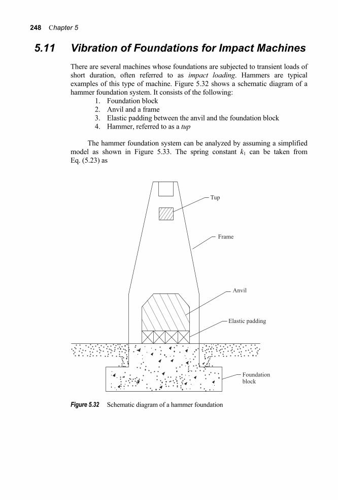
248 Chapter 5
5.11 Vibration of Foundations for Impact Machines There are several machines whose foundations are subjected to transient loads of short duration, often referred to as impact loading. Hammers are typical examples of this type of machine. Figure 5.32 shows a schematic diagram of a hammer foundation system. It consists of the following:
1. Foundation block 2. Anvil and a frame 3. Elastic padding between the anvil and the foundation block 4. Hammer, referred to as a tup
The hammer foundation system can be analyzed by assuming a simplified model as shown in Figure 5.33. The spring constant k1 can be taken from Eq. (5.23) as
Figure 5.32 Schematic diagram of a hammer foundation

Foundation Vibration 249
Figure 5.33 Simplified model for analysis of hammer foundation
k1 = kz = 041
Grm-
(5.93)
The spring constant due to the elastic pad is
k2 = Et
A (5.94)
where E = modulus of elasticity of the pad material t = thickness of the pad A = area of the anvil base in contact with the pad
When the tup drops on the anvil, due to the impact the following are the initial conditions:
z1 = 0 and z1 = 0 (5.95a) z2 = 0 and z2 = 0u (5.95b) The equation of motion for the free vibrations may be given as [see Figure
250 Chapter 5
2.13b and Eqs. (2.116) and (2.117)] m1z1 + k1z1 + k2(z1 – z2) = 0 (5.96) m2z2 + k2(z2 – z1) = 0 (5.97)
where m1 = mass of the foundation + frame (if attached to the foundation block)
m2 = mass of the anvil + frame (if attached to the anvil)
The solutions for the natural circular frequencies of the system have been given in Eq. (2.122) as
1 2 1 2
4 2 2 2 2 2(1 )( ) (1 )( )( ) 0n nl nl n nl nlw h w w w h w w− + + + + = (5.98) where
1
1
1 2nl
km m
w =+
(5.99)
2
2
2nl
km
w = (5.100)
η = mm
2
1 (5.101)
The amplitudes of vibration due to impact can also be given by Eqs. (2.134a) and (2.134b) as
( ) ( )
( )2 1 2 2
2 1 2 2
2 2 2 2
1 02 2 2
nl n nl n
nl n n nZ
w w w wu
w w w w
- -=
- (5.102)
( )( )
2 1
1 2 2
2 20
2 2 2
nl n
n n nZ
w w u
w w w
-=
- (5.103)
The preceding two equations can be solved to determine the amplitudes of vibration if 0u is known. This value can be estimated in the following manner. Using the theory of conservation of momentum, the momentum of the tup and the anvil after impact is
2 0h am mu u+
where mh = mass of the tup
Foundation Vibration 251
au = velocity of the tup after impact
Thus 2 0h b h am m mu u u= + (5.104)
where bu = velocity of the tup before impact.
A second equation may be obtained from Newton’s second law as
0 a
bn
u uu-
= (5.105)
where n is the coefficient of restitution. Combining Eqs. (5.104) and (5.105),
( )02
11 b
h
nm m
u u+=+
(5.106)
For a single-acting drop hammer, the magnitude of the coefficient of restitution may vary from 0.2 to about 0.5. Also,
bu (m/s) = Ef 2gH (5.107)
where H = height of fall of the tup (m) g = acceleration due to gravity (9.81 m/s2) Ef = efficiency of drop (≈ 0.65 to about 1)
Vibration of Embedded Foundations In the theories for the vibration of foundations in various modes, as developed in Sections 5.2 through 5.9, it was assumed that the foundation rests on the ground surface. In reality, however, all foundations are constructed below the ground surface. For an embedded foundation, soil resistance is mobilized at its base and also along its sides. A limited number of theories have so far been developed for the dynamic response of embedded block foundations. The findings from these studies are summarized in the following four sections.
5.12 Vertical Vibration of Rigid Cylindrical Foundations The dynamic response of vertically vibrating rigid cylindrical foundations (Figure 5.34) has been studied by Novak and Beredugo (1972). The foundation

252 Chapter 5
shown in Figure 5.34 has a radius of r0. The shear modulus and the density of the side layer of soil are Gs and ρs, respectively. Similarly, the shear modulus and the density of the soil beneath the foundation are, respectively, G and ρ. If the foundation is subjected to a vertical exciting force, the equation of motion may be written in the form
( ) ( ) ( ) ( )z zmz t Q t R t N t= - - (5.108)
The dynamic reaction Rz(t) is considered to be independent of the depth of embedment. Using the elastic half-space solution, the dynamic reaction can be expressed as
Rz(t) = Gr0(C1 + iC2)z(t) (5.109) where
C1 = 12 2
1 2
ff f- ¢+¢ ¢
(5.110)
and
C2 = 22 2
1 2
ff f
¢+¢ ¢
1f ¢ , 2f ¢ = functions of nondimensional frequency a0 [Eq. (5.5)], (5.111)
Poisson’s ratio, and stress distribution at the base
Figure 5.34 Embedded rigid cylindrical foundation – vertical vibration

Foundation Vibration 253
The dynamic soil reaction on the sides can be obtained as
Nz(t) = 0
( , )fDs z t dzÚ (5.112)
where s is the dynamic reaction per unit depth of embedment.
If s is considered to be independent of depth (Baranov, 1967), then s = s(t), or
s(t) = Gs(S1 + iS2) z(t) (5.113)
where
S1 = 2πa0J a J a Y a Y a
J a Y a1 0 0 0 1 0 0 0
02
0 02
0
b g ( ) ( ) ( )( ) ( )
++
(5.114a)
and
S2 = 4
02
0 02
0J a Y a( ) ( )+ (5.114b)
J0(a0), J1(a0) = Bessel functions of the first kind of order 0 and 1, respectively Y0(a0), Y1(a0) = Bessel functions of the second kind of order 0 and 1, respectively
So Nz(t) =
0
Dfz Gs(S1 + iS2)z(t)dz = GsDf(S1 + iS2)z(t) (5.115)
Now, combining Eqs. (5.108), (5.109), and (5.115)
mz (t) + Gr0[C1 + iC2 + GG
Dr
s f
0 (S1 + iS2)]z(t)
= Q(t) = Q0i te w = Q0(cos tw + i sin tw ) (5.116)
The steady-state response is
z(t) = z i te w (5.117) In the preceding two equations, Q0 and z are, respectively, the real force amplitudes and real response. The relationships for the spring constant and the

254 Chapter 5
damping coefficient can thus be derived as
kz = Gr0 C GG
Dr
Ss f1
01+
FHG
IKJ (5.118)
cz = 02 2
0
fs DGr GC S
G rwÊ ˆ
+Á ˜Ë ¯ (5.119)
Note that kz and cz, as expressed by the two preceding relationships, are frequency dependent. However, without losing much accuracy, one can assume that
C1 = C1 = constant S1 = S1 = constant C2 = a0C2 (where C2 is a constant) S2 = a0S2 (where S2 is a constant) When the preceding assumptions are substituted into Eqs. (5.118) and (5.119), one obtains the frequency-independent kz and cz as follows:
1 100
fsz
DGk Gr C S
G rÊ ˆ
= +Á ˜Ë ¯ (5.120)
22 20
0
f s sz
D Gc r G C S
r Grrr
Ê ˆ= +Á ˜Ë ¯
(5.121)
Hence, the damping ratio can be given as
2 2
0
1 10
12
f s s
zfs
D GC Sr G
Db DGC S
G r
rr
Ê ˆ+Á ˜Ë ¯Ê ˆ= Á ˜Ë ¯+
(5.122)
where b = mass ratio = 30
mrr
[Eq. (5.4)]
The values of C C S1 2 1, , ,and S2 (Novak and Beredugo, 1972) are given in Table 5.2.

Foundation Vibration 255
Table 5.2 Values of C C S1 2 1, , , and S2
Poisson’s ratio, μ aC1 aC2 bS1 bS 2
0.0 3.9 3.5 2.7 6.7 0.25 5.2 5.0 2.7 6.7 0.5 7.5 6.8 2.7 6.7
a Validity range: 0 ≤ a0 ≤ 1.5 b Validity range: 0 ≤ a0 ≤ 2
Once the spring constant, dashpot coefficient, and the damping ratio are determined, the foundation response (natural frequency, amplitude of vibration at resonance and at frequencies other than the resonance) can be calculated using the formulae given below.
Undamped natural frequency:
zn
km
w =
1
2z
nkfm
=p
Amplitude of vibration at resonance:
Az = Qk D Dz z z
02
12 1-
(for constant force excitation)
Az = m em D Dz z
12
12 1-
(for rotating mass excitation)
Amplitude of vibration at frequency other than resonance:
Az =
( ) ( )022 2 2 2 21 4
z
n z n
Q k
Dw w w wÈ ˘- +Î ˚
(for constant force excitation)
Az =( ) ( )
( ) ( )2
122 2 2 2 21 4
n
n z n
m e m
D
w w
w w w wÈ ˘- +Î ˚
(for rotating mass excitation)
The natural frequency of the foundation-soil system increases and its amplitude of vibration decreases, if depth of embedment is taken into account.
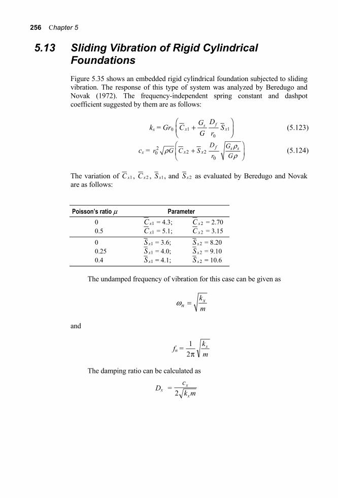
256 Chapter 5
5.13 Sliding Vibration of Rigid Cylindrical Foundations Figure 5.35 shows an embedded rigid cylindrical foundation subjected to sliding vibration. The response of this type of system was analyzed by Beredugo and Novak (1972). The frequency-independent spring constant and dashpot coefficient suggested by them are as follows:
kx = Gr0 C GG
Dr
Sxs f
x10
1+FHG
IKJ (5.123)
cx = 22 20
0
f s sx x
D Gr G C S
r Grrr
Ê ˆ+Á ˜Ë ¯
(5.124)
The variation of Cx1 , Cx2 , S x1, and S x2 as evaluated by Beredugo and Novak are as follows:
Poisson’s ratio μ Parameter
0 Cx1 = 4.3; Cx2 = 2.70 0.5 Cx1 = 5.1; Cx2 = 3.15
0 S x1 = 3.6; S x2 = 8.20 0.25 Sx1 = 4.0; Sx2 = 9.10
0.4 Sx1 = 4.1; Sx2 = 10.6
The undamped frequency of vibration for this case can be given as
xn
km
w =
and
fn = 12p
km
x
The damping ratio can be calculated as
Dx = ck mx
x2
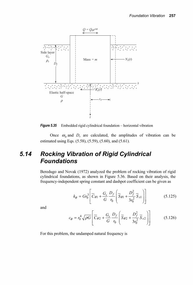
Foundation Vibration 257
Figure 5.35 Embedded rigid cylindrical foundation – horizontal vibration
Once nw and Dx are calculated, the amplitudes of vibration can be estimated using Eqs. (5.58), (5.59), (5.60), and (5.61).
5.14 Rocking Vibration of Rigid Cylindrical Foundations Beredugo and Novak (1972) analyzed the problem of rocking vibration of rigid cylindrical foundations, as shown in Figure 5.36. Based on their analysis, the frequency-independent spring constant and dashpot coefficient can be given as
2
31 1 10 2
0 03f fs
xD DG
k Gr C S SG r r
q qq
È ˘Ê ˆÍ ˙= + +Á ˜Á ˜Í ˙Ë ¯Î ˚
(5.125)
and
2
42 2 20 2
0 03f fs
xD DG
c r G C S SG r r
q qq rÈ ˘Ê ˆÍ ˙= + +Á ˜Á ˜Í ˙Ë ¯Î ˚
(5.126)
For this problem, the undamped natural frequency is

258 Chapter 5
Figure 5.36 Embedded rigid cylindrical foundation – rocking vibration
0
nkIqw =
For the definition of I0, see Eq. (5.40). The damping ratio is
02
cD
k Iq
=
The amplitudes of vibration can be calculated using Eqs. (5.46), (5.47), (5.48), and (5.49).
The variation of S x1, and S x2 was given in the preceding section. For μ = 0,
1Cq = 2.5 2Cq = 0.43 and, for any value of μ, 1Sq = 2.5 2Sq = 1.8

Foundation Vibration 259
5.15 Torsional Vibration of Rigid Cylindrical Foundations Figure 5.37 shows a rigid cylindrical foundation subjected to a torsional vibration. Novak and Sachs (1973) evaluated the frequency-independent spring constant and dashpot coefficient, and they are as follows:
31 10
0
fs DGk Gr C S
G ra aaÊ ˆ
= +Á ˜Ë ¯ (5.127a)
and
42 20
0
f s sD Gc r G C S
r Ga aarrr
Ê ˆ= +Á ˜Ë ¯
(5.127b)
The values of the parameters 1 2 1, ,C C Sa a a and 2Sa are
10
2
4.3for 0 2.0
0.7
Ca
Ca
a
¸= Ô £ £˝= Ô
Figure 5.37 Embedded rigid cylindrical foundation – torsional vibration

260 Chapter 5
10
2
12.4for 0 0.2
2.0
Sa
Sa
a
¸= Ô £ £˝= Ô
10
2
10.2for 0.2 2.0
5.4
Sa
Sa
a
¸= Ô £ £˝= Ô
Once the magnitudes of kα and cα are calculated, the undamped natural circular frequency can be obtained as
nzz
kJaw =
where Jzz = mass moment of inertia of the foundation about the z axis [see Eq.(5.63)]
The damping ratio is
Dα = 2 2
0
1 10
12
f s s
fs
D GC Sr G
B DGC SG r
a
a a
a a
rr
Ê ˆ+Á ˜Ê ˆ Ë ¯
Á ˜Á ˜Ë ¯ +
(5.128)
where Bα = mass ratio = 50
zzJrr
[see Eq. (5.66)]
The amplitudes of vibration can be calculated using Eqs. (5.68) and (5.69) and Figures 5.12 and 5.13.
Effect of Layering In general soils are layered in nature and shear modulus increases with depth. Several researchers attempted to develop approximate, analytical as well as numerical solutions to calculate the vibration response of foundations on the surface of an incompressible soil layer for which shear modulus increases linearly with depth. The effect of layer thickness and depth of embedment have also been reported in the literature. It is generally concluded that omission of layering in theoretical solutions lead to underestimation of vibration amplitudes. Parametric studies are also reported by considering soil as a two layer system, the bottom layer being an elastic half space. The presence of rigid layer below the elastic layer, produces a stiffening effect and increases the natural frequency.

Foundation Vibration 261
Vibration Screening In Section 5.4, the allowable vertical vibration amplitudes for machine foundation were considered. It is sometimes possible that, for some rugged vibratory equipment, the intensity of vibration may not be objectionable for the equipment itself. However, the vibration may not be within a tolerable limit for sensitive equipment nearby. Under these circumstances it is desirable to control the vibration energy reaching the sensitive zone. This is referred to as vibration screening. It needs to be kept in mind that most of the vibratory energy affecting structures nearby is carried by Rayleigh (surface) waves traveling from the source of vibration. Effective screening of vibration may be achieved by proper interception, scattering, and diffraction of surface waves using barriers such as trenches, sheet pile walls, and piles.
5.16 Active and Passive Isolation: Definition While studying the problem of vibration screening, it is convenient to group the screening problems into two major categories.
Active Isolation: Active isolation involves screening at the source of vibration, as shown in Figure 5.38, in which a circular trench of radius R and depth H surrounds the foundation that is the source of disturbance.
Passive Isolation: The passive isolation process involves providing a barrier at a point remote from the source of disturbance but near a site where vibration has to be reduced. An example of this is shown in Figure 5.39, in which an open trench of length L and depth H is used near a sensitive instrument foundation to protect if from damage.
5.17 Active Isolation by Use of Open Trenches Woods (1968) reported the results of a field investigation for active isolation using open trenches. The field tests were conducted at a site with a deep stratum of silty sand. The experimental study consisted of applying vertical vibrations by a small vibrator [80.1 N maximum force] resting on a circular pad. Trenches were constructed around the circular pad to screen the surface displacement due to the surface waves. Vertical velocity transducers were used for measurement of surface displacement around the trench over a 7.62 m diameter area. Other conditions remaining the same, measurements for the surface displacement due to the vibration of the circular pad were also taken without the trenches surrounding the pad. Some results of this investigation are shown in Figure 5.40 in the form of amplitude-reduction-factor contour diagrams. The amplitude-reduction factor (ARF) is defined as

262 Chapter 5
Figure 5.38 Schematic diagram of vibration isolation using a circular trench
surrounding the source of vibration for active isolation
Figure 5.39 Passive isolation by using an open trench
ARF = vertical amplitude of vibration with trenchvertical amplitude of vibration without trench
(5.129)

Foundation Vibration 263
Figure 5.40 Amplitude-reduction factor contour diagrams (after Woods, 1968)

264 Chapter 5
Also note that in Figure 5.40, θ is the angular length of the trench (in degrees) and λr is the length of Rayleigh waves. The value of λr for a given frequency of vibration at a given site can be determined in a manner similar to that described in Section 4.15.
The tests of Woods (1968) were conducted for R/λr = 0.222 to 0.910 and H/λr = 0.222 to 1.82. For satisfactory isolation, Woods defined the ARF to be less than or equal to 0.25. The conclusions of this study can be summarized as follows:
1. For θ = 360º, a minimum value of H/λr = 0.6 is required to achieve ARFs less than or equal to 0.25.
2. For 360º > θ > 90º, the screened zone may be defined as an area
outside the trench bounded on the sides by radial lines from the center of the source through points 45º from the ends of the trench. To obtain ARFs less than or equal to 0.25 in the screened zone, a minimum value of H/λr = 0.6 is required.
3. For θ ≤ 90º, effective screen of vibration by trenches cannot be
obtained.
5.18 Passive Isolation by Use of Open Trenches Woods (1968) also investigated the case of passive isolation in the field using open trenches. The plan view of the filed site layout used for screening at a distance is shown in Figure 5.41. The layout consisted of two vibrator exciter footings (used one at a time for the tests), a trench barrier, and 75 pickup benches. For these tests, it was assumed that the zone screened by the trench will be symmetrical about the 0º line. The variables used to study the passive isolation tests were:
• Distance form the source of vibration to the center of the open trench, R
• Length of the trench, L • Width of the trench, W, and • Depth of the trench, H.
In this investigation, the value of R/λr was varied from 2.22 to 9.10. For satisfactory isolation, it was defined that ARF’s [Eq. (5.129)] should be less than or equal to 0.25 in a semicircular zone of radius L/2 behind the trench.

Foundation Vibration 265
Figure 5.42 shows the ARF contour diagram for one of these tests. The conclusions of this study may be summarized as follows:
1. For a satisfactory passive isolation (for R = 2λr to about 7λr), the minimum trench depth H should be about 1.2λr to 1.5λr. This means that, in general, H/λr should be about 1.33.
2. The trench width W has practically no influence on the effectiveness of screening.
3. To maintain the same degree of isolation, the least area of the trench in the vertical direction (that is LH = AT) should be as follows:
AT = 2.5 2rl at R = 2λr
and AT = 6.0 2
rl at R = 7λr
Figure 5.41 Plan view of the field site layout for passive isolation by use of open trench
(after Woods, 1968)

266 Chapter 5
Figure 5.42 Amplitude-reduction-factor contour diagram for passive isolation (after
Woods, 1968)
5.19 Passive Isolation by Use of Piles There are several situations where Rayleigh waves that emanate from manufactured sources may be in the range of 40 to 50 m. For these types of problems, a trench depth of 1.33 times 60 to 75 m is needed for effective passive isolation. Open trenches or bentonite-slurry-filled trenches deep enough to be effective are not practical. At the same time, solidification of bentonite-slurry will also pose a problem. For this reason, possible use of rows of piles as an energy barrier was studied by Woods, Barnett, and Sagesser (1974) and Liao and Sangrey (1978). Woods, Barnett, and Sagesser.

Foundation Vibration 267
Figure 5.43 Void cylindrical obstacles for passive isolation
used the principle of holography and observed vibrations in a model half-space in order to develop the criteria for void cylindrical obstacles for passive isolation (Figure 5.43). The model half-space was prepared in a fine sand medium in a box. In Figure 5.43, the diameter of the cylindrical obstacle is D, and the net space for the energy to penetrate between two consecutive void obstacles is equal to Sn. The numerical evaluation of the barrier effectiveness was made by obtaining the average ARFs from several lines beyond the barrier in a section ±15º on both sides of an axis through the source of disturbance and perpendicular to the barrier. For all tests, H/λr and L/λr were kept at 1.4 and 2.5, respectively. These values of H/λr, and L/λr are similar to those suggested in Section 5.18 for open trenches. A nondimensional plot of the isolation effectiveness developed from these tests is given in Figure 5.44. The isolation effectiveness is defined as
Effectiveness = 1 – ARF (5.130)
Based on these test results, Woods, Barnett, and Sagesser (1974) suggested that a row of void cylindrical holes may act as an isolation barrier if
r
Dl
≥ 16
(5.131)
and
n
r
Sl
< 14
(5.132)

268 Chapter 5
Liao and Sangrey (1978) used an acoustic model employing sound waves in a fluid medium to evaluate the possibility of the use of rows of piles as passive isolation barriers. Model piles for the tests were made from aluminum, steel, Styrofoam, and polystyrene plastic. Based on their study, Liao and Sangrey determined that Eqs. (5.131) and (5.132) suggested by Woods, Barnett, and Sagesser are generally valid. They also determined that Sn = 0.4λr may be the upper limit for a barrier to have some effectiveness. However, the degree of effectiveness of the barrier will depend on whether the piles are soft or hard compared to the soil in which they are embedded. The degree of softness or hardness may be determined by the term impedance ratio (IR), defined as
IR = ( )
( )
P P
S S
r
r
r u
r u (5.133)
where Pr and Sr = the densities of the pile material and soil, respectively ( )Pru and ( )Sru = the velocities of Rayleigh waves in the pile material and soil, respectively
The piles are considered soft if IR is less than 1 and hard if IR is greater than 1. Soft piles are more efficient as isolation barriers compared to hard piles.
Figure 5.44 Isolation effectiveness as a function of hole diameter and spacing (redrawn
after Woods, Barnett, and Sagesser, 1974)

Foundation Vibration 269
Figure 5.45 Estimated values of Rayleigh wave impedance for various soils and pile
materials (after Liao and Sangrey, 1978)
Figure 5.45 gives a general range of the Rayleigh wave impedance (= rru ) for various soils and pile materials. For a more detailed discussion, the reader is referred to the original paper of Liao and Sangrey.
Problems 5.1 A concrete foundation is 2.5 m in diameter. The foundation is supporting
a machine. The total weight of the machine and the foundation is 270 kN. The machine imparts a vertical vibrating force Q = Q0 sinw t. Given Q0 = 27 kN (not frequency dependent). The operating frequency is 150 cpm. For the soil supporting the foundation, unit weight = 19.5 kN/m3, shear modulus = 45000 kPa. , and Poisson’ ratio = 0.3. Determine: a. resonant frequency, b. the amplitude of vertical vibration at resonant frequency, and c. the amplitude of vertical vibration at the operating frequency.

270 Chapter 5
5.2 Redo Problem 5.1 assuming the foundation is 2.5 m × 2 m in plan. Assume the total weight of the foundation and the machine is the same as in Problem 5.1.
5.3 A concrete foundation (unit weight = 23.5 kN/m3) supporting a machine is 3.5 m × 2.5 m in plan and is subjected to a sinusoidal vibrating force (vertical) having an amplitude of 10 kN (not frequency dependent). The operating frequency is 2000 cpm. The weight of the machine and foundation is 400 kN. The soil properties are unit weight = 18 kN/m3, shear modulus = 38,000 kPa, and Poisson’ ratio = 0.25. Determine a. the resonant frequency of the foundation, and b. the amplitude of vertical vibration at operating frequency.
5.4 Consider the case of a single-cylinder reciprocating engine (Figure 5.15a). For the engine, operating speed = 1000 cpm, crank (r1) = 90 mm, connecting rod (r2) = 350 mm, weight of the engine = 20 kN, and reciprocating weight = 65 N. The engine is supported by a concrete foundation block of 3 m × 2 m × 1.5 m (L × B × H). The unit weight of concrete is 23.58 kN/m3. The properties of the soil supporting the foundation are unit weight = 19 kN/m3, G = 24,000 kPa, and μ = 0.25. Calculate a. the resonant frequency, and b. the amplitude of vertical vibration at resonance.
5.5 Refer to Problem 5.4. What will be the amplitude of vibration at operating frequency?
5.6 Solve Example 5.2, parts (b) and (c) by assuming that the Poisson’s ratio is μ = 0.25. Also determine the amplitude of vertical vibration at operating frequency.
5.7 The concrete foundation (unit weight = 23.5 kN/m3) of a machine has the following dimensions (refer to Figure 5.18): L = 3 m, B = 4 m, height of the foundation = 1.5 m. The foundation is subjected to a sinusoidal horizontal force from the machine having an amplitude of 10 kN at a height of 2 m measured from the base of the foundation. The soil supporting the foundation is sandy clay. Given G = 30,000 kPa, μ = 0.2, and ρ = 1700 kg/m3. Determine a. the resonant frequency for the rocking mode of vibration of the
foundation, and b. the amplitude of rocking vibration at resonance.
(Note: The amplitude of horizontal force is not frequency dependent. Neglect the moment of inertia of the machine.)

Foundation Vibration 271
5.8 Solve Problem 5.7 assuming that the horizontal force is frequency dependent. The amplitude of the force at an operating speed of 800 cpm is 20 kN.
5.9 Refer to Problem 5.7. Determine a. the resonant frequency for the sliding mode of vibration, and b. amplitude for the sliding mode of vibration at resonance. Assume the weight of the machinery on the foundation to be 100 kN.
5.10 Repeat Problem 5.9 assuming that the horizontal force is frequency dependent. The amplitude of the horizontal force at an operating frequency of 800 cpm is 40 kN. The weight of the machinery of the foundation is 100 kN.
5.11 A concrete foundation (unit weight = 23.5 kN/m3) supporting a machine has the following dimensions: length = 5 m, width = 4 m, height = 2 m. The machine impart a torque T on the foundation such that 0
i tT T e w= . Given T0 = 3000 Nm. The mass moment of inertia of the machine about the vertical axis passing through the center of gravity of the foundation is 75 × 103 kg-m2. The soil has the following properties: μ = 0.25, unit weight = 18 kN/m3, and G = 28,000 kPa. Determine a. the resonant frequency for the torsional mode of vibration, and b. angular deflection at resonance.
5.12 Consider the case of a drop hammer foundation. For this system the frame is attached to the anvil. Given are the following: weight of the anvil and frame = 580 kN; weight of foundation = 900 kN; spring constant for the elastic pad between the anvil and foundation = 2.2 × 10⁶ kN/m; spring constant for the soil supporting the foundation = 320 × 106 N/m; weight of tup = 35 kN; velocity of tup before impact = 3 m/s; coefficient or restitution, n = 0.4. Determine the amplitude of vibration of the anvil and the foundation.
5.13 Refer to Figure 5.34 for the vertical foundation of a rigid cylindrical concrete foundation. Given the following:
Foundation Radius = 1.3 m; Height = 1.5 m
Depth of embedment, Df = 1 m;
unit weight of concrete = 24 kN/m3
Vibrating machine Weight = 100 kN; amplitude of vibrating force = 10 kN (not frequency dependent); operating speed = 600 cpm
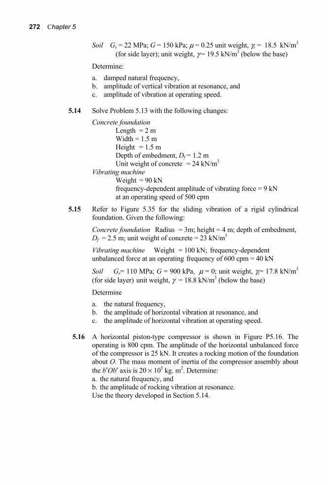
272 Chapter 5
Soil Gs = 22 MPa; G = 150 kPa; μ = 0.25 unit weight, γs = 18.5 kN/m3 (for side layer); unit weight, γ = 19.5 kN/m3 (below the base)
Determine: a. damped natural frequency, b. amplitude of vertical vibration at resonance, and c. amplitude of vibration at operating speed.
5.14 Solve Problem 5.13 with the following changes: Concrete foundation Length = 2 m Width = 1.5 m Height = 1.5 m Depth of embedment, Df = 1.2 m Unit weight of concrete = 24 kN/m3 Vibrating machine Weight = 90 kN frequency-dependent amplitude of vibrating force = 9 kN at an operating speed of 500 cpm
5.15 Refer to Figure 5.35 for the sliding vibration of a rigid cylindrical foundation. Given the following:
Concrete foundation Radius = 3m; height = 4 m; depth of embedment, Df = 2.5 m; unit weight of concrete = 23 kN/m3
Vibrating machine Weight = 100 kN; frequency-dependent unbalanced force at an operating frequency of 600 cpm = 40 kN
Soil Gs= 110 MPa; G = 900 kPa, μ = 0; unit weight, γs= 17.8 kN/m3 (for side layer) unit weight, γ = 18.8 kN/m3 (below the base)
Determine a. the natural frequency, b. the amplitude of horizontal vibration at resonance, and c. the amplitude of horizontal vibration at operating speed.
5.16 A horizontal piston-type compressor is shown in Figure P5.16. The operating is 800 cpm. The amplitude of the horizontal unbalanced force of the compressor is 25 kN. It creates a rocking motion of the foundation about O. The mass moment of inertia of the compressor assembly about the b′Ob′ axis is 20 × 105 kg. m2. Determine: a. the natural frequency, and b. the amplitude of rocking vibration at resonance.
Use the theory developed in Section 5.14.

Foundation Vibration 273
Figure P5.16
References Arnold, R. N., Bycroft, G. N., and Wartburton, G. B. (1955). “Forced Vibrations
of a Body on an Infinite Elastic Solid,” Journal of Applied Mechanics, ASME, Vol. 77, pp. 391-401.
Baranov, V. A. (1967). “On the Calculation of Excited Vibrations of an Embedded Foundation,” (in Russian), Vopr. Dyn. Prochn., Vol. 14, pp. 195-209

274 Chapter 5
Barkan, D. D. (1962) Dynamic Bases and Foundations, McGraw-Hill Book Company, New York.
Beredugo, Y. O., and Novak, M. (1972). “Coupled Horizontal and Rocking Vibration of Embedded Footing,” Canadian Geotechnical Journal, Vol. 9, No. 4, pp. 477-497.
Borowicka, H. (1943). “Uber Ausmittig Belastere Starre Platten auf Elastischisotropem Undergrund,” Ingenieur-Archiv, Berlin, Vol. 1, pp. 1-8.
Bycroft, G. N. (1956). “Forced Vibrations of a Rigid Circular Plate on a Semi-Infinite Elastic Space and on an Elastic Stratum,” Philosophical Transactions of the Royal Society, London, Ser. A., Vol. 248, pp. 327-368.
Dobry, R., and Gazetas, G. (1986). “Dynamic Response of Arbitrarily Shaped Foundations,” Journal of the Geotechnical Engineering Division, ASCE, Vol. 112, No. GT2, pp. 109-135.
Fry, Z. B. (1963). “Report 1: Development and Evaluation of Soil Bearing Capacity, Foundation of Structures, Field Vibratory Test Data,” Technical Report No. 3-362, U.S. Army Engineers Waterways Experiment Station, Vicksburg, Mississippi.
Gorbunov-Possadov, M. I., and Serebrajanyi, R. V. (1961). “Design of Structures upon Elastic Foundations,” Proceedings, 5th International Conference on Soil Mechanics and Foundation Engineering, Vol. 1, pp. 643-648.
Hall, J. R. Jr. (1967). “Coupled Rocking and Sliding Oscillations of Rigid Circular Footings,” Proceedings, International Symposium on Wave Propagation and Dynamic Properties of Earth Materials, Albuquerque, New Mexico, pp. 139-148.
Hsieh, T. K. (1962), “Foundation Vibrations,” Proceedings, Institute of Civil Engineers, London, Vol. 22, pp. 211-226.
Lamb, H. (1904). “On the Propagation of Tremors over the Surface of an Elastic Solid,” Philosophical Transactions of the Royal Society, London, Ser. A., Vol. 203, pp. 1-42.
Liao, S., and Sangrey, D. A. (1978). “Use of Piles an Isolation Barriers,” Journal of the Geotechnical Engineering Division, ASCE, Vol. 104, No. GT9, pp. 1139-1152.
Lysmer, J., and Richart, F. E., Jr. (1966). “Dynamic Response to Footings to Vertical Loading,” Journal of the Soil Mechanics and Foundations Division, ASCE, Vol. 92, No. SM1, pp. 65-91.
Novak, M., and Beredugo, Y. O. (1972). “Vertical Vibration of Embedded Footings,” Journal of the Soil Mechanics and Foundations Division, ASCE, Vol. 98, No. SM12, pp. 1291-1310.
Novak, M., and Sachs, K. (1973). “Torsional and Coupled Vibrations of Embedded Footings,” International Journal of Earthquake Engineering and Structural Dynamics, Vol. 2, No. 1, pp. 11-33.
Prakash, S., and Puri, V. K. (1981). “Observed and Predicted Response of a Machine Foundation,” Proceedings, 10th International Conference on Soil Mechanics and Foundation Engineering, Strockholm, Vol. 3, pp. 269-272.
With permission from ASCE.
With permission from ASCE.

Foundation Vibration 275
Prakash, S., and Puri, V. K. (1988). Foundations for Machines: Analysis and Design, John Wiley and Sons, New York.
Quinlan, P. M. (1953). “The Elastic Theory of Soil Dynamics,” Symposium on Dynamic Testing of Soils, Special Technical Publication 156, ASTM, pp.3-34.
Reissner, E. (1936). “Stationare, axialsymmetrische durch eine Schuttelnde Masseerregte Schwingungen eines homogenen elastischen halbraumes,” Ingenieur-Archiv., Vol. 7, No. 6. pp. 381-396.
Reissner, E. (1937). “Freie and erzwungene Torsionschwingungen des elastischen halbraumes,” Ingenieur-Archiv., Vol. 8, No. 4, pp. 229-245.
Reissner, E., and Sagochi, H. F. (1944). “Forced Torsional Oscillations of an Elastic Half Space,” Journal of Applied Physics, Vol. 15, pp. 652-662.
Richart, F. E., Jr. (1962). “Foundation Vibrations,” Transactions, ASCE, Vol. 27, Part 1, pp. 863-898.
Richart, F. E., Jr., Hall, J. R., and Woods, R. D. (1970). Vibration of Soils and Foundations, Prentice-Hall, Inc., Englewood Cliffs, New Jersey.
Richart. F. and Whitman, R. V. (1967). “Comparison of Footing Foundation Tests with Theory,” Journal of the Soil Mechanics and Foundations, ASCE, Vol. 93, No. SM6, pp. 143-167.
Sung, T. Y. (1953). “Vibration in Semi-Infinite Solids Due to Periodic Surface Loadings,” Symposium on Dynamic Testing of Soils, Special Technical Publication No. 156, ASTM, pp. 35-54.
Timoshenko, S. P., and Goodier, J. H. (1951). Theory of Elasticity. McGraw-Hill Book Company, New York.
Whitman, R. V., and Richart, F. E., Jr. (1967). “Design Procedures for Dynamically Loaded Foundations,” Journal of the Soil Mechanics and Foundations Division, ASCE, Vol. 93, No. SM6. pp. 169-193.
Woods, R. D. (1968). “Screening of Surface Waves in Soils,” Journal of the Soil Mechanics and Foundations Division, ASCE, Vol. 94, No. SM4, pp. 951-979.
Woods, R. D., Barnett, N. E., and Sagesser, R. (1974). “Holography – A New Tool for Soil Dynamics,” Journal of Geotechnical Engineering Division, ASCE, Vol. 100, No. GT11, pp. 1231-1247.
With permission from ASCE.
With permission from ASCE.
With permission from ASCE.
With permission from ASCE.
With permission from ASCE.
E., Jr.,

276
6 Dynamic Bearing Capacity of Shallow Foundations
6.1 Introduction The static bearing capacity of shallow foundations has been extensively studied and reported in literature. However, foundations can be subjected to single pulse dynamic loads which may be in vertical or horizontal directions. The dynamic loads due to nuclear blasts are mainly vertical. Horizontal dynamic loads on foundations are due mostly to earthquakes. These types of loading may induce large permanent deformation in foundations. Isolated column footings, strip footings, mat footings, and even pile foundations all may fail during seismic events. Such failures are generally attributed to liquefaction (a condition where the mean effective stress in a saturated soil reduces to zero, as explained in Chapter 10). However, a number of failures have occurred where field conditions indicate there was only partial saturation or a dense soil and therefore liquefaction alone is a very unlikely explanation. Rather, the reason for the seismic settlements of these foundations seems to be that the bearing capacity was reduced (Richards, Elms and Budhu,1993).
Though large amount of information on the dynamic bearing capacity of foundations is available in literature, it is mostly based on theoretical procedures and not supported by field data. Hence most of such published studies are yet to enter the design offices. Most of the important works on this topic are summarized in this chapter.
However, one must keep in mind that, during the analysis of the time-dependent motion of a foundation subjected to dynamic loading or estimating the bearing capacity under dynamic conditions several factors need to be considered. Most important of these factors are
a) nature of variation of the magnitude of the loading pulse, b) duration of the pulse, and c) strain-rate response of the soil during deformation

Dynamic Bearing Capacity of Shallow Foundations 277
Ultimate Dynamic Bearing Capacity
6.2 Bearing Capacity in Sand The static ultimate bearing capacity of shallow foundations subjected to vertical loading (Figure 6.1) can be given by the equation
12u c c c q q qq cN S d qN S d BN S dg g gg= + + (6.1)
where qu = ultimate load per unit area of the foundation γ = effective unit weight of soil q = γDf Df = depth of foundation B = width of foundation c = cohesion of soil Nc, Nq, Nγ = bearing capacity factors which are only functions of the soil friction angle φ Sc, Sq, Sγ = shape factors dc, dq, dγ = depth factors
In sands, with c = 0, Eq. (6.1) becomes
12u q q qq qN S d BN S dg g gg= + (6.2)
Figure 6.1 Static ultimate bearing capacity of continuous shallow foundations

278 Chapter 6
The values of Nq (Reissner, 1924) and Nγ (Caquot and Kerisel, 1953; Vesic, 1973) can be represented by the following equations:
2tan tan 452qN e f fp ⎛ ⎞= +⎜ ⎟
⎝ ⎠ (6.3)
2( 1)tanqN Ng f= + (6.4)
where φ is the angle of friction of soil. The values of Nq and Nγ for various soil friction angles are given in Table 6.1. Table 6.1 Valuesa of Bearing Capacity Factors, Nq and Nγ φ (deg) Nq Nγ φ (deg) Nq Nγ
0 1.00 0.00 26 11.85 12.54 27 13.20 14.47 1 1.09 0.07 28 14.72 16.72 2 1.20 0.15 29 16.44 19.34 3 1.31 0.24 30 18.40 22.40 4 1.43 0.34 5 1.57 0.45 31 20.63 25.99 32 23.18 30.22 6 1.72 0.57 33 26.09 35.19 7 1.88 0.71 34 29.44 41.06 8 2.06 0.86 35 33.30 48.03 9 2.25 1.03 10 2.47 1.22 36 37.75 56.31 37 42.92 66.19 11 2.71 1.44 38 48.93 78.03 12 2.97 1.69 39 55.96 92.25 13 3.26 1.97 40 64.20 109.41 14 3.59 2.29 15 3.94 2.65 41 73.90 130.22 42 85.38 155.55 16 4.34 3.06 43 99.02 186.54 17 4.77 3.53 44 115.31 224.64 18 5.26 4.07 45 134.88 271.76 19 5.80 4.68 20 6.40 5.39 46 158.51 330.35 47 187.21 403.67 21 7.07 6.20 48 222.31 496.01 22 7.82 7.13 49 265.51 613.16 23 8.66 8.20 50 319.07 762.89 24 9.60 9.44 25 10.66 10.88 a After Vesic (1973)

Dynamic Bearing Capacity of Shallow Foundations 279
The shape and depth factors have been proposed by DeBeer (1970) and Brinch Hanson (1970):
Shape Factors
1 tanqBSL
f⎛ ⎞= + ⎜ ⎟⎝ ⎠
(6.5)
1 0 4 BS .Lg
⎛ ⎞= − ⎜ ⎟⎝ ⎠
(6.6)
Depth Factors
For DB
f £ 1, dq = 1 + 2 tan φ (1 – sin φ)2 DB
fFHGIKJ (6.7)
dγ = 1 (6.8)
For DB
f >1, dq = 1 + 2 tan φ (1 – sin φ)2 tan−1 DB
fFHGIKJ (6.9)
dγ = 1 (6.10)
In Eqs. (6.5)-(6.10), B and L are the width and length of rectangular foundations, respectively. For circular foundations, B is the diameter, and B = L.
The preceding equations for static ultimate bearing capacity evaluation are valid for dense sands where the failure surface in the soil extends to the ground surface as shown in Figure 6.1. This is what is referred to as the case of general shear failure. For shallow foundations (i.e., fD B £ 1), if the relative density of granular soils RD is less than about 70%, local or punching shear failure may occur. Hence, for static ultimate bearing capacity calculation, if 0 ≤ RD ≤ 0.67, the values of φ in Eqs. (6.3)-(6.10) should be replaced by the modified friction angle
1 2tan [(0.67 0.75 ) tan ]D DR Rf f−′ = + − (6.11)
The facts just described relate to the static bearing capacity of shallow foundations. However, when load is applied rapidly to a foundation to cause failure, the ultimate bearing capacity changes somewhat. This fact has been shown experimentally by Vesic, Banks, and Woodward (1965), who conducted several laboratory model tests with a 101.6 mm diameter rigid rough model footing placed on the surface of a dense river sand (i.e., Df = 0), both dry and saturated. The rate of loading to cause failure was varied in a range of 2.54 × 10⁻⁴ mm/s to over 254 mm/s. Hence, the rate was in the range of static (2.54 × 10⁻⁴ mm /s) to impact (254 mm/s) loading conditions. All but the four

280 Chapter 6
most rapid tests in submerged sand [loading velocity, (14.63-20.07 mm/s)] showed peak failure loads as obtained in the case of general shear failure of soil.
The four most rapid tests in submerged sand gave the load-displacement plots as obtained in the case of punching shear failure, where the failure planes do not extend to the ground surface.
For surface footings (Df = 0) in sand, q = 0 and dγ = 1. So
12uq BN Sg gg= (6.12)
or
(1 2)
uq N SB g gg
= (6.13)
The variation of (1 2)uq Bg with load velocity for the tests of Vesic, Banks, and Woodward (1965) is shown in Figure 6.2. It may be seen that, for any given series of tests, the value of (1 2)uq Bg gradually decreases with the loading velocity to a minimum value and then continues to increase.
Figure 6.2 Plot of bearing capacity factor versus loading velocity (after Vesic, Banks,
and Woodward, 1965)
Dynamic Bearing Capacity of Shallow Foundations 281
This, in effect, corresponds to a decrease in the angle of friction of soil by about 2º when the loading velocity reached a value of about 50.8 × 10⁻³ mm/s. Such effects of strain rate in reducing the angle of friction of sand has also been observed by Whitman and Healy (1962), as described in Chapter 4.
Based on the experimental results available, the following general conclusions regarding the ultimate dynamic bearing capacity of shallow foundations in sand can be drawn:
1. For a foundation resting on sand and subjected to an acceleration level of amax ≤ 13g, it is possible for general shear type of failure to occur in soil (Heller, 1964).
2. For a foundation on sand subjected to an acceleration level of amax > 13g, the nature of soil failure is by punching (Heller, 1964).
3. The difference in the nature of failure in soil is due to the inertial restrain of the soil involved in failure during the dynamic loading. The restrain has almost a similar effect as the overburden pressure as observed during the dynamic loading which causes the punching shear type failure in soil.
4. The minimum value of the ultimate dynamic bearing capacity of shallow foundations on dense sands obtained between static to impact loading range can be estimated by using a friction angle φdy, such that (Vesic, 1973)
2dyf f= - (6.14)
The value of dyf can be substituted in place of f in Eqs. (6.2)-(6.10). However, if the soil strength parameters with proper strain rate are known from laboratory testing, they should be used instead of the approximate equation [Eq. (6.14)].
5. The increase of the ultimate bearing capacity at high loading rates as seen in Figure 6.2 is due to the fact that the soil particles in the failure zone do not always follow the path of least resistance. This results in an higher shear strength of soil, which leads to a higher bearing capacity.
6. In the case of foundations resting on loose submerged sands, transient liquefaction effects (Chapter 10) may exist (Vesic, 1973). This may results in unreliable prediction of ultimate bearing capacity.
7. The rapid increase of the ultimate bearing capacity in dense saturated sand at fast loading rates is due to the development of negative pore water pressure in the soil.
Example 6.1 A square foundation with dimensions B × B has to be constructed on a dense sand. Its depth is Df = 1 m. The unit weight and the static angle of friction of the soil can be assigned representative values of 18 kN/m3 and 39º, respectively. The

282 Chapter 6
foundation may occasionally be subjected to a maximum dynamic load of 1800 kN increasing at a moderate rate. Determine the size of the foundation using a safety factor of 3. Solution
Given that φ = 39º in the absence of any other experimental data, for minimum ultimate dynamic bearing capacity
2 39 2 37dyf f= - = - = From Eq. (6.2)
12u q q qq qN S d BN S dg g gg= +
q = γDf = (18)(1) = 18 kPa
For φdy = 37º, Nq = 42.92 and Nγ = 66.19.
1 tanqBSL
f⎛ ⎞= + ⎜ ⎟⎝ ⎠
= 1 + tan 37º = 1.754
1 0 4 BS .Lg
⎛ ⎞= − ⎜ ⎟⎝ ⎠
= 1 – 0.4 = 0.6
dq = 1 + 2 tan φ (1 – sin φ)2 DB
fFHGIKJ
= 1 + 2 tan 37 (1 – sin 37)2 BLFHIK = 1 + 0 239.
B
dγ = 1
Thus
qu = (18)(42.92) (1.754) 1 0 239+FHIK
.B
+ 12
(18) (B) (66.19) (0.6) (1)
= 1355 + 323 9.B
+ 357.4B (a)
Given
qu = 1800 32¥
B kPa (b)
Combining Eq. (a) and (b),
5400
2B = 1355 + 323 9.
B + 357.4B (c)

Dynamic Bearing Capacity of Shallow Foundations 283
Following is a table to determine the value of B by trial and error. Clearly, B ≈ 1.6 m. B 5400/B2 1355 + 323.9/B + 357.4B (m) (kPa) (kPa) 2.0 1350 2331.75 1.5 2400 2107.00 1.6 2109 2133.00
6.3 Bearing Capacity in Clay For foundations resting on saturated clays (φ = 0 and c = cu; i.e., undrained condition), Eq. (6.1) transforms to the form
u u c c c q q qq c N S d qN S d= + (6.15)
(Note: 0Ng = for φ = 0 in Table 6.1)
Nc = 5.14 (6.16) and Nq = 1 (6.17)
The values for Sc and Sq (DeBeer, 1970) and dc and dq (Brinch Hansen, 1970) are as follows:
Sc = 1 + BL
NN
q
c
FHIKFHGIKJ
For φ = 0,
Sc = 1 + BLFHIKFHIK
1514.
= 1 + 0.1946 BLFHIK (6.18)
Sq = 1 + tan φ Sq = 1 (6.19)
dc = 1 + 0.4DB
fFHGIKJ for
DB
f ≤ 1 (6.20)
dc = 1 + 0.4 tan−1 DB
fFHGIKJ for
DB
f > 1 (6.21)
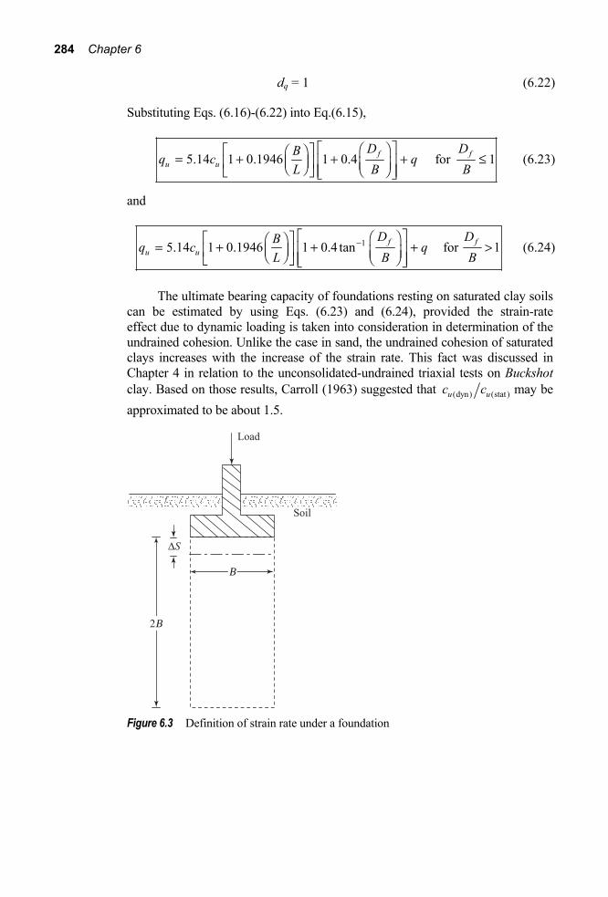
284 Chapter 6
dq = 1 (6.22)
Substituting Eqs. (6.16)-(6.22) into Eq.(6.15),
5.14 1 0.1946 1 0.4 for 1f fu u
D DBq c qL B B
È ˘Ê ˆÈ ˘Ê ˆ= + + + £Í ˙Á ˜Í ˙ Á ˜Ë ¯ Ë ¯Í ˙Î ˚ Î ˚ (6.23)
and
15.14 1 0.1946 1 0.4 tan for 1f fu u
D DBq c qL B B
-È ˘Ê ˆÈ ˘Ê ˆ= + + + >Í ˙Á ˜Í ˙ Á ˜Ë ¯ Ë ¯Í ˙Î ˚ Î ˚ (6.24)
The ultimate bearing capacity of foundations resting on saturated clay soils can be estimated by using Eqs. (6.23) and (6.24), provided the strain-rate effect due to dynamic loading is taken into consideration in determination of the undrained cohesion. Unlike the case in sand, the undrained cohesion of saturated clays increases with the increase of the strain rate. This fact was discussed in Chapter 4 in relation to the unconsolidated-undrained triaxial tests on Buckshot clay. Based on those results, Carroll (1963) suggested that (dyn) (stat )u uc c may be approximated to be about 1.5.
Figure 6.3 Definition of strain rate under a foundation
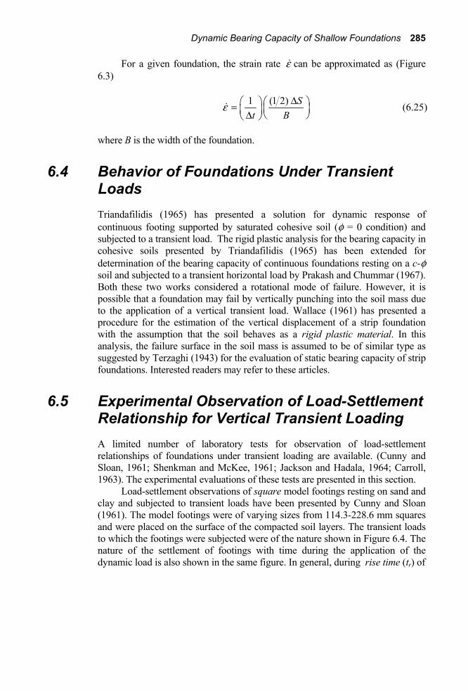
Dynamic Bearing Capacity of Shallow Foundations 285
For a given foundation, the strain rate e can be approximated as (Figure 6.3)
1 (1 2) St B
e Δ⎛ ⎞ ⎛ ⎞= ⎜ ⎟⎜ ⎟Δ ⎝ ⎠⎝ ⎠ (6.25)
where B is the width of the foundation.
6.4 Behavior of Foundations Under Transient Loads Triandafilidis (1965) has presented a solution for dynamic response of continuous footing supported by saturated cohesive soil (φ = 0 condition) and subjected to a transient load. The rigid plastic analysis for the bearing capacity in cohesive soils presented by Triandafilidis (1965) has been extended for determination of the bearing capacity of continuous foundations resting on a c-φ soil and subjected to a transient horizontal load by Prakash and Chummar (1967). Both these two works considered a rotational mode of failure. However, it is possible that a foundation may fail by vertically punching into the soil mass due to the application of a vertical transient load. Wallace (1961) has presented a procedure for the estimation of the vertical displacement of a strip foundation with the assumption that the soil behaves as a rigid plastic material. In this analysis, the failure surface in the soil mass is assumed to be of similar type as suggested by Terzaghi (1943) for the evaluation of static bearing capacity of strip foundations. Interested readers may refer to these articles.
6.5 Experimental Observation of Load-Settlement Relationship for Vertical Transient Loading A limited number of laboratory tests for observation of load-settlement relationships of foundations under transient loading are available. (Cunny and Sloan, 1961; Shenkman and McKee, 1961; Jackson and Hadala, 1964; Carroll, 1963). The experimental evaluations of these tests are presented in this section.
Load-settlement observations of square model footings resting on sand and clay and subjected to transient loads have been presented by Cunny and Sloan (1961). The model footings were of varying sizes from 114.3-228.6 mm squares and were placed on the surface of the compacted soil layers. The transient loads to which the footings were subjected were of the nature shown in Figure 6.4. The nature of the settlement of footings with time during the application of the dynamic load is also shown in the same figure. In general, during rise time (tr) of

286 Chapter 6
Figure 6.4 Nature of dynamic load applied to laboratory model footings
the dynamic load, the settlement of a footings increases rapidly. Once the peak load [Qd(max)] is reached, the rate of settlement with time decreases. However, the total settlement of a footing continues to increase during the dwell time of the load (tdw) and reaches a maximum value (Smax) at the end of the dwell time. During the decay period of the load (tde), the footing rebounds to some degree.
The results of the model footings tests on sand obtained by Cunny and Sloan are given in Table 6.2. Also, the results of model tests for square surface footings on clay as reported by Cunny and Sloan are shown in Table 6.3. Based on these results, a few general observations may be made: 1. The settlement of foundations under transient loading is generally uniform.
This can be seen by observing the settlement at three corners of the model footings – both in sand and clay.
2. Footings under dynamic loading may fail by punching type of failure in soil, although general shear failure may be observed for the same footings tested under static conditions.
3. In Table 6.2, the 228 mm footing failed at a load of 11.52 kN under static loading conditions. The total settlement after the failure load application was 66.55 mm. However, under dynamic loading conditions, when Qd(1)/Qu was equal to 1.25 (Test 4), the settlement of the footing was about 10.16 mm. Similarly, in Table 6.3, the static failure load Qu of the 114.3 mm footing was 10.94 kN with a settlement of 50.8 mm. The same footings under

Dynamic Bearing Capacity of Shallow Foundations 287
dynamic loading with Qd(1)/Qu = 1.17 (Test 2) showed a total settlement of about 17.78 mm.
Table 6.2 Load-Settlement Relationship of Square Footings on Sand Due to Transient Loadinga
Size of Qd(1) Smax(mm)c Test footing Qu Qd(max) Qd(1) Qu tr tdw tde No. (mm) (kN)b (kN) (kN) % (ms) (ms) (ms) Pot.1 Pot.2 Pot.3 1 152 × 152 3.43 3.56 3.56 104 18 122 110 7.11 1.27 2.79 2 203 × 203 8.09 13.97 12.46 154 8 420 255 — — — 3 203 × 203 8.09 10.12 9.67 120 90 280 290 21.08 23.62 24.13 4 228 × 228 11.52 15.57 14.46 125 11 0 350 10.16 10.67 10.16 a Complied from Cunny and Sloan (1961): Compacted dry unit weight of sand = 16.26 kN/m3; relative density of compaction of sand = 96%; triaxial angle of friction of sand = 32º. b Ultimate failure load tested under static conditions. c Settlement of footings measured at three corners of each footing by linear potentiometer.
Table 6.3 Load-Settlement Relationship of Square Footings on Clay Due to Transient Loadinga
Size of Qd(1) Smax(mm)c Test footing Qu Qd(max) Qd(1) Qu tr tdw tde No. (mm) (kN)b (kN) (kN) % (ms) (ms) (ms) Pot.1 Pot.2 Pot.3 1 114 × 114 10.94 12.68 10.12 93 9 170 350 12.70 12.70 12.19 2 114 × 114 10.94 13.79 12.54 117 9 0 380 16.76 18.29 17.78 3 114 × 114 10.94 15.39 13.21 121 10 0 365 43.18 42.67 43.18 4 127 × 127 13.52 15.92 13.12 97 9 0 360 14.73 13.97 13.97 a Complied from Cunny and Sloan (1961): Compacted moist unit weight =14.79-1547 kN/m3; moisture content = 22.5 ± 1.7%; c = 115 kPa; φ = 4º (undrained test). b Ultimate failure load tested under static loading conditions. c Settlement of footings measured at three corners of each footing by linear potentiometer.
These facts show that, for a limiting settlement condition, a foundation can
support higher load under dynamic loading conditions than those observed from static tests.
Dynamic Load versus Settlement Prediction in Clayey Soils Jackson and Hadala (1964) reported several laboratory model tests on 114.3-203.2 mm square footings resting on highly saturated, compacted, plastic Buckshot clay. The tests were similar in nature to those described previously in this section. Based on these results, Jackson and Hadala have shown that there is a unique nondimensional relation between 2
(max)d uQ B c and maxS B (cu is undrained shear strength). This is shown in Figure 6.5. Note that the tests on

288 Chapter 6
which Figure 6.5 are based have tdw = 0. However, for dynamic loads with tdw > 0, the results would not be too different.
The preceding finding is of great practical importance in estimation of the dynamic load-settlement relationships of foundations. Jackson and Hadala have recommended the following procedure for that purpose.
1. Determine the static load Q versus settlement S relationship for a foundation from plate bearing tests in the field.
2. Determine the unconfined compression strength of the soil quc in the laboratory.
2uc uq c=
3. Plot a graph of 2uQ B c versus statS B . (See Figure 6.6, curve a.)
Figure 6.5 Nondimensional relationship of 2(max)d uQ B c and (max)S B for model
footing tests in Buckshot clay (after Jackson and Hadala, 1964)

Dynamic Bearing Capacity of Shallow Foundations 289
Figure 6.6 Prediction of dynamic load-settlement relationship for foundations on clay
4. For any given value of statS B , multiply 2
uQ B c by the strain rate factor (≈1.5) and plot it in the same graph. The resulting graph of statS B versus
21.5 uQ B c will be the predicted relationship between 2(max)d uQ B c and
maxS B . (See Figure 6.6, curve b.)
Example 6.2
The estimated static plate load bearing test results of a foundation resting on stiff clay and 1.5 m in diameter are given below. Q Settlement Q Settlement (kN) (mm) (kN) (mm) 0 0 27.0 41.9 4.5 6.4 36.0 73.7 9.0 12.2 40.5 94.0 18.0 27.9 45.0 172.7
The unconfined compression strength of this clay was 160 kPa.

290 Chapter 6
a. Plot a graph of estimated Smax /B versus Qd(max)/QB2cu assuming a strain-rate factor of 1.5.
b. Determine the magnitude of the maximum dynamic load Qd(max) that produces a maximum settlement Smax of 0.15 m.
Solution
Given B = 1.5 m = 1500 mm. and cu = 12
(160) = 80 kPa, the following table can
be prepared. Q Sstat S/B (kN) (mm) (%) Q/B2cu 1.5Q/B2cu (1) (2) (3) (4) (5) 0 0 0 0 0 4.5 6.4 0.4267 0.025 0.037 9.0 12.2 0.8133 0.050 0.075 18.0 27.9 1.8600 0.100 0.150 27.0 41.9 2.7930 0.150 0.225 36.0 73.7 4.9130 0.200 0.300 40.5 94.0 6.2670 0.225 0.337 45.0 172.7 11.5130 0.250 0.375
Figure 6.7
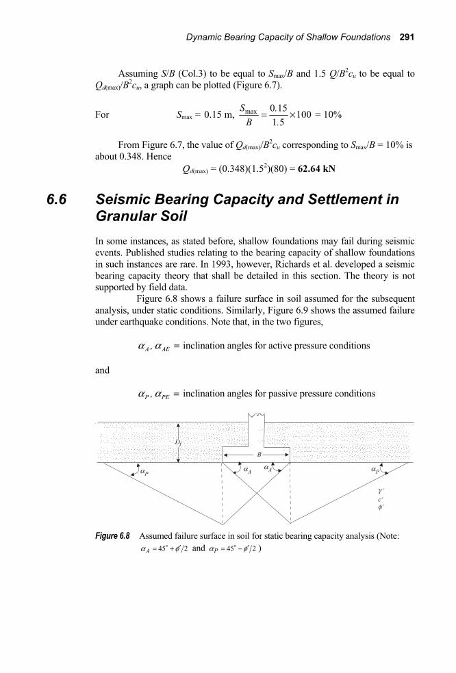
Dynamic Bearing Capacity of Shallow Foundations 291
Assuming S/B (Col.3) to be equal to Smax/B and 1.5 Q/B2cu to be equal to
Qd(max)/B2cu, a graph can be plotted (Figure 6.7).
For Smax = 0.15 m, max 0 15 1001 5
S .B .
= ¥ = 10%
From Figure 6.7, the value of Qd(max)/B2cu corresponding to Smax/B = 10% is about 0.348. Hence Qd(max) = (0.348)(1.52)(80) = 62.64 kN
6.6 Seismic Bearing Capacity and Settlement in Granular Soil In some instances, as stated before, shallow foundations may fail during seismic events. Published studies relating to the bearing capacity of shallow foundations in such instances are rare. In 1993, however, Richards et al. developed a seismic bearing capacity theory that shall be detailed in this section. The theory is not supported by field data. Figure 6.8 shows a failure surface in soil assumed for the subsequent analysis, under static conditions. Similarly, Figure 6.9 shows the assumed failure under earthquake conditions. Note that, in the two figures, A AE,a a = inclination angles for active pressure conditions
and
P PE,a a = inclination angles for passive pressure conditions
Figure 6.8 Assumed failure surface in soil for static bearing capacity analysis (Note:
45 2Aa f′= + and 45 2Pa f′= − )
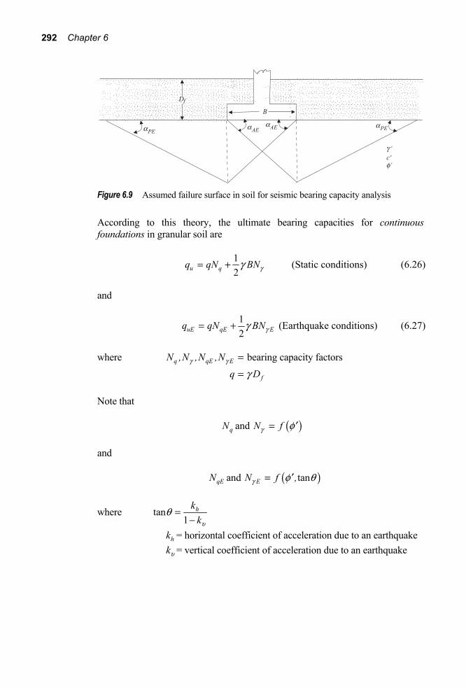
292 Chapter 6
Figure 6.9 Assumed failure surface in soil for seismic bearing capacity analysis
According to this theory, the ultimate bearing capacities for continuous foundations in granular soil are
12u qq qN BNgg= + (Static conditions) (6.26)
and
12uE qE Eq qN BNgg= + (Earthquake conditions) (6.27)
where q qE EN ,N ,N ,Ng g = bearing capacity factors fq Dg=
Note that
( )andqN N fg f= ¢
and
( )and tanqE EN N f ,g f q= ¢
where tan1
hkku
q =−
hk = horizontal coefficient of acceleration due to an earthquake ku = vertical coefficient of acceleration due to an earthquake

Dynamic Bearing Capacity of Shallow Foundations 293
Using the failure surface shown in Figure 6.8, Richards, Elms and Budhu (1993) provided the values of bearing capacity factors qN and Ng . They are given in Table 6.4.
Table 6.4 Bearing capacity factors φ(deg) Nq Nγ 0 1.0 0 10 2.4 1.4 20 5.9 6.4 30 16.5 23.8 40 59.0 112.0
The variations of qN and Ng with f ¢ are shown in Figure 6.10. Figure 6.11 shows the variations of EN Ng g and qE qN N with tanq and the soil anglef ¢ based on this analysis.
Under static conditions, bearing capacity failure can lead to a substantial sudden downward movement of the foundation. However, bearing capacity related settlement in an earthquake is important and it takes place when the ratio tan (1 )hk kuq = − reaches the critical value ( )1hk k .u
∗− If 0ku = ,
then ( )1hk ku∗− becomes equal to hk .∗
Figure 6.12 shows the variation of hk∗ (for 0ku = ) with the factor of safety (FS) applied to the ultimate static bearing capacity [Eq. 6.26], with f ¢ , and with fD B (for 30 and 40f =¢ ).
The settlement of a strip foundation due to an earthquake using a sliding block approach can be estimated (Richards, Elms and Budhu, 1993) as
( )42
Eq m 0 174 tanhAE
kVS .Ag A
a−∗⎡ ⎤
= ⎢ ⎥⎣ ⎦
(6.28)
where V = peak velocity for the design earthquake (m/sec) A = acceleration coefficient for the design earthquake g = acceleration due to gravity (9.81 m/sec2)
The values of hk∗ and AEa can be obtained from Figure 6.12 and Table 6.5, respectively. This approach can be used to design a footing based on limiting seismic settlements.

294 Chapter 6
Figure 6.10 Variation of qN and Ng based on failure surface assumed in Figure 6.8
Table 6.5 Variation of AEa with hk∗ and soil friction anglef ¢ (Compiled from Richards, Elms and Budhu, 1993)
tana AE
hk∗ ¢ o20f = ¢ o25f = ¢ o30f = ¢ o35f = ¢ o40f = 0.05 1.10 1.24 1.39 1.57 1.75 0.10 0.97 1.13 1.26 1.44 1.63 0.15 0.82 1.00 1.15 1.32 1.48 0.20 0.71 0.87 1.02 1.18 1.35 0.25 0.56 0.74 0.92 1.06 1.23 0.30 0.61 0.77 0.94 1.10 0.35 0.47 0.66 0.84 0.98 0.40 0.32 0.55 0.73 0.88 0.45 0.42 0.63 0.79 0.50 0.27 0.50 0.68 0.55 0.44 0.60 0.60 0.32 0.50

Dynamic Bearing Capacity of Shallow Foundations 295
Figure 6.11 Variation of EN Ng g and qE qN N with tanq
Figure 6.12 Critical acceleration hk∗ for 0ku =

296 Chapter 6
Example 6.3
A strip foundation is to be constructed on a sandy soil with B = 1.2 m, fD = 0.9
m,g =17.6 kN/m3, and f ¢ = 30º. a. Determine the gross ultimate bearing capacity uEq . Assume that
0ku = and 0 176hk .= . b. If the design earthquake parameters are V = 0.4 m/sec and A = 0.32,
determine the seismic settlement of the foundation. Use FS = 3 to obtain the static allowable bearing capacity.
Solution:
a. From Figure 6.10, for 30 16 51 and 23 76q,N . N . .gf = = =¢ Also,
0 176tan 0 1761 1 0
hk . .kυ
θ = = =− −
For tan 0 176.q = , Figure 6.11
0 4EN.
Ng
g= and 0 63qE
q
N.
N=
Thus, ENg = (0.4)(23.76) = 9.5 qEN = (0.63)(16.51) = 10.4 and
12uE qE Eq qN BNgg= +
( )( ) ( )( )( )117 6 0 9 10 4 17 6 1 2 9 52
. . . . . .⎛ ⎞= × + ⎜ ⎟⎝ ⎠
= 265.06 kPa
b. For the foundation, 0 9 0 751 2
fD . .B .
= =

Dynamic Bearing Capacity of Shallow Foundations 297
From Figure 6.12, for 30f =¢ , FS = 3, and 0 75fD B .= , the value of
0 26hk .∗ ≈ . Also, from Table 6.5, for 0 26hk .∗ = , the value of tan 0 92AE . .α ≈ From Eq. (6.28), we have
( )42
Eq m 0 174 tanhAE
kVS .Ag A
−∗⎡ ⎤= ⎢ ⎥
⎣ ⎦α
with V = 0.4 m/sec,
it follows that
( ) ( )( )( )
24
Eq0 40 260 174 0 92
0 32 0 32 9 81..S . .
. . .
−⎡ ⎤= ⎢ ⎥⎣ ⎦
0 0187 m =. 18.7 mm=
Problems 6.1 A 0.9 m square shallow foundation is supported by dense sand. The
relative density of compaction, unit weight, and angle of friction (static) of this sand are 75%, 19.2 kN/m3, and 38%, respectively. Given the depth of the foundation to be 0.9 m, estimate the minimum ultimate bearing capacity of this foundation that might be obtained if the vertical loading velocity on this foundation were varied from static to impact range.
6.2 Redo Problem 6.1 with the depth of the foundation as 1.40 m. 6.3 Redo Problem 6.1 with the following: Foundation width = 1.6 m Foundation depth = 0.75 m Angle of friction of sand = 35º Unit weight of compacted soil = 17.4 kN/m3 Relative density of the compaction of sand = 80% 6.4 A rectangular foundation has a length L of 2.5 m. It is supported by a
medium dense sand with a unit weight of 17 kN/m3. The sand has an angle of friction of 36º. The foundation may be subjected to a dynamic load of 735 kN increasing at a moderated rate. Using a factor of safety equal to 2, determine the width of the foundation. Use Df = 0.8 m.
6.5 A foundation 2.25 m square is supported by saturated clay. The unit weight of this clay is 18.6 kN/m3. The depth of the foundation is 1.2 m. Determine the ultimate bearing capacity of this foundation assuming that

298 Chapter 6
the load will be applied very rapidly. Given the following for the clay [laboratory unconsolidated-undrained triaxial (static) test results]:
Undrained cohesion, cu = 90 kPa Strain-rate factor = 1.4 6.6 Redo Problem 6.5 with the following changes: Foundation width = 1.5 m Foundation length = 2.6 m Foundation depth = 1.75 m 6.7 A clay deposit has an undrained cohesion (static test) of 90 kPa. A static
field plate load test was conducted with a plate having a diameter of 0.5 m. When the load per unit area q was 200 kPa, the settlement was 20 mm. a. Assume that, for a given value of q, settlement is proportional to the
width of the foundation. Estimate the settlement of a prototype circular foundation in the same clay with a diameter of 3 m (static loading).
b. The strain-rate factor of the clay is 1.4. If a vertical transient load pulse were applied to the foundation as given in part (a), what would be the maximum transient load (in kN) that will produce the same maximum settlement (Smax) as calculated in part (a)?
References Brinch Hansen, J. (1970). “A Revised and Extended Formula for Bearing
Capacity,” Bulletin No. 28, Danish Geotechnical Institute, Copenhagen, Denmark.
Carroll, W. F. (1963). “Dynamic Bearing Capacity of Soils. Vertical Displacements of Spread Footings on Clay: Static and Impulsive Loadings,” Technical Report No. 3-599, Report 5, U.S. Army Corps of Engineers, Waterways Experiment Station, Vicksburg, Mississippi.
Caquot, A., and Kerisel, J. (1953). “Sur le Terme de Surface Dans le Calcul des Foundations en Milieu Pulverulent,” Proceedings, 3rd International Conference on Soil Mechanics and Foundation Engineering, Zurich, Switzerland, Vol. I, pp. 336-337.
Cunny, R. W., and Sloan, R. C. (1961). “Dynamic Loading Machine and Results of Preliminary Small-Scale Footing Tests,” Special Technical Publication No. 305, American Society for Testing and Materials, pp. 65-67.
DeBeer, E. E. (1970). “Experimental Determination of the Shape Factors and the Bearing Capacity Factors of Sand,” Geotechnique, Vol. 20, No. 4, pp. 387-411.

Dynamic Bearing Capacity of Shallow Foundations 299
Heller, L. W. (1964). “Failure Modes of Impact-Loaded Footings on Dense Sand,” Technical Report R – 281, U.S. Naval Civil Engineering Laboratory, Port Hueneme, California.
Jackson, J. G., Jr., and Hadala, P. F. (1964). “Dynamic Bearing Capacity of Soils. Report 3: The application of Similitude of Small-Scale Footings Tests,” U.S. Army Corps of Engineers, Waterways Experiment Station, Vicksburg, Mississippi.
Prakash, S., and Chummar, A. V. (1967). “Response of Footings to Lateral Loads,” Proceedings, International Symposium on Wave Propagation and Dynamic Properties of Earth Materials, Ed., G. E. Triandafilidis, University of New Mexico, Albuquerque, New Mexico, pp. 679-691.
Reissner, H. (1924). “Zum Erddrukproblem,” Proceedings, First International Conference on Applied Mechanis, Delft, The Netherlands, pp. 294-311.
Richards, R., Jr., Elms, D. G., and Budhu, M. (1993). “Seismic Bearing Capacity of and Settlements of Foundations,” Journal of Geotechnical Engineering Division, ASCE, Vol. 119, No. 4, pp. 662-674.
Shenkman, S., and Mckee, K. E. (1961). “Bearing Capacity of Dynamically Loaded Footings,” Special Technical Publication No. 305, American Society for Testing and Materials, pp. 78-90.
Terzaghi, K. (1943). Theoretical Soil Mechanics, Wiley, New York. Triandafilidis, G. E. (1965). “The Dynamic Response of Continuous Footings
Supported on Cohesive Soils,” Proceedings, 6th International Conference on Soil Mechanics and Foundation Engineering, Montreal, Canada, Vol. II, pp. 205-208.
Vesic, A. S. (1973). “Analysis of Ultimate Loads of Shallow Foundations,” Journal of the Soil Mechanics and Foundations Division, ASCE, Vol. 99, No. SM1, pp. 45-73.
Vesic, A. S., Banks, D. C., and Woodard, J. M. (1965). “An Experiment Study of Dynamic Bearing Capacity of Footings of Sand,” Proceedings, 6th International Conference on Soil Mechanics and Foundation Engineering, Montreal, Canada, Vol. II, pp. 209-213.
Wallace, W. F. (1961). “Displacements of Long Footings by Dynamic Loads,” Journal of the Soil Mechanics and Foundation Division, ASCE, Vol. 87, No. SM5, pp. 45-68.
Whitman, R. V., and Healy, K. A. (1962). “Shear Strength of Sands During Rapid Loadings,” Journal of the Soil Mechanics and Foundations Division, ASCE, Vol. 88, No. SM2, pp. 99-132.
With permission from ASCE.

300
7 Earthquake and Ground Vibration
7.1 Introduction The study of earthquakes is important for scientific, social and economic reasons. Earthquakes attest to the fact that dynamic forces are operating within the earth. Stress builds up through time, storing strain energy and earthquakes represent the release of this stored strain energy.
The ground vibrations due to earthquake have resulted in several major structural damages in the past. In the North American continent, earthquakes are believed to originate from the rupture of faults. The ground vibration resulting from an earthquake is due to the upward transmission of the stress waves from rock to the softer soil layers(s). In recent times, several major studies have been performed to study the nature of occurrence of earthquakes and the associated amount of energy released. Also, modern techniques have been developed to analyze and estimate the physical properties of soils under earthquakes conditions and to predict the ground motion. These developments are the subjects of discussion in this chapter.
7.2 Definition of Some Earthquake-Related Terms Focus (or hypocenter): The focus of an earthquake is a point below the ground surface where the rupture of a fault first occurs (point F in Figure 7.1a). Focal Depth: The vertical distance from the ground surface to the focus (EF in Figure 7.1a). The maximum focal depth of all earthquakes recorded so far does not exceed 700 km, because they are confined to the rigid lithosphere, which can undergo brittle fracture.
Focal depths are normally related the type of plate boundary from which earthquakes are originating. Based on focal depth, earthquakes may be divided into the following three categories:

Earthquake and ground vibration 301
Figure 7.1 Definition of focus and epicenter: (a) section; (b) plan
1. Deep-focus earthquakes: These have focal depths of 300 – 700 km. They constitute about 3% of all earthquakes recorded around the world and are mostly located in the Circum-Pacific belt.
2. Intermediate-focus earthquakes: These have focal depths of 70 – 300 km. 3. Shallow-focus earthquakes: The focal depth for these is less than 70 km.
About 75% of all the earthquakes around the world belong to this category. The California earthquakes have focal depths of about 10 – 15 km.
Epicenter: The point vertically above the focus located on the ground surface (point E in Figure 7.1).
Epicentric Distance: The horizontal distance between the epicenter and the given site (line EA in Figure 7.1).
Hypocentric Distance: The distance between a given site and the focus (line FA in Figure 7.1a).
Effective Distance to Causative Fault: The distance from a fault to a given site for calculation of ground motion (Figure 7.2).

302 Chapter 7
This distance is commonly presumed to be the epicentric distance. This type of assumption, under circumstances, may lead to gross errors. It can be explained with reference to Figure 7.2, which shows the plans of two cases of fault rupture. In Figure 7.2a, the length of the fault rupture L is small as compared to the epicentric distance EA. In this case, the effective distance could be taken to be equal to the epicentric distance. However, a better estimate of the effective distance is BA (B is the midpoint of the ruptured fault). Figure 7.2b shows the case where the length of the fault rupture is large. In such circumstances, the length AC is the effective distance, which is the perpendicular distance from the site to the line of fault rupture in the plan.
Intensity: An arbitrary scale developed to measure the destructiveness of an earthquake at the surface. It is qualitative and is based on the damage caused by the earthquake. The same earthquake may have different intensities at two different locations depending on: soil conditions, ground water location and type of construction at that particular location. It is worth noting that there are several intensity scales available in the literature and the Modified Mercalli Scale (reported in Roman numerals) is presently in use in the United States for that purpose, divided into 12 degrees of intensity. An abridged version of the Modified Mercalli Scale is given in Table 7.1.
Figure 7.2 Effective distance from a site to the causative faults (Note: L is the length of
the fault rupture.)

Earthquake and ground vibration 303
Table 7.1 Abridged Modified Mercalli Intensity Scalea
Intensity Description I Detected only by sensitive instruments II Felt by a few persons at rest, especially on upper floors; delicate
suspended objects may swing III Felt noticeably indoors, but not always recognized as a quake;
standing autos rock slightly, vibration like passing trucks IV Felt indoors by many, outdoors by a few; at night some awaken;
dishes, windows, doors disturbed; motor cars rock noticeably V Felt by most people; some breakage of dishes, windows and
laster; disturbance of tall objects VI Felt by all; many are frightened and run outdoors; falling plaster
and chimneys; damage small VII Everybody runs outdoors; damage to building varies, depending
on quality of construction; noticed by drivers of autos VIII Panel walls thrown out of frames; fall of walls, monuments,
chimneys; sand and mud ejected; drivers of autos disturbed IX Buildings shifted off foundations, cracked, thrown out of plumb;
ground cracked; underground pipes broken X Most masonry and frame structures destroyed; ground cracked;
rails bent; landslides XI New structures remain standing; bridges destroyed; fissures in
ground; pipes broken; landslides; rails bent XII Damage total; waves seen on ground surface; lines of sight and level distorted; objects thrown up into air. a After Wiegel, R. W. (1970).
7.3 Earthquake Magnitude Magnitude: Is a measure of the size of an earthquake, based on the amplitude of elastic waves it generates, at known distances from the epicentre, using seismographs. The magnitude scale presently in use was first developed by C. F. Richter. The historical developments of the magnitude scale have been summarized by Richter himself (1958).
Richter’s earthquake magnitude is defined by the equation
log10 E = 11.4 + 1.5M (7.1)
where E is the energy released (in ergs) and M is magnitude. Bath (1966) slightly modified the constant given in Eq. (7.1) and presented it in the form
log10 E = 12.24 + 1.44M (7.2)

304 Chapter 7
From Eq. (7.2), it can be seen that the increase of M by one unit will generally correspond to about a 30-fold increase of the energy released (E) due to the earthquake. A comparison of the magnitude M of an earthquake with the maximum intensity of the Modified Mercalli Scale is given in Table 7.2. Table 7.3 gives a list of some of the past major earthquakes around the world with their magnitudes. The Richter scale is based on P – wave amplitudes. Similarly there are other magnitude scales in use that use surface wave amplitudes. Of late, seismologists are using moment magnitude, MW, as body and surface wave magnitudes saturate for large earthquakes.
[ ]10 0(log ) 1.5 10.73WM M= -
where M0 is the seismic moment. Seismic moment is a function of the area of fault rupture, average displacement across the fault during earthquake and shear modulus of the rock.
As mentioned previously, the main cause of earthquakes is the rupture of faults. In general the length of fault rupture, the greater the magnitude of an earthquake. Several relations for the magnitude of the earthquake and the length of fault rupture have been presented by various investigators (Tocher, 1958; Bonilla, 1967; Housner, 1969). Tocher (1958), based on observations of some earthquakes in the area of California and Nevada, suggested the relationship
log L = 1.02 M – 5.77 (7.3)
where L is the length of fault rupture (kilometers). Based on Eq. (7.3), it can be seen that for an earthquake of magnitude 6, the
length of fault rupture is about 2.3 km. However, when the magnitude is increased to 8, the length of fault rupture associated is about 250 km.
Table 7.2 Comparison of Richter Scale Magnitude with the Modified Mercalli Scale Richter scale Maximum intensity, Magnitude, M Modified Mercalli Scale 1 – 2 I, II 3 III 4 IV 5 VI, VII 6 VIII 7 IX, X 8 XI

Earthquake and ground vibration 305
Table 7.3 Some Past Major Earthquakes Name Epicenter Location Date Magnitude Alaska 61.1° N, 147.5° W March 27, 1964 8.4 Chile (South America) 38° S, 73.5 W May 22, 1960 8.4 Colombia (South America) 1° N, 82°W January 31, 1906 8.6 Peru (South America) 9.2° S, 78.8° W May 31, 1970 7.8 San Francisco, California 38° N, 123° W April 18, 1906 8.3 Kern County, California 35° N, 119° W July 21, 1952 7.7 Dixie Valley, Nevada 39.8°N, 118.1° W December 16, 1954 6.8 Hebgen Lake, Montana 44.8° N, 111.1°W August 17, 1959 7.1
7.4 Characteristics of Rock Motion During an Earthquake The ground motion near the surface of a soil deposit is mostly attributed to the upward propagation of shear waves from the underlying rock or “rocklike” layers. The term rocklike implies that the shear wave velocity in the material is similar to that associated with soft rocks. The typical range of shear wave velocities in hard rocks such as granite is about 3050 – 3660 m/s. Shear wave velocities associated with soft rocks can be in the low range of 762 – 915 m/s. However, the rocklike material may not exhibit the characteristics associated with hard base rocks (Seed, Idriss, and Kiefer, 1969). Hence, for arriving at a solution of the nature of ground motion at or near the ground surface, one needs to know some aspects of the earthquake-induced motion in the rock or rocklike materials. The most important of these are
• duration of the earthquake, • predominant period of acceleration, and • maximum amplitude of motion.
Each of these factors has been well summarized by Seed, Idriss, and Kiefer.
Duration of an Earthquake Duration of an earthquake is related to the magnitude, but not in a perfectly strict sense. In general, it can be assumed that the duration of an earthquake will be some what similar to that of the fault rupture. The rate of propagation of fault rupture has been estimated by Housner (1965) to be about 3.2 km/s. Based on this, Housner has estimated the following variation of the duration of fault rupture with the magnitude of an earthquake.

306 Chapter 7
Magnitude of earthquake Duration of fault break (Richter scale) (s) 5 5 6 15 7 25-30 It may be noted that the approximate duration of fault rupture can be estimated from Eq. (7.3). Once the length of rupture L for a given magnitude of earthquake is estimated, the duration can be given by L/(velocity of rupture).
Predominant Period of Rock Acceleration Gutenberg and Richter (1956) have given an estimate of the predominant periods of accelerations developed in rock for California earthquakes. Similar results for earthquakes of magnitude M > 7 have been reported by Figueroa (1960). Using these results, Seed, Idriss, and Kiefer (1969) developed a chart for the average predominant periods of accelerations for various earthquakes magnitudes. This is shown in Figure 7.3. Note that in this figure the predominant periods are plotted against the distance from the causative fault (Figure 7.2).
Figure 7.3 Predominant period for maximum rock acceleration (after Seed, Idriss, and
Kiefer, 1969)

Earthquake and ground vibration 307
Maximum Amplitude of Acceleration The maximum amplitude of acceleration in rock in the epicentric region for shallow earthquakes [focal depth about 16 km] can be approximated as (Gutenberg and Richter, 1956)
log a0 = – 2.1 + 0.81 M – 0.027 M 2 (7.4)
where a0 is the maximum amplitude of acceleration. At any other point away from the epicenter, the magnitude of the maximum
amplitude of acceleration decreases. Relations for the attenuation factor of maximum acceleration have been given by Gutenberg and Richter (1956), Banioff (1962), Esteva and Rosenblueth (1963), Kanai (1966) and Blume (1965). Based on these studies, Seed, Idriss, and Kiefer (1969) have given the average values of maximum acceleration for various magnitudes of earthquakes and distances from the causative faults. These are given in Figure 7.4.
Figure 7.4 Variation of maximum acceleration with earthquake magnitude and distance
from causative fault (after Seed, Idriss, and Kiefer, 1969)

308 Chapter 7
7.5 Vibration of Horizontal Soil Layers with Linearly Elastic Properties As stated before, the vibration of the soil layers due to an earthquake is due to the upward propagation of shear waves from the underlying rock or rocklike layer. The response of a horizontal soil layer with linearly elastic properties, developed by Idriss and Seed (1968), is presented in this section.
Homogeneous Soil Layer Figure 7.5 shows a horizontal soil layer of thickness H underlain by a rock or rocklike material. Let the underlying rock layer be subjected to a seismic motion ug that is a function of time t. Considering a soil column of unit cross-sectional area, the equation of motion can be written as
Figure 7.5 Cross section and boundary conditions of a semi-infinite soil layer subjected
to a horizontal seismic motion at its base

Earthquake and ground vibration 309
( ) ( ) ( ) ( )22
2 2– – guu u uy c y G y yt y yt t
r r∂È ˘∂ ∂ ∂ ∂+ =Í ˙∂ ∂ ∂∂ ∂Î ˚
(7.5)
where u = relative displacement at depth y and time t G(y) = shear modulus at depth y c(y) = viscous damping coefficient at depth y p(y) = density of soil at depth y
The shear modulus can be given by the equation (see the discussion in Chapter 4)
G(y) = AyB (7.6)
where A and B are constant depending on the nature of the soil. Substituting Eq. (7.6) into Eq. (7.5), we obtain
2
2Bu u uc Ay
t y ytr ∂ ∂ ∂ ∂È ˘+ - Í ˙∂ ∂ ∂∂ Î ˚
2
2– gut
r∂
=∂
(7.7)
For the case of B ≠ 0 (but < 0.5), using the method of separation of variables, the solution to Eq. (7.7) can be given in the form
1
( , ) ( ) ( )n
n nn
u y t Y y X t= •
== Â (7.8)
where
( ) ( )/ 1/
–1 1 –2
b b
n n b ny yY y b JH H
q q
b bÈ ˘Ê ˆ Ê ˆ Ê ˆ= G Í ˙Á ˜ Á ˜ Á ˜Ë ¯ Ë ¯ Ë ¯Í ˙Î ˚
(7.9)
and 22 –n n n n n n n gX D X X R uw w+ + = (7.10)
J–b is the Bessel function of first kind of order – b, βn represents the roots of J–b(βn) = 0, n = 1, 2, 3…, and the circular natural frequency of nth mode of vibration is
1//n
nA
H qb r
wq
= (7.11)
The damping ratio in the nth mode is

310 Chapter 7
12
nn
cD
rw= (7.12)
and Γ is the gamma function,
( ) ( )11
11 12
b
n n b nR b Jb b-+
-
È ˘Ê ˆ= G -Í ˙Á ˜Ë ¯Î ˚ (7.13)
The terms b and θ are related as follows:
Bθ – θ + 2b = 0 (7.14) and Bθ – 2θ + 2 = 0 (7.15)
For detailed derivations, see Idriss and Seed (1967).
For obtaining the relative displacement at a depth y, the general procedure is as follows:
1. Determine the system shape Yn(y) during the nth mode of vibration
[Eq. (7.9)]. 2. Determine Xn(t) from Eq. (7.10). This can be done by direct numerical step-
by-step procedure (Berg and Housner, 1961; Wilson and Clough, 1962) or the iterative procedure as proposed by Newmark (1962).
3. Determine u(y, t) from Eq. (7.8). 4. The relative velocity [u (y,t)], relative acceleration [u (y, t)], and strain ∂u/∂y
can be obtained by differentiation of Eq. (7.8). 5. The values of total acceleration, velocity, and displacement can be obtained as
Total acceleration = u + gu Total velocity = u + gu Total displacement = u + ug The values of gu and ug can be obtained by integration of the acceleration record [ gu (t)].
Special Cases Cohesionless Soils: In the case of cohesionless soils, the shear modulus [Eq. (7.6)] can be approximated as

Earthquake and ground vibration 311
G(y) = 1/ 2Ay or G(y) = 1/ 3Ay Assuming the latter to be representative (i.e., B = 1 3 ), Eqs. (7.14) and (7.15) can be solved, yielding
b = 0.4 and θ = 1.2
Hence, Eqs. (7.9)–(7.11) take the following form:
( ) ( )1/ 3 5 / 6
0.41– 0.42( ) 0.6n n n
y yY y JH H
b bÈ ˘Ê ˆ Ê ˆ= G Í ˙Á ˜ Á ˜Ë ¯ Ë ¯Í ˙Î ˚
(7.16)
( ) ( )–11.4
20.62 – 0.6
2n
n n n n n n g nX D X X u Jbw w b
È ˘Ê ˆ+ + = GÍ ˙Á ˜Ë ¯Í ˙Î ˚ (7.17)
and
5 / 6/
1.2n
nA
Hb r
w = (7.18)
(Note: β1 = 1.7510, β2 = 4.8785, β3 = 8.0166, β4 = 11.1570….) Cohesive Soils: In cohesive soils, the shear modulus may be considered to
be approximately constant with depth; so, in Eq. (7.6), B = 0 and
G(y) = A (7.19)
With this assumption, Eqs. (7.9)–(7.11) are simplified as
( )1( ) cos 2 – 12n
yY y nH
È ˘Ê ˆ= Á ˜Í ˙Ë ¯Î ˚ (7.20)
( ) ( )2 42 – 1
2 – 1n
n n n n n n gX D X X un
w wÈ ˘
+ + = Í ˙pÍ ˙Î ˚ (7.21)
and
( )2 – 1
2nn G
Hw
rÈ ˘p
= Í ˙Î ˚
(7.22)
Computer programs for determination of acceleration, velocity, and displacement of soil profiles for these two special cases can be found in Idriss and Seed (1967, Appendix C).

312 Chapter 7
An example of a solution for cohesionless (granular) soil is given in Figure 7.6. Figure 7.7 shows the variation of shear modulus, maximum shear strain, and maximum shear stress with depth for the same soil layer shown in Figure 7.6. For this example, H = 30 m Total unit weight of soil = γ = 19.65 kN/m3
Effective unit weight of soil = g ¢ = 9.43 kN/m3
Shear modulus of soil = 4.79 × 10³ y1/3 kPa D = 0.2 (for all modes, n = 1, 2,.. ∞)
Figure 7.6 Surface response of layer with modulus proportional to cube root of depth
(after Idriss and Seed, 1968)

Earthquake and ground vibration 313
Figure 7.7 Stress and strain developed within the layer of soil shown in Figure 7.6
(after Idriss and Seed, 1968)
For a discussion on the damping coefficient of soil under earthquake conditions, see Chapter 4.
Layered Soils If a soil profile consists of several layers of varying properties that are linearly elastic, a lumped mass type of approach can be taken (Idriss and Seed, 1968). These lumped masses (m1, m2,…,mN) are shown in Figure 7.8. Note
m1 = 1 1hg
g (7.23)
where m1 is a lumped mass placed at the top of soil layer 1, 1g is the unit weight of soil in layer 1, h1 is the half thickness of soil layer 1, and
mi – 1 – 1 ,i i i ih h
gg g+
= i = 2, 3, …, N (7.24)
These masses are connected by springs which resist lateral deformation. The spring constant can be given by
ki = ,2
i
i
Gh
i = 1, 2, …, N (7.25)

314 Chapter 7
Figure 7.8 Lumped mass idealization of horizontal soil layers
where ki is the spring constant of the spring connecting the masses mi and mi + 1, and Gi is the shear modulus of layer i.
The equation of motion of the system can be given by the expression
[ ]{ } [ ]{ } [ ]{ } { ( )}M u C u K u R t+ + = (7.26)
where [M] is a matrix for mass, [C] is a matrix for viscous damping, [K] is the stiffness matrix, and {u}, { u }, and { u } are relative displacement, relative velocity, and relative acceleration vectors, respectively. The matrices [M], [C], and [K] are of the order N (the number of layers considered). The matrix [M] is a diagonal matrix such that
Earthquake and ground vibration 315
diag[M] = (m1, m2, m3, …, mN) (7.27)
The matrix [K] is tridiagonal and symmetric and K11 = k1 Kij = ki – 1 + ki for i = j Kij = – ki for i = j – 1 Kij = – kj for i = j + 1 All other Kij are equal to zero.
The load vector {R(t)} is
{R(t)} = – col (m1, m2,…,mN) gu (7.28)
A computer program for solution of Eq. (7.26) is given in Idriss and Seed (1967, Appendix C). The general outline of the solution is as follows: 1. The number of layers of soil (N) and the mass and stiffness matrices are first
obtained. 2. The mode shapes and frequencies are obtained from the characteristic value
problem as
2[ ]{ } [ ]{ }n nnK Mf w f= (7.29)
where nif is the mode shape at the ith level during the nth mode of vibration
and nw is the circular frequency at the nth mode of vibration. 3. Eq. (7.26) is then reduced to a set of uncoupled normal equations. The normal
equations are solved for the response of each mode at each instant of time. The relative displacements at level i can then be expressed as
( )1
( )N
ni i n
nu t X tf
== Â (7.30)
where Xn(t) is the normal coordinate for the nth mode and ui(t) is the relative displacements at the ith level at time t.
4. The relative velocity [ ( )iu t ] and the relative acceleration [ ( )iu t ] can be obtained by differentiation of Eq. (7.30), or
( )1
( )N
ni i n
nu t X tf
== Â (7.31)
( )1
( )N
ni i n
nu t X tf
== Â (7.32)

316 Chapter 7
5. The total acceleration, velocity, and displacement at level i and time t can be given as follows:
Total acceleration = iu (t) + gu Total velocity = iu (t) + gu Total displacement = ui (t) + ug
6. The shear strain between level i and i + 1 can be expressed as
1Shear strain [ ( ) ( )]/ 2i i iu t u t h+- (7.33)
7. The shear stress between level i and i + 1 can now be obtained as
( ) (Shearstrain)i t Gt = (7.34)
Degree of Accuracy and Stability of the Analysis
The degree of accuracy of the lumped mass solution depends on the number of layers of soils used in an analysis. (Note: The value of the shear modulus for each layer is assumed to be constant.) In order to select a reasonable number of layers N with a tolerable degree of accuracy, Idriss and Seed (1968) prepared the graph shown in Figure 7.9, where ERS means the percentage of error in the lumped mass representation.
Figure 7.9 Plot of N versus, T1 for equal values of ERS (after Idriss and Seed, 1968)
Earthquake and ground vibration 317
The use of this figure can be explained as follows: Let the height, shear modulus, and unit weight of the ith layer of soil be Hi,
Gi, and ig respectively. The fundamental frequency of this layer can be obtained from Eq. (7.22) as
( )
( )2 – 1
2i
n ii i
n GH
wr
È ˘p= Í ˙
Î ˚
for 12
i
i i
G nH r
Ê ˆp= =Á ˜Ë ¯
Hence, the fundamental period can be given by
( )
1( )1
42/i
ii i i
HT
G gw gp= = (7.35)
where g is acceleration due to gravity. Using the value of this, T1(i) and a given value of ERS, the value of Ni can be
obtained from Figure 7.9; this is number of layers into which the ith layer has to be divided for the analysis of the ground vibration. Since this needs to be done for each layer of soil,
iN N= Â (7.36)
For the stability of the lumped mass solution, Idriss and Seed (1978) have suggested the following condition.
For the step-by-step solution (Berg and Housner, 1961; Wilson and Clough, 1962):
2NNT t≥ D (7.37)
For Newmark’s iterative solution (1962)
5NNT t≥ D (7.38)
where Δt is the time interval used for integrating the normal equations and TNN is the lowest period included in the analysis. Note that this corresponds to the highest mode of vibration.
General Remarks for Ground Vibration Analysis First of all, it should be kept in mind that soil deposits, in general, tend to amplify the underlying rock motion to some degree.

318 Chapter 7
Secondly, for appropriate analysis of ground motion due to an earthquake, it is necessary that an earthquake acceleration – time record be available at the level of the bedrock or bedrock-like material for a given site. The design accelerogram can be obtained by selecting an actual motion, which has been recorded in the past, of a somewhat similar magnitude and fault distance as the design conditions. This accelerogram is then modified by taking into account the differences between the recorded and design conditions. This modification can be better explained by the following example.
Let the design earthquake be of magnitude 7 and the site be located at a distance of 80 km. Hence, its predominant period at bedrock or bedrocklike material is 0.4 s (Figure 7.3) and the maximum acceleration is of the order of 0.04g (Figure 7.4). The estimated duration of this earthquake is about 30 sec (equal to the duration of the fault break; Section 7.4). Also, let the recorded earthquake have a predominant period of 0.45 s, maximum acceleration of 0.05g, and a duration of 40 s. The recorded earthquake may now be modified by reducing the ordinates (i.e., magnitudes of acceleration) by 0.04/0.05 = 4 5 and by compressing the time scale by 0.40/0.45 =8 9 . This results in a maximum acceleration of 0.04g with a predominant period of 0.4 s and a duration of 35.5 s. The first 30 s of this accelerogram can now be taken for the analysis of ground motion.
Appropriate parts of an accelerogram could be repeated to obtain the desired period of predicted significant motion.
Example 7.1
In a soil deposit, a clay layer has a thickness of 16 m. The unit weight and the shear modulus of the clay soil deposit are 17.8 kN/m3 and 24,000 kPa, respectively. Determine the number of layers into which this should be divided so that the ERS in the lumped mass solution does not exceed 5%.
Solution
Given that Hi = 16 m and Gi = 24,000 kPa,
T1(i) = 4
/i
i i
HG g g
= ( )( )
( )4 16
24,000 9.81 /17.8¥ = 0.566 s
From Figure 7.9, with T1(i) = 0.556 s and ERS = 5%, the value of Ni is equal to 3. Thus, this clay layer should be subdivided into at least 3 layers with thickness of 5.33 m each.
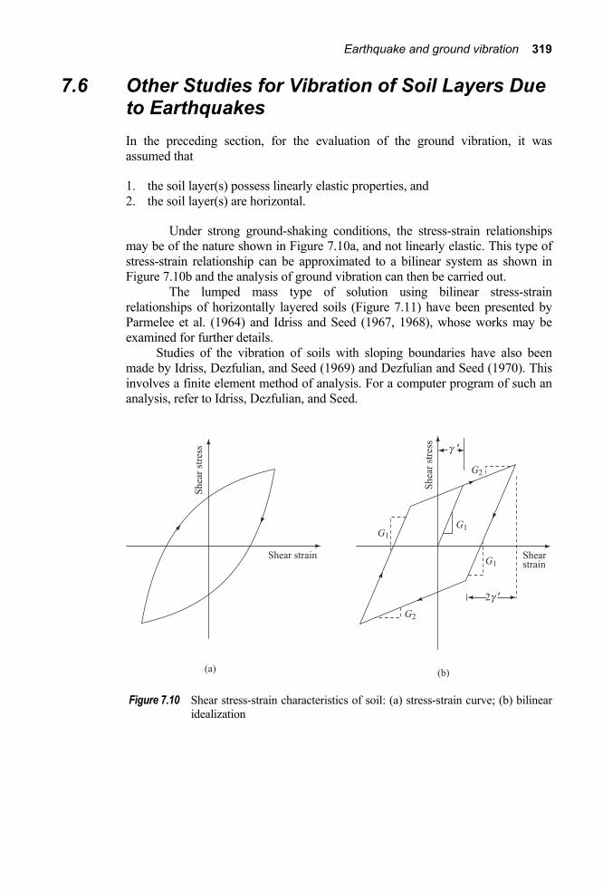
Earthquake and ground vibration 319
7.6 Other Studies for Vibration of Soil Layers Due to Earthquakes In the preceding section, for the evaluation of the ground vibration, it was assumed that
1. the soil layer(s) possess linearly elastic properties, and 2. the soil layer(s) are horizontal.
Under strong ground-shaking conditions, the stress-strain relationships may be of the nature shown in Figure 7.10a, and not linearly elastic. This type of stress-strain relationship can be approximated to a bilinear system as shown in Figure 7.10b and the analysis of ground vibration can then be carried out.
The lumped mass type of solution using bilinear stress-strain relationships of horizontally layered soils (Figure 7.11) have been presented by Parmelee et al. (1964) and Idriss and Seed (1967, 1968), whose works may be examined for further details.
Studies of the vibration of soils with sloping boundaries have also been made by Idriss, Dezfulian, and Seed (1969) and Dezfulian and Seed (1970). This involves a finite element method of analysis. For a computer program of such an analysis, refer to Idriss, Dezfulian, and Seed.
Figure 7.10 Shear stress-strain characteristics of soil: (a) stress-strain curve; (b) bilinear idealization
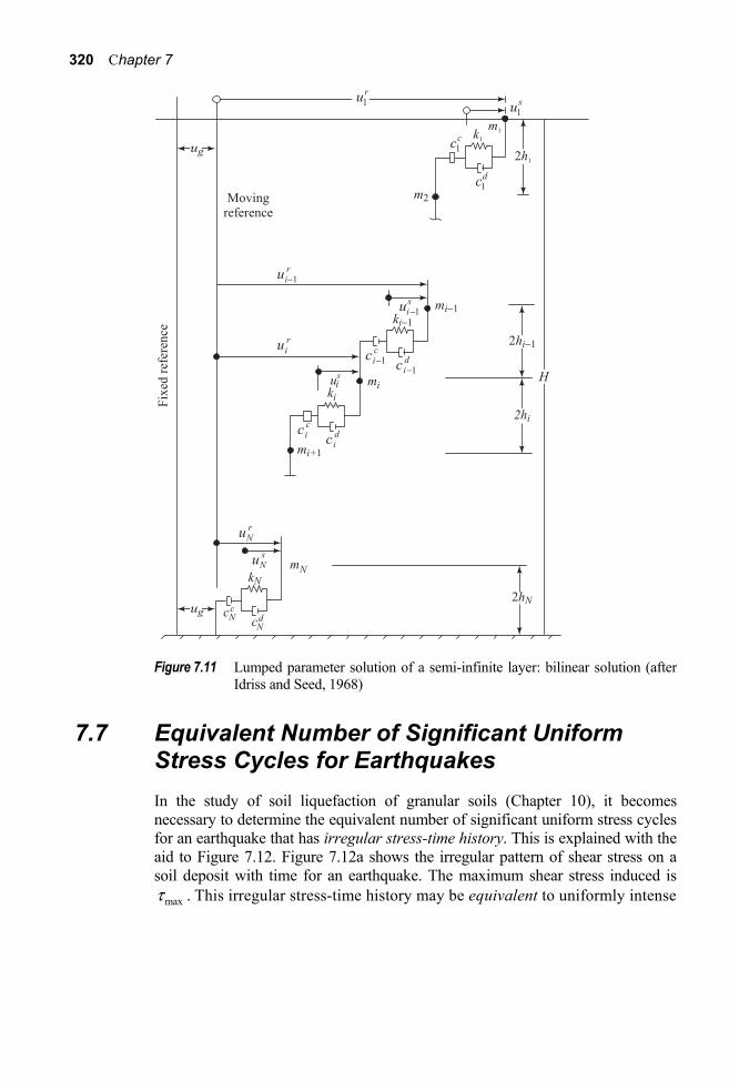
320 Chapter 7
Figure 7.11 Lumped parameter solution of a semi-infinite layer: bilinear solution (after
Idriss and Seed, 1968)
7.7 Equivalent Number of Significant Uniform Stress Cycles for Earthquakes In the study of soil liquefaction of granular soils (Chapter 10), it becomes necessary to determine the equivalent number of significant uniform stress cycles for an earthquake that has irregular stress-time history. This is explained with the aid to Figure 7.12. Figure 7.12a shows the irregular pattern of shear stress on a soil deposit with time for an earthquake. The maximum shear stress induced is
maxt . This irregular stress-time history may be equivalent to uniformly intense

Earthquake and ground vibration 321
Figure 7.12 Equivalent uniform stress cycles: (a) irregular stress-time history;
(b) equivalent uniform stress – time history
N number of cyclic shear stresses of maximum magnitude equal to β maxt (Figure 7.12b). The term equivalent means that the effect of the stress history shown in Figure 7.12a on a given soil deposit should be the same as the uniform stress cycles as shown in Figure 7.12b. From the point of view of soil liquefaction, this fact has been studied by Lee and Chan (1972), Seed et al. (1975), Seed (1976, 1979), and Valera and Donovan (1977).
The basic procedure involved in developing the equivalent stress cycles is fairly simple and has been described by Seed et al. (1975). This is done by using the results of the soil liquefaction study by simple shear tests obtained by DeAlba, Chan, and Seed (1975). Figure 7.13 shows a plot of maxt t against the equivalent number of uniform cyclic stresses N at a maximum stress magnitude of 0.65 maxt . This means, for example, that one cycle of shear stress of maximum magnitude of
maxt is equivalent to three cycles of shear stress of maximum magnitude 0.65 maxt . Similarly, one cycle of shear stress with maximum magnitude of 0.75 maxt is equivalent to 1.4 cycles of shear stress with a maximum magnitude of 0.65 maxt . Figure 7.13 can be used to evaluate the values of N for various earthquakes for a maximum magnitude of uniform cyclic shear stress level equaling 0.65 maxt . (Note: β = 0.65.) This can be most effectively explained by a numerical example. While doing this, one must recognize that, within the top 6 –7 m of a given soil deposit, the cyclic shear stress – time history of an earthquake is similar in form to the acceleration – time history at the ground surface.
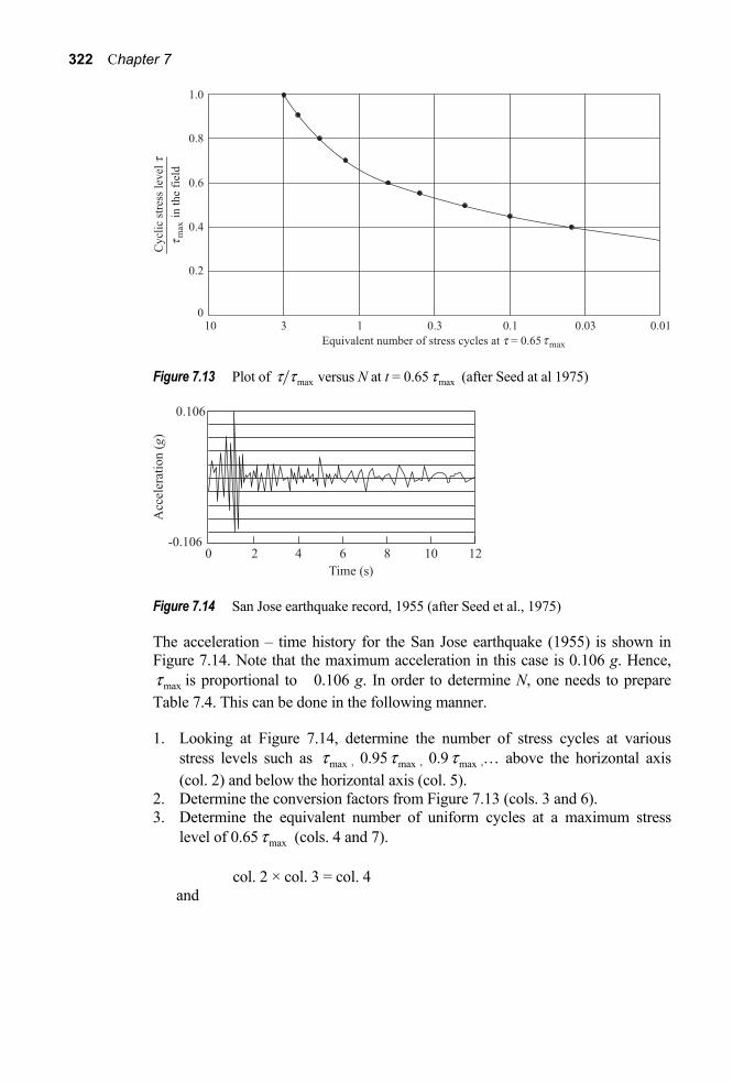
322 Chapter 7
Figure 7.13 Plot of maxt t versus N at t = 0.65 maxt (after Seed at al 1975)
Figure 7.14 San Jose earthquake record, 1955 (after Seed et al., 1975)
The acceleration – time history for the San Jose earthquake (1955) is shown in Figure 7.14. Note that the maximum acceleration in this case is 0.106 g. Hence,
maxt is proportional to 0.106 g. In order to determine N, one needs to prepare Table 7.4. This can be done in the following manner.
1. Looking at Figure 7.14, determine the number of stress cycles at various stress levels such as maxt , 0.95 maxt , 0.9 maxt ,… above the horizontal axis (col. 2) and below the horizontal axis (col. 5).
2. Determine the conversion factors from Figure 7.13 (cols. 3 and 6). 3. Determine the equivalent number of uniform cycles at a maximum stress
level of 0.65 maxt (cols. 4 and 7).
col. 2 × col. 3 = col. 4 and

Earthquake and ground vibration 323
col. 5 × col. 6 = col. 7
4. Determine the total number of equivalent stress cycles at 0.65 maxt above and below the horizontal axis.
5. N = 12
(equivalent no. of cycles above the horizontal
+ equivalent no. of cycles below the horizontal)
Table 7.4 Example of Determination of Equivalent Uniform Cyclic Stress Series from Figure 7.14a
Above horizontal axis Below horizontal axis Equivalent Equivalent No. of no. of No. of no. of Stress level stress Conversion cycles at stress Conversion cycles at maxt(ƒ ) cylces factor 0.65 maxt cycles factor 0.65 maxt
(1) (2) (3) (4) (5) (6) (7) 1.00 1 3.00 3.00 0.95 0.90 – – – 0.85 – – – 1 2.05 2.05 0.80 – – – 1 1.70 1.70 0.75 – – – 0.70 – – – 0.65 – – – 0.60 1 0.70 0.70 0.55 1 0.40 0.40 1 0.40 0.40 0.50 0.45 0.40 1 0.04 0.04 1 0.04 0.04 0.35 2 0.02 0.04 1 0.02 0.02 Total 4.2 Total 4.2
Average number of cycles of 0.65 maxt ≈4.2
aSeed et al. (1975)
Equivalent numbers of uniform stress cycles (at a maximum level of 0.65 maxt ) for several earthquakes with magnitudes of 5.3–7.7 analyzed in the preceding manner are shown in Figure 7.15. These are for the strongest component of the ground motion recorded. The mean and the mean ±1 standard deviation (i.e., 16, 50, and 84 percentile) are also shown. This helps the designer to choose the proper value of the equivalent uniform stress cycles depending on the degree of conservation required.

324 Chapter 7
Figure 7.15 Equivalent numbers of uniform stress cycles based on strong component of
ground motion (after Seed et al. 1975)
Using a similar procedure, Lee and Chan (1972) have given the variation of N with the earthquake magnitude for maximum uniform cyclic stress levels of 0.65 maxt , 0.75 maxt , and 0.85 maxt . A cumulative damage approach has also been described by Valera and Donovan (1977) for determination of N. This approach is based on Miner’s law and involves the natural period of the soil deposit and the duration of earthquake shaking.
References Banioff, H. (1962). Unpublished report to A. R. Golze, Chief Engineer,
Department of Water Resources, Sacramento, California, by Department of Water Resources Consulting Board for Earthquake Analysis.
Bath, M. (1966). “Earthquake Seismology,” Earth Science Reviews, Vol. 1, p. 69. Berg, G. V., and Housner, G. W. (1961). “Integrated Velocity and Displacement
of Strong Earthquakes Ground Motion,” Bulletin, Seismological Society of America, Vol. 51, No. 2, pp. 175-189.

Earthquake and ground vibration 325
Blume, J. A. (1965). ‘Earthquake Ground Motion and Engineering Procedures for Important Installations Near Active Faults,” Proceedings, 3rd World Conference on Earthquake Engineering, New Zealand, Vol. 3.
Bonilla, M. G. (1967). “Historic Surface Faulting in Continental United States and Adjacent Parts of Mexico,” Interagency Report, U.S. Department of the Interior, Geological Survey.
DeAlba, P., Chan, C., and Seed, H. B. (1975). ‘Determination of Soil Liquefaction Characteristics by Large-Scale Laboratory Tests,” Earthquake Engineering Research Center, Report EERC 75-14, University of California, Berkeley.
Dezfulian, H., and Seed, H. B. (1970). “Seismic Response of Soil Deposits Underlain by Sloping Rock Boundaries,” Journal of the Soil Mechanics and Foundations Division, ASCE, Vol. 96, No. SM6, pp. 1893-1916.
Esteva, L., and Rosenblueth, E. (1963). “Espectros de Temblores a Distancias Moderadas y Grandes,” Proceedings, Chilean Conference on Seismology and Earthquake Engineering , Vol. 1, University of Chile.
Figueroa, J. J. (1960). “Some Considerations About the Effect of Mexican Earthquakes,” Proceedings, 2nd World Conference on Earthquake Engineering, Japan, Vol. III.
Gutenberg, B, and Richter, C.F. (1956), “Earthquake Magnitude, Intensity, Energy and Acceleration,” Bulletin, Sesismological Society of America, Vol. 46, No. 2, pp. 105–146.
Gutenberg, G. W. (1965). “Intensity of Earthquakes Ground Shaking Near the Causative Fault,” Proceedings, 3rd World Conference on Earthquake Engineering, New Zealand, Vol. I.
Housner, G. W. (1969). “Engineering Estimate of Ground Shaking and Maximum Earthquake Magnitude,” Proceedings, 4th World Conference on Earthquake Engineering, Santiago, Chile.
Housner, G. W. (1970). “Design Spectrum” in Earthquake Engineering, ed., R. W. Wiegel, Prentice-Hall, Englewood Cliffs, New Jersey, pp. 97-106.
Idriss, I. M., Dezfulian, H., and Seed, H. B. (1969). “Computer Programs for Evaluating the Seismic Response of Soil Deposits with Nonlinear Characteristics Using Equivalent Linear Procedures,” Research Report, Earthquake Engineering Research Center, College of Engineering, University of California, Berkeley.
Idriss, I. M., and Seed, H. B. (1967). “Response of Horizontal Soil Layers During Earthquakes,” Research Report, Soil Mechanics and Bituminous Materials Laboratory, University of California, Berkeley.
Idriss, I. M. and Seed, H. B. (1968). “Seismic Response of Horizontal Soil Layers.” Journal of the Soil Mechanics and Foundations Division, ASCE, Vol. 94, No. SM4, pp. 1003-1031.
Kanai, K. (1966). “Improved Empirical Formula for the Characteristics of Strong Earthquakes Motions,” Proceedings, Japan Earthquake Engineering Symposium, Tokyo, pp. 1-4.
With permission from ASCE.

326 Chapter 7
Lee, K. L., and Chan, K. (1972). ‘Number of Equivalent Significant Cycles in Strong Motion Earthquakes,” Proceedings, International Conference on Microzonation, Seattle, Washington, Vol. 2, pp. 609-627.
Newmark, N. M (1962). “A Method of Computations for Structural Dynamics,” Transactions, ASCE, Vol. 127, Part I, pp. 1406-1435.
Parmelee, R., Penzien, J., Scheffey, C. F., Seed, H. B., and Thiers, G. R. (1964). “Seismic Effects on Structures Supported on Piles Extending Through Deep Sensitive Clays,” Report No. 64-2, Institute of Engineering Research, University of California, Berkeley.
Richter, C. F. (1958). Elementary Seismology, W. H. Freeman, San Francisco, California.
Seed, H. B. (1976). “Evaluation of Soil Liquefaction Effects on Level Ground During Earthquakes,” Preprint No. 2752, ASCE National Convention, Sept. 27-Oct. 1, pp. 1-104.
Seed, H. B. (1979). “Soil Liquefaction and Cyclic Mobility Evaluation for Level Ground During Earthquakes,” Journal of the Geotechnical Engineering Division, ASCE, Vol. 105, No. GT2, pp. 102–155.
Seed, H. B., Idriss, I, M., and Kiefer, F. W. (1969). “Characteristics of Rock Motion During Earthquakes,” Journal of the Soil management and Foundations Division, ASCE, Vol. 95, No. SM5, pp. 1199-1218.
Seed, H. B., Idriss, I. M., Makdisi, F., and Banerjee, N. (1975). “Representation of Irregular Stress – Time Histories by Equivalent Uniform Stress Series in Liquefaction Analysis,” Report No. EERC 75-29, Earthquake Engineering Research Center, University of California, Berkeley.
Tocher, D. (1958). “Earthquake Energy and Ground Breakage,” Bulletin, Seismological Society of America, Vol. 48, No.2, pp. 147-153.
Valera, J. E. and Donovan, N. C. (1977). “Soil Liquefaction Procedures – A Review,” Journal of the Geotechnical Engineering Division, ASCE, Vol. 103, No. GT6, pp. 607-625.
Wiegel, R. W. (ed.)(1970). Earthquake Engineering, Prentice-Hall, Englewood Cliffs, New Jersey.
Wilson, E. L., and Clough, R. W. (1962). “Dynamic Response by Step-by-step Matrix Analysis,” Proceedings, Symposium on the Use of Computers in Civil Engineering, Lisbon, Portugal.
With per-mission from ASCE.

327
8 Lateral Earth Pressure on Retaining Walls
8.1 Introduction Excessive dynamic lateral earth pressure on retaining structures resulting from earthquakes has caused several major damages in the past. The increase of lateral earth pressure during earthquakes induces sliding and/or tilting to the retaining structures. The majority of case histories of failures reported in the literature until now concern waterfront structures such as quay walls and bridge abutments. Some of the examples of failures and lateral movements of quay walls due to earthquakes are given in Table 8.1. Seed and Whitman (1970) have suggested that some of these failures may have been due to several reasons, such as
1. increase of lateral earth pressure behind the wall, 2. reduction of water pressure at the front of the wall, and 3. liquefaction of the backfill material (see Chapter 10)
Nazarian and Hadjan (1979) have given a comprehensive review of the dynamic lateral earth pressure studies advanced so far. Based on this study, the theories can be divided into three broad categories, such as
1. fully plastic (static or pseudostatic) solution, 2. solutions based on elastic wave theory, and 3. solutions based on elastoplastic and nonlinear theory.
Because of the complex soil-structure interaction (mode of wall movement) during earthquakes, the lateral earth pressure theory based on the fully plastic solution (also known as pseudostatic method) which is widely used by most of the design engineers, is detailed in this chapter. In most of the codes of practice, for the soils that do not lose shear strength during shaking, an increase (about 33%) in bearing capacity and passive earth pressure is generally recommended.

328 Chapter 8
8.2 Mononobe-Okabe Active Earth Pressure Theory In 1776, Coulomb derived an equation for active earth pressure on a retaining wall due to a dry cohesionless backfill (Figure 8.1), which is of the form
212A AP H Kg= (8.1)
Table 8.1 Failures and Movements of Quay Wallsa Distance from Approximate Earthquake Date Me Harbor Epicenter Damage Movement Kitaizu 25 November 1930 7.1 Shimizu 48 km Failure of 7.93 m gravity wallsb Shizuoka 11 July 1935 Shimizu Retaining 4.88 m wall collapseb Tonankai 7 December 1944 8.2 Shimizu 175 km Sliding of retaining wallb Nagoya 128 km Outward movement 3.05– of bulkhead with 3.96 m relieving platformb Yokkaichi 144 km Outward movement 3.66 m of pile- supported deckb Nankai 21 December 1946 8.1 Nagoya 200-304 km Outward movement 3.96 m of bulkhead with relieving platformb Osaka 200-304 km Failure of retaining 4.27 m wall above relieving platformb Yokkaichi 200-304 km Outward movement 3.66 m of pile-supported deckb Uno Outward movement 0.61 m of gravity wallb Tokachioki 4 March 1952 7.8 Kushiro 144 km Outward movement 5.49 m of gravity wallb Chile 22 May 1960 8.4 Puerto 112 km Complete over- >4.57 m Montt turning of gravity wallsc Outward movement 0.60– of anchored 0.9 m bulkheadsc Niigata 16 June 1964 7.5 Niigata 51.2 km Tilting of gravity 3.05 m
walld Outward movement 0.30– of anchored 2.1 m bulkheadsd
a After Seed and Whitman (1970) b Reported by Amano, Azuma, and Ishii (1956) c Reported by Duke and Leeds (1963) d Reported by Hayashi, Kubo, and Nakase (1966) e Magnitude

Lateral Earth Pressure on Retaining Walls 329
Figure 8.1 Coulomb’s active earth pressure (Note: BC is the failure plane; W = weight
of the wedge ABC; S and N = shear and normal forces on the plane BC; F = resultant of S and N)
where PA = active force per unit length of the wall γ = unit weight of soil H = height of the retaining wall KA = active earth pressure coefficient
2
21/ 22
cos ( )
sin ( ) sin ( )cos cos( ) 1cos( ) cos( )
ii
f b
d f fb d bd b b
-=È ˘Ï ¸+ -Í ˙+ + Ì ˝+ -Í ˙Ó ˛Î ˚
(8.2)
where φ = soil friction angle δ = angle of friction between the wall and the soil β = slope of the back of the wall with respect to the vertical i = slope of the backfill with respect to the horizontal
The values of KA for β = 0° and various values of φ and δ are given in Table 8.2.
In the actual design of retaining walls, the value of the wall friction δ is assumed to be between 2f and 2
3 .f The active earth pressure coefficients for
various values of φ, i, and β with δ = 23 φ are given in Table 8.3. This is a very
useful table for design considerations.
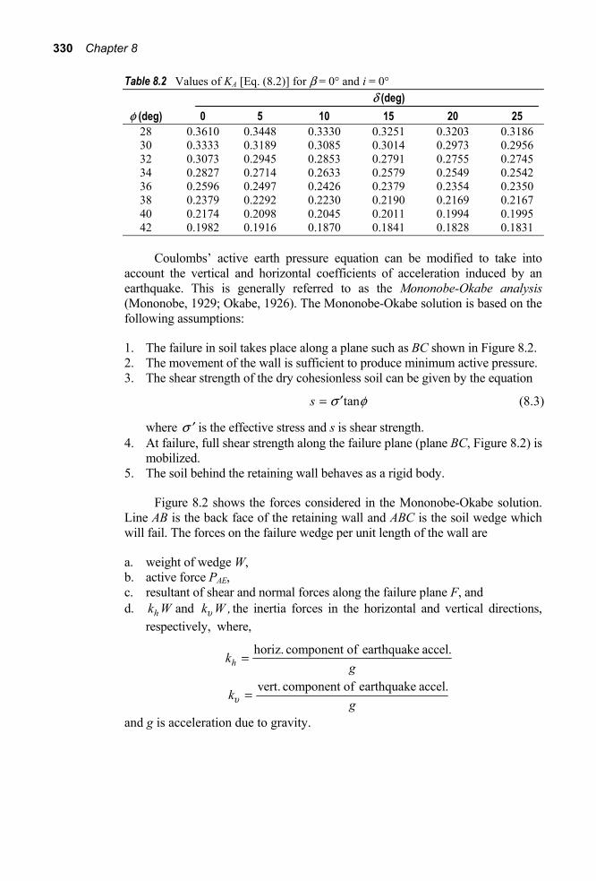
330 Chapter 8
Table 8.2 Values of KA [Eq. (8.2)] for β = 0° and i = 0° δ (deg) φ (deg) 0 5 10 15 20 25 28 0.3610 0.3448 0.3330 0.3251 0.3203 0.3186 30 0.3333 0.3189 0.3085 0.3014 0.2973 0.2956 32 0.3073 0.2945 0.2853 0.2791 0.2755 0.2745 34 0.2827 0.2714 0.2633 0.2579 0.2549 0.2542 36 0.2596 0.2497 0.2426 0.2379 0.2354 0.2350 38 0.2379 0.2292 0.2230 0.2190 0.2169 0.2167 40 0.2174 0.2098 0.2045 0.2011 0.1994 0.1995 42 0.1982 0.1916 0.1870 0.1841 0.1828 0.1831
Coulombs’ active earth pressure equation can be modified to take into account the vertical and horizontal coefficients of acceleration induced by an earthquake. This is generally referred to as the Mononobe-Okabe analysis (Mononobe, 1929; Okabe, 1926). The Mononobe-Okabe solution is based on the following assumptions:
1. The failure in soil takes place along a plane such as BC shown in Figure 8.2. 2. The movement of the wall is sufficient to produce minimum active pressure. 3. The shear strength of the dry cohesionless soil can be given by the equation
tans s f= ¢ (8.3)
where s ¢ is the effective stress and s is shear strength. 4. At failure, full shear strength along the failure plane (plane BC, Figure 8.2) is
mobilized. 5. The soil behind the retaining wall behaves as a rigid body.
Figure 8.2 shows the forces considered in the Mononobe-Okabe solution. Line AB is the back face of the retaining wall and ABC is the soil wedge which will fail. The forces on the failure wedge per unit length of the wall are
a. weight of wedge W, b. active force PAE, c. resultant of shear and normal forces along the failure plane F, and d. hk W and k W ,u the inertia forces in the horizontal and vertical directions,
respectively, where,
horiz. component of earthquake accel.hk
g=
vert. component of earthquake accel.kgu =
and g is acceleration due to gravity.

Lateral Earth Pressure on Retaining Walls 331
Table 8.3 Values of KA [Eq. (8.2)] (Note: δ = 23 φ in all cases)
β (deg) i φ (deg) (deg) 0 5 10 15 20 25 0 28 0.3213 0.3588 0.4007 0.4481 0.5026 0.5662 30 0.2973 0.3349 0.3769 0.4245 0.4794 0.5435 32 0.2750 0.3125 0.3545 0.4023 0.4574 0.5220 34 0.2543 0.2916 0.3335 0.3813 0.4367 0.5017 36 0.2349 0.2719 0.3137 0.3615 0.4170 0.4825 38 0.2168 0.2535 0.2950 0.3428 0.3984 0.4642 40 0.1999 0.2361 0.2774 0.3250 0.3806 0.4468 42 0.1840 0.2197 0.2607 0.3081 0.3638 0.4303 5 28 0.3431 0.3845 0.4311 0.4843 0.5461 0.6191 30 0.3165 0.3578 0.4043 0.4575 0.5194 0.5926 32 0.2919 0.3329 0.3793 0.4324 0.4943 0.5443 34 0.2691 0.3097 0.3558 0.4088 0.4707 0.5443 36 0.2479 0.2881 0.3338 0.3866 0.4484 0.5222 38 0.2282 0.2679 0.3132 0.3656 0.4273 0.5012 40 0.2098 0.2489 0.2937 0.3458 0.4074 0.4814 42 0.1927 0.2311 0.2753 0.3271 0.3885 0.4626 10 28 0.3702 0.4164 0.4686 0.5287 0.5992 0.6834 30 0.3400 0.3857 0.4376 0.4974 0.5676 0.6516 32 0.3123 0.3575 0.4089 0.4683 0.5382 0.6220 34 0.2868 0.3314 0.3822 0.4412 0.5107 0.5942 36 0.2633 0.3072 0.3574 0.4158 0.4849 0.5682 38 0.2415 0.2846 0.3342 0.3921 0.4607 0.5438 40 0.2214 0.2637 0.3125 0.3697 0.4379 0.5208 42 0.2027 0.2441 0.2921 0.3487 0.4164 0.4990 15 28 0.4065 0.4585 0.5179 0.5869 0.6685 0.7671 30 0.3707 0.4219 0.4804 0.5484 0.6291 0.7266 32 0.3384 0.3887 0.4462 0.5134 0.5930 0.6895 34 0.3091 0.3584 0.4150 0.4811 0.5599 0.6654 36 0.2823 0.3306 0.3862 0.4514 0.5295 0.6239 38 0.2578 0.3050 0.3596 0.4238 0.5006 0.5949 40 0.2353 0.2813 0.3349 0.3981 0.4740 0.5672 42 0.2146 0.2595 0.3119 0.3740 0.4491 0.5416 20 28 0.4602 0.5205 0.5900 0.6715 0.7690 0.8810 30 0.4142 0.4728 0.5403 0.6196 0.7144 0.8303 32 0.3742 0.4311 0.4968 0.5741 0.6667 0.7800 34 0.3388 0.3941 0.4581 0.5336 0.6241 0.7352 36 0.3071 0.3609 0.4233 0.4970 0.5857 0.6948 38 0.2787 0.3308 0.4233 0.4970 0.5857 0.6948 40 0.2529 0.3035 0.3627 0.4331 0.5185 0.6243 42 0.2294 0.2784 0.3360 0.4050 0.4889 0.5931

332 Chapter 8
Figure 8.2 Derivation of Mononobe–Okabe equation
The active force determined by the wedge analysis described here may be expressed as
21 (1 )2AE AEP H k Kug= - (8.4)
where KAE is the active earth pressure coefficient with earthquake effect:

Lateral Earth Pressure on Retaining Walls 333
2
22
cos ( )
sin( )sin( )cos cos cos( ) 1cos( )cos( )
AEKi
i
f q b
f d f qq b d b qd b q b
- -=È ˘+ - -+ + +Í ˙+ + -Î ˚
(8.5)
1tan
1hkku
q - Ê ˆ= Á ˜-Ë ¯
(8.6)
Equation (8.4) is generally referred to as the Mononobe-Okabe active earth pressure equation. For the active force condition (PAE), the angle α that the soil wedge ABC located behind the retaining wall (Figure 8.2) makes with the horizontal (for ku = 0°, β = 0°, i = 0°, φ = 30°, and δ = 0° and 20°) is shown in Figure 8.3.
Table 8.4 gives the values of KAE [Eq. (8.5)] for various values of φ, δ, i, and kh with ku = 0 and β = 0°.
Figure 8.3 Inclination of the failure plane with the horizontal (after Davies, Richards,
and Chen, 1986)

334 Chapter 8
Table 8.4 Values of KAE [Eq. (8.5)] with ku = 0 and β = 0° φ (deg) δ i kh (deg) (deg) 28 30 35 40 45 0.1 0 0 0.427 0.397 0.328 0.268 0.217 0.2 0.508 0.473 0.396 0.382 0.270 0.3 0.611 0.569 0.478 0.400 0.334 0.4 0.753 0.697 0.581 0.488 0.409 0.5 1.005 0.890 0.716 0.596 0.500 0.1 0 5 0.457 0.423 0.347 0.282 0.227 0.2 0.554 0.514 0.424 0.349 0.285 0.3 0.554 0.514 0.424 0.349 0.285 0.4 0.942 0.825 0.653 0.535 0.442 0.5 - - 0.855 0.673 0.551 0.1 0 10 0.497 0.457 0.371 0.299 0.238 0.2 0.623 0.570 0.461 0.375 0.303 0.3 0.856 0.748 0.585 0.472 0.383 0.4 - - 0.780 0.604 0.486 0.5 - - - 0.809 0.624 0.1 2f 0 0.396 0.368 0.306 0.253 0.207 0.2 0.485 0.452 0.380 0.319 0.267 0.3 0.604 0.563 0.474 0.402 0.340 0.4 0.778 0.718 0.599 0.508 0.433 0.5 1.115 0.972 0.774 0.648 0.552 0.1 2f 5 0.428 0.396 0.326 0.268 0.218 0.2 0.537 0.497 0.412 0.342 0.283 0.3 0.699 0.640 0.526 0.438 0.367 0.4 1.025 0.881 0.690 0.568 0.475 0.5 - - 0.962 0.752 0.620 0.1 2f 10 0.472 0.433 0.352 0.285 0.230 0.2 0.616 0.562 0.454 0.371 0.303 0.3 0.908 0.780 0.602 0.487 0.400 0.4 - - 0.857 0.656 0.531 0.5 - - - 0.944 0.722 0.1 (2 3) φ 0 0.393 0.366 0.306 0.256 0.212 0.2 0.486 0.454 0.384 0.326 0.276 0.3 0.612 0.572 0.486 0.416 0.357 0.4 0.801 0.740 0.622 0.533 0.462 0.5 1.177 1.023 0.819 0.693 0.600 0.1 (2 3) φ 5 0.427 0.395 0.327 0.271 0.224 0.2 0.541 0.501 0.418 0.350 0.294 0.3 0.714 0.655 0.541 0.455 0.386 0.4 1.073 0.921 0.722 0.600 0.509 0.5 - - 1.034 0.812 0.679 0.1 (2 3) φ 10 0.472 0.434 0.354 0.290 0.237 0.2 0.625 0.570 0.463 0.381 0.317 0.3 0.942 0.807 0.624 0.509 0.423 0.4 - - 0.909 0.699 0.573 0.5 - - - 1.037 0.800

Lateral Earth Pressure on Retaining Walls 335
8.3 Some Comments on the Active Force Equation Considering the active force relation given by Eqs. (8.4)-(8.6), the term sin(φ – θ – i) in Eq. (8.5) has some important implications.
First, if φ – θ – i < 0 (i.e., negative), no real solution of KAE is possible. Physically it implies that an equilibrium condition will not exist. Hence, for stability, the limiting slope of the backfill may be given by
i f q£ - (8.7)
For no earthquake condition, θ = 0; for stability, Eq. (8.7) gives the familiar relation
i f£ (8.8)
Secondly, for horizontal backfill, i = 0; for stability,
q f£ (8.9)
Since 1tan [ (1 )]hk kuq -= - , for stability, combining Eqs. (8.6) and (8.9) results in
(1 )tanhk ku f£ - (8.10)
Hence, the critical value of the horizontal acceleration can be defined as
(cr) = (1 )tanhk ku f- (8.11)
where (cr)hk = critical value of horizontal acceleration (Figure 8.4).
8.4 Procedure for Obtaining PAE Using Standard Charts of KA Since the values of KA are available in most standard handbooks and textbooks, Arango (1969) developed a simple procedure for obtaining the values of KAE from the standard charts of KA. This procedure has been described by Seed and Whitman (1970). Referring to Eq. (8.1),

336 Chapter 8
Figure 8.4 Critical values of horizontal acceleration (Eq. 8.11)
2 2 2 11 1 (cos )2 2A A cP H K H Ag g b -= = (8.12)
where
2cosc AA K b=
= 2
21/ 2
cos ( )
sin ( )sin ( )cos( ) 1cos( ) cos( )
ii
f b
d f fd bd b b
-
È ˘Ï ¸+ -Í ˙+ + Ì ˝+ -Í ˙Ó ˛Î ˚
(8.13)

Lateral Earth Pressure on Retaining Walls 337
In a similar manner, from Eq. (8.4)
21 (1 )2AE AEP H k Kug= -
2 2 11 (1 )(cos cos ) ( )2 mH k Aug q b -= - (8.14)
where
2cos cosm AEA K q b=
2
21/ 2
cos ( )
sin ( ) sin ( )cos( ) 1cos( ) cos( )
ii
f b q
f d f qd b qd b q b
- -=È ˘Ï ¸+ - -Í ˙+ + + Ì ˝+ + -Í ˙Ó ˛Î ˚
(8.15)
Now let
i i q= +¢ (8.16) and b b q= +¢ (8.17)
Substitution of Eqs. (8.16) and (8.17) into Eq. (8.15) yields
2
21/ 2
cos ( )
sin ( ) sin ( )cos( ) 1cos( ) cos( )
mAi
i
f b
f d fd bd b b
- ¢=È ˘Ï ¸+ - ¢Í ˙+ +¢ Ì ˝+ -¢ ¢ ¢Í ˙Ó ˛Î ˚
(8.18)
The preceding equation is similar to Eq. (8.13) except for the fact that i ¢ and b ¢ are used in place of i and β. Thus, it can be said that
2( ) ( )cosm c AA A i , K i ,b b b= =¢ ¢ ¢ ¢ ¢
The active earth pressure PAE can now be expressed as
2
22
1 cos(1 ) ( , )2 cos cosAE AP H k K iu
bg bq b
Ê ˆ¢= - ¢ ¢Á ˜Ë ¯
( )(1 )( )*AP i , k pub= -¢ ¢ (8.19)

338 Chapter 8
where
2
*2
coscos cos
p bq b
Ê ˆ¢= Á ˜Ë ¯ (8.20)
In order to calculate PAE by using Eq. (8.19), one needs to follow these steps:
1. Calculate i ¢ [Eq. (8.16)]. 2. Calculate b ¢ [Eq. (8.17)].
Figure 8.5 Variation of *p and θ

Lateral Earth Pressure on Retaining Walls 339
3. With known values of φ, δ, i ,¢ and ,b ¢ calculate KA (from Tables 8.2, Table 8.3, or other available charts).
4. Calculate PA as equal to 212 AH Kg (KA from Step 3)
5. Calculate (1 )ku- .
6. Calculate *p [Eq. (8.20)]. 7. Calculate
( )(1 ) ( )*AE AP P i , k pub= -¢ ¢
For convenience, some typical values of *p are plotted in Figure 8.5.
Example 8.1
Refer to Figure 8.2. If β = 0°, i = 0°, φ = 36°, δ = 18°, H = 4.5 m, γ = 17.6 kN/m3, ku = 0.2, and kh = 0.3, determine the active force per unit length of the wall.
Solution
1tan
1hkku
q - Ê ˆ= Á ˜-Ë ¯ = tan–1
0.31 0.2Ê ˆÁ ˜Ë ¯- = 20.56°
= +i i q¢ = 0 + 20.56° = 20.56° b b q= +¢ = 0 + 20.56° = 20.56°
2
21/ 22
cos ( )( , )sin ( ) sin( )cos cos( ) 1
cos( ) cos( )
AK ii
i
f bbd f fb d bd b b
- ¢=¢ ¢È ˘Ï ¸+ - ¢Í ˙¢ + ¢ + Ì ˝+ ¢ ¢ - ¢Í ˙Ó ˛Î ˚
2
21/ 22
cos (15.44)
(sin 54)(sin15.44)(cos 20.56) (cos38.56) 1(cos 38.56) (cos0)
=È ˘Ï ¸Í ˙+ Ì ˝Í ˙Ó ˛Î ˚
= 0.583
21( , ) = ( , )2A AP i H K ib g b¢ ¢ ¢ ¢
= 12
(17.6)(4.5)2 (0.583) = 103.89 kN/m

340 Chapter 8
2 2
*2
cos cos 20.56(cos20.56) (cos0)cos cos
p bq b
Ê ˆ¢= =Á ˜Ë ¯
= 0.9363 Hence, from Eq. (8.19),
( )(1 ) ( )*AE AP P i , k pub= -¢ ¢ = (103.89)(1 – 0.2)(0.9363) = 77.81 kN/m.
8.5 Effect of Various Parameters on the Value of the Active Earth Pressure Coefficient Parameters such as the angle of wall friction, angle of friction of soil, and slope of the backfill influence the magnitude of the active earth pressure coefficient KAE to varying degrees. The effect of each of these factors is considered briefly.
A. Effect of Wall Friction Angle δ Figure 8.6 shows the variation of the active earth pressure coefficient KAE with kh for φ = 30° with δ = 0°, φ/2, and 2
3 φ ( ku = 0, β = 0°, and i = 0°), It can be seen
from the plot that, for 0 ≤ δ ≤ 23 φ, the effect of wall friction on the active earth
pressure coefficient is rather small.
Figure 8.6 Influence of wall friction, δ, on KAE

Lateral Earth Pressure on Retaining Walls 341
B. Effect of Soil Friction Angle φ
Figure 8.7 shows the plot of KAE cosδ (that is, the horizontal component of the active earth pressure coefficient) for a vertical retaining wall with horizontal backfill (β = 0° and i = 0°). In this plot, it has been assumed that δ = 1
2 φ. From
the plot, it may be seen that, for ku = 0, kh = 0 and δ = 12 φ, KAE (φ = 30°) is about
35% higher than KAE (φ = 40°). Hence, a small error in the assumption of the soil friction angle could lead to a large error in the estimation of PAE.
Figure 8.7 Effect of soil friction angle, φ, on KAE cosδ
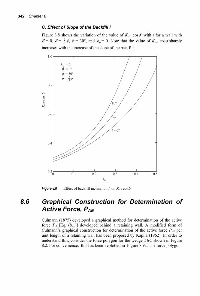
342 Chapter 8
C. Effect of Slope of the Backfill i
Figure 8.8 shows the variation of the value of KAE cosδ with i for a wall with β = 0, δ = 2
3 φ, φ = 30°, and ku = 0. Note that the value of KAE cosδ sharply increases with the increase of the slope of the backfill.
Figure 8.8 Effect of backfill inclination i, on KAE cosδ
8.6 Graphical Construction for Determination of Active Force, PAE Culmann (1875) developed a graphical method for determination of the active force PA [Eq. (8.1)] developed behind a retaining wall. A modified form of Culmann’s graphical construction for determination of the active force PAE per unit length of a retaining wall has been proposed by Kapila (1962). In order to understand this, consider the force polygon for the wedge ABC shown in Figure 8.2. For convenience, this has been replotted in Figure 8.9a. The force polygon

Lateral Earth Pressure on Retaining Walls 343
Figure 8.9 (Continued)
can be reduced to a force triangle with forces PAE, F, and W 2 2(1 ) hk ku- + (Figure 8.9b). Note that in Figure 8.9a, b, α is the angle that the failure wedge makes with the horizontal.
The idea behind this graphical construction is to determine the maximum value of PAE by considering several trial wedges. With references to Figure 8.9c, following are steps for the graphical construction:
1. Draw line BE, which makes an angle φ – θ with horizontal. 2. Draw a line BD, which makes an angle 90° – β – δ – θ with the line BE. 3. Draw BC1, BC2, BC3,…, which are the trial failure surface.
4. Determine kh and ku and then 2 2(1 ) hk ku- + 5. Determine the weights W1, W2, W3,…of trial failure wedges ABC1, ABC2,
ABC3,…, respectively (per unit length at right angle to the cross section shown).
Note W1 = (area of ABC1) × γ × 1 W2 = (area of ABC2) × γ × 1
6. Determine 1 2 3, , ,W W W¢ ¢ ¢… as
2 21 1(1 ) hW k k Wu= - +¢

344 Chapter 8
2W ¢ = 2 22 2(1 ) hW k k Wu= - +¢
7. Adopt a load scale. 8. Using the load scale adopted in step 7, draw BF1 = 1W ¢ , BF2 = 2W ¢ , BF3 =
3W ¢ , …on the line BE. 9. Draw F1G1, F2G2, F3G3,…, parallel to line BD. Note that BF1G1 is the force
triangle for the trial wedge ABC1 smaller to that shown in Figure 8.9b. Similarly, BF2G2, BF3G3,…, are the force triangles for the trial wedges ABC2, ABC3,…, respectively.
10. Join the points G1, G2, G3,…, by a smooth curve. 11. Draw a line HJ parallel to line BE. Let G be point of tangency. 12. Draw line GF parallel to BD. 13. Determine active force PAE as GF × (load scale).
Figure 8.9 Modified Culmann construction
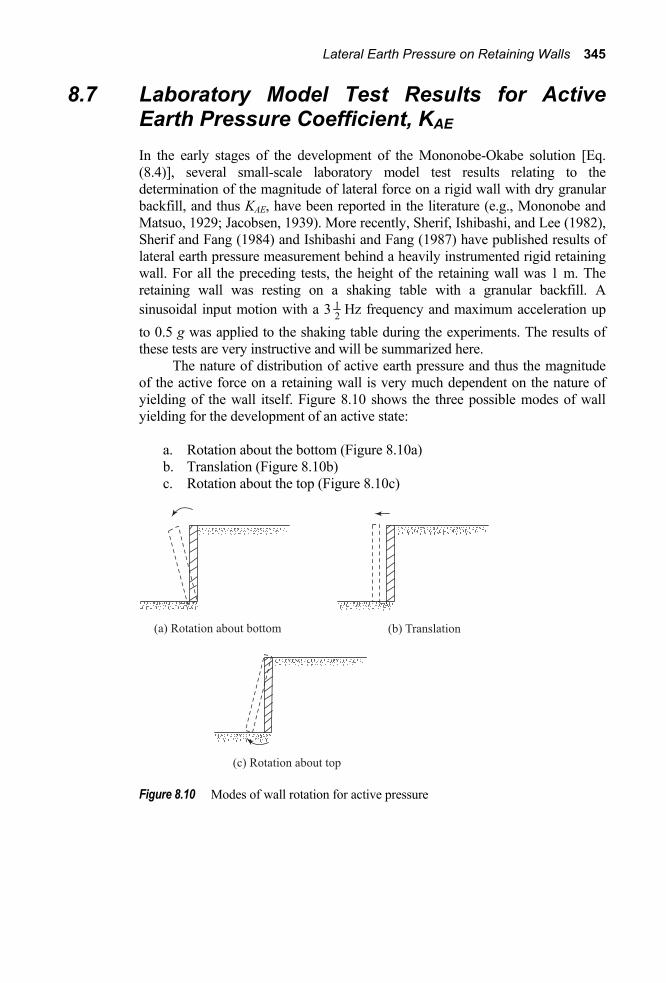
Lateral Earth Pressure on Retaining Walls 345
8.7 Laboratory Model Test Results for Active Earth Pressure Coefficient, KAE In the early stages of the development of the Mononobe-Okabe solution [Eq. (8.4)], several small-scale laboratory model test results relating to the determination of the magnitude of lateral force on a rigid wall with dry granular backfill, and thus KAE, have been reported in the literature (e.g., Mononobe and Matsuo, 1929; Jacobsen, 1939). More recently, Sherif, Ishibashi, and Lee (1982), Sherif and Fang (1984) and Ishibashi and Fang (1987) have published results of lateral earth pressure measurement behind a heavily instrumented rigid retaining wall. For all the preceding tests, the height of the retaining wall was 1 m. The retaining wall was resting on a shaking table with a granular backfill. A sinusoidal input motion with a 3 1
2 Hz frequency and maximum acceleration up to 0.5 g was applied to the shaking table during the experiments. The results of these tests are very instructive and will be summarized here.
The nature of distribution of active earth pressure and thus the magnitude of the active force on a retaining wall is very much dependent on the nature of yielding of the wall itself. Figure 8.10 shows the three possible modes of wall yielding for the development of an active state:
a. Rotation about the bottom (Figure 8.10a) b. Translation (Figure 8.10b) c. Rotation about the top (Figure 8.10c)
Figure 8.10 Modes of wall rotation for active pressure
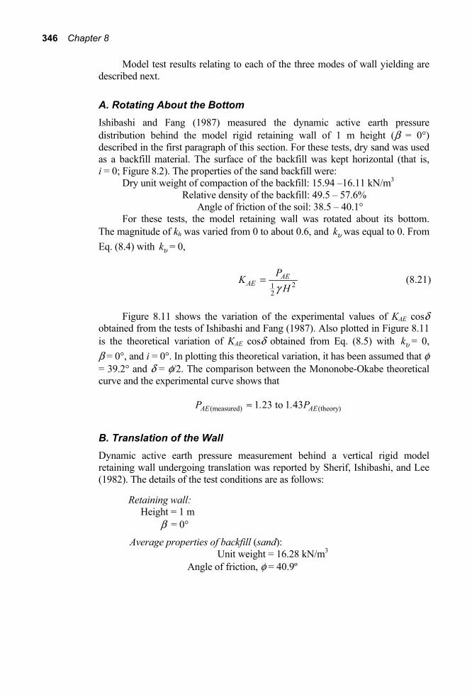
346 Chapter 8
Model test results relating to each of the three modes of wall yielding are described next.
A. Rotating About the Bottom Ishibashi and Fang (1987) measured the dynamic active earth pressure distribution behind the model rigid retaining wall of 1 m height (β = 0°) described in the first paragraph of this section. For these tests, dry sand was used as a backfill material. The surface of the backfill was kept horizontal (that is, i = 0; Figure 8.2). The properties of the sand backfill were:
Dry unit weight of compaction of the backfill: 15.94 –16.11 kN/m3 Relative density of the backfill: 49.5 – 57.6% Angle of friction of the soil: 38.5 – 40.1° For these tests, the model retaining wall was rotated about its bottom.
The magnitude of kh was varied from 0 to about 0.6, and ku was equal to 0. From Eq. (8.4) with ku = 0,
212
AEAE
PKHg
= (8.21)
Figure 8.11 shows the variation of the experimental values of KAE cosδ obtained from the tests of Ishibashi and Fang (1987). Also plotted in Figure 8.11 is the theoretical variation of KAE cosδ obtained from Eq. (8.5) with ku = 0, β = 0°, and i = 0°. In plotting this theoretical variation, it has been assumed that φ = 39.2° and δ = φ/2. The comparison between the Mononobe-Okabe theoretical curve and the experimental curve shows that
(measured) (theory)1 23 to 1 43AE AEP . . Pª
B. Translation of the Wall Dynamic active earth pressure measurement behind a vertical rigid model retaining wall undergoing translation was reported by Sherif, Ishibashi, and Lee (1982). The details of the test conditions are as follows:
Retaining wall: Height = 1 m β = 0°
Average properties of backfill (sand): Unit weight = 16.28 kN/m3 Angle of friction, φ = 40.9º

Lateral Earth Pressure on Retaining Walls 347
Angle of wall friction, δ = 23.9º
Slope of the backfill, i = 0º
For these tests the magnitude of KAE cos δ was varied from 0 to 0.5 and ku was 0. Figure 8.12 shows the experimental variation of KAE cos δ obtained from these model tests. Also shown in this figure is the variation of KAE cos δ obtained from the Mononobe-Okabe theory [Eq. (8.5)]. Based on this plot it appears that the experimental values PAE are about 30% higher than those obtained from Eqs. (8.4) and (8.5).
Figure 8.11 Wall rotation about the bottom for active pressure—comparison of theory with model test results
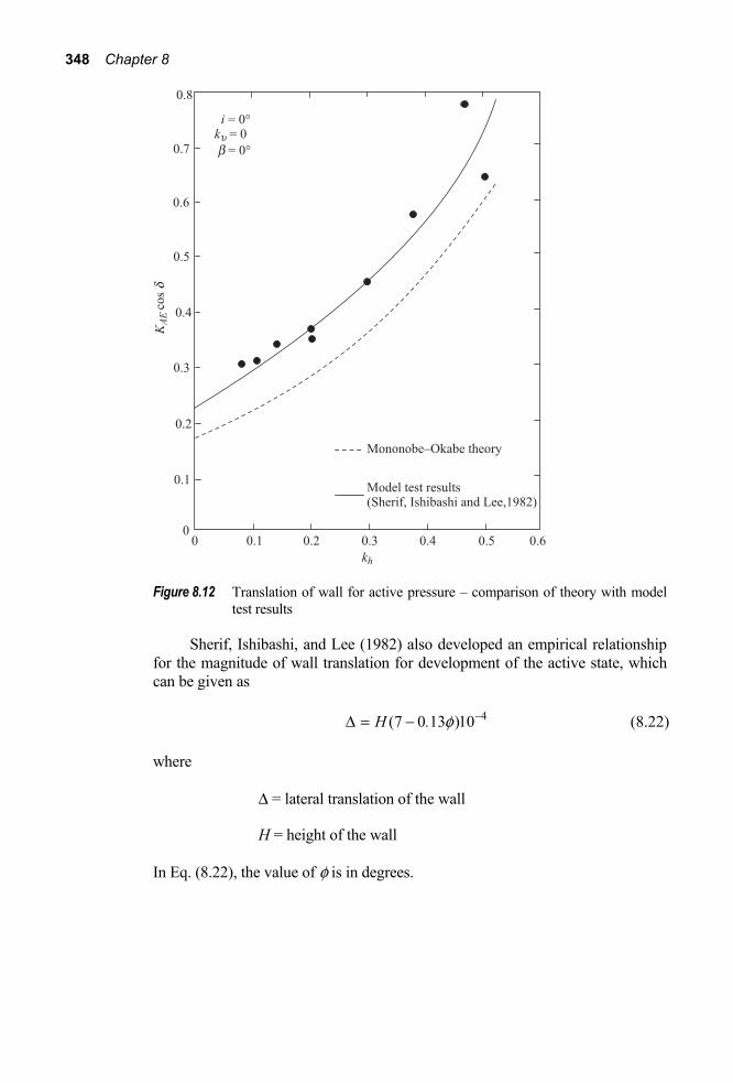
348 Chapter 8
Figure 8.12 Translation of wall for active pressure – comparison of theory with model
test results
Sherif, Ishibashi, and Lee (1982) also developed an empirical relationship for the magnitude of wall translation for development of the active state, which can be given as
4(7 0 13 )10H . f -D = - (8.22)
where
Δ = lateral translation of the wall
H = height of the wall
In Eq. (8.22), the value of φ is in degrees.

Lateral Earth Pressure on Retaining Walls 349
C. Rotation of the Wall about the Top Sherif and Fang (1984) reported the dynamic earth pressure distribution behind a 1 m high rigid vertical retaining wall (β = 0º) undergoing rotation about is top. A sand with an average unit weight of 15.99 kN/m3 was used as a backfill. The surface of the backfill was horizontal (that is, i = 0º). The nature of variation of the maximum active horizontal earth pressure distribution (pAE cos δ, where p = active earth pressure at a given depth) obtained from these tests is shown in Figure 8.13. Also plotted in this figure are the theoretical variations of pAE cos δ obtained from the Mononobe-Okabe solution (with β = 0º, i = 0, and ku = 0) for various values of kh. From the comparison of the theoretical and experimental plots, the following general conclusions can be drawn. 1. The nature of variation of dynamic earth pressure for wall rotation about the
top is very much different than that predicted by the Mononobe-Okabe theory.
2. For a given value of kh,
cos ( cos )AE AEP p dyd d= Ú (8.23)
where y = depth measured from the top of the wall.
Figure 8.13 Rotation of wall about the top for active pressure—comparison of theory
with model test results (i = 0º, β = 0º, ku = 0)

350 Chapter 8
3. For a given value of kh, the horizontal component of the lateral force, PAE cosδ, calculated from the experimental curves by using Eq. (8.23), is about 15% to 20% higher than the predicted by the Mononobe-Okabe theory.
8.8 Point of Application of the Resultant Active Force, PAE A. Rotation about the Bottom of the Wall The original Mononobe-Okabe solution for the active force on retaining structures implied that the resultant force will act at a distance of 1
3 H measured from the bottom of the wall (H = height of the wall) similar to that in the static case (kh = ku = 0). However, all the laboratory tests that have been conducted so far indicate that the resultant pressure PAE acts at a distance H , which is somewhat greater than 1
3 H measured from the bottom of the wall. This is shown in Figure 8.14.
Prakash and Basavanna (1969) have made a theoretical evaluation for determination of H . Based on the force-equilibrium analysis, their study shows that H increases from 1
3 H for kh = 0 to about 12 H for kh = 0.3 (for φ = 30º,
δ = 7.5º, ku = 0, i = β = 0). For similar conditions, the moment-equilibrium analysis gave a value of H = 1
3 H and kh = 0, which increases to a value of
1 9H H .ª at kh = 0.3.
For practical design considerations, Seed and Whitman (1969) have proposed the following procedure for determination of the line of action of PAE.
1. Calculate PA [Eq. (8.1)]. 2. Calculate PAE [Eq. (8.4)] 3. Calculate AE AE AP P PD = - . The term ΔPAE is the incremental force due
to earthquake condition. 4. Assume that PA acts at a distance of 1
3 H from the bottom of the wall (Figure 8.15).
5. Assume that ΔPAE acts at a distance of 0.6H from the bottom of the wall (Figure 8.15); then
1( ) ( ) (0 6 )3A AE
AE
P H P . HH
P
ΔÊ ˆ +Á ˜Ë ¯=

Lateral Earth Pressure on Retaining Walls 351
Figure 8.14 Point of application of resultant active earth pressure
Figure 8.15
B. Translation of the Wall Sherif, Ishibashi, and Lee (1982) suggested that, for wall translation, the following procedure can be used to estimate the location of the line of action of the active force, PAE.
1. Calculate PA [Eq. (8.1)]. 2. Calculate PAE [Eq. (8.2)]. 3. Calculate AE AE AP P PD = - .

352 Chapter 8
4. Referring to Figure 8.16, calculate
( )( ) 0 42 ( ) (0 48 )A AE
AE
P . H P . HH
PΔ+
=
C. Rotation about the Top of the Wall
For rotation of the wall about its top (Figure 8.17), H is about 0.55 H (Sherif and Fang, 1984).
Figure 8.16
Figure 8.17

Lateral Earth Pressure on Retaining Walls 353
Example 8.2
Referring to Example 8.1, determine the location of the line of action for PAE. Assume rotation of the wall about its bottom.
Solution
The value of PAE in Example 8.1 has been determined to be 77.81 kN/m.
212A AP H Kg=
For φ = 36º, δ = 18º, KA = 0.236 [Eq. (8.2)]. Thus,
PA = 12
(17.6)(4.5)2(0.236) = 42.06 kN/m
This acts at a distance equal to 4.53
= 1.5 m from the bottom of the wall. Again,
ΔPAE = 77.81 – 42.06 = 35.75 kN/m The line of action of ΔPAE intersects the wall at a distance of 0.6H = 2.7 m measured from the bottom, so
( ) ( ) ( ) ( )1.5 42.06 2.7 35.7577.81
H+
= = 2.05 m
8.9 Design of Gravity Retaining Walls Based on Limited Displacement Richards and Elms (1979) have proposed a procedure for design of gravity retaining walls based on limited displacement. In this study, they have take into consideration the wall inertia effect and concluded that there is some lateral movement of the wall even for mild earthquakes. In order to develop this procedure, consider a gravity retaining wall as shown in Figure 8.18, along with the forces acting on it during an earthquake. For stability, summing the forces in the vertical direction,
sin ( )w w AEN W k W Pu d b= - - + (8.24)
where N is the vertical component of the reaction at the base of the wall and Ww is the weight of the wall. Similarly, summing the forces in the horizontal direction,

354 Chapter 8
Figure 8.18 Derivation of Eq. (8.28)
cos( )h w AES k W P d b= + + (8.25)
where S is the horizontal component of the reaction at the base of the wall. At sliding,
tan bS = N f (8.26)
where bf is the soil-wall friction angle at the base of the wall.
Substituting Eqs. (8.24) and (8.25) into Eq. (8.26), one obtains
cos( ) = [ (1 ) sin ( )]tanh w AE w AE bk W P W k Pud b d b f+ + - + +
or
[(1 )tan ] [cos( ) sin ( )tan ]w b h AE bW k k Pu f d b d b f- - = + - +
( ) ( )( )
cos sin tan1 tan
AE bw
b h
PW
k ku
d b d b ff
È ˘+ - +Î ˚=- -
(8.27)

Lateral Earth Pressure on Retaining Walls 355
From Eq. (8.4), 212 (1 )AE AEP H k Kug= - . Substitution of this equation into
Eq. (8.27) yields
( ) ( )
( )
21 cos sin tan2
tan tan
AE bw
b
H KW
g d b d b f
f q
È ˘+ - +Î ˚=
- (8.28)
where tan (1 )hk kuq = - . It may be noted that, in Eq. (8.28), Ww is equal to infinity if
tan tanbf q= (8.29)
This implies that infinite mass of the wall is required to prevent motion. The critical value of kh = kh(cr) can thus be given by relation
(cr)tan = tan1
hb
kku
q f=-
or (cr) (1 )tanh bk ku f= - (8.30)
Equation (8.27) can also be written in the form
( )21 12w AE IEW H k K CugÈ ˘= -Í ˙Î ˚
(8.31)
where
( ) ( )( ) ( )
cos sin tan1 tan tan
bIE
bC
ku
d b d b ff f
+ - +=
- - (8.32)
Figure 8.19 shows the variation of CIE with kh for various values of ku
(φ = φb = 35º, δ = 12
φ, i = β = 0). Also, Figure 8.20 shows the variation of CIE
with kh for various values of wall friction angle, δ (φ = φb = 35º, i = β = 0, ku = 0).
Note that Eq. (8.31) is for the limiting equilibrium condition for sliding with earthquake effects takes into consideration. For the static condition (i.e.,
0hk ku= = ), Eq. (8.31) becomes
21
2 A IW H K Cg= (8.33)

356 Chapter 8
Figure 8.19 Effect of ku on the value of CI E (after Richards and Elms, 1979)
where W = Ww (for static condition) and
( ) ( )cos sin tantan
bI
bC
d b d b ff
+ - += (8.34)
Thus, comparing Eqs. (8.31) and (8.33), we can write that
wT I W
WF F F
W= = (8.35)

Lateral Earth Pressure on Retaining Walls 357
Figure 8.20 Effect of wall friction on CI E (after Richards and Elms, 1979)
where
(1 )AE
TA
K kF
Ku-
= = soil thrust factor
IEI
I
CFC
= = wall inertia factor
and FW is a factor of safety applied to the weight of the wall to take into account the effect of soil pressure and wall inertia. Figure 8.21 shows a plot of FT, FI, and FW for various values of kh (φ = φb = 35º, δ = 1
2 φ, ku = 0, β = i = 0).
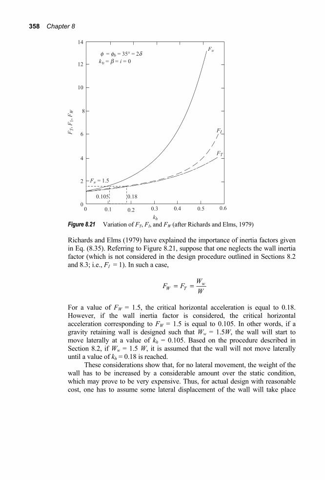
358 Chapter 8
Figure 8.21 Variation of FT, FI, and FW (after Richards and Elms, 1979)
Richards and Elms (1979) have explained the importance of inertia factors given in Eq. (8.35). Referring to Figure 8.21, suppose that one neglects the wall inertia factor (which is not considered in the design procedure outlined in Sections 8.2 and 8.3; i.e., FI = 1). In such a case,
wW T
WF F
W= =
For a value of FW = 1.5, the critical horizontal acceleration is equal to 0.18. However, if the wall inertia factor is considered, the critical horizontal acceleration corresponding to FW = 1.5 is equal to 0.105. In other words, if a gravity retaining wall is designed such that Ww = 1.5W, the wall will start to move laterally at a value of kh = 0.105. Based on the procedure described in Section 8.2, if Ww = 1.5 W, it is assumed that the wall will not move laterally until a value of kh = 0.18 is reached.
These considerations show that, for no lateral movement, the weight of the wall has to be increased by a considerable amount over the static condition, which may prove to be very expensive. Thus, for actual design with reasonable cost, one has to assume some lateral displacement of the wall will take place

Lateral Earth Pressure on Retaining Walls 359
during an earthquake; the procedure for determination of the wall weight (Ww) is then as follows:
1. Determine an acceptable displacement d of the wall. 2. Determine a design value of kh from the equation
1 425.08
h aa
Ak A
A duÊ ˆ
= Á ˜Ë ¯ (8.36)
where Aa and Au are effective acceleration coefficient and displacement d is in mm. The values of Aa and Au for a given region in the United States are given by the Applied Technology Council (1978).
Equation (8.36) has been suggested by Richards and Elms (1979) and is based on study of Newmark (1965) and Franklin and Chang (1977).
3. Using the above value of kh, and assuming kv = 0, determine the value of KAE.
4. Determine the weight of the wall Ww from Eq. (8.31). 5. Apply a factor of safety to Ww obtained in Step 4.
A slight modification of this design procedure was proposed by Nadim and Whitman 1983). This modification is intended primarily to account for the amplification of the ground motion in the backfill.
Example 8.3
Determine the weight of a retaining wall 4 m high (given β = 0, i = 0, γ = 17.29
kN/m3, φb = φ = 34º, δ = 12
φ, Au = 0.2, Aa = 0.2, factor of safety = 1.5)
a. for static condition, b. for zero displacement condition under earthquake loading, and c. for a displacement of 50.8 mm under earthquake loading.
Solution
a. From Eq. (8.33),
21
2 A IW H K Cg=
From Table 8.2, KA = 0.256 (for φ = 34º, δ = 17º, i = 0, β = 0).

360 Chapter 8
( ) ( )cos sin tantan
bI
bC
d b d b ff
+ - += = ( )cos17 sin 17 tan 34
tan 34-
= 1.125 Thus
W = 12
(17.29)(4)2(0.256)(1.125) = 39.84 kN/m
With a factor of safety of 1.5, the weight of the wall is equal to (1.5)(39.84) = 59.76 kN/m.
b. From Eq. (8.31),
( )21 12w AE IEW H k K CugÈ ˘= -Í ˙Î ˚
Assume ku = 0.
( ) ( )( ) ( )
cos sin tan1 tan tan
bIE
bC
ku
d b d b ff f
+ - +=
- -
0.2tan1 1
hkku
q = =-
= 0.2; θ = 11.31º
( )cos17 sin 17 tan 34tan 34 0.2IEC-
=-
= 1.6
Again, from Eq. (8.5), ( )
( ) ( ) ( ) ( )( )
2
2cos 34 11.31
sin 34 17 sin 34 11.31cos 11.31 cos 17 11.31 1
cos 17 11.31
AEK-
=È ˘+ -
È ˘+ +Í ˙Î ˚ +Í ˙Î ˚
= 0.393
Ww = 12
(17.29)(4)2(1 – 0)(0.393)(1.6) = 86.98 kN/m
With a factor of safety of 1.5, the weight of wall = (86.98)(1.5) = 130.47 kN/m. c. From Eq. (8.36),
1 425.08h a
a
Ak A
A duÈ ˘
= Í ˙Í ˙Î ˚
= 0.2 ( ) ( )( ) ( )
1 425.08 0.20.2 50.8
È ˘Í ˙Í ˙Î ˚
= 0.075
0.075tan1 1 0
hkku
q = =- -
= 0.075

Lateral Earth Pressure on Retaining Walls 361
or θ = 4.29º
( )cos17 sin 17 tan 34 0.7591tan 34 0.075 0.5995IEC-
= =-
= 1.27
Using Eq. (8.5) ( )
( ) ( ) ( ) ( )( )
2
2cos 34 4.29
sin 34 17 sin 34 4.29cos 4.29 cos 17 4.29 1
cos 17 4.29
AEK-
=È ˘+ -
È ˘+ +Í ˙Î ˚ +Í ˙Î ˚
= 0.3 Thus, with a factor of safety of 1.5,
Ww = (1.5) 12FHIK (17.29)(4)2(0.3)(1.27) = 79.05 kN/m
8.10 Hydrodynamic Effects of Pore Water The lateral earth pressure theory developed in the preceding sections of this chapter has been for retaining walls with dry soil backfills. However, for quay walls (Figure 8.22), the hydrodynamic effect of the water also have to be taken into consideration. This is usually done according to the Westergaard theory (1933) which was derived to obtain the dynamic water pressure on the face of a concrete dam. Based on this theory, the water pressure due to an earthquake at a depth y (Figure 8.22) may be expressed as
1 2 1 21
78 h wp k h yg= (8.37)
where p1 is the intensity of pressure on the seaward side, γw is the unit weight of water, and h is the total depth of water. Hence, the total dynamic water force on the seaward side per unit length of the wall [P1(w)] can be obtained by integration as
1 2 1 2 21 1 0
7 78 12
h( w ) h w h wP p dy k h y dy k hg g= = =Ú Ú (8.38)
The location of the resultant water pressure is
( )( )
( ) ( )1 2 1 210 01( ) 1
1 1 78
h hh w
w wy p dy y k h y y dy
P PgÊ ˆ= = Á ˜Ë ¯Ú Ú

362 Chapter 8
Figure 8.22 Hydrodynamic effects on a quay wall
( )
( )( )
1 2 5 2 3
1 1
1 7 2 1 78 5 20h w h w
w wk h h k h
P Pg gÊ ˆ Ê ˆ= =Á ˜ Á ˜Ë ¯ Ë ¯
or
1
2 37 712 20h w h wy k h k hg g
-Ê ˆ Ê ˆ= Á ˜ Á ˜Ë ¯ Ë ¯ = 0.6h (8.39)
Matsuo and O’Hara (1960) have suggested that the increase of the pore
water pressure on the landward side is approximately 70% of that on the seaward side. Thus,
1/ 2 1/ 2 1/ 2 1/ 22
70.7 0.61258 h w h wp k h y k h yg gÊ ˆ= =Á ˜Ë ¯
(8.40)
where p2 is the dynamic pore water pressure on the landward side at a depth y. The total dynamic pore water force increase [P2(w)] per unit length of the wall is
2 22( )
70.7 0.408312w h w h wP k h k hg gÊ ˆ= =Á ˜Ë ¯
(8.41)
During an earthquake, the force on the wall per unit length on the seaward side will be reduced by P1(w) and that on the landward side will be increased by P2(w). Thus, the total increase of the force per unit length of the wall is equal to

Lateral Earth Pressure on Retaining Walls 363
2 21( ) 2( )
71.7 0.991712w w w h w h wP P P k h k hg gÊ ˆ= + = =Á ˜Ë ¯
(8.42)
Example 8.4
Refer to Figure 8.22. For the quay wall, h = 10 m. Determine the total dynamic force increase due to water for kh = 0.2.
Solution
From Eq. (8.42)
20.9917w h wP k hg= = 0.9917(0.2)(9.81)(10)2 = 194.6 kN/m
8.11 Mononobe –Okabe Active Earth Pressure Theory for c -f Backfill
The Mononobe-Okabe equation for estimating AEP for cohessionless backfill also can be extended to c -f soil (Prakash and Saran, 1966; Saran and Prakash, 1968). Figure 8.23 shows a retaining wall of height H with a horizontal c -f soil as backfill. The depth of tensile crack that may develop in a c -f soil is given as
02
a
czKg
= (8.43)
where 2tan 452aK f⎛ ⎞= −⎜ ⎟
⎝ ⎠ (8.44)
Referring to Figure 8.23, the forces acting on the soil wedge (per unit length of the wall) are as follows:
a. The weight of the wedge ABCDE, W b. Resultant of the shear and normal forces on the failure surface CD, F c. Active force, AEP d. Horizontal inertia force, hk W
e. Cohesive force along CD, ( )C c CD=
f. Adhesive force along BC, ( )C c BC=¢

364 Chapter 8
Figure 8.23 Trial failure wedge behind a retaining wall with c -f backfill
It is important to realize that the following two assumptions have been made:
1. The vertical inertia force ( k Wu ) has been taken to be zero. 2. The unit adhesion along the soil-wall interface (BC) has been taken to be
equal to the cohesion ( c ) of the soil.
Considering these forces, we can show that
( )20 0( )AE a acP H z N c H z Ngg= - - -¢ ¢ (8.45)
where
( )cos sec cos sec
sinaciN h b f
h d+¢ ¢=¢+¢
(8.46)
( )( ) ( ) ( )( )
20.5 tan tan tan cos sin
sinh
a
n i n i k iN g
b b f fh d
È ˘ È ˘+ + + + + +Î ˚Î ˚=¢+¢
(8.47)
in which
ih b f= + +¢ (8.48)
0
0
zn
H z=
- (8.49)

Lateral Earth Pressure on Retaining Walls 365
The values of acN ¢ and aN g¢ can be determined by optimising each coefficient
separately. Thus, Eq. (8.45) gives the upper bound of AEP . For the static condition, 0hk = . Thus,
( )20 0( )AE a acP H z N c H z Ngg= - - - (8.50)
The relationships for acN and aN g can be determined by substituting 0hk = into Eq. (8.46) and (8.47). Hence,
( )cos sec cos sec
sinac aciN N h b f
h d+¢= =¢+¢
(8.51)
( )( ) ( )
( )
20.5 tan tan tan cos
sina
a
n i n iNN g
gb b f
l h d
È ˘ È ˘+ + + +¢ Î ˚Î ˚= =+¢
(8.52)
The variations of acN , aN g and l with f and q are shown in Figures 8.24 through 8.27.
Figure 8.24 Variation of ac acN N ′= with f and b (Based on Prakash and Saran, 1966,
and Saran and Prakash, 1968)

366 Chapter 8
Figure 8.25 Variation of aN g with f and ( 0 2)n .b = (Based on Prakash and Saran,
1966, and Saran and Prakash, 1968)
Figure 8.26 Variation of aN g with f and ( 0)nb = (Based on Prakash and Saran, 1966,
and Saran and Prakash, 1968)

Lateral Earth Pressure on Retaining Walls 367
Figure 8.27 Variation of l with hk ,f and b (Based on Prakash and Saran, 1966, and
Saran and Prakash, 1968)

368 Chapter 8
8.12 Dynamic Passive Force on Retaining Wall Figure 8.23 shows a retaining wall having a granular soil as the backfill material. If the wall is pushed toward the soil mass, at a certain stage failure in the soil will occur along a plane BC. At failure the force, PPE, per unit length of the retaining wall is the dynamic passive force. The force per unit length of the wall that needs to be considered for equilibrium of the soil wedge is shown in Figure 8.28. The notations W, φ, δ, γ, kh, and ku have the same meaning as described in Figure 8.2 (Section 8.2). Using the basic assumptions for the soil given in Section 8.2, the passive force (PPE) may also be derived as (Kapila, 1962)
21 (1 )2PE PEP H k Kug= - (8.53)
where
( )
( ) ( ) ( )( ) ( )
2
21/ 22
cos –
sin sin –cos cos cos – 1 –
cos – cos –
PEKi
i
f b q
f d f qq b d b q
b d b q
+=
È ˘Ï ¸+ +Ô ÔÍ ˙+ Ì ˝+Í ˙Ô ÔÓ ˛Î ˚
(8.54)
and 1tan [ (1 )]hk kuq -= -
Figure 8.28 Passive force, PPE, on a retaining wall

Lateral Earth Pressure on Retaining Walls 369
Note that Eq. (8.53) has been derived for dry cohesionless backfill. Kapila has also developed a graphical procedure for determination of PPE.
Figure 8.29 shows the variation of KPE for various values of soil friction angle φ and hk (with ku = i = β = δ = 0). From the figure it can be seen that, with other parameters remaining the same, the magnitude of KPE increases with the increase of soil friction angle φ.
Figure 8.30 shows the influence of the backfill slope angle of KPE. Other factors remaining constant, the magnitude of KPE increases with increase of i.
A more advanced analysis based on kinematical method of limit analysis on seismic passive earth pressure coefficients can be found in Soubra (2000).
Figure 8.29 Variation of KPE with soil friction angle and kh (after Davies, Richards, and
Chen, 1986)
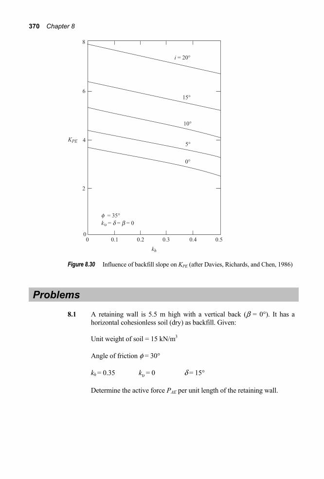
370 Chapter 8
Figure 8.30 Influence of backfill slope on KPE (after Davies, Richards, and Chen, 1986)
Problems
8.1 A retaining wall is 5.5 m high with a vertical back (β = 0°). It has a horizontal cohesionless soil (dry) as backfill. Given:
Unit weight of soil = 15 kN/m3
Angle of friction φ = 30°
kh = 0.35 ku = 0 δ = 15°
Determine the active force PAE per unit length of the retaining wall.

Lateral Earth Pressure on Retaining Walls 371
8.2 Refer to Problem 8.1. Determine the location of the point of intersection of the resultant force PAE with the back face of the retaining wall. Assume the wall (a) rotates about the bottom, and (b) translates.
8.3 Refer to Figure 8.2. Given:
H = 3 m φ = 40° kh = 0.3 β = 10° δ = 13° ku
= 0.1 i = 10° γ = 15.72 kN/m3
Determine the active forcer per unit length PAE and the location of the resultant. Assume that the wall is rotating about its bottom.
8.4 Refer to Problem 8.3. Where would be the location of the resultant if the wall is rotating about its top?
8.5 Redo Example 8.1 using the modified Culmann graphical solution procedure outlined in Section 8.6.
8.6 Redo Problem 8.1 using the modified Culmann graphical solution procedure.
8.7 Redo Problem 8.3 using the modified Culman graphical solution procedure.
8.8 For the retaining wall and the backfill given in Problem 8.1, determine the passive force PPE per unit length of the wall.
8.9 For a retaining wall and the backfill given in Problem 8.3, determine the passive force PPE per unit length.
8.10 Consider a 3.6 m high vertical retaining wall (β = 0°) with a horizontal backfill (i = 0°).
Given for the soil are φ = 32°, γ = 19.5 kN/m3, and δ = 0. a. Calculate PAE and the location of resultant with ku = 0.1and kh =
0.15. b. For the results of (a), what should be the weight of the wall per
meter length for no lateral movement? The factor of safety against sliding is 1.4.
c. What should be the weight of the wall for an allowable lateral displacement of 25 mm? Given Au = Aa = 0.15; the factor of safety against sliding is 1.4.
References Amano, R., Azuma, H., and Ishii, Y. (1956). “Aseismic Design of Quay Walls in
Japan,” Proceedings, 1st World Conference on Earthquake Engineering, Berkeley, California.
Arango, I. (1969). Personal communication with Seed, H. B. and Whitman, R. V. (1970).

372 Chapter 8
Applied Technology Council (1978). “Tentative Provisions for the Development of Seismic Regulations for Buildings,” Publication ATC 3-06, Palo Alto, California.
Coulomb, C. A. (1776). “Essai sur une Application des Regles de Maximis et Minimis a quelques Problemes de Statique, relatifs a 1’Architecture,’ Mem. Roy. des Sciences, Paris, Vol 3. p. 38.
Culmann, C. (1875). Die graphische Statik, Meyer and Zeller, Zurich. Davies, T. G., Richards, R., and Chen, K. H. (1986). “Passive Pressure during
Seismic Loading.” Journal of Geotechnical Engineering, ASCE, Vol. 112, No. GT4, pp. 479-484.
Duke, C. M., and Leeds, D. J. (1963). “Response of Soils, Foundations, and Earth Structures,” Bulletin of the Seismological Society of America, Vol. 53, No. 2, pp. 309 – 357.
Franklin, A. G., and Chang, F. K. (1977). “Earthquake Resistance of Earth and Rockfill Dams,” Report 5, Miscellaneous Paper S71 – 17, Soils and Pavement Laboratory, U. S. Army Engineer Waterways Experiment Station, Vicksburg, Mississippi.
Hayashi, S., Kubo, K., and Nakase, A. (1966). “Damage to Harbor Structures in the Nigata Earthquake,” Soils and Foundations, Vol. 6, No. 1, pp. 26-32.
Ishibashi, I., and Fang, Y. S. (1987). “Dynamic Earth Pressures with Different Wall Movement Modes,” Soils and Foundations, Vol. 27, No. 4, pp. 11-12.
Jacobsen, L. S. (1939). Described in Appendix D of “The Kentucky Project,” Techincal Report No. 13, Tennessee Valley Authority, 1951.
Kapila, J. P. (1962). “Earthquake Resistant Design of Retaining Walls,” Proceedings, 2nd Earthquake Symposium, University of Roorkee, Roorkee, India.
Matsuo, H., and O’Hara S. (1960). “Lateral Earth Pressures and Stability of Quay Walls During Earthquakes,” Proceedings, 2nd World Conference on Earthquake Engineering, Japan, Vol.1.
Mononobe, N. (1929). “Earthquake-Proof Construction of Masonry Dams,” Proceedings, World Engineering Conference, Vol. 9, pp. 274-280.
Mononobe, N.,and Matsuo, H. (1929). “On the Determination of Earth Pressures During Earthquakes,” Proceedings, World Engineering Conference, Vol. 9, pp. 176-182.
Nadim, F., and Whitman, R. V. (1983). “Seismically Induced Movement of Retaining Walls,” Journal of Geotechnical Engineering, ASCE, Vol. 109, No. GT7, pp. 915-931.
Nazarian, H. N., and Hadjan, A. H. (1979). “Earthquake-Induced Lateral Soil Pressure on Structures,” Journal of the Geotechnical Engineering Division, ASCE, Vol. 105, No. GT9, pp. 1049-1066.
Newmark, N. M. (1965). “Effect of Earthquakes on Dams and Embankments,” Geotechnique, Vol. 15, No.2, pp. 139-160.
Okabe, S. (1926), “General Theory of Earth Pressure,” Journal of the Japanese Society of Civil Engineers, Vol. 12, No.1.
With permission from ASCE.

Lateral Earth Pressure on Retaining Walls 373
Prakash, S., and Basavanna, B. M (1969). “Earth Pressure Distribution Behind Retaining Wall During Earthquake,” Proceedings, 4th World Conference on Earthquake Engineering, Santiago, Chile.
Prakash, S., and Saran, S. (1966). “Static and Dynamic Earth Pressure Behind Retaining Walls,” Proceedings, 3rd Symposium on Earthquake Engineering, Roorkee, India, Vol. 1, pp. 277-288.
Richards, R., and Elms, D. G. (1979 ). “Seismic Behavior of Gravity Retaining Walls,” Journal of the Geotechnical Engineering Division, ASCE, Vol. 105, No. GT4, pp. 449-464.
Saran, S., and Prakash, S. (1968). “Dimensionless Parameters for Static and Dynamic Earth Pressure for Retaining Walls,”, Indian Geotechnical Journal, Vol. 7, No. 3, pp. 295-310.
Seed, H. B., and Whitman, R. V. (1970). “Design of Earth Retaining Structures of Dynamic Loads,” Proceedings, Speciality Conference on Lateral Stresses in the Ground and Design of Earth Retaining Structures, ASCE, pp. 103-147.
Sherif, M. A., and Fang, Y. S. (1984). “Dynamic Earth Pressures on Walls Rotating About the Top,” Soils and Foundations, Vol. 24, No. 4, pp. 109-117.
Sherif, M. A., Ishibashi, I., and Lee, C. D. (1982). “Earth Pressure Against Rigid Retaining Walls,” Journal of the Geotechnical Engineering Division, ASCE, Vol. 108, No. GT5, pp. 679-696.
Soubra, A.-H. (2000). “Static and seismic passive earth pressure coefficients on rigid retaining structures,” Canadian Geotechnical Journal, Vol. 37, pp. 463–478.
Wastergaard, H. M. (1933). “Water Pressures on Dams During Earthquakes,” Transactions, ASCE, Vol. 98, pp. 418-433.
With permission from ASCE.
With permission from ASCE.

374
9 Compressibility of Soils Under Dynamic Loads
9.1 Introduction Permanent settlements under vibratory machine foundation can generally be placed under two categories:
1. Elastic and consolidation settlement due to the static weight 2. Settlement due to vibratory compaction of the foundation soil
Permanent settlement in soils can also be induced due to the vibration caused by an earthquake. The elastic and consolidation settlement due to static loads is not discussed here since the conventional methods of calculation can be found in most standard soil mechanics texts. In this chapter, the present available methods of evaluation of permanent settlement due to dynamic loading conditions are presented.
9.2 Compaction of Granular Soils: Effect of Vertical Stress and Vertical Acceleration The fact that granular soils can be compacted by vibration is well known. Dry granular soils are likely to exhibit more compaction due to vibration as compared to moist soils. This is because of the surface tension effect in moist soils, which offers a resistance for the soil particles to roll and slide and arrange themselves into a denser state.
Laboratory studies have been made in the past to evaluate the effect of cycling controlled vertical stress at low frequencies, i.e., at low acceleration levels on confined granular soils (D’Appolonia, 1970). Such laboratory tests can be performed by taking a granular soil specimen in a mold, as shown in Figure 9.1a. A confining vertical air pressure zs is first applied to the specimen, after which a vertical dynamic stress of amplitude ds is applied repeatedly.

Compressibility of Soils Under Dynamic Loads 375
Figure 9.1 Compaction of granular soil by (a) controlled vertical stress; (b) controlled
vertical acceleration
The permanent compressions of the specimen are recorded after the elapse of several cycles of dynamic stress application. Also, several investigations on confined dry granular soils have been conducted (e.g., see D’Appolonia and D’Appolonia, 1967; Ortigosa and Whitman, 1968) in which a controlled vertical acceleration is imposed on the specimen, which produces small dynamic stress changes. For these tests, the specimen is placed in a mold fixed to a vibrating table (Figure 9.1b). Then a vertical confining air pressure zs is applied to the specimen. After that, the specimen is subjected to a vertical vibration for a period of time.
Note that, for a vertical vibration,
sinzz A tw=
where Az is the amplitude of the vertical vibration. The magnitude of the peak acceleration is equal to 2 2(2 )z zA A fw = p . Thus, the peak acceleration is controlled by the amplitude of displacement and the frequency of vibration. For constant peak acceleration of vibration, the drive mechanism has to be adjusted for Az and f. The vertical compression of the specimen can be determined at the end of a test.
Thus the first type of test described above is run with repeated stresses with negligible acceleration; the second type is for repeated acceleration with small dynamic stress on soils.
Figure 9.2 shows the results of a number of tests conducted on a dune sand for controlled vertical stress condition. For all tests, the sand specimens were compacted to an initial relative density of about 60%.

376 Chapter 9
Figure 9.2 Compression of a dune sand under controlled vertical stress condition (after
D’Appolonia, 1970)
The frequencies of load application were in a range of 1.8-6 Hz. Along the ordinate are plotted the vertical strain, which is equal to ΔH/H (where H is the initial height of the specimen and ΔH is the vertical compression of the specimen after a given number of load cycles). It may be seen that, for a given value of
,d zs s
logH NHD μ
where N is the number of load cycle applications. Also note that, for a given number of load cycles, the vertical strain increases with increasing values of
.d zs s
Figure 9.3 shows the nature of the results obtained from controlled vertical acceleration tests on dry sand by Ortigosa and Whitman (1968). Note that, even at zero confining pressure, no vertical strain is induced up to a peak acceleration of about 1g (1¥ acceleration due to gravity). Similar test results of D’Appolonia (1970) are shown in Figure 9.4, for which 0zs = . The terminal dry unit weight shown in Figure 9.4 is the unit weight of sand at the end of the test.
Krizek and Fernandez (1971) also conducted several laboratory tests with controlled vertical acceleration to study the densification of damp clayey sand.

Compressibility of Soils Under Dynamic Loads 377
Figure 9.3 Nature of variation of void ratio or dry unit weight of dry sand in controlled
vertical acceleration tests
Figure 9.4 Correlation between terminal unit weight and peak vertical acceleration for
a dune sand (redrawn after D’Appolonia, 1970)
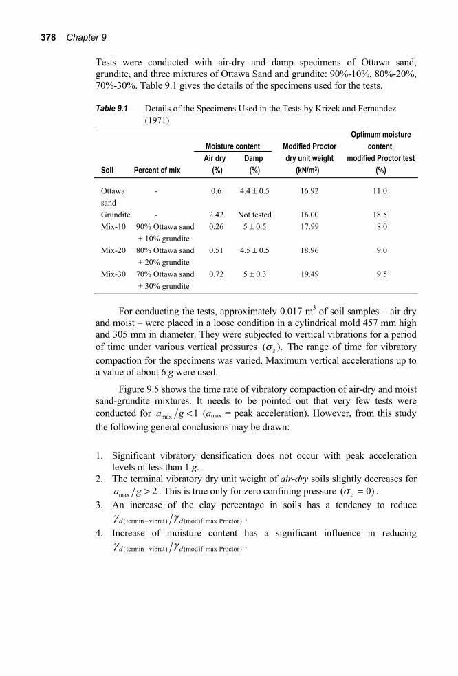
378 Chapter 9
Tests were conducted with air-dry and damp specimens of Ottawa sand, grundite, and three mixtures of Ottawa Sand and grundite: 90%-10%, 80%-20%, 70%-30%. Table 9.1 gives the details of the specimens used for the tests.
Table 9.1 Details of the Specimens Used in the Tests by Krizek and Fernandez (1971)
Optimum moisture Moisture content Modified Proctor content, Air dry Damp dry unit weight modified Proctor test Soil Percent of mix (%) (%) (kN/m3) (%)
Ottawa - 0.6 4.4 ± 0.5 16.92 11.0 sand Grundite - 2.42 Not tested 16.00 18.5 Mix-10 90% Ottawa sand 0.26 5 ± 0.5 17.99 8.0 + 10% grundite Mix-20 80% Ottawa sand 0.51 4.5 ± 0.5 18.96 9.0 + 20% grundite Mix-30 70% Ottawa sand 0.72 5 ± 0.3 19.49 9.5
+ 30% grundite
For conducting the tests, approximately 0.017 m3 of soil samples – air dry and moist – were placed in a loose condition in a cylindrical mold 457 mm high and 305 mm in diameter. They were subjected to vertical vibrations for a period of time under various vertical pressures ( ).zs The range of time for vibratory compaction for the specimens was varied. Maximum vertical accelerations up to a value of about 6 g were used.
Figure 9.5 shows the time rate of vibratory compaction of air-dry and moist sand-grundite mixtures. It needs to be pointed out that very few tests were conducted for max 1a g < (amax = peak acceleration). However, from this study the following general conclusions may be drawn:
1. Significant vibratory densification does not occur with peak acceleration
levels of less than 1 g. 2. The terminal vibratory dry unit weight of air-dry soils slightly decreases for
max 2a g > . This is true only for zero confining pressure ( 0)zs = . 3. An increase of the clay percentage in soils has a tendency to reduce
( ) ( )termin vibrat modif max Proctord dg g- . 4. Increase of moisture content has a significant influence in reducing
( ) ( )termin vibrat modif max Proctord dg g- .

Compressibility of Soils Under Dynamic Loads 379
Figure 9.5 Time rate of vibratory compaction for air dry and moist sand-grundite
mixtures (redrawn after Krizek and Fernandez, 1971)

380 Chapter 9
9.3 Settlement of Strip Foundation on Granular Soil under the Effect of Controlled Cyclic Vertical Stress In Section 9.2, some laboratory experimental observations of settlement of laterally confined sand specimens were presented. In these cases, the loads have been applied over the full surface area. However, in the field, the load covers only a small area and settlement in these cases include those caused by the induced shear strains. In the case of foundations, the shear strain increase with the increase of d uqs (where ds is the amplitude of dynamic load and qu is the ultimate bearing capacity). In this section, some developments on settlement of strip footings under the effect of controlled cycling vertical stress applied at low frequencies (i.e., negligible acceleration) are discussed.
Raymond and Komos (1978) conducted laboratory model tests with strip footings with widths of 75 mm and 228 mm resting on 20-30 Ottawa sand in a large box. The cyclic loads on model strip footings were applied by a Bellofram loading piston activated by an air pressure system. The loadings approximated a rectangular wave from as shown in Figure 9.6a with a frequency of 1 Hz. The settlement of the footings were measured by a dial gauge together with a DVDT activating a strip chart recorder. For conducting the tests, the ultimate static bearing capacities ( )uq were first experimentally determined. The footings were then subjected to various magnitudes of cyclic load ( d uqs = 13.5%-90%, where
0 ,d Q As = and A is the area of the model footing). The load settlement relationships obtained from the tests for the 228 mm footing are shown in Figure 9.6b. In this figure, SN is the permanent settlement of the footing and N is the number of cycles of load application. Such plots may be given by an empirical relation as
log
NN
Sa bS
N= + (9.1)
where a and b are two constants.
The experimental values of a and b for these two footings may be approximated by the following equations.
For 75 mm wide footing:
0.0811 0.0115a F= - + (9.2) 0.12420 0.00127b F= + (9.3)

Compressibility of Soils Under Dynamic Loads 381
Figure 9.6 Plastic deformation due to repeated loading in plane strain case (redrawn
after Raymond and Komos, 1978)

382 Chapter 9
For 228 mm wide footing:
0.1053 0.0421a F= - + (9.4) 0.0812 0.0031b F= + (9.5) where d uF qs= and SN is measured in millimeters. Equations (9.1)-(9.5) are valid up to a load cycle of N = 105
Figure 9.7 shows the experimental results of the variation of ds with log N for various values of SN. For a given value of SN, the plot of ds versus log N is approximately linear up to a value of (1 4)d uqs ª . For (1 4)d uqs < , the slope of ds versus log N becomes smaller and the response tends toward elastic conditions.
From Eqs. (9.2)-(9.5), it may be seen that, for a given soil, the parameters a and b are functions of the width of the footing B. Thus, Eqs. (9.2) and (9.4) have been combined by Raymond and Komos to the form
1.180.15125 0.0000693 ( 6.09)a B F= - + + (9.6) where B is the width of the footings. Similarly, Eqs. (9.3) and (9.5) can be combined as 0.8210.153579 0.0000363 ( 23.1)b B F= + - (9.7)
Equations (9.6) and (9.7) are valid for only two different sizes of footing and for one soil. The general form of the equations for all sizes of footings and all soils can be written as
1.18 1.181 2 3a a a B F a B= + + (9.8)
and 0.821 0.821
1 2 3b b b B F b B= + - (9.9)
where a1, a2, a3, b1, b2, b3 are parameters for a given soil. However,
d
uF
qs
=
and
12uq BNgg= (for surface foundation) (9.10)
where Ng is the static bearing capacity factor (Chapter 6) and γ is the unit weight of soil.

Compressibility of Soils Under Dynamic Loads 383
Figure 9.7 Variation of ds with log N for various values of permanent settlement
(redrawn after Raymond and Komos, 1978)
Thus,
(1 2)
dFBNg
sg
= (9.11)
Substitution of Eq. (9.11) into Eqs. (9.8) and (9.9) yields
0.18 1.181 4 3da a a B a Bs= + + (9.12)
and 0.18 0.82
1 4 3db b b B b Bs -= + - (9.13) where
24 (1 2)
aaNgg
= (9.14)
24 (1 2)
bbNgg
= (9.15)
and B is in millimeters.

384 Chapter 9
Figure 9.8 Plot of settlement versus number of load cycles for a constant value of σd
(redrawn after Raymond and Komos, 1978)
If the values of a1, a3, a4, b1, b3, b4, which are the plastic properties of given soil at a given density of compaction, can be determined by laboratory testing, the settlement of a given strip footing can be determined by combining Eqs. (9.1), (9.12), and (9.13). It needs to be pointed out that, for given values of ds and N, the value of SN decreases with the increase of the width of the footing. This fact is demonstrated in Figure 9.8 for five different footings.
Analysis of this type may be used in the estimation of the settlement of railroad ties subjected to dynamic loads due to the movement of trains.
9.4 Settlement of Machine Foundation on Granular Soils Subjected to Vertical Vibration For machine foundation subjected to vertical vibrations, many investigators believe that the peak acceleration is the main controlling parameter for the settlement of the foundation. Depending on the relative density of granular soils, the solid particles come to an equilibrium condition under a given peak acceleration level. This threshold acceleration level must be exceeded before additional densification can take place.

Compressibility of Soils Under Dynamic Loads 385
The general nature of the settlement-time relationship for a foundation is shown in Figure 9.9. Note that in Figure 9.9, Az is the amplitude of the foundation vibration and W is the weight of the foundation. The foundation settlement gradually increases with time and reaches a maximum value, beyond which it remains constant.
Brumund and Leonards (1972) have studied the settlement of circular foundations resting on sand subjected to vertical excitation by means of laboratory model tests. According to them, the energy per cycle of vibration imparted to the soil by the foundation can be used as the parameter for determination of settlement of foundations.
The model tests of Brumund and Leonards were conducted in a 0.057 m3 container. They used 20-30 Ottawa sand, compacted to a relative density of 70%. The model foundation used for the tests was 101.6 mm in diameter. The static ultimate bearing capacity was first experimentally determined before beginning the dynamic tests. The duration of vibration of the model foundation was chosen to be 20 min for all tests. Figure 9.10 shows the plot of the experimental results of settlement S against the peak acceleration for a constant frequency of vibration. For a given foundation weight W, the settlement increases linearly with the peak acceleration level. However, for a given frequency of vibration and peak acceleration level, the settlement increases with the increase of W.
Figure 9.9 Settlement-time relationship for a machine foundation subjected to vertical
vibration

386 Chapter 9
Figure 9.10 Plot of settlement versus peak acceleration for model foundation at a
frequency of 20 Hz (after Brumund and Leonards, 1972)
Figure 9.11 shows a plot of settlement S against the energy transmitted per cycle to the soil by the foundation.
The data include the following: 1. A frequency range of 14-59.3 Hz (both above and below the resonant
frequency) 2. A range in static pressure of 0.27-0.55 × static ultimate bearing capacity qu.
The static pressure q can be defined as
WqA
= (9.16)

Compressibility of Soils Under Dynamic Loads 387
Figure 9.11 Plot of settlement versus transmitted energy per cycle (after Brumund and
Leonards. 1972)
where A is the area of the foundation. 3. A range in maximum downward dynamic force of 0.3W – W. The maximum
downward dynamic force may theoretically be obtained from Eq. (2.90) as
2 2dynam(max) zF A k ( c )w= +
where Az = amplitude of foundation vibration
k = spring constant = 041
Grm-
(see Chapter 5)
c = 20
3.41
r Grm
Ê ˆÁ ˜-Ë ¯
(see chapter 5)
G = shear modulus of soil r0 = radius of foundation μ = Poisson’s ratio of soil ρ = density of soil w = 2πf (f = frequency of vibration)

388 Chapter 9
The equation for determination of energy transmitted to the soil per cycle (ETr) may be obtained as follows:
Tr a zE Fdz F Au= =Ú (9.17)
where F is the total contact force on the soil and aF u is the average contact force on the soil per cycle; however,
max min1 ( )2aF F Fu = + (9.18)
max dynam(max)F W F= + (9.19) and max dynam(max)F W F= - (9.20)
Substituting Eqs. (9.19) and (9.20) into Eq. (9.18),
aF Wu = (9.21)
Thus, from Eqs. (9.17) and (9.21),
Tr zE WA= (9.22)
Figure 9.11 shows that the transmitted energy per cycle of oscillation ETr varies linearly with the settlement. A plot of the experimental results of settlement against peak acceleration for different ranges of ETr is plotted in Figure 9.12. This clearly demonstrates that, if the value of the transmitted energy is constant, the residual settlement remains constant irrespective of the level of peak acceleration.
The preceding concept is very important for the analysis of settlement of foundation of machineries subjected to vertical vibration. However, at this time, techniques of extrapolation of settlement of prototype foundations from laboratory model tests are not available. In any case, if the foundation soil is granular and loose, it is always advisable to take precautions to avoid possible problem in settlement. A specification of at least 70% relative density of compaction is often cited.
On similar lines, the settlement of structures such as tall buildings, due to vibratory load, is often a result of structure rocking back and forth. This type of settlement is caused by dynamic structural loads that momentarily increase the foundation pressure acting on the soil. Lightly loaded structures are least vulnerable to this type of settlement.
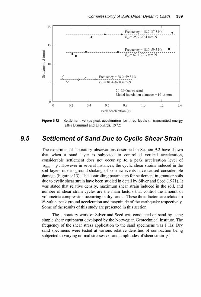
Compressibility of Soils Under Dynamic Loads 389
Figure 9.12 Settlement versus peak acceleration for three levels of transmitted energy
(after Brumund and Leonards, 1972)
9.5 Settlement of Sand Due to Cyclic Shear Strain The experimental laboratory observations described in Section 9.2 have shown that when a sand layer is subjected to controlled vertical acceleration, considerable settlement does not occur up to a peak acceleration level of
maxa g= . However in several instances, the cyclic shear strains induced in the soil layers due to ground-shaking of seismic events have caused considerable damage (Figure 9.13). The controlling parameters for settlement in granular soils due to cyclic shear strain have been studied in detail by Silver and Seed (1971). It was stated that relative density, maximum shear strain induced in the soil, and number of shear strain cycles are the main factors that control the amount of volumetric compression occurring in dry sands. These three factors are related to N–value, peak ground acceleration and magnitude of the earthquake respectively. Some of the results of this study are presented in this section.
The laboratory work of Silver and Seed was conducted on sand by using simple shear equipment developed by the Norwegian Geotechnical Institute. The frequency of the shear stress application to the sand specimens was 1 Hz. Dry sand specimens were tested at various relative densities of compaction being subjected to varying normal stresses zs and amplitudes of shear strain xzg ¢ .

390 Chapter 9
Figure 9.13 Settlement of sand due to cyclic shear strain
An example of the nature of variation of the vertical strain z H He = D (H = initial height of the specimen, ΔH = settlement) with number of cycles of shear strain application for a medium dense sand is shown in Figure 9.14. For these tests, the initial relative density (RD) of compaction was 60%. Based on Figure 9.14, the following observations can be made.
a. For a given normal stress zs and amplitude of shear strain xzg ¢ , the vertical strain increases with the number of strain cycles. However, a large portion of the vertical strain occurs in the first few cycles. For example, in Figure 9.14, the vertical strain occurring in the first 10 cycles is approximately equal to or more than that occurring in the next 40-50 cycles.
b. For a given value of the vertical stress and number of cycles N, the vertical strain increases with the increase of the shear strain amplitude.
However, one has to keep in mind that a small amount of compaction (i.e., increase in the relative density) could markedly reduce the settlement of a given soil. Silver and Seed (1971) also observed that at higher amplitudes of cyclic shear strain ( xzg ¢ > 0.05%, for a given value of N), the vertical strain is not significantly affected by the magnitude of the vertical stress. This may not be true where the shear strain is less than 0.05%.

Compressibility of Soils Under Dynamic Loads 391
Figure 9.14 Variation of vertical strain with number of cycles (after Silver and Seed,
1971)
The basic understanding of the laboratory test results for the settlement due to cyclic shear strain application may now be used for calculation of settlement of sand layers due to seismic effect. This is presented in the following section.
9.6 Calculation of Settlement of Dry Sand Layers Subjected to Seismic Effect Seed and Silver (1972) have suggested a procedure to calculate the settlement of a sand layer subjected to seismic effect. This procedure is outlined in a step-by-step manner. 1. Since the primary source of ground motion in a soil deposit during an
earthquake is due to the upward propagation of motion from the underlying rock formation, adopt a representative history of horizontal acceleration for the base.
2. Divide the soil layer into n layers. They need not be of equal thickness.

392 Chapter 9
3. Calculate the average value of the vertical effective stress zs for each layer (Note: In dry sand, total stress in equal to effective stress.)
4. Determine the representative relative densities for each layer. 5. Using the damping ratio and the shear moduli characteristics given in
Section 4.19, calculate the history of shear strains at the middle of all n layers.
6. Convert the irregular strain histories obtained for each layer (Step 5) into average shear strains and equivalent number of uniform cycles (see Chapter 7).
7. Conduct laboratory tests with a simple shear equipment on representative soil specimens from each layer to obtain the vertical strains for the equivalent number of strain cycles calculated in Step 6. This has to be done for the average effective vertical stress levels zs calculated in Step 3 and the corresponding average shear strain levels calculated in Step 6.
8. Calculate the total settlement as
(1) 1 (2) 2 ( )z z z n nH H H He e eD = + + + (9.23)
where (1)ze , (2)ze ,.. are average vertical strains determined in Step 7 for layers 1, 2, …and H1, H2,…are layer thicknesses.
The applicability of this procedure is explained in Example 9.1.
Example 9.1
A 20-m-thick sand layer is shown in Figure 9.15a. The unit weight of soil is 16.1 kN/m3. Using a design earthquake record, the average shear strain in the soil layer has been evaluated and plotted in Figure 9.15a. (Note: It was assumed that
aυ max0.65g gª¢ ¢ ). In this evaluation, the procedure outlined in Section 4.19 was followed with 1 2
max 2(max)218.82G K s= kPa and damping = 20%. The number of equivalent cycles of shear strain application was estimated to be 10. Cyclic simple shear tests on representative specimens of this sand were conducted with their corresponding vertical stresses as in the field. The results of these tests are shown in Figure 9.15b. Estimate the probable settlement of the sand layer. Solution
Form Figure 9.15b, it can be seen that, even though tests were conducted with different values of zs , the results of ze versus xzg ¢ are almost linear in a log-log plot. This shows that the magnitude of the effective overburden pressure has practically no influence on the vertical strain. Thus, for this calculation, the average line of the experimental results is used. For calculation of settlement, the following table can be prepared.

Compressibility of Soils Under Dynamic Loads 393
Figure 9.15 (a) Plot of average shear strain induced due to earthquake (sand unit weight
= 16.1 kN/m3; relative density = 50%); (b) laboratory simple shear test results (number of cycles = 10)

394 Chapter 9
Shear strain at the middle of layer, Depth (m) H (m) xzg ¢ (%) εz (%) Hεz × 10−2 (m)
0 – 2.5 2.5 0.025 0.043 0.1075 2.5 – 5.0 2.5 0.065 0.13 0.325 5.0 – 7.5 2.5 0.100 0.22 0.55 7.5 – 10.0 2.5 0.125 0.28 0.700 10.0 – 12.5 2.5 0.140 0.31 0.775 12.5 – 15.0 2.5 0.135 0.30 0.750 15.0 – 17.5 2.5 0.125 0.28 0.700 17.5 –20.0 2.5 0.105 0.23 0.575
ΔH = ΣHεz = 4.4825 × 10⁻² m ≈ 44.8 mm
9.7 Settlement of a Dry Sand Layer Due to Multidirectional Shaking Pyke, Seed, and Chan (1975) have made studies to calculate the settlement of a dry sand layer subjected to multidirectional shaking; i.e., shaking with accelerations in the x, y, and z directions as shown in Figure 9.16. The conclusions of this study show that the settlements caused by combined horizontal motions are approximately equal to the sum of the settlement caused by the components acting separately. The effect of the vertical acceleration is again to increase the settlement.
Figure 9.17 shows the effect of the vertical acceleration on settlement on Monterey No. 0 sand with an initial relative density of 60%. As an example, let us consider the problem of settlement given in Example 9.1. If the same sand layer is subjected to similar base accelerations in the x and y directions, and if the average vertical acceleration in the layer is about 0.2g, the total settlement can be estimated as follows:
Settlement due to the component in the x direction = 44.8 mm
Settlement due to the component in the y direction = 44.8 mm
Total settlement due to horizontal motions = 89.6 mm
For az(max) = 0.2 g, from Figure 9.17 the ratio of settlement is about 1.3. Thus, the total settlement due to all three components is equal to 1.3(89.6) = 116.48 mm. It needs to be pointed out that vertical acceleration acting alone without horizontal motion has practically no effect on settlement up to about 1g. However, when it acts in combination with the horizontal motion, it produces a marked increase of total settlement.

Compressibility of Soils Under Dynamic Loads 395
Figure 9.16 Multidirectional shaking – definition
Figure 9.17 Effect of vertical motion superimposed on horizontal motion (after Seed
and Chan, 1975)

396 Chapter 9
Problems 9.1 The results of a set of laboratory simple shear tests on a dry sand are given
below (vertical stress zs = 20 kPa; number of cycles = 12; frequency = 1 Hz; initial relative density of specimens = 65%). Peak shear Vertical Peak shear Vertical strain xzg ¢ strain strain xzg ¢ strain (%) (%) (%) (%) 0.02 0.035 0.10 0.095 0.04 0.060 0.15 0.200 0.06 0.075 0.20 0.280 0.08 0.090
Plot the results on log-log graph paper. Approximate the results in the form of an equation
nxz zmg e=¢
9.2 A dry sand deposit is 12 m thick and its relative density is 65%. This layer of sand may be subjected to an earthquake. The number of equivalent cycles of shear stress application due to an earthquake is estimated to be 12. Following is the variation of the average expected shear strain with depth. Depth Average shear strain Depth Average shear strain (m) (%) (m) (%) 0 0 7.5 0.186 1.5 0.080 9.0 0.170 3.0 0.135 10.5 0.160 4.5 0.155 12.0 0.140 6.0 0.175
Estimate the probable settlement of the sand layer using the laboratory test results given in Problem 9.1.
9.3 Repeat Problem 9.2 for the following (depth of sand layer = 10 m): Depth Average shear strain (m) (%) 0 0 2.5 0.100 5.0 0.140 7.5 0.135 10.0 0.117

Compressibility of Soils Under Dynamic Loads 397
References Brumund, W. F., and Leonards, G. A (1972). “Subsidence of Sand Due to
Surface Vibration,” Journal of the Soil Mechanics and Foundations, ASCE, Vol. 98, No. SM1, pp. 27 – 42.
D’Appolonia, D. J., and D’Appolonia, E. (1967). ”Determination of the Maximum Density of Cohensionless Soils,” Proceedings, 3rd Asian Regional Conference on Soil Mechanics and Foundation Engineering, Haifa, Israel, Vol. 1, p. 266.
D’Appolonia, E. (1970). “Dynamic Loadings,” Journal of the Soil Mechanics and Foundations Division, ASCE, Vol. 96, No. SM1, pp. 49-72.
Krizek, R. J., and Fernandez, J. J. (1971). “Vibratory Densification of Damp Clayey Sands,” Journal of the Soil Mechanics and Foundations Division, ASCE, Vol. 98, No. SM8, pp. 1069-1079.
Ortigosa, P., and Whitman, R. V. (1968). “Densification of Sand by Vertical Vibrations with Almost Constant Stress,” Publication No. 206, Department of Civil Engineering, Massachusetts Institute of Technology, Cambridge.
Pyke, R., Seed, H. B., and Chan, C. K. (1975). “Settlement of Sands Under Multi-Directional Shaking,” Journal of the Geotechnical Engineering Division, ASCE, Vol. 101, No. GT4, pp. 379-398.
Raymond, G. P., and Komos, F. E (1978). “Repeated Load Testing of a Model Plane Strain Footings,” Canadian Geotechnical Journal, Vol. 15, No.2, pp. 190-201.
Seed, H. B., and Silver, M. L. (1972). “Settlement of Dry Sands During Earthquakes,” Journal of the Soil Mechanics and Foundations Division, ASCE, Vol. 98, No. SM4, pp. 381-397.
Silver, M. L., and Seed, H. B. (1971). “Volume Changes in Sands During Cyclic Loading,” Journal of the Soil Mechanics and Foundations Division, ASCE, Vol. 97, No. SM9, pp. 1171-1182.
With per-mission from ASCE.
With permission from ASCE.
With permission from ASCE.
With permission from ASCE.
With permission from ASCE.

398
10 Liquefaction of Soil
10.1 Introduction During earthquakes, major destruction of various types of structures occurs due to the creation of fissures, abnormal and/or unequal movement, and loss of strength or stiffness of the ground. The loss of strength or stiffness of the ground results in the settlement of buildings, failure of earth dams, landslides and other hazards. The process by which loss of strength occurs in soil is called soil liquefaction. The phenomenon of soil liquefaction is primarily associated with medium – to fine-grained saturated cohesionless soils. Examples of soil liquefaction-related damage are the June 16, 1964, earthquake at Niigata, Japan, the 1964 Alaskan earthquake, and also the 2001 Republic Day earthquake at Bhuj, India. Most of the destruction at port and harbour facilities during earthquakes is attributable to liquefaction. Classical examples are Kobe Port, Japan (1995 earthquake) and at Kandla Port, India (2001 earthquake).
One of the first attempts to explain the liquefaction phenomenon in sandy soils was made by Casagrande (1936) and is based on the concept of critical void ratio. Dense sand, when subjected to shear, tends to dilate; loose sand, under similar conditions, tends to decrease in volume. The void ratio at which sand does not change in volume when subjected to shear is referred to as the critical void ratio. Casagrande explained that deposits of sand that have a void ratio larger than the critical void ratio tend to decrease in volume when subjected to vibration by a seismic effect. If drainage is unable to occur, the pore water pressure increases. Based on the effective stress principles, at any depth of a soil deposit
us s= -¢ (10.1)
where s ¢ = effective stress s = total stress u = pore water pressure

Liquefaction of Soil 399
If the magnitude of s remains practically constant, and the pore water pressure gradually increases, a time may come when s will be equal to u. At that time, s ¢ will be equal to zero. Under this condition, the sand does not possess any shear strength, and it transforms into a liquefied state. However, one must keep in mind the following facts, which show that the critical void ratio concept may not be sufficient for a quantitative evaluation of soil liquefaction potential of sand deposits:
1. Critical void ratio is not a constant value, but changes with confining pressure.
2. Volume changes due to dynamic loading conditions are different than the one-directional static load conditions realized in the laboratory by direct shear and triaxial shear tests.
For that reason, since the mid-1960s intensive investigations have been carried out around the world to determine the soil parameters that control liquefaction. In this chapter, the findings of some of these studies are discussed.
10.2 Fundamental Concept of Liquefaction Figure 10.1 shows the gradual densification of sand by repeated back-and-forth straining in a simple shear test. For this case drainage from the soil occurs freely. Each cycle of straining reduces the void ratio of the soil by a certain amount, although at a decreasing rate. It is important to note that there exists a threshold shear strain, below which no soil densification can take place, irrespective of the number of cycles. Decrease in volume of the sand, as shown in Figure 10.1, can take place only if drainage occurs freely. However, under earthquake conditions, due to rapid cyclic straining this will not be the condition. Thus, during straining gravity loadings is transferred from soil solids to the pore water. The result will be an increase of pore water pressure with a reduction in the capacity of the soil to resist loading.
This is schematically shown in Figure 10.2. In this figure, let A be the point on the compression curve that represents the void ratio ( 0e ) and effective state of stress ( As ¢ ) at a certain depth in a saturated sand deposit. Due to a certain number of earthquake related cyclic straining, let AB = Δe be the equivalent change of void ratio of the soil at that depth if full drainage is allowed. However, if drainage is prevented, the void ratio will remain as 0e and the effective stress will be reduced to the level of Cs ¢ , with an increase of pore water pressure of magnitude Δu. So the state of the soil can be represented by point C. If the number of cyclic straining is large enough, the magnitude of Δu may become equal to As ¢ , and the soil will liquefy.

400 Chapter 10
Figure 10.1 Void ratio versus cyclic shear displacement for densification of a sand with
successive cycles of shear (after Youd, 1972)
Figure 10.2 Mechanism of pore water pressure generation due to cyclic loading in
undrained conditions

Liquefaction of Soil 401
10.3 Laboratory Studies to Simulate Field Conditions for Soil Liquefaction If one considers a soil element in the field, as shown in Figure 10.3a, when earthquake effects are not present, the vertical effective stress on the element is equal to s ¢ , which is equal to us , and the horizontal effective stress on the element equals 0K us , where K0 is the at-rest earth pressure coefficient. Due to ground-shaking during an earthquake, a cyclic shear stress ht will be imposed on the soil element. This is shown in Figure 10.3b. Hence, any laboratory test to study the liquefaction problem must be designed in a manner so as to simulate the condition of a constant normal stress and a cyclic shear stress on a plane of the soil specimen. Various types of laboratory test procedure have been adopted in the past, such as the dynamic triaxial test (Seed and Lee, 1966; Lee and Seed, 1967), cyclic simple shear test (Peacock and Seed, 1968; Finn, Bransby, and Pickering, 1970; Seed and Peacock, 1971), cyclic torsional shear test (Yoshimi and Oh-oka, 1973; Ishibashi and Sherif, 1974), and shaking table test (Prakash and Mathur, 1965). However, the most commonly used laboratory test procedures are the dynamic triaxial tests and the simple shear tests. These are discussed in detail in the following sections.
Figure 10.3 Application of cyclic shear stress on a soil element due to an earthquake
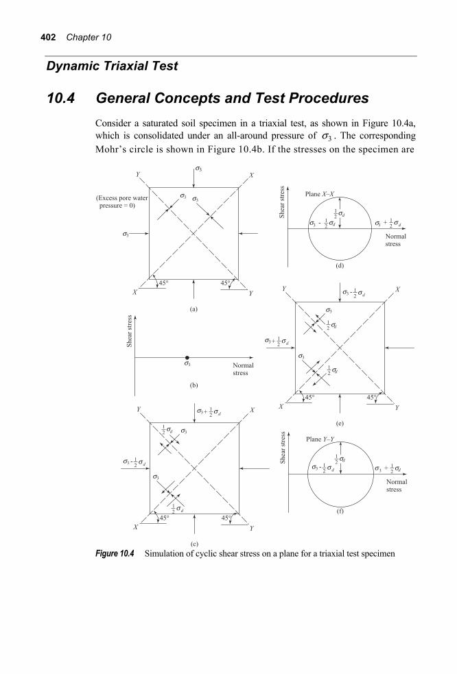
402 Chapter 10
Dynamic Triaxial Test
10.4 General Concepts and Test Procedures Consider a saturated soil specimen in a triaxial test, as shown in Figure 10.4a, which is consolidated under an all-around pressure of 3s . The corresponding Mohr’s circle is shown in Figure 10.4b. If the stresses on the specimen are
Figure 10.4 Simulation of cyclic shear stress on a plane for a triaxial test specimen

Liquefaction of Soil 403
changed such that the axial stress is equal to 3 (1 2) ds s+ and the radial stress is
3 (1 2) ds s- (Figure10.4c), and drainage into or out of the specimen is not allowed, then the corresponding total stress Mohr’s circle is of the nature shown in Figure 10.4d. Note that the stresses on the plane X – X are
Total normal stress = 3s , shear stress = + 12 ds
and the stresses on the plane Y – Y are
Total normal stress = 3s , shear stress = − 12 ds
Similarly, if the specimen is subjected to a stress condition as shown in Figure 10.4e, the corresponding total stress Mohr’s circle will be as shown in Figure 10.4f. The stresses on the plane X – X are
Total normal stress = 3s , shear stress = − 12 ds
The stresses on the plane Y – Y are
Total normal stress = 3s , shear stress = + 12 ds
It can be seen that, if cyclic normal stresses of magnitude (1 2) ds are applied simultaneously in the horizontal and vertical directions, one can achieve a stress condition along planes X – X and Y – Y that will be similar to the cyclic shear stress application shown in Figure 10.3b.
However, for saturated sands, actual laboratory tests can be conducted by applying an all-around consolidation pressure of 3s and then applying a cyclic load having an amplitude of ds in the axial direction only without allowing drainage as shown in Figure 10.5a. The axial strain and the excess pore water pressure can be measured along with the number of cycles of load ( ds ) application.
The question may now arise as to how the loading system shown in Figure 10.5a would produce stress conditions shown in Figure 10.4c and e. This can be explained as follows. The stress condition shown in Figure 10.5b is the sum of the stress conditions shown in Figure 10.5c and d. The effect of the stress condition shown in Figure 10.5d is to reduce the excess pore water pressure of the specimen by an amount equal to (1 2) ds without causing any change in the axial strain. Thus, the effect of the stress conditions shown in Figure 10.5b (which is the same as Figure 10.4c) can be achieved by only subtracting a pore water pressure u = (1 2) ds from that observed from the loading condition shown in Figure 10.5c. Similarly, the loading condition shown in Figure 10.5e is
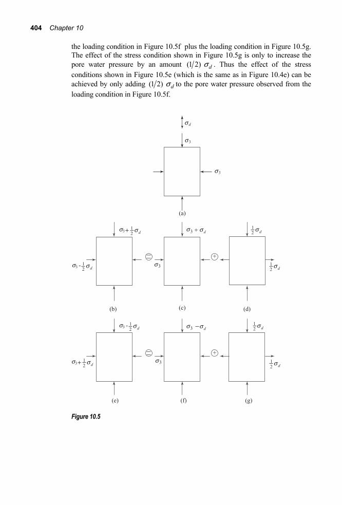
404 Chapter 10
the loading condition in Figure 10.5f plus the loading condition in Figure 10.5g. The effect of the stress condition shown in Figure 10.5g is only to increase the pore water pressure by an amount (1 2) ds . Thus the effect of the stress conditions shown in Figure 10.5e (which is the same as in Figure 10.4e) can be achieved by only adding (1 2) ds to the pore water pressure observed from the loading condition in Figure 10.5f.
Figure 10.5

Liquefaction of Soil 405
10.5 Typical Results from Cyclic Triaxial Test Several cyclic undrained triaxial tests on saturated soil specimens have been conducted by Seed and Lee (1966) on Sacramento River sand retained between No. 50 and No. 100 U.S sieves. The results of a typical test in loose sand (void ratio, e = 0.87) is shown in Figure 10.6. For this test, the initial all around pressure and initial pore water pressure were 200 kPa and 100 kPa respectively. Thus the all around consolidation pressure σ3 is equal to 100 kPa. The cyclic deviator stress σd was applied with a frequency of 2 Hz. Figure 10.7 is a plot of the axial strain, change in pore water pressure u, and the change in pore water pressure corrected to mean extreme principal stress conditions (i.e., subtracting or adding (1 2) σd from or to
Figure 10.6 Typical pulsating load test on loose saturated Sacramento River sand
(redrawn after Seed and Lee, 1966)
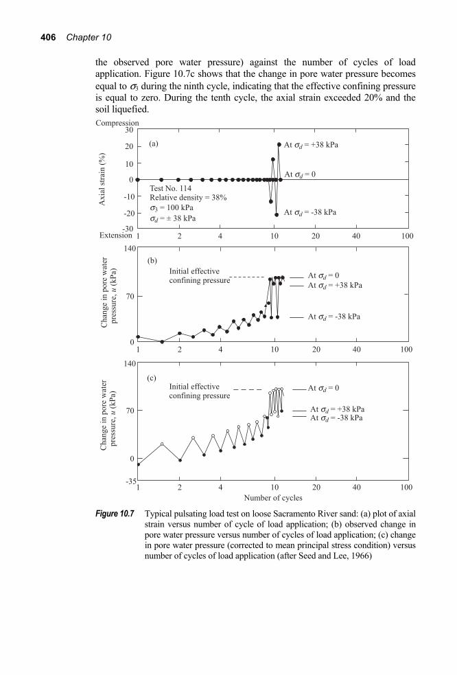
406 Chapter 10
the observed pore water pressure) against the number of cycles of load application. Figure 10.7c shows that the change in pore water pressure becomes equal to σ3 during the ninth cycle, indicating that the effective confining pressure is equal to zero. During the tenth cycle, the axial strain exceeded 20% and the soil liquefied.
Figure 10.7 Typical pulsating load test on loose Sacramento River sand: (a) plot of axial
strain versus number of cycle of load application; (b) observed change in pore water pressure versus number of cycles of load application; (c) change in pore water pressure (corrected to mean principal stress condition) versus number of cycles of load application (after Seed and Lee, 1966)

Liquefaction of Soil 407
The relationship between the magnitude of σd against the number of cycles of pulsating stress applications for the liquefaction of the same loose sand [e = 0.87, σ3 = 100 kPa is shown in Figure 10.8. Note that the number of cycles of pulsating stress application increases with the decrease of the value of σd.
The nature of variation of the axial strain and the corrected pore water pressure for a pulsating load test in a dense Sacramento River sand is shown in Figure 10.9. After about 13 cycles, the change in pore water pressure becomes equal to σ3; however, the axial strain amplitude did not exceed 10% after even 30 cycles of load application. This is a condition with a peak cyclic pore pressure ratio 100%, with limited strain potential due to the remaining resistance of the soil to deformation, or due to the fact that the soil dilates. Dilation of the soil reduces the pore water pressure and helps stabilization of soil under load. This may be referred to as cyclic mobility (Seed, 1979). More discussion on this subject is given in Section 10.11.
A summary of axial strain, number of cycles for liquefaction, and the relative density for Sacramento River sand are given in Figure 10.10 [for σ3 = 100 kPa]. However, a different relationship may be obtained if the confining pressure σ3 is changed.
It has been mentioned earlier that the critical void ratio of sand cannot be used as a unique criterion for a quantitative evaluation of the liquefaction potential. This can now be seen from Figure 10.11, which shows the critical void ratio line for Sacramento River sand. Based on the initial concept of critical void
Figure 10.8 Relationship between pulsating deviator stress and number of cycles
required to cause failure in Sacramento River sand (redrawn after Seed and Lee, 1966)

408 Chapter 10
Figure 10.9 Typical pulsating load test on dense Sacramento River sand: (a) plot of
axial strain versus number of cycles of load application; (b) corrected change of pore water pressure versus number of cycles of load application (after Seed and Lee, 1966)
Figure 10.10 Axial strain after initial liquefaction for pulsating load tests at three
densities for Sacramento River sand (after Seed and Lee, 1966)

Liquefaction of Soil 409
ratio, one would assume that a soil specimen represented by a point to the left of the critical void ratio line would not be susceptible to liquefaction; likewise, a specimen that plots to the right of the critical void ratio line would be vulnerable to liquefaction. In order to test this concept, the cyclic load test results on two specimens are shown as A and B in Figure 10.11. Under a similar pulsating stress
ds = ±120 kPa, specimen A liquefied in 57 cycles, whereas specimen B did not fail even in 10,000 cycles. This is contrary to the aforementioned assumptions.
Thus, the liquefaction potential depends on five important factors:
1. Relative density RD 2. Confining pressure 3s 3. Peak pulsating stress ds 4. Number of cycles of pulsating stress application 5. Overconsolidation ratio
The importance of the first four factors is discussed in the following section. The overconsolidation ratio is discussed in Section 10.9. Soil grain size characteristics, particle shape, aging and cementation, depositional environment, drainage conditions, construction induced loads are also known to have some effects on the liquefaction potential.
Figure 10.11 Critical confining pressure-void ratio relationship for Sacramento River
sand (redrawn after Seed and Lee, 1966)

410 Chapter 10
10.6 Influence of Various Parameters on Soil Liquefaction Potential
Influence of the Initial Relative Density The effect of the initial relative density of a soil on liquefaction is shown in Figure 10.12. All tests shown in Figure 10.12 are for σ3 = 100 kPa.
The initial liquefaction corresponds to the condition when the pore water pressure becomes equal to the confining pressure σ3. In most cases, 20% double amplitude strain is considered as failure. It may be seen that, for a given value of
Figure 10.12 Influence of Initial relative density on liquefaction for Sacramento River sand (redrawn after Lee and Seed, 1967)

Liquefaction of Soil 411
σd, the initial liquefaction and the failure occur simultaneously for loose sand (Figure 10.12a). However, as the relative density increases, the difference between the number of cycle to cause 20% double amplitude strain and to cause initial liquefaction increases.
Influence of Confining Pressure
The influence of the confining pressure σ3 on initial liquefaction and 20% double amplitude strain condition is shown in Figure 10.13. For a given initial relative density and peak pulsating stress, the number of cycles to cause initial liquefaction or 20% strain increases with the increase of the confining pressure. This is true for all relative densities of compaction. Conditions that can create greater confining pressure are deeper ground water table, soil located at a deeper
Figure 10.13 (Continued)

412 Chapter 10
Figure 10.13 Influence of confining pressure on liquefaction of Sacramento River sand:
(a) initial liquefaction; (b) 20% strain (redrawn after Lee and Seed, 1967)
depth and addition of surcharge on the ground surface.
Influence of the Peak Pulsating Stress
Figure 10.14 shows the variation of the peak pulsating stress σd with the confining pressure for initial liquefaction in 100 cycles (Figure 10.14a) and for 20% axial strain in 100 cycles (Figure 10.14b). Note that for a given initial void ratio (i.e., relative density RD) and number of cycles of load application, the variation of σd for initial liquefaction with σ3 is practically linear. A similar relation also exists for loose sand with a 20% axial strain condition. It is worth noting that the peak pulsating stress is a function of peak ground acceleration expected at the site.
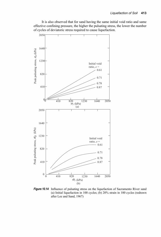
Liquefaction of Soil 413
It is also observed that for sand having the same initial void ratio and same effective confining pressure, the higher the pulsating stress, the lower the number of cycles of deviatoric stress required to cause liquefaction.
Figure 10.14 Influence of pulsating stress on the liquefaction of Sacramento River sand
(a) Initial liquefaction in 100 cycles; (b) 20% strain in 100 cycles (redrawn after Lee and Sand, 1967)
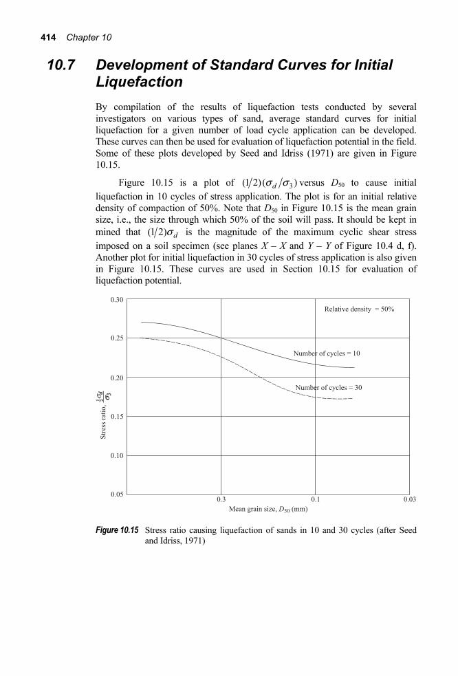
414 Chapter 10
10.7 Development of Standard Curves for Initial Liquefaction By compilation of the results of liquefaction tests conducted by several investigators on various types of sand, average standard curves for initial liquefaction for a given number of load cycle application can be developed. These curves can then be used for evaluation of liquefaction potential in the field. Some of these plots developed by Seed and Idriss (1971) are given in Figure 10.15.
Figure 10.15 is a plot of 3(1 2)( )ds s versus D50 to cause initial liquefaction in 10 cycles of stress application. The plot is for an initial relative density of compaction of 50%. Note that D50 in Figure 10.15 is the mean grain size, i.e., the size through which 50% of the soil will pass. It should be kept in mined that (1 2) ds is the magnitude of the maximum cyclic shear stress imposed on a soil specimen (see planes X – X and Y – Y of Figure 10.4 d, f). Another plot for initial liquefaction in 30 cycles of stress application is also given in Figure 10.15. These curves are used in Section 10.15 for evaluation of liquefaction potential.
Figure 10.15 Stress ratio causing liquefaction of sands in 10 and 30 cycles (after Seed and Idriss, 1971)

Liquefaction of Soil 415
Cyclic Simple Shear Test
10.8 General Concepts Cycle simple shear tests can be used to study liquefaction of saturated sands by using the simple shear apparatus (also see Chapter 4). In this type of test, the soil specimen is consolidated by a vertical stress us . At this time, lateral stress is equal to K0 us (K0 = coefficient of earth pressure at rest). The initial stress conditions of a specimen in a simple shear device are shown in Figure 10.16a; the corresponding Mohr’s circle is shown in Figure 10.16b. After that, a cyclic horizontal shear stress of peak magnitude τh is applied (undrained condition) to the specimen as shown in Figure 10.16c. The pore water pressure and the strain are observed with the number of cycles of horizontal shear stress application.
Using the stress conditions on the soil specimen at a certain time during the cyclic shear test, a Mohr’s circle is plotted in Figure 10.16d. Note that the maximum shear stress on the specimen in simple shear is not τh, but
τmax = ( )2
20
1 12h Kut sÈ ˘+ -Í ˙Î ˚
(10.2)
Figure 10.16 Maximum shear stress for cyclic simple shear test

416 Chapter 10
10.9 Typical Test Results Typical results of some soil liquefaction tests on Monterey sand using simple shear apparatus are shown in Figure 10.17. Note that these are for the initial liquefaction condition. From the figure the following facts may be observed: 1. For a given value of us and relative density RD, a decrease of τh requires an
increase of the number of cycles to cause liquefaction. 2. For a given value of RD and number of cycles of stress application, a
decrease of us requires a decrease of the peak value of τh for causing liquefaction.
3. For a given value of us and number of cycles of stress application, τh for causing liquefaction increases with the increase of the relative density.
Another important factor – the variation of the peak value of τh for causing initial liquefaction with the initial relative density of compaction (for a given value of us and number of stress cycle application) – is shown in Figure 10.18. For a relative density up to about 80%, the peak value of τh for initial liquefaction increases linearly with RD. At higher relative densities (which may not be practical to achieve in the field, particularly if fines are present), the relationship is nonlinear.
Figure 10.17 Initial liquefaction in cyclic simple shear test on Monterey sand (redrawn after Peacock and Seed, 1968)

Liquefaction of Soil 417
Figure 10.18 Effect of relative density on cyclic shear stress causing initial liquefaction of Monterey sand (redrawn after Peacock and Seed, 1968)
Influence of Test Condition In simple shear test equipment, there is always some nonuniformity of
stress conditions. This causes specimens to develop liquefaction under lower applied horizontal cyclic stresses as compared to that in the field. This happens even though care is taken to improve the preparation of the specimens and rough platens are used at the top and bottom of the specimens to be tested. For that reason, for a given value of us , RD, and number of cyclic shear stress application, the peak value of τh in the field is about 15% - 50% higher than that obtained from the cyclic simple shear test. This fact has been demonstrated by Seed and Peacock (1971) for a uniform medium sand (RD ≈ 50%) in which the field values are about 20% higher than the laboratory values.
Influence of Overconsolidation Ratio on the Peak Value of τh Causing Liquefaction
For the cyclic simple shear test, the value of τh is highly dependent on the value of the initial lateral earth pressure coefficient at rest (K0). The value of K0, is in turn, dependent on the over consolidation ratio (OCR). The variation of h ut s

418 Chapter 10
Figure 10.19 Influence of overconsolidation ratio on stresses causing liquefaction in
simple shear tests (redrawn after Seed and Peacock, 1971)
for initial liquefaction with the overconsolidation ratio as determined by the cyclic simple shear test is shown in Figure 10.19. For a given relative density and number of cycles causing initial liquefaction, the value of h ut s decreases with the decrease of K0. It needs to be mentioned at this point that all the cyclic triaxial studies for liquefaction are conducted for the initial value of K0 = 1.
10.10 Rate of Excess Pore Water Pressure Increase Seed and Booker (1977) and DeAlba, Chan, and Seed (1975) measured the rate of excess pore water pressure increase in saturated sands during liquefaction using cyclic simple shear tests. The range of the variation of pore water pressure generation ug during cyclic loading is shown in Figure 10.20. The average value of the variation of ug can be expressed in a nondimensional form as (Seed, Martin, and Lysmer, 1975)
1 2
2 arcsing
i
u NNu
a
sÊ ˆÊ ˆ= Á ˜ Á ˜Ë ¯p Ë ¯
(10.3)

Liquefaction of Soil 419
where ug = excess pore water pressure generated us = initial consolidation pressure N = number of cycles of shear stress application Ni = number of cycles of shear stress needed for initial
liquefaction α = constant (≈ 0.7)
Hence, the rate of change of ug with N can be given as
2 1
2 1
sin cos2 2
g
iu u
uN N r r
u
a
sa -
È ˘Í ˙∂ Ê ˆ Í ˙= Á ˜ p p∂ p Ê ˆ Ê ˆË ¯ Í ˙
Á ˜ Á ˜Í ˙Ë ¯ Ë ¯Î ˚
(10.4)
where
ru = gu
us (10.5)
The preceding relationship is very useful in the study of the stabilization of potentially liquefiable sand deposits.
Figure 10.20 Rate of pore water pressure build up cyclic simple shear test (after Seed and
Booker, 1977)

420 Chapter 10
10.11 Large-Scale Simple Shear Tests In the study of soil liquefaction of granular soils, certain aspects of the test procedures have remained a matter for concern. Some of those concerns are as follows:
a. Stress concentration in small-scale simple shear tests leads to some inaccuracy in the results (Castro, 1969).
b. Stress concentration at the base and cap of cyclic triaxial test specimens and the possibility of necking leads to nonuniformity of strain and redistribution of water content (Castro, 1975).
c. Attempts to study liquefaction by using shaking table tests (e.g., Emery, Finn, and Lee, 1972; Finn, Emery, and Gupta, 1970; O-Hara, 1972; Ortigosa, 1972; Tanimoto, 1967l; Whitman, 1970; Yoshimi, 1967) have also raised some equations, since the results, in some cases, have been influenced by the confining effects of the sides of the box.
For that reason, DeAlba, Seed, and Chan (1976) conducted large-scale simple shear tests with one-directional cyclic stress application. The specimens of sand used for testing had dimensions of 2300 mm × 1100 mm × 100 mm (depth). Each specimen was constructed over a shaking table. A rubber membrane was placed over the sand to prevent drainage. An inertia mass was also placed on top of the sand. Movement of the shaking table produced cyclic stress conditions in the sand. The cyclic shear stress was determines as
τh = Wg
am (10.6)
where W = total pressure exerted at the base by the specimen and the inertia mass
am = peak acceleration of the uniform cyclic motion g = acceleration due to gravity
From the measured displacement of the inertia mass during shaking, the average single-amplitude cyclic shear strain could be obtained as
2h
g D= ±¢ (10.7)
where g ¢ = average single amplitude cyclic shear strain h = specimen height

Liquefaction of Soil 421
Figure 10.21 Corrected h ut s versus Ni for initial liquefaction from large-scale simple
shear tests (after DeAlba, Seed, and Chan, 1976)
Figure 10.21 shows the variation of h ut s against the number of cycles of initial liquefaction (N = Ni) for various values of the relative density of sand (RD). Note that this has been corrected for the compliance effects of the specimens and the pore water pressure-measuring system and the effects of membrane penetration. The nature of these plots is similar to those shown in Figure 10.17.
Figure 10.22 shows a comparison of the variation of h ut s versus Ni (for RD = 50%) obtained from the reported results of Ortigosa (1972), O-Hara (1972), Finn, Emery, and Gupta (1971), and the large-scale simple shear test results of DeAlba, Chan, and Seed (1976). The differences between the results are primarily due to (1) the effect of membrane penetration and compliance effects, (2) the length-to-height ratio of the specimens and hence the boundary conditions, and (3) the nature of sample preparation. It is thus evident from Figure 10.22 that care should be taken to provide proper boundary conditions if meaningful data are to be obtained from shaking table tests.
Figure 10.23 shows the comparison of h ut s versus number of cycles for initial liquefaction of saturated sand at RD = 50% obtained from various studies using small-scale and large-scale simple shear devices. The sample preparation techniques in all the studies were similar. Based on Figure 10.23, it can be concluded that the results are in good agreement and the errors due to stress concentration in small-scale simple shear tests are not very large.
The variation of single-amplitude cyclic shear strain [Eq. (10.7)] with N for dense sands obtained from large-scale simple shear tests is shown in Figure 10.24. Note that the magnitude of γ ′ increased gradually with N after initial liquefaction up to a maximum limiting value and remained constant thereafter.
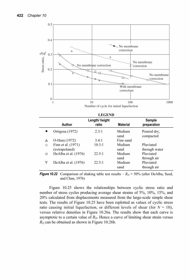
422 Chapter 10
LEGEND Length/ height Sample Author ratio Material preparation
• Ortigosa (1972) 2.3:1 Medium Poured dry, sand compacted O-Hara (1972) 3.4:1 Fine sand ○ Finn et al. (1971) 10.3:1 Medium Pluviated (extrapolated) sand through water DeAlba et al. (1976) 22.5:1 Medium Pluviated sand through air — DeAlba et al. (1976) 22.5:1 Medium Pluviated sand through air
Figure 10.22 Comparison of shaking table test results – RD = 50% (after DeAlba, Seed, and Chan, 1976)
Figure 10.25 shows the relationships between cyclic stress ratio and number of stress cycles producing average shear strains of 5%, 10%, 15%, and 20% calculated from displacements measured from the large-scale simple shear tests. The results of Figure 10.25 have been replotted as values of cyclic stress ratio causing initial liquefaction, or different levels of shear (for N = 10), versus relative densities in Figure 10.26a. The results show that each curve is asymptotic to a certain value of RD. Hence a curve of limiting shear strain versus RD can be obtained as shown in Figure 10.26b.

Liquefaction of Soil 423
Curve No. Reference Type of Test
1 Yoshimi and Oh-oka (1973) Ring torsion 2 Finn (1972) Simple shear 3 DeAlba et al (1976) Shaking table (corrected)
4 Seed and Peacock (1971) Simple shear
Figure 10.23 Comparison of shaking table and simple shear liquefaction test results – RD = 50% (after DeAlba, Seed, and Chan, 1976)
Figure 10.24 Nature of variation of γ ′ with number of cycles of load application

424 Chapter 10
Figure 10.25 Relationship between h ut s and number of cycles causing different levels of strain (after DeAlba, Seed, and Chan, 1976)
Based on Figure 10.26, the following conclusions can be drawn.
1. For initial RD ≤ 45%, the application of cyclic stress ratio high enough to cause initial liquefaction also causes unlimited shear strain. This corresponds to a condition of liquefaction.
2. For initial RD > 45%, the application of cyclic stress ratio high enough to cause initial liquefaction will result in a limited amount of shear strain. This is the case of soil with limited strain potential or the condition of cyclic mobility.
3. The limiting strain potential decreases with the increase of the initial relative density of soil.
Before moving on to establish procedures for determination of liquefaction in the field, the results from the laboratory tests can be summarizes as following:
1. Liquefaction is a phenomenon in which the strength and stiffness of a soil is reduced by earthquake shaking or other rapid loading. Liquefaction and related phenomena have been responsible for

Liquefaction of Soil 425
tremendous amounts of damage in historical earthquakes around the world.
2. Flow liquefaction is a phenomenon in which the static equilibrium is destroyed by static or dynamic loads in a soil deposit with low residual strength. Residual strength is the strength of a liquefied soil.
3. Cyclic mobility is a liquefaction phenomenon, triggered by cyclic loading, occuring in soil deposits with static shear stresses lower than the soil strength. Deformations due to cyclic mobility develop incrementally because of static and dynamic stresses that exist during an earthquake.
4. To understand liquefaction, it is important to recognize the conditions that exist in a soil deposit before an earthquake.
Figure 10.26 Limiting shear strains – 10 cycles of stress (after DeAlba, Seed, and Chan,
1976)

426 Chapter 10
Development of a Procedure for Determination of Field Liquefaction
10.12 Correlation of Liquefaction Results from Simple Shear and Triaxial Tests The conditions for determination of field liquefaction problems are related to the ratio of h ut s ; this is also true for the case of cyclic simple shear stress tests. However, in the case of triaxial tests, the results are related to the ratio of
3(1 2)( )ds s . It appears that a correlation between h ut s and 3(1 2)( )ds s needs to be developed (for a given number of cyclic stress application to cause liquefaction). Seed and Peacock (1971) considered the following alternative criteria for correlation for the onset of soil liquefaction. 1. The maximum ratio of the shear stress developed during cyclic loading to
the normal stress during consolidation on any plane of the specimen can be a controlling factor. For triaxial specimens, this is equal to 3(1 2)( )ds s , and for simple shear specimens it is about 0( )h K ut s . Thus,
0
hK u
ts
= 3
12 ds
s
or
simple shear
h
u
tsÈ ˘Í ˙Î ˚
= 03
12 d
Ks
s
È ˘Í ˙Í ˙Î ˚
(10.8)
2. Another possible condition for the onset of liquefaction can be the maximum ratio of change in shear stress during cyclic loading to the normal stress during consolidation on any plane. For simple shear specimens this is about 0( )h K ut s , and for triaxial specimens it is
3(1 2)( )ds s . This leads to the same equation as Eq. (10.8) 3. The third possible alternative can be given by the ratio of the maximum
shear stress induced in a specimen during cyclic loading to the mean principal stress on the specimen during consolidation. For simple shear specimens:
Maximum shear stress during cyclic loading = ( )220
1 12h Kut sÈ ˘+ -Í ˙Î ˚
(10.2)
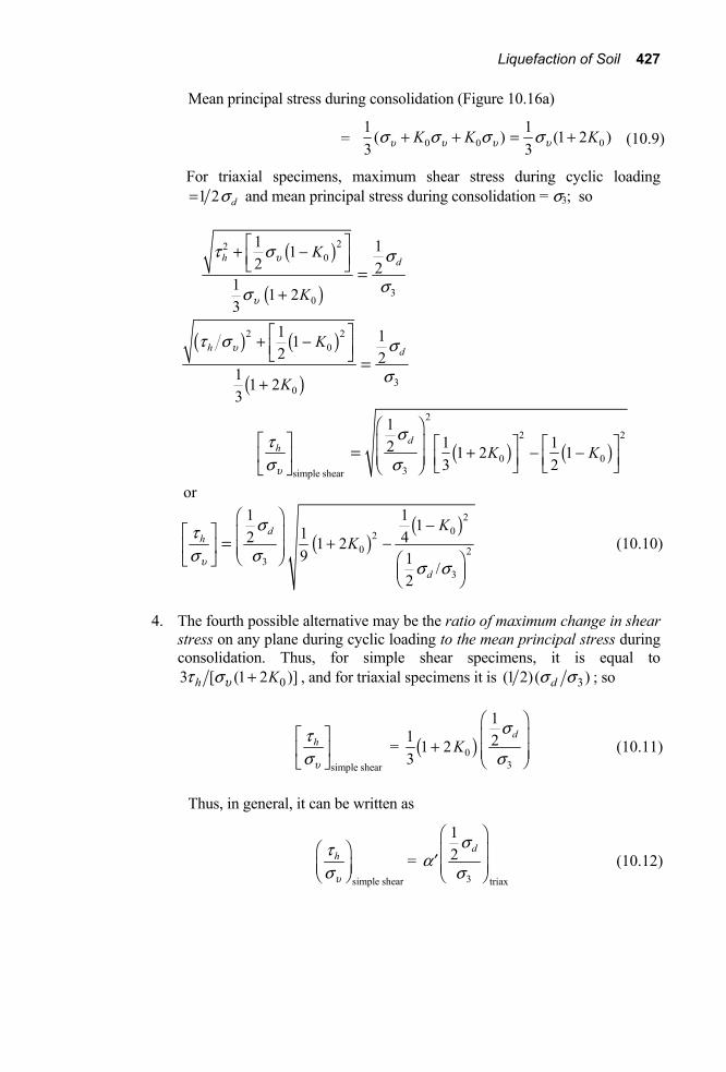
Liquefaction of Soil 427
Mean principal stress during consolidation (Figure 10.16a)
= 0 0 01 1( ) (1 2 )3 3
K K Ku u u us s s s+ + = + (10.9)
For triaxial specimens, maximum shear stress during cyclic loading 1 2 ds= and mean principal stress during consolidation = σ3; so
( )
( )
220
30
1 112 2
1 1 23
h dK
K
u
u
t s s
ss
È ˘+ -Í ˙Î ˚
+=
( ) ( )
( )
2 20
30
1 112 2
1 1 23
h dK
K
ut s s
s
È ˘+ -Í ˙Î ˚
+=
( ) ( )
2
2 2
0 03simple shear
11 12 1 2 13 2
dh K Ku
sts s
Ê ˆÈ ˘ Á ˜ È ˘ È ˘+ - -Í ˙ Á ˜ Í ˙ Í ˙Ë ¯ Î ˚ Î ˚Î ˚
=
or
( )( )2
020 2
33
1 1 112 41 29 1 /
2
dh
d
KK
u
sts s
s s
Ê ˆ -È ˘ Á ˜ + -Í ˙ Á ˜Ë ¯ Ê ˆÎ ˚Á ˜Ë ¯
= (10.10)
4. The fourth possible alternative may be the ratio of maximum change in shear stress on any plane during cyclic loading to the mean principal stress during consolidation. Thus, for simple shear specimens, it is equal to
03 [ (1 2 )]h Kut s + , and for triaxial specimens it is 3(1 2)( )ds s ; so
simple shear
h
u
tsÈ ˘Í ˙Î ˚
= ( )03
11 21 23
dK
s
s
Ê ˆÁ ˜+ Á ˜Ë ¯
(10.11)
Thus, in general, it can be written as
simple shear
h
u
tsÊ ˆÁ ˜Ë ¯
= 3 triax
12 ds
as
Ê ˆÁ ˜¢ Á ˜Ë ¯
(10.12)

428 Chapter 10
where a ¢ = K0 for Cases 1 and 2,
( )( )2
020 2
3
1 11 41 29 1
2 d
KKa
s s
-= + -¢
Ê ˆÁ ˜Ë ¯
for Case 3
and
a ¢ = 13
(1 + 2K0) for Case 4
The values of α′ for the four cases considered here are given in Table 10.1.
From Table 10.1 it may be seen that for normally consolidated sands, the value of α′ is generally in the range 45% - 50%, with an average of about 47%.
Finn, Emery, and Gupta (1971) have shown that, for initial liquefaction of normally consolidated sands, a ¢ is equal to 0(1 2)(1 )K+ . The value of K0 can be given by the relation (Jaky, 1944)
K0 = 1 – sin φ (10.13)
Table 10.1 Values of a ¢ [Eq. (10.12)]a K0 Case 1 Case 2 Case 3 Case 4
0.4 0.4 0.4 - 0.60 0.5 0.5 0.5 0.25 0.67 0.6 0.6 0.6 0.54 0.73 0.7 0.7 0.7 0.80 0.8 0.8 0.8 0.83 0.87 0.9 0.9 0.9 0.93 1.0 1.0 1.0 1.00 1.00 a After Seed and Peacock (1971).
Castro (1975) has proposed that the initial liquefaction may be controlled by the criteria of the ratio of the octahedral shear stress during cycle loading to the effective octahedral normal stress during consolidation. The effective octahedral normal stress during consolidation octs ¢ is given by relation
( )oct 1 2 313
s s s s= + +¢ ¢ ¢ ¢ (10.14)
where 1s ¢ , 2s ¢ , 3s ¢ are, respectively, the major, intermediate, and minor effective principal stresses.

Liquefaction of Soil 429
The octahedral shear stress octt during cyclic loading is
2 2 2 1/2oct 1 3 1 2 2 3
1= [( - ) +( - ) +( - ) ]3
t s s s s s s (10.15)
where 1s , 2s , 3s are, respectively, the major, intermediate, and minor principal stresses during cyclic loading. For cyclic triaxial tests,
oct
oct 3triax triax
12 223
dsts s
Ê ˆÊ ˆ Á ˜= Á ˜Á ˜¢Ë ¯ Ë ¯
(10.16)
For cyclic simple shear tests,
oct
oct 0simple shear simple shear
61 2
hK u
t ts s
Ê ˆÊ ˆ Ê ˆ= Á ˜Á ˜ Á ˜+¢Ë ¯ Ë ¯Ë ¯
(10.17)
Thus,
oct oct
oct octsimple shear triax
t ts sÊ ˆ Ê ˆ
=Á ˜ Á ˜¢ ¢Ë ¯ Ë ¯
or
0 3simple shear triax
16 2 22
1 2 3
dhK u
sts s
Ê ˆÊ ˆ Ê ˆ Á ˜=Á ˜ Á ˜Á ˜+ Ë ¯ Ë ¯Ë ¯
or
oct 0
oct 3simple shear triax
11 22 22
3 6
dK sts s
Ê ˆÊ ˆ +Ê ˆ Á ˜= Á ˜ Á ˜Á ˜ Ë ¯¢Ë ¯ Ë ¯
= ( )0
3 triax
2 11 23 2
3
dK s
s
Ê ˆ+ Á ˜Á ˜Ë ¯
(10.18)
Comparing Eqs. (10.12) and (10.18),
a ¢ =
23
1 2
3
0( )+ K (10.19)

430 Chapter 10
10.13 Correlation of the Liquefaction Results from Triaxial Tests to Field Conditions Section 10.9 explained that the field value of ( )h ut s for initial liquefaction is about 15% – 50% higher than that obtained from simple shear tests. Thus,
field simple shear
h h
u u
t tbs sÊ ˆ Ê ˆ
=Á ˜ Á ˜Ë ¯ Ë ¯ (10.20)
The approximate variation of β with relative density of sand is given in Figure 10.27. Combining Eqs (10.12) and (10.20), one obtains
3 3field simple shear triax
1 12 2d d
h hrC
u u
s st tb a bs s s s
Ê ˆ Ê ˆÊ ˆ Ê ˆ Á ˜ Á ˜= = ¢ =Á ˜ Á ˜Á ˜ Á ˜Ë ¯ Ë ¯ Ë ¯ Ë ¯
(10.21)
where rC a b= ¢
Using an average value of a ¢ = 0.47 and the values of β given in Figure 10.27, the variation of Cr with relative density can be obtained. This is shown in Figure 10.28.
Figure 10.27 Variation of correction factor β with relative density [Eq. (10.20)]

Liquefaction of Soil 431
Figure 10.28 Variation of Cr with relative density [Eq. (10.21)]
Eq. (10.21) presents the correlations for initial liquefaction between the stress ratios in the field, cyclic simple shear tests, and cyclic triaxial tests for a given sand at the same relative density. However, when laboratory tests are conducted at relative density, say, RD(1), whereas the fields conditions show the sand deposit to be a relative density of RD(2), one has to convert the laboratory test results to correspond to a relative density of RD(2). It has been shown in Figure 10.18 that τh for initial liquefaction in the laboratory in a given number of cycles is approximately proportional to the relative density (for RD ≤ 80%).
Thus,
(1)(2)
(2)
(1)D D
Dh R h R
D
RR
t tÈ ˘ È ˘Î ˚ Î ˚
È ˘= Í ˙
Í ˙Î ˚ (10.22)
where (1)[ ]Dh Rt is the cyclic peak shear stress required to cause initial liquefaction
in the laboratory for a given value of us and number of cycles, by simple shear test; and
( 2)[ ]Dh Rt is the cyclic peak stress required to cause initial liquefaction in
the field for the same value of us and number of cycles, by simple shear test. Combining Eqs. (10.21) and (10.22)
( )
( )( 2) (1)
2
3 1field triax
12 .
D D
d Dhr
DR R
RC
Ru
sts sÈ ˘ È ˘Î ˚ Î ˚
Ê ˆÊ ˆ Á ˜= Á ˜Á ˜Ë ¯ Ë ¯
(10.23)

432 Chapter 10
10.14 Zone of Initial Liquefaction in the Field There are five general steps for determining the zone in the field where soil liquefaction due to an earthquake can be initiated:
1. Establish a design earthquake. 2. Determine the time history of shear stresses induced by the earthquake
at various depths of sand layer. 3. Convert the shear stress–time histories into N number of equivalent
stress cycles (see Section 7.8). These can be plotted against depth, as shown in Figure 10.29.
4. Using the laboratory test results, determine the magnitude of the cyclic stresses required to cause initial liquefaction in the field in N cycles (determined from Step 3) at various depths. Note that the cyclic shear stress levels change with depth due to change of us . These can be plotted with depth as shown in Figure 10.29.
5. The zone in which the cyclic shear stress levels required to cause initial liquefaction (Step 4) are equal to or less than the equivalent cyclic shear stresses induced by an earthquake is the zone of possible liquefaction. This is shown in Figure 10.29.
Figure 10.29 Zone of initial liquefaction in the field

Liquefaction of Soil 433
10.15 Relation between Maximum Ground Acceleration and the Relative Density of Sand for Soil Liquefaction This section discusses a simplified procedure developed by Seed and Idriss (1971) to determine the relation between the maximum ground acceleration due to an earthquake and the relative density of a sand deposit in the field for the initial liquefaction condition. Figure 10.30a shows a layer of sand deposit in which we consider a column of soil of height h and unit area of cross section. Assuming the soil column to behave as a rigid body, the maximum shear stress at a depth h due to a maximum ground surface acceleration of amax can be given by
max maxh a
ggt Ê ˆ
= Á ˜Ë ¯ (10.24)
where τmax = the maximum shear stress γ = the unit weight of soil g = acceleration due to gravity.
However, the soil column is not a rigid body. For the deformable nature of the soil, the maximum shear stress at a depth h, determined by Eq. (10.24), needs to be modified as
max(modif ) maxDhC a
ggt
È ˘Ê ˆ= Í ˙Á ˜Ë ¯Î ˚
(10.25)
where CD is a stress reduction factor. The range of CD for different soil profiles is shown in Figure 10.30b, along with the average value up to a depth of 12.0 m.
It has been shown that the maximum shear stress determined from the shear stress–time history during an earthquake can be converted into an equivalent number of significant stress cycles. According to Seed and Idriss, one can take
a max(modif ) max0.65 0.65 DhC a
gugt t
È ˘Ê ˆ= = Í ˙Á ˜Ë ¯Î ˚
(10.26)
The corresponding number of significant cycles N for aut is given in Table 10.2.

434 Chapter 10
Figure 10.30 (a) Maximum shear stress at a depth for a rigid soil column; (b) range of the
shear stress reduction factor CD for the deformable nature of soil (after Seed and Idriss, 1971)

Liquefaction of Soil 435
Table 10.2 Significant Number of Stress Cycles N Corresponding to aut
Earthquake magnitude N 7 10 7.5 20 8 30
Note that although the values of N given in the table are somewhat different from those given in Figure 7.15, it does not make a considerable difference in the calculations. One can now combine Eq. (10.23), which gives the correlation of laboratory results of cyclic triaxial test to the field conditions, and Eq. (10.26) to determine the relationships between amax and RD. This can be better shown with the aid of a numerical example.
In general, the critical depth of liquefaction (see Figure 10.29) occurs at a depth of about 6.0 m) when the depth of water table dw is 0 – 3.0 m; similarly, the critical depth is about 9.0 m when the depth of water table is about 4.5 m.
Liquefaction occurs in sands having a mean size D50 of 0.075 – 0.2 mm.
Consider a case where
D50 = 0.075 mm dw = 4.5 m g = unit weight of soil above the ground water table (GWT) = 18.5 kN/m3
satg = unit weight of soil below GWT = 19.6 kN/m3
g ¢ = effective unit weight of soil below GWT = (19.6 – 9.81) = 9.79 kN/m3 significant number of stress cycles = 10 (earthquake magnitude = 7)
The critical depth of liquefaction d is about 9 m. At that depth the total normal stress is equal to
4.5 ( )g + 4.5 satg = 4.5(18.5) + 4.5(19.6) = 171.45 kPa
From Eq. (10.26)
max0.65a DhC a
gugt
È ˘Ê ˆ= Í ˙Á ˜Ë ¯Î ˚
The value of CD for d = 9 m is 0.925 (Fig. 10.30). Thus,

436 Chapter 10
( )( )( ) max max0.65 0.925 171.45 103.08a
a ag gut = = (10.27)
Again, from Eq. (10.23)
( )
( )( 2 )
(1)
2(field) [ ]
3 1triax[ ]
(1/ 2).
D
D
Ddh R r
DR
RC
Rust s
sÊ ˆ= Á ˜Ë ¯
At a depth 9 m below the ground surface, the initial effective stress us is equal to 4.5(γ ) + 4.5(γ ′) = 4.5(18.5) + 4.5(9.79) = 127.31 kPa.
From Figure 10.15, for D50 = 0.075 mm, ( )1
3 triaxial 50%
(1/ 2)
D
d
R
ss =
Ê ˆÁ ˜Ë ¯
≈ 0.215.
Hence
( )(2 )
(2)(field) [ ]
127.31 0.21550D
r Dh R
C Rt
È ˘Î ˚= = 0.547 CrR D(2) (10.28)
For liquefaction, aut of Eq. (10.27) should be equal to ( 2)(field) [ ]Dh Rt .
Hence,
max103.08ag
= 0.547CrRD (2)
or
a
gmax = 0.0053CrRD(2) (10.29)
It is now possible to prepare Table 10.3 to determine the variation of amax/g with RD(2). Note that RD(2) is the relative density in the field.
Figure 10.31 shows a plot of amax/g versus the relative density as determined from Table 10.3. For this given soil (i.e., given D50, dw, and number of significant stress cycles N), if the relative density in the field and amax/g are such that they plot as point A in Figure 10.31 (i.e., above the curve showing the relationship of Eq. (10.29)], then liquefaction would occur. On the other hand, if the relative density and amax/g plot as point B [i.e., below the curve showing the relationship of Eq. (10.29)], then liquefaction would not occur.
Diagrams of the type shown in Figure 10.31 could be prepared for various combinations of D50, dw, and N. Since, in the field, for liquefaction the range of D50 is 0.075 − 0.2 mm and the range of N is about 10–20, one can take the critical

Liquefaction of Soil 437
combinations (i.e., D50 = 0.075 mm, N = 20; D50 = 0.2 mm, N = 10) and plot graphs as shown in Figure 10.32. These graphs provide a useful guide in the evaluation of liquefaction potential in the field.
These graphs are also useful, particularly when implementing a possible ground improvement technique in the field to reduce the liquefaction susceptibility. Using this graph, one can find how much increase in relative density or in other words, how much compaction is required to be achieved in the field (using principles of basic soil mechanics), once the in-situ conditions of the soil and the possible maximum ground acceleration the site likely to experience are known. Table 10.3 Relation Between amax/g versus RD(2) Eq. (10.29) RD(2) Ratioa
(%) Cr maxag
20 0.54 0.0572 30 0.54 0.0859 40 0.54 0.1144 50 0.56 0.1484 60 0.61 0.1940 70 0.66 0.2449 80 0.71 0.3010 a From Figure 10.28.
Figure 10.31 Plot of amax/g versus relative density from Table 10.3

438 Chapter 10
Figure 10.32 Evaluation of liquefaction potential for sand below the ground surface
(redrawn after Seed and Idriss, 1971)
10.16 Liquefaction Analysis from Standard Penetration Resistance Another way of evaluating the soil liquefaction potential is to prepare correlation charts with the standard penetration resistance. After the occurrence of the Niigata earthquake of 1964, Kishida (1966), Kuizumi (1966), and Ohasaki (1966) studied the area in Niigata where liquefaction had and had not occurred. They developed criteria, based primarily on standard penetration resistance of sand deposits, to differentiate between liquefiable and nonliquefiable conditions. Subsequently, a more detailed collection of field data for liquefaction potential was made by Seed and Peacock (1971). These results and some others were presented by Seed, Mori, and Chan (1971) in a graphical form, which is a plot of
h ut s versus N ¢ . This is shown in Figure 10.33. In this figure note that N ¢ is the corrected standard penetration resistance for an effective overburden pressure of 100 kPa. Figure 10.33 shows the lower bounds of the correlation curve causing liquefaction in the field. However, correlation charts such as this cannot be used with confidence in the field, primarily because they do not take into consideration the magnitude of the earthquake and the duration of shaking.
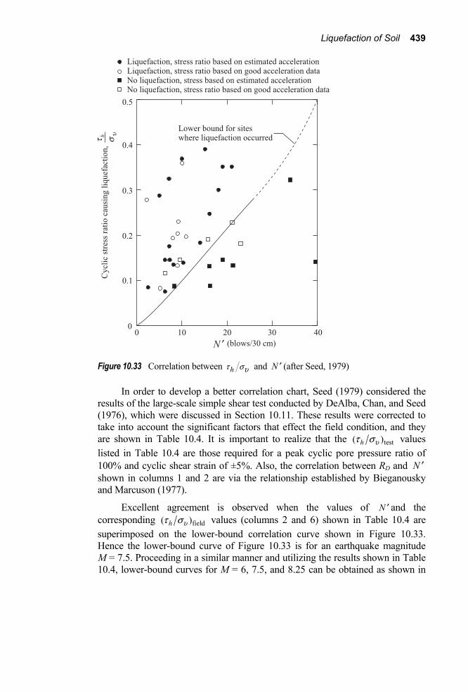
Liquefaction of Soil 439
Figure 10.33 Correlation between ht su and N ¢ (after Seed, 1979)
In order to develop a better correlation chart, Seed (1979) considered the results of the large-scale simple shear test conducted by DeAlba, Chan, and Seed (1976), which were discussed in Section 10.11. These results were corrected to take into account the significant factors that effect the field condition, and they are shown in Table 10.4. It is important to realize that the test( )h ut s values listed in Table 10.4 are those required for a peak cyclic pore pressure ratio of 100% and cyclic shear strain of ±5%. Also, the correlation between RD and N ¢ shown in columns 1 and 2 are via the relationship established by Bieganousky and Marcuson (1977).
Excellent agreement is observed when the values of N ¢ and the corresponding field( )h ut s values (columns 2 and 6) shown in Table 10.4 are superimposed on the lower-bound correlation curve shown in Figure 10.33. Hence the lower-bound curve of Figure 10.33 is for an earthquake magnitude M = 7.5. Proceeding in a similar manner and utilizing the results shown in Table 10.4, lower-bound curves for M = 6, 7.5, and 8.25 can be obtained as shown in

440 Chapter 10
Figure 10.34. Also shown in this figure is the variation of the limited strain potential in percent (for effective overburden pressure of 100 kPa). Figure 10.34 can be used for determination of the liquefaction potential in the field. In doing so, it is important to remember that
N FN C N=¢ (10.30)
Table 10.4 Data from Large-scale Simple Shear Tests on Freshly Deposited Sanda
M = 5 – 6 M = 7 – 7.5 M = 8 – 8.25 5 cycles 15 cycles 25 cycles
Ê ˆÁ ˜Ë ¯testu
ts
h Ê ˆÁ ˜Ë ¯fieldu
ts
h Ê ˆÁ ˜Ë ¯testu
ts
h
Ê ˆÁ ˜Ë ¯fieldu
ts
h
Ê ˆÁ ˜Ë ¯testu
ts
h
Ê ˆÁ ˜Ë ¯fieldu
ts
h
(1) (2) (3) (4) (5) (6) (7) (8)
54 13.5 0.22 0.25 0.17 0.19 0.155 0.175 68 23 0.30 0.34 0.24 0.27 0.210 0.235 82 33 0.44 0.49 0.32 0.37 0.280 0.315
90 39 0.59 0.66 0.41 0.46 0.360 0.405
Note: N ¢ = standard penetration resistance corrected to an effective overburden pressure of 100 kPa; M = magnitude of earthquake. a After Seed (1979).
where
NF = field standard penetration test values CN = correction factor to convert to an effective overburden pressure
( us ¢ ) of 100 kPa
The correction factor can be expressed as (Liao and Whitman, 1986)
19.78NCus
=¢
(10.31)
where us ¢ is in kPa.
A slight variation of Figure 10.34 is given by Seed, Idriss, and Arango (1983) and Seed and Idriss (1982). It can be seen from this figure that, if N ¢ is more than 30, liquefaction is unlikely to occur, in general.
Relative ¢N density, RD (blows/30 cm)
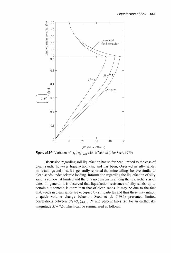
Liquefaction of Soil 441
Figure 10.34 Variation of field( )ht su with N ¢ and M (after Seed, 1979)
Discussion regarding soil liquefaction has so far been limited to the case of clean sands; however liquefaction can, and has been, observed in silty sands, mine tailings and silts. It is generally reported that mine tailings behave similar to clean sands under seismic loading. Information regarding the liquefaction of silty sand is somewhat limited and there is no consensus among the researchers as of date. In general, it is observed that liquefaction resistance of silty sands, up to certain silt content, is more than that of clean sands. It may be due to the fact that, voids in clean sands are occupied by silt particles and thus these may inhibit a quick volume change behavior. Seed et al. (1984) presented limited correlations between field( )h ut s , N ¢ and percent fines (F) for an earthquake magnitude M = 7.5, which can be summarized as follows:

442 Chapter 10
Lower bound of field( )h ut s Percent of fines, for which liquefaction is F N ¢ likely (M = 7.5)
≤5 5 0.055 10 0.115 15 0.170 20 0.220 25 0.295 30 0.500 10 5 0.098 10 0.160 15 0.225 20 0.295 25 0.500 35 5 0.130 10 0.185 15 0.260 20 0.400
Example 10.1 Geotechnical investigations carried out in a deposit of sand provided the field standard penetration numbers N as given in the table below. During the geotechnical investigations, it is also observed that groundwater table is encountered at a depth of 3.0 m measured from the ground surface. Given for the sand:
Dry unit weight = 17.6 kN/m3 Saturated unit weight = 19.6 kN/m3
Determine, for an earthquake magnitude of 7.5, if liquefaction will occur at the site. Assume that the maximum peak ground acceleration at the site is amax = 0.15 g. Depth (m) NF (blows/30cm) 1.5 6 3.0 8 4.5 10 6.0 14 7.5 16 9.0 20 10.5 20
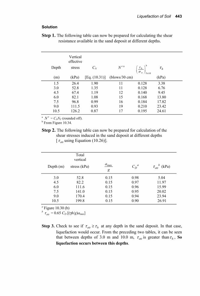
Liquefaction of Soil 443
Solution
Step 1. The following table can now be prepared for calculating the shear resistance available in the sand deposit at different depths.
Vertical effective Depth stress CN N ¢ a b
f ie ld
h
u
ts
Ê ˆÁ ˜Ë ¯
ht
(m) (kPa) [Eq. (10.31)] (blows/30 cm) (kPa) 1.5 26.4 1.90 11 0.128 3.38 3.0 52.8 1.35 11 0.128 6.76 4.5 67.4 1.19 12 0.140 9.45 6.0 82.1 1.08 15 0.168 13.80 7.5 96.8 0.99 16 0.184 17.82 9.0 111.5 0.93 19 0.210 23.42 10.5 126.2 0.87 17 0.195 24.61 a N ¢ = CNNF (rounded off). b From Figure 10.34.
Step 2. The following table can now be prepared for calculation of the shear stresses induced in the sand deposit at different depths [ aut using Equation (10.26)].
Total vertical
Depth (m) stress (kPa) a
gmax a
DC baut (kPa)
3.0 52.8 0.15 0.98 5.04 4.5 82.2 0.15 0.97 11.97 6.0 111.6 0.15 0.96 15.99 7.5 141.0 0.15 0.95 20.02 9.0 170.4 0.15 0.94 23.94 10.5 199.8 0.15 0.90 26.91 a Figure 10.30 (b) b aut = 0.65 CD [(γh/g)amax]
Step 3. Check to see if a hut t≥ at any depth in the sand deposit. In that case, liquefaction would occur. From the preceding two tables, it can be seen that between depths of 3.0 m and 10.0 m, aut is greater than ht , So liquefaction occurs between this depths.

444 Chapter 10
10.17 Other Correlations for Field Liquefaction Analysis
Correlation with Cone Penetration Resistance In many cases during field exploration, the variation of the cone penetration resistance is measured with depth. Similar to the standard penetration number NF, the field cone penetration resistance needs to be corrected to a standard effective overburden pressure. Thus, for clean sand (Ishihara, 1985)
c N cq C q=¢ (10.32)
where qc = field cone penetration resistance (kg/cm2) CN = correction factor cq¢ = corrected cone penetration number (kg/cm2)
If the value of cq¢ for us ¢ = 100 kPa is needed, then Eq. (10.31) may be used. It has been noted from several field tests that
( 100 kPa)cqus =¢¢ = A N ¢ (10.33)
where A = 4 to 5 for clean sands.
Assuming the value of A to be about 4,
( 100 kPa)cqus =¢¢ ≈ 4 N ¢
Thus,
N ¢ ≈ ( 100 kPa)
4cq
us ¢ =¢ (10.34)
Once the estimated values for N ¢ are known, Figure 10.34 can be used to check the possibility for liquefaction in the field.
Use of Threshold Strain It was discussed in Section 10.2 that for densification of sand under drained condition, a threshold shear strain level must be exceeded. Similarly, under undrained conditions, a threshold cyclic shear strain level needs to be exceeded to cause build up of excess pore water pressure and thus possible liquefaction. So if it can be shown that a cyclic shear strain in soil as a result of an earthquake does not exceed a certain threshold level, liquefaction cannot occur. This would provide a conservative evaluation due to the fact that liquefaction may not

Liquefaction of Soil 445
always occur even if the strains do exceed the threshold level (Committee on Earthquake Engineering, Commission of Engineering and Technical Systems, 1985).
The peak shear strain caused by an earthquake ground motion can be estimated from Eq. (10.25) as
( )max (modif) max/DC h g a
G Gt g
gÈ ˘Î ˚= =¢ (10.35)
where γ ′ = peak shear strain G = shear modulus
or
( )( ) ( )max max max
2max max max
D D D
s
C ha C ha C haG G G G G Grg
r u= = =¢ (10.36)
where su = shear wave velocity in soil Gmax = maximum shear modulus (see Chapter 4)
The magnitude of G/Gmax can be assumed to be about 0.8. Substituting into Eq. (10.36) and combining with an average value of CD,
max2
1.2
s
a hg
u=¢ (10.37)
By measuring su with depth h, the variation of g ¢ can be calculated. The typical value of the threshold strain is about 0.01% (Dobry et al., 1981). If the magnitude of the calculated g ¢ does not exceed this threshold limit, then there is safety against liquefaction.
Correlation with Overlying Liquefaction-Resistant Stratum The earthquake of magnitude 7.7 that occurred of May 26, 1983, in the northern part of Japan has provided enough data to study the effect of an overlying liquefaction-resistant stratum on the liquefaction potential of sand with standard penetration resistance NF ≤ 10. Figure 10.35 defines the terms H1 and H2 which are, respectively, the liquefaction resistant stratum and the liquefiable stratum. Based on field observations, Ishihara (1985) developed a correlation chart between H1, H2, and maximum acceleration amax. This correlation chart is shown in Figure 10.36.

446 Chapter 10
Figure 10.35 Definition of liquefaction-resistance stratum (H1) and liquefiable stratum (H2)
Figure 10.36 Ishihara’s proposed boundary curves for site identification of liquefaction-
induced damage

Liquefaction of Soil 447
10.18 Remedial Action to Mitigate Liquefaction In order to ensure the functionality and safety of engineering projects that are likely to be subjected to damage due to possible liquefaction of the subsoil, several actions can be taken: 1. Removal or replacement of undesirable soil. If liquefaction of a soil layer
under a structure is a possibility, then it may be excavated and recompacted with or without additives. Otherwise the potentially liquefiable soil may be replaced with nonliquefiable soil.
2. Densification of the in situ material. This can be achieved by using several techniques such as vibroflotation, dynamic compaction, and compaction piles.
3. In situ soil improvement by grouting and chemical stabilization. 4. Use of relief wells such as gravel or rock drains for the control of undesirable
pore water pressure. Figure 10.37 is a schematic diagram of gravel or rock drains. The purpose of the installation of gravel or rock drains is to dissipate the excess pore water pressure almost as fast as it is generated in the same deposit due to cyclic loading. The design principles of gravel and rock drains have been developed by Seed and Booker (1977) and are described here. Assuming that Darcy’s law is valid, the continuity of flow equation in the sand layer may be written as
h h v
w w w
k k ku u ux x y y z z t
eg g gÊ ˆ Ê ˆ Ê ˆ∂ ∂ ∂ ∂ ∂ ∂ ∂+ + =Á ˜ Á ˜ Á ˜∂ ∂ ∂ ∂ ∂ ∂ ∂Ë ¯ Ë ¯ Ë ¯
(10.38)
where kh = coefficient of permeability of the sand in the horizontal direction
kυ = coefficient of permeability of the sand in the vertical direction
u = excess pore water pressure wg = unit weight of water ε = volumetric strain (compression positive)
During a time interval dt, the pore water pressure in a soil element changes by du. However, if a cyclic shear stress is applied on a soil element, there is an increase of pore water pressure. In a time dt, there are dN number of cyclic shear stresses; the corresponding increase of pore water pressure is ( )gu N dN∂ ∂ (where ug is the excess pore water pressure generated by cyclic shear stress – see also Section 10.10). Thus, the net change in pore water pressure in time dt is equal to [ ( ) ]gdu u N dN- ∂ ∂ , and

448 Chapter 10
Figure 10.37 Gravel drains: (a) plan; (b) section at S – S
3[ ( ) ]gm u u N dNue∂ = ∂ - ∂ ∂
or
3
guu Nmt t N tue ∂Ê ˆ∂ ∂ ∂= -Á ˜∂ ∂ ∂ ∂Ë ¯
(10.39)

Liquefaction of Soil 449
Figure 10.38 (Continued)
where 3
mu = coefficient of volume compressibility.
Combining Eqs. (10.38) and (10.39),
3
gh h v
w w w
uk k ku u u u Nmx x y y z z t N tug g g
∂Ê ˆÊ ˆ Ê ˆ Ê ˆ∂ ∂ ∂ ∂ ∂ ∂ ∂ ∂+ + = -Á ˜Á ˜ Á ˜ Á ˜∂ ∂ ∂ ∂ ∂ ∂ ∂ ∂ ∂Ë ¯ Ë ¯ Ë ¯ Ë ¯ (10.40)
If 3
mu is a constant and radial symmetry exists, then Eq. (10.40) can be
written in cylindrical coordinates as
33
2 2
2 21 – gh
w w
uk ku u u u Nm r r m t N tr z
u
u ug gÊ ˆ ∂∂ ∂ ∂ ∂ ∂+ + =Á ˜∂ ∂ ∂ ∂∂ ∂Ë ¯
(10.41)
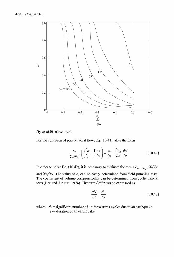
450 Chapter 10
Figure 10.38 (Continued)
For the condition of purely radial flow, Eq. (10.41) takes the form
3
2
21 – gh
w
uk u u u Nm r r t N trug
Ê ˆ ∂∂ ∂ ∂ ∂+ =Á ˜∂ ∂ ∂ ∂∂Ë ¯ (10.42)
In order to solve Eq. (10.42), it is necessary to evaluate the terms kh, 3
mu , ∂N/∂t,
and ∂ug/∂N. The value of kh can be easily determined from field pumping tests. The coefficient of volume compressibility can be determined from cyclic triaxial tests (Lee and Albaisa, 1974). The term ∂N/∂t can be expressed as
s
d
NNt t
∂ =∂
(10.43)
where Ns = significant number of uniform stress cycles due to an earthquake td = duration of an earthquake.

Liquefaction of Soil 451
Figure 10.38 (Continued)
The rate of excess pore water pressure build up, ∂ug/∂N, in a saturated undrained cyclic simple shear test is given by Eq. (10.4) (Section 10.10). For radial flow conditions, the relation given by Eq. (10.42) has been solved by Seed and Booker (1977). It has been shown that the ratio u us is a function of the following parameters:
RR
d
e = radius of rock or gravel drains
effective radius of the rock or gravel drains (10.44)
Ns/Ni, and
3
2h d
adw d
k tT
m Rug
Ê ˆÁ ˜=Á ˜Ë ¯
(10.45)
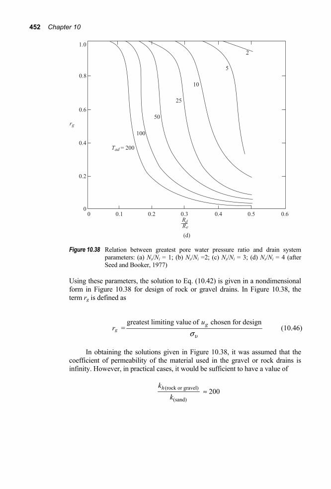
452 Chapter 10
Figure 10.38 Relation between greatest pore water pressure ratio and drain system parameters: (a) Ns/Ni = 1; (b) Ns/Ni =2; (c) Ns/Ni = 3; (d) Ns/Ni = 4 (after Seed and Booker, 1977)
Using these parameters, the solution to Eq. (10.42) is given in a nondimensional form in Figure 10.38 for design of rock or gravel drains. In Figure 10.38, the term rg is defined as
rg =greatest limiting value of chosen for designgu
us (10.46)
In obtaining the solutions given in Figure 10.38, it was assumed that the coefficient of permeability of the material used in the gravel or rock drains is infinity. However, in practical cases, it would be sufficient to have a value of
(rock or gravel)
(sand)
hkk
≈ 200

Liquefaction of Soil 453
Example 10.2
For a sand deposit, it is given that
3
mu = 2.8 × 10⁻⁵ m2/kN
kh = 0.02 mm/s = 2 × 10⁻⁵ m/s
For a design earthquake, the equivalent number of uniform stress cycles (for uniform stress = aut ) was determined to be 30. The duration of the earthquake is about 65 s.
From laboratory tests, it was determined that 12 cycles of cyclic stress application (the peak magnitude of the cyclic stress is equal to aut ) would be enough to cause initial liquefaction in the sand.
Assuming that the radius of the gravel drains to be used is 0.25 m, and
rg = 0.6, determine the spacing of gravel drains.
Solution
From Eq. (10.45),
τad = ( )3
5
2 252 10 65
9.81 2.8 10 0.25h d
w d
k tm Rug
-
-
È ˘¥Ê ˆ Í ˙=Á ˜ Í ˙¥Ë ¯ Î ˚ = 75.72
NN
s
i = 30/12 = 2.5, rg = 0.6
Referring to Figure 10.38b, for Tad = 75.72, Ns/Ni = 2, rg = 0.6,
RR
d
e ≈ 0.17
From Figure 10.38c, for Tad = 75.72, Ns/N1 = 3, rg = 0.6,
RR
d
e ≈ 0.2
Thus, for Ns/Ni = 2.5, Rd/Re ≈ 12
(0.17 + 0.2) = 0.185. Hence,
Re = Rd
0 1850 250 185.
..
= = 1.35 m
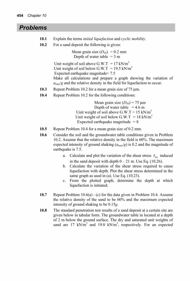
454 Chapter 10
Problems 10.1 Explain the terms initial liquefaction and cyclic mobility. 10.2 For a sand deposit the following is given:
Mean grain size (D50) = 0.2 mm Depth of water table = 3 m
Unit weight of soil above G.W.T = 17 kN/m3 Unit weight of soil below G.W.T = 19.5 kN/m3 Expected earthquake magnitude= 7.5 Make all calculations and prepare a graph showing the variation of
amax/g and the relative density in the field for liquefaction to occur. 10.3 Repeat Problem 10.2 for a mean grain size of 75 μm. 10.4 Repeat Problem 10.2 for the following conditions:
Mean grain size (D50) = 75 μm Depth of water table = 4.6 m Unit weight of soil above G.W.T = 15 kN/m3 Unit weight of soil below G.W.T = 18 kN/m3 Expected earthquake magnitude = 8
10.5 Repeat Problem 10.4 for a mean grain size of 0.2 mm. 10.6 Consider the soil and the groundwater table conditions given in Problem
10.2. Assume that the relative density in the field is 60%. The maximum expected intensity of ground shaking (amax/g) is 0.2 and the magnitude of earthquake is 7.5.
a. Calculate and plot the variation of the shear stress at u induced in the sand deposit with depth 0 – 21 m. Use Eq. (10.26).
b. Calculate the variation of the shear stress required to cause liquefaction with depth. Plot the shear stress determined in the same graph as used in (a). Use Eq. (10.23).
c. From the plotted graph, determine the depth at which liquefaction is initiated.
10.7 Repeat Problem 10.6(a) - (c) for the data given in Problem 10.4. Assume the relative density of the sand to be 60% and the maximum expected intensity of ground shaking to be 0.15g.
10.8 The standard penetration test results of a sand deposit at a certain site are given below in tabular form. The groundwater table in located at a depth of 2 m below the ground surface. The dry and saturated unit weights of sand are 17 kN/m3 and 19.0 kN/m3, respectively. For an expected

Liquefaction of Soil 455
earthquake magnitude M = 6 and maximum acceleration amax = 0.1 g, will liquefaction occur?
Depth (m) NF (blows/30 cm) 1.5 8 3.0 7 4.5 12 6.0 15 7.5 17
9.0 17
10.9 In a sand deposit, the groundwater table is located at a depth of 2 m measured from the ground surface. Following are the shear wave velocities in the sand deposit.
Depth Shear wave velocity, (m) su (m/s)
2 – 4 450 4 – 6 600
6 – 10 675
For a maximum ground acceleration amax = 0.16 g, determine whether liquefaction is likely to occur.
10.10. Solve the gravel drain problem given Example 10.2 for rg = 0.7. 10.11. Repeat Example 10.2 of the gravel drain with the following data:
3
mu = 3.5 × 10⁻⁵ m2/kN
kh = 1.4 × 10⁻⁵ m/s Equivalent number of uniform stress cycles due to earthquakes = 20 Duration of earthquake = 50 s Number of uniform stress cycles for liquefaction = 12 Radius of gravel drains = 0.3 m rg = 0.7
References Bieganousky, W. A., and Marcuson, W. F., III (1977). “Liquefaction Potential of
Dams and Foundations, Report 2. Laboratory Standard Penetration Test on Platte River Sand and Standard Concrete Sand,” WES Report No. 76-2, U.S Army Waterways Experiment Station, Vicksburg, Mississippi.
456 Chapter 10
Casagrande, A. (1936). Characteristics of Cohesionless Soils Affecting the Stability of Slopes and Earthfills,” Journal of the Boston Society of Civil Engineers, January, Vol. 23 pp. 257-276.
Castro, G. (1969). “Liquefaction of Sands,” Harvard Soil Mechanics Series No. 81, Cambridge, Massachusetts.
Castro, G. (1975). “Liquefaction and Cyclic Mobility of Saturated Sands,” Journal of the Geotechnical Engineering Division, ASCE, Vol. 101, No. GT6, pp. 551-569.
Commission on Engineering and Technical Systems – Committee on Earthquake Engineering (1985). “Liquefaction of Soils During Earthquakes,” National Academy Press, Washington, D.C.
DeAlba, P., Chan, C. K., and Seed, H. B. (1975), “Determination of Soil Liquefaction Characteristics by Large Scale Laboratory Tests,” Report No. EERC 75-14, Earthquake Engineering Research Center, University of California, Berkeley, California.
DeAlba, P., Seed, H. B., and Chan, C. K. (1976). “Sand Liquefaction in Large-Scale Simple Shear Tests,” Journal of Geotechnical Engineering Division, ASCE, Vol. 102, NO. GT9, pp. 909-927.
Dobry, R., Stokoe, K. H., Land R. S., and Youd, T. L. (1981). “Liquefaction for S-wave Velocity,” Preprint 81-544, ASCE National Convention, St. Louis, Missouri.
Emery, J. J., Finn, W. D. L., and Lee, K. W. (1972). “Uniformity of Saturated Sand Samples,” Soil Mechanics Series, University of British Columbia, Vancouver, British Columbia, Canada.
Finn, W. D. L. (1972). “Soil Dynamic – Liquefaction of Sands,” Proceedings, International Conference on Microzonation for Safer Construction Research and Application, Seattle, Washington, Vol. 1.
Finn, W. D. L., Bransby, P. L., and Pickering D. J. (1970). “Effect of Strain History on Liquefaction of Sands,” Journal of the Soil Mechanics and Foundations Division, ASCE, Vol. 96. No. SM6, pp. 1917-1934.
Finn, W. D. L., Emery, J. J., and Gupta, Y. P. (1970). “A Shaking Table Study of the Liquefaction of Saturated Sands during Earthquake Engineering,” Proceedings, 3rd European Symposium on Earthquake Engineering, Sofia, Bulgaria.
Finn, W. D. L., Emery. J. J., and Gupta, Y. P. (1971). “Soil Liquefaction Studies Using a Shaking Table,” Closed Loop Magazine, Fall/Winter, MTS Systems Corporation, Minneapolis, Minnesota.
Finn, W. D. L., Pickering, D. J., and Bransby, P. L. (1971). “Sand Liquefaction in Triaxial and Simple Shear Tests,” Journal of the Soil Mechanics and Foundations Division, ASCE, Vol. 97, No. SM4, pp. 639-659.
Ishibashi, I., and Sherif, M. A. (1974), “Soil Liquefaction by Torsional Simple Shear Device,” Journal of the Geotechnical Engineering Division, ASCE, Vol. 100, No. GT8, pp. 871-888.
With permission from ASCE.

Liquefaction of Soil 457
Ishihara, K. (1985). “Stability of Natural Deposits During Earthquakes,” Proceedings, 11th International Conference on Soil Mechanics and Foundation Engineering, Vol. 1, pp. 321-376.
Jaky, J. (1944). “The Coefficient of Earth Pressure at Rest,” Journal of the Society of the Hungarian Architectural Engineers, Vol. 21, pp. 355-358.
Kishida, H. (1966), “Damage to Reinforced Concrete Buildings in Niigata City with Special Reference to Foundation Engineering,” Soils and Foundations, Tokyo, Japan, Vol. 7, No. 1, pp. 75-92.
Kuizumi, Y. (1966). “Changes in Density of Sand Subsoil Caused by the Niigata Earthquake,” Soils and Foundations, Tokyo, Japan, Vol. 8, No. 2, pp. 38-44.
Lee, K. L., and Albaisa, A. (1974). “Earthquake Induced Settlements in Saturated Sands,” Journal of the Geotechnical Engineering Division, ASCE, Vol. 100, No. GT4, pp. 387-404.
Lee, K. L., and Seed, H. B. (1967). “Cyclic Stress Conditions Causing Liquefaction of Sand,” Journal of the Soil Mechanics and Foundations Division, ASCE, Vol. 93, No. SM1, pp. 47-70.
Liao, S. and Whitman, R. V. (1986). “Overburden Correction Factors for SPT in Sand,” Journal of Geotechnical Engineering, ASCE, Vol. 112, No. GT3, pp. 373-377.
O-Hara, S. (1972). “The Results of Experiment on the Liquefaction of Saturated Sands with a Shaking Box: Comparison with Other Methods,” Technology Report of the Yamaguchi University, Vol. 1, No. 1, Yamaguchi, Japan.
Ohasaki, Y. (1966). “Niigata Earthquake 1964, Building Damage and Soil Conditions,” Soils and Foundations, Tokyo, Japan, Vol. 6, No.2, pp. 14-37.
Ortigosa, P. (1972). “Licuacion de Arenas Sometidas a Vibraciones Horizontales,” Revista del Instituto de Investigaciones de Ensoyes de Materials, Vol. II, No. 3.
Peacock, W.H., and Seed, H. B. (1968), “Sand Liquefaction Under Cyclic Loading Simple Shear Conditions,” Journal of the Soil Mechanics and Foundations Division, ASCE, Vol. 94, No. SM3, pp. 689-708.
Prakash, S., and Mathur, J. N. (1965). “Liquefaction of Fine Sand Under Dynamic Loading,” Proceedings, 5th Symposium of the Civil and Hydraulic Engineering Departments, Indian Institute of Science, Bangalore, India.
Seed, H. B. (1979). “Soil Liquefaction and Cyclic Mobility Evaluation for Level Ground During Earthquakes,” Journal of the Geotechnical Engineering Division, ASCE, Vol. 105, No. GT2, pp. 201-255.
Seed, H. B., and Booker, J. R. (1977). “Stabilization of Potential Liquefiable Sand Deposits Using Gravel Drains,” Journal of the Geotechnical Engineering Division, ASCE, Vo. 103, No. GT7, pp. 757-768.
Seed, H. B. and Idriss, I. M. (1971). “Simplified Procedure for Evaluating Soil Liquefaction Potential,” Journal of the Soil Mechanics and Foundations Division, ASCE, Vol. 97, No. SM9, pp. 1249-1273.
With permission from ASCE.
With permission from ASCE.
With permission from ASCE.
With permission from ASCE.
With permission from ASCE.
458 Chapter 10
Seed, H. B., and Idriss, I. M. (1982). “Ground Motion and Soil Liquefaction During Earthquakes,” Monograph Series, Earthquake Engineering Research Institute, University of California, Berkeley, California.
Seed, H. B., Idriss, I. M., and Arango, I. (1983), “Evaluation of Liquefaction Potential Using Field Performance Data,” Journal of Geotechnical Engineering, ASCE, Vol. 109, NO. GT3, pp. 458-482.
Seed, H. B., and Lee, K. L. (1966). “Liquefaction of Saturated Sands During Cyclic Loading,” Journal of the Soil Mechanics and Foundations Division, ASCE, Vol. 92, No. SM6, pp. 105-134.
Seed, H. B., Martin, P. O., and Lysmer, J. (1975). “The Generation and Dissipation of Pore Water Pressure During Soil Liquefaction,” Report No. EERC 75-26, Earthquake Engineering Research Institute, University of California, Berkeley, California.
Seed, H. B., Mori, K., and Chan, C. K. (1977). “Influence of Seismic History on Liquefaction of Sands,” Journal of the Geotechnical Engineering Division, ASCE, Vol. 103, No. GT4, pp. 246-270.
Seed, H. B., and Peacock, W. H. (1971). “The Procedure for Measuring Soil Liquefaction Characteristics,” Journal of the Soil Mechanics and Foundations Division, ASCE, Vol. 97, No. SM8, pp. 1099-1119.
Seed, H. B., Tokimatsu, K., Harder, L. F., and Chung, R. M. (1984). “The Influence of SPT Procedures in Soil Liquefaction Resistance Evaluation,” Report NO. EERC-84/15, Earthquake Engineering Research Institute, University of California, Berkeley, California.
Tanimoto, K. (1967). “Liquefaction of a Sand Layer Subjected to Shock and Vibratory Loads,” Proceedings, 3rd Asian Regional Conference on Soil Mechanics and Foundation Engineering, Haifa, Israel, Vol. 1.
Whiteman, R. V. (1970). “Summary of Results from Shaking Table Tests at University of Chile Using a Medium Sand,” Progress Report No. 9, Effect of Local Soil Conditions upon Earthquake Damage, Research Report R70-25, Soils Publication No. 258, Massachusetts Institute of Technology, Cambridge, Massachusetts.
Yoshimi, Y. (1967). “An Experimental Study of Liquefaction of Saturated Sands,” Soils and Foundations, Tokyo, Japan, Vol. 7, No. 2.
Yoshimi, Y. (1970). “Liquefaction of Saturated Sand During Vibration Under Quasi-plane-Strain Conditions,” Proceedings, 3rd Japan Earthquakes Engineering Symposium, Tokyo, Japan.
Yoshimi, Y., and Oh-oka, H. (1973). “A Ring Torsion Apparatus for Simple Shear Tests,” Proceedings, 8th International Conference on Soil Mechanics and Foundation Engineering, Vol. 1.2, Moscow, USSR.
Youd, T. L. (1972). “Compaction of Sand by Repeated Straining,” Journal of the Soil Mechanics and Foundations Division, ASCE, Vol. 98, No. SM7,
709-725.
With permission from ASCE.
With permission from ASCE.
With per-mission from ASCE.
pp.

459
11 Machine Foundations on Piles
11.1 Introduction It was mentioned in Section 5.4 that for low-speed machineries subjected to vertical vibration, the natural frequency of the foundation-soil system should be at least twice the operating frequency. In the design of these types of foundations, if changes in size and mass of the foundation (more popularly known as tuning of a foundation) do not lead to a satisfactory design, a pile foundation may be considered. It is also possible that the subsoil conditions are such that the vibration of a shallow machine foundation may lead to undesirable settlement. In many circumstances the load-bearing capacity of the soil may be low compared to the static and dynamic load imposed by the machine and the shallow foundation. In that case the design will then dictate consideration of the use of piles. It should be kept in mind that the use of piles will, in general, increase the natural frequency of the soil–pile system and may also increase the amplitude of vibration at resonance.
The soil–structure interaction of the deep foundations is not well understood and though rigorous theoretical solutions exist, they are mostly confined to researchers than designers. The practice in design offices is usually based on ignoring the stiffness of the soil and only the stiffness of the pile is taken into account.
In this chapter, the fundamental concepts of pile foundations of vibrating machines will be considered. It should also be kept in mind that the piles supporting machine foundation are for cases of low amplitudes of vibration (because allowable motion is small and dynamic loads are small compared to static loads) in contrast to those encountered under earthquake-type loading (large strain conditions). For that reason, when encountered with the selection of proper parameters for soil such as the shear modulus G, the value (s) that correspond to low amplitudes of strain should be used. Elastic theory thus is the basis of design methods described in this chapter.

460 Chapter 11
Piles Subjected to Vertical Vibration In general, piles can be grouped into two broad categories: 1. End-bearing piles. These piles penetrate through soft soil layers up to a hard
stratum or rock. The hard stratum or rock can be considered as rigid. 2. Friction piles or floating plies. The tips of these piles do not rest on hard
stratum. The piles resist the applied load by means of frictional resistance developed at the soil-pile interface.
11.2 End-Bearing Piles Figure 11.1 shows a pile driven up to a rock layer. The length of the pile is equal to L, and the load on the pile coming from the foundations is W. This problem can be approximately treated as a vertical rod fixed at the base (that is, at the rock layer) and free on top. For determining the natural frequency of the piles, three possible cases may arise.
Case 1. If W is very small (≈ 0), the natural frequency of vibration can be given by following Eq. (3.57) as
12π 4
n Pn
P
EfL
wr
= = (11.1)
where fn = natural frequency of vibration nw = natural circular frequency EP = modulus of elasticity of the pile material Pr = density of the pile material
Case 2. If W is of the same order of magnitude as the weight of the pile, the natural frequency of vibration can be given by Eq. (4.20). (Note similar end conditions between Figure 4.13 and Figure 11.1.) Thus,
( ) ( )
tann nP
c P c P
L LALW
w wgu uÈ ˘ È ˘= Í ˙ Í ˙Î ˚ Î ˚
(11.2)
or
( ) ( )0
tann nP
c P c P
L LLσ
w wgu uÈ ˘ È ˘= Í ˙ Í ˙Î ˚ Î ˚
(11.3)
where A = area of the cross section of the pile

Machine Foundations on Piles 461
Figure 11.1 End-bearing pile
Pg = unit weight of the pile material nw = natural circular frequency ( )c Pu = longitudinal wave propagation velocity in the pile
0WA
s =
Figure 11.2 shows a plot of ( )n c PLw u against 0PLg s that can be used to determine nw and fn. Note that
2π
nnf
w= (11.4)
Case 3. If W is larger and the weight of the pile is negligible in comparison, then from Equation (11.2)
( )
2nP
c P
LALW
wguÈ ˘ª Í ˙Î ˚

462 Chapter 11
However,
( ) = P Pc P
P P
E E gur g
=
where g = acceleration due to gravity. So,
Pn
AE gLW
w =
or
0
12
Pn
E gfσ L
=p
(11.5)
where σ0 = axial stress = W/A.
Figure 11.2 Plot of Eq. (11.3)

Machine Foundations on Piles 463
Richart (1962) prepared a graph for fn with various values of pile length L and σ0, and this is shown in Figure 11.3. In preparing Figure 11.3, the following material properties have been used.
Material EP(kPa) Pg (kN/m3)
Steel 200 × 106 75.5 Concrete 21 × 106 23.6 Wood 8.25 × 10⁶ 6.3
Figure 11.3 Resonant frequency for vertical vibration of a point bearing pile (after
Richart, 1962)

464 Chapter 11
Example 11.1
A machine foundation is supported by four prestressed concrete plies driven to bedrock. The length of each pile is 24 m, and they are 0.3 m × 0.3 m in cross section. The weight of the machine and the foundation is 1360 kN. Given: unit weight of concrete = 24 kN/m3 and the modulus of elasticity of the concrete used for the piles = 24.5 × 10⁶ kPa. Determine the natural frequency of the pile-foundation system. Solution
There are four piles. The weight carried by each pile is
1360 kN 340kN4
W = =
The weight of each pile is ( )
LengthArea of
cross section
0.3 0.3 24 24 51.84kNpALg≠
= ¥ ¥ ¥ =
≠
( )( )624.5 10
3164.6 m/s(24 / 9.81)
Pc P
P
Eur
¥= = =
From Eq. (11.2),
( ) ( )
tann nP
c P c P
L LALW
w wgu uÈ ˘ È ˘= Í ˙ Í ˙Î ˚ Î ˚
So ( )( )( )
( )( )( )
24 2451.84 tan340 3164.6 3164.6
n nw wÈ ˘ È ˘= Í ˙ Í ˙Î ˚ Î ˚
or 0.1525= [( nw )(0.00758)] tan [( nw )(0.00758)]
From Figure 11.2, for 0
PLgs
= 0.1525
( )
n
c P
Lwu
≈ 0.36
(0.36)(3164.6) 47.524nw = ª rad/s
fn = 7.56 Hz

Machine Foundations on Piles 465
11.3 Friction Piles Figure 11.4a shows a pile having a length of embedment equal to L and a radius of R. The pile is subjected to a dynamic load
0i tQ Q e w= (11.6)
It is possible to idealize the pile to a mass-spring-dashpot system, as shown in Figure 11.4b. The mass m shown in Figure 11.4b can be assumed to be the mass of the cap and machinery. The mathematical formulation for obtaining the stiffness (kz) and the damping (cz) parameters has been given by Novak (1977). In developing the theory, the following assumptions were made: 1. The pile is vertical, elastic, and circular in cross section. 2. The pile is floating. 3. The pile is perfectly connected to the soil. 4. The soil above the pile tip behaves as infinitesimal, thin, independent
linearly elastic layers.
The last assumption leads to the assumption of plane strain condition. Referring to Figure 11.5, the dynamic stiffness and damping of the pile can then be described in terms of complex stiffness (Novak and El-Sharnouby, 1983) as
Figure 11.4 Friction pile-vertical vibration

466 Chapter 11
Figure 11.5 Dynamic stiffness and damping constant for a single pile–vertical mode of
vibration
1 2=K K iK+ (11.7)
The applied force Q and displacement z are related to K in the following manner:
1 2= ( )Q Kz K iK z= + (11.8)
where = – 1i K1 = real part of K = Re K K2 = imaginary part of K = Im K
Hence, the spring constant is
kz = K1 = Re K (11.9)
and the equivalent viscous damping is
2 Imz
K Kcw w
= = (11.10)
Combining Equation (11.7), (11.9), and (11.10),
z zK k i cw= + (11.11)

Machine Foundations on Piles 467
So, the force-displacement relation can be expressed as
( )z zQ k i c zw= + or z zQ k z c z= + (11.12) where z = dz/dt.
The relationships for kz and cz have been given by Novak and El-Sharnouby (1983) as
1P
z zE Ak f
RÊ ˆ= Á ˜Ë ¯ (11.13)
and
2/P
z zE Ac fG r
Ê ˆ= Á ˜Ë ¯ (11.14)
where EP = modulus of elasticity of the pile material A = area of pile cross section G = shear modulus of soil ρ = density of soil fz1, fz2 = nondimensional parameters
The variations of fz1, and fz2 for end-bearing piles are shown in Figures 11.6 and 11.7. Similarly, the fz1 and fz2 variations for floating piles are shown in Figures 11.8 and 11.9.
Pile foundations are generally constructed in groups. The stiffness and damping constants of a pile group are not simple summations of the stiffness and damping constant of individual piles. Novak (1977) suggested that when piles are closely spaced, the displacement of one pile is increased due to the displacement of all other piles and conversely, the stiffness and damping of the group are reduced. Hence, the stiffness of the pile group can be obtained as
( )1
1
n
z
z g n
rr
kk
a=
=Â
 (11.15)
and

468 Chapter 11
Figure 11.6 Variation of fz1 with L/R and EP/G for end-bearing piles (after Novak and
Ei-Sharnouby, 1983)
( )1
1
n
z
z g n
rr
cc
a=
=Â
 (11.16)
where kz(g) = spring constant for the pile group cz(g) = dashpot constant for the pile group n = number of piles in the group αr = the interaction factor describing the contribution of the rth
pile to the displacement of the reference pile (that is, α1 =1)
Since no analytical solutions for the dynamic interaction of piles are available at the present time, an estimate of αr can be obtained from the static solution of Poulos (1968). This is shown in Figure 11.10.

Machine Foundations on Piles 469
Figure 11.7 Variation of fz2 with L/R and EP/G for end-bearing piles (after Novak and
EI-Sharnouby, 1983)
Figure 11.8 Variation of fz1 with L/R and EP/G for floating piles (after Novak and EI-
Sharnouby, 1983)

470 Chapter 11
Figure 11.9 Variation of fz2 with L/R and EP/G for floating piles (after Novak and EI-
Sharnouby, 1983)
Text not available due to copyright restrictions

Machine Foundations on Piles 471
For group piles, a cap is constructed over the piles (Figure 11.11). In the estimation of stiffness and damping constants, the contribution of the pile cap should be taken into account. The relationships describing the stiffness and geometric damping of embedment foundations are given in Chapter 5 as
( ) 0 1 1cap0
fsz
DGk Gr C S
G rÈ ˘
= +Í ˙Î ˚
(5.120)
and
( )2
0 2 2cap0
f s sz
D Gc r G C S
r Grrr
È ˘= +Í ˙
Í ˙Î ˚ (5.121)
Since the soil located below the pile cap may be of poor quality and it may shrink away with time, it would be on the safe side to ignore the effect of the cap base – that is, 1C = 0 and 2C = 0. So
Figure 11.11 Group pile with pile cap

472 Chapter 11
( ) 1capz s fk G D S= (11.17)
and ( ) 0 2capz f s sc D r S G r= (11.18)
Thus, for the group pile and cap,
( )1
1
1
n
z
z s fT n
rr
kk G D S
a=
= +Â
 (11.19)
and
( )1
0 2
1
n
z
f s sz T n
rr
cc D r S G r
a=
= +Â
 (11.20)
where kz(T) and cz(T) are the stiffness and damping constants for the pile group and cap, respectively.
The variations for 1S and 2S are given in Table 5.2. Once the values of kz(T) and cz(T) are determined, the response of the system can be calculated using the principles described in Chapter 2, as briefly outlined here.
a. Damping ratio:
( )
( )2z T
zz T
cD
k m= (11.21)
where m = mass of the pile cap and the machine supported by it. b. Undamped natural frequency:
( )z Tn
km
w = (11.22)
( )12π
z Tn
kf
m= (11.23)
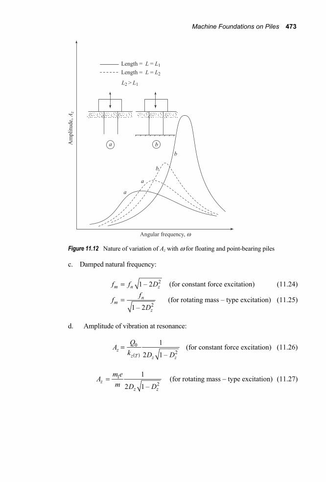
Machine Foundations on Piles 473
Figure 11.12 Nature of variation of Az with ω for floating and point-bearing piles
c. Damped natural frequency:
21 – 2m n zf f D= (for constant force excitation) (11.24)
21 – 2
nm
z
ffD
= (for rotating mass – type excitation) (11.25)
d. Amplitude of vibration at resonance:
( )
02
1
2 1 –z
z T z z
QAk D D
= (for constant force excitation) (11.26)
12
1
2 1 –z
z z
m eAm D D
= (for rotating mass – type excitation) (11.27)

474 Chapter 11
e. Amplitude of vibration at frequency other than resonance:
( )
0
22 22
2 21 – 4
z Tz
zn n
Qk
A
Dw ww w
=Ê ˆ
+Á ˜Ë ¯
(for constant force excitation) (11.28)
21
22 22
2 21 – 4
nz
zn n
m em
A
D
ww
w ww w
Ê ˆÁ ˜Ë ¯
=Ê ˆ
+Á ˜Ë ¯
(for rotating mass – type excitation) (11.29)
The nature of variation of Az with ω for floating piles and point-bearing piles is shown in Figure 11.12. From this figure, it can be seen that the relaxation of the pile tips reduces both the resonant frequency and amplitude of vibration.
Example 11.2
A group of four piles is supporting a machine foundation, as shown in Figure 11.13. Determine kz(T) and cz(T). Given: EP = 21 × 106 kPa, G = Gs = 28,000 kPa, γ = sg = 19 kN/m3. Assume Poisson’s ratio of soil, μ = 0.5.
Solution
Equivalent radius of pile cross section:
1 20.3 0.3 0.17 m.
πR ¥Ê ˆ= =Á ˜Ë ¯
Length of piles = L = 12 m:
12 70.60.17
LR= =
Given EP = 21 × 106 kPa; Gs = G = 28,000 kPa. So
621 10 750
28000PE
G¥= =
Referring to Figures 11.8 and 11.9, for EP/G = 750 and L/R = 70.6, the magnitudes of fz1 and fz2 are
fz1 ≈ 0.034 and fz2 ≈ 0.06
Hence, from Eqs. (11.13) and (11.14)

Machine Foundations on Piles 475
Figure 11.13
( )( ) ( )
9
121 10 0.3 0.3
0.0340.17
Pz z
E Ak fR
È ˘¥ ¥Ê ˆ Í ˙= =Á ˜Ë ¯ Î ˚
= 378 ×106 N/m.
2/P
z zE Ac fG r
Ê ˆ= Á ˜Ë ¯
However,
28000 9.81 120.24 m/s19
Gr
¥= =
So

476 Chapter 11
( )( )
( )921 10 0.3 0.3
0.06120.24zc
È ˘¥ ¥Í ˙=Í ˙Î ˚
= 94.311 × 10⁴ N-s/m.
In order to determine the stiffness and damping constants for group piles, Eqs.
(11.15) and (11.16) can be used. However 1
n
rr
a=Â needs to be considered first.
This can be done by using Figure 11.10 and preparing the following table.
Reference pile → Aa B C D Interacting pile A 1.00 0.54 0.48 0.54 B 0.54 1.00 0.54 0.48 C 0.48 0.54 1.00 0.54 D 0.54 0.48 0.54 1.00
2.56 2.56 2.56 2.56 a Note: Reference pile A.
For interaction between piles A and A, S = 0 and S/2R = 0. So αr = 1. For interaction between piles A and B, S = 1.5 m, 2R = (2)(0.17) = 0.34 m., and S/2R = 1.5/0.34 = 4.412. So αr ≈ 0.54. Similarly, for interaction between piles A and D, αr ≈ 0.54. Between piles A and C,
( ) ( )2 21.5 1.5
6.232 0.34SR
+= =
or
2 0.16RS
= αr ≈ 0.48
The average value of 1
n
rr
a=Â = 2.56. Hence, using Eq. (11.15),
( )( )( )6
64 378 10590.63 10 N m
2.56z gk×
= = ×
( )( )( )3
44 943.11 10147.36 10 N - s m
2.56z gc×
= = ×
Again, for the contributions of the pile cap, kz(cap) [Eq. (11.17)] and cz(cap) [Eq. (11.18)] need to be determined. Given:

Machine Foundations on Piles 477
Df = 1.5 m; G = 28,000 kPa 1S = 2.7 (Table 5.2); 2S = 6.7 (Table 5.2)
02.1 2.1r ¥=
p = 1.185 m.
From Eq. (11.17), ( )
31cap (28000 10 ) (1.5) (2.7)z s fk G D S= = ¥ ¥ ¥
= 113.4¥ 106 N/m Similarly, from Eq. (11.18),
( ) 0 2capz f s sc D r S G r=
= (1.5) × (1.185) × (6.7)( )( )3 328000 10 19 10
9.81¥ ¥
= 277.33 × 10⁴ N-s/m So
( ) ( ) ( )capz zT z gk k k= + = 590.63 × 10⁶ + 113.4 × 106
= 704.03 × 10⁶ N/m = 704.03 × 10³ kN/m ( ) ( ) ( )capz zT z gc c c= + = 147.36 × 10⁴ + 277.33 × 104
= 424.69 × 10⁴ N-s/m
Example 11.3
Refer to Example 11.2. If the weight of the machine being supported is 70 kN, determine the damping ratio. Solution
Weight of the pile cap: (2.1)(2.1)(1.8)(24) = 190.512 kN = 190512 N
Total weight of pile cap and machine:
190.512 + 70 = 260.512 kN = 260512 N
From Eq. (11.21),
( )
( ) ( )[ ]
4
6
424.69 102 2 704.03 10 260512
z Tz
z T
cD
k m¥= =
¥ = 0.491
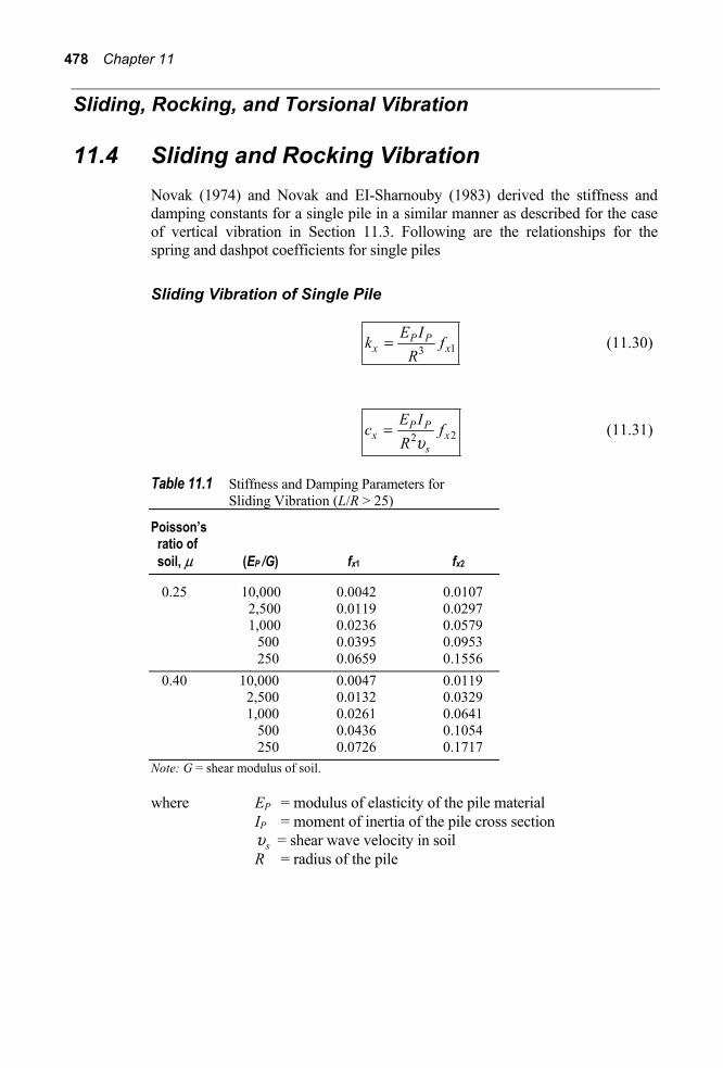
478 Chapter 11
Sliding, Rocking, and Torsional Vibration
11.4 Sliding and Rocking Vibration Novak (1974) and Novak and EI-Sharnouby (1983) derived the stiffness and damping constants for a single pile in a similar manner as described for the case of vertical vibration in Section 11.3. Following are the relationships for the spring and dashpot coefficients for single piles
Sliding Vibration of Single Pile
13P P
x xE Ik f
R= (11.30)
22P P
x xs
E Ic fR u
= (11.31)
Table 11.1 Stiffness and Damping Parameters for Sliding Vibration (L/R > 25)
Poisson’s ratio of soil, μ (EP /G) fx1 fx2
0.25 10,000 0.0042 0.0107 2,500 0.0119 0.0297 1,000 0.0236 0.0579 500 0.0395 0.0953 250 0.0659 0.1556 0.40 10,000 0.0047 0.0119 2,500 0.0132 0.0329 1,000 0.0261 0.0641 500 0.0436 0.1054 250 0.0726 0.1717 Note: G = shear modulus of soil.
where EP = modulus of elasticity of the pile material IP = moment of inertia of the pile cross section su = shear wave velocity in soil R = radius of the pile

Machine Foundations on Piles 479
The variations of fx1 and fx2 are given in Table 11.1, which is based on the analysis on Novak (1974) and Novak and El-Sharnouby (1983).
When piles are installed in groups and subjected to sliding vibration, the spring constant and the damping coefficient of the group can be given as
( )( )
1
1
n
x
x g n
L rr
kk
a=
=Â
 (11.32)
and
( )( )
1
1
n
x
x g n
L rr
cc
a=
=Â
 (11.33)
where αL(r) = interaction factor (Poulos, 1971) kx(g) = spring constant for the pile group cx(g) = damping coefficient for the pile group n = number of piles in the group.
The variation of αL(r) is given in Figure 11.14.
As in the case of vertical vibration, the effect of the pile cap (Figure 11.15) needs to be taken into account in the determination of total stiffness and damping constant. In Eqs. (5.123) and (5.124), the relationships for kx and cx for embedded foundations have been described as
0 1 10
fsx x x
DGk Gr C S
G rÈ ˘
= +Í ˙Î ˚
(5.123)
20 2 2
0
f s sx x x
D Gc r G C S
r Grrr
È ˘= +Í ˙
Í ˙Î ˚ (5.124)
Assuming 1xC = 0 and 2xC = 0
1(cap) xx s fk G D S= (11.34) and

480 Chapter 11
Figure 11.14 Variation of αL(r) (after Poulos, 1971)
(cap) 0 2x f x s sc D r S G r= (11.35)
Hence, for the group pile and cap,
( )( )
11
1
n
x
s f xx T n
L rr
kk G D S
a=
= +Â
 (11.36)
and

Machine Foundations on Piles 481
Figure 11.15 Effect of pile cap on stiffness and damping constants-sliding vibration
( )( )
10 2
1
n
x
f x s sx T n
L rr
cc D r S G r
a=
= +Â
 (11.37)
The damping ratio Dx for the system can then be determined as
( )
( )2x T
xx T
cD
k m= (11.38)
where m = mass of the pile cap and the machine supported. The damped natural frequency fm is given as
( ) 21 1 – 22
z Tm x
kf D
m
È ˘ È ˘= Í ˙ Î ˚p Î ˚ (for constant force excitation) (11.39)
and

482 Chapter 11
( )
2
/12 1 – 2
x Tn
x
k mf
D=
p (11.40)
The amplitudes of vibration can be calculated using Eqs. (5.58), (5.59), (5.60), and (5.61). While using these equations, kx needs to be replaced by kx(T).
Rocking Vibration for Single Pile
1P PE Ik fRq q= (11.41)
2P P
s
E Ic fq qu= (11.42)
The terms EP, IP, su and R have been defined in relation to Eqs. (11.30) and (11.31). The numerical values of 1fθ and 2fθ obtained by Novak (1974) and Novak and El-Sharnouby (1987) are given in Table 11.2. Table 11.2 The Stiffness and Damping Parameters for Rocking Vibration (L/R > 25)
Poisson’s ratio of soil, μ (EP /G) fθ 1 fθ 2
0.25 10,000 0.2135 0.1577 2,500 0.2998 0.2152 1,000 0.3741 0.2598 500 0.4411 0.2953 250 0.5186 0.3299 0.4 10,000 0.2207 0.1634 2,500 0.3097 0.2224 1,000 0.3860 0.2677 500 0.4547 0.3034 250 0.5336 0.3377
Note: G = shear modulus of soil.
For coupling between horizontal translation and rocking, the cross stiffness and damping constants are as follows:
12P P
x xE Ik f
Rq q= (11.43)

Machine Foundations on Piles 483
2P P
x xs
E Ic fRq qu
= (11.44)
The numerical values for 1xf θ and 2xf θ are given in Table 11.3, which is based on the works of Novak (1974) and Novak and El-Sharnouby (1983).
Table 11.3 Values of 1xf θ and 2xf θ
Poisson’s ratio of soil, μ (EP /G) xf θ 1 xf θ 2
0.25 10,000 – 0.0217 – 0.0333 2,500 – 0.0429 – 0.0646 1,000 – 0.0668 – 0.0985 500 – 0.0929 – 0.1337 250 – 0.1281 – 0.1786 0.4 10,000 – 0.0232 – 0.0358 2,500 – 0.0459 – 0.0692 1,000 – 0.0714 – 0.1052 500 – 0.0991 – 0.1425 250 – 0.1365 – 0.1896
Note: G = shear modulus of soil.
For group piles the stiffness ( )gkθ and damping ( )gcθ constants can be written as
2 2( )
1– 2
n
g z r x c c xk k k x k Z Z kθ θ θ⎡ ⎤= + +⎣ ⎦∑ (11.45)
The terms xr and Zc are defined in Figure 11.16. Similarly,
2 2( )
1– 2
n
g z r x c c xc c c x c Z Z cθ θ θ⎡ ⎤= + +⎣ ⎦∑ (11.46)
The stiffness (cap)kθ and damping (cap)cθ for the pile cap can be obtained from the following equations (Prakash and Puri, 1988):
22
2 2(cap) 0 1 0 1
0 0–
3c c
s f s f xZ Z
k G r D S G r D Sr rq q
d dÈ ˘Ê ˆ Ê ˆ= + +Í ˙Á ˜ Á ˜Ë ¯ Ë ¯Í ˙Î ˚
(11.47)

484 Chapter 11
Figure 11.16 Definition of parameters in Eqs. (11.45) and (11.46)
and
22
4(cap) 0 2 2
0 0–
3c c
s s xZ Z
c r G S Sr rq q
dd r dÏ ¸È ˘Ô ÔÊ ˆ Ê ˆ= + +Í ˙Ì ˝Á ˜ Á ˜Ë ¯ Ë ¯Í ˙Ô ÔÎ ˚Ó ˛
(11.48)
where r0 = equivalent radius of the pile cap
δ = 0
fDr
(11.49)
Thus, the total stiffness ( )Tkθ and damping ( )Tcθ constants are

Machine Foundations on Piles 485
( ) ( ) (cap)T gk k kθ θ θ= + (11.50) and ( ) ( ) (cap)T gc c cθ θ θ= + (11.51)
Once the magnitudes of ( )Tkq and ( )Tcq are determined, the response of the system can be calculated in the same manner as outlined in Chapter 2 and Section 5.5. For convenience, this is outlined here as well. a. Damping ratio:
( )
( )2T
gT
cD
k Iq
= (11.52)
where Ig = mass moment of inertia for the pile cap and the machinery about the centroid of the block. Referring to Figure 11.17a,
Ig = mass moment of inertia about the y axis
= ( )2 2
12m L h+ (11.53a)
and, similarly, referring to Figure 11.17b,
Ig = mass moment of inertia about the y axis
= ( )2 203
12m r h+ (11.53b)
b. Undamped natural frequency:
( )Tn
g
kIqw = (11.54)
( )12
Tn
g
kf
Iq=
p (11.55)
c. Damped natural frequency:
21 – 2m nf f Dq= (for constant force excitation) (11.56)
21 – 2
nm
ff
Dq
= (for rotating mass-type excitation) (11.57)

486 Chapter 11
Figure 11.17 Mass moment of inertia Ig
The amplitude of vibration can be determined by using Eqs. (5.46), (5.47), (5.48), and (5.49). Example 11.4
Refer to Example 11.2. Determine kx(T) and cx(T) for the sliding mode of vibration. Assume Poisson’s ratio of soil, μ = 0.25. Solution
Stiffness and damping constants for single pile: From Eqs. (11.30) and (11.31),
13P P
x xE Ik f
R=
and
22P P
x xs
E Ic fR u
=
Given EP = 21 × 106 kPa; R = 0.17 m.
IP = 4
4Rp = 4(0.17)
4p = 6.56 × 10⁻⁴ m4

Machine Foundations on Piles 487
sGur
= = 28000 9.8119¥ = 120.24 m/s
PEG
= 621 10
28,000¥ = 750
From Table 11.1, for μ = 0.25 and EP/G = 750, fx1 = 0.027 and fx2 = 0.068. So
( )( )
( )( )
6 3 -4
13 321 10 10 6.54 10
0.0270.17
P Px x
E Ik fR
¥ ¥ ¥= =
= 75.48 × 10⁶ N/m
( )( )( ) ( )
( )6 3 -4
23 221 10 10 6.54 10
0.0680.17 120.24
P Px x
s
E Ic fR u
¥ ¥ ¥= =
= 268.76 × 10³ N-s/m Stiffness and damping constants for group pile: From Eqs. (11.32) and (11.33),
( )
1( )
1
n
x
x g n
L rr
kk
a=
=Â
Â
and
( )
1( )
1
n
x
x g n
L rr
cc
a=
=Â
Â
To find αL(r) with A as the reference pile, the following table can be prepared using Figure 11.14. Assume piles to be flexible.
Reference pile → A
( )Ø
L rInteracting pile (deg)2SR
b a
A 0 0.00 1.00 B 0 4.41 0.32 C 45 6.24 0.27 D 90 4.41 0.18
1.74

488 Chapter 11
Similarly, for the other reference piles, ( )L ra will be 1.74. So, the average
value of ( )1
n
L rr
a=Â = 1.74. Thus,
( )( )6
( )4 75.48 10
1.74x gk¥
= = 173.52 × 10⁶ N/m
( )( )3
( )4 268.76 10
1.74x gc¥
= = 617.84× 10³ N-s/m
Stiffness and damping for pile cap: From Eqs. (11.34) and (11.35),
1(cap) xx s fk G D S= and
(cap) 0 2x f x s sc D r S G r=
From Chapter 5 with μ = 0.25, 1xS = 4.0 and 2xS = 9.10. So kx(cap) = (28000 × 103 ) × (1.5) × (4.0)
= 168 × 106 N/m
cx(cap) = (1.5) × (1.185) × (9.1)( ) ( )3 328000 10 19 10
9.81¥ ¥ ¥
= 3.77 × 10⁶ N-s/m
Total stiffness and damping:
( ) ( ) (cap)T gk k kq q q= + = 173.52 × 10⁶ + 168 × 106
= 341.52 × 10⁶ N/m
( ) ( ) (cap)T gc c cq q q= + = 617.84 × 10³ + 3.77 × 106
= 4.39 × 10⁶ N-s/m
Example 11.5
In Example 11.4, if the weight of the machine being supported is 90 kN, determine the damping ratio. Solution

Machine Foundations on Piles 489
Weight of the pile cap: 190.512 kN Total weight of the pile cap and machine:
190.512 + 90 = 280.512 kN = 280512 N
From Eq. (11.38),
Dx = ( )
( )2x T
x T
ck m
= ( ) ( )[ ]
6
6
4.39 10
2 341.52 10 280512 / 9.81
¥
¥ = 0.732
Example 11.6
Refer to Example 11.2. Determine kθ(T) and cθ(T) for the rocking mode of vibration. Assume Poisson’s ratio of soil to be 0.25. Solution
Stiffness and damping constants for single pile: From Eqs. (11.41) and (11.42),
1P PE Ik fRq q=
and
2P P
s
E Ic fq qu=
PEG
= 621 10
28,000¥ = 750
From Table 11.2, for μ = 0.25 and EP/G = 750, the values of fθ 1 and fθ 2 are 0.39 and 0.275, respectively.
( ) ( ) ( )6 3 421 10 10 6.56 10
0.390.17
kq-¥ ¥ ¥ ¥
=
= 31.60 × 10⁶ N-m/rad
( ) ( ) ( )
6 3 421 10 10 6.56 100.275
120.24cq
-¥ ¥ ¥ ¥=
= 31.51 × 10³ N-m-s/rad Cross-stiffness and cross-damping constants: From Eqs. (11.43) and (11.44),
12P P
x xE Ik f
Rq q=

490 Chapter 11
2P P
x xs
E Ic fRq qu
=
From Table 11.3, fxθ1 = –0.076 and fxθ2 = –0.115. Thus, ( ) ( )
( )( )
6 3 4
221 10 10 6.56 10
– 0.0760.17
xk q
-¥ ¥ ¥ ¥=
= – 36.23 × 10⁶ N/rad
( )( )( )( ) ( )
6 3 421 10 10 6.56 10– 0.115
0.17 120.24xc q
-¥ ¥ ¥=
= –77.50 × 10³ N-s/rad Stiffness and damping constants for pile group: From Eqs. (11.45) and (11.46),
2 2( )
1– 2
n
g z r x c c xk k k x k Z Z kq q qÈ ˘= + +Î ˚Â
and 2 2
( )1
– 2n
g z r x c c xc c c x c Z Z cq q qÈ ˘= + +Î ˚Â
From this problem, n = 4 kθ = 31.60 × 10⁶ N-m/rad kz = 378 × 106 N/m (from Problem 11.2) xr = (1.5/2) = 0.75 m kx = 75.58 × 10⁶ N/m (from Problem 11.4) kxθ = –36.23 × 10⁶ N/m Zc = 0.9 m So kθ(g) = 4[31.6 × 10⁶ + (378 × 106)(0.75)2 + (75.48 × 10⁶)(0.9)2 – (2)(0.9)(–36.23 × 10⁶)] = 1.48 × 10⁹ N-m/rad. Similarly, with n = 4 cθ = 31.51 × 10³ N-m-s/rad cz = 943.11 × 10³ N-s/m (from Problem 11.2) xr = 0.75 m cx = 268.76 × 10³ N-s/m (from Problem 11.4)

Machine Foundations on Piles 491
cxθ = –77.50 × 10³ N-s/rad Zc = 0.9 m the result is
cθ(g) = 4[(31.51 × 10³) + (943.11 × 10³)(0.75)2 + (268.76 × 10³)(0.9)2 – (2)(0.9)( –77.5 × 10³)] = 3.17 × 10⁶ N-m-s/rad Stiffness and damping of pile cap: From Eq. (11.47),
22
2 2(cap) 0 1 0 1
0 0–
3c c
s f s f xZ Zk G r D S G r D Sr rq q
d dÈ ˘Ê ˆ Ê ˆ= + +Í ˙Á ˜ Á ˜Ë ¯ Ë ¯Í ˙Î ˚
where
δ = 0
fDr
= 1.51.185
= 1.266
So kθ(cap) = (28000 × 103)(1.185)2 (1.5)(2.5) + (28000×103)(1.185)2(1.5) ×
( ) ( )
2 21.266 0.9 0.9– 1.2663 1.185 1.185
È ˘Ê ˆ Ê ˆ+Í ˙Á ˜ Á ˜Ë ¯ Ë ¯Î ˚(4)
= 182.73 × 10⁶ N-m/rad Again, from Eq. (11.48)
224
(cap) 0 2 20 0
–3
c cs s x
Z Zc r G S S
r rq qdd r d
Ï ¸È ˘Ô ÔÊ ˆ Ê ˆ= + +Í ˙Ì ˝Á ˜ Á ˜Ë ¯ Ë ¯Í ˙Ô ÔÎ ˚Ó ˛
or ( )( )4 3 3
(cap) (1.266)(1.185) 28000 10 19 10 9.81cq = ¥ ¥
( ) ( ) ( )
2 21.266 0.9 0.91.8 – 1.266 9.13 1.185 1.185
Ï ¸È ˘Ô ÔÊ ˆ Ê ˆ+ +ÍÌ ˝Á ˜ Á ˜ ˙Ë ¯ Ë ¯Í ˚ÎÔ ÔÓ ˛
= 1.84 × 10⁶ N-m-s/rad Total stiffness and damping:
( ) ( ) (cap)T gk k kq q q= + = 1.48 × 10⁹ + 182.73 × 106
= 1.66 × 10⁹ N-m/rad

492 Chapter 11
( ) ( ) (cap)T gc c cq q q= + = 3.17 × 10⁶ + 1.84 × 106 = 5.01 × 10⁶ N-m-s/rad
11.5 Torsional Vibration of Embedded Piles Torsional vibration of an embedded pile was analyzed by Novak and Howell (1977) and Novak and El-Sharnouby (1983). According to these analyses, the pile (Figure 11.18) is assumed to be vertical, circular in cross section (radius = R), elastic, end-bearing, and perfectly connected to the soil. The soil is considered to be a linear, viscoelastic medium with frequency-independent material damping of the hysteretic type. Referring to Figure 11.18, the pile is undergoing a complex harmonic rotation around the vertical axis, which can be described as
( , ) ( ) i tz t z e wa a= (11.58)
where α(z) = complex amplitude of pile rotation at a depth z i = – 1
The motion of the pile is resisted by a torsional soil reaction. The elastic soil reaction setting on a pile element dz can then be given as
Figure 11.18 Torsional vibration of embedded pile

Machine Foundations on Piles 493
21 2( )[ ( , )]GR S iS z t dza a a+ (11.59)
where 1 0( )S aa = stiffness parameter
= 0 1 0 10 2 2
1 12 2 –
J J Y Ya
J Y+Ê ˆpÁ ˜+Ë ¯
(11.60)
2 0( )S aa = damping parameter
= 2 21 1
4J Y+
(11.61)
a0 = dimensionless frequency = RGrw
R = pile radius G = shear modulus of soil ρ = density of soil J0(a0), J1(a0) = Bessel functions of the first kind and of order
0 and 1, respectively Y0(a0), Y1(a0) = Bessel functions of the second kind and of order
0 and 1, respectively
The parameters Sα1 and Sα2 also depend on the material damping of the soil. It was mentioned in Chapter 5 that the material damping is more important for torsional mode of vibration than any other. This damping can be included by addition of an out-of-phase complement to the soil shear modulus, or
*1 2 1(1 tan )G G iG G i d= + = + (11.62)
where tan δ = 2
1
GG
G1, G2 = real and imaginary parts, respectively, of the complex shear modulus δ = loss angle
Thus, the term G in Eq. (11.59) can be replaced by G∗. Also G∗ enters Eqs. (11.60) and (11.61) through the dimensionless frequency a0. Using this method of analysis, Novak and Howell (1977) showed that the stiffness and damping constants of fixed-tip single piles can be given as
1PG Jk fRa a= (11.63)
and

494 Chapter 11
2PG Jc f
Ga ar= (11.64)
where Gp = shear modulus of the pile material J = polar moment of inertia of the pile cross section fa1, fa2 = nondimensional parameters
The variations of fα1 and fα2 for timber piles ( 2)Pr r = are shown in Figures 11.19 and 11.20. Figures 11.21 and 11.22 show similar variations for concrete piles ( 0.7).Pr r = It is important to note the following: 1. For a given type of pile, the nondimensional parameter 2fa is relatively more
frequency dependent than fα1. 2. Novak and Howell (1977) showed that the displacement of slender piles
rapidly diminishes with increasing depth and varies to a lesser degree with frequency. So the effect of the tip condition is less important for slender piles in which the tip is fixed by the soil.
3. The pronounced effect of material damping may be seen in Figures 11.20 and 11.22. The value of tan δ = 0.1 is of typical order in soil. At low frequencies the material damping significantly increases the torsional damping of the pile. (Compare 2fa values for tan δ = 0.1 to those for tan δ = 0 for a given value of a0).
Group Piles Subjected to Torsional Vibration If a group pile is subjected to torsional vibration as shown in Figure 11.23, the torsional stiffness ( )[ ]gka and damping ( )[ ]gca constants can be expressed as
( )2 2( )
1
n
g x r rk k k x ya aÈ ˘= + +Î ˚Â (11.65)
and
( )2 2( )
1
n
g x r rc c c x ya aÈ ˘= + +Î ˚Â (11.66)
The expressions for kα and cα are given in Equations (11.63) and (11.64), and kx and cx are the stiffness and damping constants for sliding vibration [Eqs. (11.30) and (11.31)]. Note that the contribution of the sliding component for a pile in the
group increases with the square of the distance 2 2( )r r rR x y= + from the reference point. So the torsion of piles in a group is more important for a small

Machine Foundations on Piles 495
Figure 11.19 Variation of fα1 for timber pile– 2Pr r = ; Pr =density of pile material (after Novak and Howell, 1977)
number of large-diameter piles than a larger number of small-diameter piles. The contribution of the pile cap to the stiffness and damping constants can
be obtained from Eqs. (5.127a) and (5.127b). Assuming 1Ca and 2Ca in those equations to be equal to zero
2(cap) 0 1f sk D G r Sa a= (11.67)
and 3
(cap) 0 2f s sc D r S Ga a r= (11.68)

496 Chapter 11
Thus, the total stiffness ( )[ ]Tka and damping ( )[ ]Tca constants are as follows.
( )( ) ( ) (cap)
2 2 20 1
1
T g
n
x r r f s
k k k
k k x y D G r S
a a a
a a
= +
È ˘= + + +Î ˚Â (11.69)
Figure 11.20 Variation of fα2 for timber pile- 2Pr r = ; Pr =density of pile material (after Novak and Howell, 1977)

Machine Foundations on Piles 497
Figure 11.21 Variation of fα1 for concrete pile- 0.7Pr r = ; Pr =density of pile material (after Novak and Howell, 1977)
( )( ) ( ) (cap)
2 2 30 2
1
T g
n
x r r f s s
c c c
c c x y D r S G
a a a
a a r
= +
È ˘= + + +Î ˚Â (11.70)
Following are the relationships for calculation of response of the system.

498 Chapter 11
Figure 11.22 Variation of fα2 for concrete pile- 0.7Pr r = ; Pr =density of pile material (after Novak and Howell, 1977)
a. Damping ratio:
( )
( )2T
zzT
cD
k Ja
aq
= (11.71)
where Jzz = mass moment of inertia of the pile cap and machinery about a

Machine Foundations on Piles 499
vertical axis passing through the centroid. Referring to Figure 11.24a,
Jzz = mass moment of inertia about the z axis
= ( )2 2
12m L B+ (11.72)
Figure 11.23 Group pile subjected to torsional vibration

500 Chapter 11
Figure 11.24 Mass moment of inertia Jzz
Referring to Figure 11.24b,
Jzz = mass moment of inertia about the z axis = 2
0
2mr
(11.73)
b. Undamped natural frequency:
( )Tn
zz
kJaw = (11.74)
( )12
Tn
zz
kf
Ja=
p (11.75)
c. Damped natural frequency:
21 – 2m nf f Da= (for constant force excitation) (11.76)
21 – 2
nm
ffDa
= (for rotating mass – type excitation) (11.77)

Machine Foundations on Piles 501
d. Amplitude of vibration at resonance: Equations (5.68) and (5.69) can be used to calculate the amplitude of vibration. [Replace kα in Eq. (5.68) by
( ) .Tka ]
Problems 11.1 A machine foundation is supported by six piles, as shown in Figure
P11.1. Given:
Type: concrete Size: 405 mm × 405 mm in cross section Length: 30 m Unit weight of concrete = 23 kN/m3 Modulus of elasticity = 21 × 106 kPa Machine and foundation Weight = 2030 kN
Determine the natural frequency of the pile-foundation system for vertical vibration. Use the procedure outlined in Section 11.2.
Figure P11.1
11.2 A wooden pile is shown in Figure P11.2. The pile has a diameter of 230 mm. Given: EP = 8.5 × 10⁶ kPa. Determine its stiffness and damping constants for

502 Chapter 11
a. vertical vibration, b. sliding, and c. rocking vibration.
Figure P11.2
11.3 Refer to Problem 11.2. Assume that the Poisson’s ratio for wooden piles is 0.35. Determine the approximate stiffness and damping constants for the pile for torsional vibration.
11.4 Solve Problem 11.2 assuming that the piles are made of concrete with EP = 21 × 106 kPa.
11.5 Refer to Problem 11.4. Assume that the Poisson’s ratio for concrete piles is 0.33. Determine the approximate stiffness and damping constants for the pile for torsional vibration.
11.6 – 11.13 For Problems 11.6-11.13, refer to the accompanying figure. Given:
Pile L = 25 m Size = 380 mm × 380 mm in cross section EP = 21 × 106 kPa Poisson’s ratio, μpile = 0.35 Pile cap B = 3.4 m x¢ = 0.5 m Df = 2 m h = 3 m
The pile cap is made of concrete. Unit weight of concrete is 23 kN/m3. Soil G = Gs = 24,500 kPa Unit weight, γ = γs = 18.5 kN/m3 Poisson’s ratio, μ = 0.25

Machine Foundations on Piles 503
11.6 Determine ( )z gk and ( )z gc for the pile group for the vertical mode of vibration.
11.7 Determine the total stiffness and damping constants ( )z Tk and ( )z Tc for the vertical mode of vibration.
11.8 Determine ( )x gk and ( )x gc for the pile group for the horizontal mode of vibration.
11.9 Determine the total stiffness and damping constants ( )x Tk and ( )x Tc for the horizontal mode of vibration.
11.10 Determine ( )gkq and ( )gcq for the pile group for the rocking mode of vibration.
11.11 Determine the total stiffness and damping constants ( )Tkq and ( )Tcq for the rocking mode of vibration.
Figure P11.6–P11.11

504 Chapter 11
References Novak, M. (1974). “Dynamic Stiffness and Damping of Piles,” Canadian
Geotechnical Journal, Vol. 11, No. 4, pp. 574-598. Novak, M. (1977). “Vertical Vibration of Floating Piles,” Journal of the
Engineering Mechanics Division, ASCE, Vol. 103, No. EM1, pp. 153-168. Novak, M., and El-Sharnouby, B. (1983). “Stiffness and Damping Constants of
Single Piles,” Journal of the Geotechnical Engineering Division, ASCE, Vol. 109, No. GT7, pp. 961-974.
Novak, M., and Howell, J. F. (1977). “Torsional Vibrations of Pile Foundations,” Journal of the Geotechnical Engineering Division, ASCE, Vol. 103,
GT4, pp. 271-285. Poulos, H. G. (1968). “Analysis of Settlement of Pile Groups,” Geotechnique,
Vol. 18, No. 4, pp. 449-471. Poulos, H. G. (1971). “Behavior of Laterally Loaded Piles: II. Pile Groups,”
Journal of the Soil Mechanics and Foundation Division, ASCE, Vol. 97, SM5, pp. 733-751.
Prakash, S. and Puri, V. K. (1988). Foundation for Machines: Analysis and Design, John Wiley and Sons, Inc., New York.
Richart, F. E., Jr. (1962). “Foundation Vibrations,” Transaction, ASCE, 127, Part I, pp. 863-898.
With permission from ASCE.
With permission from ASCE.
With permission from ASCE.
With permission from ASCE.No.
No.
Vol.

505
12 Seismic Stability of Earth Embankments
12.1 Introduction Sudden ground displacement during earthquakes induces large inertia forces in embankments. As a result, the slope of an embankment is subjected to several cycles of alternating inertia force. There are several recorded cases in the past that show severe damage or collapse of earth embankment slopes due to earthquakes-induced vibration (e.g., Ambraseys, 1960; Seed, Makdisi, and DeAlba, 1978). These damages include flow slides of saturated cohesionless soil slopes and slopes of cohesive soil with thin lenses of saturated sand inside them. Such flow slides are due to liquefaction of saturated sand deposits. Fundamental concepts of liquefaction were presented in Chapter 10. Other types of damages include collapse or deformation of dry or dense slopes in sand and also in cohesive soils. In the following sections, the analysis for the stability of earth embankments for these types of slopes under earthquake loading conditions will be treated. It will be assumed that these soils experience very little reduction in strength due to cyclic loading. This is what is generally known as inertial stability analysis.
In general, deformations suffered by an earth embankment during a strong earthquake may take several forms, such as those shown in Figure 12.1a, b, and c. Figure 12.1a shows a type of deformation pattern that may be concentrated in a narrow zone with a definite slip surface. However, substantial deformation may occur without the development of a slip surface, as shown in Figure 12.1b. In cohesionless slopes, the slip surface is usually a plane, as shown in Figure 12.1c (Seed and Goodman, 1964).
12.2 Free Vibration of Earth Embankments For a proper evaluation of the seismic stability of earth embankments, it is necessary to have some knowledge of the vibration of embankments due to

506 Chapter 12
earthquakes, with some simplifying assumptions. This can be done by the use of one-dimensional shear slice theory (Mononobe, Takata, and Matumura, 1963; Seed and Martin, 1966). Figure 12.2 shows an earth embankment in the form of a triangular wedge. The height of the wedge is H. Now, the following assumptions will be made:
Figure 12.1 Deformation of earth embankments
Figure 12.2 Free vibration of an earth embankment

Seismic Stability of Earth Embankments 507
1. The earth embankment is infinitely long. 2. The foundation material is rigid. 3. The width-to-height ratio of the embankment is large. This means that the
deformation of the embankment is due only to shear. 4. The shear stress on any horizontal plane is uniform.
Regarding the first assumption made, it can be shown that when the length-to-height ratio of an embankment is four or greater, then effect of end restraints on the natural frequencies of vibration is negligible. So, for all practical purposes most of the embankments can be assumed to be infinitely long.
Consider an elementary strip of thickness dz, as shown in Figure 12.2. The forces acting on this elementary strip (per unit length at right angles to the section shown) are a. Shear force:
1 1uF G Xz
∂=∂
b. Shear force:
12 1
FF F dzz
∂= +
∂
c. Inertia force:
I = (mass) (acceleration)
2 2
1 2 2. . u uX dz Az dzg t tg rÊ ˆ ∂ ∂= =Á ˜Ë ¯ ∂ ∂
where G = shear modulus of the embankment material u = displacement in the x direction g = unit weight of embankment material A = a constant of proportionality gr g= = density of the embankment material
Note that F2 – F1 = I So
2
2–u u u uAG z AG z z AG z Az dzz z z z t
rÈ ˘∂ ∂ ∂ ∂ ∂Ê ˆ È ˘+ ∂ =Á ˜Í ˙ Í ˙Ë ¯∂ ∂ ∂ ∂ ∂Î ˚Î ˚

508 Chapter 12
or
2 2
2 21u G u uz zt zr
Ê ˆ∂ ∂ ∂= +Á ˜∂∂ ∂Ë ¯ (12.1)
In the preceding equation, the viscous damping force has been neglected, and the boundary conditions for solving it are as follows: a. = 0u z∂ ∂ at z = 0 for all values of t. b. u = 0 at z = H for all values of t. The solution to Eq. (12.1) is
[ ] 01
( , ) sin cosn
n n n n nn
zu z t A t B t JH
w w b= •
=
Ê ˆ= + Á ˜Ë ¯Â (12.2)
where An, Bn = constants J0 = Bessel function of first kind and order 0
βn = the zero value of the frequency equation 0 0nJ HGrw
Ê ˆ¥ =Á ˜Ë ¯
(So β1 = 2.404, β2 = 5.22, β3 = 8.65,…) nw = undamped natural circular frequency of embankment in the
nth mode of vibration = n GHb
r
Thus,
11
2
3
2.404
5.52
8.65
G GH H
GH
GH
bwr r
wr
wr
= =
=
=
(12.3)
Here it is worth noting that implicitly the shear modulus is assumed to be constant throughout the height of the dam, which is not true. However, for an accurate estimation of 1w , this is a good assumption.

Seismic Stability of Earth Embankments 509
12.3 Forced Vibration of an Earth Embankment Figure 12.3 shows a triangular earth embankment being subjected to a horizontal ground motion, ug(t). The equation of motion for the analysis of the vibration of an embankment for such a case can be given as (Seed and Martin, 1966)
22 2
2 2 21– – guu G u uz tt t tr
∂È ˘∂ ∂ ∂+ =Í ˙∂∂ ∂ ∂Í ˙Î ˚ (12.4)
The solution to Eq. (12.4) can be given as
( )( ) ( )0
011
2 /( , ) sin[ – ]
n tng n
n n nn
J z Hu z t u t t dt
Jb
ww b b
= •
=
È ˘Î ˚= ¢ ¢Â Ú (12.5)
where J1 = Bessel function of the first order.
Like all materials, soil possesses the property of damping out vibrations. The viscous damping factor of soil in the embankment has not been included in Eqs. (12.4) and (12.5). If viscous damping (see Chapter 2) is included, then Eq. (12.5) will be modified to the form
Figure 12.3 Forced vibration of an earth embankment

510 Chapter 12
( ) ( )0 – –
011
2 /( , ) sin[ ( – )]
( )n n
n tn D t tg d
n n nn
J z Hu z t u e t t dt
Jwb
ww b b
= •¢
=
È ˘Î ˚= ¢ ¢Â Ú (12.6)
where Dn = damping factor in the nth mode 21 –d n nDw w= = damped natural angular frequency in the nth mode
The relative velocity, ( , )u z t , and acceleration, ( , )u z t , at any depth z and
time t can be obtained by proper differentiation of Eq. (12.6). The absolute acceleration can be given by
( , ) ( , ) ( )a gu z t u z t u t= + (12.7)
where ( , )au z t = absolute acceleration. For the case of zero damping (Dn = 0), it can be shown from Eq. (12.4) that the modal contribution to the absolute acceleration can be given by
2( , ) ( , )an n nu z t u z tw= (12.8)
For small values of damping (that is, Dn ≈ 0), ωd ≈ ωn. Thus, from Eq. (12.6),
( ) ( )
( )
( )
– –0 011
1, 2
sin –
n nn t D t t
a n n gn nn
n
zu z t J u eHJ
t t dt
ww bb b
w
= •¢
=
È ˘ È ˘Ê ˆ= Í ˙ Á ˜Í ˙Ë ¯Î ˚Í ˙Î ˚È ˘¥ ¢ ¢Î ˚
Â Ú (12.9a)
The preceding equation can be rewritten as
( )1
( , ) ,n
a ann
u z t u z t= •
== Â (12.9b)
where ( , ) ( ) ( )an n n nu z t z V tw h= (12.10)
nn
GHbw
r= (12.11)
( )0
1
2 /( )
( )n
nn n
J z Hz
Jb
hb bÈ ˘Î ˚= (12.12)
( ) ( )– –0
( ) sin –n nt D t t
n g nV t u e t t dtw w¢ È ˘= ¢ ¢Î ˚Ú (12.13)

Seismic Stability of Earth Embankments 511
For a given ground acceleration record [ gu (t)] and embankment, Eq. (12.9) can be programmed in a computer and the variation of the absolute acceleration with depth can be obtained. An example for such a case is shown in Figure 12.4. Figure 12.4b shows the variation of acceleration of a 30 m high embankment with time that has been subjected to a ground acceleration, as shown in Figure 12.4a.
12.4 Velocity and Acceleration Spectra The term Vn(t) given by Eq. (12.13) is a function of the ground acceleration ( gu ),
damping (Dn), natural frequency ( )nw and the time (t). For a given earthquake record, the maximum value of Vn(t) that will correspond to a given value of
nw can easily be determined. This is referred to as the spectral velocity, SVn, where
( ) ( ){ }– –0 max
sin –n nt D t t
Vn g nS u e t t dtw w¢ È ˘= ¢ ¢Î ˚Ú (12.14)
The spectral velocities, SVn, corresponding to various values of nw can be calculated and plotted in a graphical form (for a given value of Dn). This is called a velocity spectrum. Note that SVn has the units of velocity. Similar plots can be made for a number of values of the damping ratio. Figure 12.5 shows the nature of the plot of SVn with the natural period. Note that
2n
nT
wp= (12.15)
where Tn = natural period. For a given mode of vibration of an embankment, the maximum value of
the acceleration can be given as
max[ ( )] ( )an n n Vnu z z Sw h= (12.16)
Again, keeping in mind that acceleration is equal to natural frequency times the velocity, Eq. (12.16) can be rewritten as
max[ ( )] ( )an n anu z z Sh= (12.17)
where San = spectral acceleration = n VnSw

512 Chapter 12
Figure 12.4 (a) Accelerogram of EI Centro, California, earthquake, May 18, 1940 — N-S component; (b) Acceleration distribution at 0.1-s intervals for 30-m-high dam subjected to EI Centro earthquake (after Seed and Martin, 1966)

Seismic Stability of Earth Embankments 513
The expression for ( )n zh is given by Eq. (12.12). Since the values of nb (for n = 1, 2, 3,…) are known, ( )n zh can easily be calculated. The variation of
( )n zh for n = 1, 2, 3 is shown in Figure 12.6. Thus, the spectral acceleration for a given value of Dn and nw (or Tn) can be calculated. A plot of San versus Tn is referred to as the acceleration spectrum. Figure 12.7 shows an example of an acceleration response spectra.
12.5 Approximate Method for Evaluation of Maximum Crest Acceleration and Natural Period of Embankments Based on the theory presented in Section 12.3, Makdisi and Seed (1979) have presented a simplified method for estimating the maximum crest acceleration [ (max)au at z = 0] and the natural period of embankment (Figure 12.8). According to this theory, the maximum crest acceleration can be given approximately by the square root of the sum of the square of maximum acceleration at the crest for the first three modes, or
(max)au (at z = 0) = [ ]3
2max
1(0)an
nu
=Â (12.18)
Text not available due to copyright restrictions

514 Chapter 12
Figure 12.6 Variation ( )n zh with z/H [Eq. (12.12)] (after Seed and Martin, 1966)
Text not available due to copyright restrictions

Seismic Stability of Earth Embankments 515
Figure 12.8 Approximate method for evaluation of maximum crest acceleration
From Eq. (12.17)
[ ]21 1 1max(0) = (0)a au Sh
But 1(0)h = 1.6 (Figure 12.6). So
[ ]1 1max(0) = 1.6a au S (12.19)
Similarly, for the second and third modes,
[ ]2 2max(0) = 1.06a au S (12.20)
[ ]3 3max(0) = 0.86a au S (12.21)
Now, combining Eqs. (12.18) through (12.21),
[ ] ( ) ( ) ( )2 2 21 2 3max(0) 1.6 1.06 0.86a a a au S S S= + + (12.22)
The step-by-step procedure for obtaining the maximum crest acceleration is given next. 1. Plot graphs of the variations of G/Gmax versus shear strain ( )g ¢ and D versus
shear strain ( )g ¢ for the soil present in the embankment as shown in Figure 12.9 (Note: G = shear modulus, Gmax = maximum shear modulus, D = damping ratio.) This can be done by using the principles outlined in Chapter 4.
2. Obtain an acceleration spectra for the design earthquake.

516 Chapter 12
3. Assume a value of the shear modulus G and calculate G/Gmax. 4. For the assumed value of G/Gmax (Step 3), determine the shear strain g ¢
(Figure 12.9). 5. Corresponding to the shear strain obtained in Step 4, obtain the damping
ratio D (Figure 12.9). 6. Calculate nw (n = 1, 2, and 3) using Eq. (12.3). The value of the shear
modulus to be used is from Step 3. 7. Using the damping ratio obtained in Step 5 and 1w , 2w , and 3w obtained in
Step 6, obtain spectral accelerations Sa1, Sa2, and Sa3. (This is from the acceleration spectra obtained in Step 2.)
8. Calculate the maximum crest acceleration using Eq. (12.22). 9. Calculate the average equivalent shear strain in the embankment as follows.
The shear strain, ( , )z tg ¢ , can be given by (Figure 12.8)
( ) ( )1
11
2( , )
( )n
nn nn
J z Hz t V t
H Jb
gw b
•
=
È ˘Î ˚=¢  (12.23)
The terms in the right-hand side of Eq. (12.23) have all been defined in Sections 12.2 and 12.3. In Section 12.2, we have defined nw as
Figure 12.9 Nature of variation of G/Gmax and D with shear strain

Seismic Stability of Earth Embankments 517
nn
GHbw
r=
or
2
22
nn
GHbw
r= ¥ (12.24)
Substituting Eq. (12.24) into Eq. (12.23), we obtain
( )( ) ( )1
21 1
2( , )
( )n
n nn n n
J z Hz t H V t
G J
brg wb b
•
=
È ˘Í ˙=¢Í ˙Î ˚ (12.25)
1
( ) ( )n n nn
H z V tGr f w
•
=
È ˘= ¢Í ˙
Í ˙Î ˚Â (12.26)
where
[ ]12
1
2 ( / )( )
( )n
nn n
J z Hz
Jb
fb b
=¢ (12.27)
The variations of nf ¢ with depth (z) for n = 1, 2, and 3 are given in Figure 12.10. The maximum shear strain at any depth z of embankment can be approximated by considering the contribution of the first mode only. Thus,
( )max 1 1( ) az H z SGrg f=¢ ¢ (12.28)
The average value of the maximum shear strain can be given as
( ) ( )a 1 1amax aH SGrg fu u=¢ ¢ (12.29)
( )1 af u¢ can be obtained from Figure 12.10 as 0.3. So
( )a 1max 0.3 aH SGrg u =¢ (12.30)
The average equivalent maximum cyclic shear strain can be about 65% of ( )a maxg u¢ . Thus

518 Chapter 12
( ) ( )( )a 1 1eq 0.3 0.65 0.195a aH S H SG Gr rg u = =¢ (12.31)
10. Compare ( )a eqg u¢ to the shear strain obtained in Step 4. If they are the same,
then the maximum crest acceleration obtained in Step 8 is correct. The natural period of the embankment can be calculated at 12 .wp
11. If ( )a eqg u¢ from Step 9 is different than the strain obtained in Step 4, then
obtain new values for G and D corresponding to the strain level ( )a eqg u¢
obtained in Step 9. Repeat Steps 6 through 10. A few iterations of this type will give the correct values of [ au (0)]max, G, D, and the natural period.
Figure 12.10 Variation of ( )n zf ¢ with z/H (after Makdisi and Seed, 1979)

Seismic Stability of Earth Embankments 519
Example 12.1
An earth embankment is 30 m high. For the embankment soil, given: Unit weight, γ = 19.65 kN/m3 Maximum shear modulus = 160,000 kPa Figure 12.11 shows the nature of variation of G/Gmax and D with shear strain. Figure 12.12 shows a normalized acceleration spectra (maximum ground acceleration is 0.25 g). Determine the maximum crest acceleration.
Figure 12.11
Figure 12.12 Normalized acceleration response spectra – Taft Record, N – S component
(after Makdisi and Seed, 1979)

520 Chapter 12
Solution
Iteration 1 Let G/Gmax be equal to 0.4. From Figure 12.11, for G/Gmax = 0.4, the magnitude of shear strain is 0.07% and D ≈ 14%. If G/Gmax = 0.4,
G = (0.4)(160,000) = 64,000 kPa
From Eq. (12.3),
12.404 G
Hw
r= = ( )
2.404 64,00030 19.65/ 9.81
= 14.32 rad/s
So
Period T1 = 1
2 0.435 swp =
25.52 GH
wr
= = ( )5.52 64,000
19.65/ 9.81H = 32.89 rad/s
Period T2 = 2
2wp = 0.191 s
( )38.65 8.65 64,000
30 19.65/ 9.81G
Hw
r= = = 51.54 rad/s
Period T3 = 3
2wp = 0.122 s
From Figure 12.12, for these values of T1, T2, and T3 and D ≈ 14%, the spectral accelerations are as follows:
Sa1 = (1.35)(0.25 g) = 0.3375 g Sa2 = (1.41)(0.25 g) = 0.3525 g Sa3 = (1.18)(0.25 g) = 0.295 g
From Eq. (12.22)
( ) max0auÈ ˘Î ˚ = ( ) ( ) ( )2 2 2
1 2 31.6 1.06 0.86a a aS S S+ +
= ( ) ( ) ( )2 2 21.6 0.3375 1.06 0.3525 0.86 0.295g g g¥ + ¥ + ¥ = 0.704 g
Using Eq. (12.31),
( )a equg ¢ = 10.195 aH SGr

Seismic Stability of Earth Embankments 521
= (0.195)(30) 19.65/ 9.8164,000
Ê ˆÁ ˜Ë ¯
(0.3375 × 9.81) = 0.061%
The above value of ( )a equg ¢ is approximately the same as the assumed value. So
[ au (0)]max ≈ 0.70 g.
12.6 Fundamental Concepts of Stability Analysis Until the mid-1960s, most of the earth embankment slopes were analyzed by the so-called pseudostatic method. According to this method, a trial failure surface ABC, as shown in Figure 12.13 is chosen. ABC is an arc of a circle with its center at O. Considering the unit length of the embankment at a right angle to the cross section shown, the forces acting on trail failure surface are as follows: a. Weight of the wedge, W. b. Inertia force on the wedge, khW, which accounts for the effect of an
earthquake on the trial wedge. The factor kh is the average coefficient of horizontal acceleration.
c. Resisting force per unit area, s, which is the shear strength of the soil acting along the trial failure surface, ABC.
The factor of safety with respect to strength, Fs, is calculated as
( )1 2
resisting moment aboutoverturning moment abouts
h
s ABC ROFO WL k WL
= =+
Figure 12.13 Stability analysis for slope

522 Chapter 12
This procedure is repeated with several trial failure surfaces to determine the minimum values of Fs. It is assumed that if the minimum value of Fs is equal to or greater than 1, the slope is stable.
The magnitude of kh used for the design of many dams in the past ranged from 0.05 to 0.15 in the United States. In Japan, this value has been less than 0.2. Following are some examples of this type of assumption in the design of earth dams (Seed, 1981). Horizontal Minimum Seismic factor of Dam Country coefficient, kh safety, Fs Aviemore New Zealand 0.1 1.5 Bersemisnoi Canada 0.1 1.25 Digma Chile 0.1 1.15 Globocica Yugoslavia 0.01 1.0 Karamauri Turkey 0.1 1.2 Kisenyama Japan 0.12 1.15 Mica Canada 0.1 1.25 Misakubo Japan 0.12 — Netzahualcoyote Mexico 0.15 1.35 Oroville United States 0.1 1.2 Paloma Chile 0.12 to 0.2 1.25 to 1.2 Ramganga India 0.12 1.2 Tercan Turkey 0.15 1.2 Yeso Chile 0.12 1.5
A second method that has gained acceptance more recently is the determination of the displacement of slopes due to earthquakes. This method is primarily based on the original concept proposed by Newmark (1965) and can be explained in the following manner.
Consider a slope as shown in Figure 12.14. When this slope is subjected to an earthquake, the stability of the slope will depend on the shear strength of the soil and the average coefficient of horizontal acceleration. The factor of safety of the soil mass located above the most critical surface ABC will become equal to 1 when kh becomes equal to ky. This value of kh = ky may be defined as the coefficient of yield acceleration. Now refer to Figure 12.15a, which shows a plot of the horizontal acceleration with time to which the soil wedge ABCD is being subjected (Figure 12.14). At time t = t1, the horizontal acceleration is kyg (g = acceleration due to gravity). Between time t = t1 to t = t2, the velocity of the sliding wedge will increase. This velocity can be determined by integration of the shaded area. The velocity will gradually decrease and become equal to zero at t = t3 (Figure 12.15b). The displacement of the soil wedge can now be determined by integration of the area under the velocity versus time plot between t = t1 and t = t3 (Figure 12.15c).

Seismic Stability of Earth Embankments 523
Figure 12.14 Soil slope
Figure 12.15 Integration method to determine down-slope displacement
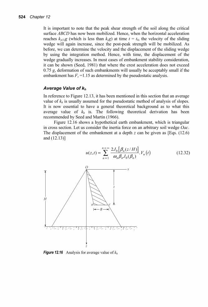
524 Chapter 12
It is important to note that the peak shear strength of the soil along the critical surface ABCD has now been mobilized. Hence, when the horizontal acceleration reaches ky(1)g (which is less than kyg) at time t = t4, the velocity of the sliding wedge will again increase, since the post-peak strength will be mobilized. As before, we can determine the velocity and the displacement of the sliding wedge by using the integration method. Hence, with time, the displacement of the wedge gradually increases. In most cases of embankment stability consideration, it can be shown (Seed, 1981) that where the crest acceleration does not exceed 0.75 g, deformation of such embankments will usually be acceptably small if the embankment has Fs =1.15 as determined by the pseudostatic analysis.
Average Value of kh In reference to Figure 12.13, it has been mentioned in this section that an average value of kh is usually assumed for the pseudostatic method of analysis of slopes. It is now essential to have a general theoretical background as to what this average value of kh is. The following theoretical derivation has been recommended by Seed and Martin (1966).
Figure 12.16 shows a hypothetical earth embankment, which is triangular in cross section. Let us consider the inertia force on an arbitrary soil wedge Oac. The displacement of the embankment at a depth z can be given as [Eqs. (12.6) and (12.13)]
[ ] ( )0
01
2 ( / )( , ) .
( )
nn
nn n nn
J z Hu z t V t
Jb
w b b
= •
== Â (12.32)
Figure 12.16 Analysis for average value of kh

Seismic Stability of Earth Embankments 525
So, the distribution of shear strain can be obtained as
( ) [ ] ( )1
11
2 ( / ), .
( )
nn
nn nn
J z Hu z t V tz H J
bw b
= •
=
∂ =∂ Â (12.33)
Hence, the distribution shear stress, ( , )z tt is
( ),z tt = ( ),uG z tz∂∂
= ( )( ) ( )1
11
2 /nn
nn nn
GJ z HV t
H Jb
w b
= •
=
È ˘Î ˚ (12.34)
The shear force, F(z, t), acting on the base of the wedge Oac is
( , ) ( , )F z t z t Bt= (12.35)
However,
F(z, t) = (mass of the wedge Oac) a( )au t u
= ( )a12 aBz u tr u
Ê ˆÁ ˜Ë ¯
(12.36)
where a( )au t u = average lateral acceleration ρ = density of the soil in the wedge
So
( ) ( ) ( )
a,2 2 , 2 ,
( )atF z z t B z t
u tBz Bz z
t tr r ru = = = (12.37)
Combining Eqs. (12.34) and (12.37),
[ ] ( )1a
11
4 ( / )( )
( )
nn
a nn nn
GJ z Hu t V t
H zJb
r w b
= •
u=
= Â (12.38)
So
( ) ( )( ) ( )1
a11
4 /1 .n
nh a n
n nn
GJ z Hk u t V t
g g H zJb
r w b
= •
u=
È ˘Î ˚= =  (12.39)

526 Chapter 12
Figure 12.17 Values of average seismic coefficient for 30-m-high embankment subjected to El Centro earthquakes (shear wave velocity, su = 300 m/s, 20% critical damping) (after Seed and Martin, 1966)
The value of kh is a function of time. Since the average acceleration varies with the depth z, the magnitude of kh also varies with time. Figure 12.17 shows the results of a calculation for kh for a model embankment at four different levels.
Yield Strength In the analysis of stability for earth embankments, it is important to make proper selection of the yield strength of soil to determine the shear strength parameters. The yield strength is defined as the maximum stress level below which the material exhibits a near-elastic behavior when subjected to cyclic stresses of numbers and frequencies similar to those induced by earthquake shaking.
Figure 12.18 shows the concept of cyclic yield strength of a clayey soil (Makdisi and Seed, 1978). The material in this case has an yield strength of about 90% of its static undrained strength. In Figure 12.18, it can be seen that under 100 cycles of stress, which amounts 80% of static undrained strength, the material behaves in a near-elastic manner. However when 10 cycles of stress, which amounts to 95% of static undrained strength, is applied, substantially large

Seismic Stability of Earth Embankments 527
Figure 12.18 Concept of cyclic yield strength
permanent deformation is observed (Figure 12.18). Hence the yield strength is about 90% of its static undrained strength.
Stability Analysis The remainder of this chapter is divided into two parts. The first part is devoted to the pseudostatic methods of stability analysis and the second part, to the determination of the deformation of slopes.
Pseudostatic Analysis
12.7 Clay Slopes (φ = 0 Condition)— Koppula’s Analysis A clay (φ = 0 condition) slope of height H is shown in Figure 12.19a. In order to determine the minimum factor of safety of the slope with respect to strength, we consider a trial failure surface ABC, which is an arc of a circle with its center located at O. Let the saturated unit weight and the undrained cohesion of the clay soil be equal to γ and cu, respectively. The undrained cohesion cu may increase with depth z measured from the top of the slope and can be expressed as

528 Chapter 12
Figure 12.19 Koppula’s analysis for clay slopes (φ = 0 condition)
0 0uc c a z= + (12.40)
where a0 = a constant.
Per unit length of the slope, for consideration of the stability of the soil mass located above the trial failure surface, the following forces need to be considered:
a. Weight of the soil mass, W b. Undrained cohesion, cu, per unit area along the trial failure surface ABC c. Inertia force on the soil mass, khW (where kh = average horizontal
acceleration of the mass)
The overturning moment, MD, about O can be given as
1 2D h
W E
M Wl k WlM M
= + (12.41)
Koppula (1984) has expressed MW and ME in the following forms:
MW = 3
12Hg (1 – 2cot2 β – 3cot α cot β + 3cot β cot λ
+ 3cot λ cot α – 6n cot β – 6n2 – 6n cot α + 6n cot λ) (12.42)

Seismic Stability of Earth Embankments 529
ME = 3
12hk Hg
(cot β + cot3 λ + 3 cot α cot2 λ
– 3cot α cot β cot λ – 6n cot α cot λ) (12.43)
The restoring moment MR about O is
–R uM R c R da
aq
+= Ú (12.44)
where R = radius of the circular arc
0 0[ cos( ) cos( ) ]uc c a R R Hl q a l= + + - - + (12.45)
Combining Eqs. (12.44) and (12.45)
( )3 2
0 02 2 2 21 – cot cos cot
4sin sin 2sin sinRa H c H
Maa a l l
a l a lÈ ˘= + +Î ˚ (12.46)
The factor of safety Fs against sliding can be given as
Rs
W E
MFM M
=+
(12.47)
The minimum value of Fs has to be determined by considering several trial failure surfaces. Koppula (1984) has expressed a minimum factor of safety in the form
0 01 2s
a cF N N
Hg g= + (12.48)
where N1 and N2 = stability numbers. Stability numbers are functions of kh, the slope angle β, and also the depth factor, D (for the definition of depth factor, see Figure 12.19). Figure 12.20 shows the variation of N1 and kh varying from 0 to 0.4 and β varying from 0° to 90°. In a similar manner, the variation of N2 with kh and D for β ≤ 50° is shown in Figure 12.21. For β ≥ 55°, the variation of N2 with kh is given in Figure 12.22. In order to use Eq. (12.48) and Figures 12.20, 12.21, and 12.22, the following points needs to be kept in mind. 1. If the undrained shear strength of the soil increases linearly from zero at the
top, then
0uc a z= (12.49)

530 Chapter 12
For this case, the critical slip surface associated with minimum Fs passes through the toe of the slope and lies within the slope. So
00
nD= ¸
˝= ˛ (12.50)
Also
01s
aF N
g= (12.51)
2. If the magnitude of cu is constant with depth, then
0
0
0
u
ac c
= ¸˝= ˛
(12.52)
For this case
02s
cF N
Hg= (12.53)
The stability number N2 is a function of β, D, and kh if β ≤ 53°. However if β ≥ 53°, then N2 is a function of β and kh only (that is, n = 0 and D = 0).
Text not available due to copyright restrictions

Seismic Stability of Earth Embankments 531
Text not available due to copyright restrictions
Text not available due to copyright restrictions

532 Chapter 12
Example 12.2
Refer to the slope shown in Figure 12.19. Given:
H = 15 m γ = 18 kN/m3
β = 60° cu = 48 + 3z (kPa)
Determine the factor of safety Fs for kh = 0.3.
Solution
From Eq. (12.48)
0 01 2s
a cF N N
Hg g= +
From Figure 12.20, for β = 60° and kh = 0.3, the magnitude of N1 ≈ 2.38. Again, from Figure 12.22, for β = 60° and kh = 0.3, the magnitude of N2 is about 3.28. So
Fs = 318Ê ˆÁ ˜Ë ¯
(2.38) + ( )( )48
18 15 (3.28) = 0.397 + 0.583 = 0.98
12.8 Slopes with c – φ Soil — Majumdar’s Analysis Taylor (1937) proposed the friction circle method of analyzing the stability of slopes with c – φ soils. In this analysis, the effect of earthquakes was not taken into consideration. The details of this slope stability analysis can be found in most soil mechanics textbooks (for example, Das, 2007). However, it can be summarized as follows.
Figure 12.23 shows a slope made of a soil having a shear strength that can be given as
tanf ct s f= + ¢ (12.54)
where τf = shear strength c = cohesion σ′ = effective normal stress φ = drained friction angle
For φ greater than about 3°, the critical circle for stability analysis always passes through the toe, as shown in Figure 12.23.
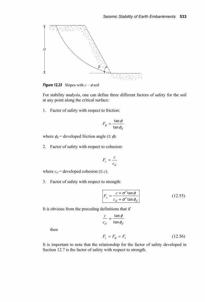
Seismic Stability of Earth Embankments 533
Figure 12.23 Slopes with c – φ soil
For stability analysis, one can define three different factors of safety for the soil at any point along the critical surface: 1. Factor of safety with respect to friction:
tantan d
Ffff
=
where φd = developed friction angle (≤ φ). 2. Factor of safety with respect to cohesion:
cd
cFc
=
where cd = developed cohesion (≤ c). 3. Factor of safety with respect to strength:
tantans
d d
cFc
s fs f
+ ¢=+ ¢
(12.55)
It is obvious from the preceding definitions that if
tantand d
cc
ff
=
then c sF F Ff= = (12.56)
It is important to note that the relationship for the factor of safety developed in Section 12.7 is the factor of safety with respect to strength.

534 Chapter 12
Using the preceding concepts for factor of safety, Taylor’s analysis (1937) for the stability of slopes by the friction circles method can be given in a graphical form, the nature of which is shown in Figure 12.24. Note that in Figure 12.24 the term m is defined as
dcmHg
=
Majumdar (1971) expanded Taylor’s analysis of slope by taking into consideration the horizontal earthquake forces as shown in Figure 12.25. By simple mathematical manipulations, Majumdar showed that if the actual effective friction angle φ of the soil can be modified to φm, it can then be used in Taylor’s analysis to determine the factor of safety with respect to strength (Fs) for the critical surface of a slope.
Figure 12.24 Nature of variation of m with β and φd
Figure 12.25 Analysis of slopes with c – φ soil
The relationship between φ and φm can be expressed as

Seismic Stability of Earth Embankments 535
1tan ( tan )m Mf f-= (12.57)
The term M in Eq. (12.57) is a function of the slope angle (β) and the horizontal coefficient of acceleration (kh). Figure 12.26 shows the variation of M with kh for β = 15°, 30°, 45°, 60°, and 75°.
Text not available due to copyright restrictions

536 Chapter 12
Text not available due to copyright restrictions

Seismic Stability of Earth Embankments 537
Figure 12.27 Modified Taylor’s chart
Figure 12.27 shows the modified plot of Taylor’s chart (that is, m versus β) for use of stability analysis. It is important to note that φd for a given soil is always less than or equal to φm.
In order to determine the factor of safety for a given slope, the following step-by-step procedure can be applied. 1. Determine the soil parameters φ and c and the unit weight γ. 2. Determine the parameters for the slope, that is, β and H. 3. For given values of φ, β, and kh, determine the factor M from Figure
12.26. 4. Assume several values for the developed friction angle φd (such as φd(1),
φd(2), φd(3),..). Note that φd ≤ φm. 5. For each assumed value of φd, determine the factor of safety with respect
to friction, or
( )
(1)1
tantan
m
dFf
ff
=
( )
(2)2
tantan
m
dFf
ff
=

538 Chapter 12
Figure 12.28 Calculation of Fs
( )
(3)3
tantan
m
dFf
ff
=
6. With each assumed value of φd and the slope angle β, go to Figure 12.27 and determine the stability number m.
7. From the values of m calculated in Step 6, calculate cd and the factor of safety with respect to cohesion (Fc) as
cd(1) = m1γ H; ( )
(1)1
cd
cFc
=
cd(2) = m2γ H; ( )
(2)2
cd
cFc
=
8. Plot a graph of Fφ versus Fc as determined from Steps 5 and 7 (Figure 12.28) and determine Fs = Fc = Fφ.
Example 12.3
A homogenous slope is shown in Figure 12.29a. Using the procedure described in this section, determine the factor of safety with respect to strength. Use kh = 0.3. Solution
Given H = 12 m, β = 30°, γ = 16 kN/m3, c = 20 kPa, and φ = 34°. Now, referring to Figure 12.26b, for kh = 0.3, M ≈ 0.54. So φm= tan –1(M tan φ) = tan –1[(0.54)(tan 34)] = 20° The following table can be prepared.

Seismic Stability of Earth Embankments 539
Assumed Developed Friction angle, φd
(deg) tan φd Fφ = m
d
φφ
tantan
(Figure12.27)
m Fc =
d
cc
= cm Hg
5 0.0875 4.16 0.110 0.95 10 0.1760 2.07 0.075 1.39 15 0.2680 1.36 0.046 2.26 20 0.3640 1.00 0.025 4.17
A plot of Fφ versus Fc is shown in Figure 12.29b, from which Fs = Fc = Fφ = 1.73.
Figure 12.29

540 Chapter 12
12.9 Slopes with c – φ Soil – Prater’s Analysis It was mentioned in Section 12.6 that, due to earthquakes, slopes may undergo permanent deformation. Prater (1979) has analyzed slopes with c – φ soils to determine the yield horizontal acceleration, which is defined as the threshold horizontal acceleration, kh = ky, acting upon a sliding mass, above which permanent deformation occurs. It corresponds to a factor of safety with respect to strength (Fs) of unity. In this analysis the failure surface was assumed to be an arc of a logarithmic spiral defined by the equation (Figure 12.30)
tan0r r eq q= (12.58)
where φ = soil friction angle. Prater’s analysis for determination of the yield acceleration is summarized next.
Figure 12.31 shows a homogenous slope. The unit weight, cohesion, and angle of friction of the soil are, respectively, γ, c, and φ. ABC is a trial failure surface that is the arc of a logarithmic spiral. Referring to Figure 12.31,
tanpm e f= (12.59)
–1
20 sin 1 – 2 cosr
d t m m pH
È ˘= = +Î ˚ (12.60)
1
2
sinsin1 – 2 cos
pj tm m p
- Ê ˆ= + Á ˜+Ë ¯ (12.61)
q p j= p - - (12.62)
Figure 12.30 Log spiral

Seismic Stability of Earth Embankments 541
Figure 12.31 Prater’s analysis for determination of yield acceleration
Considering a unit length of the embankment at right angles to the cross section shown, the overturning moment about O can be given as
(1 )D W E g EM M M k M Mu= + = +∓ (12.63) where
Mg = moment due to gravity force
= (M1 – M2 – M3) (12.64)
M1 = moment of the soil weight in the area OABC about O
= ( )3 3
23 9 tan 1d Hg
f + [(m3 sin j – sin q) – 3 tan φ(m3 cos j + cos q)] (12.65)
M2= moment of the soil weight in the area OAF about O
= 3 3
6d Hg [sin3 q(cot2 q – cot2 j)] (12.66)
M3 = moment of the soil weight in the area CDF about O
= 3
6Hg [cot2 β – cot2 j – 3md cos j(cot β – cot j)] (12.67)

542 Chapter 12
kυ = average vertical acceleration ME = moment due to horizontal inertia force = Mekh = (M4 – M5 – M6)kh (12.68)
M4 = ( )3 3
23 9 tan 1d Hg
f + [(m3 cos j + cos q) + 3 tan φ(m3 sin j – sin q)]
(12.69)
M5 = 3 3
3d Hg [sin3 q(cot q + cot j)] (12.70)
M6 = 3
6Hg (3d sin q + 1)(cot β – cot j) (12.71)
kh = average horizontal acceleration
Hence, combining Eqs. (12.63) through (12.71), an expression for the overturning moment, MD, can be obtained.
The restoring moment, MR, can now be expressed as
moment of the frictionalmoment of the cohesiveforce developed alongforce developed along
the trial failurethe trial failuresurface ,surrace ,
R
fc
M
ABC MABC M
È ˘È ˘Í ˙Í ˙Í ˙Í ˙= + Í ˙Í ˙Í ˙Í ˙Í ˙Î ˚ Î ˚
However, based on the property of logarithmic spiral, the line of action of the resultant frictional force at any given point along the trial failure surface will pass through the origin O. Hence
Mf = 0
Mc = ( )2 2 2 – 1
2 tancd H m
f (12.72)
So, for equilibrium of the soil mass located above the trial failure surface
= 0D cM M- (1 ) 0g e h cM k M k Mu + - =∓ 0g g e h cM M k M k Mu + - =∓ or
–c g
he g
M Mk
M bM=
∓ (12.73)
where

Seismic Stability of Earth Embankments 543
h
kb
ku= (12.74)
Prater (1979) has suggested that a realistic value of b would be 0.3. The yield acceleration kh for the most critical surface can be determined by trial and error. Table 12.1 shows the magnitudes of the yield acceleration determined in this manner with b = 0.
12.10 Slopes with c – φ Soil — Conventional Method of Slices In the analysis for the stability of slopes provided in Section 12.7, 12.8, and 12.9, it is assumed that the soil is homogeneous. However, in a given slope, layered soil can be encountered. The method of slices is a general method that can easily account for the change of γ, c, and φ in the soil layers.
In order to explain this method, let us consider a slope as shown in Figure 12.32. Let ABC be a trial failure surface. Note that ABC is an arc of a circle with its center at O.
Figure 12.32 Conventional method of slices
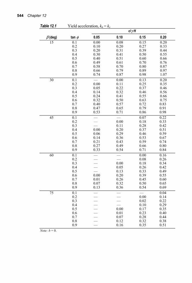
544 Chapter 12
Table 12.1 Yield acceleration, kh = ky c/γ H β (deg) tan φ 0.05 0.10 0.15 0.20 15 0.1 0.00 0.08 0.15 0.20 0.2 0.10 0.20 0.27 0.33 0.3 0.20 0.31 0.39 0.44 0.4 0.30 0.41 0.50 0.55 0.5 0.40 0.51 0.60 0.66 0.6 0.49 0.61 0.70 0.76 0.7 0.58 0.70 0.80 0.87 0.8 0.66 0.79 0.89 0.97 0.9 0.74 0.87 0.98 1.07 30 0.1 — 0.00 0.13 0.20 0.2 0.00 0.11 0.25 0.35 0.3 0.05 0.22 0.37 0.46 0.4 0.14 0.32 0.46 0.56 0.5 0.24 0.41 0.55 0.66 0.6 0.32 0.50 0.63 0.75 0.7 0.40 0.57 0.72 0.83 0.8 0.47 0.65 0.79 0.91 0.9 0.53 0.71 0.86 0.98 45 0.1 — — 0.07 0.22 0.2 — 0.00 0.18 0.33 0.3 — 0.11 0.28 0.42 0.4 0.00 0.20 0.37 0.51 0.5 0.06 0.29 0.46 0.59 0.6 0.14 0.36 0.53 0.67 0.7 0.21 0.43 0.59 0.74 0.8 0.27 0.49 0.66 0.80 0.9 0.33 0.54 0.71 0.84 60 0.1 — — 0.00 0.16 0.2 — — 0.08 0.26 0.3 — 0.00 0.18 0.34
0.4 — 0.05 0.26 0.42 0.5 — 0.13 0.33 0.49 0.6 0.00 0.20 0.39 0.55 0.7 0.01 0.26 0.45 0.60 0.8 0.07 0.32 0.50 0.65 0.9 0.13 0.36 0.54 0.69 75 0.1 — — — 0.04 0.2 — — 0.00 0.14 0.3 — — 0.02 0.22 0.4 — — 0.10 0.29 0.5 — 0.00 0.17 0.35 0.6 — 0.01 0.23 0.40 0.7 — 0.07 0.28 0.44 0.8 — 0.12 0.32 0.38 0.9 — 0.16 0.35 0.51 Note: b = 0.

Seismic Stability of Earth Embankments 545
The soil above the trial failure surface is divided into several slices. The length of each slice need not be the same. For the nth slice, consider a unit thickness at right angles to the cross section shown. The weight and the inertia forces are, respectively, Wn and khWn. The forces Pn and Pn+1 are the normal forces acting on the sides of the slice. Similarly, the shearing forces acting on the sides of the slice are Tn and Tn+1. The forces Pn, Pn+1, Tn and Tn+1 are difficult to determine. However we can make an approximate assumption that the resultant of Pn and Tn are equal in magnitude to the resultants of Pn+1 and Tn+1 and also their lines of action coincide. The normal reaction at the base of the slice is Nr = Wn cosαn. It is assumed that the inertia force khWn has no effect on the magnitude of Nr. So the resisting tangential force Tr can be given as
1 ( sec tan )r n n rs
T cB NF
a f= +
1 ( sec cos tan )n n n ns
cB WF
a a f= + (12.75)
Now, taking the moment about O for all the slices,
( ) ( )1 1
sin sec cos tanp p
n n h n n n n n nsn n
RW R k W L cB WF
a a a f= =
+ = +Â Â (12.76)
or
( )
( )1
1
sec cos tan
sin /
p
n n n nn
s p
n n h n nn
cB WF
W k W L R
a a f
a
=
=
+
=È ˘+Î ˚
Â
 (12.77)
Note that the value of αn may be either positive or negative. The value of αn is positive when the slope of the arc is in the same quadrant as the ground slope. To find the minimum factor of safety—that is, the factor of safety with reference to the critical circle—several trials have to be made, each time changing the center of the trial circle.
For convenience, a slope in homogeneous soil is shown in Figure 12.32. However, the method of slices can be extended to slopes of layered soil, as shown in Figure 12.33. The general procedure of stability analysis is the same; however, some minor points need to be kept in mind. While using Equation (12.77), the values of φ and c will not be the same for all slices. For example, for slice 2, one

546 Chapter 12
Figure 12.33 Method of slices for slopes in layered soil
has to use φ = φ2 and c = c2; similarly, for slice 3, φ = φ3 and c = c3 will need to be used.
Deformation of Slopes
12.11 Simplified Procedure for Estimation of Earthquake-Induced Deformation The concept relating to the deformation of embankment slopes due to earthquake-induced vibration was briefly described in Section 12.6. Following is a simplified step-by-step procedure developed by Makdisi and Seed (1978) for estimation of the deformation. When this procedure is applied, it is assumed that the shear strength of the soil does not change during shaking. Hence this method cannot be used in cases where there is pore pressure buildup. 1. Determine the height of the embankment (H) and the shear strength
parameters of the soil (c and φ). 2. Determine the maximum crest acceleration max[ (0)]au and the first natural
period 1( 2 )T w= p by using the method described in Section 12.5. 3. With reference to Figure 12.34, choose the critical section likely to deform
and determine the magnitude of (max) max[ (0)]h ak g u from Figure 12.34. Note that kh(max) is the coefficient of the maximum average horizontal acceleration for a given value of z/H. The concept of the coefficient of average acceleration was explained in Section 12.6. Now determine the magnitude of kh(max)g.
4. Determine the yield acceleration—that is, the acceleration kyg (see Section 12.9) for which the sliding mass has Fs = 1.
5. Determine [ky/kh(max)] and the magnitude of the earthquake (M). With these values go to Figure 12.35 to obtain (max) 1[ ]hU k gT (in seconds). With the known values of kh(max)g (Step 3) and T1 (Step 2), the magnitude U can be determined. Note that U is the deformation in the horizontal direction.
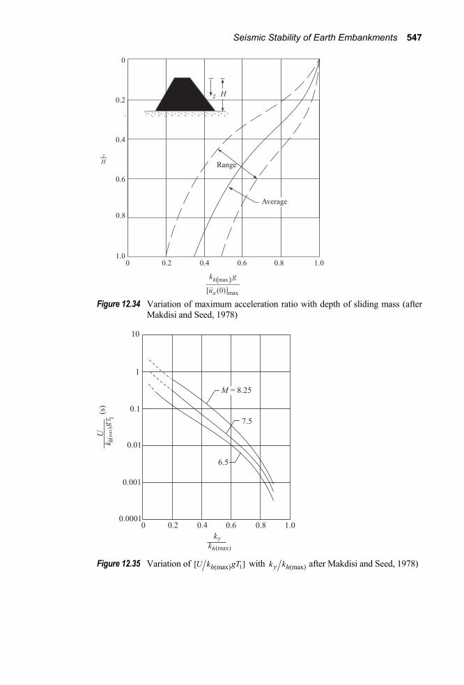
Seismic Stability of Earth Embankments 547
Figure 12.34 Variation of maximum acceleration ratio with depth of sliding mass (after
Makdisi and Seed, 1978)
Figure 12.35 Variation of 1(max)[ ]hU k gT with (max)y hk k after Makdisi and Seed, 1978)
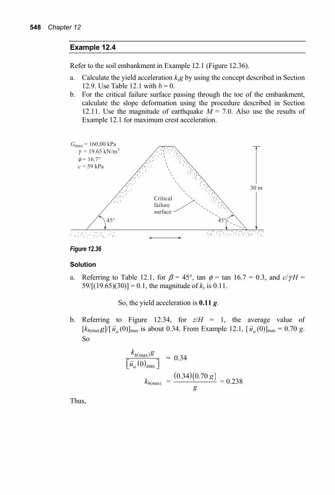
548 Chapter 12
Example 12.4
Refer to the soil embankment in Example 12.1 (Figure 12.36). a. Calculate the yield acceleration kyg by using the concept described in Section
12.9. Use Table 12.1 with b = 0. b. For the critical failure surface passing through the toe of the embankment,
calculate the slope deformation using the procedure described in Section 12.11. Use the magnitude of earthquake M = 7.0. Also use the results of Example 12.1 for maximum crest acceleration.
Figure 12.36
Solution
a. Referring to Table 12.1, for β = 45°, tan φ = tan 16.7 = 0.3, and c/γ H = 59/[(19.65)(30)] = 0.1, the magnitude of ky is 0.11.
So, the yield acceleration is 0.11 g. b. Referring to Figure 12.34, for z/H = 1, the average value of
[kh(max)g]/[ au (0)]max is about 0.34. From Example 12.1, [ au (0)]max = 0.70 g. So
( )
( )max
max0h
a
k guÈ ˘Î ˚
= 0.34
kh(max) = ( )( )0.34 0.70 g
g = 0.238
Thus,

Seismic Stability of Earth Embankments 549
( )max
y
h
kk
= 0.110.238
= 0.462
Also, from Example 12.1, T1 = 0.435 sec. For earthquake magnitude M = 7.0, referring to Figure 12.35,
( ) 1maxh
Uk gT
≈ 0.036
So
U = (0.036)(0.238)(9.81)(0.435) = 0.0366 m = 36.6 mm
Problems 12.1 An earth embankment is 25 m high. For the embankment soil,
Unit weight = 18 kN/m3 At a certain shear strain level G = 50,000 kPa and D = 15%
Using the acceleration spectra given in Figure 12.12 (maximum ground acceleration is 0.23 g), estimate the maximum crest acceleration of the embankment.
12.2 An earth embankment is 18 m high. For the embankment soil,
Unit weight = 18.5 kN/m3 Maximum shear modulus = 165,000 kPa
Using the variation of G/Gmax and D with shear strain as given in Figure 12.11 and the acceleration spectra given in Figure 12.12 (maximum ground acceleration = 0.2 g), determine the maximum crest acceleration.
12.3 A clay (φ = 0°) is built over a layer of rock. For the slope,
Height = 20 m Slope angle, β = 30° Saturated unit weight of soil = 17.8 kN/m3 Undrained shear strength, cu = 5z kPa (z = depth measured from the top of the slope) Determine the factor of safety Fs if kh = 0.4. Use the procedure outlined
in Section 12.7. 12.4 Redo Problem 12.3 assuming cu = 40 + 5z kPa and other parameters
remain the same.

550 Chapter 12
12.5 Refer to Problem 12.3. Other parameters remaining the same, let the slope angle β be changed from 30° to 75°. Calculate and plot the variation of the factor of safety (Fs) with β. Use the procedure outlined in Section 12.7.
12.6 For a homogenous soil,
Slope angle, β = 30° Height, h = 15 m Soil cohesion = 60 kPa Soil friction angle, φ = 25° Unit weight of soil = 19.5 kN/m3 kh = 0.25
Determine the factor of safety with respect to strength. Use the procedure described in Section 12.8.
12.7 Repeat Problem 12.6 with the following:
Slope angle, β = 45° Height, h = 25 m Soil cohesion = 60 kPa Soil friction angle, φ = 20° Unit weight of soil = 19 kN/m3 kh = 0.3
12.8 For the slope described in Problem 12.6, what would be the yield acceleration (that is, hk g )? Use the procedure described in Section 12.9. Use b = 0.
12.9 The properties of the soil of a given slope 15.3 m high are as follows:
Unit weight, g = 18.5 kN/m3 Cohesion, c = 42.5 kPa Angle of friction, φ = 20°
The yield acceleration for the slope was estimated to be 0.36. This was done using the procedure described in Section 12.9 with b = 0. Estimate the slope angle β.
12.10 A homogeneous slope is shown in Figure P12.10. For the trial failure surface shown, determine the factor of safety with respect to strength. Use the method of slices. (Note: The slope angle is β = 30°.)

Seismic Stability of Earth Embankments 551
Figure P12.10
12.11 A 25 m high embankment (c-φ soil) is constructed over a hard stratum, The critical failure circle passes through the toe of the slope and the average yield acceleration of the slope is 0.15 g. The maximum crest acceleration due to an earthquake of magnitude M = 7.5 has been estimated to be 0.6 g. The first natural period is 0.8 s. Estimate the slope deformation. Use the procedure described in Section 12.11.
12.12 Refer to Example 12.4. Other quantities remaining the same, if the soil friction angle φ is changed to 21.8°, estimate the slope deformation.
References Ambraseys, N. N. (1960). “On the Seismic Behavior of Earth Dams,”
Proceedings, 2nd World Conference on Earthquake Engineering, Tokyo, Vol. I, pp. 331-345.
Das, B. M. (2007). Principles of Geotechnical Engineering, 6th ed., Thomson, Toronto.
Koppula, S. D. (1984). “Pseudo-Static Analysis of Clay Slopes Subjected to Earthquakes,” Geotechnique, Institute of Civil Engineers, London, Vol. 34, No. 1, pp. 71-79.
Majumdar, D. K. (1971). “Stability of Soil Slopes under Horizontal Earthquake Force,” Geotechnique, Institute of Civil Engineers, London, Vol. 21, No. 1, pp. 372-378.
Makdisi, F. I., and Seed, H. B. (1978). “Simplified Procedure for Estimating Dam and Embankment Earthquake-Induced Deformations,” Journal of the Geotechnical Engineering Division, ASCE, Vol. 104, No. GT7, pp. 849-859. With permission from ASCE.

552 Chapter 12
Makdisi, F. I., and Seed, H. B. (1979). “Simplified Procedure for Evaluating Embankment Response,” Journal of the Geotechnical Engineering Division, ASCE, Vol. 105, No. GT12, pp. 1427-1434.
Mononobe, N., Takata, A., and Matumura, M. (1936). “Seismic Stability of Earth Dams,” Proceedings, 2nd Congress of Large Dams, Vol. 4, Washington, D. C.
Newmark, N. M. (1965). “Effect of Earthquakes on Dams and Embankments,” Geotechnique, Institute of Civil Engineers, London, Vol. 15, No.2, p. 139.
Prater, E. G (1979). “Yield Acceleration for Seismic Stability of Slopes,” Journal of the Geotechnical Engineering Division, ASCE, Vol. 105, NO. GT5, pp. 682-687.
Seed, H. B. (1975). “Earthquake Effects on Soil-Foundation System” in Foundation Engineering Handbook (H. F. Winterkorn and H. Y. Faud, eds.), Van Nostrand Reinhold, New York.
Seed, H. B. (1981). “Earthquake-Resistant Design of Earth Dams,” Proceedings, International Conference on Recent Advances in Geotechnical Earthquake Engineering and Soil Dynamics, University of Missouri-Rolla, Vol. III, pp. 1157-1177.
Seed, H. B., and Goodman, R. E. (1964). “Earthquake Stability of Slopes of Cohesionless Soils,” Journal of the Soil Mechanics and Foundations Division, ASCE, Vol. 90, No. SM6, pp. 43-56.
Seed, H. B., and Martin, G. R. (1966). “The Seismic Coefficient of Earth Dam Designs,” Journal of the Soil Mechanics and Foundations Division, ASCE, Vol. 92, No. SM3, pp. 25-58.
Seed, H. B., Makdisi, F. I., and DeAlba, P. (1978). “Performance of Earth Dams During Earthquakes,” Journal of the Geotechnical Engineering Division, ASCE, Vol. 104, No. GT7, pp. 967-944.
Taylor, D. W. (1937). “Stability of Earth Slopes,” Journal of the Boston Society of Civil Engineers, Vol. 24, No. 3, pp. 197-246.
With permission from ASCE.
With permission from ASCE.

553
Appendix A
PRIMARY AND SECONDARY FORCES OF SINGLE-CYLINDER ENGINES
Machineries involving a crank mechanism produce a reciprocating force. This mechanism is shown in Figure A.1a, in which
OA = crank length = 1r
AB = length of the connecting rod = 2r
Let the crank rotate at a constant angular velocityw . At time t = 0, the vertical distance between O and B (Figure A.1b) is equal to 1 2r r+ . At time t, the vertical distance between O and B is equal to 1 2r r z+ − , or
( ) ( )1 2 2 1cos cosz r r r r ta w= + − + (A.1)
But,
2 1sin sinr r ta w= (A.2)
Now,
22 21
2cos 1 sin 1 sinr t
ra a w
⎛ ⎞= − = − ⎜ ⎟
⎝ ⎠
2
21
2
11 sin2
r tr
w⎛ ⎞
≈ − ⎜ ⎟⎝ ⎠
(A.3)
Substituting Eq. (A.3) into Eq. (A.1),
( ) ( )1 2 2 1cos cosz r r r r ta w= + − + ( ) ( )2 11 cos 1 cosr r ta w= − + −
( )2
212 1
2
11 1 sin 1 cos2
rr t r tr
w w⎡ ⎤⎛ ⎞⎢ ⎥= − + + −⎜ ⎟⎢ ⎥⎝ ⎠⎣ ⎦

554 Appendix A
Figure A.1
( )2
12
12
12 sin 1 cos
rt r t
rw w
⎛ ⎞⎜ ⎟
= + −⎜ ⎟⎜ ⎟⎝ ⎠
(A.4)
However,
( )2 1sin 1 cos 22
t tw w= − (A.5)
Substituting Eq. (A.5) into Eq. (A.4), one obtains
( ) ( )2
1
12
14 1 cos2 1 cos
rz t r t
rw w
⎛ ⎞⎜ ⎟
= − + −⎜ ⎟⎜ ⎟⎝ ⎠

Appendix A 555
2 21 1
1 12 2
1 14 4cos cos2
r rr r t t
r rw w
⎡ ⎤⎛ ⎞ ⎛ ⎞⎢ ⎥⎜ ⎟ ⎜ ⎟
= + − +⎢ ⎥⎜ ⎟ ⎜ ⎟⎢ ⎥⎜ ⎟ ⎜ ⎟⎢ ⎥⎝ ⎠ ⎝ ⎠⎣ ⎦
(A.6)
The acceleration of the piston can be given by
2 11
2cos cos2rz r t t
rw w w
⎡ ⎤⎛ ⎞= +⎢ ⎥⎜ ⎟
⎢ ⎥⎝ ⎠⎣ ⎦ (A.7)
If the mass of the piston is m, the force can be obtained as 2
2 211
2cos cos 2rF mz mr t m t
rw w w w
⎛ ⎞= = + ⎜ ⎟
⎝ ⎠ (A.8)
The first term of Eq. (A.8) is the primary force, and the maximum primary force
( )2
1max primF mrw= (A.9)
Similarly, the second term of Eq. (A.8) is generally referred to as the secondary force, and
( )
221
max sec2
rF mr
w⎛ ⎞
= ⎜ ⎟⎝ ⎠
(A.10)

Index
Acceleration pickup, 41 Acceleration spectra, 511-513 Active earth pressure coefficient:
Coulomb, 328-330, 331 effect of slope of backfill, 342 effect of soil friction angle, 341 effect of wall friction angle, 340 Mononobe-Okabe solution, 330, 332-334, 363-367 rotation about bottom, 346 rotation about top, 349-350 translation, 346-348
Active isolation: definition of, 261 by use of open trench, 261-263
Amplitude attenuation, elastic waves, 90-93 Amplitude, foundation vibration:
rocking, 222-223 sliding, 228-229 torsional, 231-232 vertical, 210-212
Amplitude of acceleration, rock, 307 Amplitude of vibration:
allowable vertical, foundation, 214-215 impact machine, 250 at resonance with damping, 33, 37
Amplitude reduction factor, 261, 262 Analog solution, foundation:
Hsieh's analog, 205-207 Lysmer's analog, 207-209 rocking vibration, 220 sliding vibration, 226 torsional vibration, 229
Anvil, 2481 At-rest earth pressure coefficient, 172 Attenuation of elastic waves, 90-93 Backfill slope, effect on earth pressure, 342 Bandwidth method, 38 Bearing capacity:
clay, 283-285 factors, 278 general shear failure, 279 punching shear failure, 279 sand, 277-281, 291-295 strain rate for, 284, 285 variation with loading velocity, 280-281
Bedrock-like material, 305 Bilinear idealization, 124, 125 Boussinesq problem, dynamic, 197 Calculation of foundation response:
rocking vibration, 221-223 sliding vibration, 228-229 torsional vibration, 231-232 vertical vibration, 209-214
Characteristics of rock motion, 305-307 Coefficient of:
restitution, 251 subgrade reaction, 10, 11
Compaction, granular soil, 374-379 Cone penetration resistance, liquefaction,
444 Contact pressure:
flexible foundation, 199, 200 parabolic pressure distribution, 199, 200 rigid foundation, 199, 200
Correlation for: at-rest earth pressure coefficient, 172 damping ratio in clay, 178-183 damping ratio in gravel, 176-177 damping ratio in lightly cemented sand, 187 damping ratio in sand, 173, 174-175 liquefaction, 430-431 maximum ground acceleration, 433-438 shear modulus in clay, 178-180 shear modulus in gravel, 176 shear modulus in lightly cemented sand, 186 shear modulus in sand, 171-173 shear wave velocity, sand, 171
668 Index
Coupled rocking and sliding, foundation, 244-247
Crest acceleration, embankment, 513-518 Critical angle of incidence, 139 Critical damping, 23 Critical horizontal acceleration, earth
pressure, 335 Critical void ratio, 398-399 Cross-hole shooting, 162 Cyclic mobility, liquefaction, 407 Cyclic plate load tests: 164-166
shear modulus determination, 165 spring constant determination, 164-165
Cyclic shear strain, settlement of sand, 389-391
Cyclic simple shear tests: 121-125 advantages of, 125 shear modulus-shear strain relationship, 114 typical results for liquefaction, 416-418
Cyclic strength, clay, 130-132 Cyclic torsional simple shear test, 125-128 Cyclic triaxial test, 128-132 Damped natural frequency, definition of, 28 Damping, definition of, 23 Damping ratio:
in clay, 180, 182 definition of, 24 determination of, 37-40 effect of stress cycles, 122, 123, 124 in gravel, 177 in lightly cemented sand, 187 in sand, 173, 174-175
Damping ratio, foundation vibration: rocking, 221 sliding, 227 torsional, 229 vertical, 210
Dashpot coefficient, 23 Dashpot coefficient, foundation vibration:
rocking, 221 sliding, 227 torsional, 229 vertical, 209
Deep-focus earthquake, 301 Deformation of slope, 546-547 Degree of freedom, 9 Depth factor, 277, 279 Dimensionless frequency, 199 Dimensionless mass ratio:
sliding vibration, 227 torsional vibration, 231 vertical vibration, 208
Displacement function, 198, 205 Displacement of Rayleigh waves, 88-90 Distortional wave, 77-78 Double amplitude, definition of, 14 Duration, earthquake, 305-306 Dynamic Boussinesq problem, 197 Dynamic force, subgrade, 33-34 Dynamic laboratory test:
parameters measured, 134 range of applicability, 133 relative quantities, 134
Dynamic triaxial test, liquefaction: procedure for, 402-404 typical results for, 405-409
Earth pressure theory:
Mononobe-Okabe solution, 330, 332-334, 363-367
Earthquake: duration of, 305-306 equivalent number of cycles, 320-324 length of fault rupture during, 304 magnitude of, 303-305 modified Mercalli scale for, 304
Earthquake-induced slope deformation, 546-547
Effective distance to. causative fault, 301-302
Effective octahedral stress, 172 Effective principal stress:
for torsional shear test, 126-127 Effectiveness, isolation, 267 Elastic half-space solution, 196-205 Elastic wave:

669 Index
attenuation of, 90-93 reflection of, 135-137 refraction of, 135-137
Embedded foundation: amplitude of vibration, vertical, 255 damping ratio, 254, 256, 258, 260 dashpot coefficient, 254, 256, 257, 259 rocking vibration, 257-258 sliding vibration, 256-257 spring constant, 254, 256, 257, 259 torsional vibration, 259-260 vertical vibration, 251-255
Energy transmission, machine foundation, 388
End-bearing pile: definition of, 460 natural frequency derivation for, 460-463
Epicenter, 301 Epicenter distance, 301 Equation for stress waves:
compression wave, 75-77 Rayleigh wave, 82-88 shear wave, 77-78
Equation of motion, elastic medium, 74-75 Equivalent radius, foundation vibration:
rocking, 223 sliding, 227 torsional, 232 vertical, 213-214
Fixed-free resonant column test, 108 Flexible circular area, vibration of, 197-199 Focal depth, 300 Focus, earthquake, 300 Footing vibration, comparison with theory,
235-238 Forced vibration:
definition of, 8-9 of earth embankment, 509-511 spring-mass system, 16-22 steady state with viscous damping, 30-34
Foundation subgrade: maximum force on, 21-22, 33-34 minimum force on, 21-22
Free vibration: definition of, 8 of earth embankment, 505-508 spring-mass system, 10-15 with viscous damping, 23-29
Freedom, degree of, 9 Free-free resonant column test, 106-108 Frequency of oscillation, definition of, 14 Friction pile:
dashpot coefficient for, 467 definition of, 460 spring constant for, 467 vertical vibration of, 465-474
General shear failure, 279 Geometric damping, 92 Granular soil, compressibility of, 374-379 Graphical construction, active force,
342-344 Gravel:
damping ratio of, 177, 178 drain, 447-452 shear modulus of, 176, 177, 178
Gravity retaining wall: inertia factor, 357 limited displacement of, 353-359 thrust factor, 357
Group pile, vertical vibration: amplitude of vibration, 473, 474 damped natural frequency, 473 damping ratio for, 472 dashpot coefficient for, 472 spring constant for, 472
Halls' analog, 220 High-speed machine, 215 Homogeneous soil layer vibration, 308-313 Hooke's law, 58-59

670 Index
Horizontal layering: reflection survey, 151-153 refraction survey, 137-143
Hsieh's analog, 205-207 Hydrodynamic effect, pore water, 361-363 Hyperbolic strain, 180 Hypocentric distance, 301 Impact machine vibration, 248-251 Inclined layering:
reflection survey, 154-157 refraction survey, 145-148
Inertia factor, gravity wall, 357 Inertia ratio, rocking vibration, 221 Initial liquefaction:
influence of confining pressure, 411 influence of overconsolidation ratio, 417-418 influence of peak pulsating stress, 412-413, 416 influence of relative density, 410 influence of test condition, 417 standard curves for, 414
Intermediate focus earthquake, 301 Internal damping, 117-120 Isolation:
active, 261-264 by use of pile, 266-269 effectiveness, 267 passive, 261, 264-266
Length of fault rupture, 304 Lightly cemented sand:
damping ratio for, 187 shear modulus for, 186
Limited displacement, gravity wall, 353-359 Liquefaction:
analysis, standard penetration resistance, 438-442 correlation, cone penetration resistance, 444 cyclic mobility, 407 development of standard curves for, 414
dynamic triaxial test for, 402-404 fundamentals of, 399-400 influence of .parameters on, 410-413 remedial action for mitigation of, 447-452 resistant stratum, 445-446 threshold strain for, 444-445 typical results for, 405-409 zone of, 432
Logarithmic decrement: definition of, 28 in torsional vibration of sand, 119
Longitudinal elastic wave: in a bar, 60-62 travel time method for, 104-106
Longitudinal stress wave velocity, 60-62 Longitudinal vibration, short bar:
fixed-fixed end condition, 70-71 fixed-free end condition, 71-73 free-free end condition, 69-70
Low-speed machine, 215 Lumped parameter, definition of, 8 Lysmer's analog, 207-209 Machine foundation, settlement, 384-389 Magnitude, earthquake, 303-305 Mass ratio, 199 Material damping, 92 Maximum amplitude, rock motion, 307 Maximum crest acceleration,
embankment, 513-518 Modified Mercalli scale, 304 Mononobe-Okabe earth pressure theory,
330, 332-334, 363-367 Multidirectional shaking, settlement,
394-395 Multilayer soil, refraction survey, 143 Natural frequency, end-bearing pile,
460-462 Nature of dynamic load, 1-4 Number of stress cycles, equivalent, 320-324

671 Index
Overdamping, 24-25 Parameters measured, dynamic test, 134 Passive isolation:
definition of, 261 by use of piles, 266-269 by use of trenches, 264-266
Passive pressure, 368-370 Pickup:
acceleration, 41 velocity, 41
Plate load test: procedure for, 164-166 shear modulus determination, 165 spring constant determination, 164-165 sub grade modulus determination, 165
Point of application, active force: wall rotation about bottom, 350 wall rotation about top, 352 wall translation, 352
Poisson's ratio, choice of, 242-243 Pore water pressure:
hydrodynamic effect on, 361, 362 rate of increase of, 418-419
Pseudostatic analysis, slope: c − φ soil, 532-538, 540-542 conventional method of slices, 543-546 in saturated clay, 543-546 yield acceleration, 544
Punching shear failure, 279 Range of applicability, dynamic test, 133 Rapid load, shear strength, 97-100 Rayleigh wave: 82-88
displacement of, 88-90 Reference strain, geostatic stress, 179 Reflection of elastic waves, end of bar,
65-67 Reflection survey:
horizontal layering, 151-153 inclined layering, 154-157
Refraction survey: horizontal layering, 137-143 multilayer soil, 143 three-layered soil medium, 141-143 with inclined layering, 145-148
Relative quality, laboratory measurement, 124
Resonance condition, 19 Resonant column test: 106-121
determination of internal damping, 117-121 fixed-free test, 108 free-free test, 106 for large strain amplitude, 114-117 typical results from, 114
Rigid foundation: dimensionless amplitude, 201, 202
Rock acceleration: maximum amplitude of, 307 predominant period, 306
Rock motion, characteristics of, 305-307 Rocking vibration, foundation:
amplitude of vibration, 222-223 contact pressure distribution in, 219 damping ratio, 221 dashpot coefficient, 221 Hall's analog for, 220 inertia ratio, 221 static spring constant for, 221
Rocking vibration, pile: 482-486 damping ratio, 485 dashpot coefficient, group, 483 dashpot coefficient, single, 483 spring constant, group, 483 spring constant, single, 482
Rotating mass type excitation, 35-37 Seismic survey:
reflection, horizontal layering, 151-153 reflection, inclined layering, 154-157 refraction, horizontal layering, 137-143 refraction, inclined layering, 145-148

672 Index
Settlement: of machine foundation, 380-384 prediction for foundation, 293
SH-wave, 135 Shape factor, bearing capacity, 277, 279 Shallow-focus earthquake, 301 Shear modulus:
correlation with standard penetration resistance, 176 effect of prestraining on, 117 for gravel, 176-178 for large strain amplitude, 114-117 for lightly cemented sand, 186-187 from plate load test, 165 variation with shear strain, 116
Shear strength, rapid loading: sand, 99-100 saturation clay, 97-99
Shear wave: correlation for velocity, 171 equation for, 77-78 travel time method for, 106 velocity, 68, 78
Shearing strain, 54 Short bar:
longitudinal vibration of, 68-73 torsional vibration of, 73
Simple shear test, 121-125 Single amplitude, definition of, 14 Single degree of freedom system, 9 Sliding vibration, foundation:
amplitude of vibration, 228-229 damping ratio, 227 dashpot coefficient, 227 mass ratio, 227 static spring constant, 227
Sliding vibration, pile: 478-482 dashpot coefficient, group, 479, 481 dashpot coefficient, single, 478 spring constant, group, 479, 481 spring constant, single, 478
Soil friction angle, effect on earth pressure, 341
Spring constant: definition of, 10 from plate load test, 164-165
Spring-mass system: forced vibration, 16-22 free vibration, 10-15
Stability analysis, embankment: coefficient of acceleration, average values, 524-526 fundamental concepts, 521-527
Standard penetration resistance: correlation for shear modulus, 176
Static spring constant, foundation: rocking, 221, 241 sliding, 227, 241 torsional, 229, 241 vertical, 209, 241
Steady state vibration: subsoil exploration, 158-160 viscous damping, 30-34
Strain, 57-58 Strain rate:
on bearing capacity, 284 for clay, 97, 99 for sand, 100
Stress, 56-57 Stress-strain relationship, bilinear
idealization, 124, 125 Stress cycle, equivalent number, 320-324 Stressed zone:
velocity of particles in, 63-64 Subgrade:
modulus, 165 reaction, coefficient of, 10
Subsoil exploration: cross-hole shooting, 162 shooting down the hole, 160 shooting up the hole, 160 steady state vibration, 158-160
SV-wave, 135 Terminal dry unit weight, 378-379 Three-layered medium, refraction survey,
141-143

673 Index
Threshold strain, liquefaction, 444-445 Thrust factor, gravity wall, 357 Torsional vibration, foundation:
calculation for foundation response, 231-232 damping ratio, 229 dimensionless mass ratio, 231 shear stress distribution, 229 spring constant, 214
Torsional vibration, pile: 492-501 dashpot coefficient, group, 494, 497 dashpot coefficient, single, 494 spring constant, group, 494, 496 spring constant, single, 493
Torsional wave in a bar, 67-68 Torsional wave velocity, 68 Torsional simple shear test: 125-128
effective principal stress, 126-127 Travel time method, 104-106 Triaxial test, cyclic: 128-132
cyclic strength of clay, 130-132 Two degrees of freedom:
coupled translation and rotation, 48-51 mass-spring system, 42-46
Types of dynamic load, 1-4 Typical results, resonant column test, 114 Ultimate bearing capacity:
depth factor for, 277, 279 in sand, 277 shape factor for, 277, 279
Ultimate residual settlement, 385, 386, 387, 389
Undamped natural frequency: definition of, 11 of embankment, 508
Underdamping, 24, 26 Uniformly loaded flexible area, vibration of,
197-199 Unit weight, terminal, 378-379 Velocity of particle, stressed zone, 63-64 Velocity pickup, 41
Velocity spectra, 511-513 Vertical vibration, foundation:
amplitude at resonance, 201, 202 calculation of foundation response, 209-214 damping ratio, 210 dashpot coefficient, 209 displacement functions, 205, 207-208 effect of contact pressure distribution, 203 effect of Poisson's ratio, 204 elastic half-space solution, 196-205 flexible circular foundation, 197-198 Hsieh's analog, 205-207 Lysmer's analog, 207-209 resonant frequency, 210 static spring constant, 209 uniformly loaded flexible area, 197
Vibration: forced, 8 free, 8 measuring instrument, 40-41
Vibration of embedded foundation: amplitude of vibration, 255 damping ratio, 254, 256, 258, 260 dashpot coefficient, 254, 256, 257, 259 spring constant, 254, 256, 257, 259
Vibration of soil, earthquake: homogeneous layer, 308-313 layered, 313-318
Wall friction angle, effect of earth pressure,
340 Wave velocity:
compression, 77 compression in water, 81 longitudinal, 62 Rayleigh, 82 shear, 77-78 torsional, 68
Yield strength, stability analysis, 526-527 Zone of:
initial liquefaction, 432 isolation, passive, 264-266


![Oxford English for Information Technology [Second Edition]](https://static.fdokumen.com/doc/165x107/63278e22e491bcb36c0b56c6/oxford-english-for-information-technology-second-edition.jpg)