MECH 460: Final Report Active Rocket Apogee Control (ARAC)

MECH 460: Final Report

Active Rocket Apogee Control (ARAC)

Team 03

Client:

Brad Taylor

PhD Student, Department of Mechanical and Materials Engineering, Queen’s University

Faculty Advisor:

Dr. Ciccarelli

Professor, Department of Mechanical and Materials Engineering, Queen’s University

SUBMISSION DATE:

Dec. 5th, 2018

i

Department of Mechanical and Materials Engineering Queen’s University, Kingston, Ontario

Executive Summary

The Queen’s Rocket Engineering Team (QRET) designs and builds a new rocket every year to compete at

the international Spaceport America Cup. They receive points depending on how accurately their

rocket’s maximum altitude, or apogee, reaches 3,048 m (10,000 ft). It is not feasible to model the

rocket, weather, wind patterns, and all other factors affecting rocket trajectory with high enough

accuracy to be certain the rocket will achieve the target apogee. As such, QRET has asked for a closed-

loop system to be developed by which the apogee of their rocket may be controlled. This system has

been referred to as the Active Rocket Apogee Control (ARAC) system.

QRET has specified several design constraints, including limiting the design space to within the tube of

their 2018 rocket, Brigid. All components required for autonomous actuation must fit within the design

space. It is critical that the design is analyzed in detail; competition judges do not allow the rocket to

launch if any doubt exists in system behavior.

The designed system featured four aerodynamic drag flaps situated symmetrically about the rocket’s

circumference. Once the motor-burn stage of flight has completed, a microcontroller on-board the

rocket would predict apogee and actuate a servomotor, pivoting the four flaps symmetrically via slider-

crank mechanisms into the free-stream air around the rocket. This would produce additional drag forces

and reduce apogee to the targeted altitude if properly controlled. The controller would continuously

iterate between measuring current rocket state from a suite of sensors and actuating flaps during the

entire post-burn flight. The flaps were limited to actuate at angles between 0° and 45° to minimize

linkage bending as these may seize with large deflections; a mechanical stop was also utilized to prevent

a singularity in the slider-crank mechanism.

A methodology for performing computational fluid dynamic (CFD) studies of the ARAC system was

developed. CFD studies helped the team quantitatively and qualitatively understand various aspects of

the flow physics around the ARAC. Conditions at which the ARAC was deemed unstable were identified

and used to guide the development of the control system; these include flows where Mach number

(Ma) was > 0.5. Additionally, the aerodynamic forces on the ARAC flap were computed at various Mach

numbers, which were used as load cases in the structural analysis.

It was determined that minimal flap actuations at Ma > 0.25 were required in order to significantly

affect apogee; actuation at these speeds would be electronically limited to below the 45° limit. In this

way, a single flap would only experience up to 100 N which was the load case considered in a finite

element (FE) analysis. The results of this analysis revealed the system would handle the expected loads

with a safety factor of greater than 1.68. Note that both yield stress as well as deflection of all

components were considered.

An analysis, similar to that conducted within the CFD section but with varying angles, is still required in

order to provide the maximum safe actuation angle for various rocket speeds. As well, a 3D CFD analysis

is recommended to better determine the effects of flap actuation on rocket stability, specifically relating

to fin effectiveness. Additionally, conducting an assembly level contact FE analysis, along with building a

prototype version, is recommended to investigate clearances related to seizing under load.

ii


Contents 1 Introduction .......................................................................................................................................... 1

1.1 Background Information ............................................................................................................... 1

1.2 Problem Definition ........................................................................................................................ 1

1.3 Project Scope ................................................................................................................................ 1

1.4 Design Benefits ............................................................................................................................. 1

2 Design Criteria & Functional Specifications .......................................................................................... 2

3 Alternative Designs Considered ............................................................................................................ 3

3.1 Cold Gas thruster .......................................................................................................................... 3

3.2 Pneumatic Actuator Flaps ............................................................................................................. 4

3.3 Linear Jack Screw Actuator Flaps .................................................................................................. 4

3.4 Servo Motor Linkage ..................................................................................................................... 4

4 Selection Methodology ......................................................................................................................... 5

5 Technical Plan ....................................................................................................................................... 7

6 Final Design ........................................................................................................................................... 8

6.1 Overview ....................................................................................................................................... 8

6.2 CAD Model .................................................................................................................................... 8

6.3 Analysis: Computational Fluid Dynamics (CFD) ............................................................................ 9

6.3.1 Definitions ............................................................................................................................. 9

6.3.2 Objective ............................................................................................................................... 9

6.3.3 Mesh ................................................................................................................................... 10

6.3.4 Solution Setup ..................................................................................................................... 12

6.3.5 Results ................................................................................................................................. 14

6.4 Finite Element Analysis (FEA) of Mechanical Components ........................................................ 16

6.4.1 Feasible Design Criteria and Material Properties ............................................................... 16

6.4.2 Finite Element Analysis of the Aerodynamic Flaps ............................................................. 17

6.4.3 Finite Element Analysis of a Flap Arm ................................................................................. 18

6.4.4 Finite Element Analysis of Connecting Linkage ................................................................... 20

6.4.5 Finite Element Analysis of the Servo Arm ........................................................................... 20

6.5 Control System ............................................................................................................................ 22

6.5.1 Kinematics ........................................................................................................................... 22

6.5.2 Apogee Prediction ............................................................................................................... 24

6.5.3 Control Structure ................................................................................................................ 25

iii


6.5.4 Servo Motor ........................................................................................................................ 27

6.5.5 Microcontroller ................................................................................................................... 28

6.5.6 Accelerometer/Orientation Sensor and Altimeter ............................................................. 28

6.5.7 Pitot Tube ............................................................................................................................ 28

6.6 Materials Selection and Economic Analysis ................................................................................ 28

6.6.1 Carbon Fiber ........................................................................................................................ 30

6.6.2 Aluminum 6061-T6 .............................................................................................................. 30

6.6.3 Grade 5 Steel ....................................................................................................................... 30

6.6.4 Machining............................................................................................................................ 30

6.6.5 Servo Motor ........................................................................................................................ 30

7 Project Planning .................................................................................................................................. 30

7.1 Risk Management ....................................................................................................................... 30

7.2 Project Schedule ......................................................................................................................... 32

8 Discussion and Future Recommendations .......................................................................................... 33

8.1 Computational Fluid Dynamics Conclusions Recommendations ................................................ 33

8.1.1 Conclusions ......................................................................................................................... 33

8.1.2 Future Objectives ................................................................................................................ 33

8.1.3 Mesh ................................................................................................................................... 33

8.1.4 Solution Setup and Schemes ............................................................................................... 34

8.2 Finite Element Analysis Recommendations ................................................................................ 34

8.3 Manufacturing ............................................................................................................................ 34

8.4 Controls ....................................................................................................................................... 35

9 Bibliography ........................................................................................................................................ 37

10 Appendix ......................................................................................................................................... 39

10.1 Evaluation Matrix ........................................................................................................................ 39

10.2 Uncertainty Analysis of Evaluation Matrix .................................................................................. 41

10.3 Mesh Sizing calculations ............................................................................................................. 41

10.4 Drag component calculation method ......................................................................................... 42

10.5 Time Marching conditions for Numerical Schemes of PDE’s ...................................................... 42

10.6 CFD Contour Plots ....................................................................................................................... 43

10.6.1 Mach Plots ........................................................................................................................... 43

10.6.2 Cp Plots ................................................................................................................................ 44

1


1 Introduction 1.1 Background Information Queen’s Rocket Engineering Team (QRET) is a student engineering design team at Queen’s University [1].

Every year they design and build a rocket to compete in the Intercollegiate Rocket Engineering

Competition (IREC) at the Spaceport America Cup (SA Cup) in Spaceport America, New Mexico [2]. The

rules of this competition dictate that 35% of the team’s overall score is determined by the accuracy of the

launch vehicle’s apogee [3]. This is calculated according to:

𝑃𝑜𝑖𝑛𝑡𝑠 = 350 − (350

0.3 × 𝐴𝑝𝑜𝑔𝑒𝑒𝑇𝑎𝑟𝑔𝑒𝑡) × |𝐴𝑝𝑜𝑔𝑒𝑒𝑇𝑎𝑟𝑔𝑒𝑡 − 𝐴𝑝𝑜𝑔𝑒𝑒𝐴𝑐𝑡𝑢𝑎𝑙| (1)

QRET competes in the 3048 m (10,000 ft) category, thus:

𝐴𝑝𝑜𝑔𝑒𝑒𝑇𝑎𝑟𝑔𝑒𝑡 = 10 000 ft above ground level (AGL)

Additional points are also awarded for the team’s design implementation and project technical report.

Designing a rocket to obtain a specific apogee with no closed loop control is very challenging given the

high number of unpredictable variables that impact a rocket’s flight. As such, one proposed method of

overcoming this is to design a rocket that would intentionally overshoot the target apogee and

incorporate an autonomous braking system which would decelerate the rocket to achieve the desired

apogee. This design problem is the focus of this project.

1.2 Problem Definition Queen’s Rocket Engineering Team, the client, has asked the team to develop a system which can control

the apogee of their rocket (Active Rocket Apogee Control, ARAC). The system must be able to be

autonomously controlled with on-board electronics and must not destabilize the rocket during flight.

When not in use, the system must also not affect the drag characteristics of the rocket. Preliminary

aerodynamic models should be developed to scale the design accordingly to meet QRET’s desired apogee

of 3,048 m (10,000 ft). The exact method by which the apogee is to be controlled was undefined, leaving

the team with some design freedom.

1.3 Project Scope Deliverables for this project included an overview of the final design with an explanation of how the

system will control apogee, a 3D CAD model of any mechanical components designed, and a bill of

materials for the entire system. A structural analysis was also done to reduce the risk of mechanical failure.

Although the control algorithm was not within the project scope, the client expected the designed system

to be tunable and a high-level overview of the control logic to be provided. As well, any aerodynamic

models developed must also be provided to the client.

1.4 Design Benefits Currently, QRET is highly reliant on simulations and modeling software when predicting rocket apogee

and designing the rocket to achieve a target apogee. While simulations are highly beneficial and can help

the team design a rocket with an apogee close to the desired altitude, they are severely limited and often

have an error on the predicted apogee of approximate ±10%. There are many factors that are unknown

and cannot be accounted for within modeling software, such as weather and wind, imperfections in

2


surface finish, manufacturing deformities, and unknown weight distributions. As such, the current rocket

design process lacks any adjustability to changing conditions.

The implementation of an active rocket apogee control system has numerous advantages as follows:

1. Apogee control – the system will adapt as needed to obtain an apogee closer to the target altitude

2. Technical points – novel features aid the team in obtaining points not only for flight performance,

but also within the Project Technical Report and the design implementation evaluation

3. Inspiration – tackling complex challenges inspires new members and promotes creative solutions to

the team’s challenges

4. Advancing understanding – The students who develop the rocket do so through a process of self-

learning and experimentation; such a system has not been analyzed to this level of detail and

provides valuable learning opportunities

2 Design Criteria & Functional Specifications Table 1 below outlines the functional specifications and design criteria of each system component.

Table 1: Functional specifications and design criteria for different system components.

System Component

Functional Specifications

Design Criteria

Activation System

Decides when to engage and

disengage the ARAC system

1. Compute the rocket’s altitude and velocity to accurately calculate required change in momentum to attain a target apogee

2. React fast enough (milliseconds) so measured data is still relevant

Deployment System

Deploys the ARAC system once the

activation system has required it to do

so

Aerodynamic Flaps Cold Gas Thruster

1. Successfully deploy 2. Flaps must handle expected

loads 3. Linkages, connections, fasteners

must sustain all loads during activation and drogue chute deployment

a. no seizing in the tracks

1. Successfully deploy 2. Produce enough

reverse thrust to actively slow the rocket

Housing Holds ARAC system within the rocket

1. Fit within the 6.0” inner diameter of the rocket 2. Weigh <= 1 kg 3. Be <= 20 cm in length to prevent interference with other

components housed within the rocket

Testing

Test speed at which system can compute required information

and actuate successfully

*Expanded on in MECH 462

1. System must compute data fast enough to ensure deployment is happening at the appropriate time

2. System must be reprogrammable 3. The device does need to be reusable 4. All components able to handle their applied loadings

without yield or fracture or seizing within the tracks

3


3 Alternative Designs Considered

3.1 Cold Gas thruster A cold gas thruster (CGT) is a system that accelerates a

pressurized gas through a nozzle to create thrust. Team 03

considered designing a cold gas thruster pointed in the

opposite direction of the flow to reduce the rocket velocity

and thus apogee. Typical CGT’s (Pictured in Figure 1) consist

of the following four components:

1. Gas storage tank to hold the propellant.

2. Regulator to maintain or vary back pressure to

regulate the CGT thrust. A

3. Remote valve to actuate the CGT.

4. Nozzle(s) to accelerate and direct the propellants.

The team performed a preliminary thrust analysis to determine the feasibility of using a CGT as an ARAC.

Given the volume and mass limits required to fit a CGT in the payload tube of Brigid, the pressure and

volume of the air tank was determined to be 4500 psi and 68in2 respectively. The pressure and volume

are comparable to paintball gun air tanks. To perform the analysis, several justifiable assumptions were

made:

1. No losses in feed lines, valve, or regulator

2. No pressure or mass flow losses in the Nozzle

3. Isentropic flow from the regulator to the nozzle exit

4. Constant specific heat ratio of air (γ=1.4)

Given the tank dimensions and the assumptions, the thrust and maneuver time were calculated for

various regulator pressures and nozzle throat diameters. A plot shown in Figure 2 visualizes the design

space. A second graph was plotted to display the total impulse with respect to chamber pressure and

nozzle throat diameter and may be seen in Figure 3. Calculations were based on equations found in [4].

As the impulse of the CGT varies with chamber pressure and not throat diameter, a throat of 0.3182 cm

was chosen. At this design point the CGT would be able to output 15.06 N for 15 seconds (the time window

where the CGT could be used during flight), giving a total impulse of 225.8 Ns. Given these preliminary

results, the thrust curve of the CGT was plugged into OpenRocket, QRET’s flight simulator, which predicted

a change in altitude of only 13 feet; Thus, this system was deemed non-feasible.

R

Regulator

On/Off Valve

Gas storage

Nozzle(s)

Figure 1: Typical cold gas thruster system.

Figure 2: CGT produced force and maneuver time for various design parameters. P01 = 4500 psi.

Figure 3: Impulse with respect to throat diameter and chamber pressure. P01 = 4500 psi.

4


3.2 Pneumatic Actuator Flaps Pneumatic actuators work using an air pump and a pressure sealed piston. Pneumatic actuators are small

and powerful actuators that have been used for a long time in the aerospace industry along with larger,

hydraulic actuators that work off the same principle but use a fluid instead of air [4]. Pneumatic actuators

are limited due to the requirement of having a reserve air cylinder, valves and other plumbing necessary

to actuate them. Though the actuator itself is portable, its required infrastructure does require volume

and mass elsewhere on the rocket for it to function. Pneumatic actuators are also limited in their control

discretization. Pneumatic actuators only have 2 positions that they can actuate to. For accurate apogee

control the team needs a solution that can discretize multiple positions so that the system can meet the

apogee accuracy goals set out by the client.

3.3 Linear Jack Screw Actuator Flaps Linear Jack Screws are electromechanically driven threaded rods. The threaded rod moves linearly. This

system would be connected to the flaps via arms. The fixed ring would be the pivot point for the flap. This

is shown in Figure 4. Linear Jack Screws are cheap, accurate and fast linear actuator solutions and are used

in a variety of fields and devices including robotics, medical imaging and 3-D printing.

Figure 4: ARAC system – Airbrake Linkage with Linear Actuator; closed and opened positions.

Threaded rods are limited in their torque, which for the team’s application is important due to the

aerodynamic loads that the stepper motor will have to resist. The jack screw will have to hold its position

and be able to still actuate under these loads. The connection between the arm and the motor would also

have to be custom built and secured tightly to the motor, which is a commercial product. Due to the ability

to mitigate loads and difficult connection types this design solution did not score well in the matrix and

the team understood that its mechanical deficiencies would mean it would not be a feasible solution.

3.4 Servo Motor Linkage A mechanism was considered in which flaps, similar to the above, were actuated by a servomotor. In order

to convert the rotary motion of the servomotor to linear translation required to actuate the flaps, slider-

crank mechanisms (pictured below) would be utilized.

Threaded Rod

Jack Screw

Motor

Fixed Ring

5


Figure 5: Diagram of a slider-crank mechanism [15].

Each flap would require its own slider-crank mechanism, and in order to ensure symmetric actuation of

the flaps, the slider-cranks would utilize the same dimensions. The linear translation of the slider-crank

would be fixed via a slotted pin-joint to the flap. The flap would also be pinned such that it pivots with

linear translation of the slider-crank. More detailed explanation can be found in the Final Design Section

7.

4 Selection Methodology The Quality Function Deployment (QFD) technique was utilized during the design selection process. It

involved comparing a list of 15 needs defined by the client to a list of 17 controllable and measurable

engineering specifications defined by the team in order to determine their relative importance. This QFD

technique also yielded two threshold values, used to compare proposed designs. One threshold defines

the point at which a potential solution would be considered usable, referred to as the minimum threshold

and the other threshold would be considered ideal, referred to as the target threshold.

Based on their order of importance from 1 to 17 defined by the QFD, each of the engineering specifications

was assigned weightings. The structure of the weightings was such that the most critical specification was

weighted 17 times higher than the least critical and the sum of the weightings was 100%. Each of the

proposed designs were then evaluated on a five to one scale by each of the team members; the average

team score was used as the total grade for that proposed design. Note that the evaluation scale was

defined as follows:

5 – Design confidently exceeds expectations 4 – Design confidently meets expectations 3 – Design meets expectations 2 – Design may meet expectations 1 – Design likely will not meet expectations Where the expectations were defined using the minimum and target thresholds in the Appendix. The

following is a summarized version of the evaluation matrix comparing the four proposed designs; a more

detailed version including an explanation of the engineering specification, individual scores, and

uncertainty analysis can be found in the Appendix, Section 10.1.

6


Table 2: Summarized evaluation matrix comparing various proposed designs.

Engineering Specification

Weight (%)

Option 1 - Cold Gas Thruster

Option 2 - Pneumatic Actuator

Option 3 - Lead Screw Linear

Actuator

Option 4 - Servo Motor Linkage

Average Grade Average Grade Average Grade Average Grade

# of Comm. Parts

11.1 5 55.6 3 33.3 2.8 31.1 3 33.3

Safety Rules 10.5 3.2 33.5 4.2 43.9 4 41.8 4.8 50.2

Stability 9.8 3.4 33.3 3 29.4 2.8 27.5 3.8 37.3

∆ Height 9.2 3.8 34.8 4 36.6 4 36.6 4 36.6

Tuneability 8.5 3 25.5 3 25.5 3.8 32.3 3.4 28.9

Sand Resistance

7.8 4.2 32.9 3.2 25.1 2.8 22.0 2.8 22.0

User Safety 7.2 2.6 18.7 4 28.8 4.6 33.1 4.8 34.5

Failure Risk 6.5 2.8 18.3 3.4 22.2 3.2 20.9 3 19.6

Predictability 5.9 3.6 21.2 3 17.6 3 17.6 3 17.6

# of Parts 5.2 3.4 17.8 2.8 14.6 3.4 17.8 3 15.7

# of Failure Modes

4.6 3.8 17.4 2.6 11.9 2.8 12.8 2.4 11.0

Mass 3.9 2.2 8.6 2.8 11.0 3.2 12.5 3.6 14.1

Initial Drag 3.3 3.2 10.5 4.2 13.7 4.2 13.7 4.4 14.4

Fine Control 2.6 3.2 8.4 2.4 6.3 2.8 7.3 3.6 9.4

Plug-and-Play

2.0 4.4 8.6 2.2 4.3 2 3.9 2.8 5.5

Low Cost 1.3 3.2 4.2 2.2 2.9 2.8 3.7 3 3.9

# of Rocket Mods

0.7 3.8 2.5 2.2 1.4 2.2 1.4 2.4 1.6

Total Grade 352±7 329±7 336±7 356±7

Note that all of the designs scored above the minimum threshold value of 200, however, none achieved

the target threshold value of 400 defined by the QFD. This suggested that although the designs meet

specifications, each may still be improved by focusing on key areas of low ratings. Although all four

proposed designs achieved similarly high grades, the Cold Gas Thruster (option 1) and the Servo Motor

Linkage (option 4) designs were determined to be equally the best within uncertainty.

Because of this tie, the team has conducted further research and considered additional factors outside

the scope of MECH 460 for these two designs only in order to best benefit the client. The first factor was

that the team has had ample experience with sizing and implementing servo motors and no experience

with electro-pneumatic systems. Furthermore, the manufacturing tolerances required for producing

pneumatic components are very high as the components must seal high pressure air, whereas mechanical

linkages require much lower tolerances. Lastly, it was determined that the control algorithm for the Cold

Gas Thruster would be very complicated, involving additional inputs beyond the current rocket sensor

suite such as tank pressure and volumetric airflow sensors; the control theory within the Servo Motor

7


Linkage design would be simpler and could rely solely on the current sensor suite. As such, it was decided

to move forward with the Servo Motor Linkage (option 4) design.

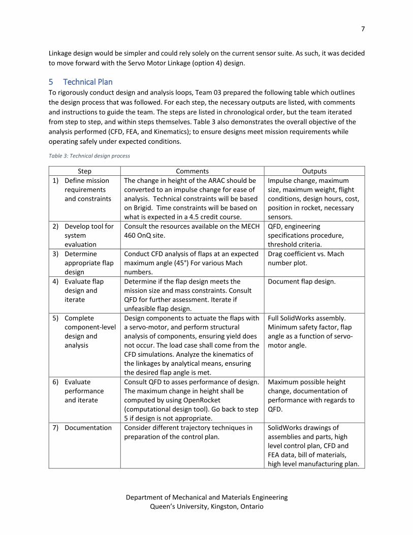
5 Technical Plan To rigorously conduct design and analysis loops, Team 03 prepared the following table which outlines

the design process that was followed. For each step, the necessary outputs are listed, with comments

and instructions to guide the team. The steps are listed in chronological order, but the team iterated

from step to step, and within steps themselves. Table 3 also demonstrates the overall objective of the

analysis performed (CFD, FEA, and Kinematics); to ensure designs meet mission requirements while

operating safely under expected conditions.

Table 3: Technical design process

Step Comments Outputs

1) Define mission requirements and constraints

The change in height of the ARAC should be converted to an impulse change for ease of analysis. Technical constraints will be based on Brigid. Time constraints will be based on what is expected in a 4.5 credit course.

Impulse change, maximum size, maximum weight, flight conditions, design hours, cost, position in rocket, necessary sensors.

2) Develop tool for system evaluation

Consult the resources available on the MECH 460 OnQ site.

QFD, engineering specifications procedure, threshold criteria.

3) Determine appropriate flap design

Conduct CFD analysis of flaps at an expected maximum angle (45°) For various Mach numbers.

Drag coefficient vs. Mach number plot.

4) Evaluate flap design and iterate

Determine if the flap design meets the mission size and mass constraints. Consult QFD for further assessment. Iterate if unfeasible flap design.

Document flap design.

5) Complete component-level design and analysis

Design components to actuate the flaps with a servo-motor, and perform structural analysis of components, ensuring yield does not occur. The load case shall come from the CFD simulations. Analyze the kinematics of the linkages by analytical means, ensuring the desired flap angle is met.

Full SolidWorks assembly. Minimum safety factor, flap angle as a function of servo-motor angle.

6) Evaluate performance and iterate

Consult QFD to asses performance of design. The maximum change in height shall be computed by using OpenRocket (computational design tool). Go back to step 5 if design is not appropriate.

Maximum possible height change, documentation of performance with regards to QFD.

7) Documentation Consider different trajectory techniques in preparation of the control plan.

SolidWorks drawings of assemblies and parts, high level control plan, CFD and FEA data, bill of materials, high level manufacturing plan.

8


6 Final Design

6.1 Overview After several iterations of design analysis, discussed in the following sections, a final design was proposed

for the Active Rocket Apogee Control (ARAC) system. The final solution utilized a servo motor to actuate

four slider-crank linkage assemblies; the ends of each slider-crank was in-turn connected to separate flaps.

When actuated, these flaps pivot such that they enter the free-stream air surrounding the rocket. The

intent of this design was to increase the total drag of the rocket in order to decrease the rocket’s speed

and hence control its apogee. The linkage components were designed such that the four flaps would be

actuated simultaneously, ensuring symmetric loading on the rocket body and maintaining stability.

6.2 CAD Model A 3D model of the flap and linkages were produced using SolidWorks to ensure their geometries fit within

the rocket tube (15.25 cm diameter) and none of the components would conflict during actuation. Several

iterations in the design were required as the analysis progressed due to identification of stress

concentrations. Figures 6-9 show the final design solution. Based on the analysis within the following

sections, it was determined that four flaps, with dimensions identified in the Appendix, symmetrically

placed around the rocket’s circumference would provide sufficient drag to effect apogee (see Section 6.3).

Note that the mechanism limited the flap angles up to 45o by mechanical stops to prevent a mechanical

singularity. As well, the weight of the system was minimized to decrease effects on Brigid’s center of mass.

PLUG PLUG

ROCKET

TUBE

Figure 6: ARAC model in fully closed state.

PLUG

ROCKET TUBE

Figure 7: Isometric view of ARAC model in max extension state.

FLAP

CONNECTING

LINKAGE

SERVO

ARM

FLAP

ARM

FLAP

Figure 8: Underside view of ARAC system near max extension; linkage mechanism identified.

9


The mechanism actuates in the following manner. The servomotor rotates the servo arm, the rotary

motion of the servo arm is converted to radial translation of the flap arm. Note that the flap arm is trapped

within the plug which limits the motion to strictly radial translation. This was a typical application of a

slider-crank mechanism. This translation is then transferred to the flaps as they pivot about their pivot

points located on the top of the plug, thus forcing the flaps to change angle.

6.3 Analysis: Computational Fluid Dynamics (CFD)

6.3.1 Definitions This section briefly covers the mathematical definitions of essential dimensionless parameters repeatedly

used in Section 6.3. These definitions are defined below in Table 4.

Table 4: Fluid dynamics dimensionless parameters.

Symbol Definition Where

𝑀𝑎 Mach number

𝑉

𝑎=

𝑉

√𝛾𝑅𝑇

𝑉 is fluid velocity, and 𝑎 is the speed of sound. Speed of sound is defined by 𝛾, the gas specific heat ratio (1.4 for air), 𝑅 ,

specific gas constant (287𝐽

𝑘𝑔 𝐾 for air) and 𝑇, gas Temperature.

𝐶𝑝

Coefficient of pressure

𝑝 − 𝑝∞

12 𝜌∞𝑉∞

2=

𝑝 − 𝑝∞

𝑝0 − 𝑝∞ 𝑝 is the local pressure, 𝑝∞ is the free stream pressure, 𝜌∞ is

the free stream density, and 𝑉∞is the free stream velocity, and 𝑝0 is stagnation pressure of the flow.

𝐶𝐷 Coefficient of

Drag

𝐹𝐷

12 𝐴𝜌∞𝑉∞

2

𝐹𝑑 is drag force, and 𝐴 is reference area.

6.3.2 Objective Computational Fluid Dynamics (CFD) is a design tool used by Engineers to understand the flow physics

around or inside a body. CFD is often used in the aerodynamic industry to optimize designs for varying

objectives. CFD will be used in the design of the ARAC to understand the following performance and design

constraints of the rocket:

1. Quantify the maximum force and moment on the flap. The ARAC system is required to be as

lightweight as possible, like all components of the rocket. The ARAC system must be optimized

such that, the materials and design minimize weight, but are still rigid enough to handle the

aerodynamic forces on the rocket.

2. Investigate CFD’s ability to model the rocket’s and the ARAC system’s aerodynamic performance.

CFD codes have often had difficulty determining absolute magnitude of the drag and lift forces on

a body. The increase in drag from the ARAC system will need to be quantified for an effective

control system. The drag values produced from CFD will be compared to empirical values at low

speeds to validate the CFD force calculations. If this can be determined the drag values of the

rocket with the brake open will be calculated.

3. Investigate the recirculating flow behind the flap. When in use, the flap separates flow from the

rocket body and creates large Eddies behind the flap. These Eddies may interact with the rocket

fins behind the flap, impeding on the rocket’s aerodynamic stability. The size and strength of the

Eddies will need to be understood, especially as speed increases and the Eddies grow and increase

10


in intensity. CFD captures the steady state solution of the flow. This won’t entirely capture the

Eddies though should give an estimate into the size of the recirculation area.

4. Determine the safe operating speeds for the ARAC system to be used. At high speeds it is expected

that the loads on the flap and the changes in stability caused by the flap could cause the rocket

to have a failure. This risk is extremely high and thus an instability condition should be given a

wide berth. The drag, center of pressure and flow conditions will be monitored as the flow velocity

increases to determine what the speed constraint on the ARAC system is.

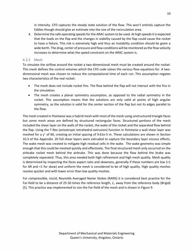
6.3.3 Mesh To simulate the airflow around the rocket a two-dimensional mesh must be created around the rocket.

This mesh defines the control volumes which the CFD code solves the various flow equations for. A two-

dimensional mesh was chosen to reduce the computational time of each run. This assumption negates

two characteristics of the real rocket:

• The mesh does not include rocket fins. The flow behind the flap will not interact with the fins in

the simulation.

• The mesh creates a planar symmetry assumption, as opposed to the radial symmetry in the

rocket. This assumption means that the solutions are only valid at points of high angular

symmetry, so the solution is valid for the center section of the flap but not its edges parallel to

the flow.

The mesh created in Pointwise was a hybrid mesh with most of the mesh using unstructured triangle faces

but some mesh areas are defined by structured rectangular faces. Structured portions of the mesh

included the shear layer on the walls of the rocket, the wake of the rocket and the separated flow behind

the flap. Using the T-Rex (anisotropic tetrahedral extrusion) function in Pointwise a wall shear layer was

meshed for a y+ of 60, creating an initial spacing of 9.61e-5 m. These calculations are shown in Section

10.3 of the Appendix. 20 full shear layers were extruded to capture the boundary layer viscous effects.

The wake mesh was created to mitigate high residual cells in the wake. The wake geometry was simple

enough that this could be meshed quickly and effectively. The final structured mesh only occurred on the

airbrake rocket mesh behind the airbrake. This was done because the flow behind the brake was

completely separated. Thus, this area needed both high refinement and high mesh quality. Mesh quality

is determined by inspecting the faces aspect ratio and skewness, generally if these numbers are low (≈1

for AR and <1 for skew) and uniform the mesh is considered to be of high quality. High quality meshes

resolve quicker and with lower error than low quality meshes.

For compressible, viscid, Reynolds Averaged Navier Stokes (RANS) it is considered best practice for the

Far-field to be a distance of 25-50 times the reference length, 𝐿, away from the reference body (Brigid)

[5]. This practice was implemented to size the Far-field of the mesh and is shown in Figure 9.

11


Figure 9: CFD mesh used for both the rocket at 0° and 45° flap angle deployment. Sizing of Far-field and areas of mesh refinement shown, as well as the types of meshes used in each zone.

The base of the rocket produces 2 counter-rotating vortices at the base, creating a low-pressure area with

high turbulent kinetic energy. As the rocket is being modelled in it coast phase where the motor has

already burned, no motor exit flow exists in this area. To mitigate this area from our calculations, the blunt

base of the rocket has been “bubbled”. This creates a circular wall around the base and keeps flow

attached longer, reducing the recirculation behind the rocket. Though this effect is not realistic to the

actual rocket, what it dissipates is called base drag. Base drag can be added to our model using empirical

formula from Fleeman [6] base drag can be added to the CD value. The formula for base drag is shown in

Section 10.4 of the Appendix. The bubble is shown in detail in Figure 10.

Figure 10: Structured mesh behind the flap shown in detail (left), mesh behind flap approximately 850,000 faces. Shear layer around bubble. Straight vertical line shows where real rocket body ends (right).

The mesh of Brigid with the airbrake deployed is a much more difficult task to resolve. The airbrake causes

flow tangential and behind the brake to be completely separated. Steady state solvers like Stanford

University Unstructured (SU2) are not designed to completely resolve separated vortices. To aid in

resolving this, the mesh on the back portion of the rocket was modified by making a highly refined,

structured mesh behind the flap. This increased the number of faces in the mesh and the computational

time by a multiple of 4 and 5 respectively.

To improve shear layer mesh transition between surfaces and to avoid flow singularities, the sharp corners

of the brake were mitigated. Manually drawn curves that approximated the corners replaced the sharp

corner connectors. This is shown in Figure 11.

12


Figure 11: Sharp corners on the flap at the base (left) and tips (right) are curved to mitigate computational singularities and aid in shear layer meshing.

The resulting meshes created were of reasonable size and resolution. It was understood that these

meshes would need to be further refined in the future to determine the mesh dependency of the outputs.

The meshes created met the skewness requirement of the standard practice for high quality meshing. The

meshes has higher aspect ratios than what is usually acceptable for meshes, though the high aspect ratio

faces were in the structured shear layer and structured flap separation area.

Table 5: Overview of mesh size and quality.

Mesh Face Count Average Aspect Ratio Average Skewness Equiangle

0° Flap 280,270 1.7215 0.102 45° Flap 1,208,724 3.23 0.406

6.3.4 Solution Setup To simulate the flow around the rocket, the mesh needs to be imported into the solver, along with

conditions for the simulation. For SU2, this is in the form of a “cfg” configuration file. In this file all

numerical, physical, solution, convergence and boundary condition settings are established. This

configuration was modified from a test case from the SU2 documentation [7].

6.3.4.1 Boundary Conditions

Boundary conditions used in the mesh are mostly labeled in Figure 9. The rocket and the bubble at the

base of the rocket have wall conditions associated to them. Wall conditions in SU2 institute that the wall

be adiabatic (zero heat flux) and no-slip velocity at the wall. The far-field conditions institute a zero-

gradient solution to the turbulence model [8], far-fields were imposed on the West, North and East

boundaries. A symmetry condition was imposed on the South boundary, as it went through the radial

symmetry of the rocket.

6.3.4.2 Viscosity and Turbulence Model

The viscosity model used for this simulation was a Sutherland viscosity model and using a Menter’s SST

model. Menter’s two equation model was chosen over Spalart-Allmaras one equation model because of

the recirculation on both the 0° and 45° behind the base of the rocket and behind the flap respectively.

The extra computational time used by a larger model was considered negligible.

13


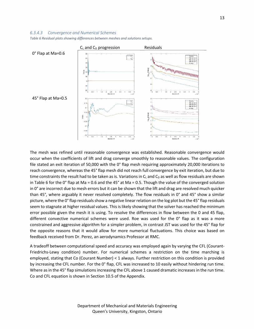
6.3.4.3 Convergence and Numerical Schemes Table 6 Residual plots showing differences between meshes and solutions setups.

CL and CD progression Residuals

0° Flap at Ma=0.6

45° Flap at Ma=0.5

The mesh was refined until reasonable convergence was established. Reasonable convergence would

occur when the coefficients of lift and drag converge smoothly to reasonable values. The configuration

file stated an exit iteration of 50,000 with the 0° flap mesh requiring approximately 20,000 iterations to

reach convergence, whereas the 45° flap mesh did not reach full convergence by exit iteration, but due to

time constraints the result had to be taken as is. Variations in CL and CD as well as flow residuals are shown

in Table 6 for the 0° flap at Ma = 0.6 and the 45° at Ma = 0.5. Though the value of the converged solution

in 0° are incorrect due to mesh errors but it can be shown that the lift and drag are resolved much quicker

than 45°, where arguably it never resolved completely. The flow residuals in 0° and 45° show a similar

picture, where the 0° flap residuals show a negative linear relation on the log plot but the 45° flap residuals

seem to stagnate at higher residual values. This is likely showing that the solver has reached the minimum

error possible given the mesh it is using. To resolve the differences in flow between the 0 and 45 flap,

different convective numerical schemes were used. Roe was used for the 0° flap as it was a more

constrained and aggressive algorithm for a simpler problem, in contrast JST was used for the 45° flap for

the opposite reasons that it would allow for more numerical fluctuations. This choice was based on

feedback received from Dr. Perez, an aerodynamics Professor at RMC.

A tradeoff between computational speed and accuracy was employed again by varying the CFL (Courant-

Friedrichs-Lewy condition) number. For numerical schemes a restriction on the time marching is

employed, stating that Co (Courant Number) < 1 always. Further restriction on this condition is provided

by increasing the CFL number. For the 0° flap, CFL was increased to 10 easily without hindering run time.

Where as in the 45° flap simulations increasing the CFL above 1 caused dramatic increases in the run time.

Co and CFL equation is shown in Section 10.5 of the Appendix.

14


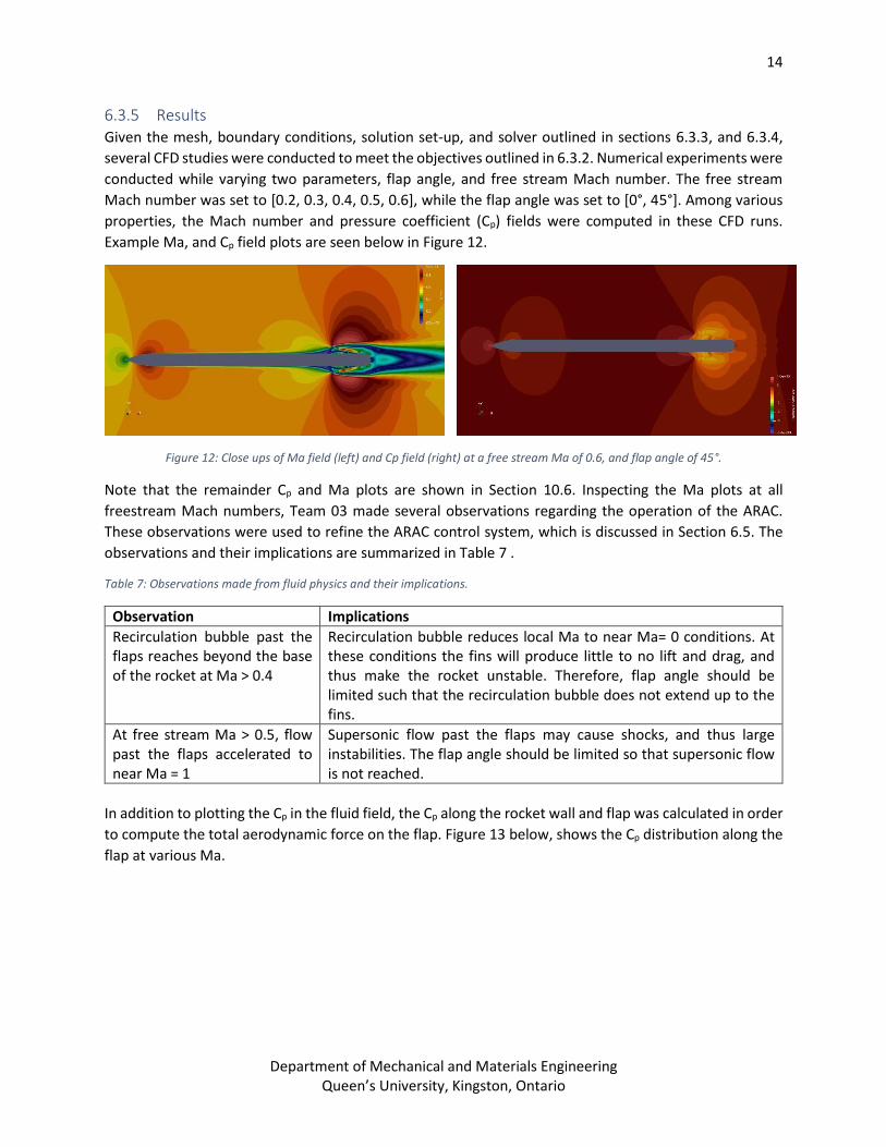
6.3.5 Results Given the mesh, boundary conditions, solution set-up, and solver outlined in sections 6.3.3, and 6.3.4,

several CFD studies were conducted to meet the objectives outlined in 6.3.2. Numerical experiments were

conducted while varying two parameters, flap angle, and free stream Mach number. The free stream

Mach number was set to [0.2, 0.3, 0.4, 0.5, 0.6], while the flap angle was set to [0°, 45°]. Among various

properties, the Mach number and pressure coefficient (Cp) fields were computed in these CFD runs.

Example Ma, and Cp field plots are seen below in Figure 12.

Figure 12: Close ups of Ma field (left) and Cp field (right) at a free stream Ma of 0.6, and flap angle of 45°.

Note that the remainder Cp and Ma plots are shown in Section 10.6. Inspecting the Ma plots at all

freestream Mach numbers, Team 03 made several observations regarding the operation of the ARAC.

These observations were used to refine the ARAC control system, which is discussed in Section 6.5. The

observations and their implications are summarized in Table 7 .

Table 7: Observations made from fluid physics and their implications.

Observation Implications

Recirculation bubble past the flaps reaches beyond the base of the rocket at Ma > 0.4

Recirculation bubble reduces local Ma to near Ma= 0 conditions. At these conditions the fins will produce little to no lift and drag, and thus make the rocket unstable. Therefore, flap angle should be limited such that the recirculation bubble does not extend up to the fins.

At free stream Ma > 0.5, flow past the flaps accelerated to near Ma = 1

Supersonic flow past the flaps may cause shocks, and thus large instabilities. The flap angle should be limited so that supersonic flow is not reached.

In addition to plotting the Cp in the fluid field, the Cp along the rocket wall and flap was calculated in order

to compute the total aerodynamic force on the flap. Figure 13 below, shows the Cp distribution along the

flap at various Ma.

15


Figure 13: Pressure coefficient along the ARAC flap at various Mach numbers.

The forces on the flap were calculate by integrating the data visualized in Figure 13 along each wall of the

flap and multiplying by the width of the flap. This analysis assumes that the pressure does not change

along the width of the flap. The assumption could not be avoided due to the 2D nature of the solution.

However, this assumption is valid as the curvature of the flap is nearly 0. The relationship between Ma

and the force on the flap was plotted and shown in Figure 14.

Figure 14 demonstrates that Team 03’s design produces significant drag (axial) forces, which have the

same order of magnitude as the base rocket. For example, at Ma = 0.6, the ARAC can produce 1100 N of

drag force (275 N per flap), more than doubling the drag and CD of the base rocket. Furthermore, this

analysis provides the loading cases necessary for the team to conduct structural calculations using FEA.

𝑀𝑎 = 0.2 𝑀𝑎 = 0.3

𝑀𝑎 = 0.5 𝑀𝑎 = 0.6

16


Since the ARAC flaps can be approximated to have a two-dimensional profile, the forces on them could

be computed. However, the same is not true for the eternity of the rocket, since it is axisymmetric. As

such, the drag or CD of the full rocket was not calculated. Further work is required to solve the three-

dimensional flow field, which can then be used to determine the overall drag of the rocket and ARAC

combination.

6.4 Finite Element Analysis (FEA) of Mechanical Components To validate that the mechanical design was robust enough to handle the expected aerodynamic loads

calculated within the CFD section above, a finite element analysis (FEA) was conducted on the flap, along

with each of the linkages within the slider crank mechanism. Due to its large size and light loading, the

ARAC plug was omitted from the analysis. Note that ANSYS Workbench software was utilized to conduct

the linear elastic study of each component individually. As such, the forces required to maintain

component’s displacement boundary conditions were propagated to the following part as reaction forces.

In this way, the aerodynamic load applied to the flap may be transferred to each successive part.

6.4.1 Feasible Design Criteria and Material Properties As the Flap component will be thrust into the free-stream air around the rocket, which travels at up to

Mach 0.8, the large drag forces the part will produce will also cause significant loading of the part. Two

criteria were identified as the structural constraints which the part must sustain in order to ensure design

feasibility.

One such constraint was that the flap must not experience a Von-Mises stress of larger than the yield

strength of the material with a safety factor of 1.5 at any point during loading. This will prevent plastic

deformation which otherwise could introduce rocket instability, decrease part longevity, and reduce the

accuracy of the ARAC system. The second structural constraint was that the flap must not deflect beyond

a certain point as this will introduce additional uncertainty in the drag characteristics which the system

relies on for accurate apogee control. Based on the sensitivity of the CFD results to flap deflection

conducted previously, the deflection threshold was determined to be 2 mm. These two inequality

constraints were defined in conventional FEA terms as follows:

Figure 14: Components of drag force with flap at 45° for various Ma.

17


𝜎𝑉𝑀 −𝜎𝑌

1.5≤ 0 (2)

𝛿𝑓𝑙𝑎𝑝 − 2 mm ≤ 0 (3)

Where 𝜎𝑉𝑀 is the largest Von-Mises stress in the component in MPa, 𝜎𝑌 is the yield strength of the

material in MPa, and 𝛿𝑓𝑙𝑎𝑝 is the largest deflection of the flap in mm. Note that, due to expertise

limitations in analyzing anisotropic materials, the carbon fiber flap was modelled using isotropic aluminum

6061 instead. For further details, refer to the material selection section. As well, initial analysis of the

slider-crank components was conducted using aluminum 6061; however, it was determined that the servo

arm would require a stronger material due to the high loads. Further discussion of this can be found in

the following servo arm analysis section.

The aluminum 6061 properties were defined as Young’s modulus of 68.9 GPa, Poisson’s ratio of 0.33, and

yield strength of 276 MPa [1]. It was initially chosen for its isotropic material properties to reduce

idealization error in the analysis, along with its high machinability and high availability to reduce

manufacturing costs.

The mechanical linkages were also modelled with the same yield criterion. However, as the system relies

on smooth motion of the slider-crank mechanism, the deflection constraints for the linkages were

decreased to prevent seizing:

𝛿𝑙𝑖𝑛𝑘𝑎𝑔𝑒 − 0.5 mm ≤ 0 (4)

Where 𝛿𝑙𝑖𝑛𝑘𝑎𝑔𝑒 is the largest deflection of any linkage in mm. Note that the tolerancing specified in the

slider-crank track must account for this maximum deflection; see the FEA recommendation section for

further elaboration.

6.4.2 Finite Element Analysis of the Aerodynamic Flaps Based on the constraints identified above, the part was analyzed using ANSYS Workbench. Preliminary

analysis revealed that the maximum load of 427 N, which would occur if the flap was opened to its limit

of 45° while the rocket was at maximum speed after burn (Ma 0.6), would cause significant stresses and

deflections on the components beyond allowable limits. As well, it was determined that minimal

asymmetricity in the system, such as not installing the ARAC plug level, would cause significant deviations

in loading because of these high forces which promoted rocket instability.

Based on the CFD analysis, it was determined that a load of 100 N per flap would provide sufficient drag

forces to effectively decrease the apogee. As such, the flap was designed to handle up to 100 N load while

satisfying the above constraints. To ensure loads on the flap would not be above this, the control system

would limit actuation to within certain regions. For more details, refer to the Control System section. Note

that the largest load on the system was determined to occur at the maximum flap angle of 45° which was

considered for the following analysis. This load was the equivalent of rocket speed of Ma 0.25, flap angle

45°. The load was applied as a uniformly distributed pressure across the surface of the flap exposed to the

incoming stream in the direction parallel to the rocket’s axis.

To decrease computation time and increase analysis accuracy, regularly shaped hexahedral elements

were defined when possible. However, due to the curvature and complex geometry in certain areas,

tetrahedral elements were required; the mesh density in these locations were increased to improve result

18


accuracy. Due to symmetry, the part was split along the plane coincident with the rocket’s axis to decrease

computation cost. The face produced by this split was constrained as necessary to reflect this symmetry

plane. Additionally, the revolute joint which the flap pivots about was set as a contact pivot joint to reflect

the pinned connection at this location. The flap was also fixed at an approximated contact patch where

the slider-crank mechanism meets the flap. Based on the geometry, the specific area of interest was about

the pivot point and neck of the flap; as such, the local behaviour about the fixed contact patch was not

necessary for the analysis. In this way, approximating an otherwise complex contact analysis was justified.

The part was separated into 12 volumes identified by distinct local geometries in order to maximize mesh

quality and computation time. For the simple volumes, such as the bottom of the flap, a highly structured

hexahedral mesh was utilized with aspect ratio of nearly one. However, to accommodate the complicated

geometries such as near the neck and fillets, a hybrid meshing technique was necessary. The following

photos display the boundary conditions, loads applied to the flap, and mesh utilized. Also included are the

deflection and stress contour plots calculated based on this analysis; see Table 8 for a summary of results.

Table 8: Summary of FE analysis results.

Constraint Maximum Value Location Satisfied

Maximum Deflection 1.24 mm Bottom (tail-end) of flap Meets criteria

Maximum Stress 185 MPa Slotted connection point to slider crank Meets criteria

From the analysis, the reaction force at the fixed contact patch was also calculated to be approximately

200 N acting colinear to the flap arm linkage. These solutions were as expected based on preliminary

calculations. Based on the above, it can be seen that the feasibility constraints have been maintained; as

such, the flap design is expected to sufficiently handle the loading conditions.

6.4.3 Finite Element Analysis of a Flap Arm To analyze the structural integrity of the flap arm design, the 100 N force applied directly to the flap had

to be propagated to the flap arm by determining the reaction force at the pin that connects the flap to

the flap arm. This method is not 100% accurate but serves as a good estimate given that a full assembly

analysis of the system is beyond the capabilities of the team at their education level. A reaction force of

Figure 15: Deflection of flap based on maximum loading scenario.

Figure 16: Stress contour plot across exposed flap surface.

Figure 17: Deflection contour plot of flap. Figure 18: Loading and boundary conditions applied to flap.

19


approximately 200 N was determined and applied to the end of the flap arm that attaches to the flap’s

pin as seen in Figure 23. To satisfy this boundary condition assumption for further components – the

linkage and the servo arm – the opposite end of the flap arm was fixed in all directions. The reaction force

of 200 N at this fixed end is then applied to the linkage, and to the servo arm. Because the system is

assumed to be horizontally linear from this point to the servo arm, the assumption is made that there are

minimal losses between the flap arm and the linkage and the linkage and the servo arm, so the 200 N

remains a constant applied force to all 3 components. In addition, the loads were applied as bearing loads

to get a better estimate of the deformations expected at the bolt holes. Using a mesh size of 0.75 mm,

the stress contours and deflections of the flap arm were calculated and can be seen in the following

figures. The results of this analysis are summarized in Table 9.

Table 9: Summary of FEA results for the flap arm with an applied load of 200 N.


Maximum Deflection

0.00425 mm End of flap arm at slotted connection point to

slider crank Meets criteria

Maximum Stress 27.748 MPa Point of applied load Meets criteria

The original design for the flap arm was not thick enough in the vertical direction which induced a bending

moment in the prongs. This caused the threshold deflection of 0.5 mm to be surpassed. To resolve this

issue the flap arm was increased 2 mm in thickness in the vertical direction. As can be seen from the

results in Table 9, the deflection is now within the acceptable range. This modified design is now expected

to sufficiently handle the expected loading conditions and has been approved to continue through the

remainder of the analysis.

Figure 19: Loading of 200 N and boundary conditions applied to the flap arm in the directions shown. Point A is fixed in

space.

Figure 20: Stress [MPa] contour plot on all surfaces of the flap arm.

Figure 21: Deflection [mm] of the flap arm based on the maximum loading of 100 N on the flap, which is then

propagated through to the flap arm at 200 N.

Figure 22: Side view of the deflection [mm] of the flap arm.

20


6.4.4 Finite Element Analysis of Connecting Linkage A force of 200 N was applied as a bearing load to the linkage at the point where it connects to the flap

arm. This force is in the direction of the length of the linkage, and similar to the flap arm, the other end

of the linkage is fixed in space. Using a mesh size of 0.75 mm, the stress contours and deflections of the

flap arm were calculated and can be seen in the following figures. The results of this analysis are

summarized in Table 10.

Table 10: Summary of FEA results for the linkage with an applied load of 200 N.


Maximum Deflection 0.00278 mm End of linkage connected to the flap arm Meets criteria

Maximum Stress 10.879 MPa Point of applied load Meets criteria

No modifications were made to the original linkage design. The shape of the part does not encourage

stress concentrations at specific points, and as such the load distributed well along the length of the part.

Minimal deflection is noted at the end where the load is applied, but is well below the constraint of 0.5

mm. The same can be found for the stress, which is much less than the yield strength of aluminum. The

part is said to satisfy all constraints and can be used for further analysis of the system.

6.4.5 Finite Element Analysis of the Servo Arm The servo arm takes the highest load of all the parts, even more than the flaps themselves. The

propagated force of 200 N is applied as a bearing force at each of the 4 corners of the servo arm

perpendicular to the radial direction. This means that the servo arm experiences a load of 800 N total for

this analysis. Given this increased loading, the material selected for the servo arm composition was

Structural Steel A36 with Young’s modulus of 200 GPa, Poisson’s ratio of 0.26, and yield strength of 250

MPa [9]. Using a mesh size of 1 mm, the stress contours and deflections of the servo arm were calculated

and can be seen in the following figures. The result of this analysis is summarized in Table 11.

Figure 23: Loading of 200 N and boundary conditions applied to the linkage in the direction shown. Point A is fixed in space.

Figure 24: Stress [MPa] contour plot on all surfaces of the linkage.

Figure 25: Stress [MPa] contour plot of the top surface of the linkage with an applied load of 200 N.

Figure 26: Deflection [mm] of the linkage. Deflection is greatest at the end where the force is applied.

21


By performing FEA on the initial servo arm design (as seen in Figures 31 - 34) it was found that it yielded

under the loads applied. The servo arm was then improved upon by expanding the size of the fillets

between each of the 4 corners, and increasing the thickness by 3 mm. This brought the maximum stress

below the yield as discussed below.

Table 11: Summary of FEA results for the servo arm with an applied load of 200 N at each corner.


Maximum Deflection 0.04056 mm Corners of servo arm Meets criteria

Maximum Stress - Singularity 377.7 MPa Center bolt hole Does not meet criteria

The maximum stress in the servo arm exists at the center bolt hole with a magnitude of 377.7 MPa, far

over the yield of the material. However, upon analysis of Figure 32 and Figure 33 above, it was determined

that this high stress concentration can be considered a singularity within the finite element analysis.

Singularities occur at the location of an applied point load, which is only a theoretical possibility. Due to

the lack of real point loads in this system, this singularity can be ignored and the stress concentration

around the bolt hole assumed to be between 53.997 MPa and 215.85 MPa which satisfies the yield

strength of this A36 steel.

Figure 27: Loading of 200 N and boundary conditions applied to the servo arm in the directions shown. Point E is fixed in space.

Figure 28: Stress [MPa] contour plot on all surfaces of the servo arm.

Figure 29: Stress [MPa] contour plot of the top surface of the servo arm with an applied load of 200 N at each corner. Stress

is concentrated at the center of the servo arm where it connects to the servo.

Figure 30: Deflection [mm] of the servo arm. Deflection is greatest at the corners where the forces are applied.

22


6.5 Control System A high-level overview of the control system required for the ARAC was created. This system must be

reliable, accurate, and fast. In order to create this system, the relationship between the servo angle and

flap angles was determined. Furthermore,

6.5.1 Kinematics In order to design the control system, first the mechanical system must be understood. Therefore, a

kinematic analysis was conducted. A bottom view schematic of the system in its resting position can be

seen in Figure 31, with the flaps resting flush against the body of the rocket. The lengths of each link, 𝐴,

𝐵, and 𝐶, can be seen in Table 12. 𝜃 is defined as the angle the servo (installed at the center joint) has

rotated clockwise from the resting position. 𝛼 and 𝛽 are respectively the angles of the servo arm and

connecting linkage from the axis of the flap arm. As the servo arm turns, the flap arms are pushed

outwards, each constrained to move along a single radial axis. This subsequently pushes the flaps into an

extended position. A bottom view schematic of the system in its active position can be seen in Figure 32,

with the flaps extended from the rocket body. Additionally, a side view schematic of the same position

can be seen in Figure 33. Δ is the distance the flap arm has extended along its axis, ℎ is the height the flap

joint sits above the planar mechanism (value in Table 12), and 𝛾 is the angle between the flap and the

rocket body.

Figure 31: Bottom view schematic of mechanism in resting position (flap in neutral position, flush with rocket body).

Figure 32: Bottom view of schematic in active position (flap

extended).

Table 12: Important mechanism dimensions.

Dimension Length [mm]

Inner link length, 𝑨 21.6

Middle link length, 𝑩 38.1

Outer link length, 𝑪 34.9

Flap joint offset from planar mechanism, 𝒉 18.0

Rocket radius, 𝑹 72.9

(a) (b)

23


The relationship between the servo motor angle, 𝜃, and the flap angle, 𝛾, must be determined. Using the

rocket radius, 𝑅, listed in Table 12, 𝛼 at the rocket’s resting position can be found using cosine law:

𝛼 = cos−1 (𝐴2 − 𝐵2 + (𝑅 − 𝐶) 2

2𝐴(𝑅 − 𝐶)) (5)

Using the values from Table 12, it was determined that at resting position 𝛼 = 73.8°. The relationship

between 𝛼 and 𝜃 is:

𝛼 = 73.8° − 𝜃 (6)

𝛽 can be determined from 𝛼 as follows:

𝛽 = sin−1 (𝐴 sin 𝛼

𝐵) (7)

The length of the mechanism in meters along the axis of the last link, 𝐿, can be written as:

𝐿 = 𝐴 cos 𝛼 + 𝐵 cos 𝛽 + 𝐶 (8)

The distance in meters that the outer link has extended, Δ, is therefore:

Δ = 𝐿 − 𝑅 (9)

From Figure 33, it is evident that:

𝛾 = tan−1 (Δ

ℎ) (10)

Combining Equations 6, 7, 8, 9, and 10 gives 𝛾 as a function of 𝜃:

𝛾 = tan−1 (𝐴 cos(73.8° − 𝜃) + 𝐵 cos (sin−1 (

𝐴 sin(73.8° − 𝜃)𝐵 ) ) + 𝐶 − 𝑅

ℎ) (11)

This equation can be rearranged to give 𝜃 in terms of 𝛾 (using Wolfram|Alpha [10]):

Figure 33: Side view schematic of mechanism in active position (flaps extended). Planar mechanism not visible in side view.

24


𝜃 = 73.8° − cos−1 (−𝐴2 + 𝐵2 − 𝐶2 + 2ℎ(𝐶 − 𝑅) tan 𝛾 + 2𝐶𝑅 − ℎ2 tan2 𝛾 − 𝑅2

2𝐴(𝐶 − ℎ tan 𝛾 − 𝑅)) (12)

The relationship between 𝜃and 𝛾 can be seen graphically in Figure 34.

It should be noted that a singularity occurs when the mechanism is at maximum extension (𝜃 = 73.8°).

However, this is not a concern as the flap angle, 𝛾, is mechanically limited to never exceed 45° to avoid

damage to the flaps from large loads, thus 𝜃𝑚𝑎𝑥 = 46.6° and the system will never reach the singularity.

Figure 34: Flap angle, 𝛾, as a function of servo motor angle, 𝜃.

6.5.2 Apogee Prediction The apogee of the rocket, 𝑧𝑚𝑎𝑥 (m), can be related to the terminal velocity, 𝑣𝑡 (m/s), instantaneous

vertical velocity, 𝑣𝑧 (m/s), current altitude, 𝑧 (m), and gravitational acceleration, 𝑔 (m/s2), by (modified

from reference [11]):

𝑧𝑚𝑎𝑥 =𝑣𝑡

2

2𝑔ln (

𝑣𝑧2 + 𝑣𝑡

2

𝑣𝑡2 ) + 𝑧 (13)

Due to the complexity of this equation, it was determined that having the controller refer to a set of pre-

tabulated values would be more computationally efficient than solving Equation 13 for 𝑣𝑡. Based on

instantaneous measurements of 𝑣𝑧 (determined from the pitot tube in conjunction with the orientation

sensor) and 𝑧, along with constant 𝑔 (9.8 m/s2) and 𝑧𝑚𝑎𝑥 (3048 m), the desired value of 𝑣𝑡 can be

interpolated from this table. Using this, the desired coefficient of drag, 𝐶𝑑, can be calculated from:

𝐶𝑑 =2𝑚𝑔

𝑣𝑡2𝜌𝐴

(14)

25


Where 𝑚 is mass of the rocket (kg), 𝜌 is air density (kg/m3), and 𝐴 is the cross-sectional area of the rocket

(m2).

The coefficient of drag, 𝐶𝑑, is a function of both flap angle, 𝛾, and total velocity, 𝑣. The relationship

between these values must be determined experimentally or using computational fluid dynamics. For the

control system, an additional table will be compiled such that the system can interpolate to find the

appropriate flap angle to achieve the desired drag for a given velocity. The development of this table is

part of recommended future work, discussed in Section 8.4.

It should be noted that Equations 13 and 14 assume the coefficient of drag does not vary with velocity. As

drag on the rocket was largely dependent on pressure differential across the flap, as discussed within the

CFD analysis in Section 6, the coefficient of drag is largely a function of velocity for the proposed system.

By recalculating the coefficient of drag throughout the flight, the effects of approximating 𝐶𝑑 as constant

are mitigated. Hence, a fast processor is necessary such that the time between calculations is decreased

to improve the accuracy of this assumption.

6.5.3 Control Structure With the known relationships defined in the previous two sections, a proper control structure can now be

described. A flowchart outlining the control structure can be seen in Figure 35. The program initializes

when the system is powered on at the launch rail in preparation for flight. The system then constantly

measures acceleration using an accelerometer and waits until motor ignition has begun, which is

characterized by high upward acceleration. The maximum estimated upward acceleration is 112 m/s2,

however, to maintain a safety factor, 50 m/s2 can be used as the indicator. The rocket will never reach

this acceleration before motor ignition, thus the system will not be prematurely triggered. The system

then returns to measuring acceleration and waits until burnout is complete, which is characterize by a

downward acceleration of approximately 9.8 m/s2. This ensures the system will not deploy during the

burn phase of flight, as the apogee is difficult to predict at this phase and deployment of the flaps could

cause problems with stability.

Once the motor burnout is complete, the system measures velocity using a pitot tube inserted in the tip

of the rocket’s nosecone and altitude using an altimeter. The system will not actuate the flaps until

velocity is less than the system’s rated maximum velocity of Mach 0.5 to maintain stability. Once the

velocity is in the acceptable range, the desired terminal velocity is interpolated from a precalculated table

of terminal velocities for different instantaneous velocities and altitudes. This terminal velocity is then

used in Equation 14 to calculate the desired drag coefficient. An appropriate flap angle can then be

interpolated from a table of associated flap angles, drag coefficients, and velocities determined from the

CFD analysis. Thus far the drag has only been determined for a flap angle of 45° at various velocities,

however future work includes determining drag for different angles, as discussed in Section 8.1. Finally,

the servo motor angle will be calculated using Equation 12 and the servo will be actuated to this angle.

After every measurement the program checks if altitude is decreasing, indicating that apogee has been

reached. When this is true, the system will pull in the flaps before shutting down, to prevent damage to

the flaps on impact.

26


Figure 35: Control algorithm overview of the Active Rocket Apogee Control (ARAC) system.

27


6.5.4 Servo Motor In order to properly size a servo motor, the maximum expected torque on the motor must be calculated.

The flaps have been designed to experience a maximum downward (parallel to the rocket) load of 100N.

The controls shall limit the maximum angle of the flaps such that a downward load greater than this is

never experienced. The force propagated to the linkage mechanism will be greatest at the maximum

possible extension of the flaps, when 𝛾 = 45°.

Free body diagrams of the planar linkages can be seen in Figure 36. As discussed in Section 6.4, using FEA

it was determined that 200N is propagated to the flap arm, perpendicular to the rocket surface. This is

represented as 𝐹𝑥𝑓𝑙𝑎𝑝. The sum of forces on the flap arm in the x-direction are zero, therefore:

|𝐹𝑥1| = |𝐹𝑥𝑓𝑙𝑎𝑝| (15)

The net torque on the connecting linkage is zero, therefore 𝐹1 must be along the axis of the linkage. This

yields:

𝐹1 =𝐹𝑥1

cos 𝛽(16)

The sum of forces on the connecting linkage in the x-direction and y-direction are zero, therefore:

|𝐹2| = |𝐹1| (17)

The net torque on the servo arm must be zero, therefore:

|𝜏𝑀| = |𝐹2 cos(𝛼 + 𝛽 − 90°) 𝐴| (18)

Combining Equations 15, 16, 17, and 18 yields:

|𝜏𝑀| = |𝐹𝑥𝑓𝑙𝑎𝑝

cos 𝛽 2

cos(𝛼 + 𝛽 − 90°) 𝐴| (19)

Figure 36: Free body diagrams of planar linkages when net torque and net acceleration are zero. From left to right: servo arm, connecting linkage, flap arm.

As stated in Section 6.5.1, when 𝛾 = 45°, 𝜃 = 46.6°. Using Equation 6, 𝛼 is found to be 27.7°. Equation 7

subsequently gives 𝛽 = 15.3°. Substituting all values into Equation 19 produces |𝜏𝑀| = 3 N ∙ m. This is

the torque to maintain a single flap at 45° for a downward force of 100 N. To maintain four flaps in this

configuration, 12 N∙m would be required.

A servo motor was chosen rather than a DC motor or stepper motor, as servos offer higher torque and

precision. The RMCS-225X High-Torque Encoder DC Servo Motor and Driver is capable of a maximum 11.8

28


N∙m [12]. This is slightly less than the required torque and provides no safety factor, however it is unlikely

that a higher torque DC servo motor can be found. This servo motor weighs 0.350 kg and takes up a

volume of 120 mm × 60 mm × 60 mm. A 12 V DC power supply capable of providing up to 7.5 A is required

for this servo.

6.5.5 Microcontroller The STM32 USB Development Board can be used as a microcontroller for this system [13]. This board

features 29 I/O pins and 10 analog inputs, which is capable of supporting the required sensor suite. It has

128 KB of flash, 20 KB of RAM, and a clock speed of 72 MHz. The STM32 can also connect to external

memory cards to store large data sets, allowing the board to save data for post-flight processing. The board

is also only 53 mm × 22 mm, weighs 0.036 kg, and costs $5.50. Finally, this board is opensource with many

user tutorials and can be programmed using the Arduino IDE, making it user-friendly.

6.5.6 Accelerometer/Orientation Sensor and Altimeter The Adafruit BNO055 Absolute Orientation Sensor can provide the absolute orientation of the rocket as

well as its acceleration vector [14]. It is user friendly, compatible with the chosen microcontroller, and

reads data at a frequency of 100 Hz. It been previously used by QRET and the team already has a BNO055

which it can provide at no cost.

The MPL3115A2 – I2C Barometric Pressure/Altitude/Temperature Sensor can measure altitude up to

10,000 m at a resolution of ±0.1 m and a frequency of 100 Hz [15]. This sensor has also been previously

used by QRET and can be provided at no cost.

For the airbrake to be deployed, the rocket should be travelling no higher than Ma 0.5, which is

approximately 200 m/s at the rocket’s temperature and pressure during flight. With a frequency of 100 Hz,

this yields one measurement every 2 m, minimum. This is reasonable, as the OpenRocket model predicts

motor burnout at 581 m after 3.5 s, and velocities below Ma 0.5 at 2172 m after 10.5 s. This would allow

the ARAC 876 m to make a minimum of 438 measurements and subsequent adjustments.

6.5.7 Pitot Tube A pitot tube is recommended for this control system, as the integration of acceleration to determine

velocity is highly inaccurate, and velocity is critical to apogee prediction. Selecting a pitot tube for the

purpose of this project is complex, as a supersonic pitot tube would be necessary. Additionally, the

geometry and layout of the rocket complicates pitot tube choice. It was therefore determined that pitot

tube optimization is outside the scope of this project and left as future work, as discussed in Section 8.4.

6.6 Materials Selection and Economic Analysis QRET has a variable budget for the implementation, manufacturing, and assembly of the active rocket apogee control system pictured below.

29


The chosen design, Servo Motor Linkage, will be first constructed for a kit rocket, which is simply a small-

scale rocket on the order of 4 feet tall with a 4” diameter, in which all the parts come together in a

package. Kit rockets are a great way to test new technologies that can later be implemented on the full-

size competition rocket. Because the kit rocket only flies to an apogee of roughly 1,000 ft, the forces acting

upon the airbrake design are much less, therefore 3D printing may be used. A full analysis of the cost for

the implementation of the smaller ARAC system will be detailed in MECH 462. The scope of the project in

MECH 460 is for the feasibility of the system on the full-scale 6” diameter competition rocket, and as such

is analyzed below. The materials selected for the Servo Motor Linkage design are as follows; their

justifications can be found below the table:

Table 13: This materials list is based off of Figure 41. Tax and shipping not included. All aluminum and steel parts estimates made from McMaster Carr.

Part Name Machined [yes/no]

Material Cost [CND]

Aerodynamic Flaps (x4) no Carbon Fiber $40.00

Flap Arm (x4) yes Aluminum 6061 $10.00

Linkage (x4) yes Aluminum 6061 $10.00

Servo Arm (x1) yes Aluminum 6061 $20.00

Plug (x1) yes Aluminum 6061 $90.00

RMCS-225X High-Torque Encoder DC Servo Motor and Driver (x1) [12]

no Off the shelf $117.80

STM32 USB Development Board (x1) [13] no Off the shelf $5.50

Adafruit BNO055 Absolute Orientation Sensor (x1) [14]

no Off the shelf -

MPL3115A2 – I2C Barometric Pressure/Altitude/Temperature Sensor (x1) [15]

no Off the shelf -

Screws - Flap to Flap Arm (x8)

no Steel (Grade 5)

$9.00 (x20) Screws – Flap Arm to Linkage (x4) no Steel (Grade 5)

Screws – Linkage to Servo Arm (x4) no Steel (Grade 5)

Total $473.30

PLUG

ROCKET TUBE

Figure 37: Isometric view of ARAC model in max extension state.

30


6.6.1 Carbon Fiber The aerodynamic flaps will be made of carbon fiber so that when the system is inactive, the flaps integrate

seamlessly into the carbon fiber body of the rocket. Due to the team’s limited experience with ANSYS,

FEA was performed on the flap assuming its material was aluminum 6061. It can be assumed for the

purposes of this project that the structural limits of the carbon fiber flaps are the same if not higher than

the aluminum flaps analyzed in Section 6. The flaps will be cut from the same carbon fiber tube that is

used to make the rocket to ensure a perfect fit. Since the carbon fiber tube consists of 4 layers of carbon,

ANSYS will be used to perform Finite Element Analysis to ensure the structural integrity of these flaps.

Once cut from the tube, the carbon fiber flaps can be laid-up further with additional layers of carbon fiber

should the FEA results require it. This is explained further in Section 8.2 of the report.

6.6.2 Aluminum 6061-T6 The remainder of the system – the flap arms, linkages, and plugs– will be manufactured out of aluminum

due to its high strength to weight ratio. FEA has been performed on a flap arm and linkage as seen in

Section 6.4.

6.6.3 Grade 5 Steel Most commonly used for automotive applications, Grade 5 steel is standard Grade 2 steel that has been

through a hardening process to increase strength. As the forces acting on the screws in this system will be

rather large, hardened steel is critical for successful ARAC actuation. The servo arm will be manufactured

out of A36 Structural Steel due to the immense loading it is put under to deploy the flaps. A further

discussion of this choice was seen in Section 6.4.

6.6.4 Machining Several components will be machined out of aluminum and steel by the McLaughlin Machine Shop in

second semester. Although the servo motor comes with its own servo arm, the team has chosen to

manufacture their own servo arm out of steel to maintain quality assurance. The linkages, flap arms, and

plug will be manufactured out of aluminum. The manufacturing will be done by the members of the team

to save money on labour costs.

6.6.5 Servo Motor A servo motor will be purchased off the shelf, not custom designed as that is outside the scope of this

project. The motor will need to have enough torque to open the flaps, which will require the purchase of

an expensive servo motor. The chosen servo motor is discussed in Section 6.5.4.

7 Project Planning

7.1 Risk Management Various safety and design risks were taken into account when designing this system to ensure successful

actuation. Many of the risks associated with the system rely on the successful implementation of the

controls system, which as mentioned is beyond the scope of this project. Regardless, the table below

summarizes the expected risks and their respective mitigation strategies.

31


Table 14: Table of risks and their corresponding mitigation strategy.

Risk Risk Mitigation Strategy

Pre-flight damage to flap, flap arm,

linkage, servo arm, or servo system.

Travelling to and from New Mexico with the rocket and its subsequent systems poses a great threat to the integrity of the rocket and its assembly. Every year QRET creates an APSC 100 Mod 3 project to manufacture a new case for the rocket. This year’s case would have a special compartment to house the ARAC system, as well as a portable container to place the ARAC system in when carrying it around on site in the desert. Sand is a threat to the slider-crank assembly, as well as the servo motor itself and should be mitigated.

Insufficient data collection in-flight

There is the possibility that the system does not collect data correctly or at all during flight. To mitigate this issue the system would be programmed to default to an inactive setting should it not receive the data necessary to make a decision to actuate the system.

Premature deployment of the

system during flight

The premature deployment of the system would be due to faulty programming. If programmed as mentioned above, pre-mature deployment should never be possible.

In-flight flap breakage

This would likely be due to the above-mentioned premature deployment of the airbrake due to the high speeds at which the rocket could be travelling if the system were actuated too early. To account for this possibility, the flaps have been designed to withstand forces 1.68 times greater than predicted at the actuation speed. This will allow for a small margin of error, however if the ARAC system is accidentally actuated at speeds any higher than Mach 0.5, the flaps and associated internal components will likely not be able to withstand the forces exerted upon them.

32


7.2 Project Schedule The Gantt chart below outlines the tasks completed by the team throughout the duration of the project. Note that the timeline for the

preliminary CFD changed due to issues with modelling methods experienced early on in October. This prevented the CFD, CAD, and FEA

optimizations from taking place until later in November and December. The schedule proved to be optimistic, however all tasks were

accomplished by the submission date of December 5th.

Figure 38: Team 03 Gantt chart outlining key events and deadlines throughout the semester.

33


8 Discussion and Future Recommendations The following section discusses recommendations for future work to improve the accuracy of the

modelling, expansion of the analysis scope to provide additional information, and a discussion of

considerations.

8.1 Computational Fluid Dynamics Conclusions Recommendations

8.1.1 Conclusions Team 03 developed a methodology for resolving the fluid field around the rocket and ARAC system. This

methodology will be of great use to QRET as their aerodynamics team members may refer to it and expand

on Team 03’s efforts. The CFD studies helped the team to quantitatively and qualitatively understand

various aspects of the ARAC’s flow physics. Flow regimes and flap angles where the ARAC was deemed

unstable were identified and used to guide the development of the control system. Additionally, the

aerodynamic forces on the ARAC flap were computed at various Mach numbers, which were used as load

cases in the structural analysis.

8.1.2 Future Objectives For the team to gain enough confidence to flight test the proposed ARAC, several questions regarding the

aerodynamics, and CFD analysis of the system must be answered.

1. If a 2-D symmetric RANS case cannot produce accurate CD values, what mesh and configurations

can? Once values are within reasonable territory of empirical formula’s, how will the reduced, but

not distinguished, base drag be combined with CFD results?

2. A mesh convergence study is necessary to discover the mesh dependency of the solutions gained.

It was known that the meshes used were of, or close to, minimum resolution, further simulations

with more refined meshes are required.

3. If the flap at 45° produces too much load for the components at Ma>0.25, what is an acceptable

angle at higher Ma numbers? Before a control system can be accurately designed, the loads within

the studied speed range needs to be understood for different flap angles.

4. The solutions produced showed that the recirculation area created by the flap was large and of

significant energy. Future studies should investigate the effect of this recirculation on fin

pressures behind the flap. It is expected that the recirculation will reduce fin pressure and thus

decrease aerodynamic stability.

8.1.3 Mesh It is recommended that a similar mesh generation procedure to the present work is followed but adapted

to a 3D mesh. The same number of meshes, wall spacing calculations, and boundary conditions may be

used. It is also advised that a structured mesh is generated rather that an unstructured mesh due to the

increase in computation speed and accuracy. To generate the 3D meshes, one may take the current 2D

meshes and revolve them by 180 to produce a half section of the rocket. Symmetry conditions may be

used as in the 2D case to avoid computing the flow field around the whole rocket. Special attention must

be taken to insert the rocket’s fins in the revolution, as the fins are not modeled in the 2D case. Similarly,

to the ARAC flap, mesh refinement must be performed in the region after the fin to ensure that the fin’s

wake is adequately captured. Lastly, the density of the 3D mesh shall be decreased such that the total

number of cells does not surpass 1,000,000. Producing meshes with more than 1,000,000 cells will require

more computational power than QRET currently has access to.

34


8.1.4 Solution Setup and Schemes Much of the same approach taken in the present work can be mimicked to run three dimensional RANS

CFD studies. Adapting configuration files from a 2D case to a 3D case is a trivial task. However, it is

recommended that QRET explores the use of Large Eddy Simulation (LES), which is a type of CFD

turbulence model that more accurately captures vortex phenomena. This technique may prove

specifically useful in resolving the interaction of the flaps with the fins. Prior to flight testing, QRET must

demonstrate (either experimentally or numerically) that the presence of the flaps will not render the

rocket’s fins useless.

8.2 Finite Element Analysis Recommendations Due to the complex geometry of the part, along with expertise limitations, the Finite Element Analysis

conducted required several approximations. One approximation which may not accurately represent the

real system relates to the contact patch between the flap and the flap arm pin (Figure 18). In the model,

this connection was estimated as a perfectly fixed face; however, in reality the pin at this location will

experience sliding as the flap arm deflects under load. If the arm were to deflect significantly, this will

change the location of the contact patch and thus change the structural characteristics of the flap.

Incorporating this level of detail within the FEA model requires additional time and expertise beyond the

expectation of the project scope; however, it was recommended that any future work should consider

this aspect of contact stress analysis.

Furthermore, in order to more accurately represent the real system, consider developing an assembly

model with the various linkages, flap, and their connecting pins included. By introducing this

interdependency amongst the parts of the system, the stresses and deflections of one component would

directly propagate through the linkage system. This level of analysis would yield the compounded

deflection values necessary for determining if the linkage will bind under load.

As well, consider conducting a transient analysis in which the pressure load applied to the flap not only

changes with time, but also across the face of the flap. This requires additional and more detailed CFD

analysis; however, if implemented, can provide valuable information relating to the control system

necessary for flap actuation as well as rocket stability.

Although the flaps were modeled as aluminum in ANSYS, the flaps are expected to be machined out of

carbon fiber for the implementation of the system in Brigid. It is suggested that FEA be performed on the

flaps assuming that they are made of carbon fiber. While this is difficult to do and at this time beyond the

capabilities of the team members, given more time the required skills could be learned and an appropriate

analysis conducted.

Lastly, due to the rocket’s sensitivity to weight, it was recommended that topology optimization be

conducted. The ARAC plug would benefit significantly from this as it had the largest volume of all

components, fewest design constraints, and experienced the smallest loading. As such, it was expected

that most weight savings may be obtained from optimization of this part.

8.3 Manufacturing Due to the complexity of the part, it is recommended that a 4-axis or greater CNC milling machine be

utilized for manufacturing the flap, while the linkages may be manufactured using a 3-axis milling

machine. The plug which fixes the ARAC assembly to the rocket tube should be hybrid machined using a

35


lathe and 3-axis mill. The hardware, including the pins, screws, and servomotor, should be bought off-the-

shelf components. components necessary for the ARAC system to function.

To save on time and manufacturing costs during the prototyping process, it is recommended that one arm

of the system, where an arm consists of one of the four flaps with supporting linkage assembly, be 3D

printed using ABS. This will better identify the scale of the parts which may provide useful information

which can be used to adjust the model. Then, one arm should be manufactured to scale from the chosen

6061 aluminum material. Extensive testing of this part should be conducted on a test-stand similar to that

of the ARAC plug; specifically, the flap and linkage mechanism should be tested under load to determine

if binding is of concern.

If it was determined that binding of the mechanism occurs under load, the tolerancing of the linkage tracks

should be further modified. If binding persists, consider replacing the linkage material with one that has

a higher modulus of elasticity. As well, although not expected based on the above analysis, ensure none

of the components yield while testing; if any plastic deformation occurs, the material of that linkage or

flap should also be replaced with a stronger counterpart.

8.4 Controls Within the scope of this project, only a high-level overview of the controls was developed. The control

system still requires coding and all hardware must be assembled and wired according to the specifications.

Additionally, the tables discussed in Section 6.5.2 must be created and saved on the microcontroller.

These tables can be created with further computational dynamics or through air tunnel testing.

Some hardware components must also be selected. As discussed in Section 6.5.7, the optimization of a

pitot tube is outside the scope of this project, as the geometry and layout of the rocket as well as the flight

conditions limit the available options. An alternative solution would be the development of a custom pitot

tube for the conditions expected.

Additionally, a power source must be chosen for both the microcontroller and the servo motor. This

introduces numerous challenges as batteries will need to be large as the system may be powered on the

launch rail for an undetermined amount of time, as the time between set-up and launch can be

unpredictable and lengthy. One possible solution to this challenge could be the integration of the ARAC

with the on-board avionics, such that the ARAC is only powered once the avionics find that motor burnout

is complete. This, however, is not ideal, as having the ARAC system separate makes it independently

reliable and does not limit the placement of the avionics within the rocket. Furthermore, the servo motor

will also require a large battery as it pulls up to 7.5 A at 12 V. It will require a large power supply in order

to supply the required torque for prolonged periods of time. The placement of these batteries must also

be considered carefully as weight distribution is critical to rocket stability, however they also cannot be

placed too far from the ARAC system itself.

Given that such a high torque servo motor is required, alternative solutions should also be investigated,

given more time. It is possible that a smaller, lighter servo motor and power source may be used. Due to

time restrictions, it was not possible to determine accurately what maximum change in apogee the

proposed ARAC can achieve. If the required forces have been overestimated, a smaller servo may be a

superior alternative.

36


It would also be ideal to compare multiple control methods. The chosen method relies on known

coefficients of drag. An alternative possibility considered was the implementation of PD control. The

control could calculate what its apogee will be from its known velocity, acceleration, and altitude. The

flaps would then be adjusted proportionally to how far from its target apogee it estimates it will be and

how quickly that estimated apogee is changing. Since the system can only reduce apogee, this would need

to be done conservatively as slowing the rocket excessively would not be reversible.

The control system should also be tested. A number of tests can be performed, including physically

measuring the amount of torque the servo can provide and the maximum angle it can maintain with a

downward force of 100 N. Additionally, the system can be given simulated data to ensure it responds as

expected. Wind-tunnel testing would be ideal as this would allow the team to measure the system’s

response in a controlled environment. Finally, a test launch should be performed with this system before

competition to ensure functionality in an unstructured environment.

37


9 Bibliography

[1] Queen's Rocket Engineering Team (QRET), "Queen's Rocketry," 2018. [Online]. Available:

http://queensrocketry.ca/. [Accessed 8 October 2018].

[2] Experimental Sounding Rocket Association (ESRA), "Spaceport America Cup," 2018. [Online].

Available: https://www.spaceportamericacup.com/. [Accessed 4 October 2018].

[3] Experimental Sounding Rocket Association (ESRA), Spaceport America Cup: Intercollegiate Rocket

Engineering Competition Rules & Requirements Document, 2018.

[4] R. W. H. G. N. A. L. W. J. HUMBLE, Space propulsion analysis and design, New York: McGraw-Hill,

2007.

[5] Koll Morgen, "The Trend Towards Increasing Use of Electrical," 2015. [Online]. Available:

https://www.kollmorgen.com/en-us/service-and-support/knowledge-center/white-papers/trend-

towards-increasing-electrical-actuators-in-aerospace-and-defense/. [Accessed 18 October 2018].

[6] R. Cummings, W. Mason, S. Morton and D. McDaniel, Applied Computational Aerodynamics, New

York: Cambridge University Press, 2016.

[7] E. Fleeman, Missile Design and System Engineering, AIAA, 2012.

[8] T. D. Eonomon, "Turbulent Flat Plate," 10 November 2011. [Online]. Available:

https://su2code.github.io/tutorials/Turbulent_Flat_Plate/. [Accessed 3 Oct 2018].

[9] F. Palacios and T. D. Economon, "Stanford University Unstructured (SU2): Open-source Analysis

and Design Technology for Turbulent Flows," in AIAA SciTech, National Harbor, Maryland, 2014.

[10] MatWeb, "ASTM A36 Steel, bar," 2018. [Online]. Available: http://amet-

me.mnsu.edu/userfilesshared/DATA_ACQUISITION/mts/met277/9_13-12/MaterialData_14015-

A36HotRolled.pdf.

[11] Wolfram|Alpha, Wolfram Alpha LLC, [Online]. Available:

https://www.wolframalpha.com/input/?i=solve+T+%3D+atan((A*cos(73.8-

x)%2BB*cos(asin(A*sin(73.8-x)%2FB))%2BC-R)%2Fh). [Accessed 10 November 2018].

[12] NASA, "Flight Equations with Drag," [Online]. Available: https://www.grc.nasa.gov/www/k-

12/airplane/flteqs.html.

[13] Active Robots, "High Torque DC Servo Motor 10RPM With Step/Dir Drive," [Online]. Available:

https://www.active-robots.com/motors-wheels/servo-motors/high-torque/high-torque-dc-servo-

motor-10rpm-with-step-dir-drive.html. [Accessed 3 December 2018].

[14] Amazon.ca, "STM32duino Blue Pill STM32F103C8T6-72MHz - RTC - Arduino Boot Loader Installed

#1047," [Online]. Available: https://www.amazon.ca/STM32duino-Blue-Pill-STM32F103C8T6-

38


72MHz-Installed/dp/B07B2DS1NH/ref=sr_1_3?ie=UTF8&qid=1543999255&sr=8-

3&keywords=stm32+blue+pill. [Accessed 3 December 2018].

[15] Adafruit, "Adafruit BNO055 Absolute Orientation Sensor," [Online]. Available:

https://learn.adafruit.com/adafruit-bno055-absolute-orientation-sensor/overview. [Accessed 3

December 2018].

[16] Adafruit, "MPL3115A2 - I2C Barometric Pressure/Altitude/Temperature Sensor," [Online].

Available: https://www.adafruit.com/product/1893. [Accessed 3 December 2018].

[17] P. Flores, "Schematic representation of a planar slider-crank mechanism," Jan 2016. [Online].

Available: https://www.researchgate.net/figure/Schematic-representation-of-a-planar-slider-

crank-mechanism_fig14_299604992. [Accessed Dec 2018].

[18] Robot Shop, "Vector Airspeed Sensor w/ Pitot," [Online]. Available:

https://www.robotshop.com/en/vector-airspeed-sensor-pitot.html. [Accessed 3 December 2018].

39


10 Appendix

10.1 Evaluation Matrix The following table defines the engineering specifications in detail, along with the criteria allotted to the target threshold and the minimum

threshold. Note that although all items are measurable, some are complex to determine and fall out of the scope of a proposal report. As such,

when necessary the team called upon our individual experiences and personal judgement for the grades with the expectation that the complex

analysis will be conducted for the final design. For this reason, utilizing the average score in the evaluation matrix was critical.

Table 15: Engineering specification thresholds.

Engineering Specification Weight % Target Threshold Minimum Threshold

Quantity Score Total Quantity Score Total

High Number of Commercially Available Parts 11.1 >70% 4 44.4 <30% 2 22.2

Confidently Meets Safety rules 10.5 Definitely yes 4 41.8 Yes 2 20.9

Maintains Rocket Stability 9.8 Definitely yes 4 39.2 Potential for instability 2 19.6

Large Change in Height 9.2 >1000 ft 4 36.6 <400ft 2 18.3

High number of tunable parameters 8.5 5 4 34.0 1 2 17.0

High Sand Resistance (% of parts affected by sand) 7.8 <5% 4 31.4 >10% 2 15.7

Very Safe to Use 7.2 Very safe 4 28.8 Safe 2 14.4

Low Risk After Failure (% likelihood F.M's cause flight fail/instability)

6.5 <5% 4 26.1 >20% 2 13.1

Easy to Predict (Hours spent modeling) 5.9 <15 hours 4 23.5 >30 hours 2 11.8

Small Number of parts 5.2 <50 4 20.9 >90 2 10.5

Small Number of Failure Modes 4.6 <10 4 18.3 >20 2 9.2

Low Mass 3.9 <500g 4 15.7 >1000g 2 7.8

Small Effect of Initial Drag 3.3 0N 4 13.1 40N 2 6.5

Ability to Finely Control to make minute height adjustments

2.6 Definitely yes 4 10.5 Potentially yes 2 5.2

% of "Plug and Play" Components 2.0 >30% 4 7.8 <5% 2 3.9

Low Cost 1.3 <$400 4 5.2 >$900 2 2.6

Small Number of/ Low Severity of Modifications to Rocket

0.7 <3 4 2.6 >6 2 1.3

Total Weight 100 Target Threshold Grade 400 Minimum Threshold Grade 200

40


The following table is the expanded version of the evaluation matrix in which the individual scores given by each team member (A – Abby, D –

David, E – Emily, J – Jose, and S – Stewart) can be seen.

Table 16: Expanded evaluation matrix grading.

Eng. Spec. Option 1 - Cold Gas Thruster

Option 2 - Pneumatic Actuator

Option 3 - Lead Screw Linear Actuator

Option 4 - Servo Motor Linkage

A D E J S Avg. A D E J S Avg. A D E J S Avg. A D E J S Avg.

# of Comm. Parts

5 5 5 5 5 5 3 3 3 3 3 3 2 3 3 3 3 2.8 3 3 4 4 1 3

Safety Rules 4 3 3 4 2 3.2 4 5 4 4 4 4.2 3 5 3 4 5 4 4 5 5 5 5 4.8

Stability 4 3 3 5 2 3.4 3 2 2 3 5 3 2 2 2 3 5 2.8 3 4 4 3 5 3.8

∆ Height 5 5 4 3 2 3.8 4 3 3 5 5 4 4 3 3 5 5 4 4 3 3 5 5 4

Tuneability 3 3 3 3 3 3 2 2 2 4 5 3 2 4 4 4 5 3.8 2 4 3 4 4 3.4

Sand Resistance

2 4 5 5 5 4.2 2 3 3 5 3 3.2 1 3 3 5 2 2.8 2 3 3 3 3 2.8

User Safety 2 2 3 3 3 2.6 5 3 3 4 5 4 5 4 4 5 5 4.6 5 4 5 5 5 4.8

Failure Risk 2 2 2 4 4 2.8 4 4 4 2 3 3.4 4 3 4 2 3 3.2 4 3 4 2 2 3

Predictability 5 2 5 5 1 3.6 5 3 2 1 4 3 5 3 2 1 4 3 5 3 2 1 4 3

# of parts 1 2 5 5 4 3.4 2 3 2 3 4 2.8 4 3 3 3 4 3.4 2 3 4 4 2 3

# of Failure Modes

2 3 4 5 5 3.8 1 3 2 3 4 2.6 2 3 2 3 4 2.8 1 3 3 3 2 2.4

Mass 3 1 3 2 2 2.2 4 2 2 3 3 2.8 4 2 2 3 5 3.2 4 3 4 4 3 3.6

Initial Drag 1 4 3 3 5 3.2 5 3 4 5 4 4.2 5 3 4 5 4 4.2 5 3 4 5 5 4.4

Fine Control 4 3 2 4 3 3.2 3 2 2 3 2 2.4 3 3 3 3 2 2.8 3 4 4 4 3 3.6

Plug-and-Play 3 5 5 5 4 4.4 1 2 2 4 2 2.2 1 2 2 3 2 2 1 2 4 5 2 2.8

Low Cost 5 2 3 3 3 3.2 3 3 2 2 1 2.2 3 3 3 3 2 2.8 3 3 3 4 2 3

# of Rocket Mods

5 4 3 3 4 3.8 2 2 2 3 2 2.2 2 2 2 3 2 2.2 2 2 2 3 3 2.4

Total Grade 56 53 61 67 57 59 53 48 44 57 59 52 52 51 49 58 62 54 53 55 61 64 56 58

41


10.2 Uncertainty Analysis of Evaluation Matrix The uncertainty within the final grade was determined as follows.

Uncertainty in score, based on ½ of measurement division:

𝛿𝑠𝑐𝑜𝑟𝑒 = 0.5

Uncertainty in average score based on averaging population of 4:

𝛿𝑎𝑣𝑒𝑟𝑎𝑔𝑒 =𝛿𝑠𝑐𝑜𝑟𝑒

√4= 0.25 (2)

Uncertainty in weight based on ½ of measurement division:

𝛿𝑤𝑒𝑖𝑔ℎ𝑡 =1

2×

1

17=

1

34 (3)

Uncertainty in grade, using number of commercial parts as sample:

𝛿𝐺𝑟𝑎𝑑𝑒 𝑓𝑜𝑟 # 𝑜𝑓 𝑐𝑜𝑚𝑚. 𝑝𝑎𝑟𝑡𝑠 = |𝐺𝑟𝑎𝑑𝑒| × (𝛿𝐴𝑣𝑒𝑟𝑎𝑔𝑒

𝐴𝑣𝑒𝑟𝑎𝑔𝑒+

𝛿𝑤𝑒𝑖𝑔ℎ𝑡

𝑊𝑒𝑖𝑔ℎ𝑡)

= 55.5 × (0.25

5+

(1

34)

11.1) = 2.92

(4)

Uncertainty in total grade, using Option 1 as sample:

𝛿𝑇𝑜𝑡𝑎𝑙 𝐺𝑟𝑎𝑑𝑒 𝑓𝑜𝑟 𝑂𝑝𝑡𝑖𝑜𝑛 1 = √𝛿12 + 𝛿2

2 + 𝛿32 + ⋯ + 𝛿17

2 = 7.28 ≈ 7 (5)

10.3 Mesh Sizing calculations Table 17: Value and definition of variables in Wall spacing calculations [5].

Input Definition Value

𝑈∞ Free-stream Velocity 312.5𝑚

𝑠

𝜌 Free-stream Density 1.16310

𝑘𝑔

𝑚3

𝐿 Reference Length (length of rocket)

2.87 𝑚

𝜇 Free-stream dynamic viscosity

1.71𝑒 − 5𝑘𝑔

𝑚𝑠

𝑦+ Non-dimensional wall spacing

60

Δ𝑠 Initial cell distancing 9.61𝑒 − 5 𝑚

𝑅𝑒𝐿 =𝜌𝑈∞𝐿

𝜇 (6)

𝐶𝑓 =0.026

𝑅𝑒𝑥1/7

(7)

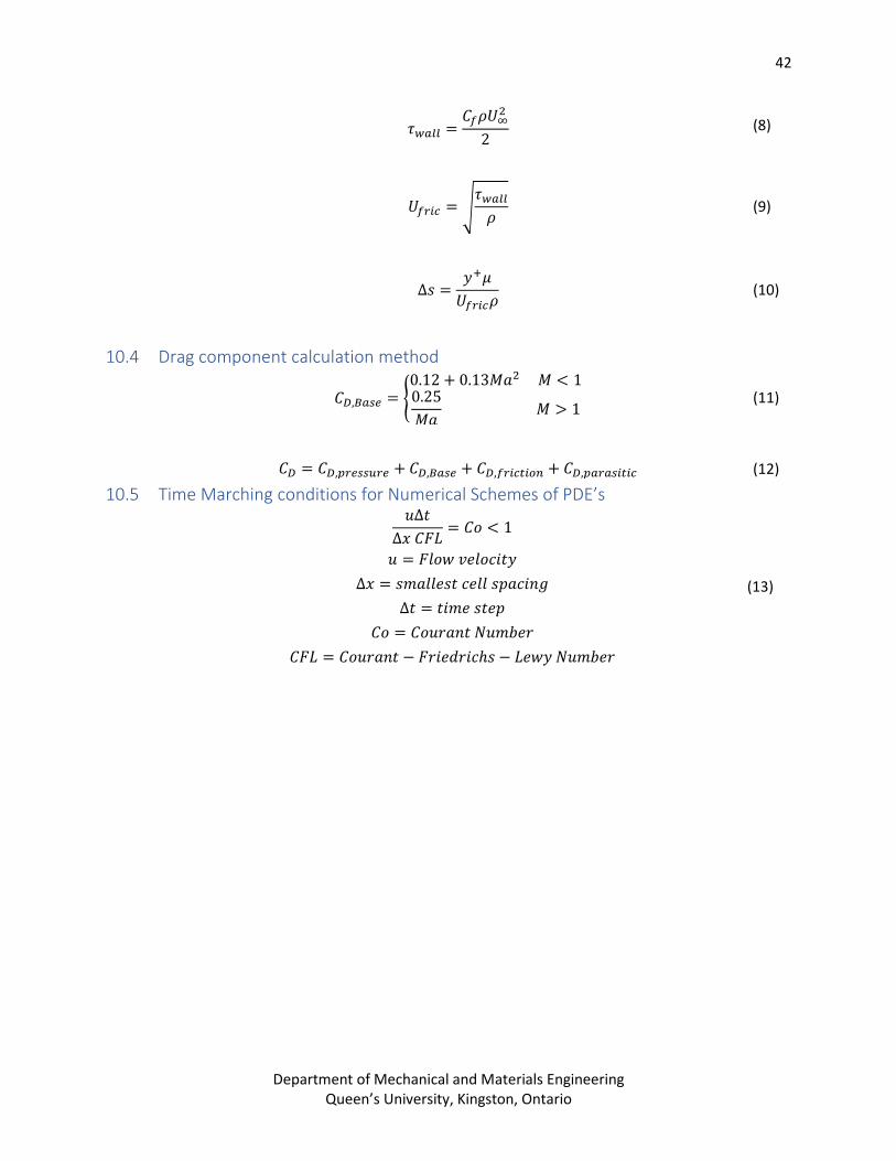
42


𝜏𝑤𝑎𝑙𝑙 =𝐶𝑓𝜌𝑈∞

2

2 (8)

𝑈𝑓𝑟𝑖𝑐 = √𝜏𝑤𝑎𝑙𝑙

𝜌 (9)

∆𝑠 =𝑦+𝜇

𝑈𝑓𝑟𝑖𝑐𝜌 (10)

10.4 Drag component calculation method

𝐶𝐷,𝐵𝑎𝑠𝑒 = {0.12 + 0.13𝑀𝑎2 𝑀 < 10.25

𝑀𝑎 𝑀 > 1

(11)

𝐶𝐷 = 𝐶𝐷,𝑝𝑟𝑒𝑠𝑠𝑢𝑟𝑒 + 𝐶𝐷,𝐵𝑎𝑠𝑒 + 𝐶𝐷,𝑓𝑟𝑖𝑐𝑡𝑖𝑜𝑛 + 𝐶𝐷,𝑝𝑎𝑟𝑎𝑠𝑖𝑡𝑖𝑐 (12)

10.5 Time Marching conditions for Numerical Schemes of PDE’s

𝑢Δ𝑡

Δ𝑥 𝐶𝐹𝐿= 𝐶𝑜 < 1

𝑢 = 𝐹𝑙𝑜𝑤 𝑣𝑒𝑙𝑜𝑐𝑖𝑡𝑦

Δ𝑥 = 𝑠𝑚𝑎𝑙𝑙𝑒𝑠𝑡 𝑐𝑒𝑙𝑙 𝑠𝑝𝑎𝑐𝑖𝑛𝑔

Δ𝑡 = 𝑡𝑖𝑚𝑒 𝑠𝑡𝑒𝑝

𝐶𝑜 = 𝐶𝑜𝑢𝑟𝑎𝑛𝑡 𝑁𝑢𝑚𝑏𝑒𝑟

𝐶𝐹𝐿 = 𝐶𝑜𝑢𝑟𝑎𝑛𝑡 − 𝐹𝑟𝑖𝑒𝑑𝑟𝑖𝑐ℎ𝑠 − 𝐿𝑒𝑤𝑦 𝑁𝑢𝑚𝑏𝑒𝑟

(13)

43


10.6 CFD Contour Plots

10.6.1 Mach Plots

Figure 39: Ma= 0.2. 0° flap (left) and 45° flap (right). Mach plots shown.




44


Figure 43: Ma= 0.6. 0° flap (left) and 45° flap (right) Mach plots shown.

10.6.2 Cp Plots

Figure 44: Ma=0.2. 0° flap (left) and 45° flap (right). Cp plot shown.



45




MECH 460: Final Report Active Rocket Apogee Control (ARAC)

Documents

Transcript of MECH 460: Final Report Active Rocket Apogee Control (ARAC)