NOTA DILAVORO92.2009

Global Climate Policy Architecture and Political Feasibility: Specific Formulas and Emission Targets to Attain 460 ppm CO2 Concentrations

By Valentina Bosetti, Fondazione Eni Enrico Mattei Jeffrey Frankel, Harvard University

The opinions expressed in this paper do not necessarily reflect the position of Fondazione Eni Enrico Mattei

Corso Magenta, 63, 20123 Milano (I), web site: www.feem.it, e-mail: working.papers@feem.it

SUSTAINABLE DEVELOPMENT Series Editor: Carlo Carraro Global Climate Policy Architecture and Political Feasibility: Specific Formulas and Emission Targets to Attain 460 ppm CO2 Concentrations By Valentina Bosetti, Fondazione Eni Enrico Mattei Jeffrey Frankel, Harvard University Summary Three gaps in the Kyoto Protocol most badly need to be filled: the absence of emission targets extending far into the future, the absence of participation by the United States, China, and other developing countries, and the absence of reason to think that members will abide by commitments. To be politically acceptable, any new treaty that fills these gaps must, we believe, obey certain constraints regarding country-by-country economic costs. We offer a framework of formulas that assign quantitative allocations of emissions, across countries, one budget period at a time. The two-part plan: (i) China and other developing countries accept targets at BAU in the coming budget period, the same period in which the US first agrees to cuts below BAU; and (ii) all countries are asked in the future to make further cuts in accordance with a formula which sums up a Progressive Reductions Factor, a Latecomer Catch-up Factor, and a Gradual Equalization Factor. An earlier proposal for specific parameter values in the formulas – Frankel (2009), as analyzed by Bosetti, et al (2009) – achieved the environmental goal that concentrations of CO2 plateau at 500 ppm by 2100. It succeeded in obeying our political constraints, such as keeping the economic cost for every country below the thresholds of Y=1% of income in Present Discounted Value, and X=5% of income in the worst period. In pursuit of more aggressive environmental goals, we now advance the dates at which some countries are asked to begin cutting below BAU, within our framework. We also tinker with the values for the parameters in the formulas. The resulting target paths for emissions are run through the WITCH model to find their economic and environmental effects. We find that it is not possible to attain a 380 ppm CO2 goal (roughly in line with the 2°C target) without violating our political constraints. We were however, able to attain a concentration goal of 460 ppm CO2 with looser political constraints. The most important result is that we had to raise the threshold of costs above which a country drops out, to as high as Y =3.4% of income in PDV terms, or X =12 % in the worst budget period. Some may conclude from these results that the more aggressive environmental goals are not attainable in practice, and that our earlier proposal for how to attain 500 ppm CO2 is the better plan. We take no position on which environmental goal is best overall. Rather, we submit that, whatever the goal, our approach will give targets that are more practical economically and politically than approaches that have been proposed by others. The authors would like to thank for support the Sustainability Science Program, funded by Italy’s Ministry for Environment, Land and Sea, at the Center for International Development at Harvard University and the Climate Impacts and Policy Division of the EuroMediterranean Center on Climate Change (CMCC). The paper was written while Valentina Bosetti was visiting at the Princeton Environmental Institute (PEI) in the framework of cooperation between CMCC and PEI. Keywords: International Climate Agreements JEL Classification: Q, Q40, Q54 Address for correspondence: Valentina Bosetti Fondazione Eni Enrico Mattei Corso Magenta 63 20123 Milano Italy E-mail: valentina.bosetti@feem.it

FIRST DRAFT Sept. 21+Nov. 5, 2009

Global Climate Policy Architecture and Political Feasibility: Specific Formulas and Emission Targets to Attain 460 ppm CO2 Concentrations

Valentina Bosetti, FEEM, Milan, and Jeffrey Frankel, Harvard University

The authors would like to thank for support the Sustainability Science Program, funded by Italy’s Ministry for Environment, Land and Sea, at the Center for International Development at Harvard University and the Climate Impacts and Policy Division of the EuroMediterranean Center on Climate Change (CMCC). The paper was written while Valentina Bosetti was visiting at the Princeton Environmental Institute (PEI) in the framework of cooperation between CMCC and PEI.

Abstract

Three gaps in the Kyoto Protocol most badly need to be filled: the absence of emission targets extending far into the future, the absence of participation by the United States, China, and other developing countries, and the absence of reason to think that members will abide by commitments. To be politically acceptable, any new treaty that fills these gaps must, we believe, obey certain constraints regarding country-by-country economic costs. We offer a framework of formulas that assign quantitative allocations of emissions, across countries, one budget period at a time. The two-part plan: (i) China and other developing countries accept targets at BAU in the coming budget period, the same period in which the US first agrees to cuts below BAU; and (ii) all countries are asked in the future to make further cuts in accordance with a formula which sums up a Progressive Reductions Factor, a Latecomer Catch-up Factor, and a Gradual Equalization Factor. An earlier proposal for specific parameter values in the formulas – Frankel (2009), as analyzed by Bosetti, et al (2009) – achieved the environmental goal that concentrations of CO2 plateau at 500 ppm by 2100. It succeeded in obeying our political constraints, such as keeping the economic cost for every country below the thresholds of Y=1% of income in Present Discounted Value, and X=5% of income in the worst period. In pursuit of more aggressive environmental goals, we now advance the dates at which some countries are asked to begin cutting below BAU, within our framework. We also tinker with the values for the parameters in the formulas. The resulting target paths for emissions are run through the WITCH model to find their economic and environmental effects.

We find that it is not possible to attain a 380 ppm CO2 goal (roughly in line with the 2°C target) without violating our political constraints. We were however, able to attain a concentration goal of 460 ppm CO2 with looser political constraints. The most important result is that we had to raise the threshold of costs above which a country drops out, to as high as Y =3.4% of income in PDV terms, or X =12 % in the worst budget period. Some may conclude from these results that the more aggressive environmental goals are not attainable in practice, and that our earlier proposal for how to attain 500 ppm CO2 is the better plan. We take no position on which environmental goal is best overall. Rather, we submit that, whatever the goal, our approach will give targets that are more practical economically and politically than approaches that have been proposed by others.

2

Summary

This paper offers a framework of formulas that produce precise numerical targets

for emissions of carbon dioxide (CO2) in all regions of the world in all decades of this

century. The formulas are based on pragmatic judgments about what is possible

politically. The reason for this approach is the authors’ belief that many of the usual

science-based, ethics-based, and economics-based paths are not politically viable. It is

not credible that successor governments will be able politically to abide by the

commitments that today’s leaders make, if those commitments would be costly.

Three political constraints seem inescapable if key countries are to join a new

treaty and abide subsequently by their commitments: (1) Developing countries are not

asked to bear any cost in the early years. (2) Thereafter, they are not asked to make any

sacrifice that is different in kind or degree from what was made by those countries that

went before them, with due allowance for differences in incomes. (3) No country is

asked to accept an ex ante target that costs it more than Y% of income in present

discounted value (PDV), or more than X% of income in any single budget period. The

logic is that no country will agree to ex ante targets that have very high costs, nor abide

by them ex post.

Further, one major country or region dropping out is fatal. The reason is that

others will become discouraged and may also fail to meet their own targets; the entire

framework may unravel. If such unraveling in a future decade is foreseeable at the time

that long-run commitments are made, then those commitments will not be credible from

the start. Firms, consumers, and researchers base their current decisions to invest in

plant and equipment, consumer durables, or new technological possibilities on the

expected future price of carbon: If government commitments are not credible from the

start, then they will not raise the expected future carbon price.

The proposed targets for emissions are formulated assuming the following

framework. Between now and 2050, the European Union follows the path laid out in the

2008 European Commission Directive; the United States follows the path in the version

of the Waxman-Markey bill passed by the House in June 2009; and Japan, Australia and

Korea follow statements that their own leaders have recently made. China, India and

3

other countries agree immediately to quantitative emission targets, which in the first

decades merely copy their business-as-usual (BAU) paths, thereby precluding leakage.

These countries are not initially expected to cut emissions below their BAU trajectory.

When the time comes for developing countries to join mitigation efforts their

emission targets are determined using a formula that incorporates three elements: a

Progressive Reductions Factor, a Latecomer Catch-up Factor, and a Gradual Equalization

Factor. These three factors are designed to persuade the joining countries that they are

only being asked to do what is fair in light of actions already taken by others. In the

second half of the century, the formula that determines the emissions path for

industrialized countries is dominated by the Gradual Equalization Factor. But

developing countries, which will still be in earlier stages of participation and thus will

have departed from their BAU paths only relatively recently, will still follow in the

footsteps of those who have gone before. This means that their emission targets will be

set using the Progressive Reductions Factor and the Latecomer Catch-up Factor, in

addition to the Gradual Equalization Factor. The glue that holds the agreement together

is that every country has reason to feel that it is only doing its fair share.

We use the WITCH model to analyze the results of this approach in terms of

projected paths for emissions targets, permit trading, the price of carbon, lost income, and

environmental effects. Overall economic costs, discounted (at 5 percent), average 1.39

percent of Gross Product. The largest discounted economic loss suffered by any country

from the agreement overall is 3.4 percent of income. The largest loss suffered by any

country in any one period is 12.6 percent of income. Atmospheric CO2 concentrations

level off at 460 parts per million (ppm) in the latter part of the century. We were unable

to attain CO2 concentrations of 380 ppm (the equivalent of 450 ppm for all greenhouse

gases), without more serious violations of our political constraints. The latter

concentrations would be required, approximately, to achieve the more aggressive

collective goal set by the G-7 leaders meeting in Italy in July 2009: limiting the global

temperature increase to 2°C.

4

Introduction The political context of Copenhagen

The clock is running out on negotiations under the UN Framework Convention on

Climate Change for a successor agreement to the Kyoto Protocol. But the road has been

blocked by a seeming insurmountable obstacle. The United States, which until recently

was the world’s largest emitter of Greenhouse Gases (GHGs), is at loggerheads with

China, the world’s new largest emitter, and with India and other developing countries.

Fortunately, there just might be a way to break through the roadblock.

On the one hand, the US Congress is clear: it will not impose quantitative limits

on US GHG emissions if it fears that emissions from China, India, and other developing

countries will continue to grow unabated. Indeed, that is why the Senate was unwilling

to ratify the Kyoto Protocol ten years ago. Why, it asks, should US firms bear the

economic cost of cutting emissions if energy-intensive activities such as aluminum

smelters and steel mills would just migrate to countries that have no caps and therefore

have cheaper energy -- the problem known as leakage -- and global emissions would

continue their rapid rise?

On the other hand, the leaders of India and China are just as clear: they are

unalterably opposed to cutting emissions until after the United States and other rich

countries have gone first. After all, the industrialized countries created the problem of

global climate change. And they got rich in the process. The poor countries should not

be denied their turn at economic development. As the Indians point out, Americans emit

more than ten times as much carbon dioxide per person as they do.

In June 2009, the US House of Representatives passed the American

Conservation and Energy Security Act, known as the Waxman-Markey bill, which

(among many other things) would set targets for American GHG emissions. But largely

5

due to fears of leakage, the bill is unlikely to pass the Senate as long as major developing

countries have not accepted quantitative targets of their own.

What is needed is a specific framework for setting the actual numbers that future

signers of a Kyoto-successor treaty are realistically expected to adopt as their emission

targets. There is one practical solution to the apparently irreconcilable differences

between the US and the developing countries regarding binding quantitative targets. The

United States would indeed agree to join Europe in adopting emission targets, something

along the lines of the big cuts specified in the Waxman-Markey bill. Simultaneously, in

the same agreement, China, India, and other developing countries would agree to a path

that immediately imposes on them binding emission targets as well—but targets that in

the first phase simply follow the so-called Business-as-Usual (BAU) path. BAU is

defined as the path of increasing emissions that these countries would experience in the

absence of an international agreement, as determined by experts’ projections.

Of course an environmental solution also requires that China and the other

developing countries subsequently make cuts below their Business as Usual path in future

years, and eventually make cuts in absolute terms as well. This negotiation can become

easier over time, as everyone gains confidence in the framework. But the developing

countries can and should be asked to make cuts that do not differ in nature from those

made by Europe, the United States, and others who have gone before them, taking due

account of differences in income. Emission targets can be determined by formulas

(i) that give lower-income countries more time before they start to cut emissions, and

(ii) that lead to gradual convergence across countries of emissions per capita over the

course of the century, while

(iii) taking care not to reward any country for joining the system late.

Speaking realistically, no country – rich or poor – will abide by targets in any

given period that entail extremely large economic sacrifice, relative to the alternative of

simply not participating in the system. It is time to stop making sweeping proposals that

assume otherwise, and to pursue instead the narrow thread of the politically possible.

6

The problem to be solved

There are by now many proposals for a post-Kyoto climate change regime, even if

one considers only proposals that accept the basic Kyoto approach of quantitative,

national-level limits on GHG emissions accompanied by international trade in emissions

permits. The Kyoto targets applied only to the budget period 2008–2012, which we are

now in, and only to a minority of countries (in theory, the industrialized countries). The

big task is to extend quantitative emissions targets through the remainder of the century

and to other countries—especially the United States, China, and other developing

countries.

Virtually all the existing proposals for a post-Kyoto agreement are based on

scientific environmental objectives (e.g., stabilizing atmospheric CO2 concentrations at

380 ppm in 2100), or ethical/philosophical considerations (e.g., the principle that every

individual on earth has equal emission rights), or economic cost-benefit analyses

(weighing the economic costs of abatement against the long-term environmental

benefits).1 This paper proposes a way to allocate emission targets for all countries and

for the remainder of the century that is intended to be more practical in that it is also

based on political considerations, rather than on science or ethics or economics alone.2

The industrialized countries did, in 1997, agree to quantitative emissions targets

for the Kyoto Protocol’s first budget period, so in some sense we know that it can be

done. But the obstacles are enormous. For starters, most of the Kyoto signers will

probably miss their 2008–2012 targets, and of course the United States never even

ratified. At multilateral venues such as the United Nations Framework Convention on

Climate Change (UNFCCC) meeting in Bali (2007) and the Group of Eight (G8) meeting

in Hokkaido (July 2008), world leaders agreed on a broad long-term goal of cutting total

global emissions in half by 2050. At a meeting in L’Aquila, Italy, in July 2009, the G8

1 Important examples of the science-based approach, the cost-benefit-based approach, and the rights-based approach, respectively, are Wigley (2007), Nordhaus (1994, 2006), and Baer et al. (2008). 2 Aldy, Barrett, and Stavins (2003) and Victor (2004) review a number of existing proposals. Numerous others have offered their own thoughts on post-Kyoto plans, at varying levels of detail, including Aldy, Orszag, and Stiglitz (2001); Barrett (2006); Nordhaus (2006); Olmstead and Stavins (2006); Karp and Zhao (2009) and Birdsall and Subramanian (2009).

7

leaders agreed to an environmental goal of limiting the temperature increase 2°C,3 which

corresponds roughly to a GHG concentration level of 450 ppm (or approximately 380

ppm CO2 only).

But these meetings did not come close to producing agreement on who will cut

how much, nor agreement on multilateral targets within a near-enough time horizon that

the same national leaders are likely to still be alive when the abatement commitment

comes due. To quote Al Gore (1993, p.353), “politicians are often tempted to make a

promise that is not binding and hope for some unexpectedly easy way to keep the

promise.” For this reason, the aggregate targets endorsed so far cannot be viewed as

anything more than aspirational.

Moreover, nobody has ever come up with an enforcement mechanism that

simultaneously has sufficient teeth and is acceptable to member countries. Given the

importance countries place on national sovereignty it is unlikely that this will change.

Hopes must instead rest on weak enforcement mechanisms such as the power of moral

suasion and international opprobrium. It is safe to say that in the event of a clash

between such weak enforcement mechanisms and the prospect of a large economic loss

to a particular country, aversion to the latter would win out.

Necessary elements of a workable successor to Kyoto

Any proposed successor-agreement to the Kyoto Protocol should deliver five

desirable attributes4:

• More comprehensive participation—specifically, getting the United States, China,

and other developing counties to join the system of quantitative emission targets.

• Efficiency—incorporating market-flexibility mechanisms such as international permit

trading and providing advance signals to allow the private sector to plan ahead, to the

extent compatible with the credibility of the signals.

3 Financial Times, July 9, 2009, p. 5. 4 Frankel (2007). (A sixth attribute, robustness under uncertainty is equally important to these five and also motivates out approach. But it is not explicitly addressed in this paper.) Similar lists are provided by Bowles and Sandalow (2001), Stewart and Weiner (2003), and others.

8

• Dynamic consistency—addressing the problem that announcements about steep cuts

in 2050 are not credible.

• Equity—taking account of the point made by developing countries that industrialized

countries created the problem of global climate change, while poor countries are

responsible for only about 20 percent of the CO2 that has accumulated in the

atmosphere from industrial activity over the past 150 years. From an equity

standpoint, developing countries argue they should not be asked to limit their

economic development to pay for a climate-change solution; moreover, they do not

have the capacity to pay for emissions abatement that richer countries do. Finally,

many developing countries place greater priority on raising their people’s current

standard of living. These countries might reasonably demand quantitative targets

that reflect an equal per capita allotment of emissions, on equity grounds.

• Compliance —recognizing that no country will join a treaty if it entails tremendous

economic sacrifice and that therefore compliance cannot be reasonably expected if

costs are too high. Similarly, no country, if it has already joined the treaty, will

continue to stay in during any given period if staying in means huge economic

sacrifice, relative to dropping out, in that period.

Unlike the Kyoto Protocol, our proposal seeks to bring all countries into an

international policy regime on a realistic basis and to look far into the future. But we

cannot pretend to see with as fine a degree of resolution at a century-long horizon as we

can at a five- or ten-year horizon. Fixing precise numerical targets a century ahead is

impractical. Rather, we need a century-long sequence of negotiations, fitting within a

common institutional framework that builds confidence as it goes along. The framework

must have enough continuity so that success in the early phases builds members’

confidence in each other’s compliance commitments and in the fairness, viability, and

credibility of the process. Yet the framework must be flexible enough that it can

accommodate the unpredictable fluctuations in economic growth, technology

development, climate, and political sentiment that will inevitably occur. Only by

9

striking the right balance between continuity and flexibility can we hope that a

framework for addressing climate change would last a century or more.

Political constraints

We take as axiomatic five claims regarding political feasibility:

1. The United States will not commit to quantitative targets if China and other major

developing countries do not commit to quantitative targets at the same time. (This

leaves completely open the initial level and future path of the targets.) Any plan will

be found unacceptable if it leaves the less developed countries free to exploit their

lack of GHG regulation for “competitive” advantage at the expense of the

participating countries’ economies and leads to emissions leakage at the expense of

the environmental goal.

2. China, India, and other developing countries will not make sacrifices they view as

a. fully contemporaneous with rich countries,

b. different in character from those made by richer countries who have gone

before them,

c. preventing them from industrializing,

d. failing to recognize that richer countries should be prepared to make greater

economic sacrifices than poor countries to address the problem (all the more

so because rich countries’ past emissions have created the problem), or

e. failing to recognize that the rich countries have benefited from an “unfair

advantage” in being allowed to achieve levels of per capita emissions that are

far above those of the poor countries.

3. In the short run, emission targets for developing countries must be computed relative

to current levels or BAU paths; otherwise the economic costs will be too great for the

countries in question to accept. 5 But in the longer run, no country can be rewarded

for having "ramped up” emissions far above 1990 levels, the reference year agreed to

at Rio and Kyoto. Fairness considerations aside, if post-1990 increases are

permanently “grandfathered,” then countries that have not yet agreed to cuts will have

a strong incentive to ramp up emissions in the interval before they join. Of course

5 Cuts expressed relative to BAU have been called “Action Targets” (Baumert and Goldberg 2006).

10

there was nothing magic about 1990 but, for better or worse, it is the year on which

Annex I countries have long based planning.6

4. No country will accept a path of targets that is expected to cost it more than Y percent

of income throughout the 21st century (in present discounted value). Frankel (2009)

set Y at 1 percent.

5. No country will accept targets in any period that are expected to cost more than X

percent of income to achieve during that period; alternatively, even if targets were

already in place, no country would in the future actually abide by them if it found the

cost to doing so would exceed X percent of income. In this paper, income losses are

defined relative to what would happen if the country in question had never joined.

Frankel (2009) set X at 5 percent.

Squaring the circle

Of the above propositions, even the first and second alone seem to add up to a

hopeless stalemate: Nothing much can happen without the United States, the United

States will not proceed unless China and other developing countries start at the same

time, and China will not start until after the rich countries have gone first.

There is only one possible solution, only one knife-edge position that satisfies the

constraints. At the same time that the United States agrees to binding emission cuts in

the manner of Kyoto, China and other developing countries agree to a path that

immediately imposes on them binding emission targets—but these targets in their early

years simply follow the BAU path. The idea of committing to only BAU targets in the

early decades will provoke strong objections from environmentalists and business

interests in advanced countries. But they might come to realize that this commitment is

more important than it sounds: It precludes the carbon leakage which, absent such an

agreement, would undermine the environmental goal and it moderates the

competitiveness concerns of carbon-intensive industries in the rich countries. The

developing countries can’t exploit the opportunity to go above their BAU paths as they

would in the absence of this commitment.

6 If the international consenus base year shifts from 1990 to 2005, our proposal will do the same.

11

This approach recognizes that it would be irrational for China to agree to

substantial actual cuts in the short term. Indeed China might well register strong

objections to being asked to take on binding targets of any kind at the same time as the

United States. But the Chinese may also come to realize that they would actually gain

from such an agreement, by acquiring the ability to sell emission permits at the same

world market price as developed countries. (China currently receives lower prices for

lower-quality project credits under the Kyoto Protocol’s Clean Development

Mechanism.)

How do we know they would come out ahead? China is currently building

roughly 100 power plants per year, to accommodate its rapidly growing demand. The

cost of shutting down an already-functioning coal-fired power plant in the United States

is far higher than the cost of building a new clean low-carbon plant in China in place of

what otherwise might be a new dirty coal-fired plant. For this reason, when an American

firm pays China to cut its emissions voluntarily, thereby obtaining a permit that the

American firm can use to meet its emission obligations, both parties benefit, even in

strictly economic terms. The environmental benefit is that China’s emissions would

(voluntarily) fall below its BAU commitment from the beginning. From a dynamic

perspective, the incentive to shift towards a less carbon intensive capital stock will

provide substantial additional benefits in ten or twenty years time, when China will face a

constraining target, given the long-lived nature of these plants.

In later decades, the formulas we propose do ask substantially more of the

developing countries. But these formulas also obey basic notions of fairness, by asking

only for cuts that are analogous in magnitude to the cuts made by others who began

abatement earlier and making due allowance for developing countries’ low per capita

income and emissions and for their baseline of rapid growth. These ideas were

developed in earlier papers7 which suggested that the formulas used to develop emissions

targets incorporate four or five variables: 1990 emissions, emissions in the year of the

negotiation, population, and income. One might also include a few other special

7 Frankel (1999, 2005, 2007) and Aldy and Frankel (2004). Some other authors have made similar proposals.

12

variables such as whether the country in question has coal or hydroelectric power --

though the 1990 level of emissions conditional on per capita income can largely capture

these special variables -- and perhaps a dummy variable for the transition economies.

We narrow down the broad family of formulas to a more manageable set, by the

development of the three factors: a short-term Progressive Reductions Factor, a medium-

term Latecomer Catch-up Factor, and a long-run Gradual Equalization Factor. We then

put them into operation to produce specific numerical targets for all countries, for all

remaining five-year budget periods of the 21st century (presented in Table 2). These are

then fed into the WITCH model to see the economic and environmental consequences.

International trading plays an important role. The framework is flexible enough that one

can tinker with a parameter here or there—for example if the economic cost borne by a

particular country is deemed too high or the environmental progress deemed too low—

without having to abandon the entire formulas framework.

Emission targets for all countries: rules to guide the formulas

All developing countries that have any ability to measure emissions would be

asked to agree immediately to emission targets that do not exceed their projected BAU

baseline trajectory going forward. The objective of getting developing countries

committed to these targets would be to forestall emissions leakage and to limit the extent

to which their firms enjoy a competitive advantage over carbon-constrained competitors

in the countries that have already agreed to targets below BAU under the Kyoto Protocol.

We expect that the developing countries would, in most cases, receive payments for

permits and thus emit less than their BAU baseline. Most countries in Africa would

probably be exempted for some years from any kind of commitment, even to BAU

targets, until they had better capacity to monitor emissions.

One must acknowledge that BAU paths are neither easily ascertained nor

immutable. Countries may “high-ball” their BAU estimates in order to get more

generous targets. Even assuming that estimates are unbiased, important unforeseen

13

economic and technological developments could occur between 2010 and 2020 that will

shift the BAU trajectory for the 2020s, for example. Any number of unpredictable

events have already occurred in the years since 1990; they include German reunification,

the 1997–1998 East Asia crisis, the boom in the BRIC countries (Brazil, Russia, India,

and China), the sharp rise in world oil prices up to 2008, and the world financial crisis of

2007–2009.

A first measure to deal with the practical difficulty of setting the BAU path is to

specify in the Kyoto-successor treaty that estimates must be generated by an independent

international expert body, not by national authorities. A second measure, once the first

has been assured, is to provide for updates of the BAU paths every decade. To omit such

a provision—that is, to hold countries for the rest of the century to the paths that had been

estimated in 2010—would in practice virtually guarantee that any country that achieves

very high economic growth rates in the future will eventually drop out of the agreement,

because staying in would mean incurring costs far in excess of X percent of income.

Allowing for periodic adjustments to the BAU baseline does risk undermining the

incentive for carbon-saving investments, on the logic that such investments would reduce

future BAU paths and thus reduce future target allocations. This risk is the same as the

risk of encouraging countries to ramp up their emissions, which we specified above to be

axiomatically ruled out by any viable proposal. That is why the formula gives decreasing

weight to BAU in later budget periods and why we introduce a Latecomer Catch-up

Factor (explained below), which tethers countries to their 1990 emission levels in the

medium run.

Countries are expected to agree to the second step, quantitative targets that entail

specific cuts below BAU, at a time determined by their circumstances. In our initial

simulations, the choice of year for introducing an obligation actually to cut emissions was

generally guided by two thresholds: when a country’s average per capita income exceeds

$3000 per year and/or when its per capita annual emissions approach 1 ton or more.

But we found that starting dates had to be further modified in order to satisfy our

constraints regarding the distribution of economic losses.

14

As already noted, this approach assigns emission targets in a way that is more

sensitive to political realities than is typical of other proposed target paths, which are

constructed either on the basis of a cost-benefit optimization or to deliver a particular

environmental and/or ethical goal. Specifically, numerical targets are based (a) on

commitments that political leaders in various key countries have already proposed or

adopted, as of early 2009, and (b) on formulas designed to assure latecomer countries that

the emission cuts they are being asked to make represent no more than their fair share, in

that they correspond to the sacrifices that other countries before them have already made.

Finally comes the other important concession to practical political realities: If the

simulation in any period turns out to impose on any country an economic cost of more

than X% of income, we assume that this country drops out. Dropping out could involve

either explicit renunciation of the treaty or massive failure to meet the quantitative

targets. For now, our assumption is that in any such scenario, other countries would

follow by dropping out one by one, and the whole scheme would eventually unravel.

This unraveling would occur much earlier if private actors rationally perceived that at

some point in the future major players will face such high economic costs that

compliance will break down. In this case, the future carbon prices that are built into most

models’ compliance trajectories will lack credibility, private actors today will not make

investment decisions that reflect those projected future prices, and the effort will fail in

the first period. Therefore, our approach to any scenario in which any major player

suffers economic losses greater than X% has been to go back and adjust some of the

starting dates or other parameters of the emission formulas, so that costs are lower and

this is no longer the case.

We hope by these mechanisms to achieve political viability: non-negative

economic gains in the early years for developing countries, average costs over the course

of the century below Y percent of income per annum, and protection for every country

against losses in any period as large, or larger than, X percent of income. Only if they

achieve political viability are announcements of future cuts credible. And only credible

announcements of future cuts will send firms the long-term price signals and incentives

needed to guide investment decisions today.

15

Guidelines from policies and goals already announced by national leaders

Our model produces country-specific numeric emission targets for every fifth

year: 2010, 2015, 2020, etc. For each five-year budget period, such as the Kyoto period

2008–2012, computations are based on the midpoint.

The European Union. The EU emissions target for 2008–2012 was agreed at

Kyoto: 8 percent below 1990 levels. Regarding the second budget period, 2015–2020,

Brussels announced in January 2008 and confirmed in December 20088 a target of 20

percent below 1990 levels. As with other targets publicly supported by politicians in

Europe and elsewhere, skepticism is appropriate regarding EU member countries’

willingness to make the sacrifices necessary to achieve this target.9 However, conditional

on other countries joining in, the European Union has said it would cut emissions 30

percent below 1990 levels if other countries joined in. For the year 2020, given

assumptions on other countries commitment, we chose a target of 30% below 1990

levels.

For the third period (2020–2025), and thereafter up to the eighth period (2045–

2050), the EU targets progress in equal increments to a 50 percent cut below 1990 levels:

In other words, targets relative to 1990 emissions start at 35 percent below, and then

progress to 50 percent below.

Japan, Canada, and New Zealand. These three Pacific countries are assigned

the Kyoto goal of a 6 percent reduction below 1990 levels. Of all ratifiers, Canada is

probably the farthest from achieving its Kyoto goal.10 But Japan dominates this country

8 Financial Times, Jan. 2, 2009, p.5. 9 It is not entirely clear to Americans that even Europe will meet its Kyoto targets. Perhaps the European Union will need to cover its shortfall with purchases of emission permits from other countries. European emissions were reduced in the early 1990s by coincidental events: Britain moved away from coal under Margaret Thatcher and Germany with reunification in 1990 acquired dirty power plants that were easy to clean up. But Americans who claim on this basis that the European Union has not yet taken any serious steps go too far. Ellerman and Buchner (2007, 26-29) show that the difference between allocations and emissions in 2005 and 2006 was probably in part attributable to abatement measures implemented in response to the positive price of carbon. 10 The current government’s plan calls for reducing Canadian emissions in 2020 by 20 percent below 2006 levels (which translates to 2.7 percent below 1990 levels) and in 2050 by 60–70 percent below 2006 levels.

16

grouping in size. We assume that by 2010 the United States has taken genuine measures,

which helps motivate these three countries to get more serious than they have been to

date. In a small concession to realism, we assume that they do not hit the numerical

target until 2012 (versus hitting it on average over the 2008–2012 budget period).11

Japan’s then-Prime Minister, Yasuo Fukuda, on June 9, 2008, announced a

decision to cut Japanese emissions 60–80 percent by mid-century and successor Taro Aso

on June 10, 2009, announced a plan to cut 15 per cent by 2020.12 On September 7, the

incoming Prime Minister, Yukio Hatoyama, declared a goal of cutting emissions to 25

per cent below 1990 levels over the next 10 years, provided other countries were

similarly ambitious.13 We interpret Japan’s targets as cuts of 10 percent every five years

between 2010 and 2050, computed logarithmically. The cumulative cuts are 80 percent

in logarithmic terms, or 51 percent in absolute terms (i.e., to 49 percent of the year–2010

emissions level).

The United States. The Lieberman–Warner bill of 200714 would have begun by

reducing emissions in 2012 to below 2005 levels and would have tightened the emissions

cap gradually each year thereafter, such that by the year 2050, total emissions would be

held to 30 percent of 2012 levels.15 A slightly revised “manager’s” version of the

Lieberman–Warner bill earned significant congressional support in June 2008,. though it

did not garner a large enough majority to become law. During the 2008 US presidential

election campaign, the Republican candidate, John McCain advocated a 2050 emissions

(“FACTBOX – Greenhouse gas curbs from Australia to India,” Sept.5, 2008, Reuters. www.alertnet.org/thenews/newsdesk/L5649578.htm.) 11 In 2007, Japanese Prime Minister Shinzo Abe supported an initiative to half global emissions by 2050. (Financial Times, May 25). But ahead of the 2008 G8 Summit, Japan declined to match the EU’s commitment to cut its emissions 20 per cent by 2020 (FT, April 24, 2008, p.3). 12 “Japan Pledges Big Cut in Emissions,” FT, June 10, 2008 p.6; and Associated Press, June 10, 2009, respectively. 13 The Japan Times, September 8, 2009. 14 S. 2191: America's Climate Security Act of 2007 15 In other words, a 70 percent reduction from emissions levels at the start date of the policy. Section 1201, pages 30-32. (The percentage is measured non-logarithmically.)

17

target of 60 percent below 1990 levels16 while Barack Obama endorsed a more

aggressive target of reducing 2050 emissions 80 percent below 1990 levels.17

.

The earlier paper (Frankel, 2009) assumed targets that cut the average annual

emissions growth rate in half during the period 2008–2012, to 0.7 percent per year.18 At

that point, we assumed emissions plateau (growth is held to zero) for the period 2012–

2017. Then we implemented the rest of the Lieberman–Warner formula, such that

emissions in 2050 reach a level that is 67 percent below 1990 levels.19 Spread over 38

years, this implies sustained reductions of 2.6 percent per year on average, or 13 percent

every five years.

The Waxman-Markey bill that was passed by the House of Representatives in

June 2009-- the American Clean-Energy and Security Act, or ACES Act -- was

substantially less aggressive with respect to the near-term targets. The ACES Act

specifies that US emission allowances continue to grow at 3 per cent per year from 2012

to 2017.20 On the other hand, it is very aggressive with respect to the subsequent 33

years: Waxman-Markey or ACES assumes a US rate of reduction of about 5 per cent

per year from 2017 to 2050 -- unless the price ceiling specified by an escape clause kicks

in.

Australia. Canberra has been reluctant to take strong actions because the country

is so dependent on coal. In July of 2008, however, Australian Prime Minister Kevin

Rudd announced plans to cut emissions to 60 percent below 2000 levels by 2050.21 In

16 Or 66 percent below 2005 levels. Washington Post, May 13, 2008, p. A14; and FT, May 13, 2008, p.4. 17 FT, Oct. 17, 2008. 18 Or 3.5 percent cumulatively, so that emissions in 2012 are 31.5 percent above 1990 levels. That is, 27 percent logarithmically. This is the preferred way of defining percentage changes. True, logarithms are too technical for non-specialist audiences. But measuring changes non-logarithmically has the undesirable property that a 50 percent increase [to 1.50] followed by a 50 percent reduction [to 0.75] does not get you back to your starting point [1.00].) 19 Using our postponed base this is 98.5 percent below 2012 levels, logarithmically. 20 Title VII, Part C, Section 721, sub-section (e) of HR 2454, also known as the Waxman-Markey bill. The preceding draft of the bill, proposed March 31, 2009, called for emissions targets that increased at about 2% per year from 2012 to 2017, peaked in 2021, and hit the same 2050 level as in the version passed by the House in June. 21 A July 16, 2008, government “green paper,” Carbon Pollution Reduction Scheme, reported details on implementation via a domestic cap-and-trade program. Rudd’s initiative appears to have domestic political support (The Economist, July 26, 2008, p.52). The government went on to set a target of 15 percent above

18

the regional groupings of our model, Australia is classified together with South Korea

and South Africa, which are also coal-dependent..

Korea and South Africa. Until recently it looked unlikely that any “non-Annex

I” countries would consider taking on serious cuts below a BAU growth path within the

next decade. But in March 2008, the new president of South Korea, Myung-bak Lee,

“tabled a plan to cap emissions at current levels over the first Kyoto period.”22 This was

an extraordinarily ambitious target in light of Korea’s economic growth rate. He also

“vowed his country would slash emissions in half by 2050,”23 like the industrialized

countries—of which Korea is now one. Emissions have risen 90 percent since 1990 and

it is hard to imagine any country applying the brakes so sharply as to switch instantly

from 5 percent annual growth in emissions to zero. We chose to interpret the Korean

plan to flatten emissions as covering a period that stretches out over the next eleven

years, so that in 2020 the level of emissions is the same as in 2005.24

Meanwhile, South Africa has evidently proposed that its emissions would peak by

2025 and begin declining by 2030. 25

Mexico. President Felipe Calderon's environment minister, Juan Rafael Elvira,

announced in mid-2009 that Mexico was committing itself to reduce its greenhouse gas

emissions by 50 million metric tons a year between then and 2012, and by 50 percent

below 2002 levels by 2050.26

1990 levels by 2020 (FT, Jan. 2, 2009, p.5) and then 5 per cent below 2000 levels by 2020 (The Economist, June 6, 2009, p. 39). 22 “South Korea Plans to Cap Emissions,” International Herald Tribune, March 21, 2008. 23 “South Korea: Developing Countries Move Toward Targets,” Lisa Friedman, ClimateWire, Oct. 3, 2008. 24 One could note, first, that President Lee came to office setting a variety of ambitious goals beyond his power to bring about, especially for economic growth, and second that his popularity quickly plummeted. At the time of writing, his ability to persuade his countrymen to take serious measures was in question. 25 ClimateWire, Oct.3, 2008, op cit. Statements from environmental or foreign ministries do not necessarily carry a lot of weight, if they have not been vetted by finance or economics ministries let alone issued by heads of government or approved by parliaments,. An example would be Argentina’s announcement of a target in 1998. 26 “Mexico: A Model for Developing Countries,” Council on Hemispheric Affairs, August 12, 2009. http://www.coha.org/2009/08/mexico-a-model-for-developing-countries/.

19

China. Getting China to agree to binding commitments is the sine qua non of any

successful post-Kyoto plan. In mid-August 2009, a Chinese top climate change policy-

maker set a target for emissions to peak by 2050.27 In the earlier paper we assumed that

China starts cutting relative to BAU in 2030. But since we are now assuming more

aggressive cuts by the industrialized countries during this period, and the year-2100 goal

of CO2 concentrations at 460 ppm cannot be met without substantial effort by China as

well, we now move up the date at which it begins to cut to 2025.

This still leaves three questions: (1) how to determine the magnitude of China’s

cuts in this first budget period—that is, for the first period in which it is asked to make

cuts below BAU; (2) how to determine Korea’s cuts in its second budget period; and (3)

how to set targets for everyone else. The other regions are Latin America—which like

Korea should logically act before China and India, in light of its stage of development—

Russia, Middle East/North Africa, Southeast Asia, India/South Asia, and Africa. Table 1

shows the starting dates for each, which are placed earlier than in the preceding paper, in

order to hit the more aggressive environmental goal.

Our general guiding principle for the emission targets, once they are to start

cutting below BAU, is to ask countries only to do what is analogous to what has been

done by others who have gone before them. This general principle is put into practice

by means of the three factors.

Guidelines for formulas that ask developing countries to accept “fair” targets,

analogous to those who have gone before

This section discusses the three factors for determining “fair” emissions targets

for developing countries. The three factors are additive (logarithmically).

We call the first the Progressive Reductions Factor. It is based on the pattern of

emission reductions (relative to BAU) assigned to countries under the Kyoto Protocol, as

27 Su Wei, Director-General of the climate change department of China's planning body, as quoted in the Financial Times, August 15/16, 2009.

20

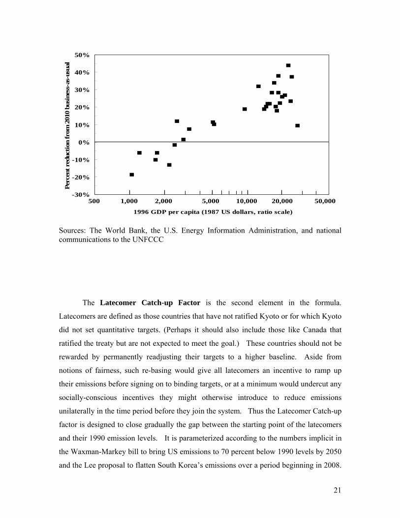
a function of income per capita. This pattern is illustrated in Figure 1, which comes from

the data as they were reported at that time. Other things equal, richer countries are asked

to make more severe cuts relative to BAU, the status quo from which they are departing

in the first period. Specifically, each 1 percent difference in income per capita, measured

relative to EU income in 1997, increases the abatement obligation by 0.14 percent, where

the abatement obligation is measured in terms of reductions from BAU relative to the EU

cuts agreed at Kyoto. Normally, at least in their early budget periods, most countries’

incomes will be below what the Europeans had in 1997, so that this factor dictates milder

cuts relative to BAU than Europe made at Kyoto. In fact the resulting targets are likely to

reflect a “growth path”—that is, they will allow for actual emission increases relative to

the preceding periods. The formula is:

PRF (expressed as country cuts vs. BAU)

= EU's Kyoto commitment for 2008 relative to its BAU + .14 * (gap between the country’s income per capita and the EU’s 2007 income per capita).

The parameter (0.14) was suggested by ordinary least squares (OLS) regression estimates

using the data shown in Figure 1. Other parameters could be chosen instead, if the

parties to a new agreement wanted to increase or decrease the degree of progressivity.

Figure 1: The Emissions Cuts Agreed at Kyoto Were

Progressive with Respect to Income, when Expressed Relative to BAU

21

-30%

-20%

-10%

0%

10%

20%

30%

40%

50%

2.699 3.699 4.699

Perc

ent r

educ

tion

from

201

0 bu

sine

ss-a

s-us

ual

500 1,000 2,000 5,000 10,000 20,000 50,000

1996 GDP per capita (1987 US dollars, ratio scale)

Sources: The World Bank, the U.S. Energy Information Administration, and national communications to the UNFCCC

The Latecomer Catch-up Factor is the second element in the formula.

Latecomers are defined as those countries that have not ratified Kyoto or for which Kyoto

did not set quantitative targets. (Perhaps it should also include those like Canada that

ratified the treaty but are not expected to meet the goal.) These countries should not be

rewarded by permanently readjusting their targets to a higher baseline. Aside from

notions of fairness, such re-basing would give all latecomers an incentive to ramp up

their emissions before signing on to binding targets, or at a minimum would undercut any

socially-conscious incentives they might otherwise introduce to reduce emissions

unilaterally in the time period before they join the system. Thus the Latecomer Catch-up

factor is designed to close gradually the gap between the starting point of the latecomers

and their 1990 emission levels. It is parameterized according to the numbers implicit in

the Waxman-Markey bill to bring US emissions to 70 percent below 1990 levels by 2050

and the Lee proposal to flatten South Korea’s emissions over a period beginning in 2008.

22

In other words, countries are asked to move gradually in the direction of 1990 emissions

in the same way that the United States and Korea under current proposals will have done

before them.

The formula for a country’s Latecomer Catch-up Factor (LCF) is as follows.

Further percentage cuts (relative to BAU plus a Progressive Reductions Factor) are

proportional to how far emissions have been allowed to rise above 1990 levels by the

time the country joins in. That is, it is given by:

LCF = α + λ (percentage gap between country’s lagged emissions and 1990).

The parameter λ represents the firmness with which latecomers are pulled back toward

their 1990 emission levels. The value of λ implicit for Europe at the time the Kyoto

Protocol was negotiated was sufficient to pull the EU-average below its 1990 level. But

to calibrate this formula, the most relevant countries are not European (since the

Europeans are not latecomers), but rather the United States and Korea, since these are the

only countries among those that did not commit themselves to Kyoto targets whose

political leaders have said explicitly what targets they are willing to accept in the second

budget period. The parameters α and λ were chosen as the unique solutions to two

simultaneous equations representing the US target in the 2009 Waxman-Markey bill and

the Korean target (a flattening of emissions being interpreted here as holding absolute

emissions in 2020 equal to 2005 levels). The parameters then work out to

α = 0.54 and λ = -0.773

Thus:

LCF = 0 . 54 - 0 .773 log(country’s current emissions / country’s 1990 emissions). 28

In order to come close to our environmental target (460 ppmCO2 is as close as we

get) without an unacceptable allocation of economic costs across countries, we had to

sacrifice a little of the simplicity of the LCF equation, by adding a dummy variable for

both TE and China. Transition Economies experienced emissions in 1990 that were

28 If Korea were to back away from its president’s commitment, but some other important middle-income country were to step up to the plate with explicit and specific numerical targets, then the calculation could be redone.

23

higher than the subsequent trend; whereas China would be experiencing extremely high

costs due to the projected baseline. Hence, we introduced two dummy variables (εChina = -

0.13 and εTE = 0.38) so that the LCF becomes:

LCF

= 0 . 54 + εcountry - 0 .773 log(country’s current emissions / country’s 1990 emissions)29

The third element is the Gradual Equalization Factor (GEF). Even though

developing countries under the proposal benefit from not being asked for abatement

efforts until after the rich countries have begun to act, and face milder reduction

requirements, they will still complain that it is the rich countries that originally created an

environmental problem for which the poor will disproportionately bear the costs, rather

than the other way around. Such complaints are not unreasonable. If we stopped with

the first two factors, the richer countries would be left with the permanent right to emit

more GHGs, every year in perpetuity. This seems unfair.

In the short run, pointing out the gap in per capita targets is simply not going to

alter the outcome. India and other poor countries will have to live with it. Calls for the

rich countries to cut per capita emissions rapidly, in the direction of poor-country levels,

ignore the fact that the economic costs of such a requirement would be so astronomical

that no rich country would ever agree to it. When one is talking about a lead time of 50

to 100 years, however, the situation changes. With time to adjust, the economic costs are

not impossibly high, and it is reasonable to ask rich countries to bear their full share of

the burden. Furthermore, over a time horizon this long some of the poor countries will in

any case become rich (and possibly vice versa).

Accordingly, during each decade of the second half of the century, the formula

includes an equity factor that moves per capita emissions in each country a small step in

the direction of the global average. This means downward in the case of the rich

countries and upward in the case of the poor countries. Asymptotically, the repeated

application of this factor would eventually leave all countries with equal emissions per 29 This is a departure from our preferred principle of applying the same formula for all countries, a simplicity that is appealing aesthetically and, more important, politically. (As in Frankel, 2009.) But it is one of the concessions we have to make to attain the more aggressive environmental goal.

24

capita, although corresponding national targets need not necessarily converge fully by

2100.30

The parameter (δ) for the speed of adjustment in the direction of the world

average was initially chosen to match the rate at which the EU’s already-announced goals

for 2045–2050 converge to the world average. This number is δ=0.1 per decade, which

is also very similar to the rate of convergence implicit in the goals set by the Lieberman

bills for the United States during 2045–2050. Thus:

GEF

= -0.1 ( percentage gap between country’s lagged emissions per capita and the world’s).

In order to attain lower stabilization levels one could adjust δ, but the effect would

be that costs increase dramatically, especially for some countries like China and

Transition Economies.

The formulas are summarized overall as follows:

Log Target (country i, t) = log (BAU i, t ) – (PCF i, t ) + (LCF i, t ) + (GEF i, t ) ,

where the three factors (except in periods when set = 0 as indicated in Table 1) are given

by:

PCF i,t = log (emission target EU 2008/ BAU EU 2008)

+ 0.14 log (country i's income/cap t-1 / EU income/cap 2007);

LCF i,t = 0.54 +εcountry- 0.773 log (country i's emissions t-1 / country i's emissions 1990).

GEFi,t = - 0.1 log (country i's emissions per capt-1 / global ave. emissions per cap t-1).

The numerical emission target: paths that follow from the formulas

30 Zhang (2008) and others, motivated by a rights-based approach, propose that countries “contract and converge” to targets that reflect equal emissions per capita. The Greenhouse Development Rights approach of Baer et al. (2008), as extended by Cao (2008), emphasizes, from a philosophical standpoint, the allocation of emission rights at the individual level, though these authors apparently recognize that, in practice, individual targets would have to be aggregated and implemented at the national level.

25

Table 2, at the end of the chapter, reports the emissions targets produced by the

formulas for each of eleven geographical regions, for every period between now and the

end of the century. We express the emission targets in several terms:

• in absolute tons (which is what ultimately matters for determining economic and

environmental effects),

• in per capita terms (which is necessary for considering any issues of cross-country

distribution of burden),

• relative to 1990 levels, which is the baseline used for Kyoto, and which remains

relevant in our framework in the form of the Latecomer Catch-up term, and

• relative to the BAU path, which is important for evaluating the sacrifice asked of

individual countries as they join the agreement in the early decades.

The eleven regions are: EU = West Europe and Est Europe

US = United States KOSAU = Korea, South Africa, and Australia

CAJAZ = Canada, Japan, and New Zealand TE = Russia and other Transition Economies

MENA = Middle East and North Africa SSA = Sub-Saharan Africa

SASIA= India and the rest of South Asia CHINA = PRC

EASIA = Smaller countries of East Asia LAM = Latin America and the Caribbean

Table 1 summarizes the dates at which all countries are asked to take on BAU

targets and then reductions below BAU as governed by the different formula elements

discussed previously (i.e., PRF, LCF, and then GEF).

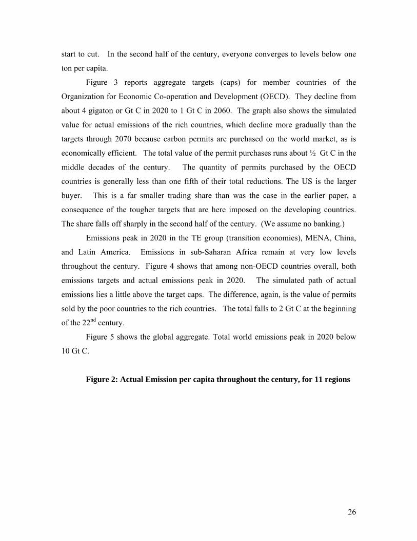
The bar chart in Figure 2 shows actual emissions, expressed in per capita terms,

for every region in every budget period. The United States, even more than other rich

countries, is currently conspicuous by virtue of its high per capita emissions. But its

target path begins to come down after 2010. Emissions in all the rich regions decline

rapidly between 2020 and 2050. Emissions in developing countries continue to rise for a

bit longer, and then come down more gradually. But their emissions per capita numbers

of course start from a much lower base. China peaks at about 1 ½ ton C per capita in

2020. None of the other developing countries ever get above 1 ton C per capita. The

industrialized countries, in contrast, emit between 2 and 5 ½ tons C per capita before they

26

start to cut. In the second half of the century, everyone converges to levels below one

ton per capita.

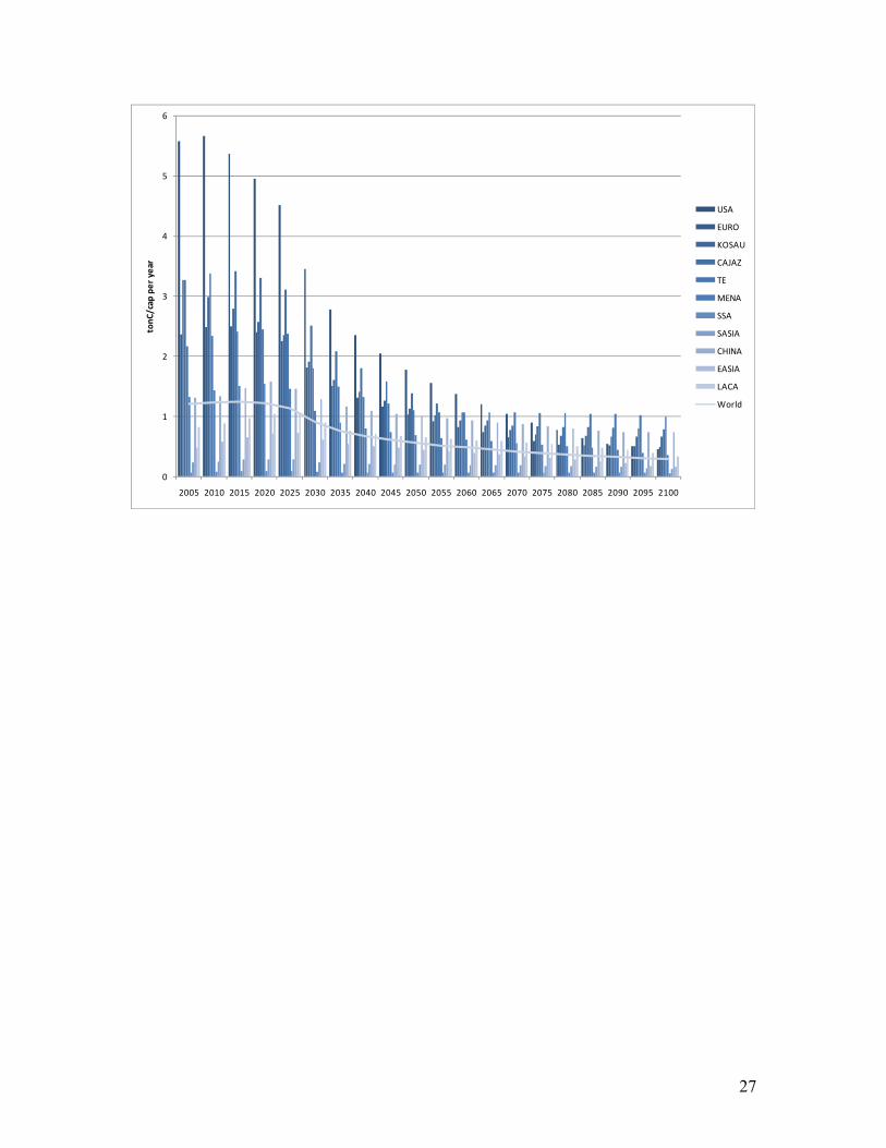
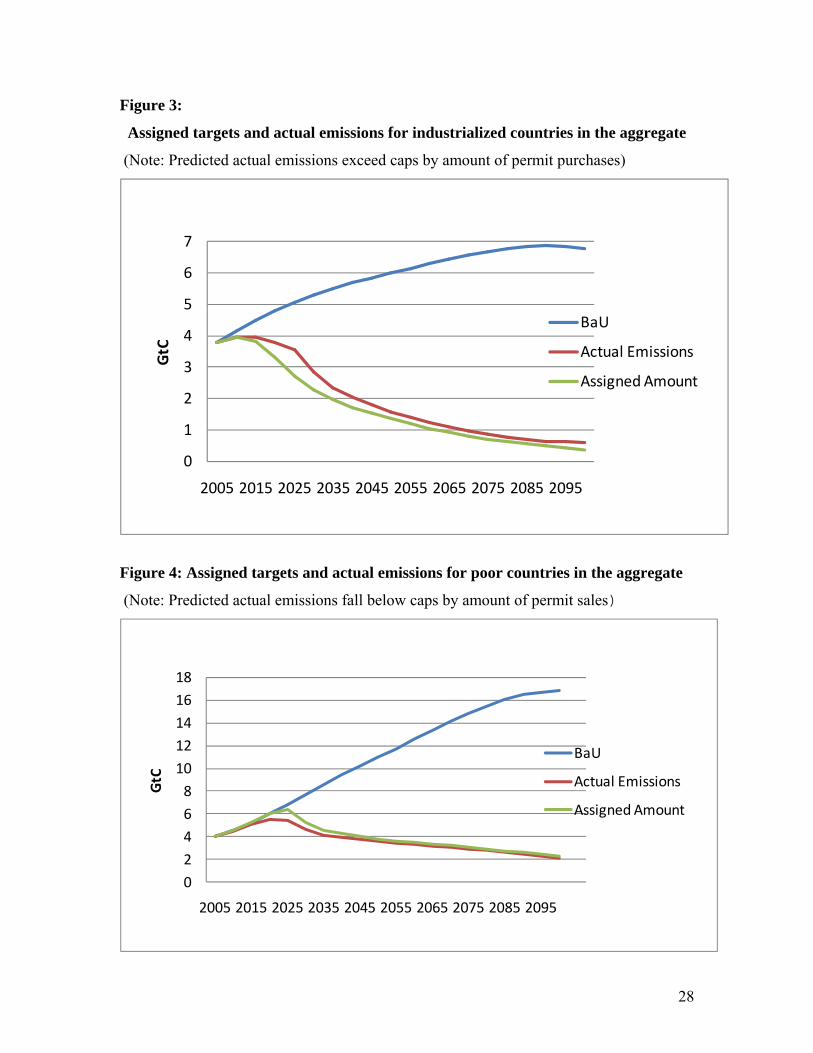
Figure 3 reports aggregate targets (caps) for member countries of the

Organization for Economic Co-operation and Development (OECD). They decline from

about 4 gigaton or Gt C in 2020 to 1 Gt C in 2060. The graph also shows the simulated

value for actual emissions of the rich countries, which decline more gradually than the

targets through 2070 because carbon permits are purchased on the world market, as is

economically efficient. The total value of the permit purchases runs about ½ Gt C in the

middle decades of the century. The quantity of permits purchased by the OECD

countries is generally less than one fifth of their total reductions. The US is the larger

buyer. This is a far smaller trading share than was the case in the earlier paper, a

consequence of the tougher targets that are here imposed on the developing countries.

The share falls off sharply in the second half of the century. (We assume no banking.)

Emissions peak in 2020 in the TE group (transition economies), MENA, China,

and Latin America. Emissions in sub-Saharan Africa remain at very low levels

throughout the century. Figure 4 shows that among non-OECD countries overall, both

emissions targets and actual emissions peak in 2020. The simulated path of actual

emissions lies a little above the target caps. The difference, again, is the value of permits

sold by the poor countries to the rich countries. The total falls to 2 Gt C at the beginning

of the 22nd century.

Figure 5 shows the global aggregate. Total world emissions peak in 2020 below

10 Gt C.

Figure 2: Actual Emission per capita throughout the century, for 11 regions

27

0

1

2

3

4

5

6

2005 2010 2015 2020 2025 2030 2035 2040 2045 2050 2055 2060 2065 2070 2075 2080 2085 2090 2095 2100

tonC

/cap

 per year

USA

EURO

KOSAU

CAJAZ

TE

MENA

SSA

SASIA

CHINA

EASIA

LACA

World

28

Figure 3:

Assigned targets and actual emissions for industrialized countries in the aggregate

(Note: Predicted actual emissions exceed caps by amount of permit purchases)

0

1

2

3

4

5

6

7

2005 2015 2025 2035 2045 2055 2065 2075 2085 2095

GtC

BaU

Actual Emissions

Assigned Amount

Figure 4: Assigned targets and actual emissions for poor countries in the aggregate

(Note: Predicted actual emissions fall below caps by amount of permit sales)

0

2

4

6

8

10

12

14

16

18

2005 2015 2025 2035 2045 2055 2065 2075 2085 2095

GtC

BaU

Actual Emissions

Assigned Amount

29

Figure 5: Emissions target path for the world, in the aggregate

0

5

10

15

20

25

2005 2015 2025 2035 2045 2055 2065 2075 2085 2095

GtC

BaU

Assigned Amount

30

Economic and environmental consequences of the proposed targets,

according to the WITCH model

Estimating the economic and environmental implications of any set of targets is a

complex task.31 WITCH (www.feem-web.it/witch) is an energy-economy-climate model

developed by the climate change modeling group at FEEM. The model has been used

extensively in the past four years to analyze the economic impacts of climate change

policies. WITCH is a hybrid top-down economic model with energy sector

disaggregation. Those who might be skeptical of economists’ models on the grounds that

“technology is the answer” should rest assured that technology is central to this model.

(Economists are optimists when it comes to what new technologies might be called forth

by a higher price for carbon, but pessimists when it comes to how much technological

response to international treaties will occur absent an increase in price.) The model

features endogenous technological change via both experience and innovation processes.

Countries are grouped in twelve regions, where Western Europe and Eastern Europe are

counted separately, that cover the world and that strategically interact following a game

theoretic set-up. The WITCH model and detailed structure are described in Bosetti et al.

(2006) and Bosetti, Massetti, and Tavoni (2007).

Original baselines in many models have been disrupted in recent years by such

developments as stronger-than-expected growth in Chinese energy demand and the

unexpected spike in world oil prices that culminated in 2008. WITCH has been updated

with more recent data and revised projections for key drivers such as population, GDP,

fuel prices, and energy technology characteristics. The base calibration year has been set

at 2005, for which data on socio-economic, energy, and environmental variables are now

available (Bosetti, Carraro, Sgobbi, and Tavoni, 2008).

31 Researchers have applied a number of different models to estimate the economic and environmental effects of various specific proposed emission paths; see, for example, Edmonds, Pitcher, Barns, Baron, and Wise (1992); Edmonds, Kim, McCracken, Sands, and Wise (1997); Hammett (1999); Manne, Mendelsohn, and Richels (1995); Manne and Richels (1997); McKibbin and Wilcoxen (2006); and Nordhaus (1994, 2008). Weyant (2001) provides an explanation and comparison of different models.

31

Economic effects

Although economists trained in cost-benefit analysis tend to focus on economic

costs expressed as a percentage of income, the politically attuned tend to focus at least as

much on the predicted carbon price, which in turn has a direct impact on the prices of

gasoline, home heating oil, and electric power. Figure 6 illustrates the price of carbon

dioxide under these targets. It rises very substantially, reaching $1800 per ton in 2100,

approximately twice what the CO2 price was with an environmental goal of 500 ppm.

But at least the rise is smooth, which is a desirable property. (Kinks or discontinuities in

the rate of price increase, such as a temporary flattening around 2020-2030 in the earlier

paper, could distort behavior.) The right margin of the graph translates the cost from

dollars per ton of carbon to terms that the American consumer can relate to: the

increment to the cost of gasoline. It rises to European levels by 2040, and to $16 per

gallon in 2100.

Figure 6: Price of Carbon Dioxide Rises Steadily Over the Century

0

2

4

6

8

10

12

14

16

0

200

400

600

800

1000

1200

1400

1600

1800

2000

2015 2025 2035 2045 2055 2065 2075 2085 2095

$ pe

r gallon motor asoline

$ pe

r ton

 of CO

2

32

Economic losses measured in terms of national income are illustrated in Figure 7a

and 7b, for the first and second halves of the century, respectively. They too rise

gradually. Given a positive rate of time discount, this is a good outcome. As late as

2055, all regions sustain economic losses that are no greater than 3.5 per cent of income.

(As of mid-century, the US is running the largest cost among OECD countries, relative to

BAU, and MENA and China are running the largest costs among non-OECD countries.)

Later in the century, the costs go much higher, above 11 percent of income in the case of

TE and China. 32 The combination of parameters used produced imply costs that rise

above our self-imposed threshold of 5 percent of national income, after 2065, a

consequence of the more aggressive environmental goal. All economic effects are gross

of environmental benefits—that is, no attempt is made to estimate environmental benefits

or net them out.

Figure 7: Income Losses by Region and Period Over the Century

a) 2010-2045

32 These costs of participation are overestimated in one sense, and increasingly so in the later decades, if the alternative to staying in the treaty one more decade is dropping out after seven or eight decades of participation. The reason is that countries will have already substantially altered their capital stock and economic structure in a carbon-friendly direction. The economic costs reported in the simulations and graphs treat the alternative to participation as never having joined the treaty in the first place. In another sense, however, the costs are underestimated: any country that drops out can in fact exploit leakage opportunities to the hilt. Its firms can buy fossil fuels at far lower prices than their competitors in countries that continue to participate.

33

‐4.00%

‐3.00%

‐2.00%

‐1.00%

0.00%

1.00%

2.00%

2010 2015 2020 2025 2030 2035 2040 2045

USA

EU

KOSAU

CAJAZ

TE

MENA

SSA

SASIA

CHINA

EASIA

LAM

b) 2050- 2100

‐15.00%

‐10.00%

‐5.00%

0.00%

5.00%

10.00%

15.00%

20.00%

25.00%

2050 2055 2060 2065 2070 2075 2080 2085 2090 2095 2100

USA

EU

KOSAU

CAJAZ

TE

MENA

SSA

SASIA

CHINA

EASIA

LAM

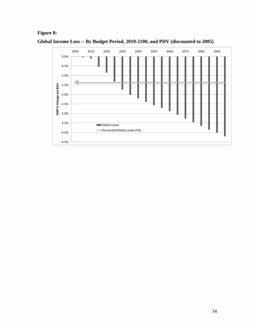
Figure 8 provides Gross World Product loss aggregated across regions worldwide,

and discounted to present value using a discount rate of 5 percent. Total economic costs

come to 1.39 percent of annual gross world product. Figure 9 provides the regional detail

for these figures.

34

Figure 8:

Global Income Loss -- By Budget Period, 2010-2100, and PDV (discounted to 2005)

‐4.5%

‐4.0%

‐3.5%

‐3.0%

‐2.5%

‐2.0%

‐1.5%

‐1.0%

‐0.5%

0.0%

2005 2015 2025 2035 2045 2055 2065 2075 2085 2095

GWP % Change wrt BAU

Global Losses

Discounted Global Losses (5%)

35

Figure 9:

Losses by Region -- PDV (discounted to 2005 at 5% discount rate), 2010-2100

‐4.0%

‐3.0%

‐2.0%

‐1.0%

0.0%

1.0%

2.0%

3.0%

4.0%

USA EU KOSAU CAJAZ TE MENA SSA SASIA CHINA EASIA LAM

Net Present Value

 Income Losses wrt BAU

Environmental effects

The outcome of this proposal in terms of cumulative emissions of GHGs is close

to those of some models that build in environmental effects or science-based constraints,

even though no such inputs were used here: The concentration of CO2 in the atmosphere

reaches 460 ppm in the latter half of the century.

36

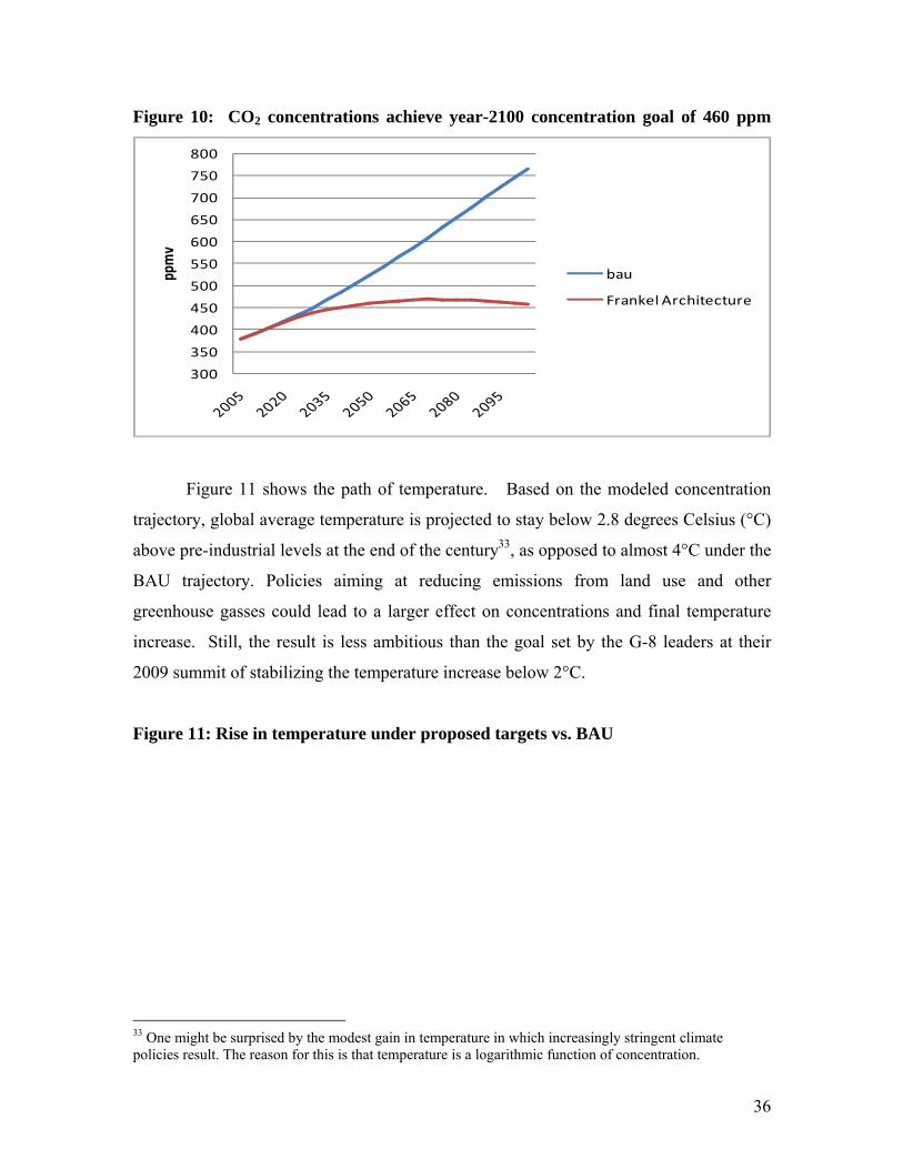
Figure 10: CO2 concentrations achieve year-2100 concentration goal of 460 ppm

300

350

400

450

500

550

600

650

700

750

800pp

mv

bau

Frankel Architecture

Figure 11 shows the path of temperature. Based on the modeled concentration

trajectory, global average temperature is projected to stay below 2.8 degrees Celsius (°C)

above pre-industrial levels at the end of the century33, as opposed to almost 4°C under the

BAU trajectory. Policies aiming at reducing emissions from land use and other

greenhouse gasses could lead to a larger effect on concentrations and final temperature

increase. Still, the result is less ambitious than the goal set by the G-8 leaders at their

2009 summit of stabilizing the temperature increase below 2°C.

Figure 11: Rise in temperature under proposed targets vs. BAU

33 One might be surprised by the modest gain in temperature in which increasingly stringent climate policies result. The reason for this is that temperature is a logarithmic function of concentration.

37

0

0.5

1

1.5

2

2.5

3

3.5

4

2005

2015

2025

2035

2045

2055

2065

2075

2085

2095

2105

bau

Frankel Architecture

38

Conclusion

Several particular extensions are possible for future research.

Directions for future research

First, we could compare our proposed set of emissions paths to other proposals

under discussion in the climate change policy community or being analyzed using other

integrated assessment models.34 Our conjecture is that we could identify countries and

periods in alternative pathways where an agreement would be unlikely to hold up because

its targets were not designed to limit economic costs for each country.

Second, we could take into account GHGs other than CO2.

Third, we could implement constraints on international trading, along the lines

that the Europeans have sometimes discussed. Such constraints can arise either from a

philosophical worldview that considers it unethical to pay others to take one’s medicine,

or from a more cynical worldview that assumes international transfers via permit sales

will only line the pockets of corrupt leaders. Constraints on trading could take the form

of quantity restrictions—for example, that a country cannot satisfy more than Z percent of

its emissions obligation by international permit purchases. Or eligibility to sell permits

could be restricted to countries with a score in international governance ratings over a

particular threshold, or to countries that promise to use the funds for green projects, or to

those that have a track record of demonstrably meeting their commitments under the

treaty.

The fourth possible extension of this research represents the most important step

intellectually: to introduce uncertainty, especially in the form of stochastic growth

processes. The variance of the GDP forecasts at various horizons would be drawn from

historical data. We would adduce the consequences of our rule that if any country makes

an ex post determination in any period that by staying in the treaty it loses more than X

percent of income, even though this had not been the expectation ex ante, that country 34 For example, the CLEAR path proposed by Wagner et al. (2008, Table 2) proposes that by 2050 Russia has cut its emissions 30 percent below 1990 levels, China 46 percent below 2012 levels, India 8 percent above 2012 levels, and the other non-Annex I countries 23 percent below 2012. The Global Development Rights approach of Baer et al. (2008) apparently proposes a US emissions target for 2025 that is 99 percent below its BAU path.

39

will drop out. At a first pass, we could keep the assumption that if one country pulls out,

the entire system falls apart. The goal would then be to design a version of the formulas

framework that minimizes the probability of collapse.

The ultimate objective in making the model stochastic is to seek modifications of

the policy framework that are robust, that protect against inadvertent stringency on the

one hand—that is, a situation where the cost burden imposed on a particular country is

much higher than expected—or inadvertent “hot air” on the other hand. “Hot air” refers

to the possibility that targets are based on obsolete emission levels with the result that

countries are credited for cutting tons that wouldn’t have been emitted anyway. Three

possible modifications to deal with uncertainty are promising. First, we could allow for

some degree of re-adjustment to emission targets in the future, based solely on

unexpected changes in the evolution in population and income. Second, when the

target for each decade is set, it should be indexed to GDP within that budget period.

Perhaps the constant of proportionality in the indexation formula would simply equal 1,

in which case it becomes an efficiency target, expressed in carbon emissions per unit of

GDP. This approach would be much less vulnerable to within-decade uncertainty.35 A

third possible feature that would make the policy more robust and that is strongly favored

by many economists is an escape clause or safety valve that would limit costs in the event

that mitigation proves more expensive than expected, perhaps with a symmetric floor on

the price of carbon in addition to the usual ceiling.

A politically credible framework

Some may wish to conclude from the results in this paper that the environmental

goals of 380 or 450 ppm in CO2 concentrations are not attainable in practice, and that our

earlier proposal for how to attain 500 ppm is the better plan (Frankel, 2009). We take no

position on which environmental goal is best overall, with economic and political

realities factored in. Rather, we submit that, whatever the environmental goal, our

approach will give targets that are more practical economically and politically than the

various approaches that have been proposed by others.

35 Lutter (2000).

40

Our framework specifies the allocation of emission targets across countries in

such a way that every country is given reason to feel that it is only doing its fair share and

in such a way as to build trust as the decades pass. Without such a framework,

announcements of distant future goals are not credible and so will not have the desired

effects. Furthermore, this framework—in providing for a decade-by-decade sequence of

emission targets, each determined on the basis of a few principles and formulas—is

flexible enough that it can accommodate, by small changes in the formula parameters,

major changes in circumstances during the course of the century.

References Aldy, Joseph, Scott Barrett, and Robert Stavins, 2003, “Thirteen Plus One: A Comparison of Global Climate Architectures,” Climate Policy, 3, no. 4, 373-97. --- and Jeffrey Frankel, 2004, “Designing a Regime of Emission Commitments for Developing Countries that is Cost-Effective and Equitable,” G20 Leaders and Climate Change, Council on Foreign Relations. --- , Peter Orszag, and Joseph Stiglitz, 2001, "Climate Change: An Agenda for Global Collective Action." Prepared for The Pew Center Workshop on the Timing of Climate Change Policies. The Westin Grand Hotel, Washington, D.C. October 11-12. Baer, Paul, Tom Athanasiou, Sivan Kartha and Eric Kemp-Benedict, 2008, The Greenhouse Development Rights Framework: The Right to Development in a Climate Constrained World (Hendrich Boll Stiftung, Stockholm, 2nd edition). Barrett, Scott, 2006, “Climate Treaties and ‘Breakthrough’ Technologies,” American Economic Review, Papers and Proceedings, vol. 96, no. 2, May, 22-25. Baumert, Kevin and Donald Goldberg, 2006, “Action targets: A New Approach to International Greenhouse Gas Controls,“ Climate Policy, 5, pp. 561-81. Bosetti, V., C. Carraro, M. Galeotti, E. Massetti and M. Tavoni, 2006, “WITCH: A World Induced Technical Change Hybrid Model.” The Energy Journal, Special Issue on Hybrid Modeling of Energy-Environment Policies: Reconciling Bottom-up and Top-down, 13-38. ---, C. Carraro, A. Sgobbi, M. Tavoni, 2008, "The 2008 WITCH Model: New Model Features and Baseline," Mimeo, August. Forthcoming as a FEEM Working paper,

41

--- , E. Massetti and M. Tavoni, 2007, “The WITCH Model. Structure, Baseline, Solutions”. Working Paper 10. (Fondazione Eni Enrico Mattei: Milan). Cao, Jing, 2008, "Reconciling Human Development and Climate Protection: Perspectives from Developing Countries on Post-2012 International Climate Change Policy." Discussion Paper 08-25, Cambridge, Mass.: Harvard Project on International Climate Agreements, December. Edmonds, J.A., H.M. Pitcher, D.Barns, R.Baron, and M.A. Wise, 1992, “Modeling Future Greenhouse Gas Emissions: The Second Generation Model,” in Modeling Global Climate Change, Lawrence Klein and Fu-chen Lo, editors (United Nations University Press: Tokyo) pp. 295-340.

--- S.H. Kim, C.N.McCracken, R.D. Sands, and M.A. Wise, 1997, “Return to 1990: The Cost of Mitigating United States Carbon Emission in the Post-2000 Period,” October, Pacific Northwest National Laboratory, Operated by Battelle Memorial Institute. Ellerman, Denny, and Barbara Buchner, 2007, "Over-Allocation or Abatement? A Prelminary Analyusis of the EU ETS Based on the 2005-06 Emissions Data." Forthcoming, Environmental and Resource Economics.

Frankel, Jeffrey, 1999, “Greenhouse Gas Emissions,” Policy Brief no.52, Brookings Institution, Washington, DC, June.

--- 2005, “You’re Getting Warmer: The Most Feasible Path for Addressing Global Climate Change Does Run Through Kyoto,” in Trade and Environment: Theory and Policy in the Context of EU Enlargement and Transition Economies, edited J.Maxwell and R.Reuveny (Edward Elgar Publishers, UK). --- 2007, “Formulas for Quantitative Emission Targets,” in Architectures for Agreement: Addressing Global Climate Change in the Post Kyoto World, J.Aldy and R. Stavins, eds. (Cambridge University Press).

--- , 2009, “An Elaborated Proposal For Global Climate Policy Architecture: Specific Formulas and Emission Targets for All Countries in All Decades,” Chapter 2, forthcoming in Post-Kyoto International Climate Policy, edited by Joe Aldy and Rob Stavins, Cambridge University Press. HPICA DP 08-08. NBER WP 18476.

Gore, Al, 1993, Earth in the Balance (Penguin Books, New York). Hammett, James, 1999, “Evaluation Endpoints and Climate Policy: Atmospheric Stabilization, Benefit-Cost Analysis, and Near-Term Greenhouse Gas Emissions, Harvard Univ. Climatic Change 41: 447-468. Karp, Larry, and Jinha Zhao, 2009, Suggestions for the Road to Copenhagen, Report to the Expert Group on Environmental Studies, Ministry of Finance, Sweden. Lutter, Randy, 2000, “Developing Countries’ Greenhouse Emissions: Uncertainty and Implications for Participation in the Kyoto Protocol,” Energy Journal 21(4): 93-120. Manne, Alan, Robert Mendelsohn, Richard Richels, 1995, "MERGE: A Model for Evaluating Regional and Global Effects of GHG Reduction Policies." Energy Policy 23:17.

42

--- and Richard Richels, 1997, “On Stabilizing CO2 Concentrations – Cost-Effective Emission Reduction Strategies,” Stanford University and Electric Power Research Institute, April. McKibbin, Warwick, Adele Morris and Peter Wilcoxen, 2008, “Expecting the Unexpected: Macroeconomic Volatility and Climate Policy,” HPICA, Discussion Zpaper No. 08-16, November. --- and Peter Wilcoxen, 2007, “A Credible Foundation for Long Term International Cooperation on Climate Change,” in Architectures for Agreement: Addressing Global Climate Change in the Post-Kyoto World, edited by Joseph Aldy and Robert Stavins, Cambridge University Press. Nordhaus, William, 1994, Managing the Global Commons: The Economics of Climate Change, MIT Press: Cambridge. --- 2006, “Life After Kyoto: Alternative Approaches Global Warming Policies,” American Economic Review, Papers and Proceedings, vol. 96, no. 2, May: 31-34. --- 2008, A Question of Balance: Weighing the Options on Global Warming Policies (Yale University Press). Olmstead, Sheila, and Robert Stavins, 2006, “An International Policy Architecture for the Post-Kyoto Era,” American Economic Review, Papers and Proceedings, vol. 96, no. 2, May: 35-38. Pizer, William, 2006, “The Evolution of a Global Climate Change Agreement,” American Economic Review, Papers and Proceedings, vol.96, no.2, May, 26-30. Stewart, Richard, and Jonathan Weiner, 2003, Reconstructing Climate Policy: Beyond Kyoto (American Enterprise Institute Press, Washington DC). Subramanian, Arvind, and Nancy Birdsall, 2009, “Energy Not Emissions: Equitable Burden-Sharing on Climate Change” (Center for Global Development, Washington, DC). Victor, David, 2004, Climate Change: Debating America’s Policy Options (Council on Foreign Relations, New York). Wagner, Gernot, James Wang, Stanislas de Margerie and Daniel Dudek, 2008, “The CLEAR Path: How to Ensure that if Developing Nations Adopt Carbon Limits, Their Early Actions Will be Rewarded,” Environmental Defense Fund Working Paper, October 30. Weyant, John, 2001, "Economic Models: How They Work & Why Their Results Differ." In Climate Change: Science, Strategies, & Solutions. Eileen Claussen, Vicki Arroyo Cochran, and Debra Davis, editors, The Pew Center on Global Climate Change (Brill Academic Press, Leiden), pp. 193-208. Zhang, Yongsheng, 2008, “An Analytical Framework and Proposal to Succeed Kyoto Protocol: A Chinese Perspective, “ Development Research Center of the State Council, China, Dec 8.

43

EU = West Europe and East Europe KOSAU = Korea, South Africa + Australia (all coal-users)

CAJAZ = Canada, Japan + New Zealand TE = Russia and other Transition Economies

MENA = Middle East + North Africa SSA = Sub-Saharan Africa

SASIA= India and the rest of South Asia CHINA = PRC

EASIA = Smaller countries of East Asia LAM = Latin America + the Caribbean

Table 1: Years when signers are to commit to targets at BAU and then below BAU

 year when they are 

assumed to commit to TARGET or BAU 

year when they are assumed to commit to TARGET (PCF & LCF) never 

above BAU year when GEF kicks in 

USA  2010  2010  2050 

EU  2010  2010  2050 

KOSAU  2010  2020  2050 

CAJAZ  2010  2015  2050 

TE  2010  2025  2055 

MENA  2010  2025  2055 

SSA  2025  2050  2080 

SASIA  2010  2025  2055 

CHINA  2010  2025  2055 

EASIA  2010  2025  2055 

LAM  2010  2020  2050 

Table 2: Emission Targets for each of 11 regions, according to the formulas

Table 2.a Fossil Fuel Emission Targets in Gton C   USA  EU  KOSAU  CAJAZ  TE  MENA  SSA  SASIA  CHINA  EASIA  LAM 

2010  1.88  1.11  0.40  0.58  0.84  0.51  0.06  0.41  1.83  0.40  0.50 2015  1.88  0.97  0.42  0.54  0.90  0.59  0.08  0.51  2.08  0.48  0.58 2020  1.88  0.84  0.25  0.36  0.96  0.66  0.09  0.64  2.41  0.58  0.68 2025  1.37  0.81  0.19  0.33  1.09  0.70  0.12  0.68  2.50  0.70  0.57 2030  1.00  0.77  0.17  0.32  0.84  0.59  0.14  0.56  2.05  0.58  0.49 2035  0.73  0.75  0.17  0.31  0.72  0.51  0.17  0.48  1.74  0.50  0.45 2040  0.54  0.70  0.16  0.30  0.66  0.47  0.20  0.45  1.59  0.46  0.42 2045  0.48  0.61  0.16  0.29  0.61  0.44  0.23  0.42  1.47  0.43  0.40 2050  0.43  0.53  0.15  0.24  0.57  0.42  0.26  0.39  1.36  0.40  0.38 2055  0.39  0.46  0.13  0.20  0.54  0.40  0.30  0.37  1.28  0.38  0.37 2060  0.35  0.41  0.12  0.17  0.45  0.37  0.34  0.50  1.12  0.38  0.36 2065  0.31  0.36  0.10  0.15  0.38  0.34  0.39  0.58  0.98  0.37  0.34 2070  0.28  0.31  0.09  0.12  0.32  0.31  0.44  0.63  0.86  0.35  0.32 2075  0.25  0.27  0.08  0.11  0.27  0.28  0.49  0.65  0.75  0.34  0.30 2080  0.23  0.24  0.07  0.09  0.23  0.26  0.54  0.65  0.66  0.31  0.27 2085  0.20  0.21  0.06  0.08  0.19  0.23  0.59  0.63  0.58  0.29  0.25 2090  0.18  0.19  0.05  0.07  0.17  0.21  0.63  0.60  0.51  0.27  0.23 2095  0.16  0.16  0.05  0.06  0.14  0.18  0.67  0.57  0.45  0.24  0.21 2100  0.14  0.14  0.04  0.05  0.12  0.16  0.70  0.52  0.40  0.22  0.19 

44

Table 2.b Fossil Fuel Emission Targets in per capita terms   USA  EU  KOSAU  CAJAZ  TE  MENA  SSA  SASIA  CHINA  EASIA  LAM 

2010  6.0  2.2  3.4  3.5  2.4  1.4  0.1  0.2  1.3  0.6  0.9 2015  5.7  1.9  3.4  3.2  2.5  1.5  0.1  0.3  1.5  0.7  1.0 2020  5.5  1.6  2.0  2.2  2.7  1.6  0.1  0.3  1.7  0.8  1.1 2025  3.9  1.6  1.5  2.0  3.1  1.6  0.1  0.3  1.7  0.9  0.9 2030  2.7  1.5  1.3  2.0  2.4  1.3  0.1  0.3  1.4  0.7  0.7 2035  1.9  1.5  1.3  1.9  2.1  1.1  0.1  0.2  1.2  0.6  0.7 2040  1.4  1.4  1.3  1.9  1.9  0.9  0.1  0.2  1.1  0.5  0.6 2045  1.2  1.2  1.3  1.9  1.8  0.8  0.1  0.2  1.0  0.5  0.6 2050  1.1  1.1  1.2  1.6  1.7  0.8  0.1  0.2  1.0  0.4  0.5 2055  1.0  0.9  1.0  1.4  1.7  0.7  0.2  0.2  0.9  0.4  0.5 2060  0.8  0.8  1.0  1.2  1.4  0.7  0.2  0.2  0.8  0.4  0.5 2065  0.7  0.8  0.8  1.1  1.2  0.6  0.2  0.2  0.7  0.4  0.5 2070  0.7  0.7  0.7  0.9  1.0  0.5  0.2  0.3  0.6  0.4  0.4 2075  0.6  0.6  0.7  0.8  0.9  0.5  0.2  0.3  0.6  0.4  0.4 2080  0.5  0.5  0.6  0.7  0.8  0.5  0.2  0.3  0.5  0.3  0.4 2085  0.5  0.5  0.5  0.6  0.6  0.4  0.3  0.3  0.5  0.3  0.4 2090  0.4  0.4  0.4  0.5  0.6  0.4  0.3  0.2  0.4  0.3  0.3 2095  0.4  0.4  0.4  0.5  0.5  0.3  0.3  0.2  0.4  0.3  0.3 2100  0.3  0.3  0.4  0.4  0.4  0.3  0.3  0.2  0.3  0.3  0.3 

Table 2.c Fossil Fuel Emission Targets relative to 1990 levels   USA  EU  KOSAU  CAJAZ  TE  MENA  SSA  SASIA  CHINA  EASIA  LAM 

2010  1.30  0.92  1.72  1.30  0.89  1.63  1.69  2.03  2.20  3.17  1.69 2015  1.30  0.80  1.81  1.21  0.95  1.89  2.25  2.52  2.50  3.81  1.96 2020  1.30  0.70  1.08  0.81  1.01  2.12  2.53  3.17  2.90  4.60  2.30 2025  0.95  0.67  0.82  0.74  1.15  2.24  3.38  3.37  3.01  5.56  1.93 2030  0.69  0.64  0.73  0.72  0.89  1.89  3.94  2.77  2.47  4.60  1.66 2035  0.51  0.62  0.73  0.70  0.76  1.63  4.79  2.38  2.09  3.97  1.52 2040  0.37  0.58  0.69  0.67  0.70  1.51  5.63  2.23  1.91  3.65  1.42 2045  0.33  0.51  0.69  0.65  0.64  1.41  6.48  2.08  1.77  3.41  1.35 2050  0.30  0.44  0.65  0.54  0.60  1.35  7.32  1.93  1.64  3.17  1.28 2055  0.27  0.38  0.56  0.45  0.57  1.28  8.45  1.83  1.54  3.02  1.25 2060  0.24  0.34  0.52  0.38  0.48  1.19  9.57  2.48  1.35  3.02  1.22 2065  0.21  0.30  0.43  0.34  0.40  1.09  10.98  2.87  1.18  2.94  1.15 2070  0.19  0.26  0.39  0.27  0.34  0.99  12.39  3.12  1.03  2.78  1.08 2075  0.17  0.22  0.34  0.25  0.29  0.90  13.80  3.22  0.90  2.70  1.01 2080  0.16  0.20  0.30  0.20  0.24  0.83  15.21  3.22  0.79  2.46  0.91 2085  0.14  0.17  0.26  0.18  0.20  0.74  16.61  3.12  0.70  2.30  0.84 2090  0.12  0.16  0.22  0.16  0.18  0.67  17.74  2.97  0.61  2.14  0.78 2095  0.11  0.13  0.22  0.13  0.15  0.58  18.87  2.82  0.54  1.90  0.71 2100  0.10  0.12  0.17  0.11  0.13  0.51  19.71  2.57  0.48  1.75  0.64 

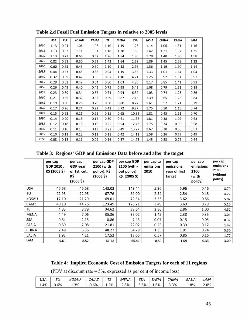
45

Table 2.d Fossil Fuel Emission Targets in relative to 2005 levels   USA  EU  KOSAU  CAJAZ  TE  MENA  SSA  SASIA  CHINA  EASIA  LAM 

2010  1.13  0.94  1.06  1.08  1.10  1.19  1.26  1.14  1.06  1.31  1.16 2015  1.13  0.82  1.11  1.01  1.18  1.38  1.69  1.42  1.21  1.57  1.35 2020  1.13  0.71  0.66  0.67  1.26  1.54  1.90  1.78  1.40  1.90  1.58 2025  0.82  0.68  0.50  0.62  1.43  1.64  2.53  1.89  1.45  2.29  1.32 2030  0.60  0.65  0.45  0.60  1.10  1.38  2.95  1.56  1.19  1.90  1.14 2035  0.44  0.63  0.45  0.58  0.94  1.19  3.58  1.33  1.01  1.64  1.04 2040  0.32  0.59  0.42  0.56  0.87  1.10  4.21  1.25  0.92  1.51  0.97 2045  0.29  0.51  0.42  0.54  0.80  1.03  4.85  1.17  0.85  1.41  0.93 2050  0.26  0.45  0.40  0.45  0.75  0.98  5.48  1.08  0.79  1.31  0.88 2055  0.23  0.39  0.34  0.37  0.71  0.94  6.32  1.03  0.74  1.25  0.86 2060  0.21  0.35  0.32  0.32  0.59  0.87  7.16  1.39  0.65  1.25  0.84 2065  0.19  0.30  0.26  0.28  0.50  0.80  8.22  1.61  0.57  1.21  0.79 2070  0.17  0.26  0.24  0.22  0.42  0.72  9.27  1.75  0.50  1.15  0.74 2075  0.15  0.23  0.21  0.21  0.35  0.65  10.32  1.81  0.43  1.11  0.70 2080  0.14  0.20  0.18  0.17  0.30  0.61  11.38  1.81  0.38  1.02  0.63 2085  0.12  0.18  0.16  0.15  0.25  0.54  12.43  1.75  0.34  0.95  0.58 2090  0.11  0.16  0.13  0.13  0.22  0.49  13.27  1.67  0.30  0.88  0.53 2095  0.10  0.13  0.13  0.11  0.18  0.42  14.12  1.58  0.26  0.79  0.49 2100  0.08  0.12  0.11  0.09  0.16  0.37  14.75  1.45  0.23  0.72  0.44 

Table 3: Regions’ GDP and Emissions Data before and after the target   per cap 

GDP 2010 , K$ (2005 $)    

per cap GDP year of 1st  cut, K$  (2005 $) 

per cap GDP 2100 (with policy), K$  (2005 $) 

per cap GDP 2100 (with‐out policy)  K$  (2005 $) 

per capita emissions 2010 

per cap emissions, year of first target 

per cap emissions 2100 (with policy) 

per cap emissions 2100 (without policy)  

USA  46.68  46.68  143.03  149.44  5.96  5.96  0.46  8.79 EU  22.95  22.95  67.76  69.00  2.54  2.54  0.48  4.22 KOSAU  17.10  21.29  69.01  72.34  3.33  3.62  0.66  5.02 CAJAZ  40.10  44.76  123.49  126.71  3.49  3.69  0.79  5.16 TE  4.83  8.79  34.62  39.64  2.36  2.86  1.00  4.32 MENA  4.49  7.06  35.36  39.02  1.45  2.38  0.35  3.04 SSA  0.64  2.13  8.86  7.45  0.07  0.15  0.05  0.32 SASIA  0.89  2.08  21.81  22.02  0.25  0.39  0.12  1.47 CHINA  2.49  6.36  48.27  54.29  1.35  1.91  0.74  5.30 EASIA  1.93  4.21  17.52  18.06  0.57  0.85  0.16  1.77 LAM  5.61  8.52  61.78  65.41  0.89  1.09  0.33  3.00 

Table 4: Implied Economic Cost of Emission Targets for each of 11 regions

(PDV at discount rate = 5%, expressed as per cent of income loss)

USA  EU  KOSAU  CAJAZ  TE  MENA  SSA  SASIA  CHINA  EASIA  LAM 1.4%  0.6%  1.3%  0.6%  1.2%  2.8%  ‐3.6%  1.6%  3.3%  1.8%  2.0% 

46

Appendix

We have performed a substantial number of alternative simulations -- changing

starting dates for regional policies, and changing the parameters in the Latecomer Catch

Up and Gradual Equalization factors -- in the quest for a set of targets abiding to our

political rules and leading to increasingly stricter environmental targets.

We present below (Figures A1, A2 and A3) the results for a subset of policy

agreements spanning the space of the long-term environmental target. Figure A1 reports

global costs expressed as present value GWP losses. Figure A2 reports the maximum

national income loss that is incurred in any period by any country. Finally, Figure A3

reports the maximum present value national income loss that is incurred by the major

regional loser.

In figures A1, A2 and A3, agreements represented by blue diamonds differ only

with respect to when developing regions get a target below BAU and in how fast they

gradually converge to equal per capita emissions. All parameters are equal for all regions.

Within this group the red square represent the agreement presented in the present paper.

Agreements represented by green triangles were obtained by changing Latecomer Catch

Up and Gradual Equalization factors for different regions, thus tailoring rules to regional

cases with the aim of improving efficiency and lowering maximum regional costs.

First, it is immediately visible how the choice of target, mainly defined by the

speed of long term equalization and the delaying of active reduction in developing

countries, is the major driver of costs. Hence, although our general formulae could be

improved in terms of maximum losses to any country (see green triangles in figure A1,

A2 and A3), losing the simplicity and the political appeal of equal rules for all countries

might not be justified in terms of global efficiency gains.

The second basic fact is that, given realistic assumptions on what will happen

during the first half of the century, it will be increasingly costly to pursue policies aiming

at 470 ppm CO2 and below. No matter how much we tailor the parameters to regional

necessities and how we might change the ranking losers, maximum national income

losses will be higher than 10% in the latest part of the century for any parameter

specification.

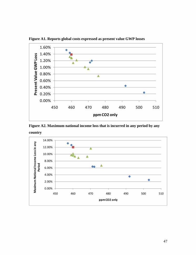
47

Figure A1. Reports global costs expressed as present value GWP losses

0.00%

0.20%

0.40%

0.60%

0.80%

1.00%

1.20%

1.40%

1.60%

450 460 470 480 490 500 510

Presen

t Value

 GWP Loss

ppm CO2 only

Figure A2. Maximum national income loss that is incurred in any period by any

country

0.00%

2.00%

4.00%

6.00%

8.00%

10.00%

12.00%

14.00%

450 460 470 480 490 500 510Maximum

 Nationa

l Incom

e Loss in any

 Perio

d

ppm CO2 only

48

Figure A3. Maximum present value national income loss incurred by greatest loser

0.00%

0.50%

1.00%

1.50%

2.00%

2.50%

3.00%

3.50%

4.00%

4.50%

450 460 470 480 490 500 510Maxim

um Present Value

 National Incom

e Loss 

ppm CO2 only

NOTE DI LAVORO DELLA FONDAZIONE ENI ENRICO MATTEI

Fondazione Eni Enrico Mattei Working Paper Series

Our Note di Lavoro are available on the Internet at the following addresses: http://www.feem.it/Feem/Pub/Publications/WPapers/default.htm

http://www.ssrn.com/link/feem.html http://www.repec.org

http://agecon.lib.umn.edu http://www.bepress.com/feem/

NOTE DI LAVORO PUBLISHED IN 2009 SD 1.2009 Michael Hoel: Bush Meets Hotelling: Effects of Improved Renewable Energy Technology on Greenhouse Gas

Emissions SD 2.2009 Abay Mulatu, Reyer Gerlagh, Dan Rigby and Ada Wossink: Environmental Regulation and Industry LocationSD 3.2009 Anna Alberini, Stefania Tonin and Margherita Turvani: Rates of Time Preferences for Saving Lives in the

Hazardous Waste Site Context SD 4.2009 Elena Ojea, Paulo A.L.D. Nunes and Maria Loureiro: Mapping of Forest Biodiversity Values: A Plural

Perspective SD 5.2009 Xavier Pautrel : Macroeconomic Implications of Demography for the Environment: A Life-Cycle Perspective IM 6.2009 Andrew Ellul, Marco Pagano and Fausto Panunzi: Inheritance Law and Investment in Family Firms IM 7.2009 Luigi Zingales: The Future of Securities Regulation SD 8.2009 Carlo Carraro, Emanuele Massetti and Lea Nicita: How Does Climate Policy Affect Technical Change? An

Analysis of the Direction and Pace of Technical Progress in a Climate-Economy Model SD 9.2009 William K. Jaeger: The Welfare Effects of Environmental Taxation SD 10.2009 Aude Pommeret and Fabien Prieur: Double Irreversibility and Environmental Policy Design SD 11.2009 Massimiliano Mazzanti and Anna Montini: Regional and Sector Environmental Efficiency Empirical Evidence

from Structural Shift-share Analysis of NAMEA data SD 12.2009 A. Chiabai, C. M. Travisi, H. Ding, A. Markandya and P.A.L.D Nunes: Economic Valuation of Forest

Ecosystem Services: Methodology and Monetary Estimates SD 13.2009 Andrea Bigano, Mariaester Cassinelli, Fabio Sferra, Lisa Guarrera, Sohbet Karbuz, Manfred Hafner, Anil

Markandya and Ståle Navrud: The External Cost of European Crude Oil Imports SD 14.2009 Valentina Bosetti, Carlo Carraro, Romain Duval, Alessandra Sgobbi and Massimo Tavoni: The Role of R&D

and Technology Diffusion in Climate Change Mitigation: New Perspectives Using the Witch Model IM 15.2009 Andrea Beltratti, Marianna Caccavaio and Bernardo Bortolotti: Stock Prices in a Speculative Market: The

Chinese Split-Share Reform GC 16.2009 Angelo Antoci, Fabio Sabatini and Mauro Sodini: The Fragility of Social Capital SD 17.2009 Alexander Golub, Sabine Fuss, Jana Szolgayova and Michael Obersteiner: Effects of Low-cost Offsets on

Energy Investment – New Perspectives on REDD – SD 18.2009 Enrica De Cian: Factor-Augmenting Technical Change: An Empirical Assessment SD 19.2009 Irene Valsecchi: Non-Uniqueness of Equilibria in One-Shot Games of Strategic Communication SD 20.2009 Dimitra Vouvaki and Anastasios Xeapapadeas: Total Factor Productivity Growth when Factors of Production

Generate Environmental Externalities SD 21.2009 Giulia Macagno, Maria Loureiro, Paulo A.L.D. Nunes and Richard Tol: Assessing the Impact of Biodiversity

on Tourism Flows: A model for Tourist Behaviour and its Policy Implications IM 22.2009 Bernardo Bortolotti, Veljko Fotak, William Megginson and William Miracky: Sovereign Wealth Fund

Investment Patterns and Performance IM 23.2009 Cesare Dosi and Michele Moretto: Auctioning Monopoly Franchises: Award Criteria and Service Launch

Requirements SD 24.2009 Andrea Bastianin: Modelling Asymmetric Dependence Using Copula Functions: An application to Value-at-

Risk in the Energy Sector IM 25.2009 Shai Bernstein, Josh Lerner and Antoinette Schoar: The Investment Strategies of Sovereign Wealth Funds SD 26.2009 Marc Germain, Henry Tulkens and Alphonse Magnus: Dynamic Core-Theoretic Cooperation in a Two-

Dimensional International Environmental Model IM 27.2009 Frank Partnoy: Overdependence on Credit Ratings Was a Primary Cause of the Crisis SD 28.2009 Frank H. Page Jr and Myrna H. Wooders (lxxxv): Endogenous Network Dynamics SD 29.2009 Caterina Calsamiglia, Guillaume Haeringer and Flip Klijnb (lxxxv): Constrained School Choice: An

Experimental Study SD 30.2009 Gilles Grandjean, Ana Mauleon and Vincent Vannetelbosch (lxxxv): Connections Among Farsighted Agents SD 31.2009 Antonio Nicoló and Carmelo Rodríguez Álvarez (lxxxv): Feasibility Constraints and Protective Behavior in

Efficient Kidney Exchange SD 32.2009 Rahmi İlkiliç (lxxxv): Cournot Competition on a Network of Markets and Firms SD 33.2009 Luca Dall'Asta, Paolo Pin and Abolfazl Ramezanpour (lxxxv): Optimal Equilibria of the Best Shot Game SD 34.2009 Edoardo Gallo (lxxxv): Small World Networks with Segregation Patterns and Brokers SD 35.2009 Benjamin Golub and Matthew O. Jackson (lxxxv): How Homophily Affects Learning and Diffusion in

Networks

SD 36.2009 Markus Kinateder (lxxxv): Team Formation in a Network SD 37.2009 Constanza Fosco and Friederike Mengel (lxxxv): Cooperation through Imitation and Exclusion in Networks SD 38.2009 Berno Buechel and Tim Hellmann (lxxxv): Under-connected and Over-connected Networks SD 39.2009 Alexey Kushnir (lxxxv): Matching Markets with Signals SD 40.2009 Alessandro Tavoni (lxxxv): Incorporating Fairness Motives into the Impulse Balance Equilibrium and Quantal

Response Equilibrium Concepts: An Application to 2x2 Games SD 41.2009 Steven J. Brams and D. Marc Kilgour (lxxxv): Kingmakers and Leaders in Coalition Formation SD 42.2009 Dotan Persitz (lxxxv): Power in the Heterogeneous Connections Model: The Emergence of Core-Periphery

Networks SD 43.2009 Fabio Eboli, Ramiro Parrado, Roberto Roson: Climate Change Feedback on Economic Growth: Explorations

with a Dynamic General Equilibrium Mode GC 44.2009 Fabio Sabatini: Does Social Capital Create Trust? Evidence from a Community of Entrepreneurs SD 45.2009 ZhongXiang Zhang: Is it Fair to Treat China as a Christmas Tree to Hang Everybody’s Complaints? Putting

its Own Energy Saving into Perspective SD 46.2009 Eftichios S. Sartzetakis, Anastasios Xepapadeas and Emmanuel Petrakis: The Role of Information Provision

as a Policy Instrument to Supplement Environmental Taxes: Empowering Consumers to Choose Optimally SD 47.2009 Jean-François Caulier, Ana Mauleon and Vincent Vannetelbosch: Contractually Stable Networks GC 48.2009 Massimiliano Mazzanti, Susanna Mancinelli, Giovanni Ponti and Nora Piva: Education, Reputation or

Network? Evidence from Italy on Migrant Workers Employability SD 49.2009 William Brock and Anastasios Xepapadeas: General Pattern Formation in Recursive Dynamical Systems

Models in Economics SD 50.2009 Giovanni Marin and Massimiliano Mazzanti: Emissions Trends and Labour Productivity Dynamics Sector

Analyses of De-coupling/Recoupling on a 1990-2005 Namea SD 51.2009 Yoshio Kamijo and Ryo Kawasaki (lxxxv): Dynamics, Stability, and Foresight in the Shapley-Scarf Housing

Market IM 52.2009 Laura Poddi and Sergio Vergalli: Does Corporate Social Responsibility Affect the Performance of Firms? SD 53.2009 Valentina Bosetti, Carlo Carraro and Massimo Tavoni: Climate Change Mitigation Strategies in Fast-

Growing Countries: The Benefits of Early Action GC 54.2009 Alireza Naghavi and Gianmarco I.P. Ottaviano: Firm Heterogeneity, Contract Enforcement, and the Industry

Dynamics of Offshoring IM 55.2009 Giacomo Calzolari and Carlo Scarpa: On Regulation and Competition: Pros and Cons of a Diversified

Monopolist SD 56.2009 Valentina Bosetti, Ruben Lubowski and Alexander Golub and Anil Markandya: Linking Reduced

Deforestation and a Global Carbon Market: Impacts on Costs, Financial Flows, and Technological Innovation

IM 57.2009 Emmanuel Farhi and Jean Tirole: Collective Moral Hazard, Maturity Mismatch and Systemic Bailouts SD 58.2009 Kelly C. de Bruin and Rob B. Dellink: How Harmful are Adaptation Restrictions SD 59.2009 Rob Dellink, Michel den Elzen, Harry Aiking, Emmy Bergsma, Frans Berkhout, Thijs Dekker, Joyeeta Gupta:

Sharing the Burden of Adaptation Financing: An Assessment of the Contributions of Countries SD 60.2009 Stefania Tonin, Anna Alberini and Margherita Turvani: The Value of Reducing Cancer Risks at Contaminated

Sites: Are More Heavily Exposed People Willing to Pay More? SD 61.2009 Clara Costa Duarte, Maria A. Cunha-e-Sá and Renato Rosa: The Role of Forests as Carbon Sinks: Land-Use

and Carbon Accounting GC 62.2009 Carlo Altomonte and Gabor Békés: Trade Complexity and Productivity GC 63.2009 Elena Bellini, Gianmarco I.P. Ottaviano, Dino Pinelli and Giovanni Prarolo: Cultural Diversity and Economic

Performance: Evidence from European Regions SD 64.2009 Valentina Bosetti, Carlo Carraro, Enrica De Cian, Romain Duval, Emanuele Massetti and Massimo Tavoni:

The Incentives to Participate in, and the Stability of, International Climate Coalitions: A Game-theoretic Analysis Using the Witch Model

IM 65.2009 John Temple Lang: Article 82 EC – The Problems and The Solution SD 66.2009 P. Dumas and S. Hallegatte: Think Again: Higher Elasticity of Substitution Increases Economic Resilience SD 67.2009 Ruslana Rachel Palatnik and Roberto Roson: Climate Change Assessment and Agriculture in General

Equilibrium Models: Alternative Modeling Strategies SD 68.2009 Paulo A.L.D. Nunes, Helen Ding and Anil Markandya: The Economic Valuation of Marine Ecosystems IM 69.2009 Andreas Madestam: Informal Finance: A Theory of Moneylenders SD 70.2009 Efthymia Kyriakopoulou and Anastasios Xepapadeas: Environmental Policy, Spatial Spillovers and the

Emergence of Economic Agglomerations SD 71.2009 A. Markandya, S. Arnold, M. Cassinelli and T. Taylor: Coastal Zone Management in the Mediterranean:

Legal and Economic Perspectives GC 72.2009 Gianmarco I.P. Ottaviano and Giovanni Prarolo: Cultural Identity and Knowledge Creation in Cosmopolitan

Cities SD 73.2009 Erik Ansink: Self-enforcing Agreements on Water allocation GC 74.2009 Mario A. Maggioni, Francesca Gambarotto and T. Erika Uberti: Mapping the Evolution of "Clusters": A

Meta-analysis SD 75.2009 Nektarios Aslanidis: Environmental Kuznets Curves for Carbon Emissions: A Critical Survey SD 76.2009 Joan Canton: Environmentalists' Behaviour and Environmental Policies SD 77.2009 Christoph M. Rheinberger: Paying for Safety: Preferences for Mortality Risk Reductions on Alpine Roads

IM 78.2009 Chiara D’Alpaos, Michele Moretto, Paola Valbonesi and Sergio Vergalli: "It Is Never too late": Optimal Penalty for Investment Delay in Public Procurement Contracts

SD 79.2009 Henry Tulkens and Vincent van Steenberghe: “Mitigation, Adaptation, Suffering”: In Search of the Right Mix in the Face of Climate Change

SD 80.2009 Giovanni Bella: A Search Model for Joint Implementation SD 81.2009 ZhongXiang Zhang: Multilateral Trade Measures in a Post-2012 Climate Change Regime?: What Can Be

Taken from the Montreal Protocol and the WTO? SD 82.2009 Antoine Dechezleprêtre, Matthieu Glachant, Ivan Hascic, Nick Johnstone and Yann Ménière: Invention and

Transfer of Climate Change Mitigation Technologies on a Global Scale: A Study Drawing on Patent Data SD 83.2009 László Á. Kóczy: Stationary Consistent Equilibrium Coalition Structures Constitute the Recursive Core SD 84.2009 Luca Di Corato and Michele Moretto: Investing in Biogas: Timing, Technological Choice and the Value of

Flexibility from Inputs Mix SD 85.2009 Valentina Bosetti, Enrica De Cian, Alessandra Sgobbi, and Massimo Tavoni: The 2008 WITCH Model: New

Model Features and Baseline IM 86.2009 Rocco Macchiavello: Vertical Integration and Investor Protection in Developing Countries SD 87.2009 Massimiliano Mazzanti and Antonio Musolesi: Carbon Kuznets Curves: Long-run Structural Dynamics and

Policy Events GC 88.2009 Gianmarco I.P. Ottaviano and Christian Volpe Martincus: SMEs in Argentina: Who are the Exporters GC 89.2009 Gianpaolo Rossini and Cecilia Vergari: Input Production Joint Venture SD 90.2009 Angelo Antoci, Simone Borghesi and Marcello Galeotti: Environmental Options and Technological

Innovation: An Evolutionary Game Model GC 91.2009 Cristina Cattaneo: The Decision to Migrate and Social Capital: Evidence from Albania SD 92.2009 Valentina Bosetti and Jeffrey Frankel: Global Climate Policy Architecture and Political Feasibility: Specific

Formulas and Emission Targets to Attain 460 ppm CO2 Concentrations

(lxxxv) This paper has been presented at the 14th Coalition Theory Network Workshop held in Maastricht, The Netherlands, on 23-24 January 2009 and organised by the Maastricht University CTN group (Department of Economics, http://www.feem-web.it/ctn/12d_maa.php).