THE WILLIAM DAVIDSON INSTITUTE AT THE UNIVERSITY OF MICHIGAN BUSINESS SCHOOL

Measuring the Value Added by Money in Trade

By: Vlad Ivanenko

William Davidson Institute Working Paper Number 635 November 2003

Measuring the Value Added by Money in Trade By Vlad Ivanenko†

August 2003

Abstract: The paper tests the proposition that money generates value in trade. It examines the data

for 5,746 Russian companies for 1997 and finds that money accounts for 24.6 percent of their value-added.

The functional form of the return on money in trade is determined to be positive and marginally declining.

The paper imputes that Russian GDP lost 8.1 percent in 1997 because of diminished use of money

in trade. It hypothesizes that the severity of the Great Depression in the USA of 1930s could have been

significantly reduced if the proposed barter networks were implemented at the time.

JEL code: E4, N10, P34

Keywords: Money, Value-added, Empirical econometrics

† Dept. of Economics, University of Western Ontario, London, Ontario N6A 5C2, Canada, e-mail

vivanenk@uwo.ca. Vera Ivanenko has checked that the authors’ grammar complies with generally accepted rules.

1

1. Introduction

The statement that the institute of money provides important services to economic

agents is broadly accepted within the profession. Undergraduate textbooks on money and

banking present vivid pictures of the world without money emphasizing how the need to

satisfy the “double coincidence of wants” condition increases transaction costs.1 As

traders spend more time and other resources searching for customers, the volume of trade

falls and cost grows. Thus the use of monetary as compared with non-monetary trade is

viewed as a positive development that increases economic welfare.

General agreement that money is useful should not preclude us from attempting to

measure the degree of its usefulness. A quantitative evaluation of the role played by

money in trade is a necessary input that monetary authorities can take into account while

contemplating the tightening of money supply.2 Such knowledge may also be relevant to

the branch of monetary theory that seeks to understand how and why money is such an

important part of market transactions. Finally, economic historians may find it useful to

reconsider how non-monetary trade contributed to the severity of the Great Depression in

the USA of 1930s and transition economies in 1990s.3

This paper estimates how the use of monetary trade by firms affects the creation

of value by examining cross-sectional data on 5,746 publicly traded Russian companies

for 1997. The choice of the country and year is not accidental. Russia as a number of

other transition economies witnessed a surge in non-monetary trade prior to the default of

1998.4 This unique situation set a natural experiment for the investigation of properties

that money exhibits in trade. Further, the use of monetary trade in Russia was lowest in

1997 implying that the variation in the use of money in trade across firms was highest.

This makes econometric analysis less sensitive to other, unobserved factors.5 The firm-

1 See, for example, p. 22 in Mishkin, Frederic S. (1993). The Economics of Money, Banking and

Financial Institutions, 3rd Edition, HarperCollins Publishers, New York. 2 Kashyap et al (1993) present evidence that tight monetary policy affects the composition of corporate

finances. In a closely related paper, Oliner and Rudebusch (1996) extend this line of research showing that small firms keep less money balances and large firms – switch to non-banking sources of finance.

3 Sam Lubelsky (New York Times, March 12, 1933) reported that up to a million of Americans were employed in fully barter-operating establishments at that time. See Keehn (1982).

4 See Seabright (2000). 5 By monthly data, the fraction of non-monetary in total trade was highest in August 1998. However,

the default of the same month might introduce disturbances that affect firms unevenly. To make the identification problem less challenging a “calmer” year 1997 was chosen.

2

level data indicate that monetary trade adds value to the firm’s output at a positive but

declining rate.

This study does not have close predecessors. In style, it is related to the empirical

research on the demand for money by firms, e.g. Mulligan (1997). In substance, the paper

can be broadly associated with literature that explores the credit channel of monetary

policy, e.g. Bernanke (1983). This work differs from other papers in two aspects. Unlike

Mulligan (1997), it focuses on the relationship between the mode of trade and the value-

added and not on the link between money holdings and output. Compared with Bernanke

(1983), the paper explores a non-monetary financial phenomenon that belongs to the

same group of credit-affecting factors but is not suggested in the previous work.

2. An Empirical Model of the Value-added Generated by Monetary Trade

Since the topic of this paper is of general economic interest, it is necessary to keep

the number of identifying restrictions low. This stress on generality warns against

building a detailed behavioral model of the choice between monetary and non-monetary

trade extending, for example, the model developed in Kiyotaki and Wright (1993). The

behavioral approach is definitely worth pursuing because it can shed light on other

important issues, e.g. in corporate finance.6 Yet, it does not generate additional insight for

the purposes of this paper while diverts attention from the main question.

Let the value-added relative to the output produced by firm j (V j) be a function of

the fraction of monetary to total trade that it uses (M j) – that we measure in percentage

points M j ∈ [0,100] – and other firm-specific factors (Z j)

),( jjj ZMfV = [1]

It is uncontroversial to say that a higher value of M j results in a continuous and monotone

increase in the value-added V j on the whole interval [0,100]. Then, it is reasonable to

assume that V j is differentiable in M j on the same interval. Economic theory is less

certain about the relationship between M j and Z j. Firms take into consideration diverse

factors such as their individual production technology, optimal scale of operations, or

6 One interesting question to ask is to investigate if a higher use of non-monetary trade is compatible

with the trade-off versus pecking order models of corporate finance; see Myers (1977) and Myers and Majluf (1984) respectively. Another promising venue is to study how the costs of non-monetary trade are distributed among different claimants on the value-added – owners, workers, and government.

3

geographic location when they choose how much money to use in trade.7 Let us assume

that M j is related to Z j with a continuous and monotone function g’ (M j). Denoting the

inverse function of g’ (M j) as g (M j), equation [1] can be rewritten as

))(,( MgMfV = [2]

where subscript j is dropped for expositional purposes. Using Taylor’s formula equation

[2] can be approximated as

RMggVV

MgV

VMgMV MMMMMMMM ++++

++

+= ...!2

)2(!1

)()0())(,( 200000000 [3]

where M 0 is normalized to 0. An econometric analogue of equation [3] is

εββα ++++= ...221 MMV [4]

where error term ε can be correlated with explanatory parameters.8

Note that when the effect of factors Z j on M j and V j is accounted for, the impact

of M j on V j is independent from firm-specific characteristics. Therefore, as the sample

size increases, the statistical estimates of the terms of f (.) in [3] converge to their true

values. Estimating and testing β’s for significance is the primary exercise that this paper

conducts.

3. Firm-Level Data

The firm-level data for this study were mostly obtained from the website of the

Federal Committee for Security Markets of the Russian Federation.9 In accordance with

the regulations, certain Russian publicly traded companies are obliged to disclosure its

extended balance sheet (forms 1 and 5), financial statement (form 2), and statement on

money flows (form 4), which the author has used to build a database that eventually has

comprised 5,746 companies. The choice of companies was based on the availability of

data that were necessary to calculate the present value of the firm’s value-added and the

fraction of monetary in total trade.10

7 For example, firms locked in long-term contracts – like coal mines and power plants, gas producers

and distributors – are more likely to engage in mutual clearance of debts by non-monetary means. 8 The error term ε includes the cross-products of G M and G MM with M, and M 2 that may be

statistically different from 0. 9 The website address is http://disclosure.fcsm.ru 10 Not all companies complied with the regulations. Reports for many firms, including some largest

ones, were unavailable. This fact suggests that the obtained reports were not deliberately falsified; see the

4

Given that Russian statistics is commonly suspected to be flawed if not

deliberately distorted, a significant effort has been extorted in insuring the consistency of

data. To this end, the author has checked that sums in forms 1, 2, and 4 correspond to

their components (14, 4, and 2 checks respectively), entries on money holdings are

identical for forms 1 and 4 (2 checks), and entries on total costs coincide for forms 2 and

5(6). Significant amount of errors have been discovered. Up to a third of firms in the total

sample presented reports with typing errors. Most commonly, a person responsible for the

report omitted or added a digit to an entry, which led to the wrong summation of the

entries. Sometimes, the typist attempted to balance books ad hoc being obviously

unaware of the error. Such inconsistencies were uncovered and corrected. The other

crosscheck of documents has revealed about 60 reports that combined forms 1 and 4

prepared for different years. These firms have been deleted from the sample. A deliberate

misrepresentation of results was found in few separate instances.11 They were not

considered in this study. The most troubling was the finding that 129 firms received more

cash in payment for goods and services, entry 4(30), than they reportedly sold, entry

2(10). A closer look on industrial affiliation of this group has revealed that it consisted of

enterprises in sectors commonly suspected of participating in informal activities such as

distilleries and traders. These enterprises were left in the sample but to avoid the

problems created by outliers, the author imposed low and upper bounds on the parameters

of interest.12 It is worth noting that most of errors and misrepresentations could be

corrected or, at least, flagged. This conclusion indicates that a massive and consistent

distortion of actual accounting information was challenging undertaking for the great

majority of enterprises present in the sample.13

Two variables of interest have been constructed using primary accounting

information. The present value of the value-added PV (V j) at producer prices has been

discussion below. Dishonest managers could always choose not to report than to get engaged in expensive matching of false statements in a consistent way.

11 For example, an identical report was submitted for 5 different companies registered on two addresses in Moscow.

12 The value-added as a percentage fraction of revenue has been limited to the interval [-100,100] and the fraction of monetary to total trade – [0,100].

13 The easiest way to conceal actual information from outsiders like the author would be to ignore the requirement to disclose information. This is what many companies did in 1997. Consequently, they were not included in the sample.

5

found as the percentage difference between the present value of total revenue PV (Y j) and

the present value of the costs of intermediate inputs PV (C j m) and normalized by PV (Y j)

100)(

)(/

)()(

1(100))()(

1()()( 12

1

12

1×

+

+−=×−= ∑∑

== t jj

j

t jmj

mj

j

mj

j

j

tptY

tptC

YPVCPV

YPVVPV

τν [5]

where Y j (t) and C j m (t) are imputed revenue and intermediate costs for month t, p j (t)

and p m j (t) are changes in prices of output and intermediate costs for month t, and τ j and

ν j are the average duration of the grace period in months granted to consumers and

received from suppliers if any.14

The percentage fraction of monetary to total trade cannot be determined on the

basis of accounting information unless two simplifying assumptions are made. It has been

assumed in the paper that the dynamics of payments and deliveries did not change in two

adjacent years. The problem is that monetary receipts or advance payments are reported

on historical basis. As such the amount of money received in 1997 includes payment for

deliveries that took place in 1996 and exclude payments for deliveries of 1997 that were

received in 1998. Similarly, advance payments made in 1996 for deliveries of 1997 are

not reported in the statement on money flow for 1997. The assumption of unchanged

dynamics allows approximating the value of payment made in 1998 for deliveries of

1997 with the value of payment made in 1997 for deliveries of 1996. The same argument

applies to the value of advance payments. Then, the value of monetary receipts for

deliveries made in 1997 becomes equal to the sum of advance payments and payments

for goods and services received in the same year. Their percentage fraction in total sales

is the value of monetary receipts for 1997 divided by the total revenue of 1997 and

multiplied by factor 100

100×+

=j

jjj Revenue

ymentMonetaryPamentAdvancePayM [6]

A scatter plot of both parameters is presented on Figure 1.

14 If prepayment was required τ and ν become negative. Complete formulas for transformation of

original data are presented in Appendix A. The use of present values instead of values at current prices is explained by large variations across

firms in their stocks of receivables or payables. Stocks accumulated exactly because firms’ customers or firms did not have money to complete transactions promptly. This loss in value because of waiting is relevant to the question that we study, namely what is the value that money generates in trade.

6

Figure 1: Scatter plot of the value-added and the fraction of monetary to total

trade, in percent. Sources: Author’s dataset

4. Estimates of the Value Added by Money in Trade

The empirical part focuses on the estimation of the functional relationship

between the value-added and the fraction of monetary to total trade; see equation [4]. We

begin with ordinary least squares (OLS) estimates under the assumption that the

polynomial form of [4] is unknown. Column 2 of Table 1 presents the obtained results

that we discuss next.

First, the regression suggests the quadratic form of the polynomial function f (.).

The inclusion of explanatory variables of a higher power than two generates statistically

insignificant coefficients. This result makes sense from the theoretic point of view. It is

generally accepted that the return on inputs in the production function is positive and

diminishes as the relative consumption of the input increases. There is no rationale to

expect that the use of money in transactions does not exhibit a similar pattern.

Second, tests for heteroskedasticity strongly reject the hypothesis of

homoskedastic errors. This result is not unexpected given our previous note of a potential

7

correlation between explanatory variable M j and the vector of omitted firm-specific

parameters Z j.15 To correct for heteroskedasticity, we employ weighed least squares

(WLS) regression, the results of which are reported in column 3 of Table 1.16

OLS WLS

Intercept 41.032 41.895

MT 0.268 0.237

t-stat (6.03) (5.16)

MT2 -0.0013 -0.00103

t-stat (-3.21) (-2.55)

R 2 0.0326 0.0295

N 5,746 5,746

White statistics 172.4 6.67

Breusch-Pagan statistics a 78.44 1.81

Table 1: Regression of quadratic form of equation [4]. Results significant at 1%

are in bold, at 5% - in italics. Sources: Author’s calculations using SAS software a With intercept, MT, and MT2 as explanatory variables.

The correction for heteroskedastic errors does not change our previous analysis in

important ways. The WLS regression results indicate that the likeliest functional form of f

(.) is still quadratic.17 The magnitude and the sign of coefficients stay the same. The tests

of their statistical significance strongly reject the hypothesis that they are equal to zero.

Finally, we construct confidence intervals for the estimates obtained by WLS

regression using nonparametric method of local maximum likelihood (LOESS).18

15 See the derivation of equation [2]. 16 The author has used the WLS regression technique as explained in Greene (1990, p. 405-6). The

main problem in WLS is to find appropriate weights. This is done by regressing squared residuals obtained by OLS regression on explanatory variables. In this case, the weights were obtained by regressing residuals on MT of up to 4th power. The reason for inclusion of additional terms is that the distribution of observations is bimodal and cannot be replicated by a quadratic function; see Figure 3 below.

17 That is the estimates of coefficients of higher power are insignificant. 18 The author has used procedure LOESS of SAS software, which stands for ‘local regression’. The

main task in the procedure is to find a suitable smoothing parameter that determines the limits of localities, which are included in local regression. The author has relied on Akaike Information Criterion choosing the value of smoothing parameter 1.3. Unfortunately, LOESS requires building and manipulating with a covariance matrix, of size 5747×5747 in our case, to construct the confidence interval, which is impractical

8

Nonparametric methods are preferable in this case because no assumptions about the

parametric form of the regression can be made a priori. Figure 2 plots the estimates that

are obtained with WLS and LOESS regressions and shows the 95% confidence interval.

Figure 2: Estimates of the quadratic form of equation [4]. Sources: Author’s

calculations using SAS software

Nonparametric estimation shows that WLS estimate of the quadratic form of

equation [4] lies within 95% confidence bounds. This result supports our previous

conclusion that the use of money in trade exhibits positive and diminishing return in

terms of adding value.

5. Testing for Stability of the Coefficients

In section 4 we have derived and tested for stability the functional form of

equation [4]. Here we estimate how omitted parameters, such as the firm’s industrial

affiliation, its geographic location, and size can affect the impact that the use of money in

trade makes on the value-added. It may be significant because firms presented in the

at the moment. The author has followed Yatchew (1998, Fig. 7) constructing the confidence interval asymptotically. An accessible introduction to LOESS is available at http://www.ats.ucla.edu/stat/sas/library/loesssugi.pdf.

9

sample compose at least two distinct groups in the use of money in trade as the graph of

their joint probability density function shows; see Figure 3.19

Figure 3: Estimated joint probability density function of (M, V) found using

kernel density estimate with the bandwidth M = 1.4, V = 1.4. Sources: Author’s calculations

using SAS software.

To this end we run WLS regression for sub-samples of firms that possess similar

characteristics.20 The obtained results are presented in Table 2.

The findings presented in Table 2 lead to several conclusions. First, we see that

the sampling size matters, which is unsurprising. Money plays a secondary role in

generating value and as the sample is subdivided into groups the relationship between

money and the value-added becomes obscured. This observation warns against mechanic

extrapolation of the obtained results. Our estimates of the effects that non-monetary trade

made on GDP historically – see the next section – should be treated with reservation. Yet,

19 Values for figure 3 have been obtained using KDE, which stands for ‘kernel density estimator’, procedure of SAS software. The bandwidth parameter is 1.4 that was the smallest parameter that generated smooth surface. Figure 3 is drawn with procedure G3d. An accessible introduction to KDE and G3d can be found at www.cpcug.org/user/sigstat/PowerPointSlides/kde.ppt

10

OLS or WLS

Average MT, % MT (t-stat) MT2 (t-stat) R 2 Sample

size

Industrial affiliation

1 Machine building WLS 46.144 0.354 (4.06) -0.003 (-3.19) 0.025 1,039

2 Food processing OLS 70.976 -0.053 (-0.62) 0.001 (1.65) 0.036 667

3 Other manufacturing and mining WLS 44.516 0.185 (2.76) -0.001 (-1.64) 0.019 1,452

4 Agriculture OLS 55.844 -0.267 (-0.97) 0.002 (0.94) 0.004 246

5 Transportation and communication WLS 73.247 0.617 (3.26) -0.004 (-2.68) 0.041 477

6 Construction WLS 53.429 0.294 (2.49) -0.001 (-0.76) 0.090 617

7 Trade and business services WLS 74.621 0.431 (2.36) -0.002 (-1.72) 0.014 920

8 Science and earth exploration WLS 73.008 0.181 (0.77) -0.001 (-0.82) 0.002 328

Geographic location

9 Moscow and region WLS 79.374 0.395 ( 2.10) -0.002 (-1.24) 0.026 986

10 Saint Petersburg and region WLS 73.761 0.029 (0.11) 0.000 (0.21) 0.010 313

11 North and Center WLS 54.307 0.098 (0.72) 0.000 (0.15) 0.031 550

12 ‘Black Earth’ regions WLS 56.479 0.236 (1.94) -0.001 (-0.92) 0.032 862

13 Central Volga WLS 47.205 0.254 (2.78) -0.001 (-1.68) 0.023 1,016

14 South WLS 59.551 0.117 (0.78) 0.000 (0.23) 0.046 511

15 Ural OLS 45.635 0.132 (0.91) -0.000 (-0.21) 0.029 328

16 Western Siberia WLS 46.710 0.302 (2.27) -0.002 (-1.36) 0.030 599

17 Central Siberia and Pacific WLS 56.660 0.470 (3.31) -0.003 (-2.48) 0.037 581

Scale of operation (revenue)

18 Large ( > 60,000 mil Ruble) WLS 51.905 0.131 (2.25) -0.000 (-0.51) 0.030 1,838

19 Medium (10,000-59,999 mil Ruble) WLS 57.943 0.054 (0.86) 0.000 (0.45) 0.017 2,096

20 Small ( < 10,000 mil Ruble) WLS 64.741 0.481 (4.30) -0.003 (-3.23) 0.024 1,812

Table 2: OLS or WLS if tests reject the hypothesis of homoskedastic errors

regressions for sub-samples. Results significant at 1% are in bold, at 5% - in italics. Sources: Author’s calculations using SAS software. Appendix B contains descriptors of the aggregates for

industrial affiliation and geographic location

the estimates built on smaller samples generally preserve the upward slope of the

regression line implying that the finding that money generates value in trade is robust.

Second, the grouping of significant results shows that the industrial affiliation is one of

20 We use the same econometric techniques as described above to obtain the results of Table 2.

11

the main omitted factors that affect the relationship between money and value-added.

This finding is uncontroversial. Industries vary in relative capital and labor intensity and

the effectiveness of the use of money may be unevenly correlated with each of them: e.g.

owners receive the return on capital in form of shares and other non-monetary means

more often than workers do. Third, the use of money in trade is more valuable in

situations where the maintenance of trust is costly or, reinterpreting Williamson (1989),

where money saves on transactions costs when contracts are incomplete or not fully

enforceable. As an example, the sector of machine building requires a larger degree of

cooperation, or coordination along the technological chain, than the sector of food

processing where the problem of opportunistic behavior is less severe because

intermediate products are easier to convert for alternative use. Thus, if enterprises in the

former sector employ money in trade more effectively, they see a larger increase in total

productivity that food producers do. This argument is supported by the finding that

money is the most valuable in trade for small firms. Small firms usually have few

customers or suppliers and they are most vulnerable to their opportunistic behavior. In

this respect the present work is consistent with finding by Kashyap et al (1993) and

Oliner and Rudebusch (1996) who report that small firms contract more in time of tight

monetary policy than large companies do.21

6. The Role Played and Not Played by Money in Two Great Depressions:

Russia of 1990s and the USA of 1930s

The preceding analysis enables us to address the question of how detrimental or

useful non-monetary trade can be for GDP. The situation in which Russia found itself in

1990s is particularly relevant. According to GKS (2000, Table 2.19) Russian GDP of

1997 amounted to 63.7% of GDP in 1991. At the same time the fraction of monetary

trade for industrial establishments fell from 92% in February 1992 to 53% in December

21 Non-linearity of responses to the use of money in trade that firms of different size exhibit is an interesting finding. The result that the largest firms receive more value from the use of money than medium companies do is consistent with the proposition advanced independently by two researchers. Humphrey (2000) notes that large Russian companies serve as clearing houses for their smaller clients. As such they receive a return on monetary credit extended to cash-constrained customers. Kashyap and Stein (1994) suggest that an increase in the fraction of commercial papers in total external finance in the USA flags the shift of external financing from banks to large producers who increase the volume of trade credit extended

12

1997.22 Can it be that the growth of less efficient non-monetary trade is partially

responsible for decline in GDP?

To answer this question we impute losses associated with non-monetary trade for

23 economic sectors that appear in the input-output table for 1997.23 Since almost every

sector of the table is represented in our sample – government being a notable exemption –

the function of the value-added with the fraction of monetary trade as its argument can be

estimated using WLS regression for equation [4] for each of them. The obtained formulas

are used to forecast the amount of the value-added that the sectors would generate if they

traded only with money. These forecasts are compared with the average of the value-

added found for sub-samples and their ratio is applied to the sectoral value-added as

reported in the input-output table to arrive at the imputed estimates of the value-added

when all trade is monetary. Mathematically, we calculate the forecasted value-added for

each sector, including the low and upper bounds, as

GDPV

VsetVV UL ×

±=

)ˆ(ˆ~ 2/,

λ [7]

where ULV ,~ is the forecast confidence interval for V; V̂ is the predicted amount of the

value-added if all trade is monetary (M = 100) and se (V̂ ) is its standard error; V is the

average value-added for the sub-sample, t λ/2 is t-statistics with λ determining the power

of the test, and GDP is the amount of the sectoral value-added taken from the input-

output table. The results of calculations are presented in Table 3.

Comparing the sums of columns 2 and 3 of Table 3 we see that if Russian

companies traded only with money in 1997, the expected increase in GDP, at producer

prices, would amount to 8.1 percent. This finding indicates that the decline in monetary

trade significantly contributed to the severity of the Russian depression of 1990s. This

conclusion partially explains why the economy rebounded so quickly after the default of

August 1998. As monetary trade became more widespread, it brought about gains that

were caught and reported in general statistics.

to their customers. In both cases a higher return on money that the largest companies receive is explained by their financial activity, which is unrelated to production.

22 According to the monthly survey conducted by the Russian Economic Barometer, which is available at http://www.imemo.ru/eng/barom/survey.htm, Table 18.

23 See Ivanenko (2001) for the derivation of the table.

13

GDP:

I/O table

Imputed value-added (average

ULV ,~ )

LV~ : 95% confidence

interval

UV~ : 95% confidence

interval

1 Electricity 102,471 148,316 127,955 168,678

2 Oil and gas extraction and processing 146,487 159,130 137,574 180,686

3 Coal and other fuels mining 20,658 21,997 17,696 26,299

4 Iron and steel 32,474 34,793 28,944 40,642

5 Non-ferrous metallurgy 43,123 45,812 34,180 57,444

6 Chemical and petrochemical 26,925 30,541 27,694 33,388

7 Machine building and metal processing 124,254 129,200 122,843 135,556

8 Wood and paper 21,018 20,171 17,994 22,349

9 Construction materials 28,695 31,610 29,342 33,878

10 Textile, apparel, and footwear 12,399 13,617 12,669 14,564

11 Food processing 83,103 90,495 83,728 97,262

12 Other manufacturing 17,781 18,338 16,072 20,604

13 Construction 179,200 204,887 195,589 214,184

14 Agriculture and forestry 149,269 153,088 123,888 182,288

15 Transportation services 233,421 236,720 221,987 251,453

16 Communications 44,213 45,731 31,118 60,343

17 Trade, intermediation, and food services 494,837 504,066 449,402 558,730

18 Other activities related to production of goods and services 19,667 18,912 14,762 23,063

19 Residential, communal, and household services 133,620 172,789 133,241 212,337

20 Health, education, and culture 191,707 186,723 120,970 252,477

21 Science, geology, and meteorology 28,543 29,745 27,468 32,021

22 Finance, credit, and insurance 16,493 17,182 14,439 19,925

23 State and business management and NGO 157,858 181,071 175,586 186,556

Memo: Total (in billion of Rubles) 2,308,216 2,494,933 2,165,138 2,824,728

Table 3: Actual and imputed value-added at producer prices under the condition

of all monetary trade, in billion of Rubles. Sources: column 2 is from the input-output table for

1997, see Ivanenko (2001); column 3 – the predicted amount of the value-added (V hat); columns 4 and 5 –

low and upper bounds (V L, U tilde), author’s calculations

14

While the application of the obtained results to the Russian situation of 1990s is

straightforward, the relevance of the suggested relationship between money and the

value-added to other historical instances is questionable. Certainly, the Russian

depression of 1990s differs in significant ways from the Great Depression of 1930s. One

important and unobserved parameter is the state of financial technology. We have

estimated that trading without money reduces the value-added by 24.3 percent; see

column 3 of Table 1. This number is dependent on financial innovations. For example, an

introduction of a new system of mutual debt clearance reduces the demand for money to

serve the same number of transactions, as the operation of inter-banking clearance centers

show.24 Another parameter that has obviously changed in time is the average size of the

firm. We have found that small firms are more dependent on money in trade than large

companies; see the last three rows in Table 2. Though Berle and Means noticed the

growth of large American corporations in 1930s,25 the average size of Russian companies

was larger in 1990s compared with the size of Americans firms in 1930s.

With these warnings in mind, let us hypothesize how the use of non-monetary

trade would affect the American GDP in 1933 if it was widely practiced. This proposition

would not sound strange to America of 1930s.26 Barter exchanges operated in a number

of states and were at least contemplated nationwide. New York Times reported on March

12, 1933 that up to a million of Americans learned how to live without money. A

Democratic Party nominee for Governor of California in 1934 and famous novelist Upton

Sinclair based his unsuccessful election platform, End Poverty in California, on the

premises that trade without money should be publicly promoted. Federal Emergency

Relief Act of 1933 contained a provision that authorized the making of federal aid grants

to ‘self-help associations for the barter of goods and services’.

24 In limit, as the tracking of trade deals becomes all-embracing, money services become worthless as

the work by Kocherlakota (1998) shows. Yet, with respect to financial innovations, Russian financial system was rather similar to the American system of 1930s. Its inter-banking clearance centers operated manually and severe delays in the processing of checks in 1992-4 were the reason for numerous complaints.

25 See Berle, Adolf A. Jr. and Gardiner C. Means. The Modern Corporation and Private Property, The Macmillan company, New York, 1933

26 The information related to American experience with barter or, more generally, non-monetary trade that is presented further has been taken from Keehn (1982).

15

Yet, trade without money did not take roots during that time. Assuming that 2

percent of the labor force – which is what one million barter users meant in 1933 – is

representative of the scale of non-monetary operations in the USA in1933, our estimates

show that it accounted for mere 1.5 percent share in total GDP.27 This amount is

insignificant in comparison with 45.9 percent drop in GDP that took place between 1929

ad 1933.28 The miniscule share of barter in total sales apparently explains why economic

historians ignored this phenomenon. However, if the proposition to sponsor non-

monetary trade by the state that was advocated by Upton Sinclair would be implemented

it resulted in quite substantial economic gains.

Let us consider what would happen if 24.9 percent of the labor force reported to

be unemployed in 1933 started to work on public script or other form of compensation

unrelated to money. Assuming that their idleness was responsible for total decline in

GDP, their work in the non-monetary sector would restore up to 34.8 percent of GDP.

This would reduce the scale of the Great Depression to 11.3 percent.29 Thus, in the

retrospect, Upton Sinclair and his followers might not be communist conspirators as

many their contemporaries believed but thinkers whose time was yet to come.30

References

Bernanke, Ben S. (1983). “Nonmonetary Effects of the Financial Crisis in

Propagation of the Great Depression”, American Economic Review, 73(3): 257-76, June

GKS (Russian State Committee for Statistics), (2000). Natzional’nie Scheta Rossii

1992-9 (Russian National Accounts 1992-9), Moscow

Greene, William H. (1990). Econometric Analysis, MacMillan Publishing Co. NY

27 From column 3 of Table 1: %515.1)1000000103.0100237.0895.41(

895.412 ≈

×−×+×=∆V

28 GDP is taken from Table 1.1 of the Bureau of Economic Analysis, available at http://www.bea.gov/bea/dn/nipaweb/TableViewFixed.asp#Mid

29 From column 3 of Table 1: %777.34)1000000103.0100237.0895.41(

895.419.45 ≈

×−×+×=∆V

30 Certainly, the above calculations merely highlight potential magnitude of the effect that non-monetary trade would make on American GDP of 1930s but cannot serve as a basis for judgment of particular policies that were implemented during that period.

16

Humphrey, Caroline (2000). “How is Barter Done? The Social Relations of Barter in

Provincial Russia”, pp. 259-97 in The Vanishing Rouble by Seabright, Paul (ed.),

Cambridge University Press, Cambridge

Ivanenko, Vlad (2001). “Searching for the Value-subtraction in the Russian

Economy”, William Davidson Institute working paper, December

Kashyap, Anil K., Jeremy C. Stein, and David W. Wilcox (1993). “Monetary Policy

and Credit Conditions: Evidence from the Composition of External Finance”, American

Economic Review, 83(1), 78-98, March

Kashyap, Anil K. and Jeremy C. Stein (1994). “Monetary Policy and Bank Lending”,

pp. 221-56 in Monetary Policy by N. Gregory Mankiw (ed.), University of Chicago Press

Keehn, Pauline A. (1982). The Barter Economy: a Partially Annotated Bibliography,

CPL Bibliographies, Chicago, Ill., December

Kiyotaki, Nobuhiro and Randall Wright (1993). “A Search-Theoretic Approach to

Monetary Economics”, American Economic Review, 83 (1), 63-77, March

Kocherlakota, Narayana R. (1998). “Money Is Memory”, Journal of Economic

Theory, 81(2), 232-251, August

Mulligan, Casey B. (1997). “Scale Economies, the Value of Time, and the Demand

for Money: Longitudinal Evidence from Firms”, Journal of Political Economy, 105(5):

1061-79, October

Myers, Stewart C. (1977). “Determinants of Corporate Borrowing”, Journal of

Financial Economics, 5(2): 147-75, November

Myers, Stewart C. and Nicholas S. Majluf (1984). “Corporate Financing and

Investment Decisions when Firms Have Information that Investors Do not Have”,

Journal of Financial Economics, 13(2), 187 – 221, June

Oliner, Stephen D. and Glenn D. Rudebusch (1996). “Monetary Policy and Credit

Conditions: Evidence from the Composition of External Finance: Comment”, American

Economic Review, 86(1), 300-9, March

Seabright, Paul (ed.) (2000). The Vanishing Rouble: Barter Networks and Non-

monetary Transactions in Post-Soviet Societies, Cambridge University Press, Cambridge

17

Williamson, Oliver (1989). “Transaction Costs Economics”, pp. 136-182 in

Handbook of Industrial Organization, Richard Schmalensee and Robert Willig (eds.),

Elsevier Science Publishers, Amsterdam

Yatchew, Adonis (1998). “Nonparametric Regression Techniques in Economics”,

Journal of Economic Literature, 36(2): 669-721, June

18

Appendix A: Deriving the Estimates of the Value-added and the Fraction of

Monetary Trade

The following original data have been used in derivation of the value-added. The

annual costs of intermediate inputs C m j (t) have been found as the fraction of material

costs reported in form 5, entry 610 – referred to as 5(610) in what follows – plus 0.1

times the fraction of other costs 5(650) divided by total costs 5(660) and multiplied by

total operational costs 2(20+30+40). The item “other costs” includes payments for

outside business services such as communication and information technologies, which

should be added to the costs of intermediate inputs. Unfortunately, they also comprise the

value of several taxes levied on businesses, such as property tax, which is a part of the

value-added. The choice of factor 0.1 is somewhat arbitrary representing the author’s

judgement of what the fraction of the costs of business services compared with other

costs is. The use of operational costs reported in form 2 instead of total costs reported in

5(660) is justified on the grounds that form 2 reports costs related to present sales

whereas form 5 reports historical costs. To arrive at monthly costs, annual costs were

divided in 12 equal parts, which amounts to the assumption of linear consumption of

intermediate products. Monthly revenue Y j (t) comes from 2(10) divided by 12.

The present value of the both parameters is found by discounting their imputed

monthly values with price level p (t). Y j (t) has been discounted using normalized

(January index is equal to 1) price indices p j (t) reported for a number of industries. In

total 20 monthly price series have been used: 18 PPI series for manufacturing sectors,

agriculture, construction, transportation, and communication; and 2 CPI series for trade

and residential services. The series for 1997 have been taken from the database

constructed by Russian Economic Trends.31 They are series 362, 367, 369, 372-4, 377,

380, 384, 386-96. Cost prices have been averaged using the multiplication of the

transposed matrix of intermediate costs A from the input-output table for 1997, reported

in Ivanenko (2001), by the vector of price indices for corresponding entries p (t) for

month t

)(tpA(t)pm oT= [A1]

31 The database is available at http://www.recep.org/ret/retdb.htm

19

The grace period for receivables τ j has been found as the difference between the

averaged stocks of receivables 1(231-3 and 241-3) and advance payments 1(627) at the

beginning and end of the year divided by total revenue 2(10) times 12. The grace period

for payables ν j is the difference between the averaged stocks of payables 1(621-3) and

advance payments 1(234 and 245) divided by annual costs of intermediate inputs C m j (t),

defined above, times 12.

The percentage fraction of monetary to total trade is the sum of advance payments

4(50) and payments for goods and services 4(30) divided by total value of deliveries

2(10) and multiplied by factor 100. One adjustment has been made when the assumption

of unchanged dynamics of receivables is violated. Some firms report growth or fall in

receivables that cannot be extrapolated in 1996 or 1998 without moving into negative

territory. To impose the non-negativity constraint, the sum of receivables for adjacent

years has been approximated by the sum of receivables at the beginning or the end of the

year respectively. Then, the fraction of imputed present or future monetary revenue paid

for former or present deliveries has been increased or decreased by a corresponding

amount. This adjustment has amounted to the modification of the assumption of

permanent dynamics in receivables by introducing bounds on their values.

Appendix B: Notation to Table 2

Russia uses the Soviet industrial classification system OKONKh that is not fully

compatible with American SIC or NAICS. OKONKh combines manufacturing with

mining into industrial group, which is the main difference. Table 2 considers the

following groups:

- machine building and metal processing outside of foundries (groups 14000-999);

- food and grain processing (groups 18000-300 and 19200-20);

- other industries including electric generation and transmission (groups 11000-

13999, 15100-17999, 19110-30, and 19310-19790);

- agriculture and forest maintenance (groups 21100-32000);

- transportation and communication (groups 51000-52300);

- construction (groups 61000-69000);

20

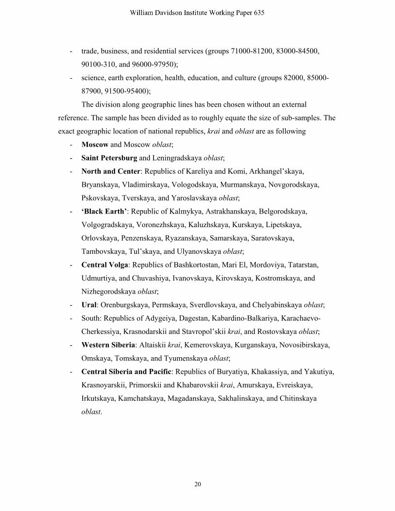
- trade, business, and residential services (groups 71000-81200, 83000-84500,

90100-310, and 96000-97950);

- science, earth exploration, health, education, and culture (groups 82000, 85000-

87900, 91500-95400);

The division along geographic lines has been chosen without an external

reference. The sample has been divided as to roughly equate the size of sub-samples. The

exact geographic location of national republics, krai and oblast are as following

- Moscow and Moscow oblast;

- Saint Petersburg and Leningradskaya oblast;

- North and Center: Republics of Kareliya and Komi, Arkhangel’skaya,

Bryanskaya, Vladimirskaya, Vologodskaya, Murmanskaya, Novgorodskaya,

Pskovskaya, Tverskaya, and Yaroslavskaya oblast;

- ‘Black Earth’: Republic of Kalmykya, Astrakhanskaya, Belgorodskaya,

Volgogradskaya, Voronezhskaya, Kaluzhskaya, Kurskaya, Lipetskaya,

Orlovskaya, Penzenskaya, Ryazanskaya, Samarskaya, Saratovskaya,

Tambovskaya, Tul’skaya, and Ulyanovskaya oblast;

- Central Volga: Republics of Bashkortostan, Mari El, Mordoviya, Tatarstan,

Udmurtiya, and Chuvashiya, Ivanovskaya, Kirovskaya, Kostromskaya, and

Nizhegorodskaya oblast;

- Ural: Orenburgskaya, Permskaya, Sverdlovskaya, and Chelyabinskaya oblast;

- South: Republics of Adygeiya, Dagestan, Kabardino-Balkariya, Karachaevo-

Cherkessiya, Krasnodarskii and Stavropol’skii krai, and Rostovskaya oblast;

- Western Siberia: Altaiskii krai, Kemerovskaya, Kurganskaya, Novosibirskaya,

Omskaya, Tomskaya, and Tyumenskaya oblast;

- Central Siberia and Pacific: Republics of Buryatiya, Khakassiya, and Yakutiya,

Krasnoyarskii, Primorskii and Khabarovskii krai, Amurskaya, Evreiskaya,

Irkutskaya, Kamchatskaya, Magadanskaya, Sakhalinskaya, and Chitinskaya

oblast.

DAVIDSON INSTITUTE WORKING PAPER SERIES - Most Recent Papers The entire Working Paper Series may be downloaded free of charge at: www.wdi.bus.umich.edu

CURRENT AS OF 1/13/04 Publication Authors Date No. 638: The Politics of Economic Reform in Thailand: Crisis and Compromise

Allen Hicken Jan. 2004

No. 637: How Much Restructuring did the Transition Countries Experience? Evidence from Quality of their Exports

Yener Kandogan Jan. 2004

No. 636: Estimating the Size and Growth of Unrecorded Economic Activity in Transition Countries: A Re-Evaluation of Eclectric Consumption Method Estimates and their Implications

Edgar L. Feige and Ivana Urban Dec. 2003

No. 635: Measuring the Value Added by Money Vlad Ivanenko Nov. 2003 No. 634: Sensitivity of the Exporting Economy on the External Shocks: Evidence from Slovene Firms

Janez Prašnikar, Velimir Bole, Aleš Ahcan and Matjaž Koman

Nov. 2003

No. 633: Reputation Flows: Contractual Disputes and the Channels for Inter-firm Communication

William Pyle Nov. 2003

No. 632: The Politics of Development Policy and Development Policy Reform in New Order Indonesia

Michael T. Rock Nov. 2003

No. 631: The Reorientation of Transition Countries’ Exports: Changes in Quantity, Quality and Variety

Yener Kandogan Nov. 2003

No. 630: Inequality of Outcomes and Inequality of Opportunities in Brazil

François Bourguignon, Francisco H.G. Ferreira and Marta Menéndez

Nov. 2003

No. 629: Job Search Behavior of Unemployed in Russia Natalia Smirnova Nov. 2003 No. 628: How has Economic Restructuring Affected China’s Urban Workers?

John Giles, Albert Park, Feng Cai Oct. 2003

No. 627: The Life Cycle of Government Ownership Jiahua Che Oct. 2003 No. 626: Blocked Transition And Post-Socialist Transformation: Siberia in the Nineties

Silvano Bolcic Oct. 2003

No. 625: Generalizing the Causal Effect of Fertility on Female Labor Supply

Guillermo Cruces and Sebastian Galiani

Oct. 2003

No. 624: The Allocation and Monitoring Role of Capital Markets: Theory and International Evidence

Solomon Tadesse Oct. 2003

No. 623: Firm-Specific Variation and Openness in Emerging Markets Kan Li, Randall Morck, Fan Yang and Bernard Yeung

Oct. 2003

No. 622: Exchange Rate Regimes and Volatility: Comparison of the Snake and Visegrad

Juraj Valachy and Evžen Kočenda

Oct. 2003

No. 621: Do Market Pressures Induce Economic Efficiency?: The Case of Slovenian Manufacturing, 1994-2001

Peter F. Orazem and Milan Vodopivec

Oct. 2003

No. 620: Compensating Differentials in Emerging Labor and Housing Markets: Estimates of Quality of Life in Russian Cities

Mark C. Berger, Glenn C. Blomquist and Klara Sabirianova Peter

Oct. 2003

No. 619: Are Foreign Banks Bad for Development Even If They Are Efficient? Evidence from the Indian Banking Sector

Sumon Bhaumik and Jenifer Piesse

Oct. 2003

No. 618: The Echo of Job Displacement Marcus Eliason and Donald Storrie

Oct. 2003

No. 617: Deposit Insurance During Accession EU Accession Nikolay Nenovsky and Kalina Dimitrova

Oct. 2003

No. 616: Skill-Biased Transition: The Role of Markets, Institutions, and Technological Change

Klara Sabirianova Peter Oct. 2003

No. 615: Initial Conditions, Institutional Dynamics and Economic Performance: Evidence from the American States

Daniel Berkowitz and Karen Clay Sept. 2003

No. 614: Labor Market Dynamics and Wage Losses of Displaced Workers in France and the United States

Arnaud Lefranc Sept. 2003

No. 613: Firm Size Distribution and EPL in Italy Fabiano Schivardi and Roberto Torrini

Sept. 2003