Measuring heat distribution in bone during radiofrequency ...

Measuring heat distribution in bone during radiofrequency ablation

(RFA)

Bram Kraeima

S3027279

3D lab UMCG

Period: 18/04/2017 - 01/07/2017

Internship Project

Supervisor: dr. P.C. Jutte orthopedic surgeon at UMCG

Mentor: Prof. dr. ir. G.J Verkerke faculty of medical sciences RUG/UMCG

faculty of science and

engineering

biomedical engineering

1

ABSTRACT

MEASURING HEAT DISTRIBUTION IN BONE

DURING RADIOFREQUENCY ABLATION

(RFA)

by

BRAM KRAEIMA

Radiofrequency ablation (RFA) is an increasingly desirable method for treating small tumors

in bone, however adapting RFA treatment to the variations in bone tumor size is still challenging.

Models on heat distribution during RF ablation in bone are rarely available. Therefore this research

focused on defining the important parameters and methods involving temperature measurements and

gaining insight in heat distribution in bone through performing a RF ablation experiment on pork

femurs while recording temperature data at ascending distances from the ablation electrode. The

temperature data shows variation between the used samples and deviations from the expected values.

Variation is assumed to be caused by inaccurate sensor placement, variation in diameter of drilled

holes required for sensor placement and uncontrolled ambient temperatures during the ablation.

Furthermore a limited amount of temperature sensors reduced the temperature resolution from ideal.

An ideal method for measuring and visualizing the heat distribution in bone during RF ablation

includes MRI thermometry, based on ultra-short echotime sequences, to visualize the heat distribution

in 3D and validate through using an fiber optic FBG sensor. MRI thermometry also enables online

feedback, however continuous RFA and MRI thermometry requires MRI compatible RFA needles and

a low pass filter between the RFA generator and electrode.

2

ACKNOWLEDGEMENTS

I would like to express my appreciation to a number of people who supported me

during the time I have been working on this internship. First I would like to thank Paul Jutte as

initiator of the project and supporting me on all required medical knowledge as company supervisor.

Secondly I would like to thank Peter van Ooijen and Joep Kraeima in further supervision of the

project. Furthermore I would like to thank Delia Ruppert and Ricardo Rivas for contributing to the

research and experiments. A final thanks to Bart Verkerke as mentor and second assessor of the

internship project

3

TABLE OF CONTENTS

Page

Chapter

I. INTRODUCTION --------------------------------------------------------------------------------------- 4

1.1 Reason for this research ---------------------------------------------------------------------------- 4

1.2 Research question ----------------------------------------------------------------------------------- 4

1.3 RFA Procedure--------------------------------------------------------------------------------------- 5

1.4 Temperature measurement methods ------------------------------------------------------------- 6

II. MATERIALS AND METHODS --------------------------------------------------------------------- 11

2.1 Repeatability ----------------------------------------------------------------------------------------- 11

2.2 Measurement technique ---------------------------------------------------------------------------- 11

2.3 Bone preparation ----------------------------------------------------------------------------------- 12

2.4 Data acquisition ------------------------------------------------------------------------------------- 13

2.5 Data analysis ----------------------------------------------------------------------------------------- 13

III. RESULTS ------------------------------------------------------------------------------------------------- 14

3.1 CT results --------------------------------------------------------------------------------------------- 14

3.2 Ablation results -------------------------------------------------------------------------------------- 15

IV. DISCUSSION -------------------------------------------------------------------------------------------- 21

V. CONCLUSION ------------------------------------------------------------------------------------------ 23

VI. RECOMMENDATIONS ------------------------------------------------------------------------------- 24

REFERENCES CITED --------------------------------------------------------------------- 25

4

CHAPTER 1

INTRODUCTION

1.1 Reason for this research

Recently minimally invasive techniques for tumor treatment have gained popularity and

effectiveness within orthopedics, compared to the alternative traditional surgical resection. The

minimal invasive techniques generally rely on thermal ablation procedures which include;

Radiofrequency Ablation (RFA), Laser Ablation (LA), Microwave ablation (MWA), High Intensity

Focused Ultrasound (HIFU) and Cryo ablation. Radio frequency ablation (RFA) has become one of

the most frequently used techniques because of its many benefits. For example, RFA is a relatively

quick and cheap procedure which results in rapid recovery because it is minimally invasive,

furthermore it has high success rates and offers the possibility to treat certain tumors which are

unsuitable for surgical resection[1]. Currently RFA is labeled as the gold standard for treating osteoid

osteoma, which is a benign bone tumor. However RFA does have certain restrictions. In order to

evaluate the effect of RFA during the procedure, the temperature should be monitored. Furthermore it

is hard to adapt the procedure to a specific tumor size because temperature or ablation zone prediction

models are rarely available for ablation in bone.

During RF ablation a RF needle is inserted into the tumor where radio waves in the range of 350-

500kHz are transferred to the target tissue causing vibration of adjacent ions, which results in

frictional heating. The goal during RFA is heating the tumor cells until the point of coagulation

necrosis, without damaging healthy tissue. Temperatures between 46-480C results in irreversible

cellular damage when sustained for 45 minutes, where 50-520C results in coagulation necrosis at four

to six minutes. Temperatures higher than 600C result in near instantaneous coagulation necrosis[2],

[3]. The temperature at the RF needle can be controlled by regulation of the RF generator, however the

heat distribution throughout the bone is not well described yet. Knowing that the small differences in

temperature have significant consequences on healthy tissue, it is important to have a well-defined

heat distribution. This allows for both a more complete ablation of the tumor and lower necrosis rate

of healthy tissue.

1.2 Research question

Research question:

What are the optimal methods and requirements to determine an accurate heat distribution in bone

marrow during radio frequent ablation.

5

1.3 RFA Procedure

Radiofrequency Ablation (RFA) is a minimally invasive procedure for treating liver, lung, kidney

and bone tumors. During a RFA procedure, radio waves within a frequency range of 350-500 kHz are

transferred from an electrode needle to grounding pads transmitting through the target tissue. The RFA

electrode is placed in the tumor, often under CT guidance, whereas the grounding pads are placed on

the skin of the patient. The high frequency radio waves cause water molecules to vibrate, friction

during this vibration results in an increased temperature[4]. The temperature increase decays over

distance from the RFA electrode and depends on the size of the electrode exposure tip and the ablation

time and settings.

Radio frequent ablation in bone tumors can be both palliative as well as curative. Palliative treatment

focusses on treatment of the painful bone metastases secondary to advanced cancer, by mainly

targeting the bone-tumor interface which is the primary source of pain[5]. The curative treatment

mainly involves treating osteoid osteomas, which are small benign bone tumors with an average

diameter of around 1.5 cm. Osteoid osteoma occurs most frequently in long bones of the lower

extremities, 50-60% of all osteoid osteoma cases have been reported in the femur and tibia[6].

Using the right setup and settings during RF ablation is important, a small ablation zone can result in

partly untreated tumor tissue whereas a large ablation zone will damage healthy tissue. When a tumor

is not completely destructed it might regrow. Current treatment on bone tumors in the UMCG,

Groningen, The Netherlands includes an MRI or CT scan to determine the tumor size, then a RF

needle electrode is selected with an exposure length equal to the tumor diameter. The ablation is

performed for at least six minutes with a desired temperature of 900C at the tip of the needle electrode.

However the desired temperature is not always reached or stable during the procedure, a predictive

model for reached temperatures and resulting ablation zones is not available for bone treatment.

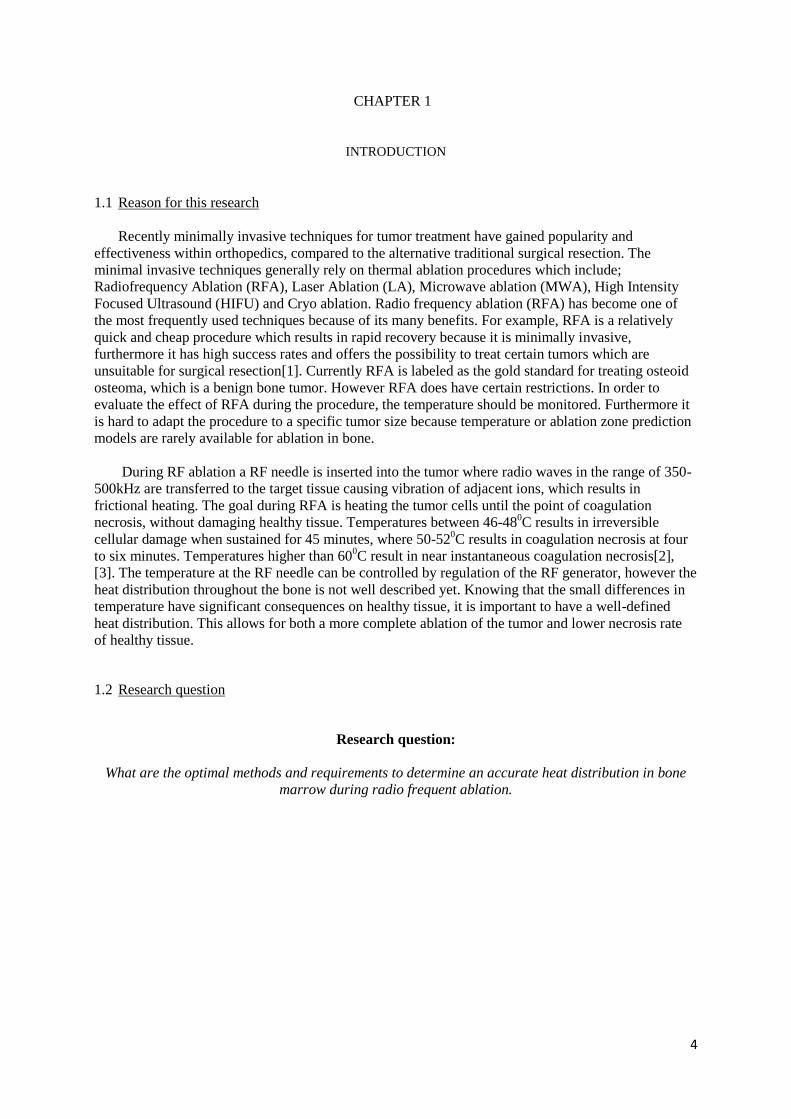
COVIDIEN provides a lesion size chart which suggests setup settings based on lesion size, however

these suggestions resulted from ex-vivo tests on healthy bovine liver tissue at 200C.

Figure 1: Ablation lesion size chart for liver tissue at 200C[7]

Previous research by Rachbauer[8] reported increased temperatures in bone marrow resulting in

coagulation necrosis during ablation up to a distance of 15mm from the ablation needle.

6

1.4 Temperature measurement methods

Currently in RFA temperature is measured trough a thermocouple placed at the tip of the electrode

and is used to control the energy output of the RFA generator. However more options to measure

temperature during RF ablation are available and discussed here.

1.4.1 Electrical temperature sensors

There are mainly two types of electrical temperature sensors, thermo resistive sensors

(thermistors) and thermoelectric contact sensors (thermocouples). In a thermistor the electrical

resistance of a conductor element changes as a function of temperature. By applying a driving current

the output voltage functions as a temperature indicator. The conductor element can either have a

positive temperature coefficient (PTC) where the electrical resistance increases with increasing

temperature, or a negative temperature coefficient (NTC) where the electrical resistance decreases

with increased temperature. Metals have a positive linear relation between temperature and resistance,

however the temperature coefficient of resistivity is low which results in a low sensitivity. Other

materials such as ceramics and silicon can be used as conductor material to significantly increase the

sensitivity, however these sensors are general nonlinear. The general advantage of using thermistors

are simplicity of circuitry and long term stability.[9]

Unlike the thermistors, thermocouples do not require any excitation power. Thermocouples

produce a voltage in response to a temperature difference between two thermocouple junctions based

on the Seebeck effect. When two metals are connected, a thermoelectric voltage is produced due to the

difference in binding energies of the electrons tot the metal ions. This voltage depends on both the

connected metals and the temperature. Generally thermocouples are inexpensive, accurate to around

10C and have a quick response time within 1 second. Furthermore thermocouples offer a significant

advantage over thermistors in measuring range for high temperatures up to thousand degrees Celsius.

There are different types of thermocouples (Type T, E, K, R and B) which differ in metal composition

of the thermocouple junctions, different metals result in different properties such as; temperature

measuring range, resistance to environmental conditions and developed electromotive force per

degree. [9]

Measuring the RFA heat distribution with electrical sensors will require multiple sensors

placed at various locations from the RFA needle

1.4.2 Optical temperature sensors

Optical temperature sensors can be divided into contact and non-contact methods. The non-

contact methods are related to infrared optical measurements and are limited to surface temperatures.

The RFA temperature measurements will be performed inside bone samples, therefore this research

focusses on the contact optical sensor methods which can be divided into intrinsic (fluoroptic) and

extrinsic (FBG) temperature measurements. Both methods use optical fiber to guide light through the

desired measurement area however in the intrinsic method the optical fiber constitutes the sensing

element whereas in the extrinsic method the optical fiber is just a medium for the light to pass through

to the sensing element.

7

1.4.3 Fluoroptic measurement

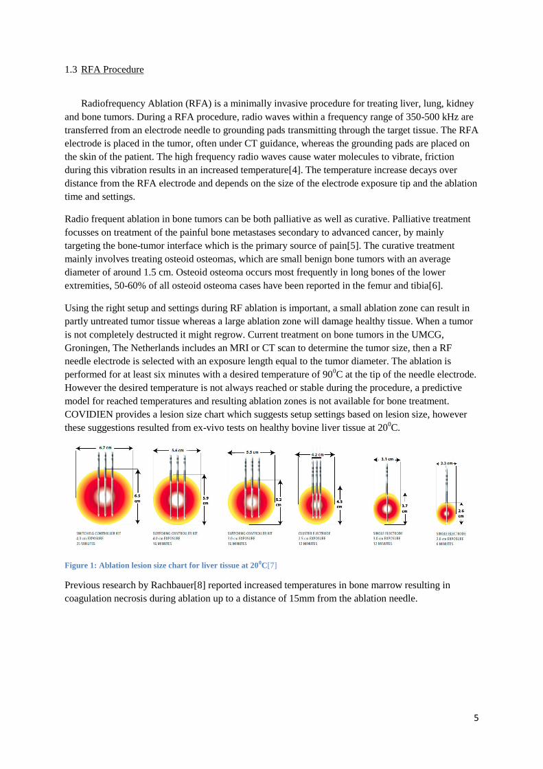
Fluoroptic temperature measurements rely on the fluorescent properties of a phosphor material

which can be applied to the measurement sample. The phosphor compound emits an afterglow when

illuminated with ultra violet light, the shape of the response afterglow is directly related to the

temperature. The decay of the afterglow is a highly reproducible indicator for temperature, a higher

temperature results in a higher rate of decay.

Figure 2 Spectral response and emission decay of the phosphor compound, from[9]

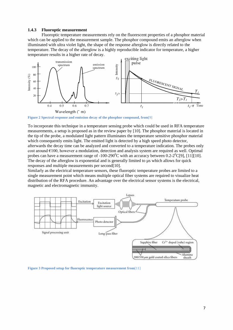
To incorporate this technique in a temperature sensing probe which could be used in RFA temperature

measurements, a setup is proposed as in the review paper by [10]. The phosphor material is located in

the tip of the probe, a modulated light pattern illuminates the temperature sensitive phosphor material

which consequently emits light. The emitted light is detected by a high speed photo detector,

afterwards the decay time can be analyzed and converted to a temperature indication. The probes only

cost around €100, however a modulation, detection and analysis system are required as well. Optimal

probes can have a measurement range of -100-2900C with an accuracy between 0.2-2

0C[9], [11][10].

The decay of the afterglow is exponential and is generally limited to µs which allows for quick

responses and multiple measurements per second[10].

Similarly as the electrical temperature sensors, these fluoroptic temperature probes are limited to a

single measurement point which means multiple optical fiber systems are required to visualize heat

distribution of the RFA procedure. An advantage over the electrical sensor systems is the electrical,

magnetic and electromagnetic immunity.

Figure 3 Proposed setup for fluoroptic temperature measurement from[11]

8

1.4.4 Fiber Bragg Grating

Extrinsic optical fiber system most often rely on fiber Bragg grating (FBG), which reflects

only a narrow wavelength band that shifts in response to temperature. The Bragg Grating is positioned

in the fiber optic cable

The Bragg grating is an optical filter which filters through modulation of the refractive index

within the fiber. A change in refractive index induces a reflective propagation of light, multiple

reflections are induced by repeating the alternation in refractive index. The phase of the reflected light

is determined by the wavelength and the period of modulation of the refractive index. At the Bragg

wavelength, all reflections are in phase and interfere constructively resulting in a reflected signal

centered at the Bragg wavelength. At other wavelengths the signal interferes destructively and is not

reflected but transmitted through the Bragg grating.[12], [13]

The Bragg wavelength is given by formula 1

Where is the Bragg wavelengths, n is the refractive index of the fiber and is the distance

between the changes in refractive index which is also known as the grating period. This means the

FBGs can be designed to a desired Bragg wavelength by varying the grating period. Both the

refractive index and the grating period are affected by temperature, therefore changing the temperature

results in a shift in Bragg wavelength. The shift in Bragg wavelength relates linear to the change in

temperature[12][13]. By monitoring the reflected light signal with a spectroscopy system, the Bragg

wavelength shift can be obtained as an indication on temperature up to an accuracy of 0.10C. The fiber

optic cables including Bragg grating is relatively cheap around €35, however the system to analyze

Bragg wavelength shift will cost around €10.000. [10]

Figure 4 FBG principle from [14]

The FBG only reflects the Bragg wavelength band and transmits all other wavelengths, this

allows for placing multiple Bragg gratings sensors in series which measure temperature at different

Bragg wavelengths. Having multiple sensor elements in a single optical fiber is the biggest advantage

over fluoroptic systems, currently commercial sensors are available with 1FBG/cm resolution in a

single optical fiber[10]. Because only 1 FBG sensor with multiple sensing elements can be used, the

repeatability of an experiment with multiple bone samples increases. The distance in between the

sensing elements and from the RFA needle can be equal on every sample. More advanced fiber optic

sensors are being developed and can result in 1mm resolutions.

9

1.4.5 Noninvasive methods

Besides the invasive sensor systems to measure temperature during RF ablation, non-invasive

methods with imaging systems like magnetic resonance imaging (MRI), computed tomography (CT)

and ultrasound have potential to become of great importance. These methods have a potential to

visualize the three-dimensional temperature distribution obtained during ablation, and can also be used

for online thermal feedback during the ablation procedure. However the non-invasive methods are

often less accurate, sensitive to motion artifacts and not compatible with available RFA equipment.

1.4.5.1 MRI thermometry

Magnetic resonance imaging is generally used to visualize different types of tissue, the tissue

type affects MR parameters such as T1 and T2 relaxation which are used to create an image. Besides

being sensitive to tissue type, some MR parameters like T1 and T2 relaxation as well as the proton

resonance frequency (PRF) are sensitive to temperature[15], [16]. Currently using PRF as a MR

parameter is labeled as the gold standard in MRI thermometry which relates a change in hydrogen

bonds in water molecules with a change in temperature. The hydrogen nucleus is shielded from its

surrounding electron cloud, this shielding effect increases with temperature as the hydrogen bonds

between water molecules start to stretch and break which results in a lower resonance frequency.

Increasing the temperature results in a negative proton resonance frequency shift[17]. Unlike the T

relaxation parameters, PRF is relatively independent of tissue type and has a linear relation towards

temperature making it a promising method in MRI thermometry. However PRF thermometry requires

a long echo time (TE) as well as high water content of the tissue whereas bone has a very short echo

time and low water content, making PRF based thermometry very challenging in bone

structures[15][18]. The low water content, short echo time and low intensity signal make it impossible

to get temperature related information with conventional MRI thermometry techniques, however ultra-

short echotime (UTE) MRI techniques do allow for detecting signals from bone. Using UTE, the T1

and T2 parameters of bone can be measured and related to temperature. Besides being temperature

dependent, both the T1 and T2 relaxation parameters are also influenced by tissue type[16].

Furthermore physiological response of living tissue to heat, can affect these parameters.

Quantification of temperature using these parameters requires known temperature coefficients the

individual bone tissue or a calibration experiment. Once the relation between these parameters and

temperature is set, UTE based MRI thermometry can be used for real time temperature measurements

in bone and 3D visualization of the heat distribution.

Radio frequent ablation uses a frequency range of 350-500 kHz, however harmonics of the RF

generator signal can deviate from this range significantly[19], [20]. A MR scanner also uses RF

signals at a frequency band equal to the larmor frequency in order to obtain an image. The Larmor

frequency is defined by the magnetic field strength of the MR scanner and the gyroscopic constant of

the material. The gyroscopic constant of hydrogen protons, which is used to obtain an image, is equal

to 42.57 MHz/T. Even MR scanners with a low magnetic field (T) will not have interference caused

by the frequency range generated by the RF generator, however the harmonics from the generator can

significantly interfere with the imaging making simultaneously RF ablation and MR thermometry

impossible[19][20]. Nevertheless, the interference can be filtered out through a hardware filter

between the generator and the ablation needles. Furthermore conventional ablation needles and the

RFA generator are not compatible with the magnetic field generated by the MR scanner. Simultaneous

RF ablation and MRI thermometry requires special MRI compatible RFA needles and the RFA

generator will have to be placed outside the MRI room[19], [20].

10

1.4.5.2 CT thermometry

A CT scan creates an image which consist of a matrix of pixels that represent the average X-

ray attenuation of the scanned tissue in the corresponding voxel. A voxel is a three-dimensional pixel

which represents a certain location and volume of the scanned tissue. The attenuation data in the

voxels is processed to reconstruct an attenuation intensity value for each pixel in the final image, these

values are called CT numbers which are expressed in Hounsfield units (HU)[21].

X-ray attenuation is proportional to the electron density of the measured tissue, whereas electron

density is proportional to tissue type and temperature. The CT numbers can therefore also be used to

relate to tissue temperature.

The effect of temperature on the CT number is relatively low with a thermal sensitivity coefficient of

around -0.50 HU per ⁰C, with common CT scanners the thermal resolution is limited to 3-5 0C[22].

Besides the limited resolution, CT thermometry adds excess effective dose to the patient which should

always be kept to a relative minimum. The advantage of CT thermometry is the availability and costs

of the scanner compared to MR thermometry. Furthermore CT thermometry suffers less from

interference caused by the RFA setup, only the RFA needle can cause minimal artifacts in the image at

its location.

1.4.5.3 Ultrasound thermometry

Ultrasonography uses acoustic transducers to both transmit and detect sound pulses. The

transmitted pulses are reflected at different interfaces because of the change in acoustic impedance of

the different tissues. The reflected echoes which contain information about the propagated tissues are

measured by the detector and constructed into an acoustic image of the tissues. Besides tissue type,

ultrasonography can also relate temperature to the measured echoes. A change in temperature affects

the speed of sound and causes thermal expansion which results in an echo shift[23]. Quantification of

an echo shift and thereby the temperature shift comes with the challenge to separate the displacement

caused by thermal effects from true motion unrelated to temperature change. Furthermore the

variation in speed of sound caused by temperature is only linear up to 45 -500C which makes it less

useful in monitoring thermal ablation[23].

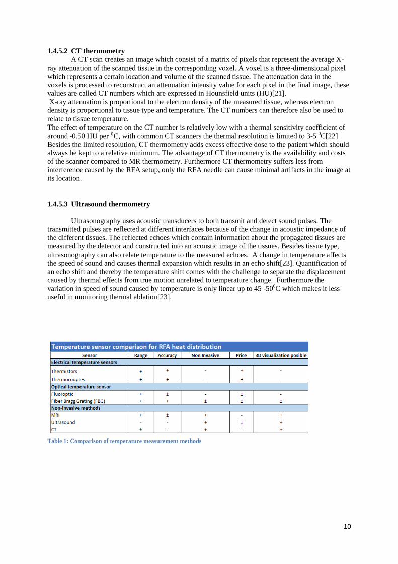
Table 1: Comparison of temperature measurement methods

11

CHAPTER 2

MATERIALS AND METHODS

The goal of this research project is to find a well-defined heat distribution describing the heat

transfer in bone during radio frequency ablation. Literature comparison of different measurement

techniques showed several promising techniques. In this experiment electrical temperature

measurement with thermocouples will be used due to their simplicity in setup, low price and

availability in the UMCG.

The majority of RFA procedures in bone are performed on the femur, therefore this

experiment is focused on fresh pork femurs. Three pork femurs will be subjected to radio frequent

ablation while temperature measurements are performed with thermocouple probes to assess the heat

distribution. The RFA is performed with a Covidien E Series RF generator and a cool-tip RF ablation

E series electrode with an exposure tip of 3 cm. A target temperature of 900C was set with an ablation

time of 10 minutes.

2.1 Repeatability

In order to get comparable results, the ablation and measurements should be performed on the

same anatomical location in all femur samples. The patella normally slides through a groove between

the two trochlear ridges located distally on the pork femur. This groove visually and sensibly present

on each pork femur and is therefore used as anatomical landmark in order to create comparable

ablation measurements. From the start of this groove the center of the bone is found and marked as

location for the first drilling hole which will be the ablation electrode entrance.

Figure 5 A: Start of the groove in between the trochlear ridges, B: Center of the bone and the first drill hole

2.2 Measurement technique

The electrical thermocouple measurement will be a contact measurement based on the

Seebeck effect. Multiple thermocouple probes are placed at ascending distance from the ablation site

and record temperatures continuously during the ablation. The temperature probes are placed at 5, 10

and 15mm distance from the RFA needle. At 5mm a Covidien RF ablation remote temperature probe

E series is used which has a diameter of 1.5mm, whereas at 10 and 15mm a DTM55 precision hand

thermometer with a 3mm probe diameter is used.

12

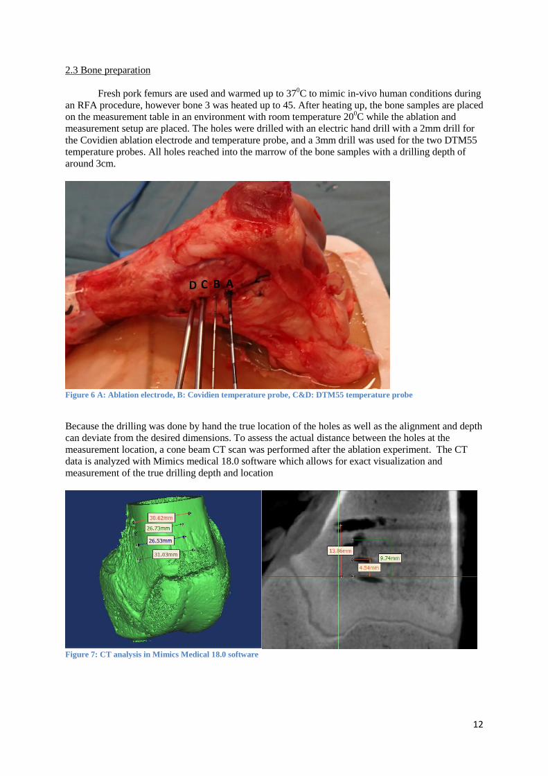
2.3 Bone preparation

Fresh pork femurs are used and warmed up to 370C to mimic in-vivo human conditions during

an RFA procedure, however bone 3 was heated up to 45. After heating up, the bone samples are placed

on the measurement table in an environment with room temperature 200C while the ablation and

measurement setup are placed. The holes were drilled with an electric hand drill with a 2mm drill for

the Covidien ablation electrode and temperature probe, and a 3mm drill was used for the two DTM55

temperature probes. All holes reached into the marrow of the bone samples with a drilling depth of

around 3cm.

Figure 6 A: Ablation electrode, B: Covidien temperature probe, C&D: DTM55 temperature probe

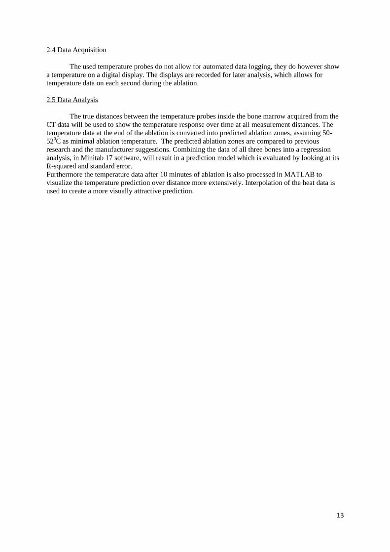
Because the drilling was done by hand the true location of the holes as well as the alignment and depth

can deviate from the desired dimensions. To assess the actual distance between the holes at the

measurement location, a cone beam CT scan was performed after the ablation experiment. The CT

data is analyzed with Mimics medical 18.0 software which allows for exact visualization and

measurement of the true drilling depth and location

Figure 7: CT analysis in Mimics Medical 18.0 software

13

2.4 Data Acquisition

The used temperature probes do not allow for automated data logging, they do however show

a temperature on a digital display. The displays are recorded for later analysis, which allows for

temperature data on each second during the ablation.

2.5 Data Analysis

The true distances between the temperature probes inside the bone marrow acquired from the

CT data will be used to show the temperature response over time at all measurement distances. The

temperature data at the end of the ablation is converted into predicted ablation zones, assuming 50-

520C as minimal ablation temperature. The predicted ablation zones are compared to previous

research and the manufacturer suggestions. Combining the data of all three bones into a regression

analysis, in Minitab 17 software, will result in a prediction model which is evaluated by looking at its

R-squared and standard error.

Furthermore the temperature data after 10 minutes of ablation is also processed in MATLAB to

visualize the temperature prediction over distance more extensively. Interpolation of the heat data is

used to create a more visually attractive prediction.

14

CHAPTER 3

RESULTS

3.1 CT results

Table 2 shows the measured distances and drilling depth of the holes for the electrode and

sensor placement, obtained through analysis of the CT data showed in figure 8. The CT analysis

revealed deviations from the desired distances between the sensor probes and the ablation needle. Also

the drilling depths have variations which affect the sensor placement.

CT analysis

Desired distance (mm) Measured distance (mm) Measured drilling depth (mm)

Bone1

0 0 31

5 4,5 26,53

10 9,7 26,73

15 13,9 30,62

Bone 2

0 0 29,44

5 5 26,15

10 12,2 26,05

15 16,8 24,61

Bone 3

0 0 30,11

5 2 27,88

10 11,6 24,77

15 17,8 24,19 Table 2: Obtained dimension from CT analysis

Figuur 8 CT analysis in Mimics Medical 18.0 software, showing the measured distances between the locations of the

holes

15

3.2 Ablation results

Table 3 shows the temperatures before and after ablation. Bone 1 and 2 start at 380C and 37

0C

respectively, whereas bone 3 starts at 450C. Where the first two bones stay well under the 50

0C around

10mm distance, the third bone does reach coagulation necrosis temperatures at the same distance.

Temperatures

Sensor placement (mm) Start temp (°C) End temp (°C)

Bone 1

0 38 90

4,5 35 57

9,7 31,2 40,7

13,9 31,3 36,9

Bone 2

0 37 91

5 35 58

12,2 33,6 45,3

16,8 34,2 39,9

Bone 3

0 45 90

2 43 77

11,6 38,2 51,4

17,7 38,7 41,6 Table 3: Temperatures before and after ablation

16

Figure 9 shows the measured temperatures at the end of the ablation of all three bone samples.

Ablation on the first bone sample resulted in lower measured temperatures compared to the 2nd

bone

sample, which in turn resulted in lower temperatures compared to the 3rd

bone sample.

Figure 9: Temperatures after ablation related to the measurement distance, with distance reaching 500C pointed out.

Coagulation necrosis occurs when temperatures between 50-52 0C are reached and maintained

for four to six minutes. Connecting the measured temperatures and reading the distance around 500C

does give an indication on the predicted ablation radius. Figure 10 shows the predicted ablation

diameters of the bone samples and the suggested ablation diameter from the manufacturer.

Figure 10: Predicted ablation zones based on the measured data, together with the predicted ablation from Covidien

0

10

20

30

40

50

60

70

80

90

100

0 5 10 15 20

Tem

pe

ratu

re (

°C)

Distance (mm)

Bone 1 afterablation



17

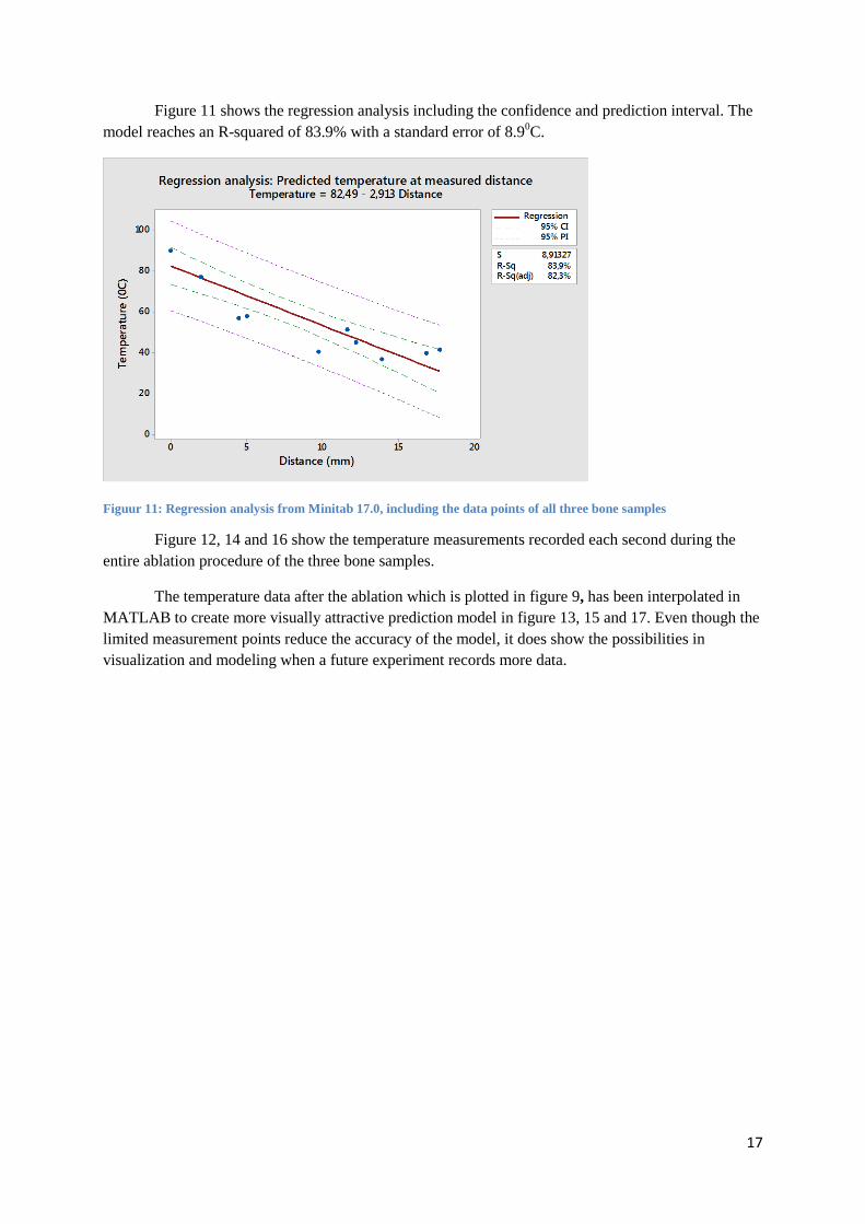
Figure 11 shows the regression analysis including the confidence and prediction interval. The

model reaches an R-squared of 83.9% with a standard error of 8.90C.

Figuur 11: Regression analysis from Minitab 17.0, including the data points of all three bone samples

Figure 12, 14 and 16 show the temperature measurements recorded each second during the

entire ablation procedure of the three bone samples.

The temperature data after the ablation which is plotted in figure 9, has been interpolated in

MATLAB to create more visually attractive prediction model in figure 13, 15 and 17. Even though the

limited measurement points reduce the accuracy of the model, it does show the possibilities in

visualization and modeling when a future experiment records more data.

18

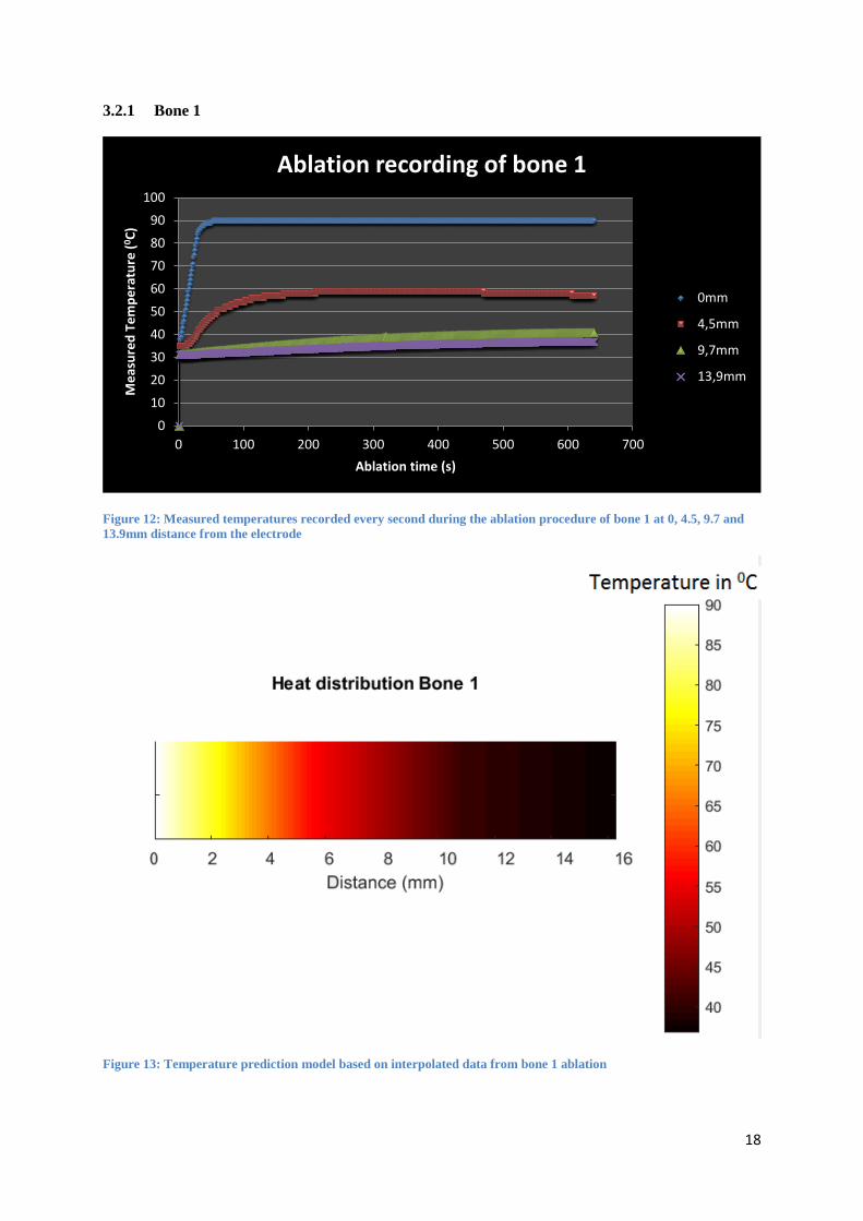
3.2.1 Bone 1

Figure 12: Measured temperatures recorded every second during the ablation procedure of bone 1 at 0, 4.5, 9.7 and

13.9mm distance from the electrode

Figure 13: Temperature prediction model based on interpolated data from bone 1 ablation

0

10

20

30

40

50

60

70

80

90

100

0 100 200 300 400 500 600 700

Me

asu

red

Te

mp

era

ture

(0C

)

Ablation time (s)

Ablation recording of bone 1

0mm

4,5mm

9,7mm

13,9mm

19

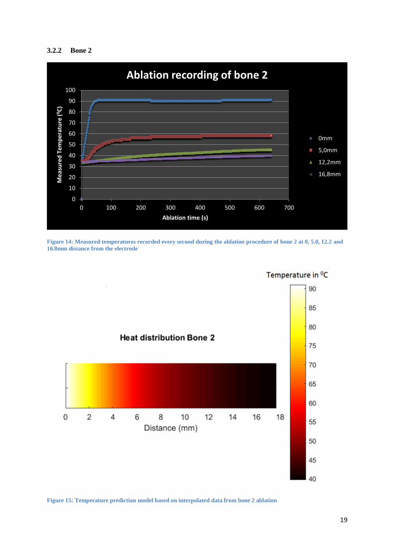
3.2.2 Bone 2




0

10

20

30

40

50

60

70

80

90

100

0 100 200 300 400 500 600 700

Me

asu

red

Te

mp

era

ture

(0 C

)

Ablation time (s)


0mm

5,0mm

12,2mm

16,8mm

20

3.2.3 Bone 3




0

10

20

30

40

50

60

70

80

90

100

0 100 200 300 400 500 600 700

Me

asu

red

Te

mp

era

ture

(0 C

)

Ablation time (s)


0mm

2,0mm

11,6mm

17,7mm

21

CHAPTER 4

DISCUSSION

The experiment was performed using electrical thermocouple temperature probes because of

their good performance, simplicity and availability. Even though the fiber Bragg Grating optical

sensors can be beneficial for this experiment, they are not used because of the limited availability and

costs. Using MRI thermometry was not feasible for this project because of the complex measurement

methods and limited availability of a MR scanner. Furthermore CT and ultrasound thermometry are

both not sensitive enough in the desired temperature range and ultrasound thermometry does not work

in bone.

From table 3 can be observed that the starting temperature can affect the end temperature, higher

starting temperature seems to result in a higher temperature after the ablation. Furthermore all three

samples show that the starting temperature of the two closest sensors is higher than the temperature of

the two around 10 and 15mm. This can be explained by imperfections in the measurement method.

After the bones are preheated to around 370C, they are placed on the measuring table where the

ambient temperature is 200C. During setting up the ablation equipment and preparing the bone sample

for measurement, the bone will be slightly cooled by the ambient temperature. The first two holes have

a diameter of 2mm whereas the last two holes have a diameter of 3mm. It seems a bigger diameter

results in more heat loss which could be expected because a larger diameter results in a larger surface

area for heat exchange.

Figure 9 shows a clear descending trend between distance and temperature, however there is

variation between the different bone samples. Again the starting temperatures of the bone samples

seems to have influenced the maximum reached temperatures. Even though the second measurement

distance (2mm) of the 3rd

bone is much smaller, the measured temperature still follows the trend of

both the first and second bone sample. However at the third and fourth measurement distances, a clear

difference is present. This is also the distance where the starting temperatures are deviating more from

the desired temperature.

The suggested ablation diameter from the manufacturer is significantly larger than the

predictions based on the measured temperatures compared in figure 10. However this can explained by

the difference in tissue type, since those predictions are based on healthy liver tissue at 20 0 C instead

of bone tissue at 370C[24].

The regression model in figure 11 shows a relative good fit with an R-squared of 83.9%,

however the standard error is relatively high at 8.9 0C. This means the predicted temperature can be

8.9 0C off from the true temperature where deviations of 1-2

0C are already critical when reaching

temperatures resulting in coagulation necrosis. The significance and accuracy of this model is

questionable because of the very limited amount of input data.

Figure 12 and 16 at 4.5 and 2 mm respectively both show a minimal decline in temperature

near the end of the ablation, even though the temperature at the electrode tip stays constant and the

other distances also continue their own trend. This could be explained by cooling through ambient

temperature, however this behavior is not observed during ablation of the second bone. Another

explanation can be a change in tissue structure as a result of the ablation induced necrosis which may

affect the heat transfer inside the bone sample.

22

Furthermore at all three bone samples the first two measurements around 0 and 5 mm both

show an exponential response of temperature versus ablation time, whereas the last two measurements

around 10 and 15mm show a slow linear response. This can be explained by differentiating in the

cause of the temperature increase, the bone tissue can be heated through vibration caused by radio

waves or just by general heat transfer. RF induced heating is expected to have a fast response because

the RF waves cause instant heating and has a temperature limit as a result from the set target

temperature. This behavior is showed in the two closest measurements of all three bone samples,

whereas the remaining measurements show a much slower and more linear response for increasing

temperature. Therefore the longer distances are assumed to be mainly heated through general heat

transfer within the bone

23

CHAPTER 5

CONCLUSION

The RFA experiment on pork femurs yielded more insight in the heat distribution during

radiofrequency ablation in bone. The temperature data at the end of the ablation was converted into

predicted ablation zones, assuming 50-520C as minimal ablation temperature. Previous research of RF

ablation in bone marrow reported[8] temperatures of 50-520C at a maximal distance of 15mm from

the RF needle electrode, whereas the results show these temperatures at distances ranging between 6.5

and 12.5mm from the electrode. The variation between the samples is assumed to be caused by the

difference in starting temperature. The previous research [8] regulated the bone temperature to 370C

during the entire procedure and cooled the electrode tip during the ablation. Cooling the electrode can

allow for more powerful ablation settings which can explain the larger predicted ablation zones.

Compared to the suggested ablation zone from the manufacturer Covidien, the predicted zones from

the measured data are smaller. However these lesion sizes are difficult to compare because the

manufacture suggestions are based on liver tissue at 200C.

The interpolated prediction models resulted in a good way for visualizing the predicted

temperature at a certain distance from the ablation needle electrode. The accuracy of the model is

questionable because of the limited input data. It does however show a promising method of

visualizing the predicted temperature when more temperature data is measured at several distances.

The experiment also yielded a lot of insight in important parameters and methods which

should be controlled better, like ambient temperature and drilling dimensions and locations.

The CT analysis showed significant variations in both depth and location of the drilling holes required

for electrode and sensor placement. Drilling the holes by hand showed to be inaccurate and made the

comparison between the bone samples more challenging.

Furthermore the diameter of the drilled holes showed to have an effect on the temperature at the start

of the ablation. Larger diameters showed to lose more heat during setting up of the equipment and

sample, resulting in a difference in starting temperature between the measurement distances.

The difference in starting temperatures results in variation in the maximum reached temperatures and

thereby the ablation zone. The temperature data over time of the first and third bone sample shows a

slight decrease in temperature near the end of the ablation at 4.5 and 2.0 mm distance. This is assumed

to be caused by cooling from a lower ambient temperature or a change in tissue structure. Another

observation can be made from the temperature data over time is that the smaller distances are heated

through ionic agitation as a result of the RFA, where at higher distances the temperature increase

seems to be caused solely by conductive heat transfer.

Literature research showed other promising methods to measure the temperature besides the

used thermocouple sensors. Fluoroptic sensors are an alternative for the electrical sensors, however

their accuracy and price are less attractive. An advantage of optic sensors is that they are MRI

compatible in contrast to the electric sensors, this can be critical in future research combining sensors

and MRI thermometry. Another optical method that is more promising, are Fiber Bragg Grating (FBG)

sensors, as they can reduce the amount of required sensors while increasing the temperature resolution.

These fiber optic sensors can measure temperature at multiple desired locations in a single fiber, which

could reduce the required drilling holes. Besides the use of invasive sensor probes to measure the

temperature, non-invasive methods are available as well. The non-invasive methods are based on

scanning techniques like MR, CT and ultrasound, where both CT and ultrasound are less promising

due to limited sensitivity in bone and excess effective radiation dose. However MRI thermometry does

show promising possibilities in 3D visualization and measurement of temperatures in bone through

ultra-short echotime sequences.

24

CHAPTER 6

RECOMMENDATIONS

The experiment of RFA ablation on pork femurs yielded more insight in the heat distribution in bone

during an RFA procedure, however the significance of the found results is limited because of

variations in important parameters like starting temperature and sensor placement. To further improve

the significance of the results and find a more accurate and useful heat distribution, more research and

more experiments have to be performed.

Some of the biggest variations in the measured parameters, like distance between holes, were caused

by inaccurate drilling. To prevent these variations, 3D printed surgical drilling guides can be designed

with help of CT data scanned before the experiment. These drilling guides are more commonly used to

guide the surgeon to a pre-planned location, since the guides will only fit the patient or sample in 1

way. Using these guides will reduce the drilling caused variations. Another parameter which seems to

have an effect on the ablation results was the variation in starting temperature before the ablation

procedure. This variation was caused by both the difference in diameter of the drilled holes as well as

the difference in temperature between preheating and the ambient temperature during the ablation

procedure. If a future experiment requires multiple measurement holes they should be of the same

diameter. Furthermore, the general temperature of the sample should be constant at 370C to mimic in-

vivo human conditions.

The electrical thermocouples sensors require holes in the bone for each measurement probe, limiting

the temperature resolution by the amount of holes and sensor size. In a future experiment using

temperature sensors to measure the heat distribution during RF ablation fiber optic FBG sensors are

preferred over electrical sensors because they only require 1 sensor to measure at multiple locations,

minimizing variations in sensor placement. Also, the temperature resolution can become higher

compared to using electrical sensors resulting in a more accurate and significant prediction model.

The ideal temperature measurement would result in a 3 dimensional visualization of the heat

distribution in bone. This can be achieved through MRI thermometry based on the T1 relaxation

parameter and ultra-short echotime techniques. Another advantage of using MRI thermometry is its

promising possibility of giving real time temperature feedback during the ablation procedure.

Validation of the accuracy of MRI thermometry during RF ablation should performed, therefore

additional research in this field is required as well an experiment combining optical temperature

sensing and MRI thermometry. A challenge arises when combining RFA and MRI thermometry, the

RFA generator interferes with the MR imaging. Nevertheless using MRI compatible RFA electrodes

and hardware filtering techniques can reduce the interference and result in tolerable imaging.

This research resulted in more insight in the heat distribution in bone during RF ablation, and revealed

the important parameters for future research as well as the preferred measurement methods.

25

CHAPTER 7

REFERENCES CITED

[1] K. K. T. Lee M. Ellis, Steven A. Curley, Radiofrequency Ablation for Cancer: Current

Indications, Techniques, and Outcomes. Springer Science & Business Media, 2006, p. 308.

[2] S. A. Sapareto and W. C. Dewey, “Thermal dose determination in cancer therapy,” Int. J.

Radiat. Oncol. Biol. Phys., vol. 10, no. 6, pp. 787–800, 1984.

[3] M. W. Dewhirst, B. L. Viglianti, M. Lora-Michiels, M. Hanson, and P. J. Hoopes, “Basic

principles of thermal dosimetry and thermal thresholds for tissue damage from hyperthermia,”

Int. J. Hyperth., vol. 19, no. 3, pp. 267–294, 2003.

[4] B. J. Wood, J. R. Ramkaransingh, T. Fojo, M. M. Walther, and S. K. Libutti, “Percutaneous

tumor ablation with radiofrequency,” Cancer, vol. 94, no. 2, pp. 443–451, 2002.

[5] M. Hu, X. Zhi, and J. Zhang, “Radiofrequency ablation (RFA) for palliative treatment of

painful non-small cell lung cancer (NSCLC) rib metastasis: Experience in 12 patients,” Thorac.

Cancer, vol. 6, no. 6, pp. 761–764, 2015.

[6] S. Raux, K. Abelin-Genevois, I. Canterino, F. Chotel, and R. Kohler, “Osteoid osteoma of the

proximal femur: Treatment by percutaneous bone resection and drilling (PBRD). A report of 44

cases,” Orthop. Traumatol. Surg. Res., vol. 100, no. 6, pp. 641–645, 2014.

[7] C. AG, “Valleylab TM

RF Ablation System Electrode with Cool-tip TM

Technology Lesion Size

Chart.”

[8] F. Rachbauer, J. Mangat, G. Bodner, P. Eichberger, and M. Krismer, “Heat distribution and

heat transport in bone during radiofrequency catheter ablation.,” Arch. Orthop. Trauma Surg.,

vol. 123, no. 2–3, pp. 86–90, 2003.

[9] J. Fraden, HANDBOOK OF MODERN SENSORS, Physics, Design and Applications, Third

Edition, 3rd ed. Ney York: Springer, 2004, p. 555.

[10] E. Schena, D. Tosi, P. Saccomandi, E. Lewis, and T. Kim, “Fiber Optic Sensors for

Temperature Monitoring during Thermal Treatments: An Overview,” Sensors, vol. 16, no. 8, p.

1144, 2016.

[11] Y. B. Yu and W. K. Chow, “Review on an Advanced High-Temperature Measurement

Technology: The Optical Fiber Thermometry,” J. Thermodyn., vol. 2009, pp. 1–11, 2009.

[12] Q. Chen and P. Lu, “Fiber Bragg Gratings and Their Applications as Temperature and

Humidity Sensors,” At. Mol. Opt. Phys. New Res., pp. 235–260, 2008.

[13] M. Fokine, “Fiber Bragg Gratings in Temperature and Strain Sensors,” no. May, 2014.

[14] “Fundamentals of Fiber Bragg Grating (FBG) Optical Sensing - National Instruments.”

[Online]. Available: http://www.ni.com/white-paper/11821/en/. [Accessed: 24-Apr-2017].

26

[15] L. Frich, “Non‐invasive thermometry for monitoring hepatic radiofrequency ablation,” Minim.

Invasive Ther. Allied Technol., vol. 15, no. 1, pp. 18–25, 2006.

[16] L. Winter, E. Oberacker, K. Paul, Y. Ji, C. Oezerdem, P. Ghadjar, A. Thieme, V. Budach, P.

Wust, and T. Niendorf, “Magnetic resonance thermometry: Methodology, pitfalls and practical

solutions,” Int. J. Hyperth., vol. 32, no. 1, pp. 63–75, 2016.

[17] J. De Poorter, C. De Wagter, Y. De Deene, C. Thomsen, F. St??hlberg, and E. Achten,

“Noninvasive MRI Thermometry with the Proton Resonance Frequency (PRF) Method: In

Vivo Results in Human Muscle,” Magn. Reson. Med., vol. 33, no. 1, pp. 74–81, 1995.

[18] C. Calcagno, M. E. Lobatto, P. M. Robson, and A. Millon, “Quantifying Temperature-

Dependent T1 Changes in Cortical Bone Using Ultrashort Echo-Time MRI,” vol. 28, no. 10,

pp. 1304–1314, 2016.

[19] A. Cernicanu, M. Lepetit-Coiffé, M. Viallon, S. Terraz, and C. D. Becker, “New horizons in

MR-controlled and monitored radiofrequency ablation of liver tumours.,” Cancer Imaging, vol.

7, pp. 160–166, 2007.

[20] K. Will, J. Krug, K. Jungnickel, F. Fischbach, J. Ricke, G. Rose, and A. Omar, “MR-

compatible RF ablation system for online treatment monitoring using MR thermometry,” 2010

Annu. Int. Conf. IEEE Eng. Med. Biol. Soc. EMBC’10, pp. 1601–1604, 2010.

[21] F. Fani, E. Schena, P. Saccomandi, and S. Silvestri, “CT-based thermometry: An overview,”

Int. J. Hyperth., vol. 30, no. 4, pp. 219–227, 2014.

[22] G. D. Pandeya, M. J. W. Greuter, K. P. de Jong, B. Schmidt, T. Flohr, and M. Oudkerk,

“Feasibility of Noninvasive Temperature Assessment During Radiofrequency Liver Ablation

on Computed Tomography,” J. Comput. Assist. Tomogr., vol. 35, no. 3, pp. 356–360, 2011.

[23] M. A. Lewis, R. M. Staruch, and R. Chopra, “Thermometry and ablation monitoring with

ultrasound,” Int. J. Hyperth., vol. 31, no. 2, pp. 163–181, 2015.

[24] Y. N. Kim, H. Rhim, D. Choi, Y. Kim, M. W. Lee, I. Chang, W. J. Lee, and H. K. Lim, “The

effect of radiofrequency ablation on different organs: ex vivo and in vivo comparative

studies.,” Eur. J. Radiol., vol. 80, no. 2, pp. 526–32, 2011.

Measuring heat distribution in bone during radiofrequency ...

Documents

Transcript of Measuring heat distribution in bone during radiofrequency ...