Measuring Climatic and Hydrological Effects on Cash Crop Production and Production Forecasting in...

Mathematical Theory and Modeling www.iiste.org

ISSN 2224-5804 (Paper) ISSN 2225-0522 (Online)

Vol.4, No.6, 2014

138

Measuring Climatic and Hydrological Effects on Cash Crop

Production and Production Forecasting in Bangladesh Using

ARIMAX Model

Mohammed Amir Hamjah1, Md. Ahmed Kabir Chowdhury

2

1) B.Sc. (Honors), MS (Thesis) in Statistics, Shahjalal University of Science and Technology, Sylhet-3114,

Bangladesh. Email: [email protected].

2) Professor, Department of Statistics, Shahjalal University of Science and Technology, Sylhet-3114,

Bangladesh. Email: [email protected].

Abstract

The objective of this study is to measure the climatic and hydrological effects on cash crop productions in

Bangladesh using Box-Jenkins Auto-Regressive Integrated Moving Average (ARIMA) model with external

regressor variables, that is, ARIMAX model. At the same time, forecasting cash crop production using the same

model under consideration of the climatic and hydrological effects. It is not very easy to measure the climatic

and hydrological effects on different types of agricultural crop production in as usual regression model because

of time sequence dataset. Because of time sequence data, Box-Jenkins ARIMAX model is used in this study to

measure the climatic and hydrological effects on different major cash crop production in Bangladesh, where

climatic and hydrological variables are used as external regressor variable. This is the new study to measure

climatic and hydrological effects on crop production using ARIMAX model. The best fitted ARIMAX model for

Sugarcane, Tea, Tobacco and Cotton production are ARIMAX(0,1,1), ARIMAX(0,1,1), ARIMAX(0,1,1),

ARIMAX(1,1,0) respectively.

Keywords: Climate, Hydrology, Cash Crop, ARIMAX Model, Forecasting, Bangladesh.

1. Introduction

Bangladesh has a large agrarian base country with 76 percent of total population is living in the rural areas and 90

percent of the rural population directly related with agriculture. Agriculture is the single largest producing

sector of the economy since it comprises about 18.6% (data released on November, 2010) of the country's GDP

and employs around 45% of the total labor force. Considering the climatic conditions Jute, Tabaco, Sugarcane,

Cotton, Tea, etc. are the major cash crop productions in Bangladesh.

Tea is an important export item in Bangladesh. Bangladesh ranks tenth among the ten largest tea-producing and

exporting countries in the world. In the year 2000, the country’s tea production was 1.80% of the 2,939.91

million kg produced worldwide. Most of the 163 tea estates in Bangladesh are located in the North-eastern

region of Bangladesh-Maulvi Bazar, Hobiganj, Sylhet, Brahmanbaria districts. There are a few number of tea

estates in Panchagar District and in Chittagong and South-eastern district (rasheeka.wordpress.com, Archive for

Tea Industry)

In Bangladesh, particularly in Kushtia, Chakaria upazila of Cox’sbazar and Bandarban, farmers have

experienced expansion of tobacco cultivation. According to the official Agricultural Statistics (Bangladesh

Bureau of Statistics, Ministry of Planning, GOB, August 2010) three varieties of tobacco - Jati, Motihari and

Virginia - are grown in different districts of Bangladesh. Jati and Motihari are mostly grown in Rangpur and

Bandarban, while Virginia is mostly grown in Kushtia, Rangpur, Jessore and Dhaka. In terms of land area

covered by all three kinds of tobacco, Rangpur still remains highestwith 40345 acres during 2008-09 followed by

Kushtia 22241 and Bandarban 4678 acres of land. Besides tobacco is extending to Jessore, Jhenaidah,

Nilphamari, Lalmonirhat and even in Manikganj and Tangail.

Cotton is commonly known is kapas tula in Bangladesh. Cotton is one of the important cash crops in

Bangladesh. It is the main raw materials of textile industry. Annual requirement of raw cotton for textile industry

of Bangladesh is estimated around 2.5 million bales. Local production is only about 0.1 million bales. Around 4-

5% of the national requirement is fulfilled through the local production, remaining 95-96% is fulfilled by

importing raw cotton from USA (40%), CIS (35%), Australia, Pakistan, South Africa and other country

producing countries (25%) (BTMA, March, 2002). (BBS, 2000, Statistical Year book of Bangladesh).In

Bangladesh Garments Industries contribute 27% of GDP, due to low labor costs and quota free export to the

http://www.iiste.org/

http://en.wikipedia.org/wiki/Agriculture

http://en.wikipedia.org/wiki/GDP

http://rasheeka.wordpress.com/



Vol.4, No.6, 2014

139

European market. The Garments industry has been flourishing in Bangladesh, Readymade garments (RMG)

accounts for about 75% of the total export earnings.

Sugarcane is another important cash crop in Bangladesh. It is considered as one of the most efficient converters

of solar energy. It is very important industrial crops; accounting for 66% of sugar production in the world. It is

also known as “ikshu” in Bangladesh and is the main source of sugar and gur. The contribution of sugarcane to

national GDP is about 0.78%. about 5 million people depend on sugarcane cultivation in Bangladesh.

Climate change in Bangladesh is an extremely crucial issue and according to National Geographic, Bangladesh

ranks first as the nation most vulnerable to the impacts of climate change in the coming decades. Climate change

and agriculture are interrelated processes, both of which take place on a global scale. Global warming is

projected to have significant impacts on conditions affecting agriculture, including temperature, carbon dioxide,

glacial run-off, precipitation and the interaction of these elements. These conditions determine the carrying

capacity of the biosphere to produce enough food for the human population and domesticated animals. The

overall effect of climate change on agriculture will depend on the balance of these effects. Assessment of the

effects of global climate changes on agriculture might help to properly anticipate and adapt farming to maximize

agricultural production.

2. Review of Literature

There are not enough review of the literature for measuring the climatic and hydrological effects on agricultural

crop productions such as Cash crop productions using ARIMAX model. But some of such works in the other

relevant fields by using ARIMAX model has been done such as Julio J. Lucia and hipolit torro (2005) have

conducted an analysis with the title “short term electricity future prices at Nord Pool forecasting power and risk

premiums”. This study analyses how weekly prices at Nord pool are formed. Forecasting power of future prices

is compared with an ARIMAX model in the spot prices. The time series model contains external lagged variable

like temperature, precepitation, reservoious level and the basis (future price less the spot price.

3. Objectives of the Study

The main objective of this study is to develop an ARIMAX model for measuring the climatic and hydrological

effects on major cash crop production in the Bangladesh and production forecasting using the same model. The

specific objective of the study is to develop an Autoregressive Integrated Moving Average with external

regressors (ARIMAX) model for different types of cash crop productions such as Sugarcane, tobacco, Tea and

Cotton in Bangladesh and forecasting these cash crop production considering the climatic and hydrological

effects.

4. Reasons for Using ARIAMX model

To measure any cause-effect relationship among the variables, generally, we use Multiple Regression

Model but this model is a suitable model for cross-sectional dataset. The dataset used in this study is a

time sequence data set, that is, it has time effects on the variable under study which should be considered.

We don’t avoid the problem of time effects on the variable under study, that’s why, we try to fit the

model using Box-Jenkins (Box and Jenkins, 1970) ARIMA approach with external regressors, that is,

ARIMAX model. By ARIMAX model, we can overcome time effects problem by adding some Auto-

Regressive and/or Moving Average term in the model to adjust these time effects. Definitely, in as usual

Regression model, we don’t consider these time effects, so ARIMAX model is the best model for

considering time effects in this study.

5. Methodology

A time series is a set of numbers that measures the status of some activity over time. It is the historical record of

some activity, with measurements taken at equally spaced intervals with a consistency in the activity and the

method of measurement.

The Box and Jenkins (1970) procedure is the milestone of the modern approach to time series analysis. Given an

observed time series, the aim of the Box and Jenkins procedure is to build an ARIMA model. In particular, passing

by opportune preliminary transformations of the data, the procedure focuses on Stationary processes.


http://en.wikipedia.org/wiki/Climate_change

http://en.wikipedia.org/wiki/Bangladesh

http://en.wikipedia.org/wiki/National_Geographic_%28magazine%29

http://en.wikipedia.org/wiki/Climate_change

http://en.wikipedia.org/wiki/Global_warming

http://en.wikipedia.org/wiki/Carbon_dioxide

http://en.wikipedia.org/wiki/Precipitation_%28meteorology%29

http://en.wikipedia.org/wiki/Carrying_capacity

http://en.wikipedia.org/wiki/Carrying_capacity

http://en.wikipedia.org/wiki/Biosphere

http://en.wikipedia.org/wiki/Human_population

http://en.wikipedia.org/wiki/Agriculture



Vol.4, No.6, 2014

140

In this study, it is tried to fit the Box-Jenkins Autoregressive Integrated Moving Average (ARMIA) model with

external regressor, that is, ARIMAX model. This model is the generalized model of the non-stationary ARMA

model denoted by ARMA(p,q) can be written as

Where, Yt is the original series, for every t, we assume that is independent of Yt−1, Yt−2, Yt−3, …, Yt−p .

And it consists of the combination of Auto-Regressive series, AR(p) and Moving Average series, MA(q) , where

AR(p) can be defined as ; and MA(q) can be defined as

A time series {Yt} is said to follow an integrated autoregressive moving average (ARIMA) model if the dth

difference Wt = ∇dYt is a stationary ARMA process. If {Wt} follows an ARMA (p,q) model, we say that {Yt} is

an ARIMA(p,d,q) process. Fortunately, for practical purposes, we can usually take d = 1 or at most 2.

Consider then an ARIMA (p,1,q) process. with , we have

Again ARIMA model with external regressor, that is, ARIMAX model with d=1 can be written as

Where X’s are regressor variables and β’s are the coefficients of regressor variable

Box and Jenkins procedure’s steps

1. Preliminary analysis: create conditions such that the data at hand can be considered as the realization of a

stationary stochastic process.

2. Identification: specify the orders p, d, q of the ARIMA model so that it is clear the number of parameters

to estimate. Recognizing the behavior of empirical autocorrelation functions plays an extremely important

role.

3. Estimate: efficient, consistent, sufficient estimate of the parameters of the ARIMA model (maximum

likelihood estimator).

4. Diagnostics: check if the model is a good one using tests on the parameters and residuals of the model. Note

that also when the model is rejected, still this is a very useful step to obtain information to improve the model.

5. Usage of the model: if the model passes the diagnostics step, then it can be used to interpret a

phenomenon, forecast.

5.1. Procedure of Maximum Likelihood Estimation (MLE) Methods

The advantage of the method of maximum likelihood is that all of the information in the data is used rather than

just the first and second moments, as is the case with least squares. Another advantage is that many large-sample

results are known under very general conditions. For any set of observations, Y1, Y2, …,Yn time series or not, the

likelihood function L is defined to be the joint probability density of obtaining the data actually observed.

However, it is considered as a function of the unknown parameters in the model with the observed data held

fixed. For ARIMA models, L will be a function of the ’s, θ’s, μ, and given the observations Y1, Y2, …,Yn.

The maximum likelihood estimators are then defined as those values of the parameters for which the data

actually observed are most likely, that is, the values that maximize the likelihood function.

We begin by looking in detail at the AR (1) model. The most common assumption is that the white noise terms

are independent, normally distributed random variables with zero means and common variance, . The

probability density function (pdf) for each is then

and, by independence, the joint pdf for , …, is

∑

Now consider




Vol.4, No.6, 2014

141

If we condition on Y1= y1 Equation (5) defines a linear transformation between e2, e3,…, en and Y2, …,Yn (with

Jacobian equal to 1). Thus the joint pdf of Y2, …,Yn given Y1= y1 can be obtained by using Equation (5) to

substitute for the e’s in terms of the Y’s in Equation (4). Thus we get

| [

∑

]

Now consider the (marginal) distribution of Y1. It follows from the linear process representation of the AR(1)

process that Y1 will have a normal distribution with mean μ and variance . Multiplying the

conditional pdf in equation (6) by the marginal pdf of Y1 gives us the joint pdf of Y1, Y2, …, Yn that we require.

Interpreted as a function of the parameters φ, μ and , the likelihood function for an AR(1) model is given by

(

) [

]

Where, ∑

The function S(φ,μ) is called the unconditional sum-of-squares function. As a general rule, the logarithm of the

likelihood function is more convenient to work with than the likelihood itself. For the AR (1) case, the log-

likelihood function, denoted by , is given by

For given values of φ and μ, can be maximized analytically with respect to in terms of the yet to

be determined estimators of φand μ. We obtain

As in many other similar contexts, we usually divide by n −2 rather than n (since we are estimating two

parameters, and μ) to obtain an estimator with less bias. For typical time series sample sizes, there will be very

little difference.

Consider now the estimation of φ and μ. A comparison of the unconditional Sum of Squares function S( ,μ)

with the conditional Sum of Squares function ∑ of AR process reveals

one simple difference. Since Sc( ,μ) involves a sum of n −1 components, whereas does not

involve n, we shall have . Thus the values of φ and μ that minimize S( ,μ) or Sc( ,μ) should

be very similar, at least for larger sample sizes. The effect of the rightmost term in Equation (9) will be more

substantial when the minimum for occurs near the stationarity boundary of ±1.

5.2. Diagnostic Tests of Residuals

5.2.1. Jarque-Bera Test

We can check the normality assumption using Jarque-Bera (Jarque & Bera, 1980) test, which is a goodness of fit

measure of departure from normality, based on the sample kurtosis(k) and skewness(s). The test statistics Jarque-

Bera(JB) is defined as

(

)

Where n is the number of observations and k is the number of estimated parameters. The statistic JB has an

asymptotic chi-square distribution with 2 degrees of freedom, and can be used to test the hypothesis of skewness


http://en.wikipedia.org/wiki/Jarque%E2%80%93Bera_test#CITEREFJarqueBera1980



Vol.4, No.6, 2014

142

being zero and excess kurtosis being zero, since sample from a normal distribution have expected skewness of

zero and expected excess kurtosis of zero.

5.2.2. Ljung-Box Test

Ljung-Box (Box and Ljung, 1978) Test can be used to check autocorrelation among the residuals. If a model fit

well, the residuals should not be correlated and the correlation should be small. In this case the null hypothesis is

H0 : ρ1(e) = ρ2 (e)=……= ρ k(e)=0 is tested with the Box-Ljung statistic

Q* = N(N+1) ∑

ρ

2k(e)

Where, N is the no of observation used to estimate the model. This statistic Q* approximately follows the chi-

square distribution with (k-q) df, where q is the no of parameter should be estimated in the model. If Q* is large

(significantly large from zero), it is said that the residuals autocorrelation are as a set are significantly different

from zero and random shocks of estimated model are probably auto-correlated. So one should then consider

reformulating the model.

6. Used Software

This analysis has completely done by statistical programming based open source Software named as R, (version

2.15.1). The additional library packages used for analysis are forecast, tseries and TSA.

7. Data Source and Data Manipulation

The climatic datasets are available from the Bangladesh Government’s authorized websites www.barc.gov.bd.

The crop data-sets are also available from Bangladesh Agricultural Ministry’s websites named as

www.moa.gov.bd. These data-set are available from the year1972 to 2006. Climatic information was in the

original form such that it is arranged in the monthly average information corresponding to the years from 1972 to

2006 according to the 30 climatic stations. The name of these stations are Dinajpur, Rangpur, Rajshahi, Bogra,

Mymensingh, Sylhet, Srimangal, Ishurdi, Dhaka, Comilla, Chandpur, Josser, Faridpur, Madaripur, Khulna,

Satkhira, Barisal, Bhola, Feni, MaijdeeCourt, Hatiya, Sitakunda, Sandwip, Chittagong, Kutubdia, Cox's Bazar,

Teknaf, Rangamati, Patuakhali, Khepupara, Tangail, and Mongla. We take the month October, November,

December, January and February as a “dry season” and March, April, May, June, July, August, September as a

“summer season” considering the weather and climatic conditions of Bangladesh. Then, finally we take average

seasonal climatic information of 30 climatic stations corresponding to the year from 1972 to 2006 for the

purpose of observing seasonal effects of Climatic and hydrological variable. We take the average of 30 climatic

areas because of focusing the overall country’s situation and overall model fitting for whole Bangladesh.

To serve our research objective, we divide the dataset two parts, where the first part is made of initial 31 years

(1972-2001) to fit the model and second part contain last five years (2002-2006) dataset, from which climatic

and hydrological variable are used to forecast five years forward forecasting considering the demand of

ARIMAX model (because we have to give input as regressor variables to forecast using the ARIMAX model).

8. Climatic and Hydrological Variables Used in This Study

sun.sum = Sunshine of the Summer Season, sun.dry = Sunshine of the Dry Season , clo.sum = Cloud Coverage

of the Summer Season, clo.dry = Cloud Coverage of the Dry Season, max.tem.dry = Maximum Temperature of

the Dry Season, max.tem.sum = Maximum Temperature of the Summer Season, min.tem.dry = Minimum

Temperature of the Dry Season, min.tem.sum = Minimum Temperature of the Summer Season, rain.dry=

Ammount of Rainfall of the Dry Season, rain.sum= Amount Rainfall of the Summer Season, rh.dry = Relative

Humidity of the Dry Season, rh.sum= Relative Humidity of the Summer Season, wind.dry = Wind Speed of the

Dry Season and wind.sum = Wind Speed of The Summer Season.

9. ARIMAX Modeling for Different Cash Crop Production(Analysis)

9.1 ARIMAX Modeling for Sugarcane Production

Dickey-Fuller unit root test is used to check whether time sequence sugarcane production data satisfies the

sationarity conditions. It is found that stationarity condition satisfied at the difference order one with p-value =


http://www.barc.gov.bd/



Vol.4, No.6, 2014

143

0.01 which suggests that there is no unit root at the first order difference of sugarcane production at 1% level of

significance. The graphical stationarity test using ACF and PACF is shown in the Figure-1

Figure 1: Graphically Stationarity Checking for Sugarcane Production

From the Figure 1, it is clear that original series does not show a constant variance and slightly shows an

increasing trend but first order differenced series shows a more stable variance than the original series. Again,

from the ACF and PACF, it is clear that there is no significant spike in the first order differenced series which

also tell us that the series is stationary with first order difference and at the same time, there are no significant

effects of Autoregressive and Moving Average order at first order difference series, which also implies stable

variance.

From the tentative order analysis, the best selected ARIMAX model for measuring the climatic and hydrological

effects on Sugarcane production in Bangladesh is ARIMAX (0,1,1) with the AIC = 433.73 and BIC = 455.61.

The parameter estimates of the fitted ARIMAX (0,1,1) are given in the Table 1.

Table 1: Summary Statistics of the ARIMAX Model for Sugarcane Production

Coefficients Estimates Std. Error t-value p-value

ma1 -1 0.0895 -11.1754 0.0284

sun.sum -95.7717 446.4682 -0.2145 0.4327

sun.dry -900.8863 259.5937 -3.4704 0.0893

clo.sum -182.1219 587.544 -0.31 0.4043

clo.dry -480.9725 579.3279 -0.8302 0.2794

max.tem.dry -449.0541 328.4169 -1.3673 0.201

max.tem.sum 625.7998 583.4032 1.0727 0.2388

min.tem.dry 737.8143 366.7051 2.012 0.1468

min.tem.sum -639.0952 461.7818 -1.384 0.1992

rain.dry -3.8714 4.0049 -0.9667 0.2554

rain.sum -3.4251 2.0106 -1.7035 0.169

rh.dry -107.816 75.8186 -1.422 0.1951

rh.sum 256.4301 149.6737 1.7133 0.1682

wind.dry 294.5875 1062.5695 0.2772 0.4139

wind.sum 530.4545 481.0136 1.1028 0.2345

Original series(Sugarecane)

Time

sugarc

ane p

roductio

n

1975 1980 1985 1990 1995 2000

5500

7000

First Differenced Series

Time

First diff

ere

nce o

f S

ugaecane

1975 1980 1985 1990 1995 2000

-500

500

0 2 4 6 8 10 12 14

-0.4

0.2

0.8

Lag

AC

F

ACF plot of 1st difference

2 4 6 8 10 12 14

-0.4

0.0

Lag

Part

ial A

CF

PACF plot of 1st difference




Vol.4, No.6, 2014

144

From the Table 1, it is clear that Sugarcane production depends on the first order Moving Average Lag, which

has statistically significant effects at 3% level of significance. At the same time, sun.dry has statistically

significant effects on Sugarcane production at 10% level of significance. Again, sun.sum, sun.dry, clo.sum,

clo.dry, max.tem.dry, min.tem.sum, rain.dry, rain.sum and rh.dry have negative and max.tem.sum, min.tem.dry,

rh.sum, wind.dry and wind.sum have positive effects on Sugarcane production

To check Autocorrelation assumption, “Box-Ljung test” is used. From the test, it is found that the Pr(| | ≥

0.1286) = 0.7199, which suggests that we may accept the assuption that there is no autocrrelation among the

residuals of the fitted ARIMAX(0,1,1) for Sugarecane production model at 5% level of significance. Again, to

check the normality assumption, “Jarque-Bera test” is uesd, from which, we find the Pr(| | ≥ 1.0401) =

0.5945, which refers to accept the norality assumpytion that the residuals are from normal distribution. Graphical

Residuals Diagnostics are shown in the Figure 2.

Figure-2: Graphical Diagnostics Checking for ARIMAX Model of Sugarcane Production

From the Figure 2, it is clear that almost all of the points are very closed to the Q-Q line or on the Q-Q line,

which indicates that residuals are normally distributed of the Sugarcane production model. At the time, from the

Boxplot, it is clear that residuals are symmetrically (normally) distributed and there is no unusual or outlier

observation, that is, this model is going to make a good inference.

Finally, considering all of the Graphical and Formal test, it is obvious that our fitted model ARIMAX (0,1,1) is

the best fitted model for measuring the Climatic and hydrological effects on Sugarcane production in the

Bangladesh.

9.2 ARIMAX Modeling for Tea Production

Dickey-Fuller unit root test is used to test whether time sequence tea production data series are stationary or not.

It is found that stationarity condition satisfied without any difference with the Pr(|t| ≥ -13.9946) = 0.01, which

suggests that there is no unit root in the original series at 5% level of significance. The graphical stationarity test

is shown in the Figure-3

-2 -1 0 1 2

-400

0400

Q-Q plot for Sugarcane productions

Theoretical Quantiles

Sam

ple

Quantil

es

-400

0400

Boxplot of residuals for Sugarcane productions




Vol.4, No.6, 2014

145

Figure 3: Graphically Stationarity Checking for Tea Production

From the Figure 3, it is clear that original tea production series shows a constant variance. Again, from the ACF

and PACF, it is clear that there is no significant spike in the original series which also indicates that there are no

significant effects of Auto-Regressive and Moving Average in the original series, that is, the tea production

series is stationary without any difference.

From the tentative order analysis, our finally, the best selected ARIMAX model for measuring the climatic and

hydrological effects on tea production in Bangladesh is ARIMAX (1,0,0) with the AIC = 206.63 and BIC =

230.45. The parameter estimates of the fitted ARIMAX (1,0,0) model are given in the Table-2.

Table 2: Summary Statistics of ARIMAX Model for Tea Production

Coefficients Estimates Std.Error t-value p-value

ar1 -0.7907 0.1404 -5.6321 0.0559

intercept 1040.9484 294.4137 3.5357 0.0877

sun.sum -36.273 8.6402 -4.1982 0.0744

sun.dry 12.3276 4.8729 2.5298 0.1198

clo.sum -53.5081 12.2081 -4.383 0.0714

clo.dry 65.9457 14.5708 4.5259 0.0692

max.tem.dry 36.1332 7.5984 4.7554 0.066

max.tem.sum -46.988 12.4349 -3.7787 0.0823

min.tem.dry -40.2493 7.7132 -5.2182 0.0603

min.tem.sum 35.9612 9.4144 3.8198 0.0815

rain.dry -0.2993 0.076 -3.9366 0.0792

rain.sum -0.1409 0.0456 -3.0917 0.0996

rh.dry 5.5314 1.2996 4.2563 0.0735

rh.sum -9.0652 2.539 -3.5704 0.0869

wind.dry -22.7006 18.5342 -1.2248 0.2179

wind.sum -34.3451 8.3034 -4.1363 0.0755

From the Table 2, it is clear that tea production depends on the first order Autoregressive Lag, which has

statistically significant effects at 6% level of significance. At the same time, sun.dry, clo.sum, clo.dry,

max.tem.dry, max.tem.sum, min.tem.dry, min.tem.sum, rain.sum,rain.sum, rh.dry, rh.sum and wind.sum have

statistically significant effects on tea productions at 10% level of significance. Again, sun.dry, clo.dry,

Original(Tea)series

Time

Tea p

roductio

n

1975 1980 1985 1990 1995 2000

30

50

70

0 2 4 6 8 10 12 14

-0.4

0.2

0.8

Lag

AC

F

ACF plot of Original Series

2 4 6 8 10 12 14

-0.3

0.0

0.3

Lag

Part

ial A

CF

PACF plot of Original Series




Vol.4, No.6, 2014

146

max.tem.dry, min.tem.sum and rh.dry have positive and sun.sum, clo.sum, max.tem.sum, min.tem.dry, rain.dry,

rain.sum, rh.sum, wind.dry and wind.sum have negative effects on tea production in Bangladesh.

To check the Autocorrelation assumption, “Box-Ljung test” is used. From the test, we find the Pr(| | ≥ 1.1773)

= 0.2779, which suggests that we may accept the assuption that there is no autocrrelation among the residuals.

Again, to check the normality assumptions, “Jarque-Bera test” is used, which gives the Pr(| | ≥ 0.0552) =

0.9728, which suggests to accept the norality assumption, that is, residuals follow normal distribution. Graphical

Residuals Diagnostics are shown in the Figure 4.

Figure 4: Graphical Diagnostics Checking for ARIMAX Model of Tea Production


which suggests that residuals are normally distributed of the Tea production model. At the time, from the

Boxplot, it is clear that residuals are slightly negatively skewed and it contains single outlier.

Finally, considering all of the Graphical and Theoretical test, it is clear that our fitted model ARIMAX (1,0,0) is

the best fitted model for measuring the climatic and hydrological effects on tea production in Bangladesh.

9.3 ARIMAX Modeling for Cotton Production

Dickey-Fuller unit root test is used to test whether the time sequence cotton production series is stationary or not.

It is found that stationarity condition satisfied at first order difference with the p-value = 0.01, which suggests

that there is no unit root in the first order difference at 5% level of significance, that is, the series is stationary.

The graphical stationarity test is shown in the Figure 5.

From the Figure 5, it is clear that at the first difference cotton production series shows a constant variance but in

the original series is not stationary, that is, our difference order is one to make the cotton production series

stationary. Again, from the ACF and PACF, it is clear that there is no significant spike in the first order

difference series, which also indicate that there are no significant effects of Auto-Regressive and Moving

Average in the first order difference, that is, the cotton production series is stationary at the first order difference.

-2 -1 0 1 2

-10

05

Q-Q plot for Tea production model


Sam

ple

Quantil

es

-10

05

Boxplot of residuals for Tea production




Vol.4, No.6, 2014

147

Figure-5: Graphically Stationarity Checking for Cotton Production

From the tentative order analys, the best selected ARIMAX model for measuring the climatic and hydrological

effects on cotton production is ARIMAX (1,1,0) with the AIC = 237.95 and BIC = 259.82. The parameter

estimates of the fitted ARIMAX (1,1,0) are shown in the Table 3.

Table 3: Summary Statistics of the ARIMAX Model for Cotton Production

Coefficients Estimates Std.Error t-value p-value

ar1 0.5749 0.1859 3.0931 0.0995

sun.sum 6.7974 11.5496 0.5885 0.3307

sun.dry -31.7327 9.0473 -3.5074 0.0884

clo.sum -7.3014 16.3115 -0.4476 0.366

clo.dry -24.7835 11.1699 -2.2188 0.1348

max.tem.dry -17.5668 7.3996 -2.374 0.1269

max.tem.sum 28.5494 19.6168 1.4553 0.1916

min.tem.dry 30.2768 8.6389 3.5047 0.0885

min.tem.sum -36.0005 13.393 -2.688 0.1134

rain.dry 0.0887 0.0857 1.0343 0.2446

rain.sum 0.0064 0.0441 0.1439 0.4545

rh.dry -3.4872 2.0874 -1.6706 0.1717

rh.sum 9.2769 4.6811 1.9818 0.1488

wind.dry -50.5128 29.3197 -1.7228 0.1674

wind.sum 38.5358 18.4037 2.0939 0.1418

From the Table 3, it is obvious that first order Auto-Regressive Lag has significant effects on cotton production

at 10% level of significance. Again, the regressor variables sun.dry, and min.tem.dry have a significant effects

on cotton production at 8% level of significance. Similarly, sun.sum, max.tem.sum, min.tem.dry, rain.dry,

rain.sum, rh.sum and wind.sum have positive and sun.dry, max.tem.dry, min.tem.sum, clo.dry, clo.sum, rh.dry

and wind.dry have negative effects on cotton production.

To check Autocorrelation assumption, “Box-Ljung test” is used. From the test, it is obtained that the Pr(| | ≥

1.0272) = 0.3108, which suggests that we may accept the assuption that there is no autocrrelation among the

residuals at 5% level of significance. Again, to check the normality assumptions, “Jarque-Bera” test is used.

Original series(Cotton)

Time

Cotton p

roductio

n

1975 1980 1985 1990 1995 2000

20

60

100


Time

First diff

ere

nce o

f C

otton

1975 1980 1985 1990 1995 2000

-20

20

0 2 4 6 8 10 12 14

-0.4

0.2

0.8

Lag

AC

F


2 4 6 8 10 12 14-0

.20.2

Lag

Part

ial A

CF





Vol.4, No.6, 2014

148

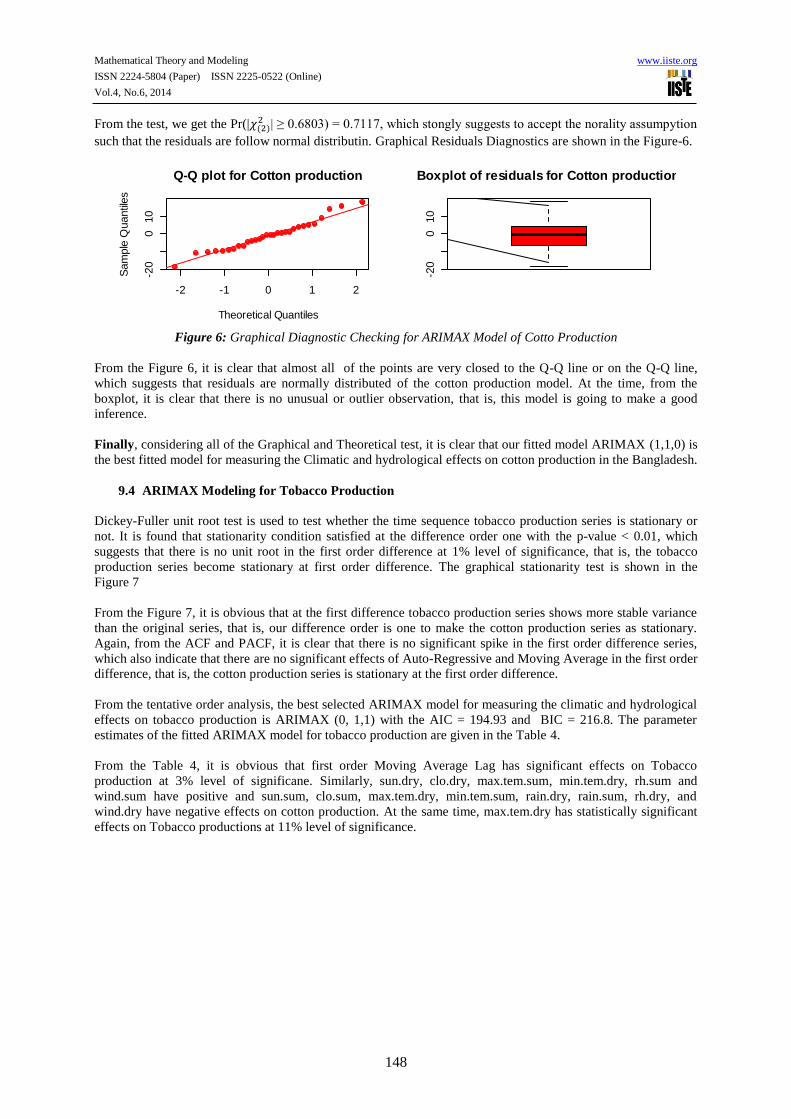
From the test, we get the Pr(| | ≥ 0.6803) = 0.7117, which stongly suggests to accept the norality assumpytion

such that the residuals are follow normal distributin. Graphical Residuals Diagnostics are shown in the Figure-6.

Figure 6: Graphical Diagnostic Checking for ARIMAX Model of Cotto Production


which suggests that residuals are normally distributed of the cotton production model. At the time, from the

boxplot, it is clear that there is no unusual or outlier observation, that is, this model is going to make a good

inference.

Finally, considering all of the Graphical and Theoretical test, it is clear that our fitted model ARIMAX (1,1,0) is

the best fitted model for measuring the Climatic and hydrological effects on cotton production in the Bangladesh.

9.4 ARIMAX Modeling for Tobacco Production

Dickey-Fuller unit root test is used to test whether the time sequence tobacco production series is stationary or

not. It is found that stationarity condition satisfied at the difference order one with the p-value < 0.01, which

suggests that there is no unit root in the first order difference at 1% level of significance, that is, the tobacco

production series become stationary at first order difference. The graphical stationarity test is shown in the

Figure 7

From the Figure 7, it is obvious that at the first difference tobacco production series shows more stable variance

than the original series, that is, our difference order is one to make the cotton production series as stationary.

Again, from the ACF and PACF, it is clear that there is no significant spike in the first order difference series,

which also indicate that there are no significant effects of Auto-Regressive and Moving Average in the first order

difference, that is, the cotton production series is stationary at the first order difference.

From the tentative order analysis, the best selected ARIMAX model for measuring the climatic and hydrological

effects on tobacco production is ARIMAX (0, 1,1) with the AIC = 194.93 and BIC = 216.8. The parameter

estimates of the fitted ARIMAX model for tobacco production are given in the Table 4.

From the Table 4, it is obvious that first order Moving Average Lag has significant effects on Tobacco

production at 3% level of significane. Similarly, sun.dry, clo.dry, max.tem.sum, min.tem.dry, rh.sum and

wind.sum have positive and sun.sum, clo.sum, max.tem.dry, min.tem.sum, rain.dry, rain.sum, rh.dry, and

wind.dry have negative effects on cotton production. At the same time, max.tem.dry has statistically significant

effects on Tobacco productions at 11% level of significance.

-2 -1 0 1 2

-20

010

Q-Q plot for Cotton production


Sam

ple

Quantil

es

-20

010

Boxplot of residuals for Cotton production




Vol.4, No.6, 2014

149

Figure 7: Graphically Stationarity Checking for Tobacco Production

Table 4: Summary Statistics of the ARIMAX Model for Tobacco Production

Coefficients Estimates Std. Error t-value p-value

ma1 1 0.093 10.7527 0.0295

sun.sum -7.5628 6.8696 -1.1009 0.2347

sun.dry 2.4157 5.0897 0.4746 0.3589

clo.sum -15.2521 7.73 -1.9731 0.1493

clo.dry 6.5076 4.5953 1.4161 0.1957

max.tem.dry -10.2569 3.8105 -2.6918 0.1132

max.tem.sum 7.4327 11.0168 0.6747 0.3111

min.tem.dry 6.6123 4.1402 1.5971 0.1781

min.tem.sum -1.5544 7.3401 -0.2118 0.4336

rain.dry -0.0728 0.0513 -1.4182 0.1955

rain.sum -0.0084 0.0243 -0.3462 0.3939

rh.dry -0.0062 1.1931 -0.0052 0.4983

rh.sum 4.5699 2.4324 1.8788 0.1557

wind.dry -5.5083 16.9135 -0.3257 0.3998

wind.sum 1.3588 11.9038 0.1141 0.4638

To check Autocorrelation assumption, “Box-Ljung test” is used. From the test, it is obtained the Pr(| | ≥

0.1198) = 0.7293, which suggests that we may accept the assuptions that there is no autocrrelation among the

residuals at 5% level of significance. Again, to check the normality assumptions, “Jarque-Bera ” test is used.

From the test, we get the Pr(| | ≥ 2.0714) = 0.355, which refers to accept the norality assumpytion such that

the residuals are follow normal distributin.

Finally, considering all of the Graphical and Formal test, it is clear that our fitted model ARIMAX (0, 1, 1) is

the best fitted model for measuring the Climatic and hydrological effects on tobacco production in the

Bangladesh.

Original(Tobacco)series

Time

Tobacco p

roductio

n

1975 1980 1985 1990 1995 2000

30

45

60


Time

First diff

ere

nce o

f T

obaco

1975 1980 1985 1990 1995 2000

-15

010

0 2 4 6 8 10 12 14

-0.4

0.2

0.8

Lag

AC

F


2 4 6 8 10 12 14-0

.20.2

Lag

Part

ial A

CF





Vol.4, No.6, 2014

150

10. Forecasting Cash Crop Production Using Fitted ARIMAX Model

After, selecting the best model, now we are going to use these models to forecast cash crop production in

Bangladesh. To forecast the following modern “Forecasting Criteria” are considered. The most useful forecast

evaluation criteria are Root Mean Square Error (RMSE) proposed by Ou and Wang (2010), Mean Absolute

Error(MAE), Root Mean Square Error Percentage(RMSPE), Mean Absolute Percentage Error (MAPE)

proposed by Sutheebnjard and Premchaiswadi (2010). The results of these criteria for forecasting cash crop

production in Bangladesh are shown in the Table 5.

Table 5: Forecasting Criteria for the Best Selected Model

Cash Crop Selected Model Forecasting Criterion

ME RMSE MAPE MAE

Cotton ARIMAX(1,1,0) -0.6321079 8.2321 35.28611 6.347396

Sugarcane ARIMAX(0,1,1) 24.59022 228.5847 2.625375 176.2629

Tea ARIMAX(1,0,0) 0.1937676 4.228393 8.277093 3.289199

Tobacco ARIMAX(0,1,1) -0.0987441 3.854004 7.292685 3.062968

11. Comparison between Original and Forecasted Series

It is tried make a comparison between the original series and forecasted series from the fitted ARIMAX model.

These forecasted results are shown in the Figure 8.

Figure 8: Graphical Comparison between Original and Forecasted Series

From the Figure 8,

It is clear (top-left) that the original series of the cotton production (red color), which show initially

almost constant tendency, after sometimes it increases and decreases consecutively and the forecasting

series (blue color) also shows the same manner. That is, forecasting cotton productions may be good

under consideration of climatic and hydrological effects.

It is clear (top-right) that the original series of the Sugarcane productions (red color), which shows an

upward production tendency and the forecasting series also shows similar pattern (blue color). In the

forecasting plot, in sample forecasting part shows an upward trend and similarly, the out sample

forecasting part also shows almost an upward tendency. That is, forecasting Sugacane productions may

be good under consideration of climatic and hydrological effects.

It is clear (left-bottom) that the original series of the tea production (red color), which shows an upward

production tendency and the forecasting series also shows an upward production tendency (blue color).

In the forecasting plot, in sample forecasting part shows an upward trend and similarly, the out sample

Forecasting Cotton production

1975 1985 1995 2005

-50

050

Forecasting Sugarcane production

1975 1985 1995 2005

5500

7000

Forecasting Tea production

1975 1985 1995 2005

30

50

70

Forecasting Tobacco production

1975 1985 1995 2005

10

40

70




Vol.4, No.6, 2014

151

forecasting part also shows an upward trend under consideration of climatic and hydrological effects.

That is, forecasting tea productions may be good.

It is clear (bottom-right) that the original series of the tobacco production (red color), which shows a

downward production tendency and the forecasting series also shows a downward production tendency

(blue color). In the forecasting plot, in sample forecasting part shows a downward trend and similarly

the out sample forecasting part also shows a downward trend under consideration of climatic and

hydrological effects. That is, forecasting Tobacco productions may be good.

Finally, all of the fitted models clearly explain the practical situation which implies that these fitted models are

statistically good fitted model for measuring climatic and hydrological effects in cash crop production and

forecasting the cash crop under consideration of these effects covering the Bangladesh area.

12. Conclusion and Recommendations

In this study, it is tried to fit an ARIMAX model because of time sequence cash crop data set, where climatic and

hydrological variables are used as a regressor variable. In this study, it is tried to fit the best model to measure

the Climatic and hydrological effects on different types of cash crop productions named as Sugarcane, Cotton,

Tobacco and Tea, covering the whole Bangladesh. To select the best model for measuring the climatic and

hydrological effects on different types of Cash crop productions, the latest available model selection criteria such

as AIC, BIC, ACF and PACF are used. Again, to select the fitted model, it is tried to fit the best simple model

because the model contains less parameters give the good representative results. The best selected Box-Jenkins

ARIMAX model for measuring the climatic and hydrological effects on Cash crop production are ARIMAX

(1,1,0), ARIMAX (1,0,0), ARIMAX (0,1,1) and ARIMAX (1,1,0) for Sugarcane, Tea, Tobacco and Cotton

production respectively. From the analysis, sun.dry for Sugarcane production; sun.dry, clo.sum, clo.dry,

max.tem.dry, max.tem.sum, min.tem.dry, min.tem.sum, rain.sum,rain.sum, rh.dry, rh.sum and wind.sum for Tea

production; max.tem.dry has statistically significant effects on Tobacco productions; and sun.dry and

min.tem.dry for Cotton production have significant effects. The main objective of this study is to fit an

appropriate model and we are interested to forecast. At the same time, to forecast ARIMAX model, there are

need to future input variable which is not available base on which we can forecast for long time. We are tried to

forecast five years forward by using our dataset in which we used thirty one year’s data to fit model and

remaining five years dataset (for regressor variable) are used as input variable to forecast. From the Comparison

between original series and forecasted series, it is clear that each of the model are good to forecast because in

sample and out sample forecasting shows the same manner which implies the best representation of empirical

situation. Again, all of the formal and graphical tests show that they are very well managed to fit the ARIMAX

model for specific cash crop production. These selected models are the best selected model to measure climatic

and hydrological effects and forecasting cash crop in Bangladesh.

After conducting these analyses, the following recommendations can be made such as

The policy makers and researchers could use these model to make a decision for agricultural

productions under consideration of climatic and hydrological effects on agricultural productions.

Similar regional models could be further studied to find variations of the models.

The climatic zone similar to Bangladesh could also be compared in the future studies.

References

Julio J. Lucia and Hipolit Torro (2005). Short Term Electricity Future Prices at Nord Pool: Forecasting

Power and Risk Premiums JEL Classifications, University of Valencia.

Box, G. E. P., & Jenkins, G. M. (1976). Time Series Analysis, Forecasting and Control. San

Francisco, Holden- Day, California, USA.

Box, G. E. P. and Pierce, D. A. (1970) , Distribution of Residual Autocorrelations in Autoregressive-

Integrated Moving Average Time Series Models, Journal of the American Statistical Association, 65:

1509–1526.

Jonathan D. Cryer and Kung-Sik Chan (2008). Time Series Analysis with Applications in R, 2nd

edition, Springer.

Gujarati D N.(2003). Basic Econometrics, 4th edition, McGraw-Hill Companies Inc., New York.


http://en.wikipedia.org/wiki/Journal_of_the_American_Statistical_Association



Vol.4, No.6, 2014

152

Bruce H. Andrews, Matthew D. Dean, Robert Swain, Caroline Cole (2013). Building ARIMA and

ARIMAX Models for Predicting Long-Term Disability Benefit Application Rates in the Public/Private

Sectors, University of Southern Maine

Jarque, Carlos M. Bera, Anil K. (1980), Efficient tests for normality, homoscedasticity and serial

independence of regression residuals, Economics Letters 6 (3): 255–259.

www.barc.gov.bd, Bangladesh Agricultural Research Council, Bangladesh.

www.moa.gov.bd, Ministry of Agriculture, Bangladesh.


http://en.wikipedia.org/wiki/Carlos_Jarque

The IISTE is a pioneer in the Open-Access hosting service and academic event

management. The aim of the firm is Accelerating Global Knowledge Sharing.

More information about the firm can be found on the homepage:

http://www.iiste.org

CALL FOR JOURNAL PAPERS

There are more than 30 peer-reviewed academic journals hosted under the hosting

platform.

Prospective authors of journals can find the submission instruction on the

following page: http://www.iiste.org/journals/ All the journals articles are available

online to the readers all over the world without financial, legal, or technical barriers

other than those inseparable from gaining access to the internet itself. Paper version

of the journals is also available upon request of readers and authors.

MORE RESOURCES

Book publication information: http://www.iiste.org/book/

Recent conferences: http://www.iiste.org/conference/

IISTE Knowledge Sharing Partners

EBSCO, Index Copernicus, Ulrich's Periodicals Directory, JournalTOCS, PKP Open

Archives Harvester, Bielefeld Academic Search Engine, Elektronische

Zeitschriftenbibliothek EZB, Open J-Gate, OCLC WorldCat, Universe Digtial

Library , NewJour, Google Scholar


http://www.iiste.org/journals/

http://www.iiste.org/book/

http://www.iiste.org/conference/

Measuring Climatic and Hydrological Effects on Cash Crop Production and Production Forecasting in...

Documents

Transcript of Measuring Climatic and Hydrological Effects on Cash Crop Production and Production Forecasting in...