Measurement of the copy number of the master

quorum-sensing regulator of a bacterial cell

Shu-Wen Teng*, Yufang Wang

*, Kimberly C. Tu

†, Tao Long

*, Pankaj Mehta

†,

Ned S. Wingreen†, Bonnie L. Bassler

†,‡, N. P. Ong

*

*Department of Physics,

†Department of Molecular Biology, Princeton University,

Princeton, NJ 08544, USA, ‡Howard Hughes Medical Institute, Chevy Chase, MD

20815, USA

ABSTRACT

Quorum sensing is the mechanism by which bacteria communicate and synchronize

group behaviors. Quantitative information on parameters such as the copy number of

particular quorum-sensing proteins should contribute strongly to understanding how the

quorum-sensing network functions. Here we show that the copy number of the master

regulator protein LuxR in Vibrio harveyi, can be determined in vivo by exploiting small-

number fluctuations of the protein distribution when cells undergo division. When a cell

divides, both its volume and LuxR protein copy number N are partitioned with slight

asymmetries. We have measured the distribution functions describing the partitioning of

the protein fluorescence and the cell volume. The fluorescence distribution is found to

narrow systematically as the LuxR population increases while the volume partitioning is

unchanged. Analyzing these changes statistically, we have determined that N = 80-135

dimers at low cell density and 575 dimers at high cell density. In addition, we have

measured the static distribution of LuxR over a large (3,000) clonal population.

Combining the static and time-lapse experiments, we determine the magnitude of the

Fano factor of the distribution. This technique has broad applicability as a general, in vivo

technique for measuring protein copy number and burst size.

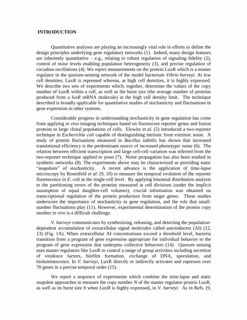
INTRODUCTION

Quantitative analyses are playing an increasingly vital role in efforts to define the

design principles underlying gene regulatory networks (1). Indeed, many design features

are inherently quantitative – e.g., relating to robust regulation of signaling fidelity (2),

control of noise levels enabling population heterogeneity (3), and precise regulation of

circadian oscillations (4). We report measurements on the protein LuxR which is a master

regulator in the quorum-sensing network of the model bacterium Vibrio harveyi. At low

cell densities, LuxR is repressed whereas, at high cell densities, it is highly expressed.

We describe two sets of experiments which, together, determine the values of the copy

number of LuxR within a cell, as well as the burst size (the average number of proteins

produced from a luxR mRNA molecule) in the high cell density limit. The technique

described is broadly applicable for quantitative studies of stochasticity and fluctuations in

gene expression in other systems.

Considerable progress in understanding stochasticity in gene regulation has come

from applying in vivo imaging techniques based on fluorescent reporter genes and fusion

proteins to large clonal populations of cells. Elowitz et al. (5) introduced a two-reporter

technique in Escherichia coli capable of distinguishing intrinsic from extrinsic noise. A

study of protein fluctuations measured in Bacillus subtilis has shown that increased

translational efficiency is the predominant source of increased phenotypic noise (6). The

relation between efficient transcription and large cell-cell variation was inferred from the

two-reporter technique applied to yeast (7). Noise propagation has also been studied in

synthetic networks (8). The experiments above may be characterized as providing static

“snapshots” of stochasticity. A recent advance is the application of time-lapse

microscopy by Rosenfeld et al. (9, 10) to measure the temporal evolution of the reporter

fluorescence in E. coli at the single-cell level. By applying binomial distribution analysis

to the partitioning errors of the proteins measured at cell divisions (under the implicit

assumption of equal daughter-cell volumes), crucial information was obtained on

transcriptional regulation of the protein production from target genes. These studies

underscore the importance of stochasticity in gene regulation, and the role that small-

number fluctuations play (11). However, experimental determination of the protein copy

number in vivo is a difficult challenge.

V. harveyi communicates by synthesizing, releasing, and detecting the population-

dependent accumulation of extracellular signal molecules called autoinducers (AI) (12,

13) (Fig. 1A). When extracellular AI concentrations exceed a threshold level, bacteria

transition from a program of gene expression appropriate for individual behavior to the

program of gene expression that underpins collective behaviors (14). Quorum sensing

uses master regulators like LuxR to control a range of group activities including secretion

of virulence factors, biofilm formation, exchange of DNA, sporulation, and

bioluminescence. In V. harveyi, LuxR directly or indirectly activates and represses over

70 genes in a precise temporal order (15).

We report a sequence of experiments which combine the time-lapse and static

snapshot approaches to measure the copy number N of the master regulator protein LuxR,

as well as its burst size b when LuxR is highly expressed, in V. harveyi. As in Refs. (9,

10), we have determined the relative partitioning error of LuxR (fused to mCherry

protein) at cell division by single-cell fluorescence time lapse microscopy. When a cell

divides, both N and the cell volume V are partitioned between the daughter cells in nearly

even proportions. In individual cells, however, slight asymmetries in the partitioning of

both N and V occur stochastically. As a result, the bell-shaped distribution curves

describing the partitioning of the fluorescence signal and the volume acquire widths

which we have measured in detail. We show that it is essential to measure the

distribution function governing the volume partitioning (in addition to the fluorescence

partitioning function). Relative fluctuations in the two quantities are comparable in

magnitude. Applying binomial distribution analysis to the two measured distributions,

we obtain N, or equivalently, the calibration between the observed fluorescence signal

and the LuxR copy number. Turning to the snap-shot approach, we next captured the

distribution of LuxR-mCherry fluorescence density over a population of ~3,000 cells.

Past studies have shown that the width of the distribution is much larger

(“overdispersed”) compared with a Poisson distribution. In models analyzing the

distribution (16-18), the burst size b is identified with the Fano factor (the ratio of the

variance to the mean). However, if the copy number N is not known, b can be

determined only up to an unknown constant (this also precludes quantitative comparisons

of distributions taken on different samples). By fixing the copy number, we provide the

final link that allows the numerical value of b to be obtained from these broad

distributions. We find that the burst size is ~50 dimers in the high-cell density limit when

LuxR is highly expressed. This implies that, on average, ~11 messenger RNAs are

transcribed during a cell cycle. These are the first measurements of burst values of a key

protein in a quorum-sensing network (b has been measured recently in E. coli using other

techniques (19, 20)).

MATERIALS and METHODS

V. harveyi strain construction.

The mCherry plasmid pRSET-B was a generous gift from Roger Tsien (UCSD)

(21). V. harveyi strains used in the experiment were derived from wild-type V. harveyi

BB120 (22). The N-terminal mCherry-LuxR construct was engineered using overlapping

PCR to generate a (Gly4Ser)3 amino acid linker between the two proteins in the fusion.

The gene encoding the fusion protein was linked to a CmR marker and used to replace the

native luxR gene in a genomic library cosmid containing the luxR locus (pBB1805) to

generate pKT1550 (23). A KanR marker was recombined into pKT1550, to replace the

CmR marker and generate pKT1630. This construct was subsequently conjugated into the

V. harveyi reporter strain TL27 (luxM, luxS, cqsA, cqsS) (24) to generate strain

KT792. The luxR-mCherry construction was introduced onto the V. harveyi chromosome

by allelic replacement (25). A plasmid pTL93 carrying gfp driven from the constitutive

Ptac promoter was constructed to make an internal indicator Ptac-GFP. The cosmid,

pTL65, was constructed by recombining the Ptac-GFP-KanR

fragment into the intergenic

region downstream of the entire lux operon (23). Final insertion of Ptac-GFP-KanR

onto

the V. harveyi chromosome was accomplished by allelic recombination to generate strain

TL112.

Time-lapse microscopy and distribution measurement

Time-lapse fluorescence images of V. harveyi KT792 cells were obtained with an

epi-fluorescence microscope TE-2000U (Nikon, Melville, NY). Custom Basic code was

used to control the microscope and related equipment. In order to monitor gene

expression in real time, fluorescent images were taken every 2 minutes via a 100X oil-

immersion objective (NA=1.4, Nikon, Melville, NY). In our optical system, the pixel size

corresponds to a width of 160 nm. To track dividing cells, phase-contrast images were

also taken and used for auto-focusing the cells. The fluorescent signal was collected with

a cooled (-60˚C) CCD camera (Andor iXon, South Windsor, CT). The total power from

the objective is 67 μW at λ=570 nm, and the variance between experiments was <8%.

Time-lapse movies were recorded every 2 minutes over a period of 6 hours with the

exposure time fixed at 0.3 seconds. To minimize bleaching, the appropriate shutter was

opened only during the exposure time. The sample was heated by a temperature-regulated

heating stage (Warner, Hamden, CT) and maintained at 30 ˚C during the experiment (Fig.

S2). An electronic feedback system stabilized the temperature within ±0.3˚C. The drift of

the focus was automatically corrected throughout the experiment via a contrast-based

autofocus algorithm. Data analysis was performed using MATLAB (The MathWorks,

Natick, MA). V. harveyi TL112 was grown in AB medium (0.3 M NaCl, 0.05M MgSO4,

0.2% vitamin-free casamino acids, 0.01M Potassium phosphate, 0.01 M L-arginine, 1%

glycerol, pH 7.5) overnight for static distribution measurement, rediluted and grown to an

OD600≈0.05 at 30˚C. After concentrating by centrifugation, cells were observed on

microscope slides at room temperature. Cells were observed with automated stage (Prior,

Rockland, MA); ~3000 cells were measured per sample.

RESULTS

Time-lapse fluorescence microscopy results

In the V. harveyi circuit, at low cell density small antisense RNAs (sRNAs) are

made that bind to and repress translation of the luxR mRNA. At high cell density, the

sRNAs are not synthesized; luxR mRNA is translated and LuxR protein is produced.

Current evidence suggests that the functional unit of LuxR is a dimer (26) (Note that the

V. harveyi LuxR protein is not an acyl-homoserine lactone binding protein as the LuxR in

Vibrio fischeri.) In order to understand quantitatively how LuxR directs this cascade, it is

important to know the copy number in individual cells, and to understand how it changes

in response to changing AI inputs. To image the protein, we engineered a functional

LuxR-mCherry fluorescent protein fusion and introduced it onto the V. harveyi

chromosome at the native luxR locus. We verified that our LuxR fusion retains its

functionality (see Supporting Material). Figure S1 shows that both wild type LuxR and

LuxR-mCherry activate and repress candidate genes to the same extent, implying that the

wild type (wt) and fusion proteins are produced at nominally the same level.

The V. harveyi quorum-sensing circuit is shown in Fig. 1A. The strain of V.

harveyi used for this work lacks the genes encoding the three AI synthases (luxM, luxS

and cqsA), and is therefore incapable of producing endogenous AI. The background

strain is also deleted for the cqsS gene encoding the CAI-1 receptor CqsS, so the strain is

impervious to CAI-1. Thus, the CAI-1-CqsS system neither contributes nor removes

phosphate from the quorum-sensing circuit (24). The LuxR-mCherry construct was

introduced into this strain (Fig 1B).

We recorded the red fluorescent signal F(t) vs. time t from LuxR-mCherry in

time-lapse movies during the growth of the above V. harveyi strain, both in the absence

and presence of AIs. In each experiment, we monitored the fluorescent signal from three

well-separated colonies growing under nearly identical conditions. We define the total

number M~250 of cell-division events (indexed by i) in the three colonies as one sample.

Altogether, six samples (labeled 1-6) were investigated (see Table I). The mCherry

fluorescence F(t) and the phase-contrast image, from which the cell areas A(t) were

computed, were recorded every two minutes for 5 hours (Fig. 1C). Because the cells

grow densely packed in the confined space, V is proportional to the imaged area A (see

Supporting Material). An automated program computes the boundaries of each cell, and

also traces the lineage trees of all cells in the colony (Fig. 2). To eliminate uncertainties

caused by temperature fluctuations, we regulated the temperature of the sample chamber

to within ±0.3°C of 30°C over the entire 5 hours. Several tests were performed to verify

that our results are not affected by errors in cell area estimation or by nonlinear response

in F to the incident light intensity (see Supporting Material).

We find that, in each of the 6 samples, the trace of A(t) displays a regular saw-

tooth pattern (Fig. 2A). At the time of cell-division (event i), the trace splits into two

branches as the mother cell area A0

i divides into two approximately even halves Ai and A’i

= A0

i - Ai. We define the subscripted quantities Ai and A’i as the areas measured

immediately following the ith

cell division (superscripts or subscripts “0” refer to the

mother cell). Subsequently, the daughter cell areas increase to values close to A0i,

whereupon cell division repeats. A similar branching pattern is observed in the trace of

the mCherry fluorescence signal (Fig. 2B). Analogous to the area measurements, we

have F0

i = Fi + F’i, where F0

i is the peak mCherry signal in the mother cell immediately

prior to cell division. In each sample, the values of F0

i cluster tightly around the

ensemble-averaged value F0 = F

0i (the standard deviation in each sample is reported in

Table I). The ensemble-averaged peak fluorescence F0 is a convenient parameter that

distinguishes the 6 samples. Clearly, F0 is proportional to the ensemble-averaged copy

number in the mother cell N0, viz. F

0 = N

0, with the scaling constant yet to be fixed.

At time t, the normalized signal F(t)/A(t) defines the fluorescence density, which is

proportional to the LuxR concentration [LuxR](t). The trace of the fluorescence density

(Fig. 2C) shows that, if the AI concentration is unchanged during the 5-hour experiment,

[LuxR](t) remains nominally constant.

For each of the Samples 1-6, we collected two sets of area and fluorescence data

{A0

i, Ai} and {F0

i, Fi}, where i indexes the cell-division events. As we are interested in

the relative fluctuations of these quantities about their mean, we computed the fractional

areas xi = Ai/A0

i and fractional fluorescence yi = Fi/F0

i. Each cell-division event (xi,yi) can

be represented as a point in the x-y plane. The scatter plot of the events {(xi,yi)} (shown

in Fig. 3A for Sample 1) suggests an ellipse centered at (x0, y0) = (½, ½). The value of

the tilt-angle (~70o) of the semi-major axis to the x-axis demonstrates that a correlation

exists between fluctuations in x and fluctuations in y. The histogram obtained by

projecting the distribution onto the x-axis represents the area-partition distribution PA(x),

which defines the probability distribution for partitioning of cell area without regard to

fluorescence distribution. The “error” in the area partitioning is small (~3.5%), in close

agreement with previous experiments (27, 28). Empirically, we find that PA(x) in all 6

samples is well described by a Gaussian function centered at x = ½, viz.

220 2

22

1Axx

A

A exP

. For each sample, we have fixed the standard deviation A

using the method of maximum likelihood estimation (MLE) discussed below. The bold

curve in Fig. 3B represents PA(x) in Sample 1. The corresponding projection onto the y-

axis yields the fluorescence-partition distribution PF(y) which also fits a Gaussian form

(Fig. 3C). Significantly, the standard deviationF of PF(y) (also found by MLE) is larger

than that of PA(x) (5.64% vs. 3.4%). This implies that, in addition to area fluctuation, the

total standard deviationF derives an additional contribution, which we identify with

small-number fluctuations of the protein population. (As discussed in the Supporting

material, pixelation and defocusing contribute a negligible uncertainty of 0.8% to A0

i and

Ai. The uncertainties in our final determination of A are further reduced by the large

sample size M involved in MLE.)

We next examine how the standard deviations F and A change with N0. In

Table I, we have ranked Samples 1 to 6 in the order of increasing average peak

fluorescence F0~ N0. (As noted, the variance of F

0i measured within each sample is

small, so we may regard N0 as a nominal constant in our analysis. The small cell-cell

fluctuation in N0 within each sample colony is the main source of uncertainty in N0.) The

peak fluorescence F0

increases rapidly with AI concentration [AI], but even when [AI] =

0, F0

is sample dependent, as in 1-3. In this experiment, the crucial observation is the

systematic narrowing of the widths of the fluorescence distribution functions PF(y) as F0

increases. By contrast, PA(x) remains unchanged within our resolution. Results for

Sample 4 are shown on the second row of Fig. 3 (D, E, F) while those for Sample 6 are

shown in the 3rd

row (G, H, I). Compared with Sample 1 (first row), the peak

fluorescence F0 in Samples 4 and 6 are larger by a factor of 2.2 and 3.3, respectively.

Inspection of Figs. 3C, 3F and 3I reveals that the fluorescence distribution PF(y) narrows

systematically with increasing F0.

Determining the copy number N0

We show that narrowing of the distributions reflects the suppression of the small-

number fluctuation contribution to F with increasing N0. As discussed, the area of the

mother cell is partitioned in the ratio x : (1-x), according to the probability PA(x). We

assume that, at cell division, the N0 dimers of LuxR move freely in the cytoplasm.

Hence, they distribute between the daughter cells stochastically. For a given area

partitioning x, we model the stochastic process as N0 tosses of a coin of bias x

(Supporting Material). The conditional probability that, given x, N copies are found in

the daughter of area Ai is the binomial distributionNNN xx

N

NxNP

0)1()|(

0. In the

limit N, N0 » 1, we have 22 2

22

1Nxy

N

exyP

/)()|(

, where y = N/N0 and

0

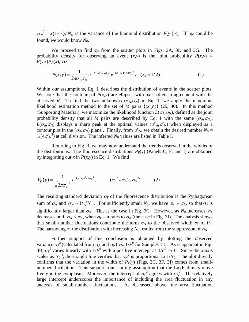
21 NxxN /)( is the variance of the binomial distribution P(y | x). If N could be

found, we would know N0.

We proceed to findN from the scatter plots in Figs. 3A, 3D and 3G. The

probability density for observing an event (x,y) is the joint probability P(x,y) =

P(y|x)PA(x), viz.

)/(,),(/)(/)(

212

10

2222

022

xeeyxP AN xxxy

NA

. (1)

Within our assumptions, Eq. 1 describes the distribution of events in the scatter plots.

We note that the contours of P(x,y) are ellipses with axes tilted in agreement with the

observed . To find the two unknowns (AN) in Eq. 1, we apply the maximum

likelihood estimation method to the set of M pairs {(xi,yi)} (29, 30). In this method

(Supporting Material), we maximize the likelihood function L(AN), defined as the joint

probability density that all M pairs are described by Eq. 1 with the same (AN).

L(AN) displays a sharp peak at the optimal values (A

N) when displayed as a

contour plot in the (AN) plane . Finally, from N, we obtain the desired number N0 ≈

1/(4N

2) at cell division. The inferred N0 values are listed in Table I.

Returning to Fig. 3, we may now understand the trends observed in the widths of

the distributions. The fluorescence distributions PF(y) (Panels C, F, and I) are obtained

by integrating out x in P(x,y) in Eq. 1. We find

220 2

22

1Fxy

F

F eyP

/)()(

, (F

2 = A

2 + N

2). (2)

The resulting standard deviation F of the fluorescence distribution is the Pythagorean

sum ofA and 01 NN /~ . For sufficiently small N0, we haveN » A, so thatF is

significantly larger than A. This is the case in Fig. 3C. However, as N0 increases,F

decreases untilN < A, when F saturates toA (the case in Fig. 3I). The analysis shows

that small-number fluctuations contribute the term N to the observed width F of PF.

The narrowing of the distribution with increasing N0 results from the suppression of N.

Further support of this conclusion is obtained by plotting the observed

varianceF2

(calculated from A and N) vs. 1/F0 for Samples 1-5. As is apparent in Fig.

4B,F2

varies linearly with 1/F0 with a positive intercept as 1/F

0 0. Since the x-axis

scales as N0-1

, the straight line verifies that N2 is proportional to 1/N0. The plot directly

confirms that the variation in the width of PF(y) (Figs. 3C, 3F, 3I) comes from small-

number fluctuations. This supports our starting assumption that the LuxR dimers move

freely in the cytoplasm. Moreover, the intercept of F2 agrees with A

2. The relatively

large intercept underscores the importance of including the area fluctuation in any

analysis of small-number fluctuations. As discussed above, the area fluctuation

distribution is independent of the LuxR copy number so the widthA of PA(x) is

insensitive to F0. This is confirmed in Fig. 4A. Figure 4C summarizes the linear

relationship between N0 inferred from the MLE and the F0 measured in Samples 1-5. As

the peak fluorescence F0 increases from 1.2×10

4 to 3.4×10

4 counts in Samples 1-5, N0

rises in proportion from 80 to 180. The slope of this linear relationship fixes the scaling

constant = F/N.

Protein burst and the Fano factor

Following transcription, protein molecules are produced stochastically at the translation

stage. There is now strong evidence for the hypothesis that protein production occurs in

bursts, with a burst of proteins translated from a single mRNA molecule (the luxR mRNA

half-life m~3 min (31)). Bursts associated with mRNA transcription in E. coli were

recently imaged (32), but in vivo cytoplasm protein bursts from a single mRNA have not

been imaged to date. Stochastic fluctuations at the transcription and translation stages

lead to a broad, skewed distribution G(p) of the protein concentration p measured on a

large population (the “static snapshot”). Numerical simulations suggest that the Fano

factor -- the ratio of variance to mean -- greatly exceeds 1, the value predicted for a

Poisson distribution. The relation between the Fano factor and the mean burst magnitude

b has drawn considerable theoretical attention (16-18).However, experimental progress

has been slower. As noted, while the snapshot distribution is readily captured, the Fano

factor cannot be pinned down unless the scaling constant = F/N is known.

Using the calibration for , we have obtained the Fano factor for LuxR in V.

harveyi in the two extreme quorum-sensing modes of low and high cell densities. As in

the time-lapse experiment, LuxR proteins are imaged by mCherry fluorescence. In

addition, we introduced a constitutively expressed GFP, which is under the control of the

Ptac promoter, into the chromosome. Because the gfp gene is not part of the quorum-

sensing circuit, this reporter serves to evaluate the effect of global fluctuations. We

assayed the response of single cells to two different levels of external autoinducers by

using automated snapshot fluorescence microscopy. In each experimental run, we

measured the cell area A and the fluorescence signals of both mCherry and GFP reporters

in each of the ~3000 cells in the sample. We are interested in the distribution G(p) of

protein concentration p rather than copy number over the whole sample (this factors out

the 2-fold cell-to-cell fluctuation in volume or area). Figure 5A shows the scatter plot of

the fluorescence levels for the entire population in the low density limit ([AI] = 0 nM).

(The vertical axis plots the concentration of LuxR dimers p. To facilitate computation of

the Fano factor, however, we express p in the dimensionless form Np = pA, where A is

the mean value of the observed cell area in the sample. Np would be the number of

dimers per cell if all cells had an area equal to A. The Fano factor is then Np2 / Np.

See Supporting Material for details.)

At low cell density, the average LuxR concentration Np is ~80 dimers per cell.

At high cell density ([AI-1]+[AI-2]=1000 nM), Np is observed to increase to ~575

dimers per cell (Fig. 5B), implying a 7-fold increase of LuxR concentration between the

2 limits.

Projecting the data in the scatter plots onto the y-axis, we obtain the distribution

function G(p) displayed in Figs. 5C and 5D in the low- and high-cell-density limits,

respectively. We note that the Fano factor in the high-cell-density limit is significantly

larger than that in the low-cell-density limit. At low cell densities, the expression of LuxR

is regulated post-translationally by sRNAs which bind to luxR mRNAs and target them

for degradataion. This leads to a decrease in the average luxR mRNA lifetime, and a

corresponding reduction in the average bust size, b. In contrast, at high cell densities,

sRNAs are not produced, and mRNAs are no longer degraded by the sRNAs, resulting in

a larger average burst size, b. Due to the complexity of post-transcriptional regulation by

sRNAs, the Fano factor corresponds to the burst size only at high cell densities. At low

cell densities, the Fano factor become a more complicated function of the burst size and

other sources of noise associated with mRNA-sRNA binding (33). Nonetheless, the

increase in width of G(p) between Figs. 5C and 5D is consistent with this scenario.

Significantly, the Fano factor Np2 / Np also increases by a factor of 4 (from ~12 in

Fig. 5C to ~50 in 5D).

In the simplest situation when the mRNA concentration exceeds that of the

sRNAs (high cell density), the Fano factor reduces to the burst size, viz. Np2 / Np ≈

1+b (17, 18). Applying this relation to Fig. 5D, we find that b 50 dimers – on average,

each mRNA produces 50 LuxR dimers in the high-cell density limit.

DISCUSSION

We have developed an in vivo method to measure the copy number of LuxR-

mCherry in V. harveyi. By capturing the time trace of the cell volume and LuxR-

mCherry fluorescence over 6 cell cycles, we have measured both the distribution

functions that govern the volume partitioning and the fluorescence partitioning during

cell division. Applying binomial analysis to the distribution functions, we can then infer

the copy number in each cell. By varying the concentration of autoinducers outside the

cell, we verified that the inferred LuxR copy number scales linearly with the observed

fluorescence signal. With the scaling factor between the 2 quantities so determined, we

next investigated the distribution of fluorescence over a large population of cells (in a

snapshot measurement). In the high-cell density limit, the Fano factor of this distribution

allows the burst size of LuxR proteins to be found.

Our finding of the absolute number of LuxR dimers under no AI, low-cell-density

conditions (80 dimers/cell) and saturating AI, high-cell-density conditions (575

dimers/cell) is intriguing given what we know about Vibrio quorum-sensing regulons.

Numerous studies in different Vibrio species suggest that typically ~70 genes are under

LuxR control. If we make the simple assumption that one or two LuxR dimers is

required to bind DNA per regulated promoter (we note that this is probably an

underestimate given that DNA binding regulatory proteins often oligomerize on DNA),

then in low-cell-density conditions, according to our measurements, there is insufficient

LuxR in the cell to occupy all of its cognate sites and control the set of target genes.

Thus, under the low-cell-density condition, LuxR-repressed target genes are expressed

while LuxR-activated target genes are not. By contrast, at high cell density, with 575

LuxR dimers present, sufficient LuxR is present to bind to and control all of the target

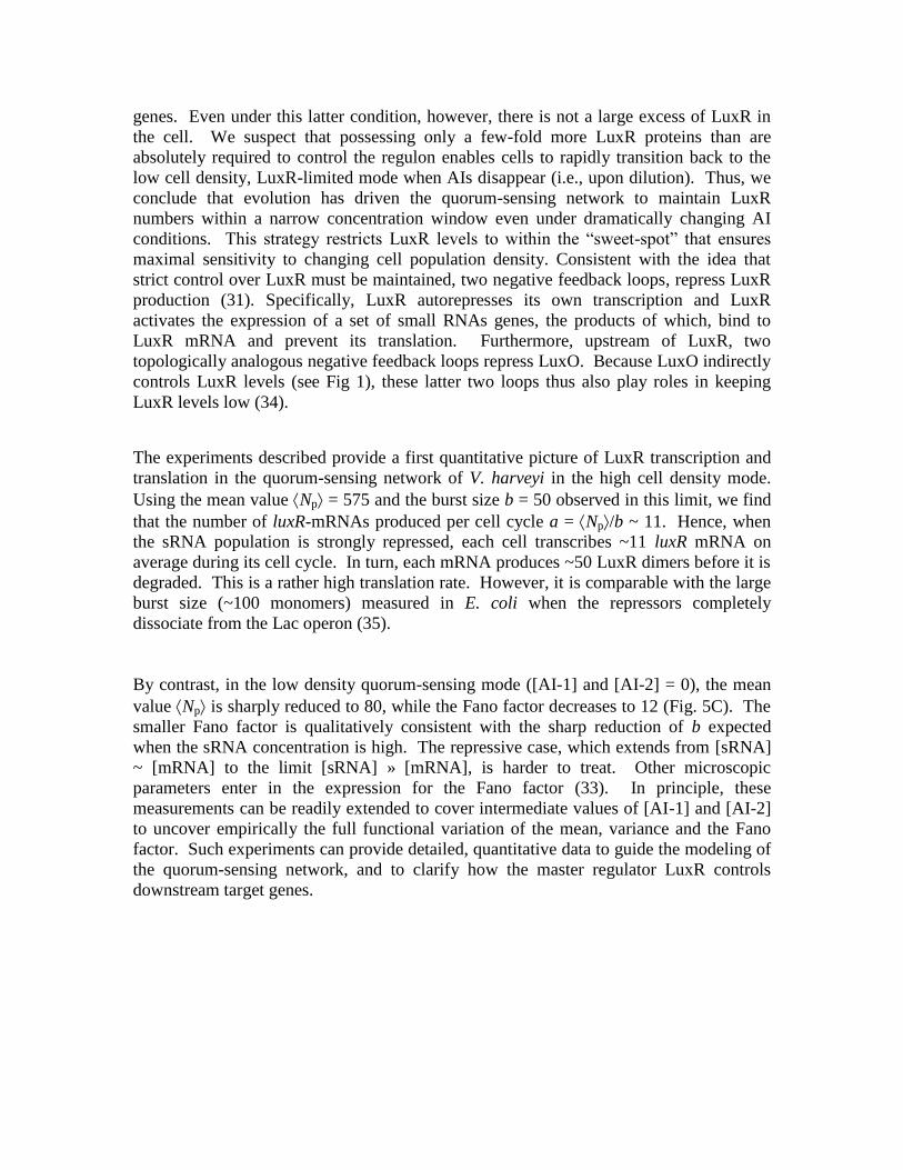
genes. Even under this latter condition, however, there is not a large excess of LuxR in

the cell. We suspect that possessing only a few-fold more LuxR proteins than are

absolutely required to control the regulon enables cells to rapidly transition back to the

low cell density, LuxR-limited mode when AIs disappear (i.e., upon dilution). Thus, we

conclude that evolution has driven the quorum-sensing network to maintain LuxR

numbers within a narrow concentration window even under dramatically changing AI

conditions. This strategy restricts LuxR levels to within the “sweet-spot” that ensures

maximal sensitivity to changing cell population density. Consistent with the idea that

strict control over LuxR must be maintained, two negative feedback loops, repress LuxR

production (31). Specifically, LuxR autorepresses its own transcription and LuxR

activates the expression of a set of small RNAs genes, the products of which, bind to

LuxR mRNA and prevent its translation. Furthermore, upstream of LuxR, two

topologically analogous negative feedback loops repress LuxO. Because LuxO indirectly

controls LuxR levels (see Fig 1), these latter two loops thus also play roles in keeping

LuxR levels low (34).

The experiments described provide a first quantitative picture of LuxR transcription and

translation in the quorum-sensing network of V. harveyi in the high cell density mode.

Using the mean value Np = 575 and the burst size b = 50 observed in this limit, we find

that the number of luxR-mRNAs produced per cell cycle a = Np/b ~ 11. Hence, when

the sRNA population is strongly repressed, each cell transcribes ~11 luxR mRNA on

average during its cell cycle. In turn, each mRNA produces ~50 LuxR dimers before it is

degraded. This is a rather high translation rate. However, it is comparable with the large

burst size (~100 monomers) measured in E. coli when the repressors completely

dissociate from the Lac operon (35).

By contrast, in the low density quorum-sensing mode ([AI-1] and [AI-2] = 0), the mean

value Np is sharply reduced to 80, while the Fano factor decreases to 12 (Fig. 5C). The

smaller Fano factor is qualitatively consistent with the sharp reduction of b expected

when the sRNA concentration is high. The repressive case, which extends from [sRNA]

~ [mRNA] to the limit [sRNA] » [mRNA], is harder to treat. Other microscopic

parameters enter in the expression for the Fano factor (33). In principle, these

measurements can be readily extended to cover intermediate values of [AI-1] and [AI-2]

to uncover empirically the full functional variation of the mean, variance and the Fano

factor. Such experiments can provide detailed, quantitative data to guide the modeling of

the quorum-sensing network, and to clarify how the master regulator LuxR controls

downstream target genes.

ACKNOWLEDGEMENTS

We thank R. Y. Tsien for his kind gift of plasmid; W. S. Ryu for his help with the

temperature control system; A. Pompeani and A. Sengupta for helpful discussions. This

work was funded by HHMI, NIH grant 5R01GM065859, NIH grant 5R01AI054442,

NSF grant MCB-0639855, NIH Grant R01 GM082938, Princeton Center for Quantitative

Biology grant P50GM071508. T.L. is supported by Burroughs Wellcome Fund Graduate

Training Program.

REFERENCES

1. Megason, S. G. and S.E. Fraser 2007. Imaging in systems biology. Cell. 130, 784-795.

2. Batchelor, E. and M. Goulian 2003. Robustness and the cycle of phosphorylation and

dephosphorylation in a two-component regulatory system. Proc. Natl. Acad. Sci. U.

S. A. 100, 691-696.

3. Maamar, H., A. Raj and D. Dubnau 2007. Noise in gene expression determines cell

fate in bacillus subtilis. Science. 317, 526-529.

4. Nakajima, M., K. Imai, H. Ito, T. Nishiwaki, Y. Murayama, H. Iwasaki, T. Oyarna and

T. Kondo 2005. Reconstitution of circadian oscillation of cyanobacterial KaiC

phosphorylation in vitro. Science. 308, 414-415.

5. Elowitz, M. B., A.J. Levine, E.D. Siggia and P.S. Swain 2002. Stochastic gene

expression in a single cell. Science. 297, 1183-1186.

6. Ozbudak, E. M., M. Thattai, I. Kurtser, A.D. Grossman and A. van Oudenaarden 2002.

Regulation of noise in the expression of a single gene. Nat. Genet. 31, 69-73.

7. Raser, J. M. and E.K. O'Shea 2004. Control of stochasticity in eukaryotic gene

expression. Science. 304, 1811-1814.

8. Pedraza, J. M. and A. van Oudenaarden 2005. Noise propagation in gene networks.

Science. 307, 1965-1969.

9. Rosenfeld, N., T.J. Perkins, U. Alon, M.B. Elowitz and P.S. Swain 2006. A fluctuation

method to quantify in vivo fluorescence data. Biophys. J. 91, 759-766.

10. Rosenfeld, N., J.W. Young, U. Alon, P.S. Swain and M.B. Elowitz 2005. Gene

regulation at the single-cell level. Science. 307, 1962-1965.

11. Berg, O. G. 1978. Model for statistical fluctuations of protein numbers in a microbial-

population. J. Theor. Biol. 71, 587-603.

12. Bassler, B. L. and R. Losick 2006. Bacterially speaking. Cell. 125, 237-246.

13. Waters, C. M. and B.L. Bassler 2005. Quorum sensing: Cell-to-cell communication in

bacteria. Annu. Rev. Cell Dev. Biol. 21, 319-346.

14. Bassler, B. L., M. Wright and M.R. Silverman 1994. Multiple signaling systems

controlling expression of luminescence in vibrio-harveyi - sequence and function of

genes encoding a 2nd sensory pathway. Mol. Microbiol. 13, 273-286.

15. Waters, C. M. and B.L. Bassler 2006. The vibrio harveyi quorum-sensing system uses

shared regulatory components to discriminate between multiple autoinducers. Genes

Dev. 20, 2754-2767.

16. Paulsson, J. and M. Ehrenberg 2000. Random signal fluctuations can reduce random

fluctuations in regulated components of chemical regulatory networks. Phys. Rev.

Lett. 84, 5447-5450.

17. Thattai, M. and A. van Oudenaarden 2001. Intrinsic noise in gene regulatory

networks. Proc. Natl. Acad. Sci. U. S. A. 98, 8614-8619.

18. Friedman, N., L. Cai and X.S. Xie 2006. Linking stochastic dynamics to population

distribution: An analytical framework of gene expression. Phys. Rev. Lett. 97,

168302.

19. Yu, J., J. Xiao, X.J. Ren, K.Q. Lao and X.S. Xie 2006. Probing gene expression in

live cells, one protein molecule at a time. Science. 311, 1600-1603.

20. Cai, L., N. Friedman and X.S. Xie 2006. Stochastic protein expression in individual

cells at the single molecule level. Nature. 440, 358-362.

21. Wang, L., W.C. Jackson, P.A. Steinbach and R.Y. Tsien 2004. Evolution of new

nonantibody proteins via iterative somatic hypermutation. Proc. Natl. Acad. Sci. U.

S. A. 101, 16745-16749.

22. Bassler, B. L., E.P. Greenberg and A.M. Stevens 1997. Cross-species induction of

luminescence in the quorum-sensing bacterium vibrio harveyi. J. Bacteriol. 179,

4043-4045.

23. Datsenko, K. A. and B.L. Wanner 2000. One-step inactivation of chromosomal genes

in escherichia coli K-12 using PCR products. Proc. Natl. Acad. Sci. U. S. A. 97,

6640-6645.

24. Long, T., K.C. Tu, Y. Wang, P. Mehta, N.P. Ong, B.L. Bassler and N.S. Wingreen

2009. Quantifying the integration of quorum-sensing signals with single-cell

resolution. PLoS Biology. 7, e68 OP.

25. Bassler, B. L., M. Wright, R.E. Showalter and M.R. Silverman 1993. Intercellular

signaling in vibrio-harveyi - sequence and function of genes regulating expression of

luminescence. Mol. Microbiol. 9, 773-786.

26. Pompeani, A. J., J.J. Irgon, M.F. Berger, M.L. Bulyk, N.S. Wingreen and B.L.

Bassler 2008. The vibrio harveyi master quorum-sensing regulator, LuxR, a TetR-

type protein is both an activator and a repressor: DNA recognition and binding

specificity at target promoters. Mol. Microbiol. 70, 76-88.

27. Guberman, J. M., A. Fay, J. Dworkin, N.S. Wingreen and Z. Gitai 2008. PSICIC:

Noise and asymmetry in bacterial division revealed by computational image analysis

at sub-pixel resolution. PLoS Comput Biol. 4, e1000233.

28. Trueba, F. J. 1982. On the precision and accuracy achieved by escherichia-coli-cells

at fission about their middle. Arch. Microbiol. 131, 55-59.

29. Gelman, A.,J. B. Carlin,H. S. Stern and D. B. Rubin 1995. Bayesian data analysis.

Chapman & Hall, London New York.

30. Taylor, J. R. 1997. An introduction to error analysis : the study of uncertainties in

physical measurements. University Science Books, Sausalito Calif.

31. Tu, K. C., C.M. Waters, S.L. Svenningsen and B.L. Bassler 2008. A small-RNA-

mediated negative feedback loop controls quorum-sensing dynamics in vibrio

harveyi. Mol. Microbiol. 70, 896-907.

32. Golding, I., J. Paulsson, S.M. Zawilski and E.C. Cox 2005. Real-time kinetics of gene

activity in individual bacteria. Cell. 123, 1025-1036.

33. Mehta, P., S. Goyal and N.S. Wingreen 2008. A quantitative comparison of sRNA-

based and protein-based gene regulation. Molecular Systems Biology. 4.

34. Tu, K. C., T. Long, S.L. Svenningsen, N.S. Wingreen and B.L. Bassler

Synergistic negative feedback loops involving small regulatory RNAs precisely

control the

vibrio harveyi quorum-sensing response.

35. Choi, P. J., L. Cai, K. Frieda and S. Xie 2008. A stochastic single-molecule event

triggers phenotype switching of a bacterial cell. Science. 322, 442-446.

TABLES

Sample [AI]

(nM)

M F 0

(count)

σA σN N0

(copy)

1 0 230 12559±2794 3.39%±0.13% 5.64%±0.20% 79±5

2 0 256 19133±3693 3.49%±0.10% 4.80%±0.12% 108±5

3 0 178 23916±5682 3.19%±0.15% 4.30%±0.20% 135±12

4 10 292 27485±4371 3.94%±0.25% 3.84%±0.20% 169±18

5 18 156 33726±7123 3.15%±0.20% 3.75%±0.22% 178±21

6 22.5 264 16902*±2589 3.97%±0.18% 360*±55

Table I. Parameters for Samples 1-6. AI is the exogenous concentration of AI-1 and AI-

2 (in nM of each molecule) during growth of the colony. M is the total number of

division events in each sample. F0 is the ensemble-averaged peak fluorescence

immediately prior to cell division. A andN are the standard deviations of PA(x) and

P(y|x), respectively, inferred by MLE (see text). N0 is the LuxR dimer number

immediately prior to cell division inferred by MLE (in samples 1-5). In Sample 6, the

incident power was reduced significantly to avoid photo-toxicity arising from the

enhanced photon absorption by the much higher concentration of LuxR-mCherry

(incident powers are identical for Samples 1-5). In Sample 6, the value ofN was too

small to be reliably obtained by MLE. In this case, values of N0 are inferred from F0

using the scaling constant established in Fig. 4C.

FIGURE LEGENDS

Fig. 1. The quorum-sensing circuit and growth of a colony of V. harveyi. (A) Wild-type

V. harveyi uses three autoinducers (AIs) to gauge the population density as well as the

species composition of the vicinal community. The AIs are AI-1, an intra-species signal,

CAI-1 an intra-genera signal, and AI-2 an inter-species signal. In V. harveyi, detection of

AI-1, CAI-1 and AI-2 involves the trans-membrane receptors LuxN, CqsS and LuxPQ,

respectively. Black arrows denote the direction of phosphate flow when the concentration

of AI is low. In the absence of AIs (low cell density), the receptors are kinases which

funnel phosphate through a shared pathway that ultimately represses translation of the

mRNA encoding the master quorum-sensing regulator, LuxR. In response to AIs (i.e., at

high cell density), the receptors convert from being kinases to being phosphatases.

Phosphate is drained from the signaling pathway which relieves repression of luxR

mRNA translation. (B) In the V. harveyi strain used here, only exogenously added AI-1

and AI-2 are detected (by the sensors LuxN and LuxPQ, respectively) which ultimately

controls production of the master regulator LuxR (here labeled with mCherry). (C)

Sequence of fluorescent images (red) overlaid with simultaneous phase images (gray)

showing the growth of V. harveyi cells containing LuxR-mCherry.

Fig. 2. Time traces of the cell area A(t) and LuxR-mCherry fluorescence signal F(t) at

fixed concentration of AI. (A) Time trace of cell area A(t) (expressed as pixel count)

derived from the time-lapse fluorescence-phase movie shown in Fig. 1C. (B) The

observed LuxR-mCherry fluorescence I(t) measured in photon counts. A second-order,

linear-regression fit to A(t) and F(t) during each cell cycle was used to obtain the

quantities A0i, F

0i at the i

th cell division (the peak values in the traces in Panels A and B).

The ensemble-averaged peak fluorescence F0 is defined as < F

0i >. (C) The time trace of

the fluorescence density F(t)/A(t) ~ [LuxR](t). (D) Lineage tree diagram of a colony

growing from a single mother cell. Each branch point i represents a cell-division event.

The four highlighted lineages correspond to the plots in (A), (B), and (C). The average

cell cycle (45±10 min) at 30o C is roughly equal to that observed in agitated liquid

medium (~40 min).

Fig. 3. Scatter plot and the area and fluorescence signal distributions in Samples 1, 4 and

6 (in successive rows) with AI-1 and AI-2 each at = 0, 10 and 22.5 nM, respectively.

Panel A plots the distribution of the events {xi,yi} in sample 1 in the x-y plane, where xi =

Ai/A0i and yi = Fi /F

0i. Histograms created by projection of the data onto the x-axis are

approximations of the area-partitioning distribution PA(x) (Panel B). Projections onto the

y-axis approximate the fluorescence-partitioning distribution PF(y) (Panel C). The bold

curves in panels B and C are Gaussian functions with values of A and F derived from

MLE (see text). The corresponding quantities are displayed for Sample 4 in the second

row (D, E, F), and for Sample 6 in the third row (G, H and I). Note that, in the right

column, PF(y) decreases in width from Panel C to Panel I. In the scatter plots, a

correlation exists between the fluctuations in x and y. The correlation coefficient = 0.45,

0.60 and 0.58 in Panels A, D and G, respectively.

Fig. 4. Test of the model (Eqs. 1 and 2), and of linear scaling between N0 and the

observed peak fluorescence F0 in Samples 1-5. (A) Plot of A

2 (obtained from MLE)

versus 1/F0

~ 1/N0 in Samples 1-5. (B) Plot of F2 (calculated from A and N) versus

1/F0

~ 1/N0 in Samples 1-5. The straight-line fit to F2 verifies that N

2 is proportional to

1/N0. (C) Plot of F0 versus N0 obtained from MLE in the five samples. The straight-line

fit confirms that N0 scales linearly with the ensemble-averaged peak fluorescence F0. In

all panels, error bars along the axes F0 and 1/F

0 reflect the standard deviations of F

0i

reported in Table I. Error bars for N0 (Panel C) reflect the variation in N caused by

decreasing loge L by one unit from its peak value in the contour plot (see SI).

Fig. 5. Scatter plot and the fluorescence density distributions in two samples with the

concentration [AI] set at 0 and 1000 nM, respectively. Panels A and B show the scatter

plots of LuxR concentration p versus the GFP reporter count for ~3000 cells in the

samples with [AI] = 0 and 1000 nM, respectively. With = F/N known, we can calibrate

the concentration p (on the vertical axis). We express p as Np = pA, where A is the

mean of the cell area. On the horizontal axis, the GFP signal is expressed in counts per

pixel. In Panels C and D, the distribution function G(Np) of the LuxR concentration is

plotted vs. Np for the zero-AI and large-AI samples, respectively. Solid circles are

histogram values obtained by projecting the scatter plot onto the y axis. The Fano factor

Np2 / Np equals 12 and 50 in C and D, respectively. This implies that the burst size b

~50 dimers per mRNA in D. The bold curves are fits to the Gamma distribution using

MLE.

FIGURES

Fig. 1.

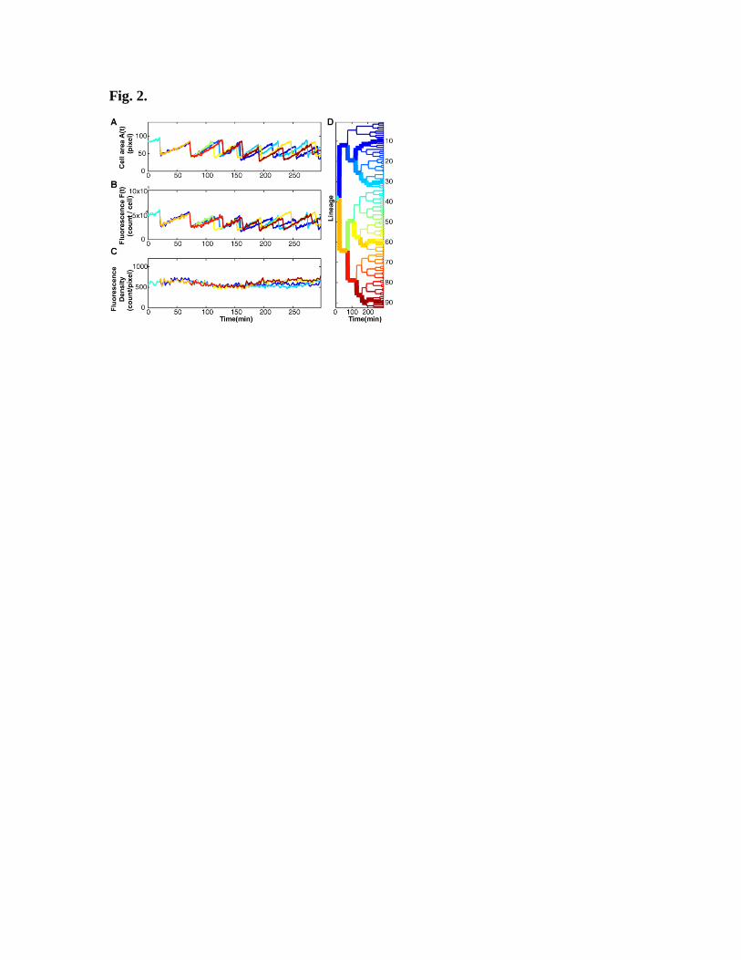
Fig. 2.

Fig. 3.

Fig. 4.

Fig. 5.

Supporting Material

Measurement of the copy number of the master

quorum-sensing regulator of a bacterial cell

Shu-Wen Teng*, Yufang Wang

*, Kimberly C. Tu

†, Tao Long

*, Pankaj Mehta

†,

Ned S. Wingreen†, Bonnie L. Bassler

†,‡, N. P. Ong

*

*Department of Physics,

†Department of Molecular Biology, Princeton University,

Princeton, NJ 08544, USA, ‡Howard Hughes Medical Institute, Chevy Chase, MD

20815, USA

1. V. harveyi strain construction

To demonstrate that the LuxR-mCherry fusion retains functionality, we measured

activity from promoter-gfp fusions to LuxR-controlled target genes in wild-type V.

harveyi and two isolates of the same V. harveyi strain carrying the LuxR-mCherry fusion.

Both LuxR-mCherry fusions activated fluorescence similarly to WT LuxR (Panel A of

Fig. S1). Conversely, when fluorescence is repressed by WT LuxR, similar repression by

theLuxR-mCherry fusions is observed (Panels B and C).

Fig. S1. Comparison of activation and repression by WT LuxR and LuxR-mCherry fusions. A

plasmid encoding a vector, V. harveyi WT LuxR protein, or the V. harveyi LuxR-mCherry fusion

was transformed into E. coli. Plasmids containing promoter-gfp fusions to direct targets of LuxR

were transformed into the various strains (1). Fluorescence production was measured using a flow

cytometer. (A) The target pCMW352 is activated by LuxR and LuxR-mCherry. (B) The target

pCMW275 is repressed by LuxR and LuxR-mCherry. (C) The target pCMW342 is also repressed by

LuxR and LuxR-mCherry. Each sample was assayed in triplicate and error bars denote the standard

deviation of the mean.

2. Growth conditions and Experimental set-up

V. harveyi strains were grown overnight in AB (autoinducer bioassay) medium (0.3 M

NaCl, 0.05 M MgSO4, 0.2% vitamin-free casamino acids, 0.01M KxHyPO4, 0.01M

arginine, 1% glycerol, pH7.5). Overnight cultures were subsequently diluted (1:2000)

into fresh AB medium and grown for 12 hours (until OD600 reached 0.4). One-half micro-

liter of culture was spotted on a clean No. 1.5 glass bottom Petri-dish (Willco Wells) and

covered with a 1% agarose pad made of the same medium. As shown in Fig. S2, a small

piece of coverslip was placed on top of the agarose pad, and the annular space between

the 2 coverslips surrounding the pad was filled with mineral oil to prevent evaporation.

To obtain the real boundary of cells, we stained the colony with FM4-64, a fluorescence

dye that is known to accumulate in the cytoplasmic membrane.

Fig. S2. Schematic of the experimental set-up. V. harveyi cells (red ovals) were grown under an

agarose pad (yellow rectangle) placed between a coverslip and the bottom of a Petri dish (light blue

strips). The space was surrounded by mineral oil as indicated. A thermistor continuously monitored

the temperature of the experimental space.

3. Image analysis: Area determination

Custom software was developed using MATLAB (The MathWorks, Natick, MA) to

estimate the areas of the individual cells in each frame of the time-lapse movies. The V.

harveyi microcolony grows with a dense-packed morphology. In the phase-contrast

images, each pixel was broadened by the point-spread function as well as the interference

halo. However, because of the dense packing, the broadening severely affected the

boundaries of the cells at the edges of the colony inferred from phase-contrast images

leading to an overestimate of their area (by 20-30%). The enhanced distortion of the

edges of cells was detected when we compared the phase-contrast images with the

fluorescence images of test colonies used for calibration. Specifically, we stained live V.

harveyi with F4-64, a fluorescent dye that accumulates in the cytoplasmic membrane.

The high-intensity fluorescence image produced by the stained membrane accurately

located the true microcolony boundary. Thus, to avoid overestimating area, stained

images and the phase-contrast images of the same microcolony were captured in rapid

succession and compared with one another.

In Fig. S3A, the upper and lower insets show such (grey) phase-contrast images

and (red) stained fluorescence images, respectively. The fluorescence profiles at the

regions indicated by vertical yellow lines are plotted in Figs. S2B and S2C for the phase-

contrast (Fp vs. y) and stained (Fs vs. y) images, respectively. Comparing the profiles of

Fp and Fs, we note that their peaks agree well in the interior. Hence, this method can be

used to define the edges of the interior cells. However, the images disagree significantly

at the boundaries. The strong peaks in Fp at the right and left edges (Fig. S3B) are shifted

outward compared with the true cell boundaries (located by the small peaks of Fs at the

edges in Fig. S3C). After examining large numbers of such sections, we found an

empirical, iterative method to accurately locate the true boundary using the phase contrast

trace Fp vs. y. As a starting approximation, we used the midpoint ymid between the first

maximum and the first minimum in Fp to approximate the true cell boundary.

Fig. S3. Comparison of phase-contrast and membrane-stained images. (A) Comparison of

individual cell areas Ak measured with phase-contrast microscopy of a microcolony (upper inset) and

A’k measured using stained-membrane fluorescence images of the same microcolony (lower inset).

Each symbol represents a cell. The linear array of the symbols confirms that Ak agrees well with A’k.

(B) Fluorescence signal profile Ip vs. y along the vertical yellow line shown in the phase-contrast

image in A. Peaks correspond to bright areas in the phase-contrast image. (C) Fluorescence profile

Is vs. y along the same section using the membrane-stained fluorescence image. The small peaks at

the right and left edges show the true boundaries of the colony. (D) Plot of the cell width wk of cell k

(obtained from the phase-contrast image) versus its distance from the colony center. (E) Plot of cell

area Ak versus the cell distance from the colony center. The flat profiles in Panels D and E confirm

that there are no spurious correlations between the two quantities compared. The five colored cells

in the upper inset of Panel A correspond to the same-color symbols plotted in the three panels A, D

and E.

An improved estimate was subsequently obtained by shifting ymid inward by one

pixel. Hence, in the trace of Fp, the true boundary was located at y0 = ymid ± 1 (where the

correct sign is the one that shifts y0 toward the interior). By incorporating these

algorithms, the program automatically traces out the boundaries of both interior and

exterior cells of the microcolony and computes the cell areas Ak. The quality of the

image processing was subsequently examined, and poorly segmented cells were corrected

by hand. As a verification, we have plotted Ak of all the cells in the microcolony,

determined from the phase-contrast image, against A’k, the corresponding areas

determined from the stained-membrane image only (Fig. S3A). The linear correlation

confirms the expected, strictly linear scaling between Ak and A’k. The colored symbols

correspond to the five cells shown with the same colors in the upper inset. Figs. S3D and

S3E plot the measured cell widths wk and areas Ak, respectively, versus their positions

from the center of the microcolony. A spurious enhancement of either quantity at the

edges of the colony would be immediately apparent as an increasing curve. Clearly, the

horizontal arrays in both panels show that these spurious effects are negligible.

4. Scaling between area and volume

In the confined space of the experimental set-up, cross sections of the growing V. harveyi

cells were significantly distorted from circular cross-sections. The distortion results from

both vertical compression (the “low-ceiling” effect) and horizontal compression (dense

packing). Hence, we assumed that the measured area Ak scales linearly with the volume

Vk. By contrast, for a circular cross-section, the observed Ak should scale as √Vk

(ignoring small end-corrections). To test this assumption, we examined how the

measured (areal) fluorescence density Fk/Ak varied with Ak over a large population. Our

test relies on the observed constancy of the concentration of LuxR protein over the 5-hour

experiment. Since LuxR concentration is strictly proportional to the volume fluorescence

density Fk/Vk, we expect Fk/Vk to be independent of Vk. Hence, if Ak is indeed

proportional to Vk, we should observe Fk/Ak to be independent of Ak. By contrast, if Ak

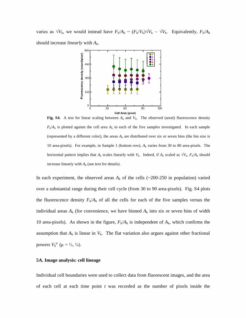
varies as √Vk, we would instead have Fk/Ak ~ (Fk/Vk)√Vk ~ √Vk. Equivalently, Fk/Ak

should increase linearly with Ak.

Fig. S4. A test for linear scaling between Ak and Vk. The observed (areal) fluorescence density

Fk/Ak is plotted against the cell area Ak in each of the five samples investigated. In each sample

(represented by a different color), the areas Ak are distributed over six or seven bins (the bin size is

10 area-pixels). For example, in Sample 1 (bottom row), Ak varies from 30 to 80 area-pixels. The

horizontal pattern implies that Ak scales linearly with Vk. Indeed, if Ak scaled as √Vk, Fk/Ak should

increase linearly with Ak (see text for details).

In each experiment, the observed areas Ak of the cells (~200-250 in population) varied

over a substantial range during their cell cycle (from 30 to 90 area-pixels). Fig. S4 plots

the fluorescence density Fk/Ak of all the cells for each of the five samples versus the

individual areas Ak (for convenience, we have binned Ak into six or seven bins of width

10 area-pixels). As shown in the figure, Fk/Ak is independent of Ak, which confirms the

assumption that Ak is linear in Vk. The flat variation also argues against other fractional

powers Vk( = ⅓, ¼).

5A. Image analysis: cell lineage

Individual cell boundaries were used to collect data from fluorescent images, and the area

of each cell at each time point t was recorded as the number of pixels inside the

boundary. The sum of the fluorescent counts of these pixels was recorded as fluorescence

in the fluorescence channel. Background values were subtracted from the fluorescence

channel. This algorithm was applied to six samples to create six ensembles. The quality

of the image processing was subsequently verified for each frame. A tracking algorithm

was applied to the time series of segmented images to obtain a time course for each cell

and its descendant lineage. Tracking is based on the fact that there is little cell movement

between frames. We therefore assume that the cell that occupies the location of the

previous cell is the same cell or its descendant. This tracking analysis was also checked

manually.

5B. Errors from pixelation and defocusing

Uncertainties in determining Ai and A0

i caused by pixelation (CCD camera digitization)

and errors associated with slight defocusing occur following an automated stage

translation. The cell areas A(t) were recorded every two minutes. In an average life cycle,

this corresponds to ~25 measurements of the trace of A(t) vs. t. A second-order, linear

regression fit to the 25 points gives the “best fit” Afit(t) = at2+bt+c, from which both Ai

and A0

i+1 may be found. To display the relative fluctuations of the 25 measurements

about Afit(t), we plot in Fig. S5 the trace of the measured A(t) normalized to Afit(t) [this is

the first 120 minutes of the lineage (index 90) shown in Fig. 2D]. The fluctuations

around 1 correspond to a standard deviation x of 4%, which we identify with the

standard deviation of each measurement. By a standard result (application of the Central-

Limit Theorem) in error analysis (2), the standard deviation of the mean xm equals

x/√25 = 0.8% (x andxm are unrelated to A and N in the main text). Hence, we

estimate that the uncertainties in Ai (or A0

i) are roughly 0.8%. This is the maximum error

(caused by pixelation and defocusing) in locating the x-coordinate of each of the M

(~250) points in the scatter plot in Fig. 3A. In the MLE process of finding N, the

standard deviation of the mean involves a further reduction of √250, which renders this

source of error insignificant. We discuss a more important source of error in determining

N0 in Sec. 8 (MLE).

Fig. S5. Trace of the normalized area A(t)/Afit(t) (blue curve) in the first 120 minutes of the lineage

(index 90) shown in Fig. 2D, where Afit(t) is the linear regression fit. The normalized quantity

randomly fluctuates about 1 (black line) with a standard deviation of 4%. This implies that, on

average, a single measurement of A(t) has an uncertainty of 4%. Because the values of Ai are

extracted from Afit(t) which is based on 25 measurements within a cell cycle, the uncertainty in Ai is

given by the standard deviation of the mean, or 4%/√25 = 0.8%.

6. Distribution functions as joint probability

We describe in more detail the derivation of Eq. 1 of the text. The primary measured

quantity in our experiment is the fluorescence-partition distribution PF(y), which changes

in a reproducible, quantifiable way as the LuxR concentration is varied over a large

range. By contrast, the area-partition distribution PA(x), fixed by biological and physical

mechanisms outside of our control, does not change with LuxR concentration, and may

be considered as given by the normal distribution Eq. 1, with fixed standard deviation .

We consider the subset of events in which the mother-cell area divides in the ratio 1-x : x

(with 0<x<½). These events fall within the interval x dx in the scatter plot (Fig. 3A). The

N0 molecules distribute between the daughter cells according to this ratio, but the process

is stochastic. Thus, our method is analogous to estimating the number N of “heads” in N0

tosses of a coin with bias x (“heads” means the protein ends up in the cell with relative

area x). The conditional probability is the binomial distribution NNN xxN

NxNP

0)1()|(

0 .

For a binomial distribution, the mean N = N0x, while the variance N2 = (N-N)

2 =

Nx(1-x), where N

NNPN , etc. Consequently, the distribution of N is a bell-shaped

curve that peaks at N0x with a width [N0x(1-x)] N0/2. The peak increases linearly

with N0 while the width broadens as N0.

For our purpose, it is preferable to regard the measurement of the fluorescence as

constituting N0 attempts to measure the relative area x. This implies that, instead of N,

we take the ratio y = N/N0 as the sampling variable. Transforming the binominal

distribution PN given above to the y axis, it is clear that the distribution of y becomes a

bell-shaped curve centered at y = x with a width parameterN equal to N/N0 = 1/(2N0).

With increasing N0, the uncertainty in estimating x decreases as 1/(2N0). Thus, when

the sampling count is very large (N « A, as in Sample 6), the fluorescence partitioning

faithfully determines x without adding measurably to the uncertainty (whenceF A).

Conversely, if the sampling count is low (Samples 1-5), the measurements y add an

additional uncertainty (N >A) which reflects small-number fluctuations. This results in

an enhanced total widthF for the fluorescence-partition distribution. We have exploited

this additional broadening to determine N0. In the limit N, N0 » 1, the bell-shaped curve

is well-approximated by a Gaussian function. Finally, multiplying P(y|x) by PA(x) we

obtain the joint-probability density P(x,y) for observing a point (x,y), as given by Eq. 2.

7. Maximum Likelihood Estimation (MLE)

In MLE, we postulate an analytic function to describe a set of measurements. The

function is characterized by a few parameters (a,b,…) whose values are unknown. The

best estimates of the parameters are obtained by maximizing a “likelihood” function

L(a,b,…) (3). In our experiment, the measurements are the set {xi, yi} in an ensemble (i =

1,…, M). As shown in Fig. 3 and Fig. S6A, these events are plotted in the x-y plane. The

distribution of the points is postulated to be given by the probability density

22

022 2/)(2/)(

2

1),( AN xxxy

NA

eeyxP

(S2)

where x0 = ½, and (A,N) are the two parameters to be determined. The likelihood

function is the joint probability that all M measurements are described by Eq. S2 with the

same values of (A,N), viz.

M

i

xxxy

M

NA

NAAiNii eeL

220

22 2/)(2/)(

2

1),(

. (S3)

To maximize L(A,N), it is convenient to take derivatives of loge L(A,N). Setting to

zero the derivatives with respect toA and N, we find that the optimal values are given

by

,1

1

2

212*

M

i

iA xM

M

i

iiN xyM 1

22* 1 . (S4)

A measure of how likely the postulate is to be correct is obtained by plotting the contours

of L(A,N) in the A-N plane. The existence of saddle points or local maxima in close

proximity would imply that the starting postulate is in doubt. However, as shown in Fig.

S6B, the contour plot of Eq. S3 gives a single sharp maximum.

Error in finding N0

In the MLE method, the contours of logeL near its peak provide an estimate of the total

uncertainties in fixing the optimal values of A and N. The contour representing the

value of loge L(A,N) one unit less than its maximum value (the smallest oval in Panel B

of Fig. S6) gives the uncertainties in fixing A and N. We used the latter to define our

error bars for N0 plotted in Fig. 4C (values reported in Table I). For each sample, the

largest source of this uncertainty is the fluctuation of the peak fluorescence F0

i about its

ensemble average F0 (as explained in Sec. 6B, errors from pixelation and defocusing

contribute insignificantly to the uncertainties in A and N).

Fig. S6. Maximum likelihood estimation applied to the ensemble in Sample 2 (grown with AI = 0

nM). (A) Cluster plot of the set {xi, yi} (i = 1,…, M) plotted in the x-y plane. As explained in the

main text, xi = Ai/A0i is the fractional area, and yi = Fi/F

0i is the fractional fluorescence for the cell-

division event i. (B) Contour plot of the likelihood function L(A,N) in the A-N plane defined in

Eq. S3. Adjacent contours differ by a log unit of L(A,N). The function L(A,N) displays a single

sharp peak at the optimal values A ≈ 0.035 and

N ≈ 0.048. The smallest closed-loop contour

determines the uncertainty in determining A and N.

8. Linearity between protein fluorescence signal and incident power

At high concentrations of LuxR (Sample 6), the high fluorescence intensity leads to a

reduction in the viability of the V. harveyi colonies. This is apparent in the significant

lengthening of the cell division time and increased cell death which we suspect arises

from photon toxicity or local heating of the cells. We eliminated these problems by

sharply reducing the incident beam intensity in high-concentration samples. In order to

compare signals across samples taken at different incident powers, we needed to verify

that the fluorescence response of the LuxR-mCherry is linear for the power levels

employed.

Fig. S7. Examination of linearity between the observed mCherry fluorescence density F(t)/A(t) and

the incident light power at wavelength λex=570 nm in three colonies containing dramatically

different LuxR protein levels. (A) Curves of the fluorescence density observed in three colonies

grown with AI = 0 (top panel), 10 nM (middle), and 1000 nM (bottom panel). At time tc = 2.75

hours (dashed line), the incident power was increased by a factor of 4, causing F(t)/A(t) to increase

abruptly by a factor of ~4. (B) The lineage tree of the three colonies with AI =0, 10, 1000 nM are in

the left, middle, and right panels, respectively. Dashed lines mark t = tc. The three boxes identify

the cells exposed to the 4-fold power increase. (C) Plot of fluorescence density F(t1)/A(t1) (low

power) versus I(t2)/A(t2) (high power) measured in the three colonies, where t1 < tc and t2> tc. The

linear correlation between the symbols verifies that the observed fluorescence density is strictly

proportional to the incident power. Moreover, the linearity holds up even with large LuxR

concentrations corresponding to very high AI concentrations (i.e., 1000 nM).

To verify the linearity, we grew three colonies in three micro-chambers containing

dramatically different AI concentrations (0, 10 and 1000 nM). At time tc, the incident

power was increased 4-fold, causing the fluorescence signal to increase proportionately.

Comparing the measured F after the step increase with that before, we found that the

increase in F is also 4–fold in all three samples, verifying the linearity of the response to

the incident power (Fig. S7).

8. Protein Distribution Data Acquisition Analysis

For the static snapshot technique, overnight cultures were rediluted 106-fold in AI free

and AI saturated AB media and grown to OD600~0.05. A volume 1ml of the culture was

pelleted by centrifugation, re-suspended in ~10 μL of new media, and ~1μL placed

between 1% agarose pad and a glass cover slip. By automating the stage control in the x-

y directions and the focusing control in the z direction, we can search and measure the

area and fluorescence in ~3000 cells in ~6 mins. Data analysis was performed using

MATLAB (The Mathworks, Natick, MA). The phase contrast images were used to

identify cell boundary and the corresponding pixels from the fluorescence image used to

calculate the integrated cell fluorescence intensity, normalized by cell-size, to contruct

histograms for single cell snapshot analysis. Objects with green fluorescence (internal

standard) smaller than 0.5% of the mean were discarded. Matlab was used to calculate the

variance and mean of the distribution function and for fitting to proposed distributions,

e.g., the Gamma function.

Within the colony of 3,000 cells measured by the snapshot technique, the volume

(or observed area) varies by a factor of ~2, reflecting different stages of the cell cycle.

Since we are interested in intrinsic fluctuations of the protein fluorescence, we should

factor out the cell-to-cell variation in volume. For each cell, we measured the observed

area A as well as the total fluorescence signal from the cell. This allows the protein

concentration p to be computed as fluorescence count per unit area. Thus the distribution

function G(p) does not include the trivial volume fluctuation factor. Knowing the scaling

factor = F/N from the time-lapse experiments allows us to calibrate the protein

concentration p in the plot of G(p), which is plotted in Figs. 5C and 5D. In our

experimental set-up, the scaling factor is determined to be ~175 counts per copy. The

results show that ~40 photons per copy number per sec are collected by the CCD camera.

At the set illumination level, each molecule’s emission is estimated as ~400 photons/s

before bleaching sets in. [This is computed from the spectrum of the xenon lamp, the

transmission of the excitation filter, the reflection of the dichroic mirror and the

fluorescence quantum yield of mCherry (4)]. The value of implies that only ~5% of the

photons emitted from each mCherry molecule are collected. This seems reasonable if we

take into account the strong scattering inside the cell, the numerical aperture of the

objective, the transmission of the emission filter and the dichroic mirror, and the

sensitivity of the camera.

For the purpose of computing the Fano factor, however, it is convenient to

express p as the dimensionless number Np = pA, where A is the mean area over the

whole sample. Hence Np is effectively the copy number per cell in the hypothetical case

that all cell areas are equal to A. Expressing p as Np allows us to read off the

(dimensionless) Fano factor Np2 / Np from the variance Np

2 and the mean Np.

Supplementary references:

1. Waters, C. M. and B.L. Bassler 2006. The vibrio harveyi quorum-sensing system uses

shared regulatory components to discriminate between multiple autoinducers. Genes

Dev. 20, 2754-2767.

2. Taylor, J. R. 1997. An introduction to error analysis : the study of uncertainties in

physical measurements. University Science Books, Sausalito Calif.

3. Gelman, A.,J. B. Carlin,H. S. Stern and D. B. Rubin 1995. Bayesian data analysis.

Chapman & Hall, London New York.

4. Shaner, N. C., R.E. Campbell, P.A. Steinbach, B.N.G. Giepmans, A.E. Palmer and

R.Y. Tsien 2004. Improved monomeric red, orange and yellow fluorescent proteins

derived from discosoma sp red fluorescent protein. Nat. Biotechnol. 22, 1567-1572.