MATHEMATICS FOR ENVIRONMENTAL PROBLEMS: FROM

MODELLING TO APPLICATIONS

LUIS FERRAGUT AND M. ISABEL ASENSIO

1. Introduction

Fortunately, in recent decades, environmental protection has become a challeng-ing scientific and technological task as we became aware of the need to protect theenvironment. The scientific and technological progress had made possible the swiftindustrial development, and that, in turn, has caused a myriad of environmentalproblems. Likewise, the scientific and technological progress must serve now to theenvironmental protection.

An interesting anecdote points to the insights that mathematics can offer into en-vironmental problems: the commonly used today term greenhouse effect to describehuman effects on the global climate, was originally coined by a mathematician,Joseph Fourier (1768-1830), in an article in 1819.

There are thousands of scientific works that examine ways in which mathematicscan contribute to understanding and solving environmental problems such as pollu-tion, global warming, biodiversity and genetic diversity (loss of species), populationgrowth, impending losses of resources, etc. The ability to accurately understand andinterpret mathematical environmental data in these critical areas through mathe-matical models can contribute to the health and welfare of Earth.

Most of these environmental problems operate on very different scales of spaceand time, and mathematical methods provide the only way such problems can beapproached, with techniques of scaling, aggregation, and simplification that areessential. Numerical methods and computer technology are other two mainstayssupporting mathematical models.

One of the world’s most alarming processes of environmental degradation is de-forestation, and one of its causes is wildfires. Natural and man-made wildfires causea heavy environmental impact and have a significant impact on global warming bykilling trees that could absorb carbon in the atmosphere. Furthermore, as forestfires devour trees and other plants, they release the carbon stored in the vegeta-tion into the atmosphere. In turn, the effects of global warming on temperature,precipitation levels, and soil moisture have led to a worsening of wildfires aroundthe world, with longer wildfire seasons, increasing the frequency and duration ofwildfires.

In this paper we summarize some aspects of the simplified physical wildfire spreadmodel developed by the authors and of the Geographical Information System toolspecially developed to provide a real usable wildfire spread tool based on this model.

Key words and phrases. Mathematical environmental models.Authors were supported in part by Conserjerıa de Educacion of the Junta de Castilla y Leon

(SA020U16) and by University of Salamanca General Foundation, both with the participation ofFEDER.

1

2 LUIS FERRAGUT AND M. ISABEL ASENSIO

Similarly, we outline the grounds of a wind field model developed by the authors asa key component of the wildfire spread model, but that has its own applications.

The two models we present here are just a drop in the ocean of environmentalprotection that the scientific progress should provide. Unfortunately, however, hu-mans fail to listen to the scientific community warnings about the environmentaldestruction. In 1992, the Union of Concerned Scientists and more than 1.700 in-dependent scientists including many Nobel laureates, signed the World ScientistsWarning to Humanity calling to curtail environmental destruction, imploring thatwe cut greenhouse gas emissions and phase out fossil fuels, reduce deforestation,and reverse the trend of collapsing biodiversity. Twenty five years later, arrives theWorld Scientists Warning to Humanity: A Second Notice, with more than 15.000signatures, evaluating the human response to that warning by exploring availabletime-series data. The conclusions are devastating: ”Since 1992, with the exceptionof stabilizing the stratospheric ozone layer, humanity has failed to make sufficientprogress in generally solving these foreseen environmental challenges, and alarm-ingly, most of them are getting far worse”.

2. PhyFire: a simplified physical wildfire spread model

The current version of the PhyFire model is the result of the development of asimple 2-D one-phase physical model first published in [1], based on the energy andmass conservation equations, considering convection and diffusion. In [2] radiationwas incorporated to the initial model with a local radiation term, so that the modelconsiders one of the dominant thermal transfer mechanism in wildfires, radiation. Amultivalued operator representing the enthalpy was carried out in [3] to representthe influence of moisture content and heat absorption by pyrolysis. The way oftaking into account radiation was modified in [4] by means of a non-local radiationterm that allows the modelling of the radiation from the flame above the fuel layer,enabling to cope with the effect of wind and slope over the flame tilt.

The numerical methods used to solve the non-dimensional equations derived fromthe model, include finite element method combined with different finite differenceschemes in time, characteristic method for the convective term, Yosida approxima-tion for the multivalued operator and discrete ordinate method for the non localradiation equation. In addition, efforts have been made to reduce the computationalcost by means of definition of active nodes and parallel computation techniques inorder to become competitive compared with experimental models. This first oper-ative model was named PhFFS (Physical Forest Fires Spread), although it appearsin an international review as UoS in 2009 [5].

Since the first versions of the model, sufficient account has been taken of theissue of visualization of the simulations, in order to devise a handy tool for the finaluser [6]. Recently, the PhyFire model has been integrated in a Geographical Infor-mation System (GIS), specifically the commercial ArcMap 10.4 of Esri’s ArcGISDesktop suite 1, in order to attach the wildfire model to the spatial data, providingan efficient and fully operational tool over the Spanish territory [7]. This tool auto-mates data acquisition, pre-processes spatial data, launches the model and displays

1ArcGIS R© and ArcMapTM are the intellectual property of Esri and are used herein underlicense. Copyright c© Esri. All rights reserved. For more information about Esri R© software,

please visit www.esri.com.

MATHEMATICS FOR ENVIRONMENTAL PROBLEMS: FROM MODELLING TO APPLICATIONS3

the corresponding results in the ArcMap environment. This GIS integrated simula-tion tool is now accessible through the url: http://sinumcc.usal.es. A detaileddescription of the development of this tool is given in Section 4.

Work has also gone into improving the feasibility of the PhyFire model withsimulations of real fires in [8], and experimental fires in [9]. The simulation of ex-perimental examples has been used to perform a global sensitivity analysis of inputvariables and parameters of the model allowing to conclude that the model properlyreflects the most important factors affecting a wildfire spread. Besides that, theglobal sensitivity analysis is also the previous step to the parameter adjustment ofthe model. The simulation of real fires is critical in order to carry out the challeng-ing task of the model parameter adjustment, and it is one of the main motivationsof automating the simulating process by its integration into GIS in order to auto-mate the processes of input data capture and output data visualization. On theother hand, with the objective of achieving a more helpful tool, we have also in-corporated data assimilation techniques based on Kalman filter in [10], allowing tocorrect the approximations obtained by the model simulations and providing morerealistic predictions.

The last improvement added to the PhyFire model is a flame length submodeldeveloped to deal with the influence of wind and slope over the flame length asevidenced in [13].

Model equations. The non-dimensional equations governing the current versionof the PhyFire model are,

∂te+ βv · ∇e+ αu = r in S t ∈ (0, tmax),(2.1)

e ∈ G(u) in S t ∈ (0, tmax),(2.2)

∂tc = −g(u)c in S t ∈ (0, tmax).(2.3)

The surface S where the fire occurs, is large enough so that the fire does not arriveto the boundary during the time of study (0, tmax), so we complete the problem withhomogeneous Dirichlet boundary conditions and the initial conditions representingthe initial fuel and temperature.

The unknowns, e = EMCT∞

, dimensionless enthalpy, u = T−T∞T∞

, the dimension-

less temperature of the solid fuel and c = MM0

, the mass fraction of solid fuel, are

bidimensional variables defined in S × (0, tmax), representing the correspondingphysical quantities E (J m−2), enthalpy, T (K), temperature of solid fuel, and M(kgm−2), fuel load, respectively. T∞ (K), is a reference temperature related withthe ambient temperature measured far enough away from the fire front that T ≥ T∞in order to assure u ≥ 0. C (J K−1 kg−1), is the heat capacity of solid fuel andM0 (kgm−2) is the maximum solid fuel load, both depending on the fuel type. Weshall assume that vegetation can be represented by a given fuel load M (kgm−2)together with a moisture content Mv, (kg of water/kg of dry fuel). M and Mv arescalar functions defined in the surface S, where Mv depends also on the fuel type.

The multivalued operator G in Equation (2.2) represents the enthalpy whichmodels the influence of moisture content and depends on the fuel moisture contentMv and pyrolysis temperature Tp.

The convective term, βv · ∇e in Equation (2.1), represents the energy convectedby the gas pyrolyzed through the elementary control volume, where the surfacewind velocity, v, is re-scaled by a correction factor β, which can be found explained

4 LUIS FERRAGUT AND M. ISABEL ASENSIO

in detail in [9]. The surface wind velocity v can be considered as given data orcan be computed by a wind model, as for example the High Definition Windfield(HDWind) explained in the following section. The coupling of this convection modelwith the wind model was detailed by the authors in [3].

Although the PhyFire model is a two-dimensional model, it takes into accountsome important three-dimensional factors. One of these three-dimensional factorsis the energy lost by natural convection in the vertical direction, represented by azero-order term αu in the partial differential Equation (2.1) of temperature. The

parameter α is related to physical quantities by α = H[t]MC , where H (J s−1m−2K−1)

is the natural convection coefficient and [t] is a time scale.Other important three-dimensional factor is the radiation from the flames above

the surface where the fire takes place. The effect of the surface slope and wind is tak-ing into account through the flame tilt in the radiation computation that depends onthe flame length F , and total radiation intensity I. The radiation intensity is com-puted by solving the corresponding differential equation on the three-dimensionalair layer over the surface S. For further details about the radiation computationsee [10] and [9].

Finally, the right hand side of Equation (2.3) represents the loss of solid fuel dueto combustion, that is null if the temperature is below the pyrolysis temperature,and it remains constant when the temperature of pyrolysis is reached. This constantvalue is inversely proportional to the solid fuel half-life time t1/2.

Some important simplifications are assumed in the PhyFire model. The modelconsiders only the solid phase of the combustion process: the mass fraction of solidfuel, c, is a non-dimensional variable between 0 and 1, and the maximum value

of non-dimensional solid fuel temperature, u, is up =Tp−T∞

T∞, the non-dimensional

pyrolysis temperature, where Tp (K) is the pyrolysis temperature that depends onthe fuel type. The gaseous phase is parameterized through flame temperature, Tf(K), and flame length, F (m), in the radiation term r. Flame temperature dependson fuel type, but flame length also depends on wind intensity and surface slope bymeans of the following submodel

F = (FH + Fv|v|1/2)(1 + (Fss)2)1/2

where , FH is a flame length independent parameter, Fv is a wind correction factor,Fs is a slope correction factor, |v| is the wind strength, and s represents the slopeon each point of the surface.

The three generally accepted forms of heat transfer in wildfires are conduction,convection and radiation, although the most important physical processes drivingheat transfer in a wildfire are convection and radiation. In low wind conditions,the dominating mechanism is radiation [11], but when the wind is not insignificantit is convection that dominates [12]. The relative importance of radiation andconvection varies from fire to fire and estimation of their exact combination is notsimple, although it is possible to rule out diffusion. The PhyFire model takes intoaccount both, radiation and convection, and allows to avoid the convective termβv · ∇e when wind conditions are negligible. The global sensitivity analysis ofthe PhyFire model developed in [9] allows us to conclude that the most relevantparameter in terms of rate of spread and fire thickness in low wind conditions isthe mean absorption coefficient a of the radiation term, which is coherent with theimportance of radiation in low wind fires. This analysis also reflects the importance

MATHEMATICS FOR ENVIRONMENTAL PROBLEMS: FROM MODELLING TO APPLICATIONS5

of the convection in fires driven by high winds through the relevance that thecorrection factor of convective term β achieves in the global sensitivity analysisof windy examples. All these assumptions provide a simplified model that onlydepends on several factors, that can be differentiated between model parametersand input variables. Among these can be distinguish those that depend on fueltype. The three unknown parameters are the mean absorption coefficient a, thenatural convection coefficient H and the correction factor of convective term β,which must be adjusted in each case. Some of the input variables strongly affectthe evolution of a fire and define different scenarios, these are the wind and theslope, the ambient temperature and fuel load, which are represented in the PhyFirerespectively through the non-dimensional wind velocity v, the height of the surfaceh, the fuel load M , and the reference temperature T∞. The other input variablesdepend on each type of fuel: the flame temperature Tf , the pyrolysis temperatureTp, the half-life time of combustion t1/2, the flame length parameters FH , Fv andFs, the heat capacity C and the fuel moisture content Mv.

Examples. Here we present some simulations of several real wildfires along differ-ent regions of the country. The wildfires simulated have diverse sizes and charac-teristics, both as regards topography and fuel type.

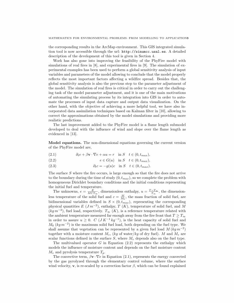
Figure 1. Osono: burnt simulated area (grey) and active front(orange) after 4 hours and real perimeter (black line).

The first example corresponds to a wildfire near Osono, Ourense province, on 17August 2009. The fire spread and its behaviour were reconstructed and documentedby the coordinator of the fire-suppression operations in [14], providing detailedinformation about this case. This fire destroyed 224ha, 185ha of forest area (83hawere tree-covered interspersed with heath) and 39ha of agricultural area for about 4hours. In this case the slope is lower, the altitude ranges from 540m (ignition pointarea) to 680m (end fire area) above sea level, with a relative humidity below 25%,temperatures above 30◦ C, and winds about 15 km/h with gust about 25 km/h.The simulation area is a rectangle of 3.315m × 2.740m. In Fig. 1 we show the

6 LUIS FERRAGUT AND M. ISABEL ASENSIO

simulated perimeter after 4 hours compared with the real perimeter, the similarityindex obtained show substantial agreement: Sorensen similarity index S = 0.82,Jaccard similarity coefficient J = 0.69 and Kappa coefficient K = 0.77 [15]. Thesimulation results are displayed on the GIS environment developed.

Figure 2. Donana: burnt simulated area (grey) and active front(orange) after 48 hours.

The second example corresponds to a larger and more recent wildfire that hitedDonana National Park. The fire broke out in Moguer (Huelva) on 24 June 2017,burning 8486ha (6761ha inside the Park) during four days due to the strong windsup to 80 km/h. In this case, data were obtained from satellite images. The simula-tion area was a rectangle of 20300m × 20000m. In Fig. 2 we show the simulatedperimeter after 48 hours.

3. HDWind: a High Definition Wind Field Model

Wind models are a fundamental tool in the study of environmental problems suchas dispersion of pollutants, fire propagation, among others. In problems where themeteorology plays an important role the resolution methods depend on the temporaland spatial scales that are chosen. With deterministic models only predictions canbe made for a few days.

The HDWind is a mass consistent vertical diffusion wind field model. If the sig-nificant phenomena that we want to simulate occur in a zone, where the horizontaldimensions are much larger than the vertical one, then an asymptotic approxi-mation of the primitive Navier-Stokes equations can be derived as in the modeldeveloped in [16, 17]. The most salient feature of this asymptotic approach is thatit provides a three-dimensional velocity wind field (which satisfies the incompress-ibility condition in the air layer) governed by a two-dimensional equation, so thatit can be coupled with the temperature surface distribution in order to take intoaccount the thermal effects such as sea breezes. In addition, the terrain elevationinformation is also taken into account by the model, as well as surface roughness.

MATHEMATICS FOR ENVIRONMENTAL PROBLEMS: FROM MODELLING TO APPLICATIONS7

The validity of this model has the following limits: the nonlinear terms areneglected and it is assumed that the air temperature decreases linearly with theheight. Besides that, the model takes into account buoyancy forces, slope effects,and mass conservation.

In the rest of the section a brief description of the wind model is included.Finally, a numerical example in a real-data scenario is presented.

HDWind model description. A complete description can be found in [16, 17].Our model arrives from an asymptotic analysis of Navier–Stokes equations and givesa three-dimensional convective model governed by a two-dimensional equation. Thismodel adjusts a three-dimensional velocity wind field in a layer under the influenceof the topography and temperature distribution.

Consider an air velocity field U = (U, V,W ) and a potential P satisfying theNavier–Stokes equations. We assume that the height δ is small compared to thewidth, and that the surface height at point (x, H(x)), is smaller than δ. We obtainthe following vertical diffusion model:

−∂2zzV +∇xP = 0,(3.1)

∂zP = µT,(3.2)

∇x ·V + ∂zW = 0,(3.3)

where V = (U, V ) denotes the horizontal velocity, µ is related to buoyancy forcesand T is the temperature.

Equations (3.1)-(3.2)-(3.3) together with the corresponding boundary conditionsyield

(3.4) V(x, z) = m(x, z)∇xp(x) + k(x, z)∇xt(x),

where m(x, z) and k(x, z) are polinomial fuctions in z and t is a re-scaled temper-ature. The function p(x) is a potential that satisfies the following boundary valueproblem:

−∇x(a∇xp) = ∇x(r∇xt) in ω,

a∂p

∂n= −r ∂t

∂n+ (δ −H)vm · n on ∂ω,

(3.5)

where a(x) and r(x) are functions depending on δ and H(x). ω is a two dimensionalbounded domain, representing the projection of the three dimensional geographicalsurface.

Summarizing, the solution V of problem (3.1)-(3.3) is obtained by solving thetwo-dimensional boundary value problem (3.5) and then V is explicitly computedusing the expression (3.4).

In practical applications, the wind on the boundary is unknown. Instead, mea-surements of the wind intensity and direction are given at the points where theweather stations are placed. So we have to reformulate problem (3.5) so that thegiven data be the wind velocity at some fixed points.

Given E experimental measurements of the wind velocity Vi, i = 1, . . . , E, at Efixed points Pi = (xi, zi), i = 1, . . . , E, we look for the function v = (δ −H)vm · nsuch that the values of V(xi, zi) given by the expression in (3.4) are as close as

8 LUIS FERRAGUT AND M. ISABEL ASENSIO

possible to the experimental values of Vi. The cost functional to be minimized isgiven by

(3.6) J(v) =1

2

E∑i=1

∫ω

ρε,i(x)|m(x, zi)∇p(x)+k(x, zi)∇t(x)−Vi|2dx+α

2

∫∂ω

v2dσ,

where α is a regularization parameter and ρε,i is a suitable smoothing function.The minimum u of the functional J is characterized by the vanishing of the first

variation: J ′(u) = 0. We refer to [18] for a general characterization of this solutionusing the adjoint state approach and [17] for the application to this particular case.

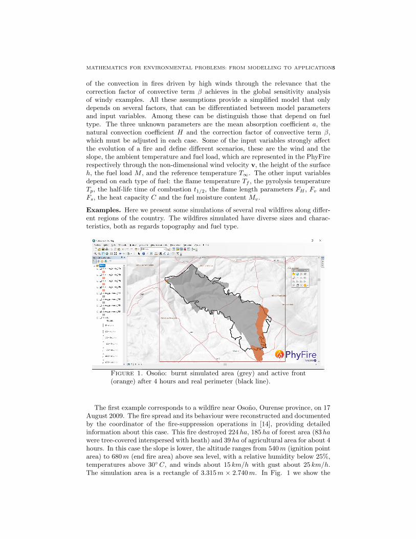
Example. We consider a domain located at La Serena (Chile, IV Region) ( 14km × 8 km), with two weather stations: Ceaza and Cerro Grande. We use CerroGrande measurement to estimate the wind velocity at Ceaza. Data: 25 days, 1measurement per hour (25× 24 = 600)

Figure 3. La Serena (Chile, IV Region).

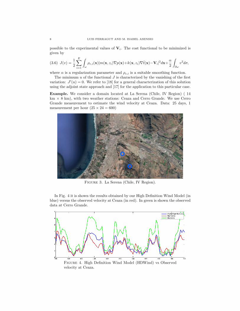
In Fig. 4 it is shown the results obtained by our High Definition Wind Model (inblue) versus the observed velocity at Ceaza (in red). In green is shown the observeddata at Cerro Grande.

Figure 4. High Definition Wind Model (HDWind) vs Observedvelocity at Ceaza.

MATHEMATICS FOR ENVIRONMENTAL PROBLEMS: FROM MODELLING TO APPLICATIONS9

4. PhyFire & HDWind: the development of a GIS tool

Both models, PhyFire and HDWind, can be compiled for any platform, andcan operate either together or separately: the PhyFire model can operate withconstant wind or with wind data provided by the HDWind or any other windmodel. Furthermore, the HDWind model can provide wind field data from punctualmeteorological data for other purposes. But in order to make these models morereadily accessible to the potential end-user by providing a simple, intuitive and easy-to-use tool, both have been integrated on a GIS-based interface. This has a dualpurpose, on the one hand, as we have mentioned, this provides a more accessibletool to a broader audience that might not be familiar with these models; and onthe other hand, this facilitates the testing and validation process, by automatingand simplifying the data acquisition process and the display of the solution. Thecomplete simulation of either one of the physical processes integrated on the GISinterface, includes three steps: pre-processing the requested data, calculating themodels and post-processing the solution. The developed tool reduces preprocessingand post-processing times and prevent input data errors.

The PhyFire and HDWind models have an interface provided through ASCIIgrid text files as inputs and outputs. The GIS tool chosen for the integration of ourmodels, ArcMap 10.4 of Esri’s ArcGIS Desktop suite, provides options for expand-ing its features through custom tools. For more information about Esri software,visit www.esri.com. The interface with both models has been developed as a Pythonadd-in for ArcMap, that is, a customization, in this case a collection of tools ona toolbar, which plugs into an ArcGIS for Desktop application (ArcMap in thiscase) to provide supplemental functionality for performing customized tasks. Thefunctionality of each tool is implemented as a script using the Python programminglanguage and the ArcPy geoprocessing library. The PhyFire integrated in the GIStool uses the following input data: topography, fuel load and type, weather condi-tions, ignition location and fire suppression tactics; and predicts the fire spread forthe established time period, providing the following outputs at each time step: theburnt area perimeter and the fire front position. Likewise, the HDWind integratedin the GIS tool also uses topography, surface roughness and weather conditions,and provides a wind velocity field that is well adapted to the domain studied, de-fined by wind velocity. Both have been developed for its use throughout Spain,so the scope of the spatial information currently used is limited to that area. Wedefine a common spatial reference for all the heterogeneous spatial data resources.According to Spanish regulations, the selected spatial reference is the Projected Co-ordinate System ETRS1989 UTM Zone 30N, except for the Canary Islands, wherethe Projected Coordinate System ETRS1989 UTM Zone 28N is used instead.

The first geographical resource is the base map used to identify the area inwhich the simulation is to be carried on, to locate the fire ignition point, as well aspossible fire suppression tactics and meteorological wind data positions, and finally,to display the simulation results. The base map selected for our operating systemis the Spanish Topographic Base Map provided by the c© Instituto GeograficoNacional de Espana (IGN) via a Web Map Service [22].

Each simulation needs three raster files corresponding to the topography, fueltype and fuel load of the study domain. For this purpose, a geodatabase has beendeveloped containing the three maps needed for extracting the spatial informationour models use.

10 LUIS FERRAGUT AND M. ISABEL ASENSIO

The first map processed contains the height of the surface h required for bothmodels. This information is provided by a Digital Elevation Model (DEM). Weselect the DEM also published by the IGN via a Web Coverage Service (WCS) [23]with resolution 25m and the reference system mentioned above.

The second map processed gathers all the information related to fuel type, toset the fuel type-dependent input variables for both models. Depending on theregion and/or year we use the Spanish Forestry Map 1 : 25.000 (MFE25) [24]combined with the Fourth Spanish National Forest Inventory (IFN4) [25] or theSpanish Forestry Map 1 : 50.000 (MFE50) [26] with the information from theThird Spanish National Forest Inventory (IFN3) [27]. Both inventories have beendeveloped by the Ministry of Agriculture, Food and Environment of the SpanishGovernment. The fuel type distribution managed is BEHAVE classification [28],adapted to Spanish forestry by the Nature Conservation Institute [29].

The third map processed collects all the elements involving the function of eitherartificial or natural fuelbreaks that affect the fire spread, only used by the PhyFiremodel. These data have been extracted from the Spanish Land Cover InformationSystem (SIOSE) [30] by selecting all the surfaces where a fire cannot occur (barrenland, waterbodies, transport infrastructures, etc.), providing zero load fuel data forthe model.

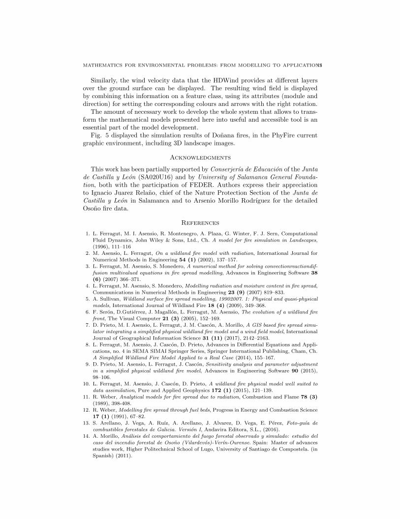
The simulation results are displayed on the base map during the post-processstep. The PhyFire model provides two types of output data: the solid fuel massfraction c and the non-dimensional solid fuel temperature u. Comparing the out-put solid fuel mass fraction with the initial fuel mass fraction inputted into themodel provides the state of the landscape. So for each point of the domain we candetermine whether or not that specific point has been burnt. This information istransformed to a vector layer and represented on the base map in order to establishthe fire perimeter at different instants, using a layer for each time step. The solidfuel temperature is also transformed into a vector layer and represented on the basemap for identifying those areas burning at the indicated time step, establishing thefire front position.

Figure 5. Donana: burnt simulated area (grey) and active front(orange) after 48 hours over 3D satellite image.

MATHEMATICS FOR ENVIRONMENTAL PROBLEMS: FROM MODELLING TO APPLICATIONS11

Similarly, the wind velocity data that the HDWind provides at different layersover the ground surface can be displayed. The resulting wind field is displayedby combining this information on a feature class, using its attributes (module anddirection) for setting the corresponding colours and arrows with the right rotation.

The amount of necessary work to develop the whole system that allows to trans-form the mathematical models presented here into useful and accessible tool is anessential part of the model development.

Fig. 5 displayed the simulation results of Donana fires, in the PhyFire currentgraphic environment, including 3D landscape images.

Acknowledgments

This work has been partially supported by Conserjerıa de Educacion of the Juntade Castilla y Leon (SA020U16) and by University of Salamanca General Founda-tion, both with the participation of FEDER. Authors express their appreciationto Ignacio Juarez Relano, chief of the Nature Protection Section of the Junta deCastilla y Leon in Salamanca and to Arsenio Morillo Rodrıguez for the detailedOsono fire data.

References

1. L. Ferragut, M. I. Asensio, R. Montenegro, A. Plaza, G. Winter, F. J. Sern, Computational

Fluid Dynamics, John Wiley & Sons, Ltd., Ch. A model for fire simulation in Landscapes,

(1996), 111–1162. M. Asensio, L. Ferragut, On a wildland fire model with radiation, International Journal for

Numerical Methods in Engineering 54 (1) (2002), 137–157.

3. L. Ferragut, M. Asensio, S. Monedero, A numerical method for solving convectionreactiondif-fusion multivalued equations in fire spread modelling, Advances in Engineering Software 38

(6) (2007) 366–371.4. L. Ferragut, M. Asensio, S. Monedero, Modelling radiation and moisture content in fire spread,

Communications in Numerical Methods in Engineering 23 (9) (2007) 819–833.

5. A. Sullivan, Wildland surface fire spread modelling, 19902007. 1: Physical and quasi-physicalmodels, International Journal of Wildland Fire 18 (4) (2009), 349–368.

6. F. Seron, D.Gutierrez, J. Magallon, L. Ferragut, M. Asensio, The evolution of a wildland fire

front, The Visual Computer 21 (3) (2005), 152–169.7. D. Prieto, M. I. Asensio, L. Ferragut, J. M. Cascon, A. Morillo, A GIS based fire spread simu-

lator integrating a simplified physical wildland fire model and a wind field model, International

Journal of Geographical Information Science 31 (11) (2017), 2142–2163.8. L. Ferragut, M. Asensio, J. Cascon, D. Prieto, Advances in Differential Equations and Appli-

cations, no. 4 in SEMA SIMAI Springer Series, Springer International Publishing, Cham, Ch.

A Simplified Wildland Fire Model Applied to a Real Case (2014), 155–167.9. D. Prieto, M. Asensio, L. Ferragut, J. Cascon, Sensitivity analysis and parameter adjustment

in a simplified physical wildland fire model, Advances in Engineering Software 90 (2015),98–106.

10. L. Ferragut, M. Asensio, J. Cascon, D. Prieto, A wildland fire physical model well suited todata assimilation, Pure and Applied Geophysics 172 (1) (2015), 121–139.

11. R. Weber, Analytical models for fire spread due to radiation, Combustion and Flame 78 (3)(1989), 398-408.

12. R. Weber, Modelling fire spread through fuel beds, Progress in Energy and Combustion Science17 (1) (1991), 67–82.

13. S. Arellano, J. Vega, A. Ruız, A. Arellano, J. Alvarez, D. Vega, E. Perez, Foto-guıa decombustibles forestales de Galicia. Version I, Andavira Editora, S.L., (2016).

14. A. Morillo, Analisis del comportamiento del fuego forestal observado y simulado: estudio delcaso del incendio forestal de Osono (Vilardevos)-Verın-Ourense. Spain: Master of advances

studies work, Higher Politechnical School of Lugo, University of Santiago de Compostela. (inSpanish) (2011).

12 LUIS FERRAGUT AND M. ISABEL ASENSIO

15. J. Filippi, V. Mallet, and B. Nader, Representation and evaluation of wildfire propagation

simulations. International Journal of Wildland Fire, 23 (2014), 46–57.

16. M. Asensio, L. Ferragut, J. Simon, A convection model for fire spread simulation, AppliedMathematics Letters 18 (2005), 673–677.

17. L. Ferragut, M. I. Asensio, J. Simon, High definition local adjustment model of 3d wind fields

performing only 2d computations, International Journal for Numerical Methods in BiomedicalEngineering 27 (2011), 510–523.

18. J. L. Lions, Controle Optimal de Systemes Gouvernes par des Equations aux Derives Par-

tielles, Springer series in computational mathematics, Dunod/Gauthier-Villars, Paris, (1968).19. J.M. Cascon, A. Engdahl Y, L. Ferragut, E. Hernandez, A reduced basis for a local definition

wind model. Computer Methods in Applied Mechanics and Engineering, Computer Methods

in Applied Mechanics and Engineering 23, (2016) 438–456.20. W. C. Skamarock, et. al, A Description of the Advanced Research WRF Version 3, NCAR

Technical Nore.(2008)21. D. Barker, et.al The Weather Research and Forecasting Model’s Community Varia-

tional/Ensemble Data Assimilation System: WRFDA American Meteorological Society.

https://doi.org/10.1175/BAMS-D-11-00052.122. IGN Spanish Base Map Instituto Geografico Nacional de Espana [online]. Available from:

http://www.ign.es/wms-inspire/ign-base [Accessed May 2016].

23. Spanish Digital Elevation Model Instituto Geografico Nacional de Espana [online]. Availablefrom: http://www.ign.es/wcs/mdt [ May 2016].

24. Spanish Forestry Map 1 : 25.000. Ministerio de Agricultura, Alimentacion y Medio

Ambiente [Online]. Available from: http://www.magrama.gob.es/es/desarrollo-rural/

temas/politica-forestal/inventario-cartografia/mapa-forestal-espana/mfe25.aspx

[Accessed May 2016b].

25. Fourth Spanish National Forest Inventory Ministerio de Agricultura, Alimentacion y MedioAmbiente [Online]. Available from: http://www.magrama.gob.es/es/desarrollo-rural/

temas/politica-forestal/inventario-cartografia/inventario-forestal-nacional/ [Ac-cessed May 2016a].

26. Spanish Forestry Map 1 : 50.000 Ministerio de Agricultura, Alimentacion y Medio Ambiente

[Online], 3 (4). Available from: http://www.magrama.gob.es/es/biodiversidad/servicios/

banco-datos-naturaleza/informacion-disponible/mfe50.aspx [Accessed May 2016a].

27. Third Spanish National Forest Inventory Ministerio de Agricultura, Alimentacion y

Medio Ambiente [Online]. Available from: http://www.magrama.gob.es/es/biodiversidad/

servicios/banco-datos-naturaleza/informacion-disponible/ifn3.aspx [Accessed May

2016b]

28. P. Andrews Behave: fire behaviour prediction and fuel modellings system - burn subsystem,part 1, Ogden, UT: U.S. Department of Agriculture, Forest Service, Intermountain Forest and

Range Experiment Station, General Technical Report INT-194, (1986).

29. MAPA, Photographic key to the identification of fuel models, Madrid: Ministerio de Agricul-tura Pesca y Alimentacion, Instituto para la Conservacion de la Naturaleza ICONA, Technical

report. [in Spanish].30. Spanish Land Cover Information System. Instituto Geogrfico Nacional de Espana [online].

Available from: http://www.ign.es/ign/layoutIn/siose.do [Accessed May 2016].

Department of Applied Mathematics, University of Salamanca

Current address: Department of Applied Mathematics, University of Salamanca, Casas delParque, 2, 37008 Salamanca

E-mail address: ferragut@usal.es

Department of Applied Mathematics, University of SalamancaE-mail address: mas@usal.es