How to solve Basic Engineering and Mathematics Problems
301
General report How to solve Basic Engineering and Mathematics Problems using Mathematica, Matlab and Maple Nasser M. Abbasi March 27, 2022
-
Upload
khangminh22 -
Category
Documents
-
view
1 -
download
0
Transcript of How to solve Basic Engineering and Mathematics Problems

General report
How to solve Basic Engineering andMathematics Problems
using Mathematica, Matlab and Maple
Nasser M. Abbasi
March 27, 2022


Contents
1 Control systems, Linear systems, transfer functions, state space relatedproblems 31.1 Creating tf and state space and different Conversion of forms . . . . . . . . 31.2 Obtain the step response of an LTI from its transfer function . . . . . . . . 121.3 plot the impulse and step responses of a system from its transfer function . 131.4 Obtain the response of a transfer function for an arbitrary input . . . . . . 151.5 Obtain the poles and zeros of a transfer function . . . . . . . . . . . . . . 161.6 Generate Bode plot of a transfer function . . . . . . . . . . . . . . . . . . . 171.7 How to check that state space system x′ = Ax+Bu is controllable? . . . . 181.8 Obtain partial-fraction expansion . . . . . . . . . . . . . . . . . . . . . . . 191.9 Obtain Laplace transform for a piecewise functions . . . . . . . . . . . . . 201.10 Obtain Inverse Laplace transform of a transfer function . . . . . . . . . . . 211.11 Display the response to a unit step of an under, critically, and over damped
system . . . . . . . . . . . . . . . . . . . . . . . . . . . . . . . . . . . . . . 221.12 View steady state error of 2nd order LTI system with changing undamped
natural frequency . . . . . . . . . . . . . . . . . . . . . . . . . . . . . . . . 251.13 Show the use of the inverse Z transform . . . . . . . . . . . . . . . . . . . 271.14 Find the Z transform of sequence x(n) . . . . . . . . . . . . . . . . . . . . 291.15 Sample a continuous time system . . . . . . . . . . . . . . . . . . . . . . . 301.16 Find closed loop transfer function from the open loop transfer function for
a unity feedback . . . . . . . . . . . . . . . . . . . . . . . . . . . . . . . . 331.17 Compute the Jordan canonical/normal form of a matrix A . . . . . . . . . 341.18 Solve the continuous-time algebraic Riccati equation . . . . . . . . . . . . 351.19 Solve the discrete-time algebraic Riccati equation . . . . . . . . . . . . . . 361.20 Display impulse response of H(z) and the impulse response of its continuous
time approximation H(s) . . . . . . . . . . . . . . . . . . . . . . . . . . . . 371.21 Find the system type given an open loop transfer function . . . . . . . . . 411.22 Find the eigenvalues and eigenvectors of a matrix . . . . . . . . . . . . . . 421.23 Find the characteristic polynomial of a matrix . . . . . . . . . . . . . . . . 431.24 Verify the Cayley-Hamilton theorem that every matrix is zero of its char-
acteristic polynomial . . . . . . . . . . . . . . . . . . . . . . . . . . . . . . 441.25 How to check for stability of system represented as a transfer function and
state space . . . . . . . . . . . . . . . . . . . . . . . . . . . . . . . . . . . . 451.26 Check continuous system stability in the Lyapunov sense . . . . . . . . . . 461.27 Given a closed loop block diagram, generate the closed loop Z transform
and check its stability . . . . . . . . . . . . . . . . . . . . . . . . . . . . . 471.28 Determine the state response of a system to only initial conditions in state
space . . . . . . . . . . . . . . . . . . . . . . . . . . . . . . . . . . . . . . . 501.29 Determine the response of a system to only initial conditions in state space 521.30 Determine the response of a system to step input with nonzero initial
conditions . . . . . . . . . . . . . . . . . . . . . . . . . . . . . . . . . . . . 531.31 Draw the root locus from the open loop transfer function . . . . . . . . . . 541.32 Find exp(A t) where A is a matrix . . . . . . . . . . . . . . . . . . . . . . 541.33 Draw root locus for a discrete system . . . . . . . . . . . . . . . . . . . . . 561.34 Plot the response of the inverted pendulum problem using state space . . . 581.35 How to build and connect a closed loop control systems and show the
response? . . . . . . . . . . . . . . . . . . . . . . . . . . . . . . . . . . . . 611.36 Compare the effect on the step response of a standard second order system
as ζ changes . . . . . . . . . . . . . . . . . . . . . . . . . . . . . . . . . . . 63
iii

Contents CONTENTS
1.37 Plot the dynamic response factor Rd of a system as a function of r = ωωn
for different damping ratios . . . . . . . . . . . . . . . . . . . . . . . . . . 651.38 How to find closed loop step response to a plant with a PID controller? . . 661.39 How to make Nyquist plot? . . . . . . . . . . . . . . . . . . . . . . . . . . 67
2 Linear algebra, Linear solvers, common operations on vectors andmatrices 712.1 introduction . . . . . . . . . . . . . . . . . . . . . . . . . . . . . . . . . . . 712.2 Multiply matrix with a vector . . . . . . . . . . . . . . . . . . . . . . . . . 722.3 Insert a number at specific position in a vector or list . . . . . . . . . . . . 752.4 Insert a row into a matrix . . . . . . . . . . . . . . . . . . . . . . . . . . . 762.5 Insert a column into a matrix . . . . . . . . . . . . . . . . . . . . . . . . . 772.6 Build matrix from other matrices and vectors . . . . . . . . . . . . . . . . 782.7 Generate a random 2D matrix from uniform (0 to 1) and from normal
distributions . . . . . . . . . . . . . . . . . . . . . . . . . . . . . . . . . . . 832.8 Generate an n by m zero matrix . . . . . . . . . . . . . . . . . . . . . . . . 852.9 Rotate a matrix by 90 degrees . . . . . . . . . . . . . . . . . . . . . . . . . 862.10 Generate a diagonal matrix with given values on the diagonal . . . . . . . 872.11 Sum elements in a matrix along the diagonal . . . . . . . . . . . . . . . . . 882.12 Find the product of elements in a matrix along the diagonal . . . . . . . . 882.13 Check if a Matrix is diagonal . . . . . . . . . . . . . . . . . . . . . . . . . 892.14 Find all positions of elements in a Matrix that are larger than some value . 902.15 Replicate a matrix . . . . . . . . . . . . . . . . . . . . . . . . . . . . . . . 902.16 Find the location of the maximum value in a matrix . . . . . . . . . . . . 922.17 Swap 2 columns in a matrix . . . . . . . . . . . . . . . . . . . . . . . . . . 922.18 Join 2 matrices side-by-side and on top of each others . . . . . . . . . . . . 932.19 Copy the lower triangle to the upper triangle of a matrix to make symmetric
matrix . . . . . . . . . . . . . . . . . . . . . . . . . . . . . . . . . . . . . . 942.20 extract values from matrix given their index . . . . . . . . . . . . . . . . . 952.21 Convert N by M matrix to a row of length N M . . . . . . . . . . . . . . . 962.22 find rows in a matrix based on values in different columns . . . . . . . . . 972.23 Select entries in one column based on a condition in another column . . . . 982.24 Locate rows in a matrix with column being a string . . . . . . . . . . . . . 992.25 Remove set of rows and columns from a matrix at once . . . . . . . . . . . 1012.26 Convert list of separated numerical numbers to strings . . . . . . . . . . . 1032.27 Obtain elements that are common to two vectors . . . . . . . . . . . . . . 1042.28 Sort each column (on its own) in a matrix . . . . . . . . . . . . . . . . . . 1042.29 Sort each row (on its own) in a matrix . . . . . . . . . . . . . . . . . . . . 1052.30 Sort a matrix row-wise using first column as key . . . . . . . . . . . . . . . 1062.31 Sort a matrix row-wise using non-first column as key . . . . . . . . . . . . 1072.32 Replace the first nonzero element in each row in a matrix by some value . 1082.33 Perform outer product and outer sum between two vector . . . . . . . . . 1102.34 Find the rank and the bases of the Null space for a matrix A . . . . . . . . 1112.35 Find the singular value decomposition (SVD) of a matrix . . . . . . . . . . 1122.36 Solve Ax = b . . . . . . . . . . . . . . . . . . . . . . . . . . . . . . . . . . 1142.37 Find all nonzero elements in a matrix . . . . . . . . . . . . . . . . . . . . . 1152.38 evaluate f(x) on a vector of values . . . . . . . . . . . . . . . . . . . . . . . 1172.39 generates equally spaced N points between x1 and x2 . . . . . . . . . . . . 1172.40 evaluate and plot a f(x,y) on 2D grid of coordinates . . . . . . . . . . . . . 1182.41 Find determinant of matrix . . . . . . . . . . . . . . . . . . . . . . . . . . 1202.42 Generate sparse matrix with n by n matrix repeated on its diagonal . . . . 1202.43 Generate sparse matrix for the tridiagonal representation of second differ-
ence operator in 1D . . . . . . . . . . . . . . . . . . . . . . . . . . . . . . . 1212.44 Generate sparse matrix for the Laplacian differential operator ∇2u for 2D
grid . . . . . . . . . . . . . . . . . . . . . . . . . . . . . . . . . . . . . . . 1222.45 Generate sparse matrix for the Laplacian differential operator for 3D grid . 1232.46 Generate the adjugate matrix for square matrix . . . . . . . . . . . . . . . 1272.47 Multiply each column by values taken from a row . . . . . . . . . . . . . . 1312.48 extract submatrix from a larger matrix by removing row/column . . . . . . 1332.49 delete one row from a matrix . . . . . . . . . . . . . . . . . . . . . . . . . 138
iv

Contents CONTENTS
2.50 delete one column from a matrix . . . . . . . . . . . . . . . . . . . . . . . 1392.51 generate random matrix so that each row adds to 1 . . . . . . . . . . . . . 1402.52 generate random matrix so that each column adds to 1 . . . . . . . . . . . 1412.53 sum all rows in a matrix . . . . . . . . . . . . . . . . . . . . . . . . . . . . 1432.54 sum all columns in a matrix . . . . . . . . . . . . . . . . . . . . . . . . . . 1442.55 find in which columns values that are not zero . . . . . . . . . . . . . . . . 1442.56 How to remove values from one vector that exist in another vector . . . . . 1452.57 How to find mean of equal sized segments of a vector . . . . . . . . . . . . 1462.58 find first value in column larger than some value and cut matrix from there 1472.59 make copies of each value into matrix into a larger matrix . . . . . . . . . 1482.60 repeat each column of matrix number of times . . . . . . . . . . . . . . . . 1492.61 How to apply a function to each value in a matrix? . . . . . . . . . . . . . 1492.62 How to sum all numbers in a list (vector)? . . . . . . . . . . . . . . . . . . 1502.63 How to find maximum of each row of a matrix? . . . . . . . . . . . . . . . 1502.64 How to find maximum of each column of a matrix? . . . . . . . . . . . . . 1512.65 How to add the mean of each column of a matrix from each column? . . . 1512.66 How to add the mean of each row of a matrix from each row? . . . . . . . 1522.67 Find the different norms of a vector . . . . . . . . . . . . . . . . . . . . . . 1532.68 Check if a matrix is Hermite . . . . . . . . . . . . . . . . . . . . . . . . . . 1532.69 Obtain the LU decomposition of a matrix . . . . . . . . . . . . . . . . . . 1542.70 Linear convolution of 2 sequences . . . . . . . . . . . . . . . . . . . . . . . 1562.71 Circular convolution of two sequences . . . . . . . . . . . . . . . . . . . . . 1562.72 Linear convolution of 2 sequences with origin at arbitrary position . . . . . 1582.73 Visualize a 2D matrix . . . . . . . . . . . . . . . . . . . . . . . . . . . . . 1592.74 Find the cross correlation between two sequences . . . . . . . . . . . . . . 1622.75 Find orthonormal vectors that span the range of matrix A . . . . . . . . . 1632.76 Solve A x= b and display the solution . . . . . . . . . . . . . . . . . . . . 1642.77 Determine if a set of linear equations A x= b has a solution and what type
of solution . . . . . . . . . . . . . . . . . . . . . . . . . . . . . . . . . . . . 1652.78 Given a set of linear equations automatically generate the matrix A and
vector b and solve Ax = b . . . . . . . . . . . . . . . . . . . . . . . . . . . 1672.79 Convert a matrix to row echelon form and to reduced row echelon form . . 1682.80 Convert 2D matrix to show the location and values . . . . . . . . . . . . . 1692.81 Find rows in matrix with zeros in them, and then remove the zeros . . . . 1712.82 How to apply a function to two lists at the same time? . . . . . . . . . . . 1722.83 How to apply a function to two lists are the same time, but with change
to entries? . . . . . . . . . . . . . . . . . . . . . . . . . . . . . . . . . . . . 1722.84 How to select all primes numbers from a list? . . . . . . . . . . . . . . . . 1732.85 How to collect result inside a loop when number of interation is not known
in advance? . . . . . . . . . . . . . . . . . . . . . . . . . . . . . . . . . . . 1732.86 How flip an array around? . . . . . . . . . . . . . . . . . . . . . . . . . . . 1742.87 How to divide each element by its position in a list? . . . . . . . . . . . . . 1742.88 How to use GramSchmidt to find a set of orthonomal vectors? . . . . . . . 175
3 signal processing, Image processing, graphics, random numbers 1773.1 Generate and plot one pulse signal of different width and amplitude . . . . 1773.2 Generate and plot train of pulses of different width and amplitude . . . . . 1783.3 Find the discrete Fourier transform of a real sequence of numbers . . . . . 1793.4 Generate uniform distributed random numbers . . . . . . . . . . . . . . . . 1813.5 Obtain Fourier Series coefficients for a periodic function . . . . . . . . . . 1853.6 Obtain Fourier Series approximation . . . . . . . . . . . . . . . . . . . . . 1903.7 Determine and plot the CTFT (continuous time Fourier Transform) for
continuous time function . . . . . . . . . . . . . . . . . . . . . . . . . . . . 1923.8 Determine the DTFT (Discrete time Fourier Transform) for discrete time
function . . . . . . . . . . . . . . . . . . . . . . . . . . . . . . . . . . . . . 1933.9 Determine the Inverse DTFT (Discrete time Fourier Transform) . . . . . . 1933.10 Use FFT to display the power spectrum of the content of an audio wav file 1943.11 Plot the power spectral density of a signal . . . . . . . . . . . . . . . . . . 1963.12 Display spectrum of 2D image . . . . . . . . . . . . . . . . . . . . . . . . . 199
v
Contents CONTENTS
3.13 Obtain the statistical maximum likelihood estimates (MLE) of probabilitydistributions . . . . . . . . . . . . . . . . . . . . . . . . . . . . . . . . . . . 202
3.14 Make a histogram of data sampled from some probability distribution . . . 2023.15 apply a filter on 1D numerical data (a vector) . . . . . . . . . . . . . . . . 2033.16 apply an averaging Laplacian filter on 2D numerical data (a matrix) . . . . 2043.17 How to find cummulative sum . . . . . . . . . . . . . . . . . . . . . . . . . 2053.18 How to find the moving average of a 1D sequence? . . . . . . . . . . . . . 2053.19 How to select N random values from a set of numbers? . . . . . . . . . . . 2063.20 How to sample a sin signal and plot it? . . . . . . . . . . . . . . . . . . . . 2063.21 How find the impulse response of a difference equation? . . . . . . . . . . . 208
4 Differential, PDE solving, integration, numerical and analytical solvingof equations 2094.1 Generate direction field plot of a first order differential equation . . . . . . 2094.2 Solve the 2-D Laplace PDE for a rectangular plate with Dirichlet boundary
conditions . . . . . . . . . . . . . . . . . . . . . . . . . . . . . . . . . . . . 2114.3 Solve homogeneous 1st order ODE, constant coefficients and initial conditions2134.4 Solve homogeneous 2nd order ODE with constant coefficients . . . . . . . 2144.5 Solve non-homogeneous 2nd order ODE, constant coefficients . . . . . . . . 2154.6 Solve homogeneous 2nd order ODE, constant coefficients (BVP) . . . . . . 2174.7 Solve the 1-D heat partial differential equation (PDE) . . . . . . . . . . . . 2194.8 Show the effect of boundary/initial conditions on 1-D heat PDE . . . . . . 2214.9 Find particular and homogenous solution to undetermined system of equations2224.10 Plot the constant energy levels for a nonlinear pendulum . . . . . . . . . . 2254.11 How to numerically solve a set of non-linear equations? . . . . . . . . . . . 2324.12 Solve 2nd order ODE (Van Der Pol) and generate phase plot . . . . . . . . 2344.13 How to numerically solve Poisson PDE on 2D using Jacobi iteration method?2374.14 How to solve BVP second order ODE using finite elements with linear
shape functions and using weak form formulation? . . . . . . . . . . . . . . 2404.15 How to solve Poisson PDE in 2D using finite elements methods using
rectangular element? . . . . . . . . . . . . . . . . . . . . . . . . . . . . . . 2444.16 How to solve Poisson PDE in 2D using finite elements methods using
triangle element? . . . . . . . . . . . . . . . . . . . . . . . . . . . . . . . . 2634.17 How to solve wave equation using leapfrog method? . . . . . . . . . . . . . 2734.18 Numerically integrate f(x) on the real line . . . . . . . . . . . . . . . . . . 2774.19 Numerically integrate f(x, y) in 2D . . . . . . . . . . . . . . . . . . . . . . 2784.20 How to solve set of differential equations in vector form . . . . . . . . . . . 2784.21 How to implement Runge-Kutta to solve differential equations? . . . . . . 2804.22 How to differentiate treating a combined expression as single variable? . . 2834.23 How to solve Poisson PDE in 2D with Neumann boundary conditions using
Finite Elements . . . . . . . . . . . . . . . . . . . . . . . . . . . . . . . . . 283
5 plotting how to, ellipse, 3D 2855.1 Generate a plot using x and y data . . . . . . . . . . . . . . . . . . . . . . 2855.2 Plot the surface described by 2D function . . . . . . . . . . . . . . . . . . 2865.3 Find the point of intersection of 3 surfaces . . . . . . . . . . . . . . . . . . 2865.4 How to draw an ellipse? . . . . . . . . . . . . . . . . . . . . . . . . . . . . 2895.5 How to plot a function on 2D using coordinates of grid locations? . . . . . 2915.6 How to make table of x, y values and plot them . . . . . . . . . . . . . . . 2925.7 How to make contour plot of f(x, y) ? . . . . . . . . . . . . . . . . . . . . 293
6 Some symbolic operations 2956.1 How to find all exponents of list of expressions? . . . . . . . . . . . . . . . 295
vi

Contents CONTENTS
This is a collection of how to examples showing the use of Mathematica and Matlab tosolve basic engineering and mathematics problems. Few examples are also in Maple, Ada,and Fortran.
This was started as a cheat sheet few years ago, and I continue to update it all the time.
Few of the Matlab examples require the use of toolboxs such as signal processing toolboxand the control systems toolbox (these come free as part of the student version). Mostexamples require only the basic system installation.
1

Contents CONTENTS
2

Chapter 1
Control systems, Linear systems,transfer functions, state space relatedproblems
1.1 Creating tf and state space and differentConversion of forms
1.1.1 Create continuous time transfer function given the poles,zeros and gain
Problem: Find the transfer function H(s) given zeros s = −1, s = −2, poles s = 0, s =−4, s = −6 and gain 5.
1.1.1.1 Mathematica
Clear["Global`*"];num = (s+1)(s+2);den = (s)(s+4)(s+6);gain = 5;sys = TransferFunctionModel[
gain (num/den),s]
Out[30]= TransferFunctionModel[5*(1 + s)*(2 + s),s*(4 + s)*(6 + s), s]
1.1.1.2 Matlab
clear all;m_zeros = [-1 -2];m_poles = [0 -4 -6];gain = 5;sys = zpk(m_zeros,m_poles,gain);[num,den] = tfdata(sys,'v');printsys(num,den,'s')
num/den =
5 s^2 + 15 s + 10-------------------s^3 + 10 s^2 + 24 s
3

1.1. Creating tf and state space and… CHAPTER 1. CONTROL SYSTEMS, …
1.1.1.3 Maple restart;alias(DS=DynamicSystems):zeros :=[-1,-2]:poles :=[0,-4,-6]:gain :=5:sys :=DS:-TransferFunction(zeros,poles,gain):#print overview of the system objectDS:-PrintSystem(sys); exports(sys);#To see fields in the sys object, do the following# tf, inputcount, outputcount, statecount, sampletime,# discrete, systemname, inputvariable, outputvariable,# statevariable, parameters, systemtype, ModulePrinttf:=sys[tf]; #reads the transfer functionMatrix(1,1,(1,1)=(5*s^2+15*s+10)/(s^3+10*s^2+24*s))numer(tf[1,1]); #get the numerator of the tf
tf =[
5 s2+15 s+10s3+10 s2+24 s
] denom(tf[1,1]); #get the denominator of the tf
s ∗ (s2 + 10 ∗ s+ 24)
1.1.2 Convert transfer function to state space representation1.1.2.1 problem 1
Problem: Find the state space representation for the continuous time system defined bythe transfer function
H(s) =5s
s2 + 4s+ 25
1.1.2.2 Mathematica
Clear["Global`*"];sys = TransferFunctionModel[(5 s)/(s^2+4 s+25),s];ss = MinimalStateSpaceModel[StateSpaceModel[sys]] Out[48]=
0 1 0-25 -4 10 5 0
(a=Normal[ss][[1]])//MatrixForm(b=Normal[ss][[2]])//MatrixForm(c=Normal[ss][[3]])//MatrixForm(d=Normal[ss][[4]])//MatrixForm
Out[49]//MatrixForm=
0 1
-25 -4
Out[50]//MatrixForm=
01
Out[51]//MatrixForm=
( 0 5 )
Out[52]//MatrixForm=
( 0 )
4

1.1. Creating tf and state space and… CHAPTER 1. CONTROL SYSTEMS, …
1.1.2.3 Matlab
clear all;s = tf('s');sys_tf = (5*s) / (s^2 + 4*s + 25);[num,den] = tfdata(sys_tf,'v');[A,B,C,D] = tf2ss(num,den)
A =
-4 -251 0
B =10
C =5 0
D =0
1.1.2.4 Maple
restart;alias(DS=DynamicSystems):sys := DS:-TransferFunction(5*s/(s^2+4*s+25)):sys := DS:-StateSpace(sys);exports(sys); #to see what fields there area := sys:-a;
[0 1
−25 −4
]
b:=sys:-b;
[0
1
]
c:=sys:-c; [
0 5]
d:=sys:-d; [
0]
1.1.2.5 problem 2
Problem: Given the continuous time S transfer function defined by
H(s) =1 + s
s2 + s+ 1
convert to state space and back to transfer function.
Mathematica Clear["Global`*"];sys = TransferFunctionModel[(s + 1)/(s^2 + 1 s + 1), s];ss = MinimalStateSpaceModel[StateSpaceModel[sys]]
0 1 0
−1 −1 1
1 1 0
TransferFunctionModel[ss] s+ 1
s2 + s+ 1
5

1.1. Creating tf and state space and… CHAPTER 1. CONTROL SYSTEMS, …
Matlab clear all;s = tf('s');sys = ( s+1 )/(s^2 + s + 1);[num,den]=tfdata(sys,'v');%convert to state space[A,B,C,D] = tf2ss(num,den)
A =
-1 -11 0
B =10
C =1 1
D =0
%convert from ss to tf[num,den] = ss2tf(A,B,C,D);sys=tf(num,den)
sys =
s + 1-----------s^2 + s + 1
1.1.3 Create a state space representation from A,B,C,D andfind the step response
Problem: Find the state space representation and the step response of the continuous timesystem defined by the Matrices A,B,C,D as shown A =
0 1 0 00 0 1 00 0 0 1
-100 -80 -32 -8
B =00560
C =1 0 0 0
D =0
6

1.1. Creating tf and state space and… CHAPTER 1. CONTROL SYSTEMS, …
Mathematica Clear["Global`*"];
a = 0,1,0,0,0,0,1,0,0,0,0,1,-100,-80,-32,-8
;
b = 0 ,0, 5,60;c = 1,0,0,0;d = 0;
sys = StateSpaceModel[a,b,c,d];y = OutputResponse[sys,UnitStep[t],t,0,10];
p = Plot[Evaluate@y, t, 0, 10,PlotRange -> All,GridLines -> Automatic,GridLinesStyle -> LightGray]
2 4 6 8 10
0.2
0.4
0.6
0.8
1.0
1.2
Matlab clear all;A = [0 1 0 0;
0 0 1 0;0 0 0 1;
-100 -80 -32 -8];B = [0;0;5;60];C = [1 0 0 0];D = [0];
sys = ss(A,B,C,D);
step(sys);grid;title('unit step response');
0 1 2 3 4 50
0.2
0.4
0.6
0.8
1
1.2unit step response
Time (seconds)
Am
plitu
de
Maple restart:alias(DS=DynamicSystems):alias(size=LinearAlgebra:-Dimensions);a:=Matrix([[0,1,0,0],[0,0,1,0],
[0,0,0,1],[-100,-90,-32,-8]]):b:=Matrix([[0],[0],[5],[6]]):c:=Matrix([[1,0,0,0]]):d:=Matrix([[1]]):sys:=DS:-StateSpace(a,b,c,d);
DS:-ResponsePlot(sys, DS:-Step(),duration=10,color=red,legend="step");
7

1.1. Creating tf and state space and… CHAPTER 1. CONTROL SYSTEMS, …
1.1.4 Convert continuous time to discrete time transferfunction, gain and phase margins
Problem: Compute the gain and phase margins of the open-loop discrete linear time systemsampled from the continuous time S transfer function defined by
H(s) =1 + s
s2 + s+ 1
Use sampling period of 0.1 seconds.
Mathematica Clear["Global`*"];tf = TransferFunctionModel[(s+1)/(s^2+1 s+1),s]; Out[88]=
1 + s
1 + s + s2
ds = ToDiscreteTimeModel[tf, 0.1, z,
Method -> "ZeroOrderHold"] Out[89]= -0.0903292 + 0.0998375 z
0.904837 - 1.89533 z + z20.1
gm, pm = GainPhaseMargins[ds];
gmOut[28]=31.4159,19.9833pmOut[29]=1.41451,1.83932,0.,Pi
max = 100;yn = OutputResponse[ds,
Table[UnitStep[n],n, 0, max]];ListPlot[yn,
Joined -> True,InterpolationOrder -> 0,PlotRange -> 0, max, 0, 1.4,Frame -> True,FrameLabel ->"y[n]", None,
"n", "unit step response",ImageSize -> 400,AspectRatio -> 1,BaseStyle -> 14]
0 20 40 60 80 1000.0
0.2
0.4
0.6
0.8
1.0
1.2
1.4
n
y[n]
unit step response
8
1.1. Creating tf and state space and… CHAPTER 1. CONTROL SYSTEMS, …
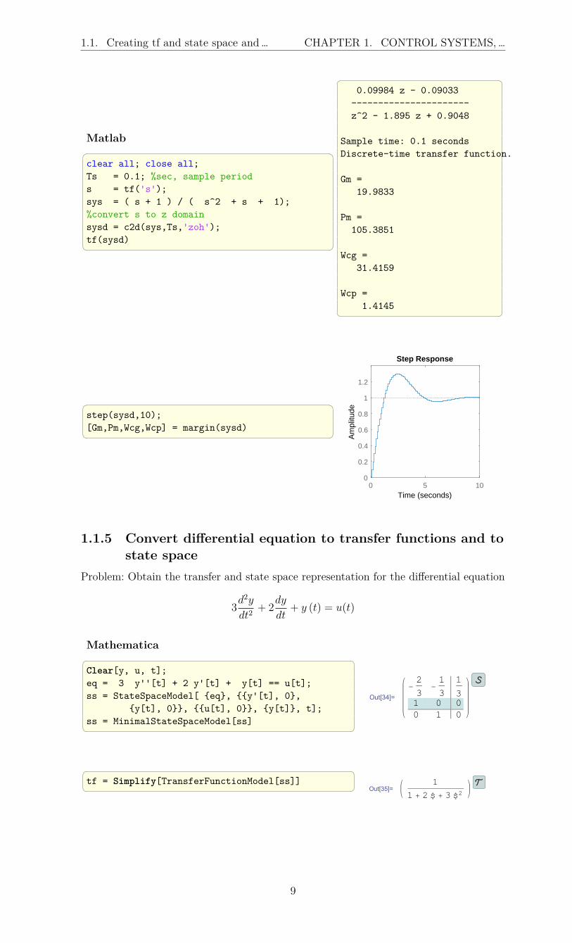
Matlab clear all; close all;Ts = 0.1; %sec, sample periods = tf('s');sys = ( s + 1 ) / ( s^2 + s + 1);%convert s to z domainsysd = c2d(sys,Ts,'zoh');tf(sysd)
0.09984 z - 0.09033----------------------z^2 - 1.895 z + 0.9048
Sample time: 0.1 secondsDiscrete-time transfer function.
Gm =19.9833
Pm =105.3851
Wcg =31.4159
Wcp =1.4145
step(sysd,10);[Gm,Pm,Wcg,Wcp] = margin(sysd)
0 5 100
0.2
0.4
0.6
0.8
1
1.2
Step Response
Time (seconds)
Am
plitu
de
1.1.5 Convert differential equation to transfer functions and tostate space
Problem: Obtain the transfer and state space representation for the differential equation
3d2y
dt2+ 2
dy
dt+ y (t) = u(t)
Mathematica Clear[y, u, t];eq = 3 y''[t] + 2 y'[t] + y[t] == u[t];ss = StateSpaceModel[ eq, y'[t], 0,
y[t], 0, u[t], 0, y[t], t];ss = MinimalStateSpaceModel[ss]
Out[34]=
-2
3-1
3
1
31 0 00 1 0
tf = Simplify[TransferFunctionModel[ss]] Out[35]=
1
1 + 2 s.. + 3 s..2
9

1.1. Creating tf and state space and… CHAPTER 1. CONTROL SYSTEMS, …
Matlab clear all;
syms y(t) Yeq = 3*diff(y,2)+2*diff(y)+y;lap = laplace(eq);lap = subs(lap,'y(0)',0);lap = subs(lap,'D(y)(0)',0);lap = subs(lap,'laplace(y(t),t,s)',Y);H = solve(lap-1,Y);pretty(H)
1
--------------2
3 s + 2 s + 1
[num,den] = numden(H);num = sym2poly(num);den = sym2poly(den);[A,B,C,D] = tf2ss(num,den)
A =
-0.6667 -0.33331.0000 0
B =10
C =0 0.3333
D =0
Maple restart;alias(DS=DynamicSystems):
ode:=3*diff(y(t),t$2)+2*diff(y(t),t)+y(t)=Heaviside(t):
sys:=DS:-DiffEquation(ode,'outputvariable'=[y(t)],'inputvariable'=[Heaviside(t)]):
sys:=DS:-TransferFunction(sys):sys:-tf(1,1);
1
3s2 + 2 s+ 1
sys:=DS:-StateSpace(sys):#show the state space matricessys:-a,sys:-b,sys:-c,sys:-d;
0 1
−1/3 −2/3
,
0
1
,[
1/3 0],[
0]
10
1.1. Creating tf and state space and… CHAPTER 1. CONTROL SYSTEMS, …
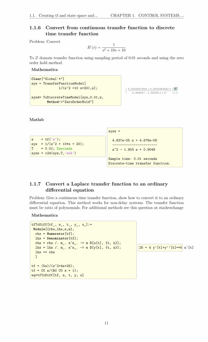
1.1.6 Convert from continuous transfer function to discretetime transfer function
Problem: ConvertH (s) =
1
s2 + 10s+ 10
To Z domain transfer function using sampling period of 0.01 seconds and using the zeroorder hold method.Mathematica Clear["Global`*"]sys = TransferFunctionModel[
1/(s^2 +10 s+20),s];
sysd= ToDiscreteTimeModel[sys,0.01,z,Method->"ZeroOrderHold"]
0.0000467806 + 0.0000483662 z
0.904837 - 1.90293 z + z20.01
Matlab
s = tf('s');sys = 1/(s^2 + 10*s + 20);T = 0.01; %secondssysz = c2d(sys,T,'zoh')
sysz =
4.837e-05 z + 4.678e-05-----------------------z^2 - 1.903 z + 0.9048
Sample time: 0.01 secondsDiscrete-time transfer function.
1.1.7 Convert a Laplace transfer function to an ordinarydifferential equation
Problem: Give a continuous time transfer function, show how to convert it to an ordinarydifferential equation. This method works for non-delay systems. The transfer functionmust be ratio of polynomials. For additional methods see this question at stackexchange
Mathematica tfToDiff[tf_, s_, t_, y_, u_]:=Module[rhs,lhs,n,m,rhs = Numerator[tf];lhs = Denominator[tf];rhs = rhs /. m_. s^n_. -> m D[u[t], t, n];lhs = lhs /. m_. s^n_. -> m D[y[t], t, n];lhs == rhs]
tf = (5s)/(s^2+4s+25);tf = C0 s/(R0 C0 s + 1);eq=tfToDiff[tf, s, t, y, u]
25 + 4 y'[t]+y''[t]==5 u'[t]
11

1.2. Obtain the step response of an LTI… CHAPTER 1. CONTROL SYSTEMS, …
1.2 Obtain the step response of an LTI from itstransfer function
Problem: Find the unit step response for the continuous time system defined by thetransfer function
H(s) =25
s2 + 4s+ 25
Mathematica Clear["Global`*"];
tf=TransferFunctionModel[25/(s^2+4s+25),s];y = OutputResponse[tf, UnitStep[t], t];
Plot[Evaluate@y, t, 0, 4,PlotRange -> 0, 4, 0, 1.4,Frame -> True,FrameLabel -> "y(t)", None,
t, "step response",GridLines -> Automatic,GridLinesStyle -> Dashed,ImageSize -> 300, 300,PlotStyle -> Red,AspectRatio -> 1]
0 1 2 3 40.0
0.2
0.4
0.6
0.8
1.0
1.2
1.4
t
y(t)
step response
Matlab clear all;s = tf('s');sys = 25/(s^2+4*s+25);[y,t] = step(sys,4);
plot(t,y,'r');xlim([0 4]);ylim([0 1.4]);title('step response');xlabel('t');ylabel('y(t)');gridset(gcf,'Position',[10,10,310,310]);
0 1 2 3 4
t
0
0.2
0.4
0.6
0.8
1
1.2
1.4
y(t)
step response
Maple restart:with(DynamicSystems):sys := TransferFunction(25/(s^2+4*s+25)):ResponsePlot(sys, Step(),duration=4);
12

1.3. plot the impulse and step responses … CHAPTER 1. CONTROL SYSTEMS, …
1.3 plot the impulse and step responses of a systemfrom its transfer function
Problem: Find the impulse and step responses for the continuous time system defined bythe transfer function
H (s) =1
s2 + 0.2s+ 1
and display these on the same plot up to some t value.
Side note: It was easier to see the analytical form of the responses in Mathematica andMaple so it is given below the plot.
Mathematica Clear["Global`*"];SetDirectory[NotebookDirectory[]]sys = TransferFunctionModel
[1/(s^2 + 2/10 s + 1), s];
yStep = Assuming[t > 0,Simplify@OutputResponse[
sys, UnitStep[t], t]]
1 - E^(-t/10) Cos[(3 Sqrt[11] t)/10]- (
E^(-t/10) Sin[(3 Sqrt[11]t)/10])/(3 Sqrt[11])
yImpulse = Simplify@
OutputResponse[sys,DiracDelta[t],t] (10 E^(-t/10) HeavisideTheta[t]
Sin[(3 Sqrt[11] t)/10])/(3 Sqrt[11]) p = Grid[
Plot[Evaluate@yStep, yImpulse,t, 0, 50,
PlotRange -> 0, 50, -0.8, 2.0,Frame -> True,FrameLabel -> "y(t)", None,
t, "step and impulse reponse",GridLines -> Automatic,GridLinesStyle -> Dashed,ImageSize -> 300, 300,PlotStyle -> Red, Black,AspectRatio -> 1],Row["step response=", Re@yStep],Row["impulse response=",Re@yImpulse], Alignment -> Left, Frame -> True]
0 10 20 30 40 50
-0.5
0.0
0.5
1.0
1.5
2.0
t
y(t)
step and impulse reponse
step response=1 - ⅇ-t/10 Cos 3 11 t10
-ⅇ-t/10 Sin 3 11 t
10
3 11
impulse response=10 ⅇ-t/10 HeavisideTheta[t] Sin 3 11 t
10
3 11
13

1.3. plot the impulse and step responses … CHAPTER 1. CONTROL SYSTEMS, …
Matlab clear all; close all;t = 0:0.05:50;s = tf('s');sys = 1/(s^2+0.2*s+1);y = step(sys,t);plot(t,y,'-r')hold ony = impulse(sys,t);plot(t,y,'-k')title('Step and Impulse responses');xlabel('t');ylabel('y(t)');xlim([0 50]);ylim([-0.8 2]);legend('step','impulse');grid on;set(gcf,'Position',[10,10,310,310]);
0 10 20 30 40 50
t
-0.5
0
0.5
1
1.5
2
y(t)
Step and Impulse responses
stepimpulse
MapleUsing Maple DynamicSystems restart:alias(DS=DynamicSystems):sys:=DS:-TransferFunction(1/(s^2+0.2*s+1)):p1:=DS:-ResponsePlot(sys, DS:-Step(),
duration=50,color=red,legend="step"):p2:=DS:-ImpulseResponsePlot(sys,
50,legend="impulse"):
plots:-display([p1,p2],axes=boxed,title=`step and impulse reponses`);
Using Laplace transform method:
with(inttrans):with(plottools):H:=1/(s^2+0.2*s+1);input:=laplace(Heaviside(t),t,s):yStep:=invlaplace(input*H,s,t);input:=laplace(Dirac(t),t,s):yImpulse:=invlaplace(input*H,s,t);plot([yStep,yImpulse],t=0.001..50,
title=`step response`,labels=[`time`,`y(t)`],color=[red,black],legend=["step","impulse"]);
14

1.4. Obtain the response of a transfer … CHAPTER 1. CONTROL SYSTEMS, …
1.4 Obtain the response of a transfer function for anarbitrary input
Problem: Find the response for the continuous time system defined by the transfer function
H(s) =1
s2 + 0.2s+ 1
when the input is given byu(t) = sin(t)
and display the response and input on the same plot.
Side note: It was easier to see the analytical form of the responses in Mathematica andMaple so it is given below the plot.
Mathematica Clear["Global`*"];SetDirectory[NotebookDirectory[]]sys=TransferFunctionModel[1/(s^2+2/10 s+1),s];u = Sin[t];y = OutputResponse[sys, u, t];p = Grid[
Plot[Evaluate@y, u, t, 0, 50,PlotRange -> 0, 50, -5, 5,Frame -> True,FrameLabel -> "y(t)", None,
"t", "input and its reponse",GridLines -> Automatic,GridLinesStyle -> Dashed,ImageSize -> 300, 300,PlotStyle -> Red, Black,AspectRatio -> 1]
, Alignment -> Left, Frame -> True]
0 10 20 30 40 50
-4
-2
0
2
4
t
y(t)
input and its reponse
Matlab clear all;close all;t = 0:0.05:50;u = sin(t);s = tf('s');sys = 1/(s^2+0.2*s+1);[num,den] = tfdata(sys,'v');y = lsim(num,den,u,t);plot(t,u,'k',t,y,'r');title('input and its response');xlabel('t'); ylabel('y(t)');xlim([0 50]);ylim([-5 5]);grid on;set(gcf,'Position',[10,10,310,310]);
0 10 20 30 40 50
t
-5
0
5
y(t)
input and its response
15

1.5. Obtain the poles and zeros of a … CHAPTER 1. CONTROL SYSTEMS, …
Maple restart;with(inttrans):H:=1/(s^2+0.2*s+1);input:=sin(t);inputS:=laplace(input,t,s):y:=invlaplace(inputS*H,s,t);plot([y,input],t=0..25,title=`system response`,labels=[`time`,`y(t)`],color=[black,red],legend=["response","input"]);
Using DynamicSystem package
restart:alias(DS=DynamicSystems):sys :=DS:-TransferFunction(1/(s^2+0.2*s+1)):p1:=DS:-ResponsePlot(sys, sin(t),duration=25,color=black,legend="response"):p2:=plot(sin(t),t=0..25,color=red,
legend="input",size=[400,"default"]):plots:-display([p2,p1],axes=boxed,title="step and impulse reponses",legendstyle= [location=right]);
1.5 Obtain the poles and zeros of a transfer functionProblem: Find the zeros, poles, and gain for the continuous time system defined by thetransfer function
H(s) =25
s2 + 4s+ 25
Mathematica Clear["Global`*"];sys=TransferFunctionModel[25/(s^2+4 s+25),s];TransferFunctionZeros[sys]
TransferFunctionPoles[sys]//N
-2.-4.58258 I,-2.+4.58258 I
Matlab clear all;s = tf('s');sys = 25/(s^2+4*s+25);[z,p,k] =zpkdata(sys,'v')
z =
Empty matrix: 0-by-1
p =-2.0000 + 4.5826i-2.0000 - 4.5826i
16

1.6. Generate Bode plot of a transfer … CHAPTER 1. CONTROL SYSTEMS, …
Maple restart;alias(DS=DynamicSystems):sys:=DS:-TransferFunction(25/(s^2+4*s+25)):r :=DS:-ZeroPolePlot(sys,output=data):zeros := r[1];poles := r[2];
zeros:= []poles:= [-2.000000000-4.582575695*I,
-2.+4.582575695*I]
1.6 Generate Bode plot of a transfer functionProblem: Generate a Bode plot for the continuous time system defined by the transferfunction
H(s) =5s
s2 + 4s+ 25
Mathematica Clear["Global`*"];
tf=TransferFunctionModel[(5 s)/(s^2+4s+25),s];
BodePlot[tf, GridLines -> Automatic,ImageSize -> 300,FrameLabel -> "magnitude (db)", None,
None, "Bode plot","phase(deg)", None,"Frequency (rad/sec)", None,
ScalingFunctions -> "Log10", "dB","Log10", "Degree",
PlotRange -> 0.1, 100, Automatic,0.1, 100, Automatic
]
0.1 1 10 100
-60
-40
-20
0magnitude
(db)
Bode plot
0.1 1 10 100
-50
0
50
Frequency (rad/sec)
phase(deg)
Matlab clear all;s = tf('s');sys = 5*s / (s^2 + 4*s + 25);bode(sys);grid;set(gcf,'Position',[10,10,400,400]);
-40
-30
-20
-10
0
10
Mag
nitu
de (
dB)
10-1 100 101 102-90
-45
0
45
90
Pha
se (
deg)
Bode Diagram
Frequency (rad/s)
17

1.7. How to check that state space system… CHAPTER 1. CONTROL SYSTEMS, …
Maple restart:alias(DS=DynamicSystems):sys:=DS:-TransferFunction(5*s/(s^2+4*s+25)):DS:-BodePlot(sys,output=dualaxis,
range=0.1..100); or can plot the the two bode figures on top of each othersas follows DS:-BodePlot(sys,size=[400,300],output=verticalplot,range=0.1..100);
1.7 How to check that state space systemx′ = Ax +Bu is controllable?
A system described by
x′ = Ax+Bu
y = Cx+Du
Is controllable if for any initial state x0 and any final state xf there exist an input u whichmoves the system from x0 to xf in finite time. Only the matrix A and B are needed todecide on controllability. If the rank of
[B AB A2B . . . An−1B]
is n which is the number of states, then the system is controllable. Given the matrix
A =
0 1 0 0
0 0 −1 0
0 0 0 1
0 0 5 0
And
B =
0
1
0
−2
Mathematica A0 = 0, 1, 0, 0,
0, 0, -1, 0,0, 0, 0, 1,0, 0, 5, 0;
B0 = 0, 1, 0, -2;sys = StateSpaceModel[A0, B0];m = ControllabilityMatrix[sys]
0 1 0 2
1 0 2 0
0 −2 0 −10
−2 0 −10 0
ControllableModelQ[sys] True MatrixRank[m] 4
18

1.8. Obtain partial-fraction expansion CHAPTER 1. CONTROL SYSTEMS, …
Matlab A0 = [0 1 0 0;
0 0 -1 0;0 0 0 1;0 0 5 0];
B0 = [0 1 0 -2]';sys = ss(A0,B0,[],[]);m = ctrb(sys)
m =
0 1 0 21 0 2 00 -2 0 -10-2 0 -10 0
rank(m) 4Maple restart:alias(DS=DynamicSystems):A:=Matrix( [ [0,1,0,0],
[0,0,-1,0],[0,0,0,1],[0,0,5,0]
]);
B:=Matrix([[0],[1],[0],[-2]]);sys:=DS:-StateSpace(A,B);m:=DS:-ControllabilityMatrix(sys);
0 1 0 2
1 0 2 0
0 −2 0 −10
−2 0 −10 0
DS:-Controllable(sys,method=rank); true DS:-Controllable(sys,method=staircase); true LinearAlgebra:-Rank(m); 4
1.8 Obtain partial-fraction expansionProblem: Given the continuous time S transfer function defined by
H(s) =s4 + 8s3 + 16s2 + 9s+ 9
s3 + 6s2 + 11s+ 6
obtain the partial-fractions decomposition.
Comment: Mathematica result is easier to see visually since the partial-fraction decompo-sition returned in a symbolic form.
Mathematica
19

1.9. Obtain Laplace transform for a … CHAPTER 1. CONTROL SYSTEMS, …
Remove["Global`*"];expr = (s^4+8 s^3+16 s^2+9 s+6)/
(s^3+6 s^2+11 s+6);Apart[expr]
2 + s +3/(1+s) -4/(2+s) -6/(3+s)
Matlab
clear all;s=tf('s');tf_sys = (s^4+8*s^3+16*s^2+9*s+6)/...
(s^3+6*s^2+11*s+6);[num,den] = tfdata(tf_sys,'v');[r,p,k] = residue(num,den)
r =
-6.0000-4.00003.0000
p =-3.0000-2.0000-1.0000
k =1 2
Maple
p:=(s^4+8*s^3+16*s^2+9*s+9)/(s^3+6*s^2+11*s+6);p0:=convert(p,parfrac); s+ 2−
7
s+ 2−
9
2 s+ 6+
9
2 s+ 2
[op(p0)]; [s, 2, 7
s+ 2,− 9
2 s+ 6,
9
2 s+ 2]
1.9 Obtain Laplace transform for a piecewisefunctions
Problem: Obtain the Laplace transform for the function defined in the following figure.
T
T
f(t)
t
Function f(t) to obtain its Laplace transform
Comment: Mathematica solution was easier than Matlab’s. In Matlab the definition of theLaplace transform is applied to each piece separately and the result added. Not findingthe piecewise maple function to access from inside MATLAB did not help.
Mathematica
20

1.10. Obtain Inverse Laplace transform of … CHAPTER 1. CONTROL SYSTEMS, …
Remove["Global`*"];f[t_] := Piecewise[0,t<0,
t,t>= 0 && t< T,T, t>T]
Simplify[LaplaceTransform[f[t],t,s] ,T>0] Out[]= (1 - E^((-s)*T))/s^2
Matlab clear all;syms T t s;syms s positive;I1 = int(t*exp(-s*t),t,0,T);I2 = int(T*exp(-s*t),t,T,Inf);result = simple(I1+I2);pretty(result)
1 - exp(-T s)-------------
2s
Maple
With Maple, had to use Heaviside else Laplace will notobtain the transform of a piecewise function. restart;assume(T>0):interface(showassumed=0):f:=t->piecewise(t<0,0,t>=0 and t<T,t,t>T,T):r:=convert(f(t),Heaviside):r:=inttrans[laplace](r,t,s);
1− e−sT
s2
1.10 Obtain Inverse Laplace transform of a transferfunction
Problem: Obtain the inverse Laplace transform for the function
H(s) =s4 + 5s3 + 6s2 + 9s+ 30
s4 + 6s3 + 21s2 + 46s+ 30
Mathematica Remove["Global`*"];f = (s^4+5 s^3+6 s^2+9 s+30)/(s^4+6 s^3+21 s^2+46 s+30);InverseLaplaceTransform[f,s,t];Expand[FullSimplify[%]]
δ(t) +
(1
234+
i
234
)e(−1−3i)t
((73 + 326i)e6it + (−326− 73i)
)− 3e−3t
26+
23e−t
18
Matlab clear all;syms s tf = (s^4+5*s^3+6*s^2+9*s+30)/(s^4+6*s^3+21*s^2+46*s+30);pretty(f)
21

1.11. Display the response to a unit step… CHAPTER 1. CONTROL SYSTEMS, …
4 3 2s + 5 s + 6 s + 9 s + 30-----------------------------4 3 2s + 6 s + 21 s + 46 s + 30
pretty(ilaplace(f))
/ 399 sin(3 t) \253 exp(-t) | cos(3 t) + ------------ |
23 exp(-t) 3 exp(-3 t) \ 253 /---------- - ----------- + dirac(t) - ---------------------------------------
18 26 117 Maple restart;interface(showassumed=0):p:=(s^4+5*s^3+6*s^2+9*s+30)/(s^4+6*s^3+21*s^2+46*s+30);r:=inttrans[invlaplace](p,s,t);
Dirac (t)− 3 e−3 t
26+
(−506 cos (3 t)− 798 sin (3 t) + 299) e−t
234
1.11 Display the response to a unit step of an under,critically, and over damped system
Problem: Obtain unit step response of the second order system given by the transferfunction
H (s) =ω2n
s2 + 2ξωns+ ω2n
in order to illustrate the response when the system is over, under, and critically damped.use ωn = 1 and change ξ over a range of values that extends from under damped to overdamped.
22

1.11. Display the response to a unit step… CHAPTER 1. CONTROL SYSTEMS, …
Mathematica Clear["Global`*"];Needs["PlotLegends`"]
sys=TransferFunctionModel[w^2/(s^2+2*z*w*s+w^2),s];zValues = Range[.2,1.2,.2];fun = OutputResponse[sys/.w->1,z->#, UnitStep[t],
t,0,20]&/@zValues;
Plot[Evaluate@Flatten@Table[fun[[i]],i,1,Length[fun]],
t,0,20,Frame->True,FrameLabel->"y(t)",None,
"t","step response for different \[Xi] values",PlotRange->0,20,0,1.6,GridLines->Automatic,GridLinesStyle->Dashed,PlotLegend->zValues,LegendPosition->0.76,-0.5,LegendSize -> 1,LegendLabel -> "\[Xi] values",ImageSize -> 450,LabelStyle -> 14,AspectRatio -> 1
]
0 5 10 15 200.0
0.5
1.0
1.5
t
y(t)
step response for different ξ values
1.2
1.
0.8
0.6
0.4
0.2
ξ values
23

1.11. Display the response to a unit step… CHAPTER 1. CONTROL SYSTEMS, …
Matlab clear; close all;wn = 1;z = .2:.2:1.2;t = 0:0.05:20;y = zeros(length(t),length(z));legendStr = cell(length(z),1);
for i = 1:length(z)[num,den] = ord2(wn,z(i));num = num*wn^2;[y(:,i),~,~] = step(num,den,t);legendStr(i) = sprintf('%1.1f',z(i));
endplot(t,y);legend(legendStr);
title(sprintf('2nd order system step response with changing %s','\zeta'));
xlabel('time (sec)');ylabel('amplitude');grid on;set(gcf,'Position',[10,10,400,400]);
0 5 10 15 20
time (sec)
0
0.2
0.4
0.6
0.8
1
1.2
1.4
1.6
ampl
itude
2nd order system step response with changing 1
0.20.40.60.81.01.2
Maple restart;alias(DS=DynamicSystems):H := (w,zeta)->w^2/(s^2+2*zeta*w*s+w^2):sys := (w,zeta)->DS:-TransferFunction(H(w,zeta)):zetaValues := [seq(i,i=0.1..1.2,.2)]:sol:=map(z->DS:-Simulate(sys(1,z),
Heaviside(t)),zetaValues):c :=ColorTools:-GetPalette("Niagara"):
plots:-display(seq(plots[odeplot](sol[i],t=0..20,color=c[i],
legend=typeset(zeta,"=",zetaValues[i]),legendstyle=[location=right]),
i=1..nops(zetaValues)),gridlines=true,
title="step response for different damping ratios",labels=[typeset(t),typeset(y(t))]); Instead of using Simulate as above, another option is to use ResponsePlot which gives
24

1.12. View steady state error of 2nd order … CHAPTER 1. CONTROL SYSTEMS, …
same plot as above. restart;alias(DS=DynamicSystems):c:=ColorTools:-GetPalette("Niagara"):H:=(w,zeta)->w^2/(s^2+2*zeta*w*s+w^2):sys:= (w,zeta)->
DS:-TransferFunction(H(w,zeta)):zetaValues := [seq(i,i=0.1..1.2,.2)]:
sol:=map(i->DS:-ResponsePlot(sys(1,zetaValues[i]),Heaviside(t),duration=14,color=c[i],legend=typeset(zeta,"=",zetaValues[i]),legendstyle=[location=right]),[seq(i,i=1..nops(zetaValues))]):
plots:-display(sol,gridlines=true,title="step response for different damping ratios",labels=[typeset(t),typeset(y(t))]);
1.12 View steady state error of 2nd order LTIsystem with changing undamped naturalfrequency
Problem: Given the transfer function
H (s) =ω2n
s2 + 2ξωns+ ω2n
Display the output and input on the same plot showing how the steady state error changesas the un damped natural frequency ωn changes. Do this for ramp and step input.The steady state error is the difference between the input and output for large time. Inother words, it the difference between the input and output at the time when the responsesettles down and stops changing.Displaying the curve of the output and input on the same plot allows one to visually seesteady state error.Use maximum time of 10 seconds and ξ = 0.707 and change ωn from 0.2 to 1.2.Do this for ramp input and for unit step input. It can be seen that with ramp input, thesteady state do not become zero even at steady state. While with step input, the steadystate error can become zero.
25

1.12. View steady state error of 2nd order … CHAPTER 1. CONTROL SYSTEMS, …
1.12.1 Mathematica1.12.1.1 ramp input Remove["Global`*"];sys = TransferFunctionModel[w^2 /(s^2+2 z w s+w^2 ),s];z = .707;nTrials = 6;maxTime = 10;
tb = Table[Plot[Evaluate@t,OutputResponse[sys/.w->0.2*i,t,t],
t,0,maxTime,Frame->True,PlotRange->All,FrameLabel->"y(t)",None,"t","Subscript[\[Omega], n]="<>ToString[0.2*i]
],i,1,nTrials];
Grid[Partition[tb,2]]
0 2 4 6 8 100
2
4
6
8
10
t
y(t)
ωn=0.2
0 2 4 6 8 100
2
4
6
8
10
t
y(t)
ωn=0.4
0 2 4 6 8 100
2
4
6
8
10
t
y(t)
ωn=0.6
0 2 4 6 8 100
2
4
6
8
10
t
y(t)
ωn=0.8
0 2 4 6 8 100
2
4
6
8
10
t
y(t)
ωn=1.
0 2 4 6 8 100
2
4
6
8
10
t
y(t)
ωn=1.2
1.12.1.2 step input tb = Table[Plot[
Evaluate@UnitStep[t],OutputResponse[sys/.w->0.2*i,UnitStep[t],t],t,0,maxTime,Frame->True,PlotRange->All,FrameLabel->"y(t)",None,"t","Subscript[\[Omega], n]="<>ToString[0.2*i]
],i,1,nTrials];
Grid[Partition[tb,2]]
26

1.13. Show the use of the inverse Z transform CHAPTER 1. CONTROL SYSTEMS, …
0 2 4 6 8 100.0
0.2
0.4
0.6
0.8
1.0
t
y(t)
ωn=0.2
0 2 4 6 8 100.0
0.2
0.4
0.6
0.8
1.0
t
y(t)
ωn=0.4
0 2 4 6 8 100.0
0.2
0.4
0.6
0.8
1.0
t
y(t)
ωn=0.6
0 2 4 6 8 100.0
0.2
0.4
0.6
0.8
1.0
t
y(t)
ωn=0.8
0 2 4 6 8 100.0
0.2
0.4
0.6
0.8
1.0
t
y(t)
ωn=1.
0 2 4 6 8 100.0
0.2
0.4
0.6
0.8
1.0
t
y(t)
ωn=1.2
1.13 Show the use of the inverse Z transformThese examples show how to use the inverse a Z transform.
1.13.1 example 1Problem: Given
F (z) =z
z − 1
find x[n] = F−1 (z) which is the inverse Ztransform.
Mathematica Clear["Global`*"];
x[n_]:= InverseZTransform[z/(z-1),z,n]
ListPlot[Table[n,x[n],n,0,10],Frame->True,FrameLabel->"x[n]",None,
"n","Inverse Ztransform of z/(z-1)",FormatType->StandardForm,RotateLabel->False,Filling->Axis,FillingStyle->Red,PlotRange->Automatic,0,1.3,PlotMarkers->Automatic,12]
0 2 4 6 8 100.0
0.2
0.4
0.6
0.8
1.0
1.2
n
x[n]
Inverse Ztransform ofz
z - 1
27
1.13. Show the use of the inverse Z transform CHAPTER 1. CONTROL SYSTEMS, …
Matlab function e19()
nSamples = 10;z = tf('z');h = z/(z-1);[num,den] = tfdata(h,'v');[delta,~] = impseq(0,0,nSamples);xn = filter(num,den,delta);
stem(xn);title('Inverse Z transform of z/(z-1)');xlabel('n'); ylabel('x[n]');ylim([0 1.3]);set(gcf,'Position',[10,10,400,400]);
end
%function from Signal Processing by Proakis%corrected a little by me for newer matlab versionfunction [x,n] = impseq(n0,n1,n2)% Generates x(n) = delta(n-n0); n1 <= n,n0 <= n2% ----------------------------------------------% [x,n] = impseq(n0,n1,n2)%if ((n0 < n1) || (n0 > n2) || (n1 > n2))
error('arguments must satisfy n1 <= n0 <= n2')endn = n1:n2;x = (n-n0) == 0;end
0 2 4 6 8 10 12
n
0
0.2
0.4
0.6
0.8
1
1.2
x[n]
Inverse Z transform of z/(z-1)
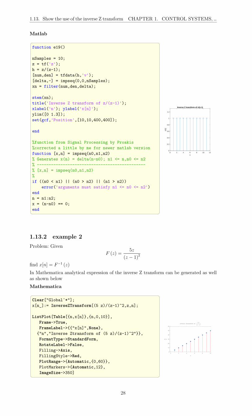
1.13.2 example 2Problem: Given
F (z) =5z
(z − 1)2
find x[n] = F−1 (z)
In Mathematica analytical expression of the inverse Z transform can be generated as wellas shown belowMathematica Clear["Global`*"];x[n_]:= InverseZTransform[(5 z)/(z-1)^2,z,n];
ListPlot[Table[n,x[n],n,0,10],Frame->True,FrameLabel->"x[n]",None,"n","Inverse Ztransform of (5 z)/(z-1)^2",FormatType->StandardForm,RotateLabel->False,Filling->Axis,FillingStyle->Red,PlotRange->Automatic,0,60,PlotMarkers->Automatic,12,ImageSize->350]
0 2 4 6 8 100
10
20
30
40
50
60
n
x[n]
Inverse Ztransform of5 z
(z - 1)2
28

1.14. Find the Z transform of sequence x(n) CHAPTER 1. CONTROL SYSTEMS, …
Matlab function e19_2()
nSamples = 10;z = tf('z');h = (5*z)/(z-1)^2;[num,den] = tfdata(h,'v');[delta,~] = impseq(0,0,nSamples);xn = filter(num,den,delta);
stem(xn);title('Inverse Z transform of 5z/(z-1)^2');xlabel('n'); ylabel('x[n]');ylim([0 60]);set(gcf,'Position',[10,10,400,400]);
end 0 2 4 6 8 10 12
n
0
10
20
30
40
50
60
x[n]
Inverse Z transform of 5z/(z-1)2
1.14 Find the Z transform of sequence x(n)
1.14.1 example 1Find the Z transform for the unit step discrete function
Given the unit step function x[n] = u[n] defined as x = 1, 1, 1, · · · for n ≥ 0 , find its Ztransform.
Mathematica Remove["Global`*"];ZTransform[UnitStep[n],n,z]
Out[] = z/(-1+z)
Matlab
syms npretty(ztrans(heaviside(n)))
1
----- + 1/2z - 1
1.14.2 example 2
Find the Z transform for x[n] =(13
)nu (n) + (0.9)n−3 u (n)
Mathematica f[n_]:=((1/3)^n+(9/10)^(n-3))UnitStep[n];ZTransform[f[n],n,z]
z (3/(-1+3 z)+10000/(729 (-9+10 z)))
Matlab
29

1.15. Sample a continuous time system CHAPTER 1. CONTROL SYSTEMS, …
syms npretty(ztrans(((1/3)^n+(0.9)^(n-3))
*heaviside(n)))
100 1
------------- + ------- + 1729/145881 (z - 9/10) 3 z - 1
1.15 Sample a continuous time systemGiven the following system, sample the input and find and plot the plant output
T 1
ZOHPlant
3s
s1s2Sampling period
1 ut T
0 Tt
1eTss
ut et sint ukT ykT
Z 1eTss
3s
s1s2
Equivalent discrete time system is given by the Z transform of the ZOH Laplace transform times the plant transfer function
In Mathematica, the above is implemented as follows
s = tf('s');
plant = (1/s)*(1/(s+0.5));
c2d(plant,sampleTime,'zoh')
In Matlab it is implemented as follows
Use sampling frequency f = 1 Hz and show the result for up to 14 seconds. Use as inputthe signal u(t) = exp(−0.3t) sin(2π(f/3)t).
Plot the input and output on separate plots, and also plot them on the same plot.
Mathematica
30

1.15. Sample a continuous time system CHAPTER 1. CONTROL SYSTEMS, …
Clear["Global`*"];
nSamples =14;f =1.0;sampleTime =1/f;u[t_] := Sin[2*Pi*(f/3)*t]*Exp[-0.3*t]ud[n_]:= u[n*sampleTime];plant = TransferFunctionModel[
(3 s)/((s+1)(s+2)),s];sysd = ToDiscreteTimeModel[plant,
sampleTime,z,Method->"ZeroOrderHold"]
-0.697632 + 0.697632 z
0.0497871 - 0.503215 z + z21.
opts = Joined->True,PlotRange->All,AspectRatio->1,InterpolationOrder->0,ImageSize->200,Frame->True,PlotRange->0,nSamples,-0.5,0.5,GridLines->Automatic,GridLinesStyle->Dashed;
inputPlot = ListPlot[Table[ud[k],k,0,nSamples],Evaluate[opts],FrameLabel->"u(t)",None,
"n","plant input u(nT)",PlotStyle->Thick,Red];
plantPlot=ListPlot[OutputResponse[sysd,Table[ud[k],k,0,nSamples]],Evaluate[opts],FrameLabel->"y(t)",None,
"n","plant output y(nT)",PlotStyle->Thick,Blue];
Grid[inputPlot,plantPlot]
2 4 6 8 10 12 14
-0.4
-0.2
0.0
0.2
0.4
0.6
n
u(t)
plant input u(nT)
2 4 6 8 10 12 14-0.6
-0.4
-0.2
0.0
0.2
0.4
n
y(t)
plant output y(nT)
Show[inputPlot,plantPlot,
PlotLabel->"input/output plot"]
31

1.15. Sample a continuous time system CHAPTER 1. CONTROL SYSTEMS, …
2 4 6 8 10 12 14
-0.4
-0.2
0.0
0.2
0.4
0.6
n
u(t)
plant input u(nT)input/output plot
Matlab clear all; close all;
nSamples = 14;f = 1;T = 1/f;u=@(t) sin(2*pi*(f/3).*t).*exp(-0.3.*t);ud=@(n) u(n*T);U=ud(1:14); %sampled inputs=tf('s');plant = (3*s)/((s+1)*(s+2));plantD = c2d(plant,T,'zoh')
plantD =
0.6976 z - 0.6976------------------------z^2 - 0.5032 z + 0.04979
Sample time: 1 secondsDiscrete-time transfer function.
lsim(plantD,U,0:nSamples-1)grid
0 5 10-0.6
-0.4
-0.2
0
0.2
0.4
0.6
0.8Linear Simulation Results
Time (seconds)
Am
plitu
de
32
1.16. Find closed loop transfer function… CHAPTER 1. CONTROL SYSTEMS, …
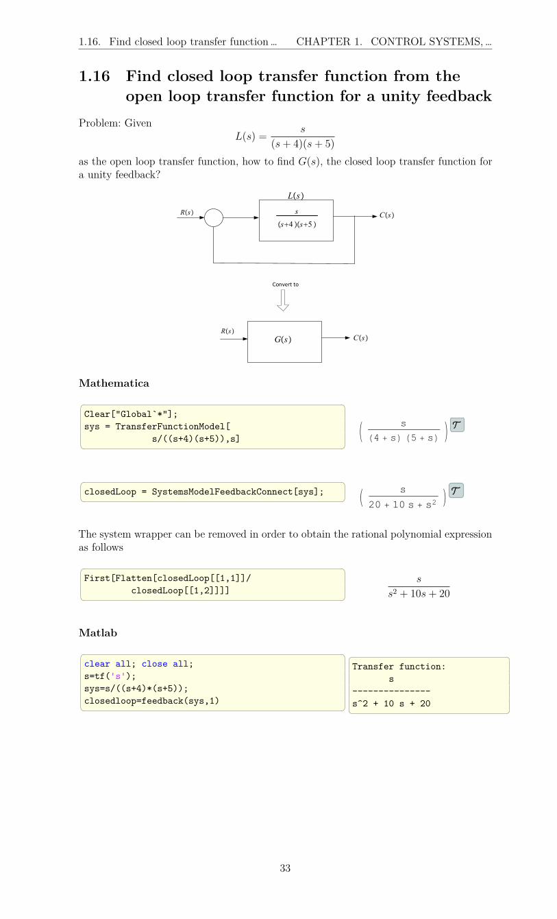
1.16 Find closed loop transfer function from theopen loop transfer function for a unity feedback
Problem: GivenL(s) =
s
(s+ 4)(s+ 5)
as the open loop transfer function, how to find G(s), the closed loop transfer function fora unity feedback?
Ls
Rs Cs
RsCs
Convert to
Gs
s
s4 s5
Mathematica Clear["Global`*"];sys = TransferFunctionModel[
s/((s+4)(s+5)),s] s
(4 + s) (5 + s)
closedLoop = SystemsModelFeedbackConnect[sys];
s
20 + 10 s + s2
The system wrapper can be removed in order to obtain the rational polynomial expressionas follows First[Flatten[closedLoop[[1,1]]/
closedLoop[[1,2]]]] s
s2 + 10s+ 20
Matlab clear all; close all;s=tf('s');sys=s/((s+4)*(s+5));closedloop=feedback(sys,1)
Transfer function:
s---------------s^2 + 10 s + 20
33

1.17. Compute the Jordan… CHAPTER 1. CONTROL SYSTEMS, …
1.17 Compute the Jordan canonical/normal form ofa matrix A
Mathematica Remove["Global`*"];m=3,-1,1,1,0,0,
1, 1,-1,-1,0,0,0,0,2,0,1,1,0,0,0,2,-1,-1,0,0,0,0,1,1,0,0,0,0,1,1;
MatrixForm[m]
3 −1 1 1 0 0
1 1 −1 −1 0 0
0 0 2 0 1 1
0 0 0 2 −1 −1
0 0 0 0 1 1
0 0 0 0 1 1
a,b=JordanDecomposition[m];b
0 0 0 0 0 0
0 2 1 0 0 0
0 0 2 0 0 0
0 0 0 2 1 0
0 0 0 0 2 1
0 0 0 0 0 2
Matlab clear all;A=[3 -1 1 1 0 0;
1 1 -1 -1 0 0;0 0 2 0 1 1;0 0 0 2 -1 -1;0 0 0 0 1 1;0 0 0 0 1 1;]
jordan(A)
ans =0 0 0 0 0 00 2 1 0 0 00 0 2 1 0 00 0 0 2 0 00 0 0 0 2 10 0 0 0 0 2
Maple
restart;A:=Matrix([[3,-1,1,1,0,0],
[1, 1,-1,-1,0,0],[0,0,2,0,1,1],[0,0,0,2,-1,-1],[0,0,0,0,1,1],[0,0,0,0,1,1]]);
LinearAlgebra:-JordanForm(A);
0 0 0 0 0 0
0 2 1 0 0 0
0 0 2 1 0 0
0 0 0 2 0 0
0 0 0 0 2 1
0 0 0 0 0 2
34

1.18. Solve the continuous-time algebraic … CHAPTER 1. CONTROL SYSTEMS, …
1.18 Solve the continuous-time algebraic Riccatiequation
Problem: Solve for X in the Riccati equation
A′X +XA−XBR−1B′X + C ′C = 0
given
A =
(−3 2
1 1
)B =
(0
1
)C =
(1 −1
)R = 3
Mathematica Clear ["Global`*"];a=-3,2,1,1;b=0,1;c=1,-1;r=3;sol=RiccatiSolve[a,b,Transpose[c].c,r];MatrixForm[N[sol]]
(0.589517 1.82157
1.82157 8.81884
)
Matlab %needs control systemclear all; close all;a = [-3 2;1 1];b = [0 ; 1];c = [1 -1];r = 3;x = care(a,b,c'*c,r)
x =
0.5895 1.82161.8216 8.8188
Maple
restart;A:=Matrix([[-3,2],[1,1]]);B:=Vector([0,1]);C:=Vector[row]([1,-1]);Q:=C^%T.C;R:=Matrix([[3]]);LinearAlgebra:-CARE(A,B,Q,R)
[0.5895174373 1.8215747249
1.8215747249 8.8188398069
]
35
1.19. Solve the discrete-time algebraic … CHAPTER 1. CONTROL SYSTEMS, …
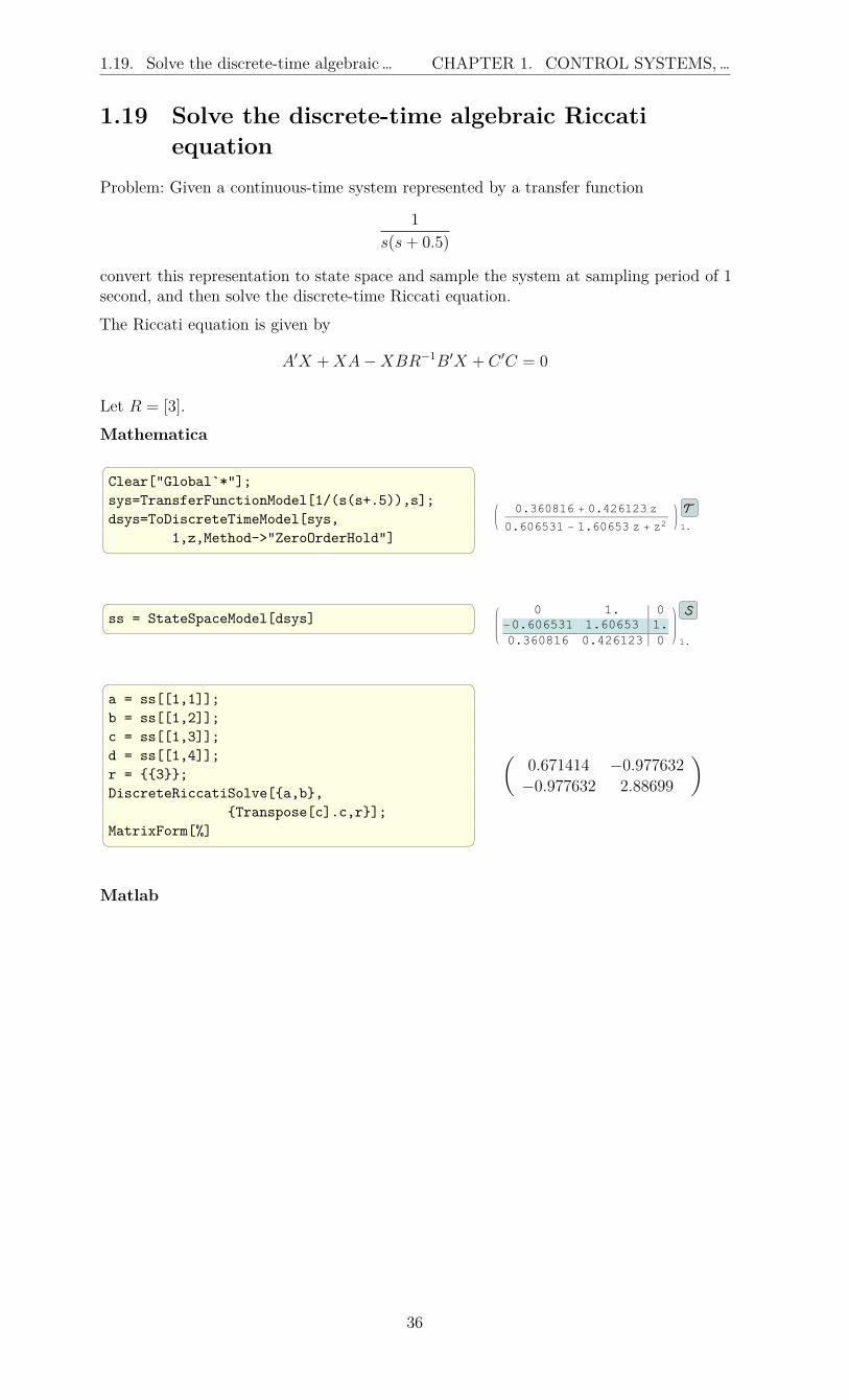
1.19 Solve the discrete-time algebraic Riccatiequation
Problem: Given a continuous-time system represented by a transfer function
1
s(s+ 0.5)
convert this representation to state space and sample the system at sampling period of 1second, and then solve the discrete-time Riccati equation.
The Riccati equation is given by
A′X +XA−XBR−1B′X + C ′C = 0
Let R = [3].
Mathematica Clear["Global`*"];sys=TransferFunctionModel[1/(s(s+.5)),s];dsys=ToDiscreteTimeModel[sys,
1,z,Method->"ZeroOrderHold"]
0.360816 + 0.426123 z
0.606531 - 1.60653 z + z21.
ss = StateSpaceModel[dsys] 0 1. 0
-0.606531 1.60653 1.0.360816 0.426123 0 1.
a = ss[[1,1]];b = ss[[1,2]];c = ss[[1,3]];d = ss[[1,4]];r = 3;DiscreteRiccatiSolve[a,b,
Transpose[c].c,r];MatrixForm[%]
(0.671414 −0.977632
−0.977632 2.88699
)
Matlab
36

1.20. Display impulse response of H(z) and… CHAPTER 1. CONTROL SYSTEMS, …
clear all; close all;s = tf('s');sys = 1/(s*(s+0.5));dsys = c2d(sys,1)
dsys =
0.4261 z + 0.3608----------------------z^2 - 1.607 z + 0.6065
Sample time: 1 secondsDiscrete-time transfer function.
[A,B,C,D]=dssdata(dsys)
A =
1.6065 -0.60651.0000 0
B =10
C =0.4261 0.3608
D =0
2.8870 -0.9776-0.9776 0.6714
dare(A,B,C'*C,3)
ans =
2.8870 -0.9776-0.9776 0.6714
Maple
restart;alias(DS=DynamicSystems):sys := DS:-TransferFunction(1/(s*(s+1/2)));sys := DS:-ToDiscrete(sys, 1, 'method'='zoh');sys := DS:-StateSpace(sys);Q:=sys:-c^%T.sys:-c;R:=Matrix([[3]]);LinearAlgebra:-DARE(sys:-a,sys:-b,Q,R)
[0.6714144604 −0.9776322436
−0.9776322436 2.8869912178
]
1.20 Display impulse response of H(z) and theimpulse response of its continuous timeapproximation H(s)
Plot the impulse response of H(z) = z/(z2 − 1.4z + 0.5) and using sampling period ofT = 0.5 find continuous time approximation using zero order hold and show the impulseresponse of the system and compare both responses.
Mathematica maxSimulationTime = 10;samplePeriod = 0.5;tf = TransferFunctionModel[z/(z^2-1.4 z+0.5),
z,
37

1.20. Display impulse response of H(z) and… CHAPTER 1. CONTROL SYSTEMS, …
SamplingPeriod->samplePeriod];
z
0.5 - 1.4 z + z20.5
Find its impulse response discreteResponse=First@OutputResponse[tf,DiscreteDelta[k],
k,0,maxSimulationTime] 0.,1.,1.4,1.46,1.344,1.1516,0.94024,0.740536,0.56663,0.423015,0.308905,0.22096,0.154891,0.106368,0.0714694,0.0468732,0.0298878,0.0184063,0.0108249,0.00595175,0.00291999 approximate to continuous time, use ZeroOrderHold ctf = ToContinuousTimeModel[tf, s, Method -> "ZeroOrderHold"]
5.60992 + 1.25559 s
0.560992 + 1.38629 s + s2
Find the impulse response of the continuous time system continouseTimeResponse=Chop@First@OutputResponse[ctf,DiracDelta[t],t]
−1.25559e−0.693147t(−13.3012θ(t) sin(0.283794t)− 1.θ(t) cos(0.283794t)) continouseTimeResponse=Chop@First@OutputResponse[ctf,DiracDelta[t],
t,0,maxSimulationTime] InterpolatingFunction
Domain: 0., 10.Output: scalar [t]
Plot the impulse response of the discrete system ListPlot[discreteResponse,DataRange->0,maxSimulationTime,Filling->Axis,FillingStyle->Red,
PlotMarkers->Graphics[PointSize[0.03],Point[0,0]],PlotRange->All,ImageSize->300,ImagePadding->45,10,35,10,AspectRatio->0.9,AxesOrigin->0,0,Frame->True,Axes->None,ImageSize->300,Frame->True]
38
1.20. Display impulse response of H(z) and… CHAPTER 1. CONTROL SYSTEMS, …
0 2 4 6 8 10
0.0
0.2
0.4
0.6
0.8
1.0
1.2
1.4
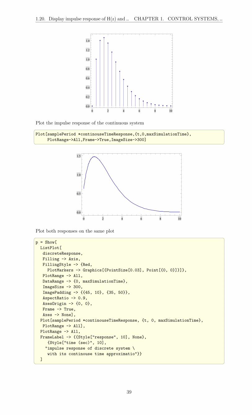
Plot the impulse response of the continuous system Plot[samplePeriod *continouseTimeResponse,t,0,maxSimulationTime,
PlotRange->All,Frame->True,ImageSize->300]
0 2 4 6 8 10
0.0
0.5
1.0
1.5
Plot both responses on the same plot p = Show[ListPlot[discreteResponse,Filling -> Axis,FillingStyle -> Red,PlotMarkers -> Graphics[PointSize[0.03], Point[0, 0]],
PlotRange -> All,DataRange -> 0, maxSimulationTime,ImageSize -> 300,ImagePadding -> 45, 10, 35, 50,AspectRatio -> 0.9,AxesOrigin -> 0, 0,Frame -> True,Axes -> None],
Plot[samplePeriod *continouseTimeResponse, t, 0, maxSimulationTime,PlotRange -> All],
PlotRange -> All,FrameLabel -> Style["response", 10], None,
Style["time (sec)", 10],"impulse response of discrete system \with its continouse time approximatio"
]
39

1.20. Display impulse response of H(z) and… CHAPTER 1. CONTROL SYSTEMS, …
0 2 4 6 8 10
0.0
0.2
0.4
0.6
0.8
1.0
1.2
1.4
time (sec)
response
impulse response of discrete system with its continouse time approximatio
Do the same plot above, using stair case approximation for the discrete plot Show[ListPlot[discreteResponse,Filling->None,PlotRange->All,DataRange->0,maxSimulationTime,ImageSize->300,ImagePadding->45,10,35,50,AspectRatio->0.9,AxesOrigin->0,0,Frame->True,Axes->None,Joined->True,InterpolationOrder->0,PlotStyle->Red],Plot[samplePeriod *continouseTimeResponse,t,0,maxSimulationTime,PlotRange->All],PlotRange->All,FrameLabel->Style["response",10],None,Style["time (sec)",10],"impulse response"]
0 2 4 6 8 100.0
0.2
0.4
0.6
0.8
1.0
1.2
1.4
time (sec)
response
impulse response of discrete system with its continouse time approximation
Matlab clear all;maxSimulationTime = 15;samplePeriod = 0.5;
z=tf('z',samplePeriod);tf=z/(z^2-1.4*z+0.5)impulse(tf,0:samplePeriod:maxSimulationTime)
ctf=d2c(tf,'zoh')
hold onimpulse(ctf,0:maxSimulationTime)title(['impulse response of discrete system with',...
' its continuous time approximation']);xlabel('time (sec)');
40

1.21. Find the system type given an open… CHAPTER 1. CONTROL SYSTEMS, …
ylabel('response');
0 5 10 15-0.5
0
0.5
1
1.5
2
2.5
3impulse response of discrete system with its continuous time approximation
time (sec) (seconds)
resp
onse
1.21 Find the system type given an open looptransfer function
Problem: Find the system type for the following transfer functions
1. s+1s2−s
2. s+1s3−s2
3. s+1s5
To find the system type, the transfer function is put in the form k∑
i(s−si)
sM∑
j(s−sj), then the
system type is the exponent M . Hence it can be seen that the first system above has typeone since the denominator can be written as s1 (s− 1) and the second system has type 2since the denominator can be written as s2 (s− 1) and the third system has type 5. Thefollowing computation determines the type
Mathematica Clear["Global`*"];p=TransferFunctionPoles[TransferFunctionModel[
(s+1)/(s^2-s),s]];Count[Flatten[p],0]
Out[171]= 1
p=TransferFunctionPoles[TransferFunctionModel[
(s+1)/( s^3-s^2),s]];Count[Flatten[p],0] Out[173]= 2
p=TransferFunctionPoles[
TransferFunctionModel[(s+1)/ s^5 ,s]];Count[Flatten[p],0] Out[175]= 5
Matlab
41

1.22. Find the eigenvalues and eigenvectors … CHAPTER 1. CONTROL SYSTEMS, …
clear all;s=tf('s');[~,p,~]=zpkdata((s+1)/(s^2-s));length(find(p:==0))
ans =
1
[~,p,~]=zpkdata((s+1)/(s^3-s^2));length(find(p:==0))
ans =
2 [~,p,~]=zpkdata((s+1)/s^5);length(find(p:==0))
ans =
5
1.22 Find the eigenvalues and eigenvectors of amatrix
Problem, given the matrix 1 2 3
4 5 6
7 8 9
Find its eigenvalues and eigenvectors.
Mathematica Remove["Global`*"](a = 1,2,3, 4,5,6, 7,8,9)
// MatrixForm 1 2 3
4 5 6
7 8 9
Eigenvalues[a]N[%]
3
2
(5 +
√33),3
2
(5−
√33), 0
16.1168,−1.11684, 0.
Eigenvectors[a]N[%]
−−15−
√33
33+7√33
4
(6+√33
)33+7
√33
1
− 15−√33
−33+7√33
4
(−6+
√33
)−33+7
√33
1
1 −2 1
0.283349 0.641675 1.
−1.28335 −0.141675 1.
1. −2. 1.
Matlab
42

1.23. Find the characteristic polynomial … CHAPTER 1. CONTROL SYSTEMS, …
Matlab generated eigenvectors are such that the sum of the squares of the eigenvectorelements add to one.
clear all; close all;
A=[1 2 3;4 5 6;7 8 9];
[v,e]=eig(A)
v =
-0.2320 -0.7858 0.4082-0.5253 -0.0868 -0.8165-0.8187 0.6123 0.4082
e =16.1168 0 0
0 -1.1168 00 0 -0.0000
Maple A:=Matrix([[1,2,3],[4,5,6],[7,8,9]]);evalf(LinearAlgebra:-Eigenvectors(A)) First vector shows eigenvalues, and matrix on the right shows the eigenvectors in sameorder. 16.1168439700
−1.1168439700
0.0
,
0.2833494518 −1.2833494520 1.0
0.6416747260 −0.1416747258 −2.0
1.0 1.0 1.0
1.23 Find the characteristic polynomial of a matrix 1 2 3
4 5 6
7 8 0
Mathematica a = 1,2,3,4,5,6,7,8,0;CharacteristicPolynomial[a,x]
−x3 + 6x2 + 72x+ 27
MatlabNote: Matlab and Maple generated characteristic polynomial coefficients are negative towhat Mathematica generated.But the sign difference is not important. clear all;A=[1 2 3;4 5 6;7 8 0];
p=poly(A)poly2str(p,'x') p =1.0000 -6.0000 -72.0000 -27.0000ans =x^3 - 6 x^2 - 72 x - 27
Maple restart;A:=Matrix([[1,2,3],[4,5,6],[7,8,0]]);
43
1.24. Verify the Cayley-Hamilton theorem… CHAPTER 1. CONTROL SYSTEMS, …
LinearAlgebra:-CharacteristicPolynomial(A,x) x3 − 6x2 − 72x− 27
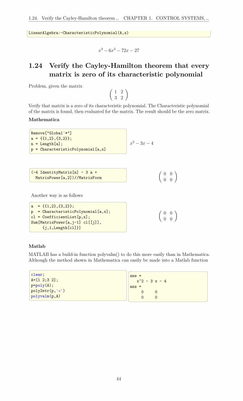
1.24 Verify the Cayley-Hamilton theorem that everymatrix is zero of its characteristic polynomial
Problem, given the matrix (1 2
3 2
)Verify that matrix is a zero of its characteristic polynomial. The Characteristic polynomialof the matrix is found, then evaluated for the matrix. The result should be the zero matrix.
Mathematica Remove["Global`*"]a = 1,2,3,2;n = Length[a];p = CharacteristicPolynomial[a,x]
x2 − 3x− 4
(-4 IdentityMatrix[n] - 3 a +MatrixPower[a,2])//MatrixForm
(0 0
0 0
)
Another way is as follows a = 1,2,3,2;p = CharacteristicPolynomial[a,x];cl = CoefficientList[p,x];Sum[MatrixPower[a,j-1] cl[[j]],
j,1,Length[cl]]
(0 0
0 0
)
MatlabMATLAB has a build-in function polyvalm() to do this more easily than in Mathematica.Although the method shown in Mathematica can easily be made into a Matlab function
clear;A=[1 2;3 2];p=poly(A);poly2str(p,'x')polyvalm(p,A)
ans =
x^2 - 3 x - 4ans =
0 00 0
44

1.25. How to check for stability of system… CHAPTER 1. CONTROL SYSTEMS, …
1.25 How to check for stability of system representedas a transfer function and state space
Problem: Given a system Laplace transfer function, check if it is stable, then convert tostate space and check stability again. In transfer function representation, the check is thatall poles of the transfer function (or the zeros of the denominator) have negative real part.In state space, the check is that the matrix A is negative definite. This is done by checkingthat all the eigenvalues of the matrix A have negative real part. The poles of the transferfunction are the same as the eigenvalues of the A matrix. Use
sys =5s
s2 + 4s+ 25
1.25.1 Checking stability using transfer function poles
Mathematica Remove["Global`*"];sys =TransferFunctionModel[(5s)/(s^2+4s+25),s];poles=TransferFunctionPoles[sys]
-2-I Sqrt[21],-2+I Sqrt[21]
Re[#]&/@poles
Out[42]= -2,-2
Select[%,#>=0&]
Out[44]=
Matlab clear all;s=tf('s');sys=5*s/( s^2+4*s+25);[z,p,k]=zpkdata(sys,'v');p
>>p =-2.0000 + 4.5826i-2.0000 - 4.5826i
find(real(p)>=0)
ans =
Empty matrix: 0-by-1
45

1.26. Check continuous system stability in … CHAPTER 1. CONTROL SYSTEMS, …
1.25.2 Checking stability using state space A matrix
Mathematica ss=StateSpaceModel[sys];a=ss[[1,1]]
Out[49]= 0,1,-25,-4
e=Eigenvalues[a]
Out[50]= -2+I Sqrt[21],-2-I Sqrt[21]
Re[#]&/@e
Out[51]= -2,-2
Select[%,#>=0&]
Out[52]=
Matlab sys=ss(sys);[A,B,C,D]=ssdata(sys);A
A =
-4.0000 -6.25004.0000 0
e=eig(A)
e =-2.0000 + 4.5826i-2.0000 - 4.5826i
find(real(e)>=0)
ans =
Empty matrix: 0-by-1
1.26 Check continuous system stability in theLyapunov sense
Problem: Check the stability (in Lyapunov sense) for the state coefficient matrix
A =
0 1 0
0 0 1
−1 −2 −3
The Lyapunov equation is solved using lyap() function in MATLAB and LyapunovSolve[]function in Mathematica, and then the solution is checked to be positive definite (i.e. allits eigenvalues are positive).
We must transpose the matrix A when calling these functions, since the Lyapunov equationis defined as ATP + PA = −Q and this is not how the software above defines them. Bysimply transposing the A matrix when calling them, then the result will be correct.
Mathematica
46

1.27. Given a closed loop block diagram, … CHAPTER 1. CONTROL SYSTEMS, …
Remove["Global`*"];(mat = 0,1,0,0,0,1,-1,-2,-3)
0 1 0
0 0 1
−1 −2 −3
p = LyapunovSolve[Transpose@mat,
-IdentityMatrix[Length[mat]]];MatrixForm[N[p]]
2.3 2.1 0.5
2.1 4.6 1.3
0.5 1.3 0.6
N[Eigenvalues[p]] 6.18272, 1.1149, 0.202375
Matlab clear all;
A=[0 1 00 0 1-1 -2 -3];
p=lyap(A.',eye(length(A)))
p =
2.3 2.1 0.52.1 4.6 1.30.5 1.3 0.6
e=eig(p)
e =
0.202381.11496.1827
Maple
with(LinearAlgebra):A:=<<0,1,0;0,0,1;-1,-2,-3>>;p,s:=LyapunovSolve(A^%T,-<<1,0,0;0,1,0;0,0,1>>);Eigenvalues(p);
6.18272045921436 + 0.0 i
1.11490451203192 + 0.0 i
0.202375028753723 + 0.0 i
1.27 Given a closed loop block diagram, generate theclosed loop Z transform and check its stability
Problem: Given the following block diagram, with sampling time T = 0.1 sec, generatethe closed loop transfer function, and that poles of the closed loop transfer function areinside the unit circle
47

1.27. Given a closed loop block diagram, … CHAPTER 1. CONTROL SYSTEMS, …
1Tss
Cs
ZOH Plant
T 1
Rs MsEss
s1
Ds
Gs
s1s5
System block diagram.
Mathematica Remove["Global`*"]plant = TransferFunctionModel[s/(1.0+s),s];plantd = ToDiscreteTimeModel[
plant,1,z,Method->"ZeroOrderHold"]
1. - 1. z
0.367879 - 1. z1.
d = ToDiscreteTimeModel[
TransferFunctionModel[(s+1)/(s+5.0),s],1,z,Method->"ZeroOrderHold"]
0.801348 - 1. z
0.00673795 - 1. z1.
sys=SystemsModelSeriesConnect[d,plantd]
(0.801348 - 1. z) (1. - 1. z)
(0.00673795 - 1. z) (0.367879 - 1. z) 1.
loopBack=SystemsModelFeedbackConnect[sys]
1.5825×10¹⁷ (-1. + 1. z) (-0.801348 + 1. z)
3.92264 ×10¹⁴ - 5.92834 ×10¹⁶ z + 1.5825×10¹⁷ z2 + 1.5825×10¹⁷ (-1. + 1. z) (-0.801348 + 1. z) 1.
Now generate unit step response ListPlot[OutputResponse[loopBack,
Table[1, k, 0, 20]],Joined->True,PlotRange->All,InterpolationOrder->0,Frame->True,PlotStyle->Thick,Red,GridLines->Automatic,
48

1.27. Given a closed loop block diagram, … CHAPTER 1. CONTROL SYSTEMS, …
GridLinesStyle->Dashed,FrameLabel->"y(k)",None,"n","plant response",
RotateLabel->False]
5 10 15 20
-0.1
0.0
0.1
0.2
0.3
0.4
0.5
n
y(k)
plant response
ss=StateSpaceModel[loopBack]
0 1. 0-0.401913 1.08798 1.0.199717 -0.356683 0.5 1.
poles=TransferFunctionPoles[loopBack]
0.543991 − 0.325556i, 0.543991 + 0.325556i Abs[#]&/@poles
(0.633966, 0.633966
)Poles are inside the unit circle, hence stable.
Matlab clear all; close all
s = tf('s');plant = s/(s+1);T = 1; %sampeling time;plantd = c2d(plant,T,'zoh');d = c2d( (s+1)/(s+5), T , 'zoh');% obtain the open loopsys = series(d,plantd);% obtain the closed looploop = feedback(sys,1) loop =
z^2 - 1.801 z + 0.8013------------------------2 z^2 - 2.176 z + 0.8038
Sample time: 1 seconds
49
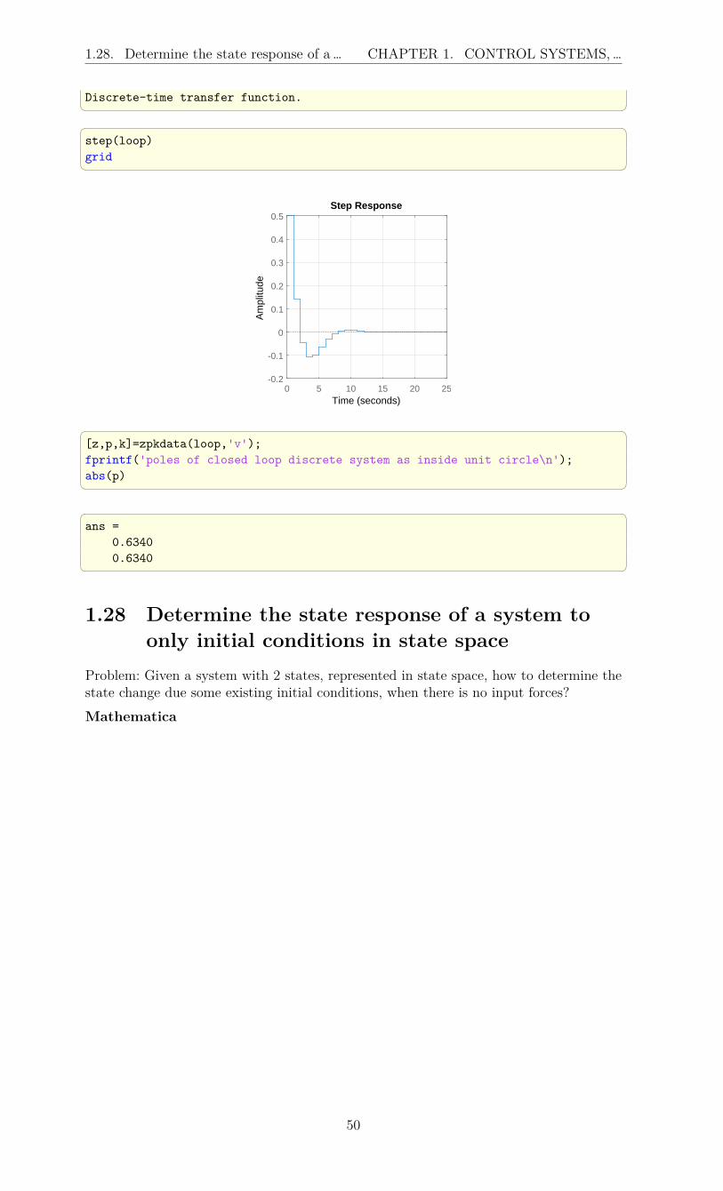
1.28. Determine the state response of a … CHAPTER 1. CONTROL SYSTEMS, …
Discrete-time transfer function. step(loop)grid
0 5 10 15 20 25-0.2
-0.1
0
0.1
0.2
0.3
0.4
0.5Step Response
Time (seconds)
Am
plitu
de
[z,p,k]=zpkdata(loop,'v');fprintf('poles of closed loop discrete system as inside unit circle\n');abs(p) ans =
0.63400.6340
1.28 Determine the state response of a system toonly initial conditions in state space
Problem: Given a system with 2 states, represented in state space, how to determine thestate change due some existing initial conditions, when there is no input forces?
Mathematica
50

1.28. Determine the state response of a … CHAPTER 1. CONTROL SYSTEMS, …
Remove["Global`*"];a = -0.5572,-0.7814,0.7814, 0;c = 1.9691, 6.4493;sys=StateSpaceModel[
a,1,0,c,0] -0.5572 -0.7814 10.7814 0 01.9691 6.4493 0
x0 = 1,0;x1,x2 = StateResponse[
sys,x0,0,t,0,20];
Plot[x1,x2,t,0,20,PlotRange->All,GridLines->Automatic,GridLinesStyle->Dashed,Frame->True,ImageSize->350,AspectRatio->1,FrameLabel->"y(t)",None,"t","first and second state\change with time",RotateLabel->False,PlotStyle->Red,Blue,BaseStyle -> 12]
0 5 10 15 20
-0.4
-0.2
0.0
0.2
0.4
0.6
0.8
1.0
t
y(t)
first and second state change with time
Matlab clear;A = [-0.5572 -0.7814;0.7814 0];B = [1;0];C = [1.9691 6.4493];x0 = [1 ; 0];
sys = ss(A,B,C,[]);
[y,t,x]=initial(sys,x0,20);plot(t,x(:,1),'r',t,x(:,2),'b');title('x1 and x2 state change with time');xlabel('t (sec)');ylabel('x(t)');gridset(gcf,'Position',[10,10,320,320]);
0 5 10 15 20
t (sec)
-0.4
-0.2
0
0.2
0.4
0.6
0.8
1
x(t)
x1 and x2 state change with time
51

1.29. Determine the response of a system… CHAPTER 1. CONTROL SYSTEMS, …
1.29 Determine the response of a system to onlyinitial conditions in state space
Problem: Given a system represented by state space, how to determine the response y(t)due some existing initial conditions in the states. There is no input forces.
Mathematica Remove["Global`*"];a = -0.5572, -0.7814, 0.7814, 0;c = 1.9691, 6.4493;sys=StateSpaceModel[a,1,0,c,0]
-0.5572 -0.7814 10.7814 0 01.9691 6.4493 0
x0 = 1,0; (*initial state vector*)y = OutputResponse[sys,x0,0,t,0,20];Plot[y,t,0,20,PlotRange->All,GridLines->Automatic,GridLinesStyle->Dashed,Frame->True,ImageSize->300,AspectRatio->1,FrameLabel->"y(t)",None,
"t","system response",RotateLabel->False,PlotStyle->Red]
0 5 10 15 20
-1
0
1
2
3
4
t
y(t)
system response
Matlab clear all;
A = [-0.5572 -0.7814;0.7814 0];
B = [1;0];C = [1.9691 6.4493];x0 = [1 ; 0];
sys = ss(A,B,C,[]);
[y,t,x]=initial(sys,x0,20);plot(t,y);title('y(t) plant response');xlabel('t (sec)');ylabel('y(t)');gridset(gcf,'Position',...
[10,10,320,320]);
0 5 10 15 20
t (sec)
-2
-1
0
1
2
3
4
5
y(t)
y(t) plant response
52

1.30. Determine the response of a system… CHAPTER 1. CONTROL SYSTEMS, …
1.30 Determine the response of a system to stepinput with nonzero initial conditions
Problem: Given a system represented by state space, how to determine the response withnonzero initial conditions in the states and when the input is a step input?
Mathematica Remove["Global`*"];a = -0.5572, -0.7814, 0.7814, 0;c = 1.9691, 6.4493;sys=StateSpaceModel[
a,1,0,c,0] -0.5572 -0.7814 10.7814 0 01.9691 6.4493 0
x0 = 1,0;y = OutputResponse[sys,x0,
UnitStep[t],t,0,20];
Plot[y,t,0,20,PlotRange->0,20,0,13,GridLines->Automatic,GridLinesStyle->Dashed,Frame->True,ImageSize->300,AspectRatio->1,FrameLabel->"y(t)",None,"t","system response to initial\
conditions and step input",RotateLabel->False,PlotStyle->Red]
0 5 10 15 200
2
4
6
8
10
12
t
y(t)
system response to combined initial conditions and step input
Matlab A = [-0.5572 -0.7814;0.7814 0];B = [1;0];C = [1.9691 6.4493];x0 = [1 ; 0];
sys = ss(A,B,C,[]);
[y1,t] = initial(sys,x0,20);y2 = step(sys,t);
plot(t,y1+y2,'r');
title(['initial conditions and step'...'input response']);
xlabel('t *sec)'); ylabel('y(t)');gridset(gcf,'Position',[10,10,320,320]);
0 5 10 15 20
t *sec)
0
2
4
6
8
10
12
y(t)
initial conditions and step input response
53

1.31. Draw the root locus from the open… CHAPTER 1. CONTROL SYSTEMS, …
1.31 Draw the root locus from the open looptransfer function
Problem: Given L(s), the open loop transfer function, draw the root locus. Let
L(s) =s2 + 2s+ 4
s(s+ 4)(s+ 6)(s2 + 1.4s+ 1)
Root locus is the locus of the closed loop dominant pole as the gain k is varied from zeroto infinity.Mathematica
Remove["Global`*"]sys = TransferFunctionModel[k*(s^2+2 s+4)/
(s(s+4)(s+6)(s^2+1.4s+1)),s];RootLocusPlot[sys,k,0,100,
ImageSize->300,GridLines->Automatic,GridLinesStyle->Dashed,Frame->True,AspectRatio -> 1]
-8 -6 -4 -2 0
-2
-1
0
1
2
Matlab
clear all; close all;s=tf('s');sys=(s^2+2*s+4)/...(s*(s+4)*(s+6)*(s^2+1.4*s+1));
rlocus(sys,0:100)set(gcf,'Position',[10,10,420,420]);
-10 -8 -6 -4 -2 0 2-3
-2
-1
0
1
2
3Root Locus
Real Axis (seconds-1)
Imag
inar
y A
xis
(sec
onds
-1)
1.32 Find exp(A t) where A is a matrixMathematica ClearAll["Global`*"]mat=0,1,
-2,-3MatrixExp[mat t];MatrixForm[%]
(−e−2t + 2e−t −e−2t + e−t
2e−2t − 2e−t 2e−2t − e−t
)
Now verify the result by solving for eAt using the method would one would do by hand,if a computer was not around. There are a number of methods to do this by hand. The
54
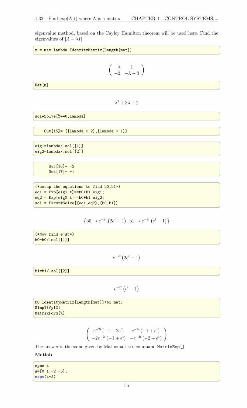
1.32. Find exp(A t) where A is a matrix CHAPTER 1. CONTROL SYSTEMS, …
eigenvalue method, based on the Cayley Hamilton theorem will be used here. Find theeigenvalues of |A− λI| m = mat-lambda IdentityMatrix[Length[mat]]
(−λ 1
−2 −λ− 3
) Det[m]
λ2 + 3λ+ 2 sol=Solve[%==0,lambda]
Out[15]= lambda->-2,lambda->-1 eig1=lambda/.sol[[1]]eig2=lambda/.sol[[2]]
Out[16]= -2Out[17]= -1
(*setup the equations to find b0,b1*)eq1 = Exp[eig1 t]==b0+b1 eig1;eq2 = Exp[eig2 t]==b0+b1 eig2;sol = First@Solve[eq1,eq2,b0,b1]
b0 → e−2t
(2et − 1
), b1 → e−2t
(et − 1
) (*Now find e^At*)b0=b0/.sol[[1]]
e−2t(2et − 1
) b1=b1/.sol[[2]]
e−2t(et − 1
) b0 IdentityMatrix[Length[mat]]+b1 mat;Simplify[%]MatrixForm[%]
(e−2t (−1 + 2et) e−2t (−1 + et)
−2e−2t (−1 + et) −e−2t (−2 + et)
)The answer is the same given by Mathematica’s command MatrixExp[]
Matlab syms tA=[0 1;-2 -3];expm(t*A)
55

1.33. Draw root locus for a discrete system CHAPTER 1. CONTROL SYSTEMS, …
ans =
[2/exp(t)-1/exp(2*t),1/exp(t)-1/exp(2*t)][2/exp(2*t)-2/exp(t),2/exp(2*t)-1/exp(t)] pretty(ans) +- -+| 2 exp(-t)- exp(-2 t),exp(-t)-exp(-2 t) || || 2 exp(-2 t)-2 exp(-t),2 exp(-2 t)-exp(-t)|+- -+ Maple restart;A:=Matrix([[0,1],[-2,-3]]);LinearAlgebra:-MatrixExponential(A,t);
[−e−2t + 2 e−t e−t − e−2t
−2 e−t + 2 e−2t 2 e−2t − e−t
]
1.33 Draw root locus for a discrete systemProblem: Given the open loop for a continuous time system as
sys =5s+ 1
s2 + 2s+ 3
convert to discrete time using a sampling rate 0.5 second, and display the root locus forthe discrete system.
Mathematica
56

1.33. Draw root locus for a discrete system CHAPTER 1. CONTROL SYSTEMS, …
Remove["Global`*"];sys=TransferFunctionModel[
k(5s+1)/(s^2+2s+3),s];
samplePeriod=0.5; (*sec*)sysd=ToDiscreteTimeModel[sys,samplePeriod,z]
-19. k + 2. k z + 21. k z2
11. - 26. z + 27. z20.5
p1 = RootLocusPlot[sysd,k,0,100,
ImageSize->300,GridLines->Automatic,GridLinesStyle->Dashed,Frame->True,AspectRatio->1,PlotPoints->200,PlotStyle->PointSize[0.01]];
p2=ParametricPlot[Sin[t],Cos[t],t,0,2Pi,AspectRatio->1,GridLines->Automatic,GridLinesStyle->Dashed];
Show[p2,p1]
-1.0 -0.5 0.5 1.0
-1.0
-0.5
0.5
1.0
Matlab
clear all; close all;s = tf('s');sys = (5*s+1)/(s^2+2*s+3);Ts = 0.5; %sample timesysd = c2d(sys,Ts,'zoh');
rlocus(sysd)grid
-1 -0.5 0 0.5 1-1
-0.8
-0.6
-0.4
-0.2
0
0.2
0.4
0.6
0.8
1
0.8:/T
0.9:/T
1:/T
0.1:/T
0.2:/T
0.3:/T
0.4:/T0.5:/T
0.6:/T
0.7:/T
0.8:/T
0.9:/T
1:/T
0.1:/T
0.2:/T
0.3:/T
0.4:/T0.5:/T
0.6:/T
0.7:/T
0.10.2
0.30.40.50.60.70.80.9
Root Locus
Real Axis
Imag
inar
y A
xis
Maple
restart;alias(DS=DynamicSystems):sys := DS:-TransferFunction((5*s+1)/(s^2+2*s+3));T :=1/2; #will fail if 0.5 is used !!sys := DS:-ToDiscrete(sys, T, 'method'='zoh');DS:-RootLocusPlot(sys,-1..1,gridlines);
57

1.34. Plot the response of the inverted… CHAPTER 1. CONTROL SYSTEMS, …
1.34 Plot the response of the inverted pendulumproblem using state space
Problem: Given the inverted pendulum shown below, use state space using one input (theforce on the cart) and 2 outputs (the cart horizontal displacement, and the pendulumangle. Plot each output separately for the same input.
mg
u
y
First system output
second system output
system input
M
Cart with inverted pendulum. One input, 2 outputs
M=20 kg
m=1 kg
g=9.8 m/s^2
L=1 meter
Mathematica Remove["Global`*"];a = 0, 1, 0, 0,
0, 0, ((-m)*g)/M, 0,0, 0, 0, 1,0, 0, ((M + m)*g)/(M*L), 0;
0 1 0 0
0 0 −gmM
0
0 0 0 1
0 0 g(m+M)LM
0
b = 0, 1/M, 0, -(1/(M*L));MatrixForm[b]
01M
0
− 1LM
c = 1, 0, 0, 0, 0, 0, 1, 0;MatrixForm[b]
(1 0 0 0
0 0 1 0
) sys=StateSpaceModel[a,b ,c]
58

1.34. Plot the response of the inverted… CHAPTER 1. CONTROL SYSTEMS, …
0 1 0 0 0
0 0 -g m
M0
1
M0 0 0 1 0
0 0g (m + M)
L M0 -
1
L M1 0 0 0 00 0 1 0 0
It is now possible to obtain the response of the system as analytical expression or aninterpolatingFunction.
It is much more efficient to obtain the response as interpolatingFunction. This requiresthat the time domain be given.
Here is example of obtaining the analytical expression of the response sys=sys/.g->9.8,m->1,M->20,L->1;y=Chop[OutputResponse[sys,UnitStep[t],t]] e−6.41561t(0.0238095e6.41561tt2θ(t) + 0.000115693e3.2078tθ(t)− 0.000231385e6.41561tθ(t) + 0.000115693e9.62341tθ(t))
, e−6.41561t(−0.00242954e3.2078tθ(t) + 0.00485909e6.41561tθ(t)− 0.00242954e9.62341tθ(t)) Plot[y[[1]],t,0,3,PlotLabel->"y(t) response",FrameLabel->"time (sec)","y (meter)",Frame->True,PlotRange->All,ImageSize->300,GridLines->Automatic,GridLinesStyle->Dashed,RotateLabel->False]
0.0 0.5 1.0 1.5 2.0 2.5 3.0
0.0
0.5
1.0
1.5
2.0
time (sec)
y (meter)
y(t) response
Plot[ y[[2]],t,0,3,PlotLabel->"\[Theta](t) response",FrameLabel->"time (sec)","\[Theta] (radians)",Frame->True,PlotRange->All,ImageSize->300,GridLines->Automatic,GridLinesStyle->Dashed,RotateLabel->False]
59

1.34. Plot the response of the inverted… CHAPTER 1. CONTROL SYSTEMS, …
0.0 0.5 1.0 1.5 2.0 2.5 3.0
-30
-20
-10
0
time (sec)
θ (radians)
θ(t) response
Matlab clear all; close all;
m=1; M=20; L=1; g=9.8;
A=[0 1 0 0;0 0 -m*g/M 0;0 0 0 1;0 0 (M+m)*g/(M*L) 0];
B=[0 1/M 0 -1/(M*L)]';C=[1 0 0 0;
0 0 1 0];D=[0];
sys=ss(A,B,C(1,:),0);step(sys,3);grid on;set(gcf,'Position',[10,10,320,320]);title('y(t) due to step input');
0 1 2 30
0.5
1
1.5
2y(t) due to step input
Time (seconds)
Am
plitu
de
figure;sys=ss(A,B,C(2,:),0);step(sys,3);title('\theta(t) due to step input');grid on;set(gcf,'Position',[10,10,320,320]);
60

1.35. How to build and connect a closed… CHAPTER 1. CONTROL SYSTEMS, …
0 1 2 3-40
-30
-20
-10
03(t) due to step input
Time (seconds)
Am
plitu
de
1.35 How to build and connect a closed loop controlsystems and show the response?
1.35.1 example 1, single input, single output closed loopGiven the following simple closed loop system, show the step response. Let mass M = 1kg,damping coefficient c = 1newton-seconds per meter and let the stiffness coefficient bek = 20newton per meter.
plant
Js
controller
Gs YsFs
1
ms2csk
Fs
YsYrs +-es
Using propertional controller J(s) = kp where kp = 400. First connect the system andthen show y(t) for 5 seconds when the reference yr(t) is a unit step function.
Mathematica
m = 1; c = 1; k = 20; kp = 400;plant = TransferFunctionModel[1/(m s^2 + c s + k), s];controller = TransferFunctionModel[kp, s];sys = SystemsModelSeriesConnect[plant, controller];sys = SystemsModelFeedbackConnect[sys];o = OutputResponse[sys, UnitStep[t], t];Plot[o, t, 0, 10, Frame -> True, PlotRange -> All,FrameLabel -> "y(t)", None,
"t (sec)", "response of closed loop",BaseStyle -> 14]
0 2 4 6 8 10
0.0
0.5
1.0
1.5
t (sec)
y(t)
response of closed loop
61

1.35. How to build and connect a closed… CHAPTER 1. CONTROL SYSTEMS, …
Matlab close all;m = 1; c = 1; k = 20;s = tf('s');plant = 1/(m*s^2+c*s+k);controller = 400;sys = series(controller,plant);sys = feedback(sys,1);[Y,T] = step(sys,0:.01:10);plot(T,Y);xlabel('time (sec)');ylabel('y(t)');title('response of closed loop'); Another way to do the above is m=1;c=1;k=20;s=tf('s');sys3=1/(m*s^2+c*s+k);sys2=400;sys1=1;sys=append(sys1,sys2,sys3);Q=[2 1 -3;3 2 0];input=[1];output=[2 3];sys=append(sys1,sys2,sys3);sys=connect(sys,Q,input,output);T=0:.01:10;[Y,T,X]=step(sys,T);
0 2 4 6 8 10
time (sec)
0
0.2
0.4
0.6
0.8
1
1.2
1.4
1.6
1.8
2
y(t)
response of closed loop
62

1.36. Compare the effect on the step… CHAPTER 1. CONTROL SYSTEMS, …
1.36 Compare the effect on the step response of astandard second order system as ζ changes
Problem: Given a standard second order system defined by the transfer function
G (s) =ω2n
s2 + 2ζωns+ ω2n
Change ζ and plot the step response for each to see the effect of changing ζ (the dampingcoefficient).It is easy to solve this using the step command in Matlab, and similarly in Mathematicaand Maple. But here it is solved directly from the differential equation.The transfer function is written as
Y (s)
U (s)=
ω2n
s2 + 2ζωns+ ω2n
Where Y (s) and U (s) are the Laplace transforms of the output and input respectively.Hence the differential equation, assuming zero initial conditions becomes
y′′ (t) + 2ζωn y′ (t) + ω2n y (t) = ω2
n u (t)
To solve the above in Matlab using ode45, the differential equation is converted to 2 firstorder ODE’s as was done before resulting in[
x′1
x′2
]=
[0 1
−ω2n −2ζωn
] [x1
x2
]+
[0
ω2n
]u (t)
For a step input, u (t) = 1, we obtain[x′1
x′2
]=
[0 1
−ω2n −2ζωn
] [x1
x2
]+
[0
ω2n
]Now ODE45 can be used. In Mathematica the differential equation is solved directly usingDSolve and no conversion is needed.Mathematica
solve[z_]:=Module[sol,eq,y,t,w=1,eq=y''[t]+2 z w y'[t]+
w^2 y[t]==w^2 UnitStep[t];sol=First@NDSolve[eq,y[0]==0,y'[0]==0,y[t],t,0,15
];
Plot[y[t]/.sol,t,0,15,PlotPoints->30,PlotRange->All,Frame->True,FrameLabel->"y(t)",None,"time (sec)","step response,Subscript[\[Omega], n]=1"
<>", different \[Xi]",ImageSize->400,PlotStyle->RGBColor[2z,z/2,z/3],LabelStyle->Directive[14]]
];
zeta = Range[0,1.4,.2];r = Map[solve,zeta];Show[r,GridLines->Automatic,
GridLinesStyle->Dashed] 63
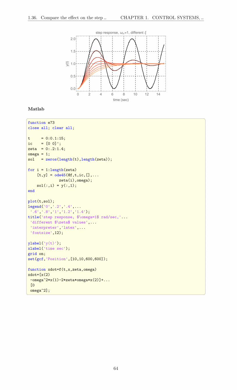
1.36. Compare the effect on the step… CHAPTER 1. CONTROL SYSTEMS, …
0 2 4 6 8 10 12 14
0.0
0.5
1.0
1.5
2.0
time (sec)
y(t)
step response, ωn=1, different ξ
Matlab
function e73close all; clear all;
t = 0:0.1:15;ic = [0 0]';zeta = 0:.2:1.4;omega = 1;sol = zeros(length(t),length(zeta));
for i = 1:length(zeta)[t,y] = ode45(@f,t,ic,[],...
zeta(i),omega);sol(:,i) = y(:,1);
end
plot(t,sol);legend('0','.2','.4',...'.6','.8','1','1.2','1.4');title('step response, $\omega=1$ rad/sec,'...'different $\zeta$ values',...'interpreter','latex',...'fontsize',12);
ylabel('y(t)');xlabel('time sec');grid on;set(gcf,'Position',[10,10,600,600]);
function xdot=f(t,x,zeta,omega)xdot=[x(2)-omega^2*x(1)-2*zeta*omega*x(2)]+...[0omega^2];
64

1.37. Plot the dynamic response factor Rd … CHAPTER 1. CONTROL SYSTEMS, …
0 5 10 15
time sec
0
0.2
0.4
0.6
0.8
1
1.2
1.4
1.6
1.8
2
y(t)
step response, ! = 1 rad/sec, di,erent 1 values
0.2.4.6.811.21.4
1.37 Plot the dynamic response factor Rd of asystem as a function of r = ω
ωnfor different
damping ratiosProblem: Plot the standard curves showing how the dynamic response Rd changes asr = ω
ωnchanges. Do this for different damping ratio ξ. Also plot the phase angle.
These plots are result of analysis of the response of a second order damped system to aharmonic loading. ω is the forcing frequency and ωn is the natural frequency of the system.
Mathematica
65

1.38. How to find closed loop step response … CHAPTER 1. CONTROL SYSTEMS, …
Rd[r_,z_]:=1/Sqrt[(1-r^2)^2+(2 z r)^2];
phase[r_,z_]:=Module[t,t=ArcTan[(2z r)/(1-r^2)];If[t<0,t=t+Pi];180/Pi t
];
plotOneZeta[z_,f_] := Module[r,p1,p2,p1 = Plot[f[r,z],r,0,3,PlotRange->All,
PlotStyle->Blue];
p2 = Graphics[Text[z,1.1,1.1f[1.1,z]]];Show[p1,p2]];
p1 = Graphics[Red,Line[1,0,1,6]];p2 = Map[plotOneZeta[#,Rd]&,Range[.1,1.2,.2]];
Show[p2,p1,FrameLabel->"Subscript[R, d]",None,"r= \[Omega]/Subscript[\[Omega], n]","Dynamics Response vs. Frequency\
ratio for different \[Xi]",Frame->True,GridLines->Automatic,GridLinesStyle->Dashed,ImageSize -> 300,AspectRatio -> 1]
0.1
0.3
0.50.70.91.1
0.0 0.5 1.0 1.5 2.0 2.5 3.0
0
1
2
3
4
5
6
r=ω
ωn
Rd
Dynamics Response vs. Frequency ratio for different ξ
p = Map[plotOneZeta[#,phase]&,Range[.1,1.2,.2]];Show[p,FrameLabel->"Phase in degrees",None,"r= \[Omega]/Subscript[\[Omega], n]","Phase vs. Frequency ratio for different \[Xi]",Frame->True,GridLines->Automatic,GridLinesStyle->Dashed,ImageSize->300,AspectRatio->1]
0.1
0.30.50.70.91.1
0.0 0.5 1.0 1.5 2.0 2.5 3.0
0
50
100
150
r=ω
ωn
Phaseindegrees
Phase vs. Frequency ratio for different ξ
1.38 How to find closed loop step response to aplant with a PID controller?
Find and plot the step response of the plant 1s2+2s+1
connected to a PID controller withP = 10, I = 3.7, D = 0.7. Use negative closed loopback.
Mathematica
66
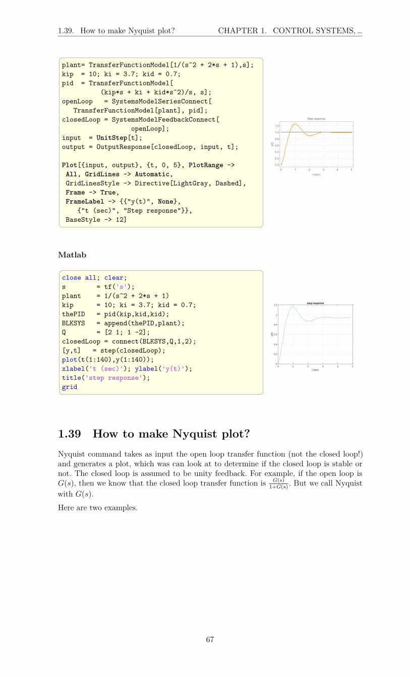
1.39. How to make Nyquist plot? CHAPTER 1. CONTROL SYSTEMS, …
plant= TransferFunctionModel[1/(s^2 + 2*s + 1),s];kip = 10; ki = 3.7; kid = 0.7;pid = TransferFunctionModel[
(kip*s + ki + kid*s^2)/s, s];openLoop = SystemsModelSeriesConnect[
TransferFunctionModel[plant], pid];closedLoop = SystemsModelFeedbackConnect[
openLoop];input = UnitStep[t];output = OutputResponse[closedLoop, input, t];
Plot[input, output, t, 0, 5, PlotRange ->All, GridLines -> Automatic,GridLinesStyle -> Directive[LightGray, Dashed],Frame -> True,FrameLabel -> "y(t)", None,
"t (sec)", "Step response",BaseStyle -> 12]
0 1 2 3 4 5
0.0
0.2
0.4
0.6
0.8
1.0
1.2
t (sec)
y(t)
Step response
Matlab close all; clear;s = tf('s');plant = 1/(s^2 + 2*s + 1)kip = 10; ki = 3.7; kid = 0.7;thePID = pid(kip,kid,kid);BLKSYS = append(thePID,plant);Q = [2 1; 1 -2];closedLoop = connect(BLKSYS,Q,1,2);[y,t] = step(closedLoop);plot(t(1:140),y(1:140));xlabel('t (sec)'); ylabel('y(t)');title('step response');grid
0 1 2 3 4 5
t (sec)
0
0.2
0.4
0.6
0.8
1
1.2
y(t)
step response
1.39 How to make Nyquist plot?Nyquist command takes as input the open loop transfer function (not the closed loop!)and generates a plot, which was can look at to determine if the closed loop is stable ornot. The closed loop is assumed to be unity feedback. For example, if the open loop isG(s), then we know that the closed loop transfer function is G(s)
1+G(s). But we call Nyquist
with G(s).
Here are two examples.
67

1.39. How to make Nyquist plot? CHAPTER 1. CONTROL SYSTEMS, …
1.39.1 Example 1Given G(s) = s
1−0.2sgenerate Nyquist plot.
Mathematica
NyquistPlot[s/(1 - 0.2 s),
NyquistGridLines -> Automatic] -5 -4 -3 -2 -1
-2
-1
1
2
Matlab
clear all; close all;nyquist([1 0],[-0.2 1])grid
-5 -4 -3 -2 -1 0 1-2.5
-2
-1.5
-1
-0.5
0
0.5
1
1.5
2
2.5
-10 dB
0 dB
-6 dB
-4 dB
-2 dB
10 dB
6 dB
4 dB
2 dB
Nyquist Diagram
Real Axis
Imag
inar
y A
xis
1.39.2 Example 2
Given G(s) = 5(1−0.5s)s(1+0.1s)(1−0.25s)
generate Nyquist plot.
Mathematica
NyquistPlot[5(1-0.5 s)/
(s(1 + 0.1 s)(1 - 0.25 s))] -1
-2
2
Matlab
68

1.39. How to make Nyquist plot? CHAPTER 1. CONTROL SYSTEMS, …
clear all; close all;s=tf('s');sys=5*(1-0.5*s)/...
(s*(1+0.1*s)*(1-0.25*s))
2.5 s - 5
------------------------0.025 s^3 + 0.15 s^2 - s
Continuous-time transfer function.
nyquist(sys)
-1.8 -1.6 -1.4 -1.2 -1 -0.8 -0.6 -0.4 -0.2 0-40
-30
-20
-10
0
10
20
30
40Nyquist Diagram
Real Axis
Imag
inar
y A
xis
However, there is a better function to do this called nyquist1.m which I downloaded andtried. Here is its results
clear all; close all;nyquist1()
-1 -0.8 -0.6 -0.4 -0.2 0 0.2-0.15
-0.1
-0.05
0
0.05
0.1
0.15Nyquist Diagram
Real Axis
Imag
inar
y A
xis
69

1.39. How to make Nyquist plot? CHAPTER 1. CONTROL SYSTEMS, …
70

Chapter 2
Linear algebra, Linear solvers,common operations on vectors andmatrices
2.1 introductionMathematica and Matlab allow one to do pretty much the same operations in the area oflinear algebra and matrix manipulation. Two things to keep in mind is that Mathematicauses a more general way to store data.Mathematica uses ragged arrays or a list of lists. This means rows can have different sizes.(these are the lists inside the list). So a Mathematica matrix is stored in a list of lists. Thisis similar in a way to Matlab cell data structure, since each raw can have different length.In a standard matrix each row must have the same length.In Matlab one can also have ragged arrays, these are called cells. In Mathematica, thereis one data structure for both.Another thing to keep in mind is that Matlab, due to its Fortran background is column ma-jor when it comes to operations on matrices. This simple example illustrate this difference.Suppose we have a matrix A of 3 rows, and want to find the location where A(i, j) = 2where i is the row number and j is the column number. Given this matrix
A =
1 2 3 4
2 3 1 5
5 6 7 2
Then the result of using the find() command in Matlab is A=[1 2 3 4;
2 3 1 5;5 6 7 2];
[I,J]=find(A==2) I =
213
J =124]
The Matlab result gives the order of the rows it found the element at based on searchingcolumn wise since it lists the second row first in its result. Compare this to MathematicaPosition[] command
71

2.2. Multiply matrix with a vector CHAPTER 2. LINEAR ALGEBRA,…
mat = 1, 2, 3, 4,
2, 3, 1, 5,5, 6, 7, 2
Position[mat, 2] which gives 1,2,2,1,3,4 Mathematica searched row-wise.
I found Mathematica for matrix operations takes more time to get familiar with comparedto Matlab’s, since Mathematica data structure is more general and therefore a little morecomplex (ragged arrays, or list of lists is its main data structure) compared to Matlab’s.This is because Mathematica has to also support symbolics in its commands and not justnumerical data.
In Maple the following short cuts can be used enter vectors and matrices: For row vector:v:=<1|2|3|4> and for column vector v:=<1,2,3,4> and for a Matrix of say 2 rows
and 3 columns A:=<1,2|3,4|5,6>. Here | acts as a column separator. For transpose ofmatrix, A^%T is the short cut notation.
2.2 Multiply matrix with a vectorHow to perform the following matrix/vector multiplication? [ 1 2 3 ] [ 1 ][ 4 5 6 ] * [ 2 ][ 7 8 8 ] [ 3 ] In Mathematica the dot ”.” is used for Matrix multiplication. In Matlab the ”*” is used.In Fortran, MATMUL is used.
Mathematica a=1,2,3,4,5,6,7,8,8;x=1,2,3;
a.x Out[7]= 14,32,47
Matlab A=[1 2 3;4 5 6;7 8 9];x=[1; 2; 3];c=A*x
143250
72

2.2. Multiply matrix with a vector CHAPTER 2. LINEAR ALGEBRA,…
JuliaSame exact code as Matlab. julia> A=[1 2 3;4 5 6;7 8 9]3×3 MatrixInt64:1 2 34 5 67 8 9
julia> x=[1;2;3]3-element VectorInt64:123
julia> c=a*x3-element VectorInt64:143250
Ada with Ada.Text_Io; use Ada.Text_Io;with Ada.Numerics.Real_Arrays;
use Ada.Numerics.Real_Arrays;
procedure t1 isA : constant real_matrix :=
(( 1.0, 2.0, 3.0),( 4.0, 5.0, 6.0),( 7.0, 8.0, 9.0));
V : constant real_vector := (1.0,2.0,3.0);procedure Put (X : real_vector) is
beginFOR e of X LOOP
put_line(float'image(e));END LOOP;
end put;begin
put(A*v);end t1; compile and run >gnatmake -gnat2012 t1.adbgcc -c -gnat2012 t1.adbgnatbind -x t1.alignatlink t1.ali>./t11.40000E+013.20000E+015.00000E+01
73

2.2. Multiply matrix with a vector CHAPTER 2. LINEAR ALGEBRA,…
Fortran PROGRAM mainIMPLICIT NONEinteger, parameter :: dp = kind(1.D0)integer, parameter :: N=3real(kind=dp), parameter, DIMENSION(N, N) :: &
A=DBLE(reshape([ 1.0, 2.0, 3.0,&4.0, 5.0, 6.0,&7.0, 8.0, 9.0], shape(A), &
order=[2,1]))
real(kind=dp), parameter, DIMENSION(N, 1) :: &x=DBLE(reshape([1.0, 2.0, 3.0], shape(x)))
real(kind=dp), DIMENSION(N, 1) :: resultinteger, DIMENSION(2) :: siz
result = MATMUL(A,x)siz = SHAPE(result)Write(*,*) result
print *, "number of rows = ",siz(1)print *, "number of columns = ",siz(2)
end program compile and run >gfortran -fcheck=all -Wall -Wconversion
-Wextra -Wconversion-extra -pedantic test.f90>./a.out14.000000000000000 32.000000000000000 50.000000000000000number of rows = 3number of columns = 1
Maple
A:=Matrix([[1,2,3],[4,5,6],[7,8,9]]):x:=Vector([1,2,3]): #default is column vectorc:=A.x;
14
32
50
Python
import numpy as npmat=np.array([[1,2,3],[4,5,6],[7,8,8]])b=np.array([1,2,3])b.shape=(3,1)r=dot(mat,b)
array([[14],
[32],[47]])
74

2.3. Insert a number at specific position in … CHAPTER 2. LINEAR ALGEBRA,…
2.3 Insert a number at specific position in a vectoror list
The problem is to insert a number into a vector given the index.
Mathematica vec=1,2,3,4;vec=Insert[vec,99,3];vec
Out[11]= 1,2,99,3,4
Matlab A=[1 2 3 4];A=[ A(1:2) 99 A(3:end) ]
A =
1 2 99 3 4 Julia A=[1,2,3,4];A=insert!(A,3,99)'
1×5 adjoint(::VectorInt64) with eltype Int64:1 2 99 3 4
Fortran program fimplicit noneREAL(4), ALLOCATABLE :: A(:)A=[1,2,3,4];A=[A(1:2), 99.0, A(3:)]Print *,A
end program f
>gfortran -std=f2008 t2.f90>./a.out1.0000000 2.0000000 99.000000
3.0000000 4.0000000
Maple
v:=Vector[row]([1,2,3,4]);v:=Vector[row]([v[1..2],99,v[3..]]); Or Using <> notation v:=<1|2|3|4>;v:=<v(1..2)|99|v(3..)>;
v :=[ 1 2 99 3 4]
Python
Python uses zero index. import numpy as npb=np.array([1,2,3,4])b=numpy.insert(b,2,99)b
Out[86]: array([ 1, 2, 99, 3, 4])
75

2.4. Insert a row into a matrix CHAPTER 2. LINEAR ALGEBRA,…
2.4 Insert a row into a matrixThe problem is to insert a row into the second row position in a 2D matrix
Mathematica mat=1,2,3,
4,5,6,7,8,9
mat = Insert[mat,90,91,92,2]
1,2,3,90,91,92,4,5,6,7,8,9
Matlab A=[1 2 3;
4 5 6;7 8 9]
A=[ A(1,:); [90 91 92]; A(2:end,:) ]
1 2 3
90 91 924 5 67 8 9
Maple
Using <<>> notation A:=< <1|2|3>,
<4|5|6>,<7|8|9>>;
A:=< A(1..2,..),<90|91|92>, A(3,..)>; Using Matrix/Vector A:=Matrix([ [1,2,3],[4,5,6],[7,8,9]]);A:=Matrix([ [A[1..2,..]],
[Vector[row]([91,92,92])],[A[3,..]
] ]);
[ 1 2 34 5 690 91 927 8 9]
Python
import numpy as npmat=np.array([[1,2,3],
[4,5,6],[7,8,9]])
mat=numpy.insert(mat,1,[90,91,92],0)
array([[ 1, 2, 3],
[90, 91, 92],[ 4, 5, 6],[ 7, 8, 9]])
Fortran
76

2.5. Insert a column into a matrix CHAPTER 2. LINEAR ALGEBRA,…
program fimplicit noneinteger iinteger, allocatable :: A(:,:)integer, allocatable :: B(:)B =[90,91,92]A = reshape ([1,2,3, &
4,5,6, &7,8,9], [3,3], order=[2,1])
A=reshape([A(1,:), &B, &A(2:,:)], [4,3],order=[2,1])
do i=LBOUND(A, 1),UBOUND(A, 1)print *,A(i,:)
end doend program f
Compile and run >gfortran f.f90>./a.out1 2 390 91 924 7 58 6 9
2.5 Insert a column into a matrixThe problem is to insert a column into the second column position in a 2D matrix.
Mathematica mat = 1, 2, 3,
4, 5, 6,7, 8, 9;
mat = Insert[Transpose[mat],90, 91, 92, 2];
mat = Transpose[mat]
1,90,2,3,4,91,5,6,7,92,8,9
Matlab A=[1 2 3;
4 5 6;7 8 9];
A=[A(:,1) [90 91 92]' A(:,2:end) ]
1 90 2 34 91 5 67 92 8 9
Fortran
77

2.6. Build matrix from other matrices and… CHAPTER 2. LINEAR ALGEBRA,…
program t4implicit noneinteger(4) ::iinteger(4), ALLOCATABLE ::A(:,:)
A = reshape ([1,2,3, &4,5,6, &7,8,9], [3,3], order=[2,1])
A = reshape ([A(:,1), [90,91,92] ,A(:,2:)] , [3,4])
do i=LBOUND(A, 1),UBOUND(A, 1)print *,A(i,:)
end do
end program t4
>gfortran t4.f90>./a.out1 90 2 34 91 5 67 92 8 9
Maple
A:=< <1|2|3>,<4|5|6>,<7|8|9>>;A:=< A(..,1)|<90,91,92>|A(..,2..)>; Using Matrix/Vector A:=Matrix([ [1,2,3],[4,5,6],[7,8,9]]);A:=Matrix([ [A[..,1],
Vector[column]([91,92,92]),A[..,2..] ]]);
[ 1 90 2 34 91 5 67 92 8 9]
Python
import numpy as npmat=np.array([[1,2,3],
[4,5,6],[7,8,9]])
mat=numpy.insert(mat,1,[90,91,92],1)
array([[ 1, 90, 2, 3],
[ 4, 91, 5, 6],[ 7, 92, 8, 9]])
2.6 Build matrix from other matrices and vectors
2.6.1 First example
Given column vectors v1 =
1
2
3
and v2 =
4
5
6
and v3 =
7
8
9
and v4 =
10
11
12
generate the matrix m =
[v1 v2v3 v4
]=
1 4
2 5
3 6
7 10
8 11
9 12
78

2.6. Build matrix from other matrices and… CHAPTER 2. LINEAR ALGEBRA,…
Matlab was the easiest of all to do these operations with. No surprise, as Matlab wasdesigned for Matrix and vector operations. But I was surprised that Maple actually hadgood support for these things, using its <> notation, which makes working with matricesand vectors much easier.
The command ArrayFlatten is essential for this in Mathematica.
Notice the need to use Transpose[v] in order to convert it to a column matrix. Thisis needed since in Mathematica, a list can be a row or column, depending on context.
Mathematica v1 = 1, 2, 3; v2 = 4, 5, 6;v3 = 7, 8, 9; v4 = 10, 11, 12;m = ArrayFlatten[Transpose@v1, Transpose@v2,Transpose@v3, Transpose@v4
]
1 4
2 5
3 6
7 10
8 11
9 12
Matlab
v1=[1,2,3]'; v2=[4,5,6]';v3=[7,8,9]'; v4=[10,11,12]';m=[v1 v2;v3 v4]
m =
1 42 53 67 108 119 12
Maple
restart;v1:=<1,2,3>; #column by defaultv2:=<4,5,6>;v3:=<7,8,9>;v4:=<10,11,12>;m:=< <v1|v2>,
<v3|v4>>;
#or using Vector/Matrix notationsrestart;v1:=Vector([1,2,3]); #column by defaultv2:=Vector([4,5,6]); #column by defaultv3:=Vector([7,8,9]); #column by defaultv4:=Vector([10,11,12]); #column by defaultm:=Matrix([ [v1,v2],[v3,v4]])
1 4
2 5
3 6
7 10
8 11
9 12
Python
79
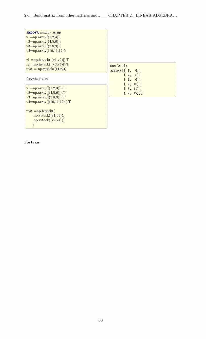
2.6. Build matrix from other matrices and… CHAPTER 2. LINEAR ALGEBRA,…
import numpy as npv1=np.array((1,2,3));v2=np.array((4,5,6));v3=np.array((7,8,9));v4=np.array((10,11,12));
r1 =np.hstack([(v1,v2)]).Tr2 =np.hstack([(v3,v4)]).Tmat = np.vstack((r1,r2)) Another way v1=np.array([(1,2,3)]).Tv2=np.array([(4,5,6)]).Tv3=np.array([(7,8,9)]).Tv4=np.array([(10,11,12)]).T
mat =np.hstack((np.vstack((v1,v3)),np.vstack((v2,v4)))
)
Out[211]:array([[ 1, 4],
[ 2, 5],[ 3, 6],[ 7, 10],[ 8, 11],[ 9, 12]])
Fortran
80

2.6. Build matrix from other matrices and… CHAPTER 2. LINEAR ALGEBRA,…
PROGRAM mainIMPLICIT noneINTEGER :: iINTEGER , DIMENSION(3) :: v1,v2,v3,v4INTEGER , DIMENSION(6,2) :: mv1 = [1,2,3]; v2=[4,5,6];v3=[7,8,9]; v4=[10,11,12];
m(1:3,1) = v1; m(1:3,2)=v2;m(4:,1)=v3; m(4:,2)=v4;
DO i=1,size(m,1)PRINT *, m(i,:)
END DO
END PROGRAM main Using the RESHAPE command PROGRAM mainIMPLICIT noneINTEGER :: iINTEGER , DIMENSION(3) :: v1,v2,v3,v4INTEGER , DIMENSION(6,2) :: mv1 = [1,2,3]; v2=[4,5,6];v3=[7,8,9]; v4=[10,11,12];
m = RESHAPE([v1,v3,v2,v4], SHAPE(m), ORDER=[1,2])
DO i=1,size(m,1)PRINT *, m(i,:)
END DO
END PROGRAM main
>gfortran -Wall foo.f90>./a.out1 42 53 67 108 119 12
2.6.2 second example
Given mix of matrices and vectors, such as v1 =
1
2
3
and v2 =
4 5
6 7
8 9
and v3 = 10
11
12
and v4 =
13
14
15
and
v5 =
16
17
18
generate the matrix 6 by 3 matrix m =
[v1 v2
v3 v4 v5
]=
1 4 5
2 6 7
3 8 9
10 13 16
11 14 17
12 15 18
Mathematica, thanks for function by Kuba at Mathematica stackexachage, this becomeseasy to do
81

2.6. Build matrix from other matrices and… CHAPTER 2. LINEAR ALGEBRA,…
Mathematica myArrayFlatten = Flatten /@ Flatten[#, 1, 3] &
v1 = 1, 2, 3;v2 = 4, 5, 6, 7, 8, 9;v3 = 10, 11, 12;v4 = 13, 14, 15;v5 = 16, 17, 18;
m=v1, v2,v3, v4, v5,
// myArrayFlatten Maple restart;v1:=<1,2,3>; #column by defaultv2:=<<4|5>,
<6|7>,<8|9>>;
v3:=<10,11,12>;v4:=<13,14,15>;v5:=<16,17,18>;m:=< <v1|v2>,
<v3|v4|v5>>; Matlab v1=[1,2,3]';v2=[4,5;6,7;8,9];v3=[10,11,12]';v4=[13,14,15]';v5=[16,17,18]';
m=[v1 v2;v3 v4 v5] Fortran PROGRAM main
IMPLICIT noneINTEGER :: iINTEGER , DIMENSION(3) :: v1,v3,v4,v5INTEGER , DIMENSION(3,2) :: v2 = RESHAPE([4,6,8,5,7,9],SHAPE(v2),ORDER=[1,2])INTEGER , DIMENSION(6,3) :: mv1 = [1,2,3]; v3=[10,11,12];v4 =[13,14,15]; v5=[16,17,18];m = RESHAPE([v1,v3,v2(:,1),v4,v2(:,2),v5], SHAPE(m), ORDER=[1,2])
DO i=1,size(m,1)PRINT *, m(i,:)
END DO
END PROGRAM main >gfortran -Wall foo.f90>./a.out
1 4 52 6 73 8 910 13 16
82

2.7. Generate a random 2D matrix from… CHAPTER 2. LINEAR ALGEBRA,…
11 14 1712 15 18
2.7 Generate a random 2D matrix from uniform (0to 1) and from normal distributions
Mathematica (*from uniform over 0,1*)mat = RandomReal[
UniformDistribution[0,1],3,4] 0.100843,0.356115,0.700317,0.657852,0.238019,0.59598,0.523526,0.576362,0.339828,0.32922,0.0632487,0.815892
(*from normal, zero mean, 1 std*)
mat=RandomReal[NormalDistribution[0,1],3,4]
-0.226424,1.19553,0.601433,1.28032,1.66596,0.176225,-0.619644,0.371884,0.895414,-0.394081,0.153507,-1.74643
Matlab
mat=rand(3,4)
mat =0.6787 0.3922 0.7060 0.04620.7577 0.6555 0.0318 0.09710.7431 0.1712 0.2769 0.8235
mat=randn(3,4)
mat =0.3252 -1.7115 0.3192 -0.0301-0.7549 -0.1022 0.3129 -0.16491.3703 -0.2414 -0.8649 0.6277
Maple
A:=ArrayTools:-RandomArray(3,4,
distribution = uniform);
#just to round to 2 decimal pointsparse~(sprintf~("%0.2f",A));
[[0.93,0.66,0.92,0.80],[0.85,0.96,0.42,0.49],[0.04,0.79,0.14,0.96]
] Or interface(displayprecision=5):A:=ArrayTools:-RandomArray(3,4,
distribution = uniform);
0.970592781760615697 0.957506835434297598 0.0975404049994095246 0.126986816293506055
0.157613081677548283 0.546881519204983846 0.632359246225409510 0.905791937075619225
0.964888535199276531 0.278498218867048397 0.913375856139019393 0.814723686393178936
83

2.7. Generate a random 2D matrix from… CHAPTER 2. LINEAR ALGEBRA,…
Fortran program t5implicit noneINTEGER(4) ::i=0,jREAL ::A(3,3),mean,sd,pi,temp
CALL RANDOM_SEED(i)CALL RANDOM_NUMBER(A)
print *, 'from uniform distribution'do i=LBOUND(A, 1),UBOUND(A, 1)
print *,A(i,:)end do
!this block below uses the logic as explained in!http://rosettacode.org/wiki/Random_numbers#Fortran!mean=0.0sd=1.0pi = 4.0*ATAN(1.0)
! Now convert to normal distributionDO i = 1, SIZE(A,1)-1, 2
DO j = 1, SIZE(A,2)-1, 2temp = sd * SQRT(-2.0*LOG(A(i,j))) * COS(2*pi*A(i+1,j+1)) + meanA(i+1,j+1) = sd* SQRT(-2.0*LOG(A(i,j)))*SIN(2*pi*A(i+1,j+1))+meanA(i,j) = temp
END DOEND DO
print *, 'from normal distribution'do i=LBOUND(A, 1),UBOUND(A, 1)
print *,A(i,:)end do
end program t5 >gfortran -Wall -std=f2008 t5.f90>./a.outfrom uniform distribution0.99755955 0.74792767 7.37542510E-020.56682467 0.36739087 5.35517931E-030.96591532 0.48063689 0.34708124
from normal distribution-4.70122509E-02 0.74792767 7.37542510E-020.56682467 5.17370142E-02 5.35517931E-030.96591532 0.48063689 0.34708124
Did not find a build-in support for random numbers from normal distribution, need tolook more.
84

2.8. Generate an n by m zero matrix CHAPTER 2. LINEAR ALGEBRA,…
2.8 Generate an n by m zero matrixMathematica
mat=Table[0,3,4]
0,0,0,0,0,0,0,0,0,0,0,0
Matlab
A=zeros(3,4)
A =
0 0 0 00 0 0 00 0 0 0
Maple
LinearAlgebra:-ZeroMatrix(3,4);
0 0 0 0
0 0 0 0
0 0 0 0
Fortran
program fimplicit noneinteger iinteger, parameter :: dp = kind(1.D0)real(kind=dp), DIMENSION(3, 4):: A
A=0
do i=LBOUND(A, 1),UBOUND(A, 1)print *,A(i,:)
end doend program f tmp>gfortran -std=f2008 f.f90tmp>./a.out0.0000000000000000 0.0000000000000000 0.0000000000000000 0.00000000000000000.0000000000000000 0.0000000000000000 0.0000000000000000 0.00000000000000000.0000000000000000 0.0000000000000000 0.0000000000000000 0.0000000000000000 Ada with Ada.Text_IO; use Ada.Text_IO;with Ada.Numerics.Real_Arrays; use Ada.Numerics.Real_Arrays;
procedure t1 isA : Real_Matrix (1 .. 3, 1 .. 4) := (others => (others => 0.0));
beginnull;
end t1;
85

2.9. Rotate a matrix by 90 degrees CHAPTER 2. LINEAR ALGEBRA,…
2.9 Rotate a matrix by 90 degrees
Mathematica mat = 1, 2, 3,
4, 5, 6,7, 8, 9;
mat = Reverse[Transpose[mat]]
3,6,9,2,5,8,1,4,7
Matlab A=[1 2 3;
4 5 6;7 8 9]
A=rot90(A)
3 6 92 5 81 4 7
Maple A:=Matrix([[1,2,3],[4,5,6],[7,8,9]]);A:=ArrayTools:-FlipDimension(A,2);
[[3,2,1],[6,5,4],[9,8,7]]
A:=A^%T;
[[3,6,9],[2,5,8],[1,4,7]]
86

2.10. Generate a diagonal matrix with… CHAPTER 2. LINEAR ALGEBRA,…
FortranUsing additional copy for the matrix program fimplicit noneinteger(4) ::i,jinteger(4), ALLOCATABLE ::A(:,:),B(:,:)
A = reshape ([1,2,3, &4,5,6, &7,8,9], &
[3,3], &order=[2,1] &)
B=Ai=0
do j=UBOUND(A, 2),LBOUND(A, 2),-1i=i+1B(i,:)=A(:,j)
end do
do i=LBOUND(B, 1),UBOUND(B, 1)print *,B(i,:)
end do
end program f mp>gfortran -std=f2008 f.f90tmp>./a.out
3 6 92 5 81 4 7
2.10 Generate a diagonal matrix with given valueson the diagonal
Problem: generate diagonal matrix with 2, 4, 6, 8 on the diagonal.
Mathematica
DiagonalMatrix[2 Range[1, 4]]
2,0,0,0,0,4,0,0,0,0,6,0,0,0,0,8
Matlab
diag(2*(1:4))
2 0 0 00 4 0 00 0 6 00 0 0 8
Maple
87

2.11. Sum elements in a matrix along the … CHAPTER 2. LINEAR ALGEBRA,…
A:=LinearAlgebra:-DiagonalMatrix([2,4,6,8]);#orA:=LinearAlgebra:-DiagonalMatrix(
[seq(i,i=2..8,2)]);
[[2,0,0,0],[0,4,0,0],[0,0,6,0],[0,0,0,8]]
2.11 Sum elements in a matrix along the diagonalMathematica mat = 1, 2, 3,
4, 5, 6,7, 8, 9
Tr[mat] Out[45]= 15
Matlab A=[1 2 3;
4 5 6;7 8 9]
sum(diag(A)) ans =
15
Maple
A:=Matrix([[1,2,3],[4,5,6],[7,8,9]]);d:=MTM:-diag(A);add(x,x in d); Another ways LinearAlgebra:-Diagonal(A);Student:-LinearAlgebra:-Diagonal(A);
15
2.12 Find the product of elements in a matrix alongthe diagonal
Mathematica mat= 1, 2, 3,
4, 5, 6,7, 8, 9
Apply[Times,Diagonal[mat]] Out[49]= 45
Matlab
88

2.13. Check if a Matrix is diagonal CHAPTER 2. LINEAR ALGEBRA,…
A=[1 2 3;
4 5 6;7 8 9]
prod(diag(A)) ans = 45
Maple
restart;A:=Matrix([[1,2,3],[4,5,6],[7,8,9]]);d:=MTM:-diag(A);mul(x,x in d);
#or simpler isrestart;A:=Matrix([[1,2,3],[4,5,6],[7,8,9]]);mul(LinearAlgebra:-Diagonal(A));
45
2.13 Check if a Matrix is diagonalA diagonal matrix is one which has only zero elements off the diagonal. The Mathematicacode was contributed by Jon McLoone.
Mathematica diagonalQ[m_List]/;ArrayDepth[m]===2&&Equal@@Dimensions[m]:=
And@@Flatten[MapIndexed[#1===0||Equal@@#2&,m,2]];
diagonalQ[m_]:=Return[False];matA = 1, 2,
2, 4;
matB = 1, 0,0, 2;
matC = 1, 0, 2,0, 2, 4;
diagonalQ[matA]diagonalQ[matB]diagonalQ[matC]
Out[59]= FalseOut[60]= TrueOut[61]= False
Maple
A:=Matrix([[1,0],[0,2]]);Student:-NumericalAnalysis:-IsMatrixShape(A,'diagonal'); true
89
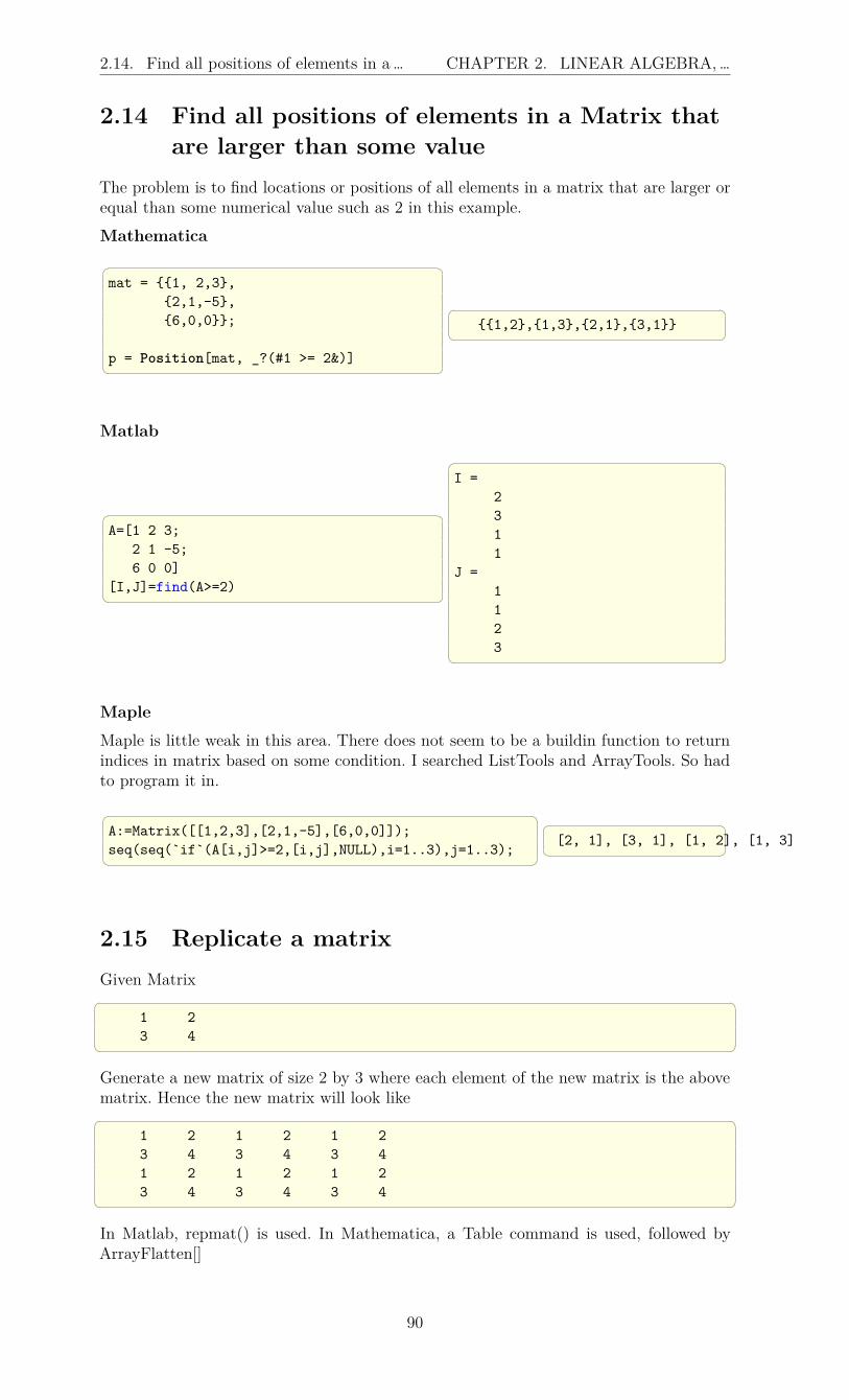
2.14. Find all positions of elements in a … CHAPTER 2. LINEAR ALGEBRA,…
2.14 Find all positions of elements in a Matrix thatare larger than some value
The problem is to find locations or positions of all elements in a matrix that are larger orequal than some numerical value such as 2 in this example.
Mathematica mat = 1, 2,3,
2,1,-5,6,0,0;
p = Position[mat, _?(#1 >= 2&)]
1,2,1,3,2,1,3,1
Matlab
A=[1 2 3;
2 1 -5;6 0 0]
[I,J]=find(A>=2)
I =
2311
J =1123
MapleMaple is little weak in this area. There does not seem to be a buildin function to returnindices in matrix based on some condition. I searched ListTools and ArrayTools. So hadto program it in.
A:=Matrix([[1,2,3],[2,1,-5],[6,0,0]]);seq(seq(`if`(A[i,j]>=2,[i,j],NULL),i=1..3),j=1..3);
[2, 1], [3, 1], [1, 2], [1, 3]
2.15 Replicate a matrixGiven Matrix
1 23 4
Generate a new matrix of size 2 by 3 where each element of the new matrix is the abovematrix. Hence the new matrix will look like
1 2 1 2 1 23 4 3 4 3 41 2 1 2 1 23 4 3 4 3 4
In Matlab, repmat() is used. In Mathematica, a Table command is used, followed byArrayFlatten[]
90

2.15. Replicate a matrix CHAPTER 2. LINEAR ALGEBRA,…
Mathematica mat = 1,2,
3,4
r = Table[mat,2,3];ArrayFlatten[r]
1,2,1,2,1,2,3,4,3,4,3,4,1,2,1,2,1,2,3,4,3,4,3,4
Matlab A=[1 2;3 4]repmat(A,2,3)
ans =
1 2 1 2 1 23 4 3 4 3 41 2 1 2 1 23 4 3 4 3 4
Another way is to use kron() in matlab, and KroneckerProduct in Mathematica andLinearAlgebra[KroneckerProduct] in Maple, which I think is a better way. As follows
Mathematica mat = 1,2,
3,4
kernel = Table[1, 2, 3];(* 1, 1, 1,
1, 1, 1 *)
KroneckerProduct[kernel, mat]
1,2,1,2,1,2,3,4,3,4,3,4,1,2,1,2,1,2,3,4,3,4,3,4
Matlab A=[1 2;3 4]kernel=ones(2,3)
kernel =1 1 11 1 1
kron(kernel,A)
ans =
1 2 1 2 1 23 4 3 4 3 41 2 1 2 1 23 4 3 4 3 4
Maple A:=Matrix([[1,2],[3,4]]);kern:=Matrix([[1,1,1],[1,1,1]]);LinearAlgebra:-KroneckerProduct(kern,A);
[[1,2,1,2,1,2],[3,4,3,4,3,4],[1,2,1,2,1,2],[3,4,3,4,3,4]]
91

2.16. Find the location of the maximum… CHAPTER 2. LINEAR ALGEBRA,…
2.16 Find the location of the maximum value in amatrix
Mathematica mat =2,4,-3,
7,9,5,0,5.4,9
m = Max[mat]; (*this gives values *)Position[mat,m](*this find locations*)
Out[142]= 2,2,3,3
Matlab h = [2, 4, -3;
7, 9, 5;0, 5.4, 9]
m = max(h(:));
[r,c]=find(h==m)
r =
23
c =23
MapleThis below finds position of first max. A:=Matrix([[2,4,-3],[7,9,5],[0,5.4,9]]);v:=max(A);member(v,A,'pos');pos
2,2
Maple support for such operations seems to be not as strong as Matlab. One way to findlocations of all elements is by using explicit loop
A:=Matrix([[2,4,-3],[7,9,5],[0,5.4,9]]);v:=max(A);r:=[seq(seq(`if`(A[i,j]=v,[i,j],NULL),i=1..3),j=1..3)];
[[2, 2], [3, 3]]
2.17 Swap 2 columns in a matrixGive a matrix
1 23 45 6
How to change it so that the second column becomes the first, and the first becomes thesecond? so that the result become
2 14 36 5
92

2.18. Join 2 matrices side-by-side and on… CHAPTER 2. LINEAR ALGEBRA,…
Mathematica a=1,2,
3,4,5,6
Reverse[a,2]
Out[29]= 2, 1,
4, 3,6, 5
Matlab a =[1 2;
3 4;5 6]
[a(:,2) a(:,1)]
2 14 36 5
Maple A:=Matrix([[1,2],[3,4],[5,6]]);A:=Matrix([ A[..,2], A[..,1] ])
[[2,1],[4,3],[6,5]]
2.18 Join 2 matrices side-by-side and on top of eachothers
MathematicaIn Mathematica, to join 2 matrices side-by-side, use Join with '2' as the third argument.To join them one on top of the other, use '1' as the third argument
a = RandomInteger[10, 3, 3]
Out[146]= 8,5, 1,
8,10,8,6,0, 8
b = RandomInteger[10, 3, 3]
9, 0,1,10,2,7,8, 0,8
(*join side-by-side as in Matlab [A B]*)Join[a, b, 2]
8,5, 1, 9,0,1,8,10,8,10,2,7,6,0, 8, 8,0,8
(*join vertically as in Matlab [A;B]*)Join[a, b, 1]
8, 5 , 1,8, 10, 8,6, 0 , 8,9, 0 , 1,10,2 , 7,8, 0 , 8
93

2.19. Copy the lower triangle to the upper … CHAPTER 2. LINEAR ALGEBRA,…
Matlab A=rand(3,3)B=rand(3,3)[A B]
0.5472 0.2575 0.8143 0.3500 0.6160 0.83080.1386 0.8407 0.2435 0.1966 0.4733 0.58530.1493 0.2543 0.9293 0.2511 0.3517 0.5497
[A;B]
0.5472 0.2575 0.81430.1386 0.8407 0.24350.1493 0.2543 0.92930.3500 0.6160 0.83080.1966 0.4733 0.58530.2511 0.3517 0.5497
Maple A:=ArrayTools:-RandomArray(3,3,distribution = uniform);B:=ArrayTools:-RandomArray(3,3,distribution = uniform);<A|B>; #side by side
<A,B>; #on top of each others
#orMatrix([A,B]); #side by sideMatrix([[A],[B]]); #on top of each others
2.19 Copy the lower triangle to the upper triangle ofa matrix to make symmetric matrix
Question posted on the net please help me with simple to apply function that will constructsymmetric matrix from given just a half matrix with diagonal.Eg:
From:1 0 0 02 3 0 04 9 5 02 2 3 4
To give:
1 2 4 22 3 9 24 9 5 32 2 3 4 Many answers were given, below is my answer, and I also show how to do it in Matlab
94

2.20. extract values from matrix given… CHAPTER 2. LINEAR ALGEBRA,…
Mathematica a = 1, 0, 0, 0,
2, 3, 0, 0,4, 9, 5, 0,2, 2, 3, 4;
Transpose[LowerTriangularize[a, -1]] + a
1, 2, 4, 2,2, 3, 9, 2,4, 9, 5, 3,2, 2, 3, 4
Matlab a =
1 0 0 02 3 0 04 9 5 02 2 3 4
a+tril(a,-1)'
ans =
1 2 4 22 3 9 24 9 5 32 2 3 4
Maple A:=Matrix([[1,0,0,0],[2,3,0,0],[4,9,5,0],[2,2,3,4]]);B:=ArrayTools:-LowerTriangle(A,-1);A:=A+B^%T;
[[1,2,4,2],[2,3,9,2],[4,9,5,3],[2,2,3,4]]
2.20 extract values from matrix given their indexGiven a matrix A, and list of locations within the matrix, where each location is given byi, j entry, find the value in the matrix at these locations
Example, given A=1,2,3,
4,5,6,7,8,9
obtain the entries at 1, 1 and 3, 3 which will be 1 and 9 in this example.
Mathematica mat=1,2,3,
4,5,6,7,8,9
pos = 1,1,3,3;Map[ mat[[Sequence@@ # ]] & , pos ]
1,9
Another method (same really as above, but usingPart explicit) Map[Part[A, Sequence @@ #] &, pos]
1,9
95

2.21. Convert N by M matrix to a row of … CHAPTER 2. LINEAR ALGEBRA,…
Matlab A=[1 2 3;
4 5 6;7 8 9];
I=[1 3]; % setup the I,J indicesJ=[1 3];A(sub2ind(size(A),I,J))
ans =
1 9
Maple A:=Matrix([[1,2,3],[4,5,6],[7,8,9]]);loc:=[[1,1],[3,3]];map(x->A[op(x)],loc);
[1, 9]
2.21 Convert N by M matrix to a row of length N MGiven a=[1 2 3
4 5 67 8 9]
covert the matrix to one vector [1 2 3 4 5 6 7 8 9] Mathematica a=1,2,3,
4,5,6,7,8,9
Flatten[a]
1,2,3,4,5,6,7,8,9
Matlab a=[1 2 3;
4 5 6;7 8 9]
a=a(:);a'
1 4 7 2 5 8 3 6 9
Maple Maple reshapes along columns, like Matlab. To get same result as Mathematica,we can transpose the matrix first. To get same result as Matlab, do not transpose.
A:=Matrix([[1,2,3],[4,5,6],[7,8,9]]);v:=ListTools:-Flatten(convert(A,list));
v:=ListTools:-Flatten(convert(A^%T,list));
[1, 4, 7, 2, 5, 8, 3, 6, 9]
[1, 2, 3, 4, 5, 6, 7, 8, 9] 96

2.22. find rows in a matrix based on values … CHAPTER 2. LINEAR ALGEBRA,…
2.22 find rows in a matrix based on values indifferent columns
Example, given Matrix 1 9 0 105 6 7 83 9 2 10
Select rows which has 9 in the second column and 10 in the last column. Hence the resultwill be the first and third rows only
1 9 0 103 9 2 10
Mathematica mat=1,9,0,10,
5,6,7,8,3,9,2,10;
p = Position[mat[[All,2,4]],x_/;x===9,10]
1,3
Extract[mat,p]
1,9,0,10,3,9,2,10
Matlab A=[1 9 0 10;
5 6 7 8;3 9 2 10];
r=bsxfun(@eq,A(:,[2 4]),[9 10]);ind=all(r,2);A(ind,:)
ans =
1 9 0 103 9 2 10
Maple restart;A:=Matrix([[1,9,0,10],[5,6,7,8],[3,9,2,10]]);nRow:=op([1,1],A);<seq(`if`(A[i,2]=9 and A[i,-1]=10,A[i,..],NULL),i=1..nRow)>;
#ORrestart;A:=Matrix([[1,9,0,10],[5,6,7,8],[3,9,2,10]]);nRow:=LinearAlgebra:-RowDimension(A);my_rows:=[seq(`if`(A[i,2]=9 and A[i,-1]=10,convert(A[i,..],list),NULL),i=1..nRow)];Matrix(my_rows)
[1 9 0 10
3 9 2 10
]
There does not seem to be a direct way in Maple to take list of row Vectors, and use theseto make a Matrix. This is why I had to convert to list in the above to make it work.
97

2.23. Select entries in one column based… CHAPTER 2. LINEAR ALGEBRA,…
2.23 Select entries in one column based on acondition in another column
Given A=[4 3
6 4 ---->7 6 ---->2 11 39 22 5 ---->1 2]
Select elements in the first column only which has corresponding element in the secondcolumn greater than 3, hence the result will be
[6 7 2] Mathematica mat = 4, 3,
6, 4,7, 6,2, 1,1, 3,9, 2,2, 5,1, 2;
r = Select[mat, #[[2]] > 3 &];r[[All, 1]]
6, 7, 2
another way is to find the index using Positionand then use Extract loc = Position[mat, x_, y_ /; y > 3]r = Extract[mat, loc];r[[All, 1]]
6, 7, 2
another way is to use Cases[]. This is the short-est way Cases[mat, x_, y_ /; y > 3 :> x]
6, 7, 2
98
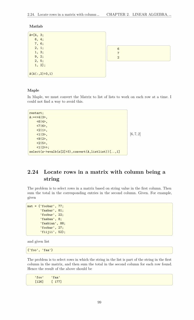
2.24. Locate rows in a matrix with column… CHAPTER 2. LINEAR ALGEBRA,…
Matlab A=[4, 3;
6, 4;7, 6;2, 1;1, 3;9, 2;2, 5;1, 2];
A(A(:,2)>3,1)
672
MapleIn Maple, we must convert the Matrix to list of lists to work on each row at a time. Icould not find a way to avoid this.
restart;A:=<<4|3>,
<6|4>,<7|6>,<2|1>,<1|3>,<9|2>,<2|5>,<1|2>>;
select(z->evalb(z[2]>3),convert(A,listlist))[..,1]
[6, 7, 2]
2.24 Locate rows in a matrix with column being astring
The problem is to select rows in a matrix based on string value in the first column. Thensum the total in the corresponding entries in the second column. Given. For example,given mat = 'foobar', 77;
'faabar', 81;'foobur', 22;'faabaa', 8;'faabian', 88;'foobar', 27;'fiijii', 52;
and given list 'foo', 'faa' The problem is to select rows in which the string in the list is part of the string in the firstcolumn in the matrix, and then sum the total in the second column for each row found.Hence the result of the above should be
'foo' 'faa'[126] [ 177]
99

2.24. Locate rows in a matrix with column… CHAPTER 2. LINEAR ALGEBRA,…
Mathematica mat = "foobar", 77,
"faabar", 81,"foobur", 22,"faabaa", 8,"faabian", 88,"foobar", 27,"fiijii", 52;
lst = "foo", "faa";
foo[mat_, lst_] :=Select[mat, StringMatchQ[lst,
StringTake[#[[1]], 3]] &];
r = Map[foo[mat, #] &, lst];
MapThread[#1,Total[#2[[All, 2]]]&,lst, r]
"foo", 126, "faa", 177
Matlab A = 'foobar', 77;
'faabar', 81;'foobur', 22;'faabaa', 8;'faabian', 88;'foobar', 27;'fiijii', 52;
lst= 'foo', 'faa';f=@(x) [x sum(cell2mat(A(strncmp(A(:,1),x,3),2)))];r=arrayfun(@(i) f(lst(i)),1:2,'UniformOutput',false)reshape([r:],2,2)
ans =
'foo' 'faa'[126] [177]
But notice that in Matlab, the answer is a cellarray. To accessthe numbers above r:r12r22
ans =
'foo' [126]ans =
'faa' [177]
ans =126
ans =177
100

2.25. Remove set of rows and columns… CHAPTER 2. LINEAR ALGEBRA,…
2.25 Remove set of rows and columns from a matrixat once
Given: square matrix, and list which represents the index of rows to be removed, and italso represents at the same time the index of the columns to be removed (it is squarematrix, so only one list is needed).output: the square matrix, with BOTH the rows and the columns in the list removed.Assume valid list of indices.This is an example: remove the second and fourth rows and the second and fourth columnsfrom a square matrix.
I asked this question at SO, and more methods are shown there at HTMLMathematica Three methods are given.method 1:(credit for the idea to Mike Honeychurch at stackoverflow). It turns out it is easier to workwith what we want to keep instead of what we want to delete so that Part[] can be useddirectly.Hence, given a list of row numbers to remove, such as pos = 2, 4; Start by generating list of the rows and columns to keep by using the command Comple-ment[], followed by using Part[] a = 0, 5, 2, 3, 1, 0,
4, 3, 2, 5, 1, 3,4, 1, 3, 5, 3, 2,4, 4, 1, 1, 1, 5,3, 4, 4, 5, 3, 3,5, 1, 4, 5, 2, 0
;pos = 2, 4;keep = Complement[Range[Length[a]], pos];a[[keep, keep]] Gives 0, 2, 1, 0,4, 3, 3, 2,3, 4, 3, 3,5, 4, 2, 0 Method 2: (due to Mr Wizard at stackoverflow) ReplacePart[a, 2,4,_, 2,_, 4
101

2.25. Remove set of rows and columns… CHAPTER 2. LINEAR ALGEBRA,…
:> Sequence[]] Gives 0, 2, 1, 0,4, 3, 3, 2,3, 4, 3, 3,5, 4, 2, 0 Method 3: (me)
use Pick. This works similar to Fortran pack(). Using a mask matrix, we set the entryin the mask to False for those elements we want removed. Hence this method is just amatter of making a mask matrix and then using it in the Pick[] command. nRow,nCol = Dimensions[a];mask = Table[True,nRow,nCol];pos = 2,4;mask[[All,pos]]=False;mask[[pos,All]]=False;r=Pick[a,mask]/.->Sequence[] gives Out[39]= 0,2,1,0,
4,3,3,2,3,4,3,3,5,4,2,0
Matlab a = [0, 5, 2, 3, 1, 0;
4, 3, 2, 5, 1, 3;4, 1, 3, 5, 3, 2;4, 4, 1, 1, 1, 5;3, 4, 4, 5, 3, 3;5, 1, 4, 5, 2, 0
]
list=[2 4];a(list,:)=[];a(:,list)=[];
a =
0 2 1 04 3 3 23 4 3 35 4 2 0
Maple A := Matrix([
[0, 5, 2, 3, 1, 0],[4, 3, 2, 5, 1, 3],[4, 1, 3, 5, 3, 2],[4, 4, 1, 1, 1, 5],[3, 4, 4, 5, 3, 3],[5, 1, 4, 5, 2, 0]
]);the_list:=[2,4];A:=LinearAlgebra:-DeleteRow(A,the_list);A:=LinearAlgebra:-DeleteColumn(A,the_list);
A:=[[0, 2, 1, 0],
[4, 3, 3, 2],[3, 4, 3, 3],[5, 4, 2, 0]]
102

2.26. Convert list of separated numerical … CHAPTER 2. LINEAR ALGEBRA,…
2.26 Convert list of separated numerical numbers tostrings
Problem: given a list of numbers such as 1, 2,5, 3, 7,4 convert the above to list of strings "12","537","4" Mathematica a=1,2,5,3,7,4;Map[ToString[#]&,a,2];Map[StringJoin[#]&,%]
List["12","537","4"]
Matlab a=[1,2],[5,3,7],[4];r=arrayfun(@(i) ...
cellstr(num2str(ai)),1:length(a));r'
ans =
'1 2''5 3 7''4'
answer below is due to Bruno Luong at Matlab news-group a=[1,2],[5,3,7],[4];map='0':'9';cellfun(@(x) map(x+1), a, 'uni', 0)
'12' '537' '4'
Maple a:=[[1,2],[5,3,7],[4]];map(x->convert(cat(op(x)), string),a);
["12", "537", "4"]
103

2.27. Obtain elements that are common to… CHAPTER 2. LINEAR ALGEBRA,…
2.27 Obtain elements that are common to twovectors
Given vector or list d = [−9, 1, 3,−3, 50, 7, 19], t = [0, 7, 2, 50], find the common elements.
Mathematica d = -9,1,3,-3,50,7,19;t = 0,7,2,50;Intersection[d,t]
Out[412]= 7,50
Matlab d=[-9 1 3 -3 50 7 19];t =[0 7 2 50];intersect(t,d)
ans =
7 50
Maple d := -9,1,3,-3,50,7,19;t := 0,7,2,50;d intersect t;
7, 50
2.28 Sort each column (on its own) in a matrixGiven
4 2 52 7 910 1 2
Sort each column on its own, so that the result is 2 1 24 2 510 7 9
In Matlab, the sort command is used. But in the Mathematica, the Sort command is thesame the Matlab’s sortrows() command, hence it can’t be used as is. Map is used withSort to accomplish this.
Mathematica mat=4,2,5,
2,7,9,10,1,2;
Map[Sort[#]&,Transpose[mat]];mat=Transpose[%]
2, 1, 2,4, 2, 5,10,7, 9
104

2.29. Sort each row (on its own) in a matrix CHAPTER 2. LINEAR ALGEBRA,…
Matlab A=[4 2 5;
2 7 9;10 1 2];
sort(A,1)
2 1 24 2 510 7 9
Maple restart;restart;A:=Matrix([[4,2,5],[2,7,9],[10,1,2]]);map(x->sort(x),[LinearAlgebra:-Column(A,[1..-1])]);Matrix(%);
#or, may simpler is
restart;A:=Matrix([[4,2,5],[2,7,9],[10,1,2]]);for n from 1 to LinearAlgebra:-ColumnDimension(A) do
A[..,n]:=sort(A[..,n]);od:A
Matrix(3, 3, [[2, 1, 2],
[4, 2, 5],[10, 7, 9]])
2.29 Sort each row (on its own) in a matrixGiven
4 2 52 7 910 1 2
Sort each row on its own, so that the result is 2 4 52 7 91 2 10
Mathematica mat=4, 2,5,
2, 7,9,10,1,2;
Map[Sort[#]&,mat]
2, 4, 5,2, 7, 9,1, 2, 10
Matlab A=[4 2 5;
2 7 9;10 1 2];
sort(A,2)
2 4 52 7 91 2 10
105

2.30. Sort a matrix row-wise using first … CHAPTER 2. LINEAR ALGEBRA,…
Maple restart;A:=Matrix([[4,2,5],[2,7,9],[10,1,2]]);map(x->convert(sort(x),list),[LinearAlgebra:-Row(A,[1..-1])]);Matrix(%);
#or, may simpler is
restart;A:=Matrix([[4,2,5],[2,7,9],[10,1,2]]);for n from 1 to LinearAlgebra:-RowDimension(A) do
A[n,..]:=sort(A[n,..]);od:A
Matrix(3, 3, [[2, 4, 5],
[2, 7, 9],[1, 2, 10]])
I had to convert each row to a list above for this to work. But for the case of columns(see last item earlier), this was not needed. Strange that one can’t not construct a Matrixfrom list of Row vectors as with a list of Column vectors.
Maple 2021.
2.30 Sort a matrix row-wise using first column askey
Given 4 2 52 7 910 1 2
Sort the matrix row-wise using first column as key so that the result is 2 7 94 2 510 1 2
In Matlab, the sortrows() command is used. In Mathematica the Sort[] command is usedas is. No need to do anything special.
Mathematica mat=4, 2, 5,
2, 7, 9,10,1, 2;
Sort[mat]
2, 7, 9,4, 2, 5,10, 1, 2
Matlab A=[4 2 5;
2 7 9;10 1 2];
sortrows(A)
2 7 94 2 5
10 1 2
106

2.31. Sort a matrix row-wise using non- … CHAPTER 2. LINEAR ALGEBRA,…
Maple restart;A:=Matrix([[4,2,5],[2,7,9],[10,1,2]]);convert(A,listlist);sort(%);Matrix(%)
Matrix(3, 3, [[2, 7, 9],
[4, 2, 5],[10, 1, 2]])
2.31 Sort a matrix row-wise using non-first columnas key
Given 4 2 52 7 910 1 2
Sort the matrix row-wise using the second column as key so that the result is 10 1 24 2 52 7 9
In Matlab, the sortrows() command is used, but now we tell it to use the second columnas key.
In Mathematica the SortBy[] command is now used but we tell it to use the second slotas key.
Mathematica mat=4, 2, 5,
2, 7, 9,10,1, 2;
(*sort by second element as key*)SortBy[mat,#[[2]]&]
10, 1, 2,4, 2, 5,2, 7, 9
Matlab A=[4 2 5;
2 7 9;10 1 2];
sortrows(A,2)
10 1 24 2 52 7 9
Maple restart;A:=Matrix([[4,2,5],
[2,7,9],[10,1,2]]);
convert(A,listlist);sort(%,key=(x->x[2]));Matrix(%)
Matrix(3, 3, [[10, 1, 2],
[4, 2, 5],[2, 7, 9]])
107

2.32. Replace the first nonzero element in … CHAPTER 2. LINEAR ALGEBRA,…
2.32 Replace the first nonzero element in each rowin a matrix by some value
Problem: Given a matrix, replace the first nonzero element in each row by some a specificvalue. This is an example. Given matrix A below, replace the first non-zero element ineach row by −1, then
A =
50 75 0
50 0 100
0 75 100
75 100 0
0 75 100
0 75 100
will become B =
−1 75 0
−1 0 100
0 −1 100
−1 100 0
0 −1 100
0 −1 100
Mathematica A= 50, 75, 0,50, 0, 100,
0, 75, 100,75, 100, 0,0, 75, 100,0, 75, 100;
ReplacePart[A,DeleteDuplicates[Position[A,_?(#!=0&)],
(#1[[1]]==#2[[1]]&)]->-1] Solution due to Bob Hanlon (from Mathematica newsgroup) r=Union[Position[A,_?(# !=0&)],
SameTest->(#1[[1]]==#2[[1]]&)];ReplacePart[A,r->-1] Solution by Fred Simons (from Mathematica newsgroup) r=Split[Position[A,_?(# !=0&),2],
#1[[1]]==#2[[1]]&][[All,1]];ReplacePart[A,r->-1] Solution due to Adriano Pascoletti (from Mathematica newsgroup) r=(First /@ Split[#1,First[#1]===First[#2]&]&)
[Position[A,x_/;x!=0]]ReplacePart[A,r->-1] Solution due to Oliver Ruebenkoenig (from Mathematica newsgroup) r=First /@ SplitBy[ Drop[ArrayRules[
SparseArray[A]][[All,1]],-1],First]ReplacePart[A,r->-1] Solution due to Szabolcs Horvát (from Mathematica newsgroup) r=MapIndexed[First[#2],1+LengthWhile[#1,#==0&]&,A]ReplacePart[A,r->-1] These all give -1,75,0,-1,0,100,0,-1,100,-1,100,0,0,-1,100,0,-1,100 Matlab
108

2.32. Replace the first nonzero element in … CHAPTER 2. LINEAR ALGEBRA,…
A=[50 75 0;50 0 100;0 75 100;75 100 0;0 75 100;0 75 100];
[I,J] = ind2sub(size(A),find(A~=0));[b,c] = unique(I,'first');A(sub2ind(size(A),b,J(c)))=-1 This solution due to Bruno Luong (from matlab newsgroup) B = cumsum(A~=0,2)>0B = [false(size(B,1),1) B]A(logical(diff(B,1,2))) = -1 This solution due to Jos from matlab newsgroup A((cumsum(~~A,2)==1) & (A ~= 0)) = -1 The above solutions all give A =
-1 75 0-1 0 1000 -1 100-1 100 00 -1 1000 -1 100
Maple restart;A:=Matrix([[50,75,0],
[50,0,100],[0,75,100],[75,100,0],[0,75,100],[0,75,100]]);
for n from 1 to LinearAlgebra:-RowDimension(A) doidx:=ArrayTools:-SearchArray(A[n,..],1);if numelems(idx)<>0 then
A[n,idx[1]]:=-1;fi;
od:A
Matrix(6, 3, [[-1, 75, 0],
[-1, 0, 100],[0, -1, 100],[-1, 100, 0],[0, -1, 100],[0, -1, 100]])
109

2.33. Perform outer product and outer … CHAPTER 2. LINEAR ALGEBRA,…
2.33 Perform outer product and outer sum betweentwo vector
Problem: Given 2 vectors, perform outer product and outer sum between them. The outeroperation takes the first element in one vector and performs this operation on each elementin the second vector. This results in first row. This is repeated for each of the elements inthe first vector. The operation to perform can be any valid operation on these elements.
Mathematicausing symbolic vectors. Outer product Remove["Global`*"]
v1=a,b,c;v2=e,f,g;Outer[Times,v1,v2]
a e, a f, a g,b e, b f, b g,c e, c f, c g
Outer sum Outer[Plus,v1,v2]
a+e, a+f, a+g,b+e, b+f, b+g,c+e, c+f, c+g
using numerical vectors. Outer product v1=1,2,3;v2=4,5,6;Outer[Times,v1,v2]
4, 5, 6,8, 10, 12,12, 15, 18
Outer sum Outer[Plus,v1,v2]
5, 6, 7,6, 7, 8,7, 8, 9
MatlabOuter product v1=[1 2 3];v2=[4 5 6];
v1'*v2
ans =
4 5 68 10 12
12 15 18
Outer sum v1=[1 2 3];v2=[4 5 6];meshgrid(v1)+meshgrid(v2)'
ans =
5 6 76 7 87 8 9
110

2.34. Find the rank and the bases of the … CHAPTER 2. LINEAR ALGEBRA,…
MapleDue to Carl Love from the Maple newsgroup restart;
Outer:= proc(OP, L1, L2)local a,b;[seq](seq(OP(a,b), b in L2), a in L1)
end proc:
L1:=[a,b,c];L2:=[d,e,f];Outer(`*`,L1,L2);
[a*d,a*e,a*f,b*d,b*e, b*f, c*d, c*e, c*f]
Outer(`+`,L1,L2);
[a+d, a+e, a+f, b+d,b+e, b+f, c+d, c+e, c+f]
2.34 Find the rank and the bases of the Null spacefor a matrix A
Problem: Find the rank and nullities of the following matrices, and find the bases of therange space and the Null space.
A =
2 3 3 4
0 −1 −2 2
0 0 0 1
Mathematica mat=2,3,3,4,
0,-1,-2,2,0,0,0,1;
nRow,nCol = Dimensions[mat] 3,4
Print["Rank (or dimension of the range space)=",
MatrixRank[mat]]
Rank (or dimension of the range space)=3 Print["Dimension of the Null Space=",
nCol-MatrixRank[mat]]
Dimension of the Null Space=1 Print["Basis for Null Space=",NullSpace[mat]]
Basis for Null Space=3,-4,2,0
111

2.35. Find the singular value … CHAPTER 2. LINEAR ALGEBRA,…
Matlab A=[2 3 3 4;
0 -1 -2 2;0 0 0 1]
[nRow,nCol]=size(A);
r = rank(A);fprintf('A range space dimension=%d\n',r);fprintf('A null space dimension= %d\n',nCol-r);fprintf('Basic for null space of A =');null(A,'r')'
A range space dimension=3A null space dimension= 1Basic for null space of A =
ans =1.5000 -2.0000 1.0000 0
Maple restart;A:=Matrix([[2,3,3,4],[0,-1,-2,2],[0,0,0,1]]);LinearAlgebra:-Rank(A);LinearAlgebra:-ColumnDimension(A)-LinearAlgebra:-Rank(A);LinearAlgebra:-NullSpace(A)
31[3/2-210]
2.35 Find the singular value decomposition (SVD) ofa matrix
Problem: Find the SVD for the matrix[1 2 3
4 5 6
]Notice that in Maple, the singular values
matrix, normally called S, is returned as a column vector. So need to call DiagonalMatrix()to format it as expected.
Mathematica mat = 1,2,3,
4,5,6
u,s,v=N[SingularValueDecomposition[mat]]
0.386318,-0.922366,0.922366,0.386318
9.50803,0.,0.,0.,0.77287,0.
0.428667,0.805964,0.408248,0.566307,0.112382,-0.816497,0.703947,-0.581199,0.408248
(*Reconstruct A from its components *)u.s.Transpose[v]
1.,2.,3.,4.,5.,6.
112

2.35. Find the singular value … CHAPTER 2. LINEAR ALGEBRA,…
Matlab A=[1 2 3;
4 5 6];[u,s,v]=svd(A);usv
u =
-0.3863 -0.9224-0.9224 0.3863
s =
9.5080 0 00 0.7729 0
v =
-0.4287 0.8060 0.4082-0.5663 0.1124 -0.8165-0.7039 -0.5812 0.4082
u*s*v'
ans =
1.0000 2.0000 3.00004.0000 5.0000 6.0000
Maple restart;with(LinearAlgebra):A:=Matrix([[1,2,3],[4,5,6.]]);
[1 2 3 ]
A := [ ][4 5 6.]
m,n:=Dimensions(A):u,s,v:=SingularValues(A,
output=['U', 'S', 'Vt']):u;
[0.386317703118612 -0.922365780077058][ ][0.922365780077058 0.386317703118612 ]
s:=DiagonalMatrix(s,m,n);v;
[9.50803200069572 0 0]
s := [ ][ 0 0.772869635673485 0]
[0.428667133548626 0.566306918848035 0.703946704147444 ]v:= [0.805963908589298 0.112382414096594 -0.581199080396110]
[0.408248290463863 -0.816496580927726 0.408248290463863 ] > s2:=DiagonalMatrix(SingularValues(A,
output=['S']),m,n);
[9.50803200069572 0 0]s2 := [ ]
[ 0 0.772869635673485 0] > evalf(u.s.v);
[1. 2. 3.][ ][4. 5. 6.]
113

2.36. Solve Ax = b CHAPTER 2. LINEAR ALGEBRA,…
2.36 Solve Ax = b
Solve for x in the following system of equations [ 1 2 3 ][x1] [ 1 ][ 7 5 6 ][x2]= [ 2 ][ 7 8 9 ][x3] [ 3 ] Mathematica mat=1,2,3,
7,5,6,7,8,9;
b = 1,2,3LinearSolve[mat,b]
0,0,1/3
Matlab format longA=[1 2 3;
7 5 6;7 8 9];
b=[1;2; 3];A\b
ans =
00
0.333333333333333
Maple restart;A:=Matrix([[1,2,3],[7,5,6],[7,8,9]]);b:=Vector([1,2,3]);LinearAlgebra:-LinearSolve(A,b)
[0,0,1/3]
114

2.37. Find all nonzero elements in a matrix CHAPTER 2. LINEAR ALGEBRA,…
Fortran program t2implicit noneinteger, parameter :: N=3real(8), DIMENSION(N, N) :: &
A=DBLE(reshape([ 1.0, 2.0, 3.0,&7.0, 5.0, 6.0,&7.0, 8.0, 9.0], shape(A), order=[2,1]))
real(8), parameter, DIMENSION(N, 1) :: &b=DBLE(reshape([1.0, 2.0, 3.0], shape(b)))
real(8), DIMENSION(N, 1) :: IPIVinteger :: INFO
CALL DGETRF( N, N, A, N, IPIV, INFO )if (INFO .eq. 0 ) then
CALL DGETRS( 'N', N,1, A, N, IPIV, b , N, INFO)if ( INFO .eq. 0 ) then
print *, 'solution is',belse
print *, 'failed DGETRS, INFO=',INFOend if
elseprint *, 'failed DGETRF, INFO=',INFO
end ifend program compile and run $ gfortran -std=f2003 -Wextra -Wall -pedantic -funroll-loops-ftree-vectorize -march=native -Wsurprising -Wconversiont2.f90 /usr/lib/liblapack.a /usr/lib/libblas.a
$ ./a.exesolution is-5.28677630773884192E-018 -3.70074341541718826E-017 0.33333333333333337
2.37 Find all nonzero elements in a matrixGiven a matrix, find the locations and the values of all nonzero elements. Hence given thematrix
0 0 1
10 0 2
3 0 0
the positions returned will be (1, 3), (2, 1), (2, 3), (3, 1) and the corresponding values are1, 10, 2, 3.
MathematicaIn Mathematica, standard Mathematica matrix operations can be used, or the matrix canbe converted to SparseArray and special named operation can be used on it.
115

2.37. Find all nonzero elements in a matrix CHAPTER 2. LINEAR ALGEBRA,…
mat = 0 , 0, 1,
10, 0, 2,3 , 4, 0;
sp = SparseArray[mat];pos = sp["NonzeroPositions"]
1,3,2,1,2,3,3,1,3,2
values=sp["NonzeroValues"]
1,10,2,3,4 Or standard list operations can be used mat = 0 , 0, 1,
10, 0, 2,3 , 4, 0;
(*find values not zero *)
Cases[mat,x_ /;Not[PossibleZeroQ[x]]:>x,2]
1,10,2,3,4
(*find the index *)
Position[mat,x_/;x!=0] 1,3,2,1,2,3,3,1,3,2
Matlab A=[0 0 1; 10 0 2; 3 4 0];values= nonzeros(A)
values =
103412
%find locations[I,J]=find(A)
I =
23312
J =11233
116

2.38. evaluate f(x) on a vector of values CHAPTER 2. LINEAR ALGEBRA,…
Maple A:=Matrix([[0,0,1],[10,0,2],[3,4,0]]);row, col:=ArrayTools:-SearchArray(A);
#valuesmap(n->A[row[n],col[n]],[$numelems(row)])
row, col := Vector[column](5, [2, 3, 3, 1, 2]),
Vector[column](5, [1, 1, 2, 3, 3])
[10, 3, 4, 1, 2]
2.38 evaluate f(x) on a vector of valuesGiven a function f(x) evaluate it for each value contained in a vector. For example, givenf(x) = x2 evaluate it on (1, 2, 3) such that the result is (1, 4, 9).
Mathematica Clear[f,x]f[x_]:=x^2v=1,2,3;f[v]
1,4,9
Matlab clear all;v=[1 2 3]f=@(x) x.^2f(v)
ans =
1 4 9
Maple map(x->x^2,[1,2,3])
[1, 4, 9]
2.39 generates equally spaced N points between x1and x2
Mathematica x1=1;x2=3;FindDivisions[x1,x2,5]
Out[48]= 1,3/2,2,5/2,3N[%]Out[49]= 1.,1.5,2.,2.5,3.
Matlab clear all;x1 = 1;x2 = 3;linspace(x1,x2,5)
ans =1.0000 1.5000 2.0000 2.5000 3.0000
117

2.40. evaluate and plot a f(x,y) on 2D grid … CHAPTER 2. LINEAR ALGEBRA,…
Maple x1 := 1; x2 := 3;ArrayTools:-RegularArray(x1..x2,5)
Vector[row](5, [1.0000, 1.5000, 2.0000, 2.5000, 3.0000])
2.40 evaluate and plot a f(x,y) on 2D grid ofcoordinates
Evaluate x exp−x2−y2 on 2D cartesian grid between x = −2 · · · 2 and y = −4 · · · 4 usingh = 0.2 for grid spacing.
Mathematica f[x_,y_]:=x Exp[-x^2-y^2];data = Table[f[x,y],x,-2,2,.2,y,-4,4,.2];ListPlot3D[data,PlotRange->All,ColorFunction->"Rainbow",AxesLabel->"x","y","z",LabelStyle->12,Ticks->Range[-2,2,1],Range[-4,4,1],Automatic,DataRange->-2,2,-4,4,Automatic,ImageSize->400]
The above can also be done using Plot3D f[x_,y_]:=x Exp[-x^2-y^2];Plot3D[f[x,y],x,-2,2,y,-4,4,PlotRange->All,ColorFunction->"Rainbow",AxesLabel->"x","y","z",LabelStyle->12,ImageSize->400]
118
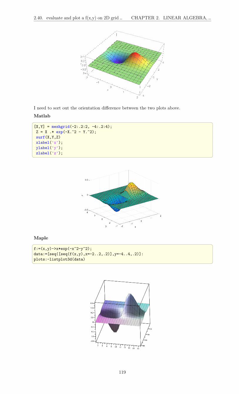
2.40. evaluate and plot a f(x,y) on 2D grid … CHAPTER 2. LINEAR ALGEBRA,…
I need to sort out the orientation difference between the two plots above.
Matlab [X,Y] = meshgrid(-2:.2:2, -4:.2:4);Z = X .* exp(-X.^2 - Y.^2);surf(X,Y,Z)xlabel('x');ylabel('y');zlabel('z');
Maple f:=(x,y)->x*exp(-x^2-y^2);data:=[seq([seq(f(x,y),x=-2..2,.2)],y=-4..4,.2)]:plots:-listplot3d(data)
119

2.41. Find determinant of matrix CHAPTER 2. LINEAR ALGEBRA,…
2.41 Find determinant of matrixGiven a square matrix, find its determinant. In Mathematica, the Det[] command is used.In Matlab the det() command is used.
Mathematica mat=Table[RandomReal[],3,3]Det[mat]
-0.317792605942287
Matlab A=rand(3,3);det(A)
-0.276653966272994
Maple A:=LinearAlgebra:-RandomMatrix(3,3,generator=-1..1.0);LinearAlgebra:-Determinant(A)
0.4101995534
2.42 Generate sparse matrix with n by n matrixrepeated on its diagonal
Given matrix
1 2 3
4 5 6
7 8 9
, generate the following sparse matrix with this matrix on the
diagonal
1 2 3 0 0 0 0 0 0
4 5 6 0 0 0 0 0 0
7 8 9 0 0 0 0 0 0
0 0 0 1 2 3 0 0 0
0 0 0 4 5 6 0 0 0
0 0 0 7 8 9 0 0 0
0 0 0 0 0 0 1 2 3
0 0 0 0 0 0 4 5 6
0 0 0 0 0 0 7 8 9
Mathematica mat = N[1,2,3,4,5,6,7,8,9];sp = SparseArray[Band[1,1]->
ConstantArray[mat,3]]MatrixForm[sp]
1. 2. 3. 0 0 0 0 0 0
4. 5. 6. 0 0 0 0 0 0
7. 8. 9. 0 0 0 0 0 0
0 0 0 1. 2. 3. 0 0 0
0 0 0 4. 5. 6. 0 0 0
0 0 0 7. 8. 9. 0 0 0
0 0 0 0 0 0 1. 2. 3.
0 0 0 0 0 0 4. 5. 6.
0 0 0 0 0 0 7. 8. 9.
120

2.43. Generate sparse matrix for the … CHAPTER 2. LINEAR ALGEBRA,…
Matlab A = [1 2 3;
4 5 6;7 8 9];
Iy = speye(3);full(Iy)
ans =
1 0 00 1 00 0 1
sp = kron(Iy,A);full(sp)
ans =1 2 3 0 0 0 0 0 04 5 6 0 0 0 0 0 07 8 9 0 0 0 0 0 00 0 0 1 2 3 0 0 00 0 0 4 5 6 0 0 00 0 0 7 8 9 0 0 00 0 0 0 0 0 1 2 30 0 0 0 0 0 4 5 60 0 0 0 0 0 7 8 9
Maple A:=Matrix([[1,2,3],[4,5,6],[7,8,9]]);Iy:=LinearAlgebra:-IdentityMatrix(3);LinearAlgebra:-KroneckerProduct(Iy,A)
Matrix(9, 9, [[1, 2, 3, 0, 0, 0, 0, 0, 0],
[4, 5, 6, 0, 0, 0, 0, 0, 0],[7, 8, 9, 0, 0, 0, 0, 0, 0],[0, 0, 0, 1, 2, 3, 0, 0, 0],[0, 0, 0, 4, 5, 6, 0, 0, 0],[0, 0, 0, 7, 8, 9, 0, 0, 0],[0, 0, 0, 0, 0, 0, 1, 2, 3],[0, 0, 0, 0, 0, 0, 4, 5, 6],[0, 0, 0, 0, 0, 0, 7, 8, 9]])
2.43 Generate sparse matrix for the tridiagonalrepresentation of second difference operator in1D
The second derivative d2udx2 is approximated by ui−1−2ui+ui+1
h2 where h is the grid spacing.Generate the A matrix that represent this operator for n = 4 where n is the number ofinternal grid points on the line
Mathematica numberOfInternalGridPoints = 4;n = 3*internalGridPoints;sp = SparseArray[Band[1,1]->-2,
Band[1,2]->1,Band[2,1]->1,n,n]
Out[103]= SparseArray[<34>,12,12]MatrixForm[sp]
−2 1 0 0 0 0 0 0 0 0 0 0
1 −2 1 0 0 0 0 0 0 0 0 0
0 1 −2 1 0 0 0 0 0 0 0 0
0 0 1 −2 1 0 0 0 0 0 0 0
0 0 0 1 −2 1 0 0 0 0 0 0
0 0 0 0 1 −2 1 0 0 0 0 0
0 0 0 0 0 1 −2 1 0 0 0 0
0 0 0 0 0 0 1 −2 1 0 0 0
0 0 0 0 0 0 0 1 −2 1 0 0
0 0 0 0 0 0 0 0 1 −2 1 0
0 0 0 0 0 0 0 0 0 1 −2 1
0 0 0 0 0 0 0 0 0 0 1 −2
121
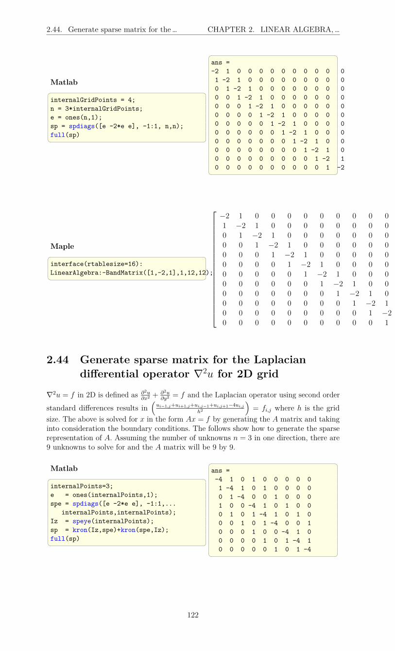
2.44. Generate sparse matrix for the … CHAPTER 2. LINEAR ALGEBRA,…
Matlab internalGridPoints = 4;n = 3*internalGridPoints;e = ones(n,1);sp = spdiags([e -2*e e], -1:1, n,n);full(sp)
ans =-2 1 0 0 0 0 0 0 0 0 0 01 -2 1 0 0 0 0 0 0 0 0 00 1 -2 1 0 0 0 0 0 0 0 00 0 1 -2 1 0 0 0 0 0 0 00 0 0 1 -2 1 0 0 0 0 0 00 0 0 0 1 -2 1 0 0 0 0 00 0 0 0 0 1 -2 1 0 0 0 00 0 0 0 0 0 1 -2 1 0 0 00 0 0 0 0 0 0 1 -2 1 0 00 0 0 0 0 0 0 0 1 -2 1 00 0 0 0 0 0 0 0 0 1 -2 10 0 0 0 0 0 0 0 0 0 1 -2
Maple interface(rtablesize=16):LinearAlgebra:-BandMatrix([1,-2,1],1,12,12);
−2 1 0 0 0 0 0 0 0 0 0 0
1 −2 1 0 0 0 0 0 0 0 0 0
0 1 −2 1 0 0 0 0 0 0 0 0
0 0 1 −2 1 0 0 0 0 0 0 0
0 0 0 1 −2 1 0 0 0 0 0 0
0 0 0 0 1 −2 1 0 0 0 0 0
0 0 0 0 0 1 −2 1 0 0 0 0
0 0 0 0 0 0 1 −2 1 0 0 0
0 0 0 0 0 0 0 1 −2 1 0 0
0 0 0 0 0 0 0 0 1 −2 1 0
0 0 0 0 0 0 0 0 0 1 −2 1
0 0 0 0 0 0 0 0 0 0 1 −2
2.44 Generate sparse matrix for the Laplaciandifferential operator ∇2u for 2D grid
∇2u = f in 2D is defined as ∂2u∂x2 +
∂2u∂y2
= f and the Laplacian operator using second order
standard differences results in(
ui−1,j+ui+1,j+ui,j−1+ui,j+1−4ui,j
h2
)= fi,j where h is the grid
size. The above is solved for x in the form Ax = f by generating the A matrix and takinginto consideration the boundary conditions. The follows show how to generate the sparserepresentation of A. Assuming the number of unknowns n = 3 in one direction, there are9 unknowns to solve for and the A matrix will be 9 by 9.
Matlab internalPoints=3;e = ones(internalPoints,1);spe = spdiags([e -2*e e], -1:1,...
internalPoints,internalPoints);Iz = speye(internalPoints);sp = kron(Iz,spe)+kron(spe,Iz);full(sp)
ans =-4 1 0 1 0 0 0 0 01 -4 1 0 1 0 0 0 00 1 -4 0 0 1 0 0 01 0 0 -4 1 0 1 0 00 1 0 1 -4 1 0 1 00 0 1 0 1 -4 0 0 10 0 0 1 0 0 -4 1 00 0 0 0 1 0 1 -4 10 0 0 0 0 1 0 1 -4
122

2.45. Generate sparse matrix for the … CHAPTER 2. LINEAR ALGEBRA,…
2.45 Generate sparse matrix for the Laplaciandifferential operator for 3D grid
The goal is to solve∂2u
∂x2+
∂2u
∂y2+
∂2u
∂z2= −f(x, y, z)
On the unit cube. The following diagram was made to help setting up the 3D scheme toapproximate the above PDE
The discrete approximation to the Laplacian in 3D is
∂2u
∂x2+∂2u
∂y2+∂2u
∂z2=
1
h2(Ui−1,j,k + Ui+1,j,k + Ui,j−1,k + Ui,j+1,k + Ui,k,k−1 + Ui,j,k+1 − 6Ui,j,k)
For the direct solver, the A matrix needs to be formulated. From
1
h2(Ui−1,j,k + Ui+1,j,k + Ui,j−1,k + Ui,j+1,k + Ui,k,k−1 + Ui,j,k+1 − 6Ui,j,k) = fi,j,k
Solving for Ui,j,k results in
Ui,j,k =1
6
(Ui−1,j,k + Ui+1,j,k + Ui,j−1,k + Ui,j+1,k + Ui,k,k−1 + Ui,j,k+1 − h2fi,j,k
)To help make the A matrix, a small example with n = 2, is made. The following diagramuses the standard numbering on each node
By traversing the grid, left to right, then inwards into the paper, then upwards, thefollowing A matrix results
123

2.45. Generate sparse matrix for the … CHAPTER 2. LINEAR ALGEBRA,…
The recursive pattern involved in these A matrices can now be seen. Each A matrixcontains inside it a block on its diagonal which repeats n times. Each block in turn containinside it, on its diagonal, smaller block, which also repeats n times.
It is easier to see the pattern of building A by using numbers for the grid points, andlabel them in the same order as they would be visited, this allowes seeing the connectionbetween each grid point to the other easier. For example, for n = 2,
The connections are now more easily seen. Grid point 1 has connection to only points2, 3, 5. This means when looking at the A matrix, there will be a 1 in the first row, atcolumns 2, 3, 5. Similarly, point 2 has connections only to 1, 4, 6, which means in the secondrow there will be a 1 at columns 1, 4, 6. Extending the number of points to n = 3 to bettersee the pattern of A results in
From the above it is seen that for example point 1 is connected only to 2, 4, 10 and point2 is connected to 1, 3, 5, 11 and so on.
The above shows that each point will have a connection to a point which is numberedn2 higher than the grid point itself. n2 is the size of the grid at each surface. Hence, thegeneral A matrix, for the above example, can now be written as
124
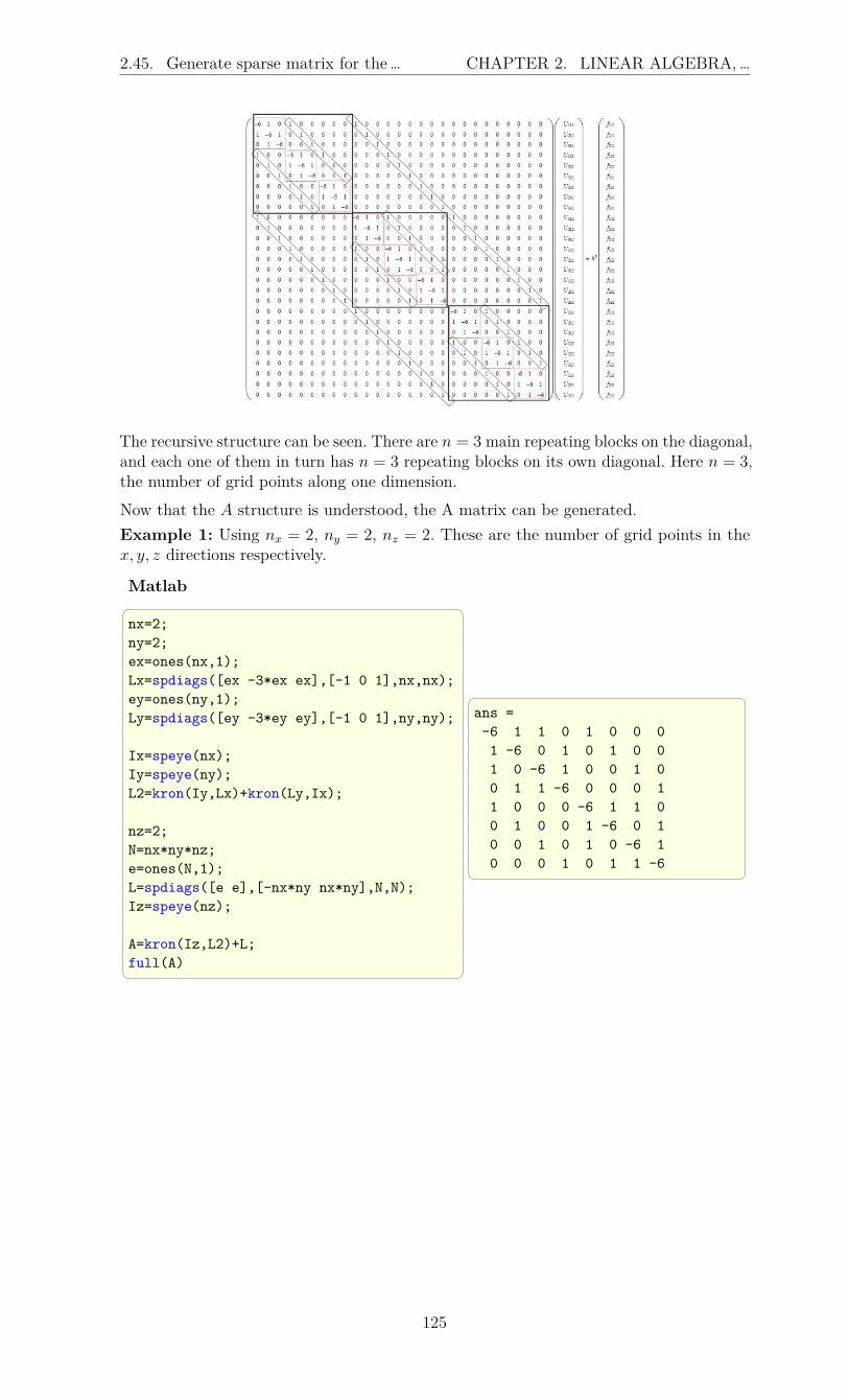
2.45. Generate sparse matrix for the … CHAPTER 2. LINEAR ALGEBRA,…
The recursive structure can be seen. There are n = 3main repeating blocks on the diagonal,and each one of them in turn has n = 3 repeating blocks on its own diagonal. Here n = 3,the number of grid points along one dimension.
Now that the A structure is understood, the A matrix can be generated.Example 1: Using nx = 2, ny = 2, nz = 2. These are the number of grid points in thex, y, z directions respectively.
Matlab nx=2;ny=2;ex=ones(nx,1);Lx=spdiags([ex -3*ex ex],[-1 0 1],nx,nx);ey=ones(ny,1);Ly=spdiags([ey -3*ey ey],[-1 0 1],ny,ny);
Ix=speye(nx);Iy=speye(ny);L2=kron(Iy,Lx)+kron(Ly,Ix);
nz=2;N=nx*ny*nz;e=ones(N,1);L=spdiags([e e],[-nx*ny nx*ny],N,N);Iz=speye(nz);
A=kron(Iz,L2)+L;full(A)
ans =-6 1 1 0 1 0 0 01 -6 0 1 0 1 0 01 0 -6 1 0 0 1 00 1 1 -6 0 0 0 11 0 0 0 -6 1 1 00 1 0 0 1 -6 0 10 0 1 0 1 0 -6 10 0 0 1 0 1 1 -6
125
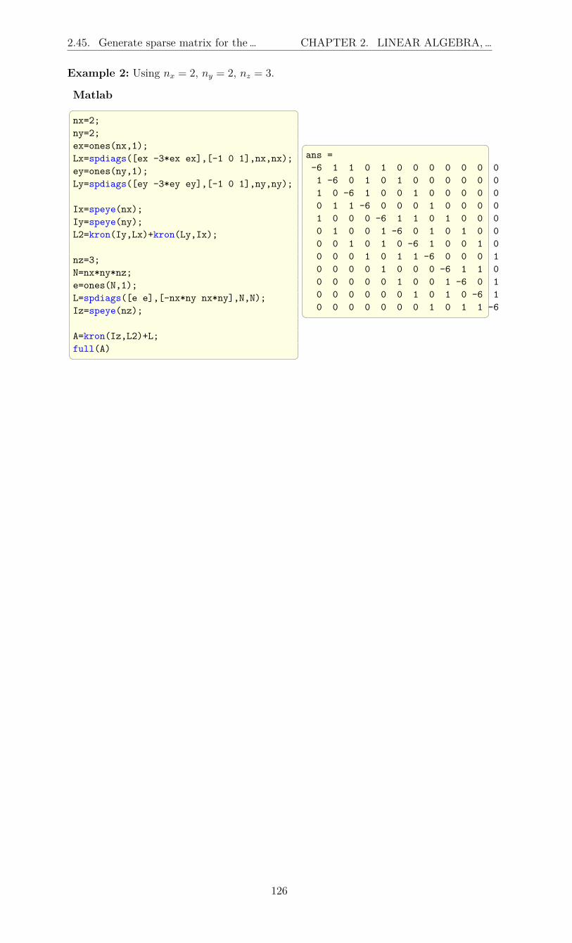
2.45. Generate sparse matrix for the … CHAPTER 2. LINEAR ALGEBRA,…
Example 2: Using nx = 2, ny = 2, nz = 3.
Matlab nx=2;ny=2;ex=ones(nx,1);Lx=spdiags([ex -3*ex ex],[-1 0 1],nx,nx);ey=ones(ny,1);Ly=spdiags([ey -3*ey ey],[-1 0 1],ny,ny);
Ix=speye(nx);Iy=speye(ny);L2=kron(Iy,Lx)+kron(Ly,Ix);
nz=3;N=nx*ny*nz;e=ones(N,1);L=spdiags([e e],[-nx*ny nx*ny],N,N);Iz=speye(nz);
A=kron(Iz,L2)+L;full(A)
ans =-6 1 1 0 1 0 0 0 0 0 0 01 -6 0 1 0 1 0 0 0 0 0 01 0 -6 1 0 0 1 0 0 0 0 00 1 1 -6 0 0 0 1 0 0 0 01 0 0 0 -6 1 1 0 1 0 0 00 1 0 0 1 -6 0 1 0 1 0 00 0 1 0 1 0 -6 1 0 0 1 00 0 0 1 0 1 1 -6 0 0 0 10 0 0 0 1 0 0 0 -6 1 1 00 0 0 0 0 1 0 0 1 -6 0 10 0 0 0 0 0 1 0 1 0 -6 10 0 0 0 0 0 0 1 0 1 1 -6
126

2.46. Generate the adjugate matrix for … CHAPTER 2. LINEAR ALGEBRA,…
Example 3: Using nx = 3, ny = 3, nz = 3.
Matlab nx=3;ny=3;ex=ones(nx,1);Lx=spdiags([ex -3*ex ex],[-1 0 1],nx,nx);ey=ones(ny,1);Ly=spdiags([ey -3*ey ey],[-1 0 1],ny,ny);
Ix=speye(nx);Iy=speye(ny);L2=kron(Iy,Lx)+kron(Ly,Ix);
nz=3;N=nx*ny*nz;e=ones(N,1);L=spdiags([e e],[-nx*ny nx*ny],N,N);Iz=speye(nz);
A=kron(Iz,L2)+L;full(A)
2.46 Generate the adjugate matrix for square matrixGiven square matrix such as
1 2 3
4 5 6
7 8 9
find the adjugate matrix which is
−3 6 −3
6 −12 6
−3 6 −3
127

2.46. Generate the adjugate matrix for … CHAPTER 2. LINEAR ALGEBRA,…
Mathematica <<"Combinatorica`" (*not needed in V9*)mat = 1,2,3,4,5,6,7,8,9;cof = Table[Cofactor[mat,i,j],
i,3,j,3];adjugate = Transpose[cof]
-3, 6, -3, 6, -12, 6,-3, 6, -3
Maple A:=Matrix([[1,2,3],[4,5,6],[7,8,9]]);LinearAlgebra:-Adjoint(A)
−3 6 −3
6 −12 6
−3 6 −3
Matlab Will try to find function in Matlab to do this. But for non-singular matricesonly the direct method of finding the inverse and then multiplying by the determinant torecover the adjunct can be used.
A=[1 2 3;4 5 6;7 8 9]det(A)*inv(A)
Warning: Matrix is close to singularor badly scaled. Results may be inaccurate.RCOND = 1.541976e-18.
ans =-3.0000 6.0000 -3.00006.0000 -12.0000 6.0000-3.0000 6.0000 -3.0000
The following is due to Matt J from the matlabnewsgroup A=[1 2 3;
4 5 6;7 8 9]
c=poly(A);adjunct_A=polyvalm(c(1:end-1),A)
adjunct_A =
-3.0000 6.0000 -3.00006.0000 -12.0000 6.0000-3.0000 6.0000 -3.0000
FortranThanks goes to James Van Buskirk and Louisa from comp.lang.fortran for the review andsuggestions which lead to improvements of the code. !-- Find the Adjugate of a square matrix!-- Version 6/22/2012 by Nasser M. Abbasi gfortran 4.6.3program t44implicit noneinteger, parameter :: n=3integer :: INFO,i,j,ii,IPIV(n-1),number_row_exchangereal (kind=kind(0.0d0)) :: A(n,n),B(n-1,n-1),C(n,n)logical :: M(n,n)
A(1,:) = [1, 2, 3];A(2,:) = [4, 5, 6];A(3,:) = [7, 8, 9];
DO j=1,nDO i=1,n
128

2.46. Generate the adjugate matrix for … CHAPTER 2. LINEAR ALGEBRA,…
M = .true.M(:,j) = .false.M(i,:) = .false.B = reshape(pack(A, M),[n-1,n-1])
!-- LU decomposition in order to obtain determinantCALL DGETRF( n-1, n-1, B, n-1, IPIV, INFO )
!-- determinant of U is the product of diagonalC(i,j)= PRODUCT( [(B(ii,ii),ii=1,n-1)] )
!-- Adjust sign based on number of row exchanges and (-1)^(i+j)number_row_exchange = count(IPIV /= [(ii,ii=1,n-1)])C(i,j) = C(i,j)*(1-2*MODULO(number_row_exchange+i+j,2))
END DOEND DOwrite(*,'(3F15.4)') Cend program t44 #compile, link and runexport LD_LIBRARY_PATH=/usr/lib/atlas-base/:/usr/lib/atlas-base/atlas/gfortran -fcheck=all -Wall t44.f90 -L/usr/lib/atlas-base/atlas/ -lblas -llapack>./a.out
-3.0000 6.0000 -3.00006.0000 -12.0000 6.0000-3.0000 6.0000 -3.0000
!>dpkg -l|grep -E "(blas|lapack)"!ii libblas3gf 1.2.20110419-2ubuntu1 Basic Linear Algebra Reference implementations, shared library!ii liblapack-dev 3.3.1-1 library of linear algebra routines 3 - static version!ii liblapack-doc 3.3.1-1 library of linear algebra routines 3 - documentation!ii liblapack3gf 3.3.1-1 library of linear algebra routines 3 - shared version!ii libopenblas-base 0.1alpha2.2-3 Optimized BLAS (linear algebra) library based on GotoBLAS2!ii libopenblas-dev 0.1alpha2.2-3 Optimized BLAS (linear algebra) library based on GotoBLAS2!>
129
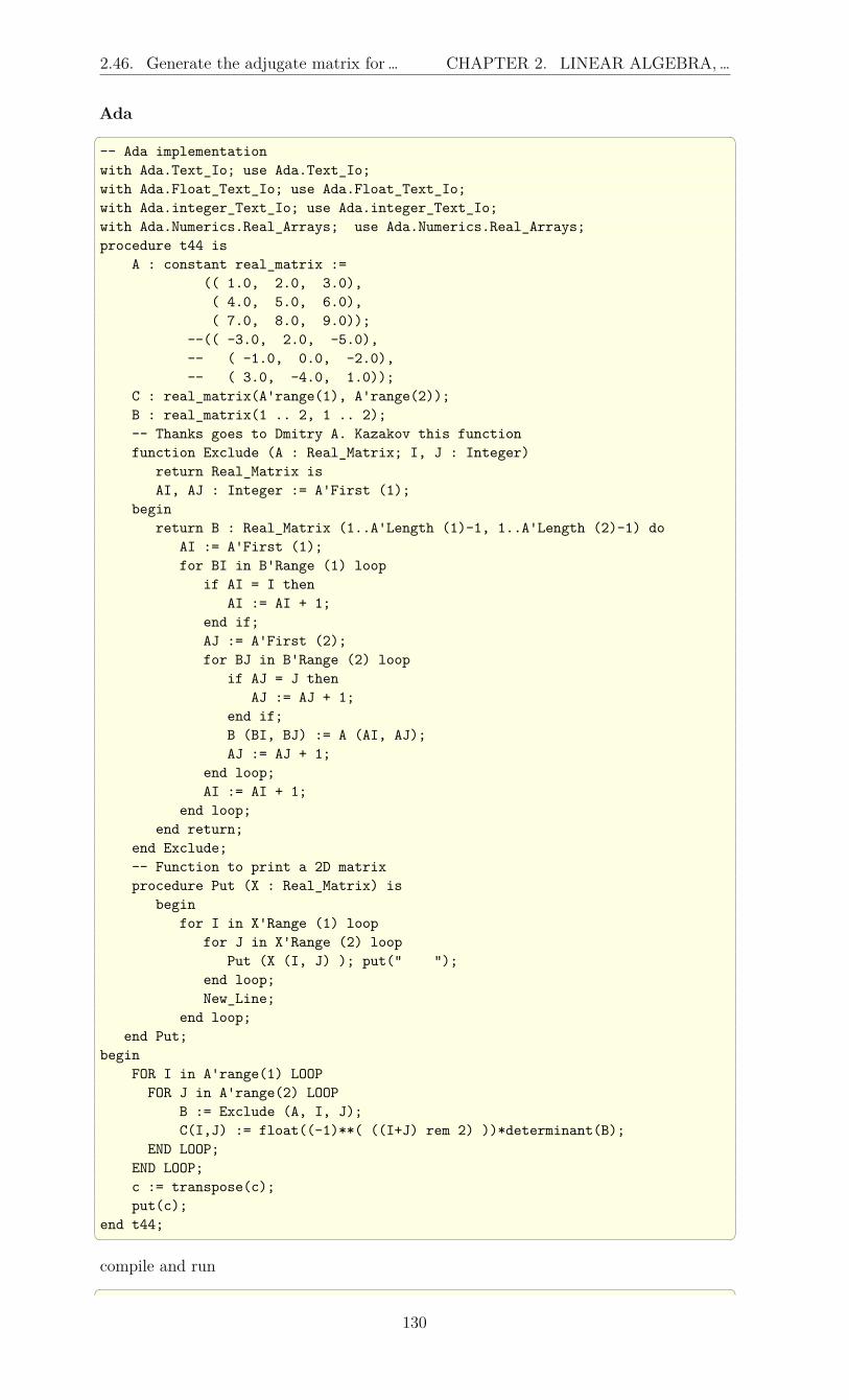
2.46. Generate the adjugate matrix for … CHAPTER 2. LINEAR ALGEBRA,…
Ada -- Ada implementationwith Ada.Text_Io; use Ada.Text_Io;with Ada.Float_Text_Io; use Ada.Float_Text_Io;with Ada.integer_Text_Io; use Ada.integer_Text_Io;with Ada.Numerics.Real_Arrays; use Ada.Numerics.Real_Arrays;procedure t44 is
A : constant real_matrix :=(( 1.0, 2.0, 3.0),( 4.0, 5.0, 6.0),( 7.0, 8.0, 9.0));
--(( -3.0, 2.0, -5.0),-- ( -1.0, 0.0, -2.0),-- ( 3.0, -4.0, 1.0));
C : real_matrix(A'range(1), A'range(2));B : real_matrix(1 .. 2, 1 .. 2);-- Thanks goes to Dmitry A. Kazakov this functionfunction Exclude (A : Real_Matrix; I, J : Integer)
return Real_Matrix isAI, AJ : Integer := A'First (1);
beginreturn B : Real_Matrix (1..A'Length (1)-1, 1..A'Length (2)-1) do
AI := A'First (1);for BI in B'Range (1) loop
if AI = I thenAI := AI + 1;
end if;AJ := A'First (2);for BJ in B'Range (2) loop
if AJ = J thenAJ := AJ + 1;
end if;B (BI, BJ) := A (AI, AJ);AJ := AJ + 1;
end loop;AI := AI + 1;
end loop;end return;
end Exclude;-- Function to print a 2D matrixprocedure Put (X : Real_Matrix) is
beginfor I in X'Range (1) loop
for J in X'Range (2) loopPut (X (I, J) ); put(" ");
end loop;New_Line;
end loop;end Put;
beginFOR I in A'range(1) LOOP
FOR J in A'range(2) LOOPB := Exclude (A, I, J);C(I,J) := float((-1)**( ((I+J) rem 2) ))*determinant(B);
END LOOP;END LOOP;c := transpose(c);put(c);
end t44; compile and run
130

2.47. Multiply each column by values … CHAPTER 2. LINEAR ALGEBRA,…
-- export LD_LIBRARY_PATH=/usr/lib/atlas-base/:/usr/lib/atlas-base/atlas/>gnatmake t44.adbgcc-4.6 -c t44.adbgnatbind -x t44.alignatlink t44.ali
>./t44-3.00000E+00 6.00000E+00 -3.00000E+006.00000E+00 -1.20000E+01 6.00000E+00-3.00000E+00 6.00000E+00 -3.00000E+00 2.47 Multiply each column by values taken from a
rowGiven a row of the same number of values as the number of columns in a matrix, how toscale each column by the corresponding value in that row? This picture explains more theproblem
r r1 r2 A
a11 a12
a21 a22
a31 a32
Multiply this value by this column
Multiply this value by this column
r1a11 r2a12
r1a21 r2a22
r1a31 r2a32
In Matlab, bsxfun is used.
2.47.1 Mathematicacredit for this solution goes to Bob Hanlon, Adriano Pascoletti, Kurt Tekolste, David Park,and Peter. J. C. Moses from the Math group r = 2,3;mat = 1,2,3,4,5,6;r #&/@mat
(*or*)Map[v*#&, mat]
2, 6,6, 12,10, 18
Another way is to use Inner[] command. Credit for this solution goes to Sswziwa Mukasaand Peter. J. C. Moses from the Math group r=2,3;mat=1,2,3,4,5,6;Inner[Times,mat,r,List] Out[66]= 2, 6,
6, 12,
131

2.47. Multiply each column by values … CHAPTER 2. LINEAR ALGEBRA,…
10, 18 2.47.2 Matlab r=[2 3];A=[1 2;
3 4;5 6]
bsxfun(@times,r,A) ans =
2 66 1210 18
2.47.3 Fortran program t45implicit none
integer, parameter :: nRow=3, nCol=2
character(len=*), parameter :: FMT = "(2I5)"integer :: v(nCol),A(nRow,nCol),B(nRow,nCol),i,j;
!-- initialization of datav = [2,3]A(1,:) = [1,2];A(2,:) = [3,4];A(3,:) = [5,6];
!F2008!do concurrent (j = 1:nCol)! B(:,j) = v(j)*A(:,j)!end do
do j=1,nColB(:,j) = v(j)*A(:,j)
end do
write(*,FMT) ( (B(i,j),j=1,nCol), i=1,nRow)
end program t45 #compile and run>gfortran -std=f2008 t45.f90>./a.out
2 66 1210 18
132

2.48. extract submatrix from a larger … CHAPTER 2. LINEAR ALGEBRA,…
2.47.4 OctaveUse automatic broadcasting r .* A 2.47.5 Maple r:=Vector[row]([2,3]);mat:=Matrix([[1,2],[3,4],[5,6]]);
f:=n->r(n)*mat(1..3,n);f~([1,2]);convert(%,Matrix)
2 6
6 12
10 18
2.48 extract submatrix from a larger matrix by
removing row/columnGiven 2D matrix A extract all submatrices by removing row/column.
For example, given the matrix
1 2 3
4 5 6
7 8 9
then the submatrix for (1, 1) is(5 6
8 9
)obtained
by removing the first row and the first column.
In Mathematica, ReplacePart can be used. In Matlab the [] operator can be used. InFortran, the pack() function can be used.
2.48.1 Mathematica
mat=1,2,3,
4,5,6,7,8,9;
nRow, nCol = Dimensions[mat];Table[ReplacePart[mat,i,i,_,_,j
:>Sequence[],Heads-> False],i,nRow,j,nCol];
r=Flatten[%,1]
5,6,8,9,4,6,7,9,4,5,7,8,2,3,8,9,1,3,7,9,1,2,7,8,2,3,5,6,1,3,4,6,1,2,4,5
133
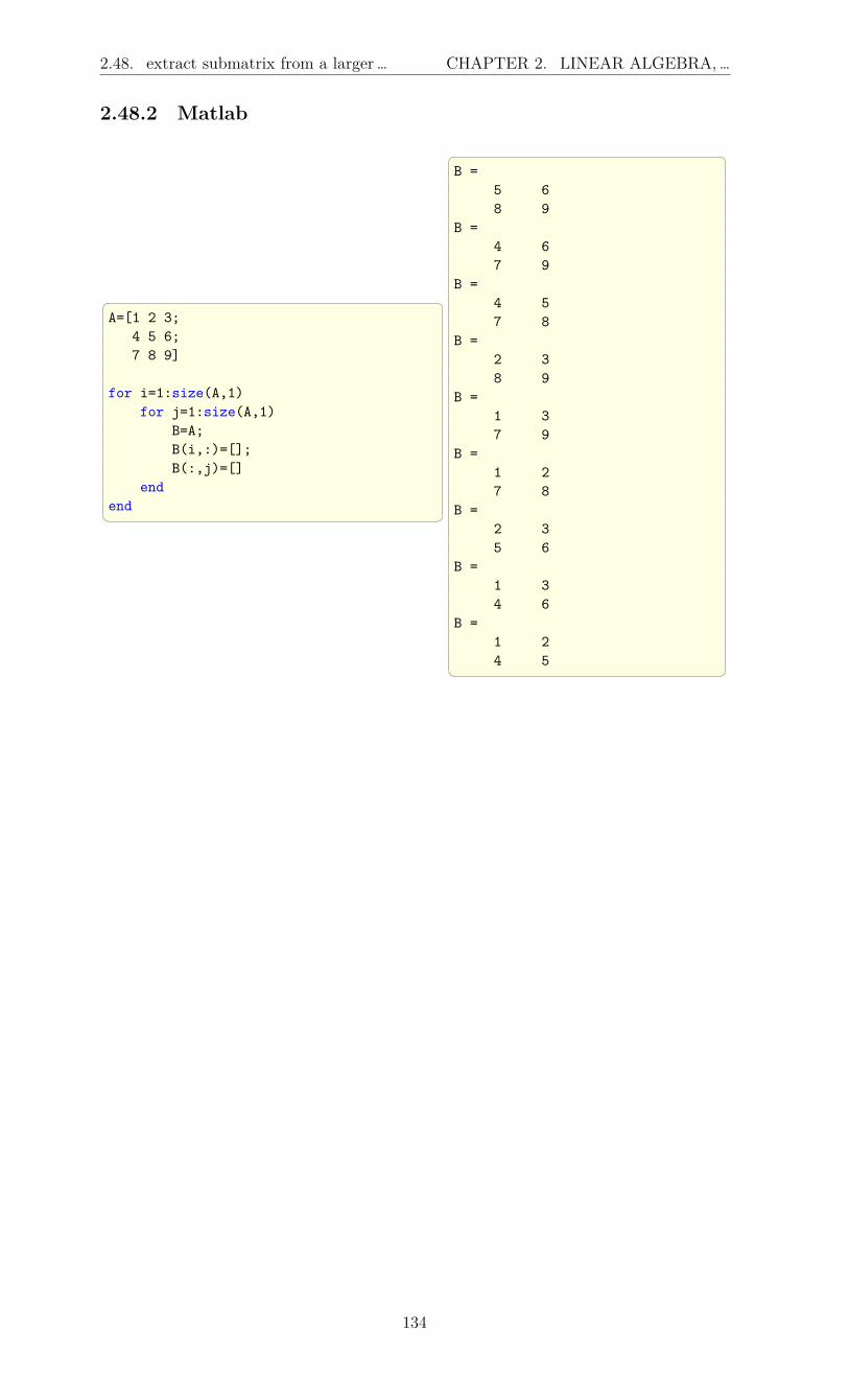
2.48. extract submatrix from a larger … CHAPTER 2. LINEAR ALGEBRA,…
2.48.2 Matlab
A=[1 2 3;
4 5 6;7 8 9]
for i=1:size(A,1)for j=1:size(A,1)
B=A;B(i,:)=[];B(:,j)=[]
endend
B =
5 68 9
B =4 67 9
B =4 57 8
B =2 38 9
B =1 37 9
B =1 27 8
B =2 35 6
B =1 34 6
B =1 24 5
134
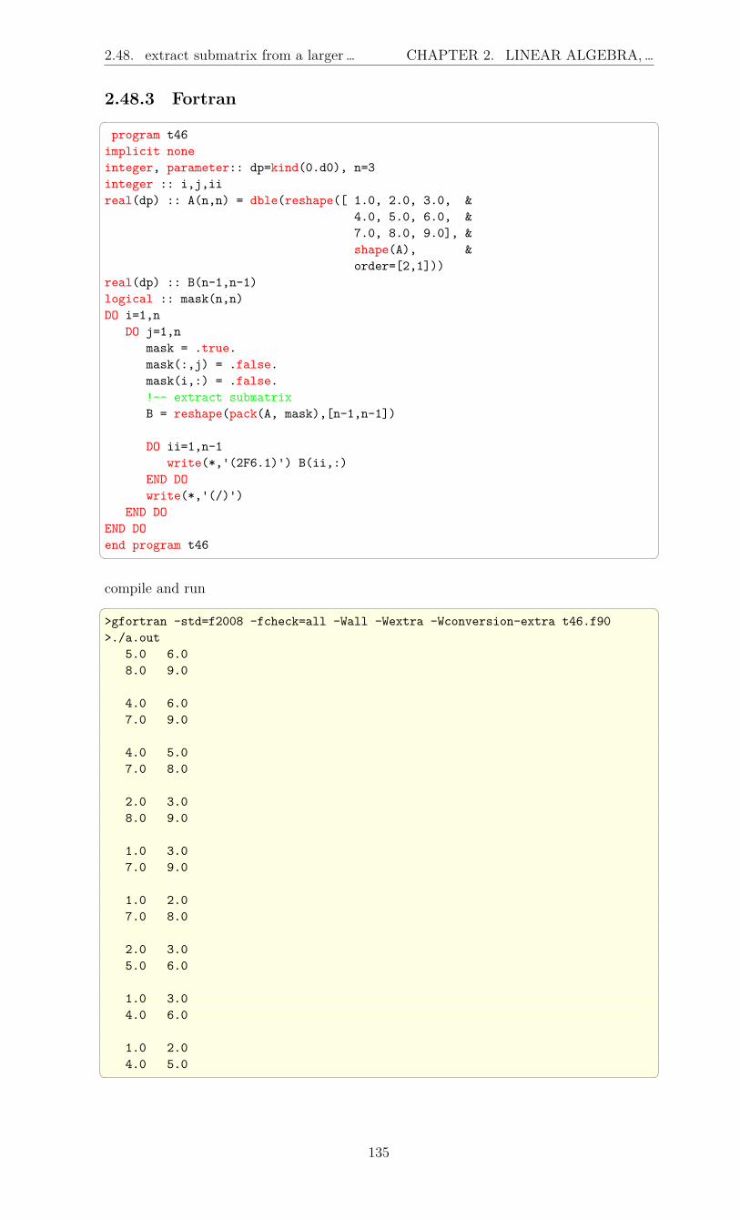
2.48. extract submatrix from a larger … CHAPTER 2. LINEAR ALGEBRA,…
2.48.3 Fortran program t46implicit noneinteger, parameter:: dp=kind(0.d0), n=3integer :: i,j,iireal(dp) :: A(n,n) = dble(reshape([ 1.0, 2.0, 3.0, &
4.0, 5.0, 6.0, &7.0, 8.0, 9.0], &shape(A), &order=[2,1]))
real(dp) :: B(n-1,n-1)logical :: mask(n,n)DO i=1,n
DO j=1,nmask = .true.mask(:,j) = .false.mask(i,:) = .false.!-- extract submatrixB = reshape(pack(A, mask),[n-1,n-1])
DO ii=1,n-1write(*,'(2F6.1)') B(ii,:)
END DOwrite(*,'(/)')
END DOEND DOend program t46 compile and run >gfortran -std=f2008 -fcheck=all -Wall -Wextra -Wconversion-extra t46.f90>./a.out
5.0 6.08.0 9.0
4.0 6.07.0 9.0
4.0 5.07.0 8.0
2.0 3.08.0 9.0
1.0 3.07.0 9.0
1.0 2.07.0 8.0
2.0 3.05.0 6.0
1.0 3.04.0 6.0
1.0 2.04.0 5.0
135

2.48. extract submatrix from a larger … CHAPTER 2. LINEAR ALGEBRA,…
2.48.4 Ada with Ada.Text_Io; use Ada.Text_Io;with Ada.Float_Text_Io; use Ada.Float_Text_Io;with Ada.Numerics.Real_Arrays; use Ada.Numerics.Real_Arrays;procedure foo is
A : constant Real_Matrix :=(( 1.0, 2.0, 3.0),( 4.0, 5.0, 6.0),( 7.0, 8.0, 9.0));
B : real_matrix(1 .. 2, 1 .. 2);-- Thanks goes to Dmitry A. Kazakov-- for providing this functionfunction Exclude (A : Real_Matrix; I, J : Integer)
return Real_Matrix isAI, AJ : Integer := A'First (1);
beginreturn B : Real_Matrix(1..A'Length(1)-1,1..A'Length(2)-1) do
AI := A'First (1);for BI in B'Range (1) loop
if AI = I thenAI := AI + 1;
end if;AJ := A'First (2);for BJ in B'Range (2) loop
if AJ = J thenAJ := AJ + 1;
end if;B (BI, BJ) := A (AI, AJ);AJ := AJ + 1;
end loop;AI := AI + 1;
end loop;end return;
end Exclude;
-- Function to print a 2D matrixprocedure put(A: Real_Matrix) isbeginfor I in A'range(1) loopfor J in A'range(2) loop
put(A(I,J));end loop;new_line;
end loop;end put;
beginFOR I in A'range(1) LOOP
FOR J in A'range(2) LOOPB := Exclude (A, I, J);put(B);new_line(1);
END LOOP;END LOOP;
end foo; compile and run >gnatmake foo.adbgcc-4.6 -c foo.adbgnatbind -x foo.alignatlink foo.ali
136

2.48. extract submatrix from a larger … CHAPTER 2. LINEAR ALGEBRA,…
>./foo>./foo5.00000E+00 6.00000E+008.00000E+00 9.00000E+00
4.00000E+00 6.00000E+007.00000E+00 9.00000E+00
4.00000E+00 5.00000E+007.00000E+00 8.00000E+00
2.00000E+00 3.00000E+008.00000E+00 9.00000E+00
1.00000E+00 3.00000E+007.00000E+00 9.00000E+00
1.00000E+00 2.00000E+007.00000E+00 8.00000E+00
2.00000E+00 3.00000E+005.00000E+00 6.00000E+00
1.00000E+00 3.00000E+004.00000E+00 6.00000E+00
1.00000E+00 2.00000E+004.00000E+00 5.00000E+00
2.48.5 Maple del:=proc(A::Matrix,idx::list)::Matrix;
local B;B:=LinearAlgebra:-DeleteRow(A,idx[1]);B:=LinearAlgebra:-DeleteColumn(B,idx[2]);return B;
end proc;
A:=Matrix([[1,2,3],[4,5,6],[7,8,9]]):r:=map2(del,A,[indices(A,indexorder)]); [[
5 6
8 9
],
[4 6
7 9
],
[4 5
7 8
],
[2 3
8 9
],
[1 3
7 9
],
[1 2
7 8
],
[2 3
5 6
],
[1 3
4 6
],
[1 2
4 5
]]
137

2.49. delete one row from a matrix CHAPTER 2. LINEAR ALGEBRA,…
2.49 delete one row from a matrixExample, Given the folowing 2D matrix A delete the second row1 2 3
4 5 6
7 8 9
2.49.1 Mathematica
mat=1,2,3,
4,5,6,7,8,9;
mat[[2]]=Sequence[];mat
Out[81]= 1,2,3,
7,8,9
or a little longer solution using Pick nRow,nCol=Dimensions[mat];mask=Table[True,nRow,nCol];mask[[2]]=False;Pick[mat,mask]
Out[70]= 1,2,3,
7,8,9
2.49.2 Matlab
A=[1 2 3;4 5 6;7 8 9];A(2,:)=[]
A =
1 2 37 8 9
2.49.3 Maple
A:=<1,2,3;
4,5,6;7,8,9>;
A:=LinearAlgebra:-DeleteRow(A,2);
[1 2 3]
A := [ ][7 8 9]
138

2.50. delete one column from a matrix CHAPTER 2. LINEAR ALGEBRA,…
2.50 delete one column from a matrixExample, Given the folowing 2D matrix A delete say the second column1 2 3
4 5 6
7 8 9
2.50.1 Mathematica
mat=1,2,3,
4,5,6,7,8,9;
mat[[All,2]]=Sequence[];mat
Out[93]= 1,3,
4,6,7,9
or a little longer solution using Pick nRow,nCol=Dimensions[mat];mask=Table[True,nRow,nCol];mask[[All,2]]=False;mat=Pick[mat,mask];mat
Out[98]= 1,3,
4,6,7,9
2.50.2 Matlab
A=[1 2 3;4 5 6;7 8 9];A(:,2)=[]
A =
1 34 67 9
2.50.3 Maple
A:=Matrix([[1,2,3],[4,5,6],[7,8,9]]);A:=LinearAlgebra:-DeleteColumn(A,2);
1 3
4 6
7 9
139

2.51. generate random matrix so that each… CHAPTER 2. LINEAR ALGEBRA,…
2.51 generate random matrix so that each row addsto 1
Generate the random matrix and divide each row by its total
2.51.1 Mathematica
mat = Table[RandomReal[],3,4]
0.76862 0.917299 0.606119 0.63735
0.610077 0.208307 0.0337861 0.473017
0.388772 0.432688 0.475881 0.68523
s = Total[mat,2] 1.15201, 1.99068, 3.05063
s = Total[mat,2];b = mat/s
0.15919 0.0553157 0.448352 0.337142
0.358594 0.264968 0.123659 0.25278
0.216269 0.248665 0.278871 0.256195
Total[b,2]
Out[24]= 1.,1.,1.
2.51.2 Matlab
A = rand(3,4)s = sum(A,2);B = bsxfun(@rdivide,A,s)sum(B,2)
A =0.6787 0.3922 0.7060 0.04620.7577 0.6555 0.0318 0.09710.7431 0.1712 0.2769 0.8235
B =0.3723 0.2151 0.3873 0.02530.4913 0.4250 0.0206 0.06300.3689 0.0850 0.1375 0.4087
ans =1.00001.00001.0000
140

2.52. generate random matrix so that each… CHAPTER 2. LINEAR ALGEBRA,…
2.51.3 Maple
restart;A:=LinearAlgebra:-RandomMatrix(3,4,generator=0..1.0 );for n from 1 to LinearAlgebra:-RowDimension(A) do
A[n,..]:=A[n,..]/add(A[n,..]);od:A;
#verify each row sums to 1map(x->add(x),[LinearAlgebra:-Row(A,[1..-1])])
[0.9705927818 0.9575068354 0.0975404050 0.1269868163][ ]
A := [0.1576130817 0.5468815192 0.6323592462 0.9057919371][ ][0.9648885352 0.2784982189 0.9133758561 0.8147236864]
[0.4508876154 0.4448085560 0.0453122684 0.0589915605][ ][0.0702799715 0.2438555046 0.2819701848 0.4038943392][ ][0.3247157951 0.0937235414 0.3073801341 0.2741805296]
[1.00000000026568, 1.00000000004739, 1.00000000023679]
2.52 generate random matrix so that each columnadds to 1
Generate the random matrix and divide each column by its total
2.52.1 Mathematica
This method due to Bob Hanlon from theMath group mat = Table[RandomReal[],3,4]s = Total[mat,1]b = #/s& /@ matTotal[b,1]
Out[31]= 0.440393,0.945076,0.0527301,0.537288,0.515868,0.565691,0.800959,0.0302484,0.509004,0.143124,0.519455,0.264779
Out[32]= 1.46526,1.65389,1.37314,0.832315
Out[36]= 0.300555,0.571426,0.038401,0.645535,0.352065,0.342036,0.583303,0.0363425,0.34738,0.0865376,0.378296,0.318123
Out[37]= 1.,1.,1.,1.
Or can use Transpose b = Transpose[Transpose[mat]/s];Total[b,1]
1.,1.,1.,1.
Another way of doing the above, withoutthe need to transpose 2 times is the follow-ing b=Inner[Divide,mat,s,List];Total[b,1]
1.,1.,1.,1.
141

2.52. generate random matrix so that each… CHAPTER 2. LINEAR ALGEBRA,…
2.52.2 Matlab
A=rand(3,4)s=sum(A,1);B=bsxfun(@rdivide,A,s)sum(B,1)
A =0.6948 0.0344 0.7655 0.48980.3171 0.4387 0.7952 0.44560.9502 0.3816 0.1869 0.6463
B =0.3541 0.0403 0.4380 0.30970.1616 0.5133 0.4550 0.28170.4843 0.4464 0.1069 0.4086
ans =1.0000 1.0000 1.0000 1.0000
2.52.3 Maple A:=LinearAlgebra:-RandomMatrix(3,4);
[ 9 -95 51 24][ ]
A := [99 -20 76 65][ ][60 -25 -44 86]
b:=MTM:-sum(A,1); #sum columnsb := [168, -140, 83, 175]
nCol:=LinearAlgebra:-ColumnDimension(A):B:=convert([seq(A[..,i]/b[i],i=1..nCol)],Matrix);
[3 19 51 24 ][-- -- -- ---][56 28 83 175][ ][33 1 76 13]
B := [-- - -- --][56 7 83 35][ ][5 5 -44 86 ][-- -- --- ---][14 28 83 175]
MTM:-sum(B,1);
[1, 1, 1, 1]
142
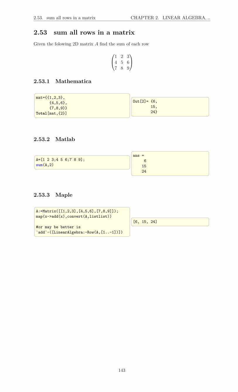
2.53. sum all rows in a matrix CHAPTER 2. LINEAR ALGEBRA,…
2.53 sum all rows in a matrixGiven the folowing 2D matrix A find the sum of each row
1 2 3
4 5 6
7 8 9
2.53.1 Mathematica
mat=1,2,3,
4,5,6,7,8,9
Total[mat,2]
Out[2]= 6,
15,24
2.53.2 Matlab
A=[1 2 3;4 5 6;7 8 9];sum(A,2)
ans =
61524
2.53.3 Maple
A:=Matrix([[1,2,3],[4,5,6],[7,8,9]]);map(x->add(x),convert(A,listlist))
#or may be better is`add`~([LinearAlgebra:-Row(A,[1..-1])])
[6, 15, 24]
143

2.54. sum all columns in a matrix CHAPTER 2. LINEAR ALGEBRA,…
2.54 sum all columns in a matrixGiven the folowing 2D matrix A find the sum of each column1 2 3
4 5 6
7 8 9
Mathematica In[3]:= mat=1,2,3,
4,5,6,7,8,9
Total[mat,1]
Out[4]= 12,15,18
Matlab A=[1 2 3;4 5 6;7 8 9];sum(A,1)
ans =12 15 18
Maple `add`~([LinearAlgebra:-Column(A,[1..-1])])
# [12, 15, 18]
2.55 find in which columns values that are not zero
given matrix
0 39 0
55 100 0
34 0 0
0 9 0
0 0 50
find the column index which contain values > 0 but do it
from top row to the bottom row. Hence the result should be
1st row︷︸︸︷2 ,
2nd row︷︸︸︷1,2 ,
︷︸︸︷1 ,︷︸︸︷2 ,︷︸︸︷3
this is becuase on the first row, nonzero is in second column, and on the second row, nonzerois at first and second column, and on the third row, nonzero is at the first column, and soon.Mathematica mat=0, 39, 0,
55,100, 0,34,0, 0,0, 9, 0,0, 0, 50;
Position[#,x_/;x>0]&/@mat;Flatten[%]
Out[18]= 2,1,2,1,2,3
144

2.56. How to remove values from one… CHAPTER 2. LINEAR ALGEBRA,…
Matlab A=[0 39 0
55 100 034 0 00 9 00 0 50];
[I,~]=find(A'>0)I'
2 1 2 1 2 3
Maple A:=Matrix([[0,39,0],
[55,100,0],[34,0,0],[0,9,0],[0,0,50]]):
f:=x->`if`(not evalb(A(x[1],x[2])=0),x[2],NULL):f~([indices(A,indexorder)])
#Or may be better ismap(x->convert(ArrayTools:-SearchArray(x),list),[LinearAlgebra:-Row(A,[1..-1])]);ListTools:-Flatten(%)
[2,1,2,1,2,3]
2.56 How to remove values from one vector thatexist in another vector
Given vector v1 = 1, 3, 4, 5, 8, 9, 20.2, 30,−44 remove from it any element that exist inv2 = 1, 7, 4. Notice that Complement[] in Mathematica or setdiff() in Matlab canbe used, but they will sort the result. Hence they are not used here in order to keep theorder the same.
2.56.1 Mathematica
#first methodv1=1,3,4,5,8,9,20.2,30,-44;v2=1,7,4;v1=DeleteCases[v1,Alternatives@@v2] 3,5,8,9,20.2,30,-44
#second methodv1=1,3,4,5,8,9,20.2,30,-44;v2=1,7,4;v1=DeleteCases[v1,x_/;MemberQ[v2,x]] 3,5,8,9,20.2,30,-44
145

2.57. How to find mean of equal sized… CHAPTER 2. LINEAR ALGEBRA,…
2.56.2 Matlab
v1=[1,3,4,5,8,9,20.2,30,-44];v2=[1,7,4];v1(ismember(v1,v2))=[]
v1 =3.0000 5.0000 8.0000 9.0000 20.2000 30.0000 -44.0000
2.56.3 Fortran program fimplicit noneREAL, ALLOCATABLE :: A(:),B(:)A =[1.0,3.0,4.0,5.0,8.0,9.0,20.2,30.0,-44.0];B =[1.0,7.0,4.0];A = pack(A, A .NE. B)Print *,A
end program f >gfortran f2.f90>./a.out3.0000000 5.0000000 8.0000000 9.0000000 20.200001 30.000000 -44.000000 2.56.4 Maple
v1:=Array([1,3,4,5,8,9,20.2,30,-44]);v2:=Array([1,7,4]);select[flatten](x->not(member(x,v2)),v1)
[3, 5, 8, 9, 20.2, 30, -44]
2.57 How to find mean of equal sized segments of avector
Given vector V of length m find the mean of segments V (1 : n), V (n+ 1 : 2n), V (2n+ 1 :3n) . . . . In otherwords, equal length segments.
Mathematica len = 52; n = 4;v = RandomReal[0, 1, len];Mean /@ Partition[v, n]
0.750653,0.410073,0.401005,0.138907,0.466247,0.568257,0.535362,0.517755,0.555368,0.705857,0.502319,0.453571,0.357949
146

2.58. find first value in column larger than… CHAPTER 2. LINEAR ALGEBRA,…
Matlab N = 52;n = 4;V = rand(N,1);mean(reshape(V,n,N/n))'
ans =
0.30260.35890.47450.62490.30420.54280.23870.32000.62240.44080.56570.54690.5696
2.58 find first value in column larger than somevalue and cut matrix from there
Given matrix 1 5
2 3
4 8
7 2
search in column 2 of matrix for the first time a value exceeds 6 and return the matrixup to that row. The result should be
(1 5
2 3
)Mathematica a = 1, 5, 2, 3, 4, 8, 7, 2;Min@Position[a, x_, y_ /; y > 6](* 3 *)
a[[1 ;; % - 1]]
1, 5, 2, 3
Matlab A = [1,5;2,3;4,8;7,2];A(1:find(A(:,2)>6)-1,:)
ans =
1 52 3
Maple A:=Matrix([[1,5],[2,3],[4,8],[7,2]]);idx := ListTools:-SelectFirst(1, x->x>6 , A[..,2],output=indices);if idx[1]>1 then
A[1..idx[1]-1,..];else
A[1..idx[1],..];fi;
[1 5
2 3
]
147

2.59. make copies of each value into matrix … CHAPTER 2. LINEAR ALGEBRA,…
2.59 make copies of each value into matrix into alarger matrix
Do the following transformation. Take each element of matrix, and replace it by a 2 by 2matrix with its values in places.
kron() in Matlab and KroneckerProduct in Mathematica and Maple can be used for this.
Mathematica mat = 1, 2, 3, 4, 5, 6, 7, 8, 9;kernel = 1, 1, 1, 1;KroneckerProduct[mat, kernel] Another method that can be used in this, but I preferthe kron method above: mat = 1, 2, 3, 4, 5, 6, 7, 8, 9;Map[ConstantArray[#, 2, 2] &, mat, 2]ArrayFlatten[%, 2]
1, 1, 2, 2, 3, 3,1, 1, 2, 2, 3, 3,4, 4, 5, 5, 6, 6,4, 4, 5, 5, 6, 6,7, 7, 8, 8, 9, 9,7, 7, 8, 8, 9, 9
Matlab A=[1 2 3; 4 5 6; 7 8 9]kernel=ones(2,2)kron(A,kernel)
1 1 2 2 3 31 1 2 2 3 34 4 5 5 6 64 4 5 5 6 67 7 8 8 9 97 7 8 8 9 9
Maple restart;mat := Matrix([[1, 2, 3], [4, 5, 6], [7, 8, 9]]);kernel := Matrix([[1, 1], [1, 1]]);LinearAlgebra:-KroneckerProduct(mat,kernel)
1 1 2 2 3 3
1 1 2 2 3 3
4 4 5 5 6 6
4 4 5 5 6 6
7 7 8 8 9 9
7 7 8 8 9 9
148

2.60. repeat each column of matrix number … CHAPTER 2. LINEAR ALGEBRA,…
2.60 repeat each column of matrix number of timesGives a matrix, repeate each column a number of time, say 3 times, in place to produce amatrix 3 times as wide as the original.
kron() in Matlab and KroneckerProduct in Mathematica and Maple can be used for this.
Mathematica mat = 1, 2, 3, 4,
5 , 6, 7, 8,9, 10, 11, 12
KroneckerProduct[mat, 1, 1, 1] Another method that can be used in this, butthe above is better r = Map[#*1, 1, 1 &, mat, 2]Partition[Flatten[r], 12]
1, 1, 1, 2, 2, 2, 3, 3, 3, 4, 4, 4,5, 5, 5, 6, 6, 6, 7, 7, 7, 8, 8, 8,9, 9, 9, 10, 10, 10, 11, 11, 11, 12, 12, 12
Matlab A=[1 2 3 4;
5 6 7 8;9 10 11 12];
kernel=ones(1,3);kron(A,kernel)
ans =1 1 1 2 2 2 3 3 3 4 4 45 5 5 6 6 6 7 7 7 8 8 89 9 9 10 10 10 11 11 11 12 12 12
Maple restart;mat := Matrix([[1, 2, 3,4], [5, 6,7,8], [9,10,11,12]]);kernel := Vector[row]([1,1,1]);LinearAlgebra:-KroneckerProduct(mat,kernel);
1 1 1 2 2 2 3 3 3 4 4 4
5 5 5 6 6 6 7 7 7 8 8 8
9 9 9 10 10 10 11 11 11 12 12 12
2.61 How to apply a function to each value in amatrix?
Apply function f(x, n) to ragged matrix where n is value taken from the matrix and x issome other value defined somewhere else. The result of the function should replace thesame position in the matrix where n was.
For example, given matrix
mat =
1 2 3
4 5
7 8 9
generate the matrix
f [x, 1] f [x, 2] f [x, 3]
f [x, 4] f [x, 5]
f [x, 7] f [x, 8] f [x, 9]
149

2.62. How to sum all numbers in a list … CHAPTER 2. LINEAR ALGEBRA,…
MathematicaThe trick is to use Map with 2 at end. ClearAll[f, x]mat = 1, 2, 3, 4, 5, 7, 8, 9;Map[f[x, #] &, mat, 2]
f(x, 1), f(x, 2), f(x, 3), f(x, 4), f(x, 5), f(x, 7), f(x, 8), f(x, 9)
Maple #use double maprestart;mat:=[[1,2,3],[4,5],[7,8,9]];map(x->map(y->f(y),x),mat)
[[f(1), f(2), f(3)], [f(4), f(5)], [f(7), f(8), f(9)]]
2.62 How to sum all numbers in a list (vector)?Given a vector or list 1, 2, 3, 4, 5, 6, 7, 8, 9, 10 how to find the sum of all its elements?
Mathematica list=Range[10]
1,2,3,4,5,6,7,8,9,10
Total[list] 55Matlab lst=1:10sum(lst) 55
Maple lst:=[seq( i, i=1..10 )];add(lst) 55
2.63 How to find maximum of each row of a matrix?Given (
1 2
3 4
)Find the maximum of each row. The result should be (2, 4). (to find the min, just changeMax with Min below.Mathematica mat = 1, 2, 3, 4Map[Max , mat] (* or Max /@ mat *)
2,4
150

2.64. How to find maximum of each column… CHAPTER 2. LINEAR ALGEBRA,…
Matlab A=[1 2;3 4];max(A')
2 4
Maple A:=Matrix([[1,2],[3,4]]);`max`~([LinearAlgebra:-Row(A,1..-1)])
[2, 4]
2.64 How to find maximum of each column of amatrix?
Given (1 2
3 4
)Find the maximum of each column. The result should be (3, 4). (to find the min, justchange Max with Min below.
Mathematica mat = 1, 2, 3, 4Map[Max , Transpose[mat]]
(* or Max /@ Transpose@mat *)
3, 4
Matlab A=[1 2;3 4];max(A)
3 4
Maple A:=Matrix([[1,2],[3,4]]);`max`~([LinearAlgebra:-Column(A,1..-1)])
[3, 4]
2.65 How to add the mean of each column of amatrix from each column?
Given (1 2
3 4
)Find the mean of each column, and add this mean to each element of the correspondingcolumn. The result should be
(3 5
5 7
)
151

2.66. How to add the mean of each row of … CHAPTER 2. LINEAR ALGEBRA,…
To subtract the mean, just replace Plus with Subtract below for Mathematica and re-place @plus with @minus for Matlab. This shows that Matlab bsxfun is analogue toMathematica’s MapThread.
Mathematica mat = 1, 2, 3, 4MapThread[Plus,Transpose@mat, Mean[mat]]
3, 5, 5, 7
Matlab A=[1 2;3 4];bsxfun(@plus, A, mean(A))
ans =
3 55 7
MapleMaple mean always return real value, even ifexact is possible. A:=Matrix([[1,2],[3,4]]);for n from 1 to LinearAlgebra:-ColumnDimension(A) do
A[..,n]:=A[..,n] +~ Statistics:-Mean(A[..,n])od;A
[3.0 5.0
5.0 7.0
]
2.66 How to add the mean of each row of a matrixfrom each row?
Given (1 2
3 4
)Find the mean of each row, and add this mean to each element of the corresponding row.The result should be
(2.5 3.5
6.5 7.5
)To subtract the mean, just replace Plus with Subtract below for Mathematica and replace@plus with @minus for Matlab. This shows that Matlab bsxfun is analogue to Mathemat-ica’s MapThread.. The main difference is that Matlab is a little bit more consistent in thisexample, since in Matlab all operations are done column wise. Hence mean(A) takes themean of each column (same as Matematica in this one case), but bsxfun also acts columnwise on the matrix A, while Mathematica Map and MapThread act row wise (list of lists).One just needs to be careful about this order difference.
Mathematica mat = 1, 2, 3, 4;MapThread[Plus,mat, Mean@Transpose@mat] // N
2.5, 3.5, 6.5, 7.5
152

2.67. Find the different norms of a vector CHAPTER 2. LINEAR ALGEBRA,…
Matlab A=[1 2;3 4];bsxfun(@plus, A', mean(A'))
ans =
2.5 6.53.5 7.5
Maple A:=Matrix([[1,2],[3,4]]);for n from 1 to LinearAlgebra:-RowDimension(A) do
A[n,..]:=A[n,..] +~ Statistics:-Mean(A[n,..])od;A
[2.5000000000 3.5000000000
6.5000000000 7.5000000000
]
2.67 Find the different norms of a vectorProblem: Given the vector say
v = 1, 2, 4
Find its norm for p = 1, 2,∞
Mathematica Remove["Global`*"];
v = 1, 2, 4;p = 1, 2, Infinity;Map[Norm[v,#]&,p]
7,Sqrt[21],4
Matlab clear all; close all;v=[1 2 4];p=[1,2,inf];arrayfun(@(i) norm(v,p(i)),1:length(p))
ans =7.0000 4.5826 4.0000
2.68 Check if a matrix is HermiteProblem: Given a matrix A, check to see if it is Hermite.
A Matrix is Hermite if it is the same as the conjugate of its transpose. One way to checkis to take the difference and check that all values in the resulting difference matrix arezero.
To account for numerical values, the check is done using machine epsilon.
Mathematica mat = -1,1-3*I,0,
1+3*I,0,-6*I,0,6*I,1;
HermitianMatrixQ[mat] True
153

2.69. Obtain the LU decomposition of a … CHAPTER 2. LINEAR ALGEBRA,…
Matlab clear all;i=sqrt(-1);mat=[-1 1-3*i 0;
1+3*i 0 -6*i;0 6*i 1];
mat2=conj(transpose(mat));diff = mat-mat2
diff =
0 0 00 0 00 0 0
r=abs(diff)<eps('double')
r =
1 1 11 1 11 1 1
all(r(:)) 1Maple mat := Matrix([[-1,1-3*I,0], [1+3*I,0,-6*I],[0,6*I,1]]);mat2:= LinearAlgebra:-HermitianTranspose(mat);LinearAlgebra:-Equal(mat,mat2)
true
2.69 Obtain the LU decomposition of a matrixProblem: Given a matrix A, find matrix L and U such that LU = A. The matrix L willhave 1 in all the diagonal elements and zeros in the upper triangle. The matrix U willhave 0 in the lower triangle as shown in this diagram.
=
A L U
*
1
1
1
0
0 0
0
0 0
154

2.69. Obtain the LU decomposition of a … CHAPTER 2. LINEAR ALGEBRA,…
Mathematica Remove["Global`*"]mat = 1, -3, 5,
2, -4, 7,-1, -2, 1;
lu,pivotVector,conditionNumber=LUDecomposition[mat]
1,-3,5,2,2,-3,-1,-(5/2),-(3/2),1,2,3,1
lower=lu*SparseArray[i_,j_/;j<i->1,3,3]+
IdentityMatrix[3] 1,0,0,2,1,0,-1,-(5/2),1
upper=lu SparseArray[i_,j_/;j>=i->1,3,3]
1,-3,5,0,2,-3,0,0,-(3/2)
lower.upper
1,-3,5,2,-4,7,-1,-2,1
Matlab clear all;
A=[1 -3 5;2 -4 7;-1 -2 1];
[L,U,p]=lu(A)
L =
1.0000 0 0-0.5000 1.0000 00.5000 0.2500 1.0000
U =2.0000 -4.0000 7.0000
0 -4.0000 4.50000 0 0.3750
p =0 1 00 0 11 0 0
L*U
ans =
2 -4 7-1 -2 11 -3 5
Maple A:=Matrix([[1,-3,5],[2,-4,7],[-1,-2,1]]);p,l,u:=LinearAlgebra:-LUDecomposition(A);
1 0 0
0 1 0
0 0 1
,
1 0 0
2 1 0
−1 −52
1
,
1 −3 5
0 2 −3
0 0 −32
155

2.70. Linear convolution of 2 sequences CHAPTER 2. LINEAR ALGEBRA,…
2.70 Linear convolution of 2 sequencesProblem: Given 2 sequences x1[n] and x2[m], determine the linear convolution of the 2sequences. Assume x1 = [1, 2, 3, 4, 5] and x2 = [3, 4, 5].
Mathematica Clear ["Global`*"]x1 = 1, 2, 3, 4, 5;x2 = 4, 5, 6;ListConvolve[x2, x1, 1, -1, 0]
4, 13, 28, 43, 58, 49, 30
Matlab clear all; close all;x1=[1 2 3 4 5];x2=[4 5 6];conv(x2,x1)
4 13 28 43 58 49 30
MapleIn Maple, had to convert lists to Array first touse Convolution. This is not good. The functionshould have accepted lists also. Maple 2021. x1 := [1, 2, 3, 4, 5];x2 := [4, 5, 6];#note, need to convert list to Array. Why?SignalProcessing:-Convolution(convert(x1,Array),convert(x2,Array))
[4.0 13.0 28.0 43.0 58.0 49.0 30.0
]
2.71 Circular convolution of two sequencesProblem: Given 2 sequences x1[n] and x2[m], determine the circular convolution of the 2sequences.
2.71.1 example 1. The sequences are of equal length
Mathematica x1 = 2, 1, 2, 1;x2 = 1, 2, 3, 4;X1 = Chop[Fourier[x1, FourierParameters -> 1, -1 ]];X2 = Chop[Fourier[x2, FourierParameters -> 1, -1]];Re[InverseFourier[X1*X2, FourierParameters -> 1, -1]]
14., 16., 14., 16.
156

2.71. Circular convolution of two sequences CHAPTER 2. LINEAR ALGEBRA,…
Matlab clear all; close all;x1=[2 1 2 1];x2=[1 2 3 4];X1=fft(x1);X2=fft(x2);y=real(ifft(X1.*X2))
y =
14 16 14 16
MapleNote: had to figure the correct normalizationto get same answer as Matlab. Also, the inputhas to be type Array. list is not accepted. x1 := Array([2, 1, 2, 1]);x2 := Array([1,2,3,4]);X1:=SignalProcessing:-FFT(x1,'normalization'='none');X2:=SignalProcessing:-FFT(x2,'normalization'='none');SignalProcessing:-InverseFFT(X1.X2,'normalization'='full');Re(%)
[14.0 16.0 14.0 16.0
]
2.71.2 example 2. The sequences are of unequal length
Mathematica Clear["Global`*"]x1 = 1, 2, 3, 4, 5;x2 = 4, 5, 6;x2 = Append[x2, 0, 0] // Flatten;X1 = Chop[Fourier[x1, FourierParameters -> 1, -1 ]];X2 = Chop[Fourier[x2, FourierParameters -> 1, -1]];Re[InverseFourier[X1*X2, FourierParameters -> 1, -1]]
53., 43., 28., 43., 58.
Matlab x1=[1 2 3 4 5];x2=[4 5 6];N=max(length(x1),length(x2));X1=fft(x1,N);X2=fft(x2,N);y=real(ifft(X1.*X2))
y =53 43 28 43 58
157

2.72. Linear convolution of 2 sequences … CHAPTER 2. LINEAR ALGEBRA,…
MaplePadding zeros to make the two list same was alittle tricky. Find if there is a better way. x1 := [1,2,3,4,5];x2 := [4,5,6];
#find max length, and padd the smaller one with zero, so that#both lists have same lengthN:= max(numelems(x1),numelems(x2));x1:=`if`(numelems(x1)<N,[op(x1),op([0$(N-numelems(x1))])],x1);x2:=`if`(numelems(x2)<N,[op(x2),op([0$(N-numelems(x2))])],x2);
X1:=SignalProcessing:-FFT(convert(x1,Array),'normalization'='none');X2:=SignalProcessing:-FFT(convert(x2,Array),'normalization'='none');SignalProcessing:-InverseFFT(X1.X2,'normalization'='full');Re(%)
[53.0 43.0 28.0 43.0 58.0
]
2.72 Linear convolution of 2 sequences with origin atarbitrary position
For simple case where the 2 sequences are assumed to start at n=0, then this can be donein the time domain using the ListConvolve in Mathematica and using conv in Matlab.
The harder case is when the origin is not located at the first element in the sequence. I.e.one or both of the sequences is not causal.
Mathematicacase 1Convolve 2 sequences where the origin is assumed to be at the first element in eachsequence. x1=1,2,3,4,5;x2=4,5,6;ListConvolve[x2,x1,1,-1,0] 4,13,28,43,58,49,30 case 2Convolve 2 sequences where the origin is located at different location from the first elementof the sequence, use DiracDelta function, and the DTFT approach.
Example convolve x = 1, 2, 0, 2, 1, 4, 01, 2, 2 with h = 1/4, 1/2, 1/4 where the originof h is under the second element 1/2. (*Write down the h and take its DTFT *)Clear[n,w]h = 1/4DiscreteDelta[n+1] +
1/2DiscreteDelta[n]+1/4 DiscreteDelta[n-1];hTransformed = FourierSequenceTransform[h,n,w]
1
4e−iw
(1 + eiw
)2Write down the x sequence and take its DTFT x = 1 DiscreteDelta[n]+2 DiscreteDelta[n-1]-
158

2.73. Visualize a 2D matrix CHAPTER 2. LINEAR ALGEBRA,…
2 DiscreteDelta[n-2]+DiscreteDelta[n-3]+4 DiscreteDelta[n-4]-DiscreteDelta[n-5]+DiscreteDelta[n-6]+2 DiscreteDelta[n-7];
xTransformed = FourierSequenceTransform[x,n,w] e−7iw
(eiw − e2iw + 4e3iw + e4iw − 2e5iw + 2e6iw + e7iw + 2
)Now multiply the DTFT’s and take the inverse z = InverseFourierSequenceTransform[
xTransformed hTransformed,w,n] -
14
n ⩵ 214
n ⩵ -112
n ⩵ 834
n ⩵ 1 || n ⩵ 5 || n ⩵ 6
1 n ⩵ 0 || n ⩵ 354
n ⩵ 7
2 n ⩵ 40 True
Now convolve z with h again, where z is the convolution of x and h found above. This canbe done as follows in one command N@InverseFourierSequenceTransform[xTransformed hTransformed hTransformed,w,n]
0.0625 n ⩵ -2.0.125 n ⩵ 9.0.3125 n ⩵ 2.0.375 n ⩵ -1.0.5625 n ⩵ 1. || n ⩵ 8.0.75 n ⩵ 0.0.875 n ⩵ 6.0.9375 n ⩵ 3. || n ⩵ 7.1.0625 n ⩵ 5.1.4375 n ⩵ 4.0. True
2.73 Visualize a 2D matrixProblem: Given a 2 dimensional matrix, say m× n , how to visualize its content?
These are some examples showing how to visualize a matrix as a 3D data, where the heightis taken as the values of the matrix entries, and the x, y indices as the coordinates.
Mathematica mat = Table[Table[RandomReal[0,100],
20],10];ListPointPlot3D[mat,Filling->Axis
,ImageSize->300]
159

2.73. Visualize a 2D matrix CHAPTER 2. LINEAR ALGEBRA,…
mat = HilbertMatrix[20,10];ListPlot3D[mat,Mesh->None,InterpolationOrder->0,
ColorFunction->"SouthwestColors",Filling->Axis,ImageSize->300]
Matlab clear all; close all;
A = (100).*rand(20,20);[X,Y] = meshgrid(1:20,1:20);
surfl(X,Y,A);shading interpcolormap(gray);
figure;A = hilb(20);[X,Y] = meshgrid(1:20,1:20);surfl(X,Y,A);
160

2.73. Visualize a 2D matrix CHAPTER 2. LINEAR ALGEBRA,…
Maple restart;A := abs(LinearAlgebra[RandomMatrix](20,10,generator=0..100)):plots[matrixplot](A,heights=histogram);
A := LinearAlgebra[HilbertMatrix](20,10):A := convert(A,listlist):plots[listplot3d](A);
161

2.74. Find the cross correlation between… CHAPTER 2. LINEAR ALGEBRA,…
2.74 Find the cross correlation between twosequences
Problem: Given
A = [0, 0, 2,−1, 3, 7, 1, 2,−3, 0, 0]
B = [0, 0, 1,−1, 2,−2, 4, 1,−2, 5, 0, 0]
Notice that the output sequence generated by Mathematica and Matlab are reversed withrespect to each others.
Also, MATLAB uses the length 2N − 1 as the length of cross correlation sequence, whichin this example is 23 because N is taken as the length of the larger of the 2 sequences ifthey are not of equal length which is the case in this example.
In Mathematica, the length of the cross correlation sequence was 22, which is 2N .
Mathematica Clear["Global`*"];
a=0,0,2,-1,3,7,1,2,-3,0,0;b=0,0,1,-1,2,-2,4,1,-2,5,0,0;c=Reverse[ListCorrelate[a,b,-1,1,0]]
Out[31]= 0,
0,0,0,10,-9,19,36,-14,33,0,7,13,-18,16,-7,5,-3,0,0,0,0
162

2.75. Find orthonormal vectors that span… CHAPTER 2. LINEAR ALGEBRA,…
MatlabIn MATLAB use the xcross in the signalprocessing toolbox clear all; close all;A=[0,0,2,-1,3,7,1,2,-3,0,0];B=[0,0,1,-1,2,-2,4,1,-2,5,0,0];C=xcorr(A,B);format longC'
ans =
0.0000000000000030.000000000000002
-0.0000000000000020
9.999999999999998-9.00000000000000219.00000000000000036.000000000000000-14.00000000000000033.000000000000000-0.0000000000000026.999999999999998
13.000000000000000-18.00000000000000016.000000000000004-7.0000000000000004.999999999999999
-2.999999999999998-0.0000000000000000.0000000000000010.000000000000002
-0.0000000000000040
Maple a:=Array([0,0,2,-1,3,7,1,2,-3,0,0]);b:=Array([0,0,1,-1,2,-2,4,1,-2,5,0,0]);SignalProcessing:-CrossCorrelation(a,b);
[7.0, 0.0, 33.0,−14.0, 36.0, 19.0,−9.0, 10.0, 0.0, 0.0, 0.0, 0.0, 0.0, 0.0, 0.0, 0.0, 0.0, 0.0, 0.0, 0.0, 0.0, 0.0]
Not able to find out now why Maple result is different. May be definition used is different,no time now to find out.
2.75 Find orthonormal vectors that span the rangeof matrix A
Problem: Given the matrix A whose columns represents some vectors, find the set oforthonormal vectors that span the same space as A and verify the result. Let
A =
0 1 1 2
1 2 3 4
2 0 2 0
Notice that A has rank 2, so we should get no more than 2 vectors in the orthonormal set.
With MATLAB use the orth(A) function, With Mathematica, use u,s,v=Singular-ValueDecomposition[A] , and since the rank is 2, then the first 2 columns of matrixu will give the answer needed (any 2 columns of u will also give a set of orthonormalvectors).
163

2.76. Solve A x= b and display the solution CHAPTER 2. LINEAR ALGEBRA,…
Mathematica Remove["Global`*"];mat = 0, 1, 1, 2,
1, 2, 3, 4,2, 0, 2, 0;
r = MatrixRank[mat] 2
u,s,v=SingularValueDecomposition[mat];orth=N[u[[All,1,r]]]
0.378151, -0.308379,0.887675, -0.146825,0.262747, 0.939864
Chop[Transpose[orth].orth]
1.,0,0,1.
Matlab clear all;A=[0 1 1 2
1 2 3 42 0 2 0];
R=orth(A)
R =
-0.3782 0.3084-0.8877 0.1468-0.2627 -0.9399
R'*R
1.0000 0.00000.0000 1.0000
2.76 Solve A x= b and display the solutionProblem: Solve for x given that Ax = b where
A =
(1 2
1 3
)and
b =
(5
8
)These 2 equations represent 2 straight lines in a 2D space. An exact solution exist if the 2lines intersect at a point. The 2 lines are x+ 2y = 5 and x+ 3y = 8.
164

2.77. Determine if a set of linear equations … CHAPTER 2. LINEAR ALGEBRA,…
Mathematica Remove["Global`*"];ContourPlot[x+2y==5,x+3y==8,
x,-3,2,y,1.5,4,ContourStyle->Red,Thickness[0.01],
Blue,Thickness[0.01],GridLines->Automatic,GridLinesStyle->Dashed,ImageSize->300]
-3 -2 -1 0 1 2
1.5
2.0
2.5
3.0
3.5
4.0
mat = 1,2,1,3;b = 5,8;x = LinearSolve[mat,b]
-1,3
Matlab A = [1 2;1 3];b = [5;8];x = A\b
x =
-13
2.77 Determine if a set of linear equations A x= bhas a solution and what type of solution
Problem: Given a general non homogeneous set of linear equations Ax = b how to test if ithas no solution (inconsistent), or one unique solution, or an infinity number of solutions?
The following algorithm summarizes all the cases
Let [A|b] be the augmented matrix, where b is appended to A.
Assume A is an M by N matrix. i.e. M equations and N unknowns.
IF rank A < rank [A|b] THEN -- system is inconsistent-- NO exact solution exist, but can use least square approximation
x= A/b -- Matlab.x= PseudoInverse[A].b -- Mathematica uses SVD to computer pseduoInverse
ELSE -- we must have rank A == rank[A|b] -- system is consistentIF rank(A) == N -- we have one solution.
IF M==N -- one unique solution, can use crammer rule.x=A/b -- Matlab. Here we get exact solution from \ operatorx=LinearSolve[A,b] -- Mathematica
ELSE -- infinite solutions, pick one.x=A/b -- Matlab. Here we get exact solution from \ operatorx=LinearSolve[A,b] -- Mathematica
ENDELSE
-- rank A < N, i.e. rank deficient, infinite solutions. will pick onex=A/bx=LinearSolve[A,b]
165

2.77. Determine if a set of linear equations … CHAPTER 2. LINEAR ALGEBRA,…
ENDEND
Let the system of equations be
y = x− 1
y = 2x+ 1
SoA =
(1 1
−2 1
)and
b =
(1
−1
)Mathematica Remove["Global`*"];ContourPlot[y==x-1,y==2 x+1 ,
x,-3,2,y,-6,3,ContourStyle->Red,Thickness[0.01],
Blue,Thickness[0.01],GridLinesStyle->Dashed,ImageSize->300]
-3 -2 -1 0 1 2
-6
-4
-2
0
2
a = -2,1,-1,1;b = 1,-1;nRow, nCol = Dimensions[a];aRank=MatrixRank[a]
2 abRank=MatrixRank[Insert[a,b,-1]]
2 The above algorithm can now be run as follows If[aRank<abRank,
Print["System is no consistent, no exact solution"];x=PseudoInverse[a].b,If[aRank==nCol,Print["System is consistent. Exact solution."];x=LinearSolve[a,b],Print["consistent, rank deficient,infinite solutions"];x=LinearSolve[a,b]
166

2.78. Given a set of linear equations … CHAPTER 2. LINEAR ALGEBRA,…
]];
Print["Solution is x=",x]; The output of the above is System is consistent. Exact solution.Solution is x=-2,-3 Matlab A=[-2 1;-1 1];b=[1; -1];
[nRow,nCol]=size(A);aRank=rank(A);abRank=rank([A b]);
fprintf('A rank=%d, [A b] rank=%d\n',aRank,abRank);fprintf('Number of unknowns=%d\n',nCol);
x=A\b;
if aRank<abRankfprintf('System not consistent. no exact solution\n');elseif aRank==nColfprintf('System consistent. Exact solution.\n');elsefprintf('consistent,rank deficient,infinite solutions\n');endend
fprintf('solution is\n');x Output is A rank=2, [A b] rank=2Number of unknowns=2
System is consistent. Exact solution.solution isx =
-2-3
2.78 Given a set of linear equations automaticallygenerate the matrix A and vector b and solveAx = b
Problem: Given4x+ 4y + 2z = 12
5x+ 6y + 3z = 7
9x+ 7y + 10z = 9
Automatically convert it to the form Ax = b and solve
167

2.79. Convert a matrix to row echelon form… CHAPTER 2. LINEAR ALGEBRA,…
Mathematica Remove["Global`*"]eqs = 4x+3y+2z==12,
5x+6y+3z ==7,9x+7y+10z ==9;
b,a = CoefficientArrays[eqs,x,y,z];
Normal[a]//MatrixForm
4 3 2
5 6 3
9 7 10
Normal[b]//MatrixForm −12,−7,−9
LinearSolve[a,-b]//N
6.71429,-2.85714,-3.14286 Maple restart;eqs:=[4*x+3*y+2*z=12,5*x+6*y+3*z=7,9*x+7*y+10*z=9];A,b := LinearAlgebra:-GenerateMatrix(eqs,[x,y,z]);LinearAlgebra:-LinearSolve(A,b)
477
−207
−227
2.79 Convert a matrix to row echelon form and toreduced row echelon form
Problem: Given a matrix A, convert it to REF and RREF. Below shows how to
convert the matrix A to RREF. To convert to REF (TODO). One reason to convertMatrix A to its row echelon form, is to find the rank of A. If matrix A is a 4 × 4, andwhen converted to its row echelon form we find that one of the rows is all zeros, then therank of A will be 3 and not full rank.Mathematica Remove["Global`*"](mat=1, 1, -2, 1,
3, 2, 4, -4,4, 3, 3, -4)//MatrixForm
1 1 −2 1
3 2 4 −4
4 3 3 −4
MatrixForm[RowReduce[mat]]
1 0 0 2
0 1 0 −3
0 0 1 −1
168

2.80. Convert 2D matrix to show the… CHAPTER 2. LINEAR ALGEBRA,…
Matlab clear all;A=[1 1 -2 1
3 2 4 -44 3 3 -4];
rref(A)
ans =
1 0 0 20 1 0 -30 0 1 -1
Maple A:=Matrix([ [1,1,-2,1],[3,2,4,-4],[4,3,3,-4]]);LinearAlgebra:-ReducedRowEchelonForm(A);
1 0 0 2
0 1 0 −3
0 0 1 −1
2.80 Convert 2D matrix to show the location andvalues
Given
A =
41 45 49 53
42 46 50 54
43 47 51 55
44 48 52 56
Generate the matrix
1 1 41
2 1 42
3 1 43
4 1 44
1 2 45
2 2 46
3 2 47
4 2 48
1 3 49
2 3 50
3 3 51
4 3 52
1 4 53
2 4 54
3 4 55
4 4 56
Which gives at each row, the location and the value in the original matrix.Mathematica mat = 41, 45, 49, 53, 42, 46, 50, 54, 43, 47, 51, 55, 44, 48, 52, 56;Flatten[MapIndexed[Flatten[#2[[2]], #2[[1]], #1] &, Transpose@mat, 2],1] Another way mat = 41, 45, 49, 53, 42, 46, 50, 54, 43, 47, 51, 55, 44, 48, 52, 56;nRow, nCol = Dimensions[mat];idx = Flatten[Table[i, j, j, nCol, i, nRow], 1]; (*similar to ind2sub*)val = Extract[mat, idx];MapThread[Flatten[#1, #2] &, idx, val] (* similar to [I;J;A(:)']' *)
169

2.80. Convert 2D matrix to show the… CHAPTER 2. LINEAR ALGEBRA,…
But I think the simplist is to use Table mat = 41, 45, 49, 53, 42, 46, 50, 54, 43, 47, 51, 55, 44, 48, 52, 56;nRow, nCol = Dimensions[mat];Table[i, j, mat[[i, j]], j, nCol, i, nRow];Flatten[%, 1] Matlab A = [ 41 45 49 53;
42 46 50 54;43 47 51 55;44 48 52 56];
[I,J] = ind2sub(size(A),1:numel(A));X = [I;J;A(:)']' gives X =
1 1 412 1 423 1 434 1 441 2 452 2 463 2 474 2 481 3 492 3 503 3 514 3 521 4 532 4 543 4 554 4 56
Maple A := Matrix([[41,45,49,53],[42,46,50,54],[43,47,51,55],[44,48,52,56]]);
A =
41 42 43 44
45 46 47 48
49 50 51 52
53 54 55 56
[seq(seq([i,j,A(i,j)],j=1..4),i=1..4)]:indx:=Matrix(%);
170
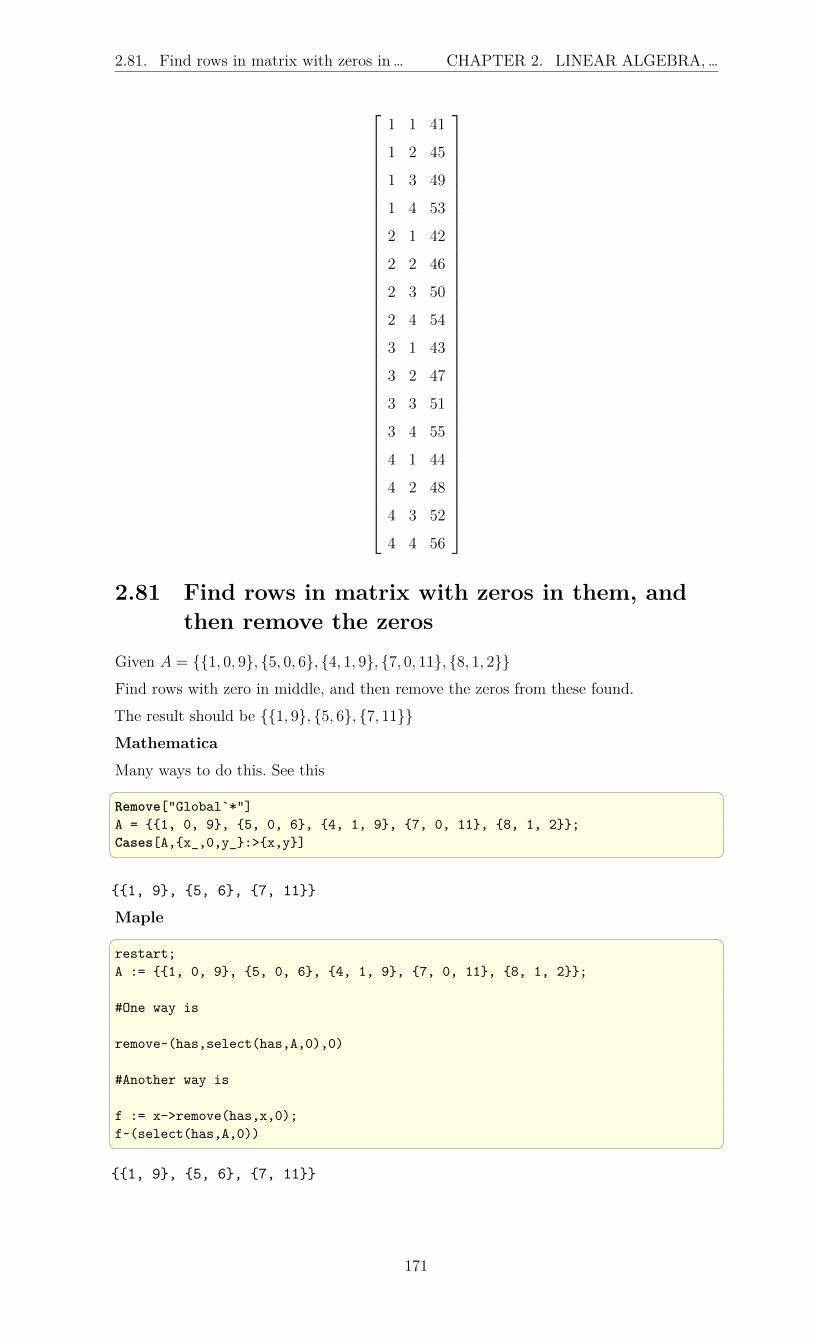
2.81. Find rows in matrix with zeros in … CHAPTER 2. LINEAR ALGEBRA,…
1 1 41
1 2 45
1 3 49
1 4 53
2 1 42
2 2 46
2 3 50
2 4 54
3 1 43
3 2 47
3 3 51
3 4 55
4 1 44
4 2 48
4 3 52
4 4 56
2.81 Find rows in matrix with zeros in them, and
then remove the zerosGiven A = 1, 0, 9, 5, 0, 6, 4, 1, 9, 7, 0, 11, 8, 1, 2
Find rows with zero in middle, and then remove the zeros from these found.
The result should be 1, 9, 5, 6, 7, 11
MathematicaMany ways to do this. See this Remove["Global`*"]A = 1, 0, 9, 5, 0, 6, 4, 1, 9, 7, 0, 11, 8, 1, 2;Cases[A,x_,0,y_:>x,y] 1, 9, 5, 6, 7, 11
Maple restart;A := 1, 0, 9, 5, 0, 6, 4, 1, 9, 7, 0, 11, 8, 1, 2;
#One way is
remove~(has,select(has,A,0),0)
#Another way is
f := x->remove(has,x,0);f~(select(has,A,0)) 1, 9, 5, 6, 7, 11
171
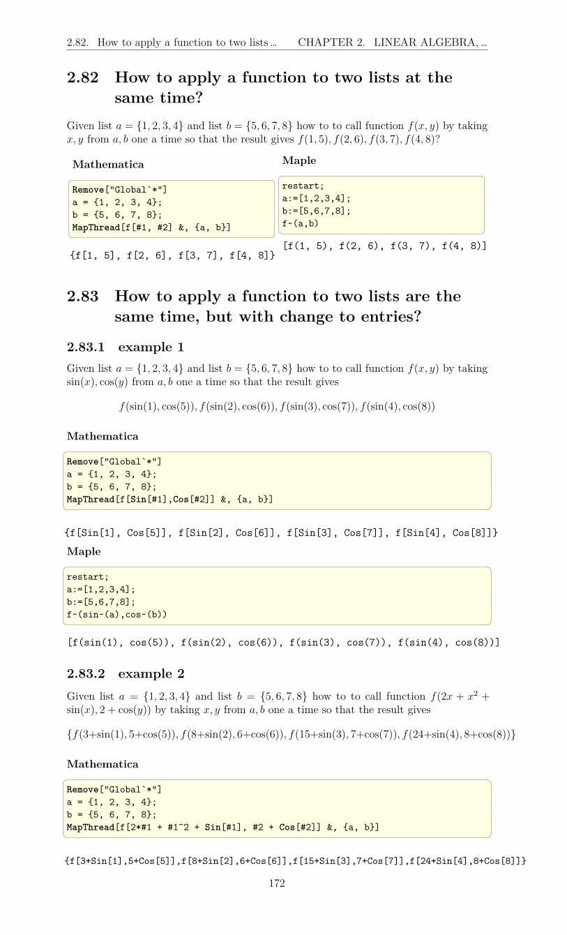
2.82. How to apply a function to two lists … CHAPTER 2. LINEAR ALGEBRA,…
2.82 How to apply a function to two lists at thesame time?
Given list a = 1, 2, 3, 4 and list b = 5, 6, 7, 8 how to to call function f(x, y) by takingx, y from a, b one a time so that the result gives f(1, 5), f(2, 6), f(3, 7), f(4, 8)?
Mathematica Remove["Global`*"]a = 1, 2, 3, 4;b = 5, 6, 7, 8;MapThread[f[#1, #2] &, a, b] f[1, 5], f[2, 6], f[3, 7], f[4, 8]
Maple restart;a:=[1,2,3,4];b:=[5,6,7,8];f~(a,b) [f(1, 5), f(2, 6), f(3, 7), f(4, 8)]
2.83 How to apply a function to two lists are thesame time, but with change to entries?
2.83.1 example 1Given list a = 1, 2, 3, 4 and list b = 5, 6, 7, 8 how to to call function f(x, y) by takingsin(x), cos(y) from a, b one a time so that the result gives
f(sin(1), cos(5)), f(sin(2), cos(6)), f(sin(3), cos(7)), f(sin(4), cos(8))
Mathematica Remove["Global`*"]a = 1, 2, 3, 4;b = 5, 6, 7, 8;MapThread[f[Sin[#1],Cos[#2]] &, a, b] f[Sin[1], Cos[5]], f[Sin[2], Cos[6]], f[Sin[3], Cos[7]], f[Sin[4], Cos[8]]
Maple restart;a:=[1,2,3,4];b:=[5,6,7,8];f~(sin~(a),cos~(b)) [f(sin(1), cos(5)), f(sin(2), cos(6)), f(sin(3), cos(7)), f(sin(4), cos(8))]
2.83.2 example 2Given list a = 1, 2, 3, 4 and list b = 5, 6, 7, 8 how to to call function f(2x + x2 +sin(x), 2 + cos(y)) by taking x, y from a, b one a time so that the result gives
f(3+sin(1), 5+cos(5)), f(8+sin(2), 6+cos(6)), f(15+sin(3), 7+cos(7)), f(24+sin(4), 8+cos(8))
Mathematica Remove["Global`*"]a = 1, 2, 3, 4;b = 5, 6, 7, 8;MapThread[f[2*#1 + #1^2 + Sin[#1], #2 + Cos[#2]] &, a, b] f[3+Sin[1],5+Cos[5]],f[8+Sin[2],6+Cos[6]],f[15+Sin[3],7+Cos[7]],f[24+Sin[4],8+Cos[8]]
172

2.84. How to select all primes numbers … CHAPTER 2. LINEAR ALGEBRA,…
MapleIn Maple, since it does not have slot numbers # to use, it is better to make a function onthe fly, which does the exact same thing. restart;a:=[1,2,3,4];b:=[5,6,7,8];
f~( (x->2*x+x^2+sin(x))~(a), (x->2+cos(x)) ~(b)) [f(3 + sin(1), 2 + cos(5)), f(8 + sin(2), 2 + cos(6)), f(15 + sin(3), 2 + cos(7)), f(24 + sin(4), 2 + cos(8))]
2.84 How to select all primes numbers from a list?Given list of numbers from 1 to 100, select the prime numbers.
Mathematica Remove["Global`*"]lst = Range[1, 100];Select[lst, PrimeQ] 2, 3, 5, 7, 11, 13, 17, 19, 23, 29, 31, 37, 41, 43, 47, 53, 59, 61, 67, 71, 73, 79, 83, 89, 97
Maple restart;lst:=[seq(i,i=1..100)];result:=select[flatten](isprime,lst);
#or. using Array instead of listlst:=Array(0..99,x->x+1): #generate numbers from 1 to 100select[flatten](isprime,lst); [2, 3, 5, 7, 11, 13, 17, 19, 23, 29, 31, 37, 41, 43, 47, 53, 59, 61, 67, 71, 73, 79, 83, 89, 97]
2.85 How to collect result inside a loop whennumber of interation is not known in advance?
Lets say we want to collect result obtained inside loop, but do not know in advance howmany iteration we need.
In Mathematica, Sow and Reap are used. In Maple, an Array can be used or a queue or atable.
Mathematica Remove["Global`*"]result = First@Last@Reap@Do[
Sow[n],n, 1, 10];
result 1, 2, 3, 4, 5, 6, 7, 8, 9, 10
Maple restart;result :=Array([]):for n from 1 to 10 do
173

2.86. How flip an array around? CHAPTER 2. LINEAR ALGEBRA,…
result(n):=n;od:result(1..10) [1, 2, 3, 4, 5, 6, 7, 8, 9, 10]
2.86 How flip an array around?Given A = [1, 2, 3, 4, 5] change it to A = [5, 4, 3, 2, 1]
Mathematica a = 1, 2, 3, 4, 5;Reverse[a]
5, 4, 3, 2, 1
Matlab A=[1,2,3,4,5];flip(A)
ans =5 4 3 2 1
Maple A:=Array([1,2,3,4,5]);ArrayTools:-Reverse(A);
[5, 4, 3, 2, 1]
2.87 How to divide each element by its position in alist?
Given A = [2, 3, 5, 7, 11, 13, 17, 19, 23, 29] change it to
[2,3
2,5
3,7
4,11
5,13
6,17
7,19
8,23
9,29
10]
2.87.1 Mathematica A = 2, 3, 5, 7, 11, 13, 17, 19, 23, 29;MapIndexed[(#1/First[#2]) &, A]
2,
3
2,5
3,7
4,11
5,13
6,17
7,19
8,23
9,29
10
174

2.88. How to use GramSchmidt to find a… CHAPTER 2. LINEAR ALGEBRA,…
2.87.2 Maple A:= [2, 3, 5, 7, 11, 13, 17, 19, 23, 29];((x,y)->x/y)~(A,[seq(i,i=1..numelems(A))])
#or simpler might be to map the divsion operator directly
`/` ~ (A,[seq(i,i=1..numelems(A))]) [2,
3
2,5
3,7
4,11
5,13
6,17
7,19
8,23
9,29
10]
2.87.3 Matlab A=[2, 3, 5, 7, 11, 13, 17, 19, 23, 29];A./(1:length(A)) 2.0000 1.5000 1.6667 1.7500 2.2000 2.1667 2.4286 2.3750 2.5556 2.9000
2.88 How to use GramSchmidt to find a set oforthonomal vectors?
Given set of linearly independent vectors V1 = [3, 0, 0], V2 = [0, 1, 2], V3 = [0, 2, 5], useGramSchmidt to find 3 orthonormal vectors from this set.
2.88.1 Mathematica v1=3,0,0;v2=0,1,2;v3=0,2,5Orthogonalize[v1, v2,v3, Method -> "GramSchmidt"]
1 0 0
0 1√5
2√5
0 − 2√5
1√5
2.88.2 Maple restart;V1:=Vector([3,0,0]);V2:=Vector([0,1,2]);V3:=Vector([0,2,5]);Student:-LinearAlgebra:-GramSchmidt([V1,V2,V3])
1
0
0
,
0
√55
2√5
5
,
0
−2√5
5√55
175

2.88. How to use GramSchmidt to find a… CHAPTER 2. LINEAR ALGEBRA,…
176

Chapter 3
signal processing, Image processing,graphics, random numbers
3.1 Generate and plot one pulse signal of differentwidth and amplitude
Problem: Generate one signal of some width and height.
Mathematica Remove["Global`*"]f[x_,w_,h_]:=If[0<=x<w,
h*If[x-IntegerPart[x]<=0.5,SquareWave[x],-SquareWave[x]],0]
w = 0.5,1,2; (*pulse width *)h = 1,1.5,0.4; (*pulse height *)plots = MapThread[Plot[
f[x,#1,#2],x,-2,2.5,PlotRange->-1,2.5,-0.3,2.5,Frame->True,Axes->False,GridLines->Automatic,GridLinesStyle->Dashed,PlotStyle->Thick,Red,FrameLabel->"y(t)",None,
"t","pulse of "<>ToString[#1]<>" sec width and amplitude"<>ToString[#2],
ImageSize -> 160,AspectRatio->1]&,w,h];
Grid[plots,Frame->All]
-1.0-0.50.00.51.01.52.02.5
0.0
0.5
1.0
1.5
2.0
2.5
t
y(t)
pulse of 0.5 sec width and amplitude1
-1.0-0.50.00.51.01.52.02.5
0.0
0.5
1.0
1.5
2.0
2.5
t
y(t)
pulse of 1 sec width and amplitude1.5
-1.0-0.50.00.51.01.52.02.5
0.0
0.5
1.0
1.5
2.0
2.5
t
y(t)
pulse of 2 sec width and amplitude0.4
Matlab clear all; close all;f = [1 0.5 0.25];w = [0.5 1 2];h = [1 1.5 0.4];
figure;
for i=1:3
177

3.2. Generate and plot train of pulses of … CHAPTER 3. SIGNAL PROCESSING,…
t=0:0.01:w(i);y=h(i)*square(2*pi*f(i)*t);subplot(3,1,i);plot(t,y,'r','LineWidth',3);grid on;xlim([-2 2.5]);ylim([-.6 2.5]);title(sprintf...
('pulse of %2.1f sec width and amplitude=%2.1f',...w(i),h(i)));
end
-2 -1.5 -1 -0.5 0 0.5 1 1.5 2 2.5
0
1
2
pulse of 0.5 sec width and amplitude=1.0
-2 -1.5 -1 -0.5 0 0.5 1 1.5 2 2.5
0
1
2
pulse of 1.0 sec width and amplitude=1.5
-2 -1.5 -1 -0.5 0 0.5 1 1.5 2 2.5
0
1
2
pulse of 2.0 sec width and amplitude=0.4
3.2 Generate and plot train of pulses of differentwidth and amplitude
Problem: Generate a pulse train of pulses of certain width and height.
Mathematica Remove["Global`*"]
w = 0.25,0.125;h = 1,1.5;plots = MapThread[Plot[#2 SquareWave[#1 x],
x,-10,10,PlotRange->All,-2,2,Frame->True,Axes->False,PlotStyle->Thick,Red,FrameLabel->"y(t)",None,"t","pulse of "<>ToString[1/(2*#1)]<>" sec width and amplitude"<>ToString[#2],
ImageSize->200,AspectRatio->1,ExclusionsStyle->Dotted]&,w,h];
Grid[plots,Frame->All]
-10 -5 0 5 10-2
-1
0
1
2
t
y(t)
pulse of 2. sec width and amplitude1
-10 -5 0 5 10-2
-1
0
1
2
t
y(t)
pulse of 4. sec width and amplitude1.5
178

3.3. Find the discrete Fourier transform of …CHAPTER 3. SIGNAL PROCESSING,…
Matlab clear all; close all;f = [1 0.5];h = [1 1.5];t = -4:0.01:4;
figure;
for i=1:2y = h(i)*square(2*pi*f(i)*t);subplot(2,1,i);plot(t,y,'r','LineWidth',3);grid on;xlim([-2 2.5]);ylim([-2 2.5]);title(sprintf...('pulse of %2.1f sec width and amplitude=%2.1f',..1/(2*f(i)),h(i)));
end
-2 -1.5 -1 -0.5 0 0.5 1 1.5 2 2.5-2
-1
0
1
2
pulse of 0.5 sec width and amplitude=1.0
-2 -1.5 -1 -0.5 0 0.5 1 1.5 2 2.5-2
-1
0
1
2
pulse of 1.0 sec width and amplitude=1.5
3.3 Find the discrete Fourier transform of a realsequence of numbers
Given the sequence of numbers x(n) = [1, 2, 3], Find X(k) =N−1∑m=0
x(m)e−j 2πN
mk where N is
the length of the data sequence x(m) and k = 0 · · ·N − 1
Mathematica Chop[Fourier[1, 2, 3,
FourierParameters ->1, -1]] 6.,-1.5 + 0.8660254037844386*I,-1.5 - 0.8660254037844386*I
Matlab fft([1,2,3])'
ans =
6.0000-1.5000 - 0.8660i-1.5000 + 0.8660i
MapleMaple need an Array for input, not list, so have to con-vert this is little strange lst:=[1,2,3];SignalProcessing[FFT](convert(lst,Array),
normalization=none );
[6.+0.*I,-1.5+.866025403784439*I,-1.5-.866025403784439*I]
179

3.3. Find the discrete Fourier transform of …CHAPTER 3. SIGNAL PROCESSING,…
Ada I posted the code below on comp.lang.ada on June 8,2010. Thanks to Ludovic Brentafor making improvement to the Ada code. ---- dtf.adb, compiled with GNAT 4.3.4 20090804 (release) 1-- under CYGWIN 1.7.5-- $ gnatmake dft.adb-- gcc -c dft.adb-- gnatbind -x dft.ali-- gnatlink dft.ali-- $ ./dft.exe-- ( 6.00000E+00, 0.00000E+00)-- (-1.50000E+00, 8.66026E-01)-- (-1.50000E+00,-8.66025E-01)
with Ada.Text_IO; use Ada.Text_IO;with Ada.Numerics.Complex_Types; use Ada.Numerics.Complex_Types;
with Ada.Numerics; use Ada.Numerics;
with Ada.Numerics.Complex_Elementary_Functions;use Ada.Numerics.Complex_Elementary_Functions;with Ada.Complex_Text_IO; use Ada.Complex_Text_IO;
procedure dft isN : constant := 3; -- named number, no conversion to Float neededX : array(0 .. N-1) of Complex := (others=>(0.0,0.0));data : constant array(0 .. N-1) of float :=(1.0,2.0,3.0);Two_Pi_Over_N : constant := 2 * Pi / N;-- named number, outside the loop, like in ARM 3.3.2(9)
beginFOR k in X'range LOOP
FOR m in data'range LOOPX(k) := X(k) + data(m)*exp(-J*Two_Pi_Over_N * float(m*k));
END LOOP;put(X(k)); new_line;
END LOOP;end dft;
180

3.4. Generate uniform distributed random…CHAPTER 3. SIGNAL PROCESSING,…
FortranThanks to Vincent Lafage for making improvment to the Fortran code. ! dtf.f90, compiled with GCC 4.3.4! under CYGWIN 1.7.5! $ gfortran -Wall -Wsurprising -Wconversion dft.f90! $ ./a.exe! ( 6.0000000 , 0.0000000 )! ( -1.4999999 , 0.86602557 )! ( -1.5000005 ,-0.86602497 )! $
PROGRAM dft
IMPLICIT NONE
INTEGER, parameter :: N = 3COMPLEX, parameter :: J =(0.0,1.0)REAL, parameter :: Pi = ACOS(-1.0)INTEGER :: k,mCOMPLEX, dimension(0:N-1) :: XREAL, dimension(0:N-1) :: data=(/1.0,2.0,3.0/)REAL, parameter :: Two_Pi_Over_N = 2.0*Pi/real(N)
DO k = lbound(X, 1), ubound(X, 1)X(k)=(0.0,0.0)DO m = lbound(data, 1), ubound(data, 1)
X(k) = X(k) + complex(data(m),0.0) &* EXP(-J*complex(Two_Pi_Over_N*real(m*k),0.0))
END DOprint *,X(k)
END DO
END PROGRAM dft 3.4 Generate uniform distributed random numbers
3.4.1 How to generate 5 uniform distributed random numbersfrom 0 to 1?
Mathematica SeedRandom[1];Table[RandomVariate[
UniformDistribution[0,1]],5]
0.817389,0.11142,0.789526,0.187803,0.241361
Matlab rand(5,1)
0.8147236863931790.9057919370756190.1269868162935060.9133758561390190.632359246225410
Fortran
181

3.4. Generate uniform distributed random…CHAPTER 3. SIGNAL PROCESSING,…
program t3implicit nonereal :: x(5)
CALL RANDOM_SEED()CALL random_number(x)print *,x
end program compile and run $ gfortran -std=f95 -Wextra -Wall -pedantic -funroll-loops
-ftree-vectorize -march=native -Wsurprising -Wconversiont3.f90 /usr/lib/liblapack.a /usr/lib/libblas.a
$ ./a.exe0.99755955 0.56682467 0.96591532 0.74792767 0.36739087
3.4.2 How to generate 5 random numbers from a to b?Generate uniform numbers from a to b, say a=-2 and b=5
Mathematica SeedRandom[1];Table[RandomVariate[
UniformDistribution[-2,5]],5]
3.72173,-1.22006,3.52668,-0.685378,-0.310473
Matlab -2 + (5+2)*rand(5,1)
-1.317217165004133-0.0505124679306611.8281706344348874.7025478480400844.754219746394936
Fortran program t3_2implicit noneinteger ::ireal, parameter :: a=-1.0,b=1.0real :: x(5)
CALL RANDOM_SEED()DO i=1,2
CALL random_number(x)x = a+(b-a)*xprint *,x
END DO
end program compile and run $ gfortran -std=f95 -Wextra -Wall -pedantic -funroll-loops
-ftree-vectorize -march=native -Wsurprising -Wconversiont3_2.f90 /usr/lib/liblapack.a /usr/lib/libblas.a
182
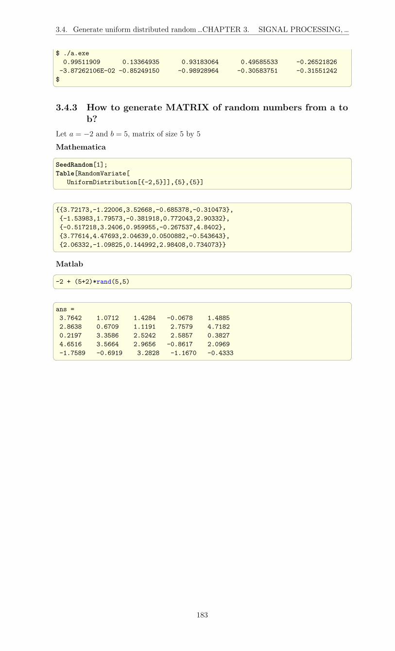
3.4. Generate uniform distributed random…CHAPTER 3. SIGNAL PROCESSING,…
$ ./a.exe0.99511909 0.13364935 0.93183064 0.49585533 -0.26521826-3.87262106E-02 -0.85249150 -0.98928964 -0.30583751 -0.31551242$ 3.4.3 How to generate MATRIX of random numbers from a to
b?Let a = −2 and b = 5, matrix of size 5 by 5
Mathematica SeedRandom[1];Table[RandomVariate[
UniformDistribution[-2,5]],5,5] 3.72173,-1.22006,3.52668,-0.685378,-0.310473,-1.53983,1.79573,-0.381918,0.772043,2.90332,-0.517218,3.2406,0.959955,-0.267537,4.8402,3.77614,4.47693,2.04639,0.0500882,-0.543643,2.06332,-1.09825,0.144992,2.98408,0.734073
Matlab -2 + (5+2)*rand(5,5) ans =3.7642 1.0712 1.4284 -0.0678 1.48852.8638 0.6709 1.1191 2.7579 4.71820.2197 3.3586 2.5242 2.5857 0.38274.6516 3.5664 2.9656 -0.8617 2.0969-1.7589 -0.6919 3.2828 -1.1670 -0.4333
183

3.4. Generate uniform distributed random…CHAPTER 3. SIGNAL PROCESSING,…
Fortran program t3_3implicit noneinteger ::ireal, parameter :: a=-1.0,b=1.0real :: x(5,5)
CALL RANDOM_SEED()DO i=1,2
CALL random_number(x)x = a+(b-a)*xCALL write(x)
END DO
!--- internal functions below ------contains
SUBROUTINE write(A)implicit noneREAL, DIMENSION(:,:) :: Ainteger :: i,j
WRITE(*,*)DO i = lbound(A,1), ubound(A,1)
WRITE(*,*) (A(i,j), j = lbound(A,2), ubound(A,2))END DO
END SUBROUTINE write
end program compile and run $ gfortran -std=f95 -Wextra -Wall -pedantic -funroll-loops
-ftree-vectorize -march=native -Wsurprising -Wconversiont3_3.f90 /usr/lib/liblapack.a /usr/lib/libblas.a
$ ./a.exe0.99511909 -3.87262106E-02 -0.56409657 0.32386434 0.711384770.13364935 -0.85249150 -0.73367929 -0.96778345 -0.197426200.93183064 -0.98928964 0.80104899 0.30170965 -0.586251380.49585533 -0.30583751 -0.22646809 0.29281759 0.93707883
-0.26521826 -0.31551242 -0.10903549 -0.35402548 0.19679904
0.34596145 0.21138644 0.22462976 0.31809497 0.45771694-8.62354040E-02 0.43809581 0.95732045 0.10801017 -0.19508958-0.33996975 0.79466915 0.99828446 0.95552015 0.85725522-0.79923415 0.31645823 -0.48640406 0.80384660 -0.704329730.51090658 -0.69856644 0.10173070 0.31584930 0.34905851
184

3.5. Obtain Fourier Series coefficients for …CHAPTER 3. SIGNAL PROCESSING,…
3.5 Obtain Fourier Series coefficients for a periodicfunction
Local contents3.5.1 Example 1 . . . . . . . . . . . . . . . . . . . . . . . . . . . . . . . . . . . . 1853.5.2 Example 2 . . . . . . . . . . . . . . . . . . . . . . . . . . . . . . . . . . . . 1873.5.3 Example 3 . . . . . . . . . . . . . . . . . . . . . . . . . . . . . . . . . . . . 189
3.5.1 Example 1
Given a continuous time function x (t) = sin(
2πT0t), find its Fourier coefficients cn, where
(Using the default definition)
x (t) =∞∑
n=−∞
cnejω0nt
and
cn =1
T0
∫ T02
−T02
x(t)e−jω0ntdt
Where T0 is the fundamental period of x (t) and ω0 =2πT0.
Notice that in Physics, sometimes the following defintions are used instead of the above
x (t) =1√T0
∞∑n=−∞
cnejω0nt
and
cn =1√T0
∫ T02
−T02
x(t)e−jω0ntdt
3.5.1.1 Mathematica Clear[T0, w0]sol = FourierSeries[Sin[2 Pi/T0 t], t, 3, FourierParameters -> 1, 2 Pi/T0]
1
2ie−
2iπtT0 − 1
2ie
2iπtT0
data = Table[i,FourierCoefficient[Sin[2 Pi/T0 t], t, i,FourierParameters -> 1, 2 Pi/T0], i, -5, 5];head = "n", "cn";
Grid[Insert[data, head, 1], Frame -> All]
185

3.5. Obtain Fourier Series coefficients for …CHAPTER 3. SIGNAL PROCESSING,…
n cn-5 0-4 0-3 0-2 0
-1 ⅈ
2
0 0
1 -ⅈ
2
2 03 04 05 0
mag = data;mag[[All,2]] = Map[Abs[#]&,data[[All,2]]];ListPlot[mag,AxesOrigin->0,0,
Filling->Axis,FillingStyle->Thick,Red,AxesLabel->"n","|Subscript[c, n]|"]
-4 -2 2 4n
0.1
0.2
0.3
0.4
0.5
|cn|
phase = data;phase[[All,2]]=Map[Arg[#]&,
data[[All,2]]]* 180/Pi;ListPlot[phase,AxesOrigin->0,0,
Filling->Axis,FillingStyle->Thick,Red,AxesLabel->"n","Phase Subscript[c, n] degrees",ImageSize->300]
186

3.5. Obtain Fourier Series coefficients for …CHAPTER 3. SIGNAL PROCESSING,…
-4 -2 2 4n
-100
-50
50
100Phase cn degrees
3.5.2 Example 2Find Fourier Series for f(t) = cos(ω0t) + sin2(ω0t)
3.5.2.1 Mathematica T0 = 2 Pi;w0 = (2 Pi)/T0;f[t_] := Cos[w0 t] + Sin[w0 t]^2;Plot[f[t], t, -10 Pi, 10 Pi, PlotRange -> All, ImageSize -> 300]
-30 -20 -10 10 20 30
-1.0
-0.5
0.5
1.0
sol = FourierSeries[f[t],t,3, FourierParameters->1,(2 Pi)/T0]
e−it
2+
eit
2− 1
4e−2it − 1
4e2it +
1
2 data = Table[i, FourierCoefficient[f[t],t,i, FourierParameters->1,2 Pi/T0],i,-5,5];
head = "n","cn";Grid[Insert[data,head,1],Frame->All]
187
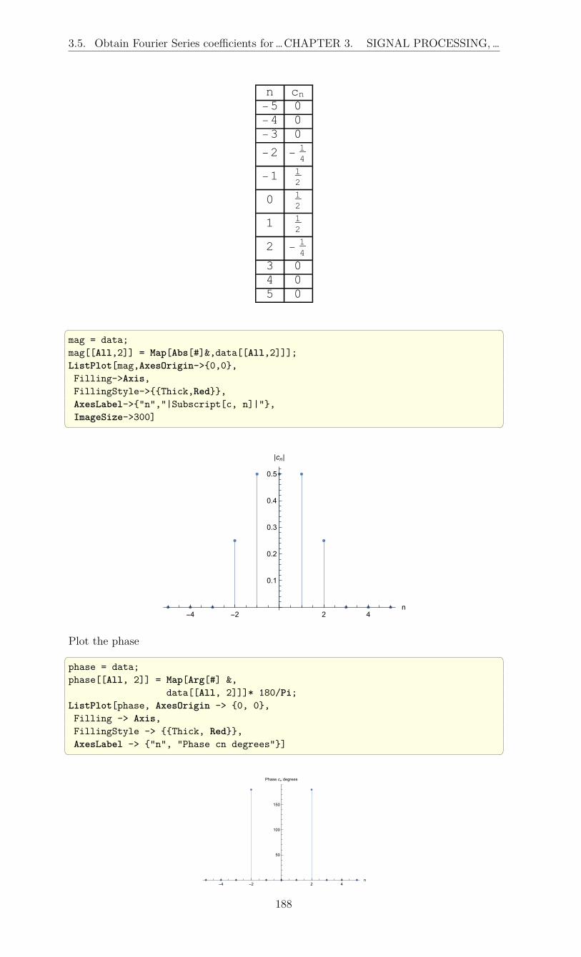
3.5. Obtain Fourier Series coefficients for …CHAPTER 3. SIGNAL PROCESSING,…
n cn-5 0-4 0-3 0
-2 -14
-1 12
0 12
1 12
2 -14
3 04 05 0
mag = data;mag[[All,2]] = Map[Abs[#]&,data[[All,2]]];ListPlot[mag,AxesOrigin->0,0,Filling->Axis,FillingStyle->Thick,Red,AxesLabel->"n","|Subscript[c, n]|",ImageSize->300]
-4 -2 2 4n
0.1
0.2
0.3
0.4
0.5
|cn|
Plot the phase phase = data;phase[[All, 2]] = Map[Arg[#] &,
data[[All, 2]]]* 180/Pi;ListPlot[phase, AxesOrigin -> 0, 0,Filling -> Axis,FillingStyle -> Thick, Red,AxesLabel -> "n", "Phase cn degrees"]
-4 -2 2 4n
50
100
150
Phase cn degrees
188

3.5. Obtain Fourier Series coefficients for …CHAPTER 3. SIGNAL PROCESSING,…
3.5.3 Example 3Find Fourier series for periodic square wave
3.5.3.1 Mathematica f[x_] := SquareWave[0,1,(x+.5)/2] ;Plot[f[x],x,-6,6,Filling->Axis, ImageSize->300]
-6 -4 -2 2 4 6
0.2
0.4
0.6
0.8
1.0
T0 = 2;sol = Chop[FourierSeries[f[t],t,6, FourierParameters->1,(2 Pi)/T0]]
0.5+0.31831e−iπt+0.31831eiπt−0.106103e−3iπt−0.106103e3iπt+0.063662e−5iπt+0.063662e5iπt
data = Chop[Table[i,FourierCoefficient[f[t],t,i, FourierParameters->1,2 Pi/T],i,-8,8]];
head = "n","cn";Grid[Insert[data,head,1],Frame->All]
n cn-8 0-7 -0.0454728-6 0-5 0.063662-4 0-3 -0.106103-2 0-1 0.318310 0.51 0.318312 03 -0.1061034 05 0.0636626 07 -0.04547288 0
data=Table[i,FourierCoefficient[f[t],t,i, FourierParameters->1,2 Pi/T],i,-20,20];mag = data;mag[[All,2]]=Map[Abs[#]&,data[[All,2]]];ListPlot[mag,AxesOrigin->0,0,Filling->Axis,FillingStyle->Thick,Red,PlotRange->All,AxesLabel->"n","|Subscript[c, n]|",ImageSize->300]
189
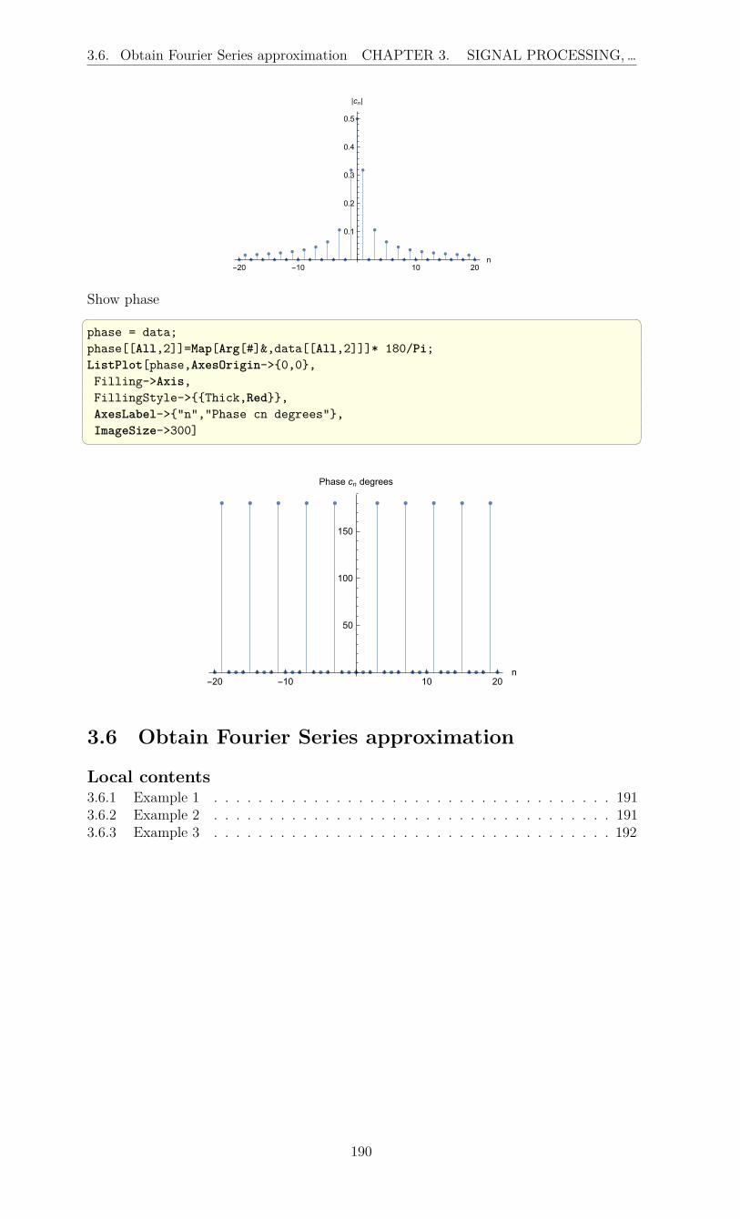
3.6. Obtain Fourier Series approximation CHAPTER 3. SIGNAL PROCESSING,…
-20 -10 10 20n
0.1
0.2
0.3
0.4
0.5
|cn|
Show phase phase = data;phase[[All,2]]=Map[Arg[#]&,data[[All,2]]]* 180/Pi;ListPlot[phase,AxesOrigin->0,0,Filling->Axis,FillingStyle->Thick,Red,AxesLabel->"n","Phase cn degrees",ImageSize->300]
-20 -10 10 20n
50
100
150
Phase cn degrees
3.6 Obtain Fourier Series approximation
Local contents3.6.1 Example 1 . . . . . . . . . . . . . . . . . . . . . . . . . . . . . . . . . . . . 1913.6.2 Example 2 . . . . . . . . . . . . . . . . . . . . . . . . . . . . . . . . . . . . 1913.6.3 Example 3 . . . . . . . . . . . . . . . . . . . . . . . . . . . . . . . . . . . . 192
190

3.6. Obtain Fourier Series approximation CHAPTER 3. SIGNAL PROCESSING,…
3.6.1 Example 1Obtain Fourier Series approximation of f(x) = e−|x| for −1 < x < 1
3.6.1.1 Maple restart;f:=x->exp(-abs(x));f_approx:=OrthogonalExpansions:-FourierSeries(f(x),x=-1..1,infinity ):f_approx:=subs(i=n,f_approx);
1− e−1 +∞∑n=1
(−2 ((−1)n e−1 − 1) cos(πnx)
π2n2 + 1
)
3.6.1.2 Mathematica
Mathematica does not have a buildin function to give general series expression as theabove with Maple. There is a user written package and answer here https://mathematica.stackexchange.com/questions/149468/a-more-convenient-fourier-series which pro-vides this.
In Mathematica it is possible to obtain the terms using the command FourierSeries .For example the terms n = 0, n = −1, n = 1 can be obtained using expr = Exp[-Abs[x]];FourierSeries[expr, x, 1, FourierParameters -> 1, Pi]
(1 + e)e−iπx
e+ eπ2+
(1 + e)eiπx
e+ eπ2+
e− 1
e
see https://reference.wolfram.com/language/ref/FourierSeries.html for defini-tions of FourierParameters used above.
3.6.2 Example 2Obtain Fourier Series approximation of
f (x) =
2xhL
0 ≤ x ≤ L2
2h(L−x)L
L2≤ x ≤ L
For 0 < x < L
3.6.2.1 Maple restart;f:=x->piecewise(0<x and x<L/2,2*x*h/L, L/2<x and x<L, 2*h*(L-x)/L);f_approx:=OrthogonalExpansions:-FourierSeries(f(x),x=0..L,infinity ):f_approx:=subs(i=n,f_approx):simplify(%) assuming L>0
2
(∞∑n=1
h ((−1)n − 1) cos(2πnxL
)π2n2
)+
h
2
191

3.7. Determine and plot the CTFT… CHAPTER 3. SIGNAL PROCESSING,…
3.6.3 Example 3Obtain Fourier Series approximation of coshx for −1 < x < 1.
3.6.3.1 Maple restart;f:=x->cosh(x);f_approx:=OrthogonalExpansions:-FourierSeries(f(x),x=-1..1,infinity ):f_approx:=subs(i=n,f_approx);convert(%,trig);
sinh (1) +
(∞∑n=1
2 sinh (1) (−1)n cos (πnx)
π2n2 + 1
)
3.7 Determine and plot the CTFT (continuous timeFourier Transform) for continuous time function
Plot the CTFT X(ω) of x(t) = 3 sin(t). By definition
X(ω) =
∫ ∞
t=−∞x(t)e−iωt dt
Mathematica Clear["Global`*"];f = 3*Sin[t];y = FourierTransform[f,t,w,FourierParameters->1, -1] Out[138]= -3 I Pi DiracDelta[-1+w]+3 I Pi DiracDelta[1+w] tab = Table[k,y/.w->k,k,-3,3]tab = tab/.DiracDelta[0]->1tab[[All,2]]=Map[Sign[Im[#]]Abs[#]&,tab[[All,2]]]
ListPlot[tab,PlotStyle->AbsolutePointSize[5],AxesLabel->"frequency \[CapitalOmega] rad/sec","|F(\[CapitalOmega]|",PlotRange->All,-12,12,Filling->Axis,FillingStyle->Thick,Red]
-3 -2 -1 1 2 3frequency Ω rad/sec
-10
-5
5
10
|F(Ω|
Matlab syms t;F=fourier(3*sin(t))
192

3.8. Determine the DTFT (Discrete time…CHAPTER 3. SIGNAL PROCESSING,…
F =-pi*(dirac(w-1)-dirac(w+1))*3*i Need to do the plot.
Maple restart;transform := expand(inttrans:-fourier(3*sin(t), t, w)) gives transform := 3*I*Pi*Dirac(w + 1) - 3*I*Pi*Dirac(w - 1) 3.8 Determine the DTFT (Discrete time Fourier
Transform) for discrete time functionFind DTFT X(Ω) of x[n] = sin(πn
8). By definition
X(Ω) =∞∑
n=−∞
x[n]e−iΩn
Mathematica Clear["Global`*"];x[n_] := Sin[(Pi*n)/8];X = FourierSequenceTransform[x[n], n, w, FourierParameters -> 1, 1] // Simplify Which gives (-(1/2))*I*(DiracComb[(Pi - 8*w)/(16*Pi)] - DiracComb[(Pi + 8*w)/(16*Pi)]) 3.9 Determine the Inverse DTFT (Discrete time
Fourier Transform)Find x[n], give its DTFT X(Ω)
x[n] =1
2π
∫ π
−π
X(Ω)eiΩn dΩ
Mathematica Clear["Global`*"];x[n_] := Sin[(Pi*n)/8];X = FourierSequenceTransform[x[n], n, w, FourierParameters -> 1, 1];InverseFourierSequenceTransform[X, w, n] Which gives Sin[(Pi*n)/8]
193

3.10. Use FFT to display the power … CHAPTER 3. SIGNAL PROCESSING,…
3.10 Use FFT to display the power spectrum of thecontent of an audio wav file
Local contents3.10.1 Mathematica . . . . . . . . . . . . . . . . . . . . . . . . . . . . . . . . . . . 1943.10.2 Matlab . . . . . . . . . . . . . . . . . . . . . . . . . . . . . . . . . . . . . . 195
Problem: download a wav file and display the frequency spectrum of the audio signal usingFFT. The Matlab example was based on Matheworks tech note 1702.
3.10.1 Mathematica
Remove["Global`*"];fname = "stereo.wav";SetDirectory[NotebookDirectory[]];ele = Import[fname,"Elements"]
AudioChannels,AudioEncoding,Data,SampledSoundList,SampleRate,Sound
(*listen to it *)sound = Import[fname,"Sound"];EmitSound[sound]
fs = Import[fname,"SampleRate"] 22050
now load the samples and do power spectrum data = Import[fname,"Data"];nChannel,nSamples=Dimensions[data]
Out[115]= 2,29016
py = Fourier[data[[1,All]],
FourierParameters->1,-1];nUniquePts = Ceiling[(nSamples+1)/2]
Out[117]= 14509
194

3.10. Use FFT to display the power … CHAPTER 3. SIGNAL PROCESSING,…
py = py[[1;;nUniquePts]];py = Abs[py];py = py/nSamples;py = py^2;
If[ OddQ[nSamples],py[[2;;-1]]=2*py[[2;;-1]],py[[2;;-2]]=2*py[[2;;-2]]
];
f = (Range[0,nUniquePts-1] fs)/nSamples;ListPlot[Transpose[f,py],
Joined->True,FrameLabel->"|H(f)|",None,
"hz","Magnitude spectrum",ImageSize->400,Frame->True,RotateLabel->False,GridLines->Automatic,GridLinesStyle->Dashed,PlotRange->0,12000,All]
0 2000 4000 6000 8000 10000 120000
1.×10-6
2.×10-6
3.×10-6
4.×10-6
hz
|H(f)|
Magnitude spectrum
3.10.2 Matlab clear all; close all;%%This script plots the frequency spectrum of a wave file.%This method of plotting the frequency spectrum is modeled after the%example on Mathworks website tech note 1702
[data,Fs]=audioread('stereol.wav');[nSamples,nChannels]=size(data);waveFileLength=nSamples/Fs;
N = 2^(nextpow2(length(data(:,1))));
Y=fft(data(:,1),N);NumUniquePts = ceil((N+1)/2);Y = Y(1:NumUniquePts);P = abs(Y);P = P/length(data(:,1));P = P.^2;
if rem(N, 2) % odd nfft excludes Nyquist pointP(2:end) = P(2:end)*2;
elseP(2:end -1) = P(2:end -1)*2;
end
f = (0:NumUniquePts-1)*Fs/N;plot(f,P);title(sprintf('Power Spectrum of a wave file'));xlabel('Frequency Hz');ylabel('|H(f)|');grid;print(gcf, '-dpdf', '-r600', 'images/matlab_e52_1');
195

3.11. Plot the power spectral density of a …CHAPTER 3. SIGNAL PROCESSING,…
0 2000 4000 6000 8000 10000 12000
Frequency Hz
0
0.5
1
1.5
2
2.5
3
3.5
4|H
(f)|
#10-6 Power Spectrum of a wave file
3.11 Plot the power spectral density of a signal
Local contents3.11.1 Mathematica . . . . . . . . . . . . . . . . . . . . . . . . . . . . . . . . . . . 1963.11.2 Matlab . . . . . . . . . . . . . . . . . . . . . . . . . . . . . . . . . . . . . . 198Problem: Given a signal
3 sin (2πf1t) + 4 cos (2πf2t) + 5 cos (2πf3t)
for the following frequency values (in Hz)
f1 = 20, f2 = 30, f3 = 50
and plot the signal power spectral density so that 3 spikes will show at the above 3frequencies. Use large enough sampling frequency to obtain a sharper spectrum
3.11.1 Mathematica Clear ["Global`*"];f1 = 20;f2 = 30;f3 = 100;maxTime = 0.2;
y[t_]:=2 Sin[2 Pi f1 t]+4 Cos[2 Pi f2 t]+5 Cos[2 Pi f3 t];
Plot[y[t],t,0,maxTime,Frame->True,FrameLabel->"y(t)",None,
"t (sec)","signal in time domain",RotateLabel->False,GridLines->Automatic,GridLinesStyle->Dashed,PlotRange->All,BaseStyle -> 12]
0.00 0.05 0.10 0.15 0.20
-10
-5
0
5
10
t (sec)
y(t)
signal in time domain
fs = 7.0*Max[f1,f2,f3];yn = Table[y[n],n,0,maxTime,(1/fs)];
196

3.11. Plot the power spectral density of a …CHAPTER 3. SIGNAL PROCESSING,…
len = Length[yn];py = Fourier[yn];nUniquePts = Ceiling[(len+1)/2];py = py[[1;;nUniquePts]];py = Abs[py];py = 2*(py^2);py[[1]] = py[[1]]/2;f = (Range[0,nUniquePts-1] fs)/len;
ListPlot[Transpose[f,py],Joined->False,FrameLabel->"|H(f)|",None,
"hz","Magnitude spectrum",ImageSize->400,Filling->Axis,FillingStyle->Thick,Red,Frame->True,RotateLabel->False,GridLines->Automatic,GridLinesStyle->Dashed,PlotRange->All,BaseStyle -> 12]
0 50 100 150 200 250 300 3500
2 ×10¹⁰
4 ×10¹⁰
6 ×10¹⁰
8 ×10¹⁰
1 ×10¹¹
hz
|H(f)|
Magnitude spectrum
Here is the same plot as above, but using InterpolationOrder -> 0
0 50 100 150 200 250 300 3500
2 ×10¹⁰
4 ×10¹⁰
6 ×10¹⁰
8 ×10¹⁰
1 ×10¹¹
hz
|H(f)|
Magnitude spectrum
And using InterpolationOrder -> 2
0 50 100 150 200 250 300 3500
2 ×10¹⁰
4 ×10¹⁰
6 ×10¹⁰
8 ×10¹⁰
1 ×10¹¹
hz
|H(f)|
Magnitude spectrum
197

3.11. Plot the power spectral density of a …CHAPTER 3. SIGNAL PROCESSING,…
3.11.2 Matlab clear all; close all;maxTime = 0.2;t = 0:0.001:maxTime;f1 =20; %Hzf2 =30; %Hzf3 =100; %Hzy = @(t) 2*sin(2*pi*f1.*t)+4*cos(2*pi*f2.*t)+...
5*cos(2*pi*f3.*t);plot(t,y(t));set(gcf,'Position',[10,10,320,320]);grid ontitle('signal in time domain');xlabel('time(msec)');ylabel('Amplitude');
0 0.05 0.1 0.15 0.2
time(msec)
-15
-10
-5
0
5
10
Am
plitu
de
signal in time domain
fs = 7.0*max([f1 f2 f3]);delT=1/fs;yn = y(linspace(0,maxTime,maxTime/delT));len = length(yn);py = fft(yn);nUniquePts = ceil((len+1)/2);py = py(1:nUniquePts);py = abs(py);py = 2*(py.^2);py(1) = py(1)/2;f = 0:nUniquePts-1;f = f*fs/len;plot(f,py);title('power spectral density');xlabel('freq (Hz)');ylabel('Energy content');grid onset(gcf,'Position',[10,10,320,320]);
198

3.12. Display spectrum of 2D image CHAPTER 3. SIGNAL PROCESSING,…
0 100 200 300 400
freq (Hz)
0
0.5
1
1.5
2
2.5
Ene
rgy
cont
ent
#105 power spectral density
3.12 Display spectrum of 2D image
Local contents3.12.1 Mathematica . . . . . . . . . . . . . . . . . . . . . . . . . . . . . . . . . . . 1993.12.2 Matlab . . . . . . . . . . . . . . . . . . . . . . . . . . . . . . . . . . . . . . 201
3.12.1 Mathematica img=Import["ExampleData/lena.tif"];Image[img,ImageSize->300]
ImageDimensions[img] 150,116 (*see how many channels*)ImageChannels[img] 3 data=ImageData[img]; (*get data*)nRow,nCol,nChannel=Dimensions[data] 116,150,3 (*look at each channel*)Map[Image[data[[All,All,#]],ImageSize->100]&,
Range[1,nChannel]] 199

3.12. Display spectrum of 2D image CHAPTER 3. SIGNAL PROCESSING,…
, ,
(*get channel 2 to FFT but center it first*)d = data[[All,All,2]];d = d*(-1)^Table[i+j,i,nRow,j,nCol];
(*make FFT,center, view spectrum and phase*)fw = Fourier[d,FourierParameters->1,1];(*adjust for better viewing as needed*)fudgeFactor = 100;abs = fudgeFactor * Log[1+Abs@fw];Labeled[Image[abs/Max[abs],
ImageSize->300],Style["Magnitude spectrum", 18]]
Magnitude spectrum
arg = Arg@fw;Labeled[Image[arg/Max[arg],
ImageSize->300],Style["Phase spectrum", 18]]
Phase spectrum
200
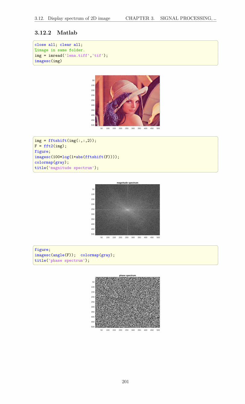
3.12. Display spectrum of 2D image CHAPTER 3. SIGNAL PROCESSING,…
3.12.2 Matlab close all; clear all;%image in same folder.img = imread('lena.tiff','tif');imagesc(img)
50 100 150 200 250 300 350 400 450 500
50
100
150
200
250
300
350
400
450
500
img = fftshift(img(:,:,2));F = fft2(img);figure;imagesc(100*log(1+abs(fftshift(F))));colormap(gray);title('magnitude spectrum');
magnitude spectrum
50 100 150 200 250 300 350 400 450 500
50
100
150
200
250
300
350
400
450
500
figure;imagesc(angle(F)); colormap(gray);title('phase spectrum');
phase spectrum
50 100 150 200 250 300 350 400 450 500
50
100
150
200
250
300
350
400
450
500
201
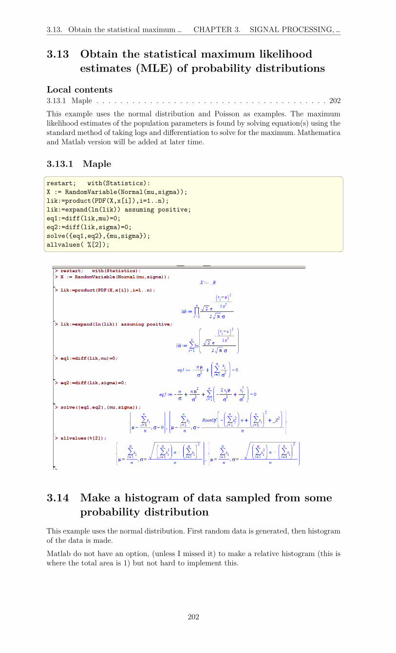
3.13. Obtain the statistical maximum… CHAPTER 3. SIGNAL PROCESSING,…
3.13 Obtain the statistical maximum likelihoodestimates (MLE) of probability distributions
Local contents3.13.1 Maple . . . . . . . . . . . . . . . . . . . . . . . . . . . . . . . . . . . . . . . 202
This example uses the normal distribution and Poisson as examples. The maximumlikelihood estimates of the population parameters is found by solving equation(s) using thestandard method of taking logs and differentiation to solve for the maximum. Mathematicaand Matlab version will be added at later time.
3.13.1 Maple restart; with(Statistics):X := RandomVariable(Normal(mu,sigma));lik:=product(PDF(X,x[i]),i=1..n);lik:=expand(ln(lik)) assuming positive;eq1:=diff(lik,mu)=0;eq2:=diff(lik,sigma)=0;solve(eq1,eq2,mu,sigma);allvalues( %[2]);
3.14 Make a histogram of data sampled from someprobability distribution
This example uses the normal distribution. First random data is generated, then histogramof the data is made.
Matlab do not have an option, (unless I missed it) to make a relative histogram (this iswhere the total area is 1) but not hard to implement this.
202

3.15. apply a filter on 1D numerical data …CHAPTER 3. SIGNAL PROCESSING,…
Mathematica data = RandomReal[NormalDistribution[],1000];Histogram[data,30,"ProbabilityDensity",
ImageSize -> 300]] -3 -2 -1 0 1 2 3
0.0
0.1
0.2
0.3
0.4
Matlab data = randn(1000,1);numberOfBins = 20;[freq,bin] = hist(data,numberOfBins);binWidth = (bin(end)-bin(1))/numberOfBins;currentArea = sum(binWidth*freq);freq = freq/currentArea;
bar(bin,freq) -4 -3 -2 -1 0 1 2 3 40
0.05
0.1
0.15
0.2
0.25
0.3
0.35
0.4
0.45
Maple restart;with(Statistics):nSamples:=1000:data := Sample(RandomVariable(Normal(0, 1)),
nSamples):
plots[display](Histogram(data,bincount=20,frequencyscale=relative));
3.15 apply a filter on 1D numerical data (a vector)Problem: suppose we want to apply say an averaging filter on a list of numbers. Saywe want to replace each value in the list by the average 3 values around each value (asmoothing filter).
In Mathematica, ListConvolve is used, in Matlab conv() is used.
Mathematica data=1,2,7,9,3,4,10,12;filter=(1/3)1,1,1;data[[2;;-2]]=ListConvolve[filter,data];N[data]
Out[66]= 1.,
3.33333,6.,6.33333,5.33333,5.66667,8.66667,12.
203

3.16. apply an averaging Laplacian filter … CHAPTER 3. SIGNAL PROCESSING,…
Matlab data = [1 2 7 9 3 4 10 12];filter = (1/3)*[1 1 1];data(2:end-1) = conv(data,filter,'valid');data'
1.00003.33336.00006.33335.33335.66678.666712.0000
3.16 apply an averaging Laplacian filter on 2Dnumerical data (a matrix)
Problem: Apply a Laplacian filter on 2D data. In Mathematica, ListConvolve is used, inMatlab conv2() is used.
Mathematica data=0,4,10,5,3,
4,4,1,8,5,5,1,2,3,8,8,6,8,8,10,10,3,7,7,8;
filter= (1/4)0,1,0,1,0,1,0,1,0;
data[[2;;-2,2;;-2]]=ListConvolve[filter,data];N[%]
0., 4., 10., 5., 3.,4., 2.5, 6., 3.5, 5.,5., 4.25, 3.25, 6.5, 8.,8., 5., 5.75, 7., 10.,10.,3., 7., 7., 8.
Matlab data=[0 4 10 5 3;
4,4,1,8,5;5,1,2,3,8;8,6,8,8,10;10,3,7,7,8];
filter= (1/4)*[0,1,0;1,0,1;0,1,0];
data(2:end-1,2:end-1)=...conv2(data,filter,'valid')
data =0 4.0000 10.0000 5.0000 3.00004.0000 2.5000 6.0000 3.5000 5.00005.0000 4.2500 3.2500 6.5000 8.00008.0000 5.0000 5.7500 7.0000 10.000010.0000 3.0000 7.0000 7.0000 8.0000
204

3.17. How to find cummulative sum CHAPTER 3. SIGNAL PROCESSING,…
3.17 How to find cummulative sum
compute10∑k=1
1k(k+1)
Mathematica N[Sum[1/(k*(k + 1)), k, 10]]
0.9090909090909091
Matlab format longk=1:10;s=cumsum(1./(k.*(k+1)));s(end)
0.909090909090909
3.18 How to find the moving average of a 1Dsequence?
Given some sequence such as 1, 2, 3, 4, 5, 6, 7 how to find the moving average for differentwindow sizes?MathematicaFor window size k = 2 v = 1, 2, 3, 4, 5, 6, 7, 8;f = 1/2, 1/2;ListConvolve[f, v] // N
1.5,2.5,3.5,4.5,5.5,6.5,7.5
For window size k = 3 v = 1, 2, 3, 4, 5, 6, 7, 8;f = Table[1/3, 3];ListConvolve[f, v] // N
2., 3., 4., 5., 6., 7.
MatlabFor a window size k = 2 V=[1 2 3 4 5 6 7 8];f=[1/2 1/2];conv(V,f,'valid')
ans =1.5000 2.5000 3.5000 4.5000 5.5000 6.5000 7.5000
For window size k = 3 V = [1 2 3 4 5 6 7 8];k = 3;f = ones(k,1)/k;conv(V,f,'valid')
ans =2.0000 3.0000 4.0000 5.0000 6.0000 7.0000
205
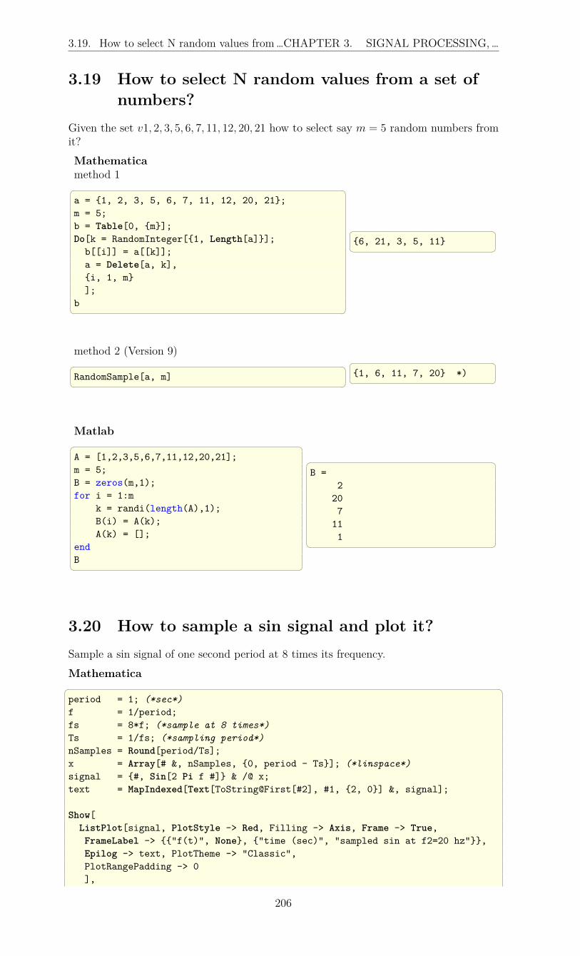
3.19. How to select N random values from…CHAPTER 3. SIGNAL PROCESSING,…
3.19 How to select N random values from a set ofnumbers?
Given the set v1, 2, 3, 5, 6, 7, 11, 12, 20, 21 how to select say m = 5 random numbers fromit?Mathematicamethod 1 a = 1, 2, 3, 5, 6, 7, 11, 12, 20, 21;m = 5;b = Table[0, m];Do[k = RandomInteger[1, Length[a]];b[[i]] = a[[k]];a = Delete[a, k],i, 1, m];
b
6, 21, 3, 5, 11
method 2 (Version 9) RandomSample[a, m]
1, 6, 11, 7, 20 *)
Matlab A = [1,2,3,5,6,7,11,12,20,21];m = 5;B = zeros(m,1);for i = 1:m
k = randi(length(A),1);B(i) = A(k);A(k) = [];
endB
B =
2207
111
3.20 How to sample a sin signal and plot it?Sample a sin signal of one second period at 8 times its frequency.
Mathematica period = 1; (*sec*)f = 1/period;fs = 8*f; (*sample at 8 times*)Ts = 1/fs; (*sampling period*)nSamples = Round[period/Ts];x = Array[# &, nSamples, 0, period - Ts]; (*linspace*)signal = #, Sin[2 Pi f #] & /@ x;text = MapIndexed[Text[ToString@First[#2], #1, 2, 0] &, signal];
Show[ListPlot[signal, PlotStyle -> Red, Filling -> Axis, Frame -> True,FrameLabel -> "f(t)", None, "time (sec)", "sampled sin at f2=20 hz",Epilog -> text, PlotTheme -> "Classic",PlotRangePadding -> 0],
206

3.20. How to sample a sin signal and plot it?CHAPTER 3. SIGNAL PROCESSING,…
Plot[Sin[2 Pi f t], t, 0, period, PlotTheme -> "Classic"],BaseStyle -> 10, PlotRange -> 0, period, -1.1, 1.1]
0.0 0.2 0.4 0.6 0.8 1.0
-1.0
-0.5
0.0
0.5
1.0
time (sec)
f(t)
sampled sin at f2=20 hz
2
3
4
5
6
7
8
Matlab clear all; close all;period = 1;f = 1/period;fs = 8*f;Ts = 1/fs;nSamples = round(period/Ts);x = linspace(0,period-Ts,nSamples);signal = sin(2*pi*f*x);
stem(x,signal)for i = 1:length(x)
text(x(i),sign(signal(i))*0.1+signal(i),num2str(i))endhold on;x = linspace(0,period,10*nSamples);plot(x,sin(2*pi*f*x))ylim([-1.2,1.2]);
0 0.2 0.4 0.6 0.8 1
-1
-0.5
0
0.5
1
1
2
3
4
5
6
7
8
207

3.21. How find the impulse response of a … CHAPTER 3. SIGNAL PROCESSING,…
3.21 How find the impulse response of a differenceequation?
Find the impulse response h[n] for the discrete system given by the difference equationy[n]− 1
2y[n− 1] = x[n]− 1
4x[n− 1]
analytical solution:
1. The first step is to replace y[n] by h[n] and x[n] by δ[n] giving
h[n]− 1
2h[n− 1] = δ[n]− 1
4δ[n− 1]
2. Taking the Fourier transform and assuming H(eiω) is the Fourier transform of h[n]results in
H(eiω)− 1
2H(eiω)e−iω = 1− 1
4e−iω
3. Solving for H(eiω) gives
H(eiω) =1− 1
4e−iω
1− 12e−iω
=1
1− 12e−iω
− 1
4
e−iω
1− 12e−iω
4. Taking the inverse discrete Fourier transform given by
h[n] =1
2π
∫ π
−π
H(eiω)eiω
which results in
h[n] =
(1
2
)n
u[n]− 1
4
(1
2
)n−1
u[n− 1]
Mathematica Clear[w, n]expr1 = -(1/4)*Exp[-I w]/(1 - (1/2)*Exp[-I w]);expr2 = 1/(1 - (1/2)*Exp[-I w]);sol1 = InverseFourierSequenceTransform[expr1, w, n];sol2 = InverseFourierSequenceTransform[expr2, w, n];sol = sol1 + sol2
−2−n−1 n > 0
0 True+
2−n n ≥ 0
0 True
And some values of h[n] starting from n = 0 are (sol /. n -> #) & /@ Range[0, 10]
1,
1
4,1
8,1
16,1
32,1
64,
1
128,
1
256,
1
512,
1
1024,
1
2048
208

Chapter 4
Differential, PDE solving,integration, numerical and analyticalsolving of equations
4.1 Generate direction field plot of a first orderdifferential equation
Problem: Given the following non autonomous differential equation, plot the line fieldswhich represents the solutions of the ODE.
dy (x)
dx= x2 − y
Direction field plot (or slope plot) shows solutions for the ODE without actually solvingthe ODE.
The following are the steps to generate direction field plot for dydx
= f(x, y)
1. generate 2 lists of numbers. The y list and the x list. These 2 lists are the coordinatesat which a small slop line will be plotted.
2. At each of the above coordinates (y, x) evaluate f(x, y).
3. Plot small line starting at the point (x, y) and having slop of f(x, y). The length ofthe line is kept small. Normally it has an arrow at the end of it.
Using Matlab, the points are first generated (the (x, y) coordinates) then the slope f(x, y)evaluated at each of these points, then the command quiver() is used. Next contour()command is used to plot few lines of constant slope.
In Mathematica, the command VectorPlot is used. In Maple dfieldplot is used.
209

4.1. Generate direction field plot of a first … CHAPTER 4. DIFFERENTIAL, PDE…
Mathematica f[x_,y_]:= x^2-yListVectorPlot[Table[1,f[x,y],
x,-2,2,0.1,y,-2,2,0.1],FrameLabel->"y(x)",None,"x","direction fields for y'(x)=x^2-y",ImageSize->350,LabelStyle->Directive[14]]
0 10 20 30 40
0
10
20
30
40
x
y(x)
direction fields for y'(x)=x2-y
StreamPlot[1,f[x,y],x,-2,2,y,-2,2,FrameLabel->"y(x)",None,"x","direction fields for y'(x)=x^2-y",
ImageSize->350,LabelStyle->Directive[14]]
-2 -1 0 1 2
-2
-1
0
1
2
x
y(x)
direction fields for y'(x)=x2-y
Matlab clear all; close all;
%direction fields for dy/dx=xyf = @(X,Y) X.^2 - Y;[X,Y] = meshgrid(-2:.4:2,-2:.4:2);YlengthOfVector = f(X,Y);XlengthOfVector = ones(size(YlengthOfVector));
quiver(X,Y,XlengthOfVector,YlengthOfVector);xlabel('x'); ylabel('y');hold on;
contour(X,Y,YlengthOfVector,...[-5 -4 -3 -2 -1 0 1 2 3 4 5]);
title(...'direction fields for $\fracdydx=x^2-y$',...'interpreter','latex','fontsize',12)
-2 -1.5 -1 -0.5 0 0.5 1 1.5 2
x
-2
-1.5
-1
-0.5
0
0.5
1
1.5
2
y
direction -elds for dydx = x2 ! y
210

4.2. Solve the 2-D Laplace PDE for a … CHAPTER 4. DIFFERENTIAL, PDE…
Maple restart;with(DEtools): with(plots):ode1:=diff(y(x),x)=(y(x))^2-x;dfieldplot(ode1,y(x),x=-6..10, y=-4..4,arrows=MEDIUM,title=`Line fields for an non-autonomous ODE`);
restart;with(DEtools): with(plots):ode1:=diff(y(x),x)=(y(x))^2-x:p1:= dfieldplot(ode1,y(x),x=-6..10, y=-6..6,
arrows=MEDIUM):sol:=dsolve(ode1,y(0)=0);
y (x) = −√3 Ai(1) (x) + Bi(1) (x)√3 Ai (x) + Bi (x)
p2:=plot(rhs(sol),x=-6..10,
color=black,thickness=3):display(p1,p2,title=`Line fields and solution lines
for an non-autonomous ODE`);
4.2 Solve the 2-D Laplace PDE for a rectangularplate with Dirichlet boundary conditions
Problem: Solve ∇2T (x, y) = 0 on the following plate, with height h = 30, and widthw = 10, and with its edges held at fixed temperature as shown, find the steady statetemperature distribution
System boundary conditions.
211

4.2. Solve the 2-D Laplace PDE for a … CHAPTER 4. DIFFERENTIAL, PDE…
10
30
T=0 degrees
T=0 degreesT=0 degrees
T=100 degrees
Plate, with sides held at the
tempretures shown. Find T(x,y),
the heat distribution anywhere
inside the plate.
Mathematica NDSolve[] does not currently support Laplace PDE as it is not an initialvalue problem.
Jacobi iterative method is used below to solve it. 100 iterations are made and then theresulting solution plotted in 3D.
212

4.3. Solve homogeneous 1st order ODE,… CHAPTER 4. DIFFERENTIAL, PDE…
Mathematica n = 32; (*grid size*)h = 1/(n-1);(*grid spacing*)u = Table[0.,n,n]; (*init to zero*)u[[1,All]] = 100; (*B.C.*)
Do[ (*iterate 100 times*)tmp=u;For[i=2,i<=n-1,i++,
For[j=2,j<=n-1,j++,tmp[[i,j]]=
(1/4)(u[[i-1,j]]+u[[i+1,j]]+u[[i,j-1]]+u[[i,j+1]])
]];
u=tmp,100
];
ListPlot3D[u,PlotRange->All,ImagePadding->20,Mesh->n,n,ImageSize->300,PlotLabel->"solution of Laplace PDE on 2D"
]
Matlab n = 32;h = 1/(n-1); %grid spacingu = zeros(n,n);u(1,:) = 100; %B.C.
% coordinates[X,Y] = meshgrid(0:h:1,0:h:1);
for k=1:100tmp = u;
for i=2:n-1for j=2:n-1tmp(i,j)=...(1/4)*(u(i-1,j)+u(i+1,j)+...u(i,j-1)+u(i,j+1));
endend
u=tmp;end
mesh(X,Y,u);title('solution of Laplace PDE on 2D');set(gcf,'Position',[10,10,320,320]);
4.3 Solve homogeneous 1st order ODE, constantcoefficients and initial conditions
Problem: Solvey′ (t) = 3y (t)
with initial condition y (0) = 1 and plot the solution for t = 0 · · · 2 seconds.
213

4.4. Solve homogeneous 2nd order ODE… CHAPTER 4. DIFFERENTIAL, PDE…
Mathematica Remove["Global`*"];sol = First@DSolve[y'[t]==3y[t],
y[0]==1,y[t],t];y = y[t]/.sol
Out[26]= E^(3 t)
Plot[y,t,0,2,FrameLabel->"y(t)",None,"t","Solution of y'=3y, y(0)=1",
Frame->True,GridLines->Automatic,GridLinesStyle->Automatic,RotateLabel->False,ImageSize->300,AspectRatio->1]
0.0 0.5 1.0 1.5 2.0
0
100
200
300
400
t
y(t)
Solution of y'=3y, y(0)=1
Matlab function e53t = 0:0.001:2; % timeinitial_y = 1;
[t,y] = ode45( @rhs, t, initial_y);
plot(t,y)title('Solution of y''=3y , y(0)=1');xlabel('time');ylabel('y(t)');grid onset(gcf,'Position',[10,10,420,420]);
function dydt=rhs(t,y)dydt = 3*y;
endend
0 0.5 1 1.5 2
time
0
100
200
300
400
500
y(t)
Solution of y'=3y , y(0)=1
4.4 Solve homogeneous 2nd order ODE withconstant coefficients
Problem: Solvey′′ (t)− 1.5y′ (t) + 5y (t) = 0
with initial conditionsy (0) = 1, y′ (0) = 0
To use Matlab ode45, the second order ODE is first converted to state space formulationas followsGiven y′′ (t)− 1.5y′ (t) + 5y (t) = 0 let
x1 = y
x2 = y′
= x′1
hencex′1 = x2
and
x′2 = y′′
= 1.5y′ − 5y
= 1.5x2 − 5x1
214

4.5. Solve non-homogeneous 2nd order … CHAPTER 4. DIFFERENTIAL, PDE…
Hence we can now write [x′1
x′2
]=
[0 1
−5 1.5
] [x1
x2
]Now Matlab ODE45 can be used.
Mathematica Remove["Global`*"];eq = y''[t]-1.5y'[t]+5y[t]==0;ic = y'[0]==0,y[0]== 1;sol = First@DSolve[eq,ic,y[t],t];y = y[t]/.sol 1.(1.e0.75t cos(2.10654t)− 0.356034e0.75t sin(2.10654t)
) Plot[y,t,0,10,
FrameLabel->"y(t)",None,"t","Solution",
Frame->True,GridLines->Automatic,GridLinesStyle->Automatic,RotateLabel->False,ImageSize->300,AspectRatio->1,PlotRange->All,PlotStyle->Thick,Red]
0 2 4 6 8 10
-1500
-1000
-500
0
500
t
y(t)
Solution
Matlab function e54
t0 = 0; %initial timetf = 10; %final time
%initial conditions [y(0) y'(0)]ic =[1 0]';
[t,y] = ode45(@rhs, [t0 tf], ic);
plot(t,y(:,1),'r')title('Solution using ode45');xlabel('time');ylabel('y(t)');grid onset(gcf,'Position',[10,10,320,320]);
function dydt=rhs(t,y)dydt=[y(2) ;
-5*y(1)+1.5*y(2)];end
end
0 2 4 6 8 10
time
-2000
-1500
-1000
-500
0
500
1000
y(t)
Solution using ode45
4.5 Solve non-homogeneous 2nd order ODE,constant coefficients
Problem: Solvey′′ (t)− 1.5y′ (t) + 5y (t) = 4 cos (t)
with initial conditionsy (0) = 1, y′ (0) = 0
To use Matlab ode45, the second order ODE is converted to state space as follows
Given y′′ (t)− 1.5y′ (t) + 5y (t) = 4 cos (t), let
x1 = y
x2 = y′
= x′1
215

4.5. Solve non-homogeneous 2nd order … CHAPTER 4. DIFFERENTIAL, PDE…
hencex′1 = x2
and
x′2 = y′′
= 1.5y′ − 5y + 4 cos (t)
= 1.5x2 − 5x1 + 4 cos (t)
Hence we can now write [x′1
x′2
]=
[0 1
−5 1.5
] [x1
x2
]+
[0
4
]cos (t)
Mathematica Remove["Global`*"];eq = y''[t]-15/10y'[t]+5y[t]==4 Cos[t];ic = y'[0]==0,y[0]== 1;sol = First@DSolve[eq,ic,y[t],t];
1
5183(−1704 sin(t) sin2
(√71 t
4
)
+ 69√71 e3t/4 sin
(√71 t
4
)+ 4544 cos(t) cos2
(√71 t
4
)
+ 639e3t/4 cos
(√71 t
4
)− 1704 sin(t) cos2
(√71 t
4
)+ 4544 sin2
(√71 t
4
)cos(t)))
Plot[y,t,0,10,
FrameLabel->"y(t)",None,"t","Solution",
Frame->True,GridLines->Automatic,GridLinesStyle->Automatic,RotateLabel->False,ImageSize->300,AspectRatio->1,PlotRange->All,PlotStyle->Thick,Red]
0 2 4 6 8 10
-50
0
50
100
150
200
t
y(t)
Solution
Matlab function e55t0 = 0; %initial time
216

4.6. Solve homogeneous 2nd order ODE,… CHAPTER 4. DIFFERENTIAL, PDE…
tf = 10; %final time%initial conditions [y(0) y'(0)]ic =[1 0]';
[t,y] = ode45(@rhs, [t0 tf], ic);
plot(t,y(:,1),'r')title('Solution using ode45');xlabel('time');ylabel('y(t)');grid onset(gcf,'Position',[10,10,320,320]);
function dydt=rhs(t,y)dydt=[y(2) ;
-5*y(1)+1.5*y(2)+4*cos(t)];end
end
0 2 4 6 8 10
time
-100
-50
0
50
100
150
200
y(t)
Solution using ode45
4.6 Solve homogeneous 2nd order ODE, constantcoefficients (BVP)
Problem: Solvey′′ (t) + t y (t) = 0
with the boundary conditions
y (0) = 3, y (20) = −1
For solving with Matlab, the ODE is first converted to state space as follows
Given y′′ (t) + t y (t) = 0, let
x1 = y
x2 = y′
= x′1
Thereforex′1 = x2
And
x′2 = y′′
= −t y
= −t x1
217

4.6. Solve homogeneous 2nd order ODE,… CHAPTER 4. DIFFERENTIAL, PDE…
This results in [x′1
x′2
]=
[0 1
−t 0
] [x1
x2
]Now bvp4c() can be used.Mathematica Clear[y,t];eq = y''[t]+t y[t]==0;ic = y[0]==3,y[20]==-1;sol = First@DSolve[eq,ic,y[t],t];
y = y[t]/.sol −√3 Ai
(3√−1 t
)+ Bi
(3√−1 t
)− 3 32/3Γ
(23
)Bi(20 3
√−1
)Ai(
3√−1 t
)+ 3 32/3Γ
(23
)Ai(20 3
√−1
)Bi(
3√−1 t
)√3 Ai
(20 3
√−1
)− Bi
(20 3
√−1
) Plot[Re[y],t,0,20,
FrameLabel->"y(t)",None,"t","Solution",
Frame->True,GridLines->Automatic,GridLinesStyle->Automatic,RotateLabel->False,ImageSize->300,AspectRatio->1,PlotRange->All,PlotStyle->Thick,Red,Exclusions->None]
0 5 10 15 20
-2
-1
0
1
2
3
t
y(t)
Solution
218

4.7. Solve the 1-D heat partial differential … CHAPTER 4. DIFFERENTIAL, PDE…
Matlab function e56
t0 = 0; %initial timetf = 20; %final time
solinit = bvpinit(linspace(t0,tf,5),[3 -1]);
sol = bvp4c(@odefun,@bcfun,solinit);
plot(sol.x(1,:),sol.y(1,:),'r')title('solution');xlabel('time');ylabel('y(t)');grid;set(gcf,'Position',[10,10,320,320]);
function dydt=odefun(t,y)dydt=[y(2); -t.*y(1)];
function res=bcfun(yleft,yright)res=[yleft(1)-3
yright(1)+1];
0 5 10 15 20
time
-3
-2
-1
0
1
2
3
y(t)
solution
4.7 Solve the 1-D heat partial differential equation(PDE)
The PDE is
∂T (x, t)
∂t= k
∂2T (x, t)
∂x2
Problem: given a bar of length L and initial conditions T (x, 0) = sin (πx) and boundaryconditions T (0, t) = 0, T (L, t) = 0, solve the above PDE and plot the solution on 3D.
Use bar length of 4 and k = 0.5 and show the solution for 1 second.
219

4.7. Solve the 1-D heat partial differential … CHAPTER 4. DIFFERENTIAL, PDE…
Mathematica Clear[y,x,t];barLength = 4;timeDuration = 1;eq = D[y[x, t], t] == k*D[y[x, t], x, x];eq = eq /. k -> 0.5;boundaryConditions = y[0,t]==0,
y[barLength,t]==0;initialConditions = y[x,0]==Sin[Pi x];sol=First@NDSolve[eq,boundaryConditions,initialConditions,y[x,t],x,0,barLength,t,0,timeDuration];y = y[x,t]/.solPlot3D[y,x,0,barLength,t,0,timeDuration,PlotPoints->30,PlotRange->All,AxesLabel->"x","time","T[x,t]",ImageSize->300]
ContourPlot[y,x,0,barLength,t,0,timeDuration,PlotPoints->15,Contours->15,ContourLines->False,ColorFunction->Hue,PlotRange->All,ImageSize->300]
220

4.8. Show the effect of boundary/initial … CHAPTER 4. DIFFERENTIAL, PDE…
Matlab function e57m = 0;x = linspace(0,4,30);t = linspace(0,1,30);
sol = pdepe(m,@pde,@pdeInitialConditions,...@pdeBoundaryConditions,x,t);
u = sol(:,:,1);
surf(x,t,u)title('Numerical PDE solution')xlabel('x'); ylabel('Time t')set(gcf,'Position',[10,10,320,320]);% ----------------function [c,f,s] = pde(x,t,u,DuDx)k=0.5;c = 1/k;f = DuDx;s = 0;% ---------------function T0 = pdeInitialConditions(x)T0 = sin(pi*x);% ---------------function [pl,ql,pr,qr] = ...
pdeBoundaryConditions(xl,ul,xr,ur,t)pl = ul;ql = 0;pr = 0;qr = 1;
4.8 Show the effect of boundary/initial conditionson 1-D heat PDE
The PDE is∂T (x, t)
∂t= k
∂2T (x, t)
∂x2
Problem: given a bar of length L , solve the above 1-D heat PDE for 4 different bound-ary/initial condition to show that the solution depends on these.
Mathematica Clear[y,x,t,k];SetDirectory[NotebookDirectory[]];barLength = 4*Pi;timeDuration = 10;eq = D[y[x, t], t] == k*D[y[x, t], x, x];eq = eq /. k -> 0.5;solveHeat[eq_,bc_,ic_,y_,x_,t_,len_,timeDuration_]:=Module[sol,sol=First@NDSolve[eq,bc,ic,y[x,t],x,0,len,t,0,timeDuration];Plot3D[y[x,t]/.sol,x,0,barLength,t,0,timeDuration,
PlotPoints->30,PlotRange->All,AxesLabel->"x","time","y[x,t]",ImageSize->200,PlotLabel->bc]
];
bc=y[0,t]==1,y[barLength,t]==1,
221

4.9. Find particular and homogenous … CHAPTER 4. DIFFERENTIAL, PDE…
y[0,t]==0,y[barLength,t]==0,y[0,t]==1,y[barLength,t]==Exp[-t barLength],y[0,t]==0,y[barLength,t]==0
;
ic=y[x,0]== Cos[x],y[x,0]==Sin[x],y[x,0]==1,y[x,0]== Cos[x]Sin[x];
sol = MapThread[solveHeat[eq,#1,#2,y,x,t,barLength ,timeDuration]&,bc,ic];Grid[Partition[sol,2],Frame->All]Export["images/mma_e58_1.pdf",%]
Each plot shows the boundary conditions used.
4.9 Find particular and homogenous solution toundetermined system of equations
Problem: Find the general solution to Ax = b
2 4 6 4
2 5 7 6
2 3 5 2
x1
x2
x3
x3
=
b1b2b3
where
b1b2b3
=
435
In Maple 11, the LinearAlgebra package was used. In Mathematica one can also get thegeneral solution, but one must find the Null space specifically and add it to the resultfrom LinearSolve[] since LinearSolve[] finds particular solutions only.
In Matlab the same thing needs to be done. I am not sure now how to make Matlab giveme the same particular solution as Maple and Mathematica since Matlab A\b uses leastsquare approach to determine a solution. I am sure there is a way, will update this onceI find out.
222
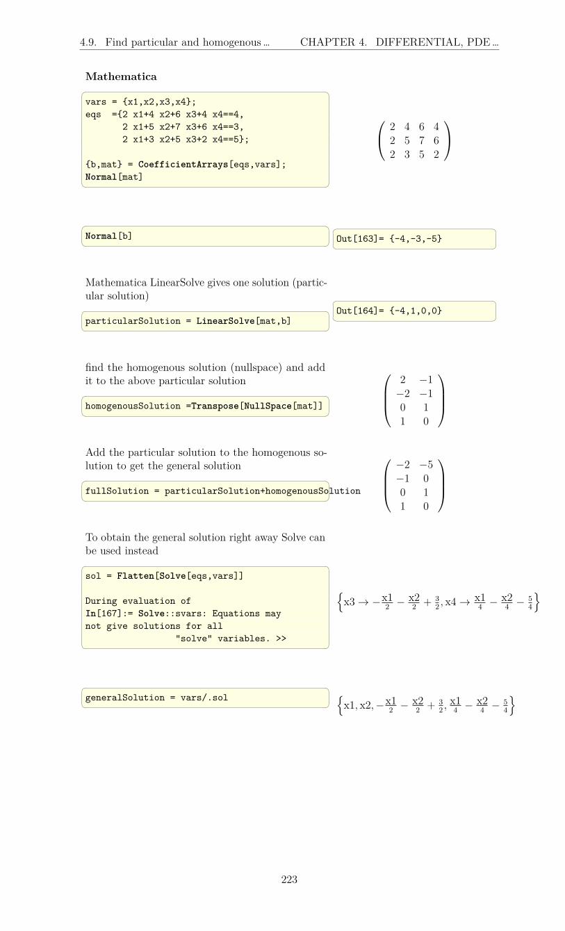
4.9. Find particular and homogenous … CHAPTER 4. DIFFERENTIAL, PDE…
Mathematica vars = x1,x2,x3,x4;eqs =2 x1+4 x2+6 x3+4 x4==4,
2 x1+5 x2+7 x3+6 x4==3,2 x1+3 x2+5 x3+2 x4==5;
b,mat = CoefficientArrays[eqs,vars];Normal[mat]
2 4 6 4
2 5 7 6
2 3 5 2
Normal[b]
Out[163]= -4,-3,-5 Mathematica LinearSolve gives one solution (partic-ular solution) particularSolution = LinearSolve[mat,b]
Out[164]= -4,1,0,0
find the homogenous solution (nullspace) and addit to the above particular solution homogenousSolution =Transpose[NullSpace[mat]]
2 −1
−2 −1
0 1
1 0
Add the particular solution to the homogenous so-lution to get the general solution fullSolution = particularSolution+homogenousSolution
−2 −5
−1 0
0 1
1 0
To obtain the general solution right away Solve canbe used instead sol = Flatten[Solve[eqs,vars]]
During evaluation ofIn[167]:= Solve::svars: Equations maynot give solutions for all
"solve" variables. >>
x3 → −x1
2− x2
2+ 3
2, x4 → x1
4− x2
4− 5
4
generalSolution = vars/.sol x1, x2,−x1
2− x2
2+ 3
2, x1
4− x2
4− 5
4
223

4.9. Find particular and homogenous … CHAPTER 4. DIFFERENTIAL, PDE…
Matlab clear all;A=[2 4 6 4;
2 5 7 6;2 3 5 2]
b=[4 3 5]'particularSolution=A\b
Warning: Rank deficient,rank = 2, tol = 4.033641e-15.
particularSolution =
00
1.5000-1.2500
nullSolution=null(A,'r')
nullSolution =
-1 2-1 -21 00 1
Maple restart;with(LinearAlgebra);vars := x[1], x[2], x[3], x[4];sys := 2*x[1]+4*x[2]+6*x[3]+4*x[4] = 4,
2*x[1]+5*x[2]+7*x[3]+6*x[4] = 3,2*x[1]+3*x[2]+5*x[3]+2*x[4] = 5;
`eqs=`, convert([sys], Vector);A, b := GenerateMatrix([sys], [vars])
A =
2 4 6 4
2 5 7 6
2 3 5 2
b =
4
3
5
`general solution=`,LinearSolve(A, b, free = 'x')
4− x3 + 2x4
−1− x3 − 2x4
x3
x4
Can solve this system to get the general so-lution using the solve command as follows s := solve([sys], [vars]);r := subs(op(s), [vars]);`general solution=`, convert(%, Vector)
4− x3 + 2x4
−1− x3 − 2x4
x3
x4
WARNING: Maple sometimes reorders the result from solve() so we can get a differentordering of the free variables as shown above.
224

4.10. Plot the constant energy levels for a … CHAPTER 4. DIFFERENTIAL, PDE…
4.10 Plot the constant energy levels for a nonlinearpendulum
Problem:
Plot the constant energy levels for the nonlinear pendulum in θ, θ
Pendulum
Assume that m = 1, g = 9.8m/s2, L = 10m
Answer:
The constant energy curves are curves in the Y-X plane where energy is constant. TheY-axis represents θ, and the X-axis represents θ
We assume the pendulum is given an initial force when in the initial position (θ = 00)that will cause it to swing anticlock wise. The pendulum will from this point obtain anenergy which will remain constant since there is no damping.
The higher the energy the pendulum posses, the larger the angle θ it will swing by will be.
If the energy is large enough to cause the pendulum to reach θ = π (the upright position)with non zero angular velocity, then the pendulum will continue to rotate in the samedirection and will not swing back and forth.
The expression for the energy E for the pendulum is first derived as a function of θ, θ
E = PE +KE
= mgL (1− cos θ) +1
2mL2θ2
The school PDF report contains more information on this topic.
This was solved in Mathematica using the ListContourPlot[] command after generatingthe energy values.
The original Matlab implementation is left below as well as the Maple implementation.However, these were not done using the contour method, which is a much simpler method.These will be updated later.
The following is the resulting plot for m = 1, g = 9.8m/s2, L = 10m
Mathematica SetDirectory[NotebookDirectory[]];energy[theta_, speed_, m_, g_, len_] := m*g*len*(1 - Cos[theta]) + (1/2)*m*len^2*speed^2;m = 1; g = 9.8; len = 10;data = Table[energy[i, j, m, g, len], j, -4, 4, 0.01, i, -3*Pi, 3*Pi, Pi/20.];ListContourPlot[data, InterpolationOrder -> 2, Contours -> 20, MaxPlotPoints -> 30,
DataRange -> -3*Pi, 3*Pi, -4, 4,FrameTicks -> -4, -3, -2, 0, 1, 2, 3, 4, None,
-3*Pi, -2*Pi, -Pi, 0, Pi, 2*Pi, 3*Pi, None,FrameLabel -> "\[Theta]'(t)", None,
"\[Theta](t)", "constant energy levels for nonlinear pendulum model", ImageSize -> 400,LabelStyle -> 14, RotateLabel -> False]
225

4.10. Plot the constant energy levels for a … CHAPTER 4. DIFFERENTIAL, PDE…
Matlab function HW2%HW2 problem. MAE 200A. UCI, Fall 2005%by Nasser Abbasi
%This MATLAB function generate the constant energy level%curves for a nonlinear pendulum with no damping
close all; clear;m=1; g=9.8; L=10;
%number of data points (positio vs speed) to find per curvenPoints=40;
nEnergyLevels = 8; %number of energy levelslowAnglesToVisit = linspace(0,pi,nEnergyLevels);lowEnergyLevels(1:nEnergyLevels)=m*g*L*(1-cos(lowAnglesToVisit));highAnglesToVisit = linspace(pi,2*pi,2*nEnergyLevels);highEnergyLevels=zeros(1,2*nEnergyLevels);
initialHighEnergy=2*m*g*L;Q=0.2;for i=1:2*nEnergyLevels
highEnergyLevels(i) = initialHighEnergy+(Q*i*initialHighEnergy);end
A = zeros(length(lowAnglesToVisit)+length(highAnglesToVisit),2);A(:,1) = [lowAnglesToVisit highAnglesToVisit];A(:,2) = [lowEnergyLevels highEnergyLevels];
[nAngles,~]=size(A);data=zeros(nPoints,2);
for j=1:nAngles
currentAngle=A(j,1);currentEnergyLevel =A(j,2) ;angles=linspace(0,currentAngle,nPoints);data(1:nPoints,1)=angles(:);
for m=1:nPointsdata(m,2)=speed(currentEnergyLevel,angles(m));
226

4.10. Plot the constant energy levels for a … CHAPTER 4. DIFFERENTIAL, PDE…
enddoPlots(data);
end
title(sprintf(['constant energy curves, nonlinear pendulum,'...'quantum=%1.3f'],Q));
xlabel('angle (position)');ylabel('speed');set(gca,'xtick',[-4*pi,-3*pi,-2*pi,-pi,0,pi,2*pi,3*pi,4*pi]);set(gca,'XTickLabel','-4pi','-3pi','-2pi','-pi',...
'0','pi','2pi','3pi','4pi')
print(gcf, '-dpdf', '-r600', 'images/matlab_e77_1');
function s=speed(energy,angle)m=1; g=9.8; L=10;if angle<pi
s=sqrt(2/(m*L^2)*(energy-m*g*L*(1-cos(angle))));else
s=sqrt(2/(m*L^2)*(energy-m*g*L*(1+cos(angle-pi))));end
function doPlots(data)plotCurves(data,0);plotCurves(data,2*pi);plotCurves(data,-2*pi);
function plotCurves(data,k)plot(data(:,1)+k,data(:,2));hold on;plot(data(:,1)+k,-data(:,2));plot(-data(:,1)+k,-data(:,2));plot(-data(:,1)+k,data(:,2));
-4pi -3pi -2pi -pi 0 pi 2pi 3pi 4pi
angle (position)
-5
-4
-3
-2
-1
0
1
2
3
4
5
spee
d
constant energy curves, nonlinear pendulum, quantum=0.200
MapleThe Maple solution was contributed by Matrin Eisenberg restart;plotEnergyLevels:= proc(m::positive, g::positive, L::positive, Erange::positive, numContours::posint)
local plotOptions, maxTheta, thetaDot, plotContour, Emax, energies, contours;plotOptions := args[6..-1];maxTheta := E- arccos(max(1-E/m/g/L, -1));thetaDot := E- theta- sqrt(max(2/m/L^2 * (E - m*g*L*(1-cos(theta))), 0));plotContour := E- plot(thetaDot(E), 0..maxTheta(E), numpoints=5, plotOptions);
227

4.10. Plot the constant energy levels for a … CHAPTER 4. DIFFERENTIAL, PDE…
# Create first quadrant of middle region of the graph.Emax := Erange*m*g*L;energies := Emax * n/numContours $ n=1..numContours;if Erange 2 then energies := energies union 2*m*g*L; fi;contours := map(plotContour, energies);
# Create other quadrants.map2(rcurry, plottools[reflect], [[0,0],[0,1]], [0,0], [[0,0],[1,0]]);contours := contours union map(f- map(f, contours)[], %);
# Create left and right regions of the graph.map2(rcurry, plottools[translate], -2*Pi,2*Pi, 0);contours := contours union map(f- map(f, contours)[], %);
# Complete the graph.plots[display]([%[], plot([[-2*Pi,0], [0,0], [2*Pi,0]], plotOptions, style=point)],view=[-3*Pi..3*Pi, -thetaDot(Emax)(0)..thetaDot(Emax)(0)],title="Constant energy levels, undamped pendulum",labels=["angle", "angular speed"],xtickmarks=[seq](evalf(k*Pi)=sprintf("%a pi", k), k=-3..3));
end:plotEnergyLevels(1, 9.8, 10, 5, 15);
;
sectionSolve numerically the ODE u””+u=f using point collocation method
Problem: Give the ODEd4u (x)
dx4+ u (x) = f
Solve numerically using the point collocation method. Use 5 points and 5 basis functions.Use the Boundary conditions u (0) = u (1) = u′′ (0) = u′′ (1) = 0
Use the trial function
g (x) =N=5∑i=1
ai (x (x− 1))i
Use f = 1
The solution is approximated using u (x) ≈ g (x) =N=5∑i=1
ai (x (x− 1))i.
N equations are generated for N unknowns (the unknowns being the undetermined coef-ficients of the basis functions). This is done by setting the error to zero at those points.
228

4.10. Plot the constant energy levels for a … CHAPTER 4. DIFFERENTIAL, PDE…
The error beingd4g (x)
dx4+ g (x)− f
Once g (x) (the trial function is found) the analytical solution is used to compare withthe numerical solution.
Mathematica Clear["Global`*"];nBasis = 5;nPoints = 5;a = Array[v,nBasis] Out[392]= v[1],v[2],v[3],v[4],v[5] trial = Sum[a[[n]] (x(x-1))^n,n,1,nBasis];residual = D[trial,x,4]+trial-1;mat = Flatten[Table[residual==0/.x->n/(2*nPoints-1),
n,1,nPoints-1]];
mat = Join[mat,2 a[[1]]+2a[[2]]==0];sol = N@First@Solve[mat,a] Out[397]= v[1.]->-0.0412493,
v[2.]->0.0412493,v[3.]->0.000147289,v[4.]->-0.0000245233,v[5.]->-3.28259*10^-8
numericalSolution=Chop@FullSimplify@Sum[sol[[n,2]](x(x-1))^n,
n,1,nBasis]
numericalSolutionDiff4 = D[numericalSolution,x,4];numericalMoment = D[numericalSolution,x,2];
0.0412493x− 0.0826459x3 + 0.0416667x4 − 0.00034374x5 − 1.51283 ∗ 10−8x6
+0.0000984213x7 − 0.0000248515x8 + 1.64129 ∗ 10−7x9 − 3.28259 ∗ 10−8x10
(*now analytical solution is obtainedusing DSolve and compared to numerical solution*)eq = u''''[x]+u[x]==1;bc = u[0]==0,u[1]==0,u''[0]==0,u''[1]==0;analyticalSolution=First@DSolve[eq,bc,u[x],x];analyticalSolution=u[x]/.analyticalSolution;analyticalSolution=FullSimplify[analyticalSolution]
−cos
(1−(1+i)x√
2
)+ cos
(1−(1−i)x√
2
)+ cosh
(1−(1+i)x√
2
)+ cosh
(1−(1−i)x√
2
)− 2
(cos
(1√2
)+ cosh
(1√2
))2
(cos
(1√2
)+ cosh
(1√2
)) analyticalMoment = D[analyticalSolution,x,2];
229
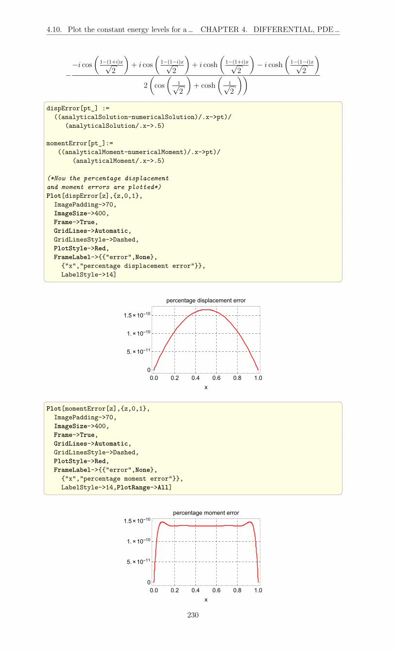
4.10. Plot the constant energy levels for a … CHAPTER 4. DIFFERENTIAL, PDE…
−−i cos
(1−(1+i)x√
2
)+ i cos
(1−(1−i)x√
2
)+ i cosh
(1−(1+i)x√
2
)− i cosh
(1−(1−i)x√
2
)2
(cos
(1√2
)+ cosh
(1√2
)) dispError[pt_] :=
((analyticalSolution-numericalSolution)/.x->pt)/(analyticalSolution/.x->.5)
momentError[pt_]:=((analyticalMoment-numericalMoment)/.x->pt)/
(analyticalMoment/.x->.5)
(*Now the percentage displacementand moment errors are plotted*)Plot[dispError[z],z,0,1,
ImagePadding->70,ImageSize->400,Frame->True,GridLines->Automatic,GridLinesStyle->Dashed,PlotStyle->Red,FrameLabel->"error",None,"x","percentage displacement error",LabelStyle->14]
0.0 0.2 0.4 0.6 0.8 1.00
5.×10-11
1.×10-10
1.5×10⁻¹⁰
x
percentage displacement error
Plot[momentError[z],z,0,1,
ImagePadding->70,ImageSize->400,Frame->True,GridLines->Automatic,GridLinesStyle->Dashed,PlotStyle->Red,FrameLabel->"error",None,"x","percentage moment error",LabelStyle->14,PlotRange->All]
0.0 0.2 0.4 0.6 0.8 1.00
5.×10-11
1.×10-10
1.5×10⁻¹⁰
x
percentage moment error
230

4.10. Plot the constant energy levels for a … CHAPTER 4. DIFFERENTIAL, PDE…
(*Now the Residual error distributionover x is plotted*)Plot[Abs[numericalSolutionDiff4+
numericalSolution-1],x,0,1,ImagePadding->80,ImageSize->400,Frame->True,GridLines->Automatic,GridLinesStyle->Dashed,PlotStyle->Red,FrameLabel->"error",None,"x","Residual error distribution over x",LabelStyle->14,PlotRange->All]
0.0 0.2 0.4 0.6 0.8 1.00
5.×10-9
1.×10-8
1.5×10⁻⁸
2.×10-8
x
error
Residual error distribution over x
231

4.11. How to numerically solve a set of … CHAPTER 4. DIFFERENTIAL, PDE…
Maple #Solve u''''+u=1 using point collocation. Zero B.C.#written by Nasser Abbasi for fun on April 25,2006.restart;Digits:=15;nBasis := 5:nPoints := 5:coef := [seq(a[i],i=1..nBasis)]:g := (x,n)-coef[n]*(x*(x-1))^n: #basis functionf := x-sum(g(x,k),k=1..nBasis): #trial functionmoment := x-diff(f(x),x$2):residual := x-diff(f(x),x$4)+f(x)-1:A := seq(subs(x=N/(2*nPoints-1),residual(x)=0),N=1..nPoints-1):A := A,2*(coef[1]+coef[2]=0):sol := solve([A],coef):coef := map(rhs,sol[1]):evalf(coef):numericalSolution:=x-sum(coef[n]*(x*(x-1))^n ,n=1..nBasis):`The numerical solution is `, numericalSolution(x);numericalSolutionMoment := x-diff(numericalSolution(x),x$2):
#Now obtain exact solution from Mapleeq := diff(W(x),x$4)+W(x)=1:bc := W(0)=0,W(1)=0,D(D(W))(0)=0,D(D(W))(1)=0:
exact := unapply(rhs(dsolve(eq,bc)),x):
exactMoment := x-diff(exact(x),x$2):
displacmentError := x-(exact(x)-numericalSolution(x))/exact(.5):momentError := x- (exactMoment(x)-numericalSolutionMoment(x))/evalf(subs(x=.5,exactMoment(x))):
plot(displacmentError(x),x=0..1,labels=['x',"Disp. error %"]);plot(momentError(x),x=0..1,labels=['x',"Moment error %"]);
4.11 How to numerically solve a set of non-linearequations?
Numerically solve the following three equations for e, a, f
eq1 = r1− a(e− 1)
eq2 = delT −
√a3
µ(e ∗ sinh(f)− f)
eq3 = r2− a(e cosh(f)− 1)
232

4.11. How to numerically solve a set of … CHAPTER 4. DIFFERENTIAL, PDE…
Mathematica ClearAll[a, e, f]delT = 5.215*60*60;r1 = 200 + 6378;r2 = 130000;mu = 3.986*10^5;eq1 = r1 - a*(e - 1) == 0;eq2 = delT - Sqrt[a^3/mu]*
(e*Sinh[f] - f) == 0;
eq3 = r2 - a*(e*Cosh[f]-1)==0;sol = NSolve[eq1, eq2, eq3,
a, e, f, Reals]
a->12029.39633,e->1.546827108,f->2.721303232
Matlab clear allsyms a e f;delT = 5.215*60*60;r1 = 200+6378;r2 = 130000;mu = 3.986*10^5;eq1 = r1 - a*(e-1);eq2 = delT - sqrt(a^3/mu)*(e*sinh(f)-f);eq3 = r2 - a*(e*cosh(f)-1);sol = feval(symengine,'numeric::solve',...
eq1,eq2,eq3);vpa(sol,6)
ans =[a == 12029.4, e == 1.54683, f == 2.7213]
Another option is solve but slower sol = solve(eq1,eq2,eq3,a,e,f);
sol =
a: [1x1 sym]e: [1x1 sym]f: [1x1 sym]
sol.a12029.396328714435126444927089827
sol.e1.5468271075497087492979481526009
sol.f2.7213032317471583123822097902877
233

4.12. Solve 2nd order ODE (Van Der Pol) … CHAPTER 4. DIFFERENTIAL, PDE…
4.12 Solve 2nd order ODE (Van Der Pol) andgenerate phase plot
Problem: Solvey′′ (t)− µ
(1− y2
)y′ (t) + y (t) = 0
for different values of µ to compare effect of changing µ on the solution trajectories. Theinitial conditions are
y (0) = 0.1
y′ (t) = 0
In both Mathematica and Matlab, numerical ODE solver was used.
For Matlab, The 2nd order ODE is first converted to 2 first order ODE’s, and then solvethe coupled ODE’s using ode45. In Mathematica NDSolve was used. This does not requirethe conversion.
Starting by writing the 2nd order ODE as 2 first order ODE’s
x1 = y
x2 = y′
derivatives ⇒
x′1 = y′
x′2 = y
′′
⇒
x′1 = x2
x′2 = µ (1− x2
1)x2 + x1
Below is the solution of the differential equation for different values of µ = 1
Mathematica process[mu_]:=Module[
sol,p1,p2,p3,data,system,z,x1,x2,t,ode1,ode2,timeScale,
ode1 =x1'[t]==x2[t];ode2 =x2'[t]==z(1-x1[t]^2)x2[t]-x1[t];timeScale =t,0,80;sol=First@NDSolve[
ode1,ode2/.z->mu,x1[0]==0.01,x2[0]==0,x1[t],x2[t],timeScale,Method->"Extrapolation",Method->"LinearlyImplicitEuler"];
sol = x1[t],x2[t]/.sol;p1 = Plot[Evaluate[sol[[1]]],
Evaluate[timeScale],Frame->True,FrameLabel->"time","y(t)",PlotLabel->"\[Mu]="<>ToString[mu]];
p2 = Plot[Evaluate[sol[[2]]],Evaluate[timeScale],
Frame->True,FrameLabel->"time","y'(t)",PlotLabel->"\[Mu]="<>ToString[mu],PlotStyle->RGBColor[1,0,0]];
data = Table[evaluate[sol[[1]]],Evaluate[sol[[2]]],Evaluate[timeScale]];
p3=ListPlot[data,Joined->True,Frame->True,PlotLabel->"\[Mu]="<>ToString[mu],FrameLabel->"y(t)","y'(t)",PlotRange->All];
p1,p2,p3];mu=0.1,.2,1,3,5,10;r = process/@mu; Grid[r]
234

4.12. Solve 2nd order ODE (Van Der Pol) … CHAPTER 4. DIFFERENTIAL, PDE…
0 20 40 60 80-0.3-0.2-0.10.00.10.20.30.4
time
y(t)
μ=0.1
0 20 40 60 80-0.3
-0.2
-0.1
0.0
0.1
0.2
0.3
time
y'(t)
μ=0.1
-0.4 -0.2 0.0 0.2
-0.4
-0.2
0.0
0.2
0.4
y(t)
y'(t)
μ=0.1
0 20 40 60 80-2
-1
0
1
2
time
y(t)
μ=0.2
0 20 40 60 80-2
-1
0
1
2
time
y'(t)
μ=0.2
-2 -1 0 1 2-2
-1
0
1
2
y(t)
y'(t)
μ=0.2
0 20 40 60 80-2
-1
0
1
2
time
y(t)
μ=1
0 20 40 60 80
-2
-1
0
1
2
time
y'(t)
μ=1
-2 -1 0 1 2
-2
-1
0
1
2
y(t)
y'(t)
μ=1
0 20 40 60 80-2
-1
0
1
2
time
y(t)
μ=3
0 20 40 60 80
-2
-1
0
1
2
time
y'(t)
μ=3
-2 -1 0 1 2
-4
-2
0
2
4
y(t)
y'(t)
μ=3
0 20 40 60 80-2
-1
0
1
2
time
y(t)
μ=5
0 20 40 60 80
-1.0
-0.5
0.0
0.5
1.0
time
y'(t)
μ=5
-2 -1 0 1 2
-5
0
5
y(t)
y'(t)
μ=5
0 20 40 60 80-2
-1
0
1
2
time
y(t)
μ=10
0 20 40 60 80
-0.4
-0.2
0.0
0.2
0.4
time
y'(t)
μ=10
-2 -1 0 1 2
-10
-8
-6
-4
-2
0
y(t)
y'(t)
μ=10
235
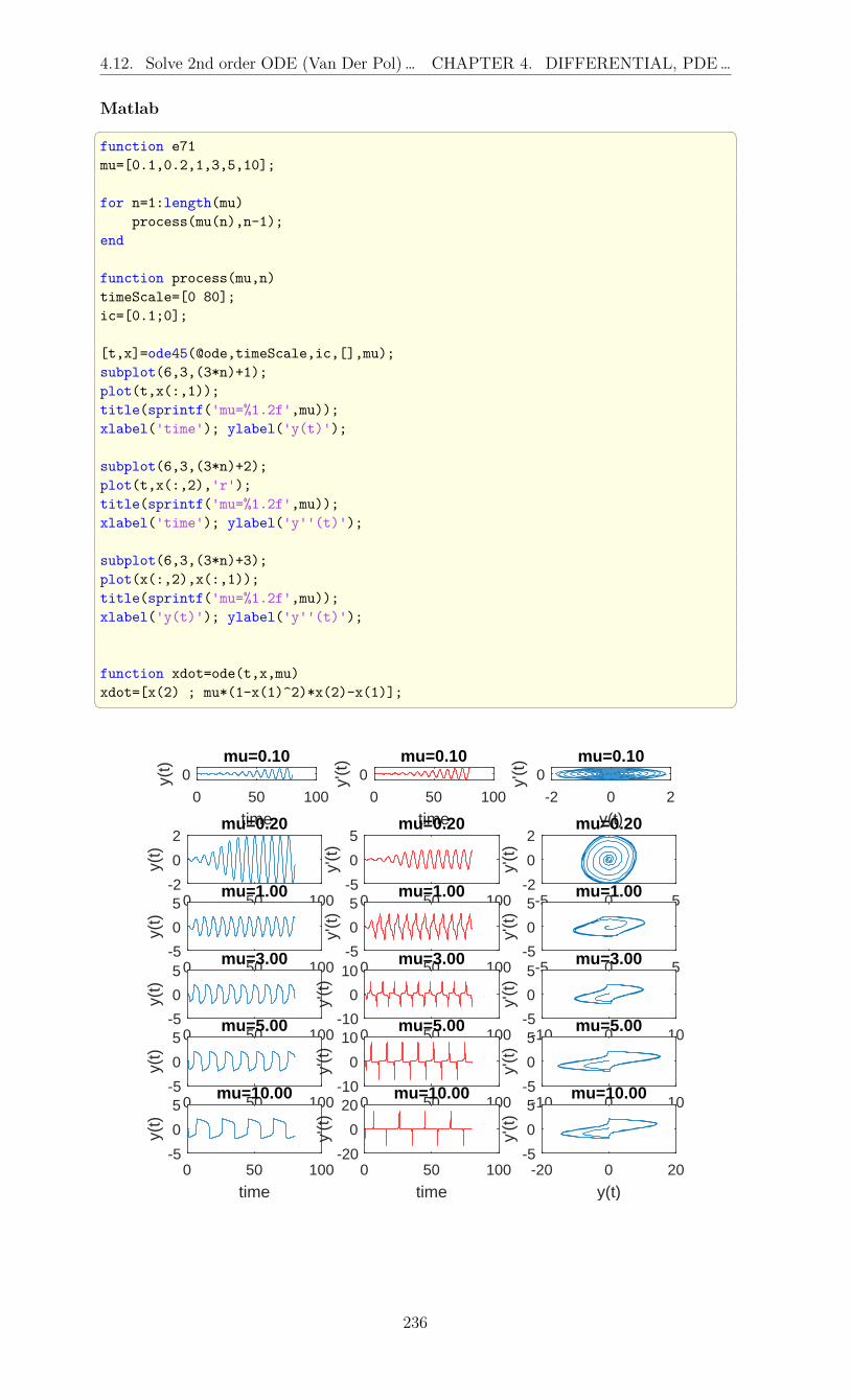
4.12. Solve 2nd order ODE (Van Der Pol) … CHAPTER 4. DIFFERENTIAL, PDE…
Matlab function e71mu=[0.1,0.2,1,3,5,10];
for n=1:length(mu)process(mu(n),n-1);
end
function process(mu,n)timeScale=[0 80];ic=[0.1;0];
[t,x]=ode45(@ode,timeScale,ic,[],mu);subplot(6,3,(3*n)+1);plot(t,x(:,1));title(sprintf('mu=%1.2f',mu));xlabel('time'); ylabel('y(t)');
subplot(6,3,(3*n)+2);plot(t,x(:,2),'r');title(sprintf('mu=%1.2f',mu));xlabel('time'); ylabel('y''(t)');
subplot(6,3,(3*n)+3);plot(x(:,2),x(:,1));title(sprintf('mu=%1.2f',mu));xlabel('y(t)'); ylabel('y''(t)');
function xdot=ode(t,x,mu)xdot=[x(2) ; mu*(1-x(1)^2)*x(2)-x(1)];
0 50 100
time
0y(t)
mu=0.10
0 50 100
time
0y'(t
) mu=0.10
-2 0 2
y(t)
0y'(t
) mu=0.10
0 50 100
time
-2
0
2
y(t)
mu=0.20
0 50 100
time
-5
0
5
y'(t
)
mu=0.20
-5 0 5
y(t)
-2
0
2
y'(t
)
mu=0.20
0 50 100
time
-5
0
5
y(t)
mu=1.00
0 50 100
time
-5
0
5
y'(t
)
mu=1.00
-5 0 5
y(t)
-5
0
5
y'(t
)
mu=1.00
0 50 100
time
-5
0
5
y(t)
mu=3.00
0 50 100
time
-10
0
10
y'(t
)
mu=3.00
-10 0 10
y(t)
-5
0
5
y'(t
)
mu=3.00
0 50 100
time
-5
0
5
y(t)
mu=5.00
0 50 100
time
-10
0
10
y'(t
)
mu=5.00
-10 0 10
y(t)
-5
0
5
y'(t
)
mu=5.00
0 50 100
time
-5
0
5
y(t)
mu=10.00
0 50 100
time
-20
0
20
y'(t
)
mu=10.00
-20 0 20
y(t)
-5
0
5
y'(t
)
mu=10.00
236

4.13. How to numerically solve Poisson… CHAPTER 4. DIFFERENTIAL, PDE…
4.13 How to numerically solve Poisson PDE on 2Dusing Jacobi iteration method?
Problem: Solve52u = f(x, y) on 2D using Jacobi method. Assume f(x, y) = −e−(x−0.25)2−(y−0.6)2 .Use mesh grid norm and relative residual to stop the iterations.Mathematica n = 21; (*number of grid points*)uNew = Table[0, n, n]; (*solution grid*)residual = uOld = uNew;
h = 1/(n - 1); (*spacing*)c = 0.1; (*controls the tolerance*)epsilon = c*h^2; (*error tolerance*)
grid = N@Table[i*h,j*h,i,0,n-1,j,0,n-1];
(*the force function*)f[x_,y_] := -Exp[-(x - 0.25)^2 - (y - 0.6)^2];
(*evaluate force on the grid*)force = Map[f[#[[1]],#[[2]]]&,grid,2];normF = Sqrt[h]*Norm[Flatten@force,2];(*force norm*)converged = False;
k = 0; (*iteration counter*)While[Not[converged],k++;For[i = 2, i < n, i++,For[j = 2, j < n, j++,uNew[[i, j]] = (1/4)*(uOld[[i-1,j]]+uOld[[i+1,j]]+ uOld[[i,j-1]]+uOld[[i,j+1]]-h^2*force[[i,j]]);
residual[[i,j]] = force[[i, j]]-1/h^2*(uOld[[i-1,j]]+uOld[[i+1,j]]+uOld[[i,j-1]]+uOld[[i,j+1]]-4*uOld[[i,j]])]
];uOld = uNew; (*updated at end*)normR = Sqrt[h] Norm[Flatten@residual, 2];If[normR/normF < epsilon, converged = True]];
(*plot solution*)ListPlot3D[uOld, PlotRange -> All, ImagePadding -> 30,
ImageSize -> 400, Mesh -> n, n,AxesLabel -> "x", "y", "u(x,y)",PlotRangePadding -> 0, BaseStyle -> 12,PlotLabel -> Row["Converged in ", k, " iterations",
" ,epsilon=", epsilon, " ,h=", h]]
237

4.13. How to numerically solve Poisson… CHAPTER 4. DIFFERENTIAL, PDE…
238

4.13. How to numerically solve Poisson… CHAPTER 4. DIFFERENTIAL, PDE…
Matlab close all; clear all;n = 21; % grid points, including internal pointsc = 0.1; % constant of tolerancemyforce = @(X,Y) -exp( -(X-0.25).^2 - (Y-0.6).^2 );
h = 1/(n-1); % grid spacingtol = c * h^2; % toleranceres = zeros(n,n); % storage for residualu = res; % storage for solutionuNew = u;k = 0; % loop counter[X,Y] = meshgrid(0:h:1,0:h:1); % coordinatesf = myforce(X,Y);normf = norm( f(:),2); % find norm
%Now start the iteration solver, stop when%relative residual < tolerancefigure;i = 2:n-1;j = 2:n-1; %the iterations vectorizeddone = false;
while ~donek = k+1;
uNew(i,j) = (1/4)*( u(i-1,j) + u(i+1,j) + ...u(i,j-1) + u(i,j+1) - h^2 * f(i,j) );
res(i,j) = f(i,j) - (1/h^2)*( u(i-1,j) + ...u(i+1,j) + u(i,j-1) + u(i,j+1) - 4*u(i,j) );
%uncomment to see it update as it runs
%mesh(X,Y,u); %hold on;%title(sprintf('solution at iteration %d',k));%zlim([0,.07]);%drawnow;
if norm(res(:),2)/normf < toldone = true;
end;
u = uNew;end
mesh(X,Y,u);title(sprintf('solution at iteration %d',k))
239

4.14. How to solve BVP second order ODE… CHAPTER 4. DIFFERENTIAL, PDE…
01
0.02
1
0.04
0.8
solution at iteration 655
0.06
0.5 0.6
0.08
0.40.2
0 0
4.14 How to solve BVP second order ODE usingfinite elements with linear shape functions andusing weak form formulation?
Solve y′′(x) − 3y(x) = −x2 over x = 0 . . . 1 with boundary conditions x(0) = 0 andx(1) = 0 using piecewise linear trial functions.solutionLet the trial function be the linear function y(x) = c1x+ c2. The residual is R = y′′(x)−3y(x)+x2. Let the test function be w(x). We need to solve for each element i the followingequation
Ii =
∫wi Ri dx
Using the weak form, we apply integration by parts to obtain
Ii =
∫ xi+1
xi
−dw
dx
dy
dx− 3w(x)y(x) + w(x)x2 dx+
[w(x)
dy
dx
]xi+1
xi
= 0 (96.1)
or
I =i=M∑i=1
Ii
=i=M∑i=1
∫ xi+1
xi
(−dw
dx
dy
dx− 3w(x)y(x) + w(x)x2 dx+
[w(x)
dy
dx
]xi+1
xi
)= 0
Where M is the number of elements. The above is the M equations we need to solve for theunknowns yi at the internal nodes. In Galerkin method, the test function is w1(x) = H1(x)
and w2(x) = H2(x) which comes from writing wi(x) =dy(x)dyi
Rewriting the trial function y(x) in terms of unknown values at nodes results in
y(x) = H1(x)yi +H2(x)yi+1
Where H1(x) =xi+1−x
hand H2(x) =
x−xi
hwhere h is the length of each element. Hence
(96.1) becomes
Ii =
∫ xi+1
xi
−
H ′
1(x)
H ′2(x)
H ′
1(x)H′2(x)
yiyi+1
− 3
H1(x)
H2(x)
H1(x)H2(x)
yiyi+1
+
H1(x)
H2(x)
x2 dx+
[w(x)
dy
dx
]xi+1
xi
(96.2)240

4.14. How to solve BVP second order ODE… CHAPTER 4. DIFFERENTIAL, PDE…
The terms[w(x) dy
dx
]xi+1
xireduce to
[w(x) dy
dx
]10since intermediate values cancel each other
leaving the two edge values over the whole domain.
But H ′1(x) = −x
hand H ′
2(x) = xh. Plugging these into (96.2) and integrating gives the
following
Ii =1
h
[−1 1
1 −1
]yiyi+1
− h
1 12
12
1
yiyi+1
+
1
12h
[3x4
i − 4x3ixi+1 + x4
i+1
x4i − 4xix
3i+1 + 3x4
i+1
]+
[w(x)
dy
dx
]10
(96.3)
The algebra above was done with Mathematica. In the following code, x1 is xi and x2 isxi+1
h1 = (x2 - x)/h;h2 = (x - x1)/h;int1 = -D[h1, x], D[h2, x].D[h1, x], D[h2, x];int2 = -3 h1, h2.h1, h2;int3 = h1, h2 x^2;sol1 = Integrate[int1, x, x1, x2];sol1 /. (x1 - x2) -> -h, (x2 - x1) -> h
-(1/h), 1/h, 1/h, -(1/h)
sol2 = Integrate[int2, x, x1, x2];sol2 /. (x1 - x2) -> -h, (x2 - x1) -> h
-h, -(h/2), -(h/2), -h
sol3 = Integrate[int3, x, x1, x2];Simplify[%];% /. (x1 - x2) -> -h, (x2 - x1) -> h
(3 x1^4 - 4 x1^3 x2 + x2^4)/(12 h),(x1^4 - 4 x1 x2^3 + 3 x2^4)/(12 h)
The above equation Ii is calculated for each element i, resulting in M equations where Mis the number of elements. Collecting all these local equations into a global stiffness matrixand then adjusting the global stiffness matrix for boundary conditions by eliminatingcorresponding rows and columns, it is then solved for the unknowns yi as a system Ax = fusing direct solver. The following code illustrates the method.
241

4.14. How to solve BVP second order ODE… CHAPTER 4. DIFFERENTIAL, PDE…
Matlab M = 9; %number of elementsN = M+1; %number of nodesdof = 2; %degree of freedom per elementkk = zeros(N);f = zeros(N,1); %force vectorh = 1/M; %length of each elementk_local=1/h*[-1 1;1 -1]-h*[1 1/2;1/2 1];
for i = 1:M %loop over all elementsx1 = (i-1)*h;x2 = i*h;f_local = -1/(12*h)*[3*x1^4-4*x1^3*x2+...
x2^4;x1^4-4*x1*x2^3+3*x2^4];f(i:i+dof-1) = f(i:i+dof-1)+f_local;kk(i:i+dof-1,i:i+dof-1) = ...
kk(i:i+dof-1,i:i+dof-1)+k_local;end%fix first and last rows since these are B.C.kk(1,:) = 0;kk(1,1) = 1;kk(end,:) = 0;kk(end,end) = 1;f(1) = 0;f(end) = 0;y = kk\f; %solve
plot(0:h:1,y,'or')hold on;plot(0:h:1,y,'-');title(sprintf...('FEM solution using to ODE using %d elements',M'));xlabel('x');ylabel('y(x)');grid
0 0.2 0.4 0.6 0.8 1
x
0
0.005
0.01
0.015
0.02
0.025
0.03
0.035
y(x)
FEM solution using to ODE using 9 elements
The analytical solution to the ODE is below. We can see it is very close to the FEMsolution above with 11 elements. More elements leads to more accurate solution.
242

4.14. How to solve BVP second order ODE… CHAPTER 4. DIFFERENTIAL, PDE…
MathematicaAnaltical solution ClearAll[y, x]sol= y[x]/.First@DSolve[y''[x]-3 y[x]==-x^2,
y[0] == 0, y[1] == 0, y[x], x];Plot[sol, x, 0, 1, Frame -> True,
FrameLabel -> "y(x)", None,"x", "analytical solution",
GridLines -> Automatic,GridLinesStyle -> Dashed, LightGray,
Dashed, LightGray]
0.0 0.2 0.4 0.6 0.8 1.0
0.000
0.005
0.010
0.015
0.020
0.025
0.030
x
y(x)
analytical solution
Numerical m = 9;n = m + 1;dof = 2;kk = Table[0., n, n];f = Table[0., n];h = 1/m;kLocal = 1/h -1, 1, 1, -1 - h 1, 1/2, 1/2, 1;Do[x1 = (i - 1) h;x2 = i h;fLocal = -1/(12 h) 3 x1^4 - 4 x1^3 x2 + x2^4,
x1^4 - 4 x1 x2^3 + 3 x2^4;f[[i ;; i + dof - 1]] += fLocal;kk[[i ;; i + dof - 1, i ;; i + dof - 1]] +=kLocal,i, m];
kk[[1, ;;]] = 0;kk[[1, 1]] = 1;kk[[-1, ;;]] = 0;kk[[-1, -1]] = 1;f[[1]] = 0;f[[-1]] = 0;y = LinearSolve[kk, f];x = Range[0, 1, h];
ListPlot[Transpose[x, y], Frame -> True, Joined -> True,PlotMarkers -> Automatic, FrameLabel ->
"y(x)", None, "x",Row["solution to y''(x)-3 y(x)=-x^2 using FEM, 9 elements"],GridLines -> Automatic,GridLinesStyle -> LightGray]
243

4.15. How to solve Poisson PDE in 2D… CHAPTER 4. DIFFERENTIAL, PDE…
0.0 0.2 0.4 0.6 0.8 1.00.000
0.005
0.010
0.015
0.020
0.025
0.030
x
y(x)
solution to y''(x)-3 y(x)=-x^2 using FEM, 9 elements
4.15 How to solve Poisson PDE in 2D using finiteelements methods using rectangular element?
Solve ∇2u = f (x, y) on square using FEM. Assume u = 0 on boundaries and solve usingf (x, y) = xy and also f (x, y) = 1 and f (x, y) = 3 (cos(4πx) + sin(3πy))
Use Galerkin method and weak form, Using a bilinear trial function. Let width of squarebe 1.
SolutionUsing as an example with 9 elements to illustrate the method. The program below canbe called with different number of elements.
987
654
2 31
1 2 3 4
5 6 7
910 11
12
13 14
8
15 16
element
node
The trial function is bilinear
u = c1 + c2x+ c3y + c4xy (1)
Looking at one element, and using local coordinates systems with element having width2a and height 2b gives
244

4.15. How to solve Poisson PDE in 2D… CHAPTER 4. DIFFERENTIAL, PDE…
1 2
34
(0,0)x
y
a,ba,b
a,ba,b
a
b
Local node numbers, always increase anti-clockwise
Evaluating the trial function (1) at each corner node of the above element gives
u1 = c1 − ac2 − bc3 + abc4
u2 = c1 + ac2 − bc3 − abc4
u3 = c1 + ac2 + by3 + abc4
u4 = c1 − ac2 + bc3 + abc4
Or u1
u2
u3
u4
=
1 −a −b ab
1 a −b −ab
1 a b ab
1 −a b ab
c1c2c3c4
Hence
c1c2c3c4
=
1 −a −b ab
1 a −b −ab
1 a b ab
1 −a b ab
−1
u1
u2
u3
u4
=
1
4ab
ab ab ab ab
−b b b −b−a −a a a
1 −1 1 −1
u1
u2
u3
u4
(2)
coor = -a, -b, a, -b, a, b, -a, b;uVal = u1, u2, u3, u4; eq = c1 + c2 x + c3 y + c4 x y;r = MapThread[eq /. u -> #1, x -> #2[[1]], y -> #2[[2]]&, uVal, coor];mat = Last@Normal[CoefficientArrays[r, c1, c2, c3, c4]];MatrixForm[Inverse[mat] // MatrixForm
Out[6]//MatrixForm=
1 -a -b a b1 a -b -a b1 a b a b1 -a b -a b
Out[7]//MatrixForm=14
14
14
14
-14 a
14 a
14 a
-14 a
-14 b
-14 b
14 b
14 b
14 a b
-1
4 a b1
4 a b-
14 a b
Substituting (2) back into (1) and rearranging terms results in
245

4.15. How to solve Poisson PDE in 2D… CHAPTER 4. DIFFERENTIAL, PDE…
u = c1 + c2x+ c3y + c4xy
=1
4ab((ab− bx− ay + xy) u1 + (ab+ bx− ay − xy) u2 + (ab+ bx+ ay + xy) + (ab− bx+ ay − xy))
Since ab is the 14of the area of element, then the above becomes
u =1
A((ab− bx− ay + xy) u1 + (ab+ bx− ay − xy) u2 + (ab+ bx+ ay + xy) + (ab− bx+ ay − xy))
The above can now be written in term of what is called shape functions
u(x, y) = N1(x, y)u1 +N2(x, y)u2N3(x, y)u3 +N4(x, y)u4
Where
N1 =1
A(ab− bx− ay + xy) =
1
A(a− x) (b− y)
N2 =1
A(ab+ bx− ay − xy) =
1
A(a+ x) (b− y)
N3 =1
A(ab+ bx+ ay + xy) =
1
A(a+ x) (b+ y)
N4 =1
A(ab− bx+ ay − xy) =
1
A(a− x) (b+ y)
Now that the shape functions are found, the next step is to determine the local elementstiffness matrix. This can be found from the weak form integral over the area of theelement.
Ii =
x=a∫x=−a
y=b∫y=−b
w(∇2u− f (x, y)
)dxdy (3)
Where w (x, y) is the test function. For Galerkin method, the test function wi =dudui
=Ni (x, y). Hence
w (x, y) =
N1 (x, y)
N2 (x, y)
N3 (x, y)
N4 (x, y)
=
1A(a− x) (b− y)
1A(a+ x) (b− y)
1A(a+ x) (b+ y)
1A(a− x) (b+ y)
Using weak form, integration by parts is applied to (2)
Ii =
x=a∫x=−a
y=b∫y=−b
(− ∂w
∂xi
∂u
∂xi
− wf (x, y)
)dxdy +
goes to zero︷ ︸︸ ︷∫Γ
w∂u
∂n
The term∫Γ
w ∂u∂n
is the integration over the boundary of the element. Since there is only an
essential boundary condition over all the boundaries (this is the given Dirchilet boundarycondition), w = 0 on the boundary and this integral vanishes. There is no natural boundaryconditions for this example.For those elements not on the external edge of the overall grid (i.e. internal elements),each contribution to this integral will cancel from the adjacent internal element. Whatthis means is that the above reduces to just the first integral
246

4.15. How to solve Poisson PDE in 2D… CHAPTER 4. DIFFERENTIAL, PDE…
Ii =
x=a∫x=−a
y=b∫y=−b
(− ∂w
∂xi
∂u
∂xi
− wf (x, y)
)dxdy
=
x=a∫x=−a
y=b∫y=−b
−
∂N1
∂x
∂N2
∂x
∂N3
∂x
∂N4
∂x
∂N1
∂x∂N2
∂x∂N3
∂x∂N4
∂x
u1
u2
u3
u4
−
∂N1
∂y
∂N2
∂y
∂N3
∂y
∂N4
∂y
∂N1
∂y∂N2
∂y∂N3
∂y∂N4
∂y
u1
u2
u3
u4
−x=a∫
x=−a
y=b∫y=−b
N1 (x, y)
N2 (x, y)
N3 (x, y)
N4 (x, y)
f (x, y) dxdy
Hence
Ii =
x=a∫x=−a
y=b∫y=−b
−
∂N1
∂x∂N1
∂x+ ∂N1
∂y∂N1
∂y∂N1
∂x∂N2
∂x+ ∂N1
∂y∂N2
∂y∂N1
∂x∂N3
∂x+ ∂N1
∂y∂N3
∂y∂N1
∂x∂N4
∂x+ ∂N1
∂y∂N4
∂y
∂N2
∂x∂N1
∂x+ ∂N2
∂y∂N1
∂y∂N2
∂x∂N2
∂x+ ∂N2
∂y∂N2
∂y∂N2
∂x∂N3
∂x+ ∂N2
∂y∂N3
∂y∂N2
∂x∂N4
∂x+ ∂N2
∂y∂N4
∂y
∂N3
∂x∂N1
∂x+ ∂N3
∂y∂N1
∂y∂N3
∂x∂N2
∂x+ ∂N3
∂y∂N2
∂y∂N3
∂x∂N3
∂x+ ∂N3
∂y∂N3
∂y∂N3
∂x∂N4
∂x+ ∂N3
∂y∂N4
∂y
∂N4
∂x∂N1
∂x+ ∂N4
∂y∂N1
∂y∂N4
∂x∂N2
∂x+ ∂N4
∂y∂N2
∂y∂N4
∂x∂N3
∂x+ ∂N4
∂y∂N3
∂y∂N4
∂x∂N4
∂x+ ∂N4
∂y∂N4
∂y
u1
u2
u3
u4
−x=a∫
x=−a
y=b∫y=−b
N1 (x, y)
N2 (x, y)
N3 (x, y)
N4 (x, y)
f (x, y) dxdy
In the above, we have the from Ii =∫Ω
−ki u dΩ−∫Ω
u fidΩ, hence the element stiffness
matrix is the first integral, and the force vector comes from the second integral.
The integration is now carried out to obtain the element stiffness matrix. This was doneusing Mathematica. The local stiffness matrix for element i is
ki =
x=a∫x=−a
y=b∫y=−b
∂w
∂xi
∂u
∂xi
dxdy
=
a2+b2
3aba6b− b
3a−a2+b2
6ab− a
3b+ b
6a
a6b− b
3aa2+b2
3ab− a
3b+ b
6a−a2+b2
6ab
−a2+b2
6ab− a
3b+ b
6aa2+b2
3aba6b− b
3a
− a3b+ b
6a−a2+b2
6aba6b− b
3aa2+b2
3ab
For example, for element of width 1 and height 1, then a = 1
2, b = 1
2and the above becomes
ki =
23
−16
−13
−16
−16
23
−16
−13
−13
−16
23
−16
−16
−13
−16
23
247

4.15. How to solve Poisson PDE in 2D… CHAPTER 4. DIFFERENTIAL, PDE…
ClearAll[a, b];area = 4 a b;phi = (1/area) (a - x) (b - y),
(a + x) (b - y),(a + x) (b + y),(a - x) (b + y);
vx = D[phi[[1]], x],D[phi[[2]], x],D[phi[[3]], x],D[phi[[4]], x];
vy = D[phi[[1]], y],D[phi[[2]], y],D[phi[[3]], y],D[phi[[4]], y];
k = Integrate[vx.Transpose[vx]+vy.Transpose[vy],x, -a, a, y, -b, b] a2+b2
3 a ba6 b
-b3 a
-a2+b2
6 a b-
a3 b
+b6 a
a6 b
-b3 a
a2+b2
3 a b-
a3 b
+b6 a
-a2+b2
6 a b
-a2+b2
6 a b-
a3 b
+b6 a
a2+b2
3 a ba6 b
-b3 a
-a3 b
+b6 a
-a2+b2
6 a ba6 b
-b3 a
a2+b2
3 a b
Hence
Ii = −ki
u1
u2
u3
u4
−x=a∫
x=−a
y=b∫y=−b
N1 (x, y)
N2 (x, y)
N3 (x, y)
N4 (x, y)
f (x, y) dxdy
Now the integration of the force vector is carried out.
Ifi =
x=a∫x=−a
y=b∫y=−b
N1 (x, y)
N2 (x, y)
N3 (x, y)
N4 (x, y)
f (x, y) dxdy
=
x=a∫x=−a
y=b∫y=−b
1A(a− x) (b− y)
1A(a+ x) (b− y)
1A(a+ x) (b+ y)
1A(a− x) (b+ y)
f (x, y) dxdy
In the above, the integration depends on the physical location of the element. We useda local coordinate system initially to obtain the shape functions. This has now to betransformed to the global coordinates system. Taking the center of each element as (x0, y0)then we need to replace a → x0 + a and b → y0 + b everywhere in the above integral. Wedid not have to do this for finding the local stiffness matrix, since that did not depend onthe physical location of the element (it was constant). But for the integration of the forcefunction, we need to do this mapping. In the code, the center of each element is found,and the replacement is done.
248
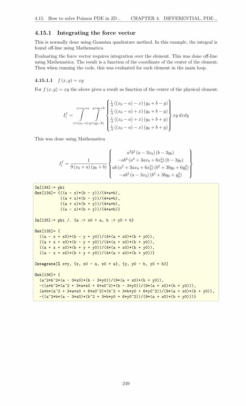
4.15. How to solve Poisson PDE in 2D… CHAPTER 4. DIFFERENTIAL, PDE…
4.15.1 Integrating the force vectorThis is normally done using Gaussian quadrature method. In this example, the integral isfound off-line using Mathematica.
Evaluating the force vector requires integration over the element. This was done off-lineusing Mathematica. The result is a function of the coordinate of the center of the element.Then when running the code, this was evaluated for each element in the main loop.
4.15.1.1 f (x, y) = xy
For f (x, y) = xy the above gives a result as function of the center of the physical element.
Ifi =
x=x0+a∫x=(x0−a)
y=y0+b∫y=(y0−b)
1A((x0 − a)− x) (y0 + b− y)
1A((x0 − a) + x) (y0 + b− y)
1A((x0 − a) + x) (y0 + b+ y)
1A((x0 − a)− x) (y0 + b+ y)
xy dxdy
This was done using Mathematica
Ifi =1
9 (x0 + a) (y0 + b)
a2b2 (a− 3x0) (b− 3y0)
−ab2 (a2 + 3ax0 + 6x20) (b− 3y0)
ab (a2 + 3ax0 + 6x20) (b
2 + 3by0 + 6y20)
−ab2 (a− 3x0) (b2 + 3by0 + y20)
In[134]:= phiOut[134]= ((a - x)*(b - y))/(4*a*b),
((a + x)*(b - y))/(4*a*b),((a + x)*(b + y))/(4*a*b),((a - x)*(b + y))/(4*a*b)
In[135]:= phi /. a :> x0 + a, b :> y0 + b
Out[135]= ((a - x + x0)*(b - y + y0))/(4*(a + x0)*(b + y0)),((a + x + x0)*(b - y + y0))/(4*(a + x0)*(b + y0)),((a + x + x0)*(b + y + y0))/(4*(a + x0)*(b + y0)),((a - x + x0)*(b + y + y0))/(4*(a + x0)*(b + y0))
Integrate[% x*y, x, x0 - a, x0 + a, y, y0 - b, y0 + b]
Out[136]= (a^2*b^2*(a - 3*x0)*(b - 3*y0))/(9*(a + x0)*(b + y0)),-((a*b^2*(a^2 + 3*a*x0 + 6*x0^2)*(b - 3*y0))/(9*(a + x0)*(b + y0))),(a*b*(a^2 + 3*a*x0 + 6*x0^2)*(b^2 + 3*b*y0 + 6*y0^2))/(9*(a + x0)*(b + y0)),-((a^2*b*(a - 3*x0)*(b^2 + 3*b*y0 + 6*y0^2))/(9*(a + x0)*(b + y0)))
249

4.15. How to solve Poisson PDE in 2D… CHAPTER 4. DIFFERENTIAL, PDE…
4.15.2 Case 1Case f(x, y) = 3 (cos(4πx) + sin(3πy))
This was done using Mathematica phiphi /. a :> (x0 + a), b :> (y0 + b)Integrate[% 3 (Cos[4 Pi x] + Sin[3 Pi y]),
x, x0 - a, x0 + a, y, y0 - b, y0 + b]
(1/(96*Pi^2*(a + x0)*(b + y0)))*(9*b^2*Cos[4*Pi*(-a + x0)] -9*b^2*Cos[4*Pi*(a + x0)] + 8*a*(12*a*b*Pi*Cos[3*Pi*(b - y0)] -
9*b^2*Pi*Sin[4*Pi*(-a + x0)] - 2*a*(Sin[3*Pi*(b - y0)] +Sin[3*Pi*(b + y0)]))), (1/(96*Pi^2*(a + x0)*(b + y0)))*
(-9*b^2*Cos[4*Pi*(-a + x0)] + 9*b^2*Cos[4*Pi*(a + x0)] +8*(12*a*b*Pi*(a + 2*x0)*Cos[3*Pi*(b - y0)] -
9*b^2*Pi*x0*Sin[4*Pi*(-a + x0)] + 9*a*b^2*Pi*Sin[4*Pi*(a + x0)] +9*b^2*Pi*x0*Sin[4*Pi*(a + x0)] - 2*a^2*Sin[3*Pi*(b - y0)] -4*a*x0*Sin[3*Pi*(b - y0)] - 2*a^2*Sin[3*Pi*(b + y0)] -4*a*x0*Sin[3*Pi*(b + y0)])), (1/(96*Pi^2*(a + x0)*(b + y0)))*
(-9*b*(b + 2*y0)*Cos[4*Pi*(-a + x0)] + 9*b*(b + 2*y0)*Cos[4*Pi*(a + x0)] -72*b*Pi*x0*(b + 2*y0)*Sin[4*Pi*(-a + x0)] + 72*b*Pi*(a + x0)*(b + 2*y0)*
Sin[4*Pi*(a + x0)] + 12*(a + x0)^2*(6*Pi*y0*Cos[3*Pi*(b - y0)] -6*Pi*(b + y0)*Cos[3*Pi*(b + y0)] + Sin[3*Pi*(b - y0)] +Sin[3*Pi*(b + y0)]) - 4*(-a + x0)*(a + 3*x0)*(6*Pi*y0*Cos[3*Pi*(b - y0)] -6*Pi*(b + y0)*Cos[3*Pi*(b + y0)] + Sin[3*Pi*(b - y0)] +Sin[3*Pi*(b + y0)])), (1/(96*Pi^2*(a + x0)*(b + y0)))*
(9*b*(b + 2*y0)*Cos[4*Pi*(-a + x0)] - 9*b*(b + 2*y0)*Cos[4*Pi*(a + x0)] +8*a*(12*a*Pi*y0*Cos[3*Pi*(b - y0)] - 12*a*Pi*(b + y0)*Cos[3*Pi*(b + y0)] -
9*b^2*Pi*Sin[4*Pi*(-a + x0)] - 18*b*Pi*y0*Sin[4*Pi*(-a + x0)] +2*a*Sin[3*Pi*(b - y0)] + 2*a*Sin[3*Pi*(b + y0)]))
4.15.2.1 case 2
Case f (x, y) = 1
Ifi =
x=x0+a∫x=(x0−a)
y=y0+b∫y=(y0−b)
1A((x0 − a)− x) (y0 + b− y)
1A((x0 − a) + x) (y0 + b− y)
1A((x0 − a) + x) (y0 + b+ y)
1A((x0 − a)− x) (y0 + b+ y)
dxdy
This was done using Mathematica
Ifi =
a2b2
(a+x0)(b+y0)
ab2(a+2x0)(a+x0)(b+y0)
ab(a+2x0)(b+2y0)(a+x0)(b+y0)
a2b(b+2y0)(a+x0)(b+y0)
phi /. a :> (x0 + a), b :> (y0 + b)Integrate[% , x, x0 - a, x0 + a, y, y0 - b, y0 + b](a^2*b^2)/((a + x0)*(b + y0)),(a*b^2*(a + 2*x0))/((a + x0)*(b + y0)),(a*b*(a + 2*x0)*(b + 2*y0))/((a + x0)*(b + y0)),(a^2*b*(b + 2*y0))/((a + x0)*(b + y0)) Now that the local ki and local fi are calculated, the next step is to assemble them to theglobal stiffness and global force vector. For 1D this process was easy and direct. For higher
250

4.15. How to solve Poisson PDE in 2D… CHAPTER 4. DIFFERENTIAL, PDE…
dimensions we need to make a table of mapping to help in the process. The followingdiagram shows this mapping table and how it is applied in this example. The mappingtable will have as many rows as there are elements, and will have as many columns asthe number of nodes per element. Hence in this example it will a matrix of size 9 × 4.Each row gives the global node number for each local node number of that element. Forexample, for element 1 the first row will show the global node number for each of the localnodes for the first element.Local node numbers are always incremented counter clockwise, starting from 1 to 4 inthis case.
1 2 6 5
2 3 7 6
3 4 8 7
4 6 10 9
6 7 11 10
7 8 12 11
9 10 14 13
10 11 15 14
11 12 16 15
1
2
3
4
5
6
7
8
9
1 2 3 4
987
654
2 31
1 2 3 4
5 6 7
910 11
12
13 14
8
15 16
Global node numbering
i
1 2
4 3
Local node numbering for element iMapping from local to global
node numbering based on element number. Used to fill in the global stiffness matrix
Now that we have the mapping done, we can now assemble the global stiffness and vectormatrix and solve for the unknowns.To evaluate the force vector, we also need a table of physical coordinates of the center ofeach element relative to the origin of the global coordinates system, since the force vectorintegration depends on physical coordinates.The integration was carried out off-line as shown above, but it was done in terms ofphysical coordinates of center of the element. The following diagram shows the mappingtable of physical coordinates to elements. This uses (0, 0) as the origin and the coordinatesof the lower left corner of the global coordinate system. Hence the coordinate the top rightcorner of the global grid will be (3h, 3h) where h is the grid spacing.
987
654
2 31
1 2 3 4
5 6 7
910 11
12
13 14
8
15 16
Global node numbering
1 2
4 3
Local node numbering for element i
Mapping from element number to physical coordinate of the center of element
0,0X
y
1
2
3
4
5
6
7
8
9
a b
3a b
5a b
a 3b
3a 3b
5a 3b
a 5b
3a 5b
5a 5b
x0 y0
6a, 0
6a, 6b0,6b
a
b
Now the solution can start. We loop over each element and fill in the global stiffness matrixusing the mapping above, and also evaluate the global force vector using the physicalcoordinates.When the global stiffness matrix and the global force vector is filled, we adjust the globalstiffness matrix by putting zero in the row numbered i that correspond to the edge nodei, and by putting 1 in the diagonal entry (i, i). We also put a zero in the force vector foreach node on the boundary conditions since we are using Dirichlet boundary conditions
251

4.15. How to solve Poisson PDE in 2D… CHAPTER 4. DIFFERENTIAL, PDE…
which is zero. When this is done, the system Ax = f is then solved for x where x now isthe displacement or value of y at the nodes. The following is an implementation of theabove. function matlab_97()close all; clear all;
number_of_elements=[16 64 256 625];function_string='1','xy','3(\cos(4\pi x)+\sin(3 \pi y))';function_handles=@f_1,@f_xy,@f_2;
figure_image_file='matlab_e97_1','matlab_e97_2','matlab_e97_3';
for i=1:length(function_handles)for j=1:length(number_of_elements)
plot_file=sprintf('%s_%d',figure_image_filei,...number_of_elements(j));
close all;solve_poisson_2D_square(function_handlesi,...
function_stringi,number_of_elements(j),plot_file);end
endend
%----------------------------------function k_local=getk(a,b)
k11=(a^2+b^2)/(3*a*b);k12=a/(6*b)-b/(3*a);k13=-(a^2+b^2)/(6*a*b);k14=-a/(3*b)+b/(6*a);k_local = [k11 k12 k13 k14;
k12 k11 k14 k13;k13 k14 k11 k12;k14 k13 k12 k11];
end%----------------------------------------------------%use this for f(x,y)=x*yfunction f_local=f_xy(x0,y0,a,b)
f_local=1/(9*(a + x0)*(b + y0))*...[a^2*b^2*(a-3*x0)*(b -3*y0);-a*b^2*(a^2 + 3*a*x0 + 6*x0^2)*(b - 3*y0);a*b*(a^2 + 3*a*x0 + 6*x0^2)*(b^2 + 3*b*y0 + 6*y0^2);-a^2*b*(a - 3*x0)*(b^2 + 3*b*y0 + 6*y0^2)...
];end%----------------------------------------------------%use this for f(x,y)=1function f_local=f_1(x0,y0,a,b)
f_local=[(a^2*b^2)/((a + x0)*(b + y0));(a*b^2*(a + 2*x0))/((a + x0)*(b + y0));
(a*b*(a + 2*x0)*(b + 2*y0))/((a + x0)*(b + y0));(a^2*b*(b + 2*y0))/((a + x0)*(b + y0))];
end%----------------------------------------------------%use this for f(x,y)= 3(cos(4 pi x)+sin(3 pi y))function f_local=f_2(x0,y0,a,b)f_local=[(1/(96*pi^2*(a + x0)*(b + y0)))*...
(9*b^2*cos(4*pi*(-a + x0)) -...9*b^2*cos(4*pi*(a + x0)) + ...
252

4.15. How to solve Poisson PDE in 2D… CHAPTER 4. DIFFERENTIAL, PDE…
8*a*(12*a*b*pi*cos(3*pi*(b - y0)) -...9*b^2*pi*sin(4*pi*(-a + x0)) - ...
2*a*(sin(3*pi*(b - y0)) +...sin(3*pi*(b + y0)))));
(1/(96*pi^2*(a + x0)*(b + y0)))*...(-9*b^2*cos(4*pi*(-a + x0)) + 9*b^2*cos(4*pi*(a + x0)) +...8*(12*a*b*pi*(a + 2*x0)*cos(3*pi*(b - y0)) -...9*b^2*pi*x0*sin(4*pi*(-a + x0)) + ...9*a*b^2*pi*sin(4*pi*(a + x0)) +...9*b^2*pi*x0*sin(4*pi*(a + x0)) - 2*a^2*sin(3*pi*(b - y0)) -...4*a*x0*sin(3*pi*(b - y0)) - 2*a^2*sin(3*pi*(b + y0)) -...4*a*x0*sin(3*pi*(b + y0))));(1/(96*pi^2*(a + x0)*(b + y0)))*...(-9*b*(b + 2*y0)*cos(4*pi*(-a + x0)) + ...9*b*(b + 2*y0)*cos(4*pi*(a + x0)) -...72*b*pi*x0*(b + 2*y0)*sin(4*pi*(-a + x0)) + ...72*b*pi*(a + x0)*(b + 2*y0)*...sin(4*pi*(a + x0)) + 12*(a + x0)^2*...(6*pi*y0*cos(3*pi*(b - y0)) -...6*pi*(b + y0)*cos(3*pi*(b + y0)) + sin(3*pi*(b - y0)) +...sin(3*pi*(b + y0))) - 4*(-a + x0)*(a + 3*x0)*...(6*pi*y0*cos(3*pi*(b - y0)) -...6*pi*(b + y0)*cos(3*pi*(b + y0)) + sin(3*pi*(b - y0)) +...
sin(3*pi*(b + y0))));(1/(96*pi^2*(a + x0)*(b + y0)))*...(9*b*(b + 2*y0)*cos(4*pi*(-a + x0)) - ...
9*b*(b + 2*y0)*cos(4*pi*(a + x0)) +...8*a*(12*a*pi*y0*cos(3*pi*(b - y0)) - ...
12*a*pi*(b + y0)*cos(3*pi*(b + y0)) -...9*b^2*pi*sin(4*pi*(-a + x0)) - ...18*b*pi*y0*sin(4*pi*(-a + x0)) +...2*a*sin(3*pi*(b - y0)) + 2*a*sin(3*pi*(b + y0))))];
end%----------------------------------------------------function solve_poisson_2D_square(fh,rhs,M,plot_file)%2a is width of element%2b is height of element%fh is function which evaluate the force vector%rhs is string which is the f(x,y), for plotting only%M=total number of elements%k=local stiffness matrixL = 1; %length of gridN = 4; %number of nodes per elementM1 = sqrt(M); %number of elements per rowa=(L/M1)/2;b=(L/M1)/2;k_local=getk(a,b);N1 = M1+1; %number of nodes per edgedof=4;nodes = N1^2; %total number of nodeskk = zeros(nodes); %global stiffness vectorf = zeros(nodes,1); %global force vectormtb = generate_coordinates_table(M1);fmtb = generate_physical_coordinates_table(M1,a,b);
for i = 1:Mx0 = fmtb(i,1); y0 = fmtb(i,2);%call to load different force vector, pre-computed offlinef_local=fh(x0,y0,a,b);
%assemble force vecotr and global stiffness matrixfor ii = 1:N
253

4.15. How to solve Poisson PDE in 2D… CHAPTER 4. DIFFERENTIAL, PDE…
f(mtb(i,ii)) = f(mtb(i,ii)) + f_local(ii);for jj = 1:N
kk(mtb(i,ii),mtb(i,jj)) = kk(mtb(i,ii),mtb(i,jj))+...k_local(ii,jj);
endend
end
%fix the global stiffness matrix and force vector for B.C.edge_nodes=[1:N1 (M1+2):(M1+1):nodes-N1 ...
(2*M1+2):(M1+1):(nodes-N1) nodes-N1:nodes];for i=1:length(edge_nodes)
z=edge_nodes(i);kk(z,:)=0;f(z)=0;
end
for i=1:length(edge_nodes)z=edge_nodes(i);kk(z,z)=1;
end
y=kk\f; %solveZ=reshape(y,N1,N1);[X,Y] = meshgrid(0:2*a:1,0:2*b:1);h=surf(X,Y,Z);shading interpset(h','edgecolor','k');set(gcf,'defaulttextinterpreter','latex');plot_title=sprintf('$\\nabla^2 u=%s$, number of elements $%d$',rhs,M);title(plot_title,'fontweight','bold','fontsize',14);
print(gcf, '-dpdf', '-r300', ['images/',plot_file]);print(gcf, '-dpng', '-r300', ['images/',plot_file]);
figure;[C,h] = contourf(X,Y,Z);clabel(C,h)set(gcf,'defaulttextinterpreter','latex');title(plot_title,'fontweight','bold','fontsize',14);colormap coolprint(gcf, '-dpdf', '-r300', ['images/',[plot_file,'_c']]);print(gcf, '-dpng', '-r300', ['images/',[plot_file,'_c']]);
end%----------------------------------------------------function mtb=generate_coordinates_table(M)%M=number_of_elements_per_rowmtb=zeros(M^2,4);for i=1:M
for j=1:Mmtb(j+M*(i-1),:) =[j j+1 j+(M+2) j+(M+1)]+(M+1)*(i-1);
endendend%----------------------------------------------------function fmtb=generate_physical_coordinates_table(M,a,b)%2a is width of element%2b is height of element%M=number_of_elements_per_rowfmtb=zeros(M^2,2);for i=1:M
for j=1:M
254

4.15. How to solve Poisson PDE in 2D… CHAPTER 4. DIFFERENTIAL, PDE…
fmtb(j+M*(i-1),:) = [(2*j-1)*a (2*i-1)*b];end
endend Here is the output for the three force functions, for different number of elements.
4.15.3 f(x, y) = 1
4.15.4 f(x, y) = xy
255

4.15. How to solve Poisson PDE in 2D… CHAPTER 4. DIFFERENTIAL, PDE…
4.15.5 case 3Case 3: f(x, y) = 3 (cos(4πx) + sin(3πy))
256

4.15. How to solve Poisson PDE in 2D… CHAPTER 4. DIFFERENTIAL, PDE…
4.15.6 Solving for reactangle gridA small modification is now made to allow one to specify different width and height forthe domain. function matlab_97_2()close all; clear all;
%number of elements per unit length, width, heightnumber_of_elements=[4 1 1;
8 1 2;16 1 4;25 1 6];
function_string='1','xy','3(\cos(4\pi x)+\sin(3 \pi y))';function_handles=@f_1,@f_xy,@f_2;
figure_image_file='matlab_e97_rectangle_1',...'matlab_e97_rectangle_2','matlab_e97_rectangle_3';
for i=1:length(function_handles)for j=1:size(number_of_elements,1)
plot_file=sprintf('%s_%d',figure_image_filei,...number_of_elements(j,1)*number_of_elements(j,2)*...
number_of_elements(j,3));close all;solve_poisson_2D_square(function_handlesi,...
function_stringi,number_of_elements(j,1),...number_of_elements(j,2),number_of_elements(j,3),...plot_file);
endendend
%----------------------------------function k_local=getk(a,b)
k11=(a^2+b^2)/(3*a*b);k12=a/(6*b)-b/(3*a);k13=-(a^2+b^2)/(6*a*b);k14=-a/(3*b)+b/(6*a);k_local = [k11 k12 k13 k14;
k12 k11 k14 k13;k13 k14 k11 k12;k14 k13 k12 k11];
end%----------------------------------------------------%use this for f(x,y)=x*yfunction f_local=f_xy(x0,y0,a,b)
f_local=1/(9*(a + x0)*(b + y0))*...[a^2*b^2*(a-3*x0)*(b -3*y0);-a*b^2*(a^2 + 3*a*x0 + 6*x0^2)*(b - 3*y0);a*b*(a^2 + 3*a*x0 + 6*x0^2)*(b^2 + 3*b*y0 + 6*y0^2);
257

4.15. How to solve Poisson PDE in 2D… CHAPTER 4. DIFFERENTIAL, PDE…
-a^2*b*(a - 3*x0)*(b^2 + 3*b*y0 + 6*y0^2)...];
end%----------------------------------------------------%use this for f(x,y)=1function f_local=f_1(x0,y0,a,b)
f_local=[(a^2*b^2)/((a + x0)*(b + y0));(a*b^2*(a + 2*x0))/((a + x0)*(b + y0));
(a*b*(a + 2*x0)*(b + 2*y0))/((a + x0)*(b + y0));(a^2*b*(b + 2*y0))/((a + x0)*(b + y0))];
end%----------------------------------------------------%use this for f(x,y)= 3(cos(4 pi x)+sin(3 pi y))function f_local=f_2(x0,y0,a,b)f_local=[(1/(96*pi^2*(a + x0)*(b + y0)))*...
(9*b^2*cos(4*pi*(-a + x0)) -...9*b^2*cos(4*pi*(a + x0)) + 8*a*(12*a*b*pi*cos(3*pi*(b - y0)) -...9*b^2*pi*sin(4*pi*(-a + x0)) - 2*a*(sin(3*pi*(b - y0)) +...
sin(3*pi*(b + y0)))));(1/(96*pi^2*(a + x0)*(b + y0)))*...(-9*b^2*cos(4*pi*(-a + x0)) + 9*b^2*cos(4*pi*(a + x0)) +...
8*(12*a*b*pi*(a + 2*x0)*cos(3*pi*(b - y0)) -...9*b^2*pi*x0*sin(4*pi*(-a + x0)) + ...9*a*b^2*pi*sin(4*pi*(a + x0)) +...9*b^2*pi*x0*sin(4*pi*(a + x0)) - 2*a^2*sin(3*pi*(b - y0)) -...4*a*x0*sin(3*pi*(b - y0)) - 2*a^2*sin(3*pi*(b + y0)) -...4*a*x0*sin(3*pi*(b + y0))));
(1/(96*pi^2*(a + x0)*(b + y0)))*...(-9*b*(b + 2*y0)*cos(4*pi*(-a + x0)) + 9*b*(b + 2*y0)*...
cos(4*pi*(a + x0)) -...72*b*pi*x0*(b + 2*y0)*sin(4*pi*(-a + x0)) + ...72*b*pi*(a + x0)*(b + 2*y0)*...sin(4*pi*(a + x0)) + 12*(a + x0)^2*(6*pi*y0*...
cos(3*pi*(b - y0)) -...6*pi*(b + y0)*cos(3*pi*(b + y0)) + ...sin(3*pi*(b - y0)) +...sin(3*pi*(b + y0))) - 4*(-a + x0)*(a + 3*x0)*...
(6*pi*y0*cos(3*pi*(b - y0)) -...6*pi*(b + y0)*cos(3*pi*(b + y0)) + ...sin(3*pi*(b - y0)) +...sin(3*pi*(b + y0))));
(1/(96*pi^2*(a + x0)*(b + y0)))*...(9*b*(b + 2*y0)*cos(4*pi*(-a + x0)) - 9*b*(b + 2*y0)*...cos(4*pi*(a + x0)) +...8*a*(12*a*pi*y0*cos(3*pi*(b - y0)) - 12*a*pi*(b + y0)*...cos(3*pi*(b + y0)) -...9*b^2*pi*sin(4*pi*(-a + x0)) - 18*b*pi*y0*sin(4*pi*(-a + x0)) +...2*a*sin(3*pi*(b - y0)) + 2*a*sin(3*pi*(b + y0))))];
end%----------------------------------------------------function solve_poisson_2D_square(fh,rhs,M,Lx,Ly,plot_file)%fh is function which evaluate the force vector%rhs is string which is the f(x,y), for plotting only%M=number of element per unit length%Lx=length in x-direction%Ly=length in y-directionN = 4; %number of nodes per elementMx=M*Lx;My=M*Ly;a=(1/M)/2;
258

4.15. How to solve Poisson PDE in 2D… CHAPTER 4. DIFFERENTIAL, PDE…
b=a;k_local=getk(a,b);dof=4;
nodes = (Mx+1)*(My+1); %total number of nodeskk = zeros(nodes); %global stiffness vectorf = zeros(nodes,1); %global force vectormtb = generate_coordinates_table(Mx,My);fmtb = generate_physical_coordinates_table(Mx,My,a,b);
for i = 1:(Mx*My)x0 = fmtb(i,1); y0 = fmtb(i,2);%call to load different force vector, pre-computed offlinef_local=fh(x0,y0,a,b);
%assemble force vecotr and global stiffness matrixfor ii = 1:N
f(mtb(i,ii)) = f(mtb(i,ii)) + f_local(ii);for jj = 1:N
kk(mtb(i,ii),mtb(i,jj)) = kk(mtb(i,ii),mtb(i,jj))+...k_local(ii,jj);
endend
end
%fix the global stiffness matrix and force vector for B.C.edge_nodes=[1:Mx+1 (Mx+2):(Mx+1):nodes-...
Mx (2*Mx+2):(Mx+1):(nodes-(Mx+1)) nodes-(Mx-1):nodes];for i=1:length(edge_nodes)
z=edge_nodes(i);kk(z,:)=0;f(z)=0;
end
for i=1:length(edge_nodes)z=edge_nodes(i);kk(z,z)=1;
end
y=kk\f; %solveZ=reshape(y,Mx+1,My+1);[X,Y] = meshgrid(0:2*b:Ly,0:2*a:Lx);h=surf(X,Y,Z);shading interpset(h','edgecolor','k');set(gcf,'defaulttextinterpreter','latex');plot_title=sprintf('$\\nabla^2 u=%s$, number of elements $%d$',rhs,Mx*My);title(plot_title,'fontweight','bold','fontsize',14);
print(gcf, '-dpdf', '-r300', ['images/',plot_file]);print(gcf, '-dpng', '-r300', ['images/',plot_file]);
figure;[C,h] = contourf(X,Y,Z);clabel(C,h)set(gcf,'defaulttextinterpreter','latex');title(plot_title,'fontweight','bold','fontsize',14);colormap cool
print(gcf, '-dpdf', '-r300', ['images/',[plot_file,'_c']]);print(gcf, '-dpng', '-r300', ['images/',[plot_file,'_c']]);
end
259
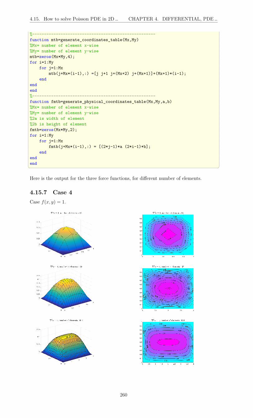
4.15. How to solve Poisson PDE in 2D… CHAPTER 4. DIFFERENTIAL, PDE…
%----------------------------------------------------function mtb=generate_coordinates_table(Mx,My)%Mx= number of element x-wise%My= number of element y-wisemtb=zeros(Mx*My,4);for i=1:My
for j=1:Mxmtb(j+Mx*(i-1),:) =[j j+1 j+(Mx+2) j+(Mx+1)]+(Mx+1)*(i-1);
endendend%----------------------------------------------------function fmtb=generate_physical_coordinates_table(Mx,My,a,b)%Mx= number of element x-wise%My= number of element y-wise%2a is width of element%2b is height of elementfmtb=zeros(Mx*My,2);for i=1:My
for j=1:Mxfmtb(j+Mx*(i-1),:) = [(2*j-1)*a (2*i-1)*b];
endendend Here is the output for the three force functions, for different number of elements.
4.15.7 Case 4Case f(x, y) = 1.
260

4.15. How to solve Poisson PDE in 2D… CHAPTER 4. DIFFERENTIAL, PDE…
4.15.8 Case 5Case : f(x, y) = xy
261

4.15. How to solve Poisson PDE in 2D… CHAPTER 4. DIFFERENTIAL, PDE…
4.15.9 case 6Case f(x, y) = 3 (cos(4πx) + sin(3πy)).
262

4.16. How to solve Poisson PDE in 2D… CHAPTER 4. DIFFERENTIAL, PDE…
4.16 How to solve Poisson PDE in 2D using finiteelements methods using triangle element?
Solve ∇2u = f (x, y) on square using FEM. Assume u = 0 on boundaries and solve usingf (x, y) = xy and also f (x, y) = 1 and f (x, y) = 3 (cos(4πx) + sin(3πy))
Use Galerkin method and weak form, Using triangle element.SolutionUsing as an example with 9 elements to illustrate the method. The program below canbe called with different number of elements.
9
8
7
6
5
42
31
1 2 3 4
5 6 7
910 11
12
13 14
8
15 16
element
Global node number
10
11
12
13
14
15
16
17
18
1 2
3 12
3 1 2
3 12
3
Local node numbers
12
3 12
3
1 2
3
Figure 4.1: node numbering
Looking at one element
y
x1,y1 x2,y2
x3,y3
1 2
3
A 12x1y2 y3 x2y3 y1 x3y1 y2
area
Figure 4.2: element in physical coordinates
The trial function is
u = c1 + c2x+ c3y (1)
Evaluating the trial function (1) at each corner node of the above element gives
u1 = c1 + c2x1 + c3y1
u2 = c1 + c2x2 + c3y2
u3 = c1 + c2x3 + c3y3
Hence263
4.16. How to solve Poisson PDE in 2D… CHAPTER 4. DIFFERENTIAL, PDE…
u1
u2
u3
=
1 x1 y11 x2 y21 x3 y3
c1c2c3
Therefore
c1c2c3
=
1 x1 y11 x2 y21 x3 y3
−1u1
u2
u3
=
1
|D|
x2y3 − x3y2 x3y1 − x1y3 x1y2 − y1x2
y2 − y3 y3 − y1 y1 − y2x3 − x2 x1 − x3 x2 − x1
u1
u2
u3
(2)
Where |D| is the determinant of
1 x1 y11 x2 y21 x3 y3
which is |D| = −y1x2+x3y1+x1y2−x3y2−
x1y3 + x2y3.
This quantity is twice the area of the triangleA = 12(x1 (y2 − y3) + x2 (y3 − y1) + x3 (y1 − y2)).
Substituting (2) into (1) in order to find the shape functions gives
u = c1 + c2x+ c3y
=1
2A[(x2y3 − x3y2) u1 + (x3y1 − x1y3) u2 + (x1y2 − y1x2) u3]
+1
2A[(y2 − y3) u1 + (y3 − y1) u2 + (y1 − y2) u3]x
+1
2A[(x3 − x2) u1 + (x1 − x3) u2 + (x2 − x1) u3] y
Collecting terms in ui
u = u11
2A((x2y3 − x3y2) + (y2 − y3)x+ (x3 − x2) y)
+ u21
2A((x3y1 − x1y3) + (y3 − y1)x+ (x1 − x3) y)
+ u31
2A((x1y2 − y1x2) + (y1 − y2)x+ (x2 − x1) y)
Hence
N1 (x, y) =1
2A((x2y3 − x3y2) + (y2 − y3)x+ (x3 − x2) y)
N2 (x, y) =1
2A((x3y1 − x1y3) + (y3 − y1)x+ (x1 − x3) y)
N3 (x, y) =1
2A((x1y2 − y1x2) + (y1 − y2)x+ (x2 − x1) y)
Therefore (1) can be written as
u = N1 (x, y) u1 +N2 (x, y) u2 +N3 (x, y) u3
Now that the shape functions are found, the test or weight function w (x, y) can be found.Since wi (x, y) =
∂u∂ui
for i = 1, 2, 3, therefore this results in
264

4.16. How to solve Poisson PDE in 2D… CHAPTER 4. DIFFERENTIAL, PDE…
w (x, y) =
w1
w2
w3
=
N1 (x, y)
N2 (x, y)
N3 (x, y)
=1
2A
(x2y3 − x3y2) + (y2 − y3)x+ (x3 − x2) y
(x3y1 − x1y3) + (y3 − y1)x+ (x1 − x3) y
(x1y2 − y1x2) + (y1 − y2)x+ (x2 − x1) y
The weak form formulation now gives
Ii = −∫Ω
∂Ni
∂x
∂Nj
∂xdΩ−
∫Ω
∂Ni
∂y
∂Nj
∂ydΩ +
∫Γ
w∂u
∂ndΓ−
∫Ω
N1 (x, y)
N2 (x, y)
N3 (x, y)
f (x, y) dΩ
Hence
Ii = −∫Ω
∂N1(x,y)
∂x
∂N2(x,y)∂x
∂N3(x,y)∂x
∂N1(x,y)∂x
∂N2(x,y)∂x
∂N3(x,y)∂x
u1
u2
u3
dΩ
−∫Ω
∂N1(x,y)
∂y
∂N2(x,y)∂y
∂N3(x,y)∂y
∂N1(x,y)∂y
∂N2(x,y)∂y
∂N3(x,y)∂y
u1
u2
u3
dΩ
+
∫Γ
N1 (x, y)
N2 (x, y)
N3 (x, y)
∂u
∂n
u1
u2
u3
dΓ
−∫Ω
N1 (x, y)
N2 (x, y)
N3 (x, y)
f (x, y) dΩ
Since w = 0 on the boundary with Dirichlet conditions, and since there are no naturalboundary conditions, the above simplifies to
Ii = −∫Ω
∂N1(x,y)
∂x
∂N2(x,y)∂x
∂N3(x,y)∂x
∂N1(x,y)∂x
∂N2(x,y)∂x
∂N3(x,y)∂x
u1
u2
u3
dΩ
−∫Ω
∂N1(x,y)
∂y
∂N2(x,y)∂y
∂N3(x,y)∂y
∂N1(x,y)∂y
∂N2(x,y)∂y
∂N3(x,y)∂y
dΩ
u1
u2
u3
−∫Ω
N1 (x, y)
N2 (x, y)
N3 (x, y)
f (x, y) dΩ
Now each integral is calculated for the triangle element. First the derivatives are found∂N1(x,y)
∂x
∂N2(x,y)∂x
∂N3(x,y)∂x
=1
2A
(y2 − y3)
(y3 − y1)
(y1 − y2)
and
265

4.16. How to solve Poisson PDE in 2D… CHAPTER 4. DIFFERENTIAL, PDE…
∂N1(x,y)
∂y
∂N2(x,y)∂y
∂N3(x,y)∂y
=1
2A
(x3 − x2)
(x1 − x3)
(x2 − x1)
Hence
∂N1(x,y)
∂x
∂N2(x,y)∂x
∂N3(x,y)∂x
∂N1(x,y)∂x
∂N2(x,y)∂x
∂N3(x,y)∂x
=
∂Ni
∂x
∂Nj
∂x
=1
(2A)2
(y2 − y3)
2 (y2 − y3) (y3 − y1) (y2 − y3) (y1 − y2)
(y3 − y1) (y2 − y3) (y3 − y1)2 (y3 − y1) (y1 − y2)
(y1 − y2) (y2 − y3) (y1 − y2) (y3 − y1) (y1 − y2)2
And
∂N1(x,y)
∂y
∂N2(x,y)∂y
∂N3(x,y)∂y
∂N1(x,y)∂y
∂N2(x,y)∂y
∂N3(x,y)∂y
=
∂Ni
∂y
∂Nj
∂y
=1
(2A)2
(x3 − x2)
2(x3 − x2) (x1 − x3) (x3 − x2) (x2 − x1)
(x1 − x3) (x3 − x2) (x1 − x3)2
(x1 − x3) (x2 − x1)
(x2 − x1) (x3 − x2) (x2 − x1) (x1 − x3) (x2 − x1)2
We see the above terms do not depend on x nor on y. Hence the next integration is doneover the area of the triangle as follow
∫Ω
∂Ni
∂x
∂Nj
∂x
u1
u2
u3
dΩ =∂Ni
∂x
∂Nj
∂x
u1
u2
u3
∫Ω
dΩ
But∫Ω
dΩ is the area of the triangle. Hence
∫Ω
∂Ni
∂x
∂Nj
∂x
u1
u2
u3
dΩ =∂Ni
∂x
∂Nj
∂x
u1
u2
u3
A
Replacing ∂Ni
∂x
∂Nj
∂xby the expression we found for it above, gives
∫Ω
∂Ni
∂x
∂Nj
∂x
u1
u2
u3
dΩ =A
(2A)2
(y2 − y3)
2 (y2 − y3) (y3 − y1) (y2 − y3) (y1 − y2)
(y3 − y1) (y2 − y3) (y3 − y1)2 (y3 − y1) (y1 − y2)
(y1 − y2) (y2 − y3) (y1 − y2) (y3 − y1) (y1 − y2)2
u1
u2
u3
=1
4A
(y2 − y3)
2 (y2 − y3) (y3 − y1) (y2 − y3) (y1 − y2)
(y3 − y1) (y2 − y3) (y3 − y1)2 (y3 − y1) (y1 − y2)
(y1 − y2) (y2 − y3) (y1 − y2) (y3 − y1) (y1 − y2)2
u1
u2
u3
(3)
Now we do the same for the second integral266

4.16. How to solve Poisson PDE in 2D… CHAPTER 4. DIFFERENTIAL, PDE…
∫Ω
∂Ni
∂y
∂Nj
∂y
u1
u2
u3
dΩ =∂Ni
∂y
∂Nj
∂y
u1
u2
u3
∫Ω
dΩ
But∫Ω
dΩ is the area of the triangle. Hence
∫Ω
∂Ni
∂y
∂Nj
∂y
u1
u2
u3
dΩ =∂Ni
∂y
∂Nj
∂y
u1
u2
u3
A
Replacing ∂Ni
∂y
∂Nj
∂yby the expression we found for it above, gives
∫Ω
∂Ni
∂x
∂Nj
∂x
u1
u2
u3
dΩ =A
(2A)2
(x3 − x2)
2 (x3 − x2) (x1 − x3) (x3 − x2) (x2 − x1)
(x1 − x3) (x3 − x2) (x1 − x3)2 (x1 − x3) (x2 − x1)
(x2 − x1) (x3 − x2) (x2 − x1) (x1 − x3) (x2 − x1)2
u1
u2
u3
=1
4A
(x3 − x2)
2 (x3 − x2) (x1 − x3) (x3 − x2) (x2 − x1)
(x1 − x3) (x3 − x2) (x1 − x3)2 (x1 − x3) (x2 − x1)
(x2 − x1) (x3 − x2) (x2 − x1) (x1 − x3) (x2 − x1)2
u1
u2
u3
(4)
Adding (3) and (4) to obtain the local stiffness matrix
ki
u1
u2
u3
i
=1
4A
(y2 − y3)
2 (y2 − y3) (y3 − y1) (y2 − y3) (y1 − y2)
(y3 − y1) (y2 − y3) (y3 − y1)2 (y3 − y1) (y1 − y2)
(y1 − y2) (y2 − y3) (y1 − y2) (y3 − y1) (y1 − y2)2
u1
u2
u3
+1
4A
(x3 − x2)
2 (x3 − x2) (x1 − x3) (x3 − x2) (x2 − x1)
(x1 − x3) (x3 − x2) (x1 − x3)2 (x1 − x3) (x2 − x1)
(x2 − x1) (x3 − x2) (x2 − x1) (x1 − x3) (x2 − x1)2
u1
u2
u3
or
ki =1
4A
(y2 − y3)
2+ (x3 − x2)
2(y2 − y3) (y3 − y1) + (x3 − x2) (x1 − x3) (y2 − y3) (y1 − y2) + (x3 − x2) (x2 − x1)
(y3 − y1) (y2 − y3) + (x1 − x3) (x3 − x2) (y3 − y1)2+ (x1 − x3)
2(y3 − y1) (y1 − y2) + (x1 − x3) (x2 − x1)
(y1 − y2) (y2 − y3) + (x2 − x1) (x3 − x2) (y1 − y2) (y3 − y1) + (x2 − x1) (x1 − x3) (y1 − y2)2+ (x2 − x1)
2
And the final integral (the force vector) depends on the nature of f (x, y). For f (x, y) = 1we obtain
∫Ω
N1 (x, y)
N2 (x, y)
N3 (x, y)
f (x, y) dΩ =
∫Ω
1
2A
(x2y3 − x3y2) + (y2 − y3)x+ (x3 − x2) y
(x3y1 − x1y3) + (y3 − y1)x+ (x1 − x3) y
(x1y2 − y1x2) + (y1 − y2)x+ (x2 − x1) y
dydx
And for f (x, y) = xy similarly
∫Ω
N1 (x, y)
N2 (x, y)
N3 (x, y)
f (x, y) dΩ =
∫Ω
1
2A
(x2y3 − x3y2) + (y2 − y3)x+ (x3 − x2) y
(x3y1 − x1y3) + (y3 − y1)x+ (x1 − x3) y
(x1y2 − y1x2) + (y1 − y2)x+ (x2 − x1) y
xydydx
267

4.16. How to solve Poisson PDE in 2D… CHAPTER 4. DIFFERENTIAL, PDE…
And similarly for other f (x, y). These were all integrated off-line and the resulting expres-sion evaluated during the run of the program. These expression are all functions of thenode coordinates (x1, y1, x2, y2, x3, y3). No actual integration is done in the code, but onlyevaluation of the integration result obtained. The integration was done using Mathematica.These are the results for the three functions of interest. The integration was done on twotriangles. The odd numbered ones and the even numbered ones due to the node numbering
difference. For odd numbered triangles, the integration limits arex2∫x1
y3−x∫y1
dydx while on the
even numbered elements the limits arex1∫x2
y2−x∫y1
dydx as shown in this diagram
9
8
7
6
5
42
31
1 2 3 4
5 6 7
910 11
12
13 14
8
15 16
element
Global node number
10
11
12
13
14
15
16
17
18
1 2
3 12
3 1 2
3 12
3 12
3 12
3
1 2
3
X
y
(0,0)
x1,y1 x2,y2
x3,y3
x1
x2
y1
y3x
dydx
yy3 x
Odd numbered triangle integration
x3,y3
x1,y1x2,y212
3
yy2 x
Even numbered triangle integration
1 2
3
x1
x2
y1
y2x
dydx
Figure 4.3: Integrating over elements
Note that this is not how integration is normally done in actual finite element methods.Using Gaussian quadrature method is the recommended way. This method was done herefor learning and to compare.
4.16.1 case 1Case f (x, y) = 1. For odd numbered elements n1 = (1/(2*area))*((x2*y3 - x3*y2) + (y2 - y3)*x + (x3 - x2)*y);n2 = (1/(2*area))*((x2*y1 - x1*y3) + (y3 - y1)*x + (x1 - x3)*y);n3 = (1/(2*area))*((x1*y2 - y1*x2) + (y1 - y2)*x + (x2 - x1)*y);w = n1, n2, n3;Integrate[w, x, x1, x2, y, y1, y3 - x]
Out[11]= (1/(12*area))*((x1 - x2)*(x2^3 + x1^2*(x2 - x3 + 2*y2 - 2*y3) +3*x3*(y1 - y3)*(y1 - 2*y2 + y3) - x2^2*(x3 - 2*y2 + 2*y3) -3*x2*(y1^2 + x3*y2 - x3*y3 + y2*y3 - y1*(y2 + y3)) + x1*(x2^2 - 3*(y2 - y3)*(x3 - y1 + y3) - x2*(x3 - 2*y2 + 2*y3)))),
-(((x1 - x2)*(x1^3 + x1^2*(x2 - x3 + 2*y1 - 2*y3) - x2^2*(x3 + y1 + 2*y3) +3*x3*(y1^2 - y3^2) + 3*x2*(-y1^2 + y3*(x3 + y3)) +
x1*(x2^2 + 3*x3*y3 - x2*(x3 + y1 + 2*y3))))/(12*area)),((x1 - x2)^2*(x1^2 + x2^2 + x1*(x2 + 2*y1 + y2 - 3*y3) + x2*(y1 + 2*y2 - 3*y3) +
3*(y1 - y3)*(y2 - y3)))/(12*area) For even numbered elements Integrate[w, x, x1, x2, y, y1, y2 - x]((x1 - x2)*(x2^3 + 3*x3*(y1 - y2)^2 + x1*(x2^2 + 3*(y1 - y2)*(y2 - y3) -
x2*(x3 + y2 - y3)) + x1^2*(x2 - x3 + 2*y2 - 2*y3) -3*x2*(y1 - y2)*(y1 - y3) - x2^2*(x3 + y2 - y3)))/(12*area),-((1/(12*area))*((x1 - x2)*(x1^3 - 3*x3*(y1 - y2)^2 - 3*x2*(y1 - y2)*
268

4.16. How to solve Poisson PDE in 2D… CHAPTER 4. DIFFERENTIAL, PDE…
(x3 - y1 + y3) + x1^2*(x2 - x3 + 2*y1 - 3*y2 + y3) -x2^2*(x3 - 2*y1 + 2*y3) + x1*(x2^2 - 3*(y1 - y2)*(x3 + y2 - y3) +x2*(-x3 + 2*y1 - 3*y2 + y3))))),
((x1 - x2)^2*(x1^2 + x1*(x2 + 2*y1 - 2*y2) + x2*(x2 + y1 - y2)))/(12*area) 4.16.2 Program outputThis is an implementation of the above for f(x, y) = 1. The coordinates mapping wasfirst carried out in order to map each elements local node numbers to the global nodenumbering so we know where to add each element stiffness matrix to the global stiffnessmatrix. Also we need to build the mapping of each element to the physical coordinatesof its local node number 1 to use for calculating the force vector since that depends onphysical location of each element.
9
8
7
6
5
42
31
1 2 3 4
5 6 7
910 11
12
13 14
8
15 16
element
Global node number
10
11
12
13
14
15
16
17
18
1 2
3 12
3 1 2
3 12
3
Local node numbers
12
3 12
3
1 2
3
1
2
3
4
5
6
7
8
9
10
11
12
13
14
15
16
17
18
1 2 5
6 5 2
2 3 6
7 6 3
3 4 7
8 7 4
5 6 9
10 9 6
6 7 10
11 10 7
7 8 11
12 11 8
9 10 13
14 13 10
10 11 14
15 14 11
11 12 15
16 15 12
1,2,3
Element numbers
Global node numbers mapping
The mapping of physical coordinate location relative to the global frame of reference isshown below
9
8
7
6
5
42
31
1 2 3 4
5 6 7
910 11
12
13 14
8
15 16
element
Global node number
10
11
12
13
14
15
16
17
18
1 2
3 12
3 1 2
3 12
3 12
3 12
3
1 2
3
X
y
(0,0)
h
h
Element number
(x,y) coordinates of nodes 1,2,3 of each element
1
2
3
4
5
6
7
8
9
10
11
12
13
14
15
16
17
18
0 0 h 0 0 h
h h 0 h h 0
h 0 2h 0 h h
2h h h h 2h 0
2h 0 3h 0 2h h
3h h 2h h 3h 0
0 h h h 0 2h
h 2h 0 2h h h
h h 2h h h 2h
2h 2h h 2h 2h h
2h h 3h h 2h 2h
3h 2h 2h 2h 3h h
0 2h h 2h 0 3h
h 3h 0 3h h 2h
h 2h 2h 2h h 3h
2h 3h h 3h 2h 2h
2h 2h 3h 2h 2h 3h
3h 3h 2h 3h 3h 2h
x1,y1,x2,y2,x3,y3
function matlab_98()close all; clear all;number_of_elements=[16*2 64*2 256*2 625*2];function_string='1';%function_handles=@f_1,@f_xy,@f_2;%something wrong with the other%cases, need to work more on it.function_handles=@f_1;figure_image_file='matlab_e98_1';
269

4.16. How to solve Poisson PDE in 2D… CHAPTER 4. DIFFERENTIAL, PDE…
for i=1:length(function_handles)for j=1:length(number_of_elements)
plot_file=sprintf('%s_%d',figure_image_filei,...number_of_elements(j));
close all;solve_poisson_2D_square(function_handlesi,...
function_stringi,number_of_elements(j),plot_file);end
endend
%----------------------------------function k_local=getk(area,x1,y1,x2,y2,x3,y3)
k11=(y2-y3)^2+(x3-x2)^2;k12=(y2-y3)*(y3-y1)+(x3-x2)*(x1-x3);k13=(y2-y3)*(y1-y2)+(x3-x2)*(x2-x1);k22=(y3-y1)^2+(x1-x3)^2;k23=(y3-y1)*(y1-y2)+(x1-x3)*(x2-x1);k33=(y1-y2)^2+(x2-x1)^2;k_local = [k11 k12 k13;
k12 k22 k23;k13 k23 k33];
k_local = k_local/(4*area);end%----------------------------------------------------%use this for f(x,y)=1function f_local=f_1(area,x1,y1,x2,y2,x3,y3,ele)
if mod(ele,2)f_local=[(1/(12*area))*((x1 - x2)*(x2^3 + x1^2*...(x2 - x3 + 2*y2 - 2*y3) +...3*x3*(y1 - y3)*(y1 - 2*y2 + y3) - x2^2*(x3 - 2*y2 + 2*y3) -...3*x2*(y1^2 + x3*y2 - x3*y3 + y2*y3 - y1*(y2 + y3)) + x1*(x2^2 -...3*(y2 - y3)*(x3 - y1 + y3) - x2*(x3 - 2*y2 + 2*y3))));-((1/(12*area))*((x1 - x2)*(x1^3 + x1^2*(x2 - x3 + 2*y1 - 2*y3) -...3*x3*(y1 - y3)^2 - 3*x2*(y1 - y3)*(x3 - y1 + y3) -...
x2^2*(x3 - 2*y1 + 2*y3) + x1*(x2^2 + 3*x3*(-y1 + y3) -...x2*(x3 - 2*y1 + 2*y3)))));
((x1 - x2)^2*(x1^2 + x2^2 + x1*(x2 + 2*y1 + y2 - 3*y3) +...x2*(y1 + 2*y2 - 3*y3) + 3*(y1 - y3)*(y2 - y3)))/(12*area)];
elsef_local=[((x1 - x2)*(x2^3 + 3*x3*(y1 - y2)^2 + x1*(x2^2 +...
3*(y1 - y2)*(y2 - y3) - x2*(x3 + y2 - y3)) + x1^2*...(x2 - x3 + 2*y2 - 2*y3) -...3*x2*(y1 - y2)*(y1 - y3) - x2^2*(x3 + y2 - y3)))/(12*area);
-((1/(12*area))*((x1 - x2)*(x1^3 - 3*x3*(y1 - y2)^2 -...3*x2*(y1 - y2)*(x3 - y1 + y3) + x1^2*...
(x2 - x3 + 2*y1 - 3*y2 + y3) -...x2^2*(x3 - 2*y1 + 2*y3) + x1*(x2^2 - 3*(y1 - y2)*(x3 + y2 - y3)...+ x2*(-x3 + 2*y1 - 3*y2 + y3)))));
((x1 - x2)^2*(x1^2 + x1*(x2 + 2*y1 - 2*y2) + ...x2*(x2 + y1 - y2)))/(12*area)];
end
end%----------------------------------------------------function solve_poisson_2D_square(fh,rhs,M,plot_file)%fh is function which evaluate the force vector%rhs is string which is the f(x,y), for plotting only%M=total number of elements
270

4.16. How to solve Poisson PDE in 2D… CHAPTER 4. DIFFERENTIAL, PDE…
L = 1; %length of gridN = 3; %number of nodes per elementh=(L/sqrt(M/2));%area is same for each element, otherwise use%area = 0.5*(x1*(y2-y3)+x2*(y3-y1)+x3*(y1-y2));area= (1/2)*h^2;
N1 = sqrt(M/2)+1; %number of nodes per edgedof=3;nodes = N1^2; %total number of nodeskk = zeros(nodes); %global stiffness vectorf = zeros(nodes,1); %global force vectormtb = generate_coordinates_table(M);fmtb = generate_physical_coordinates_table(M,h);
for i = 1:Mx1 = fmtb(i,1); y1 = fmtb(i,2);x2 = fmtb(i,3); y2 = fmtb(i,4);x3 = fmtb(i,5); y3 = fmtb(i,6);k_local=getk(area,x1,y1,x2,y2,x3,y3);%call to load different force vector, pre-computed offlinef_local=fh(area,x1,y1,x2,y2,x3,y3,i);
for ii = 1:N %assemble force vector and global stiffness matrixf(mtb(i,ii)) = f(mtb(i,ii)) + f_local(ii);for jj = 1:N
kk(mtb(i,ii),mtb(i,jj)) = kk(mtb(i,ii),mtb(i,jj))+...k_local(ii,jj);
endend
end
%fix the global stiffness matrix and force vector for B.C.edge_nodes=[1:N1 (N1+1):N1:nodes-N1+1 ...
(2*N1):N1:nodes nodes-N1+2:nodes-1];for i=1:length(edge_nodes)
z=edge_nodes(i);kk(z,:)=0;f(z)=0;
end
for i=1:length(edge_nodes)z=edge_nodes(i);kk(z,z)=1;
end
y=kk\f; %solveZ=reshape(y,N1,N1);[X,Y] = meshgrid(0:h:1,0:h:1);h=surf(X,Y,Z);shading interpset(h','edgecolor','k');set(gcf,'defaulttextinterpreter','latex');plot_title=sprintf('$\\nabla^2 u=%s$, number of elements $%d$',rhs,M);title(plot_title,'fontweight','bold','fontsize',14);
print(gcf, '-dpdf', '-r600', ['images/',plot_file]);print(gcf, '-dpng', '-r300', ['images/',plot_file]);
figure;[C,h] = contourf(X,Y,Z);clabel(C,h)set(gcf,'defaulttextinterpreter','latex');
271

4.16. How to solve Poisson PDE in 2D… CHAPTER 4. DIFFERENTIAL, PDE…
title(plot_title,'fontweight','bold','fontsize',14);colormap cool
print(gcf, '-dpdf', '-r300', ['images/',plot_file,'_c']);print(gcf, '-dpng', '-r300', ['images/',plot_file,'_c']);
end%----------------------------------------------------function A=generate_coordinates_table(M)%M=number_of_elementsA=zeros(M,3);n=2*sqrt(M/2); %number of elements per row
for i=1:n/2for j=1:n
ele=j+n*(i-1);if j==1
A(ele,:)=[(n/2+1)*(i-1)+1 (n/2+1)*(i-1)+2 (n/2+1)*i+1];else
if mod(j,2)A(ele,:) =[A(ele-1,3) A(ele-1,3)+1 A(ele-1,1)];
elseA(ele,:) =[A(ele-1,3)+1 A(ele-1,3) A(ele-1,2)];
endend
endendend%----------------------------------------------------function A=generate_physical_coordinates_table(M,h)%M=number_of_elementsA=zeros(M,6);n=2*sqrt(M/2); %number of elements per row
for i=1:n/2for j=1:n
ele=j+n*(i-1);if j==1
A(ele,:)=[0 (i-1)*h h (i-1)*h 0 i*h];else
if mod(j,2)A(ele,:) =[A(ele-1,5) A(ele-1,6) ...A(ele-1,5)+h A(ele-1,6) A(ele-1,1) A(ele-1,2)];
elseA(ele,:) =[A(ele-1,5)+h A(ele-1,6) ...
A(ele-1,5) A(ele-1,6) A(ele-1,3) A(ele-1,4)];end
endend
endend Here is the output for the three force functions, for different number of elements.
272

4.17. How to solve wave equation using… CHAPTER 4. DIFFERENTIAL, PDE…
4.16.3 case 2Case f(x, y) = 1
4.17 How to solve wave equation using leapfrogmethod?
Solve utt = c2uxx for 0 ≥ x ≤ 1 with initial data defined as f(x) = sin(2π x−0.2
0.4
)over
0.2 ≥ x ≤ 0.6 and fixed at both ends.Mathematica SetDirectory[NotebookDirectory[]];Dynamic[p]
nPoints=100;speed=351;f1[x_]:= Piecewise[Sin[2 Pi (x-0.2)/0.4],0.2<=x<=0.6,0,True];coord = Table[j h,j,0,nPoints-1];ic = f1[#]&/@ coord;h = 1/(nPoints-1);delT = h/speed;nSteps=1000;
273

4.17. How to solve wave equation using… CHAPTER 4. DIFFERENTIAL, PDE…
end = -1;uNow = ic;uLast = uNow;uNext = uNow;
Do[Which[n==1,
uNext[[2;;end-1]]=(1/2)(uNow[[1;;end-2]]+uNow[[3;;end]]);uLast=uNow;uNow=uNext,
n>2,uNext[[2;;(end-1)]]=uNow[[1;;(end-2)]]+uNow[[3;;end]]-uLast[[2;;(end-1)]];uLast=uNow;uNow=uNext
];(*Pause[.02];*)p=Grid[
Row["time",Spacer[5],N[n*delT],Spacer[5],"step number",Spacer[2],n],ListLinePlot[Transpose[coord,uNow],PlotRange->-.1,1.1,-1,1,ImageSize->400,GridLines->Automatic,GridLinesStyle->LightGray],SpanFromLeft
,Alignment->Center],n,1,nSteps];
Export["images/mma_100.pdf",p] time 0.0287778 step number1000
0.2 0.4 0.6 0.8 1.0
-1.0
-0.5
0.5
1.0
Matlab %Nasser M. Abbasi July 8, 2014%solve u_tt = wave_speed * u_xx using leap frog% 0<x<1% initial data is f(x)% initial speed = 0;% fixed at x=0 and x=1
close all;nPoints = 100;speed = 351;f = @(x) sin(2*pi*(x-0.2)/0.4).*(x>0.2&x<=0.6)coord = linspace(0,1,nPoints);ic = f(coord);h = 1/(nPoints-1);delT = h/speed;last = ic;now = last;next = now;
274

4.17. How to solve wave equation using… CHAPTER 4. DIFFERENTIAL, PDE…
nSteps = 500;
for n=1:nStepsif n==1
next(2:end-1) = 1/2*(now(1:end-2)+now(3:end));last = now;now = next;
elsenext(2:end-1) = now(1:end-2)+now(3:end)-last(2:end-1);last = now;now = next;
endplot(now,'r');xlim([0 nPoints]);ylim([-1 1]);grid;pause(.1);drawnow;
end
print(gcf, '-dpdf', '-r600', 'images/matlab_100');
0 20 40 60 80 100-1
-0.8
-0.6
-0.4
-0.2
0
0.2
0.4
0.6
0.8
1
Ada with Ada.Text_IO; use Ada.Text_IO;with Ada.Float_Text_IO; use Ada.Float_Text_IO;with Ada.Integer_Text_IO; use Ada.Integer_Text_IO;with Ada.Numerics; use Ada.Numerics;with Ada.Numerics.Elementary_Functions; use Ada.Numerics.Elementary_Functions;
procedure foo isnPoints : constant Integer := 100;type grid_type is array (1 .. nPoints) of Float;Output : File_Type;nSteps : constant Integer := 500;speed : constant Float := 351.0;coord : array (1 .. nPoints) of Float;h : constant Float := 1.0 / (Float (nPoints) - 1.0);delT : constant Float := h / speed;last : grid_type := (others => 0.0);now : grid_type := last;next : grid_type := last;
-- output one snapshot to file to plot laterprocedure put_rec (rec : in grid_type) isbegin
275

4.17. How to solve wave equation using… CHAPTER 4. DIFFERENTIAL, PDE…
for i in rec'Range loopPut (Output, rec (i));Put (Output,' ');
end loop;end put_rec;
-- define function of initial datafunction f (x : Float) return Float isbegin
if (x > 0.2 and x <= 0.6) thenreturn Sin (2.0 * Pi * (x - 0.2) / 0.4);
elsereturn 0.0;
end if;end f;
beginCreate (File => Output, Mode => Out_File, Name => "output2.txt");
for i in 1 .. nPoints loopcoord (i) := Float (i - 1) * h;last (i) := f (coord (i));
end loop;
now := last;next := now;put_rec (now);New_Line (File => Output);
for i in 1 .. nSteps loopif i = 1 then
for j in 2 .. nPoints - 1 loopnext (j) := (1.0 / 2.0) * (now (j - 1) + now (j + 1));
end loop;last := now;now := next;put_rec (now);New_Line (File => Output);
elsefor j in 2 .. nPoints - 1 loop
next (j) := now (j - 1) + now (j + 1) - last (j);end loop;last := now;now := next;put_rec (now);if i < nSteps then
New_Line (File => Output);end if;
end if;
end loop;
Close (Output);end foo; The GPR file to build the above is project One is
for Main use ("foo.adb");for Source_Files use ("foo.adb");
package Builder is
276

4.18. Numerically integrate f(x) on the … CHAPTER 4. DIFFERENTIAL, PDE…
for Executable_Suffix use ".exe";end Builder;
package Compiler isfor Default_Switches ("ada") use ("-g", "-gnata", "-gnato", "-fstack-check",
"-gnatE", "-fcallgraph-info=su,da");end Compiler;
end One; The animation for Ada was done by reading the output and using the plot command inMatlab to show the result. close all;A= dlmread('output2.txt');[nRow,nCol]=size(A);for i=1:2:nRow
plot(A(i,:))ylim([-1 1]);grid;pause(.1);drawnow;
end 4.18 Numerically integrate f (x) on the real lineProblem: Integrate
∫ 2
−2
1
5
(1
100(322 + 3x (98 + x (37 + x)))− 24
x
1 + x2
)dx
The exact answer is 94/25 = 3.76
Mathematica f[x_] := (1/5)(1/100(322+3*x(98+x(37+x)))-
24(x/(1+x^2)))r = Integrate[f[x],x,-2,2]
Out[15]= 94/25
N[r]
Out[17]= 3.76 To compare with Matlab, replace 1 by 1.0 in the expression (oruse N) f[x_]:=(1.0/5)(1/100(322+3*x(98+x(37+x)))-
24(x/(1+x^2)))r = Integrate[f[x],x,-2,2];InputForm[r]
Out[62]= 3.7600000000000007
277

4.19. Numerically integrate f(x, y) in 2D CHAPTER 4. DIFFERENTIAL, PDE…
Matlab clear all;format longf=@(x)(1/5)*(1/100*(322+3*x.*(98+x.*(37+x)))...
-24*(x/(1+x.^2)));integral(f,-2,2)
ans =
3.760000000000001
integral(f,-2,2,'AbsTol',1e-6,'RelTol',1e-6)
ans =
3.760000000000001
4.19 Numerically integrate f (x, y) in 2DProblem: Integrate
∫ 10
7
∫ 14
11
(x2 + 4y
)dxdy
The exact answer is 1719Mathematica f[x_,y_] := x^2+4 yr = Integrate[f[x,y],x,11,14,y,7,10]
Out[69]= 1719
Matlab clear all;format longf=@(x,y) x.^2+4*y;integral2(f,11,14,7,10)
ans =
1.719000000000004e+03
4.20 How to solve set of differential equations invector form
Given differential equations, written in vector form, as in(y′(t)
x′(t)
)=
(f(t, y(t), x(t))
g(t, y(t), x(t))
)
How to solve them?
Reference: https://mathematica.stackexchange.com/questions/76713/dsolve-cannot-be-used-as-a-functtion
Maple restart;A:=<1,0,0>;p:=t-> <p1(t),p2(t),p3(t)>:q:=t-> <q1(t),q2(t),q3(t)>:eq1:= diff~(p(t),t) = LinearAlgebra[CrossProduct](A,q(t));
278

4.20. How to solve set of differential … CHAPTER 4. DIFFERENTIAL, PDE…
ddtp1 (t)
ddtp2 (t)
ddtp3 (t)
=
0
−q3 (t)
q2 (t)
eq2:= diff~(q(t),t) = LinearAlgebra[CrossProduct](A,p(t));
ddtq1 (t)
ddtq2 (t)
ddtq3 (t)
=
0
−p3 (t)
p2 (t)
ic1:= p(0)=<0.5, 0.5, 0.3>;
p1 (0)
p2 (0)
p3 (0)
=
0.5
0.5
0.3
ic2:= q(0)=<0.1, 0.2, 0.3>;
q1 (0)
q2 (0)
q3 (0)
=
0.1
0.2
0.3
sol:=dsolve(eq1,eq2,ic1,ic2,convert(<p(t),q(t)>,Vector)); Notice in the above, the dependent variable had to be converted to one vector, hence theuse of the convert() command. The result is
p1 (t)
p2 (t)
p3 (t)
q1 (t)
q2 (t)
q3 (t)
=
1/2
−3/10 sin (t) + 1/2 cos (t)
1/5 sin (t) + 3/10 cos (t)
1/10
1/5 cos (t)− 3/10 sin (t)
3/10 cos (t) + 1/2 sin (t)
Mathematica Clear[P, A, t]A = 1, 0, 0P[t_] = P1[t], P2[t], P3[t]Q[t_] = Q1[t], Q2[t], Q3[t]sol = DSolve[P'[t] == Cross[A, Q[t]], Q'[t] == Cross[A, P[t]],
P[0] == 0.5, 0.5, 0.3, Q[0] == 0.1, 0.2, 0.3,Flatten@P[t], Q[t], t]
MatrixForm@sol 279

4.21. How to implement Runge-Kutta to … CHAPTER 4. DIFFERENTIAL, PDE…
P1(t) → 0.5
P2(t) → 0.5 cos(t)− 0.3 sin(t)
Q3(t) → 0.5 sin(t) + 0.3 cos(t)
P3(t) → 0.2 sin(t) + 0.3 cos(t)
Q2(t) → 0.2 cos(t)− 0.3 sin(t)
Q1(t) → 0.1
4.21 How to implement Runge-Kutta to solve
differential equations?
4.21.1 First order ODESolve dx
dt= x(t) sin(t) with initial conditions x(0) = 1
10. The exact solution is 1
10e1−cos(t)
Find x(t) for 5 seconds, using ∆t = 0.001
Matlab function [x,t] = nma_RK4_2( )%solve dx/dt= x*sin(t); with x(0)=1/10 which has solution%x(t)=1/10*exp(1-cos(t));
delT = 0.001; %time gridt = linspace(0,5,round(5/delT)); %timeN = length(t);x = zeros(N,1);x(1) = 0.1; %initial conditionsfor i = 1:(N-1)
k1 = delT * f( t(i) , x(i) );k2 = delT * f( t(i)+1/2*delT , x(i)+1/2*k1 );k3 = delT * f( t(i)+1/2*delT , x(i)+1/2*k2 );k4 = delT * f( t(i)+delT , x(i)+k3 );x(i+1) = x(i)+1/6*(k1+2*k2+2*k3+k4);
end
function r=f(t,x) %change RHS as neededr=x*sin(t);
endend Now call the above function and plot the solution [x,t]=nma_RK4_2();plot(t,x)
0 1 2 3 4 50.1
0.2
0.3
0.4
0.5
0.6
0.7
0.8
280

4.21. How to implement Runge-Kutta to … CHAPTER 4. DIFFERENTIAL, PDE…
4.21.2 second order ODETo solve second (and higher order ODE’s), we have to first rewrite the ODE as set offirst order ODE and only then implement RK similarly to the above. There will be a kiparameters for each first order ODE in the set. For this example, since we have two firstorder ode’s (since it is second order ODE), we can call the parameters for the first oderODE ki and for the second order ODE zi. For higher order, we can use a matrix to keeptrack of the RK parameters.
Solve x′′(t) = x(t) + x′(t)2 − 5tx′(t) with initial conditions x(0) = 2, x′(0) = 0.01. Theright hand side is f(x, x′(t), t) = x(t) + x′(t)2 − 5tx′(t). This is non-linear second orderode.
The first step is to convert this to two first order odes. Let x = x(t) and v(t) = x′(t),hence x′(t) = v(t) and v′(t) = x′′(t) = f(x, v, t).
Matlab function [x,v,t] = nma_RK4_3( )%solve x''(t)=x - 5 t x'(t) + (x'(t))^2 with x(0)=2,x'(0)=0.01,
delT = 0.001; %time gridt = linspace(0,5,round(5/delT)); %timeN = length(t);x = zeros(N,1);v = zeros(N,1);x(1) = 2; %initial conditionsv(1) = 0.01;
for i = 1:(N-1)k1 = delT * v(i);z1 = delT * f( t(i) , x(i) , v(i) );
k2 = delT * (v(i) + 1/2* z1);z2 = delT * f( t(i)+1/2*delT , x(i)+1/2*k1 , v(i)+1/2*z1);
k3 = delT * (v(i) + 1/2* z2);z3 = delT * f( t(i)+1/2*delT , x(i)+1/2*k2 , v(i)+1/2*z2);
k4 = delT * (v(i) + z3);z4 = delT * f( t(i)+delT , x(i)+k3 , v(i)+z3);
x(i+1) = x(i)+1/6*(k1+2*k2+2*k3+k4);v(i+1) = v(i)+1/6*(z1+2*z2+2*z3+z4);
end
function r=f(t,x,v)r=x - 5*t*v + v^2;
endend The above function is called the solution is plotted [x,v,t]=nma_RK4_3();plot(t,x);plot(t,v); Here is plot result
281

4.21. How to implement Runge-Kutta to … CHAPTER 4. DIFFERENTIAL, PDE…
0 1 2 3 4 52
2.2
2.4
2.6
2.8
3
3.2
3.4
3.6
3.8
4
0 1 2 3 4 50
0.1
0.2
0.3
0.4
0.5
0.6
0.7
0.8
0.9
1
A better way to do the above, which also generalized to any number of system of equationsis to use vectored approach. Writing
[x] = [f(t, x, x′, . . . )]
Where now [x] is the derivative of state vector and [f(t, x, x′, . . . )] is the right hand side,in matrix form. The above second order is now solved again using this method. This showsit is simpler approach than the above method. function [x,t] =nma_RK4_4( )
%solve x''(t)=x - 5 t x'(t) + (x'(t))^2 with x(0)=2,x'(0)=0.01,
delT = 0.001; %time gridt = linspace(0,5,round(5/delT)); %timeN = length(t);x = zeros(2,N);x(1,1) = 2; %initial conditionsx(2,1) = 0.01;
for i = 1:(N-1)k1 = delT * f( t(i) , x(:,i));k2 = delT * f( t(i)+1/2*delT , x(:,i)+1/2*k1);k3 = delT * f( t(i)+1/2*delT , x(:,i)+1/2*k2);k4 = delT * f( t(i)+delT , x(:,i)+k3);
x(:,i+1) = x(:,i)+1/6*(k1+2*k2+2*k3+k4);end
function r=f(t,x)r=[x(2)
x(1)-5*t*x(2)+x(2)^2];end
end The above is called as follows [x,t]=nma_RK4_4();plot(t,x(1,:)) %plot the position x(t) solutionplot(t,x(2,:)) %plot the velocity x'(t) solution Same plots result as given above.
282

4.22. How to differentiate treating a… CHAPTER 4. DIFFERENTIAL, PDE…
4.22 How to differentiate treating a combinedexpression as single variable?
Problem: Differentiate
e2r√a + 3
(r√a
)+
(r√a
)2
w.r.t r√a
to produce
2e2r√a + 3 + 2
r√a
In other words, we want to treat r√a
as x in the expression
e2x + 3x+ x2
Mathematica Clear[p, x, r, a]p[x_] := Exp[2 x] + x^2 + 3*x;v = r/Sqrt[a];With[v = x, Inactive[D][p[v], v]];Activate[%];% /. x -> v
2r√a
+ 2e2r√a + 3
MapleCredit for the Maple answer goes to an internetpost by Carl Love restart;D(x->exp(2*x)+3*x+x^2) (r/sqrt(a));
2 e2 r√
a + 3 + 2 r√a
4.23 How to solve Poisson PDE in 2D withNeumann boundary conditions using FiniteElements
Solve 52T − 20T = −20 on the unit square 0 ≤ x ≤ 1, 0 ≤ y ≤ 1 subject to insulatedboundary conditions at x = 0 and y = 0 and T = 0 at x = 1, y = 1.
4.23.1 MathematicaIn Mathematica 10.0, one can use Finite elements directly. Here is the code to solve theabove. Clear[u,x,y];r=NDSolveValue[D[u[x,y],x,2]+D[u[x,y],y,2]-20*u[x,y]==
-200+NeumannValue[0,x==0]+NeumannValue[0,y==0],DirichletCondition[u[x,y]==0,x==1],DirichletCondition[u[x,y]==0,y==1],u,x,0,1,y,0,1,Method->"FiniteElement","MeshOptions"->"BoundaryMeshGenerator"->"Continuation"];
Plotting the solution283

4.23. How to solve Poisson PDE in 2D… CHAPTER 4. DIFFERENTIAL, PDE…
Plot3D[r[x,y],x,0,1,y,0,1,Mesh->All]
Now we make a contour plot ContourPlot[r[x,y],x,0,1,y,0,1]
0.0 0.2 0.4 0.6 0.8 1.0
0.0
0.2
0.4
0.6
0.8
1.0
284

Chapter 5
plotting how to, ellipse, 3D
5.1 Generate a plot using x and y dataProblem: Generate x and y data for sin(x) and plot the data.
Mathematica Remove["Global`*"];data = Table[x,Sin[x],
x, -2Pi,2 Pi,Pi/100];ListPlot[data,
Frame -> True,GridLines->Automatic,GridLinesStyle->Dashed,ImageSize->300,AspectRatio->1,PlotStyle->Red,FrameLabel->"sin(x)",None,
"x","plot of sin(x)",FrameTicks->-2Pi,-Pi,0,Pi,2Pi,
None,Automatic,None]
-6 -4 -2 0 2 4 6
-1.0
-0.5
0.0
0.5
1.0
x
sin(x)
plot of sin(x)
Matlab clear all;x = -2*pi:pi/100:2*pi;plot(x,sin(x),'r');grid on;title('plot of sin(x)');xlabel('x');ylabel('sin(x)');set(gca,'XTick',-2*pi:pi:2*pi)set(gca,'XTickLabel',...
'-2*pi','-pi','0','pi','2*pi')set(gcf,'Position',[10,10,340,340]); -2*pi -pi 0 pi 2*pi
x
-1
-0.5
0
0.5
1
sin(
x)
plot of sin(x)
285

5.2. Plot the surface described by 2D… CHAPTER 5. PLOTTING HOW TO,…
Maple restart; with(plots);lis := [seq(sin((1/100)*theta), theta = 1 .. 1000)];listplot(lis, axes = box)
5.2 Plot the surface described by 2D functionProblem: Plot the function
f(x, y) = x2 − 2xy + 3y + 2
Mathematica Remove["Global`*"];f[x_,y_]:=x^2-2x y+3y+2;Plot3D[f[x,y],x,-4,4,y,-3,3,
PlotLabel->"Plot of x^2-2x y+3y+2",ImageSize->300]
Matlab clear all; close all;x = -4:.3:4;y = -3:.3:3;[X,Y] = meshgrid(x,y);Z = X.^2 - 2*(X.*Y) + 3*Y + 2;surf(X,Y,Z)title('plot of z=x^2-2(x y)+3y+2');set(gcf,'Position',[10,10,420,420]);
-204
0
2 4
20
plot of z=x2-2(x y)+3y+2
40
20
60
0-2 -2
-4 -4
5.3 Find the point of intersection of 3 surfacesProblem: Given 3 surfaces find the point where they intersect by solving the linear systemand display the solution.
Let the 3 surfaces be
z = 2x+ y
z = 2y
z = 2
In Mathematica, plot the surfaces using the Plot3D command, and then use LinearSolveto solve the system of equations in order to find point of intersection, then use ScatterPlotto plot the point solution. In Matlab, use surf command to do the plotting, and solve thesystem of equations using Matlab
286

5.3. Find the point of intersection of 3 … CHAPTER 5. PLOTTING HOW TO,…
Mathematica Remove["Global`*"];eq1 = z-2x-y ==0;eq2 = z-2y ==0;eq3 = z- 2 ==0;p1 = ContourPlot3D[Evaluate@eq1,
x,-5,5,y,-5,5,z,-10,10,AxesLabel->"x","y","z",PlotLabel->"z=2x+y",ImageSize->250];
p2 = ContourPlot3D[Evaluate@eq2,x,-5,5,y,-5,5,z,-10,10,AxesLabel->"x","y","z",PlotLabel->"z=2x",ImageSize->250];
p3 = ContourPlot3D[Evaluate@eq3,x,-5,5,y,-5,5,z,-10,10,AxesLabel->"x","y","z",PlotLabel->"z=2",ImageSize->250];
Grid[p1,p2,p3,Frame->All]
b,a = CoefficientArrays[eq1,eq2,eq3,
x,y,z];sol = LinearSolve[a,-b]//N Out[301]= 0.5,1.,2. Show[p1,p2,p3,
Graphics3D[PointSize[0.2],Red,Point[sol]],
PlotLabel->"point where surfaces meet)"]
287
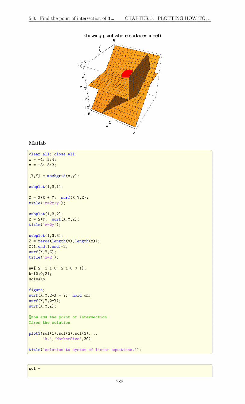
5.3. Find the point of intersection of 3 … CHAPTER 5. PLOTTING HOW TO,…
Matlab clear all; close all;x = -4:.5:4;y = -3:.5:3;
[X,Y] = meshgrid(x,y);
subplot(1,3,1);
Z = 2*X + Y; surf(X,Y,Z);title('z=2x+y');
subplot(1,3,2);Z = 2*Y; surf(X,Y,Z);title('z=2y');
subplot(1,3,3);Z = zeros(length(y),length(x));Z(1:end,1:end)=2;surf(X,Y,Z);title('z=2');
A=[-2 -1 1;0 -2 1;0 0 1];b=[0;0;2];sol=A\b
figure;surf(X,Y,2*X + Y); hold on;surf(X,Y,2*Y);surf(X,Y,Z);
%now add the point of intersection%from the solution
plot3(sol(1),sol(2),sol(3),...'k.','MarkerSize',30)
title('solution to system of linear equations.'); sol =
288
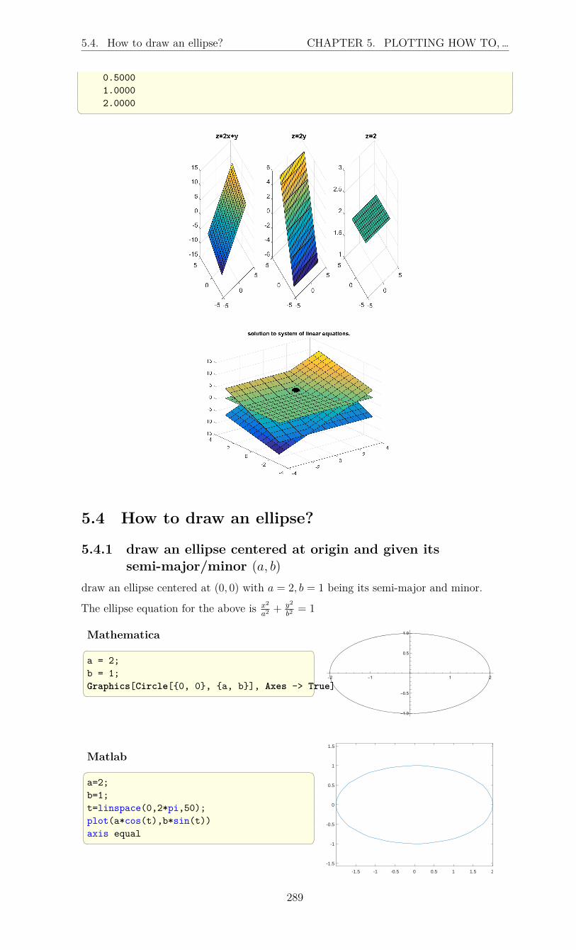
5.4. How to draw an ellipse? CHAPTER 5. PLOTTING HOW TO,…
0.50001.00002.0000
5.4 How to draw an ellipse?
5.4.1 draw an ellipse centered at origin and given itssemi-major/minor (a, b)
draw an ellipse centered at (0, 0) with a = 2, b = 1 being its semi-major and minor.
The ellipse equation for the above is x2
a2+ y2
b2= 1
Mathematica a = 2;b = 1;Graphics[Circle[0, 0, a, b], Axes -> True] -2 -1 1 2
-1.0
-0.5
0.5
1.0
Matlab a=2;b=1;t=linspace(0,2*pi,50);plot(a*cos(t),b*sin(t))axis equal
-1.5 -1 -0.5 0 0.5 1 1.5 2
-1.5
-1
-0.5
0
0.5
1
1.5
289

5.4. How to draw an ellipse? CHAPTER 5. PLOTTING HOW TO,…
5.4.2 draw an ellipse centered at (x, y) and given itssemi-major/minor (a, b)
draw an ellipse centered at (1, 2) with a = 2, b = 1 being its semi-major and minor. Theellipse equation for the above is x2
a2+ y2
b2= 1
Mathematica a = 2;b = 1;Graphics[Circle[1, 2, a, b],Point[1, 2], Axes -> True] -1 1 2 3
1.5
2.0
2.5
3.0
Matlab close all;a=2; b=1;t=linspace(0,2*pi,50);plot(a*cos(t)+1,b*sin(t)+2)axis equalxlim([-1,4]);ylim([0,4]);
-1 0 1 2 3 40
0.5
1
1.5
2
2.5
3
3.5
4
5.4.3 draw an ellipse centered at origin and given itssemi-major/minor (a, b) and rotated at angle θ
draw an ellipse centered at (0, 0) with a = 2, b = 1 being its semi-major and minor titltedat angle θ = 30 degrees anti-clockwise.
The ellipse equation for the above is x2
a2+ y2
b2= 1. After drawing it, we rotate it.
Mathematica a = 2;b = 1;Graphics[Rotate[Circle[0, 0, a, b],Line[-a, 0, a, 0],Line[0, -b, 0, b], 30 Degree], Axes -> True]
-1.5 -1.0 -0.5 0.5 1.0 1.5
-1.0
-0.5
0.5
1.0
290

5.5. How to plot a function on 2D using… CHAPTER 5. PLOTTING HOW TO,…
MatlabMatlab does not have rotate function, so use therotation tranformation matrix. close all;a = 2;b = 1;t = linspace(0,2*pi,50);rotateAngle = 30*pi/180;mat = [cos(rotateAngle) -sin(rotateAngle)
sin(rotateAngle) cos(rotateAngle)];
%2x2 times 2x50 = 2x50data = mat*[a*cos(t);b*sin(t)];plot(data(1,:),data(2,:))axis equal
-1.5 -1 -0.5 0 0.5 1 1.5
-1
-0.5
0
0.5
1
5.5 How to plot a function on 2D using coordinatesof grid locations?
Sometimes in finite difference we want to evaluate the force or the function in the RHSof the equation f(x, y) using the coordinates x, y on a 2D grid. The grid spacing can beh and the coordinates extend from some x value to some other x value and from some yvalue to some other y values. In Matlab, the coordinates are setup using meshgrid.
In Mathematica, there is really no need for meshgrid as the build-in command Map canbe used to evaluate the function at each grid point. The coodinates physical values aregenerated using the Table command. Here is example evaluating and plotting f(x, y) =sin(10xy)e−xy on a grid of spacing h = 1/N where N is number of elements. The gridgoes from x = −1 to x = 1 by spacing of h. Same for the y direction.
Mathematica Clear[x, y, z];nElem = 10.;h = 1/nElemN@Range[-1, 1, h]grid = N@Table[i, j, i, -1, 1, h, j, -1, 1, h];f[x_, y_] := Sin[x*10 y] Exp[-x y];force = Map[f[#[[1]], #[[2]]] &, grid, 2];ListPlot3D[force, AxesLabel -> x, y, z]
To use the actual physical coordinates on the axis above, then replace the plot above withthis below. This also includes an implementation of meshgrid like function in Mathematicawhich makes it easier to work with for someone familiar with Matlab:
291

5.6. How to make table of x, y values and… CHAPTER 5. PLOTTING HOW TO,…
meshgrid[x_List,y_List]:=ConstantArray[x, Length[x]],Transpose@ConstantArray[y, Length[y]];
nElem = 10.;h = 1/nElem;x, y = meshgrid[Range[-1, 1, h], Range[-1, 1, h]];f[x_, y_] := Sin[x*10 y] Exp[-x y];force = f[x, y];pts = Flatten[x, y, force, 2, 3];ListPlot3D[pts, PlotRange -> All,
AxesLabel -> Automatic, ImagePadding -> 20,ColorFunction -> "Rainbow", Boxed -> False]
To see each point value, use InterpolationOrder -> 0 in the plot command.
Matlab clear all; close all;nElem = 10;h = 1/nElem;[X,Y] = meshgrid(-1:h:1,-1:h:1);f = @(x,y) sin(x*10.*y) .* exp(-x.*y);force = f(X,Y);surf(X,Y,force)
5.6 How to make table of x, y values and plot themGenerate a list or table of (x, sin(x)) values and plot them.
Mathematica lst=Table[x, Sin[x], x, -Pi, Pi, 1/10];ListLinePlot[lst] -3 -2 -1 1 2 3
-1.0
-0.5
0.5
1.0
MatlabMatlab does not have a nice function likeTable so one can either make the x variableand then use it to make sin(x)or use arrayfun close all;x=-pi:.1:pi;plot(x,sin(x)); Using arrayfun A=cell2mat(arrayfun(@(x) [x;sin(x)],...
-pi:.1:pi, 'UniformOutput',false));plot(A(1,:),A(2,:)) -4 -3 -2 -1 0 1 2 3 4
-1
-0.8
-0.6
-0.4
-0.2
0
0.2
0.4
0.6
0.8
1
292

5.7. How to make contour plot of f(x, y) ? CHAPTER 5. PLOTTING HOW TO,…
5.7 How to make contour plot of f (x, y) ?Problem: Make contour of f(x, y) = (11 − x − y)2 + (1 + x + 10y − xy)2 over region0 < x < 20 and 0 < y < 10.
Contour label placement seems to be better in Matlab. It is put in the middle of the lineautomatically.
Mathematica f = (11 - x - y)^2 + (1 + x + 10 y - x y)^2;ContourPlot[f, x, 0, 20, y, 0, 15,Contours -> 10, ContourShading -> None,ContourLabels -> Function[x, y, z,
Text[z, x, y]], AspectRatio -> Automatic,PlotRangePadding -> 2]
Out[15]=
970
970
1940
1940
2910
2910
3880
3880
4850
48505820
5820
6790
67907760
77608730
87309700
9700
0 5 10 15 20
0
5
10
15
Matlab x = 0:0.05:20;y = 0:0.05:15;[x,y] = meshgrid(x,y);z = (11-x-y).^2 + (1+x+10*y-x.*y).^2;[C,h] =contour(x,y,z,10);clabel(C,h)title('Contours Labeled Using clabel(C,h)')
2110.6364
2110.6364
4181
.272
7
4181.2727
6251
.909
1 6251.90918322
.545
5
Contours Labeled Using clabel(C,h)
0 5 10 15 200
5
10
15
293

5.7. How to make contour plot of f(x, y) ? CHAPTER 5. PLOTTING HOW TO,…
294

Chapter 6
Some symbolic operations
6.1 How to find all exponents of list of expressions?Given f 2, g3, kp, h write code to return 2, 3, p, 1 as the exponents.
Mathematica ClearAll[f, g, k, p, h];lst = f^2, g^3, k^p, h;Cases[lst, x_^n_. :> n] 2, 3, p, 1
Maple unassign('f,g,k,p,h');foo:=proc(expr)
if nops(expr)=1 thenreturn 1;
elif hastype(expr,`^`) thenreturn( op(2,expr) );
fi;return(NULL);
end proc:
expr:=[f^2, g^3, k^p, h]:map(foo,expr)
[2, 3, p, 1]
This document was compiled using
Text Font: [lmroman12-regular]:+tlig;
Math Operator Font: cmr12
Math Letter Font: cmmi12
295