Mathematical three-dimensional solid modeling of biventricular geometry

Annals of Biomedical Engineering, Vol. 21, pp. 199-219, 1993 0090-6964/93 $6.00 + .00 Printed in the USA. All rights reserved. Copyright �9 1993 Pergamon Press Ltd.

Mathematical Three-Dimensional Solid Modeling of Biventricular Geometry

JOHN S. PIROLO,* STEPHEN J. BRESINA,~" LAWRENCE L . CRESWELL,* KENT W. MYERS,*

BARNA A . SZAB6,~ MICHAEL W. VANNIER,'~ a n d MICHAEL K. PASQUE*

*Department of Surgery, Division of Cardiothoracic Surgery, "~The Mallinckrodt Institute of Radiology, and the ,Department of Mechanical Engineering, Center for Computational Mechanics,

Washington University, St. Louis, MO

Abstract--The characterization of regional myocardial stress distribution has been limited by the use of idealized mathematical representations of biventricular geometry. State-of-the-art computer-aided design and engineering (CAD/CAE) techniques can be used to create complete, unambiguous mathematical representations (solid models) of complex object geometry that are suitable for a variety of applications, including stress-strain analyses. We have used advanced CAD/CAE software to create a 3-D solid model of the biventricular unit using planar geometric data extracted from an ex vivo canine heart. Volumetric analysis revealed global volume errors of 4.7~ -1.3~ -1.6~ and - 1.1 070 for the left ventricular cavity, right ventricular cavity, myocardial wall, and total enclosed volumes, respectively. Model errors for 34 in-plane area and circumference determinations (mean +_ SD) were 5.3 +_ 6.7~ and 3.8 _+ 2.7~ Error analysis suggested that model volume errors may be due to operator variability. These results demonstrate that solid modeling of the ex vivo biventricular unit yields an accurate mathematical representation of myocardial geometry which is suitable for meshing and subsequent finite element analysis. The use of CAD/CAE solid modeling in the representation of biventricular geometry may thereby facilitate the characterization of regional myocardial stress distribution.

Keywords-Cardiac representation, Ventricular geometry, Finite element analysis.

INTRODUCTION

An accurate description of myocardial stress distribution throughout the biventricular unit would improve our understanding of myocardial function. Considerable progress has been made in the clinical and experimental characterization of myocardial stress distribution using

Acknowledgment-This work was supported, in part, by National Institutes of Health grant #HL44511. The authors thank Robert H. Knapp and the Structural Design Research Corporation University Con- sort ium for their technical assistance, and Richard B. Schuessler for his insightful comments in reviewing this manuscript .

Address correspondence to Michael K. Pasque, Division of Cardio- thoracic Surgery, Suite 3108 Queeny Tower, Barnes Hospital, One Barnes Hospital Plaza, St. Louis, MO 63110.

(Received 7/19/91)

geometric mathematical modeling and finite element analysis (FEA). However, major limitations to the application of stress analysis to the heart (in both normal and pathologic states) still exist. To achieve acceptable fidelity and reasonable efficiency in the estimation of ventricular wall stress using FEA, the loading conditions, myocardial material properties, and three-dimensional (3-D) ventricular geometry must be defined.

Ventricular loading is typically assessed by pressure and volume measurements. The materialproperties of viable myocardium have been estimated from in vitro studies of isolated tissue (1) and in vivo global ventricular assess- ments (16). Three-dimensional left ventricular geometry has been obtained from global models based upon assumptions of axisymmetry (4,13). These simplified models are unable to represent regional myocardial geometry accurately. This inability to capture detailed regional geometry in a form mathematically suitable for advanced mechanical analysis (i.e., FEA), represents a major ob- stacle to the determination of regional myocardial stress- strain relationships in the intact heart.

The 3-D mathematical representation of physical objects encompasses a variety of modeling techniques including wireframe, surface, and solid models. While each of these techniques has specific applications, only solid modeling incorporates a complete, unique, and unambiguous mathematical description in the representation of a given object (17). As a result, a single solid model can serve any application which requires a mathematical description of object geometry. Solid models allow, and are well suited to, complex geometric manipulation and sophisticated engineering analysis such as FEA.

Modeling of discrete 3-D objects by wireframe methods was first developed with the pioneering work of Ivan Sutherland with SKETCHPAD at MIT in the 1960s. Wire- frame representations are limited in their application to very complex geometries due to orientational ambiguities (e.g., it can be impossible to tell from a static wireframe display what part of an object is near the observer and

199

200 J.S. PIROLO et al.

which is far). The nonuniqueness of wireframe displays/ representations is a major hindrance to their effective use in analysis of complex 3-D object behavior in real or sim- ulated environments. Surface modeling was developed subsequently, offering solid shaded surface visualization, typically by a faceted or polygonal surface representation. This technique has become a common means of modeling objects for display purposes, but is not suitable for analysis purposes. The computer graphic techniques used in presentations, motion pictures, and advertising/design are typically based on surface representations.

Solid models are best suited to applications where quantitative analysis is required. To synthesize a valid solid representation of geometrically complex objects, many additional processing steps and constraints must be satisfied to ensure completeness and uniqueness. It is straightforward to synthesize any of many possible wireframe and surface representations from stored solid object models, though the reverse is not necessarily true. The solid model, once created, can be interrogated to determine the object's mass properties (centroid, principal axes, moments of inertia, volume, surface area, etc.). This cannot be done, in general, with wireframe or surface models. There are efficient tests which can be applied to a solid model to ensure its integrity; such tests are not yet available for surface or wireframe models.

Over the last decade, computer-aided design and engineering (CAD/CAE) software has been used extensively by industry for the modeling and mechanical analysis of non-biological, discrete manufactured objects, such as aerospace or automotive parts and assemblies. Recently, these techniques have been extended and applied to anatomic structures with considerable success (10,20,21). We have used CAD/CAE techniques to create a 3-D solid model of the canine biventricular unit. In doing so, we have demonstrated the applicability of CAD/CAE based solid modeling techniques to the representation of 3-D cardiac geometry.

MATERIALS AND METHODS

Acquisition of Anatomic Data

An adult canine heart was excised following fibrilla- tory arrest and formalin preserved. The biventricular unit was isolated by trimming aortic, pulmonary artery, and atrial tissues. To establish longitudinal epicardial (EPI) alignment markers, optical crosshairs Were projected onto the biventricular unit so that the crosshairs intersected at the apex and extended down the EPI surface to the base. Electrocautery was then used to burn a superficial line on the EPI surface along the path of the crosshairs. Af- ter marking the heart in this manner, the biventricular unit was sliced transversely using a rotary blade at approximately 4 mm intervals from base to apex (cutting plane

perpendicular to the long axis of the left ventricle). This resulted in 15 cross-sectional slices. The most apical 3 mm remnant was discarded. The anatomic database was derived from observation and measurement of the apical surface of the remaining 14 slices. The slice specimen geometry was captured using fixed focal length 35 mm slide photography (55 mm macro lens; focal length, 15.34 cm) of the apical surface of each unit slice. For photography, each slice was placed on a rectilinear graduated rule background grid (5 mm major divisions) with fixed x and y axes. During photography, proper slice-to-slice orientation was maintained by alignment of the 4 epicardial surface marks on each slice with fixed markers on the background grid. A reference scale was placed on the apical surface of each slice for subsequent scaling of the photographic images.

Image Processing

Digitized images of the photographic slides were obtained using optical scanning digitization (Barneyscan | Color Imaging Systems, Alameda, CA). Barneyscan is a CCD (charge coupled device) linear photodiode array 35 mm color or monochrome slide scanner which allows the division of an image into a pixel array with assigned 8-bit grayscale values and subsequent storage as image files. Calibration of grayscale values was performed au- tomatically using 35 mm slides of graduated grayscale images of known intensity. The resulting image files (1024 • 1520 pixels) were imported into a public domain Macintosh computer (Apple Computer, Cupertino, CA) based digital image processing software package, Image (version 1.25, Wayne Rasband, Research Services Branch, NIMH, Bethesda, MD), which provides a variety of image processing functions including enhancement, editing, calibration, and analysis.

Using Image, biventricular slice images were scaled and the major division lines on the background grid were superimposed on the image (Fig. 1). Points along the EPI, left ventricular (LV), and right ventricular (RV) contours were then manually selected at the intersection of each superimposed grid line and the biventricular image contours. In regions of rapidly changing contour curvature, additional points were chosen to delineate the cardiac geometry more accurately. A total of 631 contour points were selected from the 14 slice specimens. The number of EPI, LV, and RV contour points selected per slice (mean + SD) were 35 + 10, 21 + 4, and 28 + 9, respectively. Fiduciary points were selected at three points on the background x-y axes of the local coordinate system in each biventricular image [(x,y): (11,0), (0,0) and (0,10); Fig. 1]. The x,y coordinate pairs of the fiduciary and EPI, LV, and RV contour points for each of the 14 slices were stored (ASCII files) for subsequent importation into the CAD/CAE program.

3-D Modeling of Cardiac Geometry 201

FIGURE 1. On screen digital representation of a biventricular slice (slice 1 1) following optical scanning and importation into the Macin- tosh II for display and analysis. In the background is the rectilinear grid, with the origin (0) , and x-y axes of the local coordinate system. Fiduciary points (F1, F2) are shown at (0,10) and (11,0) , respectively. The fixed markers (background crosshairs: BC1, BC2) were employed for slice-to-slice alignment using the electrocautery placed epicardial markers. The apical surface of the biventricular slice is shown with left ventricular cavity (LV) and right ventricular cavity (RV). The superimposed crosshairs (SC1, SC2) and grid (G) were created manually. The superimposed grid and crosshairs were used to select contour points (CPT) and to group sequences of points for spline fitting during profile creation.

Workstation Configuration

Solid modeling was performed using a mechanical computer-aided engineering (MCAE) software package, I -DEAS (Integrated Design Engineering Analysis Soft- ware Version 4.1, Structural Dynamics Research Corpo- ration, Milford, OH). I - D E A S is a comprehensive software package (9) including Geomod (a hybrid, boundary representation/constructive solid geometry modeler), a module for kinematic analysis, and a finite element solver. I -DEAS can generate photorealistic displays with ray-tracing, translucency, shadows, and reflections. An 8-bit color 3-D graphics workstation (SPARCstation 4/330CXP, Sun Microsystems, Inc., Mountain View, CA) configured with 24 mbytes of random access memory (RAM), 669 mbytes of hard disk storage, and a UNIX- based operating system (SunOs 4.0, Sun Microsystems, Inc., Mountain View, CA) was used as a platform for

the solid modeling. The workstation allows interactive manipulation of high quality anti-aliased wireframe and shaded images (screen dimensions 1152 • 900 pixels).

Solid Model Creation

A schematic diagram of the solid modeling process is shown in Fig. 2. Contour point x,y coordinate files were imported into I -DEAS using an IDL (Interactive Data Language, Research Systems Inc., Denver, CO) program to generate a batch file in the resident I -DEAS program- ming facility I -DEAL. Execution of the IDL program resulted in the automatic importation of slice-specific fiduciary and contour point coordinates into individual Geomod work sets and in the subdivision of contour points in each work set into 3 groups. Group 1 corresponded to those points lying on the EPI contour, Group 2 corresponded to those points lying on the LV contour,

.a . . vo,ume\ I and area

measurement / I

I

FIGURE 2.

Isolation and preparation of the anatomic specimen (AS)

Photography of AS slices J

Optical scanning of slice I photogaphs (Barnaymcan)

[ !rnpor tat.ion J

Image scaling and contour point selection (Image 1.25)

Importation" [

Profile, skin group and solid model creation (I-DEAS 4.0)

. ~ _ / circumference centroid, \ ~ .... comparison1 . ' . and ,,nea:r:,2eos,oo

Ci rc u m fare nce ~ and area

measurement /


Schematic diagram of geometric data acquisition, importation, and subsequent solid modeling of the canine biventricular unit.

and Group 3 corresponded to those points lying on the RV contour.

Individual profiles were created from each of these groups by the fitting of non-uniform rational B-splines (NURBS) through the contour points in each group. Four B-splines were used in the creation of each profile. The 3 fiduciary points in each work set were defined to correspond to (11,0), (0,0), and (0,10) in the local coordinate system of Geomod . The origins of x-y axes in all work sets were aligned and the relative angular deviation of the x-y axes was calculated, allowing for automatic detection and correction of any frame-of-reference shifts which occurred during optical scanning or data importation. Automatic contour point entry and profile formation re-

suited in the creation of 35 x-y planar profiles (14 EPI, 12 LV, and 9 RV profiles).

The creation of a 3-D solid model from these profiles required specification of their spatial location and vertical connectivity. In G e o m o d this is achieved by the creation of skin groups. These skin groups may be thought of as the "skeleton" from which subsequent solids are created through mathematical filling of model space and the application of a surface or "skin" by the placement of NURB surfaces through the profile boundaries. Figure 3 illustrates the arrangement of profiles following creation of a skin group. The location of each profile in the x-y plane was specified during profile creation and the location of each profile in the z-dimension was determined


FIGURE 3. A skin group resulting from the grouping of epicardial profiles. The vertical line segments joining the x-y planar profiles define the first contour point of each profile, That point is used as the start point for subsequent placement of NURB surfaces on the skin group.

f rom the anatomic specimen by measuring the distance of each slice f rom the most apical surface of the most basal slice (i.e., the sum of the thicknesses of the intervening slices). Although biventricular unit slicing was designed to result in 4 m m thick cross sections, minimal variation across each slice was apparent. In order to establish slice thickness accurately, 4 thickness measurements were made at the epicardial surface of each slice. These measurements were made at the epicardial markers described above. The mean of the 4 thickness values was taken as the thickness of a given slice. To control the size of the geometric database of the model and yet re- tain adequate geometric detail, profiles f rom 5 of the 10 most basal slices (every other slice) were used for skin group creation. Because of the rapidly changing curvature of the apical regions, profiles f rom all 4 of the most apical slices were employed in skin group creation. This resulted in the creation of skin groups with profiles located at the following z-depths: 0.00, 0.81, 1.61, 2.44, 3.35, 4.25, 4.67, 5.14, and 5.68 cm. Profiles at z-depths of 0.41, 1.21, 2.10, 2.89, and 3.77 cm were obtained, but were not used for skin group creation.

Restrictions inherent in the I D E A S software preclude the creation of a skin group f rom a set of profiles con- taining differing numbers of internal holes. When the biventricular unit is sliced perpendicular to the long axis, the RV cavity terminates superior to the LV cavity and the apical surface of the most apical slice contains nei- ther RV or LV endocardial contours. Thus, the creation

of a single profile f rom each biventricular slice would result in profiles with 2, 1 or 0 internal holes, violating modeling requirements. In order to circumvent this limitation and yet avoid the artificial creation of ana tomy via manual construction of an apical capping surface, the following methodology was employed. Three skin groups (A, B, and C) were created. All skin groups were created be- ginning with profiles derived from the contours of the apical surface of the most basal slice. The base of each skin group was defined to be located at a z-depth of 0.00 cm. Skin group A was created using profiles derived from only EPI contour points (z-depth: 0.00 to 5.68 cm). Skin groups B (z-depth: 0.00 to 3.35 cm) and C (z-depth: 0.00 to 4.67 cm) were created using profiles derived f rom the RV and LV contour points, respectively. Three solid models were created f rom these skin groups. Solid model A corresponded to the entire biventricular unit without RV or LV cavities, solid model B was an endocast of the RV cavity, and solid model C was an endocast of the LV cavity. The final solid model (SM) of the biventricular unit (solid model D) was created via Boolean subtraction of the RV and LV endocasts f rom the EPI solid model (SM biventricular unit = SM A - SM B - SM C; see Fig. 4).

The solid models created were subjected to a series of Boolean spatial operations within Geomod to isolate specific regions of model space for mass property analysis. The performance of a Boolean plane cut through a model allows the isolation of either the 2-D cross-sectional profile at the level of the cutting plane or the 3-D model vol-


A B C D

FIGURE 4. Methodology employed in the creation of the final model of the biventricular unit. Solid models derived from the RV endocardial profiles (B) and LV endocardial profiles (C) were Boolean subtracted from a solid model of the biventricular unit based only on epicardial profiles (no internal holes; A). The resulting solid model (D) was the final solid model of the biventricular unit.

umes above or below the cutting plane. A series of Boolean plane cuts thus allows the isolation f rom the model of "slices" of predetermined thickness.

The geometry created during solid modeling may be divided into two classes. One class of geometry is composed of those model regions which are spatially coinci- dent with actual anatomic data entered during contour point importation. The second class of geometry consists o f those model regions where no anatomic data was entered and where all local geometry was approximated during computer modeling. In order to examine specifically the ability of the solid modeling program to interpolate geometry in regions where no anatomic data were entered, the following methodology was employed. The two types of model regions were isolated using Boolean plane cuts through the model (Fig. 5). Class 1 2-D model areas were defined as any 2-D profile coinciding with a plane of data entry during skin group creation. Class 1 3-D model volumes were defined as any model volume bounded both apically and basally by planes of data entry during skin group creation. Class II 2-D model areas were defined as any 2-D profile coinciding with a level at which data was obtained f rom the anatomic specimen but not employed in skin group creation. Class II 3-D model volumes were defined as any 3-D volume bounded either apically or basally by a surface corresponding to an anatomic level at which profiles were obtained but not included in skin group creation. Nine Class I 2-D and 8 Class I 3-D regions were identified. Five Class II 2-D and 5 Class II 3-D regions were identified. The method of data entry resulted in all Class II model regions occurring in the most basal 4.25 cm of the model.

DATA ANALYSIS

Volumetric Analyses

The mass and myocardial wall volume were determined for each slice of the anatomic specimen by two indepen- dent observers. The volume of each slice of the anatomic

specimen was calculated using water displacement. Mass- volume regression analysis was performed to obtain a regression equation (slope = 1.047 gr/cc; R 2 = 0.99). Be- cause of the greater accuracy of mass measurements compared to direct volume measurements, the slice volumes were calculated from actual mass measurements using the density regression equation determined previously. This methodology assumes that tissue composition is constant between slices. The global myocardial wall volume of the anatomic specimen was determined by summation of the volumes of the component slices. Prior to slicing the anatomic specimen, the LV and RV cavity volumes were determined by filling with water.

Global and regional volumes of the solid model were determined using model interrogation capabilities within Geomod . Global analyses employed the final 3-D model of the biventricular unit as well as the 3-D solid models of the ventricular endocasts. Class I and Class II 3-D volume analyses were performed on cross-sectional volumes of the biventricular model isolated by Boolean plane cuts (cutting plane parallel to the local x-y plane).

Regional Area and Circumference Analyses

Cross-sectional area and circumference were determined at each level of the anatomic specimen for planar regions bounded by the EPI contour (EPI region), RV cavity contour (RV region), and LV cavity contour (LV region). Regional areas were determined by planimetry of acetate tracings of the biventricular slices. Any given region, R, on the apical surface of a given slice n, (R , ) , should theoretically be identical to the corresponding region on the basal surface of slice n - 1, (Rn-a). Thus, the final cross-sectional area of Ri, (Ai), was calculated as the mean for 3 area determinations of Rn and 3 area determinations of Rn-1, or:

AI,, + A2,, + A3,, + Aln-~ + A2,,-I + A3,,-x A i =

6

(1)


ANATOMIC SPECIMEN

ANATOMIC SLICES

LEVELS OF ANATOMIC DATA ENTRY ANATOMIC GEOMEIRY

DETERMINED AT THESE LEVELS

3D SOLID MODEL

( " * ) MODEL SPACES!

M3OEL SLICES MODEL GEOIVEITW DE-~I:~$~INEO AT THESE LEVELS

FIGURE 5. Schematic diagram showing the relationship between anatomic specimen slices and the resulting solid model. Planar contours were obtained from every other slice of the anatomic specimen in the basal regions and every slice in the apical regions. Class I 2-D model regions were those regions coinciding with levels of anatomic data entry (••). Class I 3-D model regions were those regions bounded apically and basally by levels of anatomic data entry, Class II 2-D model regions were those regions coinciding with anatomic levels at which geometric data was collected but not entered into model creation ( * * ) . Class II 3-D model regions were those regions bounded on only one surface by a level at which anatomic data was entered.

Using Image, biventricular slice representations were used to determine analogous regional cross-sectional areas and circumferences. For the area and circumference calculations, the boundaries of any given region were selected so as to include the points chosen previously for importation into 1-DEAS. Final biventricular image area and circumference measurements were taken as the average of three determinations.

Area and circumference calculations were performed on two model groups. Group 1 consisted of the 13 3-D model slices corresponding to the 13 anatomic slices represented by the model. In this group, the cross-sectional area of the myocardial wall was determined for both the apical and basal surface of each slice. The myocardial wall area of the apical surface of any slice n was compared to the myocardial wall area of slice n - 1. These calculations were per formed to assess the internal consistency of the model. Group 2 consisted of 2-D planar profiles isolated by Boolean plane cuts at levels corresponding to the levels of anatomic specimen slicing. Four-

teen 2-D profiles (9 Class I and 5 Class II) were isolated. For each of these profiles EPI , LV, and RV cross-sectional area and circumference were determined. Group 2 profiles were used for comparison with corresponding cross-sectional areas in the anatomic specimen and corresponding cross-sectional areas and circumferences in the Image representations.

Regional Centroid Analyses

Regional centroid measurements could not be made directly f rom either the anatomic specimen or Image representation because of frame-of-reference shifts. How- ever, these shifts were corrected during initial data importa t ion into Geomod. Because the original profiles (prior to skin group and solid model creation) most nearly represent frame-of-reference corrected groups of anatomic specimen contour points, those profiles were used in the determination of regional centroids. It should be noted that these centroids do not truly represent anatomic


specimen regional centroids because they are determined subsequent to fitting of NURBS through contour points. Model EPI, LV, and RV regional centroids were determined from Class I and Class II 2-D planar profiles isolated by Boolean plane cuts of the final biventricular model. These centroids were then compared to those determined from the original profiles following contour point importation.

Linear Dimensional Analyses

Anatomic specimen linear dimensional analysis was performed using on screen Image biventricular slice representations. Figure 6 illustrates the protocol for the determinations of regional myocardial wall thickness and LV cavity and RV cavity width. The demarcation of segments to be measured was made by casting mutually perpendicular rays (R1 and R2) across the biventricular image. R1 was cast from the origin to the point (10,10) and R2 was cast from point (0,10) to point (10,0). R1

intersected the biventricular slice image over 5 segments (A through E: LV freewall, LV cavity, septum, RV cavity, and RV freewall, respectively). R2 intersected the biventricular slice image over three segments (F-H: LV freewall, LV cavity, and LV freewall, respectively). The length of each of these eight segments was recorded. The segment lengths were determined solely by the path of a given ray and the epicardial and endocardial edges (no other anatomic landmarks were employed). Analogous model line segments were isolated by casting corresponding rays across the Class I and Class II 2-D planar profiles described previously. These model line segments were then measured and compared to the measurements obtained with Image.

Error Analysis

Three principal sources of error may exist in this study: (a) errors associated with acquisition and representation of anatomic specimen geometry within Image, (b) errors

FIGURE 6. On screen digital representation of a biventricular slice in Image (Macintosh II) showing the method of selection of linear segments for use in 2-D linear dimensional analyses. Two rays were cast from the background x-y axes (R 1 and R2). R1 [cast from (0,0) to (10,10)] intersects the biventricular slice image over 5 segments (A-E) and R2 [cast from (0,10) to (10,0)] intersects the biventricular slice image over 3 segments (F-H) . The length of each of these 8 segments was determined and compared with the lengths of corresponding segments identified on 2-D slices isolated from the final solid model of the biventricular unit.


in observer ability to detect and select points along the myocardial edge (either endocardial or epicardial) accurately, and (c) errors introduced during the modeling process.

Errors associated with the acquisition of geometric data can be due to optical distortions arising during photography or image digitization. Fixed focal length photography and careful slice orientation using fixed markers on the rectilinear background grid may minimize system- atic errors during initial geometric data acquisition. To assess the linearity of Image representations, a segment of known length (3.0 cm) near the outer border of each quadrant in every Image slice representation was measured and the mean deviation from 3.0 cm calculated. The performance of the image digitization system was evaluated by characterizing image quality in terms o f signal- to-noise and dynamic range.

The ability to detect the edge of an image accurately is influenced by a variety of image characteristics. In particular, the rate at which the pixel intensity is changing at the background-object border (the first derivative of pixel intensity with respect to distance, di/dx) will influence the ability to locate the object edge correctly. In order to approximate di/dx, pixel intensity profiles were plotted along 2 line segments (20-30 contiguous pixels) traversing the epicardial biventricular edge in each Im- age representation. From these pixel plots, the linear distance over which the background to myocardium transition occurred (LT) and the mean slope of intensity over the transition region were calculated. Assuming that the true edge for any given case was located in the center of the transition, the linear uncertainty associated with the selection of any given contour point (Lu) was calculated as L v = Lr /2 .

Using profile modification capabilities within Geomod, the ultimate effect of contour point uncertainty on regional volume was examined. The original EPI, LV, and RV profiles obtained at z-depth = 0.81 cm (the apical surface of slice 12) and z-depth = 1.21 cm (the apical surface of slice 11) were isolated and each contour point of these regional profiles was translated radially by both +L~, and - L u . The resulting expanded and contracted profiles were used to create two 3-D solid models of the intervening slice (slice 11). One of these, (SMraax), corresponded to the largest possible volume of the slice (a model formed from expanded EPI profiles and contracted LV and RV profiles). The other model, (SMmin), corresponded to the smallest possible volume of the slice (a model formed from contracted EPI profiles and expanded LV and RV profiles). The volume errors of these two models were then calculated.

To evaluate the effect of discretization (number of contour points selected for importation) and the method of profile construction (polylines versus B-splines) on modeling accuracy, eight 3-D solid models of a single biven-

tricular slice (slice 11) were created. The eight models were divided into two groups. In one group, models were created from profiles constructed by polylines. In the other group, models were created from profiles composed of B-splines. In each group, geometry discretization was varied by using 2, 1, 0.5, or 0.25 times the number of contour points originally imported during construction of the solid model o f the biventricular unit. The volume errors associated with each of the models was then calculated.

RESULTS

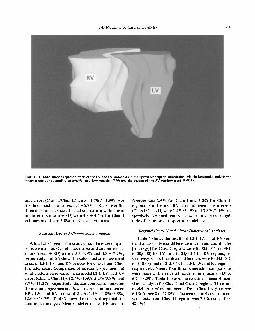
Figure 7 shows wireframe and solid shaded translucent renderings of the final model of the biventricular unit. Figure 8 is a solid shaded rendering of the RV and LV endocasts in their preserved spatial orientation. Visible anatomic features include indentations corresponding to the anterior and posterior papillary muscles and the sweep of the RV outflow tract. The solid model of the biventricular unit is a single, closed, coherent object composed of 3964 points, 6798 facets, and 16 surfaces. The RV endocast is composed of 1392 points, 2439 facets, and 6 surfaces; the LV endocast is composed of 1652 points, 2831 facets, and 6 surfaces.

All spatial manipulations performed on the biventricular model (2-D cross section isolation or Boolean creation of 3-D segmental or individual model slices) resulted in either closed 2-D profiles or closed, coherent 3-D solid objects. The internal consistency of the model was con- firmed in that for any given 3-D slice n, the cross-sectional area of the apical and basal surfaces were equal to the cross-sectional areas of the basal surface of slice n + 1 and the apical surface of slice n - 1, respectively. In addition, the total volume of the biventricular unit model was equal to the sum of the volumes of the individual model slices.

Volumetric Analysis

The total volume occupied by the anatomic specimen (i.e., myocardial wall volume + LV cavity volume + RV cavity volume) was 170.2 cm 3 and the total volume of the solid model of the biventricular unit was 172.1 cm 3. An- atomic specimen myocardial wall volume was 133.9 cm 3 and model myocardial wall volume was 136.1 cm 3. LV and RV cavity volumes of the anatomic specimen were 13.3 cm 3 and 23 cm 3, respectively. The corresponding volumes of the model LV and RV endocasts were 12.7 cm 3 and 23.3 cm 3. Therefore, overall global volume errors of the model were -4.5%0, 1.3%, 1.6%, and 1.1% for the LV cavity, RV cavity, myocardial wall, and total volumes, respectively. Table 1 shows the slice-by-slice volume comparison between anatomic specimen and corresponding Class I and Class II model regions. Both Class I and Class II model volumes underestimated basal, and overesti- mated apical anatomic specimen volumes. The mean vol-

208 J.S. PmoLo et aL

(a)

(b)

FIGURE 7. (a) Wireframe and (b) solid shaded translucent representations of the final solid model of the biventricular unit. The EPI surface and RV and LV endocardial surfaces are shown.


FIGURE 8. Solid shaded representation of the RV and LV endocasts in their preserved spatial orientation. Visible landmarks include the indentations corresponding to anterior papillary muscles (PM) and the sweep of the RV outflow tract (RVOT).

ume errors (Class I /Class II) were -1.7070/-1.907o over the three most basal slices, but -6.9070/-8.2070 over the three most apical slices. For all comparisons, the mean model errors (mean + SD) were 4.8 + 4.407o for Class I volumes and 4.4 + 5.007o for Class II volumes.

ferences was 2.6% for Class I and 3.2% for Class II regions. For LV and RV circumferences mean errors (Class I /Class II) were 5 .4%/6 .1% and 3 .8%/3 .1%, respectively. No consistent trends were noted in the magnitude of errors with respect to model level.

Regional Area and Circumference Analyses

A total of 34 regional area and circumference comparisons were made. Overall model area and circumference errors (mean + SD) were 5.3 ___ 6.7070 and 3.8 +_ 2.7%, respectively. Table 2 shows the calculated cross-sectional areas of EPI , LV, and RV regions for Class I and Class II model areas. Comparison of anatomic specimen and solid model area revealed mean model EPI , LV, and RV errors (Class I/Class II) of 2.4070/1.6070, 5.2~ and 8.7 ~176 respectively. Similar comparison between the anatomic specimen and Image representation revealed EPI , LV, and RV errors of 2.2070/1.3070, 5 .0%/6 .8%, 12.6070/13.2070. Table 3 shows the results of regional circumference analysis. Mean model errors for EPI circum-

Regional Centroid and Linear Dimensional Analyses

Table 4 shows the results of EPI , LV, and RV centroid analysis. Mean difference in centroid coordinates [cm; (x,y)] for Class I regions were (0.00,0.01) for EPI , (0.00,0.00) for LV, and (0.00,0.01) for RV regions, respectively. Class II centroid differences were (0.04,0.05), (0.04,0.05), and (0.05,0.04), for EPI, LV, and RV regions, respectively. Ninety-four linear dimension comparisons were made with an overall model error (mean _+ SD) of 6.7 +8.0~ Table 5 shows the results of linear dimensional analyses for Class I and Class II regions. The mean model error of measurements f rom Class I regions was 6.1 070 (range 0.0-27.8070). The mean model error of measurements f rom Class II regions was 7.6070 (range 0.0- 48.4%).


TABLE 1. Slice-by-slice volume comparison between anatomic specimen and corresponding Class I and Class II model regions.

CLASS I Z-DEPTH (cm) AS a VOLUME (cm 3) MODEL VOLUME (cm 3) % ERROR b

(base) 0.00 - 0.81 23.4 23.1 -1.3 0.81 - 1.61 24~ 24.3 -2.0 1.61 - 2.44 263 25.8 1.9 2.44 - 3.35 24.9 25.4 2.0 3 . 3 5 - 4.25 18~2 20.1 10.4 4.25 - 4.67 6.6 6.9 4.6 4.67 - 5.14 5~ 6.0 3.5 5.14 - 5.68 3.9 4.4 12.8

(apex) TOTAL 133.9 136.0 1.6

CLASS II Z-DEPTH (cm) AS a VOLUME (cm 3) MODEL VOLUME (cm 3) % ERROR b

(base) 0 . 0 0 - 0.41 11.4 11.1 - 2 . 6

0 . 4 1 - 0 . 8 1 1 2 . 1 1 2 . 0 - 0 . 8

0.81 - 1.21 12.4 12.1 - 2 . 4

1.21- 1.61 12.5 12.3 -1.6 1.61 - 2.01 13.3 12.5 -6.0 2.01 - 2.44 13.0 13.3 - 2 . 3

2.44 - 2.89 12.8 13.2 3.1 2.89- 3.35 12.1 12.3 1.7 3.35 - 3.77 9.8 10.3 5.1 3.77 - 4.25 8.4 9.9 17.9

(apex) TOTAL 117.8 119.0 -1.0

AS = Anatomic Specimen. b% Error = [(Model Volume - Anatomic Specimen Volume)/Anatomic Specimen Volume] x 100.

Error Analysis

Assessment of image linearity revealed the image length (mean _+ SD) of the known 3.0 cm segment in the four quadrants to be 2.94 +_ 0.03, 2.93 _+ 0.03, 2.95 _+ 0.02, and 2.94 _+ 0.03 (the absolute difference of these measurements f rom 3.0 cm is due to a magnification effect occurring as a result of the background grid lying approximately 0.4 m m behind the focal plane). These similar segment lengths suggest that the Image representations do not contain significant distortions arising from image non- linearity. Image digitization using Barneyscan | has recently been evaluated in this regard (6). For the images employed in this study, the dynamic range varied f rom 157 to 191 (mean _+ SD, 178 + 9). Image signal-to-noise ratio ranged f rom 1.41 to 3.34 (mean _+ SD, 2.35 _+ 0.60). A representative pixel intensity/location plot is shown in Fig. 9. The slope (mean _+ SD) for background-to-

myocardium pixel intensity transition was 22.0 _+ 10.2. On average, the pixel intensity changed f rom background values to myocardial values (mean _+ SD) over 4.0 _ 1.3 pixels. Given image scaling of 3.68 pixels/mm, mean LT was 1.09 + 0.35 mm. Thus, Lu was approximately 0,55 mm. This value was used to estimate the effect of point location uncertainty on the volume error of the solid model of slice 11. The volumes of SMma x and SMmi n for slice 11 were 13.0 and 10.9 cm 3, respectively. The measured volume of this anatomic specimen slice was 12.4 cm 3 and the corresponding slice isolated f rom the final biventricular model was 12.1 cm 3 (2.4O7o error).

The effect of geometry discretization and the method of profile construction (polylines vs. splines) on modeling accuracy was examined by comparing eight models of biventricular slice 11. The total number of points employed in these models were 208, 106, 52, and 27 (approximately 2, 1, 0.5 and 0.25 times the number of contour


TABLE 2. Calculated cross-sectional area of EPI, LV, and RV regions for Class I and Class II model areas.

CLASS I EPI Z-DEPTH (cm) AS a (cm 2) IMAGE b AREA MODEL AREA % ERROR r % ERROR d

(cm 2) (cm 2) MODEL vs. AS a IMAGE b vs. AS a (base)

0.00 42.7 • 1.1 44.6 • 0.2 43.8 2.6 4.5 0.81 45.3 • 0.1 45.4 • 0.3 44.2 -2.4 0.2 1.61 43.0 • 0.5 42.9 • 0.5 42.3 -1.6 -0.2 2.44 37.5 • 0.3 37.8 • 0.2 37.3 -0,5 0.8 3.35 28,5 • 0.2 28.6 • 0.1 27.9 -2.1 0.4 4.25 18.7 • 0.5 19.1 • 0.5 19.0 1.6 2.1 4.67 15.2 • 0.9 14.8 • 0.1 14.8 -2.6 -2.6 5.14 10.3 • 0.1 10.7 • 0.2 10.8 4.9 3.9 5.68 5.7 • 0.1 5.4 • 0.2 5.5 -3.5 -5.3

(apex) Mean = 2.4 Mean = 2.2

LV Z-DEPTH (cm) AS a (cm 2) IMAGE b AREA MODEL AREA % ERROR c % ERROR d

(crn 2) (crn 2) MODEL vs. AS a IMAGE b vs. AS a (base)

0.00 6.1 • 0.3 5.5 • 0.1 5.6 -8.2 -9.8 0.81 4.9 • 0.1 4.6 • 0.1 4.7 -4.1 -6.1 1.61 3.5 • 0.1 3.4 • 0.1 3.4 -2.9 -2.9 2.44 2.1 • 0,1 2.2 • 0.1 2,3 9.5 4.8 3.35 1.6 • 03 1.5 • 0.1 1.5 -6.3 -6.3 4.25 0.7 • 0.1 0.7 • 0.1 0.7 0.0 0.0


RV Z-DEPTH (cm) AS a (cm 2) IMAGE b AREA MODEL AREA %" ERRORr % ERROR d

(cm 2) (cm 2) MODEL vs. AS a IMAGE b vs. AS a (base)

0.00 10.2 + 0.2 11.8 • 0.2 11.7 14.7 15.7 0.81 9.9 • 0.l 9.8 • 0.2 9.7 2.0 -1.0 1.61 7.9 • 0.1 7.6 + 0.3 7.9 0.0 -3.8 2.44 4.3 • 0.1 4.7 • 0.t 4.5 4.7 9.3 3.35 0.9 • 0.1 1.2 • 0.1 1.1 22.2 33.3


CLASS II EPI

Z-DEPTH (cm) AS a (cm 2) IMAGE b AREA MODEL AREA % ERROR c % ERROR d (cm 2) (cm 2) MODEL vs. AS a IMAGE b vs, AS a

(base) 0.41 45.4 • 0.5 45.5 • 0.1 44,3 -2.4 0.2 1.21 44.6 • 0.3 44.7 + 0.1 43.6 -2.2 0.2 2.01 40.5 • 0.3 41,0 • 0~5 40.4 -0.3 1.2 2.89 33.5 • 0.4 34,4 :t 0.2 32.9 -1.8 2.7

3.77 23.4 + 0.2 22.9 + 0.2 23.7 -1.3 -2.1 (apex) Mean = 1.6 Mean = 1.3

LV Z-DEPTH (cm) AS a (cm 2) IMAGE b AREA MODEL AREA % ERROR c % ERROR d

(cm 2) (era 2) MODEL vs. AS a IMAGE b vs. AS a (base)

0.41 5.1 + 0.0 5.2 + 0.1 5.2 2.0 2.0 i.21 4.4 • 0.1 4.4 • 0.1 4.1 -6.8 0.0 2.01 2.5 + 0.2 2.7 + 0.I 2.8 12.0 8.0 2.89 1.9 • 0.2 1.6 • 0.0 1.9 0.0 -15.8 3.77 1.2 + 0.1 1.1 • 0.0 1.1 -8.3 -8.3


RV Z-DEPTH (cm) AS a (cm 2) IMAGE b AREA MODEL AREA % ERRORr % ERROR d

(cm 2) (cm 2) MODEL vs. AS a /MAGE b vs. AS a (base)

0.41 10.4 • 0.3 11.3 -l- 0.2 10.5 1.0 8.7 1.21 9.0 + 0.3 9.4 + 0.1 8.9 - l . l 4A 2.01 5.6 + 0.2 6.3 + 0.2 6.2 10.7 12.5 2.89 2.2 + 0.6 2.8 • 0.1 2.9 31.8 27.2


a A S = A n a t o m i c S p e c i m e n . b I M A G E r e p r e s e n t a t i o n . c % E r r o r = [ ( M O D E L A R E A - A N A T O M I C S P E C I M E N A R E A ) / A N A T O M I C S P E C I M E N

A R E A ] x 100. d % E r r o r = [ ( I M A G E A R E A - A N A T O M I C S P E C I M E N A R E A ) / A N A T O M I C S P E C I M E N

A R E A ] • 100.


TABLE 3. Results of regional circumference analysis.

CLASS I EPI

Z-DEPTH (cm) I M A G E " MODEL % ERROR b CIRCUMFERENCE (on) CIRCUMFERENCE (cm)

(base) 0.00 24.9 • 0.1 24.0 -3.6 0.81 24.6 + 0.1 24.0 -2.4 1.61 24.1 + 0.1 23.4 -2.9 2.44 22.7 + 0.1 22.0 -3.1 3.35 19.6 + 0.0 19.1 -2.6 4.25 16.2 + 0.0 15.8 -2.5 4.67 14.0 + 0.1 13.8 -1.4 5.14 12.0 + 0.2 11.8 -1.7 5.68 8.7 + 0.1 8.4 -3.5

(apex) Mean = 2.6

LV Z-DEPTH (cm) I M A G E '~ MODEL % ERROR b

CIRCUMFERENCE (cm) CIRCUMFERENCE (cm) (base) 0.00 10.6 + 0.2 10.1 -4.7 0.81 9.0 • 0.2 8.8 -2.2 1.61 9.5 • 0.1 8.7 -8.4 2.44 10.2 • 0.4 9.7 -4.9 3.35 7.7 + 0.2 7.1 -7.8 4.25 4.6 + 0.1 4.4 -4.4

(apex) Mean = 5.4

RV Z-DEPTH (cm) I M A G E * MODEL % ERROR b

CIRCUMFERENCE (am) CIRCUMFERENCE (cm) (base) 0.00 17.3 + 0.1 16.8 -2.9 0.81 16.7 + 0.1 16.1 -3.6 1.61 16.1 + 0.2 15.8 -1.9 2.44 13.8 + 0.2 13.3 -3.6 3.35 5.7 + 0.1 53 -7.0

(apex) Mean = 3.8

CLASS I1 EPI

Z-DEPTH (cm) I M A G E a MODEL % ERROR b CIRCUMFERENCE (cm) CIRCUMFERENCE (cm)

(base) 0.40 25.0 + 0.1 24.1 -3.6 1.21 24.7 + 0.0 23.8 -3.6 2.01 23.7 + 0.2 22.9 -3.4 2.89 21.7 + 0.1 20.7 -4.6 3.77 17.7 + 0.2 17.6 -0.6

(apex) Mean = 3.2

LV Z-DEPTH (cm) I M A G E a MODEL % ERROR b

CIRCUMFERENCE (cm) CIRCUMFERENCE (cm) (base) 0.40 9.5 + 0.1 9.1 -4.2 1.21 9.1 + 0.0 8.0 -12.1 2.01 9,7 + 0.2 9.5 -23 2.89 8.4 + 0.1 8.5 1.2 3.77 6.5 + 0-3 5.8 -10.8

(apex) Mean = 6.1

RV Z-DEPTH (cm) I M A G E a MODEL % ERROR b

CIRCUMFERENCE (on) CIRCUMFERENCE (cm) (base) 0.00 17.3 + 0.0 16.3 -5.8 0.81 17.1 + 0.2 16.2 -5.3 1.61 15.0 • 0.3 14.8 -1,3 2.44 10.7 + 0.2 10.7 0.0

(apex) Mean = 3.1

a l M A G E r ep resen ta t ion .

b % E r r o r = [ ( M O D E L C I R C U M F E R E N C E - I M A G E C I R C U M F E R E N C E ) / I M A G E C I R C U M - F E R E N C E ] x 100.

3-D Modeling of Cardiac Geometry

TABLE 4. Results of EPI, LV, and RV centroid analysis.

213

CLASS I III"I

EPI Z-DEPTH (cm) Ax (cm) Ay (cm)

(base) 0.00 0.00 0.01 0.81 -0.01 0.00 1.61 0.00 0.00 2.44 -0.01 0.01 3.35 0.00 0.00 4.25 0.00 0.00 4.67 0.00 0.10 5.14 0.00 0.00 5.68 0.00 0.00

(apex)

Mean 0.00 0.01 SD 0.00 0.03

LV Z-DEPTH (cm) Ax (cm) hy (cm)

EPI Z-DEPTH (cm)

(base) 0.00 0.00 0.00 0.81 0.00 0.01 1.61 0.01 0.00 2.44 0.00 0.00 3.35 0.00 0.00 4.25 0.01 0.00

(apex)

Mean 0.00 0.00 SD 0.01 0.00

RV Z-DEPTH (cm) Ax (cm) Ay (cm)

CLASS II

Ax (cm) Ay (cm) (base) 0.40 0.10 0.09 1.21 0.11 0.06 2.01 0.06 0.03 2.89 0.04 0.22 3.77 -0.10 -0.13

(apex)

Mean 0.04 0.05 SD 0.08 0.13

LV Z-DEPTH (cm) Ax (cm) Ay (cm)

(base) 0.40 -0.01 0.13 1.21 0.06 -0.02 2.01 0.02 0.07 2.89 0.09 0.22 3.77 0.02 -0.13

(apex)

Mean 0.04 0.05 SD 0.04 0.14

RV Z-DEPTH (cm) Ax (cm) Ay (cm)

(base) 0.00 0.00 0.01 0.81 0.00 0.00 1.61 0.00 0.01 2.44 -0.01 0.01 3.35 0.01 0.00

(apex)

Mean 0.00 0.01 SD 0.01 0.01

(base) 0.40 1.21 2.01 2.89

(apex)

0.10 0.22 0.15 -0.16

-0.01 0.12 0.00 0.00

Mean 0.05 0.04 SD 0.07 0.14

points used in the creation of the original model). In each case, the models were constructed from profiles created by placing both splines and polylines through the same contour points. The volume errors associated with the four models created using polylines were 1.9~ 2.1%, 3.6070, and 4.3070, respectively. The volume errors for the

four models created using splines were 2.1070, 2.2~ 2.2~ and 0.7~ respectively. Cross-sectional area and circumference errors associated with each of these single slice models are shown in Table 6. The overall mean circumference and area error associated with the polyline and spline models for each of the levels of discretization

214 J .S. PIROLO et al.

TABLE 5. Results of linear dimensional analyses for Class I and Class II regions.

CLASS I Z-DEPTH SEGMENT a

(cm) (cm) (base) a a ' b b' c c' 0.00 1.68 1.65 2.14 2.08 1.06 1.09 0.81 1.75 1.66 2.25 2.41 1.07 1.10 1.61 1.45 1.43 2.29 2.36 1.60 1.69 2.44 2.71 2.75 0.85 0.77 1.79 1.82 3.35 2.62 2.04 0.42 0.42 2.20 2.06 4.25 2.11 2.10 0.50 0.53 2.30 2.34 4.67 1.76 1.88 0.50 0.52 2.03 2.04 5.14 3.70 3.70 5.68 2.67 2.61

(apex)

d d' 1.93 1.95 1.77 1.67 1.34 1.34 1.06 1.01 0.40 0.50

Z-DEPTH SEGMENT a (cm) (cm)

(base) e e' f f ' g g' h h ' 0.00 0.68 0.70 1.29 1.35 2.16 2.32 2.56 2.66 0.81 0.65 0.83 1.45 1.58 2.12 2.35 2.55 2.47 1.61 0.76 0.78 1.95 1.97 1.93 2.04 1.85 2.02 2.44 0.75 0.77 2.25 2.31 0.25 0.28 3.02 3.06 3.35 0.69 0.74 1.15 1.12 1.80 1.92 2.07 2.18 4.25 1.21 1.13 0.98 1.19 2.54 2.51 4.67 1.22 1.19 0.54 0.69 2.22 2.30 5.14 3.17 3.50 5.68 2.13 2.23

(apex)

CLASS II Z-DEPTH SEGMENT a

(cm) (cm) (base) a a ' b b' c c' d d ' 0.40 1.83 1.55 2.31 2.56 0.87 0.86 1.68 1.78 1.21 1.78 1.62 2.07 2.30 1.49 1.44 1.57 1.55 2.01 1.66 1.53 2.07 2.17 1.64 1.72 1.20 1.17 2.89 2.79 2.83 0.58 0.42 2.14 2.33 0.84 0.94 3.77 2.38 2.38 0.49 0.64 2.91 2.70

(apex)

E-DEPTH SEGMENT a (cm) (cm)

(base) e e' f f' g g' h h ' 0.40 0.85 0.82 1.49 1.52 2.18 2.39 2.58 2.57 1.21 0.75 0.76 1.70 1.71 1.95 2.23 2.24 2.28 2.01 0.91 0.85 2.14 2.17 0.71 0.77 2.90 2.86 2.89 0.62 0.32 1.31 1.21 2.22 2.24 2.09 2.15 3.77 1.10 1.11 1.48 1.56 2.28 2.44

aa,b,c,d,e,f ,g,h = I M A G E representation linear distances; a',b',c' ,d' ,e' , f ' ,g' ,h' = MODEL linear distances.

are shown in Fig. 10. It can be seen from this comparison that modeling employing B-splines represented geometry (greater accuracy as the number of contour points was reduced) more efficiently. In addition, it is notewor-

thy that the importation of numbers of contour points in excess of those used during the original modeling process (i.e., doubling the number of contour points) did not result in greater modeling accuracy.


255~00

0 , 0 0

I I I I

M =, l-e-T'-l,'l 9 B I -- I

N=20 Mean=102.80

FIGURE 9. Pixel in tens i ty plot for a linear segment traversing the myocardial (M) to background (B} transition of a biventricular slice image. The transition (T) from tissue to background in this s e g m e n t occurs over 5 pixels (1.35 mm). Because pixel intensity scales range from 0 (black) to 255 (white) and in all cases myocardium was darker than background, signal-to-noise (myocardium-to-background) ratios were calculated as (255 - M)/(255 - B).

DISCUSSION

The potential utility of an accurate 3-D solid mathematical model of the biventricular unit may best be dem-

onstrated in its application to the analysis of myocardial function. Prerequisite to a complete understanding of ventricular function is an accurate characterization of regional myocardial stress-strain relationships. There is no direct method for measuring regional myocardial stress (22) and estimation of regional stress requires the application of finite element analysis (FEA). The power of this analytic method is directly dependent upon the availability of an accurate, mathematically suitable geometric representation of the biventricular unit. Early myocardial stress estimation employed simplified LV geometry derived from anatomic data from serial cross sections of fixed hearts (9). Subsequent studies employed LV geometry obtained from biplane cineangiography (3,4) and pro- vided more accurate anatomic data. However, in these studies the development of 3-D LV representations required axisymmetric modeling. As such, the models were non-unique idealizations which incompletely approximated normal left ventricular geometry and poorly represented the LV architecture present in many pathological states. Finally, the geometric complexity of the normal right ventricle essentially precludes the application of axisymmetric modeling to RV representation.

A nonaxisymmetric planar LV model was first developed by Pao e t al. (14), using a multi-planar x-ray technique (19). More recently, 3-D reconstruction techniques applied to a variety of imaging modalities have been employed in the representation of ventricular geometry. Perl et al. (15), using techniques devised by Ritman et al. (18),

14.00 -

13.00

12.00

11.00

10.00

9.00

8.00

7.00

IS.O0

S.O0

4.00

3,00

2.00

1.00

0.00- 2

SPtJNE . POLYUNE

~$t l l f v'" p0r_aJ14#6gIJ40~176176

i # i !

i I I

i ! i I

! i I

|1 I

i I i I

i |

| | | g

0.S 0.25

LEVEL CF ~ DISCRETIZATION

FIGURE 10. Graph showing overall mean circumference/area error associated with the solid model of a single slice of the anatomic specimen created f r o m d i f fe rent numbers of contour points using either polylines or B-splines. Y-axis = percent error, X-axis = number of contour points e m p l o y e d in the creat ion of each model (expressed relative to the level of geometry discretization employed for the creation of the solid model of the biventricular unit).

216 J.S. P]RO~O et al.

TABLE 6. Cross-sectional area and circumference errors associated with single slice models.

SLICE CIRCUMFERENCE %ERROR a ] AREA %ERROR b

N POLYLINE [ B-SPLINE POLYLINE [ B-SPLINE

EPI 12 94 -0.04 -0.17 2.16 1.39 47 0.29 -0.04 2.43 1.41 23 0.79 0.00 3.53 1.39 12 1.67 0.17 6.38 0.91

EPI 11 90 2.39 2.19 -0.07 0.54 45 2.76 2.72 0.25 0.49 23 3.16 2.84 1.26 0.52 12 4.46 3.41 5.31 0.94

LV 12 47 -0.67 -2.56 4.49 4.08 24 4.68 3.79 6.33 2.86 12 16.05 8.70 13.67 3.88

6 22.19 19.29 29.80 16.33

LV 11 42 -2.64 -4.84 -0.45 -0.91 21 3.85 3.08 -1.14 0.91 11 8.80 15.62 -4.77 0.91 6 21.89 20.13 22.50 9.32

RV 12 67 2.40 1.68 2.73 2.53 35 4.31 0.48 3.33 2.53 17 5.93 1.08 4.85 2.32 9 11.20 8.56 13.94 5.96

RV 11 65 1.99 1.47 -5.67 -5.89 33 3.34 5.74 -5.00 -6.33 17 4.45 6.92 -3.11 -2.67 9 14.42 11.14 3.89 -6.78

a% ERROR = [(MODEL CIRCUMFERENCE - ANATOMIC SPECIMEN CIRCUMFERENCE)/ANATOMIC SPECIMEN CIRCUMFER- ENCE] • 100.

b% ERROR = [(MODEL AREA - ANATOMIC SPECIMEN AREA)/ANATOMIC SPECIMEN AREA] • 100.

have reconstructed 3-D left ventricular ana tomy using 2-D CT scans. Similar reconstructions have employed 2-D echocardiographic images (12). These techniques have resulted in unique 3-D representations of left ventricular geometry. Several analyses have included biventricular geometry. In 1976, Heethaar et al. (5) modeled biventricular geometry obtained f rom multiple X rays of an excised heart filled with radiopaque contrast. Hunter (7) and Yin et al. (23) have developed biventricular representations using data f rom fixed canine hearts. Although these studies employed nonaxisymmetric biventricular geometry, actual 3-D representations were not obtained (only point coordinates for use in locating nodes during meshing were extracted from cross-sectional anatomy). As a result, mass property analyses and rapid user-prescribed manipula-

tion or modification of biventricular geometry were not possible.

Representational Techniques

Detailed 3-D mathematical representations of solid objects can be created by a variety of computer-aided techniques including wireframe, surface, and solid modeling. Wireframe models are incomplete representations, con- taining no representation of geometry between "wires." As a result, the determination of objects resulting f rom simple manipulat ion (e.g., bisection of the original object) is not possible. Surface models represent only object surfaces without description of the "substance" which composes the object. Thus, orientational ambiguity with


respect to object interior and exterior can occur and manipulation of these representations can result in un- bounded, ambiguous geometry. Such models are useful for graphical display purposes and elegant surface models of the biventricular unit have recently been developed by McLean and Prothero (11).

Solid models are unique representations of objects which contain unambiguous mathematical descriptions of 3-D geometry. These representations are complete at the time of creation, require no a priori assumptions re- garding object morphology and are suitable for any application requiring mathematically defined geometry. Solid modeling has previously been used to reconstruct 3-D object representations from 2-D CT images (2). This type of modeling (exhaustive enumeration) uses volume elements (voxels) and results in unique, unambiguous models. However, such models lack mathematically smooth boundary descriptions and are capable of pro- viding only approximate mass property calculations. In addition, high resolution modeling requires large data storage capacity (1 mm resolution in a 256 x 256 x 256 matrix requires 16.7 million voxels) and the voluminous data sets can make certain graphic displays difficult (e.g., smooth rotation of the object in space).

We have used advanced mechanical computer-aided engineering software to create an accurate 3-D solid mathematical representation of the canine biventricular unit. In this model, the biventricular unit is represented by mathematical descriptions of surface boundaries and the material which composes the myocardium. The use of NURBS surfaces allows the efficient representation of geometry based upon relatively few geometric data points. Additionally, NURBS-based representation assures con- tinuous 3-D myocardial surfaces and provides smooth extractable 3-D boundary curves which may be directly utilized in mesh generation routines required for finite element analysis.

The I -DEAS solid modeling module, Geomod, main- tains the internal representation of an object in both an approximate, faceted form and in a precise mathematical form based on untrimmed NURBS surfaces. This representational scheme allows the accurate calculation of mass properties (from the precise representation) and rapid manipulation and graphic display of model geometry (using the faceted representation). The ability to rapidly manipulate and modify object geometry confers a high degree of plasticity on the models. This has significant implications for the mechanical analysis of biventricular geometry. A given biventricular model may be employed directly for the estimation of regional myocardial stress distribution. Subsequently, morphologic alter- ations resulting from pathologic conditions or surgical intervention could be introduced and the resulting alter-

ations in stress distribution over the modified geometry assessed.

Modeling Fidelity

Examination of the final solid model of the biventricular unit and the ventricular cavity endocasts revealed reasonable anatomic fidelity. Both the biventricular model and the endocasts were able to capture the significant qualitative characteristics of the anatomic specimen (i.e., RV outflow tract and LV papillary muscle indentations). The quantitative accuracy of the biventricular model was demonstrated from both 2-D and 3-D geometric analyses. Not surprisingly, global 3-D geometric characteristics (e.g., volume) were modeled more accurately than local 2-D characteristics (e.g., specific transmural dimensions). Nevertheless, even highly specific linear dimensions were associated with a mean error of only 7.4~ Although several very large errors were associated with specific linear dimensions (30~ and 48~ for two particular Class II linear segments), these were segments of small absolute distance (0.49 and 0.62 cm, respectively). Thus, although the percentage error was large, the absolute modeling error was small (0.15 and 0.30 cm, respectively). Finally, modeling errors occurred to a greater degree in the apical regions of the model. This may be related to two factors: (a) the more rapidly changing curvatures present in the apical region (which may not be sampled adequately using the point selection protocol in this study), and (b) the smaller absolute size of apical geometry (the absolute magnitude of contour point location uncertainty is likely to remain relatively constant from slice to slice; thus, as the absolute size of the geometry being modeled decreases the contribution of contour point location uncertainty to overall error will increase).

Although evaluation of the geometry acquisition and digitization techniques revealed no significant sources of error in the creation of digitized images, the extraction of geometric data (in the form of contour points) from those images may contribute to model error. Specifically, error analysis suggests that all model volume errors may be completely accounted for by operator inaccuracies in manual selection of myocardial edge contour points. This suggests th~,t significant geometric errors are not introduced by the modeling routines per se, and is supported by the observation that, in most cases, errors associated with Class I and Class II model regions were of similar magnitude.

Limitations

This initial study has identified several limitations in the application of this methodology. This moderately complex model of the biventricular unit required 6798 fac-


ets. The version of G e o m o d utilized in this study (Ver- sion 4.1) imposes an internal limit of 7500 facets for any single object, and so this model approaches the current limit of geometric complexity. Later revisions of G e o m o d will relax this restriction and permit many more facets. In addition, G e o m o d cannot create a solid model f rom profiles with variable numbers of holes. This capability would be required to create a biventricular model f rom a single skin group without an interactive series of Bool- ean operations.

Analysis o f the location and magnitude of the errors present in this model have shown that the most marked deviations occur in the apical regions of the model. The presence of greater modeling errors in regions of rapidly changing myocardial wall curvature may limit the applicability of geometry f rom those regions. It must be noted that the precise method of data acquisition and importation (apart f rom the modeling process itself) is critically important and may significantly influence final model accuracy.

Finally, it is obvious that the model reported here differs in several significant aspects f rom what would be optimally required for accurate stress-strain determinations. Normal cardiac biventricular geometry is smoothly curvilinear throughout its extent, however, given our current modeling capabilities, artificially abrupt changes in surface topology occur, especially at the base and apex of the model and at the apical extent of the LV and RV cavities. The presence of such abrupt surface changes poses potential problems for meshing and subsequent model solution.

It can be argued that the anatomic substrate for this study, a canine biventricular unit fixed in contracture, does not reflect the regional anatomy present in the myocardium in vivo. While this is without doubt true, several factors entered into our decision to employ this geometry in our initial application. In testing the ability of the modeler to handle geometry with smaller radii of curvature (i.e., tighter anatomic curves), the geometry of the our fixed specimen is more appropriate than that present in relaxed (or diastolic) myocardium. To the extent that we can accurately model the geometry of contracture, we have demonstrated the ability to represent geometry with greater rates of curvature change than the maximum likely to be encountered in vivo (i.e., at end systole). In addition, the availability of permanently fixed tissue allowed for repeated analysis and measurement of geometry which remained unchanged over time and thus precluded the introduction of errors due to tissue defor- mation. While certain features of in vivo cardiac geometry are not captured by the current model, this methodology does result in a biventricular representation which is qualitatively and quantitatively more realistic than the axi-

symmetric models commonly employed in mechanical analyses.

The creation of a solid mathematical model of the biventricular unit demonstrates the applicability of C A D / CAE techniques in the 3-D representation of the heart. The specific solid modeling techniques used in I - D E A S create a model which is complete, accurate, highly plas- tic, and immediately available for finite element analysis. The expanded development and use of these techniques may allow a more complete description of cardiac geometry, and, subsequently, a more detailed characterization of regional myocardial mechanical properties.

R E F E R E N C E S

1. Demer, L.L.; Yin, EC.P. Passive biaxial mechanical properties of isolated canine myocardium. J. Physiol. 339:615- 630; 1983.

2. Gayou, D.E. Prototype medical MCAE solid modeling workstations. Conf. Proc. Electronic. Imaging 2:929-924; 1989.

3. Ghista, D.N.; Mothiram, P.K.; Gould, P.; Woo, K.B. Com- puterized left ventricular mechanics and control system analyses relevant for cardiac diagnosis. Comput. Biol. Med. 3:27-44; 1973.

4. Gould, P.; Ghista, D.N.; Brombolich, L.; Mirsky, I. In vivo stresses in the human left ventricular wall: Analysis account- ing for the irregular three-dimensional geometry and comparison with idealized geometry analysis. J. Biomech. 2: 521-539; 1972.

5. Heethaar, R.M.; Robb, R.A.; Pao, Y.C.; Ritman, E.L. Three-dimensional stress and strain in the intact heart. In: Martin, J.I., ed. Proceedings of the San Diego Biomedical Symposium. New York: Academic Press; 1976: pp. 337-342.

6. Hildebolt, C.F.; Vannier, M.W.; Pilgram, T.K.; Shrout, M.K. Quantitative evaluation of digital dental radiograph imaging systems. Oral. Surg. Oral. Med. Oral. Pathol. 70:661-668; 1990.

7. Hunter, P.J. Finite element analysis of cardiac muscle mechanics. University of Oxford; 1975. Ph.D. Thesis.

8. I-DEAS Geomod solid modeling and design user's guide. Milford, Ohio: Structural Dynamics Research Corp.; 1988.

9. Janz, R.E; Grimm, A.E Finite-element model for the mechanical behavior of the left ventricle: Prediction of defor- mation in the potassium arrested rat heart. Circ. Res. 30:244-252; 1972.

10. Little, R.B.; Wevers, H.W.; Siu, D.; Cooke, T.D.V. A three- dimensional finite element analysis of the upper tibia. J. Biomech. Eng. 108:111-119; 1986.

11. McLean, M.R.; Prothero, J. Coordinated three-dimensional reconstruction from serial sections at macroscopic and mi- croscopic levels of resolution; The human heart. Anat. Rec. 219:434-439; 1987.

12. McPherson, D.D.; Skorton, D.J.; Kodiyalam, S.; Petree, L.; Noel, M.P.; Kieso, R.; Kerber, R.E.; Collins, S.M.; Chandran, K.B. Finite element analysis of myocardial diastolic function using three-dimensional echocardiographic reconstructions: Application of a new method for study of acute ischemia in dogs. Circ. Res. 60:647-682; 1987.

13. Moriarity, T.F. The law of Laplace: Its limitations as a re-


lation for diastolic pressure, volume or wall stress of the left ventricle. Circ. Res. 46:321-331; 1980.

14. Pao, Y.C.; Robb, R.A.; Ritman, E.L. Plane-strain analysis of reconstructed diastolic left ventricular cross section. Ann. Biomed. Eng. 4:232-249; 1976.

15. Perl, M.; Horowitz, A.; Sideman, S. Comprehensive model for the simulation of left ventricle mechanics. Med. Biol. Eng. Comput. 24:145-149; 1986.

16. Rankin, J.S.; Arentzen, C.E.; Ring, W.S.; Edwards, C.H.; McHale, P.A.; Anderson, R.W. The diastolic mechanical properties of the intact left ventricle. Fed. Proc. 39:141- 147; 1980.

17. Requicha, A.A.G. Representations for rigid solids: Theory, methods and systems. Computing Surveys 12:437-464; 1980.

18. Ritman, E.L.; Kinsey, J.H.; Robb, R.A.; Gilbert, B.K.; Harris, L.D.; Wood, E.H. Three-dimensional imaging of heart, lung and circulation. Science 210:273-280; 1980.

19. Robb, R.S.; Greenleaf, J.F.; Ritman, E.L.; Johnson, S.A.;

Sjostrand, J.D.; Herman, G.T.; Wood, E.H. Three-dimensional visualization of the intact thorax and contents: A technique for cross-sectional reconstruction from multiplanar X-ray views. Comput. Biol. Med. Res. 4:395-418; 1974.

20. Tanne, K.; Miyasaka, J.; Yamagata, Y.; Sachdeva, R.; Tsut- sumi, S.; Sakuda, M. Three-dimensional model of the human craniofacial skeleton: Method and preliminary results using finite element analysis. J. Biomed. Eng. 10:246-252; 1988.

21. Wind, G.; Finley, R.W.; Rich, N.M. Three-dimensional computer modeling of ballistic injuries. J. Trauma 28 (supp.): 16-20; 1988.

22. Yin, F.C.P. Ventricular wall stress. Circ. Res. 49:829-842; 1981.

23. Yin, F.C.P.; Zeger, S.; Strumpf, R.; Demer, L.; Chew, P.; Maughan, W.L. Assessment of regional ventricular mechanics. In: Taylor; Hinton; Owen; Onate, eds. Numerical methods for nonlinear problems. Swansea, UK: Pineridge Press; 1983: pp. 513-524.

Mathematical three-dimensional solid modeling of biventricular geometry

Documents

Transcript of Mathematical three-dimensional solid modeling of biventricular geometry