mathematical economics - university of calicut
207
MATHEMATICAL ECONOMICS (MECICO1) STUDY MATERIAL I SEMESTER B.Sc. MATHEMATICS (2019 Admission) UNIVERSITY OF CALICUT SCHOOL OF DISTANCE EDUCATION CALICUT UNIVERSITY P.O. MALAPPURAM - 673 635, KERALA 19552
-
Upload
khangminh22 -
Category
Documents
-
view
3 -
download
0
Transcript of mathematical economics - university of calicut

MATHEMATICAL ECONOMICS (MECICO1)
STUDY MATERIAL
I SEMESTER
B.Sc. MATHEMATICS (2019 Admission)
UNIVERSITY OF CALICUT SCHOOL OF DISTANCE EDUCATION
CALICUT UNIVERSITY P.O. MALAPPURAM - 673 635, KERALA
19552

School of Distance Education University of Calicut
Study Material
I Semester
Complementary Course
B.Sc. Mathematics
MECICO1: MATHEMATICAL ECONOMICS
Prepared by:
Dr. K.X. JOSEPH Director Academic Staff College University of Calicut. Scrutinised by:
Sri. C.P. MOHAMED (Retd.) Poolakkandy House Nanmanda (P.O.) Kozhikode
DISCLAIMER
“The author(s) shall be solely responsible
for the content and views
expressed in this book”.
Printed @ Calicut University Press

CONTENTS
MODULE I DEMAND AND SUPPLY
ANALYSIS
1-36
Unit 1 Demand Analysis 1
Unit 2 Demand Curve 10
Unit 3 Determinants of Demand 15
Unit 4 Elasticities of Demand 22
Unit 5 Supply Function and Curves 32
Revision Exercises 34
MODULE II COST AND REVENUE
FUNCTIONS
37-54
Unit 1 Cost Function and Curves 37
Unit 2 Long run Cost function 43
Unit 3 Cost Elasticity 46
Unit 4 Revenue Function and Curves
Revision Exercise
48
MODULE III THEORY OF CONSUMER
BEHAVIOUR
55-72
Unit 1 Utility Analysis 55
Unit 2 Indifference Curve Analysis 61
Unit 3 Methods of Maximisation of
Utility
66
Revision Exercises 70

MODULE IV ECONOMIC APPLICATIONS
OF DERIVATIVES
73-203
Unit 1 Marginal Average and Total
Concepts
73
Unit 2 Maxima and Minima 98
Unit 3 Economic Applications of
Maxima and Minima
110
Unit 4 Functions of Several Variables 132
Unit 5 Differentials and Total
Differentials
147
Unit 6 Optimisation with Equality
Constraint
155
Unit 7 Comparative Static Analysis 172
Unit 8 Optimisation of Multivariable
Functions
185
Revision Excercises 199

MECICO1: Mathematical Economics
Shool of Distance Education, University of Calicut 1
MODULE I
DEMAND AND SUPPLY ANALYSIS
UNIT 1
DEMAND ANALYSIS
Introduction
Demand refers to the quantities of goods that
consumers are willing and able to purchase at various prices
during a given period of time. For your demand to be
meaningful in the marketplace you must be able to make a
purchase; that is, you must have enough money to make the
purchase. There are, no doubt, many items for which you have
a willingness to purchase, but you may not have an effective
demand for them because you don’t have the money to
actually make the purchase. For example, you might like to
have a 3600 square foot flat in Kochi, an equally large beach
house in Goa, and a private jet to travel between these places
on weekends and between semesters. But it is likely that you
have a budget constraint that prevents you from having these
items.
For demand to be effective, a consumer must also be
willing to make the purchase. There are many products that
you could afford (that is, you have the ability to buy them), but
for which you may not be willing to spend your income. Each
of us has a unique perspective on our own personal satisfaction
and the things that may enhance that satisfaction. The
important point is that if you do not expect the consumption of
something to bring you added satisfaction, you will not be
willing to purchase that good or service. Therefore, you do not

MECICO1: Mathematical Economics
Shool of Distance Education, University of Calicut 2
have a demand for such things despite the fact that you might
be able to afford them.
When we discuss demand, we are always referring to
purchases made during a given period of time. For example,
you might have a weekly demand for soft drinks. If you are
willing and able to buy four soft drinks at a price of Rs 5.00
each, your demand is four soft drinks a week. But your
demand for shoes may be better described on a yearly basis so
that, at an average price of Rs. 800.00 a pair, you might buy
three pairs of shoes per year. The important point here is that
when we refers to a person’s demand for a product, we usually
mean the demand over some appropriate time period, not
necessarily over the rest of the person’s life.
Think about the last time you spent money. It could
have been spent on a car, a computer, a new tennis racquet, or
a ticket to a movie, among literally thousands of other things.
No matter what you purchased, you decided to buy something
because it would please you. You are not forced to make
purchases. You do so because you expect them to increase
your personal satisfaction.
If these things give us satisfaction, we say that they
have value to us. Used in this way, value implies value in use.
Air has a value in use, because we benefit from breathing air.
But air is free. If air has value to us, why is it free? We
certainly would be willing to pay for air rather than do without
it. But air is available in such abundance that we treat it as a
free good. We also get satisfaction from using petrol. Petrol
has value is use. But unlike air, we must pay for the petrol we
use. That is, petrol has value in exchange as well as value in
use. We are willing to exchange something-usually money-for
the use of some petrol.
Why is air free, but petrol is costly? One important
reason is that petrol is scarce, whereas air is abundant. This

MECICO1: Mathematical Economics
Shool of Distance Education, University of Calicut 3
should start making you think about the role that scarcity plays
in the economy. But be careful as you do so. Just because
something is scarce does not necessarily mean it will have
value in exchange. Another reason that something may not
have value in exchange is because it has no value in use. That
is, people just do not get any satisfaction from possessing or
using it.
We all have a limited amount of money that we can
exchange for goods and services. The limit varies from
individual to individual. For example, a school teacher
typically has far less money to spend than a successful
investment banker. An unskilled labourer has less money to
exchange for goods and services than a skilled labourer.
However, we all (even the richest among us) have a limited
amount of money for buying things that can bring us
satisfaction. As a result, we all make decisions about how we
will spend, save, and/ or borrow money. This implies that how
we choose to allocate our money is an important factor in
determining the demand for various goods and services in the
economy.
The Demand Function
The demand function sets out the variables, which are
believed to have an influence on the demand for a particular
product. The demand for different products may be determined
by a range of factors, which are not always the same for each
of them. The presentation in this section is of a generic
demand function which includes some of the most common
variables that affect demand. For any individual product,
however, some of these may not apply. Thus, any attempt by
the firm to predict demand for a product on the basis of the
demand function will require some initial knowledge, or at
least informed guesswork, about the likely influences on it.
Generally,

MECICO1: Mathematical Economics
Shool of Distance Education, University of Calicut 4
The demand function can be written as:
Qd = I (Po, Pc, Ps, Yd, T, A, CR, R, E, N, 0). We can illustrate
the variables one by one as explained below.
1. Po, Pc and Ps — Price related variables
The first three variables in the function relate to price.
They are the own price of the product (Po), the price of
complements (Pc) and the price of substitutes (Ps)
respectively. In the case of the own price of a good, the
expected relationship would be, the higher the price the lower
the demand, and the lower the price the higher the demand.
This is the law of demand which is explained in greater detail
in the next section. In the case of complements, if the price of
complementary goods increases, we would expect demand to
fall both for it and for the good that it is complementary to.
This is the case as fewer people would now wish to buy either
good given that the complementary good is now more
expensive and this has the effect of reducing demand for the
other good as well. In contrast, if the price of a substitute good
rises, then demand for the good that it is a substitute for would
be expected to rise as people switched to buying the latter
rather than its more expensive substitute. Complements and
substitutes are also explained in detail later on.
2. Yd-Disposable Income
The fourth variable in the demand function, Yd stands
for disposable income, that is the amount of money available
to people to spend. The greater the level of disposable income.
The more people can afford to buy and hence the higher the
level of demand for most products will be. This assumes of
course that they are ‘normal’ goods, purchases of which
increase with rising levels of income, as opposed to ‘inferior
'goods that are purchased less frequently as income rises. The

MECICO1: Mathematical Economics
Shool of Distance Education, University of Calicut 5
use of disposable income rather than just income is justified on
the grounds that people do not have total control over their
gross incomes. There will, for example be deductions to be
made in the form of taxes. Thus the level of disposable income
can change over time, for example changes in tax rates.
3. T-Taste
The effect of changes in disposable income on the
demand for individual products will of course be determined
by the ways in which it is spent. This is where the fifth
variable, tastes (T), needs to be taken into account. Over a
period of time, tastes may change significantly, but this may
incorporate a wide range of factors. For example, in case of
food, greater availability of alternatives may have a significant
effect in changing the national diet. Thus, in India for instance,
the demand for bajra has fallen over the past 10 years as people
have switched to eating rice and wheat instead. Social
pressures may also act to alter tastes and hence demand. For
example, tobacco companies have been forced to seek new
markets as smoking has become less socially acceptable, thus
reducing demand in these areas. Changes in technology may
also have an impact. For example, as the demand for colour
televisions increased, the demand for black and white
televisions fell as tastes changed and the latter were deemed to
be inferior goods. Thus there are a number of ways in which
tastes may change overtime.
4. A-Level of Advertising
The next set of variables, the A variable, relates to
levels of advertising, representing the level of own product
advertising, the advertising of substitutes and the advertising of
complements respectively. The relationships here are as
follows. In general, the higher the level of own advertising for
a good, the higher the demand for that good would be
expected, other things being constant. Likewise, the higher the

MECICO1: Mathematical Economics
Shool of Distance Education, University of Calicut 6
level of advertising of a complimentary good, the higher the
demand for it and the good(s) which it is complementary to
will be, given their symbiotic relationship. Conversely,
however, the higher the level of advertising of a substitute
good, the lower the demand for the good for which it is an
alternative and people buy more heavily promoted good. The
overall effect of advertising will depend on the extent to which
each of these forms of advertising is used at any given point of
time as they may, at least in part, cancel each other out. This is
something the firm will also need to know in order to
determine its optimal advertising strategy.
5. CR and R-Credit and Rate of interest
The variables CR and R are also related. The former
represents the availability of credit while the latter represents
the rate of interest, that is the price of credit. These variables
will be most important for purchases of consumer durable
goods, for example cars. Someone’s ability to buy a car will
depend on his or her ability to raise money to pay for it. This
means that the easier credit is to obtain, the more likely they
are to be able to make the purchase. At the same time credit
must be affordable, that is the rate of interest must be such that
they have the money to pay. These two variables have
traditionally been regarded as exogenous to the firm that is,
they cannot be ‘controlled’ by it. In recent years, however,
major car manufacturers have increasingly sought to bring
them under the control through the provision of finance
packages.
6. E-Expectations
The letter E in the demand function stands for
expectations. This may include expectations about price and
income changes. For example, if consumers expect the price of
a good to rise in future then they may well bring forward their
purchases of it in order to avoid paying the higher price. This

MECICO1: Mathematical Economics
Shool of Distance Education, University of Calicut 7
creates an increase in demand in the short term, but over the
medium term, demand may fall in response to the higher price
charged. The firm will need to adjust its production
accordingly. An example of this might be when increased
taxes are expected to be levied on particular goods, for
example an increase in excise duties on alcohol or cigarettes,
as is usually the case after the Central Budget. Consumers of
these products may buy more of them prior to the
implementation of the duty increases in order to avoid paying
the higher prices arising from the higher level of duties.
Alternatively, expectations about incomes may be important.
For example, people who expect their incomes to rise may buy
more goods, whereas those who expect their incomes to fall
will buy less. At the level of the individual consumer this may
not be significant but when aggregated across a country’s
population it can be. Thus during a boom in the economy the
additional expected purchasing power of consumers will lead
to increases in demand for a significant number of products.
Conversely, the expectation that incomes will fall, perhaps as a
result of redundancy during a recession, will reduce demand as
consumers become more cautions.
7. N-Number of Potential Customers
The variable N stands for the number of potential
customers. Each product is likely to have a target market, the
size of which will vary. The number of potential customers
may be a function of age or location. For example, the number
and type of toys sold in a particular country will be related to
its demographic spread, in this case the number of children
within it and their ages.
8. O-Other Miscellaneous Factors
Finally, we come to O which represents any other
miscellaneous factors which may influence the demand for a
particular product. For example, it could be used to represent

MECICO1: Mathematical Economics
Shool of Distance Education, University of Calicut 8
seasonal changes in demand for a particular product if demand
is subject to such fluctuations rather than spread evenly
throughout the year. Examples of such products might include
things such as umbrellas, ice creams and holidays. In sum, this
is a ‘catch all’ variable which can be used to represent
anything else which the decision maker believes to have an
effect on the demand for a particular product.
Thus each product will have its own particular demand
function depending on which of the above variables influence
the demand for it. The ways in which the level of demand can
be estimated on the basis of this demand function will be
discussed later.
THE LAW OF DEMAND
For most goods, consumers are willing to purchase
more units at a lower price than at a higher price. The inverse
relationship between price and the quantity consumers will buy
is so widely observed that it is called the law of demand. The
law of demand is the rule that people will buy more at lower
prices than at higher prices if all other factors are constant.
This idea of the law of demand seems to be a pretty logical and
accurate description of the behaviour we would all expect to
observe and for now, this will suffice.
The law of demand states that consumers are willing or
able to purchase more units of a good or service at lower prices
than at higher prices, other things being equal. Have you ever
thought about why the law of demand is true for nearly all
goods and services? Two influences, known as the income
effect and the substitution effect, are particularly important in
explaining the negative slope of demand functions. The income
effect is the influence of a change in a product’s price on real
income, or purchasing power. If the price of something that we
buy goes down, our income will go farther and we can
purchase more goods and services (including the goods for

MECICO1: Mathematical Economics
Shool of Distance Education, University of Calicut 9
which price has fallen) with a given level of money income.
The substitution effect is the influence of a reduction in a
product’s price on quantity demanded such that consumers are
likely to substitute that good for others that have thus become
relatively more expensive.

MECICO1: Mathematical Economics
Shool of Distance Education, University of Calicut 10
UNIT 2
DEMAND CURVE
The concept of demand is often depicted in a graphic
model as a demand curve. A demand curve is a graphic
illustration of the relationship between price and the quantity
purchased at each price. When plotting a graph for demand, the
price is measured along the vertical axis and the quantities that
would be purchased at various prices are measured along the
horizontal axis. The demand curve shows the relationship
between the own price of a good and the quantity demanded of
it. Any change in own price causes a movement along the
curve as shown in the Figure. In this case, a rise in price from
P1 to P2 results in a fall in quantity demanded from Q1 to Q2 ie.,
a move from B*to A*in the figure.

MECICO1: Mathematical Economics
Shool of Distance Education, University of Calicut 11
Demand schedule
The same information can also be given in a table or
demand schedule, such as given in the following table or by an
equation for the demand function such as the following:
P=100-0.25Q
where P is price and Q is quantity. The advantage of
the equation is that it is compact to work with, and rely on
economists such functions. The following is an example of a
demand schedule.
Demand Schedule
Price(Rs) Quantity(Units)
90 40
70 120
50 200
30 280
10 360
The Market Demand Curve
The market demand curve is the total of the quantities
demanded by all individual consumers in an economy (or
market area) at each price. Economic theory supports the
proposition that individual consumers will purchase more of a
good at lower prices than at higher prices. If this is true of
individual consumers, then it is also true of all consumers
combined. This relationship is demonstrated by the example in
the following Figure, which shows two individual demand
curves and the market demand that is estimated by adding the
two curves together.

MECICO1: Mathematical Economics
Shool of Distance Education, University of Calicut 12
The Market Demand Curve
A market demand curve is the sum of the quantities
that all consumers in a particular market would be willing and
able to purchase at various prices. If we plotted the quantity
that all consumers in this market would buy at each price, we
might have a market demand curve such as the one shown the
above figure. The market demand curve in the figure shows
that at a price of Rs.15, the market demand would be 4 for the
first consumer and 2 for the second consumer, giving a total of
6 units as market demand. Analogously, at Rs.10.00 the total
market demand is 13 units.
Another way of showing the derivation of the market
demand curve is through equations representing individual
consumer demand functions. Consider the following three
equations representing three consumers' demand functions:
Consumer 1:P = 12 - Q1
Consumer 2:P = 10 - 2Q2
Consumer 3:P = 10 - Q3
You should substitute some value of Q (such as Q=4)
in each of these equations to verify that they are consistent
with the data in the Table given below. Now, add these three
demand functions together to get an equation for the market
demand curve. Be careful while doing this. There is

MECICO1: Mathematical Economics
Shool of Distance Education, University of Calicut 13
sometimes a temptation to just add equations with out thinking
about what is to be aggregated. From the table, it is easy to see
that the quantities sold to each consumer at each price have
been added. For example, at a price of Rs.6, consumer number
1 would buy six units (Q1=6), consumer number 2 would buy
two units (Q2=2), and consumer number 3 would buy four
units (Q3=4). Thus, the total market demand at a price of Rs.6
is 12 units (6+2+4=12). The important point to remember is
that the quantities are to be added; not the prices. To add the
three given demand equations, we must first solve each for Q
because we want to add the quantities (that is, we want to add
the functions horizontally, so we must solve them for the
variable represented on the horizontal axis). Solving the
individual demand functions for Q as a function of P (for
consumes 1, 2 and 3), we have
Q1 = 12–P
Q2 = 5 –0.5 P
Q3 = 10–P
Adding these equations results in the following:
Q1+ Q2+Q3+=27–2.5P
And letting QM=Q1+Q2+Q3 where QM is market
demand.
QM=27–2.5P
QM is the total quantity demanded
This is the algebraic expression for the market demand
curve. We could solve this expression for P to get the inverse
demand function:
P=10.8 – 0.4 QM
Now, check to see that this form of expression the
market demand is consistent with the data shown in the Table

MECICO1: Mathematical Economics
Shool of Distance Education, University of Calicut 14
given below.
Derivation of a Market Demand Schedule
Price Q1 Q2 Q3 QM
10 2 0 0 2
8 4 1 2 7
6 6 2 4 12
4 8 3 6 17
2 10 4 8 22
The market demand curve shows that the quantity
purchased goes up from 12 to 22 as the price falls from
Rs.6.00 to Rs.2.00. This is called a Change in quantity
demanded. As the price falls, a greater quantity is demanded.
As the price goes up, a smaller quantity is demanded. A
change in quantity demanded is caused by a change in the
price of the product for any given demand curve. This is true
of individual consumers' demand as well as for the market
demand. But what determines how much will be bought at
each price? Why are more paperback books bought today than
in previous years, even though the price has gone up?
Questions such as these are answered by looking at the
determinants of demand.

MECICO1: Mathematical Economics
Shool of Distance Education, University of Calicut 15
UNIT 3
DETERMINANTS OF DEMAND
Introduction
Many forces influence our decisions regarding the
bundle of goods and service we choose to purchase. It is
important for managers to understand these forces as fully as
possible in order to make and implement decisions that
enhance their firms' long-term health. It is probably
impossible to known about all such forces, let alone be able to
identify and measure them sufficiently to incorporate them into
a manager's decision framework. However, a small subset of
these forces is particularly important and nearly universally
applicable. As stated above, the overall level of demand is
determined by consumers' incomes, their attitudes or feelings
about products, the prices of related goods, their expectations,
and by the number of consumers in the market. These are
often referred to as the determinants of demand. Determinants
of demand are the factors that determine how much will be
purchased at each price. As these determinants change over
time, the overall level of demand may change. More or less of
a product may be purchased at any price because of changes in
these factors.
Such changes are shown by a shift of the entire demand
curve. If the demand curve shifts to the right, we say that there
has been an increase in demand. This is shown as a move
from the original demand D1, D1 to the higher demand D2 D2 in
the figure given below.
The original demand curve can be thought of as being
the market demand curve for soft drinks. At a price of
Rs.15.00, given the initial level of demand, consumes would
purchase 6,000 soft drinks. If demand increases to the higher

MECICO1: Mathematical Economics
Shool of Distance Education, University of Calicut 16
demand, consumers would purchase 13,000 soft drinks rather
than the 6,000 along the original demand curve.
A decrease in demand can be illustrated by a shift of
the whole demand curve to the left. In the second figure given
above, this is represented by a move from the original demand
D1, D1 to the lower demand D2, D2. At the price of Rs.13
initially 8,000 soft drinks are purchased, while following the
decrease in demand only 7,000 soft drinks are bought.
It is important to see that these changes in demand are
different from the changes in quantity demanded. We
discussed how changes in price cause a change in quantity
demanded. As price changes, people buy more or less along a
given demand curve. Movement from A* to B* in the demand
curve given earlier shows the change in quantity demanded as
price changes. It is not a shift in the whole demand curve.
Such as that shown in the two figures given above. When the
whole demand curves changes, there is a change in demand.
Some of the variables that cause a change in demand are
changing incomes, changing tastes of consumers, changes in
other prices, changes in consumer expectations and changes in
the number of consumers in the market etc. These variables

MECICO1: Mathematical Economics
Shool of Distance Education, University of Calicut 17
that cause a change in demand are also known as shifter
variables.
`The following are the important determinants of
demand.
1. The Product's Price as a Determinant of Demand
It has already been noted that consumers are expected
to be willing and able to purchase more of a product at lower
prices than at higher prices. In evaluating a demand or sales
function for a firm or an entire industry, one of the first things
an economist will consider is the price of a product. If
inventories have built up, a firm may consider lowering the
price to stimulate quantity demanded. Rabates have become a
popular way of doing this. Rebate programmes of one type or
another have appeared for cars, home appliances, toys and
even food products. Such rebates constitute a way of lowering
the effective purchase price and thereby increasing the quantity
that consumers demand without the negative repercussions of
realising the price back to its normal level, the firm simply
allows the rebate programme to quietly come to an end. As
has been stated above, this is called a change in quantity
demanded. As the effective price falls, a greater quantity is
demanded.
2. Income as a Determinant of Demand
On the other hand, shifter variables, as the name
implies cause the demand curve to shift ie., there is a change in
demand. Nearly all goods and services are what economists
refer to as normal goods. These are goods for which
consumption goes up as the incomes of consumers rise, and the
converse is also true. In fact, it is rare to find a demand
function that does not include some measure of income as an
important independent variable. Goods for which
consumption increases as the incomes of consumers rise are

MECICO1: Mathematical Economics
Shool of Distance Education, University of Calicut 18
called normal goods. Goods for which consumption decreases
as the incomes of consumes rise are called inferior goods.
This relationship between product demand and income
is one of the reasons that so much national attention is given to
the level of Gross Domestic Product (GDP) and changes in the
rate of growth of GDP. The GDP is the broadest measure of
income generated in the economy. In demand analysis, other
more narrowly defined measures, such as personal income or
disposable personal income, are often used; but these measures
are highly correlated with GDP. Thus, looking at the changing
trends in GDP is helpful for understanding what may happen
to the demand for a product.
3. Tastes and Preferences as Determinants of Demand
We all like certain things and dislike others. A pair of
identical twins brought up in the same environment may have
different preferences in what they buy. Exactly how these
preferences are formed and what influences them is not easy to
know. Psychologists, Sociologists and social Psychologists
have a lot to offer in helping economists and other business
analysts understand how preferences are formed and altered.
Even if we do not have a thorough understanding of
preference structures, one thing is clear. Preferences and
changes in preferences affect demand for goods and services.
All have observed how such changes in tastes and preferences
have influenced various markets. For example, consider the
automobile market. In the United States, people appeared to
have a preference for big, powerful cars throughout the 1950s
and 1960s. During the 1970's the preference structure started
to change in favour of smaller, less-powerful, but more fuel
efficient cars. In part, the change in preference structure for
cars may also have been related to lifestyle factors, such as
being sportier and more concerned with resource conservation.
Convenience factors, such as ease of driving and parking, may

MECICO1: Mathematical Economics
Shool of Distance Education, University of Calicut 19
also have been important. Demographic changes, especially a
trend toward smaller families, may have had some effect as
well. In terms of the theory, the change in preference toward
fuel-efficient cars will shift the demand curve for smaller cars
to the right. On the other hand, social attitudes towards
smoking has changed and thus one would expect that the
demand curve for cigarettes has shifted to the left. Likewise,
the growing awareness in respect of noise and environmental
pollution has resulted in a decline in the demand for crackers
during Diwali celebrations.
4. Other Prices as Determinants of Demand
How much consumers buy of a product may be
affected by the prices charged for other goods or services as
well. The figures given earlier show the effect on the demand
curve following a change in the price of a related good or
service. Both graphs are self explanatory. Earlier, it was
noted that the rise in the price of gas online during the 1970s
had some effect on the demand for large versus small cars in
the United States. Gasoline and cars are complementary
goods; they are used together and complement one another.
When the price of gasoline rose, there were at least two effects
on the automobile market. First, the higher price of gas
increased the cost of driving, and thus reduced the total
number of miles individuals tended to drive. Second, smaller,
more fuel-efficient cars became more attractive relative to big
cars.
This relationship can be stated in more general terms.
Suppose that we observe two goods, A and B, and B is
complementary to A. If the price of B goes up, we can expect
the quantity demanded for A to be reduced. Why? Because as
the price of goods B increases, its quantity demanded
decreases according to the law of demand. But now, some
individuals who would have purchased B at the lower price are

MECICO1: Mathematical Economics
Shool of Distance Education, University of Calicut 20
not longer making those purchases. These same individuals
now no longer have any use for A, because A was a good
useful only in conjunction with B. Thus, the quantity
demanded of A goes down as well. The reverse is also true: if
the price of B falls, the demand for A will rise. It should be
clear why business analysts are concerned not only about the
effect that their product's price has on sales but also with the
effect of the prices of complementary products.
Demand Curves for Substitutes and Complements
5. Other Determinants of Demand
It would be a monumental task to identify everything
that might have some influence on the demand for any product.
So far, the four most important influences have been
identified: a product's price, income, tastes and preferences,
and the price of complementary or substitute products. A
number of others were identified in earlier section, which also
affect demand. By now you will be able to establish the
direction of the effect i.e., whether it will increase or decrease
demand. For example, population growth obviously causes the
potential demand for nearly all products look at individual

MECICO1: Mathematical Economics
Shool of Distance Education, University of Calicut 21
components of the population as determinants of demand. The
changing age distribution, for example, may have differential
effects on different markets. The growing proportion of
people over 65 in the population has important ramifications
for demand for such things such as healthcare products.
Changes in other characteristics and in the geographical
distribution of the population may also be important. You may
think of a variety of other effects on consumer demand as well.

MECICO1: Mathematical Economics
Shool of Distance Education, University of Calicut 22
UNIT 4
ELASTICITIES OF DEMAND
What is Elasticity?
We studied that when price falls, quantity demanded
would increase. While we know this qualitative effect exists
for most goods and services, managers and business analysts
are often more interested in knowing the magnitude of the
response to a price change ie., by how much? There are many
situations in which one might want to measure how sensitive
the quantity demanded is to changes in a product's price.
Economists and other business analysts are frequently
concerned with the responsiveness of one variable to changes
in some other variable. It is useful to know, for example, what
effect a given percentage change in price would have on sales.
The most widely adopted measure of responsiveness is
elasticity. Elasticity is a general concept that economists,
business people, and government officials rely on for such
measurement. For example, the finance minister might be
interested in knowing whether decreasing tax rates would
increase tax revenue. Likewise, it is often useful to measure
the sensitivity of changes in demand in one of the determinants
of demand, such as income or advertising.
Elasticity is defined as the ratio of the percentage
change in quantity demanded to the percentage change in some
factor (such as price or income) that stimulates the change in
quantity. The reason for using percentage change is that it
obviates the need to know the units in which quantity and price
are measured. For example quantity could be in kilograms,
grams, litres or gallons and price could be in dollars, rupees,
euro etc. A measure of elasticity based on units would lead to
confusion and misleading comparisons across different
products. The use of percentage change makes the measure of

MECICO1: Mathematical Economics
Shool of Distance Education, University of Calicut 23
elasticity independent of units of measurement and hence easy
to understand. Elasticity is the percentage change in some
dependent variable given a one-percent change in an
independent variable, centeris paribus. If we let Y represent
the dependent variable, X the independent variable and E the
elasticity, their elasticity is represented as
E = % change in Y / % change in x
There are two forms of elasticity: arc elasticity and
point elasticity. The former reflects the average
responsiveness of the dependent variable to change in the
independent variable over some interval. The numeric value of
arc elasticity can be found as follows:
2 1 2 1
2 1 2 1
2 1 2 1
2 1 2 1
/ 0.5 ( )changeinY/average Arc elasticity
change in X/average X / 0.5 ( )
*
Y Y Y YY
X X X X
Y Y X X
X X Y Y
Where the subscripts refer to the two data points
observed, or the extremes of the interval for which the
elasticity is calculated.
Point elasticities indicate the responsiveness of the
dependent variable to the independent variable at one
particular point on the demand curve. Point elasticity's are
calculated as follows: It is denoted by e or .
So, 1
1
Y
X*
δx
δYe
This form works well when the function is bivariate:
Y = f(X). However, when there are more independent
variables, partial derivatives must be used. For example,
suppose that Y= f (W, X, Z) and we want to find the elasticity's

MECICO1: Mathematical Economics
Shool of Distance Education, University of Calicut 24
for each of the independent variables. We would have
Y
Z*
Z
Ye
Y
X*
X
Ye
Y
W*
W
Ye
z
x
w
Although economists use a great variety of elasticities,
the following three deserved particular attention because of
their wide application in the business world: price elasticity,
income elasticity, and cross-price elasticity. We discuss these
in detail in the subsequent sections.
1. The Price Elasticity of Demand
Price elasticity of demand measures the responsiveness
of the quantity sold to changes in the product's price, ceteris
paribus. It is the percentage change in sale divided by a
percentage change in price. The notation Ep will be used for
the arc price elasticity of demand, and ep will be used for the
point price elasticity of demand. If the absolute value of Ep
(or ep) is greater than one, a given percentage decrease
(increase) in price will result in an even greater percentage
increase (decrease) in sales. In such a case, the demand for the
product is considered elastic; that is, sales are relatively
responsive to price changes. Therefore, the percentage change
in quantity demanded will be greater than the percentage
change in the price. When the absolute value of the price
elasticity of demand is less than one, the percentage change in
sales is less than a given percentage change in price. Demand
is then said to be inelastic with respect to price. Unitary price
elasticity results when a given percentage change in price
results in an equal percentage change in sales. The absolute
value of the coefficient of price elasticity is equal to one in

MECICO1: Mathematical Economics
Shool of Distance Education, University of Calicut 25
such cases. These relationships are summarized as follows:
If |ep| or Ep| > 1, demand is elastic
If |ep| or Ep| < 1, demand is inelastic
If |ep| or Ep| = 1, demand is unitarily elastic
2. ARC Price Elasticity
Consider the hypothetical prices of some product and
the corresponding quantity demanded, as given in the
following table. We could calculate the arc price elasticity
between the two lowest prices ie., between Rs.30 and Rs.10 as
follows:
25.03010
3010
280360
280360
pE
Thus, demand is inelastic in this range. This value of
Ep= 0.25 means that a one percent change in price results in a
0.25% change in the quantity demanded (in the opposite
direction of the price change) over this region of the demand
function.
Demand Schedule to Demonstrate Price Elasticities
Price Rs. (P) Quantity
(Units) (Q)
Arc
Elasticity
Point
Elasticity
90
70
50
30
10
40
120
200
280
360
–4.00
–1.50
–0.67
–0.25
–9.00
–2.33
–1.00
–0.43
0.11
If we calculate the arc price elasticity between the
prices of 50 and 70, we have

MECICO1: Mathematical Economics
Shool of Distance Education, University of Calicut 26
51. - 7050
7050
120200
120200
pE
We would say that demand is price elastic in this range
because the percentage change in sales is greater than the
percentage change in price. You can calculate arc elasticity
over any price range. As an exercise estimate the arc elasticity
between the extremes of the demand function shown the table
ie., between Rs.90 and Rs.10. Satisfy yourself that the
absolute value of arc elasticity between these two points is 1.
3. Point Price Elasticity
The algebraic equation for the demand schedule given
in the above table is
P=100–0.25Q or Q = 400–4P
We can use this demand function to illustrate the
determination of point price elasticities. Let's select the point
at which P=10 and Q = 360.
11.0
)360/10)(4(
*
p
p
p
e
e
Q
P
dP
dQe
Because |ep|<1, we would say that demand is inelastic
at a price of Rs.10. Now, consider a price of Rs.70:
33.2
)120/70)(4(
*
p
p
p
e
e
Q
P
dP
dQe
Here |ep|>1, and demand is price elastic.

MECICO1: Mathematical Economics
Shool of Distance Education, University of Calicut 27
This example shows that the price elasticity of demand
may (and usually does) vary along any demand function,
depending on the portion of the function for which the
elasticity is calculated. It follows that we usually cannot make
such statements as "the demand for product X is elastic"
because it is likely to be elastic for one range of price and
inelastic for another. Usually at high prices demand is elastic,
while at lower prices demand tends to be inelastic. Intuitively,
this is so because lowering price from very high levels is likely
to stimulate demand much more compared to lowering prices
when price is already low. As an illustration, consider the
prices of cellular phones (handsets) when these were first
introduced in the Indian market at prices ranging between
Rs.25,000 to Rs. 30,000 per handset. Demand was limited to
the higher end of the market. As these prices fell, demand was
stimulated and resulted in increasing penetration in the middle
and lower end segments, indicating an elastic response.
4. Cross-Price Elasticity
The sales volume of one product may be influenced by
the price of either substitute or complementary products.
Cross-price elasticity of demand provides a means to quantify
that type of influence. It is defined as the ratio of the
percentage change in sales of one product to the percentage
change in price of another product. The relevant arc (Ec) and
point (ec) cross-price elasticities are determined as follows.
2 1 2 1
2 1 2 1
*b b a ac
a a b b
a bc
b a
Q Q P PE
P P Q Q
Q Pe
P Q
Where the alphabetic subscripts differentiate between
two products involved. A negative coefficient of cross-price
elasticity implies that a decrease in the price of product. A

MECICO1: Mathematical Economics
Shool of Distance Education, University of Calicut 28
results in an increase in sales of product B, or vice versa, we
can conclude that the products are complementary to one
another (such as cassette tape players and cassette tapes).
Thus, when the coefficient of cross-price elasticity for two
products in negative, the products are classified as
complements.
A similar line of reasoning leads to the conclusion that
if the cross-price elasticity is positive, the products are
substitutes. For example, an increase in the price of sugar
would cause less sugar to be purchased, but would increase the
sale of sugar substitutes. When we calculate the cross-price
elasticity for this case, both the numerator and the denominator
(%change in Q of sugar substitutes and % change in P of
sugar, respectively) would have the same sign, and the
coefficient would be positive.
If we goods are unrelated, a change in the price of one
will not affect the sales of the other. The numerator of the
cross-price elasticity ratio would be 0, and thus the coefficient
of cross-price elasticity would be 0. In this case, the two
commodities would be defined as independent. For example,
consider the expected effect that a 10% increase in the price of
eggs would have on the quantity of electronic calculator sales.
These relationships can be summarized as follows:
If ec or Ec > 0, goods are substitutes
If ec or Ec < 0, goods are complementary
If ec or Ec 0, goods are independent
Cross price elasticities may not always be symmetrical.
For example, consider two dailies, Time of India and the
Hindustan Times competing in the Delhi market. Most
analysts will agree that the two products are substitutes ie., the
cross price elasticity is positive. However, there is no reason
to believe that the change in demand for the Times of India

MECICO1: Mathematical Economics
Shool of Distance Education, University of Calicut 29
following a one percent change in the price of Hindustan times
will be equal to the change in demand for Hindustan Times
following a one percent change in the price of the Times of
India.
Determinants of Price Elasticity of Demand
The following are the important determinants of price
elasticity.
(i) Availability of substitutes: If close substitutes are
available then the elasticity of demand will be high.
Other wise it will be less elastic.
(ii) Position of a commodity in a consumers budget: The greater the proportion of income spent on a
commodity, the greater will be its elasticity of demand
and vice versa. Eg: Salt, clothing.
(iii) Nature of the need that a commodity satisfies:
Luxury goods are price elastic while necessities are
price inelastic.
(iv) Number of uses to which a commodity can be put:
The more the possible uses of a commodity the greater
will be its price elasticity.
For example, Milk can be put to several uses. If its
price decreases its demand will increase drastically and vice
versa.
(v) The period: In long run the demand will be more
elastic compared to short run elasticity of demand.
(vi) Consumer habits: Habitual consumption makes the
demand for a good inelastic.
(vii) Tied demand: The demand for those goods which are
tied to others is normally inelastic compared to
autonomous goods.

MECICO1: Mathematical Economics
Shool of Distance Education, University of Calicut 30
(viii) Price Range: Goods which are in very high range or
in very low price range have inelastic demand but those
in middle range have elastic demand.
Properties of Price Elasticity of Demand
Theorem 1: The elasticity of demand at different points on
the same demand curve is different.
Point p
PQe
p Q
Suppose we want to measure elasticity of demand at a
particular point A in the figure. For this purpose, draw a
straight line MN tangent to A. Line MN has the same slope
throughout.
Hence at A an B the slope is the same.
X
P
dP
dx
P
dP
X
dx
P
dP
X
dxe
OQ
OP
PP
Q
P
p
Qe
y
yy
y
y
y
cd .//
..1
1
21
31

MECICO1: Mathematical Economics
Shool of Distance Education, University of Calicut 31
Where X = quantity demanded of X, Py = price of
commodity Y.
The cross elasticity of demand for X may be positive or
negative depending upon the nature of relationship between X
and Y commodities.
If two goods X and Y are substitutes, then ecd > 0, the
higher the value of ecd the more close will be the substitutes.
If ecd < 0 then X and Y are complements
If ecd = 0 then X and Y are unrelated or independent

MECICO1: Mathematical Economics
Shool of Distance Education, University of Calicut 32
UNIT 5
SUPPLY FUNCTION AND CURVES
The supply of a product refers to different quantities
that the producer is willing to offer at given levels of prices.
Supply also depends on a number of variables applying
the ceteris paribus condition. Here we write supply function as
S= f (p) where S= Supply of the product, P= Price of
the product
Supply is positively related to price
Elasticity of Supply
The elasticity of supply can be defined as a percentage
change in quantity supplied divided by a percentage change in
the price
q
p
dp
dq
Q
P
e s
p
..P
q
pricein change %
suppliedquantity in %change

MECICO1: Mathematical Economics
Shool of Distance Education, University of Calicut 33
dq = absolute change in supply, dp = absolute change in price.
p = Price; q = quantity supplied
s
p will always be positive. The elasticity of supply is
different at different points on the supply curve.

MECICO1: Mathematical Economics
Shool of Distance Education, University of Calicut 34
Market Equilibrium
When the demand of a commodity is equal to the
supply of that commodity we say that the equilibrium is
attained. So to obtain the equilibrium price and quantity
demanded we will equate the demand function to the supply
function.
REVISION EXERCISES
I. Very Short Answer Questions
1. What is a demand function?
2. What is the law of demand?
3. What is a demand curve?
4. What is a demand schedule?
5. Define elasticity of demand
6. Define arc price elasticity of demand
7. Define a supply function
8. Define elasticity of supply
9. Define market equilibrium
10. Explain shift in demand

MECICO1: Mathematical Economics
Shool of Distance Education, University of Calicut 35
II Short answer Questions
11. Explain a demand function. State the variables
involved it.
12. Explain market demand curve.
13. Distinguish between arc price elasticity and point price
elasticity.
14. What is cross price elasticity?
15. Define demand schedule and demand function with the
help of a diagram.
16. What do you mean by expansion of demand? Illustrate
it with the help of an example.
17. What do you mean by contraction of demand? Explain
the concept with the help of a diagram.
18. How do you measure the responsiveness of demand to
the changes in price?
19. Explain the concept of supply with the help of a
diagram.
20. What are the various degrees of elasticities of supply?
III Long Answer Questions
21. Explain demand function in detail
22. What are the determinants of demand? Explain.
23. Describe the various elasticities of demand.
24. What are determinants of price elasticity of demand?
25. What are the properties of price elasticity of demand?
26. Explain the five degrees of elasticities of demand.
Explain each term briefly.
27. The elasticity of demand of different points on the
same demand curve is different, prove?

MECICO1: Mathematical Economics
Shool of Distance Education, University of Calicut 36
28. Distinguish between point elasticity and arc elasticity
of demand. Indicate their analytical significance.
29. Give the nature and property of a demand function for
a normal good.
30. Explain the four factors which are required to specify
the demand function and demand curve.
31. If x = 25 – 3p– p2 be a demand function, find the price
elasticity of demand at p=3

MECICO1: Mathematical Economics
Shool of Distance Education, University of Calicut 37
MODULE II
COST AND REVENUE FUNCTIONS
UNIT I
COST FUNCTION AND CURVES
It explains the relationship between the output of a
commodity and the expenditures incurred in its production.
Prof: Marshall has made a distinction between the cost of
production and the expenses of production.
Total cost = Explicit Cost + Implicit Cost,
The relation between cost and output is called cost
function.
The cost function of a firm depends upon production
function and the prices of factors used for production.

MECICO1: Mathematical Economics
Shool of Distance Education, University of Calicut 38
To express the problem of cost of production the
following assumptions are made.
1. Some of the factors of production are employed in
fixed amounts irrespective of the output of the firm.
2. The expenditure on these factors are fixed and known.
3. Remaining factors variable, and the condition of their
supply are known.
4. Technical condition under which production is carried
out are known and fixed.
5. The output of the firm is obtained with the lowest
possible total cost.
Mathematically, the cost function can be expressed as
C = f(q)
Where C–Total Cost, q – Output
Short run Cost Functions
During short run a firm is unable to change its inputs of
production.
In the short run the firm's decisions are confined only
to the variable inputs.

MECICO1: Mathematical Economics
Shool of Distance Education, University of Calicut 39
Hence short-run cost function may be stated, as an
explicit function of the level of output plus the cost of the fixed
inputs as given below
C = f(q)+a
Where a = fixed cost which is independent of the level
of output.
If q = 0, it means that the firm is not employing any
variable inputs in the short run.
Thus the above equation becomes C = 0 + a.
It clearly states that even at zero output level the firm
has to incur fixed costs.
Total Average and Marginal Cost Functions
Special cost functions can be derived from eq: (2) We
have C = f(q) + a = TVC + TFC
TVC = f(q)
where TVC=Total variable cost function, TFC = total
fixed cost function.
q
af(q)
q
CAC
where AC = Average cost function

MECICO1: Mathematical Economics
Shool of Distance Education, University of Calicut 40
q
f(q)
q
TVCAVC where AVC = Average variable
cost function.
q
a
q
TFCAFC where AFC = Average fixed cost
function.
(q)f"dq
dCMC where MC = Marginal cost function.
The various types of cost functions can be graphically
represented as follows.

MECICO1: Mathematical Economics
Shool of Distance Education, University of Calicut 41
The above specific cost functions may take many
different shapes.
Total cost (TC-function) is a qubic function of output.
Some of the important TC functions may be defined as
follows.
ayq
βqαqC
ayq
βqαqC
aeqC
2
βqa
Where C=Total cost function, q = output, a = fixed cost
, , are the parameters (constants) AC, AVC and MC are all
second degree curves which first decline and then increase as
output is expanded. MC reaches its minimum before AC and
AVC functions. AVC function reaches its minimum before
AV functions.
The flow of MC, AVC and AC functions can be
expressed to 3 stages.
I) MC function reaches minimum
II) AVC function - reaches minimum
III) AC function reaches minimum
MC curve cuts AVC and AC curves at the minimum
point which states that
AC = AVC = MC
The AFC function in the figure 2 is a rectangular
hyperbola. The AFC function will never be zero in the short
run. The vertical distance between AC function and AVC
function equals the AFC function. It decreases as output is
expanded.

MECICO1: Mathematical Economics
Shool of Distance Education, University of Calicut 42
Traditionally, economic theory determines the output at
the point MC = MR. It implies that
i) FC generally has no effect upon firms optimizing
decisions during the period of short-run. FC has to be
paid regardless of the level of firms output and it
merely adds a constant terms to its profit () equations.
ii) The FC term 'a' vanishes upon differentiation and MC
is independent of its level.
iii) The maximum loss that a firm would be ready to bear
in the short run, must not be greater than this constant
'a'.
If loss > FC then, it is in the interest of the firm to
discontinue production and accept a loss equal to its fixed cost.

MECICO1: Mathematical Economics
Shool of Distance Education, University of Calicut 43
UNIT 2
LONG RUN COST FUNCTION
In the long run the firm can change the size of its plant.
ie., all factors of production are variable. This means
that in the long run a firm will go on increasing its size of plant
if it adds to its total profit or it can produce at the minimum
cost. The following figure shows the long run Average Cost
curve of the firm.
The firm has '6' short run average cost curves as seen in
the figure. SAC1 to SAC6. By joining the minimum points of
these short run Average Cost curves we get the long run
average cost curve.
The long run total cost (LTC) function can be derived
from the short run total cost function.
LTC= minimum cost of producing each output level
when the plant size can be freely varied.

MECICO1: Mathematical Economics
Shool of Distance Education, University of Calicut 44
Let us assume that there are three different plant sizes
a1, a2 and a3. There are three short-run total cost curves
corresponding to each plant size (shown as a1, a2 and a3. in the
following figure).
Joining the minimum points of the short run cost curves
we get the LTC.
The firm can produce the output level OX1 in any of
the plants. Its total cost will be T1X1 for plant size a1, T2,X1
for a2 and T3X1 for plant size a3.
Here a1 gives minimum cost for output OX1. Hence T1
lies as the LTC.
For output OX2,V1 gives minimum cost, it lies on LTC.
For output OX3, R1 gives minimum cost, it lies on
LTC.
Thus long run total cost curve is defined as the locus or
path indicating the minimum cost points to produce various
output levels as shown in figure.

MECICO1: Mathematical Economics
Shool of Distance Education, University of Calicut 45
If the firms fixed inputs = 'a' then total cost function of
the firm is
C = f(q) + (a) = C (q,a)
where, f (q) = TVC and (a) = T + C
In the long run TFC is not a constant but a variable
term. Hence any change in 'a' will affect 'C'.
Different values of 'a' will yield a family of short run
cost curves. The LAC is the envelope of the short run cost
curves. Hence it is also called as envelope curve.
Equation for family of short run cost functions in
implicit form
C-f(q) –(a) = C(C, q, a) = 0
Setting the partial derivative w.r.t. a gives zero.
C' (c,q,a) = 0
Then equation of long run cost function is obtained by
eliminating 'a' from the above equations and solving for 'C' as a
function of q we get.
C=f(q)
LTC is a function of output level, given the condition
that each output level is produced in a plant of optimum size.

MECICO1: Mathematical Economics
Shool of Distance Education, University of Calicut 46
UNIT 3
COST ELASTICITY
Definition
It is the measure of responsiveness of cost to change in
output.
outputin change ateProportion
cost in total change ateProportionElasticityCost
c
q
dq
dc
c
q
q
q
c
c
cc..
q
c.
/
/Ec
Where Ec = Cost elasticity, C=Total cost, q= output
or d = change. Defining cost elasticity in terms of marginal
and Average Cost.
c
dC q MCE .
dq C AC
Cost Averageq
CAC
andCost Marginaldq
dCMC where
Elasticity of Average Cost
outputin change ateProportion
cost averagein change ateProportion ACE
2
/q
.
C C C Cd
q q q qq
q Cq dq Cq
q

MECICO1: Mathematical Economics
Shool of Distance Education, University of Calicut 47
dq
q
Cd
C
q
Cq
C
dq
d
.
q -
22
On differentiation we get
1EE
EdC
dq.
C
q Here 1, -
dC
dq.
C
q
C - dq
dCq
q
1 .
C
q
q
C -
dq
dC
q
1
C
q
CAC
C
2
2
2
2
Hence elasticity of average cost can be calculated by
subtracting one from the elasticity of total cost. If we know
the value of the coefficient Ec at different levels of output (q)
we may easily predict the stage in which a firm is operating.
Important points; Regarding Cost Elasticity
i) if Ec >1 relative change in cost is greater than relative
change in output. ie., increasing cost operates where
MC > AC. Both AC and MC curves are positively
sloped.
ii) if Ec < 1 relative change in cost is less than relative
change in output. ie., diminishing conditions operates
where MC < AC.
iii) if Ec=1, proportionate change in cost leads to
proportionate change in output. ie., constant return
operates. Here AC = MC when average cost is
minimum.

MECICO1: Mathematical Economics
Shool of Distance Education, University of Calicut 48
UNIT 4
REVENUE FUNCTION AND CURVES
Revenue is the sale proceeds of a firm. This depends
mainly upon the demand for the product.
When Q is the demand and P is the price, the product
TR = PQ is called the total revenue obtainable from this
demand and price. It represents the total money revenue of the
producers and the total money expenditure of the consumers.
Since the demand function can be expressed in the two
alternative forms Q = f (p) or p = (Q), total revenue can be
considered either as a function of price or as a function of
demand. The latter is more convenient in most cases and the
function TR = PQ is called the total revenue function of the
given demand curve, Q = f(P).
Example
If p = a–bq is the demand curve
then TR = qp = q (a–bq)
= aq–bq2 which can be reduced to the form
22
2b
a-q b-
4b
aR
The graphical presentation of this revenue function is
shown below.

MECICO1: Mathematical Economics
Shool of Distance Education, University of Calicut 49
We can see that the total revenue curve is thus a
parabola with axis vertical and pointing upwards as shown in
the figure. The highest point of the curve occurs where
q = a/2b. Total revenue increases as output increases at first,
reaches a maximum value a2/4b at the output q = a/ab and then
decreases as output increases further. The height of the total
revenue curve measure the total revenue obtainable from the
output indicated.
Average and Marginal Revenue
Price can be obtained from the total revenue curve. If p
is any point on the total revenue curve, the price.
OP ofGradient OM
MP
Q
TRP
Price can be regarded, infact, as 'average revenue' i.e.,
as the revenue per unit of the output concerned. Average
revenue is measured by the gradient or slope of the line joining
the origin to the appropriate point on the total revenue curve.
Since price decreases as demand increases, the line OP

MECICO1: Mathematical Economics
Shool of Distance Education, University of Calicut 50
becomes less and less steep as we move to the right along the
total revenue curve.
Another important concept in the theory of firm is the
Marginal Revenue. The marginal revenue is the change in the
total revenue resulting from selling an additional unit of the
commodity. Graphically, the marginal revenue is the slope of
the revenue curve at any one level of output. Mathematically
dQ
TRd is MR
Relation between AR, MR and Elasticity of Demand
The relationship between elasticity and total revenue
can be shown using calculus. Total revenue is price times
quantity. Taking the derivative of total revenue with respect to
quantity yields marginal revenue.
TR = P*Q
dQ
dpQP
dQ
d(PQ)
dQ
d(TR)MR
The equation states that the additional revenue resulting
from the sale of one more unit of a good or service is equal to
the selling price of the last unit (P), adjusted for the reduced
revenue from all other units sold at a lower price (QdP/dQ).
This equation can be written as,
pdQ
QdP1PMR
But note that (Q/P) dP/dQ=1/P. Thus

MECICO1: Mathematical Economics
Shool of Distance Education, University of Calicut 51
p
p
p
1MR P 1
η
1MR AR 1 where P AR Average Revenue
η
MR 1 1 MR-AR1 , - 1
AR AR
AR η
AR MR
p p
MR
AR
This equation indicates that marginal revenue is a
function of the elasticity of demand. For example, if demand
is unitary elastic, p = –1 then
01-
11
PMR
Because marginal revenue is zero, a price change
would have no effect on total revenue. In contrast, if demand
is elastic, say p = –2 marginal revenue will be greater than
zero. This implies that a price reduction, by stimulating a
considerable increase in demand would increase total revenue.
This equation also implies that if demand is inelastic, say p =
–0.5, marginal revenue is negative, indicating that a price
reduction would decrease total revenue.
REVISION EXERCISES
I Very Short Answer Questions
1. Define a cost function
2. Define average cost function
3. Define marginal cost function
4. Define total cost function

MECICO1: Mathematical Economics
Shool of Distance Education, University of Calicut 52
5. Define cost elasticity
6. Define elasticity of average cost
7. Define a revenue function
8. Define marginal revenue
9. Define average revenue
10. Establish the relationship between AR, MR and
elasticity of demand
II Short Answer Questions
11. What are the assumptions on the problem of cost of
production?
12. Distinguish between short run and long run cost
functions.
13. Define cost function and cost curve
14. Distinguish between cost of production and expenses of
production
15. Explain the following terms
1. c >1 2. c <1 3. c =1
16. What do you mean by total revenue function?
17. Show that MRAR
ARd
18. If the demand law is c, - x
ap show that the total
revenue decreases as output increases, MR being a
negative constant.
19. What is the nature of short run cost functions?
20. What are the different forms of cost functions? Give
examples.

MECICO1: Mathematical Economics
Shool of Distance Education, University of Calicut 53
21. Define elasticity of total cost. Show that the elasticity
of total cost K = MC/AC.
22. The demand curve of a monopolist is q = 400–20p and
the average cost function is .50
5q
AC Find the
equilibrium output and price.
23. Find MR for the demand function Q = 36–2p, evaluate
at Q = 4.
24. Find the MC function for the average cost function
.46
45.1q
qAC
III Long Answer Questions
25. Define cost function, cost curve and state their
properties.
26. The cost function is given by = a + bq + cq2, where q
is the quantity of output produced. Obtain the relation
between AC and MC.
27. Explain various cost functions of short run with the
help of a diagram.
28. If the demand function of a monopolist is p = 15 – 2x,
where x is the number of units demanded. Determine
the total revenue and sketch its graph.
29. Suppose the price p and quantity q of a commodity are
related by the equation q = 30 – 4p – p2. Find
i) Elasticity of demand at p = 2 and
ii) Marginal revenue MR
30. Let = a + bq + cq2, when q is the quantity of output
produced and a, b, c are constants. Find the expression

MECICO1: Mathematical Economics
Shool of Distance Education, University of Calicut 54
for AC, MC and prove that )(1)(
ACMCqdq
ACd
31. Show that average cost and marginal cost are equal
when average cost is minimum.
32. How will you derive long run cost curve from a
combination of short run cost curves.

MECICO1: Mathematical Economics
Shool of Distance Education, University of Calicut 55
MODULE III
THEORY OF CONSUMER BEHAVIOUR
UNIT 1
UTILITY ANALYSIS
Principle of consumption is based on fundamental
economic problem arising out of the existence of unlimited
ends and scarce means which have alternative uses. Human-
wants are unlimited but the goods and services necessary for
satisfying human wants are scarce. Every individual
consumer, group and community makes choice at different
levels and aims at maximizing his satisfaction. In a free
market economy, consumer is, however, free to choose, what
goods he will buy and to what quantum? This freedom of
choice enables the consumers maximizing their total
satisfactions. If various combinations are available to the
consumer, he will choose that combination which maximizes
his total satisfaction. This process of optimization constitutes
the subject matter of consumer's behaviour.
Theory of consumer's demand, which studies the
behaviour of a consumer confronted by an economic situation,
has undergone various vicissitudes during the last few decades.
It took about a century for the utility approach to develop in
1870 when a revolutionary change took place in economic
thinking. The utility approach developed simultaneously in
England, France, Austria, in the hands of William Stanley
Jevonns, Leon Walras and Carl Menger respectively.
Subsequent developments and refinements in the theory were,
however, made by Marshall, Clark an Fisher. The theory of
demand as developed can be divided in (a) the cardinal utility
analysis; (b) the indifference curve or ordinal utility analysis;
(c) the revealed preference analysis and (d) the cardinal utility
analysis involving risky choices. We confined ourselves to the

MECICO1: Mathematical Economics
Shool of Distance Education, University of Calicut 56
study of two methods (a) and (b).
Cardinal Utility Analysis or Utility Approach
'Utility' ia an attribute possessed by a commodity to
satisfy a human want, to yield satisfaction to consumer. It is
defined as the want satisfying power of a commodity.
Marshall contended that utility can be measured and developed
a cardinal utility analysis and observed, "the price which a
person is willing to pay for a commodity is the utility for that."
Thus, consumer was capable of assigning to every commodity
a number representing the amount of utility associated with it.
We assume that the utility of Qx is 5 units and that of Qy is 20
units. The consumer would like Qy four times as compared to
Qx.
Marshall defined Marginal utility, as, derived by the
marginal unit of the commodity. Total utility is the aggregate
of marginal utilities. Marshall assumed that Marginal utility
keeps on diminishing. The total utility shall increase to a
certain point, consequent upon every increase in the
consumption of a commodity. The point at which total utility
becomes maximum, is known as saturation point for that
commodity.
According the Marshall
MU=Marginal Utility
= Utility derived from the consumption of additional
unit of a commodity TU.
TU = Total utility = sum of MU's
Quantity U MU TU
Q1 10 10 10
Q2 40 30 40
Q3 50 20 50

MECICO1: Mathematical Economics
Shool of Distance Education, University of Calicut 57
The utility of a commodity diminishes with more
consumption of the same. Marginal utility first increase,
reaches the maximum and then diminishes. In the figure 'Z' is
called the Saturation point for a commodity because after
reaching 'Z' any additional consumption of a good will not give
more satisfaction to the consumer.
Maximization of Utility
While maximizing utility we assume the consumer to
behave rationally. He has to maximize his utility function
taking certain constraints into consideration. It was Marshall,
who tried to explain this problem theoretically through the Law
of Equi-Marginal Utility, but modern economists have given a
mathematical exposition to it. Let us suppose that Marshallian
assumptions regarding the measurement of utility exist in the
economy.
The problem of the consumer is to
Maximize U= f (q1, q2, ...... qn) (1)
Subject to Y = P1q1 + P2q2 + ..... + Pnqn (2)
where U = Consumers total utility function
Y= Consumers income

MECICO1: Mathematical Economics
Shool of Distance Education, University of Calicut 58
q1,q2,..,qn=quantities of various commodities
consumed.
P1, P2....Pn = prices of n commodities each.
For ease of exposition we take two commodity case
then
U= f (q1 q2) (3)
Y = p1 q1 + P2q2 (4)
from (4) 2
212
P
qpYq
(5)
Put (5) in (3) we get
2
111
P
qPYq fU (6)
Two conditions for maximization are
01
dq
dU (first order condition) (7)
02
1
2
dq
Ud (second order condition) (8)
Taking the Ist
order derivative of (6) we get
0P
Pff
dq
dU
2
121
1
(9)
11 2 1 2 1 2
2
pf f where f and f MU of q and q
p
2
1
2
1
P
P
f
f (10)
ie., 2
1
2
1
P
P
MU
MU (11)

MECICO1: Mathematical Economics
Shool of Distance Education, University of Calicut 59
MU1 = Marginal utility of first commodity
MU2 = Marginal utility of second commodity
For maximization of total utility the ratio of the
marginal utilities of the two commodities must be equal to the
ratio of their prices.
Rewriting eg; (11) we get
2
2
1
1
P
MU
P
MU (12)
Generalizing (12)
n
n
3
3
2
2
1
1
P
MU....
P
MU
P
MU
P
MU (13)
For second order condition
1
2
1
2
1
2
2
122
2
121
1
21212
1
2
dq
P
P d
fdq
dq
p
P f
P
Pf
dq
dqff
dq
Ud
2
1 111 12 22
2 2
P Pf 2 f f 0
P p
where 2112
2
1
1
2 ff and P
P
dq
dq
Multiplying by ,2
2P a positive number, on both sides of
the above we have 0PfPP2fPf 2
1222111
2
211 (14)
Hence the maximum satisfaction shall be obtained
when the two equations (13) and (14) hold true.
Criticisms of the Utility Approach
The criticisms of this approach are based on the
unrealistic assumptions.

MECICO1: Mathematical Economics
Shool of Distance Education, University of Calicut 60
Assumptions: (i) Utility can be measured cardinally
Criticism (i) Utility cannot be measured by price
because two persons who pays the same
price for a commodity have different
utilities
Assumptions: (ii) Utilities are independent
Criticism (ii) In real life commodities are either
substitutes or compliments. Hence their
utilities are interdependent
Assumptions: (iii) Diminishing MU law holds in the
economy
Criticism (iii) Sometimes even this is not true eg: For
greedy people MU of money never
diminishes
Assumptions: (iv) MU of money is constant
Criticism (iv) MU of money is different for different
people

MECICO1: Mathematical Economics
Shool of Distance Education, University of Calicut 61
UNIT 2
INDIFFERENCE CURVE ANALYSIS
Indifference Curves and Indifference Map
A popular alternative to the theory of consumer's
demand is indifference curve analysis; developed by
Edgeworth.
According to this theory there can be a number of
combinations of two or more commodities yielding the same
level of satisfaction. Hence all the combinations are equally
desirable or preferable to the consumer. The curve joining all
commodity combinations giving the consumer the same level of
satisfaction is called an indifference curve.
An indifference map is a collection of indifference
curves at different levels of satisfaction. Combinations of
goods situated on an indifference curve yield the same utility.
Combinations of goods lying on a higher indifference curve
give higher level of satisfaction and are preferred.
Combinations of goods on a lower indifference curve yield a
lower utility.
The total utility function in the case of two
commodities x and y is u = f(x,y). The equation of an
indifference curve is, u = f(x,y) = k where k is a constant. An
indifference map can be obtained by assigning to k every
possible value. An indifference curve is shown in fig (i) and a
partial indifference map is depicted in fig (ii).

MECICO1: Mathematical Economics
Shool of Distance Education, University of Calicut 62
Properties of the Indifference Curves
1. Indifference curve slopes downward to the right.
2. The father away from the origin an indifference curve
lies, the higher the level of utility it denotes
3. Indifference curves do not intersect.
4. Indifference curves are convex to the origin
Marginal Rate of Substitution (MRS)
The concept of marginal rate of substitution (MRS) is
an important tool of indifference curve analysis. The rate at
which the consumer is prepared to exchange one commodity
for another is known a marginal rate of substitution.
The marginal rate of substitution of x for y is defined as
the number of units of commodity y that must be given up in
exchange for an extra unit of commodity x so that the
consumer maintains the same level of satisfaction. That means
the rate at which the consumer trades off y for x is called
Marginal Rate of Substitution (MRS). As the consumer slides
down the indifference curve, he is willing to give up less and
less y for a given gain in x and therefore MRS is negative and
it is the slope of indifference curve at any one point.
Therefore MRS of two commodities x and y is given
by

MECICO1: Mathematical Economics
Shool of Distance Education, University of Calicut 63
MRSxy = Slope of the indifference curve at any given
point.
x
y -
Indifference Curve Approach for Maximizing Utility
It was for the first time in 1881 that a British
economist, Edgeworh introduced the concept of indifference
curve. In 1906, Vilfredo Pareto, an Italian Economist
modified the 'Edgeworth Technique'. However, the main
credit of developing this concept goes to British Economists
J.R. Hicks and R.G.D. Allen. Now, this technique is employed
by the consumer to solve his problem. It is based on ordinal
number. Indifference curve is however, the locus of all those
combinations of two commodities q1 and q2 which yield equal
satisfaction to the consumer.
In our analysis, we are assuming two commodities q1,
q2 and the utility function and the constraints are given below:
We know U=f (q1 q2) - Objective function
Y= P1 q1 + P2q2 - constraint
P1 q1 = expenditure incurred on Ist commodity
P2 q2 = expenditure incurred on 2nd
commodity
Where P1, P2 and y are exogenous variable and q1 and
q2 are endogenous variables
We know that for maximum satisfaction 2
1
2
1
P
P
M
MU
In the following figure
MN = Price line (Budget line)
OM = Maxim good q1 that can be purchased if entire
income is spent on it.

MECICO1: Mathematical Economics
Shool of Distance Education, University of Calicut 64
IC = Indifference curve
E = Equilibrium point
Slope of the indifference curve 2
1qq
MU
MUMRS
12
Slope of budge line = 2
1
P
P
For equilibrium the marginal rate of substitution (MRS)
must be equal to the slope of the price line.
In the diagram at 112
2
PE,MRS
P
At this point indifference curve (IC) is tangent to price
line MN.
Proof:
U= f(q1q2)
dU = f1dq1 + f2 dq2 = 0

MECICO1: Mathematical Economics
Shool of Distance Education, University of Calicut 65
f1dq1 = –f2dq2
MRSdq
dq
f
f
1
2
2
1
= negative of the slope of the
indifference curve.
–f1 q1 is the amount of satisfaction given up by a
consumer to have more utility or satisfaction from q2 which is
equal to +f2 q2.
–f1 q1 = + f2q2 in utility terms

MECICO1: Mathematical Economics
Shool of Distance Education, University of Calicut 66
UNIT 3
METHODS OF MAXIMIZATION OF UTILITY
Method 1
We have
2
111
2211
21
p Y
fqU
p
qpYq
qpq
q
Conditions of Maximization
(ii) 0U
(i)2
1
2
1 q
U
q
<0
11 2
1 2
pU f 0
pf
q
2
1
2
1
2
121
p
p
f
for
p
pf f
Here 2
1
2
1
2
1
f
f
p
p MRS thereforeMRS,
f
f
Now denoting the second partial derivates of the utility
function by f11and f22 and the second cross partial derivatives
by f11and f22 the second order condition for maximization
requires that
1
222 1 1 2
11 12 21 22 22
1 1 2 2 1 1
p
pp pf 0
dq dqU
f d f fq q p p dq dq

MECICO1: Mathematical Economics
Shool of Distance Education, University of Calicut 67
2
1 1 111 12 21 22
2 2 2
p p p f f f f
p p p
<0
Where
1
22 1
1 2 1
0
p
pq pand
q p q
because prices are assumed to be
constant, or
2
1 111 12 22
2 2
f 2 0p p
f fP p
Multiplying by 2
2p on both sides we have
02_ 2
1222112
2
211 pfppfpf
This is the required condition for maximization of utility
Method II
Lagrange's method
we form a new function as
V = f (q1q 2) + (Y–p1q1–p2q2). It can be written as
V = f (q1,q 2, )
where = Lagrange’s multiplier to budget constraint.
To maximize V1 we calculate the partial derivatives of V with
respect to the three variable q1, q2 and and set them equal to
zero.
(3) 0
(2) 0
(1) 0
2211
22
1
11
1
qpqpYV
pfq
V
pfq
V

MECICO1: Mathematical Economics
Shool of Distance Education, University of Calicut 68
From (1) and (2)
1 2
1 2
1 2 1 1
1 2 1 2
and
f f f por
p p f p
f f
p p
For second order condition we find out the second
order derivatives of (1), (2) and (3) and the relevant bordered
Hessian determinant be positive.
11 1 12 2 1 1
21 1 22 2 1 2
1 1 1 1 2 2 2 2
f dq f dq p dλ λ dp 0
f dq f dq p dλ λ dp 0
dy-p dq -q dp dq q dp 0p
(5)
Rewriting (5) i.e., constants on right hand side and
variables on the left hand side we have
11 1 12 2 1 1
21 1 22 2 2 2
1 1 2 2 1 1 2 2
f dq f dq p dλ λ dp
f dq f dq p dλ λ dp
-p dq -p dq - dy dp +q dp 6q
(6)
Converting to matrix notation
11 12 1 1 1
21 22 2 2 2
1 2 1 1 2 2
f _p dq dp
f _p dq
_ _p 0 _
f
f dp
p d dy q dp q dq
(7)
from (7) we observe the relevant bordered Hessian determinant
as
11 12 1
21 22 2
1 2
f f _p
f _p 0
_p _p 0
f
(8)

MECICO1: Mathematical Economics
Shool of Distance Education, University of Calicut 69
Expanding (8) we get
0___f __p _f _p 12221212121
2
111 pfpppf
or 0 _ 2
12221122121
2
211 pfppfppfpf
or 0 2_ 2
1222112
2
211 pfppfpf
or 0 2_ 2
1222112
2
211 pfppfpf (9)
Equation (9) is the same as we proved in the first method
Similarity of Utility approach and IC approach
1. Both approaches aims to prove that consumer tries to
maximize the satisfaction he gets from his expenditure.
2. According to Prof. Leftwich the indifference curve
analysis can be transformed into the utility analysis.
We have, 2
112
p
pMRS
In utility analysis maximum utility is at
2
2
1
1
p
MU
p
MU
MRS12 = units of q2 the consumer is willing to give up
of 1 unit of q1 and remains at the same level of total
satisfaction.
That is
1122 MU x qMU x dq d (3)
1
2
2
1
dq
dq
MU
MU (4)
Now 1
2
dq
dq= MRS12 (5)

MECICO1: Mathematical Economics
Shool of Distance Education, University of Calicut 70
Put (5) in (4) we get 12
2
1 MRSMU
MU (6)
We know 2
112
p
pMRS
Substituting in (6) we get
2
1
2
1
p
p
MU
MU (7)
or 2
2
2
1
P
MU
P
MU
Thus both approach lead to the same conclusion.
REVISIONEXERCISES
I. VeryShortAnswerQuestions
1. Define utility function.
2. State the law of equi-marginal utility
3. What is an indifference curve?
4. What is an indifference map?
5. Define marginal rate of substitution.
6. Explain the concept of utility function.
7. What are budget constraints?
8. What is ordinal utility function?
9. What is cardinal utility function?
10. Write a note on Lagrange’s multiplier
MECICO1: Mathematical Economics
Shool of Distance Education, University of Calicut 71
II Shoty Answer Questions
11. Distinguish between cardinal and ordinal utility
analysis
12. What do you mean by utility? Explain the utility
approach developed by Alfred Marshal.
13. Explain indifference curve approach of utility analysis.
14. The utility function is given by u = 3x2y
2 + y
2, prove
that the rate of change of marginal utility of x w.r.t.y
and vice versa are equal.
15. What are criticisms against utility approach?
16. What are the properties of indifference curve?
17. What is the significance of budget constraint in
consumption theory?
18. Explain the concept of 'rate of commodity substitution'
19. Explain the equilibrium of the consumer under
indifference curve analysis.
20. What are the maxima and minima conditions of
consumer's equilibrium?
III Long Answer Questions
21. Give mathematical exposition of consumer behaviour
22. Give mathematical approach of consumer behaviour
from indifference curve analysis.
23. How will a consumer maximize his utility according to
Marshallion utility approach?
24. Explain Lagrangian Method of utility maximization.
25. What are the similarities between utility approach and
indifference curve approach?

MECICO1: Mathematical Economics
Shool of Distance Education, University of Calicut 72
26. Define the concept of utility function. Examine its
properties and role in the theory of consumer
behaviour.
27. Explain the theory of utility maximization of a
consumer.
28. A utility function u = f (q1,q2) with total income
M = p1q1 + p2p2. Obtain the conditions for maximum
utility for given p1 and p2.
29. Given an utility function u = xy where x and y are
quantities. If the budgetary constraints is 2x+y = 6.
What is the maximum value of u.
30. The total utility function is given by u = q1 q2 when q1
and q2 are quantities. If the prices are p1 = Rs.4/- , p2 =
Rs.20/- and the consumers income y = Rs.100/- find the
equilibrium level of each commodity q1 and q2.

MECICO1: Mathematical Economics
Shool of Distance Education, University of Calicut 73
MODULE IV
ECONOMIC APPLICATIONS OF
DERIVATIVES
UNIT I
MARGINAL, AVERAGE AND TOTAL CONCEPTS
In economics, variation of one quantity y with respect
to another quantity x usually described in terms of two
concepts.
i) Average concept and
ii) Marginal concept
The average concept expresses the variation of y over a
whole range of values of x. It is usually measured from zero to
a certain selected value, say from 5 to 10. Whereas marginal
concept concerns with the instantaneous rate of change in the
dependent variable for every small variation of x from a given
value of x.
Therefore a marginal concept is precise only when
variation in x are made smaller and smaller i.e., considering
limiting value only. Hence dx
dyis interpreted as the marginal
value of y.
Few applications of the derivative are discussed below:
1 Average and Marginal Cost
Suppose the total cost C of producing and marketing x
units of an item is represented by the function C=C(x). Then
the average cost which represents the cost per units is given by
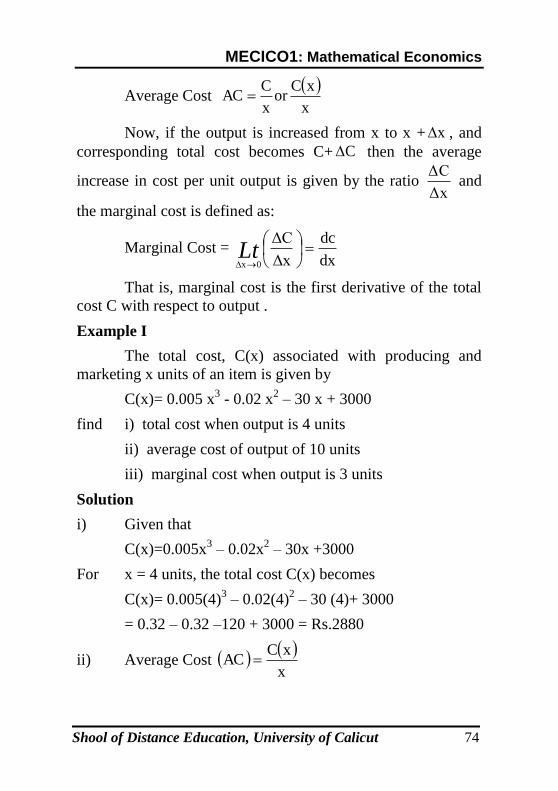
MECICO1: Mathematical Economics
Shool of Distance Education, University of Calicut 74
Average Cost x
xCor
x
CAC
Now, if the output is increased from x to x + x , and
corresponding total cost becomes C+ C then the average
increase in cost per unit output is given by the ratio ΔC
Δx and
the marginal cost is defined as:
Marginal Cost = dx
dc
Δx
ΔC
0x
Lt
That is, marginal cost is the first derivative of the total
cost C with respect to output .
Example I
The total cost, C(x) associated with producing and
marketing x units of an item is given by
C(x)= 0.005 x3 - 0.02 x
2 – 30 x + 3000
find i) total cost when output is 4 units
ii) average cost of output of 10 units
iii) marginal cost when output is 3 units
Solution
i) Given that
C(x)=0.005x3 – 0.02x
2 – 30x +3000
For x = 4 units, the total cost C(x) becomes
C(x)= 0.005(4)3 – 0.02(4)
2 – 30 (4)+ 3000
= 0.32 – 0.32 –120 + 3000 = Rs.2880
ii) Average Cost x
xCAC

MECICO1: Mathematical Economics
Shool of Distance Education, University of Calicut 75
= 3 20.005 0.02x 30x 3000
x
= 0.005x2 –0.02x–30+
x
3000
Average Cost at x = 10 units becomes
AC = 0.005 (10)2 – 0.02 (10) –30+
10
3000
= 0.5–0.2–30+300 = Rs.270.3
iii) Marginal cost at x is given by dx
dc
Therefore differentiating both sodes of C(x) with
respect to x, we have dx
dcC(x)= 0.005 x 3x
2–0.02 x 2x–30
Marginal cost at x=3 becomes
dx
dc = 0.015(3)
2 –0.04(3)–30
= 0.135–0.120–30 = Rs.30.015
2. Total Revenue (TR), Marginal Revenue (MR) and
Average Revenue (AR)
Let p be price per units and q is the number of units of
an item sold. Then the total revenue (R) is given by
R = p.q
The demand function is P=f(q). therefore R becomes
R= q.f(q)
Now average revenue (AR) or revenue per unit which
represents the price per unit is given by
X=3
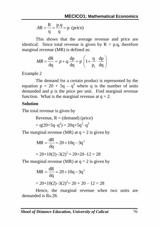
MECICO1: Mathematical Economics
Shool of Distance Education, University of Calicut 76
(price) pq
p.q
q
RR A
This shows that the average revenue and price are
identical. Since total revenue is given by R = p.q, therefore
marginal revenue (MR) is defined as:
1
dR dp q dp. p 1
dq dq p dqMR p q
Example 2
The demand for a certain product is represented by the
equation p = 20 + 5q – q2 where q is the number of units
demanded and p is the price per unit. Find marginal revenue
function. What is the marginal revenue at q = 2.
Solution
The total revenue is given by
Revenue, R = (demand) (price)
= q(20+5q–q2) = 20q+5q
2–q
3
The marginal revenue (MR) at q = 2 is given by
23q10q20
dq
dRMR
= 20+10(2)–3(2)2
= 20+20–12 = 28
The marginal revenue (MR) at q = 2 is given by
23q10q20
dq
dRMR
= 20+10(2)–3(2)2= 20 + 20 – 12 = 28
Hence, the marginal revenue when two units are
demanded is Rs.28.

MECICO1: Mathematical Economics
Shool of Distance Education, University of Calicut 77
3. Elasticity
The elasticity of a function y = f(x) at a point x is
defined as the ratio of the rate of proportional change in y per
units to the proportinal change in x. That is,
dx
dy.
y
x
dx/x
dy/yEyx
The elasticity of a function is independent of the units
in which the variables are measured because its definition is in
terms of proportional changes. Notations usually used to
denote elasticity are: ey, or ny or yx.
The above definition can also be expressed as:
Function Average
Function Marginal
y/x
dy/dx
dx/x
dy/yn y
The crucial value ny=1. However the sign of ny
depends upon the sign of dx
dy. It may be positive, negative or
zero. Apart from the sign, we are also concerned about the
absolute value |ny| of ny.
a. Price Elasticity of Supply
Let q be the supply and p be the price and the function
is expressed q = f (p). Then the formula for elasticity of
supply is same as that of ny. That is ns= dp
dq.
q
p
The sign of ns will be positive because slope of supply
curve is positive.
b. Price Elasticity of Demand
The price elasticity of demand at price 'P' is derfined
as:

MECICO1: Mathematical Economics
Shool of Distance Education, University of Calicut 78
dqdpdp
dq
q
p
p
q
q
pn Ltd
/
1
q
p- ._
0x
The sign of nd is negative, because, in general the slope of
demand dp
dqis negative.
c. Marginal Revenue and Elasticity of Demand
You know that the total revenue (R) is given by R = p.q
Where p is the price and q is the quantity sold.
Also the average revenue (AR) and marginal revenue
(MR) are defined as
Average revenue (AR) pq
qp
q
R
.
Marginal revenue (MR) ).( qpdq
d
dq
dR
dq
dp
p
qp
dq
dpqp 1 .1.
)1.....(1
11
1 .dd
ARp
Since | d | = dp
dq
q
p.
From this definition of MR, it follows that
i) If | d | = 1, then AR = 0 and hence MR = 0, i.e., total
revenue remains constant with a fall in price.

MECICO1: Mathematical Economics
Shool of Distance Education, University of Calicut 79
ii) If d | >1, then AR=0 and hence MR > 0, i.e., total
revenue increases with an increase in demand or with a
fall in price.
iii) If | d | < 1, then AR < 0 and hence MR < 0, i.e., total
revenue decreases with an increase in demand or with a
fall in price.
iv) d
d
1 hint: MR AR 1
AR
AR MR
Example 3
Suppose the price p and quantity q of a commodity are
related by the equation q = 30–4p–p2.
Find: i) Elasticity of demand d at p = 2, and
ii) Marginal revenue (MR).
Solution
i) Elasticity of demand, d is defined as:
2
d 430../
/pp
dp
d
q
p
dp
dq
q
p
pdp
qdq
2
2
2 430
2424.
430 pp
ppp
pp
p
Thus at p = 2, 9
8
18
16
)2(2430
)2(2242
2
d
x
x
ii) Marginal revenue (MR) is defined as:
dq
dp
dp
dR
dq
dRMR .

MECICO1: Mathematical Economics
Shool of Distance Education, University of Calicut 80
dpdqdp
qpd
dpdqdq
dR
/
1.
).(
/
1.
p
pppdp
d
24
.1430. 2
22 1 30 8 3
30 8 30 4 2 4 2
p pp p
p p
4. Relationship between Production, Costs and
Revenue Functions
The chain rule of differentiation can be used to
establish certain economic relationship between production,
cost and revenue functions.
Let us consider a production function where output
depends on employment of labour with fixed capital and other
inputs such that
Q = g(L) ......(1)
Where Q is output and L is labour employment.
Similarly, the total revenue function of the firm depends on the
quantity sold such that R = f (Q) .....(2)
Where R is total revenue
In order to know marginal revenue product of labour,
or in other words in order to know what is the increment of
total revenue as a result of additional employment of labour,
we are to find out the derivative of R with respect to L, i.e.,
dL
dR.
Now following chain rule of differentiation
(L) g' x (Q)f'dL
dQx
dQ
dR
dL
dR

MECICO1: Mathematical Economics
Shool of Distance Education, University of Calicut 81
Since dQ
dRis marginal revenue (MR) and
dL
dQis marginal
physical product of labour (MPP) and since dL
dRrepresent
marginal revenue product of labour (MRP).
MRP = MR x MPP .....(3)
Note: The same relationship given by (3) can be established if
we consider a demand function.
P = f (Q) ....(4)
instead of total revenue function R = f (Q).
5. Relationship between Marginal Product (MP) and
Marginal Cost (MC)
In a single explanatory variable production function
(short run), only one of the factors of production is assumed to
be variable and all other inputs are taken to be fixed. Most
common form of such production functions assume fixed
capital equipment and labour as the only variable input such
that Q = f(L). If we represents the wage rate, the total variable
cost will be V = w.L.
The marginal cost of labour is the additional variable
cost (V) due to employment of an additional labour (L) which
is given by dL
dV. But marginal cost of production is the
additional total cost due to increase in an additional output (Q).
Since the total fixed cost remains constant, the marginal cost
will be additional variable cost due to increase in an additional
output.
Thus dQ
dVMC
Using chain rule of differentiation

MECICO1: Mathematical Economics
Shool of Distance Education, University of Calicut 82
dQ
dL
dL
dV
dQ
dV
dQ
dVMC
or dV 1 w
MC dLdL dQ f '(L)
product Marginal
factor variableofcost MarginalMC
The slope of the MC curve will be given by the
derivative of MC with respect to output (Q). So the slope of
MC is
(L)f'
w
dQ
d
dQ
Vd2
2
Assuming that wage rate (w) is constant, We substitute
Z= f ' (L) to apply chain rule to find out 2
2
dQ
Vdwhich is given
by 3
(L)' f
(L)wf"- on differentiation. Since both w and f '(L) are
positive, the sign of 2
2
dQ
Vdwill depend on the sign of f "(L).
2
2
dQ
Vd>0 if and only if f " (L)<0. Thus if the marginal product
of labour is diminishing { f "(L)<0}, the slope of MC
2
2
dQ
Vdwill be positive. On the other hand if the marginal
product of labour is increasing {f "(L)>0}, the slope of
2
2
dQ
VdMC will be negagive.
a. Marginal Utility

MECICO1: Mathematical Economics
Shool of Distance Education, University of Calicut 83
In the theory of economic behaviour, normally utility
function relates to total utility (u) obtained from the
consumption of a given quantity (Q). Thus given the utility
function u = u(Q) the additional derivative from an additional
infinitesimal consumption of Q is given by derivative
'du
u QdQ
which is called marginal utility. Further, the
change in marginal utility due to infinitesimal change in Q is
given by the second order derivative.
2
n 2
d du d uu"(Q)
dQ dQ dQ
If marginal utility (MU) declines as increases, then
u"(Q) < 0 indicating the operation of the law of diminishing
marginal utility.
b. Marginal Product
In short-term analysis the production process is
assumed to have fixed inputs and only one variable, say labour
input (L). Therefore, in short-run while formulating a
production function, the output produced (Q) is a function of
labour employed (L) only such that Q = f(L). The change in
output due to infinitesimal change in the employment of labour
is given by the derivative (L)f'dL
dQ which is called marginal
product of labour. Again, the change in the marginal product
(MP) of labour due to infinitesimal change in L is given by the
derivative of MP with respect to L. That is
(Q)f"dL
Qd(MP)
dL
d2
2
Since MP declines as L increases so f"(Q) < 0 implying
the operation of the law of diminishing marginal product.

MECICO1: Mathematical Economics
Shool of Distance Education, University of Calicut 84
c. Marginal Propensity to Consume (MPC)
In macro-economics, we frequently use the concept
marginal propensity to consume (MPC) in the formulation of
consumption function. In such a consumption function, total
consumption expenditure (C) is assumed to be dependent on
aggregate income (Y) such that C = C(Y). The MPC is
defined as the change in consumption expenditure due to an
infinitesimal change in the level of income. So MPC is given
by the derivative of C with respect to Y such that
)(1 YCdy
dCMPC
If saving is denoted by S = Y – C = Y – sC(Y) = S(Y)
So the marginal propensity to save (MPS) is
).('dY
dSYS In the same way, if the import (M) is considered
to be the function of national income (Y) such taht M = M(Y),
then the derivative )('dY
dMYM is the marginal propensity to
import.
Example 4
If T = 20+x+ 20 x,x
100 and T is the total cost of
producing x chairs, find
i) Total cost for producing 100 chairs and 101 chairs
ii) The cost of 101 at chair
iii) The marginal cost at 100 chairs and 101 chairs
Solution
20,100
20 xx
xT
USER
Sticky Note
=

MECICO1: Mathematical Economics
Shool of Distance Education, University of Calicut 85
i) Total cost for producing 100 chairs is
112100
10010020100)T(at x
Total cost for producing 101 chairs is
99.112101
10010120101)T(at x
ii) The cost of 101 st chair = The cost for 101 chairs-the
total cost for 100 chairs = 0.99
iii) Marginal cost is
x
100x20
dx
d
dx
dT=
2 2
100 1000 1 1
x x
Marginal cost at x = 1000 is 0.9900 and Marginal
cost at x=101 is 0.9902.
Example 5
Find the average cost and the marginal cost functions
from the total cost function.
C = 60+10 x + 15x2
Solution
Given C = 60 +10 x 15x2
Average cost = x
15x10x60
x
C 2
= 15x10x
60
Marginal cost, 30x1015(2x)10dx
dC
USER
Sticky Note
+

MECICO1: Mathematical Economics
Shool of Distance Education, University of Calicut 86
Example 6
Find the slope of average cost curve in terms of
average cost and marginal cost.
Solution
Average cost = C/x
Slope of AC curve = /d
C Xdx
2
. 11 1
dCx C
dC Cdx MC ACx x dx x x
Note:
The above example provides the following useful
results
i) Slope< 0 if MC < AC. (This is a situation in which the
manufacturer will try to increase the production).
ii) Slope > 0 if MC > AC. (This is a situation in which the
manufacturer will try to decrease the production).
iii) Slope = 0 if MC = AC. (This is a situation in which the
manufacturer will try to maintain).
Production Function
The production function for two input variable, say
labour L and capital K, is given by
q = f(L,K) where q is the quantity of output, L is the
labour input, and K is the capital input.
Marginal product of factors of L and K are
K
qMP and
L
qMP kL
Marginal rate of technical substitution is

MECICO1: Mathematical Economics
Shool of Distance Education, University of Calicut 87
,
/
/L K
q LMRTS
q K
Factor intensity = the capital labour ratio K/L.
Average product of factors are k
q
L
qAPL kAP and
Example 7
Find out the marginal revenue function (MR) given the
average revenue function AR=10–0.5 q.
Solution
MR is the derivative of total revenue (TR) function and
TR is the product of AR and quantity (q). Now
TR = (AR). q = (10–0.5q) q = 10 q = 0.5q2
qqxTR 105.0210)(dq
dMR
Example 8
The total cost C of a firm is given by
32
3
1801001000 qqqC
Where q is the quantity produced
i) Find the marginal cost of production
ii) At what value of q does marginal cost equal average
variable cost?
Solution
(i) Marginal cost is given by the differentiation of total cost
function.

MECICO1: Mathematical Economics
Shool of Distance Education, University of Calicut 88
2
3
138021000
dq
dCMC qxqx
(ii) The average variable cost = TVC/q
3
22
q3
180q100
q
q 3
180q100q
The value of q at which MC is equal to average
variable cost (AVC) is given by the solution of the equating
MC with AVC such that
22 q
3
180q100q160q-100
or 080q160qq3
1q 22
or 22 2
q 80q 0 or q 80 i.e.,q 1203 3
Example 9
The average revenue function is given by AR=100 –3q.
Find out the elasticity of demand when q=5.
Solution
The elasticity of demand is given by the relation
AR
ηAR MR
To find out M R, we are to obtain the T R function
6q100(TR)dq
dMR
3q-100q3q)q-(100(AR)qTR 2

MECICO1: Mathematical Economics
Shool of Distance Education, University of Calicut 89
When q = 5 AR =100 - 3 x 5=85
and MR = 100- 6 x 5 = 70
66.515
85
70-85
85
MR- AR
AR
Since >1, the commodity is likely to be a luxury
good
Example 10
If the total cost function is given by
TC = 100 - 2q + 0.5q2
show that the slope of average cost (AC) curve is negative
when output is less than 10.
Solution
q
q
TCAC
25.02100
Slope of AC is given by the differentiation of AC with
respect to quantity (q).
2
22 )5.02100()5.02100(.
)(q
dq
dqqqqq
dq
dq
ACdq
d
2
25.02100)25.02(
q
qqqxq
22
2
2
22 1005.0
1005.05.021002
q
q
qqqq
2q
100-0.5AC of slope the

MECICO1: Mathematical Economics
Shool of Distance Education, University of Calicut 90
When q=10, the slope of AC is – 0.5. When q < 10, the
slope of AC will be less than -0.5.
Example 11
The total cost function of a firm is given by
TC = 625-5q+q2
show that optimum size of output of the firm is 25 units.
Solution
The optimum level of output of a firm is given by the
level of output at which average cost is minimum. The
average cost is minimum when the slope of AC curve is zero.
Now q
q5q625
q
TCAC
2
2 2
2
dq (625 5 ) (625 5 )
dq the slope of AC
dqq q q q
dq
q
2
2
q
q5q6252q)5q(
2
2
2
22 625
q
q5q6252q5q-
q
q
or slope of AC=1- 625/q2
When q = 25, the slope of AC = 0 and so 25 is the
optimum level of output. Similarly when q >25, the AC is
positively sloped as .1625
2
q
Example 12
Given the price equation, p = 100-2Q where Q is
quantity demanded, find

MECICO1: Mathematical Economics
Shool of Distance Education, University of Calicut 91
i) The Marginal Revenue
ii) Point Elasticity of demand when Q=10
iii) Nature of the commodity
Solution
i. Since marginal revenue (MR) is obtained by
differentiating the total revenue function with respect to output
(Q), we find out total revenue first, which is defined as
TR = AR x Q
or TR = (100 – 2Q) Q =100 Q – 2Q2
4Q - 100 MR
ii. Point Elasticity of demand is obtained from the
following relation
when Q 10d
AR
AR MR
MR = 100 – 4 x 10 = 60
P = AR=100–2 x 10=80
80
480 60
d
iii. Since d >1, the commodity is elastic in demand and
is supposed to be a luxury good.
Example 13
Given the production function Q = 5½ and the price
equation P = 200 – 2Q obtain the marginal revenue product of
labour (L) when L = 25.
Solution
Marginal revenue product of labour is given by the
differentiation of total revenue function with respect to labour

MECICO1: Mathematical Economics
Shool of Distance Education, University of Calicut 92
employment.
Now total revenue (R) is given by the product of price
and quantity so that
R = P x Q or R=(200-2Q) Q = 200 Q – 2Q2
Now using chain rule,
)(5LdL
d x)2Q(200Q
dQ
d
dL
dQx
dQ
dR
dL
dR ½2
-½5200 4
2Q L
5050100505
50050
(25)
500
2
20x5
2L
1000
2L
5)20L(200
½½½
½
Example 14
Given a consumption function
Y3
50001000C(Y)C
i. Find marginal propensity to consume when Y= 97
ii Find marginal propensity to save when Y = 97
iii Determine whether MPC and MPS move in the same
direction when Y changes.
Solution
MPC is given by the differentiation of the function
Y respect towith Y3
50001000C
Now C=1000 – 5000 (3+Y)-1

MECICO1: Mathematical Economics
Shool of Distance Education, University of Calicut 93
22 )3(
5000
)3(
5000)1(0
dY
dCMPC
YY
5.01000
5000
)100(
5000
)973(
500022
ii. Saving function is defined as S=Y-C
or S = Y – 1000 + 5000 (3+Y) –1
10000
50001
)3(
5000)1(01
dY
dSMPS
2
Y
=1-0.5=0.5
iii. In order to verify whether MPC and MPS move in the
same direction or not, we are to find out the rate of
growth of MPC and MPS. That means we are to find
out the derivatives of MPC and MPS.
Now 0Y)(3
50002)(
dY
Cd(MPC)
dY
d32
2
and 0)3(
25000
Y)(3
50002)(
dY
Sd(MPS)
dY
d332
2
y
x
Since 0.dY
Sd0and
dY
Cd2
2
2
2
MPC and MPS move in the
opposite direction as Y changes.
Exercises
1. Calculate the elasticity of demand of the following
functions.
a) D=10P-5
b) D=D=10+0.25p
1
2. Calculate the elasticity of demand of the following
functions when price p=10

MECICO1: Mathematical Economics
Shool of Distance Education, University of Calicut 94
a) D.100 – 2P + 0.004 p2 b) D=720 – 6.5p
3. Calculate the elasticity of supply of the following
supply functions when price p=10
a) S= -100 + 2P b) S = -77 + 4P + P2
4. Given the consumption function
Y)(5
60002000C(Y)C
i) Find out marginal propensity to consume (MPC)
and marginal propensity to save (MPS) when Y =
95.
ii) Also show that MPC and MPS move in the
opposite direction when income (Y) changes.
5. Given the production Q = 2.5L2 where Q and L are
quantity and labour and the given total revenue
function R=120 Q – 0.2 Q2 find marginal revenue
product of labour (L) when L=10.
6. A monopolist's demand curve is given by P=200 – 2.5q
Where P is price and q is quantity demanded
a) Find the marginal revenue function
b) Establish the relationship between the slopes of
average and marginal revenue curves.
c. Find out the price at which marginal revenue is
zero.
7. The total cost function of a firm is given by TC=200q –
005q3 where q is the quantity produced. Find out the
output at which marginal cost (MC) is equal to average
cost (AC).
8. A firms production is given by

MECICO1: Mathematical Economics
Shool of Distance Education, University of Calicut 95
23 10LL3
2f(L)Q
Where L is the labour employed.
Show that diminishing marginal product of labour
operates when employment of labour is 6 or more.
9. For the following total functions, state whether
marginal cost is increasing or decreasing function of
quantity produced (Q).
a) C=1000+120Q – 10Q2 +2Q
3
b. C=5050 +90Q -2Q2
10. The demand function of a firm is given by p = 50 –
0.005 q and the cost function c = 30q + 10,000 where q
is the number of outputs. Find the optimum output
level.
11. A firm has the demand function P =12 – 3 x and the
cost function T=x2 +2x. Find average cost, average
revenue, marginal cost, marginal revenue and profit for
the firm at the point of equilibrium.
12. Suppose the two demand curve of the monopolist are
P1=100-2x1 and P2 = 80 –x2 and the total cost is C=20
(x1+x2) where P1 and P2 are price and x1 and x2 are the
quantities demanded in market I and market II
respectively. Determine the equilibrium level of output
and prices in both the markets.
13. When the price of a good is x, its demand u and supply
v are given by 2x vand
2x
8xu
. Find the rate of
change of demand and the rate of change of supply at
equilibrium price. What is the elasticity of demand at
the equilibrium price?

MECICO1: Mathematical Economics
Shool of Distance Education, University of Calicut 96
14. The total cost, T of producing q units is T=100 + 7q
+ q find the marginal cost at (i) output of 100 units
(ii) output of 400 units.
15. The total cost T of manufacturing q units of a product
is 2q3q225q
3T . Find the cost of 11
th unit.
16. If the cost of selling (q units) is T and
27q4q500q
5T find the selling cost for (i)
100 units (ii) 101st units.
17. If the total cost of making q litres of an acid in Rs. is T
= -30 +80q½ . Find the number of units at which the
marginal cost is Rs.0.25.
18. Given the sales revenue function R and total cost
function T where R=1000x2 + 1000 x and T = –10000
x + 30,000 where x is the price of an item.
i) Find dR dT
and dx dx
ii) dR dt
Find x for which and dx dx
iii) Find the profit function
iv) What can you say about the value of x obtain ....
v) What is the total profit at that value of x.
vi) What can you say about this profit.
19. If the total cost is T = 50 + 10q + 25q2 find the average
and marginal cost when q =13.
20. Given the demand function q=165- 3p- 2p2 find the
elasticity of demand at the price p =5.

MECICO1: Mathematical Economics
Shool of Distance Education, University of Calicut 97
21. The supply y of a commodity at the price x is given by
y=4x2 – x+3. Find the rate at which supply is changing
when the price is 2.
22. The total money deposited in bank, y, upto the end of x
years is given by y=2x2 +x – 79. Find the rate at which
the deposit increases at the end of 5 years.
23. At the price q, the demand function y is
2
127
x
xy . Find the marginal revenue as x = 3.
24. What is the marginal revenue function for the demand
p a bx .
25. If q=100 + 10K –K2 is a production function where K
represents the capital. Find the marginal productivity
when the capital is 2.
26. If the demand function is x =25 – 4p + p2 where x is the
demand for commodity at price p, find the elasticity of
demand.
27. If the demand law is p=a – bx find the total revenue
function and marginal revenue function,
28. If the demand law is c,x
ap show that the total
revenue decreases as the output increases, MR being a
non-negative constant.
29. The demand function of a monopolist is p=15 –2x and
cost function is C(x)=x2 + 2x. Find (i) Marginal cost
(ii) Marginal Revenue (iii) Average Cost (iv) AC
when the output is 4 units.
30. For the demand law p =10–x/2 find (i) d (ii) TR
(iii) MR.
31. If the marginal revenue is 25 and elasticity of demand
w.r.f price is 2. Find the average revenue.

MECICO1: Mathematical Economics
Shool of Distance Education, University of Calicut 98
UNIT 2
MAXIMA AND MINIMA
Increasing and Decreasing Functions
We recall the definition of an increasing functions.
Function is an increasing function if the value of the function
increases with an increasing the value of the argument and
decreases with a decrease in the value of the argument in.......
f(x) is an increasing function if the following is true.
ε x,for x ),f(x)f(xxx 212121 domain of the
function. Likewise, the value of a decreasing function
increases with a fall in the value of its argument and vice-
versa.
i.e., ε x,for x ),(x f)f(xxx 212121 domain of the
function.
This section explains show the notation of the
derivative of a function can be applied to check whether given
function is an increasing function or a decreasing function in a
given interval. We have learnt that the first derivative can be
interpreted as the rate of change of the function with respect to
it argument. If the sign of the first derivative is positive, it
means that the value of the function increases as the value of
the argument increases and decreases as the value of the
argument decreases. But this is precisely the definition of an
increasing function.
Definition
A function y = f(x) differentiable in the interval (a,b) is
said to be an increasing function if and only if its derivative on
(a, b) is non negative.

MECICO1: Mathematical Economics
Shool of Distance Education, University of Calicut 99
0dx
dy i.e., in the interval (a, b).
A function y = f (x) differentiable in the interval (a,b) is
said to be a decreasing function if and only if its derivative on
(a,b) is non positive.
0dx
dy i.e., in the interval (a, b).
The derivative of a curve at a point also measures the
slope of the tangent to the curve at that point. If derivative is
positive, then it means that the tangent has a positive slope and
the function (curve) in question increases as the value of the
argument increases through the point in the neighbourhood of
this point. Similar interpretation is given to the decreasing
function and negative slope of the tangent. This is illustrated
in the following figures.
Example 1
Write down the derivative of 3x3 + 3x
2 + x – 1 and
show that this function is monotonic increasing.

MECICO1: Mathematical Economics
Shool of Distance Education, University of Calicut 100
Solution
2223 1)(3x16x9x1)x3x(3x
dx
dy
1)x3x(3xdx
d 23 is always positive since (3x+1)2
is always positive. Square of a real number is always positive.
Therefore, 3x3 +3x
3+ x – 1 is monotonic increasing
Example 2
Are the following functions monotonic?
a) y = –x6 +5 b) y=4x
5 + x
3 +3x
Solution
a) 5dy dy
= 6x . 0dx dx
when x < 0 and dy
0dx
when x > 0,
therefore, the function is not a monotonic function.
b) 4 2dy
=20 x 3 3dx
x is positive of all values of x
therefore, the function is not a monotonically
increasing function.
Convex and Concave Functions
Given a monotonic function, we know that the function
increases or decreases. What we do not know is whether the
function increases or decreases at an increasing rate or at a
decreasing rate. The sign of the second derivative of this
function gives us this knowledge. Second derivative of a
function is the rate of change of the tangent gradient. If this is
positive the function increases or decreases (depending on the
sign of the first derivative) at an increasing rate and the
function is said to be a convex function.

MECICO1: Mathematical Economics
Shool of Distance Education, University of Calicut 101
Convex Function
If second derivative of a function f(x) is positive i.e., f"
(x) > 0 b a,εx then, the function is said to be a convex
function in the given interval.
Concave Function
If b a,εx , the second derivative of a function f (x) is
negative i.e., f"(x) < 0 then, the function is said to be a concave
function in the given interval.
We notice that the slope of the tangent increases as x
increases [fig (i) ] in case of a convex function and decreases
as x increases in case of a concave function [fig I(ii)].
Example 3
Show that the curve of y=2x –3+1/x convex from
below for all positive values of x. Is same true for y=ax +
b+c/x?
Solution
We have 32
2
2 x
2
dx
yd,
x
1 - 2
dx
dy,
x
13-2x y

MECICO1: Mathematical Economics
Shool of Distance Education, University of Calicut 102
Since 2
2 3
d y 2 0dx x
for x > 0, therefore, by a
definition the curve 1
y 2x 3 x
is convex from below for
all positive value of x.
Now consider y = ax+b+c/x.
Since 02
dx
dy and
dx
dy
32
x
c
x
ca if c is positive and
in that case x
c bax y is convex from below for all
positive values of x.
Example 4
Show that the curve 3 xy is convex from below for
all negative values of x and concave from below for all
positive values of x.
Solution
We have 3 xy =x1/3
3 52
22/3
x
1
9
2
dx
ydandx
3
1
dx
dy
When 0dx
yd0,x
2
2
and the curve is concave from below.
When 2
2
d yx 0, 0
dx and the curve is concave from below.
Example 5
Show that the demand curve cb)(x
ap
is
downward sloping and convex from below. Do the same

MECICO1: Mathematical Economics
Shool of Distance Education, University of Calicut 103
properties hold of the marginal revenue curves?
Solution
We have cb)(x
ap
dx
dp since
b)(x
a-
dx
dp2
is negative (if x >0) therefore,
the demand curve is downward sloping.
b)(x
2a
dx
pd32
2
is positive for x > 0 and therefore, the
demand curve is convex from below.
Total Revenue cxb)(x
axp.xR
Marginal Revenue cb)(x
ax-b)a(x
dx
dRM
2
= cb)(x
ab2
3
2
( )
dM ab
dx x b
is negative 0x (assuming a, b > 0) and
therefore, marginal revenue curve is also downward sloping.
42
2
b)(x
6ab
dx
Md
is positive, therefore marginal revenue curve
is also convex from below.
Example 6
If the supply of a good is related to its price by
cbpax , where a, b, c are positive constants, show
that the supply curve is upward sloping and concave to axis OP

MECICO1: Mathematical Economics
Shool of Distance Education, University of Calicut 104
at all points.
Solution
We have b-pac-x c,bpax
2
a
c-xb-p ,bp
a
cx
ba
c-xp
2
02
dx
pd and 0c)-(x
a
2
dx
dp
22
2
2
a
Since 0dx
pd and c for x 0
dx
dp
2
2
, therefore,
supply curve is upward sloping and convex from below (i.e.,
concave to the OP axis).
Stationary Values - Maxima and Minima
When we talked about the sign of first derivative, we
showed that if the derivative of a function is positive
(negative), then the function is an increasing (decreasing)
function. We did not consider the possibility where the
derivate was equal to zero. We discuss this case and relate it
to the maximum and minimum value of a function.
If the first derivative of a function at some point is
zero, we say that the function is neither increasing nor
decreasing and is momentarily stationary at that point. The
value of the function at that point is known as the stationary
value. The stationary point may be a point of maximum value
or minimum value or a point of inflexion. We discuss the first
two, postponing the discussion on the third until a later section.

MECICO1: Mathematical Economics
Shool of Distance Education, University of Calicut 105
We begin by defining the maximum and minimum values of a
function.
Here we are interested in the case when the derivative
is zero at a given point say, If f '(a)=0 then f(x) is neither
increasing nor decreasing. The value of the function is
momentarily stationary and the curve has a tangent parallel to
the x-axis. The value of the function at such a point is called
Stationary value.
Maximum and Minimum Values
Consider the curve y = f(x) given above. Consider the
points A, B and C. We can see that the curve ceases to
increase through these points and beings to decrease. Where
as through the points D, E and F the curve ceases to decrease
and beings to increase. Such points where the curve ceases to
increase and beings to decrease and vice versa are called
turning points or stationary points on the curve and the value
of the function at these points are called turning values or
optimum values.
Definition
If, for a differentiable function y = f(x), x = x1, is a
point of maximum or minimum value, then the derivative of
the function at x=x1, is equal to zero i.e., 0dx
dyor 0(x)f' .

MECICO1: Mathematical Economics
Shool of Distance Education, University of Calicut 106
This is a necessary condition for maxima or minima of
functions and not a sufficient condition. If f ' (x) at some value
of x is equal to zero, we can not say that the function has
reached a maximum or a minimum. What we know from this
is merely that the function is stationary at these points and they
can be either points of maximum, or minimum or points of
inflexion. Therefore, we need something more than the
necessary conditions.
Proposition
A sufficient condition for a function to have a
maximum value (a minimum value) at the point x=x1 is that
the derivative of the function changes sign from positive
(negative) to negative (positive) as we move from the left of x1
to the right of x1 through x1.
Now, we are in a position to give a complete criterion
for maximum (minimum) value of a given function.
Definition
A point x1 is said to be a point of maximum value of a
function y=f(x) if the value of the function, in the
neighbourhood of the point x1 is smaller than
Δx)f(x)f(x i.e., f(x) 111 sufficiently close, in absolute value,
x1.
Definition
A point x2 is said to be a point of maximum value of a
function y=f(x) if the value of the function, in the
neighbourhood of the point x2 is greater than
)f(xΔx)f(xi.e., f(x i.e., f(x) 2222 for Δx sufficiently close,
in absolute value, x2.
f(x1) and f(x2) are known as maximum and minimum
values, respectively and extremum values, collectively.

MECICO1: Mathematical Economics
Shool of Distance Education, University of Calicut 107
Creterion
Given a function, y = f(x),
a) A necessary condition for extremum at x=x1 is f ' (x1)=
0, ie., 0dx
dy
b) If the sign of the second derivative at x =x1 is positive,
x1 is a point of minimum and if it is negative, x1 is a point of
maximum (sufficient condition).
Before giving examples on extreme values, we give a
working rule to evaluate the minimum or maximum values of a
function.
Working Rule to find Minimum and / or Maximum Values
Step 1: Given a function y = (x), find the first derivative f ' (x)
and solve the equation f '(x)=0, 0dx
dy to get x = x1, x2...., as
solutions [(f '(x1)=f ' ((x2) = ....0)]
Step 2: Get the second derivative at these values of x.
i) 0d
or ,0)(x f" If2
2
1 dx
y we have a maximum at x
=x1.
ii) 0d
or ,0)(x f" If2
2
2 dx
y we have a minimum at x
=x2.
Example 6
Find the maximum and minimum value of the function
2x4x1Y
Solution
Given y=1+4x–x2
dy 4 2x
dx

MECICO1: Mathematical Economics
Shool of Distance Education, University of Calicut 108
For maximum or minimum,
2 x4,2x 0,2x-4 i.e., 0 dx
dy
Now, ve- 2,- dx
yd
2
2
Y has a maximum at x = +2
The maximum value of the function is
y = 1 + 4 x 2 –(2)2 = 1 + 8–4 = 5
Example 7
Find the maximum and minimum values of
y = 2x3–3x
2 – 12 x +4
Solution
Let y = 2x3 – 3x
2 –12x + 4
For maximum or minimum, we have 0. dx
dy
Here 126x6x dx
dy 2
0126x6x demands 0. dx
dy 2
6(x2–x–2) = 0, i.e., x
2–x–2=0;
i.e., 2 1 0 2 0x x x or 1 0x
i.e., x = 2 or x= –1
Now 2
2
d y 12x -6dx

MECICO1: Mathematical Economics
Shool of Distance Education, University of Calicut 109
When 2
2
d y x 2, 12 2 6 18, ve.
dx Therefore y
has minimum when x=2.
Minimum value of y = 2 23–3.2
2–12.2 +4
= 16–12–24+4= –16
When 2
2
d y x 1, 12 (-1)-6 -18, -ve
dx
Therefore y has maximum at x= –ve
Therefore y has maximum at x = –1
Maximum value of y =2 (–1)3 –3 (–1)
2 –12(–1)+4 = 11

MECICO1: Mathematical Economics
Shool of Distance Education, University of Calicut 110
UNIT 3
ECONOMIC APPLICATIONS OF MAXIMA
AND MINIMA
1. Cost Minimization
One of the basic problems of a producer is to find out
the level of output at which the average cost of production is
minimum or the average variable cost of production is
minimum. We can apply the conditions of minimization as
given in the last section.
TC = aq2 + bq + C ....(1)
Where q is the quantity and C is the total fixed cost and
all parameters are positive.
The average cost is given by
q
Cbaq
q
TC AC ....(2)
To find out the output at which the average cost (AC)
will be minimum, we have to satisfy the following first order
and second order conditions such that
0dq
(AC)d and 0
dq
d(AC)
2
2
Now a
Ca 2
2q0r 0
q
C - 0
dq
d(AC)
a
C -or either ,
a
Cq
a
C

MECICO1: Mathematical Economics
Shool of Distance Education, University of Calicut 111
Since output cannot be negative, we choose a
Cq
Now 2
2 1
2 3
d (AC) 20 - (-2) Cq
dq
C
q
When 2
2 3
( ) 2, 0,
C d AC Cq
a dq q since a > 0 and C > 0
the average costs will be minimum at C/aq
If the average cost is given by the function
AC=aq2 + bq + C, (a > 0; b < 0; c > 0)
Then the determination of output at which the average
cost (AC) will be minimum requires that
0dq
(AC)d and 0
dq
d(AC)2
2
Now 2a
b-q 0, b aq 2
dq
d(AC)
and 0 a as 0a 2dq
(AC)d2
2
Thus the average cost will be minimum when the
output is –b/2a.
It may be noted that marginal cost curve cuts the
average cost curve at the minimum point of AC curve as
shown in figure. We take the total cost function (1). The
marginal cost is given by
b aq 2dq
d(TC)MC
Thus at minimum cost,

MECICO1: Mathematical Economics
Shool of Distance Education, University of Calicut 112
AC = MC
b2abq
Cbaq
or C/aq C/aqor aqC/q 2
Since output cannot be negative, therefore the average
cost will be minimum when C/aq . This is the same value
of output we derived using first and second order conditions of
minimization.
Example I
Find out the output at which the average cost is
minimum from the total cost function TC=2q2 + 5q + 18.
Solution
The average cost is given by
q
1852q
q
TCAC

MECICO1: Mathematical Economics
Shool of Distance Education, University of Calicut 113
Minimization of AC requires that the first order
differentiation of (1) with respect to q should be equal to zero.
So we have
0q
1802
dq
d(AC)2
or 39q 92
182 q
We take q = +3
The second order condition of maximization requires
that
2
20
d AC
dq
Now 2
2 3 3
d (AC) 18 36( 2) 0 if q 3
dq q q
The output at which average cost is minimum is 3.
Example 2
Given the short-run total cost function
C=2q3 – 15q
2 + 30q + 16
a. Find out the level of output at which average variable cost
(AVC) is minimum and also show that MC = AVC at the
total output.
b. Show that when output q=4, the average cost is minimum
and MC=AC.
Solution
a. The total variable cost is given by
TVC = 2q3 –15q
2 + 30q

MECICO1: Mathematical Economics
Shool of Distance Education, University of Calicut 114
3015q2qq
TVC AvC 2
The minimization of AVC requires
0; dq
(AVC)d and0(AVC)
dq
d2
2
Now 0(AVC)dq
d gives 4q – 15 = 0.
04dq
(AVC)d 3.75,
4
15q
2
2
q = 3.75 is the level of output at which AVC is minimum.
Now
3 2 2dC dMC 2q 15q 30q 16 6q 30q 30
dq dq
or MC = 6q2 – 30q + 30
When q=3.75, MC=1.87 and AVC = 1.87
MC = AVC at minimum point of AVC curve.
b. The average cost (AC) function is given by
q
163015q2q
q
CAC 2
The minimum value of AC requires that
0dq
(AC)d and 0
dq
d(AC)2
2
Now 2
d(AC) 160 gives 4q -15 0 - 0
dq q

MECICO1: Mathematical Economics
Shool of Distance Education, University of Calicut 115
and 2
2 3
d (AC) 324 0
dq q
when q=4, 0dq
d(AC)
the average cost is minimum when q = 4
Now at q = 4
MC = 6q2 – 30q + 30 = 6 (4)
2 – 30 (4) + 30 = 6
AC = 2q2 – 15 q + 30 + 16/q
= 2(4)2 – 15 (4) + 30 + 4 = 6
MC = AC when q = 4
2. Profit Maximization
In producer's equilibrium or in the theory of firm, the
basic problem is to choose the combination of price and
quantity in order to maximize profits (the question of choosing
price does not arise for a firm under perfect competition as the
price is given). The optimum level of output which maximizes
profit of a firm is arrived at when
a. Marginal revenue equals marginal cost and
b. Marginal cost curve cuts marginal revenue curve from
below.
C(q) - (q) R or CR
....(1)
So finally profit () is also function of quantity (q)
In order to obtain the level of output at which the profit
will be maximum, we follow the procedure of maximizing a
function in which the first derivative is zero and the second
derivative is negative.

MECICO1: Mathematical Economics
Shool of Distance Education, University of Calicut 116
Thus
MC MRor (q) ' C (q) ' Ror 0 (q) ' C - (q) ' dq
d gives 0 R
dq
d
....(2)
The second order condition states
2
2"( ) " (q) 0 or R" (q) C" (q)
dR q C
dq
or
slope of MR < slope of MC.
The conditions set by (2) and (3) imply that for profit
maximization, MR=MC and MC should cut MR from below.
The first order and second order - conditions of profit
maximization under imperfect competition as well as under
perfect competition can be more clearly seen from the figures
(1) and (2) respectively.
Figures 1 (a), 1 (b) and 1 (c) show that at equilibrium
output b q gap between total revenue and total cost is
maximum and so the profit function attains the highest point of
the profit curve and MC=MR with MC cutting MR from
below. At output q1, total cost over total revenue is maximum
and so the profit attains the minimum point with MR=MC but
MC cuts MR from above.
The same is the condition under perfect competition as
shown in figures 2 (a), 2 (b) and 2 (c).
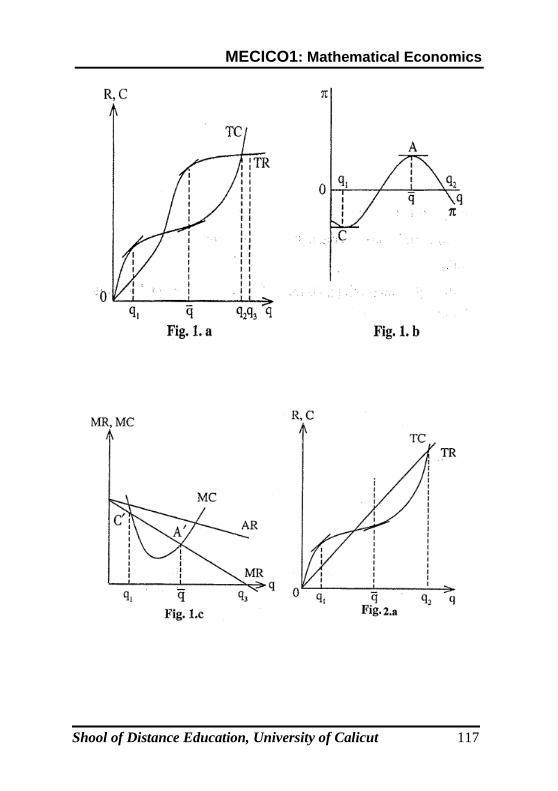
MECICO1: Mathematical Economics
Shool of Distance Education, University of Calicut 117

MECICO1: Mathematical Economics
Shool of Distance Education, University of Calicut 118
Example 3
In a perfectly competitive market, the total revenue and
total cost of a firm are given by R=20q and C= q2 + 4q +20.
Find profit maximizing output and maximum profit.
Solution
By definition profit () is the difference between total
revenue (R) and total cost (C)
= R – C or = 20 q – q2 – 4q –20
Since = f (q) , the maximum of profit requires
0. d
and 02
2
dqdq
d
Now 8 qor 16 2qor 0 4- 2q - 20 dq
d
Again 022
2
dq
d
Since the second order derivative is negative, q=8 will
maximize profit of the firm. The maximum profit is obtained
by substituting q=8 in the profit function.

MECICO1: Mathematical Economics
Shool of Distance Education, University of Calicut 119
Maximum profit = 20 x 8 – (8)2 – 4 x 8 – 20 = 44
Example 4
A monopolists has the following total revenue (R) and
total cost (C) functions R = 30 q – q2,
C= q3 – 15 q
2 + 10 q +
100
Find
a) Profit maximizing output
b) Maximum Profit
c) Equilibrium price
d) Point elasticity of demand at equilibrium level of output.
Solution
a) The profit function is given by
= R – C = 30q – q2 – q
3 + 15q
2 – 10 q – 100
or = – q3 + 14q
2 + 20 q – 100
For profit maximization, 0 d
and 02
2
dqdq
d
dq
d= 0 gives –3q
2 + 28q +20 =0 or 3q
2 – 28q – 20 =
0
2x3
20)4x3x((28)28q
2
= 28 1024 28 32 2
10 or - 6 6 3
Now 2
26 28
dq
dq

MECICO1: Mathematical Economics
Shool of Distance Education, University of Calicut 120
When 2
210, 32 0
dq
dq
the profit maximizing output is q = 10.
b. Substituting q=10 in profit function we get maximum
profit = – (10)3 + 14 (10)
2 + 20 x 10 - 100 = 500.
c. The price equation or average revenue function is
obtain as .q
R
q30q`
q2-q 30 Price
For equilibrium output q=10, Price = 30 –10 = 20
d. Point Elasticity of demand is define as MRAR
AR
Now MR= 30 – 2q = 30 –2x10=10
and AR = Price = 20 21020
20
Example 5
A firm has the total cost (C) function C=7q2 + 5q + 120
and demand function P=180 – 0.5q and also a subsidy of Rs.5/-
per unit of output is paid by the government. Find
a. Profit maximizing output and price
b. Maximum Profit
c. Impact of subsidy on equilibrium output and prices.
Solution
a. When q units of output is produced, the total cost of
subsidy will be 5q. Likewise total revenue is given by
R=p.q = (180 – 0.5q) q=180q –0.5q2

MECICO1: Mathematical Economics
Shool of Distance Education, University of Calicut 121
So profit with subsidy is defined as
= TR – TC + subsidy
= 180q –0.5q2 – 7q
2 –5q–120 + 5q
or = 180q –0.5q2 – 7q
2 –120
Profit maximization requires that
0d
and 02
2
dqdq
d
Now
12 q
180 15qor 014q - q - 180or
0 14q - q (0.5) 2180
dq
d
Now 01514102
2
dq
d
with q = 12, the profit will be maximum. The
profit maximizing price is obtained by substituting q=12 in the
price equation.
P = 180 –0.5q = 180 –(0.5) x 12 = 180 –6=174
b. Maximum profit is obtained by putting q = 12 in (1)
= 180 x 12 –0.5 (12)2 – 7 (12)
2 – 120 = 960
c. In order to study the impact of subsidy on equilibrium
price and quantity, we are to find out equilibrium values
without subsidy. So profit without subsidy (*) is given by
* = 180q –0.5q2 – 7q
2 – 5q–120
Now 05-14q- (0.5)q 2-180 gives *
dp
d
or 175–q= –14q=0 or 15q = 175 q = 11.67

MECICO1: Mathematical Economics
Shool of Distance Education, University of Calicut 122
015*
2
2
dp
d
So profit maximizing output without subsidy, q=11.67
Substituting q = 11.67 in the price equation, we have
P=180–0.5q = 180 –(0.5) (11.67)
= 180 – 5.83 = 174.17
So the equilibrium profit without subsidy.
* = 180 (11.67) –0.5 (11.67)2 – 7(11.67)
2 – 120=900
Thus equilibrium price, output and profit with and
without subsidy indicate that output increases, price falls and
also profit increases as a result of provision of subsidy to the
firm.
3. Revenue Maximization
As we stated in the previous section that the profit
maximization is the objective of the producing firm, the
revenue maximization instead of profit may also be the
objective for an imperfectly competitive firm. However, a
firm cannot pursue revenue maximization, irrespective of what
happens to profit. Even with the objective of revenue
maximization, the firm must earn a certain minimum amount
of profit which is sufficient enough to satisfy its shareholders.
So profit maximizing output without subsidy, q=11.67
Substituting q=11.67 in the price equation, we have
P=180–0.5q=180 – (0.5) (11.67)
= 180 – 5.83 = 174.17
So the equilibrium profit without subsidy
* = 180 (11.67) –0.5 (11.67)2 – 7(11.67)
2 –120=900

MECICO1: Mathematical Economics
Shool of Distance Education, University of Calicut 123
Thus equilibrium price, output and profit with and
without subsidy indicate that output increases, price falls and
also profit increases as a result of provision of subsidy to the
firm.
3. Revenue Maximization
As we stated in the previous section that the profit
maximization is the objective of the producing firm, the
revenue maximization instead of profit may also be the
objective for an imperfectly competitive firm. However, a
firm cannot pursue revenue maximization, irrespective of what
happens to profit. Even with the objective of revenue
maximization, the firm must earn a certain minimum amount
of profit which is sufficient enough to satisfy its shareholders.
Example 6
A firm has a total revenue function R=20q –2q2 where
q is quantity and a total cost (C) function C=q2–4q+20.
Find the revenue maximizing output level and the
corresponding value of profit, price and total revenue.
Solution
The maximization of total revenue function R=20q –
2q2 requires that 0
dq
Rd and 0
dq
dR2
2
Now 5. qor 0 4 dq
d 0,4q-20 gives 0
dq
dR2
2
the revenue maximizing output is 5.
With the total cost, C=q2–4q +20, the profit function is
= (20q –2q2) – (q
2 –4q + 20) or
= 20q –2q2 – q
2 + 4q – 20

MECICO1: Mathematical Economics
Shool of Distance Education, University of Calicut 124
the level of profit at revenue maximizing output q =
5 is given by
= (20x5 –2(5)2 – (5
2) +4x5– 20–25
The price if the product, when q=5, is
10 2x5- 20 2q- 20q
RP
The maximum revenue = 20q–2q2=20x5–2(5)
2=50
Example 7
The total revenue (R) and total cost (C) functions of a
firm are given as
R=26q – 3q2 where q=quantity, C=2q
2 -4q + 10
Find (a) the profit maximizing output and
corresponding profit, price and total revenue at the level of
output.
(b) The revenue maximizing output and corresponding
profit, price and total revenue at the level of output.
Solution
a. The profit function is given by
=R–C=26q – 3q2
– 2q2 + 4q –10
Profit maximization requires that
......(1)
0 dq
d and 0
dq
d2
2
1044q-6q-26 gives 0dq
d
30 10 10q

MECICO1: Mathematical Economics
Shool of Distance Education, University of Calicut 125
10 20q
2q
or 10q=20 2,q 2
2
d10 0
dq
q=3 is profit maximizing output
So maximum profit is given by
2 2π 26x3 3(3) 2(3) 4x3 10 35
Price at profit maximizing output
173x3263q26q
Rp
Total revenue R=Pq = 17 x 3=51
b. The revenue maximization requires that
0 dq
d and 0
dq
d2
2
RR
Now 33.4 3
1 4q 06q-26 gives 0
dq
d
R
At the revenue maximizing level of output q=4.33
=26(4.33)–3(4.33)2–2 (4.33)
2 + 4 (4.33)–10=26.15
133(4.33)263q26q
Rp
R=pq =13 (4.33) = 56.25
c. Since profit at the revenue maximizing output level is
26.15, the profit constraint 30 will prevent the firm to
attain revenue maximizing output. If profit is set at = 30,
then the solution of the profit function.

MECICO1: Mathematical Economics
Shool of Distance Education, University of Calicut 126
26q–3q2–2q
2 + 4q–10=30 or
5q2 – 30q +40=0 or q=4
gives the highest revenue fetching output.
Points of Inflexion
A point of inflexion for a single valued function y=f(x)
is said o exist if the function changes its curvature at the point.
The function may become concave from convex or convex
from concave at the point of inflexion. The value of the
function corresponding to this point is known as inflexion
value. We discuss some features of points of inflexion and see
how the idea of extrema can be extended in the case of
inflexion points.
The following figures illustrate points of inflexion for
the two types of inflexion cases.
Notice that, in both the types of inflexion points the
tangent to the curve at the point of inflexion crosses the curve.
In figure (i), the inflexion points is x1 where the curve changes
its curvature from convex to concave. To the left of x1 the
tangent at any point on the curve lies below the curve, to the
right of x1, the tangent to any point on the curve lies above the
curve and only at the point of inflexion does the tangent cross
the curve. The same is true for the other types of the point of
inflexion.

MECICO1: Mathematical Economics
Shool of Distance Education, University of Calicut 127
The following figure, also show the characteristics of
point of inflexion.

MECICO1: Mathematical Economics
Shool of Distance Education, University of Calicut 128
Criterion (Inflexion Points)
Given a single valued function y=f(x),
a) A necessary condition for the point of inflexion at x=x1
is f " (x1) = 0
b) The sufficient condition for the point of inflexion at
x=x1 is f "' (x1) 0
If f "(x1) > 0, we have an inflexion point for concave to
convex function f "(x1) we have an inflexion point for convex
to concave function.
Example 8
Show that the curve 1
22
x
xy has three points of
inflexion separated by a maximum and a minimum point.
We have 1
22
x
xy
2 2
2 22 2
x 1 2 2x.2x 2 1 xdy
dx x 1 1 x

MECICO1: Mathematical Economics
Shool of Distance Education, University of Calicut 129
42
2222
2
2
x1
2xx1 2x-1 24x x1
dx
yd
42
222
x1
x-1 41 2-2x x1
x
32
3
32
22
x1
3 x4x
x1
2x2x-1- 4x
3or 0 either x 0dx
yd2
2
a) Case (i) x=0
we have 2
2
dx
yd>0 for x < 0
and 2
2
dx
yd < 0 for x > 0 in the neighbourhood of x=0
therefore, x = 0 is a point of inflexion.
b) Case (ii) 3x
3for x 0 dx
yd2
2
2
2
d y
dx3for x 0 in the neighbourhood of
x + 3 therefore 3 x is a point of inflexion.
2
2 2
dy 2(1-x )0 0 1
dx (1 )x
x
USER
Sticky Note
USER
Sticky Note
x2

MECICO1: Mathematical Economics
Shool of Distance Education, University of Calicut 130
maximum, ofpoint a is 1 xe, therefor0, 1)(1
3)-(1 )1(4
maximum, ofpoint a is 1 xe, therefor0, 1)(1
3)-(1 )1(4
3
1
2
2
3
1
2
2
x
x
dx
yd
dx
yd
Thus, we have seen that 1
22
x
xy has three points of
inflexion 3,0,3- separated by a point of minimum at
x= –1 and a point of maximum at x=+1
Example 9
Prove that the curve y=x3 has a single stationary point
which is a point of inflexion.
Solution
We have 23 3x
dx
dyxy
0x 0 6xdx
yd2
2
and
2
2
d y6x 0 x 0
dx Therefore, y = x
3 has a single
stationary point which is a point of inflexion.
Exercises
1. Find the minimum value of the cost function y=5+2x2–x
3
2. Find the maximum and minimum value of the function
3x2–36 x +10
3. Find the maxima and minima 4x3–21x
2 +18 x + 20
4.
Determine the maxima and minima 2x3–3x
2 –36 x + 20

MECICO1: Mathematical Economics
Shool of Distance Education, University of Calicut 131
5. Determine the maximam value of y = xe-x
6. Find the maximum and minimum values of the function
Y = (x–1) (x + 2)2
7. Find the maximum profit that a company can make if the
profit function is given by p(x) = 41 –24x –18x2
8. Find the maximum value of y=6x4 –10x
3 +6x
2+5
9. Find the maximum and minimum values of the function
Y = x3 –9x
2 +15x +3
10. Show that the function x
xy
2
2 has a minimum and a
maximum and that the former is greater than the later.
11. A firm has revenue function R=600q – 0.003q2 and the
cost function. C=150q + 60000.
12. A firm sells all the product it makes at Rs.9/- per unit.
The cost of making x units is C=0.1 x3+3x+8. Find the
maximum profit for the firm and also the number of units
to be sold for securing maximum profit.
13. A firm sells a product at Rs.3/- per unit. The total cost of
the firm for producing x units is given by C=20+0.6x +
0.01 x2. How many units should be made to achieve
maximum profit. Verify that the condition for a
minimum is satisfied.
14. The amount (in lakhs of rupees) A invested in a firm and
the profit p are expected to have a relation p=400+200A–
50A2. For what value of A, p attains the maximum.
15. Suppose the equation connecting the profit p in rupees
and the number of units n produced in a single lot of a
factory is given by p=247 + 1243n –0.025n2. Determine
the optimum lot size of the factory?

MECICO1: Mathematical Economics
Shool of Distance Education, University of Calicut 132
UNIT 4
FUNCTIONS OF SEVERAL VARIABLES AND
PARTIAL DIFFERENTIATION
Introduction
We have already studied the rules of differentiation
relate to the functions of a single independent variable. But in
most economic problems a particular economic variable
depends on a number of other independent variables. In such
cases, some of the independent variables may have positive
effect on the dependent variable while others may have
negative effect. Let us refer to a demand function where
quantity demanded (Qd) depends on the price of the product
(P), price of related goods (PR), income of consumer (1) and
say, the size of the family (S) such that
Qd = f (P, PR, I, S)
The impact of rise in the price of the product and the
price of the complementary goods on demand is negative. But
the increase in income of the consumer and increase in the size
of the family of the consumer will raise the demand for the
product. Further, the increase in the price (s) of the substitute
(s) is likely to raise the demand of the product. In such a
situation, when all the variables like price, prices of
complementary and substituted goods, income, family size etc.
increase simultaneously, it is impossible to trace out or to
quantify the effect of an individual independent variable on the
dependent variable. Say, for instance, if the price increases
from Rs.10 to Rs.13 per unit of output and income of
consumer increases from Rs.3000 to Rs.3500 per month
simultaneously and the net demand increases form 20 kg to 21

MECICO1: Mathematical Economics
Shool of Distance Education, University of Calicut 133
kg. We cannot trace out the individual effect of rise in price by
Rs.3 and increase in incom by Rs.500 on the change in the
demand since both price and income increase at the same time.
In such a situation, we are interested to find out or quantify the
effect on individual independent variable on the change in the
value of dependent variable. This can be done only when we
assume that when a particular independent variable changes,
the other independent variables don't change at the same time.
In terms of the above example, when we want to quantify the
effect of change in price on demand we must assume that the
income of the consumer, prices of related goods and size of
family of consumer don't change. Similarly, in order to trace
the effect of change in income on demand, price of the
product, prices of related goods and size family of the
consumer are assumed to remains same. When we find out
such effects by using the technique of differentiation, it is
known as "partial derivatives". It is called "Partial derivatives"
in the sense that the effect of individual independent variable
on the dependent variable is "partial" as the other independent
variable are assumed to be unchanged.
But when all the independent variables change
simultaneously, we may be interested to find out the total net
effect on the dependent variable. This can be done with the
help of the concept of total differentiation.
Partial Differentiation
In order to define the concept of partial derivative, let
us consider a function having 'n' independent variables.
y = f (x1, x2, x3, ..... , xn) (1)
where the variables x1, x2,...., xn are all independent of each
other so that each can vary itself without resulting in any
variation in the other variables. A change in the value of x1
with all other independent variables x1, x2,...., xn remaining

MECICO1: Mathematical Economics
Shool of Distance Education, University of Calicut 134
unchanged, will bring about corresponding changes in the
value of y. If x1, denotes the change in the value of x1, the
new value of x1 becomes (x1 +x1). If the corresponding
change in the value of y is denoted by x1 the value of y will
change to (y +y).
n3211 x...,x,x,Δxx f Δy y or
yx...,x,x,Δxx f y n3211 or
x
n21n3211
1
x.., ,x,x fx...,x,x,Δxx f
x
y
1x
y
represents the rate of change in y with respect to a
change in the value of x1 assuming other independent variables
x2, x2, ....xn to be constant.
Taking the limiting value of x1 equal to zero, the limit
of the quotient 1x
y
is called the "partial derivative" of y with
respect to x1 and is denoted by
1
Δx1 Δx
Δylim
x
y
01
(2)
similarly, the partial derivative of y with respect to the second
variable is denoted by
2
Δx2 Δx
Δylim
x
y
0 2
Assuming that other variable x2, x2, ....xn remain
unchanged. In the same way, the partial derivatives of y with
respect to the other independent variables can be defined. The
process of finding the partial derivative is called partial
differentiation.

MECICO1: Mathematical Economics
Shool of Distance Education, University of Calicut 135
Partial derivates are assigned distinctive symbols.
Instead of using the letter d as in the case of ordinary
derivative dx
dy, the symbol (delta) is employed to indicate
partial derivative such as nx
y
,...,
x
y,
x
y
21
etc. The partial
derivatives ae also denoted f1, f2, .... fn etc. to express partial
derivative respect to x1.
Thus partial derivative 1x
y
measures an instantaneous
rate of change of y with respect to an infinitesimal change in
x1. So 1x
y
will then provide information about both the
direction and magnitude of change in y resulting from an
infinitesimal change in the value of x1.
Example 1
Given
2 2
1 2 1 1 2 2
1 2
y yy f(x ,x ) 2x x x 3x find out and
x x
Solution
In the process of finding 1x
y
, we treat x2 as a constant.
So in the process of differentiation the additive constant 2
23x
will vanish and the multiplicative constant (in terms of x1 x2)
will be retained. Similarly in finding 1
2
,x
yx
will be
considered as constant and usual rules of differentiation will
follow. Thus

MECICO1: Mathematical Economics
Shool of Distance Education, University of Calicut 136
21211
1
x4x0x4xfx
y
21212
2
x6xx6x0fx
y
It appears from the above results that the partial
derivatives are also functions of x1 and x2. Thus we can write
f1 = f2 (x1, x2)
f2 = f2 (x1, x2)
Example 2 Find f1 and f2 given
3
2
2
21
3
121 3x x2xx)x,(x f y
Solution 02x3xfx
y 2
2
2
11
1
constant) x(since 2x3x 2
2
2
2
1
Similarly 2
2 1 2 2
2
yf 0 2x 2x 9x
x
= 4x1 x2 +6x2 (since x1= constant)
Example 3 Find f1 and f2 given
2 2
1 2 1 1 2y f x ,x x 5 2x x
Solution: Since the function y is the product of two functions,
the partial derivatives are derived by using product rule of
differentiation.
Now
5)(x x
)x(2x)x(2xx
5)(xfx
y 2
1
1
2
21
2
21
1
2
11
1
2 2
1 1 2 1(x 5) (2-0) (2x x ) (2x 0) (since x1 is constant)

MECICO1: Mathematical Economics
Shool of Distance Education, University of Calicut 137
= 1
2
21
2
1 )2xx(2x5)2(x
2
21
2
1
2
1 xx24x102x
2 2
1 1 2 6x 2x x 10
5)(x x
)x(2x)x(2xx
5)(xfx
y 2
1
2
2
21
2
21
2
2
12
2
2 2
1 2 1 2 1(x 5) (-2x ) (2x x ) x 0 (since x is constant)
2
1 2 22 10x x x
Example 4 Given 212
2
1
2
21
x
y and
x
y find
)3x(x
)x(2xy
Solution
Since the function is a quotient of two functions, the
quotient rule of differentiation shall be applied to derive the
partial derivatives 21 x
y and
x
y
Now
2
2
2
1
2
2
1
1
2
21
2
21
1
2
2
1
1 )3x(x
)3x(xx
)x(2x)x(2xx
)3x(x
x
y
2 2
1 2 1 2 1
222
1 2
x 3x .2 2x x 2x (since x is constant)
x 3x
=2
2
2
1
2
21
2
12
2
1
)3x(x
x2x4x6x2x
MECICO1: Mathematical Economics
Shool of Distance Education, University of Calicut 138
2 2
1 2 1 2
2 2
1 2
2x 6x 2x x
(x 3x )
Similarly
2
2
2
1
2
2
1
2
2
21
2
21
2
2
2
1
2 )3x(x
)3x(xx
)x(2x)x(2xx
)3x(x
x
y
constant) is x(since )3x(x
3 )x-x2()2x (- )3x(x12
2
2
1
2
2122
2
1
2
2
2
1
2
21
2
22
2
1
)3x(x
3x6x6x2x-
x
2 2
1 2 2 1
2 2
1 2
-2x x 3x 6x
(x 3x )
Example 5
Give
21
3
2
2
21
2
121x
yand
x
y find ),xx5x(x)x,f(xy
Solution
We use here modified version of chain rule of
differentiation. So taking ,xx5xxu 3
2
2
21
2
1
We have y = (u)5.
11 x
u x
x
y
du
dy
= constant) is xsince ( 05x2xx 5u 2
2
21
4

MECICO1: Mathematical Economics
Shool of Distance Education, University of Calicut 139
2
21
43
2
2
21
2
1 52x 5 5 xxxxx
Similarly,
22 x
ux
du
dy
x
y
2
221
4 3x x2x5x0 x 5u
2
221
43
2
2
21
2
1 3xx10x xxxx 5
Example 6
Given y=log 21
4
221
2
1x
y and
x
y find,xx2x50
Solution
Here also Chain rule of differentiation is applied in a modified
way
4
221
2
1 xx2xx50u
)log(uy
constant is xsince 02x2x0x u
1
x
ux
du
dy
x
y221
11
4
221
2
1
21
250
22
xxxx
xx
Similarly
2 2
y dy ux
x du x
3
1 2 1
1 0 0 2x 4x since x is constant
u

MECICO1: Mathematical Economics
Shool of Distance Education, University of Calicut 140
4
221
2
1
3
21
x250
42
xxx
xx
Example 7
A consumer consumes two commodities x1 and x2 and
the utility function is given by 221
2
1 5xx3xxu
Fin out marginal utilities of x1 and x2.
Solution
The marginal utility is noting but the increase in total
utility as a result of consumption of additional unit and is given
by the derivatives. Since the utility function involves two
variables x1 and x2, the marginal utility of x1 and x2 will given
by the partial derivative of u with respect to x1 and x2
respectively.
Marginal utility of x1 is given by
constant is xsince 03x2xx
u221
1
=2x1 + 3x2
Similarly, marginal utility of x2 is given by
constant is xsince 53x0x
u11
2
= 5+3x1
Example 8
Given a demand function of Engel's curvetype
D=AP
N
Where D is demand, P is price, N is income and A,,

MECICO1: Mathematical Economics
Shool of Distance Education, University of Calicut 141
are parameters. Find the partial derivatives N
D and
P
D and
also interpret the values of , and .
Solution
In the function D=APN, when we differentiate D will
respect to P, N taken to be constant.
β1α NAPα,
P
D
or P
D
P
NAP α
P
D βα
Similarly,
1-βα NAP .
N
D
constant) is P (since N
NAP
βα
or N
D
N
D
From the above partial derivative
P
P
D
D
P
D
P
D
//
pricein change ateProportion
demandin change ateProportion
= Price elasticity of demand
Similarly,
N
N
D
D
N
D
P
D
//

MECICO1: Mathematical Economics
Shool of Distance Education, University of Calicut 142
incomein change ateProportion
demandin change ateProportion
= Income elasticity of demand
and represent price elasticity and income
elasticity of demand respectively.
Exercise
21 x
and x
y Find
y of the following functions:
i) 2
2
2
11 10x
x
x3xy
ii) 2
2
3
121 2x4xy xx
iii) 21
212
1
3x5
yxx
exx
iv) 2
2
1
3
1
2
221 5x 2 xxxxxy
v) 2
2
2
12
2
1 2x 23 xxxy
vi) 4
2
2
21
2
1 x10x3xy x
vii) 1072
12
2
2
21
3
1
xxxy
viii) 50x3xx2xlogy 2
2
1
3
21
ix) 21
2
2
3
1
2
1
5100
12
xx
xxxy
x)
2
2
2
11
3
2
2
21
2
1
15
3xx8x2x10
xxxy

MECICO1: Mathematical Economics
Shool of Distance Education, University of Calicut 143
Second order Partial Derivative
We can observe, from the above, that in a function
y=f(x), the derivative f ' (x) or dx
dy is also a function of x.
Similarly in case of a function y= f (x1, x2), the partial
derivatives 1 2
1 2
fy y
f andx x
are also functions of x1 and
x2. This implies that 21
and x
y
x
y
can be differentiated
partially again with respect to x1 and x2 to yield second order
partial derivatives.
So in case of a function
y=f (x1, x2) (1)
the first order partial derivative 1
1
fx
y
can be further
differentiated partially with respect to x1 to give
112
1
2
11
fx
y
x
y
x
(2)
f11 in equation (1) measures the rate of change of f1
with respect to x1 assuming x2 to be constant. Similarly the
second order partial derivative of the function (1) with respect
to x2 is defined as
222
2
2
22
fx
y
x
y
x
(3)
So, f22 in (3) measures the rate of change f2 with
respect to x2 while x1 is assumed to be constant.
We have already stated that f1 is a function of x1 and x2
just like f2 is a function of x1 and x2. When f1 is differentiated

MECICO1: Mathematical Economics
Shool of Distance Education, University of Calicut 144
partially further with respect x2 or when f2 is differentiated
partially with respect to x1 ; both the second order partial
derivation are known as "cross-second order partial
derivatives" and denoted by
12
21
2
12
fx
y
x
y
x
x (4)
and 21
12
2
21
fx
y
x
y
x
x (5)
Example 9
Given
.f and f,d,f,f,f Find .3xxx2x)x,f(xy 222112112 1
2
221
2
121
Solution: Here f1 = 4x1 + x2, f2 = x1 + 6x2
11
1 1
y
x xf
4044x
21
1
xx
22
2 2
y
x xf
6606x
21
2
xx
12
12x
y
xf
1104x
21
2
xx

MECICO1: Mathematical Economics
Shool of Distance Education, University of Calicut 145
21
21x
y
xf
21
1
6x
xx
=1+0=1.
Example 10
Find f11, f12, f22, and f21 with reference to the example 3
above
Solution
1026x )(x
2
21
2
1
1
1
1
11
xx
xff
2
21 212 xx
2 2
12 1 1 1 2
2 2
6x 2 10x
f f x xx
21 2 .2 xx
= – 4x1 x2
22
2
1
2
2
2
22 102x- )(x
xxx
ff
2
112 10x
22
2
1
1
2
1
21 10 2x- )(x
xxx
ff
= –4x1 x2
The concept of second order partial derivative can be
extended to a function having more than two independent
variables say, in
y=f (x1, x2,x3)
USER
Highlight
-2

MECICO1: Mathematical Economics
Shool of Distance Education, University of Calicut 146
We can have nine second order partial derivatives f11,
f12, f13, f21, f22, f23, f31, f32 and f33.
Example 11. Given sthe function
2 2 2
1 2 3 1 1 2 2 3y f x ,x ,x x 10 2x x 3x x
find all nine second order partial derivatives
Solution In the function 2
3
2
22
2
11 x3xx2x10x
2
233323231
3223
2
322121
13112211
213
2
23
31
2
32
2
12
32211
x6f , x12x f ,0f
x12xf , 6x f ,4xf
0f , 4x f ,4xf
constant) as xand x(assuming xx6 f
constant) as xand x(assuming x6x2xf
constant) as xand x(assuming x4xf
Exercises
1. Find the four second order partial derivatives of the
following functions.
2
2
2
121
2
2
1
2
21
2
3
21
2
1
xxx2)(x log 3 y c)
5x3xxx2y b)
xx3x2xy a)
2. Find the nine second order partial derivatives of the
following functions.
2
3
2
2
2
13
2
1
31
2
322
3
1
xxx3xx15y b)
xxxx3xxy a)

MECICO1: Mathematical Economics
Shool of Distance Education, University of Calicut 147
UNIT 5
DIFFERENTIALS AND TOTAL DIFFERENTIALS
We have already stated that in a function y= f (x1, x2),
partial derivative measures the rate of change in y with respect
to an infinitesimal change in the value of x1 assuming x2 to be
constant. Similarly f2 holding x1 to be constant. When both
x1 and x2 change simultaneously the resultant total change in y
is known as total differential. Let us now explain and define
the concept of differentials and then the concept of total
differentials.
Differentials
Let us consider a function y =f (x) where an arbitrary
change in the value of x (denoted by x) will bring about a
corresponding change in the value of y. (denoted by x), the
rate of change in y being the difference quotient Δx
Δy such that
ΔxΔx
ΔyΔy
(1)
But when we assume that the change in the value of x
is infinitesimal and corresponding change in the value of y is
infinitesimal, then the difference quotient will become the
derivative dx
dy and the infinitesimal change in x and y are
denoted by dx and dy respectively. Thus equation (1) can be
rewritten as
.dxdx
dydy

MECICO1: Mathematical Economics
Shool of Distance Education, University of Calicut 148
or dy = f ' (x).dx (2)
Where dx and dy represent what are known as
differentials of x and y respectively.
As shown in equation (2) since the differential dy is
simply equal to f ' (x) times dx, the process of finding dy is
straight forward. For example y =10x3, then the differential of
y is
dy = f ' (x) .dx =30x2 .dx
For a given value of x and dx, we can easily evaluate
the dy expression above.
Total differentials
The concept of total differentials is applied to functions
of more than one explanatory variables. Thus in a function y=f
(x1, x2) , the total change in y from simultaneous infinitesimal
change in both x and y is given by
2
2
1
1
.dx x
ydx
x
ydy
(3)
or dy = f1.dx1+f2dx2 which is called total
differential of the y function.
Here we consider a simple example in economics. A
saving function can be formulated as depending on national
income and the rate of interest such that
S=S(Y,i) (4)
Where S is savings, Y is national income and i is the
rate of interest. The partial derivative 1x
y
measures the rate of
change in S with respect to an infinitesimal change in Y
assuming that the rate of interest in constant. So the change in
S due to change in Y may be represented by the expression

MECICO1: Mathematical Economics
Shool of Distance Education, University of Calicut 149
dy.x
y
1
. Similarly effect of change in i assuming Y to be
constant can be expressed as ..i
Sdi
The total change in S or
total differentials will be equal to the sum of the differentials
of S with respect to Y and i such that.
..diS.dYs dSor
.di i
SdY
Y
SdS
iy
(5)
The process of finding such total differentials is known
as total differentiation.
We can consider another economic example where the
function depends on a large number of explanatory variables.
Say, in a utility function where the consumer consumes in
commodities, the function relation is given by
u=u (x1, x2, ... , xm). (6)
The total differential of the utility function is given by
m
m
2
2
1
1
.dxx
u......dx
x
u.dx
x
udu
or du = u1.dx1 + u2 .dx2 + ... um .dxm (7)
Each term on the right hand side of equation (7)
indicates the amount of change in u as a result of infinitesimal
change in one of the explanatory variables. The economic
interpretation is that the first term u, dx1 implies the marginal
utility of the first commodity times the increment in the
consumption of first commodity and similarly the other terms

MECICO1: Mathematical Economics
Shool of Distance Education, University of Calicut 150
also interpreted. The sum of all these terms in equation (6)
represent the total change in utility due to change in the
consumption of m commodities x1, x2, .... , xm.
The rules of differentials are broadly the same as the
rules of derivatives as studied earlier.
Example 1
a) Find differential dy of the function y = 10+2x + 3x2
Solution .dx 6x)(2 dy
).3210( 2
or
dxxxdx
ddy
b) Find differential of the function x10
2xy
2
Solution
.dx
x10
2x40xor
.dxx10
2x -4x x10dyor
.dxx10
2x
dx
ddy
2
2
2
2
2
c) Find total differential dy of the
function 2
2
2
121 2xxx2xy
Solution 1 2
1 2
y ydy .dx
x xdx
2 1 1 1 2 2or dy 2x 2x .dx 2x 4x dx
d) Find total differential of the function
2
21
2
1 xx10 xlog 2y

MECICO1: Mathematical Economics
Shool of Distance Education, University of Calicut 151
Solution
2211
2
2
1
2211
2
212
1
2
2
1
1
.dxx2xdxxx
4dyor
dxx2xdxx2xx x
2dyor
.dxx
ydx
x
ydy
Exercises
1. Find the differential dy for each of the following
functions
22
32
23
2
2
23x
10xy e)
2xx 2x y d)
4x y c)
3xx x 110 y b)
810x5xy a)
2. Find the total differential dy for each of the following
functions
2
21
2
21
2121
3
2
2
1
2
2
3
12
2
1
xx log 2xx2y c)
3x10xxxx2x y b)
x2xxxy a)
Total derivatives
While defining total differential in the previous section,
we considered a function with two independent variables such
that y=f (x1, x2). But if we consider a situation when x1 and x2
are not independent then we have the function.

MECICO1: Mathematical Economics
Shool of Distance Education, University of Calicut 152
y = f (x1, x2) where x2 = g (x1).
(1)
Since x1 is related to x2 (via function g), a change in x,
will not only affect y directly (via the function f), but also
affected y indirectly by changing y (via the function g). Thus
the rate of change in y with respect to x1 is given by
1
2
211
1
1
1
221
1
1
2
2
1
11
1
dx
x
y
x
y
dx
dyor
1dx
since dx
dyor
dx
dx
dx
dx
dx
dy
dx
dxdx
dxff
ff
(2)
1dx
dy in equation (2) is called total derivative of y with
respect to x1. The total derivative is obtained from the total
differential dy= f1dx1 + f2dx2 by dividing both sides by dx1.
1
22
1
11
1 dx
dxf
dx
dxf
dx
dy
The first term on the right hand side of equation (2)
indicates the direct effect of change in x1 on y. But the second
term 1
2
2 dx
dx.
x
y
measure the change in y resulting from change
in x2 with the change in x2 resulting from initial change in x1.
It means that the second terms of (2) measures the indirect
effect of x1 on y.
We can take an example to find out total derivative
considering a function

MECICO1: Mathematical Economics
Shool of Distance Education, University of Calicut 153
5x x where2xxy 3
122
2
1
Thus applying the definition in terms of
(2)
1
2
211 dx
dx.
x
y
x
y
dx
dy
=2
11 2x3x2x
or 2
11
1
6x2xdx
dy
If we have another function
4-x x wherexx3y 2
12
2
2
2
1
then
4x4x6xdx
dyor
)(2x 4)2(x6x
)(2x )(2x6x
dx
dx.
x
y
x
y
dx
dy
2
111
1
1
2
11
121
1
2
211
Now we consider a function y=f (x1, x2) where
x1 = g (t)
(3)
X2 = h (t)
To find out the total derivative of (3) withe respect to t,
first we find the total differential dy = f1dx1+f2dx2
Now dividing both sides by dt, we get
dt
dxf
dt
dxf
dt
dy 22
11

MECICO1: Mathematical Economics
Shool of Distance Education, University of Calicut 154
or dt
dx
x
y
dt
dx .
x
y
dt
dy 2
2
1
1
For example, let us take a function
10-2t x x wherex3x2y 2
2
12
2
1 t
6 t2t 8dt
dyor
62t 2t 4
23 2t 4x
dt
dx
x
y
dt
dx .
x
y
dt
dy
2
2
1
2
2
1
1
Exersises
1. 2
221
2
121dx
dy derivative out total find 5 x3 x wherexx4yGiven xx
2. 2
2
21
2
2211dx
dy derivative out total find 5 x wherex2x45yGiven xxx
3. 2
21
2
21dx
dy derivative out total find 2x5 x where3- x 2xyGiven
4. Find the total derivative
2t.5x,3t x where6xx5x2xy wheredt
dy2
2
1
2
221
2
1
5. Find the total derivative 2dx
dy given
.5x9 x where3x2x 5xy 211
2
2
2
1

MECICO1: Mathematical Economics
Shool of Distance Education, University of Calicut 155
UNIT 6
OPTIMIZATION WITH EQUALITY CONSTRAINT
Concept of Constrained Extrema
We have already examined the technique of
unconstrained (or free) extrema, where the optional value of a
function with more than one explanatory variable was derived
without having any constraint on the optional choice of the
values of the explanatory variables. There was no question of
choice inn determining the optimal value. But in practice,
there are many economic problems which involve finding an
optimal solution with one or more constraints. For example, in
the theory of consumer behaviour, a consumer has to choose
the combination of goods in order to maaximize his total utility
keeping in view his total income or budget of the consumer as
a constraint. So the budget limitation will restrict the choice of
the consumer in deciding the purchase of the basket of goods.
Similarly, in case of equilibrium of a firm in the factor market,
the cost of production is minimized choosing a combination of
the factor inputs keeping in view the production function as a
constraint. These types of problems are called constrained
optimization. In this chapter, we intend to discuss the
technique of finding the extreme value of a function with
equality constraint(s).
Let us consider a function having two explanatory
variables x1 and x2 such that y = f (x1 , x2) (1)
We want to find out the combination of x1, x2 that will either
maximize or minimize the function (1) subject to the
satisfaction of an equality constraint.
g (x1, x2) = C (2)
Where C is a constant

MECICO1: Mathematical Economics
Shool of Distance Education, University of Calicut 156
Whatever the values of x1 and x2 chosen optimally in
(1), they must satisfy the equation (2). Equation (1) is called
the "objective function" and the equation (2) is known as
equality constraint. The effect of an equality constraint (equ.2)
on the optimal solution of a function with two explanatory
variables (1) can be explained graphically in a three-
dimensional graph as shown in figure (1).
The unconstrained (or free) extremum of the function
is at the peak of the entire dome while the constrained
extremum is at the peak of the inverse U shaped curve lying
directly above the constraint line AB. Normally the
constrained maximum is expected to have a lower value than
the unconstrained (on free) maximum, although by
coincidence, both may happen to have the same, value. But it
should be noted that constrained maximum can never exceed
unconstrained maximum.
Lagrange Multiplier Method
As we have discussed in detail in earlier chapters when
we have a problem of unconstrained (free) extrema,
determination of optimal values requires the satisfaction of

MECICO1: Mathematical Economics
Shool of Distance Education, University of Calicut 157
straight forward first order and second order conditions. Just
for reference, when we have a function.
y=f (x1, x2, x3, ...., xn)
maximization of y requires that
f1 = f2 = f2 =f3 = .... =fn = 0
and |H1|<0,|H2|>0,|H3|<0, ..., (–1)n |Hn|>0
Similarly, for minimization of y, we need to have
f1 = f2 =f3 = .... =fn = 0
and |H1|>0,|H2|>0,|H3|>0, ..., |Hn|>0 where |Hk| is
called Hessain determinant of order k.
But when we have an objective function to be
maximized or minimized subject to the satisfaction o an
equality constraint, Lagrange multiplier method seeks to
convert the constrained extremum problem into a form to
which the first order and second order conditions of
unconstrained extremum can be still applied.
First Order Conditions
With the objective function (1) and the equality
constraint (2) in a optimizing problem with two explanatory
variables x1 and x2 , when we want to obtain the extreme value
of the objective function, we first construct the Language
function which is the modified version of the objective
function incorporating the constraint as follows,
2121 x,x gcλx,x fL (7)
The symbol (the Greek letter lambda) representing
some undetermined value is called a Lagrange multiplier. If
we have the objective of maximizing (1) subject to (2), then
the maximization of Lagrange function (7) will provide the
optimal values of x1 and x2 which will maximize.

MECICO1: Mathematical Economics
Shool of Distance Education, University of Calicut 158
y=f (x1, x2) = c
Satisfying the equality constraint
g(x1, x2) = c
Since the language function given by (7) is now a
function of three variables x1, x2 and , the maximization of L
in equation (7) requires to satisfy the first order and second
conditions of maximization. In this case, the first order
condition requires.
0λ
L and 0
x
L 0,
x
L
21
Now
0λgfLx
L111
1
0λgfLx
L222
2
(8)
0x,x gcLλ
L21λ
(since c is constant, its derivative is zero). From the first two
equations of (8)
2
2
1
1
g
f
g
fλ (9)
Since the last equation of the system of equations (8) is
simply a restatement of the equality constraint (2), Lagrange
function L will automatically satisfy the constraint of the
original objective function (1).
The same first order conditions given by (8) are true for
the minimization problem where we want to minimize the
objective function (1) subject to satisfaction of the equality
constraint (2).

MECICO1: Mathematical Economics
Shool of Distance Education, University of Calicut 159
The first order conditions of optimization (8) obtained
by using Lagrange multiplier method, can also be derived by
using total differential approach. The total differential of the
objective function y=f(x1, x2) is given by
dy = f1dx1 + f2dx2 = 0 (10)
or 1
2
2
1
f
f
dx
dx (11)
The statement (10) is still valid even if we add the
constraint g(x1, x2) = c. However, we cannot consider dx1 and
dx2 as ”arbitrary" changes is view of the constraint. Now the
total differential of the constraint is
g1dx1 + g2dx2=dc = c (12)
or 1
2
2
1
g
g
dx
dx (13)
From (11) and (13),
`1
2
1
2
2
1
f
f
dx
dx
g
g
or 1
2
1
2
g
g
f
f (14)
Thus, first order condition of optimization with an
equality constraint given by (14) using total differential
approach is the same as the first order constrained optimization
condition given by (9) using Lagrange multiplier method.
Second Order Condition
The introduction of an additional variable in the form
of in Lagrange function (7) makes it possible to apply the
same first order condition of unconstrained extremum problem
in constrained extremum problem also. However, we should
not apply the second order sufficient condition of

MECICO1: Mathematical Economics
Shool of Distance Education, University of Calicut 160
unconstrained (free) extremum in form of Hessain determinant
|H1|, |H2|, |H3|, in the Lagrange function (7). This is because of
the fact that although the optimal solution L depends on the
optimal choice of x1, x2 and , but unlike 21 x and x the choice
meaningless. Even if is replaced by any other value, no
effect will be produced on L since [c–g(x1, x2)] is identically
zero for any value of Lagrange multiplier. Thus, while it is
extremum, we should not blindly follow the second order
condition of unconstrained extremum in the present case of
Lagrange function. So we will restate the second order
conditions of constrained extremum in terms of total
differential and derive a new set of second order conditions for
constrained extremum.
With a constraint g(x1, x2)=c, the choice of x1 and x2 in
the objective function y=f (x1, x2) is not independent or
arbitrary and so dx1 and dx2 are also not arbitrary. Since from
(12), 1
2
12 dx
g
gdx , for specific value of dx1 and dx2 depends of
g1 and g2 which in turn depend x1 and x2. So dx2 will depend
on x1 and x2. The second order condition of extremum
depends on the value of second order total differential d2y. To
find the appropriate value d2y in view of the equality constraint
g(x1, x2) = cwe have.
2
2
1
2
2 dxx
(dy)dx
x
(dy)d(dy)yd
2
22212212112
2
111
22221211212111
22211
2
12211
1
dxfdxdxfdxdxfdxf
dx dxfdxfdx dxfdxf
dx
dxfdxf
xdxdxfdxf
x
or 2
2222112
2
111
2 dxfdxdxf2dxf yd (15)

MECICO1: Mathematical Economics
Shool of Distance Education, University of Calicut 161
Now from equality constraint g(x1, x2) = c, dg=0 and so d2g =
d(dg)=0
Following 1(15), in a similar way
0dxgdxdx2gdxggd 2
2222112
2
111
2 (16)
2
2
2222112
2
1112
2
g
dxgdxdx2gdxgxd (17)
2
2
2222112
2
1112
2
2222112
2
111
2
g
dxgdxdx2gdxg f-dxfdxdx2fdxfyd
or
g
dxgdxdx2gdxg fdxfgdxdxf2gdxfgyd
2
2
2222112
2
1112
2
222221122
2
11122
2
222
2
2222112
2
212
2
111
2
211 dx g
g
ff dxdx g
g
ff 2dx g
g
ff
2
2 2222211212
2
11111 dx λgf dxdx λgf 2dx λgf (18)
(14) from f
2
2 g
Now partially differentiation (8) with respect to x1, x2 and we
have
L11 = f11 – g11
L12=f12 – g12=L21
L22 = f22 – g22 (18)
Substituting (18) in (17), we get

MECICO1: Mathematical Economics
Shool of Distance Education, University of Calicut 162
2
2222112
2
111
2 dxLdxdx2LdxL yd
or 2
22221212112
2
111
2 dxLdx dxLdxdxLdxL yd (19)
When we have to determine the constrained extremum
of y = f (x1, x2) subject to g (x1, x2) c, the second order
sufficient conditions will depend on the algebraic sign of the
second order total differential d2y. While determining the sign
of d2y, the value of dx1 and dx2 (not both zero) should satisfy
the linear constraint.
g1dx1 + g2dx2 = 0 from (12)
i) For maximum value of y, d2y should be negative
definite subject dg = 0
ii) For maximum value of y, d2y should be positive
definite subject dg = 0
In case of unconstrained extremum the sufficient
conditions are expressed in form of Hessian determinant |H|,
but in case of constrained extremum, we will express the
sufficient conditions in terms of bordered Hessian determinant
|H| .
Now from (13)
1
2
12 dx
g
gdx
and substituting it in (19) , we get (20)
2
12
2
2
122
2
1
2
112
2
111
2 dx g
gLdx
g
g2LdxLyd
or 2
2
2
12
1222112
2
211
2 dx g L 2LgLyd
ggg (21)
From (21), it is distinctly clear that d2y is positive
(negative) definite if value within bracket is positive

MECICO1: Mathematical Economics
Shool of Distance Education, University of Calicut 163
(negative). Now the value within bracket of (21) can be
expressed as a 3x3 symmetric determinant such that
2
122
2
2112112
2
1222112
2
211 L - g L 2L Lgg 2LgL gggg
L L
L L
g g 0
-
2221 2
12111
21
g
g (22)
Thus for maximization d2y0 subject to dg = 0 requires
that
0 Lgg 2LgL 2
1222112
2
211 g
or 0
L L
L L
g g 0
-
2221 2
12111
21
g
g (23)
The determinants in (22) and (23) are known as
bordered Hessian determinant and symbolized by |H| and in
this case it is specifically denoted by |H| 2 as there are two
explanatory variables in the optimization problem.
Three Variable Case
When we have an objective function with a constraint
having three explanatory variables x1, x2 and x3 in the form,
say,
Maximize y = f (x1, x2, x3) (1)
Subject
g (x1, x2, x3) = c (2)
then we have the Lagrange function as
L = f (x1, x2, x3) + [c–g (x1, x2, x3) ]

MECICO1: Mathematical Economics
Shool of Distance Education, University of Calicut 164
Using the total differentials, the first order condition
requires
0λ
L L and 0
x
L L 0,
x
LL 0,
x
L
3
3
2
2
1
1
L
The second order condition requires
0
L L L
L L L
L L L
g g g 0
|H| and 0
L L
L L
g g 0
|H|
3332313
232221 2
1312111
321
3
2221 2
12111
21
2
g
g
g
g
g
For minimization of the function (1) subject to the
constraint (2), the first order conditions are the same as in case
of maximization and the second order condition requires
.0|3H| and 0|H| 2 In this manner we can generalize the
result with n explanatory variables.
Example I
Maximize y = x1x2+2x1 (1)
subject to x1+2x2=20 (2)
Solution
Now the Lagrange function is given by
L=x1x2 + 2x1+(20–x1–2x2) (3)
The first order condition of maximization requires
0λ
L L and 0
x
LL 0,
x
L
2
2
1
1
L
Now

MECICO1: Mathematical Economics
Shool of Distance Education, University of Calicut 165
L1 = x2 +2– =0
L2 = x1 +2=0 (4)
L = 20–x1 – 2x2=0
From first two equations of (4) , we have
42or x 2
2 211
2 xx
x (5)
Adding now equations (2) and (5), we get
12x 242x 11
Now substituting x1=12 in 5), we have 2x2 = 8
4x1
To test whether 12x1 and 4x 2 will maximize the
objective function (1 or not, we have to verify the value of
|H| 2 as second order condition.
Now from
L11 = 0 L12 = 1
L21 = 0 L22 = 0
04
0 1 2
1 0 1
2 1 0
L L
L L
g g 0
|H|
2221 2
12111
21
2
g
g
Since 4x and 12x ,0H| 212 will maximize the
objective function (1) subject to the constraint (2) the
maximum value will be
y = x1x2 +2x1 = 48+24=72

MECICO1: Mathematical Economics
Shool of Distance Education, University of Calicut 166
Example 2
Maximize a function y = 5x1x2 subject to x1 + 2x2 = 8
Solution The Lagragean function is given by
L=5x1x2 +(8–x1–2x2) (1)
The first order condition requires
0λ
L L and 0
x
LL 0,
x
L
2
2
1
1
L
Now
L1 = 5x2 – =0
L2 = 5x1 –2=0 (2)
L = 8 –x1 – 2x2=0
From first two equations of (2), we have
010x - 5xor 2
55 21
12
xx (3)
From the third equation of (2), we get
x1+2x2=8 (4)
Now multiplying both sides of (4) by 5 and adding to (3), we
get
4
401010
5
0105
1
2
1
1
21
x
xx
x
xx
Substituting x1 = 4 in (4) we get
2x2 =8 –4=4
x2=2
USER
Sticky Note
=
USER
Highlight
USER
Sticky Note
change
USER
Sticky Note
avoid 10x1

MECICO1: Mathematical Economics
Shool of Distance Education, University of Calicut 167
The second order condition for maximization requires that
0H| 2 .
From (2) L11 = 0., L12= L21=5 and L22 =0
Again from (4) g1=1 and g2 =2
020
0 5 2
5 0 1
2 1 0
L L
L L
g g 0
|H|
2221 2
12111
21
2
g
g
4x 1 and 2x 2 will maximize the function y = 5x1x2
and the maximum value will be 40)2( )4( 5 y .
Example 3.
Minimize 124x2x subject to2xxxxy 21221
2
1
Solution
With the objective function to minimize 221
2
1 2xxxxy
Subject to 12 – 2x1–4x2 = 0, the Lagrange function is defined
as
21221
2
1 4x2x-12 2xxxxL
(1)
For minimization, first order condition requires
0λ
L L and 0
x
LL 0,
x
L
2
2
1
1
L
Now
L1 = 2x1 – x2 – 2=0
L2 = x1 + 2 – 4 = 0 (2)
L = 12 –2x1 – 4x2=0
From the first two equations of (2), we get
USER
Sticky Note
add |
USER
Sticky Note
-x1

MECICO1: Mathematical Economics
Shool of Distance Education, University of Calicut 168
1 2 12 x 2
2 4
x x
or 8x1–4x2= –2x1+4
or 10x1 – 4x2 = 4 (3)
From the third equation of (2), we have
2x1+ 4x2 =12 (4)
Adding (3) and (4), we get
3
4 x 1612x 11
Now substituting get we(4),in 3
41 x
2 1
2
4 284 12 2 12 2
3 3
7 x
3
x x
To test whether 3
7 and
3
421 xx will maximize or
minimize the objective function or not, we find out the second
order condition |H| 2
Now from the set of equation (2),
L11=2; L12 = –1 =L21 ; L22 = 0 and g1 = 2; g2=4.
048
0 1- 4
1- 2 2
4 2 0
L L
L L
g g 0
|H|
2221 2
12111
21
2
g
g
3
7x and
3
4,0|H| 222 x

MECICO1: Mathematical Economics
Shool of Distance Education, University of Calicut 169
Will minimize the objective function
221
2
1 2xxxxy
the minimum value will be
3
10
3
72
3
7
3
4
3
42
y
Example 4
Using Lagrange multiplier method, find the extreme
value of the function
2
221
2
1 x2
3xxxy
Subject to x1+ 2x2 = 14
Solution The Lagrangean function in case of the above
problem is defined as
21
2
221
2
1 2xx14 λx2
3xxxL (1)
Now from first order condition extremum
L1 = 2x1 – =0
L2 = x1+3x2 –2=0 (2)
L = 14 –x1 – 2x2=0
From (2)
2
32 21
21
xxxx
or 4x1 = x1+3x2
or 3x1 – 3x2 = 0
or x1 – x2 = 0 (3)
From the third equation of (2) x1+2x2=14
USER
Sticky Note
delete example 4 with its solutions

MECICO1: Mathematical Economics
Shool of Distance Education, University of Calicut 170
Multiplying (3) by 2 and adding to (4), we get
7x1 =14, x1=2
Substracting (3) and 3rd
equation in (2)
2 2
1
3 14 14
14
x x
x
Now substituting x1 = 2 in eqution (4) we have x2 = 6.
To test whether x1 = 2 and x2=6 will maximize or
minimize the objective function we are to find out the value of
the bordered Hessian determinant |H| 2 for which we need to
find out.
L11 = 2; L12=1 = L21 ; L22=3 and g1; g2=2
Now -76- 1-
3 1 2
1 2 1
2 1 0
L L
L L
g g 0
|H|
2221 2
12111
21
2
g
g
Since ,0|H| 2
x1 = 2 and x2 = 6 will minimize the function
2
221
2
1 x2
3 xxxy
subject to x12x2 =14
The minimum value of y is given by
70)6(2
3 (6) )2()2( 22
Exercises
Find the extreme values of the following functions
subject to the given constraint.

MECICO1: Mathematical Economics
Shool of Distance Education, University of Calicut 171
1. 122x3x subject to xx2x2xy 212211
2. 22x xsubject to x2x4x3xy 21221
2
1
3. 24x62x subject to x2x5xx20y 21
2
221
2
1
4. 20x24x subject to x2x5xx2
1y 21
2
221
2
1
5. 9x53x subject to x3x2x2xy 21
2
221
2
1
6. 96x22x subject to 20 x2
1x2xx
2
1y 21
2
221
2
1

MECICO1: Mathematical Economics
Shool of Distance Education, University of Calicut 172
UNIT 7
COMPARATIVE STATIC ANALYSIS
Marginal Productivity
The marginal physical product of capital (MPPk) is
defined as the change in output brought about by a small
change in capital when all the other factors of production are
held constant. Given a production function such as
Q=36KL –2K2 –3L
2
the MPPk is measured by taking the partial derivative ./ KQ
Thus,
4K36LK
QMPPK
Similarly, for labor, MPPL= 6L.36KLQ/
Example Find the marginal physical productivity of the
different inputs or factors of production for the production
functions
i) Q=6x2+3xy+2y
2
ii) Q=x2+2xy+3y
2+1.5yz+0.2z
2
Solution
i)
222
K 0.2z1.5yz3y2xyxQ3y 12xx
QMPP
4y3xY
QMPP4y 3x
Y
QMPP yY
ii) MPPx = 2x+2y
USER
Sticky Note
delete from MPPy =

MECICO1: Mathematical Economics
Shool of Distance Education, University of Calicut 173
MPPy = 2x+6y+1.5z
MPPz=1.5y +0.4z
Multiplies
1. The concept of multiplier which occupies a very
significant place in the filed of economic analysis and which
become a powerful tool of economic analysis in the hands of
J.M Keynes.
The concept of multiplier was first of all introduced as
Employment Multiplier by Cambridge Economist R.F.Khan.
The theory of investment multiplier was developed by
J.M.Keynes in his book entitled 'General Theory'.
Theory of multiplier explains that increase in the total
income brought about through increased investment spending
will be a certain multiple of the original investment outlay
depending on the propensity to consume.
The investment multiplier which is defined as pro-rata
change in total income (Y) to a given initial change in
investment (for consumption) spending I with which the total
change in income is associated, as related to marginal
propensity to consume in a way such that higher the marginal
propensity to consume, larger is the multiplier and vice versa.
Since multiplier is related to marginal propensity to consume,
hence it is essential to make a reference to it.
Types of Multiplier
On the basis of factors influencing the level of income
multiplier can be classified in following categories. Some of
the specific factor multipliers are,
i. Employment multiplier
ii. Consumption multiplier
iii. Export multiplier

MECICO1: Mathematical Economics
Shool of Distance Education, University of Calicut 174
iv. Foregin investment multiplier
v. Tax multiplier
vi. Government expenditure multiplier
vii. Transfer payments multiplier
viii. Balanced budget multiplier
Employment Multiplier
The ratio between overall increase in employment and
subsequent primary employment is called employment
multiplier.
p
EmpN
NK
Where,
KEmp = Employment Multiplier
N = Change in total employment
Np = Change in the level of initial employment
Export Multiplier
Changes in the volume of exports are well manifested
through income of the country. Let us assume that amount of
export is increased by Ex, which in turn causes an increase in
the level of income. Let the increase in income be denoted by
Y. Export Multiplier (KExport) can be expressed
mathematically as:
Y = Ex/(1-b)
or Y = KExportEx
or KExport = Y/Ex
Thus, export multiplier shows the relationship between
change in income corresponding to the volume of exports.

MECICO1: Mathematical Economics
Shool of Distance Education, University of Calicut 175
Tax Multiplier
Variations in the amount of tax are very well reflected
on income. Let us suppose, an additional dose of tax causes
tax to rise by Tax, which causes a change in income
equivalent to Y. Tax multiplier which is denoted by (KTax)
can be represented mathematically as:
Y = -bTax/1-b
-b/1-b=KTax
Y = -KTax.Tax
KTax = b
b
Tax
Y
1
Thus, Tax multiplier is the ratio between change in
aggregate income and amount of tax. It is always negative.
Government Expenditure Multiplier
Alike other factors an increase in government
expenditure causes fluctuations in the level of income. If
initial government expenditure G changes by a small amount
G and Income by Y; then Government expenditure
multiplier (KGov,Expen.) can be represented mathematically as:
Y = Gb
1
1
or Y = KGov.Expn. G
ie., KGov.Expn= Y / G
Thus, Government Expenditure Multiplier is the ration
between change in aggregate income and government
expenditure.
Comparative Static Analysis in a National Income Model

MECICO1: Mathematical Economics
Shool of Distance Education, University of Calicut 176
In a macro-economic model of income determination,
we know that the growth of national income is affected by the
change in certain exogenous factors like the government
consumption expenditure of autonomous investment and some
other instruments like marginal propensity to consume, rate of
income tax, etc. The concept or technique of partial
differentiation enables us to determine the direction and
magnitude of change in the national income as a result of
changes in the above mentioned instruments like government
expenditure, autonomous investment, m.p.c., m.p.s., rate of
income tax, etc.
Let us consider a simple national income model with
three endogenous variables Y (national income), C
(consumption expenditure) and T (taxes) with three equations
such that
Y = C+I+G (1)
C = + (Y-T) (>0; 0<<I) (2)
T=r+ Y (r>0;0< <I) (3)
where I and G are exogenous variables symbolizing
autonomous investment and government expenditure and , ,
, are the parameters having appropriate economic
interpretations.
The first of the above three equations is an equilibrium
condition for national income while the second and third
equations show how consumption and taxes are determined in
the model respectively.
In the comparative static analysis, we need to find out
how the equilibrium national income Y or equilibrium
consumption expenditure C or equilibrium tax revenue T
changes as a result of changes in the autonomous investment
and government expenditure as well as the parameters , ,

MECICO1: Mathematical Economics
Shool of Distance Education, University of Calicut 177
,and . Therefore, we are to find out the equilibrium values
of Y, C and T. This is done by substituting equations (2) and
(3) in (1). Thus
Y = +(y-T) + I+G substituting (2)
or Y = +Y-T+I+G
or Y = +Y- Y +1+G substituting (3)
or Y = +Y- GY 1
or Y-Y+ Y=- +I+G
or (1-+ )Y=- +I+G
I
GIY
Now substituting (4) in (3) we get
I
GIT
or
I
GIT
or
I
GIIT
Similarly C is derived by substituting (4) and (5) in
equation (2)
I
GII
I
GIC

MECICO1: Mathematical Economics
Shool of Distance Education, University of Calicut 178
I
GIIGII 2
I
GIGI 22
I
IGI 1
or
I
GIC
1
In order to investigate the effect of an infinitesimal
change in one of the exogenous variables or in one of the
parameters on the equilibrium value of the endogenous
variables T C ororY we are to find out the partial
differentiation of T C oror with respect to I, G, , , and .
It may be noted that the parameters , ,, and simply
autonomous consumption, marginal propensity to consume,
non-income tax revenue and income tax rate respectively. Let
u now see what happens to Y
if I, G, , , and change.
0
I
I
I
Y (7)
0
I
I
G
Y (8)
0
I
IY

MECICO1: Mathematical Economics
Shool of Distance Education, University of Calicut 179
2.
I
IGIIY
2
I
GIGI
or
02
I
GIIY (9)
Similarly
20
I
GIIY
or )4 .(0 byI
YY
(10)
In the same way
20
I
GIyIY
or 0
I
Y
The restrictions of the above partial derivatives simply
that investment multiplier is positive (equation 7),
government-expenditure multiplier is also positive (equation
8). The effect of increase in the marginal propensity of
consume on national income is also positive (equation 9) while
the income tax rate multiplier as well as non-income tax
multiplier are negative (equation 10 and 11).
Similarly the effect of change in I, G, , , and on
equilibrium consumption and equilibrium tax can also be
investigated by taking partial derivatives of C and T with

MECICO1: Mathematical Economics
Shool of Distance Education, University of Calicut 180
respect to the exogenous variables and the parameters. This
has been left to the readers as an exercise.
Example
The partial derivative can also be used to derive the
various multipliers of an income determination model. Given
Y = C+I+G+ (X-Z)
where C-C0+bY G=G0 Z=Z0
I=I0+aY X=X0
As in the previous example the equilibrium level of
income can be obtained as
00000 ZXGICabI
IY
(1)
Taking the partial derivative of (1) with respect to any of the
variables or parameters gives the multiplier for that variable or
parameter. Thus, the government multiplier is given by
abI
I
G
Y
0
The import multiplier is given by
abI
I
Z
Y
0
Determination of Partial Elasticises
In earlier chapters we discussed the technique of
determining the elasticity of demand of a function where
demand is a function of price alone. But with the knowledge
of partial derivative, we can now define the partial elasticities
of a demand function having more than one independent
variable.
Let us consider a demand function of commodity Q1. It

MECICO1: Mathematical Economics
Shool of Distance Education, University of Calicut 181
is assumed to be a function of the price of commodity I(P1)
price of its substitute good (P2) and the income of the
consumer (Y). Hence the demand function may be expressed
as
Q1+ = Q1(P1, P2, Y) (1)
We can now define three partial elasticities for the
above demand function -(a) the own price elasticity of
demand, (b) the cross price elasticity of demand and (c) the
income elasticity of demand.
The own price elasticity of demand is defined as the
ration of proportionate change in quality demanded of good I
to proportionate change in the price of good I assuming that
the price of the second good and income remain constant. So
the own price elasticity of demand is expressed as
1
1
1
1
1
1
1
111 ./
Q
P
P
Q
P
P
Q
QE
where 1P
Q
is the partial differentiation (1) with respect to rp
Similarly, the cross elasticity of demand is defined as
the ratio of the proportionate change in quantity demanded of
good 1 to proportionate change in price of good 2 assuming the
price of good 1 and income remain constant. So the cross
elasticity is expressed as
1
2
2
1
2
2
1
112 /
Q
P
P
Q
P
PQE
If 12E is positive, goods 1 and 2 are substitutes of each other
and if 12E < 0, they are complementary of each other.
It may be noted that if 12E is approximately equal to
zero, it implies that there is hardly any relationship between

MECICO1: Mathematical Economics
Shool of Distance Education, University of Calicut 182
goods 1 and 2.
Finally income elasticity of demand is defined as
1
1
1
11 /
Q
Y
Y
Q
Y
Y
Q
QE Y
which measures the ratio of proportionate charge in the
demand for good 1 to proportionate change in the income of
the consumer. Here Y
Q
1 represents the partial derivative of
the function (1) with respect to y. We take an example of a
demand function in linear form to demonstrate the derivation
of the price elasticity ( 11E ) cross elasticity ( 12E ) and income
elasticity ( )( 1YE . Let the demand function be
YPPQ 2.03250 211
For a given income Y = 500, and price 21 p and 2p =
5, we have
161
22)2(
1
1
1
1
1
111
Q
P
Q
P
P
QE
since
1
2
2
112
u
1
Q
P
P
QESimilarly
161
4Eor
1615002.053x250Q
161
53
Q
P3
1
2

MECICO1: Mathematical Economics
Shool of Distance Education, University of Calicut 183
161
15Eor 12
Now
.substitues are 2 and 1 goods that theindicatesit ,0E Since
161
100Eor
161
5002.0
12
1Y
1
11
Q
Y
Y
QE Y
Exercises
1. Find the cross partial derivatives for
.1,4at evaluated3 32 yxyxz
2. Given the demand YPPQ ba 1.05.154850 with
200,000,100 aPY and the price of another good
100bP calculate (i) income elasticity of demand, (ii)
cross elasticity of demand.
3. For the above problem, calculate the percentage change
in the demand for good a resulting from a 10% increase
in the price of good b.
4. Find the marginal physical productivity of the different
inputs or factors of production for the following
production functions.
(i) 22 25.0 LKLKQ
(ii) 232 2.05.132 zyzyxyxQ
5. Given Q=700-2P+0.02Y where P=25 and Y=5000

MECICO1: Mathematical Economics
Shool of Distance Education, University of Calicut 184
Find (a) Price elasticity of demand (b) Income
elasticity of demand
6. Given a three sector income determination model in
which
TYGCY d00 Y ,1
tYbYCC d 00 TT ,
1t0 1,b0 ,0,,, 0000 TGIC
Calculate
(i) government multiplier
(ii) autonomous tax multiplier
(iii) tax rate multiplier
and comment on the result
7. Given TYGICY d00 Y
tYbYCC d 00 TT ,
75.0 ,90,100 00 bIC
20.0,240T ,330 00 tG
(a) What is the equilibrium level of income?
(b) What is the effect on Y of a 50 increase in
government spending.
(c) What is the effect on Y of a 50 in autonomous
taxation to
8. Given YPPPQ 0075.025.075.0100 3211
At 170Q 10,000,Y and 40P ,20,10 1321 PP
Find the different cross elasticities of demand

MECICO1: Mathematical Economics
Shool of Distance Education, University of Calicut 185
UNIT 8
OPTIMIZATION OF
MULTIV ARIABLE FUNCTIONS
For a multivariable function such as z=f(x, y) to be at a
relative minimum or maximum, the following three conditions
must hold good.
1. The first order partial derivatives must be equal to zero
simultaneously. This indicates that at the given point
(a, b), called critical point, the function is neither
increasing nor decreasing.
2. The second order partial derivatives, when evaluated, at
the critical point (a, b) must both be positive for a
minimum and negative for a maximum.
3. The product of the second order direct partials
evaluated at the critical point must exceed the
product of cross parties evaluated at the critical point.
The above statements can be symbolically expressed as
follows.
For relative maximum (i) 0,0 yx ff
(ii) 0,0 yyxx ff
(iii) 2xyyyxx fff
For relative minimum (i) 0,0 yx ff
(ii) 0,0 yyxx ff
(iii) 2xyyyxx fff
MECICO1: Mathematical Economics
Shool of Distance Education, University of Calicut 186
Note
(i) If 2xyyyxx fff , when fxx and fyy have the same
signs the function is at an inflexion point.
(ii) If 2xyyyxx fff , when fxx and fyy have different
signs the function is at a saddle point.
(iii) If 2xyyyxx fff , the test is inconclusive
Example 1
For the cubic function f(x, y)= 3x3 + 1.5y
2 - 18xy + 17
1) Find the critical points
2) Determine if at these points the function is at a
relative maximum, relative minimum, inflexion point or saddle
point.
Solution
1) Set the fist order partial derivatives equal to zero
Here fx=9x2
- 18 y = 0
fy = 3y - 18x = 0
Solving for critical points, we have
18y = 9x2, 3y = 18x
or 6xy ,2
1 2 xy
Equating the above, we have x6
2
1 2
i.e., x2 - 12x=0, ie., x(x-12)=0
i.e., x=0, x=12
Substituting x=0 and x=12 in y=6x, we have

MECICO1: Mathematical Economics
Shool of Distance Education, University of Calicut 187
y=60=0 and y=612=72
Therefore, the critical points are (0, 0) and (12, 72).
(2) Now find the second order partial derivatives
fxx = 18x, fyy = 3
Evaluate them at critical points and note the signs.
fxx (0, 0)=180=0, fyy (0, 0) = 3>0
fxx (12, 72) = 1872=216>0 fyy (12, 72) = 3>0
Also fxy = -18=fyx
Evaluate it at the critical points and test the third
condition
fxx(a, b). fyy (a, b) > [fxy(a, b)]2
At (0, 0) 03<(-18)2
At (12, 72) 2163>(-18)2 ie., 648 > 324
With fxx fyy > (fxy)2 and fxx, fxy > 0 at (12, 72), f (12, 72)
is a relative minimum.
With fxx fyy <(fxy)2 and fxx and fyy are of the same sign at
(0, 0), f(0,0) is an inflexion point.
Example 2
A monopolist sells two products x and y for which the
demand function are x=25-0.5Px, y=30-Py and the combined
cost function is C=x2 + 2xy+y
2+20.
Find (a) Profit maximising level of output of each product
(b) Profit maximising price for each product and
(c) Macimum profit
Solution
(a) We know that the profit function is given by

MECICO1: Mathematical Economics
Shool of Distance Education, University of Calicut 188
=TRx + TRy - TC
Here = Pxx + Pyy - C
From x=25-0.5Px Px=50-2x
y=30-Py Py = 30-y
Then =(50-2x)x+(30-y)y-(x2+xy+20)
=50x-3x2+30y-2y
2-2xy-20
x = 50-6x-2y = 0
y = 30-4y-2x=0
Solving the above, we get of x=7 and y=4
Testing the second order conditions,
xx=-6, yy=-4 and xy= -2
With both direct partials negative and xx yy > (xy)2,
we conclude that is maximised.
(b) Substituting 7x
and 4y in Px and Py, we have Px
= 50-27=36, py 30-4 = 26.
(c) Substituting x =7 and y =4 in , we get
=507-372 + 30 4-24
2- 274-20=215.
Economic Applications of Constrained Optimization of
Multivariable functions
We have already studied that the problem of choice
normally has to be solved within the limitation of certain
constraint(s). We now take up certain economic problems
when choices are to be made subjecte to satisfaction of certain
constraint(s).

MECICO1: Mathematical Economics
Shool of Distance Education, University of Calicut 189
Utility Maximization and Consumer's Behaviour
When a consumer has to maximize his total utility from
the consumption of a basket of goods, the Marshallian concept
of consumer behaviour states that the consumer has to allocate
his total budget for the consumption of the various
commodities in such a way that the ration of marginal utility to
price of each of the commodities is equal. The Hicksian
concept of consumer behaviour states that in case of a pair of
consumer goods, the utility maximization requires that the
combination of goods should be chosen in such a way that the
slope of the budget line is equal to the slope of the utility
function (or indifference curve), In other words, the budget
line should be tangent to the indifference curve as well as the
indifference curve must be convex to the origin.
Let us assume that a consumer consumes two
commodities x and y and so the utility function of the
consumer is given by
u=u(x, y) (1)
where we assume that
0,
0),
yxuudy
duand
yxuudx
du
yy
xx
(2)
in playing that both marginal utility of x and y. uy respectively,
are functions of x and y.
It is also assumed that the consumer has a fixed budget,
, and the while income spent on the consumption of x and y
such that
=xpx + uPy
where px and py are the price of x and y.

MECICO1: Mathematical Economics
Shool of Distance Education, University of Calicut 190
Now it becomes a problem of maximizing total utility function
(1) subject to the budget constraōint (3). This requires to
formulate the Lagrange function as
L=u(x, y) + (-xpx- ypy)
where is Lagrange multiplier
The first order condition of maximization of (1) subject
to (3) requires
0L
and 0,0
LL
y
LL
x
Lyx
Now
Lx=ux-px = 0
Ly=uy -py=0 (5)
Ly=-xpx-ypy=0
From first two equations of (5), we get
y
y
x
x
p
u
p
u (6)
The first order condition of utility maximization
requires that the ratio of marginal utilities of x and y (ux and
uy) to their prices should be equal which is exactly the
Marshallian condition of consumer's equilibrium.
Equation (6) can be re-arranged as
y
x
y
x
p
p
u
u (7)
When we consider the utility function (1) in terms of
indifference curve, there is no change in total utility even
though the combination of x and y change. Thus the change in
x and y gives.

MECICO1: Mathematical Economics
Shool of Distance Education, University of Calicut 191
du-uxdx+uydy (8)
Since there is no change in total utility, du=0. Thus
uxdx+uydy=0
y
x
u
u
dx
dy (9)
which represents the slope of indifference curve.
The budget equation (3) can be re-arranged in terms of
y as a function of x as
xp
p
py
y
x
y
(10)
Indicating that
y
x
P
pis the slope of the budget line. Thus,
equation (7) represents that
Slope of indifference curve = slope of budget line.
The second order condition for maximization of (1)
subject to (3) requires that
2H >0
Now
yyyx
xyxx
yx
2
L L
L L
g g 0
y
x
g
gH and it should be greater than zero
From (5),
Lxx = uxx; Lxy = uxy;
Lyx = uyx and Lyy = uyy
From the constraint (3)

MECICO1: Mathematical Economics
Shool of Distance Education, University of Calicut 192
gx = px and gy = py, since is constant.
yyyx
xyxx
yx
2
L L
L L
g g 0
y
x
g
gH
or 2H =2pxpyuxy - 022 yyxxxy upup (11)
[since uxy=uyx]'
Since the indifference curve should be convex to the
origin at the point of equilibrium as shown in the figure, the
necessary condition in terms of derivative is that 02
2
dx
yd
Now
)9( 2
2
fromu
u
dx
d
dx
dy
dx
d
dx
yd
y
x

MECICO1: Mathematical Economics
Shool of Distance Education, University of Calicut 193
or rulequotient using22
2
dx
duu
dx
duuy
u
I
dx
yd y
xx
y
(12)
Since ux and uy are both functions of x and y.
ux=ux (x, y) and uy = uy (x, y)
dux = uxx dx +uyxdy
or dxby sidesboth dividing)(
dx
dyu
dx
dxu
dx
udyxxx
x
= uxx+uyx dx
dy
of
mequilibriuat
p
p-
dx
dy
y
x
y
xyxxx
x
p
puu
dx
du (13)
Similarly,
y
xyyxy
y
p
puu
dx
du
Now substituting (13) and (14) in (12), and taking ux =
uy y
x
p
pfrom (6), we get
y
xyyxy
y
xy
y
xyxxxy
y p
puu
p
pu
p
puuu
u
I
dx
yd22
2
2
2
2
12
y
xyyy
y
xxyy
y
xyxyxxy
y p
puu
p
puu
p
puuuu
u
2
22
y
yyxxyyxyxyxxxy
y p
upuppuppup
u
I

MECICO1: Mathematical Economics
Shool of Distance Education, University of Calicut 194
2
222
yy
yyxxxyxyyx
pu
upupupp
or )11( 2
2
2
2
frompu
H
dx
yd
yy
Since 0.p and 0,0 y2 yuH (15)
02
2
dx
yd
Thus at the point of equilibrium, the shape of
indifference curve is convex to the origin.
Example 3. Given the utility function u=2+x+2y+xy and the
budget constraint 4x + 6y = 94, find out equilibrium purchase
of x and y in order to maximize total utility.
Solution. The maximization u= 2+x+2y+xy subject to
4x+6y=94 requires to formulate the Lagrange function as
L = (2+x+2y+xy)+(94-4x-6y)
The first order condition of maximization in this case
requires
0L
and 0;0
LL
y
LL
x
Lyx
Now
Lx=I+y-4=0
Ly = 2+x=6=0 (1)
L= (94-4x-6y)=0
From the first two equations of (1), we have
USER
Sticky Note
-6y

MECICO1: Mathematical Economics
Shool of Distance Education, University of Calicut 195
6
2
4
1 xy
or 6+6y=8+4x
or –4x+6y=94 (2)
Adding (2) and (3), we have
12y = 96 y = 8
Now substituting y=8 in (3), we get
4x=94–6y=94–48=46
x=11.5
The second order condition of maximization requires
that 0|| 2 H
Now from (1) Lxx =0; Lxy = 1=Lyx and Lyy = 0
From the equality constraint, g1=4 and g2 = 6
8 y and 11.5x ,0||Since 2 Hwill maximize the utility
function subject to his limited budget of Rs. 94.
Example 4. The utility function of a consumer is given by
u = 5 log x1 + 2 log x2
Find out the combination of x1 and x2 which will
maximize the utility function subject to the satisfaction of the
budget constraint.
4x1 + 2x2=28, the Lagrangean function is defined as
)24x-(28 xlog 2log5 2121 xxL
The first order condition of maximization requires
0
LL and L ;0
2
x1
1
1
x
L
x
LLx

MECICO1: Mathematical Economics
Shool of Distance Education, University of Calicut 196
Now
2
1
1
2
1 2
5 4 0
2 2 0
28 4 2 0
x
x
Lx
Lx
L x x
` (1)
From first two equations of (1) we have
21 2
2
4
5
xx
(2)
or 4x1 –5x2 = 0 (3)
From the third equation of (1)
4x1+2x2= 28
Subtracting (2) from (3) we get
7x2 = 28
42 x
Now substituting 42 x
in (3), we get
5x 204 11 x
The second order condition of maximization requires
that 0|| 2 H
Now from (1) and the budget constraint
2;4g and x
2- ;0;
x
5- 212
2
2
1
gLLLL yyyxxyxx
USER
Sticky Note
1 small

MECICO1: Mathematical Economics
Shool of Distance Education, University of Calicut 197
x2- 0 2
0 5/x 4
2 4 0
L L g
L L
g g 0
|H|
2
2
2
2
yyxy2
xyxx1
22
2 g
For x1 = 5 and x2 = 4, we get
05
14
5
42
81 0 2
0 5
1- 4
2 4 0
|H| 2
4x and 5x ,0||Since 212 H
will maximize the utility of the consumer. The maximum
utility will be
4.72log(4)5log(5)u
Exercises
1. For the quadratic function z=3x2 –xy+2y
2 –4x–7y+12
a) Find critical points at which the function may be
optimized.
b) Determine whether at these points the function is
maximized, is minimised, is at an inflexion point or is
at a saddle point.
2. For the cubic function z(x,y) = 3x3 – 5y
2 –225 x + 70y
+23.
i) Find the critical points
MECICO1: Mathematical Economics
Shool of Distance Education, University of Calicut 198
ii) Determine if at these points the functions is at a
relativemaximum, relative minimum, inflexian point or
saddle point.
3. Find the profit maximising level of (a) output (b) price
and (c) profit for a monopolist with the demand
functions.
x=50–0.5Px, y=76–Py and the total cost function is
C=3x2 + 2xy+2y
2+55
4. Use Lagrange multiplers to optimize the function
z=4x2–2xy+6y
2 subject to x+y=72.
5. Find the extreme value of the function
y=2x1+2x1x2+x2 subject to 3x1+2x2=12
REVISION EXERCISES
I. Very short Answer Questions
1. Define an increasing function
2. Define a decreasing function
3. What do you mean by optimisation of a function?
4. What do you mean by points of inflexion?
5. Define concave and convex functions
6. What are the conditions for a maximum or a minimum?
7. What do you mean by partial differentiation?
8. Define total derivative
9. Define multipliers.
10. Define employment multiplier.
11 Define tax multiplier.
12. Define government expenditure multiplier.

MECICO1: Mathematical Economics
Shool of Distance Education, University of Calicut 199
13. Define consumption multiplier.
14. Define income elasticity of demand.
15. Define cross elasticity of demand.
16. What is lagranges multiplier
17. State the condition of utility maximisation of a
consumer.
II Short answer Questions
18. Derive the conditions for maximum or minimum
19. What are the conditions for getting a relative maximum
or relative minimum.
20. What are the important multipliers?
21. Explain cross elasticity of demand.
22. Explain income elasticity of demand.
23. Find the maximum profit and the level of output for
maximum profit if the revenue and cost function of the
firm is given by R=200x10.01x2 and T=50x +20000.
24. A monopolist's cost function is given by T=x2+4x and
his average revenue is given by A.R=28–5x. Show that
x=2 is a point for maximum profits which equals 24.
25. A radio manufacturer produce x sets per week at a total
cost of Rs. (x2/25) + 3x+100. He is monopolist and the
demand of his market is x=75–3p, when the price is Rs.
P per set. Show that the maximum net revenue is
obtained when about 30 sets are produced per week.
What is the monopoly price?
26. A firm produces x units of output at a total cost of Rs,
300x –10x2+(x
2/3). Find (i) output at which marginal
cost is minimum (ii) output at which average cost is

MECICO1: Mathematical Economics
Shool of Distance Education, University of Calicut 200
minimum; and (iii) output at which average cost is
equal to marginal cost.
27. The total cost function of a firm is given by C=q3-
6q2+2q+50. Find the leve of output of which the
average variable cost is minimum. Also show that
AVC=MC at that level of output.
28. A firm has the following total cost function
C=q3–7q
2+2q+16 where q is the output produced.
a. Derive average variable cost (AVC) function and show
that when AVC is minimum, AVC =MC.
29. In a perfectly competitive market, the total revenue (R)
and total costs (C) of a firm are given by R=4q, C=q2–
6q+10.
Find (a) Profit maximizing output, (b) Maximum
profit.
30. In a perfectly competitive market, the market price of a
commodity is Rs.3 per unit of output(q). The total cost
function of a firm is given by
1010q4qq
3
1 23 C
Find (a) Profit maximizing output (b) Maximum profit
III. Long Answer Questions
31. A monopolist average revenue (AR) and total cost (TC)
functions are given by AR=16–2q, TC=20+4q–q2
Find a) Profit maximizing output
b) Equilibrium price
c) Maximum profit

MECICO1: Mathematical Economics
Shool of Distance Education, University of Calicut 201
32. A monopolists has the following average revenue (AR)
function and total cost (TC) functions.
32 q3
16q-2q40TC 3q,29AR
Find a) Profit maximizing output and price
b) Equilibrium profit
c) Point elasticity of demand at equilibrium
output level.
33. A firm has the following average revenue (AR) and
total cost functions AR=160 –q, TC=200 +4q+7q2. A
subsidy of 4 per unit of output is paid.
Find a) Profit maximizing output
b) Equilibrium profit
c) Effect of subsidy on equilibrium price
34. A monopolist has the following demand and total cost
functions P=100–q, TC= 50–2q+4q2 where P is price
and q is quantity of output. The government imposes
excise duty at a rate of Rs.2 per unit of output.
Find a) Profit maximizing output after payment of
tax
b) Show the effect of tax on equilibrium
output, price and profit.
35. A firm has the following production function q=f(L) =
–3L3+18L
2 where L is labour employment.
36. Find thefirst and second order partial derivatives of the
following functions.
i) z=x3–9xy–3y
2

MECICO1: Mathematical Economics
Shool of Distance Education, University of Calicut 202
ii) z=x4+x
3y
3–3xy
3–3y
2
iii) z=(7x+3y)3
iv) z=3x2+12xy+5y
2
v) z = 18x2y –11xy
3
37. For the following functions
a) Find the critical points at which the function may be
optimised.
`b) Determine whether at these points the function is
maximised, is at an inflexion point, or is at a saddle
point.
i) z=3x2-xy+2y
2–4x–7y+12
ii) z=60x+34y–4xy–6x2–3y
2+5
iii) z=5x2–3y
2–30x+7y+4xy
38. Find the profit maximising level of
a) output b) Price and c) Profit for the monopolistic
producer with the demand functions
22112
1 - 36Q ,
3
2 -
3
149 PPQ
and the joint cost
function 120QQ2QQC 2
221
2
1
39. Do the above problem, for the functions
Q1=5200–10P1, Q2= 8200–20P2 and
3252.01.01.0 2
221
2
1 QQQQC
40. Minimise costs for a firm with the cost function
C+5x2+2xy+3y
2+800 subject to the production quota
X+y=39.

MECICO1: Mathematical Economics
Shool of Distance Education, University of Calicut 203
41. Maximize utility U=Q1Q2, subject to P1=10, P2=2 and
B=240. What is the marginal utility of money?
42. Find the extreme value of the function
.9622x subject to 20
2
12
2
121
2
221
2
1 xxxxxxy