Mathematical analysis of a muscle architecture model

Mathematical Biosciences 217 (2009) 64–76

Contents lists available at ScienceDirect

Mathematical Biosciences

journal homepage: www.elsevier .com/locate /mbs

Mathematical analysis of a muscle architecture model

Javier Navallas a,*, Armando Malanda a, Luis Gila b, Javier Rodríguez a, Ignacio Rodríguez a

a Department of Electrical and Electronics Engineering, Public University of Navarra, Campus de Arrosadía s/n, 31006 Pamplona, Navarra, Spainb Department of Clinical Neurophysiology, Hospital Virgen del Camino, C/Irunlarrea 4, 31008 Pamplona, Navarra, Spain

a r t i c l e i n f o

Article history:Received 20 November 2007Received in revised form 14 May 2008Accepted 2 October 2008Available online 14 October 2008

Keywords:Muscle modelMuscle architectureMotor unitEMG simulation

0025-5564/$ - see front matter � 2008 Elsevier Inc. Adoi:10.1016/j.mbs.2008.10.004

* Corresponding author. Tel.: +34 948169726; fax:E-mail address: [email protected] (J. Nav

a b s t r a c t

Modeling of muscle architecture, which aims to recreate mathematically the physiological structure ofthe muscle fibers and motor units, is a powerful tool for understanding and modeling the mechanicaland electrical behavior of the muscle. Most of the published models are presented in the form of algo-rithms, without mathematical analysis of mechanisms or outcomes of the model. Through the studyof the muscle architecture model proposed by Stashuk, we present the analytical tools needed to bet-ter understand these models. We provide a statistical description for the spatial relations betweenmotor units and muscle fibers. We are particularly concerned with two physiological quantities:the motor unit fiber number, which we expect to be proportional to the motor unit territory area;and the motor unit fiber density, which we expect to be constant for all motor units. Our results indi-cate that the Stashuk model is in good agreement with the physiological evidence in terms of theexpectations outlined above. However, the resulting variance is very high. In addition, a considerable‘edge effect’ is present in the outer zone of the muscle cross-section, making the properties of themotor units dependent on their location. This effect is relevant when motor unit territories and mus-cle cross-section are of similar size.

� 2008 Elsevier Inc. All rights reserved.

1. Introduction

Muscle architecture modeling is central in the understanding ofmuscle function under different conditions and states. Both themechanical behavior (exerted power and force, stiffness, fatigueresilience, etc.) and the electrical activity originated in muscle con-traction, i.e., electromyographic (EMG) signals, are related to mus-cle architecture [1,2]. Realistic modeling allows to reach a deeperunderstanding of the mechanisms by which neural and muscleproperties give rise to electromyograms and force [3].

Skeletal muscle is composed by a bundle of muscle fibers (MFs),which are elongated cells disposed in parallel and attached by itsendings to the tendons. Each MF is innervated by a single moto-neuron, from which it receives the electrical stimuli associatedwith contraction orders. Each motoneuron innervates a group ofMFs, and the whole muscle is innervated by a number of motoneu-rons. Motor units (MUs) are functional units of muscle architec-ture, formed by a motoneuron and a set of MFs which areinnervated by it. The set of MFs of a single MU, termed motor unitfibers (MUFs) [4,5] (also known as muscle unit [6]), appear to berestricted to a particular extent of the muscle, termed motor unitterritory (MUT). MUTs of different MUs overlap in the musclecross-section (MCS), hence MUFs of different MUs are intermin-gled. Three quantities of special interest for our analysis, allow to

ll rights reserved.

+34 948169720.allas).

characterize the MU architecture: the number of MFs innervatedby each MU, i.e., the motor unit fiber number (MUFN) (also knownas MU size [7,8] or innervation ratio [9,10]); the area of the MUTwhen measured in the MCS, i.e., the motor unit territory area(MUTA); and the number of innervated MFs per unit of area insidethe MUT, i.e., the motor unit fiber density (MUFD), which is simplythe ratio of MUFN to MUTA.

Several steps must be undertaken to build a complete musclearchitecture model. First, the muscle is usually modeled by a cylin-der with given length and cross-section. Within the circular MCS, agrid of MFs is created. After this, the size and location of the MUTs,usually modeled as circles in the MCS, must be determined(Fig. 1(a)). Finally, the innervation process is recreated, selectingonly one innervating MU for each of the existing MFs in the MCS.Usually, one of the MUs whose MUTs overlap at the position ofthe MF is selected (Fig. 1(b)). As a result of the innervation process,each MU has a number of innervated MUFs scattered within its ter-ritory (Fig. 1(c)). Following the approximations used by most of thepublished models, two desirable properties should hold in a mus-cle architecture model: the MUFN should follow Fuglevand expo-nential law [5,11]; and the MUFD should be fairly constant for allthe MUs in the muscle [12,13].

Several muscle architecture models have been proposed forEMG modeling [11,14–17]. However, all of the published musclemodels are presented in an algorithmic fashion: without any ana-lytical study of the algorithms used or any statistical study of theresulting architecture. The aim of the work reported here is to

mailto:[email protected]

http://www.sciencedirect.com/science/journal/00255564

http://www.elsevier.com/locate/mbs

a b c

Fig. 1. Schematic representation of the steps involved in muscle model simulation: (a) MUTs (dashed circles) after being placed within the MCS (solid circle); (b) Grid of MFs(small circles) within the MCS, with one MF highlighted (thickened border). Only the MUs which MUTs cover the highlighted MF are represented. One of this MUs will beselected to innervate the MF; (c) One MU and its MUFs after the innervation process is completed. Note that all the MUFs lie inside the MUT (the relative size of the MFs hasbeen enlarged for the sake of clarity).

J. Navallas et al. / Mathematical Biosciences 217 (2009) 64–76 65

develop analytical tools with which to obtain a deeper understand-ing of the different muscle models, particularly of the Stashukmodel which is one of the most widely employed, and to test thedegree to which the above mentioned postulates regarding theMUFN and the MUFD hold. Special emphasis is given to identifyingthe sources of randomness within the Stashuk model and to study-ing the impact of this randomness on the MUFN and MUFD distri-butions. Identification of the statistical mechanisms underlyingmuscle models should help in the construction of new musclearchitecture models in better agreement with physiologicalobservations.

The paper begins with a formal analysis of the Stashuk model.Using the definition of the algorithm as a point of departure, weproceed to obtain the statistical distributions of the resultingMUFN and MUFD. Our analytical solutions will be compared withthe results obtained from simulations, and with the results ex-pected from an ideal muscle model which satisfies the two targetproperties. The advantages and disadvantages of the Stashuk mod-el, as well as its physiological plausibility, will be discussed. Finally,we will present some conclusions regarding the statistical proper-ties of the MUFN and MUFD of the Stashuk model.

2. Analysis of Stashuk model

Simulation of muscle architecture, MUs, and MFs must begrounded on experimental findings. The distribution of thetwitch force of the MUs in a muscle is not uniform, since thereare more weak MUs than strong ones [18,19]. According to Fug-levand et al. [5] the distribution of twitch forces can be approx-imated by an exponential law. MUFN is related to the twitchforce of the MU, as the MUFN appears to be the main factoraffecting the MU twitch-force [12,20–22]. Assuming a linear rela-tionship between these two quantities, MUFN can also beapproximated by an exponential law. This leads to the first de-sired property for a muscle architecture model, that MUFN followan exponential law. Experimental results show that MUT size in-crease is related with MUFN increase, there being a strong posi-tive correlation between the two quantities [12,13,23]. Thissuggests that MUT area also follows an exponential law. In addi-tion, experimental results show very low correlation betweenMUFN and MUFD, supporting the hypothesis that MUT size var-ies as a function of MUFN, thereby keeping the MUFD relativelyconstant across MUs [13]. This leads to the second desired prop-erty, that MUFD remains constant for all the MUs. However,there is also evidence that suggests that MUFD distribution candepend on the MU type [23]. Hence, we can consider theassumption of a constant MUFD as an approximation of the real

properties of the entire MU pool, which are incompletely under-stood at the moment.

Based on these assumptions, Stashuk proposed a muscle archi-tecture model which is built up in the following steps [11]:

� Creation of the muscle cross-section (MCS): a circle centered onð0;0Þ with radius R.

� Calculation of the radii of the N motor units, according to anexponential law, with values from Rmin to Rmax.

� Placement of motor unit territory centers such that they are uni-formly and independently distributed inside the MCS.

� Calculation of the M muscle fiber centers, evenly placed forminga rectangular grid inside the MCS.

� For each muscle fiber, selection of the innervating motor unit.Each innervating MU is randomly taken from the set of coveringmotor units, i.e., those which include the fiber in their territory.

In our analysis, we will proceed in a sequential fashion, from theprinciples of Stashuk model to the resulting MUFN and MUFD sta-tistical distributions: the relationships between the involved quan-tities are depicted in Fig. 2. In the Stashuk model we candistinguish two independent sources of randomness: the place-ment of the MUTs, and the recreation of the innervation. To char-acterize the placement of the MUTs, we will obtain theprobability that a MF is covered by a certain MU (Section 2.1) tak-ing into account that the placement of the MUs in the Stashukmodel is random. We will also calculate the probability that a pairof MFs are covered by a certain pair of MUs (Section 2.2). From therandom placement of all the MUTs, we will calculate the totalnumber of MUs covering a certain MF: the overlapping (Section2.3), which is a random variable depending on the coverageprobabilities.

After the MUTs are placed, we need to characterize the innerva-tion process. The overlapping MUs covering a certain MF are can-didates for innervating the MF, and one of them is selected atrandom. For each MF the number of overlapping MUs may be dif-ferent (Section 2.4) and so is the probability that a given MU inner-vates them (Section 2.5). From the point of view of the MU, theinnervation is a set of Bernoulli trials, each with its own innerva-tion probability calculated at every MF position within the MUT.We will see how the expectation and variance of the innervationprocess can be calculated in terms of the sample mean of boththe overlapping (Section 2.6) and the innervation probability(Section 2.7), when the sampling points are the MF positions insidethe MUT. Finally, this will allow us to obtain the number of MFsinnervated by a MU (Section 2.8) and the density of innervatedfibers per unit of area (Section 2.9).

MUC PDF Coverageprobability Overlapping Excluded -th

MU overlappingi

pρτ(ρ,τ) P r( )Ci s( )r s[ ]i ( )r

Innervationprobability

P r( )Ii

Excluded -thMU overlappingsample mean

i

s[ ]i

Innervationprobability

sample mean

Piim c( ) m c( )

MUFN

n ci( )

MUFD

d (c)i

MUFN PDF

p nni( )

MUFD PDF

p (d)di

Fig. 2. Diagram of the steps performed during the muscle model analysis. The independent variables r and c denote axial positions of a MF and a MU, respectively, while n andd denote the MUFN and MUFD, respectively (see the text for explanation).

66 J. Navallas et al. / Mathematical Biosciences 217 (2009) 64–76

Theoretical results will be compared to the results obtainedfrom simulations. Simulations were performed in the MatlabTM 7environment (The Mathworks, Natick, MA, USA) using a computinggrid of 20 personal computers programmed with TCP/UDP/IP tool-box (written by Peter Rydesäter). Critical parts of the code werewritten in C to accommodate the intensive computing require-ments of the simulations. The default settings for our simulationscorrespond to the first dorsal interosseous muscle [24–26]: a smallmuscle of the hand typically used in simulations of complete mus-cles. Its small size allows a fast simulation, while the MCS and MUsradii are such that we can observe the edge effect of the Stashukmodel. Unless explicitly stated, the input parameters for the simu-lations used throughout the paper are: R ¼ 7 mm; N ¼ 120; Rmin ¼1 mm; Rmax ¼ 5 mm; RMF ¼ 55 lm.

Considering the circular symmetry of the problem, we will usepolar coordinates. Wherever r or c is used instead of~r or~c through-out the paper, we will implicitly assume circular symmetry. InFig. 3, we sketch a muscle cross-section, C, with the ith MUT, Ci,centered at~ci, and a MF, placed at~rk, inside the MUT. Even thoughMFs have a non-zero cross-sectional area, usually determined bythe MF radius, we will consider them as point events on theMCS. This approach allows considerable simplification but isacceptable since MF areas are several orders of magnitude smallerthan the MCS area and MUTs areas. So, instead of referring to thecenter of the MF cross-sectional area, we will refer to the MF itself.

Fig. 3. Basic geometry for MU and MF-related calculations in the MCS, C. The ithMUT, Ci , has a radius of Ri and is centered at~ci . The kth MF is at~rk . We also defineKið~rlÞ as the circle of radius Ri centered at~rl (note that it is not a MUT).

2.1. Coverage probability

We define the ith MU coverage probability, PCiðrÞ, as the proba-

bility of a MF located at~r, being inside the territory of the ith MU,Ci:

PCið~rÞ ¼ Pð~r 2 CiÞ ¼ Pð~ci 2 Kið~rÞÞ ð2:1Þ

where Ri is the radius of the ith MU,~ci is the MUT center, and Kið~rÞ isthe circle of radius Ri centered at~r (see Fig. 3). This is also the prob-ability that the center of the MUT be placed inside a circle of radiusRi centered on the muscle fiber.

We define the ith motor unit center (MUC) probability densityfunction (PDF), pqhðq; hÞ, as the probability function describingthe placement of the MUT centers along the muscle cross-sectionalarea. In the Stashuk model, the MUC PDFs of different motor unitsare independent and identically distributed, with a uniform distri-bution over the muscle territory and a value of zero outside. Thenthe coverage probability can be calculated as

PCið~rÞ ¼

ZZKið~rÞ

pqhðq; hÞqdqdh ¼ 1pR2

ZZC\Kið~rÞ

q dq dh ¼ AiðrÞAR

ð2:2Þ

where AiðrÞ ¼RR

C\Kið~rÞq dq dh is the area of the intersection of the

regions C and Kið~rÞ, taking into account the fact that the uniformPDF is zero outside the muscle territory C, and AR ¼ p R2 is theMCS area.

Fig. 4(b) represents the coverage probability calculated from(2.2) as a function of the radial position, for four different MUs.Note that each MU has a region where the coverage probabilityis constant. This region depends on the MU radius, and marksthe extension where the MUT is entirely inside the MCS. Whenthe MUT partially exceeds the MCS boundary, the coverage proba-bility decays. The boundary between regions is R� Ri.

Taking the muscle as a whole we can distinguish two regions.The first one, which will be referred as S1, comprises the regionin which all the MUTs are entirely contained within the muscle ter-ritory, and so they all have a constant coverage probability in thisregion. The second one, S2, comprises the remaining muscle sec-tion, were some fraction of one or more MUTs is outside the musclecircle. The boundary between the two regions is determined by themuscle radius and the radius of the biggest MU (see Fig. 4(a)), spe-cifically, rS1�S2 ¼ R� Rmax, as this is the highest radius value forwhich all the MUT areas, and consequently all coverage probabili-ties, are constant (see Fig. 4(b)).

In the following, we will refer to this situation where the cover-age probabilities do not remain constant, as the edge effect of the

0 1 2 3 4 5 6 70

0.1

0.2

0.3

0.4

0.5

Ri=1.0mm

Ri=2.2mm

Ri=3.3mm

Ri=5.0mm

Radial distance (mm)

Cov

erag

e pr

obab

ility

, PC

i(r)

a b

Fig. 4. (a) For a point~r to be covered by the ith MU, the centre of the MUT must be inside the region Kið~rÞ (dashed). Taking the biggest MU, when the center of the MUT isinside S1, the MUT is entirely inside the MCS. If it is in S2, the MUT is partially outside the MCS. (b) Coverage probability as a function of the radial distance for four differentMU radii. The dashed line represents the division among the inner zone, S1, where all the coverage probabilities are constant, and the outer zone, S2, where at least one MU hassome area outside the MCS.


Stashuk model. The edge effect is present at S2 region and, as wewill see later, is what causes the MUFD to increase significantlyas the boundary of the MCS is approached.

2.2. Dual-coverage probability

As we will see later, the calculation of the MUFN takes into ac-count the spatial dependence of the coverage between two differ-ent points within a MU. So we need to define the probability of twoMUs covering two different MFs.

We define the ijth MUs dual-coverage probability, PCiCjð~rk;~rlÞ, as

the probability of a pair of MFs located at~rk and~rl, of being insidethe territory of the ith MU, Ci, and jth MU, Cj, respectively:

PCiCjð~rk;~rlÞ ¼ Pð~rk 2 Ci;~rl 2 CjÞ ¼ Pðk~rk �~cik 6 Ri; k~rl �~cjk 6 RjÞ

¼ Pð~ci 2 Kið~rkÞ;~cj 2 Kjð~rlÞÞ ð2:3Þ

where~ci and~cj are the centers and, Ri and Rj are the radii of Ci andCj, respectively; and Ki and Kj are circles of radii Ri and Rj, centeredon~rk and~rl respectively.

For two different MUs, considering the independence of theirplacement, the dual-coverage probability is the product of theirindividual coverage probabilities:

PCiCjð~rk;~rlÞ ¼ PCi

ðrkÞ PCjðrlÞ ð2:4Þ

On the other hand, if we consider the probability that a certain MUbe covering two different MFs, we will have

PCiCið~rk;~rlÞ ¼ Pð~rk;~rl 2 CiÞ ¼ Pðk~rk �~cik 6 Ri; k~rl �~cjk 6 RiÞ

¼ Pð~ci 2 Kið~rkÞ \Kið~rlÞÞ ð2:5Þ

This last equation is the probability that the center of the MUT isplaced inside the intersection of two circles of radius Ri centeredon both muscle fibers. Again, it will depend on the MUC PDF, andas before, if we assume the uniform MUC PDF of the Stashuk model,we can write

PCiCið~rk;~rlÞ ¼

1pR2

ZZC\Kið~rkÞ\Kið~rlÞ

q dq dh ¼ Aiið~rk;~rlÞAR

ð2:6Þ

where Aiið~rk;~rlÞ is the area of the intersection of the regions C, Kið~rkÞand Kið~rlÞ, taking into account the fact that the uniform PDF is zerooutside the muscle territory C.

If the two points,~rk and~rl, are inside S1 the intersection area liescompletely inside the MCS, hence dual-coverage probability has

translational and rotational invariance, i.e., its value only dependson the distance between the two points. In contrast, if one of thepoints is in S2, Kið~rkÞ \Kið~rlÞ may not be completely inside theMCS, thus the dual-coverage probability loses invarianceproperties.

2.3. Overlapping

We define the overlapping at a certain point~r, sð~rÞ, as the num-ber of MUs covering this point for a given MU placement. In thisway, the overlapping is a random variable (RV) defined as

sð~rÞ ¼ s1ð~rÞ þ � � � þ sNð~rÞ ð2:7Þ

where N is the number of MUs in the simulated muscle, and eachsið~rÞ stands for an indicator function of the ith MU coverage, definedas

sið~rÞ ¼1 if ~r 2 Ci

0 if ~r R Ci

�ð2:8Þ

Each of these indicator functions is a RV that is modeled by an inde-pendent Bernoulli trial with a probability of success equal to thecoverage probability at that distance, PCi

ð~rÞ. Therefore these RVsdo not have equal probability of success, as the coverage probabilityat a given radial distance depends on the MU radius, Ri (seeFig. 4(b)). Thus, the resulting overlapping discrete probability distri-bution (DPD), psðsj~rÞ, is not a binomial but a Lexian distribution [27].From this DPD, we can obtain the mean and the variance of theoverlapping at any point in the muscle as

E½sðrÞ� ¼ N lPCiðrÞ ð2:9Þ

Var½sðrÞ� ¼ N lPCiðrÞ ð1� lPCi

ðrÞÞ � Nr2PCiðrÞ ð2:10Þ

where the mean and variance of the involved MU coverage proba-bilities are calculated as

lPCiðrÞ ¼ 1

N

XN

i¼1

PCiðrÞ ð2:11Þ

r2PCiðrÞ ¼ 1

N

XN

i¼1

ðPCiðrÞ � lPCi

ðrÞÞ2 ð2:12Þ

At this stage, we have a description of the overlapping RV at eachpoint of the MCS that implies circular symmetry. But, the spatialnature of the problem introduces a spatial correlation between


the overlapping RVs of two different points in the muscle. If a pointis covered by a MU, there is a high probability that a second pointclose to the first one is also covered by the same MU. In this way,the actual overlapping is somehow linked by the spatial dependen-cies. In other words, overlapping RVs from different points on theMCS are not independent, and so it is necessary to characterizethe covariance of the overlapping RVs in the MCS.

We find that the covariance of any two overlapping RVs is (seeAppendix A):

Cov ½sð~rkÞ; sð~rlÞ� ¼ N lPCi Cið~rk;~rlÞ � N lPCi

PCiðrk; rlÞ ð2:13Þ

where the means are calculated as

lPCi Cið~rk;~rlÞ ¼

1N

XN

i¼1

PCiCið~rk;~rlÞ ð2:14Þ

lPCiPCiðrk; rlÞ ¼

1N

XN

i¼1

PCiðrkÞ PCi

ðrlÞ ð2:15Þ

where we can observe that the covariance of the overlapping onlydepends on the covariance of each sið~rÞ, as long as the differentMUs, and also their coverages, remain independent. Thus, we candescribe the mean, variance, and covariance of the overlapping be-tween any two points in the MCS in terms of the coverage and dual-coverage probability functions, PCi

ðrkÞ and PCiCið~rk;~rlÞ.

The overlapping DPD, as it is a function of the different coverageprobabilities, also suffers from the edge effect, and so we can alsoidentify the two spatial regions of the muscle previously defined. Inthe inner region S1, the overlapping DPD is identical for all the val-ues of r, as the coverage probabilities for the different MUs are alsoconstant over this region. In the external region S2, the coverageprobabilities for one or more MUs are not constant, and producea progressive variation on the overlapping DPD. Specifically, thedecrease in the coverage probabilities force the expectation andthe variance of the overlapping to decrease as we move away fromthe center of the muscle (see Fig. 5).

2.4. Excluded ith MU overlapping

We now introduce an additional formulation of the overlappingwhich will be used later in the derivation of the MUFN and MUFD.For further simplicity, we define the excluded ith MU overlappingas the overlapping that we obtain excluding the ith MU from ourcalculations:

0 1 2 3 4 5 6 76

8

10

12

14

16

18

20


Ove

rlap

pin

g, s

(r)

E[s(r)]Var[s(r)]

Fig. 5. Overlapping DPD mean (circles) and variance (stars) from simulated data atseveral radial distances, and the mean and variance of the corresponding LexianDPD analytical model (solid lines) given by (2.9) and (2.10) respectively. The dashedline represents the boundary between S1 and S2.

s½i�ð~rÞ ¼ s1ð~rÞ þ � � � þ si�1ð~rÞ þ siþ1ð~rÞ þ � � � þ sNð~rÞ ð2:16Þ

Its DPD, psðs½i�Þ, is also a Lexian distribution, allowing the calculationof the mean, variance and covariances in terms of the respectivecoverage and dual-coverage probabilities as in (2.9)–(2.15), butexcluding the ith MU.

Specifically, for a certain radial position, the excluded ith MUoverlapping DPD can be accurately approximated by a ½0;N � 1�-truncated discrete normal DPD with mean and variance given by(2.9) and (2.10), respectively, but excluding the ith MU. Thisapproximation is possible whenever N is large enough for the over-lapping DPD to tend to normality. The accuracy of the approxima-tion is shown in Fig. 6(a), where simulated and analyticaloverlapping DPDs are depicted for a certain MU centered at twodifferent radial distances. Note that as the fiber is closer to theMCS border, the overlapping DPD has significantly smaller meanand variance, as expected from the decrease of the coverage prob-abilities as the radial distance increases.

2.5. Innervation probability

Once the MUs are placed within the MCS, the next algorithmicstage is the innervation process (assignment of an innervating MUto each MF). In the Stashuk model, the innervating MU is randomlyselected from the set of MUs currently covering the MF.

We define the ith MU innervation probability, PIið~rÞ, as the prob-

ability that the ith MU innervates a MF placed at a point ~r, giventhat the MF is actually covered by the ith MU. Thus, the innervationprobability is the random variable

PIið~rkÞ ¼ PðMFk 2 MUFij~rk 2 CiÞ ð2:17Þ

where MUFi is the set of all the MFs innervated by the ith MU, alsocalled motor unit fibers (MUF), and MFk is the MF at ~rk. Note thatthe randomness in PIi

comes from the random position of the MUTsin the MCS.

Hence, the innervation probability is the probability that the ithMU innervates the kth MF (the success probability of a Bernoullitrial that is actually modeling the innervation process) and it isthe inverse of the number of MUTs covering the MF. But, as longas the number of MUTs covering the MF is also determined by arandom process (the uniform random placement of the MUTswithin the MCS), the innervation probability itself becomes a ran-dom variable. This allows us to formulate the innervation probabil-ity in terms of its DPD.

As the ith MU is currently covering the MF, and assuming in theStashuk model that all the overlapping MUs have an equal proba-bility of innervating the MF, we can express the innervation prob-ability as

PIiðrÞ ¼ 1

s½i�ðrÞ þ 1ð2:18Þ

therefore, we can obtain the transformed DPD

pPIiðPIijrÞ ¼ ps½i�

1PIi

� 1��r

� �ð2:19Þ

Applying this transformation to the normal approximation made onthe excluded ith MU overlapping, the DPD of the innervation prob-ability becomes a truncated discrete inverted normal distribution.Now we are able to obtain the mean and the variance of the inner-vation probability DPD numerically for any point of the MCS interms of the mean and variance of the overlapping sampling mean,and subsequently in terms of the coverage and dual-coverage prob-ability functions.

As can be seen in Fig. 6(b), the innervation probability DPDs cor-responding to the overlapping DPDs of Fig. 6(a) can be approxi-mated by truncated discrete inverted normal functions. In this

0 5 10 15 20 25 30 350

0.02

0.04

0.06

0.08

0.1

0.12

0.14

0.16

Overlapping MUs

Ove

rlapp

ing

PD,p

s(s)

r = 0mmr = 7mm

0 0.1 0.2 0.3 0.4 0.5 0.60

0.02

0.04

0.06

0.08

0.1

0.12

0.14

0.16

Innervation probability

Inne

rvat

ion

prob

abilit

y PD

,pP(

P I)

I

r = 0mmr = 7mm

a b

Fig. 6. (a) Excluded 1st MU overlapping DPD from simulated data at two different radial distances ðr ¼ 0 mm; r ¼ 7 mmÞ, and the corresponding discrete truncated normalDPD approximations, with mean and variance given by (2.9) and (2.10) respectively. (b) Innervation probability DPD of the 1st MU from simulated data at the same radialdistances ðr ¼ 0 mm; r ¼ 7 mmÞ, and the corresponding discrete truncated inverted normal DPD approximation. The approximations are drawn with a line only to facilitatethe comparison, and dashed to remember the discrete nature of the DPDs.


case, as we approach the MCS border, a decrease in the overlappingmean produces an increase in the innervation probability mean.

2.6. Overlapping sample mean

To continue with the derivation of the MUFN and MUFD, wehave to change our perspective from that on the individual MF tothat on the MU. Within a MUT there is a set of MFs placed in a reg-ular grid (Fig. 7). The size of the MF set, MiðcÞ, is dependent on theMUT radius and its location. The exact number will depend on theplacement of the grid of MFs, and the relative location of the MUTcenter, but we can assume that

MiðcÞ �AiðcÞAMF

ð2:20Þ

where c is the radial position of the MUT center of the ith MU, AiðcÞis the MUT area, and AMF is the area of the grid of MFs occupied by asingle MF. We can make this assumption as long as MF areas areseveral orders of magnitude lower than MUT areas, which can beaccepted for all but the smallest muscles in the human body. Inthe following we will use MiðcÞ and M indistinctly.

Within this set, only a subset of randomly selected MFs will befinally innervated by the MU; the size of this subset will be the

Fig. 7. The geometry of the sampling points for the overlapping sample mean isdetermined by the center points of the grid of MFs inside the MUT. For the sake ofclarity the dimensions of the MFs are enlarged.

MUFN. As we will see later, the MUFN can be expressed in termsof the sample statistics of the overlapping when the samplingpoints are the MFs themselves.

Therefore, we define the overlapping sample mean over the ithMU centered on~ci, ms½i� ð~ciÞ, as the RV

ms½i� ð~ciÞ ¼1M

XM

k¼1

s½i�ð~rkÞ ð2:21Þ

where M is the number of MFs inside the ith MUT, and ~rk are thepositions of these MFs when the MU centre is placed at ~ci. That is,ms½i� ð~ciÞ is the sample mean of the excluded ith MU overlappingRVs, after a centric systematic sampling [28], where the samplingpoints are the positions of the different MFs lying inside the MUT.

Note that we make the calculation only inside the ith MUT, butwe exclude this MU from the overlapping RVs since we know thatthe ith MU is currently covering all the MFs taken into consider-ation. Also note that we have changed the point of view of ouranalysis from the MF to the MU; now we are considering the setof the overlapping RVs in each MF inside the MUT.

Being ms½i� ð~ciÞ a RV, we can calculate the mean and variance ofthe overlapping sample mean as

E½ms½i� ð~cÞ� ¼1M

XM

k¼1

E½s½i�ð~rkÞ� ð2:22Þ

Var½ms½i� ð~cÞ� ¼1

M2

XM

k¼1

XM

l¼1

Cov ½s½i�ð~rkÞ; s½i�ð~rlÞ� ð2:23Þ

where c is the radial distance of the MUT center.In Fig. 8, we show the expectation (a) and variance (b) of the

overlapping sample mean of four different MUs as a function oftheir radial position. Observe that the expectation of ms½i� decreasesas we approach the boundary of the MCS for all the MUs. This canbe explained from (2.22) and Fig. 5, where we observe that theoverlapping also decreases with the radial distance. The differentslope of the expectation of the overlapping sample mean for differ-ent MUs (steeper in smaller MUs) is due to the different radii of theMUs. In this way, the overlapping sample mean of bigger MUs,which have more MFs within its MUT, will have a smoother profilesince the sample mean is taken over a broader spatial area.

For the variance of the overlapping sample mean another effectcan be observed. Bigger MUs have more dispersed MFs so the totalcovariance in (2.23) is lower. This indicates a lower structural

0 1 2 3 4 5 6 79

10

11

12

13

14

15

16

17

18

19


Ove

rlapp

ing

sam

ple

mea

n m

ean,

E[m

s(c)

]

R1=1.0mmR60=2.2mmR90=3.3mmR120=5.0mm

0 1 2 3 4 5 6 71

2

3

4

5

6

7

8

9

10

11


Ove

rlapp

ing

sam

ple

mea

n va

rianc

e,

V

ar[m

s(c)

]

a b

Fig. 8. Mean (a) and variance (b) of the overlapping sample mean from simulated data as a function of the radial position of the MUT center, for different MUs (see legend forsizes) and the corresponding theoretical calculations from (2.22) and (2.23) (lines).


dependence between MFs. However, all the MUs tend to a similarvalue at the boundary of the MCS. This is due to the diminishingnumber of MFs contained in the MUTs. In the extreme case, if welet just one MF belonging to the MUT, Var½ms½i� � will be exactlythe overlapping variance in the boundary of the MCS.

As stated before, each overlapping RV has a Lexian DPD that canbe approximated by a discrete normal DPD. Now, the joint DPD ofall the overlapping RVs in a MUT, can be approximated by a dis-crete multinormal distribution with a covariance matrix deter-mined by (2.13) [27]. When this multinormal approximationholds, the overlapping sample mean DPD can be accuratelyapproximated by a continuous Gaussian PDF, where the parame-ters of the PDF are those calculated in Eqs. (2.22) and (2.23). Thetransition from discrete RVs to a continuous RV is a reasonableapproximation considering that the number of possible values forthe overlapping sample mean is usually large, since each of theM MFs in the MUT under study can take one of N possible valuesfor the overlapping, as this is the number of MUs in the MCS.

2.7. Innervation probability sample mean

The innervation probability at each point of a MUT depends onthe number of MUs overlapping at that point. For the whole set ofMFs in the MUT, we can obtain the innervation probability samplemean as

mPIið~ciÞ ¼

1M

XM

k¼1

PIið~rkÞ ð2:24Þ

We found experimentally that this PDF can be approximated by aninverted normal PDF obtained by applying the relation given in(2.18) into the normal PDF that approximates the overlapping sam-ple mean. That is,

pmPIi

ðmPIijcÞ ¼

exp�ðm�1

PIiðcÞ�1�E½m

s½i� ðcÞ�Þ2

2 Var½ms½i� ðcÞ�

" #

m2PIiðcÞ

ffiffiffiffiffiffiffiffiffiffiffiffiffiffiffiffiffiffiffiffiffiffiffiffiffiffiffiffiffiffiffi2pVar½ms½i� ðcÞ�

p ð2:25Þ

From this model of the PDF, we can numerically obtain accurate val-ues for the expectation and variance of the innervation probabilitysample mean. As can be seen in Fig. 9, the accuracy of the approx-imation is lower when we approach the MCS boundary, and whenthe MUT is bigger. This is due to the underlying normal approxima-tion of the overlapping sample mean; in the cases where events of

low overlapping have non-zero probability of occurrence, the PDF isslightly skewed. This skewness is amplified when the variabletransformation is carried out, and so the inverted normal approxi-mation is less accurate.

For all the MUs, both the mean and the variance of the innerva-tion probability sample mean increase as we approach the MCSboundary. In both cases, the increase is higher for small MUs, assmall MUs suffer more from local variations on the innervationprobability than large MUs do. This means that a small MU hason average a higher probability of innervating MFs when placedin the border of the muscle. But the variability between simulationruns will also be higher, given the random location of the MUTs.Note that the average innervation probability for one of the small-est MUs placed in the center of the muscle will be doubled if it ismoved to the border.

2.8. Motor unit fiber number

We define the ith motor unit fiber number (MUFN), niðrÞ, as thenumber of MFs currently innervated by the ith MU which is placedat a point~ci in the MCS. As a result of the innervation process, theMUFN is a random variable given by

nið~ciÞ ¼ Iið~r1Þ þ � � � þ Iið~rMÞ ð2:26Þ

where M is the number of MFs within the ith MUT,~ci the MUT cen-ter, and each Iið~rkÞ stands for an indicator function of the innerva-tion of a single MF located at~rk, by the ith MU, defined as

Iið~rkÞ ¼1 if MFk 2 MUFi

0 if MFk R MUFi

�ð2:27Þ

Each Iið~rkÞ is a RV that is modeled by an independent Bernoulli trialwith a probability of success equal to the innervation probability ofthis MU at that site, i.e., PIi

ð~rkÞ. Then, the MUFN RV is the summa-tion of the set of Iið~rkÞ RVs, for all the MFs inside the ith MUterritory.

MUFN has a Lexis distribution with different success probabili-ties on each trial. The individual Bernoulli trials are independentand have a success probability equal to the innervation probabilityat each point. However, these innervation probabilities are, in turn,random variables, and they are not independent since there is acorrelation between the innervation probabilities of the differentMFs, which derives from the correlation existing between theMF’s constituent overlapping RVs. Applying the laws of total

0 1 2 3 4 5 6 70.05

0.06

0.07

0.08

0.09

0.1

0.11


Inne

rvat

ion

prob

abili

ty s

ampl

e m

ean

mea

n, E

[mI(c

)]R1=1.0mmR60=2.2mmR90=3.3mmR120=5.0mm

0 1 2 3 4 5 6 70

0.2

0.4

0.6

0.8

1

1.2x 10-3


Inne

rvat

ion

prob

abili

ty s

ampl

e m

ean

var

ianc

e, V

ar[m

I(c)]

a b

Fig. 9. Mean (a) and variance (b) of the innervation probability sample mean from simulated data as a function of the radial position of the MUT center, for different MUs (seelegend for sizes) and the corresponding theoretical approximations (lines) numerically obtained from (2.25).


expectation and total variance in (2.26), we obtain (see AppendixB):

E½niðcÞ� ¼ M E½mPIiðcÞ� ð2:28Þ

Var½niðcÞ� ¼ M E mPIiðcÞ

h i1� E mPIi

ðcÞh i� �

þMðM � 1Þ Var mPIiðcÞ

h i�M E½vPIi

ðcÞ� ð2:29Þ

The last term in (2.29) is negligible when M is large and the expec-tation of the innervation probability sample variance is small. In ourcase both conditions hold, so we can rewrite this equation as

Var½niðcÞ� � M E½mPIiðcÞ� ð1� E½mPIi

ðcÞ�Þ þMðM � 1ÞVar½mPIiðcÞ�ð2:30Þ

With this approximation, the only distribution that we have to con-sider to obtain the mean and variance of the MUFN is that of theinnervation probability sample mean.

Interpretation of (2.28) is straightforward: the expected MUFNis a fraction of the total number of MF inside the MUT, M, withthe proportion given by the innervation probability sample meanof the MUT. Note that, even if centered on the same point, twoMUs of different radii will have different innervation probabilitysample mean, thus the ratio of the innervated and covered MFs willbe different.

Analyzing the variance, in (2.29) we can distinguish three dif-ferent sources of variability for the MUFN: the first term,ME½mPIi

�ð1� E½mPIi�Þ, is the variance of a binomial RV, and hence

represents the MUFN variability when the innervation probabilityis constant for all the MFs in the MUT and all the trials are indepen-dent; the second term, MðM � 1Þ Var½mPIi

�, expresses an additionalMUFN variability derived from differences in the innervation prob-abilities from one simulation run to another, caused by the existingspatial correlation between the innervation probabilities of theMFs; the third term, �M E½vPIi

�, expresses the reduction of theMUFN variability derived from differences in the innervation prob-abilities within a single run of the model, and it is the term ne-glected in (2.30).

As a consequence of the edge effect, we can distinguish two dif-ferent regions for the MUFN. We define region Di

1 as the region ofthe MCS where, if we place the ith MUT center, the ith MUT re-mains completely inside S1 region. In this region the MUFN PDFdoes not depend on the radial distance, as the innervation proba-bilities of all the MFs of the MU have the same DPD. The comple-

mentary region of Di1 in the MCS is Di

2. In this region, the DPDs ofthe innervation probabilities of the different MFs in the MU dependon the radial distance, and so does the MUFN PDF. The boundarybetween the regions Di

1 and Di2 is placed (if it exists) at

rDi1�Di

2¼ rS1�S2 � Ri ¼ R� Rmax � Ri. Note that the boundary between

regions will be different for each MU, and that Di1 region will exist

only if Ri < R� Rmax.Fig. 10(a) and (b) shows the different behavior of the mean and

variance of the MUFN. Only the smallest MU in the figure showsthe D1

1 region, from 0 to 1 mm, and we can also observe how themean and variance of the MUFN is constant. For the rest of the fig-ure we observe MUs in the Di

2 region, where a part of the MUT isoutside S1, entering S2 where the overlapping decreases. This forcesthe overlapping sample mean to decrease, causing the innervationprobability sample mean, and therefore the MUFN mean and vari-ance, to increase. Finally, in Di

2 but with the MUT center in S2, theMU partially exceeds the MCS boundary, making the area, and thenumber of covered MFs, M, to decrease. Since the fall of M is fasterthan the rise of the innervation probability sample mean, there is aprogressive decrease of the MUFN mean as we approach the MCSboundary.

Finally, we are interested in the MUFN distribution over thewhole MCS. To obtain such a distribution we have to integrate overall the possible locations of the MUC. From the circular symmetryand considering the Stashuk assumption of a uniform MUC PDFover the muscle cross-section, the integral can be simplified to

pniðniÞ ¼

Z 2p

0

Z R

0pniðnijqÞ pqðqÞq dq dh

¼ 2R2

Z R

0pniðnijqÞq dq ð2:31Þ

In Fig. 10(c), the MUFN PDFs of three different MUs are shown. Asthe MUs get bigger, the mean and the variance of the MUFN in-crease and the PDF becomes more skewed, with an increase inthe probability of low MUFN events. This is due to the MUs exceed-ing the MCS boundary. General results for all the MUs can be ob-served in Fig. 10(d), where the mean and the 15 and 85percentiles are compared to the ideal value that is derived froman equitable sharing of the MFs between the MUs, in proportionto their area. Note that the expectation of the model is in goodagreement with the ideal result, but shows a slight tendency to as-sign more MFs than the ideal to the small MUs, and fewer MFs to

0 1 2 3 4 5 6 70

500

1000

1500

2000

2500


MU

FN m

ean,

E[n

i(c)] R1=1.0mm

R60=2.2mmR90=3.3mmR120=5.0mm

0 1 2 3 4 5 6 70

1

2

3

4

5

6x 104


MU

FN v

aria

nce,

Var

[ni(c

)]

0 200 400 600 800 1000 1200 1400 1600 18000

0.002

0.004

0.006

0.008

0.01

0.012

0.014

0.016

0.018

0.02

MUFN (fibers)

MU

FN P

D,p

n i(ni)

R1=1.0mmR60=2.2mmR90=3.3mm

20 40 60 80 100 120

500

1000

1500

2000

Motor Unit Index

MU

FN, n

i

IdealSimulated meanSimulatedp5 −p95 Simulatedp20−p80

a b

c d

Fig. 10. MUFN mean (a) and variance (b) from simulated data as a function of the radial position of the MUT center, for different MUs (see legend for sizes) and thecorresponding theoretical approximations from (2.28) and (2.30) (lines) obtained from (2.28) and (2.30), respectively. (c) MUFN PDF from simulated data for three differentMUs and corresponding theoretical approximations (lines). Note how the underestimation of the expectation of the MUFN is larger for big MUs, but that the actual PDF shapeis correctly approximated. (d) MUFN mean (circles) and the percentiles p5 � p95 (dashed lines) and p20 � p80 (dotted lines) from simulated data, for many of the 120 MUs andcorresponding ideal mean value (solid line).


bigger MUs. This bias is directly related to the relative proportionsof all the MU territories and the MCS, which determine the spatialprofile of the overlapping, which is common for all the MUs inthe pool. However, the innervation probability sample meanstrongly depends on the MUT size and radial position, as we ob-served in Fig. 9, hence MUFN expectation also depends on thesetwo variables. If all the MUTs were equal in size, the expectedMUFN of all the MUs would be equal, and no bias would be present.This way, it is the variability in sizes of the MUTs of the pool thatleads to the specific dependence of the MUFN bias on the MUT size.Another problem here is the high variance, which is evident in thepercentiles. This high variance indicates high variability betweensimulation runs. That is, different simulated muscles may have verydistinct MUFN distributions, even with the same input parameters.

2.9. Motor unit fiber density

We define the ith motor unit fiber density (MUFD), di, as the ra-tio of the number of MFs innervated by the MU and its MUT area.The relationship to MUFN is straightforward as they are related bya random variable transformation, namely

diðcÞ ¼niðcÞAiðcÞ

ð2:32Þ

where AiðcÞ is the MUT area for a MU centered at a distance c fromthe center of the MCS.

Thus, the mean and variance of the MUFD can also be describedin terms of the innervation probability sample mean (see AppendixC):

E½diðcÞ� ¼1

AMFE½mPIi

ðcÞ� ð2:33Þ

Var½diðcÞ� ¼1

AMF AiðcÞE½mPIi

ðcÞ� ð1� E½mPIiðcÞ�Þ þ AiðcÞ � AMF

A2MF AiðcÞ

� Var½mPIiðcÞ� � 1

AMF AiðcÞE½vPIi

ðcÞ� ð2:34Þ

where AMF is the cross-sectional area of a MF.When the innervation probability sample variance expectation

is much smaller than the innervation probability sample mean mo-ments, the last term is negligible, and when the MF cross-sectionalarea is much smaller than the MUT area, the second term can besimplified; then,

Var diðcÞ½ � � 1AMF AiðcÞ

E mPIiðcÞ

h i1� E½mPIi

ðcÞ��

þ 1

A2MF

Var mPIiðcÞ

h ið2:35Þ


where, as in (2.30), we can obtain the variance of the MUFD throughthe mean and variance of the innervation probability sample mean.

Interpretation of (2.33) is straightforward: the expected MUFDequals the mean probability of innervating a MF that is insidethe MUT, divided by the area of a MF. As in (2.28), different MUscentered on the same point do not have the same MUFD, as theinnervation probability sample mean varies from one MU to an-other, depending on their radii.

As we can see in (2.35), the variance can be approximated bytwo terms. The first one includes an inverse relationship with theMUT area. The second term depends on the variance of the inner-vation probability sample mean. For equal innervation probabili-ties, the MUFD variance decreases as the MUT area increases.

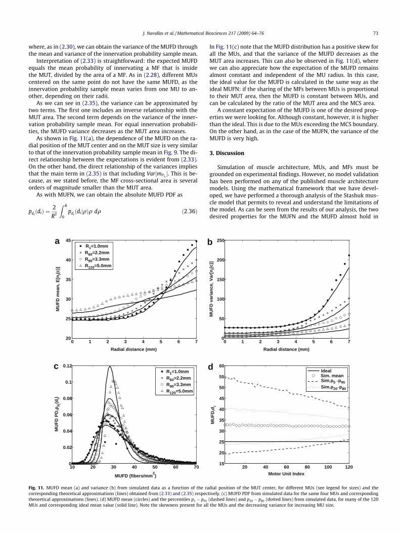
As shown in Fig. 11(a), the dependence of the MUFD on the ra-dial position of the MUT center and on the MUT size is very similarto that of the innervation probability sample mean in Fig. 9. The di-rect relationship between the expectations is evident from (2.33).On the other hand, the direct relationship of the variances impliesthat the main term in (2.35) is that including Var½mPIi

�. This is be-cause, as we stated before, the MF cross-sectional area is severalorders of magnitude smaller than the MUT area.

As with MUFN, we can obtain the absolute MUFD PDF as

pdiðdiÞ ¼

2R2

Z R

0pdiðdijqÞq dq ð2:36Þ

0 1 2 3 4 5 6 720

25

30

35

40

45


MU

FD m

ean,

E[n

i(c)]

R1=1.0mmR60=2.2mmR90=3.3mmR120=5.0mm

10 20 30 40 50 60 700

0.02

0.04

0.06

0.08

0.1

0.12

MUFD (fibers/mm2)

MU

FD P

D,p

d i(di)

R1=1.0mmR60=2.2mmR90=3.3mmR120=5.0mm

a b

c

Fig. 11. MUFD mean (a) and variance (b) from simulated data as a function of the racorresponding theoretical approximations (lines) obtained from (2.33) and (2.35) respectheoretical approximations (lines). (d) MUFD mean (circles) and the percentiles p5 � p95

MUs and corresponding ideal mean value (solid line). Note the skewness present for all

In Fig. 11(c) note that the MUFD distribution has a positive skew forall the MUs, and that the variance of the MUFD decreases as theMUT area increases. This can also be observed in Fig. 11(d), wherewe can also appreciate how the expectation of the MUFD remainsalmost constant and independent of the MU radius. In this case,the ideal value for the MUFD is calculated in the same way as theideal MUFN: if the sharing of the MFs between MUs is proportionalto their MUT area, then the MUFD is constant between MUs, andcan be calculated by the ratio of the MUT area and the MCS area.

A constant expectation of the MUFD is one of the desired prop-erties we were looking for. Although constant, however, it is higherthan the ideal. This is due to the MUs exceeding the MCS boundary.On the other hand, as in the case of the MUFN, the variance of theMUFD is very high.

3. Discussion

Simulation of muscle architecture, MUs, and MFs must begrounded on experimental findings. However, no model validationhas been performed on any of the published muscle architecturemodels. Using the mathematical framework that we have devel-oped, we have performed a thorough analysis of the Stashuk mus-cle model that permits to reveal and understand the limitations ofthe model. As can be seen from the results of our analysis, the twodesired properties for the MUFN and the MUFD almost hold in

0 1 2 3 4 5 6 70

50

100

150

200

250


MU

FD v

aria

nce,

Var

[ni(c

)]

20 40 60 80 100 12015

20

25

30

35

40

45

50

55

60

Motor Unit Index

MU

FD, d

i

IdealSim. meanSim.p5 −p95 Sim.p20−p80

d

dial position of the MUT center, for different MUs (see legend for sizes) and thetively. (c) MUFD PDF from simulated data for the same four MUs and corresponding(dashed lines) and p20 � p80 (dotted lines) from simulated data, for many of the 120the MUs and the decreasing variance for increasing MU size.


their mean values. That is, the expected value of the MUFN for thedifferent MUs in the muscle is almost linearly related with theMUT area, which means that MUFN follows an exponential distri-bution, as the MUT areas do. In addition, the expected value of theMUFD is almost constant across MUs. However, the expected valueof the MUFN and MUFD do not exactly match the ideal values. If weallow the MUT to exceed the MCS boundary, the expected MUTarea will fall, and the expected innervation probability will in-crease, causing the expected value of the MUFD to increase as well.In small MUs, with smaller probability of exceeding the MCSboundary, this MUFD increase forces MUFN to increase. However,in large MUs, as the expected MUT area is significantly reduced,MUFN decreases even with an increase of the MUFD.

The Stashuk model presents a considerable edge effect. Thisedge effect is due to the absence of MUs outside the MCS thatwould provide a constant coverage probability inside the MCS. Ide-ally, a constant coverage probability over the MCS would lead to anhomogeneous overlapping DPD, independent of the radial distance.In this case, the innervation probability would also be constantover the MCS. This situation is only attainable for an infiniteMCS, or in the Di

1 region, an inner region where the edge effect isnot present. Note that many muscle configurations may not evenhave a Di

1 region for some of its MUs, as is the case for the first dor-sal interosseus settings used in our simulations. In muscles wherethe ratio of the biggest MU radius, Rmax to the MCS radius, R, issmall, the DN

1 region occupies most of the MCS, thereby reducingthe edge effect to a thin superficial region. In contrast, for muscleswith large MUs compared to the MCSA, as is the case with the firstdorsal interosseus studied in this paper, the edge effect is consider-able. The edge effect of the Stashuk model does not depend on themuscle size but on the size of the largest MUs relative to the MCSarea.

In general, this edge effect will be present whenever MUTs areplaced in random manner, and muscle architecture models usingthis random MUT placement will suffer from it. In addition, typicalMUTA ranges observed in real muscles [4,12,23,29,30] are large en-ough for the edge effect to appear. This is a very important problemwhen dealing with simulated signals: MUs will have differentproperties depending on their location in the MCS, what will causea strong and unexpected bias on the simulated signals. The effectwill be more dramatic when using these models for surface-EMGsimulation, as in MUs near the muscle surface the MUFD can begreatly increased.

Another important problem of the model is in the high varianceof the results. For the MUFN, we found that the 2r range is alwaysgreater than the mean value. For the MUFD, the 2r range is 1.4times the mean MUFD for the smallest MUs, and 0.6 times forthe biggest MUs. This is such high variance that, even if the meanvalues follow the designed distribution, there is very low expec-tancy of finding a valid distribution for the MUFN or the MUFDin a single simulation run.

The main causes of this high variance are the two sources ofrandomness of the Stashuk model. As demonstrated in (2.7), theoverlapping is the sum of N independent Bernoulli random vari-ables since the placement of the different MUs is independent. Thisleads to a Lexian random variable defined for every point in theMCS with a very high variance (2.12) and a high covariance for dis-tances of the order of the radii of the smallest MUs (2.13). Consid-ered over the whole MUT, large overlapping variances andcovariances induce large variances in the overlapping samplemean, as given in (2.23). This, in turn, produces large variancesof the innervation probability sample mean, Var½mPIi

�; and, finally,this causes large MUFN variance. Thus, independent placement ofthe MUs determines part of the high variance of the MUFN, andconsequently of the MUFD. The second source of randomness isthe random selection of the innervating MU from the set of the

MUs covering the MF position. As stated in (2.26), this makes theMUFN a summation of Bernoulli trials. The independence betweentrials, as in the previous case, considerably enlarges the variance.

Several muscle architecture models in the literature have pro-posed different approaches in order to deal with the inaccuraciesderived from the random placement of the MUTs, specifically theedge effect and the high variability in the MUFN and MUFD. Fug-levand and Segal [31] used square MUTs with an area calculatedto satisfy the given MUFN to MUFD ratio. The territories wereplaced at random, but restricted to lie completely within theMCS. This approach, in words of the authors, is successful in reduc-ing the edge effect. However, it is based on square territories, whatmay be considered as an oversimplification of the undergoing MUanatomy, as MUTs have been described in glycogen depletion stud-ies as having rounded shapes tending to be elliptical regions of theMCS [4]. Another approach, proposed by Keenan and Valero-Cue-vas [3], consists on increasing the MUT radius when the territoryexceeds the muscle boundary, so that the area of the MUT remainsunchanged. This approach enables the preservation of the MUTarea, what may help to obtain a MUFD closer to the ideal. However,this approach does not ensure the elimination of the edge effect onthe overlapping, even if the MUT areas are preserved, as there willstill be less MUT coverage near the MCS boundary than in the cen-ter. In addition, this approach does not eliminate the variabilitydue to the random placement of the MUTs, hence a substantialamount of variance will remain in the MUFN and MUFD outcomesof the different MUs of the pool. As it stems from our analysis,these two approaches, as relying in random placement of the MUterritories, are expected to present a very high variance in the over-lapping, which in turn will lead to a high variance in the innerva-tion probability, and finally a high variance in the MUFN andMUFD.

MUT placement algorithms different from random placementhave been proposed in other models. Schnetzer et al. [16] proposedan overlapping control mechanism that creates a dependency onthe MUT placement that ensures an almost constant overlappingacross the MCS. This approach will considerably reduce the edgeeffect and it will eliminate the portion of the variability among dif-ferent runs of the algorithm which is related to the overlappingvariability. However, MUFN and MUFD will continue presentingthe variability due to the innervation algorithm. In a different line,Hamilton-Wright and Stashuk’s approach [17], bases the MUTplacement on a seed scattering algorithm, trying to obtain a rela-tively even distribution of the MU territories throughout theMCS. The problem with this approach is that a considerable edgeeffect can still be found, and the variability among algorithm runsis not reduced as a matter of fact. In the same work, several inner-vation control mechanisms are proposed to control the dispersionof the MUFN without losing the random nature of the innervationprocess.

The inclusion of new overlapping and innervation control termscould help to reduce the high variability shown in the resultingMUFN and MUFD in the Stashuk muscle architecture model. Thelevel of control required should be directly related to an acceptablelevel of variance in the results which, in turn, should reflect phys-iological observations. Possible physiological explanations for thecontrol mechanisms include competition for pre- and post-synap-tic resources, limitation of resources depending on the axonaldiameter, or more complex interactions describing the signalingpathway of the neuromuscular binding [32].

4. Conclusions

We have developed a complete methodology for the analysis ofmuscle architecture models. With this methodology, we have


carried out a mathematical analysis of the Stashuk muscle archi-tecture model. Several conclusions arise from this study:

� An important and undesirable edge effect, characterized by adecrease of the overlapping toward the boundary of the MCS,is present. This edge effect is responsible for the dependencyof the MUFN and MUFD with the radial position of the MUC.Specifically, it causes the MUFD expectation to increase as theMUC approaches the MCS boundary.

� The expectation of the overall MUFN has an almost exponentialrelationship with the MU index, and the expectation of the over-all MUFD is almost constant for all the MUs. However, the loss ofMUT area, due to the MUTs exceeding the MCS, produces anincrease in the MUFD for all the MUs, giving a MUFD valuehigher than expected.

� The uniform and independent random placement of the MUswithin the MCS and the random selection of innervating MUamong the set of covering MUs lead to high variability betweendifferent runs of the model. This is reflected in the very high var-iance of the overall MUFN and MUFD.

Apart from the particular study of the Stashuk muscle model,our methodology may help in the construction of new musclemodels that try to accommodate physiological evidences in a bet-ter way.

Appendix A. Derivation of the overlapping covariance

To calculate the covariance of two overlapping RVs taken at twodifferent locations in the MCS,~rk and~rl, note that

Cov ½sð~rkÞ; sð~rlÞ� ¼ CovXN

i¼1

sið~rkÞ ;XN

j¼1

sjð~rlÞ" #

¼XN

i¼1

XN

j¼1

Cov½sið~rkÞ; sjð~rlÞ� ð4:1Þ

Applying Stashuk independence between the different MUC PDFs,we know that

Cov sið~rkÞ; sjð~rlÞ

¼ 0 8i–j ð4:2Þ

hence we can write

Cov sð~rkÞ; sð~rlÞ½ � ¼XN

i¼1

Cov sið~rkÞ; sið~rlÞ½ �

¼XN

i¼1

ðE½sið~rkÞsið~rlÞ� � E½sið~rkÞ� E½sið~rlÞ�Þ

¼XN

i¼1

PCiCi~rk;~rlð Þ � PCi

~rkð Þ PCið~rlÞ

� �ð4:3Þ

where the interpretation of E½sið~rkÞ� is straightforward as it repre-sents the expectation of the ith MU covering a MF at ~rk, i.e., thecoverage probability PCi

ð~rkÞ. Analogously, E½sið~rkÞ sið~rlÞ� is the expec-tation of the ith MU covering two MFs at~rk and~rl respectively, i.e.,the dual-coverage probability PCiCi

ð~rk;~rlÞ.

Appendix B. Derivation of the MUFN mean and variance

From the definition of the MUFN we have

ni ¼XM

k¼1

Iið~rkÞ ð4:4Þ

and from the innervation probability sampling mean and variance

mPIi¼ 1

M

XM

k¼1

PIið~rkÞ ð4:5Þ

vPIi¼ 1

M

XM

k¼1

PIið~rkÞ �mPIi

� �2ð4:6Þ

Taking into account that each Ii is a Bernoulli trial with a successprobability of PIi

, and that this probability is, in turn, a random var-iable, to obtain the expectation of the MUFN we have to apply thelaw of total expectation. Namely,

E½ni� ¼ E½E½nijPIi�� ¼ E½M mPIi

� ¼ M E½mPIi� ð4:7Þ

And for the variance, we have to apply the law of total variance,remembering that the MUFN has a Lexian distribution:

Var ni½ � ¼ E Var½nijPIi�

þVar E nijPIi

¼E M mPIi

ð1�mPIiÞ�M vPIi

h iþVar M mPIi

h i¼M E mPIi

h i1�E½mPIi

��

þMðM�1Þ Var mPIi

h i�M E vPIi

h ið4:8Þ

Appendix C. Derivation of the MUFD mean and variance

The random variable transformation in (2.32) gives the relationbetween MUFD and MUFN PDFs:

pdiðrÞðdjrÞ ¼ AiðrÞ pniAiðrÞ djrð Þ ð4:9Þ

With this relationship we can calculate MUFD mean and variance interms of the MUFN, as

E diðrÞ½ � ¼ 1AiðrÞ

E½niðrÞ� ð4:10Þ

Var diðrÞ½ � ¼ 1

A2i ðrÞ

Var½niðrÞ� ð4:11Þ

Including (2.28) and (2.29) in (4.10) and (4.11) respectively, we canevaluate the expressions as

E diðrÞ½ � ¼ MAiðrÞ

E mPIiðrÞ

h ið4:12Þ

Var diðrÞ½ � ¼ M

A2i ðrÞ

E mPIiðrÞ

h i1� E mPIi

ðrÞh i� �

þMðM � 1ÞA2

i ðrÞVar mPIi

ðrÞh i

� M

A2i ðrÞ

E½vPIiðrÞ� ð4:13Þ

which, assuming the approximation made in (2.20), leads to

E diðrÞ½ � ¼ 1AMF

E mPIiðrÞ

h ið4:14Þ

Var diðrÞ½ � ¼ 1AMF AiðrÞ

E mPIiðrÞ

h i1�E mPIi

ðrÞh i� �

þAiðrÞ�AMF

A2MF AiðrÞ

Var mPIiðrÞ

h i� 1

AMF AiðrÞE½vPIi

ðrÞ� ð4:15Þ

Acknowledgement

This work was supported by the Spanish Ministry of Education& Science under the project SAF2007-65383.

References

[1] S.D. Nandedkar, Models and simulations in electromyography, Muscle NerveSuppl. 11 (2002) S46.

[2] K.G. Keenan, D. Farina, R. Merletti, R.M. Enoka, Influence of motor unitproperties on the size of the simulated evoked surface EMG potential, Exp.Brain Res. 169 (2006) 37.


[3] K.G. Keenan, F.J. Valero-Cuevas, Experimentally valid predictions of muscleforce and EMG in models of motor-unit function are most sensitive to neuralproperties, J. Neurophysiol. 98 (2007) 1581.

[4] S.C. Bodine, A. Garfinkel, R.R. Roy, V.R. Edgerton, Spatial distribution of motorunit fibers in the cat soleus and tibialis anterior muscles: local interactions, J.Neurosci. 8 (1988) 2142.

[5] A.J. Fuglevand, D.A. Winter, A.E. Patla, Models of recruitment and rate codingorganization in motor-unit pools, J. Neurophysiol. 70 (1993) 2470.

[6] R.E. Burke, Motor unit types of cat triceps surfae muscle, J. Physiol. 193 (1967)141.

[7] K. Roeleveld, D.F. Stegeman, B. Flack, E.V. Sta�lberg, Motor unit size estimation:confrontation of surface EMG with macro EMG, Electroencephalogr. Clin.Neurophysiol. 105 (1997) 181.

[8] K. Roeleveld, A. Sandberg, E.V. Sta�lberg, D.F. Stegeman, Motor unit sizeestimation of enlarged motor units with surface electromyography, MuscleNerve 21 (1998) 878.

[9] C. Coers, N. Tellerman-Toppet, J.M. Gérard, Terminal innervation ratio inneuromuscular disease. I. Methods and controls, Arch. Neurol. 29 (1973)210.

[10] I. Gath, E. Sta�lberg, In situ measurement of the innervation ratio of motor unitsin human muscles, Exp. Brain Res. 43 (1981) 377.

[11] D.W. Stashuk, Simulation of electromyographic signals, J. Electromyogr.Kinesiol. 3 (1993) 157.

[12] S.C. Bodine, R.R. Roy, E. Eldred, V.R. Edgerton, Maximal force as a function ofanatomical features of motor unit in the cat tibialis anterior, J. Neurophysiol.57 (1987) 1730.

[13] S. Bodine-Fowler, A. Garfinkel, R.R. Roy, V.R. Edgerton, Spatial distribution ofmuscle fibers within the territory of a motor unit, Muscle Nerve 13 (1990)1133.

[14] R. Shenhav, I. Gath, Simulation of the spatial distribution of muscle fibers inhuman muscle, Comput. Methods Programs Biomed. 23 (1986) 3.

[15] J. Duchêne, J.-Y. Hogrel, A model of EMG generation, IEEE Trans. Biomed. Eng.47 (2000) 192.

[16] M.A. Schnetzer, D.G. Ruegg, R. Baltensperger, J.P. Gabriel, Three-dimensionalmodel of a muscle and simulation of its surface EMG, in: Proceedings of the23rd Annual International Conference of the IEEE EMBS, vol. 2, 2001, pp. 1038–1043.

[17] A. Hamilton-Wright, D.W. Stashuk, Physiologically based simulation of clinicalEMG signals, IEEE Trans. Biomed. Eng. 52 (2005) 171.

[18] E. Henneman, G. Somjen, D.O. Carpenter, Functional significance of cell size inspinal motorneurons, J. Neurophysiol. 28 (1965) 560.

[19] H.S. Milner-Brown, R.B. Stein, R. Yemm, The orderly recruitment of human motorunits during voluntary isometric contractions, J. Physiol. 230 (1973) 359.

[20] R.E. Burke, P. Tsairis, Anatomy and innervation ratios in motor units of catgastrocnemius, J. Physiol. 234 (1973) 749.

[21] S. Chamberlain, D.M. Lewis, Contractile characteristics and innervation ratio ofrat soleus motor units, J. Physiol. 412 (1989) 1.

[22] V.F. Rafuse, M.C. Pattullo, T. Gordon, Innervation ratio and motor unit force inlarge muscles: a study of chronically stimulated cat medialis gastrocnemius, J.Physiol. 499 (1997) 809.

[23] K. Kanda, K. Hashizume, Factors causing differences in force output amongmotor units in the cat medialis gastrocnemius muscle, J. Physiol. 448 (1992)677.

[24] B. Feinstein, B. Lindegard, E. Nyman, G. Wohlfart, Morphologic studies of motorunits in normal human muscles, Acta Anat. 23 (1955) 127.

[25] R.D. Adams, J.D. Reuck, Metrics of muscle, in: B.A. Kakulas (Ed.), Basic Researchin Miology. Proceedings of the Second International Congress on MuscleDiseases, 1971, pp. 3–11.

[26] R.M. Enoka, A.J. Fuglevand, Motor unit physiology: some unresolved issues,Muscle Nerve 24 (2001) 4.

[27] A. Stuart, J.K. Ord, Kendall’s Advanced Theory of Statistics, Distribution Theory,fifth ed., vol. 1, Charles Griffin and Co. Ltd., 1987.

[28] B.D. Ripley, Spatial Statistics, first ed., Wiley Series in Probability and Statistics,John Wiley and Sons, Inc., New York, 1981.

[29] V.F. Rafuse, T. Gordon, Self-reinnervated cat medial gastrocnemius muscles. I.comparisons of the capacity for regenerating nerves from enlarged motor unitsafter extensive peripheral nerve injuries, J. Neurophysiol. 75 (1996) 268.

[30] E. Kugelberg, L. Edstróm, M. Abbruzzese, Mapping of motor units inexperimentally reinnervated rat muscle. interpretation of histochemical andatrophic patterns in neurogenic lesions, J. Neurol. Neurosurg. Psychiatr. 33(1970) 319.

[31] A.J. Fuglevand, S.S. Segal, Simulation of motor unit recruitment andmicrovascular unit perfusion: spatial considerations, J. Appl. Physiol. 83(1997) 1223.

[32] A. van Ooyen, Competition in the development of nerve connections: a reviewof models, Network 12 (2001) R1.

Mathematical analysis of a muscle architecture model

Documents

Transcript of Mathematical analysis of a muscle architecture model