Mathematica code for image analysis, semi-automatic parameterextraction and strain analysis

Kieran F. Mulchrone a, Dave J. McCarthy b,n, Patrick A. Meere b

a Department of Applied Mathematics, University College, Cork, Irelandb School of Biological, Earth and Environmental Sciences, University College, Cork, Ireland

a r t i c l e i n f o

Article history:Received 14 June 2013Received in revised form30 July 2013Accepted 1 August 2013Available online 9 August 2013

Keywords:Image analysisSemi-automatic parameter extractionStrain analysis

a b s t r a c t

Geological strain analysis is a common task for structural geologists. This contribution presents softwarewritten on top of the Mathematica platform which allows for rapid semi-automatic strain analysis. Afteran initial step of manual identification of strain markers, the software performs image analysis,parameter extraction and strain analysis using the shape and relative spatial positioning of markers.Bootstrap estimates of sampling errors are calculated and suitable graphical output is generated. Threerepresentative samples of lithologies typically used in strain analysis are analysed to test the software.

& 2013 Elsevier Ltd. All rights reserved.

1. Introduction

In the absence of high quality strain markers such as reductionspots, the estimation of geological strain using populations ofdeformed objects is a very important approach for understandingthe processes and products of deformation on all scales of theEarth's lithosphere. This general approach to strain analysis byestimating finite strain from randomly oriented populations ofdeformed objects, the so-called the Rf/ϕ method, was first intro-duced in the late sixties (Ramsay, 1967). Subsequently, alternativemethods based on marker shape and orientation have beendeveloped (Borradaile, 1976; Dunnet and Siddans, 1971; Dunnet,1969; Elliott, 1970; Lisle, 1985, 1977a, 1977b; Matthews et al., 1974;Mulchrone and Meere, 2001; Mulchrone et al., 2003; Peach andLisle, 1979; Robin, 1977; Shimamoto and Ikeda, 1976; Yu andZheng, 1984). A second strain analysis methodology is based onusing object to object separation and assumes that the markerobjects are anti-clustered and that the relative position of thecentres of these objects is directly related to the orientation andmagnitude of the finite strain ellipse (Ramsay, 1967). Fry (1979)developed a graphical approach using this centre to centre methodthat was subsequently further improved as the Normalised FryMethod (Erslev, 1988) and the enhanced Normalised Fry Method(Erslev and Ge, 1990). McNaught (1994) further extended thesemethods by facilitating the use of non-elliptical markers bydetermining best-fit ellipses for these irregular shaped objects.

Mulchrone (2003) went on to show that the use of Delaunaytriangulation, to characterise nearest neighbour separations, was aless subjective and more efficient strain analysis technique.

One of the key limiting steps in the automation of these strainanalysis techniques is the recognition and fitting of best fit ellipsesto geological strain markers such as sedimentary clasts. A numberof methods for automated image analysis have been successfullyutilised in the past for geological strain analysis (Ailleres et al.,1995; Erslev and Ge, 1990; Masuda et al., 1991; McNaught, 1994).Panozzo (1984) utilised digitised sets of points representing linearor elliptical objects in her projection method, while Mukul (1998)developed an approach that involved manually tracing quartzgrain boundaries and subsequently, using third party imageanalysis software, identified the centroids and areas of the grains.Heilbronner (2000) developed a ‘Lazy Grain Boundary’ methodthat can be used in a fully automatic or semi-automatic mode toidentify sedimentary grain boundaries. More recently Mulchroneet al. (2005) developed a parameter extraction program (SAPE)that rapidly extracts the required data by using a simple region-growing algorithm to identify regions of interest. The secondmoments are subsequently calculated for each region enablingthe common strain analysis parameters to be readily computed.This current study will present a new piece of software that links aroutine for image analysis, ellipse fitting and parameter extractionwith software for the Mean Radial Length (Mulchrone et al., 2003)and the Delaunay Triangulation Nearest Neighbour Method(Mulchrone, 2003) strain analysis techniques. Integration of imageanalysis, parameter extraction and strain analysis routines willsignificantly reduce the time and labour intensity of geologicalstrain analysis studies.

Contents lists available at ScienceDirect

journal homepage: www.elsevier.com/locate/cageo

Computers & Geosciences

0098-3004/$ - see front matter & 2013 Elsevier Ltd. All rights reserved.http://dx.doi.org/10.1016/j.cageo.2013.08.001

n Corresponding author. Tel.: +353 214 204 581.E-mail address: davemccarthycork@gmail.com (D.J. McCarthy).

Computers & Geosciences 61 (2013) 64–70

2. Methodology

The primary motivation for producing the software was toprovide a single integrated system for semi-automatic image-based strain analysis. The software incorporates methods for dataextraction from digital images and strain analysis of the resultingdata. The methodology for extraction of object data from suitableimages closely follows the approach of Mulchrone et al. (2005).From an algorithmic perspective, the most difficult part of extract-ing information about a population of objects in a digital image isidentification of boundaries or regions occupied by those objects.Several fully automatic methods have been developed (e.g.Heilbronner, 2000), however often the results are not entirelyaccurate and this strongly depends on the characteristics of theparticular image being analysed. Typically structural geologistswork with microphotographs of quartz-rich clastic sedimentswhich present particular difficulties for automatic methods dueto undulose extinction, deformation bands, diffuse boundaries andcolour similarities. On the other hand, object identification isusually a trivial exercise for geologists. Once the regions havebeen identified, parameters such as the aspect ratio, orientation,second moments and the centroid of the object must be extracted.Humans can also perform this task, but in a subjective mannerthat may introduce unwarranted biases into the data acquired(Mulchrone and Choudhury, 2004). Additionally, accurate para-meter estimation and recording of parameters is time consuming.By contrast, parameter estimation is a trivial task for computers.

The idea driving our approach of data capture is to divide thetasks involved in parameter extraction according to human/com-puter aptitude. Therefore, the human user is given the task ofidentifying regions. The raw input for this activity is a digitalimage, which may be a microphotograph of the thin section or afield photograph of a suitable rock surface containing the markerobjects. This is referred to as the raw image (see Fig. 1A, D and G;

Fig. 1D and G from Ramsay and Huber, 1983). The end result of thisactivity must be a white digital image with object boundariesidentified in black (see Fig. 1B, E and H), which is referred to as theinput image. There are many possible approaches to producingthe input image such as tracing objects in the raw image ingraphical software packages such as Freehand or CorelDraw.Alternatively, high quality prints of the raw image are physicallytraced using an inking pen and tracing paper. Subsequently, thetracing is digitally scanned to produce the input image. Manualtracing was found to be the fastest and the most mentally bearablemethod. The approach of tracing followed by image analysis wasfirst advocated by Mukul (1998) leading to high quality datasets(Mukul and Mitra, 1998).

Established methods for strain analysis are applied to the extracteddata (Mulchrone, 2013; Mulchrone et al., 2003; Mulchrone, 2003).Mean Radial Length (MRL) is part of the Rf/ϕ suite of methods andestimates strain based on the distribution of grain shapes(Mulchrone et al., 2003). On the other hand the mutual spatialarrangement of objects can be used to estimate strain using Fry-type methods (Hanna and Fry, 1979). Here suitable object-objectpairs are identified using Delaunay Triangulation Nearest Neigh-bour Method (DTNNM; Mulchrone, 2003) and the best fit ellipse tothe central vacancy in the resulting Fry plots is estimated using thealgorithm of Mulchrone (Mulchrone, 2013). In addition to identi-fying the best fit strain parameters the sampling error associatedwith each method is calculated using the bootstrap method(McNaught, 2002; Mulchrone et al., 2003).

3. Software description

The Mathematica code presented here consists of a collectionof useful methods for image analysis, parameter extraction andstrain analysis. The methods are grouped together in a

Fig. 1. A. Microphotograph of the arenite, B. Manual trace of grain boundaries. C. Identification of grain boundaries in Mathematica. D. Microphotograph of the ooliteexample (Ramsay and Huber, 1983), E. Manual trace of ooid boundaries, F. Identification of ooid boundaries in Mathematica, G. Microphotograph of the quartzite example(Ramsay and Huber, 1983), H. Manual trace of quartz boundaries, I. Identification of quartz boundaries in Mathematica.

K.F. Mulchrone et al. / Computers & Geosciences 61 (2013) 64–70 65

Mathematica package which can be easily integrated with anexisting installation. In this section a brief discussion and descrip-tion of the data formats, analyses and graphical outputs areprovided. A summary of the methods and their arguments is givenin Table 1.

3.1. Image analysis

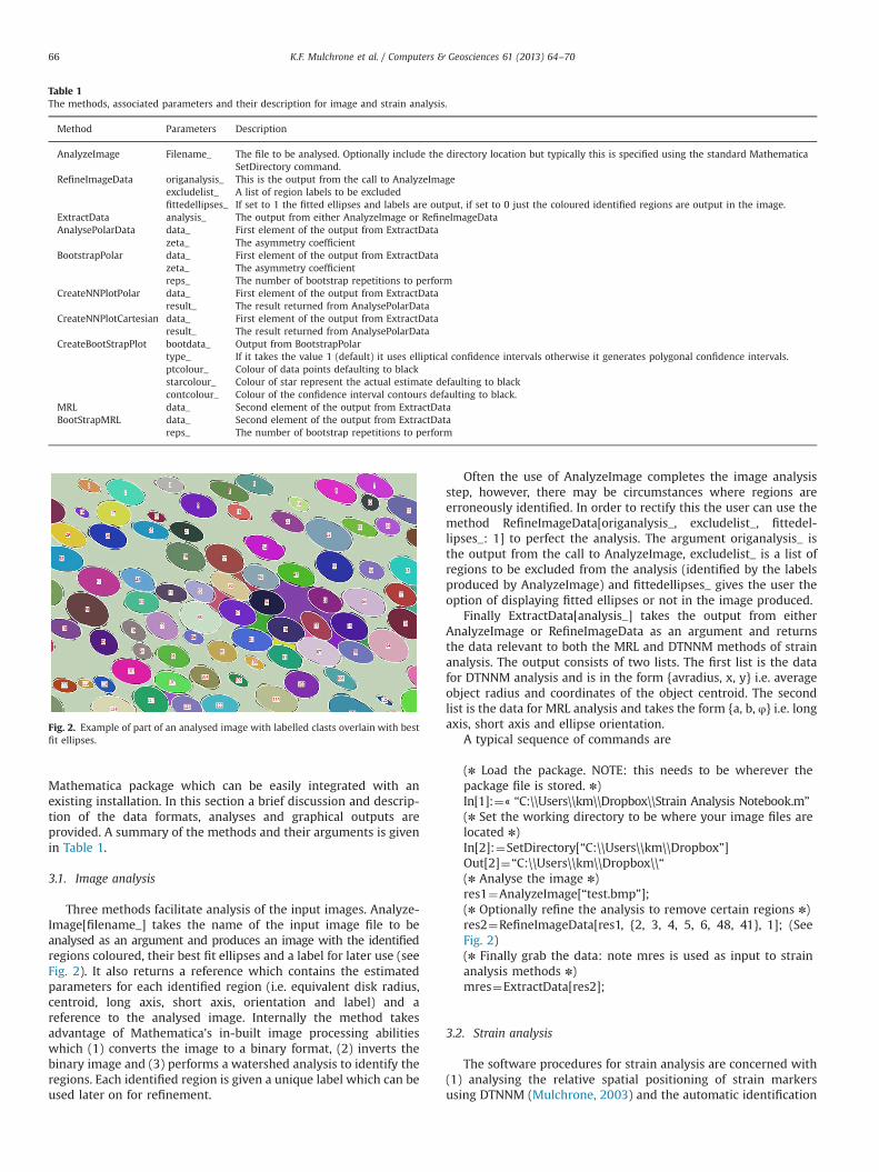
Three methods facilitate analysis of the input images. Analyze-Image[filename_] takes the name of the input image file to beanalysed as an argument and produces an image with the identifiedregions coloured, their best fit ellipses and a label for later use (seeFig. 2). It also returns a reference which contains the estimatedparameters for each identified region (i.e. equivalent disk radius,centroid, long axis, short axis, orientation and label) and areference to the analysed image. Internally the method takesadvantage of Mathematica's in-built image processing abilitieswhich (1) converts the image to a binary format, (2) inverts thebinary image and (3) performs a watershed analysis to identify theregions. Each identified region is given a unique label which can beused later on for refinement.

Often the use of AnalyzeImage completes the image analysisstep, however, there may be circumstances where regions areerroneously identified. In order to rectify this the user can use themethod RefineImageData[origanalysis_, excludelist_, fittedel-lipses_: 1] to perfect the analysis. The argument origanalysis_ isthe output from the call to AnalyzeImage, excludelist_ is a list ofregions to be excluded from the analysis (identified by the labelsproduced by AnalyzeImage) and fittedellipses_ gives the user theoption of displaying fitted ellipses or not in the image produced.

Finally ExtractData[analysis_] takes the output from eitherAnalyzeImage or RefineImageData as an argument and returnsthe data relevant to both the MRL and DTNNM methods of strainanalysis. The output consists of two lists. The first list is the datafor DTNNM analysis and is in the form {avradius, x, y} i.e. averageobject radius and coordinates of the object centroid. The secondlist is the data for MRL analysis and takes the form {a, b, φ} i.e. longaxis, short axis and ellipse orientation.

A typical sequence of commands are

(n Load the package. NOTE: this needs to be wherever thepackage file is stored. n)In[1]:¼« “C:\\Users\\km\\Dropbox\\Strain Analysis Notebook.m”

(n Set the working directory to be where your image files arelocated n)In[2]:¼SetDirectory[“C:\\Users\\km\\Dropbox”]Out[2]¼“C:\\Users\\km\\Dropbox\\“(n Analyse the image n)res1¼AnalyzeImage[“test.bmp”];(n Optionally refine the analysis to remove certain regions n)res2¼RefineImageData[res1, {2, 3, 4, 5, 6, 48, 41}, 1]; (SeeFig. 2)(n Finally grab the data: note mres is used as input to strainanalysis methods n)mres¼ExtractData[res2];

3.2. Strain analysis

The software procedures for strain analysis are concerned with(1) analysing the relative spatial positioning of strain markersusing DTNNM (Mulchrone, 2003) and the automatic identification

Table 1The methods, associated parameters and their description for image and strain analysis.

Method Parameters Description

AnalyzeImage Filename_ The file to be analysed. Optionally include the directory location but typically this is specified using the standard MathematicaSetDirectory command.

RefineImageData origanalysis_ This is the output from the call to AnalyzeImageexcludelist_ A list of region labels to be excludedfittedellipses_ If set to 1 the fitted ellipses and labels are output, if set to 0 just the coloured identified regions are output in the image.

ExtractData analysis_ The output from either AnalyzeImage or RefineImageDataAnalysePolarData data_ First element of the output from ExtractData

zeta_ The asymmetry coefficientBootstrapPolar data_ First element of the output from ExtractData

zeta_ The asymmetry coefficientreps_ The number of bootstrap repetitions to perform

CreateNNPlotPolar data_ First element of the output from ExtractDataresult_ The result returned from AnalysePolarData

CreateNNPlotCartesian data_ First element of the output from ExtractDataresult_ The result returned from AnalysePolarData

CreateBootStrapPlot bootdata_ Output from BootstrapPolartype_ If it takes the value 1 (default) it uses elliptical confidence intervals otherwise it generates polygonal confidence intervals.ptcolour_ Colour of data points defaulting to blackstarcolour_ Colour of star represent the actual estimate defaulting to blackcontcolour_ Colour of the confidence interval contours defaulting to black.

MRL data_ Second element of the output from ExtractDataBootStrapMRL data_ Second element of the output from ExtractData

reps_ The number of bootstrap repetitions to perform

Fig. 2. Example of part of an analysed image with labelled clasts overlain with bestfit ellipses.

K.F. Mulchrone et al. / Computers & Geosciences 61 (2013) 64–7066

of the associated strain (Mulchrone, 2013), (2) analysis the shapesof markers using the method of MRL (Mulchrone et al., 2003), (3)providing bootstrap sampling error estimates for both analysesand (4) providing suitable graphical output. In addition, there areseveral utility methods called inside other methods and are notdesigned for direct usage.

Spatial data may be analysed using a Polar or Cartesiancoordinate system, however the polar approach tends to outper-form the Cartesian formulation (Mulchrone, 2013) and is thusimplemented here. The method AnalyseDataPolar[data_, zeta_]takes as input the first element of the data returned from ExtractData[]above and the second argument is zeta corresponding to asymmetrycoefficient (Mulchrone, 2013). The asymmetry coefficient controlshow data are weighted when fitting an ellipse to the data.Typically, the larger the value of zeta, the higher the weightingthat is applied to a fewer number of centrally located points(which may cause the sampling error to increase). The outputgenerated is a list of data containing the long axis, the short axisand orientation of the best fit ellipse to the central vacancy. Thelong and short axes are returned because they are required togenerate graphical output later. Internally the method calls autility method GetNearestNormalPointsDT[] which calculates theDelaunay triangulation and subtracts the points on the convex hullwhich generates the raw data required for the method ofMulchrone (2013). The method BootStrapPolar[data_, zeta_, reps_]is used to estimate the sampling error associated with an analysis.The arguments have the same meaning as for AnalysePolar exceptthat reps_ determines howmany bootstrap repetitions are applied.Usually a value of between 200 and 400 is more than sufficient.The spatial analysis is computationally intensive and bootstrapanalyses may be time consuming. The output from BootStrapPolarconsists of the original result (same as that from AnalysePolar)plus an additional list of individual bootstrap results.

The bootstrap is a general computational technique invented byEfron (1979) to construct approximate sampling distributions forcomplex statistical estimates. The basic principal of the bootstrapis multiple samples of a given dataset can be generated byrepeatedly resampling the original dataset with replacement.Multiple parameter estimates are calculated by analysis of themultiple samples. The distribution of the parameter estimatesfound closely approximates the true sampling distribution of theparameters. Typically for a univariate dataset the percentiles forthe dataset of parameter estimates allow estimation of suitableconfidence intervals. In higher dimensions (in 2D strain analysisthat data are bivariate), elliptical regions centred on the mean arefound which enclose a specified percentage of the data using thebuilt-in EllipsoidQuantile function of Mathematica.

There are three methods for generated graphical output for theDTNNM strain analysis. The first method (CreateNNPlotPolar[data_, result_]) displays the data in polar form in a plot of r

(distance from origin) versus orientation and superimposes thecurve representing the best-fit ellipse (see Fig. 3). CreateNNPlot-Cartesian[data_, result_] creates a more familiar Fry style plot (Fry,1979) in Cartesian coordinates (see Fig. 4A, D and G). FinallyCreateBootStrapPlot[bootdata_, type_, ptcolour_, starcolour_, con-tcolour_] creates a plot of the bootstrap data along with con-fidence intervals at the 90%, 95% and 99% levels for the location ofthe true value as well as the location of the estimate fromAnalyseDataPolar (see Fig. 3). This method can also be used tocreate a bootstrap plot for datasets generated from MRL.

MRL is relatively simple in implementation compared withDTNNM. There are two methods available. The first method MRL[data_] takes as input the second element of the data returnedfrom ExtractData[] above and outputs the axial ratio and orienta-tion of the calculated strain ellipse. The second method Boot-StrapMRL[data_, reps_] takes as first argument the second elementof the data returned from ExtractData[] and as second argumentthe number of bootstrap repetitions to perform. Note that MRL ismuch faster than DTNNM and so taking 1000 repetitions is veryfeasible. The output comprises the original result (i.e. from MRL)plus an additional list of individual bootstrap results.

A typical sequence of commands is as follows:

(n note mres is the return value from ExtractData[] n)(n Do a DTNNM analysis n)nnres¼AnalyseDataPolar[mres[[1]], 10000](n Create a graphical representation n)CreateNNPlotPolar[mres[[1]], nnres](n Create a Fry-type plot of the result n)CreateNNPlotCartesian[mres[[1]], nnres](n Perform a bootstrap analysis n)(n Quiet prevents unnecessary feedback, note this takes sometime to \complete! n)bsres¼Quiet[BootStrapPolar[mres[[1]], 10000, 200]];(n Create a graphic of the bootstrap data n)(n Plot the bootstrap results with confidence intervals at 90, 95and 99% level n)CreateBootStrapPlot[bsres](n Do strain analysis using Mean Radial Length (MRL)Mulchrone et al. (2003) n)(n Single Analysis returns axial ratio and orientation n)MRL[mres[[2]]]bsMRL¼BootStrapMRL[mres[[2]], 1000];(n Plot Bootstrap results n)CreateBootStrapPlot[bsMRL]

4. Example applications

In this section three samples are analysed using the softwaresystem presented above. These samples have been selected torepresent the typical lithologies that are used in geological strainanalysis.

4.1. Sample locations and background geology

The first sample used in this study is a medium grained quartzarenite from the Lower Carboniferous Crows Point Formation(MacCarthy et al., 1978; MacCarthy, 1974; Murphy, 1985) takenfrom a shear zone on the north limb of the Ardmore Syncline inCounty Waterford, Ireland. In thin section (see Fig. 1A) the sampledisplays a strong fabric, dominated by elongate flattened quartzgrains, which are typically parallel to pressure solution cleavageplanes. The analysed thin section is composed of 80% quartz grainsthat are typically 1mm elongate, rounded to sub-angular andmonocrystalline.

Fig. 3. Example of a polar plot for the oolite example. r (distance from origin) isplotted against orientation and superimposes the curve representing the best-fitellipse.

K.F. Mulchrone et al. / Computers & Geosciences 61 (2013) 64–70 67

The other two examples analysed here (see Fig. 1D and G) arephotomicrographs of an oolite (Page 112, Fig 7.7. from Ramsay andHuber, 1983) and a quartzite (Page 118, Fig 7.16. from Ramsay andHuber, 1983). These images were used because they are familiar tothe majority of structural geologists and their strain estimates arefirmly established. Additionally they represent two very differentlithologies compared to the sandstone described above.

4.2. Image preparation

Grain boundary maps are manually traced from microphoto-graphs of thin sections taken in cross polarised light. Typicallysandstones are analysed and in these cases only quartzofelds-pathic grain boundaries are identified and traced. Essentially thegoal is to ensure that objects of similar size and rheology areanalysed. Hence creating reliable comparisons and ensuring thatminerals such as biotite, with exceptionally elongate crystal shapesand differing rheological properties do not affect the analysis.

When tracing grain boundaries there are a few factors thatneed to be taken into consideration. Firstly each grain boundaryneeds to be a closed loop, otherwise they will not be detected bythe image analysis routine. Secondly, grain boundaries need to betraced with an ink pen of a significant thickness (0.5 mm), so thatwhen they are scanned at low resolution the grain boundariesmaintain their integrity, i.e. no spurious gaps appear. The reason-ing behind low resolution scanning of the traced boundaries istwofold; smaller sized images are easier for Mathematica to

handle resulting in faster analysis, while at higher scanningresolutions we have found that more spurious objects are identi-fied. Experience has shown that the ideal file size and imageformat is a bitmap of approximately 500 kb, this roughly equatesto an A4 page of manually traced grain boundaries, scanned at200–300 dpi, resulting in an image of 2340�1700 pixels. The lastthing to consider is the number of objects used in the analysis. Ithas been established that approximately 150 grains is sufficient(Meere and Mulchrone, 2003). Sample sets with significantlyfewer objects than this can result in large errors in the strainestimates, whereas larger data sets do not improve the quality ofthe estimates and can dramatically increase the computing timerequired.

For the majority of sandstones it is relatively easy to includeonly quartzofeldspathic grain boundaries and for the samples usedin this study very little post processing was required. Unfortu-nately with interlocking or closely spaced grains it can be parti-cularly difficult to exclude unwanted mineral boundaries or voidsbetween grains Problematic objects can be excluded from theanalysis using RefineImageData[]. We have found that selectiveediting of the manual image prior to analysis is the most efficientmethod for reducing any errors created. For examples that are notcompletely interlocking it is usually possible to keep grainsseparate and distinct.

Besides the manual selection of objects to be analysed the onlyother significant user input in the analysis process is the determi-nation of a zeta value (see Section 3.2 and Mulchrone, 2013). The

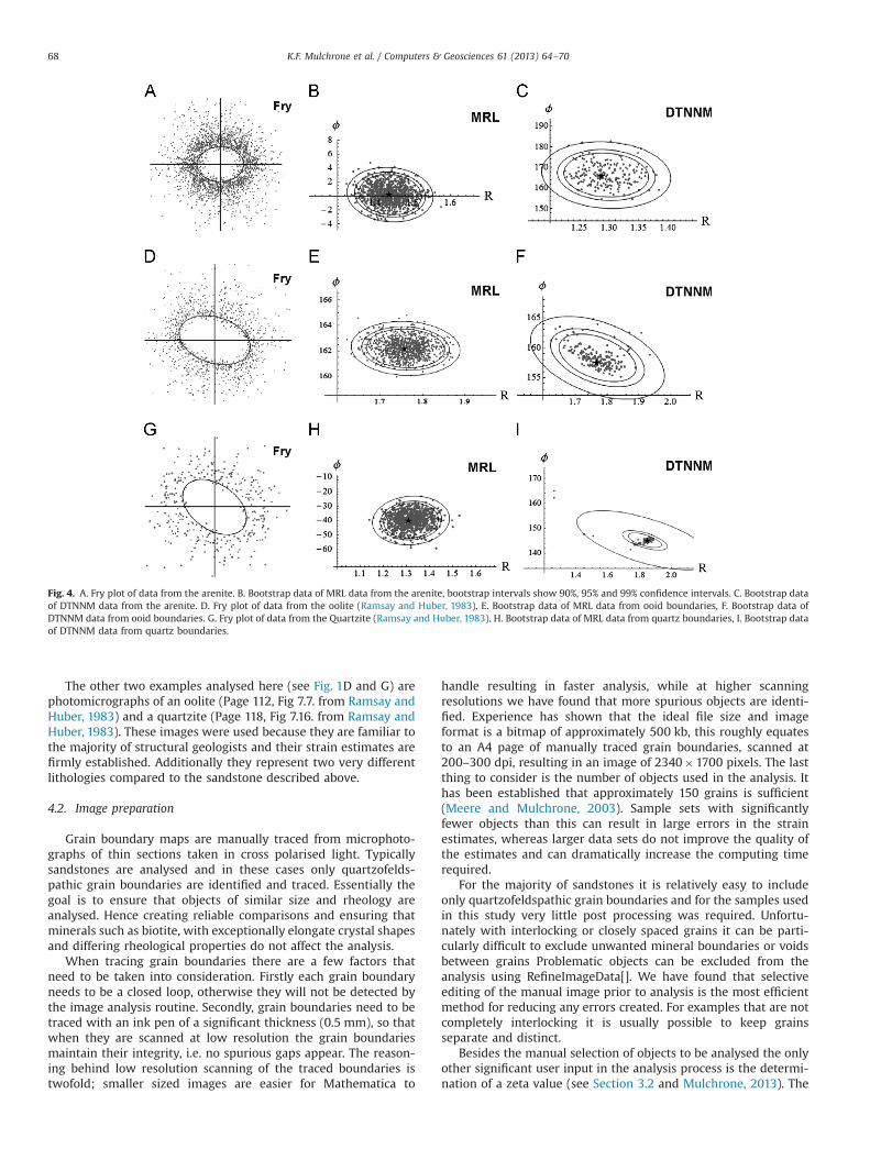
Fig. 4. A. Fry plot of data from the arenite. B. Bootstrap data of MRL data from the arenite, bootstrap intervals show 90%, 95% and 99% confidence intervals. C. Bootstrap dataof DTNNM data from the arenite. D. Fry plot of data from the oolite (Ramsay and Huber, 1983). E. Bootstrap data of MRL data from ooid boundaries, F. Bootstrap data ofDTNNM data from ooid boundaries. G. Fry plot of data from the Quartzite (Ramsay and Huber, 1983). H. Bootstrap data of MRL data from quartz boundaries, I. Bootstrap dataof DTNNM data from quartz boundaries.

K.F. Mulchrone et al. / Computers & Geosciences 61 (2013) 64–7068

function of zeta is to decide to what extent data inliers areweighted. The effects of this function are seen in the Fry orCartesian plot produced in the first stage of the analysis (i.e.Fig. 4A). A higher zeta value applies a higher weighting to pointsnear the inner void of the data (Mulchrone, 2013), it has beenfound in this study that zeta values between 100 and 4000 shouldbe sufficient to accommodate a best fit of the data. The inclusion ofthis function allows the user to ensure that a best fit is achieved bypreferential weighting of data points. This function can also beused as a measure of the quality of the data, with poor quality datathe best fit is poorly correlated, regardless of the zeta value.

4.3. Results

The analysis of the arenite yielded R¼1.3 and R¼1.4 forDTNNM and MRL respectively. The resulting Fry plot exhibits asignificant population of central inliers which leads to a sizeablesampling error. In this case a low value for Zeta was selected sothat less weight was given to the centrally located data whenfitting the ellipse (Fig. 4A). The confidence intervals for theDTNNM and MRL methods do not significantly overlap (Fig. 4Band C), which is indicative of the sensitivity of the two methods todifferent types of strain.

The analysis of the oolite yielded R¼1.68 and R¼1.76 forDTNNM and MRL respectively. These values are very close to theestimates of Ramsay and Huber (1983), R¼1.7 and R¼1.79 by theFry method and centre to centre techniques respectively. The Fryplot of the centre to centre data gives a relatively well defined bestfit ellipse as there are very few centrally located points tonegatively affect the best fit ellipse (Fig. 4D). The confidenceellipses for the bootstrapped data for MRL and DTNNM overlapsuggesting that both methods are identifying the same strainbehaviour (Fig. 4E and F).

Analysis of the quartzite yielded results of R¼1.78 and R¼1.31for DTNNM and MRL respectively. The value estimated by Ramsayand Huber (1983) by the Fry method was R¼1.7. The Fry plot of thecentre to centre data clearly identifies the best fit ellipse (Fig. 4G).However there are extreme values on the bootstrap plot forDTNNM. This can be readily explained by the small number ofdata points in the central region and this in turn is related to thesmall number of clasts used (N¼81). In this sample the confidenceintervals for the DTNNM and MRL analyses do not overlap (Fig. 4Hand I). Once again this suggests the different techniques aresensitive to different strain behaviours.

4.4. Discussion

The automatic misidentification of regions as clasts may createerrors in the strain estimates produced by the above methods maybe a concern. It could be argued that the inclusion of extra mineralspecies or voids may only represent a small portion of the totaldata and therefore would only lead to small errors in theestimates. It is our contention that even with data sets in excessof 150 objects, as recommended by Meere and Mulchrone (2003),the inaccuracies produced by these extra grains may be significant.To investigate this we have analysed the oolite sample with this inmind. This resulted in an image with 204 correctly identified ooidsand 19 misidentified regions using the image analysis techniquesabove. This data set yielded strain estimates of R¼1.36 and R¼1.63for DTNNM and MRL respectively, both significantly lower thanthe values reported earlier (R¼1.68 and R¼1.74) using a data setwithout misidentified objects. DTNNM is most affected by thisissue, probably because these misidentified regions introducespuriously close object-object separations. We propose two meth-ods to counter for this effect, (1) a second trace is manuallyproduced, that carefully ensures no interstitial areas are created, or

(2) unwanted objects are removed using the RefineImageData[]method. We strongly endorse the second approach because it doesnot involve artificially modifying the input image.

4.5. Conclusion

Geological strain analysis forms an integral component of anydetailed regional tectonic study. Historically a fundamental limitationon the breadth of this approach has been the labour intensivenature of such techniques. In this contribution we present acollection of procedures written on top of the Mathematica plat-form which allows for rapid semi-automatic strain analysis. Themethodology involves an initial step of manual identification ofstrain markers. After this the procedure is fully automatic. Thesoftware performs image analysis to identify regions and extractthe relevant parameters for subsequent strain analysis using theDTNNM and MRL methods. It calculates bootstrap estimates ofsampling errors and generates suitable graphical output.

The software has been tested using three samples which arerepresentative of typical lithologies used in geological strainanalysis. The strain estimates obtained compare well with pre-viously published estimates and the software was found toperform well.

Acknowledgements

We would like to thank an anonymous reviewer and FrederickVollmer for careful reviews which helped to improve the manu-script. Dave McCarthy acknowledges the support of an IRCSETEmbark scholarship.

Appendix A. Supporting information

Supplementary data associated with this article can be found inthe online version at http://dx.doi.org/10.1016/j.cageo.2013.08.001.

References

Ailleres, L., Champenois, M., Macaudiere, J., Bertrand, J.., 1995. Use of image analysisin the measurement of finite strain by the normalized Fry method: geologicalimplications for the'Zone Houillere' (Brianconnais zone, French Alps). Miner-alogical Magazine 59, 179–187.

Borradaile, G., 1976. A strain study of a granite–granite gneiss transition andaccompanying schistosity formation in the Betic orogenic zone, SE, Spain.Journal of the Geological Society 132, 417–428.

Dunnet, D., 1969. A technique of finite strain analysis using elliptical particles.Tectonophysics 7, 117–136.

Dunnet, D., Siddans, A., 1971. Non-random sedimentary fabrics and their modifica-tion by strain. Tectonophysics 12, 307–325.

Efron, B., 1979. Bootstrap methods: another look at the jackknife. The Annals ofStatistics 7, 1–26.

Elliott, D., 1970. Determination of finite strain and initial shape from deformedelliptical objects. Geological Society of America Bulletin 81, 2221–2236.

Erslev, E., 1988. Normalized center-to-center strain analysis of packed aggregates.Journal of Structural Geology 10, 201–209.

Erslev, E., Ge, H., 1990. Least-squares center-to-center and mean object ellipsefabric analysis. Journal of Structural Geology 12, 1047–1059.

Fry, N., 1979. Random point distributions and strain measurement in rocks.Tectonophysics 60, 89–105.

Hanna, S., Fry, N., 1979. A comparison of methods of strain determination in rocksfrom southwest Dyfed (Pembrokeshire) and adjacent areas. Journal of Struc-tural Geology 1, 155–162.

Heilbronner, R., 2000. Automatic grain boundary detection and grain size analysisusing polarization micrographs or orientation images. Journal of StructuralGeology 22, 969–981.

Lisle, R., 1977a. Estimation of the tectonic strain ratio from the mean shape ofdeformed elliptical objects. Geologie en Mijnbouw 56, 140–144.

Lisle, R., 1977b. Clastic grain shape and orientation in relation to cleavage from theAberystwyth Grits, Wales. Tectonophysics 39, 381–395.

Lisle, R., 1985. Geological Strain Analysis: A Manual for the Rf/ϕ Method. PergamonPress.

K.F. Mulchrone et al. / Computers & Geosciences 61 (2013) 64–70 69

MacCarthy, I., Gardiner, P., Horne, R., 1978. The lithostratigraphy of the Devonian–Early Carboniferous succession in parts of Counties Cork and Waterford,Ireland. Bulletin of the Geological Survey of Ireland 2, 265–305.

MacCarthy, I.A.J., 1974. The Lithostratigraphy and Sedimentology of the Devonian–Early Carboniferous Succession in Parts of Counties Cork and Waterford (PhDThesis). National University of Ireland.

Masuda, T., Koike, T., Yuko, T., Morikawa, T., 1991. Discontinuous grain growth ofquartz in metacherts: the influence of mica on a microstructural transition.Journal of Metamorphic Geology 9, 389–402.

Matthews, P., Bond, R., Berg, J., Van Den, 1974. An algebraic method of strainanalysis using elliptical markers. Tectonophysics 24, 31–67.

McNaught, M., 1994. Modifying the normalized Fry method for aggregates of non-elliptical grains. Journal of Structural Geology 16, 493–503.

McNaught, M., 2002. Estimating uncertainty in normalized Fry plots using abootstrap approach. Journal of Structural Geology 24, 311–322.

Meere, P.A., Mulchrone, K.F., 2003. The effect of sample size on geological strainestimation from passively deformed clastic sedimentary rocks. Journal ofStructural Geology 25, 1587–1595.

Mukul, M., 1998. A spatial statistics approach to the quantification of finitestrain variation in penetratively deformed thrust sheets: an example fromthe Sheeprock Thrust Sheet, Sevier. Journal of Structural Geology20,371–384.

Mukul, M., Mitra, G., 1998. Finite strain and strain variation analysis in theSheeprock Thrust Sheet: an internal thrust sheet in the Provo salient of theSevier Fold-and-Thrust belt, Central Utah. Journal of Structural Geology 20,385–405.

Mulchrone, K., 2013. Fitting the void: data boundaries, point distributions andstrain analysis. Journal of Structural Geology 46, 22–23.

Mulchrone, K., Meere, P., 2001. A Windows program for the analysis of tectonicstrain using deformed elliptical markers. Computers & Geosciences 27,1251–1255.

Mulchrone, K., Meere, P., Choudhury, K., 2005. SAPE: a program for semi-automaticparameter extraction for strain analysis. Journal of Structural Geology 27,2084–2098.

Mulchrone, K.F., 2003. Application of Delaunay triangulation to the nearestneighbour method of strain analysis. Journal of Structural Geology 25, 689–702.

Mulchrone, K.F., Choudhury, K.R., 2004. Fitting an ellipse to an arbitrary shape:implications for strain analysis. Journal of Structural Geology 26, 143–153.

Mulchrone, K.F., O'Sullivan, F., Meere, P.A., 2003. Finite strain estimation using themean radial length of elliptical objects with bootstrap confidence intervals.Journal of Structural Geology 25, 1587–1595.

Murphy, F.X., 1985. The Lithostratigraphy and Structural Geology of the DungarvanSyncline and Adjacent Areas, Co. Waterford, Southern Ireland( PhD Thesis).National University of Ireland.

Panozzo, R., 1984. Two-dimensional strain from the orientation of lines in a plane.Journal of Structural Geology 6, 215–221.

Peach, C., Lisle, R., 1979. A Fortran IV program for the analysis of tectonic strainusing deformed elliptical markers. Computers & Geosciences 5, 325–334.

Ramsay, J.G., Huber, M., 1983. The techniques of modern structural geology. StrainAnalysis, London: Academic Press.

Ramsay, J.G., 1967. Folding and fracturing of rocks. New York, MacGraw-Hill, 568p.Robin, P., 1977. Determination of geologic strain using randomly oriented strain

markers of any shape. Tectonophysics 42, T7–T16.Shimamoto, T., Ikeda, Y., 1976. A simple algebraic method for strain estimation from

deformed ellipsoidal objects. 1. Basic theory. Tectonophysics 36, 315–337.Yu, H., Zheng, Y., 1984. A statistical analysis applied to the Rf/ϕ method. Tectono-

physics 110, 151–155.

K.F. Mulchrone et al. / Computers & Geosciences 61 (2013) 64–7070