MATERIALS PHYSICS AND MECHANICS - Санкт ...

ISSN 1605-2730

MATERIALS PHYSICS AND MECHANICS

Vol. 40, No. 2, 2018

MATERIALS PHYSICS AND MECHANICS

Principal Editors: Dmitrii Indeitsev

Institute of Problems of Mechanical Engineering of the Russian Academy of Science (RAS), Russia

Andrei Rudskoi Peter the Great St.Petersburg Polytechnic University, Russia

Founder and Honorary Editor: Ilya Ovid'ko (1961-2017) Institute of Problems of Mechanical Engineering of the Russian Academy of Sciences (RAS), Russia

Staff Editors:

Anna Kolesnikova Institute of Problems of Mechanical Engineering of the Russian Academy of Sciences (RAS), Russia

Alexander Nemov Peter the Great St.Petersburg Polytechnic University, Russia

Editorial Board:

E.C. Aifantis Aristotle University of Thessaloniki, Greece

S.A. Kukushkin Institute of Problems of Mechanical Engineering (RAS), Russia

K.E. Aifantis University of Florida, USA

T.G. Langdon University of Southampton, U.K.

U. Balachandran Argonne National Laboratory, USA

V.P. Matveenko Institute of Continuous Media Mechanics (RAS), Russia

A. Bellosi Research Institute for Ceramics Technology, Italy

A.I. Melker Peter the Great St.Petersburg Polytechnic University, Russia

A.K. Belyaev Institute of Problems of Mechanical Engineering (RAS), Russia

Yu.I. Meshcheryakov Institute of Problems of Mechanical Engineering (RAS), Russia

S.V. Bobylev Institute of Problems of Mechanical Engineering (RAS), Russia

N.F. Morozov St.Petersburg State University, Russia

A.I. Borovkov Peter the Great St.Petersburg Polytechnic University, Russia

R.R. Mulyukov Institute for Metals Superplasticity Problems (RAS), Russia

G.-M. Chow National University of Singapore, Singapore

Yu.V. Petrov St.Petersburg State University, Russia

Yu. Estrin Monash University, Australia

N.M. Pugno Politecnico di Torino, Italy

A.B. Freidin Institute of Problems of Mechanical Engineering (RAS), Russia

B.B. Rath Naval Research Laboratory, USA

Y. Gogotsi Drexel University, USA

A.E. Romanov Ioffe Physico-Technical Institute (RAS), Russia

I.G. Goryacheva Institute of Problems of Mechanics (RAS), Russia

A.M. Sastry University of Michigan, Ann Arbor, USA

D. Hui University of New Orleans, USA

B.A. Schrefler University of Padua, Italy

G. Kiriakidis IESL/FORTH, Greece

N.V. Skiba Institute of Problems of Mechanics (RAS), Russia

D.M. Klimov Institute of Problems of Mechanics (RAS), Russia

A.G. Sheinerman Institute of Problems of Mechanics (RAS), Russia

G.E. Kodzhaspirov Peter the Great St.Petersburg Polytechnic University, Russia

R.Z. Valiev Ufa State Aviation Technical University, Russia

K. Zhou Nanyang Technological University, Singapore

“Materials Physics and Mechanics” Editorial Office:

Phone: +7(812)591 65 28 E-mail: [email protected] Web-site: http://www.mpm.spbstu.ru

International scientific journal "Materials Physics and Mechanics" is published by Peter the Great St.Petersburg Polytechnic University in collaboration with Institute of Problems of Mechanical Engineering of the Russian Academy of Sciences in both hard copy and electronic versions. The journal provides an international medium for the publication of reviews and original research papers written in English and focused on the following topics:

• Mechanics of nanostructured materials (such as nanocrystalline materials, nanocomposites, nanoporous materials, nanotubes, quantum dots, nanowires, nanostructured films and coatings).

• Physics of strength and plasticity of nanostructured materials, physics of defects in nanostructured materials. • Mechanics of deformation and fracture processes in conventional materials (solids). • Physics of strength and plasticity of conventional materials (solids).

Owner organizations: Peter the Great St. Petersburg Polytechnic University; Institute of Problems of Mechanical Engineering RAS.

Materials Physics and Mechanics is indexed in Chemical Abstracts, Cambridge Scientific Abstracts, Web of Science Emerging Sources Citation Index (ESCI) and Elsevier Bibliographic Databases (in particular, SCOPUS).

© 2018, Peter the Great St. Petersburg Polytechnic University © 2018, Institute of Problems of Mechanical Engineering RAS

http://www.ipme.ru/e-journals/MPM/index.html

http://www.ipme.ru/ipme/labs/he/indeng.htm

http://www.ipme.ru/index.html





http://nano.materials.drexel.edu/

МЕХАНИКА И ФИЗИКА МАТЕРИАЛОВ

Materials Physics and Mechanics

Том 40, номер 2, 2018 год

Учредители: ФГАОУ ВО «Санкт-Петербургский политехнический университет Петра Великого»

ФГБУН «Институт проблем машиноведения Российской Академии Наук»

Редакционная коллегия журнала Главные редакторы:

д.ф.-м.н., чл.-корр. РАН Д.А. Индейцев Институт проблем машиноведения Российской Академии Наук

(РАН)

д.т.н., академик РАН А.И. Рудской Санкт-Петербургский политехнический университет

Петра Великого

Основатель и почетный редактор: д.ф.-м.н. И.А. Овидько (1961-2017) Институт проблем машиноведения Российской Академии Наук (РАН)

Ответственные редакторы

д.ф.-м.н. А.Л. Колесникова Институт проблем машиноведения Российской Академии Наук

(РАН)

к.т.н. А.С. Немов Санкт-Петербургский политехнический университет Петра

Великого

Международная редакционная коллегия:

д.ф.-м.н., проф. А.К. Беляев Институт проблем машиноведения РАН, Россия

Prof., Dr. E.C. Aifantis Aristotle University of Thessaloniki, Greece

д.ф.-м.н. С.В. Бобылев Институт проблем машиноведения РАН, Россия

Dr. K.E. Aifantis University of Florida, USA

к.т.н., проф. А.И. Боровков Санкт-Петербургский политехнический у-т Петра Великого, Россия

Dr. U. Balachandran Argonne National Laboratory, USA

д.ф.-м.н., проф. Р.З. Валиев Уфимский государственный технический университет, Россия

Dr. A. Bellosi Research Institute for Ceramics Technology, Italy

д.ф.-м.н., академик РАН И.Г. Горячева Институт проблем механики РАН, Россия

Prof., Dr. G.-M. Chow National University of Singapore, Singapore

д.ф.-м.н., академик РАН Д.М. Климов Институт проблем механики РАН, Россия

Prof., Dr. Yu. Estrin Monash University, Australia

д.т.н., проф. Г.Е. Коджаспиров Санкт-Петербургский политехнический у-т Петра Великого, Россия

Prof., Dr. Y. Gogotsi Drexel University, USA

д.ф.-м.н., проф. С.А. Кукушкин Институт проблем машиноведения РАН, Россия

Prof., Dr. D. Hui University of New Orleans, USA

д.ф.-м.н., академик РАН В.П. Матвеенко Институт механики сплошных сред РАН, Россия

Prof., Dr. G. Kiriakidis IESL/FORTH, Greece

д.ф.-м.н., проф. А.И. Мелькер Санкт-Петербургский политехнический у-т Петра Великого, Россия

Prof., Dr. T.G. Langdon University of Southampton, UK

д.ф.-м.н., проф. Ю.И. Мещеряков Институт проблем машиноведения РАН, Россия

Prof., Dr. N.M. Pugno Politecnico di Torino, Italy

д.ф.-м.н., академик РАН Н.Ф. Морозов Санкт-Петербургский государственный университет, Россия

Dr. B.B. Rath Naval Research Laboratory, USA

д.ф.-м.н., чл.-корр. РАН Р.Р. Мулюков Институт проблем сверхпластичности металлов РАН, Россия

Prof., Dr. A.M. Sastry University of Michigan, Ann Arbor, USA

д.ф.-м.н., чл.-корр. РАН Ю.В. Петров Санкт-Петербургский государственный университет, Россия

Prof., Dr. B.A. Schrefler University of Padua, Italy

д.ф.-м.н., проф. А.Е. Романов Физико-технический институт им. А.Ф. Иоффе РАН, Россия

Prof. Dr. K. Zhou Nanyang Technological University, Singapore

д.ф-м.н. Н.В. Скиба Институт проблем машиноведения РАН, Россия

д.ф.-м.н., проф. А.Б. Фрейдин Институт проблем машиноведения РАН, Россия

д.ф-м.н. А.Г. Шейнерман Институт проблем машиноведения РАН, Россия

Тел.: +7(812)591 65 28 E-mail: [email protected] Web-site: http://www.mpm.spbstu.ru Тематика журнала Международный научный журнал "Materials Physics and Mechanics" издается Санкт-Петербургским политехническим университетом Петра Великого в сотрудничестве с Институтом проблем машиноведения Российской Академии Наук в печатном виде и электронной форме. Журнал публикует обзорные и оригинальные научные статьи на английском языке по следующим тематикам: Механика наноструктурных материалов (таких как нанокристаллические материалы, нанокомпозиты, нанопористые материалы,

нанотрубки, наноструктурные пленки и покрытия, материалы с квантовыми точками и проволоками). Физика прочности и пластичности наноструктурных материалов, физика дефектов в наноструктурных материалах. Механика процессов деформирования и разрушения в традиционных материалах (твердых телах). Физика прочности и пластичности традиционных материалов (твердых тел). Редколлегия принимает статьи, которые нигде ранее не опубликованы и не направлены для опубликования в другие научные издания. Все представляемые в редакцию журнала "Механика и физика материалов" статьи рецензируются. Статьи могут отправляться авторам на доработку. Не принятые к опубликованию статьи авторам не возвращаются. Журнал "Механика и физика материалов" ("Materials Physics and Mechanics") включен в систему цитирования Web of Science

Emerging Sources Citation Index (ESCI), SCOPUS и РИНЦ.

© 2018, Санкт-Петербургский политехнический университет Петра Великого © 2018, Институт проблем машиноведения Российской Академии Наук

http://www.ipme.ru/indexr.html

Contents Behavior of stainless steel at high strain rates and elevated temperatures. Experiment and mathematical modelling ................................................................................ 133-145 Anatoly M. Bragov, Alexander Yu. Konstantinov, Leopold Kruszka, Andrey K. Lomunov Experimental study of the influence of the type of stress-strain state on the dynamic compressibility of spheroplastic ..................................................................... 146-151 Anatoly M. Bragov, Alexander Yu. Konstantinov, Andrey K. Lomunov The description of elastic modulus of nanocomposites polyurethane/graphene within the frameworks of modified blends rule ....................................................................... 152-157 G.V. Kozlov, I.V. Dolbin Theory of hyperbolic two-temperature generalized thermoelasticity ................................... 158-171 Hamdy M. Youssef, Alaa A. El-Bary Anomalous heat transfer in one-dimensional diatomic harmonic crystal ............................. 172-180 E.A. Podolskaya, A.M. Krivtsov, D.V. Tsvetkov Correspondence principle for simulation hydraulic fractures by using pseudo 3D model ......................................................................................................................... 181-186 N.S. Markov, A.M. Linkov Higher-order model of prestressed isotropic medium for large initial deformations .......... 187-200 T.I. Belyankova, V.V. Kalinchuk, D.N. Sheydakov Comparison of influence forging and extrusion on microstructure of heusler alloys .......... 201-211 I.I.Musabirov, I.M. Safarov, R.M. Galeyev, D.R. Abdullina, R.Y. Gaifullin, D.D. Afonichev, V.V. Koledov, R.R. Mulyukov Modern approaches for study of eutectoid steel oxidation and decarburization ................. 212-220 Kseniya Pivovarova, Marina Polyakova, Manuele Dabala, Alexey Korchunov, Andrey Shymchenko Multiblock copoly(urethane-amide-imide)s with the properties of thermoplastic elastomers ........................................................................................................... 221-230 I.A. Kobykhno, D.A. Kuznetсov, A.L. Didenko, V.E. Smirnova, G.V. Vaganov, A.G. Ivanov, E.N. Popova, L.S. Litvinova, V.M. Svetlichnyi, E.S. Vasilyeva, O.V. Tolochko, V.E. Yudin, V.V. Kudryavtsev Revisited applicability of polymeric composite materials for designing tractor hoods ....... 231-238 A.V. Smirnov, D.O. Lebedev, M.V. Aleshin, O.I. Rozhdestvenskiy, S.P. Nikulina, A.I. Borovkov Multi-criteria problems for optimal protection of elastic constructions from vibration ..... 239-245 Dmitry V. Balandin, Egor N. Ezhov, Egor V. Petrakov, Igor A. Fedotov

Developing of phenomenological damage model for automotive low-carbon structural steel for using in validation of euroncap frontal impact ......................................................... 246-253 Dmitriy Shcherba, Alexey Tarasov, Alexey I. Borovkov Indentation of an elastic half-space reinforced with a functionally graded interlayer by a conical punch ...................................................................................................................... 254-260 Andrey S. Vasiliev, Sergey S. Volkov, Sergey M. Aizikovich, Alexander N. Litvinenko Monitoring of sliding contact with wear by means of piezoelectric interlayer parameters................................................................................................................. 261-273 V.B. Zelentsov, B.I. Mitrin, S.M. Aizikovich, P.A. Lapina, A.G. Sukiyazov Theoretical and experimental study of plastic anisotropy of Al-1Mn alloy taking into account the crystallographic orientation of the structure ...................................................... 274-284 F.V. Grechnikov, Ya.A. Erisov, S.V. Surudin, V.V. Tereshchenko Application of temperature analysis to account for the effect of sheet thickness on rolling force ................................................................................................................................. 285-295 V.A. Mikheev, G.P. Doroshko, A.F. Grechnikova, D.V. Agafonova Electromagnetic elastic ball under non-stationary axially symmetrical waves .................... 296-303 Vladimir A. Vestyak, Leonid A. Igumnov, Dmitriy V. Tarlakovsky Biophysical analysis of microtubules nonlocal beam theory .................................................. 304-312 Mohsen Motamedi, Ayesha Sohail

BEHAVIOR OF STAINLESS STEEL AT HIGH STRAIN RATES

AND ELEVATED TEMPERATURES. EXPERIMENT AND

MATHEMATICAL MODELLING

Anatoly M. Bragov1*, Alexander Yu. Konstantinov1, Leopold Kruszka2,

Andrey K. Lomunov1 1Research Institute for Mechanics of Lobachevsky State University of Nizhni Novgorod, Nizhny Novgorod,

23 Prospekt Gagarina (Gagarin Avenue) korp 6, 603950, Russia 2Military University of Technology, Warsaw, Poland

*e-mail: [email protected] Abstract. On the example of 1810 stainless steel, the results of modern experimental and theoretical analysis of high-speed deformation and destruction of a viscoplastic material are presented. The analysis used the results of basic experiments based on the Kolsky method under compression and tension, as a result of which stress-strain curves were obtained at different strain rates and temperatures. On the basis of this data, the parameters of the Johnson-Cook model with different versions of the strain-rate multiplier are obtained. For verification of the selected model, in the framework of the Kolsky method, two schemes were proposed for dynamic indentation and diametrical compression of cylindrical specimens. Comparison of the numerical simulation and experimental results allowed us to estimate the reliability of the model. Using the plane-wave shock experiment and the VISAR interferometer, the yield strength and spall strength of stainless steel at the strain rate of 105 s-1 were determined. This data, together with the results of experiments, using the Kolsky method under tension, allowed us to construct the dependence of the limiting strength characteristics of stainless steel in the range of strain rates of 103–105 s-1. Keywords: Kolsky method, plane wave experiment, material model, identification, verification, spall strength, stainless steel.

1. Introduction The study of regularities in the behaviour of materials of different physical nature in a wide range of temperature variation, strain rates, and load amplitudes is one of the topical problems in the experimental mechanics of a deformable solid. Especially important is the study of influence of the strain rate and its change on physicomechanical properties of materials at the strain rates of 102-105 s-1 [1-3].

To date, the formation of stress-strain curves of structural materials is carried out using several of the most common methods: tensile or compression tests by drop-weight machine, a cam plastometer, and a Taylor test [3]. The most popular and widely used method is the Kolsky method employing a split Hopkinson pressure bar (SHPB) [4-6]. This technique allows for testing various materials for different types of stress-strain state in the strain rate range of 102-104 s-1. To date, in addition to the basic scheme for compressing the specimen, a

Materials Physics and Mechanics 40 (2018) 133-145 Received: April 16, 2018

http://dx.doi.org/10.18720/MPM.4022018_1 © 2018, Peter the Great St. Petersburg Polytechnic University © 2018, Institute of Problems of Mechanical Engineering RAS

large number of SHPB modifications have been developed, which make it possible to study the behaviour of materials in tension, shear, torsion, at combined loading regimes [7-9].

To calculate the stress-strain state and strength of dynamically loaded structural elements, exposed to shock loading, using the LS-DYNA, ABAQUS etc. software packages, mathematical models are needed describing behaviour of the material in such conditions. The most popular are empirical models giving the relationships, the type and parameters of which are determined by the results of dynamic testing of materials.

It should be noted that at the strain rates of 102-104 s-1 there is a large number of works in which dynamic deformation diagrams, ultimate strength and deformation characteristics are given, the deformation models are selected and equipped with parameters and constants. Verification of selected models is carried out in [10-11].

For quasi-static loads, an experimental-theoretical methodology and the study of the processes of deformation and fracture of structural materials (basic experiments, selection of mathematical models, their parametric identification, verification and virtual experiments, evaluation of the adequacy of the selected model, based on a comparison of the experimental and computational results) were proposed in the last century by such famous Soviet scientists as A.A. Ilyushin, V.V. Novozhilov, A.Yu. Ishlinsky, S.A. Khristianovich, A.G. Ugodchikov et al. This approach is currently being successfully used at Lomonosov Moscow State University, the Institute of Problems of Mechanical Engineering of the Russian Academy of Sciences, the Institute of Problems of Mechanics of the Russian Academy of Sciences, etc. In Russia, for dynamic loads, an integrated approach is successfully used by Yu.V. Petrov and N.F. Morozov [13-14], R.A. Vasin [16-17], V.V. Zilberschmidt [18] etc. However, in the conditions of high-speed deformation, it is very difficult to fully realize such approach due to the lack of standard loading devices, measurement techniques for measuring short-term parameters of loads, displacements, and deformations.

It should be noted that in many studies, that implement a comprehensive experimental and theoretical approach to the analysis of high-speed deformation processes of structural materials, the authors for verifying mathematical models use the results of the same basic experiments, on the basis of which parametric identification was made. This circumstance reduces the reliability of mathematical modelling.

The purpose of this work is to show the fruitfulness of an integrated approach on the example of dynamic tests of 1810 stainless steel.

2. Experimental methods and specimens In order to study the behaviour of materials, in the microsecond range of loads, two methodological approaches are used: the Kolsky method [4-5] for determining dynamic stress-strain curves, as well as ultimate strength and plasticity characteristics, fracture toughness at 102-104 s-1 strain rates, and plane-wave experiment for determining the shock adiabat, the limit of elasticity for Hugoniot and the spall strength [19].

Using the Kolsky technique, basic experiments under compression and tension are carried out (Fig. 1). The incident εI, the reflected εR, and the transmitted εT strain pulses are recorded in measuring bars with the use of strain gauges. Then, using the Kolsky formulae, the time dependences of the specimen strain ε(t), the strain rate 𝜀𝜀(t), and the stress σ(t) are calculated [5]:

[ ]∫ ⋅ε−ε−ε=εt

dttttLCt TRI

00

)()()()( ,

( ))()()()(0

tttLCt TRI ε−ε−ε⋅=ε ,

134 Anatoly M. Bragov, Alexander Yu. Konstantinov, Leopold Kruszka, Andrey K. Lomunov

)()(0

tAEAt Tε=σ .

Here C, E, and A are the sound velocity, Young modulus and cross-sectional area of pressure bars, L0 and A0 are the initial length and the initial length and cross-sectional area of the sample, respectively.

Fig. 1. The experimental setup and equipment for compressive dynamic tests

Excluding time as a parameter, the material deformation curve σ(ε), with a known

history of changing the loading conditions 𝜀𝜀(ε), is determined. The true (logarithmic) strain εt and the stress σt in the specimen are calculated in accordance with the following formulae:

( ))(1ln)( ttt ε±=ε , ( ))(1)()( tttt ε±⋅σ=σ ,

for compressing, the "-" sign is taken, and for tension, the "+" sign is taken. A gas gun with a calibre of 20 mm, is used as a loading device which allows for

acceleration of strikers, having the length from 50 to 400 mm, in the speed range of 5–50 m/s. To carry out basic tensile tests, a simple gas gun is used (Fig. 2) which allows for

creation of a direct tensile load in the SHPB. The tubular striker accelerates in a short barrel and impacts the anvil fastened with an incident pressure bar.

Fig. 2. Scheme of gas gun creating a direct tensile wave

Behavior of stainless steel at high strain rates and elevated temperatures. Experiment and mathematical modelling 135

Sets of measuring bars, with a diameter of 20 mm, for testing under compression and tension, are made of high-strength maraging steel with a limit of elasticity equal to 2000 MPa. To implement the mode of multi-cycle loading of the specimen, in a single experiment, the loading and supporting bars have different lengths [20]. A measurement of strain pulses is carried out by using low-base foil strain gauges, glued onto the lateral surface of the pressure bars. Four gauges, connected in series, are glued in the working sections of the bars to compensate the bending vibrations in the bars and to increase the amplitude of the useful signal.

The change in a value of the specimen strain rate was obtained by varying the speed of the striker and the required degree of deformation of the specimen was achieved by varying the length of the striker.

To study the behaviour of the material at elevated temperatures, a miniature tubular furnace was used, located on the ends of the measuring bars with a specimen placed between them. To control the specimen temperature, a small thermocouple, welded to the side surface of the specimen, was used. At the test temperature of up to +350°C, no correction was made to the formulae and to the method of processing the experimental data, since at such temperatures the elastic characteristics of the material of the measuring bars (the speed of elastic waves and the modulus of elasticity) remain practically unchanged.

As a result, a stress-strain diagram, with the dependence of the strain rate, is obtained and the ultimate characteristics of strength and ductility are determined.

The above set of basic experiments allows us to obtain the mechanical properties of materials at different, but uniform, stress-strain states, at the strain rate of 5x102-5x103 s-1 and at the temperatures up to 350°С. The results of these experiments are used for direct parametric identification of mathematical models of plasticity and fracture criteria.

Determination of strength characteristics at the strain rates of 105-106 s-1 and the times from microseconds to hundredths of microseconds, under uniaxial strain conditions, was carried out along the velocity profile of the free surface, recorded by the VISAR interferometer (Fig. 3). Spalling strength is also determined by the velocity profile of the free surface in the acoustic approximation [19].

Fig. 3. Scheme of installation used for investigation of spalling strength of materials

Thus, we apply an integrated approach for investigation of high-speed deformation and

fracture of structural materials, combining the elaboration and evolution of modern methods and means for dynamic testing of materials. The study of the processes of high-speed deformation and destruction of materials, the selection of modern mathematical models and their defining relations that adequately describe the main effects of high-speed deformation, the identification of defining relations using the obtained experimental data, and finally, their verification by comparing the computational and experimental results are described.


Using the Kolsky technique, basic experiments are carried out for compression and tension. As a result, stress-strain curves are obtained for a homogeneous and uniaxial stress state, almost constant temperature, and strain rate. Based on the obtained curves, the yield stress, plastic hardening modulus, ultimate strength and final deformation characteristics, as well as their dependence on the strain rate and temperature are determined. This data are used to identify material plasticity models. According to the results of tensile tests, additionally, after the test, the characteristics of fracture are determined: the relative elongation and the relative narrowing after the rupture, as well as the temporal tensile strength σB is determined from the stress-strain curves. This data are used to equip the models of destruction.

To verify the adequacy of the constitutive models, special verification dynamic experiments have been developed using the measuring Hopkinson bar technique (Fig. 4) [10-12].

a) b)

Fig. 4. Schemes of verification dynamic experiments using indenters of various shapes (a), compression of the cylindrical specimen along its diameter (b)

These experiments, on the one hand, are simple enough and allow for unambiguous

interpretation of the results and numerical reproduction without simplifications. On the other hand - the stress state in these tests, and also changes in loading parameters differ from that in basic testing experiments.

The advantage of the proposed and made verification experiments is that, in addition to determining the residual irreversible deforming of the specimens (depth and diameter of the imprint, changing the length, diameter, etc.), the time dependences of the deformation from the measuring bars are obtained. The data, determined from verification experiments, are compared with the results of numerical simulation of the corresponding experimental schemes, thereby evaluating the adequacy of the constitutive material model. 3. Results of dynamic tests Basic dynamic testing experiments were carried out on 1810 stainless steel specimens in compression and tension at various strain rates and at the different temperatures of +20°C, +150°C, and +350°С. The change in the strain rate of the specimen was ensured by varying the striker velocity. The required test temperature was achieved by heating the ends of the measuring bars and the specimen, placed between them, using a special oven.

For each deformation modes in which strain rate and ambient temperature have changed, 3-5 tests were carried out, the results of which were averaged vs time. An example of obtaining average diagrams for compression, based on the results of three dynamic experiments, at the temperature of +20ºC and the strain rate of 1300 s-1, with their confidence intervals, is shown in Fig. 5. The curves of stress changes are shown in the upper part of the figures, while in the lower part the corresponding curves of change in the strain rate (its corresponding axis to the right) are shown.


a) b)

Fig. 5. Averaged diagrams of stress and strain rate vs time (a) and their confidence intervals vs strain (b) for dynamic compression at room temperature

As a result of the tests, the stress-strain diagrams and dependences of the strain rate

changes were obtained. Figure 6a shows the average stress-strain curves, together with the static curve obtained during compression at the room temperature, while Figure 6b shows the effect of the test temperature on the courses of the static and dynamic diagrams.

a) b) Fig. 6. The effect of strain rate (a) and temperature (b) on stress-strain curves for steel tested

under static and dynamic compression

It can be seen that the dynamic graphs are located above static one, both at room temperature and at elevated temperatures. In the studied dynamic range, the effect of the strain rate, on the courses of the stress-strain curves, does not appear. At elevated test temperatures, the stress-strain curves are lower than at the room temperature.

Figure 7 shows a comparison of the behaviour of tested steel under the tension and compression, at the same strain rates at the room temperature (a) and at the elevated temperature of +350°C (b). It can be noted that there is a difference in the yield strength and as well hardening modulus at the plastic deformation for two required temperatures during tension and compression. It means those stress-strain graphs are non-symmetric caused by


various boundary conditions of tested specimens as well friction phenomena during compressive deformation process of specimens.

a) b)

Fig. 7. Comparison of deformation graphs under dynamic compression and tension at room (a) and elevated (b) temperatures

According to the results of tensile tests, the limiting deformation characteristics δ

(relative elongation) and ψ (relative narrowing) were determined (Fig. 8).

a) b)

Fig. 8. Dependence of the relative elongation δ (a) and the relative narrowing ψ (b) on the strain rate and ambient temperature

It follows from the presented data, that δ and ψ are practically independent of the strain

rate. The value of ψ, compared with δ value, weakly depends on the test temperature. The stronger effect of ambient temperature was observed in static tests.

According to the results of experimental studies of steel behaviour, under static and dynamic loadings, the parameters of the Johnson-Cook model [21] were determined, in which the yield stress is defined as a function of strain, strain rate and temperature, and has the following form:

( )( )( )mnpJC TCBA ** 1ln1 −ε⋅+ε+=σ .


The expression in the second brackets describes the effect of strain rate. Because for many materials the slope of the stress-strain curve, due to the adiabatic nature of the deformation process, decreases with an increase in the strain rate, the use of the standard approach (in which the strain hardening parameters A, B, and n are determined from the diagram obtained at 𝜀𝜀0 =1 s-1) leads to the fact that the model cannot adequately describe the experimental data in the dynamic range of strain rates. In the latest releases of LS-DYNA, it became possible to use alternative forms of recording the strain-rate factor. There are several variants of the multiplier model, which is responsible for the effect of strain rate. In addition to the classical (linear as a function of the logarithm of the strain rate) multiplier, other variants of the strain-rate multiplier may be used:

• p

C

1*

1

ε+

from Cowper-Symonds model [22];

• ( ) ( )2* *21 ln lnC C+ ⋅ ε + ⋅ ε from Huh-Kang model [23];

• ( )* Cε from Allen-Rule-Jones model [24].

Here 0

*

εε

=ε

is dimensionless strain rate, p and C are the model parameters (material

constants). To describe the Johnson-Cook model, with strain-rate factors, in the forms given in [21-

24] (hereinafter referred to as model 1 - model 4, respectively), the experimental data were used. The parameters of different variants of the model of 1810 steel, obtained in the course of solving an optimization problem, are summarized in Table 1. A grey colour highlights the model that gives the best approximation for this material.

Table 1. Variant values of Johnson-Cook model parameters for tested 1810 steel

Parameter Variant No 1

Variant No 2

Variant No 3

Variant No 4

Unit

A 248.8 244 249 120 MPa

B 1339 1338 1339 648 MPa

n 0.6939 0.713 0.695 0.6958 -

C 8.18E-03 7.49E-03 8.18E-03 1.53E-02 -

C2 - 0.000822 - - -

p - - - 63.288 -

m 1.18 1.164 1.179 1.178 -

Figure 9 shows a comparison of Johnson-Cook constitutive curves under compression

calculated in accordance with variant No 4 (solid lines) with experimental data (points) obtained under different conditions of strain rate and temperature.


Fig. 9. Comparison of obtained experimental stress-strain data for tested 1810 steel (points)

with Johnson-Cook constitutive curves calculated in accordance with the optimization variant No 4

To verify the model adequacy, the verification experiments were carried out in

laboratory and numerical implementations for the dynamic impressing of a conic indenter, as well as for compression of a specimen along the diameter in a SHPB system (Fig. 4) with the registration of strain pulses in measuring bars as well as residual form of specimens. The numerical implementation of the relevant tests was carried out using the free Calculix software package. The indentation process is modelled in an axisymmetric formulation with allowance for friction. The task of modelling the diametric compression of an elastoplastic material is not axisymmetric and it is solved in a three-dimensional formulation. During the process of deformation, there are compared the shape and size of the specimens after loading obtained in field and numerical experiments, as well as the strain pulses in the measuring bars.

The comparison showed residual forms of the specimens after the indentation process with conical and hemispherical indenters (Fig. 10), as well as after loading using the diametrical compression method in the SHPB (Fig. 11), obtained in the laboratory test (left) and as a result of numerical simulation (right).

In addition, strain pulses were compared in the loading and support measuring bars, recorded in the experiment and obtained from numerical calculation. Due to a small contact area of the indenter (especially this of conic form) with the specimen, at the initial moment of the test, most of the loading waves were reflected and after some time they reloaded the specimen. The test facility, due to different lengths of the measuring bars [20], made it possible to authentically record two load cycles. For the conical indenter, the load amplitude in the second cycle is significant, and the indentation process is significant too. When a hemispherical indenter is used, the contact area is significantly larger, so the main plastic deformation of the specimen occurs during the first load cycle. Figure 12 compares the pulses in the supporting bar obtained in laboratory tests (solid lines) and in a numerical experiment (dotted lines) when studying the indentation of conical and hemispherical indenters.

It can be seen from the presented figures, that the results of numerical simulation are in fairly good agreement with the experimental results, when comparing both the residual shape of the specimens after the test and the strain pulses in the measuring bars. The experimental and simulation results agree well, both qualitatively and quantitatively: the deviation does not exceed 5%, therefore, the constructed dependence of the yield surface radius on the loading


conditions for 1810 steel can be considered as an adequate one, allowing for accurate description of actual behaviour of the studied material.

Fig. 10. Comparison of the imprint diameter obtained in the physical experiment (left) and as

a result of numerical simulation (right): for a conical indenter (a), for a hemispherical indenter (b)

Fig. 11. Views of the permanently deformed specimen after compressed along its diameter:

left - experiment, right – simulation

It should be noted that the modified Kolsky method on indentation can also be successfully used to determine the dynamic hardness of materials [6], [12].

In addition, to determine the tensile strength properties of steel at the strain rate 105 s-1, the spalling strength of steel in a plane wave setting was studied using a VISAR interferometer for recording the velocity of a free surface [19]. To create plane load waves, the specimens studied were loaded with a plate impact. To accelerate the strikers, a gas gun of 57 mm calibre is used.


Fig. 12. Comparison of experimentally obtained pulses and simulated ones in the supporting

bar, for conical and semispherical indenters

Fig. 13. Dependence of the maximum tensile stress on the logarithm of the strain rate for

tested stainless steel

Figure 13 shows the tensile strength of 1810 steel, obtained under static loading, under dynamic loading by the Kolsky method in the condition of a uniaxial stress state, as well as in the case of plane-wave shock loading in the conditions of uniaxial deformation.

Thus, using complementary techniques (the Kolsky method and the plane wave shock experiment), the dependence of the tensile strength of stainless steel in the range of strain rate 103-105 s-1 was obtained, which, together with the results of static tests allowed us to estimate the effect of strain rate on tensile strength of steel in a wide range of its change. A well-known trend is clearly visible: the strength of a viscoplastic material increases significantly at the strain rates greater than 103 s-1.

4. Conclusions The paper presents the results of a study of the dynamic behaviour of 1810 stainless steel at the strain rates of 103-105 s-1 and at the ambient temperatures of +20°C and + 350°C. The use of two complementary techniques (the Kolsky method and the plane-wave shock experiment), together with the results of static tests, made it possible, for the first time, to establish the


dependence of the tensile strength of stainless steel in the range of the strain rate 10-3-105 s-1. Using the Kolsky method, the experimental data was obtained in the form of deformation diagrams, as well as ultimate strength and deformation characteristics. Positive effect of the strain rate on the yield strength and tensile strength was observed. On the basis of this data, parametric identification of the Johnson-Cook model with various variants of the strain-rate factor was made. It is shown that the best coincidence of the experimental stress-strain curves with the created numerically ones, according to the chosen model, gives a model with a strain-rate factor proposed by Cowper-Symonds.

To verify the parameters of the models, special physical experiments have been carried out what makes it possible to evaluate the adequacy of mathematical models of the behaviour of materials under various loading conditions and at various types of stress-strain state of the specimen. Using original modifications of the Kolsky method for testing on dynamic indentation and diametrical compression of cylindrical specimens, laboratory verification experiments were carried out. At the same time, the numerical simulations were carried out in which different variants of the identified model were used. The resulting Johnson-Cook model with the Cowper-Symonds speed factor for 1810 stainless steel is adequate: the deviation of the results of the laboratory and numerical experiments does not exceed 5%.

It is shown that using of a modern experimental-theoretical approach, which includes carrying out basic (under a homogeneous and uniaxial stress state, constant strain rate and ambient temperature) and special (at a different stress state) verification experiments, identifying parameters of a mathematical constitutive model, performing a computational experiment and a comparison of the results of laboratory and computational experiments makes it possible to reasonably choose adequate mathematical models and to recommend them for calculation of structures and their elements under intensive dynamic loads. Acknowledgements. This experimental part of work was conducted with financial support by Federal Targeted Program No. 14.578.21.0246, unique project identifier RFMEFI57817X0246. Numerical simulation was done in the frame of the state task of the Ministry of Education and Science of the Russian Federation No 9.6109.2017/6.7.

References [1] Field JE, Walley SM, Proud WG, Goldrein HT, Siviour CR. Review of experimental techniques for high rate deformation and shock studies. International Journal of Impact Engineering. 2004;30(7): 725–775. [2] Gray GT, Blumenthal WR. Split-Hopkinson pressure bar testing of soft materials. In: Kuhn H, Medlin D (eds.) Mechanical testing and evaluation. Ohio, USA: ASM International; 2000;8. p.1093-1114. [3] Zukas JA, Nicholas T, Swift HF, Greszczuk LB, Curran DR. Impact Dynamics. New York: Wiley; 1982. [4] Kolsky H. An investigation of the mechanical properties of materials at very high rates of loading. Proc. Phys. Soc. London, Sect. B. 1949;62: 676–700. [5] Lindholm US. Some experiments with the split Hopkinson pressure bar. Journal of Mechanics and Physics of Solids. 1964;12: 317-335. [6] Bragov AM, Lomunov AK. Methodological aspects of studying dynamic material properties using the Kolsky method. International Journal of Impact Engineering. 1995;16(2): 321-330. [7] Duffy J, The JD. Campbell memorial lecture: Testing techniques and material behaviour at high rates of strain. In: Harding J (ed.) Mechanical Properties at High Rates of Strain. Institute of Physics Conference Series; 1979;47. p.l-15.


[8] Campbell JD. Dynamic plasticity: macroscopic and microscopic aspects. Materials Science and Engineering, 1973;12: 3-21. [9] Gama BA, Lopatnikov SL, Gillespie JWJr. Hopkinson bar experimental technique: A critical review. Applied Mechanics Reviews. 2004;57/4: 223-250. [10] Bragov AM, Igumnov LA, Kaidalov VB, Konstantinov AYu, Lapshin DA, Lomunov AK, Mitenkov FM. Experimental study and mathematical modeling of the behavior of St.3, 20Kh13, and 08Kh18N10T steels in wide ranges of strain rates and temperatures. Journal of Applied Mechanics and Technical Physics. 2015;56(6): 977-983. [11] Bragov A, Konstantinov A, Lomunov A, Sergeichev I, Fedulov B. Experimental and numerical analysis of high strain rate response of Ti-6Al-4V titanium alloy. Journal de Physique IV. 2009: 1465-1470. [12] Bragov AM, Konstantinov AYu, Lomunov AK, Sergeichev IV, Filippov AR, Shmotin YuN. Integrated study of dynamical properties of AK4-1 aluminum alloy. International Journal of Modern Physics B. 2008;22(9/11): 1189-1194. [13] Morozov NF, Petrov YV. Dynamics of fracture. Berlin: Springer-Velrag; 2000. [14] Petrov YV, Morozov N. On the modeling of fracture of brittle solids. ASME Journal of Applied Mechanics. 1994;61: 710–712. [15] Bylya O, Vasin R, Chistyakov P, Muravlev A. Experimental study of the mechanical behavior of materials under transient regimes of superplastic deforming. Materials Science Forum. 2013;735: 232-239. [16] Bylya OI, Chistyakov PV, Vasin RA, Bhaskaran K. On the approach to modeling of the mechanical behavior of a fine grained material. In: AIP Conference Proceedings. 2011: 132-143. [17] Bylya OI, Khismatullin T, Blackwell P, Vasin RA. The effect of elasto-plastic properties of materials on their formability by flow forming. Journal of Materials Processing Technology. 2018;252: 34-44. [18] Phadnis VA, Roy A, Silberschmidt VV. Dynamic damage in FRPs: from low to high velocity. In: Silberschmidt V (ed.) Dynamic Deformation, Damage and Fracture in Composite Materials and Structures. Woodhead Publishing; 2016. [19] Kanel GI, Razorenov SV, Fortov VE. Shock-wave phenomena and the properties of condensed matter. USA: Springer; 2004. [20] Bragov AM, Lomunov AK, Sergeichev IV. Modification of the Kolsky method for studying properties of low-density materials under high-velocity cyclic strain. Journal of Applied Mechanics and Technical Physics. 2001;42(6): 1090-1094. [21] Johnson GR, Cook WH. A constitutive model and data for metals subjected to large strains, high strain rates and high temperatures. In: Proceedings of the Seventh International Symposium on Ballistic. The Netherlands: The Hague; 1983: 541-547. [22] Cowper GR, Symonds PS. Strain Hardening and Strain Rate Effects in the Impact Loading of Cantilever Beams. Brown University, Applied Mathematics Report; 1958. [23] Huh H, Kang WJ. Crash-Worthiness Assessment of Thin-Walled Structures with the High-Strength Steel Sheet. International Journal of Vehicle Design. 2002:30(1/2): 1-21. [24] Allen DJ, Rule WK, Jones SE. Optimizing Material Strength Constants Numerically Extracted from Taylor Impact Data. Experimental Mechanics. 1997:37(3): 333-338.


EXPERIMENTAL STUDY OF THE INFLUENCE OF THE TYPE OF

STRESS-STRAIN STATE ON THE DYNAMIC COMPRESSIBILITY

OF SPHEROPLASTIC Anatoly M. Bragov*, Alexander Yu. Konstantinov, Andrey K. Lomunov

Research Institute for Mechanics of Lobachevsky State University of Nizhni Novgorod, Nizhny Novgorod, 23

Prospekt Gagarina (Gagarin Avenue) BLDG 6, 603950, Russia

*e-mail: [email protected]

Abstract. By using a set-up that implements the Kolsky method, dynamic tests were carried out at compression under conditions of uniaxial stress state and uniaxial strain of the spheroplastics in the initial state and aged. Dynamic diagrams were obtained for these modes. In the uniaxial stress state, the strength of the material was determined. In the uniaxial deformation, the lateral expansion ratio and shear strength were determined. Keywords: high-speed deformation, experiments, the Kolsky method, spheroplastic, dynamic diagrams

1. Introduction It is known that objects of rocket and space technology can be subjected to intense dynamic loading of explosive, shock and other nature in operation. In modern constructions, various composite materials are widely used, both as load-bearing structural elements and as damping materials such as metal honeycombs, porous compounds, polymeric foams, etc. [1-10]. Many aspects of the behaviour of cellular solids are summarized well in the book by Gibson and Ashby [11].To prevent damage of the structures under the impact of shock wave loads, the rocket engine body is covered with a protective layer - a spheroplastic, which reduces the action of shock-wave loads by introduction of damping caused by the work required to compress the porosity.

Spheroplastics are polymeric materials reinforced with microspheres, usually of glass, ceramic or polymer. Due to the use of microspheres, the spheroplastics possess a number of important technical characteristics: reduced density with simultaneously increased stiffness, reduced thermal conductivity, and increased radio engineering characteristics. Spheroplastics are actively used to create heat-shielding materials for rocket engines. To create composites with predetermined properties that provide resistance to impact loads, data on the properties of constituent composite materials obtained at high strain rates are needed.

The purpose of the research is experimental confirmation of the protective characteristics of the spheroplastic under conditions of dynamic shock-wave loading. For this purpose the dynamic characteristics of spheroplastic (including aged ones) under high-speed loading were determined experimentally. 2. Experimental methods and specimens Compression tests of spheroplastic were performed using the traditional Kolsky technique and its original modification. The traditional version of the Kolsky technique allows one to investigate the dynamic properties of materials at compression under uniaxial stress and



volumetric strain [12]. In this case, on the basis of the strain pulses in the measuring bars, the parametric dependences of the axial (longitudinal) components of stress σx(t), strain εx(t) and strain rate έx(t) tensors in the specimen are determined. After synchronization of those it is possible to construct the stress-strain curve σx~εx, with the dependence έx~εx and determine the parameters: conditional yield stress, hardening modulus, ultimate strength.

To investigate the compressibility of the material under conditions of volumetric stress state and uniaxial deformation, an original modification of the Kolsky technique [13] is used: the tested specimen is placed in a rigid jacket, equipped with the strain gauges, from whose impulses it is possible to determine the radial stress component in the sample σr(t). The combination of the longitudinal and radial stress components in the specimen makes it possible to determine the tangential stress τ(t), the pressure P(t), the lateral thrust coefficient ξ(t) and then to construct the curves τ~P and ξ~P.

For compression tests, specimens were used in the form of tablets with a height of ~10 mm and a diameter of ~20 mm. Such dimensions (the ratio L/D≈0.5) correspond to the minimum error in the stress measurement caused by inertia forces. Specimens were made of material in two states: as received (initial state) and artificially aged.

In the compression tests the end faces of the specimen were smeared with a thin layer of graphite grease immediately before installation into the working position. That was made to ensure acoustic contact between the ends of the bars and the specimen, and to reduce the effect of frictional forces during radial expansion. The same lubricant was used to fill the gap between the lateral surface of the sample and the inner surface of the confining jacket.

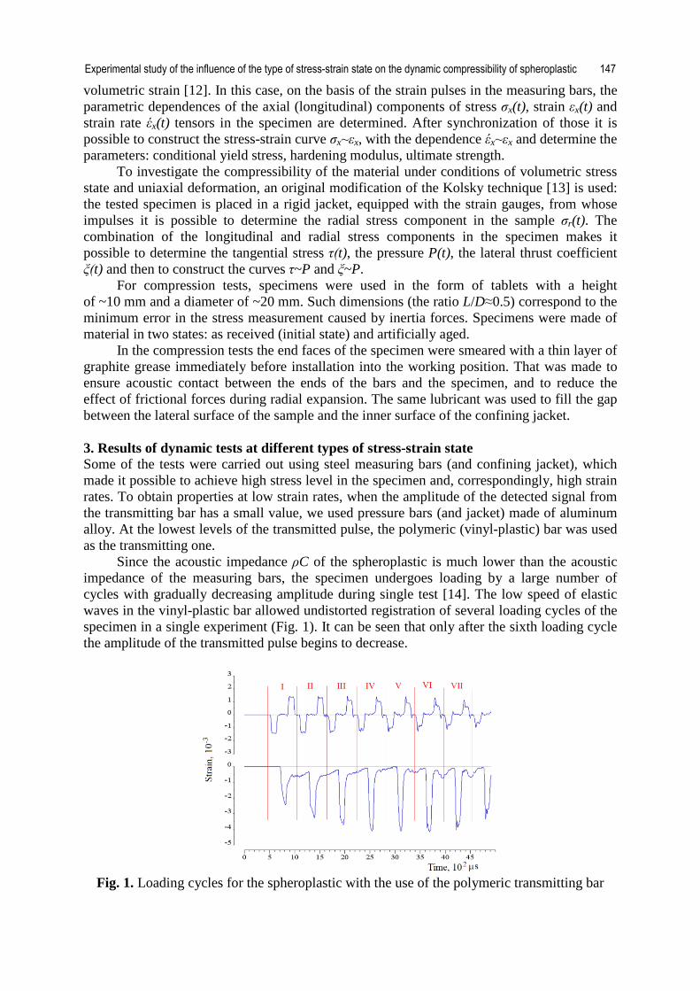
3. Results of dynamic tests at different types of stress-strain state Some of the tests were carried out using steel measuring bars (and confining jacket), which made it possible to achieve high stress level in the specimen and, correspondingly, high strain rates. To obtain properties at low strain rates, when the amplitude of the detected signal from the transmitting bar has a small value, we used pressure bars (and jacket) made of aluminum alloy. At the lowest levels of the transmitted pulse, the polymeric (vinyl-plastic) bar was used as the transmitting one.

Since the acoustic impedance ρC of the spheroplastic is much lower than the acoustic impedance of the measuring bars, the specimen undergoes loading by a large number of cycles with gradually decreasing amplitude during single test [14]. The low speed of elastic waves in the vinyl-plastic bar allowed undistorted registration of several loading cycles of the specimen in a single experiment (Fig. 1). It can be seen that only after the sixth loading cycle the amplitude of the transmitted pulse begins to decrease.

Fig. 1. Loading cycles for the spheroplastic with the use of the polymeric transmitting bar

Experimental study of the influence of the type of stress-strain state on the dynamic compressibility of spheroplastic 147

In the condition of a uniaxial stress state, strain-strain curves were obtained for the spheroplastic in the initial state and aged. In Fig. 2 shows only 3-4 loading cycles, since the subsequent cycles do not produce significant changes in the levels of achieved stress and strain. As one can see, the structural strength of the spheroplastic is very low - about 5 MPa. Spheroplastic in an aged state showed a greater dispersion of strength properties, however, this may be a consequence of poor-quality end surfaces of the tested specimens.

Fig. 2. Stress-strain curves of spheroplastic in the initial state (left) and aged (right)

Due to the high viscosity of the polymer binder the material demonstrates a very slow recovery of the initial shape after each loading cycle, as is clearly shown in Fig. 1 (lower beam). It is not possible to obtain a complete specimen unloading for several tens of microseconds (pause between cycles). Therefore, the sections of the diagram between the load cycles are rather hypothetical.

Fig. 3. Stress-strain curves for spheroplastic in the initial (left) and aged (right) states under uniaxial strain condition

When the specimen is placed in a rigid jacket the uniaxial deformation process is

realized. The stress-strain curves of spheroplastic obtained in this case for both initial and aged states for two loading cycles are shown in Fig. 3. The parameters of shear strength (the dependences τ~P and ξ~P) are shown in Fig. 4.

The dynamic properties of spheroplastic in two states (initial and aged) are compared. Next, characteristic diagrams of spheroplastic specimens are shown in tests without a jacket (Fig. 5) and in a jacket (Fig. 6). It is possible to note somewhat less deformability of the spheroplastic in the artificially aged state.

148 Anatoly M. Bragov, Alexander Yu. Konstantinov, Andrey K. Lomunov

Fig. 4. Shear strength parameters for spheroplastic in the initial (left) and aged (right) states under uniaxial strain condition

Fig. 5. Comparison of stress-strain curves for spheroplastic in the uniaxial stress state (left)

and uniaxial strain state (right)

Fig. 6. Comparison of the parameters of shear strength of spheroplastic in two states under uniaxial deformation

Comparison of the shear strength parameters (the dependences ξ~P and τ~P) is shown

in Fig. 6. The coefficient of lateral thrust of the material in the aged state is somewhat greater than in the initial one. The curve τ~P can be approximated by a linear dependence.

The appearance of the specimens after deformation with different load levels under uniaxial stress conditions is presented in Fig. 7.Analysis of the nature of the material destruction as a result of testing under uniaxial stress condition (without a confining jacket) revealed the following. At low loading pulse energy the specimen retains apparent integrity, but its actual residual strain is much less than that obtained from the curves in Fig. 2.


Apparently, the polymeric binder of the spheroplastic has a large coefficient of shape recovery, but because of high viscosity of the binder the registration of specimen's unloading after the loading pulse end seems to be impossible.

a

b

Fig. 7. The appearance of spheroplastic specimens in the initial (a) and aged (b) states after

loading without a confining jacket

The destruction of samples is fragile and occurs closer to the outer peripheral surface, while the central zone remains intact. This may be due to the presence of friction on the end surfaces of the samples, leading to triaxiality of its stress state.

4. Conclusion The structural strength of spheroplastic at compression under uniaxial stress condition was found to be about 5 MPa for both specimens in the state of delivery and artificially aged. For the condition of uniaxial strain, the coefficient of lateral thrust was determined. The average value of the lateral thrust ratio was found to be 0.35 for the spheroplastic in the initial state, and 0.45 for the aged state.

In the aged state the spheroplastic showed somewhat less deformability for both types of stress-strain states. The shear strength τ~P of the aged spheroplastic is less than that in the initial state. Acknowledgements. The work is financially supported by the Federal Targeted Programme for Research and Development in Priority Areas of Development of the Russian Scientific and Technological Complex for 2014–2020 under the contract No. 14.578.21.0246 (unique identifier RFMEFI57817X0246).

References [1] Reid SR, Reddy TY, Peng C. Dynamic compression of cellular structures and materials, In: Jones N, Wierzbicki T. (eds.) Structural Crashworthiness and Failure. Amsterdam: Elsevier; 1993. p.295-339. [2] Maiti SK, Gibson LJ, Ashby ME. Deformation and energy absorption diagrams for cellular solids. Acta Metallurgica. 1984;32(11): 1963-1975. [3] Zaretsky E, Ben-dor G. Compressive stress-strain relations and shock Hugoniot curves of flexible foams. Journal of Engineering Materials and Technology. 1995;117(3): 278-284. [4] Shim VPW, Tay BY, Stronge WJ. Dynamic Crushing of Strain-Softening Cellular Structures – A One-Dimensional Analysis. Journal of Engineering Materials and Technology. 1990;112(4): 398-405. [5] Stronge WJ, Shim VPW. Dynamic crushing of a ductile cellular array. International Journal of Mechanical Sciences. 1987;29(6): 381-406.

150 Anatoly M. Bragov, Alexander Yu. Konstantinov, Andrey K. Lomunov

[6] Calladine CR, English RW. Strain-rate and inertia effects in the collapse of two types of energy-absorbing structure. International Journal of Mechanical Sciences. 1984;26(11-12): 689-701. [7] Tan PJ, Reid SR, Harrigan JJ. On the dynamic mechanical properties of open-cell metal foams – A re-assessment of the 'simple-shock theory'. International Journal of Solids and Structures. 2012;49(19-20): 2744-2753. [8] Zou Z, Reid SR, Tan PJ, Harrigan JJ, Li S. Dynamic crushing of honeycombs and features of shock fronts. International Journal of Impact Engineering. 2009;36(1): 165-176. [9] Atroshenko SA, Krivosheev SI, Petrov YuV, Utkin AA, Fedorovskiy GD. Fracture of spheroplastic under static and dynamic stressing. Technical Physics. 2002;47(12): 1538-1542. [10] Zukas JA, Nicholas T, Swift HF, Greszczuk LB, Curran DR. (eds) Impact Dynamics. New York: Wiley; 1982. [11] Gibson LJ, Ashby MF. Cellular Solids: Structure and Properties. Cambridge Solid State Science Series. 2nd edn. Cambridge University Press; 1997. [12] Bragov AM, Lomunov AK. Methodological aspects of studying dynamic material properties using the Kolsky method. Int. Journal of Impact Engineering. 1995;16(2): 321-330. [13] Bragov AM, Lomunov AK, Sergeichev IV, Tsembelis K, Proud WG. International Journal of Impact Engineering. 2008;35(9): 967-976. [14] Bragov AM, Lomunov AK, Sergeichev IV. Modification of the Kolsky method for studying properties of low-density materials under high-velocity cyclic strain. Journal of Applied Mechanics and Technical Physics. 2001;42(6): 1090-1094.


THE DESCRIPTION OF ELASTIC MODULUS OF

NANOCOMPOSITES POLYURETHANE/GRAPHENE WITHIN THE

FRAMEWORKS OF MODIFIED BLENDS RULE G.V. Kozlov, I.V. Dolbin*

Kh.M. Berberov Kabardino-Balkarian State University

360004 – Nal’chik, Chernyshevsky st., 173, KBR, Russian Federation


Abstract. For description of elastic modulus of nanocomposites polyurethane/graphene the modified mixtures rule was proposed, which takes into consideration two factors. First, this rule assumes, that in polymer nanocomposites interfacial regions are the same reinforcing element of their structure, as actually nanofiller. Secondly, real, but not nominal, characteristics values of nanocomposite components were used. This allows the quantitative description of elastic modulus of the considered nanocomposites exactly enough. Reaching of percolation threshold of graphene platelets results to the essential enhancement of elastic modulus for both structure components and nanocomposite as a whole. Keywords: mixtures rule, nanocomposite, graphene, elastic modulus, interfacial regions 1. Introduction As a rule, the efficiency of nanofiller loading in polymer matrix is estimated with the aid of such parameter as reinforcement degree En/Em, where En and Em are moduli of elasticity of nanocomposite and matrix polymer, respectively [1-4]. From the technological point of view this parameter is an ideal quantitative characteristic of nanofiller efficiency in the process of polymer stiffness enhancement, but at theoretical treatment of reinforcement process certain difficulties arise, which are due to structure and hence properties modification of both nanofiller and polymer matrix in nanofiller loading process [5]. In case of nanofiller the indicated modification of the structure is due to a high degree of aggregation of its initial particles and their anisotropy [1] and for polymer matrix this modification is expressed by the variation of its molecular and structural characteristics, crystallization, interfacial regions formation and so on [5]. The authors [6] proposed the methods for determination of real values of an elastic modulus for nanofiller Enf and interfacial regions Eif for nanocomposites poly(vinyl alcohol)/carbon nanotubes and found out, that the value Enf =71±55 GPa at the nominal magnitude of elastic modulus of carbon nanotubes ECNT of the order of 1000 GPa and Eif =46±5.5 GPa at nominal elastic modulus of matrix poly(vinyl alcohol) Em≈2 GPa.

For theoretical description of nanocomposites elastic modulus the mixture rule is often applied [7]:

( ) mnmnforn EEEE +ϕ−η= , (1) where ηor is a factor of length efficiency, ϕn is volume content of nanofiller.

However, the equation (1) application for determination of value En for polymer nanocomposites gives exact results rarely, that is due to the factors described above. Therefore the purpose of the present work is the development of modified analogue of a

Materials Physics and Mechanics 40 (2018) 152-157 Received: November 2, 2017


mixture rule, taking into consideration real values of Enf and Eif on the example of nanocomposites polyurethane/graphene (PU/Gr) [8]. 2. Methods Graphen sheets (flaces) of firm Sigma Aldridge production were dispersed in dimethylformamide (DMF) at the initial concentration 3 mg/ml and processed in a sonic bath Branson MT-1510 for 150 h. This dispersion was split into four portions which were centrifuged at 500 rpm for 22.5 and 45 min and at 750 and 1000 rpm for 45 min. After centrifugation, the supernatants were collected. However, after such procedure graphene dispersions in DMF with low concentrations only (no higher than ~ 1 mg/ml can be obtained). Therefore the authors [8] proposed a new methods for obtaining graphene suspensions, having high concentrations. The indicated supernate of graphene suspensions in DMF was filtered onto a nylon membranes of pore size of 0.45 mcm (Sterlitech). These membranes were immersed in suspension and sonicated in a bath Branson MT-1510 for 60 min. At such procedure graphene tends to come through the membrane, after that it becomes re-dispersed in DMF but at much higher concentrations (up to 20 mg/ml), that allows to obtain composites with high graphene contents [8].

The polyurethane (PU) from firm Hydrosize of mark U2-01 with an average particle size ~ 3 mcm was used as a matrix polymer. The polymer solution was produced by drying of dispersion PU in water at 333 K for 72 h and followed by dissolution of PU in DMF to obtain solution, having concentration of 50 mg/ml [8].

Then PU solution and graphene suspension in DMF were blended to create 10 dispersions with graphene concentrations 0-90 mass %, after that they were sonicated for 4 h to homogenize. Films of composites polyurethane/graphene (PU/Gr) are obtained by drop-casting method of suspensions on smooth surface of flat Teflon trays, after that they were dried in a vacuum oven at 333 K for 12 h and further dried at 333 K for 72 h in a normal oven. The thickness of the prepared films varies within the range of 35-40 microns [8].

Tensile tests were carried out by using an apparatus Zwick Roell with a 100 N load cell at a clip rate of 50 mm/min and temperature 298 K [8]. 3. Results and Discussion As it was noted above, in paper [6] the theoretical relationship, allowing to determine real values of elastic moduli of nanofiller Enf and interfacial regions Eif was proposed, which has the look:

( ) ( )mnforn

ifmif

n

n EEdd

EEddE

−η+ϕ

ϕ−=

ϕ, (2)

where ϕif is a relative fraction of interfacial regions and parameter ηor is accepted equal to 0.38.

The volume content of nanofiller (graphene) can be determined according to the well-known formula [1]:

n

nn

Wρ

=ϕ , (3)

where Wn is mass content of nanofiller, ρn is its density, which is equal to 1600 kg/m3 for graphene [9].

The value ϕif can be estimated with the aid of the following percolation relationship [1]:

( ) 7.1111 ifnm

n

EE

ϕ+ϕ+= . (4)

The description of elastic modulus of nanocomposites polyurethane/graphene within the frameworks of... 153

This relationship takes into consideration, that interfacial regions are the same reinforcing (strengthening) element of nanofiller structure, as actually nanofiller, that follows directly from the comparison of values Em and Eif, cited above [6-13].

Construction of the plots in coordinates dEn/dϕn - dϕif /dϕn in case of their linearity together with using of the equation (2) allows to determine real values of elastic moduli of nanofiller and interfacial regions. In reference to the considered nanocomposites PU/Gr it was found out, that the indicated plot falls apart on two linear parts: for Wn≤50 mass % and for Wn>50 mass %. These plots are adduced in Fig. 1 and Fig. 2, respectively. Since the relationship (4) allows to determine values ϕif only for the first from the indicated parts in virtue of the condition En/Em≤12, then for the second part the following simple equation has been used:

nif ϕ−=ϕ 1 . (5)

Fig. 1. The dependence of derivative dEn/dϕn on derivative dϕif /dϕn, corresponding to the equation (2), for nanocomposites PU/Gr at Wn≤50 mass % (on the percolation threshold

lower)

Fig. 2. The dependence of derivative dEn/dϕn on derivative dϕif /dϕn, corresponding to the equation (2), for nanocomposites PU/Gr at Wn>50 mass % (on the percolation threshold

above)

dEn/dϕn, GPa

0.6

0.2

2 4 dϕif /dϕn

0

0.4

dEn/dϕn, GPa

4

2 3 dϕif /dϕn

2

1 0

154 G.V. Kozlov, I.V. Dolbin

The equation (5) assumes that at Wn>50 mass % structure of nanocomposites PU/Gr consists of nanofiller and interfacial regions only.

The application of the described above methods showed that values Eif and Enf are distinguished for the two indicated parts of the dependence dEn/dϕn (dϕif /dϕn): for the first (Wn≤50 mass %) part Eif =0.124 GPa and Enf =0.236 GPa and for the second one (Wn>50 mass %) Eif =1.91 GPa and Enf =2.66 GPa, i.e. more than one order above. Nevertheless, the values Eif and Enf for both indicated parts essentially (also more than the order above) exceed elastic modulus of matrix polyurethane (Em=10 MPa [8]), that gives reasons to consider both nanofiller and interfacial regions as reinforcing element of nanocomposites PU/Gr structure. Then the modified mixtures rule can be written as follows:

ififnnfn EEE ϕ+ϕ= . (6) In Fig. 3 the comparison of the calculated according to the modified mixtures rule, i.e.

to the equation (6), and the obtained experimentally dependences of elastic modulus En on nanofiller mass contents Wn for nanocomposites PU/Gr is assumed. This comparison has shown both qualitative and quantitative good correspondence of theory and experiment (their average discrepancy makes up ~ 7 %), that confirms correctness of the proposed here modified mixtures rule. The equations (1) and (6) comparison demonstrates their main distinction: if the equation (1) operates by nominal values of elastic modulus of nanofiller and matrix polymer, then the equation (6) uses their real values and takes into consideration the formation of interfacial regions in polymer matrix at the introduction of nanofiller in matrix polymer.

Fig. 3. The comparison of the calculated according to the modified mixture rule (the equation (6)) (1) and experimentally obtained (2) dependences of elastic modulus En on mass contents of nanofiller Wn for nanocomposites PU/Gr. The vertical shaded line 3 indicates percolation

threshold ϕc=54.4 mass % And in conclusion let us consider the reason of the two linear parts appearance on the

plot dEn/dϕn (dϕif /dϕn). As it is known [14-16], for spherical particles two percolation thresholds ϕc are observed, corresponding to particles contact and interpenetration. If for such strongly anisotropic particles as carbon nanotubes and graphene the first from the indicated percolation thresholds is very small (ϕc<0.01 [17-18]), then by analogy with spherical particles it can be supposed, that the interpenetration of graphene platelets is realized at ϕn=ϕc=0.34 or Wn≈54 mass % according to the formula (3). As it was noted above, just this very threshold value Wn corresponds to the decay of the plot dEn/dϕn (dϕif /dϕn) on two linear parts. In Fig. 3 this value Wn is indicated by vertical shaded line and it can be seen that it

En, GPa

1.5

Wn, mass % 100

1.0

50 0

0.5 - 2

3 1


divides two parts of the dependence En(Wn): at Wn≤50 mass % fast growth En is observed and at Wn>50 mass % the indicated dependence reaches plateau at En≈1.5 GPa. Let us note, that sharp enhancement of the parameters Eif and Enf, indicated above, at percolation threshold reaching defines anomalously high values En of the order of 1.5 GPa. At conservation of the values Eif and Enf, obtained up to percolation threshold, that value En, corresponding to the dependence En(Wn) plateau, would make up 180 MPa only, i.e. about one order below. 4. Conclusions Hence, in the present work the modified mixtures rule is proposed, which describes correctly elastic modulus of nanocomposites polyurethane/graphene. The mixtures rule modification is contained in using not nominal, but real characteristics of nanocomposites and accounting of interfacial regions properties, which are the same reinforcing (strengthening) element of nanocomposite structure, as actually nanofiller. Reaching percolation threshold of interpenetrating platelets of 2D-nanofiller (graphene) results to essential enhancement of elastic modulus of both nanofiller and interfacial regions and, as consequence, to increasing of elastic modulus of nanocomposite as a whole almost on one order of magnitude.

Acknowledgements. No external funding was received for this study.

References [1] Mikitaev AK, Kozlov GV, Zaikov GE. Polymer Nanocomposites: Variety of Structural Forms and Applications. New York: Nova Science Publishers Inc: 2008. [2] Schaefer DW, Justice RS. How nano are nanocomposites? Macromolecules. 2007;40(24): 8501-8517. [3] Mikitaev AK, Kozlov GV. Structural model for the reinforcement of polymethyl methacrylate/carbon nanotube nanocomposites at an ultralow nanofiller content. Tech. Phys. 2016;61(10): 1541-1545. [4] Kozlov GV, Dolbin IV. The fractal model of mechanical stress transfer in nanocomposites polyure-thane/carbon nanotubes. Lett. on Mater. 2018;8(1): 77-80. [5] Kozlov GV. Polymer phase behavior in nanocomposites. In: Ehlers TP, Wilhelm JK (eds.) Polymer Phase Behavior. New York: Nova Science Publishers Inc.; 2011. p.123-169. [6] Coleman JN, Cadek M, Ryan KP, Fonseca A, Nady JB, Blau WJ, Ferreira MS. Reinforcement of polymers with carbon nanotubes. The role of an ordered polymer interfacial region. Experiment and modeling. Polymer. 2006;47(26): 8556-8561. [7] Khan U, May P, O'Neill A, Bell AP, Boussac E, Martin A, Semple J, Coleman JN. Polymer reinforcement using liquid-exfoliated boron nitride nanosheets. Nanoscale. 2013;5(2): 581-587. [8] Khan U, May P, O'Neill A, Coleman JN. Development of stiff, strong, yet tough composites by the addition of solvent exfoliated graphene to polyurethane. Carbon. 2010;48(14): 4035-4041. [9] Xu Y, Hong W, Bai H, Li C, Shi G. Strong and ductile poly(vinyl alcohol)/graphene oxide composite films with a layered structure. Carbon. 2009;45(15): 3538-3543. [10] Kim H, Abdala AA, Macosko CW. Graphene/Polymer Nanocomposites. Macromolecules. 2010;43(16): 6515-6530. [11] Jang BZ, Zhamu A. Processing of nanographene platelets (NGPs) and NGP nanocomposites: a review. J. Mater. Sci. 2008;43(15): 5092-5101. [12] Zhang Y, Mark JE, Zhu Y, Ruoff RS, Schaefer DW. Mechanical properties of polybutadiene reinforced with octadecylamine modified graphene oxide. Polymer. 2014;55(21): 5389-5395.

156 G.V. Kozlov, I.V. Dolbin

[13] Yasmin A, Daniel IM. Mechanical and thermal properties of graphite platelet/epoxy composites. Polymer. 2004;45(24): 8211-8219. [14] Mikitaev AK, Kozlov GV. Description of the degree of reinforcement of polymer/carbon nanotube nanocomposites in the framework of percolation models. Physics of the Solid State. 2015;57(5): 974-977. [15] Kozlov GV, Burya AI, Dolbin IV. Fractal model of the heat conductivity of carbon plastics on the basis of phenylone. J. Engn. Thermophysics. 2005;13(2): 129-135. [16] Kozlov GV, Burya AI, Dolbin IV, Zaikov GE. Fractal Model of the Heat Conductivity for Carbon Fiber-Reinforced Aromatic Polyamide. J. Appl. Polymer Sci. 2006;100(5): 3828-3831. [17] Foygel M, Morris RD, Anez D, French S, Sobolev VL. Theoretical and computational studies of carbon nanotube composites and suspensions: Electrical and thermal conductivity. Phys. Rev. B. 2005;71(10): 104201 [18] Celzard A, McRae E, Deleuze C, Dufort M, Furdin G, Mareche JF. Critical concentration in percolating systems containing a high-aspect-ratio filler. Phys. Rev. B. 1996;53(10): 6209-6214.


THEORY OF HYPERBOLIC TWO-TEMPERATURE GENERALIZED

THERMOELASTICITY Hamdy M. Youssef1,2*, Alaa A. El-Bary3

1Mathematics Department, Faculty of Education, Alexandria University, Alexandria, EGYPT 2Engineering Mechanics Department, Faculty of Enginnering, Umm Al-Quar University, Makka, KSA

3Basic and Applied Science Department, Arab Academy of Science and Technology, Alexandria, EGYPT


Abstract. Youssef improved the generalized thermoelasticity base on two distinct temperatures; the conductive temperature and the thermodynamics temperature which coincide together when the heat supply vanishes [1, 2]. This theory has one paradox, where it offers an infinite speed of thermal wave propagation. So, this work assuming a new consideration of the two types of temperature which depends upon the acceleration of the conductive and the thermal temperature. This work introduces the proof of the uniqueness of the solution, moreover, one dimensional numerical application. According to the numerical result this new model of thermoelasticity offers finite speed of thermal wave and mechanical wave propagation. Keywords: elasticity, thermoelasticity, hyperbolic two-temperature, finite speed, wave propagation 1. Introduction Duhamel was the first to consider elastic problems with heat changes. Neumann re-derived the equations obtained by Duhamel. This theory of uncoupled thermoelasticity consists of the heat equation independent of mechanical effects, and the equation of motion contains the temperature, as a known function. Danilovskaya [3] was the first who solved a problem in the context of the theory of uncoupled thermoelasticity with uniform heat, and it was for a half-space subjected to a thermal shock. There are two defects of this theory. This theory states that the mechanical state of the elastic body does not affect the temperature, which is not in accord with right physical experiments. Second, the heat equation being parabolic predicts an infinite speed of propagation for the temperature, which again contradicts physical observations.

Biot [4] introduced the coupled theory of thermoelasticity in which the equations of elasticity and heat conduction became coupled, and that agree with physical experiments, and any change of the temperature gives a certain amount of deformation in an elastic body and vice versa. The theory of coupled thermoelasticity has proved useful for many problems. The governing equations of this theory contain the equation of motion, which is a hyperbolic partial differential equation, and of the equation of energy conservation, which is parabolic. The nature of the heat equation implies that if an elastic medium is extending to infinity subjected to a thermal or mechanical disturbance, the effect will fall instantaneously at infinity, which contradicts physical experiments. Hence, a new equation of energy with hyperbolic type is needed.

Lord and Shulman [5] introduced the theory of generalized thermoelasticity with one

Materials Physics and Mechanics 40 (2018) 158-171 Received: February 3, 2018


relaxation time for the particular case of an isotropic body. Dhaliwal and Sherief [6] extended this theory to include the anisotropic case. In this theory, a modified law of heat conduction including both the heat flux and its time derivative replaces the conventional Fourier's law (Cattaneo's heat conduction). The heat equation associated is hyperbolic and hence eliminates the paradox of infinite speeds of propagation inherent in both

The second generalization of the coupled theory of elasticity is the theory of thermoelasticity with two relaxation times. Müller [7] in a review of the thermodynamics of thermoelastic solids, suggested an entropy production inequality, with the use of which he considered restrictions on a class of constitutive equations. Green and Laws [8] proposed a generalization of this inequality. Green and Lindsay [9] got an explicit version of the constitutive equations. These equations were obtained independently by Suhubi [10]. This theory contains two parameters that act as relaxation times. The classical Fourier's law of heat conduction is not satisfied if the medium under consideration has a center of symmetry.

Chen and Gurtin [11], Chen et al. [12, 13] have constructed a theory of heat conduction in deformable bodies, which depends upon two different temperatures, the conductive temperature, and the thermodynamic temperature. For time-independent situations, the difference between these two temperatures is proportional to the heat supply. In the absence of the heat supply, the two temperatures are identical. For time-dependent problems, however, and for wave propagation problems in particular, the two temperatures are in general different regardless of the presence of heat supply. The thermodynamic temperature, conductive temperature, and the strain are found to have representations in the form of a traveling wave plus a response, which happen instantaneously throughout the body [14]. Warren and Chen [15] investigated the wave propagation in the two-temperature theory of thermoelasticity.

Youssef [1] introduced a new theory of two-temperature generalized thermoelasticity with the general uniqueness theorem for the boundary mixed initial value problems in this theory. Youssef constructed a new theory of two-temperature generalized thermoelasticity theory for the homogeneous and isotropic body without energy dissipation; he presented the general uniqueness theory for the initial mixed boundary value problems in this theory [2], and he derived its variational principle [16]. 2. Basic Equations The governing equations of an isotropic and homogeneous thermoelastic medium, as proposed by Lord and Shulman are [5]:

The equation of motion iij, j iF = ,uσ + ρ (1)

where ijσ is the stress tensor, iF is the body force components, ρ is the density, and iu is the displacement components.

The constitutive relation is: ( )ij ij kk ij 0 ij2 e e T Tσ = µ + λ δ − γ − δ , (2)

where ( ) T3 2γ = λ + µ α are the coupling parameters, T is the dynamical temperature and 0Tbeing the reference temperature, ije is the strain tensor and andλ µ are the elastic constants of the material.

The deformation

( )ij i, j j,i1e u u2

= + . (3)

The non-Fourier heat conduction

Theory of hyperbolic two-temperature generalized thermoelasticity 159

ii o ,i

qq K

t∂

+ t = − φ∂

, (4)

where φ is the conductive temperature. Moreover, we have

E 0 kk ,iC T T e qρ + γ = − , (5) where K is the thermal conductivity, iq is the heat flux components, and EC is the specific heat with constant strain .

The increment of the entropy η satisfies the following equations:

i,i 0q = T−ρ η , (6) and

0 E 0 ij ijT = C T + T eρ η ρ γ . (7) Equations (4), (6) and (7) formulate the heat conduction equations as proposed by

Youssef [1] in the form:

( )2

,ii o E 0 kk2K C T T et t

∂ ∂φ = + t ρ + γ ∂ ∂

, (8)

and ,iiT aφ− = φ , (9)

where a 0≥ is called the two-temperature parameter, while i, j, k 1,2,3= are the indeces for any general co-ordinates in 3-dimensons. 3. One-Dimensional Generalized Thermoelastic Half-Space (Classical Two-Temperature) Without losing the generality, we will consider one-dimensional isotropic and homogeneous thermoelastic medium occupies the half-space x 0≥ , and this medium is at rest in the undeformed state at zero time with uniform temperature 0T .

When t 0> , the boundary x 0= of the half-space subjected to a uniformly distributed time-dependent strain and temperature, then, the governing equations take the following forms:

( )2 2 2

2 2 2

e T e2 = ,x x t∂ ∂ ∂

λ + µ − γ ρ∂ ∂ ∂

(10)

( )2 2

o E 02 2K C T T etx t

∂ φ ∂ ∂= + t ρ + γ ∂∂ ∂

, (11)

2

2T ax

∂ φφ− =

∂, (12)

( ) ( )02 e T Tσ = λ + µ − γ − , (13) and

uex

∂=∂

. (14)

The boundary and the initial conditions are ( ) ( ) ( ) ( ) ( ) ( )T x,0 x,0 e x,0 T x,0 x,0 e x,0 0= φ = = = φ = = , (15)

and ( ) ( ) ( ) ( )o oe 0, t e t , 0, t t= φ = φ . (16)

160 Hamdy M. Youssef, Alaa A. El-Bary

For simplicity, use the following non-dimensional variables;

( ) ( ) ( ) ( ) ( )2 20 0

o o o o o0 0

E

T T T 2x ,u c x,u , t , c t, , , , , c ,T T 2

C.

K

− φ− σ λ + µ′ ′ ′ ′ ′ ′= η t = η t θ = φ = σ = =λ + µ ρ

ρη =

(17)

Hence, 2 2 2

12 2 2

e e = ,x x t∂ ∂ θ ∂

− e∂ ∂ ∂

(18)

( )2 2

o 22 2 etx t

∂ φ ∂ ∂= + t θ+ e ∂∂ ∂

, (19)

2

2x∂ φ

φ−θ = β∂

, (20)

and 1e σ = − e θ , (21)

where 01

T2

γe =

λ + µ, 2 2

ocγ

e =η

, 2 2oc aβ = η , 1 20, 0, 0e ≥ e ≥ β ≥ .

Taking the Laplace transform for the both sides of the equations (18)-(21) as follows:

( ) ( )∫∞

−=0

st tdetfsf . (22)

Hence, 2 2

212 2

d e d = s e ,d x d x

θ− e (23)

( )( )2

2o 22

d s s ed xφ= + t θ + e , (24)

2

2dd xφ

φ − θ = β , (25)

1e σ = − e θ , (26) d ued x

= , (27)

and ( ) ( ) ( ) ( )o oe 0,s e s , 0,s s= φ = φ . (28)

Eliminating θ from equations (23)-(25), then 2

2 32

d e ed x

= α φ +α , (29)

and 2

1 2 12

d edxφ= α φ + e α , (30)

where

( )2

o1 2

o

s s1 s s

+ tα =

+β + t ,

( )[ ]

1 1 12

1 1 2

11α e −βα

α =−βα e e

and ( )[ ]

21 1 2 1

31 1 2

s 11

−α e e −βαα =

−βα e e.


By solving the system in (29) and (30), the general solution will be as follows: ( ) ( )1 2k x k x

1 o o 1 2 2 o o 1 2e a , e , k , k e a , e , k , k e− −= φ + φ , (31) and

( ) ( )1 2k x k x1 o o 1 2 2 o o 1 2b , e , k , k e b , e , k , k e− −φ = φ + φ . (32) By using equations (25) and (32), we obtain

( ) ( ) ( ) ( )1 2k x k x2 21 1 o o 1 2 2 2 o o 1 21 k b , e , k , k e 1 k b , e , k , k e− −θ = −β φ + −β φ , (33)

where 1 2k and k± ± are the roots of the following characteristic equation

( )4 21 3 1 3 2 1 2k ( )k 0− α +α + α α − e α α = . (34)

By solving the above algebraic equation, then

( )21 3 1 3 1 3 2 1 2

1

( ) ( ) 4k

2α +α + α +α − α α − e α α

= ,

and

( )21 3 1 3 1 3 2 1 2

2

( ) ( ) 4k

2α +α − α +α − α α − e α α

= .

For small values of time t, this corresponds to a large value of s ( )s →∞ and by using Taylor expansion; the following cases will be discussed. 4. One-Temperature Model (Lord-Shulman) To get Lord-Shulman model, 0β = so, the roots of the characteristic equation will be in the following form

( )1,2 1,2 1 2 o1,2

s 1k Q , , OV s

= + e e t +

. (35)

Moreover, the speeds of the waves are:

1,2

o 1 2 o

2V1

=+ t + e e t ± Ψ

, (36)

where 2 2 2 2 21 2 o 1 2 o 1 2 o o o2 2 2 1Ψ = e e t + e e t + e e t + t − t + . (37) Equation (36) shows that the solutions have two waves propagated with speed 1V and 2V

( )1 2V V< . 1V is the speed propagation of the mechanical wave and 2V is the speed propagation of the thermal wave, and the medium has no disturbance for which 2x tV> with the following cases:

Case (1.1): o 0t ≠ . When o 0t ≠ , then, 1 2V and V as in equation (36), in this case, the mechanical and the

thermal waves propagate with finite speeds which depend on the material properties, where Lord and Shulman got that results in the generalized thermoelasticity theory [5].

Case (1.2): o 0t = . When o 0t = , then, 1 2V 1 and V→ →∞ , hence, only the mechanical wave propagates

with finite speed, and this speed is constant and independent on the material properties, while the thermal wave propagates with infinite speed and this case is called coupled thermoelasticity or Biot's model [4].


Case (1.3): 1 0e = and o 0t ≠ .

When 1 0e = , then, 1 2o

1V 1 and V→ →t

, in this case, the mechanical wave

propagates with finite speed that is constant and doesn't depend on the material properties, and the thermal wave propagates with finite speed and depends on the relaxation time only which is called uncoupled thermoelasticity. 5. Classical Two-Temperature Model To get the classical two-temperature thermoelasticity model of Youssef (15), 0β ≠ and hence, the roots of the characteristic equation of the system in (29) and (30) lead to the following cases:

Case (2.1): o o0 or 0t ≠ t = .

For any value of ot , then, 1 1 2 2V 1 and V→ +e e →∞ , in this case, only the mechanical wave propagates with finite speed and depends on the material properties while the thermal wave propagates with infinite speed. Also, the two-temperature parameter β does not affect the speed of the thermal or the mechanical wave propagation.

Case (2.2): 1 0e = . When 1 0e = , then, 1 2V 1 and V→ →∞ , which is equivalent to the case (1.1). So, the

classical two-temperature model of thermoelasticity Youssef (15) presents not a perfect model, where it generates the infinite speed of thermal wave propagation as the uncoupled thermoelasticity. 6. Hyperbolic Two-Temperature Generalized Thermoelasticity Theory According to the results in case (2), another form for two-temperature thermoelasticity generates to thermal and conductive heat waves propagating with finite speed is needed.

Now, define φ as the acceleration of the conductive heat, and T as the acceleration of the dynamical heat.

Assuming the difference between φ and T is the proportion of the heat supplies, i.e. 2

,iiT cφ− = φ , (38) where c (distance/time) is constant.

Definition "The constant 2c is equal to the difference between the acceleration of the conductive

temperature and the acceleration of the thermal temperature when the heat supply is a unit." To apply the last equation in the above one-dimensional problem, we have to use the

dimensionless in (18). Hence we have 2

*2T

x∂ φ

φ− = β∂

, (39)

where 2

*2o

cc

β = is the dimensionless of the hyperbolic two-temperature parameter.

Then,

( )* * *1,2 1,2 1 2 o*

1,2

s 1k Q , , , OV s

= + e e t β +

(40)

and


* *o 1 2 o*

1,2* *

o 1 2 o o

2 1V

1

+β t + e e β t=

+β t + e e t + t ± Ψ, (41)

where * 2 2 2 2 2 * 2 * 2 * *2 2

o 1 2 o o 1 2 o 1 2 o 1 2 o o o o1 2 2 2 2 2 2Ψ = − t + e e t + t + e e t + e e t − β e e t − β t + β t +β t . (42) Equation (41) shows that the solutions have two waves propagating with speed *

1V and*2V ( )* *

1 2V V< given by (41), where *1V is the speed propagation of the mechanical wave, and

*2V is the speed propagation of the thermal wave, and the medium has no disturbance for

which *2x tV> with the following cases:

Case (3.1): * 0β ≠ and o 0t ≠ . When * 0β ≠ and o 0t ≠ then, * *

1 2V and V as in equation (41), in this case, the mechanical and the thermal waves propagate with finite speeds which depend on the material properties, which agree with Lord and Shulman in case (1.1).

Now, the hyperbolic two-temperature parameter *β effects on the speed of the thermal and the mechanical wave propagation.

Case (3.2): * 0β ≠ and o 0t = . When * 0β ≠ and o 0t = , * *

1 2V 1 and V→ →∞ , in this case, only the mechanical wave propagates with finite speed and this speed is constant and independent on the material properties, while the thermal wave propagates with infinite speed, and this case is equivalent to cases (1.2) and (2.2).

Case (3.3): *o0, 0β ≠ t ≠ and 1 0e = .

When * 0β ≠ , o 0t ≠ and 1 0e = , then, *1V 1→ and * *

2o

1V → β +t

.

In this case, the mechanical wave propagates with finite speed that is constant and doesn't depend on the material properties, and the thermal wave propagates with finite speed and depends on the relaxation time and the hyperbolic two-temperature parameter, and it agrees with the case (1.3).

Case (3.4): * 0β = and o 0t ≠ . When * 0β = and o 0t ≠ , then, *

1 1V V= and *2 2V V= , which is equivalent to the

case (1.1) and agree with Lord-Shulman results [3]. Case (3.5): *

o0, 0β = t ≠ and 1 0e = .

When *o0, 0β = t ≠ and 1 0e = , then, 1 2

o

1V 1 and V→ →t

, in this case, the

mechanical wave propagates with finite speed is constant and doesn't depend on the material properties, while the thermal wave propagates with finite speed and depends on the relaxation time only. This case is equivalent to the case (1.3) of the uncoupled thermoelasticity.

Case (3.6): * 0β = and o 0t = . When * 0β = and o 0t = , then, 1 2V 1 and V→ →∞ , in this case, only the mechanical

wave propagates with finite speed, and this speed is constant and independent on the material properties, while the thermal wave propagates with infinite speed and this case is equivalent to the case (1.2) or Biot model.


7. Uniqueness Theorem Let V be an open regular region of space with boundary S occupied by the reference configuration of a homogeneous isotropic linear thermoelastic solid. S is assumed closed and bounded.

Supplement the equations of two temperature-generalized thermoelasticity (1)-(8) and (38) by prescribed boundary conditions [1]:

[ )i i 1u u on S 0,= × ∞, (43)

[ )i i ji j 1p p n on S S 0,= = σ − × ∞ , (44)

[ )i i i iand on S 0,φ = φ θ = θ × ∞

, (45)

where SS1 ⊂ and superposed "

" denotes the prescribed values on arbitrary subsets of S and their complements.

Also, the initial conditions as follows:

i i0 i i0 0 0u u , u u ,= = ϕ = ϕ = θ = θ , 0φ = θ = in V[0, )∞ at t = 0 (46) Theorem: Given a regular region of space V+S with boundary S then there exists at most one set

of single-valued functions ( )t,x kijσ and ( )t,xe kij with of C(1), ( )t,xu ki , ( )t,x kiφ and

( )t,xT ki of class C(2) in V+S, 0t ≥ which satisfy the equations (1)-(8) and (38) and the conditions (43)-(46) where E o oK ,C , , , ,T , ,c andλ µ γ ρ t all are positive.

Proof: Let there be two sets of functions )I(

ijσ and )II(ijσ , )I(

ije and )II(ije …etc. and let

(I) (II)ij ij ijσ = σ −σ , (I) (II)

ij ij ije e e= − , (I) (II)φ = φ −φ …etc. By the linearity of the problem, it is clear that these differences also satisfy the

equations mentioned above moreover, both kinematic and static boundary conditions are equal to zero (with iF Q 0= = ), and homogeneous counterparts of conditions (43)-(46), namely they satisfy the following field equations in ( )V 0,× ∞ :

iij, j = uσ ρ , (47)

( )ij ij kk ij2 e eσ = µ + λ − γ θ δ , (48)

o ,i i i + = - K q qt φ , (49)

i,i 0q - T= ρ η (50)

0 E 0 ij ijT = C + T eρ η ρ θ γ , (51)

( ) ( )E 0 0 kk o kk i iK = + + T e e, Cφ ρ θ θ γ + tt (52) 2

,iicφ−θ = φ (53)

( )ij i, j j,ie = ½ u u+ , (54) with the boundary and the initial conditions in (43)-(46).

For simplicity, the wave par has been omitted. Now, consider the integral

∫ ∫∫ σ−=σ=σv v

ij,ijj,iijv

ijij dvudvudve . (59)

Upon inserting equation (47), the latter equation reduced to ( ) 0dvuudve

viiijij =ρ+σ∫ . (60)


Using the equation (48), hence ( )[ ] 0dvuueee2

viiijijkkijij =ρ+δθγ−λδ+µ∫ . (61)

It could be written as follows: 2 i ikk ij ij kk

v v

u ud 1 e e e dv e dv 0d t 2 2

ρ λ +µ + − γ θ = ∫ ∫

. (62)

Substituting for kke from equation (52), then

2 2i i E0 kk ij ij ,ii

0v v

o E 0 o kkv v

u u Cd 1T e e e dv K dvd t 2 2 2T

C dv T e dv 0 .

ρ ρλ +µ + + θ − θφ

+ t ρ θθ +γ t θ =

∫ ∫

∫ ∫

(63)

From the well-known inequality 0q i,i ≥θ− . (64)

By using equation (49), then

,i ,i o ,i iv v

K dv q dv 0θ φ + t θ ≥∫ ∫ , (65)

which gives

,i ,i o i,iv v

K dv q dv 0θ φ − t θ ≥∫ ∫ . (66)

Inserting equations (50) and (51) in the last equation, hence

,ii o E 0 o kkv v v

K dv C dv T e dv 0− θφ + t ρ θθ + γ t θ ≥∫ ∫ ∫ . (67)

Finally, from equations (63) and (67), we obtain

2 2i i Ekk ij ij

0v

u u Cd 1 e e e dv 0d t 2 2 2T

ρ ρλ +µ + + θ ≤

∫

. (68)

The integral in the left-hand side of (68) is initially zero since the difference functions satisfy homogeneous initial conditions. By inequality (68), however, this integral either decreases (or therefore becomes negative) or remains equal to zero. Since the integral is the sum of squares, only the latter alternative is possible, that is

0t,0dvT2c

2uueee

21

v

2

0

Eiiijij

2kk ≥=

θ

ρ+

ρ+µ+λ∫

. (69)

It follows that the different functions are identically zero throughout the body and for all time this completes the proof of the theorem. 8. Numerical Application To get the numerical result which includes the three models of thermoelasticity; one temperature of L-S; classical two-temperature model and the hyperbolic two-temperature model, and then the coefficients of the governing equations (29) and (30) will be in the form

( )2

o1 2

o

s s1 s s

+ tα =

+Ω + t ,

( )[ ]

1 1 12

1 1 2

11α e −Ωα

α =−Ωα e e

and ( )[ ]

21 1 2 1

31 1 2

s 11−α e e −Ωα

α =−Ωα e e

. (72)

where

* 2

0 for one temperaturefor classical two temperature

/ s for hyperbolic two temperature

− Ω = β − β −

. (73)


Assume the thermal shock problem as follows: ( ) ( ) ( ) ( ) ( )o o 0e 0, t e t 0, 0, t t H t= = φ = φ = ϕ , (74)

where ( )H t is the Heaviside unit step function and 0ϕ is the thermal shock intensity? By using Laplace transform, and then

( ) ( ) ( ) ( ) 0o oe 0,s e s 0, 0,s s

sϕ

= = φ = φ = . (75)

Hence, the solutions in the Laplace transform domain in the forms:

( ) ( )1 2k x k x2 o

2 21 2

e x,s e es k k

− −α ϕ = − −, (76)

( ) ( ) ( ) ( )1 2k x k x2 2o1 3 2 32 2

1 2

x,s k e k es k k

− −ϕ φ = −α − −α −, (77)

( ) ( ) ( )( ) ( )( )1 2k x k x2 2 2 2o1 1 3 2 2 32 2

1 2

x,s 1 k k e 1 k k es k k

− −ϕ θ = −Ω −α − −Ω −α −, (78)

( ) ( )( )( )( )

( )( )( )1

2

k x2 22 1 1 1 3

o2 2 k x2 21 2 2 1 2 2 3

1 k k ex,s

s k k 1 k k e

−

−

α − e −Ω −αϕ σ = − − α − e −Ω −α

, (79)

and

( ) ( )1 2k x k x2 o

2 12 21 2 1 2

u x,s k e k esk k k k

− −−α ϕ = − −. (80)

To invert the Laplace transforms, we adopt a numerical inversion method based on a Fourier series expansion [17].

By this method, the inverse )t(f of the Laplace transform ( )sf is approximated by

( ) ( )vt N

1k 11 1 1

e 1 i k i k tf t f v Re f v exp , 0 t 2t,t 2 t t=

p p= + + < <

∑ (81)

where N is a sufficiently large integer representing the number of terms in the truncated Fourier series, chosen such that

( )1 1

i N i N texp v t Re f v expt t

p p+ ≤ e

, (82)

where e is a prescribed small positive number that corresponds to the degree of accuracy required. The parameter v is a positive free parameter that must be greater than the real part of all the singularities of ( )sf . The optimal choice of v was obtained according to the criteria described in [17].

The copper material was chosen for purposes of numerical evaluations, and the constants of the problem were taken as following [1]:

N/K.sec386K = , ( ) 15T K1078.1 −−=α , K/m1.383C 2

E = , 2sec/m73.8886=η

( ) 210 m/N1086.3=µ , ( ) 210 m/N1076.7=λ , 3m/kg8954=ρ , sec02.0o =t , K 293To = ,

1 1.60861e = , 2 0.0104442e = , *0.1 and 1.0β = β = (Assumed).


Fig. 1. The conductive temperature distribution

Fig. 2. The thermo-dynamical temperature distribution


Fig. 3. The stress distribution

Fig. 4. The displacement distribution


Fig. 5. The strain distribution

The Figures 1-5 show the conductive temperature, the thermo-dynamical temperature,

the stress, the displacement and the strain distributions respectively for the three models; one temperature model, classical two-temperature model, and hyperbolic two-temperature model.

In Figures 1-3, the hyperbolic two-temperature model agrees with one temperature model, and they introduce finite speed of the conductive temperature, the thermo-dynamical temperature, and the stress waves propagation, while it is not in the classical two-temperature model.

In Figures 4 and 5, the hyperbolic two-temperature model agrees with one temperature model where the displacement and the strain waves vanish before the classical two-temperature model.

In Figure 5, the peak points of the strain are closed in the two cases of the one-temperature model and the hyperbolic two-temperature model, while the peak point of the classical two-temperature model has a different value and far from the others peak point.

9. Conclusion

1- The classical two-temperature generalized thermoelasticity model Youssef [1] does not introduce finite speed of the thermal wave propagation which is physically unacceptable.

2- This work introduces hyperbolic two-temperature generalized thermoelasticity model in which the thermal wave propagation has a finite speed.

3- The two-temperature parameter has significant effects on all the studied fields for the hyperbolic two-temperature generalized thermoelasticity model and the classical two-temperature generalized thermoelasticity model.

4- The numerical results of all the studied fields show that, the thermo-mechanical waves of the hyperbolic two-temperature generalized thermoelasticity model and the one-temperature generalized thermoelasticity have the same attitude.

5- The hyperbolic two-temperature generalized thermoelasticity model is a successful model to study the behavior of the thermoelastic materials.



References [1] Youssef HM. Theory of two-temperature-generalized thermoelasticity. IMA journal of applied mathematics. 2006;71:383-390. [2] Youssef HM. Theory of two-temperature thermoelasticity without energy dissipation. Journal of Thermal Stresses. 2011;34:138-146. [3] Danilovskaya V. Thermal stresses in an elastic half-space due to a sudden heating of its boundary. Prikl Mat Mekh. 1950;14:316-324. [4] Biot MA. Thermoelasticity and Irreversible Thermodynamics. Journal of Applied Physics. 1956;27:240-253. [5] Lord HW, Shulman Y. A generalized dynamical theory of thermoelasticity. Journal of the Mechanics and Physics of Solids. 1967;15:299-309. [6] Dhaliwal RS, Sherief HH. Generalized thermoelasticity for anisotropic media. Quarterly of Applied Mathematics. 1980;38:1-8. [7] Müller I. The coldness, a universal function in thermoelastic bodies. Archive for Rational Mechanics and Analysis. 1971;41:319-332. [8] Green AE, Laws N. On the entropy production inequality. Archive for Rational Mechanics and Analysis. 1972;45:47-53. [9] Green AE, Lindsay KA. Thermoelasticity. Journal of Elasticity. 1972;2:1-7. [10] Eringen AC, Şuhubi ES. Elastodynamics: Linear Theory. New York:Academic Press; 1975. [11] Chen PJ, Gurtin ME. On a theory of heat conduction involving two temperatures. Zeitschrift für Angewandte Mathematik und Physik (ZAMP). 1968;19:614-627. [12] Chen PJ, Gurtin ME, Williams WO. On the thermodynamics of non-simple elastic materials with two temperatures. Zeitschrift für angewandte Mathematik und Physik (ZAMP). 1969;20:107-112. [13] Chen PJ, Williams WO. A note on non-simple heat conduction. Zeitschrift für angewandte Mathematik und Physik (ZAMP). 1968;19:969-970. [14] Boley BA, Tolins IS. Transient coupled thermoelastic boundary value problems in the half-space. Journal of Applied Mechanics. 1962;29:637-646. [15] Warren WE, Chen PJ. Wave propagation in the two temperature theory of thermoelasticity. Acta Mechanica. 1973;16:21-33. [16] Youssef HM. Variational Principle of Two-Temperature Thermoelasticity without Energy Dissipation. Journal of Thermoelasticity. 2013;1:3. [17] Honig G, Hirdes U. A method for the numerical inversion of Laplace transforms. Journal of Computational and Applied Mathematics. 1984;10:113-132.


ANOMALOUS HEAT TRANSFER

IN ONE-DIMENSIONAL DIATOMIC HARMONIC CRYSTAL

E.A. Podolskaya1,2*

, A.M. Krivtsov1,2

, D.V. Tsvetkov2

1Institute for Problems in Mechanical Engineering RAS, 61, Bolshoy pr. V. O., St. Petersburg, Russia

2Peter the Great St. Petersburg Polytechnic University, 29, Politechnicheskaya str., St. Petersburg, Russia


Abstract. The work is devoted to description of unsteady thermal processes in low-

dimensional materials. One-dimensional harmonic crystals with alternating masses and

stiffnesses are considered. Analytical solution demonstrates the ballistic nature of heat

propagation, which is confirmed by numerical simulations based on the particle dynamics

method. It is shown that temperature distribution propagates as two consecutive thermal

fronts with finite speed, and its initial shape is preserved.

Keywords: mathematical modeling, low-dimensional materials, discrete media, thermal

processes, heat transfer, lattice dynamics, harmonic crystal, polyatomic lattice

1. Introduction The relevance of this study is connected with the active development of new technologies for

creating materials that allow to regulate the material composition and structure at the atomic

level [1-3]. The properties of low-dimensional materials are often unique, which opens up

promising opportunities for their application [4]. For example, the hexagonal boron nitride

has high stability, chemical resistance, hardness, strength and thermal conductivity [5, 6]. In

general, low-dimensional materials have a complex crystal structure. For example, two-

dimensional graphene lattice consists of two sublattices formed by carbon atoms, and the

sublattices of hexagonal boron nitride, binary boron and nitrogen compound, are formed by

two different kinds of atoms. Filamentary nanocrystals (nanowires, nanowhiskers) can be

formed by either one type of atoms (silicon, carbon-carbine), or several ones (gallium

arsenide, indium phosphide). Hence, the development of models that would correctly describe

the physical and mechanical properties of such media and structures, including non-stationary

thermal processes, becomes particularly important. It should be noted that the existing

mathematical models are often not applicable to low-dimensional structures. For example,

recent experimental studies have shown that heat propagation at the nanoscale has peculiar

properties [6-8]. In particular, the Fourier law, which implies the diffusive type of heat spread,

is not fulfilled for low-dimensional structures; in contrast, the heat propagation in

nanostructures is of a ballistic nature [7, 9]. The analytical solution demonstrating the

anomalous heat propagation in one-dimensional harmonic chain was first presented in [10].

The solution was obtained for the stationary problem of heat propagation between two

thermal reservoirs with different temperatures, and it was shown that the thermal resistance

does not depend on the length of the chain, which contradicts the Fourier law; harmonic

crystals consisting of particles with different masses were considered, for example, in [11,

12].



In recent works [13-17], a method that allows analytical description of thermal

processes in harmonic crystals has been developed. This paper is devoted to application of

this method to one-dimensional harmonic crystals with alternating masses and stiffnesses. The

object of investigation is a harmonic crystal, which is a crystal lattice consisting of material

points interacting via linearized forces. The principle of separation of fast and slow thermal

processes is applied. Characteristic time for a fast process is of order of several periods of

atomic vibrations. Fast motions refer to fluctuations in the kinetic temperature associated with

the partial transfer of the kinetic energy to thermal energy; in polyatomic crystals, it is

accompanied by the redistribution of kinetic energy over the unit cell's degrees of freedom.

Characteristic time for a slow process is much larger than a period of atomic vibrations [18,

19]; heat transport, i.e. time evolution of the spatial distribution of kinetic temperature, is a

slow process. In this paper, analytical solutions are given for two unsteady heat transfer

problems: (i) cold and hot half space contact and (ii) propagation of an initially rectangular

thermal perturbation. Analytical results are verified by numerical simulation based on the

particle dynamics method.

2. Problem statement

Fig. 1. One-dimensional harmonic crystal with alternating masses

Lattice dynamics equations. Initial conditions. Particle dynamics equations for an

infinite one-dimensional harmonic crystal with alternating masses (Fig. 1) have the form:

( )

( ). (1)

Here and are displacements of the particles with masses and which

belong to the th unit cell; is the bond stiffness, and the respective frequencies are

√

⁄ and √

⁄ . Following [20], we introduce the equilibrium interparticle

distances: is the one inside the unit cell, and is the distance between the neighboring

particles from different cells. Hence, the so-called length of the unit cell is equal to .

Consequently, for the case of the system yields to one-dimensional harmonic chain

with the unit cell length equal to ⁄ .

In order to reduce the number of unknowns, let us introduce a parameter :

⁄ √

⁄ √ (2)

Taking the symmetry of its definition (2) into account, we can restrict ourselves to

. The initial conditions are written as follows

, (3)

where are random velocities with zero mean, i.e. their mathematical expectations are

equal to zero. Such initial conditions are used, for instance, to model an ultrashort laser

Anomalous heat transfer in one-dimensional diatomic harmonic crystal 173

impact [21, 22]. Note, that the solution of the resulting system (1)-(3) will be a set of random

values.

Dispersion relation. Let us seek the solution of (1)-(2) in the wave form with frequency

and one-dimensional wave vector :

(4)

Hence, the dispersion relation is determined as

[(

⁄ ) √ ⁄ ] (5)

Fig. 2. Dispersion curves for one-dimensional diatomic harmonic crystals with various mass

ratios . Black line ( ) corresponds to the one-dimensional harmonic chain

Figure 2 shows the branches of dispersion relation for one-dimensional diatomic

harmonic crystal at different values of the parameter . For example, the curves for

correspond to the mass ratio for the two-dimensional hexagonal boron nitride (the

exact value is 0.772), which possesses unique physical and mechanical properties [5, 6].

If the masses differ slightly, i.e. , optic and acoustic branches and merge.

Consequently, we obtain two dispersion curves for monoatomic chain, shifted by along

the horizontal axis relative to each other. The appearance of the two curves is due to the

change in the translational symmetry; in this case we still solve the system (1) of the two

equations for two neighboring particles.

Differentiation of (5) with respect to the wave vector leads to the following

representation of group velocities

⁄

(

√ ⁄

⁄

)

. (6)

Note, that the dispersion curves (Fig. 2) will look the same for the system with

alternating stiffnesses provided that the ratio of its parameters is kept

⁄ .

174 E.A. Podolskaya, A.M. Krivtsov, D.V. Tsvetkov

3. Heat propagation Kinetic temperature. Let us now follow [13-17] and consider the transfer from the

stochastic problem for particle displacements (1)-(3) to closed deterministic one for the

statistical characteristics of pairs of particles.

First, we introduce a spatial coordinate , which is one of the convenient ways to

identify a th unit cell. Then, we introduce the kinetiс temperature proportional to the

sum of the kinetic energies of the particles in the unit cell:

⁄ ( ⟨

⟩ ⟨ ⟩) (7)

where is Boltzmann constant, and brackets ⟨ ⟩ denote mathematical expectation.

Consequently, the velocities (see initial conditions (3)) are the random velocities with the

variance ⟨ ⟩

⁄ , where .

Thus, the conditions (3) mean that at the initial time, the particles have random

velocities corresponding to a certain temperature field. This field correlates with the initial

kinetic temperature of the system, while the potential energy is initially zero. This, in turn,

means that, according to the virial theorem [13, 16, 23], after a certain period of time, the

kinetic and potential energies will equilibrate. Characteristic time of this process is of order of

several periods of atomic vibrations, and it is referred to as fast process. Also, at such times

the kinetic energy is redistributed over the degrees of freedom inside the unit cell [17]. On the

contrary, heat transport is a slow process, for which the characteristic time is much larger.

It has been demonstrated that the propagation of the thermal perturbation in a

monoatomic chain is described by the formula [16]:

⁄ ∫

⁄ ∫ [ ( ) ( )]

, (8)

where is frequency, determined by the dispersion relation, is one-dimensional wave

vector, and is group velocity. At large times fast processes vanish, and temperature field

is a superposition of thermal waves travelling with the speed and having the shape of the

initial perturbation . Analysis of fast processes for one-dimensional diatomic crystal is given in [17].

Specifically, it is demonstrated that the solution oscillates around the half of the initial

temperature , and its amplitude decays as √

⁄ . At larger times when fast processes are

negligible, formulae (8) for polyatomic chain can be rewritten

⁄ ∫ ∑ * (

) ( )+

(9)

where is the number of atoms in the unit cell; for diatomic chain ; are the

respective group velocities (6). Further, several solutions will be constructed and compared

with the results of numerical simulation using the particle dynamics method. Formula (9)

means that the heat propagation has ballistic character, which differs from the Fourier law. In

the case of , formula (9) was derived for scalar lattices [16].

Cold and hot half space contact. Let the initial thermal perturbation have the form of a

Heaviside function:

(10)

where is the temperature of half-space before kinetic and potential energy

equilibrate. Then, for the considered diatomic system, formula (9) yields to


⁄ ∫ [ ( ) (

) ( )

( )] . (11)

Taking into account, that we finally obtain

( ⁄ )

⁄ ∫ * ( ⁄ ) ( ⁄

) ( ⁄ )

( ⁄ )+ . (12)

Fig. 3. Propagation of a Heaviside function in one-dimensional diatomic chain with different

mass ratios

Figure 3 shows the result of integration of (12) for different values of the parameter

. For and there are two thermal fronts travelling with finite speeds

[16], i.e. maximum values of group velocities and

respectively (6). Note, that ,

corresponding to the acoustic branch, is always larger than .

If , the two fronts merge and the solution coincides with the solution for the

monatomic chain with the unit cell length equal to ⁄ [13]:

( ⁄ )

⁄

⁄ ( ⁄ ) ⁄

⁄

⁄ (13)

To verify the obtained solution (12), a numerical simulation based on the particle

dynamics method was carried out. A sample consisting of 1000 particles was considered, for

which equations (1) were solved with initial conditions:

, (14)

and periodic boundary conditions. The kinetic temperature was calculated using formula (7),

where the mathematical expectation was approximated by averaging over 20 realizations with


various random initial conditions. Comparison of the analytical solution (12) with the

numerical solution has shown a good agreement up to small thermal oscillations near .

Propagation of rectangular thermal perturbation. For further analysis of the limiting

cases when and , let us consider the following initial temperature distribution

( ) (15)

where is a half of the interval with nonzero temperature.

The solution of this problem is a sum of solutions (12), according to superposition

principle. Temperature distribution for a diatomic chain with at several consequent

times is shown in Fig. 4. Comparison of the analytical and numerical solutions (see Fig. 5)

has also shown quite a good agreement. The deviations in the vicinity of are caused by

the residual fast processes, which have not fully decayed [17]. This effect decreases with the

increase of the sample size.

Fig. 4. Evolution of initially rectangular thermal perturbation ( ), analytical solution

Fig. 5. Comparison of analytical and numerical solutions at t = 600s


According to the classical heat conduction theory, a maximum would be observed at

and it would decay exponentially. In the case of anomalous thermal conductivity, the

solution decays faster near zero, forming four fronts that propagate two by two in opposite

directions with constant speeds.

Note that in a system with alternating masses or stiffnesses, the thermal front at large

times, when the "peaks" become less prominent, looks in a way similar to the solution of a

similar problem based on the Fourier thermal conductivity law, whereas the solution for a

monatomic chain demonstrates a fundamentally different behavior [13].

If the width of the initial perturbation decreases and its amplitude increases, the

solution tends to fundamental solution, i.e. solution with perturbation in the form of a delta

function. Numerical simulation for and has demonstrated that the thermal fronts

stay at a finite distance from each other, and the speed of the first ones ( , acoustic

branch) always turns out to be greater than the speed of the second ones ( , optic branch).

If one of the masses is negligible in comparison to another, i.e. , most of the heat is

transferred with the speed , whereas if almost all the heat propagates with

.

These observations can be further used to test the presented theory in future experiments.

4. Conclusions In the present work, the method that allows analytical description of heat propagation in

harmonic crystals [13-17] is applied to one-dimensional harmonic crystals with alternating

masses (Fig. 1). Solution (9) was obtained by analogy with (8) for scalar lattices [16]. Slow

motions are considered: the temperature field is a superposition of waves moving with group

velocities (6), and has the form of the initial temperature distribution.

Analytical solutions are given for two problems: (i) cold and hot half space contact and

(ii) propagation of an initially rectangular thermal perturbation. It is shown, that if the masses

differ slightly, all the solutions tend to the profiles for a monoatomic chain.

For the problem (i), it is demonstrated that, for any ratios between the masses, the initial

thermal perturbation propagates in the form of two successive thermal fronts having finite

speeds and repeating the form of the initial perturbation. The speed of the first, faster front

corresponds to the acoustic branch of the dispersion relation (5), and the speed of the second

front corresponds to the optical one. In turn, rectangular thermal perturbation (ii) splits into

four thermal fronts, which propagate two by two in opposite directions with constant

velocities.

Comparison of the analytical results with numerical simulation shows that the presented

theory describes the distribution of heat in a diatomic chain with high accuracy. It is

demonstrated numerically that if the masses differ slightly, the main part of the initial

perturbation propagates at a speed corresponding to the acoustic branch, but the velocities of

the fronts corresponding to the optical branch remain finite. The latter means that up to the

achievement of exact equality of the masses all fronts exist, and they are located at a finite

distance from each other.

The dispersion relation (5) is the same both for a chain with alternating masses and for a

chain with alternating stiffnesses, if the ratio of the respective parameters is the same as well.

Thus, from the point of view of the heat transfer problem, these systems are equivalent. Note

that this is true only when considering the average temperature in the unit cell (7). The

propagation of heat waves corresponding to different degrees of freedom will be significantly

different for the two systems [17].

Acknowledgements. The authors are sincerely grateful to V.A. Kuzkin, M.B. Babenkov and

O.S. Loboda for helpful discussions. This work was supported by the Russian Science


Foundation (project 17-71-10212, E.A. Podolskaya, project 18-11-00201, A.M. Krivtsov,

D.V. Tsvetkov).

References

[1] Novoselov K, Mishchenko A, Carvalho A, Castro Neto A. 2D materials and van der

Waals heterostructures. Science. 2016;353(6298): aac9439.

[2] Tantiwanichapan K, Swan A, Paiella R. One-dimensional carbon nanostructures for

terahertz electron-beam radiation. Physical Review B. 2016;93(23): 235416.

[3] Rauwel P, Salumaa M, Aasna A, Galeckas A, Rauwel E. A Review of the Synthesis and

Photoluminescence Properties of Hybrid ZnO and Carbon Nanomaterials. Journal of

Nanomaterials. 2016;2016: 1-12.

[4] Shi L, Dames C, Lukes J, Reddy P, Duda J, Cahill D et al. Evaluating Broader Impacts of

Nanoscale Thermal Transport Research. Nanoscale and Microscale Thermophysical

Engineering. 2015;19(2): 127-165.

[5] Shi Y, Hamsen C, Jia X, Kim K, Reina A, Hofmann M et al. Synthesis of Few-Layer

Hexagonal Boron Nitride Thin Film by Chemical Vapor Deposition. Nano Letters.

2010;10(10): 4134-4139.

[6] Golberg D, Bando Y, Huang Y, Terao T, Mitome M, Tang C et al. Boron Nitride

Nanotubes and Nanosheets. ACS Nano. 2010;4(6): 2979-2993.

[7] Chang C. Experimental Probing of Non-Fourier Thermal Conductors. In: Lepri S (ed.)

Thermal Transport in Low Dimensions. Lecture Notes in Physics. Springer International

Publishing; 2016;921. p.305-338.

[8] Guzev M, Dmitriev A. Oscillatory-damping temperature behavior in one-dimensional

harmonic model of a perfect crystal. Dal'nevost. Mat. Zh. 2017;17(2): 170-179.

[9] Bae M, Li Z, Aksamija Z, Martin P, Xiong F, Ong Z et al. Ballistic to diffusive crossover

of heat flow in graphene ribbons. Nature Communications. 2013;4: 1734.

[10] Rieder Z, Lebowitz J, Lieb E. Properties of a Harmonic Crystal in a Stationary

Nonequilibrium State. Journal of Mathematical Physics. 1967;8(5):1073-1078.

[11] Kannan V, Dhar A, Lebowitz J. Nonequilibrium stationary state of a harmonic crystal

with alternating masses. Physical Review E. 2012;85(4): 041118.

[12] Dhar A, Saito K. Heat Transport in Harmonic Systems. In: Lepri S (ed.) Thermal

Transport in Low Dimensions. Lecture Notes in Physics. Springer International Publishing;

2016;921. p.39-105.

[13] Krivtsov A. Heat transfer in infinite harmonic one-dimensional crystals. Doklady

Physics. 2015;60(9): 407-411.

[14] Babenkov M, Krivtsov A, Tsvetkov D. Energy oscillations in a one-dimensional

harmonic crystal on an elastic substrate. Physical Mesomechanics. 2016;19(3): 282-290.

[15] Kuzkin V, Krivtsov A. An analytical description of transient thermal processes in

harmonic crystals. Physics of the Solid State. 2017;59(5): 1051-1062.

[16] Kuzkin V, Krivtsov A. Fast and slow thermal processes in harmonic scalar lattices.

Journal of Physics: Condensed Matter. 2017;29(50): 505401.

[17] Kuzkin V. Approach to thermal equilibrium in harmonic crystals with polyatomic lattice.

Arxiv [Preprint] 2018. Available from: https://arxiv.org/abs/1808.00504 [Accessed 12th

October 2018].

[18] Sokolov A, Krivtsov A, Müller W. Localized heat perturbation in harmonic 1D crystals:

Solutions for the equation of anomalous heat conduction. Physical Mesomechanics.

2017;20(3): 305-310.

[19] Gavrilov S, Krivtsov A, Tsvetkov D. Heat transfer in a one-dimensional harmonic crystal

in a viscous environment subjected to an external heat supply. Continuum Mechanics and

Thermodynamics. 2018; Available from: https://doi.org/10.1007/s00161-018-0681-3.


[20] Ashcroft N, Mermin N. Solid state physics. Philadelphia, Pa.: Saunders college; 1976.

[21] Poletkin K, Gurzadyan G, Shang J, Kulish V. Ultrafast heat transfer on nanoscale in thin

gold films. Applied Physics B. 2012;107(1): 137-143.

[22] Indeitsev D, Osipova E. A two-temperature model of optical excitation of acoustic waves

in conductors. Doklady Physics. 2017;62(3): 136-140.

[23] Hoover W. Computational Statistical Mechanics. New York: Elsevier Science; 1991.


CORRESPONDENCE PRINCIPLE FOR SIMULATION HYDRAULIC

FRACTURES BY USING PSEUDO 3D MODEL N.S. Markov1*, A.M. Linkov2

1Peter the Great St. Petersburg Polytechnic University, Russia 2Rzeszow University of Technology, Poland


Abstract. The original pseudo three-dimensional (P3D) model is extended to an arbitrary stress contrast on the basis of the correspondence principle suggested. The principle employs the similarity between solutions to plain-strain elasticity problems for (i) the crack, corresponding to the central cross-sections of the P3D model, and (ii) the crack of the Khristianovich-Geertsma-de Klerk (KGD) model, when the sizes and average openings of the cracks are the same. This suggests using the propagation speeds of the KGD problem for assigning the speed of the height growth of the P3D model. This approach is applicable in all the cases when the KGD problem may be accurately solved; specifically, when accounting for an arbitrary stress contrast. Keywords: hydraulic fracturing, pseudo three dimensional (P3D) model, stress contrast 1. Introduction Hydraulic fracturing (HF) is the operation of injecting viscous fluid into the rock mass to create tensile cracks. The operation is widely used in petroleum industry for stimulation of oil and gas reservoirs [2]. Numerical simulators are developed for the design of this expensive operation to make it efficient. Commonly simulators are based on simplified mathematical models. Among those, the most popular is the pseudo-three dimensional (P3D) model [1, 5, 6, 10]. It combines physically clear prerequisites with computational efficiency (e.g. [1]). To assign the vertical speeds of fracture cross-sections, the authors introduced either actual [6, 9], or "apparent" [1] stress intensity factor (toughness) 𝐾𝐾𝐼𝐼𝐼𝐼 in the line of the classical fracture mechanics (e.g. [9]). Yet, being justified for high fracture toughness, the original model becomes irrelevant in practically important cases when the fluid viscosity dominates. Efforts to overcome the difficulty by assigning an apparent fracture toughness 𝐾𝐾𝐼𝐼𝐼𝐼 have actually succeeded merely for a particular case of a pay layer between half-spaces with the same (positive) stress contrast [1]. Authors obtained a solution, which in the particular case considered agrees with the solution to the truly 3D solution found by using the implicit level set algorithms (ILSA) suggested in [8]. Still, there has been no solution for the general case. The present work aims to consistently extend the P3D model to an arbitrary input of viscosity and to an arbitrary stress contrast. 2. Problem formulation The original P3D model is based on three main assumptions: 1. The length of the fracture is greater than its height (Fig. 1). Then plane-strain conditions occur in central cross-sections parallel to the fracture front;

Materials Physics and Mechanics 40 (2018) 181-186 Received: July 25, 2018


Fig. 1. Fracture footprint assumed in the P3D model

2. Elasticity modulus E and the Poisson ratio 𝜈𝜈 are the same in each layer of the elastic homogeneous isotropic media considered (Fig. 2);

Fig. 2. Profile of the opening for the P3D model

3. The physical pressure 𝑝𝑝 is the same along each cross-section, where plain-strain conditions are applicable (Fig. 3), while in-situ stress which acts and closes the fracture along the 𝑥𝑥-axis, commonly changes in the z-direction.

Fig. 3. Pressure in various cross-sections

These assumptions yield the system of equations, which is consists of 5 equation: 1. elasticity equation, obtained from the classical solution [7]

𝑤𝑤𝑎𝑎𝑎𝑎 = 2𝑧𝑧∗𝐸𝐸′𝜋𝜋𝑝𝑝𝑛𝑛𝑛𝑛𝑛𝑛

2− 1

2 ∫ ∆𝜎𝜎(𝑧𝑧(𝜍𝜍))1 − 𝜍𝜍2𝑑𝑑𝜍𝜍1−1 , (1)

where 𝑤𝑤𝑎𝑎𝑎𝑎 is the opening averaged over a cross-section, 𝐸𝐸′ = 𝐸𝐸/(1 − 𝜈𝜈2), 𝜍𝜍 = 𝑧𝑧 − (1/2(𝑧𝑧∗𝑙𝑙 + 𝑧𝑧∗𝑢𝑢) /𝑧𝑧∗, 𝑧𝑧∗(𝑥𝑥, 𝑡𝑡) = 1/2(𝑧𝑧∗𝑢𝑢 − 𝑧𝑧∗𝑙𝑙) is the half-height, 𝑧𝑧∗𝑙𝑙 (𝑧𝑧∗𝑢𝑢) is the global coordinate of the lower (upper) tip; 𝑝𝑝𝑛𝑛𝑛𝑛𝑛𝑛 = 𝑝𝑝(𝑥𝑥, 𝑡𝑡) − 𝜎𝜎𝑝𝑝 is the difference between the actual fluid pressure 𝑝𝑝 and a fixed value 𝜎𝜎𝑝𝑝 of the confining rock pressure;

182 N.S. Markov, A.M. Linkov

2. the continuity equation 𝜕𝜕(2𝑧𝑧∗𝑤𝑤𝑎𝑎𝑎𝑎)

𝜕𝜕𝑛𝑛= −𝜕𝜕(2𝑧𝑧∗𝑤𝑤𝑎𝑎𝑎𝑎𝑎𝑎𝑎𝑎𝑎𝑎)

𝜕𝜕𝜕𝜕− 𝑄𝑄𝑙𝑙 + 𝑄𝑄0𝛿𝛿(𝑥𝑥), (2)

where 𝑄𝑄𝑙𝑙 is the total leak-off through the surface of a cross-section, 𝑄𝑄0 is prescribed pumping rate at the source point;

3. the Poiseuille type equation

𝑣𝑣𝑎𝑎𝑎𝑎(𝑥𝑥, 𝑡𝑡) = 𝐹𝐹𝑎𝑎 −𝑤𝑤𝑎𝑎𝑎𝑎𝑛𝑛+1

𝜇𝜇′𝜕𝜕𝑝𝑝𝑛𝑛𝑛𝑛𝑛𝑛𝜕𝜕𝜕𝜕

1𝑛𝑛, (3)

where 𝐹𝐹𝑎𝑎(𝑥𝑥, 𝑡𝑡) =12𝑧𝑧∗

∫ 𝑤𝑤2+1/𝑛𝑛𝑑𝑑𝑧𝑧𝑧𝑧∗𝑢𝑢𝑧𝑧∗𝑙𝑙

𝑤𝑤𝑎𝑎𝑎𝑎2+1/𝑛𝑛 , 𝑛𝑛 is the fluid behavior index, 𝜇𝜇′ = 2[2(2𝑛𝑛 + 1)/𝑛𝑛]𝑛𝑛𝑀𝑀, 𝑀𝑀

is the consistency index; 4. the speed equation for the fracture front

𝑣𝑣∗𝜕𝜕(𝑡𝑡) = 𝐹𝐹𝑎𝑎(𝜕𝜕∗,𝑛𝑛)𝑛𝑛𝑛𝑛

1𝜋𝜋𝑧𝑧∗(𝑛𝑛+2)

1/𝑛𝑛

𝐶𝐶𝑤𝑤1+2/𝑛𝑛, (4)

where 𝐶𝐶𝑤𝑤 = 𝑤𝑤𝑎𝑎𝑎𝑎(𝑟𝑟𝑖𝑖)𝑟𝑟𝑖𝑖𝛼𝛼 , 𝑟𝑟 = 𝑥𝑥∗ − 𝑥𝑥 is the distance from a point 𝑥𝑥 behind the front to the front 𝑥𝑥∗,

𝛼𝛼 = 1𝑛𝑛+2

; 5. the speed equations for vertical growth of cross-sections

𝑣𝑣𝑧𝑧𝑙𝑙(𝑥𝑥, 𝑡𝑡) = 𝑑𝑑𝑧𝑧∗𝑙𝑙𝑑𝑑𝑛𝑛

= 𝑓𝑓𝑧𝑧𝑙𝑙𝑧𝑧∗𝑙𝑙 , 𝑧𝑧∗𝑢𝑢, 𝑤𝑤𝑎𝑎𝑎𝑎; 𝑣𝑣𝑧𝑧𝑢𝑢(𝑥𝑥, 𝑡𝑡) = 𝑑𝑑𝑧𝑧∗𝑢𝑢𝑑𝑑𝑛𝑛

= 𝑓𝑓𝑧𝑧𝑢𝑢𝑧𝑧∗𝑙𝑙 , 𝑧𝑧∗𝑢𝑢, 𝑤𝑤𝑎𝑎𝑎𝑎, (5) where 𝑓𝑓𝑧𝑧𝑙𝑙𝑧𝑧∗𝑙𝑙, 𝑧𝑧∗𝑢𝑢, 𝑤𝑤𝑎𝑎𝑎𝑎 and 𝑓𝑓𝑧𝑧𝑢𝑢𝑧𝑧∗𝑙𝑙 , 𝑧𝑧∗𝑢𝑢, 𝑤𝑤𝑎𝑎𝑎𝑎 are known functions.

The system (1)-(5) is complemented with the initial conditions (6) at an initial moment 𝑡𝑡0: 𝑥𝑥∗(𝑡𝑡0) = 𝑥𝑥∗0, 𝑤𝑤𝑎𝑎𝑎𝑎(𝑥𝑥, 𝑡𝑡0) = 𝑤𝑤𝑜𝑜(𝑥𝑥), 𝑧𝑧∗𝑙𝑙(𝑡𝑡0) = 𝑧𝑧∗𝑙𝑙0, 𝑧𝑧∗𝑢𝑢(𝑡𝑡0) = 𝑧𝑧∗𝑢𝑢0. (6)

To extend the original P3D model to an arbitrary regime of the fracture height growth we need to define 𝑓𝑓𝑧𝑧𝑙𝑙𝑧𝑧∗𝑙𝑙 , 𝑧𝑧∗𝑢𝑢, 𝑤𝑤𝑎𝑎𝑎𝑎 and 𝑓𝑓𝑧𝑧𝑢𝑢𝑧𝑧∗𝑙𝑙 , 𝑧𝑧∗𝑢𝑢, 𝑤𝑤𝑎𝑎𝑎𝑎. It can be done by using the correspondence principle formulated in the next section. 3. The correspondence principle As a physically consistent approach, we suggest to use the next correspondence principle. Two plane-strain HF under the same conditions are assumed equivalent, as regards to the speeds of their height growth, when the HF have the same: (i) tip positions, and (ii) fluid volumes above and below the injection point. The "same conditions" mean that the rock structure, stress contrasts, leak-off parameters, and the properties of rock, fluid and proppant are the same for the both HF. Taking into account that Khristianovich-Geertsma-de Klerk (KGD) and P3D models employ the same elasticity equation (1) for a straight crack under plain-strain conditions, one may expect that profiles of the opening for both models are similar when items (i) and (ii) are met. In fact, the difference concerns with merely near-tip zones influenced by the asymptotics, while the openings of the central parts of fractures may be almost the same (Fig. 4).

Then in any cross-section of the P3D model, the current tip positions and the current volumes above (and below) the injection point uniquely define the tip propagation speeds via the speeds in the corresponding (in the mentioned sense) KGD model (Fig. 5).

Correspondence principle for simulation hydraulic fractures by using pseudo 3D model 183

(a) (b) (c)

Fig. 4. Profiles of the opening for the KGD and P3D models: (a) full profiles; (b) comparison of the profiles; (c) magnified area with the difference between KGD and P3D openings

Fig. 5. Tip propagation speeds

The data to find the speeds via the tip positions and the volumes are prepared in

advance by solving a set of extended KGD problems (e.g. [3]). For each cross-section of the P3D model, this gives the propagation speeds needed to update the tip positions on a time step. Clearly, the method may serve for an arbitrary propagation regime when the KGD problems are solved accounting for the universal asymptotics [4].

Numerical implementation of the method has confirmed that for the particular case studied in [3], the profiles of the opening found for P3D and KGD models are practically the same. The propagation speeds are close, as well, what follows from the perfect agreement of footprints. Since the latter were verified in [1] against the truly 3D bench-mark solutions, this implies that the method developed is quite accurate.


Fig. 6. Comparison of the footprints obtained by using the correspondence principle the

benchmark solution given in [1] 4. Conclusions The correspondence principle, based on similarities between KGD and P3D models, serves to extend the original P3D model to a general case. The proposed method allows one to obtain accurate results, which are comparable with those for the truly 3D model when a fracture grows in the viscosity-dominated regime. The comparison of fracture footprints, obtained by the method suggested, with published solutions to truly 3D benchmark problems, has shown good agreement. This confirms that the speeds of height growth are evaluated correctly when employing the correspondence principle. The method can be also used to determine the limits of applicability of the original P3D model. Acknowledgement. The work was financially supported by the Ministry of Science and Higher Education of the Russian Federation in the framework of the Federal Program "Research and Development in the Priority Areas of Development of the Russian Scientific and Technical Complex for 2014-2020", Activity 1.2., Subsidy Agreement 14.575.21.0146 of 26.09.2017. Unique project identifier: RFMEFI57517X0146. References [1] Dontsov EV, Peirce AP. An enhanced pseudo-3D model for hydraulic fracturing accounting for viscous height growth, non-local elasticity, and lateral toughness. Engineering Fracture Mechanics. 2015;142: 116-139. [2] Economides MJ, Nolte KG. Reservoir stimulation. 2nd ed. Houston, Texas, USA: Schlumberger Educational Services; 1989. [3] Gladkov IO, Linkov AM. Khristianovich-Geertsma-de Klerk problem with stress contrast. To be published to Appl. Math. Techn. Phys. Arxiv. [Preprint] 2018. Available from: https://arxiv.org/abs/ 1703.05686 [Accessed 5th December 2018]. [4] Linkov AM. Particle velocity, speed equation and universal asymptotics for efficient modelling of hydraulic fractures. J. Appl. Math. Mech. 2015;79: 54–63. [5] Linkov AM, Mishuris G. Modified formulation, ε-regularization and efficient solving of hydraulic fracture problem. In: Jeffrey R. (ed.) Effective and Sustainable Hydraulic Fracturing: proceedings of the International Conference for Effective and Sustainable Hydraulic Fracturing, HF2013, 20-22 May 2013, Brisbane, Australia. 2013. p.641–657.

Correspondence principle for simulation hydraulic fractures by using pseudo 3D model 185

[6] Mack MG, Warpinski NR. Mechanics of hydraulic fracturing. In: Economides MJ, Nolte KG. (eds.) Reservoir Simulation. 3-rd edn. Chichester, England: John Willey & Sons: 2000, p.6-1-6-48. [7] Muskhelishvili NI. Some Basic Problems of the Mathematical Theory of Elasticity. Groningen, Noordhoff; 1975. [8] Peirce A, Detournay E. An implicit level set method for modeling hydraulically driven fractures. Comput. Methods Appl. Mech. Engng. 2008;197: 2858–2885. [9] Rice J. Mathematical analysis in the mechanics of fracture. In: Liebowitz H. (ed.) Fracture, an Advanced Treatise. New York: Academic Press; 1968;2. p.191–311. [10] Settari A, Cleary MP. Development and testing of a pseudo-three-dimensional model of hydraulic fracture geometry. SPE Prod. Eng. 1986;1(6): 449–466.


HIGHER-ORDER MODEL OF PRESTRESSED ISOTROPIC MEDIUM

FOR LARGE INITIAL DEFORMATIONS T.I. Belyankova1,2, V.V. Kalinchuk1,2*, D.N. Sheydakov1

1Southern Scientific Center of Russian Academy of Sciences, Chekhov Ave. 41, Rostov-on-Don 344006, Russia 2Southern Federal University, Bolshaya Sadovaya Str. 105, Rostov-on-Don 344006, Russia


Abstract. Within the theory of small deformations superposed on a finite one, a consistent linearization for the nonlinear equations of the mechanics of an originally isotropic elastic body in a neighborhood of some initial stress state is carried out in the Lagrange coordinate system. As the elastic potential for the originally isotropic body, we use the representation of the specific strain energy through the algebraic invariants of the Green-Lagrange strain tensor. The linearized constitutive relations and the equations of motion of the prestressed medium are derived that allow taking into account the nonlinear effects of the initial deformation on the elastic properties of the originally isotropic body. Keywords: initial stress, prestressed, initial deformation, elastic moduli of III orders, elastic moduli of IV orders, linearized theory, large initial deformations, elastic potential of IV orders 1. Introduction The widespread use of artificial materials in aerospace and mechanical engineering, and in electronics leads to the need for a detailed study of the physical properties of used materials, their technological and strength characteristics, depending on the operating modes and conditions. Such studies involve the solution of complex applied problems of the static and dynamic theory of elasticity, as well as the use of mathematical models that describe the processes taking place in the materials under consideration with some degree of accuracy. In turn, the modeling of these processes while taking into account various initial effects is associated with the use of an elastic potential [1, 2], which describes the energy accumulated during deformation. The choice of the particular form of the potential is determined by the specifics of the problem under consideration and by the coordinate system used. For isotropic materials, the elastic potential can be represented as a scalar function of invariants of one of the strain tensors [2-4]. Various expressions for the potential in the form of polynomials of III and IV order in invariants of the Green-Lagrange strain tensor were successfully used in [5, 6] for the modeling of highly elastic materials. For more rigid materials (rocks, metals, alloys, crystals, etc.), the Murnaghan representation of the elastic potential in the form of a cubic function of the Green-Lagrange strain tensor invariants [7] is widely used, in which, along with the elastic moduli of II order, there are also III order moduli. At present, due to theoretical and experimental studies, the values of III order moduli are known for a wide range of metals, alloys, crystals, various structural materials and for some rocks [8-12]. The use of hyperelastic material model with elastic moduli of III order made it possible to describe the properties of a prestressed medium more accurately: to analyze the second-order effects [11, 12], to determine the mechanical stresses [13, 14], and to study the features of dynamics, propagation and localization of waves [15-24]. In [21] a fairly comprehensive

Materials Physics and Mechanics 40 (2018) 187-200 Received: October 10, 2017


review on this subject is given. In order to develop a linearized contact theory for prestressed bodies, a consistent linearization for the nonlinear equations of the mechanics of an elastic solid has been carried out in the Lagrange and Euler coordinate systems [15]. The linearized equations of motion and the constitutive relations of the prestressed medium were derived in an arbitrary, generally curvilinear, coordinate system. The expressions presented in a compact form convenient for research were used in [15, 20-24] to solve a number of mixed boundary-value problems of the dynamic theory of elasticity. Particularly, for the model of originally isotropic hyperelastic material with the Murnaghan potential, the influence of the nature of the initial mechanical effects on the formation, propagation, and localization of wave fields in both homogeneous and inhomogeneous prestressed media has been studied [22-24].

Recently, a number of new materials, promising in practical applications and possessing unique physical properties, have appeared. In particular, these materials are able to withstand a very high level of elastic deformation, at which the nonlinearity of elastic properties becomes very significant. In [25-27], the results of experimental studies on the determination of elastic moduli of III and IV order for bulk metallic glasses based on zirconium (Zr) and palladium (Pd) are presented. The appearance of information about IV order moduli necessitate the improvement of the linearized contact theory for prestressed bodies developed in [15]. In this paper, we use a representation of the potential in which the elastic moduli of IV order are taken into account. The linearization is carried out in the Cartesian material coordinate system. The linearized equations of motion and the constitutive relations of the prestressed medium are derived, which allow taking into account the nonlinear effects of second-order and third-order in the influence of mechanical deformations on the elastic properties of the original material. Within the framework of the proposed model, we studied the effect of accounting for higher-order moduli on the parameters of the initial strained state and the properties of the prestressed material.

2. Nonlinear boundary-value problem for a prestressed originally isotropic elastic body Consider the reference v and the actual V configurations before and after application of surface and mass forces, respectively. The position of a material point in these configurations is given by the vectors k kx=r i and k kX=R i , where 1 2 3, ,i i i is the orthonormal Cartesian

vector basis, 1 2 3, ,x x x and 1 2 3, ,X X X are the Lagrangian and Eulerian coordinates. Here and below, we use the Einstein summation convention. Representation of the nabla-operators in the reference 0∇ and the actual ∇ configurations is defined by expressions:

0 mmx∂

∇ =∂

i , mmX

∂∇ =

∂i . (1)

Deformation of the medium is characterized by the deformation gradient C , the Cauchy-Green strain tensor G , and the Green-Lagrange strain tensor S (I is the unit tensor):

0= ∇C R , T= ⋅G C C , ( )12

= −S G I . (2)

To describe the stress state of a medium, we use the Piola stress tensor Π and the Kirchhoff stress tensor P , defined in the reference configuration:

= ⋅Π P C , χ∂

= =∂SP χS

. (3)

The tensor Sχ is the derivative of the scalar function of the elastic potential ( )χ = χ S with respect to the strain tensor S . For an isotropic elastic material, the specific strain energy function can be expressed in terms of the algebraic invariants ( )tr k

kI = S ( )1,2,3k = of the Green-Lagrange strain tensor [1-3, 7, 15, 25]:

188 T.I. Belyankova, V.V. Kalinchuk, D.N. Sheydakov

2 31 1 2 1 1 2 1 2 3 3

4 2 21 1 2 1 2 3 1 3 4 2

1 1 42 6 3

1 1 4 124 2 3 2

pI I I I I I I

I I I I I I

χ = − + λ +µ + ν + ν + ν

+ γ + γ + γ + γ (4)

where ,λ µ are the elastic moduli of II order; 1 2 3, ,ν ν ν and 1 2 3 4, , ,γ γ γ γ are the elastic moduli of III and IV orders, respectively. The moduli of III and IV orders are interpreted as linear and quadratic in deformations additives to the elastic moduli of II order, which gives one of the ways to determine them [25]. Further, when deriving the constitutive relations, we assume that the state 0=S is a state with a minimum free energy, 0p = . It should be noted that the expression (4) with the moduli of only II and III orders coincides with the Murnaghan potential [3, 7, 15].

Taking (4) into account, the Kirchhoff stress tensor (3) is written in the form: 2

0 1 22 3k

k

II∂∂χ

= = ψ + ψ + ψ∂ ∂

P I S SS

, (5)

( )

2 30 1 1 1 2 2 1 1 2 1 2 3 3

1

21 2 1 2 1 4 2 2 3 3 1

2 3

1 1 4 ,2 6 3

4/ 2 , .3

I I I I I I II

I I I II I

∂χψ = = λ + ν + ν + γ + γ + γ

∂∂χ ∂χ

ψ = = µ + ν + γ + γ ψ = = ν + γ∂ ∂

(6)

Here we used the following relations for the derivatives of algebraic invariants kI ( )1,2,3k = with respect to the strain tensor S [3]:

231 2, 2 , 3II I ∂∂ ∂= = =

∂ ∂ ∂I S S

S S S.

The boundary-value problem of the nonlinear elasticity for a prestressed originally isotropic body in Lagrangian coordinates is described by the equations of motion

2

0 0 0 2t∂

∇ ⋅ +ρ = ρ∂

RΠ b (7)

and the boundary conditions on the body surface 1 2o o o= +

1*

2

:

:

oo

⋅ =

=

n Π tR R

(8)

where b is the mass forces vector; t is the surface forces vector; *R is the position vector of a point on the deformed body surface; 0ρ is the material density in the reference configuration; and n is the unit vector normal to the surface of the undeformed body. The formulation of the problem is closed by the constitutive law of a hyperelastic isotropic body, which is described by the expression (5) with the coefficients (6). 3. Linearization about the initial stress state of a hyperelastic originally isotropic body We assume that there is an initial deformed equilibrium state of the elastic body and the quantities characterizing this state do not depend explicitly on time [3, 15]:

( )1 1=R R r , 1 0 1= ∇C R , ( )1 1S = S C , ( )1 1P = P C , ( )1 1Π = Π C . (9) Equilibrium equations in the volume and on the surface 1 2o o o= + in the basis of the

reference configuration are given by the relations: 0 1 0 1 0∇ ⋅ +ρ =Π b , (10)

Higher-order model of prestressed isotropic medium for large initial deformations 189

1 1 1*

2 1 1

: ,

: .

oo

⋅ =

=

n Π tR R

(11)

Consider a small perturbation of the initial deformed equilibrium state (9), caused by a small change in the mass or surface forces (characteristics of the perturbed state will be denoted by the superscript × ):

1× = + ηb b d , 1

× = + ηt t f . (12) Then the position of the points in the perturbed state of the medium is determined by the

vector 1

× = + ηR R u . (13) Here η is the small parameter; u is the vector of additional displacements. For the Piola stress tensor, the following representation holds in the perturbed state:

21 (...)× •= + η +η + ⋅⋅⋅Π Π Π . (14)

By retaining in the expansion only the terms linear in η , we obtain

( )1 0 0d

d•

η== + η∇η

Π Π C u . (15)

Here and below, the superscript • denotes the convective derivatives of the corresponding tensors.

The quantities (12) – (14), which determine the perturbed state of the body, must satisfy the equations of motion (7) and the boundary conditions (8). Taking into account the equilibrium of the stress-strain state (9) – (11) and the expressions (12) – (15), we derive the linearized (up to accuracy ( )2o η ) equations of motion in the absence of mass forces:

2

0 0 2t• ∂

∇ ⋅ = ρ∂

uΠ (16)

and the linearized boundary conditions on the surface 1 2o o o= + :

1*

2

:

:

oo

•⋅ =

=

n Π fu u

(17)

To find the convective derivative of the Piola stress tensor, its representation in terms of the Kirchhoff stress tensor (3) is used:

1 1• • •= ⋅ + ⋅Π P C P C . (18)

Taking (5), (6) into account, for the convective derivative of the Kirchhoff stress tensor, we obtain:

( )20 1 1 1 2 1 2 1 12 2 3 3• • • • • • •= ψ + ψ + ψ + ψ + ψ ⋅ + ⋅P I S S S S S S S , (19)

where

( )

2

12

1 2 1 3 1

T T1 1 0

, , , 0,1, 2, 1, 2,3,

, 2 , 3 ,1 , .2

mk km m km m

k m

II I k mI I

I I I

• • • •

+

• • • • • •

• • • •

∂∂ χψ = ψ ψ = = = =

∂ ∂ ∂

= = =

= ⋅ + ⋅ = ∇

SS

I S S S S S

S C C C C C u

(20)

Here denotes the full product. Further it is assumed that the initial stressed state in the originally isotropic hyperelastic

body is due to the uniform initial deformation: 1 ; const, 1, 2,3k m k k m kv v k= ⋅ = δ ⊗ = =R r Λ, Λ i i , (21)


where 1 2 3, ,v v v are the stretch ratios along the Cartesian coordinate axes; kmδ is the Kronecker delta.

Within the framework of assumptions (21), it follows from (1), (2) that the deformation gradient, the Cauchy-Green strain tensor, and the Green-Lagrange strain tensor have the form:

( )2 21 1 1

1, , ; 1 , 1, 2,32k k k k k k k k k k kv v S S v k= ⊗ = ⊗ = ⊗ = − =C i i G i i S i i . (22)

The Piola and Kirchhoff stress tensors are expressed as follows: 2

1 1 0 1 2, ; 2 3 , 1,2,3k k k k k k k k k kv P P P S S k= ⊗ = ⊗ = ψ + ψ + ψ =Π i i P i i . (23) Taking (4), (6) into account, the convective derivatives of the stress tensors (18), (19)

take the form:

( )

( )

* *

*1 2

*1 2

201 02 03 11

, ;

3 ,2

3 , , 1, 2,3;2

2 3 2

km k m km k m

n k m mkm km m n kn m k m k m k

n m k k

n k mkm km n kn k m k m

n m k

kn n n

P

u u u uv v v S S v v Px x x x

u u uP v S S v v k mx x x

S S

• •= P ⊗ = ⊗

∂ ∂ ∂ ∂ P = δ x + ψ + ψ + + + ∂ ∂ ∂ ∂ ∂ ∂ ∂ = δ x + ψ + ψ + + = ∂ ∂ ∂

x = ψ + ψ + ψ + ψ

Π i i P i i

( ) 212 212 4 , , 1, 2,3.n k kS S S k n+ ψ + ψ =

(24)

Here we used the following relations 12

k mk m k m

m k

u uv vx x

• ∂ ∂= + ⊗ ∂ ∂

S i i ,

21 2 3, 2 , 3k k k

k k k k kk k k

u u uI v I v S I v Sx x x

• • •∂ ∂ ∂= = =

∂ ∂ ∂,

( )

( )

20 01 02 03

1 11 12 2 21

2 3 ,

2 , .

nn n n

n

n nn n n

n n

uS S vx

u uS v vx x

•

• •

∂ψ = ψ + ψ + ψ

∂∂ ∂

ψ = ψ + ψ ψ = ψ∂ ∂

The coefficients kmψ defined in (20), according to (4), (21), have the form: 2

01 1 1 1 1 2 2 02 11 2 2 1

03 21 3 12 4 13 22 23

1 2 3

1 , ,2

4 , , 0,3

, 1, 2,3.m m mm

I I I I

I S S S m

ψ = λ + ν + γ + γ ψ = ψ = ν + γ

ψ = ψ = γ ψ = γ ψ = ψ = ψ =

= + + =

(25)

Using the formulae (6), (24), (25), the linearized equations (16) can be written in the scalar form ( 1,2,3m = ):

( )2 2 2 2 2

1 2 02 2 2

3 =2

n k m m mm n mn m k m k m k

m n k m k k

u u u u uv v v S S v v Px x x x x x t

∂ ∂ ∂ ∂ ∂ x + ψ + ψ + + + ρ ∂ ∂ ∂ ∂ ∂ ∂ ∂ . (26)

The expressions (24) for the components of the linearized Piola stress tensor •Π can be represented in a more compact and traditional for anisotropic materials form [2, 3, 15, 22]:

* * , , 1, 2,3kij ijkl

l

uC i jx

∂P = =

∂, (27)

where


( )

( ) ( )

* 2 2 *1 2

* * 21 2 1 2

2 3 , , ,

3 3, ,2 2

iiii i ii i i i iijj i j ij

ijij j i i j ijji j i j i

C v v S P C v v i j

C v v S S C v S S P

= x + ψ + ψ + = x ≠

= ψ + ψ + = ψ + ψ + +

(28)

and all the remaining coefficients *ijklC are zero.

The relations (28) show the influence of the initial deformations on the original properties of isotropic material, i.e. *

ijklC determine the properties of the prestressed material. According to (6), (22) – (25), in the absence of initial stresses ( 1 2 3 1v v v= = = ) we have:

* * * *2 , , ,iiii iijj ijij ijjiC C C C= λ + µ = λ = µ = µ . Taking (27) into account, the linearized equations of motion (26) for a prestressed

originally isotropic body take the form [1-3, 15, 22]: 22

*0 2 , 1, 2,3.jk

ijkll i

uuC jx x t

∂∂= ρ =

∂ ∂ ∂ (29)

When solving boundary-value problems for semi-bounded media, the problem (17), (29) is closed by additional boundary conditions, depending on the medium type: – for the half-space 1 2 3, , 0x x x≤ ∞ ≤

3 : 0x →−∞ →u ; (30) – for the layer 303021 xxxxx ≤≤∞≤ ,, , the lower bound of which is rigidly clamped

3 0 : 0x x= =u ; (31) – at the interface of n -th and 1n + -th structural elements with plane-parallel boundaries (with full coupling):

( ) ( ) ( ) ( )1 * * 13 0 3 3: , , 1, 2,3n n n n

k kx x k+ += = P = P =u u ; (32) – at the interface (in contact without friction):

( ) ( ) ( ) ( )1 * * 13 0 3 3 3 3: 0, 0, 1, 2n n n n

k kx x u u k+ += = = P = P = = . (33)

4. Determination of the initial stress state The prestressed state of a body is described by the Kirchhoff stress tensor, which, for the uniform initial deformation (21), is defined in (23) while taking into account the elastic moduli of II, III and IV orders. By grouping the terms in powers of the deformation tensor S , for the components of the Kirchhoff stress tensor we obtain:

( )( )

( )

2 31 1 2 3 1 1

2 32 1 2 3 2 2

2 32 1 2 3 3 3

2 ,

2 ,

2 .

P S S S H H

P S S S H H

P S S S H H

= λ + µ + λ + λ + +

= λ + λ + µ + λ + +

= λ + λ + λ + µ + +

(34)

If in the representation (4) only the terms with the elastic moduli of II and III orders are retained, then for ( )1,2,3k kψ = , according to (6), we have:

20 1 1 1 2 2 1 2 1 2 3

1 4, ,2 3

I I I Iψ = λ + ν + ν ψ = µ + ν ψ = ν ,

and 3 0kH = in the expressions (34). If the elastic potential (4) has only the terms with the moduli of II order, then the

coefficients ( )1,2,3k kψ = are determined by the relations:

0 1 1 2, , 0Iψ = λ ψ = µ ψ = , 2 3 0k kH H= = .


The components of the Kirchhoff stress tensor in this case are linearly related to the components of the strain tensor.

The terms 2kH and 3

kH ( )1, 2,3k = from (34) allow one to take into account the influence of the elastic moduli of III and IV orders:

( )( )( )

2 2 2 21 1 2 1 1 1 2 1 1 3 1 2 1 3 1 2 3

2 2 2 22 1 2 2 1 2 1 1 2 3 1 1 1 3 1 1 3

2 2 2 23 1 2 3 1 3 2 1 3 1 1 1 1 2 1 1 2

1 1 2 2 2 3

2 2 2 ,

2 2 2 ,

2 2 2 ,1 , 2 .2

H a a S a S S a S S a S a S S S



a a

= + + + + + + ν

= + + + + + + ν

= + + + + + + ν

= ν + ν = ν + ν

(35)

( ) ( )( ) ( )( )( )( )( ) ( )

( ) ( )( ) ( )( )( )( )( ) ( )

( ) ( )

3 3 2 2 21 1 2 4 1 1 3 2 3 1 1 2 3 1 2 2 3 1

3 31 3 2 3 1 2 3 2 3

3 3 2 2 22 1 2 4 2 1 3 1 3 2 1 1 3 1 2 1 3 2

3 31 3 1 3 1 1 3 1 3

3 33 1 2 4 3 1 3 1

1 4 2 231 2 ,3

1 4 2 231 2 ,3

1 4 23

H b b b S b b S S S b S S b b S S S

b b S S b S S S S

H b b b S b b S S S b S S b b S S S

b b S S b S S S S

H b b b S b b S

= + + + + + + + + + +

+ + + + +

= + + + + + + + + + +

+ + + + +

= + + + + +( ) ( )( )( )( )( ) ( )

2 2 22 3 1 1 2 1 2 1 2 3

3 31 3 1 3 1 1 2 1 2

2

1 2 ,3

S S b S S b b S S S

b b S S b S S S S

+ + + + +

+ + + + +

(36)

1 1 2 2 2 4 3 2 3 4 2 4 31 , 2 , 2 , 4 .2

b b b b= γ + γ = γ + γ = γ + γ = γ + γ + γ

Relations (34) represent a system of three generally nonlinear equations with respect to three unknowns: 1 2 3, ,S S S or 1 2 3, ,P P P or their combinations, depending on the method for specifying the initial stress-strain state. With the combined specification of the initial state, the deformation along one axis (for example, 1v ) is assumed to be given, as well as two conditions for the stresses. The deformations and stresses along the other axes are determined from the system (34).

Further we studied the influence of ( ), , 1, 2,3;i j k i j k= ≠ ≠ uniaxial 1 , 0i i j kx P P P P⇒ = = = , biaxial 2 0,i i j kx P P P P⇒ = = = , triaxial 3 ,i i j kx P P P P G⇒ = = = , and hydrostatic 1 2 33x P P P P⇒ = = = initial loadings.

The material used is the metallic glass 40 30 10 20Pd Cu Ni P with the following parameters [27]:

3 11 11

11 11 111 2 3

12 111 2

11 113 4

9300 / , 1.453 10 , 0.358 10 ,2.27 10 , 2.34 10 , 0.818 10 ,

105,828 10 , 15.556 10 ,

1.81 10 , 2.98 10 .

kg m Pa PaPa Pa Pa

Pa PaPa Pa

ρ = λ = ⋅ µ = ⋅

ν = − ⋅ ν = − ⋅ ν = − ⋅

γ = − ⋅ γ = ⋅

γ = ⋅ γ = − ⋅

The results of the numerical analysis are presented in the dimensionless parameters. The elastic coefficients and initial stresses are related to the shear modulus µ of the isotropic material in the reference state.


Figs. 1 and 2 show the dependences of the initial stresses on deformations obtained from the solution of the system (34), while taking into account the elastic moduli of II order only ( 2 3 0k kH H= = , 1, 2,3k = , dotted lines, Curves 1), the moduli of III order (

2 30, 0k kH H≠ = , dashed lines, Curves 2), and both the elastic moduli of III and IV orders (2 30, 0k kH H≠ ≠ , solid lines, Curves 3). Fig. 1 shows the stresses for uniaxial (1xi), biaxial

(2xi), and hydrostatic (3x) states, respectively.

a) b)

c)

Fig. 1. The effect of accounting for higher-order moduli on stresses in the case of uniaxial (a), biaxial (b) and hydrostatic (c) loadings

Fig. 2 shows the initial stresses for triaxial (3xi) states at 0.1G µ = (Fig. 2a) and

0.1G µ = − (Fig. 2b).

a) b)

Fig. 2. The effect of accounting for higher-order moduli on stresses in the case of triaxial loading: G/µ= 0.1 (a), G/µ= –0.1 (b)

In the Figs. 1 and 2, the critical values of the stretch ratio iv ( )1,2,3i = , corresponding

to the Curve k ( )2,3k = , at which the initial stresses become complex-valued are denoted by


*kv , and the values at which the stresses reach a local minimum or maximum – by kv− and kv+ ,

respectively. In the range ,k kv v− + , the condition of a one-to-one correspondence is fulfilled. The shaded area is the region of physical linearity where the effect of accounting for the elastic moduli of III and IV orders is insignificant. It should be noted that the region corresponding to the uniaxial stress state was selected. From the Figs. it is clear that generally the linearity region depends on the type of initial loading: for hydrostatic (Fig. 1c) and various triaxial loadings (Fig. 2b), it is significantly reduced and can be shifted toward compression or extension.

5. Accounting for the effect of elastic moduli of higher-order on the properties of prestressed originally isotropic bodies The role of the stress tensor in prestressed elastic body plays the linearized Piola stress tensor •Π (27) involved in the equations of motion (29) with boundary conditions (30) – (33), depending on the problem and the medium type. The influence of initial stresses on the properties of originally isotropic material is represented by the coefficients *

ijklC from (28).

We rewrite *ijklC in the form [15, 22]:

* , , , , 1, 2,3ijkl i jk j k ijklC P v v C i j k l×= δ + = . (37)

Here ijklC× depend on the material properties and the type of initial loading

( ) ( ) ( )

( ) ( )

2 22 1 1 3 4 3 1 1 1 2 2

2 2 22 1 1 3 2 1 4 2 2 1 1

23 2 1 3 1 4 2 2 1

72 4 2 4 4 ,3

4 12 4 3 2 4 ,3 2

12 2 , , 1, 2,3,2

iiii i i i

iijj i j i j i j i j

ijij ijji i j i j

C a S a I S b I S b I b I

C S S I S S S S I S S I I

C C S S I I S S I I i j i j

×

×

× ×

= λ + µ + + + γ + γ + + +

= λ + ν + + ν + γ + + γ + + γ + γ + γ

= = µ + ν + + ν + γ + + γ + γ = ≠

(38)

All the remaining coefficients ijklC× are zero; the parameters ,m ma b ( )1,2,3m = are defined in (35), (36).

Figs. 3 and 4 show the influence of deformation on four types of elastic coefficients in a prestressed body: * *,iiii iijjC C (Fig. 3) and * *,ijij ijjiC C (Fig. 4) for the uniaxial ( 11x ) and triaxial (

13x , 0.1G µ = − ) initial loadings. As before, the approximations of *ijklC which take into

account the elastic moduli of II, II and III, and also II, III and IV orders are indicated by dotted lines (Curves 1, 1'), dashed lines (Curves 2, 2') and solid lines (Curves 3, 3'), respectively. The numbers 1,2,3 and 1',2',3' in Fig. 3a,b mark the approximations of *

1111C and *2222C , in Fig. 3c,d – the approximations of *

1122C and *2233C , in Fig. 4a,b – the approximations

of *2323C and *

2332C , and in Fig. 4c,d – the approximations of *1313C and *

1331C , respectively. As can be seen from Figs. 3 and 4, even in the region of linearity for the initial stresses

(the shaded area), the account of higher-order moduli in a prestressed body leads to significant changes in the behavior of *

ijklC . So the intersection points of the approximations of *1111C and

*2222C , *

1122C and *2233C for 11x correspond to the values of the coefficients in the reference state

( 1 1v = , Fig. 3a,c). In the case of triaxial stress state ( 13 , 0.1x G µ = − ), the intersection of *1111C

and *2222C , *

1122C and *2233C occurs in a certain deformed state ( 1 1v ≠ , Fig. 3b,d), the value of

the coefficients at the point of intersection depends both on the type of this state and on the constants involved in the corresponding approximations.


a) b)

c) d)

Fig. 3. The effect of accounting for higher-order moduli of original material on the coefficients * *,iiii iijjC C in the case of uniaxial (a, c) and triaxial (b, d) initial loadings

a) b)

c) d)

Fig. 4. The effect of accounting for higher-order moduli of original material on the coefficients * *,ijij ijjiC C in the case of uniaxial (a, c) and triaxial (b, d) initial loadings It should be noted that if for uniaxial initial loadings in the shaded area there are

significant differences in the behavior of the approximations of * *,iiii iijjC C , which take into account either only Lame moduli or higher-order moduli as a whole (the differences between


the approximations taking into account the moduli of III order, and III and IV orders in the shaded area are negligible), then for more complex triaxial loadings, the differences due to taking into account the IV order moduli become more substantial. In the case of a uniaxial initial deformed state for the coefficients * *,ijij ijjiC C , as for * *,iiii iijjC C , it is typical that there is a point of intersection of all approximations (Fig. 4a,c), but for 13x ( 0.1G µ = − ) there is no such point. 6. Linear deformation approach In the case of small initial deformation, a linear approximation is used for the invariants of the strain tensor:

21 , 1 2 , 1 , , 1, 2,3,k k k k k i k iv v v v i k i k= + δ = + δ = + δ + δ = ≠ ,

1 1 2 3 2 3, , 0,k kS I I I= δ = θ = δ + δ + δ = = where 1 2 3, ,δ δ δ are the relative axial compressions/tensions.

According to (6), (25), the coefficients kψ and kmψ ( )1,2,3, 0,1,2k m= = in the linear approximation take the simple form:

( )0 1 2 2 3 3

01 1 02 11 2 2 03 21 3

12 4 13 22 23

4, , ,3

4, , ,3

, 0.

ψ = λθ ψ = µ + ν θ ψ = ν + γ θ

ψ = λ + ν θ ψ = ψ = ν + γ θ ψ = ψ = γ

ψ = γ ψ = ψ = ψ =

The components of the Kirchhoff stress tensor P then are expressed as follows: 2 , 1, 2,3k kP k= λθ+ µδ = .

The coefficients *ijklC from the representation (27), (28) of the components of the

linearized Piola stress tensor •Π in this case can be written in the form: ( ) ( )

( )( )( )( )

( )

*1 2

*1 2

*3

*3

2 2 2 2 ,

2 ,

2 ,

2 2 , , 1, 2,3, .

iiii i i

iijj i j

ijij i j

ijji i j i j

C P

C

C

C P i j i j

= + λ + µ + ν θ+ λ + µ + ν δ

= λ + ν θ+ λ + ν δ + δ

= µ + µ + ν δ + δ

= +µ + µδ + ν δ + δ = ≠

(39)

Fig. 5 shows the effect of accounting for the nonlinearity of deformation on various properties of prestressed material in the case of uniaxial ( 11x ) initial loading. As in Figs. 3 and 4, the approximations of the coefficients *

ijklC , calculated while taking into account the elastic moduli of II order (Curves 1), II and III orders (Curves 2), and II, III and IV orders (Curves 3), are presented. The number 0 indicates the approximations (39) linear with respect to initial deformation.


a) b)

c) d)

e) f)

Fig. 5. The effect of accounting for nonlinearity of deformation on the coefficients *ijklC in the

case of uniaxial initial loading

It follows from the Figs. that the sensitivity of the various coefficients *ijklC to the

nonlinearity of the initial deformation is significantly different, but for most of the coefficients there exists a region of small deformations in which the nonlinearity can be neglected. 7. Conclusions When assessing the dynamic, operational and strength characteristics of details made of artificial science-intensive and high-tech materials and working under the constant action of various kinds of loads, and when solving a wide range of applied problems, as well as problems of contact interaction, it is necessary to combine the most accurate accounting of material properties with the possibility of obtaining relatively simple and efficient solutions.

In this paper, within the theory of small deformations superposed on a finite one, a consistent linearization for the nonlinear equations of the mechanics of an elastic solid is carried out in the rectangular Lagrange coordinate system. The linearization is performed in a neighborhood of some initial stress state. We used the representation of the specific strain energy in terms of the algebraic invariants of the Green-Lagrange strain tensor, which take into account the elastic moduli of III and IV orders. Sufficiently simple and convenient


expressions for the linearized equations of motion and the constitutive relations of the prestressed medium are derived, which allow one to take into account the nonlinear effects of the initial deformation on the elastic properties of the original material.

On the basis of the linearized constitutive relations obtained, the effect of accounting for nonlinearity of the initial deformation on the behavior of elastic coefficients of the originally isotropic material is studied for various types of the initial loading. The considerable difference in the behavior of the coefficients *

ijklC for two-, five- and nine-constant material models (Curves 1, 2, 3 and 1', 2', 3' in Figs. 3 and 4) is clearly shown. With simple initial loadings, for the majority of elastic coefficients there is a region of small deformations in which the differences between linear in deformation and nonlinear approximations, which take into account higher-order moduli (Curves 0, 2, 3 in Fig. 5; Curves 2, 3 and 2', 3' in Figs. 3 and 4), are insignificant. In the case of more complex loadings (Figs. 3b,d and 4b,d), the difference in the behavior of the coefficients *

ijklC becomes significant. Additionally, it has been shown that, in order to study the effect of initial loading on the elastic properties of an originally isotropic material, even at small deformations, the use of the linear approximation (39) is more preferable than the two-constant material model (Fig. 5).

It should be noted that the appropriateness of accounting for nonlinearity in the representation (37), (38) of the coefficients *

ijklC depends not only on the type of the stress state, the values of the initial stresses and the material used, but is largely determined by the problem posed and the characteristics studied (for example, characteristics of the wave field, parameters of the stress-strain state, characteristics of the dynamic processes). Acknowledgments. This work was supported by the Russian Science Foundation (grant number 14-19-01676). References [1] Truesdell C. A First Course in Rational Continuum Mechanics. New York: Academic Press; 1977. [2] Maugin GA. Continuum Mechanics of Electromagnetic Solids. Amsterdam: Elsevier Science Publishers; 1968. [3] Lurie AI. Non-linear Theory of Elasticity. Amsterdam: North-Holland; 1990. [4] Krasil'nikov VA, Krylov VV. Introduction to Physical Acoustics. Moscow: Nauka; 1984. (In Russian) [5] Shams M, Destrade M, Ogden RW. Initial stresses in elastic solids: Constitutive laws and acoustoelasticity. Wave Motion. 2011;48(7):552-567. [6] Destrade M, Ogden RW. On the third- and fourth-order constants of incompressible isotropic elasticity. J. Acoust. Soc. Am. 2010;128(6):3334-3343. [7] Murnaghan FD. Finite deformation of an elastic solid. Am. J. of Math. 1937;59(2):235-260. [8] Thurston RN, Brugger K. Third-Order Elastic Constants and the Velocity of Small Amplitude Elastic Waves in Homogeneously Stressed Media. Phys. Rev. 1964;133(6A):A1604. [9] Smith RT, Stern R, Stephens RWB. Third-Order Elastic Moduli of Polycrystalline Metals from Ultrasonic Velocity Measurements. J. Acoust. Soc. Amer. 1966;40(5):1002. [10] Sekoyan SS. Calculation of the third-order elastic constants from results of ultrasonic measurements. Akust. Zh. 1970;16(3):453–457. (In Russian) [11] Hughes DS, Kelly JL. Second-Order Elastic Deformation of Solids. Phys. Rev. 1953;92(5):1145-1149.


[12] Bakulin VN, Protosenya AG. Nonlinear Effects in Propagation of Elastic Waves through Rocks. Dokl. Akad. Nauk SSSR. 1982;263(2):314–316. [13] Erofeev VI, Zaznobin VA, Samokhvalov RV. Determination of mechanical stresses in solids by an acoustic method. Acoustical Physics. 2007;53(5):546–552. [14] Nikitina NY, Kamyshev AV, Kazachek SV. Russ. J. Nondestruct. Test. 2015;51(3):171-178. [15] Kalinchuk VV, Belyankova TI. Dynamic contact problems for prestressed bodies. Moscow: Fizmatlit; 2002. (In Russian) [16] Hayes M, Rivlin RS. Propagation of a plane wave in an isotropic elastic material subjected to pure homogeneous deformation. Arch. Ration. Mech. and Anal. 1961;8(1):15-22. [17] Kalinchuk VV, Polyakova IB. Vibration of a die on the surface of a prestressed half-space. Int. Appl. Mech. 1982;18(6):504–509. [18] Guz AN. Elastic Waves in Initially Stressed Bodies. Vol. 1. General Aspects. Kiev: Naukova Dumka; 1986. (In Russian) [19] Guz AN. Elastic Waves in Initially Stressed Bodies. Vol. 2. Propagation Laws. Kiev: Naukova Dumka; 1986. (In Russian) [20] Belyankova TI, Kalinchuk VV. The interaction of a vibrating punch with a prestressed half-space. J. of Appl. Math. and Mech. 1993;57(4):713-724. [21] Guz AN. Elastic waves in bodies with initial (residual) stresses. Int. Appl. Mech. 2002;38(1):23-59. [22] Kalinchuk VV, Belyankova TI. Dynamics of the surface of inhomogeneous media. Moscow: Fizmatlit; 2009. (In Russian) [23] Belyankova TI, Kalinchuk VV. Peculiarities of the wave field localization in the functionally graded layer. Mater. Phys. and Mech. 2015;23(1):25-30. [24] Belyankova TI, Kalinchuk VV. Wave Field Localization in a Prestressed Functionally Graded Layer. Acoust. Phys. 2017;63(3):245-259. [25] Kobelev NP, Kolyvanov EL, Khonik VA. Higher order elastic moduli of the bulk metallic glass Zr52.5Ti5Cu17.9Ni14.6Al10. Phys. Solid State. 2007;49(7):1209-1215. [26] Kobelev NP, Khonik VA, Makarov AS, Afonin GV, Mitrofanov YuP. On the nature of heat effects and shear modulus softening in metallic glasses: A generalized approach. J. Appl. Phys. 2004;115(3):033513. [27] Kobelev NP, Kolyvanov EL, Khonik VA. Higher-order elastic moduli of the metallic glass Pd40Cu30Ni10P20. Phys. Solid State. 2015;57(8):1483-1487.


COMPARISON OF INFLUENCE FORGING AND EXTRUSION ON

MICROSTRUCTURE OF HEUSLER ALLOYS

I.I.Musabirov1*

, I.M. Safarov1, R.M. Galeyev

1, D.R. Abdullina

1,2, R.Y. Gaifullin

2,

D.D. Afonichev1, V.V. Koledov

3, R.R. Mulyukov

1

1Institute for Metals Superplasticity Problems of Russian Academy of Sciences, Ufa, Stephan Khalturin str. 39,

450001, Russia

2Bashkir State University, 32, Validy Str., 450076, Ufa, Russia

3Kotelnikov Institute of Radio Engineering and Electronics of Russian Academy of Sciences, Moscow,

Mokhovaja str. 7/1, 125009, Russia


Abstract. The results of investigation of the microstructure of two polycrystalline Ni-Mn-Ga

alloys subjected to thermo-mechanical treatment by multiple isothermal forging and extrusion

are presented. Alloy forging at a temperature of 680°C and 700°C leads to the formation of a

bimodal structure which has large grains of several hundred micrometers surrounded by a

layer of the fine-grained structure. As the result of the further treatment by extrusion at 710°C

the volume fraction of the fine-grained structure is increased. At the same time, anisotropy of

thermal expansion during the martensitic transformation is observed in the alloys in both

states due to residual tensile stresses introduced in the last stages of treatment. The performed

investigation shows high potential of the thermo-mechanical treatment for obtaining

structurally modified Heusler alloys having a sufficient level of functional and service

properties for practical applications

Keywords: Heusler alloys, martensitic transformation, thermo-mechanical treatment,

multiple isothermal forging, extrusion, EBSD, texture, anisotropy

1. Introduction

In Heusler Ni-Mn-X (X=Ga, In, Sn, Fe, Co, etc.) alloys at the martensitic transformation the

ferromagnetic shape memory effect and magnetocaloric effect are observed [1-7]. An

irreversible change by 11% in the geometric dimensions of the sample in the magnetic field of

1 T [8] is observed in a single-crystal alloy. Significant values of the effects allow referring

the alloys to promising functional materials. In the polycrystalline state, this value is an order

of magnitude smaller, which is still enough to manufacture of controlled elements in various

actuators and microelectronics. At the same time, a big disadvantage of polycrystalline

samples is accumulation of the dislocations and other defects at the repeated martensitic

transformation. It leads to a sharp embrittlement and destruction of the alloy. Accordingly, to

increase the fatigue property of the alloy, it is required to obtain a structure with a lower

frailty by formation of an impediment for origination and growth of cracks.

The thermo-mechanical treatment (TMT) is one of the most effective ways to influence

the structure of metals and alloys. Especially it is achieved by using methods of large plastic

deformations, such as high pressure torsion [9-12], rolling [13-17], and deformation by

upsetting [18, 19]. However these methods allow obtaining the workpiece only of limited

size, mainly in the form of thin tapes or plates.

Materials Physics and Mechanics 40 (2018) 201-211 Received: March 27, 2018


The authors successfully develop the method of the plastic deformation of Heusler

alloys by the multiple isothermal forging (MIF) [20, 21]. The advantage of this method is

obtaining a bulk billet of the processed material with sufficiently large internal stresses in the

volume of the workpiece. It is known being necessary to form a crystallographic texture and

tensile-compressive stresses at the treatment of the alloys by various methods. It enhances the

anisotropy of a change in sample’s dimensions during martensitic transformation. This

increases the ferromagnetic effect of shape memory. For this reason, drawing is performed at

the last stages of forging. It means that forging is carried out only in two directions and the

workpiece is elongated in one direction.

The extrusion is another way to obtain a sharp texture in material. However, the

treatment of Heusler alloys in the as-cast state does not lead to significant changes in the

microstructure. Therefore, it is necessary to prepare the structure of the billet prior to

extrusion. It was carried out by MIF. The paper presents the comparative analysis of the

microstructure of the Heusler alloy subjected to two types of treatment: forging as-cast state

and complex treatment by forging and follow extrusion. For investigation the Ni2MnGa

alloys were chosen. It is a well-studied system and may be considered as a model object. In

these alloys all kinds of physical properties at the martensitic transformation are studied and

analyzed. The results of our investigation will allow us to correlate them with other Heusler

Ni-Mn-X (X=Ga, In, Sn, Fe, Co, etc.) alloys.

2. Material and methods

Two Ni-Mn-Ga alloys for the investigation were prepared by the arc-melting method under

argon atmosphere. The elemental composition was analyzed by the energy dispersive X-ray

spectroscopy on a scanning electron microscope TESCAN Vega 3 SBH. The first alloy

marked as Ga16/6 has the composition Ni54.1Mn19.6Ga24.6Si1.7, the second alloy marked as

Ga17/3 - Ni52.9Mn21.1Ga24.6Si1.5. It should be noted that two alloys with different composition

(~1%) were compared. However, it is known that such difference in composition leads only to

a slight difference in the martensitic transformation temperature, and physical properties are

not changed significantly.

Presence of Si in the alloy is explained by its diffusion from the quartz glass during

vacuum remelting. The detailed information about this procedure is described in the previous

works [20, 21]. The Ga16/6 alloy in the as-cast state was subjected to TMT by MIF at 680°C,

and Ga17/3 alloy in the as-cast state was subjected to complex TMT by MIF at 700°C with

the following extrusion at 710°C. The temperature of the martensitic transformation was

determined by measuring of temperature dependence of thermal expansion. The

measurements were performed on the samples of 1 mm×1 mm×7 mm by the dilatometer

based on differential transformer. The microstructure of the alloys was investigated by

scanning electron microscope TESCAN Mira 3 LMH in the backscattered mode. EBSD

analysis was carried out on this microscope with Channel 5 software. Accelerating voltage

was 20 kV. Multiple isothermal forging was carried out on the machine of complex loading

Schenck Trebel RMC 100. Forged alloy was also extruded on a special tool, in which the

output circular section has a transition 10 mm→8 mm with the extrusion ratio of 1.6.

3. Results

3.1. Temperature dependence of the thermal expansion of Ga16/6 alloy after

multiple isothermal forging. The temperature dependence of thermal expansion of Ga16/6

subjected the thermo-mechanical treatment by MIF at 680°С is presented in Fig. 1. The

drawing of the workpiece at the latest stages of forging should form a crystallographic texture

and tensile stresses, which results in the anisotropy of properties. Therefore the sample for

measuring was cut along the drawing axis of forged workpiece. Heating and cooling of the

Comparison of influence forging and extrusion on microstructure of heusler alloys 202

sample was carried out in the temperature range -100°C ÷ -20°C. As it can be seen, at the

martensitic transformation a sharp anisotropy of thermal expansion is observed. In the process

of direct martensitic transformation, the sample is abruptly reduced by 0.13%. During the

reverse martensitic transformation, this deformation is recovered. Typical martensitic

transformation temperatures have the following values: MS= ‒78°C; MF= ‒89°C; AS= ‒77°C;

AF = ‒65°C. The length changing during heating and cooling in other intervals occurs

according to the anharmonic law.

Fig. 1. Temperature dependence of the thermal expansion of Ga16/6 alloy along drawing axis

after MIF at 680°С

Thus, the established anisotropy of thermal expansion at the martensitic transformation

confirms the formation of deformation texture and tensile-compressive stresses during

forging. In the process of drawing of the workpiece in the last stages of the MIF the residual

compressive stresses are formed normal to the axis of the treatment. As shown earlier [22, 23]

the anisotropy of the thermal expansion of the Heusler Ni2MnGa alloy is subjected to the

formation of a preferential orientation of the martensitic twins at the phase transformation. At

the same time, for the formation of such structure, it is necessary to have both a

crystallographic texture and residual compressive or tensile stresses in the crystal lattice.

3.2. Temperature dependence of the thermal expansion of Ga17/3 alloy after

complex treatment by forging and extrusion. The temperature dependence of thermal

expansion of Ga17/3 subjected the complex thermo-mechanical treatment by MIF at 700°С

and the following extrusion at 710°С is presented in Fig. 2. The sample for measuring, as well

as the forged alloy, was cut along the treatment axis from the central part of the workpiece.

Measurement was carried out in the field of martensitic transformation. An abrupt change of

the geometric dimensions of the sample is observed at the phase transformation. A reduction

of the length by 0.05% is observed at the direct transformation. The sample of alloy subjected

only to forging has a similar nature. The strain is recovered at the reverse transformation. The

length changing during heating and cooling in other intervals occurs according to the

anharmonic law. Typical martensitic transformation temperatures have the following values:

MS= ‒85°C; MF= ‒109°C; AS = ‒99°C; AF = ‒74°C. There are breaks of the heating and

cooling curves at the martensitic transformatiom. The reason is transformation in different

phases: the big grains phase and the small grains phase. And it is known than thermo-

203 I.I.Musabirov, I.M. Safarov, R.M. Galeyev, D.R. Abdullina, R.Y. Gaifullin, D.D. Afonichev et al.

mechanical treatment of Heusler alloy leads to a shift of the martensitic transformation to low

temperatures [24].

Fig. 2. Temperature dependence of the thermal expansion of Ga17/3 alloy along the extrusion

axis after MIF at 700°С and extrusion at 710°С

3.3. Microstructure of Ga16/6 alloy after forging. The microstructure of the forged

alloy in the parallel section to treatment axis is shown in Fig. 3 a.

Fig. 3. Microstructure of Ga16/6 alloy after MIF: a - in BSE mode; b - EBDS image in IPF

coloring mode, c - misorientation profile by line painted on EBSD map


The image is obtained by scanning electron microscope in BSE mode. As a result of the

treatment by MIF the as-cast structure with a grain size of 200-400 µm is transformed into a

bimodal structure in which the large grains of about 100-200 µm are surrounded by a fine-

grained structure. The formation of new grains on the boundaries is occurred in the process of

treatment by the mechanism of discontinuous dynamic recrystallization. In the result the areas

with fine-grained structure in the border zones are formed. A clear contrast between the grains

of the fine-grained structure indicates high-angle misorientations between the grains. There is

a characteristic contrast in the body of large grains, which indicates presence of large residual

stresses or substructure. Thus, the necessary stresses are concentrated in large grains, which

must perform the functional assignment (changing the size of the alloy sample).

The EBSD analysis was carried out for the purpose of more detailed analysis of

orientations, texture and residual stresses in the treatment alloy. A local area of

0.36 mm×0.16 mm with the step size of 0.4 µm is presented in Fig. 3 b. The map of

orientations is shown in IPF coloring mode. The nature of the results corresponds to the data

obtained in the study in the BSE mode. There is a clear color grain contrast in the fine-grained

structure. In the large grain the elongated curved shape with different contrast is observed.

The Misorientation Profile was used for the detailed analysis changes in orientation along a

line in the body of the large grains. It is indicated in Fig. 3 b by a straight line. The Profile is

shown in Fig. 3 c. The histogram shows the orientation of points relative to the first point

rather than the previous one. It can be seen that the last points of the profile are disoriented

relatively to the first at angles of about 15°. Thus, the EBSD analysis data correlates with the

results of the microstructure analysis in the BSE mode.

A EBSD map of the entire section of the workpiece with the area of 2.2 mm×9.8 mm

and the step size of 3 µm is made for the analysis of the crystallographic texture. It allows

evaluating the structure of the entire volume of the workpiece. A map of crystallographic

orientations in IPF coloring mode is shown in Fig. 4 a. It is seen that the nature of the

structure is the same throughout the section of the workpiece. In general, the structure with

bimodal grain distribution is homogeneous for the workpiece. The Pole Figures (PF) are

calculated from the EBSD data for the analysis of the crystallographic texture. At the same

time, the large and the small grains are divided into separate subsets by software for

separation of their textures. The PF for large grains is shown in Fig. 4 b, the PF of fine grain

structure is shown in Fig. 4 c. The PF are presented for the 100 and 111 planes, since it

most fully reflects the nature of the texture of the cubic lattice. Of course, the standard

analysis of the crystallographic texture of the large grains is not sufficient for the statistical

sampling. However, despite the presence of some localized maxima it is still clear that a

significant texture is absent. In case of fine-grained structure, at least three localized maxima

are observed in the central part, the upper and lower poles of the stereographic plane. These

maxima correspond to the same orientation of the cubic unit cell of the crystal. At the same

time, there are no localizations at the points of these maxima for the PF of the coarse grains.

This nature of the orientation allows us to conclude that there is the crystallographic texture of

the fine-grained phase. Thus, in the MIF process, the orientation of the large grains has not

changed. As a result of intermittent dynamic recrystallization, new fine grains have received a

slight texture.


a)

Fig. 4. EBDS analysis of Ga16/6 alloy after MIF: a - EBDS image in IPF mode, b - Pole

Figures for small grains, c - Pole Figures for big grains


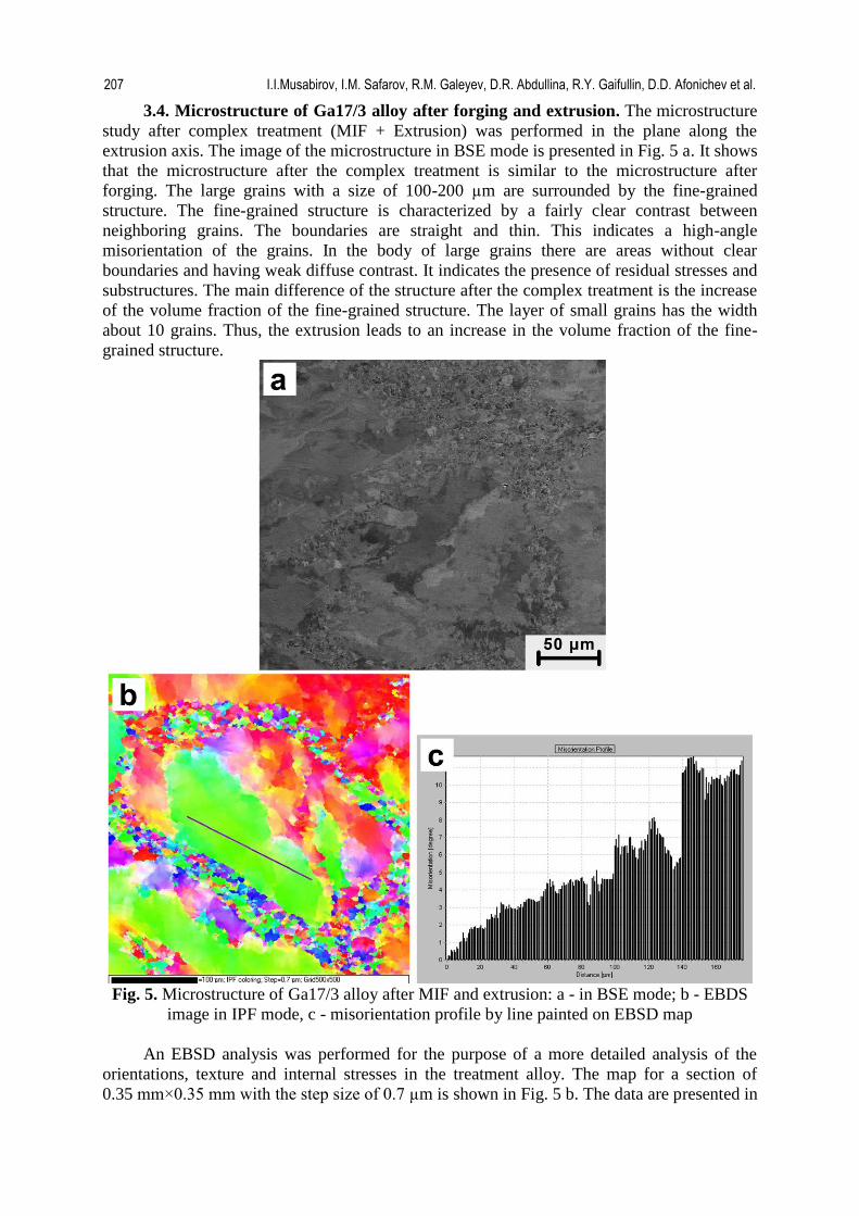
3.4. Microstructure of Ga17/3 alloy after forging and extrusion. The microstructure

study after complex treatment (MIF + Extrusion) was performed in the plane along the

extrusion axis. The image of the microstructure in BSE mode is presented in Fig. 5 a. It shows

that the microstructure after the complex treatment is similar to the microstructure after

forging. The large grains with a size of 100-200 µm are surrounded by the fine-grained

structure. The fine-grained structure is characterized by a fairly clear contrast between

neighboring grains. The boundaries are straight and thin. This indicates a high-angle

misorientation of the grains. In the body of large grains there are areas without clear

boundaries and having weak diffuse contrast. It indicates the presence of residual stresses and

substructures. The main difference of the structure after the complex treatment is the increase

of the volume fraction of the fine-grained structure. The layer of small grains has the width

about 10 grains. Thus, the extrusion leads to an increase in the volume fraction of the fine-

grained structure.

Fig. 5. Microstructure of Ga17/3 alloy after MIF and extrusion: a - in BSE mode; b - EBDS

image in IPF mode, c - misorientation profile by line painted on EBSD map

An EBSD analysis was performed for the purpose of a more detailed analysis of the

orientations, texture and internal stresses in the treatment alloy. The map for a section of

0.35 mm×0.35 mm with the step size of 0.7 µm is shown in Fig. 5 b. The data are presented in


IPF coloring mode. The EBSD data confirmed the results of the analysis of the structure in

BSE mode. The fine-grained structure also has high-angle misorientations. The substructure

of coarse grain is confirmed by the misorientation profile marked in the grain body and

indicated in Fig. 5 b. The histogram is presented in Fig. 5 c. The histogram shows the

orientation of points relative to the first point rather than a previous one. The extreme points

of the profile are misoriented by 11°.

The EBSD analysis along the extrusion axis was performed at the entire section of the

workpiece to evaluate the crystallographic texture in the material. The data for area of

2.1 mm×8.4 mm with the step size of 3 μm are shown in Fig. 6 a.

Fig. 6. EBDS analysis of Ga17/3 alloy after MIF and extrusion: a - EBDS image in IPF mode,

b - Pole Figures for small grains, c - Pole Figures for big grains


The metallographic texture is absent. There is a slight stretching of the grains along the

treatment axis only in the edge areas. The large grains are equiaxial in the central part of the

workpiece. The structure has a slight heterogeneity over the cross section of the workpiece.

The Pole Figures of 100 and 111 planes were constructed throughout the orientation map

for the analysis of the crystallographic texture. As in case of the forged state, the data for large

grains and for the fine-grained structure were separated by the software. The Pole Figures for

large grains are shown in Fig. 6 b, for the fine-grained structure in Fig. 6 c. Despite some

localized maxima for the family of 100 planes located on the stereographic plane the

texture is not evident because the statistical data for such a number of large grains is not

enough. The localized maxima of one crystallographic direction are observed for the fine-

grained structure. Thus, the fine-grained structure has a single-component crystallographic

texture.

4. Conclusions

After the thermo-mechanical treatment by multiple isothermal forging and the complex

treatment by forging and subsequent extrusion the studied Heusler alloys show the anisotropy

of the properties at the martensitic transformation. An abrupt length changing of

about 0.05-0.13% was observed at the phase transformation in the samples cut along the

deformation axes. The anisotropy of the thermal expansion is resulted due to both the

treatment texture and the residual tensile stresses in the treated samples. The jump at the

phase transformation in treatment states is lower than in as-cast state, in which it may reach

0.35%. It is suggested that the low jump occurs due to the low texture after the treatment and

insufficient strain at both forging and extrusion. Therefore, in order to enhance the texture

sharpness, it is necessary to increase the number of canting at the forging and the strain at the

extrusion. The undoubted advantage of the proposed approach for Ni2MnGa alloys is forming

of bimodal structure after the thermo-mechanical treatment by forging and forging with

subsequent extrusion. In such structure, the original large grains of 100–200 µm are

surrounded by the fine-grained structure. The stability of the functional properties of Heusler

alloys with multiple cycles of the martensitic transformation should be higher due to the phase

stresses relaxation and retardation of defects accumulation and microcracks initiation.

Moreover, the additional treatment by extrusion provides volume fraction increase of the

small grains. It enhances the relaxation ability of the alloy. Correspondingly, further increase

of the strain should enhance both the anisotropy of properties and the cyclic strength of the

alloy more by increasing the structure bimodality.

To sum up, the studies have shown a high potential of the thermo-mechanical treatment

for obtaining the structurally modified Heusler alloy having a sufficient level of functional

and service properties for the practical application.

Acknowledgements. The investigation was funded by RFBR, according to the research

project No. 16-32-60159 mol_a_dk (for I.I.M.). The deformation processing and

microstructure studies were carried out on the facilities of shared services center of the

Institute for Metals Superplasticity Problems of Russian Academy of Sciences «Structural and

Physical-Mechanical Studies of Materials».

References

[1] Pagounis E, Chulist R, Szczerba MJ, Laufenberg M. Over 7% magnetic field-induced

strain in a Ni-Mn-Ga five-layered martensite. Appl. Phys. Lett. 2014;105(5): 052405.

[2] Barmina E, Kosogor A, Khovaylo V, Gorshenkov M, Lyange M, Kuchin D, Dilmieva E,

Koledov V, Shavrov V, Taskaev S, Chatterjee R, Varga LK. Thermomechanical properties


and two-way shape memory effect in melt spun Ni57Mn21Al21Si1 ribbons. J. Alloys Comp.

2017;696: 310-314.

[3] Li Z, Yang B, Zou N, Zhang Y, Esling C, Gan W, Zhao X, Zuo L. Crystallographic

Characterization on Polycrystalline Ni-Mn-Ga Alloys with Strong Preferred Orientation.

Materials. 2017;10: 463.

[4] Pandey S, Quetz A, Aryal A, Dubenko I, Mazumdar D, Stadler S, Ali N. Magnetocaloric,

thermal, and magnetotransport properties of Ni50Mn35In13. 9B1. 1 Heusler alloy. J. Magn.

Magn. Mater. 2017;444: 98-101.

[5] Zhukova A, Rodionova V, Ilyn M, Aliev AM, Varga R, Michalik S, Aronin A,

Abrosimova G, Kiselev A, Ipatov M, Zhukova V. Magnetic properties and magnetocaloric

effect in Heusler-type glass-coated NiMnGa microwires. J. Alloys Comp. 2013;575: 73-79.

[6] Arumugam S, Devarajan U, Muthu SE, Singh S, Thiyagarajan R, Raja MM,

Rama NV Rao, Banerjee A. Structural, transport, magnetic, magnetocaloric properties and

critical analysis of Ni-Co-Mn-Ga Heusler alloys. J. Magn. Magn. Mater. 2017;442: 460-467.

[7] Rodionov ID, Koshkid'ko YS, Cwik J, Quetzd A, Pandey S, Aryal A, Dubenko IS,

Stadler S, Ali N, Titov IS, Blinov M, Prudnikova MV, Prudnikov VN, Lähderanta E,

Granovskii AB. Magnetocaloric effect in Ni50Mn35In15 Heusler alloy in low and high

magnetic fields. JETP Letters. 2015;101(6): 385-389.

[8] Pagounis E, Szczerba MJ, Chulist R, Laufenberg M. Large magnetic field-induced work

output in a NiMnGa seven-layered modulated martensite. Appl. Phys. Lett. 2015;107(15):

152407.

[9] Kourov NI, Korolev AV, Pushin VG, Marchenkova EV. Effect of the megaplastic torsion

deformation on the heat capacity of the Ni2MnGa alloy. Phys. Solid State. 2012;54(10): 2128-

2131.

[10] Chulist R, Skrotzki W, Oertel C-G, Bohm A, Lippmann T, Rybacki E. Microstructure

and texture in Ni50Mn29Ga21 deformed by high-pressure torsion. Scr. Mater. 2010;62: 650-

653.

[11] Chulist R, Bohm A, Rybacki E, Lippmann T, Oertel C-G, Skrotzki W. Texture Evolution

of HPT-Processed Ni50Mn29Ga21. Mater. Sci. Forum. 2012;702–703: 169-172.

[12] Musabirov II, Sharipov IZ, Mulyukov RR. Temperature Dependence of the

Magnetization of the Ni52Mn24Ga24 Alloy in Various Structural States. Russian Physics

Journal. 2015;58: 745-749.

[13] Lu B, Wang HB, Liu Y, Liu JX, Wang HL. Formation of texture of Ni48Mn31Ga21

polycrystalline alloy by thermal simulation pack rolling technology. Transactions of

Nonferrous Metals Society of China. 2006;16: 843-847.

[14] Besseghini S, Villa E, Passaretti F, Pini M, Bonfanti F. Plastic deformation of NiMnGa

polycrystals. Mater. Sci. Eng. A. 2004;378(1–2): 415-418.

[15] Chulist R, Potschke M, Boehm A, Brokmeier H-G, Garbe U, Lippmann T, Oertel C-G,

Skrotzki W. Cast and Rolling Textures of NiMnGa Alloys. MRS Proceedings. 2007;1050:

BB09-03.

[16] Bohm A, Roth S, Naumann G, Drossel WG, Neugebauer R. Analysis of structural and

functional properties of Ni50Mn30Ga20 after plastic deformation. Mater. Sci. Eng. A. 2008;481-

482: 266-270.

[17] Morawiec H, Goryczka T, Drdzen A, Lelatko J, Prusik K. Texture Analysis of Hot

Rolled Ni-Mn-Ga Alloys. Solid State Phenomena. 2009;154: 133-138.

[18] Cong DY, Wang YD, Peng RL, Zetterstrom P, Zhao X, Liaw PK, Zuo L. Crystal

structures and textures in the hot-forged Ni-Mn-Ga shape memory alloys. Metall. Mater.

Trans. A. 2006;37(5): 1397.


[19] Cong DY, Wang YD, Zetterstrom P, Peng RL, Delaplane R, Zhao X, Zuo L. Crystal

structures and textures of hot forged Ni48Mn30Ga22 alloy investigated by neutron diffraction

technique. Materials Science and Technology. 2005;21: 1412-1416.

[20] Musabirov II, Safarov IM, Galeyev RM, Afonichev DD, Koledov VV, Rudskoi AI,

Mulyukov RR. Plastic deformation of the Ni-Mn-Ga alloy by multiple isothermal forging.

Materials Physics and Mechanics. 2017;33(1): 124-136.

[21] Musabirov II, Safarov IM, Galeyev RM, Gaisin RA, Koledov VV, Mulyukov RR.

Anisotropy of the Thermal Expansion of a Polycrystalline Ni–Mn–Ga Alloy Subjected to

Plastic Deformation by Forging. Physics of the Solid State. 2018;60(6): 1061-1067.

[22] Musabirov II, Mulyukov RR., Koledov VV. Crystallographic texture and the preferential

orientation of a martensite in the polycrystalline Ni2.08Mn0.96Ga0.96 alloy. IOP Conference

Series: Materials Science and Engineering. 2015;82(1): 012064.

[23] Musabirov II, Mulyukov KY, Safarov IM. Texture investigations of polycrystalline

Ni2MnGa alloy. Letters on Materials. 2012; 2(3): 157-160.

[24] Musabirov II, Safarov IM, Mulyukov RR, Sharipov IZ, Koledov VV. Development of

martensitic transformation induced by severe plastic deformation and subsequent heat

treatment in polycrystalline Ni52Mn24Ga24 alloy. Letters on Materials. 2014;4(4): 265-268.


MODERN APPROACHES FOR STUDY OF EUTECTOID STEEL

OXIDATION AND DECARBURIZATION Kseniya Pivovarova1, Marina Polyakova1*, Manuele Dabala2, Alexey Korchunov1,

Andrey Shymchenko3

1Nosov Magnitogorsk state technical university 2University of Padova

3Peter the Great St.Petersburg Polytechnic University


Abstract. This paper describes the results of a laboratory study into the high-temperature surface oxidation and decarburization of eutectoid steel performed using thermal gravimetric analysis which makes it possible to understand the steel surface oxidation kinetics in non-isothermal conditions as the steel specimen is continuously heated to a specified temperature. An exponential relationship is obtained between the heating temperature and the iron loss in steel. A relationship is established between the heating temperature applied and the surface oxidation rate observed in a eutectoid steel specimen. It is shown that when the temperature of the specimen is raised from 900 to 1000°С, it leads to a triple increase in the surface oxidation rate, whereas the temperature increase to 1200°С results in an eightfold increase in the surface oxidation rate. It is noted that, within the temperature range of 720-950°С, the phase transformations observed are accompanied with intensified scale formation and surface carbon depletion. Using the emission spectrometry technique, the concentration of carbon is determined in the surface layer in relation to the heating temperature and time. The results obtained indicate that eutectoid steel is subjected to an intense surface decarburization at the temperatures of 600-1200°С. Keywords: eutectoid steel, thermal gravimetric analysis, differential scanning calorimetry, oxidation, decarburization 1. Introduction Nowadays high-carbon steel wire rod is in demand on the world market for the production of high-strength rebar stabilized ropes, which are the basis of modern effective construction technologies for the manufacture of precast concrete with pre-tensioning of reinforcement, as well as structures with subsequent tension of reinforcement on concrete. Among the various types of prestressed reinforcement, including smooth and profiled reinforcing wire and rod reinforcement, reinforcing ropes occupy a special place, which is caused by the combination of their properties unattainable for other types of reinforcement.

The raw material for their production is a high-carbon wire rod, obtained in modern high-grade rolling mills. Production of high-strength ropes is a complex technological process with a high metal consumption coefficient. Therefore, the metal intended for production of the specified products shall conform to the rigid requirements imposed to its quality.

When producing wire rods, quality parameters are strongly influenced by processes in continuous furnaces before rolling. Such processes include decarburization and the iron loss in steel, which affect the steel quality during a forming operation, as well as finished steel

Materials Physics and Mechanics 40 (2018) 212-220 Received: May 2, 2018


products [1,2,24-26]. Heating of steel billets before hot rolling in furnaces causes intensive development of scale formation, depletion of surface layers with carbon and redistribution of alloying elements in the surface layers. At the same time, the resistance of metal to alternating loads, which is typical for ropes, is determined by the depth of the carbonized layer, that is, the actual difference between the microstructure on the surface and the structure of the base metal.

Decarburization by heating occurs as a result of the interaction of oxidizing gases with carbon, which is in a solid solution or bound to iron carbides. Decarburization rate is determined mainly by the process of bilateral diffusion, which occurs under the influence of the difference in the gradient of media. On the one hand, decarbonizing gases come to the surface layers of the metal, and on the other – the resulting gaseous products containing carbon, move in the opposite direction. In this case, carbon from the inner layers of the metal diffuses into the surface layer. Therefore, decarburization and scale formation, occurring on the metal surface, in most cases are considered together. The evolution of steel rope structures and technologies of their production is due to the constant desire to increase the strength and durability, by strengthening the cold deformation or heat treatment.

When the metal is deformed by cold drawing, by pulling the rebound rolled through a system of monolithic dies, the maximum stresses are concentrated on the surface of the rolled metal. Therefore, in the manufacture of high-quality range of high-carbon rebound rolled it is necessary to ensure a minimum and uniform depth of decarburization on the surface of the wire rod. To solve such problems, fundamental concepts of decarburization, diffusion saturation and oxidation processes are needed, which occur in parallel with decarburization in metals and alloys due to their contact with various gases.

Steel surface oxidation and decarburization issues are rather deeply analyzed and theoretically evaluated, in particular, formation features of a scale phase composition and decarburization of metals and alloys have been thoroughly studied [3-13,28,29]. A general survey of high temperature oxidation in metals and alloys, demonstrating how different environmental conditions and chemical composition of the alloys determine the mode of oxidation process is presented in [14].

Principles governing the oxidation of metals are formulated in [15]. It was shown that theories which have been proposed to explain the growth of thin oxide films at low and intermediate temperatures are based on different rate-limiting processes such as electron transfer at the metal-oxide or oxide-gas interface, ion or electron migration through the oxide under the influence of electrical potential gradients or chemical potential gradients and either with or without space-charge effects and ion transfer at the oxide-metal or oxide-gas interface. These theories lead to inverse or direct logarithmic, parabolic, cubic, quartic or linear equations for oxide growth.

However, despite this, these studies remain relevant at the present time, due to the fact that the technology of obtaining wire rod, remain unresolved a number of important issues related to improving the quality and expansion of the range of finished products, which to some extent depend on the relationship of phase and structural transformations with the processes of scale resistance and decarburization in carbon wire rod.

Among known methods of oxidation kinetics of metals and alloys in different gas medium, in addition to a conventional gravimetric method, a widely used technique is a thermogravimetric method, as the simplest and most reliable one. A method showing good results is a thermal gravimetric analysis (TG), applied together with differential thermal analysis (DTA) and differential scanning calorimetry (DSC), and particularly recommended as reflecting to the fullest extent all the processes occurred during specimen heating and cooling, and ensuring good comparability of results [16,30]. However, having analyzed

Modern approaches for study of eutectoid steel oxidation and decarburization 213

literary studies, we found no thermoanalytical studies on eutectoid steel. This paper aims at the thermal analysis of eutectoid steel surface oxidation and decarburization kinetics.

2. Methods The study was conducted on the eutectoid steel specimen, whose chemical composition is given in Table 1. Microstructure of eutectoid steel is presented in Fig. 1. Table 1. Eutectoid steel chemical composition, % wt. С Si Mn S P Cr Ni V Al 0.82 0.33 0.59 0.0020 0.0031 0.022 0.032 0.0015 0.0010

The examined high-carbon steel has the following mechanical properties: time resistance to rupture MPa 1205В =σ , conditional yield strength MPa 8902,0 =σ relative elongation 10δ = 9 %, relative contraction ϕ = 31 %. The structure of the studied samples is a plate perlite. The size of the pearlite colonies is 4...8 µm. Cementite is represented mainly by lamellar form. The interplate distance inside the pearlite colonies in steel reaches a maximum of 0.12 µm.

Fig. 1. Microstructure of high carbon steel 0.8 %C

The laboratory study was performed using the STA Jupiter 449 F3 simultaneous thermal analyzer. It ensures both a differential scanning calorimetry and a thermal gravimetric analysis of a specimen at the same measurement, providing a possibility to compare results of TG and DSC directly and eliminate effects of material non-uniformity, specimen preparation and measuring conditions [17,27].

DSC has been used to fix a temperature difference, which is in proportion to a difference in a heat flow between a reference (an empty crucible for STA) and a sample in another crucible from the same material. TG has been used to measure changes in the specimen weight, depending on temperature at specific controlled conditions.

To carry out experiments, we have cut disc specimens, 3 mm in diameter and 1 mm high, ground the surface with an abrasive paper SiC 1200 grit, and degreased with acetone. Weight of the specimens amounted to 55-56 mg. Measurements were performed in corundum crucibles. Before analyzing, the device was calibrated with reference to melting temperatures of pure metals. A temperature measurement error did not exceed ± 0.1°C. During the studies a specimen weight was continuously controlled with an electronic microbalance. Its design ensures a fixed position of the hanging specimen relative to a furnace chamber, when measuring weight. Precision of weighing was ± 0.01 mg.

214 Kseniya Pivovarova, Marina Polyakova, Manuele Dabala, Alexey Korchunov, Andrey Shymchenko

Thermal curves of the specimens were recorded at a speed of 10°C/min in a flow of argon (protective gas – 10 cm3/min, working gas – 20 cm3/min) within a temperature range of 30-1000°С and 30÷1200°С in an argon/air mixture. Such mixture meets requirements for equipment operation: the balance receives argon as protective gas (10 cm3/min), which is then supplied to the furnace and mixed with air as working gas (20 cm3/min). A total flow rate of argon and the mixture was 30 cm3/min. Before measuring the specimen in an argon flow, a specimen holder of DSC together with the crucibles was pre-heated to 1000°С, in an air flow – to 1200°С. When the specimen was installed and the crucible was put on the specimen holder, the furnace was tightly closed and heated as stated in the above. TG and DSC curves were automatically fixed. Data obtained were processed by Netzsch Proteus Analysis software.

To study surface decarburization, specimens (30 mm long and 11 mm in diameter) were put into a high-temperature chamber electric furnace of the PL 20/12.5 type, preheated to a set temperature, held within a specified period (10 and 30 min) at a constant temperature (600, 800, 1000, and 1200°С) and cooled down with the furnace. Carbon content in a surface layer was calculated as per standards АSТМ Е415-08, АSТМ Е1086-08, АSТМ Е1009-95 by the SpectroMAXx optical emission spectrometer. 3. Results and Discussion It is known [18] that to develop the surface decarburization process, gas atmosphere of the furnace during heating should not produce an intense oxidation effect. Carbides of IVa-Via group metals are particularly vulnerable to the effects of oxygen impurities, and its dissolution in their lattice is accompanied by depositing carbon and a relevant metal [19,20]. Thus, a thermal analysis of eutectoid steel surface oxidation and decarburization was performed in inert (argon) and oxidizing (air) atmosphere.

Figure 2 presents a thermogram of the steel specimen subjected to high-temperature heating in the weakly oxidizing medium, whose oxidizing gases are oxygen impurities (up to 0.002 %) and water (up to 0.001 %), occurring in argon (see GOST 10157-79, Table 1). The DSC curve shows a deep endothermal effect with a peak value at 744.9°C, evidencing a phase transformation of pearlite to austenite (α → γ), and a bend at 930.6°С, corresponding to a breakdown and dissolution of carbides in austenite [21,31].

The TG curve, starting from 589.6°С, shows a minor increase in the weight of the specimen, continuing to 900°С. Within this temperature range, a weight gain amounted to 0.014 % due to steel oxidation. Steel oxidation is taking place at the same time with decarburization, evidenced by weight loss (0.07 %) within a temperature range of 900-1000°C. The decarburization process is clearly observed at 897.1°С and in an active progress to 1000°С. Within this temperature range carbides are broken and dissolved in austenite. As a result, Me-C bonds are broken, carbides are dissolved, while forming carbon (С) and elements, included in their composition (Fe, Mn, Cr), with their further intense oxidation during heating. Carbon oxidation and removal of its oxides into a gas phase contribute to some decrease in specimen weight (i.e. decarburization), which can be seen in the TG curve.


Fig. 2. Thermogram of eutectoid steel specimen continuous heating in argon

Carbon depletion of steel starts from the surface due to oxidation of carbon occurred in

a heated specimen as iron carbides, with gases in furnace atmosphere. As a rule, a steel outer layer is almost fully decarburized, which is proved by results of the below experiment (see Table 2). Table 2. Carbon content on the surface of the eutectoid steel specimen (with a carbon weight percent of 0.82 % in an original specimen) at high-temperature heating in the chamber electric furnace

Temperature [°C] Carbon weight percent for the holding time 10 min. 30 min.

600 0.81 0.73 800 0.60 0.51 1000 0.52 0.448 1200 0.395 0.212

Regarding the above values of carbon content in the steel surface layer with relation to

temperature and time, it follows that the surface decarburization process starts at 600°C and intensively takes place to 800°С. When the temperature is over 800°С, the process slows down to some extent, which is explained by a slower decarburization rate than its oxidation rate at 800°С and over, a diffusion rate of carbon towards oxygen is lower than that of iron [22]. An almost two-fold increase in a heating period entails a sharp decrease in carbon content in the steel surface layer, especially at 1200°С. At temperatures around 600°С a eutectoid steel surface decarburization process takes place rather slowly.

A composition of furnace atmosphere together with temperature and the heating period strongly influences both decarburization and oxidation rates. Such processes in an oxidizing medium take place much more intense than in a weakly oxidizing medium, which is obviously shown in the thermogram of eutectoid steel specimen heating in air.

It should be noted that when studying steel oxidation processes during heating before rolling, a term of loss is often used. The iron loss in steel is a loss in weight (due to oxidation of iron, alloying elements, and carbon) of steel after heating [23].

The DSC curve (Fig. 3) in a region of over 850-900°С shows significantly intensified oxidation, which is characterized by exothermal peaks with maximum values at 989.0; 1125.3; 1161 and 1185.6°С. The first peak corresponds to the beginning of intensified


oxidation (the iron loss in steel) after steel transformation into an austenite state (in a temperature range of 720.5-757.3°С) and formation of wustite, and others correspond to continued intensification of the iron loss in steel within a temperature range of up to 1200°С.

Fig. 3. Thermogram of steel grade 80 specimen continuous heating in air

The TG curve, starting from 900°С, shows a sharp increase in the specimen weight due

to oxidation of iron and other components. Within this temperature range, at the same time with breakdown and dissolution of carbides, alloy oxidation processes are under way, resulting in overlapping of effects, while an exothermal effect prevails over endothermal one, and the TG curve shows a weight increase only. It usually occurs, when heating steel before hot rolling at temperatures above 1100°С, and when burning fuel with excess air. There is an exponential relationship between the rate of the iron loss in steel and temperature, which is used to determine a critical temperature [21] for iron-carbon alloys. It should be noted that such relationship, as a change in weight of a heated specimen (%) in relation to temperature, presenting the iron loss, is fixed in the TG curve. A critical temperature for eutectoid steel, calculated by the TG curve, amounts to about 929°С; above this temperature oxidation processes take place at a high rate.

By differentiating the TG curve, we obtain the DTG curve (Fig. 4), allowing us to evaluate a high-temperature oxidation rate of eutectoid steel.

Fig. 4. Relationship between the eutectoid steel oxidation rate and temperature


Judging by the DTG curve, the oxidation rate is constant up to 900°С. When temperature is over 900°С, it steadily increases and achieves a maximum value at 1000°С, and then it starts decreasing almost to 1100°С. Above 1100°С the oxidation rate shows a sharp increase. Thus, when the temperature of the specimen is raised from 930 to 1000°С, it leads to a triple increase in the surface oxidation rate, whereas the temperature increase to 1200°С results in an eightfold increase. A maximum temperature of heating steel before rolling is usually by 100-150°С lower than a solidus curve for eutectoid steel. This temperature is about 1100-1250°С. Therefore, what is important is to follow a minimum steel oxidation rate in a temperature range of 1100°С and over. If one is taken as the oxidation rate at 1100°С, at 1157°С it will increase almost by 1.5 times, at 1185°С – by over twice. Thus, within a temperature range of 1100-1250°С, the minimum oxidation rate of eutectoid steel is at 1157°С. Such temperature is optimum, when heating eutectoid steel before rolling, corresponding with literary data given in [21], namely 1120-1160°С for 70-85 steel grades.

4. Conclusions 1. For the first time, a thermal gravimetric analysis and differential scanning calorimetry have been used to study oxidation and decarburization of a eutectoid steel surface within a temperature range of 20°С to 1200°С in air and argon. Having analyzed the thermograms obtained and identified extreme values of differential curves (TG and DSC), we could describe processes, occurring during heating of eutectoid steel. Within a temperature range of 720-950°С, when heating a eutectoid steel specimen, phase transformations (α → γ) are accompanied with intensified scale formation due to formation of wustite and surface carbon depletion, resulting from breakdown and dissolution of carbides in austenite.

2. It is shown that when heating a eutectoid steel specimen in air medium, the iron loss in steel is sharply intensified at 989-1000°С, entailing an increase in its weight up to 5 %, at 1200°С – to 25 %. A minimum oxidation rate of the specimen within a temperature range of 1100-1200°С is identified at 1157°С.

3. The thermal analysis results obtained have contributed to changes in temperature and time of rolling of eutectoid steel wire rods on hot rolling section mills. Acknowledgements. This research was financed by Ministry of Education and Science of the Russian Federation within the framework of the Federal Program "Research and development in priority areas for the development of the scientific and technological complex of Russia for 2014-2020", Activity 1.1, Agreement on Grant No. 14.572.21.0008 of 23 October, 2017, unique identifier: RFMEFI57217X0008. References [1] Sychkov АB, Parusov VV, Ivin YuА, Dzyuba АYu, Zajtsev GS. Osobennosti tekhnologii proizvodstva vysokouglerodistoj katanki. Vestnik Magnitogorskogo gosudarstvennogo tekhnicheskogo universiteta im. G.I. Nosova. 2014;1(45): 38-42. (In Russian) [2] Temlyantsev MV, Mikhajlenko YuE. Okislenie i obezuglerozhivanie stali v protsessakh nagreva pod obrabotku davleniem. Moscow: Teplotekhnik; 2006. (In Russian) [3] Zorc M, Nagode A, Burja J, Kosec B, Zorc B. Surface Decarburization of the Hypo-Eutectoid Carbon Steel C45 during Annealing in Steady Air at Temperatures T > AC1. Metals. 2018;8(6): 425. Available from: doi.org/10.3390/met8060425. [4] Gouveia WA, Seshadri V, Silva IA, Silva CA. Mathematical Modeling of Decarburization and Oxidation during Reheating Process of SAE1070 Steel Billets. Advanced Materials Research. 2014;845: 231-236.


https://www.scientific.net/author/C_A_Silva_1

[5] Skrbek B, Tomáš I, Kadlecová J, Ganev N. NDT characterization of decarburization of steel after long-time annealing. Kovove Mater. 2011;49: 401–409. doi: 10.4149/km 2011 6 401. [6] Parusov VV, Lutsenko VА, Sychkov АB et al. Glubina obezuglerozhennogo sloya na uglerodistoj katanke razlichnykh zavodov-izgotovitelej. Metallurgicheskaya i gornorudnaya promyshlennost'. 2003;5: 61-64. (In Russian) [7] Lutsenko VА, Matochkin VА. Vliyanie termomekhanicheskoj obrabotki na formirovanie obezuglerozhennogo sloya v vysokouglerodistoj katanke. Byulleten' nauchno-tekhnicheskoj i ehkonomicheskoj informatsii «Chernaya metallurgiya». 2006;11: 61-64. (In Russian) [8] Giovanardi R, Poli G, Veronesi P, Parigi G, Raffaelli N. Thermochemical treatments of nitriding and post-oxidation on 17-4PH steel: Optimization of the process parameters to maximize corrosion resistance. Metallurgia Italiana. 2015;107(4): 15-23. [9] Chen RY, Yeun WYD. Review of the High-Temperature Oxidation of Iron and Carbon Steels in Air or Oxygen. Oxidation of Metals. 2003;59(5): 433–468. [10] Vashhenko АI, Zen'kovskij АG, Livshits АE. Okislenie i obezuglerozhivanie stali. Moskva: Metallurgiya; 1972. (In Russian) [11] Sychkov АB, Zhigarev MА, Zhukova SYu., Perchatkin АV, Gritsaenko VI. Formirovanie svojstv okaliny dlya ee polnogo udaleniya s poverkhnosti katanki pered volocheniem. Lit'e i metallurgiya. 2012;4(68): 83-91. (In Russian) [12] Korchunov АG, Bigeev VА, Sychkov АB, Zajtsev GS, Ivin YuА, Dzyuba АYu. Usovershenstvovanie skvoznoj tekhnologii proizvodstva buntovogo prokata iz stali marki 80R v usloviyakh OAO «MMK». Vestnik Magnitogorskogo gosudarstvennogo tekhnicheskogo universiteta im. G.I. Nosova. 2013;2: 29-34. (In Russian) [13] Stepanov B, Knyazev AV. Regularities of Oxidation and Decarburization of Special Alloy Steels in the BCC→FCC Phase Transformation Temperature Range. Metallurgist. 2017;61(7–8): 574–578. [14] Zyazev VL, Vatolin NА, Gulyaeva RI, Zubarev GI, Ovchinnikova LА. Termogravimetriya intermetallida AlTSo0,158TSr0,084Y0,003. Metally. 2001;6: 17-19. (In Russian) [15] Chen Q, Yang R, Zhao B, Li Y, Wang S, Wu H, Zhuo Y, Chen C. Investigation of heat of biomass pyrolysis an secondary reactions by simultaneous thermogravimetry and differential scanning calorimetry. Fuel. 2014;134: 467-476. [16] Gubinskij VI, Minaev АN, Goncharov YuV. Umen'shenie okalinoobrazovaniya pri proizvodstve prokata. Kiev: Tekhnіka; 1981. (In Russian) [17] Vojtovich RF. Okislenie karbidov i nitridov. Kiev: Naukova Dumka; 1981. (In Russian) [18] Samsonov GV, Kosolapova TYa, Gnesin GG, Fedorus VB, Domasevich LG. Karbidy i splavy na ikh osnove. Kiev: Naukova Dumka; 1976. (In Russian) [19] Korchunov AG, Gun GS, Shiryaev OP, Piviovarova KG. Study of structural transformation of hot-rolled carbon billets for highstrength ropes for responsible applications via the method of thermal analysis. CIS Iron and Steel Review. 2017;13: 38-40. [20] Parusov EhV, Parusov VV, Lutsenko VА, Parusov OV, Chujko IN, Sychkov АB. Optimal'nye kharakteristiki kachestva katanki iz vysokouglerodistoj stali. Metizy. 2006;3(13): 34-36. (In Russian) [21] Perepyat'ko VN, Temlyantsev NV, Temlyantsev MV, Mikhajlenko YuE. Nagrev stal'nykh slyabov. Moscow: Teplotekhnik; 2008. (In Russian) [22] Kodzhaspirov G, Rudskoi A. Thermomechanical processing of steels & alloys as an advanced resource saving technique. Metal, (Anniversary) International Conference on Metallurgy and Materials. 2016;25: 248-254.


https://link.springer.com/journal/11085

https://link.springer.com/journal/11015/61/7/page/1

[23] Kononov AA, Matveev MA. Formation of orientation 110 in surface layers of electrical anisotropic steel under hot rolling. Metal Science and Heat Treatment. 2018;60(1-2): 55-60. doi: 10.1007/s11041-018-0240-3. [24] Artem'eva DA, Anastasiadi GP. Effect of nitrogen alloying on short-term and long-term mechanical properties of steel 07Kh12NMFB. Metal Science and Heat Treatment. 2018;60(1-2): 39-43. doi: 10.1007/s11041-018-0237-y. [25] Matveev MA, Kolbasnikov NG, Kononov AA. Refinement of the structure of microalloyed steels under plastic deformation near the temperatures of polymorphic transformation. Metal Science and Heat Treatment. 2017;59(3-4): 197-202. doi: 10.1007/s11041-017-0128-7. [26] Kamyshev AV, Makarov SV, Pasmanik LA, Smirnov VA, Modestov VS, Pivkov AV. Generalized coefficients for measuring mechanical stresses in carbon and low-alloyed steels by the acoustoelasticity method. Russian Journal of Nondestructive Testing. 2017;53(1): 1-8. doi: 10.1134/S1061830917010090. [27] Ziniakov VY, Gorodetskiy AE, Tarasova IL. Control of vitality and reliability analysis. Studies in Systems, Decision and Control. 2016;49: 193-204. doi: 10.1007/978-3-319-27547-5_18. [28] Andreeva NV, Naberezhnov AA, Tomkovich MV, Nacke B, Kichigin V, Rudskoy AI, Filimonov AV. Surface morphology and structure of double-phase magnetic alkali borosilicate glasses. Metal Science and Heat Treatment. 2016;58(7-8): 479-482. doi: 10.1007/s11041-016-0039-z. [29] Rudskoy AI, Kondrat'ev SY, Sokolov YA. New approach to synthesis of powder and composite materials by electron beam. Part 1. Technological features of the process. Metal Science and Heat Treatment. 2016;58(1): 27-32. doi: 10.1007/s11041-016-9959-x. [30] Kodzhaspirov G, Rudskoi A. Simulation of dynamic recrystallization of steels and alloys during rolling and forging through the use of FEM and experimental planning methods. In: METAL 2017 - 26th International Conference on Metallurgy and Materials, Conference Proceedings, May 24th-26th 2017, Hotel VoronezI, Brno, Czech Republic, EU. Ostrava: TANGER Ltd; 2017. 320-325. [31] Rudskoi AI, Kodzhaspirov GE, Kamelin EI. Simulation and prediction of the development of dynamic recrystallization during the deformation of low-alloy low-carbon steel blanks. Russian Metallurgy (Metally). 2016;(10): 956-959. doi: 10.1134/S0036029516100177.


MULTIBLOCK COPOLY(URETHANE-AMIDE-IMIDE)S WITH THE

PROPERTIES OF THERMOPLASTIC ELASTOMERS I.A. Kobykhno1*, D.A. Kuznetсov2, A.L. Didenko2, V.E. Smirnova2, G.V. Vaganov2,

A.G. Ivanov2, E.N. Popova2, L.S. Litvinova2, V.M. Svetlichnyi2, E.S. Vasilyeva1,

O.V. Tolochko1, V.E. Yudin2, V.V. Kudryavtsev2 1Peter the Great Saint-Petersburg Polytechnic University, Saint-Petersburg, Polytechnicheskaya 29, 195251,

Russia 2Institute of Macromolecular Compounds of RAS, Saint-Petersburg, Bolshoy pr. 31, 199004, Russia


Abstract. Multiblock (segmented) copoly(urethane-amide-imide)s containing flexible segments of polypropylene glycol (PPG) and rigid segments of bis(urethane-amide-imide) in repeating units were obtained and investigated. Copolymers were prepared of PPG terminated by 2,4-toluyilene diisocyanate (Mn=2300), 4-chloroformylphthalic anhydride and aromatic diamines. Thermal properties of copolymers were analyzed by TGA and DSC methods. The mechanical properties of copolymer films were measured by tensile test and DMA method. It is shown that copolymers have elastomer properties. The chemical structures of copolymers capable of processing by injection molding were determined and the mechanical properties of the obtained moldings were estimated. A conclusion was drawn that the studied copolymers have the properties of thermoplastic elastomers (thermoelastoplasts). Keywords: polyurethanes, polyamide-imides, multiblock (segmented) copolymers, thermal stability, glass transition temperature, mechanical properties, films, injection molding, thermoplastic elastomers

1. Introduction Multiblock (segmented) copoly(urethane-amide-imide)s (PUAI) were first synthesized in the 1960s with the purpose of using such polymers as membranes for the pervaporation separation of aromatic hydrocarbons from the mixtures of aromatic and aliphatic hydrocarbons [1]. Attention was drawn to the thermodynamic incompatibility of phases formed by soft (flexible) aliphatic polyester segments and rigid aromatic segments that are parts of copolymer chains. However, the dynamic mechanical properties of these copolymers were not measured, that is copolymers were not characterized as elastomers. At present, interest in multiblock (segmented) PUAI has reappeared due to interest to thermoelastoplasts, which are characterized by increased strength and higher operating temperatures compared with thermoplastic polyurethanes.

Polyurethanes are among the commercial elastomers and are used in many technical fields. For instance, materials with various mechanical properties from very soft foams to resilient elastomers and wear-resistant coatings are obtained on their basis [2]. However, in the general case, mechanical properties of polyurethanes begin to degrade noticeably at temperatures higher than 80°C, and thermal destruction starts at 200°C [3]. A promising way for improving polyurethane elastomer heat resistance and strength is their chemical modification, which consists of introducing the fragments of heterocyclic high-temperature



resistant polymers into structures of repeating units of polymer chains. Attention to this method of polyurethane modification is paid, for example, in [4-8]. In particular, thermoelastoplastic multiblock poly(ether/ester-imide)s and poly(urethane-imide)s have been successfully studied in recent years by authors’ research group [9-15].

Poly(amide-imide)s have become of industrial importance due to a combination of manufacturability and high performance characteristics. Thermoplastic poly(amide-imide)s are processed by extrusion and injection molding methods and have excellent thermal and mechanical properties [16]. Therefore, it seems expedient to modify thermoplastic poly(amide-imides) chemically in order to give these polymers highly elastic properties while maintaining the same processing methods.

Therefore, on the one hand, PUAI should be considered as products of the chemical modification of polyurethanes, which have significantly increased molecular mass and length of hard segments. On the other hand, they are products of thermoplastic poly(amide-imide)s modification. The radicals of aliphatic polyesters are introduced in the structure of their repeating units.

In this article, thermal and mechanical properties of PUAI are investigated in static and dynamic test modes. In PUAI chemical structure, there is the same flexible segment (polypropylene glycol residue) but hard aromatic segments (bis(urethane)amide-imide residues) are varying. It is shown that the studied polymers have elastomers properties and are processed by injection molding into thick-walled products. A priori, it was assumed that the variations of PUAI properties are determined by an interaction of the rigid aromatic phase and the soft aliphatic phasewith the proviso that the phases are thermodynamically incompatible. In each case, the choice of the initial aromatic diamine was proved to be crucial for the polymer properties.

2. Experimental The following reagents were used in polymer preparation: Poly(propylene glycol), tolylene 2,4-diisocyanate terminated (Mn 2300) (2300TDI), 4-Chloroformylphthalic anhydride (CFPA), Tm=66-68°C, m-Phenylenediamine (MPD) Tm=64-66°C, p-Phenylenediamine (PPD) Tm=145-147°C, 4,4'-Oxydianiline (ODA), Tm=188-192°C, 4,4′-(1,3-Phenylenedioxy)dianiline (TPE-R) Tm=116°C, 1,4-Bis(4-aminophenoxy)benzene (TPE-Q), Tm=173-177°C, 4,4'-Bis(4-aminophenoxy)biphenyl (BAPB), Tm=197-200°C, Bis[4-(4-aminophenoxy)phenyl]sulfone (BAPS), Tm=194-197°C, Polypropylene oxide (PO). N-Methyl-2-pyrrolidone (MP) was used as a solvent. All of these substances were purchased and have an analytical degree of purity. 2300TDI was used such as bought in Aldrich.

The following is an example of the preparation of PUAI based on TPE-R, designated as (CFPA-2300TDI-CFPA)(TPE-R). 13.39g (5.82 mmol) 2300TDI and 2.45g (11.64 mmol) CFPA were placed in a two-necked round-bottom flask equipped with an argon inlet-outlet and an overhead stirrer. With constant stirring, contents of the flask were heated according to the following regime: 1 h at 75°C, 1 h at 110°C, 30 min at 160°C and 30 min at 180°C. The reaction mixture was allowed to cool down to room temperature and 13 ml of MP was added into the flask, then contents of the flask were cooled down to -10°C. In the cooled mixture (with vigorous stirring), a solution 1.7 g TPE-R in 14 ml MP was added through an addition funnel. After that, to bring the concentration of the resulting solution to 30%, 13 ml of MP were added into the flask for 5 min. The obtained solution was stirred for 30 min at -10°C and for18 h at room temperature. Then, 0.8 ml PO was added into the flask in order to neutralize the hydrochloric acid formed during the reaction, by forming chloropropyl alcohol.

IR (film), cm-1: 3485, 3309 (N-H); 2972, 2932, 2868 (C-H); 1780, 1722 (C=O, imide cycle); 1682 (C=O, amid); 1276 (N-C-O); 1089 (C-O-C); 1014, 727 (imide cycle).

222 I.A. Kobykhno, D.A. Kuznetсov, A.L. Didenko, V.E. Smirnova, G.V. Vaganov, A.G. Ivanov et al.

1H NMR (DMSO-d6, 400 MHz) δ = 10.65, 9.77, 8.53, 8.44, 8.32, 8.09, 7.86, 7.50, 7.45, 7.36, 7.29, 7.23, 7.10, 6.87, 6.81, 6.72, 6.61, 4.87, 3.41, 3.31, 2.04, 1.20, 1.03 13C NMR (DMSO-d6, 100 MHz) δ = 166.9, 163.9, 159.2, 158.3, 156.4, 153.5, 152.4, 140.7, 138. 4, 137.7, 136.9, 135.9, 135.4, 134.8, 134.3, 132.3, 131.2, 130.7, 130.2, 129.6, 127.6, 124.0, 122.7, 120.1, 119.5, 115.7, 114.4, 112.7, 110.1, 108.1, 75.1, 72.9, 18.4, 17.7

All other copolymers were prepared in a similar way. The molecular masses Mw of copolymers averaged between 130000 – 150000.

IR spectra were recorded on a Vertex 70V FT-IR (Bruker, Germany) spectrometer complected with ATR attachment. 1H and 13C NMR spectra were recorded on Avance 400 spectrometer (Bruker, Germany), DMSO was used as solvent. The τ5 and τ10 temperature indices of the polymer thermal stability were determined by thermal gravimetric analysis (TGA) using the TG 209 F1 instrument (NETZSCH, Germany), in argon atmosphere in the temperature range of 30-800°C, with a heating rate 10°C/min. Glass transition temperatures Tg were determined by differential scanning calorimetry (DSC) on the DSC 204 F1 instrument (NETZSCH, Germany) in argon atmosphere, with a heating rate 10°C/min. Dynamic mechanical analyses (DMA) was performed using the DMA 242 C instrument (NETZSCH, Germany) with frequency 1 Hz, strain amplitude 0.1% and a heating rate of 5°C/min. The stretch curves of film and molding samples were recorded using the universal testing system Instron 5940 (Instron, USA) with strain rate 50 mm/min. The samples of polymer moldings were prepared by injection molding on the technological complex DSM Xplore (Xplore instruments, The Netherlands). To determine the molecular mass, the liquid chromatograph "Agilent Technologies 1260 Infinity" was used.

3. Results and discussion In the presented article, PUAI were prepared according to the two-step reaction scheme known in the literature [15]. The preparation of PUAI is based on two chemical reactions. The first –: cyclic anhydrides interact with isocyanates, forming cyclic imides with the elimination of carbon dioxide. The second – amides are formed with the elimination of hydrogen chloride during the acylation of amines with acid chlorides. Accordingly, in the first stage, Poly(propylene glycol), 2300TDI reacted with (CFPA) taken in a double molar excess to form the macro monomer CFPA-2300TDI-CFPA which had terminal chloride groups. Then, in the second stage, a сhosen aromatic diamine was acylated with macro monomer CFPA-2300TDI-CFPA to form a desired polymer. Hydrogen chloride released during the formation of amide bonds was neutralized with PO. The PUAI preparation was carried out in the one pot manner in MP solution without isolation of the intermediate formed CFPA-2300TDI-CFPA product.

The PUAIs studied were prepared on the base of 7 aromatic diamines, i. e. only diamines were varied in the reaction scheme. Fig. 1 presents the PUAI synthesis scheme (Fig. 1) with the chemical structure of chosen diamines.

As a result, a series of copolymers differing by diamine radicals R was prepared: (CFPA-2300TDI-CFPA)(MPD), (CFPA-2300TDI-CFPA)(PPD), (CFPA-2300TDI-CFPA)(ODA), (CFPA-2300TDI-CFPA)(TPE-R), (CFPA-2300TDI-CFPA)(TPE-Q), (CFPA-2300TDI-CFPA)(BAPB), and (CFPA-2300TDI-CFPA)(BAPS).

These polymers have a structure of multiblock (segmented) copolymer, which consists of soft aliphatic segments and hard aromatic segments. Aliphatic soft segment length is determined by using a TDI 2300. Aromatic hard segment includes amide-imide group, urethane group, diamine radical R, urethane group, and amide-imide group, so its length is limited by the choice of diamine. Diamine radicals contain from one to four benzene nuclei and also there is the isomerism of the position of benzene rings.

Multiblock copoly(urethane-amide-imide)s with the properties of thermoplastic elastomers 223

Fig. 1. Synthesis of the (CFPA-2300TDI-CFPA)(R)

Fig. 2. 1H and 13C NMR spectra of (CFPA-2300TDI-CFPA)(TPE-R)

The representative 1H-, 13C NMR and IR spectra of (CFPA-2300TDI-CFPA)(TPE-R)

were shown in Fig.2-3. 1H NMR method allows analyzing the macromolecular structure by a good discrimination of the different imino protons belonging to either urethane or amide groups. As is clearly shown in the spectrum recorded for polymer (CFPA-2300TDI-CFPA)(TPE-R) (Fig. 2), amide NH protons were responsible for a single peak appeared at 10.65 ppm, whereas urethane NH protons led to a peak at 9.77 ppm that is very characteristic for urethane groups within polyurethane macromolecular architectures. In 13C NMR spectrum, the region between 150 and 175 ppm showed four very characteristic peaks appeared at 153.5, 152.4, 163.9, and 166.9 ppm corresponding to urethane groups, amide groups, and imide groups, respectively. Other peaks appeared in this area correspond to (C-O-C)-carbon atoms of amide fragment. Signals at 3.41, 3.31 and 1.03 ppm in 1H NMR


spectrum and at 75.1, 72.9 and 17.7 ppm in 13C NMR spectrum corresponds to H- and C-atoms of polypropylene glycol soft segment. Hereby, qualitative interpretation of the NMR spectra fully confirmed the regularity of the proposed macromolecular architecture.

Fig. 3. FT-IR spectra of (CFPA-2300TDI-CFPA)(TPE-R)

In IR-spectrum (Fig. 3), a band with an absorption maximum of 1722 cm-1 corresponds

to C=O valence vibrations in imide cycles and urethane groups in the indicated spectrum. The arm at 1682 cm-1 refers to the C=O vibrations in amide groups. Absorptions at 1780, 727 cm-1 which are respectively responsible for the symmetric C=O oscillations and out-of-plane vibrations of imide cycles prove their presence in the polymer under investigation. Wide absorption bands in the 3300-3500 cm-1area characterize N-H groups. The presence of absorption maximum at 1276 cm-1 (N-C-O group) confirms the presence of urethane bridges. The group of bands from 2850 to 3000 cm-1 refers to the C-H valence vibrations of the aliphatic segment, which the absorption at 1089 cm-1also applies to, relating to ether groups.

As indicated previously, all the studied PUAIs were prepared in the solutions in MP. Strong elastic PUAIs films were formed by watering method. PUAI film tensile tests were carried out. The values of tensile strength, elongation at break, and the modulus of elasticity of polymers are given in Table 1.

Table 1. Mechanical properties of polymer films Polymer Tensile test

Tensile strength (MPa) Elongation at break (%) Initial modulus (MPa) MPD 1.43±0.2 116±20 1.42±0.2 PPD 0.91±0.1 81±12 2.72±0.6 ODA 1.37±0.2 60±9 8.39±2.6 TPE-R 0.52±0.1 141±20 0.77±0.2 TPE-Q 0.43±0.1 28±8 5.58±1.7 BAPB 1.63±0.4 144±50 1.80±0.2 BAPS 3.21±0.7 340±86 1.16±0.1


In all series of polymers tested, there was no clear dependence of the polymer mechanical properties on the number of benzene rings in the structure of the initial diamine. Nevertheless, it should be noted that in the case of bridged diamines, the highest values of elongation at break (340%) and tensile strength (3.21 MPa) were obtained for (CFPA-2300TDI-CFPA) polymer (BAPS), which has oxygen and sulfone bridge groups in the hard segment. There is also an effect of isomerism of the position of benzene rings in the hard segments in the case of MPD and PPD polymers. A polymer based on the MPD diamine is characterized by greater elongation at break and tensile strength values and a lower value of the modulus of elasticity compared to a PPD based polymer. This effect may be due to the fact that in the case of MPD the meta-position of the amino groups in the diamine structure causes a larger set of macromolecular conformations in PUAI as compared to the case of PPD with the para position of the amino groups.

Thermal stability of polymers is determined by the processes of their thermal decomposition. PUAI thermal stability was evaluated by means of thermal gravimetric analysis (TGA) method. The temperatures corresponding to 5% and 10% mass loss (τ5, τ10) of the samples at heating were considered as indices of thermal stability. The values of τ5, τ10 and mass residua at 800°C are given in Table 2.

TGA curves are shown in Fig. 4. Vertical section of the curve in the region around 400°C should be associated with the thermal degradation of aliphatic soft segments of the polymers. The sloping portion in the region from 450°C to 800°C can be associated with thermal degradation of aromatic hard segments of polymers. It is indicated that, in general, PUAI thermal stability is weakly dependent on the diamine structure, apparently thermal destruction processes begin with chemical bonds in the polyether radical. However, it can be noted that two polymers are significantly distinguished from the other polymer studied. The (CFPA-2300TDI-CFPA)(MPD) copolymer has the highest thermal stability (τ5=312°C, τ10=344°C), and the (CFPA-2300TDI-CFPA)(TPE-R) copolymer has the lowest thermal stability (τ5=272°C, τ10=298°C). It is reasonable to assume that the phase interactions (interpenetration of the phases) formed by the soft and hard segments are manifested with different intensity in the considered cases.

Fig. 4. TGA curves for copolymers

The mechanical properties of the PUAI films in the dynamic test mode were measured

by means of dynamic mechanical analysis (DMA) method. The temperature dependences curves of the storage modulus (E'), the loss modulus (E") and the angle of mechanical losses (tgδ) were recorded. Typical DMA curves for PUAI on the TPE-R base are shown in Fig. 5a.


First, attention is drawn to the fact that the maxima on the E', E" and tgδ on temperature dependences are observed in the negative centigrade temperature range. Secondly, these curves have areas corresponding to the practical independence of the values of modulus from temperature, the so-called plateaus of rubber elasticity. It should be noted that the observed effects are typical for multiblock (segmented) copolymers. As it can be seen from Fig. 5a, the plateau of rubber elasticity extends to 280°C, i.e. the sample is in highly elastic state at temperatures, at which polyurethanes are almost completely destructed. Besides, it is reasonable to assume that the significant difference in the values of the maxima on the E" and tgδ temperature dependence curves is a consequence of the interaction between the soft and hard phases. In the case of the polymer (CFPA-2300TDI-CFPA)(TPE-R), the thermogram (Fig. 5b) on the first scan indicates the melting of the crystalline phase in the region around 60°C, and in the second scan no traces of recrystallization were detected. That means, in our opinion, that DSC method revealed the processes of melting of the microcrystalline phase formed by the aliphatic polyesters segments.

(a) (b)

Fig. 5. DMA (a) and DSC (b) curves for polymer (CFPA-2300TDI-CFPA)(TPE-R)

The glass transition temperature (Tg) copolymers was determined using two methods: DSC (Fig. 5b) and DMA (Fig. 5a). In the case of DMA, it should be noted that the Tg values were determined as the temperature of maximum on the temperature dependence of tg δ, as well as of E". Experimental values of Tg of the investigated PUAI are presented in Table. 2.

Among the studied polymers (Table 2), a special place is occupied by MPD based polymer, which is characterized by the lowest Tg value. In other cases, both according to DSC and DMA data, Tg values decrease with the increase of number of benzene rings in the hard aromatic segments. In addition, in MPD - PPD cases, the effects of isomerism of the position of the amide bonds connected to the benzene rings is found, and in TPE-R - TPE-Q cases, the effects of isomerism of bridging oxygen atoms connecting the benzene rings take place. These effects are due to the chemical structure of the initial diamines. So, the Tg of MPD based sample is significantly lower than PPD based analogues (-65.3°C vs. -49.3°C, according to DSC data). In contrast, the Tg of the meta-(aminophenoxy) derivative TPE-R is slightly higher than that of the case of the para-(aminophenoxy)derivative TPE-Q (-43.9°C vs. -47.1°C, according to DSC data and -30°C vs. -36°C according to the MTA data). It should be assumed that in the cases investigated by us the effect of segmental motion defreezing in the aliphatic polyester chains, which are part of the domains that form the soft phase, appears at temperatures exceeding Tg. The presented data allow suggesting that conformational transitions in hard segments are among the factors affecting segmental motions in the chains that form the soft phase.


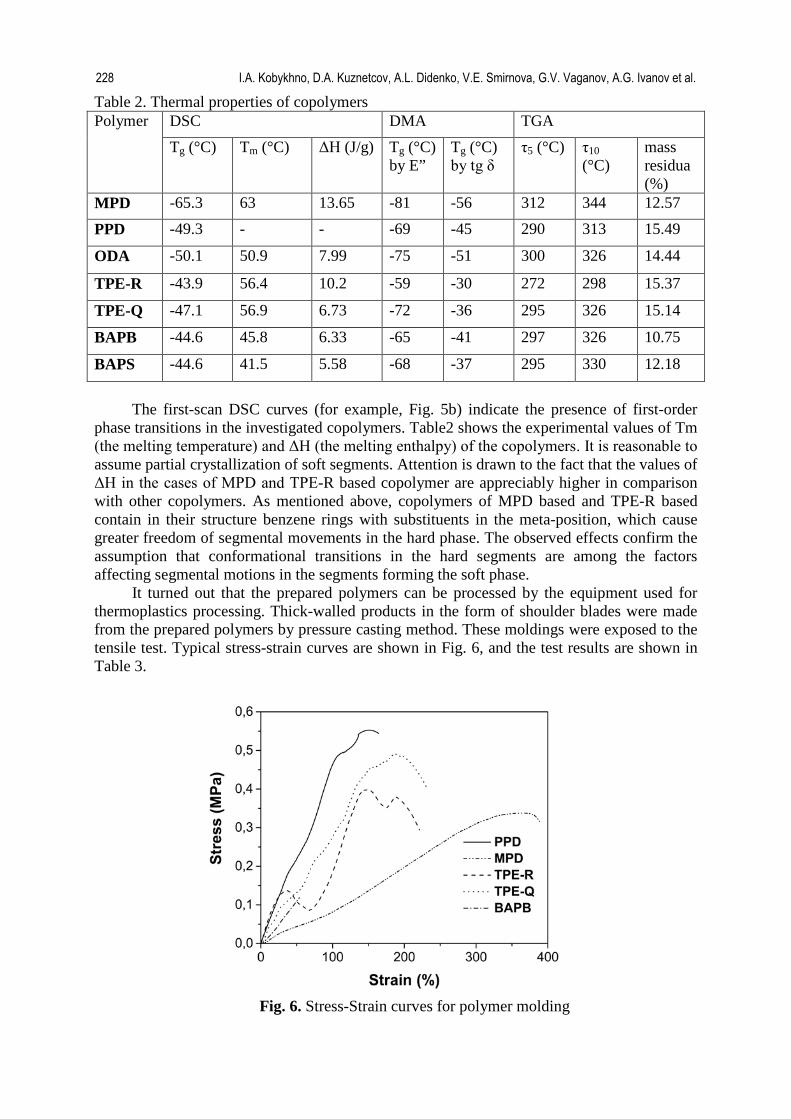
Table 2. Thermal properties of copolymers Polymer DSC DMA TGA

Tg (°C) Tm (°C) ΔH (J/g) Tg (°C) by E”

Tg (°C) by tg δ

τ5 (°C) τ10 (°C)

mass residua (%)

MPD -65.3 63 13.65 -81 -56 312 344 12.57

PPD -49.3 - - -69 -45 290 313 15.49

ODA -50.1 50.9 7.99 -75 -51 300 326 14.44

TPE-R -43.9 56.4 10.2 -59 -30 272 298 15.37

TPE-Q -47.1 56.9 6.73 -72 -36 295 326 15.14

BAPB -44.6 45.8 6.33 -65 -41 297 326 10.75

BAPS -44.6 41.5 5.58 -68 -37 295 330 12.18

The first-scan DSC curves (for example, Fig. 5b) indicate the presence of first-order

phase transitions in the investigated copolymers. Table2 shows the experimental values of Tm (the melting temperature) and ΔH (the melting enthalpy) of the copolymers. It is reasonable to assume partial crystallization of soft segments. Attention is drawn to the fact that the values of ΔH in the cases of MPD and TPE-R based copolymer are appreciably higher in comparison with other copolymers. As mentioned above, copolymers of MPD based and TPE-R based contain in their structure benzene rings with substituents in the meta-position, which cause greater freedom of segmental movements in the hard phase. The observed effects confirm the assumption that conformational transitions in the hard segments are among the factors affecting segmental motions in the segments forming the soft phase.

It turned out that the prepared polymers can be processed by the equipment used for thermoplastics processing. Thick-walled products in the form of shoulder blades were made from the prepared polymers by pressure casting method. These moldings were exposed to the tensile test. Typical stress-strain curves are shown in Fig. 6, and the test results are shown in Table 3.

Fig. 6. Stress-Strain curves for polymer molding


Table 3. Mechanical properties of polymer moldings Polymer Tensile strength (MPa) Elongation at break (%) Initial modulus (MPa)

MPD 0.11±0.03 385±39 0.35±0.1 PPD 0.65±0,2 163±20 0.44±0,3

TPE-R 0.66±0,2 176±27 0.40±0,2 TPE-Q 0.58±0,2 205±32 0.54±0,2 BAPB 0.28±0,1 53±18 0.42±0,1

Results of tensile tests of the moldings indicate that the elongation at break increased in

comparison with the film samples in the case of MPD, PPD, TPE-R and TPE-Q based copolymers. All studied moldings had lower modulus of elasticity as compared with the film samples. The tensile strength of MPD, PPD and BAPB based copolymers decreased significantly, and tensile strength of TPE-R based and TPE-Q-based polymers slightly increased within the accuracy. The observed effects can be explained by the domain restructuring during the processing of polymers in the viscous-flow state.

Among the studied moldings, the most interesting is a MPD based sample, because it has the maximum elongation at break (385%), while the initial polymer has high thermal stability (τ 5 = 312°C) and the lowest glass transition temperature (Tg = -65.3°C by DSC and Tg = -56°C by tgδ).

4. Conclusion Multiblock (segmented) copoly(urethane-amide-imide)s containing flexible segments of polypropylene glycol (PPG) and rigid segments of bis(urethane-amide-imide) in repeating units were synthesized and analyzed by 1H-, 13C NMR and IR spectroscopy. Thermal and mechanical properties of synthesized copolymers were studied by TGA, DSC, DMA and tensile tests.

Glass transition temperature (Tg) of all obtained copolymers lies in the negative temperature range on the Celsius scale and, depending on the polymer structure, varies from -65°C to -44°C (by DSC). Copolymers have relatively high thermal stability, τ5~300°С (by TGA) and are characterized by the presence of a plateau of rubber elasticity in wide temperature range under conditions of dynamic tests.

The investigated multiblock (segmental) copoly(urethane-amide-imide)s have thermoelastoplastic properties and can be processed by conventional equipment for thermoplastics processing, for example by pressure casting method. The moldings, which were made from copolymers, are characterized by tensile elongation values of the order of hundreds of percent.

References [1] Jonquieres A, Clement R, Lochon P. Permeability of block copolymers to vapors and liquids. Progress in Polymer Science. 2002;27: 1803–1877. [2] Mark HF, Kroschwitz JI. Encyclopedia of polymers science and technology.3rd ed., vol. 4. Hoboken, New Jersey: Wiley; 2003. [3] Cervantes-Uc JM, Moo Espinosa JI, Cauich-Rodríguez JV, Ávila-Ortega A, Vázquez-Torres H, Marcos-Fernández A, San Román J. TGA/FTIR studies of segmented aliphatic polyurethanes and their nanocomposites prepared with commercial montmorillonites. Polymer Degradation and Stability. 2009;94(10): 1666-1677. [4] Lee DJ, Kong JS, Kim HD. Synthesis of thermotropic polyurethanes containing imide units and their mesophase behavior. Fibers and Polymers. 2008;1(1): 12-17. [5] Chattopadhyay DK, Webster DC. Thermal stability and flame retardancy of polyurethanes. Progress in Polymer Science. 2009;34(10): 1068-1133.


[6] Radhakrishnan Nair P, Reghunadhan Nair CP, Francis DJ. Phosphazene-modified polyurethanes: Synthesis, mechanical and thermal characteristics. European Polymer Journal. 1996;32(12): 1415-1420. [7] Yeganeh H, Jamshidi S, Talemi PH. Synthesis, characterization and properties of novel thermally stable poly(urethane-oxazolidone) elastomers. European Polymer Journal. 2006;42(8): 1743-1754. [8] Winston Ho WS, Sartori G, Han SJ. Polyimide/aliphatic polyester copolymers without pendent carboxylic acid groups. US5241039A (Patent) 1993. [9] Yudin VE, Smirnova VE, Didenko AL, Popova EN, Gofman IV, Zarbuev AV, Svetlichnyi VM, Kudryavtsev VV. Dynamic Mechanical Analysis of Multiblock (Segmental) Polyesterimides. Russian Journal of Applied Chemistry. 2013;86(6): 920−927. [10] Didenko AL, Yudin VE, Smirnova VE, Gofman IV, Popova EN, Elokhovskii VYu, Svetlichnyi VM, Kudryavtsev VV. Мodification of the thermoplastic polyheteroarylenes with aliphatic polyethers and polyesters: synthesis and dynamic mechanical properties. Journal of International Scientific Publications: Materials, Methods and Technologies. 2014;(8): 31-40. [11] Yudin VE, Bugrov AN, Didenko AL, Smirnova VE, Gofman IV, Kononova SV, Kremnev RV, Popova EN, Svetlichnyi VM, Kudryavtsev VV. Composites of multiblock (segmented) aliphatic poly(ester imide) with zirconia nanoparticles: Synthesis, mechanical properties, and pervaporation behavior. Polymer Science. Series B. 2014;56(6): 919-926. [12] Nikonorova NA, Didenko AL, Kudryavtsev VV, Castro RA. Dielectric relaxation in segmented copolyurethane imides. Journal of Non-Crystalline Solids. 2016;447: 117-122. [13] Didenko AL, Yudin VE, Smirnova VE, Vaganov GV, Popova EN, Elokhovskii VYu, Kuznetcov DA, Svetlicnyi VM, Kudryavtsev VV. Modification of the thermoplastic polyheteroarylenes with aliphatic polyethers and polyesters: synthesis and dynamic mechanical properties of novel multiblock (segmtnted) copolymtrs. STEPI 10 «Polyimides& High Performance Polymers». 6-8 June 2016, Montpellier, France, p. CI-11. [14] Didenko AL, Smirnova VE, Vaganov GV, Popova EN, Tolochko OV, Vasilyeva ES, Elokhovskii VYu, Kuznetcov DA, Svetlicnyi VM, Kudryavtsev VV. Multiblock (segmental) copolyurethaneimides and copolyurethaneamideimides. Polycondensation 2016. Mosсow-St.Petersburg, Russia, September 11-15, Book of abstracts, p.46. [15] Kobykhno IA, Tolochko OV, Vasilyeva ES, Didenko AL, Kuznetсov DA, Vaganov GV, Ivanov AG, Kudryavtsev VV. Effect of Meta- and Para-Substitution of the Aromatic Diamines on the Properties of Poly(Amidoimidourethane). Key Engineering Materials. 2017;721: 23-27. [16] Sastri VR. High-Temperature Engineering Thermoplastics: Polysulfones, Polyimides, Polysulfides, Polyketones, Liquid Crystalline Polymers, and Fluoropolymers, Plastics in Medical Devices. (2nd ed.); 2014 173-213.


REVISITED APPLICABILITY OF POLYMERIC COMPOSITE

MATERIALS FOR DESIGNING TRACTOR HOODS

A.V. Smirnov, D.O. Lebedev*, M.V. Aleshin, O.I. Rozhdestvenskiy, S.P. Nikulina,

A.I. Borovkov

Peter the Great St. Petersburg Polytechnic University, Polytekhnicheskaya 29, 195251, St. Petersburg, Russia


Abstract. The paper shows the possibility of using composite materials for design and

production of tractor hoods. A method for calculating thermal loads with allowance for

convection and radiation in the underhood space and its application in thermoelastic

calculation were developed. The results of the most thermoelastic calculation of the hood,

taking into account its composite structure and using aeroelasticity approaches, are presented;

the paper shows necessity to allow for thermal loads when designing a hood of a composite

material. Application of the method described in this paper allowed calculating the hood

deformation under constant thermal loads and showed the advantages of using a composite

material.

Keywords: optimization, polymeric composite materials (PCM), aerodynamics, radiation,

convection, thermoelasticity and aeroelasticity

1. Introduction

Mathematical modeling and calculations using aeroelasticity approaches (aeroelasticity or FSI

Fluid-Structure Interaction – interaction of a fluid or a gas with a mechanical structure) [1],

for designing structures and mechanisms in combination with the opportunity of using

modern materials for their production allow significantly reducing the time of design and

manufacturing of the final product. Besides, such an approach is used to solve the problem of

product optimization in terms of reducing material consumption and minimization of

consequences of possible critical situations, particularly connected with using polymeric

composite materials, the thermal and mechanical characteristics of which can be selected by

changing the number of layers, the laying angle, and the monolayer material.

Composite materials became widespread due to their lightness, wear resistance,

durability, low heat conduction, and the possibility to give them any shape. A tractor hood

made of polymeric composite materials (PCM) is 40% lighter than made of steel. Besides,

composite materials provide the necessary rigidity, which helps to avoid a great change in the

shape of the product and the effect of this change on other parameters, for example, on the

aerodynamics of the underhood space [2].The possible use of PCM in the structure of the

tractor roof is considered in paper [3], in which its high durability efficiency is shown. PCM

attract many researchers and developers to studying their characteristics when using in

various areas [4], however, most works in this area neglect the influence of temperature due to

the considerable complexity of the necessary coherent calculation, and determining the

thermal and thermodynamic properties of a composite material is not always possible. There

emerges a need to create a method for calculating thermal loads and transferring these loads to

thermoelastic calculation to determine the hood deformation.



This paper considers the situation of emergency operation of a tractor engine

turbocharger with composite panels. During emergency operation, the turbocharger becomes

very hot, which significantly increases the temperature of the underhood space and due to

heat exchange and radiation, the hood heats up strongly, which can cause its significant

deformations. In its turn, such heating can affect the temperature inside the cab and the work

of the tractor in general. Aerodynamics of the underhood space without heat exchange is

considered in many papers, for example paper [5]. The finite element calculation of the

underhood space with elements of the cooling system not taking radiation into account is

considered in paper [6]. Thus, in many works, the strain-stress state calculation of a hood of a

composite material is made but without allowance for conjugate heat transfer, for example in

works [7, 8]. In contrast to the above-mentioned works, calculations in this paper are made

taking into account the role of heat-mass exchange (heat conduction and radiant heat transfer).

Analyzing the air flow nature in the underhood space with allowance for heat exchange

and radiation and applying the thermal and aeroelasticity approach for transferring thermal

loads make it possible to calculate the hood deformation and, further, develop approaches for

minimizing thermal loads in the case of an emergency.

2. Formulation of the problem For aerothemodynamic and thermoelastic calculation, a simplified model of a tractor, is

considered as an object of study. To calculate the strain-stress state, the shell model of the

hood was used, which is shown in Fig. 1.

Fig. 1. Shell model of the hood

The calculation of aerodynamic characteristics was made at the tractor speed of

300 m/s. The temperature of ambient air was 300 K, the temperature of the engine

turbocharger was taken equal to 1200 K, the temperature of the cylinder heads was 420 K.

Due to a large difference in the temperatures between ambient air and the turbocharger,

radiant heat transfer should be taken into account. To calculate the heat exchange by

radiation, the Stefan-Boltzmann law for gray body radiation is used:

( ) (1)

is heat radiation from the border,

is temperatures of the bodies,

is a emissivity of the body, describes the deviation of body radiation from an absolute

black body,

is Stefan-Boltzmann constant.

The Lambert law, which describes the amount of energy radiated by area element in

the direction of element , is also applied (Fig. 2).

( )

(2)

232 A.V. Smirnov, D.O. Lebedev, M.V. Aleshin, O.I. Rozhdestvenskiy, S.P. Nikulina, A.I. Borovkov

Fig. 2. Illustration of the Lambert law

With regard to the finite elements method or volumes, the general balance for the i-th

element of the surface has the form [9]:

∑

, (3)

is the absorption coefficient of the i-th area element,

is radiation flux upon the i-th element area from the rest,

is effective radiation (emitted and reflected) of the k-th element area,

is the reflection coefficient of the k-th element area,

is angle coefficients from the Lambert law.

The numerical calculation of the strain-stress state problems and aerodynamics was

made using the ANSYS software package. In both calculations, stationary calculations were

made to calculate the values sought. The strain-stress state problem was solved in a

geometrically nonlinear formulation [10]. To demonstrate the difference between the linear

and nonlinear formulations, let us consider the case of uniaxial stretching of a sample with

initial area with constant force (Fig. 3).

Fig. 3. Uniaxial stretching

True deformation is the result of the summation of infinitesimal deformations along the

strain path of the sample:

∫

(

). (4)

In the case of

, the expression for small deformations is obtained as it follows:

. (5)

True stresses are the ratio of applied force Р to the cross-sectional area at the given

moment of deformation , i.e.

. In the case of small deformations, when ,

. Since . Which is very important when fracture criteria

based on stresses are used [11].

Revisited applicability of polymeric composite materials for designing tractor hoods 233

3. Aerodynamic calculation

Due to the complexity of the geometry of the considered flow area, a Hexa-Core type finite

element model with a boundary layer of 3 elements was created. The total number of elements

in the computational domain amounted to 3.5 million. Aerodynamic calculation was

performed by the control volume method with the ANSYS Fluent software package. The

equations of continuity, conservation of momentum and energy were solved, and the air was

considered an ideal gas, i.e. the constitutive equation has the form:

, (6)

where is molar mass of air, is universal gas constant.

Since the average Reynolds number for the given geometry is quite large, ,

the flow inside the hood is turbulent, i.e. it is not stationary [11]. To describe such flows in a

stationary formulation, the Navier-Stokes equations, Reynolds-averaged, are used. The

disadvantage of this approach is the necessity of closure of the set of Reynolds equations,

which is commonly called the establishing of additional relations – the models of turbulence.

In our case, the Spalart-Allmaras turbulence model serves as such a model [12]. The choice of

this model is determined by its good numerical stability and the presence of only one

equation, which significantly speeds up the calculation in comparison with models with two

equations [11, 12]. Approximation in the initial equations was carried out by the method of

second-order accuracy in space. The connection between the velocity vector and pressure

components was made using the semi-implicit method for the equations with the connection

by pressure – SIMPLE. To simulate the radiant heat transfer, the Discrete Ordinates model

was used [13]. Based on work [14] and the Kirchhoff radiation law, the PCM absorption

coefficient was taken to be constant and equal to 0.6.

As a result of the aerodynamic calculation for the hood, a temperature field was

obtained, which is subsequently used to calculate the strain-stress state (Fig. 4).

Fig. 4. Temperature field obtained for the hood

4. Mechanical testing of the composite material

For manufacturing the tractor hood, a foreign polymeric composite material (PCM) has been

selected: Metyx glass mat, Metycore 600M/250PP1/600M with a binding substance based on

polyester resin Dugalak Depol CP-700. To determine the physicomechanical properties of the

composite material, its actual tests were carried out.


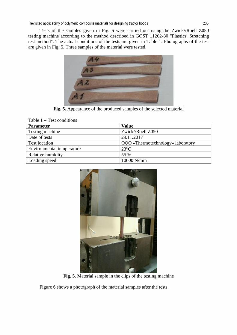
Tests of the samples given in Fig. 6 were carried out using the Zwick//Roell Z050

testing machine according to the method described in GOST 11262-80 "Plastics. Stretching

test method". The actual conditions of the tests are given in Table 1. Photographs of the test

are given in Fig. 5. Three samples of the material were tested.

Fig. 5. Appearance of the produced samples of the selected material

Table 1 Test conditions

Parameter Value

Testing machine Zwick//Roell Z050

Date of tests 29.11.2017

Test location OOO «Thermotechnology» laboratory

Environmental temperature 23С

Relative humidity 55 %

Loading speed 10000 N/min

Fig. 5. Material sample in the clips of the testing machine

Figure 6 shows a photograph of the material samples after the tests.


Fig. 6. Destroyed samples after testing

As a result of the performed tests, "strain-stress" curves were obtained for the tested

samples, one of them for sample A2 is presented in Fig. 7.

Fig. 7. "Strain-stress" curve of sample A2

5. Calculation of the strain-stress state of the hood made of PCM

According to the results of the tests, a mathematical model of the material was created. The

physicomechanical properties of the presented material are given in Table 2. The

thermodynamic properties are taken from [14].

Table 2. Physicomechanical properties of the material

Protocol parameter Value

The elasticity modulus of the monolayer under uniaxial tension 6.7 GPa

The elasticity modulus of the monolayer under uniaxial

compression

5.5 GPa

Poisson’s ratio 0.35

The stress limit of the monolayer under uniaxial tension 46 MPa

The stress limit of the monolayer under uniaxial compression 40 MPa

This composite is an isotropic material, which means it has equal elasticity moduli and

thermal expansion coefficients in each direction. To calculate the strain-stress state, a finite

element model of the hood was created; sampling was done with the Shell elements 5 mm

thick with the total number of elements equal to 250 thousand. The calculation was performed

in the ANSYS software package in the Mechanical module. The previously obtained

0

5

10

15

20

25

30

35

40

45

50

0 2 4 6 8

Sta

nd

ard

pre

ssu

re [

MP

a]

Deformation [%]

Sample A2


temperature field was transferred from the ANSYS Fluent module. The SHELL181 element

type, which allows for final deformations, was used for the calculation.

6. Calculation results

During the calculations, a temperature field was obtained, which later was used to calculate

the strain-stress state of the hood made of PCM. The displacements field for the hood in real

scale is presented in Fig. 8.

Fig. 8. Displacement field, mm

The maximum deviation is 23.82 mm which is approximately equal to 5 thicknesses of

the hood. Such deformation is significant and can affect the aerodynamics of the underhood

space. The maximum stresses at the fixing points exceeded, which means the destruction of

the material at the attaching points. It can be seen that due to large deformations and partial

destruction of the material, the necessity allow for such stresses at the design stage emerges.

In order to avoid the material destruction, it is suggested to increase thickness of PCM

in the fixing points. Also, a possible solution to this problem will be a decrease in the PCM

absorption coefficient, since the main contribution to the temperature field in this calculation

is made by radiation, it is enough to change the color of the final product.

It is worth noting that when making the bonnet of classic materials, for example,

aluminum, the material destruction will start to occur not only in fixing points but also in the

points closest to the turbocharger. It is connected to the high heat conduction of classic

materials, which gives higher thermal loads.

7. Conclucion

A method has been developed for the calculation of the tractor hood made of PCM with

allowance for the influence of thermal loads due to the emergency operation of the engine

turbocharger, and it has been shown that it should be used when designing tractor hoods.

During the aero- and thermodynamic calculations, the temperature field was obtained and

during the thermoelastic calculation – the displacement field.

It has been shown that the hood deformation under the action of thermal loads is

significant and can affect the aerodynamics of the underhood space and the material integrity

in the fixing points of the hood to the body. This result will enable creating a procedure of


optimization of the underhood space to minimize the displacement field or thermal loads, and

therefore, the stress field at the fixing points.

The obtained results showed the following advantages of PCM over classic materials:

low weight, durability not inferior to classic materials, lower thermal loads due to low heat

conduction, and ease in optimization. This gives reasons to consider high applicability of

composite materials for the production of tractor hoods.

Acknowledgements. The work has been carried out with the financial support of the Ministry

of Education and Science of Russia within the framework of the Federal Target Program

"Research and Development in Priority Areas of Development of the Scientific and

Technological Complex of Russia for 2014-2020", Activity 1.3., Grant Agreement No.

14.578.21.0206 of October 3, 2016, the unique identifier PNIER: RFMEFI57816X0206.

References

[1] Schmucker H, Flemming F, Coulson S. Two-way coupled fluid structure interaction

simulation of a propeller turbine. IOP Publishing Ltd; 2010.

[2] Skvortsov YV. Lecture notes on mechanics of composite materials. SSAU; 2013.

[3] Lebedev D, Okunev A, Aleshin M, Ivanov K, Klyavin O, Nikulina S, Rozhdestvenskiy O,

Borovkov A. Applicability of polymer composite materials in the development of trackor

falling-object protective structures(FOPS). Materials Physics and Mechanics. 2017;34(1): 90-

96.

[4] Schurov IA, Boldyrev IS. Simulation of the process of cutting blanks from composite

materials using the finite element method. Bulletin of SUSU. 2012;12: 143-147.

[5] Engineering Physics Center calculations and analysis. CFD-calculation of ventilation of

the engine compartment of a mining truck. Available from: https://multiphysics.ru/stati

/proekty/cfd-raschet-ventiliatorov-v-podkapotnom-prostranstve-karernogo-samosvala.htm

[accessed 5th

December 2018]. [In Russian].

[6] Kudryavtsev A, Kozhaev A, Tokarev A. Optimization of the cooling system elements of

the "Gazelle" car. Saratov Engineering Center; 2016.

[7] Singh AV, Gooda JP. Static and Impact Analysis of a Composite Engine Hood Assembly

for Improved Characteristics. In: 2015 India Altair technology conference, 2015 ATC, 14-15

July 2015, Bengaluru, India. 2015. p.1-6.

[8] Kwak DY, Jeong JH, Cheon JS, Im IT. Optimal design of composite hood with

reinforcing ribs through stiffness analysis. Composite Structures. 1997;38(1–4): 351-359.

[9] Kamenskaya DD, Filippov AS. Numerical modelling of heat exchange in the gas cavity of

the core melt localization device. Moscow: IBRAE RAS; 2017.

[10] Lurye AI. Nonlinear theory of elasticity. Moscow: Nauka; 1980.

[11] Loytsyanskiy LG. Mechanics of liquids and gases. 7th

edn. Мoscow: Drofa; 2003.

[12] Garbaruk AV. Course of lectures "Dynamics of a viscous liquid and turbulence". Saint

Petersburg: Peter the Great SPbPU; 2017.

[13] ANSYS, Inc. ANSYS Fluent 12.0 theory guide. Available from: http://www.afs.enea.it

/project/neptunius/docs/fluent/html/th/main_pre.htm

[14] Arkhipov VA, Zharova IK, Tatarintseva OS, Kuznetsov VT, Goldin VD. Measurement

of the emissivity coefficient of the surface of structural and insulating materials. RAS (IPCET

SB РАН); 2010.


MULTI-CRITERIA PROBLEMS FOR OPTIMAL PROTECTION

OF ELASTIC CONSTRUCTIONS FROM VIBRATION Dmitry V. Balandin1,2*, Egor N. Ezhov1, Egor V. Petrakov1, Igor A. Fedotov1

1Lobachevsky State University of Nizhni Novgorod, Nizhny Novgorod, 23 Prospekt Gagarina (Gagarin Avenue)

BLDG 2, 603950, Russia 2Research Institute for Mechanics of Lobachevsky State University of Nizhni Novgorod, Nizhny Novgorod, 23

Prospekt Gagarina (Gagarin Avenue) BLDG 6, 603950, Russia


Abstract. In a multi-objective formulation with criteria such as the maximal deformation of the elastic object to be protected and maximal forces created by protection devices, a new class of optimal vibration protection problems is considered. A general approach to solving these problems based on results of modern control theory using linear matrix inequalities technique is presented. An example of a solution of two-criteria problem for a high-storey building under seismic disturbances is given. Keywords: optimal vibration isolation, multi-criteria problem, linear matrix inequalities, Germeyer convolution 1. Introduction The problems of calculating and designing devices that provide effective protection of complex structures, instruments, equipment, and the man himself from the harmful effects of vibrations and at the same time possessing limited dimensions continue to be in focus of attention of scientists and engineers [1-6]. Such devices in engineering practice are called vibration isolators. It is known [7] that it is convenient to consider the problem of vibration protection as a task of automatic control in which the vibration isolator acts as a controller. Among the main indicators characterizing vibration isolators we usually refer to the values that determine the maximum course of this device and the maximum deformations or stresses that arise in the object to be protected. As a rule, the choice of a suitable vibration isolation device is a certain trade-off between these two most important indicators, i.e. the smaller the maximum stroke of the vibration isolation device, the greater the maximum deformations and vice versa. Taking into account this circumstance, it seems expedient to state a two-criteria problem in which it is required to synthesize the control (to choose a vibration isolation device) minimizing the above criteria in Pareto sense. It is quite possible that when several vibration isolation devices are involved in the protection of an object, then it is appropriate to consider a multi-criteria problem instead of two-criteria one. In the article, a general approach to multi-criteria vibration protection problems for multi-mass elastic objects based on modern control theory is presented. As an example, two-criteria problem of seismic protection of a high-rise building is discussed in detail, in which it is required by selecting vibration isolator to minimize in Pareto sense the maximum of maximal intersectional deformations and maximal displacement of the building relative to the foundation. This problem is complicated by the fact that the external seismic disturbance is not known in advance, so the synthesis of



the vibration isolation device is performed as the "worst" (the most dangerous) case from a certain class of disturbances. 2. Problem statement There is considered the mechanical system consisting of material points connected to each other and to the object, called the base (foundation), by elastic and dissipative elements. It is assumed that the mechanical system is subjected to uncontrolled disturbances and the control forces. The mechanical system is described by linear differential equations

, (0) 0, (0) 0,Mq Rq Kq Pv Qu q q+ + = + = = (1) where n-dimensional vector q are generalized coordinates of material points forming the system, , ,M R K are symmetric matrices that determine the inertial, dissipative and elastic properties of a mechanical system, ( )v v t= is a vector function of uncontrolled external disturbances, u is a vector of control forces. To estimate the quality of the transient and vibration processes in the system we introduce the functionals

2

0

2

( ) supmax sup ( )

, 1,..., ,i

kitk

v LJ u

z ti N

v≥

∈= = (2)

where kiz is the k-th component of the i-th vector controlled output of the system which are

scalar linear combinations of generalized coordinates q , velocities q and control forces u ,

2v is 2L -norm of external disturbance, i.е. the square root of the integral in the range from 0

to ∞ of the squared modulus of the vector function ( )v t . In essence, this form of representation of functionals makes it possible to estimate the maximum deformations and maximum forces in various elements of the mechanical system in the absence of specific data on external disturbances. The main goal of the vibration protection for this mechanical system is to form control forces of state-feedback type, i.e. as a linear combination of generalized coordinates and velocities to decrease the values of the above functionals. As a rule, it is impossible to define the control forces that would result in a "simultaneous" reduction of all functionals, so it is expedient to formulate multi-criteria problem consisting in finding control forces providing such a trade-off between the values of functionals that each of them cannot be reduced without increasing at least one of the remaining. In problems of vibration protection such a statement of the problem seems quite natural, since the reduction of deformations in certain parts of the system leads to an increase in force and vice versa.

This formulation of the optimization problem is called multi-criteria one, and the solutions to be being obtained (the feedback coefficients in the control law) are called Pareto optimal. It should be noted that obtaining solutions to multi-criteria problems and constructing Pareto optimal solutions is still one of the most difficult mathematical problems in the theory of optimization and optimal control.

3. Method of solving the multi-criteria optimal control problem To solve the stated problem, we use the results of [8-10], in which the functionals introduced above are treated as generalized operator 2H - norms of a linear system. Introducing the notation ( , )T T Tx q q= , the system (1) is rewritten in the form of a controlled linear system

, (0) 0,v ux Ax B v B u x= + + = (3) where matrices , ,v uA B B are formed from matrices , , , ,M R K P Q by the following way

1 1 1 10 0 0

, , .n nv u

IA B B

M K M R M P M Q− − − −

= = =

240 Dmitry V. Balandin, Egor N. Ezhov, Egor V. Petrakov, Igor A. Fedotov

The control u will be represented in a state-feedback form, i.e. in the form u x= Θ , the system (3) can be written as follows

( ) , (0) 0,vx A x B v x= Θ + = (4) where the matrix of a closed-loop system ( ) .uA A BΘ = + Θ Controlled output z of the system (4) is represented in the form

( ) ( )z Cx Du C D x C x= + = + Θ = Θ with scalar m components ( ) ( ) ( ) ( ) , 1, ,k k k kz C x D u C x k m= + = Θ = . According to the results of [8], the following relation holds

2*

0 1 2max

2

supmax sup (t)

( ) ( ( ) ( ))k

tk T

v LJ

zd C Y C

v≥

∈=Θ = Θ Θ , (5)

where maxd denotes the maximal diagonal entry of the matrix, and the symmetric non-negative definite matrix *Y is a unique solution to the Lyapunov matrix equation

( ) ( ) 0.T Tv vA Y YA B BΘ + Θ + = (6)

Thus, the algorithm for calculating the functional ( )J Θ is as follows: specify gain matrix ,Θ solve the Lyapunov matrix equation (6) and find matrix *Y and finally find a maximal diagonal entry of matrix *( ) ( ).TC Y CΘ Θ Further, it is required to find the gain matrix ,Θ such that minimizes the right-hand side of expression (5). Such procedure turns out to be rather difficult to perform, especially in cases when the number of elements of the matrix Θ is sufficiently large. In papers [10, 11] an alternative and very effective method for solving this problem based on the use of linear matrix inequalities [12] is proposed. It turns out that in order to find the required matrix Θ minimizing the functional (5) it is sufficient to solve the following problem: to minimize the scalar variable 2γ under constraints expressed by linear matrix inequalities

( ) ( )

( ) ( ) 20, 0,

1, ,

T T T k T T k Tu u v

T k kv

AY YA B Z Z B B Y YC Z DB I C Y D Z

k mγ

+ + + +< ≥− +

= 2

(7)

with respect to the matrices ,Y Z and the scalar variable 2γ . This optimization problem is effectively solved numerically by using a standard interior-point method of the SeDuMi and YALMIP tools of the MATLAB package. As a result, the matrices * *,Y Z and the required gain matrix Θ = 𝑍𝑍∗𝑌𝑌∗−1 are found.

Let us now consider the multi-criteria optimal control problem with N criteria 1 1( ) , , ( ) .N Nz C x z C x= Θ = Θ2

The problem consists in finding the Pareto optimal solutions, i.e. gain matrices arg min ( ), 1, , ,iP J i N

ΘΘ = Θ = … (8)

minimizing the vector criterion with components

2

0

2

sup ,max sup (t)

( ) , 1, , , 1, ,kitk

i iv L

Jz

i N k mv

≥

∈=Θ = =2 2

where im is a total number of the components of the vector output .iz To solve this problem we apply the Germeyer convolution [13], the utilization of which is described in [11] in detail, and form a new scalar objective function from the functions ( )iJ Θ

Multi-criteria problems for optimal protection of elastic constructions from vibration 241

1

( ) max ( ) / ,i ii NJ Ja a

≤ ≤Θ = Θ (9)

where ia are arbitrary positive numbers. Now we state the problem of minimizing the function ( )Ja Θ with respect to the elements of the matrix Θ for any set of parameters ia . If the controlled output of the system is represented as ( ) ,z C x= Θ where

( )1 11 1( ) ( ) ( )

TT TN NС С Ca a− −Θ = Θ Θ2 , then the minimization problem of ( )Ja Θ is reduced to

minimizing the maximal diagonal entry of the matrix ( ) ( )TC YCΘ Θ :

maxmin ( ( ) )), ( ) ( ) 0.T T Tv vd C YC A Y YA B B

ΘΘ Θ Θ + Θ + = (10)

In terms of linear matrix inequalities, the problem takes the following form [10]: minimize 2γ under linear matrix inequalities

( ) ( )

( ) ( ) 2 20, 0,

1, , , 1, ,

T T T k T T k Tu u v i i

T k kv i i i

i

AY YA B Z Z B B Y YC Z DB I C Y D Z

i N k ma γ

+ + + +< ≥

− += =2 2

(11)

with respect to the matrices ,Y Z and the scalar variable 2γ . According to [10], solving optimizing problems for positive parameters ia , we obtain a set of solutions that obviously contains the solution of the original multi-criteria problem, i.e. Pareto set. 4. Optimal isolation of a high-storey building from seismic excitation Consider the problem of optimal isolation of a high-storey building from seismic excitation. A mechanical system that simulates the oscillations of a high-storey building under seismic action on the foundation is a chain of material points (floors of the building) connected in series by dissipative and elastic elements, herewith one of the two extreme points of the chain being connected by means of a vibration isolator to the base (Fig. 1). After reduction to dimensionless form (see, for example, [14, 15]), the mathematical model of such a system has the following form

(t) , (0) 0, (0) 0,K K pv quξ β ξ ξ ξ ξ+ + = + = = (12) where ( )1, , тcolξ ξ ξ= 2 are coordinates of the material points with respect to the base the movement of which is defined by the coordinate 0ξ with respect to an inertial reference frame, 0(t) ( )v tξ= − is the external disturbance up to the sign coinciding with the acceleration of the base, u is the control force created by a vibration isolator (in particular,

0 1 0 1( )u k cξ ξ= − + for the passive isolator or ( )0 1 0 1 2 1( )u k cξ ξ a ξ ξ= − + + − for the simple hybrid isolator); β is a positive parameter characterizing the dissipative properties of a mechanical system, a positive definite symmetric matrix K and vectors p and q are defined as follows:

1 1 0 0 1 11 2 1 0 1 0

, , .0 0 1 2 1 1 00 0 0 1 1 1 0

K p q

−− −

= = =− −

−

2 2

2 2

2 2 2 2 2 2 2 2

2

2

(13)


Fig. 1. Schematic representation of the n-storey building as a multi-mass elastic system

We reduce the system (12) to the canonical form of a controlled system (3), assuming

( ) ,TT Tx ξ ξ=

1 10 0 0, , .n n n n n

v uI

A B BK K p qβ× × ×

= = =− −

(14)

Functionals characterizing the quality of vibration isolation of a multi-mass elastic system are chosen in the following form

2 2

0 2 1 0 10 11 2

2 2

max sup ( ) ( ) , ,sup ( ) ( )sup ( )( ) sup , ( ) sup .t t n nt

v L v L

x t x t x t x tx tJ u J u

v v≥ ≥ −≥

∈ ∈

− −= =

2 (15)

The first functional characterizes the maximal displacement of the first floor relative to the base and the second one determines the maximum deformation of the multi-mass system. The control problem is to find the gain matrix ,Θ i.e. parameters of the state-feedback control (vibration isolator) that minimize functionals (15) in Pareto sense. We note that the functionals under consideration have the following property: the choice of the feedback parameters leading to a decrease in one of them, for example, the maximum displacement of the first floor relative to the base implies an increase in the value of the other functional determining the maximum deformation of the system (high-storey building).

The results of solving the two-criteria problem for 10, 0.1n β= = are presented. First we consider the case, which we will call the "ideal vibration isolator", when the measurement of the total state of the controlled system is available, i.e. in the formation of feedback, both the coordinates and velocities of all the material points of the mechanical system involve. In Fig. 2, curve 1 represents a set of Pareto optimal values of functionals 1 2 , J J for the indicated case. Obviously, in practice it is hardly possible to measure the total state of a mechanical system, however, the solution obtained allows one to obtain a lower bound for the optimal values of the functionals. Then let us consider the case when the feedback is formed on the basis of the current value of the variable 1x and the rates of its change (the variable

11x ). In fact, this case corresponds to a passive vibration isolator with elastic and damping elements. In Fig. 2, curve 2 above the "limit" curve 1 corresponds to the Pareto optimal values of the functionals 1 2 , J J in the class of passive vibration isolators. Two more curves 3 and 4, shown in Fig. 2 correspond to the cases when an "active" component is added to the passive vibration isolator, that is, the displacement of the second floor relative to the first one (curve 3) and additionally displacement of the fourth floor relative to the third one (curve 4) is


additionally measured. The analysis of these curves shows that the "active" vibration isolators (curves 3 and 4) are not much better than the passive isolator (curve 2), but all these three isolators are noticeably inferior to the "ideal vibration isolator" (curve 1).

Fig. 2. Pareto set on the plane of the criteria for different types of vibration isolators

5. Conclusion The article deals with multi-criteria problems for optimal protection of elastic objects from vibration. The generalized operator 2H − norms of a system of differential equations that describe the dynamics of an object to be protected from external disturbances belonging to a given class are chosen as criteria. A general scheme for solving the multi-criteria optimal control problem based on the Germeyer convolution and linear matrix inequalities technique is proposed. Two-criteria problem of optimal vibration isolation of a high-storey building from seismic excitations is solved. Pareto set on the plane of the criteria is constructed. The "ideal" Pareto optimal isolator and optimal ones of active and passive types are compared. It is shown that the "active" vibration isolators are not much better than the passive ones, but all these isolators are noticeably inferior to the "ideal" vibration isolator. Acknowledgements. The work is financially supported by the Federal Targeted Programme for Research and Development in Priority Areas of Development of the Russian Scientific and Technological Complex for 2014–2020 under the contract No. 14.578.21.0246 (unique identifier RFMEFI57817X0246). References [1] Buckle IG, Mayes RL. Seismic Isolation History, Application, and Performance – World View. Earthquake Spectra. 1990;6: 161-201. [2] Karnopp D. Active and Semi-Active Vibration Isolation. ASME Journal of Vibration and Acoustics. 1995;117B: 117-128. [3] Balandin DV, Bolotnik NN, Pilkey WD. Review: Optimal Shock and Vibration Isolation. Shock and Vibration. 1998;5: 73-87. [4] Balandin DV, Bolotnik NN, Pilkey WD. Optimal Protection from Impact, Shock, and Vibration. Amsterdam: Gordon and Breach Science Publishers; 2001. [5] Ibrahim RA. Recent Advances in Nonlinear Passive Vibration Isolators. Journal of Sound and Vibration. 2008;314: 371-452.


[6] Patil SJ, Reddy GR. State of Art Review – Base Isolation Systems for Structure. International Journal of Emerging Technology and Advanced Engineering. 2012;2: 438-453. [7] Kolovskii MZ. Automatic Control of Vibration Protection Systems. Moscow: Nauka; 1976. (in Russian) [8] Wilson DA. Convolution and Hankel Operator Norms for Linear Systems. IEEE Trans. Autom. Control. 1989;34: 94-97. [9] Rotea MA. The Generalized H2 Control Problem. Automatica. 1993;29: 373-385. [10] Balandin DV, Kogan MM. Pareto Optimal Generalized H2-Control and Vibroprotection Problems. Automation and Remote Control. 2017;78: 1417-1429. [11] Balandin DV, Kogan MM. Pareto Optimal Generalized H2-Control and Optimal Protection from Vibration. IFAC-PapersOnLine. 2017;50: 4442-4447. [12] Balandin DV, Kogan MM. Synthesis of Control Laws Based on Linear Matrix Inequalities. Moscow: Nauka; 2007. (in Russian) [13] Germeyer Y. Introduction to Theory of Operations Research. Moscow: Nauka; 1971. (in Russian) [14] Nishimura N, Kojima A. Seismic Isolation Control for a Buildinglike Structure. IEEE Control Systems. 1999;19: 38-44. [15] Balandin DV, Kogan MM. LMI-Based Optimal Attenuation of Multi-Storey Building Oscillations Under Seismic Excitations. Structural Control and Health Monitoring. 2005;12: 213-224.


DEVELOPING OF PHENOMENOLOGICAL DAMAGE MODEL

FOR AUTOMOTIVE LOW-CARBON STRUCTURAL STEEL

FOR USING IN VALIDATION OF EURONCAP FRONTAL IMPACT Dmitriy Shcherba*, Alexey Tarasov, Alexey I. Borovkov

SPbSTU, 29 Polytechnicheskaya st., Saint-Petersburg, Russia


Abstract. Results presented in this paper demonstrate the process of material models development for automotive structural steels in order to implement it into the SUV digital twin. Developed digital twin is capable to simulate vehicle crash impact in the same way as full-scale test but among of many parameters it needs correctly defined material models. One of the most difficult things to develop is failure models which simulate the behavior of real material correctly. Usually standard approach considers using only stress-strain curves for several strain rates that does not follow the requirements of advanced model of digital twin. Implementing of damage theory based GISSMO failure description into the vehicle model, especially for high strain rates, leads to achieving good correlation with full-scale crash tests. Also it helps to improve digital twin’s quality and speed up overall process of vehicle developing. As a result of research this paper demonstrated the difference of simulations between usual and improved material models Keywords: damage, GISSMO, digital twin, vehicle, crash test, triaxiality

1. Introduction. Computer simulation of car collisions with different barriers (so-called crash tests) became standard procedure in set of activities to improve passive safety of vehicle structure. Increasing requirements to complex technical systems on the one hand, and increasing computing power, on the other hand led to a “digital twin” concept in modeling based on high quality mathematical model included thousands of input parameters [1]. Digital twins can provide an opportunity of obtaining accurate information about related real objects and their behavior. Consequently, mathematical model that digital twin is based on should represent behavior of real object with acceptable accuracy, and one of the basic components of this concept is correctly defined mathematical model of material which related part is made of.

Vehicle collision is a process which includes large high-speed deformations that often leads to failure of vehicle parts. Failure changes stress-strain state of vehicle body elements and their location after impact. These facts explain that fracture should be taken into account, but modeling it according to classical mechanics approach leads to significant increase of computational efforts.

Alternative approach consists of using phenomenological damage-based failure criteria, one of which called GISSMO (acronym of Generalized Incremental Stress-State damage Model) was proposed and developed by Neukamm et al. [2,3,4], and recently implemented into commercial finite-element code LS-DYNA. This model is based on incremental damage accumulation that depends on a failure curve which is a function of the current stress state.



Furthermore, GISSMO includes the evolution of instability measures based on a critical strain, and this feature helps to take into account behavior of steel with better accuracy. Brief description of fracture curve obtaining was provided by F. Andrade et al. [4]. Description of GISSMO development for dual-phase sheet steel was presented by J. Effelsberg et al. [5] and by Andrade et al. [6]. Herein presented a process of GISSMO developing for low-carbon automotive structural steel. 2. Description of GISSMO model. Detailed description of the model was provided by Andrade et al. [6]. Therefore, only brief description and most important equations are provided herein.

In the late 1960's and 1970's several authors provided contributions showing dependency of the fracture strain of notched sample upon notch radius [7]. As a result, the new stress-state indicator called triaxiality was proposed, defined as: 𝜂𝜂 = 𝜎𝜎𝑚𝑚

𝜎𝜎𝑒𝑒𝑒𝑒= − 𝑝𝑝

𝜎𝜎𝑒𝑒𝑒𝑒, (1)

where σm means stress and σeq – equivalent stress defined as:

𝜎𝜎𝑒𝑒𝑒𝑒 = 12

[(𝜎𝜎1 − 𝜎𝜎2)2(𝜎𝜎1 − 𝜎𝜎3)2(𝜎𝜎2 − 𝜎𝜎3)2]. (2)

A phenomenological scalar quantities D called damage measure and F called instability measure are introduced as: 𝐷 = 𝑛𝑛

Λ(𝐿𝐿𝑒𝑒,𝜂𝜂)𝜀𝜀𝑓𝑓(𝜂𝜂)𝐷𝐷1−1 𝑛𝑛 𝜀𝜀𝑝𝑝, (3)

𝐹 = 𝑛𝑛𝜀𝜀𝑐𝑐𝑐𝑐𝑐𝑐𝑐𝑐(𝜂𝜂)𝐹𝐹

1−1 𝑛𝑛 𝜀𝜀𝑝𝑝, (4) where n – damage exponent, 𝜀𝜀𝑝𝑝- accumulated plastic strain, 𝜀𝜀𝑐𝑐𝑐𝑐𝑐𝑐𝑐𝑐(𝜂𝜂) and 𝜀𝜀𝑓𝑓(𝜂𝜂) – critical strain curve and failure curve, respectively, both are functions of triaxiality η. Λ(𝐿𝐿𝑒𝑒 ,𝜂𝜂) – regularization function for spurious mesh dependence compensation:

Λ(𝐿𝐿𝑒𝑒 ,𝜂𝜂) =

⎩⎪⎨

⎪⎧

𝛽𝛽𝑠𝑠ℎ𝑒𝑒𝑒𝑒𝑐𝑐 𝑖𝑖𝑖𝑖 𝜂𝜂 ≤ 0𝛼𝛼(𝐿𝐿𝑒𝑒)−𝛽𝛽𝑠𝑠ℎ𝑒𝑒𝑒𝑒𝑐𝑐

1/3 𝜂𝜂 + 𝛽𝛽𝑠𝑠ℎ𝑒𝑒𝑒𝑒𝑐𝑐 𝑖𝑖𝑖𝑖 0 < 𝜂𝜂 ≤ 1/3

𝛼𝛼(𝐿𝐿𝑒𝑒)−𝛽𝛽𝑏𝑏𝑐𝑐𝑒𝑒𝑏𝑏𝑐𝑐𝑒𝑒𝑏𝑏

1/3 𝜂𝜂+𝛽𝛽𝑏𝑏𝑐𝑐𝑒𝑒𝑏𝑏𝑐𝑐𝑒𝑒𝑏𝑏𝛽𝛽𝑏𝑏𝑐𝑐𝑒𝑒𝑏𝑏𝑐𝑐𝑒𝑒𝑏𝑏

. (5)

Herein 𝛼𝛼(𝐿𝐿𝑒𝑒) – monotonically decreasing function of finite element size, factors 𝛽𝛽𝑠𝑠ℎ𝑒𝑒𝑒𝑒𝑐𝑐 and 𝛽𝛽𝑏𝑏𝑐𝑐𝑒𝑒𝑏𝑏𝑐𝑐𝑒𝑒𝑏𝑏 defined as: 𝛽𝛽𝑠𝑠ℎ𝑒𝑒𝑒𝑒𝑐𝑐 = 1 − [1 − 𝛼𝛼(𝐿𝐿𝑒𝑒)](1− 𝑘𝑘𝑠𝑠ℎ𝑒𝑒𝑒𝑒𝑐𝑐), (6) 𝛽𝛽𝑏𝑏𝑐𝑐𝑒𝑒𝑏𝑏𝑐𝑐𝑒𝑒𝑏𝑏 = 1 − [1 − 𝛼𝛼(𝐿𝐿𝑒𝑒)](1− 𝑘𝑘𝑏𝑏𝑐𝑐𝑒𝑒𝑏𝑏𝑐𝑐𝑒𝑒𝑏𝑏), (7) where 𝑘𝑘𝑠𝑠ℎ𝑒𝑒𝑒𝑒𝑐𝑐 and 𝑘𝑘𝑏𝑏𝑐𝑐𝑒𝑒𝑏𝑏𝑐𝑐𝑒𝑒𝑏𝑏 vary from 0 to 1. Coupling of damage and stress is considered as [8]: 𝜎𝜎 = (1 − 𝐷𝐷)𝜎𝜎, (8) where 𝜎𝜎 – undamaged stress tensor, 𝐷𝐷 – damage that take place when strain localization arise and given by:

𝐷𝐷 = 0, 𝑖𝑖𝑖𝑖 𝐹𝐹 < 1

𝐷𝐷−𝐷𝐷𝑐𝑐𝑐𝑐𝑐𝑐𝑐𝑐1−𝐷𝐷𝑐𝑐𝑐𝑐𝑐𝑐𝑐𝑐

𝑚𝑚

𝑖𝑖𝑖𝑖 𝐹𝐹 = 1 . (9)

Herein 𝐷𝐷𝑐𝑐𝑐𝑐𝑐𝑐𝑐𝑐 is accumulated damage when F = 1 and m is so called fading exponent. Finally, GISSMO model assumes defining several parameters: curves 𝜀𝜀𝑐𝑐𝑐𝑐𝑐𝑐𝑐𝑐(𝜂𝜂), 𝜀𝜀𝑓𝑓(𝜂𝜂)

and 𝛼𝛼(𝐿𝐿𝑒𝑒), factors 𝑘𝑘𝑠𝑠ℎ𝑒𝑒𝑒𝑒𝑐𝑐 and 𝑘𝑘𝑏𝑏𝑐𝑐𝑒𝑒𝑏𝑏𝑐𝑐𝑒𝑒𝑏𝑏, and exponents m and n. This provides more flexibility during calibration procedure, but, on the other hand, this procedure becomes more complex and difficult.

Developing of phenomenological damage model for automotive low-carbon structural steel for using... 247

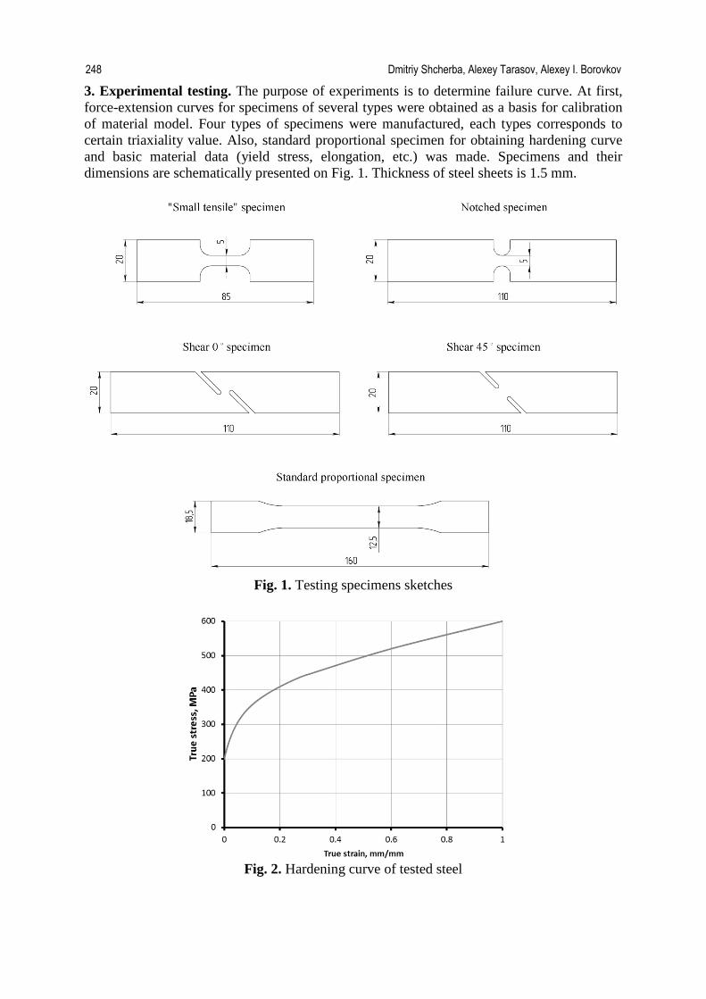
3. Experimental testing. The purpose of experiments is to determine failure curve. At first, force-extension curves for specimens of several types were obtained as a basis for calibration of material model. Four types of specimens were manufactured, each types corresponds to certain triaxiality value. Also, standard proportional specimen for obtaining hardening curve and basic material data (yield stress, elongation, etc.) was made. Specimens and their dimensions are schematically presented on Fig. 1. Thickness of steel sheets is 1.5 mm.

Fig. 1. Testing specimens sketches

Fig. 2. Hardening curve of tested steel

248 Dmitriy Shcherba, Alexey Tarasov, Alexey I. Borovkov

Tensile testing performed by universal testing machine Zwick/Roell Z100 with extensometer mounted on sample to minimize measurement error. All tests were performed at room indoor temperature, with nearly quasistatic conditions (strain rate was about 10-3s-1). Testing of standard proportional specimen resulted in obtaining basic material parameters: Young's modulus, yield stress, tensile strength and elongation. Hardening curve is presented on Fig. 2. Force-extension curves for failure curve samples presented on Fig. 3.

Usually, five types of specimens are processed, including biaxial tension. In this research we used four types and developed an approximation for boundary triaxiality value of 0.667. It saved resources spent on experimental testing and kept appropriate accuracy level.

4. Finite element modeling of tests. Calibration of model parameters. Full-scale tests presented in previous section were simulated with finite element modeling technique using commercial code LS-DYNA. Geometry of the sample repeats the shape of real samples. Sample is modeled with shell finite elements, the same as in the case of vehicle crash test modeling. Firstly, tests were performed with finite element size 1.5 mm in the central part of sample, and then regularization carried out that allowed using 5 mm finite element mesh. Elastic-plastic behavior of material defined using *MAT_024 card, GISSMO parameters defined with *MAT_ADD_EROSION card. Sample is fixed at one side by setting translational and rotational degrees of freedom equal to zero. At the other side, slightly increasing velocity applied which allows minimizing inertia effects and guaranteeing quasi-static conditions. Calibration parameters m and n for GISSMO input curves were also identified. Failure curve identified using iterative technique of comparing simulation results with corresponding experimental results. Obtained failure curve is presented on Fig. 3.

Fig. 3. Obtained failure curve for GISSMO input

Obtained force-extension curves for both experimental and virtual tensile tests are

presented on Fig. 4.


Fig. 4. Force-Displacement curves for four sample types

Fig. 5. Comparison of tensile testing results for standard proportional sample


5. Model validation. Validation of calibrated GISSMO model is conducted using sample model that did not take part in calibration process (see Fig. 1, standard proportional sample). Results are represented on Fig. 5. Comparing results of experimental and virtual testing one can see that GISSMO provide acceptable representation of sample failure. Little divergence between two curves shows that some additional calibration may be done, and this is a question for further investigation.

It should be mentioned that the localization occurs in two stages: firstly, when localization begins, one can see a decrease of sample width, and, secondly, the thickness become to decrease. Thus, second stage of localization can be modeled only concerning fully three-dimensional formulation. But in the case of vehicle collisions modeling this couldn’t be done at the moment, because of high computational efforts requirements. So, keeping in mind restrictions of shell elements, material with defined GISSMO provided good results.

Validated GISSMO damage model was implemented into a detailed FE model of 2016 four-door passenger SUV that includes the full functional capabilities of a suspension, a driveline and steering subsystems. The “digital twin” includes all the necessary parameters for prediction of object behavior during any physical interaction of the related real vehicle [9]. Deformed SUV body with standard material models that do not include difficult damage behavior is presented on figure 5, deformed SUV body with GISSMO defined presented on Fig. 6. On the figure 6 one can see the frame taken from full-scale test at the same millisecond.

Fig. 6. Deformed SUV body FE model with standard material models

Fig. 7. Deformed SUV body FE model with calibrated GISSMO damage model defined


Fig. 8. Deformed SUV body, full-scale test

Results of simulation of detailed full-scale vehicle model shows that GISSMO model helped to achieve values of floor panel and motor shield deformation that have high correlation with real crash test. 6. Summary and conclusions. GISSMO model provides researcher with possibility to model failure of structure with acceptable accuracy level and without increasing of computing time for simulation. Input parameters set provides user with wide range of possibilities for model calibration. Typical automotive low-carbon structural steel was investigated in this research, failure and critical strain curves were received, calibration parameters such as damage exponent were defined.

Developed GISSMO model was validated using standard tensile sample and showed high level of correlation with experimental data. Calibrated GISSMO model was implemented into full-scale SUV FE model. Comparing experimental and simulation results showed that material model with defined GISSMO demonstrates acceptable representation of real object behavior, and, thus may be used for creating vehicles "digital twins". Acknowledgements. The works are carried out during the implementation of the comprehensive project with the financial support of the Government of the Russian Federation (Ministry of Education and Science of Russia). Contract 02.G25.31.0140 of 01.12.2015. References [1] Borovkov A, Ryabov Yu, Maruseva V. The new paradigm of digital design and modeling of globally competitive new generation product. Saint-Petersburg; 2017. (In Russian) [2] Neukamm F, Feucht M, Haufe A, Roll K. On closing the constitutive gap between forming and crash simulation. Proceedings of the 10th international LS-DYNA users conference. Detroit; 2008. [3] Neukamm F, Feucht M, Haufe A. Considering damage history in crashworthiness simulations. Proceedings of the 7th European LS-DYNA users conference. Salzburg; 2008. [4] Andrade F, Feucht M, Haufe A. On the prediction of material failure in LS-DYNA: a comparison between GISSMO and DIEM. Proceedings of the 13th international LS-DYNA users conference. Dearborn; 2014.


[5] Effelsberg J, Haufe A, Feucht M, Neukamm F, Du Bois P. On parameter identification for the GISSMO damage model. Proceedings of the 12th international LS-DYNA users conference. Detroit; 2012. [6] Andrade FXC, Feucht M, Haufe A, Neukamm F. An incremental stress state dependent damage model for ductile failure prediction. Int. J. of Fracture. 2016;200(1-2): 127-150. [7] Bridgman PW. Studies in large flow and fracture. New York: McGraw-Hill; 1952. [8] Lemaitre J. A continuous damage mechanics model for ductile fracture. J. Eng. Mater. Technol. 1985;107(1): 83–89. [9] Alekseev S, Tarasov A, Borovkov A, Aleshin M, Klyavin O. Validation of EuroNCAP frontal impact of frame off-road vehicle: road traffic accident simulation. Materials Physics and Mechanics. 2017;34(1): 59-69.


INDENTATION OF AN ELASTIC HALF-SPACE REINFORCED WITH

A FUNCTIONALLY GRADED INTERLAYER BY A CONICAL PUNCH Andrey S. Vasiliev1*, Sergey S. Volkov1, Sergey M. Aizikovich1,

Alexander N. Litvinenko2

1Research Institute for Mechanics of Lobachevsky State University of Nizhni Novgorod, Nizhny Novgorod, 23

Prospekt Gagarina (Gagarin Avenue) BLDG 6, 603950, Russia 2Vorovich Institute of Mathematics, Mechanics and Computer Science, Southern Federal University,

Rostov-on-Don 344090, Russia


Abstract. An elastic half-space with a two-layered coating is considered. The upper layer is homogeneous while the lower layer is assumed to be made of a functionally graded material. Elastic moduli of the interlayer vary with depth according to arbitrary differentiable functions. The half-space is indented by a rigid conical punch. Approximated analytical expressions for the contact stresses are obtained using the bilateral asymptotic method. Expressions for the subsurface stresses and displacements are obtained in the form of some quadratures. Numerical results illustrating difference between the stress distributions for one- and two-layered coatings are presented. Keywords: contact, indentation, conical punch, two-layered coating, functionally graded interlayer, elasticity, analytical methods 1. Introduction The paper continues the study of contact mechanics of coatings reinforced with a functionally graded (FG) interlayer which was started by the authors in papers [1,2]. Such a structure of coatings may occur as the result of oxidation of a FG coating or may be created to obtain certain properties. For example, a coating consisting of an antifriction polymer composite attached to the load-bearing skeleton made of metal with complex nonmonotonic variation of elastic moduli is used to increase operating time and reduce wear of rails and wheel sets [3]. Most of the papers in the field of contact mechanics for FG materials address the case then the whole coating is made of a FG material [4–7]. Guler and Erdogan [4] analysed normal contact of a rigid punch and an elastic half-plane with FG coating with exponential variation of shear modulus. Ke, Wang, Liu and Zhang used piecewise linear approximation of the shear modulus to study 2D and axisymmetric contact of elastic solid with FG coating with arbitrary variation of elastic moduli. They also used similar approach to consider contact problems in more complicated formulations, for instance, thermoelastic frictional contact is considered in [7]. Coatings with FG interlayers have received less attention in research. Liu et al. [8] and Vasiliev et al. [2] considered torsion of an elastic half-space with a coating reinforced with a FG interlayer. Indentation of such a solid by a rigid flat-ended circular punch [1] and spherical punch [9,10] was also studied earlier. Guler et al. [11] considered a thin film bonded to a FG coating with exponentially varying elastic moduli on an elastic substrate.



It has to be mentioned that methods for solution of contact problems for solids with FG coatings or piecewise homogeneous coatings or elastic layer on a rigid foundation are pretty similar. A regular asymptotic method was successfully used for thick coatings by Vorovich and Ustinov [12] and Zelentsov [13]. Methods based on the Wiener–Hopf factorization were effectively used for coatings (or layers) of small thickness, for instance, in [13,14]. The orthogonal polynomial method [15] and collocation method [16] are traditionally used to solve contact problems for intermediate thicknesses of the coating (layer). The generalized image method was developed and used by Fabrikant to solve several contact problems in [17–19].

The present paper addresses indentation by a rigid conical punch. The major difference from the results obtained in [4–11] is that the solution of integral equation of the problem is constructed in an approximated analytical form using the bilateral asymptotical method [20,21] while in [4–11] it is obtained numerically using collocation technique. The solution obtained in the paper is asymptotically exact for small and large values of relative coating thickness. 2. Statement of the problem Let us consider an elastic half-space with a two-layered coating. The upper layer is homogeneous and has thickness h1 while the lower layer (interlayer of the media) has thickness h2 and made of a functionally graded material. Let us use a cylindrical coordinate system r, φ, z where z axis is normal to the coating surface and passes through the center of the punch. Lamé parameters of the half-space vary according to the following:

−<∞−=Λ−≤<−Λ

≤<−=Λ

=Λ≤ ,,const,M

,, )(,M,0,const ,M

)(,M

22

111

100

HzhzHz

zhz (1)

where H=h1+h2 is thickness of the coating, Μ1(z), Λ1(z) are arbitrary positive continuously differentiable functions. Here and after, superscripts 0, 1 and 2 correspond to the upper layer, to the interlayer and to the substrate, respectively.

A rigid conical punch is indented in the surface of the coated half-space by a normal centrally applied force P that causes elastic deformation of the half-space. Outside the contact area the surface is stress-free. The scheme of the contact is presented in the Fig. 1.

Let us introduce following notations: δ is the displacement of the punch, a is the radius of the contact area, α is the half slope of the cone, χ is the contact depth which satisfy following relation: aχ=acot . The coating and the substrate are assumed to be glued without sliding. Therefore, the boundary conditions are:

). ( ),(0 ,0 :0 1000 ararwarz zzr ≤+−=>=== −χδστ (2) , , , , : 10101010

1 uuwwhz zzzrzr ====−= σσττ (3) . , , ,: 21212121 uuwwHz zzzrzr ====−= σσττ (4)

The function to be determined is the contact normal pressure under the punch. To determine the radius of the contact region it is necessary to use an additional condition following from the continuity of the contact stress at the contact boundary:

.0)(, ),(0 =≤−== aparrp aazzσ (5)

Indentation of an elastic half-space reinforced with a functionally graded interlayer by a conical punch 255

Fig. 1. Statement of the contact problem for an arbitrary functionally graded interlayer

The linear constitutive equations for an isotropic material are:

.θ ,)(

,θ)()(2 ,θ)()(2 ,θ)()(2

zw

ru

ru

rw

zuz

zzwzz

ruzz

ruz

rz

zr

∂∂

++∂∂

=

∂∂

+∂∂

Μ=

Λ+∂∂

Μ=Λ+Μ=Λ+∂∂

Μ=

τ

σσσ φ

(6)

3. Solution of the problem The problem is reduced to the solution of a following dual integral equation:

( )

>=∫ γγγγ

≤−δχβ=∫ γγλγγ∞

−−∞

.1 ,0)()(

,1 ,)()()(

00

00*

0011

000

*

rdrJP

rrdrJLP (7)

This process was described in details in [26]. The following dimensionless variables were used above:

.)(,,,,2

)(,,,,,)(,

)(,

,,,,,)1(

,)1(

,,,,,

)2(0

0*****

)2(0

0**

***22

2)2(20

0)0()0(

)2(

00

χ

τσσσ=τσσσ

ΜΛ=ΜΛ

χδ

=δν−

=ν−

==β==λ

ϕϕ

ef

arzrzrzrz

ef

efefef

ef

Earpa

rpE

Hzz

wuwuEEE

EEE

Hzz

arHr

(8)

L(u) is the compliance function which is calculated numerically from a two-point boundary value problem for a system of ordinary differential equations with variable coefficients [1], E and v are Young's modulus and Poisson’s ratio, P*(γ) is the Hankel transform of the dimensionless contact pressure. The solution of the integral equation (7) was constructed earlier [22] by using the bilateral asymptotic method [20]. For that purpose, the following approximation for the compliance function was used:

( ) ( ).)()(1

2222∏=

++=≈N

iiiN BuAuuLuL (9)

Therefore, the solution of the integral equation has the form:

( ) .cos1cos),,(sin),,()( 2

1222

111*

γγ−

+

λ+γγ

γλγ−γλλ+γ=γ ∑

=−

−−−N

i i

iiiiiiii

AACDFAADCFD

P (10)

The contact stresses on the surface are determined by the formula:

256 Andrey S. Vasiliev, Sergey S. Volkov, Sergey M. Aizikovich, Alexander N. Litvinenko

,)cosh()sinh(11

ln)(1

1

20

2

11

20

2

1

0

20

0*

00

∑ ∫∫=

−−

−+

−+

−+=

N

i r

ii

r

ii dt

rt

tADdt

rt

tAC

rr

rpλλ (11)

where )sinh()cosh(),,( zyzxzyxF += . Constants Ci and Di (i=1,…, N) are the solution of the following system of linear algebraic equations:

∑ ∑∑= =

−

=

−

=−

λ−=

−λ

=−

N

i

N

i ki

iiki

N

i kki

ikii

kki

i NkBAAABF

DBBA

ABAFC

BBAD

1 122

1

122

1

222 .,..,1,),,(1),,(

,1

Displacements of the punch are obtained as a function of the relative coating thickness λ in the following form:

λ

λ+π

=δ ∑=

N

i

i

i

i

i

i AAD

AC

F1

* ,,12

(12)

Using (8) and (6) the following expressions for the displacements and stresses at internal points of the coated half-space are obtained:

.)(2)())(2)((

,)(,)()(2

,))(2)(()(,,

0

10

*40

*60

*0

**

52

0**4

60*

0

10

**

40

*0

*60

**3

*1

*

Μ−

λΛ−Μ+Λβ=σ

+λ

Μβ=τ

λ−Λ+Μβ=σ

λΜ+Λ−Λβ=σβ−=β=

ϕ

rIzIzIzz

IIzIIzrIz

IzzIzIwIu

r

rz

z

(13)

The following notations for the quadratures were used above:

( ) ( ) ( ) ( )

( ) ( ) ( ) ( )

( ) ( ) ( ) ( ) .J,)(),( ,J,)(),(

,J,)(),( ,J,)(),(

,J,)(),( ,J,)(),(

0000

**006

0000

**004

0010

**005

0000

**003

0010

**002

0010

**001

∫ γγγλγγ=∫ γγλγ′γ=

∫ γγγλγγ=∫ γγλγγ=

∫ γγλγ′γ=∫ γγλγγ=

∞∞

∞∞

∞∞

drzUPzrIdrzWPzrI

drzWPzrIdrzWPzrI

drzUPzrIdrzUPzrI

(14)

Here U*(γ,z0),W*(γ,z0) and their derivatives with respect to z0 are calculated numerically from the similar two-point boundary value problem for a system of ordinary differential equations with variable coefficients as the compliance function [1].

4. Numerical results Let us consider the silicon substrate with the Young’s modulus E = 146 GPa and the Poisson's ratio ν=0.22 and let the coating properties vary linearly from the pure nickel (E=203 GPa, ν = 0.31) on the surface to the pure silicon at depth. In addition, let us also consider the case when the coating was oxidized near its surface. As a result of oxidation a thin layer of NiO is occurred (E = 90 GPa, ν = 0.21). Some details of the creation and research of such a coating-substrate system, as well as the values of the elastic moduli, can be found in [23].

As it has been obtained earlier [1], the presence of the oxide upper layer sufficiently changes the compliance function. In particular, it has been shown that if the thickness of the oxide layer is small (h1<0.2H) then the compliance function has nonmonotonic variation.

Figures 2a and 2b contain graphs of the distribution of relative contact stresses

0

20

0*

0rel

11ln)()(

rr

rprp−+

=


for Ni/Si and NiO/Ni/Si in assumption that the Ni layer is oxidized to 5% of its thickness, i.e. h1 = 0.05H. The relative contact stresses are more convenient for analysis because they have no singularities at r0=0 and r0=1. To calculate numerical results, the approximations of compliance functions by the expression (9) were constructed with the relative error less than 0.15%. That allows us to be confident in the high precision of the obtained numerical results.

a b

Fig. 2. Distribution of the relative contact pressure for Ni/Si (a) and NiO/Ni/Si (b)

An important difference between the Ni and NiO/Ni coatings lays in the value of the "softness" parameter β. It is β=0.683<1 for Ni and β=1.63>1 for NiO/Ni. This parameter largely influences the distribution of the contact stresses in the vicinity of r0=0 and r0=1 especially for thin coatings [24]. As it can be seen from Fig. 2, the contact stresses near the points r0=0 and r0=1 decrease for NiO/Ni coating and increase for Ni coating, in comparison with the non-coated half-space. As λ→0 the contact stresses at any fixed value of r0 tend to unit monotonically, for Ni coating, or nonmonotonically, for NiO/Si coating. This fact is the consequence of the similar behaviour of the corresponding compliance functions.

5. Conclusion The indentation of an elastic half-space with a coating reinforced with a functionally graded interlayer by a rigid conical punch was studied. The distribution of the contact stresses for Ni/Si and NiO/Ni/Si was illustrated. It was shown that the presence of a thin oxide layer sufficiently changes the distribution of the contact stresses, especially near the central and boundary points of the contact region. The results of the paper can be easily generalized to the case of piezoelectric materials using recent results [25,26].

Acknowledgements. The work is financially supported by the Federal Targeted Program for Research and Development in Priority Areas of Development of the Russian Scientific and Technological Complex for 2014-2020 under the contract No. 14.578.21.0246 (unique identifier RFMEFI57817X0246).

References [1] Vasiliev AS, Volkov SS, Aizikovich SM. Approximated analytical solution of contact problem on indentation of elastic half-space with coating reinforced with inhomogeneous interlayer. Materials physics and mechanics. 2018;35(1): 175-180.


[2] Vasiliev AS, Volkov SS, Aizikovich SM. Torsion of an elastic transversely isotropic half-space with a coating reinforced by a functionally graded interlayer. In: Pietraszkiewicz W, Witkowski W (Eds.) Shell Structures: Theory and Applications Volume 4: Proceedings of the 11th International Conference "Shell Structures: Theory and Applications, (SSTA 2017), October 11-13, 2017, Gdansk, Poland. London: Taylor & Francis; 2017. p.185-188. [3] Kolesnikov V, Myasnikova N, Sidashov A, Myasnikov P, Kravchenko Ju. Multilayered antifriction nanostraction covering for lubrication in the tribocoupling "wheel-rail". Transport problems. 2010;5: 71–79. [4] Guler MA, Erdogan F. Contact mechanics of graded coatings. International Journal of Solids and Structures. 2004;41: 3865-3889. [5] Ke LL, Wang YS. Two-dimensional contact mechanics of functionally graded materials with arbitrary spatial variations of material properties. International Journal of Solids and Structures. 2006;43: 5779-5798. [6] Liu TJ, Wang YS, Zhang C-Z. Axisymmetric frictionless contact of functionally graded materials. Archive of Applied Mechanics. 2008;78: 267-282. [7] Liu TJ, Ke LL, Wang YS, Yang J, Alam F. Thermoelastic frictional contact of functionally graded materials with arbitrarily varying properties. International Journal of Mechanical Sciences. 2012;63: 86-98. [8] Liu TJ, Ke LL, Wang YS, Xing YM. Stress Analysis for an Elastic Semispace with Surface and Graded Layer Coatings under Induced Torsion. Mechanics Based Design of Structures and Machines. 2015;43: 74-94. [9] Liu TJ, Xing YM, Wang YS. The axisymmetric contact problem of a coating/substrate system with a graded interfacial layer under a rigid spherical punch. Mathematics and Mechanics of Solids. 2014;21: 383-399. [10] Liu TJ, Xing YM. Stress analysis for bonded materials with a graded interfacial layer under a rigid punch. Mechanics of Advanced Materials and Structures. 2016;23: 1163-1172. [11] Guler MA, Gulver YF, Nart E. Contact analysis of thin films bonded to graded coatings. International Journal of Mechanical Sciences. 2012;55: 50–64. [12] Vorovich II, Ustinov IuA. Pressure of a die on an elastic layer of finite thickness. Journal of Applied Mathematics and Mechanics. 1959;23: 637–650. [13] Zelentsov V. On the problem of shear of a functionally graded half-space by a punch. MATEC Web of Conferences. 2017;132: 03012. [14] Alexandrov VM, Vorovich II. Contact problems for the elastic layer of small thickness. Journal of Applied Mathematics and Mechanics. 1964;28: 425–427. [15] Popov GIa. On the method of orthogonal polynomials in contact problems of the theory of elasticity. Journal of Applied Mathematics and Mechanics. 1969;33: 503–517. [16] Kalandiya AI. Mathematical Methods of Two-Dimensional Elasticity. Moscow: Mir Publishers; 1975. [17] Fabrikant VI. Tangential contact problem for a transversely isotropic elastic layer bonded to an elastic foundation. Journal of Engineering Mathematics. 2011;70: 363-388. [18] Fabrikant VI. Elementary solution of contact problems for a transversely isotropic layer bonded to a rigid foundation. Zeitschrift für angewandte Mathematik und Physik. 2006;57: 464-490. [19] Fabrikant VI. Contact problems for several transversely isotropic elastic layers on a smooth elastic half-space. Meccanica. 2011;46: 1239-1263. [20] Aizikovich SM. Asymptotic solutions of contact problems of elasticity theory for media inhomogeneous in depth. Journal of Applied Mathematics and Mechanics. 1982;46: 116–124. [21] Zelentsov VB. On the solution of a class of integral equations. Journal of Applied Mathematics and Mechanics. 1982;46: 652-657.


[22] Aizikovich SM, Vasil'ev AS, Volkov SS. The axisymmetric contact problem of the indentation of a conical punch into a half-space with a coating inhomogeneous in depth. Journal of Applied Mathematics and Mechanics. 2015;79: 500-505. [23] Sadyrin EV, Mitrin BI, Krenev LI, Nikolaev AL, Aizikovich SM. Evaluation of Mechanical Properties of the Two-Layer Coating Using Nanoindentation and Mathematical Modeling. In: Parinov IA, Chang SH, Gupta VK (Eds.) Advanced Materials. Proceedings of the International Conference on "Physics and Mechanics of New Materials and Their Applications", PHENMA 2017. Springer Proceedings in Physics. Vol. 207. Cham: Springer; 2017. p.495-502. [24] Vasiliev AS, Volkov SS, Belov AA, Litvinchuk SYu, Aizikovich SM. Indentation of a hard transversely isotropic functionally graded coating by a conical indenter. International Journal of Engineering Science. 2017;112: 63–75. [25] Vasiliev AS, Volkov SS, Aizikovich SM. Approximated Analytical Solution of a Problem on Indentation of an Electro-Elastic Half-Space with Inhomogeneous Coating by a Conductive Punch. Doklady Physics. 2018;63: 18-22. [26] Volkov SS, Vasiliev AS, Aizikovich SM, Mitrin BI. Axisymmetric indentation of an electroelastic piezoelectric half-space with functionally graded piezoelectric coating by a circular punch..To be published in Acta Mechanica. [Preprint] 2017. Available from: doi.org/10.1007/s00707-017-2026-x.


MONITORING OF SLIDING CONTACT WITH WEAR BY MEANS OF

PIEZOELECTRIC INTERLAYER PARAMETERS V.B. Zelentsov1, B.I. Mitrin1*, S.M. Aizikovich1,2, P.A. Lapina1, A.G. Sukiyazov1

1Research and Education Center "Materials", Don State Technical University, 1 Gagarin square,

Rostov-on-Don 344000, Russia 2Research Institute for Mechanics of Lobachevsky State University of Nizhni Novgorod,

23 Prospekt Gagarina (Gagarin Avenue) BLDG 6, Nizhny Novgorod 603950, Russia


Abstract. The contact problem on frictional sliding of a rigid body over a coating's surface is considered. During sliding, frictional heating and wear of the coating takes place at the contact interface. A piezoelectric interlayer is placed between the coating and the rigid substrate, which edges are perfectly bonded to the substrate and to the lower boundary of the coating. Electrodes are located at the edges of the interlayer, being connected to the control circuit and subjected to electric potential difference. Solutions of the problem were represented in form of the Laplace convolutions. They allow to determine relationship between electric current in the interlayer and main parameters of the contact: temperature, contact stresses, displacements, coating's wear. Also the obtained solutions show that one can alter contact parameters by changing the potential difference on electrodes of the interlayer. Keywords: wear, sliding contact, thermoelasticity, piezoelectricity, coating, piezoelectric interlayer 1. Introduction Operation of high-speed vehicles, industrial equipment, etc. is accompanied by an increase in loads in the frictional joints of machines and mechanisms, accelerated wear of working surfaces, their heating, the emergence of critical situations. The problem of creating frictional surfaces that meet the increased operational requirements is often solved by the use of coatings for various purposes: anti-friction, anti-corrosion, thermal insulation, etc. It has been experimentally established that an increase in the relative velocity between the working surfaces of tribotechnical devices with coatings generates a rapid increase in temperature and contact stress, indicating the development of thermoelastic instability of the sliding frictional contact [1–8].

Piezoelectric sensors are widely used for monitoring the parameters of the sliding frictional contact. Mechanics of indentation of piezoelectric material was considered in [9-11]. However, the fragility and thermal sensitivity of piezoceramics does not allow placing piezoelectric sensors near the contact. Thermoelastic problems on a rigid body frictional sliding over the surface of an elastic coating with piezoelectric interlayer but without wear were considered previously in [12,13].

In the present work, in order to study the possibilities of indirect monitoring of the level of coating wear, contact stresses and temperature, a transient thermoelastic/electroelastic problem is considered on the sliding contact of a rigid plate over a surface of an elastic



coating equipped with a heat-insulated piezoelectric layer that allows monitoring the main parameters of contact and wear of the coating.

2. Problem statement The rigid half-plane I slides with constant speed V over the surface of the elastic coating A with thickness h, bonded by its lower boundary to the electroelastic thermally insulated interlayer B with thickness H (Fig. 1). Polarization vector of the piezoelectric material is normal to the boundaries of the interlayer. By its lower boundary the interlayer is bonded to the rigid substrate in the form of the half-plane II. During sliding, the half-plane I penetrates the coating by normal to its surface. Sliding of the thermally insulated rigid half-plane I is performed with account for Coulomb friction and wear of the coating. Thermal flux generated by friction on the contact interface is directed to the coating A. Boundaries of the electroelastic interlayer B are covered with electrodes with applied potential difference. At the initial moment, displacements and their velocities in the coating and the interlayer are zero, and the initial temperature of the coating is also zero.

Fig. 1. Contact geometry

According to the given formulation, all main physical parameters of the problem,

namely temperature, stresses, displacements, electric induction and electric intensity, do not depend on the horizontal coordinate. In this case, behavior of the thermoelastic coating A is described by system of differential equation of thermoelasticity together with heat equation [14] at zero initial conditions

zT

zu

∂∂

αν−ν+

=∂∂

11

2

2

, 02

2

=∂∂

zw , 01

2

2

=∂∂

κ−

∂∂

tT

zT , hz <<0 , 0>t , (1)

where ),( tzu , ),( tzw are the vertical and horizontal displacements, ),( tzT is the temperature, µ , ν , α , κ are, respectively, the shear modulus, Poisson's ratio, linear thermal expansion coefficient and thermal diffusivity of the coating A material. The Duhamel – Neumann relationships define the connection between stresses, displacements and temperature

Tzu

zz αν−ν+µ

−∂∂

ν−ν−µ

=σ21

)1(221

)1(2 , zw

xz ∂∂

µ=σ , (2)

where ),( tzzzσ , ),( tzxzσ are the normal and tangential stresses in the coating. Behavior of the electroelastic interlayer B is described by system of differential equations of

electroelasticity of a piezoceramic material polarized in the direction of z axis [15] at zero initial conditions

262 V.B. Zelentsov, B.I. Mitrin, S.M. Aizikovich, P.A. Lapina, A.G. Sukiyazov

021

2

=∂∂

zu , 02

12

=∂∂

zw , 02

2

=∂ψ∂

z, 0<<− zH , 0>t , (3)

where ),(1 tzu , ),(1 tzw , ),( tzψ are, respectively, the vertical and horizontal displacement and the electric potential inside the interlayer B. Mechanical stresses and electric intensity in the piezoceramic interlayer are taken in form

ze

zuc E

zz ∂ψ∂

+∂∂

=σ 331

331 ,

zwc E

xz ∂∂

=σ 144

1 , zue

zD S

z ∂∂

+∂ψ∂

e−= 13333 , (4)

where ),(1zz tzσ , ),(1 tzxzσ are normal and tangential stresses in the interlayer, Ec33 , Ec44 are the

elastic moduli measured at constant electric field, S33e is the dielectric permittivity measured

at constant deformation, 33e is the piezoelectric modulus of the interlayer B.. Mechanical, temperature and electric boundary conditions of the formulated quasi-static

problem on sliding contact are written as follows:

hz = )()(),( tutthu w+∆−= , ),(),( thfth zzxz σ−=σ , ),(),( thfVz

thTK zzσ−=∂

∂ ; (5)

0=z ),0(),0( 1 tutu = , ),0(),0( 1 twtw = , 0),0( =tT ; (6) ),0(),0( 1 tt zzzz σ=σ , ),0(),0( 1 tt xzxz σ=σ , )(),0( 0 tVt =ψ ;

Hz −= 0),(1 =− tHu , 0),(1 =− tHw , )(),( 0 tVtH −=−ψ , (7) where f is the friction coefficient, V is the sliding velocity, K is the thermal conductivity of the coating A material, )(t∆ is the depth of the half-plane I indentation into the elastic coating, 2 )(0 tV is the potential difference applied to the interlayer B electrodes.

The Archard's relationship [5-7] is taken as the wear model in (5):

∫ ττσ−= ∗t

xxw dhfVKtu0

),()( , 0>t , (8)

where *K is the coefficient between the work of frictional forces and the amount of removed material.

The electric current 0I through the piezoelectric interlayer B, divided by the cros-section area, is determined from the equation

tDI z

∂∂

=0 , 0>t . (9)

Horizontal displacements ),( tzw are determined from vertical displacements ),( tzu when latter are known. 3. Exact solution of the problem By using the Laplace integral transform [16] the solution of quasi-static initial boundary value problem on the sliding contact (1)–(9) was written in the form of the Laplace convolutions containing the vertical displacement )(t∆ of the sliding half-plane I and the potential difference )(0 tV on the piezoelectric interlayer B electrodes:

( ) ( )

ττ−τθ−ττ−τ∆

αν+ν−

= ∫∫ dtzgVdtzfh

VtzT T

tt

T ,)(,)(ˆ

11),( 0

00

0

0 , hz ≤≤0 ; (10)

( ) ( ) ττ−τθ+ττ−τ∆−= ∫∫ dtzgVdtzftzu u

tt

u ,)(,)(),( 0

00

0

0 , hz ≤≤0 ; (11)

Monitoring of sliding contact with wear by means of piezoelectric interlayer parameters 263

( ) ( )


ν−ν−µ

−=σ σσ ∫∫ dtzgVdtzfh

tztt

zz ,)(,)()21(

)1(2),( 0

00

0

0 , hz ≤≤0 ; (12)

=),( tzw ),(44

tzc

HzfzzE σ

µ+

µ− , hz ≤≤0 ; (13)

( ) ( ) ττ−τθ+ττ−τ∆−= ∫∫ dtzgVdtzftzu u

tt

u ,)(,)(),( 0

00

0

01 11

, 0≤≤− zH ; (14)

( ) ( )


ν−ν−µ

−=σ σσ ∫∫ dtzgVdtzfh

tztt

zz ,)(,)()21(

)1(2),( 0

00

0

01 , 0≤≤− zH ; (15)

=),(1 tzw ),()()( 144 tzHzcf zzE σ+µ− − , 0≤≤− zH ; (16)

=ψ ),( tz )()2( 01 tVHHz −+ , 0≤≤− zH ; (17)

( ) ( ) )(2,0)(,0)()( 0330

00

0

0330 tV

HtdtgVdtf

Hte

tI LS

I

tt

I ⋅e

−

ττ−τθ−ττ−τ∆−=

κκ∫∫ , (18)

where

∫Γ

ζ

κ

ζζζ

π= de

RtzN

itzf ta

a

~00

)(),(

21),( , ∫

Γ

ζ

κ

ζζζ

π= de

RtzM

itzg ta

a

~00

)(),(

21),( , (19)

κ= ttt /~ , κκ +∞+∞−ζ=Γ dtidti ,: is the contour of integration, where d is chosen in a way that all isolated singularities of the integrands in (19) would be placed left to the contour Γ . The functions ),(0 ζzNa , ),(0 ζzM a and )(zR have the form

)sh(),(),( 100 −ζζ=ζ=ζ zhzMzN TT hz ≤≤0

( )1chch)(),( 110 −ζ−ζζh+=ζ −− zhVzhzNu

hz ≤≤0

( )ζ−−ζ−ζζ−=ζ −− ch)1(chch)(),( w110 kzhVhhzzM u

hz ≤≤0

ζζ=ζ=ζ σσ ch),(),( 00 zMzN hz ≤≤0

ζhζ+=ζ − ch)1(),( 101

zHzNu 0≤≤− zH (20)

( ))1ch)1((ˆch)1(),( w10

1−ζ−−ζζ+−=ζ − kVzHzM u 0≤≤− zH

ζζ=ζ=ζ σσ ch),(),( 0011

zMzN 0≤≤− zH

ζhζ=ζ ch),( 20 zN I 0≤≤− zH

( ))1ch)1((ˆch),( w0 −ζ−−ζζζ−=ζ kVzM I 0≤≤− zH

( ) )1ch)1((ˆch1)( w −ζ−−ζζh+=ζ kVR . In (10)–(20), the following notation is used

κ=κ

2ht , 0

*

δ=h

H , ν−ν−µ

=δ21

)1(2330Ec , Ec

e

33

332=θ ,

hHH =* ,

vhv

KfVV

21)1(2ˆ

−+µα

= , ακ+

−=

∗KKvvk

11

w . (21)

The analysis shown that some of the obtained quadratures exist only in generalized sense [17]. After isolating the generalized component of the formula, the solutions of the problem taken the following form:


( ) ( )

ττ−τ∆+ττ−γτ∆

h+αν+ν−

= ∫ ∫ dtzfdtzh

VtzTt

T

t

VTV ,)(,)(1

1ˆ

11),(

0 0

hz ≤≤0 (22)

−

−−−=γ κ∞

=

κκ ∑ ntt

hzhtzq

tttzq

tttz

nn

nT ch),()1(2),(),(

10

+

−

−= κ 22

2exp),( n

hhz

tttzqn

( ) ( )

( ) ττ−τθ+

ττ−βτh+

θ+ττ−τ∆−∆

+h+h

−=

∫

∫∫−

dtzgV

dtzVdtzftzhtzu

u

t

u

tt

u

,)(

,)(1

,)()(1

),(

00

00

0

1

hz ≤≤0 (23)

ψ−+

−π

−=β ∑∞

=κ 10 ),(),()1(),(

221),(

nnn

nu tztzrtzr

hhz

tttz

+

−

−= κ 22

22exp),( nh

hztttzrn

−

−

−−

=ψ κκ ntt

hhznn

tt

hhz

hhztzn

2sh22ch2),(

( )

ττ−τ∆+∆

h+ν−ν−µ

−=σ ∫ σ

t

VVzz dtzfth

tz0

,)()(1

1)21(

)1(2),( hz ≤≤0 (24)

( )

( ) ττ−τθ

+ττ−τ∆−θ−∆h+h+

−=

∫

∫−

dtzgV

dtzftVtzHtzu

u

t

t

u

,)(

,)())()((1

1),(

1

1

00

00

1

1

0≤≤− zH (25)

( )

ττ−τ∆+∆

h+ν−ν−µ

−=σ ∫ σ

t

VVzz dtzfth

tz0

1 ,)()(1

1)21(

)1(2),(1

0≤≤− zH (26)

( )

( )

ττ−τθ

+ττ−τ∆+∆

h+−h

+∆h+

−=

∫

∫κ

κ

dtgV

dtftkV

ttHte

tI

I

t

t

IVV

,0)(

,0)()()1(

)1(ˆ)(

1)(

00

02w33

0

(27)

where

∫Γ

ζ

κ

ζζζ

π= de

RtzN

itzf ta

a

~

)(),(

21),( , ∫

Γ

ζ

κ

ζζζ

π= de

RtzN

itzg ta

a

~

)(),(

21),( (28)

)(),(),(),( 00 ζζγ−ζ=ζ RzzNzN aaa , )(),(),(),( 00 ζζβ−ζ=ζ RzzMzM aaa

ζζ

ζh+

=ζγ−

chsh

11),(

10 zh

zT , h+h+

=ζγ−

1),(

10 zhzu ,

11),(

10

+h−

=ζβ−zhzu

h+=ζγ=ζγ σσ 1

1),(),( 001

zz , hh+

+=ζhβ−=ζγ

−

11),(),(

100

11

zHzz uu


)1(ˆ)1(1

1),(),1(ˆ)1(1

),( w20

w20 kVzkVz II −

h+h

+ζh+

−=ζβ−h+h

+ζh+

h=ζγ

)()()( 0 tVttV θ−∆=∆ , and )(tV∆ in (27) is given by )()()( 0 tVttV θ−∆h=∆ .

Formulas (22)–(27) made it possible to effectively investigate behavior of the obtained solution at small t and determine effect which the problem parameters have on contact temperature and stresses, and also on the electric current in the interlayer. As it can be seen from (21), decrease in elastic modulus or increase in thickness of the piezoelectric interlayer will lead to increase of the parameter h . According to (22), it will lead to a decrease in the contact temperature. From (23) it can be seen that increase of applied potential difference

)(0 tV will lead to the elastic expansion or shrinkage of the piezoelectric interlayer, depending on the sign of )(0 tV . Formula (27) indicates that the electric current in the interlayer is sensitive to the indentation rate )(t∆ and to the applied potential difference rate )(0 tV . Further, the influence of )(t∆ and )(0 tV depends on magnitude of dimensionless parameter

wk , connected to the coating wear )(tuw , and dimensionless parameter V , which itself is proportional to friction coefficient f, sliding velocity V, thermal expansion coefficient α and elastic modulus µ of the coating material and other parameters of the problem.

Note that contour quadratures for 01 ,, Izzzz σσ do not depend on the coordinate z .

Moreover, the stresses zzσ in the coating A and 1zzσ in the interlayer B coincide.

The investigation of integrands in (28) shows that they are all meromorphic in the complex plane of the integration variable h+ξ=ζ i and have only poles as their isolated singularities. To effectively calculate the contour quadratures, it is necessary to investigate and determine poles of the integrands. The calculation of contour quadratures in (28) using the residue theorem, similarly to [7,8,12,13], allows one to construct an effective solution for any ),0( ∞∈t .

4. Effective solution of the problem For the contour integrals (28) to exist, the integrands should decay by the power law at infinity ∞→ζ || . Analysis of the integrands (28) gave the following asymptotic estimations at

∞→ζ || )(O 2/111 −−− ζ== RMRN TT

)(O,,,,,,, 11111

−−σσ ζ=RMNNMNNMN IIuuuu , (29)

where ),(),,( ζ=ζ= zMMzNN aaaa , IuuTa ,,,,, 11 σσ= , )(ζ= RR .

Let us take into account the integrands behavior at infinity (29), their meromorphity in the complex plane and consider all of their poles kζ ,1,2,...0=k to be simple. Then, to effectively calculate integrals (28), the complex analysis methods [18] can be used, giving the formulas

t

kk

Naa

kezBtzf~

0),(),( ζ

∞

=∑ ζ= , t

kk

Maa

kezBtzg~

0),(),( ζ

∞

=∑ ζ= (30)

)(),(

),(ζ′ζ

=ζκRt

zNzB aN

a , )(),(

),(ζ′ζ

=ζκRt

zMzB aM

a ,

where the integrand poles kζ are sorted by their absolute values: ......10 ≤ζ≤≤ζ≤ζ k The index a takes one of the symbols: ,,, σuT Iu ,, 11 σ .


By substituting (30) to (22)–(28) the problem solution was obtained in the form of series over the poles kζ ,1,2,...0=k , effective at 0>t

ζζ+

ττ−γτ∆

h+αν+ν−

= ∑∑ ∫∞

=∆

∞

= 00 0

),(),(),()(1

1ˆ

11),(

kkk

NT

k

t

TV tDzBdtzh

VtzTV

hz ≤≤0 (31)

( )∑

∫∞

=∆

−

ζζθ−ζζ

−ττ−βτh+

θ+∆

+h+h

−=

0

00

1

),(),(),(),(

),()(1

)(1

),(

kkVk

Mukk

Nu

t

u

tDzBtDzB

dtzVtzhtzu hz ≤≤0 (32)

ζζ+∆

h+ν−ν−µ

−=σ ∑∞

=∆σ

0),(),()(

11

)21()1(2),(

kkk

NVzz tDzBt

htz

V hz ≤≤0 (33)

( )

( )∑∞

=∆

−

ζζθ−ζζ

−θ−∆hh+

+−=

0

0

1

1

),(),(),(),(

)()(1

1),(

11k

kVkMukk

Nu tDzBtDzB

tVtzHtzu 0≤≤− zH (34)

ζζ+∆

h+ν−ν−µ

−=σ ∑∞

=∆σ

01 ),(),()(

11

)21()1(2),(

1k

kkN

Vzz tDzBth

tzV

0≤≤− zH (35)

( )

ζζθ−ζζ

+∆h+

h+

∆

h+−=

∑∞

=∆

κ

κ

0

233

0

),(),(),(),(

)()1(

ˆ)(

1)(

kkVk

MIkk

NI

VV

tDzBtDzB

tVttHte

tI

0≤≤− zH (36)

The horizontal displacements ),( tzw , ),(1 tzw and the electric potential ),( tzψ are given, respectively, by equations (13), (16) and (17). The tangential stresses ),( tzxzσ and the coating wear )(tuw are determined by the boundary condition (5). The formulas (31)–(36) use functions from (22)–(27) and (30) and the following notation

τ

τ−ζτ∆=ζ

κ∆ ∫ d

tttD

t )(exp)(),(0

, τ

τ−ζτ=ζ

κ∫ d

ttVtD

t

V)(exp)(),(

00 ,

),(),(),( tDtDtD VV ζθ−ζ=ζ ∆∆ . 5. Numerical analysis of the obtained solution The solution of the thermoelastic quasi-static problem on coating wear was obtained above. Here, the numerical analysis of the obtained solution is conducted for the temperature ),( txT , wear )(tuw (5), (32), mechanical stress ),( txzzσ (33) and electric current through the piezoelectric interlayer )(0 tI (36). Let h01,00 =∆ be the maximum penetration of the elastic coating by the rigid half-plane I be, and the indentation law )(t∆ have the form

)()( 0 tHt ∆=∆ , (37) where )(tH is the Heaviside function. Let us also consider the potential difference )(0 tV between the piezoelectric interlayer electrodes to be equal zero. Then the mechanical interaction will be only responsible for the current through the piezoelectric interlayer.

Let us consider effect of the sliding velocity V on the main contact parameters: the temperature ),( thT (17), the contact stress ),()( thtp xxσ−= from (19), the coating wear

),()()( thuttuw +∆= from (18) and the electric current )(0 tI from (22). The elastic coating is


made of the aluminum alloy with the following thermomechanical properties: μ = 36.0 GPa, ν = 0.35, κ = 33.5 ∙ 10−6 m2/s, α = 18.4 ∙ 10−6 1/K, K = 111 W/(m⋅K), h = 0.5 mm, f = 0.15,

12* 105.7 −⋅=K m2/N. The piezoelectric interlayer is made of the PZT-4 piezoceramics with the following electromechanical properties: H = 0.01 mm, Ec33 = 115 GPa, 33e = 15.1 C/m2,

,635 033 ee =S where 120 1085.8 −⋅=e F/m is the vacuum permittivity. The rigid half-plane is

pressed into the coating to the depth h01.00 =∆ = 0.05 mm and continues to slide over its surface with the constant velocity V, wearing the coating out. The wear process is considered to be finished at t = tw, when the contact stress become negligible compared to its peak value ( %1)(max/)(%100

),0(=⋅

∞∈tptp

tw ). The time tw is called the time of coating wear by

an amount 0∆ . The effect of the sliding velocity V on the main characteristics of the contact is

illustrated by Figs. 2–5 presenting the plots of )(tuw , ),( thT , )(tp , )(0 tI . The curves marked by 1 are calculated for V = 50 mm/s ( =V 0.2 ), marked by 2 are for V = 100 mm/s ( =V 0.4), 3 for V = 150 mm/s ( =V 0.6). It can be seen from Fig. 2 that the bigger sliding velocities leads to the larger maximal temperature ),(max

],0[maxw

thTTtt∈

= at the contact interface.

The larger temperatures are responsible for the greater coating wear rate (Fig. 3). At the same time, the peak contact stresses )(max

],0[maxw

tpptt∈

= are almost independent on the sliding

velocity V (Fig. 4). The electric current )(0 tI through the piezoelectric interlayer (Fig. 5) achieves significant magnitude during the narrow time interval after the initial 0=t . But then

)(0 tI changes sign, and time dependence of 0I obtain the same behavior as the contact temperature ),( thT . Moreover, the electric current )(0 tI achieves peak magnitude at the same time moments as the contact temperature ),( thT . This allows one to use the electric signal from the piezoelectric interlayer electrodes to monitor the temperature on the sliding contact.

Fig. 2. Contact temperature ),( thT Fig. 3. Coating wear )(tuw


Fig. 4. Contact pressure ),()( thtp zzσ−=

Fig. 5. Electric current )(0 tI through the unit cross-section of the piezoelectric interlayer

The time dependence of the main contact characteristics is quantitatively illustrated by

the Table 1. The provided data shows that multiplying the sliding velocity V by three one will get Tmax multiplied by 2.83, I0 by 2.90 раза, while the coating wear time tw will be the original value divided by 4.17.

Table 1. Dependence of the main contact characteristics on the sliding velocity V

Sliding velocity V, mm/s

Maximal contact temperature

Tmax, s

Coating wear time tw, s

Peak electric current through the unit cross-section of the piezoelectric

interlayer I0, A/m2

50 47.2 0.25 3.26 100 91.0 0.11 6.36 150 133.7 0.06 9.44

The results above obtained were obtained for a predefined )(t∆ which means

kinematically imposed loading. In wear contact problems (see, in particular, [19]), it makes sense to consider both kinematically and statically imposed loading. In this view, the next section also describes the case when a predefined pressure )(tσ acts on the coating. 6. Contact parameters control During the tribological devices operation one may need to control the main contact characteristics, such as the contact stress, temperature or coating wear, to prevent failures. Above, the formulas were obtained for calculation of the main characteristics of sliding contact: the temperature ),( thT , stress ),( thσ and wear )(tuw , expressed in terms of the indentation )(t∆ of the coating by the rigid half-plane I and the potential difference )(0 tV on the piezoelectric interlayer B electrodes. In applications, for example, during the grinding and polishing the tool penetration )(t∆ should satisfy some requirements to prevent damage of a workpiece. In this view, on need to select the indentation law )(t∆ which will ensure, for instance: a) the workpiece load varying in the predefined range or constant, b) the temperature of the workpiece surface varying in the predefined range or constant. To fulfill such additional requirements like a) or b) occurring in tribological or machining applications, let us consider these particular applied problems, which can be formulated as inverse to the main problem considered in Section 2.

The applied problem а) can be formulated as follows. In the conditions of the main problem (Section 2) the indentation law )(t∆ of the elastic coating by the half-plane I is need


to be determined in a way so the contact pressure ),()( thtp zzσ−= will be a predetermined function of time or constant. Using the formula (12) at hx = the solution of this problem is reduced to the Volterra integral equation [20]

)()1(2

)21(),()(),()(0

00

0

0 thdthgtVdthfttt

σν−µ

ν−=ττ−θ−ττ−∆ ∫∫ σσ 0>t , (38)

where )(tσ is the predefined function of time, ),(0 thfσ , ),(0 thgσ are defined by (19), (20). The integral equation (38) solution with respect to )(t∆ then can be obtained by the

Laplace integral transform in the form

)()~()()1(2

)21()( 0

~

0

tVdtthtt

θ+ττ−ϕτσν−µ

ν−−=∆ σκ∫ , κ= ttt /~ (39)

∫∞

∞−

ζ

σκσ ζ

ζζ

π=ϕ

i

i

t dehNt

Ri

t),(

)(21)( . (40)

Calculation of the contour integral in (27) for )(tσϕ gives the formula

)(ˆ)()1(ˆ)()1()( w tVtHkVtt Φ+−−δh+=ϕσ (41)

( )τ

πτ

τ−−=Φ ∫ dt

t

03

4/1exp)( , )()( α=Φ tOt at 0→t , 0>α ,

where )(tδ and )(tH are, respectively, the Dirac delta function and Heaviside function. By substituting (28) to (26), the expression for )(t∆ in terms of )(tσ is obtained

)()~()(ˆ)(ˆ)1()()1()1(2

)21()( 0

~

0

~

0w tVdttVdtVktht

t t

θ+

ττ−Φτσ+ττσ−−σh+

ν−µν−

−=∆ ∫ ∫ κκ . (42)

Thus, to make the contact stress develop according to some function )(tσ , one need to maintain the indentation law )(t∆ according to formula (42). If the contact stress )(tσ needs to be constant during the wear process, i.e. )()( 0 tHt σ=σ , const=σ0 , then the formula (42) takes the form

)()~(ˆ~ˆ)1()()1()1(2

)21()( 0

~

0w0 tVdtVtVktHht

t

θ+

ττ−Φ+−−h+σ

ν−µν−

−=∆ ∫ . (43)

It should be noted that application of the potential difference )(0 tV to the piezoelectric interlayer will result in expansion or shrinkage of the interlayer, so the indentation law )(t∆ should be changed accordingly to maintain the same )(tσ .

The inverse problem b) is formulated as follows: in the conditions of the main problem (Section 2) the law )(t∆ of the elastic coating indentation by the half-plane I is to be determined in a way so the contact temperature )(tT will be the predefined function of time

)()( 0 tHTtT = , constT =0 . In this case the indentation law )(t∆ is determined from the Volterra integral equation

which is obtained from (10) at hx =

)(ˆ11),()(),()(

0 0

00

0 tTVhdthgtVdthft

t t

TT αν−ν+

=ττ−θ−ττ−∆∫ ∫ 0>t , (44)

where ),(0 thfT , ),(0 thgT are defined by (19), (20). The integral equation (44) solution with respect to )(t∆ is obtained by the Laplace

integral transform in the following form:


)()~(2

)~()(ˆ11)( 0

~

03

*

tVdt

ttTVht

tT θ+τ

τ−π

τ−ϕτ

αν−ν+

=∆ ∫ κ , 0>t (45)

)(ˆ2)(ˆ)1(2)()1()( 33

1w2* tFtVttFVktFtT π+−−h+−=ϕ (46)

∑∞

=

−+=

1

21

1exp21)(n t

ntF

∑∞

=

−

−+=

1

22

21exp41)(

n tn

tnttF (47)

∑∞

=

τ

+−−

π=

0

2

31

21exp)1(2)(

n

n nt

tF .

Here the functions )(tFk 31−=k have the following asymptotic properties )(O1)(2,1

α+= ttF at 0→t , 0>α (48)

)(O)(3β= ttF at 0→t , 0>β ,

where βα, are arbitrary positive numbers. In case of )()( 0 tHTtT = , constT =0 , i.e. to maintain the constant contact temperature

)(tT , the indentation law )(t∆ is given by the formula

)()~(ˆ)~(~)1(ˆ2~

)~()1(ˆ11)( 054w

20 tVtFVtFtkV

ttFT

Vht θ+

+⋅π−

π−

πh+

αν−ν+

=∆ , 0>t (49)

∑∫∞

=

τπτ

τ−

+=1 0

2

4

1exp11)(

n

t

dn

ttF (50)

∑ ∫∞

=

τπτ

τ

+−

−=0 0

2

5

121exp

)1(2)(n

tn d

n

tF .

The functions )(5,4 tF express the following asymptotic behavior

)(O1)(4α+= ttF at 0→t , 0>α (51)

)(O)(5β= ttF at 0→t , 0>β ,

where βα, are arbitrary positive numbers, while the function )(2 tF is given by (47) and satisfies (48).

Thus, the indentation law )(t∆ can be selected by the required temperature )(tT using the formula (45). For the temperature to be constant )()( 0 tHTtT = , the half-plane I should have indentation )(t∆ proportional to 2/1−t at small 0>t . This fact represent a theoretical interests though cannot be directly implemented to the real system in pure form.

After all, it should be noted that the optimal indentation law )(t∆ may need to account more than one parameter of the contact. This require more general problems to be formulated and solved rather than one of these particular problems provided here.

7. Conclusion The obtained formulas show the possibility of controlling the sliding contact parameters. This can be achieved by adjustment either the indentation of the coating by the rigid body or the potential difference on the piezoelectric interlayer electrodes.


Acknowledgements. V.B. Zelentsov and B.I. Mitrin were supported by Russian Foundation for Basic Research grant no. 18-58-53043-GFEN_a which covered the numerical analysis and construction of a solution for the inverse problem on determination of the indentation law. The rest of work was financially supported by the Federal Targeted Program for Research and Development in Priority Areas of Development of the Russian Scientific and Technological Complex for 2014-2020 under the contract No. 14.578.21.0246 (unique identifier RFMEFI57817X0246). References [1] Barber JR. Thermoelastic instabilities in the sliding of conforming solids. Proceedings of The Royal Society A. 1969;312: 381–394. [2] Abbasi S, Teimourimanesh S, Vernersson T, Sellgren U, Olofsson U, Lundén R. Temperature and thermoelastic instability at tread braking using cast iron friction material. Wear. 2014;314(1–2): 171–180. [3] Honner M, Šroub J, Švantner M, Voldřich J. Frictionally excited thermoelastic instability and the suppression of its exponential rise in disc brakes. Journal of Thermal Stresses. 2010;33(5): 427–440. [4] Zagrodzki P. Thermoelastic instability in friction clutches and brakes–transient modal analysis revealing mechanisms of excitation of unstable modes. International Journal of Solids and Structures. 2009;46(11–12): 2463–2476. [5] Dow TA, Burton RA . The role of wear in the initiation of thermoelastic instabilities of rubbing contact. Journal of Lubrication Technology. 1973;95(1): 71–75. [6] Evtushenko AA, Pyr'ev YA. The Influence of wear on the development of a frictional contact thermoelastic instability. Mekhanika Tvyordogo Tela. 1997;(1): 114–121. [7] Zelentsov VB, Mitrin BI, Lubyagin IA. Effect of wear on frictional heating and thermoelastic instability of sliding contact. Computational Continuum Mechanics. 2016;9(4): 430–442. [8] Zelentsov VB, Mitrin BI, Aizikovich SM, Ke LL. Instability of solution of the dynamic sliding frictional contact problem of coupled thermoelasticity. Materials Physics and Mechanics. 2015;23(1): 14–19. [9] Ma J, El-Borgi S, Ke LL, Wang YS. Frictional contact problem between a functionally graded magnetoelectroelastic layer and a rigid conducting flat punch with frictional heat generation. Journal of Thermal Stresses. 2016;39(3): 245–277. [10] Elloumi R, El-Borgi S, Guler MA, Kallel-Kamoun I. The contact problem of a rigid stamp with friction on a functionally graded magneto-electro-elastic half-plane. Acta Mechanica. 2016;227(4): 1123–1156. [11] Vasiliev AS, Volkov SS, Aizikovich SM. Approximated Analytical Solution of a Problem on Indentation of an Electro-Elastic Half-Space with Inhomogeneous Coating by a Conductive Punch. Doklady Physics. 2018;63(1): 18–22. [12] Zelentsov VB, Mitrin BI, Aizikovich SM. Analytical methods for solution of sliding contact thermoelastic instability monitoring problems. In: Proceedings of the 2017 World Congress on Advances in Structural Engineering and Mechanics. Seoul: Techno-Press; 2017. [13] Zelentsov VB, Mitrin BI, Sukiyazov AG, Aizikovich SM. Indication of thermoelastic instability of sliding contact using embedded piezoceramic interlayer. PNRPU Mechanics Bulletin. 2017;(1): 63–84. [14] Kovalenko AD. Vvedenie v termouprugost'. Kiev: Naukova Dumka; 1965. (In Russian) [15] Grinchenko VT, Ulitko AF, Shul'ga NA. Elektrouprugost'. Kiev: Naukova Dumka; 1989. (In Russian) [16] Ditkin VA, Prudnikov AP. Operatsionnoe ischislenie. Moscow: Vysshaia Shkola; 1975. (In Russian)


[17] Brychkov IuA, Prudnikov AP. Integral'nye preobrazovaniia obobshchennykh funktsii. Moscow: Nauka; 1977. (In Russian) [18] Hurwitz A, Courant R. Teoriya funktsiy. Moscow: Nauka; 1968. (In Russian) [19] Argatov II, Fadin YA. A macro-scale approximation for the running-in period. Tribology Letters. 2011;42(3): 311–317. [20] Zabreiiko PP, Koshelev AI, Kransoselskii MA, Mikhlin SG, Rakovschik LS, Stetsenko VYa. Integral'nye uravneniia. Moscow: Fizmatlit; 1968. (In Russian)


THEORETICAL AND EXPERIMENTAL STUDY OF PLASTIC

ANISOTROPY OF Al-1Mn ALLOY TAKING INTO ACCOUNT THE

CRYSTALLOGRAPHIC ORIENTATION OF THE STRUCTURE F.V. Grechnikov1,2, Ya.A. Erisov2, S.V. Surudin2, V.V. Tereshchenko3*

1Samara Scientific Center of the Russian Academy of Sciences, Student lane, 3A, Samara, Russian Federation 2Samara University, Moskovskoye shosse, 34, Samara, Russian Federation

3Peter the Great St. Petersburg Polytechnic University, Polytechnicheskaya Street, 29, St. Petersburg,

Russian Federation


Abstract. The paper establishes a relationship between the indicators of plastic anisotropy (coefficient of transverse deformation) and the parameters of the structure of the material. It was also investigated the change of crystallography of the structure and anisotropy parameters on the example of rolling of Al-1Mn alloy (grade 1400). In general, the results of studies indicate a fairly good convergence of the calculated and experimental data, therefore the developed models of plastic flow of anisotropic material, taking into account the crystallographic orientation of the structure, adequately describe the anisotropy of the deformation characteristics of sheet materials. Crystallographic orientations contributing to an increase in the coefficients of transverse deformation are established and also leads to the creation of transverse isotropy. The conducted studies confirm the principal possibility of forming a given crystallographic structure in the sheets which provides an increase in the deformation capabilities of the material in the molding process. Keywords: plastic anisotropy, crystallographic orientation of the structure, the plasticity criterion, the coefficients of transverse deformation, rolling, data storage systems 1. Introduction A characteristic feature of aluminum alloys is the tendency to form a structure with an unfavorable crystallographic orientation in the sheets during rolling, which causes a significant anisotropy of deformation characteristics [1]. With the subsequent formation of products from such materials occurs the predominant development of deformation in the thickness of the sheet and its destruction, the shape and size of the products are distorted, occurs formation of metal projections on the edge of the product, the wall thickness of a mechanical component appears different at different heights, which ultimately leads to an overestimation of dimensions of a work piece and to increasing of constructions weights [2-4]. The proposed solutions to these problems are, as usual, reduced to the mechanical account of the anisotropy factor in technological calculations and to the recommendations for appropriate adjustment of the shape and size of a work piece and tool [5-8,17].

On the other hand, the above disadvantages of aluminum alloys can be eliminated if the rolling purposefully form the crystallography of the structure, taking into account the requirements of the subsequent forming processes of blanks in a particular stress-strain

Materials Physics and Mechanics 40 (2018) 274-284 Received: March 20, 2018


state [1,9,24]. However, to solve this problem in technological calculations it is necessary to use indicators quantitatively characterizing the crystallographic orientation of the structure.

To characterize the direction of the predominant development of deformations in the plastic flow, deformation anisotropy indicators are widely used, which include Poisson's ratios in the plastic region or the coefficients of transverse deformation, which is the ratio of logarithmic deformation in width to the deformation along the length of the sample at its uniaxial tension [1,18-21]. As can be seen from the definition, although the transverse deformation coefficients characterize the plastic anisotropy of the material, they do not take into account the physical basis of the anisotropy of the properties, i.e. the crystallographic orientation of the structure [25]. That means these indicators do not allow to solve the inverse problem, i.e., based on the requirements of plastic forming blanks, to determine the most effective composition of the components of the texture, which must be formed in the production of structural materials [22].

In connection with mentioned above, in this paper the relationship between the values of the transverse deformation coefficients and the parameters of the preferred crystallographic orientation of the structure is established, as well as the change in the crystallography of the structure and anisotropy parameters is studied by the example of the rolling of the Al-1Mn alloy [15,16,23].

2. Theoretical thesis Let us use the criterion of plasticity, in the basic equations of which the parameters of the structure of materials are introduced [9]:

( ) ( ) ( ) 2 2 212 11 22 23 22 33 31 33 11

122 2 2

12 12 23 23 31 31

12

5 5 54 ,2 2 2

iσ η σ σ η σ σ η σ σ

η σ η σ η σ

= − + − + − +

+ − + − + −

(1)

where iσ – stress intensity; ijσ – the components of the stress tensor; (i, j = 1, 2, 3; 1 – the direction of rolling, 2 – transverse direction; 3 – the direction of the thickness of the sheet);

ijη – generalized anisotropy indicators:

( )

( )

( )

12 1 2 3

23 2 3 1

31 3 1 2

15 1 11 ;3 2 5

15 1 11 ;3 2 5

15 1 11 ;3 2 5

AA

AA

AA

η

η

η

′− = − ∆ + ∆ −∆ − ′+ ′ − = − ∆ + ∆ −∆ − ′+ ′ − = − ∆ + ∆ −∆ − ′+

(2)

A′ – the parameter of anisotropy of the crystal lattice: 1111 1122

2323;

2S SA

S′ ′−′ =

′ (3)

ijklS ′ – elastic constants of the crystal lattice;

i∆ – parameters of crystallographic orientation of the structure:

;hkl uvw hkl uvw

i ihkl uvw

p∆ = ∆∑ (4)

Theoretical and experimental study of plastic anisotropy of Al-1Mn alloy taking into account the crystallographic... 275

hkl uvwp – weight fraction of i-th component hkl uvw ; hkl uvwi∆ – orientation factor

of ideal crystallographic orientation hkl uvw :

( )2 2 2 2 2 2

22 2 2;hkl uvw i i i i i i

ii i i

h k k l l h

h k l

+ +∆ =

+ + (5)

ih , ik , il – Miller indices determining the i-th direction in the crystal relative to the coordinate system associated with the sample.

Using the criterion of plasticity (1) and associated flow rule, the equations of connection between linear deformations ijε and stresses ijσ taking into account the parameters of the structure of the material have the form:

( ) ( )

( ) ( )

( ) ( )

11 12 11 22 31 11 33

22 12 22 11 23 22 33

33 23 33 22 31 33 11

1 ,21 ,21 ,2

i

i

i

i

i

i

εε η σ σ η σ σ

σε

ε η σ σ η σ σσε

ε η σ σ η σ σσ

= − + −

= − + −

= − + −

(6)

where iε – strain intensity: 222

3311 22 22

12 23 31 12 31 23 23 12 31

1 22 2 22

33 23 3111 12

31 23 12 12 23 31

1 1 1 1 12

1 1 .5 5 542 2 2

iεε ε ε

εη η η η η η η η η

ε ε εε εη η η η η η

− = + + − + − +

+ − + + + − − −

(7)

Let's determine the dependence of the ratio of the transverse strain directions in the plane of the sheet. Consider stretching a sample which was cut at an angle to the rolling direction. In this case, the transverse deformation coefficient is expressed as follows:

90αα

α

εµ

ε+= −

, (8)

where 90αε + – transverse plastic deformation of compression under linear tension of a flat

sample; αε – longitudinal plastic strain of the stretching. Index αµ varies from 0 to 1. The stresses and strains that occur when the specimen is cut at an angle α to the rolling

direction are related to the following dependences with stresses and strains in the main anisotropy axes [10]:

211

222

12

cos ,

sin ,sin cos ,

α

α

α

σ σ α

σ σ ασ σ α α

=

=

=

(9)

2 211 22 12cos sin sin cosαε ε α ε α ε α α= + + , (10)

where ασ – yield point at linear tension of the sample cut at an angle α to the rolling direction.

276 F.V. Grechnikov, Ya.A. Erisov, S.V. Surudin, V.V. Tereshchenko

Substituting the expression (10) in (8), taking into account the dependencies (9) and (7) after the transformation, we obtain:

( )

( )

2 2 423 31 12 23

14 2 2

12 31 12

1 sin cos sin

5cos 6 sin cos .3

αµ η α η α η η α

η η α η α α−

= − + + +

+ + + −

(11)

Using the dependence (11), it is possible to determine the value of the transverse deformation coefficient in any direction of the sheet plane, if the generalized anisotropy of the material is known. In this case, the expressions for the transverse deformation coefficients in the rolling direction, at an angle of 45° to the rolling direction and the transverse direction are written as follows:

2121

21 31

12 23 311

12 23 31

1212

12 23

;

4 10 ;4 10

.

ηµη ηη η η

µη η ηηµ

η η

=+

+ + −=

− − −

=+

(12)

3. Methods of the experiment The studies were conducted on the bullions with a thickness of 400 mm of Al-1Mn alloy, which was treated by different thermo-mechanical regimes. Schematic of rolling, indicating the mode of annealing, temperature of heating for rolling and degrees of compression during hot and cold rolling are shown in Fig. 1. Other parameters were corresponded to the conventional rolling technology. At each stage of production samples were selected for x-ray structural analysis and mechanical tests.

Texture measurements in the form of construction of pole figures were carried out on samples cut from the middle planes on the thickness of the sheet (one sample for each thickness). The plane of shooting of pole figures was parallel to the plane of rolling. Texture in the form of incomplete pole figures 111, 200, 220and 311 were measured by the method of "reflection" using x-ray diffractometer "Dron-7" (Russian name "Дрон-7") in CoKα-radiation. The orientation distribution function (ODF) is calculated from experimental pole figures. Based on the obtained ODF, the inverse pole figures were calculated for three mutually perpendicular directions in the sample (the normal direction to the rolling plane; the rolling direction; the transverse direction).

Primary crystallographic orientations and their volume fractions were determined by the results of cross-section analysis. The criterion for the adequacy of the selection of a set of such orientations was the minimum value of the standard deviation between the experimental and calculated by the sum of the individual ODF orientations. The orientational factors of the texture were then calculated using formulas (4) and (5). Based on the results of texture analysis, calculations were performed using the formulas (12) to find the calculated values of the transverse deformation coefficients.

To study the plastic anisotropy, 3 samples were cut for each direction at angles of 0°, 45° and 90° to the rolling direction. The sizes of samples were chosen according to GOST 11701-84 (in Russian "ГОСТ 11701-84") and GOST 1497-84 (in Russian "ГОСТ 1497-84") depending on the thickness of the sheet. Tests were carried out on an electromechanical testing machine Zwick/Roell Z005 with a speed of stretching of 1 mm/min. The Coefficients of transverse deformation was calculated in accordance with formula (8).


Fig. 1. Scheme of rolling ingots of Al-1Mn alloy

4. Results and their discussion As a result of texture analysis, it was found that the heterogeneity of the texture thickness is observed in the roll of the Al-1Mn alloy. For the central layer of the non-homogenized ingot is characterized by ideal orientation 139 123 , 233 133 , 110 110 (table 1). In the

surface layer is dominated by orientation type 127 123 , 139 123 , 100 100 . The texture is significantly affected by the condition of the ingot before rolling. Thus, in the Central layer of the roll, obtained from the non-homogenized ingot, there are mainly orientations 133 110 , 133 233 , 124 123 , and in the central layer of the

homogenized ingot - 139 123 , 233 133 , 110 110 . Table 1. The change of the preferential crystallographic orientation during rolling of ingots of Al-1Mn alloy

The condition of the material

Basic orientations hkl uvw

Weight fractions of orientations

hkl uvwp

The coefficients of transverse deformation of the orientations, µij

cal (defined by formulas (12)) µ21 µ1 µ12

The homogenized ingot (HI), Т=600°С, 6 hours

931<123> 321<111> 521<012> 100<010> 311<233> 110<001>

0.1664 0.1032 0.0860 0.0780 0.0730 0.0675

0.166 0.500 0.378 0.500 0.336 0.500

0.204 0.614 0.487 0.142 0.570 0.391

0.284 0.380 0.476 0.500 0.272 0.857

Non-homogenized ingot (NHI) (center)

321<139> 320<233> 521<113> 953<132>

0.1380 0.0915 0.0792 0.0792

0.500 0.386 0.452 0.446

0.480 0.602 0.447 0.571

0.715 0.340 0.483 0.463


332<203> 100<010>

0.0732 0.0704

0.550 0.500

0.603 0.142

0.659 0.500

Rolling from the HI work piece, Т=550°С, εh=75%, h=100 mm (center)

139<123> 233<133> 110<110> 130<139> 113<233> 125<311>

0.1040 0.0949 0.0663 0.0660 0.0657 0.0440

0.284 0.541 0.857 0.421 0.336 0.452

0.523 0.640 0.391 0.387 0.570 0.447

0.284 0.567 0.500 0.489 0.272 0.483

Non-homogenized ingot (NHI) Т=550°С, εh=75%, h=100 mm (center)

133<110> 133<233> 124<123> 110<223> 110<100> 113<233>

0.1053 0.1014 0.0988 0.0739 0.0704 0.0294

0.819 0.474 0.414 0.663 0.500 0.336

0.447 0.635 0.552 0.561 0.391 0.570

0.522 0.432 0.414 0.425 0.857 0.272

Non-homogenized ingot (NHI) Т=450°С, εh=75%, h=100 mm (center)

100<100> 139<123> 113<233> 233<113> 126<124> 110<100>

0.1276 0.1040 0.1012 0.0657 0.0646 0.0585

0.500 0.284 0.336 0.574 0.415 0.500

0.142 0.523 0.570 0.551 0.458 0.391

0.500 0.284 0.272 0.727 0.404 0.857

Hot rolled strip of metal from the HI work piece, Т=550°С, εh=94%, h=6 mm

100<100> 113<233> 123<139> 139<123> 233<230> 223<110>

0.0968 0.0968 0.0936 0.0832 0.0671 0.0507

0.500 0.336 0.500 0.284 0.550 0.727

0.142 0.570 0.480 0.523 0.603 0.551

0.500 0.272 0.715 0.284 0.659 0.574

Hot rolled strip of metal from the NHI work piece, Т=550°С, εh =94%, h=6 mm

233<110> 100<100> 123<139> 112<111> 111<123> 110<111>

0.1506 0.1343 0.1150 0.0650 0.0624 0.0546

0.727 0.500 0.500 0.500 0.619 0.500

0.551 0.142 0.480 0.614 0.619 0.614

0.574 0.500 0.715 0.380 0.619 0.380

Cold rolled strip of metal from the NHI work piece, εh =30%, h=4.2 mm

100<100> 100<110> 139<123> 113<233> 230<223> 110<533>

0.1364 0.0936 0.0936 0.0880 0.0854 0.0546

0.500 0.142 0.284 0.336 0.536 0.375

0.142 0.500 0.523 0.570 0.558 0.627

0.500 0.142 0.284 0.272 0.387 0.431

Cold rolled strip of metal from the NHI work piece, εh=50%, h=3 mm

100<110> 113<233> 123<111> 233<133> 110<111> 139<123>

0.1100 0.1056 0.0832 0.0657 0.0624 0.0520

0.142 0.336 0.500 0.541 0.500 0.284

0.500 0.570 0.614 0.640 0.614 0.523

0.142 0.272 0.380 0.567 0.380 0.284

Cold rolled 123<139> 0.1352 0.500 0.480 0.715


strip of metal from the NHI work piece, εh=90%, h=0.6 mm

100<100> 233<110> 139<123> 113<125> 359<130>

0.1044 0.0730 0.0728 0.0636 0.0616

0.500 0.727 0.284 0.548 0.549

0.142 0.511 0.523 0.384 0.401

0.500 0.575 0.284 0.514 0.658

Comparing the components of the roll texture obtained at 450 and 550°C, it should be

noted that the highest rolling temperature contributes to the formation of a clearer texture. This is evidenced by a smaller number of preferential orientations in the roll, rolled at 550°C, and their higher weight fractions The set of orientations is also different. So in the roll, obtained at 450°C, there was a strong orientation 100 100 . The transverse deformation coefficients change accordingly (Table 1). The maximum values of the transverse deformation coefficients are observed where the proportions of such orientations prevail, as 110 110 , 123 110 , 110 100 , 111 123 , 123 135 , 123 134 . If the material

is dominated by the orientation of the type 100 100 , 100 011 , 139 123 139 134 ,

113 110 , 113 233 , then, as can be seen from Table 1, the transverse deformation coefficients take minimum values. Alignment of anisotropy coefficients in the plane of rolled products is promoted by orientations 111 123 , 130 139 , 233 230 , 233 133 ,

125 113 , 124 123 , whereas orientations 100 100 , 100 110 , 110 001 ,

139 123 , 139 134 , 133 110 , 123 135 , 230 233 causes an increase in the plane anisotropy of the properties.

Further deformation of the roll with a degree of compression of 94% leads to the disappearance of orientations 110 110 and dominance 100 100 in a strip of the homogenized ingot. In the strip of metal obtained from the non-homogenized ingot in addition to orientation 100 001 there is also a strong orientation 112 111 and 233 110 . In accordance with this, the anisotropy parameters also change. So, for the hot rolled strips of metal obtained from the homogenized ingots coefficient 1µ smaller than 21µ and 12µ , whereas for the hot rolled strips of metal obtained from the non-homogenized ingots the picture is reversed (Table 2). Table 2. Comparison of calculated and experimental values of the transverse deformation coefficients of the Al-1Mn alloy

Research material

The coefficients of transverse deformation defined by formula

(12) defined by formula

(8)

21calµ 1

calµ 12calµ exp

21µ exp1µ exp

12µ Rolling from the HI

work piece, Т=550°С, εh=75%, h=100 mm

surface 0.410 0.528 0.365 0.388 0.476 0.496

center 0.493 0.518 0.433 0.428 0.516 0.466 Rolling from the NHI work piece, Т=550°С, εh=75%, h=100 mm

surface 0.388 0.503 0.377 0.371 0.451 0.377

center 0.406 0.533 0.433 0.424 0.544 0.494

Rolling from the NHI surface 0.524 0.494 0.470 0.494 0.497 0.402


work piece, Т=450°С, εh=75%, h=100 mm center 0.461 0.479 0.472 0.449 0.407 0.450

Hot rolled strip of metal from the HI work piece, Т=550°С, εh=94%, h=6 mm 0.510 0.487 0.506 0.471 0.454 0.472

Hot rolled strip of metal from the NHI work piece Т=550°С, εh=94%, h=6 mm 0.466 0.537 0.471 0.416 0.433 0.474

Cold rolled sheet, εh=30%, h=4.2 mm 0.362 0.518 0.359 0.341 0.567 0.417 Cold rolled sheet, εh=50%, h=3 mm 0.362 0.522 0.341 0.305 0.541 0.384 Cold rolled sheet, εh=90%, h=0.6 mm 0.425 0.493 0.507 0.371 0.463 0.433

Cold rolling with a compression ratio of 30% leads to the appearance of orientations

100 011 , 139 123 , which contribute to the reduction of 21µ and 12µ in contrast with

1µ . With cold rolling with a compression ratio of 90%, the weight fractions of the orientations increase 100 001 and 123 139 , appears a strong orientation 123 110 . As a result, the difference between the anisotropy indices in the sheet plane decreases and the value decreases 1µ .

Verification of the reliability of the obtained models of the relationship of anisotropy parameters with the texture characteristics was carried out by comparing the values of the transverse deformation coefficients calculated by the formulas (12) and determined by mechanical tests of the samples for tension by the formula (8) (Table 2). Differences in calculated and experimental values ijµ do not exceed 10% and are explained by the spread of

the values of the pole density, and also reflect the fact that expijµ the anisotropy of the

specimen deformed by stretching rather than the initial one is characterized. In general, the results of studies indicate a fairly good convergence of the calculated and

experimental data, therefore the models (12) reflect the real anisotropy of the deformation characteristics of sheet materials, and the plasticity criterion (1) adequately describes the plastic flow of anisotropic material taking into account its crystal structure orientation.

Conclusion To obtain the required values of anisotropy in the sheets, it is necessary to increase the weight fractions of the corresponding orientations. So, in the studied hot-rolled sheets of Al-1Mn alloy orientation 123 139 , 111 123 , 110 100 contribute to the increase

in the coefficients of transverse deformation and orientation 100 110 , 100 001 ,

139 123 - their reduction. To create a transversal isotropy, it is necessary to increase the

weight fractions of the orientations 111 123 , 223 230 , 233 133 and reduce the

proportion of orientations 100 001 , 139 123 , 110 011 . In general, the studies of the formation of texture components and anisotropy indicators

at the main stages of rolling, comparison of calculated and experimental values of the transverse deformation coefficients confirm the principal possibility of the formation of a given crystallographic orientation of the structure in the sheets, the requirements for which can be formulated on the basis of the analysis of the processes of forming sheet blanks using the plasticity criterion developed by the authors.

Aluminum is used as a material for manufacturing hard drive sections. Deformation of these sections can cause storage system failure. Therefore, this study is of interest to the project devoted to the development of software and hardware complex for predicting failures


of data storage systems (DSS). This project has been launched in 2017th and is being implemented with the financial support of the Ministry of Science and Higher Education of Russian Federation. The program complex developing for forecasting of data storage system failures is designing within the project. This complex is developing for the data storage systems running on the platform "YADRO TATLIN" in various configurations [11-14].

The results discussed in this paper can be used to analyze the effect of material properties on hard drive vibration. In the future, it is planned to study the properties of the material on the probability of deformation and violation of the mechanical properties of data storage system components.

Acknowledgements. This research was financed by Ministry of Education and Science of the Russian Federation within the framework of the Federal Program "Research and development in priority areas for the development of the scientific and technological complex of Russia for 2014-2020", Activity 1.1, Agreement on Grant No. 14.572.21.0008 of 23 October, 2017, unique identifier: RFMEFI57217X0008. References [1] Grechnikov FV. Deformirovanie anizotropnykh materialov: rezervy intensifikatsii. Moscow: "Mashinostroenie" Publ. House; 1998. [2] Barlat F. Crystallographic texture, anisotropic yield surfaces and forming limits of sheet metals. Materials Science and Engineering. 1987;91(C): 55-72. [3] Engler O, Hirsch J. Texture control by thermomechanical processing of AA6xxx Al-Mg-Si sheet alloys for automotive applications - a review. Materials Science and Engineering A. 2002;336: 249-262. [4] Hutchinson WB, Oscarsson A, Karlsson A. Control of microstructure and earing behaviour in aluminium alloy AA 3004 hot bands. Materials Science and Technology. 1989;5: 1118-1127. [5] Pegada V, Chun Y, Santhanam S. An algorithm for determining the optimal blank shape for the deep drawing of aluminum cups. Journal of Materials Processing Technology. 2002;125-126: 743-750. [6] Lo SW, Lee JY. Optimum blank shapes for prismatic cup drawing - Consideration of friction and material anisotropy. Journal of Manufacturing Science and Engineering, Transactions of the ASME. 1998;120(2): 306-315. [7] Park SH, Yoon JW, Yang DY, Kim YH. Optimum blank design in sheet metal forming by the deformation path iteration method. International Journal of Mechanical Sciences. 1999;41(10): 1217-1232. [8] Demyanenko EG, Popov IP, Epifanov AN. Simulation of plastic forming process of shells with minimal thickness fluctuations. Procedia Engineering. 2017;201: 489-494. [9] Erisov YA, Grechnikov FV, Surudin SV. Yield function of the orthotropic material considering the crystallographic texture. Structural Engineering and Mechanics. 2016;58(4): 677-687. [10] Eringen A. Mechanics of continua. NY: Robert E. Krieger Publishing Company, Inc.; 1980. [11] Klochkov Y, Gazizulina A, Golovin N, Glushkova A, Zh S. Information model-based forecasting of technological process state. In: 2017 International Conference on Infocom


Technologies and Unmanned Systems (ICTUS) (Trends and Future Directions). December 18-20, 2017. IEEE; 2017. p.709-712. [12] Didenko NI, Skripnuk DF, Kikkas KN, Sevashkin V, Romashkin G, Kulik SV. Innovative and technological potential of the region and its impact on the social sector development. In: The 32nd International Conference on Information Networking (ICOIN 2018). January 18-20, 2018. Chiang Mai, Thailand. IEEE; 2018. p.611-615. [13] Ziniakov VY, Gorodetskiy AE, Tarasova IL. System failure probability modelling. Studies in Systems, Decision and Control. 2016;49: 205-215. Available from: doi:10.1007/978-3-319-27547-5_19. [14] Shevkunov SV. Computer simulation of spin states of electrons in nanoscale cavities in the feynman path integrals representation. Nanotechnologies in Russia. 2016;11(7-8): 468-479. Available from: doi:10.1134/S1995078016040169. [15] Rudskoi AI, Bogatov AA, Nukhov DS, Tolkushkin AO. On the development of the new technology of severe plastic deformation in metal forming. Materials Physics and Mechanics. 2018;38(1): 76-81. Available from: doi:10.18720/MPM.3812018_11. [16] Rudskoi AI, Zolotov AM, Parshikov RA. Severe plastic deformation influence on engineering plasticity of copper. Materials Physics and Mechanics. 2018;38(1): 64-68. Available from: doi:10.18720/MPM.3812018_9. [17] Kitaeva DA, Pazylov ST, Rudaev YI. Temperature–strain rate deformation conditions of aluminum alloys. Journal of Applied Mechanics and Technical Physics. 2016;57(2): 352-358. Available from: doi:10.1134/S002189441602019X. [18] Tsemenko VN, Tolochko OV, Kol’tsova TS, Ganin SV, Mikhailov VG. Fabrication, structure and properties of a composite from aluminum matrix reinforced with carbon nanofibers. Metal Science and Heat Treatment. 2018;60(1-2): 24-31. Available from: doi:10.1007/s11041-018-0235-0. [19] Mikhailov VG, Fritzsche S, Hantelmann C, Ossenbrink R. Aluminum foam sandwiches for lightweight structures. Metal Science and Heat Treatment. 2018;60(1-2): 44-49. Available from: doi:10.1007/s11041-018-0238-x. [20] Ivanov SY, Karkhin VA, Mikhailov VG, Martikainen, J, Hiltunen E. Assessment of the sensitivity of welded joints of al –Mg – si alloys to liquation cracks under laser welding. Metal Science and Heat Treatment. 2018;59(11-12): 773-778. Available from: doi:10.1007/s11041-018-0225-2. [21] Kodzhaspirov GE, Kitaeva DA, Pazylov ST, Rudaev YI. On anisotropy of mechanical properties of aluminum alloys under high temperature deformation. Materials Physics and Mechanics. 2018;38(1): 69-75. Available from: doi:10.18720/MPM.3812018_10. [22] Mikhailov VG. Prediction of the properties of heat-affected zone of welded joints of sheets from aluminum alloys with structured surface. Metal Science and Heat Treatment. 2016;58(1): 46-50. Available from: doi:10.1007/s11041-016-9963-1. [23] Rudskoy AI, Bogatov AA, Nukhov DS, Tolkushkin AO. New method of severe plastic deformation of metals. Metal Science and Heat Treatment. 2018;60(1-2): 3-6. Available from: doi:10.1007/s11041-018-0231-4. [24] Kitaeva DA, Rudaev YI. On macrokinetics under dynamic superplasticity. Materials Physics and Mechanics. 2018;36(1): 131-136. Available from: doi:10.18720/MPM.3612018_14.


[25] Zvonov S, Klochkov Y. Computer-aided modelling of a latch die cutting in deform -2D software system. Key Engineering Materials. 2016;685: 811-815. Available from: doi:10.4028/www.scientific.net/KEM.685.811.


APPLICATION OF TEMPERATURE ANALYSIS TO ACCOUNT FOR

THE EFFECT OF SHEET THICKNESS ON ROLLING FORCE V.A. Mikheev1*, G.P. Doroshko2, A.F. Grechnikova1, D.V. Agafonova1

1Samara National Research University, 34 Moskovskoeshosse, Samara, 443086, Russia 2Samara State Technical University,bld. 244, Molodogvardeyskayast., Samara, 443100, Russia


Abstract. The relationship between the rolling force and the initial thickness of the Al-Mg-Li sheet preform for thicknesses of 1.8 mm and 4.8 mm was shown for cold rolling pre-quenched and artificial aging. Samples with a thickness of 7.3 mm were obtained by hot rolling with cooling from the deformation temperature. Thermoanalytical support of the rolling process is carried out by the method of temperature analysis based on isothermal discrete scanning (IDS) data. It gives the connection of effort with internal temperature distributions, which have general patterns of properties, regardless of the complexity of the structure and composition of the material. The presence of periodicity and steady-state temperatures after IDS makes it possible to partition the results of the temperature scanning of the samples into sections. As a result, it is possible to improve the accuracy of estimating the effect of the initial thickness of the workpiece on the force for each of the passes during cold rolling, without correction for the thermal or technological past. Keywords: Al-Mg-Li sheet, cold rolling, temperature analysis 1. Introduction During developing and introducing into production the technology for rolling sheets of the required thickness, thermal analysis (TA) methods have been applied. The heating rate is selected according to the registered thermal effects, for example, a thermoanalytical device (thermograph) with software control is used for this. The use of DTA (differential thermal analysis) allows solving a number of problems, such as determining the temperature and heat of phase transformations, determining the heat capacity of substances, determining the content of impurities in the substance, and determining the kinetic parameters of the chemical reaction.

However, like all experimental methods, thermal methods are not free of some limitations. The rate of change in temperature plays a significant role in the value of the phase transformation parameters. Sometimes with the help of rapid heating it is possible to melt the sample before its decay, while with slow heating the sample decomposes before melting. To approach equilibrium conditions, it is necessary to heat as slowly as possible. At low heating rates, it is possible to obtain signals on which the processes occurring in the sample are clearly separated, and, the lower the speed, the easier it is to divide them, in DTA, the control possibilities are limited here. During IDS (isothermal discrete scanning), the temperature and time can be any, and the speed is raised abruptly. Further, the temperature analysis (TmA) connects the description of transition structures and changes in the properties of substances with joints of temperature intervals [1]. The choice of the IDS method in the study is due to

Materials Physics and Mechanics 40 (2018) 285-295 Received: June 2, 2018


mailto:[email protected]

the fact that it can be used to obtain internal distributions of almost any material property, regardless of the complexity of the structure of the sample.

Thus, DTA method gives the heat values for the formation and decomposition of chemical compounds in the sample, and the IDS method gives the temperature distribution in the sample volume. The relationship between DTA and IDS methods is provided by meeting the isotemperature requirements for each heating and changing the samples so that the previous temperature changes can be cut off from subsequent changes at higher temperatures. As a result, they do not overlap. This provides a real distribution of temperature changes in the volume of samples and allows a sharp increase in the accuracy of determining the characteristic temperatures of single phases, chemical compounds and other parts of the material.

Investigation of the connection between mechanical impacts requires the inclusion of two discrete series [2]. The discrete series (Tπ) in the given intervals reflects the process of energy absorption by the crystal lattice, is strictly observed in the temperature periods, and is used to divide the obtained data into regions for analysis. The discrete series (Tσ) in the indicated intervals shows the changes in the volume of the sample as a reaction of the mechanical impact: (Tπ) 171.5; 514.5; 857.5; 1200.5; 1543.5; …°С;

(Тσ) 0; 343; 686; 1029; …°С. (1) IDS reflects the dynamics of modifications of structures in places of thermal effects and

a change in density as the distribution of phases in the volume of the sample, which depend on temperature and external force. Previously, the utility of complex analysis using DTA and IDS methods was shown. They actually work as independent elements of one measuring system [3, 4].

The purpose of the article is to investigate the relationship between the rolling force and the initial thickness of Al-Mg-Li sheets. Samples with a thickness of 1.8 mm and 4.8 mm were obtained by cold rolling, passed quenching and artificial aging. Sheet samples with a thickness of 7.3 mm thickness were obtained by hot rolling with cooling from the temperature of hot deformation [8 – 13]. All samples are rolled on a KVARTO K220-75/300 laboratory mill with an electronic force measuring system with piezoelectric sensors glued to the stand of the stand. The IDS method was implemented in a simplified version, in order to take into account the influence of time, each sample was heated to a certain temperature before cold rolling and kept in the furnace for one, two or three minutes.

2. Determination of the correspondence between the periodicity of plastic deformation and the periodic grid of stationary temperatures Classical concepts of plastic deformation are based on the fact that in the process of increasing the degree of deformation, dislocation defects accumulate. The greater the degree of plastic deformation, the more defects must contain a deformable crystal and, consequently, more elastic energy. However, there is an analogy between the process of energy absorption by the crystal lattice during plastic deformation and the process of metal heating. In either case, there is a critical value of the energy. In the first case, this distortion of the crystal lattice to a pseudocrystalline value in local volumes, and in the second case, a change in the heat content of the metal due to the absorption of additional energy by the crystal lattice [5, 14 – 16].

During rolling, the directional action of the deforming forces causes a rotation of the grains and their crystallographic axes along the direction of maximum deformation in the polycrystalline body. It is precisely the rotations of the grains and their crystallographic axes with rotational plasticity that are accompanied by a change in the symmetry of the order

286 V.A. Mikheev, G.P. Doroshko, A.F. Grechnikova, D.V. Agafonova

parameter. They are associated with cardinal structural transformations, which reduce the critical level of elastic energy absorbed by the crystal lattice [6, 17 – 20].

Defining a change in the symmetry of the order parameter, and knowing the symmetry of the original structure for phase transitions of the second kind, one can find changes in the symmetry of the crystals during phase transitions associated with structural instability. A measure of the change in the symmetry of the order parameter is the measure of the stability of the system i∆ and the values of the generalized "golden" proportion represented in the form of discrete sequence:

i∆ = 0.618; 0.465; 0.380; 0.324; 0.285; 0.255; 0.232; 0.213. (2) Such a change in the symmetry is localized at the appropriate temperatures and

correlates to the second discrete series (1), which must agree with another discrete series of gold sections. It is to be developed, since the increase in grain size during IDS is quite short-term and refers to individual phases, and the others are not yet activated. Increasing the temperature causes the reverse process of reducing the grain size and causes a change in the rolling forces relative to the temperature of IDS [21]. 3. Results of field research The first investigated cold-rolled Al-Li-Mg sheet with a thickness 1.8 mm. From it preliminary samples were cut with a width of 30 mm and a length of 50 mm in an amount of 28 pieces for subsequent cold rolling on a laboratory rolling mill KVARTO K220-75 / 300. Before rolling, each sample was heated to a certain temperature by IMD method and stored in a thermograph for one minute. Each sample after individual heating according to the mode of IDS method was rolled in four passes with fixation of the values of thickness and rolling force. The results are summarized in four lines corresponding to each pass (Table 1). Based on the results of Table 1, the graphs of the dependence of the rolling force on the temperature of the IDS were plotted (Figs. 1, 2, 3 and 4). The numbers next to the red marks indicate the thickness of the sample after each rolling pass.

Table 1.The results of cold rolling of samples with thickness 1.86 mm in four passes

Sample, original

thickness. IDS

temperature, °C

Pass cold

rolling

Thickness, mm

Force, kN

Sample, original

thickness. IDS

temperature, °C

Pass cold

rolling

Thickness, mm

Force, kN

Sample 1, 1.83 mm,

25°C

1 1.59 10.1 Sample 15, 1.84 mm,

425°C

1 1.58 10.6 2 1.2 13.7 2 1.26 25.8 3 0.91 41.5 3 0.91 48 4 0.58 101.8 4 0.59 91.8

Sample 2, 1.84 mm,

50°C

1 1.6 11.2 Sample 16, 1.84 mm,

450°C

1 1.57 6 2 1.27 15.2 2 1.26 29.3 3 0.93 52.4 3 0.9 55.4 4 0.59 101.2 4 0.57 92.6

Sample 3, 1.83 mm,

100°C

1 1.6 15.5 Sample 17, 1.84 mm,

475°C

1 1.57 11.1 2 1.27 19.2 2 1.26 23.7 3 0.92 43.9 3 0.9 49.3 4 0.58 99.6 4 0.58 90.5

Sample 4, 1.85 mm,

1 1.6 18.3 Sample 18, 1.85 mm,

1 1.58 15.2 2 1.27 11.8 2 1.26 29.8

Application of temperature analysis to account for the effect of sheet thickness on rolling force 287

Sample, original

thickness. IDS

temperature, °C

Pass cold

rolling

Thickness, mm

Force, kN

Sample, original

thickness. IDS

temperature, °C

Pass cold

rolling

Thickness, mm

Force, kN

150°C 3 0.92 48.4 500°C 3 0.9 54.6 4 0.57 95.3 4 0.56 91.5

Sample 5, 1.83 mm,

175°C

1 1.6 19.5 Sample 19, 1.84 mm,

525°C

1 1.57 15.2 2 1.28 17.2 2 1.26 27.3 3 0.93 51.6 3 0.9 56.6 4 0.59 103.8 4 0.57 93

Sample 6, 1.84 mm,

200°C

1 1.59 13.4 Sample 20, 1.84 mm,

550°C

1 1.58 11.5 2 1.27 17.5 2 1.25 25.2 3 0.92 48.8 3 0.89 49.4 4 0.52 102.3 4 0.55 87.2

Sample 7, 1.85 mm 225°C

1 1.6 8.2 Sample 21, 1.84 mm,

575°C

1 1.58 6.3 2 1.28 21.3 2 1.25 21.1 3 0.92 48.4 3 0.9 55 4 0.59 103.2 4 0.57 85.6

Sample 8, 1.83 mm,

250°C

1 1.59 17.3 Sample 22, 1.84 mm,

600°C

1 1.57 10.8 2 1.27 19.1 2 1.25 20.7 3 0.91 50.5 3 0.9 58 4 0.59 102.8 4 0.57 93.3

Sample 9, 1.85 mm,

275°C

1 1.59 11.3 Sample 23, 1.83 mm,

625°C

1 1.6 15.5 2 1.26 24.2 2 1.27 27.1 3 0.92 55.5 3 0.9 59 4 0.58 96.9 4 0.57 91.7

Sample 10, 1.83 mm,

300°C

1 1.58 7.3 Sample 24, 1.84 mm,

650°C

1 1.58 16.3 2 1.27 27.3 2 1.25 23.9 3 0.92 57 3 0.91 60.3 4 0.58 94.6 4 0.57 89.3

Sample 11, 1.84 mm,

325°C

1 1.59 9.1 Sample 25, 1.85 mm,

675°C

1 1.6 17.2 2 1.27 24.4 2 1.26 34.7 3 0.91 54.8 3 0.91 60.8 4 0.58 100.9 4 0.58 94.6

Sample 12, 1.83 mm,

350°C

1 1.59 12.7 Sample 26, 1.83 mm,

700°C

1 1.62 19.9 2 1.26 19.3 2 1.28 34.1 3 0.9 53.1 3 0.92 64.4 4 0.58 86.6 4 0.57 92

Sample 13, 1.83 mm,

375°C

1 1.57 14 Sample 27, 1.85 mm,

725°C

1 1.57 12.2 2 1.25 17.7 2 1.25 27.1 3 0.9 52.3 3 0.9 58.2 4 0.57 85.6 4 0.57 88.6

Sample 14, 1.83 mm,

400°C

1 1.57 18 Sample 28, 1.83 mm,

750°C

1 1.57 13 2 1.25 22 2 1.24 23.5 3 0.9 43.3 3 0.89 53.6 4 0.56 85.3 4 0.57 89.1


According to temperature analysis, graphic support is mandatory. Tabular representation is necessary for technological correction of cold rolling passes. Therefore, here are two options. This is the advantage of physicochemical analysis. In this case, according to four figures with an enlarged scale on the vertical, an important fact is revealed.

11,3 9,1 1312,2

19,9

17,216,315,515,210,1 11,2 15,5 18,3 19,5 13,4

8,217,3 7,3 181412,7 10,66 6,311,5

11,1 10,81,581,58 1,571,591,61,61,61,59 1,571,621,59 1,58 1,57 1,6 1,60

20406080

100120

0 100 200 300 400 500 600 700 800

Temperature, ˚С

Forc

e, k

N

Fig. 1. The dependence of the rolling force on the temperature of the IDS (1) samples at the

first pass

19,317,7

2225,8

29,3

23,7

29,827,3

25,221,1

20,7

27,1

23,9

34,7 34,1 27,123,5

24,427,3

21,3

19,117,517,211,819,215,213,7

1,27 1,25 1,26 1,271,271,281,271,271,271,2 1,241,251,261,25020406080

100120

0 100 200 300 400 500 600 700 800

Temperature, ˚С

Forc

e, k

N


second pass

48 53,658,2

60,864,460,3

5958

49,4

5556,6

54,6

49,3

55,4

43,3

52,3

53,1

54,857

55,550,5

48,448,851,648,443,9

52,4

41,5

0,890,910,90,890,90,90,90,93 0,92 0,93 0,92 0,92020406080

100120

0 100 200 300 400 500 600 700 800

Temperature, ˚С

Forc

e, k

N


third pass

94,685,3

101,8

101,299,6

95,3

103,8

102,3102,8103,2

96,9

100,9

86,6 85,6

91,8 92,6 91,5

90,5 9387,2

93,3

85,6

91,7

89,3

94,6

92

92

89,1

0,58 0,59 0,58 0,59 0,58 0,58 0,59 0,56 0,55 0,57 0,57 0,57020406080

100120

0 100 200 300 400 500 600 700 800

Temperature, ˚С

Forc

e, k

N

Fig. 4. The dependence of the rolling force on the temperature of the IDS (4) samples at the fourth pass


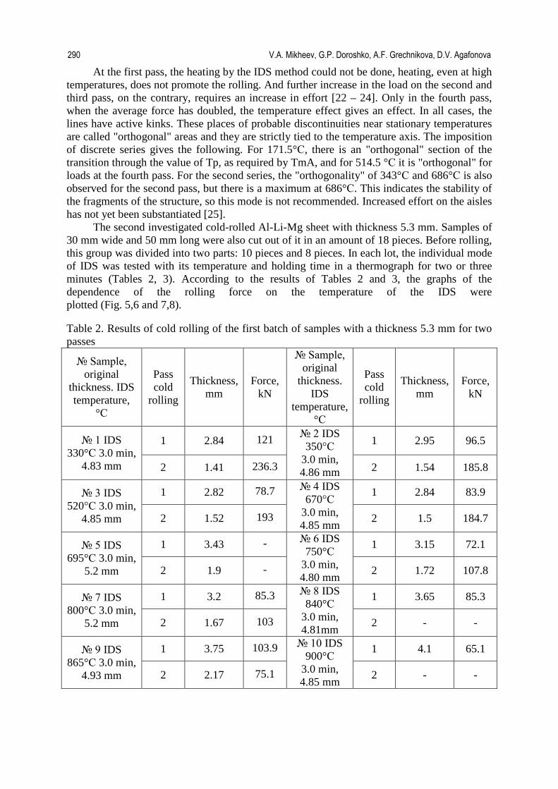
At the first pass, the heating by the IDS method could not be done, heating, even at high temperatures, does not promote the rolling. And further increase in the load on the second and third pass, on the contrary, requires an increase in effort [22 – 24]. Only in the fourth pass, when the average force has doubled, the temperature effect gives an effect. In all cases, the lines have active kinks. These places of probable discontinuities near stationary temperatures are called "orthogonal" areas and they are strictly tied to the temperature axis. The imposition of discrete series gives the following. For 171.5°С, there is an "orthogonal" section of the transition through the value of Tp, as required by TmA, and for 514.5 °С it is "orthogonal" for loads at the fourth pass. For the second series, the "orthogonality" of 343°С and 686°С is also observed for the second pass, but there is a maximum at 686°С. This indicates the stability of the fragments of the structure, so this mode is not recommended. Increased effort on the aisles has not yet been substantiated [25].

The second investigated cold-rolled Al-Li-Mg sheet with thickness 5.3 mm. Samples of 30 mm wide and 50 mm long were also cut out of it in an amount of 18 pieces. Before rolling, this group was divided into two parts: 10 pieces and 8 pieces. In each lot, the individual mode of IDS was tested with its temperature and holding time in a thermograph for two or three minutes (Tables 2, 3). According to the results of Tables 2 and 3, the graphs of the dependence of the rolling force on the temperature of the IDS were plotted (Fig. 5,6 and 7,8).

Table 2. Results of cold rolling of the first batch of samples with a thickness 5.3 mm for two passes

Sample, original

thickness. IDS temperature,

°С

Pass cold

rolling

Thickness, mm

Force, kN

Sample, original

thickness. IDS

temperature, °С

Pass cold

rolling

Thickness, mm

Force, kN

1 IDS 330°С 3.0 min,

4.83 mm

1 2.84 121 2 IDS 350°С

3.0 min, 4.86 mm

1 2.95 96.5

2 1.41 236.3 2 1.54 185.8

3 IDS 520°С 3.0 min,

4.85 mm

1 2.82 78.7 4 IDS 670°С

3.0 min, 4.85 mm

1 2.84 83.9

2 1.52 193 2 1.5 184.7

5 IDS 695°С 3.0 min,

5.2 mm

1 3.43 - 6 IDS 750°С

3.0 min, 4.80 mm

1 3.15 72.1

2 1.9 - 2 1.72 107.8

7 IDS 800°С 3.0 min,

5.2 mm

1 3.2 85.3 8 IDS 840°С

3.0 min, 4.81mm

1 3.65 85.3

2 1.67 103 2 - -

9 IDS 865°С 3.0 min,

4.93 mm

1 3.75 103.9 10 IDS 900°С

3.0 min, 4.85 mm

1 4.1 65.1

2 2.17 75.1 2 - -


Samples of thickness 5.3 mm at high forces show the work of the second series (1) 343°С, 646°С and 514.5°C separates the intervals and shows that the volume of the sample is stably differentiated into plastic regions with respect to temperature. The use of such exaggerated efforts justifies the confidence of the TmA theory, but technologically for large thicknesses of the sample the effort should be lower, and the number of passes will increase [26]. At the first pass there are higher temperatures, so that the second interval will represent a fully 857.5°C rise shows the phase discontinuity related to the joint of the two regions forming different volumes in terms of stability.

65,1

85,3

103,985,3

72,1

83,9

7878,7

96,5

121

0

20

40

60

80

100

120

140

300 400 500 600 700 800 900

Tem perature,˚С

Forc

e, k

N

Fig. 5. The dependence of the rolling force on the temperature of the IDS (1) of the samples

of the first batch with thickness of 5.3 mm at the first pass

236,3

184,7

146,25

75,189103

107,8

193

185,8

0

40

80

120

160

200

240

0 100 200 300 400 500 600 700 800 900 1000

Tem perature, ˚С

Forc

e, k

N


of the first batch with thickness of 5.3 mm at the second pass

The rolling of the second batch shows that in the intervals between the selected loads there are transformations of the transition structures. Obviously, the formation of the dominant region can be established, the maximum at 646°C, and with increasing force, the maximum is more pronounced while in the first batch it has a clearly "orthogonal" form [27].

The nature of the change in the rolling forces, taking into account the influence of the thickness of the Al-Li-Mg sheet sample, shows that the necessary individual choice of cobbing of the samples along the rolling passes is in good agreement with the series (1) of stationary temperatures of the thermal and force nature of the processes. This was clearly seen before the connection with discrete series was established in [7, 28 – 30]. In the next paper, it was assumed that when rolling samples at different thicknesses, registering thermal effects,


one can determine those modes of passages that were not previously available and had limitations on the fragmentation limit. To complete the real picture of the structural changes in Al-Mg-Li material, data on the texture are needed that will link the conditions for regulating the anisotropy of properties and the amorphization regimes in the border regions of the structural elements of the sample. In other words, the thermal effect can be accurately rationed as a disturbing factor, which causes the development of local structure dynamics. This serves as the basis for applying the methods of physics of granular materials – stereoisomeric parametrization of the structure, which are universal in the sense of addressing structures at different scales [9, 31]. Table 3. Results of cold rolling of the second batch of samples with a thickness of 5.3 mm in two passes

Sample, original

thickness. IDS temperature, °С

Pass cold

rolling

Thickness, mm

Force, kN

Sample, original

thickness. IDS

temperature, °С

Pass cold

rolling

Thickness, mm

Force, kN

1 IDS 800°С 1.5 min, 4.85 mm

1 3.13 87.6 2 IDS

740°С 2.0 min, 4.87 mm

1 3.17 91.9

2 1.66 124.7 2 1.65 132

3 IDS 710°С 2.0 min, 4.82 mm

1 3.15 91.5 4 IDS 680°С

2.0 min, 4.84 mm

1 3.14 89.6

2 1.67 124.1 2 1.65 126.2

5 IDS 650°С 2.0 min, 4.85 mm

1 3.17 98.3 6 IDS 590°С

2.0 min, 4.84 mm

1 3.15 93.8

2 1.7 147 2 1.67 124.9

7 IDS 620°С 2.0 min, 4.85 mm

1 3.14 88.2 8 IDS560°С 2.0 min, 4.85 mm

1 3.17 96.5

2 1.65 120.7 2 1.66 124.5

87,696,5

93,8

98,3

88,2

91,9

91,5

89,6

0

20

40

60

80

100

120

140

500 550 600 650 700 750 800

Tem perature, ˚С

Forc

e, k

N


of the second batch with thickness of 5.3 mm at the first pass


147

124,7

132124,1

126,2120,7124,9

124,5

020406080

100120140160

500 550 600 650 700 750 800

Tem perature, ˚С

Forc

e, k

N


of the second batch with thickness of 5.3 mm at the second pass

4. Conclusions Taking into account the influence on the rolling force of the initial thickness of the Al-Mg-Li sheet sample gives reliable guidelines for the search for the optimal rolling mode for sheet materials. It is also possible to use this approach for other initial thicknesses by means of a certain recalculation in terms of the change in the symmetry of the order parameter and the selection of the IDS modes, depending on the displacement to the stationary temperatures and temperatures of the power series.

The results obtained serve to select the mode of preliminary thermal activation by the IDS method. This greatly simplifies the processing of results in connection with the connection to the intervals of stationary temperatures and improves the accuracy of the impact evaluation.

The presence of a periodic dependence of the rolling force of the samples on their temperature, the IDS, can be used to quantify the parametrization of the participation of local quasi-liquid structures that affect the plasticity of the deformed material, as was previously established for granular materials.

Acknowledgements. This work was supported by the RussianFoundation for Basic Research (project ID 17-48-630083). References [1] Mikheev VA, Doroshko GP. Vvedeniye v temperaturnyy analiz svoystv materialov. Samara: Samarskii gosudarstvennii arkhitecturno-stroitroitel'nii universitet; 2007. (In Russian) [2] Doroshko GP. Usloviye sovmestimosti metallov za predelom deformirovaniya. In: Rudskoi AI. (ed.) Sovremennyye metalliccheskiye materially i tekhnologii (SMMT' 2015). Trudy mezhdunarodnoy nauchno-tekhnicheskoy konferentsii. Saint Petersburg: Izd-vo Politekhn. un-ta; 2015. V. 2. p. 560. (In Russian) [3] Mikheev VA, Doroshko GP. A new method of metallic alloys producing with interphases, which reformed coherent coupling of compounds' atoms. Key Engineering Materials. 2016;684: 359-365. [4] Mikheev VA, Grechnikov FV, Yerisov YA. Opredeleniye temperatury obrazovaniya nanokristallicheskikh zon v materialakh pri plasticheskom deformirovanii. In: Nanotekhnologii funktsional'nykh materialov (NFM'16). Trudy mezhdunarodnoy nauchno-tekhnicheskoy konferentsii. Saint Petersburg: Izd-vo Politekhn. un-ta; 2016. V. 1. p. 225. (In Russian)


[5] Ivanova VS, Oksogoyev AA. Analiz ustoychivosti fizicheskikh sistem s ispol'zovaniyem algoritma samoupravlyayemogo sinteza. In: Sinergetika. Moskva – Izhevsk: Institut komp'yuternykh issledovaniy; 2003. V. 5. p. 213. (In Russian) [6] Gerasimov OI. Local structural of granular materials. In: Nanotechnologies of functional matirials. Saint Petersburg: Izd-voPolitekhn. un-ta; 2010. p. 364. (In Russian) [7] Mikheev VA, Zhuravel LV. Analysis of structural changes when processing aluminum alloy roll billets produced by ingotless rolling. Izvestiya Vuzov Tsvetnaya Metallurgiya (Proceedings of Higher Schools Nonferrous Metallurgy). 2016;(3): 56-64. (In Russian) [8] Gerasymov OI, Zagorodny AG, Somov MM. Toward the Analysis of the Structure of Granular Materials. Ukrainian Journal of Physics. 2013;58(1): 32-39. [9] Erisov YA, Grechnikov FV, Oglodkov MS. The influence of fabrication modes of sheets of V-1461 alloy on the structure crystallography and anisotropy of properties. Russian Journal of Non-Ferrous Metals. 2016;57(1): 19-24. [10] Nosova EA, Grechnikov FV. Effect of Strain on the Anisotropy Coefficient of Sheet Alloys AA2024, Ti-2Al-1Mn, Titanium Grade 2, STEEL X10CrNiTi18-9. Key Engineering Materials. 2016;684: 366-370. [11] Glouschenkov VA, Grechnikov FV, Malyshev BS. Pulse-Magnetic Processing Technology when Making Parts and Units of Aerospace Engineering. J. Phys. IV France. 1997;7(C3): C3-45-C3-48. [12] Grechnikov FV, Erisov YA. Virtual Material Model with the Given Crystallographic Orientation of the Structure. Key Engineering Materials. 2016;684: 134-142. [13] Grechnikov FV, Dem'yanenko EG, Popov IP. Development of the manufacturing process of aluminum alloys with high strength and conductance. Russian Journal of Non-Ferrous Metals. 2015;56(1): 15-19. [14] Vasilyev AA, Kolbasnikov NG, Rudskoy AI, Sokolov DF, Sokolov SF. Kinetics of Structure Formation in the Heating of Cold-Rolled Automotive Steel Sheet. Steel in Translation. 2017;47(12): 830-838. [15] Baimova JA, Murzaev RT, Rudskoy AI. Discrete breathers in graphane in thermal equilibrium. Physics Letters, Section A: General, Atomic and Solid State Physics. 2017;381(36): 3049-3053. [16] Burkovsky RG, Bronwald I, Andronikova D, Wehinger B, Krisch M, Jacobs J, Gambetti D, Roleder K, Majchrowski A, Filimonov AV, Rudskoy AI, Vakhrushev SB, Tagantsev AK. Critical scattering and incommensurate phase transition in antiferroelectric PbZrO3 under pressure. Scientific Reports. 2017;7: 41512. [17] Kodzhaspirov G, Rudskoy A. The Effect of Thermomechanical Processing Temperature-Strain-Time Parameters on the Mesostructure Formation. Materials Science Forum. 2017;879: 2407-2412. [18] Apostolopoulos C, Drakakaki A, Apostolopoulos A, Matikas T, Rudskoi AI, Kodzhaspirov G. Characteristics defects-corrosion damage and mechanical behavior of dual phase rebar. Materials Physics and Mechanics. 2017;30(1): 1-19. [19] Politova GA, Pankratov NY, Vanina PY, Filimonov AV, Rudskoy AI, Burkhanov GS, Ilyushin AS, Tereshina IS. Magnetocaloric effect and magnetostrictive deformation in Tb-Dy-Gd-Co-Al with Laves phase structure. To be published in Journal of Magnetism and Magnetic Materials. [Preprint] 2017. Available from: doi.org/10.1016/j.jmmm.2017.11.016. [20] Andreeva NV, Naberezhnov AA, Tomkovich MV, Nacke B, Kichigin V, Rudskoy AI, Filimonov AV. Surface Morphology and Structure of Double-Phase Magnetic Alkali Borosilicate Glasses. Metal Science and Heat Treatment. 2016;58(7-8): 479-482.


[21] Rudskoi AI, Kodzhaspirov GE, Kamelin EI. Simulation and prediction of the development of dynamic recrystallization during the deformation of low-alloy low-carbon steel blanks. Russian Metallurgy (Metally). 2016;2016(10): 956-959. [22] Andreeva NV, Filimonov AV, Rudskoi AI, Burkhanov GS, Tereshina IS, Politova GA, Pelevin IA. A study of nanostructure magnetosolid Nd–Ho–Fe–Co–B materials via atomic force microscopy and magnetic force microscopy. Physics of the Solid State. 2016;58(9): 1862-1869. [23] Musabirov II, Safarov IM, Nagimov MI, Sharipov IZ, Koledov VV, Mashirov AV, Rudskoi AI, Mulyukov RR. Fine-grained structure and properties of a Ni2MnIn alloy after a settling plastic deformation. Physics of the Solid State. 2016;58(8): 1605-1610. [24] Lisovenko DS, Baimova JA, Rysaeva LK, Gorodtsov VA, Rudskoy AI, Dmitriev SV. Equilibrium diamond like carbon nanostructures with cubic anisotropy: Elastic properties. Physica Status Solidi (B) Basic Research. 2016;253(7): 1295-1302. [25] Imayev V, Gaisin R, Rudskoy A, Nazarova T, Shaimardanov R, Imayev R. Extraordinary superplastic properties of hot worked Ti–45Al–8Nb–0.2C alloy. Journal of Alloys and Compounds. 2016;663: 217-224. [26] Rudskoy AI, Kondrat'ev SY, Sokolov YA. New Approach to Synthesis of Powder and Composite Materials by Electron Beam. Part 1. Technological Features of the Process. Metal Science and Heat Treatment. 2016;58(1-2): 27-32. [27] Rudskoy AI, Kodzhaspirov GE, Kliber J, Apostolopoulos C. Advanced metallic materials and processes. Materials Physics and Mechanics. 2016;25(1): 1-8. [28] Rudskoy AI, Kol'tsova TS, Larionova TV, Smirnov AN, Vasil'eva ES, Nasibulin AG. Gas-Phase Synthesis and Control of Structure and Thickness of Graphene Layers on Copper Substrates. Metal Science and Heat Treatment. 2016;58(1-2): 40-45. [29] Rudskoi AI, Kondrat'ev SY, Sokolov YA, Kopaev VN. Simulation of the layer-by-layer synthesis of articles with an electron beam. Technical Physics. 2015;60(11): 1663-1669. [30] Andreeva NV, Vakulenko AF, Petraru A, Soni R, Kohlstedt H, Filimonov AV, Rudskoy AI, Vakhrushev SB, Pertsev NA. Low-temperature dynamics of ferroelectric domains in PbZr0.3Ti0.7O3 epitaxial thin films studied by piezoresponse force microscopy. Applied Physics Letters. 2015;107(15): 152904. [31] Parshikov RA, Rudskoy AI, Zolotov AM, Tolochko OV. Analysis of specimen plastic flow features during severe plastic deformation. Reviews on Advanced Materials Science. 2016;45(1-2): 67-75.


ELECTROMAGNETIC ELASTIC BALL UNDER NON-STATIONARY

AXIALLY SYMMETRICAL WAVES Vladimir A. Vestyak1*, Leonid A. Igumnov2, Dmitriy V. Tarlakovsky1,3

1Moscow Aviation Institute (national research university), Volokolamskoye Shosse 4, GSP-3, A-80, Moscow

125993, Russia 2Research Institute for Mechanics, National Research Lobachevsky State University of Nizhni Novgorod,

Gagarina Prospect 23, k.6, GSP-1000, Nizhny Novgorod 603022, Russia 3Institute for Mechanic Studies of Moscow Lomonosov University, Michurinsky Prospect 1, Moscow 119192,

Russia


Abstract. This paper studies propagation of non-stationary axially symmetrical kinematic or electromagnetic disturbances applied on the surface of a ball. To this end, linear equations of motion of an elastic ball together with Maxwell equations are used as well as linearized generalized Ohm law and Lorentz force equation. The required functions are expanded in series in terms of Legendre and Gegenbauer polynomials. Laplace integral time transformation and expansion of coefficients of series into power series in small parameter linking mechanical and electromagnetic properties of the medium enabled finding recurrent sequence of boundary value problems with respect to components of mechanical and electromagnetic fields. The solution of each problem is represented in the form of generalized convolution of functions corresponding to previous members of the recurrent sequence with Green functions. Keywords: Green functions, electromagnetic disturbances, linear equations of motion of elastic ball, Ohm law

1. Introduction Currently, the issues of considering coupled fields of mechanical and other nature, such as electromagnetic, are becoming increasingly important in various engineering problems. However, coupled problems of electromagnetic and mechanical fields inside conductors have not been enough studied at present. The relevance of this topic is beyond doubt, since the coupled fields are used in many areas of modern technology: electroacoustic, radio engineering, automatic systems. At the same time, mathematical modeling of the conjugate fields interaction is often simpler and more better visualized than physical experiment [1]. The only solutions are known is for piezoelectrics in the non-stationary formulation for a sphere. In this paper, we consider the propagation problem of electromagnetoelastic non-stationary two-dimensional waves inside isotropic conducting sphere under the influence of surface electric or mechanical disturbances.

Statements of non-stationary problems of electromagnetic elasticity are given in [2]. Solutions of corresponding uncoupled problems will be natural necessary components of this problem. The article [3] studies two-dimensional non-stationary electromagnetic fields induced by specific displacement field in a ball. The publication [4] investigates non-



stationary process of axially symmetric deformation of elastic ball under volumetric forces. In [5] the coupled problem of electromagnetoelasticity for the spherical cavity located in the infinite isotropic conductor is solved. In contrast to the listed articles, in publications prior to those reviewed, as a rule, the connection of conjugate fields occurs through physical relations. Traditionally, solutions were built numerically and numeric-analytically. The numerical results of electroelasticity are known for canonical geometry bodies made of piezoelectric materials. In particular, the existence and uniqueness theorems for generalized solutions of coupled non-stationary two-dimensional electroelasticity problems was proved in [6] for some canonical geometry domains. In addition, the problem for a hollow piezoceramic finite length cylinder polarized along the radius was numerically solved in [7] and [8]. Moreover, in [8] more efficient numerical method for finding solutions was proposed. Analytical and numeric-analytical solutions of electroelasticity for piezoceramic cylinder are described in detail in [9, 10]. Similar problems of coupled electroelasticity for the thick-walled piezoelectric sphere were considered in [11, 12]. Moreover, in [12] the algorithm of finding an analytical solution is described. To find the analytical solutions for non-stationary problem, effective method is expansion in a series by the inverse parameter of the Laplace transform. It allows us to find solutions of the problem at small time intervals. Such approach in one-dimensional formulation was demonstrated in [13] by the example of electromagneto-thermoelastic spherical cavity. The present article offers further development of the results of recent three studies, now as applied to an electromagnetic elastic ball where mechanic and electromagnetic fields are coupled by Lorentz force acting as volumetric force in motion equation, and generalized Ohm law [14]. This problem has also practical applications of investigation of electromagnetic and mechanic fields, for instance in non-destructive inspections, as well as in designing electronic devices using conductor and conductive coating in harsh operational conditions.

2. Statement of problem Consider a homogeneous isotropic conductive ball of radius 1r with a center at point O at the boundary of which there are preset kinematic or electromagnetic conditions ( , ,r θ ϑ is spherical coordinate system where 0, 0 ,r ≥ ≤ θ ≤ π − π < ϑ ≤ π ):

( ) ( ) ( )1 1 1

1 1 01, , , , ,r r r r r r

u U v V E eθ= = == τ θ = τ θ = τ θ . (1)

They are complemented by the boundary condition of the medium stress-strain components and the electromagnetic field. The initial electromagnetic field is assumed to be stationary, radial and satisfies the conditions ( )0 0 0 0, 0, 0rE E r E Hθ= ≡ ≡ (hereinafter zero indices indicate the initial condition). At the initial moment of time the ball is in undisturbed state (dots label the time derivatives):

0 0 0 0 0 0 00 0 00r ru u v v E E E E H Hθ θτ= τ= τ= τ= τ= τ= τ=τ= τ= τ=

= = = = = = = = = = ,

where u and v are radial and tangential displacements, rE and Eθ - components of electric field vectors; H is a non-zero component of magnetic field vector.

Resulting from the motion equations, Maxwell equations and generalized Ohm law, closed coupled equation system with assumed axially symmetric motion will have the form [2]. The obvious type of the corresponding system of the equations is given in [5]. To non-dimension sizes entered in work [4], in the system of the equations for a cavity for the

considered sphere the ratio is added: 1rrL′

= . At the same time, in designations which are used

in [5] and further: t is time; rj and jθ are radial and tangential densities of current; eρ is the density of surface charges; kF are non-zero radial and tangential components of Lorentz

Electromagnetic elastic ball under non-stationary axially symmetrical waves 297

forces; c , 1c and 2c are speed of light and speed of propagation of strain-stress and shear waves; λ and µ are elastic Lame constants; ε and eµ are coefficients of dielectric and magnet permittivity; σ is coefficient of electric conductivity; L and E∗ are some specific linear size and electric field intensity.

3. Expansion in series over angle Let the required functions, similar to work [5] be represented in form of series in terms of polynomials of Legendre ( )nP x and Gegenbauer ( )3 2

1nC x− [15]. Taking the functions of displacement and magnetic field strength as primary unknown variables, after Laplace time transform τ (when s is its parameter; index L designates a transform domain) and using the fact that as shown in [16], even in one-dimensional case the solution of corresponding boundary value problem has Bessels functions with indices depending on the parameter of the Laplace transformation. Obviously, for this reason it is impossible to find a solution analytically. To this reason, we represent the required functions in power series in small

parameter ( )

2

α4 λ+2μ

E∗=ε

π. Index n treats decomposition coefficients on Legendre and

Gegenbauer polynomials, m - to decomposition coefficients in the following series:

( ) ( ) ( )

( ) ( ) ( )

0 0 0

0 0 0

, , , , , ,

, , , , , .

m m mn nm n nm n nm

m m m

m m mn nm rn rnm n nm

m m m

u u r v v r H H r

r E E r E E r

∞ ∞ ∞

= = =

∞ ∞ ∞

θ θ= = =

= τ α = τ α = τ α

ρ = ρ τ α = τ α = τ α

∑ ∑ ∑

∑ ∑ ∑ (2)

Substitution of these series to the system of the equations on coefficients of series of decomposition of required functions on Legendre and Gegenbauer polynomials [5] will lead to a recurrent sequence of system of equations with respect to limited functions

( )200 110 00 ;L Ls u l u= (3)

( ) ( ) ( )20 110 0 0, 1 0, 1, , 0, 1 ;L L L L

m m u r m ms u l u g E n m− −= + = ≥ρ

2 20 0 0 ;L L

e r m e ms E s u= − ρ ( )( )2

0 00 2 , ( 0, 0)

Le mL

m

r uss n mrr

∂ ρ+ γ ρ = − = ≥

∂;

( )2 2 2 ,L L L Le e nm n nm e H nm nms H H sl u vη = ∆ + η ; (4)

( ) ( ) ( ) ( )2 20 11 0 12 0 0 21 0 22 0, ;L L L L L L

n n n n n n n n n ns u l u l v s v l u l v= + = + (5)

( ) ( ) ( )( ) ( ) ( ) ( )

211 12 , 1 , 1

221 22 , 1 , 1

, ,

, , 1, 1 ;

L L L L Lnm n nm n nm u rn m n m

L L L L Lnm n nm n nm v n m n m

s u l u l v g E

s v l u l v g E H n m

− −

θ − −

= + + ρ

= + + ≥ ≥

( )( )

( ) ( )

2 20

2 20

1 ,

1;

LnmL L

e nm e e nm

L L Le rnm nm e e nm

rHs E s v

r rn n

s E H ur

θ

∂η + γ = − − η ρ

∂+

η + γ = − η ρ

(6)

( ) ( ),L L Lnm n nm nms sl u vρ+ γ ρ = − , ( )1, 1n m≥ ≥ (7)

with the following boundary value conditions:

298 Vladimir A. Vestyak, Leonid A. Igumnov, Dmitriy V. Tarlakovsky

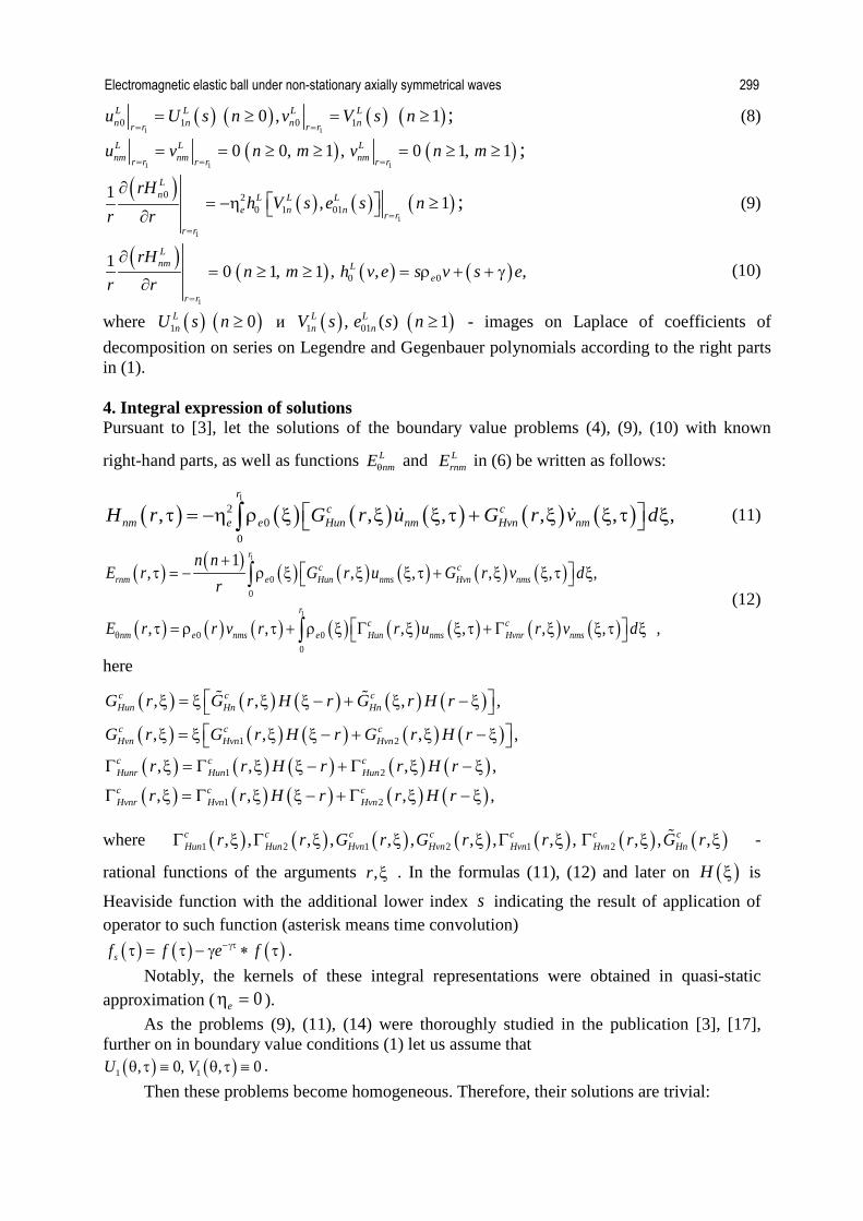
( ) ( ) ( ) ( )1 1

0 1 0 10 , 1L L L Ln n n nr r r r

u U s n v V s n= =

= ≥ = ≥ ; (8)

( ) ( )1 1 1

0 0, 1 , 0 1, 1L L Lnm nm nmr r r r r r

u v n m v n m= = =

= = ≥ ≥ = ≥ ≥ ;

( )( ) ( ) ( )

1

1

0 20 1 01

1 , 1Ln L L L

e n n r rr r

rHh V s e s n

r r ==

∂ = −η ≥ ∂

; (9)

( )( ) ( ) ( )

1

0 01 0 1, 1 , , ,

Lnm L

e

r r

rHn m h v e s v s e

r r=

∂= ≥ ≥ = ρ + + γ

∂ (10)

where ( ) ( )1 0LnU s n ≥ и ( ) ( )1 01, ( ) 1L L

n nV s e s n ≥ - images on Laplace of coefficients of decomposition on series on Legendre and Gegenbauer polynomials according to the right parts in (1).

4. Integral expression of solutions Pursuant to [3], let the solutions of the boundary value problems (4), (9), (10) with known

right-hand parts, as well as functions LnmEθ and L

rnmE in (6) be written as follows:

( ) ( ) ( ) ( ) ( ) ( )1

20

0

, , , , , ,r

c cnm e e Hun nm Hvn nmH r G r u G r v d τ = −η ρ ξ ξ ξ τ + ξ ξ τ ξ ∫ (11)

( ) ( ) ( ) ( ) ( ) ( ) ( )

( ) ( ) ( ) ( ) ( ) ( ) ( ) ( )

1

1

00

0 00

1, , , , , ,

, , , , , , ,

rc c

rnm e Hun nms Hvn nms

rc c

nm e nms e Hun nms Hvnr nms

n nE r G r u G r v d

r

E r r v r r u r v dθ

+ τ = − ρ ξ ξ ξ τ + ξ ξ τ ξ

τ = ρ τ + ρ ξ G ξ ξ τ + G ξ ξ τ ξ

∫

∫ (12)

here

( ) ( ) ( ) ( ) ( )( ) ( ) ( ) ( ) ( )( ) ( ) ( ) ( ) ( )( ) ( ) ( ) ( ) ( )

1 2

1 2

1 2

, , , ,

, , , ,

, , , ,

, , , ,

c c cHun Hn Hn

c c cHvn Hvn Hvn

c c cHunr Hun Hun

c c cHvnr Hvn Hvn

G r G r H r G r H r

G r G r H r G r H r

r r H r r H r

r r H r r H r

ξ = ξ ξ ξ − + ξ − ξ ξ = ξ ξ ξ − + ξ − ξ

G ξ = G ξ ξ − + G ξ − ξ

G ξ = G ξ ξ − + G ξ − ξ

where ( ) ( ) ( ) ( ) ( ) ( ) ( )1 2 1 2 1 2, , , , , , , , , , , , ,c c c c c c cHun Hun Hvn Hvn Hvn Hvn Hnr r G r G r r r G rG ξ G ξ ξ ξ G ξ G ξ ξ -

rational functions of the arguments ,r ξ . In the formulas (11), (12) and later on ( )H ξ is

Heaviside function with the additional lower index s indicating the result of application of operator to such function (asterisk means time convolution)

( ) ( ) ( )sf f e f−γττ = τ − γ ∗ τ . Notably, the kernels of these integral representations were obtained in quasi-static

approximation ( 0eη = ). As the problems (9), (11), (14) were thoroughly studied in the publication [3], [17],

further on in boundary value conditions (1) let us assume that ( ) ( )1 1, 0, , 0U Vθ τ ≡ θ τ ≡ .

Then these problems become homogeneous. Therefore, their solutions are trivial:


( ) ( )0 0, 0, , 0 ( 0)n nu r v r nτ ≡ τ ≡ ≥ . The solution of "mechanical" part of the problems (9) – (16) with known right-hand

pars in accordance with the conclusions of the publication [4] is also represented in integral form:

( ) ( ) ( ) ( ) ( )

( ) ( ) ( ) ( ) ( )

1 1

1 1

, 1 , 10 0

, 1 , 10 0

, , , , , , , ,

, , , , , , , ;

r r

nm uun un m uvn vn m

r r

nm vun un m vvn vn m

u r G r f d G r f d

v r G r f d G r f d

− −

− −

τ = ξ τ ∗ ξ τ ξ + ξ τ ∗ ξ τ ξ

τ = ξ τ ∗ ξ τ ξ + ξ τ ∗ ξ τ ξ

∫ ∫

∫ ∫ (13)

( ) ( ) ( ) ( ) ( )

( ) ( ) ( ) ( ) ( )

1 1

1 1

, 1 , 10 0

, 1 , 10 0

, , , , , , , ,

, , , , , , , ,

r r

nm uun un m uvn vn m

r r

nm vun un m vvn vn m

u r r f d r f d

v r r f d r f d

− −

− −

τ = Π ξ τ ∗ ξ τ ξ + Π ξ τ ∗ ξ τ ξ

τ = Π ξ τ ∗ ξ τ ξ + Π ξ τ ∗ ξ τ ξ

∫ ∫

∫ ∫

(14)

where

( ) ( ) ( ) ( ) ( )( ) ( ) ( ) ( ) ( )

( ) ( ) ( ) ( )( ) ( ) ( ) ( )

, 1 0 , 1 0 , 1

, 1 0 , 1 0 , 1

, , , ,

, , , ,

, , , , , , , , , ,

, , , , , , , , , .

un m e rn m n m

vn m e n m n m

uun uun uvn uvn

vun vun vvn vvn

f E E

f E E H

r G r r G r

r G r r G r

− − −

− θ − −

ξ τ = ρ ξ ξ τ + ξ ρ ξ τ

ξ τ = ρ ξ ξ τ − γ ξ ξ τ

Π ξ τ = ξ τ Π ξ τ = ξ τ

Π ξ τ = ξ τ Π ξ τ = ξ τ

(15)

An explicit form of kernels in (13) is specified in [5]. It is omitted here because of its awkwardness.

The function nmρ being part of (15), according to (7), is defined as follows:

( ) ( ) ( ) ( )0 0, , ,nm e nms e nmsr r u r r′ρ τ = −ρ τ − ρ χ τ , where:

( ) ( ) ( ) ( ) ( )

( ) ( ) ( ) ( )

( )( ) ( )

1 1

, 1 , 10 0

2

2

, , , , , , , ,

, , , , , , , ,

11, .

r r

nm un un m vn vn m

un n uun vun vn n uvn vvn

nn n n

r r f d r f d

r G G r G G

r u n nu v

r rr

− −χ τ = Χ ξ τ ∗ ξ τ ξ + Χ ξ τ ∗ ξ τ ξ

Χ ξ τ = χ Χ ξ τ = χ

∂ +χ = +

∂

∫ ∫

The meaning of the newly introduced function ( ),n u vχ is a coefficient of series expansion in terms of Legendre polynomials by coefficient of volumetric expansion for displacement field with components u and v .

The relations (11) – (14) are m -recurrent sequence of relations with respect to coefficients of series Legendre and Gegenbauer polynomials and (2) for displacements, strengths of electric and magnetic fields, as well as charge densities. As if follows from the publication [4], the following equations will be the initial conditions for such sequence:

( ) ( ) ( ) ( ) ( ) ( )

( ) ( ) ( ) ( ) ( ) ( ) ( ) ( ) ( )

20 0 0 1 01 01

0 1 01 0 1 01 0

, 0, , 0 ( 0), , ,

1, , , 1 , , 0,

cn n n e Hn n n

c crn Hn n n Hn n n

u r v r n H r G r e e

n nE r G r e E r r e n r

r θ

τ ≡ τ ≡ ≥ τ = −η γ τ + τ +

τ = − τ τ = G τ ≥ ρ τ ≡

(16)

where


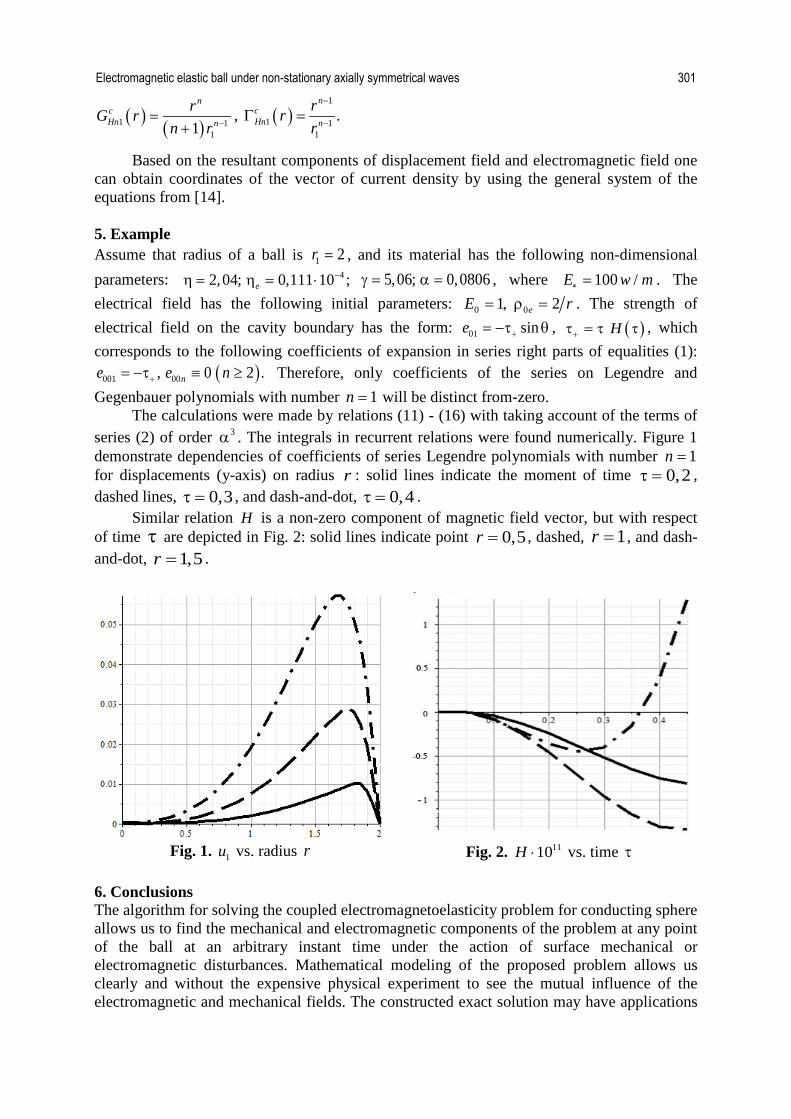
( ) ( )1 111

ncHn n

rG rn r −=+

, ( )1

1 11

.n

cHn n

rrr

−

−G =

Based on the resultant components of displacement field and electromagnetic field one can obtain coordinates of the vector of current density by using the general system of the equations from [14]. 5. Example Assume that radius of a ball is 1 2r = , and its material has the following non-dimensional parameters: 42,04; 0,111 10 ;e

−η = η = ⋅ 5,06; 0,0806γ = α = , where 100 /E w m∗ = . The electrical field has the following initial parameters: 0 01, 2eE r= ρ = . The strength of electrical field on the cavity boundary has the form: 01 sine += −τ θ , ( )H+τ = τ τ , which corresponds to the following coefficients of expansion in series right parts of equalities (1):

( )001 00, 0 2 .ne e n+= −τ ≡ ≥ Therefore, only coefficients of the series on Legendre and Gegenbauer polynomials with number 1n = will be distinct from-zero.

The calculations were made by relations (11) - (16) with taking account of the terms of series (2) of order 3α . The integrals in recurrent relations were found numerically. Figure 1 demonstrate dependencies of coefficients of series Legendre polynomials with number 1n = for displacements (y-axis) on radius r : solid lines indicate the moment of time 0,2τ = , dashed lines, 0,3τ = , and dash-and-dot, 0,4τ = .

Similar relation H is a non-zero component of magnetic field vector, but with respect of time τ are depicted in Fig. 2: solid lines indicate point 0,5r = , dashed, 1r = , and dash-and-dot, 1,5r = .

Fig. 1. 1u vs. radius r Fig. 2. 1110H ⋅ vs. time τ

6. Conclusions The algorithm for solving the coupled electromagnetoelasticity problem for conducting sphere allows us to find the mechanical and electromagnetic components of the problem at any point of the ball at an arbitrary instant time under the action of surface mechanical or electromagnetic disturbances. Mathematical modeling of the proposed problem allows us clearly and without the expensive physical experiment to see the mutual influence of the electromagnetic and mechanical fields. The constructed exact solution may have applications


for predicting the behavior of conductor materials in various tasks of modern technology such as electroacoustics, automation, microelectronics.

Acknowledgement. The work is financially supported by the Federal Targeted Program for Research and Development in Priority Areas of Development of the Russian Scientific and Technological Complex for 2014-2020 under the contract No. 14.578.21.0246 (unique identifier RFMEFI57817X0246). References [1] Vlasenko VD. The solution of dynamic problems of electroelasticity for piezoelectric materials. In: Materials of the international conference "Differential Equations, Theory of Functions and Application", Dedicated to the Centennial of Academician Ilia N. Vekua; May 28 - June 2, 2007, Novosibirsk, Russia. Novosibirsk: Novosibirsk State University; 2007. p.564-565. (in Russian) [2] Tarlakovskii DV, Vestyak VA, Zemskov AV. Dynamic processes in thermo-electro-magneto-elastic and thermo-elasto-diffusive media. In: Hetnarski RB (ed.) Encyclopedia of Thermal Stresses. Dordrecht: Springer; 2014. p.1064-1071. [3] Vestyak VA, Tarlakovsky DV. A Nonstationary Axially Symmetric Electromagnetic Field in a Moving Sphere. Doklady Physics. 2015;60(10): 433-436. [4] Vestyak VA, Tarlakovskiy DV. Elastic ball under non-stationary axially symmetrical volume forces. ZAMM Z. Angew. Math.Mech. 2017;97(1): 25-37. [5] Vestyak VA, Kuznetsova EL, Tarlakovski DV. Non-stationary axisymmetric waves in electromagnetoelastic space with a spherical cavity. PNRPU Mechanics Bulletin. 2016;3: 28-46. [6] Melnik VN. On the existence and uniqueness of generalized solutions in coupled nonstationary problems of two-dimensional electroelasticity. Dynamics of the continuous environment. 1990;99: 60-73. [7] Melnik VN, Moskalkov MN. On coupled electroelastic unsteady oscillations of a piezoceramic cylinder with radial polarization. Journal calcul. mat. and mat. Physical. 1988;28(11): 1755-1756. [8] Grigorieva LO. Numerical solution of the initial boundary value problem of electroelasticity for a hollow piezoceramic cylinder with radial polarization. Applied mechanics. 2006;42(12): 67-75. [9] Babaev AE, Savin VG. Radiation of unsteady acoustic waves by radially polarized cylindrical piezoelectric transducer. Applied mechanics (Kiev). 1995;31(4): 41-48. [10] Babaev AE, Janchevskyi IV. Radiation of non-stationary acoustic waves by elastic and electric cylinder with a wire circuit. Teor. and applied mechanics. 2010;1: 114-125. [11] Babaev AE, Savin VG. Radiation of non-stationary acoustic waves by a thick-walled elastic and electric field. Applied mechanics (Kiev). 1995;31(11): 25-32. [12] Babaev AE, Savin VG, Djulinskyi AV. Analytical method for solving the problem of radiation of unsteady waves by spherical piezoelectric transducer. Teor. and applied mechanics (Kiev). 2003;37: 195-199. [13] Aouadi M. Electromagneto-thermoelastic fundamental solutions in a two-dimensional problem for short time. Acta mech. 2005;174(3-4): 223-240. [14] Ilushin AA. Continuum Mechanics. Moscow: Moscow State University; 1978. [15] Gradstein IS, Ryzhik IM. Tables of integrals, sums, series and products. 5th ed. Moscow: Nauka; 1971. (in Russian)


[16] Vestyak VA, Lemeshev VA, Tarlakovskii DV. The propagation of time-dependent radial perturbations from a spherical cavity in an electromagnetoelastic space. Doklady Physics. 2010;55(9): 468-470. [17] Gorshkov AG, Tarlakovskiy DV. Transient Aerohydroelasticity of Spherical Bodies. Berlin: Springer; 2001.


BIOPHYSICAL ANALYSIS OF MICROTUBULES NONLOCAL BEAM

THEORY

Mohsen Motamedi1, Ayesha Sohail

2*

1Faculty of Engineering, University of Shahreza, P. O. Box 86149-56841, Isfahan, Iran

2Department of Mathematics, Comsats University Islamabad, Lahore Campus 54000, Pakistan


Abstract. Microtubules are filamentous intracellular structures that are responsible for

various kinds of movements in all eukaryotic cells. The dynamic assembly and disassembly of

microtubules and the mechanical properties of these polymers are essential for many key

cellular processes such as spermatogenesis and the processes of neurons. Mathematical and

computational modeling, especially coupled mechanochemical modeling, has contributed a lot

to understand their dynamics. However, it has remained a great challenge to reduce the

critical discrepancies, which exist between the experimental observations and modeling

results. During this research, the small scaling parameter of the nonlocal Euler-Bernoulli

beam theory is analyzed to demonstrate the free vibration problem of microtubules.

Keywords: microtubules, nonlocal parameter, finite element, Euler-Bernoulli beam theory

1. Introduction Fifty years since the discovery of tubulin [1], the microtubules are studied as dynamic

polymers of tubulin subunits that underpin many vital cellular processes for example cell

division and migration. Microtubules are polarized structures, with their minus end anchored

at the centrosome and plus end, free in the cytoplasm (or interacts with other organelles).

Microtubules (MTs) are the active filaments and play key roles in the cells, such as

maintaining the biological functioning of cells (cell division and cell motility), resisting

thermal or mechanical perturbations from the environments and other sturctural

functions [2, 3]. MTs are protein filaments which are made up of α and β tubulin and form a

closed tube (by assembling into linear proto-filaments). The structure of these polymers is

infact the key to their function (see Fig. 1). The linear proto-filaments provide a uniform

substrate for motor protein movement and the helical structure makes the polymers more rigid.

It is believed that each tubulin is composed of 4300 atoms and has a mass of 55 kDa [4].

The computer-assisted differential-interference-contrast microscopy gives high contrast

results and makes it possible to see even very small objects such as single microtubules,

which have a diameter of 0.025 μm, less than one-tenth the wavelength of light. The

individual microtubules were recently studied by many researchers (see [5] and the references

therein). Osborn et al. [6] was one of the pioneers in this field, he with his research group

studied the microtubules structure using immunofluorescence and the electron microscopy. In

all such studies, it is difficult to distinguish between the single microtubule from the bundle of

several ones due to the blurry effects caused by diffraction.

Materials Physics and Mechanics 40 (2018) 304-312 Received: December 23, 2017


Fig. 1. Microtubules(green), actin filaments (red) [7]

Different microtubules configurations exist based on the number of protofilaments.

Microtubules are typically formed by 13 protofilaments, however, this is a relatively flexible

property of tubulin assembly and the number of protofilaments in a microtubules observed

in-vivo and in-vitro conditions may vary. The protofilaments can connect with 2-4 length of

monomers and make a spiral shape [8, 9].

Microtubules are filaments and are found in bent and buckled state within a eukaryotic

cell. They provide structural support along with necessary motility to the cell, and are

essential to regulate the mechanics of cell division. To understand how microtubules perform

their functions, it is necessary to explore their mechanical properties [10]. Recently, the

nonlocal continuum mechanics has been used extensively to model the nanostructures and

biostructures such as microtubules and DNA [11, 12]. However, the recognition of the scaling

parameter in the nonlocal theory, which plays an important role in such studies, did not

receive much attention. Civalek et al. [13] studied small-scale effects on deflection and

frequencies of microtubules and used the carbon nanotube scale parameter instead of

microtubules.

In this study we used quantitative technique to measure the parameters which may help

to understand the properties of microtubules and to provide the mechanical information about

microtubules. In this work, we have used the nonlocal Euler-Bernoulli beam theory as well as

the finite element approach to explore the molecular dynamics of the microtubules. We have

provided a unique approach for the first time to evaluate the interaction energy and force

between the tubulins, natural frequencies and the important scaling parameter .

Nomenclature

u Axial displacement

transverse displacement

extensional strains

bending strains

applied axial compressive force

moment

Biophysical analysis of microtubules nonlocal beam theory 305

f(x,t) axial forces

μ nonlocal parameter

I second moment of area

(u,w,φ) terms of displacement

natural frequency

length of beam

2. Materials and Methods

Nonlocal Euler-Bernoulli beam theory. The Euler-Bernoulli beam equation has been

a representative model for the control of systems governed by partial differential equations

(PDEs). The nonlocal Euler-Bernoulli beam theory has been employed by Lei et al. [14] to

establish the governing equations of motion for the bending vibration of nanobeams. They

used a transfer function method (TFM) to obtain closed-form and uniform solution for the

vibration analysis of Euler-Bernoulli beams with different boundary conditions. Here in this

article, we will use the technique to study the structural properties of microtubules.

Euler-Bernoulli beam theory (EBT) is based on displacement:

( )

, (1)

( ), (2)

where u and are the axial and transverse displacements.

Strain of the Euler-Bernoulli beam theory is:

, (3)

, (4)

where and are the extensional and bending strains.

The expression for the principle of virtual displacement is given as:

∫ ∫ [ (

)

]

, (5)

where f(x,t) is the axial force and q(x,t) is the transverse distributed forces, is the applied

axial compressive force.

For 0<x<L, Euler–Lagrange equations is:

, (6)

(

)

. (7)

The conditions at the two boundaries (x=0) and (x=L) are given as:

, (8)

where is the equivalent to shear force.

3. Nonlocal Theories

Eringen [15] showed that in an elastic continuum, the stress field at a point x depends on the

strain field at the that point and at other points of the body. Thus, the nonlocal stress tensor σ

at point x is defined as:

∫ ( ) ( )

, (9)

306 Mohsen Motamedi, Ayesha Sohail

where t(x) is the classical stress tensor at point x and the ( ) represents the

nonlocal modulus, and are the distance and material constant respectively. The

material constant depends on internal and external characteristic lengths.

However, the integral constitutive relations can be written as:

( )

, (10)

where is the material constant, is internal characteristic length and is external

characteristic length.

Calculation of stress. For homogeneous isotropic beams, the nonlocal relation in Eq.

(10) can be written as:

, (11)

. (12)

The nonlocal behavior is negligible in the thickness direction. is Young’s modulus

and is shear modulus. is nonlocal parameter.

The axial force–strain relation is given by:

, (13)

∫

∫

. (14)

Next we will consider and only for the Euler-Bernoulli beam theory. So, the

constitutive relations are expressed as:

. (15)

In this equation, is the second moment of area about Y-axis.

Calculations for displacement. In all beam theories, the equations of motion can be

expressed in terms of the displacements (u,w,φ). So, this will be done using force-deflection

and moment-deflection relationships in Eq. (13) and Eq. (15) and replacing the stress

resultants in the equations of motion

For the first derivative of the axial force from Eq. (6) and Substituting into Eq. (13),

we obtain:

(

). (16)

Substituting from Eq. (16) into the equation of motion Eq. (6)

(

)

(

). (17)

Euler-Bernoulli beam theory. Substituting the second derivative of from Eq. (7)

into Eq. (15), we obtain

(

)

. (18)

Substituting from Eq. (18) into Eq. (6):

(

)

*

(

)

+

(

)

. (19)

Analytical solution of vibration of simply supported beams. For the simply

supported beams, the boundary conditions are:

(20)

to satisfy the boundary conditions;

( ) ∑

( ) ∑

. (21)

Using Eq. (21) into the equation of motion (19), we obtain

( (

)

( (

) ) (

) ) (22)

for any , where


(

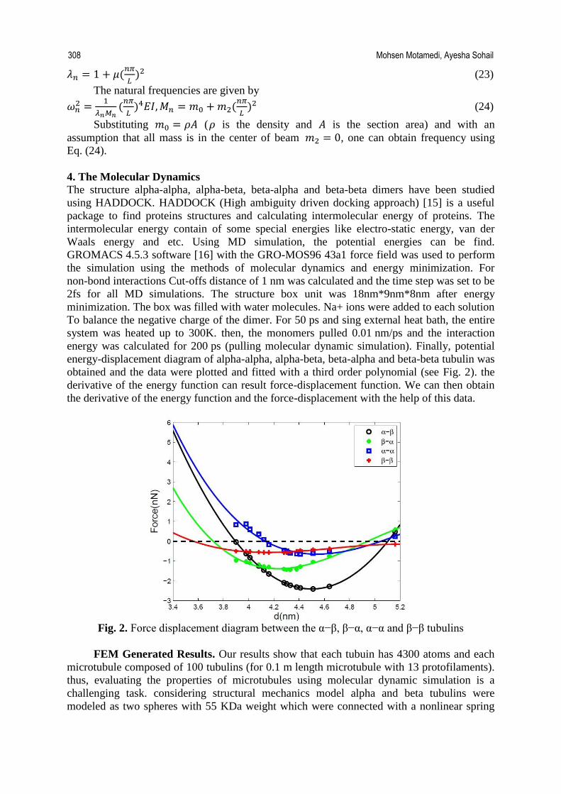
) (23)

The natural frequencies are given by

(

) (

) (24)

Substituting ( is the density and is the section area) and with an

assumption that all mass is in the center of beam , one can obtain frequency using

Eq. (24).

4. The Molecular Dynamics

The structure alpha-alpha, alpha-beta, beta-alpha and beta-beta dimers have been studied

using HADDOCK. HADDOCK (High ambiguity driven docking approach) [15] is a useful

package to find proteins structures and calculating intermolecular energy of proteins. The

intermolecular energy contain of some special energies like electro-static energy, van der

Waals energy and etc. Using MD simulation, the potential energies can be find.

GROMACS 4.5.3 software [16] with the GRO-MOS96 43a1 force field was used to perform

the simulation using the methods of molecular dynamics and energy minimization. For

non-bond interactions Cut-offs distance of 1 nm was calculated and the time step was set to be

2fs for all MD simulations. The structure box unit was 18nm*9nm*8nm after energy

minimization. The box was filled with water molecules. Na+ ions were added to each solution

To balance the negative charge of the dimer. For 50 ps and sing external heat bath, the entire

system was heated up to 300K. then, the monomers pulled 0.01 nm/ps and the interaction

energy was calculated for 200 ps (pulling molecular dynamic simulation). Finally, potential

energy-displacement diagram of alpha-alpha, alpha-beta, beta-alpha and beta-beta tubulin was

obtained and the data were plotted and fitted with a third order polynomial (see Fig. 2). the

derivative of the energy function can result force-displacement function. We can then obtain

the derivative of the energy function and the force-displacement with the help of this data.

Fig. 2. Force displacement diagram between the α−β, β−α, α−α and β−β tubulins

FEM Generated Results. Our results show that each tubuin has 4300 atoms and each

microtubule composed of 100 tubulins (for 0.1 m length microtubule with 13 protofilaments).

thus, evaluating the properties of microtubules using molecular dynamic simulation is a

challenging task. considering structural mechanics model alpha and beta tubulins were

modeled as two spheres with 55 KDa weight which were connected with a nonlinear spring


(see Fig. 3). In Fig. 4, we can see the 13 protofilaments and 3start-helix, the dimensions for

simulation are elaborated in Fig. 4.

Fig. 3. Structural model of tubulins connected by springs

Fig. 4. schematic diagram for the simulation dimensions of microtubules

The natural frequency is the frequency with which the system oscillates when it is

disturbed. In this section natural frequency of microtubule is achieved using finite element

method. Schematic of 6 mode shapes is provided in Fig. 5. Obtaining scale parameter After

substituting obtained natural frequencies from FEM into nonlocal equations, we obtained

scale parameters for microtubules. Fig. 6 depicts the nonlocal parameters for microtubules,

with values obtained in the range of 4050 nm. Heireche et al. [18] used the Timoshenko beam

model to obtain the vibrational characteristics of microtubules by considering small scaling

parameter in their work. The nonlocal Timoshenko beam theory has also been used by Gao

and Lei [19], to study the mechanical behaviors of microtubules. The parametric value which

they used was in the range of 30 to 70 nm. Therefore the approach we have discussed in this

article is more appropriate since it provides a more accurate interval for the parametric values

(40 to 50 nm).


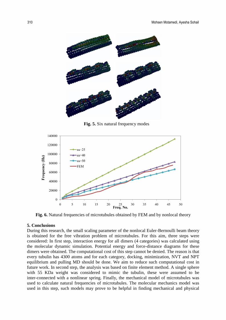
Fig. 5. Six natural frequency modes

Fig. 6. Natural frequencies of microtubules obtained by FEM and by nonlocal theory

5. Conclusions

During this research, the small scaling parameter of the nonlocal Euler-Bernoulli beam theory

is obtained for the free vibration problem of microtubules. For this aim, three steps were

considered: In first step, interaction energy for all dimers (4 categories) was calculated using

the molecular dynamic simulation. Potential energy and force-distance diagrams for these

dimers were obtained. The computational cost of this step cannot be denied. The reason is that

every tubulin has 4300 atoms and for each category, docking, minimization, NVT and NPT

equilibrium and pulling MD should be done. We aim to reduce such computational cost in

future work. In second step, the analysis was based on finite element method. A single sphere

with 55 KDa weight was considered to mimic the tubulin, these were assumed to be

inter-connected with a nonlinear spring. Finally, the mechanical model of microtubules was

used to calculate natural frequencies of microtubules. The molecular mechanics model was

used in this step, such models may prove to be helpful in finding mechanical and physical


properties of cell components more rapidly. Finally, using classical mechanics theories

especially nonlocal Euler- Bernoulli beam theory, small scaling parameter is obtained for the

free vibration problem of microtubules. Reasonably convergent results were obtained for the

scale parameter of microtubules. This work was a multi-disciplinary work between

mechanical engineering, biology, physics and mathematics. These results can prove to be

helpful in further studies on the microtubules and their role in eukaryotic cells. We aim to

extend this work in future using more robust solvers.


References

[1] Borisy GG, Taylor E. The mechanism of action of colchicine. The Journal of cell biology.

1967;34(2): 535–548.

[2] Ding Y, Xu Z. Mechanics of microtubules from a coarse-grained model. BioNanoScience.

2011;1(4): 173–182.

[3] Glade N, Demongeot J, Tabony J. Numerical simulations of microtubule self-organisation

by reaction and diffusion. Acta biotheoretica. 2002;50(4): 239–268.

[4] Bennett MJ, Chik JK, Slysz GW, Luchko T, Tuszynski J, Sackett DL, Schriemer DC.

Structural mass spectrometry of the αβ-tubulin dimer supports a revised model of microtubule

assembly. Biochemistry. 2009;48(22): 4858–4870.

[5] Hoang AT, Lowry AJ, Martin DS. Revised model, with experimental verification, for

motor densities in gliding assays. Biophysical Journal. 2017;112(3): 563a.

[6] Osborn M, Webster RE, Weber K. Individual microtubules viewed by

immunofluorescence and electron microscopy in the same ptk2 cell. The Journal of cell

biology. 1978;77(3): 27.

[7] Monroe D. Focus: How cells regulate the length of filaments. Physics. 2012;5: 69.

[8] Doodhi H, Prota AE, Rodríguez-García R, Xiao H, Custar DW, Bargsten K, Katrukha EA,

Hilbertb M, Hua S, Jiang K. Termination of protofilament elongation by eribulin induces

lattice defects that promote microtubule catastrophes. Current Biology. 2016;26(13): 1713–

1721.

[9] Linck R, Fu X, Lin J, Ouch C, Schefter A, Steffen W, Warren P, Nicastro D. Insights into

the structure and function of ciliary and flagellar doublet microtubules tektins, ca2+-binding

proteins, and stable protofilaments. Journal of Biological Chemistry. 2014;289(25): 17427–

17444.

[10] Ferry JD. Viscoelastic properties of polymers. John Wiley & Sons; 1980.

[11] Rahmani O, Pedram O. Analysis and modeling the size effect on vibration of

functionally graded nanobeams based on nonlocal timoshenko beam theory. International

Journal of Engineering Science. 2014;77: 55-70.

[12] Fakhrabadi MMS, Allahverdizadeh A, Norouzifard V, Dadashzadeh B. Mechanical

characterization of deformed carbon nanotubes. Digest Journal of Nanomaterials and

Biostructures. 2012;7(2): 717-727.

[13] Civalek Ö, Demir Ç, Akgöz B. Free vibration and bending analyses of cantilever

microtubules based on nonlocal continuum model. Mathematical and Computational

Applications. 2010;15(2): 289-298.

[14] Lei Y, Murmu T, Adhikari S, Friswell M. Dynamic characteristics of damped

viscoelastic nonlocal euler–bernoulli beams. European Journal of Mechanics-A/Solids.

2013;42: 125-136.

[15] Eringen AC. On differential equations of nonlocal elasticity and solutions of screw

dislocation and surface waves. Journal of applied physics. 1983;54(9): 4703-4710.


[16] Dominguez C, Boelens R, Bonvin AM. Haddock: a protein- protein docking approach

based on biochemical or biophysical information. Journal of the American Chemical Society.

2003;125(7): 1731-1737.

[17] Pronk S, Páll S, Schulz R, Larsson P, Bjelkmar P, Apostolov R, Shirts MR, Smith JC,

Kasson PM, van der Spoel D. Gromacs 4.5: a high-throughput and highly parallel open source

molecular simulation toolkit. Bioinformatics. 2013;29(7): 845-854.

[18] Heireche H, Tounsi A, Benhassaini H, Benzair A, Bendahmane M, Missouri M,

Mokadem S. Nonlocal elasticity effect on vibration characteristics of protein microtubules.

Physica E: Low-Dimensional Systems and Nanostructures. 2010;42(9): 2375-2379.

[19] Gao Y, Lei FM. Small scale effects on the mechanical behaviors of protein microtubules

based on the nonlocal elasticity theory. Biochemical and Biophysical Research

Communications. 2009;387(3): 467-471.


Submission of papers: Manuscript should be submitted (both MS Word and PDF) by e-mail to: [email protected] After a confirmation of the paper acceptation, the authors should send the signed hard copy of the "Transfer of Copyright Agreement" form (available at http://www.mpm.spbstu.ru section "Authors") by regular post to "Materials Physics and Mechanics" editorial office: Periodicals Editorial Office, Institute of Advanced Manufacturing Technologies, Peter the Great St.Petersburg Polytechnic University, Polytechnicheskaya, 29, St.Petersburg 195251, Russia. The scanned copy of the signed "Transfer of Copyright Agreement" should be send by e-mail to: [email protected]. Filetype: Authors are invited to send their manuscripts as MS Word file with PDF format copy. MS Word file should be prepared according to the general instructions bellow; we are kindly asking the authors to look through the detail instruction at: http://www.mpm.spbstu.ru. Length: Papers should be limited to 30 typewritten pages (including Tables and Figures placed in the proper positions in the text). Structure of the manuscript:

PAPER TITLE: CENTERED,

TIMES NEW ROMAN 14 BOLD, CAPITAL LETTERS A.B. Firstauthor1, C.D. Secondauthor2* -Times New Roman 12, bold, centered

1Affiliation, address, country - Times New Roman 10, centered

*e-mail: e-mail of the corresponding author - Times New Roman 10, centered

Abstract. Times New Roman 12 font, single line spacing. Abstract should not exceed 12 lines. Keywords: please, specify paper keywords right after the abstract. Paper organization. Use Times New Roman 12 font with single line spacing. Use Italic font in order to stress something; if possible, please, use bold for headlines only. Page numbering. Please, do not use page numbering. Tables, Figures, Equations. Please, see the sample file at http://www.mpm.spbstu.ru for more details. References References should be subsequently numbered by Arabic numerals in square brackets, e.g. [1,3,5-9], following the sample style below: [1] Koch CC, Ovid'ko IA, Seal S, Veprek S. Structural Nanocrystalline Materials: Fundamentals and Applications. Cambridge: Cambridge University Press; 2007. [2] Hull D, Bacon DJ. Introduction to Dislocations. 5nd ed. Amsterdam: Butterworth-Heinemann; 2011 Available from: https://www.sciencedirect.com/science/book// 9780080966724?via%3Dihub [Accessed 19th June 2018]. [3] Romanov AE, Vladimirov VI. Disclinations in crystalline solids. In: Nabarro FRN (ed.) Dislocations in Solids. Amsterdam: North Holland; 1992;9. p.191-402. [4] Mukherjee AK. An examination of the constitutive equation for elevated temperature plasticity. Materials Science and Engineering: A. 2002;322(1-2): 1-22.

[5] Soer WA, De Hosson JTM, Minor AM, Morris JW, Stach EA. Effects of solute Mg on grain boundary and dislocation dynamics during nanoindentation of Al–Mg thin films. Acta Materialia. 2004;52(20): 5783-5790. [6] Matzen ME, Bischoff M. A weighted point-based formulation for isogeometric contact. Computer Methods in Applied Mechanics and Engineering. 2016;308: 73-95. Available from: doi.org/10.1016/j.cma.2016.04.010. [7] Joseph S, Lindley TC, Dye D. Dislocation interactions and crack nucleation in a fatigued near-alpha titanium alloy. To be published in International Journal of Plasticity. Arxiv. [Preprint] 2018. Available from: https://arxiv.org/abs/1806.06367 [Accessed 19th June 2018]. [8] Pollak W, Blecha M, Specht G. Process for the production of molded bodies from silicon-infiltrated, reaction-bonded silicon carbide. US4572848A (Patent) 1983. [9] Brogan C. Experts build pulsed air rig to test 3D printed parts for low carbon engines. Available from: http://www.imperial.ac.uk/news/186572/experts-build-pulsed-test-3d-printed/ [Accessed 19th June 2018].

Правила подготовки статей: Рукопись (английский язык, MS Word и копия PDF) должна быть направлена в редакцию журнала по электронной почте: [email protected]. После подтверждения принятия статьи в печать, авторы должны отправить подписанные: 1. Соглашение о передаче авторских прав (http://www.mpm.spbstu.ru, раздел «Авторам»); 2. Экспертные заключения о том, что материалы статьи не содержат сведений, составляющих государственную тайну, и информацию, подлежащую экспортному контролю; по адресу: Россия, 195251, Санкт-Петербург, Политехническая, д. 29, Санкт-Петербургский политехнический университет Петра Великого, Институт передовых производственных технологий, Редакция периодических изданий. Cкан-копии подписанных документов просим направить по электронной почте: [email protected] Тип файла: Редакция принимает файлы MS Word с копией в формате PDF. Статья должна быть подготовлена в соответствии с настоящей инструкцией, мы просим авторов также следовать более подробным инструкциям на сайте журнала http://www.mpm.spbstu.ru в разделе «Авторам». Длина статьи: Статья не должна превышать 30 страниц формата А4, включая Таблицы и Рисунки, размещенные непосредственно в соответствующих местах. Общие правила оформления статьи:

НАЗВАНИЕ СТАТЬИ: ВЫРОВНЯТЬ ПО ЦЕНТРУ,

ШРИФТ, TIMES NEW ROMAN 14 BOLD, ЗАГЛАВНЫЕ БУКВЫ Автор(ы): А.Б. Первыйавтор1, В.Г. Автор2*- шрифт Times New Roman 12, bold, по центру

1Наименование организации, адрес, страна - шрифт Times New Roman 10, по центру * e-mail автора, представившего статью - шрифт Times New Roman 10, по центру

Аннотация. Аннотация статьи составляет не более 12 строк. Используйте шрифт Times New Roman 12, одинарный межстрочный интервал. Ключевые слова: укажите ключевые слова после аннотации. Как организовать текст статьи. Используйте шрифт Times New Roman 12, одинарный межстрочный интервал. При необходимости выделить какую-либо информацию используйте курсив. Используйте полужирный шрифт только для заголовков и подзаголовков. Номера страниц. Пожалуйста, не используйте нумерацию страниц Таблицы, Рисунки, Уравнения. Подробные правила оформления данных элементов статьи приведены в инструкции на сайте журнала http://www.mpm.spbstu.ru Литература Ссылки приводятся в тексте в квадратных скобках [1,3,5-9]. Стиль оформления ссылок: [1] Koch CC, Ovid'ko IA, Seal S, Veprek S. Structural Nanocrystalline Materials: Fundamentals and Applications. Cambridge: Cambridge University Press; 2007. [2] Hull D, Bacon DJ. Introduction to Dislocations. 5nd ed. Amsterdam: Butterworth-Heinemann; 2011 Available from: https://www.sciencedirect.com/science/book// 9780080966724?via%3Dihub [Accessed 19th June 2018]. [3] Romanov AE, Vladimirov VI. Disclinations in crystalline solids. In: Nabarro FRN (ed.) Dislocations in Solids. Amsterdam: North Holland; 1992;9. p.191-402. [4] Mukherjee AK. An examination of the constitutive equation for elevated temperature plasticity. Materials Science and Engineering: A. 2002;322(1-2): 1-22.

[5] Soer WA, De Hosson JTM, Minor AM, Morris JW, Stach EA. Effects of solute Mg on grain boundary and dislocation dynamics during nanoindentation of Al–Mg thin films. Acta Materialia. 2004;52(20): 5783-5790. [6] Matzen ME, Bischoff M. A weighted point-based formulation for isogeometric contact. Computer Methods in Applied Mechanics and Engineering. 2016;308: 73-95. Available from: doi.org/10.1016/j.cma.2016.04.010. [7] Joseph S, Lindley TC, Dye D. Dislocation interactions and crack nucleation in a fatigued near-alpha titanium alloy. To be published in International Journal of Plasticity. Arxiv. [Preprint] 2018. Available from: https://arxiv.org/abs/1806.06367 [Accessed 19th June 2018]. [8] Pollak W, Blecha M, Specht G. Process for the production of molded bodies from silicon-infiltrated, reaction-bonded silicon carbide. US4572848A (Patent) 1983. [9] Brogan C. Experts build pulsed air rig to test 3D printed parts for low carbon engines. Available from: http://www.imperial.ac.uk/news/186572/experts-build-pulsed-test-3d-printed/ [Accessed 19th June 2018].

МЕХАНИКА И ФИЗИКА МАТЕРИАЛОВ

40 (2) 2018

Учредители: Санкт-Петербургский политехнический университет Петра Великого,

Институт проблем Машиноведения Российской академии наук

Издание зарегистрировано федеральной службой по надзору в сфере связи,

информационных технологий и массовых коммуникаций (РОСКОМНАДЗОР),

свидетельство ПИ ФС77-69287 от 06.04.2017 г.

Редакция журнала

Профессор, д.т.н., академик РАН, А.И. Рудской – главный редактор

Профессор, д.ф.-м.н., член-корр. РАН, Д.А. Индейцев – главный редактор

Профессор, д.ф.-м.н. И.А. Овидько (1961 - 2017) – основатель и почетный редактор

Профессор, д.ф.-м.н. А.Л. Колесникова – ответственный редактор

Доцент, к.т.н. А.С. Немов – ответственный редактор

А.Ю. Зобачева, к.т.н. – выпускающий редактор

Л.И. Гузилова – редактор, корректор

Телефон редакции

+7 (812) 591-65-28

E-mail: [email protected]

Компьютерная верстка А.Ю. Зобачева

Подписано в печать 27.12.2018 г. Формат 60х84/8. Печать цифровая

Усл. печ. л. 10,0. Тираж 100. Заказ____.

Отпечатано с готового оригинал-макета, предоставленного автором

в Издательско-полиграфическом центре Политехнического университета Петра Великого. 195251, Санкт-Петербург, Политехническая ул., 29.

Тел.: (812) 552-77-17; 550-40-14.

Behavior of stainless steel at high strain rates and elevated temperatures. Experiment and mathematical modelling .................................................................................................................... 133-145 Anatoly M. Bragov, Alexander Yu. Konstantinov, Leopold Kruszka, Andrey K. Lomunov Experimental study of the influence of the type of stress-strain state on the dynamic compressibility of spheroplastic ......................................................................................................... 146-151 Anatoly M. Bragov, Alexander Yu. Konstantinov, Andrey K. Lomunov The description of elastic modulus of nanocomposites polyurethane/graphene within the frameworks of modified blends rule ........................................................................................................... 152-157 G.V. Kozlov, I.V. Dolbin Theory of hyperbolic two-temperature generalized thermoelasticity ........................................................................ 158-171 Hamdy M. Youssef, Alaa A. El-Bary Anomalous heat transfer in one-dimensional diatomic harmonic crystal ................................................................. 172-180 E.A. Podolskaya, A.M. Krivtsov, D.V. Tsvetkov Correspondence principle for simulation hydraulic fractures by using pseudo 3D model ...................................... 181-186 N.S. Markov, A.M. Linkov Higher-order model of prestressed isotropic medium for large initial deformations ............................................... 187-200 T.I. Belyankova, V.V. Kalinchuk, D.N. Sheydakov Comparison of influence forging and extrusion on microstructure of heusler alloys .............................................. 201-211 I.I.Musabirov, I.M. Safarov, R.M. Galeyev, D.R. Abdullina, R.Y. Gaifullin, D.D. Afonichev, V.V. Koledov, R.R. Mulyukov Modern approaches for study of eutectoid steel oxidation and decarburization ...................................................... 212-220 Kseniya Pivovarova, Marina Polyakova, Manuele Dabala, Alexey Korchunov, Andrey Shymchenko Multiblock copoly(urethane-amide-imide)s with the properties of thermoplastic elastomers ................................ 221-230 I.A. Kobykhno, D.A. Kuznetсov, A.L. Didenko, V.E. Smirnova, G.V. Vaganov, A.G. Ivanov, E.N. Popova, L.S. Litvinova, V.M. Svetlichnyi, E.S. Vasilyeva, O.V. Tolochko, V.E. Yudin, V.V. Kudryavtsev Revisited applicability of polymeric composite materials for designing tractor hoods ............................................ 231-238 A.V. Smirnov, D.O. Lebedev, M.V. Aleshin, O.I. Rozhdestvenskiy, S.P. Nikulina, A.I. Borovkov Multi-criteria problems for optimal protection of elastic constructions from vibration .......................................... 239-245 Dmitry V. Balandin, Egor N. Ezhov, Egor V. Petrakov, Igor A. Fedotov

Developing of phenomenological damage model for automotive low-carbon structural steel for using in validation of euroncap frontal impact ............................................................................................. 246-253 Dmitriy Shcherba, Alexey Tarasov, Alexey I. Borovkov Indentation of an elastic half-space reinforced with a functionally graded interlayer by a conical punch ............ 254-260 Andrey S. Vasiliev, Sergey S. Volkov, Sergey M. Aizikovich, Alexander N. Litvinenko Monitoring of sliding contact with wear by means of piezoelectric interlayer parameters ..................................... 261-273 V.B. Zelentsov, B.I. Mitrin, S.M. Aizikovich, P.A. Lapina, A.G. Sukiyazov Theoretical and experimental study of plastic anisotropy of Al-1Mn alloy taking into account the crystallographic orientation of the structure ......................................................................................................... 274-284 F.V. Grechnikov, Ya.A. Erisov, S.V. Surudin, V.V. Tereshchenko Application of temperature analysis to account for the effect of sheet thickness on rolling force ........................... 285-295 V.A. Mikheev, G.P. Doroshko, A.F. Grechnikova, D.V. Agafonova Electromagnetic elastic ball under non-stationary axially symmetrical waves ......................................................... 296-303 Vladimir A. Vestyak, Leonid A. Igumnov, Dmitriy V. Tarlakovsky Biophysical analysis of microtubules nonlocal beam theory ...................................................................................... 304-312 Mohsen Motamedi, Ayesha Sohail

MPM

, Vo

l. 4

0, N

o. 2

, 20

18

MATERIALS PHYSICS AND MECHANICS - Санкт ...

Documents

Transcript of MATERIALS PHYSICS AND MECHANICS - Санкт ...