Materials Manual - Idaho Transportation Department

Materials Manual

Februrary 2019

01/18 1

SECTION 100.00 – MISSION AND OBJECTIVESSECTION 110.00 – MISSION

110.01 Mission of the Idaho Transportation Department. 110.02 Mission of the Construction/Materials Section. 110.03 Vision of the Construction/Materials Section.

SECTION 120.00 – OBJECTIVES

120.01 Corridor and Environmental Planning. 120.02 Highway Design. 120.03 Highway Construction and Maintenance. 120.04 Staff Functions.

SECTION 130.00 – CONSTRUCTION/MATERIALS SECTION ACTIVITIES

130.01 Testing Support. 130.02 Project Development. 130.03 Quality Assurance. 130.04 Research. 130.05 Construction and Maintenance Support.

01/18 2

SECTION 100.00 – MISSION AND OBJECTIVES

SECTION 110.00 – MISSION

110.01 Mission of the Idaho Transportation Department. Our mission is threefold: we will commit to having the safest transportation system possible, we will provide a mobility-focused transportation system that drives economic opportunity, and we will become the best organization by continually developing employees and implementing innovative business practices

110.02 Mission of the Construction/Materials Section. We support the Department’s construction, materials and maintenance programs by providing project level technical support and by developing standards, specifications, design procedures, laboratory and field testing procedures, quality assurance procedures, and documentation requirements consistently implement the Department’s programs. We accomplish this by publishing and maintaining the Materials Manual, the Contract Administration Manual, and the Quality Assurance Manual. We also provide expertise and support to the Laboratory Operations Manual.

110.03 Vision of the Construction/Materials Section. To be recognized inside and outside the Department as the first resource to call for problem solving and solutions. We will anticipate our customer's needs and have research results ready to prevent tomorrow's problems from happening.

01/18 3

SECTION 120.00 – OBJECTIVES

120.01 Corridor and Environmental Planning. We support District corridor planning and environmental planning efforts through review and consultation of Materials Phase Reports.

120.02 Highway Design. We establish procedures for pavement designs based on subgrade characteristics and traffic loadings. We develop and assist the districts in developing designs for pavements, slopes, foundations, and subsurface drainage. We establish statewide uniformity of analysis and design methods. We review and provide expertise to the districts and consultants for materials reports and designs.

120.03 Highway Construction and Maintenance. We develop and maintain the Department’s Quality Assurance Program in accordance with the Code of Federal Regulations, Part 637 of Title 23. This including the requirements and standards for materials acceptance (minimum testing requirements), independent assurance and final project materials certification to ensure the materials and workmanship conform to the requirements of the approved plans and specifications. We provide construction support through review and analysis of materials-related problems, technical field support and analysis of laboratory tested materials.

We support maintenance activities by reviewing and analyzing materials related problems and by analyzing reports on laboratory tested materials.

120.04 Staff Functions. We provide support and technical expertise in a variety of ways as consultant to Headquarters sections and ITD Districts for geotechnical and materials-related engineering, specialized equipment, and materials testing.

01/18 4

http://www.gpo.gov/fdsys/pkg/CFR-2011-title23-vol1/pdf/CFR-2011-title23-vol1-part637.pdf

SECTION 130.00 – CONSTRUCTION/MATERIALS SECTION ACTIVITIES

130.01 Testing Support. The Construction/Materials Section provides engineering support to each laboratory unit of the Central Laboratory, the District Laboratories, and the Non-Destructive Pavement Testing Unit.

• Aggregate and Asphalt Mix Laboratories.

• Soil and Geotechnical Laboratories

• Structures and Cement Laboratories

• Asphalt Binder Laboratory

• District Laboratories

• Non-Destructive Pavement Testing (FWD, Skid, and profile/roughness).

• Research and develop/revise laboratory tests and equipment.

• Support the pavement management system.

130.02 Project Development. The Construction/Materials Section provides the following services:

• Reclamation standards for statewide material source reclamation.

• Assist in the evaluation and acquisition of new materials sources.

• Establish policy and procedures for the standardized development of Materials Phase Reports.

• Review and assist the development of Materials Phase Reports, when requested.

• Assist with identification of erosion issues and the development of erosion control applications.

• Establish policy and procedures for pavement analysis and life cycle cost analyses.

130.03 Quality Assurance. The Construction/Materials Section provides the following services to deliver support to the Department’s Quality Assurance program:

• Establish and maintain a system of materials quality assurance procedures, requirements, andadministration, including contract inspection and certification of compliance of materials onconstruction.

• When requested, arrange for outside inspection of materials to be used on construction ormaintenance projects.

• When requested, arrange for acceptance of specialty materials by appropriate certification ortesting.

• When requested, monitor project compliance with the Independent Assurance Program.

01/18 5

130.04 Research. The Construction/Materials Section provides the following services to deliver support to the Department’s Research Program:

• Coordinate highway materials related research.

• Find new and innovative processes and products for use on ITD projects.

• Work with the Districts to develop Research Needs Statements.

130.05 Construction and Maintenance Support. The Construction/Materials Section provides the following services to deliver support to construction and maintenance:

• Support construction activities by conducting field reviews and providing analyses,recommendations, and details for solution of materials-related construction problems.

• Provide training for proper testing equipment use and inspection procedures for districtpersonnel.

• Develop construction specifications.

• Organize and lead the Department standard specifications review committee.

• Assist Maintenance with analysis and details concerning slope maintenance and repair,pavement and structure repair, erosion control, and pavement seals and drainage.

01/18 6

Materials Phase Reports 210.00

01/18

SECTION 200.00 – PREPARATION & SUBMITTAL OF REPORTS 5

SECTION 210.00 – MATERIALS PHASE REPORTS 5

210.01 Requirements. 5

210.02 Treatment Selection. 6 210.02.01 4R (New Construction). 6 210.02.02 4R (Reconstruction). 6 210.02.03 3R (Resurfacing, Restoration, and Rehabilitation). 6 210.02.04 1R (Pavement Rehabilitation). 7 210.02.05 PP (Pavement Preservation). 7

210.03 Materials Phase Report Requirements 5 210.03.01 Materials Report Type and Submittal Sequence. 5 210.03.02 Submittal of Electronic Phase Reports. 6 210.03.03 Materials Reports Prepared by the District. 7

210.03.03.01 Draft Reports Prepared by the District. 7 210.03.03.02. Revisions to Reports Prepared by the District. 7 210.03.03.03 Distribution of Materials Reports. 5

210.04 Consultant Reports. 5

210.05 Professional Responsibility. 6

SECTION 220.00 – MATERIALS PHASE I AND PHASE I (G) GEOLOGIC RECONNAISSANCE REPORT 8

220.01 Introduction. 10 220.02 Conclusions. 10 220.03 Topography and Geology. 10 220.04 Surface Water. 10 220.05 Groundwater. 11 220.06 Geologic Constraints. 11 220.07 Recommendations. 12 220.08 Geologic Mapping. 12 220.09 References. 13

SECTION 225.00 – PHASE I (R) REHABILITATION FOR PAVEMENT REPORT 14 225.01 Introduction. 15 225.02 Evaluation. 15 225.03 Analysis. 15 225.04 Alternates. 16 225.05 Conclusions and Recommendations. 16 225.06 Appendix. 16 225.07 References. 16

SECTION 230.00 – PHASE II SOILS REPORT 17


01/18

230.01 Introduction. 17 230.02 Vicinity Sketch. 17 230.03 Soils Profile/Pavement Condition Survey. 17

230.03.01 Soils Profile. 18 230.03.02 Pavement Condition Survey. 18

230.04 Borrow Source Data. 22 230.05 Aggregate Inventory Report. 23 230.06 Borrow and Aggregate Source Plats. 24 230.07 Soil Report Summary. 24 230.08 Total Design Pavement Thickness. 25 230.09 Sub-subgrading. 27 230.10 Grade Pointing. 27

230.10.01 Availability of Water. 27 230.10.02 Soil Types. 27 230.10.03 Frost. 27 230.10.04 Criteria for Treatment. 28 230.10.04.01. Remove Topsoil. 28 230.10.04.02. Remove All Fine-Grained Soil, Overlying Sand, Gravel Or Rock. 28 230.10.04.03. Backfill Rock Excavation in Cuts With Granular Borrow Or Diced Shot Rock. 28 230.10.04.04. Replace Excavated Soil With Clean Granular Borrow. 28 230.10.04.05. Provide Adequate Drainage. 28 230.10.05 Typical Grade Points and Treatments. 28

230.11 Special Placement. 32 230.12 Compaction. 32 230.13 Slope Design Summary. 32 230.14 Slope Design. 34 230.15 Embankment Foundation. 34 230.16 Surface and Subsurface Water. 34 230.17 Drainage. 35 230.18 Retaining Walls. 35 230.19 Blanket Course or Filter Material. 35 230.20 Existing Roadway Material. 36 230.21 Abutment Embankment Material. 37 230.22 Rock Subgrade. 37 230.23 Topsoil. 37 230.24 Pipe. 37

230.24.01 Sampling and Testing. 37 230.24.01.01 pH. 37 230.24.01.02 Resistivity. 38 230.24.01.03 Bed Load. 38 230.24.02 New Construction and Reconstruction. 38


01/18

230.24.03 Pavement Rehabilitation and Preservation. 40 230.25 Riprap. 41 230.26 Staged Construction. 41 230.27 Dust Abatement. 41 230.28 Seismic Design. 42 230.29 References. 43

SECTION 240.00 – PHASE III PAVEMENT ESTIMATING REPORT 44

240.01 Pavement Type and Surface Smoothness. 44

240.02 Typical Section. 46

240.03 Base. 47

240.04 Surface Treatment. 49

240.05 Paving. 50 240.05.01 Performance Graded Binder Selection. 51 240.05.02 Lift Thickness and Nominal Maximum Aggregate Size. 52 240.05.03 Portland Cement Concrete Pavement. 53 240.05.04 Reduced Shoulder Pavement Thickness. 53

240.06 Seal. 54

240.07 Aggregate Estimating Data. 54 240.07.01 Disclaimer. 54

240.08 Aggregate Sources. 55

240.09 References. 55

SECTION 250.00 – PHASE IV FOUNDATION INVESTIGATION REPORT 56 250.01 Introduction. 57 250.02 Field Exploration and Laboratory Testing. 57 250.03 Surface Conditions. 58 250.04 Subsurface Conditions. 59 250.05 Conclusions and Recommendations. 59 250.06 Appendices. 67 250.07 Foundation Investigation Plat. 68 250.08 References. 5

SECTION 260.00 – PHASE V SPECIAL PROVISION REPORT 5 260.01 Source Identification. 6

260.01.01 Designated Sources. 6 260.01.02 Contractor Provided Sources. 6 260.01.03 Cost. 6 260.01.04 Source Cost Recovery Fee. 6 260.01.05 Examples of Source Identification Inserts. 7


01/18

260.02 Current Specifications and Minimum Testing Requirements. 5 260.03 Special Provisions. 6

260.03.01 Modification of Existing Specifications. 6 260.03.02 Modification of Existing MTRs or Development of New MTRs. 7 260.03.03 New Specification. 8

260.04 Notes to Contractor. 15 260.05 Notes to Designer. 15 260.06 Notes to Resident Engineer. 16

SECTION 270.00 – MATERIALS SOURCES (MOVED TO SECTION 300) 17


01/18

SECTION 200.00 – PREPARATION & SUBMITTAL OF REPORTS SECTION 210.00 – MATERIALS PHASE REPORTS

210.01 Requirements. A series of Materials Phase Reports is required for development of highway projects. Each report represents a different phase of project development. These reports are ultimately used by the designer and the information presented in each report is used to design the roadway features for the project. For this reason, these reports need to be written in a way that is clear and concise and understood by the designer. Try not to use jargon or language that can be misunderstood by those using the reports.

Following is a listing of these reports: • Phase I - Materials Report (refer to Section 220.00) • Phase I (G) - Geologic Reconnaissance Report (refer to Section 220.00) • Phase I (R) - Rehabilitation for Pavement Report (refer to Section 225.00) • Phase II - Soils Investigation (refer to Section 230.00) • Phase III - Pavement Estimating Report (refer to Section 240.00) • Phase IV - Foundation Investigation (refer to Section 250.00) • Phase V - Special Provisions (refer to Section 260.00)

NOTE: Phase I and II Reports may be developed in an abbreviated format and should be designated with an “A”. For example, an abbreviated Phase I is identified as Phase I (A). See the specific Phase report section for additional details. An abbreviated Phase I (R) Report should not be necessary.

In addition, for corridor or location studies on new alignments, a preliminary geologic reconnaissance report is typically prepared well in advance of Phase I.

This series of Materials Phase Reports is structured to elicit the information needed to design the largest, most complex projects we have and at the same time be flexible enough to work for smaller rehabilitation and preservation projects. Careful consideration should be given to the needs of the project when determining the Phase Reports selected.

Avoid forcing design treatments to fit a project type or funding category but rather let the investigation and data analysis determine the type of treatment needed. This will give decision makers information to make an informed decision regarding project needs and costs. The treatment selection decision is usually made with limited information. If, during the phase report process, the data indicates the selected treatment type will not provide the best project performance, report this. For example, if a project was selected as a pavement preservation project but, after the investigation, a rehabilitation project is determined to be more appropriate, provide your best estimation of the life and cost of the recommended project and of the programmed project.

Most highway projects deal with construction, reconstruction, rehabilitation, preservation and maintaining a paved surface of some sort. Therefore, Materials Phase Reports are usually needed.


01/18

210.02 Treatment Selection. Most of the projects defined in Section 315.00 of the Design Manual require Materials Phase Reports and are shown below with respect to the reports generally required for each type from new construction to pavement preservation. Most projects will require a Phase III and a Phase V Materials Report. The local conditions and complexity of the project will determine the type of Phase I report or Phase II, or a combination of these is appropriate. Other types of projects may be encountered and should be addressed on a case by case basis when developing the Materials Phase Reports. Phase IV Reports should be prepared when the conditions in Section 250.00 warrant them. Guidance on determining the Phase Reports needed for each type of project is included in Table 210.03.1.

210.02.01 4R (New Construction). This action involves the construction of a new highway facility where nothing of its type currently exists. These projects are normally the most complex and will nearly always require the use of all five Phase Reports. A Pavement analysis as described in Section 400.00 and Section 500.00 and a Geotechnical analysis as described in Section 400.00 and Section 600.00 is required.

210.02.02 4R (Reconstruction). This typically involves a major change to an existing facility within the same general right of way corridor. Reconstruction may involve making substantial modifications to horizontal and vertical alignment in order to eliminate safety and accident problems or making substantial modifications to the pavement section to correct structural deficiencies. These projects can be as complex as new construction and they can present more challenges because of the constraints involved with work within the existing facility and under traffic and may require the use of most if not all five Phase Reports. A Pavement analysis and a Geotechnical analysis as described above are required.

210.02.03 3R (Resurfacing, Restoration, and Rehabilitation). These design standards (NHS and Interstate) are intended to extend the service life of the existing highway and, at the same time, improve highway safety by making selective improvements to highway geometry and roadside features. The integrity of the existing ballast is maintained. The types of improvements to existing federal aid highways include: resurfacing, cold-mill-inlay/overlay, overlay, bridge deck rehabilitation, modifying bridge rail, pavement structural and joint repair, minor lane and shoulder widening, minor alterations to vertical grades and horizontal curves, and removal or protection of roadside obstacles. A project meeting the 3R NHS standard can have as little as an 8 year design life, but any less than a 20 year design life must be justified. These projects can vary significantly in complexity depending on the intent of the project. The Phase Reports will usually consist of a Phase I (R), III, and V. A Pavement analysis is required and a Geotechnical analysis may be required depending on the project.


01/18

210.02.04 1R (Pavement Rehabilitation). Pavement rehabilitation projects are intended to restore the riding surface and preserve the integrity of the existing roadway while not doing other improvements associated with non-pavement related items except for High Accident Locations, substandard end sections and grossly substandard rail. The types of improvements include: cold-mill and inlay, thick overlay (0.15’or greater), cold-in-place or hot-in-place recycle with overlay. Design life of the pavement for Pavement Rehabilitation (1R) projects will be a minimum of 8 years. The primary goal of the 1R standard is to rehabilitate pavements where a maintenance treatment would not be cost effective, but has not yet deteriorated to the point of needing major treatment or reconstruction. These projects do not decrease the existing geometrics conditions. The Phase Reports normally consist of a Phase I (R), III, and V Reports. A Pavement analysis is required and a Geotechnical analysis is seldom needed.

210.02.05 PP (Pavement Preservation). Pavement preservation consists of a series of treatments or strategies that cover a full range of activities from preservation to minor rehabilitation. Pavement Preservation activities preserve, rather than improve, the structural capacity of the pavement structure. Activities most closely associated with traditional maintenance, include roadway activities that are non-structural such as thin plant mix overlay, seal coating, fog coating, flexible pavement crack sealing, concrete pavement joint repair, grooving and grinding, pavement patching, shoulder repair and restoration of drainage systems. These types of applications normally take place early in the life of a pavement while they are still in good condition and before the onset of serious damage. It is very important for the pavement designer to know as much as possible about the pavement being treated to get the “right treatment at the right time on the right road.” Pavements with significant structural deterioration are not candidates for pavement preservation.

The level of design effort on PP projects varies depending on the amount of information available to the Materials Engineer. If pavement section thicknesses and materials properties are known, from either as-constructed plans, PMS information or other sources, PP treatments may be selected with minimal field investigation and analysis. On the other hand, pavement sections having little to no historic information available will require a more thorough investigation plan approaching the level of the other types of projects. The focus should be on determining if the pavement section has the structural capacity or remaining life to make the preservation treatment worthwhile. The Phase Reports normally consist of a Phase I (R), III, and V Reports. A Pavement analysis is required. Investigation recommendations are provided in the selected Phase Report section.

Pavement Preservation activities and the Phase Report recommendations are addressed in detail in Section 542.

The Transportation Asset Management System (TAMS), has a more complete list of treatment types at the following link: http://itdportal/sites/DES/TransSys/pave/documents/forms/allitems.aspx

http://itdportal/sites/DES/TransSys/pave/documents/forms/allitems.aspx


01/18

210.03 Materials Phase Report Requirements The requirements for submittal and approval of Materials Phase Reports are as follows:

Approved Materials Phase Reports are required for all projects. All Materials Phase Reports and investigations will be conducted to the appropriate level of detail for the specific project. The overall report shall be sealed and signed by a Professional Engineer licensed in the state of Idaho. If the report includes works performed by a geologist, then the portions of the report done under the responsible charge of a Professional Geologist could be signed and stamped by a Professional Geologist registered in the state of Idaho.

The purpose of the Materials Phase Reports is to develop project specific materials related design details. Projects conforming to established requirements will be eligible for funding. The Construction/Materials Section is a resource for information and assistance when needed, for example in the case of complex geotechnical features. Materials Phase Reports that do not conform to requirements must be revised as needed.

Elimination of Phase Reports will require a waiver approved by the District Engineer. The elimination of any Materials Phase Report should be evaluated, justified, and documented. Consider the documentation of a waived Materials Report as its approval.

The Construction/Materials Section is available to review all Phase Reports. ITD approval of Materials Phase Reports will be by the signature of the District Engineer. The approval verifies that the report(s) was developed, signed and sealed by other associates, Consultants or employees who are competent and qualified to develop materials reports and are registered or licensed.

All structural elements of the roadway should be designed and all minimums and maximums provided in the Materials Manual should be adhered to. Justify and document any deviation.

210.03.01 Materials Report Type and Submittal Sequence. Prepare Phases I through V reports at the proper time and in the proper sequence. DOH Work Breakdown Structure (WBS) Flowchart (Design Manual, Figure 3.1) and Plans Essential Requirements Checklist (See ITD-0131) indicate the relationship of the individual phase reports to the other elements of project development. If alignments are established, phase reports can be initiated earlier than the network shows. Only the Phase I report can be completed prior to Preliminary Design Review and is intended to be attached to the Project Charter.

Phase I reports of the type previously described are normally needed on all projects. Elimination of the Phase I report must be carefully considered to ensure all vital information is accounted for. For projects involving new construction, reconstruction, or rehabilitation of pavement, Section 540.00, Pavement Structure Analysis and Section 541.00, Life Cycle Cost Analysis alternatives will be incorporated into the Phase I Report.

Preliminary Phases II and IV reports may be prepared to provide guidance to designers before the project charter is finalized. These reports typically document partial investigations and are retained as


01/18

part of the file. A working relationship should be established with the designer to determine the amount of preliminary information that can be made available prior to publishing the official reports.

For projects for which the main purpose is major widening to add lanes, the ITD Life Cycle Cost Analysis computer program includes a Widen and Overlay subroutine for evaluating this option. On such projects, the condition of the existing roadway should be evaluated. The widened portion of the project should be evaluated as new construction and the existing pavement should be evaluated for new/reconstruction or rehabilitation.

Manual Sections 220.00 through 260.00 present the format for the individual phase reports. Use these sections as guidelines and checklists for preparation of the reports.

Each report should address all subjects in the applicable phase report sections. This will assure users and reviewers that no subject was overlooked. If a subject is not applicable to a particular project, briefly indicate the reason(s); do not use N/A (not applicable). Include a Table of Contents in each report.

Phase I (A) and II (A) reports may be appropriate for types of projects where addressing all subjects is of limited value. Include a Table of Contents in these reports that lists all the subjects the author believes will adequately address the work in question. This will help assure users and reviewers that no subject was overlooked or inadvertently left out.

Complete, well written reports, with supporting data included, normally take less time to review, thus shortening the turnaround time. If the reviewer has to guess how the conclusions were developed, the review time can increase significantly.

Table 210.03.1, Phase Reports for Project Type, lists the Phase Reports that are required for various types of projects as defined in the Design Manual.


01/18

Table 210.03.1

PHASE REPORTS FOR PROJECT TYPE PROJECT TYPE a PHASE REPORTS e

I or I(G) I (R) LCCA II III IV V Geotechnical Pavement (Roadway)

New Construction/New Alignment x x x x x Reconstruction x x x x x Resurfacing, Restoration Rehabilitation, (3R) x x x x x Pavement Rehabilitation, (1R) x x x x Pavement Preservation f x x Emergency Relief, (ER) x x x x

Structures New / Reconstruction x xb x x x x Structure Rehabilitation xc x Deck Rehabilitation x x Preservation x

Geotechnical Special Situation; Landslide, Slope Stability, Large Embankment, etc.

x

Rockfall Mitigation x x Retaining Structure

Major x x Minor; <10’ high x x

Railroad Crossing Contact Contracting Services Railroad Coordinator Bike Path/Enhancement d x x x a. A project may include more than one work category. As such, appropriate reports should be prepared to ensure that all issues are addressed. Appropriate reports apply on ER projects. b. A Life Cycle Cost Analysis should be prepared for structure projects with greater than 500’ approaches. The Life Cycle Cost Analysis should address pavement type and/or pavement rehabilitation options. For a new structure on the same alignment as the existing structure with less than 500’ approaches (500’ per approach), a waiver of the Phase I report should be considered. c. A Phase IV report is required only if rehabilitation of a foundation is involved. d. Refer to Design Manual for addressing specialized inspection (Idaho Association of Building Officials, etc.) e. Abbreviated Materials Phase Reports may be used when deemed appropriate. f. See Section 542 for additional information on the Phase Report requirements for each Pavement Preservation technique.


01/18

210.03.02 Submittal of Electronic Phase Reports. The Materials Phase Reports, including all attachments, should be converted to Portable Document Format (PDF) files. Free shareware is available to convert most files.

Project phase reports prepared by Consultants should be submitted to ITD by using an internet File Transfer site (FTP) or by CD or DVD. Anyone using the FTP site, ITD or Consultants, must obtain their user name and password to access the FTP site.

The electronic submittal of the final version of the phase report must comply with Idaho Code Title 54-Chapter 12, 54-1215, 3 b & c. The basic requirements are:

• All documents without a seal must indicate "preliminary, draft, not for construction" or similar words.

• The words "Original Signed By:" and "Date Original Signed:" must be placed adjacent to or across the seal.

• The storage location of the original document must be provided. • A hard copy does not have to be submitted to ITD (unless requested).

Each phase report file name must include the ITD project key number with the phase report number. For example, Prj1234_p1 is phase I for key 1234. The phase IV reports would require additional names if there is more than one phase IV required, such as, Prj1234_p4_creek bridge or Prj1234p4signalpole1-2. The attachments must also include the project key number and phase number, such as, Prj1234p2_logs 35-78 or Prj1234p2_appxII.

For revisions to the original submittals the file name must include Rev 1, Rev 2, etc. at the end of the name. The final file must include Final in the file name when there have been revisions to the original submittal.

The ITD District CADD Coordinator or District IT Coordinator uses Project Builder to manually create a new project folder structure for Materials Phase Reports for each project.

Each District must grant permissions to the reviewers to review the phase reports residing on district servers.

The Construction/Materials Section, or other sections, such as Bridge Section, will perform review of the phase reports, upon request, by adding comments to the PDF document. Any transmittal letters, approval letters, review memorandums and copies referred to in other sections of this manual will be accomplished by email or other electronic means. Copies of the correspondence will be retained by the District in the project folders on the Districts’ servers.

Review of PDF documents should be performed using the comment tools on products like Adobe® Acrobat Professional or Adobe® Reader X.


01/18

210.03.03 Materials Reports Prepared by the District. The District Materials Engineer may submit electronic phase reports to the Construction/Materials Section for review and comment. When requested by the districts, portions of reports may be prepared by the Construction/Materials Section and transmitted to the District Materials Engineer.

Distribution of the reports and/or transmittal letters is left up to the District. However, it is suggested a copy of the transmittal letter and report be retained by the District Materials Engineer and copies be distributed according to Section 210.03.03.03.

Unusual specifications or designs should be discussed with The Construction/Materials Section by telephone, e-mail, or at a review in the district. If the Construction/Materials Section has questions or comments on routine projects after reviewing the report, the questions or comments will be sent to the District Materials Engineer. All reports that are submitted to the Construction/Materials Section will be reviewed and returned with comments.

210.03.03.01 Draft Reports Prepared by the District. To expedite development of complex projects, phase reports (particularly Phases I, II, and IV) may be submitted to the Construction/Materials Section and/or the District Engineer in draft form. The Construction/Materials Section will review and return the draft report with comments to the district. Following necessary revisions, the final phase reports are then prepared and submitted as outlined above. Draft reports are typically unsigned, often incomplete, and will not be included in the project file. They should be clearly marked, or stamped, “DRAFT” to avoid confusion with later submittals.

On projects of average complexity, there is little need to prepare draft reports. Therefore, the use of draft reports should be limited to those projects of above average complexity and where the review process will be clearly enhanced by their submittal. Questions arising on these types of projects should be addressed to the individuals in the Construction/Materials Section with the expertise to assist.

210.03.03.02. Revisions to Reports Prepared by the District. When revisions to a materials report become necessary, the district should discuss the revisions, and when appropriate, involve the Construction/Materials Section by telephone, e-mail, and/or in a field review. After the concerns are addressed, the District Materials Engineer should revise the report with the changes noted and documented.

Revisions and additions may also be made by addendum to a previously approved report. Following the review, addenda are transmitted as outlined in Section 210.03.03. The addenda should be attached to the front of and made a part of the report.


01/18

210.03.03.03 Distribution of Materials Reports. Materials reports should be addressed and distributed by the District Materials Engineer as follows:

• Phases I, II, III, and V

o A report with cover letter addressed to District Project Development Engineer

o Copy of cover letter only to District Engineering Manager.

o Copy of the cover letter with report to the FHWA (full oversight projects only).

o Access to electronic reports for the Construction/Materials Section (see note)

• Phase IV

o A report with cover letter addressed to Bridge Engineer.

o Copy of cover letter only to the District Engineering Manager

o Copies of the cover letter with report to the Geotechnical Engineer in the Construction/Materials Section.

o Copies of the cover letter with report to the FHWA on full oversight projects only, (In accordance with Stewardship Agreement).

o Phase IV reports for buildings such as maintenance sheds or sand sheds, are addressed to the Facilities Manager.

NOTE: Preferably, all reports should be stored electronically on district servers with access given to those on this distribution list and as needed.


01/18

210.04 Consultant Reports. Consultant-prepared phase reports follow the same procedures as those prepared by the district. Portable Document Format (PDF) file format is required for electronic review of Consultant reports. ITD review of Consultant materials reports is necessary for the purpose of approval or concurrence as described previously in this chapter. This section covers the additional issues inherent to Consultant reports.

Except for the Phase V report, Consultant-prepared Materials Phase Reports may be submitted in the Consultant’s standard format. The format used by the districts for each Phase Report, as shown in this manual shall serve as a checklist for the Consultant to ensure that significant conditions are considered and covered in the report. The Consultant is encouraged to use a format that is similar to the Materials Manual to allow more efficient review by ITD. However, the format for specification modifications and special provisions contained in the Phase V Special Provision report shall be in accordance with the standard format used by ITD to ensure the designer inserts these items into the contract worded exactly as the author intends.

Include a Table of Contents that lists all the subjects the author believes will adequately address the work in question. This will help assure users and reviewers that no subject was overlooked or inadvertently left out.

Consultants are advised to anticipate the time and effort necessary for draft reviews and possible resubmittal of Materials Phase Reports in their scope of services. Some projects require ITD review of Consultant draft submittals prior to publication to the designer.

On highly complex and unusual projects, preliminary report(s) to summarize partial investigation are appropriate. Such reports are for ITD review only and are for the purpose of facilitating ongoing investigation rather than design. An ITD draft review of these prior to final stamp and signature by the Consultant should be performed.

Consultants submit electronic PDF files of each report to the District Project Development Section. See Section 210.03.02.

District Project Development Section sends notification to the District Materials Engineer and the District Materials Engineer reviews the report and resolves differences with the Consultant. The District Materials Engineer may request a review by the Construction/Materials Section. All reports that are submitted to the Construction/Materials Section will be reviewed and returned with comments.

Approval of the materials report or approval pending receipt of an addendum addressing comments will be by the District Engineer. The District Materials Engineer will return reports which are not approved, with recommended changes and additions, to the Consultant. The Consultant should receive the PDF copies of the reports that have been marked up with comments by both the district and headquarters reviewers as well as comments covered in transmittal emails so corrections can be considered. The Consultant will address all comments, make necessary corrections to the report, and provide a summary of the comments and the actions taken. Where recommended changes are minor, i.e., additional


01/18

information or justification for recommendations, the District Engineer may approve the report subject to receipt of an addendum addressing comments.

Orderly development of the Materials Phase Reports is essential to project development and review. Consultant-developed phase reports are to be submitted in accordance with the Design Manual requirements. Multiple phase reports will not be accepted as a package without prior approval. To avoid delays caused by problems with a part of a combined report, it is essential that these reports be developed quickly and individually, and reviewed quickly but thoroughly as each phase is completed. Draft reports will be submitted to and reviewed by the District Materials Engineer, when approved, and returned to the Consultant with comments or forwarded to the Construction/Materials Section for review depending on the situation.

The District and, if requested by the District, the Construction/Materials Section personnel, working on behalf of the district, will work closely with each Consultant from the inception of the project. Consultants should contact the District Materials Engineers and review with them the project geology and investigation requirements prior to developing their scope of services. An exploration plan shall be reviewed with District Materials prior to beginning field exploration.

Consultant reports are signed and sealed by a Professional Engineer licensed in the State of Idaho and they become the property of ITD once approved by ITD. Do not copyright phase reports prepared for ITD. A Consultant report is considered to be a final product as purchased by ITD. Consultant reports should make recommendations within the context of ITD requirements.

Consultants are expected to perform their own internal reviews.

Draft submittals, subsequent to internal Consultant review, for local roads projects of average complexity may be appropriate in the interest of timeliness of approvals.

The purpose of reviewing Materials Reports prepared by the Consultants is to ensure their completeness and that they comply with the state standard and common practices of design and construction of roadways and structures. The review and approval of Consultants’ reports by the state will not release the Consultant from their responsibility for their recommendations and the accuracy of the content of the reports.

210.05 Professional Responsibility. The requirements provided in Section 220.00 through Section 260 should be considered as the minimum required and is intended as a guide to ensure a thorough analysis of the project. It is also the intent of this chapter to provide uniform and consistent materials reports statewide.

These requirements are not intended as a substitute for experience and engineering judgment. The author must ensure the accuracy of the information and that an adequate investigation has been performed.


01/18

ITD recommendations are intended to address completeness and to ensure reports and projects meet the appropriate requirements. All comments are to be addressed to the satisfaction of the District Engineer.

Materials Phase I Report and Phase I (G) Geologic Reconnaissance Report 220.00

01/18

SECTION 220.00 – MATERIALS PHASE I AND PHASE I (G) GEOLOGIC RECONNAISSANCE REPORT

The Materials Phase I Report is the first documentation of information that is gathered for a project. This report is an accounting of the geologic information that is the basis for all the engineering decisions that will be made during the design of the project. There are three different Materials Phase I Reports that can be used depending upon the type and complexity of the project.

The three types of reports are the Phase I (G) Geologic Reconnaissance Materials Report; the Phase I Materials Report; and the Phase I (R) Rehabilitation for Pavement Report.

The purpose of the Phase I (G) Geologic Reconnaissance Materials Report is to conduct a geologic reconnaissance of corridors and to provide the designer with a report containing general information that will assist in the preparation of the design concept report. A Geologic reconnaissance is typically conducted to identify the geologic conditions and constraints which may influence the choice of alignment. The data gathered from this type of investigation is compiled in the Phase I (G) report and should follow the report outline described below. Projects that require a geologic reconnaissance of corridors are not as common as they once were and it is seldom necessary to develop a Phase I (G) report.

The Phase I Materials Report may be used to conduct a geologic investigation identifying alignment specific geologic constraints and to provide site specific recommendations for reconstruction projects where the geologic corridor is already identified. This report will be used more often than the Phase I (G) report and should follow the report outline described below.

Phase I and Phase I (G) reports follow the same report outline and will be addressed in this section. The difference is in how the author determines which items need to be emphasized.

For projects that consist primarily of pavement preservation and rehabilitation work and do not generally extend beyond the travelled way and shoulders, prepare the Phase I (R) report as described in Section 225.00.

For new alignment and major realignment projects, the geologic reconnaissance provides the materials information from which the Materials Phase I (G) Report is developed to the extent needed to identify the geologic conditions and constraints which may influence the choice of alignment and to identify the pavement type. Once a tentative alignment is selected, detailed geologic information regarding the proposed alignment is obtained, and preliminary and working design criteria are developed during the course of the Phase II Soils Investigation. The designer should be aware that information developed in the Phase II soils investigation may generate changes in the alignment identified in the Phase I (G) report.


01/18

For reconstruction projects, detailed geologic information regarding the proposed alignment is obtained, and preliminary and working design criteria are developed during the course of the Phase I investigation. A Phase II Soils Investigation may be conducted in lieu of a Phase I if deemed appropriate.

The following report outline should be used for both Phase I investigations and Phase I (G) reports. For corridor studies, the recommendations sections may be brief or presented in general terms. In an established corridor for reconstruction, the Phase I report would contain a relatively brief topography and geology section with an expanded site specific geologic constraints and recommendations section. Adequate maps and exhibits, such as a vicinity sketch and geologic map, must be included. Make reference to any relevant reports or previous investigations.

Perform the Pavement Structure Analysis and prepare an Engineering Report, Section 540.00, and perform a Life Cycle Cost Analysis, Section 541.00, and submit them with the appropriate Phase I report. The Phase I Report, the Engineering Report, and the Life Cycle Cost Analysis will all become attachments to the Charter Report. A Life Cycle Cost Analysis program is available through the Construction/Materials Section web site.

On projects involving widening, minor relocation (curve flattening, etc.), the designer needs preliminary materials design criteria to develop the concept report. An abbreviated Phase I report, Phase I (A), may be submitted on these projects. On projects primarily consisting of pavement rehabilitation or pavement reconstruction, a Phase I (R) report may be submitted (refer to Section 225.00).

In preparing the Phase I (A) report, geologic description may be omitted along with geologic mapping. The report should consist of an Introduction (Section 220.01), sections on Surface Water (Section 220.04), Groundwater (Section 220.05), Geologic Constraints or Hazards (Section 220.06) whichever are appropriate, and Recommendations (Section 220.07). Reference relevant reports or previous investigations.

Use Section 400 - Guidelines for Subsurface Investigations to gather the information required in the subsequent sections.

The recommendations in this section typically cover the minimum requirements established for the various types of Phase I Materials Reports. The Engineer responsible for developing the Materials Phase Report is responsible for the content and should carefully select the type of report that is appropriate to convey to the designer the level of information necessary to ensure a successful project.

Include a Table of Contents in these reports that lists all the subjects the author believes will adequately address the work in question. This will help assure users and reviewers that no subject was overlooked or inadvertently left out.


01/18

220.01 Introduction. Begin the report with a statement of purpose and scope of investigation. Describe the area covered, length of corridor, proposed alignment length, corridor width, termini, and route number. Indicate scope of the project (new alignment, realignment, etc.). A good introductory statement is important and will help those who are not fully familiar with the project to understand its purpose and the intent of the report.

220.02 Conclusions. State conclusions regarding the relative geologic feasibility of proposed alignment(s). Indicate major geologic conditions and constraints influencing feasibility of the alignment(s). Refer to subsequent sections in the report where constraints are discussed. Include general conclusions regarding the choice of alignment(s) or changes in alignment(s). Refer to maps where appropriate.

In large reports, this section may be replaced by a summary, which briefly states the results of the investigation. Typical summaries do not exceed 1 to 1 ½ pages.

220.03 Topography and Geology. Describe the surrounding topography and geology and its influence on roadway location.

• Topography. Provide information on the relief of the area under study, existing ground slopes, elevation range, valley or drainage width, and grade. Indicate if alignments parallel or cross topographic features, i.e., ridges, stream valleys, etc.

• Geomorphology and Stratigraphy. Describe the land forms which influence any new alignment(s), and discuss the geologic units which will be encountered. Present the stratigraphic section(s) and the influence of stratigraphy on the alignment(s) for any grade changes. Refer to mapping.

• Geologic Structure. Describe the structure of the geologic units and its influence on any new alignment(s). Include discussions of faulting, joints, bedding, foliation, attitudes, etc. Include structural attitudes on the geologic map.

• Soils and Vegetation. Describe the distribution and thickness of soil units including top soil. Indicate types and distribution of vegetation in the study area. Include land use as related to soil and vegetation.

220.04 Surface Water. Describe the surface drainage pattern and its influence on roadway location. Include information on high water, erosion, deposition, influence of lithology, and geologic structure on surface drainage patterns, etc.

For to-be-constructed bridge locations over a channel, obtain representative samples near the streambank and evaluate for sizing of riprap material and design of erosion control geotextile. When entering a channel with equipment, the conditions of U.S. Army Corps of Engineers 404 Permit Requirements may apply and an Idaho Department of Water Resources Stream Alteration Permit or written approval may be required.


01/18

State the D50 and the D90 sizes of the streambed material. Also, state the D15, D50, and D85 sizes of the in-situ material at the abutment or channel side slope locations. (Dxx is the material size for which xx% by weight of the particles are smaller.)

220.05 Groundwater. Cover the occurrence and distribution of subsurface water. Provide estimates of depth to groundwater. Cite observations which provide evidence for depth estimates. Include information regarding current groundwater uses. Provide measurements and yield data on existing wells and springs. Describe the influence of geology on groundwater and the influence of groundwater on the proposed highway construction. When field measurements are unavailable, approximate groundwater depths can be obtained from the Idaho Department of Water Resources (IDWR) website link: http://www.idwr.idaho.gov/hydro.online/gwl/default.html

220.06 Geologic Constraints. Outline the constraints or hazards presented to highway construction by geologic conditions.

• Seismic Risk. Discuss past and future earthquake occurrence in the project region. Potential hazards from seismic activity include fault rupture, ground shaking, slope failure, settlement, and liquefaction. Discuss the potential influence of these factors on the proposed construction. Indicate locations of potential problem areas. Estimate the peak ground acceleration coefficient (PGA) anticipated (7% chance of exceedence in 75 years) by using Figure 630.04.1 in this manual.

• Faults. Note location(s) of active and potentially active faults in the project vicinity. These faults are shown in Figure 630.05.1. Discuss the influence of faults and shear zones (active or inactive) on proposed construction. Faulting typically will influence slope stability and groundwater flow.

• Landslides. Indicate presence and location of existing landslides, and their influence on highway construction. Discuss possible mitigation techniques; avoidance, stabilization, removal, etc. Also, indicate areas of potential instability, including talus deposits.

• Water. Discuss potential for flooding and indicate where special construction techniques will be needed, i.e., drainage, erosion protection, etc. Estimate the effect of construction on groundwater flow and indicate possible ways to mitigate adverse effects.

• Settlement and Embankment Foundation. Describe subsurface conditions below proposed embankments and indicate locations where significant settlement of embankments may be expected. Identify relatively deep, loose, or soft soil deposits that indicate potential embankment foundation instability.

• Geologic Structure of In-Situ Rock Formations. Indicate influence of bedding, foliation, joint attitudes, and contacts on construction, i.e., adverse dip or joint intersections may dictate rock slope angles or require support.

• Highway Construction Materials. Discuss the availability of borrow sources, aggregate sources, and waste sites. Include environmental constraints to developing sources or waste sites, i.e., wetlands, zoning, etc. Include both existing ITD controlled sources and contractor provided sources in the area.

http://www.idwr.idaho.gov/hydro.online/gwl/default.html


01/18

220.07 Recommendations. Even in very early stages of project development, preliminary design criteria are needed for preliminary cost estimates and comparison of alternatives. In corridor studies, these design criteria will be largely qualitative, and most of the recommendations will be contained in the preceding sections. In Phase I, a tentative alignment is established and more quantitative, but preliminary design criteria are still needed. Indicate locations where special and/or analyses appear warranted.

• Slopes and Embankments. Preliminary recommendations should include applicability of standard cut and fill slopes and locations where slopes will be governed by geologic conditions (stratigraphy, structure, potential sliding). Indicate areas where sidehill embankments, (sliver fills), and embankment foundations need special treatment. Include recommended changes in alignment needed to accommodate geologic constraints. Identify potential rockfall problem locations.

• Structures. Indicate types of structure and locations where they will likely be required, if any. Note existing structures and comment on condition.

• Drainage. Provide locations where subdrainage and surface water interception or diversion will likely be necessary.

• Shrink/Swell. Provide estimates for shrink and swell factors for geologic units or groups of materials to be encountered in excavation. These estimates, in conjunction with the local stratigraphic sequence, will provide data for preliminary earthwork analysis.

• Tentative Ballast. Preliminary ballast thickness estimates may be based on the general materials types expected to occur at subgrade. A limited number of R-value tests are performed for typical expected subgrade soils. Make use of adjacent project data where applicable. (from Section 500).

• Tentative Material Sources. Indicate the existing materials sources, both ITD controlled and contractor provided sources, in the project vicinity and the probable material produced. The location of potential sources should be presented as well as a description of probable materials encountered. The quality and quantity of material available may have an impact on the type of pavement selected. Give consideration to access and environmental aspects of source development. Use the legal description and a descriptive location in relation to the project.

Typically, ITD will not develop materials sources for individual projects; rather the burden is on the Contractor to find material for the project. However, the Tentative Materials Sources information provided in this section will give the designer an idea of how to establish materials costs for the project.

220.08 Geologic Mapping. The scale of geologic mapping is left to the preparer. However, the scale should be large enough to show adequate detail. For filing ease, maps should be prepared on sheet sizes which are multiples of 8 1/2” × 11”, i.e., 11” × 17”, 17” × 22”, or 22” × 34”. Individual sheets should be no larger than 22” × 34”, or standard sheets.

A topographic map base is suggested. The geology, structure, and features (such as landslides and high groundwater areas) may be plotted directly on the base map or developed on an overlay or series of overlays. Screened base mapping is often an effective presentation.


01/18

The degree of geologic complexity and scope of the project will dictate the detail required. On relatively low relief, geologically simple projects, a standard county map may provide an adequate base (although a larger scale may be needed).

On more complex projects, large scale topography may be needed as a base and additional presentations such as slope maps, groundwater maps, geologic hazards, geologic structure, etc., may be needed.

220.09 References. The following are possible sources of geologic information which may be of use in preparing geologic reports and maps. In this section, provide a list of references used while preparing the report. There are many on-line resources available when preparing geologic reports and maps.

USGS quad sheets, open file reports, professional papers, etc.

US Bureau of Reclamation reports

Aerial Photo Coverage

University-developed geologic studies

Soil Conservation Service soil mapping

Bureau of Land Management

US Forest Service

Department of Energy

Idaho Geological Survey

US Bureau of Mines

Annual Engineering Geology and Soils Engineering Symposia


01/18

SECTION 225.00 – PHASE I (R) REHABILITATION FOR PAVEMENT REPORT

A Phase I (R) Rehabilitation for Pavement Report is appropriate for projects designated as pavement preservation and rehabilitation projects, including but not limited to pavement overlays, CRABS, mill and inlay, cold in place recycle and hot in place recycle. The level of field work required, such as pavement condition information, preliminary pavement drilling and/or test pits, and FWD testing should be the same as for a full Phase II report and is presented in greater detail in Section 230.03. The Phase I (R) Report is developed at the concept stage and repetition/re-review of essentially the same information and report during the design phase is not required unless changes are necessary. As previously described, a Phase I (A) with full Phase II, III, and V reports may be considered appropriate for widening, minor relocation and reconstruction projects.

Care should be taken when developing an investigation plan for this category of project. Make sure projects designated as pavement preservation and rehabilitation projects will achieve the desired result when these treatments are applied. Avoid designing treatments to fit a project type or funding category but rather let the investigation and data analysis determine the type of treatment needed. This will give decision makers enough information to make an informed decision regarding project needs.

A good resource for information concerning an investigation plan is the Mechanistic Empirical Pavement Design Guide, A manual of Practice, July 2008 Interim Edition.

The recommendations in this section typically cover the minimum requirements established for a Phase I (R) Materials Report. The Engineer responsible for developing the Materials Phase Report is responsible for the content and should carefully select the type of report that is appropriate to convey the level of information necessary to the designer to ensure a successful project.

The following is considered to be an appropriate format for a Phase I (R) Report for pavement rehabilitation projects. All applicable sections from the Phase I (A) and Phase II report format should be addressed in the Phase I (R) Report. The information corresponding to some sections may be omitted as repetitive or not relevant for pavement rehabilitation projects without explanation. Follow the guidance provided in Section 210.00.

Include a Table of Contents in these reports that lists all the subjects the author believes will adequately address the work in question. This will help assure users and reviewers that no subject was overlooked or inadvertently left out.


01/18

225.01 Introduction. Provide a brief description of the project including the location, route, beginning and ending mileposts, materials history, and current condition. A good introductory statement is important and will help those who are not fully familiar with the project to understand its purpose and the intent of the report.

225.02 Evaluation. Provide detailed description of roadway characteristics such as grade, approximate super elevations, shape condition of the roadway crown, etc. Provide additional description of cracking, rutting, roughness, edge breaking, etc. as needed.

Discuss resultant information from Section 530.00, Pavement Rehabilitation Design including discussion of information from Section 540.00, Pavement Structure Analysis as appropriate. Particular attention should be given to existing pavement thickness, truck ADT, and pavement subsurface drainage.

Provide explanation(s) of any primary usage and traffic characteristics that are anticipated to affect project design in ways other than for analysis purposes, as needed.

Identify any geologic or environmental features that may pose a constraint on the project. Such features may include, but are not limited to, areas presenting potential rockfall hazard, landslides, or obvious wetlands.

Briefly discuss or identify available materials sources in the area of the project. Provide a brief description of anticipated materials quality.

Identify any structures that may exist on the project and comment on condition.

Identify any pipes that may exist on the project and comment on condition.

Identify any roadway locations where sub-subgrading, or full reconstruction will be needed. Often it is more cost effective to reconstruct short sections of poorer roadway rather than let these areas influence the structural design of the better sections.

Address compaction and any special requirements.

Address subsurface drainage requirements from Section 550.00.

Discuss pavement geosynthetics or any other non-standard products or procedures that are being considered.

225.03 Analysis. Provide required total design pavement thickness as described in Section 230.08, based on existing layer thicknesses. If more than one design life is being evaluated, show the required total design pavement thicknesses, based on existing layer thicknesses, for each design life being considered.

Where appropriate, provide pH and resistivity information from soil tests that may have been taken. Refer to Section 670 of the Design Manual for selection of pipe materials.


01/18

Provide initial quantity estimates for any dust abatement that may be required.

Provide justification for any materials-related, non-pavement rehabilitation work that is being recommended.

225.04 Alternates. Describe each alternate being considered. Address each alternate to the pavement descriptions discussed in the Evaluation. List the Equivalent Uniform Annual Cost (EUAC) and/or Total Net Present Worth for each alternate as described in Section 541.00.

Provide justification for any non-standard products or procedures integral to an alternate.

225.05 Conclusions and Recommendations. State conclusions in regards to each alternate as developed in the report. Select and recommend the design alternate with the highest priority being the potential of that alternate to address the pavement rehabilitation needs of the project. The secondary priority for selection of the design alternate will be economics.

225.06 Appendix. Attach the following:

Vicinity Map

Data and analysis sheets from Pavement Structure Analysis

Life Cycle Cost Analysis

Manufacturer or vendor information and sample specifications for any non-standard materials or procedures to be used.

225.07 References. Provide a list of references used while preparing the report. Typical references available on-line and from other sources include:

AASHTO 1993 Guide for Design of Pavement Structures

Materials Manual Section 500.00.

TRB Publications

FHWA Research and Development Reports

NCHRP Reports

AASHTO Mechanistic Empirical Pavement Design Guide, A manual of Practice, July 2008 Interim Edition.

Basic Asphalt Recycling Manual, ARRA, FHWA, 2001

NHI Course 132040, Geotechnical Aspects of Pavement, Publication No. FHWA-NHI- 05-037

Materials Phase II Soils Report 230.00

01/18

SECTION 230.00 – PHASE II SOILS REPORT

The purpose of the Phase II Soils Report is to provide designers with specific information concerning the soils (or rock) encountered over the length of the project and geotechnical recommendations regarding slopes, embankments, and drainage required to construct the project to current design standards. Also included are sources, descriptions of borrow materials required on the project, and pavement structure thicknesses. The following is an outline of the soils report and description of the required information.

On projects primarily consisting of pavement rehabilitation or pavement reconstruction, a Phase I (R) report generally addresses the Phase II issues of concern. Refer to Section 225.00. If a Phase I (R) Report has previously been prepared, a Phase II Report may be needed only to address work to be done that is in addition to pavement rehabilitation or pavement reconstruction. On projects involving widening, minor relocation (curve flattening, etc.), an abbreviated Phase II report, Phase II (A) may be prepared.

In preparing the Phase II (A) report, care must be taken to ensure all relevant sections of the report are included. At a minimum, the report should consist of an Introduction (Section 230.01), Vicinity Sketch (Section 230.02), Soils Profile/Pavement Condition Survey (Section 230.03), Total Design Pavement Thickness (Section 230.08), Surface and Subsurface Water (Section 230.16), Drainage (Section 230.17), Existing Roadway Material (Section 230.20), References (Section 230.29), and any other sections that are appropriate. Choosing to prepare a Phase II (A) report does not relieve the author of the responsibility of preparing a complete and thorough report.

230.01 Introduction. Include a brief description of the project. Address the type of project (new alignment, realignment, widening, rehabilitation of existing, etc.) length, width, and grades; types and numbers of structures; existing facilities; and approximate heights of cuts and fills. Describe the alignment and terrain (level, rolling, stream valley, side hill, mountainous, etc.). An elevation range should also be included as well as a brief description of the geology, soils, and vegetation. Reference previous reports and investigations and subsequent investigations proposed. A good introductory statement is important and will help those who are not fully familiar with the project to understand its purpose and the intent of the report.

230.02 Vicinity Sketch. Prepare the project vicinity sketch on a county map base in accordance with Figure 230.02.1. The sketch should show project limits and the location of all potential sources, stockpile sites and waste sites, if they can be identified.

230.03 Soils Profile/Pavement Condition Survey. Prepare a drawing/document that details the subsurface conditions for the type of project as described below. Conduct a subsurface investigation according to Section 400 that will produce the information used in these sections.


01/18

230.03.01 Soils Profile. For new alignments or realignments, prepare a soils profile in accordance with Figures 230.03.1 and Figure 230.03.2. Figure 230.03.1 depicts a soils profile on a new alignment type project. Figure 230.03.2 depicts a soils profile on a reconstruction/rehabilitation type project. Cross sections should be included on the soils profile to illustrate typical conditions over the project, special problems, or areas where detailed analyses were made. All boring logs should be shown on the profile and located on the cross sections. If the district chooses, the soils profile may be submitted to the Construction/Materials Section for review. After the review, the soils profiles will be returned to the district. Soils Profiles may be prepared on a roll of paper or on sheets at plan size (11” × 17”).

230.03.02 Pavement Condition Survey. For reconstruction, rehabilitation, and preservation projects, a pavement condition survey should include a description of the surface condition using LTPP Distress Identification Manual; recap of the service and rehabilitation record; deflection testing; and a subsurface investigation to determine the thickness of each pavement structure component. See Section 540.00 for Pavement Condition Survey details.

When an existing route is upgraded, widened, or rehabilitated, and construction will not result in significant changes in vertical or horizontal alignment, subsurface soils identification and thicknesses and pavement thicknesses may be documented on Form ITD-981, Boring/Test Pit Log (Figure 445.01.1) in lieu of a soils profile. Include copies of Form ITD-981 along with the report.

The Pavement Condition Survey is performed as part of the Pavement Structural Analysis (Section 540.00).

An abbreviated Combined Phase I-II or a Phase I (R) Report may be prepared for projects requiring only a pavement condition survey. Where the roadway is to be widened, include soils profile width cross sections and a description of special problem areas.

.


01/18

Figure 230.02.1: Vicinity Sketch


01/18

Figure 230.03.1: Soils Profile for New Construction Type Project


01/18

Figure 230.03.2: Soils Profile for Rehabilitation Type Project


01/18

230.04 Borrow Source Data. Provide information for Table 230.04.1 for each source when designated sources are specified.

Table 230.04.1: Borrow Source Data

Source Location Expansion

Pressure, psi R-Value Proven Quantity, c.y

Design Estimated Quantity Required, c.y.

Note any special or selective uses of material from sources, i.e., top soil, select granular material, drain aggregate, use of overburden, etc. Also note special processing which may be needed. If material required exceeds 75% of the proven quantity, then the designer should notify the District Materials Section to confirm the material quantity.

For existing sources, use established county and number code designation for location. The source designation codes and previous test data are available from the District Materials Engineer.

When Contractor Furnished Sources are to be used, indicate in this section that Approved Contractor Furnished Sources are specified.

• Example 1: Used with Contractor Furnished sources.

Approved Contractor Furnished Sources are specified.

• Example 2: Used with Designated Sources.

Source Location Expansion

Pressure, psi R-Value

Proven Quantity, c.y.

Design Estimated Quantity Required, c.y.

Borrow #1 0.83 52 100,000 90,000

El-53-s 0.57 60 150,000 150,000


01/18

230.05 Aggregate Inventory Report. Provide information for Table 230.05.1 for each source when designated sources are specified.

Table 230.05.1: Aggregate Inventory Report

Source Location.

Ave. Haul Miles

Over-burden,

Depth, ft. *(R-Value)

Max. Size in.

S.E. Immersion

Compression Proven

Quantity, C.Y. Reclamation** Plan Approval.

Archaeological** Clearance.

*If expansion pressure controls depth, show it instead of the R-value depth. **Provide dates

Indicate the quantities of material required for the project. Provide a recommended or selected source and reasons for selection. If expansion pressure controls, so note.


• Example 1: Used with Contractor Furnished sources.


• Example 2: Used with Designated Sources.

Four sources of aggregate were reviewed for possible use on this project. The project requires a source that will supply 125,000 c.y. of aggregate for plant mix, base, cover coat material, granular borrow and borrow.

Source Location.

Ave. Haul Miles

Over-burden,

Depth, ft. (R-Value*)

Max. Size, in.

S.E. Immersion

Compression

Proven Quantity,

C.Y.

Reclamation** Plan Approval.

Archaeological** Clearance.

El-21 15 0 3” 40 OK 150,000

El-43 3 9

(*R=37) ¾” 37

Needs treatment

130,000

El-4 5’

(*R=44) 6” 40 OK 100,000

El-53-s 4 3’

*(R=77) 3” 50

Needs treatment

200,000 RP-1578

*If expansion pressure controls, show it instead of the R-value. **Provide dates

From the preceding data, Source El-53-s was selected because of the short haul and maximum aggregate size, permitting a good percentage of crushed material with less waste. Also the overburden provides an excellent source of low ballast requirement borrow, R=77.


01/18

Source El-43 has a shorter haul but the small maximum size limits the amount of crushed material and the proven quantity would be marginal. Also the overburden would not be acceptable for borrow because of its high ballast requirement, R=37.

230.06 Borrow and Aggregate Source Plats. When designated sources are specified, submit copies of drawings; retain originals for final design submittal in the contract proposal to ensure good clear drawings. (Compare source drawings to the example shown in Figure 300.07.02.1 in Section 300.07.02.)


• Example: Used with Contractor Furnished sources.


230.07 Soil Report Summary. On new alignment, realignment, and widening projects, record the main traveled way and station-to-station locations showing where material will originate for subgrade construction (Form ITD-944). Do not place high ballast requirement materials at subgrade. Cap with material having low ballast requirements.

• Example, see Figure 230.07.1, Form ITD-944.

For pavement rehabilitation projects, a Soil Report Summary is normally not necessary. The following example illustrates a pavement rehabilitation project.

• Example, used when boring logs and test pit logs replace Form ITD-944.

This project consists of pavement rehabilitation and no Soil Report Summary was prepared. Boring logs and test pit logs from the Pavement Condition Survey are included in the appendix.


01/18

230.08 Total Design Pavement Thickness. Pavement designs are determined in Section 500 Pavement Design. Show station-to-station tentative ballast using the headings in Table 230.08.1.

Table 230.08.1: Total Design Pavement Thickness

Sta. to Sta. or

MP to MP

Actual Thickness in feet Design Gravel*

Equivalency Surface Base Sub-base Total

*For plant mix pavement.

• Example:

Sta. to Sta. Actual Thickness in feet

Design Gravel* Equivalency Surface Base Sub-base Total

2373-3364 EBL & WBL 0.58 0.9 1.5 2.98 3.05

I.C. #1 Ramps AB, BC 0.23 0.45 0.6 1.28 1.42

Ramp AD, DC

IC# 1 Ramp BD 0.54

1.2 (Rock Cap)

-- 1.74 2.30

If the Total Design Pavement Thickness was determined as part of the Phase I report, reference that report. If the thickness was not determined in the Phase I or has changed for some reason, calculate the Total Design Pavement Thickness and include all information used to determine it in the appendix of the Phase II report.

The pavement thicknesses shown here are determined by the design procedures described in Section 510.00, Thickness Design for Flexible Pavement. For rigid pavement design procedures described in Section 520.00, Rigid Pavement Design, use only the applicable parts of the table. For rehabilitation pavement design procedures described in Section 530.00, Pavement Rehabilitation Design, use only the applicable parts of the table.

Check all pavement designs over two years old for possible reevaluation.


01/18

Figure 230.07.1: Soil Report Summary


01/18

230.09 Sub-subgrading. Sub-subgrading is additional excavation below pavement subgrade due to groundwater or undesirable soil characteristics. In isolated areas requiring a thicker pavement section, additional excavation, i.e. sub-subgrading, (SSG), to remove high ballast material is desirable to minimize the number of typical sections.

Prepare a station-to-station list of any areas requiring additional excavation (and thicker pavement section) below pavement subgrade due to groundwater or undesirable soil characteristics. Define the limits of sub-subgrading (SSG) on the Soils Profile for reference as shown on Figure 230.03.1. Indicate material requirements for backfill and location for disposal of excavated material. Indicate reason for sub-subgrading. If special drainage and/or a subgrade blanket or geotextile is needed, refer to subsequent sections of the report where they are described.

Sub-subgrading should not be confused with over-excavation for embankment foundation.

• Example:

Sub-subgrading 2.0 feet from finished grade is required between Stations 192+00 and 200+50 on Ramp BD, Interchange No. 1 in order to remove undesirable high ballast requirement soil and to minimize the number of typical sections. The layer of No. 4 material, (see Soil Report Summary), that is excavated, Lab No. 225123, and which has a gravel equivalent of 1.0 foot, shall not be place within 3.0 feet of finished grade and will be designated to be placed at the foot of the embankment between Stations 183+00 and 187+00 on Ramp AB, Interchange No. 1.

230.10 Grade Pointing. Grade pointing is sub-subgrading to remove undesirable soils from cut-fill transitions, provide drainage, and/or eliminate abrupt transitions. Grade points are defined as the roadbed transition from a cut to a fill, generally through soils having been cultivated or having a higher organic content than underlying soils. Grade points are potential areas of weakness and must be examined critically before the pavement is designed. Factors which contribute to pavement failure at grade points are:

230.10.01 Availability of Water. Melting snow, ponded runoff groundwater and capillary moisture all provide water to the grade point area. Adequate drainage, both surface and subsurface, is essential.

230.10.02 Soil Types. Silty soils in ML or MH category of the Unified Classification System under or in the A-4 and A-5 category of the AASHTO Classification System are the most susceptible to frost action when moisture is available. These soils also lose support very easily when saturated. Consider any soil which has been well cultivated or is capable of supporting abundant plant life as susceptible to frost action.

230.10.03 Frost. The factors of water and soil, taken together with frost action, cause greater loss of support to pavement than can be predicted by laboratory strength tests, alternating cycles of freezing and thawing seems to cause the greatest damage. Moisture migrates from warm to cold areas; hence moisture is drawn up into the pavement structure.


01/18

230.10.04 Criteria for Treatment. Selecting those grade points which require treatment is largely a matter of judgment based upon consideration of the factors above. Use the following criteria in treating those areas selected:

230.10.04.01. Remove Topsoil. Remove topsoil to a depth below top of pavement equal to:

• Pavement structure thickness, including all base courses, plus thickness of detrimental soil layer or pavement structure thickness plus one foot, whichever is less. Ordinarily the depth of the detrimental layer will vary from 0.5 to 1.0 foot. Exceptions may be highly organic silts soils which are to be removed to a depth at least one-half of the depth of the frost penetration.

• Length of treatment is determined by the extent of the detrimental layer. Designate limits on the plans in minimums of 50-foot increments rather than more refined limits.

230.10.04.02. Remove All Fine-Grained Soil, Overlying Sand, Gravel Or Rock. Remove all fine-grained soil, overlying sand, gravel or rock to a depth below top of pavement equal to the pavement structure thickness plus depth of soil, not to exceed one foot.

230.10.04.03. Backfill Rock Excavation in Cuts With Granular Borrow Or Diced Shot Rock. Make backfill of rock excavation in cuts only with granular borrow or diced shot rock. Do not use any soil as it will entrap water and cause failure during spring breakup and a weakened section all year around.

230.10.04.04. Replace Excavated Soil With Clean Granular Borrow. Replace excavated soil with clean granular borrow. Such material may be imported or it may come from selective ue of rock or gravel excavation. In any case, it should be free draining.

230.10.04.05. Provide Adequate Drainage. Provide for adequate drainage, even if this requires deeper excavation. Water must not be trapped in the backfill material but must be dissipated in the ditches or on the embankment slopes. Installation of perforated pipe drains in grade points, particularly at the downgrade end of cuts, can be beneficial in reducing pavement distress (frost heave, pumping, differential settlement, etc.) in the embankment at or near the grade point. Refer to Section 550.07 for guidance in draining grade points.

230.10.05 Typical Grade Points and Treatments. Grade points may be transverse, longitudinal, or skewed. Again, indicate materials requirements for backfilling and location for disposal of excavation. Note locations of pipe drains. Show limits defining grade points as shown in Table 230.10.1. This information is also included on the Soils Profile as shown in Figure 230.03.1 and Figure 230.03.2.

Figure 230.10.05.1 shows three examples of Longitudinal Grade Point Sections, (a), (b), and (c). These sections depict the additional excavation and backfill in the cut-fill transition zone for three different roadway grade scenarios to ensure proper drainage. Figure 230.10.05.2 shows two examples of Transverse Grade Point Sections, (d) and (e). These sections depict the additional excavation and backfill in the cut-fill transition zone based on the type of material, soil or rock or gravel. Note the bottom of the grade point area slopes to drain to the fill side.


01/18

A sketch of the grade point areas may be helpful in this section when treatment becomes complicated.

Show limits defining grade point depths as shown in Table 230.10.1.

Table 230.10.1: Grade Pointing

Station-to-Station SSG in feet Drainage Direction

• Example:

Grade pointing will be required at the following stations:

Station-to-Station SSG in feet Drainage Direction

2951+50 – 2952+00 2.2 Ahead

3155+60 – 3156+50 2.2 Back

Sub-subgrading to the depths in the table above from finished grade is required between the Stations shown. Remove all excavated material and dispose of in an approved contractor-furnished site.


01/18

Figure 230.10.05.1: Longitudinal Grade Point Sections


01/18

Figure 230.10.05.2: Transverse Grade Point Sections


01/18

230.11 Special Placement. Designate station limits when it is necessary to haul material beyond its logical location and place it elsewhere, i.e., sub-subgrade excavation, subgrade cap, top soil, or special placement of rock fill.

230.12 Compaction. Specify class of compaction recommended and locations. Special compaction requirements described in subsequent sections of this report should be referenced here. Class C compaction must be defined separately by stations. Refer to Section 205, Excavation and Embankment in the ITD Standard Specifications for compaction classes.

230.13 Slope Design Summary. Designate slopes of all cuts and fills in the summary outlined below. Include special treatment such as pre-splitting, benching, mini-benching, serration or toe keys, sub-drainage, and benching for embankment construction. Indicate dimensions on benches, slopes, and embankments as well as station-to-station locations for slopes requiring special treatment such as retaining walls, rock fall mitigation ditches, interceptor ditches, and interceptor drains. Assign shrink and swell values to the various geologic units that will be encountered in excavation. Use these values to determine average shrink and swell factors for material from each cut or series of cuts. These values should be entered into the summary outlined below.

These slope and special treatment recommendations should be more fully described in subsequent sections of the report. Embankment slopes should be included in the summary and referenced to Section 230.14. Use the following headings for Table 230.13.1.

Table 230.13.1: Slope Design summary

Sta. to Sta. Operation Height. in feet

Shrink/Swell (volume change) Slope Special Treatments

The Slope Design Summary should be provided for every project where design includes special slope treatments or slopes are more than ten feet high.


01/18

• Example:

An example slope design summary is shown in Table 230.13.2.

Table 230.13.2: Slope Design Summary Example

Station Limits Operation Height (in feet)

Shrink/Swell Slope Special Treatment

0+00-22+60

Cut L

Daylight R

60 +15% 0.5:1

Pre-split; 15’ FBD*; 10’ Bench Elev. 5,590’ *(Flat-Bottomed Ditch)

22+60-28+10

Cut L

Fill R

20

10

-5%

1.5:1

2:1

Interceptor Crown Ditch: Serrated Slope Toe Keyway 7’+/-Deep and Drain Station 23+20-27+69; Contour Sub-drain Elev. 5530’ +/-

28+10-38+40 Series of Low Cuts and Fills

0- 10 -10% Standard Serrated Slopes

38+40-42+60 Fill L & R 40 1.5:1

Rockfill; Toe Keyway 10’ Deep Sta. 39+90-40+20

On other projects, such as pavement rehabilitation, the slope design summary information may require only a brief written statement.

• Example:

Slopes shall be constructed at 2H:1V or flatter.

• Example:

This project consists of pavement rehabilitation and slope work is not anticipated.


01/18

230.14 Slope Design. Indicate basis for slope designs presented above in Section 230.13, including special slope treatments and ditches. A station-to-station summary is suggested. Discuss erosion control recommendations such as mini-benches and serrations. Equally important, indicate slopes on which mini-benching or serrations should not be constructed. Reference special reports or addendum’s which have or will be prepared for areas requiring special investigation or analysis.

Include estimated or measured strength properties used or needed in analyses. Special recommendations such as grade changes, needed to improve stability, should also be included here.

Embankment slope recommendations should be discussed. Where all embankment slopes will conform to standards, one sentence to that effect will be adequate. Special slope ratios recommended for stability, erosion, etc., geosynthetic reinforcement and features such as counter berms should be discussed in this section. Refer to the Erosion and Sediment Control (BMP) Manual where appropriate.

230.15 Embankment Foundation. Indicate amount and time required for consolidation or settlement of embankment foundations. Discuss stability analyses performed for embankments and/or reference special reports or addendums. Describe recommended special treatments for stability improvement, to mitigate settlement, or facilitate placement. These treatments may include geosynthetics, drain blankets, foundation drainage, toe keyways, benching, over excavation, wick drains, surcharging, waiting periods, counter berms, etc. Designate locations or areas of treatment by station. Refer to other sections of this report if special treatments are described elsewhere, i.e., Section 230.17, Drainage.

230.16 Surface and Subsurface Water. Describe surface water which may require special treatments such as pond or ditch relocation or interceptor ditches. Note groundwater depth and locations where groundwater may cause problems during construction.

Special groundwater investigations may be required to address problems encountered. Additional effort to resolve these issues may be needed. Show monitored or measured flow data. Evaluate effect of construction on local aquifers and discuss need for well monitoring and replacement water systems. Well data is needed for at least two years prior to construction to establish a base yield level. Refer to Section 220.05 for groundwater information.

• Example:

The groundwater table is over 100 feet below the surface throughout the length of the project and will not influence the design.


01/18

230.17 Drainage. Describe drainage features required, and designate locations or areas by station. Reference any special reports or addendums which have been or will be submitted and/or special investigations needed. Reference other sections of report such as Section 230.15, Embankment Foundations, if features are described therein. Include dimensions of drain systems, pipe sizes, aggregate design criteria, geotextiles, drain spacing, depth, discharge point, need for erosion protection, etc.

Typically, this section would not address drainage needs for drainable pavements. Subsurface pavement drainage guidance is provided in Section 550.00 and that section should be used to determine the need and to design a subsurface pavement drainage system.

230.18 Retaining Walls. Indicate station-to-station limits and heights of retaining structures required. Reference special investigations and/or Phase IV reports which have been or will be submitted. Phase IV reports may not be needed for walls less than ten feet high, and gabion walls three baskets or less in height.

Special investigations will be required for tied back walls, soil nail walls, slurry walls, and other retaining structures requiring structural design. Detailed information for design should be presented in the Phase IV report.

230.19 Blanket Course or Filter Material. It is sometimes necessary to design for a blanket course of granular material to be placed over the subgrade soil. Soils which require a blanket are those fine-grained, plastic soils which, when water saturated, tend to permeate and, thereby, contaminate otherwise free-draining subbase or base materials under the action of traffic loads.

Laboratory criteria for requiring a blanket course on the soils evaluation is as follows:

A blanket course is considered necessary if the soil tests show more than 65% passing the No. 200 sieve and if the plastic index is equal to or greater than 5. The requirement for blanket applies only if the soil appears at subgrade.

Granular material which is well-graded and contains at least 15% minus No. 40 and 25% minus No. 10 is suitable blanket material. A blanket course is usually placed 0.25 ft. thick.

Designate, by station interval, any blanket material required for finishing sub-grades, preventing pumping, or covering embankment foundations. The blanket course may be aggregate with or without a geotextile, as appropriate. Filters will typically be geotextiles.

The successful function of blankets and filters depends on their relationship with the material upon which the blanket or filter is placed. Include gradation, permeability, and soil classification data on materials to be blanketed or filtered.

For aggregate blankets, include gradation, thickness, source, and any other pertinent criteria.


01/18

For geotextiles, indicate intended function and suitable types; certain functions may require geotextiles to be woven or non-woven, slit film, needle punched, UV stabilized, etc. Approximate ranges of required geotextile properties should be recommended, such as permeability, apparent opening size, and survivability (strength) criteria.

Note that survivability (high, moderate, low) is a function of subgrade conditions and of thickness and particle size in the initial lift of aggregate or granular borrow. Indicate need for sewn seams, if required. Refer to Standard Specifications Subsection 640.00, Construction Geotextiles and Subsection 718.00, Geotextiles for specifications.

Refer to Section 550.00 Subgrade Separation and Filtration for additional information.

230.20 Existing Roadway Material. Prepare a station-to-station list of existing roadway material which will be utilized in new construction. Designate the item and its intended placement location. Also indicate if existing material is to be wasted or removed and stockpiled. Re-use or recycling of existing roadway materials is encouraged. Make sure the material being reused will meet the requirements of the item(s) it is being used for. If the recycled materials do not meet quality requirements and the deficiency can be overcome in the design process, its use may be considered as long as the final product meets standards.

For new construction and reconstruction projects, existing material does not constitute a large percentage of project material available.

For pavement rehabilitation projects, the existing material normally is either removed from the project or must remain in-place as is the case for a CRABS project.

• Example:

All existing roadway material shall be recycled and shall remain on the roadway. No material may be removed from the project unless approved by the Engineer.


01/18

230.21 Abutment Embankment Material. Designate material to be used in embankments supporting structures. Include material requirements and source, and indicate need for selective removal or special treatment such as screening. Reference Phase IV reports for the structure.

230.22 Rock Subgrade. Where granular borrow or other material (including membranes) will be used to finish exposed rock subgrades, provide station-to-station location, source, and material requirements (gradation, SE, thicknesses, etc.).

230.23 Topsoil. Indicate recommended depths and locations for removal of topsoil; note stockpile areas, and make a general statement regarding handling and use of the material. In some cases soil tests may need to be performed to determine the soils suitability for sustaining plant growth. Obtain representative samples from existing topsoil layer and the underlying layer of soil parent material. (See Section 300.09) If sufficient topsoil cannot be generated from the project, contractor furnished sources must be used.

230.24 Pipe. Provide specific information regarding the in-situ materials properties that will influence the type of culvert material used on the project. As part of the investigation, pH, resistivity, and bed load will be determined. This information will be used by the designer to select the types of culvert materials that will provide acceptable performance over the design life of the project. The designer uses Section 670 of the Design Manual.

New construction/reconstruction projects and pavement rehabilitation/preservation projects differ in the amount of information needed and effort required determining it. Examples are shown below. Use judgment when determining the level of effort needed.

230.24.01 Sampling and Testing. Sample the soils at the rate shown in Section 425 except as modified by Section 230.24.02. Perform the following tests and the results will be used to guide the designer in determining the appropriate culvert materials:

230.24.01.01 pH. Corrosion is the destructive attack on a pipe by a chemical reaction with the materials surrounding the pipe. Corrosion problems can occur when metal pipes are used in locations where the surrounding materials have excess acidity or alkalinity. The relative acidity of a substance is often expressed by its pH value. The pH scale ranges from 1 to 14, with 1 representing extreme acidity, and 14 representing extreme alkalinity, and 7 representing a neutral substance. The closer the pH value is to 7, the less potential the substance has for causing corrosion.

Soil samples are tested by AASHTO T 289, Standard Test Method for Determining pH of Soil for Use in Corrosion Testing. This test requires approximately 100 g of material finer than the No. 10 sieve.


01/18

230.24.01.02 Resistivity. Corrosion is an electrolytic process and requires an electrolyte (generally moisture) and oxygen to proceed. As a result, it has the greatest potential for causing damage in soils that have a relative high ability to pass electric current. The ability of a soil to convey current is expressed as its resistivity in ohm-cm, and a soil with a low resistivity has a greater ability to conduct electricity.

Soil samples are tested by AASHTO T 288, Standard Test Method for Determining Minimum Soil Resistivity This test requires approximately 1500 g of material finer than the No. 10 sieve.

230.24.01.03 Bed Load. All types of pipe material are subject to abrasion and can experience structural failure around the pipe invert if not adequately protected. Abrasion is the wearing away of pipe material by water carrying sands, gravels and rocks (bed load) and is dependent upon size, shape, hardness and volume of the bed load in conjunction with volume, velocity, duration and frequency of stream flow in the culvert. For example, at independent sites with a similar velocity range, bed loads consisting of small and round particles will have a lower abrasion potential than those with large and angular particles such as shattered or crushed rocks. Given different sites with similar flow velocities and particle size, studies have shown the angularity and/or volume of the material may have a significant impact to the abrasion potential of the site. Likewise, two sites with similar site characteristics, but different hydrologic characteristics, i.e., volume, duration and frequency of stream flow in the culvert, will probably also have different abrasion levels.

Perform a visual analysis of the locations where pH and resistivity samples are taken and make a determination of bed load. If sands, gravels and rocks are present and have a potential of being transported through the pipe, consider this an abrasive bed load. If sands, gravels and rocks are not present that can be transported through the pipe then consider this a non-abrasive bed load. When in doubt, classify the bed load as abrasive.

230.24.02 New Construction and Reconstruction. List station-to-station locations showing physical properties of bedding materials in the format shown below in Table 230.24.02.1. Within the station limits of soils where the pH is outside the range of 6 to 9 or where resistivity is less than 1000 ohm-cm, take individual tests at each site that requires a pipe larger than 24”. Confirm results that fall in the special design area of the selection chart (Design Manual, Figure 6-2) by check tests. Test the bed of all live streams.

This information is normally needed for new construction or reconstruction projects. The designer should provide the Materials Engineer with a list of pipe locations to be investigated.

Table 230.24.02.1: Pipe Data Table (New Construction/Reconstruction)

Pipe Data

Station-to-Station

Foundation Soil

(Unified Soil Class) pH Resistivity (ohm-cm) Bed Load*

*A = Abrasive N = Non abrasive


01/18

Example 1 below illustrates a project where a subsurface investigation was conducted according to Section 425.00 and soil samples were collected and tested. The soils between Stations 3122+00 and 3212+70 were classified as ML and pH and resistivity was in the acceptable range. The soils between Stations 3213+70 and 3224+76 were classified as CL but the pH was outside the acceptable range so additional tests were performed at the pipe locations of 3216+14, 3219+60, and 3222+30. Likewise, the soil between Stations 3268+20 and 3276+30 was outside the acceptable resistivity range so the pipe location at Station 3270+15 was tested. Stations 3224+76 to 3268+20 has soil classified as GM and a visual bed load determination was performed. The bed of Blue Creek was tested. The results for Example 1 are illustrated in Table 230.24.02.2.

• Example 1:

Table 230.24.02.2: Pipe Data Table (New Construction/Reconstruction) Example 1

Pipe Data

Station-to-Station

Foundation Soil

(Unified Soil Class) pH Resistivity (ohm-cm) Bed Load *

3122+00 to 3212+70 ML 6.7 11,000 N

3213+70 to 3224+76 CL 4.6 9,000 N

3216+14 CL 4.4 7,000 N

3219+60 CL 5.2 6,500 N

3222+30 CL 4.7 7,500 N

3224+76 to 3268+20 GM 6.4 45,000 A

3268+20 to 3276+30 ML 7.8 600 N

3270+15 ML 8.0 550 N

3276+30 to 3281+20 ML 6.7 5,500 N

Blue Creek 7.2 12,500

*A = Abrasive N = Non abrasive


01/18

230.24.03 Pavement Rehabilitation and Preservation. For projects where pipe replacement is not within the scope of work or intent of the project, indicate in this section the replacement of pipes is not anticipated on the project. Soil testing would not normally be done in this case. However, the condition of all existing pipes within the project limits should be checked and reported here so damaged pipes are not covered with a new roadway. Close communication with maintenance personnel is advised during these types of projects to ensure all issues are properly addressed.

It may be possible to program a project to replace pipes not originally intended to be replaced or allow maintenance crews the opportunity to replace them if the condition is known early enough. Complete information will allow the designers to decide how they want to handle the situation. The format shown below in Table 230.24.03.1 may be used to report pipe condition.

Table 230.24.03.1: Pipe Data Table (Rehabilitation/Preservation)

Pipe Data

Station or MP Condition of Pipe Remarks

The results for Example 2 are illustrated in Table 230.24.03.2 below illustrates a project where a subsurface investigation was not conducted but existing pipe locations were reviewed and documented.

• Example 2:

Table 230.24.03.2: Pipe Data Table (Rehabilitation/Preservation) Example 2

Pipe Data

Station or MP Condition of Pipe Remarks

MP 32.195 Pipe silted in Clean out pipe and inspect for damage

MP 33.705 Inlet damaged, invert rusted out

Recommend replacement or liner

MP 35.225 No visible damage No action needed.


01/18

230.25 Riprap. Riprap is a layer of large stones used to protect soil from erosion in areas of concentrated runoff. Riprap can also be used on slopes that are unstable because of seepage problems.

Riprap works by absorbing and deflecting the impact of a wave before the wave reaches the defended structure. The size and mass of the riprap material absorbs the impact energy of waves, while the gaps between the riprap traps and slows the flow of water, lessening its ability to erode soil or structures. Refer to Section 624 Riprap in the Standard Specifications.

It is advisable to use a Contractor provided source for all riprap required.

Unless previously addressed, state the sizes of in-situ and streambed material as described in Section 220.04 Surface Water.

Indicate sizes and thickness of riprap required. Recommend placement methods and need for geotextiles and/or cushion layer.

230.26 Staged Construction. If staged construction is desirable such as to allow for consolidation of embankments to accommodate high water, etc., indicate locations, time periods, and/or dates. Staged Construction normally does not refer to project staging or phasing resulting from programming needs or from traffic control needs.

230.27 Dust Abatement. Show requirements for dust abatement. Recommend type and quantity of dust abatement needed.

See Section EC-13 of the BMP Manual for additional guidance. The unit of measure for Water for Dust Abatement is MG, (1MG = 1,000 gallons). Show quantity of water required in MG. When determining the quantity of water for dust abatement, consider the area that water will be applied in square yards, the number of applications per day, the number of days, and the rate of application in gallons per square yard. This is a very rough estimate because it depends on temperature, wind, amount of traffic and other hard to quantify variables. Following is an example of an equation to calculate dust water:

• Example:

�40,000 𝑆𝑆𝑆𝑆𝑎𝑎𝑎𝑎𝑎𝑎

� × �3𝑎𝑎𝑎𝑎𝑎𝑎𝑎𝑎𝑑𝑑𝑎𝑎𝑑𝑑

� × (50 𝑑𝑑𝑎𝑎𝑑𝑑𝑎𝑎) × �0.5𝑔𝑔𝑎𝑎𝑔𝑔𝑆𝑆𝑆𝑆

� × �𝑀𝑀𝑀𝑀

1000 𝑔𝑔𝑎𝑎𝑔𝑔� = 3,000 𝑀𝑀𝑀𝑀

Approximately 3000 MG of water will be required for dust abatement, assuming 0.5 gallons of water per square yard of subgrade.

If dust palliatives are used, a Special Provision should be included describing the material, application rate, etc.


01/18

230.28 Seismic Design. Indicate project proximity to active and potentially active faults (see Figure 630.05.01) and include estimated peak ground acceleration (PGA) coefficients (7% probability of exceedence in 75 years, see Figure 630.04.01). Where peak ground acceleration coefficients are greater than 0.10, identify locations of high potential seismic hazards, i.e., potential rockfall, high groundwater areas where fills are high or have steep slopes, areas where slides in cuts or fills could disrupt emergency traffic or disrupt traffic on critical routes, etc.


01/18

230.29 References. List references used to perform analyses and develop recommendations.

Typical references available on-line and from other sources include:

Materials Manual Section 500.

TRB Publications

NAVFAC DM7.1 Design Manual – Soil Mechanics, 1982, U.S. Navy Facilities Command.

FHWA Research and Development Reports

Holtz, R. D., Christopher, B.R. and Berg, R.R., 1995, Geosynthetic Design and Construction Guidelines, Federal Highway Administration, FHWA HI-95-038.

Munfakh, G., Wyllie, D. and Mah, C.W., 1998. Rock Slopes Reference Manual, Federal Highway Administration, FHWA-HI-99-007

Konya, C. and Walter,E. 2003. Rock Blasting and Overbreak Control, NHI Course No. 13211, FHWA HI-92-001, Federal Highway Administration, USDOT

Dunnicliff, J., 1998. Geotechnical Instrumentation Reference Manual, NHI Course No. 13241, Module 11, FHWA-HI-98-034, Federal Highway Administration, USDOT.

Cheney, R. and Chassie, R. 2000. Soils and Foundations Workshop Manual, National Highway Institute Publication NHI-00-045, Federal Highway Administration.

Lambe, T.W. and R.V. Whitman, 1969 “Soil Mechanics,” John Wiley & Sons, New York, NY

Cedergren, H.R., 1997, “Seepage, Drainage, and Flownets” 3rd Edition, John Wiley & Sons, New York, NY

Hough, B.K., 1969 “Basic Soils Engineering”, 2nd Edition, Ronald Press Co. New York, NY

Geotechnical Engineering Publications, University of California, Berkeley

NCHRP Reports

ITD Laboratory Operations Manual

Checklists and Guidelines for Review of Geotechnical Reports and Preliminary Plans and Specs, Publication FHWA ED-88-053, Federal Highway Administration.

Distress Identification Manual for the Long Term Pavement Performance Program, FHWA-RD-03-031, June 2003, Fourth Revised Edition.


01/18

SECTION 240.00 – PHASE III PAVEMENT ESTIMATING REPORT

The purpose of the estimating report is to provide the designer with the pavement type, typical sections, materials, and estimating data necessary to compute plan quantities and cost estimates for highway paving projects. This section also provides guidance to the Materials Engineer designing the pavement for selecting the pavement type, pavement smoothness schedule, guidelines for selecting the class of paving mixture, and guidance for determining the nominal maximum aggregate size for the lift thickness being used.

When preparing the Phase III Report, use only the information contained in this section that is applicable to the project.

240.01 Pavement Type and Surface Smoothness. Provide a statement as to the pavement type approved. Refer to Section 540.00, Pavement Structure Analysis. Normally the pavement type determination is made when the Charter is approved.

For Flexible Pavements, determine the Pavement Smoothness Schedule using the following guidelines:

The Pavement Smoothness Schedule will be determined by project classification based on opportunities for improving the ride, by pre-paving smoothness value, i.e. existing pavement, or by a combination of both. Each of the following is considered one opportunity to improve the ride:

• Placing a base course • CRABS or Full Depth Reclamation • Milling • Hot or Cold Recycling • Machine laid leveling course • Each lift of plant mix surfacing

Schedule I projects include new construction, or projects with one of the following:

• Three or more opportunities for improving the ride, • A pre-paving IRI less than 140 in/mi and two opportunities for improving the ride or, • A pre-paving IRI less than 90in/mi and one opportunity for improving the ride or, • Other projects as designated.

Schedule II projects are projects with one of the following:

• A pre-paving IRI greater than 140 in/mi and two opportunities for improving the ride or • A pre-paving IRI greater than 90 in/mi and less than 140 in/mi with one opportunity for

improving the ride or, • Other projects as designated


01/18

In addition to opportunities to improve ride and pre-paving IRI; location, setting (urban or rural), utilities, cross streets, grade control and any other aspect of the project that may impact the Contractor’s ability to achieve ride should be considered. Consideration should also be given to increasing pavement depth to allow for additional opportunities to achieve a smoother ride.

Projects not meeting the above pre-paving ride guidelines may be designated as Schedule 3 projects. New construction projects should be considered Schedule I projects regardless of pre-paving IRI, unless location indicates otherwise. CRABS or full depth reclamation projects with a single lift should be considered Schedule II projects regardless of pre-paving IRI.

If no Schedule is specified, pavement smoothness will conform to Schedule II requirements.

The Pavement Smoothness Schedule will be specified here and on the typical section drawing.

• Example 1: Flexible pavement was approved October 25, 2010. Pavement Smoothness Schedule I shall be required.

Rigid pavement smoothness is measured by the California Profilograph and no smoothness schedules apply. The smoothness requirements of rigid pavement is addressed in 409.03-K.

• Example 2: Rigid pavement was approved October 25, 2010.

Materials Phase III Pavement Estimating Report 240.00

01/18

240.02 Typical Section. Enclose a sketch showing each typical section for the project. Width, depths, and dimensions need not be to scale. Multiple typical sections with labels depicting the layer material and thickness may be used or a single typical section with layer thicknesses displayed in tabular form as shown in the example. The pavement width or lane configuration shown on the typical sections depicted here are not necessarily as shown on the final plans. However, the thicknesses represented on the final plans must be as shown here. Also, identify the Pavement Smoothness Schedule. If multiple typical sections are needed, provide multiple sketches depicting the each section Figure 240.02.1 is an example of a Typical Section and Table 240.02.01 is an example of layer thicknesses in tabular form.

• Example 1: With labels depicting the layer thickness and material on Typical Section(s).

Figure 240.02.1: Pavement Typical Section Example

• Example 2: With layer thickness and material displayed in tabular form. (Using the Typical Section from above for the first section.)

Table 240.02.1: Pavement Layer Thickness Table Example

Route or Highway

Limits or Termini

Pavement Flexible or Rigid

Treated Base

Leveling Course

Aggregate Base

____

Aggregate Base ____

Granular Subbase

Smoothness Schedule

US-95 7+40 to 16+90

0.4’ PMX

0.75’-Ty A 1.5’ I

US-95 16+90 to 25+75

0.45’ PMX

0.15 1.0’ Rock cap

I


01/18

US-95 25+75 to 50+00

0.30’ PMX

0.25’ 0.5’ Ty B 1.0’

240.03 Base. Show all elements of the base and subbase with appropriate lab report numbers to substantiate the estimating basis, if available. Include asphalt requirements for treated bases, blotter material, tack and prime, fillers, excavation for soft spots, reconditioning, special compaction requirements, or any other item necessary to the designer for estimating purposes. It is desirable to identify possible materials source to be used to determine estimating information for each item.

• Examples:

Reconditioning

Reconditioning is required from Station 3301+00 to 3392+10. Water for reconditioning will be 200 MG. Excavation of soft spots is required between Stations 3304+00 and 3389+00. (Reconditioning is defined in Section 304, Reconditioning in the ITD Standard Specifications.)

Treated Base

PG 64-28 Binder for Asphalt Treated Permeable Base Course, ATPB, at 6.5% by weight and 1% hydrated lime filler, for estimating purposes only, Source El-53-s, Lab No. 229749 was used. (Asphalt Treated Permeable Base is defined in SSP 413, Asphalt Treated Permeable Base.)

CSS-1 / CMS-2 Emulsified Asphalt for Emulsion Treated Base Course at 4.9% by weight, for estimating purposes only. (Emulsion Treated Base is defined in Section 302, Emulsion Treated Base in the ITD Standard Specifications.)

Tack and Prime

A tack coat is a very light spray application of diluted asphalt emulsion. It is used to create a bond between an asphalt overlay being placed and the existing surface. A tack coat is recommended for all overlays. Asphalt emulsions commonly used for tack coats are diluted SS-1, SS-1h, CSS-1, and CSS-1h. The emulsion is diluted by adding an equal amount of water. The diluted material typically is applied at a rate of 0.05 to 0.15 gal/s.y. Tack coat should be applied only to an area that can be covered by the same day’s paving.

CSS-1 Diluted Emulsified Asphalt for Tack at 0.05 gal./s.y. Blotter Material at 10 lb./s.y., for estimating purposes only. (Section 401 ITD Standard Specifications.)

A prime coat is an application of asphalt to an absorbent surface. It is used to prepare an untreated base for an asphalt surface. The prime penetrates or is mixed into the surface or the base and plugs the voids, hardens the top and helps bind it to the overlying asphalt course. Asphalt emulsions commonly used for tack coats are diluted SS-1, SS-1h, CSS-1, and CSS-1h. The emulsion is diluted by adding an equal amount


01/18

of water. The application rate for a 1:1 diluted emulsion can range from 0.5 gal/s.y. for high fines and tight bases up to 1.5 gal/s.y. for loose sands and very porous surfaces.

CSS-1 Diluted Emulsified Asphalt for Prime at 0.8 gal./s.y. Blotter Material at 10 lb./s.y., for estimating purposes only.(Section 402 ITD Standard Specifications.)


01/18

240.04 Surface Treatment. The definition of a Surface Treatment according to Section 404-Surface Treatment is “the application of one or more seal coats, or may consist of a prime coat followed by one or more seal coats…”. What ITD calls a Surface Treatment may be more commonly known as a Bituminous Surface Treatment. According to Pavement Interactive, (http://www.pavementinteractive.org), “Bituminous surface treatments (BST) refer to a range of techniques that can be used to create a stand-alone drivable surface on a low volume road, or rehabilitate an existing pavement. Usually, the term is used to describe a seal coat or chip seal, which is constructed by spraying a layer of emulsified asphalt, and placing a layer of aggregate on top. BSTs can be applied directly to a base course, or on an existing asphalt pavement structure, and represent a low cost alternative to typical asphalt paving.”

• Type A Surface Treatment is the application of a seal coat. There is little value in using a Type A rather than traditional seal coat from Section 403 if a single seal coat in needed.

• Type B Surface Treatment is a prime coat followed by a seal coat. This could be used to improve a gravel road or it may be considered to improve unpaved shoulders on low volume roads.

• Type C Surface Treatment is the application of two seal coats. This may be a lower-cost alternative to a thin overlay when rehabilitating a pavement in poor condition. Since a Surface Treatment is flexible, underlying cracks should not reflect through as quickly as with a HMA overlay.

• Type D Surface Treatment is a prime coat followed the application of two seal coats. Like a Type B Surface Treatment, this is used on unpaved surfaces. The second seal coat should allow a Type D to be used for higher volumes of traffic.

If a Surface Treatment is being considered, contact the Construction/Materials Section for assistance with a design. A review of appropriate literature is advisable. Some guidance is provided in Section 500.00. Specify the type of surface treatment and aggregate size with type of asphalt and rate of application. Currently, Surface Treatments are very rarely used by ITD. Surface Treatments may be a treatment worth considering for the right road. For the purposes of this section, a Surface Treatment is not a Seal Coat. Seal Coats are addressed later in Section 240.06.

The aggregate gradations in Section 703.06 may not be appropriate for multiple course surface treatments. Asphalt Institute MS-19, A Basic Emulsion Manual has guidance for emulsion types and application rates and for aggregate size. The Asphalt Institute guidance refers to AASHTO M 43 standard sizes of processed aggregates. The previous link to Pavement Interactive also provides design guidance. Washington State Department of Transportation uses Bituminous Surface Treatments on their low volume roads and has good information available.

• Example:

Surface Treatment is not used for this Project.

http://www.pavementinteractive.org/

http://www.pavementinteractive.org/2011/07/19/bituminous-surface-treatments/

http://www.pavementinteractive.org/category/materials/asphalt/

http://www.pavementinteractive.org/category/materials/aggregate/




01/18

240.05 Paving. List information and estimating data based on an acceptable Job Mix Formula, showing percent asphalt, additives, and appropriate lab numbers of corresponding reports. For projects with contractor furnished sources, known lab information from probable or nearby sources may be used. If a probable source is not apparent, estimate the percent asphalt and additives typically used in that area. Replace source and lab number with “estimated”.

• Examples:

PG 70-28 Binder for the Top Course Hot Mix Asphalt at 6.4% by weight, for estimating purposes only, Source El-53-s, Lab No. 86-A0413 was used.

PG 64-34 Binder for Hot Mix Asphalt pavement at 5.4% by weight, estimated.

PG 58-28 Binder for the Bottom Course Hot Mix Asphalt at 6.4% by weight, for estimating purposes only, Source El-53-s, Lab No. 85-A0053 was used.

Concrete Pavement Using Coarse Aggregate Size No. 3 (estimated)


01/18

Table 204.05.1 provides guidelines for class of hot mix asphalt are recommended as the selection criteria for flexible pavement:

Table 240.05.1: Hot Mix Asphalt Class Requirements

Class of HMA SP2 SP3 SP5 SP6

Design ESALs a (millions)

< 1 1 < 10 10 < 30 ≥ 30

a The anticipated project traffic level expected on the design lane over a 20-year period. Regardless of the actual design life of the roadway, determine the design ESALs for 20 years.

All SP Classes of HMA use volumetric testing. The purpose of volumetric testing is to ensure Hot Mix Asphalt will perform in a satisfactory manner in view of expected future loading and environmental conditions.

Inconsistency of the material as produced is inherent to Hot Mix Asphalt for various reasons. Good construction techniques and volumetric testing during production are needed to properly limit this inconsistency.

Volumetric testing during production is used for HMA Classes SP-3, SP-5, and SP-6. Class SP-3 or greater is recommended for all projects on the state system regardless of ESALs.

In the past, production acceptance of plant mix pavement has been based on asphalt content, gradation, and density test results. While this level of testing does not provide complete information, there is a benefit of reduced initial costs to the Contractor. This benefit may be negligible in view of risk of poor performance and total cost of HMA for the project. However, HMA Class SP-2 reflects traditional satisfaction with this level of testing. Volumetric testing is conducted only during the test strip. For local roads projects, Class SP-2 may be used at the discretion of the local agency regardless of ESALs.

Exceptions to the above criteria should be individually justified.

240.05.01 Performance Graded Binder Selection. Select the appropriate Performance Grade (PG) Binder type when using LTPP-Bind software, Version 3.1. The LTPP-Bind software was developed by the FHWA as a part of the Strategic Highway Research Program, (SHRP), and is used to select the most suitable PG Asphalt Binder for asphalt paving projects. (See Section 560.00)

Asphalt binder performance grades are delineated in 6°C increments and the local asphalt binder suppliers will provide the following standard PG binder grades: PG 58-28, PG 58-34, PG 64-28, PG 64-34, PG 70-28 and PG 76-28. Limit binder selections to these standard binder grades.


01/18

Binder selection using LTPPBind is based on the 98% Desired Reliability value, and adheres to the recommended binder grade selection whenever possible. However, LTPPBind always rounds its binder selection numerically to the next higher 6°C incremental binder grade. For example, PG 65 will round up to PG 70 and PG -29.4 will round up to the next higher negative value, PG -34. It may not always be practical to follow this rounding procedure; therefore, it is acceptable to round down to the lower supplied binder grade if the adjusted PG temperature is not more than two degrees higher than the “Selected PG Binder Grade” from LTPPBind. For example; if the adjusted high PG temperature from LTPPBind is 65.4° C it is acceptable to use a PG 64 rather than the software “Selected PG Binder Grade” of PG 70 and if the adjusted low PG temperature from LTPPBind is -28.8° C it is acceptable to use a PG -28 rather than the software selected PG -34. Use PG-28 for the low binder grade selection for any temperature higher than -28° C. For example; if the selected low temperature is -24.8, use -28.

240.05.02 Lift Thickness and Nominal Maximum Aggregate Size. For Hot Mix Asphalt, the ratio of lift thickness to nominal maximum aggregate size (t/NMAS) can have a significant effect on the amount of density obtained. Thin lifts have been found to cool faster resulting in lower overall density (NCHRP Report 531). When developing information for the Typical Section, (Section 240.02), always try to use the desired minimum lift thickness. A minimum t/NMAS of 3 is recommended in Section 510.06 and Section 540.04.

Stone Matrix Asphalt (SMA) has potential for future use and the t/NMAS ratio for SMA should be at least 4.

The Resident Engineer may authorize hot mix asphalt lift thicknesses of less than two (2) times the nominal maximum aggregate size after giving due consideration to required compactive effort, time of year, temperature and location. Since thinner lifts cool off quicker, tools such as Minnesota Department of Transportation PaveCool, (http://www.dot.state.mn.us/app/pavecool/), should be used when making these decisions. For most situations the values in Table 240.05.1 are recommended.

Table 240.05.1: Minimum Lift thickness vs. NMAS

Nominal Maximum

Aggregate size (See 703.05)

Desired Minimum Lift Thickness t/NMAS=3.0

Recommended Minimum Lift Thickness when t/NMAS is

relaxed in construction t/NMAS=2.5

Minimum Lift Thickness when t/NMAS is relaxed in

construction t/NMAS=2.0

1 ½ inch 0.37 ft. 0.31 ft. 0.25 ft.

1 inch 0.25 ft. 0.21 ft. 0.17 ft.

¾ inch 0.19 ft. 0.16 ft. 0.13 ft.

½ inch 0.13 ft. 0.10 ft. 0.08 ft.

3/8 inch 0.10 ft. 0.08 ft. 0.06 ft.

http://www.dot.state.mn.us/app/pavecool/


01/18

240.05.03 Portland Cement Concrete Pavement. For concrete paving projects, refer to Section 520.02.03, Section 520.02.04 and the “C” Standard Drawings regarding joint and reinforcement design. The procedures referenced therein are resources for developing joint and reinforcement plans. A concept jointing and reinforcement plan should be included in the project plans to clarify the appropriate jointing and reinforcement applications. The final jointing and reinforcement plans are the responsibility of the Contractor and will take into consideration the Contractor’s paving operation. Describe the anticipated jointing and reinforcement applications. Also, address required curing time for use of the paved surface by roadway traffic. Include concept jointing and reinforcement plan in the Appendix.

240.05.04 Reduced Shoulder Pavement Thickness. It may be possible to use reduced pavement thickness on shoulders for appropriate projects. With careful consideration of extra work costs, reduced pavement thickness on shoulders may provide more efficient use of funds in some cases. Careful consideration should be given to the future consequences of reducing the HMA thickness on shoulders of a roadway. PCC pavements may also be designed with reduced thickness shoulders. Consideration must be given to tying pavements of different thicknesses together.

Benefits of constructing full thickness shoulders include the following:

• Provides sufficient ballast in the event traffic needs to be diverted to the shoulder. • Reduces quantities for future widening. • Avoids transmitting environmental related pavement distresses from shoulders into the

travelled way.

For PCC pavements, tied shoulders reduce edge stresses and may reduce the required design thickness.

Reduced HMA or PCC thickness on roadway shoulders may not be cost effective due to additional effort required for construction. If the decision is made to reduce shoulder thickness, observed the following:

• Pavements and shoulders shall be fully ballasted. • The outside HMA travel lane shall be widened a minimum of 2 ft. as a way to ensure adequate

edge support. The remainder of the shoulder is constructed to the reduced thickness. • The outside PCC travel lane shall be widened a minimum of 2 ft. as a way to ensure adequate

edge support. The remainder of the shoulder is constructed to the reduced thickness. If HMA shoulders are used, construct them according to the guidance herein. If PCC shoulders are used, tie the reduced thickness PCC shoulders to the full depth PCC lane.

• Reduced HMA thickness for shoulders shall consist of substituting base material for the bottom lift(s) of HMA.

• Reduced PCC thickness for shoulders shall consist of substituting base material for the removed PCC.

• The shoulder HMA thickness shall conform to the minimum thickness requirements in Section 240.05.02.

• Documentation of the reduction must be in the appropriate Materials Phase Report.


01/18

Lane lines must be placed at the proper location which may not follow the joint in the pavement.

240.06 Seal. List all data regarding the type of cover coat, asphalt additives, and lab numbers. Give consideration to providing a smooth surface for shoulder / bike lanes.

• Examples:

CRS-2R Emulsified Asphalt for Seal at 0.25 gal./s.y.

Full width 76' for four lanes. Cover Coat Material Class A at 25 lb./s.y., for estimating purposes only, Source El-53-s was used.

Fog Coat (Contingency Item) and Blotter.

CSS-1H Diluted Emulsion for Fog Coat at 0.08 gal./ s.y.. Blotter Material at 5 lb./s.y. (estimated).

240.07 Aggregate Estimating Data. List the weight in pounds per cubic foot for each size aggregate to be used on the project. Include moisture in the weight. For projects with contractor furnished sources, known lab information from probable or nearby sources may be used. If a probable source is not apparent, estimate the weight typical in that area. Replace source and lab number with “estimated”.

• Example of unit weight estimates.

Size, Estimated Aggregate Compacted lb./c.f., Lab. Number 3/4” Aggregate Type A at 140 lb./c.f. for Base, including 7% water, Lab No. 217186. 1” Aggregate at 143 lb./c.f. for Cement-Treated Base, including 7% water, Lab No. 218469. 1/2” Aggregate at 143 lb./c.f. for Plant Mix Base, including asphalt, Lab No. 219649. 3/4” Aggregate at 143 lb./c.f. for Plant Mix Pavement, including asphalt, Lab No. 219650. 1/2” Aggregate at 143 lb./c.f. for Road Mix Pavement (dry weight aggregate), (estimated). Blotter Material at 125 lb./c.f., Source El-53-s. Cover Coat Material at 87 lb./c.f., Source El-53-s.

240.07.01 Disclaimer. At the option of the District, a disclaimer regarding unit weights may be included. Following is an example:

ESTIMATING BASIS

The unit weights in this estimating basis were determined from area history and past project experience. This information is used by the designer for developing reasonable project quantities. The actual quantities will vary dependent on contractor provided source, crushing operation, and mix designs.

The Contractor is responsible for determining actual unit weights based on the material produced and providing adequate materials for the project plus any losses to stockpile operation, out of specification (rejected) materials, or other wastes.


01/18

240.08 Aggregate Sources. Include the following information on each aggregate source. When contractor provided sources are used, Table 240.08.1 does not apply.

• Example 1: When designating a materials source, include this table.

Table 240.08.1: Aggregate Source Data

Source No.

Quantity Proved c.y.

Estimated Quantity Required c.y.

Estimated Quantity of Sanding Material ton

Overburden to be Stripped c.y.

Authority for use Expiration Date

Archeological Clearance Date

El-53-s 150,000 120,000 5,000 10,000 9/1/99 No Record

• Example 2: When a materials source is not designated.

Approved Contractor Furnished Sources shall be used for all aggregates.

240.09 References. List references used to perform analyses and develop recommendations.

Typical references available on-line and from other sources include:

Optimization of Tack Coat for HMA Placement, NCHRP Report 712

A Basic Asphalt Emulsion Manual, Asphalt Institute MS-19

Pavement Interactive http://www.pavementinteractive.org/article/superpave-performance-grading/

Relationship of Air Voids, Lift Thickness, and Permeability in Hot-Mix Asphalt Pavements NCHRP Report 531

FHWA Pub. No HIF-07-004, Integrated Materials and Construction Practices for Concrete Pavement: A State-of-the-Practice Manual, Dec. 2006 FHWA, Iowa State University.

http://www.pavementinteractive.org/article/superpave-performance-grading/

Materials Phase IV Foundation Investigation Report 250.00

02/19

SECTION 250.00 – PHASE IV FOUNDATION INVESTIGATION REPORT

The purpose of the Phase IV Foundation Investigation Report is to provide structural designers and construction personnel with specific information regarding the subsurface conditions at a structure site and detailed geotechnical recommendations for use in design and construction. Structures requiring foundation investigations include bridges, buildings, high mast light poles and retaining walls or supporting structures over ten feet high. However, where the foundation soil is very weak or soft at or near the surface, a subsurface investigation and Phase IV Foundation Investigation Report will be required even though the wall or supporting structure is less than 10 feet high.

Most pipe installations under fills, including foundation considerations, are handled in the Phase II Soils Report. Arches, concrete box culverts, stiffleg culverts, superspans, machine passes, half pipes with footings, and other pipe structures which are used in lieu of bridges, will typically require a Phase IV Foundation Investigation Report.

Buildings that are larger than 500 square feet will typically require a Phase IV Foundation Investigation Report.

Poles for traffic signals, lights, or signs are normally constructed with standard foundations as shown in Standard Drawing I-7-C and therefore do not require a Phase IV Foundation Investigation Report. However, if a high mast light pole is greater than 50 feet tall or signal pole has a mast arm length exceeding 55 feet, then a Phase IV Foundation Investigation Report is required.

Traffic sign structures are normally designed by the Contractor and require a Phase IV Foundation Investigation Report. However, the report does not have to contain all the sections listed below. It can be an abbreviated report that contains just enough information for designing the foundations for these structures.

In general, the Phase IV Foundation Investigation Report should contain the following sections:

250.01 Introduction 250.02 Field Exploration and Laboratory Testing 250.03 Surface Conditions 250.04 Subsurface Conditions 250.05 Conclusions and Recommendations 250.06 Appendices 250.07 Foundation Investigation Plat 250.08 References

http://apps.itd.idaho.gov/apps/StandardDrawings/StandardDrawings.htm


02/19

Consulting with the structural engineer during Phase IV Foundation Investigation Report preparation can help avoid unnecessary engineering effort, and help tailor the report recommendations to the actual project requirements.

A Phase IV Foundation Investigation Report addendum may be needed for some projects. Certain recommendations cannot be made in the Phase IV Foundation Investigation Report until the structure has been designed by the structural engineer. For example, a structure with pile foundations may need an addendum if the pile group layout is not known and footing settlement could not be estimated during the initial Phase IV Foundation Investigation Report preparation process.

The report will be sealed and signed by a Professional Engineer licensed in the State of Idaho. If the report includes work performed by a geologist, then the report must be sealed and signed by a Professional Geologist licensed in the State of Idaho in addition to the Professional Engineer’s seal.

250.01 Introduction. State the investigation purpose and scope. Include the proposed structure description, location, type, length, number of spans, height above streambed or existing ground, approximate abutment and pier loads, height of approach fills, height of retaining structures, and ground-slope behind retaining structures. Describe any change in vertical profile or horizontal alignment. Describe anticipated embankment widening.

Existing structures and approaches should also be described, including their foundation support, if known. Previous investigations and/or other project phase reports should be referenced.

List all standards and specifications referenced in this report such as the AASHTO LRFD Bridge Design Specifications or ITD Standard Specifications for Highway Construction. Include edition number and/or adoption year to identify the version of the referenced material used in the report.

250.02 Field Exploration and Laboratory Testing. This section is a record of what was done and the methods used. Include descriptions of the materials encountered in subsequent report subsections. Where exploration and testing are extensive or require detailed description, the text can be placed in an appendix and referenced here. Subsurface evaluations should be performed per the Materials Manual, Section 400.

250.02.01 Borings/Test Pits. Describe the number, location, and depth of exploratory borings or test pits. Describe the type of borings or excavations and exploration method(s) or equipment (e.g., auger or rotary drill, casing advancer, backhoe). Note the elevation datum used. Reference the Foundation Investigation Plat, appended Boring Location or Site Plan, and boring or test pit logs. (Boring and/or test pit logs should be appended.)


02/19

250.02.02 Field Tests. Describe what field tests and measurements were performed during the foundation investigation (e.g., Standard Penetration Test (SPT), Cone Penetration Test (CPT), Vane Shear, Rock Quality Designation (RQD), or groundwater elevation determination). A test description is not necessary if it is a standard ASTM procedure, and should not be included unless the test procedure performed varied from the ASTM standard test. Describe the number and types of soil or rock samples recovered. Make reference to the location in the report where field test results are summarized (usually on boring logs). If no field tests were performed, justification should be given.

250.02.03 Geophysical Exploration. Describe the type and extent of geophysical surveys, including location, number, and length of lines, and explosives, if used. Reference the location in the report where test locations and results are summarized.

250.02.04 Laboratory Tests. List the laboratory tests performed, material type(s) tested, and purpose of the tests. Summarize the laboratory test results in a table or other appropriate format. Reference appended test results or laboratory report number(s). A test description is not necessary if it is a standard ASTM procedure, and should not be included unless the test procedure performed varied from the ASTM standard test.

250.03 Surface Conditions. Describe the surface conditions at the project site (e.g., topography, relief, stream/river channel depth, vegetation, previous and/or existing construction, damage to existing facilities if present, ground surface conditions, surface drainage or lack thereof). Present predicted scour depth and stream velocity data (normally available from the hydraulic report) here. Reference information sources if from previous documentation. Reference specific elevations to a datum (e.g. USC&GS, NOAA, local assigned benchmark elevation).

Ensure local assigned benchmark elevations are referenced to the appropriate USC&GS or NOAA datum. The local assigned benchmark location and the nearest appropriate datum benchmark should be described and shown on the Foundation Investigation Plat.

Include available Google or Bing maps of the proposed structure site to provide a visual description of the site surface conditions.


02/19

250.04 Subsurface Conditions. Describe the subsurface profile, including soil or rock classification, physical properties, soil relative density/consistency, strength, compressibility, thickness, continuity, depth-to-rock or rock-like material, groundwater elevation(s), and other conditions (e.g., animal burrows, subsurface structures, frost susceptibility, frost depth) which may have a bearing on the foundation design recommendations.

250.05 Conclusions and Recommendations. Provide geotechnical recommendations and design criteria for designing the structure foundation(s) in the following suggested format. Include the basis or justification for recommendations. Use drawings to illustrate recommendations when appropriate.

250.05.01 General. Make general conclusions regarding suitability of foundation types analyzed and recommended.

250.05.02 Foundations. Provide recommendations and design criteria for foundation support which include the following. Where more than one foundation system is appropriate or feasible, provide recommendations for each alternate.

250.05.02.01 Spread Footings. Prepare the spread footing recommendations in accordance with the current AASHTO Load and Resistance Factor Design (LRFD) method. Provide the following information:

• Recommended minimum footing width, embedment depth, and footing elevation. Setback and/or minimum embedment should be presented for footings in embankments or near slopes.

• Foundation soil or rock engineering properties (e.g., cohesion, friction angle, unit weight) and method(s) used to determine those properties (e.g., lab tests, estimating from SPT data) presented in a table not embedded in the text. Provide recommended resistance factors for soil or rock at the Strength Limit state, based on knowledge or experience with the involved materials if different than those shown in the AASHTO Specifications.

• Include a graph showing the relationship between the nominal (ultimate, unfactored) bearing capacity and the effective footing width for both Extreme and Strength Limit State Design. Report method(s) used to determine the bearing capacities shown in this graph.

• Include a graph showing the relationship between the presumptive (allowable) bearing pressure and the effective footing width for the Service Limit State. The Service Limit State for spread footings is normally governed by footing settlement. For cohesionless soils, settlement plots are typically based on estimated settlement of 1 inch. However, a family of curves for different settlement magnitudes would be more useful in some cases. Report method(s) used to determine the presumptive bearing pressures shown in these graphs.


02/19

Nominal ultimate bearing capacity and presumptive allowable bearing pressure versus effective footing width graph examples are shown in Figure 250.05.02.01.1 and 250.05.02.01.2.

Figure 250.05.02.01.1: Bearing Capacity versus Effective Footing Width

Figure 250.05.02.01.: Presumptive Allowable Bearing Capacity versus Effective Footing Width


02/19

250.05.02.02 Deep Foundations. Prepare the deep foundation recommendations in accordance with the current AASHTO Load and Resistance Factor Design (LRFD) method. Provide the following information:

• Foundation soil or rock engineering properties (e.g., cohesion, friction angle, unit weight) and method(s) used to determine those properties (e.g., lab tests, estimating from SPT data) presented in a table not embedded in the text. Provide recommended resistance factors for soils or rock at the Strength Limit State based on knowledge or experience with the involved materials if different than AASHTO Specifications.

• Graph showing the relationship between nominal (ultimate, unfactored) pile (or drilled shaft) bearing capacity and pile (or drilled shaft) penetration for both the Extreme and Strength Limit States. List method(s) used to determine pile (or drilled shaft) bearing capacities shown in this graph. An example of this graph is shown below. Provide a graph of pile (or drilled shaft) bearing capacity versus penetration for the scour or liquefaction condition if they are expected.

Figure 250.02.02.1: Ultimate (Nominal) Pile Capacity vs Pile Penetration for Extreme & Strength Limit States

• Graphs showing the relationship between nominal (ultimate, unfactored) lateral loads and pile (or drilled shaft) deflections (and moments if available) and the method(s) used to develop these relationships (e.g., COM 624 or LPILE computer programs). Provide graphs for each pile principal axis direction. Provide a graph series showing pile (or drilled shaft) top deflection from 0.25” to 2” in approximate 0.25” deflection increments for both the fixed and free head condition (include the scour or liquefaction condition, if they are expected), if anticipated lateral head movement and condition are unknown.


02/19

Otherwise, base the curve(s) on anticipated head movement and condition based on discussions with the bridge designer. Fixity is defined as the point where the deflection curve(s) indicates zero deflection. Typically, piles and drilled shafts should extend to a depth of five feet below the point of fixity.

• Settlement magnitude and rate of a single pile (or drilled shaft) and pile (or drilled shaft) group (if layout of pile or shaft group is known), caused by presumptive loads at the Service Limit State. Estimated pile (or drilled shaft) down-drag load (negative friction), or uplift resistance, if applicable.

• Include a table showing the elevation of the bottom of the pile cap, pile cutoff elevation, estimated pile tip elevation, highest allowable pile tip elevation, and estimated pile length for each abutment and pier.

• Determine pre-drilling need, and recommend pre-drill-hole diameter, depth, and backfill materials.

• For pile foundations where a wave equation analysis will be used to determine pile bearing capacity during pile installation, an LRFD resistance factor of 0.50 should be recommended for pile foundation design for the Strength Limit State (without pile dynamic or pile load tests).

• An LRFD resistance factor higher than 0.50 is recommended when pile dynamic testing with signal matching (CAPWAP analyses) or pile load tests are recommended. Pile or shaft load tests are very expensive and should be recommended only for major structures with very high pile or shaft loading (or a large number of piles or shafts), and when a substantial saving in foundation cost is expected as a result of these load tests.

• Pile dynamic testing is often recommended for friction piles (piles that are not driven to refusal in very hard soils or bedrock) that are designed to carry high vertical loads. Other factors (e.g., structure importance or lack of information on subsurface conditions) should also be considered in determining the need for pile dynamic testing. The number of pile dynamic tests and test locations should be determined by the degree of subsurface soil variance and the structure size. In situations where pile capacity is expected to increase with time due to soil set-up after initial driving, pile dynamic testing should also be performed at the time of pile re-striking, after the soil setup waiting period. An LRFD resistance factor of 0.65 is recommended if the number of pile dynamic tests meets the requirement shown in Table 10.5.5.2.3-1, Resistance Factors for Driven Piles” in the AASHTO LRFD Bridge Design Specifications.

• Translational stiffness coefficient, for all three dimensions, may have to be provided for pile foundation seismic design.

• If an LRFD resistance factor of 0.65 is used, then pile dynamic testing must be performed by preapproved Consultants per Section 521. The PDA report must be complete and sealed by a licensed Professional Engineer in the State of Idaho.


02/19

250.05.03 Lateral Pressures and Backfill. Provide recommendations for abutment or wall backfill type and source, strength parameters, recommended lateral earth pressures, and pressures associated with anticipated embankment slopes. For abutments, lateral pressures should include active, at-rest, and passive values accounting for the potential effects of hydrostatic pressures, anticipated slopes adjacent to walls, traffic or other surcharge pressures, and pressure distributions as appropriate. In high potential ground acceleration areas, dynamic pressures should also be evaluated.

Examples of recommended lateral earth pressures are presented in the below Table 250.05.03. These values were calculated with the following assumptions:

1) Backfill material is granular borrow compacted to Class A and has wet unit weight of 125 pcf, no cohesion and friction angle of 34º.

2) There is no friction between the wall and backfill material. 3) The backfill material is free draining and there is no hydrostatic pressure behind the wall.

Other loads (e.g., traffic surcharge) are not included in these pressures.

Table 250.05.03 SOIL LATERAL EARTH PRESSURES Soil Parameters & Values for Design

Parameter Horizontal Backfill 2.5H:1V Slope Backfill 2.0H:1V Slope Backfill

Unit Weight γm (moist, compacted)

125 pcf 125 pcf 125 pcf

Friction angle, ϕ 34° 34° 34°

Upward Slope

Downward Slope

Upward Slope

Downward Slope

Active Earth Pressure, Ka 0.27 0.37 0.24 0.42 0.22

Equivalent Active Fluid Pressure for walls free to rotate at top

34 pcf 46 pcf 30 pcf 52 pcf 28 pcf

At-Rest Earth Pressure, Ko 0.43 0.63 0.28 0.64 0.24

Equivalent At-Rest Fluid Pressure for walls restrained at top

53 pcf 78 pcf

35 pcf 80 pcf

30 pcf

Passive Earth Pressure, Kp

3.70 7.94 1.66 10.0 1.34

Equivalent Passive Fluid Pressure for walls free to rotate at the top

990 pcf 78 pcf 210 pcf 1250 pcf 170 pcf


02/19

250.05.04 Anchors. On tied back wall projects or where foundation anchors will be needed, provide anchor design criteria. Recommendations regarding bond zone length and bond stress should be carefully worded to include the specific conditions assumed in the analysis. Normally, these data are only for Department estimating purposes and should be so noted. Free (un-bonded) length and corrosion protection criteria should also be included.

This section may be ignored for projects without anchors.

250.05.05 Drainage. Provide recommendations for surface and subsurface drainage where required, and recommended drainage behind retaining walls, abutments, and wing walls (pipes, drain blankets, weep holes). Include protected soil material type, source(s), and gradations if filters will be used. All surface water must be collected and drained away from retaining and abutment walls, and not allowed to infiltrate into wall backfill or MSE wall reinforced zones.

Provide recommendations for abutment embankment foundation drainage where needed. These may include drain blankets, perforated pipe, prefabricated vertical drains (PVD).

Wherever MSE walls are planned, surface drainage features must prevent salt-laden water from either soaking into the MSE wall reinforced zones and/or sheet draining over the MSE wall faces. Such features should be recommended in all Phase IV reports for projects with MSE walls, and include as a minimum:

• Paving the entire top surface up to all MSE wall faces. • Raised curbs and drain inlets to pick up and direct surface runoff away from all MSE walls.

250.05.06 Embankments. Provide recommended side slopes, embankment zonation and facing, compaction classes, foundation treatments (e.g. proof rolling or soft and/or unsuitable soil removal), and estimated settlement magnitude and rate. Where appropriate, provide recommendations for special items (e.g., instrumentation, settlement monitoring, fill placement rates, waiting periods (i.e. staged construction), surcharge requirements). Refer to drainage in previous sections when necessary.

Perform stability analyses for embankments if necessary, and refer to stability analyses method(s) and results or to discussion and results presented in an appendix.

Seismic stability should be evaluated in areas of potentially high ground acceleration.

250.05.07 Erosion Control. Provide slope paving, riprap, and scour protection recommendations.

Include potential riprap sources along with the design stone size and layer thickness (available from hydraulic report), placement method, need for graded placement or a cushion layer and/or geotextile filter. Gradation, classification, and permeability estimates are needed for the filtered soil.


02/19

Provided recommendations for serrations, seeding, rock armor or rock mulch slope protection.

250.05.08 Seismic Design. The geotechnical parameters required for seismic design depend on the proposed structure type and importance, and the planned analysis type (e.g. a site-specific seismic analysis). For most structures, provide the recommended Site Class and site acceleration coefficients modified per the Site Class presented in a table not embedded in the text.

Seismic effects for box culverts, buried structures and single span bridges can be ignored unless they are located across an active fault.

The site acceleration coefficients should include the peak ground acceleration coefficient (PGA), the short period (0.2 second) spectral acceleration coefficient (SS), and the long period (1 second) spectral acceleration coefficient (S1) as modified per the Site Class. Determine values for PGA, SS and S1 from Figures 630.04.01.1 to 630.04.01.3 of the Materials Manual. These Figures are adapted from the maps prepared by USGS and published in the AASHTO LRFD Bridge Design Specification. Alternately, the USGS Earthquake Hazard Program website can be used to obtain these values based on the project latitude and longitude.

A site should be classified as A through F in accordance with the site class definitions in Table 630.04.01.1 of the Materials Manual. Sites should be classified by their stiffness as determined by the shear wave velocity, Standard Penetration Test blow counts (N-values) or undrained shear strength as indicated in Table 630.04.01.1.

A site-specific procedure to develop earthquake ground motion design response spectra should be performed for structures in the following situations:

• The structure is located within 6 miles of an active fault. Active faults are shown in Figure 630.05.01.1 or are otherwise located from geologic literature or identified during site evaluations.

• The site is classified as Site Class F. • Long duration earthquakes are expected in the area. • The structure importance is such that a lower probability of exceedance should be

considered.

Provide an estimate and/or analysis of the liquefaction potential, if applicable. A detailed liquefaction evaluation is not required if one or more of the following conditions is present:

1) Estimated highest ground water level at the project site is 75 feet or deeper.

2) Subsurface profile is characterized as having a SPT N-value of higher than 30 blows/foot or a CPT cone tip resistance of more than 160 tsf, or if bedrock is present at the ground surface.

3) The soil is clayey, which has water content to liquid limit ratio of less than 0.85 and plasticity index PI of more than 12 (Bray and Sancio, 2006).

(Add link to SPLIQ tool when this becomes available)

http://apps.itd.idaho.gov/apps/manuals/manualsonline.html


02/19

Note other potential seismic hazards (e.g., lateral spreading, slope failure, flooding, fault rupture, proximity to active or potentially active faults).

Dynamic analyses require that additional soil parameters be included in the Phase IV Investigation Report. A list of the soil parameters needed for dynamic analyses are shown in Table 250.05.08.1.

250.05.09 Construction. Describe any unusual construction problems or requirements (e.g., temporary casing needs, embankment placement sequence, equipment mobility/access, de-watering, temporary excavation support, seasonal construction, equipment size limitations).

For pile foundations, include recommended hammer energy limitations, expected hard driving, obstructions such as boulders, re-driving requirements, setup time, test pile numbers and locations, wave equation analysis results if performed during design, need for pile tip protectors or pre-drilling for piles.

Recommend pile dynamic testing and Case Pile Wave Analysis Program (CAPWAP) analyses when needed, and number of piles to be tested. These recommendations must be specific (e.g. at end of driving or when the Case Method indicates the pile has reached the required capacity). These instructions must also be included verbatim in the pile notes in the bridge plans.

Recommend non-destructive tests for drilled shafts (e.g., Crosshole Sonic Logging (CSL) or Thermal Integrity Profiling (TIP)) if needed. If TIP is recommended, CSL should still be performed.

Provide an estimate of the number of splices per pile anticipated for the proposed project based on the estimated pile lengths as follows:

1) Two splices per pile (one before driving and one during driving) for estimated pile lengths from 60 to 100 feet.

2) Three splices per pile (one before driving and two during driving) for estimated pile lengths greater than 100 feet.


02/19

Table 250.05.08.1: Soil Parameters

Foundation Type/Problem Typical Soil Parameters Needed

Abutment Design

Friction Angle, ϕ

Unit Weight, γ

Young’s Modulus, Es

Footing Stiffness Shear Modulus, G

Poisson’s Ratio, υ

Piles and Drilled Shafts

Friction Angle, ϕ

Shear Strength, c

Unit Weight, γ

Strain at 50 % of the peak axial stress of unconfined compression test, εc

Ground Stability

Liquefaction Strength, τ/σy

Unit Weight, γ

Permeability, k Coefficient of Compressibility, mυ

Relative Density, Dr

250.06 Appendices. Include a vicinity map, subsurface evaluation location plan showing all boring, CPT, test pit and other subsurface exploration locations, and a reduced size (11”x17”) Foundation Investigation Plat.

Appended material should also include boring logs, geophysical test results, and laboratory test results or ITD lab number. A detailed exploration and testing program description may precede the field and lab data if the text is not included in Section 250.02.

When needed to supplement recommendations, include bearing capacity curves and illustrations for wall backfill, drainage, lateral pressures, embankment zonation, and instrumentation details.

Prepare a separate appendix to include discussion and analyses relating to large embankments, high cuts, unusual or heavily loaded foundations, stability problems, or soft foundation problems. This discussion is intended to document and support the conclusions and recommendations.

Include calculations (e.g., calculations for footing bearing capacity, pile or drilled shaft axial capacities, embankment settlement, or slope stability) in the Appendix.


02/19

250.07 Foundation Investigation Plat. Prepare the Foundation Investigation Plat in accordance with the format example in Figure 250.08.1. (Note that for a bridge, the plat title block is for a bridge plan, not a roadway plan). Plats, including for buildings and traffic signal poles or sign structures, must be prepared and submitted in PDF format to the District Project Manager. The District Project Manager will email the Bridge Design and Construction/Materials Sections, and District Materials for review.

Basic plan controls (e.g., lettering) must be in accordance with the Roadway Design Manual, Section 700.00. The scales are left to the individual preparing the plat, but should be large enough to properly illustrate the information when reduced by 50 percent. Since plats will be published at 1/2 size, scales should be noted as applying to full size drawings. A bar or graphic scale should be included on the plan view. Where elevations and stationing are shown on the profile and elevations are shown on the graphic logs, scales may not be needed on these views.

The following note should always be included in the Foundation Investigation Plat: “The Foundation Investigation Report, boring logs, and other information related to foundation investigation for this project are available at the ITD District Materials Section.”

The final plat must be sealed and signed by a Professional Engineer or Geologist who is licensed in the State of Idaho and who was responsible for the work.

http://apps.itd.idaho.gov/apps/manuals/manualsonline.html


02/19

Figure 250.08.1: Foundation Investigation Plat

Materials Phase V Special Provision Report Section 260.00

02/19

250.08 References. References cited in the Phase IV Investigation Report should be listed in a references section following Section 250.05. The following is a partial list of foundation design references:

AASHTO LRFD Bridge Design Specifications

NAVFAC DM-7

Evaluation of Soil and Rock Properties (FHWA-IF-02-034)

Shallow Foundations (FHWA-IF-02-054)

Micropile – Design & Construction Guidelines (FHWA-SA-97-070)

FHWA Soils and Foundations Workshop Manual (FHWA-NHI-06-088)

Drilled Shafts: Construction Procedures and LRFD Design Methods (FHWA-NHI-10-016)

Design and Construction of Driven Pile Foundations (FHWA-NHI-16-009)

Design of MSE Walls and Reinforced Soil Slopes (FHWA NHI 09-083 and GEC 011)

FHWA Checklist and Guidelines for Review of Geotechnical Reports and Preliminary Plans and Specifications (FHWA- ED-88-053)

“Foundation Engineering”, Second EditionPeck, Hanson & Thornburn

“Foundation Engineering Handbook,” Winterkorn and Fang

“Principal Of Geotechnical Engineering” B. M. Das

“Earthquake Engineering,” Wiegel

“Soil Mechanics” Lambe & Whitman

“Foundation Analysis and Design,” Joseph E. Bowles

“Foundations On Rock” D.C Wyllie

“Basic Soil Engineering,” B. K. Hough

“Foundation Design,” Teng

“Geotechnical and Foundation Engineering”, Robert W. Day

“Pile Foundation Analyses and Design,” Poulos and Davis

“Lateral Stresses in the Ground and Design of Earth Retaining Structures,” ASCE, 1970 Specialty Conf.

FHWA Geotechnical Instrumentation Manual (FHWA-HI-98-034)

Geosynthetic Design and Construction Guidelines (FHWA-HI-95-038) NHI Course No. 13213


01/18

SECTION 260.00 – PHASE V SPECIAL PROVISION REPORT The purposes of the Special Provision Report are to:

1. List aggregate source and cost of materials for the project; 2. Provide materials acceptance requirements, where not addressed in the standard requirements,

for materials to be incorporated into the project; 3. Provide special provision specifications for materials and/or construction activities not covered

in the standard specifications; do not include bridge special provisions, SPB. 4. Provide Notes to Contractor for materials and/or construction activities; these are included in

the contract document and should be written accordingly. 5. Provide Notes to Designer to clarify specification and note intent to the designer and provide

additional information that will not normally be included in the contract document; 6. Provide Notes to Resident Engineer that give additional information on administering the work

described in the special provisions or modifications and will not normally be included in the contract.

The Phase V report should begin with a brief introduction paragraph to identify the project and location and include a short description of the project scope.

Information included in the Phase V Special Provision Report is intended to be inserted into the proposal by the designer as it was written by the District Materials Engineer. Therefore, it is very important that information provided in the Phase V Report be written clearly and concisely using language and formatting consistent with the standard specifications. The approved Phase V report may be provided to the Designer electronically in Microsoft Word format to facilitate inclusion in the proposal.

The District Materials Engineer or materials consultant must coordinate with the designer to ensure the requirements of the Materials Phase V report are included in the Final Design submittal. This coordination can be done by reviewing the Final Design submittal and providing written comments.

Delay of project advertisement or project changes that occur after the Final Design package often necessitate revisions to the Phase V report. The Phase V report must be reviewed and revised as necessary when any of the following occur after the original Phase V report is issued and prior to project advertisement:

• New Supplemental Specifications are released and are to be used on the project, • Revised minimum testing requirements (MTRs) are released, • Additional bid items are added to the project, • Design changes are made that have an impact on materials specification.

The District Materials Engineer or materials consultant must coordinate with the designer to ensure the requirements of the Revised Materials Phase V report are included in the PSE submittal advertised.


01/18

Note: The examples in the remainder of this section are included to illustrate the concept that is being introduced. They may not contain current information or be written in the active voice, imperative mood. The author is responsible for producing an acceptable report.

260.01 Source Identification. This is the “Source and Cost of Materials” used for the project. Materials source issues tend to “set the tone” for a project; thus the source identification section in the contract should be as concise as possible to avoid misinterpretation by the Contractor and construction/inspection personnel. It is undesirable to provide information in this section that is repeated elsewhere in the contract. Listing of specific aggregate and embankment items in this section should be avoided due to potential conflict involving other materials source and design requirements.

The ITD contract format begins with a reference to the Standard Specifications, Standard Special Provisions (S.S.P.’s), standard inserts, etc. Identification of individual specifications in this section tends to decrease emphasis on other specification requirements. For these reasons an initial statement in the Source Identification section referring the reader to specifications in general and for emphasis is considered optional. Any additional information is to be covered in the body of the Phase V report and the contract.

260.01.01 Designated Sources. Identify the source(s) and give a brief general description of those materials for which the designated source is being identified. It is not desirable to list specific pay items in this section and specific pay items may be listed only if there are no other known sources for those items in the area.

260.01.02 Contractor Provided Sources. Give a brief general description of those materials for which a Contractor Provided source is being identified. Avoid listing specific pay items.

260.01.03 Cost. A brief guidance statement regarding cost may be included in each of the above sections or a single brief guidance statement covering cost issues for both sections may follow. If Contractor Provided sources are being specified, the Contractor is responsible for all costs in obtaining approval to use the source(s) and inclusion of cost information in the report is optional. For ITD controlled sources, the source recovery fee is the applicable rate as established in Section 300.02.05 Source Control, at the time of bidding as shown below.

260.01.04 Source Cost Recovery Fee. The source cost recovery fees for ITD controlled materials sources will be:

• $0.30 per cubic yard for withdrawal, for leased or Federal Government use permitted sources. This will be in addition to any royalty required by the underlying owner if any.

• $0.98 per cubic yard for rural sources. This will be most of the sources ITD owns or controls. • $1.70 per cubic yard for sources in urban or recreational areas. This rate will be set on a source

by source basis in conjunction with Headquarters Construction/Materials Section, based upon the cost to replace these sources. This rate is higher primarily because of the high real estate costs in these areas.


01/18

To help the districts maintain a network of quality materials sources in their districts, a Materials Source Purchase Program has been developed to assist the districts with the cost of purchasing materials sources. This program is funded by a source cost recovery fee that is assessed on material removed from ITD owned or controlled sources. When a Contractor is given permission to use an ITD controlled materials source, the district will charge the Contractor the source cost recovery fee amount that is applicable to the source being used. These fees will be accumulated from each project and deposited in the Materials Source Purchase Program where they are available for district use. The source cost recovery fee schedule is listed below and the instructions for the Materials Source Purchase Program are in Section 300.03.

260.01.05 Examples of Source Identification Inserts. In developing the Source Identification clauses, consider the appropriate level of information to be provided to potential bidders in view of District experience and knowledge of sources in the area.

Note: Since the District Materials Engineer does not know what ITD controlled source the Contractor may want to use when the Phase V Report is being prepared, the general information referring to the Materials Manual in the following examples will give the Contractor a way to identify the potential cost of using an ITD materials source.

EXAMPLE 1: (specific source not anticipated; however, use of a state owned source is anticipated):

SOURCE IDENTIFICATION Refer to specifications.

Designated sources. Designated sources are not identified for this project.

Contractor Provided sources. The Contractor shall furnish approved source(s) for all materials to be embanked or processed for placement. A list of State-owned or State-controlled sources is available at the District office. Written approval of the Contractor’s source operation plan will be required prior to acceptance of material or use of State owned or State controlled sources.

Cost. The Contractor shall be responsible for all costs incurred in obtaining approval for use of source(s). If the Contractor chooses to use ITD controlled sources, the source recovery fee shall be the applicable rate as established in the ITD Materials Manual Section 300.02.05 Source Control, at the time of bidding.


01/18

EXAMPLE 2: (depleting a State owned source):

SOURCE IDENTIFICATION Refer to the specifications.

Designated sources. Source Ab-123-s is identified for use for all materials to be embanked or processed for placement on this project. A source investigation plat and proposed source operation plan are included in the plans. Reclamation of the source shall commence subsequent to roadway construction.

Contractor Provided sources. Source Ab-123 is anticipated to contain sufficient quantities of acceptable materials. If the source becomes depleted prior to substantial completion, the Contractor will be required to furnish an approved source for remaining materials in accordance with the specifications.

Cost. The Contractor shall be responsible for all costs incurred in obtaining approval for use of source(s). If the Contractor chooses to use ITD controlled sources, the source recovery fee shall be the applicable rate as established in the ITD Materials Manual Section 300.02.05 Source Control at the time of bidding.

EXAMPLE 3: (numerous Contractor Provided and state sources in the area): SOURCE IDENTIFICATION

Designated sources. Designated sources are not identified for this project.

Contractor Provided sources. The Contractor shall furnish approved source(s) for all materials to be embanked or processed for placement.


EXAMPLE 4: (source identified for rip-rap pay item, assuming no other known sources in the area):


Designated sources. Source Jo-456-s in Jones County is identified for use for Riprap. This source represents a 37 mile haul distance. Use of Jo-456-s for other than loading and hauling riprap between the hours of 7:00 am and 7:00 pm will require a county use permit. Contractor Provided sources. The Contractor shall furnish approved source(s) for all materials to be embanked or processed for placement.



01/18

EXAMPLE 5: (Differing royalty rates for sources in the area):


Designated sources. Existing embankment material is identified in the plans for use in construction of new embankments.

Contractor Provided sources. The Contractor shall furnish approved source(s) for all other materials to be embanked or processed for placement. A list of State-owned or State-controlled sources is available at the District office. Written approval of the Contractor’s source operation plan will be required prior to acceptance of material or use of State owned or State controlled sources.


EXAMPLE 6: (chip seal project with ITD supplied chips):

SOURCE IDENTIFICATION Designated sources. Cover coat material is stockpiled at Source Ab-345-s. This material will require washing, screening, and retesting for gradation to be in compliance with current specifications for Class 4 Cover Coat Material.

Contractor Provided sources. Contractor Provided sources are not identified.

Cost. Sufficient quantities of cover coat material stockpiled at Source Ab-345 are available to the Contractor at no charge for use on this project. The royalty fee for this material has been paid under a previous contract. No additional payment will be made for washing, screening, and retesting of this material.

EXAMPLE 7: (LHTAC project, ITD controlled sources not allowed):

SOURCE IDENTIFICATION Designated sources. Designated sources are not identified for this project.

Contractor Provided sources. The Contractor shall furnish approved source(s) for all materials to be embanked or processed for placement. ITD controlled sources will not be available to the Contractor for this project.

Cost. The Contractor will assume all costs incurred in obtaining approvals for use of source(s).


01/18

EXAMPLE 8: (written approval from the District to specify ITD controlled sources has been coordinated by LHTAC):

SOURCE IDENTIFICATION Designated sources. Designated sources are not identified for this project.

Contractor Provided sources. The Contractor shall furnish approved source(s) for all materials to be embanked or processed for placement.

Use of ITD controlled source(s) will be allowed for this project if approved. For ITD controlled sources, the following shall apply:

• Timely review of the Contractor’s request to use ITD controlled source(s) for this local agency project shall be at the sole convenience of ITD.

• Material produced from ITD controlled sources shall require that the primary reject screen be no more than the nominal maximum size of the material being produced unless directed by the Engineer upon evaluation of the product or otherwise indicated in the Standard Specifications.



01/18

260.02 Current Specifications and Minimum Testing Requirements. This section is used to identify the current version of the Standard and Supplemental Specifications and the current version of the Quality Assurance Manual containing the minimum testing requirements (MTRs). Should these change before the project is advertised, a review is required to ensure necessary changes to the report are made.

The minimum testing requirements (MTRs) for materials used in standard applications and paid for under standard bid items are published in Section 300.00 of the ITD Quality Assurance Manual. The Quality Assurance Manual is contractual by reference. MTRs must be identified for all materials incorporated into the project and provide the basis for acceptance (and payment) of the material. The MTRs are expected to provide satisfactory evidence that the Department received materials with the characteristics and quality specified in the contract. Non-statistical acceptance of material is typically by one or a combination of the following:

• Acceptance testing performed by the Department • Manufacturer’s certification accepted by the Department • Certification with quality control or other test results provided by the supplier or manufacturer

and accepted by the Department, and • Inspection by the Department.

Some material characteristics for some standard bid items are accepted on a statistical basis as detailed in the Department’s Quality Assurance Special Provision (QA SP). These items include 301 Granular Subbase, 303 Aggregate Base, 307 Open Graded Rock Base, 403 and 404 Cover Coat Material, 405 Superpave Hot Mix Asphalt, and 635 Anti-skid Material. For these items, acceptance for the given characteristic may be based on Contractor acceptance testing in combination with verification testing by the State.

List in this section the current Standard and Supplemental Specification versions and the current Quality Assurance Manual version upon which the report is based.


01/18

260.03 Special Provisions. This section includes any specification regarding the incorporation of materials or construction activities not covered in the Standard Specifications, Supplemental Specifications or the standard Minimum Testing Requirements.

A Special Provision, (S.P.), is developed in two ways: (1) Modification of an existing Standard or Supplemental Specification or standard minimum testing requirement, and (2) creating a project specific specification which includes bid item(s) and minimum testing requirements. Use the Active Voice, Imperative Mood when writing Special Provisions and any modifications to existing specifications shown in this section. Use the Standard Specification book as an example. See Section 101.01 of the 2012 Standard Specifications.

260.03.01 Modification of Existing Specifications. Refer to Standard Specification page, subsection, and title in the format used for Supplemental Specifications. Use terms such as add, delete, modify, or revise to alter the Specification. Modification will not create bid items unless measurement and payment are to be accomplished by a different method. Always use English units unless metric measurements are stipulated for the project.

The examples below illustrate typical applications of Modification of existing standard specifications, supplemental specifications, and Standard Special Provisions (S.S.P.).

NOTE: These examples may not refer to actual sections in the current standard specifications and the values and information contained in them are not intended for use in a Phase V report. Some of these examples are not written in the active voice. The information in these examples does not constitute validation by ITD that this information is correct for use on a project.


01/18

Example 1: Modification to the Standard Specification book:

ON PAGE 473, STANDARD SPECIFICATION, SUBSECTION 703.11, AGGREGATE FOR GRANULAR SUBBASE

Add the following:

The material shall have a Los Angeles Wear (AASHTO T96) of 45 or less. Testing will be required as part of the source approval.

Example 2: Modification to the Supplemental Specifications:

ON SHEET 72 OF 85 OF THE JULY 1998 SUPPLEMENTAL SPECIFICATIONS IN REFERENCE TO SUBSECTION 635.03, CONSTRUCTION REQUIREMENTS

Delete the second sentence and substitute the following:

Stockpiles shall be constructed in accordance with Standard Specification, Subsection 106.11 and shall be flat-topped and rectangular in shape.

Example 3: Modification to a Standard Special Provision:

ON SHEET 1 OF 1 OF SSP-307 OPEN GRADED ROCK BASE (ROCK CAP), STANDARD SPECIFICATION, SUBSECTION 307.01, DESCRIPTION

Delete the text and substitute the following:

This work shall consist of loading, hauling, placing, and compacting open-graded rock base (rock cap) as shown in the typical sections or as directed.

260.03.02 Modification of Existing MTRs or Development of New MTRs. The ITD Quality Assurance Manual includes standard MTRs typically applicable to materials used in standard applications and paid for under standard bid items. For every project, an evaluation of the materials to be incorporated into the project needs to be conducted to determine if the standard MTRs are applicable. In many cases, the standard MTRs are not appropriate or feasible due to application or quantity of material. In other cases, new MTRs need developed. The ITD Quality Assurance Manual and the AASHTO, ASTM and WAQTC test methods are recommended references when revising or developing MTRs. When modified or new MTRs are needed they must be included in the Phase V Report and become part of the contract documents.

A review of project bid items and existing MTRs is required. For materials used in non-standard, non-roadway or temporary applications minimum testing requirements must be evaluated and developed as necessary. Consultation with the District Materials Engineer and/or the Construction/Materials Section is recommended.


01/18

The examples below illustrate modified and new MTRs:

Example 1: Modification of existing MTR:

ON PAGE 473, STANDARD SPECIFICATION, SUBSECTION 703.11, AGGREGATE FOR GRANULAR SUBBASE

Add the following:

A portion of the granular subbase will be used for temporary detour. The granular subbase used in the temporary detour will not require nuclear density testing. Field density acceptance will be by inspection. The number of roller passes will be determined by the Engineer. Rolling equipment shall meet Section 306 Rolling.

Example 2: Modification to a Supplemental Specification:

ON SHEET 72 OF 85 OF THE JULY 1998 SUPPLEMENTAL SPECIFICATIONS IN REFERENCE TO SUBSECTI0N 635.03, CONSTRUCTION REQUIREMENTS

Add the following:

Moisture content of the anti-skid material at the time of stockpiling shall not exceed 4 percent. Moisture testing will be per AASHTO T255 at a minimum frequency of one test every 1000 Tons.

260.03.03 New Specification. New Specifications are incorporated into the contract by creating a Special Provision. Number Special Provisions consecutively, i.e., SP-1, SP-2, etc., and give each a title. It is not critical to give a certain number to the SPs in the Phase V report because the projects normally have other SPs and the designer will renumber them in the contract. Each specification will typically consist of the following sections:

• Description - What work is included. • Materials - Specification requirements for materials used. • Materials Acceptance. – Identify the basis of acceptance of all materials incorporated into the

work. If the acceptance requirements are not identified, the basis of acceptance defaults to the procedures described in the Quality Assurance Manual.

• Construction Requirements - Equipment, procedures, and results required. • Method of Measurement - How work is to be measured. • Basis of Payment - How work is to be paid.

At the District’s option, Erosion and Sediment Control or Roadside SP’s should be included here. Some Special Provisions are developed to create project specific bid items and, therefore, sections on materials and/or construction requirements are not needed. On more complex specifications, these sections may be further subdivided for individual materials, procedures, and testing requirements or to create multiple bid items.


01/18

Special Provisions will govern over standard specifications, supplemental specifications, and plans. Special attention must be given to the way the SP is worded. It cannot be assumed that all standard specifications will apply to the SP. If the intent of the SP is to refer to a materials or construction requirement from another section, it must be referenced in the SP.

Special provisions must include materials acceptance requirements. A Special Provision pay item may include multiple different materials, all of which require acceptance. MTRs for each material incorporated are determined based on the following criteria:

• When the material is included in the standard MTR tables of the ITD Quality Assurance Manual and is being used in a standard application, the MTR table acceptance requirements will be used and will be listed in the special provision. Special Provision items often consist of small quantities, however they may be critical to the intent of the design. Consult with the designer as needed and specify the number of tests suitable to ensure the constructed item meets the intent of the design.

• When the special provision incorporates material that is not included in the standard MTR tables of the ITD Quality Assurance Manual or when the materials is not being used in a standard application, MTRs must be determined. Consultation with the District Materials Engineer and/or the Construction/Materials Section is recommended.

• When the material is required by the special provision to meet a given specification, such as an ASTM or AASHTO specification, at minimum, acceptance of material will require a manufacturer’s certification.

MTRs developed for special provisions are included in the special provision under the section “Materials Acceptance”.

The examples below illustrate creating new Special Provisions with pay items.

SP- COLD-MILLING

Description. This work shall consist of cold-milling the existing plant mix surfacing to the depths and widths shown on the typical section(s) in the plans and in accordance with these special provisions.

Materials. The cold-milling machine shall be equipped with automatic depth controls. The depth control equipment shall produce a specified depth of cut to within 0.1 foot tolerance. The milling operations shall be referenced from a minimum 10 foot ski. An independent grade control, such as a string line rather than a ski, may be used in areas where this type of control is deemed appropriate. For this type of operation, the independent grade control shall be established and maintained by the Contractor in an acceptable manner.

The cold-milling machine shall be operated so as not to produce fumes or smoke. Sweeping with pick-up type brooms shall be required. Any tailings from the milling operation shall be loaded and hauled to the stockpile site the same day. Brooming shall follow closely until all loose material has been removed. Brooming will be considered incidental work and will not be paid for separately. Care shall be taken to


01/18

prevent milled plant mix from being spilled or swept onto any lane(s) used by traffic. Any loose material shall be promptly removed from these areas.

Construction Requirements. The texture produced by the milling shall be a uniform surface that will provide optimum conditions for the placement of the plant mix pavement which is to follow. The cold-milling machine shall be limited to a forward speed of 40 ft per minute to obtain the desired results.

The depth and width of the cut shall be indicated on the typical section(s) or as directed. The final cut shall result in a uniform surface conforming to the typical section(s).

Method of Measurement. Milling plant mix surfacing will be measured by the square meter. The quantity to be paid for will be computed from the planed area irrespective of the number of passes required.

Basis of Payment. Payment for accepted work will be made as follows:

Pay Item Pay Unit

Cold-Milling SY

The contract price paid per square meter for milling plant mix surfacing shall include full compensation for furnishing all labor, materials, tools, equipment, and incidentals for doing all work involved in milling the plant mix surfacing, and transporting and placing the material removed, as specified in these special provisions and as directed.

SP- BACKFILL FOR PIPE CULVERTS

Description. This item shall consist of furnishing and placing backfill materials consisting of approved sand or gravel, or a mixture of approved sand or stone screening with crushed rock, provided there is a substantial excess of sand or stone screening in the mixture.

Materials. All materials shall pass a 3-inch square opening. Material shall meet the requirements of Standard Specification, Subsection 703.00, Aggregates.

Gradation and compaction acceptance will be by visual inspection.

Construction Requirements. Backfill shall be placed as shown in the plans. Care shall be exercised to protect the culvert.

Method of Measurement. The method of measurement will be per cubic yard, in accordance with Standard Specification, Subsection 210.04, Method of Measurement for Compacting Backfill.

Basis of Payment. Payment for accepted work will be made as follows:

Pay Item Pay Unit

Backfill for Pipe Culverts CY


01/18

SP- HYDRATED LIME FOR PLANT MIX ADDITIVE

Description. This work shall consist of providing hydrated lime for incorporation into plant mix pavement, in accordance with these specifications.

Materials. Hydrated lime for aggregate pretreatment shall conform to the requirements of ASTM C 207, Type N. In addition, the residue retained on a No.200 sieve shall not exceed 10 % when determined in accordance with ASTM C 110. (Drying of the residue in an atmosphere free from carbon dioxide will not be required.)

Hydrated lime will be accepted by manufacturer’s certification in accordance with the requirements outlined in the Department’s Quality Assurance Manual. Sampling and testing to verify the certification will be at the option of the Department.

Construction Requirements.

Mix Design. The Contractor’s mix design shall include a job mix formula that includes 1.5% hydrated lime in the pavement mix design. Hydrated lime shall be incorporated into the aggregate and included in the gradation for establishing the laboratory mix design. The weight of lime shall be included in the total weight of the material passing the No.200 sieve.

Addition of Hydrated Lime. The hydrated lime shall be added to the aggregate such that loss of hydrated lime is minimal or nonexistent. Placement of the lime on an open conveyer belt shall not be permitted. Hydrated lime shall be added to the aggregate in accordance with one of the following methods:

(a)Lime Slurry Added to Aggregate. The hydrated lime shall be added to the aggregate in the form of a slurry and then thoroughly mixed in an enclosed pugmill. The slurry shall contain a minimum of 70 percent water by weight.

(b) Dry Lime Added to Wet Aggregate. The dry hydrated lime shall be added to wet aggregate (a minimum of three percent above saturated surface dry) and then thoroughly mixed in an enclosed pugmill.

The lime-aggregate mixture may be fed directly into the hot plant after mixing or it may be stockpiled for not more than 90 days before introduction into the plant for mixing with the bituminous material. The hydrated lime may be added to the aggregate before combining at the cold feed and stockpiled, by adding 75 percent of the lime to the aggregate passing the No.4 sieve and 25 percent to the aggregate retained on the No.4 sieve.

Method of Measurement. Hydrated Lime will be measured by the metric ton. Batch weights will not be permitted as a method of measurement.

Basis of Payment. Payment for accepted work will be as follows:

Pay Item Pay Unit

Hydrated Lime for Plantmix Additive Ton

All other work and material shall be incidental unless provided for under other items in the contract.


01/18

SP- ASPHALTIC BIKEWAYS, PATHWAYS, AND TRAILS

Description. This work shall consist of clearing and grubbing, grading, base and plant mix pavement for Bikeways, Pathways, and Trails in accordance with these specifications and in reasonably close conformity with the lines, grades, thicknesses, and typical cross section(s) shown on the plans.

Materials. All aggregate shall be obtained from approved Contractor Provided Sources. Asphalt binder shall meet the applicable requirements of Subsection 702- Asphalt.

A. Plant mix for Bikeways, Pathways, and Trails. The bituminous plant mix shall be composed of a mixture of 1/2- inch or 3/8-inch nominal maximum size aggregate, natural filler or commercial additives, if required, and asphalt binder.

The asphalt binder shall be PG 58-28 unless otherwise approved. A minimum ½ percent anti-strip additive shall be used.

The stability shall be greater than 28. Air voids shall be between 2% and 4%.

Asphalt content shall be sufficient to provide a minimum of 6 microns film thickness.

A maximum of 20% reclaimed asphalt pavement (RAP) may be included as part of the job mix formula Reclaimed asphalt pavement shall be processed as needed to pass through a 1/2-inch screen prior to introduction to the mix.

1/2-inch or 3/8-inch Class III plant mix pavement may be substituted for Plant Mix for Bikeways, Pathways, and Trails.

Aggregate for Plant Mix for Bikeways, Pathways, and Trails may be provided in a single stockpile. Aggregate shall be crushed stone or crushed gravel of such gradation that when combined with other required aggregate fractions and fillers, in proper proportion, the resultant mixture shall meet one of the following aggregate gradations.

NOMINAL MAXIMUM SIZE 1/2 in.

(12.5mm) 3/8 in.

(9.5 mm) SIEVE SIZE PERCENT PASSING 1 in (25 mm) 100 3/4 in. (19 mm) 100 1/2 in. (12.5mm) 95-100 100 3/8 in. (9.5mm) 75-90 90-100 No. 4 (4.75 mm) 50-75 60-85 No.8 (2.36 mm) 35-60 40-65 No. 30 (0.60mm) 15-35 20-40 No.50 (0.30 mm) 10-25 12-28 No. 200 (0.075 mm) 4.0-8.0 6.0-10.0


01/18

The aggregate shall not show a loss of more than 40 in the Los Angeles Abrasion Test.

The aggregate as crushed shall have a sand equivalent of not less than 30.

B. Aggregate for Base for Bikeways, Pathways, and Trails. Aggregate shall conform to one of the following gradations when tested in accordance with AASHTO T27 with no wash required:

NOMINAL MAXIMUM SIZE 3/8 in. (9.5 mm)

1/2 in. (12.5 mm)

3/4 in. (19 mm)

SIEVE SIZE PERCENT PASSING

1 in. (25 mm) 100 3/4 in. (19 mm) 100 90-100 1/2 in. (12.5 mm) 100 90-100 3/8 in. (9.5 mm) 85-100 No. 4 (4.75 mm) 55-75 50-70 40-65 No. 8 (2.36 mm) 40-60 35-55 30-50 No. 30 (0.600 mm) 20-40 12-30 No. 200 (0.075 mm) 3.0-10.0 3.0-10.0 3.0-10.0

The sand equivalent shall not be less than 30.

The aggregate shall not show a loss of more than 45 in the Los Angeles Abrasion Test.

A. Plant mix Pavement. The plant mix pavement will be accepted by certification using form ITD-851. The Contractor shall submit quality control test results for every 500 tons of plant mix placed, with a minimum one of test per project, indicating the asphalt content (AASHTO T308) and gradation (AASHTO T30) to verify the certification. The quality control sampling and testing shall be performed by a qualified independent laboratory and shall be submitted to the Engineer. The material shall conform to the job mix formula within the following tolerances for acceptance:

No. 4 and larger sieves +/- 7 percent Passing No.4 to No.100 sieves +/- 5 percent Passing No.100 and smaller sieves +/- 3 percent Asphalt content +/- 0.4 percent Asphalt binder will be accepted by manufacturer’s certification using form ITD-966.

Plant mix pavement density acceptance will be by visual observation. The Engineer will observe the Contractor’s compaction operation and document equipment and compaction effort.

B. Aggregate Base. The aggregate base will be accepted by certification using form ITD-851. The Contractor shall submit quality control test results for each 1000 tons of aggregate base placed, with a minimum one of test per project, indicating gradation (AASHTO T27 with no wash required) and sand equivalent (AASHTO T176) to verify the certification. The quality control sampling and testing shall be performed by a qualified independent laboratory and shall be submitted to the Engineer. The material shall conform to one of the specified base gradations for acceptance.


01/18

Aggregate base density acceptance will be by visual observation. The Engineer will observe the Contractor’s compaction operation and document equipment and compaction effort.

The Engineer may elect to sample and test the material to verify the certifications. Should sampling and testing indicate material not meeting specifications, the materials shall be subject to rejection. The Engineer may allow non-specification material to be left in place with a price adjustment if the finished product is found to be capable of performing its intended purpose. The price adjustment will be 50 percent of the contract unit bid price multiplied by the total quantity of material represented by the failing test results.

Construction Requirements.

A. Plant mix. The Contractor shall provide a job mix formula to the Engineer, at least five days prior to the start of paving, which meets the requirements. A qualified laboratory at the Contractor’s expense shall prepare the job-mix formula. The job-mix formula shall use the type and grade of asphalt specified and the brand and source of asphalt and additives the Contractor proposes to use on the project.

An acceptance test strip is not required. Plant mix placement shall not begin until authorized in writing by the Engineer.

Mixing and placement procedures shall be as specified in the appropriate portions of Standard Specification, Subsection 405.03.

Compaction shall consist of four to six complete coverages with a tandem steel drum vibratory roller or as directed. Finish rolling shall consist of at least one additional coverage with a steel drum roller. Compaction equipment shall be in accordance with Standard Specification, Subsection 306.03.

Profilograph testing will not be required.

Unless otherwise specified, the plant mix layer shall be 0.2’ thick.

B. Base. Aggregate Base for Bikeways, Pathways, and Trails shall be placed in accordance with the applicable portions of Standard Specification, Subsection 303.03.

Compaction shall consist of a minimum of six complete coverages with a tandem steel drum vibratory roller or as directed. Compaction equipment shall be in accordance with Standard Specification, Subsection 306.03.

Unless otherwise specified, base thickness shall be 0.4’.

Method of Measurement. Plant mix for Bikeways, Pathways, and Trails shall be measured in accordance with Standard Specification, Subsection 405.04. Aggregate Base for Bikeways, Pathways, and Trails shall be measured in accordance with Standard Specification, Subsection 303.04.


01/18

Basis of Payment. Payment for accepted work will be as follows:

Pay Item Pay Unit

Plant mix for Bikeways, Pathways, and Trails Ton

Aggregate Base for Bikeways, Pathways, and Trails Ton or CY

Plant mix for Bikeways, Pathways, and Trails shall be full compensation for this item. No separate payment will be made for asphalt and additives.

All other work and material shall be incidental unless provided for under other items in the contract.

Note: These examples are for illustration purposes only and may not necessarily be accurate.

260.04 Notes to Contractor. This section includes any Contractor’s Notes that need to be incorporated into the contract. Contractors Notes convey specific information to the Contractor that is not covered by modifications to the Standard Specifications, Standard Supplemental Specifications or Special Provisions. The information contained in these notes may come from the other Phase Reports.

The notes to Contractor are inserted into the contract by the designer as they were written in the Materials Phase Report(s).

The examples below illustrate typical Contractors Notes.

Excess Materials Site. Excess materials sites shall conform to the requirements of Standard Specification, Subsection 205.03(A), General and all excess or unsuitable material removed from the project shall become the property of the Contractor.

Soft Sub-grade Soils. The Contractor should anticipate soft, moisture sensitive sub-grade soils throughout the project. These soils will be prone to rutting or pumping under construction machinery or if they become wetter than optimum moisture content at the time of construction.

It shall be the responsibility of the Contractor to protect these soils during construction activities. The Contractor shall determine how best to achieve this requirement. No separate measurement or payment shall be made for any excavation or replacement of excavated material below sub-grade elevation made necessary from construction activities.

260.05 Notes to Designer. This section includes any Designer Notes that the District Materials section feel will help the designer to incorporate the materials information into the contract. Designers Notes convey information to the designer about a materials item, explaining its intent or how it should be incorporated into the project. It may also be used to remind the designer to include standard materials inserts. This is information that does not belong in the contract document. The information contained in these notes may be used to stress something from the other Phase Reports to the designer.


01/18

The example below illustrates typical Notes to Designer.

Insert the most current version of Standard Special Provision (S.S.P.) 308–Cement Recycled Asphalt Base Stabilization (CRABS).

260.06 Notes to Resident Engineer. This section includes any Resident Engineer Notes that the Materials section feels will help the Resident Engineer administer the contract. These notes convey information to the Resident Engineer about materials items, explaining its intent or how it should be administered. It may also be used to remind the inspector that certain testing equipment may be required for the work. This is information that does not belong in the contract document.

Notes to Designer and notes to Resident Engineer should be used if they can clarify materials information or stress an important point.


01/18

SECTION 270.00 – MATERIALS SOURCES (Moved to Section 300)

SECTION 300.00 – MATERIALS SOURCES

300.00 Introduction.

300.01 Reconnaissance.

300.02 General Procurement.

300.02.01 Lease/Purchase Option. 300.02.02 Procurement Within the Right-of-Way. 300.02.03 Procurement of Federal Lands. 300.02.04 Procurement of State Lands. 300.02.05 Source Control. 300.02.06 Conservation of Department-Owned Materials Deposits.

300.03 Source Investigation.

300.03.01 Cultural Resource Clearance Fees. 300.03.02 Environmental Resource Clearance Fees.

300.04 Source Purchase.

300.05 Leases (Private Ownership).

300.06 Materials Source Investigation.

300.07 Materials Source Plat and Investigation Record.

300.07.01 Master Plat and Investigation Record. 300.07.02 Project Plat and Investigation Record.

300.08 Requirements of a Reclamation Plan.

300.09 Seeding and Fertilizing.

300.09.01 Seeding Requirements. 300.09.02 Laboratory Testing.

300.10 Relinquishing Sources.

300.11 Source Numbers and Records.

300.12 Source Records.

300.13 Aggregate Material Sources.

01/18 186

SECTION 300.00 – MATERIALS SOURCES

300.00 Introduction. The acquisition of Materials Sources and the search for quality aggregates have the potential to impact a construction project more than any other activity. The major expense on most roadway construction projects is the materials that originate in materials sources either owned or controlled by the Department or commercially. The quality of this material is extremely important to the success of the project and will impact the expected life of the roadway. The cost of the material used on a project can affect the Department’s ability to fund needed construction projects. Normally the cost to handle, process and transport materials to a construction site for incorporation into a project far exceed the cost of the actual raw material itself.

The purpose of Section 300.00 Materials Sources is to provide the District Materials Engineer with the information necessary to find and maintain an inventory of Department owned or controlled materials sources to ensure quality materials for projects or other needs. In addition, this section provides guidance relating to Contractor-Provided Sources.

Section 300.01 to 300.12 address issues relative to Department owned or controlled sources and are intended to assist the District Materials Engineer in administering Department Materials Sources. It outlines the steps necessary to: find potential materials sources; cover procurement procedures; obtain approval to purchase and to purchase materials sources; lease materials sources; conduct source investigations; prepare materials source plat and investigation records; produce a reclamation plan; seed and fertilize the source; relinquish sources; and number and record source information.

Section 300.13 presents information that allows the District Materials Engineer to provide those interested in supplying aggregate materials to the Department, the specification requirements pertaining to Contractor-Provided Sources. The section includes guidance on permits, clearances, sampling and testing requirements, and other references.

In past years, investigation of materials sources was an important and essential part of a preliminary engineering survey for design purposes. Information on the availability and quality of aggregate materials had to be obtained before a reasonable and economic design could be developed for a highway project. More recently, this responsibility has been shifted to the Contractor to secure materials for the project. This shift can potentially make it harder for the District Materials Engineer to provide aggregate related information to the designer. The District Materials Engineer must determine general “Estimating Basis” values such as unit weight and binder percentage by anticipating where the Contractor will obtain aggregates rather than designating an aggregate source with known properties.

Currently the District Materials Engineer has the responsibility to determine the long range material needs, (20 to 50 years), of their district and to maintain the network of quality materials sources existing throughout their districts. Good management and strategic location of these district resources may encourage competition among bidders by providing sources in “necessary, remote and strategic”

01/18 187

locations that multiple Contractors would not find it economical to have sources available in the area. The resulting competition may result in lower bids.

There should be no question as to the quality and quantity of available material in any given ITD controlled source. The log of the test pits or borings must prove that an adequate quantity of acceptable material is available in the source for the intended use. The quantity of aggregate and overburden in cubic yards in each source must be determined. The District Materials Engineer should keep accurate records of the quality and quantity of material in each source and update them after each use. These records are very important to the District Materials Engineer when considering a request from a Contractor to use a Department controlled source. The records must clearly show the quality and quantity of materials in the area where the Contractor is allowed to work.

300.01 Reconnaissance. The search for adequate quality materials is never ending. As Idaho continues to grow, it becomes increasingly harder to find the necessary materials. Sources of gravel, rock, or cinders should be located to achieve a minimum haul to the project. Factors such as zoning, permitting, the type of ownership, relative quality of material, environmental impacts and ease of access should be considered in source locations. Materials sources may be considered incompatible in some areas such as urban settings or recreational areas. The District Materials Engineers must use all the resources available to maintain an adequate supply of material for their district.

The District Materials Engineer should review potential sources by one or more of the following means:

• Aerial photo reconnaissance. Properly interpreted aerial photographs can be a rapid and sometimes fruitful means of reconnoitering a large area

• Maps of the area. Sources of information include topographic maps, pedological maps, geologic maps, BLM surface and mineral management maps, county planning and zoning maps.

• Information available in area offices of the Soil Conservation Service, U.S. Geological Survey, or Department of Water Resources. Logs of well drilling operations are another source of information.

• District source records and maps. Each District office must keep a set of county maps upon which are plotted the existing sources of material, including those which have been depleted. These maps should be consulted as a guide to the area-occurrence of material. These maps may be electronic or hard copy.

Field reconnaissance will often involve a geological interpretation of geomorphic land forms, stream action, etc., in an attempt to determine where suitable materials are likely to be found. Look for mining claims in the field and search for possible mineral leases at this time to be reasonably certain that the parcel is free.

Often inquiries made of local residents will yield valuable information.

01/18 188

300.02 General Procurement. Refer to the Right-of-Way Manual for general procedures. Refer to the Design Manual Section 420.00 Materials Source Location and Acquisition, and Appendix E- Roadside Design, Subsection E.30.03.

• All options should be for a year. Weather, crop interferences, workload, appraisal, and negotiations normally require more time than the usual 6-month option provides.

• Determine long-range (20-50 years) need for the source.

• Evaluate the risk of losing use of the source through changes in environmental concerns, development, and zoning.

• Upon execution of the lease for investigation, perform the investigation in conformance with Idaho IR-142 and Section 440.00 of the Materials Manual.

• Have a land survey and plat made of the source if it is to be purchased.

• Where a land survey is not required, such as for a borrow source, tie the boundary survey to a permanent feature such as a county road intersection or a public land corner.

300.02.01 Lease/Purchase Option. This option provides three important functions:

• Establishes the right to enter and do exploration for a reasonable fee.

• Avoids the possibility of incurring exploration and other investigation costs only to find that the land cannot be purchased or leased at a reasonable price.

• Provides a legal means of paying rent and exploration-related damages.

• Clearly establish mineral right ownership.

The amount paid for the option will be based principally on a rental fee and possible damages. An agreed price per acre or royalty price must be established and entered in the option agreement.

300.02.02 Procurement Within the Right-of-Way. If a portion of an existing right-of-way is to be used as a materials site, determine how the right-of-way was obtained.

• Lands withdrawn from Federal Lands for public highway purposes are to be used only to build and maintain that section of highway.

• Use of a portion of this right-of-way for a materials site requires a withdrawal, free, or special use permit in accordance with the regulations of the agency controlling the land.

• Rights-of-way across Tribal Lands are handled the same as Federal Land except the permit must be obtained from the appropriate Tribal Council.

• Rights-of-way granted by easement deeds then abandoned revert to the underlying owner.

01/18 189

300.02.03 Procurement of Federal Lands. The use of materials from Federal Land is arranged through Free Use or Special Use Permits or other means, depending on the regulations of the government agency controlling the land.

• The district selects the materials site in cooperation with local representatives of the agency responsible for administration of the land and in accordance with applicable provisions under Section 300.02, General Procurement.

• Prior to initiating procurement of Federal Land, a check for mining claims should be made.

• The district initiates procurement by sending a request and exhibit showing location, land tie, and boundary survey of the area to the Right-of-Way Section.

• Ample time must be allowed for processing the procurement request as it goes from the Right-of-Way Section to the FHWA Division Office, the local representative of the agency, the FHWA Division Office.

300.02.04 Procurement of State Lands. Acquisition of materials from state-owned land is accomplished through a State Mineral Lease.

• The district selects the materials site in cooperation with the local representative of the Department of Lands and in accordance with applicable provisions under Section 300.02, General Procurement.

• The district initiates procurement by sending a request and exhibit showing location, land tie, and boundary survey of the area to the Right-of-Way Section.

• State Mineral Leases are granted for a maximum of 5 to 10 years.

• State Mineral Leases call for an annual rental fee plus a royalty for material used.

• Department of Lands bills ITD for the annual rental and requires a report of usage monthly from the districts.

• The district completes the reports.

• All billings and reports are handled by the Right-of-Way Section, including payment. The State Land Board has reserved the mineral rights, including sand and gravel, on all land it has sold since 1923.

• If the deed to the land reserves the mineral rights to the state, a State Mineral Lease must be obtained in addition to the lease or purchase required from the owner of the surface rights.

• The state, through the Department of Lands, claims all land between the high-water lines of any navigable river or stream in the state.

01/18 190

• A State Riverbed Lease is required for removal of material from between high-water lines of navigable rivers or streams.

• Streambeds may also be claimed by adjacent property owners or Indian Tribes if the stream crosses the Reservation.

• State Riverbed Leases require additional time, as public hearings are required prior to issuing the lease.

• The Department of Lands has accepted a conversion factor of 1 cubic yard being equal to 1 1/2 tons and will accept engineers' estimates based on either ton or cubic yard.

300.02.05 Source Control. The District is responsible for maintaining an inventory of quantities used from sources, estimated amount remaining in the source, and whether the Department desires to continue use of the source.

The District is responsible for initiating payment for materials obtained by royalty. The special provisions of a contract may require the Contractor to make these payments directly to the lessee, including the State Land Board. The district is responsible for making payments for any materials taken by Department forces.

To help the districts maintain a network of quality materials sources in their districts, a Materials Source Purchase Program has been developed to assist the districts with the cost of purchasing materials sources. This program is funded by a source cost recovery fee that is assessed on material removed from ITD owned or controlled sources. When a Contractor is given permission to use a Department controlled materials source, the district will charge the Contractor the source cost recovery fee amount that is applicable to the source being used. These fees will be accumulated from each project and deposited in the Materials Source Purchase Program where they are available for district use. The source cost recovery fee schedule is listed below and the instructions for the Materials Source Purchase Program are in Section 300.03.

The source cost recovery fees for Department owned or controlled materials sources will be:

• $0.30 per cubic yard for withdrawal, for leased or Federal Government use permitted sources. This will be in addition to any royalty required by the underlying owner if any.

• $0.98 per cubic yard for rural sources. This will be most of the sources ITD owns or controls.

• $1.70 per cubic yard for sources in urban or recreational areas. This rate will be set on a source by source basis in conjunction with Headquarters Construction/Materials Engineer based upon the cost to replace these sources. This rate is higher primarily because of the high real estate costs in these areas.

The source cost recovery fees are intended to apply only to those materials used on construction projects and that meet contact specifications. Rejects, unsuitable material, or overburden not used for

01/18 191

reclamation generated during the Contractor’s stay in a materials source are not generally intended to be subject to these fees. This is because these types of materials are not usually considered as valuable as the produced, in specification material. However, if they are used at a later time for an application where their properties meet contract specifications, apply the appropriate fee. For example, if reject materials meet the requirements for shouldering material, then apply the appropriate recovery fee to the amount of material used in the contract. If the district needs to remove rejects or unsuitable material from a source in order to make room for future use, and can find an agency that can utilize it, they should negotiate a price without applying the fee, with the money received from the sale going into the Materials Source Purchase Program fund.

The ownership of sources by private individuals or industry in urban areas should be promoted. Potential source sites being considered for Department ownership should be in “necessary, remote and strategic” locations. The new source cost recovery fee will apply to all ITD controlled materials sources and must be reviewed every 5 years. The source cost recovery fee shall be noted in the records of each source and be provided to the public upon request. The statewide source cost recovery fees shall be reviewed and updated by the Construction/Materials Engineer every five years.

See example Note to the Contractor for addressing the source cost recovery fee in contracts.

EXAMPLE

Note to the Contractor – Source Cost Recovery Fee

The source cost recovery fee for state owned or controlled sources will be established on a source by source basis. Upon notification of the Contractor’s intention to use a state owned or controlled source, the Engineer will require up to 14 calendar days to establish the source cost recovery fee if it has not been previously established for the proposed source.

After a project is advertised, the area to be worked will be flagged and cross sectioned from a base line referenced to the boundary monuments. It is essential that the Contractors operate in the designated area in order to fully utilize the source and comply with the intent of the final reclamation plan.

All material will be designated by the source number representing the site from which the material was originally extracted regardless of the location where the material is ultimately stockpiled or processed.

300.02.06 Conservation of Department-Owned Materials Deposits. The District shall manage all Department-owned or controlled deposits so that as much of the acceptable materials within the deposit as possible is used. Ensure the materials are used for its “highest and best” use. For example, don’t allow the Contractor to use plant mix quality material for granular borrow. Keep this in mind when preparing the agreement for the Contractor to use Department owned or controlled sources and work with the Contractor to ensure both parties’ needs are met. A visit to the materials source to “walk the source” with the Contractor during agreement preparation may be helpful to both parties’ in making a good agreement. It is also advisable to visit the source while the Contactor is working to verify the provisions of the agreement are being followed.

01/18 192

Managing a source also includes ensuring efficient use of the available space in our materials sources. Thought should be given to where the Contractor is going to locate his reject piles, where unsuitable materials will be placed, and what to do with the overburden, before the Contractor is allowed to begin work. Keep this in mind when establishing the terms and conditions of the agreement with the Contractor per Standard Specifications Section 106.09. Poorly placed stock piles can negatively impact source use for years to come. Standard Specifications Section 106.11 provides instructions for the Contractor when producing materials in Department owned or controlled sources and the agreement should reinforce these requirements.

Do not sell, give away, or otherwise remove any material without authorization. Sources of materials are becoming increasingly scarce and the resource must be managed prudently. This policy does not preclude a working arrangement with a county, highway district, or city whereby an exchange of material or funds will permit us to make materials available to them when it is the best interest of the District to do so.

Districts have allowed local agencies to use Department owned or controlled sources in the past and several local agencies have permitted the State to use their sources as well. This cooperation is desirable, but it is to be mutually equitable. Counties and Local Highway Technical Assistance Council, LHTAC, are expected to be responsible for procuring material sources for their own projects. Make sure when making an agreement with an agency, that the source the material is coming from allows use by other entities.

300.03 Source Investigation. When approved by the Construction/Materials Engineer, funds from the Materials Source Purchase Program will be made available to the districts for the investigation of potential material sources. These funds may only be used for the preliminary work associated with obtaining new material sources and may include subsurface investigations and archeological clearances. In-house costs such as personnel and operating, future royalty payments and maintenance and/or security of current sources are not eligible for these funds.

To request Materials Source Purchase Program funds for a source investigation, the district must submit a written request to the Construction/Materials Engineer and provide the following information:

• route and approximate milepost of the site;

• approximate acreage;

• anticipated scope of work;

• cost for each activity, and;

• the invoice(s) for completed work (if applicable);

• Estimated source procurement cost and the basis of the estimate.

01/18 193

The Construction/Materials Engineer will review the proposal and notify the District in writing if approved or denied. If approved, the district will program a project; prepare a Form ITD-2101, and forward a copy to the Construction/Materials Engineer. The fund code to be used on the ITD-2101 is 81 (Land Purchase and Materials Source). The ITD-2101 shall show the source investigation and estimated source procurement costs as separate line items on the ITD-2101.

The Construction/Materials Engineer will forward the ITD-2101 to the Highway Division Business Manager who will process the allotment transfer when requested by the Construction/Materials Engineer and will send copies to the District Engineering Manager, the District Materials Engineer, the District business Manager, and the Construction/Materials Engineer for their files. The Highway Division Business Manager will not process allotment transfers except when requested by the Construction/Materials Engineer.

The District Materials Engineer will approve all payments and assure proper coding is applied to payment.

Use of the Materials Source Purchase Program fund for purchase of stockpile sites will not be allowed.

300.03.01 Cultural Resource Clearance Fees. A Cultural Resource Clearance is required by the State Historic Preservation Office (SHPO) for the use of material sources on Federal Aid projects. SHPO assesses the Department a fixed hourly rate for review of the archaeological report, and comments on the effect of the undertaking and determination for National Register eligibility. The funding of this charge falls into three categories:

1. If the source is associated with a Federal Aid project, the fee should be charged to the project.

2. When the district is interested in acquiring a source that is not associated with a project, the fee can be paid out of the Materials Source Purchase Program.

3. For sources not associated with a Federal Aid project and that the district does not intend to acquire, but use of the source on a project is in the best interest of the Department, the district shall pay the fee from the district operating budget. Private parties developing sources for commercial use or sources not desired for use by the Department should acquire SHPO approval on their own without the assistance of the Department.

The District Materials Engineer will submit the Cultural Resource Clearance to the District Engineer, with the appropriate justification and charge codes, for approval. If approved, the District Engineer will forward this request to Environmental Section for processing.

300.03.02 Environmental Resource Clearance Fees. Environmental Resources must be addressed for the use of material sources on Federal Aid projects. Address wetlands and endangered species.

01/18 194

300.04 Source Purchase. Upon written approval by the Construction/Materials Engineer, potential source purchases shall be secured with an Option Agreement at the agreed price. The Construction/Materials Engineer will also approve the cost and duration of the Option Agreement. Negotiation of the purchase timing and price will occur during the option period. The Option Agreement may be renewed as approved in writing by the Construction/Materials Engineer. The Option Agreement shall authorize the Department to undertake measures necessary for source approval including investigation, archeological clearance, etc. A signed copy of the Option Agreement shall be forwarded to the Construction/Materials Engineer and Highway Division Business Manager for their files. The District shall show option agreement funds include renewals as separate line items on the ITD-2101. The district must follow the ITD-2101 process as described under Section 300.03 Source Investigation.

If the District has determined that a source is viable, the District will submit a written request with appropriate justification to the Construction/Materials Engineer. In-house costs such as personnel and operating, future royalty payments and maintenance and/or security of current sources are not eligible for these funds. The Source Request Package will include the following minimum items:

1. Materials Source Plat and Investigation Record

2. Reclamation Plan

3. Pertinent information as to the proven quantity and quality of material in the source and quantity of overburden to be removed.

4. A list of projects for which the materials are expected to be used and the quantities estimated based on the six-year plan to establish need.

5. A list of sources in the immediate area available to the Department and the quantities contained therein to establish need.

6. A sketch map showing location of all projects and sources mentioned in Items 4 and 5 above.

7. Market Value estimate from Right-Of-Way based on information from District Materials.

8. Cost Benefit Analysis, if required.

9. If this source was investigated using Materials Source Purchase Program funds, provide these key and project numbers, and a history of the project.

10. Estimated timeline for completion of purchase.

The Construction/Materials Engineer will review the proposal and notify the District in writing if approved or denied. The district must follow the ITD-2101 process as described under Section 300.03 Source Investigation. Show the purchase as a separate line item.

The District Materials Engineer will approve all payments for purchase of the site and assure proper coding is applied to payment. The District Engineering Manager will notify the Construction/Materials

01/18 195

Engineer, in writing, of project completion and the final cost of project. The district will de-obligate any unused funds back to Material Source Purchase Program.

The Construction/Materials Engineer will develop and maintain an expenditures database and coordinate expenditures with the Highway Division Business Manager. The District Materials Engineers shall provide an itemized accounting of expenditures the Construction/Materials Engineer for each payment. If requested, the District Materials Engineer shall provide to the Construction/Materials Engineer all receipts or reimbursements required for the expenditure of these funds.

The purchase of land for the sole purpose of stockpiling existing materials will not be allowed in this program.

300.05 Leases (Private Ownership). Upon approval of the quality and quantity of the materials in the source, the District Materials Engineer will request the District Right-of-Way Agent to complete action on the Lease Option. The written request will be accompanied by the Materials Source Plat and Investigation Record.

If the investigation establishes the source to be unsuitable, then the owner will be advised in writing by the District Right-of-Way Agent and the executed copies of the Lease Option will be returned to him.

The District will transmit to the Right-of-Way Section three signed copies and four unsigned copies of the Materials Lease (Form ITD-218) accompanied by source sketches and title reports and will be responsible for:

• Proper completion of the lease.

• Execution by the responsible persons and acknowledgments of signatures.

• Clearance of applicable encumbrances.

• Checking for adequate access and reasonable special provisions.

The Right-of-Way Section checks the title for legal sufficiency and will distribute copies as follows:

• Lessor - 1 signed copy

• District Engineer - 1 signed copy and 1 unsigned copy

• Construction/Materials Engineer - 1 unsigned copy

• Department Controller - 1 unsigned copy

The original signed copy will be recorded, indexed, and retained in the Right-of-Way Section files. The Right-of-Way Section will furnish District Materials a copy of the recorded lease.

01/18 196

300.06 Materials Source Investigation. Investigation of a materials source to determine the quality and quantity of materials is critical. The cost of a thorough subsurface investigation for a materials source is usually small compared to the value of the material that can be realized by fully utilizing the investigation results to have the right materials available that meet specification requirements. In addition, the result of the investigation will determine if funds should be expended on the source.

The general process for source investigation is found in Section 440, Subsurface Investigation for Materials Sources and Test Method Idaho IR 142. The complexity of subsurface investigation makes it impossible to detail exact instructions. Therefore, subsurface investigations shall only be performed by experienced persons. If the person performing the subsurface investigation is not a Registered Professional Engineer or Professional Geologist with experience performing subsurface investigations, then that person shall work under the direct supervision of the experienced, registered professional.

Materials source investigations performed by the districts will follow Section 440 Subsurface Investigation for Materials Sources. This section applies to investigations performed by the Department when investigating sources for state ownership or control.

The materials source investigations performed for Contractor-Provided Sources shall follow Idaho IT 142. Although the information found in Section 440 does not apply to Contractor-Provided Sources, the Contractor may find the supplemental guidance found in Section 440 useful, but is not required to use it.

300.07 Materials Source Plat and Investigation Record. For each material source, a Master Plat and Investigation Record is created that includes all the information for the source. The Master Plat and Investigation Record is used to create the project specific Project Plat and Investigation Record. The Project Plat will include working details specific to the contract and the agreement with the Contractor.

300.07.01 Master Plat and Investigation Record. An example of a Master Materials Source Plat and Investigation Record is illustrated in Figure 300.07.02.1 and in the Roadway Design Manual Appendix C, Figure C-17.

The plat and record is intended to furnish all the information required to establish the quality and quantity of material in the source, amount of overburden, required reclamation, and property ties and boundaries required for securing use of the source.

The completed Master Materials Source Plat and Investigation Record shall include all the following information:

• A legal description, source dimensions, source boundaries, boundaries of area to be worked, and area bearings and distances to appropriate land ties. An access at least 30' wide must be obtained by purchasing permanent easement or as a part of the lease to provide access at time of disposal of the source.

01/18 197

• Location and names of streams, creeks, or bodies of water within or immediately adjacent to the source area are to be shown. Existing drainage adjacent to the source is important, as is a final drainage plan after source depletion and reclamation.

• Include boundaries of lands that will become affected by the operation of the source showing the acreage, habitations, and businesses, including public streets and highways.

• Carefully locate and describe utilities, canals, and irrigation facilities giving ownership, clearances to overhead lines, and easement areas, as well as depths to buried cables, gas, sewer, or water lines.

• Show the locations of all test pits and borings. Identify by type and number. Include the log of each test pit, boring, and laboratory analyses. Include a note indicating that field logs, soil samples, rock cores, and other information related to the investigation may be available at the District Materials Section for Contractor review.

• Field logs can be included in the special provisions if necessary to better represent the conditions of subsurface materials.

• If ground water was not encountered during the investigation, state so in the plat.

• Illustrate by cross section or contours, approximate elevations of the ground, indicating how the source is to be worked and reclaimed, and method, if by stage reclamation.

• Show locations of stockpiles, waste sites, overburden piles, tailings, ponds, depth restrictions, water table, and silt or clay lenses.

• Show the complete reclamation plan and notes on the source plat.

Include a title block in the lower right-hand corner, 2” × 3”, on a reduced plan sheet showing the Source Number and Legal Description. Include in the title block the information contained in Table 300.07.01.1 to 300.07.01.3, depending on the type of ownership.

Table 300.07.01.1: Purchased Sources

If purchased include the following:

Date Purchased: ____________________ From: ______________________________

Date Recorded: ____________________ as Instrument No. _________________

in Book __________________ of Deeds on Page ______, _____ County Records.

01/18 198

Table 300.07.01.2: Leased Sources

If leased include the following:

Lessor: __________________________________

Dated: ________________________ Lease Permit No.: ______________________

Expiration date: _____________________________

Table 300.07.01.3: Withdrawal Sources

If obtained by Withdrawal of Use Permit include the following:

U.S. Government Withdrawal No.: ____________________

B.L.M. Free Use Permit No.: _________________________

U.S. Forest Service Permit No.: _______________________

Prepare a 11” × 17” plan sheet in accordance with Roadway Design Manual Appendix C, Figure C-18 converted to PDF format.

A checklist covering the source map, log of borings, laboratory data, and reclamation plan is included in Figure 300.07.01.1. This checklist should be used by the districts during preparation of the Materials Source Plat.

300.07.02 Project Plat and Investigation Record. Make a PDF file of the Master Plat and Investigation Record and modify it to meet the specific requirements of the project.

• Outline the: o “area to be worked” o stockpile areas o areas previously worked o location to stockpile overburden o outline any areas that are not part of the agreement.

• Check to make sure adequate test holes have been dug in the “area to be worked” to delineate material to be found there. The Contractor must verify the quality and quantity by testing in the area designated in the agreement.

• Under General Notes:

01/18 199

o Describe the condition the “area to be worked” is to be left in (i.e., floor slope and side slopes).

o Test holes and laboratory analysis should be identified as “Information Only”. o Provide any operational restrictions that may apply to the source.

• Under the final reclamation plan notes, add the specific requirements that pertain to the project.

• The Project Source Plat and Reclamation Plan shown in Figure 300.07.02.1 is developed from the Master Plat.

Refer to Standard Specifications Subsection 106.11 for instructions to the Contractor when they are producing materials in department controlled sources.

The project plat should be included in the written approval when the Contractor requests to use department controlled sources.

01/18 200

Table 300.07.01.1: Materials Sources Plat and Investigation Record Checklist

Source No. ___________________________ Project No. ____________________________________

Materials Source Plat and Investigation Record Checklist Source Vicinity Sketch Yes No Log of Borings (Contd) Yes No

Can projects or portions be shown? Are depths of each material and depth of hole shown to appropriate scale?

Are access roads indicated? Is log of hole representative of field log? Appropriate legend?

Are standard map symbols used? Is water present and shown on log with date of recording?

Is legal description, sections, township, and range given (locate to 1/16 section)?

Are similar holes combined on log?

Is north arrow shown? Laboratory Test Results

Detail Source Plat Are samples identified to test hole and depths?

Are bearings and distances of source boundary shown?

Are gradations bracketed for each sieve size?

Are access roads shown and jurisdiction of road?

Are number of sampling and testing adequate?

Distance to project and haul road direction?

Are all pertinent data shown (i.e., gradation, sand equivalent, wear, maximum size, etc.)?

Are bridges and culverts shown? General Notes

Scale of plat? Standard disclaimer paragraph included?

Are all utilities shown and located accurately with distances, depths, and clearances given?

Operation at source included on plan?

North arrow? Final reclamation plan on plan sheet?

Is area to be worked outlined? Title Block

Restricted areas (utilities and future reserved materials, etc.)?

Is source number shown?

Are cross sections used to clarify work plan?

Is purchase record complete?

Test hole locations and numbered identifications?

Is lease record complete?

Log of Borings Are withdrawal numbers shown, etc.?

Are borings spaced at 100-200 ft? Checked by: ___________________________ Date: _________________________________ Are borings extended to depth required

for needed quantity?

01/18 201

Figure 300.07.02.1: Source Plat and Reclamation Plan

01/18 202

300.08 Requirements of a Reclamation Plan. Provide reclamation for each source of borrow or aggregate, whether from public or private lands.

• Source Reclamation Plans are prepared in conformance with Section 47, Chapter 15, Idaho Code., i.e. the Idaho Surface Mining Act of May 31, 1972. No planting is required on certain lands as stated in Section 47-1510, Idaho Code. Refer to the Roadway Design Manual, Appendix E30.03 Reclamation of Material Sources.

• For sources to be leased from a private individual, develop an appropriate initial reclamation plan and present it to the property owner for their consideration. Should the owner not wish to use the state's plan, their wishes as to special seeding, fertilizing, mulching, grading, or other planned use should be given full consideration in developing the final plan to be presented to the State Board of Land Commissioners. However, the property owner needs to be made aware of the possibility that their wishes may not be approved by the Land Board.

• The Idaho Surface Mining Act of May 31, 1972, applies to all lands within the state and an approved reclamation plan is required from the State Land Board on all sources. The master mylar or copy of the project original mylar source plat illustrated in Figure 300.07.02.1 will be one of the prime documents of our request for approval of reclamation plans.

• Maintain the original materials source plat and investigation record in the district files. Upon approval by the State Land Board, the Construction/Materials Engineer will notify the district by letter. The district will then add the approval date to the materials source plat.

• All sources, whether for earth, borrow, sand, gravel, or rock, must have a map of the source area, with information submitted as required by Section 300.07, Materials Source Plat and Investigation Record. Send three white prints of source plat and sufficient color photographs to illustrate existing field conditions for reclamation approval to the Maintenance Supervisor, Attn: Roadside Manager. The plans will be reviewed for seeding and fertilizer details, then forwarded to the Construction/Materials Engineer for final checking and transmittal to the State Land Board.

The Construction/Materials Engineer is responsible for obtaining approval of the source reclamation plan from the State Land Board prior to use. The plan provides for restoration of stable slopes, reseeding of the area to control water and wind erosion, and to provide an area that will not become a nuisance, a hazard to life, or a dumping area. Specifically, the reclamation plan provides that:

• The steepest slopes permitted on earth and gravel cut faces are a 1.5:1. However, flatter seeding slopes are desirable and should be provided whenever reasonably economical.

• Rock quarries should be worked to provide slopes that are no steeper than 1:1 unless adjacent to and a part of naturally occurring rock faces that are steeper. Slopes should blend in with the natural slopes as much as possible.

01/18 203

http://legislature.idaho.gov/idstat/Title47/T47CH15.htm


http://legislature.idaho.gov/idstat/Title47/T47CH15SECT47-1510.htm


• Control drainage from the excavation to prevent erosion. Should the excavation be below water, make the banks gently sloping, no steeper than 4:1 to a depth of 5 feet and shall provide for egress from the water along the full length of bank. Excavation adjacent to streams shall provide for inflow and outflow of the stream to aid in keeping the water from becoming stagnant.

• Roads are to be obliterated and cross cut to control drainage in steep terrain.

• A drainage plan for the source will be included to prevent siltation of any streams or bodies of water.

• Any locations and limits on depths and areas of any tailings ponds should be shown.

• All test pits or drill holes are to be backfilled or plugged and made reasonably safe to human life, livestock, and wildlife.

• Worn-out equipment parts, tires, tracks, etc., shall not be disposed of within the source limits.

• Spread all the overburden or topsoil to a uniform depth and reseed and mulch as specified. Reseeding is not required on barren sand-gravel or rock slopes.

• The cost of all grading, drainage, topsoiling, and associated reclaiming and shaping work, including seeding operations, will be paid for in accordance with Standard Specifications, Section 211. Conform seeding operations to Contract Administration Manual, Section 621.00, Seeding. The state will furnish the seed at no cost.

• Determine seeding requirements and make seed mix selections in accordance with the Roadway Design Manual, Appendix E, and Contract Administration Manual, Section 621.00. Seed mix selections may be made in accordance with the property owner's wishes when appropriate.

• Submit an adequate number of photographs (two or more) of the materials source to document the pre-existing land form and vegetation. Use arrows on the source plat (Figure 300.07.02.1) to show the locations and directions from which the photos were taken.

• The district obtains the necessary approval or comments from the Idaho Fish and Game Department, Water Resource Board, Health and Welfare local regional office, Bureau of Reclamation, USFS, and any other governmental regulatory agency that may be involved.

300.09 Seeding and Fertilizing. An acceptable reclamation plan will almost always require some sort of seeding or re-seeding of the disturbed ground. The following section outlines the process to follow.

300.09.01 Seeding Requirements. The following information must be placed on the source plat so when the source is used, the portion worked will be reclaimed in accordance with our reclamation plan:

• Soils information required for seed and fertilizer selection:

o Topsoil thickness

01/18 204

o Topsoil pH

o pH of material at the bottom of the source (gravel pits and quarries excluded)

o Moisture characteristics:

o Is bottom rapid draining

o Is bottom poor draining

• Approximate water table elevation if near the surface Vegetation types on and in the area:

o Grasses

o Shrubs

o Trees

• Approximate area to be seeded:

o Acres to be drilled

o Acres to be broadcast

300.09.02 Laboratory Testing. If needed, soil characteristics such as pH may be obtained by submitting samples to the Headquarters Materials Lab for analysis. Laboratory testing is not always necessary if all other characteristics, especially vegetation types, are accurately provided.

Make source seeding plans identical to the related roadway seeding plans in practically all cases. Show them on each source reclamation plan sheet. Failure to show the entire source reclamation plan on the plan sheet (e.g., seeding, fertilization, topsoiling, screening, slopes intended, drainage, etc.) may cause rejection by the State Department of Lands and thus delay the project development.

In addition to an approved reclamation plan, any source altering a channel of a continuously flowing stream requires a permit from the Department of Water Resources.

The excavation in a materials source and the possible influence on the perched water table must be ascertained during the investigation. A survey of the potable water zones must be made to guard against contamination of usable supplies.

300.10 Relinquishing Sources. Sources no longer desired due to depletion or other reasons are to be relinquished. The district informs the Construction/Materials Engineer that the source may be relinquished and will furnish the Right-of-Way Manager and District Operations Engineer copies of the letter. Final approval is required from the Construction/Materials Engineer and District Operations Engineer on source and stockpile sites, respectively.

Construction/Materials Engineer requests approval from State Department of Lands to expire the reclamation plat for a source on State Land. Upon Land Board action, the Construction/Materials Engineer will advise the district and the Right-of-Way Manager of action needed to relinquish the source.

01/18 205

Reclamation of the source must be completed prior to requesting release. Borrow sources should be released immediately upon completion of construction unless further use for the source is known to exist.

300.11 Source Numbers and Records. Each aggregate, borrow, or quarry source investigated is assigned a source number in numerical sequence, by county, by the District Materials Engineer. These numbers are formed by the county name abbreviation followed by a number assigned in numerical sequence as the sources are located. In addition, the ownership of the source is identified by the suffix “s” for state or a “c” for Contractor-Provided.

For example: The ninety-sixth pit located in Latah County would be designated Lt-96. A complete county prefix list is shown in Table 300.11.1.

Table 300.11.1: County Prefix List

Ad – Ada Cs – Cassia Lw – Lewis

Am – Adams Cl – Clark Ln – Lincoln

Bk – Bannock Cw – Clearwater Ma – Madison

BL – Bear Lake Cu – Custer Md – Minidoka

Bw – Benewah El – Elmore NP – Nez Perce

Bg – Bingham Fk – Franklin On – Oneida

Be – Blaine Fr – Fremont Ow – Owyhee

Bo – Boise Gm – Gem Py – Payette

Br – Bonner Gd – Gooding Pw – Power

Bn – Bonneville Id – Idaho Sh – Shoshone

By – Boundary Jf – Jefferson Tn – Teton

Bu – Butte Jr – Jerome TF – Twin Falls

Cm – Camas Kt – Kootenai Vy – Valley

Cn – Canyon Lt – Latah Wn – Washington

Cr – Caribou Le – Lemhi

01/18 206

When a source is purchased and the Idaho Transportation Department holds a warranty deed to the property, it is designated by the letter “s” following the number of the source, e.g., TF-49-s. The same number will suffice for all purchased extensions and a new price per cubic yard will be established by the Financial Control Section. The test hole numbering for the extension is carried in sequence from the previous investigation of the original source.

For sources not owned or controlled by the Department, names are designated as described above, county , source number, Contractor-Provided Source.

• Example: Designation for Contractor-Provided Source number 136 from Ada County: Ad-136c.

For out-of-state sources, names should be designated by county name initial, state name initial, source number, Contractor-Provided Source.

• Example: Designation for Contractor-Provided Source number 12 from Spokane County in thestate of Washington: SCW-12c.

When two parcels of land are purchased and the parcels are not contiguous, different numbers will be issued and individual test hole numbering will be required for each source.

When a source for aggregate or borrow proves unacceptable during investigation, the source number is retained and a description is prepared for the source records. This information, together with any tests which may have been made, will assure that the work on this source will not be redone in the future.

300.12 Source Records. The District maintains complete records of each source and makes them available for reference.

300.13 Aggregate Material Sources. As provided in Standard Specifications, Subsection 106.09, material sources are divided into two groups: Designated Sources and Contractor-Provided Sources. Designated sources are those listed in the contract documents by number and location. Contractor-Provided sources include all sources other than designated sources. This includes sources owned or controlled by the Department. The source may be privately owned or owned by a public agency. Any aggregate or borrow material to be incorporated into the project, other than a source designated in the contract, is considered to be a Contractor-Provided Source and requires written approval from the Department for use of the material. Any costs of exploring, developing, and testing for source approval shall be borne by the Contractor. ITD may test source aggregates to evaluate the test results submitted by the Contractor. The Contractor shall provide full access to the source, including raw and crushed materials, for ITD sampling and testing.

01/18 207

Specification requirements for all types of Contractor-Provided Sources include, but are not limited to, the following:

• Material Sources, Standard Specifications, Subsection 106.09.

• Acquisition of all necessary rights to remove the material including, but now limited to, accessand conditional use permits, mineral leases, or owner’s written permission.

• Permits, Standard Specifications, Subsection 107.02.

• Reclamation plan approved by the Department of Lands.

• Cultural Resource Clearance, Standard Specifications, Subsection 107.18.

• Environmental Protection, Standard Specifications, Subsection 107.17.

• Source Investigation in accordance with contract specifications. Reference StandardSpecifications, Subsection 703.13 and Materials Manual Section 400.00.

• Sampling and Testing in accordance with contract specifications. Reference StandardSpecifications, Subsections 703.12 and 703.13 and applicable contract item specifications.

There are various types of Contractor-Provided Sources:

• Qualified Aggregate Material Suppliers:

o It shall be the responsibility of the District Materials Engineer to keep a current list ofqualified aggregate material sources. The source file shall contain all documentation ofinvestigations, clearances, test previously performed, and any other specificationrequirements. Qualification will be valid for not more than two years. Reference theQuality Assurance Manual, Section 265.00.

o The Resident Engineer may approve the use of qualified aggregate material supplierswith the concurrence of the District Materials Engineer.

• Sources Previously Utilized but not on the Qualified Aggregate Material Suppliers List:

o When the Contractor requests to use a source previously utilized or a new product froman existing source, the Contractor will furnish to the Resident Engineer sufficientdocumentation, including test data, to substantiate the request. The Resident Engineerreviews and forwards the request to the District Materials Engineer. The DistrictMaterials Engineer will evaluate the existing source data and any additional datafurnished by the Contractor for compliance with contract specifications. It is veryimportant that written or verbal approval is not extended to the Contractor untilcomplete data is furnished to verify conformance with contract specifications.

01/18 208

o If a Contractor requests to use a source owned or controlled by ITD, the DistrictMaterials Engineer will make necessary arrangements for the Contractor to have accessto the source for sampling the material and, if necessary, exploratory investigation. TheDistrict Materials Engineer will maintain control of the operation of the source andprovide the provisions for working and/or reclamation of the source to the Contractor.This may include restricting the use of certain materials, such as the use of high qualitymaterials for products that only require lesser quality material to meet the specification.It may also include restrictions in the hours of source operation. It is the responsibilityof the Contractor to determine the adequate quantity and substantiate the quality ofthe material in the source.

o The District Materials Engineer prepares the approval/disapproval letter for the DistrictEngineer’s signature.

• Sources Not Previously Investigated

o The Contractor is responsible for furnishing complete data to the Resident Engineer toindicate that the source meets the contract specification requirements. The DistrictMaterials Engineer evaluates all the documentation, including test reports, forcompliance and prepares the approval/disapproval letter for the District Engineer’ssignature.

o In all cases, complete documentation must be received before approval is granted foruse of the material on a project.

Refer to Standard Specifications, Subsection 106.09-II, Contractor Provided Source, in the Contract Administration Manual for administration of source approval.

01/18 209

Materials Guidelines for Subsurface Investigations 400.00

01/18

SECTION 400.00 – GUIDELINES FOR SUBSURFACE INVESTIGATIONS

SECTION 405.00 – SUBSURFACE INVESTIGATION FOR BRIDGE STRUCTURES 405.1 Introduction. 405.2 Preliminary Study of Structure Site Data. 405.3 Preliminary Investigation. 405.4 Planning the Exploration. 405.5 Exploration.

405.5.1 Boring Locations. 405.5.2 Boring Depths.

405.6 Reporting.

SECTION 410.00 – SUBSURFACE INVESTIGATIONS FOR BUILDINGS (OTHER THAN SAND SHEDS)

410.1 Introduction. 410.2 Building Records. 410.3 Exploration.

SECTION 415.00 – SUBSURFACE INVESTIGATIONS FOR RETAINING WALLS 415.1 Introduction. 415.2 Exploration.

SECTION 420.00 – SUBSURFACE INVESTIGATIONS FOR DRAINAGE STRUCTURES

420.1 Introduction. 420.2 Exploration. 420.3 Laboratory Testing.

SECTION 425.00 – SUBSURFACE INVESTIGATIONS FOR ROADWAYS INCLUDING CUTS AND EMBANKMENTS

425.1 Introduction. 425.2 Subsurface Investigation Scope. 425.3 Preliminary Study of Site Data. 425.4 Site Exploration.

425.4.1 Boring and Test Pit Spacing. 425.4.2 Boring and Test Pit Depth. 425.4.3 Recording Subsurface Information. 425.4.4 Field Tests. 425.4.5 Laboratory Tests. 425.4.6 Soil Profile Mapping.


01/18

425.4.7 Data Analysis. 425.4.8 Special Problems.

SECTION 430.00 - SUBSURFACE INVESTIGATIONS FOR LANDSLIDES 430.1 Introduction. 430.2 Guidelines for Exploration.

430.2.1 Preliminary Reconnaissance. 430.2.2 Exploration. 430.2.3 Instrumentation.

430.3 Sampling and Field Testing. 430.4 Laboratory Testing. 430.5 Exploration Record. 430.6 Investigation Results.

SECTION 435.00 – SUBSURFACE INVESTIGATIONS FOR MISCELLANEOUS STRUCTURES

435.1 Introduction. 435.2 Exploration.

435.2.1 Traffic Signal, Lighting, and Sign Structures. 435.2.2 Retention Ponds. 435.2.3 Sand Sheds. 435.2.4 Pavement Rehabilitation Projects.

SECTION 440.00 - SUBSURFACE INVESTIGATIONS FOR MATERIALS SOURCES 440.1 Introduction. 440.2 Subsurface Investigation Scope. 440.3 Reconnaissance. 440.4 Investigation. 440.5 Logging Test Holes. 440.6 Sampling. 440.7 Submitting Samples. 440.8 Investigation. 440.9 Proving the Quantity. 440.10 Material Source Plat and Investigation Record.

SECTION 445.00 - GUIDELINES FOR PREPARATION OF SUBSURFACE INVESTIGATION FIELD LOGS

445.1 General. 445.2 Procedure.

445.2.1 Key No., Project No., and Project Name and Location. 445.2.2 Boring/Test Pit No. 445.2.3 Date and Sheet No.


01/18

445.2.4 Collar/Ground Surface Elevation. 445.2.5 Reference Point. 445.2.6 Technician/Geologist, Engineer and Driller. 445.2.7 Location. 445.2.8 Water Level(s), Time(s). 445.2.9 Drilling Method, Driving Weight, and Average Drop. 445.2.10 Termination Elevation. 445.2.11 Sample Type and Number. 445.2.12 Sample Depth. 445.2.13 Resistance. 445.2.14 Moisture. 445.2.15 Apparent Density/Consistency.

445.02.15.01 Coarse-Grained Soils. 445.02.15.02 Fine-Grained Soils.

445.2.16 Color. 445.2.17 Description.

445.02.17.01 Soil Description. 445.02.17.01.01 Shaking (Dilatancy) Test. 445.02.17.01.02 Dry Strength Test. 445.2.17.1.3 Thread Test. 445.2.17.1.4 Smear Test. 445.2.17.1.5 Additional Descriptions.

445.2.17.2 Layered Soils. 445.2.17.3 Rock Description. 445.2.17.4 Rock Weathering and Alteration. 445.02.17.05 Discontinuity Spacing. 445.02.17.06 Stratigraphic Boundaries.

445.2.18 Group Symbol. 445.2.19 Remarks.

SECTION 450.00 - GUIDELINES FOR SAMPLING AND FIELD TESTING 450.1 General. 450.2 Utility Locate. 450.3 Field Sampling.

450.3.1 Soil Sampling. 450.3.2 Rock Sampling. 450.3.3 Core Handling and Labeling. 450.3.4 Care and Preservation of Rock Samples. 450.3.5 Sampling Methods Summary.

450.4 Field Testing. 450.4.1 Field Testing for Soils. 450.4.2 Field Testing for Rock.


01/18

450.04.02.01 Rock Quality Designation (RQD). 450.04.02.02 Core Piece Length Measurements. 450.04.02.03 Soundness Assessment. 450.04.02.04 Strength. 450.04.02.05 Hardness.

450.5 Test Pits. 450.6 Boring/Test Pit Closure.

SECTION 455.00 – GUIDELINES FOR SOIL AND ROCK CLASSIFICATION 455.1 Soil Classification.

455.1.1. Coarse-Grained Soils (Gravel and Sand). 455.1.2 Fine-Grained Soils. 455.1.3 Highly Organic Soils. 455.1.4 Minor Soil Type(s) 455.1.5 Inclusions. 455.1.6 Geological Name. 455.1.7 Laboratory Tests. 455.1.8 Soil Type Numbering. 455.1.9 Symbols for Soil Classification and Profile.

455.2 Rock Classification. 455.2.1 Rock Type. 455.2.2 Color. 455.2.3 Texture (Stratification/Foliation). 455.2.4 Mineral Composition. 455.2.5 Rock Discontinuities. 455.2.6 Fracture Description.

SECTION 460.00 – REFERENCES 460.1 Idaho Standard Methods of Test and Idaho Standard Practices. 460.2 AASHTO Test Methods. 460.3 ASTM Test Methods. 460.4 Reports and Texts.


01/18

SECTION 400.00 – GUIDELINES FOR SUBSURFACE INVESTIGATIONS

A foundation, retaining wall, highway, etc. cannot be properly designed unless the designer obtains the engineering properties of the subsurface materials involved. This necessary information is developed from a subsurface investigation, which should include planning, reconnaissance, field exploration, laboratory testing, engineering analyses, and a written report.

The cost of a thorough subsurface investigation for a large project is usually small compared to the potential savings that can be realized by fully utilizing the investigation results in design and construction, or when compared to the costs associated with a failure or construction claim due to erroneous design assumptions or changed conditions.

Subsurface investigations are also necessary for evaluation of materials sources. Although a design is not performed based on the information collected, proper characterization of the material and an estimation of the quantity of material available is important to successful and economic projects.

The goal of any subsurface investigation should be to provide characterization of the conditions encountered by performing high quality work. All subsurface investigations shall be performed under the direct supervision of experienced professionals who are either Professional Engineers or Professional Geologists registered in the State of Idaho. Any subordinate work or field work for simple projects such as pavement rehabilitation, roadway widening without significant structures, cuts or fills, or sand sheds could be performed by qualified individuals working under the direct supervision of a licensed professional as described above, and with the approval of the District Materials Engineer. Investigations involving bedrock or rock slope conditions shall be performed under the direction and responsible charge of a Professional Geologist or Professional Engineer Registered in Idaho (with experience and qualifications as appropriate to the project and setting).

The subsurface investigation program scope must consider the initial cost, the risk associated with the size and complexity of the project, and the anticipated conditions. Incomplete information must otherwise be compensated for by the use of a larger safety factor in design, which may increase construction costs through uncertainty in the bids and possible differing site conditions.

No matter how complete the subsurface investigation program, there always remains an element of uncertainty concerning the exact nature of the subsurface conditions. Laboratory tests performed on a few soil or rock samples, unlike tests on other structural material types, do not necessarily provide a satisfactory basis for design because: (1) the samples tested may not represent the critical materials or condition, and (2) the Engineer is concerned about the behavior of the soil or rock deposit as a whole rather than the action of individual samples.

The importance of close communication between the investigating personnel (Geologist, District Materials Engineer, and Geotechnical Engineer), and the design and construction personnel cannot be overemphasized. This communication is necessary to ensure that recommendations are correctly interpreted and recognized in design, and implemented during construction. Also, as construction


01/18

exposes subsurface conditions that appear to be problem areas and/or different from conditions reflected in design, materials and design personnel should be consulted before any changes are made.

Before beginning any subsurface investigation, all available pertinent information sources should be reviewed as part of the project planning process. A thorough review of available historic and geologic information during the planning phase can produce a more efficient design, and reduce the potential for proposed structure performance problems and/or construction claims for changed conditions.

Following is a partial list of existing historic, geologic, topographic and hydrologic information sources:

• Previous subsurface investigations at or near the proposed project site. • Existing construction records or other records of past performance problems for highway and

other facilities in the area. Potential sources for this type of information are local and district highway maintenance personnel.

• U. S. Geological Survey (USGS) maps, reports, and other publications. • USGS and/or FEMA flood zone maps. • Department of Agriculture Natural Resources Conservation Service (NRCS, formerly SCS) maps. • Local university libraries and geology departments. • Earthquake, seismicity and fault maps prepared by USGS, local university geology departments,

et al. • Aerial photographs (USGS, USFS, USDA NRCS, private vendors, etc.). • Google Earth, Google Map, Bing Map, etc.

The Geotechnical Engineer or Geologist in responsible charge of the subsurface investigation should use the geological mapping resources of the Idaho Geological Survey (http://www.idahogeology.org), Google Earth, Google Maps, Bing Maps or other on-line maps along with the ITD Video Log and any available historic aerial photos to become familiar with the site from as many different views as possible. After reviewing the available information, make a preliminary site visit along with the lead design engineer before finalizing the subsurface investigation plan to better understand site access and working constraints, as well as how the proposed project is to relate to significant site topographic, geologic, geotechnical and hydraulic features. The following should be noted during the site visit:

• Nearby structures should be evaluated to assess their foundation performance, structure usage, and potential for damage due to vibration or settlement caused by the proposed construction. Photos of the structures at this time may be valuable when trying to determine if construction caused damage occurred during the project.

• On water crossings, stream banks should be evaluated for scour potential, and the streambed inspected for evidence of recent soil deposits not previously indicated.

• Note any feature(s) that may affect the proposed boring or test pit program, such as access limitations, existing structures, overhead utilities, signs of buried utilities, or other property restrictions.

http://www.idahogeology.org/


01/18

• Note any feature that may be useful in the engineering analysis, such as the angle and apparent

stability (or lack thereof) of nearby existing slopes, and the stability of any nearby open excavations.

• Observe all nearby drainage features or other water sources, including signs of seasonal (or historic) high water, high ground water tables, springs or seeps.

• Note any other features that may need any additional subsurface or geophysical investigation.

All borings and test pits should be located horizontally and vertically by a licensed Land Surveyor. Where a surveyor is not available, other appropriate location methods such as taping could be used. All taping should be done from known site features to an accuracy of 1 foot or less. When a topographic survey is available, boring/test pit elevations could be estimated by interpolation between contours. However, in steep terrain where contour intervals change rapidly, the elevations should be verified by survey methods. All elevations should be reported on the exploratory logs to the nearest 3 inches, if practical. Regardless of how the surveying is accomplished, the elevation datum must be identified and provided in the corresponding phase report. All boring or test locations should be preliminarily recorded by hand held GPS for later reference. All final locations shall be reported in Idaho State Plane Coordinates, Project Specific Coordinates, Latitude and Longitude, as well as project specific (i.e. station and offset) location or Mile Post and offset. State Plane Coordinates along with Latitude Longitude become important during alignment shifts and as common references for other information systems. The coordinate data will be stored in the project geotechnical database (gINT) for access by other departmental applications as well as GIS and outside the department inquiries.

All test pit excavation and temporary shoring should be accomplished in accordance with OSHA regulations.

Written permission must be obtained from the property owners as well as all required permits (e.g. Corps of Engineers 404), and environmental and cultural clearances prior to any drilling or test pitting activity. Obtaining these permits and clearances could result in a substantial increase in time and cost to the project. An approved traffic control plan and a permit to work within the ITD right-of-way may also be required. Additionally, a utility locate should be performed for all sites as described in Section 450.00 before beginning any subsurface investigation. A Temporary Water Appropriation Permit from the Idaho Department of Water Resources may be required if drilling water is taken from surface water sources.

Subsurface investigations for all aggregate and borrow deposits shall be performed in accordance with Idaho IR142 “Investigation of Aggregate and Borrow Deposits” and Section 440.

Contact the Geotechnical Engineer for guidance concerning subsurface investigations for tunnels or any other structures not specifically described in these guidelines.

02/19


SECTION 405.00 – SUBSURFACE INVESTIGATION FOR BRIDGE STRUCTURES

405.1 Introduction. This section provides guidelines for planning and conducting subsurface investigations for bridge and culvert structures.

405.2 Preliminary Study of Structure Site Data. The District Project Development Section should prepare and submit Form ITD-210, Hydraulic Structures Survey, with all investigation requests for culverts or bridges crossing live or intermittent stream courses, canals, or other water.

All available information that can be provided by the Construction/Materials Section and Bridge Design Sections to aid the preliminary planning process should be evaluated. The following information is normally needed:

• Recommended structure type.• Highest permissible bottom of footing elevation for shallow foundations.• Estimated pile or drilled shaft length(s) for deep foundations.• Anticipated foundation material character.

Prior Bridge Design Section approval for the recommended structure type will be required for all structures that cross waterways. This is true of all structures where rivers, irrigation laterals, canals, and live streams are involved. In many cases, several structure types could be used, but if piers in the stream or certain construction methods will not be permitted, the number of possible structure types is reduced.

The highest possible bottom of footing elevation determination is necessary to make sure the structure footings are set deep enough below the stream bed to prevent a structure failure caused by the footings being undermined by scour. A streambed and contour map study, as well as the hydraulic information prepared by the district Project Development Section described above will aid in making this determination.

The anticipated piling or drilled shaft length should be estimated if the structure is in a new location. If the proposed structure is a replacement of an existing structure, the existing pile or drilled shaft penetration data could serve as a guide to estimate anticipated pile or drilled shaft penetration depths. However, the estimate anticipated depths of deep foundations should also be based upon actual investigation and analysis of the existing conditions. New structures may require heavier loadings, deeper foundations, more lateral support, and may induce greater loads on the foundations which could create unacceptable differential settlement. The existing bridge foundation load information generally may be found in Bridge Design Section files for structures built by the Idaho Transportation Department. Districts have as-built plans available that may also be of value to an investigation.

The information on the foundation material character is very important as it affects the choice of equipment that will be used for the subsurface investigation. Also, see Section 450.00 as a guide to select proper sampling equipment and methods.

02/19


405.3 Preliminary Investigation. The District Project Development Section will furnish the Bridge Design Section with a site topographic map together with the finished roadway approach profile grades and alignments. The District Project Development Section should also provide all required environmental and cultural resource clearances necessary for performance of the subsurface investigation. Also, Form ITD-210 will be submitted to the Bridge Design Section at this time for structures over drainages and channels.

In some instances, the District Materials Section may initially drill one (1) or two (2) preliminary borings at selected locations, preferably at each end of the proposed structure. The boring logs and their interpretation would then be incorporated by the District Materials Section into a preliminary report, where they would be reviewed and forwarded to the Bridge Design Section with applicable comments.

After the Bridge Design Section has approved the structure type and size, they will send copies of Form ITD-210, when available, along with the topographic map showing pier and abutment locations to the District Materials Section. Approximate dead and dead plus live loads will be included in the investigation request. The District Materials Engineer or Geologist (or other geotechnical engineer or geologist in responsible charge of the subsurface investigation) will then develop the recommended subsurface investigation plan based on their knowledge of the site.

405.4 Planning the Exploration. The District Materials Engineer and/or District Geologist (or other geotechnical engineer or geologist in responsible charge of the work) will make a site reconnaissance to determine the required investigation type and equipment, sampling or field testing procedure(s), etc. In areas of known subsoil conditions, this may not be necessary. Property ownership must be determined and written permission for right of entry and investigation must be obtained using Form ITD-363, Right- of-Way Contract. Arrangements for paying for property damage are covered in the Right-of-Way Contract.

All available literature and other data should be reviewed prior to starting field work. The investigators are encouraged to review the geological mapping resources of the Idaho Geological Survey (http://www.idahogeology.org). Topographic maps, Google Earth, Google Maps, Bing Maps, or other on-line maps that denote landforms and drainage, geologic maps, and aerial photographs should all be reviewed before beginning the drill program. Data from well drill records and previous subsurface exploration programs will yield valuable information in the determination of the type of subsurface investigation program to undertake.

A preliminary study should also include the effects of stream scour. From this, the minimum investigation boring depths can be determined. Stream bed elevations must also be known before determining minimum boring depth.

After all of the above described information is evaluated, the District Materials Engineer and/or the District Geologist (or other geotechnical engineer or geologist in responsible charge of the work) will finalize the subsurface investigation plan.


02/19


405.5 Exploration. Subsurface conditions must be investigated by means of borings and/or test pits. Geophysical tests, such as Seismic Refraction or Ground Penetrating Radar, can also be used to provide rapid and economical means of supplementing information obtained by other means, such as borings or test pits. The goal of the subsurface investigation program should be a high quality characterization of the conditions encountered. Continuous sampling methods should be employed wherever appropriate for the subsurface conditions. These may include continuous sampling augers, rock coring, vibro-coring or continuously driven devices. Casing advancer or drill-and-drive techniques should be used only in limited areas where the conditions are well understood, and recovery of a core sample would not enhance the knowledge of the site. Explorations utilizing non-continuous sampling should be supplemented by detailed observations of the drilling action, drill cuttings or return, or other characteristics in order to provide a continuous boring log.

Borings and test pits must be referenced to centerline stations with offset distances and must show elevations referenced to a datum. Each exploration log shall contain a location in reference to the Idaho State Plane Coordinate System. This information is important for future reference and incorporation into a GIS system. Representative disturbed samples must be taken for soil classification and moisture content tests. Undisturbed samples are taken if the soil in situ unit weight, or other soil engineering properties, such as shear or consolidation are to be determined by laboratory tests. The groundwater level and any artesian conditions, if they exist, must be identified and properly documented.

The following sections present guidelines regarding the number and depth of borings or test pits typically needed to develop an adequate picture of the subsurface conditions.

The Bridge Design Section will provide a layout showing proposed foundation locations and footing elevations. District Materials personnel or the geotechnical engineer (or geologist) in responsible charge of the subsurface investigation will propose boring locations utilizing the foundation layout drawing. The proposed layout should then be taken to the drill site to determine the boring locations. Drill hole collar elevations as well as station control must be determined.

405.5.1 Boring Locations. Borings shall be located in accordance with the structure layout plan submitted by the Bridge Design Section. The number and position of these borings shall be considered a minimum. Additional borings will be made when the continuity of the subsurface materials is poor or when additional data is considered necessary to address anticipated design problems. Geophysical test methods can also be used to investigate subsurface conditions between test holes.

At least one (1) boring is required per footing (abutment or pier). On bridges more than 100 ft. wide, where foundation conditions are variable, or where shallow foundations are expected to be founded on rock, additional borings with a minimum of one (1) boring at each end of the proposed footing location are required. For structure widenings, the total number of borings may be reduced, depending on the information available for the existing structure. On multiple short-span bridges, particularly in uniform subsurface conditions, borings at every footing may not be needed. Geophysical tests, such as Seismic Refraction test, can be used to provide supplemental information on subsurface conditions between test holes. However, this test should be performed only by an experienced engineer or geologist. Where

02/19


appropriate in obtaining the needed information, Dutch Cone (CPT) or solid cone penetrometer tests can also be used.

405.5.2 Boring Depths. Bridges will typically be supported on materials at least 3 ft. below the lowest adjacent grade, stream bottom, or scour elevation. Although the economics vary between bridges, spread footings will not commonly be bottomed deeper than about 15 ft. below adjacent grade.

Borings shall be advanced through any soils unsuitable for support and into competent material. Borings should extend to a depth of at least five (5) times the anticipated footing width; or 50% deeper than anticipated pile or drilled shaft penetration. Where boring depths in excess of 150 feet are anticipated, approval from the District Materials Engineer shall be obtained before the subsurface investigation plan can be finalized. The borings should penetrate deep enough below the estimated pile penetration depth to define any compressible material within the zone of influence of the foundation (typically two (2) to three (3) times the least pile or drilled shaft group outside dimension). Advance borings by rock coring methods a minimum of 10 ft. into competent rock if encountered within the planned exploration depth. Approximate abutment and pier loads, supplied by the Bridge Design Section, may be used to estimate footing width or pile (or drilled shaft) group size, which will aid in determining required boring depths.

Required boring depths at bridge locations will also depend upon the material encountered. Borings located beyond the stream scour limits should be treated similar to those for underpasses and overpasses as described below. It is usual and good practice for the first boring to be considered as a "seeking" one and be carried to 50 ft. or more below stream scour depth. The position of this first boring should be selected with care to obtain the maximum information. The "seeking hole" should in all cases examine the stratigraphy and become a prime correlation hole. Where solid rock is encountered in the “seeking hole”, core penetration of at least 10 ft. into competent rock is required. If the material encountered is non- granular (e.g., silt and clay), the boring should continue to a depth so that adequate data to determine pile length and support are obtained. Whenever rock is encountered, the drill holes are to be advanced into the rock line and core penetration of at least 10 ft. into competent rock is required. Particular attention should be paid to compressible soils. Various in-situ testing methods can be employed to aid in developing soil strength and compressibility parameters rather that attempting undisturbed sampling. The Geotechnical Engineer or Geologist should evaluate the use of in-situ testing versus “undisturbed” sampling methods.

Overpasses and underpasses are generally dry land structures and, as such, are not treated in the same manner as bridges over waterways. If the subsurface material encountered consists of competent materials and shallow foundations are anticipated, borings should be made to a minimum depth of about five (5) times the estimated footing width below the proposed footing elevation. It is a good practice to ensure an adequate depth of competent material to support the structure. A depth of 50 ft. for this boring is generally adequate.

If solid rock is encountered, core penetration of at least 10 ft. into competent rock will be required. Competent rock is defined as rock having a minimum Rock Quality Designation (RQD) of 50% or greater. If the material encountered is not suited for shallow foundations, and deep foundations are anticipated, the borings should continue until adequate data to determine the

02/19


required pile (including test piles) or drilled shaft lengths and support are obtained, but should not be less than 50 feet deep.

For each project, at least one test hole at depth of 100 feet or deeper is needed for determination of Site Class for seismic design. However, this requirement is often needed only for critical or essential structures in high seismic activity areas. For single span bridges, buried structures, such as pipes or box culverts, the 100 feet minimum deep test hole is normally not necessary. Contact the Geotechnical Engineer at the Construction/Materials Section for help to determine the need for deep test hole for seismic design.

405.06 Reporting. The structure foundation investigation results are presented in a Phase IV Foundation Investigation Report and Foundation Plat. The report and plat requirements are presented in Section 250.00.


02/19

SECTION 410.00 – SUBSURFACE INVESTIGATIONS FOR BUILDINGS (OTHER THAN SAND SHEDS)

410.01 Introduction. This section provides guidelines for planning and conducting subsurface investigations for bridge and culvert structures.

410.02 Preliminary Study of Structure Site Data. The District Project Development Section should prepare and submit Form ITD-210, Hydraulic Structures Survey, with all investigation requests for culverts or bridges crossing live or intermittent stream courses, canals, or other water.

All available information that can be provided by the Construction/Materials Section and Bridge Design Sections to aid the preliminary planning process should be evaluated. The following information is normally needed:

• Recommended structure type.• Highest permissible bottom of footing elevation for shallow foundations.• Estimated pile or drilled shaft length(s) for deep foundations.• Anticipated foundation material character

Prior Bridge Design Section approval for the recommended structure type will be required for all structures that cross waterways. This is true of all structures where rivers, irrigation laterals, canals, and live streams are involved. In many cases, several structure types could be used, but if piers in the stream or certain construction methods will not be permitted, the number of possible structure types is reduced.

The highest possible bottom of footing elevation determination is necessary to make sure the structure footings are set deep enough below the stream bed to prevent a structure failure caused by the footings being undermined by scour. A streambed and contour map study, as well as the hydraulic information prepared by the district Project Development Section described above will aid in making this determination.

The anticipated piling or drilled shaft length should be estimated if the structure is in a new location. If the proposed structure is a replacement of an existing structure, the existing pile or drilled shaft penetration data could serve as a guide to estimate anticipated pile or drilled shaft penetration depths. However, the estimate anticipated depths of deep foundations should also be based upon actual investigation and analysis of the existing conditions. New structures may require heavier loadings, deeper foundations, more lateral support, and may induce greater loads on the foundations which could create unacceptable differential settlement. The existing bridge foundation load information generally may be found in Bridge Design Section files for structures built by the Idaho Transportation Department. Districts have as-built plans available that may also be of value to an investigation.

The information on the foundation material character is very important as it affects the choice of equipment that will be used for the subsurface investigation. Also, see Section 450.00 as a guide to select proper sampling equipment and methods.


02/19

410.03 Preliminary Investigation. The District Project Development Section will furnish the Bridge Design Section with a site topographic map together with the finished roadway approach profile grades and alignments. The District Project Development Section should also provide all required environmental and cultural resource clearances necessary for performance of the subsurface investigation. Also, Form ITD-210 will be submitted to the Bridge Design Section at this time for structures over drainages and channels.

In some instances, the District Materials Section may initially drill one (1) or two (2) preliminary borings at selected locations, preferably at each end of the proposed structure. The boring logs and their interpretation would then be incorporated by the District Materials Section into a preliminary report, where they would be reviewed and forwarded to the Bridge Design Section with applicable comments.

After the Bridge Design Section has approved the structure type and size, they will send copies of Form ITD-210, when available, along with the topographic map showing pier and abutment locations to the District Materials Section. Approximate dead and dead plus live loads will be included in the investigation request. The District Materials Engineer or Geologist (or other geotechnical engineer or geologist in responsible charge of the subsurface investigation) will then develop the recommended subsurface investigation plan based on their knowledge of the site.

410.04 Planning the Exploration. The District Materials Engineer and/or District Geologist (or other geotechnical engineer or geologist in responsible charge of the work) will make a site reconnaissance to determine the required investigation type and equipment, sampling or field testing procedure(s), etc. In areas of known subsoil conditions, this may not be necessary. Property ownership must be determined and written permission for right of entry and investigation must be obtained using Form ITD-363, Right- of-Way Contract. Arrangements for paying for property damage are covered in the Right-of-Way Contract.

All available literature and other data should be reviewed prior to starting field work. The investigators are encouraged to review the geological mapping resources of the Idaho Geological Survey (http://www.idahogeology.org). Topographic maps, Google Earth, Google Maps, Bing Maps, or other on-line maps that denote landforms and drainage, geologic maps, and aerial photographs should all be reviewed before beginning the drill program. Data from well drill records and previous subsurface exploration programs will yield valuable information in the determination of the type of subsurface investigation program to undertake.

A preliminary study should also include the effects of stream scour. From this, the minimum investigation boring depths can be determined. Stream bed elevations must also be known before determining minimum boring depth.

After all of the above described information is evaluated, the District Materials Engineer and/or the District Geologist (or other geotechnical engineer or geologist in responsible charge of the work) will finalize the subsurface investigation plan.


Materials Subsurface Investigations for Buildings (Other than Sand sheds) 410.00

02/19

410.05 Exploration. Subsurface conditions must be investigated by means of borings and/or test pits. Geophysical tests, such as Seismic Refraction or Ground Penetrating Radar, can also be used to provide rapid and economical means of supplementing information obtained by other means, such as borings or test pits. The goal of the subsurface investigation program should be a high quality characterization of the conditions encountered. Continuous sampling methods should be employed wherever appropriate for the subsurface conditions. These may include continuous sampling augers, rock coring, vibro-coring or continuously driven devices. Casing advancer or drill-and-drive techniques should be used only in limited areas where the conditions are well understood, and recovery of a core sample would not enhance the knowledge of the site. Explorations utilizing non-continuous sampling should be supplemented by detailed observations of the drilling action, drill cuttings or return, or other characteristics in order to provide a continuous boring log.

Borings and test pits must be referenced to centerline stations with offset distances and must show elevations referenced to a datum. Each exploration log shall contain a location in reference to the Idaho State Plane Coordinate System. This information is important for future reference and incorporation into a GIS system. Representative disturbed samples must be taken for soil classification and moisture content tests. Undisturbed samples are taken if the soil in situ unit weight, or other soil engineering properties, such as shear or consolidation are to be determined by laboratory tests. The groundwater level and any artesian conditions, if they exist, must be identified and properly documented.

The following sections present guidelines regarding the number and depth of borings or test pits typically needed to develop an adequate picture of the subsurface conditions.

The Bridge Design Section will provide a layout showing proposed foundation locations and footing elevations. District Materials personnel or the geotechnical engineer (or geologist) in responsible charge of the subsurface investigation will propose boring locations utilizing the foundation layout drawing. The proposed layout should then be taken to the drill site to determine the boring locations. Drill hole collar elevations as well as station control must be determined.

410.06 Boring Locations. Borings shall be located in accordance with the structure layout plan submitted by the Bridge Design Section. The number and position of these borings shall be considered a minimum. Additional borings will be made when the continuity of the subsurface materials is poor or when additional data is considered necessary to address anticipated design problems. Geophysical test methods can also be used to investigate subsurface conditions between test holes.

At least one (1) boring is required per footing (abutment or pier). On bridges more than 100 ft. wide, where foundation conditions are variable, or where shallow foundations are expected to be founded on rock, additional borings with a minimum of one (1) boring at each end of the proposed footing location are required. For structure widenings, the total number of borings may be reduced, depending on the information available for the existing structure. On multiple short-span bridges, particularly in uniform subsurface conditions, borings at every footing may not be needed. Geophysical tests, such as Seismic Refraction test, can be used to provide supplemental information on subsurface conditions between test holes. However, this test should be performed only by an experienced engineer or geologist. Where appropriate in obtaining the needed information, Dutch Cone (CPT) or solid cone penetrometer tests can also be used.

410.07 Boring Depths. Bridges will typically be supported on materials at least 3 ft. below the lowest

Materials Subsurface Investigations for Buildings (Other than Sand sheds) 410.00

02/19

adjacent grade, stream bottom, or scour elevation. Although the economics vary between bridges, spread footings will not commonly be bottomed deeper than about 15 ft. below adjacent grade.

Borings shall be advanced through any soils unsuitable for support and into competent material. Borings should extend to a depth of at least five (5) times the anticipated footing width; or 50% deeper than anticipated pile or drilled shaft penetration. Where boring depths in excess of 150 feet are anticipated, approval from the District Materials Engineer shall be obtained before the subsurface investigation plan can be finalized. The borings should penetrate deep enough below the estimated pile penetration depth to define any compressible material within the zone of influence of the foundation (typically two (2) to three (3) times the least pile or drilled shaft group outside dimension). Advance borings by rock coring methodsa minimum of 10 ft. into competent rock if encountered within the planned exploration depth.Approximate abutment and pier loads, supplied by the Bridge Design Section, may be used to estimatefooting width or pile (or drilled shaft) group size, which will aid in determining required boring depths.

Required boring depths at bridge locations will also depend upon the material encountered. Borings located beyond the stream scour limits should be treated similar to those for underpasses and overpasses as described below. It is usual and good practice for the first boring to be considered as a "seeking" one and be carried to 50 ft. or more below stream scour depth. The position of this first boring should be selected with care to obtain the maximum information. The "seeking hole" should in all cases examine the stratigraphy and become a prime correlation hole. Where solid rock is encountered in the “seeking hole”, core penetration of at least 10 ft. into competent rock is required. If the material encountered is non- granular (e.g., silt and clay), the boring should continue to a depth so that adequate data to determine pile length and support are obtained. Whenever rock is encountered, the drill holes are to be advanced into the rock line and core penetration of at least 10 ft. into competent rock is required. Particular attention should be paid to compressible soils. Various in-situ testing methods can be employed to aid in developing soil strength and compressibility parameters rather that attempting undisturbed sampling. The Geotechnical Engineer or Geologist should evaluate the use of in-situ testing versus “undisturbed” sampling methods.

Overpasses and underpasses are generally dry land structures and, as such, are not treated in the same manner as bridges over waterways. If the subsurface material encountered consists of competent materials and shallow foundations are anticipated, borings should be made to a minimum depth of about five (5) times the estimated footing width below the proposed footing elevation. It is a good practice to ensure an adequate depth of competent material to support the structure. A depth of 50 ft. for this boring is generally adequate. If solid rock is encountered, core penetration of at least 10 ft. into competent rock will be required. Competent rock is defined as rock having a minimum Rock Quality Designation (RQD) of 50% or greater. If the material encountered is not suited for shallow foundations, and deep foundations are anticipated, the borings should continue until adequate data to determine the required pile (including test piles) or drilled shaft lengths and support are obtained, but should not be less than 50 feet deep.

For each project, at least one test hole at a depth of 100 feet or deeper is needed for determination of Site Class for seismic design. However, this requirement is often needed only for critical or essential structures in high seismic activity areas. For single span bridges, buried structures, such as pipes or box culverts, the 100 feet minimum deep test hole is normally not necessary. Contact the Geotechnical Engineer at the Construction/Materials Section for help to determine the need for deep test hole for seismic design.

410.08 Reporting. The structure foundation investigation results are presented in a Phase IV Foundation Investigation Report and Foundation Plat. The report and plat requirements are presented in Section 250.00.

Materials Subsurface Investigations for Retaining Walls 415.00

01/18

SECTION 415.00 – SUBSURFACE INVESTIGATIONS FOR RETAINING WALLS

415.1 Introduction. This section provides guidelines for subsurface investigations for retaining walls with shallow footings, including gravity and semi-gravity walls, cantilever walls, tied-back walls, and Mechanically Stabilized Earth (MSE) walls.

415.2 Exploration. Borings or test pits for retaining walls should be spaced a maximum of 100 to 200 feet apart on uniform sites, and as close to the wall alignment as possible. A closer spacing should be used where subsurface conditions are erratic. Some borings or test pits may be needed in front of and behind wall locations to define the subsurface conditions perpendicular to the wall. A minimum of two (2) borings or test pits are required for each wall.

Extend borings and test pits to a depth below the bottom of the wall equal to at least twice the height of the wall, or to a minimum depth of 10 feet into competent material. For walls with deep foundations, use the guidelines presented above in Section 405.00 for bridge structures.

For MSE walls, follow the guidelines for embankments presented in Section 425.00, Roadways. Borings and test pits for MSE walls should be located along the face and beneath the reinforced soil zone.

Materials Subsurface Investigations for Drainage Structures 420.00

01/18

SECTION 420.00 – SUBSURFACE INVESTIGATIONS FOR DRAINAGE STRUCTURES

420.1 Introduction. This section is intended for culverts, arches, bottomless arches supported on footings, box culverts, etc., which may be used as drainage structures, or machine or stock passes. Exploration for most culverts should be accomplished in conjunction with exploration for embankments as described in Section 425.00. Specific foundation exploration for culverts is required where foundation conditions will require treatment and/or removal of unsuitable soil, or where significant settlement is anticipated.

420.2 Exploration. Exploration for bottomless arches ("superspan," etc.), stiff-leg culverts supported on spread footings, and for box culverts is required to define footing and bottom slab support conditions. Drill at least two (2) borings for footing supported structures and box culverts. Drill additional borings on about 100 to 200 feet centers on long structures. More closely spaced borings may be needed where subsurface conditions are non-uniform, or to profile the surfaces of possible bearing layers such as rock or dense gravel at shallow depths.

The required footing depths will be dictated by scour potential as well as foundation loads and subsurface conditions. Borings and test pits should extend to depths below the anticipated footing bottom elevations equal to at least five (5) times the footing width or two (2) times the structure width for box culverts. For high fills or on compressible soils, the fill and/or structure weight may require deeper borings, as the fill weight (or structure weight) and underlying weaker/softer soils will control the settlement. All borings and test pits shall extend through weaker/softer soils encountered within the zone of influence of the overlying embankment and/or footing, and into underlying competent soil or rock. If rock is encountered at shallow depths (within the zone of influence of the fill or structure footings), extend at least two (2) borings 10 feet into the rock.

420.3 Laboratory Testing. Corrosion testing shall be performed at all culvert locations in accordance with Section 230.24.

Materials Subsurface Investigations for Roadways Including Cuts and Embankments 425.00

01/18

SECTION 425.00 – SUBSURFACE INVESTIGATIONS FOR ROADWAYS INCLUDING CUTS AND EMBANKMENTS

425.1 Introduction. Investigations performed for roadways, including cuts and embankments, should be performed to develop recommendations and design criteria for pavements, slope angles, embankments, grade points, and drainage as well as to investigate the character of the material to be excavated. For high cuts and fills (20 feet or higher), embankments on soft foundations and side hill embankments, more than a typical soils profile exploration is needed to obtain data to perform stability and settlement analyses.

The information which is required to evaluate cut slope or embankment stability varies relative to the material type. For soils, the type, deposition features, consistency/apparent density, unit weight, variation, moisture contents, and other engineering properties are needed for analyzing cut slope or embankment stability. If rock is involved, the mineralogy, strength, bedding, and jointing (including joint orientation, weathering, roughness and infilling), etc. should be investigated.

425.2 Subsurface Investigation Scope. The field work for this subsurface investigation phase consists of evaluating the soils and rocks by means of auger borings, rotary drills, test pits, road cuts, etc. There is no definite rule to follow except that the subsurface conditions should be investigated at close enough intervals to obtain representative samples, and to determine the boundaries of each significant soil or rock type occurring on the project. For more specific guidance for subsurface investigations for roadways, see Section 425.04 below. Additionally, soil sampling shall be performed at all proposed culvert locations for subsequent pH and resistivity testing in accordance with Section 230.24.

425.3 Preliminary Study of Site Data. Prior to starting field work, the available existing literature should be reviewed to obtain general information useful in planning and organizing the subsurface investigation. Topographic maps, aerial photographs, geologic maps and county agricultural soil maps have been published for many sections of the state. The use of geological mapping resources of the Idaho Geological Survey (http://www.idahogeology.org), Google Earth, Google Maps, Bing Maps or other on-line maps along with the ITD Video Log may be helpful to become familiar with the site and make preliminary observations. A study of this information type, when available for the area in which the survey is to be made, will justify the time required for the study. It is important that the limitations of various map types be recognized. Some maps show considerable detail while others are of the reconnaissance type, and only show more general features.

It should be noted that each soil type may have a characteristic range in engineering properties, parent material, relief, permeability and vegetation. Each rock type generally will have distinctive strength, jointing, weathering patterns and permeability. Localized faulting, folding, shearing, secondary mineralization, chemical alteration, or joint orientation, weathering, roughness and infilling can significantly alter the basic characteristics of the rock mass. These criteria can be used to assist in the identification of the various soil and rock types and thus enable the investigator to subdivide the study



01/18

area into various map units which reflect soil and rock conditions likely to require similar engineering treatment.

The soil and rock observed along the roads in the proposed highway vicinity should be studied, and changes in the soil profile or rock type and condition should be noted as they occur. These notes should include a complete description of each soil or rock type observed. A correlation of this information with the parent material types, the slope steepness range, the topographic position, the drainage conditions, and the land form or air photo soil pattern can be used to establish a system for the identification of different soil or rock types occurring in the area.

It may be desirable to prepare a preliminary strip map covering the area in which the road is to be located. In complex terrain, especially if adverse ground conditions exist, such a map will be useful in establishing the preliminary lines for location work. Such maps can be made on an air photo, Google or Bing maps, and prepared from the parent material delineations obtained from geologic maps. The above information sources supplemented with limited ground reconnaissance should enable the investigator to prepare a reconnaissance map showing the distribution of the major soil and rock units likely to be encountered during the detailed investigation. In many instances, adverse ground conditions can be avoided by locating the highway through terrain which has more favorable anticipated subsurface conditions from the standpoint of current design practice. This map, if prepared on the proper scale, can later be converted into a detailed subsurface map by accurately locating all borings and test pits, and showing soil or rock boundaries determined during the subsequent detailed investigation made for the selected road location.

425.4 Site Exploration. The following guidelines should assist the investigator in preparing a detailed subsurface investigation for roadways. Modifications to the indicated guidelines may be required to handle special conditions which are not encountered in the typical subsurface investigation.

425.4.1 Boring and Test Pit Spacing. Borings and test pits should be spaced at a maximum of 200 feet for erratic conditions and 500 feet for uniform conditions, with at least one (1) boring or test pit taken in each separate landform. If the subsurface conditions are very erratic, this spacing may have to be as close as 50 ft. to 100 ft., depending on the length and width of the embankment. For cuts and fills over 20 feet high and in side hill sections, a minimum of two (2) additional borings or test pits approximately perpendicular to the centerline should be drilled or dug to establish a geologic cross section for stability analysis. At least one (1) boring or test pit shall be taken at the highest point in roadway and bridge approach embankment fills, with at least one (1) additional boring or test pit at the embankment toe where stability problems are anticipated. Likewise, at least one (1) boring should be taken at the highest cut locations. One (1) boring or test pit should be located near the probable catch point in cuts, and at the grade point of cut/fill transitions. Additional borings or test pits may be needed up-slope from the catch point or down-slope from the toe in areas of potential instability.

Preliminary exploration by geophysical methods may reduce the required number of borings or test pits. This exploration type is particularly applicable where the material to be excavated is rocky, gravelly, or cemented, and gets denser or harder with depth. In this case, it may be desirable to accomplish only


01/18

sufficient borings or test pits to obtain representative samples for testing, and to check the accuracy of the geophysical exploration results. However, be aware that underlying softer or weaker strata may not be detected by some geophysical methods.

425.4.2 Boring and Test Pit Depth. For proposed cuts in stable materials extend the borings and test pits to a minimum of 10 feet below the proposed subgrade. For cuts in weak soils, extend borings and test pits below the proposed subgrade to firm materials or to a depth below the proposed subgrade equal to the proposed cut depth, whichever comes first. Extend borings and test pits in embankment areas into firm, relatively incompressible material or to a depth of at least twice the embankment height below the existing ground surface if weak compressible materials persist at depth. In firm, stable foundation materials, borings and test pits need not penetrate to a depth greater than the embankment height. In all cases, borings and test pits in proposed embankment areas should be advanced to a depth of not less than 20 feet, unless rock is encountered at a shallower depth.

425.4.3 Recording Subsurface Information. A complete and systematic record of all subsurface investigations should be prepared in accordance with Section 445.00 and Section 455.00 for each subsurface investigation.

The boring or test pit record should indicate the location of seepage zone(s) or the position of free water if it occurs in the boring. The bedrock contact, and the nature and type of bedrock penetrated by the boring should also be recorded. Fracturing, jointing, mineralization, alteration (i.e. weathering) and RQD (Rock Quality Designation) information as described in Section 445.00, Section 450.00 and Section 455.00 should be included in all rock descriptions.

425.4.4 Field Tests. Field tests, as described in Section 450.00 performed during roadway subsurface investigations, typically include Standard Penetration tests (SPT’s) and Dynamic Cone Penetration (DCP) tests for soils, Rock Quality Designation (RQD) and Point Load tests for rocks.

425.4.5 Laboratory Tests. Representative soil and/or rock samples obtained during the subsurface investigation should be submitted for laboratory tests. The test types performed will depend on the expected material use and/or the anticipated loading from the proposed construction. For a soil layer ballast requirement determination, the laboratory tests may include the following: Moisture And Density Relations Of Soils, Gradation, Atterberg Limits, and R-Value. Tests that are generally required for cut slope or embankment stability analyses are: Unit Weight, Moisture Content, Atterberg Limits, Unconfined Compressive Strength, Shear Strength, and Consolidation.

425.4.6 Soil Profile Mapping. The cut and embankment investigation results should be presented in the Phase II Soils Report and Soils Profile. Special investigations for individual cuts or embankments may be presented as an addendum or supplement to the Phase II Soils Report, or as a special Geotechnical Report. Addendum or supplemental reports should include, but not be limited to, boring (or test pit) logs, cross sections at analysis locations, special design requirements and details, and plan views showing borings (or test pits), limits of construction, and special feature locations such as drains. The Phase II Soils Report and Soils Profile requirements are presented in Section 230.00.


01/18

The data obtained from boring (or test pit) records and subsurface profile studies should be plotted on the Soils Profile sheet to assist in making design recommendations. The Soils Profile scale should be selected to adequately depict the information. Each significant layer encountered in the test borings (or test pits), and all surface features pertinent to the project design should be incorporated into the Soils Profile sheet as described in Section 230.00. Supplementary cross-sections should also be utilized where necessary to convey a clearer picture of the terrain and subsurface conditions as they relate to proposed cuts and fills.

Show boring (and test pit) logs and encountered subsurface conditions only at actual boring (or test pit) locations on the Soils Profile. Do not attempt to make a continuous profile by extending layers from one boring (or test pit) to another.

Where subsurface conditions are indicated by visible features or from previous explorations, an abbreviated exploration program may be appropriate. However, borings and/or test pits will still be needed to confirm the visible evidence or information from previous investigations.

425.4.7 Data Analysis. Recommendations for the engineering use of soil or rock should be based on physical properties, as determined from appropriate field and laboratory tests, engineering analyses, and environmental characteristics. In some instances, the known behavior of similar material based on experience from previous construction or during pavement behavior studies may be effectively used to appraise the engineering use of the material for design purposes.

425.4.8 Special Problems. The water table location, subsurface water flow magnitude, wetlands exploration, bedrock location and cut slope and fill foundation stability determination are often treated as special problems during the course of performing a highway subsurface investigation. The person conducting the investigation should be especially cognizant of these problems, however, and should be able to visualize their relationship to the proposed project design. Recognition of potential problems and gathering the right information during the subsurface investigation phase is very important.

The following are examples of problems often encountered in the field during subsurface investigations:

1. Water Table. If no trace of moisture is observed in the test pit or boring, it may be backfilled at once. But if water is found or indicated a piezometer or observation well should be installed, or the boring or test pit should be left open for 12 to 24 hours to allow the water to rise to its final level, so that this stable position can be recorded. When a boring or test pit indicates that the construction may be below the existing ground water table, special drainage may be required, and it is advisable to make a detailed study of the area. Where ground water is encountered, additional borings or test pits should be made nearby to check the magnitude and extent of the high ground water condition. All ground water information should be plotted on the Soils Profile.

Soil with a mottled color is often an indicator of areas which may have a fluctuating water table, especially if the mottling consists of gray and blue colorations interspersed with brown, yellow or rust colorations.


01/18

Certain types of vegetation are also indicators of high ground water conditions. The presence or absence of indicating vegetation can be used effectively to determine if seasonal high water table conditions are likely to occur in the area being investigated. Piezometers should be installed and water table elevations should be checked periodically if conditions warrant.

When ground water is encountered, a careful check of the surrounding area should be made to determine if any existing wells or springs in the proposed road section vicinity could be affected by the proposed construction.

2. Bedrock. Determination of the bedrock horizontal limits and surface elevation(s) usually

requires a detailed site study. Sufficient borings or test pits should be made to obtain representative samples and to accurately define the bedrock contact occurring in all road cuts. Bedrock samples should be examined to determine the uniformity and nature of the underlying rock. In areas containing variable bedrock depths, it may be desirable to explore the area first by geophysical methods. The geophysical information can then be used to determine the most advantageous locations for subsequent depth to bedrock checking by drilling or test pitting, and to evaluate whether bedrock can be excavated by ripping or will require drilling and blasting. All rock outcrops, test pits or borings used to determine the depth to bedrock should be included on the Soils Profile drawings. See Section 445.00, Section 450.00 and Section 455.00 for guidelines for describing and classifying bedrock.

Materials Subsurface Investigations for Landslides 430.00

01/18

SECTION 430.00 - SUBSURFACE INVESTIGATIONS FOR LANDSLIDES

430.1 Introduction. One of the most costly problems affecting the transportation system is landslides. Landslides are typically defined as the movement of a mass of rock, debris, or earth down a slope. Landslides can be triggered by human activities, such as road cut excavation or by natural events such as intense rainfall, earthquake shaking, volcanic eruption or stream erosion at the toe of slopes. In some areas, the natural slopes are subject to periodic slide development regardless of construction activity. Slides associated with highway construction may occur during the construction phase, or remain marginally stable for years until triggered by changes in physical or environmental factors (increased precipitation, blocked drainage, slope maintenance, subsequent construction activities, earthquakes, etc.).

Landslide investigations needed to develop preventative measures (if recognized during initial subsurface exploration) or corrective measures require diverse exploration and analysis methods.

Some potential or active slide masses defy theoretical approaches and, therefore, analyses rely mainly on experience and judgment, while others can be analyzed by established geotechnical methods.

430.2 Guidelines for Exploration.

430.2.1 Preliminary Reconnaissance. Review all available literature such as topographic maps, air photos, geologic reconnaissance reports, previous boring records, surface water and groundwater data before beginning a landslide field exploration. The District and the Construction/Materials Section personnel (or other geotechnical engineer and/or geologist in responsible charge of the work) should make a field review in order to develop an exploration program. The district will survey the area and make cross sections available to those responsible for the investigation.

Where slide movement is rapid and there is a high risk to the public, corrective action and/or exploration may have to be initiated based on the initial field reconnaissance and before survey and other background data are available.

430.2.2 Exploration. Examination of subsurface conditions must be made by borings and/or test pits. Boring and test pit locations must be referenced by centerline station and offset, and known elevations. The primary exploration purpose is to locate probable or actual failure zones. If this cannot be accomplished through borings, then open pits or instrumentation are needed.

Locate borings along a cross section to depict strata orientation, failure surface or zone location, and groundwater levels. This will require at least two (2) borings within the slide mass per cross section. Where the slide toe is not well defined, more than two (2) borings within the slide mass is desirable to define the failure plane or zone. The number of cross sections explored will depend on the extent and complexity of the problem. On active slides, if movement is too rapid to drill within the slide mass, locate borings above and below the active area(s). Borings beyond the slide flanks are sometimes needed to determine if the slide has grown in size.


01/18

Extend borings a minimum of 10 feet below potential or active failure surfaces and into stable material.

NOTE: Some failure surfaces occur below the apparent rock surface and are difficult to detect. If the failure surface is not apparent, extend borings to a depth at which geometry indicates failure is unlikely. No hard and fast rule regarding boring location or depth applies to all conditions, but little opportunity exists to return to the site of an active slide for additional information. Experience indicates that the movement depth below the ground surface at the slide center is seldom greater than the failure zone width.

See Section 450.00 for applications of various sampling equipment and methods to perform the explorations.

430.2.3 Instrumentation. In addition to recovering samples for laboratory testing, exploratory borings are used to install instrumentation for monitoring slide movement and groundwater. Inclinometers installed in exploratory borings provide information on location of the failure surface and rate of movement. When installed in potentially unstable areas prior to construction, the inclinometers are used to detect movements early enough to initiate corrective action before major failures occur. Inclinometers can also function as groundwater monitoring wells.

At least two (2) inclinometers should be installed on a cross section within the slide mass. Inclinometers must extend a minimum of 10 feet below the lowest failure surface and be socketed into firm material.

Piezometers are commonly used to monitor ground water levels and soil pore water pressures. Proper piezometer type selection should be evaluated carefully for each location, as the installation of some piezometers may be costly and they will be relied on to provide critical data.

430.3 Sampling and Field Testing. General guidelines for sampling and field testing are presented in Section 450.00.

The primary purpose of landslide explorations is to obtain undisturbed soil samples, especially in the failure surface area or zone for lab testing. Depending on the slide mass character, ring samples, Shelby tubes, or core borings may be most appropriate. Obtain continuous samples from the boring portion(s) through the failure zone to assure that the material in this zone is recovered.

NOTE: In rotary drilling using water, failure surface material will probably be washed out of core borings and lost. Therefore, this drilling method is not recommended for these investigation types. Continuous ring samples, piston samples, or pitcher barrel samples are more effective under these conditions.


01/18

430.4 Laboratory Testing. Soil samples obtained from landslide investigations are normally tested for unit weight, moisture content, Atterberg limits, and shear (peak and residual) strength. Rock core samples are normally tested for shear strength at natural fractures.

430.5 Exploration Record. Prepare record of boring, sampling, and field testing in accordance with Section 445.00, Section 450.00 and Section 455.00. Indicate failure surface location(s) on the boring logs, if known.

430.6 Investigation Results. Present the investigation results in a special report, including topographic mapping, cross sections, analysis results, boring logs, and inclinometer and piezometric data. The report should address the subsurface conditions, and analysis methods and results. Corrective action recommendations should be presented along with alternative repair method comparisons.

Materials Subsurface Investigations for Miscellaneous Structures 435.00

01/18

SECTION 435.00 – SUBSURFACE INVESTIGATIONS FOR MISCELLANEOUS STRUCTURES

435.1 Introduction. This section is intended for subsurface investigations for miscellaneous structures, including traffic signal and sign structures, such as Dynamic Message Sign (DMS), cantilever signs, sign or signal bridges, box structures, signal poles with mast arms longer than 55 feet, and high mast lighting structures. Additionally, this section addresses subsurface investigations for retention ponds, sand sheds and pavement rehabilitation projects.

Contact the Geotechnical Engineer at the Construction/Materials Section for guidelines on subsurface investigations for miscellaneous structures that are not included in this section.

435.2 Exploration. Subsurface investigations for miscellaneous structures should be done by drilling test borings. However, shallow investigations, less than 15 feet deep, can also be accomplished by digging test pits, if drilling test borings is not possible. Field tests, such as the Standard Penetration Test (SPT) or the Dynamic Cone Penetration (DCP) Test, should be performed when possible. These tests will help to determine soil type, estimate their relative density or consistency, and soil bearing capacity. Soil samples should be obtained during subsurface investigations for lab testing to determine basic soil properties, such as soil classification, moisture content, unit weight, shear strength, etc. Rock samples should also be taken where applicable.

As in any subsurface investigation, ground water should be observed and recorded if it was encountered during the investigation.

435.2.1 Traffic Signal, Lighting, and Sign Structures. Including Dynamic Message Signs, Cantilever Signs, Sign or Signal Bridges, Mast Arm Pole with Mast Arm Longer Than 55 feet, high mast lighting structures, Box Structures). Test borings or test pits shall be located at the proposed structure location, or as close to it as possible.

For drilled shaft foundations, borings shall extend to a minimum depth of 25 feet or to bedrock, whichever is shallower. For spread footings, borings or test pits shall extend to a minimum depth of 15 feet below the proposed footing depth or bedrock, whichever is shallower. The boring or test pit depth should be increased as required for those cases where large overturning loads are anticipated or where poor ground conditions are encountered during the subsurface investigation.

435.2.2 Retention Ponds. For retention ponds with embankments less than 10 feet high, a minimum of two (2) borings or test pits shall be excavated/drilled per 40,000 square feet of pond surface area. The minimum test pit/boring depth shall be 10 feet below the deepest pond bottom elevation. For retention ponds with embankments greater than 10 feet high, refer to Section 425.00 for subsurface investigation guidelines. Field permeability tests, such as Open End Borehole or Pumping tests, may be performed to determine the permeability of native soils. Sufficient additional exploration and materials testing shall also be accomplished to assess excavation difficulty and potential re-use of excavated material for embankment construction.

Materials Subsurface Investigations for Miscellaneous Structures 435.00

01/18

435.2.3 Sand Sheds. A typical sand shed is an open-wall structure, with an average size of about 60 feet by 120 feet, and supported by individual columns located on the perimeter of the structure. In most cases the columns are founded on rectangular-shaped, spread footings. The spread footings are typically founded below the frost depth, which varies from about 2.5 to 4 feet, depending on the location. The proposed structure footprint should be located by survey methods before the subsurface investigation begins.

For typical size sand sheds, a minimum of four (4) test pits or soil borings, one (1) at each corner of the proposed structure footprint area, shall be excavated/drilled. Additional subsurface investigation should be accomplished along the perimeter of the proposed building footprint if the structure is significantly larger than typical, where erratic or poor subsurface (i.e. bearing) conditions are encountered during the subsurface investigation, or where bedrock is encountered at a depth of less than 5 feet.

Borings or test pits shall extend to a minimum depth of 10 feet below the proposed footing bottom elevation or to bedrock, whichever is shallower.

435.2.4 Pavement Rehabilitation Projects. For pavement rehabilitation projects, core or drill through the existing roadway to a minimum depth of 5 feet, or as necessary to determine surface, base, and subbase thicknesses, and to field classify the subgrade soil along the project length. Borings should be drilled at intervals no greater than every 0.5 to 1.0 lane mile. A minimum of 10 to 12 borings is generally needed for pavement design regardless of the length of the project. Use the techniques in Section 445.00 classify and document the soils encountered. Use Form ITD-981, Boring/Test Pit Log (Figure 445.01.1).

Locate 2 to 3 test holes at crack locations if practicable. Include a crack description on the test hole log as being “top down” or “bottom up” cracking. This information will aid in determining the appropriate pavement rehabilitation method.

Review available subsurface information at the District Materials Section prior to developing the subsurface investigation plan. Additional borings should be drilled at any locations on the project with a history of maintenance concerns. An approved traffic control plan and a permit to work within the right-of-way are required from the District Traffic Section.

Inspect all existing culverts to assess maintenance and/or replacement needs. Obtain soil samples at all existing culvert locations warranting maintenance and / or replacement to assess soil corrosivity potential. Possible culvert replacement work may be done either prior to or concurrently with the pavement rehabilitation work.

Materials Subsurface Investigations for Materials Sources 440.00

01/18

SECTION 440.00 - SUBSURFACE INVESTIGATIONS FOR MATERIALS SOURCES

440.01 Introduction. Investigation of materials sources is an important and essential part of a preliminary engineering survey for design purposes. Information on the availability and quality of aggregate materials must be obtained before a reasonable and economic design can be developed for a highway project. The following guidance should be used as a supplement to Idaho IR 142 as the accepted procedures to be used in investigating sources of gravel, rock, and borrow as a potential ITD owned or controlled materials source for use in highway construction and maintenance. See Section 300.00 for detailed information on Materials Sources.

Subsurface investigations for materials source performed for contractor furnished sources shall follow Idaho IR 142. The Contractor may find the following information useful, but is not required to use it.

440.2 Subsurface Investigation Scope. The field work for this subsurface investigation phase consists of Reconnaissance; Investigation; Logging test holes; Sampling; Testing; Source Surveys; and Materials Source Plat and Investigation Record. There is no definite rule to follow except that the subsurface conditions must be investigated at close enough intervals to obtain representative samples, and to determine the boundaries of each significant soil or rock type occurring in the source and to reasonably be able to estimate quantities.

440.3 Reconnaissance. The source of gravel, rock, or cinders should be located to achieve a minimum haul to potential project sites. Factors such as zoning, permitting, type of ownership, relative quality of material, environmental impacts and ease of access should be considered in source locations. Potential sources should be centrally located in areas where other sources of materials are not readily available.

After reviewing the District STIP, an inspection should be made of the topography and geology near and adjacent to future projects for indications of useful material deposits. Often inquiries made of local residents will yield valuable information. Aerial photographs, Google Earth, etc., properly interpreted, can be a rapid and sometimes fruitful means of reconnoitering a large area. Sources of information also include topographic maps, geologic maps BLM surface and mineral management maps, county planning and zoning maps. Logs of well drilling operations are still another source of information.

Each District office shall maintain county maps upon which are plotted the existing sources of material, including those which have been depleted. These maps should be consulted as a guide to the area- occurrence of material. The maps may be electronic or hard copy.

440.4 Investigation. When an estimate of the quantity and type of material desired has been made, and it is thought that adequate sources have been located to fill this estimate, then the proposed sources must be investigated to prove this quantity.

Archeological clearance of the proposed source is needed prior to the investigation. Permission of the landowner must always be obtained before entering the property for test purposes, and the owner’s authority granted to bring whatever equipment is necessary to do the investigation. The necessary


01/18

consent of the owner to enter and investigate is included in materials lease and lease or purchase option agreement forms. Completion of one or the other is a prerequisite to investigation.

Give full consideration to the provisions required for a reclamation plan during the investigation. Archeological clearance of the proposed source occurs after the option is signed and prior to the investigation.

Gravel deposits may be investigated with a backhoe, power auger, dozer, scoop, dragline, or any other method that results in a visual in-place inspection of the depositional units. Power augers should be used only when other methods are unavailable for investigating sources of sand or sand and gravel. It has been proven by tests that the auger tends to mix layers and contaminate samples. Hand dug test pits often cannot match the depth of machine excavation without costly cribbing to prevent cave in. In the case of shallow deposits (less than 10 feet), test pits need to be located at not more than 150 to 200 feet on centers. The test pit sites must be selected to form an effective grid over the entire source area. Whenever possible all pits should be fenced. Test pits should be photographed or videotaped for evaluation later.

Rock deposits should be investigated with a rotary or core drill. Drill holes must be spaced no further apart than 200 feet on center to form an effective grid covering the entire area prospected. Cores from each hole will be boxed and labeled so that the strata of each boring are available for visual inspection. Samples will be provided from each stratum of different quality of material for tests. Samples may be obtained from cores or from the face of a representative outcrop or an existing quarry. A color photograph should be taken of each core box, including date, scale, source number, boring number, and box number. Core samples utilized for testing should be split or additional drilling performed to provide material for testing and source representative.

Friable cinders should be investigated in the same manner as gravel deposits.

Geophysical tests, such as seismic refraction, can be used to investigate the materials in areas between test holes or test pits if needed.

440.5 Logging Test Holes. The investigator must keep an accurate, detailed record of each test pit and boring. This information must include (1) depth of soil overburden; (2) depth of each layer or stratum and description of material encountered; (3) water level; and (4) pertaining to gravels, the approximate maximum size found. Each test pit or boring will be given a number, and its location relative to the source area will be included on a source plat. Test pit and boring information is to be recorded on a boring/test pit logs and should include at a minimum the same information found on field boring and test pit Form ITD-981.

Materials Source Plat and Investigation and Record will be prepared according to the Materials Manual Section 300.07.01.

A detailed log of each test pit or boring should be kept with the source records. In quarry sites the rotary drill cores will be described in detail with particular emphasis to the fracture regularity, degree of


01/18

alteration, and deleterious material associated with the deposit. Rock’s RQD and percent recovery should always be recorded during drilling. See Section 445.00.

440.6 Sampling. Representative samples will be taken from test pits in a gravel source. Samples will be obtained by vertically channeling the entire cross section of the individual strata of material excavated. By this means a sample of each stratum is secured. When the deposit is uniform vertically the sample may be taken in portions of dragline or backhoe bucket loads at the top, middle, and bottom of the pit. Limit the maximum size of the aggregate in the sample to about four inches keeping in mind all the quality of all sizes must be represented in the sample as if it were being processed during crushing. Some sources may contain a significant quantity of material in excess of 4 inches or may contain significant quantities of finer sizes that could be included in the final product. If a sample is secured from the exposed face of an existing gravel source, it should come from a point at least 3 feet horizontally back of the face to ensure the sample represents undisturbed materials.

A field sample shall consist of approximately 150 pounds of material, separated into individual bags of less than 50 pounds each.

A representative sample of each type of soil overburden covering the deposit will be submitted for each source.

If visual examination of quarry rock indicates a possibility of mineral alteration to the extent that harmful degradation might occur, samples may be submitted for petrographic examination. These samples must be representative but need not be large. A piece of core two to three inches long will be sufficient for each type rock represented in the source.

Take samples of all materials encountered in the source. One sample of each material encountered is taken from each test hole. The majority of these samples will be tested in the District Laboratory to establish the test hole log. A representative sample, or combination of samples, is to be sent to the Central Laboratory for complete testing.

Section 450.00 provides additional guidance on sampling.

440.7 Submitting Samples. Samples will be submitted indicating the intended aggregate product required. Each sample will be accompanied by form ITD-1044, a copy which is to be placed inside the sack and a copy enclosed in an envelope (Figure 440.07.1) attached firmly to the outside of the sack. Figure 440.07.2 shows an example of and ITD-1044 Form and Figure 440.07.3 are the instructions for the 1044 Form.


01/18

Figure 440.07.1: Sample Envelope


01/18

Figure 440.07.2: ITD 1044


01/18

Figure 440.07.3: ITD 1044 Instructions

01/18

440.8 Investigation. Tentative approval of the material may be granted on the basis of gradation, Atterberg's Limits (L.L. and P.I.), Sand Equivalent, LA wear, Idaho degradation, ethylene glycol, and immersion compression test results. Acceptance of the material will be based on complete tests, including special tests the District Materials Engineer deems necessary. A complete test for surfacing plant mix may require 15 days or longer. Forty days should be allowed to obtain approval of a previously untested source of concrete aggregates. Preliminary tests required for aggregates and soils are shown in Section 703 of the Standard Specifications.

Rock cores will be tested for unconfined compressive strength if necessary.

All sources of aggregate are to be purchased if possible. In order to prepare a warranty deed, a proper metes and bounds description from a field survey which is tied into an established section corner or quarter section corner and a plat for the survey complete with the drawing to appropriate scale shall be prepared (Figure 300.07.02.1 in the Materials Manual).

440.9 Proving the Quantity. There can be no question as to the availability of material in any given source. The log of the test pits or borings must prove that an adequate quantity of acceptable material is available on the source for the intended use. The quantity of aggregate and overburden in cubic meters in each source must be furnished. The quantity of overburden is necessary to bid purposes in payment for stripping.

440.10 Material Source Plat and Investigation Record. Prepared this record in accordance with Section 300.07 in the Materials Manual.

Materials Guidelines for Preparation of Subsurface Investigation Field Logs 445.00

01/18

SECTION 445.00 - GUIDELINES FOR PREPARATION OF SUBSURFACE INVESTIGATION FIELD LOGS

445.1 General. This section contains general instructions for preparation of field logs on Form ITD- 981, Boring/Test Pit Log (Figure 445.01.1). However, other boring/test pit log forms could be substituted by Consultants provided the same minimum information as required herein is clearly and logically presented. Soil description and identification as described herein is based on ASTM D 2488 Standard Practice for Description and Identification of Soils (Visual-Manual Procedure).

The purpose of these instructions is to promote clarity and uniformity in logging soil and rock as they are encountered in the field. This work phase is very important and proper recording cannot be overemphasized. The log may be the only reference or information available to the geologist and geotechnical engineer for their use in providing design recommendations.

The field logs prepared using the instruction found in this section are used to prepare the Soils Profile described in Section 230.03.

Subsurface investigations shall only be performed by experienced persons. If the person performing the subsurface investigation is not a Registered Professional Engineer or Professional Geologist with experience performing subsurface investigations, then that person shall work under the direct supervision of the experienced, registered professional. All test pit and boring logs, and exploration descriptions shall be reviewed for completeness and accuracy by the registered professional in responsible charge of the work. By stamping and signing the final report, the person(s) in responsible charge shall take full responsibility for the information in the boring logs.

Boring and test pit logs shall provide a continuous profile of the exploration. Contacts between units or strata shall be indicated by dashed or solid lines, or other appropriate methods. Contacts may not be observed, but may be inferred by the results of the work. Lost core or other samples shall be indicated on the log.


01/18

Figure 445.01.01.1: Field Boring/Test Pit Log


01/18

445.2 Procedure.

445.2.1 Key No., Project No., and Project Name and Location. Obtain this information from the project data furnished by the district.

445.2.2 Boring/Test Pit No. On projects where there is more than one (1) type of exploration, such as borings and test pits, use the symbols described on Figure 445.02.02.1, Drill Hole/Test Pit Log Nomenclature. Each boring or excavation type under the same project should be numbered consecutively without regard to feature, location, or drilling dates.

Table 445.02.02.1: Drill Hole/Test Pit Log Nomenclature

DDH = Diamond Drill Hole

AH = Auger Hole

HAH = Hand Auger Hole

RDH(W) = Rotary Drill Hole (Water)

RDH(A) = Rotary Drill Hole (Air)

BH = Backhoe Hole

TP = Trench or Pit

CE = Collar Elevation of Drill Hole

VS = Vane Shear Test

SS = Standard Split Spoon Sample

RS = Ring Sample

BK = Bulk Sample

TW = Thin Wall Shelby

N = Standard Penetration Test Result

CR = Core Recovery

NCR = No Core Recovery

CS = Continuous Sample

RQD = Rock Quality Designation

PL = Plastic Limit

LL = Liquid Limit

PI = Plasticity Index


01/18

445.2.3 Date and Sheet No. Show the date that drilling or test pit excavation was started and completed, and the total consecutive number of sheets used for that particular boring or test pit.

445.2.4 Collar/Ground Surface Elevation. Determine the collar elevation (ground surface elevation for test pits) from a survey reference point or by interpolation from a topographic map. Determine the elevation to the nearest 3 inches, if practical.

445.2.5 Reference Point. Provide survey benchmark location and datum. If no survey benchmark is available, use a permanent object as a temporary benchmark that will not be removed or disturbed.

445.2.6 Technician/Geologist, Engineer and Driller. Provide the full names of all personnel performing subsurface investigations.

445.2.7 Location. Give a brief description of the boring or test pit location, including station and offset. Describe any deviation from planned boring or test pit locations, including reasons for deviations.

445.2.8 Water Level(s), Time(s). Ground water information (including the ground water table elevation) is one of the most important parts of the log. Try to determine what strata the water is coming from, including a flow rate estimate. The ground water information plays an important part in foundation, drainage and slope stability recommendations. Note the time required for the water level to stabilize in the boring or test pit, and if artesian conditions exist.

Ground water, if encountered, must be documented. Excuses for not determining the groundwater level, such as water or slurry was used during drilling and, therefore, the ground water level could not be determined, are not acceptable.

445.2.9 Drilling Method, Driving Weight, and Average Drop. Describe the type and size of drilling equipment. Show the driving weight and average drop height for the driving sampler. Also, hole diameter, rod size, whether split barrel sampler used liners, and whether liners were used or not, including any other pertinent information about the drilling process used should be noted here.

445.2.10 Termination Elevation. Indicate the boring/test pit termination elevation in feet.

445.2.11 Sample Type and Number. Report the sample type in accordance with Drill Hole/Test Pit Log Nomenclature (Figure 445.02.02.1, located at the end of Section 445.00). The numbering of each sample type should be consecutive with increasing depth (e.g., the second ring sample will be RS-2), even though many samples of other types have been obtained above this point. Note all unsuccessful sampling attempts.

445.2.12 Sample Depth. Indicate the sample top and bottom depth.


01/18

445.2.13 Resistance. Record the number of blows, if driven. If the sampler is pushed part way, record the depth pushed and required hydraulic pressure for pushing, and the number of blows required to complete the sample. If pushed only, this should be noted along with the hydraulic pressure required to push the sampler. When performing Standard Penetration Tests (SPT’s), record the number of blows for each 6-inch increment driven, and indicate by putting “N” under Sample Type.

445.2.14 Moisture. Indicate the soil moisture as follows:

• Dry (D)- No sign of water, dusty, soil dry to touch, • Moist (M)- No visible sign of water, soil is damp to touch, • Wet (W)- Visible signs of water, soil wet to touch, granular soils may exhibit some free water

when disturbed.

445.2.15 Apparent Density/Consistency. Depends upon the soil type. A different system is used for each of the following soil types. See Section 455.00 Guidelines for Soil and Rock Classification for further details.

445.2.15.1 Coarse-Grained Soils. For coarse-grained (cohesionless) soils classified as GW, GP, GM, GC, SW, SP, SM, SC (i.e. Sands and Gravels), describe relative density based on the SPT N-values. Coarse grain soil apparent density can be estimated in the field as shown in Table 445.02.15.01.1.

Table 445.02.15.01.1: Coarse Grained Soils

Descriptive Term (Relative Density, %)

SPT N-value (Number of Blows Per Foot)

Remarks

Very Loose (0 to 15) 0 to 4

Loose (16 to 35)

5 to 10

Easily penetrated with a ½-inch rebar pushed by hand

Medium Dense (36 to 65)

11 to 30

Easily penetrated with a ½-inch rebar driven with a 5-pound hammer

Dense (66 to 85)

31 to 50

Penetrates 1 foot with a ½-inch rebar driven with a 5-pound hammer

Very Dense (86 to 100)

>50

Penetrates only a few inches with a ½-inch rebar driven with a 5-pound hammer


01/18

445.2.15.2 Fine-Grained Soils. For fine-grained (cohesive) soils classified as ML, CL, OL, MH, CH, OH, PT (i.e. Silts and Clays), report the soil consistency based on SPT N-values, Torvane or Pocket Penetrometer readings. Test values should be recorded in the Remarks column when these tests are performed.

Fine grain soil consistency can be estimated in the field as shown in Table 445.02.15.02.1.

Table 445.02.15.02.1: Fine Grained Soils

Fine Grain Soil Consistency

SPT N-value (No. of Blows Per Foot)

Unconfined Compressive strength* Tons Per Square Foot

Remarks

Very Soft <2 <0.25 Squeezes between fingers when molded

Soft 2 to <4 0.25 to <0.50 Easily molded with fingers

Firm 4 to <8 0.50 to <1.00 Can be molded with strong finger pressure

Stiff 8 to <15 1.00 to <2.00 Indents with hard thumb pressure

Very Stiff 15 to 30 2.00 to 4.00 Readily indents with thumbnail

Hard >30 >4.00 Indented with difficulty by thumbnail

* Undrained shear strength is equal to one half (1/2) of the unconfined compressive strength.


01/18

445.2.16 Color. Describe the colors observed in the moist condition in accordance with Figure 445.02.16.1, General Instructions in Using Color to Describe Soils and Rock. Listed in parentheses after each color is an abbreviation that may be used on field logs. The abbreviations in brackets may be used when typing. However, abbreviate only when necessary.

Table 445.02.16.1 General Instructions in Using Color to Describe Soil and Rock

White (w.) [wh.]

Yellow (y.) [yell.]

Orange (o.) [or.]

Red (r.) [rd.] Colors may be combined and color or combination may be modified by the adjectives light (lt.) or dark (dk.).

Brown (br.) [brn.]

Green (gn.) [grn.]

Blue (bl.) [bl.]

Gray (gr.) [gr.]

Black (blk.) [blk.]

445.2.17 Description.

445.2.17.1 Soil Description. Describe the soil encountered from the recovered samples. The field soil classification should be made in accordance with ASTM D 2488 Standard Practice for Description and Identification of Soils (Visual-Manual Procedure), and include group names and group symbols. Dual classification symbols may be put on the field logs, but their use should be minimized where possible. Terms like SILTY, CLAYEY SAND and SANDY, CLAYEY SILT and CLAYEY, SILTY, GRAVELLY SAND, etc. are not in accordance with ASTM D 2488 and should not be used. The soil description methodology is shown on Figures 445.02.17.01.1A and 445.02.17.01.1B.

A close approximation to the final soil description can be ascertained in the field by visual methods and simple field tests. For coarse-grained soils, the description is made by estimating grain sizes. The soil should be further described by indicating any secondary constituents observed. In this case, terms such as “with silt” or “with sand” would be used. Add the grain size description, such as well graded or poorly graded, and fine, medium, or coarse grained. For grain size, the following information serves as a guide:

• Boulder- Greater than 12 inch diameter, • Cobble- Diameter is between 3 and 12 inches, • Coarse Gravel- Diameter is between ¾ and 3 inches, • Fine Gravel- Diameter is between 0.2 and ¾ inches, • Sand- Diameter is between 0.003 and 0.2 inches (No. 200 to No. 4 sieves), • Silt and Clay- Individual grains (i.e. passing the No. 200 sieve) cannot be seen with the naked

eye.


01/18

The terms "cobble" and "boulder" are intended to apply to sub-rounded or rounded pieces of rock. Where angular or sub-angular rock fragments are encountered, use the term "rock fragment" and indicate the size and angularity. Where rubble is encountered, indicate the type and the size of the fragment.

The soil unit percentages composed of larger than gravel-sized particles (e.g. cobbles and boulders) shall be estimated on a volume basis per ASTM D 2488, and the percentages, and maximum particle size shall be reported on the boring or test pit log. This information shall also be presented on the Soil Profile in the Phase II Report.

Soil cementation can be described as follows:

• Weak: Break under little finger pressure. • Moderate: Break under considerable finger pressure. • Strong: Will not break under finger pressure.

For fine-grained soils, the simple tests for reaction to hydrochloric acid (HCl), dilatancy, dry strength, toughness, and plasticity are sometimes required for proper description. A summary of these methods are described below and in Table 445.02.17.01.1.

Based on correlations and laboratory tests, the following simple field identification tests can be used to estimate the degree of plasticity of fine-grained soils.

445.2.17.1.1 Shaking (Dilatancy) Test. Water is dropped or sprayed on a part of fine-grained soil, it is then mixed and held in the palm of the hand until it shows a wet surface appearance when shaken or bounced lightly in the hand or a sticky nature when touched. The test involves lightly squeezing the soil pat between the thumb and forefinger and releasing it alternatively to observe its reaction and the speed of the response. Soils which are predominantly silty (non-plastic to low plasticity) will show a dull dry surface upon squeezing and a glassy wet surface immediately upon releasing of the pressure. With increasing fineness (plasticity) and the related decreasing dilatancy, this phenomenon becomes less and less pronounced.

445.2.17.1.2 Dry Strength Test. A portion of the sample is allowed to dry out and a fragment of the dried soil is pressed between the fingers. Fragments which cannot be crumbled or broken are characteristic of clays with high plasticity. Fragments which can be disintegrated with gentle finger pressure are characteristic of silty materials of low plasticity. Thus, materials with great dry strength are clays of high plasticity and those with little dry strength are predominantly silts.


01/18

445.2.17.1.3 Thread Test. (After Burmister, 1970). Moisture is added or worked out of a small ball (about 1.5 inches in diameter) and the ball kneaded until its consistency approaches medium stiff to stiff (compressive strength of about 15 psi), it breaks, or crumbles. A thread is then rolled out to the smallest diameter possible before disintegration. The smaller the thread achieved, the higher the plasticity of the soil. Fine-grained soils of high plasticity will have threads smaller than 1/8 inch in diameter. Soils with low plasticity will have threads larger than 1/8 inch in diameter.

445.2.17.1.4 Smear Test. A fragment of soil smeared between the thumb and forefinger or drawn across the thumbnail will, by the smoothness and sheen of the smear surface, indicate the plasticity of the soil. A soil of low plasticity will exhibit a rough textured, dull smear while a soil of high plasticity will exhibit a slick, waxy smear surface.

445.2.17.1.5 Additional Descriptions. Add an additional description of the materials, such as organic, micaceous, desiccated, visibly porous, etc. when observed. Indicate if the materials have shiny surfaces, or if salt, alkali deposits or calcium carbonate are present.

• Calcium carbonate cementation should be field classified as follows: • Weak- Crumbles or breaks with handling or little finger pressure, • Moderate- Crumbles or breaks with considerable finger pressure, • Strong- Will not crumble or break with finger pressure.


01/18

Table 445.02.17.01.1: Fine Grained Soil Tests

A) Criteria for Describing the Reaction with HCl:

Description

Criteria

None

No visible reaction

Weak

Some reaction, with bubbles forming slowly

Strong

Violent reaction, with bubbles forming immediately

B) Criteria for Describing Dry Strength:

Description

Criteria

None

The dry specimen crumbles into powder with mere pressure of handling.

Low

The dry specimen crumbles into powder with some finger pressure.

Medium

The dry specimen breaks into pieces or crumbles with considerable finger pressure.

High

The dry specimen cannot be broken with finger pressure. The specimen breaks into pieces between the thumb and a hard surface.

Very High

The dry specimen cannot be broken between the thumb and a hard surface.

C) Criteria for Describing Dilatancy:

Description

Criteria

None

No visible change in the specimen.

Slow

Water appears slowly on the surface of the specimen during shaking and does not disappear or disappears slowly upon squeezing.

Rapid

Water appears quickly on the surface of the specimen during shaking and disappears quickly upon squeezing.

D) Criteria for Describing Toughness:

Description

Criteria

Low

Only slight pressure is required to roll the thread near the plastic limit. The thread and the lump are weak and soft.

Medium

Medium pressure is required to roll the thread near the plastic limit. The thread and the lump have medium stiffness.

High

Considerable pressure is required to roll the thread near the plastic limit. The thread and the lump have very high stiffness.


01/18

Table 445.02.17.01.1: Fine Grained Soil Tests (Continued)

E) Criteria for Describing Plasticity:

Description

Criteria

Non-plastic

A 1/8-inch thread cannot be rolled at any water content.

Low

The thread can barely be rolled and the lump cannot be formed when drier than the plastic limit.

Medium

The thread is easy to roll and not much time is required to reach the plastic limit. The thread cannot be re-rolled after reaching the plastic limit. The lump crumbles when drier than the plastic limit.

High

It takes considerable time rolling and kneading to reach the plastic limit. The thread can be re-rolled several times after reaching the plastic limit. The lump can be formed without crumbling when drier than the plastic limit.

F) Identification of inorganic Fine-Grained Soils from Manual Tests:

USCS Soil Symbol Dry Strength Dilatancy Toughness

ML None to low Slow to rapid Low or thread cannot be formed

CL Medium to high None to slow Medium

MH Low to medium None to slow Low to medium

CH High to very high None High


01/18

445.2.17.2 Layered Soils. Soils of different types can be found in repeating layers of various thicknesses. It is important that all such formations and their thicknesses are noted. Each layer is described as if it is a non-layered soil using the sequence for soil descriptions discussed above. The thickness and shape of layers and the geological type of layering are noted using the descriptive terms presented in Table 445.02.17.02.1.

Table 445.02.17.02.1: Layered Soils

Type of Layer Thickness, inches Occurrence

Parting <0.06

Seam

0.06 to 0.4

Layer 0.4 to 12

Stratum >12

Pocket

Small erratic deposit

Lens

Lenticular deposit

Varved

(also layered)

Alternating seams or layers of silt and/or clay and sometimes fine sand

Occasional

One (1) or less per 12 inches of thickness or laboratory sample inspected

Frequent

More than one (1) per 12 inches of thickness or laboratory sample inspected

Place the thickness designation before the type of layer, or at the end of each description and in parentheses, whichever is more appropriate.

Examples of descriptions for layered soils are:

• Medium stiff, moist to wet 0.2 to 0.8 inches interbedded seams and layers of: gray, medium

plastic, silty CLAY (CL); and light gray, low plasticity SILT (ML); (Alluvium). • Soft, moist to wet, varved layers of: gray-brown, high plasticity CLAY (CH) 0.2 to 0.8 inches; and

nonplastic SILT, with trace fine sand (ML) 0.4 to 0.6 inches; (Alluvium).

It is also proper to add the geologic description (such as alluvium, tallus, colluvium, or weathered rock).


01/18

445.2.17.3 Rock Description. Rock conditions shall be evaluated and descriptions developed under the direction and responsible charge of a Professional Geologist or Professional Engineer Registered in Idaho (with experience and qualifications as appropriate to the project and setting) as described below, and as described in Sections 450.00 and Section 455.00. Describe the physical condition of the rock, including identification, width, spacing, infilling and roughness of discontinuities, degree of weathering, presence or absence of vesicles, existence of slickensides, etc. Describe whether discontinuities are filled or unfilled, including the composition of the infill material. Describe whether fractures are natural or are mechanical fractures caused during the drilling or core recovery process. Describe the lithology of the bedrock by its common geological name, such as siltstone, basalt, granite, etc. Core run length, percentage of core recovery, and RQD (Rock Quality Designation), if appropriate for the core size, must be recorded for each rock core.

445.2.17.4 Rock Weathering and Alteration. Weathering as defined here is due to physical disintegration of the minerals in the rock by atmospheric processes while alteration is defined here as due to geothermal processes. Terms and abbreviations used to describe weathering or alteration are presented in Table 445.02.17.04.1.

Table 445.02.17.04.1: Weathering or Alteration Descriptions

Description Recognition

Residual Soil Original rock minerals have been entirely weathered to secondary minerals, and the original rock fabric is not apparent; material can be easily broken by hand.

Completely Weathered/Altered

Original rock minerals have been almost entirely weathered to secondary minerals, although original rock fabric may be intact; material can be granulated by hand.

Highly Weathered/Altered

More than half of the rock has been weathered so that a minimum 2-inch- diameter sample can be broken readily by hand across the rock fabric.

Moderately Weathered/Altered

Rock is discolored and noticeably weakened, but less than half is weathered; a minimum 2-inch-diameter sample cannot be broken readily by hand across the rock fabric.

Slightly Weathered/Altered

Rock is slightly discolored, but not noticeably lower in strength than fresh rock.

Fresh

Rock shows no discoloration, loss of strength, or other effects of weathering/alteration.


01/18

445.2.17.5 Discontinuity Spacing. Rock discontinuity spacing descriptions are presented in Table 445.02.17.05.1.

Table 445.02.17.05.1: Discontinuity Spacing

Discontinuity Spacing Description

>10 feet Very Widely Spaced

3 feet to 10 feet Widely Spaced

1 foot to 3 feet Moderately Spaced

0.3 feet to 1 Foot Closely Spaced

<0.3 feet Very Closely Spaced

445.2.17.6 Stratigraphic Boundaries. Stratigraphic (contacts) boundaries should be depicted on the test pit or boring logs with solid lines to separate the various soil and/or rock layers, or with dashed or wavy lines where the contact is inferred or gradational. Soil classifications, including layer descriptions and stratigraphic boundaries should also identify existing fill, topsoil, pavement system layers, etc. if encountered.

445.2.18 Group Symbol. Assign the group symbol in accordance with ASTM D 2488, (Figures 445.02.17.01.1A and 445.02.17.01.1B.

445.2.19 Remarks. Indicate the ground surface condition such as smooth, rough, vegetated, etc. Also use this column to add anything pertinent, such as information on ground water and drilling. Indicate the relative drilling ease or difficulty (or other drilling information such as down time, clean hole, raveling, or caving). Indicate the presence of any organic or unusual odors, such as petroleum product, chemical, etc. that are encountered.

Note: sample recovery here in inches. For example, if you have pushed or driven a sample 1 foot and recover only 6 inches, this is important. If you observe that the sample has been disturbed, this should be noted.

Drilling fluid loss during boring advancement can be indicative of the presence of open joints, fracture zones or voids in the rock mass being drilled. Therefore, the fluid loss volumes and the intervals over which they occur should be recorded. For example, "no fluid loss" means that no fluid was lost except through spillage and filling the hole. "Partial fluid loss" means that a return was achieved, but the amount of return was significantly less than the amount being pumped in. "Complete fluid loss" means that no fluid returned to the surface during the pumping operation. A combination of the field personnel and the driller opinions on this matter can result in the best estimate of both how much fluid loss has occurred and why it has occurred.


01/18

Figure 445.02.17.01.1A: Group Symbol/Group Name


Figure 445.02.17.01.1B: Group Symbol/Group Name

01/18

Materials Guidelines for Sampling and Field testing 450.00

01/18

SECTION 450.00 - GUIDELINES FOR SAMPLING AND FIELD TESTING

450.1 General. Materials encountered during subsurface explorations are sampled in several ways; e.g., continuous samples from augers or special samplers, bag samples from auger borings or test pits, cuttings from rotary borings, Standard Penetration Test (SPT) samples, split barrel ring samples, thin- wall Shelby tube samples, or coring. Each is suited to particular materials or a specific purpose. Undisturbed samples suitable for laboratory consolidation and strength tests are primarily recovered from fine-grained soils (silts and clays) using split barrel ring samplers or thin-wall Shelby tubes. The split barrel ring sampler provides lower quality samples, but may be used to obtain adequate samples for strength testing in sands, silts, and non-sensitive clays. Samples of sandy soils for consolidation testing are usually obtained using the split barrel ring sampler. Hard or cemented soils and rock are typically sampled using a pitcher barrel or diamond core barrel. Only double or triple-tube, NQ-size or larger, diamond core barrels should be used for rock coring. Triple tube core barrels are recommended.

All sampling, field testing, and sample preservation, transport and storage shall be done in accordance with the applicable test method(s) as referenced in Section 460.00. All samples shall have a unique identification which shall include as a minimum: project number, key number, test pit/boring number, sample number, sample depth, sampling date. All samples brought to the Headquarters Materials Lab shall be accompanied by a completed ITD Form 1044. Undocumented samples will not be processed and may be discarded.

In all cases where little or no material is recovered when sampling in a test boring, a second attempt should always be made to obtain the sample after appropriate modifications are made to the drilling and/or sampling method. This may require modification of the sampling tool or drilling a second boring to the same depth to obtain representative samples of important soil layers. If the second attempt is made in the same boring, then the hole should be cleaned out to undisturbed material before the second sample is attempted.

As a minimum, a representative, 75-lb soil sample should be obtained from each soil layer from either an exposed back slope or a test pit during the detailed investigation phase. A sufficient number of samples should be taken to establish the full range of both physical and engineering properties for each soil layer. For cuts and fills, undisturbed soil samples in critical layers should also be obtained for testing and stability analyses. Particular attention should be paid to sampling representative soils that will form the subgrade. R-value samples should be provided from all soil horizons that will exist at the proposed pavement subgrade, or that will come from cuts or potential borrow sources that will provide embankment material at the proposed pavement subgrade.

Samples of each potential embankment or subgrade soil unit should be collected for moisture-density relationship determination. In-place density and moisture content should also be determined for each soil unit where possible by either nuclear or other volumetric methods.


01/18

Geologic mapping of bedrock joint systems, shear planes, weathered zones and other areas of potential weakness will yield meaningful information for the design of roadway cuts or fills. The method used will vary with the particular project or setting, and with the type or condition of material encountered.

Information regarding the present topography and landform, as well as dimensions of the proposed structure or embankment, should be noted. This, plus the estimated unit weight of a proposed embankment, should be recorded and the information supplied (as applicable) to the Headquarters Materials Laboratory with submitted undisturbed samples for testing.

Subsurface investigations should not be started until all required permits, and environmental and cultural clearances have been obtained.

450.2 Utility Locate. By law, a utility locate must be requested by contacting the appropriate One-Call center for all sites a minimum of 48 business hours before beginning any subsurface investigation. Do not begin an investigation until the utility location has been completed. The Department or Engineering Consultant can be held responsible for all direct and consequential damages to property or persons if a utility locate is not requested and a utility line is damaged; or if the request is made and a correctly located utility line is damaged anyway. However, liability for damages may not apply in cases where the utility line is not correctly located. Therefore, if at any time a utility line is encountered and damaged, field personnel should immediately verify whether or not the utility line was correctly located. This information should be forwarded to the district and be made a part of the project file.

For District 1 all utility locate requests should be made to the appropriate County One Call service. Separate toll-free phone numbers for the five counties in District 1 are provided as follows: Bonner and Boundary (1-800-626-4950), Benewah and Shoshone (1-800-398-3285), Kootenai (1-800-428-4950). For all other districts, utility locate requests should be made to Digline by calling 1-800-342-1585.

If possible, record the latitude and longitude of each exploration location. This information will aid the One-Call center in locating the proposed work.

The One-Call center will then contact all member utilities who have facilities in the vicinity of the project site. The One-Call center does not contact non-member utility companies. ITD is not currently a member of any One-Call center. Therefore, other means should be used to locate subsurface installations owned by ITD. Field personnel should review the utilities that will be contacted by the One- Call center and determine if other utilities should be directly contacted which may not be One-Call center members. Examples of other non-members include municipal water and sewer agencies, and irrigation companies.

Before a utility locate request is completed, field personnel should record the following information and place it in the project file:

• One-Call center ticket number, • Name of the utility coordinator taking the call, • Date and time when the utility locate will be complete, • Utilities or other entities who will be contacted.


01/18

In those cases where the site location is difficult to describe over the phone or where the site geometry is complicated, field personnel have the option of arranging for a utility meet through the One-Call center. However, only a limited number of time slots are available for utility meets, so these may need to be arranged more than 48 business hours in advance of field work. All suspected non-member utilities should also be contacted directly by field personnel when utility meets are being arranged. The utility meet is also an efficient way to accomplish a utility locate in the event that inclement weather (which could cover or otherwise obscure utility markings) is anticipated before the field work is planned to begin. An option for submitting drawings to Dig Line is to use the electronic method, such as PDF files, for cases where the geometry is complicated.

In the event the field work is anticipated to be accomplished during the time of the year when frequent inclement weather is expected, other markings, such as colored flags, should be used to mark utility locations. Field personnel should also always insist that the various utility representatives either directly mark the utility location, or leave a mark which indicates the site is clear. Field personnel should not assume a site is clear unless this is communicated directly by a utility representative. Arrangements should be made beforehand for all “clear” paint marks to be left at the same location at the site, so they can be easily (and quickly) found. Photo documenting a site after the markings have been made and before excavating or drilling is advised. If a utility line is encountered or damaged, field personnel should immediately call the effected utility company, so the line can be inspected and repaired as soon as possible. The district should also be notified as soon as possible. All particulars regarding the incident should be written down, and this information placed in the project file.

Additional information regarding onsite utilities and utility locate requests can be found in the “Guide for Utility Management” published by ITD.

450.3 Field Sampling.

450.3.1 Soil Sampling. The following minimum information should be taken in the field and transmitted with the samples where appropriate:

• Boring/test pit project identification and date. • Boring/test pit location, including centerline offset distance. • Boring/test pit number. • Collar or ground surface elevation. • Boring/test pit log. • Sample location/depth. • Sample type and number. • SPT blow count or other sampler advancement method. • Sample recovery. • Water table or artesian elevation data.

The dimensions of all proposed structures, embankments, etc., if available, should also be provided.


01/18

Standard Penetration Tests (SPT – ASTM D 1586-08) and other disturbed samples should be taken at 5- foot intervals or less, and at all changes in materials. However, the sampling interval should be reduced where critical structures, heavy concentrated loads or highly variable soil conditions are anticipated. Shelby tube or ring samples should be taken at minimum 5-foot intervals in at least one (1) boring in soft or sensitive soils where consolidation and strength data are needed. Undisturbed samples should be obtained from more than one (1) boring where possible. Testable samples should be concentrated in the depth interval between zero and five (5) times the estimated width of the spread footing below footing subgrade elevation, and from the bottom of estimated pile cap elevation to a minimum of 20 feet below anticipated pile tip elevation. Samples should also be obtained from the ground surface to a minimum of 10 feet below the bottom of proposed cuts, and to a minimum depth below subgrade elevation of half the proposed embankment height for embankment exploration.

Undisturbed samples should be taken only in soils that are reasonably free of gravel or rock fragments and are of a consistency that will cause the sample to remain in the tubes. Immediately on surfacing the sample, it must be sealed and packed to minimize loss of moisture and sample disturbance, including freezing. These samples must then be taken to the laboratory for determination of pertinent engineering properties from tests such as direct and triaxial shear, consolidation, and permeability. See Idaho IR62 and ASTM Test D4220 for instructions outlining the procedure for taking, preserving and transporting of undisturbed samples. Undisturbed samples shall not be transported to the laboratory via common carrier.

As a minimum, the depth to ground water and the presence of artesian conditions should be recorded both at the time water is first encountered and after the water level has stabilized, unless a piezometer or observation well is planned to be installed at the boring or test pit location. All ground water level determination and monitoring well installation shall be accomplished in accordance with ASTM D4750 and ASTM D5092, respectively. The date and time of all ground water observations should be recorded.

450.3.2 Rock Sampling. Rock cores should be taken for rock classification, percent recovery, Rock Quality Designation (RQD) determination and unconfined compressive strength testing. The core recovery is the length of rock core recovered from a core run, and the recovery ratio (or percent recovery) is the ratio of the length of core recovered to the total length of the core drilled on a given run, expressed as either a fraction or a percentage. Core length should be measured along the core centerline. When the recovery is less than the length of the core run, the non-recovered section should be assumed to be at the end of the run unless there is reason to suspect otherwise (e.g., weathered zone, drop of rods, plugging during drilling, loss of fluid, and rolled or recut pieces of core). Non-recovery should be marked as NCR (no core recovery) on the boring log, and entries should not be made for bedding, fracturing, or weathering in that interval.

Recoveries greater than 100 percent may occur if core that was not recovered during a previous run is subsequently recovered in a later run. These should be recorded as such; adjustments to data should not be made in the field.


01/18

450.3.3 Core Handling and Labeling. Rock cores from geotechnical explorations should be stored in structurally sound core boxes made of either corrugated plastic, corrugated, waxed, heavy cardboard, or wood as approved by the District Geologist or Materials Engineer, since long-term storage at the district may be required. All core boxes shall be provided with a proper lid or cover. The lid shall be secured by heavy rubber bands or other means acceptable to the District Geologist or Materials Engineer.

Cores should be handled carefully during transfer from barrel to box to preserve mating across fractures and fracture-filling materials, and to make sure that the core is placed in the box in the same sequence as it came out of the barrel. Any breaks that occur as a result of the drilling process, or during or after the transfer from barrel to box should be refitted and marked with three (3) short parallel lines across the fracture trace with a black permanent marker to indicate a mechanical break. Breaks made to fit the core into the core box and breaks made to examine an inner core surface should be marked as such. These deliberate breaks should be avoided unless absolutely necessary.

Cores should be placed in the boxes from left to right, top to bottom. The top and bottom core depths and each noticeable gap in the formation should be marked by a clearly labeled wooden spacer block.

If a core run has less than 100 percent core recovery, a wooden spacer block should be placed in the core box at the core loss depth. The core loss interval, if known, or length of core loss should be marked on the spacer block with a black permanent marker.

All rock core should be photographed in the wet condition as soon as it is placed in the core box. A label should be included in the photo to identify the boring, and the core depth and depth interval. A tape measure or ruler should also be included in the photo to provide scale. All photographs should be made under similar lighting conditions.

The core box labels should be completed using an indelible black marking pen. The core box lid should have identical markings both inside and out, and both exterior ends of the box should be marked.

For angled borings, depths marked on core boxes and boring logs should be those measured along the boring axis. The angle and orientation of the boring should be noted on the core box and the boring log.

450.3.4 Care and Preservation of Rock Samples. A detailed discussion of sample preservation and transportation is presented in ASTM D 5079. Four (4) levels of sample protection are identified:

• Routine care • Special care • Soil-like care • Critical care

Most geotechnical explorations will require routine care in placing rock core in core boxes.


01/18

Special care is considered appropriate if the rock core moisture state (especially for shale, claystone and siltstone) and/or the corresponding rock core properties may be adversely affected by changes. This same procedure can also apply if it is important to maintain fluids other than water in the sample. Critical care is needed to protect samples against shock and vibration or variations in temperature, or both. For soil-like core, samples should be treated as indicated in ASTM D 4220. Rock core samples shall not be transported to the laboratory via common carrier.


01/18

450.3.5 Sampling Methods Summary. Table 450.03.05.1 indicates the recommended applications for available sampling methods. References relating to exploration and sampling are listed in Section 460.00, References.

Table 450.03.05.1: Recommended Sampling Methods

Sample Type Applicable Tests Appropriate Soil Type

Bulk or Bag Classification, pavement design (i.e. R-value), compaction (i.e. moisture density relationship), remolded strength, grain size analyses

All

Cuttings

Visual description

All

Standard Penetration

Classification, moisture

All

Ring Sample*

Classification, moisture, density, strength and consolidation**

All except gravels

Shelby Tube and Piston Samples

Classification, moisture, density, strength and consolidation

Fine grained soils (i.e. silts and clays)

Pitcher or Soils Core Barrel

Classification, moisture, density, strength Stiff to hard silts and clays, cemented soils, soft rock

Diamond Core

Density, strength, mineralogy

Rock and some hard or strongly cemented soils

* May be driven like a standard penetration test in dense or stiff soils. ** Primarily in sandy soils. Also satisfactory for strength tests in non-sensitive and very stiff clays.

Not suitable in soft silts and clays or layered clays.

450.4 Field Testing.

450.4.1 Field Testing for Soils. Field tests are performed to provide in situ strength data, water levels, and estimates of permeability. They can also reduce the number of borings needed or rapidly explore conditions between borings. Standard Penetration Tests (SPT), Field Vane Shear Tests, and Cone Penetrometer (Dutch Cone) Tests (CPT) are the primary methods available to develop in situ strength data. Pressuremeter or dilatometer equipment can also be obtained or contracted in special cases.

The Dutch Cone (CPT), Electric Cone Penetrometer (ECPT) with or without pore pressure measurements, solid cone penetrometer, and geophysical methods such as seismic refraction are the primary recommended field tests available for extending information between borings.


01/18

The Standard Penetration Test (SPT) should be performed to estimate the relative density and bearing capacity of cohesionless soils, and to give an indication of the consistency and bearing capacity of cohesive soils. SPT work should be performed with calibrated automatic hammer systems. The relative density is a guide for estimating the bearing capacity and settlement for shallow footings, and resistance to penetration and bearing capacity for piles. Disturbed soil samples are recovered from the SPT sampler for visual classification and index testing such as moisture content determination, Atterberg Limits, and grain size tests.

It should be clearly stated in the boring logs wherever non-standard SPT tests are done, such as when blow counts are from other than a standard, 2-inch-outside-diameter, split-spoon sampler. In these cases, the blow counts obtained from non-standard tests shall be converted to equivalent blow counts for the Standard Penetration Test. Additionally, a variety of other factors can have a significant effect on the resulting N-value as follows:

• Additional rope wraps on the cathead (1 ¾ wraps with counterclockwise rotation are standard) • Improper drop height • Rope condition • Weather condition (e.g. wet rope vs. dry rope) • Presence of rust, oil or grease on the cathead • Friction between the hammer and hammer guide • Insufficient slack in rope when releasing the hammer • Hammer type (e.g. automatic, safety, donut, etc.)

The Dutch Cone (CPT) is the preferred method for obtaining in-place strength data in sands and silts. Standard Penetration Tests (SPT) will often underestimate the relative density of sands and silts below the water table due to heaving of soil into the auger stem or casing. Therefore, when drilling below the water table it is imperative that measures such as maintaining a positive head in the drill casing or hollow stem auger should be taken to prevent bottom heave.

The Vane Shear Test is recommended for organic silts and soft, plastic clays, that are free from rock particles. The equipment used is a shear device that measures the shear strength of soil in place. Use of the vane shear equipment is practical in soils that are so soft that adequate undisturbed samples cannot be obtained for laboratory tests or for supplementary shear test data to accompany laboratory testing. See AASHTO T 223 for instructions outlining procedures for performing in-place vane shear strength testing.

Full scale or modeled footing or pile load tests, or plate bearing tests can be used in special cases to estimate bearing capacity and deformation directly. However, on modeled footing or plate bearing tests, the zone of influence of the footing or plate may not extend into deeper and/or weaker (i.e. more compressible) materials if they exist.

Subsurface pre-determinations in the area being investigated could also be accomplished by using seismic refraction or reflection studies.


01/18

Table 450.04.01.1 indicates the recommended applications for available field testing methods. Test methods and references relating to exploration and field testing are listed in Section 460.00, References.

Table 450.04.01.1

Test Properties Measured Appropriate Soil Type

Standard Penetration Test (SPT)- AASHTO T 206

Relative density in cohesionless soils, consistency in cohesive soils

All (may be unreliable in soft to firm clays, silts and in gravelly soils)

Solid Cone Penetrometer

Relative density (qualitative) approximate correlations with Standard Penetration in sands

All

Cone Penetration Test (CPT)- ASTM D3441

Continuous relative density, soil stratigraphy, in situ strength, undrained shear strength in clays

Sands, silts, clays (unreliable in gravels and cemented soils)

Field Vane Shear Test (FVT)- AASHTO T 223

Undrained shear strength, use with care, particularly in fissured, varved or highly plastic clays

Clays and clayey silts

Pressuremeter Test (PMT)- ASTM D4719

Compressibility

Soft rock and dense sand, gravel & till

Pumping Tests Permeability All (granular soils may require casing)

Dilatometer Test (DMT)

Empirical correlation for soil type, Ko, overconsolidation ratio, undrained shear strength, and modulus

Sand and clay

Seismic Refraction- ASTM D5777

Depth to rock, rock hardness/strength, rock quality, weathering, ripability

Soils underlying rock layers will not be detected. Correlate data with subsurface data from adjacent borings and/or test pits.


01/18

450.4.2 Field Testing for Rock.

450.4.2.1 Rock Quality Designation (RQD). The Rock Quality Designation (RQD) is a modified core recovery percentage in which the lengths of all pieces of sound core over four (4) inches long (not including mechanical breaks that occurred during drilling) are summed and divided by the length of the core run. The correct procedure for measuring RQD is illustrated in Figure450.04.02.01.1.

Figure 450.04.02.01.1: Measuring Procedure for RQD

The RQD is a rock quality index that indicates problematic rock (e.g. that is highly weathered, soft, fractured, sheared, and jointed) by lower RQD values. Thus, RQD is simply a measurement of the percentage of "good" rock recovered from an interval of a borehole. It should be noted that the original correlation for RQD reported by Deere (1963) was based on measurements made on NX-size core.


01/18

Experience in recent years reported by Deere and Deere (1989) indicates that cores with diameters both slightly larger and smaller than NX may be used for computing RQD. Therefore, wire line cores using NQ, HQ, and PQ are considered acceptable. However, the smaller BQ and BX sizes shall not be used because of greater potential for core breakage and loss.

450.4.2.2 Core Piece Length Measurements. The core length should always be measured along the centerline.

Core breaks caused by the drilling process should be fitted together and counted as one (1) continuous piece. Drilling breaks are usually evidenced by rough fresh surfaces. For schistose and laminated rocks, it is often difficult to discern the difference between natural breaks and drilling breaks. When in doubt about a break, it should be considered as natural in order to be conservative in the RQD calculation for most uses. However, this practice would not be conservative when the RQD is used as part of a ripping or dredging estimate.

450.4.2.3 Soundness Assessment. Core pieces which are not "hard and sound" should not be included in the RQD calculation even though they possess the requisite 4-inch length. The purpose of the soundness requirement is to downgrade the rock quality where the rock has been altered and weakened either by surface weathering agents or by hydrothermal activity. Obviously, in many instances, experience and judgment must be used as to whether or not the degree of chemical alteration is sufficient to reject the core piece.

One commonly used procedure is to not include a piece of core if there is any doubt about its meeting the soundness requirement (e.g. because of discolored or bleached grains, heavy staining, pitting, or weak grain boundaries). This procedure may unduly penalize the rock quality, but it errs on the conservative side. Conversely, a second procedure which occasionally has been used is to include the altered rock in the RQD calculation, but to show its inclusion by means of an asterisk (RQD*) which indicates that the soundness requirements have not been met. The advantage of this method is that the RQD* will provide some indication of the rock quality with respect to the degree of fracturing, while also noting its lack of soundness.


01/18

450.4.2.4 Strength. The Point Load Test (ISRM) is recommended for the measurement of rock core strength. The Point Load Index, Is, from the Point Load Test, should be converted to uniaxial compressive strength in the field. Various categories and terminology recommended for describing rock strength based on the point load test are presented in Table 450.04.02.04.1.

Table 450.04.02.04.1: Rock Strength Based on the Point Load Test

Description

Recognition

Approximate Uniaxial Compressive Strength, psi

Extremely Weak Rock

Can be indented by thumbnail.

36 to 145

Very Weak Rock

Can be peeled by pocket knife.

145 to 725

Weak Rock

Can be peeled with difficulty by pocket knife.

725 to 3600

Medium Strong Rock

Can be indented 0.2 inches with sharp end of pick.

3600 to 7200

Strong Rock

Requires one (1) hammer blow to fracture.

7200 to 14500

Very Strong Rock

Requires many hammer blows to fracture.

14,500 to 36000

Extremely Strong Rock

Can only be chipped with hammer blows.

>36000

The above table also presents guidelines for common qualitative strength assessment while mapping or primary core logging at the investigated site by using a geological hammer and pocket knife. The field estimates should be confirmed where appropriate by comparison with selected laboratory tests.


01/18

450.4.2.5 Hardness. Rock hardness is commonly assessed by the scratch test. Descriptions and abbreviations used to describe rock hardness are presented in Table 450.04.02.05.2.

Table 450.04.02.05.2: Terms to Describe Relative Rock Hardness

Description

Hardness Designation

Field Test

Approx. Unconfined Compressive Strength,

psi

Extremely Soft

R0 Can be indented with difficulty by a thumbnail. May be moldable or friable with finger pressure.

<100

Very Soft

R1

Crumbles under firm blows with point of a geology pick. Can be peeled by a pocket knife or scratched with a finger nail.

100 to 1000

Soft

R2

Can be peeled with a pocket knife with difficulty. Cannot be scratched with a finger nail. Shallow indentation made by a firm blow of a geology pick.

1000 to 4000

Medium Hard

R3 Can be scratched by a knife or a geology pick. Specimen can be fractured with a single firm blow of a hammer/geology pick.

4000 to 8000

Hard

R4 Can be scratched with a knife or pick only with difficulty. Several hard hammer blows are required to fracture the specimen.

8000 to 16000

Very Hard

R5

Cannot be scratched with a knife or sharp pick. Specimen requires many hammer blows to fracture or chip. Hammer rebounds after impact.

>16000

Note: Other Hardness Scales such as the Mohs Scale can also be used to describe rock hardness.


01/18

450.5 Test Pits. Judgment and caution should always be used by field personnel when entering test pits. Test pits should not be entered by unqualified personnel. Test pits with vertical sides can be safely entered only when the total depth is less than five (5) feet and a qualified person has determined that no indication of a potential for cave-in exists per OSHA regulations. Field personnel should not enter test pits greater than five (5) feet deep with near vertical soil slopes. Test pits greater than five (5) feet deep should be excavated with a combination of vertical walls and horizontal benches that are proportioned so that the test pit walls are “sloped” (when averaging the change in test pit width over the depth) in accordance with OSHA guidelines.

450.6 Boring/Test Pit Closure. All borings shall be properly closed and sealed at the end of the subsurface investigation phase. Boring closure and sealing shall be accomplished in accordance with Idaho Department of Water Resources (IDWR) regulations and, as a minimum, all borings that encounter ground water shall be backfilled with bentonite hole plug to a depth of not less than 20 feet below the ground surface or to the bottom of the hole, whichever comes first. That portion of all borings extending through an existing road prism shall be backfilled with sand/cement grout or with aggregate and suitable pavement patching material, flush with existing finish grade.

All test pits shall be completely backfilled even with existing grade. That portion of the test pit that may remain in place after the proposed construction is completed shall be backfilled in maximum 2-foot- thick, loose lifts, and each lift be compacted with a large, vibratory compactor such as a hoepack.

Materials Guidelines for Soil and Rock Classification 455.00

01/18

SECTION 455.00 – GUIDELINES FOR SOIL AND ROCK CLASSIFICATION

455.1 Soil Classification. After performing a field description per ASTM D 2488 and performing appropriate soil index testing on the 3-inch-minus portion, all soils shall be classified in accordance with ASTM D 2487 Standard Practice for Classification of Soils for Engineering Purposes (Unified Soil Classification System) as summarized in Figure 455.01.1. All persons classifying soils for ITD projects shall have read and be familiar with these ASTM methods. All final test pit or boring logs, including all soil and rock classification and description shall be prepared under the direct supervision and be checked by either a Professional Engineer or Geologist registered in the State of Idaho. The registered professional’s full name shall appear on the final log. Field logs shall be modified to include final soil classifications, which should include as a minimum:

• Apparent consistency (for fine-grained soils) or density (for coarse-grained soils) adjective (Section 445.00)

• Water content condition adjective (e.g. moist) (Section 445.00) • Color description (Section 445.00) • Minor soil type • Descriptive adjective for main soil type, • Particle-size distribution adjective for gravel and sand, • Plasticity adjective and soil texture (silty or clayey) for inorganic and organic silts or clays, • Main soil type name (all capital letters), • Descriptive term for minor soil type(s), • Inclusions (e.g., concretions), • The Unified Soil Classification System (USCS) group name and symbol in parenthesis

appropriate for the soil type in accordance with AASHTO M145, ASTM D 3282, or ASTM D 2487. • Geological or formation name (e.g., Pleistocene, Revett Formation), if known, (in parenthesis

or in notes column).

The various elements of the soil description should generally be stated in the order given above. For example:

• Fine-grained soils: Soft, wet, gray, fat CLAY, trace fine sand, (CH), (Lacustrine, Clay of the Bonneville Flood Slack Water);

• Coarse-grained soils: Dense, moist, brown, silty, medium to fine, SAND, trace fine to coarse gravel (SM), (Alluvium of the Boise and Snake Rivers).

When changes occur within the same soil layer, such as change in apparent density, the log should indicate a description of the change, such as "same, except very dense".


01/18

Figure 455.01.1 Unified Soil Classification System


01/18

The constituent parts of a given soil type are defined on the basis of texture in accordance with particle- size designators separating the soil into coarse-grained, fine-grained, and highly organic designations. Soil with more than 50 percent of the particles (by weight) larger than the (U.S. Standard) No. 200 sieve is designated coarse-grained. Soil (inorganic and organic) with 50 percent or more of the particles finer than the No. 200 sieve is designated fine-grained. Soil primarily consisting of less than 50 percent by volume of organic matter, dark in color, and with an organic odor is designated as organic soil. Soil with organic content more than 50 percent is designated as peat. The soil type designations follow ASTM D 2487; i.e., gravel, sand, silt, clay, organic silt, organic clay, and peat.

455.01.01. Coarse-Grained Soils (Gravel and Sand). Coarse-grained soils consist of gravel, sand, and fine-grained soil, whether separately or in combination, and in which more than 50 percent of the soil (by weight) is retained on the No. 200 sieve. The gravel and sand components are defined on the basis of particle size as indicated in Table 455.01.01.1.

Table 455.01.01.1: Coarse Grained Soils Definitions

Soil Component Description

Grain Size

Determination

Boulders* >1 foot Measurable

Cobbles* 1 foot to 3 inches Measurable

Gravel:

Coarse

Fine

3 inches to ¾ inch

¾ inch to #4 sieve

Measurable

Measurable

Sand:

Coarse

Medium

Fine

#4 to #10 sieve

#10 to #40 sieve

#40 to #200 sieve

Measurable and visible to the naked eye

Measurable and visible to the naked eye

Measurable and barely visible to the naked eye

*Boulders and cobbles are not considered soil or part of the soil's classification or description, except under miscellaneous description; e.g. with cobbles at about 5 percent (volume).

The particle-size distribution is identified as well graded or poorly graded. Well graded coarse-grained soil contains a good representation of all particle sizes from largest to smallest, with less than or equal to 12 percent fines. Poorly graded coarse-grained soil is uniformly graded with most particles about the same size or lacking one (1) or more intermediate sizes, with less than or equal to 12 percent fines.

Gravels and sands may be described by adding particle-size distribution adjectives in front of the soil type following the criteria given in Figure 455.01.1.


01/18

For sands and gravels containing more than 5 percent fines, the type of inorganic fines (silt or clay) can be identified by performing a shaking/dilatancy test. See fine-grained soils section.

Sand and gravel particles can be readily identified visually but silt particles are generally indistinguishable to the naked eye. With an increasing silt component, individual sand grains become obscured, and when silt exceeds about 12 percent, it masks almost entirely the sand component from visual separation. Note that gray, fine-grained sand visually appears siltier than the actual silt content.

455.1.2 Fine-Grained Soils. Fine-grained soils are those in which 50 percent or more (by weight) pass the No. 200 sieve, and the fines are inorganic or organic silts and clays as defined by the plasticity chart in Figure 455.01.1 and decrease in liquid limit (LL) upon oven drying. Inorganic silts and clays are those which do not meet the organic criteria as given in Figure 455.01.1. Dual symbols are used to indicate the organic silts and clays that are above the "A"-line. For example, CL/OL instead of OL and CH/OH instead of OH.

455.1.3 Highly Organic Soils. Colloidal and amorphous organic materials finer than the No. 200 sieve are identified and classified in accordance with their drop in plasticity upon oven drying (ASTM D 2487). Further identification markers are:

• Dark gray and black and sometimes dark brown colors, although not all dark colored soils are organic;

• Most organic soils will oxidize when exposed to air and change from a dark gray/black color to a lighter brown; i.e., the exposed surface is brownish, but when the sample is pulled apart the freshly exposed surface is dark gray/black;

• Fresh organic soils usually have a characteristic odor which can be recognized, particularly when the soil is heated;

• Compared to non-organic soils, less effort is typically required to pull the material apart and a friable break is usually formed with a fine granular or silty texture and appearance;

• Their workability at the plastic limit is weaker and spongier than an equivalent non-organic soil; • The smear, although generally smooth, is usually duller and appears more silty; • The organic content of these soils can also be determined by combustion test method (AASHTO

T 267, ASTM D 2974). • Unusually low in-situ dry unit weights and/or high moisture contents.

Fine-grained soils, where the organic content appears to be less than 50 percent of the volume (about 22 percent by weight) should be described as soils with organic material or as organic soils such as clay with organic material or organic clays etc. If the soil has an organic content higher than 50 percent by

volume it should be described as peat. The engineering behavior of soils below and above the 50 percent dividing line presented here is entirely different. It is therefore critical that the organic content of soils be determined in the laboratory (AASHTO T 267, ASTM D 2974). Simple field or visual identification of soils as organic or peat is normally not advisable.


01/18

It is very important not to confuse topsoil with organic soils or peat. Topsoil is the thin layer of deposit found on the surface composed of partially decomposed organic materials, such as leaves, grass, small roots, etc. It contains many nutrients that sustain plant and insect life. These should not be classified as organic soils or peat, and should not be used in engineered structures.

455.1.4 Minor Soil Type(s) In many soils two (2) or more soil types are present After completing the required laboratory index testing, minor soil types should be described and the overall soil description revised by following the procedures in ASTM D 2487 (Unified Soil Classification System).

455.1.5 Inclusions. Additional inclusions or characteristics of the sample can be described by using "with" and the descriptions described above. Examples are given below:

• With petroleum odor, • With organic matter, • With foreign matter (roots, brick, etc.), • With shell fragments, • With mica, • With parting(s), seam(s), etc. of (give complete description of soils in partings, seams, etc.).

455.1.6 Geological Name. The soil description should include the origin of the soil unit and the geologic name, if known, placed in parentheses at the end of the soil description or in the remarks column of the boring or test pit log.

455.1.7 Laboratory Tests. The soil and/or rock samples obtained during the subsurface investigation should be submitted for laboratory tests. The test types will depend on the expected material use. For determination of the ballast requirement for a soil layer, the following tests, but not limited to, are generally required: Moisture And Density Relations of Soils, Gradation, Atterberg Limits, and R-Value. For cut slope or embankment stability analysis, tests that are generally required are: Unit Weight, Moisture Content, Atterberg Limits, Unconfined Compressive Strength, shear strength (Direct Shear or Triaxial), and Consolidation.

455.1.8 Soil Type Numbering. The first soil type encountered is to be designated as Soil No. 1. Any place this soil is subsequently found on the project, regardless of position, its designation will be the same. The second soil type encountered will be designated as Soil No. 2 and will be treated the same as Soil No. 1 described above, etc., until all of the different soils have been given a soil type designation. These soil type designations will be shown on the soil profile with appropriate symbols. The soil type designation and depth in the profile represented shall be shown on the ITD-1044 form submitted with the soil sample. Rock units are generally not given rock type designations on the subsurface profile.

455.1.9 Symbols for Soil Classification and Profile. Recommended symbols for soil classification and profile are shown in Tables 455.01.09.1A and 455.01.09.1B.


01/18

455.2 Rock Classification. Rock classifications should use technically correct geological terms, although local terms in common use may be acceptable if they help describe distinctive characteristics. Rock cores should be logged when wet for color description consistency and greater visibility of rock features. The guidelines presented in the "International Society for Rock Mechanics Commission on Standardization of Laboratory and Field Tests" (1978, 1981), should be reviewed for additional information regarding logging procedures for core drilling.

The rock's final lithologic description should include as a minimum the following items:

• Rock type, • Color, • Core recovery and RQD- see Section 450.00, • Weathering and alteration- see Section 445.00, • Strength and hardness- see Section 450.00, • Rock discontinuity spacing, aperture size and infill- see also Sections 445.00 and Section 450.00.

Other relevant items such as grain size and shape, texture (stratification/foliation), mineral composition, and fracture description should also be evaluated and noted as appropriate for the project at hand.

The various elements of the rock's classification should be stated in the order listed above. For example:

"Limestone, light gray, very fine-grained, un-weathered, strong, thin-bedded"

The rock description should also contain discontinuity and fracture identification, including a drawing of the naturally occurring fractures and mechanical breaks.

455.2.1 Rock Type. Rocks are classified according to origin into three (3) major divisions: igneous, sedimentary, and metamorphic. See Table 455.02.01.1 below. These three (3) groups are further subdivided into types according to mineral and chemical composition, texture, and internal structure. For some projects a library of hand samples and photographs representing examples of the lithologic rock types present in the project area should be maintained.


01/18

Table 455.02.01.1: Rock Classifications

Table 455.02.01.2: Igneous Rock

Igneous Rocks Intrusive (Coarse-Grained)

Extrusive (Fine-Grained)

Essential Materials

Granite

Rhyolite

Quartz K-feldspar

Diorite Andesite Plagioclase

Gabbro

Basalt Plagioclase Pyroxene

Table 455.02.01.3: Sedimentary Rock

Sedimentary Rocks

Mechanical Sedimentary Rocks

Name Original Sediment

Conglomerate Gravel or sand and gravel

Sandstone Sand

Siltstone Silt

Claystone Clay

Mudstone Silt/clay, possibly with some sand or gravel

Chemical Sedimentary Rocks

Limestone Calcite

Dolomite Dolomite

Chert Quartz

ROCK CLASSIFICATION

Rocks can be divided into three (3) general classification categories:

Igneous, Sedimentary, and Metamorphic


01/18

Table 455.02.01.4: Metamorphic Rock

ntine

Metamorphic Rock

Foliated Metamorphic Rocks

Name Texture

Main

Minerals

Slate Platey, fine- grained Mica, quartz

Irregular layers, Mica, Schist

medium-grained amph quartz, feldspar, ibole

Mica,

Gneiss Layered, coarse-grained amph

quartz, feldspar, ibole

Nonfoliated Metamorphic Rocks

Marble Crystalline Calcit e, dolomite

Quartzite Crystalline Quart z

Massive to l Serpentinite

to coarse-gr

ayered, fine Serpe

ained


01/18

455.2.2 Color. Colors should be consistent with a Munsell Color Chart, and be recorded for the wet condition.

455.2.3 Texture (Stratification/Foliation). Significant non-fracture structural features should be described. The thickness should be described using the terms in the table below. The bedding/foliation orientation should be measured from the horizontal with a protractor.

Table 455.02.03.1: Stratum Thickness

Descriptive Term Stratum Thickness,

inches

Very Thickly Bedded

>40

Thickly Bedded 20 to 40

Thinly Bedded 2 to 20

Very Thinly Bedded

0.4 to 2

Laminated 0.1 to 0.4

Thinly Laminated <0.1

455.2.4 Mineral Composition. If the mineral composition of the rock is identified, it shall be done by a geologist based on experience and the use of appropriate references. The most abundant mineral should be listed first, followed by minerals in decreasing order of abundance. For some common rock types, mineral composition need not be specified (e.g. dolomite, limestone).

455.2.5 Rock Discontinuities. Discontinuity is the general term for any naturally occurring, mechanical discontinuity in a rock mass having zero or low tensile strength. It is the collective term for most joint types, weak bedding planes, weak schistosity planes, foliation, weak zones, shear zones and faults. As a minimum, discontinuity descriptions should include discontinuity spacing, aperture size and infilling. Other discontinuity features should also be evaluated and described as presented below and as applicable to the project at hand. Discontinuity descriptive terms are presented in the table below.

The discontinuity spacing is the perpendicular distance between adjacent discontinuities. The spacing should be measured in inches, perpendicular to the planes in the set.

The discontinuities should be described as closed, open, or filled. Aperture is used to describe the perpendicular distance separating the adjacent rock walls of an open discontinuity in which the intervening space is air or water filled. Width is used to describe the distance separating the adjacent rock walls of filled discontinuities. The terms presented in Table 455.02.1 should be used to describe apertures.


01/18

Table 455.02.05.1: Rock Discontinuity Terms

TERMS TO CLASSIFY DISCONTINUITIES BASED ON APERTURE SIZE

Aperture Size, inches Description <0.004 Very tight

"Closed Features" 0.004 to 0.01 Tight

0.01 to 0.02 Partly open 0.02 to 0.1 Open

"Gapped Features" 0.1 to 0.4 Moderately open

>0.4 Wide 0.4 to 4 Very wide

"Open Features" 4 to 40 Extremely wide >40 Cavernous

Terms such as "wide", "narrow" and "tight" are also used to describe the width of discontinuities such as thickness of veins or fault gouge filling.

For the faults or shears that are not thick enough to be represented on the boring log, the measured thickness is recorded numerically in inches.

In addition to the above characterization, discontinuities are further characterized by the surface shape of the joint and the roughness of its surface.

Filling is the term for material separating the adjacent rock walls of discontinuities. Filling is characterized by its type, amount, width (i.e., perpendicular distance between adjacent rock walls) and strength. The strength of any filling material along discontinuity surfaces can be assessed by the guidelines for fine grained soil consistency presented in Section 445.00. If non-cohesive fillings are identified, then identify the filling qualitatively, e.g., fine sand.

455.2.6 Fracture Description. The location of each naturally occurring fracture and mechanical break should be shown in the fracture column of the rock core log. The naturally occurring fractures are numbered and described using the terminology described above for discontinuities.

The naturally occurring fractures and mechanical breaks are sketched in the drawing column. Dip angles of fractures should be measured using a protractor and marked on the log. For non-vertical borings, the angle shall be measured and marked as if the boring was vertical, and the boring orientation shall be noted on the log. If the rock is broken into many pieces less than 1 inch long, the log may be crosshatched in that interval or the fracture may be shown schematically.


01/18

The number of naturally occurring fractures observed in each 20 inches of core should be recorded. Mechanical breaks, thought to have occurred due to drilling, are not counted. The following criteria can be used to identify natural breaks:

1. A rough brittle surface with fresh cleavage planes in individual rock minerals indicates an

artificial fracture. 2. A generally smooth or somewhat weathered surface with soft coating or infilling materials, such

as talc, gypsum, chlorite, mica, or calcite obviously indicates a natural discontinuity. 3. In rocks showing foliation, cleavage or bedding it may be difficult to distinguish between

natural discontinuities and artificial fractures when these are parallel with the incipient weakness planes. If drilling has been carried out carefully then the questionable breaks should be counted as natural features, to be on the conservative side (except for ripping and dredging studies).

4. Depending upon the drilling equipment, part of the length of core being drilled may occasionally rotate with the inner barrels in such a way that grinding of the surfaces of discontinuities and fractures occurs. In weak rock types it may be very difficult to decide if the resulting rounded surfaces represent natural or artificial features. When in doubt, the conservative assumption should be made; i.e., assume that they are natural (except for ripping and dredging studies).

The core logging results (frequency and RQD) can be strongly time dependent and moisture content dependent in the case of certain varieties of shales and mudstones having relatively weakly developed diagenetic bonds. A not infrequent problem is "discing", in which an initially intact core separates into discs on incipient planes, the process becoming noticeable perhaps within minutes of core recovery. The phenomena are experienced in several different forms:

1. Stress relief cracking (and swelling) by the initially rapid release of strain energy in cores recovered from areas of high stress, especially in the case of shaley rocks.

2. Dehydration cracking experienced in the weaker mudstones and shales which may reduce RQD from 100 percent to 0 percent in a matter of minutes, the initial integrity possibly being due to negative pore pressure.

3. Slaking cracking can be exhibited by some of the weaker mudstones and shales when subjected to wetting and drying.

All of these phenomena may make core logging of fracture frequency and RQD unreliable. Whenever such conditions are anticipated, core should be logged by an engineer or geologist as it is recovered and at subsequent intervals until the phenomenon is predictable. An added advantage is that the engineer or geologist can perform mechanical index tests, such as the Point Load Test (see Section 450.00), while the core is still in a saturated condition.


01/18

Table 455.01.09.1A: RECOMMENDED SYMBOLS FOR SOIL CLASSIFICATION


01/18

Table 455.01.09.1B: RECOMMENDED SYMBOLS FOR SOIL PROFILES

The following are examples of variations to standard Unified Classification Symbols that could be used on soils profiles.

Materials References 460.00

01/18

SECTION 460.00 – REFERENCES

460.1 Idaho Standard Methods of Test and Idaho Standard Practices.

IR62 Taking Undisturbed Soil Samples for Laboratory Consolidation, Shear and Permeability Tests IR142 Investigation of Aggregate and Borrow Deposits

460.2 AASHTO Test Methods.

M145 Classification of Soils and Soil-Aggregate Mixtures for Highway Construction Purposes R 13 Standard Practice for Conducting Geotechnical Subsurface Investigations T206 Penetration Test and Split-Barrel Sampling of Soils (see also ASTM D 1586) T207 Thin-Walled Tube Sampling of Soils (see also ASTM D 1587) T223 Field Vane Shear Test in Cohesive Soil (see also ASTM D 2573) T225 Diamond Core Drilling for Site Investigation (see also ASTM D 2113) T254 Installing, Monitoring, and Processing Data of the Traveling Type Slope Inclinometer T267 Determination of Organic Content in Soils by Loss on Ignition T306 Progressing Auger Borings for Geotechnical Explorations

460.3 ASTM Test Methods.

D420 Standard Guide to Site Characterization for Engineering Design and Construction Purposes D2487 Standard Classification of Soils for Engineering Purposes (Unified Soil Classification System) D2488 Standard Practice for Description and Identification of Soils (Visual-Manual Procedure) D2974 Standard Test Methods for Moisture, Ash, and Organic Matter of Peat and Other Organic Soils D3282 Standard Classification of Soils and Soil-Aggregate Mixtures for Highway Construction Purposes D3441 Standard Test Method for Mechanical Cone Penetration Tests of Soil D3550 Standard Practice for Thick Wall, Ring-Lined, Split Barrel, Drive Sampling of Soils for Geotechnical Purposes D4220 Standard Practices for Preserving and Transporting Soil Samples D4719 Standard Test Method for Prebored Pressuremeter Testing in Soils D4750 Standard Test Method for Determining Subsurface Liquid Levels in a Borehole or Monitoring Well (Observation Well) D5079 Standard Practices for Preserving and Transporting Rock Core Samples D5092 Standard Practice for Design and Installation of Ground Water Monitoring Wells in Aquifers D5777 Standard Guide for Using the Seismic Refraction Method for Subsurface Investigation D6032 Standard Test Method for Determining Rock Quality Designation (RQD) of Rock Core

Materials References 460.00

01/18

460.4 Reports and Texts. The following typical references are available on-line and from other sources include:

“International Society for Rock Mechanics Commission on Standardization of Laboratory and Field Tests” (1978, 1981).

“Training Course in Geotechnical and Foundation Engineering, NHI Course No. 13231 – Module 1, Subsurface Investigations, Participant’s Manual”, Publication No. FHWA HI-97-021, November 1997.

“Geotechnical Aspects of Pavements”, NHI Course No. 132040, Reference Manual/Participant Workbook, Publication No. FHWA NHI-05-037, May 2006

"Manual on Subsurface Investigations", NCHRP Final Report 24-1, July 1984, Haley and Aldrich, Inc.

"Checklist and Guidelines for Review of Geotechnical Reports and Preliminary Plans and Specifications", FHWA, Publication No. FHWA-ED-88-053, August 1988, Revised February 2003.

"Proceedings of a Symposium on Site Exploration in Soft Ground Using In-Situ Techniques", FHWA Report TS-80-202, May 1978.

"Guidelines for Cone Penetration Test, Performance, and Design", FHWA Report TS-78-209, July 1978.

"Basic Procedures for Soil Sampling and Core Drilling", W. L. Acker III, Acker Drill Co., 1974.

"Manual on Foundation Investigations", AASHTO, 1978.

"In-Situ Measurement of Soil Properties", ASCE, Specialty Conference, Raleigh, North Carolina, June 1975.

"Foundation Engineering Handbook", Fang, Kluwer Academic Publishers, July 1997, ISBN 0412988917.

“Soils and Foundations Workshop Manual”, FHWA Publication No. FHWA NHI-00-045, August 2000

“Soil And Rock Classification Manual”, Oregon DOT, Highway Division, 1987.

“Guide For Utility Management”, ITD, January, 2012

SECTION 500.00 – PAVEMENT DESIGN 500.01 Introduction. 500.02 Pavement Design Methodology.

500.02.01 Flexible Pavement Design Methodology. 500.02.02 Rigid Pavement Design Methodology. 500.02.03 Other Pavement Design Considerations.

500.03 Traffic Considerations. 500.03.01 Equivalent Single Axle Load, (ESAL). 500.03.02 Load Equivalency Factors. 500.03.03 Generalized Fourth Power Law. 500.03.04 LEF Example. 500.03.05 General Observations Based On Load Equivalency Factors. 500.03.06 Estimating ESALs.

500.03.06.01 ITD ESAL Estimate. 500.03.06.02 Generic ESAL Estimate.

SECTION 510.00 – THICKNESS DESIGN FOR FLEXIBLE PAVEMENT, IDAHO R-VALUE

510.01 Summary of Design Factors. 510.02 Traffic Evaluation.

510.02.01 Traffic Analysis Methods. 510.02.02 Lane Distribution Factors. 510.02.03 Traffic Index. 510.02.04 On-System Route Traffic Index.

510.02.04.01 Acquiring On-System Route Traffic Index. 510.02.04.02 On-System Route Traffic Index.

510.02.05 Off System Routes. 510.03 Idaho R-Value.

510.03.01 Design by R-Value. 510.03.02 Expansive Soils. 510.03.03 Design by Expansion Pressure.

510.04 Climate Factor. 510.04.01 Design Adjustments for Climate Factor.

510.05 Design Adjustments for Material Cohesion, Stability and Drainage. 510.06 Minimum Thickness of Pavement Elements. 510.07 Reduced Design Period Thickness Design for Flexible Pavement. 510.08 Economic Design of Flexible Pavement. 510.09 Computerized Solutions to the Flexible Pavement Design Equations. 510.10 Design Examples.

510.10.01 Four-Lane Interstate Example.

01/18 288

510.10.02 Four-Lane Interstate, Expansion Pressure Governs Example. 510.10.03 Interstate Ramp Example. 189 510.10.04 Major Route with Rock Cap Example. 510.10.05 Four-Lane Interstate Example.

510.11 References.

SECTION 511.00 – SUBGRADE SEPARATION AND FILTRATION (Moved to Section 550.05)

SECTION 515.00 – THICKNESS DESIGN FOR FLEXIBLE PAVEMENT, AASHTO 93

515.00 Introduction. 515.01 Summary of Design Factors.

515.01.01 Traffic Evaluation. 515.01.02 Serviceability, ΔPSI.

515.01.02.01 Initial Serviceability. 515.01.02.02 Terminal Serviceability.

515.01.03 Reliability Level. 515.01.04 Overall Standard Deviation. 515.01.05 Roadbed Soil Resilient Modulus. 515.01.06 Drainage Coefficient. 515.01.07 Structural Layer Coefficients. 515.01.08 Number of Construction Stages. 515.01.09 Structural Number.

515.02 Selection of Layer Thicknesses. 515.03 Solving the Flexible Pavement Equation.

515.03.01 1993 AASHTO Guide For Design of Pavement Structures. 515.03.02 Design and Rehabilitation for Windows (DARWin™). 515.03.03 Pavement Interactive Design Utility.

515.04 Thickness Design Procedures. 515.04.01 Layered Analysis Thickness Design. 515.04.02 Layered Analysis Thickness Design Using a Graphical Solution.

515.04.02.01 Structural Number: 515.04.02.02 Determine Structural Number: 515.04.02.03 Selection of Layer Thicknesses: 515.04.02.04 Design Example:

515.04.03 Layered Analysis Thickness Design Using AASHTOWare DARWin™ 3.0 or later. 515.04.03.01 Structural Number:

515.04.03.01.01 Using DARWin to Determine the Structural Number. 515.04.03.02 Selection of Layer Thicknesses. 515.04.03.03 Design Example:

515.04.04. Layered Analysis Thickness Design Using the Pavement Interactive Design Utility. 515.04.04.01 Structural Number and Layer Thickness.

01/18 289

515.04.04.02 Design Example: 515.05 Summary of Design Examples. 515.06 Design Analysis. 515.07 References. 244

SECTION 520.00 – THICKNESS DESIGN FOR RIGID PAVEMENT, AASHTO 93 520.00 Introduction. 520.01 Summary of Factors.

520.01.01 Traffic Evaluation. 520.01.02 Serviceability, ΔPSI.

520.01.02.01 Initial Serviceability. 520.01.02.02 Terminal Serviceability.

520.01.03 Reliability Design Factor, R. 520.01.04 Overall Standard Deviation, So. 520.01.05 Mean Effective Modulus of Subgrade Support. 520.01.06 Strength of Portland Cement Concrete (PCC).

520.01.06.01 28-Day Mean PCC Modulus of Rupture Sʹc. 520.01.06.02 28-Day Mean Elastic Modulus of Slab, Ec.

520.01.07 Load Transfer Coefficient, J. 520.01.08 Drainage Coefficient, Cd. 520.01.09 Loss of Support. 520.01.10 Thickness of Concrete Pavement, D.

520.02 Solving the Rigid Pavement Equation. 520.02.01 1993 AASHTO Guide For Design of Pavement Structures. 520.02.02 Design and Rehabilitation for Windows (DARWin™). 520.02.03 Pavement Interactive Design Utility. 520.03 Solve the Rigid Pavement Equation With the 1993 AASHTO Design Guide. 520.03.01 Determine Effective Modulus of Subgrade Reaction Using AASHTO 93 Design Charts. 520.03.02 Determine Required Slab Thickness. 520.03.03 Joint Design. 14 520.03.04 Reinforcement Design.

520.03.04.01 Continuously Reinforced Concrete Pavement Design, (CRCP). 520.03.05 Shoulders. 520.03.06 Minimum Thickness and Reinforcement Requirements. 520.03.07 Design Charts.

520.04 Solve the Rigid Pavement Equation Using DARWin. 520.04.01 Navigate DARWin Software Screens. 24 520.04.02 Effective Modulus of Subgrade Reaction, k.

520.04.02.01 Season. 520.04.02.02 Season Description. 520.04.02.03 Roadbed Resilient Modulus. 520.04.02.04 Base Elastic Modulus.

01/18 290

520.04.02.05 Base Type. 520.04.02.06 Base Thickness. 520.04.02.07 Depth to Bedrock. 520.04.02.08 Projected Slab Thickness. 520.04.02.09 Loss of Support. 520.04.02.10 Calculated Effective Modulus of Subgrade Reaction. 520.04.02.11 Thickness, D.

520.05 Solve the Rigid Pavement Equation the Pavement Interactive Design Utility. 520.05.01 Using the Pavement Interactive Design Utility to Calculate Slab Thickness.

520.06 Design Examples. 520.06.01 Four-Lane Interstate Example. 520.06.02 Rigid Thickness Design Example Using AASHTO 92 Design Charts:

520.06.02.01. Determine Effective Modulus of Subgrade Reaction. 520.06.02.02 Determine Required Slab Thickness.

520.06.03 Rigid Thickness Design Example Using DARWin: 520.06.03.01 Using DARWin to Calculate Design Thickness. 520.06.03.02 Sensitivity Analysis.

520.06.04 Rigid Thickness Design Using the Pavement Interactive Design Utility. 520.06.04.01 Design Example:

520.07 Summary of Design Examples. 520.08 Design Analysis. 50 520.09 References.

SECTION 530.00 – PAVEMENT REHABILITATION DESIGN

530.00 Introduction. 530.00.01 History of Pavement Rehabilitation in Idaho. 530.00.02 Current Status. 530.00.03 Pavement Rehabilitation Strategies.

530.00.03.01 Full Depth Reclamation (FDR). 530.00.03.02 Cold Recycle (CR). 530.00.03.03 Hot In Place Recycle (HIR). 530.00.03.04 Overlays.

530.00.03.04.01 Asphalt Overlays. 530.00.03.04.02 Concrete Overlays. 530.00.04 Crack Repair and Pavement Interlayers. 530.00.05 Rehabilitation Methods Other Than Overlay. 530.00.06 Pavement Recycling.

530.01 Pavement Rehabilitation Design Methods. 530.01.01 Summary of Design Factors. 530.01.02 Structural Quality of Existing Pavement. 530.01.03 Traffic. 530.01.04 Climatic Factors.

01/18 291

530.01.05 Deflection Under Wheel Load. 530.01.06 Economic Factors.

530.02 Flexible Inlay/Overlay of Flexible Pavement. 530.02.01 Inlay/Overlay Requirements by Component Analysis, R-Value Design. 530.02.01.01 Substitution Ratios for Existing Pavement Materials.

530.02.01.02 Computing the Inlay/Overlay Thickness. 530.02.01.03 Design Example.

530.02.01 Design by Deflection Analysis. 530.02.02 Deflection Testing.

530.02.02.01 Deflection Data Reduction. 530.02.02.02 Calculation of Required Inlay/Overlay.

530.02.03 AASHTO Design Guide. 530.03 Flexible Overlay of Rigid Pavement. 225

530.03.01 Flexible Overlay Design by Pavement Deflection Analysis. 530.03.01.01 Calculation of Effective k-value. 530.03.01.02 Calculation of Concrete Pavement Modulus.

530.03.02 Overlay Design Based on Structural Deficiency. 530.03.02.01 Joints and Cracks Adjustment Factor. 530.03.02.02 Durability Adjustment Factor. 530.03.02.03 Fatigue Damage Adjustment Factor.

530.04 Rigid Overlays. 530.04.01 Rigid Overlay of Flexible Pavement. 530.04.02 Rigid Overlay of Rigid Pavement.

530.05 Cement Recycled Asphalt Base Stabilization (CRABS). 530.06 Hot In-Place Recycling (HIR). 530.07 Cold In-place Recycling (CIR). 530.08 Deflection Based Analysis and Design.

530.08.01 Back Calculation. 530.08.02 Evaluation of Existing Pavements. 530.08.03 Deflection Analysis Using MODULUS.

530.08.03.01 Using MODULUS 6.0. 530.08.03.02 Recommendations for MODULUS.

530.08.04 Rehabilitation Design Using WINFLEX. 530.08.05. WINFLEX Input Screens.

530.08.05.01 Pavement Data. 530.08.05.01.01 Description. 530.08.05.01.02 Pavement Section. 530.08.05.01.03 Failure Mode. 530.08.05.01.04 Revert To Gravel. 530.08.05.01.05 Overlay. 530.08.05.01.06 Traffic.

530.08.05.02 Material Types.

01/18 292

530.08.05.03 Models. 530.08.05.04 Seasonal Adjustment.

530.08.05.04.01 Temperature Adjustment. 530.08.05.04.02 Seasonal Variation.

530.08.05.04.02.01 Default Values for Seasonal Variation. 530.08.05.04.02.02 User Defined Values for Seasonal Variation.

530.08.05.05 Run. 530.08.05.06. Data Output and Reports.

530.08.05.06.01 Results for Multiple Locations. 530.08.05.06.02 Show Strains. 530.08.05.06.03 Export Results to Excel. 530.08.05.06.04 View Report. 530.08.05.06.05. Overlay Results.

530.08.05.06.05.01 Damage Definitions. 530.08.05.07. Summary.

530.09 References.

SECTION 540.00 - PAVEMENT STRUCTURE ANALYSIS

540.01 General. 540.02 Engineering Evaluation.

540.02.01 Data Acquisition. 540.02.01.01 New Alignment.

540.02.01.02 Pavement Rehabilitation/Preservation. 540.02.02 Pavement Condition Survey.

540.02.02.01 Determine the History of Construction and Maintenance. 540.02.02.02 Review Aerial Views. 540.02.02.03 Review Video Logs. 540.02.02.04 Perform Distress Analysis. 540.02.02.05 Complete Field Review. 540.02.02.06 Request Falling Weight Deflectometer (FWD) Testing. 540.02.02.07 Subsurface Investigation.

540.02.03 Traffic Analysis. 540.02.04 Analyze FWD Data.

540.03 Determine the Pavement Surface Requirements. 540.04 Analysis/Selection. 540.05 Cost Analysis. 540.06 Pavement Report.

540.06.01 Report Format. 540.06.01.01 Introduction. 540.06.01.02 Design Criteria. 540.06.01.03 Alternatives. 540.06.01.04 Recommendations.

01/18 293

540.06.01.05 Appendix. 540.07 References.

SECTION 541.00 – LIFE CYCLE COST ANALYSIS

541.01 Information Used to Perform Life Cycle Cost Analysis. 541.02 Standard Rehabilitation/Reconstruction Alternatives.

541.02.01 Rehabilitation/Reconstruction Alternatives List. 541.03 Standard Costs. 541.04 Standard Time Lines. 541.05 Salvage Value and Present Worth and Capital Recovery. 541.06 Reconstruct Plant Mix Pavement Example. 541.07 Reconstruct Concrete Pavement Example.

Section 542.00 Pavement Preservation

542.00 Introduction. 542.01 Preservation Design Considerations. 542.02 Additional Information. 542.03 Pavement Preservation Techniques. 542.04 Pavement Preservation Thickness Design Techniques. 542.04 References.

SECTION 543.00 – PAVEMENT INTERLAYER SYSTEMS

543.01 General. 543.02 System I - Pavement Sealant Geotextile. 543.03 System II – Stress Absorbing Layer of Straight Asphalt (SALSA). 543.04 System III - Pavement Repair Geosynthetic. 543.05 System IV - Pavement Reinforcement Geotextile. 543.06 System V - Seal Coat Underlayer. 543.07 System VI - Bond-Breaker Interlayer for Unbonded Concrete Overlay. 543.08 References.

SECTION 550.00 – SUBSURFACE PAVEMENT DRAINAGE

550.01 General. 550.01.01. Pavement Drainage Guidelines.

550.02. General Design Considerations. 550.02.01 Drainage Requirements by Roadway Type.

550.03 Drainage Collection System. 550.04 Selecting Permeable Bases.

550.04.01 Open Graded Base, Class I (Rock Cap). 550.04.02 Open Graded Base, Class II and III. 550.04.03 Stabilized Permeable Bases.

01/18 294

550.04.04 Other Drainable Bases. 550.05. Subgrade Separation and Filtration. 550.06 Retrofitting Existing Pavements. 550.07 Cross Drains. 550.08 Drainage Construction Issues. 550.09 Drainage Maintenance Issues. 550.10 Theoretical Design Method. 550.11 References.

SECTION 560.00 Binder Selection Using LTPPBIND Software

560.01 General. 560.02 Performance Graded (PG) Binders. 560.03 PG Binder Grades in Idaho. 560.04 Determining PG Binder Grades. 560.05 Program Settings.

560.05.01 Climatic Database and Algorithms. 560.05.02 Main Screen.

560.06 User Input Steps. 560.07 LTPPBIND Outputs.

560.07.01 Selected Weather Station. 560.07.02 PG Binder Selection. 560.07.03. Five Closest Weather Stations Report.

560.07.03.01 PG Chart Button. 560.07.03.02 Using the PG Charts.

560.08 Reports. 560.08.01 Save.

560.08.01.01 Save Map. 560.08.02 File Print.

560.09 Example. 560.10 References.

01/18 295

SECTION 500.00 – PAVEMENT DESIGN

500.01 Introduction. Pavement Design is a project level activity where detailed engineering and economic considerations are given to alternative combinations of subbase, base, and surface materials which will provide adequate load carrying capacity at the lowest possible cost during its life. Factors which are considered include: Materials, traffic, climate, maintenance, drainage, and life-cycle costs.

The basic elements of the paving structure include the surfacing, base course; stabilized or unstabilized, and subbase courses as required. Geogrids and geosynthetics can also be part of the pavement section but these items are not addressed here. Pavement structures are divided into two general classifications – flexible and rigid – based on the type of pavement structure. Flexible pavements have some type of bituminous surfacing and rigid pavements have a surfacing of portland cement concrete (PCC). Discussion of the following considerations can be found later in this Section.

The two main types of pavement in common use are flexible and rigid pavements. The difference between the two is the manner in which they distribute the applied load to the subgrade.

A rigid pavement, Portland cement concrete (PCC), due to its high rigidity and high stiffness (modulus of elasticity), tends to distribute the loads over a wide area of subgrade, resulting in the PCC slab carrying the majority of the load. Load distribution is considered the major factor in the performance of rigid pavements. This characteristic allows minor variations in the subgrade strength to have little effect on the structural capacity of the rigid pavement. However, severe cracking problems can arise if the subgrade cannot support the slab. Uniform subgrade support is more important than strength in rigid pavement.

By contrast, flexible pavements consist of layers of granular materials and/or asphalt bound materials (such as hot mix asphalt or asphalt surfacing) with lower rigidity and stiffness compared with rigid pavements. Such pavements generate their load-bearing capacities based largely on the load distribution characteristics of the individual layers. The strength of a flexible pavement is built up with thick layers. These layers distribute the applied loads over the subgrade. As a result, the design thickness of the pavement is influenced by the load distribution mechanism and the strength of the subgrade. For these reasons, the material properties comprising each layer, its thicknesses, the subgrade strength, and the loading level are critical design parameters.

The purpose of Section 500 is to summarize the design requirements used by ITD District Materials Engineers and Consultant Engineers who are engaged in the preparation of pavement designs for projects administered through the Department. Throughout this Section, there are references to responsibilities of the “Designer”. Designer means the Department technical staff responsible for pavement designs for “in-house” projects completed by the Department. For out-sourced projects, “Designer” means the professional consultant under contract to provide pavement design services for projects administered through the Department.

01/18 296

The intent of this Section is to provide general guidance and outline the minimum acceptable standards for design analysis. Supporting documentation, the necessary reference materials, procedures, and tools needed for Professional Engineers, qualified in pavement design, and for technicians working under the direct charge of a qualified Professional Engineer to design uniform and stable highway pavement sections and drainage facilities are included here. Another important purpose is to provide a consistent approach in the way pavement problems and solutions are handled within ITD. Section 500 allows for engineering judgment to be applied on a project basis; however, deviations from the guide must be justified. The Construction/Materials Section is available to review all pavement designs for structural adequacy and compliance with the guidelines set forth in this document.

Throughout the Pavement Design Section, information from other sources has been reproduced here for convenience and continuity. AASHTO Guide for Design of Pavement Structures, 1993, DARWin User’s Guide, Mechanistic-Empirical Pavement Design Guide, A Manual of Practice, and Pavement Interactive were relied upon as the basis for much of the information.

500.02 Pavement Design Methodology. The department is adopting the new AASHTO pavement design and analysis software called AASHTO Pavement ME formerly called DARWin-ME, sold through AASHTOWare, as its official pavement design method for flexible and rigid pavements.

Each Pavement ME pavement design project for flexible or rigid pavements; whether new construction, an overlay, or restoration, uses an iterative process that follows three basic steps:

1. Create a trial design for your project.

2. Run Pavement ME to predict the key distresses and smoothness for your trial design.

3. Review the predicted performance of your trial design against the performance criteria and modify your trial design as needed until you produce a feasible design that satisfies the performance criteria. This step may require several runs of Pavement ME.

Pavement ME functions as a thickness design analysis tool where the designer creates a trial thickness design using an established pavement design method to determine the pavement, base, and subbase course thickness, as required. This information is combined with traffic, materials and climate inputs to develop a trial design. The IDAHO AASHTOWare Pavement ME Design User’s Guide has detailed information on the use of this analysis tool.

Because Pavement ME currently does not determine layer thicknesses directly, the designer will need to perform a pavement design using the approved methods that are discussed in detail in this Section to develop the layer thicknesses used in the Pavement ME analysis.

Pavement ME is currently being calibrated and it is not required to be used at this time. However, it is recommended that all designs be analyzed using Pavement ME.

01/18 297

500.02.01 Flexible Pavement Design Methodology. The Department employs rational pavement design practices. The “top down” design approach for flexible pavement ensures the pavement section is designed with a surface course sufficiently thick to distribute the applied loads over the layer below it. The pavement and base layers combine to form a sufficient thickness to distribute the applied loads over the layer below them and so on with the full pavement structure designed to distribute the applied loads over the subgrade soil while not exceeding its load bearing capacity. Each layer from the base layer down should be equal to or thicker than the layer above it due to the material properties comprising each successive layer. The surface layer is designed so its thickness is based on the support value of the material beneath it and can be thicker than the initial base layer below.

Designers may use any of the following flexible pavement design methods to determine the pavement, base, and subbase course thicknesses for analysis in Pavement ME:

• Idaho R-Value Method for Flexible Pavement (510.00) • AASHTO 93, Guide for Design of Pavement Structures, DARWin 3.0 for flexible pavement,

Pavement Interactive (515.00) • WinFlex 2006 for flexible overlays (530.00) • Alternate design methodologies may be used with permission, provided the resultant design

successfully pass Pavement ME analysis.

The pavement design methods mentioned above all use traffic information developed during the AASHO Road Test in the early 1960’s and will be further discussed in Section 500.03.

Pavement ME, which designers will use to analyze their designs for structural adequacy, uses Load Spectra as the traffic input. This is a more precise characterization of traffic but relies on the same input data needed above. Typical load spectrum input would be in the form of a table that shows the relative axle weight frequencies for each common axle combination (e.g. single axle, tandem axle, tridem axle, quad axle) over a given time period. Often, load spectra data can be obtained from weigh-in-motion stations. Load spectra will be addressed in detail in the IDAHO AASHTOWare Pavement ME Design User’s Guide.

500.02.02 Rigid Pavement Design Methodology. Rigid pavement designs do not result in multiple layers of different materials as is the case in flexible designs. Layers below the surface are generally selected for reasons other than structural support. These reasons could be for drainage or frost susceptibility.

Designers may use the following pavement design methods to determine the pavement thicknesses for analysis in Pavement ME:

• AASHTO 93, Guide for Design of Pavement Structures, DARWin 3.0 for flexible and rigid pavement, Pavement Interactive (520.00)

• Alternate design methodologies may be used with permission, provided the resultant design successfully pass Pavement ME analysis.

01/18 298

http://www.pavementinteractive.org/article/loads/weigh-in-motion

http://www.pavementinteractive.org/article/loads/weigh-in-motion

500.02.03 Other Pavement Design Considerations. The remainder of the pavement design topics covered in Section 500 includes Section 540 - Pavement Structure Analysis which provides guidance for performing pavement investigations, evaluating the data, and developing a Pavement Report. Section 541 - Life Cycle Cost Analysis provides guidance in performing Life cycle Cost Analysis for a number of different reconstruct/rehabilitation alternatives. Section 542 – Pavement Preservation provides guidance to determine the proper pavement preservation technique for flexible and rigid pavements. Section 550 – Subsurface Pavement Drainage provides guidance on the design of positive drainage for pavements. Section 560 - Binder Selection Using LTPPBind Software provides guidance in using the LTPP binder selection software. Binder selection is an important component of Pavement ME analysis as well as in selecting Superpave mixtures.

500.03 Traffic Considerations. Traffic information is needed in all pavement design procedures but the type of information changes depending on the pavement type and pavement structure being considered and the pavement design methodology being used. Therefore, traffic considerations are presented generally in the introduction of the Pavement Design section and they will be addressed specifically as they are used in Section 510, Section 515, Section 520, Section 530, and the IDAHO AASHTOWare Pavement ME Design User’s Guide.

The following discussion on ESALs is taken from Pavement Interactive and is modified to meet the needs of the Department.

500.03.01 Equivalent Single Axle Load, (ESAL). Although it is not too difficult to determine a wheel or an axle load for an individual vehicle, it becomes quite complicated to determine the number and types of wheel/axle loads that a particular pavement will be subject to over its design life. Furthermore, it is not the wheel load but rather the damage to the pavement caused by the wheel load that is of primary concern. The most common historical approach is to convert damage from wheel loads of various magnitudes and repetitions (“mixed traffic”) to damage from an equivalent number of “standard” or “equivalent” loads. The most commonly used equivalent load in the U.S. is the 18,000 lb. equivalent single axle load (normally designated ESAL). At the time of its development (early 1960s at the AASHO Road Test) it was much easier to use a single number to represent all traffic loading in the somewhat complicated empirical equations used for predicting pavement life.

There are two standard U.S. ESAL equations (one each for flexible and rigid pavements) that are derived from AASHO Road Test results. Both these equations involve the same basic format; however the exponents are slightly different. The two ESAL equations can be found on Pavement Interactive at: http://www.pavementinteractive.org/article/flexible-pavement-esal-equation/ and http://www.pavementinteractive.org/article/rigid-pavement-esal-equation/ .

01/18 299

http://www.pavementinteractive.org/article/equivalent-single-axle-load/aasho-road-test


http://www.pavementinteractive.org/article/equivalent-single-axle-load/flexible-pavement-esal-equation

http://www.pavementinteractive.org/article/equivalent-single-axle-load/rigid-pavement-esal-equation


http://www.pavementinteractive.org/article/flexible-pavement-esal-equation/

http://www.pavementinteractive.org/article/rigid-pavement-esal-equation/

500.03.02 Load Equivalency Factors. The equation outputs are load equivalency factors (LEFs) or ESAL factors. This factor relates various axle load combinations to the standard 18 kip (kip=1,000 lb.) single axle load. It should be noted that ESALs as calculated by the ESAL equations are dependent upon the pavement type (flexible or rigid) and the pavement structure (structural number for flexible and slab depth for rigid). As a rule-of-thumb, the 1993 AASHTO Design Guide, Part III, Chapter 5, Paragraph 5.2.3 recommends the use of a multiplier of 1.5 to convert flexible ESALs to rigid ESALs (or a multiplier of 0.67 to convert rigid ESALs to flexible ESALs).

The load spectra are dependent on the ESAL equations and the same data is used for both flexible and rigid pavements. There is no need for flexible-rigid ESAL conversions.

500.03.03 Generalized Fourth Power Law. The AASHTO load equivalency equation is quite cumbersome and certainly not easy to remember. Therefore, as a rule-of-thumb, the damage caused by a particular load is roughly related to the load by a power of four (for reasonably strong pavement surfaces). For example, given a flexible pavement with SN = 3.0 and pt = 2.5:

A 18,000 lb single axle, LEF =1.0

A 30,000 lb single axle, LEF = 7.9

Comparing the two, the ratio is: 7.9/1.0 = 7.9

Using the fourth power rule-of-thumb:

Thus, the two estimates are approximately equal.

500.03.04 LEF Example. Assume a logging truck has three axles:

Truck tractor: Steering axle (single axle) = 14,000 lb. Drive axle (tandem axle) = 34,000 lb.

Trailer:

Pole trailer axle (tandem axle) = 30,000 lb.

The total equivalent damage by this truck when pt = 3.0 and SN = 3 is:

Steering axle @ 14,000 lb. = 0.47 ESAL Drive axle @ 34,000 lb. = 1.15 ESAL Pole axle @ 30,000 lb. = 0.79 ESAL Total = 2.41 ESAL

(From: AASHTO Guide for Design of Pavement Structures: Appendix D, Table D.7.)

01/18 300

http://www.pavementinteractive.org/article/equivalent-single-axle-load/structural-number

If a pavement is subjected to 100 of these trucks each day (in one direction) for 20 years (5 days per week), the total ESAL for this truck would be:

(5 days/week)(1 week/7 days)(365 days/year)(20 years)(100 trucks/day)(2.41 ESAL/truck)

= 1,256,643 ESAL

500.03.05 General Observations Based On Load Equivalency Factors. The relationship between axle weight and inflicted pavement damage is not linear but exponential. For instance, a 10,000 lb. single axle needs to be applied to a pavement structure more than 12 times to inflict the same damage caused by one repetition of an 18,000 lb. single axle. Similarly, a 22,000 lb. single axle needs to be repeated less than half the number of times of an 18,000 lb. single axle to have an equivalent effect.

• An 18,000 lb. single axle does over 3,000 times more damage to a pavement than a 2,000 lb. single axle (1.000/0.0003 ≈ 3,333).

• A 30,000 lb. single axle does about 67 times more damage than a 10,000 lb. single axle (7.9/0.118 ≈ 67).

• A 30,000 lb. single axle does about 11 times more damage than a 30,000 lb. tandem axle (7.9/0.703 ≈ 11).

• Heavy trucks and buses are responsible for a majority of pavement damage. Considering that a typical automobile weighs between 2,000 and 7,000 lbs. (curb weight), even a fully loaded large passenger van will only generate about 0.0003 ESALs while a fully loaded tractor-semi trailer can generate up to about 3 ESALs (depending upon pavement type, structure and terminal serviceability). The fully loaded tractor-semi trailer does about 10,000 times more damage than an automobile

(3.0/0.0003 ≈ 10,000).

01/18 301

500.03.06 Estimating ESALs. A basic element in pavement design is estimating the ESALs a specific pavement will encounter over its design life. This helps determine the pavement structural design (as well as the HMA mix design in the case of Superpave). This is done by forecasting the traffic the pavement will be subjected to over its design life then converting the traffic to a specific number of ESALs based on its makeup.

500.03.06.01 ITD ESAL Estimate. For Department projects, the designer will generate ESAL reports through TAMS. The traffic counts, vehicle classification, and growth rate are incorporated in the traffic reports that are generated and all that is required of the designer is the Segment Code, Beginning and Ending Milepost, the forecast start year and the number of years to estimate. See Section 510.02.04.01 for details.

The remainder of this section is intended for information only to illustrate how typical ESAL estimate may be performed manually.

500.03.06.02 Generic ESAL Estimate. A typical ESAL estimate consists of:

1. Traffic count. A traffic count is used as a starting point for ESAL estimation. Most urban areas have some amount of historical traffic count records. If not, simple traffic tube counts are relatively inexpensive and quick. In some cases, designers may have to use extremely approximate estimates if no count data can be obtained.

2. A count or estimate of the number of heavy vehicles. This usually requires some sort of vehicle classification within the traffic count. The simplest classifications divide vehicles into two categories: (1) heavy trucks and (2) others. Other, more elaborate schemes can also be used such as the FHWA’s vehicle classification.

3. An estimated traffic (and heavy vehicle) growth rate over the design life of the pavement. A growth rate estimate is required to convert a single year traffic count into the total traffic experienced over the pavement design life. Typically, multiplying the original traffic count by the pavement design life (in years) will grossly underestimate total ESALs. For example, Interstate 5 at mile post 176.35 (near Shoreline, Washington) has experienced a growth from about 200,000 ESALs per year in 1965 (original construction) to about 1,000,000 ESALs per year in 1994. Thus, over a 30 year period, the ESALs per year have increased by a factor of five or an annual growth rate of about six percent.

4. Select appropriate LEFs to convert truck traffic to ESALs. Different regions may experience different types of loads. For instance, a particular area may experience a high number of trucks but they may be mostly empty thus lowering their LEF.

5. An ESAL estimate. An ESAL estimate can be made based on the preceding steps. Depending upon circumstances these estimates may vary widely.

01/18 302

http://www.pavementinteractive.org/category/design/structural-design/

http://www.pavementinteractive.org/category/design/mix-design/

http://www.pavementinteractive.org/article/equivalent-single-axle-load/superpave

http://www.pavementinteractive.org/category/construction/

SECTION 510.00 – THICKNESS DESIGN FOR FLEXIBLE PAVEMENT, IDAHO R-VALUE

The design procedure described herein is based on methods developed by the California Department of Transportation (Caltrans), which have been modified to accommodate Idaho conditions. Minimum design standards are based on recommendations of Caltrans, AASHTO, The Asphalt Institute, and local experience.

510.01 Summary of Design Factors. There are a number of design factors used in the Idaho R-Value method. They are summarized below and each is discussed in detail later in the chapter:

1) Traffic - Expressed in terms of Traffic Index (TI) for the design period (generally 20 years) and is determined by different methods for On-System and Off-System Routes. (510.02)

2) Structural Quality of the Subgrade Soil - Expressed in terms of Resistance Value (R-value) as measured by the Hveem Stabilometer and expansion pressure as determined by the expansion pressure test. (510.03)

3) Climate - Express in terms of the Climatic Factor (F) is used to adjust the roadway structure thickness (ballast depth) to account for the detrimental effects of climate on the ability of the structural cross section to support traffic loading. (510.04)

4) Stiffness - Expressed in terms of the Substitution Ratio (Gf) is used to adjust the thickness of the individual pavement layers in consideration of the cohesive strength of the binder materials, relative stiffness of unbound layers and drainage capability. (510.05)

5) Economics - Design the structural cross section necessary to accommodate the estimated traffic loading for the design period, using various combinations of base and surfacing materials that will result in the lowest overall life cycle cost. (510.08 and 541.00)

510.02 Traffic Evaluation. Pavements are engineered to carry the truck traffic loads expected during the pavement design life. Truck traffic, which includes transit vehicle trucks and truck-trailers, is the primary factor affecting pavement design life and its serviceability and the magnitude of the axle load and the number of load repetitions must be determined. Passenger cars and pickups are considered to have negligible effect when determining traffic loads. A detailed description of traffic characterization is found in Section 500.03.

For the purpose of thickness design for flexible pavement, roadways are put into two categories; On-System and Off-System routes. On-System routes are those on the Idaho State Highway System.

01/18 303

510.02.01 Traffic Analysis Methods. Different methods of traffic analyses are required for on-system and off-system routes due to the availability of load data. Common to both analysis techniques is the Traffic Index (TI), which is a direct input into the thickness design equation. The Traffic Index for both methods is based on the anticipated traffic loading for a 20-year design period and determined as follows:

The Department currently estimates traffic loading by converting truck traffic data into 18-kip ESALs. The total projected ESALs during the pavement design life are in turn converted into a TI that is used to determine minimum pavement thickness.

Since axle load data are not available for all roadways throughout the state, the data available, (estimate of current and future traffic volumes, Average Daily Traffic (ADT) and commercial volume percentage), are combined to give a figure applicable to all routes. Thus, corrections are necessary only for traffic volume and classifications.

State Highway Routes (On-System) - use the estimate of accumulated 18 kip ESALs from the Projected Commercial and 18,000 Equivalent Single Axle Loadings report, Figure 510.02.04.1,.to compute the Traffic Index directly by formula in Section 510.02.03. Refer to Section 510.02.04.02 for an example of calculating TI using ESALS.

Off-System Routes - use the estimate of current and future Average Annual Daily Traffic (AADT) and the Commercial Vehicle portion of the AADT, i.e. the Commercial Average Annual Daily Traffic (CAADT) from the ADT Volume Projection Report, Figure 510.02.04.2 to compute the Commercial ADT (CADT). Then use the commercial classification (truck density) from Table 510.02.01.1, or Figure 510.02.04.1 and Traffic Index Chart (Figure 510.02.05.1) to determine the Traffic Index graphically. Refer to Section 510.02.05 for an example of calculating TI using AADT.

Classify commercial vehicles into “Heavy,” “Medium,” and “Light” categories according to the percentages of two-axle and five-axle vehicles within the commercial volume as shown in Table 510.02.01.1. From this, the 18 kip Equivalent Single Axle Loads (ESALs) can be estimated for the design period, which in turn are used to calculate the Traffic Index.

Table 510.02.01.1 Commercial Vehicle Classification by Volume

% of Commercial Volume (CADT)

Classification Two Axle Five Axle

Heavy 30 - 50 25 - 40

Medium 50 - 70 10 - 25

Light 70 - 100 0 - 10

01/18 304

If the two-axle classification differs from the five-axle, use the higher classification for design. Interstate highways are always classified as “Heavy.”

Commercial Average Daily Traffic, CADT, is sometimes reported as Average Daily Truck Traffic, ADTT, or Truck ADT.

Another method for estimating pavement loading known as Axle Load Spectra is used with the Mechanistic-Empirical (ME) design procedure, Pavement ME, but not with the R-Value design.

510.02.02 Lane Distribution Factors. Truck/bus traffic on multilane highways normally varies by lane with the lightest volumes generally in the median lanes and heaviest volumes in the outside lanes. For this reason, the distribution of truck/bus traffic by lanes must be considered in the engineering of all multilane facilities to ensure that traffic loads are appropriately distributed. Because of the uncertainties and the variability of lane distribution of trucks on multilane interstates, statewide lane distribution factors have been established. The design lane is considered the outside lane on multilane facilities. Interstates with more than two lanes in each direction typically only occur in urban areas. Trucks are more likely to be distributed across all lanes in urban areas while the majority of trucks operate in the driving lane on rural interstates. 80% CADT in the design lane is suggested for facilities with two lanes per direction. If truck speed is posted lower than overall traffic speed, 100% CADT in the design lane is suggested.

Lane distribution of commercial vehicle traffic should be as shown in Table 510.02.02.1.

Table 510.02.02.1 Lane Distribution of Commercial Vehicle Traffic

Lanes Per Direction % CADT in

Design Lane

1 100

2 70 - 100

3 60 - 80

4 50 - 75

510.02.03 Traffic Index. The Traffic Index (TI) is a measure of the number of ESALs expected in the traffic lane over the pavement design life of the facility. The TI does not vary linearly with the ESALs but rather according to the following exponential formula. The TI should be determined to the nearest 0.5. Determining the TI to closer than 0.5 is not normally justified.

𝑇𝑇𝑇𝑇 = 9.0(𝐸𝐸𝐸𝐸𝐸𝐸𝐸𝐸𝐸𝐸 106⁄ )0.119

01/18 305

Where: GE = TI = Traffic Index

TI = ESAL = Total number of cumulative 18-kip Equivalent Single Axle Loads corrected for lane distribution by Table 510.02.02.1.

Examples of ESAL counts are shown in Figure 510.02.04.1.

510.02.04 On-System Route Traffic Index. Figure 510.02.04.1 shows the projected, cumulative ESALs for a particular pavement segment. Two ESAL projections will be returned, one will account for truck ESAL growth on flexible pavements and the other will represent rigid pavement ESAL counts. Flexible pavement ESALs will be lower than rigid pavement ESALs. Figure 510.02.04.2 shows the ADT Volume Projection Report.

510.02.04.01 Acquiring On-System Route Traffic Index. The designer will generate traffic index reports for the project through TAMS as described in Figure 510.02.04.01.1 through Figure 510.02.04.01.4.

Log into TAMS and select Reports as shown in Figure 510.02.04.01.1.

Figure 510.02.04.01.1: TAMs Home Screen

Choose the type of Traffic Report desired as shown in Figure 510.02.04.01.2. Select ESALs Forecast Report2.jrxml or Traffic Volume Projection Report.jrxml.

01/18 306

Figure 510.02.04.01.2: TAMs Report Screen

Create both an ESAL Forecast Report and a Traffic Volume Projection Report by clicking on Show Report. The designer may choose the format they want to receive the report in. the choices are; Excel, PDF, or HTML. This step is shown in Figure 510.02.04.01.3.

Figure 510.02.04.01.3: TAMs Report Menu

01/18 307

Input the project specific information in the box in Figure 510.02.04.01.4 and hit OK.

Figure 510.02.04.01.4: TAMs Data Input Screen

The designer inputs Segment from and to and milepost from and to along with the year the forecast is to begin and the number of years requested in the boxes in Figure 510.02.04.01.4. The designer should input the longest evaluation period practical to accommodate rigid, flexible, and rehabilitation analysis periods. This is normally 40 years. The Traffic Volume Projection Report is normally used only with Flexible Pavement Designs for Off-System Routes or when ESAL date is not available.

510.02.04.02 On-System Route Traffic Index. To calculate the design Traffic Index for a 20-year design, begin by subtracting the design year’s cumulative ESALs (furthest right column for flexible pavement) from the same column 20 years later. Shorter term analysis will require the design year’s ESALs be subtracted from the corresponding design period, cumulative ESALs. ESALs shown are in thousands. Use the equation from Section 510.02.03 to compute the design Traffic Index.

EXAMPLE:

Refer to the flexible pavement ESAL report (Figure 510.02.04.1). The TI is calculated in the following manner: the ESALs accumulated by 2013 are 1,533,000. A 20-year design (year 2033) shows cumulative ESALs of 54,432,000. The 20-year ESAL loading on this segment is the difference between the two numbers, or 52,899,000 ESALs. Calculate the TI with 52,899,000 ESALs. This example assumes 100% of the truck traffic in the design lane.

𝑇𝑇𝑇𝑇 = 9.0(52,899,000 106⁄ )0.119 = 14.43

01/18 308

Round the TI to 14.5 for use in the design thickness equation (see Section 510.03).

510.02.05 Off System Routes. Use the estimate of current and future traffic volumes (ADT) and commercial volume percentage to compute the Commercial Average ADT (CAADT), (Figure 510.02.04.2) then use the commercial classification (truck density) (Figure 510.02.04.1) and TI chart (Figure 510.02.05.1) to determine the TI graphically. Round the result to the nearest half unit. Commercial vehicles are defined as having at least one (1) dual-wheeled axle and at least 10, 000 lb GVW.

EXAMPLE:

Refer to the ADT Volume Projection Report (Figure 510.02.04.2). The TI is calculated in the following manner: the CADT for 2013 is 4,516. A 20-year design (year 2033) shows the CADT is 8,816. The 20-year CADT on this segment is the average of the two numbers, or (4,516 + 8,816)/2 = 6,666. Determine the TI with traffic density of Heavy (Figure 510.02.04.1) to select the line to use. This example assumes 100% of the truck traffic in the design lane. Round the TI to 15 for use in the design thickness equation (see Section 510.03). In this example, the weighted average CAADT value was used for the entire segment requested from the ADT Volume Projection Report in order to compare the resulting TI with the TI calculated using the Rigid and Flexible ESAL Projection report. The designer may prefer to limit the TI calculation to smaller sections of the overall project.

This illustration returned a larger TI using the CAADT than when the TI was calculated using ESALs in the previous example. This is because Figure 510.02.04.2 is intended for lower traffic volumes and it is more accurate in the lower CAADT range. The data used was for an Interstate highway with high traffic.

01/18 309

Figure 510.02.04.1: Rigid and Flexible ESAL Projections

01/18 310

Figure 510.02.04.2: ADT Volume Projection Report

01/18 311

Figure 510.02.05.1: Commercial Vehicles to Traffic Index conversion

01/18 312

510.03 Idaho R-Value. The Idaho R-value is the measure of resistance to deformation of the soils under wheel loading and saturated soil conditions. It is used to determine the bearing value of the subgrade. Determination of R-value for subgrade is provided under Idaho Test Method IT 8. This is NOT the same test as AASHTO T-190. Typical R-values used by the Department range from less than five for very soft material to 80 for aggregate base and treated base material.

The R-value is determined based on the following separate measurements under IT 8:

• The exudation pressure test determines the thickness of cover or pavement structure required to prevent plastic deformation of the soil under imposed wheel loads.

• The expansion pressure test determines the pavement thickness or weight of cover required to withstand the expansion pressure of the soil.

The R-value of subgrade within a project may vary substantially but cost and constructability should be considered in specifying one or several R-value(s) for the project. Engineering judgment should be exercised in selecting appropriate R-values for the project to assure a reasonably "balanced design" which will avoid excessive costs resulting from over conservatism. The following should be considered when selecting R-values for a project:

• If the measured R-values are in a narrow range with some scattered higher values, the lowest R-value should be selected for the pavement design.

• If there are a few exceptionally low R-values and they represent a relatively small volume of subgrade or they are concentrated in a small area, it may be more cost effective to remove or treat these materials.

• Where changing geological formations and soil types are encountered along the length of a project, it may be cost-effective to design more than one pavement structure to accommodate major differences in R-values that extend over a considerable length. Care should be exercised to avoid many variations in the pavement structure that may result in increased construction costs that exceed potential materials cost savings.

510.03.01 Design by R-Value. The Resistance Value (R-value) is a test value, which measures the ability of a soil to resist lateral flow due to vertically applied load. This test is performed in the Soils Laboratory at Headquarters using the Hveem Stabilometer in accordance with Idaho IT 8, wherein the soil is tested at an applied load of 2,500 lbs. The soil is tested at three (3) or more moisture conditions and the R-values obtained are plotted as shown in Figure 510.03.01.1.

The intersection of this curve with 2,500 lbs. ordinate gives the design R-value.

The Moisture-Density curve is shown in Figure 510.03.01.1A.

The gravel equivalent (GE) of each layer or the entire flexible pavement structure is the thickness of gravel (aggregate base) that would be required to prevent permanent deformation in the underlying

01/18 313

layer or layers due to cumulative traffic loads anticipated during the design life of the pavement structure. The GE requirement of the entire flexible pavement or each layer is calculated using the following equation:

GE(in feet) = 0.0032(TI)(100− R)(CF)

Where: GE = Equivalent thickness of gravel TI = Traffic index (510.02) R = Resistance value (510.03) CF = Climatic Factor (510.05)

The GE requirement of each type of material used in the flexible pavement structure is determined for each structural layer, starting with the surface course and proceeding downward to base and subbase as needed. The GE requirement for each layer is adjusted by the methods found in Section 510.05 to account for the effects of climate. The gravel factor, Gf, or Substitution Ratio, is applied to the GE to determine the actual layer thickness.

Design each layer in the pavement structure based on the R-value of the layer below. Apply the substitution ratio to the calculated GE and round the surface layer result to the next higher 0.01 foot and round the result of each of the other layers to the next higher 0.05 foot. For convenience, Figure 510.03.01.2 can be used to solve this equation graphically. (Note: Correct for regional (climate) factor before rounding.) An example using this graph is shown in Figure 510.09.01.2.

Some moisture sensitive soils will exhibit severe reductions in R-value with small increases in moulding moisture content. For these soils, it may be advisable to use lower exudation pressures to estimate design R-value. Subgrade improvement and/or use of separation geotextiles may be necessary.

The Soils Laboratory performs Idaho IT-8 testing on materials submitted by the districts. The ITD-803, Report of Tests on Soils form will be published that include the results from IT-8 along with other soils test results.

There are three graphs on the ITD-803 form. The R-Value graph and the Expansion Pressure graph are on the first sheet and the Moisture-Density Curve is on the next sheet. The R-Value is explained below and the Expansion Pressure graph is explained in Section 510.03.03.

The graph on the left side of the form is the R-Value graph. The R-Value of the soil is determined by entering the graph on the vertical axis at the Exudation load of 2,500 pounds. Draw a horizontal line from that point to a point that intersects the R-Value plot and draw a vertical line that intersects the horizontal axis and read the R-Value of the soil. The Soils Laboratory determines the R-Value and reports it in the Soil Properties section above the graphs.

01/18 314

Figure 510.03.01.1: Report of Tests on Soils, R-Value & Expansion Pressure

01/18 315

Figure 510.03.01.1A: Report of Tests on Soils, Moisture Density Curve

01/18 316

Figure 510.03.01.2: Thickness from Resistance Value and Traffic Index

01/18 317

510.03.02 Expansive Soils. With an expansive subgrade (Plasticity Index greater than 12), special engineering or construction considerations will be required. Engineering alternatives, which have been used to compensate for expansive soils, are:

a. Treating expansive soil with lime or other additives to reduce expansion in the presence of moisture. Lime is often used with highly plastic, fine-grained soils. When mixed and compacted, the plasticity and swelling potential of clay soils are reduced and workability increased, as lime combines with the clay particles. It also increases the R-value of the subgrade. Soil treated with lime is considered to be lime treated subbase. Lime treating of subbase should be discussed with Materials Engineer.

b. Replacing the expansive material with a non-expansive material to a depth where the seasonal moisture content will remain nearly constant.

c. Providing a pavement structure of sufficient thickness to counteract the expansion pressure. d. Utilizing two-stage construction by placing a base or subbase to permit the underlying material

to expand and stabilize before placing leveling and surface courses. e. Stabilizing the moisture content by minimizing the access of water through surface and

subsurface drainage and the use of a waterproof membrane (i.e., geomembrane, asphalt saturated fabric, or rubberized asphalt membrane).

f. Relocating the project alignment to a more suitable soil condition.

Treatment (c) is discussed in this section. The District Materials Engineer determines which treatment(s) is/are practical and may request assistance from the Materials Engineer.

Rigid pavement should not be specified in areas with expansive soils unless the soil has been adequately treated to address soil expansion. Flexible pavement may be specified in areas where expansive soils are present with the understanding that periodic maintenance would be required.

The District Materials Engineer should select the most appropriate method to treat expansive soils for individual projects. The final decision as to which treatment to use rests with the District.

Designing pavement thickness to compensate for expansive soils is not needed very often but it should be considered for each project.

510.03.03 Design by Expansion Pressure. When the subgrade soils are expansive, the designer must account for this condition by ensuring the pavement section is thick enough to provide sufficient weight to prevent any volume change in the subgrade soil caused by expansion. Idaho Test Method IT-8 determines the expansion pressure of the soil along with the R-Value and is reported on ITD-803.

Because the expansion pressure is dependent upon the TI, and traffic information is not normally provided on the ITD 1044 when these tests are being performed, the Soils Laboratory no longer publishes the expansion pressure value on the ITD 803. The designer must follow the steps described below and that are illustrated in the following examples to determine design expansion pressure for use in the pavement design procedure.

01/18 318

The graph on the right side of the ITD 803 form is the Expansion Pressure graph. The design expansion pressure of the soil is determined by drawing the Expansion Pressure Balance Line from Figure 510.03.03.1 on to the Expansion Pressure graph.

The Expansion Pressure Balance Line provides an expansion pressure and an exudation pressure corresponding to a TI. The design expansion pressure is the point where the plotted expansion pressure curve intersects the diagonal balance line, using Figure 510.03.03.1. The balance line represents the condition at which the ballast requirement from R-Value, at the governing TI, is equal to that from expansion pressure. The overlying material must provide sufficient weight to prevent any volume change in the subgrade soil caused by expansion. For design purposes, the unit weight of this material is assumed to be 130 pcf for most granular materials, with the exception of some volcanic aggregates.

The designer must select the proper balance line according to the Traffic Index for the project. When the proper balance line is selected, note where this line crosses the Exudation Load on the right vertical axis and the Expansion Pressure on the left vertical axis of Figure 510.03.03.1. Transfer these two points onto the appropriate axes of the Expansion Pressure graph on Form ITD 803. Drawing a horizontal line that intersects these points will put the Expansion Pressure Balance Line on the Expansion Pressure graph. Draw a horizontal line from the intersection of the Expansion Pressure line and the Expansion Pressure Balance Line that intersects the vertical expansion pressure axis and read the expansion pressure of the soil.

The thickness in feet necessary to confine soil with expansive properties is computed with the following formula:

𝐵𝐵(𝑓𝑓𝑓𝑓𝑓𝑓𝑓𝑓) =Expansion pressure (psi) × 144

Unit weight of aggregate (lb/ft3)

Examples of these procedures are given later in this chapter.

For convenience, Figure 510.03.03.2 can be used to solve this equation graphically. See Example 510.09.01.

01/18 319

Figure 510.03.03.1: Expansion Pressure Balance Line

01/18 320

Figure 510.03.03.2: Ballast Thickness Using Expansion Pressure and Density Lines

01/18 321

510.04 Climate Factor. The effects that climate will have on pavement must be considered as part of pavement engineering. Temperatures will cause pavements to expand and contract creating pressures that can cause pavements to buckle or crack. Binders in flexible pavements will also become softer at higher temperatures and more brittle at colder temperatures. Precipitation can increase the potential for water to infiltrate the base and subbase layers, thereby resulting in increased susceptibility to erosion and weakening of the pavement structural strength. In freeze/thaw environments, the expansion and contraction of water as it goes through freeze and thaw cycles, plus the use of salts, sands, chains, and snow plows, create additional stresses on pavements. Solar radiation can also cause pavements to oxidize. To help account for the effects of various climatic conditions on pavement performance, the State has been divided into the four climate regions shown in Section 510.04.01.

510.04.01 Design Adjustments for Climate Factor. The Climate Factor (CF) is used to adjust the required pavement structure thickness to compensate for the detrimental effects of severe climate on the ability of the pavement to carry traffic.

Apply the climate factor (CF) as shown in Section 510.04.1

Where: CF = 1.00 for Region 1

CF = 1.05 for Region 2



The various regions were defined through a study of precipitation records during the periods when the 30-year mean temperature remained below 32°F and from the experience of the District Maintenance Engineers. Figure 510.04.01.1 illustrates the climatic regions to be used.

01/18 322

510.04.01.1: Climate Regions and Regional Factors

01/18 323

510.05 Design Adjustments for Material Cohesion, Stability and Drainage. The cohesion of compacted asphalt treated mixtures gives additional strength to the pavement structure. In consideration of this cohesive strength, it is then reasonable to adjust the total pavement thickness determined from R-value design after adjustment for climatic effects. Likewise, the stability and drainage capacity of unbound mixtures affects the strength of the pavement structure. Adjust the total pavement thickness in accordance with the relative strength of the unbound materials.

The Substitution Ratios (Gf) of pavement structural material is the relative strength of that material compared to gravel. Substitution Ratios for HMA decrease as TI increases. Table 510.05.1 shows Substitution Ratios for common pavement and base materials.

The design thickness of each structural layer of flexible pavement is obtained by dividing the GE by the appropriate gravel factor for that layer material. The layer thickness determined by dividing GE by Gf is rounded up to the next higher value in 0.01-foot increments for pavement and 0.05-foot for all others.

Obtain the adjustment in pavement thickness by use of Substitution Ratios (Gf) as follows:

𝐸𝐸𝐿𝐿𝐿𝐿𝑓𝑓𝐿𝐿 𝑇𝑇ℎ𝑖𝑖𝑖𝑖𝑖𝑖𝑖𝑖𝑓𝑓𝐸𝐸𝐸𝐸,𝑇𝑇 =Design Thickness, GE

Gf

Table 510.05.1: Substitution Ratios

SUBSTITUTION RATIOS (Gf) FOR COMMON PAVEMENT AND BASE MATERIALS

Traffic Index

Plant Mix Pavement

Road Mix Pavement and ATB

(ATPB) Asphalt Treated

Permeable Base

Untreated Aggregate

Base*

Granular Subbase **

14.5-16.5 1.4 1.10 1.2 1.0 0.85 12.7-14.4 1.5 1.20 1.2 1.0 0.85 10.0-12.6 1.6 1.30 1.2 1.0 0.85

8.1-9.9 1.8 1.45 1.2 1.0 0.85 6.7-8.0 2.0 1.60 1.2 1.0 0.85 5.6-6.6 2.2 1.75 1.2 1.0 0.85 0.0-5.5 2.4 1.90 1.2 1.0 0.85

*Open graded shot rock base material has been assigned an equivalency value of 1.2:1. For untreated aggregate base with an R-value less than 75, but greater than 70, reduce the substitution ratio to 0.90:1.

**For Subbase with an R-value of less than 60 reduce the substitution ratio to that of granular borrow, (0.75:1).

Granular borrow is material designated as improved subgrade and should have an R-value greater than the natural subgrade to be improved. Granular borrow may include cinder aggregate and selected granular excavation if quality is satisfactory.

01/18 324

510.06 Minimum Thickness of Pavement Elements. In any design procedure, it is also necessary to consider construction and maintenance operations in order to avoid the possibility of producing an impractical design. Based on these considerations, it is generally impractical to place surface, base, or subbase layers less than some minimum thickness. For purposes of this design procedure, the following are considered to be minimum practical thicknesses that are to be applied to each pavement layer:

Surface 0.15 foot

Base 0.35 foot (ATB, ATPB, UTB)

Subbase 0.35 foot ((If used) or a minimum of 2 times the maximum particle size.)

The minimum thickness of asphalt pavement placed upon asphalt treated permeable base (ATPB) shall be 0.25 foot, regardless of Traffic Index.

Plant Mix Pavement lift thickness of three (3) times the nominal maximum aggregate size is recommended. (See Section 240.05.02)

The minimum thickness of open graded shot rock base (rock cap) shall be 0.6 foot.

Establish the minimum thicknesses with the following stipulations:

• Design Traffic Index shall not be less than 6.0 for routes on the state highway system.

• Where traffic, including construction traffic, will run on exposed base prior to placing the surface, the gravel equivalent of the base and subbase shall support a Traffic Index of at least 7.0 on Interstate and NHS routes.

• Design thicknesses shall not be less than 0.50 foot actual depth for off-system routes, nor less than 0.80 foot actual depth for on-system routes.

• Treat base course aggregates with an R-value less than 80 to a depth that will satisfy the ballast requirements of the underlying base and/or subbase courses, keeping in mind the minimum thicknesses stated above.

• In lieu of treating base course aggregates, increase the surface course thickness to satisfy the ballast requirements of the underlying base and/or subbase course, if more economical to do so.

• Design base course thickness for the actual subbase R-value where possible.

• The overall thickness design must satisfy the ballast requirements of the subgrade soil.

• Granular borrow, placed as improved subgrade, must be thick enough to protect the native subgrade.

• Structural elements of a flexible pavement are illustrated in Figure 510.06.1.

Any deviation from these recommendations must be carefully considered and justified on a case by case basis.

01/18 325

Figure 510.06.1: Structural Elements of Flexible Pavements

0.50

ft.

Min

imum

Ditc

h

NO

TE: W

hen

sele

ctiv

e pl

acem

ent o

f ex

cava

tion

or g

ranu

lar b

orro

w is

use

d, in

gr

ound

wat

er o

r whe

n pe

rmea

ble

base

s ar

e us

ed, s

peci

al d

rain

age

desig

n m

ay b

e ne

eded

.

01/18 326

510.07 Reduced Design Period Thickness Design for Flexible Pavement. It is the policy of the Department to build projects with completed pavements. However, there are circumstances where a reduced design period will permit increased benefits to the public or provide a higher type pavement. Careful consideration should be given to using a design period less than 20 years.

In many cases, a reduced design period cannot be effectively provided, i.e., in sections with curb and gutter or where several bridges are included within the project boundaries. Large traffic volumes may also pose difficulties. Make a detailed economic analysis before a reduced design period is selected.

For projects where a reduced design period is feasible and desirable, design the pavement structural cross section according to the following criteria:

• Step 1: Determine the pavement structural cross section required for a 20-year design, as if areduced design period was not to be considered.

• Step 2: Determine the Traffic Index for a reduced design period by using the design trafficloading for at least the first 8 years of the 20-year design period used in Step 1 above (use ESALsfor on-system routes, CADT for off-system routes).

• Step 3: Determine the surface course thickness for a reduced design period using the TrafficIndex computed in Step 2 above. Complete the pavement structural cross section for thereduced design period by using the base and subbase thicknesses computed in Step 1 above.

• Step 4: The addition of the desired future wearing surface to the pavement structural crosssection determined in Step 3 above fulfills the requirements for the 20-year design.

• Step 5: The pavement structural cross section for a reduced design period shall not be less thanthe minimum standards specified in Section 510.06.

• Step 6: In all cases, fulfill expansion pressure thickness requirements during a reduced designperiod.

510.08 Economic Design of Flexible Pavement. As previously stated, we want to design a structural cross section to accommodate the estimated traffic loading for the design period, using various combinations of base and surfacing materials that will result in the lowest overall life cycle cost. The Idaho R-value design method returns the most cost effective combination of pavement and base by designing a pavement section so each course is sufficiently thick enough to distribute the applied loads over the layer below it. This results in thinner layers of more expensive materials (surfacing) and thicker layers of less expensive materials (base and subbase). The layer thicknesses determined in this section will be used in Section 541 Life Cycle Cost Analysis to predict the pavement type with the lowest overall life cycle cost.

510.09 Computerized Solutions to the Flexible Pavement Design Equations. There are many spreadsheets created to simplify the design process. One is available from the Materials Engineer to solve the equations. R-Value Pavement Design Spreadsheet.

01/18 327

510.10 Design Examples. The following examples are offered to illustrate the design method described previously when used in a variety of scenarios and by different techniques.

510.10.01 Four-Lane Interstate Example. Assume a four-lane interstate highway with the design data provided in Table 510.10.01.1.

Table 510.10.01.1: Example 1 Design Data

2007 2027

Accumulated ESALs (design lane) 545,000 21,392,000

Subgrade Soil R-value 30

Subgrade expansion pressure in psi 0.60*

Unit weight base and surface in pcf 130

Climate region 2

*In this example, the subgrade expansion pressure is given. This value is determined in 510.03.03.

Assume that the available crushed aggregate base material has an R-value of 80+, and that a granular subbase source is also available with an R-value of 60.

Begin by making a sketch of the pavement cross section to be designed.

Calculate the design ESALs.

𝐸𝐸𝐸𝐸𝐸𝐸𝐸𝐸𝐸𝐸 = 21,392,000− 545,000

EASLs = 20,847,000

𝑇𝑇𝑇𝑇 = 9.0 �20,847,000106� �

0.119

TI = 12.92, use 12.9

01/18 328

Calculate the ballast requirement for the plant mix surface, including climatic adjustment.

𝐺𝐺𝐸𝐸 = 0.0032(𝑇𝑇𝑇𝑇)(100 − 𝑅𝑅)(𝐶𝐶𝐶𝐶)

𝐺𝐺𝐸𝐸 = 0.0032(12.9)(100− 80)(1.05)

GE = 0.87 ft.

Calculate the layer thickness by applying the substitution ratio for plant mix pavement. (Table 510.05.1)

𝑇𝑇 =0.87 𝑓𝑓𝑓𝑓.

1.5

T = 0.58 ft., use 0.58 ft.

GE 1 (actual) = 0.58 × 1.5 = 0.87 ft.

Calculate the ballast requirement for the crushed aggregate base course.

𝐺𝐺𝐸𝐸 = 0.0032(12.9)(100− 60)(1.05)

GE = 1.73 ft.

Calculate the layer thickness by applying the substitution ratio for aggregate base. (Table 510.05.1)

𝑇𝑇 =(1.73 𝑓𝑓𝑓𝑓.−0.87𝑓𝑓𝑓𝑓. )

1.00

T = 0.86 ft., use 0.90 ft.

𝐺𝐺𝐸𝐸2(𝐿𝐿𝑖𝑖𝑓𝑓𝑎𝑎𝐿𝐿𝑎𝑎) = (0.90 𝑓𝑓𝑓𝑓.× 1.00) + 0.87𝑓𝑓𝑓𝑓.

GE 2 (actual) = 1.77 ft.

Calculate the ballast requirement for the granular subbase.

𝐺𝐺𝐸𝐸 = 0.0032(12.9)(100− 30)(1.05)

GE = 3.03 ft

Calculate the layer thickness by applying the substitution ratio for granular subbase. (Table 510.05.1)

𝑇𝑇 =(3.03 𝑓𝑓𝑓𝑓.−1.77𝑓𝑓𝑓𝑓. )

0.85

T = 1.48 ft., use 1.50 ft.

𝐺𝐺𝐸𝐸3 (𝐿𝐿𝑖𝑖𝑓𝑓𝑎𝑎𝐿𝐿𝑎𝑎) = (1.50 × 0.85) + 1.77


01/18 329

Check the actual pavement thickness provided by R-value design against the actual thickness requirement by expansion pressure.

𝑇𝑇(𝐿𝐿𝑖𝑖𝑓𝑓𝑎𝑎𝐿𝐿𝑎𝑎) = 0.58𝑓𝑓𝑓𝑓. +0.90𝑓𝑓𝑓𝑓. +1.50𝑓𝑓𝑓𝑓.

T (actual) = 2.98 ft.

𝐵𝐵 =(0.60 𝑝𝑝𝐸𝐸𝑖𝑖 × 144)

130 𝑝𝑝𝑖𝑖𝑓𝑓

B = 0.66 ft. < 2.98 ft., OK. The R-Value design thickness exceeds the expansion pressure thickness.

The typical section is then composed of:

0.58 foot plant mix pavement 0.90 foot crushed aggregate base 1.50 feet granular subbase

The section provides an actual total thickness of 2.98 feet and a gravel equivalent total thickness of 3.05 feet

NOTE: For convenience, R-value ballast requirements can be determined graphically using Figure 510.03.01.2 and the expansion pressure requirements can be determined graphically using Figure 510.03.03.2.

The previous example will be rerun using the graphical methods for R-value and expansion pressure.

Graphically determine the ballast requirement for each of the layers. See Figure 510.10.01.1 for the graphical solution using Figure 510.03.01.2.

On Figure 510.03.01.2, select the diagonal line that corresponds with the project TI. In this example use TI = 12.9. Enter the chart along the top at the R-value for the layer in question and proceed down to the appropriate TI line. From there, draw a horizontal line to the left side of the chart and select the GE.

Calculate the ballast requirement for the surface course. From Figure 510.10.01.1, the GE for R-value of 80 is 0.83 ft. Apply climate adjustment factor of 1.05

𝐺𝐺𝐸𝐸 = (0.83)(1.05)

GE = 0.87 ft.



1.5

T = 0.58 ft., use 0.58 ft.

GE 1 (actual) = 0.58 × 1.5 = 0.87 ft.

01/18 330

Calculate the ballast requirement for the crushed aggregate base course. From Figure 510.10.01.1, the GE for R-value of 60 is 1.65 ft. Apply climate adjustment factor of 1.05

𝐺𝐺𝐸𝐸 = (1.65)(1.05)

GE = 1.73 ft.

Calculate the layer thickness by applying the substitution ratio for aggregate base. (Table 510.05.1)

𝑇𝑇 =(1.73 𝑓𝑓𝑓𝑓.−0.87𝑓𝑓𝑓𝑓. )

1.00

T = 0.86 ft., use 0.90 ft.



Calculate the ballast requirement for the granular subbase. From Figure 510.10.01.1, the GE for R-value of 30 is 2.89 ft. Apply climate adjustment factor of 1.05

𝐺𝐺𝐸𝐸 = (2.89)(1.05)

GE = 3.03 ft.


𝑇𝑇 =(3.03 𝑓𝑓𝑓𝑓.−1.77𝑓𝑓𝑓𝑓. )

0.85

T = 1.48 ft., use 1.50 ft.






In this example, the Expansion Pressure and the Unit Weight of aggregate is given in Table 510.10.01.1 and is 0.60 psi. and 130 pcf respectively.

On Figure 510.10.01.2, select the diagonal line that corresponds with the given Unit Weight of the Aggregate of 130 pcf. (In most cases we can assume 130 pcf as an average of all the layers.) Enter the chart along the Expansion Pressure value axis for the material in question and draw a line to intersect

01/18 331

the appropriate Unit Weight line. From there, draw a line to intersect the Ballast Depth axis and select the Ballast Depth.

Calculate the ballast requirement for the pavement section. From Figure 510.10.01.2, the ballast depth for an Expansion Pressure of 0.60 psi and a unit weight of 130 pcf is 0.66 ft.

B = 0.66 ft. < 2.98 ft., OK.



The section provides an actual total thickness of 2.98 feet and a gravel equivalent total thickness of 3.05 feet.

In this example, both solutions came out the same. Due to variations in rounding and the variability in interpolating graphic solutions, differences between calculated and graphical solution are to be expected.

01/18 332

Figure 510.10.01.1 Graphical Solution of Example 510.09.01 for GE

01/18 333

Figure 510.10.01.2 Graphical Solution of Example 510.09.01 for Expansion Pressure

01/18 334

510.10.02 Four-Lane Interstate, Expansion Pressure Governs Example. This example will be performed twice to demonstrate expansion pressure governing the design thickness. First it will be designed with aggregate base only and no granular subbase, then it will be recalculated with a granular subbase layer included. Assume a four-lane interstate highway with the design data provided in Table 510.10.02.1.


2007 2027



Subgrade expansion pressure in psi 1.36 *


Climatic region 1

*In this example, the subgrade expansion pressure is given. This value was determined using the principals in Section 510.03.03.



Calculate the design ESALs.

𝐸𝐸𝐸𝐸𝐸𝐸𝐸𝐸𝐸𝐸 = 1,070,000− 30,000

EASLs = 1,040,000

𝑇𝑇𝑇𝑇 = 9.0 �1,040,000106� �

0.119

TI = 9.04, use 9.0


01/18 335


𝐺𝐺𝐸𝐸 = 0.0032(9.0)(100− 80)(1.00)

GE = 0.58 ft.



1.8

T = 0.32 ft., use 0.32 ft.

GE 1 (actual) = 0.32 × 1.8 = 0.58 ft.

Calculate the ballast requirement for the plant mix and crushed aggregate base course, assuming granular subbase is not used.

𝐺𝐺𝐸𝐸 = 0.0032(9.0)(100− 54)(1.00)

GE = 1.32 ft.

Calculate the layer thickness by applying the substitution ratio for aggregate base and subtracting the gravel equivalent for plant mix. (Table 510.05.1)

𝑇𝑇 =(1.32 𝑓𝑓𝑓𝑓.−0.58𝑓𝑓𝑓𝑓. )

1.00

T = 0.74 ft., use 0.75 ft.




𝑇𝑇(𝐿𝐿𝑖𝑖𝑓𝑓𝑎𝑎𝐿𝐿𝑎𝑎) = 0.32𝑓𝑓𝑓𝑓. +0.75𝑓𝑓𝑓𝑓.


𝐵𝐵 =(1.36 𝑝𝑝𝐸𝐸𝑖𝑖 × 144)


B = 1.51 ft. > 1.07 ft., additional material is needed.

In this case, expansion pressure governs and additional material is needed. We can simply add more aggregate base to make up this difference. An additional 0.45’ of aggregate base will be needed to equal the thickness requirement by expansion pressure. This solution may not be the most economical so we

01/18 336

should look at using granular subbase. This only considers the value of the various materials and not construction costs.

Since the granular subbase has an R-Value different than that of the subgrade soil, and subsequently a different substitution ratio, recalculate the ballast requirement for the aggregate base layer to include a layer of granular subbase.

𝐺𝐺𝐸𝐸 2 = 0.0032(9.0)(100 − 60)(1.00)

GE 2 = 1.15 ft.

Recalculate the layer thickness by applying the substitution ratio for aggregate base. (Table 510.05.1)

𝑇𝑇 =(1.15 𝑓𝑓𝑓𝑓.−0.58𝑓𝑓𝑓𝑓. )

1.00

T = 0.57 ft., use 0.60 ft. aggregate base

𝑇𝑇 = 1.51 𝑓𝑓𝑓𝑓.−(0.32 𝑓𝑓𝑓𝑓. +0.60 𝑓𝑓𝑓𝑓. )

T = 0.59 ft., use 0.60 ft. granular subbase

𝐺𝐺𝐸𝐸3 (𝐿𝐿𝑖𝑖𝑓𝑓𝑎𝑎𝐿𝐿𝑎𝑎) = (0.60 × 1.00) + (0.58)


Recheck the actual pavement thickness provided by R-value design against the actual thickness requirement by expansion pressure.



𝐵𝐵 =(1.36 𝑝𝑝𝐸𝐸𝑖𝑖 × 144)


B = 1.51 ft. < 1.52 ft., OK.

Recalculate the depth of granular subbase necessary to fulfill the ballast requirement from expansion pressure.



Check the ballast provided against the ballast required by the subgrade soil.

𝐺𝐺𝐸𝐸 = 0.0032(9.0)(100− 54)(1.00)

GE (provided) = 1.32 ft

01/18 337

GE (provided) = 1.69 ft. > 1.32 ft., OK


0.32 foot plant mix pavement 0.60 foot crushed aggregate base 0.60 foot granular subbase

The section provides an actual total thickness of 1.52 feet and a gravel equivalent total thickness of 1.69 feet. This solution appears to be more economical than using 1.2 ft. of aggregate base. Using granular subbase reduces the aggregate base thickness from 0.75 ft. to 0.60 ft.

01/18 338

510.10.03 Interstate Ramp Example. Assume a ramp on the interstate project shown in example 510.10.02 above with the design data in Table 510.10.03.1. This example is presented to illustrate the necessity to establish a new expansion pressure balance line when the traffic changes for a given soil. It will also show the alternate method of determining Traffic Index.


2007 2027

Total CAADT 10* 30*

Commercial classification Medium**

Subgrade R-value 54

Subgrade expansion pressure in psi 1.36***

Unit Weight base in surface in pcf 130

Climatic region 1 *In this example, ESALs were not available and traffic was counted on this ramp and CAADT for 2007 and 2027 was projected. See Section 510.02 for more information. **In this example, Commercial Classification is given. This information comes from Classification by Volume. ***This subgrade expansion pressure was determined for a TI of 9.0 in the previous example. An expansion pressure for a TI of 7.0 will be determined in this example.

Traffic on the ramp is one-way. Calculate the design ADT.

ADT = (83 + 250) / 2 = 167

Compute the commercial vehicles per day.

CADT = 167 × 0.12 = 20

Use Figure 510.10.03.1 with the CADT and a Medium Commercial Classification as shown above to determine that the Traffic Index is 7.0.

Using Figure 510.10.03.2, a Traffic Index of 7.0, and R-value of 54, the total unadjusted thickness (gravel equivalent) is 1.03 feet.

Since expansion pressure is related to traffic index, we cannot use the expansion pressure given for the previous example. Therefore, the new expansion pressure is determined using the ITD-803, Report of

01/18 339

Tests on Soils and the expansion pressure balance line graph. Select the expansion pressure balance line for a TI of 7.0 from Figure 510.10.03.3 below and find the values for Expansion Pressure and Exudation Load where the balance line crosses the vertical axis for Expansion Pressure and Exudation Load respectively. Locate these values for Expansion Pressure and Exudation Load on the vertical axes of the Expansion Pressure graph on the Report of Tests on Soils in Figure 510.10.03.4 and draw a line between the two. Select the expansion pressure value for the changed traffic conditions at the intersection of the expansion pressure curve and the expansion pressure balance line (Figure 510.10.03.4). This gives an expansion pressure of the subgrade soil equal to 1.14 psi.

Note: the light blue line in Figure 510.10.03.4 is the expansion pressure balance line for a TI of 9 which results in the subgrade expansion pressure of 1.36 given in Table 510.10.03.1.

Using Figure 510.10.03.5 with the 1.14 psi expansion pressure and 130 pcf for weight of base and pavement materials results in a required thickness of 1.26 feet. (Or use the equation from 510.04.)

𝐵𝐵(𝑓𝑓𝑓𝑓𝑓𝑓𝑓𝑓) =1.14 lb.

𝑖𝑖𝑖𝑖.2 × 144 𝑖𝑖𝑖𝑖.2𝑓𝑓𝑓𝑓.2 .

130 𝑎𝑎𝑙𝑙.𝑓𝑓𝑓𝑓.3

Bfeet = 1.26 feet.

The climatic factor for Region 1 is 1.00 (Figure 510.10.03.1), resulting in no increase for climate.

It should be noted at this point, that if a comparison is made with Example 510.10.02 above, the change in Traffic Index from 9.0 to 7.0 has decreased the required thickness for the ramps from 1.32 feet to 1.03 feet gravel equivalent by R-Value and from 1.51 feet to 1.26 feet actual thickness by expansion pressure.


𝐺𝐺𝐸𝐸 = 0.0032(7.0)(100− 80)(1.00)

GE = 0.45 ft.

Calculate the layer thickness by applying the substitution ratio for plant mix pavement

𝑇𝑇 =0.45 𝑓𝑓𝑓𝑓

2.0

T = 0.23 ft., use 0.23 ft.

GE 1 (actual) = 0.23 × 2.0 = 0.46 ft.

Calculate the ballast requirement for the crushed aggregate base course.

𝐺𝐺𝐸𝐸 = 0.0032(7.0)(100− 54)(1.00)

01/18 340

GE = 1.03 ft. (Or use Figure 510.10.03.2.)

Calculate the layer thickness by applying the substitution ratio for aggregate base and subtracting the gravel equivalent for plant mix. (Table 510.05.1)

𝑇𝑇 =(1.03 𝑓𝑓𝑓𝑓.−0.46𝑓𝑓𝑓𝑓. )

1.00

T = 0.57 ft., use 0.60 ft.





T(actual) = 0.83 ft.

𝐵𝐵 =(1.14 𝑝𝑝𝐸𝐸𝑖𝑖 × 144)


B = 1.26 ft. > 0.83 ft., add material.

In this case, expansion pressure governs and additional material is needed. We can simply add more aggregate base to make up this difference. An additional 0.43’ of aggregate base will be needed to equal the thickness requirement by expansion pressure. This solution may not be the most economical so we should look at using granular subbase. This only considers the value of the various materials and not construction costs.

Since the granular subbase has an R-Value different than that of the subgrade soil, recalculate the ballast requirement for the aggregate base layer to include a layer of granular subbase

𝐺𝐺𝐸𝐸 = 0.0032(7.0)(100− 60)(1.00)

GE = 0.90 ft.

Recalculate the layer thickness by applying the substitution ratio for aggregate base. (Table 510.05.1)

𝑇𝑇 =(0.9 𝑓𝑓𝑓𝑓.−0.46𝑓𝑓𝑓𝑓. )

1.00

T = 0.44 ft., use 0.45 ft. (Note: The aggregate base reduced in thickness from 0.60 ft. to 0.45 ft.)

𝐺𝐺𝐸𝐸 2 (𝐿𝐿𝑖𝑖𝑓𝑓𝑎𝑎𝐿𝐿𝑎𝑎) = (0.45 × 1.00) + 0.46


01/18 341

Recalculate the depth of granular subbase necessary to fulfill the ballast requirement from expansion pressure.

𝑇𝑇 = 1.26 𝑓𝑓𝑓𝑓.−(0.23 𝑓𝑓𝑓𝑓. +0.45 𝑓𝑓𝑓𝑓. )

T = 0.58 ft., use 0.60 ft.



Check the ballast provided against the ballast required by the subgrade soil.

𝐺𝐺𝐸𝐸 = 0.0032(7.0)(100− 54)(1.00)

GE (provided) = 1.03 ft.

GE (provided) = 1.42 ft. > 1.03 ft., OK


0.23 foot plant mix pavement 0.45 foot crushed aggregate base 0.60 foot granular subbase

The section provides an actual total thickness of 1.28 feet and a gravel equivalent total thickness of 1.42 feet. This solution appears to be more economical than using 1.26 ft. of aggregate base. Using granular subbase reduces the aggregate base thickness from 0.60 ft. to 0.45 ft.

01/18 342

Figure 510.10.03.1: TI from Commercial Vehicle Count Chart

01/18 343

Figure 510.10.03.2: R-Value – TI Thickness Determination Chart

01/18 344

Figure 510.10.03.3: Expansion Pressure Balance Line Selection Example

01/18 345

Figure 510.10.03.4:ITD 803 R-Value and Expansion Pressure Example

01/18 346

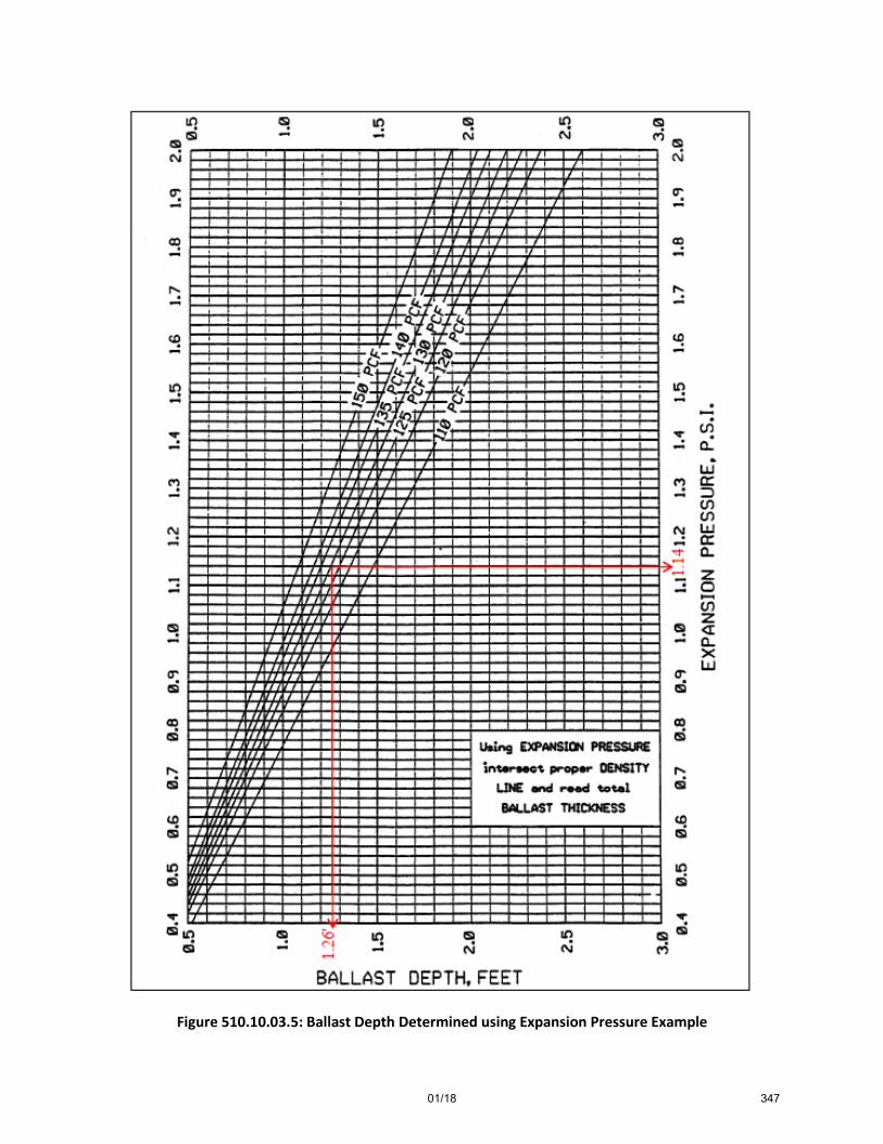
Figure 510.10.03.5: Ballast Depth Determined using Expansion Pressure Example

01/18 347

510.10.04 Major Route with Rock Cap Example. Assume an Interstate or major NHS Highway with the following design data: This is a major route, carrying in excess of 1000 trucks per day. To achieve pavement drainage, Open-graded Shot Rock Base (Rock Cap) is selected for base.

Table 509.10.04: Example 4 Design Data

2005 2025

Accumulated ESALs (Design Lane)

2,950,000 16,500,000

Subgrade R-value 48

Subgrade Expansion Pressure, psi 0.4

Unit Weight – Surfacing, pcf 147

Unit Weight - Rock Cap, pcf 110

Unit Weight - Rock Cap, pcf 130

Climatic Region 3

Assume Rock Cap has an R-value of at least 80, and that a source of granular subbase is available with an R-value of at least 60.


1. A plantmix binder/leveling course is placed an average of 0.15 feet thick over the rock cap before placing plantmix surface. This binder course is given no structural value. An overrun of 5 to 10% in plant mix binder should be expected due to penetration into the rock cap.

2. If aggregate base is used to level the surface of the rock cap, an overrun of up to 40% may occur depending on the gradation of the rock cap. Unless filter criteria is satisfied, this option is not recommended, since infiltration of the aggregate base may continue after paving. In certain conditions, where traffic must be routed over the Rock Cap before the plant mix binder can be placed, an aggregate base binder becomes necessary.

01/18 348

Calculate Traffic Index:

𝐸𝐸𝐸𝐸𝐸𝐸𝐸𝐸𝐸𝐸 = 29,500,000− 16,500,000

EASLs = 13,500,000

𝑇𝑇𝑇𝑇 = 9.0 �13,500,000106� �

0.119

TI = 12.27, use 12.3


𝐺𝐺𝐸𝐸 = 0.0032(12.3)(100− 80)(1.10)

GE = 0.87 ft.


𝑇𝑇 =0.87 𝑓𝑓𝑓𝑓

1.6

T = 0.54 ft., use 0.54 ft.

GE 1 (actual) = 0.54 × 1.6 = 0.86 ft.

Calculate the ballast requirement over subgrade.

𝐺𝐺𝐸𝐸 = 0.0032(12.9)(100− 48)(1.10)

GE = 2.25 ft.

Calculate the layer thickness by applying the substitution ratio for Rock Cap. (Table 510.05.1)

𝑇𝑇 =(2.25 𝑓𝑓𝑓𝑓.−0.86𝑓𝑓𝑓𝑓. )

1.20

T = 1.16 ft., use 1.20 ft.



NOTE: A subgrade separation geotextile must be placed over the subbase when rock cap is used. A subbase layer may be placed beneath the rock cap in some instances provided the filter criterion in Section 550.00 is satisfied.


01/18 349



𝐵𝐵 =(0.40 𝑝𝑝𝐸𝐸𝑖𝑖 × 144)


B = 0.44 ft. < 1.74 ft., OK.


0.54 foot plant mix pavement 1.20 foot Rock Cap


The above calculations were based on an averaged unit weight of 130 pcf. Where pavement components have different unit weights, a weighted average may be used to calculate the equivalent thickness, or make the comparison based on vertical pressure. The following example will recalculate the thickness when the unit weight of Rock Cap is 110 pcf rather than the assumed 130 pcf.

Compute weighted average unit weight:

[(0.54 ft.× 147) + (1.2 ft.× 110)](1.20 + 0.54)

= 121 pcf

Recalculate thickness required by expansion pressure. (Or use Figure 510.10.03.5.)


𝐵𝐵 =(0.40 𝑝𝑝𝐸𝐸𝑖𝑖 × 144)


B = 0.47 ft. (a 7% increase) < 1.74 ft., OK.

Calculate subgrade pressure exerted by pavement section.

𝑃𝑃 = (147 pcf × 0.54 ft) + (110 pcf × 1.2 ft. )

P = 211.38 pcf

𝑃𝑃 = �211.38 pcf

144�

P = 1.47 psi > 0.4 psi OK.

01/18 350

This example mentioned that Granular subbase is available so we will rerun the design using it as an additional layer and compare designs for cost effectiveness.

Since the granular subbase has an R-Value different than that of the subgrade soil, recalculate the ballast requirement for the Rock Cap layer to include a layer of granular subbase.

𝐺𝐺𝐸𝐸 = 0.0032(12.3)(100− 60)(1.10)

GE = 1.73 ft.

Recalculate the layer thickness by applying the substitution ratio for Rock Cap. (Table 510.05.1)

𝑇𝑇 =(1.73 𝑓𝑓𝑓𝑓.−0.86𝑓𝑓𝑓𝑓. )

1.20

T = 0.73 ft., use 0.75 ft. (Note: The Rock Cap reduced in thickness from 1.20 ft. to 0.75 ft. Check this thickness against the minimum thicknesses from Section 510.07, 0.75 ft. exceeds the minimum recommended Rock Cap layer thickness of 0.60 ft.)



Calculate the ballast requirements for granular subbase.

𝐺𝐺𝐸𝐸 = 0.0032(12.3)(100− 48)(1.10)

GE = 2.25 ft.


𝑇𝑇 =(2.25 𝑓𝑓𝑓𝑓.−1.76𝑓𝑓𝑓𝑓. )

0.85

T = 0.58 ft., use 0.60 ft.






𝐵𝐵 =(0.40 𝑝𝑝𝐸𝐸𝑖𝑖 × 144)


01/18 351

B = 0.44 ft. < 1.89 ft., OK.


0.54 foot plant mix pavement 0.75 foot Rock Cap 0.60 foot granular subbase


The above calculations were based on an averaged unit weight of 130 pcf. Where pavement components have different unit weights, a weighted average may be used to calculate the equivalent thickness, or make the comparison based on vertical pressure. As was done in the previous example, the following example will recalculate the thickness when the unit weight of Rock Cap is 110 pcf rather than the assumed 130 pcf and a granular subbase unit weight of 130 pcf.

Compute weighted average unit weight:

[(0.54 ft.× 147) + (0.75 ft.× 110) + (0.60 ft.× 130)](0.75 + 0.54 + 0.60)

= 127 pcf

Recalculate thickness required by expansion pressure. (Or use Figure 510.10.03.5.)


𝐵𝐵 =(0.40 𝑝𝑝𝐸𝐸𝑖𝑖 × 144)


B = 0.45 ft. (a 2% increase)

Calculate subgrade pressure exerted by pavement section.

𝑃𝑃 = (147 pcf × 0.54 ft) + (110 pcf × 0.75 ft. ) + (130 pcf × 0.60 ft. )

P = 239.88 pcf

𝑃𝑃 = �239.88 pcf

144�

P = 1.67 psi > 0.4 psi OK.

01/18 352

510.10.05 Four-Lane Interstate Example. Assume a four-lane interstate highway with the design data provided in Table 510.10.01.1. There is a need to perform a Reduced Design Period Thickness design for a period of eight years. This design will be run following the guidance in Section 510.07.

Table 510.10.01.1: Example 1 Design Data10364000

2007 2027


Reduced Design Period ESALS, 8 years 545,000 7,364,000


Subgrade expansion pressure in psi 0.60*


Climate region 2

*In this example, the subgrade expansion pressure is given. This value is determined in 510.03.03.



From Example 510.10.01, the typical section is composed of:


The section provides an actual total thickness of 2.98 feet and a gravel equivalent total thickness of 3.05 feet

Now, calculate the reduced design period ESALs.

01/18 353

𝐸𝐸𝐸𝐸𝐸𝐸𝐸𝐸𝐸𝐸 = 7,364,000− 545,000

EASLs = 6,819,000

𝑇𝑇𝑇𝑇 = 9.0 �6,819,000106� �

0.119

TI = 11.31, use 11.3



𝐺𝐺𝐸𝐸 = 0.0032(11.3)(100− 80)(1.05)

GE = 0.76 ft.



1.5

T = 0.51 ft., use 0.51 ft.

GE 1 (actual) = 0.51 × 1.5 = 0.77 ft.

Using the base and subbase from the full design, the reduced design period typical section is composed of:


Check the reduced design period pavement thickness provided by R-value design against the actual thickness requirement by expansion pressure.



𝐵𝐵 =(0.60 𝑝𝑝𝐸𝐸𝑖𝑖 × 144)


B = 0.66 ft. < 2.91 ft., OK. The R-Value design thickness exceeds the expansion pressure thickness.

Reducing the design period from 20 years to 8 years results in a plant mix thickness reduction of 0.07’. The designer will now have to decide of reducing the design period will achieve its intended purpose.

01/18 354

510.11 References.

Manual of Tests, California Department of Transportation, 1978, 2006, 2012.

AASHTO Guide for the Design of Pavement Structures, Washington D.C.: American Association of State Highway and Transportation Officials, 1993. AASHTO 93 is available to ITD employees at http://itdintranetapps/apps/ihs/ihs.aspx

Highway Research Record No. 13, "Thickness of Flexible Pavements by the California Formula Compared to AASHO Road Test Data," F.N. Hveem and G.B. Sherman.

Research Project No. 20, “An Evaluation of Flexible Pavement Design Methods”, 1964, L.F. Erickson, Research Division Idaho Department of Highways

Load Distribution Factors for Idaho Highways, 1984, R.C. Juola and J.R. Kilchoer.

Thickness Design - Asphalt Pavements for Highways and Streets (MS-1), 1991, The Asphalt Institute.

Asphalt Overlays for Highways and Street Rehabilitation (MS-17), 2000, The Asphalt Institute.

Principles of Pavement Design, 1975, E.J. Yoder and M.W. Whitczak.

Study of the Effectiveness of ITD Pavement Design Method, RP 199, F.M. Bayomy, S. F. El-Badawy, 2011

ARA, Inc., ERES Consultants Division. Guide for Mechanistic-Empirical Design of New and Rehabilitated Pavement Structures. Prepared for National Cooperative Highway Research Program, NCHRP 1-37A Final Report,” Washington, D.C.: March 2004.

Mechanistic-Empirical Pavement Design Guide, A Manual of Practice, July 2008 Interim Edition

Pavement Interactive, http://www.pavementinteractive.org/

Idaho AASHTOWare Pavement ME Design User’s Guide, Version 1.1, Mallela, J., L. Titus-Glover, B. Bhattacharya, M. Darter, H. Von Quintas, Applied Research Associates, Idaho Transportation Department ITD-RP 211B, (March 2014).

01/18 355

http://itdintranetapps/apps/ihs/ihs.aspx


SECTION 511.00 – SUBGRADE SEPARATION AND FILTRATION (Moved to Section 550.05)

01/18 356

SECTION 515.00 – THICKNESS DESIGN FOR FLEXIBLE PAVEMENT, AASHTO 93

515.00 Introduction. The design procedure described herein is based on the 1993 AASHTO GUIDE FOR DESIGN OF PAVEMENT STRUCTURES. The design guide may be used to determine the pavement thickness by hand following the step by step instructions that solve the design equation graphically using a series of figures. Computer software recognized by the department for flexible pavement design is DARWin™ 3.0 (or later) PAVEMENT DESIGN AND ANALYSIS SYSTEM. Alternatively a design utility created by Pavement Interactive that solves the 1993 AASHTO Guide basic design equation for flexible pavements is available.

Because Pavement ME currently does not determine layer thicknesses directly, the designer will need to perform a pavement design using the approved methods that are discussed in detail in this Section to develop the layer thicknesses used for the Pavement ME analysis trial design.

Perhaps the most widely used pavement design method in the United States and throughout the world is the American Association of State Highway and Transportation Officials (AASHTO) Guide for Design of Pavement Structures. A long history of pavement studies has led to the current edition. This empirical design procedure is based on the results of the AASHO road test conducted in Ottawa, Illinois, in the late 1950s and early 1960s. The first design guide was published in 1961 and was revised in 1972, 1981, and 1986, and 1993. The empirical performance equations obtained from the road test under certain traffic, climatic and subgrade conditions are used to compute the pavement layer thickness. The various versions of the AASHTO Design Guides have served well for several decades.

This design guide works for both flexible and rigid pavement designs. There are some variables common to both rigid and flexible pavement, including: serviceability, traffic loading, reliability, overall standard deviation, and roadbed soil resilient modulus. These variables and the ones specific to flexible pavement for the design of a flexible pavement structure are detailed in this section. The rigid equation and variables are addressed in Section 520.00.

The AASHTO pavement design equation for flexible pavement is shown in Figure 515.00.1 and each variable will be addressed in greater detail in Section 515.01.

𝑎𝑎𝑙𝑙𝑙𝑙10(𝑊𝑊18) = 𝑍𝑍𝑅𝑅 × 𝐸𝐸𝑜𝑜 + 9.36 × 𝑎𝑎𝑙𝑙𝑙𝑙10(𝐸𝐸𝑆𝑆 + 1)− 0.20 +𝑎𝑎𝑙𝑙𝑙𝑙10 �

∆𝑃𝑃𝐸𝐸𝑇𝑇4.2− 1.5�

0.40 + 1094(𝐸𝐸𝑆𝑆 + 1)5.19

+ 2.32 × 𝑎𝑎𝑙𝑙𝑙𝑙10(𝑀𝑀𝑅𝑅)− 8.07

Figure 515.00.1: AASHTO Pavement Design Equation for Flexible Pavement

The designer may use the design charts in the Design Guide or a computerized method to design the pavement structure.

01/18 357

515.01 Summary of Design Factors. The AASHTO pavement design equation for flexible pavement requires a number of inputs that the designer must determine before using. Some of the inputs values must be measured, such as the traffic evaluation to determine EASLs. Others must be determined by laboratory testing or in-place testing for properties such as soil resilient modulus. The remaining inputs are determined by selecting values from tables created as a result of the AASHO Road Test. These design inputs are common to the graphical solution, DARWin, or the Pavement Interactive design utility. The following is a summary of the user inputs into the AASHTO equation:

• Traffic, W18 – 18 kip equivalent single axle loads (ESALs).

• Serviceability, ΔPSI= po - pt.

o Initial Serviceability, po.

o Terminal Serviceability, pt.

• Reliability Level, R

• Overall Standard Deviation, So.

• Roadbed Soil Resilient Modulus, Mr.

• Drainage Coefficient, mi

• Structural Layer Coefficient, ai

• Number of Construction Stages

• Structural Number, SN.

01/18 358

515.01.01 Traffic Evaluation. Refer to Section 500.03 for a detailed discussion of traffic. Evaluate traffic according to Section 510.02. Use the estimate of accumulated, 18-kip ESALs for the design period as input to the design procedure. The design period is normally 20 years. Observe the directional split and lane distribution shown on the traffic data sheet. There is generally no need to use the EASL calculation capabilities of DARWin to determine EASLs.

515.01.02 Serviceability, ΔPSI. The AASHTO pavement design method was developed around the concept of serviceability. Serviceability is defined as the ability of a pavement to serve the type of traffic that uses the facility. The Present Serviceability Rating (PSR) was developed to measure serviceability. PSR is a rating of pavement ride based on a scale of 0, for impassible, to 5, for perfect. For the development of the original AASHTO pavement design equation, individuals (the raters) would ride the pavements and assign a PSR value. To avoid riding and rating every pavement by all raters to determine serviceability, a relationship between PSR and measurable pavement attributes (roughness and distress) was developed. This relationship is defined as the Present Serviceability Index (PSI). AASHTO’s recommendations for the selection of the terminal serviceability are shown in Table 515.01.02.1.

515.01.02.01 Initial Serviceability. Initial Serviceability (po) is a measure of the pavement’s smoothness or rideability immediately after construction. Serviceability is rated on a scale of 0 to 5, with 5 being a perfectly smooth pavement and 0 being a very rough impassible pavement. In most cases, the initial serviceability of a new pavement should be above 4. The average initial serviceability for flexible pavement at the AASHO Road Test was 4.2.

515.01.02.02 Terminal Serviceability. Terminal Serviceability (pt) is the tolerable serviceability of a pavement on the same 0 to 5 scale. When the serviceability of a pavement reaches its terminal value, rehabilitation is required. In contrast to initial serviceability, when measured based on construction records, terminal serviceability is a function of many factors, including pavement classification, traffic volume, and location. Typical terminal serviceability values are between 2 and 3, depending upon the functional classification of the roadway.

Values given in the Pavement Management System reports assign a terminal serviceability index of 2.5 for NHS designated routes and 2.0 for non-NHS routes. Therefore, an NHS route will have a Design Serviceability Loss, ΔPSI of 4.5 - 2.5 = 2.0. A Pt of 2.5 for major highways and 2.0 for highways of lesser traffic volumes should be the lowest allowable Terminal Serviceability Index (Pt) tolerated before rehabilitation, or reconstruction becomes necessary. AASHTO’s recommendations for the selection of the Terminal Serviceability Index are given in Table 515.01.02.1.

Table 515.01.02.1: AASHTO Recommended Terminal Serviceability Index

Functional Classification Recommended Terminal Serviceability Index, Pt

High Volume (>10,000 ADT) 3.0 – 3.5

Medium Volume (3,000 to 10,000 ADT) 2.5 – 3.0

Low Volume (<3,000) 2.0 – 2.5

01/18 359

515.01.03 Reliability Level. The inclusion of a reliability input in the pavement design process is a means of addressing variability. As defined by AASHTO Design Guide, reliability (R) is the probability (expressed as a percentage) that a pavement structure will survive the design period traffic. Generally, as traffic volumes become larger, and as the difficulty of diverting traffic and the public expectation of availability increases, the consequences of premature pavement failure increase dramatically; therefore, high-volume roadways must be constructed with a much higher level of reliability than low-volume roadways. The concept of reliability in rigid pavement design is identical to reliability in flexible pavement design. Reliability is represented in the AASHTO pavement design equation for flexible pavement as Standard Normal Deviate, ZR as shown in the AASHTO Design Guide, Part I, Chapter 4, Table 4.1.

Application of the reliability concept requires the following steps:

• Define the functional classification of the facility and determine whether a rural or urban condition exists.

• Select a reliability level from the range given in Table 515.01.03.1. The greater the value of reliability, the more pavement structure required.

• A standard deviation (So) should be selected that is representative of local conditions. Standard deviation is addressed in the next section.

AASHTO’s recommendation for the selection of the reliability values are given in Table 515.01.03.1.

Table 515.01.03.1: Recommended Level of Reliability

Functional Classification Recommended Level of Reliability, R

Interstate and Other Freeways 90%

Principal Arterial 85%

Minor Arterial 85%

Major Collector 80%

When considering reliability in stated construction (or planned rehabilitation), compound reliability must be taken into account. That is, if the overall reliability desired is a certain value, x, and n number of

stages are planned, including the initial construction, the reliability for each stage is 𝑥𝑥1𝑛𝑛. For example, if

the desired reliability is 90 percent and two stages are planned, the reliability factor for each stage must be, 0.901

2� or 95 percent. Staged construction is discussed in the section entitled Number of Construction Stages found later in this chapter.

Bayomy and El-Badawy found the 1993 AASHTO Design Guide, using 85% reliability, for flexible pavement design produced similar results to the Idaho R-Value design method. The conservative nature of ITD’s ESAL calculation which predicts higher ESAL values and the conservative conversion of the Idaho

01/18 360

R-value of soil to resilient modulus resulting in a lower Mr allow ITD to use a lower reliability level than recommended by the design guide. Caution should be observed when considering reducing the reliability level. It is permissible to use R= 50% for secondary or lower volume roadways.

515.01.04 Overall Standard Deviation. The overall standard deviation (So) accounts for all errors or variability associated with design and construction, including variability in material properties, roadbed soil properties, traffic estimates, climatic conditions, and quality of construction. Ideally, these values should be based on local conditions; however, in the absence of other values, the AASHTO Design Guide does provide recommended values. For the case where the variance of projected future traffic is not considered, the AASHTO Design Guide recommends a value of 0.44. In situations where the variance of projected future traffic is considered, a value of 0.49 is recommended.

The two different values reflect the designer’s confidence in the projected ESALs. If there is a strong confidence in the ESAL calculation, then the lower value of 0.44 should be used.

It is important to note that by accounting for design uncertainties through the use of reliability and standard deviation. Average values should be used for all other design inputs rather than conservative values.

ITD has not established variability values based on local conditions and the recommendations provided above should be used.

01/18 361

515.01.05 Roadbed Soil Resilient Modulus. The resilient modulus (Mr) is the material property used to characterize the support characteristics of the roadbed soil in flexible pavement design. In general terms, it is a measure of the soil’s deformation in response to repeated (cyclic) applications of loads much smaller than a failure load.

The AASHTO design procedure requires the input of an effective roadbed resilient modulus. This effective roadbed resilient modulus is a means of representing the combined effect of all the seasonal modulus values by a type of weighted average. If the effective resilient modulus value is known, it may be entered directly. If seasonal modulus values are known, DARWin can calculate the effective resilient modulus. The Pavement Interactive design utility will not calculate the effective resilient modulus from seasonal data. When using the graphical method, refer to the AASHTO Design Guide, Part II Section 2.3.1 and Figure 2.3, for guidance.

515.01.06 Drainage Coefficient. This section describes the selection of inputs to treat the effects of certain levels of drainage on predicted pavement performance. See Section 550.00 Subsurface Pavement Drainage for detailed guidance on drainage design.

The effect of drainage on pavement life for flexible pavements is quantified through the use of the drainage coefficient (mi). This factor has been integrated into the structural number equation as a modifier to the layer coefficient (ai) and the layer thickness (di).

𝐸𝐸𝑆𝑆 = 𝐿𝐿1𝑑𝑑1 + 𝐿𝐿2𝑑𝑑2𝑚𝑚2 + 𝐿𝐿3𝑑𝑑3𝑚𝑚3

The drainage coefficient is only meaningful in considering the effects of drainage on untreated base and subbase. The possible effects of drainage on asphalt concrete surface course and on stabilized layers is not considered (i.e. m1 = 1). Thus for any such layer, including the pavement surface, a mi of 1 should be entered. This is shown in the above equation by the omission of the drainage coefficient as a modifier to the surface course.

The effect of drainage on pavement performance is a function of the quality of drainage (i.e., the time required for the pavement to drain) and the amount of time during the year that the pavement structure is exposed to moisture levels approaching saturation. It is up to the designer to determine the relative levels of each of these values for the specific conditions being considered for design.

The quality of drainage depends on the permeabilities of the base and foundation materials, the design of the structural cross section, and the presence of edge drains. The amount of time during the year that the pavement will be exposed to near saturation levels is a function of precipitation and evapotranspiration characteristics that are inherent to a particular climate region. Guidance on the selection of the drainage coefficient is provided in Table 515.01.06.1 and Table 515.01.06.2.

Table 515.01.06.1 shows the general definitions corresponding to different drainage levels from the pavement structure and Table 515.01.06.2 presents the recommended mi values as a function of the quality of drainage and the percent of time during the year the pavement would normally be exposed to moisture levels approaching saturation:

01/18 362

Table 515.01.06.1: General Definitions of Drainage Levels

Quality of Drainage Water Removed within:

Excellent 2 hours

Good 1 day

Fair 1 week

Poor 1 month

Very Poor (water will not drain)

After obtaining the quality of drainage from the Table above, the drainage coefficient (Cd) for rigid pavement design is provided from Table 515.01.06.2.

Table 515.01.06.2: Recommended mi for Modifying Structural Layer Coefficients of Untreated Base and Subbase Materials in Flexible Pavement.

Percent of Time Pavement Structure is Exposed

to Moisture Levels Approaching Saturation.

Quality of Drainage

Less Than 1%

1 - 5% 5 – 25% Greater Than

25%

Excellent 1.40-1.35 1.35-1.30 1.30-1.20 1.20

Good 1.35-1.25 1.25-1.15 1.15-1.00 1.00

Fair 1.25-1.15 1.15-1.05 1.05-0.80 0.80

Poor 1.15-1.05 1.05-0.80 0.80-0.60 0.60

Very Poor 1.05-0.95 0.95-0.75 0.75-0.40 0.40

The value of drainage coefficient, Cd, can be obtained from Table 520.01.07.2. The recommended values for flexible pavement design based on ITD aggregates are provided from Table 520.01.07.3 below:

Table 520.01.07.3: Recommended Values of Cd

Type of Material Drainage Coefficient, Cd

Rock Cap 1.20

3/4" Aggregate Base 0.50 – 1.00* *Use higher value range for Type A and lower for Type B aggregate bases.

01/18 363

515.01.07 Structural Layer Coefficients. This section describes method for estimating the AASHTO structural layer coefficients (ai values) required for standard flexible pavement structural design. A value for this coefficient is assigned to each layer material in the pavement structure in order to convert actual layer thickness into structural number (SN). This layer coefficient expresses the empirical relationship between SN and thickness and is a measure of the relative ability for the material to function as a structural component of the pavement. The AASHTO Design Guide published charts for several different materials as follows:

• Asphalt Concrete Surface Course. Figure 515.01.07.1 provides a chart that may be used to estimate the structural layer coefficient of dense graded asphalt concrete surface course based on its elastic (resilient) modulus (EAC) at 68 °F. Caution is recommended for modulus values above 450,000 psi. Although higher modulus asphalt concretes are stiffer and more resistant to bending, they are also more susceptible to thermal and fatigue cracking.

• Granular Base Layers. Figure 515.01.07.2 provides a chart that may be used to estimate a structural layer coefficient, a2, from one of four different laboratory test results on a granular base material, including base resilient modulus EBS. The AASHO Road Test basis for these correlations is:

o a2 = 0.14 o EBS = 30,000 psi o CBR = 100 (approx.) o R-value = 85 (approx.) (Note: The R-Value described here is not an Idaho R-Value, IT-8).

• Granular Subbase Layers. Figure 515.01.07.3 provides a chart that may be used to estimate a structural layer coefficient, a3, from one of four different laboratory test results on a granular subbase material, including base resilient modulus ESB. The AASHO Road Test basis for these correlations is:

o a3 = 0.11 o ESB = 15,000 psi o CBR = 30 (approx.) o R-value = 60 (approx.) (Note: The R-Value described here is not an Idaho R-Value, IT-8).

• Cement-Treated Base. Figure 515.01.07.4 provides a chart that may be used to estimate a structural layer coefficient, a2, for a cement-treated base material from either its elastic modulus, EBS, or, alternatively its 7-day unconfined compressive strength (ASTM D 1633).

• Bituminous-Treated Base. Figure 515.01.07.5 provides a chart that may be used to estimate a structural layer coefficient, a2, for a bituminous-treated base material from either its elastic modulus, EBS, or, alternatively its Marshall stability (AASHTO T 245).

• Subgrade Soils. Figure 515.01.07.6 provides a chart that may be used to estimate a roadbed soil resilient modulus from Idaho R-value based on the equation.

01/18 364

515.01.08 Number of Construction Stages. Experience has shown that regardless of the structural capacity of some pavements, there may be a maximum performance period associated with a given initial structure subjected to significant levels of heavy truck traffic. If this performance period is less than the analysis period, there may be a need to consider staged construction or planned rehabilitation in the design analysis. Staged construction is also appropriate when the pavement structure needed to carry the projected traffic cannot be constructed for economic reasons.

When considering staged construction, it is especially important to recognize the need to compound the design reliability for each individual stage of strategy. For example, if each stage of a three-stage strategy (e.g. an initial pavement design with two overlays) has 90 percent reliability, the overall reliability of the design strategy is 0.903, or 72.9 percent. Conversely, if an overall reliability of 95 percent is desired for the same three stage project, the individual reliability for each stage must be 0.951/3 or 98.3 percent.

The input that is called for is the number of planned construction stages. DARWin will make the necessary adjustments to the reliability factor based on the number of stages selected. The Pavement Interactive design utility will not calculate the design reliability for staged construction.

515.01.09 Structural Number. The Structural Number is an abstract number expressing the structural strength of a pavement required for given combinations of soil support (MR) total traffic expressed in ESAL, terminal serviceability and environment. The structural number represents the ability of a flexible pavement to withstand structural loadings and can be solved using a Nomograph or computer.

The AASHTO equation may be solved for SN when ESAL are known or it can be solved for ESAL if the SN is known. For ITD pavement designs, the designer will solve the equation for SN.

01/18 365

Figure 515.01.07.1: Chart for Estimating Structural Layer Coefficient of Dense Graded Asphalt Concrete Based on the Elastic (Resilient) Modulus

01/18 366

Figure 515.01.07.2: Variation in Granular Base Layer Coefficient (a2) with various Base Strength Parameters

01/18 367

Figure 515.01.07.3: Variation in Granular Subbase Layer Coefficient (a3) with various Subbase Strength Parameters

01/18 368

Figure 515.01.07.4: Variation in a2 for Cement-Treated Base with Base Strength Parameters

01/18 369

Figure 515.01.01.5: Variation in a2 for Bituminous-Treated Base with Base Strength Parameters

01/18 370

Figure 515.01.07.6: Approximate Relationship Between R-value and Resilient Modulus

01/18 371

515.02 Selection of Layer Thicknesses. Once the design structural number (SN) for an initial pavement structure is determined by solving the empirical equation for SN in Figure 515.00.1, it is necessary to identify a set of pavement layer thicknesses which, when combined, will provide the load carrying capacity corresponding to the design SN. The following equation provides the basis for converting SN into actual thicken of surfacing, base, and subbase:

𝐸𝐸𝑆𝑆 = 𝐿𝐿1𝐷𝐷1 + 𝐿𝐿2𝐷𝐷2𝑚𝑚2 + 𝐿𝐿3𝐷𝐷3𝑚𝑚3

Where

a1, a2, a3 = layer coefficients representative of surface, base, and subbase courses respectively (see Section 515.01.07)

D1, D2, D3 =actual thickness (in inches), of surface, base, and subbase courses respectively, and;

m2, m3 = drainage coefficients for base and subbase layers, respectively (see Section 515.01.06)

The SN does not have a single unique solution; i.e., there are many combinations of layer thicknesses that are satisfactory solutions. The thickness of flexible pavement layers should be rounded to the nearest ½ inch. When selecting appropriate values for the layer thicknesses, it is necessary to consider their cost effectiveness along with the construction and maintenance constraints.

Since it is generally impractical and uneconomical to place surface, base, or subbase courses of less than some minimum thickness, the minimum thicknesses provided in Section 510.06 should be used.

01/18 372

515.03 Solving the Flexible Pavement Equation. This section allows the designer to use three different methods to solve the AASHTO equation. The reason for this flexibility is that it is unclear which of these design tools the designer will have available to them when they are performing the design. The design may be performed in any of the following ways:

515.03.01 1993 AASHTO Guide For Design of Pavement Structures. This design guide may be used to solve the flexible pavement equation and determine the pavement structure. The design guide covers all of the information previously summarized in this section and uses a series of figures and tables as input into a Nomograph, shown in Figure 515.03.01.1, to graphically solve the equation in Figure 515.00.1. For assistance contact the Construction/Materials Section. ITD personnel may access this document at: http://itdintranetapps/apps/ihs/ihs.aspx

515.03.02 Design and Rehabilitation for Windows (DARWin™). This computer software was developed to solve the flexible pavement equation for flexible pavement designs. DARWin 3.0 (or later) PAVEMENT DESIGN AND ANALYSIS SYSTEM is an AASHTOWare product that is no longer supported, maintained or licensed as of July 1, 2012. Existing unlimited license holders may continue using the software at their own risk without technical support or maintenance. This program is available to ITD personnel and cannot be shared with non-ITD personnel. This program will not work on newer operating systems but it will run in virtual Windows XP mode. Use the following link to install Windows Virtual PC: http://windows.microsoft.com/en-us/windows7/install-and-use-windows-xp-mode-in-windows-7. Follow the design procedures in the AASHTOWare DARWin 3.0 Pavement Design and Analysis System User’s Guide for further information on using the DARWin software. For assistance contact the Construction/Materials Section.

515.03.03 Pavement Interactive Design Utility. Alternatively the design inputs can be used in conjunction with the design utility created by Pavement Interactive that solves the 1993 AASHTO Guide basic design equation for flexible pavements:

http://www.pavementinteractive.org/article/1993-aashto-flexible-pavement-structural-design/

This design utility only solves the basic design equation for flexible pavements and does not have the full functionality that DARWin 3.0 has. For assistance contact the Construction/Materials Section.

01/18 373


http://windows.microsoft.com/en-us/windows7/install-and-use-windows-xp-mode-in-windows-7


515.04 Thickness Design Procedures. The designer may use any of the three methods described above for determining the thickness of the various layers in a flexible pavement. These are all based on the Layered Analysis Thickness Design method and are recommended for ITD designs.

515.04.01 Layered Analysis Thickness Design. It should be recognized that, for flexible pavements, the structure is a layered system and should be designed accordingly. The structure should be designed in accordance with the principals shown in Figure 515.04.01.1. (This is very similar to the procedure of Section 510.00.) First, the structural number required over the roadbed soil is computed. In the same way, the structural number required over the subbase layer and base layer are also computed, using the applicable strength value of each. By working with differences between the computed structural numbers required over each layer, the maximum allowed thickness of any given layer can be computed.

For example, the maximum allowable structural number for subbase material would be equal to the structural number required over the subbase subtracted from the structural number required over the roadbed soil. In a like manner, the structural numbers for the other layers may be computed. The thicknesses for all such layers may then be determined as indicated in Figure 515.04.01.1. Working from the subgrade up, a SN is calculated for each specified layer, and the corresponding thickness of that layer is calculated by dividing that SN by the product of the structural coefficient and the drainage coefficient for that layer.

The designer should begin by making a sketch of the pavement cross section to be designed as in Figure 515.04.01.1. This is the same sketch as in Section 510.00 except this sketch is labeled with SN rather than GE. When using the DARWin software, it will create a sketch that can be printed.

The equation is not valid for calculating the SN for any layer above a layer that has an elastic modulus greater than 40,000 psi.

A Layered Analysis worksheet for flexible pavement design is provided in Figure 515.04.01.2 for convenience in solving for the pavement thickness. The designer may input the SN values determined from the nomograph along with the ai and mi values for each layer onto the sketch of the pavement section and fill in the boxes with the appropriate values and do the calculations.

01/18 374

Figure 515.03.01.1: Design Chart for Flexible Pavements Based on Using Mean Values for Each Input

01/18 375

Figure 515.04.01.1: Procedure for Determining Thickness of Layers Using a Layered Analysis Approach

01/18 376

Figure 515.04.01.2: Layered Analysis Worksheet

01/18 377

515.04.02 Layered Analysis Thickness Design Using a Graphical Solution. The following steps describe the design procedure using the Nomograph in Figure 515.04.02.01.1 to determine the SN.

515.04.02.01 Structural Number: The designer must provide the following information:

1) The estimated future traffic, W18 (Section515.01.01), for performance period

2) The design serviceability loss, ΔPSI = po-pt (Section 515.01.02)

3) The reliability, R (Section 515.01.03), which assumes all input is at average value

4) The overall standard deviation, So, (Section 515.01.04)

5) The effective resilient modulus of roadbed material, MR (Section 515.01.05),

515.04.02.02 Determine Structural Number: Determine the Structural Number manually from Figure 515.04.01.1 for the subgrade soil, the subbase, and the aggregate base as follows:

1) Start at the left edge of the graph. Using a straightedge, draw a line from the appropriate Reliability, R through the appropriate Overall Standard Deviation, SO to the first turning line.

2) From the first turning line, draw a line through the appropriate Estimated Total 18-kip Equivalent Single Axle Load (ESALs), W18 to the second turning line.

3) From the second turning line, draw a line through the appropriate MR, Effective Roadbed Soil Resilient Modulus, Subbase, or base, to the Design Structural Number chart.

4) From the design Structural Number chart draw a horizontal line to intersect with the appropriate Design Serviceability Loss, ΔPSI line.

5) From the appropriate Design Serviceability Loss, ΔPSI line, draw a vertical line down to intersect the appropriate Design Structural Number. This is the SN value.

Normally, Steps 1 and 2 do not have to be repeated for each material. The designer may draw separate lines from the second turn line through the appropriate MR and determine all SN values on a single chart. An example of a completed chart is shown in Figure 515.04.02.02.1.

515.04.02.03 Selection of Layer Thicknesses: Using the SN values determined above, determine trial layer thicknesses D1, D2, and D3. Using the layer coefficients and drainage coefficients representative of the respective layers, solve the equations in Figure 515.04.01.1. Di* and SNi* are the actual rounded up values used and must be equal to or greater than the required values.

Using the equation 𝐷𝐷1∗ ≥ 𝐸𝐸𝑆𝑆1 𝐿𝐿1⁄ , and knowing SN1 from Figure 515.04.02.02.1 and a1, solve for D1*. Calculate SN* by rounding D* up to the nearest one-half inch. Determine SN1* as follows:

01/18 378

𝐸𝐸𝑆𝑆1∗ = 𝐷𝐷1∗ × 𝐿𝐿1 ≥ 𝐸𝐸𝑆𝑆1. Using the equation 𝐷𝐷2∗ ≥ (𝐸𝐸𝑆𝑆2 − 𝐸𝐸𝑆𝑆1∗) (𝐿𝐿2 × 𝑚𝑚2)⁄ and knowing SN1* from above and SN2 from Figure 515.04.02.02.1 along with a2 and m2, solve for D2*. Determine SN2* as follows: 𝐸𝐸𝑆𝑆2∗ = 𝐷𝐷2∗ × 𝐿𝐿2 × 𝑚𝑚2 ≥ 𝐸𝐸𝑆𝑆2, and 𝐸𝐸𝑆𝑆1∗ + 𝐸𝐸𝑆𝑆2∗ ≥ 𝐸𝐸𝑆𝑆2.

Finally, solve the equation 𝐷𝐷3∗ ≥ �𝐸𝐸𝑆𝑆3 − (𝐸𝐸𝑆𝑆1∗ + 𝐸𝐸𝑆𝑆2∗)� (𝐿𝐿3 ×𝑚𝑚3)⁄ knowing SN1* and SN2*from above and SN3 from Figure 515.04.02.02.1 along with a3 and m3, solve for D3*. Determine SN3* as follows: 𝐸𝐸𝑆𝑆3∗ = 𝐷𝐷3∗ × 𝐿𝐿3 × 𝑚𝑚3 ≥ 𝐸𝐸𝑆𝑆3, and 𝐸𝐸𝑆𝑆1∗ + 𝐸𝐸𝑆𝑆2∗ + 𝐸𝐸𝑆𝑆3∗ ≥ 𝐸𝐸𝑆𝑆3.

The worksheet in Figure 515.04.01.2 may be used to keep this series of equations in the proper order and as an aid in solving them.

515.04.02.04 Design Example: From Example 510.09.01, the information in Table 515.04.02.04.1 is given:

Table 515.04.02.04.1: Example 1 Design Data Needed for AAASHTO 93 vs. Idaho R-value.

Idaho R-value AASHTO 93

ESALs (design lane), W18 20,847,000 20,847,000

Aggregate Base, R-value R-value = 80 MR ≈ 30,000 (Figure 515.01.07.2)

Granular Subbase, R-value R-value = 60 MR ≈ 11,000 (Figure 515.01.07.3)

Subgrade Soil, R-value R-value = 30 MR ≈ 5,000* (Figure 515.01.07.6)

Plant Mix Surface N/A MR ≈ 400,000 (Figure 515.01.07.1)

Plant Mix Surface Substitution Ratio = 1.5 a1 = 0.44 (515.01.07)

Aggregate Base Substitution Ratio = 1.0 a2 = 0.14 (515.01.07)

Granular Subbase Substitution Ratio = 0.85 a3 = 0.08 (515.01.07)

Climate Region 2 N/A

Plant Mix Surface N/A m1 = 1.0 (515.01.06)

Aggregate Base N/A m2 = 1.0 (515.01.06)

Granular Subbase N/A m3 = 1.0 (515.01.06)

Reliability Level, R N/A 85%

Overall Standard Deviation N/A 0.44

ΔPSI N/A 2.0 (for Interstate)

Subgrade Expansion Pressure 0.60 psi N/A

Unit Weight of base and surface 130 pcf N/A

*MR value in this example is given and not derived from Figure 515.01.07.6 or AASHTO 93 Figure 2.3

01/18 379

Figure 515.04.02.02.1: Design Chart for Flexible Pavement Based on Using Mean Values for Each Input

01/18 380

From Figure 515.04.02.02.1, SN1 ≈ 3.2 for the subgrade soil. SN2 ≈ 4.5 for granular borrow, and SN3 ≈ 5.9 for aggregate base.

𝐷𝐷1∗ ≥𝐸𝐸𝑆𝑆1 𝐿𝐿1� , and

𝐷𝐷1∗ = 3.20.44�

D1 = 7.27, Use 7.5” or 0.62 ft. plant mix pavement.

𝐸𝐸𝑆𝑆1∗ = 7.5 × 0.44 = 3.3

𝐸𝐸𝑆𝑆1∗ ≥ 𝐸𝐸𝑆𝑆1

3.3 ≥ 3.2

𝐷𝐷2∗ ≥(𝐸𝐸𝑆𝑆2 − 𝐸𝐸𝑆𝑆1∗)

(𝐿𝐿2 × 𝑚𝑚2)� , and

𝐷𝐷2∗ = (4.5− 3.3)(0.14 × 1.0)�

D2 = 8.57, Use 9.0” or 0.75 ft. aggregate base.

𝐸𝐸𝑆𝑆2∗ = 9 × 0.14 × 1.0 = 1.26"

𝐸𝐸𝑆𝑆1∗ + 𝐸𝐸𝑆𝑆2∗ ≥ 𝐸𝐸𝑆𝑆2

3.3 + 1.26 = 4.56 ≥ 4.5

𝐷𝐷3∗ ≥�𝐸𝐸𝑆𝑆3 − (𝐸𝐸𝑆𝑆1∗ + 𝐸𝐸𝑆𝑆2∗)�

(𝐿𝐿3 × 𝑚𝑚3)�

𝐷𝐷3∗ ≥�5.9 − (3.3 + 1.26)�

(0.08 × 1.0)�

D3 = 16.75, Use 17” or 1.42 ft. granular subbase.

𝐸𝐸𝑆𝑆3∗ = 17 × 0.08 × 1.0 = 1.36

3.3 + 1.26 + 1.36 = 5.92 ≥ 5.9



Figure 515.04.02.04.1 shows the above example solved using the worksheet.

01/18 381

Figure 515.04.02.04.1: Solution to Design Example Using Worksheet

01/18 382

515.04.03 Layered Analysis Thickness Design Using AASHTOWare DARWin™ 3.0 or later. The following steps describe the design procedure using the DARWin program to determine the SN and to determine the pavement layer thicknesses.

515.04.03.01 Structural Number: The designer must provide the same information as was needed for the graphical solution and input it into DARWin. The designer should refer to the DARWin User’s guide for additional information.

515.04.03.01.01 Using DARWin to Determine the Structural Number. The designer will determine SN for use in the design as described in Figure 515.04.03.01.01.1 through Figure 515.04.03.01.01.5.

Start DARWin by clicking on the icon and the screen in Figure 515.04.03.01.01.1 should appear.

Figure 515.04.03.01.01.1: AASHTOWare DARWin™3.0 Opening Screen

Click on “File” then “New” to get to the screen in Figure 515.04.03.01.01.2.

01/18 383

Figure 515.04.03.01.01.2: DARWin New Project Entry Screen

Enter Project Name, click “English”, click “DARWin Project” and click OK to get Figure 515.04.03.01.01.3.

Figure 515.04.03.01.01.3: Project Screen

Click “Insert” from the menu bar at the top of the screen and “New DARWin Module” box will appear as shown in Figure 515.04.03.01.01.4.

01/18 384

Figure 515.04.03.01.01.4: New DARWin Module Screen

Select Flexible Structural Design and click OK and get the screen in Figure 515.04.03.01.01.5.

Figure 515.04.03.01.01.5: Primary Design Inputs for Flexible Pavement Design SN

01/18 385

Fill in all the boxes with the same information that was used for the graphical solution of SN. Click the box in the bottom left corner to calculate SN. The SN calculated here is used in the thickness design described in the next section. If the designer has a single Roadbed Soil Resilient Modulus value, insert in the appropriate box. If the designer has seasonal data, follow the instructions from Section 515.01.05.

515.04.03.02 Selection of Layer Thicknesses. Using the SN values determined above, determine layer thicknesses D1, D2, and D3. Using the layer coefficients and drainage coefficients representative of the respective layers, DARWin will solve the equations in Figure 515.04.1 using the following steps.

From the screen in Figure 515.04.03.01.01.5, click on “Design” from the menu bar at the top of the screen. The screen in Figure 515.04.03.02.1 will appear and make sure the “Layered” tab is highlighted. Click on the “Insert New Row” button in the top right corner of the screen and add the number of layers needed.

Figure 515.04.03.02.1: Flexible Pavement Layers by the Layered Thickness Design Method20

Once the data is input into the thickness design screen, the screen should look like Figure 515.04.03.02.2. DARWin allows a minimum thickness to be input to satisfy design policy. Also, the width of the pavement in one direction may be input to create a cross section and to calculate quantities. These columns may be left blank by the designer. With the SN previously calculated, the thickness of each layer is determined along with the SN of each layer.

01/18 386

Figure 515.04.03.02.2: Thickness Design Screen

515.04.03.03 Design Example: The information from Example 515.04.02.04 and Table 515.04.02.04.1 is input into DARWin as shown in Figure 515.04.03.03.1 and a SN of 5.73 is calculated.

Figure 515.04.03.03.1: Flexible Design Example

01/18 387

Input the information for each layer of the pavement section as shown in Figure 515.04.03.02.2. DARWin calculated the thicknesses that will provide an appropriate SN for each layer and compares the total to the design SN. The calculated SN must be equal to or greater than the design SN just as was the case in the graphical example.

Figure 515.04.03.03.2: Flexible Design Example, (continued)

From DARWin, the pavement thickness for the example from Section 515.04.03.03 is as follows:

7.14” or 0.60 foot plant mix pavement 9.41” or 0.80 foot crushed aggregate base 15.87” or 1.32 feet granular subbase

Figure 515.04.03.03.3 shows the pavement design report that DARWin prints out. The DARWin software also allows the designer to create sensitivity plots for ESALs, Serviceability, Reliability, Standard Deviation, and Resilient Modulus. Refer to the DARWin User’s Guide for further information regarding the printing capabilities of this software.

01/18 388

Figure 515.04.03.03.3: Flexible Design Example DARWin Report

01/18 389

515.04.04. Layered Analysis Thickness Design Using the Pavement Interactive Design Utility. A third way of calculating the pavement thickness by the AASHTO method is by using the Pavement Interactive design utility. The following steps describe this design procedure:

515.04.04.01 Structural Number and Layer Thickness. The designer goes to the Pavement Interactive website and navigates to the following website.


This article provides additional information concerning the flexible empirical equation and includes instructions on using the utility. At the bottom of the article is the design utility that the designer will input the project information. Figure 515.04.04.01.1 below is a screen shot of the design utility showing the inputs required and the outputs that are calculated.

Figure 515.04.04.01.1: Flexible Pavement Design Utility

Section 515.04.04.02 shows an example using the data used in Example 515.04.02.04.

01/18 390


515.04.04.02 Design Example: From Example 510.09.01, the information in Table 515.04.02.04.1 is input in the design utility as shown in Figure 515.04.04.01.1. Type in data into the grey boxes and click the calculate button. By selecting the “See Solution Details” button, Figure 515.04.04.02.2 through Figure 515.04.04.02.4 appears and provides detailed information on the design. These are the same calculations that were performed in the graphical solution example and by DARWin.

Figure 515.04.04.02.1 Design Example

From Figure 515.04.04.02.1, the pavement thickness for the example from 515.04.02.04 using the Pavement Interactive Utility is as follows:

7.5” or 0.63 foot plant mix pavement 8” or 0.67 foot crushed aggregate base 16.5” or 1.38 feet granular subbase

01/18 391

Figure 515.04.04.02.2: Solution Details

Figure 515.04.04.02.3: Solution Details, continued

Figure 515.04.04.02.4: Solution Details, continued

01/18 392

515.05 Summary of Design Examples. Section 515.00 provides the designer with three ways to use the 1993 AASHTO Guide for the Design of Pavement Structures to determine pavement thicknesses. The results from using the graphical methods, DARWin, and Pavement Interactive, shown in Table 515.05.1, give slightly different answers for the example provided in this section. The designer should not expect identical thickness vales but they should be close enough to be considered equivalent for design purposes. Idaho R-value method gives slightly thinner surface and slightly thicker base and subbase. The pavement thickness determined in these chapters will be analyzed by Pavement ME to determine if they will achieve the intended design life.

Table 515.05.1

Design Method Idaho R-Value

AASHTO 93

Graphical DARWin Pavement Interactive

Surface 0.58’ 0.62’ 0.6’ 0.63 Base 0.9’ 0.75’ 0.8’ 0.67 Subbase 1.5’ 1.42’ 1.32’[ 1.38’

515.06 Design Analysis. Once the designer has determined the thickness of the flexible pavement layers, by any of the methods described in Section 510.00 or Section 515.00, these values will be used as the initial trial thickness design in Pavement ME. The Idaho AASHTOWare Pavement ME Design User Guide will provide guidance to analyze and adjust the layer thicknesses to meet the requirements of Pavement ME.

01/18 393

515.07 References.

AASHTO Guide for Design of Pavement Structures, Washington D.C.: American Association of State Highway and Transportation Officials, 1993. This document is available to ITD employees at: http://itdintranetapps/apps/ihs/ihs.aspx

AASHTOWARE DARWin™ 3.0 Pavement Design and Analysis System, User’s Guide





Bayomy, F.M., S. F. El-Badawy, Study of the Effectiveness of ITD Pavement Design Method, Moscow, ID: National Institute for Advanced Transportation Technology, University of Idaho, Idaho Transportation Department, ITD RP 199, (November 2011).


Idaho AASHTOWare Pavement ME Design User’s Guide, Version 1.1, Mallela, J., L. Titus-Glover, B. Bhattacharya, M. Darter, H. Von Quintas, Applied Research Associates, Idaho Transportation Department ITD-RP 211B, (March 2014).

01/18 394



SECTION 520 – THICKNESS DESIGN FOR RIGID PAVEMENT, AASHTO 93

520.00 Introduction. The design procedure described herein is based on the 1993 AASHTO GUIDE FOR DESIGN OF PAVEMENT STRUCTURES. The design guide may be used to determine the pavement thickness by hand following the step by step instructions that solve the design equation graphically using a series of figures. Computer software recognized by the department for rigid pavement design is DARWin™ 3.0 (or later) PAVEMENT DESIGN AND ANALYSIS SYSTEM. Alternatively a design utility created by Pavement Interactive that solves the 1993 AASHTO Guide basic design equation for rigid pavements is available.

Because Pavement ME currently does not determine layer thicknesses directly, the designer will need to perform a pavement design using the approved methods that are discussed in detail in this Section to develop the layer thicknesses used for the Pavement ME analysis trial design.

Perhaps the most widely used pavement design method in the United States and throughout the world is the American Association of State Highway and Transportation Officials (AASHTO) Guide for Design of Pavement Structures. A long history of pavement studies has led to the current edition. This empirical design procedure is based on the results of the AASHO road test conducted in Ottawa, Illinois, in the late 1950s and early 1960s. The first design guide was published in 1961 and was revised in 1972, 1981, and 1986, and 1993. The empirical performance equations obtained from the road test under certain traffic, climatic and subgrade conditions are used to compute the pavement layer thickness. The various versions of the AASHTO Design Guides have served well for several decades.

This design guide works for both flexible and rigid pavement designs. There are some variables common to both rigid and flexible pavement, including: serviceability, traffic loading, reliability, overall standard deviation, and roadbed soil resilient modulus. These variables and the ones specific to rigid pavement for the design of a rigid pavement structure are detailed in this section. The flexible equation and variables are addressed in Section 515.00.

The AASHTO pavement design equation for rigid pavement is shown in Figure 520.00.1 and each variable will be addressed in greater detail in Section 520.01.

𝑎𝑎𝑙𝑙𝑙𝑙10(𝑊𝑊18) = 𝑍𝑍𝑅𝑅 × 𝐸𝐸𝑜𝑜 + 7.35 × 𝑎𝑎𝑙𝑙𝑙𝑙10(𝐷𝐷 + 1) − 0.06 +𝑎𝑎𝑙𝑙𝑙𝑙10 �

∆𝑃𝑃𝐸𝐸𝑇𝑇4.5− 1.5�

1 + 1.624 × 107(𝐷𝐷 + 1)8.46

+ (4.22− 0.32𝑝𝑝𝑡𝑡) × 𝑎𝑎𝑙𝑙𝑙𝑙10

⎣⎢⎢⎢⎢⎢⎢⎡

(𝐸𝐸ʹ𝑐𝑐)�(𝐶𝐶𝑑𝑑)�(𝐷𝐷0.75 − 1.132)

215.63(𝐽𝐽)�𝐷𝐷0.75 − 18.42

��𝐸𝐸𝑐𝑐 𝑖𝑖� �0.25

��

⎦⎥⎥⎥⎥⎥⎥⎤

Figure 520.00.1: AASHTO Pavement Design Equation for Rigid Pavement

01/18 395

520.01 Summary of Factors. The AASHTO pavement design equation for rigid pavement requires a number of inputs that the designer must determine before using. Some of the input values must be measured, such as the traffic evaluation to determine EASLs. Others must be determined by laboratory testing or in-place testing for properties such as soil resilient modulus. The remaining inputs are determined by selecting values from tables originally created as a result of the AASHO Road Test. These design inputs are common to the graphical solution, DARWin, or the Pavement Interactive design utility. The following is a summary of the user inputs into the AASHTO equation:

• Traffic, W18 - 18 kip equivalent single axle loads (ESALs).

• Design Serviceability Loss, ΔPSI = po - pt.

o Initial Serviceability, po.

o Terminal Serviceability, pt.

• Reliability, R - Reliability design factor.

• Overall Standard Deviation, SO.

• Effective Modulus of subgrade reaction, k.

• Concrete Elastic Modulus, Ec.

• Concrete Modulus of Rupture, Sʹc.

• Load Transfer Coefficient, J

• Drainage Coefficient, Cd

• Loss of Support, LS

• Thickness of Concrete, D

01/18 396

520.01.01 Traffic Evaluation. Refer to Section 500.03 for a detailed discussion of traffic. Evaluate traffic according to Section 510.02.04. Use the estimate of accumulated, 18-kip ESALs for the design period as input to the design procedure. The design period is normally 40 years. Observe the directional split and lane distribution shown on the traffic data sheet. ESALs for rigid pavement design are greatly different than those for flexible pavement design due to the difference in the load carrying mechanisms of the two pavement types. Therefore, exercise caution when extracting these data from the computer printout so that the appropriate loadings are used. There is generally no need to use the ESAL calculation capabilities of DARWin to determine ESALs.

520.01.02 Serviceability, ΔPSI. The AASHTO pavement design method was developed around the concept of serviceability. Serviceability is defined as the ability of a pavement to serve the type of traffic that uses the facility. The Present Serviceability Rating (PSR) was developed to measure serviceability. PSR is a rating of pavement ride based on a scale of 0, for impassible, to 5, for perfect. For the development of the original AASHTO pavement design equation, individuals (the raters) would ride the pavements and assign a PSR value. To avoid riding and rating every pavement by all raters to determine serviceability, a relationship between PSR and measurable pavement attributes (roughness and distress) was developed. This relationship is defined as the Present Serviceability Index (PSI). AASHTO’s recommendations for the selection of the terminal serviceability are shown in Table 520.01.02.1.

520.01.02.01 Initial Serviceability. Initial Serviceability (po) is a measure of the pavement’s smoothness or rideability immediately after construction. Serviceability is rated on a scale of 0 to 5, with 5 being a perfectly smooth pavement and 0 being a very rough impassible pavement. In most cases, the initial serviceability of a new pavement should be above 4.0. The average initial serviceability for rigid pavement at the AASHO Road Test was 4.5.

520.01.02.02 Terminal Serviceability. Terminal Serviceability (pt) is the tolerable serviceability of a pavement on the same 0 to 5 scale. When the serviceability of a pavement reaches its terminal value, rehabilitation is required. In contrast to initial serviceability, when measured based on construction records, terminal serviceability is a function of many factors, including pavement classification, traffic volume, and location. Typical terminal serviceability will be between 2 and 3, depending upon the functional classification of the roadway.

Values given in the Pavement Management System reports assign a terminal serviceability index of 2.5 for NHS designated routes and 2.0 for non-NHS routes. Therefore, an NHS route will have a Design Serviceability Loss, ΔPSI of 4.5 - 2.5 = 2.0. A Pt of 2.5 for major highways and 2.0 for highways of lesser traffic volumes should be the lowest allowable Terminal Serviceability Index (Pt) tolerated before rehabilitation, or reconstruction becomes necessary. AASHTO’s recommendations for the selection of the Terminal Serviceability Index are given in Table 520.01.02.1.

01/18 397

Table 520.01.02.1: AASHTO Recommended Terminal Serviceability Index

Functional Classification Recommended Terminal Serviceability Index, Pt

High Volume (>10,000 ADT) 3.0 – 3.5

Medium Volume (3,000 to10,000 ADT) 2.5 – 3.0

Low Volume (<3,000) 2.0 – 2.5

520.01.03 Reliability Design Factor, R. The reliability level (R), expressed as a percentage, is a means of addressing the uncertainty and variability that is inherent in pavement materials, construction, and hence performance. As defined by AASHTO Design Guide, reliability (R) is the probability (expressed as a percentage) that a pavement structure will survive the design period traffic. Generally, as traffic volumes become larger, and as the difficulty of diverting traffic and the public expectation of availability increases, the consequences of premature pavement failure increase dramatically; therefore, high-volume roadways must be constructed with a much higher level of reliability than low-volume roadways. The concept of reliability in rigid pavement design is identical to reliability in flexible pavement design. Reliability is represented in the AASHTO pavement design equation for rigid pavement as the Standard Normal Deviate, ZR as shown in the AASHTO Design Guide, Part I, Chapter 4, Table 4.1.

Application of the reliability concept requires the following steps:

• Define the functional classification of the facility and determine whether a rural or urban condition exists.

• Select a reliability level from the range given in Table 520.01.03.1. The greater the value of reliability, the more pavement structure required.

• A standard deviation (So) should be selected that is representative of local conditions. Standard deviation is addressed in the next section.

AASHTO’s recommendation for the selection of the reliability values are given in Table 520.01.03.1:

Table 520.01.03.1: Recommended Level of Reliability

Functional Classification Recommended Level of Reliability

Interstate and Other Freeways 90%

Principal Arterial 85%

Minor Arterial 85%

Major Collector 80%

01/18 398

Using these AASHTO recommended reliability levels has resulted in thicker than necessary pavements. The designer may consider reducing the reliability level when designing a pavement for analysis by Pavement ME.

520.01.04 Overall Standard Deviation, So. The overall standard deviation (So) accounts for all error or variability associated with design and construction, including variability in material properties, roadbed soil properties, traffic estimates, climatic conditions, and quality of construction. Ideally, these values should be based on local conditions; however, in the absence of other values, the AASHTO Design Guide provides recommended values. For the case where the variance of projected future traffic in not considered, the AASHTO Design Guide recommends a value of 0.34. When the variance of projected future traffic is considered, a value of 0.39 is used.

The two values represent the confidence in the projected ESALs. If there is a strong confidence in the ESAL calculation, then the lower value of 0.34 should be used.

It is important to note that by accounting for design uncertainties through the use of reliability and standard deviation. Average values should be used for all other design inputs rather than conservative values.

ITD has not established variability values based on local conditions and the recommendations provided above should be used.

520.01.05 Mean Effective Modulus of Subgrade Support. The quality of subgrade support is expressed in terms of the modulus of subgrade reaction (k). Determine “k” according to Section 520.03.01 or by direct measurement according to AASHTO T 222. The effective modulus of subgrade reaction (k) is a measure of the support provided to the concrete slab by the underlying layers. It is termed the effective modulus of subgrades support because it considers the support provided by all the underlying layers: base, subbase, and subgrade. As such, it should not be confused with the modulus of subgrade reaction for roadbed soil material, which is typically determined through plate load tests. However, if the slab is to be constructed directly on the subgrade, then the modulus of subgrade reaction is the same as the effective modulus of subgrade reaction. Additionally, for the case of the slab placed directly on the subgrade, the composite modulus of subgrade reaction (uncorrected for loss of support and rigid foundation) is related to the roadbed soil resilient modulus by the following equation:

𝑖𝑖(𝑝𝑝𝐸𝐸𝑖𝑖 𝑖𝑖𝑖𝑖⁄ ) = 𝑀𝑀𝑅𝑅(𝑝𝑝𝐸𝐸𝑖𝑖) 19.4⁄

Since the effective k-value is dependent upon several different factors besides the roadbed soil resilient modulus, the list of items below is to identify the combinations that are to be considered:

1. Subbase Types - Different types of subbase have different strengths, or modulus values. The consideration of a subbase type in estimating an effective k-value provides a basis for evaluating its cost-effectiveness as part of the design process.

2. Subbase Thickness - Potential design thickness for each subbase type should also be identified, so that its cost-effectiveness may be considered.

01/18 399

3. Loss of Support – This factor is to account for the potential loss of support arising from subbase erosion and/or differential vertical soil movements. It is treated in the actual design procedure by diminishing the effective or composite k-value based on the size of the void that may develop beneath the slab. Recommended Loss of Support values are covered in detail in Section 520.04.02.09.

4. Depth to rigid foundation - If bed rock lies within 10 feet of the surface of the subgrade for any significant length along the project, its effect on the overall k-value and the design slab thickness for that segment should be considered.

It is important that subgrade support be uniform. Any improvements to the subgrade should be oriented toward providing uniformity rather than strength.

For each combination of these factors that is to be evaluated, Section 520.03.01 covers these factors in developing a corresponding effective modulus of subgrade reaction, k.

The effective modulus of subgrade reaction, k, can be directly input as a single value for all three design procedures described here. However, the effective modulus changes as a function of the moisture content and temperature of the subgrade, the thickness and elastic modulus of the subgrade ,the depth from the slab to bedrock, and the loss of support capability of the pavement. If multiple values of the resilient modulus of the subgrade and elastic modulus of the subbase are available, then these can be input and a single value will be output. To input seasonal values, use Table 520.03.1 for the graphical and Pavement Interactive solutions and use the appropriate screen in DARWin. Calculation of the effective k-value by season using seasonal resilient modulus values is discussed in Section 520.02.03.

520.01.06 Strength of Portland Cement Concrete (PCC). The strength of Portland Cement Concrete (PCC) is expressed in terms of two material properties. The S’c (Modulus of Rupture) and Ec (Elastic Modulus) Tests are performed on 28-day old samples produced and cured according to AASHTO T 23 or AASHTO R 39

520.01.06.01 28-Day Mean PCC Modulus of Rupture Sʹc. The concrete modulus of rupture (Sʹc) is the extreme fiber tensile stress under a breaking load. The modulus of rupture for input into the design procedure is the mean value determined after 28 days using the third-point loading test AASHTO T 97, Flexural Strength of Concrete (using simple beam with third-point loading). The construction specification for modulus of rupture should not be used as the input, since it represents a value below which only a small percent of the distribution of strengths may lie, rather than the mean value. If center point loading is used, a correlation with third-point loading should be established.

The strength of PCC will vary depending on the aggregate source, mix design, curing conditions and other factors. Use actual test values for S’c when available. If not, use the following value for design purposes:

S’c = 700 psi. An S’c of 700 psi is equivalent to a mean concrete compressive strength of 5,200 psi.

01/18 400

520.01.06.02 28-Day Mean Elastic Modulus of Slab, Ec. The concrete elastic modulus (Ec) is a measure of the rigidly of the slab. The higher the elastic modulus value, the stiffer the slab is. Slab stresses, strains, and deflections are all influenced by the elastic modulus value. The elastic modulus value is best determined using procedures outlined in ASTM C469, Test for Static Modulus of Elasticity and Poisson’s Ratio of Concrete in Compression.

The strength of PCC will vary depending on the aggregate source, mix design, curing conditions and other factors. Use actual test values for Ec when available. If not, use the following value for design purposes:

Ec = 4,200,000 psi.

520.01.07 Load Transfer Coefficient, J. Load transfer coefficients, or joint factors (J), are used in rigid pavement design to account for the lateral support provided to concrete slab corners. Load transfer devices, aggregate interlock, and the presence of tied concrete shoulders all have an effect on this value. Higher load transfer coefficients correspond to less support provided to the pavement. With less support, it is expected that the pavement will be more susceptible to pumping faulting, corner breaks, and other load related joint and corner deterioration.

As a general guide for the range of load transfer coefficients, higher coefficients should be used with low k-values, high thermal coefficients, and large variations of temperatures. This factor is related to the shoulder type and the use of dowel bars. Factors recommended for design are given in Table 520.01.07.1. If the outside lanes of a pavement are designed to keep the edge of the lane at least 2 feet from the edge of the pavement (i.e., a lane width of 14 feet or more, striped for 12 feet), then the coefficients for concrete shoulders may be used regardless of the shoulder type.

Table 520.01.07.1 Load Transfer Coefficient, J

Pavement Type Shoulder Joint Factor (J)

Continuously Reinforced Concrete Asphalt 3.2

Continuously Reinforced Concrete Tied PCC 2.6

Plain Jointed PCC With Dowels Tied PCC 2.9

Plain Jointed PCC Without Dowels Tied PCC 4.2

01/18 401

520.01.08 Drainage Coefficient, Cd. The drainage coefficient incorporates the effect of drainage on rigid pavement life. The effect of drainage on pavement performance is a function of the quality of drainage (i.e. the time required for the pavement to drain) and the amount of time during the year that the pavement structure is exposed to moisture levels approaching saturation. It is up to the design engineer to determine the relative levels each of these values for the specific conditions being considered for design. Figure 520.05.01.04.2 shows the sensitivity of slab thickness to the drainage coefficient.

The quality of drainage depends on the permeabilities of the base and foundation materials, the design of the structural cross section, and the presence of edge drains. The amount of time during the year that the pavement is exposed to near saturation levels is a function of precipitation and evapotranspiration characteristics that are inherent to a particular climate region. Guidance on the selection of the drainage coefficient is provided in Tables 520.01.08.1 through 520.01.08.3. Section 550.00 covers in great detail subsurface pavement drainage issues and the designer is encouraged to refer to the information contained there.

Table 520.01.08.1 General Definitions of Drainage Levels

Quality of Drainage Water Removed Within

Excellent 2 Hours

Good 1 Day

Fair 1 Week

Poor 1 Month

Very Poor (Water will not drain)

After obtaining the quality of drainage from the Table above, the drainage coefficient (Cd) for rigid pavement design is provided from Table 520.01.08.2.

01/18 402

Table 520.01.08.2 Recommended Values of Drainage Coefficient, Cd, For Rigid Pavement Design.

Percent of Time Pavement Structure is Exposed to Moisture Levels Approaching Saturation.

Quality of Drainage

Less Than 1% 1 - 5% 5 – 25%

Greater Than 25%

Excellent 1.25-1.20 1.20-1.15 1.15-1.10 1.10

Good 1.20-1.15 1.15-1.10 1.10-1.00 1.00

Fair 1.15-1.00 1.10-1.00 1.00-0.90 0.90

Poor 1.10-1.00 1.00-0.90 0.90-0.80 0.80

Very Poor 1.00-0.90 0.90-0.80 0.80-0.70 0.70

The value of drainage coefficient, Cd, can be obtained from Table 520.01.08.2. The recommended values for rigid pavement design based on ITD aggregates are provided from Table 520.01.08.3 below:

Table 520.01.08.3: Recommended Values of Cd

Type of Material Drainage Coefficient, Cd

Rock Cap 1.20

3/4" Aggregate Base 0.50 - 1.00* *Use higher value range for Type A and lower for Type B aggregate bases.

520.01.09 Loss of Support. The loss of support (LS) factor is included in the calculation of the effective modulus of subgrade reaction to account for the potential loss of support arising from base or subbase or differential vertical soil movements. When the potential for loss of support exists, it has the effect of reducing the effective modulus of subgrade reaction.

Table 2.7 in the 93 AASHTO Guide for Design of Pavement Structures, shown below in Table 520.01.09.1, provides suggested ranges of LS for a variety of materials. For active swelling clays or excessive frost heave, LS values of 2.0 to 3.0 may be appropriate.

01/18 403

Table 520.01.09.1: Typical Loss of Support Values

Type of Material Loss of Support (LS)

Cement treated Base (E=1,000,000 to 2,000,000 psi)

0.0 to 1.0

Cement Aggregate mixtures (E=500,000 to 1,000,000 psi)

0.0 to 1.0

Asphalt treated base (E=350,000 to 1,000,000 psi)

0.0 to 1.0

Bituminous stabilized mixtures (E=40,000 to 300,000 psi)

0.0 to 1.0

Lime stabilized (E=20,000 to 70,000 psi)

1.0 to 3.0

Unbound granular materials (E=15,000 to 45,000 psi)

1.0 to 3.0

Fine grained natural subgrade materials (E=3,000 to 40,000 psi)

2.0 to 3.0

Ref: AASHTO Design Guide, part II, Section 2.4.3, Table 2.7.

The values listed below in Table 520.01.09.2 are suggested values for typical subbase materials encountered in Idaho.

Table 520.01.09.2: Loss of Support for Typical ITD Materials


Asphalt Treated Base 0 – 0.5

Rock Cap 0.1 – 0.5

3/4" Aggregate Base 0.5 – 1.0

01/18 404

520.01.10 Thickness of Concrete Pavement, D. The output of the design process is the thickness of the portland cement concrete slab. In a rigid pavement, this is the layer that is expected to carry most of the load. However, most designs contain additional layers that serve a range of important functions, including additional support, drainage, and frost protection of the subgrade. The selection of the thickness and specification of the materials used in these additional layers may also be documented in the design process.

520.02 Solving the Rigid Pavement Equation. As mentioned in Section 520.00, the rigid pavement thickness can be determined using the 1993 AASHTO GUIDE FOR DESIGN OF PAVEMENT STRUCTURES. The design guide may be used to determine the pavement thickness by hand following the step by step instructions that solve the design equation graphically using a series of figures. Computer software adopted by the department for rigid pavement design is DARWin 3.0 (or later) PAVEMENT DESIGN AND ANALYSIS SYSTEM. Alternatively a design utility created by Pavement Interactive that solves the 1993 AASHTO Guide basic design equation for rigid pavements is available.

The following discussion will describe each of the methods described above in greater detail.

520.02.01 1993 AASHTO Guide For Design of Pavement Structures. This design guide may be used to solve the rigid pavement equation and determine the pavement structures. The design guide covers all of the information previously summarized in this section and uses a series of figures and tables as input into a Nomograph, shown in Figure 520.03.5-1 and Figure 520.03.5-2, to graphically solve the equation in Figure 520.00.1. For assistance contact the Construction/Materials Section. ITD personnel may access this document at: http://itdintranetapps/apps/ihs/ihs.aspx

520.02.02 Design and Rehabilitation for Windows (DARWin™). This computer software was developed to solve the rigid pavement equation for flexible pavement designs. DARWin 3.0 (or later) PAVEMENT DESIGN AND ANALYSIS SYSTEM is an AASHTOWare product that is no longer supported, maintained or licensed as of July 1, 2012. Existing unlimited license holders may continue using the software at their own risk without technical support or maintenance. This program is available to ITD personnel and cannot be shared with non-ITD personnel. This program will not work on newer operating systems but it will run in virtual Windows XP mode. Use the following link to install Windows Virtual PC: http://windows.microsoft.com/en-us/windows7/install-and-use-windows-xp-mode-in-windows-7. Follow the design procedures in the AASHTOWare DARWin -3.0 Pavement Design and Analysis System User’s Guide for further information on using the DARWin software. For assistance contact the Construction/Materials Section.

520.02.03 Pavement Interactive Design Utility. Alternatively the design inputs can be used in conjunction with the design utility created by Pavement Interactive that solves the 1993 AASHTO Guide basic design equation for flexible pavements:


This design utility only solves the basic design equation for rigid pavements and does not have the full functionality that DARWin 3.0 has. For assistance contact the Construction/Materials Section.

01/18 405


http://windows.microsoft.com/en-us/windows7/install-and-use-windows-xp-mode-in-windows-7


520.03 Solve the Rigid Pavement Equation With the 1993 AASHTO Design Guide. The designer may use the methods listed above to solve the equation. Regardless of the method selected, the information required is the same. Described below are the steps followed, starting first with AASHTO 93. Similarities between the methods are mentioned when appropriate.

520.03.01 Determine Effective Modulus of Subgrade Reaction Using AASHTO 93 Design Charts. Before the design chart for determining design slab thickness can be applied, or one of the computerized methods can be used, it is necessary to estimate the possible levels of slab support that can be provided. When using AASHTO 93 and Pavement Interactive, this is accomplished using Table 520.03.1 and Figure 520.03.1, 520.03.2, 520.03.3, and 520.03.4 to develop an effective modulus of subgrade reaction, k.

When using DARWin, the same information is needed, and once the subgrade and subbase moduli are entered, DARWin makes the remaining calculations for each combination of factors mentioned in Section 520.01.05 to be evaluated. Additional information on DARWin procedures will be presented in Section 520.04.

The following procedure describes manual determination of Effective Modulus of Subgrade Reaction.

1. The factors the effective k-value are dependent upon, as described in Section 520.01.05, and for each combination of these factors that are to be evaluated, it is necessary fill out the top section of Table 520.03.1 and develop a corresponding effective modulus of subgrade reaction.

The remaining steps describing manual determination of Effective Modulus of Subgrade Reaction are as follows:

2. Identify the seasonal roadbed soil resilient modulus value and enter them in Column 2 of each table (You may either use two values per month or one value per month). If subgrade support is expressed by the R-value, refer to Figure 520.03.6 for the corresponding soil resilient modulus, MR.

3. Assigned subbase elastic (resilient) modulus (ESB) values for each season are entered into Column 3 of Table 520.03.1. If subgrade support is expressed by the R-value, refer to Figure 520.03.6 for the corresponding subbase elastic (resilient) modulus, ESB. For those types of subbase materials which are insensitive to season (e.g., cement treated material), a constant value of subgrade modulus may be assigned for each season. For those unbound materials which are sensitive to season but were not tested for the extreme conditions, values for ESB of 50,000 psi and 15,000 psi may be used for the frozen and spring thaw periods, respectively. For unbound materials, the ratio of the subbase to the roadbed soil resilient modulus should not exceed 4 to prevent an artificial condition.

4. Estimate the composite modulus of subgrade reaction for each season, assuming a semi-infinite depth (i.e. depth to bedrock greater than 10 feet and enter in Column 4. This is accomplished with the aid of Figure 520.03.1. Note that the starting point in this chart is subbase thickness, DSB. If the slab is placed directly on the subgrade (i.e. no subbase), the composite modulus of

01/18 406

subgrade reaction is defined using the following theoretical relationship between k-values from a plate bearing test and elastic modulus of the roadbed soil:

𝑖𝑖 = 𝑀𝑀𝑅𝑅19.4�

Note: the development of this relationship is described as part of Volume 2 Appendix HH of the AASHTO Guide for Design of Pavement Structures.

5. Develop a k-value, which includes the effect of a rigid foundation near the surface (within 10 feet). This step should be disregarded if the depth to a rigid foundation is greater than 10 feet. Figure 520.03.2 provides the chart that may be used to estimate this modified k-value for each season. It considers roadbed resilient modulus and composite modulus of subgrade reaction, as well as the depth to the rigid foundation the values for each modified k-value should subsequently be recorded in Column 5 of Table 520.03.1.

6. Estimate the thickness of the slab that will be required, (estimated in Step 1), and then use Figure 520.03.3 to determine relative damage, ur, in each season and then enter in Column 6 of Table 520.03.1. The ur value from the left side of Figure 520.03.3 is multiplied by 10-2 before entering column 6.

7. Add all the ur values in Column 6 of Table 520.03.1 and divide by the total number of seasonal increments (12 or 24) to determine the average relative damage, ur. The effective modulus of subgrade reaction, then, is the value corresponding to the average relative damage (and minimum projected slab thickness) in Figure 520.03.3.

8. Adjust the effective modulus of subgrade reaction to account for the potential loss of support arising from subbase erosion. Figure 520.03.4 provides the chart for correcting the effective modulus of subgrade reaction based on Loss of Support factor, LS, determined in Section 520.01.09.

520.03.02 Determine Required Slab Thickness. Manually determine the required pavement slab thickness as follows, using Figure 520.03.5-1 and Figure 520.03.5-2 (parts 1 and 2). In addition to the design k-value, other inputs required by this rigid pavement design Nomograph include:

• The estimate of future traffic, W18 (Section 520.01.01) for the performance period

• Design serviceability loss. ΔPSI= pi-po (Section 520.01.02)

• The reliability, R (Section 520.01.03)

• The overall standard deviation, S0, (Section 520.01.04)

• Concrete elastic modulus, Ec, (Section 520.01.06.02)

• Concrete modulus of rupture, Sʹc (Section 520.01.06.01)

• Load transfer coefficient, J, (Section 520.01.07)

• Drainage coefficient, Cd, (Section 520.01.08)

Figure 520.03.5 (in 2 segments) presents the Nomograph used for determining the slab thickness for each effective k-value identified in the previous section.

01/18 407

1. On Figure 520.03.5-1 (Part 1), using a straightedge, draw a line from the appropriate Effective Modulus of Subgrade Reaction, k to the appropriate Concrete Elastic Modulus, Ec. From Ec draw a line through the appropriate Mean Concrete Modulus of Rupture, S’c to the turning line 1.

2. From turning line 1 draw a line through the appropriate Load Transfer Coefficient, J to turning line 2.

3. From turning line 2 draw a line through the appropriate Drainage Coefficient, Cd to match line. 4. From the match line on Figure 520.03.5 Part 2, draw a line through the appropriate Design

Serviceability Loss, ΔPSI to the design slab thickness chart. 5. From the appropriate Reliability, R draw a line through the appropriate Overall Standard

Deviation, SO to turning line 3. 6. From turning line 3 draw a line through the appropriate Estimated Total 10-kip Equivalent Single

Axle Load (ESALs) to the design slab thickness chart. 7. From steps 4 and 6 draw lines in the appropriate orientation until they intersect. The

intersection of the two lines on the design slab thickness chart will be the required depth of concrete in inches. This value should be rounded up to the next ½ inch in thickness.

The designer may then select the optimum combination of slab and subbase thicknesses based on economics and other agency policy requirements. Generally, the layer thickness is rounded up to the nearest inch to allow for future diamond grinding, but the designer may round in ½ inch increments.

520.03.03 Joint Design. Information on rigid pavement joint design can be found in Part II, Section 3.3 of the 93 AASHTO Guide For Design of Pavement Structures. Joint design details are shown on the following Idaho Transportation Dept., Standard Drawings: C-1-A: Urban Concrete Pavement Details; C-1-B: Doweled Concrete Pavement Details; C-1-C: Ramp Gore Details

Because all joint details are provided on the Standard Drawings listed above, this section of the Design Guide is not used and specific joint design information is not reproduced herein.

01/18 408

520.03.04 Reinforcement Design. The procedure for rigid pavement reinforcement design can be found in Part II, Section 3.4 of the 93 AASHTO Guide For Design of Pavement Structures. Continuously reinforced and jointed reinforced concrete pavements are rarely constructed in Idaho. Therefore, specific reinforcement design information is not reproduced herein.

520.03.04.01 Continuously Reinforced Concrete Pavement Design, (CRCP). Although the Department does not use CRCP as a concrete pavement type, additional information is available on the design and construction of continuously reinforced concrete pavement from the document Continuously Reinforced Concrete Pavement Design and Construction Guidelines.

520.03.05 Shoulders. For interstate routes, tied concrete shoulders (full width concrete paving) should be used in new construction. For rural primary and secondary routes, concrete paving should be carried 2 feet outside the shoulder line if tied shoulders are not specified. For urban paving, monolithic or tied curb and gutter should be used. Each of these treatments will strengthen the pavement edge and reduce shoulder-joint problems. Widened driving lanes should be used with asphalt shoulders.

520.03.06 Minimum Thickness and Reinforcement Requirements. The recommended minimum allowable thickness of PCC pavement is 10.0 inches for interstate routes and 8.0 inches for all other roadways. When these designs are analyzed using Pavement ME, thinner pavements may satisfy the distress criteria. Use caution when accepting thicknesses less than recommended minimums above. Transverse joints containing dowels are required for all roadways regardless of traffic volumes.

520.03.07 Design Charts. Design charts for the AASHTO rigid pavement design method are presented in Table 520.03.1 and Figure 530.03.1 to Figure 530.03.6 below.

01/18 409

Table 520.03.1: Table for Estimating Effective modulus of Subgrade Reaction

Effective Modulus of Subgrade Reaction, K (pci) = (Calculated from Ur using

Figure 520.03.3)

Corrected for Loss of Support: K (pci) = (From Figure 520.03.4)

01/18 410

FIGURE 520.03.1: Chart for estimating Modulus of Subgrade Reaction, k∞, Assuming a Semi-infinite Subgrade Depth

01/18 411

FIGURE 520.03.2: Chart to Modify Modulus of Subgrade Reaction to Consider Effects of Rigid

Foundation Near Surface (within 10 feet)

01/18 412

FIGURE 520.03.3: Chart for Estimating Relative Damage to Rigid Pavements Based on Slab Thickness

and Underlying Support

01/18 413

FIGURE 520.03.4: Correction of Effective Modulus of Subgrade Reaction for Potential Loss of Subgrade Support

01/18 414

FIGURE 520.03.5-1: Design chart for Rigid Pavement Based on Using Mean Values for Each Input Variable (Segment 1)

01/18 415

FIGURE 520.03.5-2: Design chart for Rigid Pavement Based on Using Mean Values for Each Input Variable (Segment 2)

01/18 416

FIGURE 520.03.6: Relationship Between R-Value and Resilient Modulus

01/18 417

520.04 Solve the Rigid Pavement Equation Using DARWin. The designer may determine effective modulus of subgrade reaction and the rigid pavement thickness using the program DARWin.

520.04.01 Navigate DARWin Software Screens. Figure 520.04.01.1 through Figure 520.04.01.5 describe the steps required to use DARWin software.

Start DARWin by clicking on the icon and the screen in Figure 520.04.01.1 should appear.

Figure 520.04.01.1: AASHTOWare DARWin™3.0 opening screen

Click on “File” then “New” to get to the screen in Figure 520.04.01.2.

01/18 418

Figure 520.04.01.2: DARWin New Project Entry Screen

Enter Project Name, click “English”, click “DARWin Project” and click OK to get Figure 520.04.01.3.

Figure 520.04.01.3: Project Screen

01/18 419

Click “Insert” then “New Module” from the menu bar at the top of the screen and “New DARWin Module” box will appear as shown in Figure 520.04.01.4.

Figure 520.04.01.4: New DARWin Module Screen

Select Rigid Structural Design and click OK and get the screen in Figure 520.04.01.5. From this screen, the designer can input all the design details previously described. All the information comes from the tables except ESAL, 28-day Mean concrete moduli, and the Mean effective k-value. The ESALs are known, the concrete moduli come from tests or from Section 520.01.06 and k is calculated in Section 520.04.02.

01/18 420

Figure 520.04.01.5: Primary Design Inputs for Rigid Pavement Design

Click “Calculate” from the menu bar at the top of the screen and “Effective Modulus of Subgrade Reaction” box will appear as shown in Figure 515.04.01.6.

Figure 520.04.01.6: Select Effective Modulus of Subgrade Reaction from Menu

01/18 421

520.04.02 Effective Modulus of Subgrade Reaction, k. From the screen in Figure 520.04.01.6, click on “Effective Modulus of Subgrade Reaction” box and the screen in Figure 520.04.02.1 will appear. This screen is used to calculate the effective k-value based on changing support conditions throughout the year. Click on the “Insert New Row” button in the top right corner of the screen and add the number of layers needed in which seasonal roadbed and base modulus values are entered. The following series of steps in this section describe each of the input boxes and what is needed for each. (This information is same as that described for manual calculation with adjustments made for inputting into the software.)

Figure 520.04.02.1: Effective Modulus of Subgrade Reaction Screen

01/18 422

520.04.02.01 Season. The number of seasons is entirely up to the user, but should be based on the periods during a typical year in which the resilient modulus changes significantly. Seasons are added by clicking the leftmost of the row of buttons in the window’s upper right corner. The other buttons in this row move a highlighted season and the corresponding data up and down with in the window and delete rows that are highlighted.

520.04.02.02 Season Description. When seasons are entered, they are automatically numbered. If desired, they can also be described, using whatever text or combination of text and characters are desired. Both the duration of the seasons and their description are provided by the user and are based on conditions that are present on the proposed pavement. The seasons are usually defined by a meaningful change in the roadbed or base resilient modulus and need not correspond to months, the four seasons of the year, or there uniform periods of time. Note, however, that the application of this procedure requires that the defined seasons be of equal duration. Thus, if there are 4 seasons, they must each be 3 months long; if there are 8 seasons, they must each be 1.5 months long and so on.

520.04.02.03 Roadbed Resilient Modulus. For each season defined, an accompanying roadbed resilient modulus is entered. DARWin only uses the moduli that are input in its calculation, so if 24 seasons are entered but moduli are only provided for 6 seasons only those 6 seasons will be used in the calculation.

520.04.02.04 Base Elastic Modulus. A base elastic modulus should be assigned for each period in which there is a roadbed soil resilient modulus. For those base materials that are insensitive to seasonal changes, such as stabilized bases, a constant value may be input.

For granular materials that are sensitive to seasonal changes but have not been tested, the AASHTO design guide recommends using a value of 50,000 psi for frozen conditions and 15,000 psi for spring thaw conditions; for any unbound materials, it is recommended that the base elastic modulus not exceed four times the subgrade resilient modulus.

Ref: AASHTO Design Guide, Part II, Section 3.2.1.

520.04.02.05 Base Type. The base is a user-entered description of the base, using any combination of text and numbers. The entered base type does not have an effect on the calculations but should be considered in the determination of the base elastic modulus values. Generally, higher quality base types will have higher modulus values and contribute to a higher effective k-value.

520.04.02.06 Base Thickness. The base thickness is an indication of how much support material is available. It is used in the calculation of the composite k-value, which is an intermediate calculation step in the determination of the effective k-value.

01/18 423

520.04.02.07 Depth to Bedrock. The depth to bedrock is used to adjust the effective k-value based on the support provided by this underlying layer. If bedrock (extremely rigid foundation) lies with 10 ft. of the surface of the subgrade for any significant length of the project, it will have an effect on the overall effective k-value. If the depth to bedrock is greater than 10 ft., the rigid foundation is not considered to influence the effective k-value.

520.04.02.08 Projected Slab Thickness. The projected slab thickness is an input in the calculation of the effective k-value because it affects the calculated result. Inclusion of this input follows the procedure described in the AASHTO Design guide. There may be instances when the designer wishes to calculate an effective modulus without calculating a slab thickness, or export the calculated effective modulus value into the thickness design procedure. At first, this might seem to create a conflict, as the slab thickness is required as one of the inputs to an input used in the calculation of slab thickness. However, by substituting several different values for this input, it can be seen that the effect of this is input on the output is negligible.

520.04.02.09 Loss of Support. The loss of support (LS) factor is included in the calculation of the effective modulus of subgrade reaction to account for the potential loss of support arising from base or subbase or differential vertical soil movements. When the potential for loss of support exists, it has the effect of reducing the effective modulus of subgrade reaction.

Suggested ranges of values for loss of support are provided in Table 520.04.02.09.1.

Table 520.04.02.09.1: Typical Loss of Support Values


Cement treated Base (E=1,000,000 to 2,000,000 psi)

0.0 to 1.0

Cement Aggregate mixtures (E=500,000 to 1,000,000 psi)

0.0 to 1.0

Asphalt treated base (E=350,000 to 1,000,000 psi)

0.0 to 1.0

Bituminous stabilized mixtures (E=40,000 to 300,000 psi)

0.0 to 1.0

Lime stabilized (E=20,000 to 70,000 psi)

1.0 to 3.0

Unbound granular materials (E=15,000 to 45,000 psi)

1.0 to 3.0

Fine grained natural subgrade materials (E=3,000 to 40,000 psi)

2.0 to 3.0

Ref: AASHTO Design Guide, part II, Section 2.4.3

01/18 424

520.04.02.10 Calculated Effective Modulus of Subgrade Reaction. With all the correct inputs entered, clicking the Calculate button causes the calculation of the effective modulus of subgrade reaction. This value can be exported to the primary design window by clicking the Export button.

520.04.02.11 Thickness, D. The output of the design process is the thickness of the Portland cement concrete slab as determine in Figure 520.04.01.5. In a rigid pavement, this is the layer that is expected to carry most of the load. Hoverer, most designs contain additional layers that serve a range of important functions, including additional support, drainage, and frost protection of the subgrade. The selection of the thickness and specification of the materials used in these additional layers is accomplished by clicking Design Information under the Design Menu from the menu bar at the top of the screen. This information does not change the resulting slab thickness but provides documentation for the report. For further guidance, see the DARWin user’s Guide.

520.05 Solve the Rigid Pavement Equation the Pavement Interactive Design Utility. The designer may determine the rigid pavement thickness using the Pavement Interactive design utility.

520.05.01 Using the Pavement Interactive Design Utility to Calculate Slab Thickness. The designer goes to the Pavement Interactive website and navigates to the website in Section520.02.03 and inputs the design data. Figure 520.05.01.1 shows the input screen for this utility. The user inputs the same information that was used for the previous two methods.

01/18 425

Figure 520.05.01.1: Pavement Interactive Utility Screen

520.06 Design Examples. The following examples are offered to illustrate the design methods described previously when used in a variety of scenarios and by different techniques.

01/18 426

520.06.01 Four-Lane Interstate Example. Assume a four-lane interstate highway with the design data provided in Table 520.06.01.1. This project adds two lanes in each direction in the median of the existing interstate.


1995 2035

Accumulated ESALs (design lane) 4,554,000 115,899,000

Initial Serviceability 4.5

Terminal Serviceability 2.5

28-day Mean PCC Modulus of Rupture, psi 700

28-day Mean Elastic Modulus of Slab, psi 4,200,000

Reliability Level, % 90

Overall Standard Deviation 0.39

Load Transfer Coefficient 3.2

Overall Drainage Coefficient 1.1

Loss of Support, LS 0.1

Depth to Rigid Foundation, ft. 30

Subbase Type Crushed Agg.

Subbase Thickness, in. 18

01/18 427

520.06.02 Rigid Thickness Design Example Using AASHTO 92 Design Charts: The information from Example 520.06.01 and Table 520.06.01.1 is input into Table 520.03.1, repeated here as Table 520.06.02.01.1. From Figure 520.03.1 to Figure 520.03.6 in Section 520.03 this example used 3 of them repeated here as Figure 520.06.02.01.1, Figure 520.06.02.01.2, and Figure 520.06.02.01.3.

520.06.02.01. Determine Effective Modulus of Subgrade Reaction. Before the design chart for determining design slab thickness can be applied, it is necessary to estimate the possible levels of slab support that can be provided.

Use Table 520.06.02.01.1 and Figure 520.06.02.01.1, Figure 520.06.02.01.2, and Figure 520.06.02.01.3 to develop an effective modulus of subgrade reaction, k.

The following procedure describes manual determination of Effective Modulus of Subgrade Reaction.

1. Fill out the top section of Table 520.06.02.01.1, identifying the combinations (or levels) that are to be considered and enter them into the appropriate blanks with the following information from Table 520.06.02.01.1:

a. Subbase type is Crushed Aggregate.

b. Subbase thickness is 18 inches.

c. Loss of Support is 0.1

d. Depth to rigid foundation is 30 feet.

2. Identify the seasonal roadbed soil resilient modulus value and enter them in Column 2. For this example, the designer used two values per month as shown in Column 2 of Table 520.06.02.01.1.

3. Assigned subbase elastic (resilient) modulus (ESB) values for each season are entered into Column 3 of Table 520.06.02.01.1. For this example, the designer used two values per month as shown in Column 3 of Table 520.06.02.01.1. Note: The recommended ratio of the subbase to the roadbed soil resilient modulus not exceeding 4 to prevent an artificial condition was not met in this design.

4. Estimate the composite modulus of subgrade reaction for each season, assuming a semi-infinite depth (i.e. depth to bedrock greater than 10 feet) and enter in Column 4. Use Figure 520.06.02.01.2 since this design states the depth to rigid foundation is 30 feet, column 5 is not used. Figure 520.06.02.01.1 shows an example using the first set of values in Columns 1 and 2. Repeat this for each set of values in Columns 1 and 2.

5. Develop a k-value, which includes the effect of a rigid foundation near the surface (within 10 feet). This step is disregarded in this example because the depth to the rigid foundation is greater than 10 feet.

01/18 428

6. Determine relative damage, ur using the estimated thickness of the slab that will be required (This was estimated to be 13 inches), and the values from Column 4. Figure 520.06.02.01.2 shows an example of this step using the first value in Column 4 and thickness to determine relative damage, ur. Enter the value 700 psi at the bottom of the figure, draw a vertical line intercepting the 13 inch curve and draw a horizontal line intercepting the vertical axis. The value 220 is multiplied by 10-2 and entered in column 6. Repeat this for each value in Column 4 and then enter in Column 6 of Table 520.06.02.01.1.

7. Add all the ur values in Column 6 of Table 520.06.02.01.1 and divide by 24, the total number of seasonal increments, to determine the average relative damage, ur. The effective modulus of subgrade reaction, then, is the value corresponding to the average relative damage (and minimum projected slab thickness) in Figure 520.06.02.01.2.

8. Adjust the effective modulus of subgrade reaction to account for the potential loss of support arising from subbase erosion. Use Figure 520.06.02.01.3 to correct the effective modulus of subgrade reaction based on loss of support factor, LS. For this design, LS is determined to be 0.1.

01/18 429

Table 520.06.02.01.1: Example 1, Estimating Effective Modulus of Subgrade Reaction

01/18 430

FIGURE 520.06.02.01.1: Example 1, Estimating Modulus of Subgrade Reaction, k

01/18 431

FIGURE 520.06.02.01.2: Example 1, Estimating Relative Damage to Rigid Pavement

01/18 432

FIGURE 520.06.02.01.3: Example 1, Correction of Effective Modulus of Subgrade Reaction for Potential Loss of Subgrade Support

01/18 433

520.06.02.02 Determine Required Slab Thickness. With the modulus of subgrade reaction determined in Table 520.06.02.02.1, manually determine the required pavement slab thickness as follows, using Figure 520.03.5-1 and Figure 520.03.5-2 (parts 1 and 2) repeated here as Figure 520.06.02.02.1-1 and Figure 520.06.02.02.1-2.In addition to the design k-value, other inputs required by this rigid pavement design Nomograph include:

• The estimate of future traffic, W18 (Section 520.01.01) for the performance period is 111,345,000 ESAL.

• Design serviceability loss. ΔPSI= pi-po (Section 520.01.02) is 4.5-2.5=2.0.

• The reliability, R (Section 520.01.03) is 90%.

• The overall standard deviation, S0, (Section 520.01.04) is 0.39.

• Concrete elastic modulus, Sʹc, (Section 520.01.06.01) is 700 psi

• Concrete modulus of rupture Ec, (Section 520.01.06.02) is 4,200,000 psi

• Load transfer coefficient, J, (Section 520.01.07) is 3.2.

• Drainage coefficient, Cd, (Section 520.01.08) is 1.1

Figure 520.06.02.02.1 (in 2 segments) presents the Nomograph used for determining the slab thickness for the effective k-value identified in the previous section.

1. On Figure 520.06.02.02.1-1 (Part 1), use a straightedge to draw a line from the Effective Modulus of Subgrade Reaction, k of 400 pci to the Concrete Elastic Modulus, Ec of 4,200,000 psi.

2. From Ec draw a line to the edge of the graph and from the edge of the graph draw a line through the Mean Concrete Modulus of Rupture, S’c of 700 psi to the turning line 1.

3. From turning line 1 draw a line through the Load Transfer Coefficient, J of 3.2 to turning line 2.

4. From turning line 2 draw a line through the Drainage Coefficient, Cd of 1.0 to the match line value of 58.

5. Enter the match line on Figure 520.06.02.02.1-2 (Part 2), at 58 and draw a line through the Design Serviceability Loss, ΔPSI of 2.0 to the design slab thickness chart.

6. Now go to the Reliability, R line at the bottom of the Nomograph and enter at 90% and draw a line through the Overall Standard Deviation, SO of 0.39 to turning line 3.

7. From turning line 3 draw a line through the Estimated Total 18-kip Equivalent Single Axle Load (ESALs) of 111,345 to the design slab thickness chart.

8. From Steps 5 and 7 draw lines in the appropriate orientation until they intersect. This is the required depth of concrete in inches and is slightly more than 13 inches. This value should be rounded up to the next ½ inch in thickness to allow for future diamond grinding.

The designer may then input the resulting layer thicknesses into Pavement ME for analysis select the optimum combination of slab and subbase thicknesses based on economics and other requirements.

01/18 434

FIGURE 520.06.02.02.1-1: Example Using Design chart for Rigid Pavement (Segment 1)

01/18 435

FIGURE 520.06.02.02.1-2: Example Using Design chart for Rigid Pavement (Segment 2)

01/18 436

520.06.03 Rigid Thickness Design Example Using DARWin: The information from Example 520.05.01 and Table 520.05.01.1 is input into DARWin as shown in Figure 520.06.02.1 through Figure 520.06.02.6.

520.06.03.01 Using DARWin to Calculate Design Thickness. The designer will follow the steps in Figure 520.06.02.determine k for use in the design as described in Section 520.04.02.

Start DARWin by clicking on the icon and the screen in Figure 520.06.03.1 should appear.

Figure 520.06.03.1: AASHTOWare DARWin™3.0 opening screen

Click on “File” then “New” to get to the screen in Figure 520.06.03.2.

01/18 437

Figure 520.06.03.2: DARWin New Project Entry Screen

After Entering Project Name, click “English”, click “DARWin Project” and click OK to get Figure 520.06.03.3.

Figure 520.06.03.3: Project Screen

Click “Insert” then “New Module” from the menu bar at the top of the screen and “New DARWin Module” box will appear as shown in Figure 520.06.03.4.

01/18 438

Figure 520.06.03.4: New DARWin Module Screen

Select Rigid Structural Design and click OK and get the screen in Figure 520.06.03.5 with all the design details previously described input except k which must be calculated.

Figure 520.06.03.5: Example Design Inputs for Rigid Pavement Design

Click “Calculate” from the menu bar at the top of the screen or click the button, circled above, and “Effective Modulus of Subgrade Reaction” box will appear as shown in Figure 520.06.03.6.

01/18 439

Figure 520.06.03.6: Effective Modulus of Subgrade Reaction Screen

Click on the “Insert New Row” button in the top right corner of the screen and add the number of layers needed in which seasonal roadbed and base modulus values are entered. Insert the Layer Information with the same data that was used in the top of Table 520.06.02.01.1. Clicking the Calculate button causes the calculation of the effective modulus of subgrade reaction. This value can be exported to the primary design window by clicking the Export button. Click OK to close this screen and go back to the primary design window shown in Figure 520.06.03.7.

Figure 520.06.03.7: Primary Design Screen with Calculated Design Thickness

01/18 440

The output of the design process is the thickness of the portland cement concrete slab as determine in Figure 520.06.03.7, which is 12.98 inches. This will round up to 13 inches and is the same as the result from the graphical design.

In a rigid pavement, this is the layer that is expected to carry most of the load. Hoverer, most designs contain additional layers that serve a range of important functions, including additional support, drainage, and frost protection of the subgrade. The selection of the thickness and specification of the materials used in these additional layers is accomplished by clicking Design Information under the Design Menu from the menu bar at the top of the screen. This information does not change the resulting slab thickness but provides documentation for the report and is not reported here. For further guidance, see the DARWin User’s Guide.

520.06.03.02 Sensitivity Analysis. DARWin has a Sensitivity Plot feature that provides a graphical screen display showing the effect on the calculated output of a variation in any of the primary inputs to the structural design equation. This feature is accessed by clicking on the “View” menu from the menu bar and clicking on “Sensitivity Plot”. This will bring up the screen in Figure 520.06.03.02.1. The input variables that can be analyzed are shown in Figure 520.06.03.02.1.

Figure 520.06.03.02.1: Sensitivity Analysis Input Variable Screen

For this design example, the effective k-value was selected to demonstrate the sensitivity plot capabilities. From Figure 520.06.03.02.2, effective k-value is plotted against slab thickness and a change in effective k-value from 300 to 900 psi/in results in a change in thickness of from 12.4 to 13.18 inches.

01/18 441

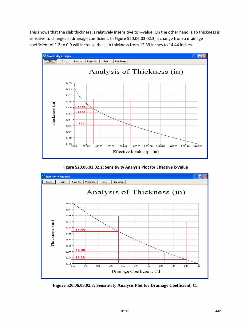
This shows that the slab thickness is relatively insensitive to k-value. On the other hand, slab thickness is sensitive to changes in drainage coefficient. In Figure 520.06.03.02.3, a change from a drainage coefficient of 1.2 to 0.9 will increase the slab thickness from 12.39 inches to 14.44 inches.

Figure 520.06.03.02.2: Sensitivity Analysis Plot for Effective k-Value

Figure 520.06.03.02.3: Sensitivity Analysis Plot for Drainage Coefficient, Cd

01/18 442

520.06.04 Rigid Thickness Design Using the Pavement Interactive Design Utility. The information from Example 520.05.01 and Table 520.05.01.1 is input into Figure 520.06.04.01 and is an illustration of using the Pavement Interactive design utility to solve Example 520.05.01.

520.06.04.01 Design Example: Type the data from Table 520.05.01.1 into the grey boxes of Figure 520.06.04.01.1 and click the calculate button.

Figure 520.06.04.01.1: Rigid Pavement Design Utility Solution

The Pavement Interactive utility returns the resulting pavement thickness of 13 inches.

01/18 443

520.07 Summary of Design Examples. Section 520.00 provides the designer with three ways to use the 1993 AASHTO Guide for the Design of Pavement Structures to determine rigid pavement thicknesses. The results from using the graphical methods, DARWin, and Pavement Interactive, shown in Table 520.07.1, give slightly different answers for the example provided in this section. The designer should not expect identical thickness vales but they should be close enough to be considered equivalent for design purposes. The pavement thickness determined here will be analyzed by Pavement ME to determine if it will achieve the intended design life.

Table 520.07.1: Summary of Results

Design Method

AASHTO 93

Graphical DARWin Pavement Interactive

Surface 13+” 12.98” 13”

520.08 Design Analysis. Once the designer has determined the thickness of the flexible pavement layers, by any of the methods described in Section 520.00, these values will be used as the initial trial thickness design in Pavement ME. The IDAHO AASHTOWare Pavement ME Design User’s Guide will provide guidance to analyze and adjust the layer thicknesses to meet the requirements of Pavement ME.

01/18 444

520.09 References.

AASHTO Guide for Design of Pavement Structures, Washington D.C.: American Association of State Highway and Transportation Officials, 1993. This document is available to ITD employees at: http://itdintranetapps/apps/ihs/ihs.aspx



Rasmussen, R.O., R. Rogers. T.R. Ferragut, Continuously Reinforced Concrete Pavement Design and Construction Guidelines, Federal Highway Administration and Concrete Reinforcing Steel Institute, Draft May 2009

Idaho AASHTOWare Pavement ME Design User’s Guide, Version 1.1, Mallela, J., L. Titus-glover, B. Bhattacharya, M. Darter, H. Von Quintas, Applied Research Associates, Idaho Transportation Department ITD-RP 211B, (March 2014).

01/18 445


SECTION 530.00 – PAVEMENT REHABILITATION DESIGN

530.00 Introduction. The procedures described herein are accepted methods to design a wide range of pavement rehabilitation alternatives. Pavement rehabilitation is needed to extend the life of a pavement structure by treating structural deficiencies, roughness or environmentally induced deficiencies such as thermal cracking. Rehabilitation is needed periodically on otherwise adequately designed pavements due to increased traffic, excessive thermal cracking and surface deficiencies such as stripping, raveling, joint faulting, rutting and roughness. Badly fatigued (alligator cracked) pavements may be more economical to reconstruct. Pavement rehabilitation is performed on both flexible and rigid pavements.

Pavement Rehabilitation consists of “structural enhancements that extend the service life of an existing pavement and/or improve its load carrying capacity. Rehabilitation techniques include restoration treatments and structural overlays.” Source: AASHTO Highway Subcommittee on Maintenance

Rehabilitation projects extend the life of existing pavement structures either by restoring existing structural capacity through the elimination of age-related, environmental cracking of embrittled pavement surface or by increasing pavement thickness to strengthen existing pavement sections to accommodate existing or projected traffic loading conditions. Two sub-categories result from these distinctions, which are directly related to the restoration or increase of structural capacity:

Minor rehabilitation consists of non-structural enhancements made to the existing pavement sections to eliminate age-related, top-down surface cracking that develop in flexible pavements due to environmental exposure. Because of the non-structural nature of minor rehabilitation techniques, these types of rehabilitation techniques are placed in the category of Pavement Preservation.

Major rehabilitation “consists of structural enhancements that both extend the service life of an existing pavement and/or improve its load-carrying capability.”

Source: AASHTO Highway Subcommittee on Maintenance Definition.

From this definition, it’s clear that pavement rehabilitation and pavement preservation are not the same, although they are sometimes lumped together. Pavement Preservation is discussed in detail in Section 542.00. Table 542.03.1, shows the pavement preservation techniques used in Idaho, and lists thin hot mix overlays, stone matrix asphalt, cold-in-place and hot-in-place recycling. These techniques are also included in this section as pavement rehabilitation techniques. Section 210.00 discusses the Phase Reports required for pavement rehabilitation projects.

Note: Pavement preservation is sometimes called preventive maintenance.

Figure 530.00.1 depicts a generic pavement performance curve showing the relationship between pavement condition and the different categories of pavement treatments. There can be significant differences in the shape of the performance curve for different pavements due to various issues (e.g.,

01/18 446

environment, design, or construction). As shown in the figure, pavement rehabilitation treatments can overlap pavement preservation and reconstruction and there may not be a single solution.

Figure 530.00.1 RELATIONSHIP BETWEEN PAVEMENT CONDITION AND TYPICAL TYPES OF TREATMENT

All pavement rehabilitation strategies should include an investigation of the existing pavement condition. High priority should be given to recycling existing pavement materials and is discussed in Section 530.00.06. The following is a listing of the pavement rehabilitation strategies which have been applied in Idaho or are common in the western states:

• Overlay: An overlay is any operation that consists of placing either Hot Mix Asphalt (HMA) or Portland Cement Concrete (PCC) over an existing pavement structure. This is different than a total replacement of the structure, and is typically done when there is only minor to modest damage to the existing pavement structure. When constructing an overlay, a portion of the old surface may be milled or ground off. Any minor structural deficiencies are then repaired and a new surface is applied.

o Overlays can be flexible overlay of flexible or rigid pavement or rigid overlay of flexible or rigid pavement. Flexible overlay over flexible pavement can be placed on the existing surface with or without a leveling course or scrub coat or over a milled flexible surface as described in the next bullet. A flexible overlay over rigid pavement consists of placing flexible pavement directly on the existing rigid pavement; over crack and seated; break and seated or rubblized rigid pavement. A rigid overlay of flexible pavement consists of an unbonded rigid overlay placed on existing flexible pavement, previously known as “white topping”. A rigid overlay of rigid pavement may be “bonded” or “unbonded”. An unbonded concrete overlay consisting of a concrete layer over an existing PCC pavement in poor condition with an interlayer of flexible pavement or other material between them to break the bond between the two pavement layers. A bonded PCC overlay consists of a relatively thin PCC layer (typically less than 4 inches thick) over an

01/18 447

existing rigid pavement in good condition. The overlay is intentionally bonded to the existing pavement in order to create a composite pavement section. Bonded overlays are generally used to add structural capacity to existing rigid pavements that have little deterioration.

• Mill and Inlay: Removing and replacing a portion of the roadway surface course with new pavement. Depending on if there is an overlay included and the thickness of the overlay, this technique may be considered a rehabilitation treatment or a preservation treatment.

• In-place Recycling: Treat or process a portion of the pavement section in-place, to a depth depending on the technique, without removing existing material. The following are in-place recycling strategies presented in order of the amount of roadway that is processed.

o Hot in-place recycling includes heating, milling to a depth of 2 to 3 in. and relaying existing asphaltic concrete as a rejuvenated surface. Deficiencies in gradation and/or asphalt content can be corrected by the addition of aggregate and asphalt.

o Cold-In-Place Recycling involves cold milling to a depth of 2 to 4 inches, pulverizing and relaying existing asphalt surfacing with the addition of hydrated lime and a rejuvenating agent or emulsified asphalt. Except for low volume roads, cold-in-place recycled pavements will need a high type plant mix surface. A seal coat is needed as a minimum to reduce raveling.

o Full Depth Reclamation: Pulverizing the existing plant mix surface thickness including a predetermined portion of the aggregate base, mixing with a small amount of cement, emulsified asphalt or foamed asphalt, or lime and relaying the material as a stabilized base, with placement of a new surface course. Full Depth Reclamation pulverizes the existing plant mix and base to a depth of 4 inches to over 12 inches. CRABS (Cement Recycled Aggregate Base Stabilization) is the most commonly used full-depth reclamation alternative at ITD.

Additional information concerning these rehabilitation strategies will be provided in later sections and in references.

01/18 448

530.00.01 History of Pavement Rehabilitation in Idaho. From the time of initial construction of the state system until the early 1990’s, the predominant method of pavement rehabilitation was to place a plantmix overlay on the existing pavement. A relatively small number of Cold in Place Recycle (CIR) and Hot-in-Place Recycle (HIR) projects were constructed beginning in approximately the mid-1980’s to mid-1990’s. Beginning in the mid 1990’s through about 2010, the predominant method of pavement rehabilitation has been Cement Recycled Asphalt Base Stabilization (CRABS) with a plantmix overlay. While usage of plantmix overlays without treating the existing pavement has remained significant, at this time CRABS is the most widely used method for major rehabilitation of existing pavement in Idaho.

Initial construction of the state system for the most part included adequate base materials for providing a long lasting pavement. Some roadways, however, were constructed with marginal or thin base materials. Geotextiles were not used in Idaho until about the mid-1990’s. Over time, the aggregate base layers of many roadways became contaminated with fine particles from the underlying soils. This contamination reduces the stability of the base materials and inhibits drainage. With the primary method of pavement rehabilitation being a plantmix overlay, many State and NHS highways consisted of a thick asphalt layer (up to 1 foot) on poor contaminated base materials as of the early 1990’s.

Asphalt pavement is often referred to in engineering terms as flexible pavement. This is because the pavement is intended to flex under loads and with varying temperatures. However, the asphalt in pavement ages over time and becomes more rigid. Due to environmental conditions, stiff pavement material will crack at regular intervals along the length of the roadway. Over time, these cracks widen due to additional loading and deterioration. By the early 1990’s, these cracks were often up to 2 inches wide at the pavement surface.

At that time it was evident that an asphalt overlay without treating the existing thick pavements would not address future cracking in an acceptable manner. Also, future performance of any pavement rehabilitation would be reduced due to existing contaminated base materials.

Based on these issues, it was determined that full depth reclamation followed by a HMA overlay would be the most cost effective pavement rehabilitation for many roadways. The full depth reclamation process would convert the existing thick pavement materials into a stabilized base type of material. This allowed the pavement to be more flexible. Pulverization and recompaction of the asphalt materials into a less dense base material provided a minimal grade raise that is beneficial for surface drainage and could be controlled during construction. ITD modeled the CRABS process after the Roadbed Modification procedure that was in use at the time in Nevada.

530.00.02 Current Status. The situation that generated development of the CRABS process no longer exists (and never existed for local roads). Most if not all of the projects where CRABS is clearly the most viable alternate for pavement rehabilitation have been constructed. The procedure has been generally successful, although there have been a few projects where the process is considered underperforming. This is primarily due to lack of subsurface drainage and silty subgrade materials.

The Department adopted the Performance Graded Binder (PG) system in 1998 and the problems with thermal cracking and rutting have been reduced dramatically. Thicker pavements do not appear to be

01/18 449

developing thermal cracks like the older pavements that used the viscosity grading system that gave us AC-10 and AC-20.

Currently, the CRABS process tends to be selected for rehabilitating pavements with relatively thin existing asphalt and base thicknesses where benefits to the process are not as dramatic. ITD continues to use the CRABS process primarily for “non-materials” reasons. These reasons include familiarity with the process and a lack of specialty contractors in Idaho that use other procedures.

Other pavement rehabilitation procedures that have been used in Idaho include CIR and HIR as mentioned above. While ITD is very familiar with the CRABS process, other pavement rehabilitation procedures have also been used.

Specialty contractors for procedures other than CRABS exist in nearby states. For non-Idaho contractors, there is a perception of high mobilization costs. However, Idaho contractors regularly mobilize for large distances across the state. In difficult economic times, contractors will give more attention to developing competitive bid prices.

530.00.03 Pavement Rehabilitation Strategies. The following paragraphs discuss rehabilitation strategies that are considered viable for use in Idaho. Not all processes described are currently used by the Department. Each procedure has merits as well as limitations. The strategies are presented in order from those used on the most deteriorated pavements to those in good condition. Part 3 Design Analysis, Chapter 5, Section 3.5.4 “IDENTIFICATION OF FEASIBLE REHABILITATION STRATEGIES” of the Guide for Mechanistic-Empirical Design of New and Rehabilitated Pavement Structures provides additional guidance to develop feasible rehabilitation strategies.

530.00.03.01 Full Depth Reclamation (FDR). Full Depth Reclamation is the generic term for the rehabilitation technique in which the full thickness of the asphalt pavement and a predetermined portion of the underlying materials (base, subbase, and/or clean subgrade) is uniformly pulverized and blended to provide an upgraded, homogeneous material. Often this blend of material alone, without any additional stabilizing additives, is sufficient to act as the base for a new surface course. However, if after proper project evaluation it is determined that the reclaimed materials need improvement or modification, there are three different types of stabilization that can be used:

• Mechanical stabilization is achieved with the addition of granular materials such as virgin aggregate or recycled materials such as reclaimed asphalt pavement (RAP) or crushed Portland cement concrete.

• Chemical stabilization is achieved with the addition of lime, Portland cement, fly ash, lime or cement kiln dust, calcium/magnesium chloride or various proprietary chemical products.

• Bituminous stabilization is accomplished with the use of liquid asphalt, asphalt emulsion, and/or foamed (expanded) asphalt.

For increased stabilization requirements, combinations of all three can also be used.

Pavement distresses which can be treated by FDR include:

01/18 450

• cracking in the form of age, fatigue, edge, slippage, block, longitudinal, reflection, and discontinuity

• reduced ride quality due to swells, bumps, sags, and depressions • permanent deformations in the form of rutting, corrugations, and shoving • loss of bonding between pavement layers and stripping • loss of surface integrity due to raveling, potholes, and bleeding • excessive shoulder drop off • inadequate structural capacity

Pavements that have extensive distortion or deterioration due to subgrade or drainage problems are candidates for FDR only when additional work is undertaken to correct the subgrade and drainage deficiencies. To correct subgrade problems the reclaimed material typically is moved to one side, the subgrade is reworked or stabilized with an additive, a subgrade separation geotextile is placed, and then the reclaimed material is placed back on the prepared subgrade.

Pavements that have distresses or deficiencies deeper in the pavement section than about sixteen inches may not be candidates for FDR unless the new section is able to provide enough support that the future traffic loads do not overstress the poor underlying materials. Poor materials several feet below the new pavement section may be deep enough to not affect the new pavement section.

The expected design life, performance requirements during the design life, and acceptable future maintenance requirements are related to the treatment depth of the FDR, the types and amount of stabilizing agents used, and on the type and depth of the subsequent wearing course.

The CRABS process is a specific type of full depth reclamation process that falls into the chemical stabilization category. As mentioned above, it consists of pulverizing the existing asphalt materials and a portion of the base. The materials are then mixed with cement, usually at the rate of 2%, and then recompacted. This is followed by a HMA overlay. The 2% cement rate is considered low by the Portland Cement Association definition for FDR. See Section 530.05 for further details. The Basic Asphalt Recycling Manual published by the Asphalt Recycling and Reclaiming Association is the basis for this information and is an excellent resource for all asphalt recycling needs.

530.00.03.02 Cold Recycle (CR). Cold Recycling (CR) is the rehabilitation of asphalt pavements without the application of heat during the recycling process. The two sub-categories of CR, based on the process used, are Cold Central Plant Recycling (CCPR) and Cold In-Place Recycling (CIR).

CCPR is the process in which Reclaimed Asphalt Pavement (RAP) is processed in a central location to produce a recycled mix which can be used immediately or stockpiled for later use. CCPR is most frequently used as part of a total reconstruction of an existing roadway or in new construction where an existing source of RAP is available. The project issues associated with CCPR are similar to any centrally produced material used on a new or reconstruction project. CCPR has not been used in Idaho.

CIR is used and this procedure consists of coldmilling up to 4 inches depth, mixing emulsified asphalt and additives, relaying the material and recompacting it. Additives are included for timely stabilization of the material. Shoulders may be widened using imported RAP or crushed aggregate base material.

01/18 451

The CIR process consists of the on-site rehabilitation of the asphalt pavement with a recycling train which can range in size from a single unit to a multi-unit train. Pavement distresses which can be treated by CIR, include:

• raveling • potholes • bleeding • skid resistance • rutting • corrugations • shoving • fatigue, edge, and block cracking • slippage, longitudinal, and transverse thermal cracking • reflection and discontinuity cracking • poor ride quality caused by swells, bumps, sags, and depressions

It is noted that unless the cause or causes of the pavement distress are addressed during the rehabilitation process, the distresses will be mitigated but they will not be eliminated. The expected design life, performance during the design life and future maintenance requirements, are related to the treatment depth of the CIR, and on the type and depth of the subsequent wearing course. Hence, the detailed project analysis will further refine the CIR treatment depth and subsequent wearing course requirements.

Performance of CIR in Idaho was considered less than stellar in the past for various reasons. However, those issues have been successfully addressed with recent projects. CIR results in the processed layer having up to 12 to 14% air voids in comparison to the 4 to 7% in a typical HMA pavement. This results in a tendency for the surface to ravel and thus the need to place a seal coat or overlay on top. ITD has a number of CIR projects on lower volume roads that were covered with only a conventional seal coat that have performed well.

ITD is aware of no research that identifies the reduction in stiffness strength of the pavement material when the CIR process is used. However, the depth of the process into the existing pavement is limited to approximately 4 inches. It has been suggested that the CIR layer provides a crack mitigation layer because of the higher voids content. Also, a minimum of approximately 1 to 1 ½ inches of the existing asphalt thickness remains to provide a paving platform. If this material is deteriorated, it may be beneficial for construction purposes to allow more thickness to remain. This layer provides the foundation for recompaction of the asphalt material.

Cold in-place recycle is generally performed by a specialty subcontractor. Selection of cold in place recycle does not preclude several prime contractors from bidding the project in the event only one CIR subcontractor is interested in the project. Paving remains the major portion of the work of a cold in place recycle project.

01/18 452

For rehabilitation of pavements that have previously been CRABS processed, CIR is a viable alternative. Pavement thickness is a concern because most CRABS were overlaid with fairly thin pavement layers and CIR may be more practical after a CRABS project is overlaid once.

Generally speaking, at this time CIR is a viable alternative for any project where the CRABS process is being considered provided the project has adequate support from the underlying layers. CIR does not address contamination of existing base materials, if such contamination exists. However, CIR eliminates the risk of problems associated with loosening the base material. See Section 530.07 for further details. The Basic Asphalt Recycling Manual published by the Asphalt Recycling and Reclaiming Association is the basis for this information and is an excellent resource for all asphalt recycling needs.

530.00.03.03 Hot In Place Recycle (HIR). Hot In-Place Recycling (HIR) is an on-site, in-place rehabilitation method which consists of heating, softening, scarifying, mixing, placing, and compacting the existing pavement. Virgin aggregates, asphalt binder, recycling agents, and/or new HMA can be added, on an as required basis, to improve the characteristics of the existing pavement. Virgin aggregates or new HMA which is incorporated into the HIR process, is commonly referred to as “admix”. Pavement distresses which can be treated by HIR include:

• raveling • potholes • bleeding • friction number • rutting • corrugations • shoving • slippage • longitudinal, transverse, and reflection cracking • poor ride quality caused by swells, bumps, sags, and depressions

The objective of HIR is to address these pavement distresses while they remain near the surface in the top two inches or so of the pavement. Top down cracking is best addressed with HIR.

There are three sub-categories of HIR, defined by the construction process used, consisting of:

• Surface Recycling; • Remixing and; • Repaving.

Surface recycling is the most common HIR process and the one that has been used most in Idaho. No virgin aggregates or HMA are added. Remixing is similar to Surface Recycling except specific pavement distresses or defects may be corrected by adding aggregates or binders. Repaving is the addition of a thin surface course of new pavement included in the recycling process.

01/18 453

Not all of the HIR processes described treat all of the above noted pavement distresses equally. In addition, unless the cause or causes of the pavement distress are addressed during the rehabilitation process, the distresses will be mitigated but they will not be eliminated.

The expected design life, performance requirements during the design life, and acceptable future maintenance requirements are also different for the three HIR processes. Hence, the detailed project analysis will further refine which of the three HIR processes is most appropriate.

This process recycles the top 1 to 1 ½ inch of the asphalt pavement layer. This is accomplished by heating the existing pavement, milling the material, and relaying the material as new hot mixed pavement in a continuous operation. Current practice is to use emulsified asphalt as a rejuvenating agent. HFRS-2P (high-float) emulsion seems to be preferred in states where this process is used extensively.

HIR is predominantly a pavement preservation application. The Department has performed pavement preservation on Interstate 84 with HIR. If HIR is used for pavement rehabilitation, a structural overlay that meets pavement design requirements must be included.

Long project lengths (10 – 15 miles) with minimal curvature are usually preferable due to the length of the recycling train. Pavement materials should contain no cutback materials due to the tendency for this material to flame in the heating process.

Hot in-place recycle is performed by a specialty contractor typically acting as a sub-contractor. Selection of HIP does not preclude several prime contractors from bidding the project.

Equipment and technology of this procedure has evolved since past ITD projects. At this time, use of the Hot in Place Recycle for pavement preservation project(s) would be appropriate for evaluating current technology. See Section 530.06 for further details. The Basic Asphalt Recycling Manual published by the Asphalt Recycling and Reclaiming Association is the basis for this information and is an excellent resource for all asphalt recycling needs.

530.00.03.04 Overlays. Overlays are used to remedy functional or structural deficiencies of existing pavements. Functional deficiencies arise from any conditions that adversely affect the highway user. These include poor surface friction and texture, hydroplaning and splash from wheel path rutting, and excess surface distortion (e.g. potholes corrugations, faulting, blowups, settlements, and heaves). Structural deficiencies arise from any conditions that adversely affect the load-carrying capability of the pavement structure. These include inadequate thickness as well as cracking, distortion, anddisintegration. Asphalt overlays placed on cracked pavement will exhibit reflective cracking despite a structurally adequate design. These cracks allow water to infiltrate the pavement structure and cause premature damage. The techniques in Section 530.00.04 will help mitigate reflective cracking. Overlays can be flexible or rigid and both can be placed on existing flexible or rigid pavement.

01/18 454

530.00.03.04.01 Asphalt Overlays. As previously mentioned, asphalt overlays are the most common pavement rehabilitation technique used. Depending on the application, an asphalt overlay can be used for pavement rehabilitation or pavement preservation. Asphalt overlays for pavement preservation can take the form of a plant mix seal, thin hot mix overlay, or stone matrix asphalt as described in Section 542.00. Design of flexible overlays will be addressed in Section 530.01 and Section 530.02.

530.00.03.04.02 Concrete Overlays. Concrete overlays for pavement rehabilitation are not as common as asphalt overlays but they warrant consideration. Design of rigid overlays will be addressed in Section 530.04.

530.00.04 Crack Repair and Pavement Interlayers. Crack repairs may consist of sawcutting and removing approximately a 2 ft. section of the existing pavement and base at locations where cracks are wider than ¾ inch. The pavement shall be reconstructed to pre-existing thicknesses followed by a pavement interlayer and a HMA overlay. A pavement interlayer may consist of a Stress Absorbing Layer of Straight Asphalt (SALSA) or a pavement geotextile. The pavement interlayer is intended to delay the return of cracks.

The sawcut pavement edges shall be tack coated prior to placing HMA in the reconstructed patch.

Alternative methods of crack repair may be used to reduce expenditure of funds. Equipment consisting of a cold mill or reclaimer attachment replacing the bucket on a loader arm exists and may be viable for use. Routing the cracks and filling with loose HMA immediately prior to placing the overlay appears relatively cost effective. System III Pavement Repair Geosynthetic with the physical properties shown in Section 543.03 should be considered with these alternative methods for crack repair.

SALSA consists of a heavy application of hot PG grade asphalt followed by a minimal application of cover coat material as needed to carry construction traffic. SALSA is followed immediately by the HMA overlay. Roadway traffic is not allowed on the SALSA.

SALSA seems preferred for rural applications. Some tracking of asphalt is expected with SALSA. Pavement geotextile is appropriate for locations where tracking of SALSA asphalt needs to be avoided and where paving conditions are considered difficult. When a leveling course is used, application of the SALSA and full width paving subsequent to the leveling course is considered more practical than applying the SALSA prior to the leveling course.

To avoid unsatisfactory results, all cracks that are not removed and patched (i.e. less than ¾” wide) should be blown out with compressed air prior to applying SALSA. Eliminating this effort is not cost effective.

Application rates for SALSA typically consist of 0.25 gal/sy of PG 58-34 asphalt, and 10 lbs/sy of cover coat material.

01/18 455

530.00.05 Rehabilitation Methods Other Than Overlay. Many different rehabilitation techniques can be applied to pavements to extend their lives without the placement of an overlay. Only structurally adequate pavements or pavements restored to a structurally adequate state are candidates for rehabilitation without overlay. Some of the methods available for use are as follows:

• Full Depth Repair • Partial Depth Repair • Joint-Crack Sealing • Subsealing-Undersealing • Grinding and Milling • Subdrainage • Pressure Relief Joints • Load Transfer Restoration • Surface Treatments

Chapter 4 of the 1993 AASHTO GUIDE FOR DESIGN OF PAVEMENT STRUCTURES and Part 3 Design Analysis, Chapter 5, Section 3.5.2.3 “REHABILITATION WITH NON-STRUCTURAL OVERLAY” of the Guide for Mechanistic-Empirical Design of New and Rehabilitated Pavement Structures provides guidance on non-overlay methods. These methods are not typically part of a pavement design process.

530.00.06 Pavement Recycling. Recycling is encouraged in all aspects of construction whether it is new construction, reconstruction, rehabilitation or preservation. Part 3 Design Analysis, Chapter 5, Section 3.5.3 “RECYCLING OF EXISTING PAVEMENT OR THER MATERIALS” of the Guide for Mechanistic-Empirical Design of New and Rehabilitated Pavement Structures provides additional guidance.

530.01 Pavement Rehabilitation Design Methods. The procedures described herein are a collection of accepted methods of pavement rehabilitation design. Some have been modified to accommodate the design considerations unique to Idaho. The following is a partial list of the sources used in developing these procedures:

• AASHTO Guide for Design of Pavement Structures, 1993 • AASHTOWare DARWin -3.0 Pavement Design and Analysis System User’s Guide • Washington State DOT, Pavement Guide, 1995, 2011 • California DOT,(CalTrans), Manual of Test, 1978, 2012 • Cost Effective Pavement Rehabilitation Evaluation of The Interstate System – Part One, Nevada

DOT, 1997 • MODULUS, Computer Program, Texas Transportation Institute • EVERCALC and EVERPAVE, Computer Programs, Washington DOT, 1999 • WINFLEX, Computer Program, ITD / University of Idaho, 2006

Additional resources related to these methods may be found in Section 530.09.

01/18 456

Alternate design methodologies may be used with permission, provided the resultant design successfully pass Pavement ME analysis.

530.01.01 Summary of Design Factors. A condition survey for rehabilitation projects is to be completed in accordance with Section 540.00 Pavement Structures Analysis. The results of the survey and design recommendations are included in the Phase I Materials Report for rehabilitation projects.

Consider the following major factors in developing a structural rehabilitation project:

530.01.02 Structural Quality of Existing Pavement. The existing pavement structure is composed of layers of material that may have degraded or otherwise become deficient in quality since the time of original construction. The presence of moisture in the pavement structure can contribute to cracking and stripping in the surface course and can promote pumping in fine-grained subgrade soils, leading to contamination of base course aggregate. The pavement condition survey provides the evaluation of the thickness and structural quality of each layer of the existing section. A condition survey should reflect the actual condition of the pavement structure on a section-by-section basis.

With the actual layer thicknesses, analyze the deflection data to develop back-calculated moduli for the various pavement layers and the subgrade for each of the homogeneous segments identified.

Calculate the existing structural capacity and additional ballast requirements, if needed, using both the back-calculated moduli from deflection tests and the laboratory R-Value test data (component analysis). Deflection-based methods will most often yield slightly lower additional ballast requirements since the deflection data represents the stabilized, in-place condition of the pavement layers.

530.01.03 Traffic. Evaluate traffic data according to Section 510.02, carefully considering past and estimated future traffic loading. The design period for major rehabilitation strategies is normally 20 years for flexible pavements. For rigid pavements rehabilitation design periods vary from 18 to 36 years. If a lesser design period is justified, use the design traffic loading appropriate for the reduced design period. In no case shall a rehabilitation strategy be designed for less than 8 years on federally funded projects. Regardless of the intended design life of the project, the design alternatives for flexible pavements should be evaluated for both 20 year and the shorter determined project life. Minimum layer thicknesses as provided in Section 510.06 may result in a design life much greater than the minimum 8 year design.

Load Spectra data is discussed in the AASHTOWare Pavement ME Help Menu and the ITD AASHTO Pavement ME Design User’s Guide.

01/18 457

530.01.04 Climatic Factors. The climatic factors described in Section 510.05 are used to adjust the roadway structure thickness, in a component analysis, to account for the detrimental effects of climate on the ability of the structural cross section to support traffic loading. Use the appropriate climatic factors when the rehabilitation design is based on R-value. Flexible pavements are temperature dependent, meaning their strength increases or decreases as the temperature changes. While unbound materials are moisture dependent and their strength increases or decreases as the moisture content of the material changes.

Climate factors are discussed in the AASHTOWare Pavement ME Help Menu and the ITD AASHTO Pavement ME Design User’s Guide.

530.01.05 Deflection Under Wheel Load. It is possible for a pavement structure to be adequately designed on the basis of R-value or expansion pressure, yet exhibit higher than normal deflections due to the presence of moisture and resilience of the subgrade soils. Conversely, many pavements that appear to be inadequate structurally, based on component analysis, may exhibit lower than expected deflections due to good drainage or subgrade strength gain.

530.01.06 Economic Factors. Design the alternate rehabilitation strategies to accommodate the estimated traffic loading for the design period appropriate to the specific strategy and use the life cycle cost to determine the most economical alternate. Life cycle cost analysis is described in Section 541.00.

530.02 Flexible Inlay/Overlay of Flexible Pavement. This type of work makes up the majority of the rehabilitation projects performed by ITD. The flexible pavement is the most expensive part of these types of projects and an optimized design is critical. ITD uses design by Component Analysis, i.e. R-Value Design and by deflection analysis i.e. WINFLEX.

530.02.01 Inlay/Overlay Requirements by Component Analysis, R-Value Design. The design procedure described below is based on the methods developed by CalTrans which have been modified to conform to the Idaho design process and to Idaho conditions. This approach to overlay design essentially requires that the total pavement structure be developed as a new design for the specified service conditions using the techniques described in Section 510.00 and then compared to the existing pavement structure (taking into account pavement condition, type, and thickness of the pavement layers). Current component design procedures require substantial judgment to effectively use them. This judgment is mainly associated with selection of “weighting factors” to use in evaluating the structural adequacy of the existing pavement layers (i.e., each layer of the pavement structure is assigned a layer coefficient often on the basis of experience).

530.02.01.01 Substitution Ratios for Existing Pavement Materials. Assign substitution ratios to common pavement materials according to Section 510.05, except as noted below:

• For base course aggregates that do not meet present specification and quality requirements, i.e., R-value, sand equivalent, and gradation, reduce the substitution ratio to that of granular subbase (R-value 60 or greater) or to that of granular borrow as appropriate. For Rock Cap,

01/18 458

which has degraded or has been infiltrated by subgrade soils, reduce the substitution ratio to that of aggregate base.

• For plant mix or road mix pavements that exhibit alligator or block cracking, raveling or stripping, reduce the substitution ratio proportionately to the extent of the distress (not to exceed a total reduction of 30%). If the 30% reduction will result in a substitution ratio of less than 1.0, use 1.0.

• Cement treated bases, which exhibit severe cracking and deterioration should be replaced. However, if the cement treated base is intact and is to be retained in the short term, the substitution ratio should be the same as that for aggregate base. Use substitution ratios applicable to plant mix surfacing for plant mix base.

530.02.01.02 Computing the Inlay/Overlay Thickness. Compute the overlay thickness using the procedures of Section 510.03 through Section 510.07. Determine the thickness in gravel equivalency required based on the R-value of each layer in the pavement structure and the R-value and expansion pressure of the subgrade. To determine inlay/overlay requirements, replace the existing plant mix with new plant mix to the depth of the desired inlay and re-compute the required overlay.

01/18 459

530.02.01.03 Design Example. Assume an existing two-lane highway composed of 0.30 ft. plant mix surfacing; 0.50 ft. crushed aggregate base, and 1.0 ft. granular subbase. The condition survey indicates that the existing plantmix surface is rough, but shows little evidence of rutting, raveling or stripping. Alligator cracking covers approximately 5% of the total pavement surface and block cracking covers approximately 15% of the total pavement surface. From experience and following the guidance from Section 530.02.01.01, we rate this pavement as having a 20% reduction in the substitution ratio or 80% remaining. The aggregate base meets all current specifications and quality requirements, with an R-value of 79. From experience and following the guidance from Section 530.02.01.01, we rate this aggregate base as having a 0% reduction in the substitution ratio or 100% remaining. The subbase is reasonably clean and free of excess minus #200 material, with an R-value of 53. From experience and following the guidance from Table 510.05.1, we rate this subbase with an R-value of 53 and we reduce the substitution ratio to that of granular borrow or 0.75. The sandy silt subgrade R-Value is 35. No drainage deficiencies are apparent.

With a thin overlay, the cracks may reflect through relatively quickly, therefore, a combination of inlay and overlay may provide the best solution to the structural requirements, smoothness and crack propagation.

Current design data are provided in Table 530.02.01.03.1 as follows:

Table 530.02.01.03.1: Example 1 Design Data

2007 2027

Accumulated ESALS (Design Lane)

30,000

1,750.000

Subgrade R-value 35

Subgrade expansion pressure In psi

0.60*

Unit weight, base and surface In pcf

130

Climatic Region 2

*In this example, the subgrade expansion pressure is given. This value may be determined in Section 510.03.03.

Begin by making a sketch of the existing pavement cross-section and the inlay / overlay to be designed.

01/18 460

Calculate the design ESALS.

𝐸𝐸𝐸𝐸𝐸𝐸𝐸𝐸𝐸𝐸 = 1,750,000− 30,000

EASLs = 1,720,000

Calculate the Traffic Index.

𝑇𝑇𝑇𝑇 = 9.0 �1,720,000106� �

0.119

TI = 9.6

Calculate the ballast requirement for all layers of the pavement structure existing above the base course, including the proposed overlay.


𝐺𝐺𝐸𝐸 1 = 0.0032(9.6)(100 − 79)(1.05)

GE = 0.68 ft.

Calculate the overlay thickness, applying the appropriate substitution ratios, subtracting the value of the existing plant mix surface (reduced substitution ratio). Where 0.30’ is the existing plant mix surfacing, 1.80 is the substitution ratio from Table 510.05.1, and 0.8 is the reduced substitution ratio from Section 530.02.01.01. The reduced substitution ratio for the existing plant mix is 1.8 x 0.8= 1.44.

𝑇𝑇 =0.68 𝑓𝑓𝑓𝑓.−0.30 𝑓𝑓𝑓𝑓. (1.8 × 0.8)

1.8

T = 0.138 ft., use 0.14 ft.

GE 1 (actual) = (0.14 ft. × 1.8) + (0.30 ft. x 1.44) = 0.68 ft.

Calculate the ballast requirement for all layers of the pavement structure existing above the subbase, including the proposed overlay.

𝐺𝐺𝐸𝐸 = 0.0032(9.6)(100− 53)(1.05)

GE = 1.52 ft.

01/18 461

Calculate the overlay thickness applying the appropriate substitution ratios, subtracting the value of the existing plant mix surface, (1.8 x 0.8= 1.44 reduced substitution ratio) and aggregate base (no reduction required).

𝑇𝑇 =1.52 𝑓𝑓𝑓𝑓.−�(0.3 𝑓𝑓𝑓𝑓.× 1.44) + (0.5 𝑓𝑓𝑓𝑓.× 1.0 )�

1.8

T = 0.33 ft., use 0.33 ft.

𝐺𝐺𝐸𝐸2(𝐿𝐿𝑖𝑖𝑓𝑓𝑎𝑎𝐿𝐿𝑎𝑎) = �(0.33 𝑓𝑓𝑓𝑓.× 1.8) + (0.3 𝑓𝑓𝑓𝑓 × 1.44) + (0.5 𝑓𝑓𝑓𝑓.× 1.0)�


Calculate the ballast requirement for all layers of the pavement structure existing above the subgrade soil, including the proposed overlay.

𝐺𝐺𝐸𝐸 = 0.0032(9.6)(100− 35)(1.05)

GE = 2.10 ft.

Calculate the overlay thickness applying the appropriate substitution ratios, subtracting the value of the existing plant mix surface (1.8 x 0.8 = 1.44 reduced substitution ratio), base (no reduction required), and subbase (R-Value < 60 reduce substitution ratio to 75).

𝑇𝑇 =2.10 𝑓𝑓𝑓𝑓.−�(0.3 𝑓𝑓𝑓𝑓.× 1.44) + (0.5 𝑓𝑓𝑓𝑓.× 1.0 ) + (1.0 𝑓𝑓𝑓𝑓.× 0.75)�

1.8

T = 0.23 ft., use 0.23 ft.

𝐺𝐺𝐸𝐸3(𝐿𝐿𝑖𝑖𝑓𝑓𝑎𝑎𝐿𝐿𝑎𝑎) = �(0.23 𝑓𝑓𝑓𝑓.× 1.8) + (0.3 𝑓𝑓𝑓𝑓 × 1.44) + (0.5 𝑓𝑓𝑓𝑓.× 1.0) + (1.0 𝑓𝑓𝑓𝑓.× 0.75)�


Review the overlay thicknesses from each set of calculations above, to determine which controls the design:

Overlay thickness when the base is the controlling layer: 0.14’

Overlay thickness when the subbase is the controlling layer: 0.33’

Overlay thickness when the subgrade soil is the controlling layer: 0.23’

The greatest overlay thickness is based on the R-value of the subbase. Therefore the subbase is the controlling layer and an overlay thickness of 0.33 ft. is selected.

Because of the thickness of the overlay, it would be advisable to provide an alternate consisting of reconstructing the base and surfacing to meet the ballast requirements of the subbase.

01/18 462

Another alternate to be considered for reducing the overlay thickness is an inlay/overlay. Calculations for this alternate design are as follows:

Calculate the overlay thickness required in conjunction with a 0.15 ft. inlay. Apply the appropriate substitution ratios, subtracting the value of the remaining existing plant mix and aggregate base (reduced substitution ratio for the remaining existing plant mix). The required ballast thickness over the subbase is 1.53 ft., as calculated above.

Note: Actual inlay and overlay lift thickness is governed by the nominal aggregate particle size; see Section 510.00.

𝑇𝑇 =1.53 𝑓𝑓𝑓𝑓.−�(0.15 𝑓𝑓𝑓𝑓.× 1.8) + (0.15 𝑓𝑓𝑓𝑓.× 1.44 ) + (0.5 𝑓𝑓𝑓𝑓.× 1.0)�

1.8

T = 0.30 ft., use 0.30 ft.

𝐺𝐺𝐸𝐸2(𝐿𝐿𝑖𝑖𝑓𝑓𝑎𝑎𝐿𝐿𝑎𝑎) = �(0.30 𝑓𝑓𝑓𝑓.× 1.8) + (0.15 𝑓𝑓𝑓𝑓 × 1.8) + (0.15 𝑓𝑓𝑓𝑓.× 1.44) + (0.50 𝑓𝑓𝑓𝑓.× 1.0)�


By using a 0.15 ft. inlay, the overlay is cut from 0.33 ft. to 0.30 ft. However, the total new asphalt plant mix placed increased to 0.45 ft. The overall asphalt thickness is reduced by about 0.03 ft., and the total of uncracked plant mix has increased to 0.45 ft. Crack propagation will be slowed with the increased thickness and the additional lift will increase smoothness. Even so, this does not appear to be an economical alternative, but serves to illustrate the procedure.

Now, check the actual pavement thickness including the overlay against the thickness required by expansion pressure.

𝑇𝑇(𝐿𝐿𝑖𝑖𝑓𝑓𝑎𝑎𝐿𝐿𝑎𝑎) = 0.30𝑓𝑓𝑓𝑓. +0.30𝑓𝑓𝑓𝑓. +0.50 𝑓𝑓𝑓𝑓. +1.0 𝑓𝑓𝑓𝑓.


𝐵𝐵 =(0.60 𝑝𝑝𝐸𝐸𝑖𝑖 × 144)

1.30 𝑝𝑝𝑖𝑖𝑓𝑓

B = 0.66 ft. < 2.10 ft., OK.

It is unlikely that the overlay will be governed by expansion pressure but it is a good idea to check each design. If an existing pavement is governed by expansion pressure, rehabilitation techniques other than an overlay should be considered.

Spreadsheets are available to solve these equations.

01/18 463

530.02.01 Design by Deflection Analysis. The design procedures outlined below are based, in part, on methodologies used by Washington DOT, Texas DOT, California DOT and the Strategic Highway Research Program (SHRP). Much of the methodology and data manipulation programs have been developed within the Idaho Transportation Department. A summary of the theory underlying deflection based analysis and design is presented in Section 530.08.

530.02.02 Deflection Testing. Deflection testing is performed by the Transportation Systems Roadway Data Section in Headquarters. The Falling Weight Deflectometer (FWD) is the primary tool used to collect the deflection data needed for pavement design and rehabilitation. The District Materials Engineer will submit requests for deflection testing to the Roadway Data Section prior to the beginning of the field testing season. FWD and Skid Request and Calendar may be accessed at the following site: http://itdintranetapps/Apps/ScheduleFWDWeb/. FWD testing is temperature dependent and collecting data for pavement design must be performed when the pavement temperature is above 40°F. This typically falls between April and October in most parts of the state. See Section 540.02.02.06 to request FWD data.

The standard deflection testing program consists of the following actions by the FWD crew:

• FWD tests will be made in at least one direction on two lane roadways and in the travel lane in both directions on four lane roadways. The standard testing interval is one test every 0.1 mile. Intermediate tests should be made in localized areas of significantly different distress. If the Materials Engineer needs something other than the standard testing, they need to provide those instructions in their testing request.

• Test locations will be in the outer wheel path on flexible pavements unless otherwise directed. On rigid pavement test locations will be in the center of the slab except for load transfer across joints. Where rutting is too deep to achieve uniform contact with the loading plate, the test point will be relocated so that the plate makes adequate contact.

• Tests will be made with at least one force level of 12,000 lb. Once every ten tests, at least two force levels will be used; one at 9000 lb. and the other at 12,000 lb. These force levels will not always result in loads that are exact but will vary from the intended 9,000 and 12,000 lb. targets. On extremely weak pavements, the force level may have to be further reduced to keep the deflections within an acceptable range.

• Indicate the degree of distress at the point of test in the comments column of the data file. Use the SHRP Distress Identification Guide. In addition indicate whether test point is in cut or fill. Digital photos may also be included to document distress conditions.

• The Roadway Data Section will perform a quality control check on the field deflection data as it is collected and then will post it at: FWD Data Files.

• The file naming convention is as follows. Route #, Direction, Lane (multilane sections), and Milepost plus appropriate file extension, Example: S41A0032 – State Highway 41, Ascending direction, Milepost 32. I84D1013 – Interstate 84, Descending direction, passing lane, Milepost 13.

01/18 464

http://itdintranetapps/Apps/ScheduleFWDWeb/

http://itdportal/sites/DES/TransSys/RD/FWDSKID/Documents/Forms/Standard%20View.aspx?RootFolder=/sites%2FDES%2FTransSys%2FRD%2FFWDSKID%2FDocuments%2FFWD%20Data%20Files&View=%7bA7B8BEE9-76BA-40C1-9A09-290E8CA63371%7d

A zero or one in the position after the direction designates travel lane, or passing lane respectively. This may cause problems for route numbers with 3 digits and more than 100 mile length, a condition not currently existing in Idaho. This naming convention was necessary with the original DOS based Dynatest software that limited the naming convention to 8 characters. This is no longer the case with the latest FWD software but the FWD crew will continue using the 8 character naming convention because it is simple, familiar, and conveys the necessary information. The designer may rename the file, if desired, after retrieving it from the Roadway Data Section site.

530.02.02.01 Deflection Data Reduction. The computer program MODULUS, developed by the Texas DOT and Texas Transportation Institute, (TTI) is the primary deflection analysis tool used by ITD to back-calculate pavement layer stiffness (moduli). ITD began using the DOS based Modulus 4.0 in the early 1990’s which was upgraded to Modulus 4.2. In the mid 1990’s, TTI released Modulus 5.0 which they updated to Modulus 6.0 for Windows in 2001. See Section 530.08.01 for a detailed description of analysis using MODULUS 6.0 and for a list of other computer programs available to perform the back-calculation analysis. MODULUS was selected by ITD because it is able to calculate individual layer moduli while some of the other programs provide a single modulus for the pavement structure.

As a check on the results of the MODULUS program, EVERCALC©, 5.0 for Windows (developed by Washington State DOT (WSDOT) and University of Washington) is recommended at each milepost. Two force levels are required at each test point for the program to normalize the moduli to a 9000 lb. wheel load. The program also corrects the calculated moduli to 77°F. If the user is interested in this design check, please contact the Materials Engineer for assistance. WSDOT EVERSERIES© User’s Guide can be found in Section 530.09. Note: This program does not run on Windows 7 computers.

Note: In back-calculation programs, it is extremely important that layer thicknesses be as accurate as possible. Variations of as little as 10% in asphalt pavement thickness can make significant differences in the calculated moduli. See Section 540.00 for recommendations for the Pavement Condition Survey.

530.02.02.02 Calculation of Required Inlay/Overlay. The program available for use in calculating required inlay or overlay thickness based on deflection analysis is WINFLEX 2006 developed specifically for WINDOWS by the University of Idaho, for the Idaho Transportation Department. Specific information on this program is contained in the reports generated for the project, RP 121. All RP 121 reports are available in Section 530.09. WINFLEX 2006 Program descriptions, summaries of recommended input parameters and operating suggestions for WINFLEX in Section 530.08.04.

530.02.03 AASHTO Design Guide. The AASHTO 93 Design Guide part III, Chapter 5 discussed Rehabilitation Methods with Overlays. Chapter 5 covers flexible overlays of flexible and rigid pavements and rigid overlays of flexible and rigid pavements. See the AASHTOWare DARWin Pavement Design and Analysis System User’s Guide for guidance in using the DARWin program.

The AASHTO method has some advantages including the ability to account for drainage and reliability of the input data, and allows input of the subgrade modulus at two-week intervals.

01/18 465

There are some major drawbacks. The design equations are based on the data from the original AASHO Test Road in Illinois and represent the subgrade at that site. The pavement section is combined into a composite modulus, eliminating the ability to analyze the effect of individual layers. The dependence on structural numbers is more empirical than mechanistic. The subgrade modulus from back calculation of FWD data must be modified by a correction factor to match laboratory results that were the basis of the equations from the AASHO Test Road. Generally we find that the asphalt overlay thickness is larger than with other methods when using the recommended reliability.

Overlay design using the 1993 AASHTO Design Guide for Design of Pavement Structures can provide a flexible design check of the results from WINFLEX. The currently recommended design methods using WINFLEX more closely fit the requirement for a mechanistic design method.

The 1993 AASHTO Design Guide should be used to design overlays that include rigid pavement as the overlay material. Further discussion of this is in Section 530.03.

530.03 Flexible Overlay of Rigid Pavement. A flexible overlay is a feasible rehabilitation alternative for PCC pavements that are intact, cracked and seated or broken and seated or rubblized, except when the condition of the existing pavement dictates substantial removal and replacement. Severe deterioration of joints and cracks, severe aggregate reactivity, and inadequate right of way to allow widening slopes and raising signs and guardrails are conditions which render a flexible overlay infeasible.

The recommended design methods presented here are intended for jointed plain concrete pavement only. Currently only one continuously reinforced concrete pavement section exists in Idaho.

Prior to design of flexible overlays of rigid pavement, perform a pavement condition survey as outlined in following sections.

The following types of distress should be repaired prior to placement of a flexible overlay over rigid pavement:

• Working cracks • Spalled Joints • Punchouts • Deteriorated previous repairs • Pumping/faulting • Settlement or heaves

01/18 466

530.03.01 Flexible Overlay Design by Pavement Deflection Analysis. The back calculation programs used in deflection analysis of flexible pavement are not appropriate for determining the modulus of base and subbase under rigid pavement, although they may be suitable for estimating surface concrete modulus, subgrade k-value and load transfer. Finite element analysis is typically used to analyze deflection tests on concrete. The overlay design programs currently in use are designed for flexible pavements over existing flexible pavement.

Illinois has developed deflection-based techniques such as ILLIBACK for deflection analysis on rigid pavements. Further analysis of rigid pavement analysis and overlay design programs will be made by the Construction/Materials Section. The following sections provide methods for calculating dynamic subgrade modulus and concrete modulus from deflection tests as presented in the 1993 AASHTO Guide for Design of Pavement Structures.

For overlays over cracked and seated concrete pavement, the methods of presented in Section 530.04 are appropriate. Both the literature and ITD deflection testing indicate that the modulus of the cracked and seated concrete is on the order of 1,000,000 +/- psi. To minimize crack reflection the modulus of the cracked and seated slabs should not be greater than 1,000,000 psi.

Base course moduli may be obtained through back calculation of deflection data on cracked and seated concrete pavement using the methods of Section 530.02.01. Overlay designs using the methods of Section 530.02 appear appropriate for cracked and seated concrete pavement.

Deflection based analysis may be possible on broken and seated concrete, but analysis of rubblized sections will need component analysis. The rubblized concrete should be assigned a substitution ratio equivalent to aggregate base or rock cap.

530.03.01.01 Calculation of Effective k-value. The effective k-value or Modulus of Subgrade Reaction can be determined from back calculation or alternately from the Area of each deflection basin. The Area may be calculated from the deflections at 12, 24 and 36 inches from the center of the FWD loading plate. The deflections are based on a load magnitude of 9000 lb. For loads within 2000 lb. of the standard load, the deflections can be scaled linearly. The Area is calculated as follows:

AREA = 6�1 + 2(𝑑𝑑12 𝑑𝑑0⁄ ) + 2(𝑑𝑑24 𝑑𝑑0⁄ ) + (𝑑𝑑36 𝑑𝑑0⁄ )�

Where d0, d12, d24 and d36 are the deflections at the center of the load plate, and at 12, 24, and 36 inches respectively. Area will typically range from 29 to 32 inches for sound concrete.

Using the Area calculated above enter Figure 530.04.01.1 to determine the effective dynamic k-value. Static k-value is dynamic k-value/2 for cohesive soils. For granular soils the ratio is 1.0.

01/18 467

Figure 530.03.01.01.1 − Effective Dynamic K -Value Determination from D0 and Deflection Basin Area (1993 AASHTO Guide for Design of Pavement Structures Figure 5.10)

530.03.01.02 Calculation of Concrete Pavement Modulus. The elastic modulus of the concrete pavement can be determined from back calculation, or alternately from the Area of each deflection basin. The Area may be calculated from the deflections at 12, 24 and 36 inches from the center of the FWD loading plate. The deflections are based on a load magnitude of 9000 lb. For loads within 2000 lb. of the standard load, the deflections can be scaled linearly. The Area is calculated using the relationship presented above in Section 530.03.01.01.

Using the Area calculated above enter Figure 530.03.01.02.1 to determine the effective concrete modulus. The modulus of the concrete will normally be in the range of 3 million to 8 million psi. If modulus values obtained are out of this range, an error may exist in the assumed slab thickness, the deflection basin may have been measured over a crack or the concrete may be significantly deteriorated.

If an overlay thickness is being designed for a uniform section, use the average of dynamic modulus of subgrade reaction and modulus of concrete for the section.

01/18 468

Figure 530.03.01.02.1 − PCC Elastic Modulus Determination from K-Value, Area, and Slab Thickness (1993 AASHTO Guide for the Design of Pavement Structures, Fig. 5.11)

530.03.02 Overlay Design Based on Structural Deficiency. This method is taken directly from the 1993 AASHTO Guide for Design of Pavement Structures, Section 5.6.5. The overlay thickness is calculated as follows:

𝐷𝐷𝑜𝑜𝑜𝑜 = 𝐸𝐸�𝐷𝐷𝑓𝑓 − 𝐷𝐷𝑒𝑒𝑓𝑓𝑓𝑓�

Where: Dol = Depth or thickness of overlay (inches) A = Factor to convert PCC thickness deficiency to Asphalt Concrete overlay thickness Df = PCC slab thickness to carry future traffic (inches) (Determine in accordance with

Section 520.00) Deff = Effective thickness of existing slab (inches)

The A-Factor, which is a function of PCC slab thickness deficiency is given by the following relationship and can be determined graphically from Figure 530.03.02.1.

01/18 469

Figure 530.03.02.1 – “A”-Factor for Conversion of PCC Thickness Deficiency to AC Overlay Thickness (1993 AASHTO Guide For Design Of Pavement Structures Fig 5.9)

A = 2.2233 + 0.0099�𝐷𝐷𝑓𝑓 − 𝐷𝐷𝑒𝑒𝑓𝑓𝑓𝑓�2 − 0.1534�𝐷𝐷𝑓𝑓 − 𝐷𝐷𝑒𝑒𝑓𝑓𝑓𝑓�

Calculate the slab thickness, Df, required to carry future traffic as in Section 520.00.

Determine the effective thickness, Deff, of the existing concrete pavement from the results of the condition survey. On concrete pavement, the condition survey should contain information on the following:

• Number of deteriorated transverse joints per mile

• Number of deteriorated transverse cracks per mile

• Number of full-depth asphalt concrete patches, exceptionally wide joints (>25mm or 1in.), and expansion joints per mile, (except at bridges)

• Presence and general severity of PCC durability problems, such as reactive aggregate cracking

• Evidence of pumping of fines or water

From the condition survey, the effective thickness of the existing slab (Deff) is computed from the following equation:

𝐷𝐷𝑒𝑒𝑓𝑓𝑓𝑓 = 𝐶𝐶𝑗𝑗𝑐𝑐 × 𝐶𝐶𝑑𝑑𝑑𝑑𝑑𝑑 × 𝐶𝐶𝑓𝑓𝑓𝑓𝑡𝑡 × 𝐷𝐷

01/18 470

Where: D = Existing slab thickness in inches. Fjc = Joints and cracks Adjustment Factor (Figure 530.03.02.01.1) Fdur = Durability Adjustment Factor (Figure 530.03.02.02.1) Ffat = Fatigue Damage Adjustment Factor (Figure 530.03.02.03.1)

Each of these factors is explained in the following subsections.

530.03.02.01 Joints and Cracks Adjustment Factor. This factor adjusts for the extra loss in Present Serviceability Index (PSI) caused by deteriorated reflection cracks in the overlay that will result from any unrepaired, deteriorated joints, cracks and other discontinuities existing prior to overlay. Therefore, all deteriorated joints and cracks (not related to durability distress) should be repaired full-depth with doweled or tied concrete.

If it is not possible to repair all deteriorated joints, cracks and major discontinuities, the total number of unrepaired, deteriorated cracks, joints, wide joints (>1 in.), and full-depth, full-lane asphalt patches per

mile is used to determine the Fjc from Figure 530.03.02.01.1.

Figure 530.03.02.01.1 − Fjc Adjustment Factor (1993 AASHTO Guide for the Design of Pavement Structures, Fig. 5.12)

01/18 471

530.03.02.02 Durability Adjustment Factor. This factor adjusts for an extra loss in PSI of the overlay when the existing slab has durability problems. Using the results of the condition survey determine Fdur from Table 530.03.02.02.1.

Table 530.03.02.02.1 Durability Adjustment Factor, Fdur

Fdur Condition

1.00 No sign of durability problems

0.96 – 0.99 Aggregate reactivity cracking exists, no spalling

0.88 – 0.95 Substantial durability cracking and some spalling exists

0.80 – 0.87 Extensive durability cracking and severe spalling exists

530.03.02.03 Fatigue Damage Adjustment Factor. This factor adjusts for past fatigue damage that may exist in the slab. It is determined by observing the extent of transverse cracking (Plain Jointed PCC) or punchouts (CRCP) that may be caused primarily by repeated loading. Use condition survey data and Table 530.03.02.03.1 to estimate Ffat in the design lane.

Table 530.03.02.03.1: Fatigue Damage Adjustment Factor, Ffat

Ffat Condition

0.97 – 1.00 Few transverse cracks (None caused by “D” cracking or reactive aggregate)

JPCP: < 5 percent slabs are cracked

0.94 – 0.96 A significant number of transverse cracks(None caused by “D” cracking or reactive aggregate)

JPCP: 5 – 15 percent slabs are cracked

0.90 – 0.93 A large number of transverse cracks(None caused by “D” cracking or reactive aggregate)

JPCP: > 15 percent slabs are cracked

For CRCP or JRCP, see 1993 AASHTO Guide for Design of Pavement Structures, Section 5.6.5

01/18 472

530.04 Rigid Overlays. Concrete overlays on existing pavements are often referred to as either a bonded or unbonded concrete overlay systems depending on the design assumptions made.

There are two types of concrete overlay systems:

• Bonded concrete overlay. Typically 2 to 5 inches thick, with joint spacing ranging from 2 to 6 feet, this type of concrete overlay is used primarily for urban intersections, city streets, and overall low-volume roads. Bonded concrete overlay relies on its bond to the existing asphalt or concrete or composite pavement for performance. The concrete overlay and the existing underlying pavement act as one monolithic pavement.

• Unbonded concrete overlay. This type is typically 4 to 11 inches in thick with joint spacing from 4 to 12 ft. This type of concrete overlay follows the behavior of a concrete pavement in terms of performance and can be placed on existing asphalt or concrete or composite pavement but does not rely on bonding to the layer. The unbonded concrete overlay serves as a new pavement on a stable platform.

Concrete overlays are not new. In fact, ITD constructed several projects that could be considered bonded or unbonded on Interstate 90 during the 1970’s and 1980’s when temporary asphalt pavement was placed and used for several years until the final concrete surface was placed. Interstate 84 projects that utilized crack and seat of the existing concrete pavement with a thick rock cap interlayer could be considered unbonded concrete overlays. These types of concrete overlays tend to fall into the unbonded overlay system category. In general, unbonded overlays are used to rehabilitate pavements with some structural deterioration. They are basically new pavements constructed on an existing stable platform (the existing pavement).

Thin concrete overlays on the other hand area a new procedure in Idaho that has been increasing in popularity elsewhere over the past 15 years. One experimental project has been constructed at an intersection in Southwest Idaho with no problems being observed. Thickness of the slabs is 4” to 8” however a minimum thickness of 5” appears optimal. Thin concrete overlays are designed as a bonded pavement and functions as a composite section. In general, bonded overlays are used to add structural capacity and/or eliminate surface distress when the existing pavement is in good structural condition. Bonding is essential, so thorough surface preparation is necessary before resurfacing. The national trend for thin concrete overlays is towards use of a 6 inch by 6 ft. by 6 ft. panel.

Projects must be selected as conducive to the design. Success with concrete overlays has been attributed to selection of appropriate projects. This includes projects where the concrete overlays was placed on a minimum of 5” AC in good condition i.e. no moisture problems, etc. Typically, this method is most conducive to use on commuter type roadways and not heavily loaded commercial type roadways. For these roadways, concrete overlays appear to be a cost effective alternative for pavement rehabilitation. As with any concrete pavement, uniform support is critical.

A design method has been developed by Colorado DOT. The method uses bridge design techniques to design the panels. Due to differences in the way ESALs are calculated, the method overdesigns the

01/18 473

panels for Idaho. However the additional PCC thickness is of negligible concern. The Guide to Concrete Overlays published by the National Concrete Pavement Technology Center is an excellent resource for all types of concrete overlays. For additional resources on concrete overlays, see Section 530.09 or contact the Construction/Materials Section.

Over the past 15 years, many research studies have been conducted on bonded concrete overlay projects aimed at formulating guidelines for properly designing and constructing them. Major findings from these studies include the following:

• Bonded concrete overlays behave as partially bonded systems. (Concrete overlays over rigid pavements are considered bonded systems and will be addressed in a later section.)

• A strong bond at the concrete-asphalt interface is essential for good performance of bonded concrete overlays. Milling and cleaning the asphalt surface enhances the bond and improves performance.

• Newly paved asphalt pavements (milled or nonmilled) are not recommended for bonded concrete overlays because bonding potential is dramatically reduced.

• Tie bars are recommended for longitudinal joints to prevent slab slippage.

• Load transfer devices have an insignificant effect on pavement performance in bonded concrete overlays. Load transfer is recommended for unbonded overlays because the design lives of these pavements are similar to new construction in excess of 40 years.

• A rule of thumb for joint spacing is one foot of joint space for every inch of thickness. For example, a 6-inch thick overlay would have joints at approximately 6-foot spacing.

530.04.01 Rigid Overlay of Flexible Pavement. Refer to the design procedures in Section 520.00. The concrete overlay thickness for bonded and unbonded concrete overlays can be determined using the 1993 AASHTO GUIDE FOR DESIGN OF PAVEMENT STRUCTURES. The design guide may be used to determine the pavement thickness by hand following the step by step instructions that solve the design equation graphically using a series of figures and the specific instructions of Chapter 5 of the design guide. Computer software adopted by the department for rigid pavement design is DARWin 3.0 (or later) PAVEMENT DESIGN AND ANALYSIS SYSTEM will also perform this design.

530.04.02 Rigid Overlay of Rigid Pavement. Refer to the design procedures in Section 520.00. The concrete overlay thickness for bonded and unbonded concrete overlays can be determined using the 1993 AASHTO GUIDE FOR DESIGN OF PAVEMENT STRUCTURES. The design guide may be used to determine the pavement thickness by hand following the step by step instructions that solve the design equation graphically using a series of figures and the specific instructions of Chapter 5.8 and Chapter 5.9. Computer software adopted by the department for rigid pavement design is DARWin 3.0 (or later) PAVEMENT DESIGN AND ANALYSIS SYSTEM will also perform this design.

Contact the Construction/Materials Section to ensure the most current design procedures and software are being used.

01/18 474

530.05 Cement Recycled Asphalt Base Stabilization (CRABS). The CRABS process, or Full Depth Reclamation is a recycling process in which all of the existing asphalt pavement and a portion of the existing aggregate base is pulverized (rototilled) full depth to a maximum particle size of 3 inches mixed with a small amount of cement, usually 2%, and reshaped and compacted into base for a new surface course. Other additives, emulsified asphalt or hydrated lime, may be substituted for the cement under specific conditions.

Not all pavement rehabilitation projects are suitable candidates for the CRABS process. No FDR process will address subgrade failures or correct large ballast section deficiencies. The best candidates for CRABS rehabilitation are structurally adequate pavement sections with relatively thick asphalt surfaces and sufficient aggregate base to allow pulverizing and mixing at least a thickness of 8 inches without penetrating through the base or through pavement sections that have a contaminated base/subbase that cement modification will stabilize. A clean aggregate base layer is preferred for optimal performance. For projects where significant contamination of the base exists, the 2% cement additive may or may not be successful at stabilizing the materials. For projects where the existing base layer is contaminated to the point of not being effective or where no base exists, another alternative should be selected. The CRABS thickness may vary on a project specific basis. However, the process must extend completely through any asphalt layers. Ideally the aggregate base should make up no more than 50% of the total pulverized and remixed material. A CRABS base that is contaminated with pre-existing fines is expected to not perform as well as one with fewer fines. Additionally, for roadways where the existing base consists of uncrushed materials the benefits of the CRABS process may be reduced.

Typical surface distress on projects with a high CRABS potential are transverse thermal cracking, rutting and raveling. Pavements exhibiting extensive fatigue distress (alligator cracking) may not be good candidates for CRABS rehabilitation. This type of distress may be indicative of subgrade failure and moisture damage. Since a thick new surface course may be required to achieve structural adequacy, reconstruction may be a more cost effective solution. When the existing pavement is pulverized, the pavement section is significantly weakened and susceptible to traffic damage until a new surface is placed. The CRABS process loosens material that was previously compacted or consolidated. It has been found that most of the compaction of a CRABS base takes place in the top 4 to 6 inches of this layer when a strong aggregate base layer remains. The process reduces the stiffness strength of high quality existing asphalt pavement materials by approximately 70%. Care must be taken when compacting the CRABS layer to make sure it is compacted full depth and that there is sufficient moisture to ensure full hydration of the cement.

By pulverizing the entire thickness of the existing asphalt surface, the cracks are completely removed. A small amount of cement (on the order of 2% of the weight of the pulverized material) is added to bind the fines and provide some added stiffness to the pulverized material. Compressive strengths of the mixture after cement has hydrated and cured should be around 400 psi to prevent the brittleness and transverse cracking potential associated with traditional cement treated base.

Pulverization typically makes the existing materials swell up and this needs to be considered in the design process. The CRABS treated material cannot be compacted back to its original density. Therefore,

01/18 475

there is usually a 10 to 20% increase in volume, requiring trimming and removal of the excess where existing finished grades are to be maintained. Most often, the material that is removed tends to be the highest quality material in the roadway. If at all possible, try to keep as much of the pulverized material as possible on the road. This may be accomplished by reestablishing roadway crown and superelevation prior to allowing any of the pulverized material to be removed. A portion of the pulverized material may be removed and used to widen the shoulders. This material should be accounted for in the design process. In the case of thick pavement and good clean subsurface materials, a portion of the existing HMA material may be milled off prior to pulverizing and used as RAP in the HMA or given to local agencies. If this is being considered, make sure that the remaining material provides the necessary structural capacity and any corrections to roadway cross slope or superelevation deficiencies are made.

Design of CRABS sections is based on FWD deflection measurements made prior to construction. The subgrade modulus, derived from the deflection testing, and the modulus of the remaining base course, its measured thickness minus the amount included in the CRABS, is used in conjunction with a typical modulus for the CRABS to design the thickness of the new asphalt concrete surface course using the methods of Section 530.02.01 and Section 530.08.

Based on limited data, a design modulus value of 100,000 to 150,000 psi has been developed. If the thickness of aggregate base included in the CRABS is significant, the modulus may be lower. As more data is collected, modifications to the recommended design modulus will be made. In analysis, the CRABS is considered to act as a slightly cemented aggregate and is not treated as temperature sensitive. It is recommended that a sensitivity analysis be performed by varying the CRABS modulus from 100,000 psi to up to 200,000 psi in the Winflex program and see how sensitive the pavement thickness is to the varying modulus.

The minimum surface course thickness which should be placed over CRABS is 0.2 ft. On Interstate highways the recommended minimum surface course thickness is 0.3 ft. On other NHS routes with heavy truck traffic the recommended minimum surface course thickness is 0.25 ft. With a modulus value of 100,000 to 150,000 psi for the CRABS layer, the structural requirement for the overlay may result in a fairly thin pavement. However, a thin pavement may not be able to withstand the shearing action of stopping and turning trucks which may result in shoving failures.

Underperformance of pavements where the CRABS process was used has also been attributed to moisture intrusion due to a high water table or other reasons. Literature has identified stripping of asphaltic materials where Portland cement has been used as the additive. This seems to imply that moisture problems may be alleviated by eliminating the cement. However, eliminating the cement from a CRABS/Full Depth Reclamation base does not address moisture problems. See Section 550.00 for guidance to address moisture in pavement sections.

Table 530.05.1 provides a simple way to determine the amount of cement, in pounds per square yards, needed based on the density of the pulverized material, the percent of cement specified and the thickness specified.

01/18 476

Table 530.05.1-Estimated Cement Requirement for CRABS

paTW =

where: W = weight of cement in lb/SY

a = maximum density of pulverized material, lb/CF

(assumed if value is not known. 135 to 140 lb/CF is common)

p = percent of cement by volume

T = depth of soil to be mixed, feet

If d= 6 inches or 0.5 ft and P= 2% or 0.02, then

W= (p)(a)(T)=0.02 x 135 lb/CF x 0.5 ft. x 9 SF/SY

W = 12.2 lb/SY

If d= 8 inches or 0.67 ft. W = 16.3 lb/SY



From Soil Stabilization With Portland Cement, Bomag 1987.

530.06 Hot In-Place Recycling (HIR). Hot in-place recycling of asphalt pavement is performed by heating the existing pavement, hot milling the surface and relaying the milled material as new hot mixed pavement. Typically the depth that can be achieved is approximately 2 inches. Some equipment has been modified with an additional heater to extend the milling depth to 3 inches. Milling is accomplished by two or more milling heads, each removing about 1 inch. The maximum particle size required is 2 inches. The milled material is windrowed and picked up, remixed and laid down through a conventional paver. The hot in-place recycling train contains all units necessary to heat, mill, mix and place the material in one pass. Additional aggregate can be added in the process to correct gradation and /or asphalt content. A rejuvenating agent can also be added to soften age-hardened asphalt.

With proper speed, the resulting milled material can be heated to temperatures nearly as high as plant mixing. The resulting surface is considered to be equal to new plant mix, although, to reduce the potential for raveling, a seal coat or thin plant mix seal is recommended. Because of the shallow depth of treatment, hot in-place recycling will remove minor top down cracks and ruts but only delay the reflection of pre-existing cracks.

Asphalt seal coats, roadmix pavements and moisture in the pavement surface will all reduce the heating ability of the recycling equipment, requiring reduced production. Asphalt surface treatments (seal coats)

01/18 477

will, on the average, add about 0.5% asphalt to the milled pavement for each treatment. Milling and disposing of asphalt surface treatments was considered critical at one time but is not a normal part of hot in-place recycling projects anymore.

Pre-coated aggregate added to the process can improve existing gradations. Most recycling systems have the capacity to add up to about 65 lb. per square yard of additional material. A few systems are capable of adding enough material to add significant thickness to the pavement. An additional thickness of 0.05 ft. of would require 66 lb./sq. yd. of additional material.

It is extremely important to get representative samples from any potential hot in-place recycling project. Coring appears to be the best method to collect existing surfacing for analysis. Non-uniformity of the pavement to be recycled can seriously reduce the effectiveness of the recycled product.

The average anticipated life of a hot in-place recycled surface has not been determined. However, a life of 5 to 8 years is probable if the pavement is otherwise structurally sound. Hot in-place recycling should be considered on structurally adequate pavements to re-level the surface, eliminate ruts and to temporarily remove cracks. It can also be used effectively as a leveling course under a proposed overlay. The number of times a pavement can be hot, in-place, recycled has not been established. But, at least 3 times is likely.

HIP should be considered in lieu of the mill and inlay and also for the inlay/overlay operation in the life cycle cost analysis.

Design of a hot in-place recycled section, used as a leveling course, will be essentially the same as for an inlay/overlay using the methods of Section 530.02 and Section 530.08. The output of the program would be the thickness of overlay required over the recycled section.

530.07 Cold In-place Recycling (CIR). Cold in-place recycling of flexible pavement is a process in which the existing pavement is cold-milled either partial or full depth, mixed with a hydrated lime slurry and emulsified asphalt and/or a rejuvenating agent and relayed. Because the material is cold-milled there is no temperature requirement and as a result the process can extend deeper into the existing pavement. The particle size requirements are the same as for hot in-place recycling; (2 inches). Additional aggregate may be added to the milled material with some equipment systems.

Because the milled material is mixed with an emulsified binder or rejuvenator the final mix contains as significant amount of water. This will dissipate over time, but final compaction and placement of the final surface must be delayed until the moisture content drops to 1% or less. Also, because the material is milled and laid cold, the compacted density may be significantly less than for hot mix. Air void contents typically run in the 10-12% range. As a result of the added asphalt binder, the recycled material is temperature sensitive, and will act as an asphalt base in analysis.

Currently the range of moduli for cold recycled plant mix has not been clearly established. A modulus at 77°F of not more than 200 ksi may be appropriate for the combined layer of cold in place recycle and underlying bituminous material until new information becomes available. Until more information

01/18 478

becomes available, use the range of moduli shown in Table 530.08.3 for the purposes of deflection based design.

Because of the probable high void content, a surface course should be placed over cold in-place recycled asphalt pavement on all but the low volume roads. The potential for raveling and rutting can be significant. A minimum surface course thickness of 0.2 ft. is recommended over cold in-place recycled pavement. Interstate and heavily loaded Primary routes will require more. A deflection analysis should be performed on completed cold in-place recycled pavements to assess the surface course needs.

Cold in-place recycling is appropriate as a leveling course for an overlay, provided the planned overlay meets the minimum thickness requirements.

530.08 Deflection Based Analysis and Design. Deflection based, or mechanistic-empirical design is based on measurement of pavement responses to imposed load, such as, stresses, strains, and deflections of the pavement layers, through the use of mathematical models. These responses are related empirically to the pavement performance or life. The mathematical models relate the deflection under load to the stresses and strains produced in each pavement. From the stresses and strains, the mechanical properties (stiffness or elastic moduli) can be calculated. The stiffness values are then used to determine the structural adequacy of the pavement structure, and/or structural improvements needed.

530.08.01 Back Calculation. The primary tool in the mechanistic analysis of pavement structures is the Falling Weight Deflectometer (FWD), which measures the deflection of the pavement surface under a dynamic load, at several locations beneath and adjacent to the loading plate. The maximum deflection and the shape of the deflection basin are related to the mechanical properties of the pavement layers through a “back-calculation” process. The back calculation process uses a mathematical model to calculate the stiffness (modulus) of each pavement layer. Generally the model used is a layered, elastic analysis. Figure 530.08.01.1 illustrates the layered elastic model. The model assumes that individual pavement layers are homogeneous, isotropic and infinite in lateral extent. The subgrade thickness is assumed infinite unless there is a hard layer assumed at depth. A four-layer model is shown; however the base and subbase often are sufficiently similar to be combined for a three-layer analysis.

01/18 479

Figure 530.08.01.1 − Layered Elastic Pavement System

In the above figure, “P” represents the force applied to the surface of the pavement. Lower case “p” represents the contact pressure by the loaded area. “R” is the radius of the loaded surface. The thickness of each layer is represented by “h”. Each layer is represented by the modulus (E) and Poisson’s ratio (µ). Typical values of Modulus and Poisson’s ratio are presented in Table 530.08.1.

Layer thickness must be known within about 10% at each test point to achieve reasonable results. Figure 530.08.01.2 shows the effect of varying stiffness on deflection measurements.

Figure 530.08.01.2 − Comparative Deflection Basins

01/18 480

Table 530.08.01.1 − Typical Values of Modulus and Poisson’s Ratio for Pavement Layers

530 MATERIAL MODULUS

(KSI) POISSON’S

RATIO Asphalt Concrete, Surface & Base (Temperature dependent material) 400 @ 77ºF 0.35

Crushed Aggregate Base (1) 25 – 70 0.40

Granular Subbase (1) 15 – 50 0.40

CRABS 100 – 150 0.35 – 0.40

Cold In-Place Recycled Asphalt Concrete 150 – 200 0.35 – 0.40

Asphalt Treated Permeable Base 200 – 300 0.35

Rock Cap 25 – 60 0.40

Subgrade – Fine Grained < 20 0.45

Subgrade – Coarse Grained 5 – 35 0.40 – 0.45

(1) Where possible should be combined into one layer for analysis.

A number of computer programs are available to perform the back-calculation analysis. At this time it is impossible to know about all of them, or to provide a comprehensive list. Among the more widely used programs are the following:

• ELMOD (Dynatest)

• EVERCALC (Washington State DOT)

• MODCOMP (Cornell University)

• MODULUS (Texas A&M University)

• PADAL (University of Nottingham)

• WESDEF (U.S. Army, Waterways Experiment Station)

The program used by the Department is MODULUS, developed by the Texas Transportation Institute at Texas A&M University.

01/18 481

530.08.02 Evaluation of Existing Pavements. Evaluation of existing pavements and design of pavement rehabilitation alternatives using deflection analysis is essentially the reverse of the back-calculation process. The thicknesses, moduli and Poisson’s ratio for each of the pavement layers are input. The forward calculation process, again elastic layer analysis, calculates the stresses and strains and deflections under a design wheel load. The lateral strains at the bottom of an asphalt layer (fatigue) and the vertical strain at the subgrade level (rutting) are compared to predetermined failure criteria.

Rutting is difficult to evaluate. Rutting can occur in any layer. A large portion of the rutting occurring on Idaho highways is confined to the upper lifts of the asphalt surface, and is a mix problem. Rutting in the subgrade is usually accompanied by premature fatigue failure in the wheel paths. Failure criteria have been developed by several agencies and researchers, primarily from laboratory testing. Currently considerable emphasis is being placed on data from accelerated loading facilities. These data will significantly influence the failure criteria in the future.

Fatigue Models. Failure criteria developed by the Asphalt Institute and Shell Oil are the most commonly used. Fatigue model equations usually take the form of:

𝑆𝑆𝑓𝑓 = 𝑓𝑓1 × 𝜀𝜀𝑡𝑡−𝑓𝑓2 × 𝐸𝐸𝑓𝑓𝑐𝑐−𝑓𝑓3

Where:

𝑆𝑆𝑓𝑓 = number of load applications to failure in lab tests,

𝜀𝜀𝑡𝑡 = tensile strain at the bottom of the asphalt layer, and

𝐸𝐸𝑓𝑓𝑐𝑐 = dynamic modulus of the asphalt layer (psi), and

f1, f2,f3 are constants derived from the analysis of laboratory tests.

Several of the sources for fatigue models neglect the asphalt modulus term. Asphalt Institute, Shell Research and the Army Corps of Engineers include it. Several fatigue model equations are plotted as shown on Figure 530.08.4. The Asphalt Institute equation is shown below.

Asphalt Institute fatigue Model:

𝑆𝑆𝑓𝑓 = [(4.23 × 10−3)(𝜀𝜀𝑡𝑡)−3.29(𝐸𝐸𝑓𝑓𝑐𝑐)−0.854]

Where: 𝑆𝑆𝑓𝑓 = number of load applications to failure in lab tests. 𝜀𝜀𝑡𝑡 = tensile strain at the bottom of the AC layer, and 𝐸𝐸𝑓𝑓𝑐𝑐 = dynamic modulus of the AC layer (psi). 𝑓𝑓1 = 4.23𝑥𝑥10−3, 𝑓𝑓2 = 3.291, 𝑓𝑓3 = 0.854

The above equation is multiplied by the following factor to reflect differences in asphalt and air void contents:

01/18 482

𝐶𝐶 = 10𝑀𝑀

Where:

C is a function of air voids (Vv) and asphalt volume (Vb)

𝑀𝑀 = 4.84 ��𝑉𝑉𝑏𝑏

𝑉𝑉𝑏𝑏 + 𝑉𝑉𝑑𝑑� − 0.69�

Subgrade Strain (Rutting):

𝜀𝜀𝑣𝑣 = 1.05 × 10−2 �1𝑆𝑆�0.223

Where:

𝜀𝜀𝑣𝑣 = compressive strain at the subgrade surface, and

𝑆𝑆 = number of load applications which should not result in more than 0.5 in. of rutting at the pavement surface.

Rewriting the equation to solve for N:

𝑆𝑆 = �1.05 × 10−2

𝜀𝜀𝑣𝑣�4.4843

Figure 530.08.4 − Fatigue Equations

01/18 483

Shell Method fatigue Model:

The Shell method includes the ability to estimate the effect of horizontal loads on layer interfaces with variable friction, and looks at the permanent deformation of the Asphalt surface.

Fatigue:

𝑆𝑆𝑓𝑓 = �4.91 × 10−13(0.856𝑉𝑉𝑏𝑏 + 1.08)5.00 �1𝜀𝜀𝑡𝑡�5.00

�1𝐸𝐸𝑓𝑓𝑐𝑐

�1.80

�

Where: 𝑆𝑆𝑓𝑓 = number of load applications to cause failure in lab tests, 𝑉𝑉𝑏𝑏 = volume of asphalt in mix, 𝜀𝜀𝑡𝑡 = horizontal tensile strain at the bottom of the AC layer, and 𝐸𝐸𝑓𝑓𝑐𝑐 = dynamic modulus of the asphalt layer (ksi)

Subgrade Rutting:

𝑆𝑆 = �2.8 × 10−2

𝜀𝜀𝑣𝑣�4

Where: 𝑆𝑆 = number of strain repetitions and 𝜀𝜀𝑣𝑣 = vertical strain at the top of the subgrade

Figure 530.08.5 − Subgrade Rutting Models

01/18 484

Shift Factor: The fatigue equations have been predominantly developed from either the AASHO road test or from laboratory analysis. The Asphalt Institute and Illinois methods are essentially laboratory failure mechanisms. There is a difference between the definition of failure in the laboratory and that in actual service. This difference requires that a correction factor be applied to the laboratory fatigue equations to recognize the longer fatigue life observed in the field.

𝑆𝑆𝑓𝑓𝑓𝑓𝑒𝑒𝑜𝑜𝑑𝑑 = 𝑆𝑆𝑜𝑜𝑓𝑓𝑏𝑏(𝐸𝐸𝐶𝐶)

Where:

𝐸𝐸𝐶𝐶 = Shift Factor (correction factor)

𝑆𝑆𝑜𝑜𝑓𝑓𝑏𝑏 = number of load repetitions to failure from lab data, and

𝑆𝑆𝑓𝑓𝑓𝑓𝑒𝑒𝑜𝑜𝑑𝑑 = number of load repetitions to failure for field conditions

Finn and the Asphalt Institute recommended shift factors for new pavement of 10 for 10% fatigue cracking in the wheel paths, and 18.4 for 20% cracking.

The University of Illinois developed the following Shift Factors for the Bonnaure fatigue equation (AAPT, 1980) which are also applicable to the Asphalt Institute equation.

12.32 - 10% or less fatigue cracking in the wheel paths

16.20 - 20% or less fatigue cracking in the wheel paths

The Washington State DOT Pavement Manual recommends values between 4 and 10. With 10 being applicable to new pavement and thinner intact pavements. Values toward the lower end of the range are recommended for thick (>7 in.) existing pavements because maximum tensile strains occur in the upper portion of the layer. Where cores of thinner existing pavements show tensile cracking, the Shift Factor should be toward the lower end of the range

The Shell Research Model is reported to be correlated to field performance. Therefore, Shift Factors of 1.0 (one) should be used with this model.

Current ITD practice recommends Shift Factors between about 4 and 12 for the Asphalt Institute or Illinois models. Higher values should be used for new pavement and for existing pavement with little evidence of fatigue cracking. Shift factors toward the lower end of the range should be used for thicker existing pavement (>7 in.) and those thinner pavements exhibiting fatigue cracking. Where the existing pavement exhibits extensive alligator cracking on the surface, fatigue analysis may not be appropriate. Where fatigue cracking is present, the modulus of the asphalt surfacing at 77ºF will be considerably lower than that for new pavement.

01/18 485

Temperature Correction: During deflection testing, the mid-depth temperature of the asphalt pavement is measured directly or can be calculated from air temperature data, using BELLS-3 or Southgate methods. Due to the distance and elevation differences between many project sites and established weather stations, direct measurements of mid-depth temperatures using SHRP procedures should be made on all projects. The mid-depth temperature is recorded hourly during testing and at the beginning and ending of a test section by the FWD crew. Since the modulus of the asphalt surfacing is dependent on the temperature, the modulus derived from back calculation must be corrected to 77°F before input to design programs. Several correlations between temperature and modulus of asphalt concrete are available. Variations between these correlations occur due to variations in the viscosity of the asphalt used. Currently good correlations for polymer modified asphalt are not common. The effect is to flatten the curve. As these correlations become available, they will be included in the design process. Data from the Washington State DOT and from the Strategic Highway Research Program (SHRP) has been used to develop the correlation used by ITD. This is presented graphically in Figure 530.08.6. A computer program has been developed to make the correction and automatically insert the modulus into the output from the back-calculation process. This will be described in the following sections.

Figure 530.08.6 – Asphalt Modulus versus Temperature

01/18 486

530.08.03 Deflection Analysis Using MODULUS. Modulus is an elastic analysis back- calculation program developed by the Texas Transportation Institute and the Texas DOT. The following discussion pertains to MODULUS Version 6.0. The MODULUS 6.0 for Windows computer program is coded based on Windows technology for user to do the remaining life analysis and the moduli backcalculation with the FWD deflection as the previous DOS versions MODULUS program (Version 5.1).

530.08.03.01 Using MODULUS 6.0. The field data are contained in the .FWD file. Typically the third drop is used. Examine the .FWD file (Figure 530.08.03.01.2) to be sure that the third drop is representative of a stable condition. Also check for comments regarding the distress observed and whether the section is in cut or fill. Open Modulus 6.0 for Windows (Figure 530.08.03.01.1) and click on the Read FWD button or Input FWD Data. Refer to the Modulus 6.0 for Windows User’s Manual for detailed instructions. The following are comments directed at the instructions from the user’s guide specifically for ITD users.

Figure 530.08.03.01.1. Main Menu Screen for MODULUS for Windows.

By clicking the Read FWD button in Figure 530.08.03.01.1, a screen similar to Figure 2 on Page 5 of the Modulus 6.0 for Windows User’s Manual will appear. Navigate to the folder where the FWD data is located and run the MODULUS program using the desired FWD files as input. Click on the FWD file and a Select Drop screen will appear graphically depicting the drops at each station. The screen in Figure 3 will appear when the Main Button is selected in the Select Drop screen. By clicking the arrow to the right of the Read FWD button, User Input Data screen appears as shown in Figure 4. The Non-Standard Data Format section is not normally needed. Section 3.2 Drop Select Routine is accessed by clicking on the

01/18 487

Input FWD Data dropdown menu, (above the Read FWD button), and selecting Drop Select or by clicking on the FWD Drop Select button. This will bring up the screen in Figure 6. (The information related to Figure 5 on Page 8 is accessed in 3.3 Station Select Routine.) Since the drop height does not change during testing, there should be no reason to adjust this. All that should be required is to look at the graph and see that most of the pink circles are somewhere around 12,000 pounds and at each milepost there is a pink circle around the 9,000 pound mark.

Section 3.3 Station Select Routine of the user’s guide is accessed by clicking on the Input FWD Data dropdown menu and selecting Station Select or by clicking on the FWD Stat. Select button. The sensor spacing currently used is the SHRP spacing: 0, 8, 12, 18, 24, 36, 60 inches. Make sure these numbers are used. The program will probably initially have the Texas DOT sensor spacing loaded which is shown in Figure 7. An asphalt thickness is needed in the box on this screen but it does not have to be exact. We are not looking for a Depth to Bedrock at this point. We are using this function to select the FWD drops we want to analyze. Click on Run will bring up the screen in Figure 8. By following the instructions on pages 11 – 14, the user can select the FWD data that they want to analyze. This section will be used mostly to delete the light drops at the milepost and to split up FWD data into smaller segments.

Chapter 4. Remaining Life Routine, pages 15 – 18, is not used because ITD does not use the sensor spacing used in this routine.

Chapter 5. Modulus Backcalculation Routine, beginning on page 19, is the chapter that is used to determine the moduli values. This section can be followed as it is written. The information on pages 24 – 27 will not normally be used in determining the modulus values we use. The screen in Figure 18 on page 23, View Backcalculation Result File is the file that will be used to create an EFT file for WINFLEX. Figure 530.08.03.01.2 shows Figure 18 with the Save as button circled.

01/18 488

Figure 530.08.03.01.2: Save View Backcalculation Result File

When the results are acceptable, click “Save as”, navigate to the folder you want this file saved in, name the .asc file and click “Save”. The District, County, and Highway/Road may be typed in to add more detail to the Summary Report.

Chapter 6. Segmentation and Chapter 7. Postprocessing Graphing Routines will not be discussed here and the user should follow the instructions in the user’s guide.

Modulus 6 will check the data to make sure the deflections decrease as distance from the load plate increases. If the data file has non-decreasing data, the screen in Figure 530.08.03.01.3 will appear when the Main button is clicked on the Select Drop screen. The user has the choice to accept the data as is, discard the station, or manually change the sensor that is non-decreasing by clicking on the red dot and sliding the dot to the deflection desired or by typing the desired deflection in the appropriate cell under the graph.

Any location should be eliminated if the deflections do not decrease as distance from the load plate increases.

01/18 489

Figure 530.08.03.01.3: Non-Decreasing Check Form

The Help Menu in the Modulus 6.0 program has similar information and should be accessed as needed.

530.08.03.02 Recommendations for MODULUS. The comments in this section refer to sections of the Modulus 6.0 for Windows User’s Manual. One drawback is the inability to input layer thicknesses at each test point. Average values for the analysis section are used or the section can be divided up into smaller sections that represent the thickness better according to Section 3.3. The number of layers, thickness data and modulus ranges for each layer and Poisson’s ratio are input manually in the screen represented by Figure 14. Sensor spacing is set according to Section 3.3. The load plate Radius is fixed at 5.9 inches.

Manually input the Modulus Range for the Surface and use the “Other Material” selection for base and subgrade and manually select the Modulus Range for base. For the surface moduli range, select a value less than 100 for the minimum and 2,000,000 or more for the maximum. For the base moduli, use a value of 10 or less and a maximum in the 500,000 range. Hit Run and the screen in Figure 17 will appear. Click the Report icon to display the result file as shown in Figure 18.

Examine the results and adjust the input modulus ranges as necessary to eliminate as many of those locations where modulus values are at the limits of the range. It is often advisable to alter the input modulus ranges and rerun the program. If, in the rerun results, the moduli for some locations are

01/18 490

significantly different from the initial runs, those locations are considered unstable and should be eliminated before doing further analysis. An * on a data line indicates that the moduli are out of the input range. Change the input range to eliminate the *.

It is desirable to limit the error per sensor to approximately 2%. This is not always possible and in most cases, errors in the 3-5% range may not adversely affect the subsequent analysis. One or more of the following error reduction methods may be used to minimize the error per sensor.

On a three-layer system, isolate about 12 in. of the subgrade (or section thicker than the overlying base and subbase) and include as a separate layer. Do not include this as a separate layer above subgrade in design.

On a four-layer system or when the base or subbase is thinner than the asphalt surface, the upper about 12 in. of subgrade may be included within the subbase. During design this option may result in an erroneous estimate of subgrade rutting potential.

After all other error reduction measures are applied locations with a significantly high error should be eliminated from the analysis.

Change the stiff or hard layer modulus. If the error appears to be predominantly in the 7th sensor, the stiff or hard layer modulus may not be appropriate for the project. The stiff layer, modulus ratio can be altered by following the instructions on page 20 and Figure 15. The preset default value for stiff or hard layer modulus is about 1,000 ksi. A 50 ksi value is more appropriate for many stiff layer conditions. A groundwater table in fact will return a stiff layer estimate of about 50 ksi. Another alternative on thin pavement sections is to eliminate the 7th sensor.

An example field data or .FWD file is shown in Figure 530.08.03.02.2, an example .asc file is shown in Figure 530.08.01.3.

01/18 491

Figure 1 Figure 530.08.03.01.2 − Example Field Data (.FWD) File

(Note: See FWD Operator’s Manual for a description of the fields in the FWD file.)

01/18 492

Figure 530.08.01.5 − Example Modulus Summary Report (.asc file)

01/18 493

Some additional tips in running MODULUS:

Errors in thickness of 10% in the asphalt surface can produce significant errors in the asphalt modulus. Errors produced by mismeasurements of 10% in the base and subbase may occur, but will be less pronounced. The subgrade modulus is the most accurate.

The program may not give reasonable modulus values for layer thicknesses less than about 2.5 in. For thin layers, an assigned modulus may be necessary or the thin layers of like materials combined.

The thickness of each layer should be equal to or greater than that of the layer above. If individual base and subbase layers are thinner than the asphalt surface layer, these layers should be combined in the analysis. Combining base and subbase layers is suggested to reduce the computation time unless the quality of the layers is significantly different.

The maximum number of layers is four, in addition to the stiff layer.

530.08.04 Rehabilitation Design Using WINFLEX. WINFLEX is a mechanistic, deflection based design program developed by the University of Idaho for the Idaho Transportation Department. It will either analyze single locations or a multiple location file, and is designed to run in WINDOWS 2000 up to Windows 7. Instructions for operating the program are contained in the WINFLEX User’s Manual. Additional reference documents are included in Section 530.09. Input data is further discussed below.

When opening the program, the user has the option of creating a new input file or loading a pre-existing file as shown in Figure 530.08.04.1 by clicking the New or Open button. Choosing the Open button allows the designer to find an existing Input File, (.IMP File) and load it. The IMP file contains all the project information that is input into the four data entry forms of WINFLEX. The data is saved and is used with the layer thickness and moduli data contained in the corresponding E vs. Temperature File, (.ETF file). An interactive Help Menu is available when the user presses the F1 key. This will provide help on the screen the user was in when F1 was pressed. Pressing the Help topics button will bring up the entire Help Menu if needed.

01/18 494

Figure 530.08.04.1: WINFLEX Opening Screen

When choosing the “New” button, the Select a Design Case screen appears and the choice between single and multiple locations is requested as shown in Figure 530.08.04.2. Nearly all of the ITD projects will require multiple locations (batch loading).

When “Single Location” is selected, the designer inputs the project data including the layer thicknesses and moduli values for the single station into the four data Entry Forms.

MULTIPLE LOCATIONS will require the layer modulus data in an ETF file before the input file (.INP) can be developed. The ETF file is developed in the using the “Create New ETF File” routine in the WINFLEX program.

01/18 495

Figure 530.08.04.2: Select a Design Case Screen

When the MULTIPLE LOCATIONS button is selected, Figure 530.08.04.3 appears and the user can choose between loading an existing ETF file, creating a new ETF file or converting a DAT file to an ETF file. “Load Existing ETF File” is normally used when the designer is rerunning a problem and “Convert DAT to ETF File” is no longer used.

Figure 530.08.04.3: ETF File Selection Screen

01/18 496

When the Create New ETF File button is selected, the ETF File Editor screen in Figure 530.08.04.4 opens when “File” is selected.

Figure 530.08.04.4: Create New ETF File

Create a NEW ETF File is selected and the screen in Figure 530.08.04.5 appears. Input the name of the file being used, the 8 character FWD file name works well, in the Header of the File location. Then, select the number of layers that was used in Modulus 6.

Figure 530.08.04.5: ETF Editor Screen

01/18 497

Select OK and the screen in Figure 530.08.04.6 will appear and clicking OK will open the screen in Figure 530.08.04.7.

Figure 530.08.04.6: Excel Data Sheet Note

Figure 530.08.04.7: Excel Spreadsheet Used To Prepare Data For ETF Generator

01/18 498

Find the file that was created by Modulus 6 for the project. This is an .acs file that was created in Figure 530.08.01.2. The Modulus Summary Report in Figure 530.08.04.8 shows the .acs file that will be used to create the ETF file.

Figure 530.08.04.8: Modulus Summary Report

Open the .acs file shown in Figure 530.08.04.8 in WordPad or Notepad and highlight the data between the dashed lines, as shown in the red box above, and copy. Open the Excel spreadsheet shown in Figure 530.08.04.7 and copy this on the Sheet 2 Tab as shown in Figure 530.08.04.9.

Click the Data Tab.

01/18 499

Figure 530.08.04.9: Modulus Summary Report

Click the Text to Columns button on the Data Tab and open the Convert Text to Columns Wizard. In Step 1 of 3, choose Delimited and click Next Shown in Figure 530.08.04.10.

Figure 530.08.04.10: Convert Text to Columns Wizard Step 1 of 3

01/18 500

In screen 2 of 3 check the Space box as the Delimiter and click Next shown in Figure 530.08.04.11.


Screen 3 of3 appears and click Finish shown in Figure 530.08.04.12. This will place the data in to columns where it can be manipulated.


Figure 530.08.04.13 shows the data in columns ready to be used. Highlight the columns and rows in the red boxes and delete them. Then move the remaining columns together and copy them.

01/18 501

Figure 530.08.04.13: Data Eliminated From .acs File

Paste the remaining columns of data into Sheet 1 of the spreadsheet shown in Figure 530.08.04.7. When using the data from Figure 530.08.04.13, the milepost values are in Column B, and E1, E2, and E3 are in Columns C, D, and E respectively shown in Figure 530.08.04.14. The pavement temperature from the Modulus Comment File, see Figure 3 of the Modulus User’s Guide, is input into Column A and the layer thicknesses, in inches, as used in the Modulus analysis, for the surfacing, H1, and base, H2, are input into columns F and G as shown in Figure 530.08.04.14.

Follow the instructions in Row 2 of the spreadsheet and copy the data from Cell A3 to the end of the data range, shown in the red box in Figure 530.08.04.14. The information in the circle is from Figure 530.08.04.5 where the number of layers was selected and the file header was named.

Paste the copied data from above into the ETF File Editor shown in Figure530.08.04.15. Save the ETF file by clicking on File, then Save File As and select the desired folder location and name the file. It will be given an ETF extension. Then click Exit to Main Screen. This returns the user to the Select a Design Case screen as shown in Figure 530.08.04.2.

From the Select a Design Case screen, select Multiple Locations and select Load Existing ETF File. This will open up the folder where the ETF file that was just created was saved. Select the desired file; click Open, and the name of the ETF file that was selected is placed next to the Load Existing ETF File button. Click OK and the ETF file is loaded into WINFLEX as shown Figure 530.08.04.16 below

01/18 502

Figure 530.08.04.14: Data Copied to ETF File Editor

Figure 530.08.04.15: Completed ETF File Data

01/18 503

Figure 530.08.04.16:

Once the ETF file is loaded, input can continue. Loading an existing file presumes that an ETF file exists. If existing Input files are to be used with new ETF files, these should be developed prior to loading the input files.

01/18 504

530.08.05. WINFLEX Input Screens. The input screens for WINFLEX consist of four Data Entry Forms: Pavement Data, Materials Types, Models, and Seasonal Adjustment which will be discussed in detail. Examples of the input screens are shown in Figures 530.08.05.01.1, through 530.08.05.05.1.

530.08.05.01 Pavement Data. The Pavement Data Entry form is shown in Figure 530.08.05.01.1 and the following describes the inputs:

530.08.05.01.01 Description. A description of the project is type in this box.

530.08.05.01.02 Pavement Section. In the Pavement Section file, the number of layers option is shown as a choice of option buttons for full depth asphalt, FULL AC, asphalt surface and base, BS ONLY, or asphalt surface, base and subbase, BS AND SBS. When using Single Location mode, the option button selected will determine the number of layers used and the temperature, moduli, Poisson’s ratios and thicknesses of the pavement layers may be input in the cells. When using Multiple Location Mode, the temperature, moduli, Poisson’s ratios and thicknesses of the pavement layers for each location will be provided in an ETF file for batch processing.

530.08.05.01.03 Failure Mode. The user may select the mode of failure WINFLEX uses. Consider Failure in New Overlay Only, Consider Failure in New Overlay or Old Asphalt, Consider Failure in old Asphalt Only. Additional information on what failure mode to use is provided in Section 530.08.05.06.05.

530.08.05.01.04 Revert To Gravel. WINFLEX includes an option to treat the existing asphalt as a granular material. Where the asphalt surface modulus is very low at 77°F, and fatigue cracking is evident over a large percentage of the project, choosing to treat asphalt as gravel will eliminate fatigue failure in the existing surfacing. This option requires a fixed modulus be input for the asphalt layer. This same option can be used for CRABS design by writing in the CRABS modulus. The minimum modulus which can be entered is 50ksi. Suggested input data default values for the WINFLEX 2006 program are presented in Section 530.05.

530.08.05.01.05 Overlay. An overlay modulus of 400 ksi at 77°F, a Poisson’s ratio of 0.35 and an initial thickness greater than 0 (0.1 in. is suggested) are appropriate for WINFLEX. The overlay increment used will depend on the precision desired (0.1 in. is suggested).

530.08.05.01.06 Traffic. The Estimated Future ESALs is the total number of ESALs in the design lane over the design life of the project as determined in Section 500.03. When entering ESALs, do not include commas (e.g. 2million should be entered 2000000 or 2E6 not 2,000,000). The program will read the comma as a decimal point. 4500 lb. axle load, dual wheel spacing of 13.5” and 80 psi tire pressure are all fixed and cannot be altered. The analysis method is based on this configuration from the AASHO Road Test. Tire pressures have increased through the years and 80 psi is not strictly correct, however, increasing tire pressures do not result in more accurate results.

When all data is input, click Next and move to the next input screen, Material Types.

01/18 505

Figure 530.08.05.01.1: WINFLEX Pavement Data Input Screen

530.08.05.02 Material Types. The Material Types entry form is shown in Figure 530.08.05.02.1. After entering pavement data, clicking next will bring up the Material Types screen. This is where the material analysis models are input. For stress independent (linear) aggregate base analysis choose GRAN. (LINEAR). Granular, Cement Treated and Bituminous Treated base options are also available. The GRANULAR option is stress dependent, requiring the stress dependency parameters. Call Headquarters Materials for assistance. Choosing Cement Treated and Bituminous Treated base options require adjustments to modulus values in Data Entry Form 1.

The only subbase options are GRANULAR (stress dependent) and GRAN(LINEAR). Choose GRAN(LINEAR) for most analyses. Subbase will be displayed only when a 4 layer system is used.

Subgrade options include FINE and GRANULAR (both stress dependent) and LINEAR (stress independent). For most analyses, choose LINEAR.

When the appropriate material types are selected, click Next and move to the Models input screen.

01/18 506

Figure 530.08.05.02.1 WINFLEX Material Types Input Screen

530.08.05.03 Models. The Models entry form is shown in Figure 530.08.05.03.1. WINFLEX has a provision for selecting the failure model to be used in the design computations. It allows selecting either fatigue failure or rutting in the subgrade or both. In addition the user can select between nine fatigue models and six rutting models. For project applications, the Asphalt Institute models are required for both fatigue and rutting. The Asphaalt Institute fatigue model has been chosen for use in the Pavement ME Design Guide. The Asphalt Institute models will be considered the standard for project level work.

For all pavement design analyses, both the Failure Controlled by Fatigue and Failure Controlled by Rutting in Subgrade models should be checked.

Shift factors for the Asphalt Institute fatigue model selected for new and old asphalt should range from 4 for old AC to 10 for new AC. If assistance is needed in developing the appropriate shift factors, contact Headquarters Construction/Materials.

This software can be used as a research tool by clicking the “Other” buttons and inputting f1 thru f5 values in the fatigue and rutting models. In normal project designs, this should never be done.

When the appropriate models are selected, click Next and move to the Seasonal Adjustment screen.

01/18 507

Figure 530.08.05.03.1 WINFLEX Models Input Screen

530.08.05.04 Seasonal Adjustment. The Seasonal Adjustment entry form consists of Temperature Adjustment and Seasonal Variation and is shown in Figure 530.08.05.04.1.

530.08.05.04.01 Temperature Adjustment. The adjustment made in this section deals with the bound layers of the pavement section. WINFLEX adjusts the asphalt modulus for temperatures in each of four seasons. In addition the input asphalt modulus is temperature corrected by the default temperature-modulus correlation (SHRP) or by a user input correlation. Always use the Default Relationship. Correcting the moduli for field temperature prior to running the program is not required.

As previously mentioned, this software can be used as a research tool. Additional temperature-modulus correlations may be developed and saved within the program. The Temperature Adjustment may be customized by clicking the “Custom Relationship” button and inputting new Slope and Exponent “n” values. In normal project designs, this should never be done.

01/18 508

530.08.05.04.02 Seasonal Variation. Seasonal temperature and modulus adjustment factors may be input or default values for six different climatic zones may be used. Winflex 2006, Mechanistic-Empirical Overlay Design System for Flexible Pavement, Technical Background for Program Development, RP 121, provides the basis for these zones. The default values should normally be used. Additional reference documents are included in Section 530.09. Input data is further discussed below.

530.08.05.04.02.01 Default Values for Seasonal Variation. WINFLEX determines the Seasonal Adjustment Factors for each of six climatic zones based on work by Hardcastle in RP 110. These default values are based on data from climate indices such as Thornthwaite Moisture Index and Freezing Index, air temperature and precipitation. These defaults are suitable if no other site specific data is available.

The Seasonal Adjustment Factor for Modulus is local climate and subgrade soil dependent. The critical spring thaw period is usually a month to six weeks and base and subgrade moduli may be reduced by as much as half during that period. Summer and fall values will usually be 1.0, unless fall rains produce a wetter than normal subgrade. The six climatic zones in WINFLEX are based on this. Zone 3 and 6 require selection of Subgrade Classification. See RP 121, for further information.

530.08.05.04.02.02 User Defined Values for Seasonal Variation. Similar to the temperature-modulus correction, additional Seasonal Adjustment Factors for new zones may be created and saved in the program. To utilize user defined climatic adjustment factors. Select “Other” in the list of climatic zones. This will allow editing of the factors existing in the cells or select Clear Cells to clear all data in them to enter new data. The newly entered values can be saved under a separate Zone name with the .ZON extension. To load a Zone from the file, press “Other”, Clear Cells, and load new data. Season lengths must add up to 12. Relative seasonal traffic variation numbers need not add up to 4. Typically seasonal adjustment factors are relative to the season when field data was collected. That season is assigned an adjustment factor of 1.0. For assistance contact Headquarters Materials.

When the appropriate data is input, click Finish and move to the Run screen.

01/18 509

Figure 530.08.05.04.1: WINFLEX Seasonal Adjustment Input Screen

01/18 510

530.08.05.05 Run. The screen in Figure 530.08.05.05.1 shows all the forms are completed. At this time the IMP file can be saved by clicking the Save button and then select the desired folder location. The file will be named the same as the ETF file used. Make sure this file is given an IMP extension. Click the Run Multiple button and the screen in Figure 530.08.05.05.2 appears and the appropriate ETF file is loaded.

Figure 530.08.05.05.1: Run Screen

01/18 511

Figure 530.08.05.05.2: Open ETF File Screen

Click on the file needed for the project and click Open and the screen in Figure 530.08.05.05.3 appears while the program is Calculating Multiple Designs Cases.

Figure 530.08.05.05.3: Calculating Multiple Design Cases

When the calculations are complete, the screen in Figure 530.08.05.05.4 appears notifying the user the calculation was successfully completed.

01/18 512

Figure 530.08.05.05.4: Calculation is Successfully Completed Screen.

Click OK and the Save Output File (*.txt) screen appears in Figure 530.08.05.05.5. Name the file or accept the default name and click Save and the file is saved as a .txt file and the screen in Figure 530.08.05.06.1.

Figure 530.08.05.05.5: Save Output File Screen.

If the file was not saved as in Figure 530.08.05.05.5, then the View Report button in 530.08.05.06.1 will not work.

01/18 513

530.08.05.06. Data Output and Reports. WINFLEX allows the user to display the overlay results in several different formats.

530.08.05.06.01 Results for Multiple Locations. The calculated overlay thicknesses are displayed as shown in Figure 530.08.05.06.1 following the decision to save. This screen also shows the IMP file used, and the name of the Saved Output File, if saved. The user can click View Report and the saved report is displayed. The Show Strains button will open the screen shown in Figure 530.08.05.06.2. The summary of results can also be viewed as an Excel spread sheet and printed as shown in Figure 530.08.05.06.3.

Figure 530.08.05.06.01.1 WINFLEX Results for Multiple Locations Screen

01/18 514

530.08.05.06.02 Show Strains. Figure 530.08.05.06.2 shows the calculated strains displayed with the Show Strains option. In this screen, the user can toggle through all of the stations and view the strains by clicking on the Next Station button. Clicking the Print this Form button will print a screenshot of this form. When Print a Report for Strains is clicked, all the strains at every station will be printed.

Figure 530.08.05.06.02.1: WINFLEX Strain Data Output Screen

01/18 515

530.08.05.06.03 Export Results to Excel. The output file or .xlxs file is shown as an EXCEL spread sheet in Figure 530.08.05.06.3. The input file name is recorded, the fatigue and rutting models used are named, the station, overlay thickness and damage information along with existing layer thicknesses are presented in this report. This option can be used when the user wants to use the data for additional analysis. For example, when the data is in the Excel format, the mean and standard deviation of the overlay thickness can easily be determined using Excel tools.

Figure 530.08.05.06.03.1 WINFLEX Output – Multiple Location Analysis

01/18 516

530.08.05.06.04 View Report. The View Report option provides the user the most information and this report is the one that should be included in the Materials Phase Reports. An example report is provided in Figure 530.08.05.06.04.1a to Figure 530.08.05.06.04.1e. The following parts of the report have sections highlighted and notes provided to explain the information included in the report. The first four Figures are self-explanatory and no further information is given. The information in 2.2 Overlay Results in Figure 530.08.05.06.04.1e will be discussed in greater detail in Section 530.08.05.06.05.

Figure 530.08.05.06.04.1a: WINFLEX Output – Multiple Location Analysis

01/18 517

01/18 518

Figure 530.08.05.06.04.1b WINFLEX Output – Multiple Location Analysis

Figure 530.08.05.06.04.1c WINFLEX Output – Multiple Location Analysis

01/18 519

Figure 530.08.05.06.04.1d WINFLEX Output – Multiple Location Analysis

01/18 520

Figure 530.08.05.06.04.1e WINFLEX Output – Multiple Location Analysis

530.08.05.06.05. Overlay Results. The information in 2.2 Overlay Results as shown in Figure 530.08.05.06.04.1e consists of a station number that corresponds to the milepost in the ETF file, the overlay thickness at each location, and accumulated damage at various points in the pavement section.

530.08.05.06.05.01 Damage Definitions. WINFLEX checks the fatigue damage and the rutting damage in various layers and they are defined in the program as follows:

• DAMA1 = FATIGUE DAMAGE ON OVERLAY • DAMA2 = FATIGUE DAMAGE ON OLD AC • DAMA3 = FATIGUE DAMAGE ON BTB • DAMA4 = RUTTING DAMAGE

The damage ratio does not need to exceed 1.00 for the selected criteria. For example, if the user chooses fatigue in the overlay only, (by selecting Consider Failure in New Overlay or Old Asphalt in Pavement Data form.) then DAMA 1 will control the design where the DAMA1 will be less than or equal to 1.00, and DAMA 2 can have any value. This means we are allowing the old asphalt layer to crack and we are only protecting against the surface (overlay) layer fatigue. At the same time, the program looks

01/18 521

at the Rutting damage (DAMA4) and tries to maintain it below 1.00. DAMA 3 is only used for conditions where you have Bituminous Treated Base. Both DAMA 2 and DAMA3 will be overlooked if the designer chooses damage in overlay only. If the designer chooses damage in both overlay and old asphalt, the program will look into DAMA2 as well as DAMA3 for the BTB section.

In all cases, the program checks for rutting (DAMA 4) and this could control the overlay design unless the rutting model is disabled (in the models screen)

When you treat old asphalt as gravel, you only have one for the fatigue options. That is fatigue in Overlay only, in addition to the rutting if chosen. In this case the program checks only for DAMA1 and DAMA 4, and the value that comes close to 1.00 first is the one that controls the design.

530.08.05.07. Summary. In summary, the input data is entered in the following sequence: Pavement Data, Material Types, Models, and Seasonal Adjustment selection screens. Once entered, these data are all saved in an .INP file

The Pavement Data, shown in Figure 530.08.05.01.1, is for a batch Mode or multiple location analysis. Moduli, temperatures and thicknesses are contained in the .ETF file and N/A is automatically input into the appropriate cell locations. Single Location mode is similar except there is no ETF file to create. All the information needed for Data Entry Form 1 through 4 is the same. The Run screen has a Run Single button rather than Run Multiple. The Results form has the information for the single station and the user can view strains and view a report but there is no Export to Excel option. The report has to be saved by clicking Save Report before it can be viewed.

01/18 522

530.09 References.

Manual of Tests, California Department of Transportation, 1978, 2006, 2012.

AASHTO Guide for Design of Pavement Structures, Washington D.C.: American Association of State Highway and Transportation Officials, 1993. This document is available to ITD employees at: http://itdintranetapps/apps/ihs/ihs.aspx. (Direct link below)

http://specs4.ihserc.com/Document/Document/ViewDoc?docid=CRPJCBAAAAAAAAAA

AASHTO Interim Guide for the Design of Pavement Structures, 1993. This document is available to ITD employees at: http://itdintranetapps/apps/ihs/ihs.aspx (Direct link below)

http://specs4.ihserc.com/Document/Document/ViewDoc?docid=CGYHCAAAAAAAAAAA


Highway Research Record No. 13, "Thickness of Flexible Pavements by the California Formula Compared to AASHTO Road Test Data," F.N. Hveem and G.B. Sherman.

Load Distribution Factors for Idaho Highways, 1984, R.C. Juola and J.R. Kilchoer.

Pavement Deflection Analysis, Federal Highway Administration Publication No. FHWA-HI-94-021, U.S. Department of Transportation, February 1994. NHI Course 13127




Study of the Effectiveness of ITD Pavement Design Method, RP 199, F.M. Bayomy, S. F. El-Badawy, University of Idaho, Idaho Transportation Department, 2011



EVERSERIES© USER’S GUIDE Pavement Analysis Computer Software and Case Studies, Washington State Department of Transportation, August 2005

EVERSERIES© USER’S GUIDE Pavement Analysis Computer Software and Case Studies Part 2 Appendices, Washington State Department of Transportation, August 2005

ITD AASHTO Pavement ME Design User’s Guide

01/18 523




http://specs4.ihserc.com/Document/Document/ViewDoc?docid=CGYHCAAAAAAAAAAA


Basic Asphalt Recycling Manual, Asphalt Recycling and Reclaiming Association (ARRA). 2001

Thin and Ultra-Thin Whitetopping, NCHRP Synthesis 338, The Transtec Group, Inc., Austin, Tx., 2004.

Guide to Concrete Overlays, Second Edition, September 2008 D Harrington, National Concrete Pavement Technology Center, Iowa State University, American Concrete Pavement Association, FHWA

Concrete Overlay Field Application Program, G. Flick, D Harrington, July 2012, National Concrete Pavement Technology Center, Iowa State University, American Concrete Pavement Association, FHWA (DTFH-61-06-H-00011 (Work Plan 13))

Concrete Overlay Field Application Program, Engineer Packet, G. Flick, D Harrington, October 2013, National Concrete Pavement Technology Center, Iowa State University, American Concrete Pavement Association, FHWA

Modulus 6.0 for Windows: User’s Manual, W. Liu, T. Scullion, Texas Transportation Institute, Texas Department of Transportation, October 2001

Winflex 2006, Mechanistic-Empirical Overlay Design System for Flexible Pavement, Technical Background for Program Development, RP 121, F.M. Bayomy, S. J. Taylor, University of Idaho, Idaho Transportation Department, 2006

Development of Recommendations and Guidelines for Pavement Rehabilitation Design Procedures for the State of Idaho, Phase 2: Development of a Mechanistic-Based Overlay Design System, RP 121 Volume I, F.M. Bayomy, W.M. Nassar, F. Al-Kandari, University of Idaho, Idaho Transportation Department, June 1996

Development of Recommendations and Guidelines for Pavement Rehabilitation Design Procedures for the State of Idaho, Phase 2: Development of a Mechanistic-Based Overlay Design System, RP 121, Volume II, F.M. Bayomy, W.M. Nassar, F. Al-Kandari, University of Idaho, Idaho Transportation Department, June 1996

Winflex 2000, Mechanistic-Empirical Overlay Design System for Flexible Pavement, Program Documentation, RP 121, F.M. Bayomy, M.A. Abo-Hashema, University of Idaho, Idaho Transportation Department, June 2001

Winflex 2000, Mechanistic-Empirical Overlay Design System for Flexible Pavement, User Guide, RP 121, F.M. Bayomy, M.A. Abo-Hashema, University of Idaho, Idaho Transportation Department, June 2001

Temperature Predictions and Adjustment Factors for Asphalt Pavement, Lukanen, E.O., R. Stubstad, R. Briggs, Publication No. FHWA-RD-98-085, U.S. Department of Transportation, June 2000

Subgrade Resilient Modulus for Idaho Pavements, RP110, Hardcastle, J.H., University of Idaho, Idaho Transportation Department, Boise, ID, June 1992

01/18 524

SECTION 540.00 - PAVEMENT STRUCTURE ANALYSIS

540.01 General. A Pavement Report covering the pavement type determination and life cycle cost analysis of the pavement structure is prepared for each project that involves new construction, reconstruction, or rehabilitation of pavement. The Pavement Report will be incorporated as an attachment to the Phase 1 Materials Report and, subsequently, to the Charter Report. Refer to Section 540.06.

The Pavement Report will address the pavement type as determined from Section 540.02 Engineering Evaluation and Section540.04 Analysis/Selection and will be reviewed and updated as needed as part of the Phase II Report and again reviewed prior to advertising for bids if the report is more than 2 years old.

• A Pavement Report will not be required on projects where the primary work is other than paving.

• The overall design concept should start with current design standards to provide a basis for comparing alternates.

• The Pavement Report should address the need and estimated cost for additional right-of-way, excavation, borrow, structures, and cross drain extension and/or replacement. These costs should be used to help describe the project. The costs are not to be included in the life cycle cost analysis.

• Review the roadway beyond the project limits to evaluate roadway continuity.

• When appropriate, address the historical performance of applicable design alternatives.

540.02 Engineering Evaluation. The purpose of the Engineering Evaluation is to provide a general guideline to follow while gathering the information necessary to analyze pavement types and make the appropriate selection. The level of effort and the amount of information needed will vary depending on the type of project being considered. The Engineering Evaluation consists of data acquisition and data assessment.

540.02.01 Data Acquisition. The data collected for new construction and rehabilitation projects are somewhat different. In many instances, it may be necessary to design for both pavement reconstruction and pavement rehabilitation. The final selection between the two will involve a study of costs, traffic handling, and other related items.

540.02.01.01 New Alignment. Follow the guidance provided in Section 425.00 for new construction, major widening, or realignment of existing facilities, use the information collected from the soils profile to determine the ballast thickness. The Guide for Mechanistic-Empirical Design of New and Rehabilitated Pavement Structures, Part 2 Design Inputs, Chapter 1, “SUBGRADE/FOUNDATION DESIGN INPUTS” provides procedures and recommended guidelines for determining the design parameters of the subgrade soils or foundation for use in new pavement designs. Refer to this guide for helpful

01/18 525

checklists and detailed information needed to conduct an engineering evaluation. When the guidance in Part 2 Design Inputs, Chapter 1, conflicts with Section 425.00, use the guidance in Section 425.00.

540.02.01.02 Pavement Rehabilitation/Preservation. The pavement rehabilitation/preservation project will take the largest data collection effort. The amount data collected for these types of projects increases by the fact the existing pavement structure must be analyzed along with the subgrade soils.

Perform a subsurface investigation in accordance with Section 435.02.04 Pavement Rehabilitation Projects. The Guide for Mechanistic-Empirical Design of New and Rehabilitated Pavement Structures Part 2 Design Inputs, Chapter 5, “EVALUATION OF EXISTING PAVEMENTS FOR REHABILITATION” provides an introduction to project-level pavement evaluation, guidance for data collection, and an overall condition assessment and problem definition for existing flexible and rigid pavements. Refer to this guide for helpful checklists and detailed information needed to conduct an engineering evaluation. When the guidance in Part 2 Design Inputs, Chapter 5, conflicts with Section 435.02.04, use the guidance in Section 435.02.04.

540.02.02 Pavement Condition Survey. The following items should be used to perform a thorough evaluation of the project. Not all of this information needs to be collected for every project.

540.02.02.01 Determine the History of Construction and Maintenance. Review the history of the project under consideration, including typical section and summary of soils profile. Review original materials reports and tests, construction files and as-constructed plans from stored original documents or electronic documents stored in File 360. The Transportation Asset Management System, TAMS, has useful information.

540.02.02.02 Review Aerial Views. Review Google Earth, Google Maps, Bing Maps or other on-line maps and any available historic aerial photos to become familiar with the site from as many different views as possible.

540.02.02.03 Review Video Logs. Review the video logs collected by the Transportation Systems Section. This video allows the designer to look at the overall project, identify items adjacent to the roadway that might affect the design, view pavement distresses from the pavement facing cameras and isolate areas that need additional attention. As stated previously, review the pavement beyond the project limits to identify items that might affect the design.

540.02.02.04 Perform Distress Analysis. Perform a distress analysis using the Distress Identification Manual for the Long Term Pavement Performance Project, Publication No. FHWA-RD-03-031. This review is intended to supplement the pavement rating performed by the Pavement Management Engineer. Some of the data from this distress survey is needed for the pavement design analysis and is not readily available from TAMS.

01/18 526

540.02.02.05 Complete Field Review. Request input from Maintenance personnel and designers. The District Materials Engineer should attend project concept field reviews conducted in the districts. Request assistance from the Construction/Materials Section, if needed.

540.02.02.06 Request Falling Weight Deflectometer (FWD) Testing. Request FWD testing from the Transportation Systems Roadway Data Section in Headquarters when projects consist of reconstruction or rehabilitation of existing facilities. See Figure 540.02.02.06.1 for the ITD 978 Pavement Testing Worksheet. To request FWD or Skid testing from Transportation Systems Roadway Data Section, click on the link and follow the instructions: http://itdintranetapps/Apps/ScheduleFWDWeb.

Note: This is a temperature dependent process and consideration should be given to when this information is needed. FWD data is collected from approximately April to October depending on weather conditions.

540.02.02.07 Subsurface Investigation. Perform a subsurface investigation in accordance with Section 435.02.04 Pavement Rehabilitation Projects.

540.02.03 Traffic Analysis. Use TAMS to determine required traffic information. Both load spectra and ESAL information is needed. Typically 20 years of traffic are needed for flexible pavement and 40 years for rigid pavement. Normally both rigid and flexible ESAL's are needed to perform Life Cycle Cost Analysis comparisons.

540.02.04 Analyze FWD Data. Evaluate the FWD run using Analysis Unit Delineation by Cumulative Difference (Appendix J, AASHTO Guide for Design of Pavement Structures) and take samples in each segment between the break points for soil classification and R-Value testing. Determine the existing layer thickness of each structural component at these points. See Figure 540.02.04.1 for an example of delineating unique segments in FWD data. In this example, the first segment could be subdivided further, if necessary.

540.03 Determine the Pavement Surface Requirements. Using the data compiled in Section 540.02 to calculate the pavement thickness as follows:

• Using R-values and traffic data, and other data as required, calculate new plant mix surface requirement based on the appropriate design period. See Section 510.00, Thickness Design for Flexible Pavement, R-Value design and Section 515.00, Thickness Design for Flexible Pavement, AASHTO 93 design.

• Using the appropriate design factors, calculate new concrete surface requirement based on the appropriate design period. See Section 520.00, Thickness Design for Rigid Pavement.

• Using FWD deflection data, condition surveys, and traffic data, calculate overlay thickness based on the appropriate design period. See Section 530.00, Pavement Rehabilitation Design, specifically Section 530.02.01, Inlay / Overlay Requirements by Component Analysis, and Section 530.00.03.04.02 Concrete Overlays, and Section 530.08 Deflection Based Analysis and Design, for design.

01/18 527

http://itdintranetapps/Apps/ScheduleFWDWeb

• An engineering evaluation will be made of the extent and effect of low R-value soils found at depth during the breakpoint testing.

• Deflection readings from an FWD run indicate uniformity of support and should be used to locate test sites for R-value and as a guide for engineering judgment. In addition, the deflection data should be used to develop an independent overlay thickness for comparison.

• Select appropriate alternates for consideration from Standard Rehabilitation Reconstruction Alternatives (see Section 541.01). For new construction, evaluate at least one plant mix and one concrete alternate over a 36-year cycle. For plant mix pavement rehabilitation and widening projects that are low volume, secondary roads, the concrete reconstruct alternate may be eliminated but consider a concrete overlay option. Use at least one plantmix reconstruct alternate and as many rehabilitation techniques as needed.

• When structural requirements call for an overlay on only part of a rehabilitation project, the segments shall be evaluated as separate projects, i.e., W.B.L. and E.B.L. of an interstate section.

• Prepare a Life Cycle Cost Analysis (see Section 541.00).

• Prepare Materials Phase I report as described in Section 220.00.

Assistance with data analysis may be obtained from the Construction/Materials Section.

01/18 528

Figure 540.02.04.1: Delineating Analysis Units by Cumulative Difference

01/18 529

Figure 540.02.02.06.1: Pavement Testing Worksheet

01/18 530

540.04 Analysis/Selection. The purpose of this section is to provide the user some of the pavement design parameters used by the Department. The following guidelines should be considered while performing the pavement analysis:

• On rehabilitation projects, lean toward the least cost alternative. Avoid using rehabilitation techniques that use the minimum design life. Design for the longest life alternative that is practical.

• On reconstruct projects, lean toward full design standards for the pavement structure. • Normally short, weak areas will be corrected by excavation and backfill or application of a

thicker overlay to the area to provide uniform support throughout the project. • The gravel equivalent for intact road mix pavement shall be in accordance with the table in

Section 510.05. The gravel equivalent used for plant mix pavement scheduled for rehabilitation shall be in accordance with Section 530.02.01, except pavement greater than 0.6 foot thick that exhibits no stripping will be considered new for calculation purposes.

• When the evaluation calls for reconstruction, schedule the work far enough in the future to receive maximum practical benefit from the existing surface.

• On high-volume roads carrying over 1,000 trucks per day, the normal design must provide for 20-year pavement structure design for plant mix and 40 years for concrete. (See Section 550, Pavement Drainage, for pavement drainage requirements.)

• The minimum structural overlay must be 0.15 foot or three time the nominal maximum aggregate size of the pavement. (See Section 240.05.02 for additional direction.)

• For designs requiring 0.1 foot overlay or less, engineering analysis and judgment will determine whether or not to place the overlay. If the overlay is primarily needed to address ride quality issues rather than structural needs, the minimum overlay thickness will be used. The need for a leveling course or cold milling to achieve smoothness should be considered.

• When the pavement structure design for a high-volume road indicates need for an overlay greater than 0.1 foot but the overlay will not correct a widespread problem such as frost heaving, engineering analysis and judgment shall determine the course of action.

• On those projects where the primary work is not paving, such as railroad crossings, turn bays, or traffic signals, the paving and widening required to meet new grades and widths will, as a minimum, provide a pavement structure equal to the existing street or highway. If the pavement is excessively thick, the merits of matching the existing pavement thickness should be evaluated.

• Underdrains should not be installed in flat terrain with a roadway grade of 0.5 percent or flatter. (See Section 550, Pavement Drainage, for pavement drainage requirements.)

• Dowels must be used in all concrete alternates, including urban concrete paving. Concrete overlays may be excluded depending on the overlay thickness.

• On concrete pavement that has received the design axle loading, the practicality of performing rehabilitation will be based on a study of the rate of deterioration, engineering analysis, and judgment.

01/18 531

540.05 Cost Analysis. The purpose of this section is to provide the user some of the cost analysis parameters used by the Department. The following items should be considered while performing the pavement analysis:

• On rehabilitation projects, always run an analysis of reconstruction alternates for comparison. Each alternative shall be described on a separate page beginning with a brief narrative of the work included. The costs included will follow Section 541.03 and Section 541.04.

• Always address the next major work (rehabilitation or reconstruction) in evaluating alternatives. • All pavement costs comparisons will be based on a 20-year pavement structure design, even

though the next rehabilitation is estimated to occur 12 years from the current design year. • Pavement structure designs for less than 20 years should be used only as a guide for engineering

judgment. • When the cost of a concrete alternate is substantially higher than plant mix, the concrete

alternate may be chosen based on engineering judgment for such things as steep grades predicted to exhibit chain and stud wear, stripping, heavy traffic movement such as city streets, and availability of materials.

540.06 Pavement Report. The purpose of the Pavement Report is to convey technical design information that supplements the Phase I Materials Report. This report compiles information on the pavement design performed in accordance with Section 510.00, Section 515.00, Section 520.00, and Section 530.00 and the information on the LCCA performed in accordance with Section 541.00. The readers of this report may not be fully informed of the details of the project that would allow thorough review and understanding. Typically, the audience for the report will include the designers and the reviewers.

540.06.01 Report Format. Follow the report outline below to develop a Pavement Report meeting the requirements of this section.

540.06.01.01 Introduction. The introduction will briefly cover the history and current condition of the roadway and its relation to the roadway adjacent to the project, along with a typical section and summary of the investigation. This should include an analysis of existing drainage and the causes of distress in the existing pavement.

Include project data such as key number, project number, location, length, current pavement condition, section thicknesses, summary of previous projects, and past pavement experience in the vicinity and on adjacent roadway sections.

Describe scope of proposed project: widening; reconstruction; realignment; or new alignment. Include height of cuts and/or fills; long-term settlement expectations; etc.

Include a brief summary of conclusions and recommendations, a comparison of the Equivalent Uniform annual Cost (EUAC) of the alternatives, a discussion of the risks involved, and a test for reasonableness.

Include an outline and timeline with EUAC and years to equal annual cost figures, as needed as attachments. Include traffic data.

01/18 532

540.06.01.02 Design Criteria. Include data gathered during the Engineering Evaluation (Section 540.02) and used as basis for design alternates:

• subgrade support;

• climatic factor;

• layer properties and substitution ratios;

• design traffic;

• FWD Data;

• materials availability; and

• construction considerations.

540.06.01.03 Alternatives. Describe the alternatives selected for analysis. For rehabilitation projects, include reconstruction alternatives for comparison using both flexible and rigid as deemed appropriate. Use Analysis/ Selection (Section 540.04) and Cost Alternatives (Section 540.05) as a guide.

540.06.01.04 Recommendations. Based on the life cycle cost analyses of alternatives, historical performance, weather, and foundation or materials availability considerations, present conclusions regarding the recommended alternate(s).

540.06.01.05 Appendix. Include in the appendix of the report the following information:

• Traffic data report;

• Modulus run;

• Soil Test Data;

• Thickness Design for Flexible Pavement, R-Value Design or AASHTO 93; (Section 510.00 or Section 515.00)

• Pavement Rehabilitation Design, i.e. Winflex, etc.; (Section 530)

• Pavement ME reports

• Cost data;

• Life Cycle Cost Analysis; (Section 541.00)

• Time Lines (Section 541.04 and Section 541.05).

01/18 533

540.07 References.




Guide for Mechanistic–Empirical Design of New and Rehabilitated Pavement Structures, Part 2 Design Inputs, Chapter 5, “EVALUATION OF EXISTING PAVEMENTS FOR REHABILITATION”

Mechanistic-Empirical Pavement Design Guide, A Manual of Practice, July 2008 Interim Edition

IDAHO AASHTOWare Pavement ME Design User’s Guide

Hallin, J. P., S. Sadasivam, J. Mallela, D. K. Hein, M. I. Darter, H. L. Von Quintus. 2011. Guide for Pavement Type Selection. NCHRP Report 703. Transportation Research Board, Washington, DC.

01/18 534



SECTION 541.00 – LIFE CYCLE COST ANALYSIS

541.01 Information Used to Perform Life Cycle Cost Analysis. A Life Cycle Cost Analysis will be completed using the following information:

• Choose the appropriate alternates from the list of standard rehabilitation/reconstruction alternates (Section 541.02.01).

• Complete the life cycle cost analysis for reconstruction with rigid and flexible pavements, using standard costs and a 36-year time line. Outline each alternate on a separate page. See examples in Section 541.06 and Section 541.07.

• Select the appropriate standard remaining life, i.e., 24 years or 12 years for flexible, or 18 years for rigid.

• Only one standard remaining life will be used per project. Construct a 36-year time line for each rehabilitation alternate (see Figures 541.04.1 and Figure 541.04.2).

• Start with the rehab cost at year zero and extend the time line to cover the selected standard remaining life.

• At the end of the standard remaining life (year 24 or year 12 for flexible, or year 18 for rigid), insert the appropriate reconstruct time line.

• Cut off the reconstruct time line insert at year 36 of the rehab time line. Calculate the salvage value for the portion of the reconstruct time line not used in the 36-year rehab time line (see Figure 541.05.1).

• The salvage value for the standard 24-year remaining life shall be 80 percent of the initial flexible reconstruct cost.

• The salvage value for the standard 12-year remaining life shall be 40 percent of the initial flexible reconstruct cost.

• The salvage value for the standard 18-year remaining life shall be 60 percent of the initial rigid reconstruct cost.

• The salvage value is always a positive number; all other costs are negative. This convention must be followed in making the net present value calculations.

• Calculate the net present worth using the table of present worth and capital recovery factors (Figure 541.01.4) for the years 1 through 36 at 4 percent compounded interest.

• Find the EUAC by multiplying the net present worth times the capital recovery factor for time represented by the time line.

• A "feel" for the validity of a rehabilitation alternate can be gained by dividing the EUAC of the higher cost alternate by the net present worth of the lower cost alternate. Using an interest table, find the nearest year represented by this capital recovery factor. This indicates how long the rehabilitation must last to equal the annual cost of the compared alternative.

• The life cycle cost analysis provides a standard of comparison for the pavement structure on projects involving new construction, reconstruction, or rehabilitation.

01/18 535

• Calculation of the life cycle cost for reconstruction provides an "experience benchmark" for comparison purposes and is to be performed even if there is no intent to reconstruct the section.

• The long-range 4R schedule will indicate a time in the life cycle of the pavement for reconstruction. At that point, life cycle cost comparisons for other than reconstruct alternates will not be required.

• A 36-year life cycle has been chosen for comparison purposes. This cycle is within practical budget constraints and close to the theoretical life of concrete pavement using 100 percent of design flexural stress.

• The 4 percent interest rate has been chosen, as it is close to the deterioration rate for streets and highways.

• The cost of traffic disruption is not normally warranted in the economic analysis of Idaho highways.

• Due to the inaccuracies in estimating the life and cost of an alternative, the life cycle cost analysis should not be used as a sole deciding factor but one of the many tools used in the selection process.

541.02 Standard Rehabilitation/Reconstruction Alternatives. The list of standard rehabilitation/reconstruction alternatives (Section 541.02.01) should be used in the life cycle cost analysis. The list is not intended to be all inclusive. Use of the list of standard alternatives is intended to form the basis of comparison for treatment of the roadway surface. The specifics of such things as widening, handling of soft spots, and alignment changes would normally be kept separate from the pavement structure analysis as they generally affect all options on a one-time basis and should be considered in the overall economic analysis in the project concept.

541.02.01 Rehabilitation/Reconstruction Alternatives List.

• 2-Lane Roadway

Recycle, inlay, and seal coat

Recycle, inlay/overlay, and seal coat

Leveling course, overlay, and seal coat

Mill, overlay, and seal coat

Reconstruct with asphalt concrete pavement

Reconstruct with jointed plain concrete pavement (JPCP)

Reconstruct with doweled concrete pavement (JRCP)

Reconstruct with continuously reinforced concrete pavement (CRCP)

01/18 536

• 4-Lane Roadway

Recycle-inlay travel lanes and seal coat

Recycle-inlay passing lanes and seal coat

Recycle-inlay travel lanes, overlay, and seal coat

Recycle-inlay passing lanes, overlay, and seal coat

Reconstruct with asphalt concrete pavement

Grind and subseal PCC travel lanes, seal joints

Grind and subseal PCC passing lanes, seal joints

Subseal PCC travel and passing lanes, level, fabric, AC overlay

Crack and seat PCC, AC overlay

Reconstruct with jointed plain concrete pavement (JPCP)

Reconstruct with doweled concrete pavement (JRCP)

Reconstruct with continuously reinforced concrete pavement (CRCP)

• Selected Menus

Edge drains

Fabric layer

541.03 Standard Costs. The list of standard costs should be used in the life cycle cost analysis. The standard costs are intended for use at the concept stage and should not be used for final estimating purposes. The standard costs are based on recent bid prices that have been multiplied by 1.3 to cover engineering and contingencies, traffic control, and mobilization. The standard costs for construction are found in Table 541.03.1 and for recycling are found in Table 541.03.2. The standard total cost for rehabilitation, as indicated in the examples titled "Reconstruct Plant Mix Pavement" (Section 541.06) and "Reconstruct Concrete Pavement" (Section 541.07), shall be used in the time line for new construction and reconstruction as described in Section 541.04.

541.04 Standard Time Lines. The standard time lines should be used in the life cycle cost analysis. The standard time lines are intended describe the rehabilitation activities that are assumed to take place over the design life of the pavement. The flexible standard time line (Figure 541.04.1) assumes three cases: new construction, 24 year remaining life and 12 year remaining life. The rigid standard time line (Figure 541.04.2) assumes two cases: new construction or 18 year remaining life. Other standard time lines may be developed to address other construction processes and rehabilitation techniques.

01/18 537

Table 541.03.1: Standard Construction Costs

Description Cost per Mile

Cost per Unit Units

Seal Coat [76 ft. wide] 32,000 0.72 S.Y.

SAMI Seal Coat [76 ft. wide] 115,800 2.60 S.Y.

Plant Mix Seal [0.75 in. x 76 ft. wide] 62,070 45.00 ton

Seal Joints (concrete to asphalt) (4 joints) 21,200 1.00 L.F.

Seal Joints (concrete) [352 ft. x 48 ft. transverse] 29,568 1.75 L.F.

Seal Joints (concrete) (2 longitudinal) 18,432 1.75 L.F.

Subseal [12 ft. lane] 32,000 4.55 S.Y.

Grind [12 ft. lane] 32,000 4.55 S.Y.

Rotomill [50 ft. wide 0.15 ft. depth] 21,000 0.53 C.F.

Overlay-Inlay [25 ft. wide .15 ft. depth] (no milling included) 44,170 31.20 ton

Excavation [25 ft. wide x 1 ft. depth] 28,000 5.73 C.Y.

Borrow [25 ft. wide x 1 ft. depth] 31,800 6.50 C.Y.

Base Aggregates [0.5 ft. x 76 ft.] 76,100 8.06 ton

Rock Cap [1 ft. x 76 ft.] 108,600 5.75 ton

Rock Cap [1 ft. x 76 ft.] South Idaho 174,900 9.26 ton

Add Haul [$0.20/ton mile] [0.5 ft. x 76 ft.] 3,800 0.26 ton mile

Plant Mix/Rubber [top 0.20 ft. only] [0.20 ft. x 76 ft.] 328,950 57.33 ton

Plant Mix/AC-20R [top 0.20 ft. only] [0.20 ft. x 76 ft.] 223,000 38.86 ton

Furnish Dowelled Concrete Urban Commercial [12 in. x 76 ft.] 966,000 65.00 C.Y.

Place and Finish CRC Pavement [76 ft. wide] 735,900 16.50 S.Y.

Furnish Dowelled C Concrete [12 in. x 23 76 ft.] 828,800 55.77 C.Y.

Place and Finish Dowelled Pavement [76 ft. wide] 275,500 6.18 S.Y.

Soft Spot Excavation and Backfill [76 ft. wide/ mile] 288,000 8.00 C.Y.

01/18 538

Table 541.03.2: Standard Costs for Recycling

Description Mile Cost per Unit

Units

Overlay-Inlay [25 ft. wide 0.15 ft. depth] (no milling included) 35,000 24.72 ton

Cold In-Place Emulsified Asphalt [0.15 ft. x 56 ft.] 62,400 1.90 S.Y.

Free Draining (ATPB) [4 in. x 76 ft.] 197,000 26.57 Ton

Lean Concrete Base [4 in. x 56 ft.] 215,000 1.64 S.Y./In.

Overlay-Inlay [25 ft. wide 0.15 ft. depth] (no milling included) 35,000 24.72 Ton

Hot In-Place Recycled [2 in. x50 ft.] 66,900 3.35 S.Y.

Hot In-Place Virgin Addition [50 lb./S.Y.] 26,400 0.90 S.Y.

Crack and Seat Concrete [18 in. OC both ways at $2.63/S.Y.] ( k b l d b )

13,000 2.63 S.Y.

Rubblized Concrete [$2.13/S.Y. @ 24 ft. wide] (no work on b l d b )

30,000 2.13 S.Y.

Polystyrene Insulate Installed [$1.03/S.F. @ 25 ft. wide] 136,000 1.03 S.F.

Edge Drains (2 each) 58,000 5.49 L.F./Dr.

2% Slab Replace [$53 S.Y. @9 in. x m (12 ft.) lane] 12,250 87.00 S.Y./In.

Route and Seal Random Cracks(asphalt pavement) 36,000 1.00 L.F./Jt.

Fabric Full Width [$1.20/S.Y. @ 24 ft. wide] 17,000 1.21 S.Y.

Remove 12 in. Concrete @ 48 ft. wide 82,500 2.93 S.Y.

Pulverized Base Stabilization [0.5 ft. x 48 ft.] 103,600 3.68 S.Y.

Cross Over @ $250,000 for 2 150,000 Ea.

Footnote Transverse Joints [15 ft. = 352 per mile] [12 ft. = 440 per mile]

01/18 539

Figure 541.04.1 – Standard Time Line Flexible Pavement

01/18 540

Figure 541.04.2– Standard Time Line Rigid Pavement

01/18 541

541.05 Salvage Value and Present Worth and Capital Recovery. The salvage values shown in Figure 541.05.1 were developed based on Washington State DOT General Performance Curve Equations and are used when the rehabilitation alternative selected extends beyond the standard remaining life.

The present worth and capital recovery values in Table 541.05.1 show the Present Worth Factor (PWF) and the Capital Recovery Factor (CRF) for each year of the standard 36 year time line. These values are normally determined from a financial calculator or from a spreadsheet.

The Department has an Excel Spreadsheet available to perform the LCCA calculations as shown in Section 541.06 and Section 541.07.

Figure 541.05.1 – Approximate Salvage Values for Use in Life Cycle Cost Analyses of New or Reconstructed Pavement

Curves Based on WSDOT General Performance Curve Equation: (𝑺𝑺𝑺𝑺 = 𝟏𝟏𝟏𝟏𝟏𝟏 − 𝑩𝑩(𝑨𝑨𝑨𝑨𝑨𝑨)𝒙𝒙)

RIGID (40 YEARS): (𝐸𝐸𝑉𝑉 = 100 − 0.65(𝐸𝐸𝐺𝐺𝐸𝐸)1.25)

RIGID (20 YEARS): (𝐸𝐸𝑉𝑉 = 100 − 0.95(𝐸𝐸𝐺𝐺𝐸𝐸)1.25)(MODIFIED BEYOND 24 YRS. TO FIT 36 YR. ANAL.)

FLEXIBLE: (𝐸𝐸𝑉𝑉 = 100 − 0.66(𝐸𝐸𝐺𝐺𝐸𝐸)1.4) PRESUMES REHAB @ 12 &24 YEARS.

01/18 542

Table 541.05.1 PRESENT WORTH AND CAPITAL RECOVERY COST FACTOR TABLE 4% COMPOUNDED INTEREST RATE (for use with life cycle cost analysis)

Year Present Worth Factor (PWF)*

Capital Recovery Factor (CRF)**

0 1.0000 N/A 1 0.9615 1.0400 2 0.9246 0.5203 3 0.8890 0.3603 4 0.8548 0.2755 5 0.8219 0.2246

6 0.7903 0.1908 7 0.7599 0.1666 8 0.7307 0.1485 9 0.7026 0.1345

10 0.6756 0.1233

11 0.6496 0.1141 12 0.6246 0.1066 13 0.6006 0.1001 14 0.5775 0.0947 15 0.5553 0.0899

16 0.5339 0.0858 17 0.5134 0.0822 18 0.4936 0.0790 19 0.4746 0.0761 20 0.4564 0.0736

21 0.4388 0.0713 22 0.4220 0.0692 23 0.4057 0.0673 24 0.3901 0.0656 25 0.3751 0.0640

26 0.3607 0.0626 27 0.3468 0.0612 28 0.3335 0.0600 29 0.3207 0.0589 30 0.3083 0.0578

31 0.2965 0.0569 32 0.2851 0.0559 33 0.2741 0.0551 34 0.2636 0.0543 35 0.2534 0.0536 36 0.2444 0.0529

*Given single future value (FV), find present value (PV), PV = FV x PWF.

**Given present value (PV), find uniform payments (PMT), PMT = PV x CRF.

01/18 543

541.06 Reconstruct Plant Mix Pavement Example.

LIFE CYCLE COST ANALYSIS MOUNTAIN HOME - HAMMETT

PROJECT IR-84-2(29)105 KEY NO. 3823 WA = I863340 ALTERNATE NO. 1 (36 YEARS)

Reconstruct with plant mix 0.55 ft. by 76 ft. on 0.30 ft. of Asphalt-Treated Permeable Base (ATPB) with 0.30 to 0.45 ft. of 3/4 in. base. Subgrade will be improved as required to provide a minimum R value of 60. Edge drains will be provided full-length (two each). Existing grade will be maintained unless isolated areas are raised to provide minimum slope for underdrains. The existing base and surfacing will be removed. Traffic crossovers will be provided at 5-mile intervals.

Cost Per Mile Summary: Traffic Crossovers 38,000 Additional Excavation 129,000 Additional Borrow 20,000 Plant Mix [0.55 ft. x 82.6 ft.] 780,400 Permeable Base [0.30 ft. x 76 ft.] 214,200 Aggregate Base [0.30 ft. x 101 ft.] 177,100 Edge Drains (2 each) 27,000

Total Initial 1,385,700 Seal Coat Full Width 32,100 Seal Coat Driving Lanes 21,100 Seal Cracks [2 longitudinal + 160 x76 ft.] 32,300 Rehabilitation at 12 Years: Cold mill Travel Lanes [0.20 ft. x 25 ft.] 29,000 Plant Mix Inlay (Recycle) [0.20 ft. x 25 ft.] 46,700 Seal Cracks 32,300 Seal Coat Full Width 32,100

Total for 12-Year Rehabilitation 140,100 Rehabilitation at 24 Years: Rotomill Travel Lanes [0.20 ft. x 50 ft.] 58,100 Plant Mix Inlay (Recycle) [0.20 ft. x 50 ft.] 93,300 Fabric Membrane 53,900 Plant Mix Overlay [0.20 ft. x 76 ft.] 94,600 Seal Cracks 32,300 Seal Coat Full Width 32,100

Total for 24-Year Rehabilitation 464,300 Total 36-Year Cost (from time line chart) 2,279,300 Equivalent Uniform Annual Cost (EUAC) 94,700

Figure 541.06.1 Reconstruct Plant Mix Pavement (36-Year)

01/18 544


PROJECT IR-84-2(29)105 KEY NO. 3823 WA = I863340

STANDARD TIME LINES 36-YEAR LIFE CYCLE UNIFORM COST PER MILE

Flexible Pavement Alternate No. 1 New Construction Work

Cost

Present Worth Factor

Capital Recovery Factor

Equivalent Uniform Annual Cost

0}--- Initial Cost $1,385,700 1.00000 0.05289 $73,300 }--- Seal Coat 32,100 0.96150 0.05289 1,600 } } } 5} } } }--- Seal Coat 21,100 0.75990 0.05289 800 } 10} } }--- Rehab Seal Cracks 140,100 0.62460 0.05289 4,600 } } 15}--- Seal Cracks 32,300 0.55530 0.05289 900 } } }--- Seal Cracks 32,300 0.49360 0.05289 800 }--- Seal Coat 21,100 0.47460 0.05289 500 20} }--- Seal Cracks 32,300 0.43880 0.05289 700 } } }--- Rehab Seal Cracks 464,300 0.39010 0.05289 9,600 25} } }--- Seal Cracks 32,300 0.34680 0.05289 600 } } 30}--- Seal Cracks 32,300 0.30830 0.05289 500 }--- Seal Coat 21,100 0.29650 0.05289 300 } }--- Seal Cracks 32,300 0.27410 0.05289 500 } 35} }--- End Life Total Flexible Pavement $2,279,300 EUAC--- $94,700

Figure 541.06.2 Reconstruct Plant Mix Pavement, Standard Timeline

01/18 545

541.07 Reconstruct Concrete Pavement Example.



ALTERNATE NO. 2 (36 YEARS)

Reconstruct with 11.5 in. by 76 ft. doweled concrete pavement on a 0.30 ft. by 76 ft. Asphalt-Treated Permeable Base (ATPB) with 0.25 ft. of 3/4 in. aggregate base (choker). Subgrade will be improved as required to provide a minimum R value of 60. Edge drains will be provided full length (two each). Existing grade will be maintained unless isolated areas are raised to provide minimum slope for underdrains. The existing base and surfacing will be removed. Traffic crossovers will be provided at 5-mile intervals.

Cost Per Mile Summary: Cost (In Dollars)

Traffic Crossovers 38,000

Additional Excavation 129,000

Additional Borrow 20,000

Doweled Concrete [11.5 in. x 76 ft.] 915,900

Permeable Base [0.30 ft. x 76 ft.] 214,200

Aggregate Base [0.25 ft. x 109 ft.] 225,900

Edge Drains (2 each) 27,000

Total Initial 1,570,000

Rehabilitation at 9 Years:

Seal Longitudinal Joints (4) 37,000

Seal Transverse Joints (352 joints. x 76 ft.) 46,800

Total for 9-Year Rehabilitation 83,800

Rehabilitation at 18 Years: Slab Replacement at 2% 49,000

Grinding Driving Lanes 128,100

Seal Longitudinal Joints (4) 37,000

Seal Transfer Joints (352 joints. x 76 ft.) 46,800

Total for 18-Year Rehabilitation 260,900

Total 36-Year Cost (from time line chart) 1,998,500

Equivalent Uniform Annual Cost (EUAC) 94,400

Figure 541.07.1 – Reconstruct Concrete Pavement (36-Year)

01/18 546



STANDARD TIME LINES 36-YEAR LIFE CYCLE UNIFORM COST PER KM (MILE)

Concrete Pavement Alternate No. 2 New Construction

Work Cost Present Worth Factor

Capital Recovery Factor

Equivalent Uniform Annual Cost

0}--- Initial Cost $1,570,000 1.00000 0.05289 $51,600 } } } } 5} } } } }--- Seal Joints 51,600 0.70260 0.05289 1,900 10} } } } } 15} } } }--- Rehab Seal Joints 162,100 0.49360 0.05289 4,200 } 20} } } } } 25} } }--- Seal Joints 52,000 0.34680 0.05289 950 } } 30} } } } } 35} }--- End Life

Total Concrete Pavement $1,241,500 EUAC--- $58,600

Figure 541.07.2 – Reconstruct Concrete Pavement Standard Timeline

01/18 547

Section 542.00 Pavement Preservation

542.00 Introduction. Pavement Preservation is a planned strategy of cost-effective surface treatments applied to an existing roadway to preserve the roadway system, retard future deterioration, and maintain or improve the functional condition of the system. The preventive treatments of existing pavements increase pavement longevity by reducing damage from sun and water and a safer road surface for the user, but these treatments cannot solve fatigue-related pavement distress or problems within the base, subbase, or subgrade layers. Only structurally designed rehabilitation or reconstruction alternatives will mitigate fatigue-related distress and/or inadequate pavement structural capacity. Pavement Preservation was referred to as Preventive Maintenance in previous editions of this manual.

542.01 Preservation Design Considerations. The various maintenance alternatives described in the following sections will guide the designer to select and design appropriate Pavement Preservation surface treatment and understand the general conditions under which these treatments work. To assure success for surface treatments, the designer must consider:

• Whether the selected pavements can actually be improved by a surface treatment. (Pavement Preservation needs to be done early in the pavement’s life cycle before distress begins to affect pavement integrity. Cracks must be sealed while they are narrow, ruts are shallow, etc.)

• Proposed Pavement Preservation in relation to the next road surface reconstruction activity.

• The life cycle of durable pavement markings.

• Product consistency in the specification and use from project to project within the District. (Each change of product, i.e., a change in type of asphalt, can require re-calibration and re-establishment of what works the best -- possible problems.)

• Straightforward, simple contracts that are easily understood, administered, and executed.

• New asphalt pavements including overlays should not be sealed in the first three years following construction

• For roadways with ADT of 5000 vehicles per lane or greater, the district should consider plantmix seal, microsurfacing, or other high volume application other than chip seal.

• Chip seal applications should consist of rubberized or polymerized emulsion and one sized chips. A one sized chip gradation is defined as having 95% retained on two adjacent sieves.

• Non-rubberized / non-polymerized emulsions are prohibited from use for chip sealing.

Each District should assign an individual, who is well versed in surface treatments, to administer and inspect the District’s Pavement Preservation projects. The physical properties of the materials to be worked and engineering judgment control each situation. Pavement Preservation projects move rapidly

01/18 548

and have little or no margin for indecision. Failure of a surface treatment creates public outcry, is difficult to clean up, and wastes dollars. Additional references are listed in Section 542.04.

542.02 Additional Information. For additional information, contact the Construction/Materials Section. Additional information can also be found in Pavement Maintenance Effectiveness Pavement Preservation Treatments, FHWA-SA-96-027.

542.03 Pavement Preservation Techniques. The following table (Table 542.03.0) list techniques and offers guidance in selection of the appropriate technique to address various problems Tables 542.03.01 through 542.03.15 detail Pavement Preservation techniques for asphalt (flexible) pavement. Tables 542.03.16 through 542.03.19 cover Pavement Preservation techniques for concrete (rigid) pavement.

As pavement preservation evolves, new processed products and techniques will become available. Proprietary preservation products and processes are continually being developed and evaluated. As they progress and gain acceptance, this list will be updated. And as the distinction between preservation and rehabilitation becomes clearer, some of the current preservation techniques on this list may be moved to the pavement rehabilitation category.

Methods other than those shown in the table exist and may be suited to particular projects depending on the specific application. For assistance with techniques that do not appear in the tables, contact the Construction/Materials Section.

542.04 Pavement Preservation Thickness Design Techniques. Follow the methods described in previous sections when designing thickness for pavement preservation treatments.

01/18 549

Table 542.03.0 – Pavement Preservation Techniques – Asphalt Pavement Surfaces

Pavement Preservation

Technique

Reason for Use Traffic

Volume Average

Life Average

Cost

Friction Raveling Rutting Seal

Minor Cracks

Aging & Oxidation

Keep Out

Water Low High (Years)

Per lane-mile

Phase Reports-**

542.03.01 Crack Sealing X X X 1-4 2,000-4,000

N

542.03.02 Fog Seal & Rejuvenators

X X X X X 1-2 1,400-1,700

N

542.03.03 Slurry Seal X X X X X X 2-5 5,000-8,000

III, V

542.03.04 Micro-Surfacing

X X X X X X X 5-8 18,000-24,000

III, V

542.03.05 Sand Seal X X X X 2–5 8,000-13,000

III, V

542.03.06 Chip Seal X X X X X X 5-8 7,000-10,000

III, V

542.03.07 Quick Setting Chip Seal

X X X X X X 5-8 7,000-10,000

III, V

542.03.08 Cape Seal X X X X X X X 6-10 8,000-13,000

III, V

542.03.09 Double Chip Seal

X X X X X X 8-14 8,000-13,000

III, V

542.03.10 Fiber Chip Seal*

X X X X X X 8-14 8,000-13,000

III, V

542.03.11 Plant Mix Seal (SSP-412)

X X X X X X 5-8 10,000-16,000

III, V

542.03.12 Thin Hot Mix Overlay

X X X X X X X X 7-10 11000-18,000

I(R), III,V

542.03.13 Stone Matrix Asphalt

X X X X X X X X 7-10 13,000-19,000

I(R), III,V

542.03.14 Cold-in-Place Recycling

X X X X X X X X 5-10 11,000-18,000

I(R), III,V

542.03.15 Hot-in-Place Recycling

X X X X X X X X 7-10 14,000-19,000

I(R), III,V

542.03.16 Clean Drainage System

X X X n/a n/a I(R), III,V

542.03.17 Concrete Overlay

X X X X X X X X 7-10 11000-18,000

I(R), III,V

*Stress Absorbing Fiberglass Layer with Emulsified Asphalt. Also known by the trade name Fibermat®. This product requires approval as a Proprietary Product.

01/18 550

Table 542.03.0-(Continued) – Pavement Preservation Techniques – Concrete Pavement Surfaces

Pavement Preservation Technique

Reason for Use Traffic Volume

Average Life

Average Cost

Friction Raveling Rutting Seal Minor Cracks

Aging & Oxidation

Keep Out Water

Low High (Years) Per lane-mile

Phase Reports-**

542.03.18 Crack Joint Sealing

X X X 1-5 35,000-70,000

N

542.03.19 Subsealing X X 10 32,000-64,000

N

542.03.20 Retrofit of Dowel Bars

X X X 10 50,000-87,000

III, V

542.03.21 Grinding Concrete Pavement

X X X X X 10 16,000-27,000

III, V

542.03.22 Concrete Overlay

X x X x X X X 10 16,000-27,000

III, V

** N = None required I = Phase I Report Required II = Phase II Report Required III= Phase III Report Required IV = Phase IV Report Required V = Phase V Report Required

01/18 551

Table 542.03.01 Crack Sealing.

Description A flexible sealant that is applied to cracked plant mix pavement.

Purpose Adds waterproofing to the surface and keeps out incompressible material.

Treatment Timing Can be done any time cracks develop in the surface, usually one to two (1-2) years on overlays and four to five (4-5) years on new construction. Crack sealing should be accomplished on a continual basis and before cracks exceed 1/8 - 1/4 inch.

Existing Pavement Condition

Should be in good condition with very little secondary cracking.

Surface Preparation Surface and cracks should be dry. Route, clean, and dry all cracks, and use backer rods if appropriate.

Construction Limitations Need cool and dry weather to ensure maximum crack width. Do not overfill the crack as will cause surface roughness in warmer weather. A light application of clean blotter (reduces dust and penetration into the crack) immediately following the sealant application can help reduce bleeding and keep seal from being damaged by traffic.

Existing/Projected Traffic Use on all roads.

Traffic Control/Release Restrict traffic and reduce speeds to minimize danger to the work crew. Restriction time generally depends on ambient conditions and the number of cracks to seal prior to reopening to unrestricted traffic.

Anticipated Performance/Service Life

Generally one to four (1-4) years depending on type and severity of cracks, amount of traffic, and the geometry of the road. Heavy commercial traffic and frequent stopping and turning movements reduce the life and cause localized deterioration.

01/18 552

Table 542.03.02 Fog Seal and Rejuvenators.

Description A sealant or chemical that is applied to oxidized plant mix pavement surface.

Purpose Provides water proofing surface membrane to enrich the asphalt content of the surface and reduce the rate of surface oxidation and raveling.

Treatment Timing Can be applied as temporary water proofing membrane and rejuvenators can be applied during warm weather once oxidation and raveling are imminent.


New plant mix placed late in the construction season, open surfaces due to roller cracking, aggregate segregation, surface smoothness, grinding, or raveling.

Surface Preparation Dry and clean the surface with a power broom.

Construction Limitations Best applied during warm or hot, dry weather. Perform a permeability test prior to applying a fog seal to new pavement.

Existing/Projected Traffic Best on lower volume roads, but can be used on all roads when needed.

Traffic Control/Release Restrict traffic and reduce speeds to minimize danger to the work crew. Restriction time generally depends on ambient conditions prior to reopening to unrestricted traffic. Blotter may be required under certain conditions.


Depends on the type of seal applied. May be one to two years for sealants, depending on type and severity of oxidation or raveling, permeability, amount of traffic, and the geometry of the road. Rejuvenators may add three to seven years to the life of a pavement if applied at the proper point in the pavement service life.

01/18 553

Table 542.03.03 Slurry Seal.

Description A mixture of asphalt emulsion, well graded fine aggregate, mineral filler, and water. A slurry machine mixes the materials (slurry) and the mixture is then applied to the pavement surface.

Purpose

Seals an existing pavement and produces some minor leveling without the inconvenience of loose gravel. Can also be used for mass crack filling, to improve skid resistance, to enhance appearance, to reduce studded tire wear, slow the rate of oxidation and weathering, and retard raveling by renewing the surface. Slurry made with coal tar emulsion can protect the pavement in parking areas from petroleum drips/spills.

Treatment Timing As minor surface cracking first develops, or to treat light to moderate raveling and/or oxidation.


Should have a good sound base and minimal transverse or longitudinal cracks. Larger cracks should be addressed before application. The pavement can have some minor rutting. If ruts are over 1/2 inch, the ruts should be filled prior to full width lane application.

Surface Preparation

Immediately prior to application of the slurry seal, clean the existing surface with a power broom of all loose material, oil spots, vegetation, and other objectionable material. If water is used, cracks must be thoroughly dried. If the surface is very dry or moderately raveled, apply a tack coat. In hot weather, pre-wet the surface to control premature breaking of the emulsion. Manholes, valve boxes, drop inlets, and other service entrances must be protected by a suitable method.

Construction Limitations

SHALL NOT be applied if either the pavement or air temperature is below 50°F and falling, but may be applied when both pavement and air temperature are above 45°F and rising. DO NOT apply when there is danger that the finished product will freeze during the next twenty-four (24) hours. DO NOT apply when weather conditions prolong opening traffic beyond a reasonable time. Static rolling to force water expelled from the emulsion to the surface may be advantageous.

Existing/Projected Traffic Use on low volume city streets, county roads, and shoulders of high volume roadways.

Traffic Control/Release Reroute traffic until slurry sets; about two (2) hours in warm weather and up to six to twelve (6-12) hours in cold weather. Additives can be added to slurry mixture to accelerate the set time


On roads with moderate to heavy traffic, nominal life is two to five (2-5) years.

01/18 554

Table 542.03.04 Microsurfacing.

Description A thin surface cold-mix paving system composed of polymer-modified asphalt emulsion, 100% crushed aggregate, mineral filler, water, and additives. A self-propelled, continuous-loading slurry machine is used to proportion and mix the materials and apply the mixture to the pavement surface. NCHRP Synthesis 411

Purpose

A thin, restorative surface on urban arterials and heavy traffic intersections. Does not alter drainage --no loss of curb reveal. In quick-traffic applications as thin as 3/8 inch, can improve skid resistance, add service life to high-speed roadways (interstates), fill ruts, retard raveling and oxidation, correct surface irregularities, and increase color contrast. May often be reopened to traffic within an hour.

Treatment Timing Best when non-plastic ruts do not exceed 5/8 inch or friction drops to unacceptable levels. May be used when oxidation becomes moderate to severe on pavements with minor cracking.


A stable pavement with minimal cracking. Visible surface distresses may include minor cracking, non-plastic rutting, polished surface, moderate raveling, and moderate to severe oxidation. Little to no patching is required, however cracks should be sealed prior to work.

Surface Preparation Thoroughly clean the surface immediately prior to application. Place a tack coat on heavily oxidized or excessively dry plantmix pavement surfaces and concrete pavement surfaces. Pre-wet the pavement in hot weather to reduce pavement temperature to control premature breaking of the emulsion and to improve bonding with the existing surface.

Construction Limitations Avoid late season application. Do not use on pavements with moderate to heavy cracking. Poor crack sealer due to brittle nature.

Existing/Projected Traffic No limits on traffic volumes or traffic classification.

Traffic Control/Release Reroute traffic until the Microsurfacing cures and develops strength (which occurs much faster than conventional slurry seals). Roads can be reopened to rolling traffic in about one (1) hour.


Provides a reasonably long-term solution for friction improvement, rut filling, and reduction of surface oxidation and weathering when applied on stable pavements. Expected service life is five to eight (5-8) years.

01/18 555

Table 542.03.05 Sand Seal.

Description A sprayed application of asphalt that is immediately followed by a thin layer of sand aggregate.

Purpose Used on pavements that have lost some of their matrix. Is desirable for tightening the pavement texture and reducing raveling.

Treatment Timing

Sand seal may be scheduled with paving projects or as soon as practical after plant mix placement. Can be done anytime following plant mix placement, but should not be performed until actually warranted, i.e., loss of friction, oxidation, excessive permeability, etc. (Typically three to four years after paving.) Seals over new road mix pavements should not be done for at least two (2) weeks for volatiles to evaporate.


A minor amount of patching in good condition is acceptable, provided a good cross section has been maintained. The surface may show signs of slight to moderate block cracking, moderate to severe oxidation, and/or slight to moderate flushing or polishing.

Surface Preparation Clean with power broom to remove all loose debris.


Surface temperatures between 80° F and 140° F are recommended. Require a period of warm weather and relatively low humidity following the treatment for proper breaking or curing of the asphalt.

Existing/Projected Traffic

Use on low volume, low speed pavements, parking areas, and bike/pedestrian paths.

Traffic Control/Release Restrict traffic and reduce speeds to minimize the damage to the newly treated surface. The length of time depends on ambient conditions.


Generally two to five (2-5) years, depending on type and amount of traffic and the geometry of the surface. Heavy commercial traffic and frequent stopping and turning movements reduce the life and cause localized deterioration.

01/18 556

Table 542.03.06 Chip Seal.

Description Also known as Seal coat. A sprayed application of asphalt, typically a rubberized or polymerized emulsion, immediately covered by a layer of one-sized aggregate and typically followed by an application of clean choke sand.

Purpose Adds waterproofing to the surfaces, improves surface friction, seals small to medium sized cracks, and retards mix binder stripping and oxidation.

Treatment Timing

Sealcoats may be scheduled with paving projects or as soon as practical after plant mix placement. Can be done anytime following plant mix placement, but should not be performed until actually warranted, i.e., loss of friction, oxidation, excessive permeability, etc. (Typically three to four years after paving.) Seals over new road mix pavements should not be done for at least two (2) weeks for volatiles to evaporate.


A stable pavement on a sound base with a good cross section and good lateral support. Visible surface distresses may include raveling, surface wear, longitudinal cracks and transverse thermal cracks with some secondary cracking, and some deterioration along crack faces. A minor amount of patching in good condition is acceptable, provided a good cross section has been maintained. The surface may show signs of slight to moderate block cracking, moderate to severe oxidation, and/or slight to moderate flushing or polishing.

Surface Preparation The surface should be dry,. Cracks over 1/8-1/4 inches should be sealed. Excessively flushed pavements require milling to prevent future flushing problems.


Recommend surface temperatures between 80° F and 140° F and requires warm weather and relatively low humidity following the treatment for proper breaking or curing of the asphalt and embedment of the chips. A light application of clean choke sand (blotter) immediately following the application can reduce bleeding and keep chips from being removed by traffic. A fog coat can provide better chip retention if applied chips are not embedded to at least 30% of the largest chip size.

Existing/Projected Traffic Use on predominantly low to medium volume roads (ADT <1000- 5000/lane) or roads with low speeds.

Traffic Control/Release Restrict traffic and reduce speeds to minimize the loss of chips from the pavement surface. The length of time generally depends on ambient conditions. Broom the surface to remove loose chips prior to reopening to unrestricted traffic.


Generally five to eight (5-8) years, depending on type and amount of traffic and the geometry of the road. Heavy commercial traffic and frequent stopping and turning movements reduce the life and cause localized deterioration.

01/18 557

Table 542.03.07 Quick-Setting Chip Seal.

Description A sprayed application of nonpolymerized, paving grade asphalt immediately covered by one or more layers of hot, precoated aggregate.

Purpose Adds waterproofing to the surfaces, improves surface friction, seals small to medium sized cracks, and retards mix binder stripping and oxidation. Produces minimal loose rock and traffic can be released in a short time.

Treatment Timing

Sealcoats may be scheduled with paving projects or as soon as practical after plant mix placement. Can be done anytime following plant mix placement, but should not be performed until actually warranted, i.e., loss of friction, oxidation, excessive permeability, etc. (Typically three to four years after paving.) Seals over new road mix pavements should not be done for at least two (2) weeks for volatiles to evaporate.



Surface Preparation The surface should be dry, especially when using cutbacks. Can address light cracking, but cracks wider than 1/8-1/4 inch should be sealed. Excessively flushed pavements require milling prior to sealing to prevent future flushing problems.


Projects must be located relatively close to hot mix facilities for the precoated aggregate. Cover coat material should be placed at a minimum temperature of 225° F. The chip spreader must follow closely behind the sprayed asphalt because the asphalt is a paving grade and there is no “curing” time. The seal is set as the asphalt cools. Polymerized asphalts SHOULD NOT be used (sticks to rubber tires if not completely cooled).

Existing/Projected Traffic Designed for use on higher volume roadways or areas that cannot tolerate lengthy traffic disruptions.

Traffic Control/Release Shorter delays than standard chip seals. Restrict traffic and reduce speeds to minimize the loss of chips from the pavement surface. The length of time generally depends on ambient conditions. Broom the surface to remove loose chips prior to reopening to unrestricted traffic.


Generally five to eight (5-8) years, depending on type and amount of traffic and the geometry of the road. Heavy commercial traffic, frequent stopping, and turning movements reduce the life and cause localized deterioration.

01/18 558

Table 542.03.08 Cape Seal.

Description A two-layer maintenance technique consisting of a chip seal followed by a slurry seal.

Purpose Produces a seal with no loose cover stone and adds minor structure. The maximum size of chip used for the seal establishes the depth of the mat.

Treatment Timing

Cape Seals may be scheduled with paving projects or as soon as practical after plant mix placement. Can be done anytime following plant mix placement, but should not be performed until actually warranted, i.e., loss of friction, oxidation, excessive permeability, etc. (Typically three to four years after paving.) Seals over new road mix pavements should not be done for at least two (2) weeks for volatiles to evaporate.



Surface Preparation The surface should be dry, especially when using cutbacks. Can address light to moderate cracking, but cracks wider than 1/8 - 1/4 inch should be sealed. Excessively flushed pavements require milling prior to sealing to prevent future flushing problems.

Construction Limitations Limitations of each treatment (chip seal/slurry seal) apply. Requires approximately four to ten (4-10) days curing period between the chip seal and slurry seal. Remove loose chips prior to the slurry seal.

Existing/Projected Traffic May be best suited to higher volume roadways.

Traffic Control/Release Traffic is disrupted on two different occasions. Restrict traffic and reduce speeds to minimize the loss of chips from the pavement surface. The length of time generally depends on ambient conditions. Broom the surface to remove loose chips prior to reopening to unrestricted traffic.


Six to ten (6-10) years, depending on type and amount of traffic and the geometry of the road. Heavy commercial traffic, frequent stopping, and turning movements reduce the life and cause localized deterioration.

01/18 559

Table 542.03.09 Double Chip Seal.

Description A two-layer chip seal application.

Purpose Waterproofs the surfaces, improves surface friction, seals small to medium sized cracks, and retards mix binder stripping and oxidation.

Treatment Timing

Double Sealcoats may be scheduled with paving projects or as soon as practical after plant mix placement. Can be done anytime following plant mix placement, but should not be performed until actually warranted, i.e., loss of friction, oxidation, excessive permeability, etc. (Typically three to four years after paving.) Seals over new road mix pavements should not be done for at least two (2) weeks for volatiles to evaporate.



Surface Preparation The surface should be dry, especially when using cutbacks. Can address light to moderate cracking, but cracks larger than 1/8 - 1/4 inch should be sealed. Excessively flushed pavements require milling prior to sealing to prevent future flushing problems.

Construction Limitations Recommend surface temperatures between 80° F and 140° F, followed by a period of warm weather and relatively low humidity for proper breaking or curing of the asphalt and embedment of the chips. A light application of clean, dust free blotter immediately following the chip application can help reduce bleeding and keep chips from being removed by traffic.

Existing/Projected Traffic Designed for use on higher volume roadways or areas that cannot tolerate lengthy traffic disruptions.

Traffic Control/Release Second application increases traffic disruption.


Can double the life of a single chip seal - generally eight to fourteen (8-14) years. Gives increased service life over a single chip seal while adding minor structure at approximately 1½ times the cost of a single chip seal.

01/18 560

Table 542.03.10 Fiber Reinforced Chip Seal.

Description A sprayed application of asphalt, typically a rubberized or polymerized emulsion, placed in two layers with a layer of glass fibers placed in between and immediately covered by a layer of one-sized aggregate and typically followed by an application of clean choke sand.

Purpose Adds waterproofing to the surfaces, improves surface friction, seals small to medium sized cracks, and retards mix binder stripping and oxidation. Fibers retard reflective cracking.

Treatment Timing

Sealcoats may be scheduled with paving projects or as soon as practical after plant mix placement. Can be done anytime following plant mix placement, but should not be performed until actually warranted, i.e., loss of friction, oxidation, excessive permeability, etc. (Typically seven to eight years after paving.) Seals over new patches should not be done for at least two (2) weeks for volatiles to evaporate.



Surface Preparation The surface should be dry,. Cracks over 1/8-1/4 inches should be sealed. Excessively flushed pavements require milling to prevent future flushing problems.


Recommend surface temperatures between 80° F and 140° F and requires warm weather and relatively low humidity following the treatment for proper breaking or curing of the asphalt and embedment of the chips. A light application of clean choke sand (blotter) immediately following the application can reduce bleeding and keep chips from being removed by traffic. A fog coat can provide better chip retention if applied chips are not embedded to at least 30% of the largest chip size.

Existing/Projected Traffic Use on predominantly low to medium volume roads (ADT <1000- 5000/lane) or roads with low speeds.

Traffic Control/Release Restrict traffic and reduce speeds to minimize the loss of chips from the pavement surface. The length of time generally depends on ambient conditions. Broom the surface to remove loose chips prior to reopening to unrestricted traffic.


Generally five to eight (5-8) years, depending on type and amount of traffic and the geometry of the road. Heavy commercial traffic and frequent stopping and turning movements reduce the life and cause localized deterioration.

01/18 561

Table 542.03.11 Plant Mix Seal (PMS).

Description A thin overlay of plant mix pavement, typically ¾ to 1½ inches thick. SSP 412 Plant Mix Seal is used as the specification document.

Purpose

Waterproofs the surfaces, improves surface friction, seals small to medium sized cracks, and retards mix binder stripping and oxidation. Use as an alternative to chip seals in urban areas. Can choose:

PMS-OG - open graded mix with approximately twenty percent (20%) air voids to allow water to pass through, leaving the surface “dry.” The underlying pavement should be in very good condition and have a tight or sealed surface.

PMS-MG - medium graded mix commonly specified in Idaho. Seals the underlying pavement and provides a good friction course.

PMS-DG - dense graded mix similar to a thin hot mix overlay. May be counted as part of the ballast section. Seals the underlying pavement and provides a good friction course.

Treatment Timing Can be done anytime following plant mix placement. Generally used when needed. Seals over new roadmix pavements should not be done for at least two (2) weeks for volatiles to evaporate.


Any existing defects in the pavement will come through. Visible surface distresses may include raveling, surface wear, rutting, longitudinal cracks and transverse thermal cracks with some secondary cracking, and some deterioration along crack faces. A minor amount of patching in good condition is acceptable, provided a good cross section has been maintained. The surface may show signs of moderate to severe oxidation, and/or slight to moderate flushing or polishing. If the surface shows signs of block cracking or alligator cracking the section should be cut out and patched with full depth plant mix pavement. Base failures should be repaired prior to patching.

Surface Preparation Cracks quickly come through. Cracks wider than 1/8 - 1/4 inch should be sealed and the crack filler allowed to cure. Repair distressed areas.


Thin lifts lose heat quickly. Do not consider PMS a structural element or able to solve structural deficiencies. Thickness of PMS requires cold milling off at the end of service life, particularly in urban areas where gutter elevations must be maintained.


Use on high speed, high volume roads (ADT > 6,000 /lane) and in urban areas where dust or flying chips and high traffic volumes cannot be tolerated.

Traffic Control/Release Pilot or divert traffic around the paving operation and keep off until the PMS is rolled and cooled enough to allow traffic again.


Generally five to eight (5-8) years, depending on type and amount of traffic and the geometry of the road. PMS-OG (open graded) has a tendency to plug with sanding material and may not perform well in areas where heavy sanding is common.

01/18 562

Table 542.03.12 Thin Hot Mix Overlay.

Description A dense graded hot mix overlay limited to 1½ inch thickness as an overlay or an overlay of a previously milled surface (inlay).

Purpose The highest type of alternatives available in the Pavement Preservation program. Thin overlays protect and enhance the pavement structure, reduce the rate of pavement deterioration, correct surface deficiencies, reduce permeability, and improve the ride quality of the pavement, particularly when accompanied by surface milling.

Treatment Timing Generally later in a pavement’s service life, but always prior to the onset of fatigue-related pavement distress.


A stable pavement on a sound base with a fair cross section and good lateral support. Visible surface distresses may include moderate to extreme raveling, surface wear, longitudinal cracks and transverse thermal cracks with some secondary cracking and deterioration along crack face. A moderate amount patching in good condition is acceptable, provided the repair is confined to the surface course and a good cross section has been maintained. Surface may show signs of moderate to severe block cracking, moderate to severe oxidation, and/or moderate to severe flushing or polishing. Milling prior to overlay is recommended when severe surface distress is encountered.

Surface Preparation

(Milling) Remove the entire existing surface course approximately 1/4 inch into the intermediate layer. Correct the longitudinal and transverse profiles according to contract specifications. Pavement surface should be cleaned, dry, and tacked prior to the overlay.

(No Milling) Seal any cracks wider than 1/8 - 1/4 inch. Repair minor base instabilities and depressions, fill voids in the pavement surface, and/or provide plant mix leveling course. Remove patched areas with high asphalt contents and replace with new material to prevent bleeding through the new plant mix surface. Pavement surface should be dry, cleaned and tacked prior to the overlay.

Construction Limitations (Seasonal) All requirements of ITD Standard Specifications Section 405 Plant Mix Pavement apply. Consider reduction in skid resistance. DO NOT use on pavements exhibiting structural distress or deterioration. Due to the lift thickness, recommend maximum nominal plant mix aggregate.

Existing/Projected Traffic Applicable for all traffic levels and loadings when pavement structure is properly designed.

Traffic Control/Release All requirements of ITD Standard Specifications Section 405 Plant Mix Pavement apply.


Anticipated life is seven to ten (7-10) years for moderate to heavy traffic provided adequate pavement structure exists. The condition of the existing pavement, the adequacy of the mix design and the quality of the overlay construction all affect the extension in service life.

01/18 563

Table 542.03.13 Stone Matrix Asphalt.

Description A dense graded plant mix with a high percentage of coarse aggregate to provide a stone-on-stone "skeleton". Stone Matrix Asphalt should be considered an experimental alternative.

Purpose Resists rutting/shoving from the mechanical interlock of coarse particles

Treatment Timing Generally later in a pavement’s service life than for other alternatives, but prior to the onset of fatigue-related pavement distress.


Light to moderate lateral rutting and shoving in wheelpaths or corrugations and shoving in stopping, accelerating, or turning locations.

Surface Preparation Existing pavements should be milled at least to a depth to allow a minimum thickness of stone matrix plant mix (typically 3 to 5 times the nominal maximum aggregate size).


Cannot be feathered due to the large percentage of coarse aggregate. Functions best in a patching application and should be confined to be effective.

Seal shortly after placement because of the coarse, open texture of the surface.


Designed for high volume roads or low speed locations with high turning movements.

Traffic Control/Release All requirements of Section 405 Plant Mix Pavement apply.


Similar to conventional plant mix - seven to ten (7-10) years for moderate to heavy traffic provided adequate pavement structure exists. Rutting should be significantly reduced/retarded.

01/18 564

Table 542.03.14 Cold-in-Place Recycling (CIR).

Description A pavement recycling application. Uses a milling machine, a hammermill crusher, and a pugmill mixer without the application of heat to pulverize a portion of an existing bituminous pavement, then mix a small amount of emulsified asphalt (as a binder rejuvenator) and cement or lime slurry (as a mineral filler and for stabilization), and place a base for a subsequent overlay of chip seal or hot mix overlay.

Purpose Reworks the upper layers of the pavement structure to improve stability, resist moisture intrusion, and correct a variety of distresses in the upper pavement layers, including light fatigue-related distress.

Treatment Timing Limited to pavements in relatively good structural condition that has a stable and adequate base.


Light alligator cracking and rutting - if confined to the surface or upper layers, and all environmentally related surface distresses. Distresses from subgrade or base failures cannot be effectively remedied.

Surface Preparation The pavement surface should be dry and cleaned immediately prior to recycling the existing pavement.


May 1 - September 30 if overlaid; June 15 - September 1 if seal coated. A detailed mix design is suggested to determine the type/grade of recycling agent to be used. Projects characterized by shady areas are not recommended. Plant mix overlay is recommended; double chip seal or other sealcoat measures may be considered as a wearing course; however, justification is required. Excessive moisture in the cold recycled material critically impacts performance. The recycled surface cannot adequately resist moisture intrusion or traffic abrasion on its own. Depth is limited to within 1 to 1 3/8 inch of the base layer to preclude tearing of the pavement base and deficiencies in the CIR layer. The depth can extend through the entire depth of pavement to approximately 6 inches (greater than 6 inches requires justification). If less than the total pavement depth is recycled, the recycle depth must penetrate the plane of previous paving courses to avoid slip planes.

Existing/Projected Traffic Usually low volume roads; not recommended for roads characterized by high volumes of truck traffic (additional maintenance during the curing period would be needed).

Traffic Control/Release Requires a curing period of seven to fourteen (7-14) days to dry the material to a moisture content of 1 to 1 ½ percent. Keep traffic off the recycled pavement for about two (2) hours after compaction.


Service life of five to ten (5-10) years. Proper binder content and distribution of the binder in the recycled mixture is critical for satisfactory performance.

Precaution A CIR application of 1.5% lime slurry/1.5% CMS-2S emulsified asphalt has had medium success as a general application.

01/18 565

Table 542.03.15 Hot-in-Place Recycling (HIR).

Description

An asphalt pavement recycling technique, which consists of softening the surface with heat, mechanically removing the surface material, mixing the recycled material, and replacing and recompacting the material on the roadway. Three HIR techniques in common use are: 1) Heater scarification process where the old pavement is heated, scarified, mixed with a recycling agent, leveled and recompacted. Scarification depths range from 3/4 to 2 inches. 2) Repaving process where the newly constructed hot layer is placed as a leveling course followed with a plant mix surface course to form a thermal bond between the new and recycled layers. 3) Remixing process where the surface of the existing pavement is scarified and mixed with controlled amounts of virgin mix and/or rejuvenating agents in an on-board pugmill, then the resultant mixture is placed as a single homogenous course and seal coated to prevent raveling and keep out moisture.

Purpose Address surface pavement distress, including rutting, corrugations, raveling, flushing, loss of surface friction, and minor thermal cracking; improve pavement cross slope and surface drainage; and/or correct gradation and/or asphalt content problems.

Treatment Timing Limited to pavements in relatively good structural condition that has a stable and adequate base. Existing Pavement Condition

Good structural condition and at least 1/4 inch thick. Requires substantial testing to confirm consistency of existing plantmix pavement for mix design development.

Surface Preparation Dry pavement surface – damp/wet surface requires increased heating to remove the surface layer, slows the speed of the operation, and increases the Contractor’s energy costs. Clean the pavement surface and remove all raised pavement markers.


Limited to pavements in relatively good structural condition with a stable and adequate base. Only the top one to two (1-2) inches of the pavement are reconditioned and only modest additions to the pavement structure result. Cracks will return very quickly. Interstate usage may have shorter service life. Requires extra steps and can have greater variability within a project and between projects. Best performed in warm to hot weather, April 1-September 30. If a seal coat is specified, must be completed by August 31.

Existing/Projected Traffic Use on higher volume routes. Traffic Control/Release Cool the pavement surface below 150° F prior to releasing traffic. Anticipated Performance/Service Life

Performance should be seven to ten (7-10) years. The surface course used in conjunction with HIR influences the service life.

Precaution

Existing pavement materials must be identified so the type and amount of the recycling agent can be determined and the need for virgin aggregate ascertained. Seal coats add extra asphalt to the mixture and may require to be milled off prior to recycling. Most HIR projects use an asphalt emulsion or an emulsified recycling agent as an additive to the recycled mix. The recycle depth must be designed to penetrate the plane of previous paving courses to avoid creation of slip planes.

01/18 566

Table 542.03.16 Clean Drainage System (Asphalt or Concrete Pavements).

Description Activity preserves the functionality of the pavement structural drainage features of existing asphalt and concrete pavements and consists of cleaning soil, debris and vegetation at underdrain outlets, inspection of edge drain pipes and flushing underdrain systems as needed.

Purpose Preserve the drainage system that removes water from the pavement structure.

Treatment Timing Periodic maintenance of drainage outlets and systems is critical to achieve optimum pavement performance, particularly on sections constructed with permeable bases. Perform at least once a year and more often if needed. The work can be done at any time of the year. Use a pipe camera to determine the functionality of edge drain pipes and underdrain systems.


N/A

Surface Preparation N/A


No seasonal limits.

A Corps of Engineers Section 404 Permit may be required.

Evaluate the condition of the existing drainage system prior to using high-pressure water jets to remove debris.

Existing/Projected Traffic N/A

Traffic Control/Release N/A


Preservation of the drainage system extends the service life of asphalt pavements.

01/18 567

Table 542.03.17 Concrete Overlay.

Description Coming Soon.

Purpose

Treatment Timing


Surface Preparation



Traffic Control/Release


01/18 568

Table 542.03.18 Crack and Joint Sealing (Concrete Pavements).

Description Application of a sealant (thermoplastic materials, thermosetting materials, or preformed compression seals) to concrete pavement cracks and joints that are open enough to permit the entry of joint sealant or mechanical routing tools. Refer to SSP’s 423, 425, and 428.

Purpose Inhibit the intrusion of surface water/keep out incompressible material.

Treatment Timing Excessive delay in replacing a failing sealant system can result in rapid deterioration of the concrete pavement. Reseal joints and cracks when twenty-five to fifty percent (25-50%) of the existing sealant material has failed or moisture and/or incompressible materials are past the sealant to underlying layers.


Good condition with very little secondary cracking or spalling.

Surface Preparation

Surface and crack must be dry. Remove the old sealant and clean the crack (compressed air, heat lance, or sandblasting) completely free of dirt, dust, and other materials that might prevent bonding of the sealant.

The depth should be approximately twice the width of the crack. For open cracks, make a groove about 3/8 inch wide and 3/4 inch deep along the crack using a diamond blade; random cut saws, random crack grinders, or vertical bit routers, whichever is capable of closely following the path of the crack and widening the top without causing excessive spalling or other damage to the concrete.


For bituminous sealants, cool, dry weather is required to ensure maximum crack width and dry conditions. Do not overfill the crack, which causes surface roughness in warmer weather. Apply clean, dust free blotter immediately following the sealant application to reduce bleeding and damage by traffic.

May not be effective if the existing pavement is badly deteriorated. Routing could actually contribute to further spalling by stressing the weakened surface.

Existing/Projected Traffic Use on all concrete pavements.

Traffic Control/Release Restrict traffic and reduce speeds to minimize danger to the work crew. The length of time depends on ambient conditions and the number of cracks to seal prior to reopening to unrestricted traffic. See manufacturer recommendations regarding release time for traffic.


Depending on the product used, joints may be temporarily sealed for one to two (1-2) years until the pavement is rehabilitated or replaced, sealed and maintained watertight for three to five (3-5) years, or sealed and maintained watertight for five or more years.

01/18 569

Table 542.03.19 Subsealing (Concrete Pavements).

Description Method of filling the voids under the concrete pavement slab. Material such as cement grout or bituminous material is placed under pressure through holes drilled in the slab. Refer to SSP 421 regarding use of cement grout and SSP 426 for repair of pavement spalls.

Purpose Inhibits pumping and migration of fine grained materials and water beneath the slab through joints and cracks that can lead to erosion of granular and stabilized subbases. Also, inhibits faulting.

Treatment Timing Early detection of voids under the concrete pavement is critical since traffic induced stresses in an unsupported slab are much greater than allowed for in pavement design.


Slabs in good condition exhibiting deflections of 1/4 to 3/4 inch.

Surface Preparation Clean the surface. Pre-wet and wash holes as necessary to obtain a thorough distribution of the injected material.


Requires considerable expertise (specialty contractors) and unique equipment. Ineffective when used alone -- use with load transfer restoration and diamond grinding.


Use on all concrete pavements.

Traffic Control/Release Restrict traffic and reduce speeds to minimize danger to the work crew. The length of time generally depends on ambient conditions, subsurface conditions, and the time required for subsealant material to gain sufficient set prior to reopening to unrestricted traffic.


May extend the life of the pavement by ten (10) years when used in conjunction with diamond grinding and/or retrofit of dowel bars.

01/18 570

Table 542.03.20 Retrofit of Dowel Bars (Concrete Pavements).

Description Reestablishment of load transfer applied on one slab to an adjacent slab across joints and cracks by retrofitting steel or synthetic dowels. Generally, three dowel bars are retrofitted into each wheel path. Longitudinal cracks should be stitched with tie bars. Refer to SSP 426 for repairing pavement spalls.

Purpose Reduce faulting, pumping, corner breaks, and spalling of the existing pavement.

Treatment Timing May be appropriate for any concrete pavement that does not currently include load transfer devices. Use ground-penetrating radar to confirm the non-existence of dowel bars in the pavement.


Slabs that include two or more (2+) full length or full width cracks should be replaced.

Surface Preparation Clean the pavement surface. Clean slots for dowel placement with sand blasting followed by air blowing to produce a clean, dry, roughened surface free of loose particles. Slots should be slightly deeper than one half of the slab depth to permit the dowel being placed at mid-depth.


Limited effectiveness in addressing existing corner breaks.

DO NOT install dowel bars where a longitudinal crack exists in the wheel path.


Use on all concrete pavements that do not contain existing dowel bars.

Traffic Control/Release Restrict traffic and reduce speeds to minimize danger to the work crew. The length of time generally depends on ambient conditions, and the time required for the grout to gain sufficient set prior to reopening to unrestricted traffic.


Estimated to extend the life of pavements by ten (10) years when used in conjunction with diamond grinding and/or subsealing.

01/18 571

Table 542.03.21 Grinding Concrete Pavement.

Description Method for improving concrete pavement surface smoothness.

Purpose Eliminate joint faulting and/or restore proper surface drainage, riding characteristics, and skid resistance to the pavement surface.

Treatment Timing Cracking or faulting affect ride characteristics.


Distressed surface cracks and joint faulting make ride characteristics unacceptable.

Surface Preparation Clean the pavement surface. Profilograph the roadway prior to grinding to identify “must grind” locations.


Limited short- and long-term effectiveness if not used in conjunction with other measures. Such as dowel bar retrofit or subsealing.


Use on all concrete pavements.

Traffic Control/Release Restrict traffic and reduce speeds to minimize danger to the work crew.


Estimated to extend the life of pavements by ten (10) years when used in conjunction with retrofit of dowel bars and/or subsealing.

01/18 572

Table 542.03.22 Concrete Overlay.

Description Coming Soon.

Purpose

Treatment Timing


Surface Preparation



Traffic Control/Release


01/18 573

542.04 References.

AASHTO Guide for Design of Pavement Structures, Washington D.C.: American Association of State Highway and Transportation Officials, 1993.



Rasmussen, R.O., R. Rogers. T.R. Ferragut, Continuously Reinforced Concrete Pavement Design and Construction Guidelines, Federal Highway Administration and Concrete Reinforcing Steel Institute, Draft May 2009

Basic Asphalt Recycling Manual, Asphalt Recycling and Reclaiming Association (ARRA). 2001

Thin and Ultra-Thin Whitetopping, NCHRP Synthesis 338, The Transtec Group, Inc., Austin, Tx, 2004.

Microsurfacing, NCHRP Synthesis 411, D. D. Gransberg, Iowa State University, Ames, Iowa, 2010.

Guide to Concrete Overlays, Second Edition, September 2008 D Harrington, National Concrete Pavement Technology Center, Iowa State University, American Concrete Pavement Association, FHWA

Concrete Overlay Field Application Program, G. Flick, D Harrington, July 2012, National Concrete Pavement Technology Center, Iowa State University, American Concrete Pavement Association, FHWA (DTFH-61-06-H-00011 (Work Plan 13))

Concrete Overlay Field Application Program, Engineer Packet, G. Flick, D Harrington, October 2013, National Concrete Pavement Technology Center, Iowa State University, American Concrete Pavement Association, FHWA

01/18 574

SECTION 543.00 – PAVEMENT INTERLAYER SYSTEMS

543.01 General. Pavement Interlayer System shall be a thin membrane of one or more component materials installed below the wearing surface for the purpose of providing a moisture barrier, reinforcement and / or separation. Various systems are discussed in the follows sections.

543.02 System I - Pavement Sealant Geotextile. The intent of this system is to provide a moisture barrier and to allow loads to be distributed laterally into the asphalt / geotextile layer. Only non-woven geotextiles are acceptable. The geotextile shall meet the requirements of Table 543.02.1.

Table 543.02.1

Geotextile Property Test Method Minimum Average Roll Value, MARV

(in weaker principal direction)

Grab Tensile Strength – lb. (N) ASTM D4632 80 (355)

Grab Tensile Elongation (%) ASTM D4632 50

Trapezoidal Tear Strength – lb (N) ASTM D4533 40 (175)

Asphalt Retention – gal/yd2 (L/M2) ASTM D6140 0.20 (0.90)

This system may also be used in a System V application on roadways characterized by light truck loadings. Use of a pavement sealant geotextile under a seal coat generally has had moderate success in the U.S. however is considered unsuccessful for high volume roads in Idaho.

543.03 System II – Stress Absorbing Layer of Straight Asphalt (SALSA). System II consists of a pavement sealant layer using cover coat material to carry construction traffic instead of a geotextile. This system is applied immediately prior to paving and roadway traffic is not allowed on the SALSA. The pavement sealant material consists of a heavy application of asphalt. PG 58-34 is typically used to obtain the cold weather benefit of polymerized asphalt. The intent of this system is to provide a moisture barrier and allow loads to be distributed laterally into the asphalt layer. All cracks wider than ½ inch shall be blown out with compressed air prior to the SALSA application. For cracks ¾ inch and wider, a System III Geosynthetic or Crack Repair as described in Section 530.00.04 shall be used for spot repairs.

This application may not be suitable for projects in urban locations.

A Special Provision for SALSA is available from the Construction/Materials Section.

01/18 575

543.04 System III - Pavement Repair Geosynthetic. System III shall be a knitted, glass fiber strand grid. The mesh shall be self-adhesive or shall be a fabric bonded to a reinforcement grid. Adhesion fabric shall meet the requirements for System I or AASHTO M288. The system shall provide sufficient bond to allow normal construction traffic and pavement machinery operations. The reinforcement grid shall be either an epoxy or elastomeric polymer coated glass fiber grid. The intent of this system is to restrain severe cracks at isolated locations from becoming wider and distribute loads into the layers below. The System III Geosynthetic shall be placed on a leveling patch to bridge the crack. The geosynthetic shall be in accordance with the physical properties of Table 543.04.1.

Table 543.04.1

Property Test Method Requirements

Grid Tensile Strength a ASTM D6637 560 lbs/in. (100 kn/m)

Grid Elongation at Break ASTM D6637 < 5%

Grid Melting Point, Min. ASTM D276 425°F (218°C)

Grid Size (nominal) -- 0.5 in. x 0.5 in. (12.5 x 12.5 mm)

a All numeric values shall represent MARV in the weaker principle direction.

543.05 System IV - Pavement Reinforcement Geotextile. System IV shall be a geotextile paving mat composed of 50 percent or more fiberglass fibers. The intent of this system is to provide a moisture barrier, restrain cracks from becoming wider and distribute loads into the layers below. For projects characterized by cracks greater than ¼ inch wide, the System IV Geotextile should be placed on a leveling course to bridge the cracks. For isolated crack locations, a leveling patch may be used. The paving mat shall meet the requirements of Table 543.05.1:

Table 543.05.1

Property Test Method Requirements a

Breaking Strength ASTM D5035 45 lbs./ 2 in. (200 N/50 m)

Ultimate Elongation ASTM D5035 < 5%

Weight (Mass) Per Unit Area, Min ASTM D5261 4.0 oz./s.y. (136 g/m2)

Asphalt Retention b,c, Min. ASTM D6140 0.20 gal./s.y. (0.90 l/m2)

Melting Point, Min. ASTM D276 425°F (218°C)

a All numeric values shall represent MARV in the weaker principle direction.

b The asphalt binder value shall be the amount required to saturate the paving fabric only. Asphalt retention shall be provided in the manufacturer’s certification. Numerical value does not indicate the asphalt application rate required for construction.

c Product asphalt retention property shall meet the specified MARV value.

01/18 576

543.06 System V - Seal Coat Underlayer. System V shall consist of a pavement geotextile followed by a seal coat. For roadways characterized by heavy truck loadings, the geotextile application shall be in accordance with System IV requirements. A double chip seal is typically recommended.

543.07 System VI - Bond-Breaker Interlayer for Unbonded Concrete Overlay. System VI shall consist of a nonwoven geotextile interlayer for separating cementitious pavement layers. The geotextile shall meet the property requirements of Table 543.07.1.

Table 543.07.1

Property Test Method Requirements a

Mass per unit area ASTM D5261 ≥ 13.3 oz/yd2 (450 g/m2) ≤ 16.2 oz/yd2 (550 g/m2)

Thickness under load (pressure) ASTM D5199 [a] At 0.29 psi: ≥ 0.12 in (2 kPa: ≥ 3.0 mm) [b] At 2.9 psi: ≥ 0.10 in (20 kPa: ≥ 2.5 mm) [c] At 29 psi: ≥ 0.04 in (200 kPa: ≥ 1.0 mm)

Wide-width tensile strength ASTM D4595 ≥ 685 lb/ft (10 kN/m) Wide-width maximum elongation ASTM D4595 ≤ 130% Water permeability in normal direction under load (pressure)

ASTM D5493 or ASTM D4491

At 2.9 psi: ≥ 3.3x10-4 ft/s (20 kPa: ≥ 1x10-4 m/s)

In-plane water permeability (transmissivity) under load (pressure)

ASTM D6574 or ASTM D4716

[a] At 2.9 psi: ≥ 1.6x10-3 ft/s (20 kPa: ≥ 1x10-4 m/s) [b] At 29 psi: ≥ 6.6x10-4 ft/s (200 kPa: ≥ 2x10-4 m/s)

Alkali resistance EN 13249, Annex B (Manufacturer certification of polymer)

≥ 96% polypropylene/polyethylene

For small projects, 6 mil polyethylene sheeting may be used as a bond-breaker. The contractor shall propose for approval the method of securing the polyethylene sheeting to the cementitious surface. Materials Acceptance for Bond Breaker Interlayer. The Contractor shall furnish the Engineer a Certificate of Compliance certifying that the applicable materials comply with the specifications. Materials not conforming to the specification in the contract documents shall not be used.

01/18 577

543.08 References.

The following is a partial list of references available.

Designing with Geosynthetics, Koerner, Sixth Edition, 2012.

Nonwoven Geotextile Interlayers for Separating Cementitious Pavement Layers: German Practice and U.S. Field Trials, International Scanning Program, FHWA, May 2009.

ASTM D 7239-06 Standard Specification for Hybrid Geosynthetic Paving Mat for Highway Applications

Geosynthetic Materials in Reflective Crack Prevention, Oregon DOT, 2007

Examination of the Benefits of Enhancing Chip Seal Surface Layers with Paving Fabric Interlayers (conference paper), Dendurent, 2009

An Evaluation of Interlayer Stress Absorbing Composite (ISAC) Crack Relief System, Illinois DOT, 2005

Geotextile Reinforced Sprayed Seals, Pavement Work Tips - No. 25, Australian Asphalt Pavement Association, 2001

Guidelines for Using Geosynthetics with HMA overlays to Reduce Reflective Cracking, Report 1777-P2, Button, J., R. Lytton, Texas transportation Institute, April 2003.

Asphalt Interlayer Association, www.aia-us.org

Use of Nonwoven Geotextiles as Interlayers in Concrete Pavement Systems, CP Road Map, May 2009

01/18 578

http://www.aia-us.org/

SECTION 550.00 – SUBSURFACE PAVEMENT DRAINAGE

550.01 General. This section of the Materials Manual will provide guidance on ways to effectively manage the amount of moisture in our pavement systems. The design of edgedrain systems to provide positive drainage for pavements is the primary focus of this section. This section covers subsurface pavement drainage systems only and does not address surface drainage issues such as open channels, culverts, storm drainage systems, or hydrology. For guidance on these topics, refer to Section 600 of the Design Manual.

Pavement geometry, which is governed by the “AASHTO Green Book”, is a surface drainage issue to consider because of its potential impact on subsurface moisture. The pavement geometry is a contributing factor in subsurface drainage issues, both good and bad, and the Materials Engineer should review this feature carefully with the designer to ensure drainage problems will not be created. Minimum cross-slopes and longitudinal grades must be maintained to achieve this objective. If this is not possible, an engineered solution must be developed. Cross slope and longitudinal grade will be discussed only to the extent needed to perform time-to-drain design analyses.

550.01.01. Pavement Drainage Guidelines. NCHRP Project 137-A, “Development of the 2002 Guide for the Design of New and Rehabilitated Pavement Structures: Phase II” produced a mechanistic-empirical (M-E) pavement design guide that includes 1) a Guide for M-E design and analysis, 2) companion software with documentation and a user manual, and 3) implementation and training materials. This project is complete and the software called Pavement-ME, (formerly DARWin-ME), is pavement analysis software used by the Department and is discussed in detail in the Idaho AASHTOWare Pavement ME User’s Guide.

The Guide for Mechanistic-Empirical Design and Analysis was completed in 2004 and is one of the most comprehensive pavement design efforts ever undertaken. As such, the Department uses the applicable portions of this completed work as a general guide for pavement drainage. Part 3, Design Analysis, Chapter 1, Drainage, is an excellent subsurface pavement drainage resource and is referred to throughout this section as a general guide for the design and construction of subsurface pavement drainage structures. Appendix SS “Hydraulic Design, Maintenance, and Construction of Subsurface Drainage Systems” and Appendix TT “Drainage Requirements in Pavements (DRIP) User’s Guide” of the Guide for Mechanistic-Empirical Design of New and Rehabilitated Pavement Structures provide additional information to the designer.

The Mechanistic-Empirical Pavement Design Guide, A Manual of Practice, July 2008 Interim Edition is available and presents the design guide in a usable form. This manual presents the information necessary for pavement design engineers to begin to use the MEPDG design and analysis method.

This guide does not supersede the Standard Specifications for materials or construction requirements. When the Department’s requirements differ from direction given in these documents, the Department’s requirements will be provided and reference made to the Standard Specification section in question.

01/18 579

These documents refer to the MEPDG Design methodology but are equally valid for use with any other approved design method to evaluate pavement drainage characteristics.

550.02. General Design Considerations. Refer to Part 3 Design Analysis, Chapter 1, Section 3.1.2 “GENERAL DESIGN CONSIDERATIONS FOR COMBATING MOISTURE” of the Guide for Mechanistic-Empirical Design of New and Rehabilitated Pavement Structures. As shown in this section and in the comments below, excess moisture in pavements is a leading cause of pavement distress. By managing this moisture, it may be possible to extend pavement life by reducing the rate of distress. Since there is no way of stopping water from infiltrating the pavement surface, removing the water from the pavement structure once it is there, is essential to extending the life of the pavement. The purpose of subsurface drainage is to remove water as quickly as possible from the pavement structure. When moisture susceptible granular layers beneath a flexible pavement surface become saturated with water and are not allowed to drain, they become weak. Since the granular layer is a structural component of a flexible pavement system, water will weaken the entire pavement structure, causing more damage from each vehicle load (i.e., premature failure). For rigid pavements, water trapped beneath slabs may lead to pumping at the joints and loss of material (voids) beneath the slab. This in turn may lead to loss of support and premature failure of the pavement.

NCHRP Synthesis 239, Pavement Subsurface Drainage Systems, states that based on a national survey, drained and maintained pavements may last two to three times as long as undrained pavements. It also found that maintenance and overlays do not greatly improve the life of pavements that do not have good subsurface drainage.

A major objective in pavement design should be to keep the base, subbase, subgrade, and other susceptible paving materials from becoming saturated or even being exposed to constant high moisture levels over time. Pavement drainage can have an impact on pavement performance. As previously stated, research indicates that drained and maintained pavements last longer than undrained pavements. For this reason, an engineering analysis should be performed on most projects to determine the benefit/cost of incorporating these design features to minimize moisture damage. The information provided in this section will allow the designer to tailor the drainage analysis to fit the project need.

Four approaches commonly employed to control or reduce moisture problems, and explained in more detail in Part 3 Design Analysis, Chapter 1, Section 3.1.2, are as follows:

• Prevent moisture from entering the pavement system.

• Use materials that are insensitive to the effects of moisture.

• Incorporate design features to minimize moisture damage.

• Quickly remove moisture that enters the pavement system.

From FHWA Publication No. FHWA-SA-93-004 “Soil and Base Stabilization and Associated Drainage Considerations”: Stabilization can play an effective role in the improvement of pavement performance with drainage. Subgrade modification can improve the load carrying capacity of the pavement. It provides a stable platform for improved construction of drainage layers such as open graded subbases.

01/18 580

It reduces the capillary action, reducing frost heave and ice lensing in the stabilized material. Stabilization of aggregate materials improves their erosion resistance when they become exposed to moisture. However, stabilization by itself is no substitute, in the long term, for adequate drainage which controls the moisture in the pavement. This statement holds true for CRABS projects also. The designer should investigate the effects of moisture when considering a CRABS design.

The use of rock cap by the Department has proven to be a benefit as these materials are insensitive to the effects of moisture and they quickly remove moisture that enters the pavement system. Bayomy, Hardcastle, and Salem found this to be true in Research Project 124, Phases I - III “Monitoring and Modeling Subgrade Soil Moisture for Pavement Design and Rehabilitation in Idaho”. This benefit is quantified in the Idaho R-Value design method by the increase of the rock cap substitution ratio to 1.2 from the aggregate base substitution ratio of 1.0 to account for this improved performance Section 550.04 will address this topic in greater detail.

550.02.01 Drainage Requirements by Roadway Type. Refer to Part 3 Design Analysis, Chapter 1, 3.3.5,“SYSTEMETIC APPROACH FOR SUBSURFACE DRAINAGE DESIGN: CONSIDERATIONS IN NEW OR RECONSTRUCTED PAVEMENTS” and specifically 3.1.5.1, “Step1: Assessing the Need for Drainage” of the Guide for Mechanistic-Empirical Design of New and Rehabilitated Pavement Structures. Address the following items when determining the need for subsurface drainage. These items will supersede that given in the documents cited above when discrepancies arise. The designer is encouraged to read Section 3.1.5 prior to assessing the need for drainage.

For all Interstate Highway design projects subsurface drainage must be addressed: • Each Interstate Highway design should incorporate a Positive Drainage System for new or

reconstructed Asphalt Concrete and Portland Cement Concrete Pavement. • A cost/benefit analysis will determine if a positive drainage system is used. • Such things as rainfall, groundwater, subgrade type, topography and drainage areas must be

considered. • Positive drainage discharge must be incorporated when a subsurface drainage system is used.

For all other highway types, subsurface drainage must be addressed and a Positive Drainage System should be considered when any of the following conditions exists:

• The projected Truck ADT is greater than 1000. • A bathtub section must be constructed. A bathtub section is defined as any section with any

portion of the pavement structural ballast layers below natural subgrade or sections with less than a 1 foot ditch below subgrade.

• The subgrade soils consist predominantly of silt and/or clays and poor subsurface drainage is evident.

• Surface and/or subsurface drainage may be inhibited (by necessity) by lack of surface drainage features (ditches, grading, etc.)

• A cost/benefit analysis should be used to determine if a positive drainage system is used. • Such things as rainfall, groundwater, subgrade type, topography and drainage areas must be

considered.

01/18 581

• Positive drainage discharge must be incorporated when a subsurface drainage system is used.

For non-Interstate highways, a Positive Drainage System is not required when subgrade soils consist predominantly of sand and gravel and the above conditions do not exist.

On highways with less than 1,000 truck-ADT, subsurface drainage should be addressed on a project by project basis utilizing the process outlined in Section 3.1.5.1 of Chapter 1.

For pavement rehabilitation projects, drainable pavement (permeable base and edge drains) should be considered at isolated locations as needed.

The value of retrofit edgedrains depends on the pavement type and condition, base type and permeability, subgrade conditions, climate and type of distress evident. Therefore, their use will be addressed on a case-by-case basis. Where retrofit edgedrains are recommended, design them in accordance with applicable portions of this section.

When required, a preliminary permeable base design will be included in the Phase I Materials Report.

550.03 Drainage Collection System. Refer to Part 3 Design Analysis, Chapter 1, Section 3.1.4 “SUBSURFACE DRAINAGE ALTERNATIVES” of the Guide for Mechanistic-Empirical Design of New and Rehabilitated Pavement Structures. As previously stated, once moisture gets into the pavement system, it must be removed as quickly and thoroughly as possible to prevent premature failure. The subsurface drainage alternatives presented here and in Part 3 Design Analysis, Chapter 1, Section 3.1.4 of the Guide for Mechanistic-Empirical Design of New and Rehabilitated Pavement Structures are intended to provide the designer several options to address these needs.

• A conventional collection system consisting of trench, slotted pipe and aggregate backfill is recommended rather than geocomposite drains because of problems inherent in proper installation, blinding of the geotextile and the build-up of fines that pass through the geotextile and settle in the core.

• Edge drains should be placed approximately 2 ft. outside of the edge of the pavement and the drainage layer should extend completely across the edge drain trench.

• Use a drainage geotextile around the edge drain trench with enough excess on each side to cover the width of the trench. Prior to placing the permeable layer, fold the excess geotextile so it lays flat outside the trench on each side. This will permit direct contact between the permeable layer and the trench backfill material. Drainage Geotextiles shall conform to Standard Specifications Subsection 718.05 - Drainage Geotextile Property Requirements.

• The edge drain trench should be a minimum of 4 in. below the subgrade elevation and provide for at least 2 in. of bedding material under the edge drain pipe.

• The trench must be deep enough to accommodate the intended drainage pipe and it should be 12 in. wide but not less than 10 in. wide.

• Trench backfill material shall be clean drain aggregate such as pea gravel [1/2 in - No. 4] or coarse aggregate for concrete, Standard Specifications Subsection 703.03.

01/18 582

• The edge drain pipe must be slotted or perforated, have a diameter of 4 in. or 6 in. and must meet the requirements of Standard Specifications Subsection 706.10 - Corrugated Polyethylene Drainage Tubing or Standard Specifications Subsection 706.14 - Class PS-46 Polyvinyl Chloride (PVC) Pipe.

• The edge drain pipe should have a minimum grade of 0.5%. In special cases, gradients as flat as 0.2% can be used. However, silting of the pipe may be a problem and larger pipe diameters may be needed.

• Outlet pipes should be non-perforated, smooth-wall pipes with a diameter of 4 in. or 6 in. at a maximum spacing based on the hydraulic capacity of the edge drain, typically 300 ft. (Also consider maintenance of the system when spacing outlets. Most edge drain cleanout equipment is limited to around 300 feet of reach.)

• Where outlet pipes are close to the ground surface and may be damaged by construction or maintenance equipment (such as where outlet pipes exit the shoulder foreslope), the outlet pipes will be placed in 10 foot long corrugated steel pipe sleeves extending from the rodent protectors as shown on the plans. The diameter of the corrugated steel pipes will be just large enough to allow the outlet pipes to fit through.

• Outlet pipes should have a minimum grade of 1% with a grade of approximately 3% being desirable and should be skewed 45 degrees to the edge drains.

• Outlet pipes must be located at the bottom of all sag vertical curves and these must be turned 90 degrees to the edge drains.

• The pipes must be turned or skewed using large radii bends, 2 to 3 ft. to facilitate maintenance of the drainage system. Typically, the upstream-end of edge drains are brought to the surface, capped and used as clean outs.

• Pipes should outlet with a minimum of 6 in. of freeboard above the bottom of the ditch. Where this cannot be obtained, a system should be designed to collect the outlet flow and discharge it at an acceptable outfall.

• Joints in all edge drain pipes and outlets should be kept to a minimum. Where joints are required, couplings are to be used.

• Precast or cast-in-place concrete outlet headwalls must be used and must include removable rodent screens.

• NPDES requirements should be considered when determining the locations of the drainage outlets.

• In urban applications with curb and gutter or where day lighting outlet pipes is not possible, connection to storm drain system is recommended.

• Typical drainage type details are shown in Standard Drawing D-4-C. • To ensure the edge drains are installed properly and have not sustained damage during

subsequent construction, all edge drains will be inspected by the contractor using video inspection equipment and witnessed by the Department. Video inspection will be performed prior to final acceptance and any damage will be repaired.

01/18 583

550.04 Selecting Permeable Bases. Refer to Part 3 Design Analysis, Chapter 1, Section 3.1.3 “SUBSURFACE DRAINAGE TERMINOLOGY” of the Guide for Mechanistic-Empirical Design of New and Rehabilitated Pavement Structures. A permeable base is defined as an open-graded drainage layer with a typical laboratory permeability value of 1,000 ft/day or greater. Figure 550.04.01 shows typical permeability values for various gradations for filter material and open graded bases. The purpose of the permeable base is to remove the gravity drainable water from the pavement structure. The construction and performance of permeable bases will depend on the type of material, gradation, layer treatment, separation layer, pavement cross slope, shoulder material and edgedrain system. The permeable base must provide four very important functions:

• Must be permeable enough and thick enough to allow 50% of the free water to drain within the design time period. Recommended design time periods are 2 hours for interstate pavements and 2 to 5 hours for non-interstate pavements.

• Must provide enough stability to support the pavement construction operation.

• Must have enough stability to provide the necessary structural support for the pavement structure.

• Must have sufficient hydraulic gradient in the desired flow path.

Time to drain of permeable base may be determined by the methods outlined in “Participant’s Notebook on Drainable Pavement Systems, Demonstration Project 87”, Federal Highway Administration Publication No. FHWA-SA-92-008, U.S. Department of Transportation, March 1992 and “Drainable Pavement Systems Instructor’s Guide” Federal Highway Administration Publication No. FHWA-SA-94-062, U.S. Department of Transportation, March 1994 The FHWA software program DRIP is the computerized version of Demo Project 87 and is recommended. See Appendix TT for the DRIP User’s Manual.

Permeable base material could be asphalt treated, cement treated, or untreated depending on the structural requirements. All permeable base material shall consist of durable, crushed, angular aggregate that is moisture-insensitive. Asphalt Treated material will meet the requirements of SSP 413 Asphalt Treated Permeable Base (ATPB). Cement Treated Permeable Base (CTPB) is not commonly used by the Department at this time and no Standard Special Provision is available. Contact the Construction/Materials Section for assistance. Untreated permeable aggregate is defined as Open Graded Base, Classes I, II, and III. Class I Open Graded Base is the Department’s traditional Rock Cap consisting of crushed quarry rock. Class II and III Open Graded Base are also unstabilized aggregate base materials consisting of crushed quarry rock or highly fractured river gravels. The following sections provide additional guidance on permeable base types used by the Department.

01/18 584

550.04.01 Open Graded Base, Class I (Rock Cap). When Open Graded Base or Rock Cap is chosen for the permeable base, an extensive drainage analysis is not necessary when the following requirements are met. Rock Cap will meet the following requirements:

• The rock cap will consist of 100% open graded crushed stone and the maximum LA abrasion shall not exceed 40% in accordance with Standard Specifications Subsection 703.08. In almost all cases, rock cap will come from quarried basalt material.

• The minimum layer thickness will be 1.0' unless placed on existing pavement in which case the minimum thickness will be 0.6'. The minimum thickness is based on particle size and geotextile protection rather than permeability.

Rock cap is assigned a structural equivalent of 1.2:1, with respect to crushed aggregate base for R-Value pavement design (See Section 510). A subgrade separation geotextile must be placed between the subgrade and the rock cap.

A 0.15' average thickness binder course of asphalt pavement should be placed on top the rock cap to facilitate the paving operation. Aggregate base is not recommended due to its low permeability and it will restrict drainage. If aggregate base is used, the drainage analysis must account for its low permeability.

If the pavement is to be concrete, the binder course should be an asphalt treated permeable leveling course (ATPLC). The ATPLC allows the asphalt binder coarse to be cooled with water ahead of the concrete placement. The high permeability allows the cooling water to drain into the rock cap and not affect the water cement ratio of the plastic concrete. Dense graded plant mix pavement may be used provided the concerns above are properly addressed.

Partial longitudinal edge drains, i.e., 50' run of edge drain at 300' to 500' intervals will be used.

Additional drainage may be needed at springs, sag curves or in areas of high ground water. Cross drainage may be needed at grade points, sag curves, cuts experiencing artesian flow, bridge abutments, project termini and at maximum intervals of 500' on grades of 4% or steeper. (See Section 550.08)

Class I rock cap will conform to the gradation in Table 550.04.01.1 per Standard Specifications Subsection 703.08:

Table 550.04.01.1: Class I Rock Cap Gradation

Sieve Size % Passing

3" 100

1½" 55 - 85

¾" 10 - 35

½" 5 - 15

No. 4 0 - 5

01/18 585

This gradation results in permeability on the order of 30,000 to 100,000 ft./day (see Figure 550.04.1). To prevent erosion of the subgrade and/or intrusion of fines into the rock cap, a filter layer or geotextile filter/separator will be needed between the rock cap and subgrade on all but coarse sand and gravel subgrades (which meet filter criteria). Section 550.05, Subgrade Separation and Filtration will address filter/separator criteria.

550.04.02 Open Graded Base, Class II and III. In areas where quarried basalt material is not readily available too expensive, Open Graded Base, Class II or III meeting the following requirements may be substituted for Class I rock cap.

Ninety percent of the aggregate retained on the No. 4 sieve shall have a minimum of two fractured faces as determined when tested by FOP for AASHTO T 335, Method 1.

Flat and elongated particles (those coarse aggregate particles that have a ratio of length to thickness equal to or greater than 5:1 on any individual coarse aggregate sieve) shall not exceed 10 percent by weight when tested by FOP for ASTM D4791.

The material shall meet the requirements of Section 703.08 of the Standard Specifications and shall have a loss of not more than 35% in the Los Angeles Abrasion test, AASHTO T 96.

The minimum layer thickness will be greater than 1.0' unless placed on existing pavement in which case the minimum thickness will be 0.6'.

The minimum thickness is based on particle size and geotextile protection rather than permeability.

Angular Rock Base is assigned a structural equivalent of 1:1, with respect to crushed aggregate base for R-Value pavement design. (See Section 510).

A subgrade separation geotextile must be placed between the subgrade and the angular rock base.

A 0.15' average thickness binder course of asphalt pavement should be placed on top the angular rock base to facilitate the paving operation. Aggregate base is not recommended due to its low permeability and it will restrict drainage.

If the pavement is concrete, the binder course should be an asphalt treated permeable leveling course (ATPLC).

Partial longitudinal edge drains, i.e., 50' run of edge drain at 300' to 500' intervals will be used. Additional drainage may be needed at springs, sag curves or in areas of high ground water. Cross drainage may be needed at grade points, sag curves, cuts experiencing artesian flow, bridge abutments, project termini and at maximum intervals of 500' on grades of 4% or steeper. (See Section 550.08)

Open Graded Base Class II and III will conform to the gradations in Table 550.04.02.1 per Standard Specifications Subsection 703.08:

01/18 586

Table 550.04.02.1: Class II and Class II Gradations

Screen/Sieve Size %Passing (by weight)

Class II Class III

3 in.

2 in. 100

1 1/2 in. 90 – 100

1 in. 100

* 3/4 in. 40 – 75 80 - 98

1/2 in. 20 – 40 60 – 85

3.8 in. 30 - 65

* No. 4 0 – 10

No. 8 0– 5 0 – 10

* No. 200 0 – 5.0

It is possible the partially rounded nature of this crushed gravel may result in constructability difficulties. This material may not be as stable under traffic and equipment as crushed basalt. The Contractor should exercise caution when choosing this material as a drainage layer. The Contractor is encouraged to demonstrate that this layer and the courses placed above it can be constructed before beginning the crushing operation. A Contractor’s Note to this affect may be advisable when this product is likely to be used by the Contractor.

This gradation results in permeability on the order of 20,000 ft/day (see Figure 550.04.1). See the recommendations given in Rock Cap, above, to address erosion.

01/18 587

Figure 550.04.02.1: Gradation Bands for Open Graded Rock Base

When choker material is needed to stabilize rock cap, the choker material will consist of:

• plant mix leveling course used in conjunction with hot mix asphalt surfacing

• SSP 414, Asphalt Treated Permeable Leveling Course (ATPLC), used in conjunction with PCC pavement.

• “Type A” Aggregate for Base has permeability on the order of 100 feet per day and may be considered but should generally be avoided, if possible. The use of type B aggregate base for choker material on rock cap is not recommended due to its low permeability.

01/18 588

550.04.03 Stabilized Permeable Bases. Stabilized Permeable Base should be open-graded asphalt treated aggregate conforming to the requirements of SSP 413, Asphalt Treated Permeable Base (ATPB). ATPB is stabilized with approximately 3.0% asphalt cement by weight.

Recommendations for Cement Treated Permeable Base (CTPB) are found in Subsection 3.1.3.1 of the literature.

The minimum thickness of stabilized permeable base should be 0.3'. Stabilized permeable bases should be placed over a filter consisting of at least 0.5' of crushed aggregate base meeting the requirements of Section 550.05.

550.04.04 Other Drainable Bases. If the use of a permeable base has a low benefit/cost ratio by engineering analysis, a ballast section consisting of “Type A” Aggregate for Base and Granular Subbase should be used in lieu of the permeable bases described in Section 550.04. “Type A” Aggregate for Base has permeability on the order of 100 feet per day and a section consisting of this material is preferable to a section with an impermeable base and granular subbase is relatively free draining.

2-inch Aggregate for Base has been used successfully as a base layer and it provides sufficient permeability.

550.05. Subgrade Separation and Filtration. Refer to Part 3 Design Analysis, Chapter 1, Subsection 3.1.3.2 “Separator Layer”, Subsection 3.1.5. “SYSTEMETIC APPROACH FOR SUBSURFACE DRAINAGE DESIGN: CONSIDERATIONS IN NEW OR RECONSTRUCTED PAVEMENTS”, pages 3.1.8-3.1.9, Appendix SS, Separator Layer Design, page SS-9 to SS-11, and Appendix TT, DRIP User’s Guide of the Guide for Mechanistic-Empirical Design of New and Rehabilitated Pavement Structures.

Note: This information was formerly contained in Section 511.00

One mode of failure in pavements is pumping of the subgrade into the base, weakening the structure and leading to excessive deflection and fatigue failure and / or subgrade rutting.

To minimize the potential for pumping, a separator must be placed between the base and any subgrade soil, which can infiltrate the base. The separator may be a graded filter, sand blanket or geotextile. Geotextiles are currently the most common separators used. Like a filter, the geotextile must allow water to pass through but retain the subgrade soil particles without plugging. See Standard Specification Subsection 718 for geotextile properties.

Soils which need separation and filtration in almost all conditions are: silts, sandy and clayey silts, and silty to clayey fine sands. Non-plastic silts and silty fine sands exhibit the most potential for pumping. If the base course placed over these soils does not meet the filter criteria shown below for the subgrade soil, a geotextile separator / filter is needed.

01/18 589

𝐷𝐷15(𝑓𝑓𝑖𝑖𝑎𝑎𝑓𝑓𝑓𝑓𝐿𝐿) 𝐷𝐷85(𝐸𝐸𝑎𝑎𝑙𝑙𝑙𝑙𝐿𝐿𝐿𝐿𝑑𝑑𝑓𝑓 𝐸𝐸𝑙𝑙𝑖𝑖𝑎𝑎)⁄ ≤ 5

The grain diameter (D) is in mm. D15 for example is the diameter of the soil particle for which 15% of the material is smaller.

The U.S. Army Corps of Engineers added another criterion to produce gradation curves for the soil and filter which are somewhat parallel.

𝐷𝐷50(𝑓𝑓𝑖𝑖𝑎𝑎𝑓𝑓𝑓𝑓𝐿𝐿) 𝐷𝐷50(𝐸𝐸𝑎𝑎𝑙𝑙𝑙𝑙𝐿𝐿𝐿𝐿𝑑𝑑𝑓𝑓 𝐸𝐸𝑙𝑙𝑖𝑖𝑎𝑎) ≤ 25⁄

When the subgrade soil contains appreciable gravel, base the filtration criteria on the portion of the soil finer than the 1 inch sieve.

For highly plastic clays, a base or subbase material with at least 15% finer than the #40 sieve will often provide adequate filtration. Geotextile separators may still provide a benefit in reducing the potential for heaving of the subgrade.

The soils which are the most moisture sensitive and should be separated by a geotextile in almost all circumstances will typically have more than 50% finer than the #200 sieve and Plastic Indices greater than 10%. The most unstable soils will show a severe drop in R-value with very small increases in moisture content above optimum, and in some cases at or very near optimum.

Rock Cap will require subgrade separation, preferably a geotextile separator in nearly all cases. If Rock Cap is to be placed on granular subbase or on shot rock embankment, check the filter requirements to see if the geotextile is needed. The open graded nature of the Rock Cap will allow infiltration of most all subgrade soils, and a geotextile separator is needed. This guidance also applies to Angular Rock Base.

A slit film woven geotextile will usually be satisfactory over most subgrade soils where groundwater is not present and the moisture entering the pavement structure is due to surface infiltration only. Where ground water is present within a depth where capillary action will draw moisture into the subgrade, a separation geotextile with the filtration and permeability properties of a drainage geotextile should be used. The Apparent Opening Size (AOS) and Permittivity should be selected to adequately filter the subgrade soil and provide at least ten times the permeability of the subgrade soil. A non-woven geotextile is typically necessary to meet the filtration and drainage requirements.

The design of aggregate and geotextile separator layers is discussed in Appendix SS. Guide Specifications for Materials Selection and Construction of aggregate and geotextile separator layers are available. An example of an aggregate separation layer design is found in “Drainable Pavement Systems" FHWA-SA-92-008 on pages 106-111.

01/18 590

550.06 Retrofitting Existing Pavements. Refer to Part 3 Design Analysis, Chapter 1, Section 3.1.6 “SYSTEMATIC APPROACH FOR SUBSURFACE DRAINAGE DESIGN: CONSIDERATIONS FOR REHABILATION PROJECTS” of the Guide for Mechanistic-Empirical Design of New and Rehabilitated Pavement Structures. Retrofit edgedrains are used for rehabilitation, restoration or maintenance projects that do not have existing functioning subsurface drainage systems.

Retrofits are generally effective for the following pavements: • is relatively young (<15 years old) • has signs of moisture damage, • pavements in cut sections, • in areas that have adequate ditch depth or means for outlet drainage.

These projects should be based on a needs analysis and cost effectiveness. Guidance is given in Part 3 Design Analysis, Chapter 1, Section 3.1.6 with Figure 3.1.8, a sub-drainage consideration flow chart, several drainage evaluation questions, and Figure 3.1.9, drainage survey form. Consult with the Construction/Materials Section for assistance to determine the need for a retrofitted edgedrain system.

Retrofitting is not generally recommended for portland cement concrete pavements exhibiting the following conditions:

• More than 10% of the surface exhibits cracking. • A high number of transverse joints are spalled. • Where pumping has occurred (unless the voids under the pavement are to be corrected). • Localized distress exists such as: edge punchouts, transverse cracking, longitudinal and diagonal

cracking, which require extensive patching to return the pavement to an adequate level of service.

• A cement treated base exists which is no longer intact.

Retrofitting is not recommended for any pavement which has unbound base material containing greater than 15% passing the No. 200 sieve.

Fine grained subgrade materials may not benefit from edge drains unless the base is drainable.

For most retrofit applications the edgedrain is typically placed longitudinally as close to the edge of pavement as possible. When cement/lime treated base or subbase extends beyond the edge of the pavement, the edge drain should be located at the outside edge of this layer or trenched through the treated base. When the edge drain must be placed outside the treated base, untreated drainage aggregate and a geotextile should be used to provide positive drainage from the edge of the pavement to the edge drain.

Retrofit edgedrains generally do not use permeable base layers, unless the roads being retrofitted have existing permeable base layers. Use the outletting methods described in Section 550.03. Pipe Edgedrain is preferred since it has an estimated service life of 10 to 25 years, (compared with 5 to 10 years for a Prefabricated Geocomposite Edge Drain), it has greater hydraulic capacity and it requires fewer outlets.

01/18 591

The retrofit longitudinal edge drain and outlet pipes should be designed as previously recommended for new construction.

550.07 Cross Drains. Cross drains are narrow drains that run transversely or diagonally across the road. Cross drains can alleviate problem downhill areas where water is seeping through the pavement or where there is an edgedrain only on one side of the road, or for sag areas to drain from one side to the other. Cross drains should also be used upgrade of bridge abutments to stop water from getting behind bridge abutments. Cross drains should be considered in locations where Grade Pointing has been specified in the Phase II report. (See Section 230.10). Cross drains can be used in new construction or rehabilitation projects. Use of cross drains, however, should be kept to a minimum since they are a discontinuity in an otherwise uniform pavement section.

The cross drain should be a four-inch perforated pipe in a one-foot wide cut trench, filled with underdrain filter material and oriented to drain downhill (except in a sag where should be perpendicular to the centerline). This should handle most flow situations. The trench should extend from one-foot below the subbase layer to the top of the subbase layer with pavement placed directly over. The downhill end of the cross drain should extend to the edgedrain or may directly outlet, into a ditch, side slope, or into a closed drainage system as discussed in Section 550.03. Extend the uphill end of the cross drain to the outer edge of the shoulder or to the edgedrain, if available. Provide a location plan/chart and cross section detail showing the width and depth of the cross drain in the plans. A typical cross drain is shown in Figure 550.07.01.

Figure 550.07.01: Cross Drain

01/18 592

550.08 Drainage Construction Issues. All drainage designs should be reviewed for constructability. This relatively simple activity during the design process can prevent problems in the field. The following construction problems along with a suggested solution should be considered when designing the drainage system:

• Poor grades can leave water pooled in the pipes (check drainage profiles). • Guardrail and sign posts driven through drains (show guardrail and post locations on typical

sections). • Pipes and other parts of the system susceptible to crush and collapse during construction

(include video inspection and provide rigid sleeves at outlets). • Inadequate or altered drainage outlet spacing (specify outlet spacing on plans). • Bad or poor headwall connections (include outlet details as shown). • Improper use of connectors such as T-connectors used on grades (include connection details as

shown). • High ditch lines that do not allow proper drainage from outlets (include outlet location table). • Outlets that have been left out altogether (check outlet locations and include outlet location

table). • Deep ditch lines that drain well but are not traversable or trap vehicles (See Design Manual).

Drainage inspection is required on all projects. Once the pavement is finished, it will be difficult to repair or replace the drainage system and the pavement life may be reduced. Drainage inspection will include using video inspection. Video inspection involves sending a video probe into the outlet end and inspecting the edgedrain and outlet for discontinuities or problems.

Maintaining an open drainage aggregate is critical during the remaining construction period. A shovelful of fines can clog the drain. The drainage system should be protected from contamination until the pavement section is complete. If a contamination problem is anticipated, geotextile can be placed over the edgedrain to catch fines: this should be shown in the edgedrain details.

See page SS-15 to SS-20 of APPENDIX SS “Hydraulic Design, Maintenance, and Construction of Subsurface Drainage Systems” for further guidance on this topic.

550.09 Drainage Maintenance Issues. A well designed and constructed drainage system will not perform properly without adequate maintenance. Realistically, given the other maintenance demands, drainage systems will receive little or no maintenance over the life of the pavement. These systems should be designed to last as long as possible and to be as maintenance free as practical. By the time pavement distress is identified, the subgrade and subbase usually have already failed and the problem cannot be corrected without removing the pavement. A poor design can be corrected during construction if a deficiency is recognized, but maintenance can seldom correct a poor design.

The combination of vegetative growth, debris, and fines discharging from the edgedrains can eventually plug the outlet pipe. Rodent nests, mowing clippings, and sediment collecting on rodent screens at the headwalls are common maintenance problems. However, outlets often cannot be located or

01/18 593

maintained because they are hidden by vegetative growth. The use of outlet markers will alleviate this problem.

Inadequately designed outlet aprons will be rutted easier when mowers travel over them during saturated conditions, blocking the outlet. Some outlets are so plugged that water gushes from the pipes when the obstructions are removed. Therefore, make sure the outlets are adequately designed.

Maintaining drainage systems involves cleaning outlets, replacing rodent screens, flushing or replacing outlet pipes, repairing damage, and cleaning ditches.

See Section 3.1.7 EDGEDRAIN MAINTENANCE of Part 3 Design Analysis and page SS-20 to SS-23 of APPENDIX SS “Hydraulic Design, Maintenance, and Construction of Subsurface Drainage Systems” of the Guide for Mechanistic-Empirical Design of New and Rehabilitated Pavement Structures for further guidance on this topic.

550.10 Theoretical Design Method. A theoretical method of designing a drainage system is provided in the Federal Highway Administration Manual "Drainable Pavement Systems", Demonstration Project 87 FHWA-SA-92-008 dated March 1992.

01/18 594

550.11 References. The following is a partial list of references available.

Development of the 2002 Guide for the Design of New and Rehabilitated Pavement Structures: Phase II, NCHRP Project 137-A, ARA Inc, ERES Consultant Division, 2004.

Mechanistic-Empirical Pavement Design Guide, A Manual of Practice, Washington D.C.: American Association of State Highway and Transportation Officials July 2008 Interim Guide,



Geotechnical Aspects of Pavements, Federal Highway Administration Publication No. FHWA-NHI-05-037, NHI Course No. 132040, U.S. Department of Transportation, May 2006.

Research Project 124, Phase I, “Monitoring and Modeling Subgrade Soil Moisture for Pavement Design and Maintenance in Idaho”, Phases One: Development of Scope of Work, J. Hardcastle, F.M. Bayomy, Department of Civil Engineering , University of Idaho, July 1996

Research Project 124, Phase III, “Monitoring and Modeling Subgrade Soil Moisture for Pavement Design and Rehabilitation in Idaho”, Phases III: Data Collection and Analysis, F.M. Bayomy, H. Salem, NIATT, University of Idaho, July 2004

Participant’s Notebook on Drainable Pavement Systems, Demonstration Project 87, Federal Highway Administration Publication No. FHWA-SA-92-008, U.S. Department of Transportation, March 1992.

Instructor’s Guide, Drainable Pavement Systems, Demonstration Project 87, Federal Highway Administration Publication No. FHWA-SA-94-062, U.S. Department of Transportation, March 1994.

Soil and Base Stabilization and Associated Drainage Considerations, Federal Highway Administration Publication No. FHWA-SA-93-004, U.S. Department of Transportation, December 1992.

Pavement Notebook for FHWA Engineers, Federal Highway Administration Publication No. FHWA-PD-96-037, U.S. Department of Transportation, October 1996.

Pavement Subsurface Drainage Design, Participant Workbook, Federal Highway Administration Publication No. FHWA-NHI-99-030, ERES Consultants, April 1999.

Pavement Subsurface Drainage Systems, Synthesis of Highway Practice 239, National Cooperative Highway Research Program, 1997.

Comprehensive Pavement Design Manual, Chapter 9, Subsurface Pavement Drainage, New York State Department of Transportation

01/18 595



Guidelines for the Design of Subsurface Drainage Systems for Highway Structural Sections, Federal Highway Administration Publication No. FHWA-RD-72-30, Cedergren, Harry R., O'Brien, Ken H., and Arman, Jorge A.

Guide for Mechanistic–Empirical Design of New and Rehabilitated Pavement Structures, 2Appendices_SS: Hydraulic Design, Maintenance, and Construction Details Of Subsurface Drainage Systems

Guide for Mechanistic–Empirical Design of New and Rehabilitated Pavement Structures, 2Appendices_TT: Drainage Requirement in Pavements (Drip) Microcomputer Program User’s Guide

Design Manual for Roadway Geocomposite Underdrain Systems, 2001, B.C. Christopher, A. Zhao

Geosynthetic Design and Construction Guidelines, Federal Highway Administration Publication No. FHWA-HI-95-038, NHI Course No. 13212, U.S. Department of Transportation, Revised April 1998.

FHWA-IF-01-014: Construction of Pavement Subsurface Drainage Systems (Reference Manual)

FHWA-IF-01-015: Construction of Pavement Subsurface Drainage Systems (Participant Notebook)

FHWA-IF-01-016: Construction of Pavement Subsurface Drainage Systems (Instructor’s Manual)

Publication No. FHWA-NHI-01-021, August 2001 Hydraulic Engineering Circular No. 22, Second Edition, Urban Drainage Design Manual

Highway Subdrainage Design, Federal Highway Administration Publication No. FHWA-TS-80-224, U.S. Department of Transportation, August 1980 (Reprinted July 1990).

Video Inspection of Highway Edgedrain Systems, Federal Highway Administration Publication No. FHWA-SA-98-044, U.S. Department of Transportation, April 1998.

Maintenance of Pavement Underdrain Systems, Federal Highway Administration, February 1995.

Maintenance of Highway Edgedrains, R.H. Baumgardener, February 2002.

NCHRP Report 499, Effects of Subsurface Drainage on Performance of Asphalt and Concrete Pavements, 2003

NCHRP Research Result Digest 268, Performance of Pavements Subsurface Drainage, November 2002

NCHRP Synthesis 285, Maintenance of Highway Edgedrains, A Synthesis of Highway Practice, 2000

01/18 596

SECTION 560.00 Binder Selection Using LTPPBIND Software

560.01 General. Superpave asphalt binders are selected using the Performance Grade (PG) methodology introduced by the Strategic Highway Research Program, SHRP. PG grading system has two components; low-temperature and high-temperature. According to the SHRP definition, high-temperature PG binders are selected such that rutting damage is below a critical value. SHRP assumed that highest annual mean 7-day pavement temperature at the depth of 20 mm relates to rutting performance and thus, the mean annual value of this parameter was used as the high-temperature Performance Grade (PG). SHRP introduced a regression model to estimate highest mean 7-day pavement temperature from highest mean 7-day air temperature. For low temperature, the surface temperature was assumed to be equal to the air temperature. An equation was developed for the change in temperature with depth for low temperature.

560.02 Performance Graded (PG) Binders. PG binders have two numbers in their designation, such as PG 58-28 as shown in Figure 560.02.1 PG Binder Grading System. Both numbers describe the pavement temperatures in degrees Celsius at which the pavement must perform. The first number (58 in the example) is the high temperature standard grade for the pavement, and the second number (minus 28 in the example) is the low temperature standard grade. The PG binder must be polymerized when the sum of grade designation temperatures exceeds 90. For example, the PG 70-28 grade designation is 70 + |−28| = 98. Therefore, PG 70-28 must be polymerized. As a general rule, PG 70-28 or PG 76-28 should only be placed directly on an existing pavement or milled surface that does not show signs of stripping or severe raveling. Cores should be taken to determine if stripping is present.

Superpave Asphalt Binder Superpave Asphalt Binder SpecificationSpecification

Grading System Based on ClimateGrading System Based on Climate(Pavement Temperatures)(Pavement Temperatures)

PG PG 5858--2828

PerformancePerformanceGradeGrade

Average 7Average 7--daydaymax pavementmax pavement

design tempdesign temp

Min pavementMin pavementdesign tempdesign temp

Figure 560.02.1 PG Binder Grading System

01/18 597

560.03 PG Binder Grades in Idaho. In theory, it is possible to specify an unlimited number of PG binder grades using the Superpave asphalt binder specification. However, Idaho’s local suppliers only have the capacity to supply a limited number of PG Binder grades because of a limited number of storage tanks. ITD has determined which PG binder grades will be needed and has limited the number of binders to six grades. Table 560.03.1 Available PG Binder Grades in Idaho, show available grades that maybe used on ITD projects or that are available for use on ITD projects. Binders adjusted for RAP content may result in PG grades that do not conform to this table.

Table 560.03.1 Available PG Binder Grades in Idaho

Polymer Modified Unmodified

PG 76-28

PG 70-28

PG 64-34

PG 64-28

PG 58-34 PG 58-28

560.04 Determining PG Binder Grades. The theory of determining the required PG binder grade for a particular location or application is relatively straightforward as was shown previously. Unfortunately, in practice, it is almost impossible to determine the proper PG grade without a specialized program. The good news is a program was developed for this purpose. The LTPPBIND program has been developed to aid highway agencies and their contractors with the selection of the most suitable PG binder for a given paving project.

LTPPBIND (Version 3.1 Beta - September 15, 2005) is a working version used by ITD. The computer program may be obtained from the following web address:

http://www.infopave.com/ Click on Tools, then LTTPBind and Sign in.

The user must register to use this web site.

This program allows the user to select the asphalt binder grade for the appropriate project site conditions by solving the algorithm equations that will be discussed in a late section.

560.05 Program Settings. When the program is started, the Main Screen is displayed with a map of North America, (the United States and Canada), with the weather stations in the LTPPBIND Database displayed, Figure 560.05.1. The LTPPBIND program uses a series of pull-down menus and dialog boxes that ask for a minimal amount of user input. The pull-down menu item toolbar options of File, Select Station. Report, View Map, Show Stations, and Help can also be accessed through the Button Bar. These features are covered in greater detail in Section 560.05.02 and in the Help Menu.

01/18 598

http://www.infopave.com/

Figure 560.05.1: LTPPBIND Database Main Screen

01/18 599

When the LTTPBIND software is first used, make sure the default values are properly set. In the "File" menu drop down dialog box, select “Preferences", or select the third button in the button bar to open the Preferences menu. In the High Temp Model box, type in 12.5mm (1/2 inch) for the target rut depth. The target rut depth in the high temperature PG algorithm is set by inputting a value in this box. 12.5 mm is the LTPP default value and the value used by ITD. Figure 560.05.2 shows the values that must be used.

Figure 560.05.2 Preferences

The computer program has a Help Menu, accessed by clicking Help or the question mark button, to assist the user and to provide supporting technical information regarding most of the screens that are displayed. Much of the information in this chapter is taken from the Help Menu.

The entire map of North America is too large to visually locate a weather station in Idaho so the user should move the cursor over Idaho and click the left mouse button and a cross-hair marker is then shown at the selected location. Next, Zoom in by either clicking on “View Map” and selecting the desired magnification or by clicking on the “-“, “2”, “4”, or “+” magnifying glass. “Zoom 6x” is the “+” button and is recommended. Adding the “US Route” layer to the map is recommended to give a better visual representation of where the weather stations are in relation to the highways. Click on “View Map” or on the “Layer” button on the Button Bar and click the box next to US Routes and click Apply.

01/18 600

mk:@MSITStore:C:%5CProgram%20Files%5CPaveSys%5CLTPPBindV31%5CBind31.chm::/Algorithm_H.htm

560.05.01 Climatic Database and Algorithms. The climatic database and the algorithms are what make the LTPPBIND program select the most suitable PG binder. The "Climatic Data” and “Algorithms" help sections provide the user with the background information on where the climatic data came from. The climate data comes from “Canadian Daily Climate Data on CD-Rom” and “Surface Land Daily - Cooperative Summary of the Day (TD-3200)” for the United States. This data is stored in the LTPPBIND Database. The algorithms are broken down into four subsections. Each algorithm equation shown in the Help Menu is shown below and briefly explained for high temperature, low temperature, PG with depth, and PG grade bumping:

• High Temperature - The high temperature is based on a rutting damage model. The LTPP high temperature model was not used in this version since it provided very similar results to the SHRP model at 98% reliability. Initially the user must select a preference for a target rut depth. The default is 12.5 mm (1/2 inch). The user has the option to change the target rut depth but as mentioned above, use the 12.5 mm value here.

• Low Temperature - The low temperature is based on LTPP climatic data using air temperature, latitude and depth to surface.

• Adjusting PG with depth - LTPP pavement temperature algorithms were used to adjust PG for a depth into the pavement. The LTPP algorithms are empirical models developed from seasonal monitoring data.

• PG Grade Bumping - PG grade bumping was based on the rutting damage concept for high temperature adjustments. Adjustments were developed as the difference between PG for standard traffic conditions (ESAL of 3 million and high speed) and PG site conditions. 187 sites throughout the U.S. and for five different target rut depths. The PG adjustments were then averaged by different ESAL ranges, traffic speeds and base PG.

560.05.02 Main Screen. The Main Screen as shown in Figure 560.05.02.1 has a ribbon across the top with the name of the program, the version number and version date. The most current version is 3.1 Beta with a date of September 15, 2005. Older versions may still available such as Version 2.1 and Version 3.0. Make sure to use the latest version for the most accurate binder predictions. Note Version 2.1 will not run on Windows 7 or newer computers.

There are two ways to interact with the program. Figure 560.05.02.1 shows the Pull-Down Menu Item Toolbar options of File, Select Station, Report, View Map, Show Stations, and Help and corresponding Button Bar buttons. The letters in Figure 560.05.02.1 correspond to Figure 560.05.02.1A-F.

01/18 601

Figure 560.05.02.1

When an item on the Pull-Down Menu Item Toolbar is selected, the menu is opened as shown in Figure 560.05.02.1A-F. When the user hovers over a button with the pointer, the name appears that corresponds to the name in the pull-down menu as shown in Figure 560.05.02.1G.

Figure 560.05.02.1A: File Pull-Down Menu Figure 560.05.02.1D: View Map Pull-Down Menu

Figure 560.05.02.1B: Select Station Pull Figure 560.05.02.1E: Show Station Pull-Down Menu Down Menu

Figure 560.05.02.1C: Report Pull-Down Menu Figure 560.05.02.1F: Help Pull-Down Menu

01/18 602

Figure 560.05.02.1G: Button Name

560.06 User Input Steps. There are several different ways to use LTPPBIND to determine the proper PG binder grade for a given project. The following steps should be followed to determine the proper PG binder grade for a given project:

1. Determine proper reliability to satisfy pavement temperature property requirements. The first decision is to determine what type of project is being designed. For new construction or reconstruction, PG binder with 98% reliability for both low and high pavement temperature properties is recommended. For overlays, PG binder with 98% reliability for high pavement temperature properties (rutting resistance) and 50% reliability for low pavement temperature properties (cracking resistance) are recommended. PG binders with lower than 98% reliability against rut resistance should not be specified.

In the PG binder system, anything between 50% and 98% reliability is considered 50% reliability for the purpose of binder selection. The low pavement temperatures are specified at a lower reliability for overlays because reflection cracking will be the failure mechanism rather than thermal cracking. See Figure 560.06.1 PG Binder Grades for a graphical representation of reliability. -4

01/18 603

0 -30 -20 -10 0 10 2

00 1010 2020 3030 4040 5050 6060--1010--2020--3030--4040 7070

PG 64PG 64--34 (98% minimum reliability)34 (98% minimum reliability)

PG 58PG 58--28 (50 % minimum reliability)28 (50 % minimum reliability)

PG Binder GradesPG Binder GradesSomewhere, USASomewhere, USA

PG grades PG grades -- six degree Celsius incrementssix degree Celsius increments

Figure 560.06.1 PG Binder Grades Reliability

2. Select Weather Stations. For most normal project level binder selections, the user may place the cursor and click anywhere on the map for the desired weather station or project location. A cross-hair marker is then shown at the selected location and the closest weather station to that location is displayed at the bottom of screen following "Weather Station." The program calculates the reliability of various asphalt cements for that given location. By clicking on the Report Pull-down menu or buttons for “Five Closest Weather Station Report” or “PG Binder selection”, the designer will get information about that location. This source will yield the 98% and 50% reliability asphalt cement for a project area for a free flowing traffic condition, which is described later. For example, when the recommendations call for a PG 58-22 for a given project, due to the available binder grades in Idaho, a PG 58-28 would be specified. This selection provides for rut resistance while preserving the same level of resistance to cracking. Because of the danger of rutting, in no case should the recommended high temperature requirements be lowered based on availability.

LTPPBIND also allows the designer to select weather stations based on four different criteria from the Select Station menu. Weather stations can be selected using different criteria through this menu option. After one or more weather stations are selected, several reports are available.

01/18 604

Refer to the "Report" or "Main Screen" help sections for details. The types of selection are as follows:

a. Select by temperature range/all. This menu option allows the selection of weather stations by four different temperature parameters or the selection of all weather stations. Choosing more than one parameter does not narrow the selection. A group of weather stations is picked for each parameter chosen. Refer to the "LTPPBIND Database" section for a detailed description of the selection parameters. Weather stations with values equal to the limiting values are included in the group of selected stations.

b. Select by location. With this option the user can specify one or more States to select all their weather stations. The user may also enter keywords for station ID, county name, and/or weather station name to select sections by these parameters. The program selects all weather stations matching the criteria (i.e., letters) entered in the fields. Where multiple criteria are chosen any station meeting at least one of them will be included in the selection. If all fields are left blank, the program selects no stations. If selection by a specific criterion is not desired, the appropriate box must be left empty.

c. Select by Coordinate. This option allows the user to select all stations within a certain radial distance from the specified location. When this option is selected, a dialog box appears on the screen with three input fields as follows:

• Longitude • Latitude • Radial distance

d. Select by Performance Grade. This option can be used to select all weather stations with performance grades matching the user input values at the user-defined reliability. All three fields should have entries. The temperature PG entries are identified by highlighting them. All sections meeting at least one of the PG criteria in each temperature box will be included in the selection.

These four other methods would be appropriate when the user needs to find all weather stations that meet the given criteria.

Another way to use LTPPBIND to select weather station data based on user needs involves using Show Station. The weather stations on the map are color-coded according to elevation, 50 percent and 98 percent reliability high or low temperature grades, low temperature drop, and degree days over 10° C. To display the weather stations by the desired range of color-coded data, select one of the options listed. For example, the user may choose to use the Show Stations Pull-Down menu and select High PG 98% Rel. or Low PG 98% Rel. to show the High and Low 98% pavement temperature for each weather station. Each temperature is reported in a different color

01/18 605

mk:@MSITStore:C:%5CProgram%20Files%20(x86)%5CPaveSys%5CLTPPBindV31%5CBind31.chm::/report.htm

mk:@MSITStore:C:%5CProgram%20Files%20(x86)%5CPaveSys%5CLTPPBindV31%5CBind31.chm::/main.htm

mk:@MSITStore:C:%5CProgram%20Files%20(x86)%5CPaveSys%5CLTPPBindV31%5CBind31.chm::/database.htm

mk:@MSITStore:C:%5CProgram%20Files%20(x86)%5CPaveSys%5CLTPPBindV31%5CBind31.chm::/database.htm

and this provides a good visualization of the binder distribution throughout the state. Additional details are provided in the Help Menu under “Show Station”.

3. Adjust HMA Performance Grade Binder to meet layer depth, traffic flow and loading requirements. PG Binder high temperature reliability factors are based on historical weather data and algorithms to predict pavement temperature. At a depth layer of one inch or more below the surface, high temperature recommendations are changed because of their depth and the temperatures at that pavement depth.

For pavements with multiple layers, a lower PG binder grade may be specified for lower layers based on the amount of material needed and other economical design decisions. In many cases, the requirements for lower layers might be obtained with an unmodified or more economical grade of asphalt cement. It is recommended that at least 10,000 tons of mix in the lower layer is needed before a different PG binder is specified for the lower layer.

Adjustments can be made to the base high temperature binder through the PG Binder Selection screen. Adjustments to reliability, depth of layer, traffic loading, and traffic speed (fast and slow) will be required. These adjustments are called grade bumping. Additional grade bumping may be performed for stop and go traffic characteristics, such as in intersections. This extra grade bump may be applied and is suggested to have prior regional experience on doing such. Traffic is measured in ESALs according to Section 510.02.

Section 240.05.01 discusses additional binder grade adjustments allowed for ITD projects as follows: “It may not always be practical to follow this rounding procedure; therefore, it is acceptable to round down to the lower supplied binder grade if the adjusted PG temperature is not more than two degrees higher than the Selected PG Binder Grade from LTPPBIND.”

560.07 LTPPBIND Outputs. This section will describe the output from LTPPBIND and how to interpret the data on the screens.

560.07.01 Selected Weather Station. When the designer places the cross hair at the project location and selects a project to determine the PG Binder grade for, the result should look like Figure 560.07.01.1.

560.07.02 PG Binder Selection. Figure 560.07.02.1 LTPP PG Binder Selection at 98% Reliability shows the data at the closest weather station to the Bayview Model Basin when the project was selected in

Figure 560.07.01.1. “PG Binder Selection” is selected from the Report Tab or the button is selected from the button bar. This report provides the five nearest weather stations to where the cross-hair is located. The designer could select the closest weather station or use the weather stations surrounding the project location.

From the screen shot shown in Figure560.07.02.1, Station ID1363 was eliminated by clicking the green check and turning it into a red “X” because it is higher in elevation and farther away from the project than the other stations. (Keeping ID1363 changes the final binder grade one-tenth of a degree.)

01/18 606

The designer should carefully select the weather stations using local knowledge of the project area. There is no single answer and the designer may have to try several combinations to arrive at the most reasonable binder grade.

From Figure 560.07.02.1 the desired Reliability is 98% and the Depth of Layer is 0 mm meaning it is the top layer. In the Help topics, Depth of Layer is defined as Depth to Surface of Layer, which makes more sense. If the designer is determining the binder grade of a lower lift, then the depth to surface of that layer would be entered as the thickness of the upper layer. For example, 50 mm would be entered if the lift above the one being analyzed was 2 inches thick.

From Figure 560.07.02.1 traffic adjustments for high temperatures is made by knowing the EASLs and traffic speed. In this example, the number of ESALs is a little more than 11,000,000 and the traffic speed is designed to be fast but slow speed should be checked also. For 10 to 30 million ESALs, the fast traffic temperature adjustment is 13.2 and the slow adjustment is 15.5.

The adjusted PG temperature is determined by adding the traffic adjustment to the PG Temp. at Desired Reliability. In Figure 560.07.02.1, this is 54.6 + 13.2 = 67.8. The next highest PG grade is 70 so LTPPBIND rounds this up to a PG 70. If “Slow” traffic speed has been selected, 15.5 would have been added to 54.6 for an adjusted PG binder temperature of 70.1. This would be adjusted up to the next highest PG binder grade of 76. See Section 560.06 Part 3 for recommendations on bumping the binder in this example to the next highest grade.

Note the traffic adjustment only affects the high temperature and not the low temperature.

01/18 607

Figure 560.07.01.1 LTPPBind Weather Station Selection

01/18 608

Figure 560.07.02.1: LTPP PG Binder selection at 98% Reliability

01/18 609

560.07.03. Five Closest Weather Stations Report. Figure 560.07.03.1 LTPP Five Closest Weather Stations Report shows the data at the weather stations that are closest to the cross-hair from Figure

560.07.01.1. “Five Closest Weather Stations Report” is selected from the Report Tab or the button is selected from the button bar. This report provides the five nearest weather stations to where the cross-hair is located. The designer could select the closest weather station or use the weather stations surrounding the project location.

From the screen shot shown in Figure560.07.03.1, Station ID1363 was eliminated because it was also eliminated in the PG Binder Selection screen example.

From Figure 560.07.03.1 in the top box, note that the circled weather station ID and the distance from the cross-hair is the same for both reports. However this report includes the county, weather station name, elevation, longitude/latitude, and last year data was available. This additional information may be useful to the designer.

NOTE: The elevation for this report is reported in meters and on the PG Selection Report it is reported in feet even though the units are stated as meters.

From Figure 560.07.03.1 in the middle box, these tables include statistical mean, standard deviation, and number of years, N, of data used in the calculations for different temperature parameters listed. The information circled here is the Standard Deviation and number of years of data in parenthesis.

From Figure 560.07.03.1 in the lower box, the estimated high and low pavement temperatures and all possible PG binder grades between the reliability levels of 50 percent and 98 percent are displayed. From the circled information, the estimated high and low pavement temperatures are 49.3-18.0. The first PG grade possible is PG 52-22 and this gives high/low reliabilities of 90 and 84 respectively. The next PG grade possible is PG 52-28 and this gives high/low reliabilities of 90 and 98 respectively. We still don’t have 98% reliability so the next PG grade possible is PG 58-28 and this gives high/low reliabilities of 98 and 98 respectively.

01/18 610

Figure 560.07.03.1: LTPP Five Closest Weather Stations Report

560.07.03.01 PG Chart Button. Clicking on the PG Chart button from LTPP Five Closest Weather Stations Report will bring up a screen with four tabs as described below.

PG Reliab. Figure 560.07.03.01.1 is a graph of high versus low pavement temperature for different reliabilities for the selected weather station. PGs from 50 to 98 percent reliability are displayed to help users in determining the PGs for a desired reliability. Each colored square represents a reliability level in 2% increments from 98 to 50%. The blue color represents values in the 50’s, the green color shades represent values in the 60’s and 70’s and the red color shades represent values from the 80’s to 98%. The letters correspond to the weather station it represents. The values that are used to graph each of these points come from the LTPG Reliability and HTPG Reliability graphs described below.

LTPG Reliab. Figure 560.07.03.01.2 is a graph of low pavement temperature versus reliability for the selected weather station(s). It can be used in determining the low temperature PG for a desired reliability.

HTPG Reliab. Figure 560.07.03.01.3 is a graph of high pavement temperature versus reliability for the selected weather station(s). It can be used in determining the high temperature PG for a desired reliability.

01/18 611

PG versus Depth. Figure 560.07.03.01.4 is a graph of high temperature PG versus low temperature PG for different depths within the pavement surface. The point for surface is depth of zero. Points are shown for every 25 mm depth up to the depth of 200 mm.

None of these binder grades in these graphs are adjusted for traffic.

560.07.03.02 Using the PG Charts. The designer may find these PG charts helpful when trying to decide how much risk is involved in using the PG Binder grade nearest the adjusted grade rather than using the Selected PG Binder Grade by the method in 560.06 Part 3. The Five Closest Weather Stations Report along with their PG Charts were used from several weather stations around the state when the decision to allow reverting to the lower PG binder grade if the adjusted temperature is within 2 degrees.

01/18 612

Figure 560.07.03.01.1: PG Reliability Tab

Figure 560.07.03.01.2: Low Temperature PG Reliability Tab (LTPG)

01/18 613

Figure 560.07.03.01.3: High Temperature PG Reliability Tab (HTPG)

Figure 560.07.03.01.4: PG Versus Depth Tab

01/18 614

560.08 Reports. A series of reports may be generated by LTPPBIND to document the binder selection and for inclusion in a Materials Report. These reports are saved as bitmap files or text files that may be included in a Materials Report.

560.08.01 Save. Each of the reports may be saved by clicking the “Save” button on the screen. Figure 560.08.01.1 is a shot of the screen that appears when the “Save” button is clicked. The File Name will identify which report is being saved. The user should further identify the file to be associated to the project.

Figure 560.08.01.1: Save Report Screen

01/18 615

560.08.01.01 Save Map. The map on the main screen can be saved into a bitmap file for later use. To save the map, choose "File-Save Map" option (the leftmost toolbar icon, see Figure 560.05.02.1A). A dialog box then appears. Enter the name of the ".bmp" file for the map and click on the Enter key to save the map. The map will be saved in the program directory by default and a message appears with the path to the saved file. To save it elsewhere the path must be included with the name. The program warns if a file with the same name already exists before saving.

Figure 560.08.01.01.1: Save Map Screen

01/18 616

560.08.02 File Print. This menu option allows the saved report files to be edited, printed or deleted. When user selects this option from the toolbar or the pull-down menu, Figure 560.05.02.1A, the following dialog box appears:

Figure 560.08.02.1: FilePrint Screen

This function does not work with Windows 7 and an error message appears. To print any of these files, the user must navigate to the Program Directory where this program resides and click the “Compatibility Files” button in the middle of the bar at the top of the screen as shown in Figure 560.08.02.2. the LTPPBind program should reside in the Program files (x86) directory in the PaveSys folder. Click on the LTPPBindV31 folder and click on the Compatibility files button. This will show the saved reports. Double click on the report or map that is desired and open it in Notepad. The report can printed or made into a PDF file from Notepad.

01/18 617

Figure 560.08.02.2: Program Directory Compatibility Files Button.

Figure 560.08.02.3:

01/18 618

560.09 Example. A new roadway project will be constructed near Athol on US 95 in District 1. It will have two lanes per direction. It will have a traffic characteristic of free flowing traffic at 65 miles per hour but slow moving traffic is also present because of heavy traffic congestion during peak hours. Find the appropriate PG binder grade. The road is designed for a 20 year design life with 80% trucks in the design lane.

Step 1. Determine 18k ESAL. From the methods in Section 510.02, determine the ESALs. Use the ESALs as determined for the pavement thickness design. Design Lane ESALs =11,048,800 from TAMS web site.

Step 2. Use LTPPBind software database. Use the LTPPBIND software database to obtain the data from the nearest weather station(s). For this example, the weather stations are Coeur d’ Alene, Sandpoint and Bayview Model basin. Open the LTPPBIND software as described in Section 560.05 making sure the preferences are set, zoom to 6x, and US Routes is checked. Find the project location on the map and place the cross-hair at the project location. Figure 560.07.01.1 shows the desired results.

Step 3. Select the desired weather stations. The LTPPBIND software gives the option to select the weather stations that provide the best weather data at the project location. Figure 560.07.02.1 shows PG Binder Selection screen and Figure 560.7.03.1 shows the Five Closest Weather Station screen.

Open PG Binder Selection per the instructions in Section 560.07.02 and remove weather station “E”.

Step 4. Select the Temperature Adjustments. Because this is a principal arterial and because this is a new construction project, 98% reliability is chosen with a layer depth of zero (0) for the surface layer. Again, see Figure 560.07.02.1 LTPP PG Binder Selection at 98% Reliability for the selection.

Step 5. Select the Traffic Adjustments for High Temperature. Select the appropriate traffic loading and traffic speed. The design lane ESALs are 11,048,800 and the traffic speed is fast. Grade bumping is automatic and is demonstrated by toggling in appropriate cells. Click in the cell for “10 to 30 m. ESAL” and “Fast” to determine the traffic adjustment required. Clicking in the “Slow” cell will increase the traffic adjustment. After adjustments, LTPPBIND selects PG 70-28 for fast traffic speed and PG 76-28 for slow traffic speed.

Step 6. Select Final Binder. Table 560.03.1 lists the binder grades that are available in Idaho. A PG 70-28 is available and meets the high and low temperature requirement. However, if a binder is selected for slow speed, a PG 76-28 is selected. Note the adjusted high PG Temperature is 70.1 and is rounded to the next higher PG grade of 76. It is permissible to use a PG 70-28 in this case. For this example, the recommended PG binder grade for both fast and slow traffic conditions is the same. Save and print this page using the instructions in Section 560.08.02 and include in the appropriate Phase Report.

Step 7. Check the Five Closest Weather Stations for Additional Information. Open PG Binder Selection by following the instructions in Section 560.07.03 and remove weather station “E”. Review the information here and in the PG Charts for anything else that may be of value to the project. Save and print this page per Section 560.08.02 and include in the appropriate Phase Report, as needed.

01/18 619

560.10 References.

LTPP Seasonal Monitoring Program: Instrumentation Installation and Data Collection Guide, FHWA-RD-94-110, Randa, G.R., G.E. Elkins, B. Henderson, R.J. Van Sambeek, A. Lopez,Jr, April 1994.

CDOT Pavement Design Manual, Colorado Department of Transportation, 2008

Huber, G.A., "Weather Database for the SUPERPAVE Mix Design System", SHRP-A-648A, February, 1994.

Solaimanian, M. and P. Bolzan, "Analysis of the Integrated Model of Climatic Effects on Pavements: Sensitivity Analysis and Pavement Temperature Prediction", SHRP-A-637, June 1993.

LTPP Seasonal Asphalt Concrete (AC) Pavement Temperature Models, FHWA-RD-97-103, Mohseni, A.

01/18 620

Materials Geotechnical Analysis and Design 600.00

01/18

SECTION 600.00 - GEOTECHNICAL ANALYSIS AND DESIGN SECTION 601.00 – ROLE OF HEADQUARTERS AND DISTRICTS

601.1 Coordination between Districts and Headquarters Regarding Emergency Response. 601.2 Geotechnical Report Preparation and Review Process. 601.3 Information for Bidders. 601.4 Geotechnical Designs and Their Basis. 601.5 Geotechnical Construction Support Policy. 601.6 Proprietary Retaining Walls.

SECTION 610.00 - FIELD INVESTIGATIONS

SECTION 615.00 - SOIL AND ROCK CLASSIFICATION

SECTION 620.00 - ENGINEERING PROPERTIES OF SOIL AND ROCK 620.1 Methods of Determining Soil and Rock Properties. 620.2 In Situ Field Testing. 620.3 Laboratory Testing of Soil and Rock. 620.4 Developing the Testing Plan. 620.5 Engineering Properties of Soil. 620.6 Correlations for Estimating Engineering Properties of Soil. 620.7 Engineering Properties of Rock. 620.8 Final Design Values. 620.9 References.

SECTION 630.00 - SEISMIC DESIGN 630.1 Seismic Design Responsibility. 630.2 Seismic Design Policy and Objectives.

630.2.1 Governing Design Specifications. 630.2.2 Additional Resources.

630.3 Geotechnical Seismic Design Considerations. 630.3.1 Overview of Design Options. 630.3.2 Site Characterization. 630.3.3 Soil Profile. 630.3.4 Information for Structural Design.

630.4 Seismic Hazard and Site Response. 630.4.1 Determination of Seismic Hazard Level. 630.4.2 Site Ground Response Analysis. 630.4.3 Site Response For Structures Using IBC. 630.4.4 Near-Field Adjustments. 630.4.5 Earthquake Magnitude.


01/18

630.5 Seismic Geologic Hazards.

630.05.01. Fault Rupture. 630.5.2 Liquefaction.

630.05.02.01 Evaluation of Liquefaction Potential. 630.05.02.02 Minimum Factor of Safety Against Liquefaction. 630.05.02.03 Liquefaction Induced Settlement. 630.05.02.04 Residual Strength Parameters. 630.05.02.05 Flow Failures and Lateral Spreading.

630.5.3 Slope Instability. 630.05.03.01 Pseudo-Static Analysis. 630.05.03.02 Deformations.

630.6 Input for Structural Design. 630.6.1 Shallow Foundations. 630.6.2 Deep Foundations. 630.6.3 Earthquake Induced Earth Pressures on Retaining Structures. 630.6.4 Lateral Spread / Slope Failure Loads on Structures.

630.06.04.01 Displacement Based Approach. 630.06.04.02 Force Based Approach.

630.6.5 Mitigation Alternatives. 630.06.05.01 Structural Options 630.06.05.02 Ground Improvement.

630.7 Seismic Hazard and Site Response Analysis. 630.7.1 Background Information and Regional Seismicity. 630.7.2 Design Earthquake Magnitude. 630.7.3 Attenuation Relationships. 630.7.4 Site Specific Response Analysis.

630.07.04.01 Simplified Analysis: 630.07.04.02 Equivalent-Linear-One Dimensional Site Response Analysis: 630.07.04.03 Two Dimensional Site Response Analysis:

630.8 References.

SECTION 640.00 - SLOPE STABILITY 640.1 Introduction. 640.2 Design Parameters and Other Input Data for Slope Stability Analysis. 640.3 Design Requirements. 640.4 Safety Factors for Slope Stability Analysis. 640.5 Stability Analysis Computer Programs. 640.6 References.

SECTION 641.00 - ROCK SLOPE STABILITY 641.1 Mechanics of Rock Slope Stability.

641.1.1 Planar Failure.


01/18

641.1.2 Wedge Failure. 641.01.03 Toppling Failure. 641.01.04 Circular Failures. 641.01.05 Blasting.

641.2 Stabilization of Rock Slopes. 641.2.1 Tied Back Walls. 641.2.2 Shotcrete. 641.2.3 Buttresses. 641.2.4 Drainage. 641.2.5 Re-sloping and Unloading. 641.2.6 Trimming and Scaling. 641.2.7 Rock fall. 641.2.8 Benches. 641.2.9 Barriers. 641.2.10 Rock Slope Ratings.

641.3 References.

SECTION 645.00 – LANDSLIDES 645.01 References.

SECTION 648.00 - FILTRATION AND INFILTRATION 648.01 References.

SECTION 650.00 - EMBANKMENT DESIGN 650.1 Field Exploration and Laboratory Testing. 650.2 Design Considerations.

650.2.1 Rock Embankments. 650.2.2 Soil Embankments and Bridge Approach Embankments. 650.2.3 Placement of Fill Below Water.

650.3 Embankments for Water Detention / Retention. 650.4 Stability Assessment.

650.4.1 Safety Factors. 650.4.2 Strength Parameters. 650.4.3 Embankment Settlement Assessment.

650.04.03.01 Settlement Impacts. 650.04.03.02 Settlement Analysis. 650.04.03.03 Stress Distribution. 650.04.03.04 Rate of Settlement.

650.5 Stability Mitigation. 650.5.1 Staged Construction. 650.5.2 Base Reinforcement. 650.5.3 Ground Improvement. 650.5.4 Lightweight Fills.


01/18

650.5.4.1 Geofoam. 650.5.4.2 Lightweight Aggregate. 650.05.04.03 Wood Fiber. 650.05.04.04 Scrap Rubber Tires. 650.05.04.05 Light Weight Cellular Concrete.

650.05.05 Toe Berms and Shear Keys. 650.6 Settlement Mitigation.

650.6.1 Settlement Acceleration Using Wick Drains. 650.6.2 Settlement Acceleration Using Surcharges. 650.6.3 Lightweight Fill. 650.6.4 Over-excavation.

650.7 Construction Considerations. 650.7.1 Settlement and Pore Pressure Monitoring. 650.7.2 Instrumentation.

650.07.02.01 Piezometers. 650.07.02.02 Instrumentation for Settlement.

650.8 References.

SECTION 655.00 - GROUND IMPROVEMENT 655.1 Development of Design Parameters for Ground Improvement Analysis. 655.2 Design Requirements.

SECTION 660.00 - STRUCTURE FOUNDATIONS 660.1 Design Process for Structure Foundations. 660.2 Data Needed for Foundation Design. 660.3 Considerations for Foundation Selection. 660.4 Overview of LRFD for Foundations. 660.5 Loads, Load Groups and Limit States.

660.5.1 Foundation Analysis to Establish Load Distribution. 660.5.2 Downdrag Loads. 660.5.3 Uplift Loads Due to Expansive Soils. 660.5.4 Soil Loads on Buried Structures. 660.5.5 Service Limit States.

660.05.05.01 Foundation Movement. 660.05.05.02. Overall Stability Evaluation of Earth Slopes. 660.05.05.03. Abutment Transitions.

660.5.6 Strength Limit States. 660.5.7 Extreme Limit States.

660.6 Resistance Factors for Foundation Design, Design Parameters. 660.7 Resistance Factors for Foundation Design, Service Limit States. 660.8 Resistance Factors for Foundation Design – Strength Limit States. 660.9 Resistance Factors for Foundation Design – Extreme Limit States.


01/18

660.9.1 Scour. 660.9.2 Other Extreme Events Limit States.

660.10 Spread Footing Design. 660.10.1 Loads and Load Factor Application to Footing Design. 660.10.2 Foundation Design, Spread Footings.

660.10.02.01 Nearby Structures. 660.10.02.02 Service Limit State Design of Footings. 660.10.02.03 Strength Limit State Design of Footings. 660.10.02.04 Extreme Event Limit State Design of Footings.

660.11 Driven Pile Foundation Design. 660.11.1 Loads and Load Factor Application to Driven Pile Design. 660.11.2 Driven Pile Foundation, Geotechnical Design. 660.11.02.01 Driven Pile, Maximum Resistance. 660.11.02.02 Minimum Pile Spacing. 660.11.2.3 Lateral Pile Resistance. 660.11.2.4 Service Limit State Design of Pile Foundations.

660.11.2.4.1 Overall Stability. 660.11.02.04.02 Horizontal Movement.

660.11.2.5 Strength Limit State Design of Pile Foundations. 660.11.2.5.1 Scour. 660.11.2.5.2 Downdrag. 660.11.2.5.3 Determination Of Nominal Axial Pile Resistance In Compression. 660.11.02.05.04. Nominal Horizontal Resistance of Pile Foundations.

660.11.2.6 Extreme Event Limit State Design of Pile Foundations. 660.12 Construction of Driven Pile Foundations.

660.12.1 Pile Capacity. 660.12.2 Pile Points. 660.12.3 Pre-Drilling.

660.13 Drilled Shaft Foundations. 660.13.1 Loads and Load Factor Application to Drilled Shaft Design. 660.13.2 Drilled Shaft Geotechnical Design.

660.13.02.01 Nearby Structures. 660.13.2.2 Service Limit State Design of Drilled Shafts. 660.13.2.3 Strength Limit State, Geotechnical Design of Drilled Shafts. 660.13.02.04 Extreme Event Limit State Design of Drilled Shafts.

660.14 Micropiles. 660.15 Proprietary Foundation Systems. 660.16 References.

SECTION 670.00 - RETAINING STRUCTURES AND REINFORCED SLOPES 670.1 Wall Systems.


01/18

670.2 Geotechnical Data Required for Retaining wall and Reinforced Slope Design. 670.3 Walls and Slopes Requiring Additional Exploration.

670.3.1 Soil Nail Walls. 670.3.2 Walls With Ground Anchors. 670.3.3 Walls With Steep Back and Toe Slopes.

670.4 Field and Laboratory Testing for Retaining Walls and Reinforced Slopes. 670.5 Groundwater. 670.6 General Design Requirements.

670.6.1 Special Requirements. 670.6.2 Tiered Walls. 670.6.3 Back-to-Back Walls. 670.6.4 Walls on Slopes. 670.6.5 MSE Wall Supported Abutments. 670.6.6 Minimum Embedment. 670.6.7 Serviceability Requirements. 670.6.8 Earth Pressures. 670.6.9 Surcharge Loads. 670.6.10 Seismic Earth Pressures. 670.6.11 Liquefaction. 670.6.12 Overall Stability. 670.6.13 Wall Drainage. 670.6.14 Utilities. 670.6.15 Guardrail and Barriers.

670.7 Specific Design Requirements. 670.7.1 Abutments and Conventional Retaining Walls. 670.7.2 Non-gravity Cantilever and Anchored Walls.

670.07.02.01 Non-Gravity Ccantilever Walls. 670.07.02.02 Anchored/Braced Walls. 670.07.02.03 Permanent Ground Anchors. 670.07.02.04 Deadmen.

670.7.3 Mechanically Stabilized Earth (MSE) Walls. 670.7.4 Prefabricated Modular Walls. 670.7.5 Reinforced Slopes. 670.7.6 Soil Nail Walls.

670.8 References.

SECTION 675.00 - REVIEW AND ACCEPTANCE PROCEDURES FOR EARTH- RETAINING SYSTEMS

675.1 Background. 675.2 General Requirements. 675.3 Initial System Approval. 675.4 Wall Selection Procedure.


01/18

675.5 Economic Considerations for Wall Selection. 675.6 Conceptual Plan Preparation. 675.7 Bidding Instructions. 675.8 Requirements for Supplier-Prepared Design and Plans. 675.9 Materials Approval. 675.10 ITD Responsibility.

675.10.01: Initial System Approval. 675.10.02: Retaining System Selection. 675.10.03 Post-Award Design and Plan Review. 675.10.04: Construction.

SECTION 680.00 - SETTLEMENT ANALYSIS 680.1 Stress Analysis. 680.2 Immediate Settlement. 680.3 Consolidation Settlement. 680.4 Secondary Compression. 680.5 References.

SECTION 685.00 - SIGN AND SIGNAL STRUCTURES 685.1 Geotechnical Investigation. 685.2 Foundation Design.


01/18

SECTION 600.00 - GEOTECHNICAL ANALYSIS AND DESIGN

The focus of this Geotechnical Analysis and Design Section is to present methods and guidelines for developing design parameters for Geotechnical Design, Construction and Maintenance Support. Development of this manual section relied heavily on the Washington State DOT Geotechnical Design Manual for organization and content.

Typical Geotechnical activities include the following:

• Subsurface field investigations • Field and laboratory characterization of soil and rock • Soil cut and fill slope stability • Embankment design • Subsurface ground improvement • Seismic site characterization and design parameters • Rock slope design • Landslide analysis and remediation • Structure foundation and retaining wall design • Infiltration and subsurface drainage • Preparation of Materials Phase Reports and special geotechnical reports • Site monitoring for geotechnical purposes • Design and Construction with geosynthetics • Research • Support to District and Headquarters Construction staff regarding geotechnical issues • Support to District and Headquarters Maintenance staff regarding geotechnical

problems that arise on the Statewide transportation system

The analysis methods and guidelines presented in this section should be performed by or under the supervision of a registered professional engineer, experienced in geotechnical analysis or a registered professional geologist with training and experience in geotechnical analysis.

Materials Field Investigations 601.00

01/18

SECTION 601.00 – ROLE OF HEADQUARTERS AND DISTRICTS

The responsibility for geotechnical investigation and analysis rests in the District Materials Sections, with support of the Construction/Materials Section Geotechnical Engineer. The Geotechnical Engineer will provide detailed analysis and design recommendations as necessary, depending on the level of experience at the District level. The Geotechnical Engineer will review all analyses performed at the District Level.

Analyses and recommendations developed by Consultants shall be reviewed by the Districts and the Geotechnical Engineer. The Districts have primary responsibility for overseeing Consultant investigations as outlined in Section 400.00 of this manual. Responsibility for certain geotechnical analyses will be retained by the Geotechnical Engineer except when Consultants are responsible for design and/or will be administering the construction contract.

601.1 Coordination between Districts and Headquarters Regarding Emergency Response. The need for emergency geotechnical response is typically due to slope failure or structural foundation distress due to settlement, flooding or earthquake.

District Maintenance usually will make the initial assessment of the site of a slope failure or structural problem. District Materials is called out by District Maintenance to make a geotechnical assessment

District Materials performs a site review as soon as possible to assess the magnitude of the problem. District Materials informs the Geotechnical Engineer of the problem and either may request a joint review if the problem appears to require a detailed geotechnical assessment.

Recommendations from the initial geotechnical assessment will be evaluated by District Materials, Construction/Materials Section, and Maintenance personnel to determine if the problem presents a danger to the public. As a result, road closure or restriction may be necessary during a subsequent investigation and/or repair.

Depending on the scope of a proposed geotechnical investigation for the problem, a Consultant may be retained to perform the investigation and recommend solutions. The Consultant contract will typically be administered by District Materials. The Geotechnical Engineer and the District will jointly review the Consultants exploration plan, analysis and recommendations.

During stabilization activities, the point of contact for the construction activities will be the District Resident Engineer or District Materials Engineer for Consultant investigations. Multiple activities by several District and Headquarters’ offices will occur simultaneously in addressing emergency geotechnical problems, so frequent meetings or teleconferences between the various parties should be held throughout the duration of the repairs.

Investigations shall be conducted in accordance with the requirements of Section 400.00.


01/18

601.2 Geotechnical Report Preparation and Review Process. The process of preparing and reviewing Materials Phase Reports is documented in Manual Section 210.00. Special Geotechnical Reports may include landslide investigations, specific problem studies for embankments, cut stability, retaining wall distress, structure foundation distress and drainage. The requirements for preparation of these Geotechnical Reports are presented in Manual Section 400.00.

The majority of these involve slope instability. Guidelines for reporting the results of landslide investigations are presented in Manual Section 430.06. The Geotechnical Reports are typically authored by the Geotechnical Engineer or jointly between the Geotechnical Engineer and the District Materials Section. If, due to time requirements, or equipment availability, the Department cannot respond to a geotechnical problem, Consultants may be retained to make the investigation. Pre-qualified Consultants may be chosen from the Term Agreements List. Where those reports are prepared by the Districts or Consultants, the review will be performed by the Geotechnical Engineer, and the District Engineer may approve the report or request approval by the Geotechnical Engineer.

Design recommendations for geogrid reinforced embankments, steepened slopes; subgrade stabilization, etc. are typically provided by the Geotechnical Engineer.

A second type of geotechnical report concerns construction support. Providing the results of Wave Equation analysis for pile driving is one example. The Pile Driving analysis is performed by the Geotechnical Engineer and transmitted to the District Resident Engineer.

601.3 Information for Bidders. There are three types of samples obtained during geotechnical exploration: disturbed soil samples (includes sack samples from test pits), undisturbed samples, and rock cores. Disturbed soil samples are most often used for index properties and classification, although they may be re-compacted and used for more sophisticated tests. Undisturbed samples are typically used for more sophisticated tests such as consolidation and strength tests. The undisturbed samples may also be used for classification and for evaluation of soil structure. Undisturbed samples degrade with time and are probably not suitable for the more sophisticated tests after from 3 to about 6 months, depending on moisture content and soil type and structure. Cohesionless soil samples are less affected by time.

Disturbed and undisturbed soil samples that have not been tested by the Districts, Headquarters’ Laboratory or a Consultant will be retained for a minimum of 90 days after the Materials Phase or Geotechnical Report is completed. Prior to disposal, Consultants shall contact the District Materials Engineer or Geologist so that they may take possession of the samples if so desired.

Rock cores are typically retained until after the construction project is complete, and it is clear that there are no claims related to the rock. After construction and the project is given final inspection, the cores may be disposed. Rock Cores recovered by Consultant exploration shall be delivered to the District Materials Section as part of the Geotechnical or Phase Report.

All soil and rock samples recovered by Consultants on ITD projects and delivered to the Department shall become the property of ITD.


01/18

For more information on soil and rock sampling and care and preservation of samples, see Manual Sections 450.03.01, Soil Sampling, Section 450.03.02, Rock Sampling and Section 450.03.03, Sampling Methods Summary.

601.4 Geotechnical Designs and Their Basis. Technical policies and design requirements provided in this manual have been derived from national standards and design guidelines such as those produced by AASHTO, FHWA, USCOE, WSDOT and ITD sponsored research.

• AASHTO LRFD Bridge Design Specifications, most current edition plus interims • AASHTO Manual on Subsurface Investigations • FHWA Geotechnical Design Manuals • USCOE Engineering Manuals • NAVFAC DM-7 • WSDOT Geotechnical Design Manual

(Link available to ITD Employees only.)

601.5 Geotechnical Construction Support Policy. Geotechnical support to Headquarters Construction, and support to District Resident offices must be technical in nature. Construction administration issues are left to the construction offices. District Materials Sections are the lead on technical construction issues. If the problem cannot be resolved at the District level, the District Materials Section or the Resident Engineer will solicit the assistance of the Geotechnical Engineer. Direct communications by the Geotechnical Engineer to the Contractor are to be avoided unless previously authorized by District construction personnel. Any communication in writing, including e-mail correspondence, must only communicate technical issues.

If potential Contractor claims are involved in the construction project, the Geotechnical Engineer will provide assistance to the District as requested.

Where a Consultant is retained to administer a construction project, geotechnical support will be provided at the request of the Consultant and will consist of only technical assistance or review. The District may request geotechnical review of Consultant’s recommended problem solution. When a Consultant is retained by the District to investigate a construction problem, District Materials and the Geotechnical Engineer will provide technical review of the Consultant’s recommendations.

Construction support, in the form of a wave equation analysis for pile driving criteria, analysis of test pile results, review and approval of Contractor’s geotechnical designs for retaining walls or temporary support systems, Contractor qualifications, and construction plans for geotechnical works, review and approval of geotechnical field testing performed by the Contractor, etc. will be provided by the Geotechnical Engineer. The results of the analysis or review shall be transmitted to the District Resident Engineer and to the District Materials Engineer. Where a Consultant is retained to do these works, the Geotechnical Engineer will act in a review capacity.

Blasting plans and rock slope stabilization submittals (rock bolts or rock-fall mitigation) will be reviewed at the District Level. The Geotechnical Engineer will provide technical review when requested by the District.



01/18

601.6 Proprietary Retaining Walls. Preapproved wall manufacturers submittals of MSE wall designs will be reviewed by District Materials, the Bridge Design Section and the Geotechnical Engineer. The review of non-MSE walls, such as concrete cantilever walls and gabion walls will be made by the District Materials, Headquarters’ Bridge Design Section and the Geotechnical Engineer.

Criteria for proprietary retaining wall submittals for preapproval are presented in Section 675.00.


01/18

SECTION 610.00 - FIELD INVESTIGATIONS

The requirements for field investigations are presented in Section 400.00. For guidelines for preparation of boring logs see Section 445.00, guidelines for Preparation of Subsurface Investigation Field Logs. Guidelines for field sampling and testing are presented in Section 450.00.

SECTION 615.00 - SOIL AND ROCK CLASSIFICATION

For detailed information on soil and rock classification, see Section 455.00.

Materials Engineering Properties of Soil and Rock 620.00

01/18

SECTION 620.00 - ENGINEERING PROPERTIES OF SOIL AND ROCK

The purpose of this section is to identify appropriate methods of estimating soil and rock properties and how to use these properties to develop design parameters. The final properties to be used for design should be based on the results of field exploration and testing and the laboratory testing. Site performance data, if available, should be used to help determine the geotechnical design parameters. The Geotechnical Engineer, in coordination with District Materials, will determine which parameters and test methods are appropriate for a given project and then supervise the laboratory testing to develop those parameters. Where a Consultant is responsible for the investigation, the determination of the design parameters is the geotechnical Consultant’s responsibility subject to review by District Materials and the Geotechnical Engineer.

The focus of geotechnical design parameter development is the geologic strata that exist at the project site. An individual stratum is characterized by the same geologic depositional history and stress history. The characteristics, such as density, mineralogy, stress history and hydrogeology, have similarities throughout a given stratum. The physical and mechanical properties within any given stratum may vary significantly from point to point. Even if the properties at one point in a stratum may have more similarity to properties of a different stratum, soil and rock properties for design should not be averaged across stratum boundaries. Strength properties may also vary within a stratum, depending on depth below the top of a stratum or overburden stress; for instance, normally consolidated clays. Where the mechanical property varies in this manner, the variation should be taken into account in developing the design parameters.

Many soil and rock properties used for design vary depending on in-situ and laboratory test conditions. In-situ stresses, the presence of water or a water table or the rate and direction of loading during testing can affect the behavior of the material. It is important to determine how conditions may change over the life of a project. New surcharge loads may be applied due to construction of new embankments, for instance. Seasonal or more permanent changes in ground water level may increase or decrease in-situ stresses.

620.1 Methods of Determining Soil and Rock Properties. Subsurface soil or rock properties are typically determined using one or more of the following methods.

• In-situ or Field Testing during the Field Exploration Program.

• Laboratory Testing

• Analysis based on Site Performance Data.

Indirect determination based on correlations with other soil or rock properties.


01/18

620.2 In Situ Field Testing. The two most common in-situ tests for use in soil are the Standard Penetration Test (SPT) and the Cone Penetrometer test (CPT). Refer to Materials Manual Section 450.04.01- Field Testing for Soils and Section 450.04.02 – Field Testing for Rock for descriptions and applications of these and other in-situ tests. Guidelines for the interpretation of soil and rock properties are presented in FHWA-IF-02-034, “Evaluation of Soil and Rock Properties”, Geotechnical Engineering Circular No. 5, Sabatini et al (2002).

620.3 Laboratory Testing of Soil and Rock. Laboratory testing is an important part of any geotechnical investigation. The purpose of laboratory testing is to use repeatable procedures to confirm and/or refine the visual observations and field tests made during the field exploration program. Laboratory testing is intended to provide information on how a soil or rock will behave when subjected to the impact of the proposed project. Depending on the scope of the project, the laboratory testing program may be as simple as soil and rock classification or require more complex strength and deformation testing.

Improper storage, transportation and handling of samples can significantly alter the properties of soil and rock samples; particularly “undisturbed samples”. This can lead to erroneous test results and design parameters. The requirements of Manual Section 450, Guidelines for Sampling and Field Testing shall be followed. For additional information on handling samples, see ITD Laboratory Operations Manual.

Laboratories conducting geotechnical testing shall be AASHTO accredited meeting the requirements of AASHTO R18 for qualifying testers, test methods and equipment calibration for the tests being performed. In addition, consider the following guidelines for Laboratory testing of soils:

1. Protect samples to prevent moisture loss and structural disturbance.

2. Carefully handle undisturbed samples during extrusion; samples must be extruded properly and

supported upon their exit from the tube.

3. Avoid long term storage of samples in Shelby tubes.

4. Properly number and identify samples.

5. Store samples in properly controlled environments.

6. Visually examine and identify soil samples after removal of smear from the sample surface.

7. Use pocket penetrometer or miniature vane only for an indication of strength.

8. Carefully select “representative” specimens for testing.

9. Have a sufficient number of samples to select from.

10. Always consult the field logs for proper selection of specimens.


01/18

11. Recognize disturbances caused by sampling, the presence of cuttings, drilling mud, or other

foreign matter and avoid during the selection of specimens.

12. Do not depend solely on the visual identification of soils for classification.

13. Always perform organic content tests when classifying soils as peat or organic. Visual classifications of organic soils may be very misleading.

14. Do not dry soils in overheated or underheated ovens.

15. Discard old worn-out equipment; old screens for example, particularly fine (< #40) mesh screens

need to be inspected and replaced often, worn compaction molds or compaction hammers (an error in the volume of a compaction mold is amplified 30X when translated to unit volume.

16. Performance of Atterberg Limits requires carefully adjusted drop height of the Liquid Limit device and proper rolling of the Plastic Limit specimens.

17. Do not use tap water for tests where distilled water is specified.

18. Properly cure stabilization test specimens.

19. Never assume that all samples are saturated as received.

20. Saturation must be performed using properly staged back pressures.

21. Use properly fitted o-rings, membranes, etc. in triaxial or permeability tests.

22. Evenly trim the ends and sides of undisturbed samples.

23. Be careful to identify slickensides and natural fissures. Report slickensides and natural fissures.

24. Also, do not mistakenly indentify failures due to slickensides as shear failures.

25. Do not use unconfined compression test results (stress-strain curves) to determine elastic

modulus values.

26. Incremental loading of consolidation tests should only be performed after the completion of each primary stage.

27. Use proper loading rate for strength tests.

28. Do not guesstimate e-log p curves from accelerated, incomplete consolidation tests.

29. Avoid “Reconstituting” soil specimens, disturbed by sampling or handling, for undisturbed testing.

30. Correctly label laboratory test specimens.

31. Do not take shortcuts; using no-standard equipment or non-standard test procedures.


01/18

32. Periodically calibrate all testing equipment and maintain calibration records.

33. Always test a sufficient number of samples to obtain representative results is variable material.

See Laboratory Operations Manual, Section 320.00, Soils Laboratory and Section 330.00, Geotechnical Laboratory for Laboratory testing information. For sample handling and test procedures, see Section 330.01, Preparing Samples and 330.03, List of Test Procedures.

620.4 Developing the Testing Plan. The amount of laboratory testing required for a project will depend on the nature of the project, the soils encountered and the amount of pre-existing site or structure information. Laboratory testing should be sufficient to provide the necessary data and design parameters as economically as possible. The requirements of the Materials Phase II – Soils Report and the Phase IV – Foundation Report are presented in Section 230.00 and Section 250.00 respectively. The requirements of investigations for various structures are presented in Section 405.00 through 440.00.

Laboratory testing should be performed on both representative and critical samples obtained from the various strata encountered. Critical areas are those where laboratory test results could result in significant changes to the project design. In general, index tests and soil classification are used to correlate a few, more complex, tests covering the range of soil properties across the site. The following should be considered when developing a testing program.

• Type of project (building, bridge, embankment, etc)

• Project dimensions

• Type and magnitude of loads to be imposed.

• Whether the loading duration will be short or long term

• Limitations on movement or deformation

• Horizontal and Vertical variation in the properties of the various strata encountered.

• Conditions requiring special attention (i.e. swelling soils, collapse potential, organics, earthquake risk, etc.)

• Presence of slickensides, fissures, cementation, etc.

• Schedule and budget

A listing of the Laboratory Test methods is presented in the Laboratory Operations Manual, Sections 320.03 and 330.03.

On some projects, typically slope failures, the soil or rock properties may be developed from analysis of the failure mechanism. Back calculation of soil strength parameters from site conditions and the results


01/18

of inclinometer data are often performed in lieu of more detailed field and laboratory data due to safety and the need for more rapid results.

620.5 Engineering Properties of Soil. Soil Index Properties are primarily used for classification, but may also be used to estimate design parameters through correlations with performance. Index Properties are also used to extend performance test data across soil strata. Index tests include grain- size analysis and plasticity indices. Physical properties such as moisture content and density are also important in interpreting site data and choosing samples for more complex performance testing.

Grain-size analysis may include hydrometer analysis of material finer than the #200 sieve. Some project conditions will require a hydrometer analysis including liquefaction analysis and hydrologic analysis.

Laboratory performance testing is used to estimate strength, compressibility and permeability characteristics of soil and rock. In rock, the intact strength and the shear resistance of joints and seams within the rock mass are of most interest. In soil, strength parameters can be determined on undisturbed specimens of fine grained and cohesive soils and on remolded specimens where undisturbed samples are impossible or very difficult to obtain, such as in sandy or gravelly cohesionless soils. There are a variety of strength tests that can be used. The specific test in any instance will be dictated by the particular project applications. The Geotechnical Engineer provides guidance in determining the appropriate tests for each project. Additional guidance regarding the specific tests appropriate for various applications is presented in FHWA: IF-02-034, Geotechnical Engineering Circular #5 and in Section 400 of this Manual. A list of the current geotechnical test methods is presented in Laboratory Operations Manual, Section 330.03

It is difficult to get very accurate results from strength tests on remolded or disturbed specimens. These tests are most often used to supplement information from back analysis of existing slopes in slope stability analysis. The in-place density will not typically be known However, for estimating the strength parameters of compacted embankment material, tests on remolded specimens may provide more accurate results, since the physical properties of the compacted fill can be recreated in the laboratory Where the material contains a significant percentage of gravel-sized particles, fairly large test specimens are required, which may exceed the capacity of the laboratory equipment.

To limit the size of the test specimen to a size (3 or 4 inch diameter) that will not exceed the capacity of the triaxial compression test equipment, disturbed samples are sieved to remove gravel particles larger than ¼ of the test specimen diameter. In the direct shear test, the particle size must be restricted to about ¼ the thickness (typically 1 inch) of the test specimen. Disturbed material is compacted in a mold to a density and moisture content that simulates the field conditions.

If necessary to simulate in service conditions, saturation of either remolded or undisturbed triaxial test specimens is performed using appropriate back pressure methods. In saturated specimens the triaxial compression test can simulate drained conditions by measuring internal pore-pressures during the test. In the direct shear test, the test speed is reduced to the point that the specimen is fully drained during the test. Estimating the appropriate testing speed can be difficult. Multiple specimens should be tested using at least three different confining pressures. In triaxial compression tests, two or more confining


01/18

pressures may be applied to the same specimen, by increasing the confining pressure for the next stage to a level close to that of the effective compressive stress from the previous test.

Compressive strength, compressibility or permeability of existing finer grained soils must be determined using undisturbed samples. Disturbance adversely affects consolidation or compressibility tests by obscuring the preconsolidation pressure and retarding lateral drainage. Permeability of a soil is influenced by grain-size and the size and distribution of voids. Mineral composition and soil fabric significantly affect permeability in clays, but sands and gravels are primarily dependent on grain-size and distribution. Correlations between particle size and permeability are commonly available

620.6 Correlations for Estimating Engineering Properties of Soil. Correlations relating in-situ test results or laboratory index tests may be used to estimate, often preliminary, geotechnical design parameters. These index test results may be used in lieu of performance tests or in conjunction with performance tests to extend the results. If possible, multiple index test results should be used when correlating with the engineering properties of a geologic stratum.

The most common correlation is estimating the effective stress internal angle of friction in sands from the results of the Standard Penetration Test (SPT). The penetration test results must be corrected for overburden pressures and hammer efficiencies different from the standard 60%. The assumption may be made that the N value recorded in the field represents 60% efficiency. Depending on the type of hammer system used, the actual efficiency may be considerably different.


01/18

Use Table 620.06.1 to correlate SPT N-value results to relative density and internal angle of friction for sands with an overburden pressure of one ton per square foot.

Table 620.06.1: Relationship between Standard Penetration Resistance and Relative Density and

Internal Angle of Friction for Cohesionless Soils (Modified from Mitchell and Katti, 1981)

Descriptive

Relative Density

Standard

Penetration

Resistance

N *

Relative Density

Angle of

Internal

Friction

Φ

Blows / ft % Degrees

Very Loose < 4 < 15 < 30

Loose 4 - 10 15 - 35 30 - 32

Medium Dense 10 - 30 35 - 65 32 - 35

Dense

30 - 50

65 - 85

35 - 38

Very Dense > 50 85 - 100 > 38 * N-value at an effective vertical overburden pressure of one tsf. For sand with little or no fines, use the higher angle


01/18

Figure 620.06.1 can be used to correct the SPT N-values for the effective overburden pressures, where N is the measured value and N’ is the corrected value.

Figure 620.06.1: Correction of SPT N Value for Effective Overburden Pressure (Bazaraa, 1967)

Care must be exercised when using correlations of SPT results to soil engineering properties. Not all correlations are based on the standard N-values (60% efficiency) and often the soil will not meet the assumptions of the correlation. Fine uniform sands, silty sands and gravelly sands may not meet the requirements of the correlation. The angle of internal friction may higher for well drained gravelly soils and lower in dirty sands or fine uniform sands. Penetration resistance in gravel will often be erroneous. Individual particles may lodge in the driving shoe or the sampler may refuse on a cobble causing the blow counts to be unrealistically high. As pointed out in Materials Manual Section 450.04.01, soil heaving up into the casing when sampling below the water table can result in unrealistically low blow counts.


01/18

Table 620.06.2, correlation between Angle of Internal Friction and Static Cone Resistance is also modified from Mitchell and Katti (1981).

Table 620.06.2 Correlation between Angle of Internal Friction and Static Cone Resistance (Mitchell & Katti, 1981)

Descriptive Relative

Density

Static Cone Resistance

Qc

Angle of Internal

Friction , Φ’

Tons / sq ft Degrees

Very Loose < 50 < 30

Loose 50 - 100 30 - 32

Medium Dense 100 - 150 32 - 35

Dense

150 - 200

35 - 38

Very Dense > 200 > 38

Meyerhoff, (1976) extended the correlation to a Limiting Static Cone Resistance of 400 tsf. as in Table 620.06.3.

Table 620.06.3: Correlation between Static Cone Resistance (> 200 tsf) and Angle of Internal

Friction (Meyerhoff, 1976)

Static Cone

Resistance

Qc

Angle of Internal

Friction

Φ’

Tons / Sq. Ft. Degrees

200 - 250 39 - 41

250 - 300 41 - 42

300 - 350 42 - 43

350 - 400 43 - 44

The CPT – Angle of Internal Friction correlation is also affected by the overburden pressure. The correlations above are assumed to be applicable to an overburden pressure of one ton per square foot. There are a number of relationships presented in “Shear Strength Correlations for Geotechnical Engineering” by Duncan, Holtz and Yang, Virginia Polytechnic University, August


01/18

1989. Correlations between Cone Penetration Resistance (CPT), SPT and Relative Density have been developed by the Bureau and Reclamation, 1974, and between CPT, SPT and mean grain size by Robertson and Campanella, 1984. Schmertmann, 1970, developed the following correlation between CPT tip resistance, uncorrected SPT and Soil Types in Table 620.06.4.

Table 620.06.4: Correlation between Soil Type, CPT Tip Resistance and SPT N-Value

(Schmertmann, 1970)

Soil Type

qc/N

Silts, sandy silts, slightly cohesive silt – sand mixtures 2.0

Clean, fine to medium sands and slightly silty sands 3.5

Coarse sands and sands with little gravel 5.0

Sandy gravel and gravel 6.0

Note: Units of qc are tons per square foot (tsf); units of N are blows per foot.

Correlations between cohesive soil strengths and Standard Penetration Resistance are not reliable. Therefore, the correlation in Section 445.02.15 should be considered as preliminary estimates only. The moisture content and degree of saturation can vary significantly affect the penetration resistance. The unconfined compressive strengths shown are assumed to be for the saturated condition.

Correlations between SPT blow count (N), and undrained shear strength for cohesive soils are approximate at best, and are best used for classification purposes. The SPT blow count will be highly dependent on the moisture content, sand or gravel content and sensitivity, and would be best suited to estimating the undrained strengths of relatively insensitive clays. The following relationship in Table 620.03.5 was presented by Terzaghi and Peck (1967).


01/18

Table 620.03.5: Correlation SPT N Value and Undrained Shear Strength of Cohesive Soils (Terzaghi & Peck, 1967)

Soil Consistency SPT

(N)

Su

(psf)

Very Soft < 2 < 250

Soft 2 - 4 250 - 500

Medium 4 - 8 500 - 1000

Stiff 8 - 15 1000 - 2000

Very Stiff 15 - 30 2000 - 4000

Hard > 30 > 4000

Sabatini, et al, (2002), provides correlations with soil properties other than those listed above. Local correlations may be based on local geology and comparisons with laboratory test data.

620.7 Engineering Properties of Rock. The properties of rock are typically controlled by the discontinuities within the mass rather than the properties of the intact rock. Developing engineering properties of rock much take into account both the properties of the intact material and the properties of the mass.

Intact rock properties are typically determined from laboratory tests such as compression, tension and shear tests on small samples, usually from cores. Rock mass properties are determined by visual examination of the discontinuities and their effect on the behavior of the mass. Original work on rock mass strength properties was published by Hoek and Brown (1988) and has been updated by Hoek et al (2002).

ASTM D5731 is the standard method of test to estimate uniaxial compressive strength of rock from point load tests. The results of the point load test are primarily intended as an aid to rock classification. Rock classification descriptions and the corresponding approximate uniaxial compressive strength ranges are shown in Section 450.04.02.


01/18

620.8 Final Design Values. After the field and laboratory testing is completed, the District Materials Engineer, District Geologist and the Geotechnical Engineer should review the data for consistency and validity. In addition to the field and laboratory information, the geotechnical project manager may have previous experience in the local area and with the geologic units encountered. Field and laboratory test data that is inconsistent with previous experience should be carefully evaluated to determine the reasons for the discrepancy.

The intent of the field and laboratory testing is to develop a geotechnical model of the individual geologic strata at the project site. The data for any given strata will show an inherent variability in the geotechnical properties. There is also variability due to the sampling and testing procedures. In addition to a review of the reliability of the test data, the variability should be evaluated. Sabatini, et al. (2002) provides a step by step method of analyzing data and variability

Guidance for developing final design parameters for various transportation-related projects is contained in Manual Section 400 - Guidelines for Subsurface Investigations.


01/18

620.9 References.

Bowles, J.E., (1979), Physical and Geotechnical Properties of Soils, McGraw Hill, Inc.

Duncan, J.M., Horz, R.C., Yang, T.L, (1989) “Shear Strength Correlations for Geotechnical Engineering”, Civil Engineering Dept., Virginia Polytechnic Institute, Blacksburg, VA.

Hoek E., and Brown, E.T., (1988), “The Hoek-Brown Failure Criterion – a 1988 Update”, Proceedings 15th Canadian Rock Mechanics Symposium, Toronto, Ontario, Canada.

Hoek, E., Carranza-Torres,C., and Corkum, B. (2002), “Hoek-Brown Criterion-2002 Edition”, Proceedings NARMS-TAC Conference, Toronto, Ontario, Canada.

Lunne, T. and Kleven, A., (1982), “Role of The CPT in North Sea Foundation Engineering”, Norwegian Geotechnical Institute Publication 139.

Meyerhoff, G.G., (1976), “Bearing Capacity and Settlement of Pile Foundations”, Journal of the Geotechnical Division, ASCE, Volume 102, GT3.

Mitchell J.K., and Katti, R.K., (1981), “Soil Improvement, State-of-The-Art Report, Proceedings Tenth International Conference of Soil Mechanics and Foundation Engineering, Stockholm, General Reports”, P 2 64.

Robinson, P.K., and Campanella, R.G., (1983),”Interpretation of Cone Penetrometer Tests- Part I ,Sand”, Canadian Geotechnical Journal, Vol. 20, No.4.

Robinson, P.K. and Campanella, R.G., (1984), “Guideline for Use and Interpretation of the Electronic Cone Penetrometer Test”, Soil Mechanics Series, No. 69, Dept. of Civil Engineering, The University of British Columbia, Vancouver, British Columbia, Canada.

Sabatini, P.J., Bachus, R.C., Mayne, P.W., Schneider, J.A., Zettler, T.E., (2002), Geotechnical Circular #5, “Evaluation of Soil and Rock Properties”, FHWA-IF-02-034.

Schmertmann, J.H., 1970, “Static Cone to Compute Static Settlement Over Sand” Journal of the Soil Mechanics and Foundation Engineering Division, American Society of Civil Engineers, Vol. 96, SM3.

Terzaghi, K., and Peck, R.B. (1967), Soil Mechanics in Engineering Practice, John Wiley, New York, NY.

Materials Seismic Design 630.00

02/19

SECTION 630.00 - SEISMIC DESIGN

630.1 Seismic Design Responsibility. The Geotechnical Engineer in the Headquarters’ Construction/Materials Section is responsible for providing geotechnical seismic design parameters to the Districts and to the Bridge Sections upon request. The specific information includes design ground motion parameters, site response and input for evaluation of soil- structure interaction such as liquefaction and seismic earth pressures on retaining structures.

630.2 Seismic Design Policy and Objectives. The latest AASHTO Load and Resistance Factor Design (LRFD) specifications shall be followed for structural classification of bridges as Critical, Essential or Other. Most structures will fall in the “Other “category, with a few being “essential” or “critical”.

The seismic design philosophy is based on a low probability loss of life or serious injury due to structure collapse during seismically induced ground shaking. Small to moderate earthquakes should be resisted within the elastic range of the structural components without significant damage. Ground shaking due to large earthquakes should not cause collapse of all or part of the bridge. Realistic seismic ground motion intensities and forces should be used in design.

Essential bridges are those which should be remain open at least to emergency vehicles and for security/defense purposes immediately following the design earthquake (1000 year return period – 7% probability of exceedance in 75 years). Critical bridges must remain open to all trafficimmediately following the design earthquake and be useable for emergency vehicles immediatelyafter a “large” earthquake, e.g. a maximum probable event defined as an event with a 2500 yearreturn period (2% probability of exceedance in 50 years).

In keeping with the low potential for collapse, approach embankments and fills over or adjacent to structures should be designed to remain stable during the design earthquake. The extent of the seismically designed embankments should be adequate to preclude collapse of the structure due to instability or loading imposed by the embankment. Typically the distance of evaluation and mitigation is within 100 ft. of the abutment or structure. Instability including hazards such as liquefaction, lateral spreading, downdrag, and settlement may require mitigation near the structure to ensure that the structure integrity is not compromised during the design earthquake. These hazards should also be evaluated at internal pier locations to provide stable foundation conditions and minimize the potential for structural failure.

Retaining walls, including abutments, shall be evaluated for seismic stability both internally and externally. All walls supporting the roadway or walls more than 10 ft. high that are adjacent to the roadway should be designed to remain stable during the design earthquake. Walls less than 10 feet high adjacent to the roadway and walls more than 10 feet from the roadway have much lower risk to the traveling public. These may include retaining structures, unless they are supporting adjacent structures or buildings, and sound walls.


02/19

It may not be practical to design walls for seismic forces where they are located on a marginally stable area such as an existing landslide. Such a wall usually has a very minor effect on a large marginally stable area, and it is not feasible to design a wall to stabilize an existing landslide during a seismic event. Seismic effects for sign structures, box culverts or buried structures need not be considered unless failure of the box culvert or buried structures will affect the function of the bridge.

630.2.1 Governing Design Specifications. The specifications applicable to seismic design of a given project depend upon the type of facility.

The most current version of the AASHTO Guide Specifications for LRFD Seismic Bridge Design (referred to in this manual as the AASHTO Guide Specifications) and the latest AASHTO LRFD Bridge Design Specifications shall be used for geotechnical seismic design, in addition to the ITD Geotechnical Manual and ITD Bridge LRFD Design Manual. The Geotechnical Manual provides specific application of the AASHTO Specifications to ITD design policy and practice.

The most current International Building Code (IBC) should be used for seismic design of new buildings and non-roadway infrastructure.

630.2.2 Additional Resources. In addition to the above-mentioned design specifications, geotechnical designers may utilize other resources that are available for geotechnical earthquake engineering to provide more detailed guidance in seismic design for design issues and areas not addressed in detail in the AASHTO specifications or herein. Four of these additional references are listed below:

1. FHWA Geotechnical Engineering Circular No. 3 (Kavazanjian, et al., 2011). This documentprovides design guidance for geotechnical earthquake engineering for highways, rangingfrom fundamentals, hazard analysis, site characterization, ground motion, site response,seismic slope stability, liquefaction, foundation and wall design as well as designexamples.

2. NCHRP Report 472 (ATC-MCEER Joint Venture, 2001 and 2002). This report contains thefindings of a study completed to develop recommended specifications for seismic designor highway bridges. The report covers design earthquakes and performance objectives,foundation design, and liquefaction hazard assessment and design. Of particular interestis a case-study on liquefaction assessment of a hypothetical bridge inWashington State, including the resulting lateral spreading induced loads.

United States Geological Survey (USGS) Website. www.usgs.gov. The USGS NationalHazard Mapping Project website assists in characterizing the seismic hazard for aspecific site. The website allows the user to Identify the USGS developed peak groundacceleration (PGA) on soft bedrock / very dense or hard soils and spectral accelerationordinates at periods of 0.2, 0.3 and 1 second for hazard levels of 2, 5 and 10 percentprobabilities of exceedence in 50 years. The 5% in 50 years is roughly equivalent to the

http://www.usgs.gov/


02/19

7% in 75 years in the AASHTO Guide Specifications. It also provides interactive de- aggregation of a site’s probabilistic seismic hazard, useful in liquefaction hazard evaluation.

3. Idaho Geologic Survey Web site: www.idahogeology.org. This site presents aninteractive map of Miocene and younger faults in Idaho. A description of each fault isactivated by clicking on the fault or selecting the fault from the drop down list. This wasthe source of the faults shown in Figure 630.05.01.1

4. Geotechnical Earthquake Engineering Textbook: The textbook titled GeotechnicalEarthquake Engineering (Kramer, 1996) provides a wealth of information togeotechnical engineers for seismic design. Included are: a comprehensive summary ofseismic hazards, seismology, ground motion, seismic hazard analysis, dynamic soilproperties, ground response, liquefaction, slope stability, seismic design of retainingwalls and ground improvement.

Geotechnical seismic design is a rapidly developing sub-discipline. New resources, such as journal articles and research reports are increasingly available. Where new methods not given in the AASHTO Specifications or herein are proposed, the new methods shall be discussed with the Geotechnical Engineer before use on the project under consideration.

630.3 Geotechnical Seismic Design Considerations.

630.3.1 Overview of Design Options. Four basic options are available for seismic design. • Use specification / code based hazard (Section 630.04.01) with specification / code

based ground motion response (Section 630.04.02)• Use specification / code based hazard (Section 630.04.01) with site specific ground

motion response (Section 630.04.03)• Use site specific hazard (Section 630.04.03) with specification / code based ground

motion response (Section 630.04.02)• Use site specific hazard (Section 630.04.03) with site specific ground motion response

(Section 630.04.03)

630.3.2 Site Characterization. The geotechnical parameters required for seismic design depend on the type and importance of the structure or roadway feature, and the type of analysis planned. For most structures, specification based design criteria that are appropriate for the site conditions, may be all that is needed. Unusual, important and critical structures may require more detailed design requiring additional geotechnical parameters. Site conditions such as proximity to an active or potentially active fault or potentially unstable soils may require detailed geotechnical evaluation to quantify the geologic hazards.

With any geotechnical investigation, the goal is to characterize the site’s soil conditions and determine their effect on the proposed construction. Seismic design is a cooperative effort



01/18

between the geotechnical and structural engineering areas. The geotechnical investigation should do the following as a minimum.

• Identify performance criteria (e.g., limiting settlements, collapse prevention, etc.) and design risk levels (e.g., 7% in 75 yrs.).

• Identify potential geologic hazards, (e.g., soft or liquefiable soils, fault rupture) and the variability of the local geology.

• Identify the method by which risk-compatible ground motion parameters will be established.

• Identify the geotechnical analyses to be performed, such as site specific response analyses.

• Identify the engineering properties needed for these analyses. • Determine the methods to obtain these properties. • Determine the number and location of samples or field tests needed.

It is assumed that basic geotechnical investigations as outlined in Section 400.00 have been or will be conducted for the various transportation elements in the project. Additional subsurface data needed for seismic design would typically be obtained as a part of the basic study. Additional exploration is usually not necessary for seismic design. However, the field testing and sampling programs may need adjustment to obtain the necessary seismic design parameters. Geophysical methods may be needed to provide shear velocity data. Rotary drilling methods may be needed for liquefaction analysis. It may be necessary to extend at least one boring to develop an adequate shear wave velocity profile. The goal is to develop the subsurface profile and soil property information needed for seismic analysis. Soil parameters generally needed for seismic design include:

• Shear wave velocities or dynamic shear modulus at small strains; • Equivalent viscous damping ratio; • Shear modulus reduction and damping characteristics as a function of shear strain; • Peak and residual cyclic shear strength parameters; • Liquefaction resistance parameters.

Table 630.03.02.1 is adapted from WSDOT (after Sabatini, et al., 2002) and provides a summary of the site characterization needs and testing considerations for geotechnical seismic design.


01/18

Table 630.03.02.1: Summary of Site Characterization Needs and Testing Considerations for Seismic Design (modified from WSDOT GDM Table 6-1)

Geotechnic al

Issues

Engineering Evaluations

Necessary Information for Analyses

Field Testing

Lab. Testing

Site Response

◦ Source characterization and ground motion attenuation

◦ Site response spectra

◦ Time History

◦ Subsurface profile (soil, groundwater, depth to rock) ◦ Shear wave velocity ◦ Shear modulus at low strains ◦ Shear modulus reduction with increasing shear strain ◦ Equivalent viscous damping ratio ◦ Poisson’s ratio ◦ Unit weight ◦ Relative density ◦ Seismicity (design earthquakes-source, distance, magnitude, recurrence).

◦ SPT ◦ CPT ◦ Seismic

cone ◦ Geophysical Testing (shear wave velocity) ◦ Piezometer

◦ Cyclic Triaxial ◦ Atterberg Limits ◦ Specific Gravity ◦ Unit Weight ◦ Resonant Column ◦ Cyclic direct simple

shear ◦ Torsional simple

shear

Geologic Hazards Evaluation (e.g., liquefactio n, lateral spreading, slope stability)

◦ Liquefaction susceptibility

◦ Liquefaction induced settlement

◦ Settlement of dry sands

◦ Lateral spreading ◦ Slope Stability and

deformations

◦ Subsurface profile ◦ Shear strengths (peak and

residual) ◦ Unit weights ◦ Grain Size Distribution ◦ Plasticity ◦ Relative Density ◦ Penetration Resistance ◦ Shear wave Velocity ◦ Seismicity (Peak ground

acceleration, design earthquake ground motion).

◦ Site topography

◦ SPT ◦ CPT ◦ Seismic cone ◦ Becker

Penetration test

◦ Vane shear ◦ Piezometers ◦ Geophysical

testing (shear wave velocity.)

◦ Soil shear tests ◦ Triaxial tests

include cyclic ◦ Grain size distr. ◦ Atterberg Limits ◦ Specific gravity ◦ Organic content ◦ Moisture content ◦ Unit Weight

Input for Structural Design

◦ Soil stiffness for shallow foundation (e.g. Spring)

◦ P-y data for deep foundations

◦ Down drag on deep foundations

◦ Residual strength ◦ Lateral earth

pressures ◦ Lateral spreading/

slope movement loading

◦ Post earthquake settlement

◦ Subsurface profile (soil, groundwater, rock)

◦ Shear strength (peak and residual)

◦ Seismic horizontal earth pressure coefficients

◦ Shear Modulus at low strains or shear wave velocity.

◦ Shear Modulus / Strain relationship

◦ Unit weight ◦ Poisson’s ratio ◦ Seismicity, PGA, design

earthquake, Response spectrum, ground motion

◦ Site topography

◦ CPT ◦ SPT ◦ Seismic cone ◦ Piezometers ◦ Geophysical

testing (shear wave velocity.)

◦ Vane Shear

◦ Triaxial tests ◦ Soil shear tests ◦ Unconfined

compression ◦ Grain size

distribution ◦ Atterberg limits ◦ Specific gravity ◦ Moisture content ◦ Unit weight ◦ Resonant column ◦ Cyclic direct simple

shear test ◦ Torsional simple

shear test


01/18

630.3.3 Soil Profile. Section 620.00 of this manual covers the development of design parameters from the results of the field exploration and field and laboratory test programs. For routine designs, in-situ field testing or laboratory testing to develop parameters such as the dynamic shear modulus at small strains, equivalent viscous damping, shear modulus and damping ratio characteristics versus shear strain and residual shear strength are generally not done. Instead, correlations based on index properties may be used to estimate these values. More rigorous testing and analysis may be needed for critical or unusual structures.

The AASHTO LRFD Bridge Design Specifications, Section 3.10.3.1 establishes six site classes depending on the shear wave velocity of the soil profile in the uppermost 100 ft. The geotechnical investigation shall be of sufficient scope to define the appropriate soil profile. To define the site specific period of vibration of the soil column, at least one boring must extend to bedrock or to a very stiff soil layer. In the absence of rock or very stiff soils, one boring should extend to a depth of at least 100 feet. In addition to the soil and rock parameters developed in a typical geotechnical investigation, parameters such as relative density, shear wave velocity, and peak and residual shear strength are needed for seismic response analysis. Relative density is commonly estimated using SPT or CPT data. See Section 620.06. Shear wave velocity is most often measured in the field using Cross-hole or Down-hole geophysical surveys or more recently spectral analysis of surface waves. The surface wave velocity and the shear wave velocity are usually within 5% of each other in most soils. Peak and residual shear strengths are typically measured in direct shear tests. The shear wave velocity may be estimated based on average SPT blow count or average undrained shear strength.

If a site specific ground motion response analysis is conducted, field measurements of the shear wave velocity should be obtained. Correlations between field measurements of compression wave velocity and shear wave velocity may be satisfactory. Table 630.03.03.2 shows typical values of shear modulus for various soil types.

Table 630.03.03.2: Typical Values of Initial Shear Modulus (Modified from Table 5 Kavazanjian,

et al, 1997)

Type of Soil

Initial Shear Modulus, Gmax (ksf)

Soft Clays

55 - 285

Firm Clays

145 - 720

Silty Sands

575 - 2880

Dense Sands and Gravels

1200 - 7200


01/18

If correlations are used to obtain soil properties for seismic design, and site- or region-specific relationships are not available, then the following correlations should be used.

• Table 630.03.03.3, which presents correlation for estimating initial shear modulus based on relative density, penetration resistance or void ratio.

• Shear modulus reduction curves and equivalent viscous damping ratios for sands as a function of shear strain and depth shown in Figure 630.03.03.1 and Figure 630.03.03.2 which respectively show shear modulus reduction curves and equivalent viscous damping ratios for fine grained soils as a function of cyclic shear strain and plasticity index.

• Figures 630.03.03.3 through 630.03.03.5 present charts for estimating undrained residual strength for liquefied soils from SPT blow counts. A weighting scheme should be used to average the results of all of these figures. Table 630.03.03.4 is an example of a weighting scheme recommended by Kramer (2008). Geotechnical designers should familiarize themselves with the assumptions underlying these correlations before selecting a final weighting scheme for a project.

Other property value correlations may be used after discussing with the Geotechnical Engineer. Alternate correlations based on CPT data may also be considered. Regional or project specific correlations for these seismic design properties are strongly recommended.

Two curves are shown in Figure 630.03.03.4. One curve is for use when void redistribution is likely and the other when void redistribution is not likely. Void redistribution is more likely if a relatively thick liquefiable layer is capped by a relatively impermeable layer. Use of this figure will need engineering judgment to determine which curve to use.

These correlations are based on the response of a range of soil types and the behavior of any specific soil may depart significantly from these averages. Conduct sensitivity studies to determine the effects of variation in properties on the design. Typical variations are:

• In situ shear wave velocity : 10 to 20% • Shear modulus and viscous damping versus shear strain: 20% • Residual strength: 20%

There are a number of correlations between SPT, N value and Gmax for cohesionless soils and between Over-consolidation Ratio, Void Ratio and Gmax for cohesive soils.


01/18

Table 630.03.03.3: Correlations for Estimating Initial Shear Modulus

Notes: • Modified from Washington DOT Geotechnical Manual, Table 6.2; original pressures in

Kpa • σ’m is overburden pressure at mid-depth, in ksf • Pa is atmospheric pressure (2116 psf), qc is CPT tip resistance in psf and eo is soil void

ratio

The shear modulus, G, is the parameter used to develop the dynamic properties of the soil profile. Shear modulus at very low strain (Gmax) can be estimated directly from SPT, but must be reduced for larger strain levels. A soil strain of 0.1% is recommended in Kavazanjian, et al, FHWA Geotechnical Circular No. 3, 1997 for earthquakes of Magnitude 6.0 and ground accelerations of 0.4g or less. Very large earthquakes could produce strains approaching 1% or more.


01/18

Shear Modulus Reduction Curves for Sand

1.2

1

0.8

0.6

0.4

0.2

0 0.000 0.001 0.01 0.1 1.0 10

Damping Ratios for Sand

35

30

25

20

15

10

5

0

0.0001 0.001 0.01 0.1 1.0 10.0 Shear Strain %

Figure 630.03.03.1 Shear Modulus Reduction and Damping Ratio Curves for Sand (Modified from WSDOT GDM Figure 6-1 after EPRI , 1993)

0 - 20 ft. 20 - 50 ft 50 - 120 ft

120 - 250 ft 250 - 500 ft

500 - 1000 ft 0 - 20 ft ft 500 -1000

0 - 20 ft 0-20 ft

20-50 ft 50-120 ft

120-250 ft 250-500 ft

500-1000 ft

500 - 100

0 ft

Dam

ping

Rat

io %

G

/Gm

ax

Shear Strain %


01/18

Figure 630.03.03.2: Shear Modulus Reduction and Damping Ratio Curves for Fine Grained Soil (Modified from WSDOT GDM Fig. 6-2 and 6-3 After Vucetic and Dobry, 1991)


01/18

1400

1200

1000

800

600

400

200

0 0 4 8 12 16 20 24

Equivalent Clean Sand SPT Corrected Blowcount (N1)60

Figure 630.03.03.3: Equivalent Undrained Residual Shear Strength for Liquefied Soils as a Function of SPT Blow counts (Idriss and Boulanger, 2007) (Modified from WSDOT Geotechnical

Design Manual Figure 6.4)

Figure 630.03.03.4: Estimation of Residual Strength Ratio from SPT Resistance (Idriss and Boulanger, 2007) (Adapted from WSDOT GDM Fig. 6.6)

● Earthquake-induced liquefaction and sliding case histories where SPT data and residual strength parameters have beenmeasured.

SPT data corrected for fines content

Und

rain

ed R

esid

ual S

hear

Str

engt

h - p

sf


01/18

Figure 630.03.03.5: Variation of Residual Strength Ratio with SPT Resistance and Initial

Vertical Effective Stress Using Kramer-Wang Model (Kramer, 2008) (Adapted from WSDOT GDM Fig. 6-7)

Table 630.03.03.4: Weighting Factors for Residual Strength Estimation (Kramer, 2008)

(Adapted from WSDOT GDM Table 6-3)

Model Weighting Factor

Idriss 0.2

Olson – Stark

0.2

Idriss – Boulanger 0.2

Hybrid 0.4


01/18

630.3.4 Information for Structural Design. The geotechnical designer, Geotechnical Engineer, District Materials (with the concurrence of the Geotechnical Engineer) or geotechnical Consultant, shall recommend a design ground motion, and shall evaluate geologic hazards for the project. For code-based seismic ground motion analysis, the geotechnical designer shall provide the expected Site Class B Peak Ground Acceleration (PGA) and spectral accelerations at periods of 0.2 and 1.0 seconds, and the multipliers to the PGA and spectral accelerations for the project Site Class. The Site Class determination includes consideration of the site soils up to the ground surface, not just the soil below the foundation. In addition, the geotechnical designer should evaluate the site and soil conditions to the extent necessary to provide the following design parameters.

• Foundation spring values for both lateral and vertical dynamic loading and geotechnical parameters for evaluation of sliding resistance appropriate for foundation design. If liquefaction is possible, provide the spring values for liquefied conditions.

• Earthquake induced earth pressures for retaining structures and below grade walls and other needed geotechnical parameters such as sliding resistance.

• If requested, passive soil springs for use in modeling the abutment fill resistance to seismic motion of the bridge.

• Impacts of seismic geologic hazards including fault rupture, liquefaction, lateral spreading and slope instability on the project. Include estimated loads and deformations acting on the structure due to seismic hazard.

• When requested, provide information on the potential for incoherent ground motions for long bridges.

• Options to mitigate seismic geologic hazards, such as ground improvement, e.g., vibrofloatation, vibroreplacement, drainage, dynamic compaction, etc. Geotechnical seismic design parameters should reflect the hazard mitigation.

630.4 Seismic Hazard and Site Response. For most projects, design code ( based seismic hazard and site response are appropriate and should be used. More critical facilities or projects, where the use of code response spectra may result in unconservative design, may require more detailed analysis such as probabilistic seismic hazard analysis and or site-specific response analysis. Sites within 6 miles of an active or probably active fault will require site-specific analysis. See Figure 630.05.1 for locations of active fault. A site-specific seismic hazard analysis should be considered if information regarding active or potentially active seismic sources postdates the USGS / AASHTO Seismic Hazard Maps and may result in significant changes in the seismic hazards at the site.

Site-specific seismic hazard analysis should also be performed for facilities identified as critical or essential, at sites where geologic conditions will likely result in unconservative spectral accelerations if the code response spectra are used, and where site subsurface profiles are classified as Site Class F. Table 630.04.1 describes the Site Classes A through F.


01/18

Site-specific seismic hazard analysis should also be considered for sites where the effects of liquefaction could cause the code-based ground motion response to be overly conservative or unconservative, or where the site subsurface conditions do not adequately fit the AASHTO or IBC site classes.

Site-specific response analysis shall be conducted in accordance with AASHTO Guide Specifications and procedures in Section 630.07. Where the response spectrum is developed using site-specific analysis and / or a site-specific response analysis, the AASHTO specifications require that the spectrum not be lower than two-thirds of the response spectrum at the ground surface determined by the code-based procedure in the AASHTO Guide Specifications, Article 3.4.1, adjusted by the site coefficients (FPGA) in Article 3.4.2.3 in the region of 0.5 TF to 2.0 TF of the response spectrum. TF is the fundamental period of the structure. For liquefaction analyses and retaining wall design, the ground surface acceleration developed in a site-specific analysis should not be less than two-thirds of the PGA as adjusted by the specification-based site coefficient FPGA.

There are currently no site coefficients for liquefiable sites or for Site Class F. When estimating the minimum ground surface response spectrum using two-thirds of response spectrum from the procedures in the AASHTO Guide Specifications, The following approach should be used.

• For liquefiable sites, use the specification-based site coefficient for soil conditions without liquefaction. This is believed to be conservative for higher frequency motions (TF < 1.0 sec). If a site-specific ground response analysis is used, the recommended response spectrum should be no lower than two-thirds of the non-liquefied specification-based spectrum. For structures having fundamental periods (TF) greater than 1.0 sec., a site-specific ground response analysis should be considered if liquefiable soils are present.

• For Site Class F sites, conduct a site-specific ground response analysis.

630.4.1 Determination of Seismic Hazard Level. All non-critical transportation structures including bridges and walls shall be designed for no-collapse based on a risk level of 7% probability of being exceeded in 75 years. This is essentially the same as 5% probability of being exceeded in 50 years (recurrence interval of 1000 years) Figure 630.04.01.1 shall be used to estimate the Peak Ground Acceleration on bedrock or firm ground (shear wave velocity 2500 fps or higher) for ITD transportation facilities, unless a site specific seismic hazard evaluation is conducted in accordance with Section 630.07.

Figures 630.04.01.1, 630.04.01.2 and 630.04.01.3, shall be used to estimate PGA, and the spectral accelerations at 0.2 sec. (SS) and 1.0 sec. (S1) unless a site response analysis is performed as discussed in Section 630.07. PGA, Ss and S1 are applied to Site Class B (very hard or very dense soil or soft rock conditions, shear wave velocity 2500 fps or higher). The PGA contours in Figure 630.04.01.1, and those of SS and S1 in Figure 630.04.01.2 and Figure 630.04.01.3 respectively, are based on information published by the USGS (Seismic Design Parameters 2008) and included in the AASHTO LRFD Bridge Design Specifications. When


01/18

estimating a PGA for Site Class B for a project, interpolation between contours should be used in Figure 630.04.01.1. Acceleration coefficients are expressed in percent of gravity.

All critical transportation structures, as designated by the ITD Bridge Design Engineer, shall be designed based on a risk level of 2% probability of being exceeded in 50 years (an approximate 2,500 year recurrence interval). For critical structures, the most current seismic hazard mapping, for this probability level, from the USGS National Seismic Hazards Mapping Project should be used to estimate the PGA and spectral acceleration coefficients unless a site specific seismic hazard evaluation is conducted in accordance with Section 630.07.

If a probabilistic, site–specific seismic hazard analysis is conducted, it shall be conducted in a manner to generate a uniform-hazard acceleration response spectrum for the chosen probability of exceedence over the entire period range of interest. This analysis shall follow the same basic approach used by the USGS in developing the seismic hazard maps in the AASHTO Guide Specifications. The following are necessary

• The contributing seismic sources • A magnitude fault-rupture-length or source area relationship for each contributing fault

or source area to estimate an upper-bound or maximum credible earthquake magnitude for each fault or source zone.

• Median attenuation relations for acceleration response spectral values and their associated standard deviations.

• A magnitude-recurrence relationship for each fault and source area used. • Weighting factors, with justification, for all branches of logic trees used to establish

ground shaking hazards.

AASHTO allows site-specific ground motion hazard levels to be on a deterministic seismic hazard analysis (DSHA) in regions of known active faults, provided that deterministic spectrum is no less than two-thirds of the probabilistic spectrum (see AASHTO Article 3-10.2.2). This requires that:

• Ground motion at a particular site is largely from known faults, not random seismicity. • The recurrence interval for large earthquakes on the known faults are generally less

than the return period corresponding to the specified seismic risk level (1000 years or less if the risk level is 7% in 75 years).

These conditions are generally not met in Idaho except possibly along the Montana- Wyoming- Idaho border (Yellowstone vicinity) or along the Lost River Fault.

Where a deterministic spectrum is appropriate, the spectrum shall be either:

• The envelope of a median spectra calculated for characteristic maximum magnitude earthquakes on known active faults; or

• The deterministic spectra for each fault, ad in the absence of a clearly controlling spectrum, each spectrum should be used.


01/18

If the site specific deterministic seismic hazard analysis is combined with a site specific ground motion response analysis, the ordinates of the response spectrum may be as low as two-thirds of the response spectrum at the ground surface using the specification based procedures in Articles 3.4.1 and 3.4.2.3 of the AASHTO Guide Specifications in the region of 0.5 TF to 2TF. The same would apply to the free field acceleration AS in this case.

If a site-specific hazard analysis is not conducted, design response spectra shall be constructed using the response spectral accelerations (PGA, SS and S1) taken from Figures 630.04.01.1, 630.04.01.2 and 630.04.01.3 and the site factors in Tables 630.04.01.1 and 630.04.01.2.


01/18

Table 630.04.01.1: Site Classes for Seismic Design

Site Class Soil Type and Profile

A Hard Rock with an average measured shear wave velocity, VS ≥ 5000 fps

B Rock with 2500 fps ≤ VS < 5000 fps

C Very dense soil and soil rock mixtures with 1200 fps ≤ VS < 2500 fps, or NAVG > 50 blows per foot or Avg. Su > 2.0 ksf

D Stiff soil with 600 fps ≤ VS < 1200 fps or with either 15 blows / ft < NAVG ≤ 50 blows / ft or 1.0 ksf < Avg. Su ≤ 2.0 ksf

E Soil profile with avg. VS < 600 fps or with either NAVG < 15 blows / ft. or Su < 1.0 ksf, or any profile with more than 10 ft. of soft clay ( PI > 20, w >40% and Su < 0.5 ksf)

F Soils requiring site-specific ground motion response evaluations, such as Peats or highly organic clays (H > 10 ft of peat or highly organic clay, Very high plasticity clays (H > 25 ft. with PI = >75) Very thick soft / to medium stiff clays (H > 120 ft.)

Exceptions: Where the soil properties are not known in sufficient detail to determine the site class, a site investigation shall be undertaken sufficient to determine the site class, Site Class E or F should not be assumed unless the authority having jurisdiction determines that Site Class E or F could be present at the site or in the event that Site Class E or F is established by geotechnical data.

Where: VS = average shear wave velocity for the upper 100 feet of the soil profile as defined below. NAVG = average standard penetration resistance test (SPT) blow count (blows per ft, ASTM

D1586) for the upper 100 feet of the soil profile as defined below. Su = average undrained shear strength in ksf (ASTM D2166 or D2850 for the upper 100 feet

of the soil profile as defined below. PI = Plasticity Index (ASTM D4318) w = moisture content (ASTM D 2216) H = Soil layer thickness Average values of shear wave velocity, SPT blow count, and undrained shear strength are determined by dividing the sum of the individual layer thicknesses by the sum of the individual layer thickness divided by the value of the desired parameter in that layer. ie. Σ di/ Σ (di/VS) as i goes from 1 to n


01/18

Table 630.04.01.2: Steps for Site Classification (Table C3.10.3.1-1, AASHTO LRFD Bridge Design Specifications, 2008)

Step

Description

1

Check for the three categories of Site Class F in Table 630.04.01 requiring site specific evaluation. If the site corresponds to any of these categories, classify the site as Class F and conduct site-specific evaluation

2

Check for the existence of a soft layer with total thickness > 10 ft., where soft layer is defined by Su < 0.5 ksf, w > 40%, and PI > 20. If these criteria are met, classify site as Site Class F.

3

Categorize the site into one of the site classes in Table 630.04.01 using one of the following 3 methods to calculate:

Vs for the top 100 feet (Vs method)

N for the top 100 feet ( N method)

Nch for the cohesionless soil layer (PI <20) in the top 100 feet and Su for cohesive soil layers (PI > 20) in the top 100 feet (Su method)

To make these calculations, the soil profile is subdivided into n distinct soil and rock layers, and in the methods below the symbol i refers to any one of these layers from 1 to n.


01/18

Note: When using Method C, if the site class resulting from Nch and Su differs, select the site class that gives the highest site factors for design spectral response in the period of interest. For example, if Nch was equal to 20 blows/ ft. and Su was equal to 0.8 ksf, the site would be classified as D or E in accordance with Method C and the class definition of Table 630.04.01.2. In this example, for relatively low response spectral and long period motions, Table 630.04.02.2 indicates that the site factors are highest for Site Class E. However, for relatively high short- period spectral acceleration (SS > 0.75), short period site factors, Fa, are higher for Site Class.

3 (cont)


01/18

Figure 630.04.01.1: Horizontal Peak Ground Acceleration Coefficient for Idaho


01/18

Figure 630.04.01.2: Horizontal Response Spectral Acceleration Coefficient of 0.2 Sec. for Idaho


01/18

Figure 630.04.01.3: Horizontal Response Spectral Acceleration Coefficient of 1 Sec. for Idaho


01/18

630.4.2 Site Ground Response Analysis. The AASHTO Guide Specifications require that site effects be included in determining seismic loads for bridge design. The Guide Specifications define all subsurface conditions with six site classes (A through F) as shown in Table 630.04.01.1. Site soil coefficients are provided for Site Classes A through E. Site Class F may require a site- specific response analysis. Code/ specification based response spectra that include the effect of ground motion amplification or de-amplification due to the soil / rock stratigraphy at the site can be developed from the PGA, Ss and S1 and the Site-Class-Based site coefficients FPGA, Fa and FV . These coefficients are shown below in Tables 630.04.02.1 and 630.04.02.2 for Site Classes A through E. No specification based site coefficients are shown for Site Class F. A site-specific ground response analysis must be conducted. See Table 630.04.01.1 and the AASHTO Guide Specifications for conditions that are considered to be included in Site Class F. The site factors in Tables 630.04.02.1 and 630.04.02.2 modify the ground motions imparted to a structure founded on Site Class B rock for the site-specific soil profile. The modified Peak Ground Acceleration and Spectral Accelerations are used to develop the site-specific response spectrum as shown in Figure 630.04.02.1.

Note that the site class should be determined considering the soils up to the ground surface, not just the soil below the foundations.

Table 630.04.02.1: Values of FPGA and Fa as a Function of Site Class and Mapped Peak Ground Acceleration or Short-Period Spectral Acceleration Coefficient (Adapted from AASHTO Guide

Specifications for LRFD Seismic Bridge Design, Table 3.4.2.3-1)

SITE CLASS

Mapped Peak Ground Acceleration or Short Period Spectral Response Coefficient, FPGA or Fa

PGA ≤ 0.10 Ss ≤ 0.25

PGA = 0.20 Ss = 0.50

PGA = 0.30 Ss = 0.75

PGA = 0.40 Ss = 1.00

PGA ≥ 0.50 Ss ≥ 1.25

A 0.8 0.8 0.8 0.8 0.8 B 1.0 1.0 1.0 1.0 1.0 C 1.2 1.2 1.1 1.0 1.0 D 1.6 1.4 1.2 1.1 1.0 E 2.5 1.7 1.2 0.9 0.9 F (1) (1) (1) (1) (1)

(1) Site-specific response geotechnical investigation and dynamic site response analyses should be considered

Note: Use straight line interpretation for intermediate values of PGA and Ss, where PGA is peak ground acceleration and Ss is the spectral acceleration coefficient at 0.2 seconds, obtained from Figures 630.04.01.1 and 630.04.01.2.

.


01/18

Table 630.04.02.2: Values of FV as a Function of Site Class and Mapped 1-second Period Spectral Acceleration Coefficient. (Adapted from AASHTO Guide Specifications for LRFD

Seismic Bridge Design, Table 3.4.2.3-2)

SITE CLASS

Mapped Spectral Response Acceleration Coefficient at 1-second Periods S1 ≤ 0.1 S1 = 0.2 S1 = 0.3 S1 = 0.4 S1 ≥ 0.5

A 0.8 0.8 0.8 0.8 0.8 B 1.0 1.0 1.0 1.0 1.0 C 1.7 1.6 1.5 1.4 1.3 D 2.4 2.0 1.8 1.6 1.5 E 3.5 3.2 2.8 2.4 2.4 F (1) (1) (1) (1) (1) (1) Site-specific response geotechnical investigation and dynamic site response analyses should be considered.

Note: Use straight line interpolation for intermediate values of S1, where S1 is the spectral acceleration coefficient at 1.0 second, obtained from Figure 630.04.02.2.

SDS = FaSS

Sa = SD1 / T

SD1 = FVS1

As =FPGA PGA

0 0.2 TO = 0.2TS

TS = SD1

/ SDS

1.0

Period, T (Seconds)

Figure 630.04.02.1: Design Response Spectrum Construction Using Three Point Method (Adapted from AASHTO Guide Specifications for LRFD Seismic Bridge Design Fig 3.4.4-1

Design earthquake response spectral acceleration coefficients for the free field acceleration coefficient AS, the short period acceleration coefficient, SDS and the 1-second period acceleration coefficient, SD1 shall be determined from the following equations:

Res

pons

e S

pect

ral A

ccle

ratio

n S


01/18


01/18

For periods great than TS, the design response spectral acceleration coefficient, Sa, shall be defined as follows:

𝑆𝑆a = 𝑆𝑆𝐷𝐷1/𝑇𝑇

Response spectra constructed using maps and procedures described above are for a damping ratio of 5 percent and do not include near field ground adjustments. See Section 630.04.04 for near-field adjustments.

The AASHTO LRFD Bridge Design Specifications do not specifically require a site-specific seismic response analysis be completed for potentially liquefiable sites. The AASHTO Guide Specifications require the use of the specification-based ground motion spectral response for non-liquefied conditions unless a site –specific ground motion response analysis is conducted. However, for structures with a fundamental Period, TS, greater than 1.0 seconds, a site-specific response analysis is recommended if the site soils are potentially liquefiable.

Sites that contain a strong impedance contrast, such as a boundary between adjacent layers with shear wave velocities that differ by a factor of 2 or more, may benefit from a site-specific response analysis. The strong impedance can occur at sites with a thin (less than about 30 ft.) soil layer over rock, or where soft and stiff soil layers occur.

For liquefaction, lateral spreading, slope stability and retaining wall analyses, the PGA should be multiplied by the appropriate FPGA for the site class. The site coefficient presented in the AASHTO Guide Specifications should be used, unless a site-specific ground response analysis is conducted in accordance with the AASHTO Guide Specifications and this manual.

For short bridges with a limited number of spans, the motion at the abutment is generally the primary way energy is transmitted from the ground to the superstructure. If the abutment is backed by an approach fill, the site class should be determined at the base of the approach fill. The potential effects of the approach fill overburden pressure on the shear wave velocity of the soil should be accounted for in the site class determination.

It may be necessary to determine the site class at a pier location for a long bridge. Then the motion computed at the ground surface is appropriate. For deep foundations, the location of the motion will depend on the lateral stiffness of the soil-pile system. If a stiff pile cap is used, then the motion should be defined at the pile cap. If the pile cap does not provide lateral stiffness or there is no pile cap, then the controlling motion will likely be at some depth below the ground surface. The determination of this elevation requires considerable judgment and should be discussed by the geotechnical bridge designers.


01/18

630.4.3 Site Response For Structures Using IBC. Sections 1613 through 1615 of the IBC provide procedures to estimate the earthquake loads for the design of buildings and similar structures. The Earthquake loads are defined by acceleration response spectra, developed through the use of the IBC procedures or through site-specific procedures. The intent of the Maximum Considered Earthquake (MCE) is to preserve life safety and prevent collapse of the structure. The MCE corresponds to a 2 percent probability of exceedence in 50 years or a return period of 2500 years. The IBC general response spectrum uses the mapped MCE spectral response accelerations at short periods (Ss) and at 1-second (S1) to define the seismic hazard at a specific site in the United States.

630.4.4 Near-Field Adjustments. For sites located within 6 mile of an active surface or shallow fault, as shown on the USGS Active Fault Map and on Figure 630.05.01.1, near fault effects on ground motions should be considered to determine if there is significant influence on the structure response.

Near fault effects on horizontal response spectra include: • Higher ground motions due to the proximity of the active fault • Directivity effects that increase ground motions for periods greater than 0.5 seconds if

the ground motion propagates toward the site, and • Directionality effects that increase ground motions for periods greater than 0.5 seconds

in the direction perpendicular to the strike of the fault.

If the active fault is included in the development of national ground motion maps, then the first is already included in the maps shown in Figures 630.04.01.1, 630.04.01.2 and 630.04.01.3. The second and third effects are not included in these maps. They are significant only for periods longer than 0.5 seconds and normally would be evaluated only for essential or critical bridges. For faults shown on Figure 630.05.01.1 which are not included on the USGS Active Fault Map, site-specific attenuation analyses will be necessary to determine PGA.

630.4.5 Earthquake Magnitude. An estimate of earthquake magnitude is necessary for assessment of liquefaction and lateral spreading. The magnitude should be assessed using the seismic de-aggregation data for the site, available through the USGS national seismic hazard website (http://earthquake.usgs.gov/research/hazmaps/) and as discussed in Section 630.07. The de-aggregation used should be for a seismic hazard level consistent with the hazard level for the structure for which liquefaction analysis is being conducted. The ITD Geotechnical Engineer in the Construction/Materials Section can provide assistance with magnitude determination for faults not included in the USGS mapping. Information on earthquake magnitude relationships with fault length are shown in several references. See Figure 630.05.01.1 and Table 630.05.01.1 for locations and information on active and probably active faults in Idaho and those near the borders which could affect response analysis in Idaho.

For routine liquefaction and lateral spreading analysis a default moment magnitude of 7.0 should be used in the Basin and Range and Basin and Range Structure provinces of eastern and

http://earthquake.usgs.gov/research/hazmaps/


01/18

east central Idaho and adjacent to Wyoming and Yellowstone. A default magnitude of 6.0 should be used in the Idaho Batholith and in southwestern Idaho. The faults in northwestern Montana, near the Idaho border are capable of an estimated 6.0 magnitude event. A default magnitude of 5.5 should be used in ITD Districts 1 and 2 except for Kootenai, Shoshone, Bonner and Boundary Counties. These counties are closer to the faults in northwest Montana and have a high incidence of deep soft sediments, and a default magnitude of 6.0 should be used. Note that these default magnitudes are intended for use in preliminary liquefaction and lateral spreading analysis only and should not be used for developing design ground motion parameters.

630.5 Seismic Geologic Hazards. The geotechnical designer shall evaluate seismic geologic hazards including fault rupture, liquefaction, lateral spreading, ground settlement and slope stability, and their potential effects on the structure and adjacent roadway.

630.5.1. Fault Rupture. The intermountain seismic belt, which includes Idaho, is one of the most active seismic regions in the country. There are a number of faults in and near the borders of Idaho that are considered active or potentially active. Several of the fault systems are receiving renewed interest in light of recent seismicity. Additional faults that could be considered active may be added to the list. Figure 630.05.01.1 shows the faults that are currently considered active or probably active. The mapped faults include some that are not shown on the USGS hazard mapping, but are considered to be Holocene or very late quaternary in age by the Idaho Geologic Survey. Active and probably active faults are primarily those that appear to have been active in the Holocene (last 10,000 years). Some Late Quaternary age faults have been included that are in the vicinity of historic moderate to large earthquakes. Table 630.05.01.1 lists the mapped faults and provides some information on activity where documented.

Thick sequences of recent geologic deposits, heavy vegetation and the limited amount of instrumentally recorded events on identified faults contribute to the difficulty of identifying active or potentially active faults in Idaho. The major known faults consist of northwest – southeast trending systems in the Basin and Range and Basin and Range Structure provinces of southeastern and east-central Idaho and smaller north and northeast trending faults in the Idaho Batholith and west-central mountains. The Snake River Plain covers a major portion of Southern and eastern Idaho. It consists of hundreds of feet of sediments and volcanic materials. Any continuity of faulting across the plain is obscured by these recent deposits. Northern Idaho is heavily forested and the valleys consist of thick alluvium and glacial outwash, which could conceal evidence of potentially active faulting. There has been almost no recorded seismic activity in northern Idaho.

Potential impacts of fault rupture include abrupt, large, differential ground movements and associated damage to structures that might straddle a fault. The limited number of mapped faults and the thick overburden and relatively recent volcanic activity limit the ability to identify


01/18

the surface expression of potentially active faulting. However, the potential for fault rupture should be evaluated and considered in the planning and design of new facilities.

630.5.2 Liquefaction. Liquefaction has been one of the most significant causes of damage to bridge structures in past earthquakes (ATC-MCEER Joint Venture, 2002). Liquefaction can damage bridges and other structures in many ways, including:

• Modifying the nature of ground motions; • Bearing failures of shallow foundations founded in or above liquefied soil; • Liquefaction induced ground settlement; • Lateral spreading of liquefied ground; • Large displacements associated with low frequency ground motions; • Increased earth pressure on subsurface structures; • Floating of buoyant buried structures; and • Retaining wall failure.


01/18

Figure 630.05.01.1: 01 Active Faults in Idaho


01/18

Table 630.05.01.1: Idaho Fault Catalog

Fault

State

Slip Rate (mm/yr)

Characteristic Magnitude

Recurrence Interval

Bear River Fault

Beaverhead Fault

Big Flat – Jakes Creek

Boulder Front Fault

Centennial Fault

Cuddy Mtn-Lick Creek

East Bear Lake

East Pocatello Valley

Halfway Gulch

Lemhi Fault

Lone Pine Fault

Lost River Fault

Madison Fault

Rush Peak Fault

Squaw Creek Fault

Snake River Fault

Teton Fault

Water Tank Fault

Wasatch (W. Cache)

West Bear Lake Fault

Wyoming

Idaho

Idaho

Idaho

Mont.- Idaho

Idaho

Idaho

Idaho

Idaho

Idaho

Idaho

Idaho

Mont.-Idaho

Idaho

Idaho

Idaho- Wyo

Wyoming

Idaho

Utah-Idaho

Idaho

1.5

0.12

0.04

0.9

0.05

0.6

1.2

0.22

0.15

0.4

0.05

0.1

<1

1.3

0.14

0.4

6.9

7

6.81

7.17

6.82

7.29

Historically

7

7

7.45

6.78

7.03

7.16

6.66(Utah Seg)

Active 1975

6500 Yrs

25,000 Yrs

15-30000 Yrs

5200 Yrs

Note: The Characteristic Magnitude given for the Lost River Fault may refer to the average of the segments. The Borah Peak Earthquake of 1983 occurred on a segment of the Lost River Fault and was assigned a magnitude of 7.3.

The fault identified as Wasatch by the Idaho Geologic Survey is a northern extension of the West Cache fault in Northern Utah.

Fault data is as published by the USGS and Idaho Geologic Survey.

Liquefaction refers to the significant loss of strength and stiffness resulting from the generation of excess pore water pressure in saturated cohesionless soils. Liquefaction can occur in soils ranging in size from gravel to silt. However, it is most common in sands. Kramer (1996) and the National Research Council, Committee on Earthquake Engineering Report (1985), provide


01/18

detailed description of liquefaction including types of liquefaction, evaluation of liquefaction susceptibility and the effects of liquefaction.

Liquefaction assessment includes identifying soils prone to liquefaction, evaluating whether the design earthquake loading will initiate liquefaction, and estimating the potential effects of liquefaction.

630.5.2.1 Evaluation of Liquefaction Potential. Liquefaction potential should be based on soil characteristics using in-situ testing such as Standard Penetration Test (SPT) or Cone Penetration Tests (CPT). Liquefaction potential may also be assessed using shear wave velocity, but the SPT and CPT tests are preferred in most soil conditions. Shear wave velocity or Becker Penetration Tests may be more appropriate in gravelly soils. Samples must be recovered to evaluate the grain-size distribution and provide input into the simplified method. The new criterion for liquefaction potential proposed by Bray and Sancio (2006) is preferred over older methods.

Once preliminary screening is performed, liquefaction potential shall be evaluated using the Simplified Procedure as originally developed by Seed and Idriss (1971) and periodically modified and improved since.

Preliminary Screening. If one or more of the following conditions is present, a detailed evaluation of liquefaction potential is not required.

• The estimated highest groundwater level at the site is determined to be deeper than 75 ft. below existing ground or finished grade, whichever is deeper.

• The subsurface profile is characterized as having a minimum SPT resistance (corrected for overburden depth and hammer energy) N60 of 30 blows/ft. or a CPT cone tip resistance qc of more than 160 tsf or if bedrock is present to the ground surface.

• The soil is clayey, as defined by Bray and Sancio (2006) criteria described below.

If the site does not meet one of the conditions described above, a more detailed assessment of liquefaction shall be conducted.

The Bray and Sancio (2006) criteria should be used to assess the susceptibility of fine and cohesive soils. According to these criteria, fine grained soils are considered susceptible to liquefaction if:

• The soil has a water content (wc) to liquid limit ratio of more than 0.85; and • The soil has a Plasticity Index (PI) of less than 12.

Laboratory cyclic triaxial shear tests may be used to evaluate liquefaction potential in fine grained soils due to the higher quality samples usually recovered.

Liquefaction of Gravels. No specific guidance regarding the susceptibility of gravels is currently available. The primary reason why gravels may not liquefy is the high permeability precludes the development of undrained conditions. However, if bounded by low permeability layers, the


01/18

liquefaction potential of gravels should be evaluated. If gravel contains sufficient fine sand to restrict permeability, the liquefaction potential should be evaluated.

Simplified Procedure. The Simplified Procedure is based on comparing the cyclic resistance ratio (CRR) of a soil layer (i.e. the cyclic shear stress required to cause liquefaction) to the earthquake induced cyclic shear stress ratio (CSR). The resistance value is estimated based on empirical charts relating the resistance available to specific index properties (i.e. SPT, CPT, BPT or shear wave velocities) and corrected to an equivalent magnitude of 7.5 using a magnitude scaling factor. Youd et al. (2001) provides the empirical liquefaction resistance charts for both SPT and CPT data to be used with the Simplified Method.

The earthquake induced CSR for the Simplified Method shall be estimated using the following equation:

𝐶𝐶RS = 0.65(𝐴𝐴max ⁄𝑔𝑔) (𝜎𝜎𝜎𝜎𝑜𝑜𝑜𝑜⁄𝜎𝜎𝑜𝑜′ )

Where:

Amax = peak ground acceleration accounting for site amplification

g = acceleration due to gravity (32.19 ft/sec.2) σo = initial total vertical stress at depth being evaluated (psf) σo’ = initial effective vertical stress at depth being evaluated (psf)

rd = stress reduction coefficient; ratio of the peak shear stress for the soil column to that of a rigid body. rd may be developed from a site response analysis or, in the absence of site response analysis, from Figure 56 (Kavazanjian et.al. 1997). For depths less than 40 ft., the Seed and Idriss average values are typically used. Alternatively, rd = 1 - 0.0046z where z is depth in feet.

Another source for calculation of CRR is Chapter 8 of Kavazanjian et.al. (1997).

CRR = (𝐶𝐶RR7.5) (𝑘𝑘𝑀𝑀) ( 𝑘𝑘𝜎𝜎 ) ( 𝑘𝑘a)

Where:

CRR7.5 = Critical stress ration resisting liquefaction for Magnitude 7.5 (Figure 58, Kavazanjian et.al.)

kM = Correction for magnitudes other than 7.5 (Figure 59, Kavazanjian et.al.) kσ = Correction for stress levels larger than one tsf (Figure 60, Kavazanjian et.al.)

kα = Correction for initial driving static shear stress. kα depends on both the initial shear stress and the relative density of the soil. The initial shear stress below sloping ground, embankments or footings can be calculated with closed form solutions. With both values known, kα can be estimated from Figure 61, Kavazanjian, et al.


01/18

CRR in the above reference is based on N60. A correlation between the ratio of qc from CPT and N60 and mean grain size is shown in Figure 55, Kavazanjian, et al. Youd, et al. (2001) provides procedures using SPT, CPT, shear wave and BPT criteria.

The factor of safety against liquefaction is defined by:

𝐹𝐹𝑆𝑆liq = CRR⁄𝐶𝐶SR

630.5.2.2 Minimum Factor of Safety Against Liquefaction. Liquefaction hazards assessment and the development of hazard mitigation measures shall be conducted if the factor of safety against liquefaction is less than 1.2. Liquefaction hazards to be assessed include settlement and related effects, and liquefaction induced instability (e.g. flow failure or lateral spreading).

630.5.2.3 Liquefaction Induced Settlement. Both dry and saturated deposits of loose granular soils tend to densify and settle during earthquake shaking. Settlement of dry sands is well documented by Tokimatsu and Seed (1987). The procedure is presented in Section 8.5 in FHWA, Geotechnical Engineering Circular No. 3 ( Kavazanjian et.al., 1997). Settlement of saturated granular deposits due to liquefaction shall be estimated using techniques based on the Simplified Procedure. Non-linear effective stress models may also be used to assess liquefaction potential and related settlement with permission from the Geotechnical Engineer.

If the Simplified Procedure is used to evaluate liquefaction potential, liquefaction induced ground settlement of saturated granular deposits should be estimated using the procedures In Figure 630.05.02.1 (Tokimatsu and Seed 1987) or Figure 630.05.02.2 (Ishihara and Yoshimine 1992).


01/18

Figure 630.05.02.1: Liquefaction Induced Settlement Estimated Using the Tokimatsu and Seed Procedure (Tokimatsu and Seed, 1987) (Adapted from WSDOT GDM Figure 6-12)


01/18

Figure 630.05.02.2: Liquefaction Induced Settlement Estimated Using the Ishihara and Yoshimine Procedure (Ishihara and Yoshimine, 1992) (Adapted from WSDOT

GDM Figure 6-13)

630.5.2.4 Residual Strength Parameters. Liquefaction induced instability is strongly influenced by the residual or reduced strength of the liquefied soil. Instability occurs when the shear stresses required to maintain equilibrium exceed the residual or reduced strength of the soil deposit. Evaluation of this residual or reduced strength is a very difficult problem. Even so there are a number of methods available to estimate the residual strength of liquefied soils. The most widely accepted procedure is that proposed by Idriss and Boulanger, (2007), which is shown in Figure 630.03.03.3 or Figure 630.03.03.4.

The Idriss and Boulanger procedure is based on an empirical relationship between residual undrained shear strength and equivalent clean sand SPT blow counts. This relationship is based


01/18

on back-calculation of the apparent shear strengths from case histories of flow slides. The Idriss and Boulanger approach yields a range of residual undrained shear strengths for a given corrected SPT N value.

630.5.2.5 Flow Failures and Lateral Spreading. Liquefaction can lead to catastrophic flow failures. Flow failures are driven by large static stresses that lead to large deformations or flow following triggering of liquefaction. Such failures are similar to debris flows. Flow failures are characterized by sudden initiation, rapid failure, and large displacements. Flow failures typically occur during or shortly after shaking. However, delayed flow can occur, based on post- earthquake redistribution of pore water pressure; particularly if the liquefiable layer is capped by relatively impermeable layers. Both stability and deformation should be assessed for flow failures, and mitigated if stability failure or excessive deformation is predicted.

Conventional limit equilibrium slope stability analysis is most often used to assess the likelihood of liquefaction induced slope failures. Residual undrained shear strength parameters are used for the liquefied soil and the slope failure is modeled as an infinite slope or as a block failure. Flow failures are considered likely where the factor of safety is less than unity. In these instances the deformation is usually too large to be acceptable for design of structures, and some form of mitigation is needed. The exception is where the liquefied material and crust flow past the structure and the structure can resist the imposed loads. Where the factor of safety is greater than unity for static conditions, deformations can be estimated using a Newmark type analysis or the empirical approach presented in Youd et.al. (2002). Free field liquefaction- induced lateral displacement can be estimated using the following equation modified from that proposed by Hamada et.al. (1987), to calculate ΔL in feet.

𝛥𝛥𝐿𝐿 = 1.358(𝐻𝐻)1/2(𝑆𝑆𝑆𝑆)1/3

Where H is the thickness of the liquefied layer in feet and S is the ground slope in percent The above equation is based primarily on Japanese observations of liquefaction displacements of very loose sand deposits having a slope less than 10%. Therefore it should be considered only a rough upper bound estimate of the lateral displacement. Neither density nor the N60 value is reflected in the formula, nor is the depth of the liquefied layer. In contrast to flow failures, lateral spreading occurs when the shear strength of the liquefied soil is incrementally exceeded by the inertial forces induced during an earthquake. Lateral spreading typically results in horizontal movement of non-liquefied soils located above liquefied soils, in addition to the liquefied soils themselves.

The potential for liquefaction-induced lateral spreading on gently sloping sites or where the site is located near a free face should be evaluated using empirical relationships such as the procedure of Youd et.al. (2002). Youd includes equations for estimating lateral spreading at sites with a free face as well as those with sloping ground.


01/18

630.5.3 Slope Instability. Slope instability can be due to inertial effects associated with ground accelerations, liquefaction or increased pore water pressures in slopes associated with a design seismic event. Slope instability can also be initiated during a seismic event due to the weakening of sensitive fine grained soils. If liquefiable soils are present below embankments or within cut slopes, rapid strength loss in the liquefied soil could trigger a general slope failure. The liquefiable layer(s) should be assigned residual strength parameters consistent with Section 630.05.02.04. When using liquefied soil shear strengths, the horizontal and vertical pseudo- static coefficients, kh and kv should be equal to zero, unless the controlling earthquake is of very long duration. Very long duration earthquakes are typical of an Interplate Source Zone, and are not anticipated in Idaho.

630.5.3.1 Pseudo-Static Analysis. Pseudo-static slope stability analysis should be used to evaluate the seismic stability of natural or cut-slopes and embankments. The pseudo-static analysis consists of conventional limit equilibrium static slope stability analysis as described in Materials Manual Section 640.00, combined with horizontal and vertical pseudo-static acceleration coefficients (kh and kv) that act on the critical failure mass.

A horizontal pseudo-static coefficient, kh, of 0.5 peak ground acceleration (PGA) and a vertical pseudo-static coefficient, kv, of zero should be used when the seismic stability of slopes is evaluated and not considering liquefaction. For these conditions, the target factor of safety is 1.1. When bridge foundations or retaining walls are involved the LRFD approach shall be used. In these cases, a resistance factor of 0.9 would be used for slope stability and the slope would be designed at the service limit state.

630.5.3.2 Deformations. Deformation analyses should be employed where an estimate of the magnitude of seismically-induced slope deformation is required. Acceptable methods of estimating the magnitude of seismically-induced slope deformation include Newmark sliding block analysis, simplified charts based on Newmark-type analyses (Makdisi and Seed, 1978 or Bray and Rathje, 1998), or dynamic stress-deformation models. These methods should not be employed to estimate displacements associated with liquefaction or cyclic strength loss if the static factor of safety with the reduced strength parameters is less than 1.0.

Newmark (1965) proposed a seismic slope stability analysis that provides an estimate of seismically-induced slope deformation. The advantage of the Newmark analysis over pseudo- static analysis is that it provides an index of permanent deformation. The Newmark analysis treats the unstable soil mass as a rigid block on an inclined plane. The procedure for the Newmark analysis consists of three steps described as follows.


01/18

• Identify the yield acceleration of the slope by completing limit equilibrium stability

analysis. The yield acceleration is the horizontal pseudo-static coefficient, kh, required to bring the factor of safety to 1.0.

• Select an earthquake time history representative of the design earthquake. • Double integrate all relative accelerations (i.e., the difference between acceleration and

yield acceleration) in the earthquake time history.

A number of commercially available computer programs are available to complete Newmark analysis, such as Shake 2000 (Ordoñez, 2000).

Makdisi and Seed (1978) developed a simplified procedure for estimating seismically-induced slope deformations based on Newmark sliding block analysis. The Makdisi-Seed procedure provides and estimated range of permanent seismically-induced slope deformation as a function of the ratio of yield acceleration over maximum acceleration and earthquake magnitude as shown on Figure 630.05.03.1. The Makdesi-Seed procedure provides a useful index of the magnitude of slope deformation, because the procedure includes the dynamic effects of the seismic response of dams. Its results should be interpreted with caution when applied to other slopes.

Figure 630.05.03.1: The Makdisi-Seed Procedure for Estimating the Range of Permanent Seismically-Induced Slope Deformation as a Function of the Ratio of Yield Acceleration over

Maximum Acceleration (Makdisi and Seed, 1978)

Note: 1 cm = 0.3937 inches, Metric vertical scale retained to facilitate use of the data.


01/18

Bray and Rathje (1998) developed an approach to estimate permanent base sliding deformation for solid waste landfills. The method is based on the Newmark sliding block model, and is similar to the Makdisi-Seed approach. However, the Bray-Rathje charts are based on significantly more analyses and a wider range of earthquake magnitudes, peak ground accelerations and frequency content than the Makdisi-Seed Charts and may be more reliable. A Bray-Rathje chart showing permanent base deformation as a function of yield acceleration (ky) over the maximum horizontal equivalent acceleration (kmax) acting on the slide mass is presented in Figure 630.05.03.2. See Bray and Rathje (1998) for additional discussion.

Figure 630.05.03.2: Permanent Base Sliding Block Displacements as a Function Of Yield Acceleration to Maximum Horizontal Equivalent Acceleration (Bray and Rathje, 1998)

Note: 1 cm = 0.3937 inches, Metric vertical scale retained to facilitate use of the data

Seismically- induced slope deformations can also be estimated through a variety of dynamic stress-deformation computer models such as PLAXIS, DYNAFLOW, and FLAC. These programs are very sensitive to the quality of the input parameters. Due to the complexity, these models should not be used for routine design.


01/18

630.6 Input for Structural Design. Structural dynamic response analysis incorporates the foundation stiffness into the dynamic model of the structure to capture the effects of soil structure interaction. The foundation stiffness is typically represented by a system of equivalent springs placed in a foundation stiffness matrix. The typical foundation stiffness matrix incorporates a set of six springs that is a vertical spring, horizontal springs in the orthogonal plan dimensions, rocking about each horizontal axis, and torsion around the vertical axis.

The parameters for calculating the individual springs are the foundation type (either shallow spread footings or deep foundations), foundation geometry and dynamic shear modulus. The dynamic shear modulus is dependent on the shear strain i.e. displacement, so developing the foundation springs can be an iterative process.

630.6.1 Shallow Foundations. For evaluating shallow foundation springs, the structural engineer will need values for the dynamic shear modulus, Poisson’s ratio and the unit weight of the foundation soils. The maximum or low-strain shear modulus can be estimated using index properties and the correlations presented in Table 630.03.03.3. Alternatively, the maximum shear modulus can be calculated using the equation below, if the shear wave velocity is known. Shear wave velocity can be measured using geophysical methods or calculated based on index properties, i.e. SPT blow count, CPT or laboratory undrained shear strength tests.

𝐺𝐺max = 𝛾𝛾⁄𝑔𝑔 (𝑉𝑉𝑠𝑠)2

where:

Gmax = maximum dynamic shear modulus (psf)

𝛾𝛾 = soil unit weight (pcf)

𝑉𝑉𝑠𝑠 = shear wave velocity (ft/sec.)

𝑔𝑔 = acceleration due to gravity (32.19 ft/sec.2)

The maximum dynamic shear modulus is associated with small shear strains (<0.0001%). As shear strain increases, dynamic shear modulus decreases. At large cyclic shear strain of 1% the dynamic shear modulus approaches a value of about 10% of Gmax (Seed et al., 1986). At a minimum, the shear moduli at 0.2% and 0.02% shear strain should be presented to the structural engineer, to simulate large and small earthquake magnitudes. A shear strain of 0.1% is typical for Magnitude 6.0 and horizontal peak ground accelerations of 0.4 g or less. The shear modulus at other strain levels can also be provided as needed. Shear modulus values may be estimated using Figures 630.03.03.1 and 630.03.03.2. Shear moduli can also be developed using resonant column or cyclic triaxial tests. Poisson’s ratio can be estimated based on soil type, relative density / consistency of the soils and correlation charts such as those presented in textbooks such as Foundation Analysis and Design (Bowles, 1996).

If the specification –based general procedure described in Section 630.04 is used, then the effective Shear Modulus, G, should be calculated in accordance with Table 630.06.01.1.


01/18

Table 630.06.01.1: Effective Shear Modulus Ratio (G/G0) (Adapted from Table 4.7, FEMA 356,

ASCE 2000)

Site Class

Effective Peak Acceleration, 𝑺𝑺𝑿𝑿𝑺𝑺⁄𝟐𝟐.𝟓𝟓 𝑺𝑺𝑿𝑿𝑺𝑺⁄𝟐𝟐.𝟓𝟓 + 𝟎𝟎 𝑺𝑺𝑿𝑿𝑺𝑺⁄𝟐𝟐.𝟓𝟓 + 𝟎𝟎.1 𝑺𝑺𝑿𝑿𝑺𝑺⁄𝟐𝟐.𝟓𝟓 + 𝟎𝟎.4 𝑺𝑺𝑿𝑿𝑺𝑺⁄𝟐𝟐.𝟓𝟓 + 𝟎𝟎.8

A 1.00 1.00 1.00 1.00 B 1.00 1.00 0.95 0.90 C 1.00 0.95 0.75 0.60 D 1.00 0.90 0.50 0.10 E 1.00 0.60 0.05 * F * * * Notes: Use straight line interpolation for intermediate values of 𝑺𝑺𝑿𝑿𝑺𝑺⁄𝟐𝟐.𝟓𝟓 * Site-specific geotechnical investigation and dynamic site response analyses shall be performed

Note that 𝑺𝑺𝑿𝑿𝑺𝑺⁄𝟐𝟐.𝟓𝟓 in the table is essentially equivalent to 𝐴𝐴s (i.e., 𝑃𝑃𝐺𝐺𝐴𝐴 × 𝐹𝐹𝑃𝑃G A )

630.6.2 Deep Foundations. Lateral load capacity for deep foundations shall be determined in accordance with Materials Manual Section 660.00. Downdrag loads on foundations shall be estimated in accordance with Manual Section 660.00.

630.6.3 Earthquake Induced Earth Pressures on Retaining Structures. The Monobe- Okabe pseudo-static method shall be used to estimate the seismic lateral earth pressure, as specified in Materials Manual Section 670.00.

630.6.4 Lateral Spread / Slope Failure Loads on Structures. In general there are two different approaches to estimate the lateral spread induced load on deep foundation systems: a displacement based method and a force based method. Displacement based methods are more common in the United States. The force based approach has been specified in Japanese codes and is based on case histories from past earthquakes, especially the pile foundation failures observed during the 1995 Kobe earthquake. Overviews of both approaches are presented below.

630.6.4.1 Displacement Based Approach. The recommended displacement based approach for evaluating the impact of liquefaction induced lateral spreading loads on deep foundations is presented in the NCHRP Report 472 titled “Comprehensive Specification for Seismic Design of Bridges” The general procedure is as follows.

• Evaluate the Liquefaction Potential and assign residual and reduced strength parameters to liquefied and partially liquefied soil layers

• Conduct slope stability analysis if liquefaction is predicted, using residual and / or reduced strength parameters as appropriate. If the static factor of safety is less than one, a flow failure is predicted. If the static factor of safety is greater than one, conduct pseudo-static stability analysis to determine the yield acceleration.


01/18

• Check zone of influence to determine if the estimated failure surface could impact

bridge foundations. If the foundation is within the zone of influence, estimate the ground deformations.

• For potential failure surfaces with static factors of safety less than one for post liquefaction conditions, flow failure is predicted and displacements are expected to be large. For potential failure surfaces with yield accelerations greater than zero, estimate the maximum lateral spread induced displacements.

• Assess whether the soil will displace and flow around a stable foundation or whether foundation movement will occur in concert with the soil. This assessment requires a comparison between the passive soil forces exerted on the foundation and the ultimate resistance of the foundation system.

The magnitude of the shear induced in the foundations by the ground displacement can be estimated using soil-pile interaction programs such as L-PILE. See Section 660.00.

630.6.4.2 Force Based Approach. A force base approach to estimate lateral spreading induced loads on deep foundations is specified in the Japanese codes. The method is based on back-calculations from pile foundation failures caused by lateral spreading. The pressures on pile foundations are simply specified as follows:

• The liquefied soil exerts a pressure equal to 30 % of the total overburden pressure. That is, a lateral earth pressure coefficient of 0.30 applied to the total vertical stress.

• Non-liquefied layers exert full passive pressure on the foundation system.

Data from simulated earthquake loading of model piles in liquefiable sands in centrifuge tests indicate the Japanese Force Method is an adequate design method (Finn and Fujita, 2004)

Another force-based approach to estimate lateral spreading induced foundation loads is to use a limit equilibrium slope stability program to determine the load the foundation must resist to achieve a target safety factor of 1.1. This force is distributed over the foundation in the liquefiable zone as a uniform stress. See Section 640.00 for slope stability procedures.

630.6.5 Mitigation Alternatives. The two basic options to mitigate the lateral spread induced loads on the foundation system are to design the structure to accommodate the loads or improve the ground such that the hazard does not occur.

630.6.5.1 Structural Options

• If the soil is expected to displace around the foundation elements, the foundation is designed for the maximum passive force exerted on the foundation by the flowing soil. The maximum loads determined from the P-y springs for large deflections are applied to the pile / shaft, and the pile / shaft is evaluated using a soil-structure interaction program such as L-PILE. The pile/shaft stiffness, strength and embedment is adjusted until the desired structural response is achieved. It is customary to evaluate lateral spreading induced loads separately from forces from earthquake shaking. The peak


01/18

vibration response is likely to occur in advance of maximum ground displacement and at shallower depths.

• If the assessment indicates that movement of the foundation is likely to occur in concert with the soil, then the structure is evaluated for the maximum expected ground displacement. In this case the soil loads are generally not the maximum possible, but instead some fraction thereof. The P-y data for the soils in question are used to estimate the loading.

• If the deformations are beyond tolerable limits for structural design, the options are: A; To re-evaluate the deformations based on the pinning or doweling action that piles/shafts provide as they cross a potential failure plane, or B; Redesign the system to accommodate the anticipated loads. Simplified procedures for evaluating the available resistance to slope movements provided by foundation “pinning” action are presented in (ATC-MCEER Joint Venture, 2002 and Martin et al, 2002.

630.6.5.2 Ground Improvement. It is often cost prohibitive to design the bridge foundation system to resist the loads imposed by liquefaction induced lateral loads, especially if the depth of liquefaction extends more than about 20 feet below the ground surface and if a non-liquefied layer is part of the failure surface. In these cases, ground improvement is the likely alternative.

• The primary ground improvement techniques to mitigate liquefaction fall into three general categories, densification, altering the soil composition and drainage. A general description of these ground improvement approaches is provided below. See Section 655.00 for more information on ground improvement.

• Ground improvement by densification consists of sufficiently compacting the soil such that it is no longer susceptible to liquefaction during a design seismic event. Densification techniques include vibrocompaction, vibroflotation, vibroreplacement, deep dynamic compaction, blasting and compaction grouting. Vibroreplacement and compaction grouting also reinforce the soil by creating columns of stone and grout, respectively. The primary parameters for selection include grain-size distribution of soils being improved, depth to groundwater, depth of improvement required, proximity to vibration sensitive infrastructure, and access constraints.

• Altering the composition of the soil typically refers to changing the soil matrix so that it is no longer susceptible to liquefaction. Example ground improvement techniques include permeation grouting, jet grouting, and deep soil mixing. These types of ground improvement are typically more costly than densification/reinforcement techniques, but may be the most effective if access is limited, induced vibrations must be kept to a minimum, and/or the improved ground has a secondary function such as a seepage barrier.

• By improving the drainage properties of soils susceptible to liquefaction, it may be possible to prevent the build-up of excess pore pressure and thus liquefaction. However, drainage improvement may not be entirely successful due to the influence of drainage path on the time required for dissipation, and the tendency for drainage structures to become clogged either during installation or in service.


01/18

630.7 Seismic Hazard and Site Response Analysis. Site specific analyses shall be completed where required by the AASHTO specification of where geologic conditions may result in unconservative results if the generalized code hazard and response spectra are used. Special studies may be required to determine site acceleration coefficients where the site is located close to a fault, or if the importance of the bridge dictates a longer exposure period. When site specific hazard characterization is conducted it shall be conducted using the design risk levels specified in Section 630.04.01.

630.7.1 Background Information and Regional Seismicity. Idaho is located in a seismically active region. The intermountain seismic zone includes areas of active faulting in Utah, Idaho, Montana and Wyoming. In Idaho, the highest seismic activity occurs in the Basin and Range Province in Southeastern Idaho, the Basin and Range Structure Province in the East Central Mountain ranges, and the Idaho Batholith and West Central mountains. These geologic provinces are described in ITD Research Project 79, “Maximum Probable Earthquake Accelerations on Bedrock in the State of Idaho”. Greensfelder, R.W. (1976). The Intermountain Seismic Belt and adjacent areas have experienced a Magnitude 6+ event approximately every 10 years. Two earthquakes in recent years in Idaho or near the Montana border were larger than Magnitude 7; Hebgen- Quake Lake in 1959 and Borah Peak in 1983. In the Basin and Range Structure province and in the Yellowstone area, the Maximum Probable event may be as high as Magnitude 7.5. The Hebgen Lake (M-7.1) and the Borah Peak (M7.3) are the two largest known earthquakes to occur in these areas. Greensfelder (1979) estimated the Maximum probable event in the Basin and Range Province in Southeastern Idaho to be Magnitude 6.5. Two earthquakes of Magnitude 6+ occurred in the vicinity of the Pocatello Valley along the Utah- Idaho border; Hansel Valley, 1934 M-6.6 and Pocatello Valley, 1975 M-6.1.

Since publication of Research Project 79, Quaternary activity has been reported on the Cat Creek Fault, northeast of Lowman in Boise County (Luthy 1981), and the Big Flat, Jakes Creek and Squaw Creek Faults in Gem and Washington Counties that extend north from Black Canyon Dam near Emmett ( Gilbert, et al. 1983). More recent work by Gilbert and by Zollweg and Wood in the Hell’s Canyon area may yield additional fault data. Based on fault segment length, the above listed faults can be expected to generate a maximum probable earthquake of Magnitude 6.4 – 6.7.

The Cat Creek Fault described by Luthy is not shown on the Idaho Geologic Survey fault mapping. This fault may be a part of the Deadwood system shown on both the USGS and Idaho Geologic Survey mapping. Another Fault further east along SH 75 is the Sawtooth Fault which also shows late Quaternary activity. The M6+ epicenters located in the Batholith in the 1940s may have been associated with either of these two systems.


01/18

630.7.2 Design Earthquake Magnitude. In addition to identifying the site’s source zones, the design earthquake must be characterized for use in evaluating seismic geologic hazards such as liquefaction and lateral spreading. Typically the design earthquake(s) are defined by a specific magnitude, source-to-site distance and peak ground acceleration. The design earthquake should be consistent with the design risk levels prescribed in Section 630.04.01. More than one design earthquake may be appropriate depending on the sources that contribute to the site’s seismic hazard and the impact these earthquakes may have on the site response.

The USGS Interactive de-aggregation tool provides a summary of contribution to seismic hazard for earthquakes of various magnitudes and source-to-site distances for a given risk level and may be used to evaluate relative contribution to ground motion from seismic sources. The magnitudes should not be averaged for input into hazard analysis. If any source contributes more than about 10% of the total hazard, design earthquakes representative of each of the sources should be used for ground motion analysis.

Probabilistic seismic hazard analysis (PSHA) and deterministic seismic hazard analysis (DSHA) can be used to characterize the seismic hazard at a site. A DSHA consists of evaluating the seismic hazard at a site for a specific magnitude earthquake occurring at a specific location. A PSHA consists of completing a number of DSHA for all feasible combinations of earthquake magnitude and source-to-site distance. PSHA’s and DSHA’s may be required where the site is located close to a fault or if the importance of the structure is such that a longer exposure period is required.


01/18

630.7.3 Attenuation Relationships. Attenuation relationships describe the decay earthquake energy as it travels from the seismic source to the project site. Many of the published relationships are capable of accommodating site soil conditions as well as varying fault type, location relative to the fault, near field effects etc. For both PSHA and DSHA, attenuation relationships used in analysis should be selected based on applicability to both the site conditions and the type of seismic source. Clearly document the rationale for the selection of and assumptions underlying the use of attenuation relationships for risk characterization. One attenuation relationship was developed by Campbell (1987) for earthquakes occurring on basin and range faults in Utah, and was used to develop the acceleration contour maps in this Manual. Using at least three attenuation relationships is recommended.

630.7.4 Site Specific Response Analysis. Site-specific seismic response analyses are generally based on the assumption of a vertically propagating shear wave through uniform horizontal soil layers of infinite lateral extent. The influence of vertical motions, compression waves, laterally non-uniform soil conditions, incoherence and spatial variation of ground motions are typically not accounted for in conventional seismic site response analyses (Kavazanjian, et al., 1997). Evaluation solely of the impact of vertically propagating shear waves in a site response analysis is consistent with common design and code practices. It is also consistent with geotechnical engineering analysis for liquefaction potential and seismic slope stability, which consider only the horizontal component of the seismic motions. Three different levels of site-specific seismic response analysis are available.

• Simplified (empirical) analysis; • Equivalent-linear one-dimensional site response analyses; and • Advanced one- and two-dimensional site response analyses.

630.7.4.1 Simplified Analysis: For screening purposes and preliminary analysis, the influence of local soil conditions on seismic site response can be assessed in a simplified manner using empirical relationships. Earthquake magnitude and peak acceleration at a hypothetical bedrock outcrop at the project site are generally evaluated as part of the seismic hazard analysis. Several investigators have developed empirical relationships between the peak ground acceleration at a hypothetical rock outcrop at the project site to the peak ground acceleration at the site as a function of the local soil conditions. Table 630.04.01 shows NEHRP site classifications and amplification factors for peak rock acceleration. An additional break down of soil classification is presented by Borchert, (1994). Relationships between Peak Horizontal Ground Acceleration on Rock for different local soil conditions have been published by Seed and Idriss (1982) and updated for soft soils by Idriss (1990). Harder (1991) published a comparison of horizontal acceleration at the base of an embankment and crest accelerations. The simplified analysis consists of four steps.

1. Classify the site: Using Table 630.04.1 and/or the published relationships referenced

above, classify the site on the basis of the average shear wave velocity for the top 100 feet of soil.


01/18

2. Estimate the hypothetical free-field bedrock acceleration at the site: Using methods

discussed in Section 630.04.01 and Section 630.07.01.

3. Estimate the free-field acceleration at the site: Estimate the potential amplification of the hypothetical bedrock peak ground motion by the local soil conditions based on the soil profile classification.

4. Estimate the peak acceleration at the top of the embankment. Use the relationships by

Makdisi and Seed, (1978), or Harder,(1991). For a given embankment height and peak acceleration at the crest, the peak average acceleration may be estimated at any elevation within and embankment from the Makdisi and Seed (1978) chart.

630.7.4.2 Equivalent-Linear-One Dimensional Site Response Analysis: When an analysis more accurate than the simplified analysis is desired, a formal seismic site response analysis can be performed. Equivalent-linear one-dimensional analysis is by far the most common method used in engineering practice to analyze seismic site response. Even if a two dimensional embankment or slope is to be analyzed, a one-dimensional analysis can be used.

The soil profile is modeled as a horizontally layered, linear visco-elastic material characterized by an initial shear modulus and an equivalent viscous damping ration. To account for strain- dependent behavior the equivalent-linear modulus and equivalent viscous damping ration are evaluated from the modulus reduction and damping curves, Figures 630.03.1 and 630.03.2.

The computer program SHAKE, originally developed by Schnabel et.al. (1972), updated by Idriss and Sun (1992) as SHAKE91, and further updated as SHAKE2000 by Ordoñez, (2000), is the most commonly used computer program for one-dimensional equivalent-linear seismic site response analysis. The original SHAKE program is available in Headquarters’ Materials. SHAKE91 is available from the National Information Service for Earthquake Engineering (NISEE) at the University of California, Berkeley.

Basic input includes the soil profile, soil parameters and the input acceleration time history. Soil parameters include the shear wave velocity or initial (small strain) shear modulus and the unit weight for each soil layer. Also curves relating the shear modulus reduction and equivalent viscous damping ratio to shear strain for each soil type are used. The acceleration time history may be input either as the motion at a hypothetical rock outcrop or at the bedrock-soil interface at the base of the soil column. The results include shear stress, shear strain, and acceleration time histories and peak values for the ground surface, hypothetical rock outcrop, and for each soil layer.

Selecting the input acceleration time history is difficult in Idaho, since there are few available rock records for the range of probable magnitudes and site distances. The record of the 1935 earthquake in Helena, Montana has been used to represent Intermountain Seismic Zone events. More recent records may be available for the 1959 Hebgen and 1983 Borah Peak events. In selecting a time-history from the catalog of available records, an attempt should be made to


01/18

match as many of the relevant characteristics of the design earthquake as possible. Important characteristics that should be considered include:

• Earthquake Magnitude • Source mechanism (e.g., strike-slip, dip slip, or oblique faulting) • Focal depth • Site-to-source distance • Site geology • Peak ground accelerations • Frequency content • Duration, and • Energy content

The relative importance of these factors varies from case to case. Scaling of the peak acceleration is often necessary to match the design earthquake, but scaling by more than a factor of two should be avoided.

In the absence of an appropriate rock record, generic publically available synthetic ground motions generated to represent and event of the target magnitude may be used. Simulation techniques can be used to generate a project-specific time history starting from the source and propagating the appropriate wave forms to the site to generate a suite of time histories to represent the ground motions at the site of interest.

A very comprehensive discussion of the equivalent-linear one-dimensional seismic site response analysis and selection of the site specific parameters and time histories is presented in FHWA Geotechnical Engineering Circular No. 3. by Kavazanjian et.al. (1997).

630.7.4.3 Two Dimensional Site Response Analysis: A variety of finite element and finite difference computer programs are available for use in two dimensional seismic site response analyses. The computer programs QUAD4 by Idriss et. al. (1973) and updated version QUAD4M by Hudson (1994) are two of the most commonly used finite element programs for two- dimensional analysis. QUAD4 M uses an equivalent-linear soil model similar to that used in SHAKE. Time history of vertical motion may also be applied at the rock soil interface. Limited pre- and post-processing capabilities make finite element mesh generation and processing and interpretation of the results difficult and time consuming. QUAD4M is available from NISEE at the University of California at Berkeley.


01/18

630.08 References.

Bray, J. and Rathje, E., 1998, “Earthquake Induced Displacements of Solid Waste Landfills.” ASCE Journal of Geotechnical and Geoenvironmental Engineering, Bol. 124.

Bray, J.D., and Sancio, R.B., 2006, “Assessment of the Liquefaction Susceptibility of Fine Grained Soils.” ASCE Journal of Geotechnical and Geoenvironmental Engineering, Vol. 132, No. 9.

Bowles, J.E., 1996, Foundation Analysis and Design, Fifth Edition, The McGraw-Hill Companies, Inc., New York.

ATC-MCEER Joint Venture, 2001, Recommended LRFD Guidelines for the Seismic Design of Highway Bridges, Parts I and II, National Cooperative Research Program, NCHRP Project 12-49.

ATC-MCEER Joint Venture, 2002. Comprehensive Specification for the Seismic Design of Bridges, NCHRP Report 472, National Cooperative Research Program, Washington D.C.

Campbell, K.W., 1987. “Predicting Strong Ground Motion in Utah.” U.S. Geological Survey, Open File Report 87-585, Denver, Colorado.

Electrical Power Research Institute, 1993, Guidelines for Site Specific Ground Motions. Palo Alto CA., EPRI, November-TR-10/22/93.

Finn, W.D. Liam and Fujita, N., 2004, “Behavior of Piles in Liquefiable Soils During Earthquakes, Analysis of Design Issues.” Proceedings: Fifth International Conference on Case Histories in Geotechnical Engineering, New York, NY, April 13-17, 2004.

Gilbert, J.D., Piety, L. and LaForge, R., 1983. “Seismotechtonic Study, Black Canyon Diversion Dam and Reservoir, Boise Project, Idaho.” U.S. Bureau of Reclamation, Seismotectonic Report, 83 – 7.

Greensfelder, R.W., 1976. “Maximum Probable Earthquake Accelerations on Rock in the State of Idaho,” Research Project 79, Idaho Transportation Department, Boise, Idaho.

Hamada, M., Towata, I., Yasuda, S. and Isoyama, R., 1987. “Study on Permanent Ground Displacements Induced by Seismic Liquefaction,” Computers and Geomechanics, Vol. 4.

Harder, L.F. Jr., 1991. “Performance of Earth Dams During the Loma Prieta Earthquake.” Proceedings, Second International Conference on Recent Advances in Geotechnical Earthquake Engineering and Soil Dynamics, University of Missouri, Rolla.

Hudson, M., Idriss, I.M. and Beikae, M., 1994 (“ QUAD4M – A Computer Program to “Evaluate the Seismic Response of Soil Structures using Finite Element Procedures and Incorporating a Compliant Base.” User’s Manual, Center for Geotechnical Modeling, Department of Civil and Environmental Engineering, University of California, Davis California.


01/18

Idriss, I.M., 1990. “Response of Soft Soil Sites During Earthquakes.” Proceedings, Memorial Symposium to Honor Professor H.B. Seed, Berkeley, CA.

Idriss, I.M., and Sun, J.I. 1992. “User’s Manual for SHAKE91.” Center for Geotechnical Modeling , Department of Civil and Environmental Engineering, University of California, Davis, California.

Idriss, I.M., and Boulanger, R.W., 2007, “Residual Shear Strength of Liquefied Soils,” Proceedings of the 27th USSD Annual Meeting and Conference, Modernization and Optimization of Existing Dams and Reservoirs.

Idriss, I.M. and Boulanger, R.W. 2008, Soil Liquefaction During Earthquakes, Earthquake Engineering Research Institute (EERI), MNO-12.

Idriss, I.M.; Lysmer, j.; Hwang, R. and Seed, H.B., 1973. “QUAD4 – A Computer Program for Evaluating the Seismic Response of Soil Structures by Variable Damping Finite Element Procedures.” Report No. EERC 73-16, Earthquake Engineering Research Center, University of California, Berkeley, California.

International Code Council, Inc. 2006, 2006 International Building Code, Country Club Hills, Illinois.

Ishihara, K., and Yoshimine, M., 1992. “Evaluation of Settlements in Sand Deposits Following Liquefaction During Earthquakes.” Soils and Foundations, ASCE JSSMFE, Vol 32, No.1

Kavazanjian, E., Matasovic, J. Wang, G. Martin, A. Shamsabadi, I. Lam, S. Dickenson and J. Hung. August 2011 (Rev 1) Geotechnical Engineering Circular #3, LRFD Seismic Analysis of Design of Transportation Geotechnical Features and Structural Foundations, Report No. FHWA-NHI-11- 032, U.S. Dept. of Transportation Federal Highway Administration.

Kramer, S.L., 1996. Geotechnical Earthquake Engineering. Prentice-Hall, Inc., Upper Saddle River, NJ.

Luthy, S.T., 1981, “The Petrology of Cretaceous and Tertiary Intrusive Rocks of the Red Mountain – Bull Trout Point Area, Boise, Custer and Valley Counties, Idaho.” University of Montana, M.A. Thesis

Makadisi, F.I. and Seed, H.B., 1978. “Simplified Procedure for Estimating Dam and Embankment Earthquake Induced Deformations.” ASCE Journal of the Geotechnical Engineering Division, Vol. 104, No. GT7.

Newmark, N.M., 1965. “Effects of Earthquakes on Dams and Embankments.” Geotechnique, 15(2).

Ordoñez, G.A., 2000. Shake 2000, Computer Software.


01/18

Sabatini, P.J., Gachus, R.C., Mayne, P.W., Schneider, J.A., and Zetter, T.E., 2002. Geotechnical Engineering Circular No. 5, Evaluation of Soil and Rock Properties, Report No. FHWA-IF-02-034. U.S. Dept. of Transportation, FHWA, Washington, D.C.

Schnabel, P.B., Lysmer, J. and Seed, H.B., 1972. “SHAKE: A Computer Program for Earthquake Response Analysis of Horizontally Layered Sites,” Report No. EERC 72-12, Earthquake Engineering Research Center, University of California, Berkeley, California. http://nisee.berkeley.edu/elibrary/getpkg?id=SHAKE91

Schmidt. D.L. and Mackin, J.H., 1970, “Quaternary Geology of Long and Bear Valleys, West Central Idaho.” U.S. Geological Survey Bulletin, 1311 – A.

Seed, H.B. and Idriss, I.M, 1970. Soil Moduli and Damping Factors for Dynamic Response Analysis. Report No. EERC 70-10. University of California, Berkeley.

Seed, H.B. and Idriss, I.M., 1971. “Simplified Procedure for Evaluating Soil Liquefaction Potential.” ASCE Journal of Soil Mechanics, Foundations Division, Volume 97, No. SM9.

Seed, H.B. and Idriss, I.M., 1982, “Ground Motions and Soil Liquefaction During Earthquakes.” Monograph No. 5, Earthquake Engineering Research Institute, Berkeley, CA.

Seed, H.B. and Harder, L.F., 1990. “SPT-Based Analysis of Cyclic Pore Pressure Generation and Undrained Residual Strength.” Proceedings, H. Bolton Seed Memorial Symposium, University of California, Berkeley, Vol. 2.

Stewart, J.P., Liu, A.H. and Choi, Y., 2003. “Amplification Factors for Spectral Acceleration in Tectonically Active Regions.” Bulletin of Seismological Society of America, Vol. 93, No. n1.

Tokimatsu, K. and Seed, H.B., 1987. “Evaluation of Settlement in Sands Due to Earthquake Shaking.” ASCE Journal of Geotechnical Engineering. Vol. 113, No.8.

Vucetic, M. and Dobry, R. 1991. “Effect of Soil Plasticity on Cyclic Response.” ASCE, Journal of Geotechnical Engineering, Vol. 117, No. 1.

Youd, T.L.; Idriss, I.M.; Andrus, R.D.; Arango, I.; Castro, G,; Christian, J.T.; Dobry, R.; Finn, W.D.; Harder, L.; Hynes, M.E.; Ishihara, K.; Koester, J.P.; Liao, S.S.C.; Marcuson, W.F.; Martin, G.R.; Mitchell, J.K.; Moriwaki, Y.; Power, M.S.; Robertson, P.K.; Seed, R.B. and Stokoe, K.H., 2001. “Liquefaction Resistance of Soils, Summary Report from the 1996 NCEER and 1998 NCEER/NSF Workshops on Evaluation of Liquefaction Resistance of Soils.” ASCE Journal of Geotechnical and Geoenvironmental Engineering. Volume 127, No 10.

Youd, T.L..; Hansen, C.M. and Bartlett, S.F., 2002. “Revised Multilinear Regression Equations for Prediction of Lateral Spread Displacements.” ASCE Journal of Geotechnical and Geoenvironmental Engineering, vol. 128, n. 12.

http://nisee.berkeley.edu/elibrary/getpkg?id=SHAKE91

Materials Slope Stability 640.00

01/18

SECTION 640.00 - SLOPE STABILITY

640.1 Introduction. Slope stability analysis is used in a wide variety of geotechnical engineering problems including, but not limited to:

• Determination of stable cut and fill slopes. • Assessment of overall stability of retaining walls, including permanent and temporary

shoring systems. • Assessment of overall stability of shallow and deep foundations for structures located

on slopes or over potentially unstable soils, including determination of lateral forces applied to foundations and walls due to potentially unstable slopes.

• Stability assessment of landslides (mechanism of failure, back calculation of design properties) and design of mitigation or stabilization techniques.

• Evaluation of instability due to liquefaction.

Types of slope stability analyses include rotational slope failure, sliding block analysis, irregular surfaces of sliding and infinite slope failure. Analysis techniques for soil slopes are also appropriate for highly fractured rock masses that can in effect be treated as soil. Stability analysis for intact rock slopes is described in Section 641.00. Stability Analysis of Landslides is described in Section 645.00.

640.2 Design Parameters and Other Input Data for Slope Stability Analysis. The input data needed for slope stability analysis is described in Section 400.00, Guidelines for Subsurface Investigations. Section 620.00 provides requirements for the assessment of design property input parameters.

A detailed assessment of soil and rock stratigraphy is critical to the assessment of slope stability, and in itself is an input parameter for slope stability analysis. Define any thin and or weak layers present, the presence of slickensides or other evidence of previous instability, etc. as these details could control the stability of the slope in question. Knowledge of the geologic nature of the units present at the site and knowledge of past performance of these units may also be critical factors.

Whether short-term (end of construction ) or long-term conditions will control stability of the slope in question , will affect the soil and rock shear strength parameters used in the analysis. For short-term analysis, undrained shear strength parameters should be obtained. For long- term analysis, drained shear strength parameters should be obtained. Coarse granular soils may exhibit drainage regardless of whether short-term or long-term conditions are analyzed. For assessing the stability of landslides, residual shear strength parameters will be needed. For heavily over consolidated, stiff fissured clays in particular, residual strength parameters should be used for design

Detailed information regarding the ground water regime within and beneath the slope is also critical. Piezometric data at multiple locations and depths within and below the slope may be


01/18

needed depending on the complexity of the groundwater conditions. Possible seepage at the face of the slope must be addressed and in some cases a flow net analysis may be needed. The potential for soil piping should be addressed if seepage exits the slope face, particularly in erodible silts and sands. Long-term monitoring may be needed if the groundwater level fluctuates seasonally or responds quickly to significant rain fall.

640.3 Design Requirements. Limit equilibrium methods shall be used to assess slope stability. The Modified Bishop, simplified Janbu, Spencer or other widely accepted slope stability analysis methods should be used for rotational and irregular surface failure mechanisms. In cases where the stability failure mechanisms are not well modeled by limit equilibrium methods, or if deformation analysis is required, more sophisticated analysis techniques (such as finite difference methodologies) may be used in addition to the limit equilibrium methods. Since these more sophisticated methods are sensitive to the quality of the input data, limit equilibrium methods should also be used. Engineering judgment should be applied in conjunction with field observations to assess differences between methods.

If the potential slope failure mechanism is expected to be relatively shallow and parallel to the slope face, with or without seepage effects, an infinite slope analysis should be performed. For infinite slope analysis, slope heights should be at least 15 to 20 feet. For infinite slopes consisting of cohesionless soils, either above the water table or fully submerged, the factor of safety for slope stability is determined as follows:

𝐹𝐹𝑆𝑆 = tan Φ⁄tan β Where:

𝐹𝐹𝑆𝑆 = Factor of Safety Φ = the angle of internal friction for the soil.

Β = the slope angle relative to the horizontal.

For infinite slopes that have seepage at the slope face, the factor of safety for slope stability is determined as follows:

𝐹𝐹𝑆𝑆 = (𝛾𝛾𝑏𝑏 ⁄ 𝛾𝛾s)(tan 𝜙𝜙⁄ tan 𝛽𝛽) Where:

𝛾𝛾𝑏𝑏 = Buoyant unit weight of the soil (pcf).

𝛾𝛾 s = Saturated unit weight of the soil (pcf).

Since the buoyant unit weight is roughly half of the saturated unit weight, seepage on the slope face can reduce the factor of safety by a factor of two. This condition should be avoided with some type of drainage or a much flatter slope. If the factor of safety in an infinite slope analysis is below 1.15, severe erosion or shallow slumping is likely to occur. Vegetation on the slope can help alleviate this problem. Note that an infinite slope analysis does not preclude the need to check for deeper slope failure mechanisms.

For very simplified cases, design charts are available to assess slope stability. Examples of simplified design charts are presented in Chapter 7, NAVFAC DM-7.1. These charts are for a cohesive (Φ = 0) soil, and apply only to relatively uniform soil conditions within and below the


01/18

slope These parameters should be considered for general guidance, and good engineering judgment should be applied to the task of estimating soil parameters for this type of analysis. Simplified design charts should not be used for final design except on non-critical slopes approximately 10 ft. high or less that are consistent with the simplified assumptions used in the design chart. The simplified charts can be used for preliminary analysis of larger slopes.

640.4 Safety Factors for Slope Stability Analysis. Stability analyses for structure foundations, retaining structures and reinforced slopes shall be consistent with Materials Manual Section 630.00, Section 660.00 and Section 670.00.

Required slope stability safety factors are presented in the following tables.

Larger safety factors should be used if there is significant uncertainty in the slope analysis input parameters. The Monte Carlo simulation features now available in some slope stability programs may be used to determine the probability of failure, provided a coefficient of variation can be determined for each of the input parameters.

For temporary support and temporary cut slopes, a lower factor of safety may be justified through the use of the Monte Carlo simulation if the soil properties are well defined and have low variability. In this case, a probability of failure of 0.01 or smaller shall be targeted. However, in no case shall a slope safety factor of less than 1.2 be used for the design of temporary cut slopes.

MINIMUM SAFETY FACTORS FOR EMBANKMENTS Embankment Condition Static Condition Seismic Condition

Embankments on Minor Highways (Local, City Road, etc.) or Embankments not Supporting Structures

1.25 1.05

Embankments on Major Highways (Interstate, State Routes, etc.) or Embankments Supporting Non-Critical Structures

1.30 1.1

Embankments Supporting Critical Structures (1) 1.50 1.1

Approach Embankments around Bridge Abutments (with or without Front and/or Wing Walls)

1.50 1.1

Approach Embankments behind Abutments (more than 30 feet beyond abutments)

1.30 1.1

(1) Critical structures are those for which failure would result in a life threatening safety hazard for the public, or for which failure and subsequent replacement or repair would be an intolerable financial burden to the citizens of Idaho.


01/18

MINIMUM SAFETY FACTORS FOR PERMANENT CUT SLOPES AND LANDSLIDE REPAIRS

Static Condition Seismic Condition Permanent Cut Slopes 1.25(1) 1.05 Permanent Cut Slopes Adjacent to Structures 1.3(2)(3) 1.1

Landslide Repairs 1.25(1) 1.05 (1) Higher FS should be used if there is significant uncertainty in soil

parameters used in the analysis. (2) Minimum FS=1.5 for cut slopes in fine-grained soils, such as clay.

(3) Minimum FS = 1.5 for critical structures.

MINIMUM SAFETY FACTORS FOR TEMPORARY SUPPORT AND TEMPORARY CUT SLOPES

Static Condition Seismic Condition Temporary Cut Slopes Not

Supporting Structures 1.25(1) N/A

Temporary Cut Slopes Supporting Structures 1.30 N/A

(1) Minimum FS=1.20 if soil properties used in analysis are well defined.

Slope Stability – Probability of Failure (Adapted from WSDOT GDM Table 7- 1 after Santamarina, et al.,1992)

Conditions Probability of Failure,(Pf) Unacceptable in most cases > 0.1

Temporary structures with no potential life loss and low repair cost

0.1

Slope of riverbank at docks no alternative docks, pier shutdown threatens operations

0.01 to 0.02

Low consequences of failure, repairs when time permits, repair cost less than cost to go to a lower Pf

0.01

Existing large cut on Interstate Highway 0.01 to 0.02

New large cut (i.e., to be constructed on Interstate Hi h )

0.01 or less

Acceptable in most cases except that lives may be lost 0.001

Acceptable for all slopes 0.0001

Unnecessarily low 0.00001

640.5 Stability Analysis Computer Programs. Two computer programs for performing slope stability analysis are available in the ITD Construction/Materials Section, X-STABL and SLIDE. X- STABL was developed by the University of Idaho for ITD in 1991, with periodic updates. It is DOS based and handles most of the well-known limit equilibrium programs. It handles anchors by increasing the strength of the anchored layer. It will handle walls and reinforced sections. X- STABL is available in some Districts.


01/18

SLIDE, v5.0, developed by Rocscience in 2007 is a comprehensive slope stability program which handles the well-known limit equilibrium methods plus back calculation, and probability analysis. It includes built-in steady-state unsaturated groundwater analysis, and sensitivity analysis for parametric studies. SLIDE 5.0 is available in the Construction/Materials Section and in some Districts. For further information on slope stability analysis, contact the Construction/Materials Section (Geotechnical Engineer).

640.6 References.

NAVFAC DM – 7.1 Soil Mechanics Design Manual, 1982, Department of the Navy, Naval Facilities Engineering Command.

Rocscience, 2007. SLIDE, A Slope Stability Computer Program. Toronto, Ontario, Canada.

Santamarina, L.C., Altschaeffl, A.G. and Chameau, J.L.,1992. “Reliability of Slopes: Incorporating Qualitative Information.” Transportation Research Board, TRR 1343.

Materials Rock Slope Stability 641.00

01/18

SECTION 641.00 - ROCK SLOPE STABILITY

The assessment of stability and the design of intact rock cuts is usually concerned with the details of the structural geology, that is, the orientations and characteristics (such as length, roughness, and infilling materials) of the joints, bedding planes and faults that occur behind the rock face. For most rock cuts on highway projects, the stresses in the rock are much less than the rock strength, so there is little concern that fracturing of intact rock will occur, and slope design is concerned with the stability of blocks of rock formed by the discontinuities. The requirements for the geotechnical investigation of slopes are presented in Section 425.00. Information on field testing of rock is contained in Section 450.04.02. Guidelines for the classification of rock are contained in Section 455.00.

Instability in rock cuts typically takes the form of plane failure, wedge failure, toppling failure or circular failure. Circular failure is limited to highly fractured or weathered rock that exhibits the characteristics of a soil slope. Plane failure could occur on bedding planes or joints which dip into the slope at an angle flatter than the slope face. Wedge failures can occur when a block of rock is bounded by bedding, joints or faults that create an unsupported block of rock. Toppling failure can occur when bedding or joints dip steeply into the slope. Stereographic projection can aid in determining the potential for failure. See Hoek and Bray, (1977) and (1988).

641.1 Mechanics of Rock Slope Stability. The stability of rock slopes for the geologic condition in which bedding planes or other discontinuities daylight on the slope face depends on the shear strength generated on the sliding surface. For all shear type failures, the rock can be assumed to be a Mohr-Coulomb material in which the shear strength is expressed in terms of cohesion and a friction angle. The shear stress developed where the effective normal stress is acting on a sliding surface is:

𝜏𝜏 = c = 𝜎𝜎′ tan 𝜙𝜙 where:

𝜏𝜏 is the shear stress (psf)

c is cohesion (psf),

𝜎𝜎 is the effective normal stress (psf),

𝜙𝜙 is the friction angle (degrees).

641.1.1 Planar Failure. The calculation of the factor of safety for the conditions shown in Figure 641.01.01.1 involves the resolution of forces acting on the sliding surface into components acting perpendicular and parallel to this surface. If the dip of the sliding surface is ψp (degrees), the area of the sliding surface is A, and the weight of the block lying above the sliding surface is W, then the normal and shear stresses on the sliding plane are:

Normal stress 𝜎𝜎 = 𝑊𝑊cos 𝜓𝜓𝑝𝑝 ⁄𝐴𝐴 (psf)

Shear stress 𝜏𝜏𝑠𝑠 = 𝑊𝑊sin 𝜓𝜓𝑝𝑝 ⁄𝐴𝐴 (psf)


01/18

Figure 641.01.01.1: Method of Calculating Factor of Safety of a Sliding Block

This shows that for a clean, dry surface with no support installed, the block of rock will slide when the dip angle of the sliding surface equals the friction angle of the surface, and that stability is independent of the size of the block. Limit Equilibrium analysis can be applied to a wide range of conditions and can incorporate internal forces such as water pressure acting on the sliding surface, applied forces such as earthquake loading and external reinforcing forces such as rock anchors.

Water pressure acting on a tension crack (V, psf) and as uplift (U, psf) on the sliding surface can be calculated as follows:

𝑉𝑉 = 0.5𝛾𝛾𝑤𝑤ℎ𝑤𝑤2 𝑈𝑈 = 0.5𝛾𝛾𝑤𝑤ℎ𝑤𝑤𝐴𝐴

where: 𝛾𝛾𝑤𝑤 is the unit wt. of water (pcf)

ℎ𝑤𝑤 is the height of water in the tension crack (feet)

𝐴𝐴 is the area of sliding surface (sq. ft.) The factor of safety is then calculated by the following:

𝐹𝐹= [𝑐𝑐𝐴𝐴 + (𝑤𝑤 cos 𝜓𝜓𝑝𝑝 – 𝑈𝑈 – 𝑉𝑉 sin 𝜓𝜓𝑝𝑝) tan ] / [𝑤𝑤 sin 𝜓𝜓𝑝𝑝 + 𝑉𝑉 cos 𝜓𝜓𝑝𝑝]


01/18

Similarly and equation can be developed for a reinforced slope with a tensioned rock bolt anchor is installed with the anchor below the sliding plane. Earthquake accelerations are applied as horizontal loads on the sliding mass as discussed in Section 630.06.01.

The computer program SLIDE will handle the sliding block analysis as well as irregular sliding surfaces and provide a probability of failure. It is a two-dimensional analysis method and is not suitable for wedge failure analysis.

641.1.2 Wedge Failure. A wedge failure occurs when a wedge of rock is bounded on one side by a bedding plane, joint or other discontinuity and by an intersecting discontinuity. Analysis of a wedge failure is presented in Munfakh, Wylie, and Mah, Rock Slopes Reference Manual, FHWA HI-99-007 (1998). This reference includes wedge stability charts for friction only by Hoek and Bray (1977).

641.1.3 Toppling Failure. Toppling occurs when steeply dipping strata or columns rotate about some fixed base. In flexural toppling, continuous strata or columns are separated by well- developed steeply dipping discontinuities and break in flexure as they bend forward. Block toppling occurs when individual columns of hard rock are divided by widely spaced orthogonal joints. The short columns forming the toe of the slope are pushed forward by the loads from the longer overturning columns behind. This movement at the toe allows further toppling upslope. The base of the failure is better defined than in flexural toppling. There are a number of secondary toppling modes, often in response to overburden pressure or upslope slides.

A limit equilibrium method for analyzing toppling is described in Munfakh et. al (1998). A computer program UDEC by the Itasca group in Minnesota is one of the most suitable programs for analyzing toppling. It can incorporate a number of materials with differing strength properties.

641.1.4 Circular Failures. Circular failures in rock occur in very closely fractured, highly weathered rock and in weakly cemented rock in which there is no strongly defined structure. Broken rock in a large fill will also behave in a similar fashion to that of soil. Analyses of circular failures in rock are performed as in soil slope stability analysis presented in Section 640.00.

Circular failure charts developed by Hoek and Bray (1977) are presented in Munfakh et.al.,(1998), Chapter 7. These charts were developed by running a search routine for the critical combination of failure surface and tension crack for a wide range of slope geometries and ground water conditions. They are valuable for checking the sensitivity of the factor of safety of a slope to a wide range of conditions, particularly in preliminary analyses. These charts


01/18

are based on the assumption that the material forming the slope has uniform properties throughout, and that the circular failure passes through the toe of the slope. When these conditions do not apply, use analysis methods such as Bishop’s or Janbu’s, included in the computer programs described in Section 640.05. Janbu’s method will handle irregular surfaces, and is most suitable for relatively shallow failures in materials with friction angles of 30 degrees or more. Janbu’s method should be avoided for analysis of deep failures in material with low friction angles.

641.1.5 Blasting. Blasting can produce fractures in a rock slope well behind the slope face. The zone of crushed rock around the blast holes is controlled by reducing the energy or decoupling the explosive charge in the holes, and by reducing the explosive weight per delay. The design of the blast is the responsibility of the Contractor, but the Contractor should retain the services of a qualified blasting Consultant. Munfakh et. al., (1998) Chapter 9, is devoted to an extensive discussion of blasting techniques, blast design and damage control. Seminar material provided to the department by Konya provides up dated and detailed information on blast design.

641.2 Stabilization of Rock Slopes. Constructing and maintaining transportation facilities in mountainous terrain often require controlling or mitigating rock falls and rock slope failures. A system of hazard rating of rock slopes has been developed by ITD Maintenance and Materials through a research contract with the University of Idaho. The program, called Highway Slope Instability Management System (HiSIMS), is available on the ITD Intranet at: http://intranetapps/apps/hisims/.

Rock slope stabilization programs to minimize rock falls or rock slope failures are described in a number of sources, including Munfakh et al, (1998). It is essential that appropriate stabilization methods be used for the particular conditions at each site. For most rock slopes in highway construction, a factor of safety for long term stability should be at least 1.5. Transportation Research Board Special Report 247, Landslide Investigation and Mitigation, 1966, provides in depth description of rock slope stabilization methods and is extensively used by Munfakh et al. (1998).

The causes of rock fall will vary from site to site, depending on local weather, vegetation, earthquakes, seepage, weathering, geologic structure, etc. In one study, done in California, over half of the rock falls were caused by rain or freeze-thaw. Rock slope stabilization measures consist of reinforcement and removal methods. Re-sloping, trimming, scaling and individual rock removal are the common methods of combating rock fall. Reinforcement methods include rock bolting and dowels, tied-back walls, buttresses, (either rock or concrete), shotcrete, and drainage. Rock fall protection measures include, crown ditches, mesh curtains, catch fences, warning fences, and tunnels or rock sheds. The appropriate stabilization techniques will need to take into account topography, access, costs and issues with the environment. Environmental aspects involve the visual impact of the stabilization method and issues like acid drainage. Rock with a significant percentage of iron sulfides will produce highly acidic runoff, which can damage metal items such as culverts or drainage facilities, and degrade stream quality.

http://intranetapps/apps/hisims/


01/18

Typical reinforcement techniques are shown in Figure 641.02.01.1. Each of these techniques must be designed appropriately for the specific problem.

The various types of anchors and installation techniques are presented in Munfakh et. al.,(1998). Allowable bond stress for grouted anchors related to rock strength are presented in Wylie,(1991). Tensioned anchors are typically used to provide normal stress to discontinuities in order to increase shear strength. Where preconstruction reinforcement is installed prior to making a cut in rock, fully grouted, un-tensioned rock anchors are often used. The stress in the anchor is applied due to the excavation.

Figure 641.02.01.1: Rock Slope Reinforcement Methods (Landslide Investigation and Mitigation, TRB Special Report 247, 1996).

641.2.1 Tied Back Walls. Tiebacks are another anchoring system. Here, the anchors are tensioned to provide support to a rock cut. The wall is typically constructed as the cut is excavated. Anchors are installed as the cut progresses. Soldier piles or drilled piers are typically installed prior to making the cut. Typically, timber lagging is installed between the soldier piles as the cut progresses. The wall is intended to distribute the anchor loads into the rock face. Drainage of the rock behind the wall is of utmost importance.


01/18

641.2.2 Shotcrete. Shotcrete or gunnite can be used to prevent raveling of closely fractured or degradable rock zones, but will provide little support against sliding. Shotcrete is typically applied in a 3 or 4 inch-thick lift and may be reinforced with welded wire mesh or steel fibers. The effectiveness of shotcrete depends largely on the condition of the rock surface. The surface should be damp, free of loose rocks, soil, vegetation and ice. Drain holes should be drilled 18 inches to 2 feet deep through the shotcrete into the rock, at about 3 to 6 foot spacing.

641.2.3 Buttresses. Overhanging rock layers can be effectively supported by buttresses, and they can prevent further erosion of weaker rock. Buttresses should be designed so that the thrust from the rock supports the buttress in compression. In some instances, the buttress can be anchored with steel pins to prevent sliding. Non-shrink additives should be used to maintain contact with the overhanging rock. To maintain contact with the overhang, the top of the buttress may need to be placed through a hole drilled through the overhang or pressure grouted. As with other support schemes, drain holes are needed to prevent hydrostatic pressure on the buttress.

641.2.4 Drainage. Positive drainage is a necessity in almost all rock support schemes. Ground water in rock slopes is often a contributory cause of instability. Drains are usually drilled into the rock at the toe of the slope. It is important that the drain holes intersect the discontinuities that are carrying water. The holes are drilled on an upward slope to facilitate gravity drainage. The angle, depth and spacing of drain holes are dependent on the specific site geology. As a rule of thumb, drain holes should extend to a depth at least one-third the height of the cut, and should be spaced 10 to 30 feet apart. Perforated casing is often installed in the drain holes to maintain an open hole. The discharge from several individual drains is often collected in a manifold and directed away from the cut.

Other methods of reducing water pressures in rock slopes include diversion ditches behind the crest of the slope and sealing surface cracks above the slope with clay or plastic sheeting. Piezometers installed in the slope can be used to monitor the ground water levels and indicate the effectiveness of drainage.

641.2.5 Re-sloping and Unloading. This process can take the form of excavation of material from the top of the slope or flattening the slope where weaker or more weathered rock occurs at the top of a slope. The effect of long term weathering must also be taken into account. Slopes in granite will often degrade with time. The slope should account for the weathered condition, through flatter slopes, periodic benches and wide ditches to facilitate clean up of debris.


01/18

641.2.6 Trimming and Scaling. Removing overhanging rock and loose blocks in shattered zones is accomplished by trimming and scaling. Trimming is usually done by presplit blasting techniques with closely spaced, lightly loaded holes. Scaling removes loose rock, soil and vegetation on the face of a slope using hand tools. On steep slopes, scaling personnel are usually supported by ropes anchored at the crest of the slope.

641.2.7 Rock fall. Protection from rock fall is usually provided by controlling the distance and direction in which the rocks travel. Wide ditches with side slopes designed to reduce the rock travel distance, wire mesh fences, wire mesh slope facing, energy absorbing walls and mid-slope benches. Rigid structures such as concrete walls or fences with stiff attachments to fixed supports are rarely effective in reducing rock fall damage. The Colorado Rock Fall Simulation Program shows the trajectory and ending location for a single falling rock or the distribution of a number of falling rocks. The inputs to the program are slope height, slope and ditch geometry, the irregularity (roughness) of the slope, slope attenuation characteristics and the size and shape of the falling block. The program can be used to evaluate ditch geometry, the effect of slope and mid-slope benches, and rock shape and size. In general, the program supports Richie’s criteria for ditches. For slopes steeper than 75 degrees, (measured from horizontal), rocks tend to stay close to the slope face and land near the toe of the slope unless launched by bouncing off a bench. For slope angles between about 55 and 75 degrees, the rocks tend to bounce and spin which can project them a considerable distance from the toe. For slope angles between 40 and 55 degrees, rocks will tend to roll down the slope face and into the ditch.

641.2.8 Benches. Benches should be constructed at the top of less resistant beds in horizontally bedded rock. The primary purpose of benches is to place more resistant rock away from the face of the slope to minimize undermining of the more resistant beds. The purpose is not to stop falling material, and benches often increase the rock fall hazard as rocks tend to bounce off the benches and away from the slope face; landing considerably further from the toe. Bench widths vary considerably depending on their purpose. Bench widths are greater when lifts exceed 30 feet in height, or where weathering of the weaker strata will be rapid.

641.2.9 Barriers. Barriers can be used to either enhance the performance of excavated ditches or to form catchment areas at the toes of slopes. Typical barriers are gabions, concrete blocks or concrete Jersey rails and are effective protection for falling rock up to about 18 inches in diameter. Larger mass barriers constructed of soil wrapped in geotextile and faced with rubber tires or railroad ties, have been shown to withstand high energy impacts without significant damage. Back-to-back Mechanically Stabilized Earth (MSE) walls can also be used as barriers.

641.2.10 Rock Slope Ratings. The rock slope rating system can be accessed by the following ITD Intranet link: http://intranetapps/apps/hisims/.

http://intranetapps/apps/hisims/


01/18

641.03 References.

Hoek, E. and Bray, J.W., 1977. Rock Slope Engineering. Institution of Mining and Metallurg, London U.K.

Konya, C.J. Personal Communication

Munfakh, G., Wyllie, D. and Mah, C.W., 1998. Rock Slopes Reference Manual, Federal Highway Administration, FHWA-HI-99-007

Turner A.K. and Schuster, R.,L., 1996. Landslides: Investigation and Mitigation. Transportation Research Board, TRB Special Report 247.

Materials Sign and Signal Structures 645.00

01/18

SECTION 645.00 – LANDSLIDES

Investigation requirements for landslide analysis and stabilization are presented in Section 430. An extensive treatment of landslide analysis and stabilization is presented in Transportation Research Board, Special Report 247, Landslide Investigation and Mitigation, (1996), Turner and Schuster, editors, and in Cornforth, Landslides in Practice (2005). Determination of the type and location of the failure surface is critical in the analysis of landslides. The presence of water is a major factor in nearly all landslides. Drainage is a part of nearly every slide repair or prevention option. Section 640 and Section 641 apply to landslide analysis and stabilization as well as to slope design.

645.01 References.

Cornforth, D.H., 2005. Landslides in Practice. John Wiley & Sons, Hoboken, NJ.

Turner, A.K., and Schuster, R. L. 1996. Landslides: Investigation and Mitigation, Transportation Research Board, TRB Special Report 247.


01/18

Materials Embankment Design 648.00

01/18

SECTION 648.00 - FILTRATION AND INFILTRATION

This section includes the design of filtration for drainage facilities, pavement structures, retaining structures and the design of ponds, dry wells, and other Best Management Practices intended to encourage infiltration of storm water back into the ground. Geotechnical design of these facilities includes assessment of the groundwater regime, soil stratigraphy, permeability or hydraulic conductivity of the soil being drained, protected from erosion, or as it affects the hydraulic functioning of an infiltration facility, the geotechnical stability of the facility, roadway or structure or of adjacent structures or slopes. Section 550.00 provides the criteria for designing or evaluating filter characteristics. The ITD Erosion and Sediment Control (Best Management Practices) Manual includes the design of infiltration facilities.

Filtration is designed to eliminate piping of soil through drainage systems and plugging of drains. For geotechnical stability, the information presented in Section 640.00, Section 641.00, Section 650.00 and Section 655.00 is appropriate. Cornforth (2005) and TRB Special Report 247(1986) provide descriptions and design requirements for drainage features appropriate to slope design and landslide mitigation.

648.1 References.

Idaho Transportation Department, 2008 edition. Erosion and Sediment Control Manual

Cornforth, D.H., 2005. Landslides in Practice. John Wiley & Sons, Hoboken, NJ.


01/18


01/18

SECTION 650.00 - EMBANKMENT DESIGN

This section addresses the design and construction of soil and rock embankments, bridge abutment embankments and light weight fills. Static as well as seismic loading conditions are covered. However, Section 630.00 provides a more detailed assessment of seismic loading on embankment design and performance. The primary geotechnical issues that impact embankment performance are overall stability, internal stability, settlement, materials and construction. For the purposes of this section, embankments are defined as follows:

• Rock embankments are defined as fills in which the material in all or any part of theembankment contains 25% or more, by volume, gravel or stone 4 inches or more indiameter. The ITD Standard Specifications for Highway Construction, Section 205.03defines rock fill as material that is “to granular to test” as having more than 30% byweight retained on the ¾ inch sieve or at least 10% retained on the 3 inch sieve. Materialmeeting the “too granular to test” criteria may still qualify as soil embankment. Thecriteria for rock embankment require sufficiently large particles to have point topoint contact probably resulting in a higher void ratio. Rock fills are often subject topost construction settlement upon wetting.

• Bridge approach embankments, defined as fill beneath a bridge structure and extendingbeyond the structure’s end a distance equal to greater than half the height of theembankment (but not less than 15 ft.) and extending back from the base of theembankment at a slope of 1-1/2 horizontal to 1 vertical to the pavement subgrade.

• Soil embankments are fills that are not classified as rock or bridge approachembankments, but that are constructed of soil, including some materials meeting thedefinition of “too granular to test”

• Lightweight fills contain lightweight or recycled materials as a significant portion of theembankment volume. Lightweight fills are most often used to mitigate settlement or inlandslide repairs. Lightweight materials include, but are not limited to, sawdust, woodfiber, pumice, geofoam and ground rubber.


01/18

650.1 Field Exploration and Laboratory Testing. Field exploration and testing requirements for cuts and embankments are presented in Section 425.00. Guidelines for sampling and field testing are presented in Section 445.00. Laboratory testing should include the evaluation of strength and consolidation characteristics of the foundation soil, and proposed embankment material where feasible. Strength characteristics of rock or gravel embankments are usually estimated from correlations with physical characteristics or published data. Consolidation characteristics of rock and gravel fills are dependent on construction methods as well as embankment height. The soil characteristics or parameters generally required include total and effective stress strength parameters, unit weight, compression indices and coefficient of consolidation for time rate estimates. Section 620.00, Engineering Properties of Soil and Rock, presents correlation data and methods of developing the design parameters.

In the investigative phase it is necessary to identify performance criteria (e.g., allowable settlement, time available for construction, seismic design requirements etc.), potential geologic hazards, engineering analyses required, and the engineering properties required for the analyses. It is necessary to determine the methods to obtain the needed characteristics and the validity of the methods for the materials involved. A summary of site characterization needs and field and laboratory testing considerations for embankment design is presented in FHWA-IF- 02-034, Geotechnical Engineering Circular No. 5: Evaluation of Soil and Rock Properties, Sabatiniet al. (2002), and in Section 425.00.

650.2 Design Considerations. General instructions for embankment construction are contained in ITD Contract Administration Manual, Section 205.00. Specifications for embankment construction are contained in the ITD Standard Specifications, Section 205.00.

650.02.01 Rock Embankments. The ITD Standard Specifications defines rock embankment as material with more than 30% by weight retained on the ¾ inch sieve, or more than 10% by weight retained on the 3 inch sieve. This definition relates to the inability to develop a representative density standard when the material contains the referenced quantity of coarse material. In many cases this definition includes embankment with larger particles surrounded by fines. These cases will act like soil fill and not exhibit point to point contact.Most embankments in Idaho, that meet the criteria for rock embankments are constructed of ripped or shot rock and contain considerably more than 25% of particles larger than 4 inches. The performance of the rock embankment will be very dependent on the quality of the rock. Rock embankments settle primarily due to water softening of the points of contact between rocks and/or degradation of the rock in the presence of water. It is imperative that rock material be placed in the embankment visibly wet and compacted with vibration. Grid rollers, extensively used over the years, produce a smooth surface, but do not compact the rock at depth.

The point to point rock contact in rock embankments can produce very high pressures at the point of contact. Even the harder rocks like basalt will degrade due to corner breakage. Compression of rock fills constructed of thin, rolled and wetted lifts of hard durable rock are likely to be less compressible than the least compressible rolled earth embankment, and that


01/18

the most compressible rock fills are many times more compressible than any well-constructed rolled-earth fill (Earth and Earth-Rock Dams, Sherard et al., 1963. Depending on the height, embankments constructed of properly compacted coarse granular soils can be expected to compress between 0.3% and 1.4%. Based on limited data in Idaho, compression of rock fills constructed dry could be in excess of 2% of the height upon subsequent wetting.

Special compaction requirements are needed for rock fill. ITD Standard Specifications Section 205.03 contains the compaction requirements for material that is too granular to test. Rock which fails the Idaho degradation test or the Micro Duval should not be placed as rock fill. It should be broken down and compacted as soil fill.

650.2.2 Soil Embankments and Bridge Approach Embankments. Two types of material are commonly used in soil embankments in Idaho. Unspecified from excavation or from borrow and granular borrow. Unspecified material can include broken rock, and/or granular material. These materials are separated according to appropriate compaction standard for the maximum particle size in accordance with Standard Specifications, Section 205.03.F.

Where granular material is needed it may be Granular Borrow, material by special provision or a specification material such as Granular Subbase, or concrete aggregate for drainage. Procedures for compacting embankment and classes of compaction are described in Standard Specifications, Section 205.03 F. Where compaction class is not specified, Class A will be used. Class A compaction requires adherence to a minimum percentage of the appropriate standard listed above. Unless otherwise specified by Special Provision, material outside 2H:1V slopes are compacted only by routing earthmoving equipment for one complete coverage of the embankment outside the above limits (Class D). The surface 8 inches of embankment foundation beneath the projection of the pavement section is typically given Class A compaction (Class C).

The actual degree and limits of foundation soil compaction should be carefully evaluated. The foundation soil beneath the embankment slopes may be susceptible to failure, particularly on sloping ground. Excavation of keyways at the toes of sloping embankments, benches in the embankment foundation and drainage are typical methods of improving embankment stability. Where embankments are placed on very soft foundation material, it may be necessary to control the rate of embankment material placement, or make other provisions to improve the foundation support. Wick drains, stone columns, deep soil mixing are a few of the available options. Geogrid reinforcement at the base or within the embankment may be needed. Monitoring of pore pressures and vertical and lateral deformation of the embankment should be considered in all soft ground construction.


02/19

650.2.3 Placement of Fill Below Water. If material will be placed below the water table, material that does not require compaction such as coarse Concrete Aggregate, Rock Cap or other uniformly graded material should be used. Evaluate filter requirements between the material below the water and the material placed above in accordance with the criteria in Section 550.00. If infiltration will be a problem, a heavy duty separation geotextile could be placed over the open graded material.

650.03 Embankments for Water Detention / Retention. Descriptions, limitations, and design parameters for temporary sediment control basins and permanent retention basins are presented in ITD Sediment and Erosion Control Manual (BMP) Sections 3.8 and 4.10 respectively. Embankments for retention basins which exceed the limitations in drainage area, embankment height and water depth will come under the jurisdiction of the Idaho Department of Water Resources as earth dams. Even those meeting the limitations in the BMP should be designed as small dams in accordance with Department of Water Resources’ guidelines. Design of all sediment control and retention basins shall evaluate the potential geologic hazards including stability and settlement of the embankment under static and earthquake loads. Construction specifications are contained in Standard Specifications, Sections 205.00 and 212.00. Subsurface investigation requirements for embankment are presented in Section 425.00 of this manual.

Unlined drainage facilities shall be analyzed for seepage and piping through the embankment fill and underlying soils. Stability of the fill and underlying soils subject to seepage forces shall have a minimum safety factor of 1.5. The minimum factor of safety for piping stability shall also be 1.5.

650.4 Stability Assessment. In general, for embankments 20 feet in height on firm and relatively level ground and not retaining water, will not require investigation beyond that typical for soils profile development (Section 230.00). Large embankments, embankments on soft foundations, side hill embankments and retention basin embankments will require site specific investigation in accordance with Section 425.00. Proper attention must be given to the embankment materials and slope geometry even on the low embankments to prevent instability and erosion.

Embankments 10 feet or less in height with 2H:1V or flatter side slopes may typically be designed using engineering judgment and past performance of the materials and foundation conditions provided there are no know problem soil conditions such as liquefiable sands or soft or potentially unstable foundation soils. Embankments over 10 feet in height or any embankment on soft or potentially unstable soil, and light weight fills will require more in depth stability analyses. Any fill placed near or against a bridge abutment or foundation, or that can impact a nearby buried or above-ground structure will also require stability analyses. Slope stability analysis shall be conducted in accordance with Section 640.00.


02/19

Prior to the start of the stability analysis, the designer should determine which key issues need to be addressed. These include:

• Is the site underlain by soft soils or peat? If so a staged stability analysis may be needed.• Are site constraints such that the side slope ratios are limited?• Is the embankment permanent or temporary? This affects the minimum factor of safety• Will the new embankment impact nearby structures or facilities such as railroads or

roadways?• Are there potentially liquefiable soils at the site? See Section 630.00.

Several methodologies for analyzing the stability of slopes are described or identified in Section 640.00 and are directly applicable to earth embankments and to rock-fill embankments. In addition finite element programs are available to evaluate deformation within the embankment and foundation.

650.4.1 Safety Factors. Embankments that support structure foundations or walls, or that could potentially impact such structures, should be designed in accordance with the current version of the AASHTO LRFD Bridge Design Specifications and Section 630.00, Section 640.00, Section 641.00, and Section 645.00 of this manual. Required embankment stability safety factors are as follows:

MINIMUM SAFETY FACTORS FOR EMBANKMENTS Embankment Condition Static Condition Seismic Condition

Embankments on Minor Highways (Local, City Road, etc.) or Embankments not Supporting Structures

1.25 1.05

Embankments on Major Highways (Interstate, State Routes, etc.) or Embankments Supporting Non Critical Structures

1.30 1.1

Embankments Supporting Critical Structures(1) 1.50 1.1

Approach Embankments around Bridge Abutments (with or without Front and/or Wing Walls)

1.50 1.1

Approach Embankments behind Abutments (more than 30 feet beyond abutments)

1.30 1.1

(1) Critical structures are those for which failure would result in a life threateningsafety hazard for the public, or for which failure and subsequent replacement orrepair would be an intolerable financial burden to the citizens of Idaho.

Under seismic conditions, only those new embankment portions that could impact adjacent structures such as bridge abutments and foundations or nearby buildings require seismic analyses and a minimum safety factor of 1.1. See Section 630.00 of this manual for specific requirements regarding embankment seismic design.


02/19

650.4.2 Strength Parameters. Strength parameters are required for any stability analysis. Strength parameters appropriate for the different types of stability analyses shall be determined based on Section 425.00, Section 620.00, and Section 630.00, and by reference to FHWA Geotechnical Engineering Circular No. 5, FHWA-IF-02-034, (Sabatini et. al., 2002).

If the critical stability is under drained conditions, such as in sand or gravel, then effective stress analysis using peak friction angle is appropriate and should be used for stability assessment. In the case of over-consolidated, stiff fissured clays, clay shales and other soils that exhibit strain softening or are potentially liquefiable, a friction angle based on residual strength may be more appropriate.


02/19

If the critical stability is under undrained conditions (end-of-construction case), such as in most clays and silts, a total stress analysis using the undrained cohesion and no (or very low) friction angle is appropriate. Unconsolidated-undrained (UU) and unconfined compression tests often show an increase in strength with depth in normally consolidated fine-grained soils. This increase is essentially an internal angle of friction.

For staged construction, both short (undrained) and long term (drained) stability need to be assessed. At the start of a stage the input strength parameter is the undrained value. The total shear strength of the fine-grained soil increases with time as the excess pore water pressure dissipates and friction contributes more to the strength. A more detailed discussion regarding strength gain is presented in Section 650.05.

650.4.3 Embankment Settlement Assessment. New embankments will add load to the underlying soils and cause those soils to settle or compress. As discussed in Section 660.00 and Section 680.00, the total settlement has up to three potential components: (1) immediate or elastic settlement, (2) consolidation settlement, and (3) secondary compression. Settlement shall be assessed for all embankments. Even if the embankment has a adequate overall factor of safety, the performance of a highway embankment can be adversely affected by excessive differential settlement at the road surface.

Settlement analyses for embankments over soft soils require the compression index parameters for input. These parameters are typically obtained from standard one-dimensional consolidation tests of the fine grained soil (see Section 620.00 and Section 680.00) for additional information. For granular soils these parameters can be estimated empirically See Section 660.00 and Section 680.00. Consolidation tests should be extended to at least twice the preconsolidation pressure, with at least 3 or 4 points on the virgin compression curve. The coefficient of consolidation for the portion of the curve below preconsolidation pressure can be 10 times higher than that above preconsolidation.

650.4.3.1 Settlement Impacts. Because primary consolidation and secondary compression can continue to occur long after the embankment is constructed, they represent the major settlement concerns for embankment design and construction. Post construction settlement can damage structures and utilities located within the embankment, especially if those facilities are also supported by adjacent soils or foundations that do not settle appreciably, leading to differential settlements. Embankment settlement adjacent to or near an abutment could create an unwanted dip in the roadway surface or down-drag and lateral squeeze forces on the foundations. See Section 660.00 for more information on downdrag.

If the primary consolidation is allowed to occur prior to placing utilities or building structures that would otherwise be impacted by the settlement, the impact is essentially mitigated. However it can take weeks to years for primary settlement to be complete, and significant secondary settlement of organic soils can continue for decades. Many construction projects cannot absorb the scheduling impacts associated with waiting for primary consolidation or


02/19

secondary compression to occur. Therefore the effects of anticipated settlement on the structure may have to be taken into account during the design of the structure.

650.4.3.2 Settlement Analysis. Initial compression is essentially elastic and occurs instantaneously as the load is applied. Primary consolidation and secondary settlement can have post-construction impacts.

Primary Consolidation requires knowledge of: • The subsurface profile including soil types, layering, groundwater level and unit weights.• The compression indices for primary, rebound and secondary compression from lab test

data, correlations from index properties, and results from on-site settlementmonitoring. See Section 425.00 and Section 620.00 for additional information regardingselecting design parameters.

• The geometry of the proposed embankment, including the unit weight of fill materialsand any surcharge loads.

The detailed methodology to estimate primary consolidation settlement is provided in Section 680.00, except that the stress distribution below the embankment should be as calculated in Section 650.04.03.03. The soil profile is typically divided into layers for analysis, with each layer reflecting changes in soil properties. In addition, thick layers are often subdivided for refinement of the stress levels in each layer. The total settlement is the sum of the settlement from each of the compressible layers.

If the preconsolidation pressure of any of the soil layers being evaluated is greater than its current initial effective vertical stress, the settlement will follow its rebound compression curve rather than its virgin compression curve (represented by Cc). In this case, the recompression index (Cr), should be used instead of Cc in the analysis, up to the point where the initial effective stress plus the change in effective stress imposed by the embankment surpasses the preconsolidation pressure. Pre-consolidation pressures in excess of the current vertical effective stress occur in soils that have been over-consolidated, such as from glacial loading, preloading or desiccation.

Secondary Compression should be determined as described in Section 680.00. Organic soils and highly plastic soils often have a secondary settlement component. The secondary compression is typically independent of the stress state and theoretically is a function only of the secondary compression index and time. Secondary compression can result in significant long term settlement. The secondary compression index is usually determined in the consolidation test. In the absence of consolidation test data, the coefficient of secondary compression can be estimated using Figure 650.04.01 and the methods in FHWA NHI-00-045, Soils and Foundations Workshop, Reference Manual. The Secondary Compression Index can also be estimated as follows:

Cα = (0.032)Cc


02/19

0.04

0.03

0.02

0.01

0 0 50 100 150 200 250 300 350 400

NATURAL WATER CONTENT - (ω%)

Figure 650.04.03.1 Coefficient of Secondary Compression vs Water Content (Modified from FHWA NHI-00-045 Figure 6.9)

The contributions from the individual layers are summed to estimate the total secondary compression. Since secondary compression is a function of how the soil breaks down rather than the stress state of the soil, techniques such as surcharging to pre-induce the secondary settlement are often on partially effective. If the cost/benefit analysis indicates that mitigation techniques such as lightweight fill or over-excavation are too costly, the maintenance and risks resulting from secondary compression must be accepted.

650.4.3.3 Stress Distribution. One of the primary inputs for settlement analysis is the increase in vertical stress at the midpoint of the layer being evaluated. Assuming the increase in stress at depth due to an embankment or other imposed load is equal to the bearing pressure exerted at the ground surface is overly conservative. In addition to the surface pressure, other factors influencing the stress distribution at depth are the geometry or dimensions of the embankment, the inclination of the side slopes, depth below the ground surface to the layer being evaluated and the horizontal distance from the center of the load to the point in question. Several methods are available to estimate the stress distribution.

The simplest approach is to estimate the stress distribution at depth using the 2V:1H (vertical to horizontal) or 60 degree approximation. This approach is based on the assumption that the area the load acts over increases geometrically with depth. The load is assumed to spread out on a plane oriented at an angle of 60 degrees from the horizontal, as shown in Figure 650.04.03.03.2 below:

Cα = Ratio of Decrease in Sample Height To Initial Sample Height for One Cycle

Of Time on Log Scale Following Completion Of Primary

Consolidation

Average

Range

Undisturbed Samples: Cα in Range of Virgin Compression

Cα in Range of Recompression Lies Below This Upper Limit

Cα For Completely Remolded Samples Falls in This Zone CO

EF

FIC

IEN

T O

F S

EC

ON

DA

RY

CO

MP

RE

SS

ION

- C

α


02/19

B

Stress σo = P / B

60o

z 2 SSttrreessssσizs=pPer/ l(iBn+eaz)r

1

z / 2 B z /2

Figure 650.04.03.03.2: 2V:1H or 60 º Approximation Method to estimate Vertical Stresses as a Function of Depths Below Ground for a Strip Footing

The above described method is appropriate for a long strip load. Stresses at the ends of embankments such as bridge abutment embankments can be distributed ahead using the same relationship. Where embankments have side slopes, the stress distribution is more complex and methods based on the theory of elasticity are more appropriate.

In 1885, Boussinesq developed equations for evaluating the stress state in a homogeneous, isotropic, linearly elastic half-space for a point load acting perpendicular to the surface. Elasticity based methods should be used to estimate the vertical stress in subsurface strata due to an embankment loading or embankment loading in combination with other surcharge loads. Most soils are not linearly elastic materials, but the theory of elasticity is the most widely used methodology to estimate the stress distribution in a soil stratum due to a surface load. Most simplifying charts and the subroutines in programs such as EMBANK are based on the theory of elasticity. In 1938, Westergaard developed equations for stress on subsurface strata which include Poisson’s ratio ( Relationship between vertical and lateral strain) In addition, the FHWA embankment design program FoSSA can be used to compute lateral and vertical foundation stresses, and magnitude and time rate of settlement resulting from a wide range of highway loading (both permanent and temporary). These programs are available from the Construction/Materials Section.

Equations for a number of loading conditions and stress distribution charts for embankment loads, triangular loads strip loads and irregular loads are presented in NAVFAC, DM-7.1, Chapter 4. The charts are based on both Boussinesq and Westergaard’s equation. Stress distributionsare also presented for buried conduits and tunnels in the fill. Stress distribution charts for anumber of embankment configurations are also presented in the Foundation EngineeringHandbook, Winterkorn and Fang (1975).

LOAD -

Stress σz = P / (B+z) Stress is per linear


02/19

650.4.3.4 Rate of Settlement. The time rate of primary consolidation is typically estimated using equations based on Terzaghi’s one-dimensional consolidation theory. The process for estimating time rate of settlement is described in Section 680.00.

The value of CV should be determined from laboratory consolidation test data, piezocone testing and /or back calculation from settlement monitoring data obtained at the site or from a nearby site with similar geologic and soil conditions.

The length of the drainage path is probably the most critical parameter because the time to achieve a certain percentage of consolidation is a function of the square of the length of the drainage path. Incorporating CPTs into the exploration program can be beneficial because a nearly continuous soil profile is developed; including thin sand layers that can be easily missed in conventional drilling and sampling programs. These thin lenses can significantly reduce the length of the drainage path.

Some of the assumptions used by Terzaghi’s theory have limitations. It is important to understand these limitations. The theory assumes small strains such that the coefficient of compressibility of the soil and the coefficient of permeability are essentially constant. The theory also assumes no secondary compression. Both of these assumptions are not completely valid for extremely compressible soils (organic soils and some clays). Considerable judgment is needed to evaluate the time rate of settlement for these types of soil. In these instances or when the consolidation process is very long, it may be helpful to complete a preload at the site, or install prefabricated wick drains, with sufficient monitoring to assess both magnitude and time rate of settlement.

650.5 Stability Mitigation. There are a variety of techniques to mitigate inadequate slope stability for new embankments or embankment widening, including stage construction, which allows the underlying soil to gain strength. Additional techniques include base reinforcement, ground improvement, light weight fills, and toe berms and shear keys. A summary of these mitigation techniques is presented below along with key design considerations.

650.5.1 Staged Construction. Where soft compressible soils underlie a new embankment location and over-excavation and replacement is not economical, the embankment can be constructed in stages to allow the compressible soils to gain strength between periods of embankment construction. Construction of the second and subsequent stages is delayed until the strength of the compressible soil is sufficient to maintain stability. A detailed geotechnical analysis is needed to determine the timing of the individual stages.

This analysis usually requires consolidated undrained (CU), consolidated drained (CD) or consolidated undrained with pore pressure measurements (CUp), and unconsolidated undrained (UU) shear strength parameters for the foundation soils plus the at-rest earth pressure coefficient (Ko), soil unit weights and the coefficient of consolidation (Cv).


01/18

The analysis to define the height of fill during each stage and the rate at which the fill is placed is typically completed using a limit equilibrium slope stability program along with time rate of settlement analysis to estimate the percent consolidation required for stability. There are two general approaches to evaluating the criteria used to control the rate of fill placement; total stress analysis and effective stress analysis.

For the Total Stress approach the rate of embankment construction is controlled through development of a schedule of maximum fill lift heights and intermediate delay periods. During the delays, the fill lift that was placed is allowed to settle until an adequate amount of consolidation has occurred. Once the desired amount of consolidation has occurred, the next lift is placed. The maximum lift thicknesses and delay periods are established during design. In this approach, field measurements such as the rate of settlement or rate of pore pressure decrease should be obtained to confirm the design assumptions are correct, or to allow modifications to the sequence.

For the Effective Stress approach, the pore pressure increase beneath the embankment in the soft subsoil is monitored and used to control the rate of embankment placement. During construction, pore pressures are not allowed to exceed a critical amount to ensure embankment stability. The critical amount is generally controlled in the contract by the use of the pore pressure ratio (ru), which is the ratio of the pore pressure to total overburden stress. Pore pressure transducers are typically placed in key locations beneath the embankment to monitor the pore pressure increase caused by the fill placement. Again some judgment is needed to interpret the data and determine if modifications to the delay periods or lift thicknesses are needed. If the soil contains a high proportion of organic material and or trapped gasses, the measured pore pressure may be too high and the rate of dissipation too slow.

Since both approaches have limitations and uncertainties, it is generally desirable to analyze the embankment using both approaches, and to have available a backup plan to control the rate of fill placement. An example of the total stress approach is provided in FHWA, NHI-00-045 Soils and Foundations Workshop, Chapter 6. Descriptions of both approaches are presented in a number of geotechnical references and are presented in detail in WSDOT Geotechnical Design Manual, Chapter 9, Section 9.3.1 and Appendix 9-A.


01/18

650.5.2 Base Reinforcement. Base reinforcement may be used to increase the factor of safety against slope failure. Base reinforcement typically consists of placing a geogrid or geotextile (or both) at the base of an embankment prior to constructing the embankment. A base reinforcement geosynthetic can be very effective in the placement of the first lifts of an embankment over very soft ground. Once the embankment is high enough that the equipment does not overstress the soft subsoil, the geosynthetic’s usefulness is over. Base reinforcement can also be part of a permanent installation. Additional layers of geosynthetic placed in the embankment during construction can also allow steeper fill slopes to be constructed because of the stronger embankment section. Temporary installations can allow less stringent requirements for geosynthetic properties such as creep and chemical resistance to degradation. Only design deformation, strength and installations damage would need to be addressed. Permanent installations should be designed for a 75 year life. Where base reinforcement used, granular borrow may be appropriate to increase the strength of the embankment. Detailed design procedures are provided in Publication No. FHWA NHI-07-092, Geosynthetic Design and Construction Guidelines, August 2008. Contact the Geotechnical Engineer for design assistance.

650.5.3 Ground Improvement. Ground improvement can be used to mitigate inadequate slope stability for both new and existing embankments, as well as reduce settlement. The primary ground improvement techniques fall into two general categories; densification and altering the soil composition. Section 655.00 contains a more detailed discussion of ground improvement including wick drains.

These techniques may be used in combination with staged embankment construction to accelerate strength gain and improve stability. Wick drains, (or stone columns) in addition to accelerating long term settlement, also drastically reduce the drainage patch length which accelerates the rate of strength gain.


01/18

650.5.4 Lightweight Fills. Lightweight embankment fill is another means of improving embankment stability. Lightweight fills are typically used for two conditions: the reduction of driving forces contributing to instability, and reduction of potential settlement resulting from consolidation of foundation soils. Lightweight fills may be appropriate in conditions where the construction schedule does not allow the use of staged construction, where existing utilities or adjacent structures are present that cannot tolerate the magnitude of settlement induced by conventional fill placement, and at locations where post-construction settlements may be excessive. Lightweight fill can consist of a variety of materials including polystyrene blocks (geofoam), light weight aggregates (expanded shale, pumice, fly ash), foamed concrete, wood fiber and sawdust, shredded rubber tires and other materials. The relatively high cost and other disadvantages can limit the use of these materials.

650.5.4.1 Geofoam. Geofoam is approximately one percent of the weight of conventional soil fill and is particularly effective in reducing driving forces or reducing settlement. Geofoam is soluble in gasoline and other organic solvents and vapors. It must be encapsulated where such fluids can reach the geofoam. Other considerations include creep, flammability, buoyancy, moisture absorption, degradation in sunlight, and differential icing of pavements. Due to buoyancy, geofoam should not be used where the water table could rise into the fill. Design guidelines for geofoam embankments are contained in NCHRP document “Guideline and Recommended Standard for Geofoam Applicationsin Highway Embankments” NCHRP Report, 529, and “Geofoam Applications in the Design and Construction of Highway Embankments” NCHRP Web Document 65, (Stark et.al., 2004).

650.5.4.2 Lightweight Aggregate. Lightweight aggregate includes mineral aggregates such as expanded shales, pumice, fly ash or blast furnace slag. Expanded shales and pumice are inert mineral aggregates that have shear strengths similar to that of conventional aggregates, but weigh half as much. The disadvantage is cost and availability. Fly ash can be used as a light weight fill, but is difficult to place and control moisture content. In addition fly ash has a pH of over 12, or highly alkaline. Due to potential durability and chemical issues, the use of lightweight aggregates should be used in consultation with the Geotechnical Engineer.

650.5.4.3 Wood Fiber. Wood fiber or sawdust, hog fuel, etc. may be used for lightweight fill. For permanent installations only fresh wood fiber should be used to prolong the life of the fill. Wood fiber typically weighs between 35 and 55 pcf. Due to the probability of leachate, the amount of water allowed to enter the wood fiber fill should be minimized and a drainage system provided. Wood fiber fill will deform under wheel loads and may be subject to creep settlement for several years after construction. Adequate cover, on the order of 2-3 ft. thick, should be placed on top of wood fiber fill prior to placing pavement. Some pavement distress may be expected. Typically, the exposed faces of wood fiber fill are sealed with asphalt emulsion to exclude air and water or covered with top soil.


01/18

650.5.4.4 Scrap Rubber Tires. Scrap rubber tires used as lightweight fill caught fire in several locations due to some type of exothermic reaction which has not been fully defined to date. Scrap rubber tires have not been used to date in Idaho, and their use is not recommended.

650.5.4.5 Light Weight Cellular Concrete. Lightweight cellular concrete is a porous concrete containing large quantities of entrained air which can be poured in place of soil to reduce driving forces. Typical unit weights range from 20 to 80 pcf, and the shear strength is relatively high. However, it is brittle and will crack when subjected to differential settlement, and it is the most expensive of the light weight fill materials described herein.

650.5.5 Toe Berms and Shear Keys. Toe berms and shear keys are not typically constructed of lightweight materials. They are used to increase resistance along potential failure surfaces. The material used is typical a granular borrow or shot rock that does not require heavy compaction, but has relatively high shear strength. The resistance is increased by 1) lengthening the failure surface, 2) adding weight to the toe area and increasing the shear strength of the material outside the toe, and 3) adding high strength material for additional shearing resistance.

Toe berms are placed at the toe of an embankment to increase the resisting forces. The size and thickness of toe berms should be established with the limit equilibrium stability analyses.

Shear keys are excavated below the toe or embankment slope to intersect the potential failure surface and increase the resisting shear strength. They are best suited to conditions where they can extend into a stronger underlying formation. Shear keys are typically backfilled with relatively clean free draining granular material such as shot rock that is easy to place below the water table. Shear keys typically range up to 25 feet in width and extend up to 20 feet below the ground surface. The extent of the shear key should be established with the limit equilibrium stability analysis.


01/18

650.6 Settlement Mitigation. Methods available to reduce or accelerate settlement of embankments include wick or sand drains, surcharges, light weight fill, and over-excavation and ground improvement.

650.6.1 Settlement Acceleration Using Wick Drains. Wick drains or prefabricated drains are vertical drainage paths that can be installed into compressible soils to decrease the distance pore water must travel to dissipate. The reduced drainage path decreases the time required for primary consolidation to occur. Wick drains normally consist of a long plastic core surrounded by a geotextile. The geotextile functions as a filter to prevent plugging of the holes in the plastic core. The plastic core functions to allow dissipation of the excess pore pressure. A drainage blanket is usually placed across the ground surface prior to installing the wick drains and acts as a conduit beneath the embankment for the water flowing from the wick drains. Wick drains are attached to a mandrel and driven/pushed or vibrated into place. After installing wick drains the embankment and possibly a surcharge is placed above the drain blanket. Site conditions are a primary concern in the use of wick drains. Predrilling may be needed to penetrate a harder stratum above the compressible material. Depths of over 60 feet may require special equipment.

A significant design consideration is the spacing of the wick drains since the length of the drainage path controls the time rate of consolidation. The time required for a percentage of primary consolidation is related to the square of the drainage path length. Cutting the drainage path length in half would theoretically reduce the consolidation time to one fourth the initial time. However, the installation of the wick drain creates a smear zone which retards the drainage. The smear zone thickness for closed end mandrels is usually about one third to one half of the diameter of the drain minimizing the smear zone is a primary construction concern.

Sand drains preceded the use of prefabricated or wick drains. Design of wick drains or sand drains is essentially the same. To design wick drains, establishing an equivalent diameter of sand drain is necessary. In FHWA-RD-86-168, Prefabricated Vertical Drains Vol. 1, (Rixner et al. 1986) the equivalent diameter of prefabricated drains is calculated as half of the sum of the length and width of the prefabricated drain. Information for the design of vertical drains is presented in NAVFAC DM 7.1 Chapter 5, FHWA, NHI-00-045, Chapter 6 (Cheney et. al., 2000), and FHWA-RD-86-168 (Rixner et al., 1986).


01/18

650.6.2 Settlement Acceleration Using Surcharges. Surcharge loads are additional loads place on an embankment over and above the design height. The purpose of the surcharge is to speed up the consolidation process. Once consolidation under the surcharged load reaches the anticipated consolidation under the design load, the surcharge can be removed and further consolidation would be minimal. For example it takes less than one fourth the time required for 50% consolidation to occur than for 90% consolidation. If a surcharge is sufficiently large for 50% consolidation under the surcharge to equal the anticipated 90% consolidation under the design load, the time required for the 90% consolidation would be less than one fourth that without surcharge. Based on experience, a surcharge would have to be at least one third of the design embankment height to provide any significant time savings.

Surcharges can also be used to reduce the impact of secondary settlement. If the surcharge is designed to achieve the total primary settlement plus a major part of the secondary settlement of the design embankment in primary consolidation, the long term settlement can be significantly reduced. Using a surcharge typically will not completely eliminate secondary settlement, but can be successful in reducing long term settlement. For highly organic soils or peat, secondary settlements can be very large. Surcharges would have limited success in reducing long term settlement in these soils. Other methods, such as removal, may be needed.

Two significant design and construction considerations for using surcharges are stability and the re-use of the surcharge materials. Surcharges may increase stability problems for embankments over soft soils. A stability analysis should be made to ensure that the placement of a surcharge does not result in slope failure. Once the surcharge has achieved the intended purpose, it must be removed. Unless the material can be used on the project, the cost of bringing in and removing material may outweigh the benefits of the surcharge.

650.6.3 Lightweight Fill. Lightweight fills can also be used to mitigate settlement issues by reducing the weight on the underlying compressible soil. Section 650.05.04 contains information regarding the use of lightweight fill materials.

650.6.4 Over-excavation. Over-excavation simply refers to excavating soft compressible soils from below the embankment foot print and replacing these materials with higher quality materials. Because of the high cost of excavating and disposing of the unsuitable soils as well as the difficulties associated with excavating below the water table, over-excavation and replacement is economically feasible only under certain conditions. Some of these conditions include but, are not limited to:

• The area requiring over-excavation is limited;• The unsuitable soils are near the ground surface and do not extend very deep (typically,

even in the most favorable construction conditions, over excavation depths greater thanabout 10 feet are generally not economical);

• Temporary shoring and dewatering are not required to support or facilitate theexcavation;


01/18

• The unsuitable soils can be wasted on site; and • Suitable excess fill material or borrow material are readily available to replace the over-

excavated material.

650.7 Construction Considerations. Consideration should be given to the time of year that construction will likely occur. If unsuitable soils are encountered during the field exploration, the depth and lateral extent for removal should be shown on the plans. Section 511 of this manual provides information and guidance for the use of geosynthetics for separation or stabilization. For extremely soft and wet soil, a site specific design should be performed for geosynthetics.

Hillside benching or terracing is required in ITD Standard Specifications Section 205.03 E, for all slopes steeper than 5 horizontal to 1 vertical (5H:1V). Where embankments are constructed on existing hillsides or on existing embankment slopes, the existing soil surface may form a plane of weakness unless the slope is terraced or benched. However, there are specific cases where terracing or benching may be waived during design, such as when existing slopes are steeper than 1H:1V and benching would cause instability in the existing slope. Slope terracing or benching is required as shown on ITD Standard Drawing A-6 is required on new embankment and cut slopes to retard erosion and aide in establishing vegetation.

650.7.1 Settlement and Pore Pressure Monitoring. If settlement is expected to continue after embankment construction, some type of monitoring program should be provided. Settlement should be monitored if post construction settlements will affect pavements or settlement sensitive structures. Delaying pavement construction or bridge foundation construction until post construction settlement is within tolerable limits will require a monitoring program. Estimates of the time required for settlement should be conservative so that completing construction will not be delayed longer than anticipated.

As discussed in Section 650.05.01, embankments constructed over soft ground may require the use of staged construction to ensure stability. A geotechnical monitoring program is essential during staged construction to provide information on the timing of subsequent stages. The monitoring program should include settlement and pore pressure measurements to assess the rate of strength gain. In relatively soft, saturated soil, the applied load from an embankment increases the pore water pressure. With time the excess pore water pressure dissipates and shear strength will increase as consolidation occurs. So measurement of pore water pressure is important in assessing the allowable rate of embankment construction.


01/18

650.7.2 Instrumentation. Following is an overview of the geotechnical monitoring equipment typically used in embankment construction. A more comprehensive discussion is presented in FHWA-HI-98-034, “Geotechnical Instrumentation Reference Manual” NHI course 13241(Dunnicliff, 1998).

650.7.2.1 Piezometers. Three types of piezometers are commonly used to monitor embankment construction: open standpipe, pneumatic and vibrating wire. Each type has advantages and disadvantages. These are further described below.

Open standpipe piezometers are installed in a drilled hole. A porous zone or screen is installed in the soil layer of interest. To measure pore water pressure and dissipation in the zone of interest, it is necessary to seal the porous zone to prevent inflow of water from shallower zones. They are relatively simple to install and measurements are easily made. Unless the diameter of the standpipe is relatively small, less than an inch, the response may be very slow in low permeability soils. Even with small diameters, the response is slow. The standpipe piezometers are easily damaged during construction. Therefore, they are not a good choice for measuring pore water pressure dissipation during stage construction. Measurements can be made at only one location in an individual boring. To measure the pore water pressure at different depths, multiple borings are needed.

Pneumatic piezometers are usually installed in drilled holes, but they can be sealed so that changes in pore water pressure result in smaller volume changes and a more rapid response. The pneumatic piezometers do not need an open stand pipe. However, the tubes may be damaged during construction or due to the embankment settlement. Depending on the distance from the piezometer to the toe of the embankment, pneumatic piezometers can be installed prior to embankment placement and the tubes brought out at the foundation level. Not more than two piezometers should be installed in one boring and they should be separated by about 18 to 20 feet vertically.

Vibrating wire piezometers are also usually installed in drilled holes, but some models can be pushed into soft soils. The cables can be extended relatively long distances so monitoring of several piezometers can be combined at one location outside the embankment. They can be easily connected to automatic data acquisition systems. As with pneumatic piezometers, no more than two piezometers should be installed in the same boring.

650.7.2.2 Instrumentation for Settlement. Measurement of embankment settlement can be as simple as surveyed surface monuments to multi-sensor subsurface installations and horizontal inclinometers. Following is an overview of the more common systems used.

Settlement plates may consist of surface monuments or settlement plates with extendable pipes brought up through the embankment. Steel settlement plates are usually installed at the surface of the foundation soil. As the embankment is constructed, a steel pipe, welded to the plate, is extended up through the embankment as the fill is placed. An outer steel or PVC pipe is placed around the inner pipe to isolate it from the embankment, eliminating any frictional


01/18

resistance that could reduce the settlement measurement. Both pipes are brought up with the fill. Survey monitoring is necessary to record the elevations of the top of the inner pipe or on surface monuments. While these devices are simple, each plate provides information at only one point and the pipe extensions are subject to construction damage.

Pneumatic settlement cells are usually placed at the interface between the embankment and the native ground. A flexible tube is laid along the ground surface or in a shallow trench to a reservoir which must be located well away from the embankment area subject to settlement. The reservoir must be kept at a constant elevation. The settlement or relative elevation change is determined either by the change in water level in a manometer or from the pressure transmitted by the liquid. In single point sensors, the reservoir can be higher in elevation than the sensor.

The Sondex system or multi-position probe extensometer is installed in a boring and consists of a telescoping casing with stainless steel rings located at intervals along the length of the casing. The induction coil sensor is passed down through the casing and the location (elevation) of each of the stainless steel rings is measured. The casing is grouted in place so there is a positive connection between the casing and the foundation soil. If the grout mix is stronger than the surrounding soil, the measured settlement will be less than the actual.

Horizontal inclinometers can be used to measure the settlement profile beneath the entire width of an embankment. The horizontal inclinometer is essentially the same casing as used for vertical inclinometers, but the grooves must be aligned vertically. The probe must be pulled through the horizontal casing and because it is 2 feet long, abrupt or large settlements may stop passage of the probe. With this system, the continuous profile of settlement beneath and adjacent to an embankment can be monitored. The elevations of the ends of the casing must be measured and the casing must be extended outside the settlement area.


01/18

650.8 References.

Boussinesq, J., 1885. “Application des Potentiels a L’Etude de L’Equilibre et due Mouvement des Solides Elastiques,” Gauthier – Villars, Paris.

Cheney, R. and Chassie, R. 2000. Soils and Foundations Reference Manual, National Highway Institute Publication NHI-00-045, Federal Highway Administration.

Dunnicliff, J., 1998. Geotechnical Instrumentation Reference Manual, NHI Course No. 13241, Module 11, FHWA-HI-98-034, Federal Highway Administration, USDOT.

Holtz, R. D., Christopher, B.R. and Berg, R.R., Revised 1998, Geosynthetic Design and Construction Guidelines, Federal Highway Administration , FHWA HI-95-038.

Idaho Transportation Department, Sediment and Erosion Control Manual, 2008 Edition.

NAVFAC DM7.1 Design Manual – Soil Mechanics, 1982, U.S. Navy Facilities Command.

Rixner, J.J., Kraemer, S.R. and Smith, A.D., 1986. Prefabricated Vertical Drains – Vol. I, Engineering Guidelines, Federal Highway Administration Report FHWA-RD-86-168.

Sabatini, P.J., Bachus, R.C., Mayne, P.W., Schneider, J.A. and Zettler, T.E., 2002. Geotechnical Engineering Circular 5 – Evaluation of Soil and Rock Properties. Report No. FHWA-IF-02-034.

Sherard, J.L., Woodward, R.J., Gizienski, S.F. and Clevenger, W.A.,1963. Earth and Earth – Rock Dams, John Wiley and Sons.

Stark, T., Arellano, D., Horvath, J. and Leshchinsky, D., “Guideline and Recommended Standard for Geofoam Applications in Highway Embankments” NCHRP Report, 529, Transportation Research Board.

Stark, T., Arellano, D., Horvath, J. and Leshchinsky, D., “Geofoam Applications in the Design and Construction of Highway Embankments,” NCHRP Web Document 65, Transportation Research Board.

Washington State Department of Transportation, 2006, Geotechnical Design Manual.

Westergaard, H., 1938. “ A Problem of Elasticity Suggested by a Problem in Soil Mechanics: A soft Material Reinforced by Numerous Strong Horizontal Sheets,” in Contributions to the Mechanics of Solids, Stephen Timoshenko 60th Anniversary Volume, McMillan, New York, NY.

Winterkorn, H.F. and Fang, H., 1975. Foundation Engineering Handbook, Van Nostrand.

Materials Structure Foundation 655.00

01/18

SECTION 655.00 - GROUND IMPROVEMENT

Ground improvement is used to mitigate a wide range of geotechnical problems including the following:

• Improvement or densification of soft or loose soil to reduce settlement and/or to increase bearing capacity for foundations or embankments.

• To decrease liquefaction potential. • To improve slope stability for landslide mitigation. • To make use of typically unstable soils. • To improve workability of fill materials. • To accelerate settlement and strength gain.

Following is a list of commonly used ground improvement techniques.

• Vibrocompaction techniques such as stone columns, vibroreplacement and vibrofloatation and other methods that use a vibratory probe and that may or may not introduce additional material in the hole created.

• Deep dynamic compaction, typically with a falling weight. • Blasting for densification. • Reinforcement of embankments with geogrid or geotextile. • Wick drains, sand drains, and similar methods that improve the drainage of the subsoil

and help by removing excess pore water pressure. • Injection grouting. • Lime and/or cement treatment of soils to improve strength and workability.

Each of these methods has limitations regarding applicability and the degree of improvement possible.

Ground improvement techniques for stabilizing rock masses, such as rock bolting, shotcreting, doweling etc. are presented in Section 641.02.


01/18

655.1 Development of Design Parameters for Ground Improvement Analysis. The geotechnical investigation for design of the cut, fill, structure foundation or retaining structures that will be supported by the improved ground must be adequate for design of the ground improvement proposed. The improvement method selected may require emphasis of different specific soil information. For vibro-compaction, deep dynamic compaction or blast densification, detailed gradation information is needed as small changes in the gradation could affect the feasibility of the method. It is important that the same method (SPT, CPT) is used in assessing the density of the treated soil before and after treatment. The data developed in the site exploration will be the base line for determining the effectiveness of the ground improvement. The impact of the proposed treatment on adjacent structures or utilities may require more extensive exploration of the foundation soils for these adjacent facilities. Pre- condition surveys should be conducted to enable determination of the effect the treatment has on adjacent facilities. This is necessary for essentially any construction activities such as driving piles, adjacent excavation etc.

For wick drains, the ability of the mandrel to penetrate the subsoil to the required depth is of primary importance. Any data which provides information on penetrability, as well as overconsolidation and permeability is of utmost importance. Information on the design of wick drains is contained in Section 650.06.01.

Soil density and the presence of material that could stop the penetration of the grouting equipment are of primary importance in assessing the feasibility of compaction grouting or grout injection.

Permeation grouting, such as lime injection, is dependent characteristics which affect the ability for the grout to penetrate the soil matrix. Detailed gradation information is necessary as is the effect of ground water. Specialized technical assistance is mandatory in permeation grouting.

655.2 Design Requirements. Design requirements for the various ground improvement techniques are contained in the following sources.

FHWA-NHI-06-019-020 “Ground Improvement Technical Summaries” (Elias etal., 2006)

FHWA-RD-83-026 “Design and Construction of Stone Columns, Vol. 1” (Barksdale and Bachus, 1983)

FHWA-RD-83-027 “Design and Construction of Stone Columns, Vol. 2” (Barksdale and Bachus, 1983)

FHWA-SA-95-037 Geotechnical Circular No.1 “Dynamic Compaction” (Lukas, 1995)

FHWA-RD-86-168 “Prefabricated Vertical Drains – A Design and Construction Guidelines Manual” (Rixner, et al., 1986)

FHWA-AK-RD-01-6B “Alaska Soil Stabilization Design Guide” (Hicks, 2002)

FHWA-HI-95-038 “Geosynthetic Design and Construction Guidelines” (Holtz, et al,. 1998)


02/19

SECTION 660.00 - STRUCTURE FOUNDATIONS

This section covers the geotechnical design of foundations for bridges, walls, buildings and hydraulic structures. Geotechnical design of foundations for sign and signal structures is contained in Section 685.00. The geotechnical design of retaining structures is contained in Section 670.00. Proprietary wall acceptance procedures are contained in Section 675.00.

Both shallow spread footing and deep foundations (piles, drilled shafts, micro-piles etc.) are included in this section. In general, the load and resistance factor design approach (LRFD) as presented in the AASHTO LRFD Bridge Design Specifications shall be used, unless a LRFD methodology has not been developed for the specific foundation type under consideration. The structural design of the foundation elements is not addressed in this manual.

All structure foundations within the ITD Right of Way or on which the construction contract is administered by ITD shall be designed in accordance with this manual and AASHTO LRFD Bridge Design Specifications. The most current versions of these manuals shall be used, including all modifying interims or design memoranda. When a conflict occurs between these documents, the more stringent requirement will apply.

660.1 Design Process for Structure Foundations. The overall process for geotechnical investigation and design is outlined in Section 601.00. The ITD geotechnical design process for structure foundations begins with the field exploration by the ITD District or a consultant. The geotechnical recommendations and design parameters are contained in the Phase IV Materials Report (Foundation Investigation Report). The requirements for the foundation investigation are presented in Section 400.00, Guidelines for Subsurface Investigations. Detailed guidelines for the production and submittal of Materials Reports are presented in Section 210.00. A brief outline of the process for geotechnical design of structure foundations is presented below.

The Phase IV reports by ITD District Materials are submitted to the Geotechnical Engineer in the Construction/Materials Section for review. Consultant-produced Phase IV reports are submitted for review to District Materials by the design consultant, and are in turn submitted to the Construction/Materials Section for review. The approved Phase IV reports for bridge foundations, retaining walls and drainage structures are submitted to the Bridge Design Section. Most building foundation investigations are for maintenance structures or rest areas and the reports will be reviewed by the Geotechnical Engineer, and approved by the District Engineer, before submitting to ITDs Facilities Manager. Office Building foundation investigation reports are submitted to the Department of Administration and the project architect. Phase IV reports for signs and signal structures will be reviewed by the Geotechnical Engineer and approved by the District, before submitting to the Traffic Safety Section.

Based on the Transportation Board’s approved Transportation Improvement Projects, the Bridge Design Section develops the site data and a preliminary Situation and Layout of the proposed


02/19

structure. Using this Situation and Layout, the District (or Consultant) plans the investigation. Close cooperation between the structural designer and the geotechnical designer (and the ITD Geotechnical Engineer) is needed as changes in the preliminary design concept can require revisions to the investigation or the completed report. On more complex structures, a preliminary investigation is needed to allow the structural designer to develop the structure concept. The preliminary investigation would provide general site characteristics based on limited exploration.

Prior to initiating the final investigation, the structural designer provides feedback on the preliminary information. The feedback may include anticipated foundation loads (including load factors and load groups used), probable foundation type and dimensions required structurally, foundation details that could affect geotechnical design and anticipated length, type and number of piers or piles. The final investigation would include any exploration and testing needed as a result of the preliminary structural data, modification of recommendations as necessary and publication of the final report.

660.2 Data Needed for Foundation Design. The data needed for foundation design shall be as described in the AASHTO LRFD Bridge Design Specifications, Section 10 Foundations (most current version). The expected project requirements and site conditions should be analyzed to determine the scope of the geotechnical investigation. These include design and constructability requirements, performance criteria (e.g. settlement limitations, time constraints), areas of concern on site and of local geology, construction phases and sequences, types of engineering analysis needed and necessary properties, exploration methods and scope.

The requirements for geotechnical investigations for bridge structures are contained in Manual Section 405.00; for buildings in Manual Section 410.00; for retaining walls in Manual Section 415.00: and for drainage structures in Manual Section 420.00.

660.3 Considerations for Foundation Selection. Factors which must be considered in selecting the appropriate foundation include:

• The ability of the selected foundation to meet performance requirements for all limitstates given the subsurface conditions encountered.

• Constructability• Impact of construction on right-of-way and on traffic• Physical constraints, such as overhead clearance or utilities• The impact on adjacent structures or utilities• Cost, considering the issues above.

Spread footings are typically very cost effective if the conditions are appropriate. Footings work best in soils that have adequate bearing resistance and exhibit tolerable settlement. Footings can get very large if eccentrically loaded, and if subjected to uplift can exhibit differential settlement or tilt. Footings are not effective where soil liquefaction can occur at or below footing level. If the liquefiable soil is thin, confined or well below the footing, or if ground improvement techniques are cost effective, spread footings may still be cost effective. Other factors affecting the suitability of spread footings include the need for a coffer dam and dewatering if footings will be below the


02/19

water table or water surface, the possibility of scour, the need for shoring to protect adjacent structures or the need for removal and disposal of contaminated materials. Footings may not be feasible on expansive or collapsible soils. The potential for deformation often controls the feasibility of spread footings. Footings on slopes may be subject to instability of the slope and will require reduced bearing pressures.

Deep foundations are a better choice when spread footings cannot be founded on competent materials. At locations where the potential exists for deep scour, liquefaction, lateral spreading or unacceptable settlement, deep foundations can mitigate these problems. Right-of-way or space limitations may also favor deep foundations.

Deep foundations are a better choice when spread footings cannot be founded on competent materials. At locations where the potential exists for deep scour, liquefaction, lateral spreading or unacceptable settlement, deep foundations can mitigate these problems. Right-of-way or space limitations may also favor deep foundations.

Two general types of deep foundations are commonly used; driven piles and drilled shafts. Drilled shaft foundations are most advantageous where dense strata must be penetrated to develop bearing, uplift or lateral resistance, or where there are obstructions which must be penetrated. Shafts can also be advantageous where large loads would require a large number of driven piles. Drilled shafts may be the better choice when adjacent facilities are sensitive to the vibration from pile driving. However, disposal of the drill cuttings can be a problem, particularly where contaminated soils are present, and especially over water. Belled caissons, can support very heavy loads by gaining support from deeper dense layers, and are an attractive alternative to resist large uplift loads. However, it is usually necessary for the bearing surfaces to be cleaned by hand, and the safety regulations have diminished their cost effectiveness.

Piles may be more cost effective where pile cap construction is easy and when the depth to gain adequate bearing is very large (e.g. over 100 ft.). Conditions requiring casing for drilled shafts, or artesian pressures at the bearing layer may also favor driven pile foundations. Artesian pressures can make keeping a positive head in the boring difficult to impossible, thereby increasing the probability of heaving or caving of the hole.

Micro-piles may be the best choice for underpinning or retrofitting existing structures and where head-room is limited or where small, light-weight equipment is required. Micro piles are small concrete piles, with diameters from 8 to 12 inches, and are normally installed by drilling and filling the drilled holes with concrete and steel reinforcement.

In certain situations, auger-cast piles can be very cost effective in certain situations. Where the bearing stratum is relatively shallow (under about 50 ft.) and the drilling of the overburden presents little difficulty, auger-cast piles can be installed very rapidly. Developing lateral load capacity is difficult. Typically, reinforcement consists of one or two bars placed in the upper 10 or 12 feet of pile for connection to the superstructure. Pressure must be applied to the concrete while withdrawing the casing to minimize the possibility of creating voids in the pile. Quality assurance of auger-cast piles needs further development.


02/19

660.4 Overview of LRFD for Foundations. The basic equation for load and resistance factor design (LRFD) states that the loads multiplied by factors to account for uncertainty, ductility, importance and redundancy must be less than or equal to the available resistance multiplied by factors to account for Variability and uncertainty in the resistance per the AASHTO LRFD Bridge Design Specifications. The basic equation is as follows:

ΣηtγiQi ≤ φRn Where: ηt = Factor for ductility, redundancy, and importance of structure γi = Load factor applicable to the i’th load Qi Qi = Load φ = Resistance Factor Rn = Nominal (predicted) resistance

Foundations shall be proportioned so that the factored resistance is not less than the factored loads.

660.5 Loads, Load Groups and Limit States. The specific loads and load factors to be used for foundation design are as contained in AASHTO LRFD Bridge Design Specifications.

660.5.1 Foundation Analysis to Establish Load Distribution. When the appropriate load factors and load groups for each limit state have been established by the structural designer, the loads are distributed to the various parts of the structure in accordance with Sections 3 and 4 of the AASHTO LRFD Bridge Design Specifications. The distribution of loads considers the deformation characteristics of the supporting soil or rock and the foundation elements as well as the superstructure.

To accomplish the load distribution, stiffness values must be developed for the soil surrounding and supporting foundations and behind abutments. For deep foundations, P-y curves or strain wedge theory for short shafts should be used to develop soil stiffness (springs) in the service or strength states. The geotechnical investigation provides the soil/rock input parameters to the structural designer to develop the foundation springs and to determine the load distribution in accordance with AASHTO LRFD Bridge Design Specifications. Maximum (un-degraded) strength parameters and those degraded by repetitive loading are provided to develop the soil stiffness in the strength and service states respectively.

For the extreme limit state (seismic) on deep foundations, soil strength parameters degraded by liquefaction are provided in addition to maximum and in-service values.

Throughout all of the analysis procedures, the soil parameters and stiffness values are unfactored. The geotechnical designer must develop a best estimate for these parameters. Using conservative values could result in unconservative estimates of structure loads or inaccurate deflection estimates. See the AASHTO LRFD Bridge Design Specifications, Article 10.6 for elastic settlement / bearing resistance of footings for static analysis. See Section 630.00 of this manual for soil / rock stiffness determination for seismic design of spread footings. See


02/19

Section 660.00 and related AASHTO LRFD Bridge Design Specifications for developing lateral soil stiffness for deep foundations.

660.5.2 Downdrag Loads. Possible development of downdrag loads on deep foundations shall be evaluated where the following conditions are present.

• Sites are underlain by compressible materials such as clays, silts, organic soils and peat,• Fill will be or has been recently placed adjacent to the piles or shafts.• Groundwater levels have been or will be lowered.• Liquefaction can occur

Downdrag loads shall be developed and applied in accordance with AASHTO LRFD Bridge Design Specifications, Section 3, Loads and Factors.

660.5.3 Uplift Loads Due to Expansive Soils. If removal of expansive soil is not possible, deep foundations such as driven piles or drilled shafts shall be extended into stable soil. Spread footings are not recommended on expansive soils. Isolating the deep foundation from the expansive soil is a possibility if the expansive layer is relatively thin. Without isolation, deep foundations should extend to a depth into stable soils sufficient to resist the uplift. Grade beams and pile or pier caps should be constructed with enough clearance above the ground surface to accommodate the potential swell without application of load to the beams or caps. Evaluation of the potential uplift on deep foundations extending through an expansive soil layer requires evaluation of the swell potential and the extent or thickness of the layer. Swell potential can be large if montmorillinite minerals are present and / or the saturation moisture content in-situ is considerably lower than the Liquid Limit. Quantitative estimates of swell potential can be determined in an oedometer test such as ASTM D4829, Expansion Index Test. Estimates of swell pressure can also be determined from oedometer tests.

The thickness of potentially expansive material can be determined by examining the soil samples for presence of jointing, slickensides or blocky structure and color change. Laboratory testing to determine soil moisture content profiles and plasticity provides quantitative identification.

660.5.4 Soil Loads on Buried Structures. The soil loads to be used for the design of buried structures (e.g. cut-and-cover tunnels, culverts and pipe arches) shall be as specified in Sections 3 and 12 of the AASHTO LRFD Bridge Design Specifications.

660.5.5 Service Limit States. Foundation design at the service limit state shall include: • Settlement• Horizontal movement• Overall or global stability• Scour at the design flood


02/19

Consideration of settlement, horizontal movements and rotation shall be based on the structure’s tolerance to total and differential movements, rideability and economy. Where the bridge superstructure is not integral with the abutment or pier foundations, corrections for settlement can be made by jacking and shimming the bearings.

The design flood for scour, as applicable to the service limit state, is defined in Article 2.6.4.4.2 and specified in Article 3.7.5 of the 2008 AASHTO LRFD Bridge Design Specifications.

660.05.05.01 Foundation Movement. Foundation settlement, horizontal movement, and rotation of foundations shall be investigated using all applicable loads in the Service 1 Load Combination specified in AASHTO LRFD Bridge Design Specifications. Short duration live loads or transient loads may be omitted from settlement analyses where foundation soils are cohesive and are subject to time dependent consolidation. Tolerable movement criteria for a structure shall be provided to the geotechnical designer by the structural designer.

Experience has shown that bridges can and often do accommodate more movement than typically allowed or anticipated in design. Creep, relaxation, and redistribution of forces allow the structure to accommodate the additional movement. Studies indicate that angular settlement distortions should not be permitted between adjacent foundations that are greater than 0.005 (ft/ft) in simple spans and 0.004 (ft/ft) in continuous spans (Moulton, et al., 1985). Design tolerances are typically much lower. The following tables show acceptable settlement criteria.


02/19

Table 660.05.1: Settlement Criteria for Bridges (After WSDOT GDM Table 8 -3)

Total Settlement at Pier or Abutment

Differential Settlement Over 100 ft Or Settlement Between Piers Action

ΔH ≤ 1 in. ΔH100 ≤ 0.75 in. Design and Construct

1 in < ΔH ≤ 4 in. 0.75 in < ΔH100 ≤ 3 in. Ensure Structure can Tolerate Settlement

ΔH ≥ 4 in. Δ H100 ≥ 3 in. Obtain Special Approval

Table 660.05.2: Settlement Criteria for Cut and Cover Tunnels, Concrete Culverts and Concrete Pipe Arches (After WSDOT GDM Table 8-4)

Total Settlement Differential Settlement over 100 ft. Action

ΔH ≤ 1 in. ΔH100 ≤ 0.75 in Design and Construct

1 in < ΔH ≤ 2.5 in. 0.75 in < ΔH100 ≤ 2 in. Ensure Structure can Tolerate Settlement

ΔH ≥ 2.5 in. Δ H100 ≥ 2 in Obtain Special Approval

Table 660.05.3: Settlement Criteria for Flexible Culverts (After WSDOT GDM Table 8.5)

Total Settlement Differential Settlement Over 100 ft. Action

ΔH ≤ 2 in. ΔH100 ≤ 1.5 in Design and Construct

2 in < ΔH ≤ 6 in. 1.5 in < ΔH100 ≤ 5 in. Ensure Structure can Tolerate Settlement

ΔH ≥ 6 in. Δ H100 ≥ 5 in Obtain Special Approval


02/19

660.5.5.2. Overall Stability Evaluation of Earth Slopes. Overall stability evaluation of earth slopes, with or without a foundation unit, shall be investigated at the service limit state as specified in Article 11.6.2.3 of the AASHTO LRFD Bridge Design Specifications. Overall stability should be evaluated using limit equilibrium methods as outlined in Section 640.00 and Section 650.00 of this manual. As stated, Article 11.6.2.3 recommends that overall stability be evaluated at the Service limit state (i.e. load factor =1.0 and resistance factor, φos of 0.65 for slopes which support a structural element. See Section 640.00 of this manual for additional information and requirements regarding slope stability analysis.

Current slope stability programs produce only a single safety factor, FS. Overall slope stability shall be checked to ensure that foundations designed for a maximum bearing stress equal to the specified service limit state bearing resistance will not result in a slope stability safety factor to be below 1.5. The foundation loads should be as specified for the Service 1 limit state for this analysis. If the foundation is located on the slope such that the foundation load contributes to slope instability, the designer shall establish the maximum footing load that is acceptable for maintaining overall slope stability for Service and Extreme Event limit states. If the foundation is located on the slope in a location that increases stability, the footing load shall be ignored in the overall stability analysis or the foundation load may be included as a resisting element and the foundation designed to resist the lateral loads applied by the slope.

660.5.5.3. Abutment Transitions. Abutment transitions such as approach slabs, may be used to mitigate the settlement of foundation soils caused by embankment loads. These settlements can result in excessive movements of abutments and piers. Both short and long term settlement potential should be considered. Lateral earth pressure behind abutments or lateral squeeze below abutments can also contribute to lateral movement of abutments.

The bump at the end of the bridge can be caused by settlement of poorly placed or compacted backfill behind abutments. This can be minimized by placing high quality material behind abutments and as a pad beneath spread footings.

In addition to considerations of material placement for minimizing settlement behind abutments, approach slabs are recommended at the ends of each bridge on ITD projects. The decision to include or delete approach slabs shall be made in the District with concurrence of the Bridge Design Engineer. Approach slabs may be deleted for the following geotechnical considerations.

• Excessive settlement, resulting in angular distortion of the slab sufficient to cause ahazard to motorists. Excessive settlement is defined as 8 inches differential betweenthe bridge and approach fill.

• Creep settlement of the approach fill will be less than 0.5 inch, and less than 20 feet offill will be placed in the approach.

• Approach fill heights are less than 10 feet.• Differential settlement between centerline and shoulder could exceed 2 inches.


02/19

Other issues such as design speed, average daily traffic or accommodation of structural details may over-ride the geotechnical reasons for deletion of approach slabs. Approach slabs shall be used on all stub abutment bridges to accommodate expansion and contraction. ITD policy is to use approach slabs as often as possible.

660.5.6 Strength Limit States. Design of foundations at strength limit states shall include evaluation of the nominal geotechnical and structural resistance of the foundation elements as specified in the AASHTO LRFD Bridge Design Specifications.

660.5.7 Extreme Limit States. Foundations shall be designed for extreme events (e.g. floods, earthquakes) where applicable as specified in the AASHTO LRFD Bridge Design Specifications.

660.6 Resistance Factors for Foundation Design, Design Parameters. Load and resistance factors are the result of uncertainties in the design model and soil / rock properties, and unknown uncertainty assumed by the allowable stress design and load factor design included in previous AASHTO Bridge Design Specifications.

It should be assumed that the characteristic soil / rock properties to be used in conjunction with the load and resistance factors herein are average values obtained from laboratory test results or from correlated field in-situ test results. The use of lower bound soil / rock properties could result in overly conservative foundation designs. Depending on the availability of soil and rock property data and the geologic variability of the site, it may not be possible to reliably estimate the average values of the properties needed for design. The geotechnical designer may have little choice but to use conservative values in these cases.

Section 400.00 and Section 620.00 of this manual discuss the exploration and testing needed to justify the use of load and resistance factors provided herein.

660.7 Resistance Factors for Foundation Design, Service Limit States. Resistance factors for the service limit states shall be as specified in the AASHTO LRFD Bridge Design Specifications, Article 10.5 (most current version).

660.8 Resistance Factors for Foundation Design – Strength Limit States. Resistance factors for the strength limit states for foundations shall be as specified in the AASHTO LRFD Bridge Design Specifications, Article 10.5 (most current version). Locally, higher specific values may be used in lieu of the specified factors, but should be determined based on statistical data in combination with calibration or successful prior experience. Smaller factors should be used if the variability of the site or material properties is expected to be unusually high or if assumptions are required that increase uncertainty in design that have not been compensated by use of conservative design parameters.

All other resistance factor considerations and limitations provided in the AASHTO LRFD Bridge Design Specifications Article 10.5 shall be applicable to ITD design practice.


02/19

660.9 Resistance Factors for Foundation Design – Extreme Limit States. Design of foundations at extreme limit states shall be consistent with the expectation that structure collapse will be prevented and that safety of the public will be protected.

660.9.1 Scour. The resistance factors and application shall be as specified in the AASHTO LRFD Bridge Design Specifications Article 10.5 (latest version).

660.9.2 Other Extreme Events Limit States. Resistance factors for other extreme event limit states including earthquake, ice impact or vehicle impact loads shall be 1.0, with the exception of sliding and bearing resistance of spread footing foundations. The load factor used for the seismic lateral earth pressure is currently 1.0. To obtain the same level of safety resulting from use of the AASHTO Standard Specification design for sliding and bearing, a resistance factor of slightly less than 1.0 is required. A resistance factor of 0.90 should be used for sliding and bearing resistance during seismic loading. The resistance factor of 0.80 or less shall be used for uplift resistance of deep foundations to account for the difference in skin friction between compression and tension.

660.10 Spread Footing Design. The following lists the sequence of steps normally required for geotechnical analysis and recommendations for spread footing design.

1. Structural designer provides the Situation and Layout for the structure and approximatepier and abutment loads.

2. Perform the geotechnical investigation, including field exploration, testing and sampling.3. Determine depth of footing based on geometry and bearing material.4. Determine depth of footing for scour (with assistance from Hydraulic Engineer).5. Determine soil /rock properties for foundation design, and resistance factors

appropriate for the degree of soil property uncertainty and methods used for calculatingnominal resistance.

6. Determine active, passive, at rest and seismic earth pressure parameters as needed forabutments and piers if appropriate.

7. Determine nominal footing resistance at the strength and extreme limit states.8. Determine nominal footing resistance at the service limit state.9. Check overall stability and determine maximum feasible bearing load to maintain

adequate stability.10. Present recommendations in Phase IV report.11. Structural designer designs the footing at the service limit state.12. When design footing dimensions are significantly different from the preliminary

dimensions, the geotechnical designer, at the request of the structural designer, maycheck nominal footing resistances in all limit states and overall stability in light of newfooting dimensions, depth and loads. The footing dimensions may influence settlementwhich may in turn influence the nominal footing resistances.


02/19

660.10.1 Loads and Load Factor Application to Footing Design. Definitions and locations of the forces and moments that act on structural footings are shown in Figure 660.10.01.1. This figure illustrates forces on a typical simple span abutment with an approach slab. The forces on an integral abutment will be similar except that the superstructure force will be directly applied to the abutment rather than as a frictional force on the bearing pad. Forces on interior or pier footings will be similar to those shown except for the approach slab force.


02/19

DLSL LLSL

LLS

0.5KaeγH

Figure 660.10.01.1: Definitions and Locations of Forces for L-Shaped Abutments and Interior Footings (modified from WSDOT, GDM)

The variables shown above in Figure 660.10.01.1 are defined as follows:

DL LL EQ = Vertical structural loads applied to footing wall (dead load, live load, and Earthquake load respectively). DLSL & LLSL from approach slab DLA = Dead load -weight of abutment EQA = Inertial force on abutment due to earthquake loading VH = Soil load on heel of wall VT = Soil load on toe of wall DLS = Dead load- lateral force due to active or at-rest earth pressure behind abutment LLS = Live load – lateral earth pressure EQS = Lateral load to combined effect of active or at rest earth pressure plus earth pressure from seismic loading behind abutment RP = Ultimate soil passive resistance – height of triangular pressure distribution is project specific and determined by geotechnical designer. RSH = Shear resistance along footing base at soil concrete interface σV = Resultant vertical bearing stress at base of footing R = Resultant force at base of footing eO = Eccentricity calculated about point “O” at toe of footing XO = Distance to Resultant R from toe of wall B = Footing Width H = Total height of abutment plus superstructure thickness

RSH

VH

DL LL EQ

Superstructure Forces (Parallel to Abutment)

Superstructure Forces (Normal to Abutment)

EQA

VTDLA

RP

σV

B/2 POINT "O"

eO XO

R

B CL Footing

DLS

EQS

H

Sub

stru

ctur

e F

orce

s

0.5H

0.3

D


02/19

Load factors applied to all of the above forces are assigned by the structural designer in accordance with the AASHTO LRFD Bridge Design Specifications. Lateral earth pressures and bearing resistances for the various limit states shall be developed by the geotechnical designer.

660.10.2 Foundation Design, Spread Footings. Geotechnical design of spread footings and all related considerations shall be conducted as specified in the AASHTO LRFD Bridge Design Specifications Article 10.6 (most current version), except as specified below. The Geotechnical Engineer in the Construction/Materials Section has available the FHWA computer program CBEAR “Bearing Capacity Analysis of Shallow Foundations”. This program determines bearing capacities of shallow strip, rectangular and square foundations, following methods of Meyerhof and Vesic.

660.10.2.1 Nearby Structures. Where foundations are placed adjacent to existing structures, the influence of the existing structure on the new foundation and the effect of the new foundation on the existing structure shall be included in the investigation. Issues to be investigated include, but are not limited to, settlement of the existing structure due to the stress increase caused by the new footing, decreased overall stability due to the increased load from the new footing, and effect on the existing structure of excavation, shoring and /or dewatering to allow construction of the new footings.

660.10.2.2 Service Limit State Design of Footings. Spread footings shall be designed at the service limit state to meet the tolerable movements for the structure in accordance with Section 660.05.05.01 of this manual. The nominal unit bearing resistance at the service limit state shall be equal or less than the maximum bearing stress that results in settlement that meets the tolerable movement criteria in Section 660.05.05.01, calculated in accordance with the AASHTO LRFD Bridge Design Specifications, and shall also be less than the maximum bearing stress that meets overall stability requirements.

Other factors may affect settlement, such as embankment loading and eccentric loading, and for footings on granular soils, vibration loading should also be considered where appropriate. For Guidance regarding settlement due to vibrations see Kavazanjian, et al. (1997).

Settlement of footings on cohesionless soils calculated by the Hough method was reported by Kimmerling (2002) to be overestimated in dense sands and underestimated in very loose silty sands and silts. WSDOT experience indicates a reduction in settlement estimated by the Hough method by a factor of up to 1.5 may be considered in sands and gravels with an N60 of 20 or more or in sands and gravels that are known to have been subjected to preloading or deep compaction, provided soil parameters have not been used that offset the apparent conservatism of the Hough method. Settlement characteristics of cohesive soils should be investigated using undisturbed sample in laboratory consolidation tests as prescribed in AASHTO LRFD Bridge Design Specifications.

Resistance factors for the service limit states shall be taken as 1.0 except as provided for overall stability in the AASHT0 LRFD Bridge Design Specifications.


02/19

Stress distribution in the analysis of settlement of spread footings presented in Article 10.6.2.4 of the 2012 AASHTO LRFD Bridge Design Specifications uses the Boussinesq stress contours. Layered soils, particularly cohesive soils with interbedded sands or silts may attenuate the stress quicker and the Westergaard distribution contours would be appropriate. The Boussinesq and Westergaard stress distributions are shown in Figure 660.10.02.02.1 and Figure 660.10.02.02.2.

660.10.2.3 Strength Limit State Design of Footings. The design of spread footings at the strength limit state shall address the considerations presented in the AASHTO LRFD Bridge Design Specifications, Section 10.5.3.

Spread footings should not be inclined on soil slopes. Horizontal stepped footings should be used instead. Inclined footings on competent rock shall be anchored in accordance with Article 10.6.1.5 of the 2012 AASHTO LRFD Bridge Design Specifications.

Bearing resistance equations for footings, as provided in the AASHTO LRFD Bridge Design Specifications, have no theoretical limit of the bearing resistance predicted. However, ITD limits the nominal bearing resistance for strength and extreme limit states to 50 ksf on soil. Values above 50 ksf should not be used for spread footing design in soil.


02/19

Figure 660.10.02.02.1: Boussinesq Stress Distribution Beneath Continuous and Square Spread Footings (Bowles, 1977, Fig. 5.4)


02/19

Figure 660.10.02.02.2: Westergaard Stress Distribution Below Continuous and Square Spread Footings (Bowles, 1977, Fig. 5.6)

660.10.02.04 Extreme Event Limit State Design of Footings. Footings shall not be located on or within liquefiable soil, unless the soil has been improved through densification or other means to prevent liquefaction. Footings may be located above liquefiable soil in a non-liquefiable layer, if the footing is designed to meet all Extreme Event Limit States. In this case liquefiable parameters shall be used for the analysis (See Section 630 of this manual)

Footings located above liquefiable soil, but within a non-liquefiable layer, shall be designed to meet the bearing resistance criteria established for the structure for the Extreme Limit State. The bearing resistance of a footing located above liquefiable soils shall be determined considering the potential for punching shear to develop, and shall be evaluated using a two layer bearing resistance calculation in accordance with the AASHTO LRFD Bridge Design Specifications, Section 10.6. The liquefiable soil shall be considered to be in a liquefied condition. Settlement of the liquefiable zone shall also be considered. The Tokimatsu and Seed (1987) procedure can be used to estimate settlement.


02/19

660.11 Driven Pile Foundation Design. The following is a list of steps in the geotechnical design process for a pile foundation design. The initial step in the process is preparation of the situation and layout sheet by the bridge section, following which the field exploration is planned and executed.

• Bridge Design Section submits Situation and Layout showing bridge location,topography, abutment and pier locations, approximate top of foundation elevations.

• Geotechnical designer determines scour depth, if present, from hydraulic report.• Perform field exploration, field testing and sampling.• Determine soil properties for foundation design, liquefaction potential, and resistance

factors in consideration of the uncertainty in the soil properties and the methodselected for calculating the nominal soil resistances.

• Determine active, passive, at-rest and seismic earth pressure parameters as needed forabutments.

• Select best pile types and determine nominal single pile resistance at the strength andextreme limit states as a function of depth. Estimate down drag loads if present.

• Provide estimate of settlement for pile / pile group, or foundation depth to mitigateunacceptable settlement. Determine nominal uplift resistance as a function of depth.

• Determine p-y curve parameters and soil properties for pile lateral load analysis.• Once the structural designer develops the size and depth of the pile group needed,

evaluate the pile group for nominal resistance at the strength and extreme limit statesand the settlement and resistance at the service limit state.

• Confirm the estimated tip elevations and pile nominal resistance from step 7, as well asthe minimum tip elevation from the greatest depth needed to meet uplift, lateral loadand serviceability requirements. Determine need for pre-drilling to achieve minimumtip elevation.

660.11.1 Loads and Load Factor Application to Driven Pile Design. Figure 660.11.01.1 provides definitions and typical locations of the forces and moments that act on driven pile foundations.


02/19

DL, LL, EQ superstructure

Superstr bearing forces (transverse to bridge)

Column Superstr. Bearing forces (parallel to bridge)

New Fill

Soft or Loose Soil

DLcol

EQcol

DD

For a pile foundation, pile and column may be one continous unit

DLnet

qs

Shaft or pile

Bearing Soil / Rock

qp

Figure 660.11.01.1: Definition and Location of Forces for Pile Bent Foundation

Where: DL = Superstructure dead load LL = Superstructure live load EQ = Superstructure Seismic load DLcol = Dead load of column EQcol = Seismic load due to weight of column qp = Ultimate end bearing resistance at base of shaft or pile (unit resistance) qs = Ultimate side resistance on shaft (unit resistance) DD = Ultimate down drag load on shaft (total load) DLnet = Unit weight of concrete in shaft or weight of pile minus the unit weight of soil in the shaft volume below the ground line ( may include part of the column if the top of the shaft is deep due to scour for example)

In the case of the pile group supporting a pile cap, the same loads that are acting on the single shaft in Figure 660.11.1 would be acting on each pile or pier in the group. Moments would be calculated at the bottom of the column.


02/19

660.11.2 Driven Pile Foundation, Geotechnical Design. Geotechnical design of driven pile foundations shall be conducted as specified in the AASHTO LRFD Bridge Design Specifications Article 10.7(most current version) except as specified in the following paragraphs and sections. Computer programs for pile foundation design, available in the Construction/Materials Section, include:

DRIVEN: To determine static vertical pile capacities using methods of Nordlund, Thurman, Meyerhof and Tomlinson.

ALLPILE: To determine vertical pile capacity and settlement, lateral capacity and deflection, plus pile group vertical and lateral analysis

LPILE: To analyze piles and drilled shafts subjected to lateral loading.

STRAIN- WEDGE: To analyze single piles or pile groups under lateral loads.

660.11.2.1 Driven Pile, Maximum Resistance. Maximum resistance in the strength limit state is usually limited by the structural capacity of the pile. Based on experience with local soil and rock characteristics, the maximum vertical capacity of the pile may be reduced to reflect the local conditions. For instance, in loose to medium dense sands and gravels, the capacity of the pile may not achieve an increase in capacity for penetrations deeper than 60 feet. Experiences indicated that the DRIVEN program has a tendency to overestimate pile capacity in dense saturated sand and rounded gravel.

660.11.2.2 Minimum Pile Spacing. A center to center spacing of the minimum 30 inches or 2.5 diameters, whichever is larger, is recommended. Lesser spacing may be considered on a case by case basis, subject to the approval of the Geotechnical Engineer and the Bridge Design Engineer.

660.11.2.3 Lateral Pile Resistance. Pile foundations are subjected to horizontal or lateral loads due to wind, traffic loads, bridge curvature, vehicle impact and earthquake. The nominal resistance of pile foundations to lateral loads shall be evaluated based on both soil/rock properties and structural properties, considering soil-structure interaction. Determination of the soil/rock properties required as input for design is presented in Section 620.00 of this Manual.

Methods of manual analysis were developed by Broms (1964) and discussed in detail by Hannigan et al (2005) “Design and Construction of Driven Pile Foundations” Vol. 1 and 2, Federal Highway Administration Report No. FHWA-NHI-05-042 Vol. 1 and FHWA-NHI-05-042 Vol. 2 respectively. Horizontal movement of pile foundations may be analyzed using computer applications such as LPILE and STRAIN-WEDGE listed above.

Reese (1984) developed analysis methods that model the horizontal soil resistance using P-y curves. This analysis is now commonly used and software is available for analyzing single piles or pile groups. The program LPILE is most often used by ITD to estimate lateral resistance. The


02/19

P-y curves for use in the program can be developed from lateral pile load tests, pressuremetertests, or from published values for typical soil types. The program contains typical values forseveral basic soil types. The development of P-y curves depends on the ability of a pile to bendand deflect. In the case of short piles or piers that act as a rigid element and tilt rather thanbend, Strain-wedge theory is more applicable. Broms’ method includes design curves for shortstiff piles.

Lateral resistance of single piles may be determined by static load test, performed in accordance with the procedure specified in ASTM D 3966. To determine the profile of the deflected pile it is necessary to provide for inclinometer measurements the length of the pile.

The lateral response of the piles shall be modified to account for group effects. For P-y curves the P-multipliers (Pm), as in Table 10.7.2.4-1 of the AASHTO LRFD Bridge Design Specifications (2012), used to modify the single pile curves are applied usually by the structural designer. If the Geotechnical Engineer is given the opportunity to check the lateral resistance of the group, the pile load modifiers presented in Hannigan, et.al., (2005) shall be used. These modifiers are not applicable if Strain-wedge theory is used. In applying the modifiers, Row 1 is defined as the row in the pile group furthest from the applied load.

The use of batter piles for lateral resistance should be avoided unless no other option is available. Settlement of abutment embankments or abutments can induce very high loads along batter piles, occasionally pulling the piles out of the pile caps.

660.11.2.4 Service Limit State Design of Pile Foundations. Driven Pile foundations shall be designed at the service limit state to meet the tolerable movements for the structure in accordance with Section 660.05.05.01 of this manual.

Service limit state design of driven piles includes the evaluation of settlement due to static loads, downdrag loads (if applicable), overall stability, lateral deformation and lateral squeeze. Overall stability of a pile foundation shall be evaluated when the foundation is placed through an embankment, located on or near a slope, subject to scour and the bearing strata are inclined into the roadway at an abutment.

660.11.2.4.1 Overall Stability. The overall stability analysis shall be in accordance with Section 660.05.05.02 of this manual.

660.11.2.4.2 Horizontal Movement. The horizontal movement of pile foundations shall be estimated using procedures as specified in Section 660.11.02.03 of this manual.

660.11.2.5 Strength Limit State Design of Pile Foundations. The nominal axial resistance of piles shall include analysis of scour and downdrag where applicable.


02/19

660.11.2.5.1 Scour. Scour shall be considered in static analysis of pile nominal axial resistance. If a static analysis method is used to determine the final pile bearing resistance, the available bearing resistance and the required pile tip penetration shall be determined by assuming the material subject to scour is completely removed. There would be no overburden stress at the scour depth and no lateral support above the bottom of the scour zone.

If dynamic measurements (wave equation or pile analyzer) or dynamic formula are used to determine final pile bearing resistance during construction, the total driving resistance needed to obtain the nominal axial resistance must include the skin friction in the scour zone that does not contribute to the design pile resistance. The static skin friction contributed by the material in the scour zone must be added to the nominal pile resistance to determine the required driving resistance. The static skin friction in the scour zone is unfactored.

660.11.2.5.2 Downdrag. Downdrag shall be included in the total loads to be resisted by the pile foundation. The total factored geotechnical resistance must be greater than the factored loads applied to the pile, including the downdrag, at the strength limit state. Only the positive skin and tip resistance, below the lowest layer contributing to the down drag, shall be considered in developing the nominal pile resistance available to support the structure loads. The piles must be designed to structurally resist the structure and downdrag loads. The total nominal driving resistance needed to obtain the nominal pile resistance includes the static skin friction that must be overcome during driving that does not contribute to the design resistance of the pile.

Where it is not possible to obtain adequate resistance for friction piles, below the lowest layer contributing to down drag, to fully resist downdrag, or if significant deformation will be required to mobilize the frictional resistance needed to resist the factored structure loads including downdrag, the structure should be designed to tolerate the anticipated settlement in accordance with Section 10 of AASHTO LRFD Bridge Design Specifications. For the purposes of this static analysis procedure, the soil layers subject to downdrag are assumed to contribute overburden stress to the bearing layers. Resistance estimated using a dynamic method in accordance with AASHTO LRFD Bridge Design Specifications, Section 10, must subtract the skin friction within the downdrag zone from the resistance determined from the dynamic method used during pile driving.


02/19

660.11.2.5.3 Determination of Nominal Axial Pile Resistance In Compression. Determination of nominal axial pile resistance in compression during pile driving shall be made using the results of the preconstruction wave equation analysis or from pile analyzer data during driving. The wave equation analysis is performed for each project by the Geotechnical Engineer in the Construction/Materials Section. In the instance that a wave equation analysis cannot be provided, nominal axial pile resistance shall be determined by the dynamic formula in Section 505.03-G of the Idaho Transportation Department Standard Specifications for Highway Construction. Notify the Engineer who designed the bridge before using the dynamic formula to determine the nominal axial pile resistance so that he/she can change the nominal axial resistance if necessary. Nominal axial pile resistance may also be determined by static loading tests in accordance with ASTM D 1143, although pile load tests are seldom used due to high cost.

The dynamic formula in the Standard Specifications may not be valid where a follower is used. The pile top must not be damaged, the penetration must occur at a reasonably quick and uniform rate and the hammer must be in good condition and operating normally.

Pile drivability analysis is made as a part of the preconstruction wave equation analysis. If the dynamic formula is used drivability is not checked and the pile design stresses must be limited to levels that will assure that the pile can be driven without damage. For steel piles, guidance is provided in the AASHTO LRFD Bridge Design Specifications.


02/19

660.11.02.05.04. Nominal Horizontal Resistance of Pile Foundations. Nominal Horizontal Resistance of Pile Foundations shall be evaluated based on both geotechnical and structural properties. The horizontal soil resistance should be modeled using the p-y curves applicable to the soils at the site or by strain wedge theory. The analysis may be performed on a representative single pile with the appropriate pile head boundary condition (degree of fixity). If p-y curves are used, they shall be modified for group effects in accordance with Section660.11.02.03 of this manual. P-multipliers, (Pm) shall not be used if strain wedge theory is used.Group effects shall be addressed through evaluation of the overlap of stresses between shearzones formed by the passive wedge developed in front of each pile in the group. The horizontalresistance of the soil on the face of the pile cap may be included if the cap will always beembedded.

660.11.02.06 Extreme Event Limit State Design of Pile Foundations. See the latest AASHTO LRFD Bridge Design Specifications, Section 3 for applicable factored loads for each extreme event limit state. Factored axial and lateral resistance shall exceed the factored loads applied to the pile. For seismic design, all soil within and above liquefiable zones shall not contribute to axial compressive resistance. Downdrag resulting from liquefaction induced settlement shall be determined as specified in Section 630.05.02.03 and Section 660.11.02.05 of this manual and The AASHTO LRFD Bridge Design Specifications, and included in the loads applied to the foundation. Static downdrag loads should not be combined with seismic downdrag loads.

As in static downdrag analysis, the total driving resistance needed to obtain the axial resistance, must account for the skin friction that must be overcome in driving but does not contribute to the design resistance of the pile. Where it is not possible to obtain adequate geotechnical resistance to the liquefaction induced down drag, or if significant settlement is anticipated to develop the resistance needed to resist the loads including the downdrag, the structure must be designed to tolerate the settlement from the downdrag and other applied loads in accordance with the AASHTO LRFD Bridge Design Specifications.

The static analysis procedures in the AASHTO LRFD Bridge Design Specifications, Section 10 may be used to estimate the available pile resistance and to estimate the pile lengths required to support the downdrag plus structure loads. The soil subject to downdrag may still be assumed to contribute to the overburden stress on the bearing zone.

The available pile resistance may also be estimated using a dynamic method per AASHTO LRFD Bridge Design Specification. The skin friction resistance with the zone contributing liquefaction induced downdrag is subtracted from the resistance estimated from the dynamic method. The skin friction in the downdrag zone can be estimated using the static analysis specified in the AASHTO LRFD Bridge Design Specifications, Section 10 or from the pile dynamic analysis or from pile load tests.

The pile foundation shall also be designed to resist the horizontal force from lateral spreading or the soil improved to prevent liquefaction and lateral spreading. If the P-y curves are used to


02/19

estimate lateral pile resistance, the soil input parameters should be reduced to account for liquefaction. The duration of strong shaking and the ability of the soil to fully liquefy during the period of strong shaking should be considered in determining the amount of reduction.

Fully liquefied soil can be treated as soft clay, using residual strength parameters from Seed and Harder (1990), assuming the strain required to mobilize 50% of the ultimate resistance to be 0.02, or alternatively the soil can be treated as a very loose sand. Research at University of Nevada- Reno, (Ashour and Norris, 1999 and 2003) indicated both the sand and clay P-y models are inaccurate and a strain hardening response is more correct. Initially the stiffness is low, but increases with increasing strain. Computer programs that predict the liquefaction induced pore pressures can calculate the stiffness of liquefied soils directly.

Lateral spreading force should be calculated as described in Section 630.00 of this manual. For earthquake magnitudes anticipated in Idaho, the lateral spreading forces should not be combined with the seismic forces.

The timing of the development of full liquefaction and full seismic forces is not certain. It depends on the duration of the strong shaking. Load distributions can be determined using full seismic forces and both un-liquefied and fully liquefied soil parameters. Both loads and parameters are unfactored. Factoring is applied once the loads have been distributed. The design resistance factor applied to the soil stiffness is 1.0 for evaluation of pile fixity.

Designing for scour in the extreme limit state shall be in accordance with the 22012 AASHTO LRFD Bridge Design Specifications, Article 10.7.3.6.

660.12 Construction of Driven Pile Foundations. Most of the piles used in Idaho’s transportation projects are steel piles, either pipe or H piles. Pile sizes typically range from 12 to 42 inches in diameter for pipe piles and 12 to 14 inches for H piles.

660.12.1 Pile Capacity. Pile capacities are determined during driving by using pile driving criteria developed with the Wave Equation (WE) Analysis. Before piles are driven, the Resident Engineer must request information on the hammer from the contractor, which is given to the Construction/Materials Section Geotechnical Engineer with a request for pile driving criteria. The Geotechnical Engineer then enters this information and other information on the pile and soils encountered into the WE analysis program to develop the pile driving criteria for the project. A typical pile driving criteria, developed with WE analysis includes a graph showing the relationship between pile capacities and the hammer blow count per foot of driving. The graph includes capacity curves developed for a range of hammer strokes; typically in 0.5 foot increments. An example of the pile driving criteria developed from the WE analysis is shown in Figure 660.12.01.1.


02/19

450

400

350

300

250

200

150

100

50

0 50 100 150 200 250 300 350 400

ULTIMATE PILE CAPACITY, TONS

Figure 660.12.01.1: Results of Wave Equation Analysis – Pile Driving Criteria

When piles are to be driven to refusal in hard or very dense soils or in rock, definitions of refusal must be developed. Pile driving refusal is typically defined as blows per inch of penetration, and is mostly dependent on the type and size of the pile and hammer. To define refusal using the WE analysis, the following criteria should be considered: 1) At refusal, the pile capacity will exceed the ultimate capacity, 2) The stresses induced in the pile during driving must be kept below the allowable limits, 3) The required blow count is reasonable (say, no more than about 25 blows/inch), and 4) The pile capacity curve indicates that increasing blow counts, beyond the defined refusal, will not significantly increase the pile capacity.

Hammers used for driving piles typically have a rated energy from about 25,000 ft-lbs to over 100,000 ft-lb. Most of the pile driving hammers used on Idaho transportation projects are open ended diesel hammers. However, hydraulic hammers have been used recently and closed end diesel and steam hammers have been used in the past.

660.12.2 Pile Accessories. When piles must penetrate hard or dense soils, soils containing cobbles or boulders, or when piles must be driven to refusal into rock, pile tip protectors should be used to help in achieving the required depth and to reduce the potential for damage to the pile tip. Pre-approved prefabricated splicers can be used to join pile sections. Tables 660.12.02.1 and 660.12.02.2 list all the pre-approved pile tip protectors and pile splicers. These tip protectors and

ULTIMATE PILE CAPACITY vs BLOW COUNT FOR PILES AT ABUTMENTS SNAKE RIVER BRIDGE at WEISER

6.0' STROKE

6.5' STROKE

7.0' STROKE

7.5' STROKE

8.0' STROKE

8.5' STROKE

9.0' STROKE

9.5' STROKE

10' STROKE

Design Pile Capacity,

HAMMER: DELMAG D 19-42 PILE:

NUM

BER

OF

BLO

W/L

AST

FOO

T O

F DR

IVIN

G


02/19

splicers are shown graphically in Figure 660.12.02.1 and Figure 660.12.02.2. Refer to ITD’s Qualified Product List (QPL) website for the most updated lists of pre-approved pile accessories.

Table 660.12.02.1: Approved Tip Protectors and Splicers for H Piles

APPROVED TIP PROTECTORS FOR STEEL H PILES

POINT TYPE &USE APF DFP ICE VERSA STEEL

CONSTRUCTION SUPPLY CO.

Square tip end bearing in gravel, level rock

1) 755002) VB-300

Series

Common point for gravels

1) 77750-B2) 7780-B*3) PAR Series

H-777 HPH Series

Common point with teeth for rock or gravel with boulders

1) 77600-B2) PAR Series4) VB-300P

Series

H-776 HPH-RB Series

VS-300 Series HT 3300

Rock point, slim section with teeth

1) 77750-B2) 7780-B*3) PAR Series

H-777 HPH-RB Series

* Point 7780B is available for 12” H piles only

APPROVED SPLICERS FOR STEEL H PILES

PILE TYPE APF DFP ICE VERSA

STEEL CONSTRUCTION

SUPPLY CO. H Piles HP-30000 HP-300 HSA

SERIES VS400 HS 1000


02/19

Table 660.12.02.2 Approved Tip Protectors and Splicers for Pipe Piles APPROVED POINTS, SHOES, BOOTS FOR STEEL PIPE PILES

POINT,SHOE, BOOT TYPE APF DFP ICE

VERSA STEEL

CONSTRUCTION SUPPLY CO.

60 Degree Conical Point

Inside Fit

1) P-13006

2) VB-900

Series

60HD Series VS-900 Series

CP 9900

60 Degree Conical Point – Inside Fit(bullet nose)

P-14006 P-77R CP 9900 B

Open End Cutting Shoe -

Inside Fit

1) O-140012) VB 700

Series

0140

ICE Inside Cutting Shoe

VS-700 Series CS 7700

Closure Boot PB-20000 PB-170 ICE Round Tite Boot

APPROVED SPLICERS FOR STEEL PIPE PILES

PILE TYPE APF DFP ICE VERSA STEEL CONSTRUCTION

SUPPLY CO.

PIPE Piles

1) S-18000

2) S-20000

3) VB 800

Series

S-1800 Round Bite Coupler

VS800 PS 8800

APF: Associated Pile & Fitting – Phone: 800 526 9047

DFP: Dougherty Foundation Products – Phone: 201 337 5748

ICE: ICE products are manufactured by MID- AMERICA FOUNDATION SUPPLY INC. Phone: 888 893 7453

VERSA STEEL Inc.: Phone: 800 678 0814

CONSTRUCTION SUPPLY CO.: Phone: 503 620 2971


02/19

Figure 660.12.02.1: Tip Protectors and Splicer for H Piles


02/19

Figure 660.12.02.2: Protective Points, Cutting Shoe and Splicer for Pipe Piles


02/19

660.12.3 Pre-Drilling. Pre-drilling may be necessary to allow piles to penetrate hard or dense soil and/or rock layers to the highest pile tip elevation per the bridge plans. Pre-drilling requirements are typically found in Section 520 of the Standard Specifications.

660.13 Drilled Shaft Foundations. The following lists the steps required in the geotechnical design process for drilled shaft foundations:

1. Bridge Design submits the Situation and Layout for the structure2. Plan and initiate field exploration (drilling, geophysical testing etc.)3. Determine soil properties for foundation design, liquefaction potential, and resistance

factors, with consideration of the uncertainty of the properties and the analysismethods.

4. Determine depth of scour if applicable from Hydraulic reports.5. Develop active, passive, at-rest and seismic earth pressures as needed for abutments.6. Determine nominal single shaft resistance at the strength and extreme limit states as a

function of depth, for most probable shaft diameters. Consider constructability.7. Estimate downdrag loads if applicable.8. Provide settlement estimates and settlement limited resistance available (service state)

for single shaft and or group. Estimate foundation depth required to preventunacceptable settlement.

9. Determine nominal uplift resistance as a function of depth10. Estimate lateral load resistance of single shafts and or shaft group.11. Prepare and submit Phase IV Foundation Investigation Report to Structural Designer.12. If necessary evaluate shaft /group of shaft as structurally designed for nominal

resistance at the strength and extreme limit states and settlement and resistance at theservice limit state.

660.13.1 Loads and Load Factor Application to Drilled Shaft Design. Definitions and typical location of the forces and moments that act on drilled shafts are essentially the same as on driven piles as shown on Figure 660.11.1. Shafts with enlarged bases (belled caissons) will depend on end bearing for resistance to axial load rather than friction. Resistance to lateral load will be similar to that for driven piles. Uplift will depend on the total weight of shaft and soil overlying the bell, and shaft skin friction. See Section 10 of the latest AASHTO LRFD Bridge Design Specifications for the computation of uplift resistance of drilled shafts and belled caissons.

660.13.2 Drilled Shaft Geotechnical Design. The geotechnical design of drilled shaft foundations shall be as specified in the AASHTO LRFD Bridge Design Specifications Article 10.8(most current version) except as specified in the following paragraphs and sections.

Procedures for the design and construction of drilled shafts are thoroughly described in FHWA- NHI-10-016, Drilled Shafts: Construction Procedures and LRFD Design Methods, 2010.


02/19

660.13.2.1 Nearby Structures. Where shaft foundations are placed adjacent to existing structures, the influence of the existing structure on the behavior of the foundation, and the influence of the shaft foundation on the existing structure should be evaluated. Vibration from installation and caving of soils during shaft excavation are two major concerns. Caving of the sides of the shaft excavation could cause loss of support to the existing structure. If caving is of concern, casing should be advanced as the shaft excavation proceeds.

660.13.2.2 Service Limit State Design of Drilled Shafts. Drilled shaft foundations shall be designed at the service limit state to meet the tolerable movements for the structure in accordance with Section 660.05.05.01 of this manual. Design shall include evaluation of settlement from static or downdrag loads, overall stability and lateral squeeze and deformation as outlined in Section 660.11.02.04.

The effect of scour shall be considered in accordance with the AASHTO LRFD Bridge Design Specifications Section 10 (latest version).

Horizontal movement of shafts and shaft groups shall be evaluated in accordance with Section 660.11.02.03 of this manual.

Overall stability of shafts and shaft groups shall be evaluated in accordance with Section 660.05.05.03 of this manual.

660.13.2.3 Strength Limit State, Geotechnical Design of Drilled Shafts. The nominal shaft resistances that shall be evaluated at the strength limit state include; axial compression, axial uplift, punching of shafts into a weak layer, lateral resistance of the soil or rock strata. The effect of scour and downdrag on the axial resistance shall also be included in the strength limit state design.

Scour shall be considered in the estimate of shaft penetration based on applicable provisions of the AASHTO LRFD Bridge Design Specifications Section 10. The shaft foundation shall be designed so that the shaft penetration after the design scour event satisfies the nominal axial and lateral resistance. The soil lost to scour is not available to provide overburden pressure in the soil below the scour zone.

Downdrag loads shall be added to the axial structure loads on the shaft foundation. Only the positive skin friction and end bearing resistances below the lowest layer that contributes to the downdrag load shall be considered in estimating the nominal axial resistance to the shaft. The available factored geotechnical resistance should be greater than the factored applied loads including the downdrag.

Where adequate resistance cannot be obtained below the lowest layer contributing to the downdrag, to fully resist the downdrag, the structure should be designed to tolerate the settlement.


02/19

Nominal Horizontal Resistance of Shaft and Shaft Group Foundations shall be evaluated in accordance with Section 660.11.02.05. For shafts classified as long using the equation presented below, P-y methods may be used with computer programs such as LPILE. Short or intermediate shafts maintain a lateral deflected shape that is nearly a straight line. A shaft is defined as short if its Length to relative stiffness ratio (L/T) is less than or equal to 2. Intermediate shafts are defined as having a stiffness ratio greater than two but less than or equal to 4. Shafts with a stiffness ratio greater than 4 are considered long. The relative stiffness, T, is defined as:

T = (EI/f)0.2

where: E = Shaft modulus I = Moment of inertial for the shaft, and EI is the bending stiffness of the shaft and

f = Coefficient of subgrade reaction for the soil in which the shaft is embedded in accordance with Fig. 9 , Chapter 5, Section 7, NAVFAC DM 7.2 (1982).

LPILE is suitable for estimating the lateral resistance of drilled shafts, long or short, as well as driven piles.

660.13.2.4 Extreme Event Limit State Design of Drilled Shafts. The provisions of Section 660.11.02.06 shall apply, except for liquefaction induced downdrag. The nominal shaft resistance available to support loads plus the downdrag shall be estimated by including only the positive skin friction and tip resistance below the lowest layer contributing to the downdrag.

660.14 Micropiles. Micropiles are small diameter piles, typically less than 1 foot, drilled and grouted replacement piles and typically are reinforced. Micropiles are classified by type, from A to E, based on their method of installation. Micropiles can support large axial loads but only moderate lateral loads. Micropiles are installed by small equipments that cause minimal disturbance to adjacent structures, soils or environment. Micropiles are often considered for the following conditions: At locations where difficult subsurface conditions, e.g. cobbles, boulders, etc would hinder installation of driven piles or drilled shafts; where there is limited headroom or difficult access; where vibration limits preclude conventional pile driving operations or access by drilled shaft equipments.

Design of micropiles shall be in accordance with Article 10.9 of the Most current AASHTO LRFD Design Specifications, FHWA publication No. FHWA-NHI-05-039 “Micropile Design and Construction Reference Manual” (Sabatini, et al., 2005), or FHWA publication No. FHWA-SA-97- 070 Micropile Design and Construction Guidelines (June 2000).

660.15 Proprietary Foundation Systems. Only proprietary foundation systems that have been reviewed and approved by the ITD Approved Products Committee and the Geotechnical Engineer may be used for structural foundation support.


02/19

660.16 References.

AASHTO, 2012 LRFD Bridge Design Specifications, American Association of State Highway and Transportation Officials, 6th Edition.

Sabatini, et al, 2005 “Micropile Design and Construction Reference Manual” FHWA publication No. FHWA-NHI-05-039 “

Amour, T., Groneck, T., Keeley, J. and Sharma, S., 2000. Micropile Design and Construction Guidelines, Implementation Manual, FHWA-SA-97-070.

Ashour, M. and Norris, G.M., 1999. “Liquefaction and Undrained Response Evaluation of Sands from Drained Formulation,” ASCE Journal of Geotechnical and Geoenvironmental Engineering, Vol 125, No. 8.

Ashour, M. and Norris, G.M., 2003. “Lateral Loaded Pile Response in Liquefiable Soil,” ASCE Journal of Geotechnical and Geoenvironmental Engineering. Vol. 126, No. 6.

Ashour, M., Norris, G.M. and Pilling, P. 1998. “Lateral Loading of a Pile in Layered Soil Using the Strain Wedge Model,” ASCE Journal of Geotechnical and Geoenvironmental Engineering,

Broms, B.B., 1964a. “Lateral Resistance of Piles in Cohesive Soil,” ASCE, Journal for Soil Mechanics and Foundation Engineering, Vol. 90, SM2.

Broms, B.B., 1964b. “Lateral Resistance of Piles in Cohesionless Soils,” ASCE Journal for Soil Mechanics and Foundation Engineering, Vol. 90, SM3.

Cheney, R. and Chassie, R., 2000. Soils and Foundations Workshop Reference Manual, National Highway Institute Publication NHI-00-045, Federal Highway Administration.

Hannigan, P.J., Goble, G.G., Likins, G.E. and Rousche, 2005. “Design and Construction of Driven Pile Foundations”, - Vol. I and Vol. II, Federal Highway Administration Report, FHWA-NHI-05-42 Vol. 1 and FHWA-NHI-05-42 Vol. 2.

Hough, B.K., 1959. “Compressibility as the Basis for Soil Bearing Value,” Journal of the Soil Mechanics and Foundations Division, ASCE, Vol. 85, Part 2.

Kavazanjian, E., Jaw-Nan, J.W., Martin, G.R., Shamsabadi, A, Lam, I. Dickenson, S.E., and Hung, C.J., 2011, “Geotechnical Engineering Circular No. 3, LRFD Seismic Analysis and Design ofTransportation Geotechnical Features and Structural Foundations,” Federal HighwayAdministration Report, FHWA-NHI-11-032.

Kimmerling, R.E., 2002, Geotechnical Engineering Circular 6, Federal Highway Administration Report, FHWA-SA-02-054.

Moulton, L.K., GangaRao, H.V.S. and Halverson, G.T., 1985. “Tolerable Movement Criteria for Highway Bridges,” Federal Highway Administration Report, FHWA-RD-85-107.

Norris, G.M., 1986. “Theoretically Based BEF Laterally Loaded Pile Analysis, “ Proceedings, Third International Conference on Numerical Methods in Offshore Piling, Nantes, France.


02/19

Brown, D.A., Turner, J.P., and Castelli, P.E., 2010. Drilled Shafts: Construction Procedures and LRFD Design Methods, FHWA Report, FHWA-NHI-10-016.

Reese, L.C., 1984. Handbook on Design of Piles and Drilled Shafts under Lateral Load, Federal Highway Administration Report No. FHWA-IP-85/106.

Seed, R.B. and Harder, L.F. Jr., 1990. “SPT Based Analysis of Cyclic Pore Pressure Generation and Undrained Residual Strength,” Proceedings, H.B. Bolton Seed Memorial Symposium, J.M Duncan, Editor, BiTech, Vol. 2.

Tokimatsu, K. and Seed H.B., 1987. “Evaluation of Settlements in Sands de to Earthquake Shaking,” ASCE Journal of Geotechnical Engineering, Vol. 113, No. 8.

Washington State Department of Transportation, 2006. Geotechnical Design Manual.

Materials Retaining Structures and Reinforced Slopes 670.00

01/18

SECTION 670.00 - RETAINING STRUCTURES AND REINFORCED SLOPES

Retaining structures include bridge abutments, wing walls, retaining walls and shoring. This section addresses the lateral earth pressures acting on these retaining structures and on reinforced slopes. Retaining structures and reinforced slopes are commonly used to reduce Right of Way requirements for new or reconstruction, minimize or prevent encroachment on wet lands or other sensitive areas and to widen existing facilities.

Except for bridge abutments, stiff legs, and box culverts, the appropriate location and type of retaining structure or reinforced slope is subject to some uncertainty. Roles and responsibilities overlap or change depending on the wall type and use. All retaining structures and reinforced slopes designed by ITD or its consultants and administered during construction by ITD shall be designed in accordance with this Manual and the AASHTO LRFD Bridge Design Specifications (most current edition).

The following publications provide additional design and construction guidance for retaining structures and reinforced slopes.

• Lazarte et al., (2003) Geotechnical Engineering Circular No. 7, Soil Nail walls, U.S.Department of Transportation, Federal Highway Administration, FHWA-IF-03-017.

• Cheney, R and Chassie, R .( 2000), Soils and Foundations Workshop Reference Manual,Washington D.C., Federal Highway Administration, National Highway InstitutePublication, NHI-00-045.

• Elias, V., Christopher, B.R., and Berg, R.R., (2001), Mechanically Stabilized Earth Wallsand Reinforced Soil Slopes – Design and Construction Guidelines, Federal HighwayAdministration, National Highway Institute Publication, FHWA-NHI-00-043.

• Sabatini, et al., (1999), Geotechnical Engineering Circular No. 4, Ground Anchors andAnchored Systems, FHWA-IF-99-015.


01/18

670.1 Wall Systems. ITD does not incorporate standard wall designs in the Standard Drawings. Wall systems used by ITD can be categorized non-standard and proprietary or non-proprietary. The proprietary systems are those which are patented or trademarked and for which the wall manufacturer is responsible for the internal and external stability, except bearing resistance, settlement and overall stability which are determined by the geotechnical designer at ITD or its consultants. Non-proprietary systems are not patented or trademarked systems, but may include proprietary products or elements, such as gabions. Gabion walls incorporate patented gabion baskets, but the design of the wall and the arrangement of the baskets is the responsibility of the user. Non-standard, non-proprietary walls are fully designed by the geotechnical designer and, if structural design is required, by the structural designer. Reinforced slopes are similar to non-standard, non-proprietary walls in that the geotechnical designer is responsible for the design, but the reinforcing may be a proprietary item.

A number of proprietary wall systems have been extensively reviewed by the Earth Retaining Wall Review Committee, and accepted for use on ITD projects. The ITD Geotechnical Engineer may be contacted to obtain a list of approved proprietary wall systems. These wall systems are also listed in the ITD Prequalified Product List QPL. Not all pre-qualified wall systems may be used for each specific project due to the limitations on the use of each system, aesthetic, or any other reasons that may precludes the use of a wall system. The specific details and system specific design requirements for proprietary wall systems is presented in Section 675.00 of this manual.

The procedure for development and construction of retaining walls for ITD transportation projects is shown in Figure 670.01.1.


01/18

Design by ITD Design by Contractor

Design Wall Prepare Concept Design for Wall

Prepare Bid Documents Prepare Bid Documents

Award Contract

Figure 670.01.1: Procedure for Development and Construction of Retaining Walls

(1) Walls less than 10 feet high may not need a specific subsurface investigation and report and may be handled as part of the overall project Phase II Report.

Accept Completed Wall

Wall Construction by Contractor

Provide Technical Assistance and Inspect Work

Perform Subsurface Investigation and Prepare Foundation Investigation Report (1)

Define Need for Wall System

Select Feasible Wall Systems

Award Contract

Review and Approve Wall Design

Prepared by Contractor


01/18

670.2 Geotechnical Data Required for Retaining wall and Reinforced Slope Design. The project requirements, site and subsurface conditions should be analyzed to determine the type and quantity of information to be developed during the geotechnical investigation. The following are necessary areas of concern.

• Areas of potential variability in subsurface conditions, and higher risk. • Likely sequence of construction and phases of construction.

o Design and constructability issues such as: o Surcharge loads from adjacent structures o Backslope and toe slope geometry o Right of way restriction o Materials Sources o Temporary Support o Easements o Excavation Limits o Wetlands o Construction staging

• Performance Criteria such as: o Tolerable Settlement for the retaining structure or slope o Tolerable settlement of structures or property being retained o Construction impact on adjacent structures or property o Long-term maintenance needs.

• Engineering analysis needed: o Bearing resistance o Settlement o Global Stability o Internal Stability

• Engineering Properties needed for the analyses. • Number of tests or samples needed to estimate engineering properties

Exploration and testing requirements for Bridge abutments and retaining structures are contained in Section 400.00 of this manual. For all retaining walls and reinforced slopes greater than 10 ft. in exposed height, field exploration shall be completed in accordance with Manual, Section 415.00.


01/18

670.3 Walls and Slopes Requiring Additional Exploration. Soil nail wall, anchored walls and walls with steep back slopes and toe slopes will require additional exploration. Anchored walls include walls with tiebacks or deadman anchors.

670.3.1 Soil Nail Walls. Additional borings should be located to explore the soil nail zone behind the wall approximately 1.0 to 1.5 times the height of the wall. Borings should be spaced no more than 500 ft. apart in uniform dense soils and 100 to 200 ft. apart in most soil conditions. In highly variable or potentially unstable areas, the borings should be more closely spaced. Boring depth should be sufficient to explore the full depth of the soil nail zone and enough to address overall stability.

At least one test pit should be excavated to evaluate the stand-up time for the soils to be exposed at the face of the wall during construction. The test pit should be as close to the wall location as possible but outside the nail pattern. Observations of the stability of the test pit walls should be made routinely for at least 24 hours. In variable soil conditions, a test pit should be excavated in each soil type. The test pits should extend to a depth at least twice the nail spacing and the length should be at least 1-1/2 times the excavation depth to minimize soil arching effects.


01/18

670.3.2 Walls With Ground Anchors. Tied-back walls with ground anchors or deadman anchors should have additional borings drilled to explore the soil conditions within the anchor bond zone and at the deadman locations. The typical spacing of borings is 100 to 200 feet. In dense uniform soils, the spacing may be increased to 500 feet and in highly variable soils the spacing should be less than 100 ft. The depth of the borings should be sufficient to explore the full thickness of the soil in the anchor zone and address overall stability.

670.3.3 Walls With Steep Back and Toe Slopes. To define overall stability and bearing issues, at least one additional boring should be located in the back slope and toe slope areas where a wall or reinforced slope has a back slope and or toe slope steeper than 2H:1V and a slope length of at least 10 ft.

670.4 Field and Laboratory Testing for Retaining Walls and Reinforced Slopes. Guidelines for sampling and field testing are contained in Section 450 of this Manual. In soft soils, CPT or Vane Shear testing may be required. Laboratory testing for walls and reinforced slopes will typically include classification tests (Grain-size analysis, Atterberg Limits), moisture content, density, shear strength and consolidation. Additional tests may include Loss on Ignition, pH, Resistivity. Laboratory Tests methods are contained in Laboratory Operations manual.

670.5 Groundwater. The presence or absence of groundwater significantly affects the design and constructability of retaining structures. Characterization of the groundwater conditions at a wall site is a primary goal in the investigation. Piezometers or observation wells are usually necessary to investigate the groundwater conditions. Groundwater tests shall be conducted in accordance with Section 450.03.01 of this manual. At least one measurement point should be established at each wall or reinforced slope location. If groundwater can significantly affect the performance of the wall, additional measurement points should be installed.

670.6 General Design Requirements. The AASHTO LRFD Bridge Design Specifications shall be used for all abutments and retaining walls covered in the latest version of the specifications. Walls shall be designed to address all limit states (strength, service and extreme event). Gabion walls, soil nail walls, and reinforced slopes are not specifically covered in the AASHTO specifications and shall be designed in accordance with this manual, although gabion walls can be designed as semi-gravity walls using AASHTO. Allowable stress procedures in this manual or incorporated by reference shall be used in the design of wall types and reinforced slopes for which LRFD procedures are not available. Design will address all applicable limit states.

670.6.1 Special Requirements. All walls shall meet the requirements of the ITD Design Manual for layout and geometry. All walls shall be constructed in accordance with the ITD Standard Specifications, Supplemental and Special Provisions and Standard Drawings.


01/18

670.6.2 Tiered Walls. Special design is required for walls that retain other walls or have walls as surcharges, to account for the surcharge loads from the upper wall. Proprietary wall systems used as the lower walls, must also be designed for this surcharge. The use of proprietary wall systems on ITD projects is outlined in Section 675.00 of this manual.

670.6.3 Back-to-Back Walls. The face to face dimension shall be at least 1.1 times the average wall height for back-to-back MSE walls. Back-to-back MSE walls with a width to height ratio of less than 1.1 shall not be used unless approved by the Geotechnical Engineer and the Bridge Engineer. The soil reinforcement for back-to-back MSE walls may be connected to both faces, continuous from one wall to the other provided the reinforcement is designed for double the design loading. Reinforcement may overlap provided the reinforcement from one wall does not touch that from the other wall. Preapproved proprietary wall systems may be used for back-to-back MSE walls provided they meet the height/width ratio and overlap requirements specified herein.

670.6.4 Walls on Slopes. Walls on slopes shall have a four-foot wide nearly horizontal bench at the wall face to provide wall overall stability and access for maintenance. Bearing resistance and overall stability of walls, including proprietary MSE walls, shall meet the requirements of the AASHTO LRFD Bridge Design Specifications.

670.6.5 MSE Wall Supported Abutments. MSE walls can be used to directly support spread footing abutments. However this application must be carefully evaluated. In general the span should be about 100 ft. or less and the wall should be not more than 25 ft. in height and the abutment spread footing service loads should not exceed 2.0 tsf. The front edge of the abutment footing shall be at least 2 feet from the back of the MSE facing units. To provide access for bridge inspection, there shall be at least 5 feet vertical clearance between the MSE facing units and the bottom of the superstructure. Also, there shall be at least 5 feet horizontal clearance between the back of the MSE facing units and the face of the abutment wall. These MSE wall criteria are also applicable to proprietary wall systems.

670.6.6 Minimum Embedment. All walls and abutments shall meet the minimum embedment criteria in the AASHTO LRFD Bridge Design Specifications. The final embedment depth shall be based on frost protection and geotechnical bearing and stability requirements provided in the AASHTO LRFD Bridge Design Specifications, as determined by the geotechnical designer. Walls that have a sloping ground line at the wall face may need to have a stepped foundation. Sloped foundations (not stepped) are not recommended on soil unless approved by the Geotechnical Engineer and Bridge Design Engineer, and then may require anchoring. Sloping foundations on competent rock shall be anchored in accordance with Section 10 of the AASHTO LRFD Bridge Design Specifications. Stepped foundations shall be stepped at 1.5H:1V or flatter as determined by a line through the corners of the steps. MSE wall units are typically rectangular in shape. Therefore, stepped leveling pads are preferred. These embedment requirements are also applicable to proprietary wall systems designed by allowable stress methods.


01/18

670.6.7 Serviceability Requirements. Walls shall be designed to structurally withstand the total and differential settlements estimated at the site, as prescribed in the AASHTO LRFD Bridge Design Specifications. In addition, the criteria shown in Table 660.05.01 shall be used to establish acceptable settlement criteria for reinforced concrete walls including abutments), non gravity cantilever walls, anchored walls and MSE walls with full height pre-cast concrete panels. For MSE walls with block, segmented or flexible facings and reinforced slopes, the criteria in Tables 670.06.1 and 670.06.2 shall be used. More stringent tolerances may be necessary to meet aesthetic requirements.

Table 670.06.1: Settlement Criteria for MSE Walls with Modular Block Facings and

Prefabricated Modular Walls

Total Settlement Differential Settlement

Over 100 Ft. Action

ΔH ≤ 2 in. ΔH100 ≤ 1.5 in. Design and Construct 2 in. < ΔH ≤ 4 in. 1.5 in. < ΔH100 ≤ 3 in. Ensure structure can tolerate settlement

ΔH > 4 in. ΔH100 > 3 in. Obtain special approval

Table 670.06.2: Settlement Criteria for MSE Walls with Flexible Facings, Gabions and Reinforced Slopes

Total Settlement Differential Settlement

Over 50 Ft. Action

ΔH ≤ 4 in. ΔH50 ≤ 3 in. Design and Construct 4 in. < ΔH ≤ 12 in. 3 in. < ΔH50 ≤ 9 in. Ensure structure can tolerate settlement

ΔH > 12 in. ΔH50 > 9 in. Obtain special approval

For MSE walls with precast panel facings up to 75 sq. ft. in area, differential settlement limiting criteria shall be as provided in the most current AASHTO LRFD Bridge Design Specifications.


01/18

670.6.8 Earth Pressures. The geotechnical designer shall develop active, passive and at-rest earth pressure diagrams, as applicable, for all walls in accordance with the AASHTO LRFD Bridge Design Specifications. Earth pressures may be based on either Coulomb or Rankine theories. For walls that are free to translate or rotate, i.e. flexible walls, active earth pressures shall be used for design. Standard concrete walls, MSE walls, soil nail walls, soldier pile walls and anchored walls are generally considered to be flexible walls. Flexible walls are those where wall faces are able to translate a distance of at least 0.1% of the wall height. Non-yielding walls, such as integral abutments, wall corners, cut and cover tunnel and box culvert walls and walls that are cross-braced to another wall or structure, shall be designed for at-rest earth pressures. Passive earth pressures may act on the face of footings and the embedded portions of non- gravity cantilever walls and anchored walls. Passive earth pressure will also act on the face of deadman anchors. Considerably more movement is required to develop passive pressures than to develop active pressures. See Table 670.06.3 for a relationship between wall movement and earth pressure.

Table 670.06.3: Relationship Between Wall Movement and Development of Active and

Passive Lateral Earth Pressures (AASHTO LRFD Bridge Design Specifications)

Type of Backfill Ratio of Top of Wall Movement / Wall Height

Active Passive

Dense Sand 0.001 0.01

Medium Dense Sand 0.002 0.02

Loose Sand 0.004 0.04

Compacted Silt 0.002 0.02

Compacted Lean Clay 0.01 0.05

Compacted Fat Clay 0.01 0.05

If external bracing is used, active earth pressures may be used for design. The earth pressure acting on walls used to stabilize landslides shall be estimated from the limit equilibrium stability analysis of the slide and wall. The earth pressure shall be that necessary to stabilize the slope, and it may exceed passive pressure.


01/18

670.6.9 Surcharge Loads. Section 3 of the most current AASHTO LRFD Bridge Design Specifications shall be used for surcharge loads acting on all walls and abutments. Walls with a back fill surface slope of 4H:1V or flatter shall be designed for a temporary live load surcharge of 250 psf on the ground surface immediately behind the wall to account for construction equipment loads.

670.6.10 Seismic Earth Pressures. The Mononobe-Okabe method as described in the AASHTO 2008 LRFD Bridge Design Specifications, Section 11 and Appendix A11.1.1.1 shall be used to estimate seismic earth pressures for all walls and abutments. The Mononobe-Okabe approach assumes that the backfill is cohesionless, drained and not susceptible to liquefaction.

A reduced horizontal acceleration of approximately one-half peak ground acceleration may be used on walls and abutments that are free to translate or move during an earthquake. The reduced horizontal pressure in the Mononobe-Okabe method may be specifically calculated as in the AASHTO LRFD Bridge Design Specifications. Vertical acceleration should be zero.

A horizontal acceleration of 1.5 times peak ground acceleration should be used for all walls and abutments that are not free to translate during earthquake. Here also, vertical acceleration should be zero.

In the Mononobe-Okabe seismic earth pressure analysis, the total static plus seismic earth pressure is calculated as one force and then separated into the static and seismic components. The seismic “component” of the Mononobe-Okabe earth pressure may be separated from the static earth pressure acting on a wall as shown in Section 11 in the most current AASHTO LRFD Bridge Design Specifications. The seismic component may be calculated by subtracting the active earth pressure from the total Mononobe-Okabe earth pressure for walls that are free to move, and by subtracting the at-rest earth pressure from the Mononobe-Okabe earth pressure for walls that are not free to move. To complete the seismic design of the wall the active or at- rest earth pressure must be added to the seismic component to obtain the total earth pressure acting on the wall in the extreme event limit state.

The resultant force of the Mononobe-Okabe earth pressure distribution should be applied 0.6H from the bottom of the pressure distribution. If the seismic earth pressure force is calculated and distributed as a single force as specified in Appendix A11 of the AASHTO LRFD Bridge Design Specifications, the combined earth pressure resultant force shall be applied at 0.5H from the bottom of the pressure distribution. This pressure distribution includes both static and seismic components of lateral earth pressure.

Except for cantilever walls, and anchored or braced walls, the pressure distribution should be applied from the bottom of the wall to the top of the wall. For the cantilever and anchored walls, the distribution extends from the top of the wall to the ground line in front of the wall.

For most gravity walls, the Mononobe-Okabe assumption of a single layer, drained, cohesionless backfill is applicable. For non-gravity cantilever or anchored walls, these assumptions may not


02/19

be applicable. In such cases, a weighted average of the soil properties, based on the thickness of each layer, should be used to calculate the lateral pressure. Only the soil above the dredge line or finished grade should be included in the weighted average. Any water remaining in the backfill should be included in the weighted average, either as additional soil mass or as a hydrostatic head. The residual drained friction angle should be used to determine the seismic lateral earth pressure for cohesive backfill.

The slope of the active failure plane flattens as the seismic acceleration increases, requiring longer anchors for anchored walls to extend behind the failure plane. The methodology in FHWA Geotechnical Engineering Circular No. 4, FHWA-IF-99-015 (Sabatini et al., 1999) should be used to locate the active failure plane for anchored walls.

The seismic design criteria provided in this section are applicable to proprietary wall systems designed using allowable stress methodology.

670.6.11 Liquefaction. Liquefaction and lateral spreading may occur under extreme event loading. The potential for liquefaction and lateral spreading shall be assessed and identified as geologic hazards for the site if applicable. Design to assess and to mitigate these hazards shall be conducted in accordance with the provisions in Section 630.00 of this manual.

670.6.12 Overall Stability. All retraining walls and reinforced slopes shall have minimum safety factors per the table below.

Minimum Safety Factors for Retaining Walls Wall Condition Static Condition Seismic Condition

Walls Do Not Support Structures 1.3 1.05 Walls Do Not Support Non-Critical Structures 1.3 1.1

Walls Support Critical Structures 1.5 1.1

All abutments and retaining walls and slopes considered critical shall have a safety factor of 1.5. Critical walls and slopes are those that support important structures like bridges, buildings and other walls. Walls and slopes whose failure would result in a life threatening safety hazard to the public or whose failure and reconstruction cost would be prohibitive would also be considered critical.

Stability shall be assessed using limit equilibrium methods in accordance with Section 640.00 of this manual.

670.6.13 Wall Drainage. Drainage should be provided for all walls. If wall drainage cannot be provided, the hydrostatic pressure shall be included in the design of the wall. In general, the provisions of 3.11.1, 11.6.6 and 11.8.8 of the AASHTO LRFD Bridge Design Specifications will apply. See also Sections 501.03 d, 618 and 703 of the ITD Standard Specifications. Specific drainage provisions are as follows: Gabion Walls are generally considered to be permeable and do not require wall drainage systems. A drainage geotextile should be placed against the native soil or backfill to minimize erosion and piping.

02/19


01/18

• Soil nail walls shall use composite drainage material centered between each column of nails. The drainage material shall be connected to weep holes or shall be wrapped around an underdrain.

• Cantilever and anchored wall systems which use lagging shall have composite drainage material attached to the lagging prior to casting the permanent facing. If no facing will be placed, or if precast panels are used similar to Reinforced Earth or VSL walls, composite panels are not required provided water can freely pass through the lagging.

670.6.14 Utilities. MSE, soil nail and anchored walls commonly have conflicts with utilities located behind the wall, and should not be used when utilities are or may be located in the reinforced soil zone, unless there is no other option. Utilities that are placed in the reinforced soil zone and are encapsulated by the reinforcement may not be accessible for replacement or repair. Utility agreements should specifically address future access, such as sleeves, if wall reinforcing will restrict future access.

670.6.15 Guardrail and Barriers. Guardrail and barriers shall meet the requirements in the ITD Standard Drawings, appropriate portions of the Design Manual, Bridge Design Manual, the ITD Standard Specifications, and the AASHTO LRFD Bridge Design Specifications. Guardrail shall not be placed closer than 3 ft. from the back of the wall facing elements where guardrails will be placed through an MSE wall or other reinforcement zone. If guardrail posts must be installed through the soil reinforcement, they shall be installed in a manner that prevents ripping and distortion of the reinforcement. The soil reinforcement shall be designed to account for the reduced cross section due to the guard rail post holes.

670.7 Specific Design Requirements.

670.7.1 Abutments and Conventional Retaining Walls. Abutment foundations shall be designed in accordance with Section 660.00 of this manual. Abutments, wing walls and curtain walls shall be designed in accordance with the most current AASHTO LRFD Bridge Design Specifications. Abutments that are backfilled prior to constructing the superstructure shall be designed using active earth pressure. Active earth pressure can also be used for abutments that are backfilled after construction of the superstructure, if the abutment can move sufficiently to develop active pressure. At-rest pressures shall be used for restrained abutments. “U” shaped abutments or those with curtain/wing walls, should be designed to resist at-rest pressures in the corners, as the walls are restrained at the corners.

The internal stability design and external stability design, overall stability, bearing resistance and settlement for abutments and conventional retaining walls shall be in accordance with the most current AASHTO LRFD Bridge Design Specifications.


01/18

be placed, or if precast panels are used similar to Reinforced Earth or VSL walls, composite panels are not required provided water can freely pass through the lagging.

670.6.14 Utilities. MSE, soil nail and anchored walls commonly have conflicts with utilities located behind the wall, and should not be used when utilities are or may be located in the reinforced soil zone, unless there is no other option. Utilities that are placed in the reinforced soil zone and are encapsulated by the reinforcement may not be accessible for replacement or repair. Utility agreements should specifically address future access, such as sleeves, if wall reinforcing will restrict future access.

670.6.15 Guardrail and Barriers. Guardrail and barriers shall meet the requirements in the ITD Standard Drawings, appropriate portions of the Design Manual, Bridge Design Manual, the ITD Standard Specifications, and the AASHTO LRFD Bridge Design Specifications. Guardrail shall not be placed closer than 3 ft. from the back of the wall facing elements where guardrails will be placed through an MSE wall or other reinforcement zone. If guardrail posts must be installed through the soil reinforcement, they shall be installed in a manner that prevents ripping and distortion of the reinforcement. The soil reinforcement shall be designed to account for the reduced cross section due to the guard rail post holes.

670.7 Specific Design Requirements.

670.7.1 Abutments and Conventional Retaining Walls. Abutment foundations shall be designed in accordance with Section 660.00 of this manual. Abutments, wing walls and curtain walls shall be designed in accordance with the most current AASHTO LRFD Bridge Design Specifications. Abutments that are backfilled prior to constructing the superstructure shall be designed using active earth pressure. Active earth pressure can also be used for abutments that are backfilled after construction of the superstructure, if the abutment can move sufficiently to develop active pressure. At-rest pressures shall be used for restrained abutments. “U” shaped abutments or those with curtain/wing walls, should be designed to resist at-rest pressures in the corners, as the walls are restrained at the corners.

The internal stability design and external stability design, overall stability, bearing resistance and settlement for abutments and conventional retaining walls shall be in accordance with the most current AASHTO LRFD Bridge Design Specifications.


01/18

670.7.2 Non-gravity Cantilever and Anchored Walls. Permanent soldier piles for soldier pile and anchored walls are often installed in drilled holes to maintain accurate alignment. Impact or vibratory methods may be used to install soldier piles, but drilled holes are preferred. Geotechnical design requirements for non-gravity and anchored walls are contained in the AASHTO LRFD Bridge Design Specifications (latest version).

670.7.2.1 Non-Gravity Ccantilever Walls. Non-gravity cantilever walls are generally not more than 20 feet in height in competent, compact soils. The exposed height is usually controlled by the acceptability of deflection at the top of the wall. Using a larger section modulus pile or secant/tangent piles and shorter pile spacing can increase the allowable exposed height. If even a single row of dead man anchors is used to support a non-gravity cantilever wall, it is considered an anchored wall.

Drilled holes for soldier piles are typically backfilled with lean concrete, flowable backfill or grout in dry holes and tremied concrete if groundwater is present. The design assumption is that the full width of the drilled hole governs the development of passive resistance, as long as the backfill develops adequate strength. The stability of the wall depends on the development of passive resistance available in front of the wall.

Where shearing resistance is needed to help with overall stability, such as in a deep seated landslide, full strength concrete should be used to backfill soldier pile holes from bottom to cut line.

670.7.2.2 Anchored/Braced Walls. Anchored/braced walls generally consist of vertical structural elements such as soldier piles or drilled shafts and lateral anchorage elements placed through or beside the vertical elements. Design of these walls shall be in accordance with the most current AASHTO LRFD Bridge Design Specifications.

In general, the drilled hole for soldier piles for a anchored/braced wall should be filled with a relatively lean concrete, flowable or controlled density fill. The passive resistance in front of the anchored/braced wall is not as critical to overall stability as it is in non-gravity cantilevered walls. Although not necessary from a strength standpoint, it may be expedient to use full strength concrete to backfill soldier pile walls in wet areas. If shearing strength is needed to resist large kick out loads on the soldier piles or the anchors are steeply dipping, which imparts a vertical load on the piles, full strength concrete backfill should be placed in the soldier pile holes from the bottom to the cut line.


01/18

670.7.2.3 Permanent Ground Anchors. Permanent Ground Anchors are those which will provide long term support to an anchored wall. Anchors derive their resistance to pull out in a zone of the material behind the wall, beyond the “active” zone. The active zone consists of the portion of the soil behind the wall that is in the active wedge or is unstable. Where the anchors are installed through landslide material, they should extend beyond the entire unstable zone plus at least 5 ft. The geotechnical designer shall define the active zone for permanent ground anchors in accordance with AASHTO LRFD Bridge Design Specifications.

The drill hole in the active zone should be backfilled with non-structural filler. Grout may be used providing bond breakers are installed on the bars or strands, the un-bonded length is increased by at least 8 ft. and the grout in the active zone is not placed by pressure grouting. The minimum unbonded length is 15 feet for strand and 10 feet for bar tendons.

The geotechnical designer shall determine the factored anchor pullout resistance that can reasonably be used in the structural design with the site soil conditions, and shall estimate the nominal anchor bond stress for the soil conditions and common anchor grouting methods. AASHTO LRFD Bridge Design Specifications and FHWA publications such as Sabatini et al, (1999) provide guidance on the acceptable bond stress values for various types of soil or rock. The geotechnical designer shall then apply a resistance factor to the nominal bond stress to determine a feasible factored pullout resistance. When estimating the feasible anchor resistance, a 5-inch diameter low pressure grouted anchor with a bonded length of 15 to 40 ft. can be assumed. FHWA research indicates that bond lengths greater than 40 ft. are not fully effective. Using anchor lengths greater than 40 ft. must be consulted with the Geotechnical Engineer in the Construction/Materials Section.

The factored anchor pullout resistance will be used to determine the number of anchors and will be the required anchor resistance in the contract documents. The anchors will typically be designed by the contractor. Compression anchors may be acceptable, but conventional grouted anchors are preferred by ITD. The contractor will typically design the anchor bond zone to provide the resistance specified, and will be responsible for determining the actual length of the bonded and un-bonded zone, hole diameter, drilling methods, and grouting methods used for the anchors.

All ground anchors shall be proof tested except for the minimum 5% that shall be subjected to performance tests. The AASHTO LRFD Bridge Design Specifications provides guidance and requirements for anchor stressing and testing. FHWA Geotechnical Engineering Circular No. 4, Ground Anchors and Anchored Systems, FHWA-IF-99-015 (Sabatini, et al. 1999) provides detailed recommendations for load levels and durations for testing ground anchors. Anchor tests include proof tests on every anchor, performance tests on about 5 %, extended creep tests, lift-off tests and pull-out tests.


01/18

Pullout tests are typically used if anticipated soil or rock conditions are significantly different than those assumed in developing the presumptive values, or if preliminary anchor design using the published bond stresses, indicate that the wall is marginally infeasible.

Anchor test loads for proof tests, performance tests and extended creep tests shall be increased in increments to a maximum of at least 1.33 times the design load for permanent anchors and 1.2 times the design load for temporary anchors.

Proof tests are the most common and shall be performed on the majority of the ground anchors for a project (essentially all anchors not subjected to more stringent tests) Performance tests shall be performed on at least the first two production anchors and on a minimum or 5 % of the remaining production anchors. Additional performance tests may be necessary where creep susceptible soils may be present and in variable ground conditions.

Extended creep tests shall be performed for anchors installed in cohesive soil (typically with a Plasticity Index of 20 or greater or Liquid Limit greater than 50). A minimum of two anchors shall be tested in these ground conditions. Where performance tests indicate significantly extended load holding time, additional extended creep tests shall be performed.

Proof testing involves a single load cycle and a load hold at the maximum test load. An unload cycle may be included to allow calculation of residual and elastic movements. Elastic movement results from elongation of the tendon and elastic movement of the ground anchor through the ground. Residual movement includes elongation of the anchor grout and movement of the entire anchor through the ground. Residual movement is the net non-recoverable movement that occurs upon application of a load and relaxation or the load. Elastic movement is the arithmetic difference between the total movement at the maximum load for the cycle and the movement remaining upon returning to the alignment load (recoverable movement). Typically the applied load is measured using the pressure gauge on the jack.

Lock-off loads of less than 100 % of Design Load will allow movement of the wall.

The AASHTO LRFD Bridge Design Specifications provides detailed information on loading increments and duration of loading.

Performance testing involves incremental loading and unloading of a production anchor. In addition to confirming anchor capacity, performance testing is used to establish load- deformation behavior and to confirm that the actual un-bonded length is equal or greater than that assumed in design.

See the AASHTO LRFD Bridge Design Specifications for information on loading increments and duration of loading. Sabatini, et al (1999) also provides detailed testing procedure.

Extended Creep Testing is a long duration procedure used to evaluate the creep deformation of anchors. Extended creep testing is required in cohesive soils (PI >20 or LL >50) and in soil/rock materials where performance or proof tests require extended load holds. A load cell shall be


01/18

used to measure the loads in the extended creep test to be sure that the load is held constant. The load is assumed to remain reasonably constant if the deviation from the desired test pressure does not exceed 50 psi.

Sabatini, et al (1999) and AASHTO LRFD Bridge Design Specifications provide detailed information on the test procedure.

Lock-off Loads are typically on the order of 80 to 100 % of the design anchor load for unfactored loads. The structural designer should specify the lock-off load in the contract plans and specifications.

The following requirements be placed in the contract where the contractor is responsible for the design and installation of anchors.

1. Factored design load shall not exceed 60% of the specified minimum tensile strength for the anchor.

2. Lock-off loads shall not exceed 70% of the specified minimum tensile strength for the anchor.

3. Test loads shall not exceed 80% of the specified minimum tensile strength for the anchor.

4. All anchors shall be double corrosion protected (encapsulated). Epoxy coated or bare strands shall not be used unless the wall is temporary..

5. Ground anchor installation angle should be 15 to 30 degrees from horizontal, but may be as steep as 45 degrees to install anchors in competent materials or below failure planes.

670.07.02.04 Deadmen. Deadmen shall be located as shown in Figure 20 from NAVFAC DM- 7.2, Foundations and Earth Structures, May 1982. The geotechnical designer shall develop earth pressures and passive resistance for deadmen in accordance with AASHTO LRFD Bridge Design Specifications.

670.7.3 Mechanically Stabilized Earth (MSE) Walls. The maximum height of pre-approved wall systems including proprietary walls shall be as contained in the MSE wall special provision specification maintained by the Geotechnical Engineer in the Construction/Materials Section. Wall design (including proprietary walls) shall be in accordance with the AASHTO LRFD Bridge Design Specifications. ADAMA Engineering, under contract to FHWA, developed a computer program MSEW in 1998 for the Design of MSE walls utilizing either conventional or LRFD methods. This computer program is often used for designing MSE Walls.

For walls with a traffic barrier, design of the traffic barrier and distribution of the applied impact load to the wall top shall be as described in the AASHTO LRFD Bridge Design Specifications.

Proprietary wall acceptance procedures are presented in Section 675.00 of this manual.


01/18

670.7.4 Prefabricated Modular Walls. Modular block walls without reinforcement, gabion, bin and crib walls shall be considered as prefabricated modular walls.

Modular block walls without soil reinforcement often have heights (including embedment depth) no greater five times the depth of the block into the soil perpendicular to the face of the wall. These walls shall be stable for all modes of internal and external stability failure mechanisms.

Gabion walls shall be designed in accordance with Section 11.6 of the current AASHTO LRFD Bridge Design Specifications. Detailed descriptions of materials and construction requirements are contained in Section 512 of the Standard Specifications for Highway Construction. Gabion walls shall be stable for all modes of internal and external stability failure mechanisms.

670.7.5 Reinforced Slopes. Reinforced slopes do not have a height limit. Reinforced slopes with a face slope steeper than 1.25H:1V shall have a wrapped geogrid, geotextile or wire face to minimize erosion of the material between reinforcement layers. A turf or vegetated slope face may only be used where annual rainfall is adequate to support the vegetation. In drier areas, a wrapped face is required regardless of slope.

The primary reinforcing layers shall be spaced at vertical intervals of three feet or less. Primary reinforcement shall be steel, geogrid or geotextile. Primary reinforcement shall be designed in accordance with Elias et al. (2001) Mechanically Stabilized Earth Walls and Reinforced Slopes – Design and Construction Guidelines, FHWA-NHI-00-043. ADAMA Engineering also developed a computer program for the design of reinforced slopes, ReSSA, for the FHWA in 2001. The program is an interactive program to analyze both rotational and translational stability. Materials and construction requirements for geogrid slope reinforcement are contained in a Special Provision maintained by the Geotechnical Engineer in the Construction/Materials Section.

The durability and corrosion requirements specified for reinforcement and backfill for MSE walls in the AASHTO LRFD Bridge Design Specifications shall be used for reinforced slopes.

670.7.6 Soil Nail Walls. A soil nail wall is typically used to stabilize existing slope or in supporting vertical or near vertical excavations where top to bottom construction is more advantageous than other retaining wall systems. Soil types that are well suited for soil nail walls are stiff or hard fine grained soils, dense to very dense granular soils, weathered rocks with no weak planes, and glacial soils. Detailed design, material and construction requirements for Soil Nail Walls are contained in a Special Provision available in the Construction/Materials Section. Design may be by LRFD or allowable stress methods. The following manuals provide additional information for design and construction of Soil Nail Walls.

• Lazarte, et, al.,(2003) Geotechnical Circular No. 7, Soil Nail Walls, U.S. Department of Transportation, Federal Highway Administration, FHWA-IF-03-017.


01/18

• Byrne, R.J, et, al., (1996) Demonstration Project 103, Manual for Design and

Construction Monitoring of Soil Nail Walls, Federal Highway Administration, FHWA-SA- 96-069R.

• Singla, S., (1996) Demonstration Project 103, Design and Construction Monitoring of Soil Nail Walls, Project Summary Report, Federal Highway Administration, FHWA-IF-99-026.

• Porterfield, J. A., et, al. (1994), Soil Nail Walls-Demonstration Project 103, Soil Nailing Field Inspector’s Manual, Federal Highway Administration, FHWA-SA-93-068.

The geotechnical designer shall design the wall at critical sections. Each critical wall section shall be evaluated during construction of each nail lift. The wall shall be analyzed for the case where excavation has occurred for that lift, but the nails have not been installed. For the allowable stress method, the minimum construction safety factor shall be 1.2 for noncritical walls and 1.35 for critical walls such as those underpinning abutments.

Permanent soil nails shall be installed in predrilled holes. Self- drilling nails that are installed concurrently with drilling may be used in temporary walls. Using of this type of nails for permanent walls must be approved by the Geotechnical Engineer and the Bridge Design Engineer.

The nail spacing should be not less than 3 feet vertically and 3 feet horizontally. In general nail spacing should be 6 feet or less in both directions. In dense, over-consolidated soils such as glacial deposits, nail spacing may be increased if approved by the Geotechnical Engineer.

Walls underpinning structures shall have double corrosion protected (encapsulated) nails within the zone of influence of the structure being supported. All other nails in permanent walls shall be epoxy coated.

Nail testing shall be in accordance with the ITD Standard Specifications and special provisions.


01/18

670.08 References.

AASHTO, 2012. Standard Specifications for Highway Bridges, American Association of State Highway and Transportation Officials, 17th Edition.

AASHTO, 2008. LRFD Bridge Design Specifications, , American Association of State Highway and Transportation Officials, 6th Edition.

Byrne, R. J., Cotton, D., Porterfield, J., Woschlag, C. and Ueblacker, G., 1996. Demonstration Project 103, Manual for Design and Construction Monitoring of Soil Nail Walls, Federal Highway Administration Report No. FHWA-SA-96-069R.

Singla, S., (1996) Demonstration Project 103, Design and Construction Monitoring of Soil Nail Walls, Project Summary Report, Federal Highway Administration, FHWA-IF-99-026

Cheney, R. and Chassie, R., 2000. Soils and Foundations Workshop Reference Manual, National Highway Institute Publication NHI-00-045. Federal Highway Administration.

Elias, V., Christopher, B. R. and Berg, R.R., 2001. Mechanically Stabilized Earth Walls and Reinforced Slopes – Design and Construction Guidelines, National Highway Institute Publication FHWA-NHI-00-043, Federal Highway Administration.

Lazarte, C.A., Elias, V., Espinoza, R.D. and Sabatini, P.J., 2003. Geotechnical Engineering Circular No. 7, Soil Nail Walls, Federal Highway Administration Report No. FHWA-IF-03-017.

NAFAC DM-7.2, Design Manual: Foundation and Earth Structures, Chapter 3, Naval Facilities Engineering Command.

Sabatini , P.J., Pass, D.G. and Bachus, R.C., 1999. Geotechnical Engineering Circular No. 4, Ground Anchors and Anchored Systems , Federal Highway Administration Manual No. FHWA-IF- 99-015.

Washington Department of Transportation, 2006. Geotechnical Design Manual.

Materials Review and Acceptance Procedures for Earth Retaining Systems 675.00

01/18

SECTION 675.00 - REVIEW AND ACCEPTANCE PROCEDURES FOR EARTH- RETAINING SYSTEMS

The purpose of these reviews and acceptance procedures are to provide: (1) a formal review and acceptance procedure for an earth-retaining system, and (2) a review procedure for use of approved retaining systems and for plans submitted by contractors/suppliers on specific projects.

675.1 Background. Since 1982, bids on alternate earth-retaining systems have been required by the Federal Highway Administration (FHWA) on federal-aid projects. Until April 1987, FHWA provided technical assistance in reviewing the numerous proprietary earth-retaining systems available. This review responsibility now rests with the individual state transportation departments.

A formal review and acceptance procedure is necessary to minimize the potential for design and construction problems. Therefore, the Idaho Transportation Department (ITD) has developed these procedures to:

• Provide statewide uniformity. • Establish standard policies and procedures for technical review and acceptance of earth-

retaining systems. • Establish responsibility for the acceptance of new proprietary earth-retaining systems. • Establish standard procedures and responsibility for preparation of retaining system plans,

design review, and construction control.

Approval of any new earth-retaining system will require a rigorous engineering evaluation by ITD or a consultant selected by the supplier and approved by ITD. Appropriate alternative retaining systems will be evaluated base on project-specific constraints and criteria.

675.2 General Requirements. Information from the FHWA regarding the acceptability of earth- retaining systems should be used as reference material only.

All proprietary retaining systems, bid as alternates, must have been previously approved by ITD as outlined in Section 675.03.

Prefabricated or Mechanically Stabilized Earth (MSE) retaining systems may be bid as alternates in competition with conventional reinforced concrete walls where conventional walls are competitive. However, alternatives to conventional walls are not required for all projects.

A proprietary retaining system bid without alternates must be considered experimental, unless it can be established that no other system is cost effective or technically feasible.

The same opportunity (degree of involvement) should be offered to all suppliers of proprietary earth-retaining systems which are approved and can accomplish the project objectives.


01/18

A conceptual plan approach to alternative earth-retaining systems is included in these procedures. Where conventional, nonproprietary retaining systems (cast-in-place concrete, metal bin walls, gabions, and tied-back walls) are viable alternatives, plans may be incorporated into the final contract documents.

675.3 Initial System Approval. The recent growth of many different types of earth-retaining systems requires consideration of different alternates prior to preparation of contract documents so that contractors are given an opportunity to bid using a feasible, cost-effective system. Any proprietary system must undergo ITD evaluation and be approved prior to inclusion as an alternate system during the design phase. The criteria for selection and placement on the approved list are as follows:

• A wall manufacturer or their representative requests in writing to be placed on this list. • ITD approves the system and the wall manufacturer, based on the following considerations:

o The wall manufacturer has a large enough operation to supply the necessary wall components and documentation on time.

o The system has a sound theoretical and practical basis for the engineers to evaluate its claimed performance.

o Past experience in building and performance of the proposed system.

For this purpose, the wall manufacturer or their representative must submit a package that satisfactorily addresses the following items:

• System theory and the year it was proposed. • Where and how the theory was developed. • Laboratory and field experiments which support the theory:

o Practical applications with descriptions and photos. o Limitations and disadvantages of the system. o List of users including names, addresses, and telephone numbers. o Details of wall elements, analysis of structural elements, design calculations for both

static and dynamic (earthquake) loading, estimated life, corrosion design procedure for soil reinforcement elements, procedures for field and laboratory evaluation including instrumentation, and special requirements, if any. The design procedure shall be in accordance with AASHTO LRFD Bridge Design Specifications, latest version.

o Sample material and construction control specifications showing material type, quality, certifications, field testing, acceptance and rejection criteria, and placement procedures.

o A well-documented field construction manual describing in detail, with illustrations where necessary, the step-by-step construction sequence. Copies of this manual should also be provided to the contractor and the project engineer at the beginning of wall construction.

o Typical unit costs, supported by data from actual projects.


01/18

o List of government agencies that have approved or used the wall system, including

names and phone numbers of persons that can be contacted for reference.

This submittal will be given a thorough review by the ITD Earth-Retaining Systems Review Committee or consultant with regard to the design/construction practicality and anticipated performance of the system. The committee will consist of representatives of the Construction/Materials Section (Geotechnical) and Bridge Design Section. ITD's position on the submittal (i.e., acceptance or rejection), with technical comments and limitations, will be provided by a written notification from QPL Engineer after review of the committee recommendations.

Up to1 year should be allowed for ITD review of initial supplier submittals. Review by ITD should be considered a courtesy, and will be performed as time allows. Delineation of responsibilities within ITD is outlined in Section 675.10. If ITD, for any reason, believes that they will not be able to complete the review of the submittal within a reasonable period of time, ITD will request the wall manufacturer or supplier to retain a consultant to perform the review and evaluation for their wall system. This consultant must have a minimum of 10 years of experience in designing earth retaining systems and be registered as a Professional Engineer in the state of Idaho. The supplier shall submit the qualifications of the consultant to ITD for approval. Once the consultant has completed the review and evaluation, the wall manufacturer shall send the report of the consultant’s review and recommendations to ITD for consideration. ITD will consider the recommendations in this report in making decision on the approval of the wall system.

Systems that have been successfully constructed on ITD projects will be accepted without a complete initial submittal, but the supplier or their representative will be asked to submit the above information to see if limitations regarding height or application are appropriate.

675.4 Wall Selection Procedure. All previously approved walls currently on the QPL, that are feasible, innovative, and cost-effective alternates must be seriously considered:

• Alternate systems during the design phase - Consultants and ITD should consider all feasible alternates and provide at least two alternates whenever possible. It is not necessary to provide for alternatives to conventional or tied-back systems if they are clearly the most feasible system.

• Experimental use - Any new system which has either previously not been used or is being used in an untried application by ITD, and/or which meets the FHWA guidelines (single alternate) as an experimental feature, will require performance documentation. Performance documentation shall include the data on wall performance for at least three years after completion of the wall.

• Alternates will not be permitted on earth-retaining systems that have been designated as experimental features during a project's design phase.


01/18

675.5 Economic Considerations for Wall Selection. The decision to select a particular earth- retaining system for a specific project requires a determination of both technical feasibility and comparative economy. With respect to economy, the factors which should be considered are:

• Cut or fill earthwork situation. • Size of wall. • Average wall height. • Foundation conditions (i.e., would a deep or shallow foundation be appropriate for a cast-

in-place concrete retaining wall?). • Maintenance of traffic during construction. • Future maintenance costs. • Aesthetics. • Availability and cost of select backfill material. • Cost and availability of right-of-way needed. • Complicated horizontal and vertical alignment changes. • Need for temporary excavation support systems.

Evaluation and selection of proposed alternative retaining system(s) will be made by the districts or consultants with assistance from the Construction/Materials Section, and Bridge Sections, as appropriate. Design criteria for the proposed system(s) will be included in the materials phase reports. Materials investigation results may alter the feasibility of initially proposed systems. Additional or different systems and design criteria may be proposed in the phase reports.

675.6 Conceptual Plan Preparation. For the majority of projects containing proprietary earth- retaining structure alternates, ITD will use a conceptual plan approach, i.e., a fully detailed set of retaining wall plans will not be contained in the contract documents. However, when proprietary systems are allowed as alternates to a conventional reinforced concrete wall or other nonproprietary retaining structure, the detailed plans for the conventional wall may be included in the contract documents.

The conceptual plan, prepared by ITD or consultant in the bidding documents, will contain the following project-specific information:

• Geometric o Beginning and end of wall stations. o Elevation on top of wall at beginning and end of wall and all profile break points and

roadway profile data at wall line. o Original and proposed profiles in front of and behind the retaining wall. o Cross sections at the retaining wall location at 50 to 100 foot intervals. o Horizontal wall alignment. o Details of wall appurtenances such as traffic barriers, coping, drainage outlets,

location and configurations of signs, and lighting including conduit locations. o Right-of-way limits.


01/18

o Construction sequence requirements, if applicable, including traffic control, access,

and stage construction sequences. o Elevation of highest permissible level for foundation construction. Location, depth,

and extent of any unsuitable material to be removed and replaced. o Quantities table showing estimated square feet of wall area and quantity of

appurtenances and traffic barriers. o At abutments, elevation of bearing pads, location of bridge seats, skew angle, and

all horizontal and vertical survey control data including clearances and details of abutments.

o At stream locations, extreme high water, and normal water levels.

• Reports

o A copy of the Phase II Soils Report and Phase IV Foundation Investigation Report, which contain specific design criteria for the geotechnical parameters applicable to the proposed project, should be made available the wall designer.

• Structural and Geotechnical Design Requirements o Design life of the structure (e.g., permanent mechanically stabilized earth walls are

commonly designed, based on corrosion, for minimum service lives of 75 years). An analysis for overall external slope stability is project-specific and will be performed by ITD or its consultant.

o Nominal and presumptive foundation bearing pressure, minimum wall footing embedment depth, and maximum tolerable total and differential settlements.

o Internal design requirements for MSE system products in accordance with the most current AASHTO LRFD Bridge Design Specifications.

o Magnitude, location, and direction of external loads due to bridges, overhead signs and lights, traffic surcharge, and rapid groundwater drawn down.

o Limits and requirements for drainage features beneath, behind, or through the retaining structure.

o Backfill requirements for both within and behind the retaining structure. (Both material and placement requirements should be specified, i.e., gradation, plasticity index, electrochemical, soundness, maximum loose lift thickness, minimum density, and allowable moisture content.)

o Special facing panel and module finishes or colors. o Governing sections of the ITD Design Manual, Materials Manual, and Construction

Specifications and Special Provisions.

The preparation of the conceptual plan is a coordinated activity among the Construction/Materials Section, the Bridge Design Section where structures are involved, and the District. Geometric, geotechnical, and structural considerations must be complementary for the conceptual plan to convey the desired end product to the bidders.


01/18

675.7 Bidding Instructions. In order to give suppliers of proprietary walls sufficient time to prepare bids, the presence of these items in forthcoming projects should be included in the project description of the bid proposal. The wall types permitted at each location should be shown and basic information such as wall length, square footage, etc., described. This is especially important for proprietary walls because these designs must be prepared in sufficient depth to enable reliable pricing by the suppliers during the advertising period. The successful bidder will be required to indicate the type of preapproved proprietary wall he intends to construct on or before the date of the preconstruction conference. Prior to the beginning of wall construction, the selected wall supplier will be required to submit a detailed design and detailed plans for approval according to Subsection 105.02 of the Standard Specifications and the contract special provisions.

675.8 Requirements for Supplier-Prepared Design and Plans. The final design to be submitted subsequent to contract award shall include detailed design computations, limits of design responsibility, if any, and all details, dimensions, quantities, and cross sections necessary to construct the wall. The fully detailed plans shall be prepared to ITD standards and shall include, but not be limited to, the following items:

• A plan and elevation sheet or sheets of each wall, containing the following: o An elevation view of the wall which shall indicate the elevation at the top of the

wall, at all horizontal and vertical break points, and at least every 50 feet along the wall; elevations at the top of leveling pads and footings; the distance along the face of the wall to all steps in the footings and leveling pads; the designation as to the type of panel or module; the length, size, and number of backfill reinforcing elements and the distance along the face of the wall to where changes in length of the backfill reinforcing elements occur; and the location of the original and final ground line.

o A plan view of the wall which shall indicate the offset from the construction centerline to the face of the wall at all changes in horizontal alignment; the limit of the widest module, or reinforcement and the centerline of any drainage structure or drainage pipe which is behind or passes under or through the wall.

o Any general notes required for design and construction of the wall. o All horizontal and vertical curve data affecting wall construction. o A listing of the summary of quantities provided on the elevation sheet of each wall

for all items, including incidental items. o Cross section showing limits of construction and, in fill sections, limits and extent of

select granular backfill material placed above original ground. o Limits and extent of reinforced soil volume.

All details, including reinforcing steel bending details. Bending details shall be in accordance with ITD standards.

All details for foundations and leveling pads, including details for steps in the footings or leveling pads, as well as allowable and actual maximum bearing pressures.


01/18

• All modules and facing elements shall be detailed. The details shall show all dimensions

necessary to construct the element, all reinforcing steel in the element, and the location of reinforcement element attachment devices embedded in the facing.

• All details for construction of the wall around drainage facilities, overhead sign footings, and abutment piles or shafts shall be clearly shown.

• All details for connections to traffic barriers, coping, parapets, noise walls, and attached lighting shall be shown.

• MSE wall end treatment, consisting of burying the ends of the walls, or turning the wall ends into the slope, or placing a riprap geotextile next to the wall and keying riprap into the slope, or other designs approved by the Engineer.

• The plans shall be prepared and signed by a professional engineer licensed in the state of Idaho.

Five sets of design drawings and detailed design computations shall be submitted to the Resident Engineer. The computations shall include a detailed explanation of any symbols and computer programs used in design. The Resident Engineer shall retain three sets for district use.

The remaining design drawings and computations will be distributed as follows:

• One set to the Bridge Design Section

• One set to the Construction/Materials Section

All designs and construction details will be checked by the Construction/Materials Section and Bridge Design Sections against the preapproved design and procedures for that system. Design and construction details will be checked by all recipients for conformance with the conceptual design constraints and criteria. Results of the reviews and/or approvals will be forwarded to the Construction/Materials Section for transmittal to the District. Notification to the contractor will be made by the District.

675.9 Materials Approval. Prior to delivery of any material used in the retaining wall construction, the sources must be accepted in conformance with Section 106.01 of ITD Standard Specifications.

675.10 ITD Responsibility. The following sequence of tables outlines the organizational unit and necessary actions by that unit to select, coordinate, and review designs and monitor construction of earth-retaining structures.


01/18

675.10.1 Initial System Approval. See Table 675.10.01.1

Table 675.10.01.1: Initial System Approval.

Organization Unit* Responsibility and Action

Construction/Materials Section** (Geotechnical Engineer)

Reviews geotechnical and materials aspects of new earth-retaining system supplier submittal.

Acts as Chairman of Earth-Retaining System Evaluation Committee. Transmits committee recommendations to QPL Engineer.

Bridge Design Section**

Reviews structural aspects of new earth-retaining system supplier submittal and provides formal comments to the Committee Chairman.

QPL or Geotechnical Engineer

Reviews and approves committee action. Notify wall manufacturer of committee decision on wall approval

* Earth-retaining system evaluation committee composed of representatives of the Construction/Materials Section, Bridge Design, the Geotechnical Engineer acts as chairman.

** Structural and geotechnical system reviews apply to all methods of retaining system selection, alternate bidding, and experimental.


01/18

675.10.2 Retaining System Selection. See Table 675.10.02.1

Table 675.10.02.1: Retaining System Selection.

Organization Unit Responsibility and Action

District Project Development

Determine need for a retaining structure or system at a specific location on a project.

Request subsurface investigation and retaining system selection recommendations from District Materials (or consultant).

Designers should advise District Materials (or consultant) of particular conditions, design constraints, environmental, or aesthetic requirements.

District Materials, Consultant

Perform subsurface investigation and prepare foundation Investigation report. Subsurface investigation may be a Phase IV structure foundation investigation (i.e., cast-in-place concrete walls and tied-back walls), but may be a special investigation addendum to or included in Phase II soil investigation. The report should include specific engineering design criteria for recommended retaining system(s) and alternates and supporting data for recommendations.

Transmit report along with investigation plat, if applicable, and/or boring logs to the Construction/Materials Section for review.

Construction/Materials Section Review and comment on the report and send it back to the District.

District, Bridge Design Section Consultant

Based on investigation report, cost estimates, and project constraints or aesthetic considerations, the designer selects retaining system alternates to be allowed.

If conventional reinforced concrete, steel bin, gabion, or tied-back walls are proposed, design and plans are prepared.

For proprietary systems, a conceptual design is prepared in accordance with Sections 675.04 through Section 675.07 of this procedure.

District, Bridge Design Section, Consultant

Prepare special provisions for contract documents, including "generic" specifications for supplier-designed retaining systems. Transmit special provisions to Construction/Materials Section Geotechnical Engineer.

Construction/Materials Section (Geotechnical Engineer)

Reviews special provisions. Transmits special provisions to District Materials and Bridge Design Section.

District Design & Materials, Bridge Design Section

Make final design review of retaining system design, plans or conceptual design, and special provisions.

Comments submitted to Construction/Materials Section.

Construction/Materials Section

Prepares final contract documents.

Makes PS&E review, advertises project, and publishes contract documents.


01/18

675.10.3 Post-Award Design and Plan Review. On projects bid on conceptual design, and where proprietary retaining systems are bid as alternates, the contractor shall designate the system to be constructed on or before the date of the preconstruction conference. Contractor submits eight sets of supplier-developed plans and design computations to the Resident Engineer.

Table 675.10.03.1: Post-Award Design and Plan Review

Organization Unit Responsibility and Action

Resident Engineer Transmits one set of supplier-prepared plans and design computations to District Materials, Bridge Design and Geotechnical Engineer. Retain two sets for review.

District

Makes design review of supplier-prepared plans and design computations and transmits comments to the Construction/Materials Section.

Bridge Design Section

Reviews structural aspects of supplier-developed plans in accordance with Section 675.08, Requirements for Supplier- Prepared Design and Plans.

Comments are transmitted to the Construction/Materials Section.

FHWA and Consultant

FHWA and consultants also transmit their comments to the Construction/Materials Section.

Construction/Materials Section

Reviews geotechnical considerations of supplier-prepared design and plans in accordance with Section 675.08, Requirements for Supplier-Prepared Design and Plans.

Transmits approval of supplier-prepared plans and computations to the district.

District

Notifies contractor and supplier of approval and/or comments and changes required.

The review of supplier-prepared plans is intended to be of the same scope as a final design review. If substantial changes, corrections, and/or revisions are needed, re-submittal of plans may be required.


01/18

675.10.4 Construction. See Table 675.10.04.1

Table 675.10.04.1: Construction.

Organization Unit

Responsibility and Action

District, Bridge Design Section Construction/Materials Section

Provide technical assistance to project construction personnel prior to and during retaining wall construction (preconstruction problems and experimental evaluation of new or unusual systems).

Resident Engineer

Provides construction supervision and inspection.

Immediately notifies District Materials and Bridge and Construction/Materials Section of construction problems.

Supplier

Provides technical assistance to Contractor and ITD during wall construction.

Materials Settlement Analysis 680.00

01/18

SECTION 680.00 - SETTLEMENT ANALYSIS

Settlement of a structure or embankment occurs due to a change in volume of the underlying soil in response to load. Settlement is of two general types, immediate or elastic settlement and long term or consolidation settlement.

Immediate settlement occurs as fast as load is applied. In cohesionless soils, such as sands and gravels, immediate settlement occurs under dead and live load. Dead load settlement is typically complete by the time a structure or embankment is constructed. Post construction settlement is almost totally due to live load. In cohesive soils, such as clays, the immediate settlements are typically small. Immediate settlement in saturated cohesive soil is due to distortion under the load, without volume change. Estimating the amount of immediate settlement requires a measurement or estimate of the Modulus of Elasticity of the soil. This can be measured either in a consolidation test or undrained compression test. With immediate settlements, there is very little if any rebound upon unloading, except in very cohesive soils.

Long term or consolidation settlement occurs as water is dispelled from a cohesive soil. As the water is dispelled, the volume is compressed. The rate at which this occurs is a function of the permeability of the soil. The higher the clay content, the slower the water moves through the soil. As the water is dispelled the load is transferred to the soil particles. Upon unloading, there is typically a rebound as the soil reabsorbs water. The load to which a cohesive soil has been subjected in the past is the preconsolidation pressure. Reloading a soil below the preconsolidation pressure is essentially elastic. The amount of consolidation settlement is estimated based on consolidation tests. Consolidation takes two forms, primary consolidation and secondary compression. Primary consolidation is complete when the entire load is transferred to the soil skeleton. That is when the water in the soil pores is no longer supporting the load and the water pressure in the pores has dissipated. Secondary compression occurs as the soil structure breaks down. This can amount to a significant volume decrease over a very long time. Secondary compression is particularly severe in highly organic soils.

In highly plastic clays, particularly those containing the clay mineral montmorillinite, consolidation volume change of the saturated clay can be very high and rebound upon unloading can also be high due to the swelling from re-absorption of water into the clay mineral structure. Swell pressures can be very large, often larger than that due to the applied load from a structure or embankment.

680.1 Stress Analysis. Estimating settlement beneath a structure or embankment due either to immediate settlement or consolidation requires determination of the level of stress in the foundation materials prior to construction and the distribution of stress due to the new construction. The difference in these stress levels is the driving force causing settlement. Section 2, Chapter 5, Navfac DM 7.1 describes a range of profiles of preconstruction vertical stress and applied vertical stress. A complete discussion of stress distribution is


01/18

presented in Navfac DM 7.1, Chapter 4. Both Boussinesq and Westergaard theories are presented. Boussinesq theory assumes a homogeneous, isotropic and semi-infinite soil mass. Actual soil deposits are seldom homogeneous or isotropic. The modulus of elasticity varies from layer to layer and soils are typically more rigid in the horizontal direction than in the vertical.

The Westergaard analysis assumes that the soil is reinforced by closely spaced horizontal layers which prevent horizontal displacement. The effect is a significantly more rapid dissipation of applied stress with depth. The Westergaard analysis is applicable to soil profiles with alternating layers of soft and stiff materials.

Stress distributions beneath spread footings for the Boussinesq and Westergaard theories are presented in Figure 660.10.2 and Figure 660.10.3 respectively.

When foundation soils consist of several layers of substantial thickness which have differing elastic properties, the distribution of stresses is considerably different from those obtained from Boussinesq theory. Influence values for circular loaded areas over a two layer foundation are shown in Figures 14 and 15, Chapter 4, Navfac DM-7.1. References are cited for rigid layer conditions and for multilayer systems.

Figure 17, Chapter 4, Navfac DM-7.1, presents influence values for both point and shaft resistance for a pile in a homogeneous, isotropic and semi-infinite elastic solid.

Backfill coefficients, embankment loads and load factors for three different loading conditions on rigid conduits are also presented in Chapter 4, Navfac DM-7.1.

680.2 Immediate Settlement. Total settlement consists of immediate and long term settlements. Immediate settlement of granular soils is essentially the total settlement. On unsaturated or over- consolidated cohesive soils, immediate settlement may be a substantial portion of the total. Immediate or elastic settlement of cohesive soil is estimated as:

Representative values of Poisson’s Ratio are as shown in Table 680.02.1, and values of undrained Elastic Modulus are as shown in Table 680.02.3.


01/18

Table 680.02.1: Representative Values of Poisson’s Ratio (After Bowles, Table 2-4)

Type of Soil Poisson’s Ratio, μ Clay (Saturated) 0.4 – 0.5

Clay (Unsaturated) 0.1 – 0.3

Sandy Clay 0.2 – 0.3

Silt 0.3 – 0.35

Sand (dense, coarse), void ratio 0.4 – 0.7 0.15 Fine grained, void ratio 0.4 – 0.7 0.25

Loess 0.1 – 0.3

Influence factors for calculating immediate settlement of foundations are as follows:

Table 680.02.2: Influence Factors for Immediate Settlement of Spread Footings (After Bowles, 1977, Table 5-4)

Flexible Footing Rigid Footing

Shape Center Corner Average Iw Im**

Circle 1.00 0.64 (edge) 0.85 0.88* 6.0

Square 1.12 0.56 0.95 0.82 3.7

Rectangle

L/B = 0.2

2.29

0.5

3.33

1.5 1.36 0.68 1.15 1.06 4.12

2 1.53 0.77 1.30 1.20 4.38

5

2.10

1.05

1.83

1.70

4.82

10 2.54 1.27 2.25 2.10 4.93

100 4.01 2.00 3.69 3.40 5.06

*Others have used 0.79 (π/4) for the rigid footing influence factor for circular footings. ** Rotational influence factors by Lee (1962)


01/18

The influence factors for rotation of rigid footings proposed by Lee can be used in the following equation:

Where: V = Vertical load on Foundation (kips) e = eccentricity of loading (feet)

B = Footing width (feet)

L = Footing length (feet)

μ = Poisson’s Ratio

Es = Modulus of Elasticity of Soil (ksi)

tan θ = tangent of the angle of rotation from horizontal

The typical range of values for the static stress-strain modulus Es for selected soils is presented in the following Table 680.02.03. Field values depend on stress history, water content, density, etc.

Table 680.02.3 Representative Values of Elastic Modulus of Selected Soils (Modified from Bowles, 1977, Table 2-3)

Soil Type Es (ksi)

Soft Clay 0.2 – 0.6

Medium Clay 0.6 – 1.2

Hard Clay 1 – 3

Sandy Clay

4 – 6

Loess 2 – 8

Silt 0.3 – 3

Silty Sand 1 – 3

Loose Sand 1.5 – 3.5

Dense Sand

7 – 12

Loose Sand & Gravel 7 – 20

Dense Sand & Gravel 14 - 28


01/18

For cohesionless soils, immediate settlement is dependent not only on the unit load but also on the footing width, depth below ground surface and the modulus of vertical subgrade reaction. The modulus of elasticity of coarse grained or cohesionless soils increases linearly with depth. The modulus of subgrade reaction is a measure of the rate of that increase with depth. Figure 6, in Chapter 5 of Navfac DM-7.1 shows the relationship of immediate settlement with footing width and depth and the relationship of the Modulus of vertical Subgrade Reaction with relative density. The following Figure 680.02.1 can be used to modify immediate settlement estimates for depth of footing below ground surface.

Figure 680.02.1: Influence Factor For a Footing at Depth D. (After Bowles, 1977, Figure 5-8)

In Figure 680.02.1, use actual footing and depth dimensions to calculate D/B ratio. The settlement, corrected for depth of footing (Sf) is then:

𝑆𝑆𝑓𝑓 = (𝐹𝐹3) Settlement of spread footings on cohesionless soil can also be estimated using the empirical Hough method as follows:


01/18


01/18

Figure 680.02.2: Bearing Capacity Index C’ Values for Granular Soils (After Hough 1959)


01/18

680.3 Consolidation Settlement. Where excess pore water pressures are developed during load application and if preconsolidation stress or pressure can be reliably determined, total settlement can be predicted with reasonable accuracy. High quality undisturbed samples are needed for the best estimates. The consolidation test measures the rate of consolidation with time under a series of applied pressures. The time rate of consolidation depends on the permeability of the soil and on the length of the drainage path. The Consolidation Coefficient is a measure of the time for completion of primary consolidation. Consolidation tests should be completed to at least twice the preconsolidation pressure with at least three and preferably four points on the virgin consolidation curve. The coefficient of consolidation for the consolidation curve below preconsolidation pressure (i.e. in the recompression portion of the consolidation curve) can be ten times higher than that at stresses higher than preconsolidation pressure (i.e., on virgin curve, i.e. that portion of the curve never subjected to past loading).

Excavation for foundations can cause uplift and heave. Application of a structural load or embankment recompresses the uplifted soil and may extend consolidation into the virgin compression range. Volume changes from each individual pressure increment are plotted against the logarithm of pressure to form the Pressure-Void Ratio diagram. Settlement is computed from the change in void ratio corresponding to the change in stress from initial to final conditions. The Compression Index (CC ) is the slope of the virgin portion of the Pressure-Void Ratio diagram. Typical plots of the time rate of consolidation for a single stress level are shown in Figure 680.03.1(log of time) and Figure 680.03.2 (Square root of time). A typical Pressure-void ratio diagram (e – log P diagrams) is shown in Figure 680.03.3.

Figure 680.03.1: Consolidation versus Log of Time

soil Do = 182

Hav = 0.8448 for this increment of load

D50 = 144 cv = 0.197 (0.8448 / 2 )2 = 7.8 x 10-3 in2/min 4.5

D100 = 106

200

180

160

140

120

100

80 60

0.1 1.0 10 Time - Min.

100 1000

Dia

l Rea

ding

.001

in.

t 50 =

4.5

min

t 100=

35

min


01/18

200

180

160

140

120

10

80

60 0 2.1 5 10 15

√ time - min

The time rate of consolidation is recorded to estimate the time required for consolidation to occur in the field. The Coefficient of Consolidation Cv is a function of the length of the drainage path, the time required for consolidation, and the time factor (T) for the degree of consolidation and type of drainage. For double drainage (drainage from top and bottom) and 50% consolidation, T is 0.197. For 90% consolidation, the accepted factor for double drainage is 0.848. To calculate the time for a percentage of consolidation to occur in the field, the same relationship shown on Figure 680.03.1 is used with the expected drainage path distance appropriate for the project and the Time Factor corresponding to the desired percent consolidation. Determining D0, D100, t0 and t100 is described in the consolidation test method.

Figure 680.03.2: Consolidation vs Square Root of Time

The Square Root of Time method to determine the time rate of consolidation makes use of the same relationship for Cv. The calculated time rate is often faster than the Log of Time method and may fit field conditions better; particularly in silts and other soils that consolidate relatively quickly. Cv is typically significantly higher in recompression than in virgin compression, except in badly disturbed samples where the stress history is destroyed.

D0 = 187

187-100 = 87 87 x 1.1= 96

D100 = 187-96 = 91

D50 t100 = 36 min

t50 = 4.4 min D90

D100

t50 t 100

Dia

l Rea

ding

- .0

01


01/18

eo σo cr σpc

Rel. Undisturbed Sample Field Virgin

Consolidation Curve

cr cc

Laboratory Consolidation Test

Disturbed Sample cv

0.42 eo 0.42 eo

0.1 0.3 0.5 0.7 1.0 3.0 5.0 7.0 10 30 5 70 100 Log Effective Pressure - tsf

Figure 680.03.3: Void Ratio – Log Pressure Diagram

The void ratio- log pressure diagram in Figure 680.03.3 shows the characteristics of an over- consolidated soil. Typical test data are shown for both high quality “undisturbed” specimens and disturbed specimens. Shelby or other thin-walled tube samplers generally recover higher quality samples than the standard ring sampler. The advantage in the ring sample is the ease of handling. In this figure, the pre-consolidation pressure is higher than the current overburden pressure, significantly reducing the amount of settlement under loads that produce effective stresses less than the pre-consolidation pressure. Determining the pre-consolidation pressure is described in the consolidation test procedure.

Even the highest quality tube samples will show some evidence of disturbance. Based on the illustration in Figure 3-12 of the U.S. Army C.O.E. Engineer Manual 1101-1-1904, Settlement Analysis, the virgin consolidation curve, applicable to the field conditions, can be developed using Schmertmann’s (1955) construction. The reconstructed field consolidation curve is shown on Figure 680.03.3. The field consolidation curve and the laboratory curve are presumed to coincide at 0.42 of the initial void ratio. The slope of the virgin consolidation curve over one log cycle is the Compression Index (CC). Compression from the initial void ratio is assumed to be negligible to the current overburden stress. From that point to the pre-consolidation pressure the compression diagram follows the slope of the recompression curve (Recompression Index – CR ). The recompression index is determined by unloading or rebounding the specimen from a point beyond the pre-consolidation pressure and reloading the specimen. The average slope of the rebound and reload line over one log cycle is the Recompression index. The straight line drawn from the point on the recompression curve corresponding to the pre-consolidation pressure to the intersection

Void

Rat

io (e

)

Coe

ffici

ent o

f Con

solid

atio

n (c

v)


01/18

with the test curve at 0.42 of the initial void ratio, is the field virgin consolidation curve. Settlement under loads that apply pressures beyond the pre-consolidation pressure follows the slope of the field settlement consolidation curve. Both Chapter 5, NAVFAC, DM-7.1, and USCOE Engineer Manual 1110-1-1904, have in-depth presentations on settlement beneath footings and embankments.

Table 3, Chapter 5, NAVFAC, DM 7.1 shows relationships for estimating the Compression Index, Cc

(referred to as Coefficient of Consolidation in NAVFAC) for several different soils. These values can be useful in making preliminary settlement estimates, but should not be used in lieu of consolidation tests. As a rule, the amount of settlement is often less than calculated and the time required is frequently longer.

680.4 Secondary Compression. The example time / consolidation curves and the void ratio – log


01/18

pressure curve contain some secondary compression. To isolate the primary and secondary consolidation characteristics, the primary void ratio – log pressure curve must plot the void ratios at t100. Void ratio changes beyond that point will be due to secondary compression. Plotting only the test data beyond t100 will produce a diagram with a slope over one log cycle of CS or the Secondary Compression Index. The secondary settlement would then be:

Note: Time of completion of primary consolidation and life of structure must be in the same time units.

Secondary compression can be a very large percentage of the total settlement and can occur over very long periods of time. In highly organic soils and peats, particularly, secondary compression can result in severe long term settlement.

680.5 References.

AASHTO LFRD Bridge Design Specifications, 6th Edition (2012

Bowles, J.E., 1977. Foundation Analysis and Design, McGraw-Hill.

Hough, B.K., 1959. “Compressibility as the Basis for Soil Bearing Value,” ASCE Proceedings, August 1959.

NAVFAC DM-7.1, 1982. Design Manual – Soil Mechanics, Naval Facilities Engineering Command.

Schmertmann, J.H., 1955. “The Undisturbed Consolidation Behavior of Clay,” ASCE Transactions, Vol. 120, American Society of Civil Engineers.

U.S. Army Corps of Engineers, 1990. Settlement Analysis, Engineer Manual 1110-1-1904, Department of the Army.

Washington Department of Transportation, 2006. Geotechnical Design Manual.


01/18

SECTION 685.00 - SIGN AND SIGNAL STRUCTURES

This section covers the geotechnical design of lightly loaded structures including sign bridges, cantilevered sign and signal structures and noise barriers. These structures, due to generally high lateral loading from wind and cantilevered loads, are typically supported on deep foundations or relatively large diameter, short shaft footings. The design of these structures, except where detailed in the Standard Drawings, is normally left to the Contractor. The designs of these structures should be in accordance with the latest version of the AASHTO Standard Specifications for Structural Supports for Highway Signs, Luminaires and Traffic Signals.

685.1 Geotechnical Investigation. Section 435.00 of this manual contains recommendations and requirements for subsurface investigations for Signal Poles, lighting and sign structures as well as miscellaneous small buildings.

685.2 Foundation Design. Details of foundations for light poles and signal poles with mast arms of less than 55 ft. are presented in ITD Standard Drawing I-7-C. Foundation requirements for electronic and signal cabinets are presented in ITD Standard Drawing I-7-A and I-7-B. Signal poles with mast arms of 55 ft. or more and all sign bridges require a Phase IV Foundation Investigation Repost, in accordance with Section 250.05.02 of this manual.

The foundation investigation report may be abbreviated, but it must contain all the necessary information for design. Due to the high torque and overturning loads on sign structures, information on rotational friction coefficient and passive resistance is needed for drilled shaft of pile foundations, and coefficient of subgrade reaction for mat foundations. The requirements for Phase IV recommendations are presented in Manual Section 250.05.02.01 and Section 250.05.02.02. Parameters necessary to design for lateral resistance include consistency (from SPT or CPT), unit weight, SPT (N-value), internal friction angle, initial lateral subgrade modulus and rotational frictional coefficient.

Foundation design parameters for sound walls should be similar to those required for sign bridges due to the high lateral wind load anticipated. Rotational friction data is not required for sound walls.

Materials Qualified Products List (QPL) Program 900.00

1/13

SECTION 900.00 – QUALIFIED PRODUCTS LIST (QPL) PROGRAM

SECTION 910.00 – PROGRAM OVERVIEW. The Division of Highways has established a Qualified

Products List (QPL) program to formalize the process for the use of pre-qualified products on ITD

highway projects and to create a process for specifying a sole source of supply in accordance with

federal requirements.

All information pertaining to QPL is found at the following location:

http://apps.itd.idaho.gov/apps/materials/QPL.aspx

01/18 815

http://apps.itd.idaho.gov/apps/materials/QPL.aspx

Materials Manual - Idaho Transportation Department

Documents

Transcript of Materials Manual - Idaho Transportation Department