Markov random field segmentation of brain MR images

Markov Random Field Segmentation of Brain MR Images

Karsten Held1,2, Elena Rota Kops1, J. Bernd Krause1, William M. Wells III3

Ron Kikinis3, Hans-Wilhelm Müller-Gärtner1

1Institut für Medizin, Forschungszentrum Jülich, D-52425 Jülich,2Institut für Theoretische Physik, Universität Augsburg, D-86135 Augsburg,

3Harvard Medical School and Brigham and Women's Hospital, Department ofRadiology, 75 Francis St., Boston, MA 02115

Correspondence to:

Dr. E. Rota KopsInstitut für MedizinForschungszentrum Jülich GmbHD - 52425 Jülich, Germany

Fax Nr. +49 - 2461 - 61-2770e-mail: [email protected]

Held et al., Markov Random Field Segmentation of Brain MR Images 2

Abstract

We describe a fully-automatic 3D-segmentation technique for brain MR images. By

means of Markov random fields the segmentation algorithm captures three features

that are of special importance for MR images: non-parametric distributions of tissue

intensities, neighborhood correlations and signal inhomogeneities. Detailed simula-

tions and real MR images demonstrate the performance of the segmentation algo-

rithm. In particular the impact of noise, inhomogeneity, smoothing and structure

thickness is analyzed quantitatively. Even single-echo MR images are well classified

into gray matter, white matter, cerebrospinal fluid, scalp-bone, and background. A

simulated annealing and an iterated conditional modes implementation are

presented.

Keywords: Magnetic Resonance Imaging, Segmentation, Markov Random Fields

I. INTRODUCTION

Excellent soft-tissue contrast and high spatial resolution make magnetic resonance

imaging the method for anatomical imaging in brain research. Segmentation of the

MR image into different tissues, i.e. gray matter (GM), white matter (WM), cerebro-

spinal fluid (CSF), scalp-bone and other non-brain tissues (SB) and background

(BG)1, is an important prerequisite for

• 3D visualization and peeling off non-brain structures,

• quantitative analysis of brain morphometry,

• matching MR onto functional images [1], [2],

• partial volume correction [3].

1 For clinical applications specific abnormal tissues can be added.


Though several segmentation techniques are present in the literature, the fully-auto-

matic segmentation of MR images remains difficult (for a review see [4]), mainly due

to the somewhat noisy MR data, caused by time and equipment limitations. Another

persistent difficulty is the spatial inhomogeneity of the MR signal. Some promising

algorithms exist, but most of them require multi-echo images and some pre- and

post-processing to improve segmentation. To this end non-linear filters [5], [6],

morphological [7] and connectivity [8] operations and even snake models [9] are

discussed in the literature. Besides additional effort, these processes frequently tend

to suppress fine details of high-resolution images. The improvement undoubtedly

obtained by the use of multi echo (high-resolution) MR images imposes the penalty

of long acquisition times, which are unacceptable for some applications.

In order to address these difficulties, we have developed a new Markov random field

(MRF) segmentation algorithm based on an adaptive segmentation algorithm

described by Wells et al. [10]. The new approach uses MRF as a convenient means

for introducing context or dependence among neighboring voxels. It incorporates the

following important characteristics:

1. non-parametric distribution of tissue intensities are described by Parzen-window

statistics [11],

2. neighborhood tissue correlations are taken into account by MRF to manage the

noisy data,

3. signal inhomogeneities are also modeled by a priori MRF.

Several methods for addressing these issues can be found in the literature, but the

algorithm presented here is the first that addresses all three simultaneously.


Wells et al. [10] use non-parametric, Parzen-window statistics [11] and adapt a bias

field to the inhomogeneities but do not regard neighborhood dependencies for the

tissue segmentation. Additional filtering and connectivity operations are also used.

Geman and Geman [12] were the first to apply the methods of statistical mechanics2

to image segmentation. They use an a priori probability model for neighboring voxels

and some additional, hidden edge elements. But they do not take account of non-

parametric intensity distributions and the inhomogeneities that are important for MR

images.

Pappas [16] adaptive K-means clustering algorithm uses neighborhood dependen-

cies but only parametric Gaussian intensity distributions. Inhomogeneities are spa-

tially adapted by adjusting the Gaussian means. In medical imaging this algorithm

was applied to CT images [17]. Related MRF clustering algorithms without

inhomogeneity correction were also employed for MR images [18], [19], [20].

In MATERIALS AND METHODS we explain the MRF segmentation, i.e. the statistical

model (capturing the neighborhood MRF, the inhomogeneity MRF and the Parzen-

window intensity distribution) and the optimization (by simulated annealing (SA) or

iterated conditional modes (ICM)). The acquisition and simulation of MR images is

described thereafter. The segmentation of these images and a quantitative analysis

of the impact of noise, inhomogeneity, smoothing and structure thickness follow in

section III. In section IV we discuss the advantages and disadvantages of the SA

and two ICM algorithms, differing in the inhomogeneity correction and compare the

MRF segmentation to the adaptive segmentation [10].

2 The same methods are employed in statistical mechanics for microscopic models, on a O(10-6) finerscale, to calculate the T1 and T2 relaxation times [13], [14], [15] used in MR imaging to discriminatebetween tissues.


II. MATERIALS AND METHODS

A. Markov Random Field Segmentation

A natural way of incorporating spatial correlations into a segmentation process is to

use Markov random fields [12], [16], [21], [22] as a priori models. The MRF is a

stochastic process that specifies the local characteristics of an image and is com-

bined with the given data to reconstruct the true image. The MRF of prior contextual

information is a powerful method for modeling spatial continuity and other features,

and even simple modeling of this type can provide useful information for the seg-

mentation process. The MRF itself is a conditional probability model, where the

probability of a voxel depends on its neighborhood. It is equivalent to a Gibbs joint

probability distribution [12] determined by an energy function. This energy function is

a more convenient and natural mechanism for modeling contextual information than

the local conditional probabilities of the MRF. The MRF on the other hand is the

appropriate method to sample the probability distribution.

In the following we denote the observed MR echo intensities as z, a vector containing

an individual intensity zi for every voxel i in the 3D MR image. The segmentation task

is to classify the tissue of every voxel i, i.e. to determine the segmentation vector x

with discrete values xi ∈ {BG, WM, GM, CSF, SB}. To model intensity in-

homogeneities an additional vector y has to be calculated. By multiplying yi with the

echo intensity zi, the inhomogeneity corrected MR echo is obtained [10].

As pointed out in the introduction, the MR segmentation algorithm includes non-

parametric statistics, neighborhood correlations and signal inhomogeneities. A MRF

a priori probability p(x) for the segmented image is used to model the spatial correla-

tions within the image. A smooth inhomogeneity field y is provided by a restrictive

a priori MRF distribution p(y). Given the a priori probabilities for the tissue xi and the

https://www.researchgate.net/publication/225115689_Adaptive_Segmentation_of_MRI_Data?el=1_x_8&enrichId=rgreq-1d091785-8d33-45db-a972-38011bc30b64&enrichSource=Y292ZXJQYWdlOzUxMzI1OTcyO0FTOjEwMjYyNzgyODMwNTk1MEAxNDAxNDc5NzkwOTMy


inhomogeneity yi at a voxel i, the conditional probability of the observed echo inten-

sity zi is calculated by a Parzen-window distribution p(zi|xi,yi).

For given MR intensities z, Bayes rule is used to calculate the a posteriori probability

of the segmentation x and the inhomogeneity y

p(x,y|z) ∝ p(z|x,y) p(x) p(y). (1)

This probability is maximized either by simulated annealing or iterated conditional

modes. The corresponding segmentation x is called the maximum a posteriori (MAP)

estimator of the true image. The three terms on the right side of eqn. (1) are now

explained.

Neighborhood MRF

The discrete Fourier transformation to reconstruct MR image has the effect that

neighboring voxels contribute to echo intensities by a sinc function. Partial volume

effects additionally smooth fine anatomical structures. These effects and especially

the anatomic arrangement of the tissues lead to spatial correlations in the MR inten-

sities. These correlations are exploited to manage with the somewhat noisy MR data

and, hence, to improve the segmentation.

Balancing computing time versus a priori information the first order neighborhood of

6 nearest neighbors was chosen. Including dependencies between more voxels will

dramatically increase the computing time, e.g. by a factor of 26/6 if all third order

neighbors of a voxel are included. On the contrary, information gain is small since

strong dependencies between distant voxels cannot model the complex, convoluted

boundaries between brain tissues. With a neighborhood system of 6 nearest

neighbors in 3D we employ the probability distribution

p(x) ∝ e− E(x) (2)


with the Gibbs energy

E(x) =∑>< j,i

xx jie , (3)

where < i,j > denotes the sum over all voxels i and their 6 nearest, first order

neighbors j. The local potential exix j is the most general potential between two

voxels. It must be minimal for neighboring voxels of the same tissue (xi = xj) to prefer

equal segmentation at neighboring voxels, i.e. to incorporate the spatial correlations

within the MR image.

The additional a priori information that the scalp-bone tissue is not connected with

cerebral tissues is used by setting a high potential exix jfor xi = SB and xj ∈

{GM,WM,CSF}, or vice versa. This potential facilitates the correct classification of

scalp-bone even with strongly varying intensities.

Inhomogeneity MRF

A main difficulty in MR segmentation is the variation of the MR signal caused by in-

homogeneities of the magnetic fields, especially of the excitation (B1) field3, and the

sensitivity profile of the receiving coil. Therefore, a segmentation that is correct in

one part of the volume will likely fail in another part.

This is corrected by adapting an additional, continuous inhomogeneity field y, also

called the bias field [10]. As the magnetic field is slowly varying the a priori probability

p(y) must provide a smooth inhomogeneity field y. We present a new approach using

a Markov random field with a local potential connecting 6 nearest neighbors:

3 The tissue, the patient’s head, may have significant impact on the inhomogeneity of the MR signal. Inour approach we do not take into account this possible dependence, i.e. details on a possible origin ofthe inhomogeneity. Furthermore, the inhomogeneity is assumed to have a multiplicative effect on theMR echo intensities that is the same for all tissues.

https://www.researchgate.net/publication/225115689_Adaptive_Segmentation_of_MRI_Data?el=1_x_8&enrichId=rgreq-1d091785-8d33-45db-a972-38011bc30b64&enrichSource=Y292ZXJQYWdlOzUxMzI1OTcyO0FTOjEwMjYyNzgyODMwNTk1MEAxNDAxNDc5NzkwOTMy


p(y) ∝ e− U(y) (4)

with the Gibbs energy

U(y) = ( ) ∑∑><

β+−αi

2i

j,i

2ji yyy . (5)

At first sight it seems to be insufficient to regard a local neighborhood of 6 neighbors

only to get a smooth inhomogeneity field. But it is well known from statistical mech-

anics that such local potentials yield high spatial correlations, as two distant points

are connected by a number of local potentials4. Indeed, similar local potentials are

used in physics to model ferromagnetic phases with infinite correlation length. The

Gaussian MRF was chosen since the quadratic potential grows quickly and will

therefore yield a smooth bias field. In image segmentation MRF with a linear poten-

tial for large neighbor differences are frequently used (e.g. see [17]). These poten-

tials are of interest to preserve edges that are absent in the inhomogeneity field.

Further a priori information of the inhomogeneity field y is modeled by β, i.e. small

inhomogeneity corrections are more probable than large. In section III we compare

this approach to implementation of the inhomogeneity field used in the adaptive

segmentation algorithm by Wells et al. [10]. While the theory of the adaptive seg-

mentation is based on a priori bias field models, in the implementation the bias field

is smoothed by a linear low-pass filter (eqn.(21) in [10]). This smoothing and the

calculation of the segmentation are iterated.

Parzen-Window Intensity Distribution

Physical and chemical differences between tissues lead to different T1 and T2

Blochian relaxation times visualized in T1 and T2 weighted MR echos. Noise and in-

4 At n iterations the inhomogeneity field is influenced by all voxels in a nth order neighborhood.


tissue variations yield non-Gaussian, T1-T2 correlated distributions of the MR echo

intensities.

Non-parametric statistics are used to describe the – insufficiently separated – tissue

intensity distributions as accurately as possible. To this end the conditional probabil-

ity of observing the echo intensity zi for given segmentation xi and inhomogeneity yi is

modeled by a Parzen-window distribution [11]. For every tissue class x a set of nx

training points )n,,1k(z xx,k K= is selected by a supervisor (see Kikinis et al. [23]).

The Parzen-window distribution is obtained by centering a small Gaussian of width

Σ around each training point

( ) ∑=

−Σ−− −

Σπ=

ixix,kii

1tix,kii

i

n

1k

)zzy()zzy(21

2/12/dx

iii e||)2(

1n1

y,x|zp (6)

where the covariance matrix Σ is equal to σ2 in the case of single-echo MR images

(d=1) and to σ2 times the two-dimensional unit matrix for double-echo MR images

(d=2). In the latter case yi, zi, and ix,kz have two components, one for each echo.

This distribution deals with correlations between the echo signals. Even non-

connected probability distributions can be described, e.g. SB tissue shows non-

connected small and high echo intensities. For computational efficiency this

probability distribution is stored in a look-up table as proposed in [23].

Simulated Annealing (SA)

A Markov process is used to generate random configurations {x,y} according to the

probability distribution eqn. (1). A new configuration {x’,y’} is accepted with a prob-

ability W({x,y} → {x’,y’}) preserving detailed balance

p(x’,y’|z) W({x’,y’} → {x,y}) =

p(x,y|z) W({x,y} → {x’,y’}). (7)


According to Metropolis et al. [14] a prototype acceptance probability is

W({x,y} → {x’,y’}) = min 1,( , | )( , | )

ppx’ y’ zx y z

. (8)

Due to the local potential chosen, this probability can be calculated effectively when

(x’,y’) differs from (x,y) at a single voxel. Since detailed balance is fulfilled and every

configuration is accessible from any other configuration, ergodicity is established [12]

and the Markov process will yield segmentations x and inhomogeneities y obeying

eqn.(1). Testing one new segmentation and inhomogeneity for every voxel is called a

Monte-Carlo sweep. From a set of sweeps one may calculate mean values as well

as standard deviations and correlations within the segmentation. We follow a slightly

different approach to obtain the MAP estimate instead of these mean values, i.e.

simulated annealing.

Simulated annealing was introduced by Kirkpatrick et al. [24] and refers to the slow

decrease of a control parameter T that corresponds to temperature in physical

systems. We modify eqn.(1) in the following way

pT

p( , | ) exp( log( ( , | ) )x y z x y z→ 1(9)

As T decreases, samples from the a posteriori distribution are forced towards the

minimal energy, i.e. towards the MAP. If T(l) satisfies

T lconst

l( )

log( )≥

+1(10)

at the lth Monte-Carlo sweep, it can be proved that this annealing schedule theoreti-

cally guarantees convergence to the global MAP [12]. The starting configuration for

the SA algorithm is zero inhomogeneity y=0 and the segmentation x, that would be

chosen by a point-by-point segmentation solely due to the Parzen-window distribu-

tion, maximizing eqn.(6) with y=0 (this is equivalent to eqn.(14) if the neighborhood


information, not available at this time, is disregarded). The temperature was reduced

according to T(l)=1/log(1+l).

Iterated Conditional Modes (ICM)

Especially for clinical applications the 3D SA-segmentation algorithm requires too

much computing time, at least for current single processor systems. Therefore, we

present an alternative method, i.e. iterated conditional modes proposed by Besag

[21]. Following this concept, the algorithm maximizes the a posteriori probability with

respect to the segmentation x and the inhomogeneity y iteratively.

In a first step for every voxel i, the most probable discrete segmentation xi, maximiz-

ing eqn.(1) at fixed y and neighboring segmentation i

x ∂ is chosen5:

max{ ( , | )}x

pi

x y z = (11)

∑ ∂∈

−ij jxixe

iiii

e)y,x|z(px

max .

In a second step the continuous inhomogeneity yi is maximized for every voxel i at

fixed x and neighboring inhomogeneity i

y∂

0)|,(pyi

=∂∂

zyx . (12)

To solve this equation with respect to yi the Parzen-window distribution (6) is too

complicated. Therefore, we follow Wells et al. [10] and heuristically replace eqn.(6)

by a Gaussian distribution for the logarithmic echo intensities ~ lnz zi i= with tissue

dependent mean zi and covariance matrix ix

Σ

5 If the maximal probability is below some fixed value the voxel is labeled as unclassified. Unclassifiedvoxels are indifferent in the potential exix j

.


)zyz~()zyz~(21

2/1

x2/d

iiiixii

1ix

tixii

i

e)2(

1)y,x|z(p

−+Σ−+− −

Σπ= . (13)

Differentiation of eqn.(12) yields

( ) ( ) ( ) 0yyyzyz~zyz~21

yi

iij

2i

2

jixii1

xiii

t=

β+−α+−+Σ−+∂∂ ∑

∂∈

− .

Solving this equation gives the most probable inhomogeneity yi for fixed segmenta-

tion and neighborhood inhomogeneities:

( )

−+Σα= ∑∂∈ i

iij

ixjxi z~zy2Ay 1- (14)

with

( ) 6n,12+n2=Aix =+Σβα .

Following eqn.s (11) and (14) an iterated conditional modes algorithm (ICM1) is

implemented. The algorithm ICM1 begins, as SA, with zero inhomogeneity y=0 and

the segmentation x maximizing eqn.(6) for y=0. From this segmentation an inhomo-

geneity field is calculated according to eqn.(14). The inhomogeneity field on the other

hand, together with the old neighborhood segmentation, allows determination of the

new segmentation according to eqn.(11). Continuing the iteration of eqn.s (14) and

(11) will converge to some local, not necessary global maximum of the a posteriori

probability.

Another algorithm (ICM2) using the inhomogeneity approach of Wells et al. [10] is

presented.

Here step (14) is replaced by calculating the inhomogeneity yi locally

yRNi

i

i= (15)

with residual


( ) ( )ix1

xx

iiiii z~z)x(py,x|zpRii

i

old−Σ= −∑ (16)

and normalizer

( )∑ −Σ=i

ioldx

1xiiiii )x(py,x|zpN . (17)

In addition, all possible segmentations xi are evaluated according to their probability

p z x y p xi i i iold( | , ) ( ) at the old inhomogeneity field yiold

. Instead of the a priori inhomo-

geneity distribution (4) a linear low-pass filter is used to obtain a smooth residual Ri

and normalizer Ni before calculating the inhomogeneity y according to eqn.(15).

Further details can be found in section 2.3 of [10]. ICM2 is initialized in the same way

as ICM1 and SA, and then iterates eqn.s (15) and (11).

Parameter Choice

The strength of the MRF is that simple modeling of this type yields additional infor-

mation that considerably helps to segment otherwise ambiguous voxels. The MRF

probability should not been oversized since a cluster of voxels is first of all classified

according to its MR signal. Using faithful, anatomical potentials exix j that were

calculated from the statistics of a segmented image does not always improve the

segmentation since some probabilities were extremely low, e.g. to have a CSF voxel

in a GM/WM neighborhood. Consequently, in parts of the image, CSF voxels were

misclassified as WM/GM. This led us to the following considerations for setting

suitable parameters.

To take all three features into account (i.e. neighborhood correlations, signal inho-

mogeneities and Parzen-window distribution of tissue intensities), the energies (3),

(5), and (6) must have the same order of magnitude. As the tissue intensities typi-

cally differ from their mean value by the standard deviation, the corresponding


energy is 1/2 for eqn.(6). The neighborhood contribution (3) must have the same

order of magnitude. Two different energies exix jfor neighboring voxels of the same

(set to 0) and of different tissues (set to ε) are used. With 6 neighbors contributing ε

should be about 1/2 × 1/6. As the contribution due to the MR intensity is more impor-

tant than this a priori knowledge, we actually choose ε = 0.05.

The a priori information on the inhomogeneity is described by eqn. (5). The parame-

ter β corresponds to the expected inverse variance of the inhomogeneity field, e.g. if

the inhomogeneities have a standard deviation of ∆I = 0.1 then β = 1/(2 ∆I 2) = 50. In

order to allow larger inhomogeneities and not to be too severly restricted by this a

priori information we used β = 20. The parameter α describes the standard deviation

of the inhomogeneity gradient. To obtain a smooth inhomogeneity field α is set to

100 allowing an inhomogeneity variation of I = 0.1 within about 5 voxels.

B. Acquisition of MR Images

Brain MR images of six volunteers were acquired on a Siemens Vision, 1.5 Tesla.

The sequence used was a turbo spin echo pd/T2 weighted double-echo with

TR=6536 ms, TE1=20 ms and TE2=120 ms. At an image resolution of 1x1x1 mm3 a

field of view of 256x160x32 mm3 (32 slices for each dataset) was scanned within

10.5 min. For this sequence the equipment specific noise, as estimated by the mean

BG signal, was about 30 (relative units) for both echos. Mean tissue signals

(standard deviations) were calculated from a segmented MR slice:

pd-echo: SB=456(120), WM=823(70), GM=1059( 95), CSF=1363(177);

T2-echo: SB=167( 69), WM=426(59), GM= 602(102), CSF=1223(307).


These two echos are correlated and a criterion that takes this into account is the

Mahalanobis distance D between two tissues ( ’xandx ), i.e. D2= ( ) ( )’xx1T

’xx zzzz −Σ− −

where Σ is the mean value of the two covariance matrices of the two tissues. As one

can already guess from the mean echo signals and their standard deviations, the

tissues that are most difficult to distinguish are WM-GM (D=2.9) and GM-CSF

(D=3.0).

For a direct qualitative comparison, the single-echo algorithm was tested using the

pd weighted image which has the better WM-GM contrast of the two MR echos.

C. Simulation of MR Images

To validate the segmentation algorithms as well as to compare them quantitatively

we have used simulated MR images. A template segmentation of a 256x256x16 MR

image with 1 mm isotropic resolution was used. Smoothing, noise and inhomogene-

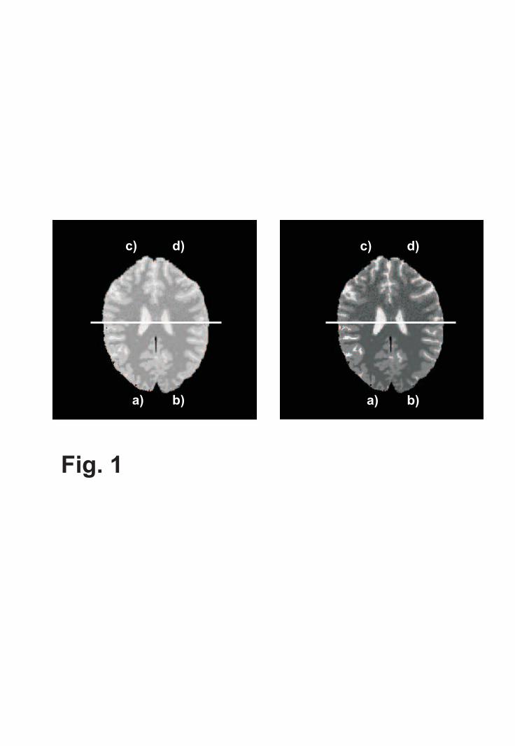
ity were modeled as follows (see Fig. 1):

1. The template segmentation was defined as the correct segmentation. From the

corresponding double-echo MR image (see II-B) the mean values were calculated

for all tissues. Each voxel intensity was set as specified in Section II.B.

2. This image was smoothed with 6 nearest, first order, neighbors in 3D. The weight

of every neighboring voxel relative to the weight of the center voxel was denoted

as S. At a value of S=1/6 the echo intensity of one voxel was 50% due to its tissue

and 50% due to the neighboring tissues.

3. 2D-Gaussian noise of standard deviation N was added. A relative measure for this

noise was the contrast to noise ratio between two tissues ( x and x’ ):

( )CNR z z Nx x x x, ’ ’ /= − . At the above mean pd echo signals a typical noise level


of N = 50 corresponded to a contrast-to-noise ratio CNRWM,GM = 4.7 and to a

signal to noise ratio SNRGM = 21 for GM.

4. The image was multiplied by an inhomogeneity factor which changed linearly with

Euclidean distance from the point (x,y,z) = (0,0,15/2). The maximal inhomogeneity

factor at a non-background tissue was set to 1 + I, whereas the minimal factor was

set to 1 − I. In this way I was a measure of the strength of the inhomogeneity. At I

= 0.125 the local GM pd echo mean varied from 927 in one part of the simulated

image to 1191 in another. The CSF variation was between 1192 and 1533.

Therefore at I = 0.125 the inhomogeneity was so large that CSF had the same

mean intensity in one part of the image as GM in the other.

III. RESULTS

We simulated MR images with different noise (N), inhomogeneity (I) and smoothing

(S). These images were segmented and compared to the correct segmentation, i.e.

the one the simulation was based on. The error was calculated as the ratio of mis-

classified voxels to non-background voxels within the entire 256x256x16 volume.

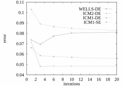
First we analyzed the convergence of the algorithms at a typical noise level N = 50,

inhomogeneity I = 0.1 and smoothing S = 0.2. In Fig. 2 no SB tissue was simulated.

It shows that at 6 iterations an adequate convergence was obtained, only the ICM1

algorithm slightly improved with further iterations. Therefore further comparisons

were done at 6 iterations. In Fig. 3 the SB tissue was simulated additionally. In this

case the ICM2 and the adaptive segmentation (AS) algorithms had huge errors of

more than the number of brain voxels after convergence. The reason for this was

that many background voxels were misclassified as SB. In practice one can reduce


these errors by pre- and postfiltering or by attaching a low a priori probability for SB.

For an appropriate comparison we did not further simulate the SB structure.

The impact of noise was analyzed in Fig. 4. Up to N = 50 the ICM1 and ICM2 algo-

rithms show low error rates of less than 0.5% whereas the adaptive segmentation

algorithm misclassified 2.3% of the voxels. For noise levels of N = 30-100 the single-

echo ICM1 yielded better results than the adaptive segmentation algorithm. For all

algorithms the error increased exponentially with the standard deviation N of the

Gaussian noise.

The influence of inhomogeneity was simulated by different values of I, see Fig. 5. For

the whole range of tested inhomogeneities the adaptive segmentation algorithm

yielded an almost constant error of 2.3%. Whereas at inhomogeneities I < 0.10 both

ICM algorithms performed better than the adaptive segmentation algorithm, at inho-

mogeneities larger than I = 0.10, i.e. larger than the tissue contrast, the ICM1

algorithm performed worse.

Smoothing, controlled by the parameter S, wipes out fine details of the simulated MR

image. Fig. 6 shows that all algorithms had difficulty to reconstruct these details, the

error considerably grew with S. Thereby, ICM1 performed slightly better with

smoothing.

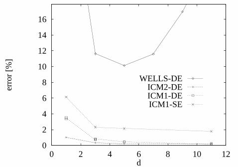
To analyze the influence of tissue thickness on the segmentation error we did not

use the brain template but an artificial image with a sinusoidal GM structure between

WM and BG. The GM „gyrus“ was d voxels thick. The error was calculated as mis-

classified voxels in a 11 voxel neighborhood of the GM structure divided by the total

number of GM voxels. At N = 50, I = 0.1 and S = 0.2 the ICM algorithms yielded good

results (see Fig. 7). The error did not improve significantly for d > 3, whereas it was

moderately higher for a fine GM structure of one voxel thickness (d=1).


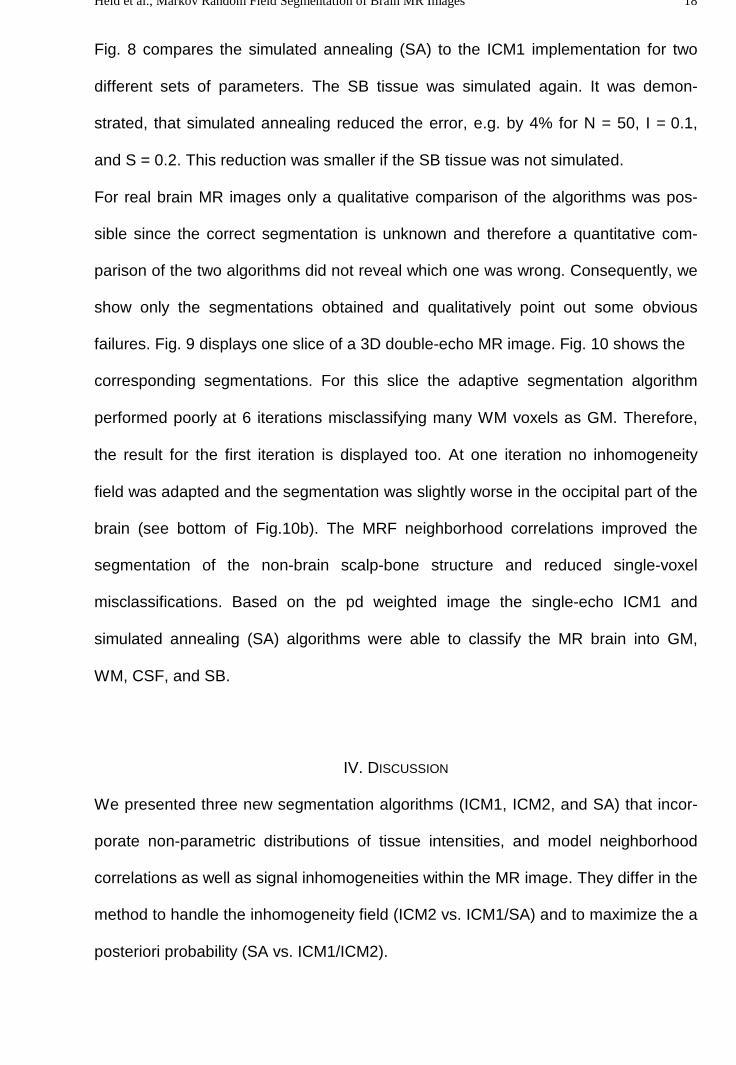
Fig. 8 compares the simulated annealing (SA) to the ICM1 implementation for two

different sets of parameters. The SB tissue was simulated again. It was demon-

strated, that simulated annealing reduced the error, e.g. by 4% for N = 50, I = 0.1,

and S = 0.2. This reduction was smaller if the SB tissue was not simulated.

For real brain MR images only a qualitative comparison of the algorithms was pos-

sible since the correct segmentation is unknown and therefore a quantitative com-

parison of the two algorithms did not reveal which one was wrong. Consequently, we

show only the segmentations obtained and qualitatively point out some obvious

failures. Fig. 9 displays one slice of a 3D double-echo MR image. Fig. 10 shows the

corresponding segmentations. For this slice the adaptive segmentation algorithm

performed poorly at 6 iterations misclassifying many WM voxels as GM. Therefore,

the result for the first iteration is displayed too. At one iteration no inhomogeneity

field was adapted and the segmentation was slightly worse in the occipital part of the

brain (see bottom of Fig.10b). The MRF neighborhood correlations improved the

segmentation of the non-brain scalp-bone structure and reduced single-voxel

misclassifications. Based on the pd weighted image the single-echo ICM1 and

simulated annealing (SA) algorithms were able to classify the MR brain into GM,

WM, CSF, and SB.

IV. DISCUSSION

We presented three new segmentation algorithms (ICM1, ICM2, and SA) that incor-

porate non-parametric distributions of tissue intensities, and model neighborhood

correlations as well as signal inhomogeneities within the MR image. They differ in the

method to handle the inhomogeneity field (ICM2 vs. ICM1/SA) and to maximize the a

posteriori probability (SA vs. ICM1/ICM2).


The ICM2 algorithm captures the intensity distribution and the inhomogeneity field in

the same way as the adaptive segmentation [10] algorithm does, but ICM2 models

neighborhood correlations as additional information to improve the segmentation The

main improvement of the use of the MRF is its better noise resistance. This can be

seen in Fig. , where ICM2 shows an error rate of less than 0.5% up to CNR=2.4.

Smoothing and even inhomogeneities are better captured (see Fig. 5 and Fig. 6).

The heuristic smoothing of the inhomogeneity field, as do the adaptive segmentation

and ICM2 algorithms, does not take into account that small inhomogeneity correc-

tions are more probable than large ones. Therefore, the ICM2 and the AS algorithms

have the tendency to overestimate the inhomogeneity. Upon more iterations the

segmentation becomes worse, see Fig. 2 and especially Fig. 3 where the additional

simulation of scalp-bone structure drastically increased the error. In practice, this has

the consequence that the operator often has to try different numbers of iterations to

yield the best segmentation result, see Fig. 10. Additionally, at fewer iterations the

inhomogeneities at the outer slices are not captured correctly. The ICM1 as well as

the SA algorithm achieved further improvement by the use of an a priori Gibbs

distribution for the inhomogeneity field. The ICM2 algorithm is superior to ICM1, see

Fig. 4, only at inhomogeneities larger than the tissue contrast which were not

observed in our MR images.

The large error of the adaptive segmentation algorithm for the artificial simulated

sinusoidal image to test the GM thickness (Fig. 7) is based on the fact that at small

GM structures the smoothing lowers the GM intensity. Therefore, many GM voxels

were misclassified as WM when using the adaptive segmentation algorithm. At large

GM structures the inhomogeneity was not captured correctly leading to a great error.


The simulated annealing algorithm (see Fig. 8) improves the segmentation, with the

penalty being long computing times. One needs 1000 SA sweeps instead of 10 ICM

iterations to obtain accurate results6. This shortcoming can be overcome by parallel-

izing the SA algorithm. Herein lies an important advantage of the local structure of

the MRF: test and update of new configurations are possible at the same time and

are only based on the information within a small neighborhood of a voxel.

V. CONCLUSION

We have presented a simulated annealing and an iterated conditional modes version

of a new Markov random field 3D segmentation algorithm. After the training of typical

echo intensities and setting one MRF parameter (β) according to the expected inho-

mogeneity (see p.14) the algorithm fully automatically segments the entire 3D MR

volume as well as different MR images, that are acquired with the same MR

sequence. For the first time non-parametric intensity distributions, neighborhood

correlations, and inhomogeneities are combined in one segmentation algorithm.

Volunteer MR images and detailed, quantitative simulations demonstrated that only

the combination of these three features leads to an accurate and robust segmenta-

tion with respect to noise, inhomogeneities, and structure thickness. Simulated

annealing allows an additional improvement compared to iterated conditional modes

at the expense of long running times.

6 This corresponds to 2000 minutes instead of about 20 minutes for the segmentation of a 256x256x64MR volume on a SPARC20 workstation.


AcknowledgmentWe thank S. Posse, H. Herzog and L. Tellmann for their advice and technical assis-tance. We appreciate the help of Dr. J. Shah in preparing the manuscript. Thecooperation between the Forschungszentrum Jülich, Institute of Medicine and theHarvard Medical School, Brigham & Women’s Hospital was supported by the DFGgrant Ro 1149/1-1; the work in the Harvard Medical School, Brigham & Women’sHospital was supported by the Whitaker Foundation grant, by the NIH pO1 CA67165-01A1 grant, and by the NSF BES-9631710 grant.

REFERENCES

[1] R. P. Woods, S. R. Cherry, and J. C. Mazziotta, „Rapid Automated Algorithmfor Aligning and Reslicing PET Images“, J. Comput. Assist. Tomogr., vol. 16,pp. 620-633, 1992.

[2] K. J. Friston, J. Ashburner, C. D. Frith, J.-B. Poline, J. D. Heather, and

R. S. J. Frackowiak, „Spatial registration and normalization of images“, preprint. [3] H.-W. Müller-Gärtner, J. M. Links, J. L. Prince, R. N. Bryan, E. McVeigh,

J. P. Leal, Ch. Davatzikos, and J. J. Frost, „Measurements of radiotracer con-centration in brain gray matter using positron emission tomography: MRI-basedcorrection for partial volume effects“, J. Cereb. Blood Flow Metab., vol. 12,pp. 571-583, 1992.

[4] N. R. Pal and S. K. Pal, „A Review on Image Segmentation Techniques“,

Pattern Recognition, vol. 26, pp. 1277-1294, 1993. [5] P. Perona and J. Malik, „Scale-Space and Edge Detection using Anisotropic

Diffusion“, IEEE Pattern Anal. Machine Intell., vol. 12, pp. 629-639, 1990. [6] G. Gerig, O. Kübler, R. Kikinis, and F. A. Jolesz, „Nonlinear Anisotropic Filtering

of MRI Data“, IEEE Trans. Med. Imag., vol. 11, pp. 221-232, 1992. [7] B. Jähne, „Digital Image Processing“, Berlin Heidelberg New York: Springer

Verlag, pp. 200-208, 1993. [8] H. E. Cline, C. L. Dumoulin, H. R. Hart, W. E. Lorensen, and S. Ludke, „3D

reconstruction of the brain from magnetic resonance imaging using a connec-tivity algorithm“, Magn. Res. Imag., vol. 5, pp. 345-52, 1987.

[9] M. Kass, A. Witkin, D. Terzopoulos, „Snakes: Active Contour Models“, Int. J.

Comput. Vision, vol. 1, pp. 321-331, 1988. [10] W. M. Wells III, W. E. L. Grimson, R. Kikinis, and F. A. Jolesz, „Adaptive Seg-

mentation of MRI data“, IEEE Trans. Med. Imag., vol. 15, pp. 429-442, 1996. [11] R. O. Duda and P. E. Hart, „Pattern Classification and Scene Analysis“, John

Wiley and Sons, 1973.


[12] S. Geman and D. Geman, „Stochastic Relaxation, Gibbs Distributions, and the

Bayesian Restoration of Images'', IEEE Trans. Pattern Anal. Machine Intell.,vol. 6, pp. 721-41, 1984.

[13] E. Ising, Zeitschrift für Physik, vol. 31, p. 253, 1925. [14] N. Metropolis, A. W. Rosenbluth, M. N. Rosenbluth, A. H. Teller, and E. Teller,

„Equations of state calculations by fast computing machine“, J. Chem. Phys.,vol. 21, pp. 1087-1091, 1953.

[15] A. W. Sandvik, „NMR relaxation rates for the spin-1/2 Heisenberg chain“, Phys.

Rev. B, vol. 52, no. 14, pp. R9831-4, 1995. [16] T. N. Pappas, „An Adaptive Clustering Algorithm for Image Segmentation“,

IEEE Trans. Signal Proc., vol. 40, pp. 901-914, 1992. [17] J. Luo, C. W. Chen, and K. J. Parker, „On the application of Gibbs random field

in image processing: from segmentation to enhancement“, J. Electron. Imag.,vol. 4, pp. 187-198, 1995.

[18] T. Taxt, and A. Lundervold, „Multispectral Analysis of the Brain Using Magnetic

Resonance Imaging“, IEEE.Trans. Med. Imag., vol. 13, pp. 470-481, 1994. [19] A. Lundervold, T. Taxt, L. Ersland, T. Bech, and K.-J. Gjesdal, „Cerebrospinal

Fluid Quantification and Visualization using 3-D Multispectral MagneticResonance Images“, Proc. 9th Scand. Conf. Image Anal., Uppsala, Sweden,1995.

[20] J.-K.. Fwu, and P. M. Djuric, „EM Algorithm for Image Segmentation Initialized

by a Tree Structure“, IEEE Trans. Imag. Proc., vol. 6, pp. 349-352, 1997. [21] J. Besag, „On the Statistical Analysis of Dirty Pictures'', J. Roy. Stat. Soc. B,

vol. 48, pp. 259-302, 1986. [22] H. Derin and H. Elliott, „Modeling and segmentation of noisy and textured im-

ages using Gibbs random field“, IEEE Trans. Pattern Anal. Mach. Intel, vol. 9,pp. 39-55, 1987.

[23] R. Kikinis, M. Shenton, F. A. Jolesz, G. Gerig, J. Martin, M. Anderson,

D. Metcalf, C. Guttmann, R. W. McCarley, W. Lorensen, and H. Cline, „Quan-titative Analysis of Brain and Cerebrospinal Fluid Spaces with MR imaging“, J.Magn. Res. Imag., pp. 619-629, 1992.

[24] S. Kirkpatrick, C. D. Gellatt, Jr., and M. P. Vecchi, „Optimization by simulated

annealing“, IBM Thomas J. Watson Research Center, NY, 1982.


FIGURE CAPTIONS

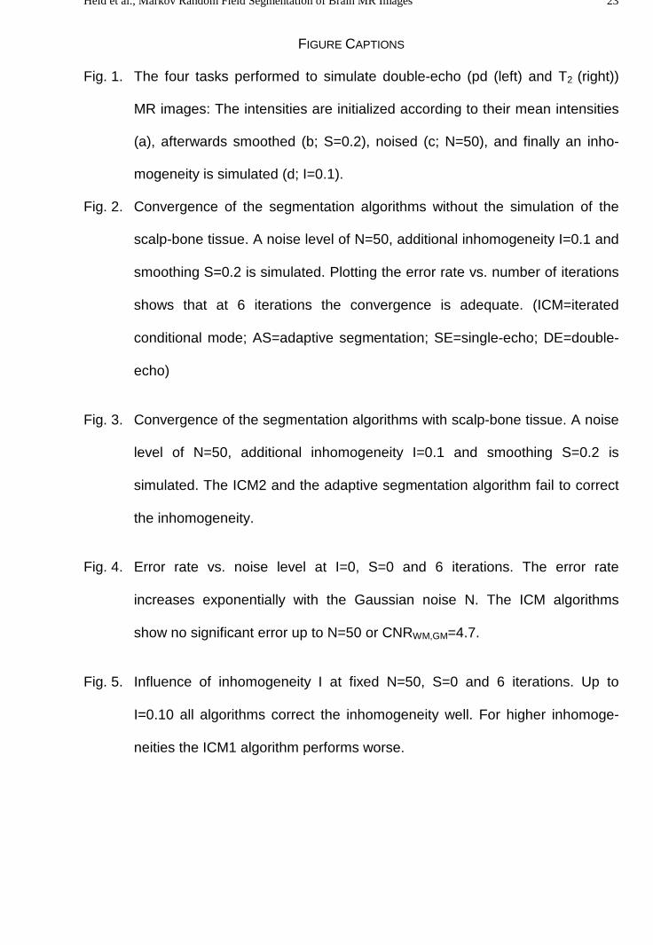
Fig. 1. The four tasks performed to simulate double-echo (pd (left) and T2 (right))

MR images: The intensities are initialized according to their mean intensities

(a), afterwards smoothed (b; S=0.2), noised (c; N=50), and finally an inho-

mogeneity is simulated (d; I=0.1).

Fig. 2. Convergence of the segmentation algorithms without the simulation of the

scalp-bone tissue. A noise level of N=50, additional inhomogeneity I=0.1 and

smoothing S=0.2 is simulated. Plotting the error rate vs. number of iterations

shows that at 6 iterations the convergence is adequate. (ICM=iterated

conditional mode; AS=adaptive segmentation; SE=single-echo; DE=double-

echo)

Fig. 3. Convergence of the segmentation algorithms with scalp-bone tissue. A noise

level of N=50, additional inhomogeneity I=0.1 and smoothing S=0.2 is

simulated. The ICM2 and the adaptive segmentation algorithm fail to correct

the inhomogeneity.

Fig. 4. Error rate vs. noise level at I=0, S=0 and 6 iterations. The error rate

increases exponentially with the Gaussian noise N. The ICM algorithms

show no significant error up to N=50 or CNRWM,GM=4.7.

Fig. 5. Influence of inhomogeneity I at fixed N=50, S=0 and 6 iterations. Up to

I=0.10 all algorithms correct the inhomogeneity well. For higher inhomoge-

neities the ICM1 algorithm performs worse.


Fig. 6. Error rate vs. smoothing at N=50, I=0 and 6 iterations. The information loss

due to the smoothing S cannot be recovered and thus the error rate

increased drastically.

Fig. 7. Error rate vs. GM thickness d. When using Markov random fields fine struc-

tures can be resolved at a low error that is only somewhat enhanced for fine

GM structures of one voxel thickness (d=1).

Fig. 8. Simulated annealing (SA) compared to ICM1 for single-echo simulations with

scalp-bone structure at two parameter sets (A: N=50, I=0.1, S=0.2; B: N=80,

I=0, S=0).

Fig. 9. Double-echo, pd (left) and T2 (right) weighted transversal slices of a 3D brain

MR image.

Fig. 10. Segmentations of the MR images from Fig. 9 (white: background, pink:

scalp-bone, yellow: csf, red: grey matter, blue: white matter, and brown:

unclassified) as determined by the AS algorithm at 6 and 1 iteration ( a and

b, respectively), double-echo ICM2 (c) and ICM1 (d), and finally by the

single-echo versions of ICM1 (e) and SA (f).

c)

a)

d)

b)

c)

a)

d)

b)

Fig. 1

0.04

0.05

0.06

0.07

0.08

0.09

0.1

0.11

0 2 4 6 8 10 12 14 16 18 20

erro

r

iterations

WELLS-DEICM2-DEICM1-DEICM1-SE

0

50

100

150

200

0 5 10 15 20

erro

r [%

]

iterations


0

5

10

15

20

25

30

0 20 40 60 80 100 120 140 160

erro

r [%

]

N


0

2

4

6

8

10

12

14

0 0.05 0.1 0.15 0.2

erro

r [%

]

I


0

2

4

6

8

10

12

0 0.1 0.2 0.3 0.4 0.5 0.6

erro

r [%

]

S


0

2

4

6

8

10

12

14

16

0 2 4 6 8 10 12

erro

r [%

]

d


0

5

10

15

20

0 200 400 600 800 1000

erro

r [%

]

iterations

ICM1-SE (A) SA-SE (A)

ICM1-SE (B) SA-SE (B)

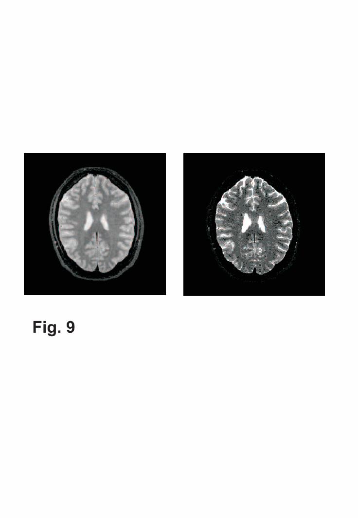
Fig. 9

adaptive segmentation6 iterations

aa

c

e

b

d

f

adaptive segmentation1 iteration

ICM1-DE

SA-SE

ICM2-DE

ICM1-SE

Fig. 10

Markov random field segmentation of brain MR images

Documents

Transcript of Markov random field segmentation of brain MR images