Retrospective Theses and Dissertations Iowa State University Capstones, Theses andDissertations

2000

Market potential for pork products with embeddedenvironmental attributes: an experimentalapproachSean Patrick HurleyIowa State University

Follow this and additional works at: https://lib.dr.iastate.edu/rtd

Part of the Agricultural and Resource Economics Commons, and the Agricultural EconomicsCommons

This Dissertation is brought to you for free and open access by the Iowa State University Capstones, Theses and Dissertations at Iowa State UniversityDigital Repository. It has been accepted for inclusion in Retrospective Theses and Dissertations by an authorized administrator of Iowa State UniversityDigital Repository. For more information, please contact digirep@iastate.edu.

Recommended CitationHurley, Sean Patrick, "Market potential for pork products with embedded environmental attributes: an experimental approach "(2000). Retrospective Theses and Dissertations. 12332.https://lib.dr.iastate.edu/rtd/12332

INFORMATION TO USERS

This manuscript has been reproduced from the microfilm master. UMl films

the text directly from the original or copy submitted. Thus, some thesis and

dissertation copies are in typewriter face, while others may be from any type of

computer printer.

The quality of this reproduction is dependent upon the quality of the

copy submitted. Broken or indistinct print, colored or poor quality illustrations

and photographs, print bleedthrough, substarxjard margins, and improper

alignment can adversely affect reproduction.

In the unlikely event that the author dkl not send UMl a complete manuscript

and there are missing pages, these will be noted. Also, if unauthorized

copyright material had to be removed, a note will indicate the deletion.

Oversize materials (e.g., maps, drawings, charts) are reproduced by

sectioning the original, beginning at the upper left-hand comer and continuing

from left to right in equal sections with small overiaps.

Photographs included in the original manuscript have t)een reproduced

xerographically in this copy. Higher quality 6' x 9' black and white

photographic prints are available for any photographs or illustrations appearing

in this copy for an additional charge. Contact UMl directly to order.

Bell & Howell lnformatk>n and Learning 300 North Zeeb Road, Ann Arbor, Ml 48106-1346 USA

800-521-0600

Market potential for pork products with embedded

environmental attributes: .Aji experimental approach

by

Sean Patrick Hurley

A dissertation submitted to the graduate faculty

in partial fulfillment of the requirements for the degree of

DOCTOR OF PHILOSOPHY

Major: Economics

Major Professor: James B. Kliebenstein

Iowa State University

.Ajnes. Iowa

2000

Copvrighl © Sean Patrick Hurley. 2000. All rights reserv ed.

UMI Number 9990456

Copyright 2000 by

Huriey, Sean Patrick

Ail rights reserved.

®

UMI UMI Microform9990456

Copyright 2001 by Bell & Howell Information and Learning Company. All rights reserved. This microform edition is protected against

unauthorized copying under Title 17, United States Code.

Bell & Howell Information and Learning Company 300 North Zeeb Road

P.O. Box 1346 Ann Arbor, Ml 48106-1346

i i

Graduate College

Iowa State University

This is to certify that the Doctoral dissertation of

Sean Patrick Hurley

Has met the dissertation requirements of Iowa State University

ajor Professor

For/the Major Program

Signature was redacted for privacy.

Signature was redacted for privacy.

Signature was redacted for privacy.

Ill

TABLE OF CONTENTS

LIST OF FIGURES v

LIST OF TABLES vi

ABSTR.^CT ix

CHAPTER ON'E: INTRODUCTION I

Dissertation Content 4

CHAPTER TWO; LITERATURE REVIEW 9

Valuation Studies for Ground Water and Livestock Odor Valuation 9

Experimental Economics and the Measure of Willingness-to-Pay 14

Ecolabeling 18

The Public Good Nature of Environmental Attributes 22

CHAPTER THREE: INTERPRETING PRICES FROM A VICICREY AUCTION 26 WHEN THE OBJECT HAS ENVIRONMENTAL ATTRIBUTES

Auctions 27

Truthful Revelation Property of the Second-Price Sealed-Bid Auction 30

Second-Pnce Auction Research 33

Interpreting the Bids from a Second-Price Auction when the Item Has 42 Embedded Environmental Attributes

Theoretical Base for Modeling Consumer Behavior with Differing 46 Information Sets

Deriving the Exogenous Factors of the Bid Function in a Multiple Round 4S \ ickrcy Auction with Different Information

Defining Willingness-to-Pay 53

CHAPTER FOUR: STUDY DESIGN AND DATA COLLECTED 61

Introduction 61

Experimental Locations 61

Participant Selection 63

Data Collection 65

The Auction (Experiment) 67

The Products 70

I V

Pretest of the Experimental Procedure "4

CHAPTER FIVE: RESULTS AND DISCUSSION' OF DATA 76

General Bid Data 79

Willingness-to-pay with Unknown Ex Ante Expectations 8S

V\'illingness-to-pay with Unknown Ex Ante Expectations: Premium Vs. Non- 9S Premium Payers

Willingness-to-pay with a Known Basis 106

\\'iiIingness-to-pay with Known Basis: Premium Vs. Non-Premium Payers 110

CHAPTER SDC: RESUXTS FROM PRE AND POST .AUCTION SURVEYS 1 IS

Pre Auction Sur\ ey 119

Premium Payers Vs. Non-Premium Payers 122

Post Auction Survey 130

CHAPTER SEVEN; ECONOMETRIC ANALYSIS 136

Lee's Polychotomous Choice Selectivity Models 143

Two-Stage Estimation with an Ordered Probit Selection Rule 146

Empirical Results 148

CHAPTER EIGHT: SUMMARY AND CONCLUSIONS 169

Summary and Conclusion 169

Future Research And Issues 178

.APPENDIX A: INTRODUCTORY LETTER 1 SO

APPENT)IX B: EXPERIMENTAL DIRECTIONS, BID SHEETS, AND PRE AND 1 S1 POST AUCTION SURVEYS

APPENDIX C: EXPERIMENTAL RESULTS BY LOC.ATION 2i

APPENDIX D: POST AUCTION SURVEY RESULTS BY LOCATION 216

APPENDIX E: LLMDEP COMMANDS FOR RUNNING ECONOMETRIC 228 MODEL

BIBLIOGRAPHY 233

LIST OF FIGURES

Figure 5.1: A\"erage Bids by Round for the Packages with Single Low- S5 Level Embedded Environmental Attributes in Comparison to the Typical Package with No Particular Environmental Attributes

Figure 5.2; Av erage Bids by Round for the Packages with Single High- S6 Le\ el Embedded Environmental Attributes in Comparison to the Typical Package with No Particular Environmental .Attributes

Figure 5.3; Average Bids by Round for the Packages with Double and S7 Triple High-Level Embedded Environmental Attributes in Comparison to the Typical Package with No Particular Environmental Attributes

Figure 5.4; Average Bids for Each Tier of Envirormiental hnprovements 93 in Comparison to the Typical Package with No Particular En% ironmental Attributes

V I

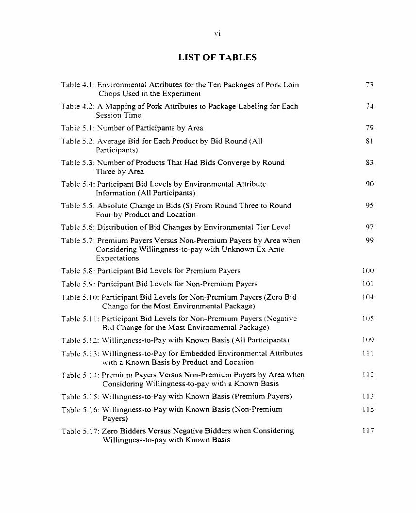
LIST OF TABLES

Table 4.1; Environmental Attributes for the Ten Packages of Pork Loin Chops Used in the Experiment

Table 4.2: A Mapping of Pork Attributes to Package Labeling for Each Session Time

Table 5.1: Number of Participants by Area

Table 5.2; Average Bid for Each Product by Bid Round (All Participants)

Table 5.3: Number of Products That Had Bids Converge by Round Three by Area

Table 5.4: Participant Bid Levels by Environmental Attribute Information (All Participants)

Table 5.5: Absolute Change in Bids (S) From Round Three to Round Four by Product and Location

Table 5.6: Distribution of Bid Changes by Environmental Tier Level

Table 5.7: Premium Payers Versus Non-Premium Payers by Area when Considering Willingness-to-pay with Unknown E.\ Ante Expectations

Table 5.S: Participant Bid Levels for Premium Payers 1

Table 5.9: Panicipant Bid Levels for Non-Premium Payers 1

Table 5.10: Participant Bid Levels for Non-Premium Payers (Zero Bid 1 Change for the Most Environmental Package)

Table 5.11: Participant Bid Levels for Non-Premium Payers (Negative I Bid Change for the Most Environmental Package)

Table 5.12: Willingness-to-Pay with Known Basis (All Participants) 1

Tabic 5.13: Willingness-to-Pay for Embedded Environmental Attributes 1 with a Known Basis by Product and Location

Tabic 5.14: Premium Payers Versus Non-Premium Payers by Area when 1 Considering Willingness-to-pay with a Known Basis

Table 5.15: Willingness-to-Pay with Known Basis (Premium Payers) 1

Table 5.16: Willingness-to-Pay with Known Basis (Non-Premium 1 Payers)

Table 5.17: Zero Bidders Versus Negative Bidders when Considering 1 Willingness-to-pay with Known Basis

/ J)

74

79

SI

83

90

95

97

99

(J(J

0 1

04

05

09

1 I

i:

13

15

17

v i i

Table 6.1: General Socioeconomic Information: All Participants 120

Tabic 6.2: Comparison of General Information: Premium Payers, Non- 123 Premium Payers for Definition One of Willingness-to-Pay

Table 6.3: Comparison of General Information: Premium Payers, Non- 124 Premium Payers for Definition Two of Willingness-to-Pay

Table 6.4: Issues of Concern: All Participants. Premium Payers. Non- 12S Premium Payers

Table 6.5: Issues of Importance: All Participants. Premium Payers. Non- 129 Premium Payers

Table 6.6: Distribution for Participant Responses on the Acceptability of 131 Methods for Odor Reduction (N = 329)

Table 6.7: Distribution for the Acceptability of Methods Used To 133 Achieve A Reduction Of Manure Seepage Into Ground Water (N = 329)

Tabic 6.8: Distribution of the Acceptability of Methods Used To 133 Achieve A Reduction In Run-off Or Spill Of Manure Into Surface Water (N = 329)

Table 6.9: Distribution of Participant Concerns About Farm Issues 134

Table 6.10: Distribution of Participant Concems About Livestock 135 Production .Methods (N = 329)

Tabic 7.1: Variable Description for Each Estimated Equation 150

Tabic 7.2: Ordered Probit Estimates for the Ex Post Categorical 154 Realization of Whether the Participant Was Negatively •Affected. Not Affected, or Positively Affected Using the First Definition of Willingness-to-Pay

Tabic " 3: Ordered Probit Estimates for the E.x Post Categoncal 1 5S Realization of Whether the Panicipant Was Negatively Affected. Not Affected, or Positively Affected Using the Second Definition of Willingness-to-Pay

Table 7.4: Frequencies of Actual and Predicted Outcomes from the 160 Estimated Ordered Probit for Definition 1 of Willingness-to-Pay

Tabic 7.5: Frequencies of Actual and Predicted Outcomes from the 160 Estimated Ordered Probit for Definition 2 of Willingness-to-Pay

Table 7.6: Second-Stage OLS Analysis of the Positive Premium Payers 163 for Definition 1 of Willingness-to-Pay

Vlll

Table 7.7: Second-Stage OLS Analysis of the Positive Premium Payers 166 for Definition 2 of Willingness-to-Pay

i x

ABSTR-\CT

This dissertation focuses on determining benefits or value of environmental

improvements in agricultural production, specifically, with an application to the pork

industry. Values or benefits from reduced odor, reduced manure run-off. and reduced

manure spills were elicited from consumers from Iowa. Kansas. \'ermont. Oregon, and North

Carolina. For the study, two pound packages of pork chops with selected combinations of

air. ground water, and surface water environmental attributes were used to obtain consumer

willingness-to-pay for environmental improvements. These benefits or willingness-to-pay

for improved environmental practices have been obtained through research using a multiple

trial sccond-price sealed-bid auction.

.A. focus of this dissertation is to investigate the relationship between willingness-to-

pay for embedded environmental attributes and socioeconomic characteristics. The

dependent variables analyzed had a mix of continuous and discrete points within the

distribution because of self-selectivity. Given this, a two-stage econometric procedure

employing a polychotomous choice function, specifically an ordered probit. was used to

investigate this relationship. Predictive ability of the model was limited and sensitive to the

\ ariables included.

Two measures of willingness-to-pay for improved envirormiental attributes were

de\ eloped and examined. It was found that under both these measures, approximately two-

thirds of the participants indicated they would be willing to pay a premium for pork products

u itli embedded environmental attributes. The average premium paid by premium payers

under botii measures ranged from SI.62 to S2.23 for the package with all three embedded

enMronmenlal attributes. Statistical methods were used to examine whether there w ere

differences in premiums with differing levels of embedded environmental attributes.

Examining the premiums across the different locations in this study shows that there were no

significant differences in the premium level by location. Demographic and attitudinal data of

the participants in this study are presented. Statistical tests are employed to see whether they

are significantly different across premium payers and non-premium payers.

I

CHAPTER ONE: INTRODUCTION

Ens'ironmental issues related to livestock production have received increased attention

in recent years. These environmental issues have included odors, and surface and ground

water quality. Asi industry at the forefront of this attention has been the pork production

indusir\-. One of the major issues the industry is facing is odor from production. This has

been due to recent scientific research which has shown the effects that odor from production

can have on nearby residents. Schiffman et al. cite studies that provide evidence of the health

risks that can occur in highly odorous environments including swine housing facilities

{I99S ). These health risks can cause localized health concems especially in large producing

states like Iowa and North Carolina.

Manure spills and odor from production have increased the concems surrounding

livestock production and the environment. Large concentrations of hog operations have

rccei\ ed a heightened focus on their effect to the environment. The three most vocalized

conccms have been odor, contamination of ground water by both slow seepage and run-off of

hog w aste, and major catastrophic events such as lagoon spills (Hone\Tnan 1995, 1996;

Perkins 1996; Beeman 1996a. 1996b; Letson and Gollehon 1996). This recent attention has

brought much scrutiny to the pig industry and effort by the industry is focusing on these

concems.

While odor has been a more local issue, the industry has attracted wide spread public

scrutiny staning in the mid 1990's. In June of 1995. North Carolina suffered a large spill that

resulted in approximately 25 million gallons of hog waste flowing into a nearby river (U.S.

New s and World Report 1996). About one month later, the Des Moines Register reported a

major spill in Iowa amounting to 1.5 million gallons of hog manure flowing into a local river

2

(19<-75). Both of these spills had a profound effect on the local environment. Additional

manure spills have occurred since that time further expanding the concern.

Due to this heightened focus, much work is currently ongoing with respect to

technologies and/or production practices that assist in reducing potential for manure spills or

leaks and resulting pollution of surface and ground water and odor reduction. However.

there is little research on what the value of improved environmental quality is for consumers.

For the past few years, the pork industry in the United Stales has been undergoing a

major structural change. In the past, this industry has been reliant on the "community"

farmer located in the region known as the Com Belt with an average hog inventor>- between

500 to 999 head. In 1988, firms marketing less than 1000 hogs a year accounted for thirty-

two percent of the market, whereas firms marketing 50,000 or more accounted for only seven

percent (Lawrence et al. 1999a). More recently the pork industr>- has seen a rapid expansion

of large production operations with inventories that well exceed 1000 head and adopt state of

the art production facilities to mass produce pigs (Meyer 1995). By 1997. the producers who

market less than a 1000 head of hogs only marketed five percent of the total United States

production. In this same year, those producers that marketed 50.000 or more hogs produced

thirts-seven percent of the market hogs (Lawrence et al. 1999a). This expansion has allowed

these larger farms to gain production cost efficiencies and caused increasing competitive

pressures for the traditional pork producer. There has been a dramatic shift from the small-

scale operations to large-scale pork production.

With the increased competitive pressure, the Iowa pork industry, too, has witnessed the

movement to large-scale operations. This adoption of large-scale operations has had two

J

major effects in Iowa. First, small-scale producers have been rapidly exiling the industry.

Second, in the adjustment process. Iowa has regained much of its competitive advantage.

States like Iowa and North Carolina have a large vested interest in the pork industr\. as

it is an important part of the economic base of the state. Swine production represents a major

industry providing much economic activity in Iowa. .Approximately 94.000 jobs are directly

related to pork production (Otto and Lawrence 1993, 1994). In a tNpical year swine gross

reccipis are 52.6 to S3 billion and represent 30 percent of all agricultural marketing

(Lawrence et al. 1994). The industry supports a multi-billion dollar input supply industry

consuming about twenty-two percent of Iowa's com production. Industry stakeholders

represent a key economic component of Iowa's economy. For a typical small rural

community in Iowa with a ten square mile trade area, swine production represents

approxmiately 58 million in economic activity.

•Along with production efficiencies, the industry's ability to effectively handle

cn\ ironmenial issues within a sustainable framework will be key to its competiti\ e position.

These cffecls have caused many debates recently in Iowa's legislature on how much

regulation is needed in Iowa's pork industry. Additionally, many people from lou a are

beginning to \oice concerns about environmental and health issues that acconipan\ large-

scale hog produclicn facilities. These issues cover ground and water quality, as w ell as air

qualiiv relating to odor and transmission of disease organisms. For the legislature lo choose

opiimal legislation (i.e. taxes on polluters, subsidies for environmental sustaining

technologies, etc.), i'. must have knowledge on how its constituents value environmental

issues.

4

Dissertation Content

While en\ ironmental issues exist about livestock production, little is known about

how society views the value or benefit of reduced livestock odors, reduced levels and or

probability of run-off from livestock production systems or manure spills. This dissertation

focuses on dcterminmg perceived benefits or value of environmental impro\ements in

livestock production, specifically, with an application to the pork industry. There are two

\ alues/benefits that can be solicited from an experimental setting that are used in this

dissertation. One value is related to the consumer's willingness-to-pay for environmental

attributes when the basis for environmental improvement is known. The other value is

related to the consumers willingness-to-pay for environmental attributes where the

consumer's environmental expectation related to the product is unknown ex ante.

The first value that is important to calculate is the consumer's willingness-to-pay for

embedded environmental attributes given an ex ante expectation of w hat levels of

environmental attributes are incorporated in the product. This expectation is deri\ ed u hen

consumers do not have complete information related to the product attributes. This value

will be known as the consumer's willingness-to-pay given unknown ex ante expectations as

to the lc\ el of embedded environmental attributes within the product, or more simply referred

to as consumer's willingness-to-pay given unknown ex ante expectations. Throughout this

dissertation this value will also be known as definition one for willingness-to-pay. Unlike

consumer's willingness-to-pay with a loiown basis, this value is calculated across different

information sets where the ex ante expectation as to the level of embedded environmental

attributes is unknown. This value represents the initial benefit the consumer receives due to

the release of environmental information.

5

The second value that is important to measure is the consumer's willingness-to-pay

when the basis for environmental improvement is known. This value is derived from taking

the difference in the value of a product with embedded environmental attributes with a

product that is considered the basis of the environmental improvement. This will be known

as the consumer's willingness-to-pay r'br pork products with embedded environmental

attributes with a known basis, or more simply consumer's willingness-to-pay with a known

basis. Throughout this dissertation this value will also be known as definition two for

willingness-to-pay. This value is calculated within a specific information set where the

consumer can compare an environmental package with a non-environmental package. This

value will anse when markets have been allowed to adjust and consumers have full

knowledge of the products they consume. Knowing this value can assist policy makers in

determining the importance of environmental attributes to consumers.

There are four main objectives of this dissertation. The first objective is- to

theoretically model the behavior of a consumer in a second-price sealed-bid auction when

there are embedded environmental attributes in the item being auctioned. A pan of this

objective is to be able to interpret what bids represent from a second-price auction when

there are embedded environmental attributes. From a second-price auction where the

products have no embedded environmental attributes, the bids given in the auction can be

interpreted as the consumer's true valuation for that product. This is a unique feature of the

second-price auction A related sub-objective is to show how the two willingness-to-pay

measures discussed above can be extracted from a multiple round, multiple object, second-

price auction when different information sets exist about the attributes of the products.

6

The second objective of this dissertation is to outline an experimental setting in which

the willingness-to-pay measures mentioned above can be collected, while the third objective

is to identify how much consumers are willing to pay for pork products with embedded

en\ ironmental attributes when looking at both of the above definitions separately—

consumer's willingness-to-pay with a known basis and consumer's willingness-to-pay given

unknown ex ante expectations. An extension of this third objective will be to investigate

w heiher these \ alues are different across different locations of the United States. .A.nother

extension is to investigate if these values differ for selected combinations of environmental

attributes.

The fourth main objective is to investigate the relationship socioeconomic factors,

specifically the core variables used in the willingness-to-pay literature, have on willingness-

to-pay for embedded environmental attributes using both definitions for willingness-to-pay.

Within this fourth objective, there are three secondary objectives. The first is to predict the

directional cffcct environmental information has on the participants using socioeconomic

\ ariables. This directional effect would be positive, negative, or no effect. This information

can assist in marketing decisions by helping marketers to more efficiently target consumers

thai will pay for products with embedded environmental attributes. Once directional mipaci

has been predicted the magnitude of the shift will be evaluated for positiv e premium pa>crs

under both definitions of willingness-to-pay. Finally, a comparison of the two models for

both definitions will be given.

Values or benefits from a reduction of odors from production facilities, and/or a

decrease in the impact to surface and ground water have been elicited from consumers from

the states of Iowa, Kansas, Vermont, Oregon, and North Carolina. Participants included pork

7

producers, their neighbors, rural community residents and urban residents. Sites selected for

the study ranged from those with a large pork production base to sites located a long distance

from pork production facilities.

Valuations are elicited from what is referred to as the experimental contingent

valuation method (XCVM). This approach uses sur\ eys to collect participant information

along with experimental economics to elicit participant values for attributes such as improved

environmental production practices (contingent value). For this study. XCVM is used to

study both definitions of consumer's willingness-to-pay for environmental sustainability

and or improvement of air, surface water, and ground water quality as it is associated with

pork production.

Sustainability within agriculture requires that at least two broad conditions be met:

one is that of environmental sustainability, and the second is economic sustainability. An

o\ erriding issue in both areas is that of social acceptability or overall impacts on society.

These societal issues feed into both the envirormiental and economic areas and will, at least

in part, be reflected in the participants' willingness-to-pay for products from systems with

differing environmental impact attributes.

The dissertation proceeds as follows. In chapter two. a discussion of related literature

is presented. The four main topics are the use of contingent valuation and hedonic pricing

studies to obtain willingness-to-pay, the use of experimental economics to elicit willingness-

to-pay. ecolabeling, and the problem of free-riding in experimental settings with public

goods. Chapter three presents a model of consumer behavior in an experimental setting with

products that have embedded environmental attributes. From this chapter, an interpretation is

gi\ en to bids that are solicited in a second-price auction when the products being sold have

s

embedded environmental attributes. Also within this chapter is a derivation of the two

willingness-to-pay measures that will be examined throughout the rest of the dissertation.

Chapter four presents the experimental process and protocol that was used for this study. It

explains how the experiment was developed and what instruments were used for collecting

data. Chapter five presents results and provides discussion of the data collected from the

experimental process. Summary statistics are also provided here along with some standard

statistical tests of pertinent hypotheses. Chapter six presents the results of the pre and post

surveys completed. It provides similarities and differences in the socioeconomic

characteristics of participants who were willing to pay a premium for embedded

environmental attributes versus those who were not. Chapter seven investigates the

relationship between willingness-to-pay and demographic and attitudinal data using a two-

stage econometric model which incorporates a polychotomous choice function. It

demonstrates how data can be modeled when the dependent variable has both continuous and

discrete points. Chapter eight presents a summary- of the findings, provides final conclusions

that can be drawn from this research, and discusses future research ideas.

9

CHAPTER TWO: LITER.\TLRE REMEW

There are four major areas in the Uterature pertaining directly to this dissertation. The

tlrst deals with sur\'ey methods to determine vvillingness-to-pay for environmental protection

and. or sustainability of the environment. These primarily use, but are not limited to.

contingent valuation methods (CVM) and hedonic price models to elicit values and- or prices

for en\ ironmental amenities. The second area pertains to the use of XCVM. i.e.. the use of

experiments, in place of CVM in eliciting consumers' willingness-to-pay for product

attributes. The third major area is that of ecolabeling and nutritional labeling. Due to the

public nature of the topic this dissertation investigates, the fourth major area in the literature

is related to the problem of free-riding and public goods being valued in an experimental

setting.

\'aluation Studies for Groundwater and Livestock Odor Valuation

Portney describes CVM studies as the use of surveys to obtain willingness-to-pay for

h\poiheiical projects or programs (1994). These elicited values are contingent upon the

constructed or simulated market presented in the survey. He defines three major elements

that are incorporated in virtually every CVM study. The first element is a description of the

scenario of the policy or program that the respondent will value or vote upon. The sccond

element is a mechanism used to elicit values or choices from the respondent. The third

element is a questionnaire that elicits dem.ographic and/or attitudinal data that will be used

for econometric and statistical purposes. For a discussion and critical evaluation of CVM.

see Portney (1994). Whitehead and Van Houtven (1997), Hanneman (1994). and Diamond

and Hausman (1994).

Much work has been completed on willingness-to-pay for ground water protection. A

primar\- approach has been the use of CVM surv eys to gain information on willingness-to-

pa\ for ground water protection (Boyle et al. 1994; Powell et al. 1994; Edwards 1998; Sun et

al. 1992; Caudill and Hoehn 1996; Poe and Bishop 1992; Jordan and Elnagheeb 1993;

Laughland et al. 1993). These studies have found an average household willingness-to-pay

for ground water protection ranging between SI to S155 per month (V\Tiitehead and \'an

Houtvcn 1997). This wide range of results is due to the various design methods used to

collect the data. For instance, there was not a clear definition across studies of ground water

contamination, or a consistent payment method used for collecting this willingness-to-pay.

e.g.. taxes, bond referendum, etc.

Boyle et al. performed a meta-analysis of current CVM studies that measure the

benefits of ground water protection (1994). This meta-analysis approach was conducted by

using unique point estimates fi"om a group of studies as observations. In their study they

found a wide range for annual willingness-to-pay. They cite three major points of interest

that relate directly to this work. First, they suggested that there is a need for improvements in

future ground water valuation studies that would more clearly identify systematic differences

in ground water \ alues. Secondly, they expressed the need for more studies to expand the

knowledge base of depth of information and specific characteristics of ground water. Third.

the\ found that educating households about ground water issues could influence the level of

willingness-to-pay.

Boyle et al. found that a major limitation to their meta-analysis was the lack of a

consistent definition for groundwater contamination (1994). Even with this limitation, which

constrained the variables they could use, they found that the core variables demonstrated

1 1

remarkable consistency. These variables were: 1) change in the probability of contamination.

2) nitrates mentioned as a source of contaminant, 3) substitute sources of portable water

mentioned. 4) cost of substitute mentioned. 5) average household income. 6) policy was to

contain contamination. 7) a dichotomous variable indicating whether the study was primarily

focused on use values, and 8) change in supply of water.

Powell et al. studied the impact CVM has on policy (1994). They point out that one of

the drawbacks of their study was that the information was collected through a mail surv ey.

Lacking from their method was a way of checking the intensity of respondent evaluation of

CVM information provided before filling out the questionnaire. They concluded that local

level decision making on ground water policy could be aided by CVM information.

However, they point out that while mail surs'eys are very useful in collecting information,

interpretation of results needs to be done with caution. It is difficult, if not impossible, to

obser\ e how the respondents filled out the survey. There is no way of knowing the time and

care respondents took in filling out the surv ey.

Recently there has been a rise in interest for organic agriculture. The importance of

organic agriculture stems from the perceived attributes embedded within organic products.

Klonsky and Tourte identify an existing perception that organic agriculture provides

soluiions to problems related to environmental quality, food safety, the viability of rural

communities, and market concentration (1998). Hence, organic farming has the perception

of a market that provides incentives for farmers to follow good environmental production

practices, providing a safe food product, having a positive community impact, and having

favorable market concentration, i.e., an acceptable mixture of small and large farms.

1 2

Due 10 this rise in interest of organic agriculture, issues such as willingness-to-pay for

organic produce (Misra et al. 1991; Weaver et al. 1992) and marketing organic products

(Thompson and Kidwell 1998; Thompson 1998; Lohr 1998; Krissoff 1998; Duram 1998)

have received increased attention. While premiums are being paid for organic agriculture

(Dobbs 1998). it is difficult to know which attributes within organic products are

commanding these premiums. There have been many studies that have investigated one of

the pcrceived attributes, the issue of food safety (Misra et al. 1991. W^eaver et al. 1992,

Roosen et al. 1998; Fox et al., 1994; Fox et al., 1995), but little has been done in the area of

embedded environmental attributes.

•A study by Misra et al. focuses on willingness-to-pay for pesticide-free fresh produce

(1991). Like most of the ground water papers, their CV'M study was also conducted through

mail sur\ey methods. They found that a majority of Georgia consumers surveyed indicated

tiiat produce certified to be pesticide free was a very important to a somewhat important

consideration in food purchases. However, consumers in general were not willing to pay

more for cenified pesticide free fresh produce.

Weaver et al. evaluate the willingness-to-pay for pesticide-free tomatoes (1992). The>

used a different methodology than Misra et al. (I99I). Instead of doing mail sur\cys. thc\

conducted face to face sur\'eys in three retail grocer\' locations in Pennsylvania. Weaver cl

al. found thai consumers were not only concerned about how pesticides affected them, but

ihcy also showed altruistic concerns about the effects pesticides had on farm workers, ground

water, and the environment. They further note that consumer's willingness-to-pay for

pesticide free tomatoes was positive and significant.

1 3

Rather than using the survey methods of Misra et al. (I99I) and Weaver et al. (1992) to

obtam \vi!Hngness-to-pay and or attitudes for pesticide free produce, Thompson and Kidw ell

(199S) did an m-store study to obtain information on consumers" choice between organic

products and conventional products. They explained the usefulness of their study comes

from actually observing consumers" choices. They were able to map attitudes into actual

purchasing behavior. Most organic food studies ha\'e focused on attributes such as pesticidcs

that may be in the food product. The study by Thompson and Kidwell focused on measuring

how cosmetic defects affect the decision of purchasing organic.

There is one area of study where willingness-to-pay work is lacking. This area deals

wiih odors from production systems. This has become an increasing problem in the hog

industr%- with the growth of large production facilities. There are three papers that have

inx estigated the effects of livestock odor on property values (Palmquist el al. 1995; .Abeles-

.•\llison and Connor 1990; Taff et al. 1996). Both Palmquist et al. and .Abeles-.Allison and

Connor show that the proximity of hog operations has a statistically significant and negative

impact on family housing property values. Taff el al. found a completely opposite result.

They found property values rising as housing was located closer to large livestock faciliiies.

They suggest that this counterintuitive result is due to livestock operation workers bidding up

housmg prices to live closer to where they work. Palmquist el al. explained that ihcy had

much difficulty with their study due to the lack of information in this area of odor valuation,

.A.1I three of these papers used hedonic price techniques to obtain a value for the effcci

li\ esiock odor has on property values. Freeman defines this technique as a "method for

estimating the implicit prices of the characteristics that differentiate closely related products

in a product class (1994, p. 125)." This technique gets at a value of a characteristic indirectly

1 4

b\- estimating implicit prices. Using this method, Palmquist et al. (1995). .Abeles-.A.llison and

Connor {1990), and the Taff et al. (1996) studies were not able to investigate whether the

food consumer would actually be willing to pay to alleviate the livestock odor problem.

The\'just show the effect livestock odor has on nearby property values. Hence, there is a

further need for a study that obtains values on what consumers" indicate they would pay for a

reduction in livestock odors.

E.vperimental Economics and the Measure of Wiilingness-to-Pay

Much of the literature and studies that have been done on willingness-to-pay for

surface and ground water impacts have utilized C\^M with mail surveys. WTiile mail surv eys

represent a cost-effective method of obtaining willingness-to-pay information, they provide

limited incentive for respondents to truthfully reveal their valuation of a good. WTiitehead

and \'an Houtven discuss three limitations of the CVM approach (1997). The first limitation

of CN'.VI is that it can be tainted by strategic bias. Strategic bias occurs when respondents

o\ crstate or understate their true willingness-to-pay because they perceive that their answer

u ill intluence policy. The second limitation arises because CVM studies can be very

sensiti\ e to the various methods for eliciting values, e.g., using an open-ended question

\ crsus a close-cnded question. The third limitation of the C\'.M comes from the hxpothetica!

nauirc of the questions asked which may cast doubts on the reliability of the values

generated.

Experimental economics, on the other hand, provides more incentive for the

participants to reveal their tnie value for a good. Fox et al. state "the non-hypothetical

experimental method provides a more accurate and reliable estimate of economic value than

traditional sur\'ey techniques (1995, p. 1048)." It uses real money, real goods, and real

auctions (Fox el al. 1996). Hence, it provides more incentive for participants in the study to

reveai their preferences truthfully compared to typical CX'M studies.

There can be a large benefit to using experiments to discover willingness-to-pay.

W ithin an experiment a researcher can control the parameters which go into the experiment

and the participant decisions can be observed (Davis and Holt 1993). Experimental

economics allows the researcher to provide information and observ e how it affects the

outcome. The XCVM method is a very controlled environment, whereas CV'Vl using mail

sur\ eys leaves many unanswered questions.

When valuing willingness-to-pay it has been argued that the second-price sealed-bid

auction is one of the most efficient methods of gaining a consumer's value of a good

(Shogren et al. 1994a). The second-price sealed-bid auction is conducted as follows. A

group of participants (consumers) are allowed to bid on a good(s). The highest bidder for the

good is obligated to buy the good at the second highest bid price. The dominant strategy in

this auction setting is for participants to reveal their true willingness-tc-pay (Hoffman et a!.

1993. .Menkhaus et al. 1992). The robustness of this auction method is shown in Shogren ci

al. (1994a). Their results "suggest that the revealed preferences for low-probability risk

reductions are relatively robust to variations in the Vickrey auction. While this does not

pro\ c that subjects revealed their true preferences, it does suggest that the bids were not

particularly susceptible to refined changes in the set of market prices (1994a, p. 1094)."

There have been multiple studies that have used experimental economics, specifically

auctions, to obtain consumers' willingness-to-pay for attributes related to products. This

method has been used to elicit values for food safety attributes in selected food products

(Fox. 1993; Fox et al., 1995; Fox et al., 1996; Hayes et al. 1996; Roosen et al. 1998). quality

1 6

differences in food products (Melton et al. 1996a. 1996b). and packaging of food products

(Hoffman et al. 1993; Menkhaus et al. 1992). Fo.\ et al. went one step further and used

e.xpenmental techniques to calibrate contingent values from a CVM study (1998).

Hoffman et al. (1993) and Menkhaus et al. (1992) have used experimental auctions to

in\ esiigate whether people have a preference on how their meat products are packaged.

Specifically, they test whether there is a difference in willingness-to-pay for packages of

steaks placed in a traditional over-wrapped stjrofoam tray versus steaks that are vacuum-skin

packaged. Packaging can be an important attribute related to a product because it can affect

the visual appeal of the good. To obtain these values, they use a fifth-price, sealed bid

auction. '

There are a few major tlndings in Hoffman et al. (1993) and Menkhaus et al. (1992)

that are of interest. First, they found that with no information, the bids for the steaks in the

stvTofoam packaging were not significantly different from the bid for the steaks in the

\ acuum-skin packaging. Once information was released about the benefits of vacuum-skin

packaging, the bids for the steaks in the vacuum-skin, as well as the styrofoam packaging,

were significantly higher than in the no information case. Releasing information also caused

the bids for the steaks in the vacuum skin packaging to be significantly greater than the bids

for the steaks in the styrofoam packaging (Hoffman et al. 1993). When regressing the

dependent variable (difference in bids for the two different packages of steaks) on the

independent variables (demographic characteristics), they found that most of the

demographic variables "'were not particularly important explanators (Menkhaus 1993. p.

' .A fifth-pnce. sealed-bid auction is where the four highest bidders purchase the good they bid on at the fifth highest price. This auction has the same demand revealing properties as the second-price, sealed-bid auction.

17

51)." Only income, number of people in household, and employment were significant factors

(Menkhaus el al. 1992).

Rather than investigating attributes that are not embedded in the product. Melton ei

al. studied the effects physical attributes have on consumers' willingness-to-pay for a pork

product (1996a, 1996b). They used a second-price, ascending bid auction to investigate pork

chop characteristics such as color, marbling, and size. This auction method works much like

the second-price, sealed-bid auction. The only difference is that there are successive rounds

where bids must stay the same or be increased. In their study, they presented these pork chop

characteristics three ways—appearance by photograph, appearance by visual inspection, and

appearance after a taste test of similar chops.

There are three major results of the Melton et al. paper (1996b). The first result is

that the level of physical attributes embodied in pork chops does matter. Secondly,

appearance and taste are not equally good sources of information for evaluating pork chop

characieristics. Third, consumers are not consistent in their preferences for fresh pork chops.

The method used to convey information does matter. Melton et al. conclude that consumers

arc able to "distinguish and value subtle differences in the attributes of a fresh food product,

such as pork chops (1996b. p. 923)." In the Mellon et al. paper, standard regression analysis

is used lo in\ osiigate the relationship between bid prices for pork chops and demographic

characteristics and physical attributes (1996a). .After the taste test for the pork chops. lhc>

found ihat women, households with children, and multi-income households tend to bid less

for the pork chops. Furthermore, age, education, and household size reduce prices bid for

chops, while household income was positively related to chop bid prices.

18

Ecolabeling

Researchers in the third area, ecolabeling, examined firms which engage in

en\ ironmenially friendly practices and then inform the public through advertising and. or

product labeling. Bagnoli and Watts cite many examples of ecolabeling; including the recent

shift to selling dolphin-safe tuna (1996). .Another example pertains to the use of recycled

materials in packaging or in the product itself, e.g.. recycled paper. \ third class of examples

is the production and sale of cruelty-free products. Each of these examples carries one

particular common denominator; these attributes have no physical effect on the product's

characteristics. This in turn has led to the production of a public good by the market without

in\olving government intervention, such as regulations or taxation. This public good

pro\ ided by the market relates to the environment.

There are five primary papers that pertain to ecolabeling. Two of the papers, one by

Bagnoli and Watts (1996) and one by Kirchhoff (1996). deal with a more theoretical view of

ecolabeling. The third paper by van Ravenswaay develops the current situation with

ccolabeling and some possible problems and policy issues related to products with

environmental attributes (1996). The fourth paper by Nimon and Beghin (1997) and the fifth

paper by Teisl et al. (1999) evaluate consumers' willingness-to-pay premiums for products

u ith embedded environmental attributes.

Bagnoli and Watts provide a basic overview of ecolabeling (1996). They also set up

a theoretical model that shows how effective ecolabeling can be in using the market to

pro\ ide a public good such as environmental protection and sustainability. Their model

incorporates a Bertrand and a Coumot economic setting. In the Coumot setting, the firm

sclects the amount of good it wants to sell and allows the market to dictate the price; while.

in the Bertrand setting, the firm sets the price and lets the market dictate the quantity sold.

Furthermore, they test this theoretical model in both the Coumot and Bertrand settings using

an experimental economic environment. Bagnoli and Watts found from their experiments

that firms would have an incentive to produce some of the public good, i.e., the

environmental good, but not necessarily the most efficient level (1996).

The second theoretical paper is by Kirchhoff (1996). She presents a model in which a

monopoly over-complies with legal en\ ironmental standards under asymmetric intormation.

She cites findings by Salop and Scheffman (1983) which have shown that "a firm might

rationally want stricter regulations if compljing with them is relatively costlier for its

competitors (1996, p. 3)." Kirchhoff further cites a poll by Greenberg/'Lake which has found

that: "In the United States, 83 percent of consumers in a 1993 poll stated that they were

willing to pay more for environmentally sound products (1996, p. 3)." Hence she is making

the argument that firms will sell goods with environmental attributes to gain the premium

that people would pay for those attributes. Furthermore, she believes that a fimi would seek

out a third-party labeling system to assist in the validity of the environmental attributes. This

third party would provide credibility to the product sold.

Having cited some evidence that this is actually going on in the United States.

Kirchhoff lays out a theoretical model to e.xplain why this might be true (1996). She states

that "voluntary over-compliance is shown to be more likely when quality premia are

relatively high, cost differences are relatively low, and the probability of cheating being

discovered is sufficiently high" (1996, p. 19). Hence her major conclusion is that if there

v\ ere a large enough premium to be gained in producing a good with environmental

20

atiributes. then the firm would have an incentive to produce and market that good with those

attributes.

This theoretical view of Bagnoli and Watts (1996 ) and Kirchhoff (1996) has been

substantiated in the real world by van Ravenswaay (1996). She states that "over the last

decade, a growing number of consumers have been demanding more environmentally

fncndly products, and manufacturers have been meeting that demand by voluntarily

including a growing number of environmental claims on their product label (1996. p. 1)."

She further cites that more than 20 countries have developed ecolabeling programs. These

countries have come together to form an international organization to facilitate

harmonization of product claims across different participating programs all over the world.

In her paper, van Ravenswaay also looks at two major controversies that arise with

ecolabcling and discusses the policy implications that arise from it (1996). The first

controx ersy she discusses pertains to the potential for consumer deception. She discusses

poienlial difficulties in substantiating environmental claims of being "environmentally

friendly." Hence she cites the key issue in this controversy is what types of environmental

labels are and are not deceptive.

The second controversy van Ravenswaay introduces is whether environmental labels

should also ser\ e environmental objectives (1996). Thus, the label should not only be

truthful, but it should reduce the environmental impact of consumption. This implies that

even though the claims on the label may be true, the claims can not come from increasing

some other environmental impact that more than offset the original impact. For example, if a

firm claims to reduce the impact of production on w'ater pollution, it cannot at the same time

21

increase its impact in another environmental area such as odor that more than offsets the

original impact. Hence, the claim must have a positive net return to environmental impacts.

.More firms are adopting ecolabeling to gain an advantage over their competitors

while meeting the changing demands of consumers. This, in turn, will lead more firms to

adopt ecolabeling methods with this approach as a method of removing or improving

competitiveness. The market can provide a public good, that of environmental sustainability.

u ith little or no government intervention. This has been verified in an area closely related to

ecolabeling. This area is nutritional and food safety product labeling. Caswell and

-Mojduszka study how information labeling of nutritional and food safety attributes can effect

the market demand of a product (1996). They cite evidence that information labeling does

have a positive influence on demand. Since information labeling can affect consumer

demand, the focus of their paper is on the economic rationales for labeling policies and issues

related to how the success or failure of these policies should be judged.

Caswell and Mojduszka (1996) cite some of the same problems of information

labeling of food safety and nutritional attributes that van Ravenswaay (1996) has espoused

with ecolabeling. In many aspects they are the same. A major difference between

ecolabeling and information labeling of food safety and nutritional attributes is that the

fomier deals with nonuse values and the latter pertains to use value. Nonuse values are

values that are independent of people's present use. WTiereas. use values are values that are

directly related to present consumption (Freeman 1994).

Nimon and Beghin investigate whether consumers pay a premium for environmental

attributes embedded in clothing (1997). The specific attributes they looked at were organic

cotton and environmental-fiiendly dyes. Using a hedonic price function, they found that

consumers paid a premium for organic cotton. On the other hand, they found no evidence

that consumers paid a premium for environmentally friendly dyes. Hence their paper suggest

that certain environmental attributes may receive a premium while others do not.

Along the same line as Nimon and Beghin (1997), TeisI et al. investigated the effect

ecolabeling has on tuna with the attribute that it was caught with nets that are safe to dolphins

(1999). Their goal was to measure the effectiveness of dolphin-safe labeling of canned tuna.

Thc> used a product e.xpenditure approach to show that dolphin-safe labeling, i.e.,

ecolabeling. affected consumer behavior. This labeling caused tuna to gain market share

o\ er substitute products. While they were able to show that ecolabeling tuna as dolphin-safe

liad an effect on market share, they were not able to deduce what the value of that ecolabel

u as. Hence, they were not able to get at willingness-to-pay for dolphin-safe tuna.

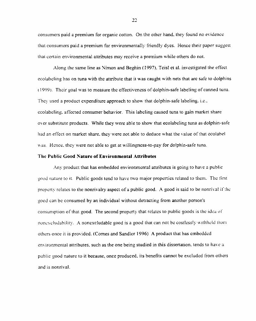
The Public Good Nature of Environmental Attributes

.Any product that has embedded environmental attributes is going to ha\ e a public

good nature lo it. Public goods tend to have two major properties related to them. The first

propertN relates lo the nonrivalry aspect of a public good. A good is said to be nonrival if the

good can be consumed by an individual without detracting from another person's

consumption of thai good. The second property that relates to public goods is the idea of

noncxcludabiiity. A nonexcludable good is a good that can not be costlessly withheld (rorrt

others once it is provided. (Comes and Sandler 1996) A product that has embedded

en\ ironmental attributes, such as the one being studied in this dissertation, tends to have a

public good nature to it because, once produced, its benefits cannot be e.xcluded from others

and is nonrival.

There is a vast Hterature on the nature of public goods. One major area of this

literature that pertains directly to this dissertation is the free-riding literature. This literature

stems from an inherent problem that arises due to the two major attributes of public goods—

nonrivalry and nonexcludability. Free-riding as it relates to provision of public goods is

hen people underrepresent their true benefits from the public good to avoid having to pay

for the total benefits they receive from that provision. Hence free-riding tends to lead to the

underprovision of public goods. In its extreme, free-riding would lead to no provision of the

public good.

.Much research has been done in the area of free-riding as it relates to the provision of

a public good in an experimental setting. One of the first papers to look at this issue was

done by Marwell and .\mes (1979). They designed an experiment to test whether people

truly free-ride when giving to the provision of a public good. In their research they found

approximately fifty-seven percent of the available resources went to the provision of the

public good. Strong free-riding tendencies of the participants would have predicted thai this

number would have been closer to zero. Hence, Marwell and Ames were able to show that

while there was an underprovision of the public good in their experiment, there were still a

substantial amount of resources given by the participants towards a public good (

Marwell and .A.mes investigated provision of the public good in a one-shot setting

(19~9). They received criticism of their work because they did not investigate what would

happen to provision to the public good over time. Isaac et al. (1985) built upon Marwell and

Ames' work (1979) by adding repetition to the experimental process. Isaac et al. had the

participants in their study give to the public good many times within one experiment. They

found that in the first round their results were much the same as Marwell and Ames. But,

24

they further found with repetition that there was a tendency of the participants to give less to

the public good in later rounds. Hence, they found that with repetition there was a signitlcani

underprovision of the public good within the experimental setting.

The two studies above show that with less e.xperienced participants there is a

tendency for them to give to the public good. But with repetition, it was also found that

provision of the public good declines. Neither of these studies systematically looked at the

free-riding principle. The first group of researchers to take a systematic investigation of what

causes free riding was Isaac, Walker, and Thomas (1984). In Isaac et al., they systematically

investigated how repetition, group size, and pay-off to providing the public good affects

participants contribution levels to the public good (1984). They found three major results.

First, having a higher pay-off to the provision of the public good leads to higher contribution

levels. Obviously, if the return from the provision of the public good is high, participants

u ill tend to give more to the public good. Second, they found that experience does matter.

In liicir study, the more experienced participants tended to give less to the pro\ ision of the

public good. Third, they found that group size had a positive correlation with contribution to

the public good, i.e., as group size increased, the contribution to the public good increased.

WTiile many researchers have investigated within an experimental setting the

p r o \ ision of public goods, there has been no definitive research which shows why people

give the amount they do. In public good experiments, some participants give to the public

good while others do not. The free-riding problem can be prevalent, i.e., underprovision of

the public good, but not to the extent that theory would suggest (Davis and Holt). It should

be noted that all of the studies looked at public goods in a ver>' abstract manner, i.e., the

public good was a pot of money. No research has been done in an experimental setting

25

testing how people would give to an actual public good. e.g.. a park bench, environment, etc..

that is not related to the participants within the respective studies. One part of this

dissenation investigates this issue.

CHAPTER THREE: INTERPRETING PRICES FROM A VICKRE^

AUCTION WHEN THE OBJECT HAS ENVIRONMENTAL

ATTRIBUTES

This chapter examines consumer behavior in a second-price sealed-bid auction with

products having different environmental quality attributes. A unique feature of this model is

that it describes consumer behavior with different information sets. From this model, a

demonstration will be given on how to derive consumers willingness-to-pay for embedded

en\ ironmental attributes through the consumer's behavioral choice using a second-price

sealed-bid auction. It will be showTi that if free-riding e.xists. then prices from the second-

price auction cannot be interpreted as the consumer's true valuation of the product being sold.

Furthermore this chapter will show how prices for products with embedded environmental

attributes from a second-price sealed-bid auction can be interpreted.

In this chapter it will also be shown that in an auction setting with different

information sets, willingness-to-pay can be derived in at least two ways. One way relates to

comparing a t\pical good to one that has an environmental improvement over the typical

good m the same round. This willingness-to-pay measure assures that the expectation of the

cn\ ironmental attributes for the consumer is known, but it does not directly account for any

\ isua! nonen^ ironmental quality differences between the two products being considered.

.\noiher wa\' to look at consumer's willingness-to-pay is to obser\ e it for similar products

\\ ith different information sets. This allows for the visual attributes of the product to remain

constant, but there is no ex ante information on the consumer's prior expectation of

embedded environmental attributes. It should be noted that, ex post, these expectations

could be inferred.

27

Auctions

McAfee and McMillan define an auction as a "market institution with an explicit set

of rules determining resource allocation and prices on the basis of bids from the market

participants." (1987, p. 701) Over the centuries, auctions have been used to establish value

for many different kinds of commodities. Some of these commodities include plundered

booi> from the people who were conquered by the Roman Empire, federal land, artwork,

limber rights, stamps, and wine. The four most common auctions are the English auction, the

Dutch auction, the first-price sealed-bid auction, and the second-price sealed-bid auction.

(.Vlilgrom and Weber, 1982)'

In a typical English auction, an auctioneer starts the bidding sequence at a low pricc

and steadily increases the price for the item until only one willing bidder remains. In this

auction, everyone involved in the auction knows the number of active bidders and the current

bid price at any point in time in the auction. While the English auction starts at a low price

and increases, the Dutch auction starts at a high price that decreases. The price in this

auction decreases until some bidder stops the auction at an acceptable price and claims the

item for the price at which the auction stopped. The Dutch auction is used to sell flowers in

Holland. In the first-price sealed-bid auction, each bidder submits a bid to the auctioneer

which is unknown to the other bidders." In this auction, the highest bidder claims ihc obicci

being auctioned at the price she bid. In the second-price sealed-bid auction, each bidder also

submits a bid to the auctioneer which is unknown to other bidders. The difference between a

• l-or an in-depth discussion on each of these auction mechanism see; Milgrom and Weber; 19S2, .Vlc.A.fee and Mc.Millan. 19S7; and .Milgrom, 19S9; V'ickrey, 1961. " .-\ seaied-bid auction is an auction where each bidder submits a bid to the auctioneer which is unknown to the other bidders. Only the auctioneer knows who submined a particular bid.

first-price and a second-price auction is that in a second-price auction the highest bidder

claims the object being auctioned at the second highest bid.

hi 1961. William Vickrey laid the foundations for the study of auctions (1961). He

in\ estigaled the four auctions mentioned above under what is now considered the benchmark

model for studying auctions. In his paper he investigated these four auctions under six basic

assumptions. One basic assumption Vickrey used for stud\'ing auctions was that the bidders

in the auction are risk neutral. Another assumption N'ickrey made was that the bidders were

svTnmetric. Bidders are said to be symmetric when they draw their valuations from the same

probability distribution. Symmetry also requires that bidders who draw the same valuation

gi\ e identical bids. A third assumption made by Vickrey is that there is no collusion among

the bidders. The fourth assumption is that paxTnent is a function of the bids alone. This

implies that there are no reservation values of the auctioneer or initial payments to the

auctioneer to enter the auction.^ No initial payment implies that anyone can participate in the

auction without paying a fee to the auctioneer. An implicit fifth assumption Vickrey made

u as that bidders have e.xpected utility maximizing beha\ ior.'* The sixth assumption in

X ickrcy's investigation is that the independent-private-values assumption applies. Under this

assumption, each bidder is assumed to know her exact valuation of the good she is bidding

on. u hile not knowing anyone else's valuation. .A.lso. the bidder perceives the value of an>

other bidder as a random draw from some probability distribution where the value of other

bidder's is statistically independent from her own.

resen. e price is the minimum price set by the auctioneer at which she will sell the item being auctioned. It" the highest bidder's bid is below the reserve price, the item being auctioned will not be sold. " This specific assumption was not given in Victj^ey's 1961 paper explicitly. Kami and Safra (1986, 1989) demonstrated that Vickrey needed to assume that the bidders are expected utility maximizing agents to make some of his arguments.

29

Under these six assumptions, which will be referred to as the benchmark model of

assumptions. Vickxey was able to demonstrate some remarkable findings through

argumentation. One of these findings is that the Dutch auction and the first-price auction are

straiegically equivalent. Strategic equivalence implies that the sets of strategies and their

mapping to outcomes are identical for both auctions. Another finding of Vickrey was that

the English auction and the second-price sealed-bid auction both have a dominant strategy

equilibrium of revealing one's true valuation." A dominant strategy is a strategy such that no

other strategy is better than it is. A third finding by Vickrey is that the English auction and

the second-price sealed-bid auction are Pareto optimal in the sense that the bidder with the

highest valuation wins the object. The most remarkable finding in Vickrey's paper relates to

expected revenue of the auctions. He conjectured that the four typical auctions described

abo\ e with the same benchmark assumptions would generate on average the same revenue to

the seller.'* This would imply that from the point of view of the seller, it would not matter

which auction mechanism was utilized to sell an object.'

Of the four auctions mentioned above, two stand out as better mechanisms for

gathering consumer's willingness-to-pay for embedded environmental attributes. These t\\ o

auctions are the second-price sealed-bid auction and the English auction. The reason these

iwo auctions stand out is because under the benchmark assumptions, they both have as

~ Kami and Safra showed that to obtain this result it is necessary to assume that bidders follow expected utility niaximizini: behavior (1989). To prove that true value revelation is a dominant strategy in a second-price sealed-bid auction it is a neccssary and sufficient condition for the bidders to have e.xpected utility maximizing behavior. Kami and Safra (1986) also showed that the existence of a dominant strategy of truth revelation does not imply utility maximizing behavior for the second-price auction. ' This IS knoN^Ti as the Revenue Equivalence Theorem. For a discussion of why this is true, see .Vlc.Afee and McMillan (1987).

It should be noted that while the four auctions under the benchmark assumptions have the same expected re\ enue. this does not imply that they have the same variance.

30

dominant strategies truthful revelation of the bidders" preferences. Theoretically, in the

Dutch auction and the first-price sealed-bid auction, it is in the interest of the bidders to bid a

\ aluc below their true valuation. The amount each bidder shaves her bid from her true

\ aluation will depend upon the probability distribution of the other bidders' valuations and

the number of competing bidders (McAfee and McMillan, 1987).

T r u t h f u l Revelation Propert>- of the Second-Price Sealed-Bid .Auction

Before consumer behavior can be understood in a second-price sealed-bid auction

where the product has embedded environmental attributes, a major characteristic of the

auction must be discussed. A major characteristic of the single-unit second-price sealed-bid

auction is that it requires the top bidder to purchase the object being bid upon at the second

highest bid price. This feature of the auction ensures that each participant will bid his/her

true willingness to pay for the product being auctioned, i.e.. each participant's true valuation

(Vickrey 1961). The reason this holds true is because in a game theoretic setting it is the

bidder's weakly dominant strategy to bid his/lier true value."^ This true valuation can be

dcfmed as the maximum income that the bidder would be willing to give up to obtain the

product. The bidder's utility in this situation is equal to the bidder's utility when she has her

full amount of income and no product.

To see why the second-price sealed-bid auction gi\ es the true willingness-to-pay for

an object, the following standard argument from the literature is presented (Vickrey 1961:

Mc.A.fee and .McMillan 1987. Kami and Safra 1989). Suppose there are N bidders where

bidder i, i = 1. 2, ... . N, gives a bid of b, for an object and has a true valuation of v, for that

^ -A weakly dominant strategy is a strategy such that no other strategy is strictly better than it is. In this case, some strategies may be equally good, but not necessarily for all cases.

31

object. It is also assumed that the benchmark model set of assumption explained above holds

true for each bidder—the bidders are risk neutral expected utility maximizers. there is no

collusion among the bidders, the independent-private-values assumption holds, the bidders

are s\Tnmetric, and the bidders pa>Tnent is a function of their bids alone. Let VV be the

maximum bid of all other bidders excluding bidder i. Without loss of generality, assume that

if bidder i does not purchase the object her utility level is 0. Also assume that if she does

purchase the good her utility is equal to her true valuation minus the second highest bid.

Hence, if her true valuation is greater than the second highest bid she obtains a positive

utility from purchasing the good.

There are two general scenarios that must be investigated. The first scenario is when

bidder i bids higher than her true valuation, i.e.. b, > v,. In this first scenario, suppose that W

> b,. This would imply that bidder i receives 0 utility whether she bids her true valuation or

not because she is not the highest bidder. Now suppose that W < v, < bi. In this case bidder

i obtains utility level v, - W, which she would have obtained by bidding her true valuation \

Suppose that the ma.ximum bid from all other participants is greater than the true valuation of

bidder i but less than the bid given by bidder i. i.e., v, < W < b,. This would imply that the

utility of bidder i is equal to v, - VV, which is obviously a negative number. In this situation,

it w ould ha\ e been better for bidder i to bid her true valuation v, and obtain a utility lc\cl ot'

U. Hencc. it has been shown that bidder i would have done no worse by bidding her true

valuation and in some cases would have been better off

The second scenario that needs to be investigated is when bidder i bids less than her

true valuation, i.e.. b, < v,. In this situation, when bidder i bids greater than or equal to the

maximum of the other bidders, i.e., b, > W, she receives a utility level of v, - W. which is a

32

positive level. Bidder i, in this case, would have received the same utility le\ el if she bid her

true valuation. If the true valuation of bidder i is less than or equal to the maximum bid of all

the other individuals, i.e., W > v„ then she received 0 utility. In this case, she could receive

the same utility level by bidding her true valuation because she will never be the highest

bidder. Finally, if the bid of bidder i is strictly less than the ma.\imum bid of the other

individuals, which is strictly less than the true valuation of bidder i, i.e., v, > \V > b„ then

bidder i foregoes a positive utility level by under bidding. In this case it would have been in

the best interest of bidder i to bid her true valuation. Hence, it has been shown under this

second scenario that bidder i would have done no worse by bidding her true valuation and in

some cases would have been better off.

Two major implications of the Vickrey auction can be drawn from the above

discussion. The first implication is that the second-price sealed-bid auction has the property

of optimizing individuals revealing their true preferences in a noncooperative game theoretic

setting. The second implication is that this auction mechanism divorces the bidders from

strategic interaction, i.e., the bidders do not base their bids on what they believe the other

bidders are doing. This can be seen from the fact that probabilities were not utilized in the

argument above.These implications will be important when looking at willingness-lo-pay

for environmental attributes and consumer behavior.

'• Implicitly, the bidder increases her probabilitv- of being the highest bidder by increasing her bid. but this does not increase her gains (utility) compared to bidding her true valuation. The assumption that relates to probability structures in the benchmark model of assumptions is used to prove revenue equivalence among the four auctions. TTiis assumption is not necessary when establishing the dominant strategy of the second-price auction.

Second-Price Auction Research

Since Vickrey's seminal paper, there has been much research done in the area of

auctions. N4uch of this research has focused on the seller's side of the auction and usually

consists of optimal auction theorems or comparing different auctions in the areas of revenue

generation and equi\ alence (Matthews. 1987). The literature on optimal auction theorems

attempts to characterize auctions which optimize seller's revenue given a particular set of

assumptions. In the literature related to revenue generation, auctions are ranked by the

amount of money each generates to the seller using a particular set of assumptions. The

re% enue equiv alence literature investigates what assumptions are required for a set of

auctions to generate equivalent e.xpected revenue.

In the benchmark model, the most fundamental assumption that is studied in the

second-price auction literature is related to the differences among the bidders" valuations of

the item. There are two extreme assumptions that can be made about the bidders' valuations

( Mc.A^fee and .VIcVIillan 1987). The first extreme is known as the independent-private-values

assumption. Under this assumption, each bidder is assumed to know exactly her true v alue

of ilie item being auctioned. She does not know any other bidder's value of the item; rather,

she perceives any other bidder's value as a random draw from some probabilit\ distribution.

This \ alue is independent of any other bidder's value. The common-value assumption is the

converse of the independent-private-values assumption. Under the common-value

assumption, the object being auctioned has a single objective value which is unknown to the

bidders. This implies that every bidder has the same valuation of the product being

auctioned, but they do not know with certainty what that valuation is. Hence, each bidder

draws her valuation from the same distribution as the other bidders given this single objective

34

value. An example of this type of item being auctioned would be a tract of oil King beneath

the ground.

Wlien valuing embedded environmental attributes, it is more appropriate to use the

independent-private-values assumption. This assumption allows the bidders to value

en\ ironmental attributes differently, i.e.. the utility derived from environmental attributes can

be different for different bidders. The common-value assumption requires that the bidders

have the same value for environmental attributes.

V\'ithin the theoretical literature related to second-price sealed-bid auctions using the

independent-private-values assumption there are three major areas that are studied which

relax the assumptions of Vickrey's seminal paper. The first set of papers examines collusion

in a second-price auction. Second-price auctions when more than one item is sold are

examined in the second set of papers. The third set of papers examines bidder's risk

behavior, conjectures, and behavior without expected utility.

There are three major papers that study collusion in a second-price auction with the

indepcndent-private-values assumption. One paper examines why the second-price auction

has a tendency of facilitating collusion among bidders compared to other auction methods

(von Ungem-Stemberg 1988). The two other papers that study collusion examine

mechanisms for maintaining collusion in a second-price auction (Graham and Marshall

.Maiiath and Zemsky 1991).

von Ungem-Stemberg studies why a second-price auction is a better facilitator of

collusive behavior than the other auctions, i.e., first-price, Dutch, and English auctions, by

modeling the collusive behavior in a second-price auction as a cartel (1988). This cartel

designates who the high bidder will be for any particular auction. The bidders that are not

35

designated the high bidder must submit a predetermined bid set by the cartel. He argues that

since the highest bidder only has to pay the second highest bid in a second-price auction,

collusion can be maintained in this type of auction by having the designated high bidder

submit a bid exorbitantly higher than the highest valuation of the other members of the

collusive group. Wlien bidders exist outside the cartel, von Ungem-Stemberg argues that the

designated highest bidder from the cartel will still submit a bid higher than his valuation if he

believes it will encourage cartel discipline. He funher argues that collusion in the second-

price auction is even more pronounced when the bidders repeatedly interact with each other

in other second-price auctions.

Graham and Marshall study collusion and the auctioneer's best response to collusion

in the second-price auction with ex ante homogeneous bidders (1987). In their model, they

have an outside agent which coordinates the collusion of a subset of bidders. This agent

operates an incentive compatible mechanism prior to the actual auction, known as a

prcauction knockout, to implement efficient collusion among any subset of bidders.

Collusive behavior in Graham and Marshall's model is maintained by the outside agent

offering side pavTnents to the collusive bidders. Except for the designated high bidder from

the preauction knockout, the rest of the members of the collusive group submit a bid less than

their true valuation in the second-price auction. From their model, Graham and Marshall

show that coalitions among a subset of bidders in the actual auction is possible and that gains

to the coalition are increasing in the size of the coalition. They also showed that the optimal

response of the auctioneer is to develop a reserve price that is a function of the coalition's

size.

36

Mailath and Zemsky (1991) take the work of Graham and Marshall (19S7 ) one siep

further by studying collusion with ex ante heterogeneous bidders. Mailath and Zemsky were

able to show that a mechanism exists to obtain an ex post budget balancing efficient

collusion in a second-price auction.In Graham and Marshall's work, their mechanism was

ex ante budget balancing, not necessarily ex post budget balancing. To obtain efficient

collusion. Mailath and Zemsky show that each bidder's net payoff from participating in the

coalition is a constant, which is independent of her valuation." They also show thai the

collusi\ e surplus can always be allocated in such a way that every subset of bidders will

alw ays wish to participate in the coalition.

In the independent-private-values setting, there are two major papers that examine

issues related to selling multiple objects in a second-price auction. The first paper examines

the auctioneer's choice of whether to sell multiple objects in multiple single unit auctions or

to group the items into one single unit auction (Chakraborty 1999).'" The second paper

studies the properties of selling multiple objects in multiple sequential auctions when the

bidders have diminishing marginal valuations of the items being sold (Katzman 1999).

In the context of a second-price auction, Chakraborty investigates under what

conditions an auctioneer would want to sell multiple objects in multiple auctions versus

selling the multiple objects in one bundle in a single auction (1999). In his model, he

assumes thai the bidders employ the same strategies whether they face a single auciion or

multiple auctions and that the values of the multiple objects are additive. Without proof, he

Budget balancing is said to exist when the summation of the side payments are less than or equal to zero. '' The net payoff of the bidder is defined as the difference between the expected payoff when colluding and the payoff when not colluding.

Noie that in a single unit auction only an item or a group of items arc sold as one unit.

37

stales thai "it is the dominant strategy for each bidder to bid his true valuation for the objects

w hen the objects are sold simultaneously or sequentially through Vickrey auctions (1999. p.

725)." In essence, he has assumed away any wealth effects that might occur in the multiple

auction setting due to a buyer having obtained an item in a previous auction.' " By assuming

away wealth effects, he is implicitly assuming that there is no complementarity or

substitutability between the products being auctioned. The major result that Chakraborty

found was the e.xistence of a unique critical number of bidders for each set of objects being

auctioned such that the seller prefers to bundle the objects when there are fewer bidders than

the critical value. When there are more bidders than the critical number of bidders, the seller

prefers to sell the objects in separate auctions. Furthermore, he was able to show that this

property still holds even when the valuations for the objects are correlated for a given bidder.

In the complicated world of multi-unit demands. Katzman studies behavior in a

second-price auction with diminishing marginal valuations (1999). To make the problem

tractable he uses the most simplistic model he can. He assumes that there are two bidders

and a sequence of two auctions. Within this setting, Katzman studies the behavior of bidders

w hen there is complete and incomplete information sets. Katzman examines four situations

that could occur with complete information. He shows that in a few situations bidders rc\cal

their true valuation of the item being auctioned, but in most situations they do not. Price

sequences tend to be constant or decreasing in the complete information setting and there is

the possibility for inefficient allocations.'"' Bidding behavior is quite different in the

incomplete information setting. In the first sequence of bidding, both bidders shave their

'' Wealth effects are when participants change their bids because they won an earlier trial (Fox et al. 19951. See Davis and Holt (1993) for a discussion of wealth effects in e.xperimental markets.

Inefficiency in this context implies that the bidder with the highest valuation does not obtain the item.

38

high \ aluations when bidding. In the final auciion. bidders bid their true valuations. Thus, in

the incomplete world, there are efficient allocations of the item being auctioned.

There are five main papers that are related to bidders' conjectures and risk attitudes in

the second-price auction with the independent-private-values assumption. .A. paper by

Rotiikopf et al. studies the question why V^ickrey auctions are rarely used in the real world

setting (1990). Two papers exsmiine the implications from the buyers and seller's point of

\ iew when bidders are risk averse (Matthews 1987; Smith and Levin 1996). N'eilson

examines second-price auctions when the bidders are not e.xpected utility maximizers (1994).

while Lo e.xamines uncertainty averse bidders (1998).

With revenue equivalence of the four auctions and the truthful revelation property of

the \'ickrey auction using the benchmark model. Rothkopf et al. ask the question of why the

\ ickrey auction is seldom used in practice (1990). To answer this question, they examine

se\ en possible reasons, five of which have been examined by other authors, why the Vickrey

auciion is rarely used. From the standpoint of Rothkopf et al. there are five inadequate

reasons for the rarity of the second-price auction studied in the literature. These reasons are;

1) man\ auctions sell multiple objects for sale, 2) bidder risk aversion. 3) bidder as\Tnmciry,

4) non-independent values, i.e., the common-value assumption, and 5) inertia.'"^ Two reasons

thai were not examined in the literature prior to Rothkopf el al. are strictly related to the

bidders. These authors argue that one of the major reasons why second-price auctions arc

rare is because the bidders fear bid takers might cheat them. A second reason, u hich the

authors argue is an even more plausible reason, is that bidders have a resistance to truih-

'• Inertia is the argument that the second-price auction is not used because bidders have become accustomed to other auction methods.

re\ ealing strategies. In this first case, the authors argue that in a Vickrey auction, it would be

lucrative for the auctioneer to place a phony bid higher than the actual second highest bid to

capture the surplus that is given to the highest bidder due to the nature of the auction.'" In an

English auction where everyone at ever\' point in time sees the bids in the auction, this phony

bid is not as big of a problem. In the second case, the authors argue that bidders are

conditioned not to give their true valuations because of later interactions with other bidders.

Bidders may fear that revealing their true valuation in a particular auction may harm them in

future auctions.

WTien e.xamining the second-price auction within the conte.xt of the independent-

pnvate-values assumption, the predominant emphasis of the literature has been placed on the

seller's point of view. To counter this bias. Matthews investigates second-price auctions

from the point of view of the buyer (1987). Specifically, he studies which auctions the

buyers would prefer when each bidder is risk averse. He examines three different auctions—

the first price auction, the second-price auction, and the first price auction when the number

of bidders is revealed—where bidders exhibit decreasing (DARA), constant (C.A.R.A.). or

increasing (IAR.A.) absolute risk aversion.' One of the major findings of Matthews is that

u iih no reserve price, it is the dominant strategy to reveal one's true valuation under all three

risk av ersion slates. Matthews is able to also show that when CAR.A holds, the bidders arc

'' The surplus that goes to the bidder is the difTerence between the highest bid and the second highest bid. In a \ ickrey auction, this surplus goes fiilly to the bidder. ' Matthews assumes that in the standard first-price and second-price auctions that the bidders do not know hou manj- bidders there are m the auction. In the second-price auction it does not matter how many bidders there are from the point of view of the optimal strategy to use when bidding (1996). But. it will matter to the bidders in the tlrst-price auction because they shave there bid from their true value based on the number of bidders in the auction.

indifferent between all three auctions. Under DAR.\. Matthews shows that the bidders prefer

the second-price auction to the first price auction, while under lARA. it is the exact opposite.

Smith and Levin (1996) take Matthews (1987) research one step further. Rather than

having a fixed number of bidders. Smith and Levin study the first-price and second-price

auction u hen entry is endogenous under the three t>pes of risk aversion. They are able to

show that under lARA and CARA, that the results of Matthews remain robust with

endogenous entr\'. However, under DARA, the ranking of the auctions can change with

endogenous entry. Smith and Levin show that the reason the ranking can change with

endogenous entry is because the first price auction "mechanism discourages entrv' to an

extent that offsets its inherent tendency to stimulate more aggressive bidding (1996. p. 550)."

Even with endogenous entry, it is still a dominant strategy for the bidders to reveal their irue

valuation in the second-price auction.

One of the assumptions made in the benchmark model is that the bidders in the

auciion must be expected utility maximizing agents. This necessar>' and sufficient condition

\\ as shown by Kami and Safra (1989). They showed that when this assumption is missing,

i.e.. when the bidder's preferences are represented by a non-expected utility functional, it is

the dominant strategy of bidders to bid their certainty equivalence of the item. Building on

Kami and Safra's work. Neilson investigates what happens to the results of the second pricc

auciion when expected utility fails (1994). Specifically, he examines what happens when the

number of bidders change in the auction, what happens to the optimal reserve price set by the

auctioneer, and what happens to revenue equivalence between the English and second-price

auction. Neilson is able to show that when the number of bidders or the reserve price

changes, the bids by the participants will change. He also shows that when e.xpected utility

fails, the English auction and the second-price auction do not give the same expected

re\ cnue.

-Ajiother author who relaxes the expected utility assumption is Lo (199S). The focus

of his paper is to study what happens to the first-price and second-price auction when bidders

are uncertainty averse. Uncertainty aversion is a state when each bidder is unsure of the

probability measures of the other bidders. While one of the main focuses of Lo's paper is to

classify the equilibrium bidding strategies of the first price auction, he does state that the

equilibrium bidding strategy for the second-price auction is still the dominant strategy of

re\ ealing one's true valuation. Under uncertainty aversion, Lo is able to show under certain

conditions that the first-price auction Pareto dominates the second price auction.

When studying the literature related to the second-price sealed-bid auction using the

independent-private-values assumption, three general results emerge. In all three papers

pertaining to collusion in a second-price auction, it is clear that the bidders who participate in

collusion and are not selected to be the winning bidder by the group have no incentive to

rc\ eal their true valuations. Hence, the first general result is that the property of truthful

revelation of preferences breaks down when collusion exists. The second result is that the

second-pnce auction from the point of view of the seller, when comparing it to other

auctions, can be ver>- sensitive to the assumptions made within the model. Excluding

collusive behavior, the third result is that the dominant strategy of bidding one's true value is

robust to change in the assumptions of bidders' behavior.

42

Interpreting the Bids from a Second-Price Auction when the Item Has Embedded

Environmental Attributes

In the literature above, it was seen that the dominant strategy in a second-price

sealed-bid auction is to bid one's true value for the item being auctioned. This result is ver\-

robust unless the bidder is not an expected utility maximizer or if collusion exists among the

bidders. One of the implicit assumptions that was made to prove the dominant strategy in the

second-price auction is that the item being auctioned is a purely private good with no public

good attributes. When examining items with embedded environmental attributes, this

implicit assumption does not hold. These items have a public good aspect to them. From

chapter two. it is known that when public good attributes exist, there is a possibility of free-

riding by consumers. This motivates the question as to how to interpret the bids from a

second-price auction when some of the goods have embedded environmental attributes. To

understand how to interpret bids in an auction when the item has embedded environmental

attributes, an understanding of a bidder's valuation is necessarv'.

It shall be assumed that there are I bidders in a second-price sealed-bid auction

bidding on one item which has embedded environmental attributes. Bidder i's. i = 1. 2

1. true valuation of the product being auctioned is v,. Bidder i's true valuation v, is assumed

lo be ihc sum of three disjoint values, i.e., v, = v,; v,; - v,;. v,i is defined to be the

maximum amount of money bidder i is willing to give up to obtain the physical attributes

embodied in the product being auctioned. In the case of a pork chop, this value is derived

from such physical attributes as tenderness, color, type of cut, marbling, etc. The second

\ alue, \ ;2, is defined as the true value the bidder receives from being the one that contributes

to the public good, i.e., it is the maximum amount of money the bidder is willing to give up

to provide lo the public good no matter what other bidders do. This value could be derived

from altruism or warm-glow altruism.'® Altruism is where people give to a public good and

receive utility from the consequences of their giving. Warm-glow altruism is where people

receive satisfaction from the process of giving to the public good with no regard to the

conscquences of giving (Kotchen et al. 2000). For this value to e.\ist. the bidder must be the

one who obtains the item from the auction, v,;. can be viewed as the \ alue one receives from

the public good being provided by some other person. It is the maximum amount of money

the bidder is willing to give to the public good, which does not overlap with v,2. assuming

that no other person is contributing to the public good. If other bidders are contributing to

the public good, this value is going to be conditional on the other bidder's contribution. This

value exists for each bidder no matter who provided the public good. Hence, this is a value

where free-riding can occur. The distinction made between v,2 and v,;. is that v,; is only

realized if the bidder is the highest bidder, whereas, v,; is realized no matter who is the

liighest bidder.

To interpret the bids from a second-price auction when the item has embedded

en\ ironmenial attributes, the same t>pe of reasoning used to prove the pure private good case

can be used. i.e.. Vickrey's argument can be adapted to this situation. First of all. it shall be

assumed thai the assumptions of the benchmark model hold.' '^ In the pure private good ease,

it was assumed without loss of generality that the utility of the bidder was 0 if she did not

purchase the object. This is no longer the case with an item that has embedded

en\ironmental attributes. Even if bidder i does not purchase the good, she still obtains v,^.

.Altruism and warm-glow altruism ha%'e been studied by Andreoni (1988, 1990). Noie that die assumption of bidders' being risk neutral can be weakened to risk averse.

44

This is because no matter who provides the public good, bidder i receives utility from the

public good characteristic of the product being auctioned. Hence, as long as bidder i believes

that someone will purchase the good with embedded environmental attributes, it will never

be in the interest of the bidder i to incorporate v,3 into her bid function.This implies that in

a second-price auction it is not a dominant strategy for the bidder to reveal her true valuation

of the item. To show this rigorously, a stronger statement will be proven. Under the

assumptions of the benchmark model, when the item has embedded environmental attributes

and the bidder has some free-riding tendencies, it shall be proven that the dominant strategy

for each bidder is for her to bid a value equal to v,i2 = v,i v,2.

Define \V as the maximum bid given by all bidders excluding bidder i. If bidder i is

the highest bidder, then W is the second highest bid. Bidder i is assumed to have a true

v aluation of the product of v,. where v, = v,i v,; v,:.. Define V, as the difference between

bidder i's true valuation, v,. and VV. There are two scenarios, one with four cases and the

other with three, that need to be examined to show that bidding v,i2 is the dominant strategy.

The first scenario is when bidder i bids higher than v,i2, i.e., b, > v,i2- In this first

scenario, suppose that W > b,. This would imply that bidder i receives a utility lev el of \

whether she bids v,i2 or not because she is not the highest bidder. Suppose that the maximum

bid from all other participants is greater than the true valuation of bidder i but less than the

bid given by bidder i, i.e., v, < W < b,. This would imply that the utility of bidder i is equal to

V, = V, - W. which is obsMously a negative number. In this situation, it would have been

better for bidder i to bid v,i2 and obtain a utility level of v.i. Under this situation, if the

In auction setting, this belief is not unrealistic. Since the item being auctioned has already been produced, the environmental characteristics have already been provided. This being the case, bidder i can view v,3 as an initial endowment of utility which she does not have to pay for.

45

bidder bid her true valuation v., she would have obtained a positive utility of v,;. Now

suppose that v,i; < W < Vj < bi. In this case bidder i obtains utility level V, = v, - W. Since

W is less than bidder i's true valuation v,, then V, > 0. While V, is nonnegative in this case,

this does not imply that bidding one's true valuation is a dominant strategy. Since W is

greater than v,i -r v,2, then the bidder would have done better off by bidding v,i:. By bidding

\ bidder i would have received utility level v,;,. In this case, V, = v, - W < v,;,. The final

case in scenario one assumes that W < v,i2 < v, < b,. While bidding b, in this case gives the

bidder a utility level greater than v,3, the bidder could have done just as well by bidding v,i:.

Hence, it has already been shown that it is not the bidder's dominant strategy to bid her true

\ aluaiion. It has also been shown for scenario one that bidder i can do no better than bidding

v.i:-

The second scenario that needs to be investigated is when bidder i bids less than v, ,;.

i.e.. b.. < V,:;. In this situation, there are only three cases that need to be examined. In case

one. assume that W > v,i2 > b,. Under this first case, bidder i could have received the same

uiiiity \if she bid v.ij. Suppose that for case two, v,i2 > W > b,. By bidding belovs- v.i;.

bidder i obtains utility v,3. Bidder i could have been better off had she bid v,i;. because \'

would ha\c been equal to v, - W > v, - v,i2 > v,;,. In this case, bidder i foregoes a greater

uiiliiy level by under bidding. Finally for case three, suppose that v,i2 ^ b; > W. In this ease,

ii would make no difference whether bidder i bid b, or v,i2- Under each bid she would obtam

the utility V, = v, -W. Hence, it has been shown under this second scenario that bidder i

would have done no worse by bidding v,i2 and in some cases would have been better off

46

Coupling the results in scenario two with scenario one's results, it has been shown

tliat bidding \-,i: = v,i -r v,2 is a dominant strategy for bidder i. The intuition behind this result

is the following. Since v,3 represents the value of the public good, which the bidder gets even

if she is not the highest bidder, it is not in her best interest to incorporate it into her bidding

strategy. v,i; represents the value to the bidder only if she obtains the item being auctioned.

Hence, if the bidder wants to maximize her probability of obtaining the largest surplus from

the auction procedure, she should bid v,i2. It should be noted that if a person is a perfect free-

rider and the product being auctioned has embedded environmental attributes, then tlie bid

received in this auction would be equal to the bid received in a second-price auction when the

item has no embedded environmental attributes.

It has been shown that in a second-price sealed-bid auction, only the private value

v,i-. which is less than Vj when free-riding exists, is submitted as the bid. WTien

en\ ironmentaI attributes exist or any other t\pe of spillover effect, the second-price auction

does not get at a bidder's true valuation.

Theoretical Base for Modeling Consumer Behavior with Differing Information Sets

It has just been shown how to interpret bids for a product with embedded

environmental attributes from a second-price sealed-bid auction. The next step in

understanding value in a multiple-round second-price auction with different information sets,

is to understand the theoretical base of consumer behavior \vhen different information sets

exist. Teisl et al. provide this theoretical framework for handling consumer behavior when

there are different information sets (1999).

In the paper by Teisl et al., they studied what effects dolphin-safe labeling had on the

tuna industry (1999). To study this issue, they adopt a model proposed by Foster and Just

A1

(19S9) thai takes into account when consumers have different information sets about the

product. Their model starts with an indirect utility function that incorporates environmental

assessments for a given set of products, a v ector of other quality characteristics for those

products, prices, and income. Specifically, they represent their indirect utility function as;

(3.1) = V(.\^ q, Y, p)

where = environmental assessments for m products given information set S.

q = vector of other quality characteristics,

Y = income,

p = a vector of prices for the m products.

They assume that this indirect utility function increases with quality characteristics and

income, and decreases with prices.

To translate environmental information into an environmental assessment A^. TeisI et

al. assume that the assessment function can be modeled as a household production process.

This process lakes into account the individual's environmental knowledge, cognitive abilities,

lime, and ihe environmental information presented at the time of purchase. They model this

process as the following:

(3.2) = f(Sj, G, tj; 0).

In this process, is the individual's subjective environmental assessment of purchasing

s s good j given information set S. Note that A j is an element in \ . Sj is the environmental

mformaiion displayed about product j at the time of purchase. The consumer's prior stock of

en\'ironmental information is represented by G. This would include any news accounts,

advertising, word-of-mouth, or any other source of information previously obtained about the

product. The time spent analyzing the environmental information about product j is denoted

by t,. Finally. 0 represents the objective levels of environmental impact from consumption of

the products.

This model lays the foundations for thinking about how consumer's value is derived

in a second-price sealed-bid auction with rounds having different information sets.

Specifically, it incorporates different information sets into the standard consumer

optimization problem. This model elaborates on what a bidder's true value v, is dependent

upon. i.e.. v, is dependent on income, prices, quality characteristics, information.

Deriving the Exogenous Factors of the Bid Function in a Multiple Round Vickrey

.Auction with Different Information

The standard utility maximization problem assumes that prices are fixed and

consumers choose the quantity they want to consume. While this is the usual setting in

which consumers make decisions, it is not necessarily indicative of how consumers make

decisions in a multiple round second-price sealed-bid auction. In this auction setting, the

consumers have a fixed quantity to consume and are allowed to submit bids. In this ease,

participants will set bids for the objects they are bidding upon at their true valuation for that

product when there are no embedded environmental attributes and v,i2. which was e.xplained

abo\ e. when environmental attributes exist. This is the unique behavioral characteristic

associated with the second-price auction and must be taken into consideration of the model.

.Another characteristic of this model is that different information sets can be used in the

different rounds of bidding. This section sketches the exogenous factors that affect the bid

function in a multiple round second-price auction with different information sets.

The utility function of a consumer can be modeled as having three different

components. The first component relates to the products that will be consumed and how they

49

show up in the uliHty function. The second component within the utiUty function is an

assessment function that maps cenain attributes of the products into utility. The third

component that is related to the utility function is the socioeconomic characteristics that

make up the consumer. Hence the consumer's utility function for an information set 1 is

represented as:

(3.3) U = U(y. .xi.x;; A', S)

\\ here y = a vector of goods not in the auction,

xi = a nonenvironmental product in the auction.

x: = an environmental product in the auction.

a' = environmental assessments for xl and x2 given information set S.

S = vector of socioeconomic characteristics of the consumer.

It is assumed that the consumer's utility function is increasing at a decreasing rate for y. xi.

X:, and any element of A*.

For this model, assume that the consumer's utility is dependent on the characteristics

of purchased goods. Further assume that these goods can be broken up into three groups.

The first group is the normal basket of goods that the consumer purchases outside of the

auction setting. This basket of goods will be denoted by y and have an associated vector of

fixed prices Pj. The second group of goods is the set of products in the auction that have no

particular environmental attributes, while the third group of goods is the set of products in ilic

auction that have embedded envirorunental attributes. The only differences between these

last tw o groups are that they differ in the level of embedded environmental attributes and

possibly perceived visual quality attributes. Without loss of generality, it is assumed that the

50

last two groups of goods only consist of one product each."' The non-environmental product,

i.e.. the t\pical product, will be denoted by Xi and the product with embedded environmental

atiribute(s) will be denoted by xi. In this setting, the choice variables for the consumer are

the normal basket of goods y. the bid for the t\'pical product p-,. and the bid for the product

with embedded environmental attribute(s) pi-

Following Teisl et al. (1999), it is assumed that within the consumers utility function

there is an assessment function .4' which evaluates the products based on a set of

characteristics given an information set I. This assessment function contains the assessment

of each product, i.e., a' = [a/, .\2'. An'] where An' is the assessment of product n based

on infonnation set I. This assessment function maps certain attributes such as quality

characteristics into utility. Within this information set I. there is information pertaining to

the attributes embodied within the products and previous market prices. In the case of an

auction for products with embedded environmental attributes, one information set may

contain no environmental information regarding the products. This could be known as a

naY\ c information set. In another information set, there could be environmental information

released.

The set of characteristics in the assessment function can be divided into two subsets.

The first subset is related to the physical attributes related to the products and will be denoted

b\ Q. These characteristics revolve mainly around visual quality—color, texture, marbling,

etc. Within this Q, the evaluation of each product can be divided by product, i.e., Q = [Q,.

"• For the second group, there is usually only one product in that set which is used as a basis for comparison. For the thu-d group of products, there will be independence between the products that have different environmental attributes. This independence will come from the fact that in this auction at most one product uill be sold after all the rounds of bidding are completed. Hence, by adding products to this group there will be no alTect on the budget constraint of the consumer.

51

Q: Qn] where Qn is the quality evaluation of product n based on visual inspection. It is

assumed that the utility function is increasing in Q, i.e.. a consumer has an ordered

preference for different visual attributes. Across information sets, these visual attributes are

constant for each product. The visual quality of a product does not change across

information sets. Due to the constant visual quality, no adjustments will need to be made

when comparing products across information sets. Within a particular information set. these

\ isual qualities can be very different across products or at least perceived as such. This

would imply that any comparison of products within an information set must account for

possible perceived visual quality differences.

The other subset of characteristics is related to environmental attributes and will be

denoted by E(I). Within E(I), the evaluation of each product can be segregated by product,

i.e.. E(I) = [Ei(r). £2(1), ..., En(I)] where £„(!) is the quality evaluation of product n based on

perceived or e.xpected environmental attributes given information set I. It is assumed that the

utility function is increasing in both the level of environmental attributes and the number of

en\ ironmental attributes. A consumer's utility will increase if they perceive that the number

of environmental attributes has increased or if the level of a panicular environmental

atiribute is perceived to increase. These characteristics are related to the perceived or

expecied environmental attributes embodied in each product. Whether these characteristics

are perceived versus expected will depend upon which information set the consumer has. In

a naive round with no environmental information, this set of characteristics would be related

to the consumer's expectation of the environmental attributes embodied in each product. In a

bid round where environmental information exists for each product, then the set of

characteristics are perceived.

52

One component that is not directly represented in the standard utility function or the

model of Teisl ei al. (1999) is the socioeconomic characteristics of the consumer. These

characteristics are usually implied within the utility function by assuming that all consumers

are the same. Since all the consumers are considered identical, there is no need to have the

socioeconomic characteristics explicitly given. However, these characteristics are seldom

equal. There are gender differences, age differences, educational differences, attitudinal

differences, etc. Each of these characteristics can have an affect on how the consumer values

products. Hence, they can cause the utility function of one person to be different to the

utility function of another person. In this model. S will denote the socioeconomic

characteristics.

For each purchase decision, the consumer will maximize her utility function given a

fixed amount of income M under the given rules of the second-price sealed-bid auction.

.Adapting the model of Teisl et al. (1999) to this situation, the consumer's indirect utility

funciion can be represented as:

(3.4) \-'= V(A'. M. pv, S)

w here A ' = f(Q, E(I)).

From this indirect utility funciion, a person's true valuation v, can be derived through

cxamuiing what happens to a person's utility when a new allocation of attributes or a new

information set is provided. A person's true valuation can be defined as the maximum

amount of income she would be willing to pay to obtain a change. In this case, it would be

the amount of money the consumer would be willing to give up to obtain the environmental

53

aliribuies or the information pertaining to the environmental attributes. This is also known as

compensating variation.""

Since a person's true valuation of a particular change is dependent on the indirect

utility function, this would imply that a person's true valuation is dependent on the same

exogenous factors. In this case, a person's true valuation depends on the assessment

function, the information set, income, socioeconomic factors, and the prices of other goods.

Taking this a step further, since it has been shown that a person's bid in an auction setting is

dependent on a person's true valuation, this would imply that the exogenous factors of a

person's true valuation would also be influencing factors in a person's bid function. With

this information, wiliingness-to-pay in a multiple round second-price auction with different

information sets can now be defined.

Defining W'illingness-to-Pay

.As mentioned above, this dissertation looks at two willingness-to-pay measures. To

see u here these different measures come from, an examination of the bids given in each

round of the second-price auction is necessary. Within this auction, the participants will bu>

no more than one of the goods being auctioned, i.e., a final characteristic of this mode! is that

only one product will be sold after the auction is over. The product sold is randoniK' selected

tVom a round that is also randomly selected. This allows an auction that investigates the

\aluc of man\ goods to maintain the properties of the Vickrey auction explained abo\ e.

Another way of defining a person's true valuation is by using equivalent variation. Equivalent variation is the amount of money would be willing to accept to forgo a change. There are two basic reasons compensating variation can be a better choice for examining a person's true valuation. First of all. a typical second-price auction for a good is a natural way for gathering compensating variation. Secondly, compensating variation is bounded by a person's income, whereas equivalent variation is unbounded.

54

Without loss of generality, it is assumed that there are two products being bid upon.

The first product is a product that has no embedded environmental attributes, while the

second product is a product that has the same physical attributes as the first product but has

embedded environmental attributes. In the naive bidding round where there is no specific

cn\ ironmental information about the two products, the bidders only have expectations about

the embedded environmental attributes. In a bidding round with environmental information,

the bidders know the embedded environmental attributes. The bids for the first and second

product are defined respectively as bi(py. M, S, A') and b^CPy, M, S. A'). These bids are a

function of the person's true valuation for each product. Since it is assumed that each bid is

derived from the second-price auction, it has been shown earlier that that b,(py. M. S. A*) will

be equal to v,i; if the bidders are strategically optimizing their payoff" \\Tien the bidder

expects or knows that the product has no environmental attributes, her bid for that product

w ill equal her true valuation. In a second-price auction setting, it can be expected that bi(Py.

M. S. .A.') and b2(py, M. S, \') will be different across different information rounds if

panicipants value envirorunental attributes. Each of these bids is independent of each other

smcc the bidder will only purchase, at most, one of the products.

To make this analysis more clear, assume that there are two information rounds in the

second price auction. In the first round, it is assumed that there is no specific infomiation I'

related to the environmental attributes. This is usually known as a naive bidding round

u here consumers usually bid on visual attributes. For the next round, information I" is

released on the embedded environmental attributes of the product. This would imply that

•' it should be noted that for the case of a product with no environmental attributes, v,,; = v,,. This is because v,j and v,3 are equal to zero when the product has no environmental attributes.

under the first information set I', the set of bids are bi(pj. M. S. A') and b;(py, M. S. A'

Under the second information set I", the set of bids are b>(py. M. S. A' ) and b:(pj. M. S.

A' ). h should be obvious that the prices for the goods outside of the experiment Py.

consumer income M. and the socioeconomic characteristics S of the consumer have not

changed. Hence, the only thing that has changed is the information in the assessment

function. This would imply that further investigation of the assessment function is necessary.

.A.S mentioned above, the assessment function can be written as A' = f(Q. E(I)). Since

there are only two products being examined, this function can be written as a' = flQi. Q;,

E;(I). E;(I)). In this case, Qi and Q: denote the visual quality assessment ofthe t\pical

package and the environmental package respectively. No matter which information set the

consumer is in, these quality attributes do not differ across information sets for each product.

Within a particular information set. these quality evaluations can be quite different. Ei(I) and

E:( I) denote the perceived or expected environmental attributes in the typical package and

the environmental package in information set I. In the naive information set I' where no

information related to environmental attributes has been released, these environmental

quality assessments are based on expectations. Within this information set, there is no u ay

for ihe researcher to know the basis for the expectation. In the environmental information sci

I", the consumer knows the level and number of environmental attributes embedded in each

product. They also know that the product with environmental attributes is using the l\pical

product as the basis, i.e., a comparison is made between the two products within this

information set where the typical product is used as the basis of comparison.

It should be noted that in this naive round, the panicipant has no environmental information. Hence, the subscripts on prices are only being used to keep track of each product through the different rounds.

Up lo this point, the bids given in the auction represent all of the attributes

incorporated in the products being auctioned, i.e., the bids represent both the visual quality

attributes and the environmental attributes. The objective of this dissertation is to value the

en\ ironmental attributes only. To do this, the visual quality attributes must be factored out.

This implies that there are two major definitions for willingness-to-pay that can be developed

from this auction setting with different information sets to obtain the value for environmental

attributes. The first definition for willingness-to-pay that arises from this setting is related to

comparing bids across information sets. In chapter one, this measure was called the

consumer's willingness-to-pay with unknown ex ante expectations. This measure of

w illingness-to-pay examines the bid differential for the product due to the release of

information. In this case, willingness-to-pay for any embedded environmental attributes in

product i due to the information provided (WTP,) can be defined as:

(3.5) WTP: = b,(pv, M, S, A'") - b,(p.v. M, S, A'')

= b,{py, M, S, f{Q,. Q2, £,(!"). £2(1"))) - b,(p,. M, S, f(Qi. Q;. EKD. £;(!')))

- b.(p,, M, S. f(Q„ E.d"), Ejd"))) - b,(py, M, S, f(Q., E.d'), E.d')))"

= WTP,(Py, M, S, Q„ E,(r'), E,d"). E,(r). E,(!•)),

for i.j = 1 or 2. This measure represents the consumer's willingness-to-pay environmental

aiiributes for product i."^ Since Q, is the same across both information sets, an advantage of

this measure is that no adjustment is needed for visual quality differences in the product. .A

major problem with this measure is that the attributes of £,(!') are unknown to the rescarcher

" The visual quality Q, for product j*i can be dropped becausc it is assumed to have no effect on the price of product 1. "' This is not the value of the new information set as a whole. This represents the value of the information related to product i. To obtain the value of the information set as a whole, WTP, would be summed over all 1. In this case WTP, ^ WTP; equals the consumer's willingness-to-pay for the new information set.

because it is based on the expectation of the consumer. There is no way of knowing ex ante

\s hat the consumer's expectations are for each product.

The real benefit of this measure is that it gives an ex post view of the consumer's

expectation. If this measure is positive, this would imply that the consumer's expectations on

a particular product were lower than the actual environmental attributes embedded in the

product. A measure of zero implies that the consumer's expectations from the naive round

are met in the round with environmental information. Finally, if this measure is negative,

then the consumer had a higher expectation of what attributes were embedded in the product

than w hat actually was. Another way of viewing this measure is to think of it as the short-

term effect when environmental information is released into the market. It is the initial gain

or loss before the market has time to react and the consumer can change her spending habits.

This measure also gives a producer a more accurate picture of the initial gains to be made by

selling a product that has environmental attributes.

The second definition of willingness-to-pay looks at the premium a consumer will

pa\ for a product with embedded environmental attributes as compared to a basis product

within the same information set. In this case, this product is the typical product. In chapter

one. this measure was known as the consumer's willingness-to-pay for environmental

aitributcs w ith a known basis. Hence, this definition of willingness-to-pay can be

represented as;

(3.6) WTP = b:(py, M, S, A'") - b,(py, M, S, A'")

= b2(p.v, M, S, fcQ:, EKI"), £2(1"))) - b,(p,., M, S, f(Q,, £,(!"), E.d")))

= WTP(p.v, M, S, Qu Q2, E.d"), E.d")).

58

Assuming Qi equals Q;. i.e.. each product has the same visual qualities, this measure

represents the consumer's willingness-to-pay for a product with embedded environmental

attributes over a typical product. As was mentioned earlier, this is a long-term measure

\\ here the consumer has information related to environmental attributes and is allowed to

adjust her market decisions.

The real advantage to this definition is that the environmental attributes embedded

within each product is known to the consumer where one of the products is being used as the

basis of comparison. Ei(r') and £2(1") are known to the researcher as well as the consumer.

The major disadvantage of this definition is that it must assume that the visual quality

attribute across products is the same. This is usually not the case. If possible, this measure

will need to be adjusted for the perceived visual quality differences. One way to adjust for

the visual quality difference is to take the difference of the two products in the nai ve round

and use it to adjust the willingness-to-pay appropriately. This of course assumes that the

expectation of embedded environmental attributes for each product in the nai ve round are

equal. Hence, the second willingness-to-pay measure adjusted for visual quality differences

can be represented as:

(3 ") WTP = \VTP(pv. M, S. Qi. Q2, Eid"), Ezd")) - (b:(r) - bid'))

where b.ll') = bi(py, M, S, .A.') for i = 1, 2.

If bid') is greater than b:(r), this would imply that the participant viewed the first product

having a better visual appeal than the second product. In this case, there would be a positive

adjustment to willingness-to-pay compared to equation 3.6. WTien visual attributes are

perceived by the participant of the auction to be the same for both products equation 3.7 is

equal to equation 3.6.

59

In this chapter two main results have been shown. The first result shows how to

interpret bids from a second-price auction when the item being sold has embedded

environmental attributes. Specifically, it is the dominant strategy of each bidder to bid the

part of her true valuation that cannot be provided by another bidder. The second result in this

chapter is that in a multiple round second-price auction with different information sets, there

are tw o approaches to define willingness-to-pay. The first approach relates willingness-to-

pay for embedded environmental attributes across the different information sets for the same

product. The second approach to derive willingness-to-pay for embedded environmental

attributes is by comparing a certain product with a base product within the same information

set. Depending on which method is used, there are advantages and disadvantages to each.

Equation 3.5, 3.6, and 3.7 all can be used to represent v,i2 explained above. Each

equation measures a person's private valuation. v,i2, from a different point of view. For each

of these willingness-to-pay measures, the policy maker must keep in mind that v.:; represents

onl> a portion of the consumers true valuation when embedded environmental attributes exist

in the product, i.e.. it is a lower bound of a person's true valuation for the embedded

env ironmental attributes. There is no way of knowing from this experiment what the

person's true valuation is when embedded environmental attributes exist because ihc le\ cl ot"

free-riding is unknown to the researcher. Equation 3.5 looks at v,i2 for embedded

environmental attributes before the consumer can adjust to all the information released about

the multiple products. It does not allow the participants to adjust the base product of

comparison for the new information provided. This is why it is a short-run view of v.i:. By

examining equation 3.5 for each product, the researcher can infer the environmental

60

expectations each participant had when no information of en\'ironmental information is

present.

Equations 3.6 and 3.7 are essentially measuring the same thing. The only difference

between them is that equation 3.7 relaxes the assumption that the visual qualities between the

products being auctioned are the same. Thus, equation 3.7 attempts to adjust for visual

quality differences. Both equations 3.6 and 3.7 represent a long-run view of v,i:. These

equations allow the consumer to adjust the bid for the product being used as a basis, as well

as. allowing her to adjust the bid for the product that has environmental attributes. Equation

3.5 does not account for the released information affecting any other products. Since

equations 3.6 and 3.7 represent a long-run view of a person's private valuation v,i:, it is a

more pertinent measure for policy makers to examine. It is also a more accurate measure of

the utility a person receives from the existence of the environmental attributes.

61

CHAPTER FOUR: STUDY DESIGN AND DATA COLLECTED

Introduction

Development of the study design for data collection can be divided into two major

components. The first component focused on initial information gathering that helped shape

the questions asked in the sur\'eys and assisted in experimental design. The second pan w as

conducting the experiments and surveys for data collection.

During the first stage of study design, information on different pork production

methods and what effects they have on the environment was anah-zed. This was an

interdisciplinary focus including persormel from the Departments of Animal Science and

.•\gricultural Engineering at Iowa State University. The National Pork Producers Council and

The Iowa Pork Producers Association were also contacted to provide information on pork

production and manure management systems.

Environmental attributes, such as level and potential for air and water degradation

from different systems were determined. From this information it was concluded that i\\o

cn\ ironmental impact levels would be used in the study; a low reduction and a high

reduction. These represent a reduction over the typical levels. Potential odor reduction

lc\ els u cre chosen to be either at a thirty to forty-percent or an eighty to ninety-percent

rcduciion over the tN-pical level. Ground and surface water impact were chosen to be at either

fifteen to twenty-five percent or forty to fifty-percent reduction levels over the typical.

Experimental Locations

The second part, conducting the experiments, was completed in six different locations

of the United States: Ames, Iowa; Iowa Falls, Iowa; Manhattan, Kansas; Raleigh, North

Carolina; Burlington, Vermont; and Corvallis, Oregon. These experiments were conducted

dunng the months of June and July over a two-year period in 1997 and 1998. Site selection

\\ as not from a random draw. Each site was selected for a particular purpose.

The first area in which the experiment was conducted was Iowa. Two sites for the

Iowa experiments represented a rural site (Iowa Falls) where there is a high concentration of

hog production and a site with a lower livestock concentration (Ames). At each site in Iowa,

three sets of surv eys/experiments were conducted. Another three experiments were

conducted in Kansas for comparisons to the Iowa results. This allowed for a test to evaluate

whether results differ for an agricultural area which has a livestock population density less

than that faced in Iowa. North Carolina was selected to provide a comparison of two major

hog producing states, one dominated by large pork production operations (North Carolina)

and one with a broader mix of types of pork production operations (Iowa). Two sets of

experiments were conducted in Raleigh. North Carolina because following the first

experiment it was determined that a random procedure had not been followed in selecting

experiment pariicipants. Thus, a second set of experiments was conducted at this location.

The personnel who recruited participants for the first Raleigh experiment had difficult}

obtaming a sufficient number of participants for the study. Hence they partially filled the

experiment with graduate students who were near at hand. Thus, the selection was not a

comparable random procedure. Using students is a well-known practice when doing

experiments and there does not seem to be any definitive evidence that use of students bias

the results. There have been some studies that have shown that behavior is not different

between students and adults.

The last six experiments, three at each location, were conducted in Burlington,

\'ermont and Cor\'allis, Oregon. These locations allowed for comparison of pork consumers

at locations which are not reliant on pork production as an economic base with states that

ha\ e a much larger \ ested interest in economic activity from hog production. Another aspect

to these locations is that some contend that there is a higher environmental awareness in

these locations.

While these sites were selected to meet specific conditions the researchers had ties

with individuals in the area. These ties allowed for better quality control when it came to

sample selection and running the experiment. It also helped in facilitating the data collection

process. Since sites were not selected randomly, care must be taken in interpreting the

results. All of the sites selected, except Iowa Falls, had a major university located within the

city. It should be noted that while Raleigh, North Carolina is not typically considered a

uni\ ersity tow n, it has many of the same properties because it is located in an area known as

tiie research triangle where much research is undertaken. Thus, these will tend to have a

population that, on average, has a higher income as well as being better educated. Sites

associated with universities tend to be more culturally diverse than that found in a t\pical

community. These factors can have a biasing effect on the data and results compared to a

pure random sample draw of the population or a comparison to a large metropolitan area.

Hence, if environmental attributes are a normal good, it is expected that participants in the

study area will lend to pay a higher price than a typical consumer for a good with embedded

environmental attributes. This fact must be taken into consideration when interpreting the

results. Given this, the directional change is an important result.

Participant Selection

A random sample of individuals from the area being studied was used to obtain

participants for the study. This sample was obtained by a random computer generated sample

64

drawn from telephone numbers found in the respective local telephone director>'. For each

locaiion. a set of 700 names was drawn.' Following the procedures established by Fox

(1994). an initial letter was sent out informing each person in the set that they would be

receiving a call in the next two to three weeks asking them to participate in a consumer

experiment. This letter was sent out four to five weeks before the experiment was to be

conducted. .A. copy of the letter is provided in Appendix A.

The letter sent to the households was used to familiarize the potential participants

with the general aspects of the study. It stated that the nature of the study was to collect

information about knowledge and concerns related to pork production. Beyond this, there

were three additional pieces of information that was provided to the household about the

nature of the study. First, they were told that the study would take less than two hours and

would be on an upcoming Saturday. Second, the potential participants were assured that

there was no risk to them and they would be paid forty dollars for their participation. Third,

ihc location of the study was revealed to them. Accompanying the letter was a map that

assisted the participants in finding the location of the experiment. There were two pieces of

infomialion left out of the letter, the actual date and time. The reasoning behind leaving this

information out was to minimize the chance that someone would not show up without ha\ ing

siuncd-Lip. On average, approximately twenty percent of these letters came back as rctuni to

sender for \ arious reasons. The majority of these were sent back because the potential

panicipant had moved.

' For the first Iowa experiment, only 350 names were drawn for the sample. Using this small sample, it was

very- difficult to sign-up the desired number of participants. Hence, for the remaining e.xpenments. the random

sample was increased to 700 to assure that there was no problems obtaining the desired number of panicipants.

Phone calls to the potential participants drawn from the sample started approximately

three u eeks before the experiment was conducted. Phone calls to sign up panicipants for the

study were usually made between the hours of 5 p.m. to 9 p.m. WTien called, each potential

participant was screened to make sure he/she was the primary food shopper in his/lier

household. The potential participant was then asked whether he/she received the letter sent

to his her household about the experiment. If they did not. the caller would explain the

contents of the letter and then asked him/her if they wanted to participate. If he/she had

recei\ed the letter, the caller would ask if he/she wanted to participate. The caller provided

no further information to the potential participant about the study to minimize study bias."

.•\t the time initial calls were made, approximately seventy-five percent of the

potential participants were not at home. In this case, messages were not left and the caller

\\ eni to the next person on the list. This was done for two reasons. First, it allows for better

control of the number of participant's signed up for each experiment. Secondly, it assures

ihat a bias does not result based on the potential participants who self-selected themseh es lo

ha\. e an answering machine. Of the people reached, approximately sixty percent turned

down the offer to participate. .A. majority of the people who turned down participating did so

because of a prior engagement.

Data Collection

Each experiment lasted about two hours at each site. The first experiment was

conducted at 9:00 a.m., the second at 13 ;30 a.m., and the third at 2:00 p.m. WTien the

participants arrived for their experiment session, they were instructed to wait outside the

" Most of the callers who solicited participants for the study had no information about the experiment. This was

to ensure that they would not release any information that would cause a self-selectivity bias.

66

experimental room until all participants arrived. Once ail participants had arrived, they were

escorted to a room where the e.vperiment was to be conducted. Participants were instructed

to sit where there was paper and pencil and were discouraged from talking to each other

during the e.xperiment. The papers were spread out across the room so participants were

sitting away from each other. Within the general instructions, the participants were notified

that talking could result in a penalty of three dollars. These measures were used to discourage

collusive behavior being formed within the auction.

WTien the participants sat down, they found three items in front of them. The first

item was a consent form notifying the participants of their rights during the experiment.

Their primar\' right was that at any time during the experiment they could leave with no

prejudice to them. It also mentioned that the results from the experiment are strictly

confidential. The second item was general instructions for the experiment. See appendix B

for these materials. Each one of these was read aloud. The third item was a piece of paper

\Mih a randomly generated number. This randomly generated number was used as the

participants' identity throughout the experiment and ensured their anonymity from the other

participants.

Once all instructions were read and the consent forms signed, the monitor went

around to each participant and collected their consent forms. Next, as done in one of the

experiments by Fox (1994), cach participant was paid forty dollars for participating in the

experiment. This forty dollars was to compensate participants for their time spent in the

experiment plus any other expenses that were incurred for participating in the experiment,

e.g.. travel costs, etc. It also gave a broad range of participants an incentive to come to the

experiment.

67

Data collection consisted of two main parts; surv eys and auction experiments. There

ere two surv eys conducted during each experimental session. The first surv ey was

conducted before the auction and collected personal information and information on

participants' perception about industrv' issues. See appendix B for the pre auction survey,

information collected included items such as participant's age, genden household income,

and education. Other questions were related to issues of concern and importance.

.•\ second survey was conducted immediately following the auction. See appendix B

for the post auction sur\'ey. This survey dealt with participant knowledge about pork

production and contained questions pertaining to perceptions and attitudes about potential

methods of improving environmental attributes in products. These questions were related to

issues such as livestock production facilities and methods of manure storage and land

application. These issues were addressed in the post survey to assure that the pre survey did

not influence participants' expectations or create biases prior or during the experiment.

The .\uction (Experiment)

There have been many studies that have demonstrated the usefulness of experimental

auctions for this tvpe of marketing research, i.e., obtaining willingness-to-pay for some sort

ofaiiribuie related to the product being studied (Hoffman et al. 1993; Menkhaus et al. 1992;

Hayes ct al. 1996; .Melton et al. 1996a. 1996b). Hoffman et al. (1993) and Menkhaus ct al.

(1992) investigated willingness-to-pay for beef that is sold in different packaging under

different information sets. Hayes et al. did various experiments to obtain consumer's

u illingness-to-pay for food safety attributes (1996). Mellon et al. studied consumer's

willingness-to-pay for pork chops with different visual characteristics (1996a, 1996b).

68

The most commonly used auction method for eliciting willingness-to-pay for an

auribute is a second-price sealed-bid auction. The second-price sealed-bid auctioned is

conducted in the following manner. Participants are shown an item (or items) which will be

put up for auction. Participants submit bids anonymously to the monitor for the item(s).

Once the monitor has collected all the bids, he/she determines which participant is the

highest bidder and what the second highest bid is. After this is completed, the highest

bidder's identification number along with the second highest bid price is posted. If there is a

lie for the highest bidder, then the winning bidder is randomly selected among the bidders

whom lied. This bidder is required to pay his/her own bid price because the second highest

bid is also ihe highest bid.

Theoretically, a second-price sealed-bid auction for a purely private good with one

round is demand revealing, i.e., people reveal their true valuation of a good when this method

is used. This demand-revealing property of the second-price auction is because the dominant

siraieg\ of the participant is to truthfully reveal his./her preferences. Hayes et al. explain thai

"bidding less than one's true value only decreases the probability of winning at what

oiherwise may have been a fair price. Bidding more than one's true value increases the

probability of winning, but at a price that is higher than one's true value." (1996, p. 367)

X'ickrcy was the first to discover this demand revealing property (1961). Hence the second-

price sealed-bid auction is also referred to as the V'ickrey auction.

WTiile the second price auction is theoretically demand revealing in a single round,

behaviorally people do not necessarily reveal their true valuations in a single round (Hoffman

el al. 1993; Menkhaus et al. 1992). Even though this has been shown to be the case, it has

also been found that in multiple round experimental second price auctions, participants have

69

a tendency to leam that their dominant strategy is to bid their true valuation for a good

(Coppinger et al. 19S0; Cox et al. 1985. Shogren et al. 1994a). Hence, the auction method

used for this study was a second-priced sealed-bid auction segmented into five bidding

rounds.

To familiarize the participants with the second price auction, a preliminary auction to

seil a brand name candy bar was used. See appendix B for the instructions and the sheet used

for bidding for this auction. This was a single round second-price sealed-bid auction and

allowed the participants to become familiar with the second price auction. To assure that the

participants understood the motivation of the second price auction, we used the following

paragraph to explain the intuition of the auction:

In this auction it is in your best interest to bid the amount you are truly willing to pay for the candy bar. If you bid more than your true willingness-to-pay. then you increase your chances of purchasing the candy bar but you may have to pay a price that is greater than your valuation of that candy bar. On the other hand, if you bid less than the amount that you are truly willing to pay. you may lose the chance to purchase the candy bar at a price that you would be willing to pay.

To further assure that participants understood the auction method, they u ere gi\ en a

tu o-question quiz concerning the auction. After answering the quiz, the monitor discussed

the correct answers and asked participants for any further questions about the auction

method.

.A.fter this first auction was completed, a multiple trial second-price sealed-bid auction

was conducted with the pork products. This involved five bidding rounds. See appendix B

for the instructions and bid sheets used for this experiment. Similar to the candy bar

experiment, the same type of motivating paragraph for the second price auction was used.

70

Before the experiment began, the participants were invited up to the front of the room to

visually inspect the packages of pork chops. They were also ad\'ised that anytime during the

experiment, they could look at the packages again.

In the first three rounds of this auction, participants bid only on the physical

aitribuies, such as color and marbling, of the product having no other information except for

the previous round's bids. This allowed participants to obtain feedback on price information.

Ii also allowed the researchers to determine if some packages of chops were perceived as

\ isual!>- more appealing than other chops. For the founh round, the participants were

informed of the specific environmental attributes associated with the respective products.

This information shock allowed for determination of the effect of releasing environmental

information had on participants' bids. In the fifth round, the implications of the

cn\ ironmental attributes were further explained and the participants were allowed to bid a

final time. See appendix B for the information provided in the fifth round.

The products used to elicit bids were two-pound packages of uniformly cut, boneless.

1' 4 inch pork loin chops. These pork loin chops were cut and packaged to look as unifomi as

possible. The first three rounds of bidding allowed us to identify whether the packages

provided were perceived as similar. In round four, participants were bidding on the

cn\ ironmenial attribute information provided. Changes in bid responses would retleci ilic

value of the respective environmental attribute.

The Products

The participants were allowed simultaneously to bid on ten different packages of pork

chops each having different environmental attributes. The packages of pork chops were

arranged in a row, and placed on ice in one of three white coolers. Each of the ten packages

71

was labeled as Package i, where i = 1..., 10. Following the third round of each experiment

each participant was told that one package was a "typical package" with no specific

cn\ ironmentai attributes. In this same round, the other nine packages were assigned vary ing

le\ els of environmental attributes dealing with ground water, surface water, and odor. See

appendi.x B for the description provided for each package of pork chops in round four for

cach e.xpcriment.

Odor reduction was at two levels: a thirty to forty-percent reduction, and an eighty to

ninety-percent reduction over the "typical" product. Ground water and surface w ater impacts

were also available at two levels: a fifteen to twenty-five percent reduction and a forty to

fifty-percent reduction over the "t>'pical" product. Packages were provided with single

attributes (only air, ground water, or surface water), double attributes, or all three attributes

embedded. The double and triple attribute pork packages were all at the high reduction

levels. The following description was given for the respective packages;

Package I has no particular environmental attributes. It is the typical pork loin chops which can be bought at any local store.

Package 2 has the environmental attribute of a pig production system using t e c h n o l o g y t h a t r e d u c e s o d o r b y 3 0 t o 4 0 % b e l o w t h e t y p i c a l ( p a c k a g e I ) .

Package 3 has the environmental attribute of a pig production system using

t e c h n o l o g y t h a t r e d u c e s o d o r b y 8 0 t o 9 0 % b e l o w t h e t y p i c a l ( p a c k a g e 1 ) .

Package 4 has the environmental attribute of a pig production system using technology that reduces seepage of nutrients, etc.. from swine manure into the g r o u n d w a t e r b y 1 5 t o 2 5 % b e l o w t h e t y p i c a l ( p a c k a g e I } .

Package 5 has the environmental attribute of a pig production system using technology that reduces seepage of nutrients, etc., from swine manure into the g r o u n d w a t e r b y 4 0 t o 5 0 % b e l o w t h e t y p i c a l ( p a c k a g e I ) .

72

Package 6 has the environmental attribute of a pig production system using technology- that reduces run-off of phosphorus, etc.. from manure into surface water b y 1 5 t o 2 5 % b e l o w t h e t y p i c a l ( p a c k a g e 1 ) .

Package 7 has the environmental attribute of a pig production system using technology that reduces run-off ofphosphorus, etc.. from manure into surface water by 40 to 50% below the typical (package 1).

Package 8 has a combination of two environmental attributes in a pig production system: one using technology that reduces odor by 80 to 90%, and the other using technology that reduces seepage into the groundwater by 40 to 50% below the

t y p i c a l ( p a c k a g e I ) .

Package 9 has a combination of Avo environmental attributes in a pig production

system; one using technology that reduces odor by 80 to 90%, and the other using technology that reduces run-off into surface water by 40 to 50% below the typical

( p a c k a g e I ) .

Package 10 has a combination of three environmental attributes in a pig production system; one using technology that reduces odor by 80 to 90%, the second using technology that reduces seepage into the groundwater by 40 to 50%, and the third

using technology that reduces run-off into surface water by 40 to 50% below the t y p i c a l ( p a c k a g e I ) .

Table 4.1 summarizes each of these attributes. For brevity, the descriptions used in this table

\\ il! be ihc description used in the discussions throughout the dissenaiion.

To control for bias bidding due to package labeling and location, package numbering

u as su itched for some of the packages across each of the different time slots at the

respective locations. This control for sequencing effects has been done before by .Mcnkhaus

c; al. (! 992). What this does is it averages out the effect that participant's may anchor on a

particular package because it has a certain number on the package or location in the display

area. Hence, the package with no specific environmental attribute was labeled Package 1 at

the 9:00 session. Package 5 at the 11:30 session and Package 10 at the 2:00 session. Sec

73

Table 4.1: Environmental Attributes for the Ten Packages of Pork Loin Chops Used in the Experiment

Pork Chop Environmental Attributes Package Labeling for (Level of Improvement over the Typical) Morning Experiment No Specific Attributes (Typical Product) Package 1

Odor 30-40% Package 2

Odor SO-90% Package 3

Ground water 15-25% Package 4

Ground water 40-50% Package 5

Surface Water 15-25% Package 6

Surface Water 40-50% Package 7

Odor S0-90%/Ground Water 40-50% Package 8

Odor S0-90%/Surface Water 40-50% Package 9

Odor 80-90° o/'Ground Water 40-50%/Surface Water 40-50% Package 10

Table 4.2 for the corresponding package numbers and respective environmental

atiribules during each time period. As done in Fox et al. (1995, 1996) and Roosen (199S). an

aticmpl was made to control for wealth effects." Wealth effects are when participants change

their bids because they won an earlier trial (Fox et al., 1995). The method used in each

experiment to control for wealth effects was a random drawing of one bidding round and one

product from that selected round to be the product sold at the end of the experiment. B>

selecting only one product to be sold, this auction had the properties of a single unit auction

rather than a multiple unit auction. Hence, the theoretical demand revealing properly still

holds for the V'ickrey second-price sealed-bid auction.

See Davis and Holt for a discussion of wealth effects in experimental markets (1993).

74

Table 4.2: A Mapping of Pork Attributes to Package Labeling for Each Session Time

Session Time

Pork Chop Environmental .Attributes (Level of Improvement)

9:00 11:30 2:00

No Specific Attributes (Typical) Package 1 Package 5 Package 10

Odor 30-40% Package 2 Package 1 Package 1

Odor SO-90% Package 3 Package 2 Package 2

Ground water 15-25% Package 4 Package 3 Package 3

Ground water 40-50% Package 5 Package 4 Package 4

Surface Water 15-25% Package 6 Package 6 Package 5

Surface Water 40-50% Package 7 Package 7 Package 6

Odor 80-90%/Ground Water 40-50% Package 8 Package 8 Package 7

Odor S0-90%/Surface Water 40-50% Package 9 Package 9 Package 8

Odor 80-90%/Ground Water 40-50" 0 Surface Water 40-50%

Package 10 Package 10 Package 9

Pretest of the Experimental Procedure

A focus group was utilized to test the experimental procedure and information

pro\ ided to participants. This provided information and feedback on the experiment, the

surv eys used, and the environmental impacts. This allowed pre-testing and refinements ol'

the surx ey questions and procedures and information developed for the experimcnis. as \\cll

as provided feedback on perception and thoughts of the focus group participants. After this,

the surv eys and experimental approach were finalized.

The focus group consisted of sixteen participants from many different backgrounds.

Each participant was selected to gain a differing prospective on the experimental process.

One of the participants was selected due to his knowledge of experimental economics. Some

75

were selected because they were from other countries. This allowed for feedback on the

clarity of the English to people with foreign backgrounds, .\nother group had industry

experience in pork production or the related marketing industry. Participant selection was

based on bringing in a diverse group of people to give feedback on the experiment from their

point of view.

During this session, comments on study design were mainly solicited after the

experiment was completed. This allowed the researchers to gauge the time length needed for

the experiment. It was found from the focus group that the experimental process and the

experiment needed no substantial changes.

While the experimental process and basic information did not change, some aspects

of the surv eys did change. There were three main changes instituted in the surv eys. The

biggest change was the addition of an 'I don't know' response for many of the questions that

pertained to pork production—including distance participant lives from a pork production

faciiiiy as well as all the questions in the second surv ey that related to production methods.

Tlie second adjustment was related to age. In the focus group session, participants were

pro\ ided different categories of ages from which to choose. In the regular experiments, this

t\pc of response was changed to asking the person how old they were as of the last birthdav.

The fmal change made in the survey was adding a question that related to whether the

panicipant wanted environmental training for pork producers. This question came from the

participants who were from the pork industry'.

76

chapter fiv e: results and discussion of data

In chapter three, a model was presented to explain how consumers make decisions in a

multiple round second-price sealed-bid auction. It was shown that when embedded

environmental attributes do not exist in the product, it is the best interest of the consumer in a

second-price sealed-bid auction to reveal her true valuation for the product being auctioned.

When embedded environmental attributes exist, it was shown that if the consumer has free-

riding tendencies she only reveals the part of her true valuation she cannot receive from

another bidder providing the environmental attributes. In chapter three, it was also explained

how to derive consumer's willingness-to-pay for embedded environmental attributes, i.e., the

premium a consumer would pay for a product with environmental attributes over a typical

good.

Two ways of defining willingness-to-pay were discussed in chapter three. The first

way dealt with looking at the amount the consumer would change his/her bid on the same

product given two different information sets. This was equation 3.5 in chapter three. In one

of ihe information sets, the consumer did not know the level of environmental attributes

\\ iihin the products. The other information set contained the actual improvement in level of

embedded environmental attributes within each product. Using this definition of a premium

assumes that the products in the naive information set are viewed as tvpical products. This

ma\ noi be the case. The other way of looking at the premium is to compare products within

the same information set where the consumer knows the basis good, i.e., the good with no

particular environmental attributes. Assuming there is no difference in visual quality, the

difference between the price paid for the typical good and the price paid for the good with

improved environmental attributes can be considered the consumer's willingness-to-pay for a

77

product with embedded environmental attributes. Since it is unlikely that the visual qualities

will be exactly the same, the visual quality adjustments shown in equation 3.7 from chapter

three is the better estimator of v,i2, i.e., the willingness-to-pay measure for embedded

environmental attributes.

Chapter four discussed the design of the experiment for collecting data on consumer's

wiilingness-to-pay for embedded environmental attributes. The experiment used to collect the

data was a multiple-round second-price sealed-bid auction that had different information sets

in some of the rounds. These information sets pertained to the embedded level of

environmental attributes. It was also noted in this chapter that the data was collected in six

different locations—Ames, Iowa; Iowa Falls, Iowa; Burlington, Vermont; Corvallis. Oregon:

.Manhattan, Kansas; and Raleigh, North Carolina.

This chapter discusses and analyzes the results of the data collection process.

Specifically, this chapter examines three different aspects of the data. The first aspect of the

data examined is the average level of bids across each bid round. The next aspect of the data

analysis is an investigation of the consumer's willingness-to-pay for embedded environmental

attributes with unknown ex ante expectations, i.e., the premium a consumer would pay under

tw o different information sets. The final aspect of the data analysis consists of examinmu

consumer's willingness-to-pay with a known basis, i.e., the premium paid over the ispical

product within the same information set.

There are two major statistical tests used in this chapter for data analysis.' The first

test examines the null hypothesis of |io = i-C-. the mean value in question is statistically

' Unless otherwise specified, these two tests will be the only tests used in this chapter.

78

equal to zero. The alternative hypothesis in this case is that it is not equal to zero. To test this

h\poihesis. a sample t-statistic is generated. This test statistic is the following:

s / \hi

where .v equals the sample mean, s is the sample deviation, and n is the number of sample

data points (Freund 1992). If this sample t-statistic is greater than 2 and n is larger than 30.

then the null hypothesis would be rejected at the five-percent level of significance. At the

0.001 level of significance this same t-statistic would have to be greater than 2.756 with n

larger than 30 to reject the null hypothesis.

The second test that is commonly used in this chapter is a statistical test to see if the

means of two samples are equal. The null hypothesis in this case is = ui, i.e.. the two

means are equal. The alternative hypothesis to this is that the means are not equal. To test this

hspothesis, a sample t-statistic is generated from the two sample means. In this case an

assumption is being made that the variances are unknown but equal. This test statistic is the

following:

-V, - .Y, — S I = . -

- -\ "l "z

where

-1)5," + (/I, - 1)5,"

n^ + /;, - 2

For this statistic, x,, for i =1 and 2, represents the sample mean from each mean in question.

The number of sample data points is represented by ni, for i = 1 and 2. The sample standard

dev iation for each sample is represented by s„ for i =1 and 2. As with the previous test, a test

79

statistic greater than 2 and n = (ni -f- n2 - 2) is greater than 30 represents a failure to accept the

null hypothesis at the five-percent significance level. At the 0.001 level of significance a t-

statistic of 2.756 with n = (ni + n2 - 2) greater than 30 would allow the null hypothesis to be

rejected.

General Bid Data

Of the 333 participants in the study, results from 329 were usable." Information

provided in Table 5.1 shows the distribution of participants by study region. The e.xperiments

were conducted during the summer 1997 through summer 1998 time periods. The number of

participants ranged from sixty for the Corvallis, Oregon and Manhattan, Kansas locations to

twenty-seven for Burlington, Vermont. In Iowa, the Ames location had forty-nine participants

while the Iowa Falls location had fifty-eight participants. Two experiments were conducted in

the Raleigh, North Carolina area because it was determined following the first experiment that

a random procedure was not followed for participant selection.

Table 5.1: Number of Participants by Area Experiment Area Number of Participants

.A.!! areas 329

.•\mes. lA 49

.Manhattan. KS 60

Rak'igh. NC (6/28/97) 31

Burlington, \'T 27

Iowa Falls, LA 58

Corvallis, OR 60

Raleigh, NC (6/27/9S) 44

" Four participants were omitted because they did not finish the experiment and sur\ eys. One person had to leave durmg the study because she was ill. The other three did not complete the survey for unknown reasons.

80

Table 5.2 provides a summary of the average bids for each product during each round.

It also provides the t-statistic related to the hypothesis test that the average bid from the

current round is equal to the average bid in the previous round for the same product. For

round one, the highest average bid for the group of pork chops was S3.47 for the package of

pork chop which was later identified with the low-level odor reduction attribute (thirty to forty

percent odor reduction). The lowest average bid in round one was S3.21 for the package

aligned with low level ground water improvement (fifteen to twenty-five percent reduction in

the impact to ground water). When testing the hypothesis that these two means are equal, a

sample t-statistic of 1.60 is calculated. This implies that the null hypothesis cannot be rejected

at the five-percent level of significance. Thus statistically, they are not significantly different.

Examining the average bids in round two compared to round one. it appears that all the

a\ erage bids by product increased. Testing the hypothesis that the average bids in round two

are equal to the average bids for the same product in round one, it is discovered that at the

fix c-perceni significance level that the bids in round two are not equal to the bids in round

one. With a second-price sealed-bid auction, the expectation is that these average bids from

round one to round two would be equal if participants were truly revealing their preferences.

Two explanations can be offered for these bids not being equal. One is that the participanis

were still in the process of discovering their preferences and responding to the market

information. Another is that participants did not fully understand the intuition behind the

second price auction. This type of bid increase has been seen in previous studies (Fox et al.

1994; Fox et al. 1995.

Table 5.2: Avt'raj»c' Bid for Mach I'rodiict l)y Mid Round (All Participants)

Average Bids($) Pork Chop Environmental Attributes (Level of No Environmental Information Environmental Information Improvement over 'I'ypii-al) Round 1 Round 2 Round 3 Round 4 Round 5 No Particular Environmental

Attributes (Typical) 3.35 3,91 (3.32) 4.13(1.28) 3.61 (-2.96) 3.57 (-0.22)

Odor 30-40% 3.47 4.01 (3.37) 4.26(1.57) 3.87 (-2.41) 3.90 (0.16)

Odor 80-907f 3.22 3.81 (3.49) 4.05(1.45) 3.92 (-0,77) 3.91 (-0,04)

Ground water 15-25% 3.21 3.72 (3.00) 3.91 (1.13) 3.85 (-0,33) 3.86 (0.03)

Ground water 40-50% 3.25 3.84(3.6!) 4.03(1.18) 3,94 (-0,50) 4.(K) (0.36)

Surface Water 15-25% 3.43 4.00(3.27) 4.15(0.87) 3,99 (-0,93) 4.05 (0.34)

Surface Water 40-50% 3.26 3.82 (3.38) 4.06(1.43) 4,10(0.23) 4.12(0.14)

Odor 80-90%/Ground Water 40-50%

3.43 4.10(3.94) 4.25 (0.88) 4.56(1,77) 4.68 (0.65)

Odor SO-W^f/Surface Water 40-50%

3.45 4.08 (3.53) 4.17(0.52) 4.58 (2.22) 4.66 (0.37)

Odor 80-90%/Ground Water 40-50%/Surface Water 40-50%

3.46 4.06 (3.28) 4.19(0.67) 5.13(5.(K)) 5.17(0.23)

Note: The number in parenthesis is tiie t-statistic for the test of whether the average bid in the current round is equal to the average bid in the previous round.

82

In round three, there were further increases in the aggregate bids of all the bids, but not

by as much as from round one to round two. The question arises vs hether the bids from round

three are statistically equal to the bids for round two. Another way of posing this is to ask

\\ heiher the bids seem to converge. One way to define convergence is to test whether the

av erage bid in a current round is not statistically different from the average bid in a previous

round. If this tv-pe of convergence occurs, this could be evidence that the intuition of the

second-price sealed-bid auction holds, i.e., participants truthfully reveal their preferences. If

participants were truthfully revealing their preferences, little change in bids should be seen

when no substantial new information has been released. Hence, from round two to round

three, little change should be noticed between the two means. Table 5.2 shows that all the

av erage bids for the products in round three are statistically equal at the five-percent

significance level to the average respective bids in round two. Hence, at the aggregate level, it

appears that bids are converging by the definition provided.

While convergence in the bids seems to be evident after the third round is completed

u hen aggregating all the participants together, it is more appropriate to evaluate each

respective study location for convergence. Drawing inferences about bid convergence at the

national level may be misleading because the set of pork chops are not exactly the same for all

the locations. A set of fresh pork chops was bought for each location on the day of the study

to assure quality. Hence, a particular package of chops could have different visual

characteristics and perceived desirability across each location. These differences could cause

v ariations between regions that could lead a particular package of chops to converge at the

aggregate level even though it does not converges within each specific location.

83

Table 5.3 shows the percent of products by region that converged by round three. It

also provides the number of the corresponding products that converged. UTien looking at

each study site separately, convergence in the third round on the local level seems to support

the aggregate data. At the five-percent level of significance, testing for difference in means

from round two to round three for each package of pork chops shows that all test sites had a

product convergence of eighty percent or greater. There were only two locations that did not

ha\ e complete convergence—Manhattan, Kansas and Corvallis, Oregon. This result coupled

u ith the aggregate data provide further support for the initial findings of Coppinger et al.

(1980) and Cox et al. (1985) that participants eventually discover their preferences and the

Vickrey auction with multiple trials does obtain true willingness-to-pay.

Prior to the participants bidding in the fourth round, they were provided information

on the environmental attributes embodied within the respective packages of pork. See chapter

four andy'or appendix B for a detailed description of these attributes. Following release of the

infomiation, each participant was allowed to bid on each package with the new information.

\S'iih this release of information, there was a substantial change in some of the bids. The

a\ erage bid levels are provided in Table 5.2 in the round four column.

Table 5.3: Number of Products That Had Bids Converge by Round Three by .Area

Experiment .\rea Percent of Products That Converged by Product Products Converging Number

.•\11 areas 100 1.2.3.4.5.6,7.8,9.10 AmcsAA 100 1.2,3,4,5.6,7,8,9.10 Manhattan. KS 80 2.3,4,5.7,8,9,10 Raleigh. NC (6/28/97) 100 1. 2. 3. 4, 5, 6. 7. 8. 9. 10 Burlington, VT 100 1.2.3,4.5,6,7.8,9,10 lowaPljlls. U 100 1,2,3,4.5.6.7,8.9.10 Cor\allis. OR 90 2, 3, 4. 5, 6, 7. 8, 9, 10 Raleigh, NC (6/27/98) 100 1,2,3,4, 5,6. 7. 8. 9. 10

84

Figure 5.1 shows the average bids in each round for the low-level environmental

attribute products with the typical product as the basis. This figure shows that ail the

packages with a low-level of envirorunental attributes increased between rounds one through

three. In round four, all of these products decreased in value substantially, hi comparison to

the previous rounds, the bid changes from round four to round five were small.

Figure 5.2 shows the average bids in each round for the single high-level

environmental attribute products again with the typical product with no particular

environmental attributes as the basis. Similar to Figure 5.1, all the packages in this group

increased substantially between rounds one and three. In round four, the packages with

embedded environmental attributes related to odor and ground water decreased in value. \\ hile

the package with the surface water increased. Again, in round five, there were few

adjustments in the bids compared to round four.

Figure 5.3 shows the average bids for the products with the highest levels of embedded

environmental attributes—those packages with the double and triple high-level environmental

aiiributes. .A.s in the previous two figures, there was a steady increase in bids betvs een rounds

one and three. It is clear from this figure that all the multi-attribute products e.xperienced a

substantial increase in bid levels from round three to round four. Again, in round five, there

was \ ery little change compared to the previous round.

To summarize Figure 5.1 through Figure 5.3. there was an increase in bids for the first

three rounds. By the fourth round, releasing environmental information caused a positive and

substantial increase in the bids for the high-level multi-attributes products, had mixed results

on the bids of single high-level attribute packages, and negative effects to bids of single low-

level attribute packages.

4.50

3

Round

Typical

Low-Level Reduction in Odor

IjOW-Level Reduction to Ground Water inpact

IjOW-Level Reduction to Surface Water Impact

Figure 5.1: Average Bids by Round for the i'ackages with Single l.ow-Levcl Embedded Environmental Attributes in Comparison to the Typical I'ackage with No Particular Environmental Attributes

QQ

oc (2 >

4.50 I-

4.25

4.00

3.75

3.50

3.25

3.00

3

Round

Typical

High-Level Rediictionl in Odor

High-Level Reduction| to Ground Water Impact

High-Level Reduction| to Surface Water Impact

Figure 5.2: Average Kids by Round for the Packages with Single High-Level Embedded Environmental Attributes in Comparison to the Typical Package with No Particular Environmental Attributes

3.00

3

Round

Tyjiical

Higli-Level Reduction m Odor and Ground Water

Impact

Higli-Level Reduction in Odor and Surface Water

Impact

High-Level Reduction in

Odor, Ground Water Impact,

aixl Surface Water Inpact

Figure 5.3: Average Bids by Round for the Packages with Double and Triple High-Level Embedded Environmental Attributes in Clomparison to the Typical Package with No Particular Environmental Attributes

In round five, another set of information was provided to the participants. This

information can be found in Appendix B and was related to more detailed environmental and

socieial health impacts of the embedded environmental attributes. Comparing round four to

round fi\ e bids showed that there were only minor movements in the bids for each product.

Examining the t-statistics in Table 5.2 shows that none of the average bids in round five are

significantly different to their corresponding average bids in round four. This would imply

that this new information did not have a large effect on participant bids.

\N illingness-to-pay with Unknown Ex Ante Expectations

In chapter three, two types of premium measures were developed from the theoretical

model. One of the premiums was known as the consumer's willingness-to-pay for embedded

en\ ironmental attributes with a known basis. This definition derived consumer's willingness-

to-pay by taking the difference of a base product with a product that has some level of

embedded environmental improvements over the base product in the environmental

information round, round four. This willingness-to-pay measure is equation 3.7 in chapter

three. The other definition of a premium derived consumer's willingness-to-pay for

embedded environmental attributes by comparing the effect the new information set had on

the same product from round three to round four. This is equation 3.5 in chapter three. It

w as explained in this case that the advantage of this definition is that it assures that the Msual

characteristics of the product are identical. The draw back to this definition is that the

consumer's ex ante expectations on the level of embedded environmental attributes is

unknown to the researcher. This section will investigate this definition, i.e.. the definition

based upon equation 3.5.

89

Table 5.4 presents an examination of the changes in average bids from round three,

the no information round, to round four, the envirorunental information round. The

difference between the average high and low bid in the no information third round is only

SO.35. This would reflect the participant perception of the visual quality of the packages and

did not represent a significant difference. For the entire group, the average bid increase for

the most environmental two-pound package of pork loin chops was S0.94. while the bid for

what was the typical package decreased by S0.52. The bids in the no information round are

much tighter than the bids in the round in which the environmental information was released.

For the three most environmental packages, the double (t-statistic of 4.81 for the product

related to odor and ground water and a t-statistic of 5.91 related to the product with odor and

surface water attributes) and triple attribute (t-statistic of 11.17) packages, the bid increases

were significantly different from zero at the O.OOl significance level." For the typical (t-

statisiic of -6.90) and low-level odor reduction (t-statistic of -5.67) packages, there was a

significant price decrease at the 0.001 significance level. .A.11 other bid changes were not

significantly different at the 0.001 level. When relaxing the significance level to five-

pcrceni. the bid decreases for the packages with the high-level reduction in odor (t-statisiic ol

-2.15) and the low-level reduction in impact to surface water (t-statistic of -2.53) were also

signincanlly different from zero.

Table 5.4 also shows when a pairvs'ise comparison was done, which bid changes are

not significantly different from each other. When comparing the typical package with the

low -level odor reduction impact package, the decreases in average bids for both are not

significantly different at the five-percent level. This also holds true for the pairvsise

" This result also holds true regionally for the most environmental package.

Table 5.4: Participant Kid Levels by Knvinmmental Attribute Information (All Participants)

Premium Bid

Pork Chop Environmental Attributes (Level of Improvement over Typical) No Information

Environmental Attribute Added

Absolute Change*

Percent Change

No Particular Environmental Attributes (Typical)

4.13 3.61 -0.52' -12.53

Odor 30-40% 4.26 3.87 •0.39" -9.19

Odor 80-90% 4.05 3.92 -0.13'' -3.23

Ground water 15-25% 3.91 3.85 -0.06'"' -1.45

Ground water 40-50% 4.03 3.94 -0.09'''-'' -2.12

Surface Water 15-25%' 4.15 3.99 -0.16''"' -3.94

Surfacc Water 40-50% 4.06 4.10 0.04''''' 0.97

Odor 80-90%/Ground Water 40-50% 4.25 4.56 0.31* 7.41

Odor 80-90%/Surface Water 40-50% 4.17 4.58 0.41' 9.88

Odor 80-90%/Ground Water 40- 4.19 5.13 0.94 22.42 5()%/Surfacc Water 40-50%

Corresponding letters indicate that at the five percent level of significance the null hypothesis of the two bid changes were equal could not be rejected. Also, note that the bold and italic changes represent a significant difference from zero at the 0.001 and 0.05 level respectively.

91

comparison between the change in bids of the two double high-level attribute packages.

Pairwise comparisons of the change in bids of the low-level and high-level single attribute

products also shows that the change in value of many of these products is not significantly

different from each other.

Based on a simple assumption, an unexpected result can be seen in Table 5.4.

•Assuming that environmental attributes are not perceived as negative attributes, and since all

the pork packages are physically the same good from round three to round four, the

e.xpectation for bidding was that the packages would either increase in value or stay the same.

This was not the case. Six of the ten products decreased in \ alue, some by significant

amounts as demonstrated above. It was not expected that the typical package, as well as

some of the single-level attribute packages, would significantly decrease in value.

This effect to the typical package might be explained by a framing bias that is

commonly seen in CVM studies. A framing bias occurs when values are affected by the

method from which market values are elicited (Cummings et al. 1986). In this case, since the

i\pical good was used as the basis for environmental improvements in the other nine

packages, participants in the study may be viewing this product as having lower overall

quality—a lower level of environmental attributes. Wliile this can explain why the i\pical

package decreased in value, it is not as clear why the single low and single high-lc\ ci

cn\ ironmental packages also decreased in value. Some of the bids for these packages

decreased significantly—the low and high level reduction in odor packages, as well as, the

low-level surface water impact package.

.As was modeled in chapter three, a more formal explanation for this effect could be that the

participants' expectations of the product attributes were not being met. These participants

92

could be modeled as having incomplete information and having environmental quality

showing up in their bid functions. Prior to the forth round, the bids were impacted by-

appearance and market price, i.e.. the bids of the second highest bidders. The participants

had no specific information on environmental quality, but they may have had a prior or ex

ante e.xpectation. Once the environmental information was released in round four, the

participants updated their prior information and changed their bids accordingly. For the

products that changed significantly in value, the participants' prior expectations of

environmental quality were not being met. Hence they changed their bids accordingly. This

could explain why the products with lower level environmental impacts experienced a

decrease in the value of the package of pork chops. For those products that did not change

significantly, the ex ante expectation of embedded environmental attributes is being met.

Figure 5.4 represents averages of the five tiers of environmental information released

in round four—typical, single low-level environmental, single high-level environmental,

double high-level environmental, and triple high-level environmental. This figure illustrates

the profound impact environmental information had on the bidding process. In rounds one

through three, the average bids for each package remained relatively close to each other. In

round three, the last naive round, the average bids for each tier of packages were not

signitlcantly different from each other. Once the information pertaining to the embedded

environmental attributes was released in round four, the bids took on a predictable pattern.

In the no information round, the bids were randomly scattered among the packages. Once

the information was released about the environmental attributes, the bids followed the pattern

of the more environmental pork packages receiving the higher bids and the less

4, 4,25

4.00

r>1)ical

Single Low-lx'vel of

linvironnvnlal Alli ibiile.s

Single lligh-lx'vel of

l^nvironniMilal AlUibiite.s

Double Higli-jjevelor linvironnienial Atlribuie.s

'lYiple lligli-lx'velor

I'lnvironniMilal Alli ibutes

K(»IIIKI

Kigiiri' 5.4: Average Kids lor Kach Tier of iMivironiiieiilal linproveiiiviit.s in C(im|)arison to llie I'ypiial I'acka^e with No Particular Knvironnu'ntaj AltrilMiles

94

environmental packages receiving lower bids. Thus, values for the single attribute packages

were higher than the typical package. Participants paid more for the dual attribute packages

than the single attribute packages, w hile the triple attribute package commanded the highest

premium. Hence, releasing environmental information had an impact on the bids.

When testing the hypothesis of whether the changes in each product differ

significantly as environmental attribute levels are increased or combined, it was found that at

the five-percent level each tier of attributes was significantly different from the other tiers.

Hence, the package with three high-level attributes was significantly different from the

packages with two high-level attributes. It did not appear to matter what level of attribute

\\ as embedded in the package; rather it was the number of attributes that were embedded.

Table 5.5 shows the average absolute change in bids from round three to round four

by package for each study area. In each area, the triple attribute package commanded the

highest change in premium due to the information shock. The highest change of S1.11

occurred in the second North Carolina experiment, while the lowest change of SO.79 w as

from ihc Iowa Falls experiment. For the typical product, every area exhibited a decrease in

\ alue. The greatest decrease of SO.77 was in the second North Carolina experiment, while

the smallest decrease of SO. 19 was in Oregon.

When testing to see whether there was a significant difference in mean bid changc

across each area for each package, only four comparisons are significantly different at the

five-percent significance level. The change in the typical attribute package is significantly

different between Corvallis and the second experiment done in North Carolina (t-statistic of

2.26). For the package with single high-level environmental attributes related to surface

water, the increase of S0.36 in Ames is significantly different from the decrease of SO.08 in

Tabic 5.5: Ahsoliilc Change in liids ($| From Koiiiui Three to Round Four hy I'roduct and Location

Location Pork Chop Knvironmcnial Ames, Manhattan, Raleigh, Kurlington, Iowa Falls, Corvallis, Raleigh,

Attributes (IA'VCI of lA KS NC(97) VT lA OR NC(98) Improvement over Typical) No Particular Environmental Attributes (Typical)

-0,59 -0.43 -0.47 -0.68 -0.66 -0.19" -0.77'

Odor 30-40% -0.41 -0.34 -0.35 -0.47 -0.45 -0.47 -0.25

Odor 80-90% -0.02 -0.12 -0.10 -0.33 -0.28 -0,10 -0.02

Ground water 15-25% 0.02 0.04 0.09 -0.02 -0.30 -0.11 -0.01

Ground water 40-50% 0.10 -0.03 -0.23 0.09 -0.31 0.06 -0.27

Surface Water 15-25% -0.05 -0.33 -0.16 -0.18 -0.24 0.05 -0.25

Surface Water 40-50% 0.36'' O . l l -0.03 0.02 -0.11 -0,08'' 0.(K)

Odor 80-90%/Ground Water 40-50%

0.59' 0.35 0.29 0.25 0.44'' 0.05''' 0.21

Odor 80-90%/Surface Water 40-50%

0.45 0.50 0.27 0.47 0.37 0,29 0.53

Odor 80-90%/Ground Water 40-50%/Surrace Wjjicr 40-

1.03 0.89 0.80 0.95 0.79 1.00 l . l l

50%

Corresponding letters indicate that at the live percent level of significance the null hypothesis of the two changes being equal across location for each product could luit be rejected.

Cor\ allis (t-statistic of 2.25). As for the package with double attributes related to odor and

ground water, Oregon is significantly different from Ames (t-statistic of 2.01) and Iowa Falls

(t-statistic of 2.14). It should be emphasized that three out of the four significant differences

arc related to Oregon for an unknown reason.

Two important conclusions can be drawn from these significance tests. First, there

are no systematically significant differences across areas or regions by package when looking

at the change in bids from round three to round four. The second conclusion that can be

drawn is that the absence of a random sample from the first North Carolina experiment had

no significant affect on the change in bids from round three to round four for North Carolina.

There were no significant differences in the changes in the bids between these two.

Table 5.6 depicts the distribution of the changes in bids from round three to round

four looking at the different tiers of environmental levels. See appendix C for a breakdown

of this distribution by location for both the tiers and the ten packages. For the typical

package, 45.9% of the participants decreased their bid. This is in contrast to the triple

aitribute product that had approximately eight percent of the participants decreasing their bid.

This decrease may be explained, in part, by a failure of prior expectations being met. The

percentage of bids that did not change ranged from 30.4 percent for the high-level attribute

package to forty-one percent for the low-level single attribute package.

The information from Table 5.6 shows that the bid distribution shifts to higher bid

levels as the number of embedded environmental attributes increases. For example, when

considering only premium payers in Table 5.6, the largest percent of participants pa>'ing a

premium for the low-level single aitribute product is ten percent at the S.OI to S.49 bid level.

Note that the distribution shifts slightly for the high level single attribute as compared to the

Table 5.6: Distribution or Hid (.'Manxes by Knvironmental Tier Level

Premium i.cvcl (Interval) per Packagc

Pork Chop Environmental Attributes (Level of Improvement over Typical)

Helow $0.(N) $0.00

$0.01-$0.49

$0.50-$0.99

$1.00-$1.49

$1.50-$1.99

$2.(K)-$2.49

Over $2.50

No Particular Environmental Attributes (Typical)

45.90% 36.17% 6.69% 3.34% 5.47% 0.61% 0.30% 1.52%

Low Level Single Attribute 31.31% 41.03% 10.03% 8.51% 5.88% 0.91% 1.11% 1.22%

High Level Single Attribute 28.57% 38.20% 10.03% 9.93% 7.40% 2,94% 1.01% 1.93%

High Level Double Attributes 17.48% 34.50% 11.55% 11.25% 13.22% 4.56%> 3.04% 4.41%

High Level Triple Attributes 7.60% 30.40% 9.73% 12,77% 13.07% 6.99% 8.21% 11.25%

98

low-level single attribute. For example, twenty-three percent of the participants are willing

to pa>' S.50 or more for the high level single attribute product, as compared to se\ enteen

percent for the low level single attribute product. For comparison, three percent of the

participants were willing to pay a premium of S2.00 or more for the high-level single

attribute product. This was eight percent of the participants for the high-level double

attribute products and nineteen percent for the high-level triple attribute product. Hence, as

the number of environmental attributes increased the percent of the participants increasing

their bids also increased. A higher percent of the participants were willing to pay a premium

for the triple environmental attribute than double attribute product, which was higher than for

the single attribute product.

iilingness-to-pay with Unknown Ex .\nte Expectations: Premium Vs. Non-Premium

Payers

One method of defining a premium payer is one who increased his/her bid from the

no information round, round three, to the information round, round four, for the most

on\ ironmental package—the package with the high-level triple environmental attributes. It

as discussed earlier that this relates to the consumers' willingness-to-pay for embedded

en\ ironmental attributes with unknov\'n ex ante expectations. By defining the premium in

this manner, we avoid the problem that the Vickrey auction in laboratory settings can be

biased. Cox et al. (1985) and Kagel et al. (1987) have shown that these biases remain

somewhat constant across bidding rounds. Coursey and Smith have also found that the bias

in absolute terms tends to be the same (1984). This would imply that if the participant has a

tendency to over bid, this overbid would be constant across rounds in absolute terms. For

99

example, if a participant has a tendency to over bid for a product by five cents, then that

panicipant will overbid by five cents in ever\' round. Hence by calculating the willingness-

io-pa\' by taking the difference fi-om the no information round to the information round

provides an unbiased true revelation of the premium a participant would be willing to pay.

Using this definition, there were approximately sixty-two percent of the 329

participants that increased their bid for the most environmental good; that product with all

three attributes—air, ground water and surface water (Table 5.7). When evaluated by study

location, the number of participants willing to pay a premium ranged from fifty-five to sixty-

six percent—fifty-five percent at Burlington, Vermont and sixty-six percent at Manhattan.

Kansas. The bottom line is that more than one-half of the participants indicated a willingness

lo pay for the pork product with all three environmental attributes.

Evaluation of the premium payers shows that their average premium was Si.60 for

the most environmental package—a premium of thirty-seven percent (Table 5.8). The non-

premium payers, for that same package, on average decreased their bids by SO.l 5 (Table 5.9).

Table 5.7: Premium Payers Versus Non-Premium Payers by Area when Considering W'illingness-to-pay with Unknown Ex .4nte Expectations

Experiment Area Number of Premium

Pavers

Number of Non-Premium

Pavers

Percent Premium Payers

•All areas 204 125 62 .A.mes, lA 30 19 61 Manhattan, KS 40 20 67 Raleigh. NC (6/28/97) 19 12 61 Burlington. VT 15 12 56 Iowa Falls. lA 35 23 60 Corvallis, OR 38 22 63 Raleigh, NC (6/27/98) 27 17 61

Table 5.8: Participant Bid Levels lor Premium Payers*

Premium Kid

Pork Chop Knvironmental Attributes (Level of Improvement over Typical) No Information

Environmental Attribute Added

Absolute Change

l*ercentaRe Change

No Particular Environmental Attributes (Typical)

4.44 3.81 -0.63 (-6.08) -14.11%

Odor 30-40% 4.53 4.15 -0.38 (-3.99) -HA1%

Odor 80-90% 4.33 4.29 -0.04 (-0.48) -0.91%

Ground water 15-25% 4.14 4.17 0.03 (0.30) 0.63%

Ground water 40-50% 4.34 4.40 0.06 (0.62) 1.28%

Surface Water 15-25% 4.41 4.31 -0.10 (-1.15) -2.20%

Surface Water 40-50% 4.36 4.54 a IS (2.06) 4.11%

Odor 80-90%/Ground Water 40-50% 4.57 5.13 0.56 (6.20) 12.20%

Odor 80-90%/Surface Water 40-50% 4.47 5.21 0.74 (7.96) 16.47%

Odor 80-90%/Ground Water 40- 4.37 5.98 1.60(14.79) 36.70%

50%/Surfacc Water 40-50%

A premium payer is a participant who paid a premium for the most cnvironntental product-** Note that the numbers in bold and italir represent a significant difference in the bid level respectively. The numbers in parenthesis represent Ihe t-statistics.

-the triple attribute package. fronj zero at the 0.(X)l and 0.05 level,

Table 5.9: Participant Hid Kcvels for Non-Premium Payers

Avcraiie Bid I.cvcl per i'ackagc ($) Premium Bid

Pork Chop Environmental Attributes Environmental Absolute Percentage (Level of Improvement over Typical) No Information Attribute Added Change** Change No Particular Environmental Attributes (Typical)

3.62 3.28 -tU4 (-3.33) -9.36%

Odor 30-40% 3.82 3.42 -0.40 (-4.39) -10.57%

Odor 80-90% 3.60 3.32 -0.28 (-3.29) -7.78%

Ground water 15-25% 3.54 3.34 -0.19 i-2.25) -5.45%

Ground water 40-50% 3.51 3.20 -0.32 (-3.54) -8.99%

Surface Water 15-25% 3.73 3.46 •{)21 (-2.73) -7.30%

Surface Water 40-509{> 3.56 3.37 -0.19 (-2.25) -5.31%

Odor 80-90%/Ground Water 40-50% 3.71 3.63 -0.08 (-1.05) -2.22%

Odor 80-90%/Surface Water 40-50% 3.68 3.56 -0.12 (-1.38) -3.20%

Odor 80-90%/Ground Water 40-50%/Surfacc Water 40-50%

3.88 3.73 -0.15 (-3.07) -3.82%

' A non-preiiiiuin payer is a participant who did not pay a premium for the most environmental product—the triple attribute package. ** Note that the numbers in bold and italic represent a significant difference from zero at the (),(X)I and O.O.S level, respectively. The numbers in parenthesis represent the t-statistics.

102

For a breakdown of bid changes for the premium payers and non-premium payers by location

from round three to round four, see appendix C. It should be noted that by definition, the

premium for the non-premium payers would always be at or below zero for the triple

attribute product. Otherwise, they would not be included in this group. This would imply

that the average premium for the most environmental package will be no greater than zero for

the non-premium payers. However, this does not imply that all the other goods are capped at

a maximum of zero. It is conceivable that participants might decrease their bid for the most

environmental package and increase the value of a package with less environmental

attributes. This decrease could be an indication that one of the attributes in the bundle is

undesirable, or that there was a misunderstanding of the experimental process.

Both the premium payers and the non-premium payers decreased their bid for the

typical package when the environmental information was released. The premium payers

decreased their bid more both in absolute and percentage terms. This group followed the

same consistent bidding pattern as the whole group, while the non-premium payers did not.

.•\s shown in Table 5.8, the single environmental attribute package ranged from an eight

percent decline for the package with the low-level odor attributes to a four percent increase

for the package with the high-level surface water attributes following release of infomiation

Bids for the double attribute packages increased from twelve to sixteen percent while the bid

for the triple attribute package increased by thirty-seven percent.

When anah'zing the change in bids from round three to round four for the premium

payers, the packages of pork chops with multiple attributes all increased significantly at the

0.001 significance level once the information was released. In contrast, the package with a

low-level reduction of odor and the typical package significantly decreased in value at the

103

0.001 significance level. At the tlve-percent significance level, the package with a single

high-level attribute related to surface water also increased significantly. As for the rest of the

packages, their bids did not significantly change. For the non-premium payers, the only

packages that did not decrease significantly at the five-percent level were the double attribute

packages.

Of the 125 participants who are considered to be non-premium payers, twenty-five of

these bidders decreased their bids for the most environmental package while the rest kept

their bid the same. Since decreasing the bids for the most environmental package was an

une.xpected result it warrants further analysis. Table 5.10 provides information on the non-

premium payers who did not change their bids from round three to round four for the most

environmental package, while Table 5.11 examines the bids for the non-premium payers that

decreased their value for this same package.

E.xamining Tables 5.9, 5.10, and 5.11. it is evident that the average bids for the non-

premium payers who decreased their bids are strictly greater for each product in the no

information round than what the bids were for either the premium payers or those that did not

change their bids. This could imply that these participants had a high demand for the

packages of pork chops. It might also imply that these participants are still adjusting lo the

markci. Also, the fourth round average bids for the non-premium payers who decreased ihcir

bids arc strictly greater for each product than the average bids for the non-premium payors

who did not change their bids. This is not the case when comparing the premium payers to

this group of negative bidders. Hence it would seem that this group of negative bidders for

the most environmental chop had a high demand for the packages but less demand for

environmental attributes.

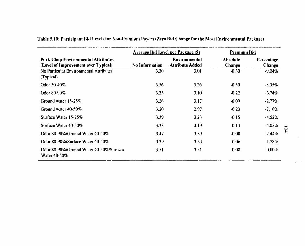
Table 5.10: Participant Bid Levels for Non-Premium Payers (Zero Bid Change for the Most Knvironmental Package)

Premium Bid

Pork Chop Knvironmcntal Attributes (Level of Improvement over Typical) No Information

Knvironmental Attribute Added

Ab.solute Change

Percentage Change

No Particular Environincntal Atlrihutes (Typical)

3.30 3.01 -0.30 -9.04%

Odor 30-40% 3.56 3.26 -0.30 -8.35%

Odor 80-90'7(. 3.33 3.10 -0.22 -6.74%

Groundwater 13-25% 3.26 3.17 -0.09 -2.77%

Ground water 40-50% 3.20 2.97 -0.23 -7.16%

Surface Water 15-25% 3.39 3.23 -0.15 -4.52%

Surfacc Water 40-50% 3.33 3.19 -0.13 -4.05%

Odor 80-90%/Ground Water 40-50% 3.47 3.39 -0.08 -2.44%

Odor 80-90%/Surface Water 40-50% 3.39 3.33 -0.06 -1.78%

Odor 80-90%/Ground Water 40-50'7(-/Surface 3.51 3.51 0.00 0.00% Water 40-50%

Table 5.11: Participant Bid Levels for Non-Premium Payers (Negative Hid Change for the Most ICnvironmental Package)

Premium Bid

Pork Chop Environmental Attributes (Level of Improvement over Typical) No Information

Knvironmental Attribute Added

Absolute Change

l*erccntage Change

No Particular Environmcnlal Attributes (Typical)

4.89 4.39 -0.50 -10.25%

Odor 30-40% 4.89 4.05 -0.83 -17.06%

Odor 80-90% 4.67 4.17 -0.50 -10.75%

Ground water 15-25% 4.63 4.03 -0.60 -12.97%

Ground water 40-50% 4.78 4.11 -0.66 -13.89%

Surface Water 15-25% 5.09 4.34 -0.75 -14.72%

Surface Water 40-50% 4.49 4.09 -0.41 -9.04%

Odor 80-90%/Ground Water 40-50% 4.69 4.62 -0.07 -1.58%

Odor 80-90%/Surface Water 40-50% 4.83 4.48 -0.35 -7.20%

Odor 80-90%/Ground Water 40-50%/Surface 5.36 4.62 -0.74 -13.84% Water 40-50%

106

There could be at least two reasons for these negative bidders. Either they did not

understand the intuition of the auction method used, or they were adversely affected by the

environmental information provided. This would imply that these participants had a higher

prior expectation of the embedded envirorunental attributes than what was actually true. If

the answer were the latter, then this would lead to a major implication for auction

experiments. The implication would be that auctions that solicit willingness-to-pay directly

without knowing the participants' prior expectations and not allow fornegative bids are

needlessly censoring an important group. This censoring of the data could cause false

conclusions to be drawn.

illingness-to-pay with a Known Basis

In the previous two sections of this chapter, willingness-to-pay with unknown ex ante

expectations was investigated. An advantage of looking at the premium in this way is that it

first assures that there are no physical differences in the packages being studied. The onK-

dilTcrcnce comes from the release of environmental information. The major disadvantage to

this particular definition is that the expectations of the consumers regarding environmental

atiributes arc unknown in the naive bidding round where there is no environmental

informalion given. It was seen above that the product that was denoted the t\pical product

wont down in \ alue when the information regarding the embedded environmental atirihuies

was released in the fourth round. This would imply that the consumer's expectations of the

packages could not be viewed as the t\pical package. Using the other definition of

willingness-to-pay discussed in chapter three, knowing the consumer's expectations is not an

issue. This is because the basis package is known with this other definition because the

comparisons of the packages are within the same information set. Hence the advantage of

107

this definition is that the expectations are known. A minor disadvantage of this method is

that it must account for the slightly different perceived physical attributes, i.e.. it must

estimate the value of the visual quality differences and adjust for it.

This section will investigate this other definition of willingness-to-pay when the basis

for product comparison is known. If all the packages were perceived as visually identical in

the third round, then the willingness-to-pay measure can be calculated by subtracting the bid

for the typical package in round four from the bid of the package with embedded

en\'ironmental attributes from round four. But it was seen above that all packages \\ ere not

percei\ ed as having exactly identical physical attributes. Otherwise, the bids for the

packages in round three would all be equal. Examining Table 5.2 shows that this was

ob\ iously not the case. This implies that the willingness-to-pay with known basis needs to

be adjusted for the perceived physical differences. To make this adjustment, the difference

betw een the typical package in round three and the corresponding package with embedded

cm ironmenial attributes in round three must be accounted for. This would imply that this

\\ illingness-to-pay measure could be defined mathematically as:

WTP, = (p,4 - Pi4) - (p,;. - P13) for i e EP.

WTP.. represents the willingness-to-pay measure with a known basis adjusted for perceived

\ isual differences for the i-th package of pork chops with embedded environmental

aitributes. The bid for the typical product in round t is represented by pn. while pu represents

the i-th package of pork chops with embedded environmental attributes in round t. EP is the

set of packages of pork chops that have embedded environmental attributes.

Table 5.12 provides information on the willingness-to-pay measure with known basis.

Except for the package with the high-level ground water impact, the willingness-to-pay for

108

embedded environmental attributes is increasing with both level and number of embedded

en\ ironmental attributes. This would be expected if en\ ironmentai attributes are desired

attributes. The package that commanded the smallest premium. SO. 13, was the package with

the low -level of reduction in odor attribute. As expected, the package that commanded the

highest premium, SI.46, was the triple attribute high-level environmental package. Unlike

the previous definition, this definition indicates a positive willingness-to-pay for ever\'

bundle of embedded environmental attributes. V^^len testing to see if these willingness-to-

pay values are strictly greater than zero, only the package with a low-level reduction of odor

is not significantly different than zero at the five-percent significance level."' The rest of the

packages are significantly greater than zero. When examining whether the premiums

differed across attribute levels, it was found that at the five-percent level of significance, all

of the premiums for the single attribute packages, excluding the package related to low-le\'el

odor reduction, were not statistically different. Utilizing this same test, shows that the

packages with double attributes are also not significantly different from each other. The

premium for the triple attribute package was significantly different from all other packages.

Examining Table 5.12 closer shows another interesting finding. It appears that the

attributes are additive. .A.ddiiivity implies that if the premiums for the single high-level

attributes are added together, then they would equal the premium for the product with those

combinations of attributes. For example, if the premiums for the three single high-level

attribute packages are added together, the combined premium value is SI.38. The actual

premium given for the triple attribute product was SI.46—only an S0.08 difference. This

also holds for the odor/groundwater combination but not necessarily for the odor/surface

.Vote that this is a one sided t-test and has a critical value approximately equal to 1.65 for n > 30.

109

Table 5.12: Willingness-to-Pay with Known Basis (All Participants)

Average Bids(S) Pork Chop Environmental Attributes (Level of Improvement over Typical) Willingness-to-Pay with Known Basis No Particular Environmental Basis

Attributes (Typical)

Odor 30-40%

Odor SO-90%

Ground water 15-25%

Ground water 40-50%

Surface Water 15-25%

Surface Water 40-50%

Odor 80-90%/Ground Water 40-50"''o

Odor S0-90°/o/Surface Water 40-50%

Odor 80-90%/Ground Water 40-50° o/Surface Water 40-50%

Note: The number in parenthesis is the t-statistic for the test of whether the average bid is difTerent from zero Those numbers in bold were significantly different from zero. Also, the letter indicates that by doing a pairwisc comparison between the premiums for the products, there was no statistical difference between the means being compared at the five-percent level of significance.

water combination. Testing to see if these two means are significantly different from each

other ro\cals that the null hypothesis of equality can not be rejected at the five-pcrccni level

of significatice. This t\pe of result holds true for the double attribute packages. .A.ssummi^

that marketing costs are same for single, double, and triple environmental attribute packages,

this approach may suggest that there may not be premium gains from selling packages of

pork chops with combined attributes. Offering single attribute products may be just as

beneficial.

0.13 (1.55)

0.39 (5.21)^

0.46 (6.10)^

0.43 (5.07)"

0.35 (4.42)"

0.56 (6.40)"

0.83 (8.58)''

0.93 (9.22)"

1.46(12.56)'

1 1 0

Table 5.13 provides the willingness-to-pay with a known basis for embedded

environmental attributes by location. In general, premiums were similar across locations.

.•\11 but one of the premiums were positive. The only exception was Oregon for the package

u ith a low-level environmental attribute related to odor reduction. Upon further

in\ esiigaiion, Oregon consistently has the lowest premiums for each package if the package

\\ ith low-level surface water attribute is excluded. This might be explained by the fact that

Oregon had consistently lower average bids overall. V\1ien testing to see if the premiums for

the packages differed across location, there were only a few differences. Most occurred in

Oregon where seventeen differences were shown. The other seven significant differences

occurred between Ames, Iowa and Manhattan Kansas. .'Amongst all the other location

comparisons, there were no statistically significant differences. When examining the package

\\ ith triple attributes, the second experiment in Raleigh, North Carolina had the highest

premium of SI.87, while the lowest occurred in Oregon at a premium of SI. 19.

\\'illingness-to-pay with Known Basis: Premium Vs. Non-Premium Payers

In the last section, willingness-to-pay with a known basis was examined. It was

found that this average premium over all participants was positive at the aggregate level for

each package. This would imply that embedded environmental attributes are desirable

atlribuies that consumers would pay for. In this section, the premium payers and the non-

premium payers will be investigated under the known basis approach to measuring

willingness-to-pay. In this case, a premium payer will be defined as a participant who has a

positive willingness-to-pay for the package with the triple attributes, i.e., a participant who

tendered a higher bid for the most environmental package over the typical package in the

fourth round.

Table 5.13: Willingiiess-to-l'ay for lOmiiedded I'lnviroiimeiital A((rit)ii(es with a Known Basis by IVodiicl and Location

Location

Pork Chop Environmental Attributes (Level of Improvement over Typical)

Ames, lA

Manhattan, KS

Raleigh, NC (97)

Burlington, vr

Iowa Falls, lA

Corvallis, OR

Raleigh, NC (98)

No Particular Environmental Attributes (Typical)

Basis Basis Basis Basis Basis Basis Basis

Odor 30-40% 0.18" 0.09 0.12 0.21 0.21 -0.28"'* 0.52"

Odor 80-90% 0.57' 0.3 r** 0.37 0.35 0.38 0.09'''-" 0.75'

Ground water 15-25% 0.61^ 0.47''' 0.56 0.66" 0.36 0.07""' 0.75'

Ground water 40-50% 0.69' 0.39' 0.24 0.77 0.35 0.24 0.50

Surface Water 15-25% 0.54 0.09 0.30 0.50 0.42 0.24 0.52

Surface Water 40-50% ().95''' 0.54" 0.44 0.70'' 0.54 0.77''

Odor 80-90%/Giound Water 40-50%

1.I8'"' 0.77'" 0.76 0.93 1.10 023^'"V 0.98'

Odor 80-90%/Surface Water 40-50%

1.04^' 0.93^ 0.74 1.15 1.03 0.48" 1.29'

Odor 80-90%/Ground Water 1.62^ 1.32^ 1.27 1.63 1.44 1.19 1.87 40-50%/Surfacc Water 40-50%

CorrcspomliiiiJ letters indicate that at the live percent level ol significance the null hypothesis of the two changes being equal across location for each product coulil not be rejecteil.

Table 5.14 presents the distribution of premium payers versus non-premium payers

across the different locations. Wlien comparing the two definitions used to define premium

pa\ ers. there was an eighty-four percent overlap between the two definitions. Hence, of the

329 participants in the study, eighty-four percent were classified as making the same decision

under both definitions—a premium payer was classified as a premium payer and a non-

premium payer was classified as a non-premium payer. Using the present definition, on the

aggregate level sixty-nine percent of the participants paid a premium. This percentage is

se\ en percent higher than with the previous definition of willingness-to-pay. The percentage

of premium payers ranged fi^om fifty-seven percent to eighty-one percent in the different

siud\' areas. The location with the highest percentage of premium payers was Burlington.

V ermont at eighty-one percent. This is in stark contrast to the previous definition where

\ermont had the lowest percent of premium payers at fifty-six percent. The location with the

lowest percentage of premium payers under this definition was Iowa Falls, Iowa at fifty-

scv cn percent. Except for Iowa Falls, the percentage of premium payers increased for all

other locations under this new definition.

Table 5.14: Premium Payers Versus Non-Premium Payers by .\rea when Considering W illingness-to-pay with a Known Basis

Experiment .Area Number of Number of Percent Premium Premium Payers Non-Premium Payers

Payers .-Ml areas 228 101 69 Ames. LA 34 15 69 Manhattan. KS 44 16 73 Raleigh. NC (6/28/97) 24 7 77 Burlingion, VT 22 5 81 Iowa Falls, lA 33 25 57 Cor\ a!lis. OR 40 20 67 Raleigh. NC (6/27/98) 31 13 70

1 1 3

Table 5.15 presents the average premium paid for each package for only those ho

paid a premium for the most environmental package. The highest premium of S2.23 went to

the package with the triple attributes while the package with a low-level of odor reduction

only received a premium of S0.35 over the typical package. As expected, the average

premium paid for each package is positive and significantly different from zero at the 0.001

significance le\"el. As with aggregate data, when the package with a low-level attribute

related to odor is excluded, the premiums for the packages with a single high and low-level

attribute are not significantly different from each other at the five-percent level of

Tabic 5.15: Willingness-to-Pay with Known Basis (Premium Payers)

.\verage Bids($) Pork Chop Environmental .Attributes (Level of Improvement over Typical) Willingness-to-Pay with Known Basis

No Particular Environmental Basis -Attributes (Typical)

Odor 30-40°b

Odor 80-90%

Ground water 15-25%

Ground water 40-50%

Surface Water 15-25%

0.35 (3.50)

0.69 (T.?!)--

0.74 (8.19)'

0.79 (7.91)''

0.65 (7.09)'

0.90 (8.35)-'

1.31 (11.10)''

.Surface Water 40-50%

Odor S0-90°/o/Ground Water 40-50%

Odor 80-90%/Surface Water 40-50'"o

1.44(11.90)"

Odor 80-90%/Ground Water 40-50%,'Surface Water 40-50%

2.23 (16.73)'

Note; The number in parenthesis is the t-statistic for the test of whether the average bid is different from zero.

.•\Iso. the letter indicates that by doing a pairwise comparison between the premiums for the products, there was

no statistical difference between the means being compared at the five-percent level of significance.

1 1 4

significance. Also, when comparing the two double attribute packages, their premiums are

not significantly different from each other at the five-percent level of significance. All other

comparisons are significantly different from each other. When examining premiums by

package, it is easy to see that the premiums follow a consistent pattern of increasing by both

le\el and number of attributes. This pattern includes the package with the high-level

attribute related to ground water. This result would imply that the inconsistency in the

pattern seen in the aggregate data, i.e.. the low-level attribute package receiving a higher

premium than the high-level attribute package, stems from the non-premium payers.

The aspect of additivity, while not as pronounced with the premium payers as it was

with the aggregate data, is still evident. WTien adding the premiums of each single high-le\ el

attribute package together would indicate that the premium for the triple package should be

S2.3S. The actual premium paid for the triple attribute product was S2.23. a difference of

onl\ SO. 15. Testing to see if the two means are equal gives a t-statistic of -0.51. This would

imply that they are not significantly different from each other at the five-percent level of

significance and that additivity holds for the premium payers.

Table 5.16 presents the information for the non-premium payers under the current

definition of willingness-to-pay. These 101 non-premium payers made up thirty-one pcrccni

of ilic participants in the study. It should be kept in mind that by definition of being a noii-

prcmium payer, the triple attribute package must have a premium no greater than zero. Thi.s

does not necessarily imply that all the other packages must have a negative premium. When

e.xamining this group, it is easy to see that the participants decreased the value for all

packages over the typical. The greatest decrease of SO.39 came from the package with a

high-level attribute related to ground water. This decrease explains the source of the

1 1 5

inconsistency seen in the aggregate data where the package with low-level ground water

attribute received a higher premium than the package with the high-level attribute.

E.xamining whether these decreases were significantly different from zero at the five-percent

le\ el of significance, two packages have premiums not statistically different from zero.

These packages were the low-level ground water attribute package and the package related to

ha\ ing a both surface water and odor reduction attributes. Inspecting the data in the table for

a reason why participants decreased their bids reveals no consistent pattern related to

environmental attributes. The smallest decrease in premium of SO. 18 was related to the

Table 5.16: Willingness-to-Pay >vith Known Basis (Non-Premium Payers)

Average Bids($) Pork Chop Environmental •Attributes (Level of Improvement over Typical) Wiliingness-to-Pay with Known Basis No Particular Environmental Basis

.Attributes (Typical)

Odor 30-40%

Odor 80-90%

Ground water 15-25%

Ground water 40-50%

Surface Water 15-25%

-0.38 (-3.09)'

-0.29(2.73)-*

-0.18 (-1.62)"

-0.39 (-3.03)"

-0.32 (-2.35)"

-0.22 (-2.00)"

-0.24 (-2.12)"

Surface Water 40-50%

Odor S0-90%/Ground Water 40-50°/b

Odor 80-90%/Surface Water 40-50%

-0.22 (-1.82)"

Odor 80-90%/Ground Water 40-50%.'Surface Water 40-50%

-0.30 (-3.29)"

Note; The number m parenthesis is the t-statistic for the test of whether the average bid is ditTerent from zero. .Also, the letter indicates that by doing a pairwise comparison between the premiums for the products, there was no statistical difference between the means being compared at the five-percent level of significance.

1 1 6

package vs ith a low-level ground water attribute. A test between a pairvvise comparison of

ihc premiums reveals that there is no significant difference between any of the premiums at

the five-percent level of significance.

Of the 101 participants that are classified as non-premium payers based on the current

definition of willingness-to-pay. twenty-seven decreased their value for the most

en\ ironmental package. This number is equivalent to the twenty-five participants that

decreased their bid under the previous definition of willingness-to-pay. Table 5.17 separates

the non-premium payers into two groups—those participants that had the same value for

i\pical and most environmental package and those participants that had a higher bid for the

i\pical package over the most environmental package. As seen in the table, these two groups

are very distinct. The participants that had a premium of zero for the most environmental

goods also had a premium bid of zero for the rest of the packages. Some of these premiums

u ere positive, while the rest were negative. Testing to see whether these premiums are

staiisiically equal to zero, the null hypothesis of equality to zero cannot be rejected at the

five-percent level of significance. This would imply that the envirormiental information had

no effect on these participants.

When examining the negative bidders' premiums for each product, a different picuirc

appears. .A.11 of the average premiums are significantly different from zero at the five-perccni

level of significance. In fact all of the premiums are strictly negative. This would impl\ that

this group is negatively affected by embedded environmental attributes within the packages.

Comparing both groups together shows that the zero bidders were not affected by the

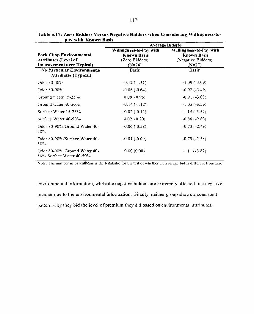
1 1 7

Table 5.17: Zero Bidders Versus Negative Bidders when Considering Willingness-to-pay with Known Basis

Average Bids(S)

Pork Chop Environmental .\ttributes (Level of Improvement over Typical)

\\'illingness-to-Pay with Known Basis

(Zero Bidders) (N=74)

Willingness-to-Pay with Known Basis

(Negative Bidders) ^ (N=27)

No Particular Environmental .Attributes (Typical)

Basis Basis

Odor 30-40°b -0.12(-1.31) -1.09 (-3.09)

Odor SO-90% -0.06 (-0.64) -0.92 (-3.49)

Ground water 15-25% 0.09 (0.96) -0.91 (-3.03)

Ground water 40-50% -0.14 (-1.12) -1.05 (-3.59)

Surface Water 15-25% -0.02 (-0.12) -1.15 (-3.54)

Surface Water 40-50% 0.02 (0.20) -0.88 (-2.S0)

Odor 80-90%''Ground Water 40-50"o

-0.06 (-0.58) -0.73 (-2.49)

Odor S0-90%/Surface Water 40-50" 0

-0.01 (-0.09) -0.79 (-2.58)

Odor S0-90%/Ground Water 40-50" (1 Surface Water 40-50%

0.00 (0.00) -1.1 1 (-3.S7)

Note. The number m parenthesis is the t-siatistic for the test of whether the average bid is different from zero.

en\ ironmenial information, while the negative bidders are extremely affected in a negaii\ e

manner due to the environmental information. Finally, neither group shows a consistent

pattern why they bid the level of premium they did based on environmental attributes.

1 1 8

chapter six: results from pre and post auction

surveys

Chapter three presented a mode! of consumer behavior in a second-price sealed-bid

auction with multiple rounds. Within chapter three, an interpretation of the bids from a

second-price auction was given. Also in chapter three, two willingness-to-pay measures are

defined. In chapter five, results are examined to determine whether consumers would pay a

premium for pork products with embedded environmental attributes. The first definition of a

premium payer considered a participant who increased their bid for the package with the

most environmental attributes from round three to round four. In this case, it was found that

approximately sixty-two percent of the participants could be considered premium payers.

.Another way of defining a premium payer is to consider a participant who bid a higher value

for the environmental package over the t\pical package in the same information round,

specifically round four. In this case, sixty-nine percent of the participants could be

considered premium payers. In this chapter, the pre and post experiment surv eys completed

b\ the participants will be anaU'zed. The pre experiment surv ey will initially be anah^zed at

the aggregate level. Then results are provided by premium payers and non-premium payers

lo e\ aluate for differences between the two groups. Both of the definitions for a premium

payer will be analyzed. The post survey, which relates to consumer's knowledge of

production practices, is only analyzed at the aggregate level.

There were two surv eys conducted during each experiment, one before the auctions and

one after the auctions. The pre auction survey asked questions that related to socioeconomic

factors, e.g., age, gender, and household income. It also asked questions related to issues of

concern, e.g.. the environment, food prices, and family farming. Furthermore, questions

1 1 9

were asked relating to the attributes that the participant consumed, e.g.. eating qualit\'. visual

appeal, and price. See appendix B for the specific questions related to the pre auction sur\ c\.

The post auction sun. ey asked questions that pertained to knowledge about pork production.

Questions were asked about the acceptability of different methods for reducing odor in

production, reducing manure seepage into ground water, and reducing manure run-off or

spills into surface water. Also asked on this sur\'ey were questions related to concerns about

farm issues and livestock production methods. See appendi.x B for the post auction

questions.

Pre Auction Survey

Table 6.1 provides general information of the socioeconomic characteristics for the

participants in the study. This information is provided by study location in .'\ppendix D. Of

the participants in the study, about six in ten were female (59.88%). This reflects

responsibility for food purchases, as when the household was initially contacted by

telephone, the primary food purchaser was encouraged to come to the experiment if the\

u ore available. The average age of participants was foay-eight years with an average of 2.69

individuals per household. Average household income for the study participants was

approximately S43.400. with an employment level of sixty-six percent.' Most participants

consumed meat. pouItr\'. and fish. Pork was consumed on a\'erage 5.S3 times per momh.

while poultrv' was consumed nearly double that at 10.04 times per month. Beef consumption

' Ii should be noted that the question related to employment asked whether the participant was employed. .•\noiher question asked what was the occupation of the participant. .Most of the participants that were homemakers labeled themselves as not employed which should be taken into consideration. When accounting for homemakers as being employed, this increases the emplovment level of the participants to seventy-seven percent.

120

Table 6.1: General Socioeconomic Information: All Participants

Item Ail Participants (N = 329)

Females "/o 59.88

Age \'ears 47.74

Number Livmg m Household 2.69

Hducaiion Level Years'* 13.98

Hmployed /o 65.65

Household Income S'' S43.400

Consume Beef % 96.65

Consume Pork % 95.72

Consume Poultrv' % 97.86

Consume Fish % 89.30

Times Consume Beef per Month 9.90

Times Consume Pork per Month 5.83

Times Consume Poultry per Month 10.04

Times Consume Fish per Month 3.91

Number of Production Facilities VVithm One Mile 0,14

Number of Production Facilities Withm Two Mile 0,4 i

Commercial Livestock and/or Crop Producers % 1.23

Read Food Labels'" 2.3s

Noticc Environmental Attributes on Labels % 52,01

Consume More Beef Due to Advertising % 15.4s

C onsume More Pork Due to Ad%-ertising % 3n ,v2

Wjni I-.nvironmental Labeling for Most Products W4 ~5

N'k'ouid Pay a Premium for Meat Products with Environmental 64.Ml .A.ttnbutcs "u"

Want Education for Pork Producers S9_54 •" This was imputed from categorical responses using mean years with in the category as the observ ation.

This was imputed from categorical responses using mean mcome within the category as the observation. ' 1 =ne\ er; 2=sometimes; 3=ahvays

Note: these questions were asked on the post auction survey.

was closer to poultry' at an average of 9.9 times per month, whereas fish consumption was

bclo\\ pork at an average of 3.91 times per month.

When asked the question "how many pork production facilities are w ithin a one mile

radius of your dwelling," the average participant response was 0.14 facilities. This number

nearly tripled when this radius is taken to two miles (0.41 production facilities), h should be

noted that a large proportion of the participants did not have any hog facilities within a two

mile radius of their dwelling. Only a small percent of the participants considered themselves

as commercial livestock and/or crop producers. Of the participants. 1.23 percent of them

commercially produced livestock or crops.

Participants indicated that they read labels on the products they buy. The average

\ alue was 2.38 where a 2 denoted "sometimes read labels" and a 3 denoted "always read

labels." .A.11 the participants in this study indicated they read labels at least sometimes.

.About one-half indicated that they had noticed environmental attributes on labels and ninety-

n\ e percent indicated they would like to have environmental information provided on

product labels. .Almost all of the participants indicated that they would buy a meat product

that had environmental attributes specified on the label. It should be clarified that this

question did not ask whether they would pay a premium, rather it asked if they would

consume meat that had environmental attributes. This implies that there is not an aversion to

meat products with environmental attributes. Hence environmental attributes are perceivcd

as a good; so much so. that almost ninety-percent want pork producers to have en\ ironmental

education on production practices. When participants were asked whether they would pay a

122

premium for meat products with environmental attributes. 64.8 percent indicated they

would." This is remarkably close to the number that actually did pay a premium.

It is interesting to note that about one-third of the participants indicated that they had

purchased more pork as a result of advertisements they had seen in the media. Approximately

fifteen percent of the participants felt they had consumed more beef as a result of

ad\ ertisements. This might imply that the pork advertising campaign. Pork. The Other IMiite

Meal, may be more effective than the beef campaign. Beef It is \Miai 's for Dinner. This

effect may also be due to the larger number of times beef was consumed per month as

compared to pork.

Premium vs. Non-Premium Payer

Table 6.2 presents a comparison of socioeconomic factors of the premium payers and

the non-premium payers when a premium payer is defined as a participant who increased her

bid from round three to round four for the most environmental package. Table 6.3 represents

a comparison of these same factors where a premium payer in this case is defined as a

participant who provided a higher bid for the most environmental good compared to the

t>pical package in the environmental information round, round four. Examining both tables

carefully shows that the characteristics of premium payers across definitions are very similar.

In fact, ai the five-percent level of significance, they are not significantly different from cach

other. " This result also holds for the non-premium payers. Since there is no significant

" It should be noted that this question was asked on the post auction survey. This was done for two reasons. First. It was in the post auction survey to reduce bias in the auction e.xperiment. If this question had been asked bei'orc the e.xpenment it may have created an expectation that environmental attributes were the focus of the study. Second, it allows for testing whether panicipants knew their own preferences. ' For the continuous variables, the t-test from chapter five was used. In the case of the proportional data, a test from Freund was used (1992, p. 481). In this case, it is assumed that these proportions are being drawn from a binomial distribution.

123

Table 6.2: Comparison of General Information: Premium Payers, Non-Payers for Definition One of Wiilingness-to-Pay'

•Premium

Item Premium Payers (N = 204)

.Non-Premium Payers(N = 125)

Females "o 63.24 54.40

Aue ^'ears 46.83 49.23

Number Living in Household 2.76 2.57

Education Level Years'' 14.36 13.2S

Employed % 71.08 56.80

Household Income S44.400 S41.700

Consume Beef % 97.06 95.97

Consume Pork % 97.06 93.50

Consume Poultrv' % 99.02 95.93

Consume Fish % 90.69 86.99

Times Consume Beef per Month 10.06 9.64

Times Consume Pork per Month 5.62 6.18

Times Consume Poultr\' per Month 9.98 10.13

Times Consume Fish per Month 3.66 4.33

Number of Production Facilities Within One Mile O.Il 0.19

Number of Production Facilities Within Two Mile 0.41 0.41

Commercial Livestock and/'or Crop Producers % 0.99 1.61

Read Food Labels'^ 2.39 2.37

Notice Environmental Attributes on Labels % 54.68 4".50

Consume More Beef Due to Advertising % 13.33 19.13

Consume .More Pork Due to Advertising % 28.36 35 04

W'ani Environmental Labeling for Most Products 96.06 92.5()

UOuld Pay a Premium for Meat Products with En\'ironmental .Attributes %'

71.64 53.33

U'ani Education for Pork Producers %' 92.61 84.43 •• A premium payer under this definition is a participant who increased her bid for the most environmental package from round three to round four. ^ This was imputed from categorical responses using mean years with in the category as the obser\ ation. ' This was imputed from categorical responses using mean income within the category as the obser\ ation. " 1 =never; 2=sometimes; 3=always ' Note: these questions were asked on the post auction survey.

124

Table 6.3: Comparison of General Information: Premium Payers, Non-Premium Payers for Definition Two of VVillingness-to-Pay'

Item Premium Payers Non-Premium (N = 228) Payers (N = 101)

Females % 65.35 47.52

Age Years 45.90 51.95

Number Living m Household 2.77 2.51

Education Level Years'' 14.20 13.44

Employed % 70.18 55.45

Household Income S44.700 S40.400

Consume Beef % 96.93 96.00

Consume Pork % 96.48 94.00

Consume Poultry % 98.68 96.00

Consume Fish % 89.87 88.00

Times Consume Beef per Month 9.88 9.94

Times Consume Pork per Month 5.55 6.45

Times Consume Poultry per Month 10.35 9.32

Times Consume Fish per Month 3.72 4.35

Number of Production Facilities Within One Mile 0.09 0.19

Number of Production Facilities Within Two Mile 0.31 0.24

Commercial Livestock and/or Crop Producers % 0.99 0.64

Read Food Labels'^ 2.37 2.40

Notice Environmental Attributes on Labels % 52.86 50.00

Consume More Beef Due to Advertising % 14.61 19.13

Consume More Pork Due to Advertising % 28.00 I ".58

N^'ant En\ ironmentaI Labeling for Most Products %' 95.59 92.7S

Would Pay a Premium for Meat Products with 71.68 48.42 Environmental Attributes %'

Want Education for Pork Producers %' 92.07 83.67 " A premium payer under this second definition is a participant who had a higher bid for the most environmental package compared to the typical package within round four. '' This as imputed from categorical responses using mean years with in the category as the observ ation. " This was imputed from categorical responses using mean income within the categor\' as the obser\ ation.

1 =ne\'er; 2=sometimes; 3=always " Note: these questions were asked on the post auction survey.

differences between socioeconomic characteristics between the two definitions, only the

comparisons in Table 6.2, the first definition mentioned, shall be discussed.

For most comparisons in Table 6.2 there were no significant differences between the

premium payers and the non-premium payers. Many of the tendencies were in the expected

direction such as a larger percent of the premium payers noticed and wanted environmental

labels. However, these differences were not significant at the five-percent level of

significance. Three factors were significantly different at the five-percent significance level

between the two groups. These dealt with employment, the desire for pork producers to have

education in environmental awareness and production practices, and paying a premium for

meal products with environmental attributes. The premium payers had a significantly higher

percentage of employment. Premium payers also had a significantly higher percentage of

participants who wanted pork producers to have environmental education.

.A.S expected the non-premium payers had a significantly lower proportion saying they

\^ould pay a premium for meat products with environmental attributes than the premium

pav ers would. For those who actually paid a premium nearly seventy-two percent said the\'

would pay a premium, while fifty-three percent of the non-premium payers said they would

pay a premium. These results also hold for the second definition of willingness-to-pay. li

was expected that the premium payers should be closer to 100 percent giving a premium,

while the non-premium payers should have been closer to zero. Using a binomial

distribution test as in Freund (1992), the premium payers are significantly less than 100

percent at the .001 significance level, while the non-premium payers are significantly above

zero at this same level of significance.

126

This result is very- interesting because it came after the experiment where the

participants had already bid according to their preferences. There may be at least two

reasons for this result. The first reason could be that the information in the experiment,

specifically from rounds four and five, changed the participants' preferences. Since the

reponed premiums for this study are due to the environmental information from round four,

the information provided in round five may have changed the participants" preferences, e.g..

the environmental information from round four became more or less important due to the

information from round five. This might explain why the premium payers are not at one

hundred percent, but it is highly unlikely that this would explain the non-premium payers.

This was because the bids in round five did not change significantly as would be expected if

the information from round five had been preference altering. .Another explanation for this

disparii\ is that there is a group of free-riders who are indicating that they would pay a

premium when in actuality they would not. This result would be strictly related to the non-

premium payers.

Since the rest of the comparisons are not statistically different, a general discussion of

trends will be provided. Comparing the premium payers to the non-premium payers, females

were more likely to pay a premium. Non-premium payers tended to be older on average b\

2.5 years, while the education level was approximately the same with the premium payers

only having on average a half a year more education. Household incomes were slightly

higher for the premium payers by Premium payers consumed more beef per month

than poultry, pork, or fish. The number of production facilities within a one-mile radius of

the participants dwelling tended to be higher for the non-premium payers, while extending

this radius to two miles made the two groups equal. Due to the direct benefit received from

127

pork products produced with embedded environmental attributes, it was expected that a

Iiighcr concentration hog production facilities would be directly associated with being a

premium payer. It seems that this may not be true for people who live very close to these

facilities. This may give some credence to the study done by Taff et al (1996). A plausible

argument given by Taff et al. is that many people self-select themselves to the en\ ironment

around \\ hich they live.

When it came to reading food labels premium payers and non-premium payers were

nearly identical in the average response. The premium payers had a higher proportion

noticing environmental attributes provided on the labels of the products they consume.

Environmental information was important to both sets of participants. Over ninety-two

percent of both groups indicated they wanted environmental labeling. The premium payers

were at a slightly higher percentage. This may imply that industry- programs focusing on

providing environmental information and education are important and are looked upon

fax Grab I y by consumers.

Information on participant response to issues of concern is shown in Table 6.4.

These results are provided by study location in Appendi.x D. Like the previous results, there

is \ cr\ little difference between which definition is used for a premium payer. In the sur\ c>

a 1 denoted "very concerned" and a 5 denoted "not concerned." In general, participants ucrc

"\ er\ concerned" to "somewhat concerned" about the en\-ironmcnl. water quality, air qualitv,

food prices and pollution. The level of concern was lower for family farming, production

methods, animal welfare, confinement livestock systems, and changing farm structure.

Under both definitions of a premium, premium payers were more concerned about air

quality, food prices, family farming, and pollution than non-premium payers were. For the

Table 6.4: Issues of ('<»na'rri: All Parlicipaiiis, IVeiiiliini Payers, Non-Freniimii Payers

Item All Participants (N = 329)

Premium Payers Detlnitioii 1"

(N = 204)

Premium Payers Delliiition 2'*

(N = 228)

Non-Premium I'ayers

Derinition 1" (N= 125)

Non-Premium Payers

Definition 2'* (N= 101)

Issues of Concern*^ Water Quality 1.3S 1,36 1..38 1.43 1.40

Pollution 1.48 1.45 1.45 1.52 1 55

Air Quality 1,55 1.50 1.53 1,62 1.59

Environment 1.64 1.60 1.64 1.71 1.64

Food Prices 1.03 1.88 1.85 2,00 2.10

Animal Welfare 2.37 2.39 2.39 2.33 2.32

Production Methods 2.44 2.44 2.47 2.45 2.38

Confinement 2.44 2.42 2,44 2.47 2.43

Family Farm 2.59 2,54 2.57 2,67 2.63

Structure Of Agriculture

2.94 2.87 2.96 3.05 2.87

A premium payer under this definilion is a participant who increased her bid lor the mt)st environmental package Ironi round three to round lour, whereas, a non-premium payer did not increase her bid,

A premium payer under this secoiul (letiiiition is a piirticipant who had a higher bid foi (he mosl environmental package coin[)aied to the typical package within round four; wheieas. llic non-premium payei had a higher bid on the typical package.

'''The question was: On a scale Iroin I thiough 5 with 1 being very concerned' and 5 being 'not concerned,' how concerned are you about the lollowing issues:

129

issues of production methods, animal confinement, and the changing structure of agriculture,

ilicre were no definitive preferences when examining the premium payers under both

defmitions of a premium.

Information in Table 6.5 focuses on participant's attitudes tow ard attributes of food

products they consume. These results are provided by study location in .Appendix D. For

this information a 1 indicated "very important" while a 5 indicated "not important." .A.11 were

Table 6.5: Issues of Importance: Ail Participants, Premium Payers, Non-Premium Payers

Item .All Premium .Non-Participants Payers Premium

Pavers Issues of Importance N = 329 N = 204 -\ = 125 Pertaining to Defrntion l""*" Freshness 1.18 1.19 1.16 Eating Quality 1.20 1.21 1.17 \'isual .Appeal 1.6S 1.71 1.63 Price 1.75 1.73 1.78 L'nifomiity of Product 2.14 2.15 2.13 Production .Methods 2.20 2.25 2.12

Issues oflmoortance N = 228 N = 101 Pertainine to Defintion 2" Freshness 1.19 1.16 Ealing Quality 1.21 1.18 X'isual .Appeal 1.70 1.62 Price 1.69 1.88 L'ni fomiity of Product 2.18 2.06 Production Methods 2.26 2.05

The question was; On a scale from 1 through 5 with 1 being "very important" and 5 being "not important." indicate how imponant the following attributes are for the products you consume;

A premium payer under this definition is a participant who increased her bid for the most environmental package from round three to round four, whereas, a non-premium payer did not increase her bid.

" .X premium payer under this second definition is a panicipant who had a higher bid for the most environmental package compared to the typical package within round four; whereas, the non-premium-payer had a higher bid on the typical package.

130

\ ery concerned to somewhat concerned about food eating quality, visual appeal, freshness,

and price. Production methods used in producing the food, and uniformity of product had

lower levels of importance. There were no significant differences between the premium and

non-premium payers under both definitions.

Post .Auction Suney

The information in Table 6.6 provides panicipant responses to acceptability of

methods producers use to reduce odors. Filtration of air from livestock buildings was an

acceptable method for odor reduction; approximately sixty-seven percent indicated it was

"\ ery acceptable" to "somewhat acceptable." .Microbial and enz\Tne additives to manure as a

method for odor reduction had a slightly lower level of acceptability; slightly more than fift\

pcrcent indicated it was "very acceptable" to "somewhat acceptable." .Another thirty-six to

thirty-seven percent indicated they had a neutral or no opinion stance. Chemical additives to

manure were less acceptable. Approximately one in five indicated that this was a "\ ery

acccpiablc" to "somewhat acceptable" method of odor control. Four in ten indicated it w as

"somcw hat unacceptable" to "not acceptable." Only ten percent of the participants indicated

thai use of chemicals in a hog's diet as a means of odor control was "very acceptable" to

"somewhat acceptable." In contrast, use of natural additives to a hog's diet was hiuhi>

acceptable. Over seventy-five percent of the participants reported that this method was \ cr\

to "somewhat acceptable." This would imply that consumers find it more desirable to ha\tj

natural solutions to odor problems.

When considering manure storage and injection methods for controlling odor,

participants' attitudes differed. The range of those indicating "somewhat acceptable" to "not

acceptable" ranged from twenty-six percent for manure storage above ground, forty-one

labic 6.6: Distribution tor Participiint Responses on the Acceptability of Methods for Odor Reduction (N = 329)

Percentage Of Participants

Very Somewhat Sonicwhut Nut Acccptabic No Opinion Method Acceptable Acceptable Neutral Unacceptable Filtralion of air from building 46.95 21.04 16.46 2.74 4.57 7.32 Additives to manure;

Chemical 6.23 12.79 21.64 17.38 23.93 18.03

Microbial 24.92 27.51 17.48 4.53 6.15 19.42

Enzyme 27.80 25.56 18.53 4.15 5.43 18.53 Additives to hog's diet:

Chemical 2.37 7.46 14.92 14.92 48.14 11.86

Natural 49.38 26.85 9.88 2.47 4.63 6.79 hijcction of manure into soil 6.12 11.93 29.05 13.76 22.02 17.13

to a depth of 4-8 inchcs Miinurc spread on top of soil 8.26 23.55 27.22 14.37 11.93 14.68

with immediate incorporation

Manure storage above 14.11 21.78 25.77 11.96 14.11 12.27 ground with cover

Manure storage below 8.62 13.85 25.54 17.23 24.00 10.77 ground with cover

Manure storage under hog 2.76 8.59 22.70 18.10 32.82 15.03 building

Composting with bedding 16.16 27.13 22.87 8.84 9.15 15.85

material

percent for manure storage below ground, and fifty-one percent for manure storage under the

hog building. Participants were more acceptable of manure storage systems that \\ ere abo\ e

ground and away from the pigs. The highest level of acceptance was for composting with

bedding material. Forty-three percent indicated that this was "ver\' acceptable" to

"somewhat acceptable."

It is important that about one-fourth of the participants were neutral with respect to

the method of manure storage and incorporation method. .Another ten to twenty percent had

no opinion in these areas. Given this, there is an educational focus needed because a large

number of participants provided a neutral to no opinion response.

Information in Table 6.7 provides participant acceptability of manure handling

methods as they perceive it relates to ground water impacts. Again, there were a large

number with a neutral (22-23%) or no opinion (12-16%). >\Tien groundwater was

considered, injection had the lowest level of acceptability; twenty-seven percent indicating

"not acceptable." It was "very acceptable" to "somewhat acceptable" for only one in five

panicipants. Half indicated that manure storage above ground in steel/cement structures was

acceptable. Below ground storage was acceptable for thirty-seven percent of the participants.

Table 6.8 provides information on participant acceptability of methods used for

manure storage and application related to surface water impacts. Results are quite similar to

Tabic 6.7 on ground water. Again, manure storage above ground was more acceptable. It

was interesting that injection was less acceptable than surface application. It should be noted

that when the injection method is used properly, it is a better method of getting your manure

on fields than spreading the manure on the top soil from the point of view of odor reduction,

and ground and surface water protection.

1

Table 6.7: Distribution for the Acceptability of Methods Used To Achieve A Reduction Of Manure Seepage Into Ground Water (N = 329)

Percentage of Participants

Method \'ery

Acceptable Somewhat Acceptable Neutral

Somewhat Unacceptable

Not .\cceptable

No Opinion

Injection of manure into the soil to a depth of 4 to S inches

4.91 14.72 21.78 15.34 27.61 15.64

Manure storage abo\ e ground in steel/cement structure

18.71 31.60 23.31 5.52 8.90 11.96

Manure storage below ground in steel cement Structure

15.38 23.38 22.46 12.00 14.46 12.31

Table 6.8: Distribution of the Acceptability' of Methods Used To Achieve A Reduction In Run-off Or Spill Of Manure Into Surface Water (N = 329)

Percentage of Participants

Method Very

.Acceptable Somewhat Acceptable Neutral

Somewhat Unacceptable

Not .Acceptable

No Opinion

Injcction of manure into the soil to a depth of 4 to 8 inches

5.21 15.34 23.62 14.11 26.99 14.72

Manure spread on top of soil u ith immediate incorporation

Manure storage above ground in steel cement structure

6.13

19.02

24.54

32.52

23.62

20.86

16.26

5.83

18.10

8.90

11.35

12.88

Manure storage below ground

14.11 23.62 22.09 11.04 15.64 13.50

in sieel cement structure

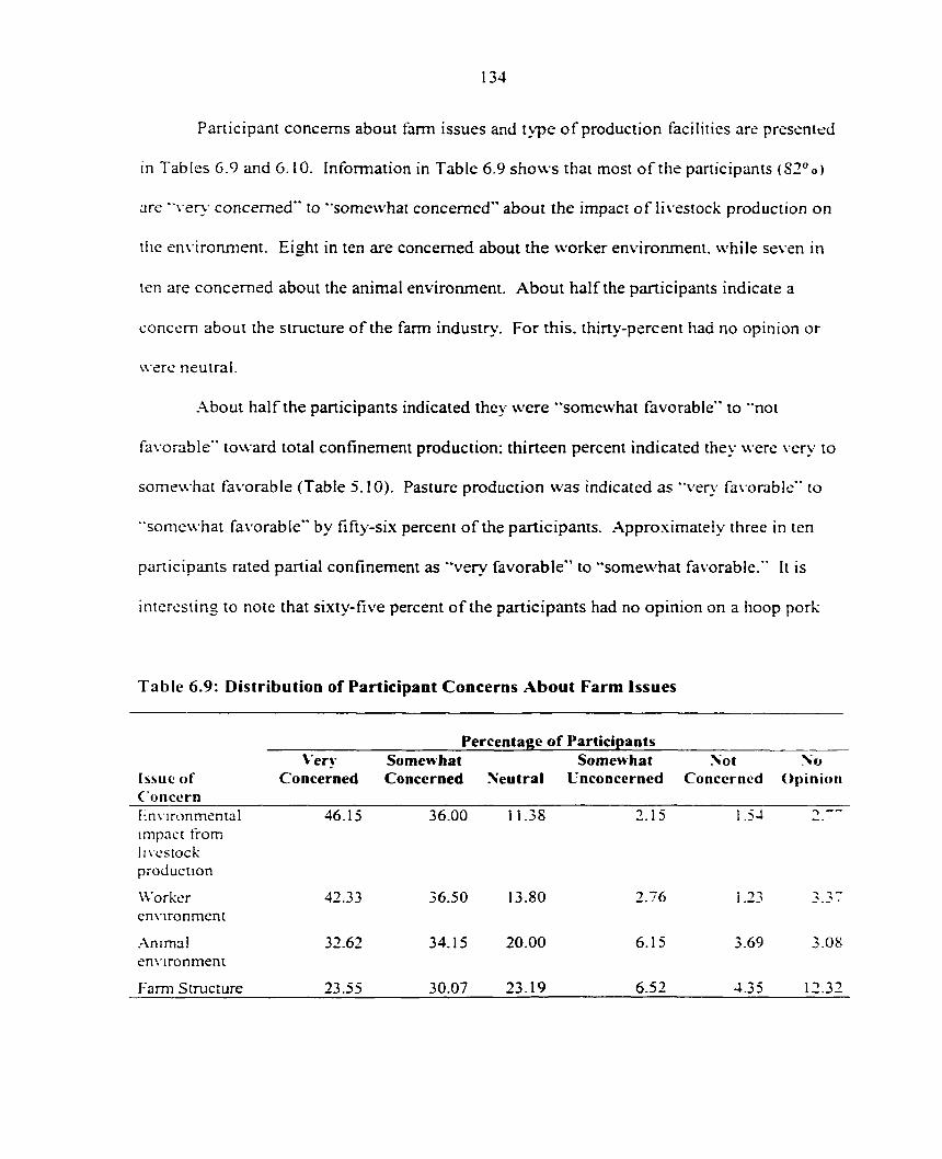
134

Participant concerns about farm issues and type of production facilities are presented

in Tab les 6 .9 and 6 .10 . In fo rma t ion in Tab le 6 .9 shows tha t mos t o f the pa r t i c ipan t s (S2°o)

are "very concerned" to "somewhat concerned" about the impact of livestock production on

the enx ironment. Eight in ten are concerned about the worker environment, while seven in

ten are concerned about the animal environment. About half the participants indicate a

concern about the structure of the farm industry. For this, thirty-percent had no opinion or

were neutral.

.A.boui half the participants indicated they were "somewhat favorable" to "not

favorable" toward total confinement production; thirteen percent indicated they were ver>' to

somewhat favorable (Table 5.10). Pasture production was indicated as "ver>' fa\ orabie" to

"somewhat favorable" by fifty-six percent of the participants. .Approximately three in ten

participants rated partial confinement as "very favorable" to "somewhat favorable." It is

interesting to note that sixty-five percent of the participants had no opinion on a hoop pork

Table 6.9: Distribution of Participant Concerns About Farm Issues

Percentage of Participants

Is.suc of Concern

Very Concerned

Somenhat Concerned Neutral

Somewhat Unconcerned

.Not Concerned

No Opinion

Hnvironmental impact from livestock production

46.15 36.00 11.38 2.15 1.54

Worker environment

42.33 36.50 13.80 2.76 1.23 y > ,

.\nima! environment

32.62 34.15 20.00 6.15 3.69 3.08

Farm Structure 23.55 30.07 23.19 6.52 4.35 12.32

production method. This indicates they were not familiar with this production method. This

result was not too surprising due to the relative newness of this technology. In general,

aititudinal responses on level of acceptability and favorability did not differ between

premium and non-premium payers. Hence they will not be discussed.

Table 6.10: Distribution of Participant Concerns About Livestock Production Methods (N =329)

Percentage of Participants

Issue of Concern

Very Favorable

Somewhat Favorable Neutral

Somewhat Unfavorable

Not Favorable

No Opinion

Hoop 2.18 4.67 16.20 2.80 8.41 65.42

Partial Confinement

5.61 23.05 29.28 13.71 9.35 19.00

Pasture 36.39 22.02 17.43 4.59 4.28 14.98

Total Confinement

4.05 9.35 15.58 10.59 42.68 17.76

136

chapter seven: econometric analysis

In chapter three, a model was developed to explain consumer behavior in a multiple

round second-price sealed-bid auction with different information sets. In one of the rounds

there was no information pertaining to embedded environmental attributes in the products

being auction. This round was known as a naive bidding round. In a later round, information

u as released pertaining to the embedded environmental attributes of each product being

auctioned. This round was considered an information round. To handle these different

information rounds, an assessment function, which relates quality attributes to utility, was

de\ eloped and incorporated into the consumer maximization problem. This function maps

both visual quality and environmental quality of the product into utility.

\\'ithin chapter three, it was discussed that there were two ways of deri\'ing

w illingness-to-pay for embedded environmental attributes in a product. The first definition

of w illingness-to-pay investigated the difference in prices from the naive round to the

infomialion round for the same product. For the remainder of this chapter, this definition of

w illingness-to-pay will be known as definition one of willingness-to-pay. It was discussed

thai the main advantage of this definition is that the products across rounds have the same

\ isua! aitributes. Hence, only the embedded environmental attributes are being valued in this

measure of willingness-to-pay. The major disadvantage to this definition is that the ex ante

expectations in the naive bidding round for the embedded environmental attributes within

each product is unknown.

The second definition of willingness-to-pay investigated the price differences

betu een a basis product with no particular environmental attributes with a product that had

embedded environmental attributes. These products were taken from the information round.

137

Hence, unlike the previous definition the basis of the consumer's expectation is known for the

en\ ironmenial product. For the remainder of this chapter, this definition of willingness-to-

pa\ u ill be known as definition two of willingness-to-pay. The disadvantage of this measure

is that it does not directly account for visual quality differences within each product. This

means that this definition must account for the visual quality difference in the products. To

do this, it was suggested that the difference in prices of the basis product and the

en\ ironmenial product in the naive bidding round be used as an adjustment factor for the

visual quality differences.

In chapter five, participants' bids for differing environmental attributes were analyzed

lo sec whether consumers would be willing to pay a premium for pork products with

embedded envirorunental attributes. Both of the definitions developed in chapter three were

in\ estigated. .A. premium payer was defined as a participant who had a positive willingness-

lo-pay for the most environmental product, i.e., the product with a high-level reduction in

odor, surface water impact, and ground water impact. Under the first definition, it was found

thai approximately sixty-two percent of the participants in the experimental study did ha\ e a

posiii\ e willingness-to-pay for a product that reduced the impact from production to air.

ground water, and surface water. For the second definition of willingness-to-pay, sixi\ -niiic

pcrccnt of the participants were willing to pay a premium for the most environmental

product.

Chapter six investigated the socioeconomic and attitudinal characteristics of premium

pa\ ers and non-premium payers for both definitions. It was found that there were only three

significantly different characteristics between the two groups—emplo\Tnent, willingness to

pay a premium (yes/no type of answer), and wanting environmental education for pork

138

producers. All of these significant differences followed a priori intuition. The rest of the

characieristics between the two groups were not significantly different—age. gender, income,

monihly consumption of different meat products, etc.

This chapter utilizes econometric techniques to investigate the relationship between

willingness-to-pay for embedded environmental attributes, specifically for the triple attribute

product, and socioeconomic characteristics. There are three objectives in this chapter. The

first objective is to try to predict who are the premium payers from those who are not

premium payers for each definition of willingness-to-pay using socioeconomic

characieristics that are typically used in the willingness-to-pay literature. It should be noted

that the non-premium payers are separated into two groups. The first group was the set of

participants who were not affected by the environmental information, while the second group

was the set of participants who were adversely affected by the information. The second

objective is to predict the magnitude of the willingness-to-pay for the premium payers using

ihe same \ ariables that were used to predict who were the premium payers and who were

not. The third objective is to compare the two willingness-to-pay definitions to see if one

definition can be better predicted than the other can.

There have been many econometric methods used to analyze the relationship between

w illingness-to-pay and socioeconomic characteristics. .Menkhaus et al. (1992) and \lchon ct

al. (1996a) used ordinary least squares (OLS), while Roosen et al. (1998) and Fo.\ (1994)

used more advance models that incorporated a two-stage analysis. Specifically, Roosen et al.

(1998) used a double hurdle model developed by Cragg (1971) to investigate the relationship

' Since ihere is such a small number of non-premium payers who were negatively affected by the information, no attempt will be made to predict the magnitude of the willingness-to-pay for this group. A larger sample size would be needed for this task.

139

betw een willingness-to-pay for apples with reductions in pesticide use and product and

socioeconomic characteristics. Fox (1994) relied on a Heckman (1976, 1979) two-stage

procedure to evaluate willingness-to-pay for milk with no trace of bovine somatotropin and

socioeconomic relationships.

There are two related reasons Roosen et al. (1998) and Fox (1994) use these more

ad\ ancc modeling techniques over OLS. The first is associated with the method they used to

collect their data. In both of their studies, they used a second-price sealed-bid multi-round

auction for collecting willingness-to-pay for food safety attributes. In their experiment, they

initially endowed each participant with a product. Using the auction, they then asked the

panicipants to bid on a product with food safety attributes. This bid reflected the participants

\\ illingness-to-pay to upgrade from their initial endowment to a product that had higher food

safety attributes. Since Fox and Roosen et al. assumed that the product being bid on was no

worse than the initial endowTnent, they placed a lower limit on the bids of zero. The

infomiaiion they collected was the willingness-to-pay for the attribute. Hence, causing a

censoring or limiting point at zero for those whom did not want to upgrade. The drawback to

usmg OLS for censored data of this sort stems from the qualitative difference between the

limit bids and the positive bids (Fox 1994). In this case, OLS tends to provide biased rcsuhs

bccause it ignores the self-seiection by the participants.

This leads into the second reason to use more advances two-stage techniques. Fo\

notes that "even in the absence of selection bias, the two stage method facilitates an

intuitively appealing decomposition of the bidding decision (1994, p. 133)." By setting the

lower limit for bids at zero, Roosen et al. (1998) and Fox (1994) caused the participants to

self-select themselves into groups—those who want to pay a premium and those who do not.

140

This would imply that the modeling techniques they use needed to incorporate some aspect

of self-selection. Standard OLS analysis cannot accommodate for this in a one-stage

procedure. In terms of the model provided in chapter three, the first stage of this two-stage

technique could be considered the assessment function.

The method used for collecting the willingness-to-pay information, as described in

chapter four, would allow for OLS estimation because it elicits continuous values. Since the

first definition of willingness-to-pay was calculated from the change in bids from the no

information round, round three, and the information round, round four, it is not restricted to a

lower or upper bound. This also holds true for the second definition of willingness-to-pay.

Hence it would first appear that OLS estimation would be appropriate and ad\ anced

modeling techniques may not be necessary. This would imply that the following equation

could be estimated:

(7.1) \VTP = p"x^e.

WTP is a vector of willingness-to-pay for the environmental attribuie(s) being studied, x is a

matrix of e.xplanatory variables with coefficient vector p. and z is the disturbance vector.

There is an issue in chapter five that makes OLS inappropriate for analysis of the

present data. This issue stems ft^om the one hundred participants in this study from the tlrst

definition of willingness-to-pay. approximately thirty-percent of the bids, which had a

\\ iliingness-to-pay of zero. For the second definition there were seventy-four participants,

approximately twenty-two percent, who had a zero willingness-to-pay. While the method of

data collection allowed for a continuous distribution of the bids, the nature of the information

given caused a similar discrete cluster point that is seen in censored or truncated data, such as

Fox (1994) and Roosen et al. (1998). Typically, censored data has an upper and-^or lower

141

bound on the distribution. The data from chapter four is. in essence, censored within the

distnbution at zero. Hence using the OLS method to model this data will cause a bias in the

estimates because the point zero will be weighted to heavily.

As mentioned above Fox (1994) and Roosen et al. (1998) handled the issue of

censoring by using a two-stage method for estimating the relationship between the dependant

and independent variables. Since the models they use are very similar, only the method by

Fox will be described. Fox (1994) employs a Heckman (1976. 1979) two-stage procedure to

handle the censoring problem in his data. Heckman's approach considers the bias that arises

to be a case of a specification error or a missing data problem. To handle this bias, he

proposes to estimate the missing variable in the first stage, and then include the estimates of

the regressors in the second-stage. In a sense, his method provides a measure of the degree

of self-selection (Fox 1994). Fox explains that one of the advantages of this method is that it

allows different variables to influence each decision, as well as it allows a single variable to

ha\ e different effects for different groups.

Fox considers the following equations to estimate;

(7.2) V;,-UI. i€r,

(7.3 ) ^ 2I ~ U21 i€I.

u hcrc r is the subset of participants with non-zero bids. He notes that equation 7.2 can be

\ iewed as an inverse demand equation and equation 7.3 is a choice function where Y2, is a

qualitative variable that takes on the value one when the participants pays a premium and

zero otherwise.

If Ui, and U;, are independent from each other and U-., has a conditional expectation

of zero, then OLS can be used to estimate equation 7.2. But these error terms are usually not

142

independent when self-selection is occurring. Fox reports that equation 7.2 is t\pically

biased. To account for the bias, he estimates the following equation:

(-4) , -

u here g\z and 022 represent the covariance between Ui. and U:, and the variance of L':,.

respectively, /.i is defined to be the inverse Mill's Ratio." It should be noted that Fox

assumed that the joint distribution of Un and U21 is bivariate normal.

To estimate this model. Fox (1994) employs Heckman's two-stage procedure. He

first estimates equation 7.3 as a probit equation on the full sample to obtain the probability

that the bid will be positive. From this, he is able to estimate the inverse Mill's Ratio for

each observ ation. Finally, he estimates equation 7.4 by OLS for the subset of participants

wlio bid a positive amount. This final equation he estimates gives a consistent estimate of Pi.

UTiile useful for standard censored data with a lower bound, the two-stage methods

thai both Roosen et al. (1998) and Fox (1994) used are not totally appropriate for modeling

the w illingness-to-pay data from chapter five. The double hurdle method and the two-siagc

Heckman method are inappropriate for the data from chapter five because the censoring in

this study rests within the distribution rather than being a lower or upper bound. .-MSG their

method allows for only two choices. In contrast, the data from chapter five for both

definitions of willingness-to-pay has three choices.

Lee (1983) offers a way of modeling this type of data using a two-stage procedure

similar to the Heckman (1976, 1979) and double hurdle models. He suggests using a two-

stage procedure that incorporates using an initial polychotomous choice function, e.g..

" See Fox (1994) for the calculation of the inverse Mill's Ratio.

143

multinomial probit. in the first stage to estimate the discrete dependent variables. In the

second stage, standard OLS procedures can be used to estimate the continuous dependent

\ ariablcs with the discrete variables factored out. One of the advantages of using the Lee

model is that it can account for more than two choices in the selection process, whereas, the

Double Hurdle model and the two-stage Heckman procedure used cannot. It should be noted

that Heckman's model is just a special case of Lee's procedure.

Lee's Polychotomous Choice Selectivit> Models

The model Lee proposes for handling dependent variables with mixed discrete and

continuous variables can be set up as follows (1983). Suppose there is a polychotomous

choice model with M categories and M regression equations. These equations can be writicn

as:

(7.5) y, = x,C,-asUs

(•".6) y\ = 2,7, ^ r|s (s = 1 .VI).

\\ here X. and z, are both exogenous explanatory variables. In equation 7.5. is the standard

de\ iaiion for a non-standardized distribution. Note that this is equal to one when u. is

normally distributed. Equation 7.6 can be viewed as the choice equation, whereas, equation

~.5 IS the observ ed dependent variable when category s is chosen. Lee assumes the error

lemis. u, and Tj,. in equations 7.5 and 7.6 each have mean zero given the explanaior\

variables x. and z. for all s. All the distributions of the error terms in equation 7.5 are

assumed to have completely specified absolutely continuous marginal distributions. .A^lso.

the joint distributions of the error terms in equation 7.6 have been specified.

Lee's model assumes that the dependent variables ys are obser\ ed if and only if

category s is chosen (1983). The choice of category s follows the rule

144

(7.7) \ ' > max ; ' wherej ^ s. / = ! . M ' '

Letting the polychotomous variable I take on the values 1 to M. variable I takes the value ofs

ii'category s is chosen. Hence 7.7 would imply that

(7.S) I = s iff ZsYs >es

where

(7.9) t : = ma.\ y , — ^ , w h e r e j ̂ s .

For each pair (Us. GS ). Lee defines the marginal distribution of u^ as Gs(u) and the marginal

distribution of as Fs(e). He states that by using the translation method, a bivariate

distribution of (u^. z^) can be specified. Note that ps can be defined as the correlation between

u. and c.. By letting gs( ) be the density function of Gs( ). and defining the dummy variable D,

such that

( ~.10) Ds = 1 iff I = s.

tor s = 1 M, the log likelihood function can be specified. This log likelihood function for

a polychotomous choicc model with random sample of size N can be written as

\\ here J;, is equal to the inverse of the cumulative distribution evaluated at F,(-) and J:, is

equa l t o the inve r se o f the cumula t ive d i s t r ibu t ion eva lua ted a t G i ( ) . By a s suming tha t y , y .

i.e., the set of e.\planator\' variables across choices are the same, for all s and the marginal

distribution of u^ are normally distributed N(0,l), a two stage method can be used to estimate

the equations

(~. 1 1) In Z. =

(7.12) y, = XsBs - asps4)(Jis(Zsy))/Fs(Zsy) r[. (s- 1 M).

145

where 4)( ) is the standard normal distribution function and the expectation of r|, given that

choice s is selected equals zero. The conditional variance of given that choice s is chosen

is

( 7 1 3 ) choaen) = a; -{a^p^)-[j,^(,zv) + (P(J^^(zj))IF^{z^y)]

It should be noted that the estimation of this variance would need correction for

heieroscedasticity because the errors are correlated across sample obserx ations.

There are two main reasons why the use of Lee's model is the appropriate way to

model the data from chapter five and six. First, due to the nature of the attribute that is being

valued, there is a definite anchoring point within the distributions of bids. .A.s mentioned

abo\ e. this anchoring point causes a discrete point within a continuous distribution. The

model by Lee is general enough to handle this issue by estimating the discrete variables first.

Once these discrete variables have been estimated, they can be factored out leaving a

continuous distribution with the appropriate probability structure, i.e.. no discrete points with

a large probability mass.

The second reason Lee's model is appropriate is it is intuitively appealing to think of

the assessment function explained in chapter three as a separate stage to developing a

u illingncss-to-pay measure. Thus in the first stage the participant assesses what effect the

released information has on the participant. !n the second stage, the participant chooses the

magnitude of the effect. This is especially pronounced in the first definition of willingness-

to-pay. Since this willingness-to-pay was calculated from the difference between a naive

bidding round and a round with information, there arises a subjective classification of how

the information affects the participant. This can be viewed as the assessment function from

146

the bchaviorai model presented in chapter three. Hence, the derivation of willingness-to-pay

from the participant's standpoint can be viewed as a two-stage procedure similar to the

double hurdle model where there is self-selection. The participants first decide what effect

the information had on them, then they choose the intensity of the effect. This decision

causes a self-selection process that also can be handled by Lee's generalized model.

It should be noted that Lee's model is general enough to allow different explanator\-

\ ariables for determining the magnitude of each categor\'. Hence the explanator\' variables

used to e.xplain the magnitude of the willingness-to-pay for the premium payers can be

different from the e.xplanatory variables for the negative premium payers.

There is a great advantage to modeling the data using Lee's model from a marketing

point of view. By using this two-stage modeling method of Lee, not only is the magnitude of

the premium being predicted, but also the classification of the magnitudes. From a marketing

point of view, even though you may not be able to predict the magnitude of the premium

u cll. \ou might be able to predict the direction of the magnitude shift with greater accuracy.

I.e.. predicting premium payers versus non-premium payers. This would allow marketers lo

focus ihcir marketing efforts on the group that matters to them.

Two-Stage Estimation with an Ordered Probit Selection Rule

Information shocks pertaining to product attributes can have a natural self-sclcciion

aspcci to them. When maximizing consumers are given new information on a product. ihc\

must dccide on how that new information impacts their purchase decision. They decide

whether the information has a positive, neutral, or negative effect. In this sense, the

consumers can be viewed as self-selecting themselves into a group. Once they have decided

which group they belong, they can reallocate their resources to maximize their utilities.

147

Since this self-selection process has a natural ordering to it. an appropriate selection rule

would be an ordered probit rule that has three choices—a negative premium, no premium,

and a positive premium.

Let z equal the ex post categorical realization of whether the consumer was

negatively affected, denoted by a zero, not affected, denoted by a one, or positively affected,

denoted by a two. The ordered probit part of the model can be written as:

(~. 14) z* = a"W - u

where, z = 0 if z* < 0, i.e., the participants negatively affected by the information;

1 if 0 < z* < (i-i. i.e., the participants not affected by the information;

2 if z* > jj-i, i.e., the participants positively affected by the information.

Equation 7.14 can be considered a latent utility function where z* is the unobserv ed utiiit\ .

This would imply that z is the observed choice that is made by the consumer. It is assumed

that the error term u is distributed as standard normal. is an unknown threshold parameter

thai is estimated along with the explanator>' values. The matrix VV is a set of explanatory

\ariables and the vector a is the set of corresponding coefficients. While Lee's model can

account for the explanatory variables being different for each category, it is also assumed that

the explanatory' variables for the ordered probit model are the same for each category. The

u illingness-to-pay equation can be written as;

(-.15) WTP, = P/Xs + es.

where s represents one of the three categories chosen—premium payers, negative premium

payers, or those unaffected. WTPs is the willingness-to-pay vector of the subset of

participants that fall into category's. Ss is assumed to be normally distributed with mean zero,

has a standard deviation of Osr and has a correlation of ps with u from the ordered probit

14S

model. is the matrix of explanator\' variables including L.WIBDA. which is the estimated

bias that occurs due to the self-selection process, p^.is the corresponding coefficient vector

for the matrix of explanatory variables.

To estimate this model, Greene describes this two-stage procedure as having four

steps in the process (1993). The first step is to estimate the ordered probit equation using

maximum likelihood estimation on all the obser\'ations. This allows for factoring out the

discrete \ ariable. The second step is to select the subset of obser\ ations to use in the OLS

regression, in this case, the negative premium payers or the positive premium payers. The

third step is to estimate this equation by OLS including the correction term that takes into

account the choice that was selected. The final step is to correct the asymptotic covariance

matnx for the estimates of this subset of observations. The econometric software LI.MDEP

u as used to estimate this model. Appendix E gives the LIMDEP commands to estimate this

model. This model and its program are discussed in more depth in the LIMDEP manual.

Empirical Results

It shall be assumed that the explanatory variables are the same for equation 7.14 and

".15 for each definition. The model estimated has two willingness-to-pay equations with a

irichotomous choice function to be estimated. Equation 7.14 is estimated first for both

denniiions of willingness-to-pay. From each equation, the bias from the self-selcclion

proccss is estimated for each participant and then used as a regressor in the corresponding

OLS estimation. Then equation 7.15 is estimated for s equal to two. i.e.. the positive

premium payers. Due to the small number of negative premium payers, this group will not

be estimated. It should be noted that the group whose willingness-to-pay was zero does not

need to be estimated by the OLS procedure. By estimating the ordered probit model, in

149

cssencc. this group has already been estimated. Since the zeros have been estimated, the\

become factored out of the estimation of equation 7.14.

The explanator>' variables for both equations for each definition of willingness-to-pay

is a subset of the socioeconomic characteristics and derived variables from the attitudinal

questions analyzed in chapter six. The choice of the subset of explanatory' variables has two

sources. The first source of the variables comes from the behavioral model developed in

chapter three. This model suggests that income and socioeconomic factors should be used as

explanatorv' variables. While the model suggests that socioeconomic factors should be used

as explanatory' variables, it does not give direction on what variables should be used from

chapter six.

The second source of explanatory variables is from the literature on willingness-to-

pay for attributes. Specifically, the papers by Roosen et al. (1998), Menkhaus et al. (1992),

and Mellon et al. (1996a) are the major sources of the socioeconomic factors that will enter

equations 7.14 and 7.15. Menkhaus et al. and Melton et al. were discussed in chapter two.

w hile Roosen et ai. was briefly discussed above. There are four socioeconomic

characteristics that are common in all three papers. These are participant's age, household

income, participant's education, and participant's gender. Each paper also incorporates a

\ ariablc that relates to the experiment and'Or location depending on whether the cxpenmciii

w as conducted in more than one location. For this model, location of the experiment is also

used as a variable. Both Melton et al. and Roosen et al. incorporate a variable that accounts

for consumption of the product being tested, while Menkhaus et al. and Melton et al. use the

number of people living in the household as an explanatory value. Hence, both pork

consumption and number of people living in the household are used in this model for both

150

definitions. These variables are outlined in Table 7.1. These variables include both

continuous variables, such as pork consumption per month, and discrete variables, such as

number of people in the household. The data also consists of categorical data including

location, income, and education.

Table 7.1: >"ariable Description for Each Estimated Equation \ ariable Description NOrNHOUS Number of people living in the household PORXM Number of times per month pork is consumed by participant GENDER 1 if female, 0 othen\'ise .•\GE Age of the participant LOCI I if the experiment was conducted in Ames. L\; 0 otherwise LOC2 1 if the experiment was conducted in Manhattan, KS; 0 otherwise L0C3 1 if the experiment was conducted in Raleigh, NC in 1997; 0 otherwise LOC4 1 if the experiment was conducted in Burlington, VT; 0 otherwise L0C5 1 if the experiment was conducted in Iowa Falls. I A; 0 otherwise L0C6 1 if the experiment was conducted in Corvallis, OR; 0 otherwise LOC7 1 if the experiment was conducted in Raleigh, NC in 1998; 0 otherwise INCl I if household income is less than S10,000; 0 othen.vise 1NC2 I ifhousehold income is between SIO.OOO and S20,000; 0 otherwise INC3 1 ifhousehold income is between 520,000 and 530,000; 0 other\% ise 1NC4 1 ifhousehold income is between 530,000 and 540.000; 0 otherwise 1NC5 1 ifhousehold income is between 540.000 and 550.000; 0 otherwise INCo 1 ifhousehold income is between 550,000 and 560.000; 0 otherwise INC" 1 ifhousehold income is between 560,000 and 570,000; 0 otherwise INCS 1 ifhousehold income is between 570,000 and 580,000 ; 0 otherwise 1NC9 1 ifhousehold income is between 580,000 and 590,000; 0 otherwise INC 10 1 ifhousehold income is over 590,000; 0 otherwise EDL'l 1 if highest level of education achieved was eight grade EDL'2 1 if highest level of education achieved was eleventh grade EDL'3 1 if highest level of education achieved was high school or G.E.D. EDL'4 1 if highest level of education achieved was some technical, trade, or

business school EDL'5 1 if highest level of education achieved was some college, no degree EDL'6 I if highest level of education achieved was a Bachelors degree EDU7 1 if highest level of education achieved was some graduate work, no degree EDU8 1 if highest level of education achieved was Masters degree EDU9 1 if highest level of education achieved was a Doctorate degree

151

The first equations to be estimated are the ordered probit equation for each definiiion.

The e.\pIanaior>' variables used in these ordered probit equations are a constant term and all

of the explanatory' variables in Table 7.1 excluding EDUl, EDU2. INCl. INCZ. and LOCT."

The exclusion of these variables is necessary to avoid the dummy variable trap/ In this case,

the first two responses in education and income and the location of the second experiment

done in Raleigh. North Carolina are being used as the bases of comparison for their

rcspecti\ e categories. Since the behavioral model does not explain what effects the

socioeconomic factors should have on willingness-to-pay, Roosen et al. (1998), Menkhaus et

al. (1992). and Melton et al. (1996a) are used to hypothesize the sign of the explanatory-

coefficients.

There are three multi-response categories used in this model. The first two are

education and income. It is hypothesized that a higher education level will increase the

probability of the participant being a premium payer. It is also expected that the coefficients

increase in magnitude as the education level goes up. These hypotheses come from the fact

ihat the three papers mentioned above all received a positive effect on willingness-to-pay

from education. Like education, income will also be hypothesized as positive and having

higher coefficients for higher income levels. There are two major reasons for these

Inpoiheses. First, environmental attributes tend to be regarded as a luxury type good, in ihis

case, a person will not buy a luxury good until they can afford it. .\nother reason for these

hypotheses is income lends to have a positive effect for normal goods.

Due lo the extremely small number of participants falling mto EDUl and INCl. EDL'2 and INC2 were also excluded to assure that there was not a problem of collinearity between the constant term and the income and education category'. " The dummy variable trap is a situation where there is perfect collinearity between the constant term and the category being analyzed. To avoid this problem, one of the responses within a category is dropped.

The other multi-response categorical variable in this model is related to where the

experiment was conducted. Since there is nothing in the literature which gives an a priori

expectation to the effect a location can ha%'e on willingness-to-pay, a benefit hypothesis w ill

be investigated. Within this benefit hypothesis, it is expected that locations closer to high

concentrations of hog production will tend to have a higher benefit received from consuming

pork u ith embedded environmental attributes. It was stated above that the second

experiment in Raleigh, North Carolina is being used as the basis for location. This being the

case, it is expected that the location variable associated with Iowa Falls, Iowa will have a

positi\ e effect on the probability of willingness-to-pay. This is because this location would

receive more benefits from environmental production of hogs than the Raleigh location. For

Manhattan. Kansas. Burlington, Vermont, and Corvallis, Oregon, it is expected that these

\ ariables would have a negative coefficient because they are farther away from the high

concentrations of hog production compared to Raleigh. Hence, these three areas would

receive less benefit than Raleigh would. It is unclear what sign Ames, Iowa and the first

Raleigh, North Carolina experiment would have based on the second Raleigh experiment.

There are three explanatory variables that are predicted to have negative coefficients.

These are the monthly pork consumption of the participant, PORKM. the number of people

liMng in the participant's household, NOINHOUS. and the participant's age. .AGE. Pork

consumption and number in household are hypothesized to have a negative coefficient

because when either of these increase, it becomes more costly for the household to purchase

products with envirormiental attributes. The negative coefficient predicted for participant's

age comes from a benefits argument. A person who is younger will receive more of the

benefits from pork that is produced with environmental attributes over someone who is older

153

because the younger person is expected to live longer. Hence, she will be able to consume

the benefits for a longer period of time than someone who is older will.

The final variable that is standard in the literature is the participant's gender.

GENDER. There has been some work done in the experimental literature on how gender and

altruistic behavior relate to each other. Andreoni and Vesterland point out that there has been

conflicting results on whether men are more altruistic than women are (2001). In their paper

the\ in\ estigate this issue by looking at how costs affects a genders altruistic nature. In their

results they find that women tend to be more altruistic when the cost of altruism is high.

while men tend to be more altruistic when the cost to altruism is low. This result would

imply for this model that women should be willing to give more than men would because the

participants in this study get to choose the cost. While this is a magnitude effect, it does not

explain \\ hich gender would be more likely to give, i.e., have a higher probability of giving.

-Another result of .Andreoni and Vesterland is that woman tend to want things equal while

men lend to be either perfectly selfish or perfectly selfless. This would imply that there

slKHiid be more women willing-to-pay a premium than men do. Hence, it shall be

hspothesized in this paper that women will have a higher probability of paying a premium.

This would imply a positive coefficient on gender.

Table 7.2 provides the result of the ordered probit model for the first definition of

u illmgness-to-pay. For this definition, there were only three estimated parameters thai u crc

significant at the five or ten percent level of significance. The constant term and the

estimated threshold parameter were significant at the five-percent level. At the ten-percent

level of significance was gender. For this definition, gender had the expected sign of

154

Table 7.2: Ordered Probit Estimates for the Ex Post Categorical Realization of Whether the Participant Was Negatively Affected, Not Affected, or Positively Affected Using the First Definition of Willingness-to-Pay'

\ ariable Coefficient" Standard Error Mean of V ariable Constant 1.2780' 0.6138 NOIN'HOUS 0.0076 0.0485 2.6S69 PORKM -0.0113 0.0150 5.8290 GENDER 0.2443" 0.1502 0.5988 AGE -0.0052 0.0049 47.7362 LOCI 0.0609 0.2763 0.1489 LOC2 0.2136 0.2716 0.1824 LOC3 -0.0079 0.2911 0.0942 LOC4 -0.2573 0.3030 0.0S2I LOC5 0.0691 0.2764 0.1763 LOC6 0.1422 0.2660 0.1824 INC3 -0.2859 0.2620 0.1376 INC4 0.1669 0.2544 0.1 S65 INC5 0.0851 0.2614 0.1407 IXC6 0.3906 0.3334 0.1040 INC" 0.0780 0.3180 0.0703 INC8 -0.2289 0.3309 0.0599 INC9 -0.0184 0.4273 0.0398 INC 10 -0.1795 0.3265 0.0734 EDL"3 0.2925 0.4754 0.1220 EDU4 0.0831 0.4792 0.0S54 EDL'5 0.3063 0.4439 0.2530 EDL'6 0.3873 0.4668 0.2409 EDL- 0.1871 0.5056 0.0732 EDLS 0.2939 0.4694 0.1220 EDU9 0.3326 0.5416 0.05~9

Threshold parameter for index u: 1.1847 0.1168 N = 329 I a) A premium payer under this definition is a participant who increased her bid for the most environriK-iuai

pajkaue from round three to round four. ( h i A P . asterisk * imphes that the coefTicient is significant at the five-percent level of significance and a d.iuhic

asterisk " implies significance at the ten-percent level.

155

posiii\ e. This implies that being a woman increased the likelihood of being a premium

payer. .A.11 of the other estimated variables were not significant.

Examining Table 7.2 shows that the variables for education have consistent signs with the

a priori expectations, i.e., positive sign. It should be kept in mind that all of these education

le\ els are being compared to the group of participants with less than a high school degree.

This implies that a person who had at least a high school diploma has a higher likelihood of

being a premium payer. WTiile the sign was consistent with expectations, the magnitude of

the effect was not. It was h>pothesized that the magnitude of the effect would increase as

education level increased. This is not the case. A participant with a Bachelors degree had

the highest magnitude effect for being a premium payer. A participant with a Doctorate

degree has the second highest likelihood of being a premium payer, while a person with some

college has the third highest magnitude effect. The group of participants that had the lowest

magnitude effect was the group that has some technical, trade, or business schooling.

Excluding income and location, two other variables have consistent signs, while one

does not. The other variables that were not significant but had consistent signs were age and

number of limes pork is consumed in a month. Both of these variables had a negali\ e effect

on ihe likelihood of being a premium payer. Hence a participant who was older had a lesser

iikeiihood of being a premium payer. Also, the likelihood that a panicipant was a premium

payer decreases as he/she consumes more pork in a month. The variable that had an

inconsistent sign and was insignificant was number in household. It was hypothesized that

this \ ariable would have a negative effect. But for definition one of willingness-to-pay. this

\ ariable look on a positive and very small value.

156

WTien looking at income for definition one, some of the variables took on consistent

signs of being positive, while others were inconsistent. The basis of comparison for the

income levels were the participants whose income was less than or equal to S20,000. The

variables for the income levels from S30.000 to S70,000 ail have the expected positive

coefficient. WTiile this group of variables has the consistent signs, they do not have the

h\pothesized increasing magnitudes. This implies that if the participant fell in one of these

income categories, he/she would have a higher likelihood of being a premium payer

compared to someone who makes 520,000 or less. The income variables for the income

levels over S70.000 have the inconsistent sign of being negative. Hence, having a high

income implies that the participant was less likely to be a premium payer compared to

someone who makes 520,000 or less. The group of participants who fell in the income range

of S20.000 to S30.000 also were less likely to be premium payers compared to those

participant who made less than 520,000.

As with income, all of the location variables have insignificant signs. Some of the

\ ariables have consistent signs, while others do not. The two location variables thai ha\ e

consistent signs are those that designate the participants from Iowa Falls, Iowa, and

Burlington. Vermont. Iowa Falls has the expected positive sign, while Burlington has the

expected negative sign. It was expected that both Manhattan, Kansas and Cor\allis. Oreuon

would have a negative coefficient. Both of these variables had the unexpected positive sign.

This would imply that the benefits hypothesis used to sign these coefficients may not be

enough to explain the effect of environmental pork on willingness-to-pay. For the two

variables whose sign was a priori indeterminate, Ames, Iowa has a positive coefficient, while

the first experiment in Raleigh, North Carolina has a negative coefficient. This implies that

157

participants in Ames are more likely to be premium payers compared to participants t'rom

Raleigh. It should be noted that while the first Raleigh experiment has a positive coefficient,

it is extremely close to zero.

Table 7.3 provides the result of the ordered probit model for the second definition of

wiliingn ess-to-pay. Under this second definition of willingness-to-pay, four estimated

parameters are significant at the five-percent level. As with definition one. the constant term

and the threshold parameter are significant at the five-percent level. For definition two.

gender is also significant at the five-percent level and has the expected sign of being positive.

The fourth parameter that is significant at the five-percent level is age. This parameter also

has the expected sign of being negative. The rest of the estimated parameters in Table 7.3

arc noi significant at the five or even ten-percent level of significance.

Siniilar to definition one, all the education variables for the second definition of willingness-

lo-pay have the expected sign of positive. Also, the magnitudes for these parameters do not

roilow the h\polhesis of increasing as education increases. The magnitudes of the education

\ ariables have no consistent pattern. For this second definition, the group with the highest

likelihood of being premium payers is the group who has some technical, trade, or business

schooling. This is completely opposite of the first definition. The group with the lov^ est

iikclihood of being premium payers is the group with some graduate education.

Excluding the income and location variables, the two variables that have consistent signs to a

priori belief but not significant are number in household and monthly pork consumption.

Both of these variables have the expected negative sign. While monthly pork consumption is

consistently negative under both definitions of willingness-to-pay, the number of people in

the participant's household is not.

158

Table 7.3: Ordered Probit Estimates for the Ex Post Categorical Realization or Whether the Participant Was Negatively Affected, Not Affected, or Positively Affected Using the Second Definition of Willingness-to-Pay'

Variable Coefficient Standard Error Mean of N'ariable Constant 1.7623' 0.5868 NOINHOUS -0.0352 0.0515 2.6869 PORKM -0.0157 0.0173 5.S290 GENDER 0.5076* 0.1647 0.5988 .AGE -0.0113* 0.0054 47.7362 LOCI -0.0716 0.3173 0.1489 L0C2 0.0048 0.3073 0.1824 L0C3 0.0095 0.3720 0.0942 LOC4 0.1900 0.3692 0.0821 LOC5 -0.1980 0.3208 0.1763 LOC6 -0.1423 0.1106 0.1824 rxc3 -0.2833 0.2896 0.1376 rNC4 -0.1158 0.2652 0.1865 rNC5 -0.1252 0.2884 0.1407 INC6 0.0413 0.3410 0.1040 INC" 0.1458 0.3706 0.0703 INCS -0.2878 0.3812 0.0599 INC9 -0.0052 0.5193 0.039S INC 10 0.3620 0.4014 0.0734 EDL'3 0.2264 0.4216 0.1220 EDL'4 0.4820 0.4557 0.0854 EDL'5 0.4656 0.3750 0.2530 EDL'6 0.1698 0.3S13 0.2409 EDL'7 0.0119 0.4440 0.U732 EDLS 0.1189 0.4176 0.1220 EDL'9 0.4374 0.5496 0.0579 Threshold parameter for index M; 0.9575 0.1106 N = 329 ( J I A p r e m i u m p a y e r u n d e r t h i s s e c o n d d e f i n i t i o n i s a p a r t i c i p a n t w h o h a d a h i g h e r b i d f o r t h e m o s i

environmental package compared to the r\pical package within round tour.

I b 1 An asterisk * imphcs that the coefilcient is significant at the five-percent lev el of significance.

The income variables under definition two perform even more dismally than for the

first definition of willingness-to-pay. Under this second definition only three income levels

carry the consistent sign. These are the variables representing the income levels from

S50,000 to 570,000 and the variable representing income level over 590,000. The rest of the

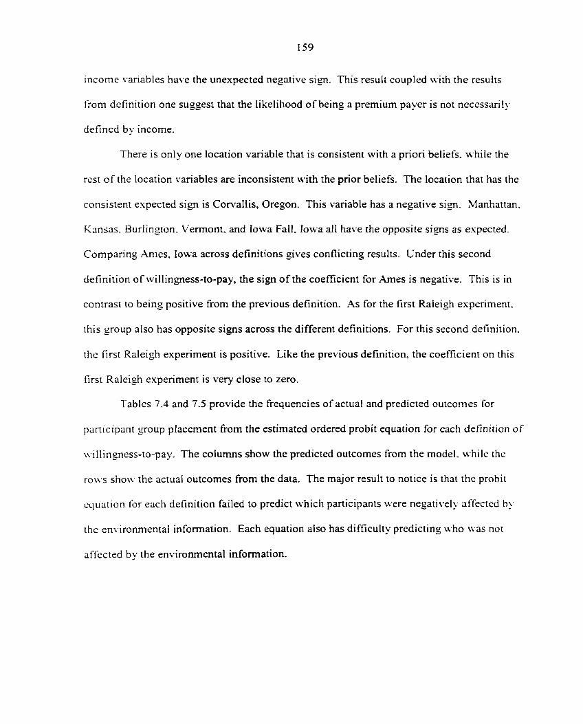
159

income variables have the unexpected negative sign. This result coupled with the results

from definition one suggest that the likelihood of being a premium payer is not necessarily

defmed by income.

There is only one location variable that is consistent with a priori beliefs, while the

rest of the location variables are inconsistent with the prior beliefs. The location that has the

consistent e.xpected sign is Corvallis, Oregon. This variable has a negative sign. Manhattan,

Kansas. Burlington. Vermont, and Iowa Fall. Iowa all have the opposite signs as e.xpected.

Comparing .A.mes, Iowa across definitions gives conflicting results. Under this second

definition of willingness-to-pay, the sign of the coefficient for Ames is negative. This is in

contrast to being positive from the previous definition. -A.s for the first Raleigh e.xperiment.

this group also has opposite signs across the different definitions. For this second definition,

the first Raleigh experiment is positive. Like the previous definition, the coefficient on this

first Raleigh experiment is very close to zero.

Tables 7.4 and 7.5 provide the frequencies of actual and predicted outcomes for

participant group placement fi-om the estimated ordered probit equation for each definition of

u illingness-to-pay. The columns show the predicted outcomes from the model, while the

rows show the actual outcomes from the data. The major result to notice is that the probit

equation for each definition failed to predict which participants were negatively affected by

the environmental information. Each equation also has difficulty predicting who was not

affected by the environmental information.

160

Table 7.4: Frequencies of Actual and Predicted Outcomes from the Estimated Ordered Probit for Definition 1 of Willingness-to-Pay'

Predicted Outcome

Actual Negatively .\ffected Outcome

Not Affected Positively .Affected Total

Negatively Affected 0 4 21 25

Not .Affected 0 8 92 100

Posili\"ely .Affected 0 6 198 204

Total 0 18 311 329 A prcrmum payer under this second definition is a participant u ho had a higher bid for the most

environmental package compared to the typical package within round four.

Table 7.5: Frequencies of .Actual and Predicted Outcomes from the Estimated Ordered Probit for Definition 2 of VVillingness-to-Pay'

Predicted Outcome

.\ctual Negatively .A.ffecied Outcome

Not Affected Positively Affected Total

Negative!}.' •Affected 0 0 •7-2 / 27

No: .Affected 0 6 68 :'4

Posiii\ cly A ffee ted 0 2 226 22S

Total 0 8 321 329 A premium payer under this second definition is a participant who had a higher bid for the most

en\ ironmemal package compared to the typical package within round tour.

The probit equations for both definitions of willingness-to-pay had a high tendency to

predict premium payers over the other two groups. Of the 329 participants, the equation for

the first definition picked 311 of them to be premium payers. Of this group selected to be

premium payers, ninety-two participants were not actually affected by the information and

161

twenty-one participants were negatively affected. For the second definition, the probit

equation chose 321 participants to be premium payers. Twenty-seven of these participants

were actually negatively affected by the information, while sixty-eight participants were

actually not affected by the environmental information.

Comparing Tables 7.4 and 7.5. it is easy to see that the probit equation for the second

equation did a slightly better job predicting than the probit equation for the first definition.

Both probit equations were not able to predict any negative premium payers correctly.

Furthermore, both probit equations had trouble predicting the participants who were not

affected by the environmental information. Both equations predicted this group with

approximately eight-percent accuracy. Given that a prediction fell in the category of the

participants not affected, the probit equation for the second definition did a better job of

predicting these participants correctly. This probit definition for the second definition also

predicted the premium payers with slightly higher accuracy.

There are two conclusions that can be drawn from Tables 7.4 and 7.5. The first

conclusion is that neither probit equation for each definition does a very good job predicting

the three dift'erent categories using the core variables used in the willingness-to-pay

literature. The second conclusion that can be drawn is that the probit equation for the second

definition of v\illingness-to-pay does a slightly better job in predicting compared to the first

definition of willingness-to-pay.

Table 7.6 presents the results from the conditional OLS model for predicting the

magnitude of the premium for those who were affected positively by the environmental

information under the first definition for willingness-to-pay. In the second column, the

uncorrected standard error for heteroscedasticity is presented, while in the third column, the

162

correcied standard error for heteroscedasiicity is presented. The e.xplanatory variables used

to predict the magnitude for this group are assumed to be the same as the variables used to

predict which category each participant falls into, i.e., the % ariables from Tables 7.2 and 7.3.

The predicted signs and magnitudes for this equation will be the same as for the probit

equations. Hence, it is expected that income and education will have positive signs with

increasing magnitudes. The number in household, monthly pork consumption, and age are

all expected to have negative coefficients. Gender is expected to have a positive coefficient.

The location variables are also expected to have the same signs as the signs from the probit

equation. Also included with these explanatory variables is LAMBDA, which is an

adjustment factor for the biased caused by the clustering of zeros.

The first thing to notice in Table 7.6 is that the number in household, age. gender, and

monthly pork consumption all have consistent a priori signs. .A.ge has the expected negative

coefficient and is significant at the five-percent level of significance. At the ten-percent level

of significance, both gender and monthly pork consumption are significant. Gender has the

expected positiv e coefficient, while monthly pork consumption has a negative coefficient.

While the number in household parameter is not significant, it has the expected sign of being

negative.

When examining the category of education, there are many education coefficients that

are significant at either the five or ten-percent level of significance. The only education

variable that is not significant is the one pertaining to having some technical, trade, or

business schooling. At the ten-percent level of significance, the variable related to a

Bachelors degree is significant. For all of the other education levels, all the parameters are

significant at the five-percent level of significance. Examining the magnitudes on education

163

Table 7.6: Second-Stage OLS Analysis of the Positive Premium Payers for Definition 1 of Willingness-to-Pay'

\'ariable Coefficient'' Standard Error (Uncorrected)

Standard Error (Corrected)

Mean of N'ariabie

Constant -5.2S14 6.1650 4.9218 NOINHOUS -0.0201 0.0924 0.0713 2.7598 PORKLM -0.0755" 0.0577 0.0458 5.6193 GENDER 1.6749" 1.1205 0.9156 0.6324 .•\GE -0.0567' 0.0255 0.0230 46.8369 LOCI 0.5133 0.5235 0.5429 0.1471 LOC2 0.9499 1.0290 0.8407 0.1961 L0C3 -0.6417 0.4547 0.4226 0.093 I LOC4 -1.3752 1.3421 1.1100 0.0735 LOC5 0.6058 0.5299 0.5265 0.1716 L0C6 0.9225 0.7621 0.6748 0.1863 rNC3 -2.5784* 1.4503 1.2601 0.1141 INC4 0.2129 0.8331 0.6922 0.2028 INC5 -0.3956 0.5728 0.4428 0.1484 INC6 1.2828 1.6751 1.4142 0.1285 INC7 -0.3034 0.6158 0.6836 0.0791 INCS -2.2129* 1.1993 0.9553 0.0495 INC9 -0.7742 0.6465 0.6357 0.0306 INC 10 -1.7473* 1.0130 0.8748 0.0644 EDLo 2.6061* 1.6032 1.2314 0.1225 EDU4 0.7413 0.8735 0.5234 0.0784 EDL'5 2.5661* 1.6343 1.2564 0.2500 r:DL"6 2.8897" 1.9599 1.5745 0.2647 EDL" 3.5634* 1.2595 1.1795 0.06S6 EDUS 2.8889* 1.6236 1.2557 U.1324 EDL'9 2.9007* 1.7731 1.4013 0.0539 L.-\MBD.-\ 10.9237" 8.2374 6.7337 0.5SOS

N R-Log-Likelihood

204 0.2041

-355.0125 Lou-Likelihood ( Restricted) -378.2970 ( a ) A p r e m i u m p a y e r u n d e r t h i s s e c o n d d e f i n i t i o n i s a p a r t i c i p a n t w h o h a d a h i g h e r b i d f o r t h e m o s t

em ironmental package compared to the typical package wuhin round four.

( b ) A n a s t e r i s k " i m p l i e s t h a t t h e c o e f T i c i e n t i s s i g n i f i c a n t a t t h e f i v e - p e r c e n t l e v e l o f s i g n i f i c a n c e a n d a d o u b l e

asterisk "* implies significance at the ten-percent level.

164

shows that the higher education levels tend to have higher magnitudes over the lower

education levels.

Similar to the probit equations above, the variables for income in the OLS model tend

to not have the expected signs. In Table 7.6, there are only two income levels that have the

expected positive sign. These are the income level associated with S30.000 to S40.000 and

the income level associated with 550,000 to S60.000. The rest of the income variables are

negative. There are three income levels that are significantly negative at the five-percent

level of significance—the income level associated with S20.000 to $30,000. the income level

associated with S70.000 to S80,000. the income level associated with the highest income.

Examining the location variables in Table 7.6 show that all the variables for location

are not significant at either the five or ten-percent level of significance. Among these

variables, only two have the hypothesized sign. Burlington. Vermont has the expected

negative coefficient, while Iowa Falls, Iowa has the expected positive coefficient. Both

.Manhattan, Kansas and Corvallis, Oregon have the unexpected sign of positive. .A.mes. Iowa

has a positix e coefficient, while the first Raleigh, North Carolina has a negative coefficient.

Examining the LAMBDA coefficient shows the level of bias due to the zeros has a

positive and significant effect at the ten-percent level of significance. Hence, deleting the

zeros and running OLS on the remaining obser\'ations would cause a serious bias to occur in

the estimates on the coefficients. Using a likelihood ratio test, the null h>'pothesis that all

coefficients are zero for this model can be rejected at the five-percent level of significance.

The critical value for this test at the five-percent level of significance is 38.89, while the

calculated likelihood ratio from the model is 46.56. Hence, the variables in this model do

have explanatory power.

165

The results from the conditional OLS model for predicting the magnitude of the

premium for those who were affected positively by the en\ ironmental information under the

second definition for willingness-to-pay are presented in Table 7.7. The second column in

this table presents the uncorrected standard error for heteroscedasticity, while in the third

column has the corrected standard error. The explanatory variables used to predict the

magnitude for this group are assumed to be the same as the variables used to predict the

previous OLS model for the first definition. The predicted signs and magnitudes for this

equation will be the same as for the probit equations. Hence, it is expected that income and

education will have positive signs with increasing magnitudes. The number in household,

monthly pork consumption, and age are all expected to have negative coefficients, while

gender is expected to have a positive coefficient. The location variables are also expected to

have the same signs as the signs from the probit equation as well as the previous OLS

equation for the first definition of willingness-to-pay. Again, the variable LAMBD.A. is

included lo account for the bias.

Examining Table 7.7 shows that the core values used in the willingness-to-pay

iiteraiure does not do a good job explaining the magnitude for the second definition of

u illingncss-to-pay. In this case there are only two significant variables at the five or icn-

pcrceni level of significance. The first significant variable is the variable denoting the llrsi

Raieigli experiment, which is significant at the five-percent level. The other significant

variable is the one denoting the group of participants who have some graduate education.

This variable was significant at the ten-percent level and had the expected positive sign. .A.s

for the rest of the variables, they were not significant at the five or ten-percent level.

166

Table 7.7: Second-Stage OLS Analysis of the Positive Premium Payers for Definition 2 of VVillingness-to-Pay'

N'ariable Coefficient" Standard Error Standard Error (Uncorrected) (Corrected)

Mean of N'ariable

Constant 3.5842 2.4698 2.5717 NOIXHOUS -0.1056 0.1413 0.1303 2.7675 PORKM 0.0046 0.0580 0.0510 5.5583 GENDER -0.1246 1.3847 1.3343 0.6535 .•\GE -0.0215 0.0316 0.0306 45.9067 LOCI -0.0055 0.5859 0.6072 0.1491 LOC2 -0.5924 0.5206 0.5132 0.1930 L0C3 -1.0280* 0.5613 0.5076 0.1053 L0C4 -0.4070 0.7706 0.7493 0.0965 LOC5 0.5736 0.7959 0.8348 0.1447 LOC6 -0.4531 0.6414 0.6368 0.1754 INC3 -0.4482 0.9212 0.9077 0.1196 INC4 -0.4691 0.5876 0.4888 0.1771 INC 5 -0.3448 0.6015 0.5265 0.1460 INC6 0.0212 0.5679 0.6028 0.1 106 INC7 -0.0338 0.7059 0.7619 0.0796 INCS -0.5427 1.0189 0.9052 0.0531 INC9 0.0663 0.7974 0.7422 0.0398 INCIU -06162 1.0674 1.0834 0.0840 EDU3 0.5894 1.2278 1.1208 0.1102 EDU4 0.1522 1.6987 1.6125 0.0881 EDU5 0.5023 1.6083 1.5929 0.2687 EDL'6 0.7030 1.0958 0.9964 0.2554 EDL-- 1.9387" 1.0106 1.0705 0.0705 EDL'S 1.0669 1.0413 0.8774 0.1 190 EDL'9 0.4900 1.6291 1.4849 0.1 I 96 L.-\.MBD.\ -0.3747 5.4082 5.4224 0.4(i~3 N R-Log-Likelihood

228 0.1276

-467.1391 Log-Likelihood ( Restricted) -482.6947 ( a ) A premium payer under this second definition is a participant who had a higher bid for the most

en\ ironmental package compared to the typical package within round four.

( b ) . A n a s t e r i s k * i m p l i e s t h a t t h e c o e f f i c i e n t i s s i g n i f i c a n t a t t h e f i v e - p e r c e n t l e v e l o f s i g n i f i c a n c e a n d a d o u b l e

asterisk •* implies significance at the ten-percent level.

167

Under this second definition of willingness-to-pay, all of the location variables and all

of the education variables have the expected signs even though they are not significant. The

\ ariable for the number in household and the variable for age both have the expected sign of

being negative. On the other hand, the variable for monthly pork consumption and the

variable for gender have the opposite of the expected sign. For this model gender had a

negative effect on magnitude, while monthly pork consumption had a positive effect.

There are only two income levels that have the expected sign of being positive.

These are the variable that denote income level of 550,000 to 560,000 and the variable that

denotes the income level of 580,000 to 590,000. Both of these variables are close to zero

relative to the income variables. All other income variables under this second definition have

the unexpected sign of being negative.

Using a likelihood ratio test, the null hypothesis that all coefficients are zero for this

model cannot be rejected at the five-percent level of significance. The critical value for this

test at the five-percent level of significance is 38.89, while the calculated likelihood ratio

from this second definitions model is 31.12. Thus, this model does not have explanatory

pou er for predicting the magnitude of the positive premium payers. Looking at the variahlc

L.A.VIBDA. which accounts for the bias, an opposite conclusion is drawn compared to the

pre\ ious model for the premium payers under the first definition. The bias for this second

definition is negative but insignificant at the ten-percent level of significance. Hence by

dropping the zeros and estimating this model with standard OLS for the premium payers for

this second definition will not cause significant bias.

Comparing the two different models leads to several conclusions. For the second

definition of willingness-to-pay, the socioeconomic factors was able to predict slightly better

168

the directional effect environmental information has on the participant. On the other hand,

the first definition does a better job explaining the magnitude of the premium for the

premium payers. The second definition has a much better R', i.e.. e.>:planator>' power, than

the first for the conditional OLS using the same core variables used in the willingness-to-pay

literature. The second definition coefficients did not do better statistically than a model with

all coefficients equal to zero. This implies that the coefficients for the second definition had

no significant e.xplanatory power over a model with just an intercept term. In both models

under both stages, the income levels rarely had the expected sign or magnitudes and were

usually not significant explanatory variables. This result was unexpected because income

usually shows up as a significant variable in most willingness-to-pay studies. Finally, the

bias due to the zero bidders is an important factor for the first definition, while it does not

seem to effect the second model significantly. This result is not too surprising considering

there were less zeros in the second definition of willingness-to-pay.

169

chapter eight: summary and conclusions

Summary and Conclusions

In chapter one a brief o\ er\ ie\v of the pork industr\' and related environmental

concerns w ere provided. These environmental concerns included odors from production, as

\\ ell as. surface and ground water impacts. This overview motivated the need to value

en\ ironmental attributes related to production from a consumer's point of view. This can

assist the development of adjustments in the industry and development of policy. Kjiowing

the \ alue consumers place on environmental attributes can also help producers make

decisions about incorporating new technologies which decrease environmental impacts trom

production.

Within chapter one, four primary objectives of this dissertation were outlined. The

first objective was to present a theoretical model that explained the behavior of a consumer in

a second-price sealed-bid auction when there are embedded environmental attributes

coniained in the item being auctioned. From this behavioral model, two willingness-to-pay

measures for environmental attributes were discussed. The second objective was lo outline

an experimental setting in which willingness-to-pay measures for embedded environmental

attributes can be collected from consumers. Examining consumer's willingness-to-pay for

pork products with embedded environmental attributes, which was derived from the

experimental setting outlined in the second objective, was the third objective. The final

objecti\e was to investigate the relationship between socioeconomic factors and respondent's

\\ illingness-to-pay for embedded environmental attributes.

.A. major objective of this dissertation was to interpret bids from a second-price

auction when embedded environmental attributes exist in the product being auctioned. It was

170

shown in chapter three that when embedded environmental attributes do not exist, the

second-price auction has the property that it is in the best interest of the participants to

iruihfuUy reveal their preferences, i.e.. their true value for the item being auctioned. This

true value was defined as the maximum amount of income the bidder is willing to give up to

obtain a new set of attributes from the product being auction. When embedded

environmental attributes exist in the product being auctioned and the bidder has some degree

of free-riding capabilities, it is no longer a dominant strategy for the bidders in a second-price

auction to bid their true value. Rather, the dominant strategy of the bidder is to bid her true

value minus any part of her true value that can be obtained from someone else. i.e.. minus the

\ alue that can be associated from free-riding.

From the behavioral model developed in chapter three, two definitions for

wiilingncss-to-pay were derived. The first definition compares the bids across information

sets for the same product. These information sets range from the naive set of the physical

iraits \ isually observ ed to those where environmental attributes are provided. In the initial

information set. only the observed physical attributes of the products are known. This first

information set was known as a naive information set. This was followed by infomialion

being released relating to the environmental attributes of each product. This second

inlbmiaiion set was known as the environmental information set. This measure uas called

consumer's willingness-to-pay with unknown ex ante e.xpectations. It was also known as

definition one. The second definition of willingness-to-pay examines the difference between

bids in the same environmental information set for a product with embedded environmental

attributes compared to a product that has no particular environmental attributes, i.e.. a typical

product. This definition was modified to account for any perceived physical quality

171

differences between the two products. This measure was known as the consumer's

willingness-to-pay for environmental attributes with a known basis. This measure was also

known as definition two. This second definition for willingness-to-pay was argued to be a

belter approximation to a person's true valuation for environmental attributes because it takes

a long-run approach to examining willingness-to-pay.

The second major objective of this dissertation was to develop a consumer

experiment to collect information from consumers about their preferences for pork products

with embedded envirormiental attributes. In chapter four, a second-price sealed-bid multiple-

round (five rounds) auction was presented as a method to obtain willingness-to-pay

information. This auction was conducted in six locations across the countr>'—.A.mes, Iowa;

Iowa Falls. Iowa; Raleigh, North Carolina; Manhattan, Kansas; Burlington. Vermont; and

Cor\ allis. Oregon. In the first three rounds of each experiment, the participants were allowed

to \ isually inspcct ten different packages of pork chops and offer bids for each. These

packages contained four pork loin chops, uniformly cut. Each package weighed

appro.\imatel\- two pounds. In round four, they were provided information that pertained to

the environmental attributes embedded in the respective packages of pork chops and allowed

10 bid agam. These attributes dealt with a reduction in odor, a reduction in ground water

mipact, and a reduction in surface water impact from production. For odor, a lou (high)

reduction level was defined as a thirty to forty-percent (eighty to ninety-percent) reduction ui

odor from production as compared to odor from a typical pork production system. In the

case of surface and ground water, the low-level (high-level) impact reduction was defined as

a reduction of fifteen to twenty-five percent (forty to fifty percent) when compared to a pork

chop from a typical production system. Not only were single low-level and high-level

attribute packages of pork chops presented, but also differing combinations (air. water

qualiiy, surface water) of the high-level attributes were also presented. The information in

round four only dealt with the improved envirorunental attributes. Societal health

implications from the attributes were provided in round fne.

The third objective of this dissertation was to examine consumer's willingness-to-pa>

for environmental attributes collected from the experiments discussed in chapter tour.

Chapter five examines three major aspects of the data collected from the experiments. The

first part examined the bids for each product for each round. The next part examined the data

in light of the first definition, definition one, of willingness-to-pay. The final part examines

the sccond detlnition of willingness-to-pay.

It is seen in chapter five that in the first three naive bidding rounds of the experiment,

av erage participant bids increased at a decreasing rate. When analv-zing the changes in bids,

ii was found that the bids for at least eighty-percent of the packages did not increase

siunificantly between round two and round three. Five out of the seven locations had one

hundred percent of the packages not significantly changing value between these two bid

rounds. Hence, bids were stabilizing. This provided further support to the findings of

Coppinuer el al. (1980) and Cox et al. (1985) that participants eventually discover their

preferences when a second-price sealed-bid auction is used with multiple trials.

.-Vfter information was released in round four, the average bid for each package took

on a consistent pattern where the most environmental package received the highest bid. the

packages with less environmental attributes received lower bids, and the typical package v\ ith

no particular environmental attributes received the lowest average bid. Between round three,

the naive bidding round, and round four, the environmental information round, half of the ten

173

packages significantly changed in value at the .001 significance level. The t\picai packagc

and the low-level odor reduction packages significantly decreased in value while both of ihe

double attribute packages and the triple attribute package increased significantly in value.

With no significant changes occurring for the products with a single high-level

cn\ ironmental attribute, it can be inferred that participants' prior expectations were that the

products ihey were bidding on had some level of environmental attributes. Thus, before any

cn\ ironmental information was provided on the products, the participants believed that the

products had some embedded environmental attributes, specifically, single high-level

environmental attributes. This would imply that environmental information does affect

consumers' willingness-to-pay for a good. It also suggests that a product that does not have

environmental characteristics will likely decrease in value when a similar product with

embedded environmental attributes is released on the market.

With the release of the societal human health implications of the environmental

attributes in round five, bid levels did not change significantly from round four. The

participants" evaluation of the societal health implications from the information released in

round four was confirmed by the information released in the fifth round, i.e., their

expectations on health implications formed in round four were in line with what was released

in round five. The changes in the bids from round three to round four demonstraicd that the

participants' initial expectations were not being met.

Chapter three presents a behavioral model that explains how consumers make

decisions when they are in a multiple-round second-price sealed-bid auction with different

information sets. In this chapter two ways of defining willingness-to-pay were developed.

One method is to observe bids between bidding rounds with two different information sets.

174

This allows for the visual attributes to be constant, but from the point of view of the

rcsearcher there is no ex ante information on the consumer's prior expectation of embedded

environmental attributes. This method of looking at willingness-to-pay was established as

definition one of willingness-to-pay. .\nother method of measuring willingness-to-pay

relates to comparing a t>pical good to one that has an environmental improvement over the

t\pical good in the same bidding round. This willingness-to-pay measure assures that the

expectation of the environmental attributes for the consumer is known to the researcher, but

it does not directly account for any visual quality differences between the two products being

considered. In chapter three, a method of adjusting for visual quality differences between

tu o packages was developed. Throughout the dissertation, this approach \\'as known as the

second definition of willingness-to-pay.

•A premium payer under the first definition of willingness-to-pay was defined as a

participant who increased her bid from the last no information round, round three, to the

inibnnation round, round four, for the most environmental product—that product with a

high-le\ el reduction in odor, surface water impact, and ground water impact compared to a

product from a typical system. It was found that of the 329 participants in the study,

approximately sixty-two percent paid a premium for the package of pork chops with the

triple high-level embedded environmental attributes. By location, this ranged from nft>-si\

percent in Burlington, Vermont to sixty-seven percent in .Vlanhattan. Kansas. The average

premium paid by the premium payers for this product was SI.60. This premium was

significantly different from zero. When examining across regions, there was no significant

difference at the five-percent level in the premiums paid for the most environmental product.

The value of the typical package decreased by S0.63. Using this definition, there is a group

175

of consumers who will pay a premium for pork products with embedded high-level

en\ ironmenial attributes.

When analyzing the non-premium payers for the first definition of willingness-to-pay.

it u as found that when the environmental information was released, all the packages of pork

chops decreased in value, some by a significant amount. A non-premium payer is someone

w ho did not increase her bid between round three and round four for the pork product with

the triple high-level embedded environmental attributes. Of the 125 participants who were

considered non-premium payers, twenty-five actually decreased their bids for the most

en\ ironmenial package. It should be noted that, while the bids decreased for this group of

tw enty-five between round three and four, the most environmental package was still \ alued

higher than the tv'pical package.

WTien the second definition of willingness-to-pay was investigated, a similar result to

the first definition was found. For this second definition, a premium payer is defined as a

participant who had a higher bid for the environmental package in round four over the t\pical

package after adjusting for visual differences. Of the 329 participants, approximately sixty

nine percent of the participants could be classified as premium payers. On average, the

premium under this definition for the premium payers was S2.23 for the most environmental

packagc. This premium was significantly greater than zero.

When examining the non-premium payers under the second definition of willingness-

lo-pay, there were 101 participants that did not pay a premium for the most environmental

good. Of this group, twenty-seven participants had a negative willingness-to-pay due to the

information provided in the experiment in round four. This implies that there was a small

group who was negatively affected by the release of the environmental information. One

176

explanation for this is that the participants in this group had higher environmental

expectations of the products before the release of environmental information or they did not

understand the system of bidding.

When analyzing the differences in socioeconomic characteristics and attitudes

between the premium payers and the non-premium payers using standard statistical tests for

both definitions of willingness-to-pay. it was found that there were ver>' few significant

differences. The three characteristics that showed up as significantly different between the

two groups with the expected outcome were if employed, willingness-to-pay a premium for

meal products with environmental attributes (yes/no type of question), and the desire for

producers to have environmental education about production practices. Characteristics such

as age, gender, and household income did not show up as significantly different. .A.ttitudes

about the environment, product attributes, and production methods also did not show up as

significantly different between the two groups.

The fourth major objective of this dissertation was to examine the relationship

bciween willingness-to-pay and socioeconomic characteristics and attitudes. To investigate

this relationship, chapter seven utilized a two-stage polychotomous choice model. The

necessity for using this model comes from the fact that under both definitions of willingness-

lo-pay there were a large number of participants having zero willingness-to-pay. In essence,

this group causes a discrete cluster point in the middle of continuous distribution. This can

be viewed as a censoring issue within a distribution. By using standard OLS techniques,

estimated coefficients for this data would be biased. The explanatory variables used in this

model were the core variables developed in the willingness-to-pay literature.

M l

To estimate this model, the first stage used an ordered probit model to predict

whether the environmental information provided affected the participants positively,

negaii\ el\'. or not at all. It was found that with both definitions the model did not perform

w ell in predicting whom the negative and zero bidders were. Additionally, of the core

variables developed in the literature, very few were significant under either definition. Under

definition one. the constant term was significant at the five-percent level, while gender

(female = 1. male = 0) was significant and positive at the ten-percent level. Using definition

two. the constant term, gender (female = 1, male = 0), and age are all significant at the five-

percent level of significance. Gender had a positive effect on willingness-to-pay, while age

had a negative effect. Under both definitions, income usually had a negative sign but it was

insignificant.

In the second stage, OLS was used to predict the magnitude of the change that was

caused by the release of envirormiental information. An equation was estimated separately

for the premium payers under both definitions of willingness-to-pay. It was found that this

model was able to predict the magnitude of the willingness-to-pay better for definition one as

compared to the second definition. The first definition had statistically significant

explanator\' power, while the second definition of willingness-to-pay did not. Under the llrst

definition of willingness-to-pay. monthly pork consumption and gender {female = 1. male ^

0) were both significant at the ten-percent level of significance. Monthly pork consumption

had a negative impact on willingness-to-pay, while gender had a positive effect. .Many of the

categorical education variables were significant and had the expected sign. Education was

divided into ten categorical levels. It was also found that under definition one the bias

17S

caused by the zero bids did have a significant effect on the estimation process. This was not

ihe case for the second definition.

From this work it is clear that some proportion of consumers are willing to pay a

premium for pork products with embedded environmental attributes. Under both definitions

of \\ illingness-to-pay. over sixty percent of the participants paid a premium for pork products

with embedded envirorunental attributes. Furthermore, these consumers want producers to

ha\ c env ironmentai education and produce in an environmentally sound fashion.

Future Research And Issues

There are three areas where this research can be expanded. The first area is related to

the theory of auctions when the product being auctioned has embedded environmental

attributes. One study that needs to be done is related to consumer behavior in the other three

major auctions (Dutch auction, first-price auction, English auction) discussed in this

dissertation when the product being auctioned has embedded environmental attributes.

Another study that can be done is one that examines the properties of an optimal auction

when environmental attributes exist fi-om both the sellers and buyers viewpoint.

The second area pertains with the experiment process. It would be useful to examine

the effects of introducing a substitute product, like beef or chicken, that would have no

en\ ironmental attributes into this auction experiment. .A.lso it would be interesting to see

what would happen if there were only two or three products rather than ten. If consumers arc

using a particular product as an anchor for the ecolabeling value, then by having many

products convolutes which product is the anchor. Another extension to this experiment is to

de\ elop a tool that will measure the level of free-riding.

179

The next logical step to this research is to do an in-store study for pork products with

en\. ironinentally embedded attributes. Participants indicated they w ould pay a premium for

pork products with embedded environmental attributes, but it is unknown whether the level

of premium given in this study would hold over time where consumers make repeated

purchases. There are many examples of products that are introduced into the market but fail

after a few months. WTiile this study was able to impose some market discipline, it was not

able to e\ aluate purchases over time. .\n in-store study would help gauge the level of market

share a product with embedded environmental attributes could gain.

The pork production industry is well positioned to address environmental issues and

de\ clop products with embedded environmental attributes. The industr\- has already

de\ eloped a program which focuses on environmental audits. Under this program pork

producers can have their pork production systems undergo an environmental audit. This, in

effect, provides a certification process built around environmentally safe production methods.

Studv participants indicated they felt producer education on environmental issues was

miportani and encouraged. The industry is already doing this. It is important to inform

consumers about what the industry is doing. Industry' education packages need to focus on

producers and consumers alike. The industr\' has done an excellent job at focusing these

i\pcs of programs on producers. These efforts need to be expanded to consumers.

180

appendix a: lntroductory letter

() June, 1997

Dear;

The Economics Department at Iowa State University is conducting a national study regarding knowledge and concerns related to pork production. Your household was scientifically selected to be included in this study and we would be grateful for your help.

U'iihin the next two weeks you will be contacted by telephone and the person who is most responsible for food purchases in your home will be asked if they would be interested in panicipatmg in a consumer experiment at Iowa State. This session will take about 2 hours of \our lime and would take place on a Saturday. It would involve no risk to you and you u ould be paid S40.00 for participating. The experiment will be located on the Iowa State campus in room 162 Heady Hall. A map is included to assist you with finding this building.

To dale, we have had over 400 people from the Ames and Story County area participate in similar sessions and we have received positive comments from almost all of those panicipants. Most people said they found the experience to be interesting and infomiaii\ c.

1 f \ou have any questions regarding the study, please call Sean Hurley at 51 5-294-21 and he will be happy to help you. Thank you for your consideration.

Smcerei\.

James B. Kliebenstein, Ph.D. Professor

181

APPENDIX B: EXPERIMENTAL DIRECTIONS, BID SHEETS, AND PRE AND POST AUCTION SURVEYS

Consent Form

>'ou are about to participate in a consumer experiment in willingness-to-pa\ for a food product. This experiment will ttike approximately two hours.

W'c need your signed consent if you are to act as a subject. Your participation in the experiment is completely voluntar\' and you may withdraw from the experiment at any time without prejudice to you. Results from the experiment vvill be strictly confidential. Any name associated with the experiment will be deleted upon completion of the experiment.

If >ou consent to participate in the e.xperiment. please sign the consent form below.

1 ha\ e read the consent form statement and agree to act as a subject in the experiment, uith the understanding that I can withdraw from the experiment at any time without prejudice lo me.

Signature / i Date

1S2

Experimental Instructions

General Instructions

\'ou are about to participate in an experiment in market decision making. Please follow all instructions carefully.

The e.xperiment will consist of 2 stages and will last approximately 2 hours. In stage 1 you will be asked to decide how much you would be willing to pay for different candy bars. This stage is designed to familiarize you with the auction procedure w e will be using. In stage 2 you will be asked how much you would be willing to pay for pork products with different attributes.

You will submit your bidding price on a recording sheet. You cannot reveal your bids to any other participant- Any communication between participants will result in an automatic penalty of S3. Please do not complete any form until instructed to do so by the monitor.

You will receive S40 for participating in this experiment. Because you actually pay for any product you choose to purchase, your take home income will consist of S4(j minus the price paid for any products purchased.

Please pay attention to the monitors at all times and do not hesitate to ask questions about any of the instructions.

183

Pre-Auction Sur\ey

About "^'ou

1. ^'our sex; Female Male

2. As of your last birthday, how old were you?

3. Ho\\ many individuals live in your household, including yourself? If you have children, how old are they?

4. Please indicate the highest level of education you have completed: Grade 8 Grade 9-11 H. S., G. E. D. Some technical, trade, or business school Some college, no degree B.S., B.A., etc. Some graduate work, no degree M.S., M.A., etc. Ph.D., DA^M.. D.D.S., etc.

5. Are you currently employed? Yes No

6. WTiat is your occupation, e.g.. homemaker, police officer, doctor, teacher, etc.?

Please indicate the approximate household income for 1996:

Less than S10.000 510,000-520,000 520,000 - 530,000 530,000 - 540,000 540,000 - 550.000 550,000 - 560.000 560,000 - 570,000 570.000 - 580.000 580,000 - 590.000 More than 590.000

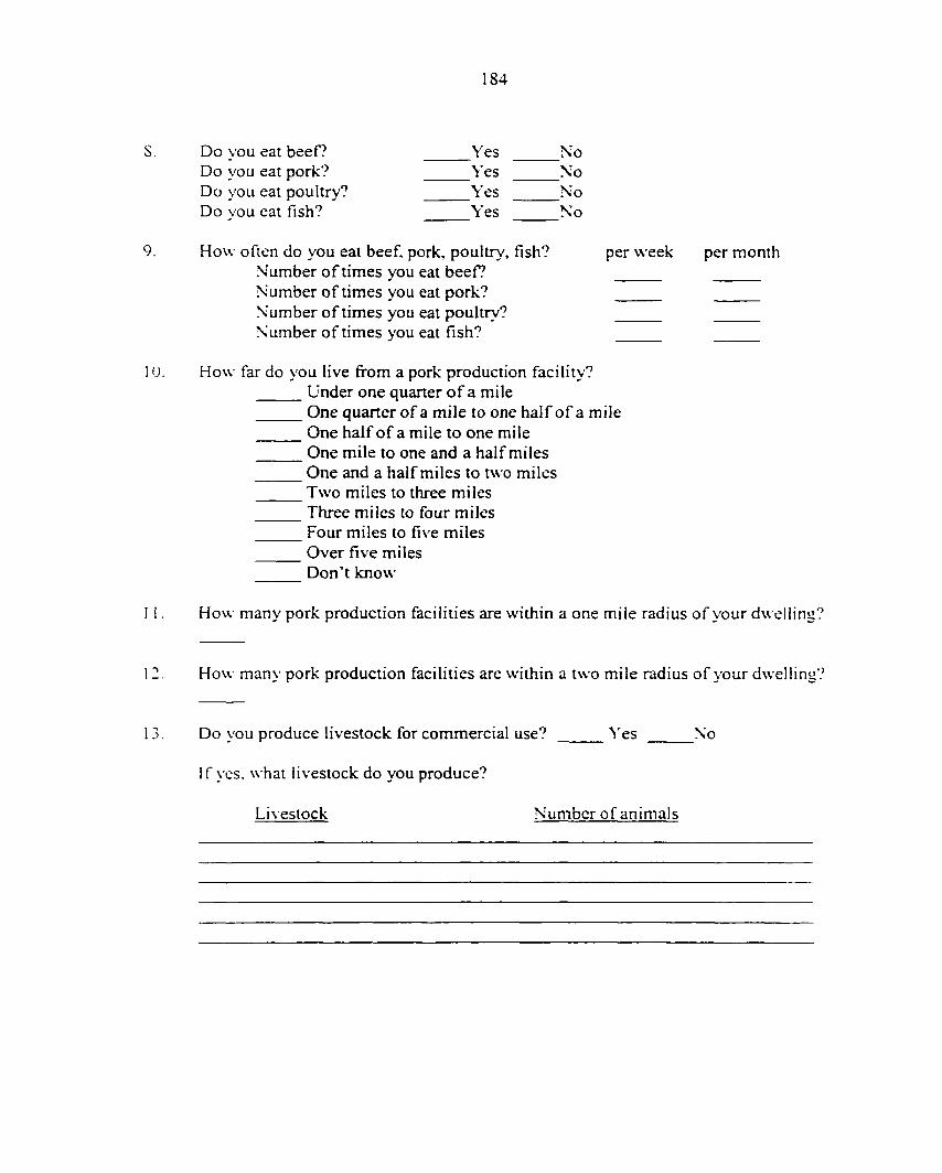
184

S. Do you eat beef? Yes No Do you eat pork? \'es No Do you eat poultr>'? Y'es No Do you eat fish? Yes No

9. How often do you eat beef, pork, poultry, fish? per week per month Number of times you eat beef? Number of times you eat pork? Number of times you eat poultry? Number of times you eat fish?

1 (J. How far do you live from a pork production facility? Under one quarter of a mile One quarter of a mile to one half of a mile One half of a mile to one mile One mile to one and a half miles One and a half miles to two miles Two miles to three miles Three miles to four miles Four miles to five miles Over five miles Don't know

I I. How many pork production facilities are within a one mile radius of your dwelling?

! 2. How many pork production facilities are within a two mile radius of your dwelling?

13. Do you produce livestock for commercial use? 'N'es No

If yes, what livestock do you produce?

Livestock Number of animals

185

14. Do you produce crops for commercial use? Yes No

If yes, what crops do you produce?

Crop Typical number of acres allocated to the crop

15. Do you read the information on the labels of the products you buy? Never Sometimes Always

14. Have you ever noticed any information labeling on the products you buy that portray env ironmental attributes or qualities?

Yes No

If yes. please give an example:

15. Do you think you have purchased more beef or pork as a direct result of the beef and pork advertisements you have seen in the media; e.g.. "Pork the other white meal", etc.?

more beef? Yes No more pork? Yes No

186

16. On a scale from 1 through 5 with 1 being 'very concerned' and 5 being "not concerned." how concerned are vou about the followina issues:

Issue Very

Concerned Not

Concerned

Environment 1

Water quality 1

Air Quality 1

Food prices 1

Family Farming 1

Production methods in livestock farmina 1

Animal welfare

Pollution

Livestock confinement SNSlcms

Changing farming structure

4

4

4

4

4

4

4

5

5

5

187

17. On a scale from 1 through 5 with 1 being "very important' and 5 being "not important." indicate how important the following attributes are for the products you consume:

Very Not Issue Important Important

Eating quality 1 2 3 4 5

X'isual appeal 1 2 3 4 5

Freshness 1 2 J 4 5

Price 1 2 J 4 5

Environmental 1 -> J 4 5

Production methods used in producing the good 1 -> -* J 4 5

Uniformity of product 1 2 J 4 5

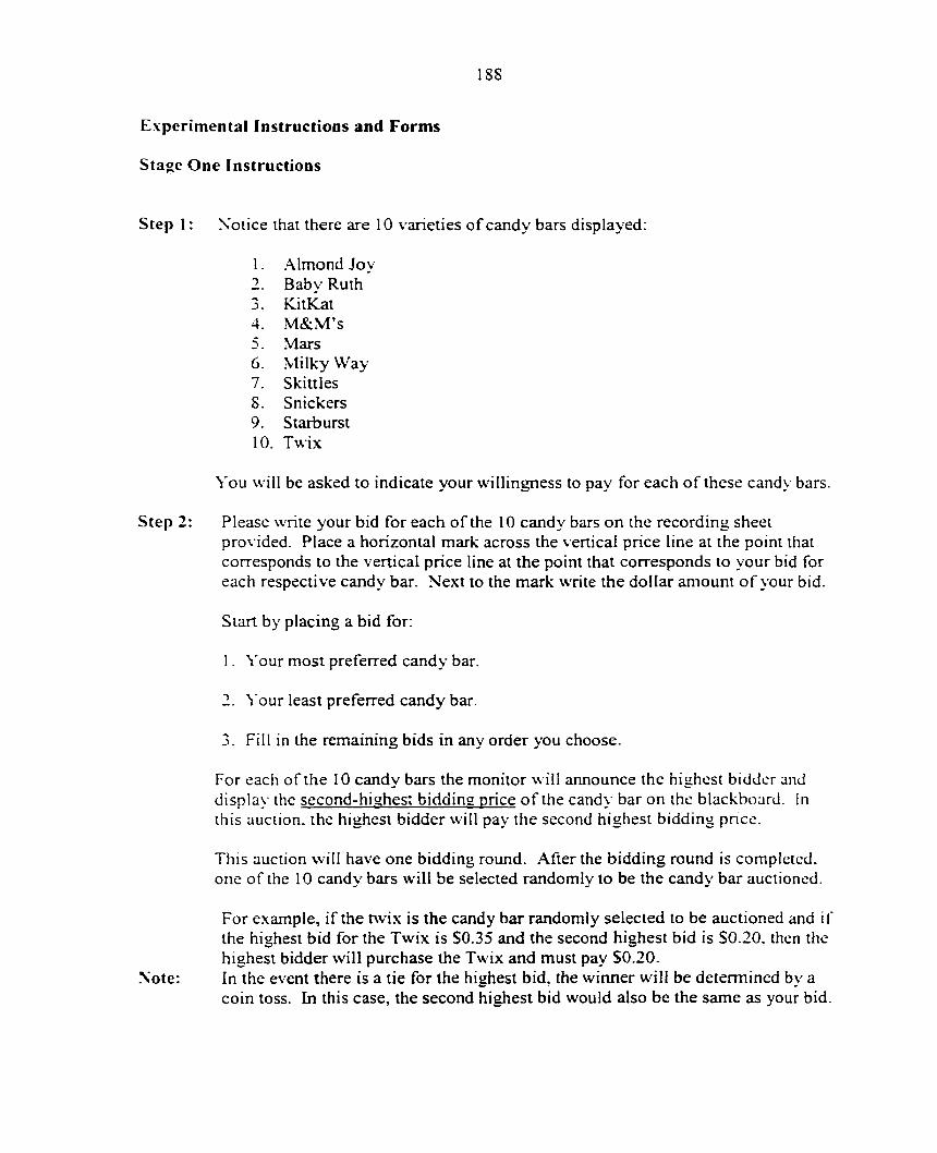
188

Experimental Instructions and Forms

Stage One Instructions

Step 1: Notice that there are 10 varieties of candy bars displayed:

1. .A.Imond Joy 2. Baby Ruth •»>

J. KitKat 4. M&M's 5. Mars 6. Milky Way 7. Skittles S. Snickers 9. Starburst 10. Twix

You will be asked to indicate your willingness to pay for each of these candy bars.

Step 2: Please write your bid for each of the 10 candy bars on the recording sheet provided. Place a horizontal mark across the vertical price line at the point that corresponds to the vertical price line at the point that corresponds to your bid for each respective candy bar. Next to the mark write the dollar amount of your bid.

Start by placing a bid for:

1. \'our most preferred candy bar.

2. Your least preferred candy bar.

3. Fill in the remaining bids in any order you choose.

For each of the 10 candy bars the monitor will announce the highest bidder and display the second-highest bidding price of the candy bar on the blackboard. In this auction, the highest bidder will pay the second highest bidding price.

This auction will have one bidding round. After the bidding round is completed, one of the 10 candy bars will be selected randomly to be the candy bar auctioned.

For e.xample, if the twix is the candy bar randomly selected to be auctioned and if the highest bid for the Twix is S0.35 and the second highest bid is S0.20. then the highest bidder will purchase the Twix and must pay SO.20.

Note; In the event there is a tie for the highest bid, the winner will be determined by a coin toss. In this case, the second highest bid would also be the same as your bid.

189

Note: In this auction it is in your best interest to bid the amount you are truly u illing to pay for the candy bar. If you bid more than your true u illingness-to-pay. then you increase your chances of purchasing the candy bar but you may ha\ e to pa\ a price that is greater than your valuation of that candy bar. On the other hand, if you bid less than the amount that you are truly willing to pay, you ma\' lose the chance to purchase the candy bar at a price that you would be willing to pay.

Kxiiinple Candy Har Hids

ALMOND BABYIUITM KITKAT MAM'S JOY

MARS

2.(K) 2.(K) 2.(KL 2.(K) 2.(K)

1.3()_ 1.50 1.50 1.50 1.50

l.(K) I.(Ml l.(KI l.(KI l.(K)

0.50 0.50 0.50 0.50 0.50

0.00 0.(K) ( ) ( H ) (MM) 0(K)

II)//

MII.KY WAY

2.(K),

1.50

i.(K)

0.50,

0 00

SKriTl.liS SNICKHRS STARBDRST TWIX

2,00_

1.50

l.(X)

0.50

().(K)

2.(ML

1.50

l.(K)

0.50

0(K)

2.(K).

1.50

l.fH)

0.50

0.(X)

2.(M)

1.50

l.(K)

0.50

0 00

191

Quiz

Please fill in the blank for each of the following questions.

1. The example bidding sheet indicates that the bidder is willing to pay S for a Mars bar and is willing to pay S for a Snickers.

2. Suppose your bid of 50.35 is the highest bid for the Skittles and the Skittles were randomly selected to be the candy bar auctioned. Also suppose that the second highest bid for the skittles is S0.21. V\1iat price will you pay for the Skittles? S

Ciiiuly Hjir Hids

ALMOND BABY HUTU KITKAT MAM'.S JOY

MARS

2.()0 2.()() 2.(X) 2.(H) 2.(K)

L50 1.50 I 50 L50 1.50

LOO LOO L(M) l . (M) L(N)

0.50 0.50 0.50 0.50 0.50

0.(M) 0.(M) ().(M) 0(M) ( ) . ( K )

ll)f/

MILKY WAY

SKriTLl-S SNICKHHS STARIUJRST TWIX

2.(M) 2.<X) 2.(M) 2.00 2.(M)

L50 1.50 1.50 1.50 1.50

L(M) L(X) i.(K) L<M) L(H)

0.50 0.50 0.50 0.50 0.50

0.00 (MM) 0.00 (MM) (),(M)

Recording Sheet for ( andy H:u' Round

Bidder tf Aliiioiul Joy

liaby Ruth

Kiikai Mc-CiM's Mars Milky Way

Skittles Snickers Starhurst Twix Twix

194

Stage Two Instructions

Step 1: You will be asked to bid on 10 packages of pork loin chops. Each package contains four pork loin chops and weighs approximately 2 pounds. These packages are labeled as the following;

1. Pork loin chop package 1.

Pork loin chop package 2.

J. Pork loin chop package 3.

4. Pork loin chop package 4.

5. Pork loin chop package 5.

6. Pork loin chop package 6.

7. Pork loin chop package 7.

S. Pork loin chop package 8.

9. Pork loin chop package 9.

10. Pork loin chop package 10

\'ou will be asked to indicate your willingness to pay for each of these packages of pork loin chops.

Step 2: Please write your bid for each of the packages on the recording sheet. Place a horizontal mark across the vertical price line at the point that corresponds lo your bid for each package of pork loin chops. Next to the mark write the dollar amount of your bid.

For each of the 10 packages, the monitor will announce the highest bidder's number and display the second-highest bidding price of the package on the blackboard. In this auction, the highest bidder will pay the second highest bidding price.

This auction will have five bidding rounds. After the fifth bidding round is completed, one of the bidding rounds will be selected by the monitor to be the

195

binding round. Then one of the 10 pork loin chop packages will be selected randomly to be the package auctioned.

Note: In the event there is a tie for the highest bid. the winner will be determined by a coin toss. In this case the second-highest bid will be the same as the highest bid.

Note: In this auction it is in your best interest to bid the amount you are truly willing to pay to purchase each package. If you bid more than your true willingness-to-pa\. you increase your chances of purchasing the package but you may ha\ e to pay a price greater than what you are willing to pay. On the other hand, if you bid less than the amount you are truly willing to pay, you may lose the chance to purchase the package at a price that you would be willing to pay.

Recording Sheet for I'ork Kxperhnent: iUddhi^ Round

Bidder ff Package 1 Package 2 Package Package 4 Package .S Package 6 Package 7 I^ickage S Package 9 Package 10 Package

Pork l.oin C hop Hids: Koiiiui I

Pork Loin Chop Packagc I

I'ork Loin Chop Packajjc 2

Pork l.oin Chop I'ackagc 3

I'ork l.oin Chop Packapc 4

I'ork Loin Chop I'ai:kai!c 5

12.00

9.00

6.00

3.(X)

0.(K)

I2 . (H)

9.0()_

6.(K)

3.(K)

( ) . ( ) ( )

I2.(K)

9.(H)

6 00

.MH)

( ) ( K )

I2.(K)_

9.(H)

6.(K)

.VIM)

( ) ( ) ( )

i2.<K)

9.(K)

6.00

.3.(K)

11)«

Pork I'ork Pork Pork Pork Loin Chop Loin Chop l.oin Chop Loin Chop Loin Chop Package 6 Packagc 7 Packagc 8 Packaged Packagc 10

12.00

9. (M)

6.(M)

( ) ( ) ( )

I2.(K)

9.(K)

6.(X)

3.(K)

().(M)

!2.(K)

9.(K)

6.(H)

.V(H)

().()()

I2(K)

9,(K)

6.(M)

.V(K)

(KM)

I2,(M)_

9,(M)_

6.0()_

.V(M).

(I.(M)

vO

198

Attributes of the Pork Loin Chop Packages (9:00 Session)

Package I has no particular environmental attributes. It is the tv'pical pork loin chops which can be bought at any local store.

Package 2 has the environmental attribute of a pig production system using technology that reduces odor by 30 to 40% below the t>pical (package 1).

Package 3 has the environmental attribute of a pig production system using technology that reduces odor by 80 to 90% below the typical (package 1).

Package 4 has the environmental attribute of a pig production system using technology that reduces seepage of nutrients, etc., from swine manure into the groundwater by 15 to 25% below the typical (package 1).

Package 5 has the environmental attribute of a pig production system using technology that reduces seepage of nutrients, etc., from swine manure into the groundwater by 40 to 50% below the typical (package 1).

Package 6 has the environmental attribute of a pig production system using technology that reduces run-off of phosphorus, etc., from manure into surface water by 15 to 25% below the typical (package 1).

Package 7 has the environmental attribute of a pig production system using technology that reduces run-off of phosphorus, etc., from manure into surface water by 40 to 50% below the typical (package 1).

Package 8 has a combination of two environmental attributes in a pig production system; one using technology that reduces odor by 80 to 90%, and the other using technology that reduces seepage into the groundwater by 40 to 50% below the typical (package 1).

Package 9 has a combination of two environmental attributes in a pig production system; one using technology that reduces odor by 80 to 90%, and the other using technology thai reduces run-off into surface water by 40 to 50% below the typical (package 1).

Package 10 has a combination of three environmental attributes in a pig production sy stem; one using technology that reduces odor by 80 to 90%, the second using technology that reduces seepage into the groundwater by 40 to 50%, and the third using technology that reduces run-off into surface water by 40 to 50% below the typical (package 1).

199

Attributes of the Pork Loin Chop Packages (11:30 Session)

Package 1 has the environmental attribute of a pig production system using technoiogy that reduces odor by 30 to 40% below the typical (package 5).

Package 2 has the environmental attribute of a pig production system using technology that reduces odor by 80 to 90% below the typical (package 5).

Package 3 has the environmental attribute of a pig production system using technology that reduces seepage of nutrients, etc.̂ from swine manure into the groundwater by 15 to 25"/o below the typical (package 5).

Package 4 has the environmental attribute of a pig production system using technology that reduces seepage of nutrients, etc., from swine manure into the groundwater by 40 to 50% below the typical (package 5).

Package 5 has no particular envirorunental attributes. It is the tj-pical pork loin chops which can be bought at any local store.

Package 6 has the environmental attribute of a pig production system using technology that reduces run-off of phosphorus, etc., from manure into surface water by 15 to 25% below ihc ix'pical (package 5).

Package 7 has the environmental attribute of a pig production system using technology thai reduces run-off of phosphorus, etc., from manure into surface water by 40 to 50% below ihc t\pical (package 5).

Package 8 has a combination of two environmental attributes in a pig production system; one using technology that reduces odor by 80 to 90%, and the other using technology that reduces seepage into the groundwater by 40 to 50% below the typical (package 5).

Package 9 has a combination of two environmental attributes in a pig production system; one using lechnology that reduces odor by 80 to 90%, and the other using technology thai reduces run-off into surface water by 40 to 50% below the typical (package 5).

Package 10 has a combination of three environmental attributes in a pig production system; one using technology that reduces odor by 80 to 90%, the second using technology thai reduces seepage into the groundwater by 40 to 50%, and the third using technology thai reduces run-off into surface water by 40 to 50% below the typical (package 5).

200

Attributes of the Pork Loin Chop Packages (2:00 Session)

Package 1 has the en\'ironmental attribute of a pig production system using technology that reduces odor by 30 to 40% below the typical (package 10).

Package 2 has the environmental attribute of a pig production system using technolog\- that reduces odor by 80 to 90% below the typical (package 10).

Package 3 has the environmental attribute of a pig production system using technology that reduces seepage of nutrients, etc., from swine manure into the groundwater by 15 to 25% below the typical (package 10).

Package 4 has the environmental attribute of a pig production system using technology that reduces seepage of nutrients, etc., from swine manure into the groundwater by 40 to 50% below the tvpical (package 10).

Package 5 has the environmental attribute of a pig production system using technology that reduces run-off of phosphorus, etc., from manure into surface water by 15 to 25% below the typical (package 10).

Package 6 has the environmental attribute of a pig production system using technology that reduces run-off of phosphorus, etc.. from manure into surface water by 40 to 50% below the t\pical (package 10).

Package 7 has a combination of two environmental attributes in a pig production system; one using technology that reduces odor by 80 to 90%, and the other using technology that reduces seepage into the groundwater by 40 to 50% below the typical (package 10).

Package 8 has a combination of two environmental attributes in a pig production system; one using technology that reduces odor by 80 to 90%, and the other using technology that reduces run-off into surface water by 40 to 50% below the typical (package 10).

Package 9 has a combination of three environmental attributes in a pig production system; one using technology that reduces odor by 80 to 90%, the second using technology that reduces seepage into the groundwater by 40 to 50%, and the third using technology that reduces run-off into surface water by 40 to 50% below the typical (package 10).

Package 10 has no particular environmental attributes. It is the typical pork loin chops which can be bought at any local store.

201

The Production Systems

Typical Production System

The tvpical pork loin chops in this experiment come from a pig production system using an earthen manure storage system with manure applied on the top (surface) of tlie land. Odor in this system is allowed to flow freely.

.Attributes of the typical pork production system with respect to odor, seepage and run­off is as follows:

Odor

A t\pical swine production system emits odor for a time period which is equivalent to about 11-18 days per year (3-5% of the time). This odor is produced primarily by sulfur compounds due to animal waste decomposition. For a 90% reduction, the swine production emits odor for a period of time which is equivalent to about 1-2 days per year, while for a 40% reduction, the swine production emits odor for a period of time which is equivalent to about 7-11 days per year.

Odor emissions from pork production facilities can have many effects to the surrounding area and its residents. They can cause unpleasant living conditions and loss of property values for surrounding neighbors; some psychological duress, as uell as health effects of coughing, wheezing, vomiting, etc.. and a more depressed general outlook on life. It creates uncertainty about planning social events by neighbors and can be a nuisance to both neighbors and those passing by.

Pig production systems with reduced odors (i.e., 40% and 90%) involve combinations of differing manure storage technologies and manure application methods along with air filtration devices attached to the production facilities to reduce odor emissions.

202

Groundwater seepage

The primary problem that can arise is leeching of nitrogen or nitrates from swine manure into the groundwater supply. This groundwater contamination can affect anyone using the underground aquifer for water consumption, e.g.. surrounding neighbors, communities, etc.

One of the major health concerns with this seepage into an aquifer is Blue Baby disease resulting from lack of oxygen. This disease affects infants under the age of 6 months and can possibly lead to death.

Once an aquifer has been polluted, it can take months and even years to clean itself

Pig production systems with reduced seepage (i.e., 40% and 90%) into the groundwater involve combinations of differing manure storage technologies and manure application methods.

Surface \> ater

The primary problem is from nutrient run-off from manure or manure spills that winds up in the surface water, i.e, stream, rivers, lakes, marshes, etc. The principal nutrient contaminant from swine manure is phosphorus.

This contamination can lead to oxygen depletion in the surface water supplies and the death of aquatic life such as fish. It can also lead to excessive algae growth in surface water supplies further depleting the oxygen supply in the affected water. Depending upon water flow of the contaminated area and level of run-off or spill, aquatic life can be affected over a short distance or cover many miles. Contamination can impact recreational use of surface water, i.e., boating, fishing, swimming, aesthetics, etc..

The amount of time for clean up depends upon surface water flow and can \ ary from a feu- days to weeks.

Pig production systems with reduced surface water contamination (i.e.. 40".. and 90" o) in\oIve combinations of differing manure storage technologies and manure application methods.

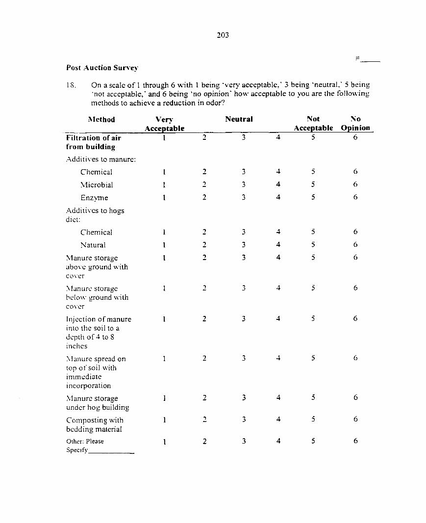
203

Post Auction Surrey

IS. On a scale of 1 through 6 with 1 being "very acceptable/ 3 being 'neutral.' 5 being 'not acceptable,' and 6 being 'no opinion" how acceptable to you are the following methods to achieve a reduction in odor?

Method Ver>-Acceptable

Neutral Not No Acceptable Opinion

Filtration of air from building

Additives lo manure:

Chemical

Microbial

Enzyme

Additives to hogs diet:

Chemical

Natural

Manure storage abo\ e ground with cover

Manure storage below ground with co\ er

Injection of manure into the soil to a depth of 4 to 8 inchcs

Manure spread on lop of soil with immediate incorporation

Manure storage under hog building

Composting with bedding material

Other: Please Specify

1

J

3

3

J

3

J

4

4

4

4

4

4

4

4

4

3

5

5

5

5

5

6

6

6

6

6

6

6

6

6

204

19. On a scale of 1 through 5 with 1 being 'very acceptable". 3 being 'neutral', and 5 being "not acceptable", how acceptable to you are the following methods to achie\ e reduction of manure seepage into groundwater?

•Method \'er\-Acceptable

Neutral Not No .Acceptable Opinion

Injection of manure into the soil to a depth of 4 to 8 inches

Manure storage above ground in steel/cement structure

Manure storage below ground in steel cement structure

Other: Please Specify

1

205

20. On a scale of 1 through 5 with 1 being "verx' acceptable'. 3 being "neutral', and 5 being 'not acceptable", how acceptable to you are the tbllowing methods to achieve a reduction in run-off or spill of manure into surface water?

Method Very Acceptable

Neutral Not No Acceptable Opinion

Injection of manure into the soil to a depth of 4 to S inches

Manure spread on top of soil with immediate incorporation

Manure storage above ground in steel cement structure

Manure storage below ground in steel cement structure

Other; Please Specify

1

21. On a scale from 1 through 6 with 1 being "very concerned', 5 being 'not concerned, and 6 being 'no opinion' how concerned are you about the following issues:

Issue Ver>^ Concerned

Not .No Concerned Opinion

Environmental 1 impact from livestock production

Worker Environment 1

Animal Environment 1

Farm Structure 1

2

->

J 4 5 6

J 4 5 6

3 4 5 6

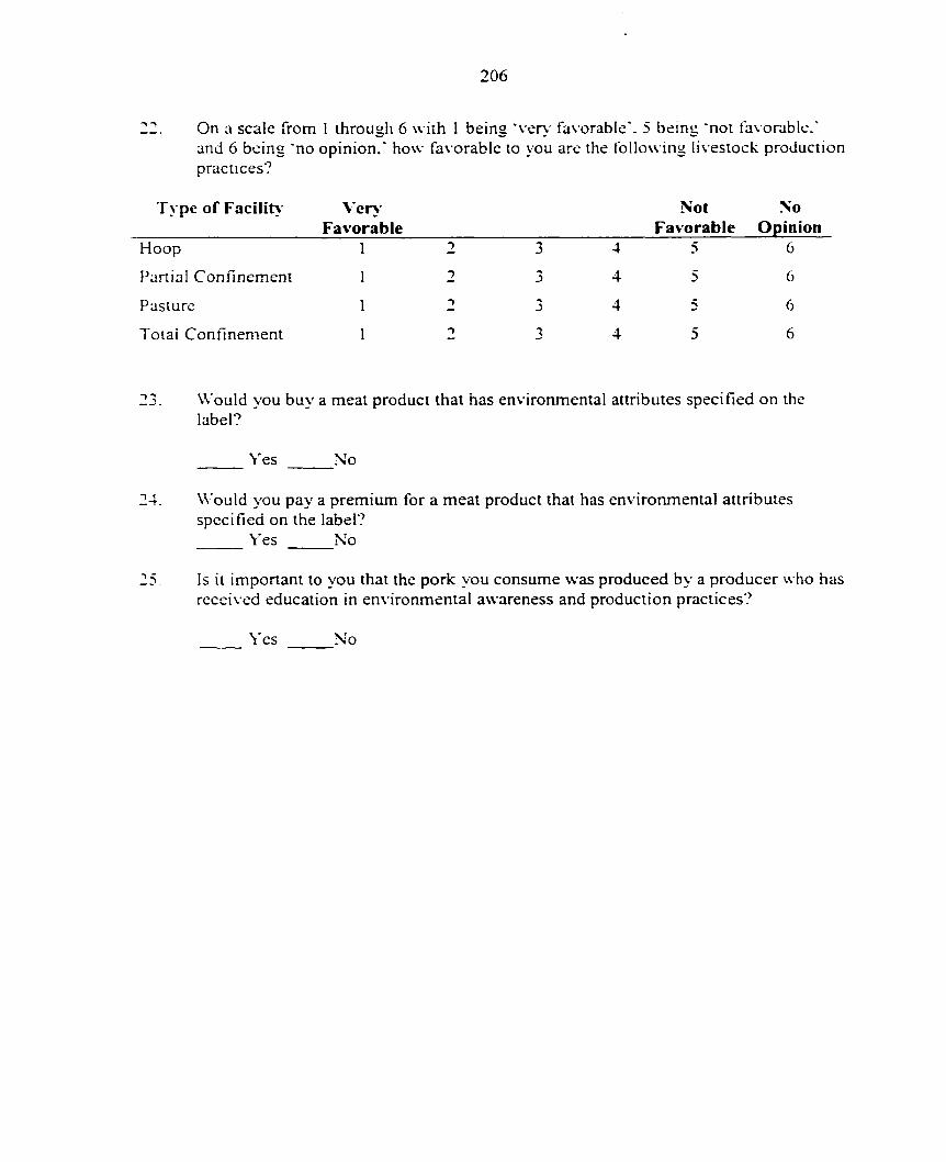
206

On a scale from 1 through 6 with I being 'ver\' favorable". 5 bemg "not fas orablc/ and 6 being "no opinion." how favorable to you are the following livestock production practices?

Type of Facilit>- Ver>' Not No Favorable Favorable Opinion

Hoop 1 2 3 4 5 6

Partial Confinement 1 2 J 4 5 6

Pasture 1 J 4 6

Total Confinement 1 -) 4 5 6

23. Would you buy a meal product that has environmental attributes specified on the label?

Ves No

24. Would you pay a premium for a meat product that has environmental attributes specified on the label?

\'es No

25. Is it important to you that the pork you consume was produced by a producer who has received education in environmental awareness and production practices?

\'es No

207

APPENDIX C: EXPERIMENTAL RESULTS BY LOCATION

Tabic CI: Bid Premiums (S) per Package by Area for Premium Payers (Ames. lA; Manhattan, KS; Raleigh, NC (97); Burlington, VT)

Location Pork Chop Environmental Ames, Manhattan, Raleigh. Burlington. Attributes (Level of Improvement lA KS NC (97) \T over Typical) No Particular Environmental -0.79 -0.47 1 P

-0.52 Attributes (T>'pical) Odor 30-40% -0.61 -0.22 -0.33 -0.05 Odor SO-90% -0.05 0.01 0.09 0.17 Ground water 15-25% 0.02 0.01 0.36 0.53 Ground water 40-50% 0.16 0.06 -0.19 0.68 Surface Water 15-25% 0.01 -0.16 0.11 0.39 Surface Water 40-50% 0.46 0.20 0.10 0.55 Odor S0-90%/Ground Water 40-50% 0.97 0.56 0.54 O.SO Odor 80-90%/Surface Water 40-50% 0.73 0.76 0.44 1.12 Odor S0-90%/Ground Water 1.74 1.38 1.33 1.89 40-50%. Surface Water 40-50%

Table C2: Bid Premiums (S) per Package by Area for Premium Payers (Iowa Falls. I A: Corvallis. OR; Raleigh, NC (98))

Location Pork Chop Environmental Iowa Falls, Cor>allis, Raleigh. .\ttributes (Level of Improvement lA OR NC (98) over Typical) No Particular Environmental -0.63 -0.44 -i.22 Attributes (T\pical) Odor 3 (-1-40" 0 -0.39 -0.55 -<).3(>

Odor 80-90° o -0.18 -0.12 -o.dl Ground water 15-25% -0.19 -0.08 Ground water 40-50% -0.01 0.21 -|).3js

Surface Water 15-25% -0.37 0.04 -'J.3iS Surface Water 40-50% 0.19 -0.02 -0.05 Odor S0-90%/Ground Water 40-50% 0.78 -0.03 0.51 Odor 80-90%/Surface Water 40-50% 0.95 0.45 0.84 Odor 80-90%/Ground Water 1.60 1.59 1.84 40-50°/b/Surface Water 40-50%

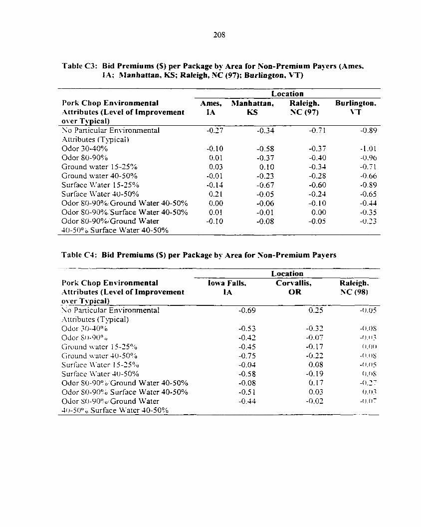
208

Table C3: Bid Premiums (S) per Package by Area for Non-Premium Payers (Ames. lA; Manhattan, I^; Raleigh, NC (97); Burlington, VT)

Location Pork Chop Environmental Ames, Manhattan, Raleigh. Burlington. Attributes (Level of Improvement lA KS NC (97) \T over Typical) No Particular Environmental -0.27 -0.34 -0.71 -0.89 Attributes (T\pical) Odor 30-40% -0.10 -0.58 -0.37 -1.01 Odor SO-QO^/o 0.01 -0.37 -0.40 -0.96 Ground water 15-25% 0.03 0.10 -0.34 -0.71 Ground water 40-50% -0.01 -0.23 -0.28 -0.66 Surface Water 15-25% -0.14 -0.67 -0.60 -0.89 Surface Water 40-50% 0.21 -0.05 -0.24 -0.65 Odor 80-90% Ground Water 40-50% 0.00 -0.06 -O.IO -0.44 Odor S0-90%/Surface Water 40-50% 0.01 -0.01 0.00 -0.35 Odor S0-90%/Ground Water -O.IO -0.08 -0.05 -0.23 40-50° b. Surface Water 40-50%

Table C4: Bid Premiums (S) per Package by Area for Non-Premium Payers

Location Pork Chop Environmental Iowa Falls, Corvallis, Raleigh. .Attributes (Level of Improvement lA OR NC (98) over Typical) No Particular Environmental -0.69 0.25 -0.05 .Aliributes (Typical) Odor 30-40°'o -0.53 -0.32 -O.OS OdorS()-90°o -0.42 -0.07 -0.113 Ground u aler 1 5-25% -0.45 -0.17 (1.0(1

Ground \^ atcr 40-50° o -0.75 -0.22 -(i.(i8

Surface Water I5-25°/o -0.04 0.08 -((.05

Surface Water 40-50% -0.58 -0.19 O.OS Odor S0-90°o Ground Water 40-50% -0.08 0.17 -0.2" Odor SO-90% Surface Water 40-50% -0.51 0.03 0.(,i3

Odor S0-90"-o Ground Water -0.44 -0.02 -(J.0~

40-50" u Surface Water 40-50%

Table C5: Percent of I'articipants Paying Preniiiinis hy Premium Level for Hoth Products and Tiers (Ames, lA)

Premium Level (Interval) i?er l*ackat;e Pork Chop Knvironmental Ik'low $0.01- $0.50- $1.00- $1.50- $2.00- Over Attributes (Level of $0.(10 $0.(N) $0.49 $0.99 $L49 $1.99 $2.49 $2.50 Improvement over Typical) By Product: No Particular HuviroiimciilJil 46.94% 34.69% 4.08% 6.12% 4.08% 2.04% 2.04% 0.(K)%

Attributes ( Typical) Odor 30-40% 26.53% 53.06% 10.20% 6.12% 4,08% 0.(M)% ().()()% ().(K)%

Odor 80-90% 26.53% 32.65% 12.24% 14.29% 10,20% 2.04';^^ 0.(K)7r. 2,04% Ground water 15-25% 30.61% 38.78% 6.11% 12.24% 6.12% 0.()()'7r 2.04% 4,08%

Ground water 40-507r) 26.53% 32.65% 12.24% 16.33% 8.16% 2.()4%> 0.(K)% 2,04%

Surface Water 15-25% 26.53% 44.90% 12.24% 8.16% 4.08% 0.00'^. 4.08% 0,009}.

Surfacc Water 40-50% 24.49% 30.61% 12.24% 12.24% 8.16% 2.04%. 2.04% 8.16% Odor 80-90%/Grouiid Water 14.29% 34.69% 12.24% 12.24% 14.29% 4.08% 0.00% 8.16%

40-50% Odor 80-90%/Surfacc Water 20.41% 38,78% 10,20% 8.16% 10.20% 2.04%. 0.(K)% 10.20% 40-50% Odor 80-90%/Ground Water 6.12% 32.65% 10.20% 10.20% 22.45% 2.04%. 4.08% 12.24% 40-50%/Surface Water 40-50% By Tier: No Particular Environmental 46.94% 34.69% 4.08% 6.12% 4.08% 1XW% 2.04% 0.00% Attributes (Typical) Low Level Single Altribule 27.89% 33.33% 9.527p 12,24% 7.48% 2.04% 0.68% 1,36% High Level Single Allribule 25.85% 31.97% 12.24% 14.29% 8.84% 2.04% 0.68% 4.08% High Level Double Attributes 17.35% 36,73% 11,22% 10,20% 12.24% 3.06% (,».(H)'7f. 9.18% High Ixvel Triple Attributes 6,12% 32,65% 10,20% 10,20% 22.45% 2.04% 4.08% 12,24%

Tiil)lc C6: Percent of Parlicipnnts I'ayin^ Preniiums hy Premium Level for Both Products and Tiers (Manhattan, KS)

Premium Level (Interval) per Package Pork Chop Knvironmcntai Below $0.01- $0.50- $I.(M)- $1.50- $2.00- Over Attributes (Level of $().()() $0.49 $0.99 $1.49 $1.99 $2.49 $2.50 Improvement over Typical) By Product: No Particular F.nviroiimcntal 45.00% 36.67% 6.67% 3.33% 5.00% 1.67% 0.00% 1.67% Attributes (Typical)

Odor 30-40% 35.00% 38.33% 8,33% 8.33% 6.67% 3.33% 0.(K)% 0.00% Odor 80-90% 28.33% 35.00% 6.67% 16.67% 8.33% 5.00% 0.00% O.OO^f. Ground water l.')-25% 25.00% 38.33% 8.33% 15.00% 8.33% 1.67% 0.(H)% 3.33% Ground water 40 .^0% 30.00% 35.00% 8.33% 6.67% 10.00% 8.33% 1.67% 0.(M)%

Surface Water 15-25% 26.67% 40.00% 5.00% 13.33% 10.00% 3.33% 0.(X)% 1.67% Surface Water 40-50% 20.00% 36.67% IO.(K)% 13.33% 8.33% 8.33% 0.00% 3.33% Odor 80-90%/Ground Water 16.67% 28.33% 6.67% 11.67% 21.67% 5.1K)% 8.33% 1.67'/r. 40-50% Odor 80-90%/Surfacc Water 15.00% 31.67% 6.67% 10.00% 20.00% 3.33% 6.67% 6.67% 40-50% Odor 80-90%/Grouiul Water 6.67% 26.67% 10.00% 16,67% 10.00% 8.33% 13.33% 8.33% 40-50%/Surface Water 40-50% By Tier: No Particular Environmental 45.00% 36.677o 6.67% 3.33% 5.(K)% 1.67% O.CX)^}, 1.67% Attributes (Typical) Low Level Single Attribute 28.89% 38,89% 7.22% 12.22% 8.33% 2.78% 0.(K)% 1.67% High Level Single Attribulc 26,11% 35.56% 8.33% 12.22% 8.89% 7.22% 0,56% 1.11% High Level Double Attributes 15.8.3% 30,{M)% 6,67% 10.83% 20.83% 4.17% 7.50% 4.17% High Level Triple Attributes 6.67% 26.67% 10.(H)% 16.67% 10.00% 8.33% 13.33% 8,33%

Table C7: Percent of Participants Paying Premiums by Premium Level for Hoth Products and Tiers (Raleigh, NC f)/2S/«)7)

Premium Level (Interval) ncr Package Pork Chop Knvinmmenlal Kelow $0.01- $0.50- $I.(M)- $L50- $2.00- Over Attributes (Level of $(K0() $0.00 $0.49 $0.99 $L49 $1.99 $2.49 $2.50 Improvement over Typical) By Product: No Particular Unvironmcntal 54.84% 29.03% 3.23% 6.45% 3.23% 0.(X)% 0.00% 3.23%

Attributes (Typical) Odor 30-40% 38.71% 38.71% 9.68% 6.45% 0.00% 0.(K)% 6.45% ().()()%

Odor 80-90% 35.48% 41.94% 9.68% 6.45% 3.23% 3.23% 0.()07f) 0.00% Ground water 15-25%; 38.71% 45.16% 3.23% 6.45% 0.00% 3.23% 0.00% 3.23%

Ground water 40-50% 35.48% 38.71% 12.90% 9.68% 0.00% O.OO'/fi 3.23% 0.00%

Surface Water 15-25% 38.71% 32.26% 16.13% 6.45% 0.00% 3.23%- 3.23% 0.00% Surface Water 40-50% 29.03% 38.71% 9.68% 6.45% 12.90% 0.00% 3.23% 0.(X)% Odor 80-90%/Ground Water 22.58% 32.26% 16.13% 9.68% 12.90% 3.23% 0.00% 3.23% 40-50% Odor 80-90%/Surfacc Water 19.35% 32.26% 16.13% 16,13% 9.68% 6.45% 0.00% 0.00%

40-50% Odor 80-90%/Ground Water 6.45% 32.26% 12.90% 12.90% 16.13% 6.45% 3.23% 9.68% 40-50%/Surface Water 40-50% By Tier: No Particular Environmental 54,84% 29.03% 3.23% 6.45% 3.23% ().(K)% 0.00% 3.23% Attributes (Typical) Low Level Single Atlribute 38.71% 38.71% 9.68% 6.45% 0.(K)% 2.15% 3.23% 1.08% High Level Single Attribute 33.337o 39.78% 10.75% 7.53% 5,38% 1.08% 2.15% 0.00%

High Level Double Atlributcs 20.97% 32,26% 16.13% 12.90% 11.29% 4.84% 0.00% 1.61% High Level Triple Altribiitcs 6.45% 32.26% 12,90% 12.90% 16.13% 6.45% 3.23% 9.68%

Table C8: Percent of Participants Paying Premiums hy Premium l,evel for Both Products and Tiers (Burlington, V'T)

Premium l.evel (Interval) per I'ackage Pork Chop Knvironmeiital Below $0.01- $0.50- $1.(M>- $1.50- $2.(M)- Over Attributes (Level of $0.(N) $().()() $0.49 $0.99 $1.49 $1.99 $2.49 $2.50 Improvement over Typical) By Product: No Particular Environmental 55.56% 29.63% 11.11% 0.00% 3.70% 0.()0%> 0.(X)% 0.00%

Attributes (Typical) Odor 30-40% 48.15% 22.22% 18.52% 3.70% 3,70% 0.(M)% 0.00% 3.70%

Odor 80-90% 40,74% 22.22% 18.52% 11.11% 3.70% 0,00% 0.00% 3.70% Ground water 15-25% 37.04% 14.81% 18.52% 11.11% 11.11% 3.707o 3.70% 0,00% Ground water 40-50% 37.04% 29,63% 11.11% 11.11% 3.70% ().(H)% 0.00% 7.41% Surface Water 15-25% 44.44% 22,22% 11.11% 11.11% 7.41% 0.(K)% 0.00% 3.70% Surface Water 40-50% 40.74% 25.93% 11.11% 7.41% 7.41% 3.70% 0.(K)% 3.70% Odor 80-90%/Ground Water 25.93% 25.93% 18.52% 3.70% 11.11% 3.70% 7.41% 3.70% 40-50% Odor 80-90%/Surfacc Waicr 22.22% 29.63% 11.11% 7,41% 14.81% 3.70% i JO% 7.41% 40-50% Odor 80-90%/Ground Water 14.81% 29,63% 11.11% 3.70% 7.41% 3,70%. 14.81% 14.81% 40-50%/Surface Water 40-50% By Tier: No Particular Environmental 55,56% 29,63% 11.11% 0.00% 3.70% 0 . (X)% 0.(K)% 0.(X)%

Attributes (Typical) Low Level Single Attribute 43.21% 19.75% 16.05% 8.64% 7.41% 1.23% 1.23% 2.47% High Level Single Attribute 39.51% 25.93% 13.58% 9.88% 4.94% 1,23%. 0.00% 4.94% High Level Double Auribulcs 24.07% 27.78% 14.81% 5.56% 12.96% 3.70% 5.56% 5..56% High Level Triple Attributes 14,81% 29,63% 11.11% 3.70% 7.41% 3,70%. 14.81% 14,81%

Table C9; Percent of Participants Paying Premiums hy Premium Level f<tr Kotli Products and Tiers (Iowa hills, lA)

Premium I.evel (Interval) per I'ackaue

Pork Chop Environmental Below $0.01- $0.50- $1.(H)- $1.50- $2.(M)- Over

Attributes (Level of $().(H) $().(N) $0.49 $0.99 $L49 $1.99 $2.49 $2.50

Improvement over Typical)

By Product: No Particular Environmental 44.83% 31.03% 10.34% 3.45% 8.62% O.OO'iJi 0.00% 1.72%

Attributes (Typical) Odor 30-40% 37.93% 37.93% 10.34% 6.90% 6.90% 0.(M)% 0.00% 0.(K)%

Odor 80-90% 32.76% 37.93% 13.79% 3.45% 8.62% 1.72% 1.72% 0.00%

Groundwater 15-25% 29.31% 39.66% 15.52% 6.90% 6.90% 0.00% 1.72% 0.(K)%

Ground water 40-50% 32,76% 34.48% 15.52% 1.72% 8,62% 3.45% 1.72% 1.72%

Surface Water 15-25% 32.76% 36.21% 13.79% 5.17% 10,34% 0.(K)% 0.00% 1.72%

Surface Water 40-50% 29.31% 34.48% 8.62% 8.62% 12.07%. 1.72% 3.45% 1.72%

Odor 80-90%/Ground Water 12.07% 31.03% 17.24% 12.07% I3.797f) 6.90% 5.17% 1.72%

40-50% Odor 80-90%/Surface Water 13.79% 29.31% 12.07% 12.07% 15.52%. 6.90% 5.17% 5.17%

40-50%

Odor 80-90%/Ground Water 10.34% 29.31% 8.62%) 10.34% 13.79% 10.34% 6.90% 10.34%

40-50%/Surface Water 40-50%

By Tier: No Particular Environmental 44.83% 31.03% 10.34% 3.45% 8.62% o.oo';{. 0.00% 1.72% Attributes (Typical) Low Level Single Attribute 33.33% 37.93%- 13.22% 6,32% 8.05% 0.00% 0.57% 0.57%

High Level Single Attribute 31.61% 35.63% 12.64% 4,60% 9.77% 2.30% 2.30% 1.15%

High Level Double Attributes 12.93% 30.17% 14,66% 12,07% 14.66% 6.90% 5.17% 3.45%

High Level Triple Attributes 10.34% 29.31%. 8.62% 10.34% 13.79% 10.34% 6.90% 10.34%

Table (MO: Percent of Participants Paying Preminms by Premium I.evel for Both Products and I'iers (Corvallis, OR)

Premium Level (Interval) per Packatie

Pork Chop Environmental Below $0.01- $0.5()- $1.00- $1.50- $2.(M)- Over

Attributes (l^evel of $0.(M) $tl.(M) $0.49 $0.99 $1.49 $1.99 $2.49 $2.50

Improvement over Typical)

By Product: No Particular nnvironmcnlal 31.67% 5().(K)% 8.33% 0.00% 6.67% ().(K)% 0.00% 3.33%

Attributes (Typical)

Odor 30-40% 43.33% 36,()7% 8.33% 6.67% 3.33% 1.67% 0.00% 0.(X)%

Odor 80-90% 26.67% 45.(K)% 6.67% 13.33% 5.(K)% 1.67% 1.67% 0.(X)''/{.

Ground water 15-25% 25.00% 50.(K)% 13.33% 8.33% 1.67% 0.(K)% 0,(X)% 1.67%

Ground water 40-50%) 23.33% 46.67% 5.(X)% 13.33% 8.33% 0.00% 0.(K)% 3.33%

Surface Water 15-23% 18.33% 41.67% 16.67% 11.67% 10.00% 0.00% 1.67% 0.00%

Surface Water 40-50^<i 26.67% 41.67% 15.00% 10.00% 1.67% 3.33% 1.67% 0.00%

Odor 80-90%/Ground Water 25.00% 36.67% 11.67% 8.33% 13.33% 1.67% 1.67% 1.67% 40-50% Odor 80-90%/Surfacc Water 13.33% 38.33%- 13.33% 20.00% 8.33% 1.67% 1.67% 3.33%

40-50% Odor 80-90%/Ground Water 3.33% 33.33% 11.67% 15.00% 8.33% 10.00% 5.(K)% 13.33%

40-50%/Surfacc Water 40-50%

By Tier: No Particular Environniental 31.67% 50.(H)% 8.33% 0.00% 6.67% ().(K)% 0.00% 3.33%

Attributes (Typical)

Low Level Single Attribute 28.89% 42.78% 12.78% 8.89% 5.(K)% 0.56% 0.56% 0.56%

High Level Single Attribute 25.56% 44.44% 8.89% 12.22%. 5.00% 1.67% 1.11% 1.11%

High Ixvel Double Attributes 19.17% 37.50% 12.50% 14.17% 10.83% 1.67% 1.67% 2.50%

High Level Triple Attributes 3,33% 33.33% 11.67% 15.(X)% 8.33% 10.(K)% 5.(K)% 13.33%

Table CI I: Percent of Participants Payinji Prenjiunis by Premium Level for Hoth Products and Tiers (Raleinh, NC mim)

Premium Level (Interval) per Packagc

Pork Chop Environmental Below $0.01- $0.50- $L00- $L50- $2.(M»- Over

Attributes (Level of $0.0(1 $0.(M) $0.49 $0.99 $L49 $L99 $2.49 $2.50

Improvement over lypical)

By Product: No Particular Environmental 54.55% 34.09% 2.27% 4.55% 4.55% 0.00% 0.00% 0.00%

Attributes (Typical) Odor 30-40% 29.55% 54,55% 0.00% 9.09% 2.27% 0.00% 2.27% 2.27%

Odor 80-90% 20.45% 59.09% 0.(K)% 9.09% 6.82% 0.00% 0.00% 4.55%

Ground water l5-259f) 22.73% 54,55% ().(K)% 11.36% 9.09% 0.00% 0.(K)% 2.27%

Ground water 40-50% 34.09% 40,91% 6.82% 6.82% 4.55% 6.82% 0,(K)% 0.00%

Surface Water 15-25% 27.27% 56.82% 9.09% 0.00% 4,55% 0.00% 2.27% 0.00%

Surface Water 40-50% 20.45% 50.00% 9.09% 6.82% 9.09% 2.27% 0.00% 2.27%

Odor 80-90%/Ground Water 20.45% 47.73% 9.09% 9.09% 4,55% 4.55% 0.00% 4.55%

40-50% Odor 80-90%/Surfacc Water 13.64% 43.18% 6.82% 11.36% 9,09% 11.36% 0,00% 4.55%

40-50% Odor 80-90%/Ground Water 9.09% 29.55% 4.55% 15.91% 13.64% 4.55% 11.36% 11.36%

40-5()%/Surfacc Water 40-50%

By Tier; No Particular Environmental 54.55% 34.09% 2.27% 4.55% 4.55% 0.00% 0,00% ().{K)%

Attributes (Typical)

Low Level Single Attribute 26.52% 55.30% 3.03% 6.82% 5.30% 0.00% 1.52% 1.52%

High Ixvel Single Attribute 25.00% 50.00% 5.30% 7.58% 6.82% 3.03% 0,00% 2.27%

High Level Double Attributes 17.05% 45.45% 7.95% 10,23% 6.82% 7.95% 0.(K)% 4.55%

High Level Triple Attributes 9,09% 29,55% 4.55% 15.91% 13.64% 4.55% 11,36% 11.36%

216

APPENDIX D: POST AUCTION SUR\ EV RESULTS BY LOCATION

Information on Participant Response to General Information by Location

Table Dl: Comparison of General Information on Participants from the Pre Survey Auction (All Participants: Ames, lA; Manhattan, KS; Raleigh, NC (97): Burlington, VT)

Location

Ames. Manhattan. Raleigh. Burlington. lA KS NC (97) \T

Females % 63.27 53.33 61.29 62.96 Age ^'ears 45.49 42.33 38.03 47.78 Number Living in Household 2.69 2.70 2 94 3.19 Education Level Years 15.88 14.74 15.48 14.60 Employed % 63.27 71.67 77.42 62.96 Household Income S 44.200 35.500 46,300 39.100 Consume Beef % 97.96 98.33 100.00 92.59 Consume Pork % 97.96 90.00 96.77 96.15 Consume Poultry' % 100.00 98.33 100.00 96.15 Consume Fish % 91.84 85.00 93.55 92.31 Times Consume Beef per Month 10.43 12.60 9.45 6.70 Times Consume Pork per Month 5.87 5.27 5.05 6.15 Times Consume Poultry per Month 10.14 10.14 13.13 9.30 Times Consume Fish per Month 4.06 2.98 4.98 4.30 Number of Production Facilities 0.22 0.10 0.06 <J.(r

Within One Mile Number of Production Facilities 0.59 0.22 0.13 ( J . O S

Within Two Miles Commercial Producers % 0.00 1.67 0.00 ( ) , ( ) { )

Read Food Labels^ 2.41 2.39 2.35 2.26 Notice Environmental Attributes on 46.94 47.46 45.16 55.5('

Labels " 0 Consume More Beef Due to 10.20 15.52 31.03 ! 1.54

Advertising "o Consume More Pork Due to 16.33 32.20 33.33 30.":^

Advertising % Want Environmental Labeling for 100.00 93.22 87.10 92.59

Most Products % Would Pay a Premium for Meat 55.10 66.10 61.29 70.37

Products with Environmental Attributes %

Want Education for Pork Producers % 81.63 89.83 90.32 96.30 ^ l=never; 2=sometimes; 3=always

217

Table D2: Comparison of General Information on Participants from the Pre Survey Auction (All Participants: Iowa Fall. lA; Corvallis, OR: Raleigh. NC (98»

Location

Iowa Fails, Corvallis, Raleigh. lA OR NC (98)

Females % 62.07 66.67 50.00 Age ^'ears 58.30 52.47 44.61 Number Living in Household 2.52 2.53 2.61 Education Level Years 14.72 15.50 16.50 Employed % 50.00 55.00 88.64 Household Income S 36,800 45.500 59,900 Consume Beef % 100.00 91.67 95.45 Consume Pork % 100.00 91.67 100.00 Consume Poultry % 96.49 95.00 100.00 Consume Fish % 85.96 88.33 93.18 Times Consume Beef per Month 12.70 7.17 8.09 Times Consume Pork per Month 7.60 5.11 5.55 Times Consume Poultry per Month 7.51 9.31 12.39 Times Consume Fish per Month 3.86 3.16 5.09 Number of Production Facilities 0.45 0.00 0.00

Wiihin One Mile Number of Production Facilities 1.54 0.02 0.00

Within Two Miles Commercial Producers % 3.64 0.00 2.27 Read Food Labels^ 2.36 2.43 2.41 Notice Environmental Attributes on 52.83 60.00 54.55

Labels % Consume More Beef Due to 21.15 14.29 "".50

Advertising % Consume More Pork Due to 39.22 37.29 2 5 . o i )

Ad\ ertising % Want Environmental Labeling for 89.09 100.00 i;- -3

Most Products % Would Pay a Premium for Meat 54.55 75.00 72."3

Products with Environmental Attributes %

Want Education for Pork Producers % 89.29 91.53 90.91 ^ I =ne\ er; 2=sometimes: 3=al\vays

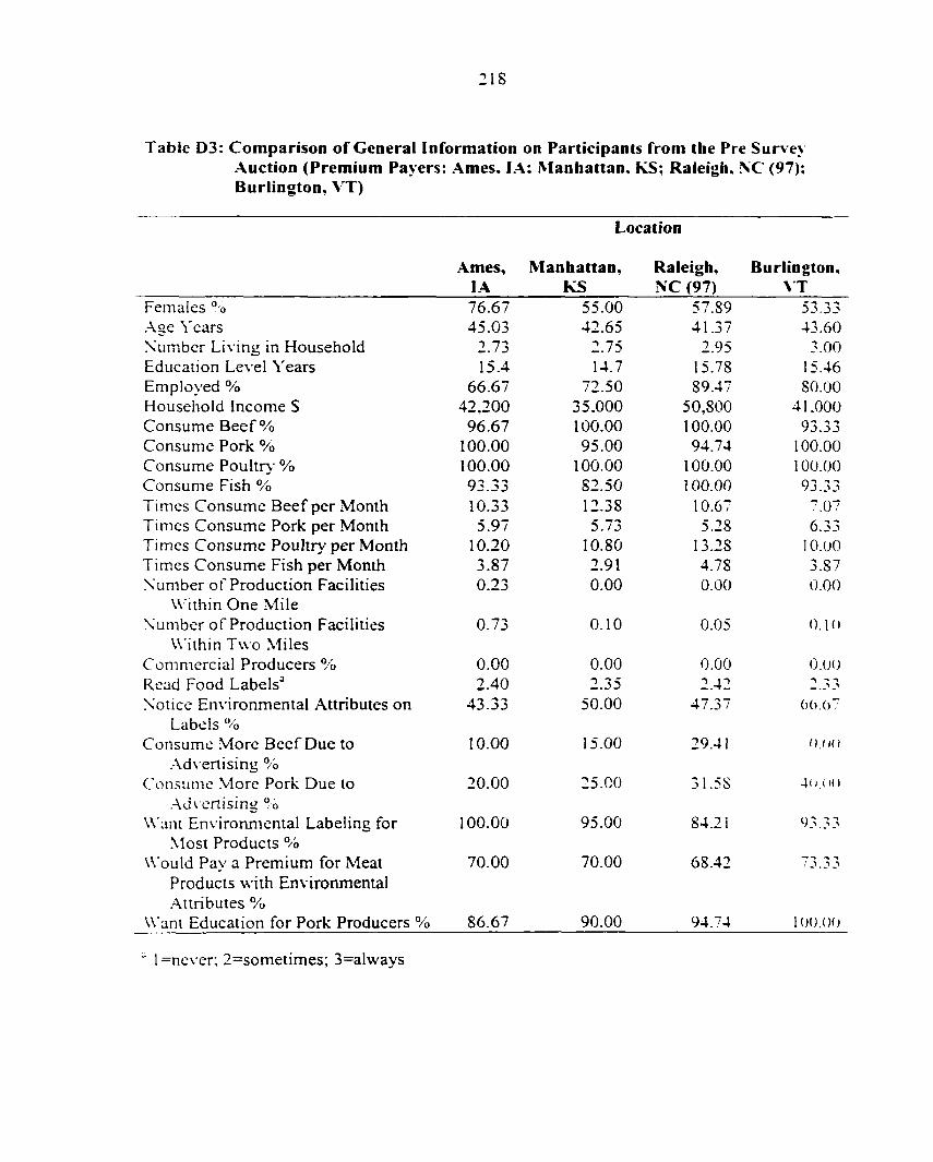
2 1 8

Table D3: Comparison of General Information on Participants from the Pre Survey Auction (Premium Payers: Ames. lA: Manhattan, KS: Raleigh. NC (97): Burlington, VT)

Location

Ames, Manhattan, Raleigh. Burlington. lA KS NC (97) \T

Females % 76.67 55.00 57.89 53.33 Age Years 45.03 42.65 41.37 43.60 Number Living in Household 2.73 2.75 2.95 3.00 Education Level Years 15.4 14.7 15.78 15.46 Employed % 66.67 72.50 89.47 80.00 Household Income S 42,200 35,000 50,800 41.000 Consume Beef % 96.67 100.00 100.00 93.33 Consume Pork % 100.00 95.00 94.74 100.00 Consume Poultrv" % 100.00 100.00 100.00 100.00 Consume Fish % 93.33 82.50 100.00 93.33 Times Consume Beef per Month 10.33 12.38 10.67 7.07 Times Consume Pork per Month 5.97 5.73 5.28 6.33 Times Consume Poultry per Month 10.20 10.80 13.28 10.00 Times Consume Fish per Month 3.87 2.91 4.78 3.87 Number of Production Facilities 0.23 0.00 0.00 0.00

Within One Mile Number of Production Facilities 0.73 0.10 0.05 O.IO

Within Two Miles Commercial Producers % 0.00 0.00 0.00 0,(J(J

Read Food Labels^ 2.40 2.35 2.42 2.33 Notice Environmental Attributes on 43.33 50.00 47.37 06.()7

Labels % Consume More Beef Due to 10.00 15.00 29.41 0.1 It)

.•\d\-ertising % Consume Vlore Pork Due to 20.00 25.00 31.5S

•Advertising "o Want Environmental Labeling for 100.00 95.00 84.21 3.3 3

.Most Products % Would Pay a Premium for Meat 70.00 70.00 68.42 / J. 3 3

Products with Environmental Attributes %

Want Education for Pork Producers % 86.67 90.00 94."4 10(J.()(j

1 =never; 2=sometimes; 3=al\vays

219

Table D4: Comparison of General Information on Participants from the Pre Survey Auction (Premium Payers: Iowa Fall, lA; Corvaliis. OR; Raleigh. NC (98))

Location

Iowa Falls, CorA'allis, Raleigh, lA OR NC (98)

Females % 74.29 65.79 51.85 Age \'ears 54.83 51.84 43.44 Number Living in Household 2.77 2.63 2.70 Education Level Years 12.54 15.9 16.88 Employed % 60.00 60.53 85.19 Household Income S 37.900 49,300 60.000 Consume Beef % 100.00 92.11 96.30 Consume Pork % 100.00 92.11 100.00 Consume Poultry % 97.14 97.37 100.00 Consume Fish % 94.29 86.84 92.59 Times Consume Beef per Month 12.94 7.18 7.89 Times Consume Pork per Month 6.57 4.62 5.07 Times Consume Poultry per Month 7.83 8.30 11.48 Times Consume Fish per Month 3.66 3.09 4.44 N umber of Production Facilities 0.47 0.00 0.00

Within One Mile Number of Production Facilities 1.61 0.03 0.00

Within Two Miles Commercial Producers % 6.06 0.00 0.00 Read Food Labels" 2.34 2.45

ri

Noiicc Environmental Attributes on 5S.S2 60.53 59.26 Labels %

Consume More Beef Due to 15.63 16.67 4.()()

Advertising % Consume More Pork Due to 31.25 34.21 -) -V -> -1

Ad\ ertising "o

\\"ani En\ ironmental Labeling for 97.14 100.00 Mosi Products %

\\ ould Pay a Premium for Meat 65.71 77.14 Products with Environmental Attributes %

Want Education for Pork Producers % 94.29 94.59 92.59

" 1 =never; 2=sometimes; 3=aKvays

220

Table D5: Comparison of General Information on Participants from the Pre Survey Auction (Non-Premium Payers: Ames, lA: Manhattan. KS; Raleigh, NC (97); Burlington, VT)

Location

Ames, Manhattan, Raleigh, Burlington. lA KS NC (97) N T

Females % 42.11 50.00 66.67 75.00 Age ^'ears 46.21 41.70 32.75 53.00 Number Living in Household 2.63 2.60 2.92 3.42 Education Level Years 16.64 14.8 15 13.75 Employed % 57.89 70.00 58.33 41.67 Household Income S 42,100 36.500 38.600 36.700 Consume Beef % 100.00 95.00 100.00 91.67 Consume Pork % 94.74 80.00 100.00 90.91 Consume Poultry % 100.00 95.00 100.00 90.91 Consume Fish % 89.47 90.00 83.33 90.91 Times Consume Beef per Month 10.58 13.05 7.63 6.25 Times Consume Pork per Month 5.71 4.31 4.71 5.92 Times Consume Poultry per Month 10.04 8.74 12.92 8.42 Times Consume Fish per Month 4.36 3.14 5.32 4.S3 Number of Production Facilities 0.21 0.30 0.17 0.33

Within One Mile Number of Production Facilities 0.37 0.45 0.25 0.00

Within Two Miles Commercial Producers % 0.00 5.00 0.00 0.0(1 Read Food Labels" 2.42 2.47 2.25 2.1" Notice Environmental Attributes on 52.63 42.1 1 41.67 41.6"

Labels % Consume More Beef Due to 10.53 16.67 J j.j_-

Advertising % Consume More Pork Due to 10.53 47.37 36.36 IS.l.s

Ad\ crtising % Want Environmental Labeling for 100.00 89.47 91.67 91.6"

Most Products % Would Pay a Premium for Meat 31.58 57.89 50.00 6().67

Products with Environmental Attributes %

Want Education for Pork Producers % 73.68 89.47 83.33 91.67

" 1 =never; 2=sometimes; 3=al\vays

221

I'able 06: Comparison of General Information on Participants from the Pre Survey Auction (Non-Premium Pavers: Iowa Fall. lA: Corvallis. OR: Raleigh. NC (98))

Location

Iowa Falls, Cor\'alIis, Raleigh, lA OR NC (98)

Females % 43.4S 68.18 47.U6 Age \'cars 64.10 53.55 46.47 Number Living in Household 2.13 2.36 2.47 Education Level Years 13.09 14.82 15.88 Employed % 34.78 45.45 94.12 Household Income S 35.000 39.100 59.700 Consume Beef % 100.00 90.91 94.12 Consume Pork % 100.00 90.91 100.00 Consume Poultry % 95.45 90.91 100.00 Consume Fish % 72.73 90.91 94.12 Times Consume Beef per Month 12.32 7.14 8.41 Times Consume Pork per Month 9.23 6.00 6.29 Times Consume Poultry per Month 7.00 11.14 13.82 Times Consume Fish per Month 4.19 3.27 6.12 Number of Production Facilities 0.42 0.00 0.00

Within One Mile Number of Production Facilities 1.42 0.00 0.00

Within Two Miles Commercial Producers % 0.00 0.00 5.SS Read Food Labels^ 2.39 2.41 2.35 Notice Environmental Attributes on 42.11 59.09 4".()()

Labels % Consume More Beef Due to 30.00 10.00 13.33

Ad\ crtising % Consume More Pork Due to 52.63 42.86 2^>.41

Advertising % Want Environmental Labeling for 75.00 100.00 1 (Jit.i II1

Most Products % Would Pay a Premium for Meal 35.00 71.43 64."]

Products with Environmental Attributes %

Want Education for Pork Producers % 80.95 86.36 88.24

" l=never; 2=sometimes; 3=always

222

Participant Response to Issues of Concern by Location

Table D7: Issues of Concern and Importance to Participants by Location (Ail Participants: Ames, lA; Manhattan, KS; Raleigh, NC (97); Burlington. NT)

Ames, lA Manhattan, Raleigh, Burlington. Item KS NC (97) V'T General Issues of Concern"" En\ironment 1.69 1.84 1.58 1.48 Water Quality 1.42 1.50 1.35 1.37 Air Quality L60 1.72 1.52 1.37 Food Prices 1.90 1.78 1.81 1.74 Family Farms 2.54 2.53 2.81 2.63 Livestock Production 2.60 2.53 2.55 2.37 Methods Animal Welfare 2.54 2.34 2.45 1.96 Pollution 1.58 1.60 1.55 1.19 Li\ estock Confinement 2.27 2.76 2.90 Changing Farm Structure 2.85 3.05 3.23 2.59

Product Attribute: Issues of Importance^'" Ealing Quality 1.15 1.32 1.19 1.15 X'isuai Appeal 1.81 1.74 1.68 i.67 Freshness 1.19 1.19 1.26 1.19 Price L79 1.63 1.84 1.74 Production Methods 2.27 2.33 2.77 1.96 L'niformitv of Product 2.38 2.21 2.19 2.04

The question was: On a scale from 1 through 5 with 1 being "very concerned' and 5 being "not concerned.' how concerned are you about the following issues;

The question was; On a scale from 1 through 5 with 1 being 'very important' and 5 being "not important." indicate how important the following attributes are for the products you consume;

Table D8: Issues of Concern and Importance to Participants by Location (All Participants: Iowa Fall, lA; Corvallis, OR; Raleigh. NC (98))

Iowa Falls. Cor>-allis, Raleigh, Item lA OR NC (98) General Issues of Concern"' Environment 1.57 1.62 1.59 Water Quality 1.26 1.35 1.43 Air Quality 1.53 1.50 1.49 Food Prices 2.02 2.02 2.12 Family Farms 2.21 2.67 2.86 Livestock Production 2.22 2.35 2.52 Methods Animal Welfare 2.52 2.20 2.43 Pollution 1.42 1.48 1.41 Li\ estock Confinement 1.75 2.57 2.70 Changing Farm Structure 2.57 3.10 3.11

Product .Attribute: Issues of Importance"" Ealing Quality 1.25 1.16 1.14 X'lsual .Appeal 1.63 1.58 1.66 Freshness 1.18 1.19 1.U9 Price 1.68 1.81 1.77 Production Methods 2.09 1.97 2.14 L'niformitv of Product 1.86 2.24 2.07

The question was: On a scale from 1 through 5 with 1 being "very concerned" and 5 being "not concerned," how concerned are you about the following issues:

"" The question was: On a scale from 1 through 5 with 1 being 'very important' and 5 being "not important," indicate how important the following attributes are for the products you consume;

224

Table D9: Issues of Concern and Importance to Participants by Location (Premium Payers: Ames, lA: Manhattan, KS; Raleigh. NC (97); Burlington. NT)

Ames, lA Manhattan, Raleigh, Burlington. Item KS NC (97) NT General Issues of Concern'"' Environment 1.S3 1.7S 1.42 1.27 Water Quality 1.45 1.4S 1.26 1.33 Air Quality 1.66 1.65 1.32 1.27 Food Prices 1.83 1.75 1.84 1.80 Family Farms 2.55 2.53 2.74 2.20 Livestock Production 2.66 2.40 2.47 2.33 Methods Animal Welfare 2.38 2.33 2.68 2.13 Pollution 1.66 1.55 1.47 1.13 Li\ esiock Confinement 2.34 2.68 3.16 2.20 Changing Farm Structure 2.69 2.93 3.26 2.13

Product Attribute: Issues of Importance"*' Ealing Quality 1.17 1.31 1.21 1.07 X'isual Appeal 1.86 1.79 1.79 1.60 Freshness 1.14 1.21 1.26 1.20 Price 1.62 1.64 1.89 l .SO Production Methods 2.14 2.38 2.89 2.07 L'niformitv of Product 2.17 2.15 2.16 2.07

The question was; On a scale from 1 Ihrough 5 with I being 'very concerned" and 5 being 'not concerned.' how concerned are you about the following issues;

' The question was; On a scale from 1 through 5 with 1 being "very important" and 5 being 'not important,' indicate how important the following attributes are for the products vou consume:

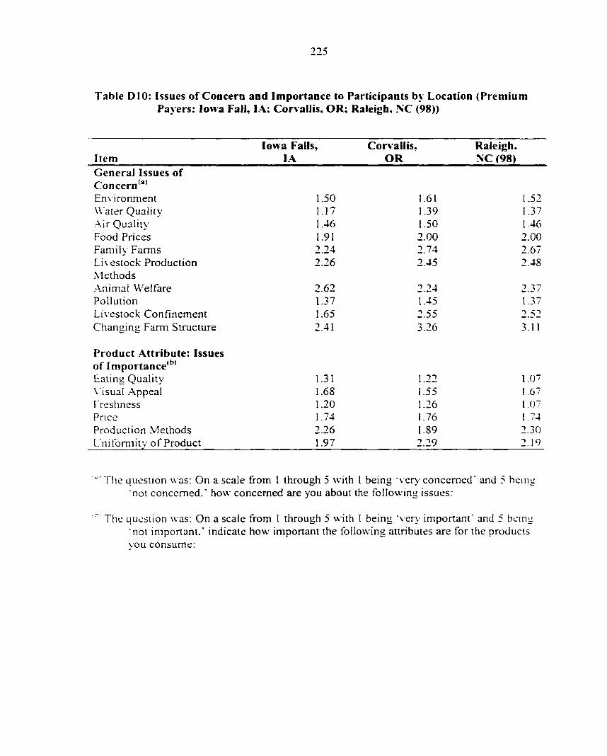
225

Table DIO: Issues of Concern and Importance to Participants by Location (Premium Payers: Iowa Fall, lA; Corvallis, OR; Raleigh, NC (98))

Iowa Falls, Cor>'allis, Raleigh. Item lA OR NC (98) General Issues of Concern'"' Environment 1.50 1.61 1.52 Water Quality LIT 1.39 1.37 Air Quality 1.46 1.50 1.46 Food Prices L91 2.00 2.00 Family Farms 2.24 2.74 2.67 Livestock Production 2.26 2.45 2.48 Methods Animal Welfare 2.62 2.24 2.37 Pollution 1.37 1.45 1.37 Livestock Confinement 1.65 2.55 2.52 Changing Farm Structure 2.41 3.26 3.11

Product Attribute: Issues of Importance'*" Ealing Quality 1.31 1.22 1.07 \'isual Appeal 1.68 1.55 1.67 Freshness 1.20 1.26 1.07 Price 1.74 1.76 1.74 Production Methods 2.26 1.89 2.30 L'nifomiitv of Product 1.97 ? ">9 2.19

The question was: On a scale from 1 through 5 with I being "very concerned" and 5 being "no: concerned,' how concerned are you about the following issues:

Tlie question was: On a scale from 1 through 5 with 1 being "very important" and 5 bemg "not important.' indicate how important the following attributes are for the products vou consume:

226

Table DI I: Issues of Concern and Importance to Participants by Location (Non-Premium Payers: Ames, lA: Manhattan, KS; Raleigh, NC (97); Burlington. \ T )

Ames, lA Manhattan, Raleigh, Burlington. Item KS NC (97) \T General Issues of Concern'"' Environment 1.47 2.00 1.83 1.75 Water Quality 1.37 1.56 1.50 1.42 Air Quality 1.53 1.89 1.83 1.50 Food Prices 2.00 1.83 1.75 1.67 Family Farms 2.53 2.56 2.92 3.17 Livestock Production 2.53 2.83 2.67 2.42 Methods .\nimal Welfare 2.79 2.39 2.08 1.75 Pollution 1.47 1.71 1.67 1.25 Livestock Confinement 2.16 2.94 2.50 2.25 Changing Farm Structure 3.11 'S ̂ J. J J 3.17 3.17

Product Attribute: Issues of Importance^*" Eating Quality 1.11 1.33 1.17 1.25 X'isual Appeal 1.74 1.61 1.50 1.75 Freshness 1.26 1.17 1.25 1.1" Price 2.05 1.61 1.75 1.67 Production Methods 2.47 2.22 2.58 1.83 L'niformitv of Product 2.68 2.25 2.0U

•" The question was: On a scale from I through 5 with 1 being 'very concerned' and 5 being "not concerned/ how concerned are you about the following issues:

" TIk' question was: On a scale from 1 through 5 with 1 being "very important' and 5 being "not important.' indicate how important the following attributes are for the products you consume:

227

Table D12: Issues of Concern and Importance to Participants by Location (Non-Premium Payers: Iowa Fall. lA; Cor\allis. OR; Raleigh. NC (98))

Item Iowa Falls,

lA Cor\'allis.

OR Raleigh. NC (98)

General Issues of Concern*"' En\ironment 1.68 1.64 1.71 Water Quality 1.41 1.27 1.53 .-Mr Quality 1.64 1.50 1.53 Food Prices 2.18 2.05 2.29 Family Farms 2.15 2.55 3.18 Livestock Production 2.14 2.18 2.59 .VIethods .•\nimal Welfare 2.36 2.14 2.53 Pollution 1.50 1.55 1.47 Livestock. Confinement 1.90 2.59 3.00 Changing Farm Structure 2.82 2.82 3.12

Product .attribute; Issues of Importance*''' Ealing Quality 1.14 1.05 1.24 Visual Appeal 1.55 1.62 1.65 Freshness 1.14 1.05 1.12 Pnce 1.59 1.90 1.82 Production .Methods LSI 2.10 1.88 L'niformitv of Product 1.68 2.14 1.88

The question was; On a scale from 1 through 5 with I being "ver^' concerned' and 5 being "not concerned,' how concerned are you about the following issues:

The question was; On a scale from 1 through 5 with 1 being •ver\- imponant" and 5 being "not imponant.' indicate how important the following attributes are for the products you consume;

22S

APPENDIX E: LIMDEP COMMANDS FOR RUNNING ECONOMETRIC MODEL

Program for Estimating the Magnitudes of the Premium for the Premium Payers

RESET

READ;tlle="C; Program Files\ES\LimdepMeodata_6_17.xls";fonnat=xls;namesS

SKIPS

NAMES ; W = ONE. NOINHOUS, NOINHSQ. EMPLY. rNC3060. INC60UP.

PORKM. PORKMSQ. ATTRIB, PREMl.GENHINCS

CREATE ; Z = ORDPRO S

NAMES : X = ONE, AGE, GR^AJDCOL. GRADGRAD.INC3060. rNC60L'P.

ATTRIB. MRPRK, ENVLVL PRKEDUIS

CREATE ; V = R4939 S

CALC ; J = 2 S

ORDERED PROBIT ; Lhs - Z ; Rhs = W ; Par S

CALC ; Nolist; JP = Max(Z) + 1 ; JPl = JP - 1 ; KP = Col(VV) ; KPl = KP+1 ; M = JP-2 ; L=KJ'~M S

MATRIX ; list ; ALPH.\=Part(B.l.KP)

; U'I= [-10000/0] ; U2- Part(B.ICPl,l) ; U3= [10000] ; MUA=[U1AJ2/LT3]

; Z11 = Part(VARB,l.KP.l,KP) ; Z21 = Init(2,ECP.O) ; Z22 = [0,0/0,0] ;Z3I =Pan(V.\RB,KPl,L,l,KP) ; Z32 = Init(M,2,0) ; Z33 = Pan(VARB,KPl,L,KPl,L)

229

; Z41 = lnit(l,KP.O) ; Z42 = [0,0] ; Z43 = Init(l.M.O) ; Z44 = [0] ;V=[Z11/ Z21.Z22/ Z3KZ32,Z33/ Z41.Z42.Z43.Z44]S

INCLUDE ; New ; Z = J S

CALC ; J1 = J - 1 ; J2 - J ^ 2 S

CREATE ; AJl = MUA(Jl) - WALPHA ; AJ = NnJA(J2) - WALPHA : DJl =N01(AJ1) ; DJ =N01(AJ) ; FJl =Phi(AJl) ; FJ =Phi(AJ) ; LAMBDA = (DJ 1 -DJ)/(FJ-FJ 1) : DELTA = (AJ1*DJ1 - AJ"^DJ)/(FJ-FJ I) - L.AMBDA " 2 S

N.AMES ; XL = XXAMBDA S

REGRESS ; Lhs = Y ; Rhs = X, LAMBDA S

CALC ; P =Col(XL) ; C =B(P) ; S2 = SUMSQDEV/NREG - C^2 • Xbr(DELTA) : RHOSQD= ^^2/52 S

CREATE ; PJl = (J>1) » DJ1/(FJ-FJ1) » (LAMBDA-AJl) ; PJ =0S

MATRLX XPl = XL'* PJl ; XP = XL'* PJ ;ZERO= lnii(P,l,0) ;R = lnit(3,JPl,0) ; R(1J1)=1 ; R(2J2)=I ; XPP = [XPl,XP,ZERO] ; XGl =XL'[DELTA]W ; XG2 = XPP * R ;XG =[XG1,XG2] S

CREATE ; H = 1 - RHOSQD • DELTA S

230

MATRIX ; list: VC = XL'[H]XL - RHOSQD * XG * V * XG' ; VC = S2 * <XL'XL> * VC * <XL'XL> ; Slat ( B,V.\RB) ; Stat ( B,VC) S

Program for Estimating tbe Magnitudes of the Premium for the Non-Premium Payers

RESET

READ;fiIe="C:'Program Files'vES\Limdep Jeodata_6_l 7.xIs";format=xIs;namesS

SKIPS

NAMES ; VV = ONE, NOINHOUS, NOINHSQ. EMPLY. INC3060. INCGOL'P,

PORKM PORtCMSQ. ATTRIB, PREM^GENHINCS

CREATE ; Z = ORDPRO S

NAMES ; X = ONE, AGE, NOINHOUS. NOINHSQ. EMPLYMNC3060

.INC60LP. \WTLAB. PREMl, PRKEDUl. GEN^INCS

CREATE ; V = R4939 S

CALC : j = 0 S

ORDERED PROBIT ; Lhs - Z ; Rhs = \V ; Par S

CALC ; Nolist ; JP = Ma.\(Z) - I ;JP1=JP-I ; K:P = Col(W) ; KPl = FCP^l ; M = JP-2 ; L=K:P-M S

MATRIX ; list ; ALPHA=Pail(B.l .KP)

: Ul= [-10000/0] ; U2= Part(B,KPI,l) ; U3= [10000] ; MUA=[U1/U2,a;3]

; Z l l = P a r t ( V A R B , l , K P , l . K P ) ; Z21 = Init(2,KP,0) ; Z22 = [0,0/0,0] ; Z31 = Pan(VARB,KPl,L,l,KP)

231

; Z32 = Init(M.2.0,) ; Z33 = Pan(V ARB.KP LL.KP l.L) ; Z41 = Init(l.KP.O) ; Z42 = [0,0] ; Z43 = Init(l,M,0) ; Z44 = [0] ;V=[Z11/ Z21,Z22/ Z31.Z32.Z33/ Z41.Z42.Z43,Z44]S

INCLUDE ; New ; Z = J S

CALC ; J1 = J 1 ; J2 =J - 2S

CREATE ; AJl = MUA(Jl) - WALPHA ; AJ = MUA(J2) - WALPHA ; DJl =N01(AJ1) ; DJ =N01(AJ) ; FJl =Phi(.AJl) ; FJ =Phi(AJ) ; L.AMBD.A. = (DJ 1 -DJ)/(FJ-FJ 1) ; DELTA = (AJ1*DJ1 - AJ*DJ)/(FJ-FJ1) - L.AMBDA '• 2 S

X.AMES ; XL = X,L.AaMBDA S

REGRESS ; Lhs = Y ; Rhs = X. LAMBD.A. S

CALC ; P =Col(XL) ; C =B(P) ; S2 = SUMSQDEV/NREG - C^2 * Xbr(DELTA) ; RHOSQD= c^2/s2 S

CREATE ; PJl =(J>1) * DJ1/(FJ-FJ1) » (LAMBDA-AJl) ; PJ =0S

MATRLX ;iist; XPl = XL'* PJl ; XP = XL'* PJ : ZERO= IniUP,1.0) ;R = lnit(3,JPl,0) ; R(1.J1)=1 ; R(2.J2)=1 ; XPP = [XPl.XP,ZERO] ; XGl =XL'[DELTA]W ; XG2 = XPP * R ;XG =[XG1,XG2] S

232

CREATE ; H = 1 - RHOSQD DELTA S

MATRLX ; list; VC = XL'[H]XL - RHOSQD * XG * V XG' ; VC = S2 • <XL'XL> * VC * <XL'XL> ; Stat ( B^VARB) ; Stat ( B , VC ) S

BIBLIOGRAPHY

Abclcs-Allison, Mark and Larr\'J. Connor. ".\n Analysis of Local Benefits and Cosls of Michigan Hog Operations Experiencing Environmental Conflicts." .A.gricultural Economics Report #536. Michigan State University; East Lansing. ML (June 1990). 1-26.

.Andreoni. James. "Impure Altruism and Donations to Public Goods: A Theory of Warm-Glow Gi% ing." Economic Journal 100 (1990): 464-477.

.Andrconi. James. "Privately Provided Public Goods in a Large Economy; The Limits of .Altruism." Journal of Public Economics 35 (1988); 57-73.

.Andreoni. James and Lise Vesterlund. "WTiich Is The Fair Se.x? Gender Differences in .Altruism." The Quarterly Journal of Economics (Forthcoming 2001).

Bagnoli, Mark and Susan G. Watts. "Ecolabeling: The Private Provision of a Public Good." Unpublished paper, (February 1996), 3-28.

Beeman. Perry. "Hog Waste Called a Bigger Threat than Thought." Des Moines Register. September 18, 1996a, 1A-2A.

Beeman. Perry. "Hog-Lot Crackdown .Anticipated." Des Moines Register, September 21. 1996b. 1 .A-5.A.

Bo\ le. Kevin J.. Gregory L. Poe. and John Bergstrom. "What Do We Know .About Groundwater Values? Preliminary" Implications from a .Meta .Analysis of Coniingcnt-X'aluation Studies." American Journal of Agricultural Economics 76 (December 1994); 1055-1061.

Casu cll. Julie .A., and Eliza M. Mojduszka. "Using Informational Labeling to Influcncc ihc .Market for Quality in Food Products." American Journal of Agricultural Econonucs

7S (December 1996): 1248-1253.

Caudill. James D. and John P. Hoehn. "The Economic Valuation of Groundwater Polliiiioii Policies; The Role of Subjective Risk Perceptions." Staff Paper No. 92-1 I. Department of .Agricultural Economics. .Michigan Stale University, 1992.

Chakraborty. Indranil. "Bundling Decisions for Selling Multiple Objects." Economic Theory 13 ('l999); 723-733.

Clemson. Roy, .Alan R. Collins, and Ken Green. "Contingent Valuation of Protecting Groundwater Quality by a Well Head Protection Program." Division of Resource Management, West Virginia University, 1995.

234

Coppinger. V'icki M., Vemon L. Smith, and Jon A. Titus. "Incentives and Behavior in English, Dutch, and Sealed-Bid Auctions." Economic Inquity IS (January 19S0); 1-22

Conies, Richard and Todd Sandler. The Theory of Externaliiies. Public Goods, and Club Goods. Second Edition. New York: Cambridge University Press. 1996.

Coursey. Don L. and Vemon L. Smith. "Experimental Tests of an Allocation Mechanism for Public. Private, or Externality Goods." Scandinavian Journal of Economics 86 (1984); 468-484.

Cox. James C.. Vemon L. Smith, and James M. Walker. "Expected Revenue in Discriminative and Uniform Price Sealed-Bid .A-uctions." In Research and Experimental Economics, Vol. 3, ed.. Vemon L. Smith, pp. 183-232. Greenwich: J.AI Press. 1985.

Cragg. John G. "Some Statistical Models for Limited Dependent Variables with .Application to Demand for Durable Goods." Econometrica 39 (September 1971); 829-844.

Cunimings. Ronald G., David S. Brookshire. and William D. Schulze. I 'aluing Environmental Goods: An Assessment of the Contingent Valuation Method. Totowa. New Jersey: RowTnan and Allanheld, 1986.

Da\ is. Douglas D. and Charles Holt. Experimental Economics. Princeton. New Jersey: Princeton University Press, 1993.

Diamond. Peter and Jerry Hausman. "Contingent Valuation: Is Some Number Better than No Number?" Journal of Economic Perspectives 8 (Fall 1994): 45-64

Dobbs, Thomas L. "Price Premiums for Organic Crops." Choices (Second Quaner. 199S): 39-41.

Duram. Leslie .A. "Organic Agriculture in the United States: Current Status and Future Regulations." Choices (Second Quarter. 1998): 34-38.

Edwards. Steven F. "Option Prices for Groundwater Protection." Journal of Environmental Economics and Management 15 (December 1998): 475-487.

Foster. William and Richard E. Just. "Measuring Welfare Effects of Product Contamination with Consumer Uncertainty." Journal of Environmental and Economics Management 17 (1989): 266-283.

235

Fox. John A. "Essays in the Measurement of Consumer Preferences in Experimental Auction Markets." Ph.D. Dissertation. Department of Economics. Iowa State University. 1994.

Fox. John A.. Brian L. Buhr, Jason F. Shogren, James B. Kiiebenstein, and Dermot J. Hayes. "A Comparison of Preferences for Pork Sandwiches Produced from Animals with and without Somatotropin Administration." Journal of Animal _Science 73 (1995): 1048-1054.

Fox. John A. . Dermot J. Hayes, James B. Kiiebenstein, and Jason F. Shogren. "Consumer .Acceptability of Milk from Cows Treated with Bovine Somatotropin." Journal of Dairy Science 77 (1994); 703-707.

Fox. John A., Dermot J. Hayes, Jason F. Shogren, and James B. Kiiebenstein. " Experimental Methods in Consumer Preference Studies." Journal of Food Distribution Research (July 1996): 1-7.

Freeman. .A. Myrick. The Measurement of Environmental and Resource Values: Theory and Methods. Washington, DC: Resources for the Future, 1994.

Freund. John E. Mathematical Statistics. Fifth Edition, Englewoods Cliff. New Jersey: Prentice Hall, 1992.

Graham. Daniel A. and Robert C. Marshall. "Collusive Bidder Behavior at Single-Object Second-Price and English Auctions." Journal of Political Economy 95 (December 1987): 1217 -1239. "

Greene, William H. Econometric Analysis. Second Edition, .New York, New '^'ork: .Macmillan Publishing Company, 1993.

Haneniann, W. Michael. "Valuing the Environment through Contingent Valuation." Journal of Economic Perspectives 8 (Fall 1994): 19-43.

Hayes. Dermot J., Jason F. Shogren, John A. Fox. and James B. Kiiebenstein. "Testing New Food Products Using a .Multitrial Nonhypothetical Experimental .Auction. Psychology and Marketing (July 1996): 365-379.

Heckman, James J. "The Common Structure of Statistical Models of Truncation, Sample Selection, and Limited Dependent Variables and a Simple Estimator for such Models." Annals of Economic and Social Measurement (1976): 475-492.

Heckman, James J. "Sample Selection Bias as a Specification Error." Econonietrica 47 (January 1979): 153-161.

236

Hoffman. Elizabeth, Dale J. Menkhaus. Dipankar Chakravani, Ray A. Field, and Glen D. Whipple. ''Using Laboratory Experimental Auctions in Marketing Research: .A Case Study of New Packaging for Fresh Beef." Marketing Science 12 (Summer 1993): 313-338.

•"Hog Heaven — .\nd Hell." U.S. IVews and World Reports. January 22, 1996: 55-59.

Honeyrnan. Mark S. "Sustainability Issues of U.S. Swine Production." Journal of .Animal 74 (1996): 1410-1417.

HonesTnan. Mark S. "Vastgotmodellen: Sweden's Sustainable Alternative for Swine Production," American Journal of Alternative Agriculture 10 (November 1995): 129-132.

Hurley. Sean P. and James B. Kliebenstein. "Determining the Benefits of Environmental Improvements in Pork Production and Their Sustainability: A Community-Based Study of Iowa's Pork Industry." A report prepared for the Leopold Center for

Sustainable Agriculture: Ames, lA. November 1998.

"ll's Dead Now: Neighbors Mourn Fouled South Fork." Des Moines Register. July 22. 1995.

Issac. R. Mark, Kemieth F. McCue, and Charles R. Plott. '^Public Goods Provision in an Experimental Environment." Journal of Public Economics 26 (1985): 51-74.

Issac. R. Mark. James M. Walker, and Susan H. Thomas. "Divergent Evidence on Free Riding:.A.n Experimental Examination of Possible E.xplanations." Public Choice 45 (1984^:113-149.

Jordan. J. L. and A. H. Elnagheeb. "Willingness to Pay for Improvements in Drinking Water Quality." Water Resources Research 29 (February 1993): 237-245.

Kagcl, John H.. Ronald M. Harstad, and Dan Levin. "Information Impact and .Mlocaiion Rules in .Auctions with Affiliated Private Values: A Laboratory Study." Econometrica 55 (1987): 1275-1304.

Kami. Edi and Zvi Safra. "Vickrey Auctions in the Theory of Expected Utility with Rank Dependent Probabilities." Economic Letters 20 (1986): 15-18.

Kami. Edi and Zvi Safra. "Dynamic Consistency, Revelations in .Auctions and Structure of Preferences." Review of Economic Studies 56 (1989): 421-434.

237

Katzman, Brett. "A Two Stage Sequential Auction with Multi-Unit Demands." Journal of Economic Theory 86 (1999): 77-99.

Kirchhoff, Stephanie. "Green Business and Blue Angels: Towards a Theor\' of Voluntary Overcompliance with Asymmetric Information." Draft of Unpublished paper. September 1996.

Klonsky, Karen and Laura Tourte. "Organic Agricultural Production in the United Slates: Debates and Directions." American Journal of Agricultural Economics 80 (Proceedings 1998): 1119-1124.

K.oichcn.Matthew J., Michael R. Moore, and Kent D. Messer. "Green Products as Impure Public Goods: Shade Grown Coffee and Tropical Forest Conservation." Selected Paper from American Agricultural Economics Association Meetings in Tampa. FL. August. 2000.

Krisoff. Barr>-. "Emergence of U.S. Organic Agriculture - Can We Compete? Discussion." American Journal of Agricultural Economics 80 (Proceedings 1998): 1130-1133.

Laughland. .A. S.. L. M. Musser, Wesley N. Musser, and James S. Shortle. "The Opportunity Cost of Time and Averting Expenditures for Safe Drinking Water." Water Resources Bulletin 29 (1993): 219-229.

Law rcnce. John D.. Marvin Hayenga. and Glen Grimes. "Iowa and Regional .Analysis of the Pork Industry." In 1998 Swine Research Report: Iowa State University E.xtension: .Ames. lA. (l'999a): 182-185.

Lawrence. John D.. Marvin Hayenga, and Glen Grimes. "The U.S. Pork Industr\' Struclurc: .•\ 1997 Snapshot." In 1998 Swine Research Report: Iowa State University Extension: Ames. lA. (1999b): 179-181.

Lau rcnce. John D.. Daniel Otto. Seth D. Meyer, and Steven Folkerts. ".A. Profile of the Iow a Pork Industry. Its Producers, and Implications for the Future." Staff Paper No. 253. June 1994.

Lee. Lung-Fei. "Generalized Econometric .Models with Selectivity." Economcincu 51 (March 1983): 507-512.

Lcison. David, and Noel Gollehon. "Confined .Animal Production and the Manure Problem." C/io/ce5 (Third Quarter, 1996): 18-24.

Lo. Kin Chung. "Sealed Bid .Auctions with Uncertainty Averse Bidders." Economic Tlieoiy

12 (1998): 1-20.

238

Lohr. Luanne. "Implications of Organic Certification for Market Structure and Trade." American Journal of Agricultural Economics 80 (Proceedings 1998); 1 125-1 129.

Maddala. G. S. "Limited Dependent and Qualitative Variables in Econometrics. Cambridge. England; Cambridge University Press, 1983.

Vlailath. George J. and Peter Zemsky. "Collusion in Second Price Auctions with Heterogeneous Bidders." Games and Economic Behavior 3 (1991): 467-486.

Marwcll. Gerald and Ruth E. Ames. "Experiments on the Provision of Public Goods I; Resources, Interest, Group Size, and the Free Rider Problem." American Journal of

84 (1979); 1335-1360.

Matthews, Steven. "Comparing Auctions for Risk Averse Buyers; A Buyers Point of View." Econometrica 55 (May 1987): 633-646.

.VIc.Afce. R. Preston and John McMillan. "Auctions and Bidding." Journal of Economic Literature 25 (June 1987): 699-738.

Mellon. Bryan E., Wallace E. Huffman, Jason F. Shogren, and John .A Fox. "Consumer Preferences for Fresh Food Items with Multiple Quality Attributes; Evidence from an Experimental Auction of Pork Cho^is" American Journal of Agricultural Economics 78 (November 1996): 916-923.

Mellon. Bryan E., Wallace E. Huffman, and Jason F. Shogren. "Economic Values of Pork .Attributes: Hedonic Price .Analysis of Experimental .\uction Data." Review of Agricultural Economics 18 (October 1996): 613-627.

Mcnkhaus. Dale J., George W. Borden, Glen D. Whipple, Elizabeth Hoffman, and Ray Field. ".An Emperical Application of Laboratory Experimental .Auctions in .Vlarketing Research." yowr/za/ of Agricultural and Resource Economics 17 (jul\-1992): 44''-55.

Mc\cr. Seth D. "Characteristics Affecting Technology .Adoption and Purchasing Pallcms of Iowa's Pork Producers." Master's Thesis. Department of Economics, Iowa State University. 1995.

Milgrom. Paul R. "Auctions and Bidding: A Primer." Journal of Economic Perspective 3 (Summer 1989): 3-22.

Milgrom. Paul R. and Robert J. Weber. "A Theory of Auctions and Competitive Bidding." Econometrica 50 (September 1982): 1089-1122.

239

Misra. Sukani K... Chung L. Huang, and Stephan L. On. "Consumer Willingness to Pay for Pcslicide-Free Produce." Western Journal of Agriciiliural Economics 16 (December 1991); 218-227.

Neilson, William S. "Second Price Auctions without Expected Utility." Journal of Economic Theory 62 (1994): 136-151.

Nimon. Wesley and John Beghin. ".Are Eco-labels Valuable? Evidence from the .Apparel Industry." Presentation at Southern Economic .Association Meetings in .Atlanta. G.A. November. 1997.

Olio. Daniel, and John Lawrence. "Economic Impact of the U.S. Pork Industry." Paper prepared for the National Pork Producers Council (December 1994): 67-84.

Oito. Daniel, and John Lawrence. "Economic Importance of Iowa's Pork Industry." Paper prepared for the National Pork Producers Association, 1993.

Palmquist. Raymond B.. Fritz M. Roka, and Tomislav Vukina. "The Effect of En\ ironmental Impacts from Swine Operations on Surrounding Residential Propeny Values," Department of Economics, and Department of .Agricultural and Resource Economics, North Carolina State University, Raleigh. May 1995.

Poe. Gregory L. and Richard C. Bishop. "Measuring the Benefits of Groundwater Protection from .Agricultural Contamination: Results from a Two-State Contingent Valuation Study." Staff Paper No. 341, University of Wisconsin-Madison .Agricultural Economics. 1992.

Porine\. Paul R. "The Contingent Valuation Debate; Why Economists Should Care." Journal of Economic Perspectives 8 (Fall 1994): 3-17.

Perkins. Jerry. "Water Users vs. Hog Lots." Des .Moines Register, .April 14. 1996. 1-2.

Po\^cll. John R.. David J. Allee. and Charles McClintock. "Groundwater Proieclion Bcncfiis and Local Community Planning: Impact of Contingent Valuation Infomiaiion." American Journal of Agricultural Economics 76 (December 1994): 106S-l')-5.

Rooscn. Julia. John .A. Fox. David A. Henessey. and Alan Schreiber. "Consumer's \ aluaiioii of Insecticide Use Restrictions; .An Application to Apples" Joi/r/ia/ of Agricultural And Resource Economics 23 (December 1998); 367-384.

Rothkopf. .Michael H., Thomas J. Teisberg. and Edward P. Kahn. "Why Are Vickre\-•Auctions Rare?" Journal of Political fco/iown-98 (February 1990); 94-109.

240

Schiffman. Susan S., John M. Walker, Rochelle Small, and Patricia D. Millner. "Workshop on Health Effects of Odors." A paper presented at the .Animal Production Systems and the En%'ironment -Meeting in Des Moines, Iowa. July 19-22. 1998. 407-412.

Shogren. Jason F.. Jolm A. Fox. Dermot Hayes, and James B. K-liebenstein. "Bid Sensitivity and the Structure of the Vickrey Auction." American Journal of Agricultural

Economics 76 (December 1994a): 1089-1095.

Shogren. Jason F., Seung Y Shin, Dermot Hayes, and James B. Kliebenstein. "Resolving Differences in Willingness to Pay and Willingness to .Accept." American Economic Review (March 1994b): 255-270.

Smith, James L. and Dan Levin. "Ranking .Auctions with Risk .Averse Bidders." Journal of Economic Theory 68 (1996): 549-561.

Sun. Henglun, John C. Bergstrom. and Jefferey H. DorfVnan. "Estimating the Benefits of Groundwater Contamination Control." Southern Journal of Agricultural Economics (1992); 63-71.

Taff. Steven J.. Douglas G. Tiffany, and Sanford Weisberg. ".Measured Effects of Feedlots on Residential Property Values in Minnesota." Staff Paper P96-12. University of Minnesota. St Paul, MN (July 1996): 1-27.

Teisl. .Mario F.. Brian Roe and Robert L. Hicks. "Can Eco-labels Tune a Market? Evidence from Dolphin-Safe Labeling." Journal of Environmental Economics and Management (Under Review. 1999).

Thompson, Gar> and Julia Kidwell. "Explaining the Choice of Organic Produce: Cosmetic Defects, Prices, and Consumer Preferences." American Journal of Agricultural Economics 80 (May 1998): 211-2^1.

Tliompson. Gary. "Consumer Demand for Organic Foods: What We Know and V\'hat We Need to Know." American Journal of Agricultural Economics 80 (Proceedings 1998): 1113-1118.

Trost. Robert P. and Lung-Fei Lee. Technical Training and Earnings: .A Polychotomous Choice Model With Selectivity." The Review of Economics and Statistics 66 (February 1994), 151-156.

\'ickrey. William. "Counterspeculation, Auctions, and Competitive Sealed Tenders." Journal of Finance 16 (1961): 8-17.

\ an Ravenswaay, Eileen O. "Emerging Demands on Our Food and Agricultural System: Developments in Environmental Labeling." Staff Paper No. 96-88, Department of .Agricultural Economics, Michigan State University, East Lansing, MI, 1996.

241

von L 'ngem-Stemberg, Thomas. "Cartel Stability in Sealed Bid Second Price Auctions." The Journal of Industrial Economics 36 (March 19SS): 351-35S.

\\ ea\ er. Roben D.. David J. Evans, and A. E. Luloff. "Pesticide Use in Tomato Production: Consumer Concerns and Willingness to Pay." Agribusiness 8 (1992): 131-142.

Whitehead. John C. and George Van Houtven. "Methods for Valuing the Benefits of the Safe Drinking Water Act: Review and Assessment." http:''vsAs-w.econ.ecu.edg/\vp/97/ecu97Q5.pdf. .\pril 1997.