ARTICLE

Potential factors in determining cross-border pricespillovers in the pork sector: Evidence from netpork-importing countriesJin Guo 1✉ & Tetsuji Tanaka1

Although food self-sufficiency is regarded as a potent strategy to secure food supply in the

policy circle, the efficacy of policy measures, especially in terms of their quantitative effects,

is still not fully understood. We analysed the relationships between international and local

prices of pork between January 2001 and December 2018 for 10 net pork-importing coun-

tries. The primary outcome obtained in our research is that high self-sufficiency and a small

trade volume of pig meat commodities could impair price volatility transmission from the

global market. This result does not suggest that a protectionist regime should be established

to stabilise the national food supply. It presents useful information to balance the benefit from

highly efficient resource allocation and the market steadiness gained from higher self-

sufficiency in food, considering the maximisation of the expected utility of economic agents.

https://doi.org/10.1057/s41599-021-01023-1 OPEN

1 Department of Economics, Setsunan University, Neyagawa 572-8508 Osaka, Japan. ✉email: kaku@econ.setsunan.ac.jp

HUMANITIES AND SOCIAL SCIENCES COMMUNICATIONS | (2022) 9:4 | https://doi.org/10.1057/s41599-021-01023-1 1

1234

5678

90():,;

Introduction

Known as an important source of protein, swine meatcomprises over one-third of meat products in the worldand is, therefore, a critical component of food security

(VanderWaal and Deen, 2018). In the same context, a risk factorin pork markets in animal infectious diseases such as Africanswine fever (ASF), discovered by R. Eustace Montgomery inKenya in 1921 and spread to other parts of the world (SanidadAnimal Info, 2020). In 2019, the ASF virus killed 180 million pigsin China, equivalent to ~40% of the nation’s pig stock (Walters,2020) and around 18% of the world’s pig population. In 2020, acase of ASF was confirmed in Germany, leading to an import banon German pork by China, South Korea, and Japan (Merco Press,2020). These events destabilised pork export prices in the chiefexporting markets such as the EU, the US, Brazil, and Canada andinduced an 86% domestic price increase in China. Infectiousdisease outbreaks are unpredictable, thus affecting both interna-tional and domestic markets, particularly in importing nations.

Food autarky measures are high-priority policies for food-deficit countries such as Egypt, Japan, Senegal, Qatar, and Bolivia.These countries expressed interest in food self-sufficiency policiesafter the 2008 food price crisis (Clapp, 2017; Tanaka and Hosoe,2011). While many economists have analysed the effectiveness offood autarky without numerical models (Bishwajit et al., 2013;Clarete et al., 2013; Ghose, 2014; Warr, 2011), only a few studiesuse econometric models and computable general equilibriummodels (Guo and Tanaka, 2019, 2020a; Tanaka, 2018; Tanaka andGuo 2019, 2020; Tanaka and Hosoe, 2011). Although the efficacyof food self-sufficiency policy needs to be clarified for aggravatedfood security, the literature has not thoroughly explored theextent to which the measure is functional.

The current research is also associated with price transmissionanalysis. Most of the literature on agricultural price pass-throughsfocuses on domestic price links (e.g., Abdulai, 2000; Baulch, 1997;Moser et al., 2009; Negassa and Myers, 2007). Several economistsexamine international price spillovers (e.g., Conforti, 2004;Minot, 2011; Mundlak and Larson, 1992; Quiroz and Soto, 1995;Robles and Torero, 2010). However, there is a notable knowledgegap in finding potential factors behind cross-boundary pricetransmissions, particularly the food autarky policy.

To fill the knowledge gaps indicated above, this study focuseson causal relationships and dynamic conditional correlations(DCCs) to identify the volatility spillover between global and localprices for 10 net pork-importing countries with generalisedautoregressive conditional heteroskedasticity (GARCH)-typemodels. Additionally, we test for the effectiveness of self-sufficiency in insulating local markets using panel regressionmodels. The data period spans January 2001 to December 2018.The experimental procedure is as follows: First, we estimate thevolatilities of pork prices for the international market and eachnet importing country of pork. Second, we conduct Grangercausality tests to uncover causal directions and lag-lead structuresbetween global and local prices. Third, the time-varying corre-lations for all pairwise global–local price correlations are descri-bed. Finally, based on the panel model, we discover how potentialfactors, such as self-sufficiency rates and trade volume rates, affectdynamic correlations. We also consider beef consumption as oneof the explanatory variables in the panel data analysis, as beefcould be a substitute for swine meat, partially absorbing the pricespillover effects of imported pork through a decrease or increasein pork demand.

The present study contributes to the literature in several ways.First, we clarify part of the international pork market mechanism,such as the association between global and local prices, usingGranger causality and DCC, which has not been understood atall. Second, we highlight the role of self-sufficiency in pork for the

first time. Third, we elucidate the effects of trade volume rate onthe intensity of links between global and domestic markets.Finally, we establish that the consumption of a substitute good(beef) impairs international price pass-throughs.

The remainder of this paper is organised as follows. Section“Literature review” contains the literature review. Section “Dataand methodology” describes the used data set and application ofeconometric methodology. Section “Empirical results” presentsthe empirical results of the analysis. Section “Policy implicationsand discussions” discusses policy implications based on the out-comes obtained. Section “Concluding remarks” summarises theconclusions and describes some limitations and futureinvestigations.

Literature reviewThis section provides an overview of previous research on agri-cultural self-sufficiency and the international price transmissionof agricultural commodities. While substantial research hastackled the issue of food autarky policy (Bishwajit et al., 2013;Clarete et al., 2013; Ghose, 2014; Warr, 2011), quantitativemethods have rarely been used. Tanaka and Hosoe (2011),Tanaka (2018), and Tanaka and Guo (2019) applied stochasticcomputable general equilibrium models to analyse the effects ofraising or lowering import tariffs for Japan and Egypt to deter-mine the efficacy of a self-sufficiency policy. Guo and Tanaka(2019, 2020a) and Tanaka and Guo (2020) utilised GARCH-typemodels with DCC to examine links between cross-border pricevolatility transmissions and the effectiveness of self-sufficiencyrates in cereal markets. Over the last two decades, there hasemerged a large body of literature using the GARCH type modeland DCC to analyse volatility transmissions and time-varyingcorrelations between the financial index and various commodities(e.g., Choi and Hammoudeh, 2010; Du et al., 2011; Guo, 2018;Hammoudeh and Yuan, 2008; Malik and Hammoudeh, 2007;Mensi et al., 2013; Mollick and Assefa, 2013; Naeem et al., 2020;Okorie and Lin, 2020; Pan et al., 2016; Sadorsky, 2014; Xu et al.,2019).

Most studies suggest that higher self-sufficiency is effective ininsulating domestic markets from foreign shocks, althoughTanaka and Guo (2019) insist that autarky measures could makedomestic prices more unstable if a domestic supply is morevolatile than foreign supply.

Guo and Tanaka (2020b) is the only study that quantifies theefficacy of meat autarky policy, concluding that a higher level ofself-sufficiency is likely to weaken the spillover effects from globalto regional markets. To the best of our knowledge, the usefulnessof self-sufficiency in swine meat markets is yet to be quantified.As mentioned, swine meat is an essential source of protein and,therefore, an influential factor for food security in low-incomehouseholds, not only in developing countries but also in devel-oped countries such as the United Kingdom, Canada, Ireland, andthe United States (Clendenning et al., 2016; Dowler, 2010; Dowlerand O’Connor, 2012; Emery et al., 2013; Lambie-Mumford andDowler, 2014).

From another perspective, price transmission has attracted theattention of economists for a long time. A large portion of thegrain market literature has explored the inter-linkages betweenlocal markets within a country, such as farm-gate, wholesale, andretail prices, by scrutinising the symmetry or asymmetry of pricemovements (e.g., Abdulai, 2000; Baulch, 1997; Moser et al., 2009;Negassa and Myers, 2007). However, relatively few studies haveinvestigated international market connections (e.g., Conforti,2004; Minot, 2011; Mundlak and Larson, 1992; Quiroz and Soto,1995; Robles and Torero, 2010;). Similarly, many studies on meat

ARTICLE HUMANITIES AND SOCIAL SCIENCES COMMUNICATIONS | https://doi.org/10.1057/s41599-021-01023-1

2 HUMANITIES AND SOCIAL SCIENCES COMMUNICATIONS | (2022) 9:4 | https://doi.org/10.1057/s41599-021-01023-1

price co-movement have analysed domestic market associations(Assefa et al., 2017; Dai et al., 2017; Gervais, 2011; Griffith andPiggott, 1994; Jong-Yeol and Brown, 2018; Kuiper and Lansink,2013; Miller and Hayenga, 2001; Sanjuán and Dawson, 2003; Xuet al., 2012), while few articles have analysed international priceliaisons (Guo and Tanaka, 2020b). The cross-border beef marketconnectivity has been thoroughly scrutinised by Guo and Tanaka(2020b). They identify not only market causal relationships butalso the efficacy of high self-sufficiency rates and conclude thathigh autarky rates are likely to weaken overseas price volatilitytransmission. Within all these research publications, a gap in theliterature is identified: Neither international price co-movementrelationships nor the effectiveness of pork self-sufficiency has everbeen investigated.

In summary, only a few articles quantify the effects of food self-sufficiency policies using numerical models and identify thedeterminants of cross-border food price transmissions.

Data and methodologyMonthly data from January 2001 to December 2018 are used forinternational and local price series for each country. To enhancethe trustworthiness of panel data analysis results, yearly data areused as a variable of self-sufficiency, suggesting that the samplesize tends to be small. We selected net importing countries of pigmeat commodities with a long series of price data, namely China(CHN), Colombia (COL), Japan (JPN), Mexico (MEX), NewZealand (NZL), Peru (PER), the Philippines (PHL), Romania(ROU), South Korea (KOR), the United Kingdom (UK), andinternational prices (IPP). The price data series for each countrywere obtained from the Price Monitoring Centre NDRC, NationalAdministrative Statistics Department, Statistics Bureau of Japan,National Institute of Statistics and Geography, Statistics NewZealand, National Institute of Statistics and Information Science,Global Information and Early Warning System (GIEWS),National Institute of Statistics, Statistics Korea, Office of NationalStatistics, and GIEWS, respectively. Following the existing studies,we converted all the local price data series into US dollar terms,which eliminated the effect of exchange rate volatilities. Exchangerates were retrieved from the Federal Reserve Economic Data forall countries except PER and ROU, which were retrieved fromCEIC data. For the panel data analysis, yearly series data forproduction, consumption, export, and import of pork meat, andbeef consumption from 2001 to 2017 were quoted from Food andAgriculture Data-FAOSTAT. Based on the production, import,export, and consumption data, the self-sufficiency rate (SSR) isdefined as (production−export+ import)/consumption, and thetrade volume rate (TVR) is defined as (export+ import)/consumption.

To eradicate the influence of cyclic fluctuations, all pork priceseries were adjusted using the X-13-ARIMA (autoregressiveintegrated moving average) method developed by the US CensusBureau, one of the most useful methods for seasonal adjustment.

The monthly returns are quantified as the first difference ofmonthly logarithmic prices rt ¼ ln pt=pt�1

� �, where rt is the

monthly pork price return at time t, and pi is the pork price attime t. Table 1 shows the summary statistics of pork price returnsfor each country. Negative mean and median values can beobserved only for ROU; CHN has the highest mean returns; KORand NZL show the highest median returns. The table also revealsthat NZL’s price returns are more volatile than those of the othersas evidenced by the largest standard deviation. It is worth notingthat the skewness values are all negative except for CHN, PER,and PHL, indicating the existence of fat tails in the return dis-tribution and a higher probability of negative rather than positivereturns for most price returns. All price returns exhibit high

kurtosis values, which suggests the existence of fat tails in thereturn distributions. Finally, Jarque–Bera statistics indicate that,apart from COL, JPN, and NZL, none of the returns were nor-mally distributed.

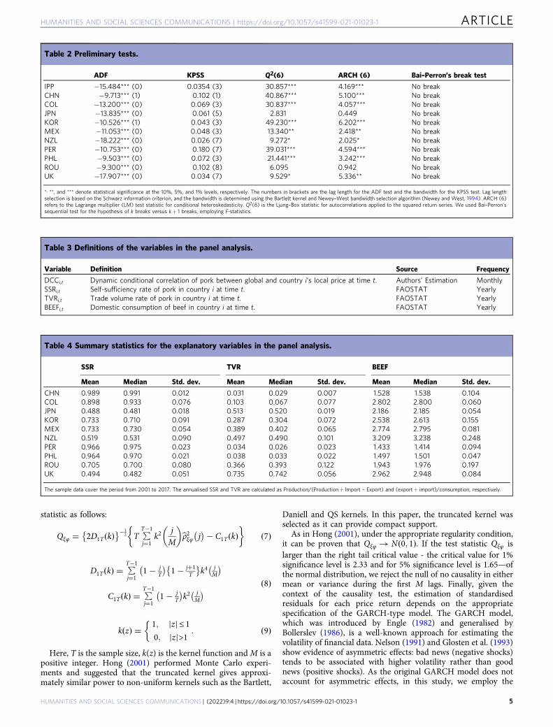
Figure 1 plots the charts for price returns of each pork price.We can observe that global and local pork prices show variabilityfrom January 2001 to December 2018 and exhibit differentvolatility patterns across pork-importing countries. For instance,some price returns (e.g., KOR and MEX) show similar patterns,with strong trends leading up to the global food and financialcrisis of 2007–2009. In contrast, fluctuations of price returns forCHN, COL, and NZL display a fairly strong trend over thesample period. The insights deduced from pork price returns maybe indicative of volatility clustering in the data series, which willbe examined in the GARCH-type model below.

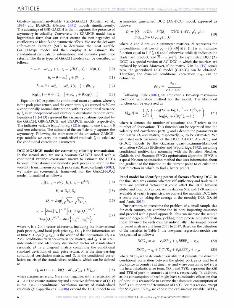
Before estimating the standardised residuals from GARCH-type models, the stationarity of each price series must be checkedusing unit root tests. Table 2 reports the results of the standardaugmented Dickey–Fuller (ADF) (Dickey and Fuller, 1979) andKwiatkowski–Phillips–Schmidt–Shin (KPSS) (Kwiatkowski et al.,1992), which indicate that all price returns are stationary. Allprice series have unit root processes in their levels (these resultscan be obtained from the authors upon request).

We can also observe that the results of the Ljung–Box statistic(Ljung and Box, 1978) for assessing residual autocorrelation, andthe Lagrange multiplier for autoregressive conditional hetero-skedasticity (LM-ARCH) test, which evaluates the presence ofconditional heteroskedasticity, suggest the usefulness and suit-ability of GARCH-based models. Moreover, considering that thepresence of structural breaks or shifts could impact the dataseries, we employ Bai and Perron’s (2003) structural break test toinvestigate the structural changes in each price return. As shownin Table 2, our results show no structural breaks for all pricereturns during the sample period. Based on the results of thepreliminary test, GARCH-type models without structural breakswill be used to investigate Granger causality and volatilitytransmission between global and local pork prices in net pork-importing countries.

Table 3 provides definitions of the variables used in the panelanalysis. Table 4 displays the summary statistics for the expla-natory variables, including SSR, TVR, and beef consumption(BEEF). Table 4 shows that SSR displays a variety of character-istics in different nations. For instance, CHN, COL, PER, andPHL have relatively high average SSR values, while the SSRs ofJPN, NZL, and the UK display the lowest average values. Incontrast, it is particularly interesting to see that JPN, NZL, andthe UK exhibit higher mean and median values of TVR. Theo-retically, an increase in SSR will decrease TVR, and vice versa.Furthermore, we can also observe that beef consumption in COL,NZL, and the UK is typically higher than in the other countries.

Granger causality tests for detecting lag-lead structure. Toexamine whether the occurrence of a change in the global market(Y1,t) can help forecast the occurrence of a change in a localmarket (Y2,t), we define the concept in terms of various principlesof Granger causality. Let Ωt−1≡ (Ω1,t-1, Ω2,t-1), whereΩ1,t−1≡ (Y1,t−1, …, Y1,1) and Ω2,t−1≡ (Y2,t−1, …, Y2,1) are theinformation sets available at time i−1 in global and local markets,respectively. We state that Y2,t does not Granger-cause Y1,t inmean, if the following null hypothesis holds:

H0 : E Y1;t

��Ω1;t�1

� �¼ E Y1;t

��Ωt�1

� �; ð1Þ

and Y2,t Granger-causes Y1,t in mean, if the following alternative

HUMANITIES AND SOCIAL SCIENCES COMMUNICATIONS | https://doi.org/10.1057/s41599-021-01023-1 ARTICLE

HUMANITIES AND SOCIAL SCIENCES COMMUNICATIONS | (2022) 9:4 | https://doi.org/10.1057/s41599-021-01023-1 3

hypothesis holds:

H0 : E Y1;t

��Ω1;t�1

� �≠ E Y1;t

��Ωt�1

� �: ð2Þ

We can also test for Granger causality-in-variance form Y2,t toY1,t given the following full and alternative hypothesis:

H0 : E Var Y1;t

��Ω1;t�1

� �n o¼ Var Y1;t

��Ωt�1

� �; ð3Þ

and

H0 : E Var Y1;t

��Ω1;t�1

� �n o≠Var Y1;t

��Ωt�1

� �: ð4Þ

The first step of our analysis is to use the Granger causality testimplemented by Hong (2001) to assess the existence anddirection of causal links between international and domesticpork prices in pork-importing countries. Hong’s (2001) approachhas more power than Cheung and Ng’s (1996) conventionalcausality by using the kernel weight function. Such a method isdesigned to detect whether lagged changes in one variable affectcontemporaneous changes in another; thus, the direction ofcausality between the two variables can be captured. In this study,we simultaneously examine causality-in-mean and causality-in-variance based on two standardised residuals and squared

standardised residuals of Y1,t and Y2,t. Using the estimated

GARCH-type models, the standardised residuals bξt for global andbφt local pork prices were estimated. The hats indicate suitableestimates of the corresponding quantitates and t= 1, 2, …, T.

Following Hong’s (2001) method, we denote bρξφ;t j� �

the lag jsample cross-correlation coefficient between the standardisedresiduals as follows:

bρξφ;t j� � ¼ bCξξ;t 0ð ÞbCφφ;t 0ð Þ

n o�12bCξφ;t j

� �; ð5Þ

where Cξξ;tð0Þ and Cφφ;tð0Þ are the subsample variances of ξt and

φt , respectively, and Cξφ;tðjÞ is the lag j cross-covariance between

ξt and φt expressed as

Cξφ;t j� � ¼ T�1 ∑T

t¼1þjbξtbφt�j; j≥ 0;

T�1 ∑Tt¼1�j

bξtþjbφt ; j < 0:

8<: ð6Þ

Hong (2001) enables us to capture the bidirectional Grangercausality test in time-series pairs by providing a modified test

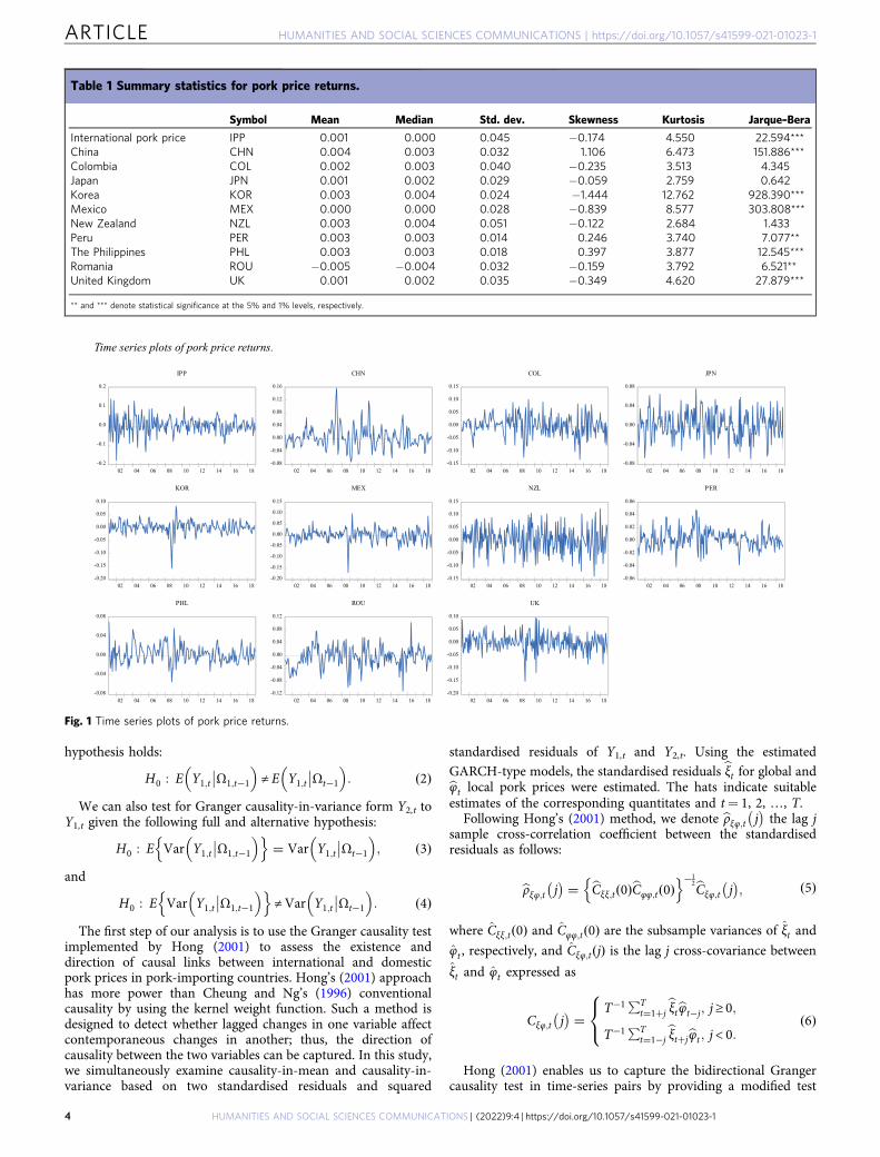
Table 1 Summary statistics for pork price returns.

Symbol Mean Median Std. dev. Skewness Kurtosis Jarque–Bera

International pork price IPP 0.001 0.000 0.045 −0.174 4.550 22.594***China CHN 0.004 0.003 0.032 1.106 6.473 151.886***Colombia COL 0.002 0.003 0.040 −0.235 3.513 4.345Japan JPN 0.001 0.002 0.029 −0.059 2.759 0.642Korea KOR 0.003 0.004 0.024 −1.444 12.762 928.390***Mexico MEX 0.000 0.000 0.028 −0.839 8.577 303.808***New Zealand NZL 0.003 0.004 0.051 −0.122 2.684 1.433Peru PER 0.003 0.003 0.014 0.246 3.740 7.077**The Philippines PHL 0.003 0.003 0.018 0.397 3.877 12.545***Romania ROU −0.005 −0.004 0.032 −0.159 3.792 6.521**United Kingdom UK 0.001 0.002 0.035 −0.349 4.620 27.879***

** and *** denote statistical significance at the 5% and 1% levels, respectively.

Fig. 1 Time series plots of pork price returns.

ARTICLE HUMANITIES AND SOCIAL SCIENCES COMMUNICATIONS | https://doi.org/10.1057/s41599-021-01023-1

4 HUMANITIES AND SOCIAL SCIENCES COMMUNICATIONS | (2022) 9:4 | https://doi.org/10.1057/s41599-021-01023-1

statistic as follows:

Qξφ ¼ 2D1T kð Þ� ��12 T ∑

T�1

j¼1k2

jM

bρ2ξφ j� �� C1T kð Þ

� �ð7Þ

D1T kð Þ ¼ ∑T�1

j¼11� j

T

� �1� jþ1

T

� �k4 j

M

� �C1T kð Þ ¼ ∑

T�1

j¼11� j

T

� �k2 j

M

� � ð8Þ

k zð Þ ¼ 1; zj j≤ 10; zj j>1

�: ð9Þ

Here, T is the sample size, k(z) is the kernel function andM is apositive integer. Hong (2001) performed Monte Carlo experi-ments and suggested that the truncated kernel gives approxi-mately similar power to non-uniform kernels such as the Bartlett,

Daniell and QS kernels. In this paper, the truncated kernel wasselected as it can provide compact support.

As in Hong (2001), under the appropriate regularity condition,it can be proven that Qξφ ! Nð0; 1Þ. If the test statistic Qξφ islarger than the right tail critical value - the critical value for 1%significance level is 2.33 and for 5% significance level is 1.65—ofthe normal distribution, we reject the null of no causality in eithermean or variance during the first M lags. Finally, given thecontext of the causality test, the estimation of standardisedresiduals for each price return depends on the appropriatespecification of the GARCH-type model. The GARCH model,which was introduced by Engle (1982) and generalised byBollerslev (1986), is a well-known approach for estimating thevolatility of financial data. Nelson (1991) and Glosten et al. (1993)show evidence of asymmetric effects: bad news (negative shocks)tends to be associated with higher volatility rather than goodnews (positive shocks). As the original GARCH model does notaccount for asymmetric effects, in this study, we employ the

Table 3 Definitions of the variables in the panel analysis.

Variable Definition Source Frequency

DCCi,t Dynamic conditional correlation of pork between global and country i’s local price at time t. Authors’ Estimation MonthlySSRi,t Self-sufficiency rate of pork in country i at time t. FAOSTAT YearlyTVRi,t Trade volume rate of pork in country i at time t. FAOSTAT YearlyBEEFi,t Domestic consumption of beef in country i at time t. FAOSTAT Yearly

Table 4 Summary statistics for the explanatory variables in the panel analysis.

SSR TVR BEEF

Mean Median Std. dev. Mean Median Std. dev. Mean Median Std. dev.

CHN 0.989 0.991 0.012 0.031 0.029 0.007 1.528 1.538 0.104COL 0.898 0.933 0.076 0.103 0.067 0.077 2.802 2.800 0.060JPN 0.488 0.481 0.018 0.513 0.520 0.019 2.186 2.185 0.054KOR 0.733 0.710 0.091 0.287 0.304 0.072 2.538 2.613 0.155MEX 0.733 0.730 0.054 0.389 0.402 0.065 2.774 2.795 0.081NZL 0.519 0.531 0.090 0.497 0.490 0.101 3.209 3.238 0.248PER 0.966 0.975 0.023 0.034 0.026 0.023 1.433 1.414 0.094PHL 0.964 0.970 0.021 0.038 0.033 0.022 1.497 1.501 0.047ROU 0.705 0.700 0.080 0.366 0.393 0.122 1.943 1.976 0.197UK 0.494 0.482 0.051 0.735 0.742 0.056 2.962 2.948 0.084

The sample data cover the period from 2001 to 2017. The annualised SSR and TVR are calculated as Production/(Production+ Import – Export) and (export+ import)/consumption, respectively.

Table 2 Preliminary tests.

ADF KPSS Q2(6) ARCH (6) Bai–Perron’s break test

IPP −15.484*** (0) 0.0354 (3) 30.857*** 4.169*** No breakCHN −9.713*** (1) 0.102 (1) 40.867*** 5.100*** No breakCOL −13.200*** (0) 0.069 (3) 30.837*** 4.057*** No breakJPN −13.835*** (0) 0.061 (5) 2.831 0.449 No breakKOR −10.526*** (1) 0.043 (3) 49.230*** 6.202*** No breakMEX −11.053*** (0) 0.048 (3) 13.340** 2.418** No breakNZL −18.222*** (0) 0.026 (7) 9.272* 2.025* No breakPER −10.753*** (0) 0.180 (7) 39.031*** 4.594*** No breakPHL −9.503*** (0) 0.072 (3) 21.441*** 3.242*** No breakROU −9.300*** (0) 0.102 (8) 6.095 0.942 No breakUK −17.907*** (0) 0.034 (7) 9.529* 5.336** No break

*, **, and *** denote statistical significance at the 10%, 5%, and 1% levels, respectively. The numbers in brackets are the lag length for the ADF test and the bandwidth for the KPSS test. Lag lengthselection is based on the Schwarz information criterion, and the bandwidth is determined using the Bartlett kernel and Newey–West bandwidth selection algorithm (Newey and West, 1994). ARCH (6)refers to the Lagrange multiplier (LM) test statistic for conditional heteroskedasticity. Q2(6) is the Ljung–Box statistic for autocorrelations applied to the squared return series. We used Bai–Perron’ssequential test for the hypothesis of k breaks versus k+ 1 breaks, employing F-statistics.

HUMANITIES AND SOCIAL SCIENCES COMMUNICATIONS | https://doi.org/10.1057/s41599-021-01023-1 ARTICLE

HUMANITIES AND SOCIAL SCIENCES COMMUNICATIONS | (2022) 9:4 | https://doi.org/10.1057/s41599-021-01023-1 5

Glosten–Jagannathan–Runkle (GJR)-GARCH (Glosten et al.,1993) and EGARCH (Nelson, 1991) models simultaneously.The advantage of GJR-GARCH is that it captures the presence ofasymmetry in volatility. Conversely, the EGARCH model has alogarithmic form that can either ensure the non-negativity ofcoefficients or identify the symmetric effects. We use the SchwarzInformation Criterion (SIC) to determine the most suitableGARCH-type model and then employ it to estimate thestandardised residuals for international and domestic pork pricereturns. The three types of GARCH models can be described asfollows:

rt ¼ μþ ωrt�1 þ εt; εt ¼ffiffiffiffiht

pζ t ; ζ t � N 0; 1ð Þ; ð10Þ

ht ¼ θ þ αε2t�1 þ βht�1; ð11Þ

ht ¼ θ þ αε2t�1 þ γε2t�1I εt�1

� �þ βht�1; ð12Þ

log ht� � ¼ θ þ α ζ t�1

�� ��þ γζ t�1 þ β log ht�1

� �: ð13Þ

Equation (10) explains the conditional mean equation, where rtis the pork price return, and the error term εt is assumed to followa conditionally normal distribution with its conditional varianceht. ζt is an independent and identically distributed random error.Equations (11)–(13) represent the variance equations specified bythe GARCH, GJR-GARCH, and EGARCH models, respectively.The indicator variable I(εt−1) in Eq. (12) is equal to one if εt−1 < 0and zero otherwise. The estimate of the coefficients γ captures theasymmetry. Following the estimation of the univariate GARCH-type models, we carry out standardised residuals ζt to calculatethe conditional correlation parameters.

DCC-MGARCH model for estimating volatility transmission.In the second step, we use a bivariate GARCH model with aconditional variance–covariance matrix to estimate the DCCsbetween international and domestic pork prices and examine thevolatility transmissions for each price pair. Based on Engle (2002),we make an econometric framework for the GARCH-DCCmodel, formulated as follows:

rt Ωt�1

�� � N 0; Ht

� �; εt ¼ H1=2

t ζ t ð14Þ

Ht ¼ DtRtDt ; ð15Þ

Dt ¼ diagffiffiffiffiffiffiffih1;t

q;

ffiffiffiffiffiffiffih2;t

q� �; ð16Þ

Rt ¼ diag Qt

� ��1=2h i

Qt diag Qt

� ��1=2h i

diag Qt

� ��1=2¼ diag q�1=211;t ; q�1=2

22;t

n o;

ð17Þ

where rt is a 2 × 1 vector of returns, including the internationalpork price r1,t and local pork price r2,t. Ωt−1 is the information setat time t−1. εt=(ε1,t, ε2,t)′ is the vector of the innovations. Ht is a2 × 2 conditional variance-covariance matrix, and ζ1 is an 2 × 1independent and identically distributed vector of standardisedresiduals. Dt is a diagonal matrix containing the conditionalstandard deviations of each price return. Rt is the time-varyingconditional correlation matrix, and Qt is the conditional corre-lation matrix of the standardised residuals, which can be definedas

Qt ¼ 1� a� bð ÞQþ aζ t�1ζ0t�1 þ bQt�1; ð18Þ

where parameters a and b are non-negative, with a restriction ofa+ b < 1 to ensure stationarity and a positive definiteness of Qt. Qis the 2 × 2 unconditional correlation matrix of standardisedresiduals ζt. Cappiello et al. (2006) expend the DCC model to an

asymmetric generalised DCC (AG-DCC) model, expressed asfollows:

Qt ¼ Q� A0QA� B0QB� �� G0NGþ A0ζ t�1ζ

0t�1Aþ

B0Qt�1Bþ G0ψt�1ψ0t�1G;

ð19Þ

where A and B are 2 × 2 parameter matrices. N represents theunconditional matrices of ψt ¼ I ζ t<0

� �� ζ t (I[.] is an indicatorfunction equal to 1 if ζi < 0 and 0 otherwise, while ⊗ indicates theHadamard product) and N ¼ E ψψ0� �

. The asymmetric DCC (A-DCC) is a special version of AG-DCC in which the matrices arereplaced by scalars. Moreover, if the matrix G in Eq. (19) equalszero, the generalised DCC model (G-DCC) can be obtained.Therefore, the dynamic conditional correlation ρ12,t can bedefined as

ρ12;t ¼q12;tffiffiffiffiffiffiffiffiffiffiffiffiffiffiffiffiq11;tq22;t

p : ð20Þ

Following Engle (2002), we employed a two-step maximum-likelihood estimation method for the model. The likelihoodfunction can be expressed as

L χ; ι� � ¼ � 1

2∑T

t�1

nlog 2πð Þ þ log Dt

�� ��2 þ ε0tD�2t εtþ

log Rt

�� ��þ ζ 0tR�1t ζ t � ζ 0tζ t

!; ð21Þ

where n denotes the number of equations and T refers to thenumber of observations. This function can be separated into thevolatility and correlation parts. χ and ι denote the parameters inthe matrix Dt and matrix, respectively, Rt to be estimated. Weestimated each parameter of the DCC, A-DCC, AG-DCC, andG-DCC models by the Gaussian quasi-maximum-likelihoodestimation (QMLE) (Bollerslev and Wooldridge, 1992), assumingconditional multivariate normality with the Broyden, Fletcher,Goldfarb, and Shannon (BFGS) optimisation algorithm (BFGS isa quasi-Newton optimisation method that uses information aboutthe gradient of the function at the current point to calculate thebest direction in which to find a better point).

Panel model for identifying potential factors affecting DCC. Inthe final step, we examine whether self-sufficiency and trade valuerates are potential factors that could affect the DCC betweenglobal and local pork prices. As the data on SSR and TVR are onlyavailable at yearly frequencies, we convert the monthly DCC intoa yearly one by taking the average of the monthly DCC (Davidand Amir, 2017).

Furthermore, to overcome the problem of a small sample sizefor each country, we combine the 10 pork-importing countriesand proceed with a panel approach. This can increase the samplesize and degrees of freedom, yielding more precise estimates thanthose obtained for each country individually. The sample periodfor panel analysis runs from 2001 to 2017. Based on the definitionof the variables in Table 3, the two-panel regression models canbe specified as follows:

DCCi;t ¼ ωi þ ς1SSRi;t þ ς2BEEFi;t þ ei;t ; ð22Þ

DCCi;t ¼ ηi þ δ1TVRi;t þ δ2BEEFi;t þ νi;t ; ð23Þwhere DCCi,t is the dependent variable that presents the dynamicconditional correlation between the global pork price and localpork price in country i at time t. ωi and ηi are constants, and ei,t isthe heteroskedastic error term. SSRi,t and TVRi,t represent the SSRand TVR of pork in country i at time t, respectively. In addition,as the consumption of beef might have substitutive effects on thatof pork, it is reasonable to assume that domestic consumption ofbeef is an important determinant of DCC. For this reason, exceptfor SSRi,t and TVRi,t, we choose the explanatory variable, BEEFi,t

ARTICLE HUMANITIES AND SOCIAL SCIENCES COMMUNICATIONS | https://doi.org/10.1057/s41599-021-01023-1

6 HUMANITIES AND SOCIAL SCIENCES COMMUNICATIONS | (2022) 9:4 | https://doi.org/10.1057/s41599-021-01023-1

which represents the rate of change of domestic consumption(FAOSTAT, 2020) of beef in country i at time t. The impact of thedetermining factors influencing the price volatility transmission ismeasured by the parameters ςi(i= 1, 2) and δi(i= 1, 2. Thoughnot reported here, the ADF unit root tests indicated that allvariables in Eqs. (22) and (23) were stationary.

For robustness, five different types of methodologies areimplemented in our panel analysis. The standard pool ordinaryleast-squares (OLS) model is used as the benchmark. The fixed-effects model, random-effects model, feasible generalised least-squares (FGLS) model (Baltagi, 1981) and Prais–Winstenregression with panel-corrected standard errors (PCSEs) (Beckand Katz, 1995) are applied simultaneously to verify therobustness of our results.

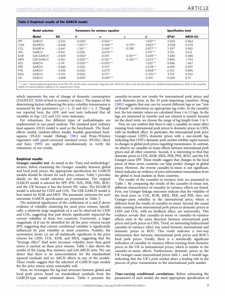
Empirical resultsGranger causality test. As noted in the “Data and methodology”section, before examining the Granger causality between globaland local pork prices, the appropriate specification for GARCHmodels should be chosen for each price return. Table 5 providesdetails on the model selection and estimation. The originalGARCH model is selected for IPP, JPN, NZL, PER, PHL, ROU,and the UK because it has the lowest SIC value. The EGARCHmodel is selected for CHN and COL. The GJR-GARCH model isbest suited for KOR and MEX. The parameter estimates for eachunivariate GARCH specification are presented in Table 5.

The statistical significance of the coefficients of α and β showsevidence of volatility clustering for most price returns. Specifi-cally, a relatively large magnitude of α can be observed for CHNand COL, suggesting that past shocks significantly impacted thecurrent volatility in these two countries. Conversely, a largermagnitude of β can be identified for all the price returns exceptJPN, suggesting that current conditional volatility is significantlyinfluenced by past volatility in most countries. Notably, theasymmetric terms (γ) are all statistically significant in the pricereturns for CHN, COL, KOR, and MEX, suggesting that the“leverage effect” (bad news increases volatility more than goodnews) is exerted on these price returns. Table 5 also shows theresults of the Ljung–Box statistics and LM-ARCH tests. We candetect that there is no autocorrelation for the standardisedsquared residuals and no ARCH effects in any of the models.These results suggest that the selection of GARCH-type modelsfits the price return series reasonably well.

Next, we investigate the lag-lead structure between global andlocal pork prices based on standardised residuals from theGARCH-type model estimated above. Table 6 presents the

causality-in-mean test results for international pork prices andeach domestic price in the 10 pork-importing countries. Hong(2001) suggests that one can try several different lags or use “ruleof thumb” to determine an appropriate lag order. In the causalitytest, the test statistic values are calculated from 1 to 12 lags. As thelags are measured in months and our interest is mainly focusedon the short term, we choose the range of lag length from 1 to 5.

First, we can confirm that there is only a causality-in-mean effectrunning from international pork prices to domestic prices in CHN,with no feedback effect. In particular, the international pork priceGranger-causes CHN’s domestic prices with a one-month lag,indicating that CHN’s domestic pork market exhibits rapid reactionto changes in global pork prices regarding transmission. In contrast,we observe no causality-in-mean effects between international porkprices and all other countries. Second, it is interesting to find thatdomestic prices in COL, KOR, MEX, PER, PHL, ROU, and the UKGranger-cause IPP. These results suggest that changes in the localprices of these seven countries can help predict changes in globalprices. However, the reverse causality-in-mean is not significant,which indicates no evidence of price information transmission fromthe global to local markets in these countries.

The results of the causality-in-variance tests are presented inTable 7. By comparing the results of the causality-in-mean test,different characteristics of causality-in-variance effects are found.First, our Granger linkage outcomes indicate that the volatility ofthe local price in COL, KOR, MEX, PER, and PHL does notGranger-cause volatility in the international price, which isdifferent from the results of causality-in-mean. Second, the causallinks running from international pork prices to domestic prices inCHN and COL, with no feedback effect, are noteworthy. Thisevidence reveals that causality-in-mean or causality-in-varianceeffects exist in the same direction between international porkprices and pork prices in CHN. Third, an interesting bidirectionalcausality-in-variance effect was noted between international anddomestic prices in ROU. This result indicates a two-wayinformation flow between international pork prices and ROU’slocal pork prices. Finally, there is a statistically significantindication of causality-in-variance effects running from domesticprices in the UK to international prices, which is similar to thecausality-in-mean effects. Furthermore, domestic prices in theUK Granger-cause international prices with 1- and 5-month lags,indicating that the UK’s pork market plays a leading role in theprocess of price transmission to the international pork market.

Time-varying conditional correlations. Before estimating theparameters of each model, the most appropriate specification of

Table 5 Empirical results of the GARCH model.

Model selection Parameters for variance equation Specification tests

Model SIC θ α γ β Q2(6) ARCH (6)

IPP GARCH −3.555 0.000* −0.063 ** 1.043*** 5.005 0.864CHN EGARCH −4.648 −1.615*** 0.348*** 0.170** 0.823*** 3.008 0.478COL EGARCH −3.641 −1.161** 0.445*** −0.138* 0.877*** 5.397 0.982JPN GARCH −4.192 0.000 0.076*** 0.115*** 3.105 0.512KOR GJR-GARCH −4.929 0.000* 0.019 0.331*** 0.649*** 3.084 0.480MEX GJR-GARCH −4.361 0.000*** −0.125*** 0.430*** 0.672*** 9.890 1.794NZL GARCH −3.114 0.000*** −0.092*** 1.050*** 9.986 1.467PER GARCH −5.685 0.000 0.172* 0.678*** 6.496 0.997PHL GARCH −5.435 0.000 0.073* 0.848*** 6.105 0.896ROU GARCH −4.129 0.000 0.117** 0.705*** 3.719 0.592UK GARCH −3.848 0.000* 0.209*** 0.414 0.609 0.111

*, **, and *** denote statistical significance at the 10%, 5%, and 1% levels, respectively. Diagnostic test: ARCH (6) refers to the LM test statistic for conditional heteroskedasticity. Q2(6) is the Ljung–Boxstatistic for autocorrelations applied to the squared return series.

HUMANITIES AND SOCIAL SCIENCES COMMUNICATIONS | https://doi.org/10.1057/s41599-021-01023-1 ARTICLE

HUMANITIES AND SOCIAL SCIENCES COMMUNICATIONS | (2022) 9:4 | https://doi.org/10.1057/s41599-021-01023-1 7

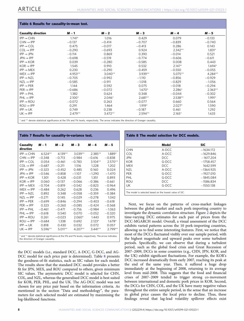
the DCC models (i.e., standard DCC, A-DCC, G-DCC, and AG-DCC model for each price pair is determined). Table 8 presentsthe goodness-of-fit statistics, such as SIC values for each model.The results show that the standard DCC model provides a betterfit for JPN, MEX, and ROU compared to others, given minimumSIC values. The asymmetric DCC model is selected for CHN,COL, and NZL, whereas the generalised DCC model is best suitedfor KOR, PER, PHL, and the UK. The AG-DCC model was notchosen for any price pair based on the information criteria. Asmentioned in the section “Data and methodology”, the para-meters for each selected model are estimated by maximising thelog-likelihood functions.

Next, we focus on the patterns of cross-market linkagesbetween the global market and each pork-importing country toinvestigate the dynamic correlation structure. Figure 2 depicts thetime-varying DCC estimates for each pair of prices from theDCC-MGARCH model. Overall, a visual assessment of the DCCexhibits varied patterns across the 10 pork-importing countries,allowing us to find some interesting features. First, we notice thatmost of the DCCs fluctuated visibly over our sample period, withthe highest magnitude and upward peaks over some turbulentperiods. Specifically, we can observe that during a turbulentperiod, such as the global food crisis and Great Recession of2007–2009, DCCs in some countries (e.g., CHN, JPN, KOR, andthe UK) exhibit significant fluctuations. For example, the KOR’sDCC increased dramatically from early 2007, reaching its peak atthe end of the same year. Then, it suffered a huge dropimmediately at the beginning of 2008, returning to its averagelevel from mid-2008. This suggests that the food and financialcrises of 2007–2009 tended to trigger strong co-movementbetween international and domestic pork prices in KOR. Second,the DCCs for CHN, COL, and the UK have many negative valuesthroughout the entire sample period, in the sense that an increasein global price causes the local price to decline. Thus, thesefindings reveal that lag-lead volatility spillover effects exist

Table 7 Results for causality-in-variance test.

Causalitydirection

M= 1 M= 2 M= 3 M= 4 M= 5

IPP→ CHN 6.524** 4.139** 3.039** 2.385** 1.889*CHN→ IPP −0.348 −0.713 −0.984 −0.616 −0.838IPP→ COL 0.054 −0.461 −0.783 3.104** 2.570**COL→ IPP −0.687 −0.211 1.516 1.228 1.202IPP→ JPN −0.323 −0.452 0.485 0.160 0.024JPN→ IPP −0.546 −0.858 −1.107 −1.290 −1.470IPP→ KOR 1.301 0.428 −0.031 1.351 0.893KOR→ IPP 0.060 −0.137 −0.066 −0.386 −0.661IPP→MEX −0.704 −0.819 −0.542 −0.823 −0.964MEX→ IPP −0.484 0.262 0.628 0.236 0.496IPP→NZL 0.892 0.348 −0.058 −0.359 −0.384NZL→ IPP −0.271 0.145 −0.029 −0.278 1.042IPP→ PER −0.699 −0.846 −0.294 −0.403 −0.618PER→ IPP 0.323 −0.260 −0.085 −0.424 −0.568IPP→ PHL −0.461 −0.471 −0.756 −0.984 −1.063PHL→ IPP −0.618 0.540 0.070 −0.052 −0.320IPP→ ROU 0.261 −0.023 2.060* 1.443 0.975ROU→ IPP −0.684 1.338 0.692 2.123* 1.678*IPP→UK 0.818 0.430 0.032 0.072 0.057UK→ IPP 5.596** 5.011** 4.207** 3.441** 2.799**

* and ** denote statistical significance at the 5% and 1% levels, respectively. The arrow indicatesthe direction of Granger causality.

Table 8 The model selection for DCC models.

Model SIC

CHN A-DCC −1634.172COL A-DCC −1629.846JPN DCC −1617.204KOR G-DCC −1758.457MEX DCC 1642.599NZL A-DCC −1364.925PER G-DCC −1927.010PHL G-DCC −1845.084ROU DCC −1586.834UK G-DCC −1550.138

The model is selected based on the lowest value of SIC.

Table 6 Results for causality-in-mean test.

Causality direction M= 1 M= 2 M= 3 M= 4 M= 5

IPP→ CHN 1.741* 1.016 0.429 0.079 −0.133CHN→ IPP −0.137 −0.414 −0.707 −0.839 −0.740IPP→ COL 0.475 −0.017 −0.413 0.286 0.143COL→ IPP −0.290 −0.693 0.924 2.342** 1.831*IPP→ JPN −0.114 0.869 0.390 −0.014 0.521JPN→ IPP −0.698 −0.519 −0.774 −0.606 −0.611IPP→ KOR 0.039 −0.280 −0.585 0.008 0.443KOR→ IPP 1.545 0.910 0.532 2.147* 1.694*IPP→MEX 0.230 −0.290 −0.459 −0.550 −0.055MEX→ IPP 4.953** 3.040** 3.939** 5.075** 4.284**IPP→NZL −0.705 −0.992 −1.110 −0.856 −0.929NZL→ IPP −0.585 −0.911 −1.018 −0.829 −1.056IPP→ PER 1.144 0.592 0.075 −0.018 −0.294PER→ IPP −0.686 −0.072 1.670* 2.286* 2.363**IPP→ PHL 1.382 0.624 0.348 −0.044 −0.302PHL→ IPP 2.100* 2.046* 2.681** 2.538** 1.991*IPP→ ROU −0.072 0.263 −0.077 0.660 0.564ROU→ IPP 0.291 1.464 1.919* 2.027* 1.590IPP→UK 0.749 0.238 −0.187 0.461 1.292UK→ IPP 2.479** 3.472** 2.594** 2.165* 1.633

* and ** denote statistical significance at the 5% and 1% levels, respectively. The arrow indicates the direction of Granger causality.

ARTICLE HUMANITIES AND SOCIAL SCIENCES COMMUNICATIONS | https://doi.org/10.1057/s41599-021-01023-1

8 HUMANITIES AND SOCIAL SCIENCES COMMUNICATIONS | (2022) 9:4 | https://doi.org/10.1057/s41599-021-01023-1

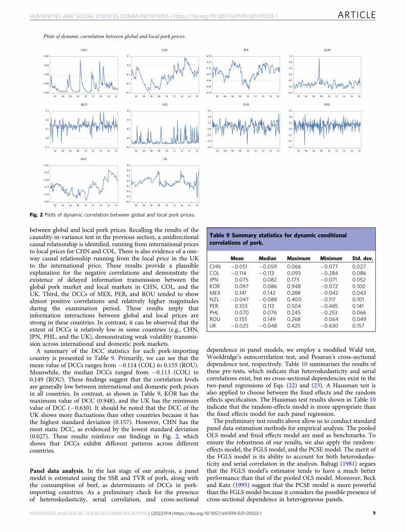
between global and local pork prices. Recalling the results of thecausality-in-variance test in the previous section, a unidirectionalcausal relationship is identified, running from international pricesto local prices for CHN and COL. There is also evidence of a one-way causal relationship running from the local price in the UKto the international price. These results provide a plausibleexplanation for the negative correlations and demonstrate theexistence of delayed information transmission between theglobal pork market and local markets in CHN, COL, and theUK. Third, the DCCs of MEX, PER, and ROU tended to showalmost positive correlations and relatively higher magnitudesduring the examination period. These results imply thatinformation interactions between global and local prices arestrong in these countries. In contrast, it can be observed that theextent of DCCs is relatively low in some countries (e.g., CHN,JPN, PHL, and the UK), demonstrating weak volatility transmis-sion across international and domestic pork markets.

A summary of the DCC statistics for each pork-importingcountry is presented in Table 9. Primarily, we can see that themean value of DCCs ranges from −0.114 (COL) to 0.155 (ROU).Meanwhile, the median DCCs ranged from −0.113 (COL) to0.149 (ROU). These findings suggest that the correlation levelsare generally low between international and domestic pork pricesin all countries. In contrast, as shown in Table 9, KOR has themaximum value of DCC (0.948), and the UK has the minimumvalue of DCC (−0.630). It should be noted that the DCC of theUK shows more fluctuations than other countries because it hasthe highest standard deviation (0.157). However, CHN has themost static DCC, as evidenced by the lowest standard deviation(0.027). These results reinforce our findings in Fig. 2, whichshows that DCCs exhibit different patterns across differentcountries.

Panel data analysis. In the last stage of our analysis, a panelmodel is estimated using the SSR and TVR of pork, along withthe consumption of beef, as determinants of DCCs in pork-importing countries. As a preliminary check for the presenceof heteroskedasticity, serial correlation, and cross-sectional

dependence in panel models, we employ a modified Wald test,Wooldridge’s autocorrelation test, and Pesaran’s cross-sectionaldependence test, respectively. Table 10 summarises the results ofthese pre-tests, which indicate that heteroskedasticity and serialcorrelations exist, but no cross-sectional dependencies exist in thetwo-panel regressions of Eqs. (22) and (23). A Hausman test isalso applied to choose between the fixed effects and the randomeffects specification. The Hausman test results shown in Table 10indicate that the random-effects model is more appropriate thanthe fixed effects model for each panel regression.

The preliminary test results above allow us to conduct standardpanel data estimation methods for empirical analysis. The pooledOLS model and fixed effects model are used as benchmarks. Toensure the robustness of our results, we also apply the random-effects model, the FGLS model, and the PCSE model. The merit ofthe FGLS model is its ability to account for both heteroskedas-ticity and serial correlation in the analysis. Baltagi (1981) arguesthat the FGLS model’s estimator tends to have a much betterperformance than that of the pooled OLS model. Moreover, Beckand Katz (1995) suggest that the PCSE model is more powerfulthan the FGLS model because it considers the possible presence ofcross-sectional dependence in heterogeneous panels.

Fig. 2 Plots of dynamic correlation between global and local pork prices.

Table 9 Summary statistics for dynamic conditionalcorrelations of pork.

Mean Median Maximum Minimum Std. dev.

CHN −0.051 −0.059 0.066 −0.077 0.027COL −0.114 −0.113 0.093 −0.284 0.086JPN 0.075 0.082 0.173 −0.071 0.052KOR 0.097 0.086 0.948 −0.072 0.100MEX 0.141 0.142 0.288 −0.042 0.043NZL −0.047 −0.088 0.400 −0.117 0.101PER 0.103 0.113 0.504 −0.485 0.141PHL 0.070 0.076 0.245 −0.253 0.066ROU 0.155 0.149 0.268 0.064 0.049UK −0.025 −0.048 0.425 −0.630 0.157

HUMANITIES AND SOCIAL SCIENCES COMMUNICATIONS | https://doi.org/10.1057/s41599-021-01023-1 ARTICLE

HUMANITIES AND SOCIAL SCIENCES COMMUNICATIONS | (2022) 9:4 | https://doi.org/10.1057/s41599-021-01023-1 9

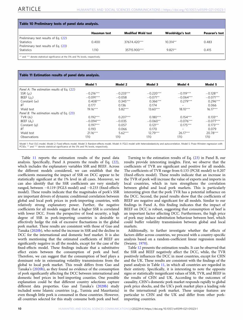
Table 11 reports the estimation results of the panel dataanalysis. Specifically, Panel A presents the results of Eq. (22),which includes the explanatory variables SSR and BEEF. Acrossthe different models considered, we can establish that thecoefficients measuring the impact of SSR on DCC appear to bestatistically significant at the 1% level in all cases. Moreover, wecan also identify that the SSR coefficients are very similarlyranged, between −0.119 (FGLS model) and −0.233 (fixed-effectsmodel). These results indicate that the magnitudes of pork’s SSRare important drivers of dynamic conditional correlation betweenglobal and local pork prices in pork-importing countries, withrelatively strong explanatory power. Further, the negativecoefficients for all models suggest that a higher SSR is correlatedwith lower DCC. From the perspective of food security, a highdegree of SSR in pork-importing countries is desirable toeffectively hedge the risk of excessive fluctuations in the globalpork market. These results are consistent with those of Guo andTanaka (2020b), who noted the increase in SSR and the decline inDCC for the international and domestic beef market. It is alsoworth mentioning that the estimated coefficients of BEEF aresignificantly negative in all the models, except for the case of thefixed-effects model. These findings indicate that a substitutiveeffect exists between the consumption of pork and beef.Therefore, we can suggest that the consumption of beef plays adominant role in extenuating volatility transmissions from theglobal to local pork market. This result differs from Guo andTanaka’s (2020b), as they found no evidence of the consumptionof pork significantly affecting the DCC between international anddomestic beef prices in beef-importing counties. One possibleexplanation could be that different country selections capturedifferent data properties. Guo and Tanaka’s (2020b) studyincluded some Islamic countries (e.g., Tunisia and Mauritania)even though little pork is consumed in these countries. However,all countries selected for this study consume both pork and beef.

Turning to the estimation results of Eq. (23) in Panel B, ourresults provide interesting insights. First, we observe that thecoefficients of TVR are significant and positive for all models.The coefficients of TVR range from 0.133 (PCSE model) to 0.207(fixed-effects model). These results indicate that an increase inthe TVR of pork will increase the value of exports and imports inlocal countries, which in turn strengthens the correlationbetween global and local pork markets. This is particularlyinteresting given that the pork TVR has a potential influence onthe DCC. Second, the panel results show that the coefficients ofBEEF are negative and significant for all models. Similar to ourfindings in Panel A, this finding indicates that the impact ofBEEF on DCC is robust, suggesting that consumption of beef isan important factor affecting DCC. Furthermore, the high priceof pork may induce substitution behaviour between beef, whichcould buffer volatility transmission between global and localmarkets.

Additionally, to further investigate whether the effects offactors differ across countries, we proceed with a country-specificanalysis based on a random-coefficient linear regression model(Swamy, 1970).

Table 12 presents the estimation results. It can be observed thatthe SSR and BEEF negatively affect the DCC, while, the TVRpositively influences the DCC in most countries, except for CHNand the UK. These results are consistent with the findings of thepanel analysis in Table 11, in which all countries are regarded intheir entirety. Specifically, it is interesting to note the oppositesigns or statistically insignificant values of SSR, TVR, and BEEF inthe results of CHN and UK. According to the outcomes ofcausality, CHN’s domestic pork market responds rapidly to globalpork price shocks, and the UK’s pork market plays a leading rolein the international pork market. These unique features areparticular to CHN and the UK and differ from other pork-importing countries.

Table 11 Estimation results of panel data analysis.

Model 1 Model 2 Model 3 Model 4 Model 5

Panel A: The estimation results of Eq. (22)SSR (ς1) −0.216*** −0.233*** −0.220*** −0.119*** −0.128**BEEF (ς2) −0.091*** −0.058 −0.071** −0.064*** −0.071***Constant (ω) 0.408*** 0.345*** 0.366*** 0.279*** 0.296***R2 0.177 0.136 0.174 – 0.066Wald test 19.16*** 5.82*** 13.60*** 18.10*** 16.17***Panel B: The estimation results of Eq. (23)TVR (δ1) 0.192*** 0.207*** 0.180*** 0.154*** 0.133**BEEF (δ2) −0.094*** −0.035 −0.060** −0.076*** −0.077***Constant (η) 0.197*** 0.057 0.121** 0.175*** 0.173***R2 0.193 0.066 0.170 – 0.079Wald test 21.16*** 5.62*** 12.79*** 26.17*** 20.78***Observations 170 170 170 170 170

Model 1: Pool OLS model. Model 2: Fixed effects model. Model 3: Random-effects model. Model 4: FGLS model with heteroskedasticity and autocorrelation. Model 5: Prais–Winsten regression withPCSEs. ** and *** denote statistical significance at the 5% and 1% levels, respectively.

Table 10 Preliminary tests of panel data analysis.

Hausman test Modified Wald test Wooldridge’s test Pesaran’s test

Preliminary test results of Eq. (22)Statistics 0.400 37674.420*** 10.314** 0.483Preliminary test results of Eq. (23)Statistics 1.110 35715.900*** 9.821** 0.415

** and *** denote statistical significance at the 5% and 1% levels, respectively.

ARTICLE HUMANITIES AND SOCIAL SCIENCES COMMUNICATIONS | https://doi.org/10.1057/s41599-021-01023-1

10 HUMANITIES AND SOCIAL SCIENCES COMMUNICATIONS | (2022) 9:4 | https://doi.org/10.1057/s41599-021-01023-1

Policy implications and discussionsThe first policy implication derived from the results is that autarkyplays a mitigating role in price volatility transmissions fromabroad. Namely, a country could increase import tariffs and/orfarming subsidies to heighten self-sufficiency and protect domesticmarkets against unexpected foreign shocks. This must be carefullyinterpreted. As Tanaka and Guo (2019) demonstrate, the nationalprice could be destabilised if the volatility of domestic supply isgreater than that of imports and the ratio of domestic productionto total supply is large enough. In addition, the result does notshow that protectionist policy improves the market or economy.Policymakers need to identify the balancing points between thebenefit from the enhanced efficiency of resource allocation andmarket stabilisation by raising self-sufficiency in food in terms ofthe expected utility of economic agents.

We also found that a greater international TVR could facilitatelarger price volatility conveyance from global to local markets,which is consistent with the outcome of self-sufficiency obtainedin our analysis because a higher autarky rate normally hints at asmaller TVR. However, even if a country reaches a level of totalself-sufficiency, it can still be exposed to external markets, with allproducts domestically produced being exported and an identicalamount being imported for internal use. This extreme exampleillustrates that a country can be self-sufficient in a commodity buthold 200% international trade exposure. Figure 3 shows the trade-off between the mean of self-sufficiency and that of the TVR forthe period between 2001 and 2017. Although the UK attains anautarky of around 50%, which is within the range of its coun-terparts in NZL and JPN, its TVR exceeds that of the other two.Accordingly, the UK could have close ties with overseas markets

relative to NZL and JPN. If policymakers need to reduce theirconnections with international markets, they should heightenautarky rates and curb exports and imports. Furthermore, netexporting nations would experience mixed effects, as higher self-sufficiency suggests greater trade quantity for the regions.Therefore, higher self-sufficiency does not necessarily alleviate theincoming external shocks.

Our experiments found a role in the consumption of a sub-stitute that mollifies foreign shocks. This indicates that nationaldietary patterns should be well-balanced with the diversificationof food consumption, which may be a rational choice as a pre-ventative policy measure on the grounds of policy implementa-tion costs. Lifting the SSR incurs tremendous financial costs,subsidises farming activities, and sacrifices the benefits frommarket efficiency. Although changing national dietary habits maytake many years, once locals accept new dietary lifestyles, nodirect financial cost is required to uphold substitutive options torarefy volatility synchronisation. After World War II, the GeneralHeadquarters of the Allied Forces recommended systematichealth education and a school lunch programme for Japaneseschoolchildren with donated foods such as meat, fish, vegetables,skim milk, and sugar from the United States (Rogers, 2015).Through this assistance, Japanese citizens gradually becameaccustomed to Western meals, and their daily dietary consump-tion patterns have since been fundamentally altered from tradi-tional Japanese cuisine.

Concluding remarksThis study employed Granger causality and DCC to examine therelationships between global and local pork meat markets. Inaddition, we analysed the efficacy of self-sufficiency in the alle-viation of international price volatility transmission to localmarkets. The primary findings are as follows. First, we found thatRomania exhibits bidirectional Granger causality between globaland domestic prices in variance. China and the United Kingdompresent unidirectional linkages from global to domestic marketsand from domestic to global markets, both in mean and variance,respectively. Second, high self-sufficiency, or a small TVR of porkmeat, mitigates price volatility pass-throughs from foreign mar-kets. Finally, beef consumption plays a preventative role againstthe transmission of foreign market shocks to local markets.

Comparisons between existing research and this study mustalso be made. While Guo and Tanaka (2019) identified the uni-lateral linkages between global and local retail prices for wheat-importing countries, bidirectional relationships were found forpork markets in our research. The Granger causality for beefmarkets also exhibits bilaterality in Guo and Tanaka (2020b). Thedifference between wheat and meat (i.e., pork and beef) marketsmay be attributed to the fact that more importing nations

Fig. 3 The relationship between self-sufficiency and trade volume rates.

Table 12 The country-specific results based on the random-coefficient regression model.

The estimation results of Eq. (22) The estimation results of Eq. (23)

SSR (ς1) BEEF (ς2) Constant (ω) TVR (δ1) BEEF (δ2) Constant (η)

CHN 0.024 0.063 −0.171 −0.916** 0.112** −0.192***COL −0.064*** −0.324** 1.365*** 0.706*** −0.213* 0.408*JPN −0.306* −0.229** 0.714*** 0.234** −0.264* 0.522KOR −0.157** −0.096** 0.452 0.180* −0.085** 0.259**MEX −0.142** 0.005 0.232** 0.140** 0.018** 0.038**NZL −0.183* −0.052** 0.211** 0.170* −0.050** 0.028PER −0.142** −0.090** 0.366** 0.054** −0.064** 0.194*PHL −0.172* −0.025** 0.273* 0.186** −0.016** 0.086ROU 0.052 −0.098* 0.304* 0.064** −0.091* 0.305**UK 0.424 0.425 −1.485 −0.162 0.169 −0.402

HUMANITIES AND SOCIAL SCIENCES COMMUNICATIONS | https://doi.org/10.1057/s41599-021-01023-1 ARTICLE

HUMANITIES AND SOCIAL SCIENCES COMMUNICATIONS | (2022) 9:4 | https://doi.org/10.1057/s41599-021-01023-1 11

participate in the global wheat market than in the world’s meatmarkets. In 2018, the cumulative share of the top 10 wheatimporters accounted for only 39.7% of total global imports, whilethe top 10 pork-importing nations accounted for 75.2%, whichimplies that fewer nations were engaged in the global pork market(FAOSTAT, 2020). Hence, a pork-importing country has a largermarket share and greater potential to influence internationalprices than a wheat-importing country.

The DCCs estimated here should also be compared to those inthe existing literature. The mean and median of the time-variantcorrelations for wheat market pairs in Guo and Tanaka (2019)show positive values for all sample countries. In contrast, thisstudy and Guo and Tanaka (2020b), estimate DCCs to be nega-tive in mean and median for four of ten pork-importing nationsand two of ten beef-importing nations, respectively. The differ-ence between cereal and meat may be due to the dissimilar natureof the markets. While cereal production depends crucially onweather conditions, meat production can be adjusted by slaugh-tering livestock, softening short-term market shocks, and dilutingthe causal relationship. However, the three studies are consistentfrom the perspective of more intimate relevance between marketsduring the global food crisis in 2008.

As mentioned in the previous section, the first limitation is thatwe did not consider internal price volatility, such as wholesale orproducer prices, simply extracting the mitigation effects of self-sufficiency on cross-border pass-throughs. Thus, autarky mea-sures are not always effective in impairing internationally trans-mitted shocks. Second, our findings are not simply applicable toexporting countries as net exporters’ self-sufficiency exceeds100% with mixed impact (i.e., higher SSR and greater TVR) whenself-sufficiency is raised.

Based on our experimental outcomes, an increase in self-sufficiency in pork is likely to stabilise domestic markets. Pro-tectionist measures, such as subsidising domestic production and/or protecting local markets from foreign pig meat products, arethe primary methods to raise autarky rates. Steady market pricescould reduce the risk of meat production and consumption andimprove the expected utility. This is especially beneficial for low-income households in developed and developing countries whosuffered severe global food price spikes in 2008, while such pro-tectionist policies worsen market efficiency.

It is essential to analyse the cost–benefit relationship in thepolicy-making process. Raising self-sufficiency in agriculturalcommodities at a national level seems to impose a massive eco-nomic burden, including both policy implementation costs, suchas subsidising farming activity, and the loss of potential benefitfrom market efficiency with an additional import tariff. To assessthe balance between costs and benefits, the reduction in pricevolatility spillover needs to be converted into a monetary value. Itis intrinsic to estimate the Arrow–Pratt measures of risk aversionto express the benefit or cost in monetary value. However, thesetopics are left for future research.

Data availabilityThe data that support the findings of this study can be obtainedfrom the corresponding author upon request.

Received: 11 June 2021; Accepted: 20 December 2021;

ReferencesAbdulai A (2000) Spatial price transmission and asymmetry in the Ghanaian maise

market. J Dev Econ 63(2):327–349

Assefa TT, Meuwissen MPM, Gardebroek C, Oude Lansink AGJM (2017) Priceand volatility transmission and market power in the German fresh porksupply chain. J Agric Econ 68(3):861–880. https://doi.org/10.1111/1477-9552.12220

Bai J, Perron P (2003) Computation and analysis of multiple structural changemodels. J Appl Econ 18(1):1–22. https://doi.org/10.1002/jae.659

Baltagi BH (1981) Simultaneous equations with error components. J Econ17(2):189–200. https://doi.org/10.1016/0304-4076(81)90026-9

Baulch B (1997) Transfer costs, spatial arbitrage, and testing for food marketintegration. Am J Agric Econ 79(2):477–487. https://doi.org/10.2307/1244145

Beck N, Katz JN (1995) What to do (and not to do) with time-series cross-sectiondata. Am Pol Sci Rev 89(3):634–647. https://doi.org/10.2307/2082979

Bishwajit G, Sarker S, Kpoghomou M, Gao H, Jun L, Yin D, Ghosh S (2013). Self-sufficiency in rice and food security: a South Asian perspective. Agric FoodSecur 2(1). https://doi.org/10.1186/2048-7010-2-10

Bollerslev T (1986) Generalised autoregressive conditional heteroskedasticity. JEcon 31(3):307–327. https://doi.org/10.1016/0304-4076(86)90063-1

Bollerslev T, Wooldridge JM (1992) Quasi-maximum likelihood estimation andinference in dynamic models with time-varying covariances. Economet Rev11(2):143–172. https://doi.org/10.1080/07474939208800229

Cappiello L, Engle RF, Sheppard K (2006) Asymmetric correlations in the globalequity and bond returns. J Financ Econ 4(4):537–572. https://doi.org/10.2202/1534-6013.1235

Cheung YW, Ng LK (1996) A causality-in-variance test and its application tofinancial market prices. J Econ 72(1–2):33–48. https://doi.org/10.1016/0304-4076(94)01714-X

Choi K, Hammoudeh S (2010) Volatility behavior of oil, industrial commodity andstock markets in a regime-switching environment. Energy Policy38(8):4388–4399. https://doi.org/10.1016/j.enpol.2010.03.067

Clapp J (2017) Food self-sufficiency: making sense of it, and when it makes sense.Food Policy 66:88–96. https://doi.org/10.1016/j.foodpol.2016.12.001

Clarete RL, Adriano L, Esteban A (2013) Rice trade and price volatility: Implica-tions on ASEAN and global food security. SSRN J 368. https://www.adb.org/sites/default/files/publication/30390/ewp368.pdf. Accessed 14 Oct 2020.

Clendenning J, Dressler WH, Richards C (2016) Food justice or food sovereignty?Understanding the rise of urban food movements in the USA. Agric HumValues 33(1):165–177. https://doi.org/10.1007/s10460-015-9625-8

Conforti P (2004) Price transmission in selected agricultural markets. Commodityand Trade Policy Research Working Paper No. 7. Food and AgricultureOrganization, Rome

Dai J, Li X, Wang X (2017) Food scares and asymmetric price transmission: thecase of the pork market in China. Stud Agric Econ 119(2):98–106. https://doi.org/10.22004/ag.econ.262421

David LB, Amir R (2017) Stocks and bonds during the gold standard. Econ Lett159(C):119–122. https://doi.org/10.1016/j.econlet.2017.07.021

Dickey DA, Fuller WA (1979) Distribution of the estimators for autoregressivetime series with a unit root. J Am Stat Assoc 74(366a):427–431

Dowler E (2010) Income needed to achieve a minimum standard of living. BMJ341:c4070. https://doi.org/10.1136/bmj.c4070

Dowler EA, O’Connor D (2012) Rights-based approaches to addressing foodpoverty and food insecurity in Ireland and UK. Soc Sci Med 74(1):44–51.https://doi.org/10.1016/j.socscimed.2011.08.036

Du X, Yu CL, Hayes DJ (2011) Speculation and volatility spillover in the crude oiland agricultural commodity markets: a Bayesian analysis. Energy Econ33(3):497–503. https://doi.org/10.1016/j.eneco.2010.12.015

Emery JCH, Fleisch VC, McIntyre L (2013). How a guaranteed annual incomecould put food banks out of business. University of Calgary. SSP Res Pap6(37). https://doi.org/10.11575/sppp.v6i0.42452

Engle R (2002) A simple class of multivariate generalized autoregressive condi-tional heteroskedasticity models. J Bus Econ Stat 20(3):339–350

Engle RF (1982) Autoregressive conditional heteroscedasticity with estimates of thevariance of UK inflation. Econometrica 50:987–1008

FAOSTAT (2020) Food and agriculture data. https://www.fao.org/faostat/en/#home/. Accessed 1 Aug 2020

Gervais JP (2011) Disentangling nonlinearities in the long- and short-run pricerelationships: an application to the US hog/pork supply chain. Appl Econ43(12):1497–1510. https://doi.org/10.1080/00036840802600558

Ghose B (2014) Food security and food self-sufficiency in China: from past to 2050.Food Energy Secur 3(2):86–95. https://doi.org/10.1002/fes3.48

Glosten LR, Jagannathan R, Runkle DE (1993) On the relation between theexpected value and the volatility of the nominal excess return on stocks. JFinanc 48(5):1779–1801. https://doi.org/10.1111/j.1540-6261.1993.tb05128.x

Griffith GR, Piggott NE (1994) Asymmetry in beef, lamb and pork farm-retail pricetransmission in Australia. Agric Econ 10(3):307–316. https://doi.org/10.1016/0169-5150(94)90031-0

Guo J (2018) Co-movement of international copper prices, China’s economicactivity, and stock returns: structural breaks and volatility dynamics. Glob FinJ 36:62–77. https://doi.org/10.1016/j.gfj.2018.01.001

ARTICLE HUMANITIES AND SOCIAL SCIENCES COMMUNICATIONS | https://doi.org/10.1057/s41599-021-01023-1

12 HUMANITIES AND SOCIAL SCIENCES COMMUNICATIONS | (2022) 9:4 | https://doi.org/10.1057/s41599-021-01023-1

Guo J, Tanaka T (2019) Determinants of international price volatility transmis-sions: the role of self-sufficiency rates in wheat-importing countries. PalgraveCommun 5:1–13. https://doi.org/10.1057/s41599-019-0338-2

Guo J, Tanaka T (2020a) Examining the determinants of global and local pricepassthrough in cereal markets: evidence from DCC-GJR-GARCH and panelanalyses. Agric Econ 8(27):1–22. https://doi.org/10.1186/s40100-020-00173-1

Guo J, Tanaka T (2020b) The effectiveness of self-sufficiency policy: Internationalprice transmissions in beef markets. Sustain 12(15):6073. https://doi.org/10.3390/su12156073

Hammoudeh S, Yuan Y (2008) Metal volatility in presence of oil and interest rateshocks. Energy Econ 30(2):606–620. https://doi.org/10.1016/j.eneco.2007.09.004

Hong Y (2001) A test for volatility spillover with application to exchange rates. JEcon 103(1–2):183–224. https://doi.org/10.1016/S0304-4076(01)00043-4

Jong-Yeol Y, Brown S (2018) An asymmetric price transmission analysis in the U.S.pork market using threshold co-integration analysis. J Rural Dev 41:41–66.https://doi.org/10.22004/ag.econ.303004

Kuiper WE, Lansink AGJMO (2013) Asymmetric price transmission in foodsupply chains: impulse response analysis by local projections applied to U.S.broiler and pork prices. Agribusiness 29(3):325–343. https://doi.org/10.1002/agr.21338

Kwiatkowski D, Phillips PCB, Schmidt P, Shin Y (1992) Testing the null hypothesisof stationarity against the alternative of a unit root. J Econ 54(1–3):159–178.https://doi.org/10.1016/0304-4076(92)90104-Y

Lambie-Mumford H, Dowler E (2014) Rising use of ‘food aid’ in the UnitedKingdom. Br Food J 116(9):1418–1425. https://doi.org/10.1108/BFJ-06-2014-0207

Ljung GM, Box GEP (1978) On a measure of lack of fit in time series models.Biometrika 65(2):297–303. https://doi.org/10.2307/2335207

Malik F, Hammoudeh S (2007) Shock and volatility transmission in the oil, US andGulf equity markets. Int Rev Econ Fin 16(3):357–368. https://doi.org/10.1016/j.iref.2005.05.005

Mensi W, Beljid M, Boubaker A, Managi S (2013) Correlations and volatilityspillovers across commodity and stock markets: Linking energies, food, andgold. Econ Modell32:15–22. https://doi.org/10.1016/j.econmod.2013.01.023

Merco Press (2020). Japan, China, South Korea ban pork imports from Germany;Spain, US and Brazil expected to benefit. https://en.mercopress.com/2020/09/14/japan-china-south-korea-ban-pork-imports-from-germany-spain-us-and-brazil-expected-to-benefit. Accessed 20 Sept 2020

Miller DJ, Hayenga ML (2001) Price cycles and asymmetric price transmission inthe U.S. pork market. Am J Agric Econ 83(3):551–562. https://doi.org/10.1111/0002-9092.00177

Minot N (2011) Transmission of world food price changes to markets in Sub-Saharan Africa. IFPRI Discussion Paper 1059, Washington

Mollick AV, Assefa TA (2013) U.S. stock returns and oil prices: the tale from dailydata and the 2008-2009 financial crisis. Energy Econ 36:1–18. https://doi.org/10.1016/j.eneco.2012.11.021

Moser C, Barrett C, Minten B (2009) Spatial integration at multiple scales: Ricemarkets in Madagascar. Agric Econ 40(3):281–294. https://doi.org/10.1111/j.1574-0862.2009.00380.x

Mundlak Y, Larson DF (1992) On the transmission of world agricultural prices.World Bank Econ Rev 6(3):399–422. https://doi.org/10.1093/wber/6.3.399

Naeem MA, Balli F, Shahzad SJH, deBruin A (2020) Energy commodity uncer-tainties and the systematic risk of US industries. Energy Econ 85:104589.https://doi.org/10.1016/j.eneco.2019.104589

Negassa A, Myers RJ (2007) Estimating policy effects on spatial market efficiency:an extension to the parity bounds model. Am J Agric Econ 89(2):338–352.https://doi.org/10.1111/j.1467-8276.2007.00979.x

Nelson DB (1991) Conditional heteroskedasticity in asset returns: a new approach.Econometrica 59(2):347–370

Newey WK, West KD (1994) Automatic lag selection in covariance matrix esti-mation. Rev Econ Stud 61(4):631–653. https://doi.org/10.2307/2297912

Okorie DI, Lin B (2020) Crude oil price and cryptocurrencies: Evidence of volatilityconnectedness and hedging strategy. Energy Econ 87:104703. https://doi.org/10.1016/j.eneco.2020.104703

Pan Z, Wang Y, Liu L (2016) The relationships between petroleum and stockreturns: an asymmetric dynamic equi-correlation approach. Energy Econ56:453–463. https://doi.org/10.1016/j.eneco.2016.04.008

Quiroz J, Soto R (1995) International price signals in agricultural prices: do gov-ernments care? Documento de Investigación no.88. Programa de Postgradoen Economia, ILADES/Georgetown University, Santiago, Chile

Robles M, Torero M (2010) Understanding the impact of high food prices in LatinAmerica. Economics 10(2):117–164. https://doi.org/10.1353/eco.2010.0001

Rogers K (2015). A brief history of the evolution of Japanese school lunches.JAPANTODAY. https://japantoday.com/category/features/food/a-brief-history-of-the-evolution-of-japanese-school-lunches. Accessed 25 Sept 2020

Sadorsky P (2014) Modeling volatility and correlations between emerging marketstock prices and the prices of copper, oil and wheat. Energy Econ 43:72–81.https://doi.org/10.1016/j.eneco.2014.02.014

Sanidad Animal Info (2020) African swine fever (ASF). https://www.sanidadanimal.info/en/activities/reseach-lines/african-swine-fever.Accessed 10 Jan 2020

Sanjuán AI, Dawson PJ (2003) Price transmission, BSE and structural breaks in theUK meat sector. Eur Rev Agric Econ 30(2):155–172. https://doi.org/10.1093/erae/30.2.155

Swamy PAVB (1970) Efficient inference in a random coefficient regression model.Econometrica 38:311–323. https://doi.org/10.2307/1913012

Tanaka T (2018) Agricultural self-sufficiency and market stability: a revenue-neutral approach to wheat sector in Egypt. J Food Secur 6(1):31–41. https://doi.org/10.12691/jfs-6-1-4

Tanaka T, Guo J (2019) Quantifying the effects of agricultural Autarky Policy:resilience to yield volatility and export restrictions. J Food Secur 7(2):47–57.https://doi.org/10.12691/jfs-7-2-4

Tanaka T, Guo J (2020) How does the self-sufficiency rate affect international pricevolatility transmissions in the wheat sector? Evidence from wheat-exportingcountries. Humanit Soc Sci Commun 7:1–13. https://doi.org/10.1057/s41599-020-0510-8

Tanaka T, Hosoe N (2011) Does agricultural trade liberalisation increase risks ofsupply-side uncertainty? Effects of productivity shocks and export restrictionson welfare and food supply in Japan. Food Policy 36(3):368–377. https://doi.org/10.1016/j.foodpol.2011.01.002

VanderWaal K, Deen J (2018) Global trends in infectious diseases of swine. ProcNatl Acad Sci USA 115(45):11495–11500. https://doi.org/10.1073/pnas.1806068115

Walters R (2020) Why China’s food crisis could get worse amid pests, pestilence.The Heritage Foundation. https://www.heritage.org/asia/commentary/why-chinas-food-crisis-could-get-worse-amid-pests-pestilence. Accessed 20 Sept2020

Warr PG (2011) Food security vs. food self-sufficiency: the Indonesian case.Crawford School Research Paper No. 2011/04. https://papers.ssrn.com/sol3/papers.cfm?abstract_id=1910356. Accessed 4 December 2020. https://doi.org/10.2139/ssrn.1910356

Xu S, Li Z, Cui L, Dong X, Kong F, Li G (2012) Price transmission in China’s swineindustry with an application of MCM. J Integr Agric 11(12):2097–2106.https://doi.org/10.1016/S2095-3119(12)60468-7

Xu W, Ma F, Chen W, Zhang B (2019) Asymmetric volatility spillovers between oiland stock markets: evidence from China and the United States. Energy Econ80:310–320. https://doi.org/10.1016/j.eneco.2019.01.014

AcknowledgementsThis paper is written with financial support from the Japan Society for the Promotion ofScience (Grant number: 20K15613). The authors thank Ana-Maria Ignat for proof-reading, formatting, and miscellaneous research supports.

Author contributionsBoth authors contributed equally to this work.

Competing interestsThe authors declare no competing interests.

Ethical approvalThis article does not contain any studies with human participants performed by any ofthe authors.

Informed consentThis article does not contain any studies with human participants performed by any ofthe authors.

Additional informationSupplementary information The online version contains supplementary materialavailable at https://doi.org/10.1057/s41599-021-01023-1.

Correspondence and requests for materials should be addressed to Jin Guo.

Reprints and permission information is available at http://www.nature.com/reprints

Publisher’s note Springer Nature remains neutral with regard to jurisdictional claims inpublished maps and institutional affiliations.

HUMANITIES AND SOCIAL SCIENCES COMMUNICATIONS | https://doi.org/10.1057/s41599-021-01023-1 ARTICLE

HUMANITIES AND SOCIAL SCIENCES COMMUNICATIONS | (2022) 9:4 | https://doi.org/10.1057/s41599-021-01023-1 13

Open Access This article is licensed under a Creative CommonsAttribution 4.0 International License, which permits use, sharing,

adaptation, distribution and reproduction in any medium or format, as long as you giveappropriate credit to the original author(s) and the source, provide a link to the CreativeCommons license, and indicate if changes were made. The images or other third partymaterial in this article are included in the article’s Creative Commons license, unlessindicated otherwise in a credit line to the material. If material is not included in thearticle’s Creative Commons license and your intended use is not permitted by statutoryregulation or exceeds the permitted use, you will need to obtain permission directly fromthe copyright holder. To view a copy of this license, visit http://creativecommons.org/licenses/by/4.0/.

© The Author(s) 2022

ARTICLE HUMANITIES AND SOCIAL SCIENCES COMMUNICATIONS | https://doi.org/10.1057/s41599-021-01023-1

14 HUMANITIES AND SOCIAL SCIENCES COMMUNICATIONS | (2022) 9:4 | https://doi.org/10.1057/s41599-021-01023-1