market-based environmental regulation in - bilkent. edu. tr

MARKET-BASED ENVIRONMENTAL REGULATION IN

THE POST-KYOTO WORLD:

ANALYSIS OF TURKEY’S ACTION PLAN IN

GENERAL EQUILIBRIUM FRAMEWORK

Graduate School of Economics and Social Sciences

of

İhsan Doğramacı Bilkent University

by

GÖKÇE AKIN OLÇUM

In Partial Fulfillment of the Requirements for the Degree of

DOCTOR OF PHILOSOPHY

in

THE DEPARTMENT OF ECONOMICS

İHSAN DOĞRAMACI BİLKENT UNIVERSITY

ANKARA

July 2012

I certify that I have read this thesis and have found that it is fully adequate, in scope and in

quality, as a thesis for the degree of Doctor of Philosophy in Economics.

________________________

Prof. Dr. Erinç Yeldan

Supervisor



________________________

Prof. Dr. Serdar Sayan

Examining Committee Member



________________________

Assoc. Prof. Dr. Selin Sayek Böke




________________________

Assoc. Prof. Dr. Süheyla Özyıldırım




________________________

Assist. Prof. Dr. H. Çağrı Sağlam


Approval of the Graduate School of Economics and Social Sciences

________________________

Prof. Dr. Erdal Erel

Director

iii

ABSTRACT

MARKET-BASED ENVIRONMENTAL REGULATION IN

THE POST-KYOTO WORLD:

ANALYSIS OF TURKEY’S ACTION PLAN IN

GENERAL EQUILIBRIUM FRAMEWORK

Akın Olçum, Gökçe

Ph.D., Department of Economics

Supervisor: Prof. Dr. Erinç Yeldan

July 2012

The purpose of this dissertation is to investigate the economic impacts of

Turkey’s environmental regulation based on emission trading schemes in the

post-Kyoto world. The dissertation is composed of two main parts. The first

part is dedicated to the methodology underlying the Multi-Region

Environmental and Trade Policy Analysis (MR-ETPA) model, which is

developed for simulating market-based environmental regulation policies in

general equilibrium framework. In the second part, the MR-ETPA model is

further used for simulating the potential emission trading schemes that

Turkey considers to apply, i.e. unilateral nationwide trading and

international trading of permits within the European Union Emission

Trading Scheme (EU ETS). The results indicate that Turkey has economic

gains under bilateral trading within the EU ETS in comparison to domestic

trading schemes. The economic benefits of the European Union highly

depend on the design of the Turkish emission trading scheme. While

unilateral trading schemes result in economic gains for the European Union,

the net effect under bilateral trading very much depends on the total cost

burden that Turkey imposes on the individual sectors.

Keywords: Climate mitigation policy, emission trading systems, computable

general equilibrium models, Turkey, European Union

iv

ÖZET

KYOTO SONRASI MARKET TEMELLİ

ÇEVRESEL REGÜLASYON UYGULAMALARI:

GENEL DENGE MODELİ ÇERÇEVESİNDE

TÜRKİYE’NİN EYLEM PLANININ ANALİZİ

Akın Olçum, Gökçe

Doktora, Ekonomi Bölümü

Tez Yöneticisi: Prof. Dr. Erinç Yeldan

Temmuz 2012

Bu tezin amacı, Türkiye ekonomisi için Kyoto sonrası dönemde uygulanması

planlanan emisyon ticaretine dayalı çevresel regülasyonların iktisadi

etkilerini analiz etmektir. Tez iki ana kısımdan oluşmaktadır. İlk kısımda,

genel denge sistematiğine dayalı olarak geliştirilmiş ve market temelli

çevresel regülasyon politikalarını analiz etmekte kullanılan “Çok Ülkeli

Çevresel ve Ticari Politikaların Analizi” (MR-ETPA) modelinin metodolojisi

ele alınmaktadır. İkinci kısımda, MR-ETPA modeli kullanılarak Türkiye’nin

Kyoto sonrası dönemde uygulamayı planladığı muhtemel emisyon ticareti

modellerinin iktisadi analizleri yapılmaktadır. Bu modellerden başlıcaları

yerel ölçekte emisyon ticareti uygulaması ile Avrupa Birliği Karbon Piyasası

(EU ETS) ile entegre olmuş yerel emisyon piyasası uygulamalarıdır.

Çalışmanın sonuçları, Türkiye’nin yerel ölçekli emisyon ticareti

uygulamalarına kıyasla EU ETS’ye entegre olmuş yerel emisyon piyasası

uygulamalarından daha fazla iktisadi kazanımları olacağını göstermektedir.

Avrupa Birliği Türkiye’nin yerel ölçekli emisyon ticareti uygulamalarından

mutlak iktisadi kazanımlar sağlarken, EU ETS ile entegrasyon altındaki

iktisadi etkiler Türkiye’nin emisyon marketi kurgusuna bağlı olarak

değişmektedir. Bu bağlamda, Türkiye’nin toplam kota uygulamalarının ve

bunun sektörler arası ayrıştırılmasının Avrupa Birliği açısından önem

taşıdığı görülmektedir.

Anahtar Kelimeler: İklim değişikliği politikaları, emisyon ticareti sistemleri,

hesaplanabilir genel denge modelleri, Türkiye, Avrupa Birliği

v

ACKNOWLEDGEMENTS

The completion of this thesis would not have been possible without the

support and assistance of many others. I would like to take this opportunity

to acknowledge my gratitude to them.

First and foremost, I would like to express my gratitude to Prof. Dr. Erinç

Yeldan for his continuous encouragement, patience and support. I have

always felt privileged and fortunate that I found the opportunity to work

with him.

I would like to thank Prof. Dr. Christoph Böhringer from the bottom of my

heart for his sincere support, insightful feedback and invaluable opinions.

I wish to express my sincere appreciation to Prof. Dr. Serdar Sayan, Assoc.

Prof. Dr. Selin Sayek Böke, Assoc. Prof. Dr. Süheyla Özyıldırım and Assist.

Prof. Dr. Çağrı Sağlam for serving on my dissertation committee and for

their invaluable feedback, support and encouragement.

Additionally, I would like to express my gratitude to Assoc. Prof. Dr. Fatma

Taşkın and Assoc. Prof. Dr. Refet Gürkaynak for supporting and giving me

the opportunities to enlarge my vision during my studies.

I wish to express appreciation to the Department of Economics at Bilkent

University and TÜBİTAK, as this thesis would not have been possible

without their financial supports.

I wish to express my gratitude to my friends Onur Doğan, Ezgi Kargan,

Doruk Başar and Finn Marten Körner. I have always felt fortunate that I got

the chance to know you. I am deeply indebted to you for all the joy that you

brought in my life.

And my beloved parents, Semiye and Kadir Yaşar... I would like to express

my eternal gratitude to you for your everlasting love, understanding and

support.

The last but definitely not the least, I am deeply indebted to my husband,

Selim, for his endless love, encouragement and support. I hope all this effort

and time bring us a happy and meaningful life together.

vi

TABLE OF CONTENTS

ABSTRACT ............................................................................................ iii

ÖZET ....................................................................................................... iv

ACKNOWLEDGEMENTS .................................................................... v

TABLE OF CONTENTS ....................................................................... vi

LIST OF TABLES ................................................................................... ix

LIST OF FIGURES ............................................................................... xii

............................................................................................. 1 CHAPTER 1

Introduction ............................................................................................. 1

............................................................................................. 6 CHAPTER 2

Market-Based Environmental Regulation ........................................... 6

2.1. Introduction .......................................................................................... 6

2.2. Market-based Instruments ................................................................... 7

2.3. Market-based Regulation in the European Union ........................... 10

2.3.1. Kyoto world ........................................................................................................ 10

2.3.2. Post-Kyoto world ............................................................................................... 13

2.4. Market-based Regulation in Turkey ................................................. 15

2.4.1. Kyoto world ........................................................................................................ 15

2.4.2. Post-Kyoto world ............................................................................................... 19

2.5. Longer Term Perspective on Market-based Regulations ................ 22

2.5.1. Linking regional cap-and-trade systems........................................................... 22

2.5.2. Linking options for the EU ETS ......................................................................... 24

vii

2.6. Concluding Comments ...................................................................... 25

........................................................................................... 27 CHAPTER 3

Analysis of Market-based Environmental Regulation in General

Equilibrium Framework ............................................................................ 27

3.1. Introduction ........................................................................................ 27

3.2. Model Description .............................................................................. 28

3.3. Model Formulation ............................................................................ 33

3.3.1. Characterization of economic equilibrium ....................................................... 33

3.3.2. Activities and zero profit conditions ................................................................. 34

3.3.3. Commodities and market clearance conditions ............................................... 43

3.3.4. Macro Balances ................................................................................................... 46

3.4. Model Implementation ...................................................................... 48

3.5. Tables of Model Variables, Parameters and Sets ............................. 48

3.6. Tables of Ancillary Variables............................................................. 52

3.7. Theoretical Basics for MCP Approach .............................................. 52

3.7.1. General equilibrium ........................................................................................... 52

3.7.2. Computable general equilibrium modeling ..................................................... 54

3.8. Constant Elasticity of Substitution Functions .................................. 57

........................................................................................... 59 CHAPTER 4

Model Calibration and Benchmark Equilibrium ............................. 59

4.1. Introduction ........................................................................................ 59

4.2. Overview ............................................................................................. 59

4.3. Data Aggregation ............................................................................... 60

4.4. Regional and Global Social Accounting Matrices............................ 62

4.5. Constructing the Benchmark Equilibrium ....................................... 64

4.5.1. Optimality (zero profit) conditions ................................................................... 65

4.5.2. Market clearing conditions ................................................................................ 69

4.5.3. Income balance constraints ................................................................................ 70

viii

4.5.4. Energy use and CO2 emissions .......................................................................... 71

4.6. Country Profiles at Benchmark Equilibrium ................................... 72

4.6.1. Turkey ................................................................................................................. 72

4.6.2. The European Union .......................................................................................... 75

4.6.3. The rest of the world .......................................................................................... 78

4.7. Social Accounting Matrices at Benchmark Equilibrium ................. 81

........................................................................................... 82 CHAPTER 5

Economic Impacts of Market-based Environmental Regulation in

Turkey .......................................................................................................... 82

5.1. Introduction ........................................................................................ 82

5.2. Business-As-Usual Scenario .............................................................. 82

5.3. Description of Policy Scenarios ......................................................... 85

5.4. NOACT: No Abatement Case ............................................................ 88

5.5. NP_rETS: Non Partitioned Regional ETS Market ............................ 95

5.6. P_rETS: Partitioned Regional ETS Market ..................................... 103

5.7. EU_ETS: The European Union ETS market ................................... 110

5.8. Concluding Comments .................................................................... 119

......................................................................................... 127 CHAPTER 6

Conclusions and Future Directions .................................................. 127

BIBLIOGRAPHY ................................................................................ 131

The GTAP 7 Data Base ........................................... 139 APPENDIX A

Mappings for Data Aggregation ........................... 141 APPENDIX B

Trade Flows in the GTAP 7 Data Base ................. 143 APPENDIX C

C.1 Turkey............................................................................................. 143

C.2 The European Union ..................................................................... 145

C.3 The Rest of the World .................................................................... 147

ix

LIST OF TABLES

Table 2.1: Key indicators of the European Union ....................................... 12

Table 2.2: Key indicators of Turkey ............................................................. 16

Table 3.1: Sets in the MR-ETPA model ........................................................ 48

Table 3.2: Price variables in the MR-ETPA model...................................... 49

Table 3.3: Quantity variables in the MR-ETPA model ............................... 49

Table 3.4: Tax parameters in the MR-ETPA model .................................... 50

Table 3.5: Cost share parameters in the MR-ETPA model ........................ 50

Table 3.6: Exogenous parameters in the MR-ETPA model........................ 51

Table 3.7: Constants of elasticity of substitution in the MR-ETPA model 51

Table 3.8: Ancillary variables ....................................................................... 52

Table 4.1: List of sectors ................................................................................ 61

Table 4.2: List of factors and regions ........................................................... 61

Table 4.3: Structure of the social accounting matrix .................................. 62

Table 4.4: Sets (indices) ................................................................................. 65

Table 4.5: Sector outputs of Turkey ............................................................. 73

x

Table 4.6: Sector outputs of the European Union ....................................... 75

Table 4.7: Sector outputs of the rest of the world ....................................... 78

Table 4.8: SAM of Turkey for year 2004 ...................................................... 81

Table 4.9: SAM of the European Union for year 2004 ................................ 81

Table 4.10: SAM of the Rest of the World for year 2004 ............................ 81

Table 5.1: Emission Reduction Requirements for the European Union ... 86

Table 5.2: Emission Reduction Requirements for Turkey ......................... 87

Table 5.3: Marginal abatement costs in the EU ........................................... 89

Table 5.4: Real GDP under NOACT scenario .............................................. 90

Table 5.5: Commodity trade volumes under NOACT scenario ................ 92

Table 5.6: CO2 emission profile under NOACT scenario ........................... 94

Table 5.7: Marginal Abatement Costs in Turkey ........................................ 95

Table 5.8: CO2 emission profile under NP_rETS scenario ......................... 96

Table 5.9: Real GDP under NP_rETS scenario ............................................ 97

Table 5.10: Commodity trade volumes under NP_rETS scenario........... 100

Table 5.11: CO2 emission profile under P_rETS scenario ........................ 103

Table 5.12: Real GDP under P_rETS scenario ........................................... 105

Table 5.13: Comparison table for commodity exports ............................. 106

Table 5.14: Commodity trade volumes under P_rETS scenario.............. 107

xi

Table 5.15: Comparison table for commodity imports ............................ 107

Table 5.16: CO2 emission profile under EU_ETS scenario ....................... 111

Table 5.17: Real GDP under EU_ETS scenario ......................................... 113

Table 5.18: Comparison table for total economic activity ........................ 116

Table 5.19: Commodity trade volumes under EU_ETS scenario ............ 117

Table 5.20: Sector outputs in Turkey ......................................................... 122

Table 5.21: Sector outputs in the European Union ................................... 123

Table 5.22: Commodity export volumes of Turkey .................................. 124

Table 5.23: Commodity import volumes of Turkey ................................. 125

Table 5.24: Carbon intensity, CO2 / GDP ................................................... 126

Table A.1: Sets (indices) .............................................................................. 139

Table A.2: Tax parameters .......................................................................... 139

Table A.3: Data arrays in the GTAP 7 data file ......................................... 140

Table B.1: Sector aggregations in the MR-ETPA model ........................... 141

Table B.2: Region aggregations in the MR-ETPA model ......................... 142

Table B.3: Factor aggregations in the MR-ETPA model .......................... 142

xii

LIST OF FIGURES

Figure 2.1: Turkey’s estimated TPES Balance ............................................. 18

Figure 3.1: Production functions of non-extractive industries .................. 37

Figure 3.2: Production functions of extractive industries .......................... 38

Figure 3.3: Nesting in Armington aggregation activity ............................. 39

Figure 3.4: Nesting structure of import activity ......................................... 40

Figure 3.5: CET transformation function .................................................... 41

Figure 4.1: The distribution of CO2 emissions across sectors in Turkey .. 73

Figure 4.2: Commodity trade volumes of Turkey. ..................................... 74

Figure 4.3: The distribution of CO2 emissions across sectors in the EU ... 76

Figure 4.4: Commodity trade volumes of the European Union. ............... 77

Figure 4.5: The distribution of CO2 emissions across sectors in the ROW 79

Figure 4.6: Commodity trade volumes of the rest of the world. ............... 80

Figure 5.1: Welfare costs of abatement strategies for the EU .................... 90

Figure 5.2: Welfare costs of abatement strategies for Turkey.................... 98

xiii

Figure C.1: Import profile of Turkey from the European Union ............ 143

Figure C.2: Import profile of Turkey from the Rest of the World ........... 144

FigureC.3: Export profile of Turkey to the European Union .................. 144

Figure C.4: Export profile of Turkey to the Rest of the World ................ 145

Figure C.5: Import profile of the European Union from Turkey ............ 145

Figure C.6: Import profile of the European Union from the Rest of the

World ................................................................................................................. 146

Figure C.7: Export profile of the European Union to Turkey ................. 146

Figure C.8: Export profile of the European Union to the Rest of the World

............................................................................................................................ 147

Figure C.9: Import profile of the Rest of the World from Turkey ........... 147

Figure C.10: Import profile of the Rest of the World from the European

Union ................................................................................................................. 148

Figure C.11: Export profile of the Rest of the World to Turkey .............. 148

Figure C.12: Export profile of the Rest of the World to the European

Union ................................................................................................................. 149

1

CHAPTER 1

Introduction

This dissertation intends to study the economic impacts of market-based

mitigation policy alternatives of Turkish economy in its efforts to stabilize

greenhouse gas emissions in the post-Kyoto period. The potential

alternatives studied are national emission trading scheme under various

market structures and direct linking of national emission market with the

European Union emission trading market (EU ETS), as part of the

negotiations for the full membership to the European Union (EU).

This chapter continues with a brief introduction to the evolution of the

need for studying these environmental policy issues and further outlines the

structure of the dissertation.

The Kyoto Protocol is the first official attempt to stabilize greenhouse gas

emissions. The Protocol enforces industrialized countries1 to reduce their

emissions by 5.2% relative to 1990 levels over the period 2008-2012

1 These countries are known to be the Annex I countries and include EU-15 countries,

Norway, Switzerland, Iceland, Canada, United States, Australia, Japan, New Zealand,

Croatia, Russian Federation, Turkey, Ukraine, Belarus and Malta.

2

(UNFCCC 1998). Although some of the Annex I parties, i.e. Turkey2, United

States, Belarus and Malta, have not ratified the Kyoto Protocol by the time it

entered into force, it is so far the most comprehensive agreement for

mitigation targets at international level.

While global mitigation efforts have sped up the turn-around in

developing sustainable mitigation policies, emission trading has become the

most widely used market-based instrument. As of 2011, emission trading

schemes (ETSs) reach a total market value of $148,881 million (World Bank

2012). Among the operational ETS, the EU ETS is the largest scheme with

the value of $147,848 million (World Bank 2012)3.

As the Kyoto Protocol expires by the end of 2012, the nations have been

negotiating on the post-Kyoto (post-2012) mitigation targets since the 13th

Conference of the Parties to the UNFCCC held in Bali in 2007. Ensuring the

participation of both industrialized and developing nations to international

mitigation efforts and cost effectiveness stay to be the biggest challenges in

designing a future international mitigation action. In that regard, it is

indispensible to have more widespread use of ETSs worldwide and direct

linkages between these systems as they enhance the cost effectiveness and

cooperation via burden sharing. The increasing number of existing and

planned ETSs4 shows that linkage of these systems is to become a significant

2 Upon Turkey’s request for its “special circumstances” as a developing market

economy, Turkey was granted its exception from international mitigation activities in the

Kyoto period (UNFCCC 2001).

3 The other operational emission trading schemes are as follows: Norway, Iceland,

Switzerland, New Zealand, Australia, Tokyo, the Regional Greenhouse Gas Initiative in the

United States, Alberta, Canada.

4 In post-2012 period, in addition to the existing ETSs, China, India, Republic of Korea,

Japan, Mexico and Brazil have also been planning to adopt national ETS.

3

aspect of post-Kyoto mitigation policies. From that point of view, the EU

ETS serves as a unique model as it involves a diverse set of sovereign

nations. Furthermore, Europe’s vision to link the EU ETS with other

compatible ETSs worldwide in the post-2012 period carries the EU ETS

beyond being just a model but constitutes it as a global prototype.

In the current conjuncture, Turkey has experienced rapid growth in its

greenhouse gas emissions since 1990. As of 2009, the rate of increase in total

emissions is 102% compared to the 1990 levels (IEA 2011a). As a member of

OECD and a candidate country for the EU, sooner or later, Turkey will have

to face the challenge of stabilizing its emissions while sustaining its carbon

intense economic growth. With these incentives, Turkey has developed its

national vision in mitigation policies and declared its environmental

objectives in the National Climate Change Action Plan: 2011-2023 (Ministry

of Environment and Urbanization 2011). The Action Plan strongly

emphasizes the need for establishing the national ETS by 2015 and its

integration with the international carbon markets. Meanwhile, the

environment chapter in the EU enlargement process has opened, which

urges Turkey to take necessary steps in order to comply with European

Environmental Law, including the integration with the EU ETS.

Despite the incentives in the political ground, there are quite a few

challenges that both Turkey and the European Union faces in formalizing

their post-2012 strategies for market-based environmental regulation. The

lack of adequate economic analysis also makes it even harder to resolve

these challenges. In that regard, one of the main contributions of this

dissertation to the environmental economics literature is that this study is

unique in its novelty and scope to analyze the unilateral use of market-based

instruments in Turkey as part of its contribution to the international

mitigation efforts in the post-Kyoto period. Secondly, this study is also the

4

first to explore the environmental and economic impacts of linkage

provisions of permit markets on both the EU and Turkey as part of the EU’s

enlargement policies in post-2012 period.

Within that perspective, CHAPTER 2 starts with a brief introduction to

the theory of market-based instruments. The evolution of European and

Turkish economies in the Kyoto period are investigated. Post-2012

mitigation alternatives for both the EU and Turkey are given with a

discussion on the relevant literature.

CHAPTER 3 continues with the modeling framework and algebraic

structure of the Multi-Region Environmental and Trade Policy Analysis

(MR-ETPA) model, which is the other contribution of this dissertation to the

economic literature. The MR-ETPA model is a multi-country, multi-sector

computable general equilibrium (CGE) model that I developed for various

environmental and trade policy analysis. As its theoretical underpinnings,

the model has Arrow-Debreu general equilibrium framework. The

underlying optimization framework increases the model’s reliability and

relevance for the policy analysis since the outcome of a policy simulation

can be traced back to rational behavior. General equilibrium framework

with multi-country setting further enhances the ability of the model in

quantifying the direct and indirect economic costs of environmental

policies. Direct costs arise as a result of internalizing environmental

externalities. The associated indirect costs occur due to the feedback effects

as a result of changes in international competitiveness and pre-existing

market distortions. Unlike the classical emission trading models, in the MR-

ETPA model, permit trading is not modeled via explicit analysis over

marginal abatement cost (MAC) curves of the traders. Instead, MAC curves

are formulated as functions of all price levels prevailing in both domestic

and world markets and permit price is implicitly calculated as the point

5

where MACs are equalized across all emitters. This approach gives the MR-

ETPA model the advantage to have a robust representation of permit

trading markets over the classical emission trading models. Hence, the

permit market outcomes, i.e., permit price, allocation of permits and

aggregate costs of abatement are assured to be robust against changes in

environmental and economic policies. Furthermore, with this approach, the

MR-ETPA model is also capable of capturing the carbon leakage effects,

which cannot be captured by the classical emission trading models.

The model calibration to a certain benchmark economy is discussed in

CHAPTER 4. The discussion starts with a brief overview of the GTAP 7 data

set and how it is aggregated and modified in order to make it compatible

with the MR-ETPA model and the current policy questions. Finally, an

overview on country profiles at benchmark economy is given.

CHAPTER 5 starts with the discussion on the need for choosing a

potential target year for mitigation policies and setting up a Business-As-

Usual scenario for each economy according to the target year. Following

that, the forward calibration technique used for constructing the Business-

As-Usual economies, i.e. future economies under no mitigation targets, is

introduced. This chapter continues with the description of policy scenarios.

The main attention in the design of policy scenarios is given to the overall

mitigation target and to the structure of the permit trading market.

CHAPTER 5 concludes with the discussion on the economic impacts of the

simulated policy scenarios.

CHAPTER 6 concludes with the overall comments and discussion on the

possible further research questions and, accordingly, on the necessary

extensions of the MR-ETPA model. The supplementary materials for model

calibration are given in appendices.

6

CHAPTER 2

Market-Based Environmental Regulation

2.1. Introduction

This chapter analyzes the use of market-based instruments in regulating

carbon dioxide emissions5 with a special focus on the applications in the

European Union and Turkey.

Section 2.2 provides a brief introduction to the theory of market-based

instruments in their use for internalizing the environmental externalities.

Two main categories are defined, i.e. price and quantity mechanisms. The

potential advantages and disadvantages of these instruments are further

discussed.

Section 2.3 analyzes the use of cap-and-trade system as a market-based

instrument in the European Union. The development of the European Union

Emission Trading System (EU ETS) is analyzed in two parts: in Kyoto world

5 Throughout this work, the general focus is on policies for curbing carbon dioxide

emissions from fossil fuel use. Yet, the current context is also applicable to the regulation of

other greenhouse gas emissions.

7

and in post-Kyoto world. The evolution of the European economy under

carbon dioxide abatement is further analyzed with the statistics.

Section 2.4 starts with the overview of the evolution of Turkish economy

under no mitigation targets in Kyoto world. Then, the alternative market-

based instruments that Turkey is considering to apply as part of its national

climate change strategy in post-Kyoto world are stated. With the help of the

existing literature, the pros and cons of these instruments are discussed.

Section 2.5 talks about the longer term perspectives on the use of market-

based regulations in the European Union and in Turkey. The theoretical

discussions on the advantages and disadvantages of linking are given. The

potential options for linking are discussed with the help of existing

literature.

Section 2.6 briefly summarizes and explains how this work fits in the

economic literature in search for the needs of current environmental policy

agenda of the European Union and also Turkey.

2.2. Market-based Instruments

Market-based instruments are kind of policy instruments which are widely

used in internalizing environmental externalities, i.e. CO2 emissions.

Theoretically, these instruments work to equate marginal benefit out of an

environmental policy and marginal cost (Baumol & Oates 1988).

It is common to compare the performances of these instruments in

terms of cost and dynamic efficiencies and also environmental

effectiveness. Cost efficiency is defined as the ability of the instrument to

reach the environmental target at the lowest possible cost. In case of

abatement policies, equalization of marginal abatement costs across

8

emitters assures cost efficiency (Perman et al. 1996). Environmental

effectiveness is the ability of the instrument in meeting the target level of

emissions. Dynamic efficiency is used as a measure for the spillover effects,

such as technological change and economic development.

Market-based instruments can be classified into two broad categories:

price instruments and quantity instruments. A price mechanism is basically

to impose a Pigouvian tax on the source of the negative externality (Pigou

1960). In the context of CO2 emissions, this translates into a carbon tax which

charges CO2 emitters a fixed fee for every ton of CO2 emitted. This fee can

either be levied directly on fossil fuel producers or on fossil fuel consumers.

Price mechanisms give different incentives to each emitter. The ones who

cannot reduce emissions at a lower cost than the fixed fee are better off

paying the charge for every ton of emission they create. On the other hand,

emitters who can reduce emissions at a cost lower than the fixed fee are

better of reducing their emissions. In that regard, price mechanisms are cost-

effective as the total abatement is guaranteed to be taken at the lowest

possible cost.

A quantity mechanism works on the basis of tradable permits and

usually referred to as a permit or a cap-and-trade system (Dales 1968). The

rationale underlying cap-and-trade systems is that lack of well defined

property rights causes externalities (Coase 1960). Thus, property rights of

emitters are clearly defined simply by allocating permits, i.e. rights to emit,

to each emitter. In a cap-and-trade system, total number of permits is limited

by CO2 quotas and emitters are obliged to hold a permit for each ton of CO2

they emit. Just like the price mechanism, the requirement to hold permits can be

imposed either on the users of fossil fuels or on the producers of fossil fuels. In

case of CO2 emissions, it is common to require fuel producers to hold permits,

since CO2 emissions can be accurately calculated from the total volume of fossil

9

fuels used. The basic advantage of quantity mechanism over price mechanism is

that in a cap-and-trade system emitters are also allowed to buy and sell permits

in order to get the lowest abatement cost option for them. In the market place,

the emitters that have cheaper mitigation options, i.e. low marginal abatement

costs, will prefer to do so and sell the excess permits. Similarly, the emitters

with high marginal cost of abatement will have the incentive not to mitigate but

instead to buy permits in the market. Hence, total emissions will exactly match

the total quota while assuring the cost-effectiveness.

When the marginal abatement costs are correctly estimated and not

subject to any uncertainty, price and quantity mechanisms lead to the same

cost efficient outcome (Montgomery 1972). A price mechanism leads to the

cost efficient outcome by adjusting for the total level of emissions while

keeping the price level fixed. A quantity mechanism leads to the cost

efficient outcome by adjusting for the permit price while holding the

emission levels constant. Hence, under certainty, both instruments can be

used in exchange. Furthermore, Pezzey (1992) and Farrow (1995) proves the

equivalence between an emission trading scheme, with auctioned permits,

and levying a carbon tax at the auction price. Thus, the permit price is equal

to the carbon tax under the same pollution target. However, under a given

target level of pollution, carbon tax requires the aggregate marginal

abatement cost curves to be determined beforehand in order to

impose the correct tax rate. Thus, cap-and-trade systems have their major

advantages in having control over total emissions without need for direct

information regarding the marginal abatement cost structure at the

aggregate level (Cropper & Oates 1992).

In case of any uncertainty, the choice of the instrument should depend on

the tradeoff between marginal benefits and costs. That is to say, if the

damage increases severely with the level of pollution while the change in

10

abatement cost stays relatively more stable than that, then quantity

mechanism should be preferred not to suffer too much from pollution. On

the contrary, if the marginal damage changes slowly but the marginal cost

increases severely, then it should be preferable to use price mechanisms not

to risk high levels of mitigation cost for low levels of environmental benefits.

Hence, as Jacoby and Ellerman (2002) states, the key element in choosing the

appropriate instrument is the difference in how rapidly costs and benefits

adjust when level of emission control changes.

The use of tradable permits raises the question of how to allocate

permits to the emitters. In that regard, there exist two possibilities,

which have been used so far: grandfathering, i.e. allocating permits for free

based on historic emission levels and auctioning permits. For the sake of

political acceptance of market-based instruments, grandfathering is seen

as an advantage especially at the beginning (Tietenberg 2006). While it is

shown that the initial allocation of permits does not affect the final allocation,

auctioning has been the main choice of preference. Montgomery (1972) and

Cramton and Kerr (2002) state the possible reasons to prefer auctioning

over grandfathering as increased flexibility in distribution of abatement

costs and also providing more incentives for innovation. Thinking in terms

of the functioning of market, it should also be noted that auctioning

improves the liquidity in the market as signaling a price level at the

beginning of trading.

2.3. Market-based Regulation in the European Union

2.3.1. Kyoto world

The Kyoto Protocol set binding emission targets for the EU 15 countries

for the period 2008 and 2012. The overall EU emission target is stated as a

11

reduction of 8% compared to the emission level in 1990. Consequently, the

EU member countries agreed on a burden-sharing arrangement,

distributing the overall emission target to the member states (European

Commission 2002). In meeting their mitigation targets, the European

Union member countries have started to use cap-and-trade systems

extensively. The European Union Emission Trading System (EU ETS) has

become the largest cap-and-trade system in the world, which is used to

regulate CO2 emissions.

The EU ETS started with a learning phase (Phase I), which covered the

period between 2005 and 2007. The system is now in its second phase of

trading (Phase II) between 2008 and 2012, which is designed to coincide with

the first commitment phase of the Kyoto Protocol.

Phase I was implemented mainly to gain some experience and also to

establish the necessary infrastructure for permit trading. Due to over

allocation of allowances, permit prices in this first trading period converged

to zero. The prices in the second “Kyoto” period have been relatively more

stable. The allowances were traded at EUR 25 per ton for much of 2008, and

in a range between EUR 13 per ton and EUR 16 per ton in the period

between 2009 and 2011 (World Bank 2012). The amount of allowances traded

in the EU ETS has been steadily increasing since 2005. In 2010, the amount is

recorded as 6789 MtCO2eq of allowances at a market value of $134 billion. In

2011, the number of traded allowances increases to 7853 MtCO2eq with a

market value of $148 billion (World Bank 2012).

The EU ETS regulates emissions from downstream entities. Thus, the

liable entities to hold allowances in equal amounts to their emissions are

defined to be the final users of dirty inputs, rather than the producers of

dirty inputs. The emitters covered by the EU ETS are electricity generators,

12

oil refineries, coke ovens, ferrous metal production, steel industry, pulp and

paper production, as well as cement production. Phase I and Phase II trading

covered only CO2 emissions from ETS sectors, which amount to 45% of total

CO2 emissions in the EU (IEA 2011a).

In Phase I, 95% of total allowances were allocated for free to the liable

entities. In the second phase, the ratio of grandfathered allowances has

decreased to 90%.

In order to reduce the compliance costs for participants, the EU Linking

Directive (European Commission 2004) also allows offsets from credit

systems to be used in the EU ETS market. These credit systems are defined to

be the ones established by the Kyoto Protocol, i.e. Clean Development

Mechanism (CDM) and Joint Implementation (JI).

Table 2.1: Key indicators of the European Union

EU 1990 1995 2000 2005 2007 2008 2009

%change

90-09

CO2

(Mt of CO2)4051.9 3847.5 3831.2 3978.9 3941.9 3868.2 3576.8 -11.7%

TPES

(Mtoe)1348.5 1406.2 1487 1565.2 1538.6 1536.4 1459.1 8.2%

GDP PPP

(billion 2000 USD)8556.4 9163.0 10591.8 11667.3 12445.5 12537.9 12007.6 40.2%

Population

(millions)472.9 478.7 482.9 492.1 496.4 498.7 500.4 5.8%

CO2/TPES

(t CO2 per TJ)59.1 56.1 54.3 53.4 53.6 52.8 51.6 -12.8%

CO2/GDP PPP

(kg CO2 per 2000 USD)0.47 0.42 0.36 0.34 0.32 0.31 0.3 -37.0%

CO2/population

(t CO2 per capita)8.57 8.04 7.93 8.09 7.94 7.76 7.15 -16.6%

Source: IEA (2011a)

Table 2.1 gives changes in some of the EU’s key environmental indicators.

As of 2009, total CO2 emissions of the EU decreases to 3576.8 Mt of CO2. This

decrease is quantified as 11.7% compared to the CO2 emission level in 1990.

13

It is worth noting that this reduction amount is already under the level set by

the Kyoto Protocol.

Within the period between 1990 and 2009, the GDP increases 40.2% from

$8566.4 billion to $12007.6 billion. As the data reveals, there is a severe

decline in GDP during 2009, which is due to the European Economic Crisis.

Hence, some of the decline in CO2 emission level is also dependent on this

negative scale effects. However, it is still a statistical fact that the EU has

managed to decrease its level of emissions while having a certain level of

economic growth. In the current context, this occurrence can be due to two

main reasons. One is the increase in the ability to transform the carbon

dependent economy to a greener economy. The other one is the ability to

recycle the revenues from cap-and-trade systems in a way fostering

economic growth in the long run. It is clear in Table 2.1 that some of the

decrease in the overall CO2 emission level is attributed to the decrease in CO2

intensity of the EU’s total primary energy supply (TPES). As renewable

energy, i.e. hydro, solar, wind, bio-fuels and waste, has become more

commonly used in the EU, the CO2/TPES ratio has also steadily declined

from 59.1 tCO2 per TJ to 51.6 tCO2 per TJ. CO2 intensity of GDP also reveals

this fact with a decline of 37% as of 2009, compared to the level in 1990. Thus,

it is clear that the EU has managed to transform its economy to a greener

economy in comparison to the past years. Taking into account the wide use

of grandfathering during Phase I and II, much of the decrease in CO2

intensity of the European economy should be attributed to the increasing use

of renewable energy in total energy supply.

2.3.2. Post-Kyoto world

The EU has already committed itself to its post-Kyoto targets, the EU 20-

20-20 targets. The European Council has agreed upon a 20% share of

14

renewable energy sources in final energy consumption, 20% increase in

energy efficiency and 20% decrease in its greenhouse gas emissions,

compared to their 1990 levels, by 2020. In case of a comprehensive

international agreement, the EU further confirmed its commitment to

moving to a 30% reduction in its greenhouse gas emissions (European

Commission 2008).

The EU ETS, which is the cornerstone of the EU climate policy in curbing

emissions, will enter its third phase (Phase III) from 2013 to 2020. According

to the revision in the legislation, there will be some major changes in the

third phase compared to the first and second trading periods. Firstly,

auctioning will start to be used more extensively in the third period. Free

allocation of allowances will gradually decline to 80% in 2013 and to 30% in

2020. Full auctioning is supposed to be applied by 2027. Secondly, the EU

ETS will start to cover all greenhouse gases from 2013 onwards, while it has

covered only CO2 emissions in Phase I and II. Lastly, aviation and aluminum

sectors will also be included in the EU ETS.

For the post-Kyoto period, the EU’s climate policy undergoes highly

significant changes in comparison with the past years. While the EU ETS

market is kept as the central pillar in curbing emissions, the necessity of

supporting that with certain levels of technological change is also included

in the climate policy objectives. This kind of a policy structure can have

different economic implications in the short run and in the long run. Within

this framework, the EU backs the segmented market structure in permit

trading and aims to use additional policy instruments to complement with

the EU ETS, i.e. promotion of renewable energy use and increasing energy

efficiency. Hence, potential side effects exist in the form of efficiency losses

and excess abatement costs due to using different policy tools for the same

environmental target. Tietenberg (2006) points out that potential loss in cost

15

effectiveness are likely to occur in case of any market segmentation. In

addition to that, Tinbergen (1952) and Johnstone (2003) argue that using a

mix of different policy instruments in achieving a total emission target can

be redundant, at the worst case, leads to high levels of cost burden.

Bohringer et al. (2009a) and Bohringer et al. (2009b) show in their

comparative statics analysis within a general equilibrium framework that the

use of second-best policies in achieving the EU 20-20-20 targets lead to

considerable increase in cost compared to the comprehensive trading case. It

is shown that two separate cap-and-trade systems EU wide, one for ETS

sectors and one for non ETS sectors, increase compliance costs by 50%.

Market structure with one ETS market and 27 separate non ETS markets in

each member state increases the compliance costs by another 40%. The

binding quota on the use of renewable energy also increases the compliance

costs by around 90%. It should be noted that in these studies, the technical

change and its potential effects in emissions in the long run are not taken

into account while quantifying the costs of compliance. Hence, the validity of

the results only holds for the short run.

2.4. Market-based Regulation in Turkey

2.4.1. Kyoto world

When the UNFCCC was adopted in 1992, Turkey was initially included

among Annex I and II countries. However, at the 7th Conference of Parties

held in Marrakech in 2001, the UNFCCC parties agreed to the removal of

Turkey from the Annex II list, upon Turkey’s request. Although listed in the

Convention’s Annex I, since Turkey was not Party to the Convention when

the Kyoto Protocol was adopted, Turkey was not in the Protocol’s Annex B

list. Therefore, while the Protocol set binding emission targets for Annex B

countries during the period between 2008 and 2012, Turkey has not had any

16

official emission reduction targets. Due to the lack of incentives for curbing

emissions, Turkey has not made use of any of market-based instruments

during the first commitment period of the Protocol.

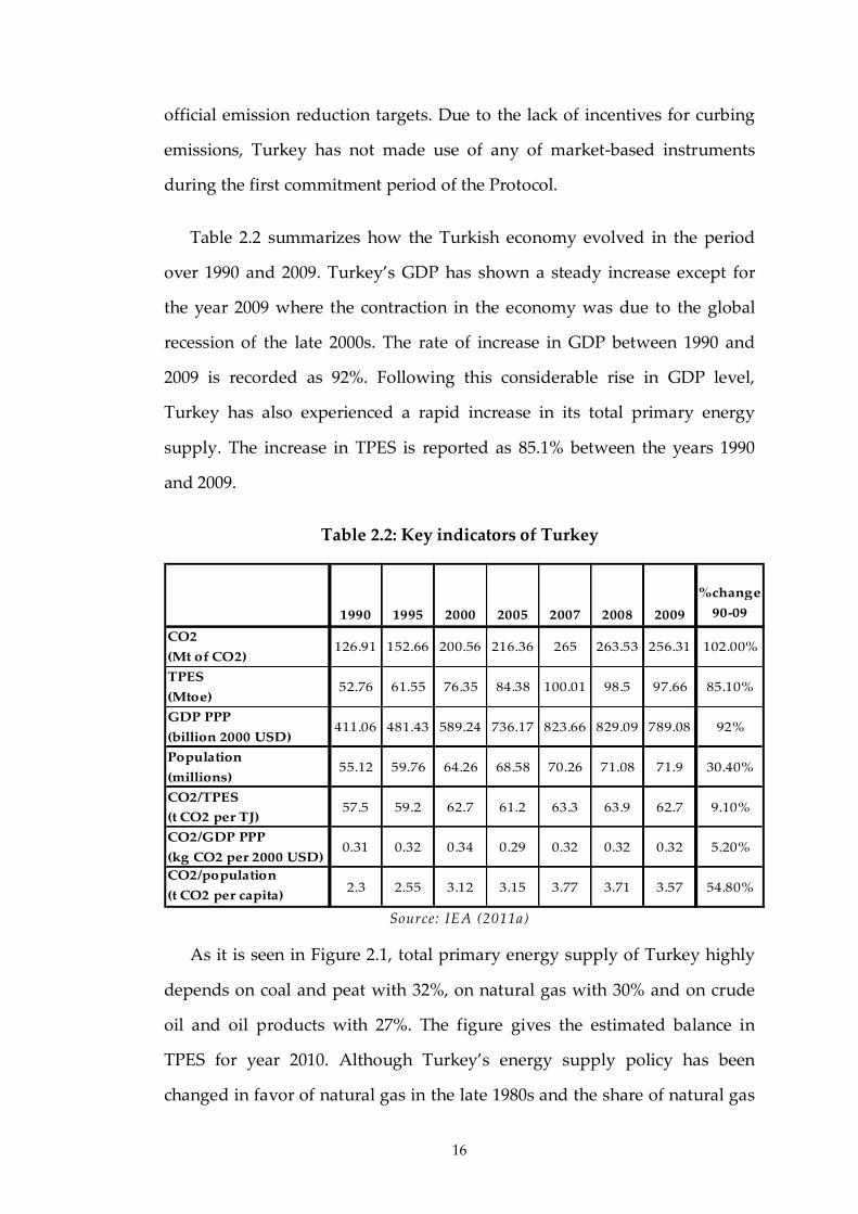
Table 2.2 summarizes how the Turkish economy evolved in the period

over 1990 and 2009. Turkey’s GDP has shown a steady increase except for

the year 2009 where the contraction in the economy was due to the global

recession of the late 2000s. The rate of increase in GDP between 1990 and

2009 is recorded as 92%. Following this considerable rise in GDP level,

Turkey has also experienced a rapid increase in its total primary energy

supply. The increase in TPES is reported as 85.1% between the years 1990

and 2009.

Table 2.2: Key indicators of Turkey

1990 1995 2000 2005 2007 2008 2009

%change

90-09

CO2

(Mt of CO2)126.91 152.66 200.56 216.36 265 263.53 256.31 102.00%

TPES

(Mtoe)52.76 61.55 76.35 84.38 100.01 98.5 97.66 85.10%

GDP PPP

(billion 2000 USD)411.06 481.43 589.24 736.17 823.66 829.09 789.08 92%

Population

(millions)55.12 59.76 64.26 68.58 70.26 71.08 71.9 30.40%

CO2/TPES

(t CO2 per TJ)57.5 59.2 62.7 61.2 63.3 63.9 62.7 9.10%

CO2/GDP PPP

(kg CO2 per 2000 USD)0.31 0.32 0.34 0.29 0.32 0.32 0.32 5.20%

CO2/population

(t CO2 per capita)2.3 2.55 3.12 3.15 3.77 3.71 3.57 54.80%

Source: IEA (2011a)

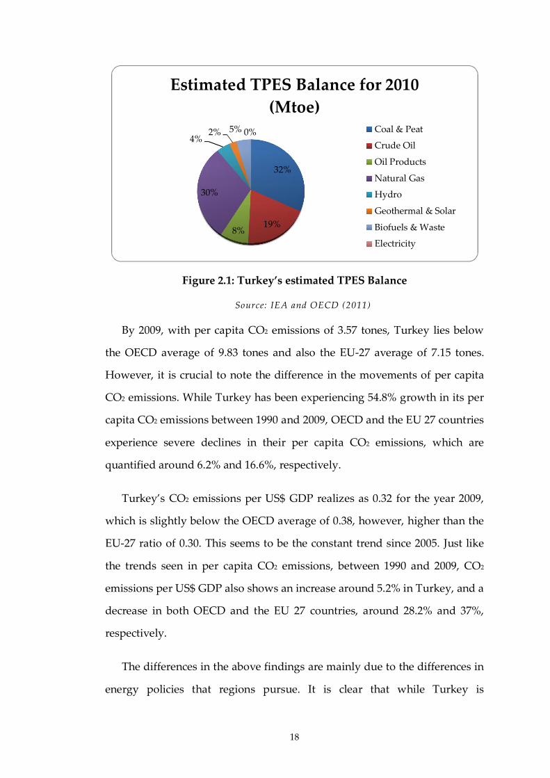
As it is seen in Figure 2.1, total primary energy supply of Turkey highly

depends on coal and peat with 32%, on natural gas with 30% and on crude

oil and oil products with 27%. The figure gives the estimated balance in

TPES for year 2010. Although Turkey’s energy supply policy has been

changed in favor of natural gas in the late 1980s and the share of natural gas

17

in TPES has been rising steadily since then, the composition of TPES has

been more stable starting with 2005. The share of renewable resources in

TPES stays fairly low at 4% for hydro, 5% for bio-fuels and 2% for

geothermal and solar resources. As coal, peat, oil and natural gas are energy

sources which are rich in carbon contents, it is not surprising to see the

highly significant rise in Turkey’s CO2 emissions between the period 1990

and 2009. Turkey’s CO2 emissions increase from 126.91 Mt CO2 in 1990 to

256.31 Mt CO2 in 2009, corresponding to a rise of 102%. Within the same

period of time, the increase in CO2 emissions of OECD countries is 8%, while

the European Union experiences a decline in total emission level at rate

11.7%.

In their quantitative studies, Lise (2006), Tunc et al. (2009) and

Kumbaroglu (2011) try to unfold the effects underlying the increase in CO2

emissions of Turkey. The potential effects are assumed to be scale effect, i.e.

change in emissions due to changing activity levels, composition effect, i.e.

change in emissions due to changes in the composition of sectors, energy-

intensity effect, i.e. change in emissions due to changes in the efficiencies of

the energy processes and conversion technologies and carbon-intensity

effect, i.e. change in emissions due to fuel substitution. As a result, it is seen

that the largest portion of the increase in CO2 emissions is mainly due to the

expansion of the economy (scale effect), which is further accompanied by the

composition effect. Taking into account this fact, Telli et al. (2008) predicts

that the increase in total CO2 emissions by 2020 will be 99% compared to the

2009 levels.

18

Figure 2.1: Turkey’s estimated TPES Balance

Source: IEA and OECD (2011)

By 2009, with per capita CO2 emissions of 3.57 tones, Turkey lies below

the OECD average of 9.83 tones and also the EU-27 average of 7.15 tones.

However, it is crucial to note the difference in the movements of per capita

CO2 emissions. While Turkey has been experiencing 54.8% growth in its per

capita CO2 emissions between 1990 and 2009, OECD and the EU 27 countries

experience severe declines in their per capita CO2 emissions, which are

quantified around 6.2% and 16.6%, respectively.

Turkey’s CO2 emissions per US$ GDP realizes as 0.32 for the year 2009,

which is slightly below the OECD average of 0.38, however, higher than the

EU-27 ratio of 0.30. This seems to be the constant trend since 2005. Just like

the trends seen in per capita CO2 emissions, between 1990 and 2009, CO2

emissions per US$ GDP also shows an increase around 5.2% in Turkey, and a

decrease in both OECD and the EU 27 countries, around 28.2% and 37%,

respectively.

The differences in the above findings are mainly due to the differences in

energy policies that regions pursue. It is clear that while Turkey is

32%

19%8%

30%

4%2% 5% 0%

Estimated TPES Balance for 2010

(Mtoe)Coal & Peat

Crude Oil

Oil Products

Natural Gas

Hydro

Geothermal & Solar

Biofuels & Waste

Electricity

19

experiencing emission intensive growth, due to its energy policies, OECD

and the EU-27 countries, on average, pursue energy policies that are more

reliant on less emission intensive inputs. This fact is also clearly reflected in

the CO2/TPES ratios, in which the change between 1990 and 2009 is

quantified as 9.1% for Turkey, -6.8% for OECD countries and -12.8% for the

EU-27 countries.

IMF (2012) projects the annual growth rate of Turkish economy for

the period between 2012 and 2017 as 3.7% on average, while IEA (2011b)

projects it as 4.0% on average. Taking into account Turkey’s energy supply

policies, in the long run, it is inevitable that Turkey will face rapid increase in

its CO2 emissions in a way closing the gap in terms of CO2 emissions per

capita and per US$ GDP with both OECD and the EU-27 countries.

2.4.2. Post-Kyoto world

As an EU candidate country and an OECD member country, Turkey has

been under pressure to formalize its national action plan against curbing its

CO2 emissions in the post-Kyoto period. In the latest progress report of

European Commission, the need for a well defined emission reduction target

and also the need for cooperation with the EU in emission trading is

emphasized (European Commission 2011). In line with the European

Commission’s report, the OECD Environmental Performance Review for

Turkey, reports that Turkey should take an action against its increasing CO2

emissions and that Turkey should consider the use of market-based

instruments like pollution charges and emission trading systems to meet its

objectives of efficiency and financing (OECD 2008).

The ministry of environment and urbanization (MEU) delivered Turkey’s

national vision within the scope of climate change in the National Climate

20

Change Action Plan: 2011 – 2023 (Ministry of Environment and Urbanization

2011). Within this document, Turkey’s objectives are stated as becoming a

country fully integrating climate change related objectives into its

development policies, improving energy efficiency, increasing the use of

renewable energy sources and decreasing its emissions. In managing CO2

emissions, the Action Plan strongly emphasizes the establishment of national

emission trading system in Turkey by 2015 and further integration with the

existing and new global and regional carbon markets. In that regard, State

Planning Organization (SPO) delivered Istanbul Finance Strategy and Action

Plan, which defines the prospective national carbon market to be established

in Turkey (DPT 2009). To make more emphasis on the dedication of Turkey,

it is also crucial to note the initial grant of $350,000 to Turkey by World

Bank’s Partnership for Market Readiness for developing and piloting of

market-based instruments for greenhouse gas reduction (World Bank 2011).

Meanwhile, the environment chapter in the EU enlargement process

has also opened. This chapter necessitates that the EU Emission Trading

Directive (European Commission 2003) is to be transposed into Turkish

Environmental Law as part of the legislation. Therefore, Turkey is eventually

expected to integrate with the EU ETS market along its accession process to

join the EU. As being world’s largest international carbon market, the EU

ETS stands as a very good example for Turkey in establishing its national

permit market and a potential partner for international carbon trading.

In case of Turkey, while the lack of clear-cut emission targets results in a

scarcity of quantitative studies, the lack of adequate economic analysis

makes it even harder to formalize well defined emission targets and a

probable design of such a cap-and-trade system. (Sahin 2004) is the first

quantitative modeling paradigm to quantify the economic impacts of a

regional cap-and-trade system and to compare and contrast the findings

21

with the applications of energy taxes. The model is set up as a static, single

country general equilibrium model. The tradable emission permits, which

are grandfathered, are added to the model following the primal approach

defined in (McKibbin & Wilcoxen 1999). The model takes 1990 as the

benchmark year. As a result of the policy simulations, it is seen that

imposition of environmental measure in Turkey does not lead to a drastic

deterioration of the economic performance and tradable permit system gives

similar results with energy taxes in terms of economic efficiency. Sahin and

Pratlong (2003) evaluate the proper regulation in a possible cap-and-trade

system within the same general equilibrium set up in (Sahin 2004). In that

regard, upstream, downstream and hybrid approaches, which are used in

determining the liable entities under a tradable permit system, are tested.

Main finding is that upstream approach is more efficient both economically

and environmentally; while downstream approach offers greater flexibility.

In a more recent study by Aydin and Acar (2010), the economic effects of the

EU’s post-Kyoto mitigation policies under the case of Turkey’s accession to

the EU are explored in a general equilibrium framework. In this study, the

EU applies 20% emission cutback with regard to 1990 levels and Turkey is

assumed to increase its CO2 emissions by 10% compared to 2010 levels.

While the scenarios are run under the assumptions of capital and labor

mobility, there exist two separate cap-and-trade systems in the model, i.e.

one in Turkey and one in the EU. In that regard, the segmented cap-and-

trade system6 that the EU is planning to run in the post-Kyoto period is not

fit accurately into the model formulation. Additionally, the integration

between Turkey’s national permit markets with the EU ETS market, which

6 ETS and non-ETS sectors are subject to separate systems.

22

will take place in case of the EU enlargement, is also not covered accurately

in the scenarios.

2.5. Longer Term Perspective on Market-based Regulations

2.5.1. Linking regional cap-and-trade systems

The literature on cap-and-trade systems has developed extensively since

trading systems started to be used as one of the flexibility mechanisms with

the Kyoto Protocol (Tietenberg et al. 1999). As the need for collective action

against rising CO2 emissions grows, the part of this literature assessing the

economic and environmental effects of linking different cap-and-trade

systems also develops.

Linking of emission trading schemes, in order to approach to a global

carbon market, can be achieved via different ways. The first best policy is

defined to be the top-down approach, i.e. imposing emission targets for all

regions by an international agreement and allowing these regions to trade in

a global carbon market. The second best policy is defined as establishing two

way direct links between regional cap-and-trade systems (Browne 2004;

Aldy & Stavins 2007a). The Kyoto Protocol and the conference of parties

succeeding that have repeatedly failed to apply the top-down approach.

Hence, bottom-up approaches started to be discussed extensively.

Efficiency gains out of linking different emission trading schemes can be

classified as static and dynamic efficiency gains. Flachsland et al. (2009)

defines dynamic efficiency as increased international cooperation in the long

run stimulated by increased bilateral cooperation. In addition to that, direct

linking of cap-and-trade schemes results in price equalization across the

linked schemes resulting in reduced aggregate abatement costs compared to

ex ante abatement costs (Haites 2001; Blyth & Bosi 2003). The proper

23

functioning of the carbon market due to increased liquidity and decreased

price volatility should also be counted as part of the static efficiency gains

out of direct linking (Baron & Bygrave 2002).

In opposed to its gains, linking may also lead to some efficiency losses

due to strategic behaviors. Helm (2003) argues that allowance trading can

give incentives for permit exporters in order to gain more from permit sales

by simply decreasing their caps. On the other hand, Carbone et al. (2009)

points out that, in case of an expectation for increase in allowance prices,

there can also be an incentive for permit exporters to increase their caps to

raise revenues from allowance sales.

Besides its direct effects on the permit markets, linking provisions can

also have some indirect effects on the overall performance of the economies,

i.e. aggregate economic activity level, sectors, employment, factor prices and

technologies. As a response to the changes in the volume of the permit

market and also in the permit price level, the distribution among permit

sellers and buyers arranges accordingly. The degree of ability to substitute

between dirty inputs, i.e. fossil fuel inputs and also the energy intensity of

production technologies determines the shifts in the regional abatement

activities. Thus, the profiles of buyers and sellers in the market may change.

Following that, the production levels and input compositions of sectors are

also affected. Hence, as a result of linking provisions, the total economic

activity also changes. In addition, shifts in abatement activities may induce

other benefits in the form of reduced fossil fuel dependence and incentives

for transforming economies into low-carbon economies (Westskog 2002).

24

2.5.2. Linking options for the EU ETS

The European Union strongly encourages to establish direct links

between the EU ETS and the other cap-and-trade systems for the post-Kyoto

period (European Commission 2009). Articles 40 and 41 approve the

cooperation with the third countries neighboring the EU, together with

candidate and potential candidate countries. In essence, the EU considers the

EU ETS to become the nucleus of an international carbon market (European

Commission 2006; Aldy & Stavins 2007b). Two important features are noted

by Ellerman and Joskow (2008), which make the EU ETS eligible for a global

prototype: the weak federal structure with member states having certain

degree of autonomy and the differences in economic and institutional

development among the EU member states.

Despite the overall cost effectiveness of bottom up linking between cap-

and-trade systems, it is not straightforward to conclude that linking is

always economically and environmentally efficient for both parties. In their

theoretical study, Eyckmans and Hagem (2011) show that the EU countries

can benefit from the bottom up linking of regional cap-and-trade systems in

case of certain trade agreements. They test their hypothesis in the numerical

simulation between the EU and China for the year 2015. They find that

under trade agreements involving permit sales requirements and certain

levels of financial transfers, linking cuts the EU’s total compliance cost

considerably. In another study, Anger (2008) states that there are strong

signs to link the EU ETS with the newly emerging permit markets in non-EU

countries by 2020. Thus, he studies bottom up linking of the EU-ETS with

these newly emerging market schemes beyond Europe, i.e. Japan, Canada,

the US and the OECD Pacific countries. Based on the numerical multi-

country, multi-sector partial equilibrium model of the world carbon market,

25

he finds that linking the EU-ETS with the emerging permit markets induces

minor economic benefits for the EU. However, the economic impacts for

non-EU countries can be various depending on the domestic inefficiencies.

Thus, it is seen that the costs and benefits from linking highly depend on the

characteristics of the linking regions. In order to accurately assess the

economic impacts of linking, it is indispensible to conduct region specific

theoretical and numerical analysis.

2.6. Concluding Comments

Cap-and-trade systems have been widely used since the Kyoto Protocol.

The need for an international cooperation in worldwide mitigation efforts

sped up the use of permit trading schemes. Though, a global carbon market

seems still not applicable. Instead, as a second best policy, the linking

between different cap-and-trade systems has started to be seen as an

alternative to a global carbon market. As a result, the regional abatement

strategies are not limited to regional permit trading anymore. Countries have

also been following the policies for integrating into existing or newly formed

permit markets worldwide.

From that point of view, the EU ETS market, which is the largest permit

trading market operating in the world, is defined to be the nucleus of a

potential international carbon market. The European Union has already

declared its commitment by integrating with national permit systems of

Norway, Iceland and Liechtenstein in 2008. In that regard, the EU

enlargement process is also seen as an opportunity for increasing

international cooperation in permit trading. Taking into account these,

Turkey seems to be one of the most likely candidate countries to integrate

with the EU ETS market as part of its EU accession process. However,

Turkey is at the onset of establishing its national permit market and linking

26

with the EU ETS should follow as the next step. Hence, the essentials of both

Turkish national permit systems and also of its integration with the EU ETS

have to be analyzed and set carefully.

27

CHAPTER 3

Analysis of Market-based Environmental Regulation in General

Equilibrium Framework

3.1. Introduction

This chapter introduces the MR-ETPA (multi-region environmental and

trade policy analysis) model, which is a multi-region, multi-sector

computable general equilibrium (CGE) model. I develop the MR-ETPA

model mainly for simulating market-based environmental policies, the so-

called permit trading together with various trade policy interventions.

Regarding the design of permit trading schemes, I give the main focus on

the market segmentation and alternative ways of burden sharing worldwide

via permit trading. Hence, the MR-ETPA model is capable of having permit

trading markets both at national and international levels. National permit

markets are able to integrate with the international permit markets. With

respect to the market segmentation, the MR-ETPA model allows the sector

coverage of CO2 abatement policies to differ across regions.

Within the current set up of the MR-ETPA model, I also model other

commonly used economic incentives for CO2 abatement, namely CO2 taxes.

28

The explicit treatment of trade linkages between regions further allows for

modeling additional measures used in climate mitigation actions, such as

CO2 border tariffs.

The detailed elaboration of the underlying economic dynamics of the

MR-ETPA model is given in Section 3.2. The methodology that I use in the

characterization of the economic equilibrium and in the characterization of

consumption and production behaviors are explained in Section 3.3. In

Section 3.4, I further provide the details regarding the numeric

implementation of the MR-ETPA model. Sections 3.5 and 3.6 have the set

definitions, parameters, endogenous, exogenous and ancillary variables that

I use in the algebraic and numerical formulation of the MR-ETPA model. I

elaborate on the linkages between the theoretical underpinnings of the

model structure and its characterization in Sections 3.7 and 3.8.

3.2. Model Description

The MR-ETPA model is a static CGE model of commodity and permit

trading in multi-country and multi-sector setting. Market-based abatement

policies incur additional costs to certain sectors in the economies, which

often differ across regions. Hence, due to the changes in relative prices, both

abating and also non-abating regions are subject to certain economic costs in

terms of output and deterioration of international competitiveness. Hence,

analyzing the economic impacts of market-based abatement policies in a

partial equilibrium setting and neglecting the likely general equilibrium

effects is definitely misleading in terms of quantifying the associated costs

and specifying the underlying dynamics. In order to grasp the potential

general equilibrium effects, I formulate the MR-ETPA model based on the

Arrow-Debreu general equilibrium framework. The assumption of

underlying optimizing behavior of all agents further enhances the relevance

29

of the MR-ETPA model for policy analysis, as the outcome of any policy

intervention can be traced back to rational behavior. For the sake of the

current policy agenda, I prefer to use general equilibrium framework in

multi-country and multi-sector setting. This kind of treatment gives the MR-

ETPA model the ability to analyze the abatement policy options that the real

world economies currently face in a more realistic way. Due to the increase

in size and complexity of the MR-ETPA model, in terms of the number of

production sectors, pre-existing taxes and externalities, I use computable

general equilibrium format. The CGE formulation is useful in quantifying

the magnitude, and thus not only the sign, of the impact of changes in

exogenous conditions on key economic variables. Therefore, it becomes

tractable with the MR-ETPA model to identify and quantify the general

equilibrium effects of changes in exogenous conditions that initially are not

obvious.

In the algebraic formulation of the MR-ETPA model, all markets are

perfectly competitive, that is to say, all agents are price takers. There is one

representative agent in each economy who owns the primary factors of

production, i.e. capital, labor and resources. Labor and capital are assumed

to be mobile across sectors within regions but internationally immobile.

Resource inputs are sector-specific inputs. All production factors are

supplied inelastically in the factor markets. Each production sector takes

primary inputs and produces only one commodity output according to

certain production technologies. Products are either consumed in the

domestic market or exported. The model also has separate government and

investment accounts. Though, in the algebraic exposition of the model, these

accounts do not have separate economic agents. Instead, representative

agent in each economy is taken as the respective agent who is also

responsible for government consumption and investment activities.

30

Demands for investment and public provision are exogenously fixed at

benchmark levels. Tax revenues add up to the income of the representative

agent. Each regional economy is open to trade with the other regions and

trade balances are fixed exogenously.

The underlying reason for using the macro closures combining fixed

foreign savings, fixed real investment and fixed real public consumption is

mainly to be able to explore the pure welfare effects in equilibrium of

alternative policies in a static framework (Johansen 1960). Such a closure rule

minimizes the biased welfare effects that would otherwise occur with

endogenous foreign savings and real investment in the later periods, which

is not possible to account for in a static model. In addition to that, since the

model does not capture the direct effects of public provision on household’s

welfare, it is also preferred to use government consumption as fixed

exogenously.

In order to include permit trading market, the static trade model is

further expanded with integrating emission creation mechanism and giving

incentives to trade permits. In the MR-ETPA model, permit trading is only

allowed for CO2 permits; other greenhouse gases are not included in the

permit trading. To establish CO2 permit trading market, permit demand side

is specified as production and consumption units which are potential users

of energy goods that cause CO2 emissions. The permit supply side is defined

as governmental unit which is obliged to supply allowances to the CO2

emitters.

In each economy, CO2 emissions are created by use of fossil fuels, i.e. coal,

oil and natural gas. The CO2 emitters which are required to hold allowances

in equal amounts to their total emissions, can be either “upstream”, i.e.

suppliers of dirty inputs, or “downstream”, i.e. users of dirty inputs. In

31

practice, it is more common to oblige downstream entities since this provides

more direct response to any change in price levels, compared to upstream

obligations (IEA 2010). In that regard, the EU ETS market also uses the

downstream approach. As one of the main purposes of this study is to

quantify the welfare effects of Turkey’s integration to the EU ETS market, in

the model formulation, the liable entities that are charged for creating

emissions are assumed to be the downstream entities. Hence, any production

and consumption activity in the MR-ETPA model are taken as CO2 emitters

which demand allowances equal to their total CO2 emissions.

CO2 emitters are subject to certain CO2 quotas which are fixed

exogenously. Allowances, in equal amounts to the target CO2 emission

levels, are supplied by the governmental bodies. Auctioning is used for

allocating allowances to the emitters. Three strategies exist for emitters. The

first strategy is that emitters abate the amount equal to the difference

between their allowance budgets and actual emission volumes. The other

strategies are to abate more or abate less than the initial abatement schedule,

which is fixed by the initial allocation. In the case of last two options, the

emitters are also free to trade allowances at the permit trading market. The

incentives to trade permits in the market come from the tradeoff between

permit prices and marginal costs of abatement, i.e. emitters with high

marginal abatement costs (MACs) have the incentives to buy permits from

the emitters with low MACs. In the model formulation, the differences in

marginal abatement cost structures mainly stems from the differences

between regions, regarding the emission limitations, production

technologies and consumption behaviors.

Marginal abatement cost curves are widely used to illustrate the main

rationale behind permit trading. They are also commonly applied in

analyzing the permit market dynamics and permit price levels prevailing in

32

any cap-and-trade system (Ellerman & Decaux 1998; Criqui et al. 1999;

Blanchard et al. 2002). In all these studies, it is implicitly assumed that MAC

curve of each region is robust against any abatement policy taken abroad.

However, the use of MAC curves should be taken with extreme caution as

they are not necessarily independent of the intersectoral, macroeconomic

and international interactions. These kind of inter-regional and intra-regional

interdependencies are likely to affect MAC structures of different regions.

Klepper and Peterson (2006) argue that MACs in a general equilibrium

framework are affected by changes in world energy prices and the

magnitude of the differences depends on trade patterns. In another study by

Morris Jennifer et al. (2008), the MAC curves derived by using the MIT

Emissions Prediction and Policy Analysis (EPPA) model are shown to be

dependent on the level of abatement policy elsewhere. They test the

robustness of MAC curves and conclude that MAC curves seem to be more

stable if they are calculated by taking into account the shifts in the baselines

for countries through changes in energy prices. In contrast to that, if the shift

is not taken into account, they found extreme instabilities in the MAC

curves, hence large errors in the predicted permit market outcomes.

Due to the aforementioned caveats in using MAC curves explicitly in

modeling permit trading, I take a different approach in the MR-ETPA model.

In his theoretical paper, Montgomery (1972) proves that the equilibrium

allocation of permits, the market-determined permit price and the aggregate

costs of abatement are independent of the initial allocation of permits. Fowlie

and Perloff (2008) further support this theoretical finding in their applied

work. Therefore, depending on the structure of the MR-ETPA model with

perfectly competitive markets and zero transaction costs, I implicitly derive

the permit price as the respective shadow price of the aggregate CO2 quotas.

The corresponding price is the price at which MACs are equalized across all

33

regions and sectors involved in permit trading. The equilibrium allocation of

permits and aggregate abatement costs are derived accordingly. This way of

modeling permit trading assures that each region’s MAC takes into account

any change in abatement or economic policies abroad. This is mainly due to

the fact that MACs are modeled as functions of both domestic and also

international price levels. Thus, robustness and accuracy of the permit

market outcomes increase.

In the MR_ETPA model, permit trading is modeled both at international

and regional levels. That is to say it is possible for regions to run their

regional cap-and-trade systems and also to integrate with international cap-

and-trade systems, simultaneously. Furthermore, the model also allows for

market segmentation, in the sense that certain sector groups are allowed to

trade permits with each other. The decision regarding the grouping of

sectors is on each region’s own initiative.

3.3. Model Formulation

3.3.1. Characterization of economic equilibrium

In the competitive economy setup of the model, the preferences of

consumers and also the technologies of activities are defined in terms of

constant return to scale functions. Constant elasticity of substitution (CES)

functions is especially preferred as they allow for different elasticity

constants between different goods via nesting structure. Further details on

the structure of CES functions are found in Section 3.8.

Economic equilibrium is characterized as a mixed complementarity

problem (MCP) (Mathiesen 1985; Cottle et al. 1992; Rutherford 1995).

Therefore, equilibrium conditions are stated as weak inequalities: zero profit

conditions, market clearance conditions and income balance constraints,

34

which feature complementary slackness with the corresponding equilibrium

variables: price variables, activity levels and income levels. More detailed

discussion of MCP approach to general equilibrium is given in Section 3.7.

Zero profit conditions are algebraically stated as in (3.1), where “p” is the

price vector, “y” is the quantity vector and “c(p)” stands for the vector of unit

cost functions of the activities. As the complementary slackness condition

implies, the activities are not slack as long as the unit cost of production is

equal to the unit revenue.

( ) 0, 0, ( ) 0 p c p y y p c p

(3.1)

Market clearance conditions are given in (3.2), in terms of the price

vector, “p” and excess demand function, “z(p)”. This condition assures the

supply and demand balance, as it implies that price level hits zero in case of

excess supply.

( ) 0, 0, ( ) 0z p p p z p

(3.2)

The necessary sets, parameters, price, quantity and income variables that

characterize the economic equilibrium are given in Section 3.5. Additionally,

ancillary variables used for the algebraic exposition of the equilibrium

conditions are given in Section 3.5, as well.

3.3.2. Activities and zero profit conditions

3.3.2.i. Private consumption activity

The representative agent (RAr) spends its income on private consumption

after saving some amount of it. Consumption activity is made to maximize

well-being, which is quantified in utility terms. RAr gets utility from

35

consumption of final goods, either domestically produced or imported. The

corresponding optimization problem is given below, where Cry represents

the utility level and Crp is the consumer price index in region r.

max

. .

Cr

C Cr r r

y

s t p y income (3.3)

The optimality condition of the utility maximization problem in (3.3),

under the assumption of convex preferences, leads to the fact that the income

balance constraint has to hold with equality at the maximum level of utility.

Therefore, the condition (3.4) is included as the necessary condition for the

utility maximization of the representative agent.

C r

Crr

incomey

p (3.4)

The consumption behavior of the RAr is formulated as a separate activity

in the model formulation. Nested CES functions are used to model the

private consumption demand. At the first level, non-energy material

aggregate trades off with the energy aggregate. At the second level, both

non-energy goods and energy goods are aggregated in separate CES nests.

The corresponding zero profit condition for private consumption activity is

given in (3.5). The left hand side of the inequality is the unit cost function,

while the right hand side stands for consumer price index of region r. The

user cost of energy goods is stated as the sum of their market prices and also

the additional cost of holding allowances in equal amounts to the emissions

they create during the consumption activities. The coefficient 2cojCrio stands for

the amount of emissions created out of unit consumption of fossil fuel j.

Under mitigation policies, this also equals to the amount of allowances that

the respective emitter must hold. The price of allowance is given by 2rpco in

36

(3.5). It is crucial to note that the price that consumers face in each region

differs from region to region.

1

11

12

( )

11

11

( )

2

1 ,

ci

cc

c csi i

c

c

se

eC E mat cor Cr jCr ir jCr r

j e j

sm

mE mat C CCr jCr jr r r

j e j

c pa io pco

pa p y

(3.5)

3.3.2.ii. Production activities

Production technologies of non-extractive industries are captured via

there level nested separable CES functions. Figure 3.1 shows the nesting

structure in more detail. At the top level, energy composite trades off with an

aggregate of factors and non-energy inputs. At the second level, Leontief

function is used to combine factor aggregate and energy aggregate. Energy

composite is a CES aggregate of electricity and other fossil fuel inputs. At the

third level, CES functions describe the substitution patterns between factor

inputs within value-added composite and also between non-energy material

inputs within non-energy aggregate. Producers pay ad-valorem factor taxes

over factor inputs and also output taxes.

1

11 11 1

1

( )

1

12

( )

1 (1 )

(1 ) 2

ydsi

vai i i

i

i

va mmYD klm va f va mat

ir ir ir fir fr fir ir jir jrf j e j

s

eklm mat coir jir ir jir r

j e j

c pf rtf pa

pa io pco

11

1

1 ,

, ( )

yd ydi i

i

se

ir ir

ir

rto pd

yd i xe i

(3.6)

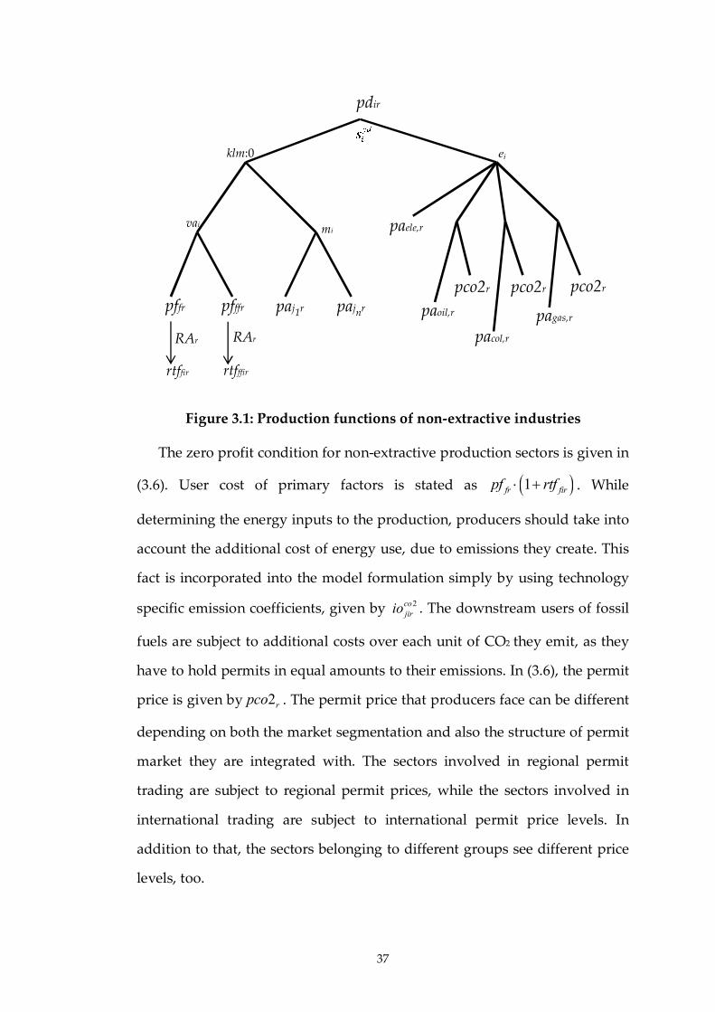
37

Figure 3.1: Production functions of non-extractive industries

The zero profit condition for non-extractive production sectors is given in

(3.6). User cost of primary factors is stated as 1fr firpf rtf . While

determining the energy inputs to the production, producers should take into

account the additional cost of energy use, due to emissions they create. This

fact is incorporated into the model formulation simply by using technology

specific emission coefficients, given by 2cojirio . The downstream users of fossil

fuels are subject to additional costs over each unit of CO2 they emit, as they

have to hold permits in equal amounts to their emissions. In (3.6), the permit

price is given by 2rpco . The permit price that producers face can be different

depending on both the market segmentation and also the structure of permit

market they are integrated with. The sectors involved in regional permit

trading are subject to regional permit prices, while the sectors involved in

international trading are subject to international permit price levels. In

addition to that, the sectors belonging to different groups see different price

levels, too.

pdir

pffr pfffr paj1r

pco2r

paele,r

pajnr … paoil,r

pacol,r

pagas,r

pco2r pco2r

klm:0

vai

ei

mi

RAr RAr

rtffir rtfffir

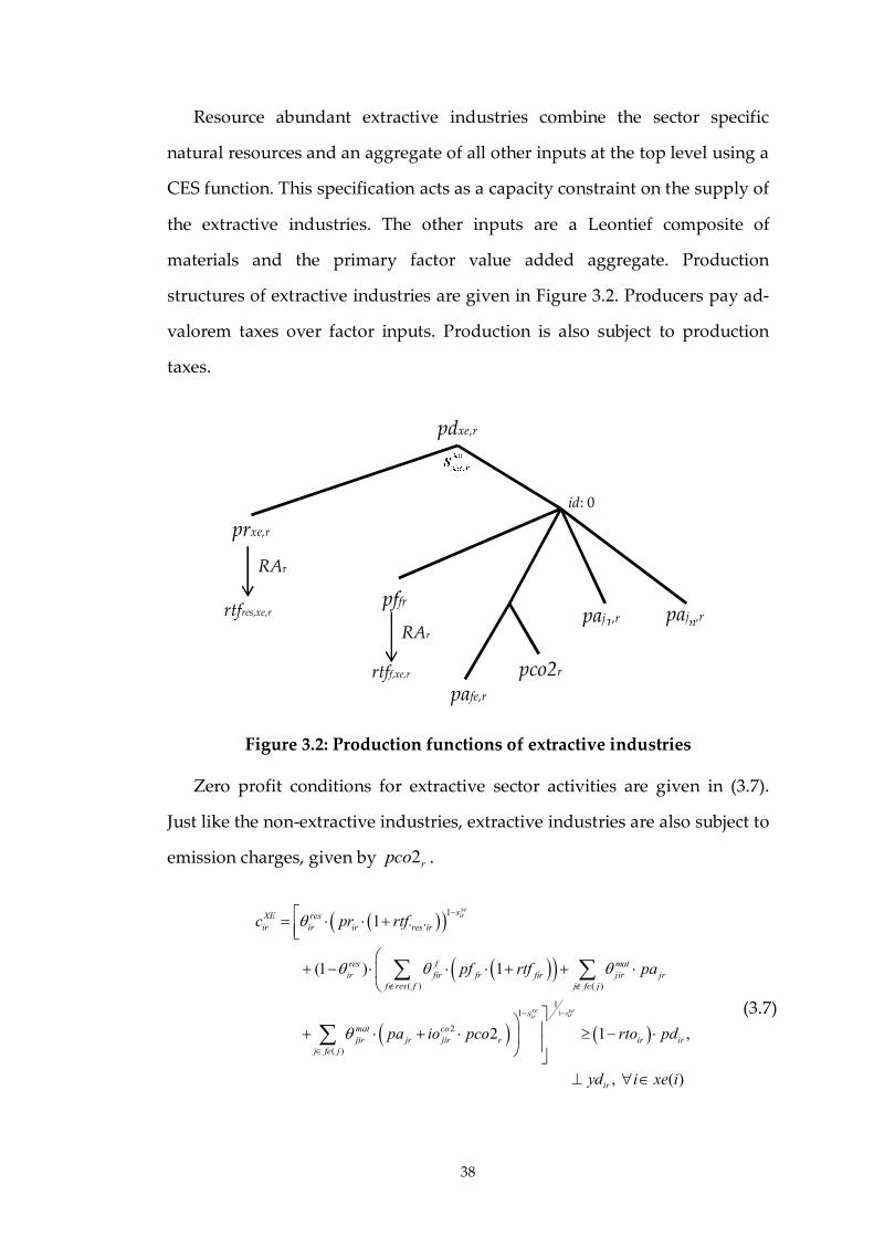
38

Resource abundant extractive industries combine the sector specific

natural resources and an aggregate of all other inputs at the top level using a

CES function. This specification acts as a capacity constraint on the supply of

the extractive industries. The other inputs are a Leontief composite of

materials and the primary factor value added aggregate. Production

structures of extractive industries are given in Figure 3.2. Producers pay ad-

valorem taxes over factor inputs. Production is also subject to production

taxes.

Figure 3.2: Production functions of extractive industries

Zero profit conditions for extractive sector activities are given in (3.7).

Just like the non-extractive industries, extractive industries are also subject to

emission charges, given by 2rpco .

1

1

' '

( ) ( )

11

2

( )

1

(1 ) 1

2 1 ,

xeir

xe xesirir

sXE res

ir ir ir res ir

res f matir fir fr fir jir jr

f res f j fe j

s

mat cojir jr jir r ir ir

j fe j

c pr rtf

pf rtf pa

pa io pco rto pd

, ( )iryd i xe i

(3.7)

pco2r

pdxe,r

pffr

prxe,r

paj1,r pajn,r …

pafe,r

id: 0

rtfres,xe,r

RAr

rtff,xe,r

RAr

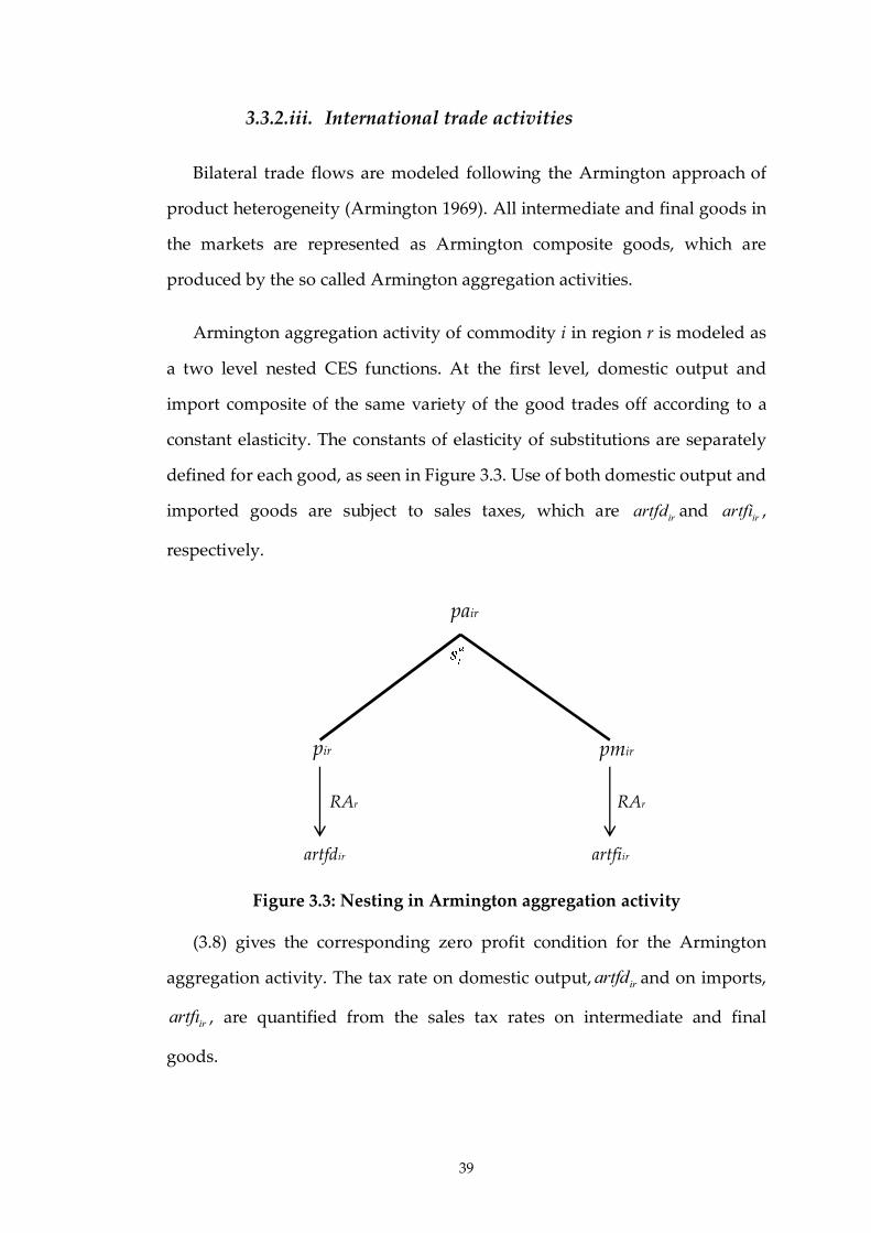
39

3.3.2.iii. International trade activities

Bilateral trade flows are modeled following the Armington approach of

product heterogeneity (Armington 1969). All intermediate and final goods in

the markets are represented as Armington composite goods, which are

produced by the so called Armington aggregation activities.

Armington aggregation activity of commodity i in region r is modeled as

a two level nested CES functions. At the first level, domestic output and

import composite of the same variety of the good trades off according to a

constant elasticity. The constants of elasticity of substitutions are separately

defined for each good, as seen in Figure 3.3. Use of both domestic output and

imported goods are subject to sales taxes, which are irartfd and irartfi ,

respectively.

Figure 3.3: Nesting in Armington aggregation activity

(3.8) gives the corresponding zero profit condition for the Armington

aggregation activity. The tax rate on domestic output, irartfd and on imports,

irartfı , are quantified from the sales tax rates on intermediate and final

goods.

pair

pir

pmir

RAr

artfdir artfiir

RAr

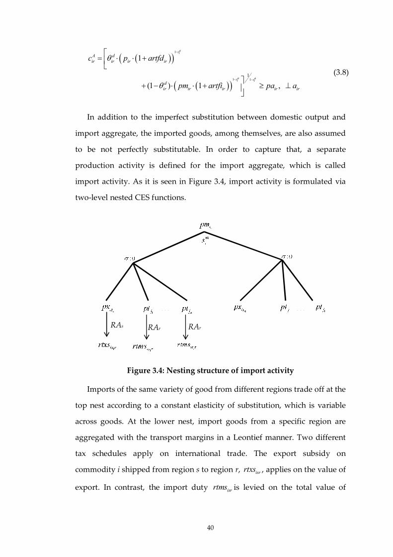
40

1

1 11

1

(1 ) 1 ,

asi

a as si i

A dir ir ir ir

dir ir ir ir ir

c p artfd

pm artfi pa a

(3.8)

In addition to the imperfect substitution between domestic output and

import aggregate, the imported goods, among themselves, are also assumed

to be not perfectly substitutable. In order to capture that, a separate

production activity is defined for the import aggregate, which is called

import activity. As it is seen in Figure 3.4, import activity is formulated via

two-level nested CES functions.

Figure 3.4: Nesting structure of import activity

Imports of the same variety of good from different regions trade off at the

top nest according to a constant elasticity of substitution, which is variable

across goods. At the lower nest, import goods from a specific region are

aggregated with the transport margins in a Leontief manner. Two different

tax schedules apply on international trade. The export subsidy on

commodity i shipped from region s to region r, isrrtxs , applies on the value of

export. In contrast, the import duty isrrtms is levied on the total value of

…

…

RAs RAr

RAr

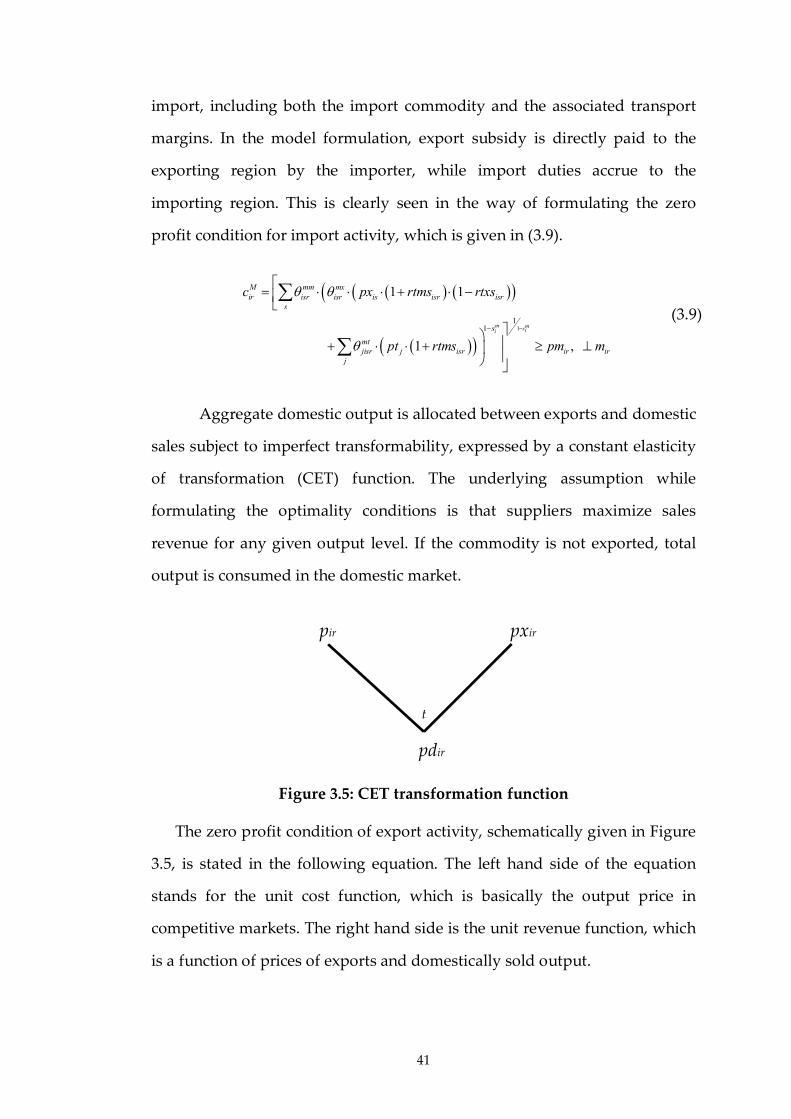
41

import, including both the import commodity and the associated transport

margins. In the model formulation, export subsidy is directly paid to the

exporting region by the importer, while import duties accrue to the

importing region. This is clearly seen in the way of formulating the zero

profit condition for import activity, which is given in (3.9).

1

11

1 1

1 ,

m msii

M mm mxir isr isr is isr isr

s

s

mtjisr j isr ir ir

j

c px rtms rtxs

pt rtms pm m

(3.9)

Aggregate domestic output is allocated between exports and domestic

sales subject to imperfect transformability, expressed by a constant elasticity

of transformation (CET) function. The underlying assumption while

formulating the optimality conditions is that suppliers maximize sales

revenue for any given output level. If the commodity is not exported, total

output is consumed in the domestic market.

Figure 3.5: CET transformation function

The zero profit condition of export activity, schematically given in Figure

3.5, is stated in the following equation. The left hand side of the equation

stands for the unit cost function, which is basically the output price in

competitive markets. The right hand side is the unit revenue function, which

is a function of prices of exports and domestically sold output.

pxir pir

pdir

t

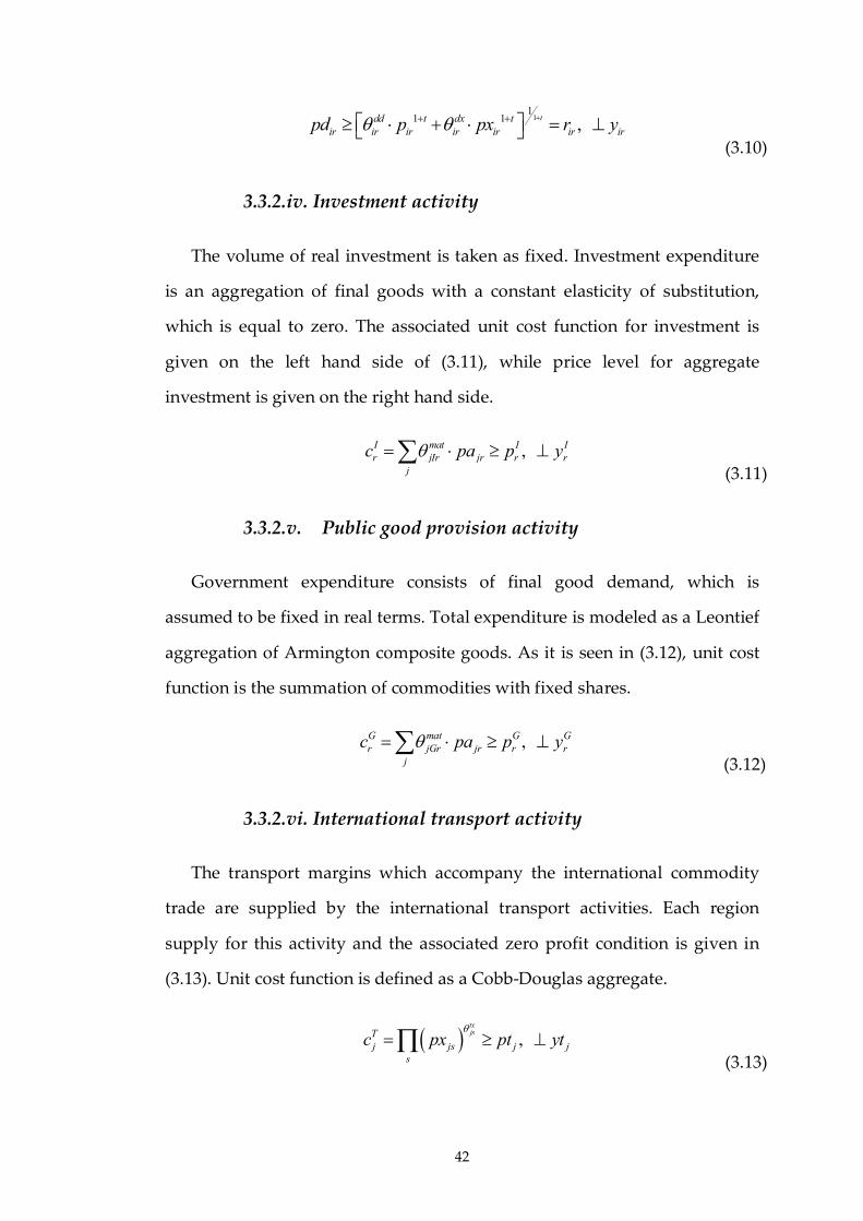
42

11

1 1 , tdd t dx t

ir ir ir ir ir ir irpd p px r y

(3.10)

3.3.2.iv. Investment activity

The volume of real investment is taken as fixed. Investment expenditure

is an aggregation of final goods with a constant elasticity of substitution,

which is equal to zero. The associated unit cost function for investment is

given on the left hand side of (3.11), while price level for aggregate

investment is given on the right hand side.

, I mat I Ir jIr jr r r

j

c pa p y (3.11)

3.3.2.v. Public good provision activity

Government expenditure consists of final good demand, which is

assumed to be fixed in real terms. Total expenditure is modeled as a Leontief

aggregation of Armington composite goods. As it is seen in (3.12), unit cost

function is the summation of commodities with fixed shares.

, G mat G Gr jGr jr r r

j

c pa p y (3.12)

3.3.2.vi. International transport activity

The transport margins which accompany the international commodity

trade are supplied by the international transport activities. Each region

supply for this activity and the associated zero profit condition is given in

(3.13). Unit cost function is defined as a Cobb-Douglas aggregate.

, txjsT

j js j js

c px pt yt

(3.13)

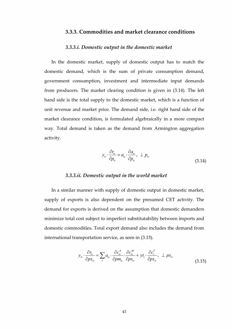
43

3.3.3. Commodities and market clearance conditions

3.3.3.i. Domestic output in the domestic market

In the domestic market, supply of domestic output has to match the

domestic demand, which is the sum of private consumption demand,

government consumption, investment and intermediate input demands

from producers. The market clearing condition is given in (3.14). The left

hand side is the total supply to the domestic market, which is a function of

unit revenue and market price. The demand side, i.e. right hand side of the

market clearance condition, is formulated algebraically in a more compact

way. Total demand is taken as the demand from Armington aggregation

activity.

, ir irir ir ir

ir ir

r ay a p

p p

(3.14)

3.3.3.ii. Domestic output in the world market

In a similar manner with supply of domestic output in domestic market,

supply of exports is also dependent on the presumed CET activity. The

demand for exports is derived on the assumption that domestic demanders

minimize total cost subject to imperfect substitutability between imports and

domestic commodities. Total export demand also includes the demand from

international transportation service, as seen in (3.15).

, A M T

ir is is iir is i ir

sir is ir ir

r c c cy a yt px

px pm px px

(3.15)

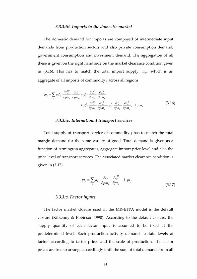
44

3.3.3.iii. Imports in the domestic market

The domestic demand for imports are composed of intermediate input

demands from production sectors and also private consumption demand,

government consumption and investment demand. The aggregation of all

these is given on the right hand side on the market clearance condition given

in (3.16). This has to match the total import supply, irm , which is an

aggregate of all imports of commodity i across all regions.

,

YD A ACjr Cir irr

ir jr rj ir ir ir ir

A AG IG Iir irr rr r ir

ir ir ir ir

c c ccm yd y

pa pm pa pm

c cc cy y pm

pa pm pa pm

(3.16)

3.3.3.iv. International transport services

Total supply of transport service of commodity j has to match the total

margin demand for the same variety of good. Total demand is given as a

function of Armington aggregates, aggregate import price level and also the

price level of transport services. The associated market clearance condition is

given in (3.17).

, A Mir ir

j ir jir ir j

c cyt a pt

pm pt

(3.17)

3.3.3.v. Factor inputs

The factor market closure used in the MR-ETPA model is the default

closure (Kilkenny & Robinson 1990). According to the default closure, the

supply quantity of each factor input is assumed to be fixed at the

predetermined level. Each production activity demands certain levels of

factors according to factor prices and the scale of production. The factor

prices are free to arrange accordingly until the sum of total demands from all

45

activities equals the quantity supplied. The market clearance conditions for

mobile factor inputs and for sector specific resource inputs are given in (3.18)

and (3.19), respectively.

, , ( )YDjr

fr jr frj fr

cevom yd pf f res f

pf

(3.18)

( )

, , ( )XEjr

fr jr jrj xe j jr

cevom yd pr f res f

pr

(3.19)

3.3.3.vi. CO2 permits

In the MR-ETPA model, there exist both international and regional CO2

permit markets. Unless the economic analysis includes market-based

abatement policies, these markets are not active. In the reverse case, the

supply and demand in the permit market equalize according to the permit

price clearing the permit market. The market clearance condition, in case of

regional permit trading, is stated as in (3.20). The left hand side gives the

total supply of allowances in the permit market in region r, while the right

hand side is the total demand for permits. Extractive and non-extractive

industries and private consumption activities are the potential demanders of

CO2 permits. Therefore, total demand is given as the summation of permit

demands from these sectors in (3.20). However, the model formulation

allows for choosing which emitting sectors are included in the regional

trading or not, just as how it happens to be in the existing permit trading

markets around the globe.

( )

2 , YD XE Cjr jrrets C r

r jr jr r rj j xe jr r r

c c cCO yd yd y prets

prets prets prets

(3.20)

In case of international permit trading, it is crucial to distinguish which

regions and which economic entities in each region are allowed to trade

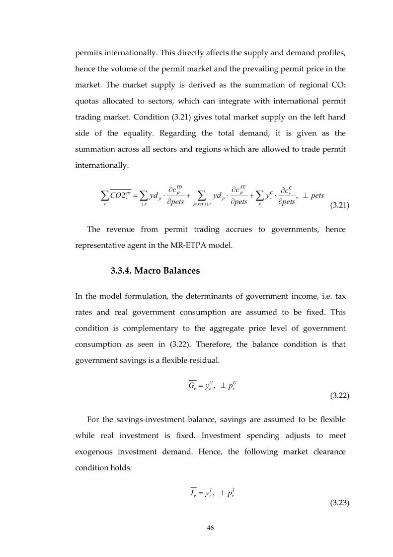
46

permits internationally. This directly affects the supply and demand profiles,

hence the volume of the permit market and the prevailing permit price in the

market. The market supply is derived as the summation of regional CO2

quotas allocated to sectors, which can integrate with international permit

trading market. Condition (3.21) gives total market supply on the left hand

side of the equality. Regarding the total demand, it is given as the

summation across all sectors and regions which are allowed to trade permit

internationally.

, ( ),

2 , YD XE Cjr jrets C r

r jr jr rr j r j xe j r r

c c cCO yd yd y pets

pets pets pets

(3.21)

The revenue from permit trading accrues to governments, hence

representative agent in the MR-ETPA model.

3.3.4. Macro Balances

In the model formulation, the determinants of government income, i.e. tax

rates and real government consumption are assumed to be fixed. This

condition is complementary to the aggregate price level of government

consumption as seen in (3.22). Therefore, the balance condition is that

government savings is a flexible residual.

, G G

r r rG y p

(3.22)

For the savings-investment balance, savings are assumed to be flexible

while real investment is fixed. Investment spending adjusts to meet

exogenous investment demand. Hence, the following market clearance

condition holds:

, I I

r r rI y p

(3.23)

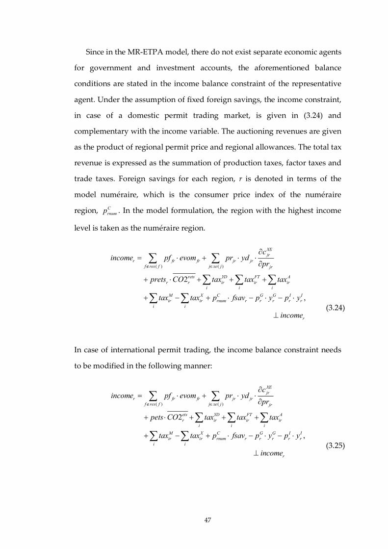
47

Since in the MR-ETPA model, there do not exist separate economic agents

for government and investment accounts, the aforementioned balance

conditions are stated in the income balance constraint of the representative

agent. Under the assumption of fixed foreign savings, the income constraint,

in case of a domestic permit trading market, is given in (3.24) and

complementary with the income variable. The auctioning revenues are given

as the product of regional permit price and regional allowances. The total tax

revenue is expressed as the summation of production taxes, factor taxes and

trade taxes. Foreign savings for each region, r is denoted in terms of the

model numéraire, which is the consumer price index of the numéraire

region, Crnump . In the model formulation, the region with the highest income

level is taken as the numéraire region.

( ) ( )

2

,

XEjr

r fr fr jr jrf res f j xe j jr

rets YD FT Ar r ir ir ir

i i i

M X C G G I Iir ir rnum r r r r r

i i

cincome pf evom pr yd

pr

prets CO tax tax tax

tax tax p fsav p y p y

rincome (3.24)

In case of international permit trading, the income balance constraint needs

to be modified in the following manner:

( ) ( )

2

,

XEjr

r fr fr jr jrf res f j xe j jr

ets YD FT Ar ir ir ir

i i i

M X C G G I Iir ir rnum r r r r r

i i

cincome pf evom pr yd

pr

pets CO tax tax tax

tax tax p fsav p y p y

rincome (3.25)

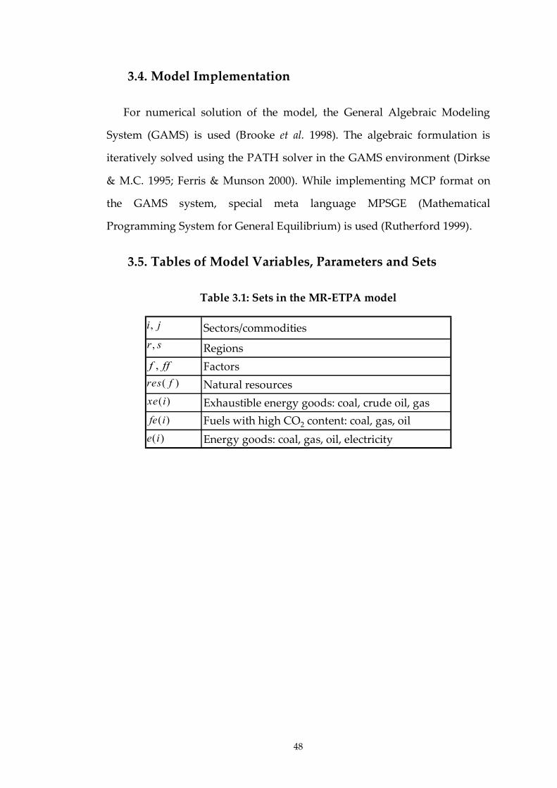
48

3.4. Model Implementation

For numerical solution of the model, the General Algebraic Modeling

System (GAMS) is used (Brooke et al. 1998). The algebraic formulation is

iteratively solved using the PATH solver in the GAMS environment (Dirkse

& M.C. 1995; Ferris & Munson 2000). While implementing MCP format on

the GAMS system, special meta language MPSGE (Mathematical

Programming System for General Equilibrium) is used (Rutherford 1999).

3.5. Tables of Model Variables, Parameters and Sets

Table 3.1: Sets in the MR-ETPA model

Sectors/commodities

Regions

Factors

Natural resources

Exhaustible energy goods: coal, crude oil, gas

Fuels with high CO2 content: coal, gas, oil

Energy goods: coal, gas, oil, electricity

,i j

,r s

,f ff

( )res f

( )xe i

( )fe i

( )e i

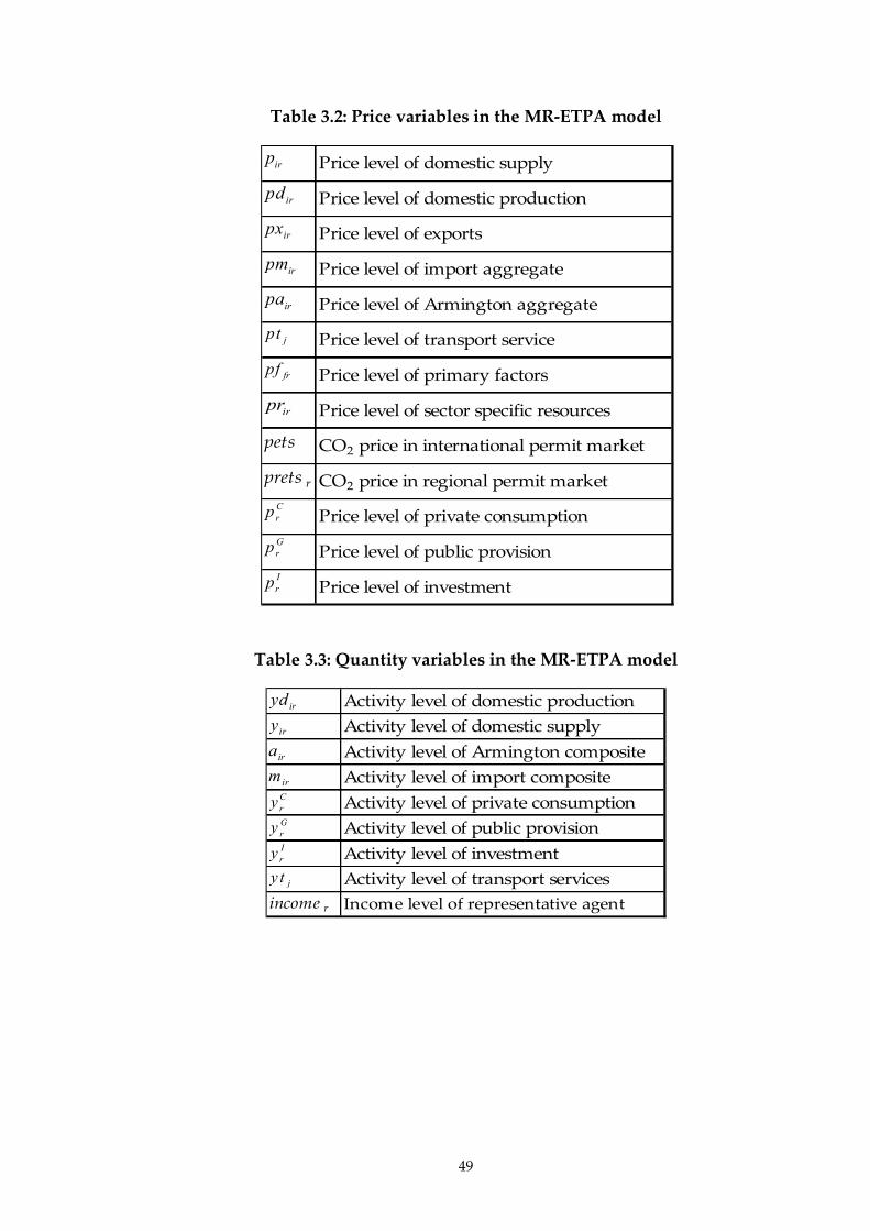
49

Table 3.2: Price variables in the MR-ETPA model

Table 3.3: Quantity variables in the MR-ETPA model

Activity level of domestic production

Activity level of domestic supply

Activity level of Armington composite

Activity level of import composite

Activity level of private consumption

Activity level of public provision

Activity level of investment

Activity level of transport services

income r Income level of representative agent

iryd

iry

ira

irmCryGryIry

jy t

Price level of domestic supply

Price level of domestic production

Price level of exports

Price level of import aggregate

Price level of Armington aggregate

Price level of transport service

Price level of primary factors

Price level of sector specific resources

pets CO2 price in international permit market

prets r CO2 price in regional permit market

Price level of private consumption

Price level of public provision

Price level of investment

irp

irpd

irpx

irpm

irpa

jpt

frpf

Crp

Grp

Irp

irpr

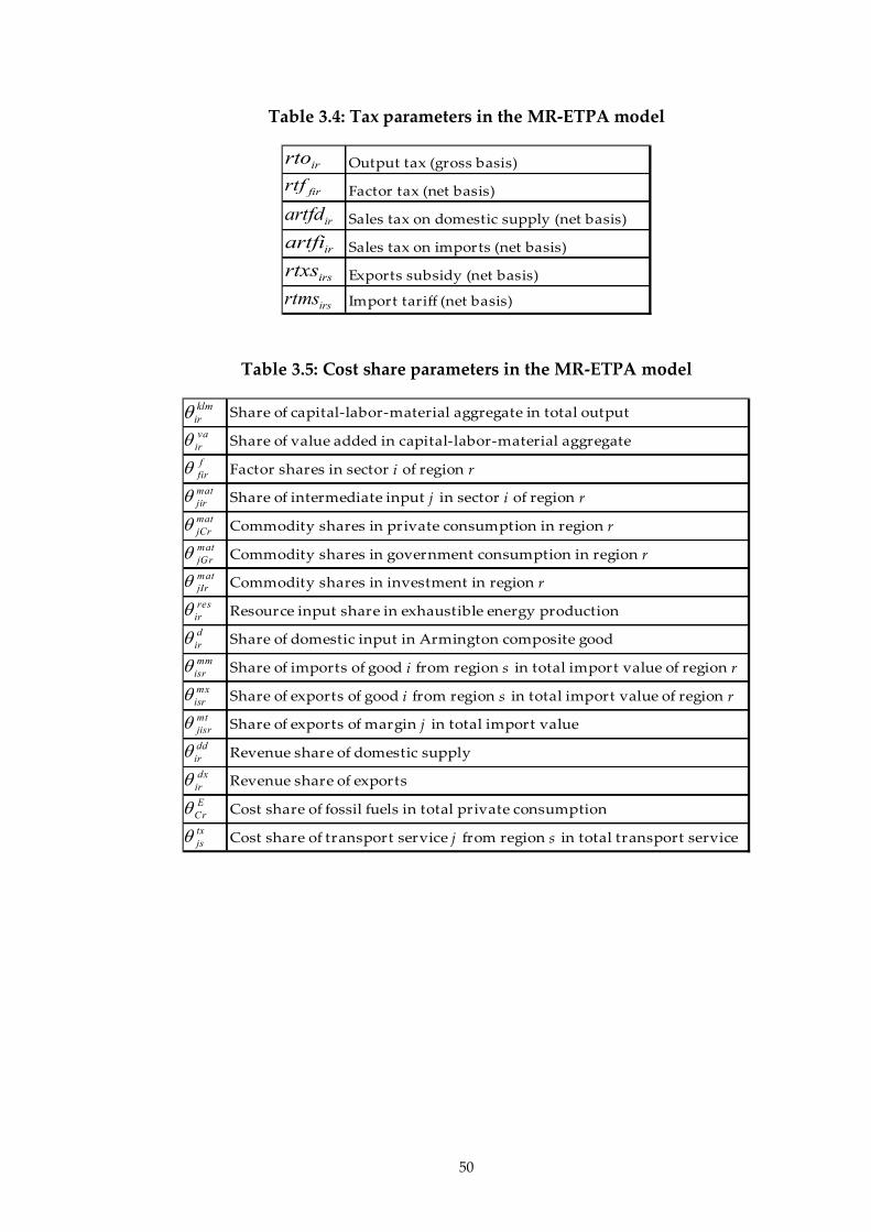
50

Table 3.4: Tax parameters in the MR-ETPA model

Output tax (gross basis)

Factor tax (net basis)

Sales tax on domestic supply (net basis)

Sales tax on imports (net basis)

Exports subsidy (net basis)

Import tariff (net basis)

irrto

firrtf

irartfd

irartfi

irsrtxs

irsrtms

Table 3.5: Cost share parameters in the MR-ETPA model

Share of capital-labor-material aggregate in total output

Share of value added in capital-labor-material aggregate

Factor shares in sector i of region r

Share of intermediate input j in sector i of region r

Commodity shares in private consumption in region r

Commodity shares in government consumption in region r

Commodity shares in investment in region r

Resource input share in exhaustible energy production

Share of domestic input in Armington composite good

Share of imports of good i from region s in total import value of region r

Share of exports of good i from region s in total import value of region r

Share of exports of margin j in total import value

Revenue share of domestic supply

Revenue share of exports

Cost share of fossil fuels in total private consumption

Cost share of transport service j from region s in total transport service

klmirva

ir

matjirmatjCr

matjIrres

irdirmm

isrmxisrmtjisrddirdx

irE

Crtxjs

ffir

matjGr

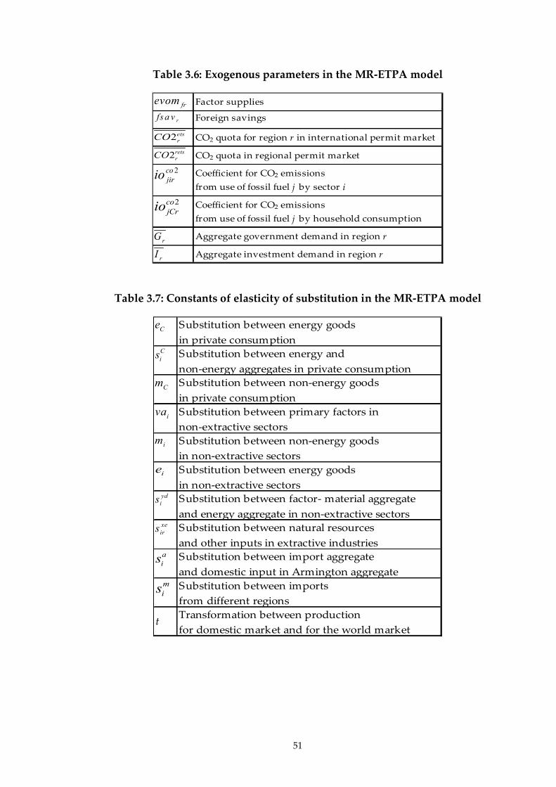
51

Table 3.6: Exogenous parameters in the MR-ETPA model

Factor supplies

Foreign savings

CO2 quota for region r in international permit market

CO2 quota in regional permit market

Coefficient for CO2 emissions

from use of fossil fuel j by sector i

Coefficient for CO2 emissions

from use of fossil fuel j by household consumption

Aggregate government demand in region r

Aggregate investment demand in region rrI

rG

2cojCrio

2cojirio

2etsrCO

frevom

rfs a v

2retsrCO

Table 3.7: Constants of elasticity of substitution in the MR-ETPA model

Substitution between energy goods

in private consumption

Substitution between energy and

non-energy aggregates in private consumption

Substitution between non-energy goods

in private consumption

Substitution between primary factors in

non-extractive sectors

Substitution between non-energy goods

in non-extractive sectors

Substitution between energy goods

in non-extractive sectors

Substitution between factor- material aggregate

and energy aggregate in non-extractive sectors

Substitution between natural resources

and other inputs in extractive industries

Substitution between import aggregate

and domestic input in Armington aggregate

Substitution between imports

from different regions

tTransformation between production

for domestic market and for the world market

Ce

Cis

Cm

iva

im

ydis

xeirs

ais

mis

ie

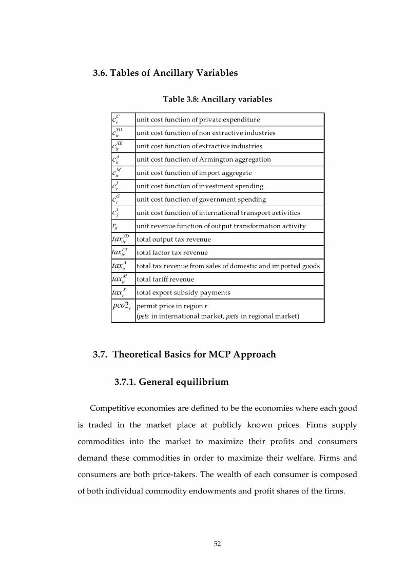
52

3.6. Tables of Ancillary Variables

Table 3.8: Ancillary variables

3.7. Theoretical Basics for MCP Approach

3.7.1. General equilibrium

Competitive economies are defined to be the economies where each good

is traded in the market place at publicly known prices. Firms supply

commodities into the market to maximize their profits and consumers

demand these commodities in order to maximize their welfare. Firms and

consumers are both price-takers. The wealth of each consumer is composed

of both individual commodity endowments and profit shares of the firms.

unit cost function of private expenditure

unit cost function of non extractive industries

unit cost function of extractive industries

unit cost function of Armington aggregation

unit cost function of import aggregate

unit cost function of investment spending

unit cost function of government spending

unit cost function of international transport activities

unit revenue function of output transformation activity

total output tax revenue

total factor tax revenue

total tax revenue from sales of domestic and imported goods

total tariff revenue

total export subsidy payments

permit price in region r

(pets in international market, prets in regional market)

CrcYDircXEircAircMircIrcGrcTjc

irrYDirtaxFTirtax

AirtaxMirtaxXrtax

2rpco

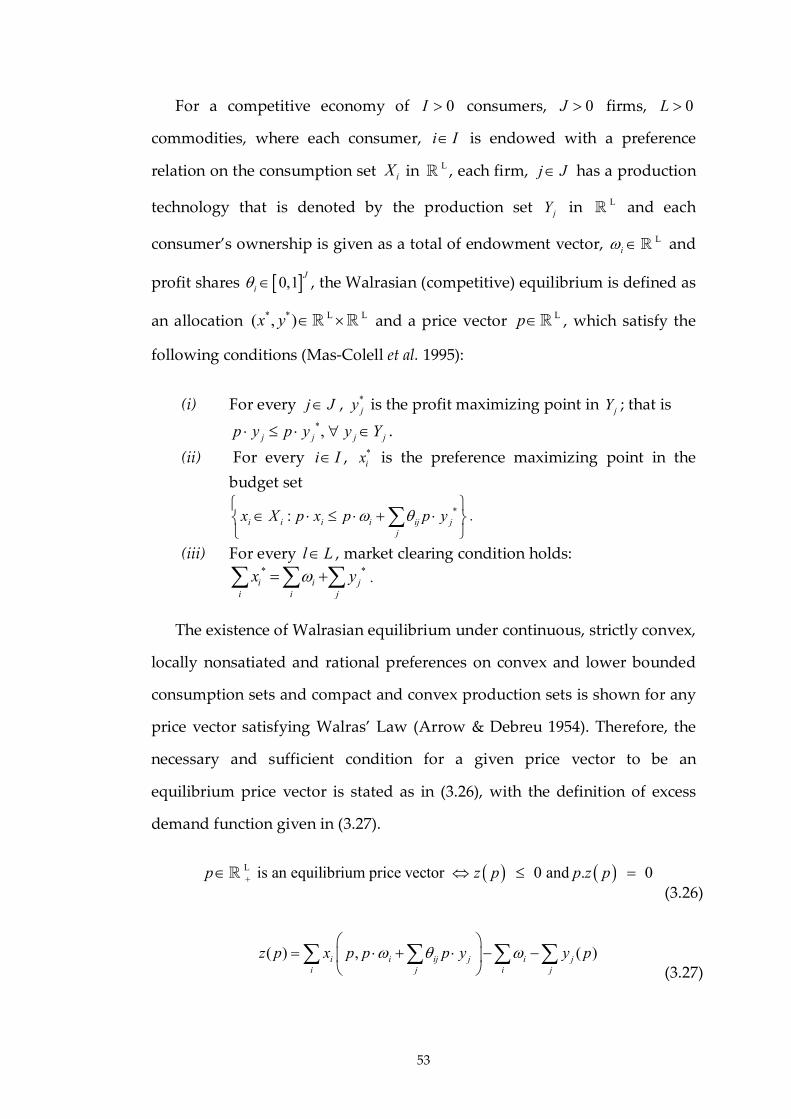
53

For a competitive economy of 0I consumers, 0J firms, 0L

commodities, where each consumer, i I is endowed with a preference

relation on the consumption set iX in L , each firm, j J has a production

technology that is denoted by the production set jY in L and each

consumer’s ownership is given as a total of endowment vector, Li and

profit shares 0,1J

i , the Walrasian (competitive) equilibrium is defined as

an allocation * * L L( , )x y and a price vector Lp , which satisfy the

following conditions (Mas-Colell et al. 1995):

(i) For every j J , *jy is the profit maximizing point in jY ; that is

*, j j j jp y p y y Y .

(ii) For every i I , *ix is the preference maximizing point in the

budget set

*:i i i i ij jj

x X p x p p y

.

(iii) For every l L , market clearing condition holds: * *

i i ji i j

x y .

The existence of Walrasian equilibrium under continuous, strictly convex,

locally nonsatiated and rational preferences on convex and lower bounded

consumption sets and compact and convex production sets is shown for any

price vector satisfying Walras’ Law (Arrow & Debreu 1954). Therefore, the

necessary and sufficient condition for a given price vector to be an

equilibrium price vector is stated as in (3.26), with the definition of excess

demand function given in (3.27).

L

is an equilibrium price vector 0 and . 0p z p p z p (3.26)

( ) , ( )i i ij j i j

i j i j

z p x p p p y y p

(3.27)

54

According to (3.26), Walrasian equilibria can be expressed as the

solutions of a system of equations. This is crucial for the sake of tractability

of the numerical analysis of general equilibrium models. The proposition

states that if 0lp , then ( ) 0lz p . Furthermore, it is possible that a

commodity l is in excess supply, i.e. ( ) 0lz p , when 0lp . Thus, the

necessary and sufficient conditions for an equilibrium price vector turns out

to be complementary conditions between price levels and excess demand

functions as follows:

( ) 0, 0, ( ) 0z p p p z p

(3.28)

Under the given assumptions for preferences and production

technologies, the excess demand function is proven to be continuous and

homogenous of degree zero. Thus, what matters for the existence of

equilibrium are not the absolute values of prices, but the relative values of

prices. Therefore, it is possible to normalize prices by choosing a numéraire

commodity for which the price is fixed to some arbitrary number, usually to

unity. Further discussions on the underlying assumptions and the existence

proof can be found in (Debreu 1959) and(Arrow & Hahn 1971).

3.7.2. Computable general equilibrium modeling

Computable general equilibrium (CGE) models simulate the general

equilibrium economies based on the Arrow – Debreu framework. Simulation

analysis starts with setting up a parameterized model. Empirical data is used

in this parameterization to get a fully specified model. The model is further

used to conduct comparative static analyses, in order to quantify the effects

of changes of certain policy instrument variables. Generally, the models are

solved using numerical methods, since closed form solutions for higher

dimension models may not exist.

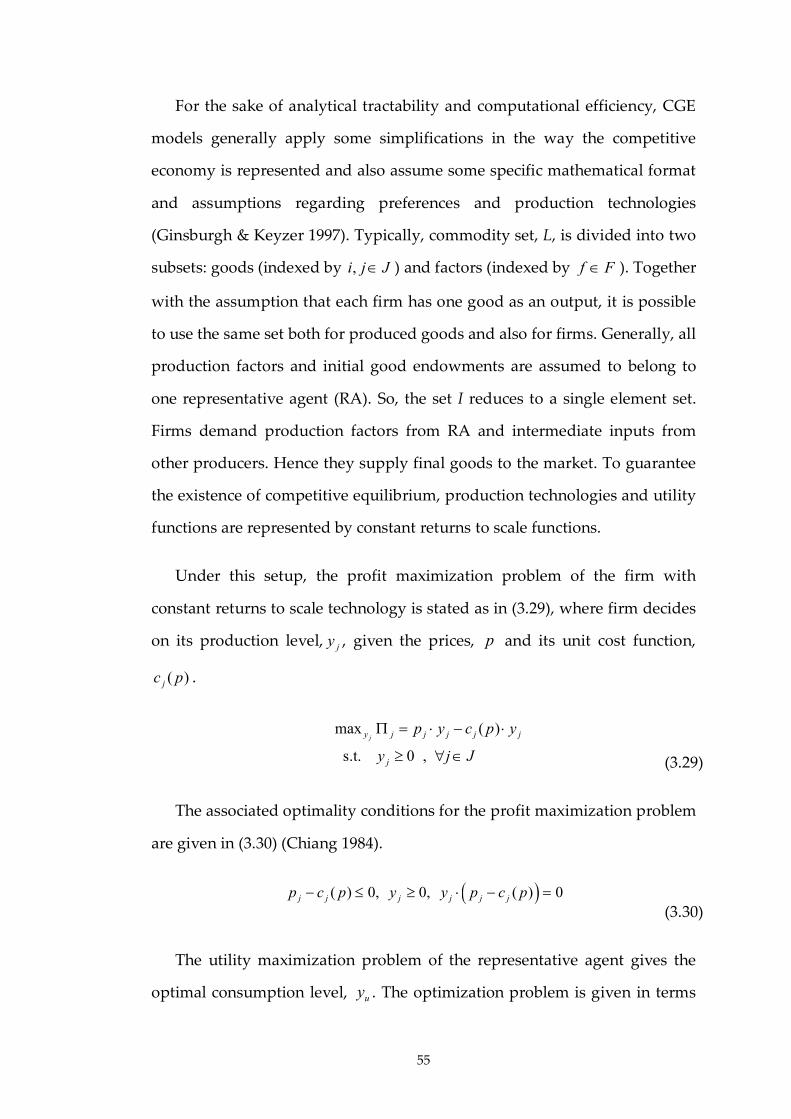
55

For the sake of analytical tractability and computational efficiency, CGE

models generally apply some simplifications in the way the competitive

economy is represented and also assume some specific mathematical format

and assumptions regarding preferences and production technologies

(Ginsburgh & Keyzer 1997). Typically, commodity set, L, is divided into two

subsets: goods (indexed by ,i j J ) and factors (indexed by f F ). Together

with the assumption that each firm has one good as an output, it is possible

to use the same set both for produced goods and also for firms. Generally, all

production factors and initial good endowments are assumed to belong to

one representative agent (RA). So, the set I reduces to a single element set.

Firms demand production factors from RA and intermediate inputs from

other producers. Hence they supply final goods to the market. To guarantee

the existence of competitive equilibrium, production technologies and utility

functions are represented by constant returns to scale functions.

Under this setup, the profit maximization problem of the firm with

constant returns to scale technology is stated as in (3.29), where firm decides

on its production level, jy , given the prices, p and its unit cost function,

( )jc p .

max ( )

s.t. 0 ,

jy j j j j j

j

p y c p y

y j J

(3.29)

The associated optimality conditions for the profit maximization problem

are given in (3.30) (Chiang 1984).

( ) 0, 0, ( ) 0 j j j j j jp c p y y p c p

(3.30)

The utility maximization problem of the representative agent gives the

optimal consumption level, uy . The optimization problem is given in terms

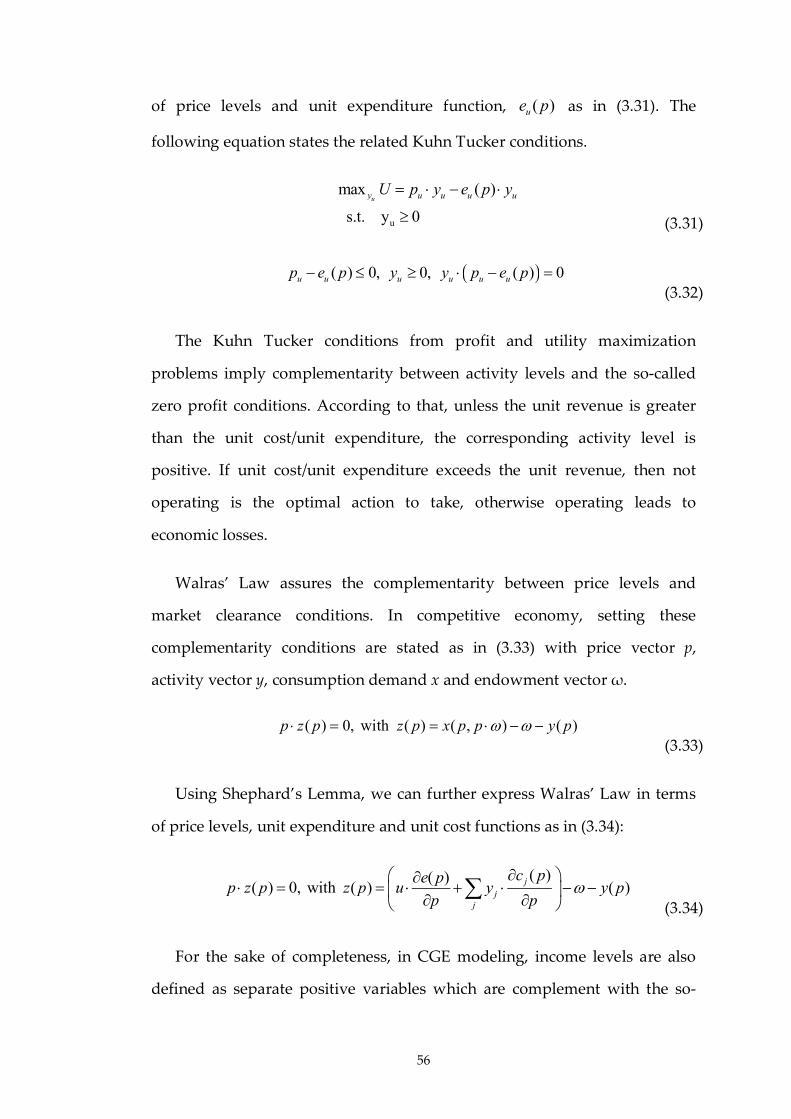
56

of price levels and unit expenditure function, ( )ue p as in (3.31). The

following equation states the related Kuhn Tucker conditions.

u

max ( )

s.t. y 0

uy u u u uU p y e p y

(3.31)

( ) 0, 0, ( ) 0 u u u u u up e p y y p e p

(3.32)

The Kuhn Tucker conditions from profit and utility maximization

problems imply complementarity between activity levels and the so-called

zero profit conditions. According to that, unless the unit revenue is greater

than the unit cost/unit expenditure, the corresponding activity level is

positive. If unit cost/unit expenditure exceeds the unit revenue, then not

operating is the optimal action to take, otherwise operating leads to

economic losses.

Walras’ Law assures the complementarity between price levels and

market clearance conditions. In competitive economy, setting these

complementarity conditions are stated as in (3.33) with price vector p,

activity vector y, consumption demand x and endowment vector ω.

( ) 0, with ( ) ( , ) ( )p z p z p x p p y p

(3.33)

Using Shephard’s Lemma, we can further express Walras’ Law in terms

of price levels, unit expenditure and unit cost functions as in (3.34):

( )( )( ) 0, with ( ) ( )

j

jj

c pe pp z p z p u y y p

p p

(3.34)

For the sake of completeness, in CGE modeling, income levels are also

defined as separate positive variables which are complement with the so-

57

called income balance conditions (Bohringer et al. 2003). The

complementarity is captured in the following equation:

0, , ( ) 0l l l l l l l ll l l l

M p p x M p p x (3.35)

Therefore, CGE models can be modeled as a square system of equations

in which price levels are complement with market clearing conditions,

activity levels are complement with zero profit conditions and income levels

are complement with income balance conditions. This is known as Mixed

Complementarity Problems (MCP) in the literature and defined as in (3.36)

(Cottle et al. 1992; Rutherford 1995; Ferris & Pang 1997):

given :

find s.t. 0, ( ) 0 and ( ) 0

with

, , , ( ) [ ( )],[ ( ( ))],[ (

n n

n T

l

f

r r f r r f r

r p y M f r z p p c p p

)]l l ll l

p x

(3.36)

3.8. Constant Elasticity of Substitution Functions

In applied general equilibrium studies, it is customary to use Constant

Elasticity of Substitution (CES) functions in formulating production

technologies and utility functions (Arrow et al. 1961). While guaranteeing the

existence of general equilibrium, CES functions further ease the analytical

formulation of AGE models. The generic form of CES functions are as

follows:

1

1, with 1 and

1i i i

i i

y x

(3.37)

58

, where is the efficiency parameter, [0,1]i are the distribution

parameters, and is the substitution parameter which is inversely related to

the elasticity of substitution parameter, σ. This general formulation of CES

functions include Cobb-Douglas and Leontief function formulation with

1 and 0 , respectively. As the above formulation allows only for equal

substitutability between all inputs, it is common in the literature to use

nested CES functions to handle different substitutability rates among inputs

(Strotz 1957). Further discussion about nested CES functions and their

analytical properties can be found in (Keller 1976).

59

CHAPTER 4

Model Calibration and Benchmark Equilibrium

4.1. Introduction

This chapter gives a brief overview of the structure of the model data and

calibration. Section 4.2 starts with a general overview of the GTAP 7 data set,

which I use in calibrating the model specific functional forms and exogenous

parameters in the MR-ETPA model. Section 4.3 follows with detailed

explanation of the specific mappings, which I use in aggregating the GTAP 7

data set for the current set up of the MR-ETPA model. Section 4.4 gives a

brief summary of the structure of the regional social accounting matrices and

how global social accounting matrix is formulated for the multi-country

setting of the MR-ETPA model. In Section 4.5, I give further information on

the construction of the benchmark equilibrium together with the checks over

macro and micro balances. Finally, country profiles at the benchmark

equilibrium are given and discussed in Section 4.6.

4.2. Overview

The data used in the model calibration is based on the GTAP 7 data base,

which represents the world economy at a global scale for the given reference

60

year, 2004 (Badri & Walmsley 2008). It contains input-output tables and

bilateral trade flows, together with the associated transportation costs, export

subsidies and import tariffs for 113 regions and 57 sectors.

4.3. Data Aggregation

For the specific requirements of the current policy analysis, I aggregate

the GTAP 7 data base into a more compact dataset using model specific

mapping routines. The model specific aggregation mapping is given in

Appendix B. I run the mapping routines on the data base within the

GTAP7inGAMS package (Rutherford 2011). Table 4.1 gives the final

aggregation of sectors according to the mapping7. The energy goods

specified in the MR-ETPA model are coal, crude oil8, natural gas, refined oil

products and electricity. These are the main driving force behind CO2

emissions generated through economic activities. In any abatement policy

analysis, the CO2 intensity of sectors, therefore the economies, together with

the technological ability of substitution between energy goods are crucial in

determining the magnitude of welfare changes. Taking into account all these,

energy goods are identified and treated separately throughout this work.

Depending on their high intensity of energy use, under possible

abatement actions, the energy intensive sectors are the ones to be affected the

most. Though, these industries also have high capability in energy

substitution, too. Therefore, it is also necessary to specify them separately in

the model formulation. The energy intensive sectors are featured as:

7 Each sector produces only one output. Hence, the set of sectors and commodities

coincide.

8 In the implementation of MR-ETPA model, crude oil is treated as material input since

the volume of CO2 emissions due to crude oil are negligible compared to other energy

goods.

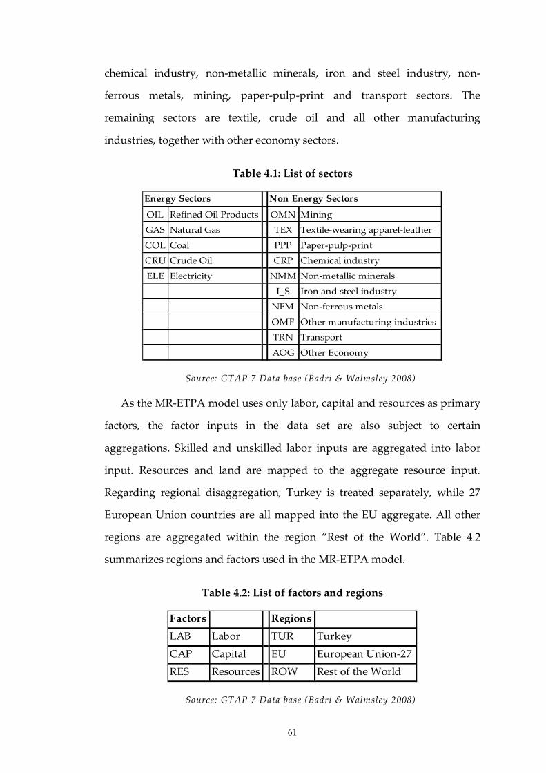
61

chemical industry, non-metallic minerals, iron and steel industry, non-

ferrous metals, mining, paper-pulp-print and transport sectors. The

remaining sectors are textile, crude oil and all other manufacturing

industries, together with other economy sectors.

Table 4.1: List of sectors

OIL Refined Oil Products OMN Mining

GAS Natural Gas TEX Textile-wearing apparel-leather

COL Coal PPP Paper-pulp-print

CRU Crude Oil CRP Chemical industry

ELE Electricity NMM Non-metallic minerals

I_S Iron and steel industry

NFM Non-ferrous metals

OMF Other manufacturing industries

TRN Transport

AOG Other Economy

Energy Sectors Non Energy Sectors

Source: GTAP 7 Data base (Badri & Walmsley 2008)

As the MR-ETPA model uses only labor, capital and resources as primary

factors, the factor inputs in the data set are also subject to certain

aggregations. Skilled and unskilled labor inputs are aggregated into labor

input. Resources and land are mapped to the aggregate resource input.

Regarding regional disaggregation, Turkey is treated separately, while 27

European Union countries are all mapped into the EU aggregate. All other

regions are aggregated within the region “Rest of the World”. Table 4.2

summarizes regions and factors used in the MR-ETPA model.

Table 4.2: List of factors and regions

Factors Regions

LAB Labor TUR Turkey

CAP Capital EU European Union-27

RES Resources ROW Rest of the World


62

4.4. Regional and Global Social Accounting Matrices

As it is customary in general equilibrium modeling, model data is

presented in a balanced social accounting matrix (SAM) (Pyatt & Round

1985). Following this tradition, the data used in this study is represented in

the form of regional SAMs which are linked directly through commodity

trade transactions.

The transactions used in each regional SAM are given in Table 4.3. Each

entry in SAM is basically a transaction between the selling and purchasing

agents, which are identified by rows and columns of SAM, respectively. The

values of transactions are given in billions of 2004 US dollars.

Table 4.3: Structure of the social accounting matrix

Commodities Activities Factors Households Government CapitalRest of the World

(ROW)Total

CommoditiesIntermediate

Input Payments

Private

Consumption

Government

Consumption

Investment

Consumption

Exports of

Margins and

Commodities

Total

Commodity

Demand

Activities Domestic SupplyTotal Domestic

Supply

FactorsPrimary Factor

Payments

Total Factor

Income

Households Factor IncomesTotal Household

Income

Government

Sales Taxes,

Import Tariffs,

Export Subsidies

Output Taxes,

Value-added

Taxes

Total

Government

Income

CapitalHousehold

Savings

Government

SavingsForeign Savings Total Savings

Rest of the

World

(ROW)

Imports of

Margins and

Commodities

Total Income

from Imports

Total

Total

Commodity

Supply

Total Expenditure

on Inputs to the

Production

Total Factor

Expenditure

Total Household

Expenditure

Total

Government

Expenditure

Total

Expenditure on

Investment

Total

Expenditure on

Exports

The standard SAM distinguishes between accounts for activities and

commodities (Francois & Reinert 1997). This is mainly to handle the

production structures of activities producing different commodities. In the

current framework, each activity produces only one commodity due to

certain production technologies using intermediate inputs and primary

factors. Production activities are also subject to output and value added

63

taxes. Domestic output is either sold in the domestic market or exported. The

commodities account in SAM includes all commodities in the market,

including domestically sold and imported commodities. Total commodity

demand is comprised of private demand, public demand, investment

demand and export expenditures. All commodity transactions are subject to

sales taxes, while imported goods are also subject to import tariffs. Total

factor income accrues to households and either spent on private

consumption or saved. Government income comes from tax revenues and

used for public provision. Total investment is financed by total savings in the

economy, which includes savings from households, government and the rest

of the world. In each regional SAM, the account for the rest of the world

keeps track of the transactions between the region and the other regions, in

the form of exports, imports and foreign savings.

Table 4.8, Table 4.9 and Table 4.10 give the regional SAMs in an

aggregate form for Turkey, the EU and the ROW, respectively. From these

SAMs, it is not possible to read more detailed data like expenditures of

individual sectors, taxation schedules, and composition of private

consumption, investment and public provision. Nevertheless, they are still

useful in the sense that they illustrate the circular process of demand leading

to production leading to income, which in turn leads back to demand.

Apart from constructing and balancing regional SAMs, it is also

necessary to formulate a global SAM since the MR-ETPA model is a multi-

country model. In the context of the GTAP 7 data base, the global SAM is

basically formulated as a series of regional SAMs that are linked via

commodity and margin trade accounts. While doing so, it is assured that

bilateral trade transactions are balanced. This balance holds for both

commodity transactions, i.e. each and every commodity import by a region

must have a counterpart commodity export transaction by other regions, and

64

also for margin transactions. Total demand for margins has to be equal to the

total supply of margins.

4.5. Constructing the Benchmark Equilibrium

In this study, the regional economies are assumed to be in equilibrium, as

given in the GTAP 7 data base, for the year 2004. This equilibrium is taken as

the benchmark equilibrium, which is mainly used for model calibration9.

In order for the necessary conditions of benchmark equilibrium to hold,

the aggregated data base is further checked for optimality and market

clearance conditions on the MR-ETPA model. Optimality conditions have to

hold for each production and import activity, also for private consumption,

public provision and investment activities. Market clearing conditions are

needed to assure that all markets, including commodity and factor markets,

clear.

The data arrays10 and tax parameters in the GTAP 7 data base, which are

necessary for the algebraic exposition of the benchmark equilibrium, are

given in Appendix A. The sets used in algebraic exposition of benchmark

equilibrium are given in Table 4.4.

9 At the benchmark equilibrium, all price variables are assumed to be unity.

10 Data arrays are given in billions 2004 US dollars.

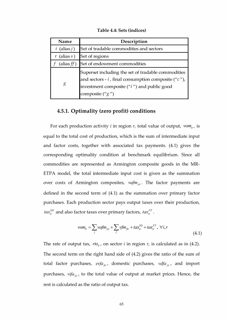
65

Table 4.4: Sets (indices)

Name Description

i (alias j ) Set of tradable commodities and sectors

r (alias s ) Set of regions

f (alias ff ) Set of endowment commodities

g

Superset including the set of tradable commodities

and sectors - i , final consumption composite (“c ”),

investment composite (“i ”) and public good

composite (“g ”)

4.5.1. Optimality (zero profit) conditions

For each production activity i in region r, total value of output, irvom , is

equal to the total cost of production, which is the sum of intermediate input

and factor costs, together with associated tax payments. (4.1) gives the

corresponding optimality condition at benchmark equilibrium. Since all

commodities are represented as Armington composite goods in the MR-

ETPA model, the total intermediate input cost is given as the summation

over costs of Armington composites, jirvafm . The factor payments are

defined in the second term of (4.1) as the summation over primary factor

purchases. Each production sector pays output taxes over their production,

YDirtax and also factor taxes over primary factors, FT

irtax .

, ,YD FTir jir fir ir ir

j f

vom vafm vfm tax tax i r (4.1)

The rate of output tax, irrto , on sector i in region r, is calculated as in (4.2).

The second term on the right hand side of (4.2) gives the ratio of the sum of

total factor purchases, firevfa , domestic purchases, jirvdfa , and import

purchases, jirvifa , to the total value of output at market prices. Hence, the

rest is calculated as the ratio of output tax.

66

( )

1fir jir jir

f j

ir

ir

evfa vdfa vifa

rtovom

(4.2)

The rate of factor tax on the use of factor f by sector i, firrtf , is calculated as

the ratio of the difference between factor purchases at agents’ prices, firevfa

and at market prices, firvfm , to the factor payments at market prices. The

corresponding formulation is given in (4.3):

1fir

fir

fir

evfartf

vfm

(4.3)

In the MR_ETPA model, each commodity in the domestic market is

represented as an Armington composite good. Hence, for each commodity i,

a separate Armington activity is defined. The total value of the Armington

aggregation iravafm is defined as the summation over domestic and import

purchases of the same variety of good together with the associated sales

taxes. The total tax amount, Airtax , which is given in (4.4), includes the taxes

paid over domestic supply and imports.

, ,Air igr igr igr ir

g g g

avafm vafm vdfm vifm tax i r (4.4)

For the sake of algebraic exposition, igrvafm is reserved for denoting the

purchases of composite good i, by sector g at agents’ prices. Hence, igrvafm

already includes domestic and import purchases at market prices and also

the associated tax payments.

Sales taxes are collected over purchases of intermediate and final goods,

which are given by igrrtfd and igrrtfi for domestically produced and imported

goods, respectively. These tax rates are obtained from the data base by using

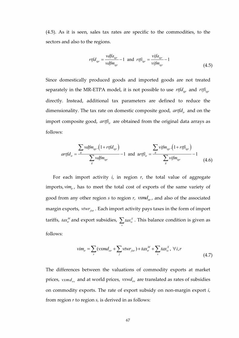
67

(4.5). As it is seen, sales tax rates are specific to the commodities, to the

sectors and also to the regions.

1 and 1igr igr

igr igr

igr igr

vdfa vifartfd rtfi

vdfm vifm

(4.5)

Since domestically produced goods and imported goods are not treated

separately in the MR-ETPA model, it is not possible to use igrrtfd and igrrtfi

directly. Instead, additional tax parameters are defined to reduce the

dimensionality. The tax rate on domestic composite good, irartfd and on the

import composite good, irartfi are obtained from the original data arrays as

follows:

. 1 . 1

1 and a 1igr igr igr igr

g g

ir ir

igr igrg g

vdfm rtfd vifm rtfi

artfd rtfivdfm vifm

(4.6)

For each import activity i, in region r, the total value of aggregate

imports, irvim , has to meet the total cost of exports of the same variety of

good from any other region s to region r, isrvxmd , and also of the associated

margin exports, jisrvtwr . Each import activity pays taxes in the form of import

tariffs, Mirtax and export subsidies, X

iss

tax . This balance condition is given as

follows:

( ) , ,M Xir isr jisr ir is

s j s

vim vxmd vtwr tax tax i r (4.7)

The differences between the valuations of commodity exports at market

prices, irsvxmd and at world prices, irsvxwd are translated as rates of subsidies

on commodity exports. The rate of export subsidy on non-margin export i,

from region r to region s, is derived in as follows:

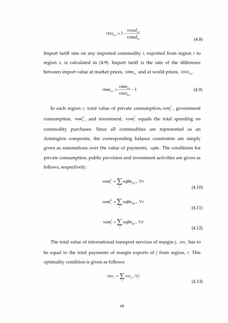
68

1 irsirs

irs

vxwdrtxs

vxmd

(4.8)

Import tariff rate on any imported commodity i, exported from region r to

region s, is calculated in (4.9). Import tariff is the rate of the difference

between import value at market prices, irsvims and at world prices, irsviws .

1irsisr

irs

vimsrtms

viws (4.9)

In each region r, total value of private consumption, Crvom , government

consumption, Grvom , and investment, I

rvom equals the total spending on

commodity purchases. Since all commodities are represented as an

Armington composite, the corresponding balance constraints are simply

given as summations over the value of payments, vafm . The conditions for

private consumption, public provision and investment activities are given as

follows, respectively:

, Cr jCr

j

vom vafm r (4.10)

, Gr jGr

j

vom vafm r (4.11)

, Ir jIr

j

vom vafm r (4.12)

The total value of international transport services of margin j, jvtw has to

be equal to the total payments of margin exports of j from region, r. This

optimality condition is given as follows:

,j jr

r

vtw vst j (4.13)

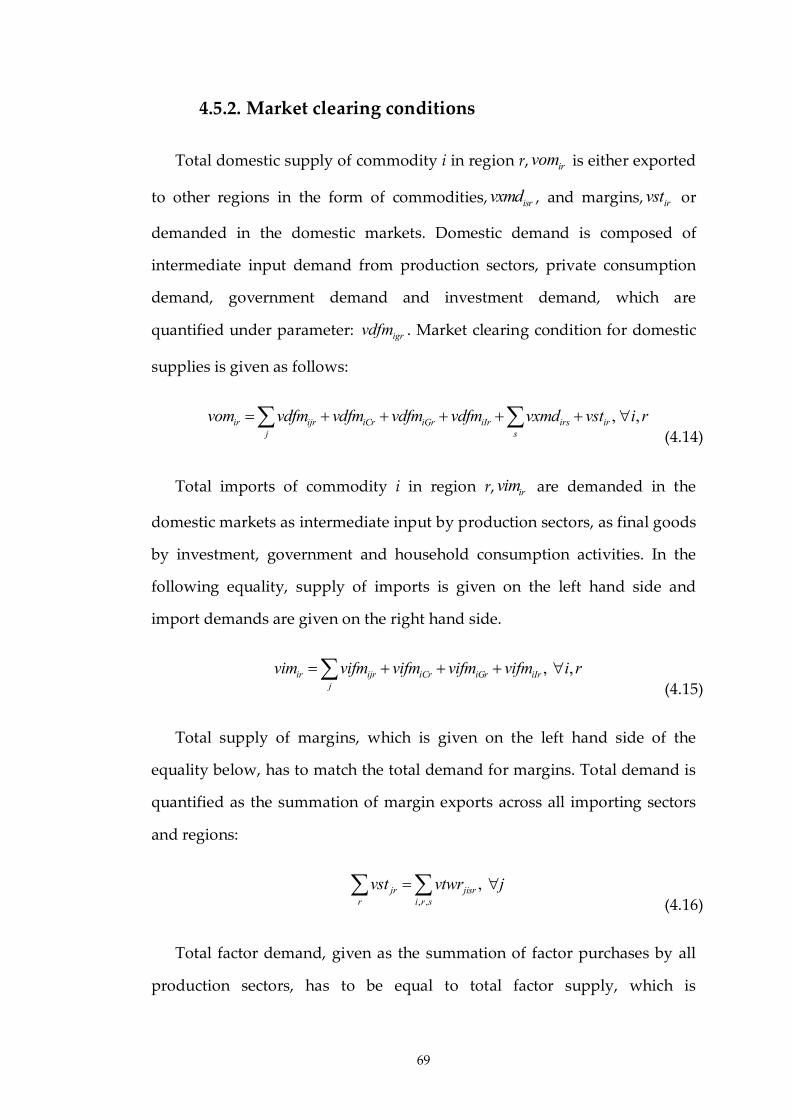
69

4.5.2. Market clearing conditions

Total domestic supply of commodity i in region r, irvom is either exported

to other regions in the form of commodities, isrvxmd , and margins, irvst or

demanded in the domestic markets. Domestic demand is composed of

intermediate input demand from production sectors, private consumption

demand, government demand and investment demand, which are

quantified under parameter: igrvdfm . Market clearing condition for domestic

supplies is given as follows:

, ,ir ijr iCr iGr iIr irs irj s

vom vdfm vdfm vdfm vdfm vxmd vst i r (4.14)

Total imports of commodity i in region r, irvim are demanded in the

domestic markets as intermediate input by production sectors, as final goods

by investment, government and household consumption activities. In the

following equality, supply of imports is given on the left hand side and

import demands are given on the right hand side.

, ,ir ijr iCr iGr iIrj

vim vifm vifm vifm vifm i r (4.15)

Total supply of margins, which is given on the left hand side of the

equality below, has to match the total demand for margins. Total demand is

quantified as the summation of margin exports across all importing sectors

and regions:

, ,

, jr jisrr i r s

vst vtwr j (4.16)

Total factor demand, given as the summation of factor purchases by all

production sectors, has to be equal to total factor supply, which is

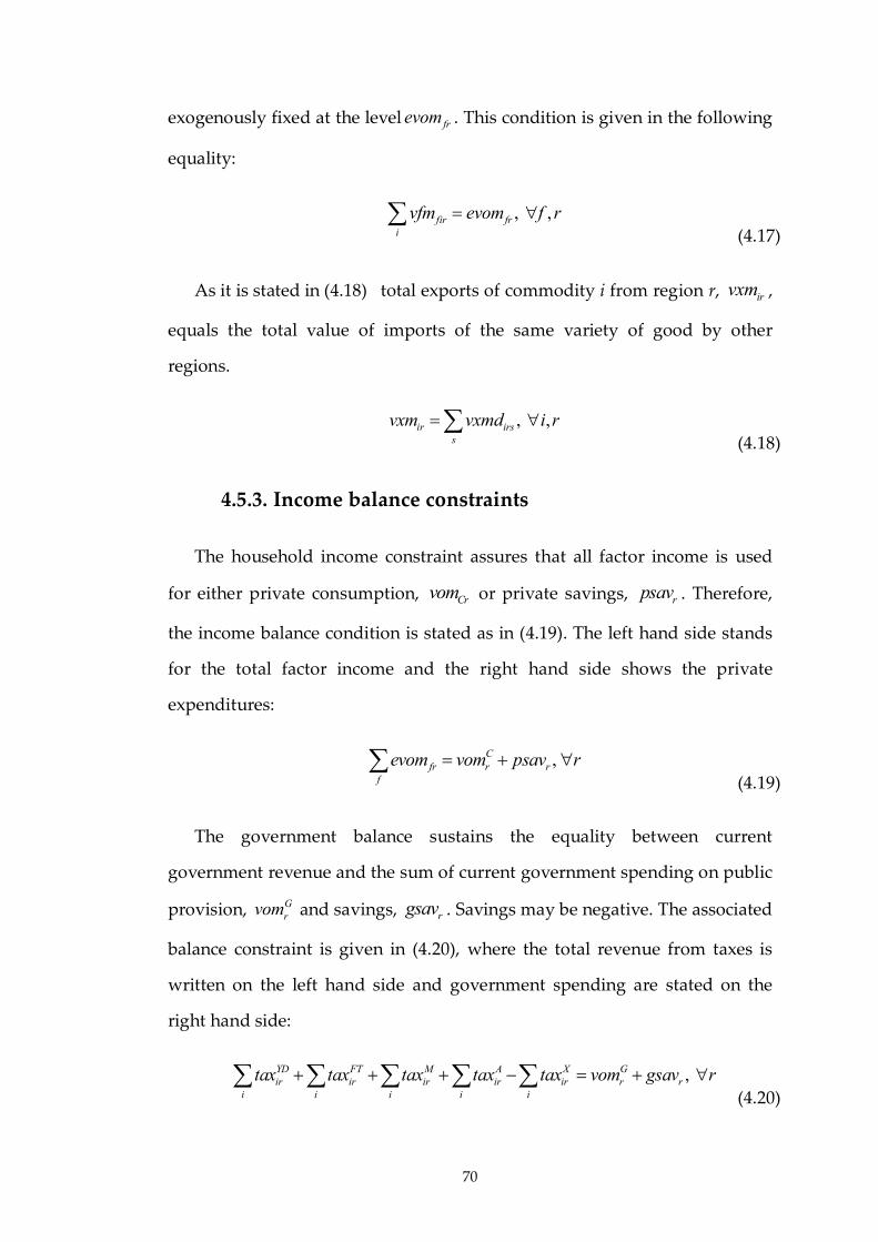
70

exogenously fixed at the level frevom . This condition is given in the following

equality:

, ,fir fri

vfm evom f r (4.17)

As it is stated in (4.18) total exports of commodity i from region r, irvxm ,

equals the total value of imports of the same variety of good by other

regions.

, ,ir irss

vxm vxmd i r (4.18)

4.5.3. Income balance constraints

The household income constraint assures that all factor income is used

for either private consumption, Crvom or private savings, rpsav . Therefore,

the income balance condition is stated as in (4.19). The left hand side stands

for the total factor income and the right hand side shows the private

expenditures:

, Cfr r r

f

evom vom psav r (4.19)

The government balance sustains the equality between current

government revenue and the sum of current government spending on public

provision, Grvom and savings, rgsav . Savings may be negative. The associated

balance constraint is given in (4.20), where the total revenue from taxes is

written on the left hand side and government spending are stated on the

right hand side:

, YD FT M A X Gir ir ir ir ir r r

i i i i i

tax tax tax tax tax vom gsav r (4.20)

71

In each region, total savings and total investment have to be equal. Total

savings is mainly the sum of private savings, government savings and also

the savings from the rest of the world. Using this equivalence relation,

foreign savings of each region, rfsav , is implicitly calculated in (4.21).

Foreign savings should exactly match the discrepancy between the total

investment and the sum of private and government savings:

,

C G Ir r r r fr

f

YD FT M A Xir ir ir ir ir

i i i i i

fsav vom vom vom evom

tax tax tax tax tax r

(4.21)

Foreign savings, calculated as in (4.22), should add up to zero. This

condition, checking for leakage in the global economy, is given in the

following equation:

0rr

fsav (4.22)

4.5.4. Energy use and CO2 emissions

In the MR-ETPA model, energy goods are specified as coal, oil, natural

gas and electricity. Crude oil is treated as a material input to the production

rather than an energy input. Depending on the production technologies and

the type of energy good used, certain levels of CO2 emissions are generated.

The amount of total emissions is linked to the use of energy volume by the

use of sector and good specific emission coefficients: 2COjirio and 2CO

jCrio . In

order to obtain the values of these coefficients at the benchmark equilibrium,

“eco2” data array in the GTAP 7 energy volume data set is used together

with “vdfm” and “vifm” data arrays in the GTAP 7 data set. These three data

arrays together tell how much CO2 emissions are generated via the use of

dirty inputs, i.e. coal, natural gas, oil and crude oil by certain production

72

sectors and household consumption. Hence, the sector and good specific

emission coefficients are calculated according to the following equations:

2 2

, ( ),1 1

jircojir

jir jir jir jir

ecoio j e j i

vdfm rtfd vifm rtfi

(4.23)

2 2

, ( ), ' '1 1

jCrcojCr

jCr jCr jCr jCr

ecoio j e j c

vdfm rtfd vifm rtfi

(4.24)

4.6. Country Profiles at Benchmark Equilibrium

4.6.1. Turkey

Turkey’s Gross Domestic Product (GDP) is given as $296.255 billion for

the year 2004. Looking at the SAM of Turkey in Table 4.8, gross output is

read as $497.434 billion. More detailed breakdown of gross output across

sectors is given in Table 4.5. Other economy sectors form the biggest share in

total output. Transport and other manufacturing industries follow that with

11% share. Textile, chemical, iron and steel and electricity sectors have the

shares of 6.4%, 3.8% and 2.7% in total output, respectively.

Total CO2 emissions are given as 202.24 Mt and the distribution across

sectors are given in Figure 4.1. According to the benchmark dataset,

emissions from electricity generation and household consumption form the

bulk of the total CO2 emissions volume. Transport and other economy

sectors follow that with 17% and 12%, respectively.

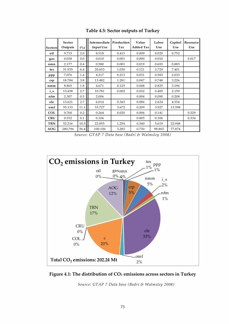
73

Table 4.5: Sector outputs of Turkey

Sectors

Sector

Outputs (%)

Intermediate

Input Use

Production

Tax

Value

Added Tax

Labor

Use

Capitol

Use

Resource

Use

oil 9.715 2.0 8.518 0.415 0.009 0.020 0.752

gas 0.038 0.0 0.010 0.001 0.000 0.010 0.017

omn 2.177 0.4 0.580 0.001 0.019 0.693 0.885

tex 31.935 6.4 20.653 1.030 0.121 2.729 7.401

ppp 7.076 1.4 4.217 0.213 0.031 0.583 2.033

crp 18.784 3.8 13.482 1.281 0.047 0.748 3.226

nmm 8.865 1.8 4.671 0.125 0.048 0.825 3.196

i_s 13.458 2.7 10.781 0.002 0.032 0.485 2.159

nfm 2.307 0.5 2.006 0.004 0.090 0.208

ele 13.621 2.7 6.014 0.343 0.086 2.624 4.554

omf 55.133 11.1 33.727 3.672 0.209 3.927 13.598

COL 0.760 0.2 0.264 0.020 0.006 0.141 0.329

CRU 0.552 0.1 0.106 0.005 0.106 0.334

TRN 52.216 10.5 22.055 1.254 0.340 5.619 22.948

AOG 280.796 56.4 100.106 3.283 0.730 98.803 77.874


Figure 4.1: The distribution of CO2 emissions across sectors in Turkey


oil

0%

gas

0%omn

0%

tex

1%ppp

1%

crp

5%

nmm

5%i_s

2%

nfm

1%

ele

33%

omf

2%

c

20%COL

0%

CRU

0%

TRN

17%

AOG

12%

CO2 emissions in Turkey

Total CO2 emissions: 202.24 Mt

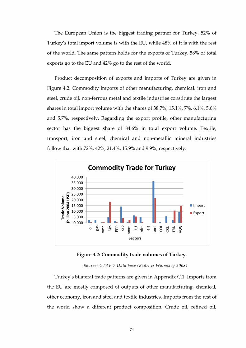
74

The European Union is the biggest trading partner for Turkey. 52% of

Turkey’s total import volume is with the EU, while 48% of it is with the rest

of the world. The same pattern holds for the exports of Turkey. 58% of total

exports go to the EU and 42% go to the rest of the world.

Product decomposition of exports and imports of Turkey are given in

Figure 4.2. Commodity imports of other manufacturing, chemical, iron and

steel, crude oil, non-ferrous metal and textile industries constitute the largest

shares in total import volume with the shares of 38.7%, 15.1%, 7%, 6.1%, 5.6%

and 5.7%, respectively. Regarding the export profile, other manufacturing

sector has the biggest share of 84.6% in total export volume. Textile,

transport, iron and steel, chemical and non-metallic mineral industries

follow that with 72%, 42%, 21.4%, 15.9% and 9.9%, respectively.

Figure 4.2: Commodity trade volumes of Turkey.


Turkey’s bilateral trade patterns are given in Appendix C.1. Imports from

the EU are mostly composed of outputs of other manufacturing, chemical,

other economy, iron and steel and textile industries. Imports from the rest of

the world show a different product composition. Crude oil, refined oil,

0.000

5.000

10.000

15.000

20.000

25.000

30.000

35.000

40.000

oil

gas

om

n

tex

pp

p

crp

nm

m i_s

nfm el

e

om

f

CO

L

CR

U

TRN

AO

G

Tra

de

Vo

lum

e

(bill

ion

200

4 U

SD)

Sectors

Commodity Trade for Turkey

Import

Export

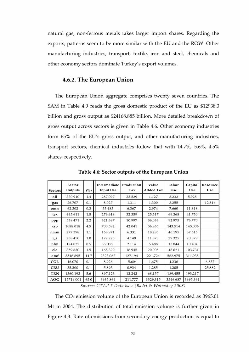
75

natural gas, non-ferrous metals takes larger import shares. Regarding the

exports, patterns seem to be more similar with the EU and the ROW. Other

manufacturing industries, transport, textile, iron and steel, chemicals and

other economy sectors dominate Turkey’s export volumes.

4.6.2. The European Union

The European Union aggregate comprises twenty seven countries. The

SAM in Table 4.9 reads the gross domestic product of the EU as $12938.3

billion and gross output as $24168.885 billion. More detailed breakdown of

gross output across sectors is given in Table 4.6. Other economy industries

form 65% of the EU’s gross output, and other manufacturing industries,

transport sectors, chemical industries follow that with 14.7%, 5.6%, 4.5%

shares, respectively.

Table 4.6: Sector outputs of the European Union

Sectors

Sector

Outputs (%)

Intermediate

Input Use

Production

Tax

Value

Added Tax

Labor

Use

Capitol

Use

Resource

Use

oil 330.910 1.4 287.097 33.529 1.127 3.232 5.925

gas 26.707 0.1 8.027 1.311 1.300 3.255 12.816

omn 62.302 0.3 33.483 6.367 2.974 7.660 11.818

tex 445.611 1.8 276.618 32.359 25.517 69.368 41.750

ppp 538.471 2.2 321.697 10.997 36.033 92.975 76.770

crp 1088.018 4.5 700.592 42.041 56.865 143.514 145.006

nmm 277.398 1.1 168.971 6.331 18.285 46.195 37.616

i_s 238.450 1.0 172.225 4.148 11.873 29.325 20.879

nfm 124.027 0.5 92.177 2.114 5.488 13.844 10.404

ele 359.630 1.5 168.329 18.945 20.005 48.621 103.731

omf 3546.895 14.7 2323.067 127.194 221.724 562.975 311.935

COL 16.070 0.1 8.926 -5.604 1.675 4.236 6.837

CRU 35.200 0.1 5.893 0.934 1.285 1.205 25.882

TRN 1360.193 5.6 897.123 12.242 68.157 189.455 193.217

AOG 15719.004 65.0 6935.864 211.777 1329.315 3546.687 3695.361


The CO2 emission volume of the European Union is recorded as 3965.01

Mt in 2004. The distribution of total emission volume is further given in

Figure 4.3. Rate of emissions from secondary energy production is equal to

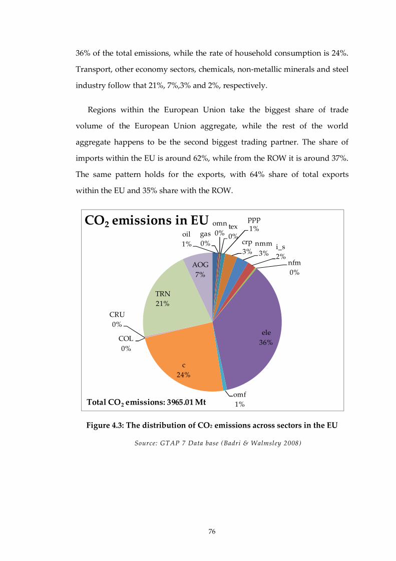
76

36% of the total emissions, while the rate of household consumption is 24%.

Transport, other economy sectors, chemicals, non-metallic minerals and steel

industry follow that 21%, 7%,3% and 2%, respectively.

Regions within the European Union take the biggest share of trade

volume of the European Union aggregate, while the rest of the world

aggregate happens to be the second biggest trading partner. The share of

imports within the EU is around 62%, while from the ROW it is around 37%.

The same pattern holds for the exports, with 64% share of total exports

within the EU and 35% share with the ROW.

Figure 4.3: The distribution of CO2 emissions across sectors in the EU


oil

1%

gas

0%

omn

0%tex

0%

ppp

1%

crp

3%nmm

3%i_s

2%nfm

0%

ele

36%

omf

1%

c

24%

COL

0%

CRU

0%

TRN

21%

AOG

7%

CO2 emissions in EU


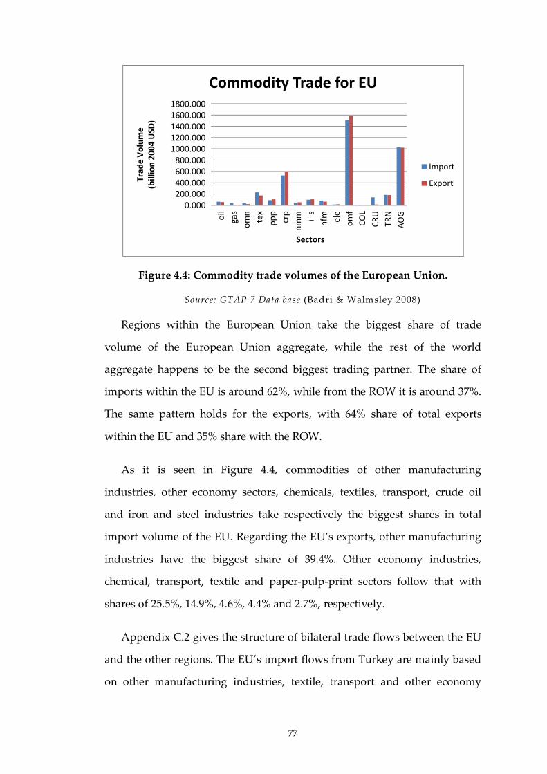
77

Figure 4.4: Commodity trade volumes of the European Union.


Regions within the European Union take the biggest share of trade

volume of the European Union aggregate, while the rest of the world

aggregate happens to be the second biggest trading partner. The share of

imports within the EU is around 62%, while from the ROW it is around 37%.

The same pattern holds for the exports, with 64% share of total exports

within the EU and 35% share with the ROW.

As it is seen in Figure 4.4, commodities of other manufacturing

industries, other economy sectors, chemicals, textiles, transport, crude oil

and iron and steel industries take respectively the biggest shares in total

import volume of the EU. Regarding the EU’s exports, other manufacturing

industries have the biggest share of 39.4%. Other economy industries,

chemical, transport, textile and paper-pulp-print sectors follow that with

shares of 25.5%, 14.9%, 4.6%, 4.4% and 2.7%, respectively.

Appendix C.2 gives the structure of bilateral trade flows between the EU

and the other regions. The EU’s import flows from Turkey are mainly based

on other manufacturing industries, textile, transport and other economy

0.000200.000400.000600.000800.000

1000.0001200.0001400.0001600.0001800.000

oil

gas

om

n

tex

pp

p

crp

nm

m i_s

nfm el

e

om

f

CO

L

CR

U

TRN

AO

G

Tra

de

Vo

lum

e

(bill

ion

200

4 U

SD)

Sectors

Commodity Trade for EU

Import

Export

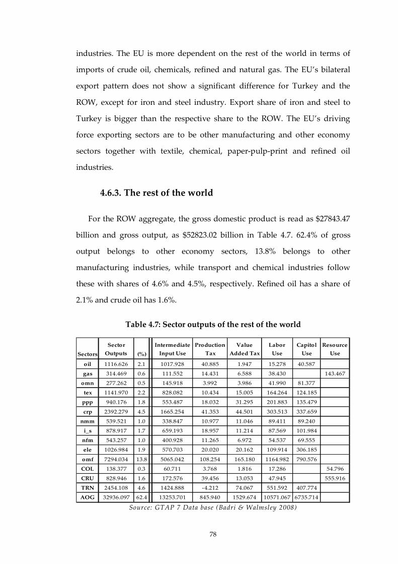
78

industries. The EU is more dependent on the rest of the world in terms of

imports of crude oil, chemicals, refined and natural gas. The EU’s bilateral

export pattern does not show a significant difference for Turkey and the

ROW, except for iron and steel industry. Export share of iron and steel to

Turkey is bigger than the respective share to the ROW. The EU’s driving

force exporting sectors are to be other manufacturing and other economy

sectors together with textile, chemical, paper-pulp-print and refined oil

industries.

4.6.3. The rest of the world

For the ROW aggregate, the gross domestic product is read as $27843.47

billion and gross output, as $52823.02 billion in Table 4.7. 62.4% of gross

output belongs to other economy sectors, 13.8% belongs to other

manufacturing industries, while transport and chemical industries follow

these with shares of 4.6% and 4.5%, respectively. Refined oil has a share of

2.1% and crude oil has 1.6%.

Table 4.7: Sector outputs of the rest of the world

Sectors

Sector

Outputs (%)

Intermediate

Input Use

Production

Tax

Value

Added Tax

Labor

Use

Capitol

Use

Resource

Use

oil 1116.626 2.1 1017.928 40.885 1.947 15.278 40.587

gas 314.469 0.6 111.552 14.431 6.588 38.430 143.467

omn 277.262 0.5 145.918 3.992 3.986 41.990 81.377

tex 1141.970 2.2 828.082 10.434 15.005 164.264 124.185

ppp 940.176 1.8 553.487 18.032 31.295 201.883 135.479

crp 2392.279 4.5 1665.254 41.353 44.501 303.513 337.659

nmm 539.521 1.0 338.847 10.977 11.046 89.411 89.240

i_s 878.917 1.7 659.193 18.957 11.214 87.569 101.984

nfm 543.257 1.0 400.928 11.265 6.972 54.537 69.555

ele 1026.984 1.9 570.703 20.020 20.162 109.914 306.185

omf 7294.034 13.8 5065.042 108.254 165.180 1164.982 790.576

COL 138.377 0.3 60.711 3.768 1.816 17.286 54.796

CRU 828.946 1.6 172.576 39.456 13.053 47.945 555.916

TRN 2454.108 4.6 1424.888 -4.212 74.067 551.592 407.774

AOG 32936.097 62.4 13253.701 845.940 1529.674 10571.067 6735.714


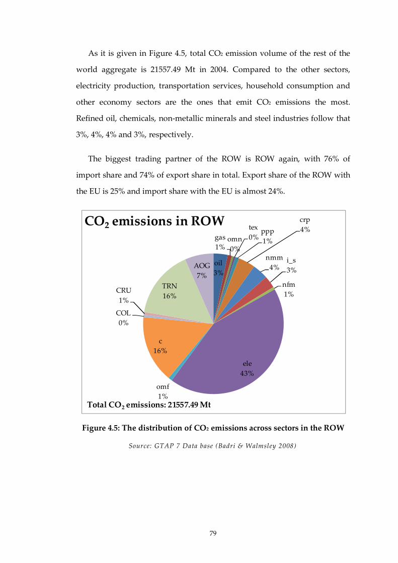
79

As it is given in Figure 4.5, total CO2 emission volume of the rest of the

world aggregate is 21557.49 Mt in 2004. Compared to the other sectors,

electricity production, transportation services, household consumption and

other economy sectors are the ones that emit CO2 emissions the most.

Refined oil, chemicals, non-metallic minerals and steel industries follow that

3%, 4%, 4% and 3%, respectively.

The biggest trading partner of the ROW is ROW again, with 76% of

import share and 74% of export share in total. Export share of the ROW with

the EU is 25% and import share with the EU is almost 24%.

Figure 4.5: The distribution of CO2 emissions across sectors in the ROW


oil

3%

gas

1%omn

0%

tex

0%ppp

1%

crp

4%

nmm

4%i_s

3%

nfm

1%

ele

43%

omf

1%

c

16%

COL

0%

CRU

1%

TRN

16%

AOG

7%

CO2 emissions in ROW


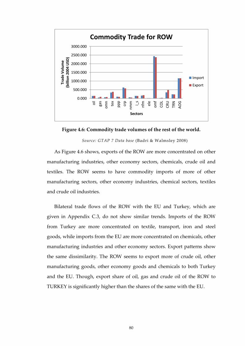
80

Figure 4.6: Commodity trade volumes of the rest of the world.


As Figure 4.6 shows, exports of the ROW are more concentrated on other

manufacturing industries, other economy sectors, chemicals, crude oil and

textiles. The ROW seems to have commodity imports of more of other

manufacturing sectors, other economy industries, chemical sectors, textiles

and crude oil industries.

Bilateral trade flows of the ROW with the EU and Turkey, which are

given in Appendix C.3, do not show similar trends. Imports of the ROW

from Turkey are more concentrated on textile, transport, iron and steel

goods, while imports from the EU are more concentrated on chemicals, other

manufacturing industries and other economy sectors. Export patterns show

the same dissimilarity. The ROW seems to export more of crude oil, other

manufacturing goods, other economy goods and chemicals to both Turkey

and the EU. Though, export share of oil, gas and crude oil of the ROW to

TURKEY is significantly higher than the shares of the same with the EU.

0.000

500.000

1000.000

1500.000

2000.000

2500.000

3000.000

oil

gas

om

n

tex

pp

p

crp

nm

m i_s

nfm el

e

om

f

CO

L

CR

U

TRN

AO

G

Tra

de

Vo

lum

e(b

illio

n 2

004

USD

)

Sectors

Commodity Trade for ROW

Import

Export

81

4.7. Social Accounting Matrices at Benchmark Equilibrium

Table 4.8: SAM of Turkey for year 2004

Table 4.9: SAM of the European Union for year 2004

Commodities Activities Factors Households Government Capital ROW Total

Commodities 12400.090 7736.819 2726.025 2532.100 4185.273 29580.306

Activities 24168.885 24168.885

Factors 9462.492 9462.492

Households 9462.492 9462.492

Government 1169.504 2306.303 3475.808

Capital 1725.673 749.783 56.644 2532.100

ROW 4241.917 4241.917

Total 29580.306 24168.885 9462.492 9462.492 3475.808 2532.100 4241.917

Table 4.10: SAM of the Rest of the World for year 2004


Commodities 26268.81 17356.628 4294.9337 6119.69 6219.58 60259.64

Activities 52823.0238 52823.02

Factors 23434.16 23434.16

Households 23434.2 23434.16

Government 1289.2577 3120.056 4409.314

Capital 6077.5277 114.3801 -72.2139 6119.694

ROW 6147.3633 6147.363

Total 60259.6447 52823.02 23434.2 23434.156 4409.3139 6119.69 6147.36


Commodities 227.189 211.774 40.729 59.322 83.694 622.708

Activities 497.434 497.434

Factors 256.917 256.917

Households 256.917 256.917

Government 26.010 13.328 39.338

Capital 45.144 -1.391 15.570 59.322

ROW 99.264 99.264

Total 622.708 497.434 256.917 256.917 39.338 59.322 99.264

82

CHAPTER 5

Economic Impacts of Market-based Environmental Regulation

in Turkey

5.1. Introduction

This chapter presents the major findings of a number of policy

simulations for various CO2 abatement policies. The simulations are

performed with the MR-ETPA model documented in Chapter 3 and

calibrated to the data sources given in Chapter 4.

Section 5.2 explains how the business-as-usual (BAU) scenario for the

current policy analyses is defined and constructed. Section 5.3 starts with

summarizing the BAU profiles of regional economies together with their

carbon footprints and continues with the description of policy scenarios. The

findings out of simulation runs for different counter-factual scenarios are

stated in Sections 5.4 – 5.7. Concluding comments are given in Section 5.8.

5.2. Business-As-Usual Scenario

In abatement policy analyses, it is customary to define a hypothetical

BAU scenario for any given target year, where the economies are assumed to

not apply any emission reduction targets. The main reason is that abatement

83

targets are generally set for the long run based on certain assumptions

regarding economic growth and potential energy efficiency improvements of

the respective regions. Therefore, defining a BAU scenario eases to quantify

and interpret the economic impacts of any abatement policy relative to the

case where no abatement takes place.

In this study, the target year is set as 2020 and the corresponding BAU

scenario is calibrated on top of the base year economies in 2004. The

European Union countries have already agreed on 2020 to be the target year

for the post-Kyoto period (European Commission 2008), in line with that,

there is also a consensus in the international arena for post-Kyoto actions to

become effective for 2020 (UNFCCC 2011). Although Turkey does not have

an official target year for binding emission limits, national permit market is

to be established by 2015, which is further expected to be integrated with the

EU ETS market as part of Turkey’s accession negotiations with the EU. From

that perspective, constructing BAU scenario with respect to the target year

2020 and taking that as the benchmark for abatement policy simulations in

Sections 5.4 —5.7 seems reasonable for all regions included in this study.

In formulating the BAU scenario, I use the forward calibration technique

(Bohringer et al. 2009a; Böhringer & Rutherford 2010). The rationale behind

the forward calibration of the model from the base year 2004 to the target

year 2020, involves calibration to a steady state where all physical quantities

grow at an exogenous rate, while keeping preference and production

structures as close as possible to the initial ones at the base year calibration.

In that regard, projections on regional GDP growth rates, energy demands,

CO2 emissions and population growth rates are indispensable for the

forward calibration technique.

84

For the projection data, I use two different sources. The projection data

from the US Energy Information Agency – International Energy Outlook

(IEO) - is used for the BAU calibration of the aggregate economies in the

model, i.e. the EU and the ROW (EIA 2010). GTAP7inGAMS routines are

used in aggregating the IEO country groupings in line with the region profile

used in this study (Rutherford 2011). Since IEO data set loses its accuracy in

more disaggregated forms of regional composition, it is further

complemented with more detailed information from the International

Energy Agency (IEA) for the BAU calibration of Turkish economy (IEA

2011b).

In the BAU calibration of each region in the MR-ETPA model, all factor

inputs and other exogenous variables, i.e. real government and investment

spending, are rescaled in proportion to regional GDP growth rate

projections. Energy demand projections are further used to recalibrate unit

cost and expenditure functions in order to match the actual projections of

energy use and CO2 emissions. This approach implicitly derives the

autonomous energy efficiency improvement (AEEI) indices for each sector i

in each region r. The AEEI index is a way of representation of non-price

driven improvements in technology in order to mimic improvements in

energy intensity of the economy which is not explained by fuel price changes

(Jorgenson & Hogan 1991; Manne & Richels 1992). Incorporating

technological change by the use of AEEI is one of the most commonly used

approaches in computable general equilibrium analysis of environmental

policies (Lee et al. 1994; Paltsev et al. 2005).

For constructing the BAU economies, the MR-ETPA model is iteratively

solved. At each iteration, technology parameters of production technologies

and parameters of preference functions are recalibrated. The new

85

equilibrium price and quantity variables for the calibrated 2020 economies

are obtained from this iterative procedure.

5.3. Description of Policy Scenarios

As this study mainly targets to quantify the potential welfare effects of

Turkey’s application of permit trading mechanism both at regional and

international level, the sets of simulations are determined accordingly. Since

Turkey has not yet engaged in any kind of legal sanctions for CO2 emissions,

the design issue of a national permit market brings lots of institutional

dimensions that have to be tackled all at once. The very first and perhaps the

most critical decision in designing an ETS is the total emission cutback ratio

that Turkey should apply countrywide. It is possible to define caps as certain

percentages of emissions for a specified time period, or as relative to various

macro aggregates, i.e. production levels or GDP (Hood 2010). It is crucial to

set emission caps tight enough to constrain emissions in order to create

incentives for emissions to be reduced. Total cap amount further gains

importance in an international permit trading market. The distribution of

permit exporters and importers in an international ETS is directly related to

the relative MACs, which is a direct consequence of the total caps imposed

on regions. The following issue is about to draw the boundaries of the permit

trading market, both in the real geographical sense and also in terms of the

sectors, which are allowed to do permit trading. In geographical sense,

different options are available, such as establishing domestic permit trading

markets or establishing one way or two way linkages with the existing

international permit trading or carbon offset markets. Needless to mention,

the partners involved in trade has direct effects on the permit price levels

and welfare consequences of any ETS application. Further issues in

designing an ETS do exist, regarding the way of allocating permits across

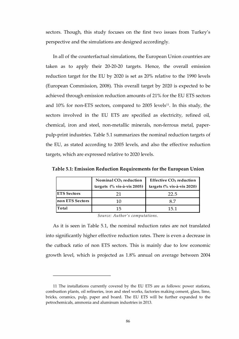
86

sectors. Though, this study focuses on the first two issues from Turkey’s

perspective and the simulations are designed accordingly.

In all of the counterfactual simulations, the European Union countries are

taken as to apply their 20-20-20 targets. Hence, the overall emission

reduction target for the EU by 2020 is set as 20% relative to the 1990 levels

(European Commission, 2008). This overall target by 2020 is expected to be

achieved through emission reduction amounts of 21% for the EU ETS sectors

and 10% for non-ETS sectors, compared to 2005 levels11. In this study, the

sectors involved in the EU ETS are specified as electricity, refined oil,

chemical, iron and steel, non-metallic minerals, non-ferrous metal, paper-

pulp-print industries. Table 5.1 summarizes the nominal reduction targets of

the EU, as stated according to 2005 levels, and also the effective reduction

targets, which are expressed relative to 2020 levels.

Table 5.1: Emission Reduction Requirements for the European Union

ETS Sectors 21 22.5

non ETS Sectors 10 8.7

Total 15 15.1

Nominal CO2 reduction

targets (% vis-à-vis 2005)

Effective CO2 reduction

targets (% vis-à-vis 2020)

Source: Author’s computations.

As it is seen in Table 5.1, the nominal reduction rates are not translated

into significantly higher effective reduction rates. There is even a decrease in

the cutback ratio of non ETS sectors. This is mainly due to low economic

growth level, which is projected as 1.8% annual on average between 2004

11 The installations currently covered by the EU ETS are as follows: power stations,

combustion plants, oil refineries, iron and steel works, factories making cement, glass, lime,

bricks, ceramics, pulp, paper and board. The EU ETS will be further expanded to the

petrochemicals, ammonia and aluminum industries in 2013.

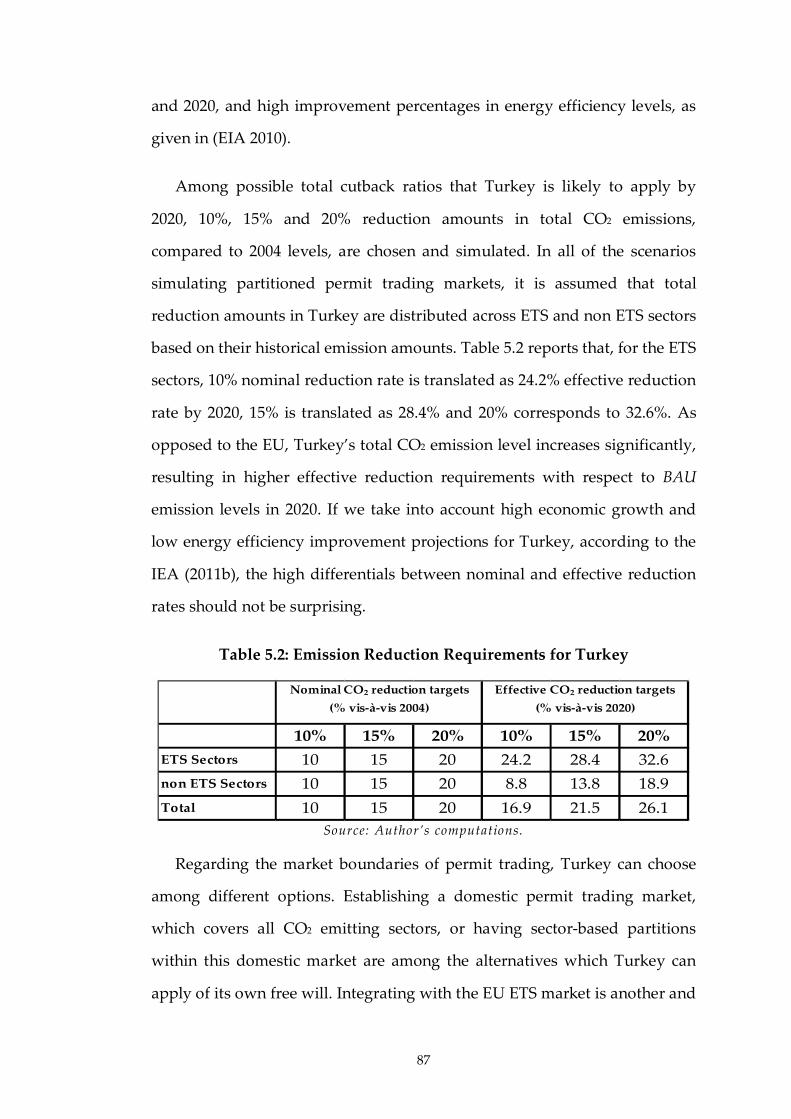
87

and 2020, and high improvement percentages in energy efficiency levels, as

given in (EIA 2010).

Among possible total cutback ratios that Turkey is likely to apply by

2020, 10%, 15% and 20% reduction amounts in total CO2 emissions,

compared to 2004 levels, are chosen and simulated. In all of the scenarios

simulating partitioned permit trading markets, it is assumed that total

reduction amounts in Turkey are distributed across ETS and non ETS sectors

based on their historical emission amounts. Table 5.2 reports that, for the ETS

sectors, 10% nominal reduction rate is translated as 24.2% effective reduction

rate by 2020, 15% is translated as 28.4% and 20% corresponds to 32.6%. As

opposed to the EU, Turkey’s total CO2 emission level increases significantly,

resulting in higher effective reduction requirements with respect to BAU

emission levels in 2020. If we take into account high economic growth and

low energy efficiency improvement projections for Turkey, according to the

IEA (2011b), the high differentials between nominal and effective reduction

rates should not be surprising.

Table 5.2: Emission Reduction Requirements for Turkey

10% 15% 20% 10% 15% 20%

ETS Sectors 10 15 20 24.2 28.4 32.6

non ETS Sectors 10 15 20 8.8 13.8 18.9

Total 10 15 20 16.9 21.5 26.1

Nominal CO2 reduction targets

(% vis-à-vis 2004)

Effective CO2 reduction targets

(% vis-à-vis 2020)


Regarding the market boundaries of permit trading, Turkey can choose

among different options. Establishing a domestic permit trading market,

which covers all CO2 emitting sectors, or having sector-based partitions

within this domestic market are among the alternatives which Turkey can

apply of its own free will. Integrating with the EU ETS market is another and

88

most likely option when Turkey backs international cooperation in

environmental policy applications. Therefore, in order to address these

possible options in front of Turkey, the following scenarios are simulated.

NOACT: Turkey does not take any abatement action.

NP_rETS: Turkey sets binding CO2 emission quota and establishes a

comprehensive domestic permit trading market, which encompasses

all CO2 emitting sectors.

P_rETS: Turkey separates its national permit trading market into two

main parts, i.e. ETS sectors and non ETS sectors12. The respective

emission reduction targets for the sectors are set in proportion to their

2004 emission levels. While ETS sectors are allowed to trade permits

with each other, non ETS sectors are subject to separate abatement

policies.

EU_ETS: Turkey separates its national permit trading market into two

segments, i.e. ETS sectors trading permits within the EU ETS and non

ETS sectors being subject to other domestic abatement policies. The

emission reduction targets for ETS and non ETS sectors are set in

proportion to their 2004 emission levels.

5.4. NOACT: No Abatement Case

As the EU applies CO2 quotas on both ETS and non ETS sectors, the

permit price in the ETS market realizes as $17.73 per ton of CO2, while MACs

of non ETS sectors are equal to $84.19 per ton of CO2. This direct cost burden

on CO2 emitting sectors affects the production costs and the supply patterns

in the EU. As Table 5.21 shows, the production levels of all sectors in the EU,

12 The distinction between ETS and non ETS sectors are made in line with the one in the

EU ETS market.

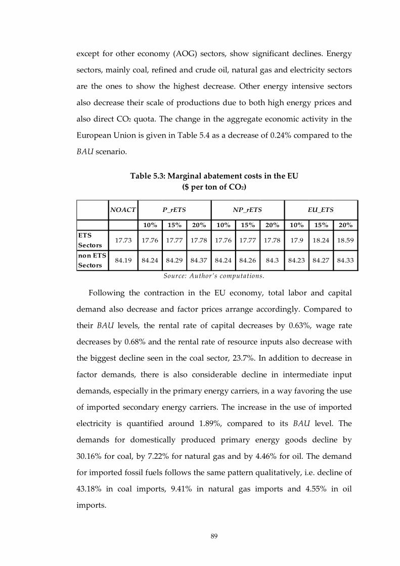
89

except for other economy (AOG) sectors, show significant declines. Energy

sectors, mainly coal, refined and crude oil, natural gas and electricity sectors

are the ones to show the highest decrease. Other energy intensive sectors

also decrease their scale of productions due to both high energy prices and

also direct CO2 quota. The change in the aggregate economic activity in the

European Union is given in Table 5.4 as a decrease of 0.24% compared to the

BAU scenario.

Table 5.3: Marginal abatement costs in the EU

($ per ton of CO2)

NOACT

10% 15% 20% 10% 15% 20% 10% 15% 20%

ETS

Sectors17.73 17.76 17.77 17.78 17.76 17.77 17.78 17.9 18.24 18.59

non ETS

Sectors84.19 84.24 84.29 84.37 84.24 84.26 84.3 84.23 84.27 84.33

P_rETS NP_rETS EU_ETS


Following the contraction in the EU economy, total labor and capital

demand also decrease and factor prices arrange accordingly. Compared to

their BAU levels, the rental rate of capital decreases by 0.63%, wage rate

decreases by 0.68% and the rental rate of resource inputs also decrease with

the biggest decline seen in the coal sector, 23.7%. In addition to decrease in

factor demands, there is also considerable decline in intermediate input

demands, especially in the primary energy carriers, in a way favoring the use

of imported secondary energy carriers. The increase in the use of imported

electricity is quantified around 1.89%, compared to its BAU level. The

demands for domestically produced primary energy goods decline by

30.16% for coal, by 7.22% for natural gas and by 4.46% for oil. The demand

for imported fossil fuels follows the same pattern qualitatively, i.e. decline of

43.18% in coal imports, 9.41% in natural gas imports and 4.55% in oil

imports.

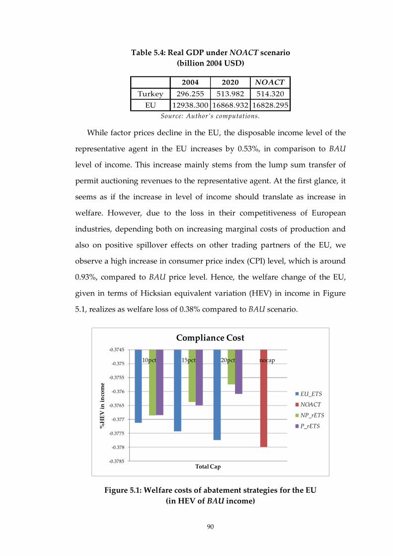
90

Table 5.4: Real GDP under NOACT scenario

(billion 2004 USD)

2004 2020 NOACT

Turkey 296.255 513.982 514.320

EU 12938.300 16868.932 16828.295 Source: Author’s computations.

While factor prices decline in the EU, the disposable income level of the

representative agent in the EU increases by 0.53%, in comparison to BAU

level of income. This increase mainly stems from the lump sum transfer of

permit auctioning revenues to the representative agent. At the first glance, it

seems as if the increase in level of income should translate as increase in

welfare. However, due to the loss in their competitiveness of European

industries, depending both on increasing marginal costs of production and

also on positive spillover effects on other trading partners of the EU, we

observe a high increase in consumer price index (CPI) level, which is around

0.93%, compared to BAU price level. Hence, the welfare change of the EU,

given in terms of Hicksian equivalent variation (HEV) in income in Figure

5.1, realizes as welfare loss of 0.38% compared to BAU scenario.

Figure 5.1: Welfare costs of abatement strategies for the EU

(in HEV of BAU income)

-0.3785

-0.378

-0.3775

-0.377

-0.3765

-0.376

-0.3755

-0.375

-0.3745

10pct 15pct 20pct nocap

%H

EV

in

in

com

e

Total Cap

Compliance Cost

EU_ETS

NOACT

NP_rETS

P_rETS

91

In opposed to the economic welfare losses, the European Union benefits

from decreasing CO2 emission levels, and furthermore, from decreasing CO2

intensity of its production technologies. As it is seen in Table 5.24, while the

CO2 intensity of the European economy is recorded as 0.236 Mt CO2 per 2004

USD under BAU scenario, it decreases to 0.200 Mt CO2 per 2004 USD under

NOACT scenario. This is mainly due to the increasing cost pressure on the

use of fossil fuels, which further gives incentives for switching to less

carbon- intense production processes.

Abatement policies in the EU affect not only the domestic markets but

also the world markets. The EU is one of the three biggest users and

importers of energy goods in the world economy. Therefore, any change in

the EU’s both domestic and import demand for energy goods, as a result of

abatement policies, results in new price and quantity adjustments not only in

domestic markets but also in world markets. These chain effects are known

as “terms of trade effects” in the literature. In CO2 abatement policies, terms of

trade effects occur mainly due to the differences in production technologies

of the economies and the relative position of countries in terms of abatement

cutbacks. Non abating countries gain comparative advantage in the

production of energy intensive commodities due to their relatively low

MACs compared to the abating countries having high MACs. Additionally,

CO2 restrictions directly affect the demand for fossil fuels in the world

markets. Change in prices due to shifts in aggregate demand for fossil fuels

creates substantial spillover effects to other regions. The literature on terms

of trade effects concludes that the effects of changes in fossil fuel prices

mostly dominate the effects of changes in comparative advantages

(Bohringer & Rutherford 2002; Babiker et al. 2004). For countries that are not

subject to any additional abatement targets, it is shown that changes in the

world energy markets affect fossil fuel exporters negatively, while fuel

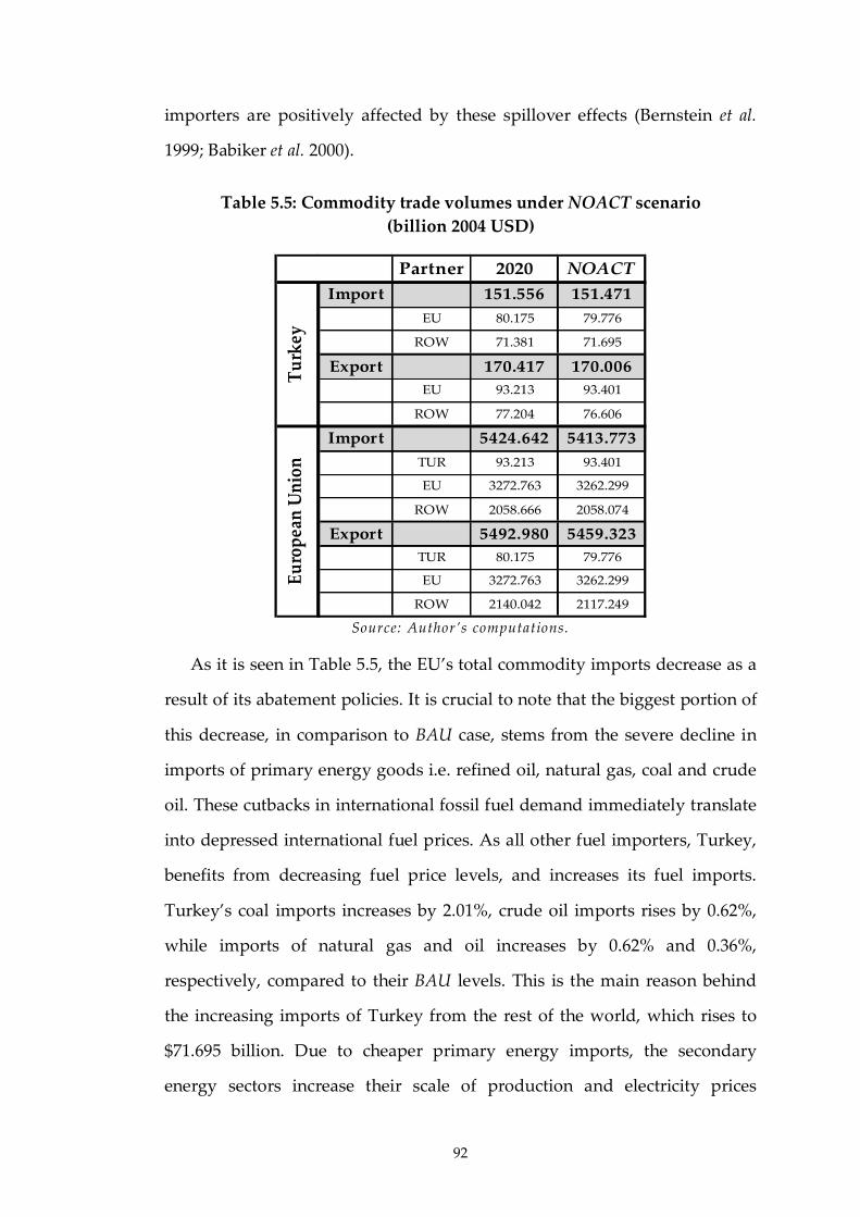
92

importers are positively affected by these spillover effects (Bernstein et al.

1999; Babiker et al. 2000).

Table 5.5: Commodity trade volumes under NOACT scenario

(billion 2004 USD)

Partner 2020 NOACT

Import 151.556 151.471

EU 80.175 79.776

ROW 71.381 71.695

Export 170.417 170.006

EU 93.213 93.401

ROW 77.204 76.606

Import 5424.642 5413.773

TUR 93.213 93.401

EU 3272.763 3262.299

ROW 2058.666 2058.074

Export 5492.980 5459.323

TUR 80.175 79.776

EU 3272.763 3262.299

ROW 2140.042 2117.249

Tu

rkey

Eu

rop

ean

Un

ion


As it is seen in Table 5.5, the EU’s total commodity imports decrease as a

result of its abatement policies. It is crucial to note that the biggest portion of

this decrease, in comparison to BAU case, stems from the severe decline in

imports of primary energy goods i.e. refined oil, natural gas, coal and crude

oil. These cutbacks in international fossil fuel demand immediately translate

into depressed international fuel prices. As all other fuel importers, Turkey,

benefits from decreasing fuel price levels, and increases its fuel imports.

Turkey’s coal imports increases by 2.01%, crude oil imports rises by 0.62%,

while imports of natural gas and oil increases by 0.62% and 0.36%,

respectively, compared to their BAU levels. This is the main reason behind

the increasing imports of Turkey from the rest of the world, which rises to

$71.695 billion. Due to cheaper primary energy imports, the secondary

energy sectors increase their scale of production and electricity prices

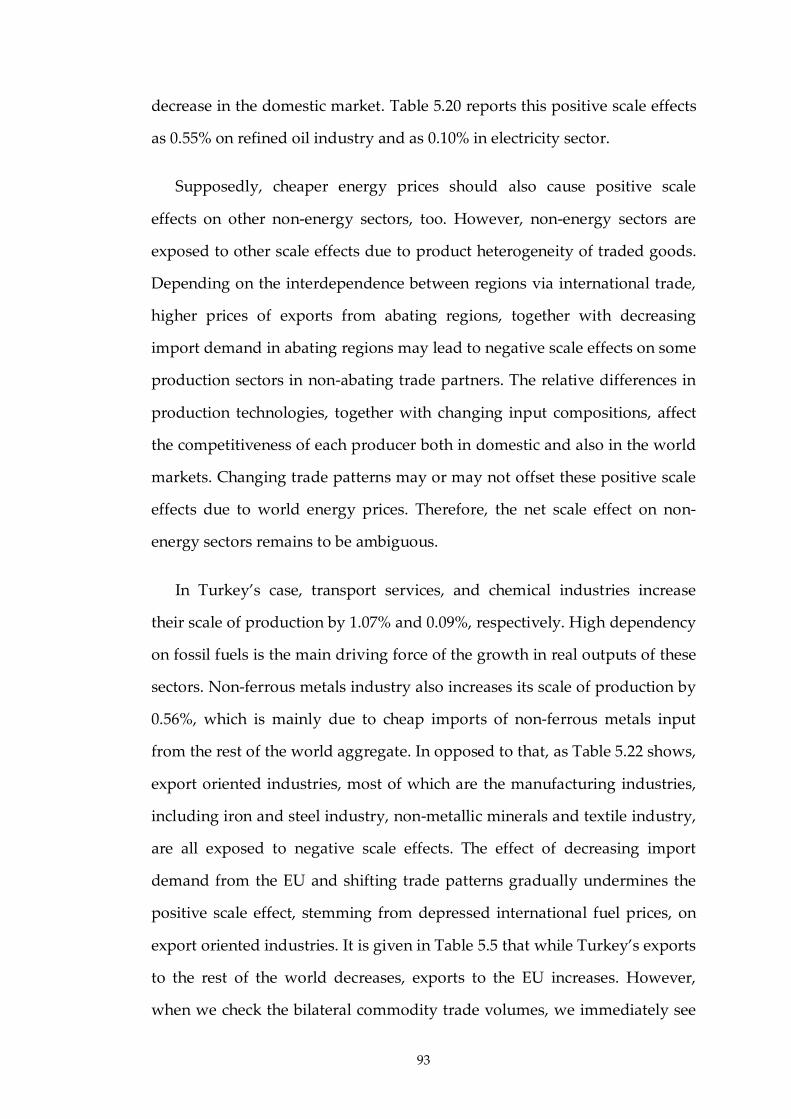
93

decrease in the domestic market. Table 5.20 reports this positive scale effects

as 0.55% on refined oil industry and as 0.10% in electricity sector.

Supposedly, cheaper energy prices should also cause positive scale

effects on other non-energy sectors, too. However, non-energy sectors are

exposed to other scale effects due to product heterogeneity of traded goods.

Depending on the interdependence between regions via international trade,

higher prices of exports from abating regions, together with decreasing

import demand in abating regions may lead to negative scale effects on some

production sectors in non-abating trade partners. The relative differences in

production technologies, together with changing input compositions, affect

the competitiveness of each producer both in domestic and also in the world

markets. Changing trade patterns may or may not offset these positive scale

effects due to world energy prices. Therefore, the net scale effect on non-

energy sectors remains to be ambiguous.

In Turkey’s case, transport services, and chemical industries increase

their scale of production by 1.07% and 0.09%, respectively. High dependency

on fossil fuels is the main driving force of the growth in real outputs of these

sectors. Non-ferrous metals industry also increases its scale of production by

0.56%, which is mainly due to cheap imports of non-ferrous metals input

from the rest of the world aggregate. In opposed to that, as Table 5.22 shows,

export oriented industries, most of which are the manufacturing industries,

including iron and steel industry, non-metallic minerals and textile industry,

are all exposed to negative scale effects. The effect of decreasing import

demand from the EU and shifting trade patterns gradually undermines the

positive scale effect, stemming from depressed international fuel prices, on

export oriented industries. It is given in Table 5.5 that while Turkey’s exports

to the rest of the world decreases, exports to the EU increases. However,

when we check the bilateral commodity trade volumes, we immediately see

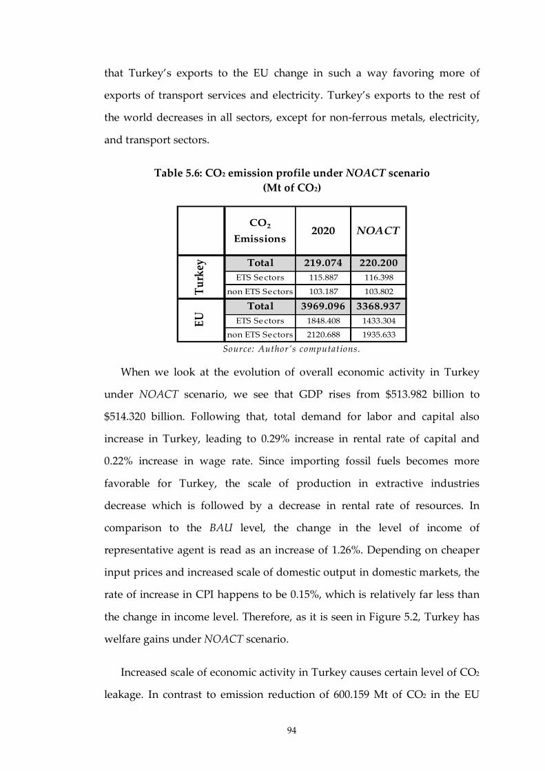
94

that Turkey’s exports to the EU change in such a way favoring more of

exports of transport services and electricity. Turkey’s exports to the rest of

the world decreases in all sectors, except for non-ferrous metals, electricity,

and transport sectors.

Table 5.6: CO2 emission profile under NOACT scenario

(Mt of CO2)

CO2

Emissions2020 NOACT

Total 219.074 220.200

ETS Sectors 115.887 116.398

non ETS Sectors 103.187 103.802

Total 3969.096 3368.937

ETS Sectors 1848.408 1433.304

non ETS Sectors 2120.688 1935.633

Tu

rkey

EU


When we look at the evolution of overall economic activity in Turkey

under NOACT scenario, we see that GDP rises from $513.982 billion to

$514.320 billion. Following that, total demand for labor and capital also

increase in Turkey, leading to 0.29% increase in rental rate of capital and

0.22% increase in wage rate. Since importing fossil fuels becomes more

favorable for Turkey, the scale of production in extractive industries

decrease which is followed by a decrease in rental rate of resources. In

comparison to the BAU level, the change in the level of income of

representative agent is read as an increase of 1.26%. Depending on cheaper

input prices and increased scale of domestic output in domestic markets, the

rate of increase in CPI happens to be 0.15%, which is relatively far less than

the change in income level. Therefore, as it is seen in Figure 5.2, Turkey has

welfare gains under NOACT scenario.

Increased scale of economic activity in Turkey causes certain level of CO2

leakage. In contrast to emission reduction of 600.159 Mt of CO2 in the EU

95

countries, Turkey increases its total CO2 emissions from 219.074 Mt of CO2 to

220.200 Mt of CO2. According to the emission profiles, given in Table 5.6,

ETS sectors are the main driving force behind the increase in Turkey’s CO2

emissions. While CO2 emissions from ETS sectors happen to be 115.887 Mt of

CO2 under BAU scenario, it increases to 116.398 Mt of CO2. The positive scale

effects on overall economic activity and also the shift in the use of energy

inputs in production sectors give rise to this CO2 leakage. Under NOACT

scenario, positive spillover effects from decreased international fuel demand,

cause primary energy goods, especially, coal, natural gas and oil, to be used

more intensely in Turkish production sectors. Hence, each unit production

results in more emissions compared to the BAU economy. This change in the

production patterns is clearly seen in the CO2 intensity data given in Table

5.24. The CO2 intensity of the Turkish economy increases to 0.428 Mt of CO2

per 2004 USD under NOACT scenario from 0.426 Mt CO2 per 2004 USD,

which is the intensity level of the BAU economy.

Table 5.7: Marginal Abatement Costs in Turkey

($ per ton of CO2)

NOACT

10% 15% 20% 10% 15% 20% 10% 15% 20%

ETS

Sectors-- 20.09 26.63 34.91 19.9 29.74 43.25 17.9 18.24 18.59

non ETS

Sectors-- 19.42 38.39 67.55 19.9 29.74 43.25 19.38 38.27 67.46

P_rETS NP_rETS EU_ETS


5.5. NP_rETS: Non Partitioned Regional ETS Market

Under comprehensive trading scheme, there realizes only a unique

permit price in Turkey. Under 10% cutback ratio, the permit price is equal to

$19.9 per ton of CO2. The permit price level, which is the respective shadow

price of the corresponding CO2 quota, is expected to raise depending on the

severity of the emission constraints. What we see in Table 5.7 is that permit

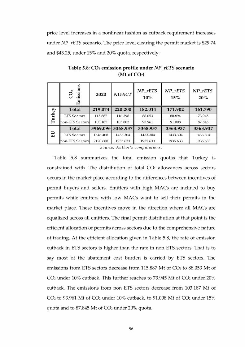
96

price level increases in a nonlinear fashion as cutback requirement increases

under NP_rETS scenario. The price level clearing the permit market is $29.74

and $43.25, under 15% and 20% quota, respectively.

Table 5.8: CO2 emission profile under NP_rETS scenario

(Mt of CO2) C

O2

Em

issi

ons

2020 NOACTNP_rETS

10%

NP_rETS

15%

NP_rETS

20%

Total 219.074 220.200 182.014 171.902 161.790

ETS Sectors 115.887 116.398 88.053 80.894 73.945

non-ETS Sectors 103.187 103.802 93.961 91.008 87.845

Total 3969.096 3368.937 3368.937 3368.937 3368.937

ETS Sectors 1848.408 1433.304 1433.304 1433.304 1433.304

non-ETS Sectors 2120.688 1935.633 1935.633 1935.633 1935.633

Tu

rkey

EU


Table 5.8 summarizes the total emission quotas that Turkey is

constrained with. The distribution of total CO2 allowances across sectors

occurs in the market place according to the differences between incentives of

permit buyers and sellers. Emitters with high MACs are inclined to buy

permits while emitters with low MACs want to sell their permits in the

market place. These incentives move in the direction where all MACs are

equalized across all emitters. The final permit distribution at that point is the

efficient allocation of permits across sectors due to the comprehensive nature

of trading. At the efficient allocation given in Table 5.8, the rate of emission

cutback in ETS sectors is higher than the rate in non ETS sectors. That is to

say most of the abatement cost burden is carried by ETS sectors. The

emissions from ETS sectors decrease from 115.887 Mt of CO2 to 88.053 Mt of

CO2 under 10% cutback. This further reaches to 73.945 Mt of CO2 under 20%

cutback. The emissions from non ETS sectors decrease from 103.187 Mt of

CO2 to 93.961 Mt of CO2 under 10% cutback, to 91.008 Mt of CO2 under 15%

quota and to 87.845 Mt of CO2 under 20% quota.

97

This extra cost burden on the Turkish economy affects the production

sectors in a negative way. All sectors, except for the transport sector,

decrease their scale of productions compared to the BAU case. It is especially

the energy sectors, i.e. coal, electricity, natural gas and oil, and also the

energy intensive sectors, such as iron and steel, chemicals and non-metallic

minerals, that have severe declines in their real output levels. As Table 5.20

summarizes, the contraction in these sectors continues to grow as the

amount of cutback ratio increases. In contrast to others, transport sector

continues to expand its scale in a decreasing rate with increasing quota level.

The effects of comprehensive regional permit trading on the GDP level is

given in Table 5.9. The GDP level of Turkey under a comprehensive trading

regime is less than the GDP level realizing under NOACT scenario.

Additionally, compared to BAU scenario, the GDP level of Turkey also

decreases by 0.23% under 10% CO2 quota. The rate of decrease in level of

GDP increases to 0.38% under 15% quota and 0.59% under 20% quota.

Table 5.9: Real GDP under NP_rETS scenario

(billion 2004 USD)

2004 2020NP_rETS

10%

NP_rETS

15%

NP_rETS

20%

Turkey 296.255 513.982 512.800 512.010 510.938

EU 12938.300 16868.932 16828.409 16828.459 16828.523


The negative scale effects on sectors in Turkish economy, except for the

transport sector, cause total factor demands to decrease. The change in rental

rate of capital compared to the BAU level realizes as -0.65% under 10%

cutback, -1.08% and -1.62% under 15% and 20% quota, respectively. In a

similar fashion, the wage rate decreases by 0.67%, under 10% quota and the

amount of decrease increases up to 1.55% under 20% quota. In contrast to the

decrease in total factor income, the disposable level of income of the

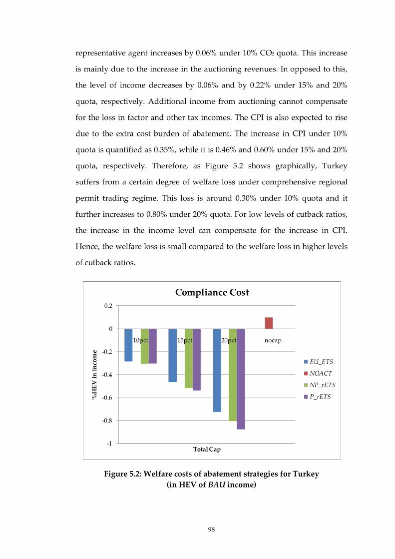
98

representative agent increases by 0.06% under 10% CO2 quota. This increase

is mainly due to the increase in the auctioning revenues. In opposed to this,

the level of income decreases by 0.06% and by 0.22% under 15% and 20%

quota, respectively. Additional income from auctioning cannot compensate

for the loss in factor and other tax incomes. The CPI is also expected to rise

due to the extra cost burden of abatement. The increase in CPI under 10%

quota is quantified as 0.35%, while it is 0.46% and 0.60% under 15% and 20%

quota, respectively. Therefore, as Figure 5.2 shows graphically, Turkey

suffers from a certain degree of welfare loss under comprehensive regional

permit trading regime. This loss is around 0.30% under 10% quota and it

further increases to 0.80% under 20% quota. For low levels of cutback ratios,

the increase in the income level can compensate for the increase in CPI.

Hence, the welfare loss is small compared to the welfare loss in higher levels

of cutback ratios.

Figure 5.2: Welfare costs of abatement strategies for Turkey

(in HEV of BAU income)

-1

-0.8

-0.6

-0.4

-0.2

0

0.2

10pct 15pct 20pct nocap

%H

EV

in

in

com

e

Total Cap

Compliance Cost

EU_ETS

NOACT

NP_rETS

P_rETS

99

Besides noting Turkey’s losses in economic welfare, it is also crucial to

emphasize the improvement in Turkey’s environmental indicators. As Table

5.24 shows, the CO2 intensity of the Turkish economy decreases to 0.355 Mt

CO2 per 2004 USD under NP_rETS scenario. As the cutback requirement

increases, the intensity further decreases to 0.336 and 0.317 under 15% and

20% caps, respectively. Hence, while Turkey suffers from welfare losses in

terms of total consumption, it also benefits from increased environmental

quality and incentives for transforming into less carbon-intense economy.

Total commodity exports of Turkey decreases from $170.417 billion to

$169.157 billion with 10% total abatement ratio. As it is reported in Table

5.10, as the cutback ratio increases, total export volume continues to decrease

due to the decline in the total economic activity. Compared to the BAU

scenario, Turkey’s total import volume also decreases from $151.556 billion

to $151.122 billion, under NP_rETS scenario. Compared to the NOACT

scenario, total imports also show a decreasing trend. Total commodity

import volume continues to decline as the cutback ratio increases. It is

crucial to note here also the changes in bilateral import patterns. Although

Turkey starts to import less under comprehensive permit market, the data

reveals that compared to NOACT scenario, Turkey’s imports from the

European Union increases. The decrease in total import volume is mainly

due to the decrease in imports from the rest of the world aggregate. In

essence, Turkey’s imports from the European Union increases from $79.776

billion to $79.881 billion under comprehensive permit market with 10%

cutback, to $79.914 billion under 15% quota and to $79.949 billion under 20%

quota. Thus, imports from the EU start to get a bigger share in total imports

as the total cutback requirement increases. That is to say European industries

become more competitive in the Turkish domestic market.

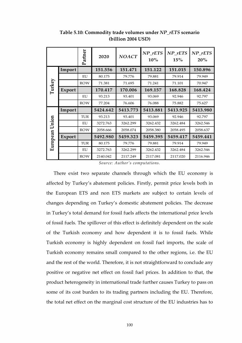
100

Table 5.10: Commodity trade volumes under NP_rETS scenario

(billion 2004 USD)

Par

tner

2020 NOACTNP_rETS

10%

NP_rETS

15%

NP_rETS

20%

Import 151.556 151.471 151.122 151.015 150.896

EU 80.175 79.776 79.881 79.914 79.949

ROW 71.381 71.695 71.241 71.101 70.947

Export 170.417 170.006 169.157 168.828 168.424

EU 93.213 93.401 93.069 92.946 92.797

ROW 77.204 76.606 76.088 75.882 75.627

Import 5424.642 5413.773 5413.881 5413.925 5413.980

TUR 93.213 93.401 93.069 92.946 92.797

EU 3272.763 3262.299 3262.432 3262.484 3262.546

ROW 2058.666 2058.074 2058.380 2058.495 2058.637

Export 5492.980 5459.323 5459.395 5459.417 5459.441

TUR 80.175 79.776 79.881 79.914 79.949

EU 3272.763 3262.299 3262.432 3262.484 3262.546

ROW 2140.042 2117.249 2117.081 2117.020 2116.946

Eu

rop

ean

Un

ion

Tu

rkey


There exist two separate channels through which the EU economy is

affected by Turkey’s abatement policies. Firstly, permit price levels both in

the European ETS and non ETS markets are subject to certain levels of

changes depending on Turkey’s domestic abatement policies. The decrease

in Turkey’s total demand for fossil fuels affects the international price levels

of fossil fuels. The spillover of this effect is definitely dependent on the scale

of the Turkish economy and how dependent it is to fossil fuels. While

Turkish economy is highly dependent on fossil fuel imports, the scale of

Turkish economy remains small compared to the other regions, i.e. the EU

and the rest of the world. Therefore, it is not straightforward to conclude any

positive or negative net effect on fossil fuel prices. In addition to that, the

product heterogeneity in international trade further causes Turkey to pass on

some of its cost burden to its trading partners including the EU. Therefore,

the total net effect on the marginal cost structure of the EU industries has to

101

be determined in a general equilibrium framework in order to get robust

results out of policy simulations. The other channel affecting the EU

economies is the change in competitiveness in international markets due to

loss of competitiveness of Turkish industries. The ability of the EU to turn

Turkey’s disadvantage in international competitiveness into gains is very

much dependent on the production technologies and also on the openness to

trade.

The permit price in the EU ETS market increases from $17.73 per ton of

CO2 to $17.76, $17.77, $17.78 under 10%, 15% and 20% quota, respectively.

International fossil fuel prices slightly decreases compared to the levels

under NOACT scenario. However, it is mainly the foregone opportunity of

importing cheaper secondary energy carriers from Turkey, which underlies

the increase in ETS permit price levels. Higher energy prices in the EU

further affects non ETS sectors, too. The marginal abatement cost of

European non ETS sectors also increase. The price level in non ETS market

increases from $84.19 per ton of CO2 to $84.24 under 10% quota and it further

reaches to $84.3, under 20% quota.

Despite the increase in abatement costs, sector output data in Table 5.21

reveals that European sectors, except for natural gas, coal, crude oil,

transport and other manufacturing, increase their scale of productions.

Regarding the fossil fuel sectors, the EU becomes more reliant on its imports

from the rest of the world aggregate due to cheaper energy prices. When we

look at Table 5.10, we see that total commodity imports increases from

$5413.773 billion to $5413.881 billion with 10% cutback. As Turkey applies

higher cutback ratios, the EU’s imports continue to rise until $5413.980

billion with 20% quota. The biggest portion of this rise is due to the increase

in fuel imports from the rest of the world aggregate. The positive scale

effects on the rest of the sectors stem from the loss of competitiveness of

102

Turkish industries which results in increasing competitiveness of European

sectors in international markets. Table 5.9 summarizes the EU’s GDP levels

for different cutback ratios under NP_rETS scenario. In comparison with

NOACT scenario, we see that total economic activity in the EU increases. The

GDP level of $16828.295 billion, under no abatement case, increases to

$16828.409 billion with 10% quota, to $16828.459 billion with 15% quota and

to $16828.523 billion with 20% quota. The increase in GDP level of the EU, in

relation to the increase in total cutback ratio, points out the fact that positive

scale effects on the EU economy increases as Turkish sector lose more of

their competitiveness in the international markets.

Total commodity export volume of the European economy also rises

following the economic growth. As Table 5.10 gives, the EU economy

increases its commodity exports from $5459.323 billion to $5459.395 billion

under 10% quota, to $5459.417 billion under 15% quota and $5459.441 billion

under 20% quota. However, as the data suggests, the increase in total exports

does not necessarily mean that bilateral exports with each trading partner

increases, too. The EU’s total export volume to the rest of the world

decreases from $2117.249 billion to $2117.081 billion under 10% quota. As the

cutback ratio increases, the decrease in total exports to the ROW continues to

decrease. On the other hand, the EU’s exports to Turkey show an increasing

trend. Under no abatement case, total exports to Turkey happen to be

$79.776 billion. When Turkey applies comprehensive permit trading, total

exports increases to $79.881 billion under 10% quota, to $79.914 billion under

15% quota and to $79.949 billion under 20% quota. These findings clearly

show that the European industries become more competitive especially in

the Turkish and also in the European domestic markets.

Positive scale effects on the EU’s economic activity result in increasing

factor demands. Depending on that, factor prices also rise. Increasing

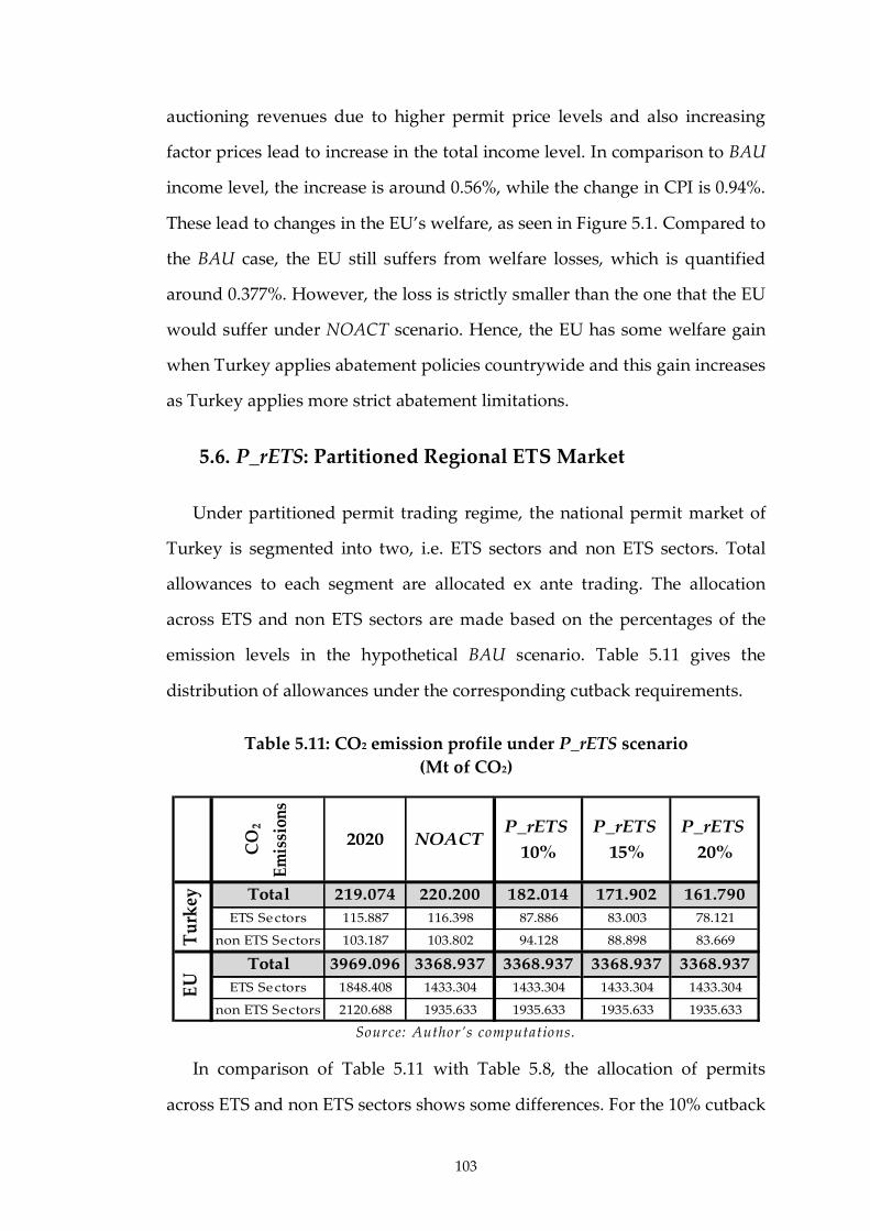
103

auctioning revenues due to higher permit price levels and also increasing

factor prices lead to increase in the total income level. In comparison to BAU

income level, the increase is around 0.56%, while the change in CPI is 0.94%.

These lead to changes in the EU’s welfare, as seen in Figure 5.1. Compared to

the BAU case, the EU still suffers from welfare losses, which is quantified

around 0.377%. However, the loss is strictly smaller than the one that the EU

would suffer under NOACT scenario. Hence, the EU has some welfare gain

when Turkey applies abatement policies countrywide and this gain increases

as Turkey applies more strict abatement limitations.

5.6. P_rETS: Partitioned Regional ETS Market

Under partitioned permit trading regime, the national permit market of

Turkey is segmented into two, i.e. ETS sectors and non ETS sectors. Total

allowances to each segment are allocated ex ante trading. The allocation

across ETS and non ETS sectors are made based on the percentages of the

emission levels in the hypothetical BAU scenario. Table 5.11 gives the

distribution of allowances under the corresponding cutback requirements.

Table 5.11: CO2 emission profile under P_rETS scenario

(Mt of CO2)

CO

2

Em

issi

ons

2020 NOACTP_rETS

10%

P_rETS

15%

P_rETS

20%

Total 219.074 220.200 182.014 171.902 161.790

ETS Sectors 115.887 116.398 87.886 83.003 78.121

non ETS Sectors 103.187 103.802 94.128 88.898 83.669

Total 3969.096 3368.937 3368.937 3368.937 3368.937

ETS Sectors 1848.408 1433.304 1433.304 1433.304 1433.304

non ETS Sectors 2120.688 1935.633 1935.633 1935.633 1935.633

EU

Tu

rkey


In comparison of Table 5.11 with Table 5.8, the allocation of permits

across ETS and non ETS sectors shows some differences. For the 10% cutback

104

requirement, ETS sectors are assigned 87.886 Mt of CO2 under P_rETS. This

is less than the amount 88.053 Mt of CO2, which is the efficient allocation

amount under NP_rETS. That is to say in such a scheme, ETS sectors are

obliged to abate more than what they would abate under a comprehensive

trading scheme. Following the increase in abatement amount, the permit

price level that ETS sectors face under P_rETS scenario increases to $20.09

from $19.9 per ton of CO2. Regarding the non ETS sectors, while they are

assigned 93.961 Mt of CO2 under NP_rETS scenario, this amount raises to

94.128 Mt of CO2 under partitioned permit market regime. Thus, MAC of

non ETS sectors becomes $19.42 per ton of CO2. The abatement cost at the

margin decreases compared to NP_rETS case.

Under 15% and 20% cutback requirements, over allocation is observed in

ETS sectors, i.e. they are assigned more allowances than the efficient amount.

In opposed to that, non ETS sectors are given less amounts of allowances

compared to the efficient allocation. Needless to mention, the gap between

the efficient allocations and the actual allocations widen as the cutback ratio

increases. The efficiency loss arising from over allocating to ETS sectors and

under allocating to non ETS sectors is further reflected in the MACs, as they

are seen in Table 5.7. In the ETS market, allowance price drops down to

$26.63 and $34.91, under 15% and 20% quota, respectively. The price level

increases following the increase in total quota, since more of the abatement

burden cause each unit of abatement at the margin to be more costly. In the

non ETS market, allowance price increases to $38.39 and $67.55, under 15%

and 20% quota, respectively.

In the aforementioned trading scheme with segmented market structure

and permit allocations done in proportion to the BAU levels of emissions, the

Turkish economy experiences efficiency losses in meeting its total abatement

objectives. Separating the market basically causes shifts in sharing the

105

abatement cost burden between sectors. Under the cutback ratios of 15% and

20%, ETS sectors shift some of their abatement duties to non ETS sectors.

That is to say, non ETS sectors abate on behalf of ETS sectors. Hence, the

permit price level that ETS sectors face falls, while permit price that non ETS

sectors face rises. In opposed to that, distribution of burden sharing shows a

different pattern under 10% quota. ETS sectors are obliged to abate more,

while non ETS sectors are obliged to abate less. The difference in the

behaviors of MACs under different cutback schedules clearly points out the

interdependencies between abatement cost structures of sectors.

Table 5.12: Real GDP under P_rETS scenario

(billion 2004 USD)

2004 2020P_rETS

10%

P_rETS

15%

P_rETS

20%

Turkey 296.255 513.982 512.806 511.892 510.574

EU 12938.300 16868.932 16828.410 16828.446 16828.487


Table 5.20 gives the changes in output levels with fixed 2004 prices.

Under P_rETS scenario, except for the transport sector, all sectors decrease

their level of outputs compared to BAU levels. Needless to mention, this is

mainly because of abatement actions, which put extra costs on the

production. Therefore, it is also crucial to look at the changes relative to the

levels under NP_rETS scenario in order to compare relative efficiencies of

both market schemes. Under a partitioned market with 10% total cap, ETS

sectors, except for oil, i.e. paper-pulp-print, chemicals, non-metallic minerals,

iron and steel, non-ferrous metals and electricity sectors, decrease their scale

of productions. Non ETS sectors, such as textiles, transport and other

manufacturing industries increase their scale of productions in a partitioned

market. The ETS sectors, formerly mentioned, are the ones that carry the

abatement cost burden stemming from the expansions of these non ETS

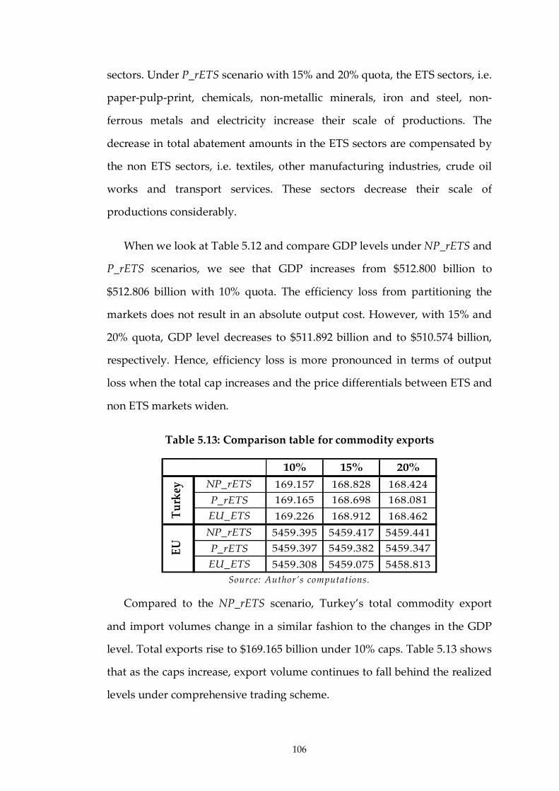
106

sectors. Under P_rETS scenario with 15% and 20% quota, the ETS sectors, i.e.

paper-pulp-print, chemicals, non-metallic minerals, iron and steel, non-

ferrous metals and electricity increase their scale of productions. The

decrease in total abatement amounts in the ETS sectors are compensated by

the non ETS sectors, i.e. textiles, other manufacturing industries, crude oil

works and transport services. These sectors decrease their scale of

productions considerably.

When we look at Table 5.12 and compare GDP levels under NP_rETS and

P_rETS scenarios, we see that GDP increases from $512.800 billion to

$512.806 billion with 10% quota. The efficiency loss from partitioning the

markets does not result in an absolute output cost. However, with 15% and

20% quota, GDP level decreases to $511.892 billion and to $510.574 billion,

respectively. Hence, efficiency loss is more pronounced in terms of output

loss when the total cap increases and the price differentials between ETS and

non ETS markets widen.

Table 5.13: Comparison table for commodity exports

10% 15% 20%

NP_rETS 169.157 168.828 168.424

P_rETS 169.165 168.698 168.081

EU_ETS 169.226 168.912 168.462

NP_rETS 5459.395 5459.417 5459.441

P_rETS 5459.397 5459.382 5459.347

EU_ETS 5459.308 5459.075 5458.813

Tu

rkey

EU


Compared to the NP_rETS scenario, Turkey’s total commodity export

and import volumes change in a similar fashion to the changes in the GDP

level. Total exports rise to $169.165 billion under 10% caps. Table 5.13 shows

that as the caps increase, export volume continues to fall behind the realized

levels under comprehensive trading scheme.

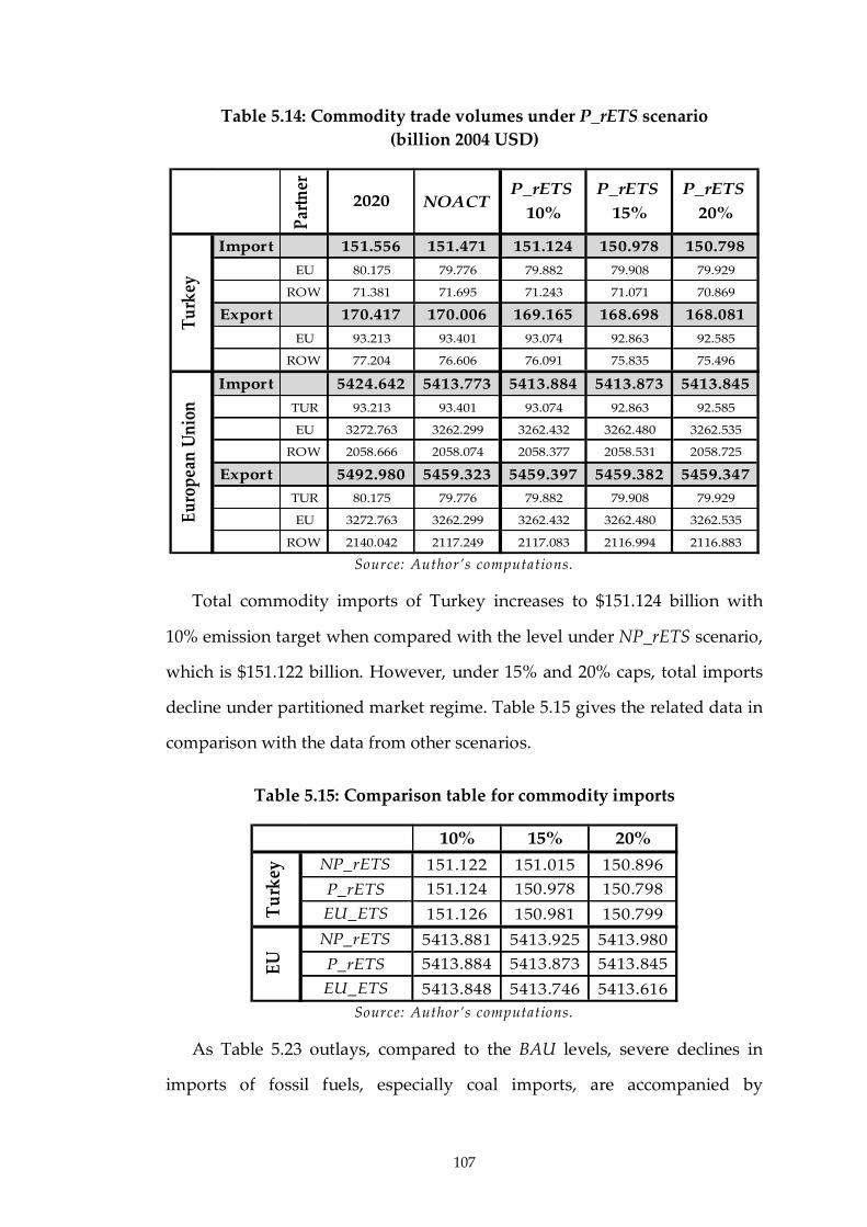
107

Table 5.14: Commodity trade volumes under P_rETS scenario

(billion 2004 USD)

Par

tner

2020 NOACTP_rETS

10%

P_rETS

15%

P_rETS

20%

Import 151.556 151.471 151.124 150.978 150.798

EU 80.175 79.776 79.882 79.908 79.929

ROW 71.381 71.695 71.243 71.071 70.869

Export 170.417 170.006 169.165 168.698 168.081

EU 93.213 93.401 93.074 92.863 92.585

ROW 77.204 76.606 76.091 75.835 75.496

Import 5424.642 5413.773 5413.884 5413.873 5413.845

TUR 93.213 93.401 93.074 92.863 92.585

EU 3272.763 3262.299 3262.432 3262.480 3262.535

ROW 2058.666 2058.074 2058.377 2058.531 2058.725

Export 5492.980 5459.323 5459.397 5459.382 5459.347

TUR 80.175 79.776 79.882 79.908 79.929

EU 3272.763 3262.299 3262.432 3262.480 3262.535

ROW 2140.042 2117.249 2117.083 2116.994 2116.883

Eu

rop

ean

Un

ion

Tu

rkey


Total commodity imports of Turkey increases to $151.124 billion with

10% emission target when compared with the level under NP_rETS scenario,

which is $151.122 billion. However, under 15% and 20% caps, total imports

decline under partitioned market regime. Table 5.15 gives the related data in

comparison with the data from other scenarios.

Table 5.15: Comparison table for commodity imports

10% 15% 20%

NP_rETS 151.122 151.015 150.896

P_rETS 151.124 150.978 150.798

EU_ETS 151.126 150.981 150.799

NP_rETS 5413.881 5413.925 5413.980

P_rETS 5413.884 5413.873 5413.845

EU_ETS 5413.848 5413.746 5413.616

Tu

rkey

EU


As Table 5.23 outlays, compared to the BAU levels, severe declines in

imports of fossil fuels, especially coal imports, are accompanied by

108

significant increases in imports of electricity. The imports of electricity

further increase following the increase in CO2 cutback requirements. On the

other hand, imports of energy intensive sector goods, such as chemicals,

non-metallic minerals, iron and steel, non-ferrous metals and other

manufacturing sectors, also increases. Regarding the exports, it is only the

transport services that Turkey continues to export under partitioned permit

trading applications. However, the amount of transport exports steadily

continue to decrease as the cutback ratio increases.

The change in the level of disposable income, compared to BAU level, is

read as 0.05%, 0.07% and 0.1%, for 10%, 15% and 20% quota, respectively.

CPI increases by 0.35% when total quota is 10%. Higher CO2 quotas result in

higher CPI levels. The total change in Turkey’s welfare is given in Figure 5.2.

Under the partitioned market regime, Turkey suffers from welfare losses.

Under 10% quota, the loss is 0.30%, while it increases to 0.54% and 0.88%

under 15% and 20% quota, respectively. In comparison with comprehensive

permit market, partitioned market structure results in more welfare loss.

That is to say, the higher the cutback requirement, the higher the cost burden

on cleaner industries, relative to the cost burden on energy intensive sectors.

The resulting high price differential between the MACs of ETS and non ETS

sectors cause efficiency losses. The same amount of cutback in CO2 emissions

costs more under a partitioned scheme than a comprehensive trading

scheme.

When Turkey applies permit trading in a partitioned market

structure, the MACs of European ETS and non ETS sectors are affected

simultaneously. In comparison to the NOACT scenario, the permit price in

the EU ETS market increases from $17.73 to $17.76 under 10% quota, $17.77

under 15% quota and $17.78 under 20% quota. At the same time, the MACs

of the EU’s non ETS sectors also increase from $84.19 to $84.24 under 10%

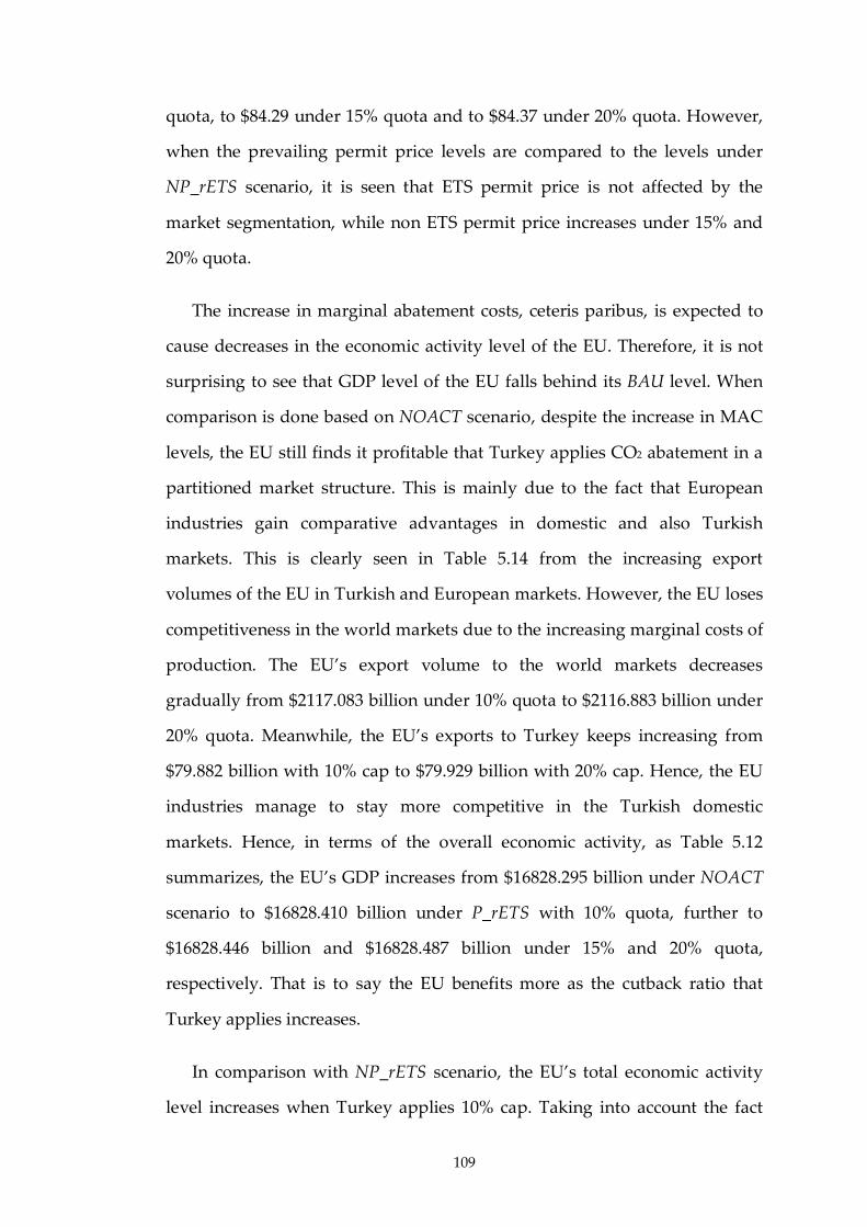
109

quota, to $84.29 under 15% quota and to $84.37 under 20% quota. However,

when the prevailing permit price levels are compared to the levels under

NP_rETS scenario, it is seen that ETS permit price is not affected by the

market segmentation, while non ETS permit price increases under 15% and

20% quota.

The increase in marginal abatement costs, ceteris paribus, is expected to

cause decreases in the economic activity level of the EU. Therefore, it is not

surprising to see that GDP level of the EU falls behind its BAU level. When

comparison is done based on NOACT scenario, despite the increase in MAC

levels, the EU still finds it profitable that Turkey applies CO2 abatement in a

partitioned market structure. This is mainly due to the fact that European

industries gain comparative advantages in domestic and also Turkish

markets. This is clearly seen in Table 5.14 from the increasing export

volumes of the EU in Turkish and European markets. However, the EU loses

competitiveness in the world markets due to the increasing marginal costs of

production. The EU’s export volume to the world markets decreases

gradually from $2117.083 billion under 10% quota to $2116.883 billion under

20% quota. Meanwhile, the EU’s exports to Turkey keeps increasing from

$79.882 billion with 10% cap to $79.929 billion with 20% cap. Hence, the EU

industries manage to stay more competitive in the Turkish domestic

markets. Hence, in terms of the overall economic activity, as Table 5.12

summarizes, the EU’s GDP increases from $16828.295 billion under NOACT

scenario to $16828.410 billion under P_rETS with 10% quota, further to

$16828.446 billion and $16828.487 billion under 15% and 20% quota,

respectively. That is to say the EU benefits more as the cutback ratio that

Turkey applies increases.

In comparison with NP_rETS scenario, the EU’s total economic activity

level increases when Turkey applies 10% cap. Taking into account the fact

110

that MACs of European sectors do not change, it is clear that this increase is

mainly due to the efficiency loss in Turkish economy arising from market

segmentation. Hence, as it is seen in Table 5.14, the EU’s exports increase to

$5459.397 billion. This is mainly due to the increase in the EU’s bilateral

export volumes with Turkey and within the EU. In opposed to this, under

15% and 20% quota, GDP level decreases from $16828.459 billion to

$16828.446 billion and from $16828.523 billion to $16828.487 billion,

respectively. This decrease in the total output is mainly due to the relative

increase in the marginal production costs of European sectors, accompanied

with decreasing market share in Turkish domestic markets.

Change in the EU’s economic welfare is given in Figure 5.1. In

comparison to the case where the EU takes unilateral abatement action, the

EU has some welfare gains when Turkey applies domestic abatement

actions. However, the EU enjoys more welfare gains under comprehensive

permit trading, compared to the partitioned permit trading.

5.7. EU_ETS: The European Union ETS market

Turkey’s integration with the EU ETS market affects the economies of

both parties. The permit price level in the ETS market is supposed to be

affected depending on the relative marginal cost structures of the potential

permit exporters and importers in the market. MACs of non ETS sectors are

also affected by these changes via energy prices. What we see in Table 5.3 is

that the permit price in the EU ETS market increases from $17.73 to $17.90

under 10% quota, to $18.24 under 15% quota and to $18.59 under 20% quota.

In comparison to the permit price levels revealed in regional ETS markets,

Turkish ETS sectors face considerable decrease in the price level after

integration. The price differential, between the EU ETS and the regional ETS

markets, gets more significant as the total cap increases. It is also crucial to

111

note that while permit price level in regional ETS markets are more volatile

against changes in total cap amounts, the price level in the EU ETS market is

less volatile against domestic policy changes.

Table 5.16: CO2 emission profile under EU_ETS scenario

(Mt of CO2)

CO2

Emissions2020 NOACT

EU_ETS

10%

EU_ETS

15%

EU_ETS

20%

Total 219.074 220.200 183.996 178.641 173.300

ETS Sectors 115.887 116.398 89.869 89.743 89.631

non ETS Sectors 103.187 103.802 94.128 88.898 83.669

Total 3969.096 3368.937 3366.955 3362.198 3357.427

ETS Sectors 1848.408 1433.304 1431.322 1426.565 1421.794

non ETS Sectors 2120.688 1935.633 1935.633 1935.633 1935.633

Tu

rkey

EU


In comparison to what Turkey experiences under integration, ETS sectors

in the EU face higher permit price levels. While the permit price in the EU

ETS market under NOACT scenario is $17.73 per ton of CO2, under the

EU_ETS scenario, it realizes as $17.9 under 10% quota, as $18.24 under 15%

quota and as $18.59 under 20% quota. This increase is mainly because of high

level of MACs of the Turkish ETS sectors, which are summarized in Table

5.7. High levels of MACs lead Turkey to buy permits in the market place

instead of abating at home, while European ETS sectors have the incentive to

sell permits in exchange of decreasing their emission levels. Thus, in the EU

ETS market, Turkey becomes a permit importer, while the EU becomes a

permit exporter. In other words, Turkey shifts some of its abatement cost

burden to the EU via international permit trading.

The amounts of permits imported and exported are summarized in Table

5.16. While the total allowances allocated to the EU ETS sectors is 1433.304

Mt of CO2, the actual emissions from ETS sectors after trading are measured

as 1431.322 Mt of CO2 under 10% quota, 1426.565 Mt of CO2 under 15% quota

112

and 1421.794 Mt of CO2 under 20% quota. The difference between the initial

allocations and the realized emission levels is the amount of permits that are

imported by Turkish ETS sectors in the EU ETS market. Total permit imports

of Turkey become 1.983 Mt of CO2 under 10% quota, 6.739 Mt of CO2 and

11.510 Mt of CO2 under 15% and 20% quota, respectively. Permit imports

increase as the cap increases due to increasing levels of MACs of Turkish

ETS sectors.

In comparison to the P_rETS scenario, the output levels of Turkish ETS

sectors increase following the decrease in their marginal production costs. As

Table 5.20 shows, the increase in the output levels of secondary energy

productions, iron and steel industry, non-ferrous metals, chemicals and non-

metallic minerals industries are significant. Due to decreasing energy prices,

the marginal abatement costs of non ETS sectors in Turkey also tend to

decrease. MACs of these sectors are given as $19.38 per ton of CO2 under

10% cap, $38.27 per ton of CO2 under 15% cap and $67.46 per ton of CO2

under 20% cap. Thus, some non ETS sectors, i.e. natural gas, mining, textile,

coal and crude oil, also increase their scale of productions. The rest of the

non ETS sectors experience decline in their activity levels due to their loss of

competitiveness in the world markets. Despite these negative scale effects, as

Table 5.17 shows, in comparison the P_rETS scenario, Turkey’s GDP

increases from $512.806 to $512.910 billion under 10% cap, from $511.892 to

$512.291 billion under 15% cap and from $510.574 to $511.342 billion under

20% cap. It is crucial to note that the realized GDP levels of the Turkish

economy under EU_ETS scenario are also higher than the levels that realize

under comprehensive regional ETS regime. Therefore, although it is

inevitable for Turkey not to have certain levels of output cost as a result of its

abatement policies, it is seen that this cost is also manageable via different

market formulations. In that regard, Turkey has certainly benefits out of

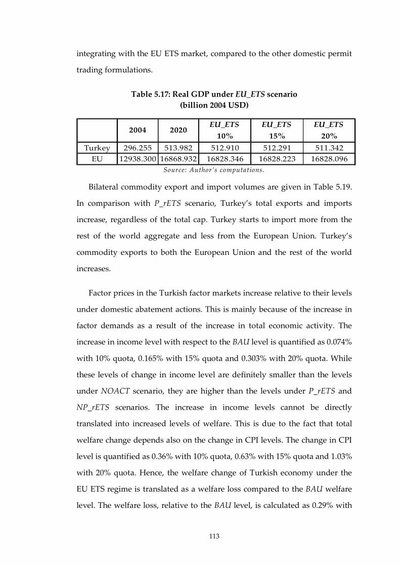
113

integrating with the EU ETS market, compared to the other domestic permit

trading formulations.

Table 5.17: Real GDP under EU_ETS scenario

(billion 2004 USD)

2004 2020EU_ETS

10%

EU_ETS

15%

EU_ETS

20%

Turkey 296.255 513.982 512.910 512.291 511.342

EU 12938.300 16868.932 16828.346 16828.223 16828.096


Bilateral commodity export and import volumes are given in Table 5.19.

In comparison with P_rETS scenario, Turkey’s total exports and imports

increase, regardless of the total cap. Turkey starts to import more from the

rest of the world aggregate and less from the European Union. Turkey’s

commodity exports to both the European Union and the rest of the world

increases.

Factor prices in the Turkish factor markets increase relative to their levels

under domestic abatement actions. This is mainly because of the increase in

factor demands as a result of the increase in total economic activity. The

increase in income level with respect to the BAU level is quantified as 0.074%

with 10% quota, 0.165% with 15% quota and 0.303% with 20% quota. While

these levels of change in income level are definitely smaller than the levels

under NOACT scenario, they are higher than the levels under P_rETS and

NP_rETS scenarios. The increase in income levels cannot be directly

translated into increased levels of welfare. This is due to the fact that total

welfare change depends also on the change in CPI levels. The change in CPI

level is quantified as 0.36% with 10% quota, 0.63% with 15% quota and 1.03%

with 20% quota. Hence, the welfare change of Turkish economy under the

EU ETS regime is translated as a welfare loss compared to the BAU welfare

level. The welfare loss, relative to the BAU level, is calculated as 0.29% with

114

10% quota, 0.46% with 15% quota and 0.73% with 20% quota. However, as

Figure 5.2 shows, in comparison with P_rETS and NP_rETS scenarios,

Turkey has welfare gains in integrating with the EU ETS market.

Despite the improvement in Turkey’s economic welfare, it is clear that

Turkey is worse off in terms of its environmental standards. In comparison

of Table 5.16 with Table 5.11, it is seen that Turkey’s CO2 emissions increase

under EU_ETS scenario. This is mainly due to two reasons. Firstly, the

increase in the scale of the Turkish economy results in certain level of

increase in Turkey’s total emission level. Secondly, due to the relative

decrease in the marginal costs of CO2 intense production factors in Turkey,

some of the Turkish sectors have tendency to use more CO2 intense

production procedures. As Table 5.24 shows, in comparison to the domestic

permit trading cases, the CO2 intensity of the Turkish economy increases

under EU_ETS scenario. The CO2 intensity is reported as 0.359 Mt CO2 per

2004 USD under 10% quota. The intensity further drops to 0.349 and 0.339

under 15% and 20% quota, respectively, due to the increase in abatement

burden.

According to the sector output data given in Table 5.21, under EU_ETS

scenario, all ETS sectors in the EU decrease their scale of productions. This is

mainly due to the burden sharing between Turkey and the EU as a result of

Turkey’s abatement actions. While Turkish ETS sectors are expanding their

scale of productions at a cost of increasing emissions, the EU abates more at

a cost of decreasing ETS production levels.

The spillover effects are not limited to just European ETS sectors. As

Table 5.7 revels, with respect to the BAU scenario, marginal abatement cost

of non ETS sectors also increases under EU_ETS scenario. The MAC level in

European non ETS market, compared to the NOACT scenario, increase from

115

$84.19 to $84.23 with 10% quota, to $84.27 with 15% quota, and to $84.33

with 20% quota. It is crucial to note here that the relative changes in MAC

levels of non ETS sectors show some differences in comparison with

domestic abatement cases. Under P_rETS scenario, regardless of the total

cap, MACs are higher and under NP_rETS scenario, they are lower. This is

mainly due to the fact that the EU industries become highly dependent on

secondary energy imports from Turkey as a result of the EU’s 20-20-20

abatement targets. Due to expensive electricity imports from Turkey under

P_rETS scenario, the permit price in European non ETS market increases

more compared to NP_rETS scenario. When Turkey integrates with the EU

ETS market, the expansion in Turkey’s secondary energy sectors lead to

cheaper import prices; hence MACs of European non ETS sectors decrease

compared to P_rETS scenario. As it is given in Table 5.21, it is only in the

European transport, other manufacturing and other economy sectors that we

see expansions in scale of productions.

When we look at the EU’s total economic activity in Table 5.17, we see

that there is an increase in GDP in comparison to the NOACT scenario under

10% cap. Thus, even Turkey’s integration with the EU ETS market imposes

extra cost burden both on European ETS and non ETS sectors, the EU still

finds it profitable that Turkey applies 10% abatement. However, as the cap

rises to 15% and more to 20%, the permit price levels prevailing in European

ETS and non ETS sectors increase, widening the price differential between

these two groups of sectors. Therefore, the EU’s GDP falls below its level

under NOACT scenario. In that regard, from the EU’s perspective, Turkey’s

total cap amount is highly critical.

Looking at Table 5.18, we also see that the EU’s GDP always decreases

under EU_ETS scenario in comparison to P_rETS and NP_rETS scenarios.

That is to say that Turkey’s domestic abatement actions always give output

116

gain to the EU via the positive terms of trade effects. Therefore, taking the

level of total economic activity as the choice criteria, the EU should favor that

Turkey establishes national permit markets in reaching its abatement targets.

However, regarding the integration of Turkish national permit market with

the EU ETS market, the EU should take it with more precaution due to the

negative scale effects of high cutback requirements. High levels of permit

prices due to high levels of caps can wipe out the positive terms of trade

effects on the EU economy that would otherwise occur under the cases

where Turkey applies domestic permit trading schemes.

Table 5.18: Comparison table for total economic activity

10% 15% 20%

NP_rETS 512.800 512.010 510.938

P_rETS 512.806 511.892 510.574

EU_ETS 512.910 512.291 511.342

NP_rETS 16828.409 16828.459 16828.523

P_rETS 16828.410 16828.446 16828.487

EU_ETS 16828.346 16828.223 16828.096

Tu

rkey

EU


Moving from NOACT case to the EU_ETS case under 10% quota, the EU

increases the level of its total economic activity. Following that, as Table 5.19

shows, total imports of the EU increases while total exports decreases. The

reason underlying the decreasing exports is that industries of the rest of the

world aggregate become more competitive than European industries in the

world markets. Hence, the EU’s import volume from the rest of the world

increases, while export volume decreases. On the other hand, the EU

industries start to get higher shares of export sales in the Turkish domestic

markets. However, under 15% and 20% quota, as a direct result of the

decline in the total economic activity, total imports and exports of the EU fall

behind their levels under the NOACT scenario. In comparison with P_rETS

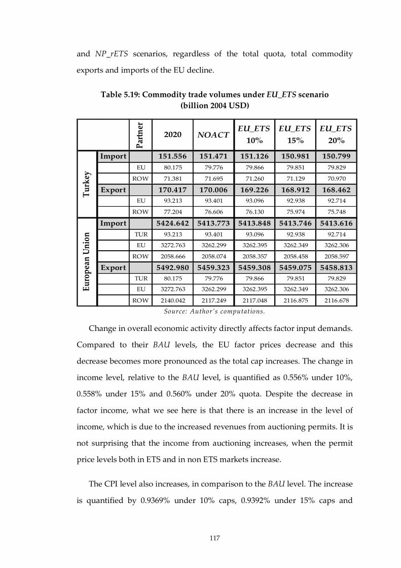
117

and NP_rETS scenarios, regardless of the total quota, total commodity

exports and imports of the EU decline.

Table 5.19: Commodity trade volumes under EU_ETS scenario

(billion 2004 USD)

Par

tner

2020 NOACTEU_ETS

10%

EU_ETS

15%

EU_ETS

20%

Import 151.556 151.471 151.126 150.981 150.799

EU 80.175 79.776 79.866 79.851 79.829

ROW 71.381 71.695 71.260 71.129 70.970

Export 170.417 170.006 169.226 168.912 168.462

EU 93.213 93.401 93.096 92.938 92.714

ROW 77.204 76.606 76.130 75.974 75.748

Import 5424.642 5413.773 5413.848 5413.746 5413.616

TUR 93.213 93.401 93.096 92.938 92.714

EU 3272.763 3262.299 3262.395 3262.349 3262.306

ROW 2058.666 2058.074 2058.357 2058.458 2058.597

Export 5492.980 5459.323 5459.308 5459.075 5458.813

TUR 80.175 79.776 79.866 79.851 79.829

EU 3272.763 3262.299 3262.395 3262.349 3262.306

ROW 2140.042 2117.249 2117.048 2116.875 2116.678

Tu

rkey

Eu

rop

ean

Un

ion


Change in overall economic activity directly affects factor input demands.

Compared to their BAU levels, the EU factor prices decrease and this

decrease becomes more pronounced as the total cap increases. The change in

income level, relative to the BAU level, is quantified as 0.556% under 10%,

0.558% under 15% and 0.560% under 20% quota. Despite the decrease in

factor income, what we see here is that there is an increase in the level of

income, which is due to the increased revenues from auctioning permits. It is

not surprising that the income from auctioning increases, when the permit

price levels both in ETS and in non ETS markets increase.

The CPI level also increases, in comparison to the BAU level. The increase

is quantified by 0.9369% under 10% caps, 0.9392% under 15% caps and

118

0.9421% under 20% caps. The change in both income and CPI level affects

the overall welfare. Figure 5.1 graphically shows the changes in the EU’s

welfare. The EU’s welfare loss increases under EU_ETS scenario when

compared to the P_rETS and NP_rETS scenarios. The higher the total cap is

the higher the welfare loss is. However, it is crucial to note that the

quantified welfare loss under EU_ETS scenario is less than the welfare loss

that the EU suffers under NOACT scenario. In that regard, the EU should

favor any of permit trading schemes that Turkey applies, i.e. domestic or

international.

Referring back to the previous findings on the EU’s output loss under

EU_ETS scenario, this result may seem to be contradictory. In terms of the

change in total output, it is shown that the EU should not favor Turkey’s

integration with the EU ETS market under 15% and 20% caps. The

underlying reason is that as a permit exporter in the ETS market, the EU

suffers from high permit prices in its permit markets and is affected by

negative terms of trade effects in the world markets. However, the welfare

analysis argues that the EU has welfare gains under EU_ETS scenario, in

comparison with the NOACT scenario. The main reason underlying this

welfare gain is mainly the revenues from permit trading. Despite the output

loss, the EU has additional income from permit trading which is transferred

lump sum to the representative agent in the model formulation and further

used for the consumption. Hence, international permit trading becomes

welfare enhancing for both trading parties, Turkey and the EU.

In terms of environmental standards, the EU is definitely better off under

EU_ETS scenario. The European Union’s CO2 emission level decreases when

Turkey integrates with the EU ETS market, which is mainly due to the

burden sharing between Turkey and the EU. It is not only the fact that the

EU becomes a permit exporter which underlies the decrease in the EU’s

119

emission level. As Table 5.24 shows, the increase in the abatement cost

burden on the EU economy further gives incentives on the European sectors

to use less CO2 intense factors in their production processes. Hence, in

comparison to the other scenarios, the European economy transforms into a

less carbon-intense economy under EU_ETS scenario.

5.8. Concluding Comments

This chapter employs the MR-ETPA model in analyzing the economic

impacts of establishing permit trading market in Turkey and further

investigating the impacts under international cooperation with the EU, via

EU ETS market. The counterfactual scenarios mainly focus on the effects of

various emission cutback requirements, on the importance of the market

segmentation in implementing these targets and, finally, on the effects of

pursuing cooperation with the EU in carbon trading.

In the analysis, I find that Turkey suffers from welfare losses in case of

regional comprehensive permit trading and these losses tend to grow larger

as the total cutback ratio increases. On the other hand, Turkey definitely has

environmental benefits in terms of decreasing CO2 emissions and CO2

intensity. From the EU’s perspective, Turkey’s engagement in permit trading

is always preferable as it gives the EU welfare gains compared to the case

where the EU continues to apply its abatement actions without any

international cooperation. The improvement in the EU’s welfare is mainly

dependent on the total output growth due to increased competitiveness of

the EU industries in the world markets. As Turkey sets higher cutback ratios,

the EU’s welfare gain gradually increases.

Turkey starts to suffer from market segmentation more as the total

cap increases. This is mainly due to the increasing price differential between

120

marginal abatement costs of sectors belonging to different market segments.

Hence, total compliance cost of meeting the same amount of cap increases.

The EU’s welfare gains from Turkey’s regional permit trading applications

also decreases when market segmentation exists. This is the direct effect of

both decreasing import demand from Turkey and also increasing marginal

abatement costs of some of the European industries due to trade linkages.

In case of Turkey’s integration with the EU ETS market, regardless of

the total abatement ratio, Turkey is definitely better off compared to

domestic abatement actions. As a permit importer, Turkey finds

opportunities to increase its total output by shifting its abatement burden to

the EU. As a result, Turkey experiences considerable expansions in its energy

and energy intensive sectors that are integrated with the EU carbon market.

This also has further spillover effects on Turkish economy, too. Depressed

marginal abatement costs of energy and energy intensive sectors have

positive spillover effects on other non-energy sectors via cheaper energy

prices. Therefore, Turkey becomes better off under the EU ETS due to the

economic growth. On the other hand, in terms of environmental

degradation, Turkey becomes worse off. This is mainly due to the burden

sharing via permit trading. Turkey, as a permit importer, finds it more

profitable to shift its abatement burden to the EU, which further increases

the level of Turkey’s emissions and also the incentives to shift to more

emission intense production procedures.

From the EU’s perspective, Turkey’s integration with the EU ETS is

preferable regarding the environmental concerns, as the emission levels and

intensities decrease. However, in terms of economic welfare it is not that

straightforward. Compared to the current situation where Turkey does not

take any abatement action, the EU should definitely prefer Turkey’s

integration with the EU ETS market based on the economic welfare concerns.

121

However, as a permit exporter, the total cap that Turkey assigns to its ETS

and non ETS sectors becomes highly critical for the European Union. The

analysis shows that as the cap increases, the EU’s output loss increases and

welfare gains decreases. Another critical issue from the EU’s perspective is

how sustainable the permit trading with Turkey will be. As the analysis

shows, the EU compensates some of its output loss with the extra income

from permit trading. While this is a reasonable policy for the short run, in the

long run, the EU should definitely pilot and implement policies to recycle

these permit revenues in such a way that also compensates for the output

loss.

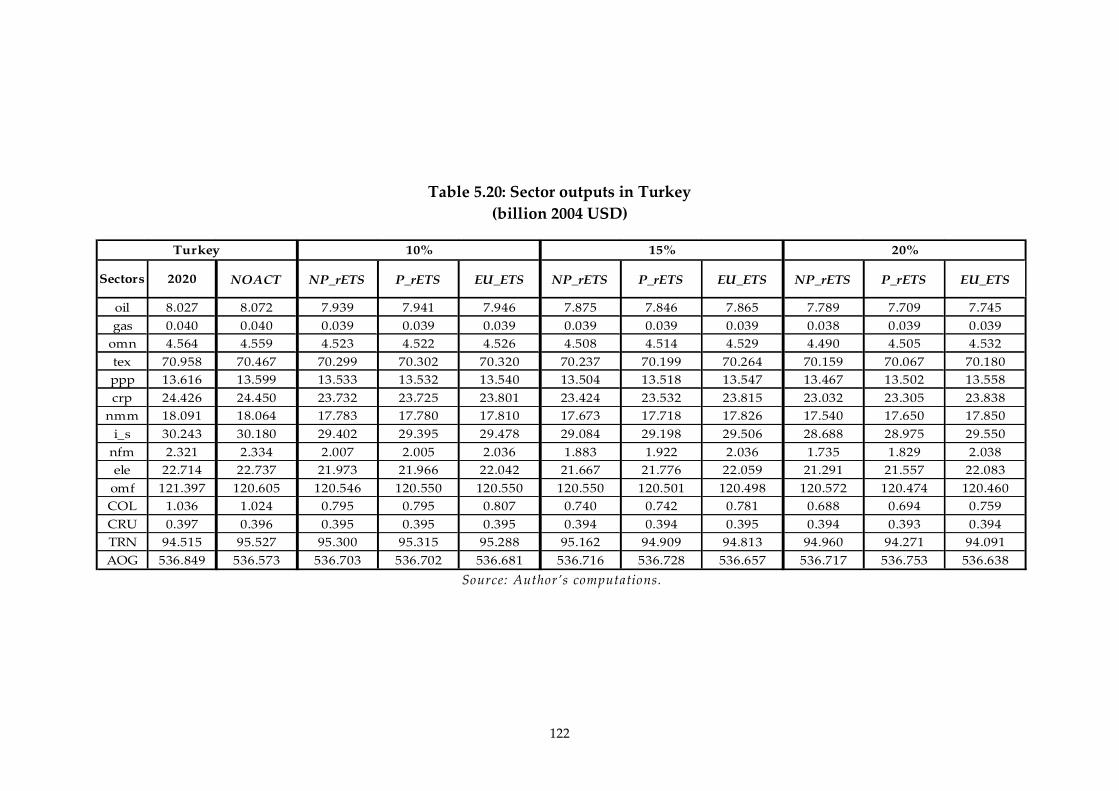
122

Table 5.20: Sector outputs in Turkey

(billion 2004 USD)

Sectors 2020 NOACT NP_rETS P_rETS EU_ETS NP_rETS P_rETS EU_ETS NP_rETS P_rETS EU_ETS

oil 8.027 8.072 7.939 7.941 7.946 7.875 7.846 7.865 7.789 7.709 7.745

gas 0.040 0.040 0.039 0.039 0.039 0.039 0.039 0.039 0.038 0.039 0.039

omn 4.564 4.559 4.523 4.522 4.526 4.508 4.514 4.529 4.490 4.505 4.532

tex 70.958 70.467 70.299 70.302 70.320 70.237 70.199 70.264 70.159 70.067 70.180

ppp 13.616 13.599 13.533 13.532 13.540 13.504 13.518 13.547 13.467 13.502 13.558

crp 24.426 24.450 23.732 23.725 23.801 23.424 23.532 23.815 23.032 23.305 23.838

nmm 18.091 18.064 17.783 17.780 17.810 17.673 17.718 17.826 17.540 17.650 17.850

i_s 30.243 30.180 29.402 29.395 29.478 29.084 29.198 29.506 28.688 28.975 29.550

nfm 2.321 2.334 2.007 2.005 2.036 1.883 1.922 2.036 1.735 1.829 2.038

ele 22.714 22.737 21.973 21.966 22.042 21.667 21.776 22.059 21.291 21.557 22.083

omf 121.397 120.605 120.546 120.550 120.550 120.550 120.501 120.498 120.572 120.474 120.460

COL 1.036 1.024 0.795 0.795 0.807 0.740 0.742 0.781 0.688 0.694 0.759

CRU 0.397 0.396 0.395 0.395 0.395 0.394 0.394 0.395 0.394 0.393 0.394

TRN 94.515 95.527 95.300 95.315 95.288 95.162 94.909 94.813 94.960 94.271 94.091

AOG 536.849 536.573 536.703 536.702 536.681 536.716 536.728 536.657 536.717 536.753 536.638

Turkey 10% 15% 20%


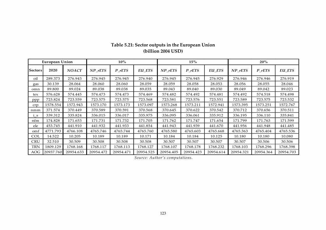
123

Table 5.21: Sector outputs in the European Union

(billion 2004 USD)

Sectors 2020 NOACT NP_rETS P_rETS EU_ETS NP_rETS P_rETS EU_ETS NP_rETS P_rETS EU_ETS

oil 289.373 276.943 276.945 276.945 276.940 276.945 276.945 276.929 276.946 276.946 276.919

gas 30.139 28.064 28.060 28.060 28.059 28.059 28.058 28.053 28.056 28.055 28.046

omn 89.800 89.024 89.038 89.038 89.035 89.043 89.040 89.030 89.049 89.042 89.023

tex 576.628 574.445 574.473 574.473 574.469 574.482 574.492 574.481 574.492 574.518 574.498

ppp 723.824 723.559 723.575 723.575 723.568 723.581 723.576 723.551 723.589 723.575 723.532

crp 1578.554 1572.943 1573.170 1573.173 1573.097 1573.268 1573.211 1572.941 1573.395 1573.251 1572.767

nmm 371.574 370.449 370.589 370.591 370.568 370.645 370.622 370.542 370.712 370.656 370.511

i_s 339.312 335.824 336.015 336.017 335.975 336.095 336.061 335.912 336.195 336.110 335.841

nfm 174.828 171.653 171.731 171.732 171.705 171.762 171.747 171.654 171.799 171.763 171.599

ele 453.745 441.910 441.932 441.933 441.854 441.943 441.939 441.670 441.956 441.948 441.485

omf 4771.793 4766.108 4765.746 4765.744 4765.760 4765.580 4765.603 4765.668 4765.363 4765.404 4765.536

COL 14.522 10.205 10.189 10.189 10.171 10.184 10.184 10.125 10.180 10.180 10.080

CRU 32.510 30.509 30.508 30.508 30.508 30.507 30.507 30.507 30.507 30.506 30.506

TRN 1809.129 1768.168 1768.117 1768.113 1768.127 1768.107 1768.178 1768.232 1768.103 1768.296 1768.398

AOG 20937.760 20954.633 20954.472 20954.471 20954.525 20954.405 20954.423 20954.614 20954.321 20954.364 20954.703

European Union 10% 15% 20%


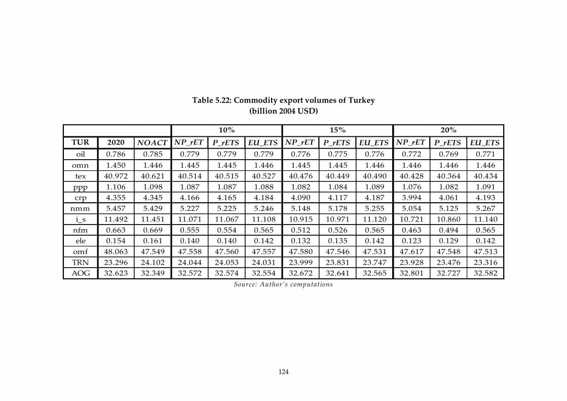
124

Table 5.22: Commodity export volumes of Turkey

(billion 2004 USD)

TUR 2020 NOACT NP_rET

S

P_rETS EU_ETS NP_rET

S


S

P_rETS EU_ETS

oil 0.786 0.785 0.779 0.779 0.779 0.776 0.775 0.776 0.772 0.769 0.771

omn 1.450 1.446 1.445 1.445 1.446 1.445 1.445 1.446 1.446 1.446 1.446

tex 40.972 40.621 40.514 40.515 40.527 40.476 40.449 40.490 40.428 40.364 40.434

ppp 1.106 1.098 1.087 1.087 1.088 1.082 1.084 1.089 1.076 1.082 1.091

crp 4.355 4.345 4.166 4.165 4.184 4.090 4.117 4.187 3.994 4.061 4.193

nmm 5.457 5.429 5.227 5.225 5.246 5.148 5.178 5.255 5.054 5.125 5.267

i_s 11.492 11.451 11.071 11.067 11.108 10.915 10.971 11.120 10.721 10.860 11.140

nfm 0.663 0.669 0.555 0.554 0.565 0.512 0.526 0.565 0.463 0.494 0.565

ele 0.154 0.161 0.140 0.140 0.142 0.132 0.135 0.142 0.123 0.129 0.142

omf 48.063 47.549 47.558 47.560 47.557 47.580 47.546 47.531 47.617 47.548 47.513

TRN 23.296 24.102 24.044 24.053 24.031 23.999 23.831 23.747 23.928 23.476 23.316

AOG 32.623 32.349 32.572 32.574 32.554 32.672 32.641 32.565 32.801 32.727 32.582

10% 15% 20%

Source: Author’s computations

125

Table 5.23: Commodity import volumes of Turkey

(billion 2004 USD)

TUR 2020 NOACT NP_rET

S


S


S

P_rETS EU_ETS

oil 2.179 2.186 2.146 2.147 2.148 2.127 2.118 2.123 2.101 2.077 2.087

gas 2.848 2.866 2.758 2.758 2.767 2.704 2.704 2.738 2.633 2.635 2.699

omn 0.680 0.677 0.668 0.667 0.668 0.664 0.665 0.669 0.659 0.663 0.670

tex 8.524 8.493 8.493 8.493 8.493 8.492 8.494 8.494 8.490 8.495 8.496

ppp 2.811 2.803 2.820 2.820 2.818 2.826 2.824 2.816 2.835 2.827 2.813

crp 27.737 27.661 27.879 27.881 27.857 27.972 27.938 27.847 28.091 28.004 27.834

nmm 0.864 0.856 0.893 0.894 0.890 0.909 0.903 0.889 0.928 0.914 0.887

i_s 13.712 13.616 13.713 13.714 13.704 13.756 13.741 13.702 13.812 13.774 13.702

nfm 12.032 11.948 12.103 12.105 12.090 12.168 12.145 12.089 12.249 12.195 12.090

ele 0.015 0.015 0.017 0.017 0.016 0.017 0.017 0.016 0.018 0.018 0.016

omf 58.171 58.318 58.194 58.192 58.203 58.126 58.162 58.209 58.032 58.115 58.209

COL 1.062 1.084 0.673 0.672 0.693 0.573 0.576 0.645 0.479 0.487 0.603

CRU 4.709 4.738 4.655 4.656 4.659 4.615 4.596 4.608 4.561 4.511 4.532

TRN 3.118 3.064 3.060 3.059 3.062 3.059 3.074 3.084 3.059 3.100 3.119

AOG 13.095 13.146 13.050 13.049 13.057 13.006 13.021 13.052 12.949 12.983 13.043

10% 15% 20%


126

Table 5.24: Carbon intensity, CO2 / GDP

(Mt CO2 per 2004 USD)

10% 15% 20% 10% 15% 20% 10% 15% 20%

Turkey 0.426 0.428 0.355 0.336 0.317 0.355 0.336 0.317 0.359 0.349 0.339

EU 0.23529 0.20019 0.20019 0.20019 0.20019 0.20019 0.20019 0.20019 0.20008 0.19980 0.19951

NP_rETS P_rETS EU_ETSNOACT2020


127

CHAPTER 6

Conclusions and Future Directions

This chapter identifies the main findings of this dissertation and

interprets on how they suit to the current environmental policy agenda

regarding the design of the post-2012 mitigation efforts. The chapter further

concludes with feasible paths for future research.

The economic impacts of Turkey’s collaboration with the international

community in mitigating greenhouse gas emissions over the post-Kyoto

period are studied in this dissertation. In regard to the possible abatement

strategies, the current research mainly focused on the use of market-based

instruments, i.e. cap-and-trade systems. As the design of a cap-and-trade

system has many critical aspects, in this study, four main dimensions are

identified and analyzed, i.e. total cutback requirement, regional permit

trading in a segmented and a comprehensive market structure, and direct

linkage with the EU ETS market.

In studying the aforementioned policy issues, I utilized a multi-country

general equilibrium framework which clearly identified the interregional

linkages via commodity and permit trading. As a result of policy

simulations, it is seen that in case of a nationwide cap-and-trade system,

128

Turkey suffers from economic losses, which is mainly due to the increasing

marginal costs of production. Segmented permit trading schemes result in

larger welfare losses compared to comprehensive schemes. As the cutback

ratio increases in a segmented scheme, due to the high permit price

differentials, cost efficiency further decreases and economic loss gets bigger

in comparison to comprehensive markets. In case of linking national ETS

sectors with the EU ETS, regardless of the total cap, Turkey is definitely

better off compared to nationwide trading scheme. Due to its highly carbon

intensive economy, Turkey finds it more expensive to abate at home than to

shift some of its abatement duties to the EU via permit trading in the EU

ETS. Hence, in terms of economic efficiency, cooperation with the EU in

mitigation efforts has certain advantages for Turkey.

As the analysis shows, the European Union has economic benefits out of

Turkey’s domestic mitigation actions due to increased competitiveness of

European industries in the world markets. This is further accompanied by

environmental efficiency gains stemming from the decrease in CO2 leakage.

However, the net economic effects of a potential linkage between Turkey’s

national ETS scheme with the EU ETS highly depend on the design

parameters of Turkey’s permit trading scheme. In case of a direct linkage, the

amount of abatement burden that the EU is supposed to carry is highly

dependent on Turkey’s mitigation target. As the analysis shows, the EU ends

up suffering more from increasing output losses with the increase in

Turkey’s mitigation target. Hence, the question of how much burden that the

Turkish authorities will put on the ETS sectors is highly critical and open to

controversies.

As this study mainly focuses on economic impacts of the use of various

forms of cap-and-trade systems, it definitely is not enough to set any kind of

environmental regulation just based on economic criteria. Environmental

129

quality is also a critical aspect of any kind of environmental policy

architecture, which is generally hard to quantify, and hence, to include in

cost and benefit analyses. The current analysis shows the necessity of taking

environmental quality into account, as it is possible to have environmental

degradation and economic well-being go in opposite directions. Hence, a

possible extension of the current setup is to extend the cost and benefit

analysis in a way including environmental degradation. The main difficulty

with this approach is to quantify environmental degradation and the related

disutility out of it.

In addition to the promotion of widespread use of market-based

instruments, post-2012 mitigation strategies also promote the electricity

generation from renewable energy sources. The European Union has already

set its target as 20% share of renewable energy sources in final energy

consumption and each member state has a corresponding target in line with

the overall target (European Commission 2008). The promotion of renewable

energy sources in Turkey is also critical for diversification of energy supply,

increasing security, environmental protection and economic benefits in the

long run. Hence, extending the MR-ETPA model to the use of renewable

energy sources in electricity generation would certainly add much to the

current analysis. It is possible to do this extension within the current setup of

the model using autonomous energy efficiency indices. However, adding

endogenous technology improvement into the current setup will give further

insights regarding the transitional dynamics of the economies and open the

question of how to finance the presumed technological change. Hence, in

such kind of setup, it will also be possible to analyze the ways and effects of

revenue recycling.

Another possible extension is to investigate the potential economic

impacts of the current environmental policy agenda under the benefits of

130

free flows of labor and capital that come with a full membership to the

European Union. Ellerman (2009) states that “club benefits” are actually the

essence underlying the expansion of the EU ETS from the initial fifteen

member states to the thirty member states currently. Thus, it is worthwhile

to analyze how large the so-called club benefits can get in case of Turkey’s

accession and whether that can give incentives to both parties for setting

more ambitious environmental targets.

131

BIBLIOGRAPHY

Aldy, J.E., Stavins, R.N., 2007a. Architectures for agreement : addressing global

climate change in the post-Kyoto world. Cambridge University Press,

Cambridge ; New York.

Aldy, J.E., Stavins, R.N., 2007b. Introduction: international policy architecture for

global climate change.

Anger, N., 2008. Emissions trading beyond Europe: Linking schemes in a post-

Kyoto world. Energy Economics 30, 2028-2049

Armington, P.S., 1969. A theory of demand for products distinguished by place of

production. Imf Staff Papers / International Monetary Fund (International)

16, No. 1, 159-78

Arrow, K.J., Chenery, H.B., Minhas, B.S., Solow, R.M., 1961. Capital-Labor

Substitution and Economic-Efficiency. Review of Economics and Statistics

43, 225-250

Arrow, K.J., Debreu, G., 1954. Existence of an Equilibrium for a Competitive

Economy. Econometrica 22, 265-290

Arrow, K.J., Hahn, F., 1971. General competitive analysis. Holden-Day, San

Francisco,.

Aydin, L., Acar, M., 2010. Economic and environmental implications of Turkish

accession to the European Union: A CGE analysis. Energy Policy 38, 7031-

7040

Babiker, M., Reilly, J., Viguier, L., 2004. Is international emissions trading always

beneficial? Energy Journal 25, 33-56

Babiker, M., Reilly, J.M., Jacoby, H.D., 2000. The Kyoto Protocol and developing

countries. Energy Policy 28, 525-536

132

Badri, N.G., Walmsley, T.L., 2008. Global Trade, Assistance, and Production: The

GTAP 7 Data Base. Center for Global Trade Analysis, Purdue University

Baron, R., Bygrave, S., 2002. Towards international emissions trading: Design

implacations for linkages. In: OECD Information Paper. OECD, Paris

Baumol, W.J., Oates, W.E., 1988. The theory of environmental policy. Cambridge

University Press, Cambridge Cambridgeshire ; New York.

Bernstein, P.M., Montgomery, W.D., Rutherford, T.F., 1999. Global impacts of the

Kyoto agreement: results from the MS-MRT model. Resource and Energy

Economics 21, 375-413

Blanchard, O., Criqui, P., Kitous, A., 2002. After The Hague, Bonn and Marrakech:

the future international market for emissions permits and the issue of hot

air.

Blyth, W., Bosi, M., 2003. Linking non-EU domestic emissions trading schemes with

the EU emissions trading scheme. In: Environment Directorate International

Energy Agency

Bohringer, C., Loschel, A., Moslener, U., Rutherford, T.F., 2009a. EU climate policy

up to 2020: An economic impact assessment. Energy Economics 31, S295-

S305

Bohringer, C., Rutherford, T.F., 2002. Carbon abatement and international spillovers

- A decomposition of general equilibrium effects. Environmental & Resource


Böhringer, C., Rutherford, T.F., 2010. The costs of compliance: a CGE assessment of

Canada's policy options under the Kyoto protocol. World Economy (U K )

33, No. 2, 177-211

Bohringer, C., Rutherford, T.F., Tol, R.S.J., 2009b. THE EU 20/20/2020 targets: An

overview of the EMF22 assessment. Energy Economics 31, S268-S273

Bohringer, C., Rutherford, T.F., Wiegard, W., 2003. Computable General

Equilibrium Analysis: Opening a Black Box. In: ZEW Discussion Papers.

ZEW, Mannheim

Brooke, A., Kendrick, D., A. Meeraus, A., Raman, R., 1998. GAMS A Users Guide.

GAMS Development Corporation, Washington D.C.

Browne, J., 2004. Beyond Kyoto. In: Foreign Affairs

Carbone, J.C., Helm, C., Rutherford, T.F., 2009. The case for international emission

trade in the absence of cooperative climate policy. Journal of Environmental

Economics and Management 58, 266-280

133

Chiang, A.C., 1984. Fundamental methods of mathematical economics. McGraw-

Hill, New York.

Coase, R.H., 1960. The Problem of Social Cost. Journal of Law & Economics 3, 1-44

Cottle, R., Pang, J.-S., Stone, R.E., 1992. The linear complementarity problem.

Academic Press, Boston.

Cramton, P., Kerr, S., 2002. Tradeable carbon permit auctions - How and why to

auction not grandfather. Energy Policy 30, 333-345

Criqui, P., Mima, S., Viguier, L., 1999. Marginal abatement costs of CO2 emission

reductions, geographical flexibility and concrete ceilings: an assessment

using the POLES model. Energy Policy (U K ) 27, No. 10, 585-601

Cropper, M.L., Oates, W.E., 1992. Environmental Economics - a Survey. Journal of

Economic Literature 30, 675-740

Dales, J.H., 1968. Pollution, property & prices. University of Toronto P., Toronto.

Debreu, G., 1959. Theory of value; an axiomatic analysis of economic equilibrium.

Wiley, New York,.

Dirkse, F.P., M.C., F., 1995. The PATH Solver: A Non-Monotone Stabilization

Scheme for Mixed Complementarity Problems. Optimization Methods and

Software 5, 123-156

DPT, 2009. Strategy and action plan for Istanbul international financial center.

Devlet Planlama Teşkilatı (State Planning Organization), Istanbul, Turkey

EIA, 2010. International Energy Outlook. U.S. Energy Information Administration,

Washington, D.C.

Ellerman, A.D., 2009. The EU's Emissions Trading Scheme : a prototype global

system. MIT Joint Program on the Science and Policy of Global Change,

Cambridge, MA.

Ellerman, A.D., Decaux, A., 1998. Analysis of post-Kyoto CO2 emissions trading

using marginal abatement curves. MIT Joint Program on the Science and

Policy of Global Change, Cambridge, MA.

Ellerman, A.D., Joskow, P.L., 2008. The European Union’s Emissions Trading

System in Perspective. Pew Center on Global Climate Change

European Commission, 2002. Council Decision of 25 April 2002 Concerning the

Approval, on Behalf of the European Community, of the Kyoto Protocol to

the United Nations Framework Convention on Climate Change and the

Joint Fulfillment of Commitments thereunder. In: 130/1. 2002/358/CE,

Official Journal of the European Union.

134

European Commission, 2003. Directive 2003/87/EC of the European Parliament and

of the Council of 13 October 2003 establishing a scheme for greenhouse gas

emission allowance trading within the Community and amending Council

Directive 96/61/EC.

European Commission, 2004. Directive 2004/101/EC of the European Parliament

and of the Council of 27 October 2004 amending Directive 2003/87/EC

establishing a scheme for greenhouse gas emission allowance trading within

the Community, in respect of the Kyoto Protocol’s project mechanisms. . In:

L338/18, Official Journal of the European Union.

European Commission, 2006. Communication from the Commission to the Council,

the European Parliament, the European Economic and Social Committee

and the Committee of the Regions. Building a global carbon market – Report

pursuant to Article 30 of Directive 2003/87/EC.

European Commission, 2008. The Climate Action and Renewable Energy Package,

Europe's climate change opportunity. In:

http://ec.europa.eu/clima/policies/package/index_en.htm

European Commission, 2009. Directive 2009/29/EC of the European Parliament and

the Council amending Directive 2003/87/EC so as to improve and extend the

Greenhouse Gas Emission Allowance trading Scheme of the Community. In:

L140/63, Official Journal of the European Union

European Commission, 2011. Turkey 2011 Progress Report.

Eyckmans, J., Hagem, C., 2011. The European Union's potential for strategic

emissions trading through permit sales contracts. Resource and Energy


Farrow, S., 1995. The Dual Political-Economy of Taxes and Tradable Permits.

Economics Letters 49, 217-220

Ferris, M.C., Munson, T.S., 2000. Complementarity problems in GAMS and the

PATH solver. Journal of Economic Dynamics & Control 24, 165-188

Ferris, M.C., Pang, J.S., 1997. Engineering and economic applications of

complementarity problems. Siam Review 39, 669-713

Flachsland, C., Marschinski, R., Edenhofer, O., 2009. To link or not to link: benefits

and disadvantages of linking cap-and-trade systems. Climate Policy 9, 358-

372

Fowlie, M., Perloff, J., 2008. Distributing polution rights in cap-and-trade programs:

Are outcomes independent of allocation? Working Paper University of

California, Berkeley

135

Francois, J.F., Reinert, K.A., 1997. Applied methods for trade policy analysis : a

handbook Cambridge University Press, Cambridge ; New York.

Ginsburgh, V., Keyzer, M., 1997. The structure of applied general equilibrium

models. MIT Press, Cambridge Mass.

Haites, E., 2001. Linking Domestic and Industry Greenhouse Gas Emission Trading

Systems. Prepared for Electric Power Research Institute (EPRI), International

Energy Agency (IEA) and International Emissions Trading Association

Helm, C., 2003. International emissions trading with endogenous allowance choices.

Journal of Public Economics 87, 2737-2747

Hood, C., 2010. Reviewing Existing and Proposed Emissions Trading Systems. In:

IEA Information Paper Series. International Energy Agency, Paris

IEA, 2010. Reviewing Existing and Proposed emissions trading systems. In:

International Energy Agency Infromation Paper Series. International Energy

Agency, Paris, France

IEA, 2011a. CO2 emissions from fuel combustion : a new basis for comparing

emissions of a major greenhouse gas. In: IEA statistics, p. v. OECD, Paris,

France

IEA, 2011b. Economic indicators. In: Energy Projections for IEA Countries.

International Energy Agency, Paris, France

IEA, OECD, 2011. Energy balances of OECD countries. p. v. OECD, Paris, France

IMF, 2012. World Economic Outlook: Growth Resuming, Dangers Remain. In:

World Economic and Financial Surveys. International Monetary Fund,

Washington, DC

Jacoby, H.D., Ellerman, A.D., 2002. The safety valve and climate policy. MIT Joint

Program on the Science and Policy of Global Change, Cambridge, MA.

Johansen, L., 1960. A multi-sectoral study of economic growth. North-Holland Pub.

Co., Amsterdam,.

Johnstone, N., 2003. The use of tradable permits in combination with other

environmental policy intruments. Working Party on National

Environmental Policy

Jorgenson, D., Hogan, W., 1991. Productivity Trends and the Cost of Reducing

Carbon Dioxide Emissions. Energy Journal 12, 67-85

Keller, W.J., 1976. Nested Ces-Type Utility Function and Its Demand and Price-

Index Functions. European Economic Review 7, 175-186

136

Kilkenny, M., Robinson, S., 1990. Computable General Equilibrium-Analysis of

Agricultural Liberalization - Factor Mobility and Macro Closure. Journal of

Policy Modeling 12, 527-556

Klepper, G., Peterson, S., 2006. Marginal abatement cost curves in general

equilibrium: The influence of world energy prices. Resource and Energy

Economics 28, 1-23

Kumbaroglu, G., 2011. A sectoral decomposition analysis of Turkish CO2 emissions

over 1990-2007. Energy 36, 2419-2433

Lee, H., Oliviera-Martins, J., Van der Mensbrugghe, D., 1994. The OECD GREEN

model: an updated overview.

Lise, W., 2006. Decomposition of CO2 emissions over 1980-2003 in Turkey. Energy

Policy 34, 1841-1852

Manne, A.S., Richels, R.G., 1992. Buying greenhouse insurance : the economic costs

of carbon dioxide emission limits. MIT Press, Cambridge, Mass.

Mas-Colell, A., Whinston, M.D., Green, J.R., 1995. Microeconomic theory. Oxford

University Press, New York.

Mathiesen, L., 1985. Computational Experience in Solving Equilibrium-Models by a

Sequence of Linear Complementarity-Problems. Operations Research 33,

1225-1250

McKibbin, W.J., Wilcoxen, P.J., 1999. The theoretical and empirical structure of the

G-Cubed model. Economic Modelling 16, 123-148

Ministry of Environment and Urbanization, 2011. National climate change action

plan. http://iklim.cob.gov.tr/iklim/Files/IDEP/%C4%B0DEPENG.pdf

Montgomery, W.D., 1972. Markets in Licenses and Efficient Pollution Control

Programs. Journal of Economic Theory 5, 395-418

Morris Jennifer, F., Paltsev, S.V., Reilly, J.M., Massachusetts Institute of Technology.

Joint Program on the Science & Policy of Global Change., 2008. Marginal

abatement costs and marginal welfare costs for greenhouse gas emissions

reductions : results from the EPPA model. MIT Joint Program on the Science

and Policy of Global Change, Cambridge, MA.

OECD, 2008. OECD environmental performance reviews: Turkey. Organisation for

Economic Co-operation and Development, Paris, France

Paltsev, S., Reilly, J.M., Jacoby, H.D., S., E.R., McFarland, J., Sarofim, M.,

Asadoorian, M., Babiker, M., 2005. The MIT emissions prediction and policy

analysis (EPPA) model: version 4. The MIT Joint Program on the Science and

Policy of Global Change, Cambridge, MA

137

Perman, R., Ma, Y., McGilvray, J., 1996. Natural resource and environmental

economics. Longman, London ; New York.

Pezzey, J., 1992. The Symmetry between Controlling Pollution by Price and

Controlling It by Quantity. Canadian Journal of Economics-Revue

Canadienne D Economique 25, 983-991

Pigou, A.C., 1960. The economics of welfare. Macmillan, London.

Pyatt, G., Round, J.I., 1985. Social accounting matrices : a basis for planning. World

Bank, Washington, D.C., U.S.A.

Rutherford, T.F., 1995. Extension of Gams for Complementarity-Problems Arising in

Applied Economic-Analysis. Journal of Economic Dynamics & Control 19,

1299-1324

Rutherford, T.F., 1999. Applied General Equilibrium Modeling with MPSGE as a

GAMS Subsystem: An Overview of the Modeling Framework and Syntax.

Computational Economics 14, 1-46

Rutherford, T.F., 2011. GTAP7inGAMS package

Sahin, S., 2004. An Economic Policy Discussion of the GHG Emission Problem in

Turkey from a Sustainable Development Perspective within a Regional

General Equilibrium Model: TURCO. Université Paris I Panthéon -

Sorbonne.

Sahin, S., Pratlong, F., 2003. Alternative options in the design of a CO2 tradeable

emission permits scheme in Turkey. In: International conference on policy

modeling

Strotz, R.H., 1957. The Empirical Implications of a Utility Tree. Econometrica 25,

269-280

Telli, C., Voyvoda, E., Yeldan, E., 2008. Economics of environmental policy in

Turkey: A general equilibrium investigation of the economic evaluation of

sectoral emission reduction policies for climate change. Journal of Policy

Modeling 30, 321-340

Tietenberg, T.H., 2006. Emissions trading : principles and practice. Resources for the

Future, Washington, DC.

Tietenberg, T.H., Grubb, M., Michaelowa, A., Swift, B., Zhang, Z., 1999.

International Rules for Greenhouse Gas Emissions Trading. In: United

Nations Conference on Trade and Development

Tinbergen, J., 1952. On the theory of economic policy. North-Holland Pub. Co.,

Amsterdam,.

138

Tunc, G.I., Turut-Asik, S., Akbostanci, E., 2009. A decomposition analysis of CO2

emissions from energy use: Turkish case. Energy Policy 37, 4689-4699

UNFCCC, 1998. Kyoto Protocol to the United Nations Framework Convention on

Climate Change. United Nations, Kyoto, Japan

UNFCCC, 2001. The Marrakesh Accords and The Marrakesh Declaration. United

Nations, Marrakesh, Morocco

UNFCCC, 2011. Establishment of an Ad Hoc Working Group on the Durban

Platform for Enhanced Action. United Nations Framework Convention on

Climate Change, Bonn, Germany

Westskog, H., 2002. Why should emissions trading be restricted? Climate Policy 2,

97-103

World Bank, 2011. Carbon Finance Unit, The Partnership for Market Readiness.

URL

http://wbcarbonfinance.org/Router.cfm?Page=PMR&ItemID=61218&FID=61

218

World Bank, 2012. State and trends of the carbon market. World Bank, Washington,

D.C.

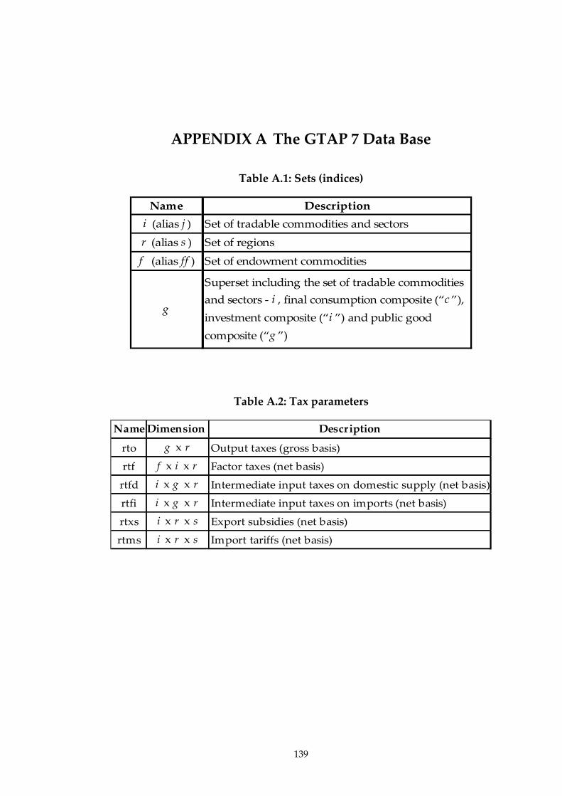
139

The GTAP 7 Data Base APPENDIX A

Table A.1: Sets (indices)

Name Description

i (alias j ) Set of tradable commodities and sectors

r (alias s ) Set of regions

f (alias ff ) Set of endowment commodities

g

Superset including the set of tradable commodities

and sectors - i , final consumption composite (“c ”),

investment composite (“i ”) and public good

composite (“g ”)

Table A.2: Tax parameters

Name Dimension Description

rto g x r Output taxes (gross basis)

rtf f x i x r Factor taxes (net basis)

rtfd i x g x r Intermediate input taxes on domestic supply (net basis)

rtfi i x g x r Intermediate input taxes on imports (net basis)

rtxs i x r x s Export subsidies (net basis)

rtms i x r x s Import tariffs (net basis)

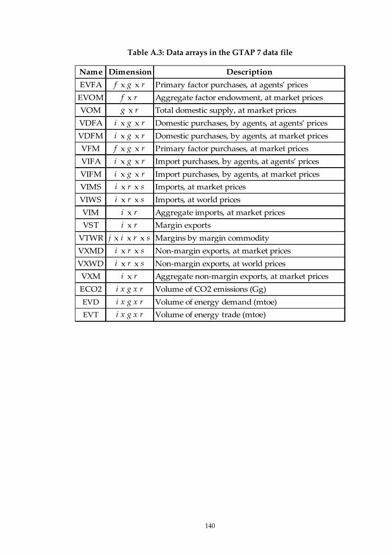
140

Table A.3: Data arrays in the GTAP 7 data file

Name Dimension Description

EVFA f x g x r Primary factor purchases, at agents’ prices

EVOM f x r Aggregate factor endowment, at market prices

VOM g x r Total domestic supply, at market prices

VDFA i x g x r Domestic purchases, by agents, at agents’ prices

VDFM i x g x r Domestic purchases, by agents, at market prices

VFM f x g x r Primary factor purchases, at market prices

VIFA i x g x r Import purchases, by agents, at agents’ prices

VIFM i x g x r Import purchases, by agents, at market prices

VIMS i x r x s Imports, at market prices

VIWS i x r x s Imports, at world prices

VIM i x r Aggregate imports, at market prices

VST i x r Margin exports

VTWR j x i x r x s Margins by margin commodity

VXMD i x r x s Non-margin exports, at market prices

VXWD i x r x s Non-margin exports, at world prices

VXM i x r Aggregate non-margin exports, at market prices

ECO2 i x g x r Volume of CO2 emissions (Gg)

EVD i x g x r Volume of energy demand (mtoe)

EVT i x g x r Volume of energy trade (mtoe)

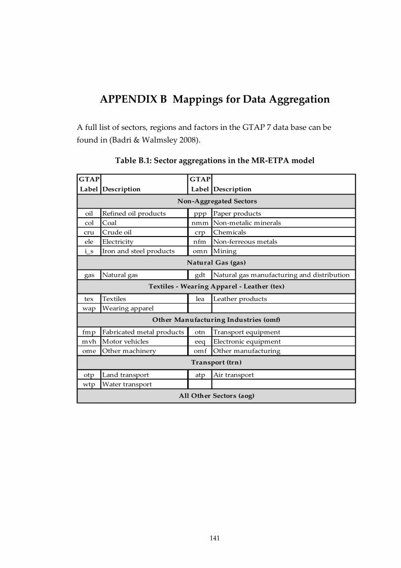
141

Mappings for Data Aggregation APPENDIX B

A full list of sectors, regions and factors in the GTAP 7 data base can be

found in (Badri & Walmsley 2008).

Table B.1: Sector aggregations in the MR-ETPA model

GTAP

Label Description

GTAP

Label Description

oil Refined oil products ppp Paper products

col Coal nmm Non-metalic minerals

cru Crude oil crp Chemicals

ele Electricity nfm Non-ferreous metals

i_s Iron and steel products omn Mining

gas Natural gas gdt Natural gas manufacturing and distribution

tex Textiles lea Leather products

wap Wearing apparel

fmp Fabricated metal products otn Transport equipment

mvh Motor vehicles eeq Electronic equipment

ome Other machinery omf Other manufacturing

otp Land transport atp Air transport

wtp Water transport

All Other Sectors (aog)

Non-Aggregated Sectors

Natural Gas (gas)

Textiles - Wearing Apparel - Leather (tex)

Other Manufacturing Industries (omf)

Transport (trn)

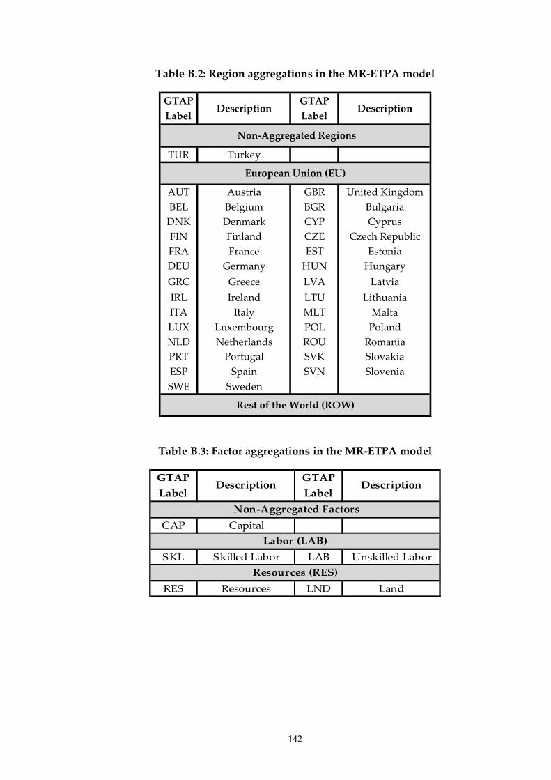
142

Table B.2: Region aggregations in the MR-ETPA model

GTAP

LabelDescription

GTAP

LabelDescription

TUR Turkey

AUT Austria GBR United Kingdom

BEL Belgium BGR Bulgaria

DNK Denmark CYP Cyprus

FIN Finland CZE Czech Republic

FRA France EST Estonia

DEU Germany HUN Hungary

GRC Greece LVA Latvia

IRL Ireland LTU Lithuania

ITA Italy MLT Malta

LUX Luxembourg POL Poland

NLD Netherlands ROU Romania

PRT Portugal SVK Slovakia

ESP Spain SVN Slovenia

SWE Sweden

Non-Aggregated Regions

European Union (EU)

Rest of the World (ROW)

Table B.3: Factor aggregations in the MR-ETPA model

GTAP

LabelDescription

GTAP

LabelDescription

CAP Capital

SKL Skilled Labor LAB Unskilled Labor

RES Resources LND Land

Non-Aggregated Factors

Labor (LAB)

Resources (RES)

143

Trade Flows in the GTAP 7 Data Base APPENDIX C

C.1 Turkey

Figure C.1: Import profile of Turkey from the European Union

oil1%

gas0%

omn0% tex

5%ppp3%

crp19%

nmm1%

i_s6%nfm

2%ele0%

omf52%

COL0%

CRU0%

TRN1%

AOG10%

Imports of Turkey from the EU

144

Figure C.2: Import profile of Turkey from the Rest of the World

FigureC.3: Export profile of Turkey to the European Union

oil4%

gas6% omn

0% tex6%

ppp1%

crp11%

nmm0%i_s

9%nfm9%

ele0%

omf24%

COL2%

CRU13%

TRN4% AOG

11%

Imports of Turkey from the ROW

oil0%

gas0%

omn1%

tex28%

ppp0%

crp5%

nmm3%i_s

4%nfm1%

ele0%

omf31%

COL0%

CRU0%

TRN11%

AOG16%

Exports of Turkey to the EU

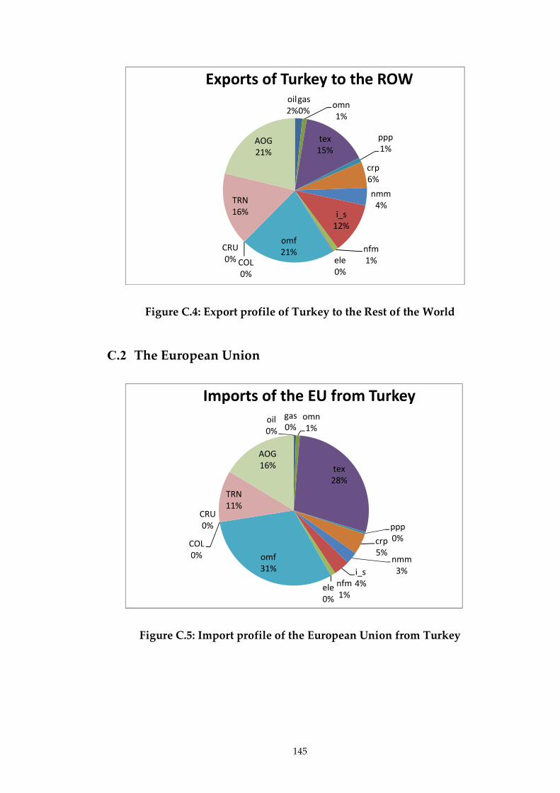
145

Figure C.4: Export profile of Turkey to the Rest of the World

C.2 The European Union

Figure C.5: Import profile of the European Union from Turkey

oil2%

gas0%

omn1%

tex15%

ppp1%

crp6%

nmm4%

i_s12%

nfm1%ele

0%

omf21%

COL0%

CRU0%

TRN16%

AOG21%

Exports of Turkey to the ROW

oil0%

gas0%

omn1%

tex28%

ppp0%crp

5%nmm

3%i_s4%nfm

1%ele0%

omf31%

COL0%

CRU0%

TRN11%

AOG16%

Imports of the EU from Turkey

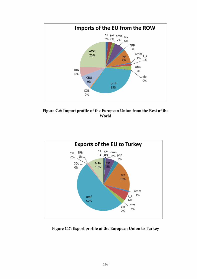
146

Figure C.6: Import profile of the European Union from the Rest of the

World

Figure C.7: Export profile of the European Union to Turkey

oil2%

gas2%

omn2%

tex6%

ppp1%

crp9%

nmm1%

i_s1%

nfm3%

ele0%

omf33%

COL0%

CRU9%

TRN6%

AOG25%

Imports of the EU from the ROW

oil1%

gas0%

omn0%

tex5%

ppp3%

crp19%

nmm1%i_s

6%

nfm2%

ele0%

omf52%

COL0%

CRU0%

TRN1%

AOG10%

Exports of the EU to Turkey

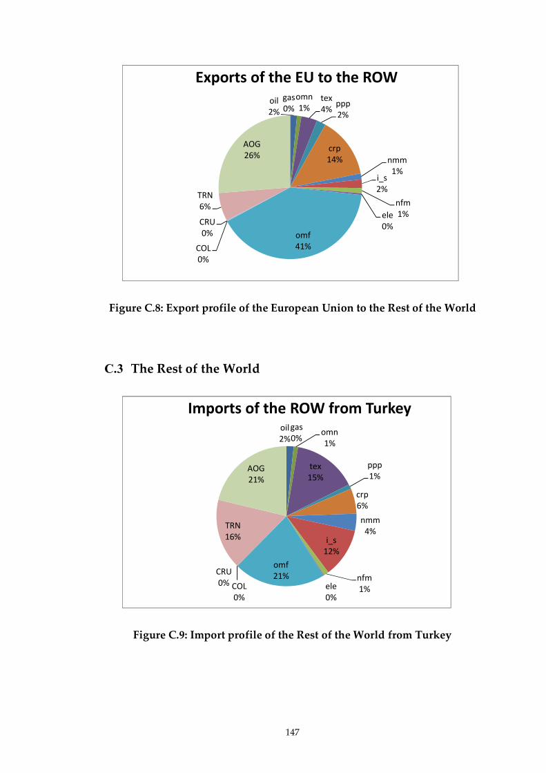
147

Figure C.8: Export profile of the European Union to the Rest of the World

C.3 The Rest of the World

Figure C.9: Import profile of the Rest of the World from Turkey

oil2%

gas0%

omn1%

tex4%

ppp2%

crp14% nmm

1%i_s2%

nfm1%ele

0%omf41%COL

0%

CRU0%

TRN6%

AOG26%

Exports of the EU to the ROW

oil2%

gas0%

omn1%

tex15%

ppp1%

crp6%

nmm4%

i_s12%

nfm1%ele

0%

omf21%

COL0%

CRU0%

TRN16%

AOG21%

Imports of the ROW from Turkey

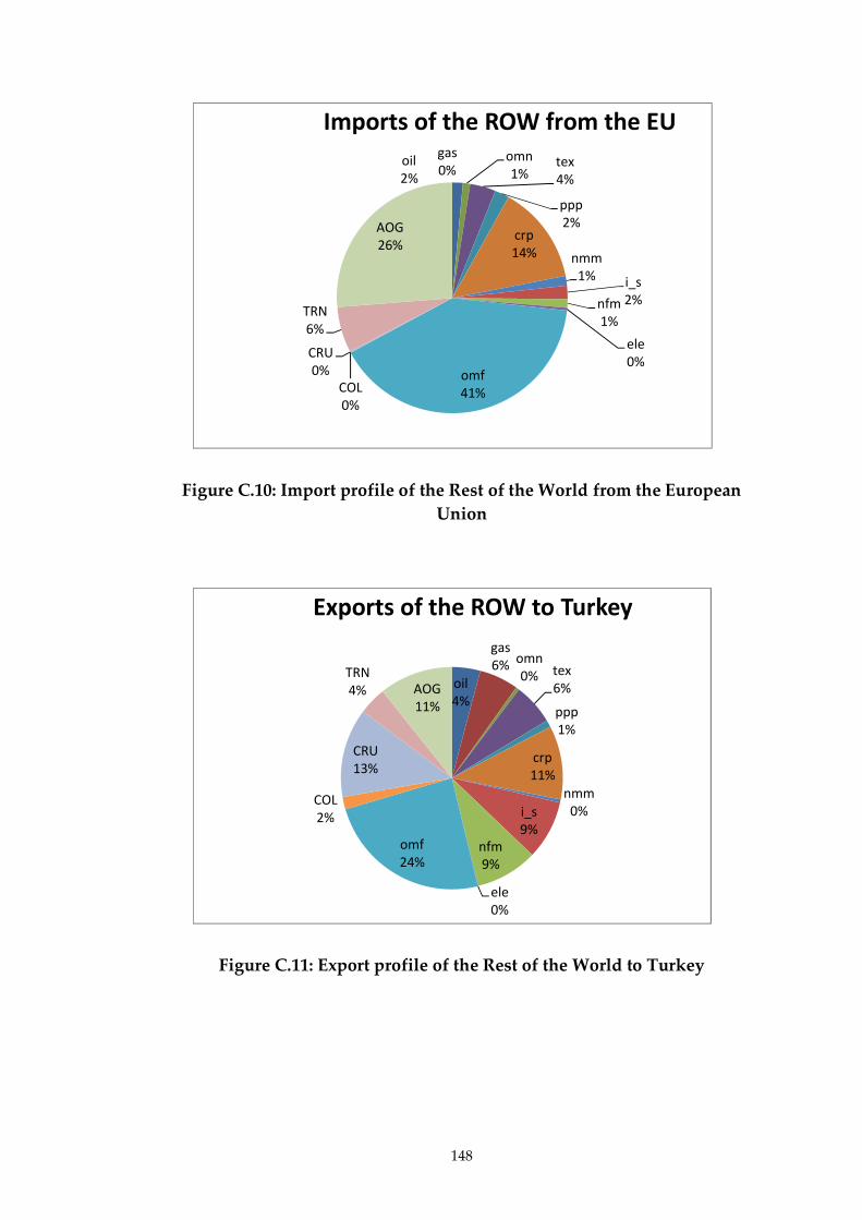
148

Figure C.10: Import profile of the Rest of the World from the European

Union

Figure C.11: Export profile of the Rest of the World to Turkey

oil2%

gas0%

omn1%

tex4%

ppp2%

crp14% nmm

1% i_s2%nfm

1%

ele0%

omf41%COL

0%

CRU0%

TRN6%

AOG26%

Imports of the ROW from the EU

oil4%

gas6% omn

0% tex6%

ppp1%

crp11%

nmm0%i_s

9%nfm9%

ele0%

omf24%

COL2%

CRU13%

TRN4% AOG

11%

Exports of the ROW to Turkey

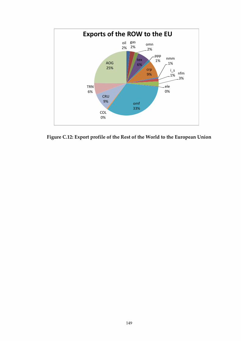
149

Figure C.12: Export profile of the Rest of the World to the European Union

oil2%

gas2%

omn2%

tex6%

ppp1%

crp9%

nmm1%

i_s1% nfm

3%

ele0%

omf33%

COL0%

CRU9%

TRN6%

AOG25%

Exports of the ROW to the EU

market-based environmental regulation in - bilkent. edu. tr

Documents

Transcript of market-based environmental regulation in - bilkent. edu. tr