The Annals of Statistics2016, Vol. 44, No. 4, 1792–1816DOI: 10.1214/16-AOS1451© Institute of Mathematical Statistics, 2016

MARGINALIZATION AND CONDITIONING FOR LWFCHAIN GRAPHS1

BY KAYVAN SADEGHI

University of Cambridge

In this paper, we deal with the problem of marginalization over and con-ditioning on two disjoint subsets of the node set of chain graphs (CGs) withthe LWF Markov property. For this purpose, we define the class of chainmixed graphs (CMGs) with three types of edges and, for this class, provide aseparation criterion under which the class of CMGs is stable under marginal-ization and conditioning and contains the class of LWF CGs as its subclass.We provide a method for generating such graphs after marginalization andconditioning for a given CMG or a given LWF CG. We then define and studythe class of anterial graphs, which is also stable under marginalization andconditioning and contains LWF CGs, but has a simpler structure than CMGs.

1. Introduction. Graphical models use graphs, in which nodes are randomvariables and edges indicate some types of conditional dependencies. Mixedgraphs, which are graphs with several types of edges, have started to play an im-portant role in graphical models as they can deal with more complex independencestructures that arise in different statistical studies.

The first example of mixed graphs in the literature appeared in [11]. This wasa chain graph (CG) with a specific interpretation of conditional independence,which is now generally known as the Lauritzen–Wermuth–Frydenberg or LWF in-terpretation. A formal interpretation, that is, a Markov property, was later providedby [5]. This Markov property, together with other properties such as the factoriza-tion property was extensively discussed in [9]. By the term LWF CGs, one refers tothe class of CGs with a specific independence structure that comes from the LWFMarkov property.

It has become apparent that CGs with the LWF interpretation of independen-cies are important tools in capturing conditional independence structure of variousprobability distributions. For example, Studený and Bouckaert [24] showed thatfor every CG, there exists a strictly positive discrete probability distribution thatembodies exactly the independence statements displayed by the graph, and Peña[15] proved that almost all the regular Gaussian distributions that factorize with

Received May 2014; revised January 2016.1Supported by Grant #FA9550-12-1-0392 from the U.S. Air Force Office of Scientific Research

(AFOSR) and the Defense Advanced Research Projects Agency (DARPA).MSC2010 subject classifications. Primary 62H99; secondary 62A99.Key words and phrases. c-separation criterion, chain graph, independence model, LWF Markov

property, m-separation, marginalization and conditioning, mixed graph.

1792

MARGINALIZATION AND CONDITIONING FOR LWF CHAIN GRAPHS 1793

respect to a chain graph are faithful to it. This means that a Gaussian distributionchosen at random to factorize as specified by the LWF CG will have the indepen-dence structure of the graph and will satisfy no more independence constraints.

However, in the corresponding models to LWF CGs, when some variables areunobserved—also called latent or hidden—or when some variables are set to spe-cific values, the implied independence structure, that is, the corresponding inde-pendence structure after marginalization and conditioning respectively, is not wellunderstood.

The same problem for the well-known class of directed acyclic graphs (DAGs),which is a subclass of LWF CGs, has been a subject of study, and several classesof graphs have been defined in order to capture the marginal and conditional inde-pendence structure of DAGs. These include MC graphs [8], ancestral graphs [18]and summary graphs [26]; see also [19]. There is also a literature pertaining to thisproblem for other types of graphs; see, for example, the class of marginal AMPchain graphs in [16] for marginalization in AMP chain graphs [1].

For LWF CGs, as it will be shown in this paper, one can capture the indepen-dence structure induced by conditioning on some variables by another LWF CG,but in general cannot capture the independence structure induced by marginaliza-tion over some variables by a CG. In this sense, CGs are stable under conditioningbut not under marginalization.

Indeed models with latent variables do not necessarily possess the desirablestatistical properties of graphical models without latent variables, such as identifi-ability, existence of a unique MLE, or being curved exponential families in somecases such as DAGs; see, for example, [6].

However, a first step in dealing with this problem is, in the case of marginaliza-tion, to come up with a more complex class of graphs with a certain independenceinterpretation that captures the marginal independence structure of CGs; and inboth cases of marginalization and conditioning, to provide methods by which thegraphs that capture the marginal and conditional independence structure are gen-erated. These are the main objectives of the current paper.

In the causal language (see, e.g., [13]) the resulting classes of graphs give asimultaneous representation to “direct effects”, “confounding”, and “non-causalsymmetric dependence structures”.

It is important to note that the classes of graphs introduced here only dealswith the conditional independence constraints, and not other constraints such asso-called Verma constraints [25]. The actual statistical model is much more com-plicated even when marginalizing DAGs; see, for example, [21].

The introduction of these classes of graphs is also justified in the paper by show-ing that, for large subclasses of these classes of graphs, there are probability dis-tributions (in fact both Gaussian and discrete) that are faithful to them. Althoughfinding the explicit parametrizations for the defined graphs is beyond the scopeof this paper, it also seems possible to extend the existing parametrizations for

1794 K. SADEGHI

smaller types of graph in the literature to these classes in a fairly natural way. Wewill provide a discussion on this in the paper.

The structure of the paper is as follows: in the next section, we define mixed andchain graphs, and, for these classes of graphs, give graph theoretical definitionsneeded in this paper. In Section 3, we provide two equivalent ways for reading offindependencies from a CG based on the LWF Markov property. In Section 4, wedefine the class of chain mixed graphs with certain independence interpretation,and show that they capture the marginal independence structure of LWF CGs andthat they are stable under marginalization, and provide an algorithm for generatingsuch graphs after marginalization. In Section 5, we show that the class of CMGs isalso stable under conditioning, provide the corresponding algorithm, and combinemarginalization and conditioning for CMGs. As a corollary, we see that LWF CGsare stable under conditioning. In Section 6, we define the class of anterial graphsas a subclass of CMGs, which also contains LWF CGs, and show that this classis stable under marginalization and conditioning. We also provide an algorithmfor marginalization and conditioning for this class. In Section 7, we discuss theimplications of the results for probabilistic independence models that are faithfulto LWF CGs, and possible ways to generalize the parametrizations existing in theliterature for CMGs and anterial graphs. In the Appendix in the supplementarymaterial [20], we provide proofs of non-trivial lemmas, propositions and theoremsin the paper as well as some more technical and yet less informative lemmas thatare used in the proofs.

2. Definitions for mixed graphs and chain graphs.

2.1. Basic graph theoretical definitions. A graph G is a triple consisting of anode set or vertex set V , an edge set E, and a relation that with each edge associatestwo nodes (not necessarily distinct), called its endpoints. When nodes i and j arethe endpoints of an edge, these are adjacent and we write i ∼ j . We say the edgeis between its two endpoints. We usually refer to a graph as an ordered pair G =(V ,E). Graphs G1 = (V1,E1) and G2 = (V2,E2) are called equal if (V1,E1) =(V2,E2). In this case, we write G1 = G2.

Notice that graphs that we use in this paper (and in general in the contextof graphical models) are so-called labeled graphs, that is, every node is consid-ered a different object. Hence, for example, graph i j k is not equal toj i k.

Here, we introduce some basic graph theoretical definitions. A loop is an edgewhose endpoints are equal. Multiple edges are edges whose endpoints are the sameas each other. A simple graph has neither loops nor multiple edges. A completegraph is a simple graph with all pairs of nodes adjacent.

A subgraph of a graph G1 is graph G2 such that V (G2) ⊆ V (G1) and E(G2) ⊆E(G1) and the assignment of endpoints to edges in G2 is the same as in G1. An

MARGINALIZATION AND CONDITIONING FOR LWF CHAIN GRAPHS 1795

induced subgraph by a subset A of the node set is a subgraph that contains thenode set A and all edges between two nodes in A.

A walk is a list 〈i0, e1, i1, . . . , en, in〉 of nodes and edges such that for 1 ≤ m ≤ n,the edge em has endpoints im−1 and im. A path is a walk with no repeated node oredge. A cycle is a walk with no repeated node or edge except i0 = in. If the graphis simple then a path or a cycle can be determined uniquely by an ordered sequenceof nodes. Throughout this paper, however, we use node sequences to describe pathsand cycles even in graphs with multiple edges, but we assume that the edges of thepath are all determined. It is usually apparent from the context or the type of thepath which edge belongs to the path in multiple edges. We say a walk or a path isbetween the first and the last nodes of the list in G. We call the first and the lastnodes endpoints of the walk or of the path. All other nodes are the inner nodes.

For a walk or path π = 〈i1, . . . , in〉, any subsequence 〈ik, ik+1, . . . , ik+p〉, 1 ≤k, k + p ≤ n, whose members appear consecutively on π , defines a subwalk or asubpath of π , respectively.

2.2. Some definitions for mixed graphs. A mixed graph is a graph containingthree types of edges denoted by arrows, arcs (two-headed arrows), and lines (solidlines). Mixed graphs may have multiple edges of different types but do not havemultiple edges of the same type. We do not distinguish between i j and j i

or i≺ �j and j ≺ �i, but we do distinguish between j �i and i �j . In thispaper, we are only considering mixed graphs that do not contain loops of any type.These constitute the class of loopless mixed graphs.

For mixed graphs, we say that i is a neighbor of j if these are endpoints of aline, and i is a parent of j and j is a child of i if there is an arrow from i to j .We also define that i is a spouse of j if these are endpoints of an arc. We use thenotation ne(j), pa(j), and sp(j) for the set of all neighbors, parents, and spousesof j , respectively.

In the cases of i �j or i≺ �j , we say that there is an arrowhead pointing to(at) j .

A walk 〈i = i0, i1, . . . , in = j 〉 is directed from i to j if all ikik+1 edges arearrows pointing from ik to ik+1. If there is a directed walk from j to i then j isan ancestor of i and i is a descendant of j . We denote the set of ancestors of i

by an(i). Notice that, unlike some authors, we do not consider i to be in the set ofancestors or descendants of i. Moreover, a cycle with the above property is calleda directed cycle.

A walk 〈i = i0, i1, . . . , in = j 〉 from i to j is a semi-directed walk if it onlyconsists of lines and arrows (it may contain only one type of edge), and everyarrow ikik+1 is pointing from ik to ik+1. Thus, a directed walk is a type of semi-directed walk. We shall say that i is anterior of j if there is a semi-directed walkfrom i to j . We use the notation ant(i) for the set of all anteriors of i. Notice againthat, similar to ancestors, we do not consider a node i to be an anterior of itself.For a set of nodes A, we define ant(A) = ⋃

i∈A ant(i) \ A. Notice also that, since

1796 K. SADEGHI

ancestral graphs have no arrowheads pointing to lines, our definition of anteriorextends the notion of anterior used in [18] for ancestral graphs. Moreover, a cyclewith the properties of semi-directed walks is called a semi-directed cycle.

A section of a walk in a mixed graph is a maximal subwalk that only consists oflines. Thus, any walk decomposes uniquely into sections (that are not necessarilyedge-disjoint and may also be single nodes). Similar to nodes, all sections on awalk between i and j are inner sections except those that contain i or j , which areendpoint sections. As in any walk, we can also define the endpoints of a section.A section ρ on a walk π is called a collider section if one of the three followingwalks is a subwalk of π : i �ρ≺ j , i≺ �ρ≺ j , and i≺ �ρ≺ �j . Allother sections on π are called non-collider sections. We may speak of collider ornon-collider sections without mentioning the relevant walk when this is apparentfrom context.

A trislide on a walk π is a subpath 〈i = i0, i1, . . . , in = j〉, where ii1 and in−1j

are arrows or arcs and the subpath ρ′ = 〈i1, . . . , in−1〉 is a section.Three types of trislides i � ◦ · · · ◦ ≺ j , i≺ � ◦ · · · ◦

≺ j , and i≺ �◦ · · · ◦ ≺ �j are collider trislides and all other typesof trislides are non-collider on any walk of which the trislide is defined.

A tripath is a trislide where the subpath ρ′ is a single node. Note that [19] usedthe term V-configuration for such a path. ([7] and most texts let a V-configurationbe a tripath with non-adjacent endpoints.) Tripaths and their inner nodes can bedefined to be colliders or non-colliders as trislides and their inner sections.

Two walks π1 and π2 (including trislides, tripaths or edges) between i and j

are called endpoint-identical if there is an arrowhead pointing to the endpointsection containing i on π1 if and only if there is an arrowhead pointing to theendpoint section containing i on π2; and similarly for j . For example, the pathsi �j , i k �l≺ �j and i �k≺ �l j are all endpoint-identical asthey have an arrowhead pointing to the section containing j but no arrowheadpointing to the section containing i on the paths, but they are not endpoint-identicalto i k≺ �j .

2.3. Chain graphs. Chain graphs (CGs) consist of lines and arrows and donot contain any semi-directed cycles with at least one arrow.

It is implied from the definition that CGs are characterized by having a node setthat can be partitioned into disjoint subsets forming so-called chain components.These are connected subgraphs consisting only of undirected edges and are ob-tained by removing all arrows in the graph. All edges between nodes in the samechain component are lines, and all edges between different chain components arearrows. In addition, the chain components can be ordered in such a way that allarrows point from a chain with a higher number to one with a lower number.

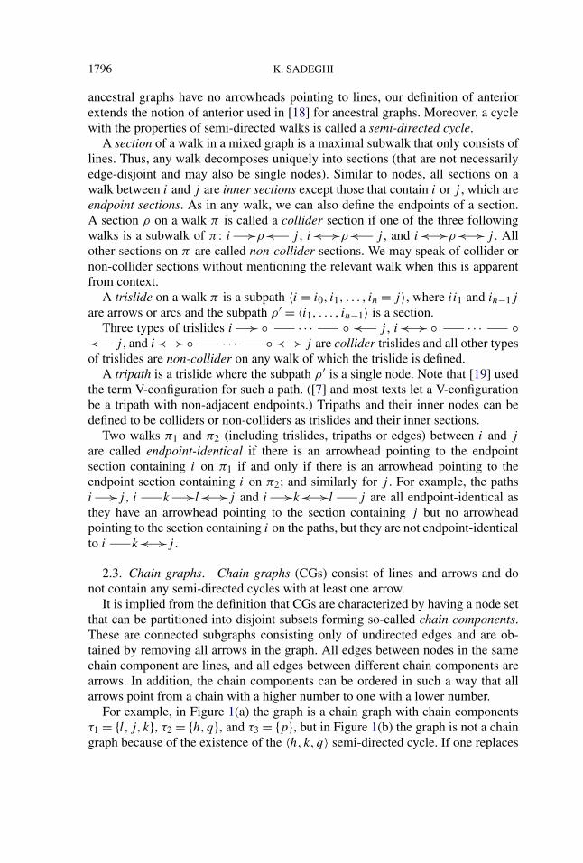
For example, in Figure 1(a) the graph is a chain graph with chain componentsτ1 = {l, j, k}, τ2 = {h,q}, and τ3 = {p}, but in Figure 1(b) the graph is not a chaingraph because of the existence of the 〈h, k, q〉 semi-directed cycle. If one replaces

MARGINALIZATION AND CONDITIONING FOR LWF CHAIN GRAPHS 1797

FIG. 1. (a) A CG. (b) A mixed graph that is not a CG.

every chain component with a single node, one obtains a directed acyclic graph(DAG), a graph consisting exclusively of arrows and without any directed cycles.

Notice that generally CGs are defined to contain arrows and one symmetric typeof edge in their chain components (namely lines or arcs). In this sense, the type ofCG with which we deal in this paper is a line CG.

3. LWF Markov property for CGs. An independence model J over a set V

is a set of triples 〈X,Y |Z〉 (called independence statements), where X, Y , and Z

are disjoint subsets of V and Z can be empty, and 〈∅, Y |Z〉 and 〈X,∅ |Z〉 are al-ways included in J . The independence statement 〈X,Y |Z〉 is interpreted as “X isindependent of Y given Z”. Notice that independence models contain probabilis-tic independence models as a special case. For further discussion on independencemodels, see [23].

A graph G also induces an independence model J (G). One way is by usinga separation criterion, which determines whether for three disjoint subsets A, B ,and C of the node set of G, 〈A,B |C〉 ∈ J (G). Such a criterion verifies whetherA is separated from B by C in the sense that there are no walks or paths of specifictypes between A and B given C in the graph. Such a separation is denoted byA⊥B |C. It is clear that J (G) satisfies the global Markov property, which statesthat if A⊥B |C in G then 〈A,B |C〉 ∈ J .

For CGs, at least four different separation criteria, that is, four different typesof global Markov property have been discussed in the literature. Drton [3] hasclassified them as (1) the LWF or block concentration Markov property, (2) theAMP or concentration regression Markov property, as defined and studied by [1],(3) a Markov property that is dual to the AMP Markov property and (4) the mul-tivariate regression Markov property, as introduced by [2] and studied extensivelyrecently; for example, see [12, 27].

In this paper, we are interested in the LWF Markov property, and we introducetwo equivalent separation criteria for this in this section. Henceforth, for the sakeof brevity, by CGs we refer to CGs with the LWF Markov property.

The moralization criterion for CGs was defined in [5] and is a generalization ofthe moralization criterion for DAGs defined in [10]; see also [9]. The moral graph

1798 K. SADEGHI

of a chain graph G, denoted by (G)m is a graph that consists only of lines and thatis generated from G as follows: for every edge ij in G there is a line ij in (G)m.In addition, if nodes i and j are parents of the same chain component in G thenthere is the line ij in (G)m.

Now let Gant(A∪B∪C) be the induced subgraph of G generated by ant(A ∪ B ∪C). The moralization criterion states that for A, B and C, three disjoint subsets ofthe node set of G, if there are no paths between A and B in (Gant(A∪B∪C))

m whoseinner nodes are outside C then A⊥ morB |C.

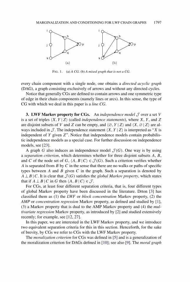
An equivalent criterion, called the c-separation criterion for CGs was definedin [24]. Here, we present a simpler version of that criterion, presented in [22], witha different notation and wording:

A walk π in a CG is a c-connecting walk given C if every collider section of π

has a node in C and all non-collider sections are outside C. A section on π is openif either: it is a collider section and one of its nodes is in C; or it is a non-collidersection and all its nodes are outside C. Otherwise, it is blocked. We say that A andB are c-separated given C if there are no c-connecting walks between A and B

given C, and we use the notation A⊥ cB |C.Notice that, as mentioned in [24], there is potentially an infinite number of walks

and, therefore, this might not be an appropriate criterion for testing independen-cies. Although, in this paper, we only use this criterion in order to prove our theo-retical results regarding marginalization and conditioning, and an infinite numberof walks is not an issue for this purpose, in [22], it was shown that this criterioncan also be implemented with an algorithm.

For example, in the graph of Figure 2(a), the independence statement j ⊥h | ldoes not hold. This can be seen by looking at the moral graph (Gant({j,h,l}))m =(G{j,h,k,q,l,r})m in Figure 2(b), and observing that the inner nodes of the path〈j, k, q,h〉 are outside the conditioning set. The same conclusion can be madeby looking at the walk 〈j, k, l, r, q, h〉, where the non-collider sections k and q areoutside the conditioning set, but the inner node l of the collider section 〈l, r〉 is inthe conditioning set.

The equivalence of the moralization criterion and the original c-separation cri-terion was proven in Consequence 4.1 in [24]. The equivalence with the mentionedsimplified criterion was proven in [22]. We use the notation Jc(G) for the inde-pendence model induced from G by the above criteria.

FIG. 2. (a) A chain graph G. (b) The moral graph (Gant({j,h,l}))m.

MARGINALIZATION AND CONDITIONING FOR LWF CHAIN GRAPHS 1799

We first prove the following lemma, which provides an equivalent type of walkto c-connecting walks.

LEMMA 1. There is a c-connecting walk between i and j given C if and onlyif there is a walk between i and j whose sections are all paths, and on whichnodes of every collider section are in C ∪ ant(C), and non-collider sections areoutside C. In addition, these walks can be chosen to be endpoint-identical.

Notice that by the same method as the proof of this lemma, one can alwaysassume that a section on a walk is a path. This is our assumption throughout thepaper unless otherwise stated.

4. Stability of CGs under marginalization and conditioning. For a subsetC of V , the independence model after conditioning on C, denoted by α(J ;∅,C),is

α(J ;∅,C) = {〈A,B |D〉 : 〈A,B |D ∪ C〉 ∈ J and (A ∪ B ∪ D) ∩ C =∅

}.

One can observe that α(J ;∅,C) is an independence model over V \ C.We now present the definition of stability under conditioning [19]: Consider a

family of graphs T . If, for every graph G = (V ,E) ∈ T and every disjoint subsetsC of V , there is a graph H ∈ T such that J (H) = α(J (G);∅,C) then T is stableunder conditioning. Notice that the node set of H is V \ C.

We will see as a corollary of the results and algorithms in the next section thatCGs are stable under conditioning.

Similar to the conditioning case, for a subset M of V , the independence modelafter marginalization over M , denoted by α(J ;M,∅), is defined by

α(J ;M,∅) = {〈A,B |D〉 ∈ J : (A ∪ B ∪ D) ∩ M = ∅

}.

One can observe that α(J ;M,∅) is an independence model over V \ M .The definition of stability under marginalization is defined similarly to the con-

ditioning case: for a family of graphs T , if, for every graph G = (V ,E) ∈ Tand every disjoint subsets C of V , there is a graph H ∈ T such that J (H) =α(J (G);M,∅) then T is stable under marginalization. We see again that the nodeset of H is N = V \ M .

CGs are not closed under marginalization. For example, it can be shown that G

in Figure 3 is a CG (in fact a DAG) whose induced marginal independence modelcannot be represented by a CG. We leave the details as an exercise to the reader.

FIG. 3. A chain graph G, by which it can be shown that the class of CGs is not stable undermarginalization. ( � �� ∈ M .)

1800 K. SADEGHI

FIG. 4. (a) A CMG. (b) A mixed graph that is not a CMG.

Hence, we define a class of graphs that is stable under marginalization and con-tains CGs: the class of chain mixed graphs (CMGs) is the class of mixed graphswithout semi-directed cycles with at least an arrow. Notice that we allow CMGsto have multiple edges consisting of arcs and arrows and arcs and lines. This is ageneralization of chain graphs since if a CMG does not contain arcs then it is achain graph.

For example, in Figure 4(a) the graph is a CMG, but in Figure 4(b) the graph isnot a CMG because of the existence of the 〈h,p, q〉 semi-directed cycle.

We provide a c-separation criterion for CMGs, and using this, show that CMGsare closed under marginalization. For this purpose, we provide in this section analgorithm that, from a CMG (or a chain graph) G and after marginalization overM , generates a CMG with the corresponding independence model after marginal-ization over M .

We define a c-separation criterion for CMGs with exactly the same wordings asthat of CGs: a walk π in a CG is a c-connecting walk given C if every collidersection of π has a node in C and all non-collider sections are outside C. We saythat A and B are c-separated given C if there are no c-connecting walks betweenA and B given C, and we use the notation A⊥ cB |C.

However, notice that this is in fact a generalization of the c-separation criterionfor CGs since, for CMGs, bidirected edges on π may make a section collider.

We now provide an algorithm that, from a chain mixed graph G and aftermarginalization over M , generates a CMG with the corresponding independencemodel after marginalization over M . Notice that this algorithm may indeed be ap-plied to a CG.

ALGORITHM 1 [αCMG(G;M,∅): Generating a CMG from a chain mixed graphG after marginalization over M].

Start from G.

1. Generate an ij edge as in Table 1, steps 8 and 9, between i and j on acollider trislide with an endpoint j and an endpoint in M if the edge of the sametype does not already exist.

MARGINALIZATION AND CONDITIONING FOR LWF CHAIN GRAPHS 1801

TABLE 1Types of edge induced by tripaths with inner node m ∈ M

and trislides with endpoint m ∈ M

1 i≺ m≺ j generates i≺ j

2 i≺ m j generates i≺ j

3 i≺ �m j generates i≺ �j

4 i≺ m �j generates i≺ �j

5 i≺ m≺ �j generates i≺ �j

6 i m≺ j generates i≺ j

7 i m j generates i j

8 m �i · · · ◦ ≺ j generates i≺ j

9 m �i · · · ◦ ≺ �j generates i≺ �j

2. Generate an appropriate edge as in Table 1, steps 1 to 7, between the end-points of every tripath with inner node in M if the edge of the same type does notalready exist. Apply this step until no other edge can be generated.

3. Remove all nodes in M .

Notice that, here and elsewhere, by removing nodes we mean also removingall the adjacent edges to those nodes. Notice also that all the cases generate anendpoint-identical edge to the tripath or the trislide. In addition, in cases 8 and 9,the node m is separate from the inner nodes of the concerned trislide since other-wise there will be a semi-directed cycle in the graph.

This algorithm is a generalization of the marginalization part of the summary-graph-generating algorithm [19]. The first seven cases are exactly the same as thecorresponding cases in the summary-graph-generating algorithm, whereas cases 8and 9 do not appear in the summary-graph-generating algorithm since in summarygraphs there are no arrowheads pointing to lines. The other reason is that herewe deal with connecting walks instead of paths, and the subwalk 〈i,m, i〉 maybe present in a connecting walk. In general, here in this algorithm, and in lateralgorithms in this paper, the sections are treated in the same way as the nodes aretreated in the algorithms that generate summary graphs, acyclic directed mixedgraphs (ADMGs) [17], or ancestral graphs. It is also worth noticing that all thesealgorithms are indeed generalizations of the ordinary latent projection operation;see [13].

Figure 5 illustrates how to apply Algorithm 1 step by step to a CG.We consider Algorithm 1 a function denoted by αCMG. Notice that for ev-

ery chain mixed graph G, it holds that αCMG(G;∅,∅) = G. We first show thatαCMG(G;M,∅) is a CMG.

PROPOSITION 1. Graphs generated by Algorithm 1 are CMGs.

1802 K. SADEGHI

FIG. 5. (a) A chain graph G, � �� ∈ M . (b) The graph after applying step 1 of Algorithm 1 (case 8of Table 1). (c) The graph after applying step 2 of Algorithm 1 (case 4 of Table 1). (d) The generatedCMG after applying step 3.

We first provide lemmas that express the global behavior of step 2 of Algo-rithm 1 as well as a generalization and an implication of step 1 (in the Appendixin [20]).

LEMMA 2. Let G be a CMG. There exists an edge between i and j inαCMG(G;M,∅) if and only if there exists an endpoint-identical walk between i

and j in the graph generated after applying step 1 of Algorithm 1 to G whoseinner sections are all non-collider and whose inner nodes are all in M .

The following theorem shows that αCMG(·; ·,∅) is well-defined in the sensethat, instead of directly generating a CMG, we can split the nodes that we marginal-ize over into two parts, first generate the CMG related to the first part, then fromthe generated CMG, generate the desired CMG related to the second part.

THEOREM 1. For a chain mixed graph G and disjoint subsets M and M1 ofits node set,

αCMG(αCMG(G;M,∅);M1,∅

) = αCMG(G;M ∪ M1,∅).

Some CMGs may not be generated after marginalization for CGs. In the follow-ing proposition, we provide the exact set of graphs to which CMGs are mappedafter marginalization. Denote by CG the set of all CGs and by CMG the set of allCMGs.

PROPOSITION 2. Define H to be the subset of CMG with the following prop-erties:

MARGINALIZATION AND CONDITIONING FOR LWF CHAIN GRAPHS 1803

1. There is no collider trislide of form k≺ �i · · · j ≺ l unlessthere is an arrow from l to i;

2. there is no collider trislide of form k≺ �i · · · j ≺ �l unlessthere are kj , il and ij arcs.

Then αCMG(·; ·,∅) maps CG and a subset of the node set of its member surjectivelyonto H.

Here, we prove the main result of this section:

THEOREM 2. For a chain mixed graph G and disjoint subsets A, B , M andC1 of its node set,

〈A,B |C1〉 ∈ Jc

(αCMG(G;M,∅)

) ⇐⇒ 〈A,B |C1〉 ∈ Jc(G).

We, therefore, have the following immediate corollary.

COROLLARY 1. The class of chain mixed graphs, CMG, with c-separationcriterion is stable under marginalization.

5. Stability of CMGs under marginalization and conditioning.

5.1. Stability of CMGs under conditioning. In the previous section, weshowed that the class of CMGs is stable under marginalization. In this section,we first show that the class of CMGs is also stable under conditioning, and pro-vide an algorithm for conditioning for CMGs:

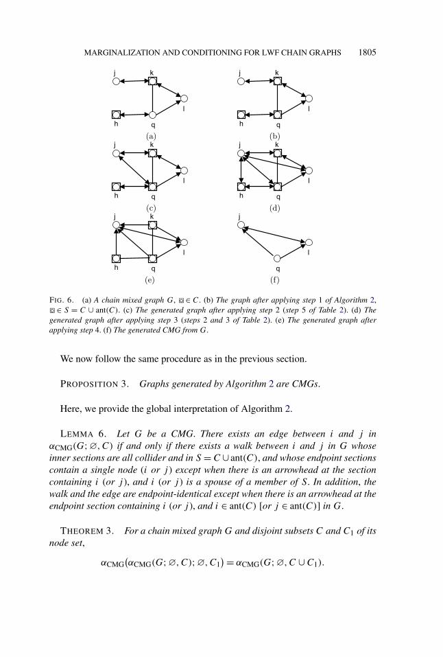
ALGORITHM 2 [αCMG(G;∅,C): Generating a CMG from a chain mixed graphG after conditioning on C].

Start from G.

1. Find all nodes in C ∪ ant(C) and call this set S.2. For collider trislides illustrated in Table 2, steps 4 and 5, with an endpoint

i and one endpoint in S, generate an ij edge following the table if the edge doesnot already exist.

3. For collider trislides (including tripaths) illustrated in Table 2, steps 1–3, with at least one inner node in S, generate an edge following the table if theedge does not already exist. Apply this step repeatedly until no other edge can begenerated, but do not use generated lines (to generate new sections).

4. Remove the arrowheads of all arrows and arcs pointing to members of S

(i.e., turn such arrows into lines and such arcs into arrows).5. Remove all nodes in C.

1804 K. SADEGHI

TABLE 2Types of edges induced by trislides with an inner node or

endpoint s ∈ S = C ∪ ant(C)

1 i �s · · · s≺ j generates i j

2 i≺ �s · · · s≺ j generates i≺ j

3 i≺ �s · · · s≺ �j generates i≺ �j

4 s≺ �i · · · ◦ ≺ j generates i≺ j

5 s≺ �i · · · ◦ ≺ �j generates i≺ �j

Notice that if a node of a section is in S then all the inner nodes are in S, thus, wemay speak of a section being in S. Notice also that all the steps of the algorithmgenerate endpoint-identical edges to the concerned trislides. In addition, we canassume that the endpoints of trislides are disjoint from the inner nodes, since (1) j

as an endpoint of an arrow cannot be also an inner node because the graph doesnot contain semi-directed cycles; and (2) cases 2 and 3 with i an inner node areequivalent to cases 4 and 5, respectively, and cases 4 and 5 with s an inner nodeare equivalent to cases 2 and 3, respectively.

Similar to Algorithm 1, this algorithm is a generalization of the condition-ing part of the summary-graph-generating algorithm [19]. The first three casesare the same when one considers sections here to be the nodes in the summary-graph-generating algorithm. Cases 4 and 5 do not appear in the summary-graph-generating algorithm for the same reasons explained before.

Figure 6 illustrates how to apply Algorithm 2 step by step to a CMG. First, letus provide a global interpretation of step 3 of Algorithm 2.

LEMMA 3. Let G be a CMG. There exists an edge between i and j in thegraph generated after step 3 of Algorithm 2 if and only if there exists an endpoint-identical walk to the edge between i and j in the generated graph after step 2whose inner sections are all collider and in C ∪ ant(C), and whose endpoint sec-tions contain a single node (i or j ).

We provide two lemmas that explain why the set S can be fixed in the begin-ning of the algorithm, and why there is no need to apply step 4 of Algorithm 2repeatedly.

LEMMA 4. Let G be a CMG. If there is an arrow from j to i or a line be-tween j and i generated by steps 3 or 4 of Algorithm 2 then j ∈ S = C ∪ ant(C).In addition, generated lines by Algorithm 2 do not lie on any collider section inαCMG(G;∅,C).

LEMMA 5. Let G be a CMG. A node i is in ant(C) in G if and only if it is inant(C) in the graph generated after every step of Algorithm 2 before step 5.

MARGINALIZATION AND CONDITIONING FOR LWF CHAIN GRAPHS 1805

FIG. 6. (a) A chain mixed graph G, �◦ ∈ C. (b) The graph after applying step 1 of Algorithm 2,�◦ ∈ S = C ∪ ant(C). (c) The generated graph after applying step 2 (step 5 of Table 2). (d) Thegenerated graph after applying step 3 (steps 2 and 3 of Table 2). (e) The generated graph afterapplying step 4. (f) The generated CMG from G.

We now follow the same procedure as in the previous section.

PROPOSITION 3. Graphs generated by Algorithm 2 are CMGs.

Here, we provide the global interpretation of Algorithm 2.

LEMMA 6. Let G be a CMG. There exists an edge between i and j inαCMG(G;∅,C) if and only if there exists a walk between i and j in G whoseinner sections are all collider and in S = C ∪ ant(C), and whose endpoint sectionscontain a single node (i or j ) except when there is an arrowhead at the sectioncontaining i (or j ), and i (or j ) is a spouse of a member of S. In addition, thewalk and the edge are endpoint-identical except when there is an arrowhead at theendpoint section containing i (or j ), and i ∈ ant(C) [or j ∈ ant(C)] in G.

THEOREM 3. For a chain mixed graph G and disjoint subsets C and C1 of itsnode set,

αCMG(αCMG(G;∅,C);∅,C1

) = αCMG(G;∅,C ∪ C1).

1806 K. SADEGHI

THEOREM 4. For a chain mixed graph G and disjoint subsets A, B , C andC1 of its node set,

〈A,B |C1〉 ∈ Jc

(αCMG(G;∅,C)

) ⇐⇒ 〈A,B |C ∪ C1〉 ∈ Jc(G).

COROLLARY 2. The class of chain mixed graphs, CMG, with c-separationcriterion is stable under conditioning.

Applying Algorithm 2 to a CG, step 2 becomes inapplicable, and step 3 spe-cializes to generating a line between the endpoints of collider trislides with at leastone inner node in S if the line does not already exist. Denote this specialization byαCG(G,∅,C). We first have the following.

PROPOSITION 4. Algorithm 2 generates CGs from CGs.

Denote now by CG the set of all CGs. We also provide the following trivialstatement.

PROPOSITION 5. The map αCG(·;∅, ·) from CG and a subset of the node setof its members to CG is surjective.

PROOF. The result follows from the fact that αCMG(G;∅,∅) = G. �

We, therefore, have the following immediate corollary.

COROLLARY 3. The class of chain graphs, CG, with the LWF Markov prop-erty is stable under conditioning.

5.2. Simultaneous marginalization and conditioning for CMGs. Corollaries 4and 2 imply that CMG with c-separation criterion is stable under marginalizationand conditioning, which formally holds when there is a graph H ∈ CMG such thatJc(H) = α(Jc(G);M,C), where

α(J ;M,C) = {〈A,B |D〉 : 〈A,B |D∪C〉 ∈ J and (A∪B ∪D)∩ (M ∪C) =∅

}.

We now deal with the case where there are both marginalization and condition-ing subsets in a CMG. We first define maximality in order to simplify the results.A graph is maximal if to every non-adjacent pairs of nodes, there is an indepen-dence statement associated in J (G). CMGs are not maximal since, for example,the class of ancestral graphs [18] is a subclass of CMGs, and there exist non-maximal ancestral graphs; see also Figure 7, for an example of a CMG that is notancestral and that induces no independence statement of form j ⊥ cl |C for anychoice of C. There is a method to generate, from a non-maximal CMG, a maximalCMG that induces the same independence model, which is beyond the scope ofthis manuscript. However, here we provide a sufficient condition for non-maximalgraphs as a lemma, which will be used in our proofs.

MARGINALIZATION AND CONDITIONING FOR LWF CHAIN GRAPHS 1807

FIG. 7. A non-maximal AnG.

LEMMA 7. If there is a collider trislide between i and j in G such that thereis an arrow from an inner node of the trislide to j (or i) and i � j then G is notmaximal.

We also provide the following lemma, which deals with the global behaviorof the simultaneous marginalization and conditioning as described later in thissection.

LEMMA 8. There is an edge between i and j in αCMG(αCMG(G;∅,C);M,∅) if and only if there is a walk between i and j in G on which (i) all nodeson collider sections are in C ∪ ant(C); (ii) on non-collider sections, (a) all nodesare in M , or (b) one endpoint is in M and also either a child of a node in M or aspouse of a node in C ∪ant(C), and the other endpoint has an arrowhead at it fromthe adjacent node on the walk. In addition, the walk and the edge are endpoint-identical except when there is an arrowhead at the endpoint section containing i

(or j ), and i ∈ ant(C) [or j ∈ ant(C)] in G.

We now have the following important result, which illustrates that, for maximalgraphs, in order to both marginalize and condition, it does not matter whether wemarginalize first by using Algorithm 1 and then condition by using Algorithm 2 orvice versa.

PROPOSITION 6. For a chain mixed graph G and two disjoint subsets M andC of its node set, it holds that

αCMG(αCMG(G;M,∅);∅,C

) = αCMG(αCMG(G;∅,C);M,∅

)

if αCMG(αCMG(G;M,∅);∅,C) is maximal.

It is also clear from the proof that if we drop the maximality assumption thenthe two concerned graphs in the proposition induce the same independence mod-els. In addition, we show that the corresponding algorithm (Algorithm 1 followedby Algorithm 2 or vice versa) is well-defined for maximal graphs. We denote thecorresponding function by αCMG(G;M,C). In general, one can first apply Algo-rithm 2 followed by Algorithm 1, in which case we showed in the proof that anedge is present between the endpoints of the walk described in Lemma 7.

1808 K. SADEGHI

THEOREM 5. For a chain mixed graph G and disjoint subsets M , M1, C andC1 of its node set,

αCMG(αCMG(G;M,C);M1,C1

) = αCMG(G;M ∪ M1,C ∪ C1)

if the two graphs are maximal.

PROOF. The result follows from the definition and Proposition 6, Theorem 3and Theorem 1. �

In Proposition 2, we showed that all CGs after marginalization are mappedonto H, which is a subclass of CMGs. Here, we show that CGs after marginal-ization and conditioning are also mapped onto H.

PROPOSITION 7. The map αCMG maps CG and two subsets of the node set ofits members surjectively onto H.

We are now ready to provide the main result, which illustrates that by applyingAlgorithm 1 followed by Algorithm 2 (or vice versa), we obtain the marginal andconditional independence model for a CMG (or a CG) after marginalization andconditioning.

THEOREM 6. For a chain mixed graph G and disjoint subsets A, B , M , C

and C1 of its node set,

〈A,B |C1〉 ∈ Jc

(αCMG(G;M,C)

) ⇐⇒ 〈A,B |C ∪ C1〉 ∈ Jc(G).

PROOF. By definition and Proposition 6, Theorem 4 and Theorem 2, it is im-plied that

〈A,B |C1〉 ∈ Jc

(αCMG(G;M,C)

) = Jc

(αCMG

(αCMG(G;M,∅);∅,C

))

⇐⇒ 〈A,B |C ∪ C1〉 ∈ Jc

(αCMG(G;M,∅)

)

⇐⇒ 〈A,B |C ∪ C1〉 ∈ Jc(G). �

6. Anterial graphs. The definition of CMGs can be considered a generaliza-tion of the definition of summary graphs (SGs) by [26]: CMGs collapse to SGswhen there are no arrowheads pointing to lines. CMGs are also analogous to SGsin the sense that they capture the marginal and conditional models for CGs, andSGs capture the marginal and conditional models for DAGs; and CMGs excludegraphs with semi-directed cycles while SGs exclude graphs with directed cycles.

The class of ancestral graphs, defined by [18], captures the same independencemodels as those of SGs, but has a simpler structure than SGs. In this section, we

MARGINALIZATION AND CONDITIONING FOR LWF CHAIN GRAPHS 1809

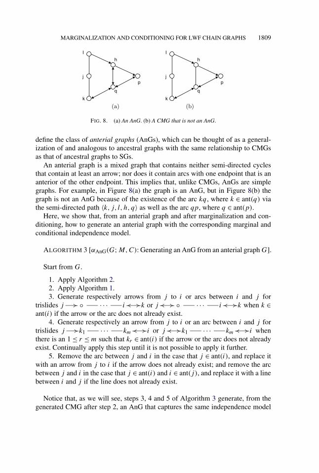
FIG. 8. (a) An AnG. (b) A CMG that is not an AnG.

define the class of anterial graphs (AnGs), which can be thought of as a general-ization of and analogous to ancestral graphs with the same relationship to CMGsas that of ancestral graphs to SGs.

An anterial graph is a mixed graph that contains neither semi-directed cyclesthat contain at least an arrow; nor does it contain arcs with one endpoint that is ananterior of the other endpoint. This implies that, unlike CMGs, AnGs are simplegraphs. For example, in Figure 8(a) the graph is an AnG, but in Figure 8(b) thegraph is not an AnG because of the existence of the arc kq , where k ∈ ant(q) viathe semi-directed path 〈k, j, l, h, q〉 as well as the arc qp, where q ∈ ant(p).

Here, we show that, from an anterial graph and after marginalization and con-ditioning, how to generate an anterial graph with the corresponding marginal andconditional independence model.

ALGORITHM 3 [αAnG(G;M,C): Generating an AnG from an anterial graph G].

Start from G.

1. Apply Algorithm 2.2. Apply Algorithm 1.3. Generate respectively arrows from j to i or arcs between i and j for

trislides j � ◦ · · · i≺ �k or j ≺ � ◦ · · · i≺ �k when k ∈ant(i) if the arrow or the arc does not already exist.

4. Generate respectively an arrow from j to i or an arc between i and j fortrislides j �k1 · · · km≺ �i or j ≺ �k1 · · · km≺ �i whenthere is an 1 ≤ r ≤ m such that kr ∈ ant(i) if the arrow or the arc does not alreadyexist. Continually apply this step until it is not possible to apply it further.

5. Remove the arc between j and i in the case that j ∈ ant(i), and replace itwith an arrow from j to i if the arrow does not already exist; and remove the arcbetween j and i in the case that j ∈ ant(i) and i ∈ ant(j), and replace it with a linebetween i and j if the line does not already exist.

Notice that, as we will see, steps 3, 4 and 5 of Algorithm 3 generate, from thegenerated CMG after step 2, an AnG that captures the same independence model

1810 K. SADEGHI

FIG. 9. (a) A chain mixed graph G. (b) The graph after applying step 3 of Algorithm 3. (c) Thegraph after applying step 4. (d) The generated AnG after applying step 5.

as that of the CMG. In addition, in step 4, one kr being in ant(i) implies that all kr ,1 ≤ r ≤ m, are in ant(i), and in this sense we can say that a section is in ant(i).

This algorithm is a generalization of the related algorithm for ancestral graphs[18, 19]. Again, one can see that sections here are treated in the same way as nodesin the ancestral-graph-generating algorithms. The idea here is that step 4 generatesa direct dependency between j and i (in fact the dependency already exists) beforestep 5 makes the graph anterial.

Figure 9 illustrates how to apply these steps to a CMG. We consider Algorithm 3a function denoted by αAnG. Notice that for every anterial graph G, it holds thatαAnG(G;∅,∅) = G. We again follow a parallel theory as that in the previoussections.

PROPOSITION 8. Graphs generated by Algorithm 3 are AnGs.

We first provide two lemmas that deal with the global behavior of the algorithm.

LEMMA 9. Let H be a chain mixed graph. It holds that i ∈ ant(j) in H if andonly if i ∈ ant(j) in the anterial graph generated after applying steps 3, 4 and 5 ofAlgorithm 3 to H .

Denote by a walk between i and j on which all sections are collider and everyinner section is in ant(i) a subprimitive inducing walk from j to i. This is a specialcase of a generalization of primitive inducing paths, defined in [18], where allnodes are anteriors of one of the endpoints, not either of the endpoints. We alsodenote the function corresponding to steps 3, 4 and 5 of Algorithm 3 by αCMG.AnG.Notice that αAnG(G;M,C) = αCMG.AnG(αCMG(G;M,C)).

LEMMA 10. Let H be a chain mixed graph. There is an edge between i andj in αCMG.AnG(H) if and only if there is a sub-primitive inducing walk from j to i

MARGINALIZATION AND CONDITIONING FOR LWF CHAIN GRAPHS 1811

in H (which might also contain i as an inner node) with single-element endpointsections. In addition, the edge and the walk are endpoint-identical except wheni ∈ ant(j) or j ∈ ant(i) in H , in which case there is no arrowhead at i or at j ,respectively, on the ij edge in αCMG.AnG(H).

We now prove that Algorithm 3 does not need to be applied to an anterial graph,but it can be applied to a chain mixed graph.

LEMMA 11. Let H be a chain mixed graph and M and C be two subsets ofits node set. It holds that αAnG(αCMG.AnG(H);M,C) = αAnG(H ;M,C).

THEOREM 7. For an anterial graph G and disjoint subsets M , M1, C and C1of its node set,

αAnG(αAnG(G;M,C);M1,C1

) = αAnG(G;M ∪ M1,C ∪ C1),

if the two graphs are maximal.

PROOF. Using Theorem 5 and Lemma 11, we have the following:

αAnG(αAnG(G;M,C);M1,C1

) = αAnG(αCMG.AnG

(αCMG(G;M,C)

);M1,C1)

= αAnG(αCMG(G;M,C);M1,C1

)

= αCMG.AnG(αCMG

(αCMG(G;M,C);M1,C1

))

= αCMG.AnG(αCMG(G;M ∪ M1,C ∪ C1)

)

= αAnG(G;M ∪ M1,C ∪ C1). �

Denote the set of all AnGs by ANG.

PROPOSITION 9. Let K be the subset of ANG with the following properties:

1. There is no collider trislide of form k≺ �i · · · j ≺ l unlessthere is an arrow from l to i.

2. There is no collider trislide of form k≺ �i · · · j ≺ �l unlessthere are jk and il arcs and an ij line.

Then αAnG maps CG and two subsets of the node set of its members surjectivelyonto K.

THEOREM 8. For an anterial graph G and disjoint subsets A, B , M , C andC1 of its node set,

〈A,B |C1〉 ∈ Jc

(αAnG(G;M,C)

) ⇐⇒ 〈A,B |C ∪ C1〉 ∈ Jc(G).

COROLLARY 4. The class of anterial graphs, ANG, with c-separation crite-rion is stable under marginalization and conditioning.

1812 K. SADEGHI

7. Probabilistic independence models for CMGs and AnGs and compar-ison to other types of graphs. The most interesting independence models areinduced by probability distributions. Consider a set V and a collection of randomvariables (Xα)α∈V with joint density fV . By letting XA = (Xv)v∈A for each subsetA of V , we then use the short notation A ⊥⊥ B |C for XA ⊥⊥ XB |XC and disjointsubsets A, B and C of V .

For a given independence model J , a probability distribution P is called faith-ful with respect to J if, for random vectors XA, XB and XC with probabilitydistribution P ,

A ⊥⊥ B |C if and only if 〈A,B |C〉 ∈ J .

We say that J is probabilistic if there is a distribution P that is faithful to J .From a given collection of random variables (Xα)α∈V with a probability distri-

bution P , one can induce an independence model J (P ) by demanding

if A ⊥⊥ B |C then 〈A,B |C〉 ∈ J (P ).

Notice that J (P ) is obviously probabilistic.For a chain graph G, we say that a probability distribution with density f fac-

torizes with respect to G if

f (x) = ∏

τ∈Tf (xτ |xpa(τ )),

where T is the set of chain components of G; and

f (xτ |xpa(τ )) = ∏

a

φa(x),

where a varies over all subsets of τ ∪ pa(τ ) that are complete in the moral graphof the subgraph of G induced by τ ∪ pa(τ ), and φa(x) is a function that dependson x through xa only; see [9] for more discussion.

Now let α(P ;M,C) be the probability distribution obtained by usual proba-bilistic marginalization and conditioning for the probability distribution P . It iseasy to show that if P is faithful to J then α(P ;M,C) is faithful to the marginaland conditional independence model α(J ;M,C); see Theorem 7.1 and Corol-lary 7.3 of [18].

It is also known that if G is a CG then there is a regular Gaussian distributionthat is faithful to it. In fact, almost all the regular Gaussian distributions that factor-ize with respect to a CG are faithful to it; see [15]. In other words, the independencemode Jc(G) is probabilistic.

By Propositions 2, 7 and 9, a considerably large subclass of CMGs or AnGsare obtained by chain graphs after marginalization and conditioning. Hence, it isimplied by the discussion above that for a graph H in these subclasses, Jc(H) isprobabilistic; that is, there is a distribution (in fact at least a Gaussian distribution)that is faithful to it.

MARGINALIZATION AND CONDITIONING FOR LWF CHAIN GRAPHS 1813

One can obtain the same result for the strictly positive discrete probability dis-tributions since there is such a distribution that is faithful to a given CG [24]. Theseresults motivate the use of CMGs and AnGs.

The next, and probably more important, question in order to justify the useof these classes is whether it is possible to find a parametrization, for example,Gaussian or discrete, of these graphs.

In the Gaussian case, there exists a known parametrization for the regular Gaus-sian distributions that factorize with respect to a CG; see [28] and [15] for twoslightly different but equivalent parametrizations. For maximal ancestral graphs(MAGs), there is a known Gaussian parametrization [18]. We believe that it is pos-sible to extend this parametrization to the class of maximal AnGs. Here is somepossible actions in order to generalize this parametrization.

Notice first that the classes of CMGs and AnGs are not maximal, as explainedin Section 5.2. However, as mentioned before, there is a method to generate, fromnon-maximal CMGs and AnGs, maximal CMGs and AnGs that induce the sameindependence models. Hence, one can then focus on the class of maximal AnGs.

Considering the Gaussian parametrization for MAGs, one then needs to define,instead of one matrix for the undirected part of the MAG, one symmetric matrixfor every chain component of the maximal AnG (as it is done in the Gaussianparametrization for CGs). It is also needed to generalize the ordering associatedto MAGs, for example, by defining an ordering for chain components contain-ing lines instead of an ordering for the nodes. One may then follow the methoddescribed in Section 8 of the mentioned paper.

Since both parametrizations for CGs and MAGs are curved exponential fami-lies, and consequently the models associated with them are identifiable, the gener-alization for AnGs seems to preserve this desirable property.

Introducing a discrete parametrization for CMGs or AnGs seems much trickier.Similar to the Gaussian case, the goal should be to find a combination of discreteparametrizations for CGs (see, e.g., [14]) and summary graphs (or alternativelyADMGs—see [4]). For CMGs, a parametrization may be derived from the originalCG with the use of structural equation models with latent variables. This can beconsidered a generalization of the method utilized in summary graph models.

Nonetheless, we again stress the importance of introducing different smoothparametrizations for CMGs and AnGs in a future work as well as studying addi-tional non-independence constraints that arise in such models.

Besides the relevant parametrizations, it is clear that CMGs act similarly tosummary graphs in the problem of marginalization and conditioning for DAGs,and AnGs act similarly to ancestral graphs. To give a more detailed comparisonbetween CMGs (and AnGs) and summary graphs (and ancestral graphs), we firstnote that the lines in all these graphs have the same meaning. As mentioned before,there are no arrowheads at lines in the latter types, and one can think of sectionswith arrowheads pointing to them in the former types in the same manner as the

1814 K. SADEGHI

nodes in the latter types. Indeed summary graphs and ancestral graphs are sub-classes of CMGs and AnGs, respectively, thus every summary or ancestral graphmodel is a CMG or AnG model.

In addition, in CMGs, for a collider trislide of from i �j l≺ k, it holdsthat i �⊥ cl, i �⊥ cl | j , but i ⊥ cl | {j, k}. However, there is no summary graph thatcan capture the same independencies and dependencies. Hence, for any inducedpath with 4 nodes (and, of course, for longer paths), one can provide a CMG thatis associated to a different model than summary graph models. By this, it is clearthat the class of CMG models is rich in the sense that when the number of nodesgrows, the number of distinct CMG models grows faster than the number of dis-tinct summary graph models.

The class of marginal AMP chain graphs (MAMP CGs) deals with a similarproblem of marginalization for AMP chain graphs. The lines in these graphs have adifferent meaning in independence interpretation (they are related to lines in AMPCGs), and naturally the class of models they represent is quite different. However,both classes of models contain the class of regression graph models [27], whichitself contains the classes of undirected (concentration) graph models and the classof multivariate regression chain graph models as a subclass. In fact, if in a CMG,there is a section with non-adjacent endpoints that is larger than a single node thenit can be seen that no MAMP CG can induce the same independence statements.This implies that, in the intersection of CMG and MAMP CG models, there isno arrowhead pointing to lines (in CMG sense). Therefore, this intersection is thesame as the intersection of maximal ancestral graph and MAMP CG models (sinceMAMP CGs are maximal, and maximal summary and ancestral graphs induce thesame independence model).

Acknowledgements. The author is grateful to Steffen Lauritzen and ThomasRichardson for helpful discussions, Nanny Wermuth for helpful discussions andcomments and anonymous referees for the most helpful comments, especially de-tecting an error in the results.

SUPPLEMENTARY MATERIAL

Proofs (DOI: 10.1214/16-AOS1451SUPP; .pdf). We provide proofs of non-trivial lemmas, propositions and theorems in the paper as well as some more tech-nical and yet less informative lemmas that are used in the proofs.

REFERENCES

[1] ANDERSSON, S. A., MADIGAN, D. and PERLMAN, M. D. (2001). Alternative Markov prop-erties for chain graphs. Scand. J. Statist. 28 33–85. MR1844349

[2] COX, D. R. and WERMUTH, N. (1993). Linear dependencies represented by chain graphs.Statist. Sci. 8 204–218, 247–283. With comments and a rejoinder by the authors.MR1243593

MARGINALIZATION AND CONDITIONING FOR LWF CHAIN GRAPHS 1815

[3] DRTON, M. (2009). Discrete chain graph models. Bernoulli 15 736–753. MR2555197[4] EVANS, R. J. and RICHARDSON, T. S. (2014). Markovian acyclic directed mixed graphs for

discrete data. Ann. Statist. 42 1452–1482. MR3262457[5] FRYDENBERG, M. (1990). The chain graph Markov property. Scand. J. Statist. 17 333–353.

MR1096723[6] GEIGER, D., HECKERMAN, D., KING, H. and MEEK, C. (2001). Stratified exponential fami-

lies: Graphical models and model selection. Ann. Statist. 29 505–529. MR1863967[7] KIIVERI, H., SPEED, T. P. and CARLIN, J. B. (1984). Recursive causal models. J. Austral.

Math. Soc. Ser. A 36 30–52. MR0719999[8] KOSTER, J. T. A. (2002). Marginalizing and conditioning in graphical models. Bernoulli 8

817–840. MR1963663[9] LAURITZEN, S. L. (1996). Graphical Models. Oxford Statistical Science Series 17. The Claren-

don Press, Oxford. MR1419991[10] LAURITZEN, S. L. and SPIEGELHALTER, D. J. (1988). Local computations with probabilities

on graphical structures and their application to expert systems. J. Roy. Statist. Soc. Ser. B50 157–224. MR0964177

[11] LAURITZEN, S. L. and WERMUTH, N. (1989). Graphical models for associations betweenvariables, some of which are qualitative and some quantitative. Ann. Statist. 17 31–57.MR0981437

[12] MARCHETTI, G. M. and LUPPARELLI, M. (2011). Chain graph models of multivariate regres-sion type for categorical data. Bernoulli 17 827–844. MR2817607

[13] PEARL, J. (2009). Causality: Models, Reasoning, and Inference, 2nd ed. Cambridge Univ.Press, New York. MR2548166

[14] PEÑA, J. M. (2009). Faithfulness in chain graphs: The discrete case. Internat. J. Approx. Rea-son. 50 1306–1313. MR2556122

[15] PEÑA, J. M. (2011). Faithfulness in chain graphs: The Gaussian case. In Proceedings of the14th International Conference on Artificial Intelligence and Statistics (AISTATS 2011) 15588–599. JMLR.org.

[16] PEÑA, J. M. (2014). Marginal AMP chain graphs. Internat. J. Approx. Reason. 55 1185–1206.MR3197803

[17] RICHARDSON, T. (2003). Markov properties for acyclic directed mixed graphs. Scand. J. Stat.30 145–157. MR1963898

[18] RICHARDSON, T. and SPIRTES, P. (2002). Ancestral graph Markov models. Ann. Statist. 30962–1030. MR1926166

[19] SADEGHI, K. (2013). Stable mixed graphs. Bernoulli 19 2330–2358. MR3160556[20] SADEGHI, K. (2016). Supplement to “Marginalization and conditioning for LWF chain

graphs”. DOI:10.1214/16-AOS1451SUPP.[21] SHPITSER, I. and PEARL, J. (2008). Dormant independence. In Proceedings of the Twenty-

Third AAAI Conference on Artificial Inteligence 1081–1087. AAAI Press, Menlo Park.[22] STUDENY, M. (1998). Bayesian networks from the point of view of chain graphs. In UAI 496–

503. Morgan Kaufmann, San Francisco, CA.[23] STUDENÝ, M. (2005). Probabilistic Conditional Independence Structures. Springer, London.

MR3183760[24] STUDENÝ, M. and BOUCKAERT, R. R. (1998). On chain graph models for description of

conditional independence structures. Ann. Statist. 26 1434–1495. MR1647685[25] VERMA, T. and PEARL, J. (1990). Equivalence and synthesis of causal models. In Proceed-

ings of the Sixth Conference on Uncertainty in Artificial Intelligence (UAI-90) 220–227.Elsevier, New York.

[26] WERMUTH, N. (2011). Probability distributions with summary graph structure. Bernoulli 17845–879. MR2817608

1816 K. SADEGHI

[27] WERMUTH, N. and SADEGHI, K. (2012). Sequences of regressions and their independences.TEST 21 215–252. MR2935353

[28] WERMUTH, N., WIEDENBECK, M. and COX, D. R. (2006). Partial inversion for linear sys-tems and partial closure of independence graphs. BIT 46 883–901. MR2285213

STATISTICAL LABORATORY

CENTRE FOR MATHEMATICAL STUDIES

WILBERFORCE ROAD

CAMBRIDGE, CB3 0WBUNITED KINGDOM

E-MAIL: k.sadeghi@statslab.cam.ac.uk