INDIAN INSTITUTE OF MANAGEMENT CALCUTTA

WORKING PAPER SERIES

WPS No. 670/ March 2011

An improved mathematical programming formulation for multi-attribute choice behavior

by

Soumojit Kumar Doctoral student, IIM Calcutta, Joka, Diamond Harbour Road, Kolkata 700104

&

Ashis Kumar Chatterjee Professor, Indian Institute of Management Calcutta, Joka, Kolkata 700104

An improved mathematical programming formulation for multi-attribute choice behavior

Soumojit Kumar

Doctoral Student, Operations Management

Indian Institute of Management Calcutta

Mobile: 9432215758

Email Id: soumojitk08@iimcal.ac.in

Ashis Kumar Chatterjee

Professor, Operations Management

Indian Institute of Management Calcutta

Email Id: ac@iimcal.ac.in

Abstract: Conjoint Analysis and Mathematical Programming approaches have been used

extensively in the past for modelling multi-attribute choice behavior. The Mathematical

Programming approaches are more versatile in their ability to capture complex behavior but

have been limited to dealing with objective attributes. Conjoint Anlysis, though limited by the

additive utility assumption, allows for both subjective and objective attributes. In the present

article, we modify the existing mathematical models to account for situations where the decision

maker may base her decisions on only a subset of the attributes. Identification of non-value

added attributes may be helpful in reducing wastage of resources. Further, we enrich the scope

of the model by accomodating both subjective and objective attributes. A limitation of the earlier

mathematical programming approaches has been the use of interval scale data implying the gap

between any two consecutive levels of an attribute are same. In the proposed model we remove

this drawback using ordinal scaled data for objective attributes. The resulting MIP problem has

been solved using the data provided by Green and Wind (1975) in the context of a Conjoint

Analysis study. A comparison of the results of the proposed model and Conjoint analysis is also

been provided.

With the shift from mass production to mass customization, there has been an ever

increasing demand for variety products from the consumers. Variety is typically manifested in

terms of different attributes or features in a product. Each attribute in its turn, may be built-in in

the product at different levels, giving rise to an increased choice for the customer. The consumer

inherently attaches some values/utilities to different levels of different attributes and hence

comes out with her final choice of the product that gives her the maximum value.

Various mathematical models have been developed for determining the “utilities” of

different attributes, or the weightages the consumer assigns in deciding on the product. In

Conjoint Analysis (CA) developed by Luce and Tuckey (1964) , product profiles are first created

whereby each product is represented by a presence of levels of different attributes. A ranking of

the product profiles are then obtained from the consumer. Finally, linear regression technique is

applied to determine the part-utilities of the attribute levels. For an extensive survey on CA one

can refer to Green and Wind (2001). Besides CA, mathematical programming models have been

developed by various authors (Srinivasan and Shocker 1973, Pekelman and Sen 1974, Mustafi

and Xavier 1985, Mustafi and Chatterjee 1989) with a view to determine the weightages placed

by the consumer, based on his ranking of different product profiles. The major assumption of

product utility as an additive function of utilities of all attributes were common in both CA and

the later models. This assumption is based on summative rule as a special type of compensatory

model suggested by Churchman and Ackoff (1954), Rosenberg (1956) and Fishbein (1967).

Green and Wind (1973) indicated the possibility of a combination of compensatory and non-

compensatory rules for explaining the multi-attribute choice behavior, which they termed as

Phased Models. The work by Mustafi and Xavier (1985) is an example of Phased Model where

they have provided for rejection of alternatives based on threshold values of the underlying

attributes.

A major limitation of the mathematical programming models is that they consider only objective

attributes, while CA acccomodates both objective and subjective attributes. Further, unlike CA

which allows for both ordinal and nominal scale data, mathematical programming models

consider all attributes to be interval scaled. This may have serious implication in the final

solution. CA on the other hand suffers from certain shortcomings like even with moderate

number of attributes, the ranking or rating process for the respondents becomes too heavy

(Malhotra 2009). Further, CA does not provide for application of Threshold concepts in the

context of choice behavior.

In the present article a mathematical programming model for multi-attribute choice behavior

has been developed with a view to remove some of the drawbacks as pointed above. As a starting

point, we have borrowed the way the utility of a product is conceptualised as a summation of

part-utilities as used in Conjoint Analysis. Binary variables have been added later to provide for

other complex behaviour that may arise. Green and Wind(1975) in an earlier study has shown

the application of Conjoint in deciding on the relative worth of the different attributes pertaining

to a “spot remover for carpets and upholstery”. We have used the data of the spot remover

example given by Green and Wind (Pg-108, Harvard Buisness Review, July- August 1975) and

obtained the optimal solution from our mathematical programming model. The result obtained

by Green and Wind (1975) has been compared with the solution obtained from our model. In

developing the model, we have tried to avoid the drawbacks in CA as mentioned in the earlier

paragraphs. We also recognize that while deciding on the product, the decision maker may

consider only a limited number of atributes from a total set of all relevant attributes.

The model with the relevant definitions and notations are presented in Section 2. The resulting

integer programming formulation is solved by ILOG CPLEX 10.2 using the data provided by

Green and Wind (1975). The results are presented in Section 3 followed by a comparison of

Mathematical programming solution and the Conjoint analysis results (Green and Wind 1975) in

Section 4. In the concluding section an attempt has been made to highlight the efficacy and

versatility of the proposed model vis-à-vis the earlier approaches.

FEW RELEVANT DEFINITIONS

Attributes and Attribute levels- Attributes are the value creating entities that make up the

whole product. Attribute levels are the various types of a particular attribute which may be

differentiated by certain performance measures or by decision maker’s preferential tastes. If we

talk about camera quality as an attribute to mobile phones, then two, three or four mega pixels

camera form the different levels of the mobile camera attribute. Considering color as attribute

different colors like red, yellow or blue will form the attribute levels for the attribute color.

Attributes combined together in a particular combination of respective levels define the

whole product or alternative. They can be both subjective and objective. Objective attributes can

be ordered according to their levels and customer preferences i.e. straight away we can say one

attribute level is better to the next level of the same attribute while the others may not be ordered

according to their various levels. Considering motor cycles as a product example, we have price,

horse power, fuel efficiency (km/litre) etc. are the objective attributes. A careful observation will

show that all of these attributes can be ordered in the customers’ preference rating. Lower prices

compared to higher price will always be better for a rational customer. Similarly, more fuel

efficiency, pick-up will be preferred to less of the same attributes. On the other hand looks, color,

brand etc will form subjective attributes and their ordering will be contextual in nature depending

upon the preference pattern of individual customers. One cannot presume that yellow is always

better to red or vice –versa. These type of attributes cannot be ordered according to their levels

and customer preference consistently and vary from consumer to consumer. Their relative order

of preference for a particular customer comes out as a solution from the proposed model.

Subjective attributes levels can only be categorized but cannot be ranked on the

customers’ preferential scale. Hence, subjective attribute levels are nominally scaled. Objective

attributes can be ordered according to the preferences of the customers but it cannot be assured

that the differences between respective attribute levels are equal in preferential scale of the

customers. Thus, objective attribute levels are typically nominally scaled.

Alternatives- Alternatives are the different products in the product line which differ in their

attribute combination. More specifically, an alternative can be defined as a vector of attributes.

Continuing in the same motor-cycle example we can say different models of motor-cycles like

Rajdoot, Bajaj Scooty, Bajaj Pulsar, and Karizzma etc form different alternatives in front of the

customers to make a buying decision.

Part-Utility of the attribute levels- Every attribute level will be associated to a utility level by a

particular customer. These attribute level utilities will contribute to the total alternative/product

utility according to the decision making scheme the customer uses.

Total utility of an alternative- It is the total utility of the product to the customer and is a

function of the part-utility of the attributes. The function may be simple additive or a complex

function of the part-utility of the attribute levels comprising the alternative. The buying decision

of one alternative to the other will be governed by these utility values and more is always

preferred to less.

REVIEW OF RELEVANT MODELS

Model 1 (Srinivasan and Shocker’s method):- The method assumes simple additive rule for

determining the total utility of an alternative and minimizes the total inconsistencies or violations

under forced choice preference to obtain the attribute weights.

Here, 1,2, … , , … . denotes the set of n alternatives on which pairwise preference

judgements are to be made. Each of the alternatives is a vector of m attributes defined under the

set:

1,2, … , , …

Also,

, , … , , … . denotes the jth alternative. Yjp specifies pth attribute for

the jth alternative.

Finally, as specifies earlier under the assumption that each of the m attributes are at least

intervally scaled another set is defined

, , … , , … , which denotes the set of attribute weights for the m

attributes and is the set of decision variables in the model. As the model is assuming simple

additive rule for total utility determination the overall utility of an alternative is given by the

following expression:

∑

Further, another set is defined as

Ω , : : , ] which denotes the set of pairwise preference

judgements such that the alternative j is preferred to k in a forced-choice pair comparison from

the decision maker under scrutiny.

Finally, Srinivasan and Shocker’s model takes the form as under:

Maximize ∑ ,

subject to 0 , Ω (1)

∑ 1, (2)

Constraint (2) is added to preclude the trivial solution 0

Model 2 (Threshold Model and suggested extension):- Threshold Model forsakes the simple

additive rule that was used by Srinivasan and Shocker (1973) to measure the total utility. Here,

another complexity is introduced where a customer will make his/her choice from a subset of

offered alternatives and the selection of an alternative in the set will be on the condition that it

satisfies certain threshold conditions. The customer or the decision maker may not be able to

express the actual threshold conditions and the subset of alternatives he/she actually considering

which is going on in the sub-conscious mind.

Similar to the above model the input sets are defined as above i.e. J, P, Yj, W,Ω are

defined identically as in the previous model. Here another decision variable is incorporated

which is defined as

1, if the jth alternative belongs to the acceptable set of the decision maker.

0, otherwise.

Overall utility of an alternative is defined as

∑

And for linearizing the above expression a new variable is defined and the model is

described as follows:

Minimize ∑ ,

subject to ∑ ∑ 0, , Ω (1)

0, , (2)

1, , (3)

0, , (4)

∑ 1, (5)

∑ (6)

, , 0 (7)

where C is a parameter fixed by the experimenter based on the case of study and the scenario

involved.

An extension to this methodology under the name “Generalized Model of Multi-Attribute

Choice” was suggested by Xavier (1985) in his thesis where he was concerned that a decision

maker may consider only a subset of all the attributes and ignore one or more of the attributes in

making a buy decision. Those attributes which are not considered by him/her is redundant to him

and contribute nothing to the overall utility of the alternative. For modeling this type of behavior

he suggested to define the overall utility value to be:

∑ , .

In this formulation number of binary variables have increased which are now associated with

each of the attributes rather than alternatives as in the former case.

Model 3: Conjoint Analysis: The basic conjoint analysis is represented by the following

formulae (Malhotra 2004)

∑ ∑

where,

Overall utility of an alternative

Part-worth utility associated with the jth level of the ith attribute.

Number of levels of attribute i.

1, if the jth level of the ith attribute is present

0, otherwise.

PROPOSED MODEL

Consider a multi-attribute choice behavior model where a decision maker is faced with a

number of alternatives. An alternative is represented by a number of attributes.The levels of

different attributes present in the alternatives determines its relative worth to the decision maker.

For attribute such as mileage in context of a car, an alternative having a higher level of mileage

is always preferred to an alternative of a lower mileage, everything else remaining same .It may

be noted that this is true for ordinal scale data. For attributes such as color no universal ordering

may be possible as such the levels of such attributes are nominally scaled. In such cases, levels

may be numbered arbitrarily, the inferences from the solutions, however, are to be consistent to

the numbering.

The decision maker is presented with a number of product alternatives, and asked to rank them in

the order of their preference. Each product alternative is represented by a vector of numbers

indicating the levels of the different attributes present in the product. Based on the ranking (or

sometimes pairwise comparison) the part utilities of each of the attribute levels are worked out.

Let, 1,2, … , , … . denotes the set of n alternatives on which preference

judgements are to be made. Now each of the alternatives is described by the m attributes:

1,2, … , , … denotes the complete set of attributes which the alternative set is

composed of. 1,2, … … , denotes the number of levels of the pth attribute.

The utility function essentially should capture the rationale for the choice behavior of the

decision maker. A purely additive model without binary variables would imply compensatory

model where the decision maker inherently allows a tradeoff amongst the different attributes.

Thus, if Uj denotes the total utility of an alternative j and upk denotes the part utility of the kth

level of the pth attribute then Uj is the summation of the all the part-utilities of the all the

underlying attribute levels present in alternative j. This part-utilities would normally have a

positive non-zero value. However, situations may arise where the decision maker decides based

on only a subset of the attributes. This can be taken care of by incorporating binary variables for

each of the attributes. A zero value of a binary variable in the final solution would imply that the

decision maker does not take into account that attribute into consideration at all.

In our model we have put binary variables not only for each attribute but for each attribute level,

which will signify whether a particular attribute level contributes any value to the decision maker

or not. We gain extra flexibility in capturing the decision maker’s choice at the attribute levels by

adding binary variables at every attribute level.

Finally, attributes have been divided into two sets, nominal and ordinal, which can be written as:-

where NP is the set of subjective attributes whose levels are nominally scaled and their

preferences vary from one decision maker to another and OP is the set of attributes whose levels

are ordinal scaled i.e. we can order the levels in a decreasing order of preference of a rational

customer but it may not be possible to know how much exactly one level is better than the other

in utility scales.

With the above assumptions, the utility for an alternative j can be expressed as:

∑ ∑ , where and denotes the levels of p type

and t type attribute are used in the jth alternative , , t OP , j J. (1)

where, = ( ,

= ( , ).

,

Presence of attribute p at level ljp in product alternative j has an associated part utility for the

decsiion maker which is denoted as . This may be considered as the analysts’ meta

perspective of the utility of the decision maker. As such we assume u(ljp) is some positive non-

zero number. While deciding on a particular alternative, the decision maker may for some reason

ignore the presence or absence of a particular attribute at any level. In such a case, the part-

utility= or allows for the utility to take a value of zero as well. This part-utility

would represent the decision maker’s “direct” perspective.

utility of the k th level of the p th attribute ,

1, if the decision maker puts k th level of the p th attribute in the decision making set

0, otherwise ,

1, if the oth attribute level of tth objective attribute in the decision making set .

0, otherwise. ,

Proceeding in a way similar to that of Srinivasan and Shocker (1973), we formulate the model as

minimization of “inconsistency”.The departure from Srinivasan and Shocker model in terms of

the decision variables and the data requirement may be noted. For the ordinal attribute levels a

constraint which forces the monotonicity of the preferences of the higher level objective

attributes has also been added.

We define all the pairwise set of the alternatives as

Ω , : : , ] which denotes set of pairwise preference judgements such

that the alternative j is preferred to k in a forced-choice pair comparison from the customer.

Given Uj and Uk are the utilities corresponding to j th and kth alternatives respectively where j is

preferred over k, Uj>Uk implies Uj-Uk =Wjk-Zjk where Zjk , Wjk >0 and are respectively

inconsistency and consistency.

Minimize ∑ ,

subject to 0 for all (j,k) Ω (2)

Let us suppose for all ,

Hence, if 1

0, otherwise, for all ,

To linearize the above non-linearity, we use the transformation used in Threshold Model

(Mustafi and Xavier 1985) which is:-

1 for all k ,

(3)

Similarly we define for all o , t OP and linearize it by the same procedure

which is:-

1 for all ,

(4)

To avoid the obvious solution of all u’s to be zero we add another constraint which is

∑ 1, (5)

For any attribute given a number of levels ordered low to high, the part-utility of the higher level

is always assumed to be higher than the part-utility of the lower level. Hence, the following

constraint

for all s>m: s,m , (6)

To prevent all the binary variables turning out zero, the following constraint is added

∑ for all (7)

∑ for all t OP (8)

The values of cp and ct are chosen judiciously.

Finally, for any level of feature or attribute there is always a positive utility implying the part-

utilities values ufg ‘s are all strictly positive.

€ 1 for all g , (9)

where € is a small finite number to restrain the part-utilities to take a value of zero. It also

signifies that for a particular attribute level to assume significance it must cross the minimum €

value of part-utility to the decision maker.

AN EXAMPLE

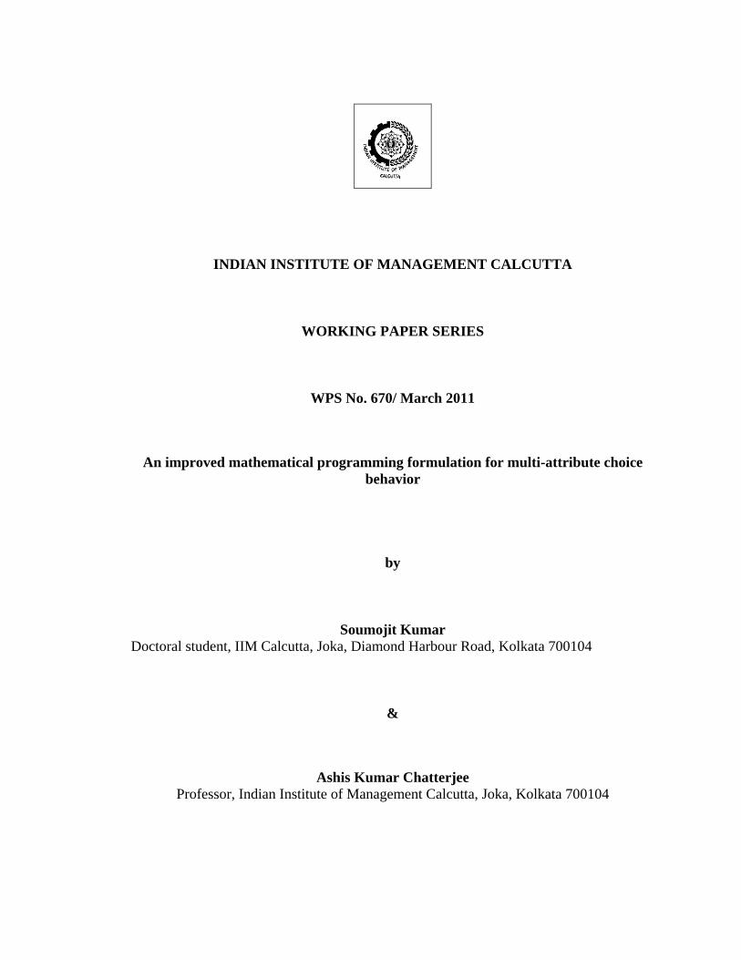
The data pertaining to the “carpet cleaner” example presented by Green and Wind (1975)

have been used to solve our model. The data on the five attributes and their corresponding levels

are reproduced in Table 1 below. Among the attributes, package design and Brand Names are

subjective attributes and are scaled nominally whereas other attributes like Prices, Good

Housekeeping seal and Money back Guarantee are objective attributes whose levels are ordinal

scaled. For objective attributes the levels are arranged in descending order of preference.

Attribute levels

Package

Design

Brand

Names

Prices Good

Housekeeping

seal

Money Back

Guarantee

1 A K2R $1.19 Yes Yes

2 B Glory 1.39 No No

3 C Biessell 1.59 - -

Table 1: Attributes and possible attribute levels for a carpet cleaner as used by Green(1975)

Alternatives Package

Design

Brand Name Price Good

Housekeeping

Seal

Money-back

Guaranteee

Respondent’s

Evaluation

(rank

number)

1 A K2R $1.19 No No 13

2 A Glory 1.39 No Yes 11

3 A Bissell 1.59 Yes No 17

4 B K2R 1.39 Yes Yes 2

5 B Glory 1.59 No No 14

6 B Bissell 1.19 No No 3

7 C K2R 1.59 No Yes 12

8 C Glory 1.19 Yes No 7

9 C Bissell 1.39 No No 9

10 A K2R 1.59 Yes No 18

11 A Glory 1.19 No Yes 8

12 A Bissell 1.39 No No 15

13 B K2R 1.19 No No 4

14 B Glory 1.39 Yes No 6

15 B Bissell 1.59 No Yes 5

16 C K2R 1.39 No No 10

17 C Glory 1.59 No No 16

18 C Bissell 1.19 Yes Yes 1

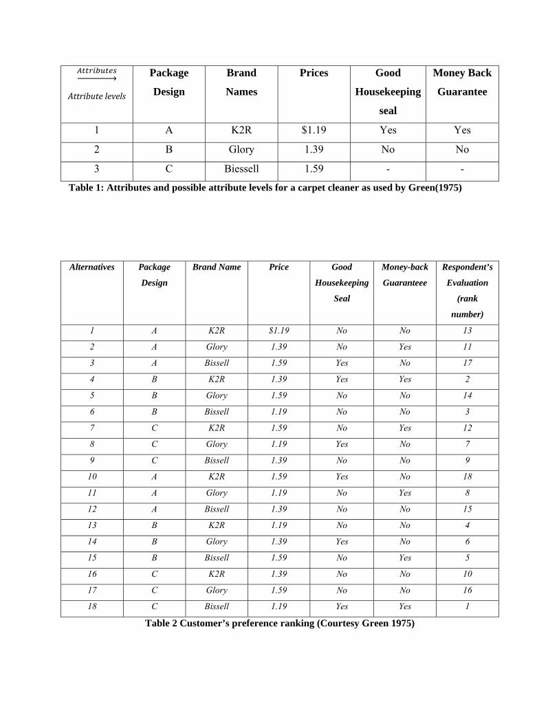
Table 2 Customer’s preference ranking (Courtesy Green 1975)

Green and Wind (1975) selected 18 alternatives by using orthogonal array design and they

obtained the preference rank of the same from the decision maker. The data on the alternatives

together with the decision makers’ prefernce ranking is reproduced in Table 2 above. Conjoint

analysis was applied by Green and Wind to find out the part utility of the attribute levels and

finally the relative importance of the attributes.

For applying the above data to our model the preference rankings were first transformed into

pairwise comparisons of the alternatives. The resulting MIP formulation has 13 binary decision

variables, 13 continuous decision variables and 244 constraints. ILOG CPLEX 10.2 and a

standard PC was used to solve the mathematical program.The solution is presented below:

Optimal Objective Function Value = 0.000000,Solution Time= 0.05 secs, Iterations = 64

SL. No.

Attributes Attribute Levels

Binary Variables( or

Continuous part‐utilities ( or

Direct part utilities of the attribute

levels ( or

Part‐utilities from

Conjoint Analysis

1 Package Design A 0 0.002 0.00 -4.16667 B 1 0.009284 0.009284 3.83333 C 1 0.005642 0.005642 0.33333

2 Brand Names K2R 1 0.002 0.002 -0.83333 Glory 0 0.002 0.00 -0.33333 Biessell 1 0.003642 0.003642 1.166667

3 Prices $1.19 1 0.007284 0.007284 3.5 $ 1.39 1 0.003642 0.003642 0.666667 $1.59 0 0.002 0.00 -4.16667

4 Good Housekeeping Seal

No 0 0.002 0.00 0.75 Yes 0 0.002 0.00 -0.75

5 Money Back Guarantee

No 0 0.002 0.00 -2.25 Yes 1 0.005642 0.005642 2.25

Table 3: Part-utilities of the attribute levels as solved by the mathematical model

SL. No.

Utilities of the alternatives Utilities from Proposed model Utilities from Conjoint Analysis

1 0.009284 ‐4

2 0.009284 ‐2.83333

3 0.003642 ‐8.66667

4 0.020568 7.16667

5 0.009284 ‐4.16667

6 0.020210 5.5

7 0.009284 ‐2.66667

8 0.012926 1.5

9 0.012926 ‐0.83333

10 0.002000 ‐10.1667

11 0.012926 0

12 0.007284 ‐5.33333

13 0.018568 4

14 0.012926 2.166667

15 0.012926 2.33333

16 0.011284 ‐2.33333

17 0.005642 ‐7.66667

18 0.022210 8

Table 4: Total Utilities of the chosen alternatives under experiment.

The problem was also solved using Conjoint Analysis. The final results on relative importance

conformed with the results obtained by Green and Wind (1975).

Comparison of results of Proposed Model and Conjoint Analysis

The major objective of developing multi-attribute choice behavior models is to determine the

decision maker’s preference for different attributes while buying a product. The preference

pattern reflected in the relative importance for each of the attributes may be taken as a basis of

comparison for the proposed model and the Conjoint Analysis approach. The results from the

alternative approaches are presented in Table 5 and the graph 1 below.

Attributes Relative importance under

Proposed Model

Relative Importance under

Conjoint Analysis

Package design 0.359121 0.338028

Brand Name 0.140879 0.084507

Price 0.281758 0.323944

Good House Keeping Seal 0 0.06338

Money back guarantee 0.218242 0.190141

Table 5: Relative Importance of the Attributes under Proposed Model and Conjoint

Contribution of the Present Study

Table 5 shows that the major difference in the results is with respect to the attribute “Good

House Keeping Seal”. The proposed model has assigned a relative importance of zero to this

particular attribute, implying that it does not add any value to the decision maker. One may

verify that the part-utilities are still positive and the corressponding binary variables have turned

out to be zero.(as shown in Table 3, Sl.No. 4). These insights are particularly helpful for a

manger because the resources wasted to procure that attributes can easily be shifted to other

value adding activities.

Graph 1 : Comparison on the relative importances of the attributes by Conjoint and Proposed

Model.

Apart from determining the preference pattern of the decision maker, the other major objective is

to utilize the part utilities corresponding to each level of different attributes for deciding on

optimal product line. The results for continous part-utilities for both the methods are given in

Table 3. The ordering of the levels based on their corresponding part-utility values for any

attribute remains the same for that attribute for both the methods. For example, price has three

levels as: (L1)$1,19, (L2)$1.39, (L3)$1.59. Ordering the levels based on their part utility values

(0.007284, 0.003642, 0) obtained through our proposed model we have L1, L2 and L3 as

descending order of preference.The ordering done based on corresponding values obtained on

0

0.05

0.1

0.15

0.2

0.25

0.3

0.35

0.4

Package Design

Brand Name Price Good Housekeeping

Seal

Money Back Guarantee

Conjoint Analysis

Proposed Model Analysis

Conjoint (3.5, 0.666667,-4.16667) yields the same ordering. This goes to reinforce the logical

consistency of the two approaches.

Finally from the results of the proposed model on “Package Design” shows clearly that the

different levels presented in descending order is given by B, C, A. The difference in utilities

between the different levels B and C, and C and A are unequal. Earlier mathematical

programming approaches have assumed interval scaled data and as such such differences would

have come out to be equal. There is no basis for such an assumption in the decision making

scenario under consideration. Ordinal scale data, which has been used in such a case, is the

realistic representation for objective attributes.

CONCLUDING REMARKS

In the present article, we have developed a mathematical programmming model for

multi-attribute choice behavior. While developing the model, an attempt has been made to

remove the drawbacks and incorporate the advantages pertaining to Conjoint analysis and

existing mathematical models. The resulting model allows for both subjective and objective

attributes and provides for situations where the decision maker may base her decisions on only

a subset of the attributes. The earlier mathematical models are based on objective attributes

entailing assumption of interval scaled data. Such assumption are limiting in nature. In the

proposed model, nominal and ordinal scaled data have been used for subjective and objective

attributes respectively. The data from earlier study on Conjoint Analysis have been used to run

the model. A comparison is also been provided to highlight the advantages of the proposed

model in modelling complex behavior.

References

Coombs, C.H. 1964. A Theory of Data. New York: Wiley

Churchman, C.W. and R.L. Ackoff. 1954. An approximate measure of Value. Operations Research. 2 172‐

181.

Day, G.S. 1972. Evaluating models of attitude structure. Journal of Marketing Research 9 279‐286.

Fenwick, I. 1978. A user’s guide to conjoint measurement in marketing. European Journal of Marketing

12 203‐211.

Fishbein, M. 1967. A Behavioural Theory Approach to Relations Between Beliefs about object and the

attitude toward the Object, in Fishbein, M. ed., Readings in Attitude Theory and measurement, New

York: Wiley 389‐399.

Green, P.E. 1974. On the Design of Experiments Involving Multiattribute Alternatives, Journal of

Consumer Research. September 1974. 61‐68

Green, P.E., A.B. Krieger, Y.Wind 2001. Thirty Years of Conjoint Analysis: Reflections and Prospects,

Interfaces. 31(3) May‐June 2001, 56‐73

Green, P.E., Y. Wind. 1973. Multi‐Attribute Decisions in Marketing‐ A Measurement Approach. Dryden

Press, London

Green, P.E., Y. Wind. 1975. New way to measure customers’ judgements. Harvard Business Review. July‐

August 1975. 107‐117

Luce, R.D., J.W. Tuckey. 1964. Simultaneous conjoint measurement: A new type of fundamental

measurement, Journal of Mathematical Psychology, Vol. 1, 1‐27.

Malhotra, N.K. 2009. Marketing Research: An Applied Orientation. Englewood Cliffs, NJ: Prentice Hall.

Mustafi, C.K., A.K. Chatterjee. 1989. Multi‐attribute choice behavior models‐ A note on two

modifications and extensions. Asia‐Pacific Journal of Operational Research 6 158‐166

Mustafi, C.K. , M.J. Xavier. 1985. Mixed‐Integer Linear‐Programming Formulation of a Multi‐Attribute

Threshold Model of Choice. Journal of Operational Reseach Society. 36(10) 935‐942

Pekelman, D., S.Sen 1974 Mathematical programming models for the determination of attribute

weights, Management Science 20 1217‐1229

Rosenberg, M.J. 1956. Cognitive Structure and Attitudinal Affect, Journal of Abnormal and Social

Psychology 53 367‐372

Srinivasan, V., A.D. Shocker. 1973. Estimating the weights for multiple attributes in a composite criterion

using pairwise judgements. Psychometrika 38 473‐493

Srinivasan, V., A.D. Shocker. 1973. Linear programming techniques for multidimensional analysis of

preference, Psychometrika 38 337‐369

Xavier, M.J. 1985. Mixed Integer Linear Programming Formulation of a Multi‐Attribute Threshold Model

of Choice. IIMC Dissertations (OM Group).1985