Micro-light-emitting diodes with quantum dots ... - CityU Scholars
Upload
khangminh22Category
view
1download
0
MANY-BODY APPROACHES
TO QUANTUM DOTS
by
PATRICK MERLOT
THESIS
for the degree of
MASTER OF SCIENCE
(Master in Computational Physics)
Faculty of Mathematics and Natural Sciences
Department of Physics
University of Oslo
Sept. 2009
Det matematisk-naturvitenskapelige fakultet
Universitetet i Oslo


Acknowledgements
I would like to acknowledge the people who helped me in completing this thesis.From Sigurd for getting me started and his assistance when I was struggling withthe C++ coding as well as with some abstract concepts of quantum mechanics, toLene, Islen, Rune and Johannes for the interesting discussions we had in the o�ce.Also, many thanks to Simen Kvaal for helping me out of some critical questions andfeeding me with a lot of new ideas. Thanks again to Rune and Simen for teaching mehow to use their simulators. Most importantly, thanks to Morten Hjorth-Jensen forhis support all along the master, for providing this interesting topic and also for hisconstant good mood. Finally many thanks to Nolwenn for pushing me and helpingme in any possible ways.
�The underlying physical laws necessary for the mathematical theory of a large part
of physics and the whole of chemistry are thus completely known, and the di�culty
is only that the exact application of these laws leads to equations much too
complicated to be soluble.�
P. A. M. Dirac, 1929
i


Abstract
In this thesis, we studied numerically systems consisting of several interacting elec-trons in two-dimensions, con�ned to small regions between layers of semiconductors.These arti�cially fabricated electron systems are dubbed quantum dots in the lit-erature. Quantum dots provide a new challenge to theoretical calculations of theirproperties using many-body methods. The size of these �arti�cial atoms� is severalorders of magnitude larger than that of atoms, leading to a much greater sensitivityto magnetic �elds. The full many-body problem of quantum dots is truly complexand simulating a quantum dot constrained by a magnetic �eld may be even morecomplicated.
Of particular interest is the reliability of the Hartree-Fock (HF) method for stud-ies of quantum dots in two-dimensions as a function of the external magnetic �eld.In order to achieve this goal, we developed a Hartree-Fock code for electrons trappedin a single harmonic oscillator potential in two-dimensions. We also developed a codeimplementing many-body perturbation theory (MBPT) up to third order either di-rectly applied to the harmonic oscillator basis or as a correction to the Hartree-Fockenergy. A discussion of the results compared with large-scale diagonalisation meth-ods indicated a quadractic error growth of HF and MBPT as the interaction strengthincreases. We tested also the reliability of a single Slater determinant approxima-tion for the ground state of closed shell systems as a function of varying interactionstrength. We found that the Hartree-Fock method, compared with large-scale diago-nalization methods, has a limited range of applicability as function of the interactionstrength and increasing number of eletrons in the dot, indicating a break of the com-putational technique before entering the limit of validity of the closed-shell model.Our study also showed that the HF approximation might become less accurate com-pared to MBPT as the number of electrons in the dot increases.
iii


Contents
1 Introduction 1
2 General presentation 5
2.1 History of Quantum Dots . . . . . . . . . . . . . . . . . . . . . . . . 62.2 Some applications of QD . . . . . . . . . . . . . . . . . . . . . . . . . 82.3 Clari�cations about computational studies . . . . . . . . . . . . . . . 9
3 Physics of Quantum Dots: the arti�cial atoms 11
3.1 Size quantization . . . . . . . . . . . . . . . . . . . . . . . . . . . . . 113.2 Quantum dots made of semiconductors . . . . . . . . . . . . . . . . . 153.3 Optical properties . . . . . . . . . . . . . . . . . . . . . . . . . . . . . 183.4 Electronic properties/Manipulation of quantum dots . . . . . . . . . . 193.5 Quantum dot in a magnetic �eld . . . . . . . . . . . . . . . . . . . . 22
4 Modelling of Quantum Dots 25
4.1 Theoretical approximation of the quantum dot Hamiltonian . . . . . 264.2 General form of H with explicit physical interactions . . . . . . . . . 27
5 Many-body treatment: the Hartree-Fock method 31
5.1 Ab initio many-body techniques . . . . . . . . . . . . . . . . . . . . . 315.2 Time-independent Hartree-Fock (HF) Theory . . . . . . . . . . . . . 325.3 Many-body perturbation corrections (MBPT) . . . . . . . . . . . . . 455.4 Variational Monte-Carlo (VMC) method . . . . . . . . . . . . . . . . 515.5 Full Con�guration Interaction (FCI) method . . . . . . . . . . . . . . 52
6 Implementation 55
6.1 Overview . . . . . . . . . . . . . . . . . . . . . . . . . . . . . . . . . . 556.2 Class implementation . . . . . . . . . . . . . . . . . . . . . . . . . . . 566.3 Running a simulation . . . . . . . . . . . . . . . . . . . . . . . . . . . 61
7 Computational Results and Analysis 65
7.1 Validation of the simulator . . . . . . . . . . . . . . . . . . . . . . . . 657.2 Restrictions to the closed-shell model . . . . . . . . . . . . . . . . . . 697.3 Convergence, stability and accuracy of the Hartree-Fock Algorithm . 807.4 Scaling of the simulator with parallelization . . . . . . . . . . . . . . 867.5 Comparison of ab initio methods applied to quantum dots . . . . . . 87
v

Contents
8 Conclusion 101
Appendices
A Analytical expression of the two-body Coulomb interaction 105
B The method of Lagrange Multipliers 107
C Results of variational Monte-Carlo simulations 111
D ERRATA 113
Bibliography 115
vi

Chapter 1
Introduction
Following their recent successes in describing and predicting properties of materials,electronic structure calculations using numerical computation have become increas-ingly important in the �elds of physics and chemistry over the past decade, especiallywith the development of supercomputers. From the basic constituents of a systemof particles and their interactions, a computational approach enables to derive theelectronic structure and the properties of the system.
A system of particles that is currently considered with attention is the quantumdot: it is an arti�cial system consisting of several interacting electrons con�ned tosmall regions between layers of semiconductors. The whole system can be seen as ananoscopic box of semiconductor with exceptional electrical and optical properties.Applications based on quantum dots are developed in numerous �elds of medicineand modern electronics.
Overview
This thesis describes a computional study of a quantum dot in two dimensions.It presents the methods used in numerical simulations and some many-body tech-niques with various levels of sophistication: Hartree-Fock method (HF), many-bodyperturbation theory (MBPT), variational Monte-Carlo (VMC) and full con�gura-tion interaction (FCI) (e.g. large scale diagonalisation) methods. It focuses on therestricted Hartree-Fock method, one of the fastest and cheapest techniques but alsoone of the less accurate. The aim of the study is to assess the appropriateness of thismethod to study quantum dots in two-dimensions con�ned by a spherical potentialand squeezed by an external magnetic �eld.
Literature review
Similar Hartree-Fock studies were performed by Johnson and Reina in 1992 [25] andPfannkuche in 1993 [46].
Johnson and Reina derived an analytical expression for the exact ground stateand the HF energy of a N-particle quantum dot [25]. They managed to derive it byapproximating the electron interactions with a cut-o� to �rst order of the Coulombinteraction. They found that the HF approximation becomes less accurate with an
1

Chapter 1. Introduction
increasing number of electrons, a decreasing magnetic �eld, an increasing dot sizeand increasing electron-electron interaction strength. Our model which includes thecomplete Coulomb interaction leads to the same conclusion regarding the accuracyof the Hartree-Fock method.
Pfannkuche computed the open-shell Hartree-Fock method and compared the re-sults to exact diagonalization. They also remarked that the usefulness of the Hartree-Fock method would be greatly enhanced if its reliability was properly understood [46].Compared to their study, our closed-shell model implementation cannot give insightson the electronic structure responsible for the inaccuracy of the correlation e�ects,but it gives more information about the convergence of HF.
Waltersson analysed quantum dots using open-shell Hartree-Fock and second-order perturbation theory [60]. Their results are used to validate our own imple-mentation of the second order perturbation correction in the basis of Hartree-Fockorbitals.
Simen Kvaal developed a large-scale diagonalization code [32] for computing theapproximated ground state using the full con�guration interaction method. We usehis results as reference for the �exact� ground state in the analysis of our results. Wealso use his simulator to validate the two-body interaction matrix in the harmonicoscillator basis.
Rune Albrigtsen studied quantum dots using closed-shell variational Monte-Carlo(VMC) method [2]. His simulator is used for few con�gurations to compare theaccuracy against HF and MBPT.
A guide to the reader
This thesis is organized as follows.Chapter 2 gives a general presentation of the quantum dot and of computational
studies.Chapter 3 describes the phenomenological aspects and properties of quantum
dots.Chapter 4 reviews some models for the quantum dot and introduces the theoreti-
cal approximations used in this thesis: the electrons are trapped in a single harmonicoscillator potential and repel each other according to the bare Coulomb interaction.
When it comes to the treatment of the quantum dot model for numerical simu-lation, chapter 5 introduces some possible many-body techniques, and more particu-larly the Hartree-Fock theory. The iterative procedure is reviewed and its descriptionis adapted to our implementation.
Chapter 6 describes our computational implementation of the Hartree-Fock methodin two-dimensions for closed shell systems. We also describe the implementation ofthe many-body perturbation corrections up to third order both as an improvementof the Hartree-Fock energy or as an independent technique.
Results are provided in chapter 7 and compared to large-scale diagonalization. Anumerical analysis provides information on the convergence, on the stability and onthe e�ciency of the Hartree-Fock method and the many-body perturbation theory.We test the reliability of a single Slater determinant approximation for the ground
2

state of closed shell systems as function of the interaction strength (7.2.1). A dis-cussion of the results (7.3) shows that the complexity of the Hartree-Fock methodgrows exponentially with the size of the basis set and that parallelization improvesthe e�ciency almost linearly with respect to the number of processors (7.4). Whencompared to large-scale diagonalisation taken as reference, we observed a quadracticerror growth of HF and MBPT as the interaction strength increases (7.3.1). We �ndthat the Hartree-Fock method, compared with large-scale diagonalization methods,has a limited range of applicability as function of the interaction strength and in-creasing number of electrons in the dot, indicating a breakdown of the validity ofthe ansatz for the ground state wave function used in the Hartree-Fock calculations.In our case this ansatz is based on a single Slater determinant constructed by �llingall single-particle levels below the chosen Fermi surface, the so-called closed-shellapproach. Our study also shows that the HF approximation becomes less accuratecompared to MBPT as the number of electrons in the dot increases (7.5.2). Con-cluding remarks and suggestions for future work are given in the chapter 8.
3


Chapter 2
General presentation
In our current understanding of nanotechnology, quantum dots are the most func-tional and reproducible nanostructures available to researchers. Common shapesinclude pyramids, cylinders, lens shapes, and spheres. Di�erent synthesis routes cre-ate di�erent kinds of quantum dots. They are very small by nature, the smallestobjects that we can synthesize on the nanoscale. From this fact, they are assimilatedto dots, though one quantum dot can be made out of roughly thousands of atoms.All the atoms pool their electrons to "sing with one voice", that is, the electronsare shared and coordinated as if there was only one atomic nucleus setting up anattraction at the centre. That property enables numerous revolutionary schemes forelectronic devices and quantum dots are often referred to as arti�cial atoms.
Depending on its application, the total diameter of a quantum dot varies between2-10 nm, corresponding to 10-50 atoms, to sizes of hundreds of nanometers that cancontain a total of 100− 100, 000 atoms within the quantum dot volume [47], with anequivalent number of electrons. Almost all electrons are tightly bound to the nucleiof these atoms, however the number of �free electrons� in the dot can be very small:between one and a few hundreds [1]. The reason why 'quantum' pre�xes the nameis because the dots exhibit quantum con�nement properties in all three dimensions.This means that electrons within the dot cannot move freely around in any directionleading to quantization as we will show in 3. The only thing that behaves likethis in nature is the atom. Compared to an atom, a quantum dot is at least tentimes bigger and above all tunable. This has a lot of important consequences forresearchers. For example they exhibit quantized energy levels like an atom. For agiven energy of excitation, for instance, a quantum dot will only emit speci�c spectraof light. Quantum theory predicts that if their diameter is decreased there will bea corresponding increase in frequency (e.g. in energy) of the emitted light, and thisproperty is now used in many applications.
This element of control over quantum dots' emission properties has huge impli-cations for both electronic devices and medical applications. Due to their excellentcon�nement properties not seen in nanowires or quantum wells, quantum dots are ex-tremely e�cient at emitting light. They have been the source of some of the world'smost powerful lasers produced to date, though the practicality of a quantum dotlaser is still being improved. In medical studies, quantum dots are already used as
5

Chapter 2. General presentation
tags that can be inserted into patients. These tags can be seen under most medicalscanning technologies and can help pinpoint biological processes as they occur.
2.1 History of Quantum Dots
In the late 50's began the �rst studies of arti�cial quantum systems, mostly theoret-ical due to the lack of funds. In the 60's, the technique of epitaxial depositions wasdeveloped and with it, the possibility to build ultra-clean composite layers of semi-conductor material sandwiched between two other layers of another semiconductor.The �rst optical properties were discovered and the two-dimensional character of thesample was observed. At the beginning of the 80's, rapid progress in technology wasmade with accurate lithography technics (the �rst quasi one-dimensional quantumwire was done based on these advances) [20].
Colloïdal quantum dots were discovered in 1981, during the development of ma-terials for the photo-cleavage of water. Bulk cadmium sul�de (CdS) is known to bean ideal electrode material; however it experiences photocorrosion upon irradiation.It was believed that colloidal particles of cadmium sul�de, coated with a protec-tive agent (i.e. RuO2), would be more resistant to corrosion. Therefore, a synthesismethod was developed to produce colloidal CdS through aqueous precipitation. Theresulting particles displayed unique properties not found in the bulk, including �uo-rescent emission. These properties were determined to be the result of quantum sizee�ects [26], and were found to be tunable by altering the size of the particle [51].This provided a method for selecting excitation and emission wavelengths and par-ticle band gaps.
In the middle of the 80's, the �rst quantum dot based on etching techniqueswas developed [Reed et al.;1986]. As a consequence, a complete quantization of theelectron free motion was possible.
At the end of the 80's and in the 90's, the methods evolved: lithography andetching are still in use, but electron or ion-lithography have replaced light-lithographyresulting in an increased precision [20].
Lent predicted in 1993 the need for building quantum cellular automata (QCA)cells of 2 nm in order to work at room temperature, where quantum cellular automatarefers to any models of quantum computation.
�Ultimately, temperature e�ects are the principal problem to be overcome inphysically realizing the QCA computing paradigm. The critical energy is the energydi�erence between the ground state and the �rst excited state of the array. If this issu�ciently large compared with kBT , the system will be reliably in the ground stateafter a characteristic relaxation time. Fortunately, this energy di�erence increasesquadratically as the cell dimensions shrink. If the cell size could be made a fewÅngstroms, the energy di�erences would be comparable to atomic energy levels (i.e.several electron-Volts!)�.
�As technology advances to smaller and smaller dimensions on the few-nanometerscale, the temperature of operation will be allowed to increase. Perhaps our envi-sioned QCA will �nd its �rst room temperature implementation in molecular elec-
6

2.1. History of Quantum Dots
Figure 2.1: Two coupledatomic quantum dots areshown in this room tem-perature scanning tunnelingmicroscopy image. In thetop frame the dots shareone electron. The elec-tron moves freely betweenthe dots just like an elec-tron in a chemical bondwithin a molecule. The lowerframe demonstrates controlover that single electron andthe potential to do compu-tations in a new way. Theelectric �eld from the con-trol charge pushes the elec-tron to prefer staying on onlyone of the quantum dots.(Image courtesy of Universityof Alberta/Prof. Robert A.Wolkow)
tronics.� [36]
Interest in the use of quantum dots in biomedicine began in 1998. Coupling thequantum dots directly to biorecognition molecules (e.g. antibodies, proteins), theparticles could be targeted to particular parts of the cell, producing a �uorescentindicator [7, 8].
Early this year (Jan. 2009), the four-quantum dot cell dreamed by Lent tobuild his �quantum cellular automata� as a replacement for classical computationusing CMOS technology has been achieved with the fabrication and control of a1 nm-scale assembly of a four coupled silicon dangling bond (In condensed matterphysics, a dangling bond occurs when an atom is missing a neighbour to which itwould be able to bind. Such dangling bonds are defects that disrupt the �ow ofelectrons and that are able to collect the electrons). Indeed single-atom quantumdots make possible a new level of control over individual electrons, a developmentthat suddenly brings quantum dot-based devices within reach [17]. Composed of asingle atom of silicon and measuring less than one nanometre in diameter, these arethe smallest quantum dots ever created. Until now, quantum dots have been useableonly at impractically low temperatures, but the new atom-sized quantum dots workat room temperature. And because they operate at room temperature and existon the familiar silicon crystals used in today's computers, researchers expect thesesingle atom quantum dots to transform theoretical plans into real devices. Figure 2.1shows how atom-sized quantum dots can be manipulated at room temperature. Thesingle-atom quantum dots have also demonstrated another advantage: signi�cantcontrol over individual electrons by using very little energy. This low energy controlis seen as the key to quantum dot application in entirely new forms of silicon-basedelectronic devices, such as ultra low power computers.
7

Chapter 2. General presentation
2.2 Some applications of QD
Exceptional electrical and optical properties make quantum dots attractive compo-nents for integration into electronic devices. One signi�cant asset of quantum dotsover traditional optoelectronic materials is that they exist in the solid state. Solidstend to be more compact, easily cooled, and allow for direct charge injection. Ad-ditionally, quantum dots can interconvert light and electricity in a tunable mannerdependent on crystal size, allowing for easy wavelength selection. This is a signi�cantimprovement over silicon-based materials, which require modi�cation of their chem-ical composition (i.e. doping) to alter optical properties [61]. As a result researchershave experimented with quantum dots in lasers, LEDS, photovoltaics and also fornew generations of transistors, prototypes of spin devices, logic gates with quantumcomputers as the ultimate goal. Most of these applications are still in early devel-opment; however the bene�ts of quantum dot components are evident, and couldlead to a complete revolution of the way of building electronic components at atomicscale.
Another application of quantum dots and one of the fastest moving and most ex-citing interfaces of nanotechnology is the use of (colloïdal) quantum dots in biology.Again their unique optical properties make them appealing as in vitro and in vivo
�uorophores in a variety of biological investigations, in which traditional �uorescentlabels based on organic molecules fall short of providing long-term stability and simul-taneous detection of multiple signals [40]. The ability to make quantum dots watersoluble and target them to speci�c biomolecules has led to promising applicationsin cellular labelling, thus improving diagnostic methods (ex. tracking cancer cells invivo during metastasis [15, 23, 59], as shown in �gure 2.2) and in developing betterdrug delivery systems to improve disease therapy [29]. It is even currently studied asneuroelectronic interface for converting optical energy into electrical signal respond-ing to the need for prosthetic devices that can repair or replace nerve function [64].However there are still many open questions about the toxicity of inorganic QD. Thesize and charge of most nanoparticles preclude their e�cient clearance from the bodyas intact nanoparticles. Without such clearance or their biodegradation into biolog-ically benign components, toxicity is potentially ampli�ed and radiological imagingis hindered. Some neutral organic coatings prevents adsorption of serum proteins(which otherwise increase the total diameter by more than 15nm and prevent renalclearance). A �nal hydrodynamic diameter of less than 5.5nm resulted in rapid ande�cient urinary excretion and elimination of quantum dots from the body [53].
These achievements, even in their premises, have laid the foundations for theo-retical investigations to enable advances in the understanding of the fundamentalstructure, stability and aqueous assembly of nanoparticle architectures. A physi-cal systems consisting of between 10s − 1000s of atoms is already too complex tobe studied otherwise than using numerical methods for a reliable description. Theconcept of arti�cial atom can even be generalized to arti�cial molecules.
Moreover QDs appear as good tools for studying atomic spectra of many-bodysystems on a theoretical point of view using computational techniques. Thanks tothe possibility to build our own arti�cial atoms without considering the complexity
8

2.3. Clari�cations about computational studies
Figure 2.2: Sensitivity and multicolor capability of quantum dot (QD) imaging in live animalscompared to classical organic �uorescent dyes.(a) About a thousand QD-tagged cancers cells (orange,upper) and organic �uorescent dye (green,lower). (b) Simultaneous in vivo imaging of multicolor QD-encoded microbeads. Approximately1-2 millions beads in each color were injected subcutaneously at three adjacent locations on a hostanimal (Image courtesy of X. Gao [15]).
of the nucleus, it becomes simpler to confront numerical and experimental results.
2.3 Clari�cations about computational studies
The usefulness of numerical simulation is more and more recognized and today itis used in many domains of research and development: mechanics, �uid mechanics,solid state physics, astrophysics, nuclear physics, climatology, quantum mechanics,biology, chemistry... More than being limited to scienti�c subjects numerical simu-lation is also used in human sciences (demography, sociology) as well as in �nanceor economy.
In physics, beside the importance for our basic understanding of quantal systems,the capability to develop and study stable numerical quantum mechanical systemswith many degrees of freedom is of great importance, as analytic solutions are rareor impossible to obtain.
Some de�nitions:
A numerical simulation reproduces the fundamental behaviour of a complex sys-tem in order to study its properties and predict its evolution. It is based on theimplementation of theoretical models, i.e. it is an adaptation of mathematical mod-els to numerical tools. Data mining and virtual reality are di�erent from numericalsimulation and should not be mistaken with it.
A numerical simulation is performed in several steps:
The model describes the system analysed by listing its essential parameters andby writing the physical laws that rule its behaviour (and link the parameters) asmathematical equations.
9

Chapter 2. General presentation
The simulation itself is the translation of the equations into computer language,associated with the discretization of the physical domain to make it �nite (select atime step, a �nite number of points, an acceptable level of accuracy, etc).
Computational techniques The resolution of the equations leads to the determina-tion of the numerical values of all the parameters of the system in every points, i.e.the state of the system is known. Various computational techniques can be used tosolve the equations, they can be grouped into two main approaches: the deterministicand the statistical (or probabilistic) methods.
In the �rst approach, an algorithm will solve predictably the equations. For ex-ample the object (or the domain) is discretized and the parameters of each elementare linked to its neighbours through algebraic equations. It is up to the computerto solve the system that links all the equations. A deterministic method will alwaysproduce the same output when given the same input, and the underlying machinewill always go through the same sequence of states (which is why it is called �deter-ministic�). The Hartree-Fock method used in this thesis belongs to this category aswell as the Finite element method or the large scale diagonalisation.
The second approach, which groups the �Monte-Carlo� methods, is particularlysuited to phenomena characterized by a sequence of steps in which each element ofthe object can be a�ected by di�erent �a priori� possible events. From step to step,the evolution of the sample will be determined through a random draw (the name ofthe method comes from this idea).
Validation of the results: the theoretical model and its translation into computerprogramming must be validated by comparing with experimental data, or by testinga very simple case for which an analytical solution can be found.
Numerical simulations, once validated, can explore more cases or unused con-�gurations that were not tested by experiments, sometimes predicting unexpectedbehaviours, leading to a greater knowledge of the physical behaviour of the system.Therefore numerical simulation is the third form of study of phenomena, after theoryand experiment.
10

Chapter 3
Physics of Quantum Dots: the
arti�cial atoms
As described previously, a quantum dot is a semiconductor whose charge-carriersare con�ned in all three spatial dimensions, so much con�ned that quantum e�ectsbecome visible in many ways: �uorescent e�ect, quantized conductance, quantizedenergy spectrum, etc.
The physics behind it involves the electronic structure of the material (here mainlysemiconductors) and some basic quantum mechanical e�ects such as size quantiza-tion, quantum tunneling or Coulomb blockade.
This chapter reviews the basic quantum mechanical e�ects that explain the prop-erties of quantum dots. First it explains what size quantization is and how it happensfor a con�ned particle. Then it presents the properties of semiconductors and thespeci�c features of semiconductors quantum dots, and how it enables the size quanti-zation to occur at larger scale. It then explains the consequences of size quantizationon the optical and electronic properties of quantum dots. Finally, it presents thequantum dots in a magnetic �eld.
3.1 Size quantization
Before applying quantum theory to quantum dots, we will explain how quantizationarises and why it is not always noticeable in everyday life.
The particle in a box We consider the well-known example of a particle in a one-dimensional box of size a trapped by an in�nite potential (see �gure 3.1a). Thepotential V (x) is given below:
V (x) = 0, for 0 < x < a,
V (x) =∞, for x ≤ 0, x ≥ a. (3.1)
How do these boundary conditions a�ect the particle? Due to the wave-particle
11

Chapter 3. Physics of Quantum Dots: the arti�cial atoms
duality we can write the time-independent Schrödinger equation for this system:
d2Ψ(x)
dx2=
2m
~2[V (x)− E] Ψ(x). (3.2)
If we write the solutions of the Schrödinger equation under the form Ψ(x) =Asin(kx) + Bcos(kx), we can �nd the constants A and B by using the boundaryconditions: at the boundaries of the box Ψ is null ie Ψ(0) = Ψ(a) = 0
Ψ(0) = 0 +B = 0, (3.3)
Ψ(a) = Asin(ka) = 0,
This can only be satis�ed by B = 0 and if either A = 0 or if ka = nπ. SettingA = 0 would mean that the wave function is always zero, which is unacceptable, weconclude that:
Ψn(x) = Asin(nπx
a), for n = 1, 2, 3, 4, . . . (3.4)
The constantA can be determined by normalization, by saying that Ψn(x)∗Ψn(x)dxis the probability density, ie the probability of �nding the particle in the interval ofwidth dx centered on x. The probability density at any given point is shown in�gure 3.1c. Because the probability of �nding the particle somewhere in the entireinterval [0, a] is one, ∫ a
0
Ψn(x)∗Ψn(x) = 1.
From that we obtain the normalized eigenfunctions plotted in �gure 3.1b
Ψn(x) =
√2
asin(nπx
a
). (3.5)
Now that we have the eigenfunctions, we can re-introduce them into the Schrödingerequation to �nd the eigenvalues (i.e. eigen-energies of the system):
EnΨn(x) = − ~2
2m
d2Ψn(x)
dx2(3.6)
=~2
2m
(nπa
)2√
2
asin(nπx
a
). (3.7)
It leads to the following expression for the eigenvalues, which are also the possibleenergies of the system:
En =~2
2m
(nπa
)2
=~2n2
8ma2, for n = 1, 2, 3, . . . (3.8)
Compared to a free particle, we see that the energy for a particle in a box isdiscrete: this is called quantization and the integer n is a quantum number. Anotherimportant result of the calculation is that the lowest energy allowed is greater thanzero. The particle has a non zero minimum energy compared to a free particle, knownas a zero point energy.
12

3.1. Size quantization
(a) The potential
(b) First eigenfunctions (c) Probability densities
Figure 3.1: (a) The potential described by equation (3.1). As the particle is con�ned to the range0 ≤ x ≤ a, we say that it is con�ned to a one-dimensional box.(b) The �rst few eigenfunctions for the particle in a box are shown together with the correspondingenergy eigenvalues. The energy scale is shown on the right with the zero for each level indicated bythe dashed line.(c) The square of the magnitude of the wavefunction, or probability density, is shown as a functionof distance together with the corresponding energy eigenvalues. The energy scale is shown on theleft. The square of the wave function amplitude is shown on the right with the zero for each levelindicated by the dashed line.
13

Chapter 3. Physics of Quantum Dots: the arti�cial atoms
Therefore quantization is simply a result of the con�nement of the particle andprovides new properties to the particle. By making the box size a tend to in�nity,the con�nement condition is removed and the discrete energy spectrum becomescontinous in this limit. More generally, it means that any particle trapped withsome boundaries will experience quantization e�ect, like the particles trapped in thequantum dots.
One way to see quantization e�ects is to look for observables. The total energy isone example of an observable that can be calculated once the eigenfunctions of thetime-independent Schrödinger equation are known. Another observable that comesdirectly from solving this equation is the probability density, which is the quantummechanical analogue of position.
Observation of size quantization depending on temperature What is the limit sizeof the con�nement so that such quantization e�ects are observable at our scale? Weconsider for example that the particle is an electron trapped in a box. The answerwill come from the very small constants we have from the Schrödinger equation:the reduced Planck constant ~ = h/π = 1.05 × 10⁻³⁴ J.s (kg.m2.s−1) and themass of the electron m = 9.11 × 10⁻¹⁶ kg. To be noticeable, the energy should bemuch greater than the thermal energy which is in the order of magnitude of kBT ,where kB = 1.38 × 10⁻³⁴ J.K−1 is the Boltzmann constant and T the temperature,otherwise thermal �uctuations will disturb the motion of electrons and will smearout the quantization e�ects.
At room temperature (i.e. 20� ' 293K), kBT ' 4.045 × 10⁻²¹ J . The gapbetween the �rst two energy levels should be greater than this value:
∆E = E2 − E1 =3~2
8ma2=
4.54× 10−54
a2& kBT, (3.9)
⇒ a . 1.06× 10⁻¹¹m = 0.0106 nm
At dilution refrigerator temperatures (i.e. ∼ 100 mK), kBT ' 1.380× 10⁻³⁵ J . Thegap between the �rst two energy levels doesn't need to be so big this time:
∆E = E2 − E1 =3~2
8ma2=
4.54× 10−54
a2& kBT, (3.10)
⇒ a . 5.734× 10⁻¹⁰m = 0.573 nm.
We notice here that it is impossible to observe quantum e�ect with such a �freeelectron� at room temperature, since the box should be roughly the size of an atom,but it could be done at very low temperature.
We could therefore deduce the same for quantum dots, that are made of one orseveral electrons con�ned in a semiconductor. From what we saw above it is notpossible to create a quantum dot small enough to observe size quantization at roomtemperature. However we will see in the following section that the mass of the chargecarriers, which in�uences the limit size of the con�nement, is not the same when thematerial is a semiconductor.
14

3.2. Quantum dots made of semiconductors
Figure 3.2: Simpli�ed diagram of the electronic band structure of metals, semiconductors andinsulators. (Image courtesy of P. Kuiper)
3.2 Quantum dots made of semiconductors
A semiconductor is a material that has a resistivity value between that of a conductorand an insulator. The conductivity of a semiconductor material can be varied underan external electrical �eld.
Most semiconductors on the market are made of silicon (Si). Dozens of othermaterials are used like germanium (Ge) or gallium arsenide (GaAs). Semiconductormaterials are the basic constituants of modern electronic devices (radio, computers,telephones, and many others). Semiconductor devices include the transistor, solarcells, many kinds of diodes including the light-emitting diode, the silicon controlledrecti�er, and digital and analog integrated circuits. Solar photovoltaic panels arelarge semiconductor devices that directly convert light energy into electrical energy.
Energy bands in semiconductors In a metallic conductor, current is carried by the�ow of electrons, but in semiconductors, current can be carried either by the �owof electrons or by the �ow of positively-charged "holes" in the electron structureof the material. As shown in the previous section 3.1 electrons trapped in matterwill experience discretized energies. However compared to the particle in a box,electrons in semiconductors as in other solids will not have narrow discrete energylevels but tickher allowed bands of energy separated by forbidden gaps between them.Therefore electrons trapped in matter can have energies only within certain energybands; the lowest energy is the ground state, corresponding to electrons tightlybound to the atomic nuclei of the material, and the highest energy is the free electronenergy, which is the energy required for an electron to escape entirely from thematerial. The energy bands each correspond to a large number of discrete quantumstates of the electrons. Most of the states with low energy (closer to the nucleus)are full, up to a particular band called the valence band. Semiconductors andinsulators are di�erent from metals because the valence band in the semiconductormaterials is very nearly full under usual operating conditions, thus causing moreelectrons to be available in the conduction band, which is the band immediatelyabove the valence band as shown in �gure 3.2. The ease with which electrons in a
15

Chapter 3. Physics of Quantum Dots: the arti�cial atoms
semiconductor can be excited from the valence band to the conduction band dependson the band gap between the bands, and it is the size of this energy bandgap thatserves as an arbitrary dividing line between semiconductors and insulators.
In the picture of delocalized states, for example in one dimension that is in a wire,for every energy band there is a state with electrons �owing in one direction and onestate for the electrons �owing in the other. For a net current to �ow, electrons mustoccupy more states corresponding to the �ow in one direction than they occupy statesfor the �ow in the other direction, and for this they need energy. For a metal thiscan be a very small energy. In the semiconductor the next higher states lie above theband gap. However, as the temperature of a semiconductor rises above absolute zero,there is more energy in the semiconductor to spend on lattice vibration and on liftingsome electrons into an energy states of the conduction band. The current-carryingelectrons in the conduction band are known as �free electrons�, although they areoften simply called �electrons� if context allows this usage to be clear.
Electrons excited to the conduction band leave behind electron holes, or unoccu-pied states in the valence band. Both the conduction band electrons and the valenceband holes (excitons) contribute to electrical conductivity. The holes themselvesdon't actually move, but a neighboring electron can move to �ll the hole, leaving ahole at the place it has just come from, and in this way the holes appear to move,and the holes behave as if they were actual positively charged particles.
One covalent bond between neighboring atoms in the solid is ten times strongerthan the binding of the single electron to the atom, so freeing the electron does notimply destruction of the crystal structure.
In semiconductors, the dielectric constant is generally large, and as a result,screening tends to reduce the Coulomb interaction between electrons and holes. Theresult is a Mott-Wannier exciton, which has a radius much larger than the latticespacing. As a result, the e�ect of the lattice potential can be incorporated intothe e�ective masses of the electron and hole (see table 3.1 for typical values),and because of the lower masses and the screened Coulomb interaction, the bindingenergy is usually much less than a hydrogen atom, typically the order of 0.1 eV(Wannier excitons are found in semiconductor crystals with small energy gaps andhigh dielectric constant).
In quantum mechanics, the positions of electrons and holes are described as wave-functions or probability distributions. The exciton has a certain size, determined bythe combined probability distribution functions, and if this size exceeds the particlediameter, quantum con�nement occurs. The size limit for quantum con�nement canbe approximated from the modi�ed version of the De Broglie wavelength equationconsidering its e�ective mass m∗:
λB =h
p=
~m∗ω
, (3.11)
where λB is the de Broglie wavelength (the wavelength associated to a particle withmomentum p), ~ the reduced Planck constant and ω the angular frequency of theparticle.
Nanocrystals contain much fewer atoms than the bulk, therefore charge screeninge�ects are reduced. The e�ective mass declines and the de Broglie wavelength can
16

3.2. Quantum dots made of semiconductors
Semiconductor material εr m∗e m∗h(Free electron mass me = 9.11× 10⁻¹⁶ kg)
(Dielectric constant of vaccuum ε0 ' 8.854× 10⁻¹² A2s4kg−1m−3)Silicon (Si) (4.2 K) 11.7 1.08 me 0.56 me
Germanium (Ge) 16.4 0.55 me 0.37 me
Gallium arsenide (GaAs) 11.1− 12.4 0.067 me 0.45 me
Indium antimonide (InSb) 15.9 (at 77K) 0.013 me 0.6 me
Zinc oxide (ZnO) − 0.19 me 1.21 me
Zinc selenide (ZnSe) − 0.17 me 1.44 me
Table 3.1: Relative dielectric constant (εr) measured at 290K [63] and e�ective mass of charge-carriers for some common semiconductors [18], m∗
e and m∗h respectively for the electron and hole
e�ective mass
become extremely large, up to several nanometers and make the nanocrystal excitedwith much less energy than an atom. For cadmium sul�de (CdS) and cadmiumtelluride (CdTe), these wavelengths are 5.5 nm and 7.5 nm [64]. For particles thatare con�ned within sizes smaller than this wavelength, the excitons �feel� restricted.Thus the nanocrystal will display a band gap and associated (optical and electrical)quantum e�ects inversely proportional to its size.
Energy spectrum of semiconductor quantum dots An additional feature to the tran-sition from bulk crystals to nanocrystals is a radical change in the energy spectrumof the free carriers. It changes when the diameter d of the crystal becomes compara-ble to the de Broglie wavelength of electrons in the crystal. Motion in the directionaccross the nanocrystal can be assumed bounded, and the energy spectrum in thisdirection becomes discrete.
Figure 3.3 illustrates the di�erent energy spectra of bulk materials, molecules andquantum dots.
Bulk semiconductor materials are characterized by bands of allowed potentialenergy values. For an electron to be excited, it must absorb an energy higher thanthe band gap. Any value greater than the band gap will produce an excited state.
When we examine a system consisting of only two atoms, the molecular orbitalsformed create discrete potential energy states. Electrons will only be excited if theenergy absorbed corresponds to speci�c discrete quantities. Other values are notpermitted and will not produce excited states.
Quantum Dots are an intermediate between discrete and continuous energy levels.As the number of atoms in the particle is reduced, the energy bands split and shrinkbut not to the point of being exactly discrete. Thus electrons in quantum dots maybe excited by energies in discrete intervals.
17

Chapter 3. Physics of Quantum Dots: the arti�cial atoms
Figure 3.3: Possible energy states as a function of the particle size.(A) Bulk materials have continuous energy bands and absorb energy at a value greater thanthe band gap. (B) Molecular materials possess discrete energy levels and only absorb energywith certain values. Moreover the band gap is greater than the one of a bulk material as a resultof shrinking and splitting of the energy bands. (C) Quantum dots lie between the extremes(A,B). They possess discrete energy bands and absorb energy in discrete intervals. The band gapis between the one of bulk material and the one of a molecular material. (Image courtesy of J.Winter [64])
3.3 Optical properties
A lot of applications rely on the optical properties of quantum dots which result fromquantum con�nement.
The electrical and optical energy of the band gap are equivalent through thefollowing conversion:
∆E = ~ω =hc
λ, (3.12)
where ∆E is the band gap di�erence (�gure 3.4), ~ is the reduced Planck's constant,c is the speed of light, λ and ω respectively the wavelength and the angular frequencyof the incident light. Thus the energy di�erence of the band gap is inversely propor-tional to the wavelength of the incident light. Nanoparticles will only absorb light ofwavelengths shorter than the one determined by the band gap value.
For example, CdS (bulk) has a band gap of 2.42 eV , which corresponds to awavelength of 512 nm. So CdS (bulk) begins to absorb light at 512 nm and absorbscontinuously into the UV (e.g. shorter wavelengths/higher energies). As particle sizedeclines, the band gap increases and the absorbance starts at shorter wavelengths(Figure 3.4).
The in�uence of particle size on optical properties is not limited to absorbance.Particle �uorescence is also a function of the band gap. After an electron is ex-cited, some of its energy is lost to atomic vibrations, satisfying the second law ofthermodynamics. Typically, this energy is converted to heat. When the electrondecays into the ground state it will emit light at a longer wavelength because of thisenergy loss (Figure 3.5a). As the band gap decreases, a smaller amount of energyis dissipated through �uorescent emission to return to the ground state, and the
18

3.4. Electronic properties/Manipulation of quantum dots
Figure 3.4: Band gap energy and optical absorption as a function of the crystal size.The band gap (eV) increases with decreasing nanoparticle size. Band gap is inversely related tothe start in absorbance (λ) through the relationship E = hc/λ. Therefore smaller particles beginto absorb at shorter wavelengths [62] (Image courtesy of J. Winter [64]).
wavelength of emitted light will shift to the red (Figure 3.5b). Because the band gapis inversely proportional to nanocrystal size, larger nanocrystals display red-shiftedemission. Additionally, the energy lost to heat decreases in a size-dependent man-ner. Figure 3.6 presents the emission spectra of quantum dots made from di�erentmaterials and compare it to the visible wavelengths.
3.4 Electronic properties/Manipulation of quantum dots
Electron-transfer between materials Quantum con�nement also a�ects the electricalproperties of nanocrystals. Since gap energies are size dependent, electrical propertiesthat depend on this di�erence will display size dependence as well. One such propertyis electron transfer. Electrons with no additional energy added prefer to move to lowerenergy states within a given material. Because there are no energy states in the bandgap, the electron will decay until it reaches the lowest state in the conduction band,and then return to the valence band through another mechanism (i.e. electron-holerecombination, non-radiative energy loss, etc). However, if the electron encountersa material with lower available energy states (i.e. lower conduction band), it cantransfer its electron to that material (Figure 3.7). This process is dependent onthe band gap. As the band gap increases, excited electrons occupy higher energylevels, and can decay to a greater number of lower state values. As a result of size-tunable band gaps within the quantum dot, electron transfer can be optimized tomany materials.
Single electron transport in quantum dots: Single-electron tunneling and Coulomb
blockade Electron transport through a quantum dot is studied by connecting the
19

Chapter 3. Physics of Quantum Dots: the arti�cial atoms
(a) Fluorescence and red-shift of λ due to energy loss.
(b) Red-shifted emission due to crystal size.
Figure 3.5: Fluorescent emission and particle band gap, functions of the crystal size.(a) Photon absorption creates an excited electron. This electron loses some energy to heat; thendecays to ground, emitting a photon. The emitted photon has a longer wavelength than the absorbedphoton because of the energy lost to heat.(b) As the band gap decreases, the particle will absorb at longer wavelengths. This will produce ared-shift in particle �uorescent emission. (Image courtesy of J. Winter [64])
Figure 3.6: Emission spectra of quantum dots built from di�erent materials.
20

3.4. Electronic properties/Manipulation of quantum dots
Figure 3.7: Electron transfer between materialswith di�erent band gaps.If an excited electron in one material (A) encoun-ters a second material (B) with a lower band gapenergy, it can transfer its electron to that mate-rial. (Image courtesy of J. Winter [64])
quantum dot to surrounding reservoirs (Figure 3.8). The fact that the charge on theelectron island is quantized in units of the elementary charge e regulates transportthrough the quantum dot in the Coulomb blockade regime. Here the transportbetween the reservoirs and the dot occurs via tunnel barriers, which are thickenough so that the transport is dominated by resonances due to quantum con�nementin the dot. This requires a small transmission coe�cient through the barriers, andthus the tunnel resistance has to be larger than the quantum resistance h/e2. If thedot is fully decoupled from its environment, it con�nes a well de�ned number N ofelectrons. For weak coupling, deviations due to tunneling through the barriers aresmall, leading to discrete values in the total electrostatic energy of the dot. Thisenergy can be estimated by N(N−1)e2/(2C), where C is the capacitance of the dot.Thus the addition of a single electron requires energy Ne2/C, which is discretelyspaced by the charging energy e2/C. If this charging energy exceeds the thermalenergy kBT , the electrons cannot tunnel on and o� the dot by thermal excitationsalone, and transport can be blocked, which is referred to as a Coulomb blockade.
The two barriers de�ne the coupling of the channel to its surroundings. Theconductance of the double-barrier channel is measured as a function of the gatevoltage at di�erent temperatures.
Following Kouwenhoven and McEuen (1999), �gure 3.9a schematically illustratesan electron island connected to its environment by electrostatic barriers, the so-calledsource and drain contacts, and a gate to which one can apply a voltage Vg as depictedin �gure 3.8.
In this example, the level structure of the quantum dot connected to sourceand drain by tunneling barriers is sketched schematically in Figures. 3.9(a)-(c). Thechemical potential inside the dot, where the discrete quantum states are �lled with Nelectrons [i.e. the highest solid line in Figures. 3.9(a)-(c)], equals µdot(N) = E(N)−E(N + 1), where E(N) is the total groundstate energy (here at zero temperature).
Figure 3.9d shows the results of the experiment. We can see how the Coulombblockade a�ects transport: clear peaks, equidistantly spaced, are separated by regionsof zero conductance.
When a bias voltage is applied to the source s and the drain d, the electrochemicalpotentials µs and µd are di�erent, and a transport window µs − µd = −eVds opensup, where e is the electron charge. In the linear regime the transport window −eVds
21

Chapter 3. Physics of Quantum Dots: the arti�cial atoms
Figure 3.8: Schematic of a Single Electron Transistor (SET).Setup for transport measurements on a lateral quantum dot. Because of the small size of the islandor quantum dot (QD) in the middle of the two tunnel junctions the capacitance becomes very highand we see coulomb blockade e�ect.
is smaller than the spacing of the quantum states, and only the ground state ofthe dot can contribute to the conductance. By changing the voltage on the backgate, µdot(N+1) can be aligned with the transport window [Fig. 3.9b], and electronscan subsequently tunnel on and o� the island at this particular gate voltage. Thissituation corresponds to a conductance maximum, as marked by the label (b) inFig. 3.9d. Otherwise transport is blocked, as a �nite energy is needed to overcomethe charging energy. This scenario corresponds to zero conductance as marked by thelabels (a) and (c) in Fig. 3.9. The mechanism of discrete charging and dischargingof the dot leads to Coulomb blockade oscillations in the conductance as a functionof gate voltage (as observed, for example, in Fig. 3.9d): at zero conductance, thenumber of electrons on the dot is �xed, whereas it is increased by one each time aconductance maximum is crossed. [49]
Spectroscopic information about the charge state and energy levels of the in-teracting quantum dot electrons can be obtained by analyzing the precise shape ofthe Coulomb oscillations and the Coulomb staircase. In this way, single electrontransport can be used as a spectroscopic tool [43].
3.5 Quantum dot in a magnetic �eld
In many experimental situations with quantum dots, the electrons in quantum dotsare manipulated using an external magnetic �eld. This �eld is usually created sothat the magnetic �eld vector
−→B is normal to the dot surface. For a typical quantum
dot this results in a complicated spectrum of energy levels shown in �gure 3.10.The theoretical approach to the quantum dot given in the following chapter will
serve as a basis to understand the spectrum of �gure 3.10, even if the model usedincludes many approximations.
22

3.5. Quantum dot in a magnetic �eld
(a) Electron-transport blocked
(b) Electron-transport allowed: maximum conductance
(c) Electron-transport blocked again
(d) Conductance of the double-barrier channelmeasured as a function of the gate voltage at dif-ferent temperatures [41]
Figure 3.9: Single-electron transport in a quantum dot.(a)-(c) Schematic picture of the level structures for single-electron transport (courtesy of A; Wacker).The solid lines represent the ionization potentials where the upper equals µdot(N), whereas thedashed lines refer to electron a�nities, where the lowest one equals µdot(N + 1). The gate biasincreases from (a) to (c) [49].(d) An example of the �rst measurements of Coulomb blockade as a function of the gate voltage.
23

Chapter 3. Physics of Quantum Dots: the arti�cial atoms
Figure 3.10: Additional energy spectrum as a function of a magnetic �eld. The magnetic �eldinduces level crossings of single particle eigenstates which appear as cusps on the �gure. (Imagecourtesy of M. Ciorga [10])
24

Chapter 4
Modelling of Quantum Dots
Quantum systems are governed by the Schrödinger equation (4th postulate of quan-tum mechanics):
H|ψ(t)〉 = i~d
dt|ψ(t)〉, (4.1)
where H is the quantum Hamilton operator (or Hamiltonian) and |ψ(t)〉 the statevector of the system.
The solutions to the stationary form of this equation determine many physicalproperties of the system at hand, such as the ground state energy of the systemwhich is the ultimate result of our simulations. Indeed as expressed in section 2.3 weneed a way to validate our model and we choose the ground state energy as physicalquantity that can be compared with experiments and other numerical simulations.
Solving the Schrödinger equation in the Hamiltonian formalism obviously requiresa de�nition of this Hamiltonian which translates as well as possible our knowledgeof the system into equations. We must identify the di�erent forces/�elds applied tothe system in order to include their respective �potentials� into the Hamiltonian.
In the case of a quantum dot, the Hamiltonian is basically characterized by thedi�erent forces applied to its constituants. This could be done by summing overall the interactions between electrons and nuclei that constitute the quantum dot.However, if the �nal objective is to perform fast predictions about the system, thecomplexity of such a model may quickly reach the limits of the computational re-sources.
Therefore we prefer a simpler model in which the system is limited to the freecharge-carriers by modelling a con�ning potential that traps them into the dotas well as an interaction potential that characterizes the repulsion between thoseelectrons.
This chapter discusses possible models for those potentials. The derivation ofa Hamiltonian is then given for electrons that repeal each other by a Coulomb in-teraction and that are trapped in a parabolic potential, and even more con�ned byapplying or not an external magnetic �eld. We show �nally that rescaling the prob-lem with proper length and energy units leads to a simple form of the Hamiltonianeven when applying an external magnetic �eld to the quantum dot.
25

Chapter 4. Modelling of Quantum Dots
4.1 Theoretical approximation of the quantum dot Hamilto-
nian
Two-body interaction potential The interaction potential between two electrons isusually approximated proportional to the Coulomb repulsion in free space V (~ri, ~rj) =1/rij. Other studies have investigated di�erent forms of potential. For exampleJohnson and Payne [24] assumed the interaction potential V (~ri, ~rj) between particlesi and j moving in the con�ning potential to saturate at small particle separationand to decrease quadratically with increasing separation. More recently, in orderto investigate spin relaxation in quantum dots, Chaney and Maksym in [9] built amodel where the electron-electron interactions were designed to follow experimentaldata.
For sake of simplicity and since it is still in use in most studies of quantum dots,we will stick to the approximation of the interaction potential proportional to theCoulomb repulsion.
The con�ning potential De�ning the second potential that con�nes these electronsis a more di�cult issue when modelling a quantum dot. Some numerical [30,38,39,54]and experimental [27,22,21] studies have shown that for a small number of trappedelectrons, the harmonic oscillator potential is a good approximation, at least to �rstapproximation. In [24], the bare (i.e. unscreened) con�ning potential V (~ri) for theith particle is also modelled to be parabolic (i.e. the harmonic oscillator potential).It has been shown theoretically that for electrons contained in a parabolic potentialthere is a strong absorption of far-infrared light at the frequency corresponding tothe bare parabola [6, 45, 65, 37]. This theoretical prediction is consistent with someexperimental measurements on quantum dots [52]. Further evidence that the barepotential in many quantum-dot samples is close to parabolic is provided by simpleelectrostatic models [12].
Relations between con�ning potential and electron interactions Other studies testeddi�erent spherically symmetric con�ning potentials with di�erent pro�les (�soft� and�hard�) on electrons in coupled QDs [35], and observed the resulting electron inter-actions. It shows very di�erent behaviours of the electron interactions between thesoft (Gaussian) and the hard (rectangular-like) con�ning potential. This means thatthe model of the con�ning potential has a strong in�uence on the electron-electroninteractions, and that it depends itself on the type and shape of the QD under study.
Motivation for the model chosen Since we are focusing on the limits of the Hartree-Fock method with respect to other techniques rather than an exhaustive study ofdi�erent types of quantum dots, we choose in the rest of the thesis to model thesingle quantum dot by a de�nite number of electron Ne, trapped by a pure isotropicharmonic oscillator potential and repealing each other with a two-body Coulombinteraction. Only closed shell systems are studied, meaning that the number ofelectrons present in the quantum dot are �lling all single particle states until theFermi level. This simpli�es greatly the problem since all combinations of single
26

4.2. General form of H with explicit physical interactions
particle states are reduced to one Slater determinant as detailled in 5.2.2.
4.2 General form of H with explicit physical interactions
In this section we derive the Hamiltonian of the quantum dot model with and with-out external magnetic �eld in order to show that the interaction with the externalmagnetic �eld will basically result in a modi�ed harmonic oscillator frequency and ashift of the energy proportional to the strength of the �eld.
4.2.1 Electrons trapped in an harmonic oscillator potential
We consider a system of electrons con�ned in a pure isotropic harmonic oscillatorpotential V (~r) = m∗ω2
0r2/2, where m∗ is the e�ective mass of the electrons in the
host semiconductor (as de�ned in section 3.2), ω0 is the oscillator frequency of thecon�ning potential, and ~r = (x, y, z) denotes the position of the particle.
The Hamiltonian of a single particle trapped in this harmonic oscillator potentialsimply reads
H =p2
2m∗+
1
2m∗ω2
0‖r‖2, (4.2)
where p is the canonical momentum of the particle.
When considering several particles trapped in the same quantum dot, the Coulombrepulsion between those electrons has to be added to the single particle Hamiltonianwhich gives
H =Ne∑i=1
(pi
2
2m∗+
1
2m∗ω2
0‖ri‖2)
+e2
4πε0εr
∑i<j
1
‖ri − rj‖ , (4.3)
where Ne is the number of electrons, −e (e > 0) is the charge of the electron, ε0 andεr are respectively the free space permitivity and the relative permitivity of the hostmaterial (also called dielectric constant), and the index i labels the electrons.
4.2.2 Electrons trapped in an harmonic oscillator potential in the pres-
ence of an external magnetic �eld
We assume that the magnetic �eld−→B is static and along the z axis. At �rst we
ignore the spin-dependent terms. The Hamiltonian of these electrons in a magnetic
27

Chapter 4. Modelling of Quantum Dots
�eld now reads [5]
H =Ne∑i=1
((pi + eA)2
2m∗+
1
2m∗ω2
0‖ri‖2)
+e2
4πε0εr
∑i<j
1
‖ri − rj‖ , (4.4)
=Ne∑i=1
(pi
2
2m∗+
e
2m∗(A · pi + pi ·A) +
e2
2m∗A2 +
1
2m∗ω2
0‖ri‖2)
(4.5)
+e2
4πε0εr
∑i<j
1
‖ri − rj‖ , (4.6)
where A is the vector potential de�ned by B = ∇×A.In coordinate space, pi is the operator −i~∇i and by applying the Hamiltonian
on the total wave function Ψ(r) in the Schrödinger equation, we obtain the followingoperator acting on Ψ(r)
A · pi + pi ·A = −i~ (A · ∇i +∇i ·A) Ψ (4.7)
= −i~ (A · (∇iΨ) +∇i · (AΨ)) . (4.8)
We note that if we use the product rule and the Coulomb gauge ∇ ·A = 0 (bychoosing the vector potential as A = 1
2B× r), pi and ∇i commute and we obtain
∇i · (AΨ) = A · (∇iΨ) + (∇i ·A)︸ ︷︷ ︸0
Ψ = A · (∇iΨ). (4.9)
This leads us to the following Hamiltonian:
H =Ne∑i=1
(− ~2
2m∗∇2i − i~
e
m∗A · ∇i +
e2
2m∗A2 +
1
2m∗ω2
0‖ri‖2)
(4.10)
+e2
4πε0εr
∑i<j
1
‖ri − rj‖ , (4.11)
The linear term in A becomes, in terms of B:
−i~em∗
A · ∇i = − i~e2m∗
(B× ri) · ∇i (4.12)
=−i~e2m∗
B · (ri ×∇i) (4.13)
=e
2m∗B · L. (4.14)
where L = −i~(ri×∇i) is the orbital angular momentum operator of the electron i.If we assume that the electrons are con�ned in the xy-plane, the quadratic term
in A appearing in 4.10 can be written under the form
e2
2m∗A2 =
e2
8m∗(B× r)2 (4.15)
=e2
8m∗B2r2
i . (4.16)
28

4.2. General form of H with explicit physical interactions
Until this point we have neglected the intrinsic magnetic moment of the electronswhich is due to the electron spin in the host material. We will now add its e�ect tothe Hamiltonian. This intrinsic magnetic moment is given byMs = −g∗s(eS)/(2m∗),where S is the spin operator of the electron and g∗s its e�ective spin gyromagnetic ratio(or e�ective g-factor in the host material).We see that the spin magnetic momentMs gives rise to an additional interaction energy [5], linear in the magnetic �eld,
Hs = −Ms ·B = g∗se
2m∗BSz = g∗s
ωc2Sz, (4.17)
where ωc = eB/m∗ is known as the cyclotron frequency.The �nal Hamiltonian reads
H =Ne∑i=1
(−~2
2m∗∇2i +
Harmonic ocscillatorpotential︷ ︸︸ ︷
1
2m∗ω2
0‖ri‖2)
+
Coulombinteractions︷ ︸︸ ︷
e2
4πε0εr
∑i<j
1
|ri − rj|
+Ne∑i=1
(1
2m∗(ωc
2
)2
‖ri‖2 +1
2ωcL
(i)z +
1
2g∗sωcS
(i)z
)︸ ︷︷ ︸
single particle interactionswith the magnetic �eld
, (4.18)
4.2.3 Scaling the problem: Dimensionless form of H
In order to simplify the computation, the Hamiltonian can be rewritten on dimen-sionless form. For this purpose, we introduce the following constants:
� the oscillator frequency ω = ω0
√1 + ω2
c/(4ω20) ,
� a new energy unit ~ω,
� a new length unit, the oscillator length de�ned by l =√
~/(m∗ω) , also calledthe characteristic length unit.
We rewrite the Hamiltonian in dimensionless units using:
r −→ r
l, ∇ −→ l ∇ and Lz −→ Lz
It leads to the following Hamiltonian:
H =Ne∑i=1
(−1
2∇2i +
1
2r2i
)+
Dimensionlesscon�nementstrength (λ)︷ ︸︸ ︷e2
4πε0εr
1
~ωl∑i<j
1
rij
+Ne∑i=1
(1
2
ωc~ω
L(i)z +
1
2g∗sωc~ω
S(i)z
), (4.19)
Lengths are now measured in units of l =√
~/(m∗ω) , and energies in units of ~ω.
29

Chapter 4. Modelling of Quantum Dots
481216202428
0 5 10 15 20Oscillator
freq.ω(T
Hz)
B (T)
6
8
10
12
14
16
0 5 10 15 20Oscillator
lengthl(nm)
B (T)
4681012141618
0 5 10 15 20Unitenergy
~ω(m
eV)
B (T)
0.8
1.0
1.2
1.4
1.6
0 5 10 15 20Con�n
ementstrengthλ
B (T)
Figure 4.1: Typical values for the oscillator frequency ω, the oscillator length l, the energy unit~ω and the dimensionless con�nement strength λ as a function of the magnetic �eld strength inGaAs semiconductors assuming: ~ω0 = 5× 10⁻³eV [28], εr ' 12 and m∗ = 0.067 me
A new dimensionless parameter λ = l/a∗0 (where a∗0 = 4πε0εr~2/(e2m∗) is thee�ective Bohr radius) describes the strength of the electron-electron interaction.Large λ implies strong interaction and/or large quantum dot [57]. Since both Lzand Sz commute with the Hamiltonian we can perform the calculations separatelyin subspaces of given quantum numbers Lz and Sz. Figure 4.1 displays values ofthe di�erent parameters as a function of the magnetic �eld strength for a particulartype of semiconductor: Gallium arsenide (GaAs) with know characteristics given intable 3.1.
The simpli�ed dimensionless Hamiltonian becomes
H =Ne∑i=1
[−1
2∇2i +
1
2r2i
]+ λ
∑i<j
1
rij+
Ne∑i=1
(1
2
ωc~ω
L(i)z +
1
2g∗sωc~ω
S(i)z
). (4.20)
The last sum which is proportional to the magnetic �eld involves only the quan-tum numbers Lz and Sz and not the operators themselves [57]. Therefore these termscan be put aside during the resolution, the squizzing e�ect of the magnetic �eld beingincluded simply in the parameter λ. The contribution of these terms will be addedwhen the other part has been solved. This brings us to the simple and general formof the Hamiltonian:
H =Ne∑i=1
(−1
2∇2i +
1
2r2i
)+ λ
∑i<j
1
rij. (4.21)
In the next chapters, we will look for approximations of the ground state of thequantum dot by solving the Schrödinger equation using this de�nition H.
30

Chapter 5
Many-body treatment: the
Hartree-Fock method
A many-body system with interactions is generally very di�cult to solve exactly,except for extremely simple cases [55, 56]. It is the same when it comes to quantumdots that can simply be seen as a many-electron problem.
In the �rst section of this chapter we will detail the derivation of exact solutions forthe two-electrons quantum dot for some particular parameters. Then some numericalapproximations techniques are used in order to get information about the propertiesof the system as close as possible from their real values. In this thesis we focuson the ground state energy of quantum dots (i.e. the energy of the system at restwithout external time-dependent excitations). In order to calculate it, several many-body techniques with di�erent accuray and e�ciency can be used, some of them arepresented here.
We will detail the Hartree-Fock method which is a major part of this thesis andintroduce other Ab initio methods such as perturbation theory, variational Monte-Carlo or large scale diagonalisation.
5.1 Ab initio many-body techniques
The term �ab initio� indicates that the calculation is from �rst principles and thatno empirical data is used.
The simplest type of ab initio electronic structure calculation is the Hartree-Fock(HF) scheme, in which the instantaneous Coulombic electron-electron repulsion isnot speci�cally taken into account. Only its average e�ect (mean �eld) is included inthe calculation. This is a variational procedure; therefore, the obtained approximateenergies, expressed in terms of the system's wave function, are always equal to orgreater than the exact energy, and tend to a limiting value called the Hartree-Focklimit as the size of the basis is increased [11].
Many types of calculations begin with a Hartree-Fock calculation and subse-quently correct for electron-electron repulsion, referred to also as electronic correla-tion. Con�guration Interaction (CI) and Coupled cluster theory (CC) may be some
31

Chapter 5. Many-body treatment: the Hartree-Fock method
Figure 5.1: Electron correlation energy in terms of various levels of theory of solutions for theSchrödinger equation. (K. Langner, 2005)
examples of these post-Hartree-Fock methods.Figure 5.1 presents a diagram illustrating electron correlation energy in terms
of various levels of theory. As shown on the �gure, HF may present the worseapproximation to the exact energy of a many-body system, but its simplicity is onall fours with its computational e�ciency (i.e. speed) compared to other methods.
In some cases, particularly for bond breaking processes, the Hartree-Fock methodis inadequate and this single-determinant reference function is not a good basis forpost-Hartree-Fock methods. It is then necessary to start with a wave function thatincludes more than one determinant.
A method that avoids making the variational overestimation of HF in the �rstplace is Quantum Monte Carlo (QMC), in its variational, di�usion, and Green'sfunction forms. These methods work with an explicitly correlated wave function andevaluate integrals numerically using a Monte Carlo integration. Such calculations canbe very time-consuming, but they are probably the most accurate methods knowntoday.
Ab initio electronic structure methods have the ability to converge toward theexact solution, when all approximations are su�ciently small in magnitude. In partic-ular, con�guration interaction, where all possible con�gurations are included (called�Full CI�) tends to the exact non-relativistic solution of the Schrödinger equation,and therefore to the best possible solution in principle.
However Full CI is often impossible for anything but the smallest systems. Moregenerally, the downside of ab initio methods is their computational cost. They oftentake enormous amounts of computer time, memory, and disk space.
5.2 Time-independent Hartree-Fock (HF) Theory
The Hartree-Fock method is a minimization method based on a mathematical tech-nique known as the Lagrange multipliers, where the functional to minimize is theenergy of the system. The energy, which is an expectation value of the Hamiltonian,can be written explicitly as an integral.
32

5.2. Time-independent Hartree-Fock (HF) Theory
5.2.1 Variational Calculus and Lagrange Multipliers
As previously mentionned, we must resort to computers in most cases to determinethe solutions of the Schrödinger equation. It is of course possible to integrate theequation using discretisation methods, but in most realistic electronic structure cal-culations we would need huge numbers of grid points, leading to high computer timeand memory requirements. The variational method on the other hand enables us tosolve the Schrödinger equation much more e�ciently in many cases [58].
Based on the Lagrange multipliers for mathematical optimization (refer to ap-pendix B for more details), the calculus of variations provides a strategy for �ndingthe stationnary points of a function subject to some constraints. Maxima and minimacan be found in this way when the function is di�erentiable.
More speci�cally the calculation of variations involves problems where the quan-tity to be minimized or maximized (the functional) is an integral.
In the general case we have an integral of the type
E[Φ] =
∫ b
a
f(Φ(x),∂Φ
∂x, x)dx,
where E is the quantity which is sought minimized or maximized.The problem is that although f is a function of the variables Φ, ∂Φ/∂x and
x, the exact dependence of Φ on x is not known. This means that even though theintegral has �xed limits a and b, the path of integration is not known. In our case theunknown quantities are the single-particle wave functions and we have to select anintegration path which makes the functional E[Φ] stationary, ie we look for minima,or maxima or saddle points. In physics we search normally for minima.
Our task is therefore to �nd the minimum of E[Φ] so that its variation δE iszero subject to speci�c constraints. In our case the constraints appear as the in-tegral which expresses the orthogonality of the single-particle wave functions. Theconstraints can be treated via the technique of the Lagrange multipliers.
In the following, we will be more speci�c with the form of the functional whichnow reads
E[Φ] =〈Φ|H|Φ〉〈Φ|Φ〉 =
∫Φ∗HΦdτ∫Φ∗Φdτ
, (5.1)
where the integration is extended over the full range of all the coordinates of thesystem.
We denote by En the eigenvalues of the Hamiltonian and by Ψn the correspondingorthonormal eigenfunctions, and assume that H has at least one discrete eigenvalue.It is clear that if the function Φ is identical to one of the exact eigenfunctions Ψn ofH; then E[Φ] will be identical to the corresponding exact eigenvalue En.
In the following, we will show that:
1. any function Φ for which the functional E[Φ] is stationary is an eigenfunctionof the discrete spectrum of H.
2. using the method of the Lagrange multipliers and varying the functional 〈Φ|H|Φ〉subject to the normalisation condition 〈Φ|Φ〉 = 1, the Lagrange multiplier itselfhas the signi�cance of an energy eigenvalue.
33

Chapter 5. Many-body treatment: the Hartree-Fock method
3. the functional E[Φ] gives an upper bound for the ground state energy, alsoknown as the variational principle.
4. it is possible to solve the Schrödinger equation using the variational method.
Any function Φ for which the functional E[Φ] is stationary is an eigenfunction of HIf Φ and an exact eigenfunction Ψn di�er by an arbitrary in�nitesimal variation δΦ,
Φ = Ψn + δΦ,
then the corresponding �rst-order variation of E[Φ] vanishes:
δE = 0, (5.2)
and the eigenfunctions of H are solutions of the variational equation 5.2.To prove this statement, we re-write the functional as
E[Φ]
∫Φ∗Φdτ =
∫Φ∗HΦdτ.
When we vary it it gives:
δE
∫Φ∗Φdτ + E
∫δΦ∗Φdτ + E
∫Φ∗δΦdτ =
∫δΦ∗HΦdτ +
∫Φ∗HδΦdτ.
Since Φ|Φ is assumed to be �nite and non-vanishing, we see that the variationalequation 5.2 is equivalent to∫
δΦ∗(H − E)Φdτ +
∫Φ∗(H − E)δΦdτ = 0. (5.3)
Although the variations δΦ and δΦ∗ are not independent, they may in fact betreated as such, so that the individual terms in 5.3 can be set equal to zero. To seehow this comes about, we replace the arbitrary variation δΦ by iδΦ in 5.3 so thatwe obtain
−i∫δΦ∗(H − E)Φdτ + i
∫Φ∗(H − E)δΦdτ = 0. (5.4)
By combining 5.3 with 5.4 we then obtain the two equations{δΦ∗(H − E)Φdτ = 0
Φ∗(H − E)δΦdτ = 0,(5.5)
which is the desired result. Using the fact that H is Hermitian, we see that the twoequation 5.5 are equivalent to the Schödinger equation (H − E[Φ])Φ = 0.
Thus any function Φ = Ψn for which the functional 5.1 is stationary is an eigen-value of H corresponding to the eigenvalue En = E[Ψn]. It is worth stressing that if Φand Ψn di�er by δΦ, the variational equation 5.2 implies that the leading term of thedi�erence E[Φ]−En is quadratic in δΦ. As a result, errors in the approximate energyare of second order in δΦ when the energy is calculated from the functional 5.1.
34

5.2. Time-independent Hartree-Fock (HF) Theory
The Lagrange multiplier has the signi�cance of an energy eigenvalue We also remarkthat the functional 5.1 is independent of the normalisation and of the phase of Φ.In particular, it is often convenient to impose the condition 〈Φ|Φ〉 = 1. The aboveresults may then be retrieved by varying the functional 〈Φ|H|Φ〉 = 1 subject to thecondition 〈Φ|Φ〉 = 1, namely
δ
∫Φ∗HΦdτ = 0,
∫Φ∗Φdτ = 1.
The constraint 〈Φ|Φ〉 = 1 may be taken care of by introducing a Lagrange mul-tiplier (as described in appendix B) which we denote by Σ.
We de�ne the Lagrangian Λ as
Λ(Φ, Σ) =
∫Φ∗HΦdτ −Σ
(∫Φ∗Φdτ − 1
),
so that the variational equation reads
δΛ(Φ, Σ) = 0 (5.6)
δ
[∫Φ∗HΦdτ −Σ
∫Φ∗Φdτ
]= 0, (5.7)
or ∫δΦ∗(H −Σ)Φdτ +
∫Φ∗(H −Σ)δΦdτ = 0.
This equation is identical to 5.3, and we see that the Lagrange multiplier Σ = Ehas the signi�cance of an energy eigenvalue.
The variational principle An important additional property of the functional 5.1 isthat it provides an upper bound to the exact ground state E0. To prove this result,we expand the arbitrary, normalisable function Φ in the complete set of orthonormaleigenfunctions Ψn of H. This reads
Φ =∑n
anΨn. (5.8)
Substituing the expansion 5.8 into the functional 5.1, we �nd that
E[Φ] =
∑n |an|2En∑n | an |2
, (5.9)
where we have used the fact that HΨn = EnΨn and 〈Φ|Φ〉 =∑
n |an|2. If we nowsubtract E0, the lowest energy eigenvalue, from both sides of the functional 5.9 wehave
E[Φ]− E0 =
∑n |an|2(En − E0)∑
n |an|2. (5.10)
Since En ≥ E0, the right-hand side of 5.10 is non-negative, so that
E0 ≤ E[Φ], (5.11)
and the functional E[Φ] gives an upper-bound, or in order words aminimum principle
for the ground state energy [5].
35

Chapter 5. Many-body treatment: the Hartree-Fock method
Solving the Schrödinger equation using the variational method In the variationalmethod, the possible solutions (i.e. the stationary states of the energy functional)are restricted to a subspace of the Hilbert space, and in this subspace we seek the�best possible� solution. An important example is linear variational calculus, in whichthe subspace is spanned by a set of basis vectors χi for i = 1, . . . , P where P is thesize of the basis set. We take these to be orthonormal at �rst, that is,
〈χi|χj〉 = δij.
For an arbitrary state |Ψ〉 =∑
iCi|χi〉, the energy functional is given by
E =〈Ψ|H|Ψ〉〈Ψ|Ψ〉 =
∑Ri,j=1C
∗i CjHij∑R
i,j=1C∗i Cjδij
,
where Hij = 〈χi|H|χj〉 is assumed to be known.The stationary states follow from the condition that the derivative of this func-
tional with respect to the Ci vanishes, which leads to
R∑j=1
(Hij − Eδij)Cj = 0, for i = 1, . . . , R. (5.12)
Equation 5.12 is then an eigenvalue problem which can be written in matrixnotation as
HC = EC. (5.13)
This is the Schrödinger equation, formulated for a �nite, orthonormal basis.The lowest eigenvalue of eq. 5.13 is always higher than or equal to the ground
state energy, as we proved that the ground state is the minimal value assumed bythe energy-functional in the full Hilbert space. If we restrict ourselves to a part ofthis space, then the minimum value of the energy functional must always be higherthan or equal to the ground state of the full Hilbert space. Including more basisfunctions into our basis set will increase the size of the subspace and consequently theminimum of the energy functional will decrease (or stay the same). The behaviour ofthe spectrum found by solving 5.13 when increasing size of the basis set R is depictedin �gure 5.2.
The variational approach discussed here provides a powerful method for obtain-ing approximate solutions of the wave function. However this might not be su�cientwhen dealing with a system made of many interacting particles, where more approx-imations have to be done about the wave function of the system in order to leadagain to a simple eigenvalue problem.
5.2.2 The many-body system with interacting particles
The Schrodinger equation for a system of N electron reads:
H(r1, r2, . . . , rN)Ψη(r1, r2, . . . , rN) = EηΨη(r1, r2, . . . , rN), (5.14)
36

5.2. Time-independent Hartree-Fock (HF) Theory
E[Φ](R=10)
E[Φ](R=20)
E[Φ](R=100)
E0
Figure 5.2: The behaviour of the ground state energy of eq. 5.12 when increasing basis set size Rin linear variational calculus. The upper index is the number of states in the basis set.
where the vector ri represents the coordinates (spatial and spin) of a particle i, ηstands for all the quantum numbers needed to classify a given N -particle state andΨη is the corresponding eigenfunction.
The Hamiltonian can be written under the form
H = T + V ,
where T represents the kinetic energy of the system
T =N∑i=1
p2i
2mi
=N∑i=1
(− ~2
2mi
∇2i
)=
N∑i=1
t(ri),
and V represents the potential energy (e.g. the harmonic oscillator potential in ourcase),
V =N∑i=1
u(ri)︸ ︷︷ ︸one-particleinteraction
+N∑i<j
v(ri, rj).︸ ︷︷ ︸two-particlesinteraction
(5.15)
Hereafter we use atomic units, viz. ~=c=e=1 with e the elementary charge and cthe speed of light. This means that momenta and masses have dimension energy. Inthe last equation we have singled out an external one-body potential term u whichis meant to represent an e�ective one-body �eld in which our particles move (i.e. theharmonic oscillator potential in our �rst approximation for the con�ning potentialof the QD model) .
We have therefore assumed that a picture consisting of individual electrons is aviable starting point for wave function approximations. We can rewrite the Hamil-tonian for N electrons as
H = H0 + H1 =N∑i=1
hi +N∑i<j
v(ri, rj), (5.16)
where we have de�ned rij =‖ ~ri − ~rj ‖ and hi = t(ri) + u(ri).
37

Chapter 5. Many-body treatment: the Hartree-Fock method
The �rst term of the eq.(5.16), H0, is the sum of the N one-body Hamiltonians hi.Each individual Hamiltonian hi contains the kinetic energy operator of an electronand its potential energy due to the con�ning potential. The potential energy termdue to the harmonic oscillator potential de�nes the one-body �eld ui = u(ri) ofeq.( 5.15). We have moved this term into the H0 part of the Hamiltonian, insteadof keeping it in V as in eq.( 5.15). The reason is that we will hereafter treat H0 asour non-interacting Hamiltonian. For a many-body wavefunction Ψη de�ned by anappropriate single-particle basis, we can solve exactly the non-interacting eigenvalueproblem
H0Ψη = EηΨη,
with Eη being the non-interacting energy. This energy is de�ned by the sum oversingle-particle energies. In our model of the quantum dot, the single-particle energiesare the harmonic oscillator single-particle energies in 2D or 3D respectively.
The second term of the eq.(5.16), H1, is the sum of the N(N − 1)/2 two-bodyinteractions between each pair of electrons. Note that the double sum carries arestriction i < j.
Irrespective of these approximations, there is a wealth of experimental evidencethat these interactions have to obey speci�c symmetries. The total Hamiltonianshould be translationally invariant. If angular momentum is conserved, the Hamilto-nian is invariant under rotations. Furthermore, it is invariant under the permutation(interchange) of two particles. Since we deal with fermions, the total wave functionis antisymmetric.
Let P be an operator which interchanges two particles. Due to the symmetrieswe have assigned to our Hamiltonian, this operator commutes with the total Hamil-tonian,
[H, P ] = 0,
meaning that Ψη(r1, r2, . . . , rN) is an eigenfunction of P as well, that is
PijΨη(r1, r2, . . . , ri, . . . , rj, . . . , rN) = βΨη(r1, r2, . . . , rj, . . . , ri, . . . , rN),
where β is the eigenvalue of P . We have introduce the su�x ij in order to indicatethat we permute particles i and j. The Pauli principle tell us that the total wavefunction for a system of fermions has to be antisymmetric, resulting in the eigenvalueβ=−1.
We approximate our many-body wave function with the product of single-particlewave functions. Since we assume that our Hamiltonian is time-independent, thesesingle-particle wave functions are normally the eigenfunctions of a selected one-bodyHamiltonian hi acting on particle i.
In Hartree-Fock we approximate the exact eigenfunction1 Ψλ by a trial wave
1We reserve Ψ as labelling for our exact wave function (eigen function, since there is no time-dependence). The Slater determinant is only an approximation of the exact solution.
38

5.2. Time-independent Hartree-Fock (HF) Theory
function Φ built as a Slater determinant
Φ(r1, r2, . . . , rN, α, β, . . . , σ) =1√N !
∣∣∣∣∣∣∣∣∣∣
ψα(r1) ψα(r2) . . . ψα(rN)
ψβ(r1) ψβ(r2) . . . ψβ(rN)
......
. . ....
ψσ(r1) ψσ(r2) . . . ψσ(rN)
∣∣∣∣∣∣∣∣∣∣, (5.17)
where the variables ri include the coordinates of spin and space of particle i, andα, β, . . . , σ encompass all possible quantum numbers needed to specify a particularsystem.
The single-particle function ψα(ri) are eigenfunctions of the onebody Hamiltonianhi, that is
hi = h(ri) = t(ri) + u(ri),
with eigenvalues
hiψα(ri) = [t(ri) + u(ri)]ψα(ri) = εαψα(ri).
For modelling a quantum dot we will equate hi with the single-particle Hamilto-nian of the harmonic oscillator. Then the energies εα are the so-called non-interactingsingle-particle energies, or unperturbed energies. The total energy is in this case thesum over all single-particle energies, if no two-body or more complicated many-bodyinteractions are present.
We note again that the wave-function is antisymmetric with respect to an inter-change of any two particles, as required by the Pauli principle. For an N -body Slaterdeterminant we have thus (omitting the quantum numbers α, . . . ,σ)
Φ(r1, r2, . . . , ri, . . . , rj, . . . , rN) = −Φ(r1, r2, . . . , rj, . . . , ri, . . . , rN).
5.2.3 The approximated energy of the system
We note E0 the ground state energy. According to the variational principle (givenin eq. 5.11) we have
E0 ≤ E[ΦT ] =
∫Φ∗T HΦTdτ,
where we have used the shorthand dτ = dr1, dr2, . . . , drN, and where ΦT is a trialfunction which we assume to be normalized∫
Φ∗TΦTdτ = 1.
In the Hartree-Fock method, correlations between electrons are not taken intoaccount and the trial function is just the Slater determinant of eq. (5.17) which canbe rewritten as
ΦT (r1, r2, . . . , rN, α, β, . . . , σ) =1√N !
∑p
(−)pPΨα(r1)Ψβ(r2) . . .Ψσ(rN) (5.18)
=√N !AΦH , (5.19)
39

Chapter 5. Many-body treatment: the Hartree-Fock method
where we have introduced the antisymmetrization operator A de�ned by thesummation over all possible permutations of 2 particles. It is de�ned as
A =1
N !
∑P
(−)pP , (5.20)
with p standing for the number of permutations. We have introduced here the so-called Hartree function, de�ned by the simple product of all possible single-particlefunctions
ΦH(r1, r2, . . . , rN, α, β, . . . , σ) = Ψα(r1)Ψβ(r2) . . .Ψσ(rN). (5.21)
Both H0 and H1 are invariant under all possible permutations of any two electronsand hence commute with A
[H0, A] = [H1, A] = 0. (5.22)
Furthermore, A satis�esA2 = A, (5.23)
since every permutation of the Slater determinant reproduces it.The expectation value of H0
〈ΦT |H0|ΦT 〉 =
∫Φ∗T H0ΦTdτ = N !
∫AΦ∗HH0AΦHdτ
= N !
∫Φ∗HH0A2ΦHdτ
= N !
∫Φ∗HH0AΦHdτ,
where we have used eq. (5.22) and ( 5.23). The next step is to replace the antisym-metrization operator by its de�nition in eq.(5.20) and to replace H0 with the sum ofone-body operators as in eq.(5.16)
∫Φ∗T H0ΦTdτ =
N∑i=1
∑P
(−)p∫
Φ∗H hiPΦHdτ.
The integral vanishes if two or more electrons are permuted in only one of theHartree functions ΦH because the individual single-particle wave functions are as-sumed orthogonal (〈Ψα|Ψβ〉 = δαβ).
We obtain then ∫Φ∗T H0ΦTdτ =
N∑i=1
∫Φ∗H hiΦHdτ.
The orthogonality of the single-particle functions allows us to further simplifythe integral, and we arrive at the following expression for the expectation values of
40

5.2. Time-independent Hartree-Fock (HF) Theory
the sum of one-body Hamiltonians (i.e. the expectation value of the non-interactingsingle particle energies)∫
Φ∗T H0ΦTdτ =N∑µ=1
∫Ψ∗µ(r)hΨµ(r)dr =
N∑µ=1
〈µ|h|µ〉. (5.24)
Regarding the interaction part, the expectation value of the two-body Hamilto-nian is obtained in a similar manner. We have
〈ΦT |H1|ΦT 〉 =
∫Φ∗T H1ΦTdτ = N !
∫AΦ∗HH1AΦHdτ,
which reduces to∫Φ∗T H1ΦTdτ =
N∑i<j=2
∑P
(−)p∫
Φ∗HV (rij)PΦHdτ,
by following the same arguments as for the one-body Hamiltonian. Because of thedependence on the inter-electron distance rij, permutations of any two electrons nolonger vanish.∫
Φ∗T H1ΦTdτ =N∑
i<j=2
∫Φ∗HV (rij)ΦHdτ −
∫Φ∗HV (rij)PijΦHdτ
=N∑
i<j=2
∫Φ∗HV (rij)(1− Pij)ΦHdτ,
where Pij is the permutation operator that interchanges electron i and electron j.Again we use the assumption that the single-particle wave functions are orthogonal(as eigenvectors of an hermitian operator, the Hamiltonian), and we get
∫Φ∗H1Φdτ = 1
2
∑Nµ=1
∑Nν=1
[∫Ψ∗µ(ri)Ψ
∗ν(rj)V (rij)Ψµ(ri)Ψν(rj)dridrj
](5.25)
−12
∑Nµ=1
∑Nν=1
[∫Ψ∗µ(ri)Ψ
∗ν(rj)V (rij)Ψµ(rj)Ψν(ri)dridrj
]. (5.26)
The �rst term is the so-called direct term. It is frequently also called the Hartreeterm, while the second is due to the Pauli exclusion principle and is called theexchange term or just the Fock term. The factor 1/2 is introduced because we nowrun over all pairs twice.
The last equation allows us to introduce some additional de�nitions. The single-particle wave functions Ψµ(r), de�ned by the quantum number µ and r (recall thatr also includes spin degree) are de�ned as
Ψα(r) = 〈r|α〉.We introduce the following shorthands for the above two integrals
〈µν|V |µν〉 =
∫Ψ∗µ(ri)Ψ
∗ν(rj)V (rij)Ψµ(ri)Ψν(rj)dridrj,
41
Chapter 5. Many-body treatment: the Hartree-Fock method
and
〈µν|V |νµ〉 =
∫Ψ∗µ(ri)Ψ
∗ν(rj)V (rij)Ψν(ri)Ψµ(rj)dridrj.
Since the interaction is invariant under the interchange of two particles it meansfor example that we have
〈µν|V |µν〉 = 〈νµ|V |νµ〉,
or in the more general case
〈µν|V |στ〉 = 〈νµ|V |τσ〉.
The direct and exchange matrix elements can be brought together if we de�nethe antisymmetrized matrix element
〈µν|V |µν〉AS = 〈µν|V |µν〉 − 〈µν|V |νµ〉,
or for a general matrix element
〈µν|V |στ〉AS = 〈µν|V |στ〉 − 〈µν|V |τσ〉.
It has the symmetry property
〈µν|V |στ〉AS = −〈µν|V |τσ〉AS = 〈νµ|V |στ〉AS.
The antisymmetric matrix element is also hermitian, implying
〈µν|V |στ〉AS = 〈στ |V |µν〉AS.
With these notations we can rewrite eq.(5.25) as
〈ΦT |H1|ΦT 〉 =
∫Φ∗T H1ΦTdτ =
1
2
N∑µ=1
N∑ν=1
〈µν|V |µν〉AS. (5.27)
Combining eqs.(5.24) and (5.27) we obtain the energy functional
E[ΦT ] =N∑µ=1
〈µ|h|µ〉+1
2
N∑µ=1
N∑ν=1
〈µν|V |µν〉AS. (5.28)
which we will use as our starting point for the Hartree-Fock calculations.
5.2.4 The restricted Hartree-Fock equations and their self-consistent
solutions
Based on the variational method discussed in section 5.2.1, the Hartree-Fock tech-nique aims at minimizing the energy functional given in eq. 5.28. Nevertheless ob-taining an eigenvalue problem to solve is not straight forward when dealing with
42

5.2. Time-independent Hartree-Fock (HF) Theory
many interacting particles (as shown in 5.2.1) until we do a second approximationon the interacting potential.
The Coulomb repulsion induces a two-body interaction. As we show in the fol-lowing, this leads to a system of coupled single-particle equations. A way to decouplethose equations is to de�ne an e�ective potential, which is an average of the Coulombrepulsion over all the electrons of the system. That is why the Hartree-Fock methodis categorized as a mean-�eld approximation.
One technique for solving this problem starts by expanding each single-particleeigenvector Ψi in terms of any convenient complete set of single-particle states |α〉:
Ψi = |i〉 =∑α
cαi |α〉. (5.29)
In our case, the complete set of single-particle states |α〉 corresponds to theharmonic oscillator states. While the expansion (5.29) in general involves an in�nitenumber of terms, we always truncate it in approximation procedures, so that we shallassume here that (5.29) is a �nite sum [44].
Introducing the expansion (5.29) in the expectation value of H (eq. 5.28), we canwrite
E[Φ] = 〈Φ|H0|Φ〉+ 〈Φ|H1|Φ〉 (5.30)
=N∑i=1
〈i|h|i〉+1
2
N∑i=1
N∑j=1
〈ij|V |ij〉AS (5.31)
=N∑i=1
∑αγ
Cα∗i Cγ
i 〈α|h|γ〉+1
2
N∑i,j=1
∑αβγδ
Cα∗i Cβ∗
j Cγi C
δj 〈αβ|V |γδ〉AS. (5.32)
The objective is of course to minimize the energy functional in eq. 5.30 withrespect to some constraints that ensure the orthonormality of the single-particleeigenvectors. For that purpose we introduce the εi as Lagrange multipliers to ensurethe constraints of orthonormality, meaning for any particle i and j
〈i|j〉 = δij∑αβ
Cα∗i Cβ
j 〈α|β〉︸ ︷︷ ︸δαβ
= δij (5.33)
∑α
Cα∗i Cα
j = δij. (5.34)
Then a variatonal analysis implies minimizing the Lagrangian Λ
Λ = Λ(Cα1 , C
α2 , . . . , C
αN , ε1, ε2, . . . , εN) (5.35)
= E[Φ]−N∑i=1
εi
(∑α
Cα∗i Cα
i
), (5.36)
with respect to the coe�cient Cα∗i (or Cα
i ).
43

Chapter 5. Many-body treatment: the Hartree-Fock method
The variational equation as de�ned in 5.6 leads to take the derivative of (5.35)with respect to Cα∗
i and to set it to zero
d
dCα∗i
[Λ(Cα1 , C
α2 , . . . , C
αN , ε1, ε2, . . . , εN)] = 0, ∀ i ∈ N∗
d
dCα∗i
[E[Φ]−
N∑i=1
εi∑α
Cα∗i Cα
i
]= 0, ∀ i ∈ N∗.
Remembering that Cαi and Cα∗
i can be treated as independent, we arrive at theHartree-Fock equations (one equation for each particle i in its state |α〉)
∑γ
〈α|h|γ〉 Cγi +
N∑j=1
∑βγδ
Cβ∗j 〈αβ|V |γδ〉AS Cγ
i Cδj = εi C
αi ,∀ i ∈ N∗ (5.37)
The Hartree-Fock equations in (5.37) may be rewritten as
∑γ
〈α|h|γ〉 Cγi +
∑γ
[N∑j=1
∑βδ
Cβ∗j 〈αβ|V |γδ〉AS Cδ
j
]Cγi = εi C
αi , ∀ i ∈ N∗∑
γ
Oαγ Cγi = εi C
αi , ∀ i ∈ N∗. (5.38)
which shows that eq.(5.37) is a system of non-linear equations in the Cαi , C
α∗i ,
since Oαγ depends itself on the unknowns, which may be solved by an iterativeprocedure.
The iterative (self-consistent) procedure may be derived as follows. We de�ne ane�ective Coulomb interaction potential U as
〈α|U |γ〉 ≡N∑j=1
∑βδ
Cβ∗j 〈αβ|V |γδ〉AS Cδ
j , (5.39)
and calculate these matrix elements with initial values for Cαi , say δ
αi . When we
substitute the result in eq.(5.37), we get a system of linear equations in the Cαi ; this
we can now solve in the standard way. If we started with a set of K states |α〉, thevectors Cα
i are K-dimensional and orthogonal, and so obey∑α
Cα∗i Cα
j = δij.
There are thusK independent vector solutions of the linearised version of eq.(5.37),∑γ
[〈α|h|γ〉+ 〈α|U |γ〉]Cγi = εi C
αi .
Among those solutions we select those for the n lowest eigenvalues εi and sub-stitute them back into (5.39); this provides the starting point for the next iteration.
44

5.3. Many-body perturbation corrections (MBPT)
The process is continued until self-consistency is reached, or in other words until theCαi converge within a certain approximation [44].The Hartree-Fock equations in (5.37) may again be rewritten as
∑γ
〈α|h|γ〉 Cγi +
∑γ
[N∑j=1
∑βδ
Cβ∗j 〈αβ|V |γδ〉AS Cγ
j Cδj
]Cγi = εi C
αi , ∀ i ∈ N∗
∑γ
[tαγ +
N∑j=1
∑γ,δ=1
Vαβγδ Cβ∗j Cδ
j
]Cγi = εi C
αi , ∀ i ∈ N∗
(5.40)
where the two-body interaction matrix element Vαβγδ can be computed in advance
Vαβγδ(ij) = 〈αβ|V (ij)|γδ〉AS, (5.41)
as well as the one-body part tαγ(i)∑γ
tαγ(i) =∑γ
〈α|h(i)|γ〉 = εHOα ,
where εHOα are the energy eigenvalues of the one-body harmonic oscillator in state|α〉 (then solution of the eigenproblem: hHO|α〉 = εHOα |α〉).
5.3 Many-body perturbation corrections (MBPT)
When we start developing the expression of an excited state of the unperturbedHamiltonian as given from the perturbation theory, it becomes complicated to writethe combinations of Slater determinants in terms of permutations of occupied andunoccupied single particle orbitals. Refer to [19,48] for an introduction to the occu-pation number formalism, also known as second quantization.
In this section we describe the Rayleigh-Schrödinger perturbation theory, whichis the elementary time-independent perturbation theory described in most text-books [48].
Let us take the Hamiltonian to be
H = H0 + H ′,
but now we shall treat H ′ as any perturbation, such as the Coulomb interaction. Wesuppose that Φn is an eigenfunction of H0 corresponding to the eigenvalue En, thatis,
H0Φn = EnΦn,
and wish to consider the e�ect of the perturbation on a particular state Φ0, where
H0Φ0 = E0Φ0.
45

Chapter 5. Many-body treatment: the Hartree-Fock method
We denote by Ψ0 the state into which Φ0 changes under the action of the pertur-bation, so that Ψ0 is an eigenfunction of H, corresponding to the eigenvalue E, say
HΨ0 = EΨ0.
Therefore Φ0 and Ψ0 denote the ground states of the unperturbed and perturbedsystems respectively. We thus have
H ′Ψ0 = (H − H0)Ψ0 = (E − H0)Ψ0, (5.42)
so that〈Φ0|H ′|Ψ0〉 = E〈Φ0|Ψ0〉 − 〈Φ0|H0|Ψ0〉. (5.43)
Now, since H0 is Hermitian, 〈Φ0|H0|Ψ0〉 = E0〈Φ0|Ψ0〉, and substitution in (5.43)gives:
E − E0 =〈Φ0|H ′|Ψ0〉〈Φ0|Ψ0〉 .
This expression is, of course, exact and independent of any particular perturba-tion method. However, it cannot be used immediately, because the right-hand sidecontains the perturbed wave function, which is unknown.
We now de�ne a so-called projection operator R for the state Φ0 by the equation
RΨ = Ψ− Φ0〈Φ0|Ψ〉, (5.44)
where Ψ is any function of the same variables as Φ0. This operator removes the Φ0
component of the function Ψ. Thus, if
Ψ =∞∑n=0
BnΦn
is the expansion of Ψ in terms of the functions Φn, assumed orthonormal, we �nd
RΨ = Ψ− Φ0
∞∑n=0
Bn〈Φ0|Φn〉 (5.45)
= Ψ−B0Φ0.
In particular,RΦ0 = 0. (5.46)
If we subsitute RΨ for Ψ in eq.(5.44), we obtain
R2Ψ = RΨ− Φ0〈Φ0|RΦ〉= RΨ− Φ0 (〈Φ0|Ψ〉 − 〈Φ0|Φ0〉〈Φ0|Ψ〉) (5.47)
= RΨ.
This also follows immediately from eq.(5.45) and (5.46).We shall in future write
〈Φ0|Ψ0〉 = C,
46

5.3. Many-body perturbation corrections (MBPT)
a constant depending upon the normalization of Ψ0. Eq.(5.44) gives
R(E − H0)Φ0 = (E0 − H0)Ψ0 − Φ0〈Φ0|E0 − H0|Ψ0〉= (E0 − H0)Ψ0 − CE0Φ0 + Φ0〈Φ0|H0|Ψ0〉 (5.48)
= (E0 − H0)Ψ0.
In other words, R commutes with E0 − H0.Now,
(E0 − H0)Ψ0 = (E0 − H + H ′)Ψ0 = (E0 − E + H ′)Ψ0,
so that(E0 − H0)RΨ0 = R(E0 − H0)Ψ0 = R(E0 − E + H ′)Ψ0,
and therefore, it is possible to write [48]
RΨ0 =R
E0 − H0
(E0 − E + H ′)Ψ0 = Ψ0 − Φ0〈Φ0|Ψ0〉,
again using eq.(5.44). The perturbed wave function Ψ0 thus satis�es the equation
Ψ0 = CΦ0 +R
E0 − H0
(E0 − E + H ′)Ψ0,
which may be iterated to give
Ψ0 = CΦ0 +R
E0 − H0
(E0 − E + H ′)
(CΦ0 +
R
E0 − H0
(E0 − E + H ′)Ψ0
)= CΦ0 +
CR
E0 − H0
(E0 − E + H ′)Φ0 +
(R
E0 − H0
(E0 − E + H ′)Ψ0
)2
(CΦ0 + . . . )
(5.49)
=C∞∑n=0
(R
E0 − H0
(E0 − E + H ′)
)nΦ0.
The perturbed energy can be obtained by substituting this expression in eq.(5.44),thus:
E − E0 =∞∑n=0
⟨Φ0|H ′
(R
E0 − H0
(E0 − E + H ′)
)n|Φ0
⟩. (5.50)
It will be observed that the right-hand side of this equation also contains E, but thisis eliminated when the terms are expanded. We shall write
∆E = E − E0 = ∆E(1) + ∆E(2) + ∆E(3) + . . .
where ∆E(m), the mth-order energy correction, contains the mth-order power of theperturbation H ′. The �rst-order correction is the term of (5.50) with n = 0, that is
∆E(1) = 〈Φ0|H ′|Φ0〉.
47

Chapter 5. Many-body treatment: the Hartree-Fock method
The second-order correction is
∆E(2) = 〈Φ0|H ′ R
E0 − H0
(E0 − E + H ′)|Φ0〉. (5.51)
From eq.(5.46)R(E0 − E + H ′)Φ0 = RH ′Φ0,
so that (5.51) can also be written
∆E(2) = 〈Φ0|H ′ R
E0 − H0
H ′|Φ0〉. (5.52)
We may expand H ′Φ0 in terms of the Φn, thus:
H ′Φ0 =∞∑n=0
BnΦn.
The coe�cient Bn are obtained by multiplying both sides of this equation by Φ∗mand integrating over the con�guraiton space of the system. This gives
〈Φm|H ′|Φ0〉 =∞∑n=0
Bn〈Φm|Φn〉 = Bm,
and
H ′Φ0 =∞∑n=0
〈Φn|H ′|Φ0〉Φn, (5.53)
so that
RH ′Φ0 =∞∑n=0
〈Φn|H ′|Φ0〉Φn,
which simply removes the Φ0 term from eq.(5.53). It then follows from eq.(5.52) that
∆E(2) = 〈Φ0|H ′ 1
E0 − H0
∞∑n=0
〈Φn|H ′|Φ0〉|Φn〉
=∞∑n=0
〈Φ0|H ′|Φn〉〈Φn|H ′|Φ0〉E0 − En ,
or, on the assumption that H ′ is Hermitian,
∆E(2) =∞∑n=0
|〈Φn|H ′|Φ0〉|2E0 − En . (5.54)
This depends only upon H ′ and the unperturbed energy levels and wave functions.The higher-order energy corrections may be found in the same way. For example
the third-order energy correction reads
48

5.3. Many-body perturbation corrections (MBPT)
Figure 5.3: Antisymmetrized Goldstone diagrams through third order in perturbation theory.The dashed lines represents the interaction. Particle and hole states are represented by upward anddownward arrows, respectively. The �rst-order diagram is omitted. All closed circles stand for asummation over hole states.(Image courtesy of M. Hjorth-Jensen)
∆E(3) =∞∑n=0
∞∑n=0
〈Φ0|H ′|Φm〉〈Φm|H ′|Φn〉〈Φn|H ′|Φ0〉(E0 − Em)(E0 − En)
(5.55)
− 〈Φ0|H ′|Φ0〉∞∑n=0
〈Φ0|H ′|Φn〉〈Φn|H ′|Φ0〉(E0 − En)2
.
When re-writing the many-body energy corrections in particle and hole stateformalism, we may bene�t from using the Goldstone diagrams [13]. Figure 5.3 showsall antisymmetrized Goldstone diagrams through third order in perturbation theory(we omit the �rst-order diagram). All closed circles stand for a summation over holestates.
In the occupation number representation, H ′ can be expressed in terms of anihi-lation (ck) and creation operators (c†k) as
H ′ =1
2
∑ijkl
〈ij|v|kl〉c†ic†jclck,
where
〈ij|v|kl〉 =
∫ ∫φ∗i (x1)φ∗j(x2)v(x1,x2)φ∗k(x1)φ∗l (x2)dx1dx2,
and the sum is over all values of i, j, k and l.This notation leads us to the following expression for the many-body energy
49
Chapter 5. Many-body treatment: the Hartree-Fock method
corrections
∆E(1) = 〈Φ0|H ′|Φ0〉. (5.56)
=1
2
∑h1h2
(〈h1h2|v|h1h2〉 − 〈h1h2|v|h2h1〉)
=1
2
∑h1h2
〈h1h2|v|h1h2〉as,
where h1 and h2 are hole states.
∆E(2) =∞∑n=0
〈Φ0|H ′|Φn〉〈Φn|H ′|Φ0〉E0 − En (5.57)
=1
4
∑h1h2p1p2
|〈h1h2|v|p1p2〉|2asεh1 + εh2 − εp1 − εp2
,
where p1 and p2 are particle states, and εh1 , εh2 , εp1 and εp2 are the single particleenergies of the basis set.
∆E(3) =∞∑n=0
∞∑n=0
〈Φ0|H ′|Φm〉〈Φm|H ′|Φn〉〈Φn|H ′|Φ0〉(E0 − Em)(E0 − En)
− 〈Φ0|H ′|Φ0〉∞∑n=0
〈Φ0|H ′|Φn〉〈Φn|H ′|Φ0〉(E0 − En)2
= ∆E(3)4p−2h + ∆E
(3)2p−4h + ∆E
(3)3p−3h, (5.58)
where ∆E(3)4p−2h is the contribution to the third-order energy correction due to the
4-particle/2-hole excitations, ∆E(3)2p−4h is the contribution to the third-order energy
correction due to the 2-particle/4-hole excitations and ∆E(3)3p−3h is the contribution
to the third-order energy correction due to the 3-particle/3-hole excitations.The contributions can be written as
∆E(3)4p−2h =
1
8
∑h1h2p1p2
(〈h1h2|v|p1p2〉as
εh1 + εh2 − εp1 − εp2∑p3p4
〈p1p2|v|p3p4〉as〈p3p4|v|h1h2〉asεh1 + εh2 − εp3 − εp4
),
(5.59)
∆E(3)2p−4h =
1
8
∑h1h2p1p2
(〈h1h2|v|p1p2〉as
εh1 + εh2 − εp1 − εp2∑h3h4
〈h1h2|v|h3h4〉as〈h3h4|v|h1h2〉asεh3 + εh4 − εp1 − εp2
),
(5.60)
∆E(3)3p−3h =
∑h1h2p1p2
(〈h1h2|v|p1p2〉as
εh1 + εh2 − εp1 − εp2
(∑h3
∑p3
〈h1h3|v|p1p3〉as〈p3h2|v|h3h2〉asεh1 + εh3 − εp1 − εp3
)),
(5.61)
where the pi denote the particle states, hi the hole states, and εi the single particleenergies of the correspon�ng state.
50

5.4. Variational Monte-Carlo (VMC) method
5.4 Variational Monte-Carlo (VMC) method
Variational Monte Carlo (VMC) is based on QuantumMonte Carlo method where thewave function is written as a function of the distance between each pair of quantumparticles to explicitly include correlation between the electrons. This increases theaccuracy, however the many-body integral becomes unseparable, so Monte Carlo isthe only way to evaluate it e�ciently.
The basic Monte Carlo strategy consists in analysing hundreds to millions ofpossible con�gurations (here: positions of the electrons) instead of few discrete sce-narios. The results provide the probabilities of the di�erent outcomes to occur. Thepoints can be sampled with an homogeneous random distribution, or preference canbe given to points located in areas where the distribution is large to obtain moreaccurate results and avoid wasting time in regions of low interest. This is calledimportance sampling. A �owchart of a typical variatonal Monte Carlo method isgiven in �gure 5.4.
First an initial point R is chosen and ψ(R) is computed. Then at each step anew position R′ is generated by adding a random vector to R (this random vectorhaving a �drift� component towards the region of large distribution in the case ofimportance sampling). The Metropolis algorithm is used to check whether the moveis accepted by calculating the ratio ω = P (R)/P (R′). If ω ≥ s, where s is a randomnumber between 0 and 1, the new position is accepted, otherwise the electron staysin the same place. At the end of Monte Carlo sampling the mean energy and thestandard deviation are calculated.
In VMC the variational method is used to approximate the ground state of thesystem. It consists in choosing a �trial wavefunction� depending on one or moreparameters, and �nding the values of these parameters for which the expectationvalue of the energy is the lowest possible. The di�culty in the VMC method isthe construction of a trial wave function: it is essential to have an optimized wavefunction as close as possible to the exact wave function, ie it must satisfy as manyknown properties of the exact wave function as possible: for example it should be wellde�ned at the origin and the derivative should be well de�ned too; the �cusps� of thewave function (discontinuities in the �rst derivative of the wave function when twocharged particles come close together) can be used as constraints that the trial wavefunction has to respect. It is also important that the value, gradient and laplacianof the trial wave function can be e�ciently computed. Di�erent strategies are usedto adjust the trial wave function: optimization of energy, variance, or a combinationof both.
Advantages of VMC This method is relatively simple to understand and then toprogram. Once the trial wave function is built no further approximation is needed.With VMC you can tell how important a given correlation is by systematically addingterms to the trial wave function. In addition, you end up with an explicit form ofthe trial wave function which helps understanding the system.
51

Chapter 5. Many-body treatment: the Hartree-Fock method
Disadvantages of VMC In order to get reliable results the trial wave function has tobe optimized. However, there is nothing internal to the method that tells us when weshould stop to introduce additional corrections. The optimization of the trial wavefunction is very time consuming, and usually it is stopped when the expected resultis obtained. This brings an element of human bias, which inevitably introducessystematic errors. Therefore the VMC method may become less reliable as thephysics of system gets more complex.
5.5 Full Con�guration Interaction (FCI) method
The Hamiltonian of a N-electron system can usually be writen under the form
H = H0 + H ′, (5.62)
where H0 is the single-particle part of the Hamiltonian and H ′ the two-particle part.Let {|φi〉}NBi=1 be an arbitrary complete orthonormal basis of the given truncatedHilbert space with dimension NB. Then the eigenvalue equation of the HamiltonianH can be written in the matrix representation as
Hc = Ec, (5.63)
where H is a matrix with the matrix elements Hnm = 〈Φn|H|Φm〉, c is a vectorwith elements (cn)NBn=1, and E is the energy of the system. By solving this matrixeigenvalue equation the exact solution of the Hamiltonian equation can ideally becalculated and the eigenstate |ψ〉 is the linear combination of the basis states |φi〉:
|ψ〉 =
NB∑i=1
ci|φi〉. (5.64)
In real computations only a �nite number of basis functions can be included. Thisis the most basic idea of the full con�guration interaction (FCI) (Exact or Large ScaleDiagonalization) method.
In the FCI method the basis states |φi〉 are chosen to be N-electron eigenstatesof the single-particle Hamiltonian H0. The basis states are Slater determinants
|φi〉 = Slater({|ϕj〉, j ∈ S}), (5.65)
where the N di�erent single-particle wave functions |ϕj〉 are eigenstates of H0, andS is a set of N indices chosen among totally M possible states. The total numberof basis states |φi〉 is thus the number of possible combinations NB =
(MN
). A basis
function |φα〉 can be written in the occupation number representation as
|φα〉 = |nα1, nα2, ..., nαM〉, (5.66)
where nαj is the number of particles in the state j. Pauli exclusion principle setsthe restriction nαj ∈ {0, 1} for fermions. N states have to be occupied and the restunoccupied.
52

5.5. Full Con�guration Interaction (FCI) method
Initialize R,set α andΨT−α(R)
Suggest a move
Computeacceptance ratio
Generate anuniformlydistributedvariable s
Isω ≥ s?
Reject move:R′
i = Ri
Accept move:Ri = R′
i
Lastmove?
Get localenergy EL
LastMCstep?
Collect samplesIs
〈E〉min?
End
yes
no
yes
yes
no
yes
no
Figure 5.4: Flowchart of our implementation of the Hartree-Fock algorithm.(Image courtesy of I. Vallejo Henao)
53
Chapter 5. Many-body treatment: the Hartree-Fock method
To solve the eigenvalue equation 5.63 the matrix elementsHnm must be calculated�rst. In second quantization the single-particle operator can be written as [48]
H0 =∑i,j
hijc†icj, (5.67)
wherehij = 〈i|h|j〉 =
∫drϕ∗i (r)h(r)ϕj(r). (5.68)
The states |i〉 = ϕi(r) are single-particle basis functions and h = h(r) is the single-particle operator. The creation operator c†i increases the number of particles in statei by 1 and the annihilation operator decreases the same by 1.
The two-particle part of the Hamiltonian can be written in the same way as thesingle-particle part:
H ′ =1
2
∑i,j,k,l
〈ij|v|kl〉c†ic†jckcl, (5.69)
where
〈ij|v|kl〉 = vijkl = δσi,σkδσj ,σl
∫dr
∫dr′ϕ∗i (r)ϕ∗j(r
′)v(r, r′)ϕk(r)ϕl(r′). (5.70)
The states |i〉 are single-particle basis functions and v(r, r′) is the two-particle oper-ator in the coordinate representation.
As the single-particle basis functions |i〉 in this case are eigenstates of h, thesingle-particle parts of the matrix elements are
H0αβ = 〈Φα|H0|Φβ〉 = δαβ∑i
nαiεi, (5.71)
where εi are single-particle energy eigenvalues.The two-particle parts of the matrix elements
H ′αβ = 〈Φα|H ′|Φβ〉, (5.72)
can be derived using the properties of creation and annihilation operators. Theseelements are di�erent sums of vijkl terms multiplied by nαi terms. More details canbe found in [4].
The total number of basis functions NB can be reduced by using the symmetriesof the Hamiltonian, for example �xing the z-component of the total spin and/orangular momentum. Finally the Hamiltonian matrix is diagonalized.
The most serious disadvantage of the FCI method is that the basis size growsexponentially with the number of electrons N and the number of Slater determinantsM as NB =
(MN
).
54

Chapter 6
Implementation
This chapter presents the simulator, its structure and a description of its implemen-tation. First we give a description of the project to clarify the structure of the codeimplementation. Then we focus on important parts of the simulator and we �nallyexplain how to run it in order to obtain the approximated ground state of a quantumdot.
The C++ language has been chosen in this project for its e�ciency as a low-levellanguage which becomes important when running expensive simulations, and for its�exibility as an object oriented language. Classes have been developed in order tore�ect the independent parts of the simulator or to de�ne global functions. We alsomake important use of the Blitz++ and Lpp / Lapack libraries which provideperformances on par with Fortran 77/90, respectively managing dense arrays andvectors, and providing routines for linear algebra.
6.1 Overview
Our simulator [42] computes approximations to the ground state energy of quantumdots in two-dimensions using two many-body techniques: the Hartree-Fock methodand the many-body perturbation theory. Both calculations are implemented in anharmonic oscillator basis, but our simulator allows also to combine the methods inorder to compute the second and third order many-body perturbation correctionsto the HF energy. Making use of the nice properties of the harmonic oscillatoreigenstates, we developed a simple and e�cient code in the energy basis. This meansthat we actually avoid to compute the matrix elements by numerical integration, butwe use analytical expressions to compute them.
The current version only considers closed-shell systems where particles are trappedwithin an isotropic harmonic oscillator potential in two-dimensions. However thecode is organized in a way to allow generalization of the problem, and more particu-larly the possibilities to compute the Hartree-Fock approximation of the total energyin three-dimensions, to use numerical integration for computing the matrix elements,to include di�erent types of basis and the possibility to include di�erent forms of thecon�ning potential.
55

Chapter 6. Implementation
This short description allows us to identify the main elements of the imple-mentation for which we built the corresponding classes: simulator, HartreeFock,PerturbationTheory, singleOrbitalEnergies. Other classes can be derived on theneed for �exibility and will be detailled in the following.
The accuracy and the stability of the simulator will depend on the arbitrary setof input parameters associated to the Hartree-Fock technique (size of the basis set,precision required in the self-consistent process), and also the parameters used tomodel the quantum dot (the number of electrons trapped into the dot, the strengthof its parabolic potential), leading to the following set of simulation parameters:
The Fermi level Rf (Rf ∈ N Rf ≥ 0) which characterizes the number of charge-carriers trapped into the dot, since our closed-shell system ��lls� the shells withelectrons up to the Fermi level (i.e. in the harmonic oscillator basis: Rf = 0 ⇒ 2electrons in the dot, Rf = 1⇒ 6 electrons in the dot, Rf = 2⇒ 12 electrons, · · · ).
The size of the basis set characterized by Rb (Rb ∈ N Rb ≥ Rf ) which de�nes themaximum shell number in the model space (i.e. the shell-truncated Hilbert space)for our Hartree-Fock computation. It implies the number of orbitals in which eachsingle particle wavefunction will be expanded. So the bigger the basis set, the moreaccurate the single particle wavefunction is expected. In mathematical notation, Rb
and the size of the basis set B are de�ned by
B = B(Rb) ={|φnml(r)〉 : 2n+ |ml| ≤ Rb
}, (6.1)
where |φnml(r)〉 are the single orbital in the Harmonic oscillator basis with quantumnumbers n, ml such that the single orbital energy reads: εnml = 2n + |ml| + 1 intwo-dimensions.
The con�nement strength λ (λ ∈ R+) de�nes the strength of the Coulomb inter-action. It is a dimensionless parameter which depends on the type and size of thematerial, and also incorporate the change in con�nement strength due to an externalmagnetic �eld as described in section 4.2.3.
The precision of the self-consistent Hartree-Fock process εHF (εHF ∈ R+) has de-fault value set to 10−12 which is a good approximation with respect to the accuracy ofother constants of the system (i.e. e, me, a∗0, ~, . . . whose accuracy does not undergo10−12). This arbitrary parameter may have important consequences for the conver-gence of Hartree-Fock when the electron interaction becomes too high if a maximumnumber of iterations was not set.
6.2 Class implementation
This section presents a short description of the important classes implemented in oursimulator.
56

6.2. Class implementation
6.2.1 The simulator class
Figure 6.1 is a �owchart of the overall simulator where each block corresponds toa speci�c function and most of the time associated to one or several classes. Thesimulator class is the main class which links all the building blocks of the simulator.It starts by initializing the parameters with the input �le written in the con�guration�le parameters.inp and eventual overwrite them using arguments given in the com-mand line. The simulator checks if the combination of parameters is correct in orderto avoid any memory con�ict. For example one cannot compute a 20-electron quan-tum dot within a model space containing only the �rst two shells. The model spaceis built by allocating memory for all the particle states and the hole states. This isdone by creating an orbitalsQuantumNumbers object. Once the tables of states arebuilt and containes their associated quantum numbers n, ml and ms, the simulatoris almost ready to start the Hartree-Fock algorithm.
A way to improve greatly the performance is done by computing the matrix ofthe two-body interactions in the harmonic oscillator basis (also called the Coulomb
matrix ) apart from the HF algorithm and to store it for all future simulation usingthe same model space. This is done in a speci�c class called CoulombMatrix whichreads the matrix from �le when it exists. Otherwise it builds it and store it to �lefor other simulations. The HartreeFock is then used to compute the Hartree-Fockapproximation to the ground state energy of the quantum dot. Other outputs ofthe Hartree-Fock algorithm includes the HF eigenenergies, the HF eigenstates andeventually the HF matrix of the two-body interaction which can be reused as inputfor other ab initio techniques to improve their performance. Once HF has converged,the functions of the class PerturbationTheory can be used to compute the secondand third-order many-body perturbation corrections using the new HF interactionmatrix and the HF eigenenergies. Independently of the Hartree-Fock algorithm,the simulator can reuse the table of particle and hole states, as well as the Coulombmatrix in order to compute all many-body perturbation corrections up to third orderdirectly in the harmonic oscillator basis set Therefore our simulator permits an easycomparison of the performance of both many-body techniques (HF, MBPT) and alsopermits to investigate the performance of HF imporved by MBPT corrections.
The overall simulation can be optimized using parallelization of the code on acluster of nodes and using the Message-Passing Interface (MPI) to manage the com-munication between the nodes. This gretaly improves some bottlenecks of the sim-ulator which are: the construction of the two-body interaction matrices and thehigh order terms in the many-body perturbation theory. This is implemented in oursimulator using the mpi_parameters class. The performance of the parallelization isdiscussed in section 7.4.
6.2.2 The orbitalsQuantumNumbers class
The orbitalsQuantumNumbers class mainly generates the list of all possible states(|α〉 → |n,ml,ms〉) in the model space up to a maximum number of shell de�ned bythe parameter Rb. It also generates a list of couple of states that will be used in thecomputation of the two-body interactions. In order to reduce the complexity of the
57

Chapter 6. Implementation
Initialize MPI parameters
Read input parameters
Check for any forbiddencombination of parameters
Build the basis set andlist the occupied states
Compute and store thesingle particle energies
HO inter-actionmatrix?
no
Read the matrix from �leCompute and save to �lethe HO interaction matrix
Hartree-Fock algorithm
Compute the many-bodyperturbation corrections
with the HF in-teraction matrix
Compute the many-bodyperturbation corrections
with the HO in-teraction matrix
Save output data to �le
Release MPI resources
End
yes
Figure 6.1: Flowchart of the complete simulator.
58

6.2. Class implementation
computations, we exploit invariance of the Hamiltonian with respect to angular mo-mentum and spin. Indeed, since [H, L2] = [H, Lz] = 0 and [H, S2] = [H, Sz] = 0, theHamiltonian matrix can be written as a block diagonal matrix where each block canbe trated independently thus improving drastically the computation of the eigenvalueproblem. This requires a function orbitalsQuantumNumbers::sort_TableOfStates()
to organize the harmonic oscillator states with respect to their angular momentumand spin quantum numbers.
6.2.3 The CoulombMatrix class
The Coulomb matrix in our simulator corresponds to the two-body Coulomb inter-action computed in the harmonic oscillator basis set:
Vαβγδ = 〈αβ|Vij|γδ〉as.This matrix will increase exponentially with respect to the size of the basis.
As for the Hamiltonian, we should note that the Coulomb interaction conservesthe total spin and the total angular momentum of the two-body interaction. Thisalso requires some sorting of the table of couple of state. This is also done in theorbitalsQuantumNumbers class. Instead of computing the matrix element (5.41), usingnumerical integration, we implemented the analytical expression derived by Anisi-movas and Matulis [3] (The analytical expression and its implementation is givenin appendix A). The implementation requires many loops over the quantum num-bers of the four states involved in the two-body interaction, and the computationof each element can really slow down the complete simulation. Therefore we im-plemented a way to read the direct terms from �les generated from OpenFCI, anopen source simulator computing the full con�guration interaction ground state ofquantum dots. An exhausive list of direct terms is generated with a simple modi�-cation of the tabulate() function provided by OpenFCI. The results are stored inan textual output �le (e.g. R06.txt for direct terms in a model space with Rb = 6),which is then used by our simulator to compute the matrix elements of the Coulombinteraction. A comparison of the results obtained using the anaytical expression andusing the numerical integration of OpenFCI is given in section 7.1.2.
6.2.4 The HartreeFock class
An important part of our simulator is included in the HartreeFock class. A �owchartof the Hartree-Fock algorithm is given in �gure 6.2 which resumes the initializationof HF and iterative procedure already discussed in section 5.2.4.
While the eigenvalue problem may lead to an impracticable matrix diagonaliza-tion in a big model space, the use of symmetry and invariance greatly simpli�es theproblem. As we mentionned it, the construction of the Fock matrix to diagonalizeand its splitting into smaller matrices depends on the block diagonal form of theCoulomb matrix, since the one-body part of the Hamiltonian is simply a diagonalmatrix in the harmonic oscillator basis set.
Therefore the construction of the eigenvalue problem is really quick and easy inthe energy basis once the Coulomb matrix is known. We initialize the coe�cients
59

Chapter 6. Implementation
Initial guess ofHF orbitals
Fock matrixcomputation
Fock matrixdiagonalization
Self-consistencyachieved?
Compute thetotal energy
End
no
yes
Figure 6.2: Flowchart of our implementation of the Hartree-Fock algorithm computing theHartree-Fock energy, the 2nd and 3rd-order many-body perturbation corrections to the HF en-ergy, and the many-body perturbation corrections in the harmonic oscillator basis set from 1st to3rd-order.
60

6.3. Running a simulation
Cαi for particle i such that each state below the Fermi level is occupied by one and
only one particle. This corresponds to the implementation of the closed-shell model.With this �rst set of coe�cients, we can now compute the initial e�ective Coulomb
potential U de�ned in equation (5.39). The HF algorithm simply reads the harmonicoscillator energies (|α〉 → εα = 〈α|h|α〉) from the singleOrbitalEnergies class in or-der to complete the Fock matrix with elements Oαγ de�ned in (5.38). In order tosolve the eigenvalue problem, we implemented the class algebra which interfacesBlitz++ and Lapack and computes the Hartree-Fock eigenenergies and eigenvec-tors.
The function HartreeFock::compute_Sigma() computes the average di�erence be-tween eigenvalues of two successive iterations. This provides a criteria for stoppingthe iterative process when compared to the precision parameter arbitrary set in thecon�guration �le. If the eigenvalues di�er from the ones of the previous iteration,the HF algorithm will use the HF eigenvectors to compute a new e�ective Coulombpotential U (k+1), which then leads to a new eigenvalue problem and so on until self-consistency is reached.
The total energy is then computed with the optimized coe�cients Cαi as detailled
in eq.(5.30).
6.2.5 The PerturbationTheory class
The computation of the many-body perturbation corrections is developed in a generalform, to be computed either with the eigenenergies/eigenvectors of the either theharmonic oscillator basis, or with those computed from the Hartree-Fock algorithm.We simply implemented the di�erent many-body perturbation corrections, from 0th-order, to 3rd-order. Each correction term can be computed in any basis set, whichmakes it general for computing the pure many-body perturbation energy in theharmonic oscillator basis from 0th-order, to 3rd-order, or to compute only 2nd-orderand 3rd-order corrections to the Hartree-Fock energy using the HF eigenstates andeigenvalues as single particle states and single particles energies. Since the second-and third-order correction terms are require many summation over the two-bodyinteraction matrix elements, we optimized their calculation withMPI parallelization,where each node of the supercluster compute parts of the sums detailled in 5.57 and5.59.
6.3 Running a simulation
Running the simulator [42] for di�erent set of parameters is rather easy. The mainprogram project reads the input parameters from �le (parameters.inp) and even-tually overwrite them with command line arguments before proceeding with theHartree-Fock algorithm and the calculations of the many-body corrections. Whilerunning the executable, the Hartree-Fock approximation of the total energy is com-puted in a self-consistent way, followed by the many-body perturbation corrections�rst wihtin the Hartree-Fock basis, then in the harmonic oscillator basis. The results
61

Chapter 6. Implementation
are �nally printed out to screen and to �le.You can either launch the simulator with default parameters included in the
con�guration �le with:
> ./project
or overwrite some of the parameters with a set of command line arguments, like inthe following example:
> ./project dim 2 Rf 1 Rb 5 lambda 1.4
which runs a simulation in two-dimensions, with particles �lling the harmonic oscilla-tor states |n,ml,ms〉 up to the maximum shell number Rf = 2n+ |ml| = 1 (includingspin degeneracy), in a model space containing all harmonic oscillator states up tothe maximum shell number Rb = 5, and �nally with a con�nement strength set toλ = 1.
A list of command line parameters is given in table 6.1 and an example of con-�guration �le is given in table 6.2.
The command lines are particularly useful for production runs where the scriptscan simply change the arguments in the command line in order to run a di�erent setsimulation.
PARAMETERS COMMAND LINE SHORTCUTS[OPTIONS] [VALUES]
Dimension of the dot d OR dim {2,3}
Size of the closed-shell model (Rf ) f OR Rf OR Rfermi ∈ N
Size of the model space (Rb) b OR Rb OR R_basis ∈ N with Rb ≥ Rf
Dimensionless con�nement strength (λ) lambda OR l ∈ R+
SCF precision epsilon OR e ∈ R+∗
boolean for including the Coulombinteractions
coulomb OR cp {0,1}
boolean for computing MBPT in theharmonic oscillator basis
perturbationTheory OR pt {0,1}
boolean for computing MBPT corrections inHF basis
HF_PT_correction OR HF_PT {0,1}
boolean for reading the direct terms fromOpenFCI output �les
openFCI OR readCI OR r {0,1}
boolean for writing input/output data to �le logInfos OR log {0,1}
Table 6.1: List of possible command line arguments for running the HF/MBPT simulator.ex.: > ./project [option1] [value1] [option2] [value2]...
62

6.3. Running a simulation
######################################################################
# *** parameters.inp contains input parameters for the simulation of #
# a quantum dot using closed-shell Hartree-Fock *** #
######################################################################
################################
# --- model space parameters ---
dimension = 2 # [dim or d] 2D or 3D
R_basis = 3 # [Rb or b] maximum shell number for the HO basis
set (ex. R=2n+|m| in 2D)
R_fermi = 1 # [Rf or f] Fermi level defining #electrons in the
closed shell system
includeCoulombInteractions = yes # [coulomb or c] Switch ON/OFF the
Coulomb piece
################################
# --- interaction parameters ---
lambda = 1.0 # [lambda or l] strength of the interaction
################################
# --- Hartree-Fock parameters ---
epsilon = 1e-12; # [epsilon or e] precision used for self-consistency
of the total energy
################################
# --- computational parameters ---
readFromOpenFCI = yes # [openFCI or r] read single element for Coulomb
piece from OpenFCI instead of analytical
expression of Rontani
perturbationTheory = yes # compute the Perturbation theory up to 3rd order
with the interaction expressed in the HO basis
HF_PT_correction = yes # compute the Perturbation theory up to 3rd order
with the interaction expressed in the HF basis
save_states = no # write table of quantum states
save_EigValPb = no # write the Blocks to diagonalize and the
eigenvalues to file
Table 6.2: Example of input �le con�guration.
63


Chapter 7
Computational Results and Analysis
7.1 Validation of the simulator
The aim of this chapter is to give a critical survey of the applicability of the Hartree-Fock method and many-body perturbation theory. We apply the theory to studiesof quantum dots with several electrons. We present several results for these systemsand compare our calculations with exact diagonalization results where possible. Wepresent also several validations and benchmarks of the developed codes.
7.1.1 Reproducing the non-interacting ground state energy
A �rst simple test consists in checking if the simulator reproduces the exact groundstate energy for a QD with non-interacting particles. It is done by switching o� theinteraction (possible by setting includeCoulombInteractions = false in the inputparameter �le), or by zeroing the con�nement strength λ (also accessible from theparameters.inp). The expected energy is the sum over each occupied single harmonicoscillator orbital with the de�nite energy εnml = 2n+ |ml|+1. The results of this testare summarized in table 7.1 and correspond exactly to the ground state energy ofparticles trapped in a harmonic oscillator when neglecting the electron interaction.
Basis Particles in the Quantum dotSize 2 6 12 20
Rb (Rf = 0) (Rf = 1) (Rf = 2) (Rf = 3)
0 2 ~ω 10 ~ω 28 ~ω 60 ~ω1 2 ~ω 10 ~ω 28 ~ω 60 ~ω2 2 ~ω 10 ~ω 28 ~ω 60 ~ω...
......
......
12 2 ~ω 10 ~ω 28 ~ω 60 ~ω
Table 7.1: Ground state energy of quantum dots with non-interacting particles.
65

Chapter 7. Computational Results and Analysis
7.1.2 Checking the two-body interaction matrix with OpenFCI results
Another test consists in comparing the Coulomb interaction matrix computed an-alytically in our simulator (the analytical expression is detailled in appendix A) tothe numerical computation developed by S. Kvaal in his Con�guration interactionsimulator called �OpenFCI� [32].
The two-body interaction Vαβγδ is stored as a matrix and acts on two couples ofsingle orbitals (|α〉, |β〉), ( |γ〉, |δ〉):
Vαβγδ = 〈α(ri)β(rj)|V (rij)|γ(ri)δ(rj)〉as= 〈α(ri)β(rj)|V (rij)|γ(ri)δ(rj)〉︸ ︷︷ ︸
Direct term
−〈α(ri)β(rj)|V (rij)|γ(rj)δ(ri)〉,︸ ︷︷ ︸Exchange term
where V (rij) = 1/rij is the Coulomb interaction operator acting on particles i andj.
It is actually possible to compare the direct term of each simulator by comparingthe results of the functions that generate them: anisimovas() in our simulator andsingleElement() in OpenFCI.
double anisimovas (const int n1, const int m1, const int n2, const int m2,const int n3, const int m3, const int n4, const int m4);
double QdotInteraction::singleElement(int N1, int m1, int N2, int m2,int N1pr, int m1pr, int N2pr, int m2pr);
It should be noted that the quantum numbers called in both functions do not ex-actly correspond. Indeed if the state |α〉 corresponds to both states |n1m1〉 fromanisimovas() and |N1m1〉 from singleElement(), the quantum number N is herede�ned by N = 2n + |m|. Therefore it is possible to call the function in OpenFCIusing the quantum numbers as de�ned in our simulator as follow
singleElement(2*n1+abs(m1), m1, 2*n2+abs(m2), m2,2*n3+abs(m3), m3, 2*n4+abs(m4), m4);
Several outputs of the functions have been computed and compared (see table7.2). The di�erence between the results of the functions is of the order of 10−15
or lower, showing an excellent agreement to numerical precision. The computationof these direct terms based on numerical integrations in OpenFCI is much fasterthan using our analytical expression, so a modi�cation of the code has been made inorder to build the Coulomb matrix of interactions by reading the values from a �lepreviously obtained by running the tabulate() function of OpenFCI (see [34, 33]for more information).
7.1.3 Comparison of MBPT results with a similar numerical experi-
ment
In a similar study of quantum dots by Waltersson [60], many-body perturbationtheory (MBPT) and many-body perturbation correction to the Hartree-Fock energyare performed on an open-shell system. Whereas closed-shell and open-shell systemsmay not yield the same results, we try here to compare and observe our results with
66

7.1. Validation of the simulator
Quantum numbers Direct terms Di�erencen1 m1 n2 m2 n3 m3 n4 m4 singleElement() anisimovas()0 -2 0 -2 0 -2 0 -2 +0.71600465852496875 +0.716004658524967640 1.11e-150 -2 0 -1 0 -2 0 -1 +0.75394678572885431 +0.753946785728855317 9.99e-160 -2 0 -1 0 -1 0 -2 +0.30353701763109730 +0.303537017631097860 5.55e-160 -2 0 0 0 -2 0 0 +0.74415526903108020 +0.744155269031077759 2.44e-150 -2 0 0 0 -1 0 -1 +0.27694591420398728 +0.276945914203986898 3.89e-160 -2 0 0 0 0 0 -2 +0.11749820037332800 +0.117498200373328198 1.94e-160 -2 0 1 0 -2 0 1 +0.75394678572885809 +0.753946785728855317 2.78e-150 -2 0 1 0 -1 0 0 +0.27694591420398728 +0.276945914203986898 3.89e-160 -2 0 1 0 0 0 -1 +0.16616754852239221 +0.166167548522392211 0.00e+000 -2 0 1 0 1 0 -2 +0.14687275046666059 +0.146872750466660123 4.72e-160 -2 0 2 0 -2 0 2 +0.71600465852497219 +0.716004658524967640 4.55e-150 -2 0 2 0 -1 0 1 +0.30353701763109858 +0.303537017631097860 7.22e-160 -2 0 2 0 0 0 0 +0.11749820037332819 +0.117498200373328198 0.00e+000 -2 0 2 0 1 0 -1 +0.14687275046666051 +0.146872750466660123 3.89e-160 -2 0 2 0 2 0 -2 +0.12851365665832831 +0.128513656658326258 2.05e-150 -1 0 -2 0 -2 0 -1 +0.30353701763109730 +0.303537017631097749 4.44e-160 -1 0 -2 0 -1 0 -2 +0.75394678572885442 +0.753946785728855317 8.88e-160 -1 0 -1 0 -2 0 0 +0.27694591420398728 +0.276945914203986842 4.44e-160 -1 0 -1 0 -1 0 -1 +0.86165346940440823 +0.861653469404406013 2.22e-150 -1 0 -1 0 0 0 -2 +0.27694591420398728 +0.276945914203986898 3.89e-160 -1 0 0 0 -2 0 1 +0.27694591420398728 +0.276945914203986842 4.44e-160 -1 0 0 0 -1 0 0 +0.93998560298662536 +0.939985602986624479 8.88e-160 -1 0 0 0 0 0 -1 +0.31332853432887497 +0.313328534328874808 1.67e-160 -1 0 0 0 1 0 -2 +0.16616754852239229 +0.166167548522392211 8.33e-170 -1 0 1 0 -2 0 2 +0.30353701763109858 +0.303537017631097749 8.33e-160 -1 0 1 0 -1 0 1 +0.86165346940440690 +0.861653469404406013 8.88e-160 -1 0 1 0 0 0 0 +0.31332853432887491 +0.313328534328874808 1.11e-160 -1 0 1 0 1 0 -1 +0.23499640074665628 +0.234996400746656397 1.11e-160 -1 0 1 0 2 0 -2 +0.14687275046666051 +0.146872750466660123 3.89e-160 -1 0 2 0 -1 0 2 +0.75394678572885776 +0.753946785728855317 2.44e-150 -1 0 2 0 0 0 1 +0.27694591420398717 +0.276945914203986898 2.78e-160 -1 0 2 0 1 0 0 +0.16616754852239229 +0.166167548522392211 8.33e-170 -1 0 2 0 2 0 -1 +0.14687275046666059 +0.146872750466660123 4.72e-16
Table 7.2: Comparison of a few Direct terms 〈n1m1, n2m2|V (rij)|n3m3, n4m4〉 computed usingnumerical integration within OpenFCI, or computed from an analytical expression within oursimulator
these calculations. Therefore we aim at reproducing a study of the convergence ofthe second order perturbation correction to the Hartree-Fock energy as a function ofthe basis size. In his open-shell model, Waltersson represents the basis size either bymax(n) or max(|ml|), whereas in our closed-shell model both max(n) and max(|ml|)depend on the value of the maximum shell number Rb which are here
max(n) = floor(Rb/2), (7.1)
max(|ml|) = Rb. (7.2)
The convergence of the second order many-body perturbation correction as a functionof the basis size by Waltersson is given in �gure 7.1 while our reproduction is givenin �gure 7.2.
The two �gures look similar in shape and values. However, the results fromWaltersson are slightly shifted to lower values when the size of the basis increaseswhich could represent a better correction to the positive Hartree-Fock energy. Thisshift probably results from the di�erent shell models.
67

Chapter 7. Computational Results and Analysis
Figure 7.1: Second-order perturbation theory correction to the energy as a function of max(n)(squares) and max(|ml|) (circles) for the two electron dot with the con�nement strength ~ω =6meV . [60]
-2
-1.5
-1
-0.5
0
0 5 10 15 20 25 30 352ndorderMBPTCorrection
[meV
]
max(n), max(|ml|)
∆E(max(|ml|)) with max(n) = 5∆E(max(|n|)) with max(|ml|) = 11
Figure 7.2: Second-order perturbation theory correction to the energy as a function of max(n)(squares) and max(|ml|) (circles) for the two electron dot with the con�nement strength ~ω =6meV which translates into a dimensionless con�nement strength of λ = 1.406 using the samematerial characteristics of GaAs than Waltersson in [60].
68

7.2. Restrictions to the closed-shell model
7.2 Restrictions to the closed-shell model
7.2.1 Limits of the model through a theoretical approximation
In this section we will show the theoretical limit of our closed-shell model as func-tion of the strength of the external magnetic �eld. This is supposed to provide atheoretical upper bound to the external magnetic �eld, above which the electronicstructure is not anymore correctly represented by the particles �lling all the shellsup to the Fermi level, but possibly by a new structure where the total spin or totalangular momentum might di�er from zero.
When neglecting the repulsions between the particles, the eigenenergies εnml as afunction of the magnetic �eld B can be solved analytically for a parabolic con�ningpotential V (r) = 1/(2m∗ω2
0r2) leading to a spectrum known as the Fock-Darwin
states [14, 31]
εnml = (2n+ |ml|+ 1) ~ω − 1
2~ωcml (7.3)
= (2n+ |ml|+ 1) ~ω0
√1 +
ω2c
4ω20
− 1
2~ωcml, (7.4)
where ~ω0 is the electrostatic con�nement strength, and ωc = eB/m∗ is the cyclotronfrequency. Each state |n,ml〉 is spin-degenerate.
Rewriting the eigenenergies in units of ~ω0, εnml becomes dimensionless and weobtain
εnml = (2n+ |ml|+ 1)
√1 +
(ωc/ω0)2
4− 1
2(ωc/ω0)ml (7.5)
= (2n+ |ml|+ 1)
√1 + (
eB
2m∗ω0
)2 − eB
2m∗ω0
ml. (7.6)
These eigenenergies are plotted in �gure 7.3 as function of the magnetic �eld. Theorbital degeneracies at B = 0 are lifted in a magnetic �eld. As B increases, a single-particle state with a positive or negative angular momentum (ml) shifts to lower orhigher energy, respectively. The lowest energy state |n,ml〉 = |0, 0〉 is a two-foldspin degenerate (The Zeeman spin-splitting in a magnetic �eld is neglected). Thenext state has a double orbital degeneracy, ε0,1 = ε0,−1. This degeneracy forms thesecond shell, which can contain up to four electrons when we include the two-foldspin degeneracy. It will be �lled for N = 6. The third shell has a triple-orbitaldegeneracy formed by |1, 0〉, |0, 2〉 and |0,−2〉 so that it can hold up to six electrons.This shell leads to the magic number N = 12.
When the magnetic �eld is increased, the electron occupying the highest energystate is forced into di�erent orbitals states. As an example, consider a seven non-interacting electrons system. The transitions for the state of the 7th electron isindicated in �gure 7.3 by a thicker line. At low B, the highest occupied state is|0, 2〉, which decreases in energy with B. At some point it crosses the increasingenergy state |0,−1〉. With a slightly higher magnetic �eld, |0, 2〉 has now a lower
69

Chapter 7. Computational Results and Analysis
0.0
0.5
1.0
1.5
2.0
2.5
3.0
3.5
4.0
4.5
0.0 1.0 2.0 3.0 4.0 5.0 6.0 7.0
Energyε n
ml(~ω
0)
Magnetic �eld (T)
|0,−1〉|0, 2〉|0, 3〉7th electron state
Figure 7.3: Spectrum of Fock-Darwin orbitals for a system of seven non-interacting particles withtypical values for GaAs: con�nement energy ~ω0 = 5meV , relative permittivity εr = 12, e�ectivemass m∗ = 0.067me.
energy than |0,−1〉. This forces the electrons to switch states and it ends up withtwo electrons in state |0, 2〉 and only one in state |0,−1〉. For ~ω0 = 3meV thisoccurs at B ' 2.1T . The seventh electron makes a second transition into the state|0, 3〉 at 2T . Similar transitions are also seen for di�erent numbers of particles andwith an increasing number of crossings for larger systems. After the last crossingthe electrons occupy states forming the so-called, lowest orbital Landau level. Thesestates are characterized by the quantum numbers (0,ml) with ml ≥ 0.
Considering such transitions, we see that increasing the magnetic �eld will changethe shell structure of our system and we may wonder what happens to the closed-shellmodel. The closed-shell system is described by a single Slater determinant. There-fore any new con�guration implying the occupation of a state with an energy higherthan the Fermi level would break it. Since our simulator is based on a single Slaterdeterminant, our shell structure is initialized and kept with particles occupying thelowest states identical to those with a zero magnetic �eld. Therefore any transitionfrom an occupied state to an �excited� state (non-occupied state when B was low ornull) will mark the end of the model. In this case the total angular momentum Mor total spin S may change from zero to a positive value, the single particle energiesassociated with the new occupied states will switch to a higher value, and our com-plete computation of the ground state with constant non-interacting eigenenergies,zero total angular momentum and zero total spin fails.
Figures 7.4 and 7.5 display with thick lines the di�erent transitions of states whenthe magnetic �eld is increased respectively for a six- and twelve-particle quantumdot. For the six-particle dot we see for example that the two electrons in the 3rd shell(�gure (7.4)) are in the state |0,−1〉 without magnetic �eld, but switch to the state|0, 3〉 when the magnetic �eld exceeds 2.1 T , whereas electrons in the �rst and secondshell stay respectively in the states |0, 0〉 and|0, 1〉, even under a high magnetic �eld.
70

7.2. Restrictions to the closed-shell model
0.0
0.5
1.0
1.5
2.0
2.5
3.0
3.5
4.0
4.5
0.0 1.0 2.0 3.0 4.0 5.0 6.0 7.0
Energyε n
ml(~ω
0)
Magnetic �eld (T)
Six-electrons dot
3rd shell electron states|0, 1〉 2nd shell electron state|0, 0〉 1st shell electron state
Figure 7.4: Spectrum of Fock-Darwin orbitals for a system with six non-interacting particles andusing typical values for GaAs: con�nement energy ~ω0 = 5meV , relative permittivity εr = 12.
Therefore a theoretical study of the Fock-Darwin orbitals predicts that our modelshould be restricted to a maximum B �eld of 2.1T for a six-particle dot, and 1.2Tfor a twelve-particle dot. In the quantum dot model the parameter is not B butthe dimensionless con�nement strength parameter λ, which is related to B by thefollowing expression (see section 4.2.3)
λ(B) =1
a∗0
(4~2
4ω20m∗ + e2B
)1/4
. (7.7)
Considering a material like GaAs (with typical values ~ω0 = 5meV , m∗ = 0.067me
and εr = 12 ⇒ a∗0 = 9.47 × 10⁻⁹m), this gives λ ≥ 1.543 for a six-particle dot,and λ ≥ 1.575 for a twelve-particle dot, and no lower bound for λ (i.e. no upperbound for B) in the case of a two-particle dot as summarized in table 7.3. Notethat a refrigerator magnet has a magnetic �eld of about 5 mT , magnetic resonanceimaging (MRI) �eld strengths range from 1.5 T to 3 T , while an NMR spectrometerworks with a �eld strength of 11.7 T . Higher strengths can be achieved: for example16 T are necessary to levitate a frog and the strongest continuous magnetic �eld yetproduced in a laboratory is about 45 T . This gives a rough idea of the domain ofapplication of the closed shell model for the simulation in laboratory experiments.
However, the above analysis does not take into account the repulsion between theelectrons. This repulsion will change the shell structure and obviously the limitationson B and λ mentioned previously. As seen in section 4.2.3 the characteristic length l
71

Chapter 7. Computational Results and Analysis
0.0
0.5
1.0
1.5
2.0
2.5
3.0
3.5
4.0
4.5
0.0 1.0 2.0 3.0 4.0 5.0 6.0 7.0
Energyε n
ml(~ω
0)
Magnetic �eld (T)
Twelve-electrons dot
6th shell electron states5th shell electron states4th shell electron states3rd shell electron states|0, 1〉 2nd shell electron state|0, 0〉 1st shell electron state
Figure 7.5: Spectrum of Fock-Darwin orbitals for a system with twelve non-interacting particlesand using typical values for GaAs: con�nement energy ~ω0 = 5meV , relative permittivity εr = 12.
Nb. of Maximum Minimum con�nementelectrons B �eld strenght λ
2 ∞ 06 2.1 T 1.54312 1.2 T 1.57520 0.85 T 1.583
Table 7.3: Restriction on λ and B for a valid closed-shell model
decreases with an increasing magnetic �eld, indicating that the con�nement becomesstronger for larger B. This is also observed as a shrinking of the wavefunctions [28].The e�ect is that when B is increased, two electrons occupying the same state will bepushed closer together. The decreasing distance between the electrons will increasethe Coulomb interactions which may change the electron con�guration. This wouldcause a breakdown of the closed-shell model and eventually may result in wrongpredictions by our Hartree-Fock technique. Numerical calculations which includethe electron interactions are then necessary to build an accurate shell structure as afunction of the magnetic �eld. This is done in the next section using full con�gurationinteraction.
72

7.2. Restrictions to the closed-shell model
7.2.2 Limits of the closed-shell model better approximated with full con-
�guration interaction
It was a rough approximation to neglect the Coulomb interaction as we did in theprevious study of the Fock-Darwin orbitals. A more realistic study of the reliabilityof the closed-shell model requires to take these interactions into account. However,as discussed in chapter 5, only numerical methods are able to provide approximationsto the ground state energy of a general quantum dot. Among ab initio methods, fullcon�guration interaction provides normally the best approximation to the groundstate because it considers almost all possible excitations within a given space.
In this section results of full con�guration interaction are produced and discussedin order to �nd the real limits of the closed shell model when including the electron-electron interactions.
With a two-electron quantum dot, it is likely that the ground state remains char-acterized by the two electrons lying in the �rst shell (n,ml) = (0, 0) when increasingthe magnetic �eld up to the maximum values achievable in laboratory.
For 6 electrons, the closed-shell model with the six electrons occupying the �rstlevels (n,ml) = {(0, 0), (0, 1), (0,−1)} might not always be the optimal electroncon�guration as the magnetic �eld increases. This is what we tried to show byusing the OpenFCI (full con�guration interaction) simulator and running it fordi�erent electron con�gurations. Taking as minimum input parameters the numberof particles N , the total angular momentumM , the total spin S and the con�nementstrength λ, this simulator computes the �rst minimum eigenenergies (the lowest onebeing the ground state energy of the system) using large scale diagonalisation.
Figures 7.6, 7.7 and 7.8 show the ground state energies of a six-particle quan-tum dot for various combinations of M and S, each plot corresponding to di�erentcon�nement strength λ = {0.1, 0.5, 1, 2} in �gure 7.6 and λ = {5, 10, 20, 50} in �g-ure 7.7 respectively from top to bottom. By �nding the exact minimum through allpossible combinations of (M,S) 7.6 and 7.7, we discovered that (M,S) = (0, 0) is thelowest ground state energy for a six-particle dot up to a con�nement strength λ = 10,whereas with λ = 15, the prefered electron con�guration exhibits (M,S) = (1, 2).
In spite of the trend of the ground state energy in the 3D plots as a function ofM and S, it might not be easy to distinguish which combination (M,S) gives thelowest energy. Tables 7.4 and 7.5 list the energies corresponding to each combinationand the lowest energy for each value of the con�nement strength λ is highlighted inbold face.
73

Chapter 7. Computational Results and Analysis
01
23
45
6
0
5
10
1510
12
14
16
18
20
22
Total spin S
Ground state energy for a six-particle QD with λ = 0.1, R = 4
Total angulart momentum M
E0(M
,S)
(hω
)
0 1 2 3 4 5 6 7 8 9 10 11 1211
12
13
14
15
16
17
18
19
20
21
Total angular momentum M
E0(M
,S)
(~ω
)
Ground state energy for a six-particle QD with λ = 0.1, R = 5
S = 0S = 2S = 4S = 6
01
23
45
6
0
5
10
1515
16
17
18
19
20
21
22
23
24
Total spin S
Ground state energy for a six-particle QD with λ = 0.5, R = 4
Total angulart momentum M
E0(M
,S)
(hω
)
0 1 2 3 4 5 6 7 8 9 10 11 1215
16
17
18
19
20
21
22
23
24
Total angular momentum M
E0(M
,S)
(~ω
)
Ground state energy for a six-particle QD with λ = 0.5, R = 5
S = 0S = 2S = 4S = 6
0
2
4
6
0
5
10
1520
21
22
23
24
25
26
27
28
Total spin S
Ground state energy for a six-particle QD with λ = 1, R = 4
Total angulart momentum M
E0(M
,S)
(hω
)
0 1 2 3 4 5 6 7 8 9 10 11 1220
21
22
23
24
25
26
27
28
Total angular momentum M
E0(M
,S)
(~ω
)
Ground state energy for a six-particle QD with λ = 1, R = 5
S = 0S = 2S = 4S = 6
0
2
4
6
0
5
10
1528
29
30
31
32
33
34
Total spin S
Ground state energy for a six-particle QD with λ = 2, R = 4
Total angulart momentum M
E0(M
,S)
(hω
)
0 1 2 3 4 5 6 7 8 9 10 11 1228
29
30
31
32
33
34
Total angular momentum M
E0(M
,S)
(~ω
)
Ground state energy for a six-particle QD with λ = 2, R = 5
S = 0S = 2S = 4S = 6
Figure 7.6: Ground state energies for a six-particle QD computed using OpenFCI as a functionof the total spin S and total angular momentum M . Each plot corresponds to a given value of thecon�nement strength λ = 0.1, 0.5, 1 and 2. Up to the dimensionless con�nement strength λ = 2,the lowest energy state is obtained for the con�guration (M,S) = (0, 0), validating thereby theclosed-shell model up to λ = 2.74

7.2. Restrictions to the closed-shell model
01
23
45
6
0
5
10
1546
47
48
49
50
51
52
Total spin S
Ground state energy for a six-particle QD with λ = 5, R = 4
Total angulart momentum M
E0(M
,S)
(hω
)
0 1 2 3 4 5 6 7 8 9 10 11 1246
47
48
49
50
51
52
Total angular momentum M
E0(M
,S)
(~ω
)
Ground state energy for a six-particle QD with λ = 5, R = 5
S = 0S = 2S = 4S = 6
0
2
4
6
0
5
10
1573
74
75
76
77
78
79
80
Total spin S
Ground state energy for a six-particle QD with λ = 10, R = 4
Total angulart momentum M
E0(M
,S)
(hω
)
0 1 2 3 4 5 6 7 8 9 10 11 1273
74
75
76
77
78
79
80
Total angular momentum M
E0(M
,S)
(~ω
)
Ground state energy for a six-particle QD with λ = 10, R = 5
S = 0S = 2S = 4S = 6
01
23
45
6
0
5
10
15122
124
126
128
130
132
134
Total spin S
Ground state energy for a six-particle QD with λ = 20, R = 4
Total angulart momentum M
E0(M
,S)
(hω
)
0 1 2 3 4 5 6 7 8 9 10 11 12122
124
126
128
130
132
134
Total angular momentum M
E0(M
,S)
(~ω
)
Ground state energy for a six-particle QD with λ = 20, R = 5
S = 0S = 2S = 4S = 6
01
23
45
6
0
5
10
15265
270
275
280
285
290
Total spin S
Ground state energy for a six-particle QD with λ = 50, R = 4
Total angulart momentum M
E0(M
,S)
(hω
)
0 1 2 3 4 5 6 7 8 9 10 11 12265
270
275
280
285
290
Total angular momentum M
E0(M
,S)
(~ω
)
Ground state energy for a six-particle QD with λ = 50, R = 5
S = 0S = 2S = 4S = 6
Figure 7.7: Ground state energies for a six-particle QD computed using OpenFCI as a functionof the total spin S and total angular momentum M . Each plot corresponds to a given value of thecon�nement strength λ = 5, 10, 20 and 50. One can observe that the lowest energy is not anymoreobtained for (M,S) = (0, 0) as the con�nement strength increases. This is a demonstration that theclosed-shell model breaks at least from λ = 20 and that we cannot trust it anymore for con�nementstrength higher than λ = 10.
75

Chapter 7. Computational Results and Analysis
01
23
45
6
0
5
10
1578
79
80
81
82
83
84
85
Total spin S
Ground state energy for a six-particle QD with λ = 11, R = 5
Total angulart momentum M
E0(M
,S)
(hω
)
0 1 2 3 4 5 6 7 8 9 10 11 1278
79
80
81
82
83
84
85
Total angular momentum M
E0(M
,S)
(~ω
)
Ground state energy for a six-particle QD with λ = 11, R = 5
S = 0S = 2S = 4S = 6
01
23
45
6
0
5
10
1583
84
85
86
87
88
89
90
91
Total spin S
Ground state energy for a six-particle QD with λ = 12, R = 5
Total angulart momentum M
E0(M
,S)
(hω
)
0 1 2 3 4 5 6 7 8 9 10 11 1283
84
85
86
87
88
89
90
91
Total angular momentum M
E0(M
,S)
(~ω
)
Ground state energy for a six-particle QD with λ = 12, R = 5
S = 0S = 2S = 4S = 6
01
23
45
6
0
5
10
1588
89
90
91
92
93
94
95
96
Total spin S
Ground state energy for a six-particle QD with λ = 13, R = 5
Total angulart momentum M
E0(M
,S)
(hω
)
0 1 2 3 4 5 6 7 8 9 10 11 1283
84
85
86
87
88
89
90
91
Total angular momentum M
E0(M
,S)
(~ω
)
Ground state energy for a six-particle QD with λ = 12, R = 5
S = 0S = 2S = 4S = 6
01
23
45
6
0
5
10
1598
99
100
101
102
103
104
105
106
107
Total spin S
Ground state energy for a six-particle QD with λ = 15, R = 5
Total angulart momentum M
E0(M
,S)
(hω
)
0 1 2 3 4 5 6 7 8 9 10 11 1298
99
100
101
102
103
104
105
106
107
Total angular momentum M
E0(M
,S)
(~ω
)
Ground state energy for a six-particle QD with λ = 15, R = 5
S = 0S = 2S = 4S = 6
Figure 7.8: Ground state energies for a six-particle QD computed using OpenFCI as a functionof the total spin S and total angular momentum M . Each plot corresponds to a given value ofthe con�nement strength λ = 11, 12, 13 and 15. This �gure shows that the �rst change in theelectronic con�guration from (M,S) = (0, 0) occurs for 13 < λ ≤ 15. We can conclude that theclosed-shell model cannot be trusted for λ ≥ 13.76

7.2. Restrictions to the closed-shell model
Energy in unit of ~ω of a six-particle dot obtained for each combination of (M ,S and λ)λ M S = 0 S = 1 S = 2 S = 3 S = 4 S = 5 S = 6
0.1
0 11.1978891344 − 13.0565458509 − 13.0306198232 − 14.86174263621 12.161788636 − 12.1228998086 − 13.9619523669 − 15.84382918472 13.0541409412 − 13.0543696462 − 13.0479092548 − 16.81508015253 12.1565732709 − 12.1286041835 − 13.9783634734 − 15.83369577664 13.0808492317 − 13.0642360558 − 14.9084543531 − 16.81027500265 14.0377732477 − 14.0097760564 − 13.9937294856 − 15.83428074946 13.0936355988 − 14.9480199174 − 14.944795351 − 16.81590765857 14.0939135823 − 14.0386678117 − 15.8883056992 − 17.78960031558 14.9868752972 − 14.9897402773 − 16.8362996072 − 18.76855569969 15.941652286 − 15.9381674099 − 17.8024364205 − 17.782000011610 16.8929103322 − 16.8993329996 − 16.8911751901 − 18.756048136711 17.8934864395 − 17.8470437348 − 17.8557578353 − 19.738425428612 18.8059869671 − 18.8084023637 − 18.8153875945 − 20.7254199174
0.5
0 15.5617751019 − 16.966166432 − 16.871772355 − 18.16224249791 16.4044292865 − 16.2537138896 − 17.5752283136 − 19.08349759742 16.9555562338 − 16.9636785505 − 16.9488349783 − 19.95899803553 16.3909605917 − 16.279069572 − 17.6459810924 − 19.03808460394 17.077692629 − 17.0081494281 − 18.345626646 − 19.93900562165 17.8923198765 − 17.7746900892 − 17.7147205056 − 19.04032321956 17.1345648299 − 18.5115121013 − 18.5052825396 − 19.96366538267 18.1412125077 − 17.9027034622 − 19.2596187485 − 20.84665776018 18.6823740646 − 18.6940902667 − 20.0384606413 − 21.7650949629 19.4781018652 − 19.4754973684 − 20.8935077402 − 20.820743957210 20.272873974 − 20.3068987984 − 20.2841911217 − 21.699748764711 21.2895239718 − 21.0858286183 − 21.1290221438 − 22.62304227712 21.9075379553 − 21.9160281905 − 21.9475742808 − 23.5741455919
1
0 20.2571791113 − 21.2789981289 − 21.1483419586 − 22.00222059411 20.9749296631 − 20.7598331889 − 21.6538800561 − 22.86616956622 21.2599579854 − 21.2821095699 − 21.2792687299 − 23.65501351033 20.9671026881 − 20.8035334518 − 21.7707471281 − 22.78667331954 21.4667705078 − 21.359594087 − 22.2749375665 − 23.62145653095 22.150155073 − 21.9721573278 − 21.884399932 − 22.78815165776 21.5630576706 − 22.5351676942 − 22.5364737402 − 23.6635060287 22.5942511253 − 22.1780128424 − 23.1282803854 − 24.46044311948 22.8188269396 − 22.8406352537 − 23.7672441229 − 25.34879932049 23.4647807574 − 23.4774102878 − 24.5237438226 − 24.43711150710 24.1348663101 − 24.1974193667 − 24.1850198476 − 25.214029355311 25.1712359394 − 24.8418490148 − 24.9187878288 − 26.085179872212 25.5513885819 − 25.5581213564 − 25.6071999655 − 27.0164861198
2
0 28.0329550231 − 28.6765243777 − 28.5433569395 − 28.98294903841 28.5875104818 − 28.3590590553 − 28.8329004272 − 29.78007813422 28.6493239207 − 28.6775309794 − 28.7364010594 − 30.46628103533 28.5996827157 − 28.4274289424 − 28.9932495629 − 29.6443717834 28.9358749584 − 28.8071713271 − 29.2994140078 − 30.40453717925 29.4418369302 − 29.2587757025 − 29.1463913256 − 29.63682352816 29.0891272881 − 29.6336201736 − 29.6403711077 − 30.47671474947 30.2288380451 − 29.5200135448 − 30.0805742171 − 31.17661331728 30.0290919414 − 30.0780756092 − 30.5833574696 − 32.08544565939 30.5051303098 − 30.5382881767 − 31.2206550065 − 31.182719421710 31.0686354739 − 31.149558625 − 31.1891682104 − 31.80401436511 32.0668783868 − 31.6399906569 − 31.7814747312 − 32.632981677512 32.2950020122 − 32.2812570977 − 32.3335540202 − 33.5602013595
Table 7.4: Ground state energies in units of ~ω obtained with OpenFCI which implements thefull con�guration interaction method (with the maximum shell number R = 5). The ground stateenergy for each value of the con�nement strength λ = {0.1, 0.5, 1, 2} is boldfaced, showing thelowest energy con�guration with respect to the total angular momentum M and total spin S.
77

Chapter 7. Computational Results and Analysis
Energy in unit of ~ω of a six-particle dot obtained for each combination of (M ,S and λ)λ M S = 0 S = 1 S = 2 S = 3 S = 4 S = 5 S = 6
5
0 46.4816466894 − 46.8289419415 − 46.7729495876 − 46.97962954961 46.821461584 − 46.6822362309 − 46.8843337823 − 47.78487264082 46.8201453068 − 46.8249059264 − 46.9848775309 − 48.44867228983 46.8779563634 − 46.7912636224 − 47.0478259205 − 47.44548180654 47.1987202116 − 47.0226098251 − 47.2249177042 − 48.30115800815 47.5068819564 − 47.3915579062 − 47.2320124154 − 47.44904652656 47.4707134722 − 47.6406084941 − 47.6225860534 − 48.44094764517 48.1568096159 − 47.7204807904 − 47.9994772522 − 49.43798116158 48.1984357789 − 48.2999644817 − 48.4746160616 − 50.19574218239 48.5541561686 − 48.59619815 − 49.0445852679 − 49.060038667910 49.1359494783 − 49.1738310071 − 49.3040250889 − 49.592240641711 49.9574758125 − 49.5945573352 − 49.7675922721 − 50.556262869812 50.3406681585 − 50.2685117969 − 50.2883288438 − 51.5769349731
10
0 73.0673544574 − 73.3937354921 − 73.2756230049 − 73.76044099121 73.5223189729 − 73.1969130995 − 73.314432723 − 74.69267306982 73.369959718 − 73.3430190975 − 73.505676967 − 75.12942847183 73.4328685759 − 73.3935786445 − 73.7640234958 − 73.58275097374 73.7779468448 − 73.6422706745 − 73.7622908159 − 75.24808047045 74.4201391726 − 73.9923135684 − 73.8249480462 − 74.16765343366 74.275657278 − 74.3145190656 − 74.2719444082 − 75.40313769117 75.2365149728 − 74.5014772184 − 74.7022012351 − 76.71507151518 75.065712931 − 75.1754875658 − 75.1587445552 − 77.25893832279 75.5338734086 − 75.5425839372 − 76.3604025086 − 75.592777122510 76.2182975427 − 76.2458499788 − 76.2016020677 − 77.033267037611 77.446936995 − 76.7277275927 − 76.8120478435 − 78.169558430612 77.5889257943 − 77.4613580659 − 77.4947139477 − 79.31688644
20
0 122.433260001 − 122.513927462 − 122.412603516 − 125.2453516661 124.83102857 − 122.325695478 − 122.349574793 − 126.3058823212 122.651699164 − 122.652094474 − 122.656796984 − 125.061242933 122.724689893 − 122.704445685 − 125.162233987 − 122.6559707324 123.274569702 − 123.144311312 − 123.155865954 − 126.7919665355 126.304835917 − 123.524537031 − 123.307211571 − 125.7176150436 124.131186017 − 124.096504504 − 124.112622923 − 127.113809137 127.556372534 − 124.437366492 − 124.571606214 − 128.4547791168 125.334635172 − 125.480351924 − 125.316900883 − 128.5634035269 126.083358337 − 126.001938857 − 128.767780557 − 125.79150915510 127.141726105 − 127.175867638 − 126.930157706 − 128.9863495711 131.023783431 − 127.831188112 − 127.842559193 − 131.76537742112 129.313935266 − 128.962957408 − 128.970840663 − 132.806412758
50
0 266.841126092 − 266.750910329 − 266.526734173 − 277.1470356971 274.228755187 − 266.208423455 − 266.157018073 − 277.628419642 267.147031866 − 267.194265882 − 267.023748867 − 271.57242013 267.147365528 − 267.057824922 − 273.347485885 − 266.7538565564 268.599530467 − 268.252383419 − 268.218253995 − 276.6297034255 275.976226157 − 268.916913575 − 268.334355515 − 278.644400776 270.45288965 − 270.396270638 − 270.458488948 − 279.9266658287 277.94909902 − 270.902043113 − 271.210761746 − 281.1226388558 273.150436294 − 273.492671773 − 273.101699304 − 280.0031378439 274.583720663 − 274.417711384 − 280.223263543 − 273.85414479810 277.220770836 − 277.175271179 − 276.687664537 − 280.20505377811 287.375386311 − 278.435414894 − 278.391012402 − 289.40789282512 282.30352042 − 281.17733536 − 280.970785713 − 289.947408632
Table 7.5: Ground state energies in units of ~ω obtained with OpenFCI which implements thefull con�guration interaction method (with the maximum shell number R = 5). The ground stateenergy for each value of the con�nement strength λ = {5, 10, 20, 50} is boldfaced, showing thelowest energy con�guration with respect to the total angular momentum M and total spin S.
78

7.2. Restrictions to the closed-shell model
Energy in unit of ~ω of a six-particle dot obtained for each combination of (M ,S and λ)λ M S = 0 S = 1 S = 2 S = 3 S = 4 S = 5 S = 6
11
0 78.143195073 − 78.413381482 − 78.313931985 − 78.9696236221 78.712832202 − 78.244926651 − 78.336027604 − 79.9248858432 78.429726984 − 78.401027036 − 78.526842185 − 80.2336797793 78.495978621 − 78.470202649 − 78.961969108 − 78.5959118254 78.842138362 − 78.729075331 − 78.814661711 − 80.4770732125 79.667256553 − 79.066249937 − 78.912363711 − 79.3771568866 79.392872079 − 79.409142326 − 79.375032229 − 80.6418550457 80.532580259 − 79.629358838 − 79.802617965 − 81.9687710768 80.207571918 − 80.316653671 − 80.271088646 − 82.4773101619 80.715571857 − 80.706306048 − 81.713423473 − 80.70143767510 81.414817055 − 81.446423472 − 81.362609720 − 82.41265078911 82.845941833 − 81.944130787 − 82.010984011 − 83.58191864612 82.840631132 − 82.697400291 − 82.734429127 − 84.733613844
12
0 83.167708584 − 83.394193093 − 83.303740571 − 84.1566001061 83.881409398 − 83.240872661 − 83.313514747 − 85.1329180372 83.437378073 − 83.410427035 − 83.509490136 − 85.2977067243 83.507358020 − 83.490277525 − 84.138461310 − 83.5712388144 83.863297552 − 83.762128115 − 83.823591310 − 85.6797970425 84.893845201 − 84.093502988 − 83.944788679 − 84.5666289646 84.457542775 − 84.457589780 − 84.432637253 − 85.8561876417 85.810237363 − 84.705736390 − 84.857914806 − 87.1940744858 85.304914828 − 85.414959288 − 85.347083513 − 87.6632253409 85.848424314 − 85.822908124 − 87.048635983 − 85.77739335310 86.570487591 − 86.605228217 − 86.490101785 − 87.76558196111 88.229997119 − 87.118791595 − 87.173065337 − 88.97669682112 88.061974379 − 87.900242635 − 87.938543965 − 90.128654898
13
0 88.151505022 − 88.344328182 − 88.257577395 − 89.3263384161 89.033058061 − 88.197386078 − 88.257291889 − 90.3215208242 88.406631105 − 88.383064086 − 88.462011769 − 90.3301967133 88.479619296 − 88.466751712 − 89.298397953 − 88.5165001734 88.851639268 − 88.754730627 − 88.800436095 − 90.8620308645 90.104399883 − 89.085924916 − 88.935726594 − 89.7406018016 89.483225708 − 89.472470474 − 89.455809279 − 91.0514194467 91.073352679 − 89.742146874 − 89.880653364 − 92.3969007988 90.368739460 − 90.481168561 − 90.395396440 − 92.8239198739 90.943614219 − 90.905029823 − 92.369007344 − 90.82794256510 91.695847699 − 91.732671823 − 91.592274306 − 93.07710479711 93.602413719 − 92.262446130 − 92.307361308 − 94.35727182112 93.260556659 − 93.078253978 − 93.115930138 − 95.505968804
15
0 98.030368353 − 98.175943830 − 98.089020148 − 99.6275784221 99.298992309 − 98.026884251 − 98.070911523 − 100.6534516902 98.265358634 − 98.249612566 − 98.299715129 − 100.3246789253 98.341455866 − 98.329682836 − 99.581785412 − 98.3392629514 98.756777622 − 98.656448463 − 98.684658346 − 101.1806766245 100.489379141 − 98.996614532 − 98.832723557 − 100.0542830156 99.455054715 − 99.431922968 − 99.428397280 − 101.3990881007 101.565816782 − 99.731093247 − 99.857712159 − 102.7517584878 100.425553944 − 100.545499985 − 100.431859839 − 103.0898121119 101.055134783 − 100.998311122 − 102.966578977 − 100.87302503810 101.882958568 − 101.921395902 − 101.741972578 − 103.48333167611 104.321280076 − 102.485133898 − 102.516690762 − 105.08489189512 103.608899864 − 103.381455766 − 103.413959297 − 106.217617700
Table 7.6: Ground state energies in units of ~ω obtained with OpenFCI which implements thefull con�guration interaction method (with the maximum shell number R = 5). The ground stateenergy for each value of the con�nement strength λ = {11, 12, 13, 15} is boldfaced, showing thelowest energy con�guration with respect to the total angular momentum M and total spin S.
79

Chapter 7. Computational Results and Analysis
2.90
2.95
3.00
3.05
3.10
3.15
3.20
3.25
3.30
0 2 4 6 8 10
EHF
0[~ω]
Max. shell number in the basis R
λ = 1exact ground-state
Figure 7.9: Hartree-Fock approximation to the ground state energy of a two-particle quantumdot, with a con�nement strength λ = 1
The tables clearly show that the closed-shell model looks valid for a con�nementstrength in the range λ = 0.1→ 13 and breaks at least for λ ≥ 15. These values canbe either translated into a possible range of the applied external magnetic �eld, orinto the size of the quantum dot itself, or even into a combination of both the sizeof the quantum dot and the magnetic �eld. These results obviously predominate theones obtained in section 7.2.1 which neglected the electron-electron interactions.
7.3 Convergence, stability and accuracy of the Hartree-Fock
Algorithm
7.3.1 Importance of the model space
Figure 7.9 presents the results of the simulator, providing the Hartree-Fock approx-imation to the ground state energy of a two-particle quantum dot where the chargecarriers are con�ned by a dimensionless con�nement strength λ = 1. In two dimen-sions, the exact ground state energy of such a system is known to be equal to E0 = 3in units of ~ω, as shown in chapter 4. Therefore we see easily that Hartree-Fockprovides an approximation to the exact energy with a di�erence of 5.33%.
Figure 7.10 presents the convergence plots (left plots) of the Hartree-Fock ap-proximation to the ground state energy for quantum dots with di�erent numbers ofparticles (2, 6, 12 and 20 particles) as a function of the maximum shell number inthe basis set (Rb) and for di�erent values of the con�nement strength λ. We seefrom these results that the Hartree-Fock approximation converges to its best ap-proximation with a basis set of a few shells above the Fermi level. For the case ofa two-electron quantum dot (top of �gure 7.10), we see that the Hartree-Fock ap-proaximation has achieved its convergence limit with a basis set up to the 4th shell.For a six-particle quantum dot, the limit seems to be achieved from the 5th shell andfrom the 7th shell for a 12-particle quantum dot.
80

7.3. Convergence, stability and accuracy of the Hartree-Fock Algorithm
0
1
2
3
4
5
0 2 4 6 8 10
EHF
0[~ω]
Ground state of a 2-particles QD
λ = 0.5λ = 1λ = 2λ = 0
10−3
10−2
10−1
100
0 2 4 6 8 10
Relativeerror
Relative error wrt best HF energy for 2-particles QD
λ = 0.5λ = 1λ = 2
0
5
10
15
20
25
30
35
40
45
0 2 4 6 8 10
EHF
0[~ω]
Ground state of a 6-particles QD
λ = 0.5λ = 1λ = 2λ = 0
10−3
10−2
10−1
100
0 2 4 6 8 10
Relativeerror
Relative error wrt best HF energy for 6-particles QD
λ = 0.5λ = 1λ = 2
0
20
40
60
80
100
120
140
0 2 4 6 8 10
EHF
0[~ω]
Ground state of a 12-particles QD
λ = 0.5λ = 1λ = 2λ = 0
10−3
10−2
10−1
100
0 2 4 6 8 10
Relativeerror
Relative error wrt best HF energy for 12-particles QD
λ = 0.5λ = 1λ = 2
0
50
100
150
200
250
300
350
0 2 4 6 8 10
EHF
0[~ω]
Max. shell number in the basis Rb
Ground state of a 20-particles QD
λ = 2
λ = 1
λ = 0.5
λ = 0
10−3
10−2
10−1
100
0 2 4 6 8 10
Relativeerror
Max. shell number in the basis Rb
Relative error wrt best HF energy for 20-particles QD
λ = 0.5λ = 1λ = 2
Figure 7.10: (Left) Hartree-Fock approximation to the ground state energy of quantum dots with2, 6, 12 and 20 trapped particles as a function of the size of the basis set, and for di�erent valuesof the con�nement strength λ = 0, 0.5, 1 or 2. As the number of particles in the dot increases, theminimum model space includes all the shells occupied by particles. This explains for example whyfor 20 particles, the �rst energies are obtained only from Rb = 3.(Right) Hartree-Fock relative error (EHF (Rb)− EHFmin)/EHFmin as a function of the size of the basisset for the same quantum dots. An exponential dependence in Rb can be observed in the caseswhere the relative error is not exactly zero.
81

Chapter 7. Computational Results and Analysis
When increasing the size of the quantum dot one shell at a time, the convergencelimit EHF (Rb
max) doesn't seem to be achieved with a linear increase in the size ofthe basis set. Then another interesting plot should show how the Hartree-Focklimit is scaled with the size of the basis set. This is displayed in the right plots of�gure 7.10), where the relative error
(EHF (Rb)− EHF
min
)/EHF
min is given as a functionof the maximum shell number in the basis set (Rb). The plots display almost linearcurves, implying a quasi-exponential dependence in Rb.
We also remark in the case of the 20-particle quantum dot (bottom of �gure 7.10)that Hartree-Fock stops improving its limit when increasing the basis set in thecase of the �high� con�nement strength λ = 2. This is our �rst observation of thebreakdown of the Hartree-Fock approach for a high number of particles within astrong con�nement strength (i.e. for a GaAs quantum dot, λ = 2 would correspondto ~ω0 = 2.96meV ).
7.3.2 Importance of the interaction strength
We discussed the ranges of the con�nement strength λ that would make sense physi-cally through an experimental approximation using large scale diagonalization 7.2.2.From a computational point of view, it is also interesting to study the convergence ofthe Hartree-Fock algorithm with respect to the con�nement strength and to observehow fast the iterative process is converging.
To do so we look at the �convergence history� of a simulation, meaning that welook at the improvement in the approximated energy as function of the number ofiterations. This could be done by plotting the energy di�erence expressed by
δ(iter) = |EHF (iter)− EHF (iter − 1)|.However since the self-consistency in our simulator depends on the convergence ofthe eigenenergies and not on the total energy, it seems more natural to plot thefollowing relative energy di�erence
δ(iter) =1
nbStates
(∑nml
|εnml(iter)−∑nml
εnml(iter − 1)|),
where εnml is the eigenenergy of the system of the single orbital |nml〉.For a higher resolution than the machine resolution (e.g. ε ≤ 2× 10⁻¹⁶), we may
experience potential losses of numerical precision. We stopped the iterative processat the maximum number of iterations (here �xed to 1000).
Assuming the following form of the convergence over iterations
δ(iter) ' 10−β iter,
a possibly more intuitive way to look at the �convergence history� would be to write:
log δ(iter) ' −β iter,where β is a constant depending on the parameters (Rb, Rf and λ). In this case wecan interpret the plot saying that, at this iteration, you improve the precision on therelative energy di�erence with β digits compared to the previous iteration.
82

7.3. Convergence, stability and accuracy of the Hartree-Fock Algorithm
Figure 7.11 is therefore plotting the variations of the eigenenergies produced bythe Hartree-Fock iterative process in a semilog form on the y− axis as a function ofiterations. From top to bottom are plotted di�erent quantum dots composed of 2, 6,12 and 20 particles respectively. Each plot compares di�erent con�nement strengths(λ = {1, 2, 5}) and di�erent basis set (Rb = {4, 8}). For each dot the completeconvergence history is given on the left and a zoom on the �rst iterations is plottedon the right. For each curve, β is computed by linear regression and indicates thenumber of digits with which the precision is improved from one iteration to the nextone. For the strange behaviour observed for some con�gurations of parameters, thelinear regression is performed on the �rst iterations only where the iterative processis actually converging.
These plots show already several behaviours of the iterative process. First, in-creasing the con�nement strength λ always results in slower convergence steps be-tween iterations.We note also the non-converging con�gurations (λ = 5, Rb = 8 forthe 12-particle dot, but not for the 20-particle dot, λ = 2, Rb = 8 for the 20-particledot while a higher con�nement strength λ = 5, Rb = 8 seems to converge aftertwo converging descents). Finally, we were looking for some limits of parametersfrom which Hartree-Fock would not converge anymore. However we see here thatwe can have a converging process for a given con�guration, and a non-convergingprocess with a lower con�nement strength keeping other parameters �xed. This wasnot really expected and could be due to an implementation issue, rather di�cult toidentify.
Studying the �convergence history� also tells us about a phenomenon to take intoaccount when dealing with the stability of the simulator. In most of the plots of�gure 7.11 we observe a plateau with small oscillations for high iteration numbers.Since the simulations have been performed with a very high resolution of ε = 10−20,we expected to observe such a plateau around the machine precision (i.e. numericalprecision ' 2 × 10⁻¹⁶). And we of course expect machine precision to prevent ourresults to be known up to a given number of digits.
However a closer look at these plateaux (�gure 7.12) reveals that the limit ofconvergence will occur for much lower precision as the interaction strength is in-creased. In a sense, one could say that increasing the interaction strength will �lowerthe machine precision�. It is di�cult to see how this process happens in the itera-tive scheme. It seems that errors are added at each iteration proportionally to theinteraction strength. Figure 7.12.
To comprehend this particular case might be complicated, but understandingthis process could be helped by studying another problem: the �cancellation error�or �round-o� error� in the �nite di�erence method. Let us compute and compare theexact second derivative of u(x) = ex for x = 1, to the numerical second derivative ofu(x) using the �nite di�erence method
u′′(x) −→ (δ2u)j =uj+1 − uj + uj−1
h2, (7.8)
where h is the spacing between discrete values of x. We note from �gure 7.13 thatthe accuracy of the derivative improves from h = 100 to 2 10−4 approximately. Withvalues of h lower than hlimit = 2 10−4, this simple scheme starts diverging. It can be
83

Chapter 7. Computational Results and Analysis
0 50 100 150 200 250 300
10−15
10−12
10−10
10−5
100
iterations
δ(iter
)
Convergence history for a 2−particles quantum dot
λ = 1, Rb = 4, β = −1.1λ = 2, Rb = 4, β = −0.8λ = 5, Rb = 4, β = −0.57λ = 1, Rb = 8, β = −1.1λ = 2, Rb = 8, β = −0.8λ = 5, Rb = 8, β = −0.51
0 5 10 15 20 25 30 35 40 45
10−15
10−12
10−10
10−5
100
iterations
δ(iter
)
First iterations of the history for a 2-particles QD
λ = 1, Rb = 4, β = −1.1
λ = 2, Rb = 4, β = −0.8
λ = 5, Rb = 4, β = −0.57
λ = 1, Rb = 8, β = −1.1
λ = 2, Rb = 8, β = −0.8
λ = 5, Rb = 8, β = −0.51
0 50 100 150 200 250 300
10−15
10−10
10−5
100
iterations
δ(iter
)
Convergence history for a 6−particles quantum dot
λ = 1, Rb = 4, β = −0.75λ = 2, Rb = 4, β = −0.66λ = 5, Rb = 4, β = −0.4λ = 1, Rb = 8, β = −0.7λ = 2, Rb = 8, β = −0.48λ = 5, Rb = 8, β = −0.32
0 5 10 15 20 25 30 35 40 45
10−15
10−10
10−5
100
iterations
δ(iter
)
First iterations of the history for a 6-particles QD
λ = 1, Rb = 4, β = −0.75
λ = 2, Rb = 4, β = −0.66
λ = 5, Rb = 4, β = −0.4
λ = 1, Rb = 8, β = −0.7
λ = 2, Rb = 8, β = −0.48
λ = 5, Rb = 8, β = −0.32
0 50 100 150 200 250 300
10−15
10−10
10−5
100
iterations
δ(iter
)
Convergence history for a 12−particles quantum dot
λ = 1, Rb = 4, β = −0.7λ = 2, Rb = 4, β = −0.63λ = 5, Rb = 4, β = −0.5λ = 1, Rb = 8, β = −0.43λ = 2, Rb = 8, β = −0.14λ = 5, Rb = 8, β = −3.6e−06
0 5 10 15 20 25 30 35 40 45
10−15
10−10
10−5
100
iterations
δ(iter
)
First iterations of the history for a 12-particles QD
λ = 1, Rb = 4, β = −0.7
λ = 2, Rb = 4, β = −0.63
λ = 5, Rb = 4, β = −0.5
λ = 1, Rb = 8, β = −0.43
λ = 2, Rb = 8, β = −0.14
λ = 5, Rb = 8, β = −3.6e− 06
0 50 100 150 200 250 300
10−15
10−10
10−5
100
iterations
δ(iter
)
Convergence history for a 20−particles quantum dot
λ = 1, Rb = 4, β = −1.2λ = 2, Rb = 4, β = −0.86λ = 5, Rb = 4, β = −0.47λ = 1, Rb = 8, β = −0.31λ = 2, Rb = 8, β = −1.5e−05λ = 5, Rb = 8, β = −0.31
0 5 10 15 20 25 30 35 40 45
10−15
10−10
10−5
100
iterations
δ(iter
)
First iterations of the history for a 20-particles QD
λ = 1, Rb = 4, β = −1.2
λ = 2, Rb = 4, β = −0.86
λ = 5, Rb = 4, β = −0.47
λ = 1, Rb = 8, β = −0.31
λ = 2, Rb = 8, β = −1.5e− 05
λ = 5, Rb = 8, β = −0.31
Figure 7.11: Convergence history of the Hartree-Fock iterative process. From top to bottom areplotted QDots with 2, 6, 12 and 20 particles respectively. Each plot compares di�erent con�nementstrengths (λ = {1, 2, 5}) and di�erent basis set (Rb = {4, 8}). For each dot the complete convergencehistory is given on the left and a zoom on the �rst iterations is plotted on the right. For each curve,β is computed and indicates the number of digits that improves the precision from one iteration tothe next one.
84

7.3. Convergence, stability and accuracy of the Hartree-Fock Algorithm
0 20 40 60 80 100 120 140 160 180 200
10−15
10−14
10−13
10−12
iterations
δ(iter
)
Zoom over the convergence plateau for a 20-particles QD
λ = 1, Rb = 4, β = −1.2
λ = 2, Rb = 4, β = −0.86
λ = 5, Rb = 4, β = −0.47
λ = 1, Rb = 8, β = −0.31
Figure 7.12: Zoom over the limit of convergence of the Hartree-Fock iterative process.
10−19 10−17 10−15 10−13 10−11 10−9 10−7 10−5 10−3 10−110−10
10−6
10−2
102
106
1010
1014
1018
spacing h
Round
-o�error
Round-o� error of the second derivation of exp(1) a function of the spacing h
|exp(1)− exp(1+h)−2∗exp(1)+exp(1−h)h2 |
Figure 7.13: Round-o� error of the second derivative of e(x) for x = 1 using the �nite di�erencemethod.
85

Chapter 7. Computational Results and Analysis
shown that the �nite di�erence method will not converge if h ≤ √ε where ε is themachine precision [16]. If now we take a value of h slightly below hlimit, we will adderrors to the computation of the second derivative; an error which will be inverselyproportional to h.
Our simulation can be a�ected in the same way when making a substraction, andaccording to the plots previously discussed, it might be related to the parameter λ.
Thinking of a substraction proportional to λ, the two-body interaction elementVαβγδ, in which we substract the exchange term from the direct term, would logicallyappear to be responsible for the round-o� error. Errors and growth of errors due tothe iterative scheme will occur when the direct term is close in value to the exchangeterm. Since the interaction is directly proportional to the con�nement strength λ,the error too will become proportional to λ. These errors then enter the eigenvaluesolver of the Hartree-Fock algorithm in a non-trivial way which might be responsiblefor the strange behaviour we observed for some con�gurations of parameters.
It was important to look at the convergence history which tells us a lot about theconvergence, the accuracy and the stability of the Hartree-Fock algorithm. Threeparameters seem to dominate the behaviour of the simulator: the strength of theinteraction which obviously dictates the choice of the precision and the maximumnumber of iterations imposed to the self-consistent scheme. Indeed we may getsome wrong and unexpected behaviour of the simulator when asking for a too highprecision in the self-consistent scheme. However one cannot �x these values oncefor all since the convergence speed and the �nal accuracy obviously depend on thecon�nement strength characterized by the dimensionless parameter λ.
7.4 Scaling of the simulator with parallelization
Our simulator is implemented in a way that it computes, writes to �le and readsfrom �le the two-body interaction matrices either in the harmonic oscillator basis(i.e. what we call here the Coulomb matrix), or in the Hartree-Fock basis (i.e. thebasis made of the Hartree-Fock orbitals after the convergence of the self-consistentprocess).
We noticed above that building these big matrices is the weakest point of thesimulator in terms of e�ciency, just before the computation of the perturbationtheory corrections. Using parallelization with MPI, the computation of the elementsof these interaction matrices and the sum performed in the perturbation theorycorrections have been equally shared among the number of processors and this sectionaims at studying the e�ciency of this parallelization, or in other words, it observesthe scaling of the complete simulator according to the number of processors used.
Table 7.7 compares the duration of di�erent con�gurations as a function of thenumber of processors when the simulations were launched on the supercomputer ofthe University of Oslo calledTITAN. The study has just been performed over 2 smallsizes of quantum dots, respectively two-electron and six-electron dots. Therefore thee�ect of the size of the dot doesn't look signi�cative here, but it seems negligiblecompared to the in�uence of the basis size. Moreover the duration is not completely
86

7.5. Comparison of ab initio methods applied to quantum dots
proportional to the number of processors, but not far to be. We did not expectto have a complete linear relationship between the number of processors used andthe duration of the overall simulation since the Hartree-Fock algorithm itself is notparallelized. However it improves a lot the speed of the complete simulation andcon�rms the usefulness of parallelizing the code.
] e− λ Basis size Duration of the simulation (in minutes) wrt the nb. of processors below(Rb) 1 9 19 49 99 199 299 399 499
2
2 ≤ 0.01 ≤ 0.01 ≤ 0.01 ≤ 0.01 ≤ 0.01 0.01 ≤ 0.01 ≤ 0.01 0.014 1.13 0.14 0.07 0.03 0.03 0.01 0.01 0.01 0.0117 751.32 83.65 37.78 17.73 9.08 4.96 3.49 2.64 2.362 ≤ 0.01 ≤ 0.01 ≤ 0.01 ≤ 0.01 ≤ 0.01 ≤ 0.01 ≤ 0.01 ≤ 0.01 ≤ 0.014 1.16 0.15 0.09 0.04 0.04 0.02 0.03 0.02 0.02107 751.45 84.28 38.18 18.03 10.45 5.24 3.91 3.1 2.38
6
2 ≤ 0.01 ≤ 0.01 ≤ 0.01 ≤ 0.01 ≤ 0.01 ≤ 0.01 ≤ 0.01 ≤ 0.01 04 1.24 0.15 0.08 0.04 0.03 0.01 0.02 0.01 0.0117 777.02 86.9 36.75 18.33 9.22 5.13 3.71 2.8 2.222 ≤ 0.01 ≤ 0.01 ≤ 0.01 ≤ 0.01 ≤ 0.01 ≤ 0.01 ≤ 0.01 ≤ 0.01 ≤ 0.014 1.23 0.19 0.13 0.08 0.07 0.06 0.07 0.06 0.06107 740.45 82.73 40.17 18.51 9.7 5.68 4.3 3.42 2.83
Table 7.7: Simulation duration (in minutes) for di�erent con�gurations of parameters as a functionof the number of processors used on the supercomputer TITAN.
7.5 Comparison of ab initio methods applied to quantum dots
In this section we discuss the reliability of two many-body techniques (Hartree-Fock and many-body perturbation theory) by comparing their approximations to theground state energy of quantum dots with the �exact� ground state energy. Since it isnot possible to compute an exact energy for any value of the con�nement strength λand any number of particles trapped in the quantum dot, we will assume the resultsfrom con�guration interaction as �exact� and we will therefore compute the relativeerror of each approximated ground state with respect to the CI energy. The relativeerror is simply de�ned by
εmethod =Emethod − ECI
ECI, (7.9)
where ECI is the ground state energy obtained using full con�guration interactionand computed thanks to OpenFCI. The quantity Emethod is the approximation tothe ground state energy either using the Hartree-Fock method or many-body pertur-bation theory, or a combination of these techniques. The parameters used to computethe �exact� ground state are listed in tables 7.9, 7.10, 7.11, 7.12, 7.13 and 7.14 withthe relative errors of each method, for each con�guration of the parameters.
In order to simplify the notations, we introduce short keywords in the plots todenote the various techniques: HF refers to the Hartree-Fock method alone whileMBPT(HF)-2nd order refers to the Hartree-Fock energy corrected with a 2nd ordermany-body perturbation correction computed in the new Hartree-Fock (HF) basisset. Similarly MBPT(HF)-3rd order refers to the Hartree-Fock energy corrected with
87

Chapter 7. Computational Results and Analysis
the 2nd and 3rd order many-body perturbation corrections computed in the newHartree-Fock basis set. When computing the ground state energy using the many-body perturbation theory directly from the Harmonic oscillator (HO) basis set, wedenote by MBPT(HO)-1st order, MBPT(HO)-2nd order and MBPT(HO)-3rd orderthe MBPT energy correcting the non-interacting ground state energy respectivelywith up to the 1st, 2nd and 3rd order corrections.
7.5.1 Quadratic error growth for HF and MBPT
Figure 7.14 summarizes most of the simulations performed in order to compare thebehaviour of all methods. It is di�cult to compare the di�erent methods fromthese �rst plots but it gives some ideas about the general trend of the techniquesimplemented.
We observe that all the methods exhibit approximately the same scaling withrespect to the con�nement strength. Since the data are plotted in logscale, we seeclearly a power law. We denote by β the slope of the logscale plot, which correspondsto the approximated error growth given by
εmethod ∝ λβ. (7.10)
The di�erent values of β are valid only for the linear part of the logscale plots. Foreach con�guration, β is given on the plot itself, and for most of them indicates β ' 2,meaning that the error of the methods increases almost quadratically with λ.
If the error grows similarly among the di�erent methods as a function of λ2, eachmethod display however a di�erent accuracy for a given λ. Figure 7.15 zooms on thequadratic part for the same previous con�gurations and highlights the di�erence inaccuracy between the methods.
7.5.2 Accuracy depending on the number of particles
Table 7.8 indicates the shifts in accuracy for each method with respect to the mostaccurate one. We see that the Hartree-Fock method corrected by second and thirdorder perturbation correction obtains the best accuracy for two-electron and six-electron QD, but the order changes when it comes to a 12-electron QD, the samemethod exhibits the worst performance. This shows a clear dependence on theaccuracy of the methods with respect to the number of particles in the system.Stated di�erently, HF gives a lower accuracy compared to MBPT as the number ofparticles increases in the dot.
7.5.3 Limit of validity or break of the methods
A quick study of the full con�guration ground state of a two-electron QD, similar tothe one done in section 7.2.2 reveals that the closed-shell model starts breaking inthe range λ ∈ [50; 100], since the lowest ground state energy for various total angularmomentum M = {0 : 12}, S = {0, 2} is achieved for (M,S)2e−
λ=100 = (1, 2) for λ = 100while it is still (M,S)2e−
λ=50 = (0, 0) for λ = 50. Recall that the break of the closed-shell model of a six-electron dot occurs in the range λ ∈ [13, 15]. Unfortunately
88

7.5. Comparison of ab initio methods applied to quantum dots
10−14
10−12
10−10
10−8
10−6
10−4
10−2
100
10−7 10−6 10−5 10−4 10−3 10−2 10−1 100 101 102
Relativeerror
Con�nement strength λ
Relative error wrt CI energy for a 2-particles QD (Rb = 4, R = 4)
β = 2.00
β = 2.97
HFMBPT(HF) 2ndorderMBPT(HF) 3rdorderMBPT(HO) 1storderMBPT(HO) 2ndorderMBPT(HO) 3rdorder 10−14
10−12
10−10
10−8
10−6
10−4
10−2
100
10−7 10−6 10−5 10−4 10−3 10−2 10−1 100 101 102
Relativeerror
Con�nement strength λ
Relative error wrt CI energy for a 2-particles QD (Rb = 8, R = 8)
β = 1.98
β = 2.96
HFMBPT(HF) 2ndorderMBPT(HF) 3rdorderMBPT(HO) 1storderMBPT(HO) 2ndorderMBPT(HO) 3rdorder
10−14
10−12
10−10
10−8
10−6
10−4
10−2
100
10−7 10−6 10−5 10−4 10−3 10−2 10−1 100 101 102
Relativeerror
Con�nement strength λ
Relative error wrt CI energy for a 6-particles QD (Rb = 4, R = 4)
β = 2.00
β = 2.00
HFMBPT(HF) 2ndorderMBPT(HF) 3rdorderMBPT(HO) 1storderMBPT(HO) 2ndorderMBPT(HO) 3rdorder 10−14
10−12
10−10
10−8
10−6
10−4
10−2
100
10−7 10−6 10−5 10−4 10−3 10−2 10−1 100 101 102
Relativeerror
Con�nement strength λ
Relative error wrt CI energy for a 6-particles QD (Rb = 8, R = 4)
β = 2.00
β = 1.99
HFMBPT(HF) 2ndorderMBPT(HF) 3rdorderMBPT(HO) 1storderMBPT(HO) 2ndorderMBPT(HO) 3rdorder
10−14
10−12
10−10
10−8
10−6
10−4
10−2
100
10−7 10−6 10−5 10−4 10−3 10−2 10−1 100 101 102
Relativeerror
Con�nement strength λ
Relative error wrt CI energy for a 12-particles QD (Rb = 3, R = 3)
β = 1.99
β = 2.96
HFMBPT(HF) 2ndorderMBPT(HF) 3rdorderMBPT(HO) 1storderMBPT(HO) 2ndorderMBPT(HO) 3rdorder
10−14
10−12
10−10
10−8
10−6
10−4
10−2
100
10−7 10−6 10−5 10−4 10−3 10−2 10−1 100 101 102
Relativeerror
Con�nement strength λ
Relative error wrt CI energy for a 12-particles QD (Rb = 8, R = 3)
β = 1.91
β = 1.91
HFMBPT(HF) 2ndorderMBPT(HF) 3rdorderMBPT(HO) 1storderMBPT(HO) 2ndorderMBPT(HO) 3rdorder
Figure 7.14: Comparison of several ab initio methods for computing the ground state energy ofquantum dots with 2, 6 and 12 electrons respectively from top to bottom. The plots display theerror on the ground state energy performed with each method with respect to the con�gurationinteraction energy obtained using OpenFCI, as a function of the con�nement strength λ. Left plotsare calculations performed with a basis size de�ned by Rb = 4, the right plots with Rb = 8.
89

Chapter 7. Computational Results and Analysis
10−12
10−11
10−5 10−4
Relativeerror
Con�nement strength λ
Relative error wrt CI energy for a 2-particles QD (Rb = 4, R = 4)
HFMBPT(HF) 2ndorderMBPT(HF) 3rdorderMBPT(HO) 1storderMBPT(HO) 2ndorderMBPT(HO) 3rdorder
10−12
10−11
10−5 10−4
Relativeerror
Con�nement strength λ
Relative error wrt CI energy for a 2-particles QD (Rb = 8, R = 8)
HFMBPT(HF) 2ndorderMBPT(HF) 3rdorderMBPT(HO) 1storderMBPT(HO) 2ndorderMBPT(HO) 3rdorder
10−12
10−11
10−5 10−4
Relativeerror
Con�nement strength λ
Relative error wrt CI energy for a 6-particles QD (Rb = 4, R = 4)
HFMBPT(HF) 2ndorderMBPT(HF) 3rdorderMBPT(HO) 1storderMBPT(HO) 2ndorderMBPT(HO) 3rdorder
10−12
10−11
10−5 10−4
Relativeerror
Con�nement strength λ
Relative error wrt CI energy for a 6-particles QD (Rb = 8, R = 4)
HFMBPT(HF) 2ndorderMBPT(HF) 3rdorderMBPT(HO) 1storderMBPT(HO) 2ndorderMBPT(HO) 3rdorder
10−12
10−11
10−5 10−4
Relativeerror
Con�nement strength λ
Relative error wrt CI energy for a 12-particles QD (Rb = 3, R = 3)
HFMBPT(HF) 2ndorderMBPT(HF) 3rdorderMBPT(HO) 1storderMBPT(HO) 2ndorderMBPT(HO) 3rdorder
10−12
10−11
10−5 10−4
Relativeerror
Con�nement strength λ
Relative error wrt CI energy for a 12-particles QD (Rb = 3, R = 3)
HFMBPT(HF) 2ndorderMBPT(HF) 3rdorderMBPT(HO) 1storderMBPT(HO) 2ndorderMBPT(HO) 3rdorder
Figure 7.15: Comparison of several ab initio methods for computing the ground state energy ofquantums dots with 2, 6 and 12 electrons respectively from top to bottom. The plots display azoom on the quadratic growth of the error when λ is relatively small (λ < 0.05), showing di�erentaccuracies with respect to the method, the number of particles and the size of the basis.
90

7.5. Comparison of ab initio methods applied to quantum dots
] e− Basis size Relative error shift between each method(Rb) (εmin indicates the lowest relative error among the methods)
2
MBPT(HF)-2ndorder and MBPT(HF)-3rdorder → εminMBPT(H0)-2ndorder and MBPT(H0)-3rdorder → 6.6 εmin
HF → 12.6 εmin4
MBPT(HO)-1st order → 20.7 εminMBPT(HF)-2ndorder and MBPT(HF)-3rdorder → εminMBPT(H0)-2ndorder and MBPT(H0)-3rdorder → 2.5 εmin
HF → 8.5 εmin8
MBPT(HO)-1st order → 12.7 εmin
6
MBPT(HF)-2ndorder and MBPT(HF)-3rdorder → εminHF → 9.8 εmin
MBPT(H0)-2ndorder and MBPT(H0)-3rdorder → 40.9 εmin4
MBPT(HO)-1st order → 54.1 εminMBPT(HF)-2ndorder and MBPT(HF)-3rdorder → εmin
HF → 1.3 εminMBPT(H0)-2ndorder and MBPT(H0)-3rdorder → 5.3 εmin
8
MBPT(HO)-1st order → 7.9 εmin
12
MBPT(HO)-2ndorder and MBPT(HO)-3rdorder → εminMBPT(HO)-1st order → 1.3 εmin
HF → 1.8 εmin4
MBPT(HF)-2ndorder and MBPT(HF)-3rdorder → 2 εminMBPT(HO)-2ndorder and MBPT(HO)-3rdorder → εmin
MBPT(HO)-1st order → 1.6 εminHF → 2.3 εmin
8
MBPT(HF)-2ndorder and MBPT(HF)-3rdorder → 2.8 εmin
Table 7.8: Classi�cation of the methods with respect to their relative accuracy in the range of λthat exhibits a quadractic error growth. The performance of each method shows a dependence tothe number of particles in the dot. MBPT obtains a better accuracy than HF as the number ofparticles increases.
we don't know for which value of λ the closed-shell model breaks in the case of thetwelve-electron dot, but we know that this happens at least before the break of thesix-electron QD, then before λ = 15. A similar study should be done for the 12-electron case, however it will require much more time and resources to compute itusing full con�guration interaction.
Therefore another interesting part to discuss on the plots of �gure 7.14 concernsthe behaviour of the methods while approaching large values of λ, e.g. approachingthe limits of the closed shell. A zoom in the region λ = [0.1, 50] is given in �gure 7.16and reports the error of each method.
It is only in this region that the 2nd and 3rd order perturbation corrections eitherin the Harmonic oscillator or in the basis set of Hartree-Fock orbitals start showingdi�erent accuracies. However they give results at the opposite of our expectations.Indeed while the 3rd correction is supposed to improve the accuracy, we see that theerror is here increasing compared to the 2nd order correction in most of the cases. Apossible explanation could be that this signals a slower convergence in terms of theinteraction and that higher-order corrections are needed.
Other di�erences are based on the evolution of each method while λ approachescritical values. We remark that the second (and third order) perturbation correctionsblow up above λ = 10, while the �rst-order perturbation theory correction tendssmoothly toward a linear error growth while all other methods starts oscillatingmore or less, showing signs of instability. We didn't expect the methods to get alower error growth when approaching the limit of the closed-shell model. Since this
91

Chapter 7. Computational Results and Analysis
10−5
10−4
10−3
10−2
10−1
100
101
102
0.1 1 2 10 50
Relativeerror
Con�nement strength λ
Relative error wrt CI energy for a 2-particles QD (Rb = 4, R = 4)
HFMBPT(HF) 2ndorderMBPT(HF) 3rdorderMBPT(HO) 1storderMBPT(HO) 2ndorderMBPT(HO) 3rdorder
10−5
10−4
10−3
10−2
10−1
100
101
102
0.1 1 2 10 50
Relativeerror
Con�nement strength λ
Relative error wrt CI energy for a 2-particles QD (Rb = 8, R = 8)
HFMBPT(HF) 2ndorderMBPT(HF) 3rdorderMBPT(HO) 1storderMBPT(HO) 2ndorderMBPT(HO) 3rdorder
10−5
10−4
10−3
10−2
10−1
100
101
0.1 1 2 10 50
Relativeerror
Con�nement strength λ
Relative error wrt CI energy for a 6-particles QD (Rb = 4, R = 4)
HFMBPT(HF) 2ndorderMBPT(HF) 3rdorderMBPT(HO) 1storderMBPT(HO) 2ndorderMBPT(HO) 3rdorder
10−4
10−3
10−2
10−1
100
101
0.1 1 2 10 50
Relativeerror
Con�nement strength λ
Relative error wrt CI energy for a 6-particles QD (Rb = 8, R = 4)
HFMBPT(HF) 2ndorderMBPT(HF) 3rdorderMBPT(HO) 1storderMBPT(HO) 2ndorderMBPT(HO) 3rdorder
10−4
10−3
10−2
10−1
100
0.1 1 2 10 50
Relativeerror
Con�nement strength λ
Relative error wrt CI energy for a 12-particles QD (Rb = 3, , R = 3)
HFMBPT(HF) 2ndorderMBPT(HF) 3rdorderMBPT(HO) 1storderMBPT(HO) 2ndorderMBPT(HO) 3rdorder
10−4
10−3
10−2
10−1
100
0.1 1 2 10 50
Relativeerror
Con�nement strength λ
Relative error wrt CI energy for a 12-particles QD (Rb = 3, R = 3)
HFMBPT(HF) 2ndorderMBPT(HF) 3rdorderMBPT(HO) 1storderMBPT(HO) 2ndorderMBPT(HO) 3rdorder
Figure 7.16: Comparison of several ab initio methods for computing the ground state energy ofquantums dots with 2, 6 and 12 electrons respectively from top to bottom for large con�nementstrength λ. The plots display a zoom for λ approaching the limit of the closed-shell model.
92

7.5. Comparison of ab initio methods applied to quantum dots
phenomenon seems more and more important as the number of electrons increases,this could be due to the smaller and smaller Hilbert space we used to compute the�exact� full con�guration interaction energy in a short time (R = 5 for 2 electrons,R = 4 for 6 electrons and R = 3 for 12 electrons). On the contrary, an accuratestudy should include more and more shells as the size of the system increases.
While the instability of the 2nd order correction has been predicted and discussedin the literature [48], we see here that up to λ = 50 which is already above the limit ofthe closed-shell model, the many-body perturbation corrections in the Hartree-Fockbasis oscillates but does not blow up as with the harmonic oscillator basis. Thismay be due to the optimized eigenstates of the Hartree-Fock basis compared to theharmonic oscillator states, but this might not be true anymore as λ further increases.
Finally we see that the Hartree-Fock approach as well as MBPT and the combi-nations of these methods actually give really high relative errors before they actuallyreach the limit of the closed-shell model. The relative errors are listed in tables 7.9,7.10, 7.11, 7.12, 7.13 and 7.14. These errors are however underestimated; �rst becausecon�guration interaction is also an approximation to the true ground state energy,and secondly, as we just mentioned, because our truncation of the Hilbert space wasreally rough, which translates into a bigger inaccuracy of our CI calculations.
93

Chapter 7. Computational Results and Analysis
]e−
Rb
λHF
HF+MBPT(H
F)-
2n
dorder
HF+MBPT(H
F)-
3r
dorder
FullCI
energy(~ω)
rel.error
energy(~ω)
rel.error
energy(~ω)
rel.error
energy(~ω)
parameters
(M,S)G
S
2
1E−
72.0
00000125331
0.0
0E
+00
2.0
00000125331
0.0
0E
+00
2.0
00000125331
0.0
0E
+00
2.0
00000125331
5E−
72.0
00000626657
2.0
0E−
14
2.0
00000626657
0.0
0E
+00
2.0
00000626657
0.0
0E
+00
2.0
00000626657
1E−
62.0
00001253314
8.9
9E−
14
2.0
00001253314
4.8
8E−
15
2.0
00001253314
4.8
8E−
15
2.0
00001253314
5E−
62.0
00006266568
2.3
0E−
12
2.0
00006266564
1.7
0E−
13
2.0
00006266564
1.7
0E−
13
2.0
00006266563
1E−
52.0
00012533131
9.2
1E−
12
2.0
00012533114
6.8
0E−
13
2.0
00012533114
6.8
0E−
13
2.0
00012533112
5E−
52.0
00062665444
2.3
0E−
10
2.0
00062665018
1.6
9E−
11
2.0
00062665018
1.7
0E−
11
2.0
00062664984
1E−
42.0
00125330363
9.2
0E−
10
2.0
00125328658
6.7
8E−
11
2.0
00125328658
6.7
8E−
11
2.0
00125328523
5E−
42.0
00626630801
2.3
0E−
08
2.0
00626588186
1.7
0E−
09
2.0
00626588196
1.7
0E−
09
2.0
00626584794
1E−
32.0
01253209074
9.2
0E−
08
2.0
01253038639
6.7
9E−
09
2.0
01253038713
6.8
2E−
09
2.0
01253025058
5E−
32.0
06263945539
2.2
9E−
06
2.0
06259689492
1.7
0E−
07
2.0
06259698750
1.7
5E−
07
2.0
06259347655
1E−
22.0
12522647963
9.1
3E−
06
2.0
12505647870
6.8
5E−
07
2.0
12505721857
7.2
2E−
07
2.0
12504269056
5E−
22.0
62404808005
2.2
2E−
04
2.0
61984602154
1.7
8E−
05
2.0
61993767625
2.2
2E−
05
2.0
61947942318
1E−
12.1
24295000418
8.5
4E−
04
2.1
22637920311
7.3
8E−
05
2.1
22710367477
1.0
8E−
04
2.1
22481353547
2E−
12.2
46574506683
3.1
9E−
03
2.2
40132733855
3.0
9E−
04
2.2
40697184146
5.6
1E−
04
2.2
39439975058
3E−
12.3
66923700288
6.7
0E−
03
2.3
52838529008
7.1
1E−
04
2.3
54688569748
1.5
0E−
03
2.3
51166061395
4E−
12.4
85425861700
1.1
2E−
02
2.4
61091716210
1.2
7E−
03
2.4
65339980045
3.0
0E−
03
2.4
57973187497
5E−
12.6
02161579782
1.6
4E−
02
2.5
65209233355
1.9
6E−
03
2.5
73230325859
5.0
9E−
03
2.5
60187735597
1E
+0
3.1
61921401726
4.9
2E−
02
3.0
33418457765
6.5
7E−
03
3.0
86386629747
2.4
1E−
02
3.0
13626129397
2E
+0
4.1
85136950885
1.2
1E−
01
3.7
87264741771
1.4
4E−
02
4.0
63355183669
8.8
3E−
02
3.7
33597603174
5E
+0
6.7
75965715485
2.7
0E−
01
5.3
65438495287
6.0
0E−
03
6.7
29277440105
2.6
2E−
01
5.3
33416434792
1E
+1
9.1
92744506771
2.4
5E−
01
8.8
02994301904
1.9
2E−
01
9.1
20632575845
2.3
5E−
01
7.3
83537264058
5E
+1
27.4
33561900391
4.9
8E−
01
26.7
76022625443
4.6
2E−
01
26.5
85406735688
4.5
2E−
01
18.3
14898304163
(0,0)
4
1E
+2
49.7
60800203239
6.8
1E−
01
48.8
40671584843
6.5
0E−
01
48.1
42443831938
6.2
6E−
01
29.6
01244919262
R=
4,
M∈
[0:12]and
S∈
[0:2]
(1,2)
1E−
72.0
00000125331
0.0
0E
+00
2.0
00000125331
0.0
0E
+00
2.0
00000125331
0.0
0E
+00
2.0
00000125331
5E−
72.0
00000626657
2.0
0E−
14
2.0
00000626657
5.1
1E−
15
2.0
00000626657
5.1
1E−
15
2.0
00000626657
1E−
62.0
00001253314
8.9
9E−
14
2.0
00001253314
9.9
9E−
15
2.0
00001253314
9.9
9E−
15
2.0
00001253314
5E−
62.0
00006266568
2.2
9E−
12
2.0
00006266563
2.6
5E−
13
2.0
00006266563
2.6
5E−
13
2.0
00006266563
1E−
52.0
00012533131
9.1
6E−
12
2.0
00012533110
1.0
6E−
12
2.0
00012533110
1.0
6E−
12
2.0
00012533112
5E−
52.0
00062665442
2.2
9E−
10
2.0
00062664931
2.6
6E−
11
2.0
00062664931
2.6
6E−
11
2.0
00062664984
1E−
42.0
00125330354
9.1
6E−
10
2.0
00125328310
1.0
6E−
10
2.0
00125328310
1.0
6E−
10
2.0
00125328523
5E−
42.0
00626630573
2.2
9E−
08
2.0
00626579481
2.6
6E−
09
2.0
00626579470
2.6
6E−
09
2.0
00626584794
1E−
32.0
01253208163
9.1
5E−
08
2.0
01253003833
1.0
6E−
08
2.0
01253003743
1.0
7E−
08
2.0
01253025058
5E−
32.0
06263922999
2.2
8E−
06
2.0
06258822370
2.6
2E−
07
2.0
06258811115
2.6
7E−
07
2.0
06259347655
1E−
22.0
12522558992
9.0
9E−
06
2.0
12502194407
1.0
3E−
06
2.0
12502104834
1.0
8E−
06
2.0
12504269056
5E−
22.0
62402810851
2.2
1E−
04
2.0
61901184611
2.2
7E−
05
2.0
61890439468
2.7
9E−
05
2.0
61947942318
1E−
12.1
24288043470
8.5
1E−
04
2.1
22318018663
7.7
0E−
05
2.1
22236352485
1.1
5E−
04
2.1
22481353547
2E−
12.2
46553680531
3.1
8E−
03
2.2
38953114069
2.1
7E−
04
2.2
38363039452
4.8
1E−
04
2.2
39439975058
3E−
12.3
66889332103
6.6
9E−
03
2.3
50382041577
3.3
3E−
04
2.3
48581651218
1.1
0E−
03
2.3
51166061395
4E−
12.4
85382115832
1.1
2E−
02
2.4
57033632929
3.8
2E−
04
2.4
53171703485
1.9
5E−
03
2.4
57973187497
5E−
12.6
02114062463
1.6
4E−
02
2.5
59293672584
3.4
9E−
04
2.5
52460563728
3.0
2E−
03
2.5
60187735597
1E
+0
3.1
61908943210
4.9
2E−
02
3.0
15743447990
7.0
3E−
04
2.9
81766772533
1.0
6E−
02
3.0
13626129397
2E
+0
4.1
85004164083
1.2
1E−
01
3.7
39173812344
1.4
9E−
03
4.1
35774696713
1.0
8E−
01
3.7
33597603174
5E
+0
6.7
75808076626
2.7
0E−
01
5.2
12459550317
2.2
7E−
02
4.8
20347271993
9.6
2E−
02
5.3
33416434792
1E
+1
12.0
39973698080
6.3
1E−
01
11.6
22115727277
5.7
4E−
01
11.3
42226056905
5.3
6E−
01
7.3
83537264058
5E
+1
22.9
66747273068
2.5
4E−
01
22.7
35888141372
2.4
1E−
01
22.6
96860293494
2.3
9E−
01
18.3
14898304163
(0,0)
8
1E
+2
38.1
20267705447
2.8
8E−
01
37.7
80344127957
2.7
6E−
01
37.7
00193736724
2.7
4E−
01
29.6
01244919262
R=
8,
M∈
[0:12]and
S∈
[0:2]
(1,2)
Table
7.9:Relative
errors
ofseveralabinitio
many-bodytechniques
withrespectto
thefullcon�gurationinteractionenergytakenhereasreference
forthegroundstate
energyofatwo-particledot.
From
leftto
right,wegivetheapproxim
atedgroundstate
andtherelative
errorrespectivelyfor:
the
Hartree-Fock
method,theHartree-Fock
methodcorrectedbya
2ndand
3rd-ordercorrectionintheHFbasis,theenergygiven
bymany-bodyperturbation
theory
intheharm
onicoscillatorbasisupto
�rst,secondandthirdorder,and�nallythecon�gurationinteractionenergywiththeparametersusedto
compute
them
.
94

7.5. Comparison of ab initio methods applied to quantum dots
]e−
Rb
λHF
HF+MBPT(H
F)-
2n
dorder
HF+MBPT(H
F)-
3r
dorder
FullCI
energy(~ω)
rel.error
energy(~ω)
rel.error
energy(~ω)
rel.error
energy(~ω)
parameters
(M,S)G
S
6
1E−
710.0
00001221981
0.0
0E
+00
10.0
00001221981
0.0
0E
+00
10.0
00001221981
0.0
0E
+00
10.0
00001221981
5E−
710.0
00006109906
0.0
0E
+00
10.0
00006109906
9.9
5E−
15
10.0
00006109906
9.9
5E−
15
10.0
00006109906
1E−
610.0
00012219811
4.0
0E−
14
10.0
00012219810
1.0
1E−
14
10.0
00012219810
1.0
1E−
14
10.0
00012219811
5E−
610.0
00061099016
1.0
8E−
12
10.0
00061099004
1.1
0E−
13
10.0
00061099004
1.1
0E−
13
10.0
00061099005
1E−
510.0
00122197937
4.3
2E−
12
10.0
00122197889
4.4
0E−
13
10.0
00122197889
4.4
0E−
13
10.0
00122197893
5E−
510.0
00610985844
1.0
8E−
10
10.0
00610984654
1.1
2E−
11
10.0
00610984654
1.1
2E−
11
10.0
00610984766
1E−
410.0
01221962092
4.3
1E−
10
10.0
01221957331
4.4
8E−
11
10.0
01221957331
4.4
8E−
11
10.0
01221957779
5E−
410.0
06109426662
1.0
8E−
08
10.0
06109307623
1.1
2E−
09
10.0
06109307626
1.1
2E−
09
10.0
06109318814
1E−
310.0
12217893980
4.3
1E−
08
10.0
12217417803
4.4
7E−
09
10.0
12217417826
4.4
7E−
09
10.0
12217462554
5E−
310.0
61051127218
1.0
7E−
06
10.0
61039218756
1.1
1E−
07
10.0
61039221609
1.1
1E−
07
10.0
61040334895
1E−
210.1
22006554490
4.2
7E−
06
10.1
21958901199
4.4
0E−
07
10.1
21958924256
4.3
7E−
07
10.1
21963352201
5E−
210.6
06237585801
1.0
2E−
04
10.6
05043121040
1.0
2E−
05
10.6
05046227528
9.9
1E−
06
10.6
05151307825
1E−
111.2
03164005504
3.9
0E−
04
11.1
98377948795
3.6
9E−
05
11.1
98404863749
3.4
5E−
05
11.1
98791644206
2E−
112.3
70396017420
1.4
3E−
03
12.3
51280581510
1.1
8E−
04
12.3
51523995048
9.8
5E−
05
12.3
52740173584
3E−
113.5
04544464008
2.9
7E−
03
13.4
61851176111
2.0
4E−
04
13.4
62746122656
1.3
7E−
04
13.4
64591945533
4E−
114.6
08605661990
4.9
0E−
03
14.5
33634757963
2.6
0E−
04
14.5
35884428949
1.0
5E−
04
14.5
37409076271
5E−
115.6
85501416282
7.1
4E−
03
15.5
70250047282
2.6
0E−
04
15.5
74818078556
3.3
2E−
05
15.5
74301411949
1E
+0
20.7
48402254288
2.1
2E−
02
20.3
37553481742
1.0
2E−
03
20.3
75264152845
2.8
8E−
03
20.3
16754002510
2E
+0
29.8
76173541426
5.3
5E−
02
28.6
14309748677
8.9
6E−
03
28.8
60853512576
1.7
7E−
02
28.3
60088424685
5E
+0
53.6
91824552566
1.1
3E−
01
50.7
63459667051
5.2
7E−
02
51.4
15859614987
6.6
3E−
02
48.2
20896992378
R=
4,only
(M,S)
={(
0,0),
(1,4)}
(0,0)
1E
+1
91.1
90697218117
2.4
8E−
01
83.7
96753131214
1.4
7E−
01
85.8
39785051119
1.7
5E−
01
73.0
67354457427
R=
5only...
(0,0)
5E
+1
373.1
66706573103
3.9
8E−
01
336.3
64762441183
2.6
1E−
01
343.8
66968316472
2.8
9E−
01
266.8
41126091951
4
1E
+2
723.5
70709199507
4.2
8E−
01
648.3
54721946766
2.8
0E−
01
665.0
70975971614
3.1
3E−
01
506.5
30170970484
R=
4only...
(1,4)
1E−
710.0
00001221981
0.0
0E
+00
10.0
00001221981
0.0
0E
+00
10.0
00001221981
0.0
0E
+00
10.0
00001221981
5E−
710.0
00006109906
0.0
0E
+00
10.0
00006109906
9.9
5E−
15
10.0
00006109906
9.9
5E−
15
10.0
00006109906
1E−
610.0
00012219811
4.0
0E−
14
10.0
00012219810
3.0
0E−
14
10.0
00012219810
3.0
0E−
14
10.0
00012219811
5E−
610.0
00061099015
9.7
0E−
13
10.0
00061098998
7.3
0E−
13
10.0
00061098998
7.3
0E−
13
10.0
00061099005
1E−
510.0
00122197932
3.8
5E−
12
10.0
00122197864
2.9
4E−
12
10.0
00122197864
2.9
4E−
12
10.0
00122197893
5E−
510.0
00610985729
9.6
3E−
11
10.0
00610984030
7.3
6E−
11
10.0
00610984030
7.3
6E−
11
10.0
00610984766
1E−
410.0
01221961630
3.8
5E−
10
10.0
01221954835
2.9
4E−
10
10.0
01221954835
2.9
4E−
10
10.0
01221957779
5E−
410.0
06109415140
9.6
3E−
09
10.0
06109245263
7.3
5E−
09
10.0
06109245259
7.3
5E−
09
10.0
06109318814
1E−
310.0
12217848026
3.8
5E−
08
10.0
12217168587
2.9
4E−
08
10.0
12217168558
2.9
4E−
08
10.0
12217462554
5E−
310.0
61050005063
9.6
1E−
07
10.0
61033032599
7.2
6E−
07
10.0
61033029056
7.2
6E−
07
10.0
61040334895
1E−
210.1
22002197025
3.8
4E−
06
10.1
21934375205
2.8
6E−
06
10.1
21934347371
2.8
7E−
06
10.1
21963352201
5E−
210.6
06152586930
9.4
4E−
05
10.6
04471080231
6.4
1E−
05
10.6
04468100180
6.4
4E−
05
10.6
05151307825
1E−
111.2
02922249993
3.6
9E−
04
11.1
96270198560
2.2
5E−
04
11.1
96257347877
2.2
6E−
04
11.1
98791644206
2E−
112.3
69968767796
1.3
9E−
03
12.3
43990196237
7.0
8E−
04
12.3
43959746947
7.1
1E−
04
12.3
52740173584
3E−
113.5
04208965361
2.9
4E−
03
13.4
47246826392
1.2
9E−
03
13.4
45612822036
1.4
1E−
03
13.4
64591945533
4E−
114.6
08357065775
4.8
8E−
03
14.5
09802433838
1.9
0E−
03
14.5
07104502585
2.0
8E−
03
14.5
37409076271
5E−
115.6
84819018465
7.1
0E−
03
15.5
35086837586
2.5
2E−
03
15.5
54143298097
1.2
9E−
03
15.5
74301411949
1E
+0
20.7
19248175282
1.9
8E−
02
20.2
01229121983
5.6
9E−
03
20.2
18329788077
4.8
4E−
03
20.3
16754002510
2E
+0
29.5
53893712856
4.2
1E−
02
27.9
82294512087
1.3
3E−
02
28.1
51482969245
7.3
6E−
03
28.3
60088424685
5E
+0
44.2
49048160124
8.2
4E−
02
42.9
99900804541
1.0
8E−
01
42.9
43908735317
1.0
9E−
01
48.2
20896992378
R=
4,only
(M,S)
={(
0,0),
(1,4)}
(0,0)
1E
+1
152.9
18469535500
1.0
9E
+00
97.9
68877514451
3.4
1E−
01
127.5
68792185046
7.4
6E−
01
73.0
67354457427
R=
5only...
(0,0)
5E
+1
227.6
85682577638
1.4
7E−
01
216.3
99780989799
1.8
9E−
01
207.7
09314596807
2.2
2E−
01
266.8
41126091951
8
1E
+2
439.5
32217979911
1.3
2E−
01
413.4
47621224150
1.8
4E−
01
396.8
51566567381
2.1
7E−
01
506.5
30170970484
R=
4only...
(1,4)
Table
7.10:Relative
errors
ofseveralabinitio
many-bodytechniques
withrespectto
thefullcon�gurationinteractionenergytaken
hereasreference
forthegroundstate
energyofasix-particledot.
From
leftto
right,wegivetheapproxim
atedgroundstate
andtherelativeerrorrespectively
for:
the
Hartree-Fock
method,theHartree-Fock
methodcorrectedbya
2ndand
3rd-ordercorrectionintheHFbasis,theenergygiven
bymany-bodyperturbation
theory
intheharm
onicoscillatorbasisupto
�rst,secondandthirdorder,and�nallythecon�gurationinteractionenergywiththeparametersusedto
compute
them
.
95

Chapter 7. Computational Results and Analysis
]e−
Rb
λHF
HF+MBPT(H
F)-
2n
dorder
HF+MBPT(H
F)-
3r
dorder
FullCI
energy(~ω)
rel.error
energy(~ω)
rel.error
energy(~ω)
rel.error
energy(~ω)
parameters
(M,S)G
S
12
1E−
728.0
00004576555
0.0
0E
+00
28.0
00004576555
0.0
0E
+00
28.0
00004576555
0.0
0E
+00
28.0
00004576555
5E−
728.0
00022882772
5.0
0E−
14
28.0
00022882772
5.7
1E−
14
28.0
00022882772
5.7
1E−
14
28.0
00022882774
1E−
628.0
00045765540
1.9
6E−
13
28.0
00045765539
2.1
8E−
13
28.0
00045765539
2.1
8E−
13
28.0
00045765545
5E−
628.0
00228827509
4.9
1E−
12
28.0
00228827495
5.4
1E−
12
28.0
00228827495
5.4
1E−
12
28.0
00228827646
1E−
528.0
00457654546
1.9
6E−
11
28.0
00457654489
2.1
6E−
11
28.0
00457654489
2.1
6E−
11
28.0
00457655095
5E−
528.0
02288253834
4.9
1E−
10
28.0
02288252424
5.4
1E−
10
28.0
02288252424
5.4
1E−
10
28.0
02288267575
1E−
428.0
04576460432
1.9
6E−
09
28.0
04576454794
2.1
6E−
09
28.0
04576454794
2.1
6E−
09
28.0
04576515396
5E−
428.0
22880412872
4.9
0E−
08
28.0
22880271860
5.4
1E−
08
28.0
22880271853
5.4
1E−
08
28.0
22881786724
1E−
328.0
45756103306
1.9
6E−
07
28.0
45755538941
2.1
6E−
07
28.0
45755538888
2.1
6E−
07
28.0
45761597478
5E−
328.2
28591777300
4.8
6E−
06
28.2
28577605242
5.3
6E−
06
28.2
28577598505
5.3
6E−
06
28.2
28728882585
1E−
228.4
56712525178
1.9
2E−
05
28.4
56655526319
2.1
2E−
05
28.4
56655471930
2.1
2E−
05
28.4
57259680513
5E−
230.2
64911808725
4.4
3E−
04
30.2
63429009206
4.9
2E−
04
30.2
63421756722
4.9
2E−
04
30.2
78318327442
1E−
132.4
84376480755
1.6
0E−
03
32.4
78202624544
1.7
9E−
03
32.4
78141067399
1.7
9E−
03
32.5
36480931004
2E−
136.7
97055408932
5.2
7E−
03
36.7
71062499380
5.9
7E−
03
36.7
70542250789
5.9
9E−
03
36.9
92010607447
3E−
140.9
61183077452
9.8
4E−
03
40.9
01512484210
1.1
3E−
02
40.8
99775842855
1.1
3E−
02
41.3
68445666447
4E−
145.0
00567680461
1.4
7E−
02
44.8
94701107258
1.7
0E−
02
44.8
90807609895
1.7
1E−
02
45.6
70810879121
5E−
148.9
36365417564
1.9
4E−
02
48.7
73724150896
2.2
7E−
02
48.7
66733218374
2.2
8E−
02
49.9
05865978617
1E
+0
67.5
69930222732
3.9
0E−
02
67.0
24446498457
4.6
8E−
02
66.9
92675350455
4.7
2E−
02
70.3
12502175757
2E
+0
102.2
92196585864
6.1
6E−
02
100.8
26555465561
7.5
1E−
02
100.7
37427532380
7.5
9E−
02
109.0
10808418516
5E
+0
200.8
26644244514
8.0
8E−
02
196.5
62566888881
1.0
0E−
01
196.5
52202980407
1.0
0E−
01
218.4
88098056035
1E
+1
359.4
43501215690
9.5
6E−
02
353.9
78643401936
1.0
9E−
01
353.7
80127476716
1.1
0E−
01
397.4
43249829703
5E
+1
1,621.7
47795925120
1.1
1E−
01
1,594.5
75953000710
1.2
6E−
01
1,593.2
92329511550
1.2
6E−
01
1,823.6
02313382110
4
1E
+2
3,198.5
33123735590
1.1
3E−
01
3,144.6
58909324040
1.2
8E−
01
3,142.0
89310529960
1.2
9E−
01
3,605.8
13353473020
R=
3,only
(M,S)
=(0,0)
(0,0)
1E−
728.0
00004576555
0.0
0E
+00
28.0
00004576555
0.0
0E
+00
28.0
00004576555
0.0
0E
+00
28.0
00004576555
5E−
728.0
00022882772
5.3
5E−
14
28.0
00022882772
6.4
3E−
14
28.0
00022882772
6.4
3E−
14
28.0
00022882774
1E−
628.0
00045765539
2.0
4E−
13
28.0
00045765538
2.4
6E−
13
28.0
00045765538
2.4
6E−
13
28.0
00045765545
5E−
628.0
00228827504
5.0
8E−
12
28.0
00228827475
6.1
3E−
12
28.0
00228827475
6.1
3E−
12
28.0
00228827646
1E−
528.0
00457654526
2.0
3E−
11
28.0
00457654409
2.4
5E−
11
28.0
00457654409
2.4
5E−
11
28.0
00457655095
5E−
528.0
02288253339
5.0
8E−
10
28.0
02288250403
6.1
3E−
10
28.0
02288250403
6.1
3E−
10
28.0
02288267575
1E−
428.0
04576458452
2.0
3E−
09
28.0
04576446710
2.4
5E−
09
28.0
04576446710
2.4
5E−
09
28.0
04576515396
5E−
428.0
22880363596
5.0
8E−
08
28.0
22880070043
6.1
3E−
08
28.0
22880070061
6.1
3E−
08
28.0
22881786724
1E−
328.0
45755907335
2.0
3E−
07
28.0
45754733030
2.4
5E−
07
28.0
45754733171
2.4
5E−
07
28.0
45761597478
5E−
328.2
28587100883
5.0
2E−
06
28.2
28557725086
6.0
6E−
06
28.2
28557742903
6.0
6E−
06
28.2
28728882585
1E−
228.4
56694897827
1.9
8E−
05
28.4
56577306641
2.4
0E−
05
28.4
56577450118
2.4
0E−
05
28.4
57259680513
5E−
230.2
64652314968
4.5
1E−
04
30.2
61697622438
5.4
9E−
04
30.2
61716167559
5.4
8E−
04
30.2
78318327442
1E−
132.4
83931929728
1.6
2E−
03
32.4
72063225263
1.9
8E−
03
32.4
72219432147
1.9
8E−
03
32.5
36480931004
2E−
136.7
96754408665
5.2
8E−
03
36.7
49159304656
6.5
6E−
03
36.7
50303251535
6.5
3E−
03
36.9
92010607447
3E−
140.9
57264235247
9.9
4E−
03
40.8
50593827221
1.2
5E−
02
40.8
56383632075
1.2
4E−
02
41.3
68445666447
4E−
144.9
81509722895
1.5
1E−
02
44.7
93597600008
1.9
2E−
02
44.8
05605335578
1.8
9E−
02
45.6
70810879121
5E−
148.8
83234063775
2.0
5E−
02
48.5
93529883188
2.6
3E−
02
48.6
17043675475
2.5
8E−
02
49.9
05865978617
1E
+0
66.9
12244170015
4.8
4E−
02
65.8
70798169807
6.3
2E−
02
66.0
38258669640
6.0
8E−
02
70.3
12502175757
2E
+0
98.0
67797155616
1.0
0E−
01
94.8
93535047153
1.3
0E−
01
96.1
45512858464
1.1
8E−
01
109.0
10808418516
5E
+0
290.2
37582802627
3.2
8E−
01
269.0
34180902363
2.3
1E−
01
261.5
49657366640
1.9
7E−
01
218.4
88098056035
1E
+1
561.8
33857484633
4.1
4E−
01
472.7
63584640851
1.9
0E−
01
18.3
47844959507
9.5
4E−
01
397.4
43249829703
5E
+1
1,178.7
95947280830
3.5
4E−
01
1,120.2
50610293640
3.8
6E−
01
1,139.1
54117277190
3.7
5E−
01
1,823.6
02313382110
8
1E
+2
2,279.6
92075613080
3.6
8E−
01
2,160.7
71693088170
4.0
1E−
01
2,201.0
68248999480
3.9
0E−
01
3,605.8
13353473020
R=
3,only
(M,S)
=(0,0)
(0,0)
Table
7.11:Relative
errors
ofseveralabinitio
many-bodytechniques
withrespectto
thefullcon�gurationinteractionenergytaken
hereasreference
forthegroundstate
energyofa12-particledot.
From
leftto
right,wegivetheapproxim
atedgroundstate
andtherelative
errorrespectively
for:
the
Hartree-Fock
method,theHartree-Fock
methodcorrectedbya
2ndand
3rd-ordercorrectionintheHFbasis,theenergygiven
bymany-bodyperturbation
theory
intheharm
onicoscillatorbasisupto
�rst,secondandthirdorder,and�nallythecon�gurationinteractionenergywiththeparametersusedto
compute
them
.
96

7.5. Comparison of ab initio methods applied to quantum dots
]e−
Rb
λMBPT(H
O)-
1s
torder
MBPT(H
O)-
2n
dorder
MBPT(H
O)-
3r
dorder
FullCI
energy(~ω)
rel.error
energy(~ω)
rel.error
energy(~ω)
rel.error
energy(~ω)
parameters
(M,S)G
S
2
1E−
72.0
00000125331
0.0
0E
+00
2.0
00000125331
0.0
0E
+00
2.0
00000125331
0.0
0E
+00
2.0
00000125331
5E−
72.0
00000626657
3.4
9E−
14
2.0
00000626657
9.9
9E−
15
2.0
00000626657
9.9
9E−
15
2.0
00000626657
1E−
62.0
00001253314
1.4
5E−
13
2.0
00001253314
4.5
1E−
14
2.0
00001253314
4.5
1E−
14
2.0
00001253314
5E−
62.0
00006266568
3.6
1E−
12
2.0
00006266566
1.1
5E−
12
2.0
00006266566
1.1
5E−
12
2.0
00006266563
1E−
52.0
00012533131
1.4
5E−
11
2.0
00012533122
4.6
2E−
12
2.0
00012533122
4.6
2E−
12
2.0
00012533112
5E−
52.0
00062665444
3.6
1E−
10
2.0
00062665215
1.1
5E−
10
2.0
00062665215
1.1
5E−
10
2.0
00062664984
1E−
42.0
00125330363
1.4
5E−
09
2.0
00125329446
4.6
2E−
10
2.0
00125329446
4.6
2E−
10
2.0
00125328523
5E−
42.0
00626630801
3.6
1E−
08
2.0
00626607881
1.1
5E−
08
2.0
00626607890
1.1
5E−
08
2.0
00626584794
1E−
32.0
01253209074
1.4
4E−
07
2.0
01253117385
4.6
1E−
08
2.0
01253117459
4.6
2E−
08
2.0
01253025058
5E−
32.0
06263945539
3.6
0E−
06
2.0
06261651873
1.1
5E−
06
2.0
06261661131
1.1
5E−
06
2.0
06259347655
1E−
22.0
12522647963
1.4
3E−
05
2.0
12513466119
4.5
7E−
06
2.0
12513540105
4.6
1E−
06
2.0
12504269056
5E−
22.0
62404808005
3.4
8E−
04
2.0
62173825512
1.1
0E−
04
2.0
62182990983
1.1
4E−
04
2.0
61947942318
1E−
12.1
24295000418
1.3
4E−
03
2.1
23363888315
4.1
6E−
04
2.1
23436335481
4.5
0E−
04
2.1
22481353547
2E−
12.2
46574506683
5.0
1E−
03
2.2
42792725798
1.5
0E−
03
2.2
43357176090
1.7
5E−
03
2.2
39439975058
3E−
12.3
66923700288
1.0
6E−
02
2.3
58286512449
3.0
3E−
03
2.3
60136553189
3.8
2E−
03
2.3
51166061395
4E−
12.4
85425861700
1.7
6E−
02
2.4
69845248267
4.8
3E−
03
2.4
74093512102
6.5
6E−
03
2.4
57973187497
5E−
12.6
02161579782
2.6
0E−
02
2.5
77468933253
6.7
5E−
03
2.5
85490025756
9.8
8E−
03
2.5
60187735597
1E
+0
3.1
61921401726
7.9
5E−
02
3.0
56561595695
1.4
2E−
02
3.1
09529767677
3.1
8E−
02
3.0
13626129397
2E
+0
4.1
85136950885
2.0
7E−
01
3.7
19618108148
3.7
4E−
03
3.9
95708550047
7.0
2E−
02
3.7
33597603174
5E
+0
6.7
75965715485
5.5
0E−
01
3.3
47757146059
3.7
2E−
01
4.7
11596090878
1.1
7E−
01
5.3
33416434792
1E
+1
9.1
92744506771
9.6
8E−
01
−5.1
42112788917
1.7
0E
+00
−4.8
24474514976
1.6
5E
+00
7.3
83537264058
5E
+1
27.4
33561900391
2.5
3E
+00
−427.2
15647186034
2.4
3E
+01
−427.4
06263075788
2.4
3E
+01
18.3
14898304163
(0,0)
4
1E
+2
49.7
60800203239
3.3
0E
+00
−1,840.1
94002475680
6.3
2E
+01
−1,840.8
92230228590
6.3
2E
+01
29.6
01244919262
R=
4,
M∈
[0:12]and
S∈
[0:2]
(1,2)
1E−
72.0
00000125331
0.0
0E
+00
2.0
00000125331
0.0
0E
+00
2.0
00000125331
0.0
0E
+00
2.0
00000125331
5E−
72.0
00000626657
3.4
9E−
14
2.0
00000626657
4.8
8E−
15
2.0
00000626657
4.8
8E−
15
2.0
00000626657
1E−
62.0
00001253314
1.4
5E−
13
2.0
00001253314
3.0
0E−
14
2.0
00001253314
3.0
0E−
14
2.0
00001253314
5E−
62.0
00006266568
3.6
1E−
12
2.0
00006266565
7.2
5E−
13
2.0
00006266565
7.2
5E−
13
2.0
00006266563
1E−
52.0
00012533131
1.4
5E−
11
2.0
00012533118
2.9
1E−
12
2.0
00012533118
2.9
1E−
12
2.0
00012533112
5E−
52.0
00062665442
3.6
1E−
10
2.0
00062665130
7.2
8E−
11
2.0
00062665130
7.2
8E−
11
2.0
00062664984
1E−
42.0
00125330354
1.4
5E−
09
2.0
00125329105
2.9
1E−
10
2.0
00125329105
2.9
1E−
10
2.0
00125328523
5E−
42.0
00626630573
3.6
1E−
08
2.0
00626599343
7.2
7E−
09
2.0
00626599331
7.2
7E−
09
2.0
00626584794
1E−
32.0
01253208163
1.4
4E−
07
2.0
01253083234
2.9
1E−
08
2.0
01253083143
2.9
0E−
08
2.0
01253025058
5E−
32.0
06263922999
3.6
0E−
06
2.0
06260798101
7.2
3E−
07
2.0
06260786846
7.1
7E−
07
2.0
06259347655
1E−
22.0
12522558992
1.4
3E−
05
2.0
12510051031
2.8
7E−
06
2.0
12509961457
2.8
3E−
06
2.0
12504269056
5E−
22.0
62402810851
3.4
8E−
04
2.0
62088448305
6.8
1E−
05
2.0
62077703161
6.2
9E−
05
2.0
61947942318
1E−
12.1
24288043470
1.3
4E−
03
2.1
23022379487
2.5
5E−
04
2.1
22940713309
2.1
6E−
04
2.1
22481353547
2E−
12.2
46553680531
5.0
1E−
03
2.2
41426690483
8.8
7E−
04
2.2
40836615866
6.2
4E−
04
2.2
39439975058
3E−
12.3
66889332103
1.0
6E−
02
2.3
55212932990
1.7
2E−
03
2.3
53412542631
9.5
5E−
04
2.3
51166061395
4E−
12.4
85382115832
1.7
6E−
02
2.4
64381107007
2.6
1E−
03
2.4
60519177563
1.0
4E−
03
2.4
57973187497
5E−
12.6
02114062463
2.6
0E−
02
2.5
68931212534
3.4
2E−
03
2.5
62098103678
7.4
6E−
04
2.5
60187735597
1E
+0
3.1
61908943210
7.9
5E−
02
3.0
22410712821
2.9
1E−
03
2.9
88434037364
8.3
6E−
03
3.0
13626129397
2E
+0
4.1
85004164083
2.0
7E−
01
3.5
83014576652
4.0
3E−
02
3.9
79615461021
6.5
9E−
02
3.7
33597603174
5E
+0
6.7
75808076626
5.5
0E−
01
2.4
93985074207
5.3
2E−
01
2.1
01872795883
6.0
6E−
01
5.3
33416434792
1E
+1
12.0
39973698080
9.6
8E−
01
−8.5
57201076326
2.1
6E
+00
−8.8
37090746698
2.2
0E
+00
7.3
83537264058
5E
+1
22.9
66747273068
2.5
3E
+00
−512.5
92854371255
2.9
0E
+01
−512.6
31882219133
2.9
0E
+01
18.3
14898304163
(0,0)
8
1E
+2
38.1
20267705447
3.3
0E
+00
−2,181.7
02831216570
7.4
7E
+01
−2,181.7
82981607800
7.4
7E
+01
29.6
01244919262
R=
8,
M∈
[0:12]and
S∈
[0:2]
(1,2)
Table
7.12:Relative
errors
ofseveralabinitio
many-bodytechniques
withrespectto
thefullcon�gurationinteractionenergytaken
hereasreference
forthegroundstate
energyofatwo-particledot.
From
leftto
right,wegivetheapproxim
atedgroundstate
andtherelative
errorrespectivelyfor:
the
Hartree-Fock
method,theHartree-Fock
methodcorrectedbya
2ndand
3rd-ordercorrectionintheHFbasis,theenergygiven
bymany-bodyperturbation
theory
intheharm
onicoscillatorbasisupto
�rst,secondandthirdorder,and�nallythecon�gurationinteractionenergywiththeparametersusedto
compute
them
.
97

Chapter 7. Computational Results and Analysis
]e−
Rb
λMBPT(H
O)-
1s
torder
MBPT(H
O)-
2n
dorder
MBPT(H
O)-
3r
dorder
FullCI
energy(~ω)
rel.error
energy(~ω)
rel.error
energy(~ω)
rel.error
energy(~ω)
parameters
(M,S)G
S
6
1E−
710.0
00001221981
0.0
0E
+00
10.0
00001221981
0.0
0E
+00
10.0
00001221981
0.0
0E
+00
10.0
00001221981
5E−
710.0
00006109906
4.9
9E−
14
10.0
00006109906
4.0
0E−
14
10.0
00006109906
4.0
0E−
14
10.0
00006109906
1E−
610.0
00012219811
2.3
0E−
13
10.0
00012219812
1.8
0E−
13
10.0
00012219812
1.8
0E−
13
10.0
00012219811
5E−
610.0
00061099016
5.8
8E−
12
10.0
00061099051
4.5
1E−
12
10.0
00061099051
4.5
1E−
12
10.0
00061099005
1E−
510.0
00122197937
2.3
5E−
11
10.0
00122198074
1.8
0E−
11
10.0
00122198074
1.8
0E−
11
10.0
00122197893
5E−
510.0
00610985844
5.8
8E−
10
10.0
00610989272
4.5
1E−
10
10.0
00610989272
4.5
1E−
10
10.0
00610984766
1E−
410.0
01221962092
2.3
5E−
09
10.0
01221975805
1.8
0E−
09
10.0
01221975805
1.8
0E−
09
10.0
01221957779
5E−
410.0
06109426662
5.8
7E−
08
10.0
06109769452
4.5
0E−
08
10.0
06109769455
4.5
0E−
08
10.0
06109318814
1E−
310.0
12217893980
2.3
5E−
07
10.0
12219264969
1.8
0E−
07
10.0
12219264992
1.8
0E−
07
10.0
12217462554
5E−
310.0
61051127218
5.8
4E−
06
10.0
61085367457
4.4
8E−
06
10.0
61085370310
4.4
8E−
06
10.0
61040334895
1E−
210.1
22006554490
2.3
2E−
05
10.1
22143341441
1.7
8E−
05
10.1
22143364498
1.7
8E−
05
10.1
21963352201
5E−
210.6
06237585801
5.5
1E−
04
10.6
09620968271
4.2
1E−
04
10.6
09624074760
4.2
2E−
04
10.6
05151307825
1E−
111.2
03164005504
2.0
7E−
03
11.2
16502589201
1.5
8E−
03
11.2
16529504155
1.5
8E−
03
11.1
98791644206
2E−
112.3
70396017420
7.3
8E−
03
12.4
22047789038
5.6
1E−
03
12.4
22291202576
5.6
3E−
03
12.3
52740173584
3E−
113.5
04544464008
1.5
0E−
02
13.6
16635599511
1.1
3E−
02
13.6
17530546057
1.1
4E−
02
13.4
64591945533
4E−
114.6
08605661990
2.4
1E−
02
14.8
00266020621
1.8
1E−
02
14.8
02515691607
1.8
2E−
02
14.5
37409076271
5E−
115.6
85501416282
3.4
4E−
02
15.9
72939052367
2.5
6E−
02
15.9
77507083641
2.5
9E−
02
15.5
74301411949
1E
+0
20.7
48402254288
9.3
7E−
02
21.6
71943370641
6.6
7E−
02
21.7
09654041743
6.8
6E−
02
20.3
16754002510
2E
+0
29.8
76173541426
2.1
4E−
01
32.2
48147804911
1.3
7E−
01
32.4
94691568810
1.4
6E−
01
28.3
60088424685
5E
+0
53.6
91824552566
4.7
4E−
01
57.4
02327489498
1.9
0E−
01
58.0
54727437434
2.0
4E−
01
48.2
20896992378
R=
4,only
(M,S)
={(
0,0),
(1,4)}
(0,0)
1E
+1
91.1
90697218117
8.0
9E−
01
77.4
11181569731
5.9
4E−
02
79.4
54213489636
8.7
4E−
02
73.0
67354457427
R=
5only...
(0,0)
5E
+1
373.1
66706573103
1.3
3E
+00
−748.6
83028521954
3.8
1E
+00
−741.1
80822646665
3.7
8E
+00
266.8
41126091951
4
1E
+2
723.5
70709199507
1.4
3E
+00
−4,246.7
13397970430
9.3
8E
+00
−4,229.9
97143945580
9.3
5E
+00
506.5
30170970484
R=
4only...
(1,4)
1E−
710.0
00001221981
0.0
0E
+00
10.0
00001221981
0.0
0E
+00
10.0
00001221981
0.0
0E
+00
10.0
00001221981
5E−
710.0
00006109906
4.9
9E−
14
10.0
00006109906
3.0
0E−
14
10.0
00006109906
3.0
0E−
14
10.0
00006109906
1E−
610.0
00012219811
2.3
0E−
13
10.0
00012219812
1.6
0E−
13
10.0
00012219812
1.6
0E−
13
10.0
00012219811
5E−
610.0
00061099015
5.8
8E−
12
10.0
00061099046
4.0
2E−
12
10.0
00061099046
4.0
2E−
12
10.0
00061099005
1E−
510.0
00122197932
2.3
5E−
11
10.0
00122198054
1.6
1E−
11
10.0
00122198054
1.6
1E−
11
10.0
00122197893
5E−
510.0
00610985729
5.8
8E−
10
10.0
00610988786
4.0
2E−
10
10.0
00610988786
4.0
2E−
10
10.0
00610984766
1E−
410.0
01221961630
2.3
5E−
09
10.0
01221973859
1.6
1E−
09
10.0
01221973859
1.6
1E−
09
10.0
01221957779
5E−
410.0
06109415140
5.8
7E−
08
10.0
06109720789
4.0
2E−
08
10.0
06109720785
4.0
2E−
08
10.0
06109318814
1E−
310.0
12217848026
2.3
5E−
07
10.0
12219070316
1.6
1E−
07
10.0
12219070288
1.6
1E−
07
10.0
12217462554
5E−
310.0
61050005063
5.8
4E−
06
10.0
61080501129
3.9
9E−
06
10.0
61080497586
3.9
9E−
06
10.0
61040334895
1E−
210.1
22002197025
2.3
2E−
05
10.1
22123876129
1.5
9E−
05
10.1
22123848295
1.5
9E−
05
10.1
21963352201
5E−
210.6
06152586930
5.5
1E−
04
10.6
09134335466
3.7
6E−
04
10.6
09131355414
3.7
5E−
04
10.6
05151307825
1E−
111.2
02922249993
2.0
7E−
03
11.2
14556057981
1.4
1E−
03
11.2
14543207298
1.4
1E−
03
11.1
98791644206
2E−
112.3
69968767796
7.3
8E−
03
12.4
14261664157
4.9
8E−
03
12.4
14231214867
4.9
8E−
03
12.3
52740173584
3E−
113.5
04208965361
1.5
0E−
02
13.5
99116818529
9.9
9E−
03
13.5
97482814172
9.8
7E−
03
13.4
64591945533
4E−
114.6
08357065775
2.4
1E−
02
14.7
69121521097
1.5
9E−
02
14.7
66423589843
1.5
8E−
02
14.5
37409076271
5E−
115.6
84819018465
3.4
4E−
02
15.9
24275771860
2.2
5E−
02
15.9
43332232371
2.3
7E−
02
15.5
74301411949
1E
+0
20.7
19248175282
9.3
7E−
02
21.4
77290248615
5.7
1E−
02
21.4
94390914709
5.8
0E−
02
20.3
16754002510
2E
+0
29.5
53893712856
2.1
4E−
01
31.4
69535316807
1.1
0E−
01
31.6
38723773964
1.1
6E−
01
28.3
60088424685
5E
+0
44.2
49048160124
4.7
4E−
01
52.5
35999438849
8.9
5E−
02
52.4
80007369626
8.8
3E−
02
48.2
20896992378
R=
4,only
(M,S)
={(
0,0),
(1,4)}
(0,0)
1E
+1
152.9
18469535500
8.0
9E−
01
57.9
45869367135
2.0
7E−
01
87.5
45784037730
1.9
8E−
01
73.0
67354457427
R=
5only...
(0,0)
5E
+1
227.6
85682577638
1.3
3E
+00
−1,235.3
15833586860
5.6
3E
+00
−1,244.0
06299979860
5.6
6E
+00
266.8
41126091951
8
1E
+2
439.5
32217979911
1.4
3E
+00
−6,193.2
44618230070
1.3
2E
+01
−6,209.8
40672886840
1.3
3E
+01
506.5
30170970484
R=
4only...
(1,4)
Table
7.13:Relative
errors
ofseveralabinitio
many-bodytechniques
withrespectto
thefullcon�gurationinteractionenergytaken
hereasreference
forthegroundstate
energyofasix-particledot.
From
leftto
right,wegivetheapproxim
atedgroundstate
andtherelativeerrorrespectively
for:
the
Hartree-Fock
method,theHartree-Fock
methodcorrectedbya
2ndand
3rd-ordercorrectionintheHFbasis,theenergygiven
bymany-bodyperturbation
theory
intheharm
onicoscillatorbasisupto
�rst,secondandthirdorder,and�nallythecon�gurationinteractionenergywiththeparametersusedto
compute
them
.
98
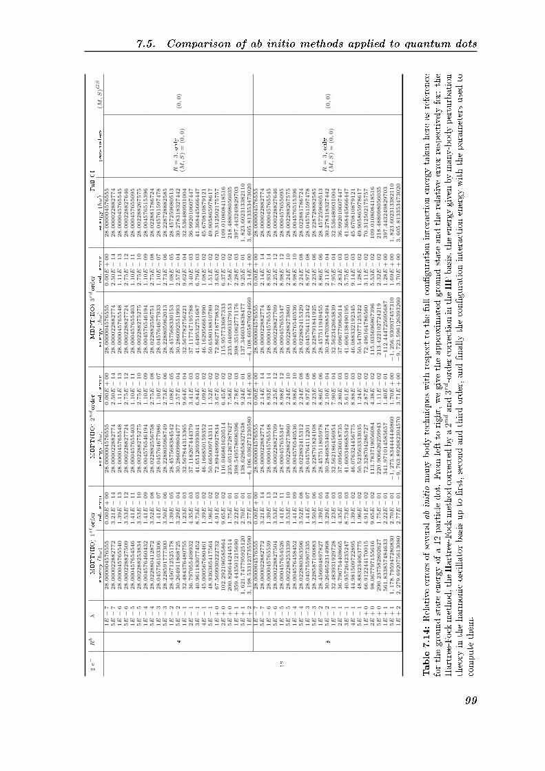
7.5. Comparison of ab initio methods applied to quantum dots
]e−
Rb
λMBPT(H
O)-
1s
torder
MBPT(H
O)-
2n
dorder
MBPT(H
O)-
3r
dorder
FullCI
energy(~ω)
rel.error
energy(~ω)
rel.error
energy(~ω)
rel.error
energy(~ω)
parameters
(M,S)G
S
12
1E−
728.0
00004576555
0.0
0E
+00
28.0
00004576555
0.0
0E
+00
28.0
00004576555
0.0
0E
+00
28.0
00004576555
5E−
728.0
00022882772
3.2
1E−
14
28.0
00022882774
2.5
0E−
14
28.0
00022882774
2.5
0E−
14
28.0
00022882774
1E−
628.0
00045765540
1.3
9E−
13
28.0
00045765548
1.1
1E−
13
28.0
00045765548
1.1
1E−
13
28.0
00045765545
5E−
628.0
00228827509
3.5
3E−
12
28.0
00228827724
2.7
5E−
12
28.0
00228827724
2.7
5E−
12
28.0
00228827646
1E−
528.0
00457654546
1.4
1E−
11
28.0
00457655403
1.1
0E−
11
28.0
00457655403
1.1
0E−
11
28.0
00457655095
5E−
528.0
02288253834
3.5
3E−
10
28.0
02288275275
2.7
5E−
10
28.0
02288275275
2.7
5E−
10
28.0
02288267575
1E−
428.0
04576460432
1.4
1E−
09
28.0
04576546194
1.1
0E−
09
28.0
04576546194
1.1
0E−
09
28.0
04576515396
5E−
428.0
22880412872
3.5
2E−
08
28.0
22882556758
2.7
5E−
08
28.0
22882556751
2.7
5E−
08
28.0
22881786724
1E−
328.0
45756103306
1.4
1E−
07
28.0
45764677986
1.1
0E−
07
28.0
45764677933
1.1
0E−
07
28.0
45761597478
5E−
328.2
28591777300
3.5
0E−
06
28.2
28805968749
2.7
3E−
06
28.2
28805962013
2.7
3E−
06
28.2
28728882585
1E−
228.4
56712525178
1.3
9E−
05
28.4
57568384542
1.0
8E−
05
28.4
57568330153
1.0
8E−
05
28.4
57259680513
5E−
230.2
64911808725
3.2
9E−
04
30.2
86099804477
2.5
7E−
04
30.2
86092551993
2.5
7E−
04
30.2
78318327442
1E−
132.4
84376480755
1.2
3E−
03
32.5
67844313365
9.6
4E−
04
32.5
67782756221
9.6
2E−
04
32.5
36480931004
2E−
136.7
97055408932
4.3
5E−
03
37.1
18267444379
3.4
1E−
03
37.1
17747195788
3.4
0E−
03
36.9
92010607447
3E−
140.9
61183077452
8.7
3E−
03
41.6
51269393041
6.8
4E−
03
41.6
49532751687
6.7
9E−
03
41.3
68445666447
4E−
145.0
00567680461
1.3
9E−
02
46.1
66850159352
1.0
9E−
02
46.1
62956661990
1.0
8E−
02
45.6
70810879121
5E−
148.9
36365417564
1.9
6E−
02
50.6
65009743311
1.5
2E−
02
50.6
58018810789
1.5
1E−
02
49.9
05865978617
1E
+0
67.5
69930222732
4.9
1E−
02
72.8
94489927834
3.6
7E−
02
72.8
62718779832
3.6
3E−
02
70.3
12502175757
2E
+0
102.2
92196585864
9.6
5E−
02
116.0
46861620514
6.4
5E−
02
115.9
57733687333
6.3
7E−
02
109.0
10808418516
5E
+0
200.8
26644244514
1.7
5E−
01
235.0
51267287627
7.5
8E−
02
235.0
40903379153
7.5
8E−
02
218.4
88098056035
1E
+1
359.4
43501215690
2.2
2E−
01
398.5
49578696396
2.7
8E−
03
398.3
51062771176
2.2
8E−
03
397.4
43249829703
5E
+1
1,621.7
47795925120
2.7
0E−
01
138.6
29658327638
9.2
4E−
01
137.3
46034838477
9.2
5E−
01
1,823.6
02313382110
4
1E
+2
3,198.5
33123735590
2.7
7E−
01
−4,106.0
36271230580
2.1
4E
+00
−4,108.6
05870024660
2.1
4E
+00
3,605.8
13353473020
R=
3,only
(M,S)
=(0,0)
(0,0)
1E−
728.0
00004576555
0.0
0E
+00
28.0
00004576555
0.0
0E
+00
28.0
00004576555
0.0
0E
+00
28.0
00004576555
5E−
728.0
00022882772
3.2
1E−
14
28.0
00022882774
2.1
4E−
14
28.0
00022882774
2.1
4E−
14
28.0
00022882774
1E−
628.0
00045765539
1.3
9E−
13
28.0
00045765548
8.9
3E−
14
28.0
00045765548
8.9
3E−
14
28.0
00045765545
5E−
628.0
00228827504
3.5
3E−
12
28.0
00228827709
2.2
5E−
12
28.0
00228827709
2.2
5E−
12
28.0
00228827646
1E−
528.0
00457654526
1.4
1E−
11
28.0
00457655347
8.9
8E−
12
28.0
00457655347
8.9
8E−
12
28.0
00457655095
5E−
528.0
02288253339
3.5
3E−
10
28.0
02288273860
2.2
4E−
10
28.0
02288273860
2.2
4E−
10
28.0
02288267575
1E−
428.0
04576458452
1.4
1E−
09
28.0
04576540536
8.9
8E−
10
28.0
04576540536
8.9
8E−
10
28.0
04576515396
5E−
428.0
22880363596
3.5
2E−
08
28.0
22882415312
2.2
4E−
08
28.0
22882415329
2.2
4E−
08
28.0
22881786724
1E−
328.0
45755907335
1.4
1E−
07
28.0
45764112201
8.9
7E−
08
28.0
45764112342
8.9
7E−
08
28.0
45761597478
5E−
328.2
28587100883
3.5
0E−
06
28.2
28791824108
2.2
3E−
06
28.2
28791841925
2.2
3E−
06
28.2
28728882585
1E−
228.4
56694897827
1.3
9E−
05
28.4
57511805978
8.8
6E−
06
28.4
57511949455
8.8
6E−
06
28.4
57259680513
5E−
230.2
64652314968
3.2
9E−
04
30.2
84685340374
2.1
0E−
04
30.2
84703885494
2.1
1E−
04
30.2
78318327442
1E−
132.4
83931929728
1.2
3E−
03
32.5
62186456954
7.9
0E−
04
32.5
62342663839
7.9
5E−
04
32.5
36480931004
2E−
136.7
96754408665
4.3
5E−
03
37.0
95636018735
2.8
0E−
03
37.0
96779965614
2.8
3E−
03
36.9
92010607447
3E−
140.9
57264235247
8.7
3E−
03
41.6
00348685342
5.6
1E−
03
41.6
06138490195
5.7
5E−
03
41.3
68445666447
4E−
144.9
81509722895
1.3
9E−
02
46.0
76324456775
8.8
8E−
03
46.0
88332192345
9.1
4E−
03
45.6
70810879121
5E−
148.8
83234063775
1.9
6E−
02
50.5
23563333035
1.2
4E−
02
50.5
47077125322
1.2
8E−
02
49.9
05865978617
1E
+0
66.9
12244170015
4.9
1E−
02
72.3
28704286727
2.8
7E−
02
72.4
96164786560
3.1
1E−
02
70.3
12502175757
2E
+0
98.0
67797155616
9.6
5E−
02
113.7
83719056084
4.3
8E−
02
115.0
35696867396
5.5
3E−
02
109.0
10808418516
5E
+0
290.2
37582802627
1.7
5E−
01
220.9
06626259943
1.1
1E−
02
213.4
22102724219
2.3
2E−
02
218.4
88098056035
1E
+1
561.8
33857484633
2.2
2E−
01
341.9
71014585657
1.4
0E−
01
−112.4
44725095687
1.2
8E
+00
397.4
43249829703
5E
+1
1,178.7
95947280830
2.7
0E−
01
−1,275.8
34444440860
1.7
0E
+00
−1,256.9
30937457310
1.6
9E
+00
1,823.6
02313382110
8
1E
+2
2,279.6
92075613080
2.7
7E−
01
−9,763.8
92682304570
3.7
1E
+00
−9,723.5
96126393260
3.7
0E
+00
3,605.8
13353473020
R=
3,only
(M,S)
=(0,0)
(0,0)
Table
7.14:Relative
errors
ofseveralabinitio
many-bodytechniques
withrespectto
thefullcon�gurationinteractionenergytaken
hereasreference
forthegroundstate
energyofa12-particledot.
From
leftto
right,wegivetheapproxim
atedgroundstate
andtherelative
errorrespectively
for:
the
Hartree-Fock
method,theHartree-Fock
methodcorrectedbya
2ndand
3rd-ordercorrectionintheHFbasis,theenergygiven
bymany-bodyperturbation
theory
intheharm
onicoscillatorbasisupto
�rst,secondandthirdorder,and�nallythecon�gurationinteractionenergywiththeparametersusedto
compute
them
.
99

Chapter 7. Computational Results and Analysis
7.5.4 Short comparison to the variational Monte Carlo method
We brie�y compare our previous results with a few runs of the variational MonteCarlo (VMC) simulator developed by Rune Albrigtsen. The details of the simula-tions performed are given in appendix C. The idea is to compare (even for a fewsimulations) the approximated energy of VMC to the FCI ground state and to theother methods. Table 7.15 indicates that the energies computed with VMC are lowerthan the FCI ground state for quantum dots with 2, 6 and 12 electrons and with acon�nement strength λ = 1.
These VMC calculations, as our Hartree-Fock implementation, use the closed-shell Slater determinant as an ansatz for the ground state. The lower energy obtainedwith VMC could be due to a breakdown of the method considering λ = 1 as a largeinteraction strength. However we have seen in section 7.2.2 that λ = 1 is still farfrom the breaking limit (λ2e−
limit ≥ 50, λ6e−
limit ≥ 13), and that increasing the modelspace of FCI usually increases this limit.
Therefore, FCI calculations should be run over a much larger space in order todecide the nature of the ground state and study the breaking of the VMC calculationsaccording to the new �exact� energies.
2-electron QD 6-electron QD 12-electron QDenergy (~ω) energy (~ω) energy (~ω)
Full CI 3.013626 20.316754 70.312502VMC 3.0025 ±1.2 10−4 20.1909 ±3.6 10−4 65.79±1.9 10−3
HF 3.16908 20.744840 66.912244HF+MBPT(HF)-2ndorder 3.015743 20.337553 65.870798
MBPT(HO)-1storder 3.253314 22.219812 73.765549MBPT(HO)-2ndorder 3.022410 21.477290 72.328704
Table 7.15: Comparison of approximation to the ground state energy of quantum dots with λ = 1.
This short comparison with the VMC results let us think that some of our previousconclusions may be altered by the accuracy of the FCI calculations within a toosmall Hilbert space. If the FCI method in a very small space becomes less accuratethan the Hartree-Fock method, and closer to the MBPT results, we would concludewrongly that MBPT performs better than Hartree-Fock (which we may have donein section 7.5.2).
This shows the importance of the FCI accuracy with respect to the size of themodel space.
100

Chapter 8
Conclusion
8.0.5 Critical discussion of the method and results
In this thesis we performed a computional study of a quantum dot in two dimensionswhere the electrons are trapped in a harmonic oscillator potential and repel eachother with a Coulomb interaction. The main objective was to compare the e�ciencyand the limits of convergence/accuracy of several ab-inito many-body techniquesto approximate the ground state energy of the quantum dot with respect to thecon�nement strength. For this purpose, we developed a simulator for computingthe Hartree-Fock (HF) and many-body perturbation theory (MBPT) energies. Themany-body perturbation corrections were implemented up to third order, howeverour results (section 7.5.3) showed that the third order never really improved theaccuracy over the second order corrected energy.
The implemented model and the origin of the dimensionless con�nement strengthλ are discussed in chapter 4, where λ shows to be proportional to the natural oscillatorlength of the host semiconductor. However the con�nement strength can also bemodi�ed by applying an external magnetic �eld which will squeeze the electrons insmaller regions of space. We derived the Hamiltonian of quantum dots in a magnetic�eld also in chapter 4 where we show that the interaction with the magnetic �eldcan simply be reformulated as a new harmonic oscillator con�nement potential witha modi�ed oscillator frequency ω, to which one should add a shift in energy due tothe interaction of the magnetic �eld with the angular and spin parts of the system.For a typical quantum dot made of Gallium arsenide (GaAs), we show that thedimensionless con�nement strength should vary in the range λ ∈ [0, 1.6], decreasingas the magnetic �eld increases. However as the magnetic �eld increases, our simplemodel may fail since it does not take into account the modi�cation in the physicallength of the quantum dot when forcing the electrons to get closer to each other.It does also not include the modi�cation in the type of interaction that modelsthe repulsion between the electrons. From a computational point of view, it wasinteresting anyway to observe the behaviour of the various computational techniquesfor a bigger range of λ (λ ∈ [0, 100]), and keeping our electron interaction in the formof a Coulomb repulsion.
If our model relies on an arbitrary form of the electron interaction, its imple-mentation is also restricted to a closed-shell model in which the wave function of
101

Chapter 8. Conclusion
the system is approximated by a unique Slater determinant. This closed-shell modelimplies that the particles of the system occupies all the shells up to the Fermi level.We made an attempt to study the limit of this model by neglecting the electroninteractions. This is done in section 7.2.1 while observing the level crossing of theFock-Darwin orbitals as a function of the magnetic �eld. It shows that the modelactually breaks for B = 2.1T (i.e. λ = 1.54 in GaAs) in a six-particles quantum dotand B = 1.2T (i.e. λ = 1.58 in GaAs) in a twelve-particles quantum dot, givingsome upper bound in magnetic �eld and lower bound in λ. Again this theoreticalcase completely neglects the e�ect of the repulsion between the electrons while themagnetic �eld increases, which should in reality results in a much lower limit for B,but in a non-trivial change in λ. As mentionned in 7.2.1 this range of magnetic �eldare easily achievable today in laboratories. Therefore the closed-shell model couldnot potentially be used to investigate any possible magnetic strength.
Anyway, introducing the electron interaction and sticking to the Coulomb in-teraction model, a numerical computation is clearly the only way to �nd an upperbound for λ indicating the limit of the closed-shell model. The study was per-formed using full con�guration interaction (FCI) on a six-electrons quantum dot(section 7.2.2). We observed a change in total angular momentum M and total spinS from (0, 0) → (1, 2) indicating a break of the closed-shell model for an increaseof the con�nement strength from λ = 13 to λ = 15. A similar study done for thetwo-electrons dot (section 7.5.3) shows a breakdown of the closed-shell model be-tween λ = 50 and λ = 100. However these �ndings regarding the limitations of theshell model should be taken with great care, or as a preliminary study for a moreaccurate investigation, since our FCI calculations were performed in a very restrictedHilbert space. For example we noticed that for a six-electrons dot, FCI calculationsindicate a breakdown between λ = 5 and λ = 10 for a maximum shell number R = 4since the lowest ground states respectively correspond to (M,S)R=4
λ=5 = (0, 0) and(M,S)R=4
λ=5 = (1, 4). Therefore one might conclude (wrongly) that this marks thelimit of the shell model. However the same calculations were done with a maxi-mum shell number R = 5, the ground state obtained for the con�guration indicates(M,S)R=5 = (0, 0) ≤ (M,S)R=4 = (1, 4), meaning that the closed-shell model isactually still valid for a six-electrons dot when λ = 10. Therefore restricting theHilbert space too much in FCI calculations could lead to wrong interpretations. Italso means that our current observations could lead to higher limits while runningFCI simulations in a bigger model space.
After studying the limits of the shell model, it was interesting to know if thecomputational techniques would actually break or not before the shell model. SinceHartree-Fock theory, perturbation theory and combinations of these techniques arein essence lower approximations to the exact ground state than FCI, we also observedhow fast the di�erent methods will diverge from the FCI calculation taken here asreference with respect to the interaction strength λ and the number of particles inthe dot. The implementation of a simulator based on the Hartree-Fock method andmany-body perturbation theory allowed us to investigate the approximated groundstates for λ = 0 → 100 and di�erent sizes of our model space characterized by themaxmum shell number Rb. The results are summarized and analyzed in section( 7.5).
102

It shows that HF, MBPT and the combinations of these methods display an errorgrowing quadratically with λ when compared to the �exact� FCI energies. It alsoshow some linear di�erence in the relative error between the methods themselves.For example, a two-electrons dot will be better approximated by HF+MBPT(HF)-2ndorder with a much smaller error than MBPT(HO)-1storder (Results are summa-rized in table 7.8). Finally this linear di�erence in accuracy appears to change withthe size of the dot, which indicates that the Hartree-Fock method becomes less accu-rate compared to many-body perturbation theory as the number of electrons in thedot increases.
8.0.6 Perspectives for future works
When investigating the performance of our simulator (section 7.3) we observed anexponential scaling of the method with respect to the size of the model space (givenby Rb). More speci�cally the duration of the simulation and the complexity of theHartree-Fock approach increase exponentially with the size of the basis. A �rst issuein the implementation was to optimize the resolution of the huge eigenvalue problemperformed at each Hatree-Fock iteration. This has been done by splitting the hugematrix to diagonalize into much smaller matrices , making use of symmetry propertiesof the system, particularly due to invariance of the two-body interaction matrix withrespect to the total angular momentum. Once this new implementation improved thee�ciency, the second bottleneck occurs when computing the matrix elements of thesame two-body interaction matrix. We saw that the parallelization of the code withMPI improves almost linearly the performance of the simulator with respect to thenumber of processors used (discussed in section 7.4). Moreover, the �rst interactionmatrix computed in the harmonic oscillator basis can be computed once for all andreused for any simulation requiring the same basis size (i.e. same Rb), which savesalready a lot of time before entering the Hartree-Fock algorithm itself. Our simulatorincludes this improvement and reads the matrix from �le if it exists. However a newinteraction matrix has to be computed at the end of Hartree-Fock calculation, andthis depends on several input parameters. The construction of this second matrix isactually not optimized yet. However a way to do it would be to compute each matrixelement using a center-of-mass transformation, as it is done in OpenFCI [32]. Thiswould of course require the implementation of numerical integration whereas oursimple simulator currently works within the energy basis, relying on nice propertiesof Harmonic oscillator orbitals. Once numerical integration is implemented, this willalso allow us to compute the matrix elements in three-dimension and to change theshape of the con�ning potential.
We already discussed a lot about the limitation of the closed-shell model andhow it might a�ect the reliability of our results. A more accurate comparison of themethod should include FCI results with a much bigger model space, which could leadto an interesting study of the shell model break while plotting variational Monte-Carlo (VMC) results which exhibits much better accuracy than HF or MBPT. Ofcourse a way to overcome the restriction due to the closed-shell model would be toimplement an open-shell model. Despite the more complex implementation (mainly
103

Chapter 8. Conclusion
combinatorics) for including the combinations of Slater determinants, it would beinteresting to compare the e�ciency and the convergence of an open-shell HF com-pared to our current closed-shell implementation. This would also give us manyinsights on the electronic structure responsible for this inaccuracy of the correlatione�ects.
Combining the techniques is usually a good tradeo� between convergence andaccuracy. We did it for example by correcting the HF energy with a second orderperturbation correction which improves the results, at least for small systems. Wecould either use the two-body interaction matrix computed in the basis set of Hartree-Fock orbitals as input of the FCI calculation, or use the FCI method to produce ane�ective interaction that would serve of starting point in our HF simulation insteadof the bare Coulomb interaction computed in the harmonic oscillator basis.
8.0.7 Further extensions
This simple numerical study of quantum dots opens many questions on how to im-prove the performance of computational techniques, how the same problem scaleswith other techniques, and also how does it improves our understanding of quantumdots themselves. Therefore it would be interesting to compare approximations tothe ground state of quantum dots with other techniques such as couple cluster (CC)theory or density functional theory (DFT).
Moreover, a time-dependent study of quantum dots would give us more informa-tion on their interaction with the environment which would be very instructive forimproving their current applications in modern electronics or in biology.
104

Appendix A
Analytical expression of the
two-body Coulomb interaction
This function computes the exchange part in the anti-symmetrized Coulomb matrixelement 〈αβ|V |γδ〉as = 〈α(ri)β(rj)|V (rij)|γ(ri)δ(rj)〉as where the α, β, γ and δare four state indices and ri, rj the positions of particle i and j. Each state |k〉can be rewritten in terms of its quantum numbers. In two dimensions, it reads|k〉 = |nkmksk〉. For simplicity the angular momentum projection quantum numberml will just be written as m in the following equations.
The complete anti-symmetrized Coulomb matrix element reads
〈αβ|V |γδ〉as = 〈αβ|V |γδ〉︸ ︷︷ ︸directterm
−〈αβ|V |γδ〉︸ ︷︷ ︸exchangeterm
, (A.1)
The exchange term 〈αβ|V |γδ〉 expands as follow
〈αβ|V |γδ〉 = δms1,ms4 δms2,ms3 〈(n1,m1), (n2,m2)|V |(n3,m3), (n4,m4)〉 (A.2)
= δms1,ms4 δms2,ms3 Vαβγδ, (A.3)
where we separate the spin part from the spatial part Vαβ|V |γδ.
Note that in our simulator, the function Anisimovas(n1,m1,n2,m2,n3,m3,n4,m4)only computes V1234 where the numbers 1→ 4 are state indices similar to α, β, γ, δ.
According to Anisimovas [3] (the detail of the derivation is also reviewed byRontani [50]), the spatial part can be solved analytically when the basis set is builtupon the single harmonic oscillator orbitals.
105

Appendix A. Analytical expression of the two-body Coulomb interaction
V1234 = δm1+m2,m3+m4
√√√√[ 4∏i=1
ni!
(ni + |mi|!)
]
×n1,...,n4∑
j1=0,...,j4=0
[(−1)j1+j2+j3+j4
j1!j2!j3!j4!
[4∏
k=1
(nk + |mk|nk − jk
)]1
2G+1
2
×γ1=0,...,γ4=0∑l1=0,...,l4=0
(δl1,l2 δl3,l4 (−1)γ2+γ3−l2−l3
[4∏t=1
(γtlt
)]Γ
(1 +
Λ
2
)Γ
(G− Λ + 1
2
))],
(A.4)
where
γ1 = j1 + j4 +|m1|+m1
2+|m4| −m4
2,
γ2 = j2 + j3 +|m2|+m2
2+|m3| −m3
2,
γ3 = j3 + j2 +|m3|+m3
2+|m2| −m2
2,
γ4 = j4 + j1 +|m4|+m4
2+|m1| −m1
2,
G = γ1 + γ2 + γ3 + γ4,
Λ = l1 + l2 + l3 + l4.
As a note, our implementation of the function Anisimovas(. . . ) which computesthe spatial part of the exchange term, includes the following subfunctions:
� minusPower(int k) which computes (−1)k,
� LogFac(int n) which computes loge(n!),
� LogRatio1(int j1,int j2,int j3,int j4) which computes the loge of 1j1!j2!j3!j4!
,
� LogRatio2(int G) which computes the loge of 1
2G+1
2,
� Product1 (int n1,int m1,int n2,int m2, int n3,int m3,int n4,int m4)
which computes the explicit (not the loge) product√[∏4
i=1ni!
(ni+|mi|!)
],
� LogProduct2(int n1,int m1,int n2,int m2, int n3,int m3,int n4,int
m4, int j1,int j2,int j3,int j4 ) which computes the loge of∏4
k=1
(nk + |mk|nk − jk
),
� LogProduct3(int l1,int l2,int l3,int l4, int γ1,int γ2,int γ3,int γ4)
which computes the loge of∏4
t=1
(γtlt
),
� lgamma(double x) which computes the loge [Γ(x)].
106

Appendix B
The method of Lagrange Multipliers
In mathematical optimization, the method of Lagrange multipliers (named afterJoseph Louis Lagrange) provides a strategy for �nding the stationnary points of afunction (and among them maxima/minima if the derivative of the function is de�nedfor those points) subject to some constraints.
B.0.8 General approach of the method
For example (see �gure B.1), consider the following optimization problem:
� maximize the functional f(x, y),
� subject to the constraint g(x, y) = c.
We introduce a new variable (λ) called a Lagrange multiplier, and study theLagrange function (or Lagrangian) de�ned by
Λ(x, y, λ) = f(x, y)− λ (g(x, y)− c) . (B.1)
If (x, y) is a maximum for the original constrained problem, then there existsa λ such that (x, y, λ) is a stationary point for the Lagrange function (stationarypoints are those points where the partial derivatives of Λ are zero). However, not
Figure B.1: Find x and y to maximize f(x, y) subject to a constraint (shown in red) g(x, y) = c.
107

Appendix B. The method of Lagrange Multipliers
Figure B.2: Illustration of the constrained optimization problem.
all stationary points yield a solution of the original problem. Thus, the methodof Lagrange multipliers yields a necessary condition for optimality in constrainedproblems.
B.0.9 Example
Let's use the method for a simple example:Suppose you wish to maximize f(x, y) = x+y subject to the constraint x2+y2 = 1.
The constraint is the unit circle as shown on �gure B.2, and the level sets of f arediagonal lines (with slope −1), so one can see graphically that the maximum occursat (√
2 /2,√
2 /2) (and the minimum occurs at (−√2 /2,−√2 /2))Formally, we get from the constraint that g(x, y) − c = x2 + y2 − 1, and the
Lagrange function reads
Λ(x, y, λ) = f(x, y) + λ(g(x, y)− c) = x+ y + λ(x2 + y2 − 1). (B.2)
Set the derivative ∂Λ = 0, which yields the system of equations:
∂Λ
∂x= 1 + 2λx = 0, (i)
∂Λ
∂y= 1 + 2λy = 0, (ii)
∂Λ
∂λ= x2 + y2 − 1 = 0, (iii)
(B.3)
As always, the ∂λ equation is the original constraint.Combining the �rst two equations yields x = y (explicitly, λ 6= 0, otherwise (i)
yields 1 = 0, so one has x = −1/(2λ) = y).Substituting into (iii) yields 2x2 = 1, so x = ±√2 /2 and the stationary points
are (√
2 /2,√
2 /2) and (−√2 /2,−√2 /2). Evaluating the objective function f onthese yields f(
√2 /2,
√2 /2) =
√2 and f(−√2 /2,−√2 /2) = −√2 ,
108

thus the maximum is√
2 , which is attained at (√
2 /2,√
2 /2) and the minimumis −√2 , which is attained at (−√2 /2,−√2 /2).
109

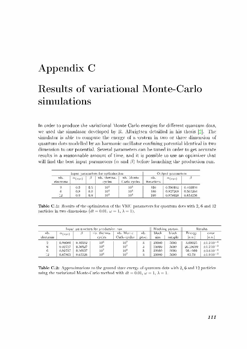
Appendix C
Results of variational Monte-Carlo
simulations
In order to produce the variational Monte Carlo energies for di�erent quantum dots,we used the simulator developed by R. Albrigtsen detailled in his thesis [2]. Thesimulator is able to compute the energy of a system in two or three dimension ofquantum dots modelled by an harmonic oscillator con�ning potential identical in twodimension to our potential. Several parameters can be tuned in order to get accurateresults in a reasonnable amount of time, and it is possible to use an optimizer thatwill �nd the best input parameters (α and β) before launching the production run.
Input parameters for optimization Output parametersnb. α{xyz} β nb. therma. nb. Monte nb. α{xyz} β
electrons cycles Carlo cycles iterations
2 0.9 0.5 104 104 100 0.990855 0.4038246 0.9 0.6 104 104 100 0.927269 0.56526612 0.9 0.6 104 104 100 0.878028 0.653256
Table C.1: Results of the optimizaton of the VMC parameters for quantum dots with 2, 6 and 12particles in two dimensions (dt = 0.01, ω = 1, λ = 1).
Input parameters for production run Blocking param. Resultsnb. α{xyz} β nb. therma. nb. Monte nb. block block Energy error
electrons cycles Carlo cycles proc. size sample [a.u.] [a.u.]
2 0.99086 0.40382 106 107 3 20000 5000 3.00025 ±1.2 10−4
6 0.92727 0.56527 106 107 3 20000 5000 20.19099 ±1.2 10−3
6 0.92727 0.56527 107 108 3 20000 5000 20.1909 ±3.6 10−4
12 0.87803 0.65326 106 107 3 20000 5000 65.79 ±1.9 10−3
Table C.2: Approximations to the ground state energy of quantum dots with 2, 6 and 12 particlesusing the variational Monte-Carlo method with dt = 0.01, ω = 1, λ = 1.
111


Appendix D
ERRATA
� section (3.1) p.14
· · · . 1.06× 10⁻¹¹m = 0.0106. nm (D.1)
should read· · · . 1.06× 10⁻¹¹m = 0.0106 nm (D.2)
� section (5.2.1) p.36 |Ψ〉 =∑
iCi|χj〉 should read |Ψ〉 =∑
iCi|χi〉� section (5.2.2) p.39
Φ(r1, r2, . . . , rN, α, β, . . . , σ) =1√N !
∣∣∣∣∣∣∣∣∣∣
ψα(r1) ψβ(r2) . . . ψσ(rN)
ψα(r1) ψβ(r2) . . . ψσ(rN)
......
. . ....
ψα(r1) ψβ(r2) . . . ψσ(rN)
∣∣∣∣∣∣∣∣∣∣, (D.3)
should read:
Φ(r1, r2, . . . , rN, α, β, . . . , σ) =1√N !
∣∣∣∣∣∣∣∣∣∣
ψα(r1) ψα(r2) . . . ψα(rN)
ψβ(r1) ψβ(r2) . . . ψβ(rN)
......
. . ....
ψσ(r1) ψσ(r2) . . . ψσ(rN)
∣∣∣∣∣∣∣∣∣∣, (D.4)
� sec. (5.2.3) p.40 �. . . nucleons.� should read �. . . particles.�
� sec. (5.3) p.49 �anihilation (ci = k). . . � should read �anihilation (ck). . . �
� sec. (7.2.1) p.71
λ(B) =1
a∗0
(4~2
4ω20m∗ + e2B
)1/4
. (D.5)
should read:
λ(B) =1
a∗0
(4~2
4ω20m∗2 + e2B2
)1/4
. (D.6)
113

Appendix D. ERRATA
� eq.(7.10) p.88εmethod ∝ (Emethod)β (D.7)
should readεmethod ∝ λβ (D.8)
� Appendix C tables C.2 p.111, �σ2� should read �error (σ)�
� Appendix C tables C.2 p.111, �dt = 0.01� should read �dt = 0.01, ω = 1, λ = 1�
� information regarding input parameters of the FCI ground state energy calcu-lation has been corrected and added in the following tables 7.9 p.94 to 7.14p.99
114

Bibliography
[1] Electron transport in quantum dots, Proceedings of the Advanced Study Insti-tute, 1997.
[2] R. Albrigtsen. Computational environment for many-electron systems. Master'sthesis, University of Oslo, 2009.
[3] E. Anisimovas and A. Matulis. Energy spectra of few-electron quantum dots.J. Phys., 10:601�615, 1998.
[4] G. Baardsen. Spin e�ects in circular quantum dots. Master's thesis, HelsinkiUniversity of Technology, 2009.
[5] B. H. Bransden and C. J. Joachain. Physics of Atoms and Molecules; 2nd ed.
Prentice-Hall, Harlow, 2003.
[6] L. Brey, N. F. Johnson, and B. I. Halperin. Optical and magneto-optical ab-sorption in parabolic quantum wells. Phys. Rev. B, 40:10647�10649, 1989.
[7] M. Bruchez, M. Moronne, P. Gin, S. Weiss, and P. A. Alivisatos. Semiconductornanocrystals as �uorescent biological labels. Science, 281:2013�2016, 1998.
[8] W. C. W. Chan and S. Nie. Quantum dot bioconjugates for ultrasensitivenonisotopic detection. Science, 281:2016�2018, 1998.
[9] D. Chaney and P. A. Maksym. Size-dependent suppression of spin relaxation inelectrostatic quantum dots. Phys. Rev. B, 75:035323, 2007.
[10] M. Ciorga, A. S. Sachrajda, P. Hawrylak, C. Gould, P. Zawadzki, S. Jullian,Y. Feng, and Z. Wasilewski. Addition spectrum of a lateral dot from coulomband spin-blockade spectroscopy. Phys. Rev. B, 61:R16315�R16318, 2000.
[11] C. J. Cramer. Essentials of computational chemistry : theories and models. JohnWiley & Sons, 2008.
[12] J. Dempsey, N. F. Johnson, L. Brey, and B. I. Halperin. Collective modes inquantum-dot arrays in magnetic �elds. Phys. Rev. B, 42:11708�11713, 1990.
[13] P. J. Ellis and E. Osnes. An introductory guide to e�ective operators in nuclei.Rev. Mod. Phys., 49:777�832, 1977.
115

Bibliography
[14] V. Fock. Bemerkung zur quantelung des harmonischen oszillators im magnetfeld.Zeitschrift für Physik A Hadrons and Nuclei, 47:446�448, 1928.
[15] X. Gao, Y. Cui, R. M. Levenson, L. W. Chung, and S. Nie. In vivo cancertargeting and imaging with semiconductor quantum dots. Nat Biotech, 22:969�976, 2004.
[16] D. Goldberg. What every computer scientist should know about �oating-pointarithmetic. ACM Computing Surveys, 23:5�48, 1991.
[17] M. B. Haider, J. L. Pitters, G. A. DiLabio, L. Livadaru, J. Y. Mutus, and R. A.Wolkow. Controlled coupling and occupation of silicon atomic quantum dots atroom temperature. Phys. Rev. Lett., 102:046805, 2009.
[18] W. A. Harrison. Electronic Structure and the Properties of Solids: The Physics
of the Chemical Bond. Dover Publications, 1989.
[19] O. Heinonen, E. Gross, and E. Runge. Many-Particle Theory. Hilger, 1991.
[20] T. Heinzel. Mesoscopic Electronics in Solid State Nanostructures. Wiley-VCH,Weinheim, 2003.
[21] D. Heitmann. Far infrared spectroscopy of quantum-dots and antidot arrays.Physica B, 212:201 � 206, 1995. Proceedings of the Workshop on Novel Physicsin Low-Dimensional Electron Systems.
[22] D. Heitmann and J. P. Kotthaus. The spectroscopy of quantum dot arrays.Physics Today, 46:56�63, 1993.
[23] A. Hoshino, K. ichi Hanaki, K. Suzuki, and K. Yamamoto. Applications oft-lymphoma labeled with �uorescent quantum dots to cell tracing markers inmouse body. Biochemical and Biophysical Research Communications, 314:46 �53, 2004.
[24] N. Johnson and M. Payne. Exactly solvable model of interacting particles in aquantum dot. Phys. Rev. Lett., 67:1157, 1991.
[25] N. Johnson and M. Reina. The accuracy of the hartree-fock approximation forquantum dots. J. Phys., 4:623�628, 1992.
[26] K. Kalyanasundaram. Cleavage of water by visible-light irradiation of colloidalcds solutions; inhibition of photocorrosion by ruo2. Angewandte Chemie Inter-
national Edition in English, 20:987�988, 2003.
[27] W. Kohn. Cyclotron resonance and de haas-van alphen oscillations of an inter-acting electron gas. Phys. Rev., 123:1242�1244, 1961.
[28] L. P. Kouwenhoven, D. G. Austing, and S. Tarucha. Few-electron quantum dots.Reports on Progress in Physics, 64:701�736, 2001.
116

Bibliography
[29] M. Kralj and K. Pavelic. Medicine on a small scale. EMBO reports,4:1008�1012, 2003.
[30] A. Kumar, S. Laux, and F. Stern. Electron states in a gaas quantum dot in amagnetic �eld. Phys. Rev. B, 42:5166�5175, 1990.
[31] W. Kutzelnigg. Diamagnetism in relativistic theory. Phys. Rev. A, 67:032109+,2003.
[32] S. Kvaal. Open source fci code for quantum dots and e�ective interactions.arXiv.org, 2008.
[33] S. Kvaal. Analysis of many-body methods for quantum dots. PhD thesis, Uni-versity of Oslo, 2009.
[34] S. Kvaal. Openfci home page at: http://folk.uio.no/simenkva/, 2009.
[35] A. Kwasniowski and J. Adamowski. E�ect of con�nement potential shape onexchange interaction in coupled quantum dots. J. Phys., 20:215208, 2008.
[36] C. S. Lent, P. D. Tougaw, W. Porod, and G. H. Bernstein. Quantum cellularautomata. Nanotechnology, 4:49�57, 1993.
[37] Q. P. Li, K. Karraï, S. K. Yip, S. Das Sarma, and H. D. Drew. Electrody-namic response of a harmonic atom in an external magnetic �eld. Phys. Rev.
B, 43:5151�5154, 1991.
[38] M. Macucci, K. Hess, and G. J. Iafrate. Electronic energy spectrum and theconcept of capacitance in quantum dots. Phys. Rev. B, 48:17354�17363, 1993.
[39] M. Macucci, K. Hess, and G. J. Iafrate. Numerical simulation of shell-�llinge�ects in circular quantum dots. Phys. Rev. B, 55:R4879�R4882, 1997.
[40] I. L. Medintz, T. H. Uyeda, E. R. Goldman, and H. Mattoussi. Quantum dotbioconjugates for imaging, labelling and sensing. Nat Mater, 4:435�446, 2005.
[41] Y. Meir, N. S. Wingreen, and P. A. Lee. Transport through a strongly interactingelectron system: Theory of periodic conductance oscillations. Phys. Rev. Lett.,66:3048�3051, 1991.
[42] P. Merlot. The code can be downloaded at: http://folk.uio.no/patrime/
src/master.php, 2009.
[43] H. Mizuta, H.-O. Muller, K. Tsukagoshi, D. Williams, Z. Durrani, A. Irvine,G. Evans, S. Amakawa, K. Nakazato, and H. Ahmed. Nanoscale coulomb block-ade memory and logic devices. Nanotechnology, 12:155�159, 2001.
[44] M. Moshinsky and Y. F. Smirnov. The Harmonic Oscillator in Modern Physics:
From Atoms to Quarks. Taylor & Francis, 1996.
117

Bibliography
[45] F. M. Peeters. Magneto-optics in parabolic quantum dots. Phys. Rev. B,42:1486�1487, 1990.
[46] D. Pfannkuche, V. Gudmundsson, and P. A. Maksym. Comparison of a hartree,a hartree-fock, and an exact treatment of quantum-dot helium. Phys. Rev. B,47:2244�2250, 1993.
[47] S. Rahman. Applications of quantum dots in the biological sciences. SimulaResearch Laboratory, Lysaker, Norway, 2008.
[48] S. Raimes. Many-electron Theory. North-Holland Publishing, 1972.
[49] S. M. Reimann and M. Manninen. Electronic structure of quantum dots. Rev.Mod. Phys., 74:1283�1342, 2002.
[50] M. Rontani. Electronic States in Semiconductor Quantum Dots. PhD thesis,Universita degli Studi di Modena e Reggio Emilia, 1999.
[51] R. Rossetti, S. Nakahara, and L. E. Brus. Quantum size e�ects in the redoxpotentials, resonance raman spectra, and electronic spectra of cds crystallites inaqueous solution. J. Phys. Chem., 79:1086�1088, 1983.
[52] C. Sikorski and U. Merkt. Spectroscopy of electronic states in insb quantumdots. Phys. Rev. Lett., 62:2164�2167, 1989.
[53] H. Soo Choi, W. Liu, P. Misra, E. Tanaka, J. P. Zimmer, B. Itty Ipe, M. G.Bawendi, and J. V. Frangioni. Renal clearance of quantum dots. Nat Biotech,25:1165�1170, 2007.
[54] M. Stopa. Quantum dot self-consistent electronic structure and the coulombblockade. Phys. Rev. B, 54:13767�13783, 1996.
[55] M. Taut. Two electrons in an external oscillator potential: Particular analyticsolutions of a coulomb correlation problem. Phys. Rev. A, 48:3561�3566, 1993.
[56] M. Taut. Two electrons in a homogeneous magnetic �eld: particular analyticalsolutions. J. Phys. A, 27:1045�1055, 1994.
[57] M. B. Tavernier, E. Anisimovas, F. M. Peeters, B. Szafran, J. Adamowski, andS. Bednarek. Four-electron quantum dot in a magnetic �eld. Phys. Rev. B,68:205305, 2003.
[58] J. Thijssen. Computational Physics. Cambridge University Press, Cambridge,UK, 2007.
[59] E. B. Voura1, J. K Jaiswal1, H. Mattoussi, and S. M. Simon. Trackingmetastatic tumor cell extravasation with quantum dot nanocrystals and �uo-rescence emission-scanning microscopy. Nature Medicine, 10:993 � 998, 2004.
[60] E. Waltersson and E. Lindroth. Many-body perturbation theory calculations oncircular quantum dots. Phys. Rev. B, 76:045314, 2007.
118

Bibliography
[61] C. Weisbuch and H. Benisty. Overview of fundamentals and applications ofelectrons, excitons and photons in con�ned structures. Journal of Luminescence,85:271 � 293, 2000.
[62] H. Weller, H. M. Schmidt, U. Koch, and A. Fojtik. Photochemistry of colloidalsemiconductors. onset of light absorption as a function of size of extremely smallcds particles. Chem. Phys. Lett., 124:557�560, 1986.
[63] R. K. Willardson and A. C. Beer. Semiconductors and semimetals. AcademicPress, 1971.
[64] J. O. Winter. Development and optimization of quantum dot-neuron interfaces.PhD thesis, The University of Texas at Austin, 2004.
[65] S. K. Yip. Magneto-optical absorption by electrons in the presence of paraboliccon�nement potentials. Phys. Rev. B, 43:1707�1718, 1991.
119
Copyright © 2022 FDOKUMEN