Earth and Planetary Science Letters, 102 (1991) 213-232 213 Elsevier Science Publishers B.V., Amsterdam

[DT]

Mantle convection with internal heating and pressure-dependent thermal expansivity

A.M. Lei tch a D.A. Y u e n a and G. Sewell b

Minnesota Supercomputer Institute and Dept of Geology and Geophysics, University of Minnesota, Minneapolis, MN 55455, USA h Univ. Texas System, Center for High-Performance Computing, Austin, TX 78758, USA

Received March 16, 1990; revised version accepted September 10, 1990

ABSTRACT

Recent laboratory work [1] suggests that the thermal expansivity a of the mantle decreases strongly with pressure, a determines the buoyancy of plumes and the rate at which plumes lose their thermal signature as they rise, and so may be expected to have a strong influence on the temperature and velocity structure of the mantle. Numerical simulations were conducted on convection in an internally heated, compressible mantle including constant and pressure-dependent a and thermal conductivity k. They show that a pressure-dependent c~ allows the existence of thermal plumes rising from the core-mantle boundary (CMB), however the plumes are weak and dissipate higher in the mantle.

1. Introduction

Finite-element simulations were carried out to study the effect of internal heating, combined with various other mantle properties, on mantle con- vection. In particular we were interested in the nature of thermal upwelling. We wished to know whether heat transfer in the deep mantle takes place through the action of narrow, hot regions of localized u p f l o w - - " p l u m e s " - - a n d whether plumes extend throughout the depth of the man- tle.

Seismic tomography [2,3] reveals localized re- gions of slow seismic velocities in the deep mantle, which may correspond to hot plumes. "Hot - spo ts" on the earth's surface (e.g. [4]) may correspond to the top of plumes originating in the deep mantle. To date, however, the resolution of seismic tomog- raphy is quite low, since only the degree six harmonics have been adequately resolved (e.g. [5]) and the depth of origin and the role of hotspots in global convection are uncertain.

The alternative to the heat transfer by hot plumes is a convection pattern where there are cold down-flowing plumes but upflow is in the form of a broad, passive return flow. This occurs in systems which are purely internally heated and

0012-821X/91/$03.50 © 1991 Elsevier Science Publishers B.V.

cooled from above [6]. In support of this, mid- ocean-ridges, which are responsible for a signifi- cant proportion of heat flow from the interior, appear to be passive features [7].

Significant advances in our knowledge of prop- erties of the deep mantle have been made in the last two years from laboratory experiments on mantle materials at high temperatures and pres- sures. In particular the experiments of Chopelas and Boehler [1] have shown that the thermal ex- pansivities a of the olivine and magnesium oxides decrease rapidly with density, according to (a in a/~ In V)T= 5.5 ± 0.5. Since the thermal buoyancy force driving convection and the adia- batic cooling term which damps hot thermal anomalies are both proportional to c~, we can expect this variation to have an important in- fluence on the convection pattern.

In the following paper we look at convection in a compressible, internally heated mantle, firstly for constant thermodynamic properties (section 3) and then including depth-dependent a and ther- mal conductivity k (section 4). Because the parameter space is already large, we consider a constant viscosity mantle. Recent work on the inversion of mantle viscosity from internal loading [8] indicates that the horizontally averaged viscos-

214

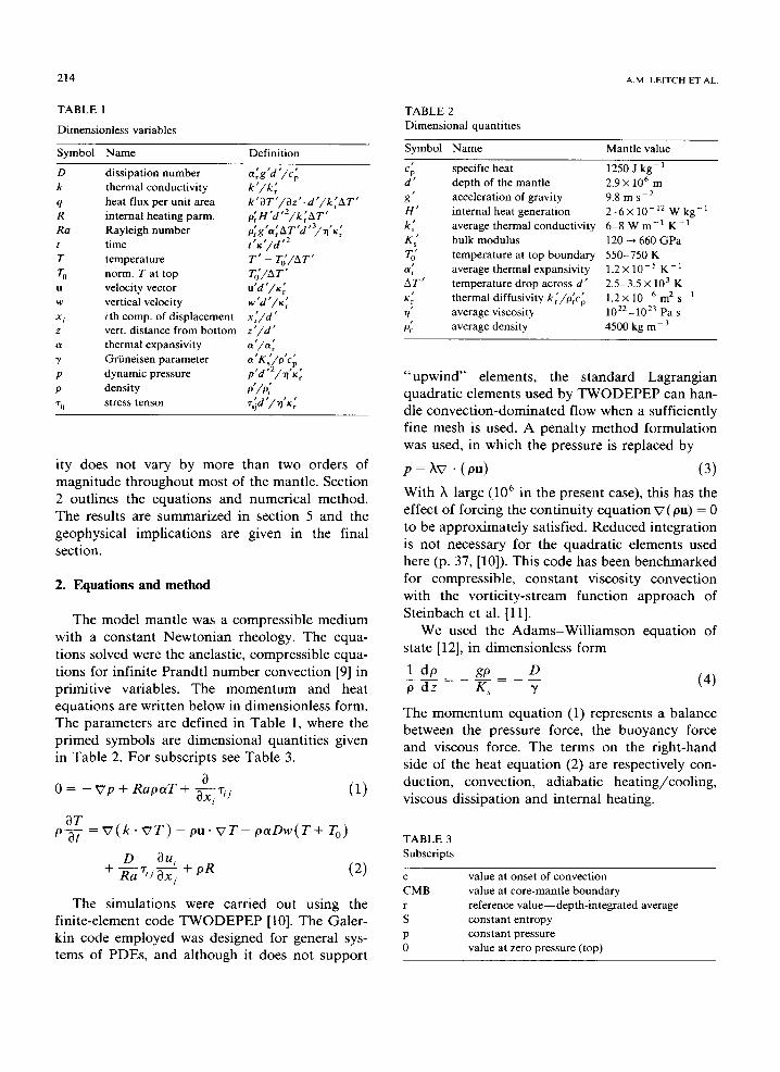
TABLE 1

Dimensionless variables

Symbol Name Definition

D dissipation number a~g'd '/% k thermal conductivity k '/k" q heat flux per unit area k'aT'/~z'-d'/k'~AT" R internal heating parm. p~H'd'2/k~AT ' Ra Rayleigh number o~g'a;AT'd '3/~'K; t time t 'x'/d'2 T temperature T" - To~AT" T o norm. T at top To~AT' u velocity vector u 'd '/K~ w vertical velocity w 'd ' / ~ x i i th comp. of displacement x' /d" z vert. distance from bottom z'/d" a thermal expansivity a'/a~ 2' Griineisen parameter a'K~/p'Cp p dynamic pressure p'd '2/~1'~ p density p'//p~ Tij stress tensor "ri~d'/'q'r~ ~

ity does not vary by more than two orders of magnitude throughout most of the mantle. Section 2 outlines the equations and numerical method. The results are summarized in section 5 and the geophysical implications are given in the final section.

2. Equations and method

The model mantle was a compressible medium with a constant Newtonian rheology. The equa- tions solved were the anelastic, compressible equa- tions for infinite Prandtl number convection [9] in primitive variables. The momentum and heat equations are written below in dimensionless form. The parameters are defined in Table 1, where the primed symbols are dimensional quantities given in Table 2. For subscripts see Table 3.

0 = - ~ T p + R a p a T + - - ' r i (1) ~X i J

3T P-3-i- = v ( k . V T ) - pu . v T - p a D w ( T + To)

D Oui + -R-~a'r,j-~j + pR ( 2 )

T h e s i m u l a t i o n s w e r e c a r r i e d o u t u s i n g t h e

f i n i t e - e l e m e n t c o d e T W O D E P E P [10]. T h e G a l e r -

k i n c o d e e m p l o y e d w a s d e s i g n e d f o r g e n e r a l s y s -

t e m s o f P D E s , a n d a l t h o u g h i t d o e s n o t s u p p o r t

TABLE 2 Dimensional quantities

A.M. L E I T C H ET AL.

Symbol Name Mantle value

d ' g '

H ' k" K" 7"0' a~ A T '

o;

specific heat 1250 J kg-1 depth of the mantle 2.9 x 106 m acceleration of gravity 9.8 m s - 2 internal heat generation 2 -6 x 10-12 W k g - ] average thermal conductivity 6 -8 W m - 1 K - 1 bulk modulus 120 --* 660 GPa temperature at top boundary 550-750 K average thermal expansivity 1.2 x 10 - 5 K - 1 temperature drop across d ' 2.5-3.5 x 103 K thermal diffusivity k~/O'Cp 1.2 x 10 6 m 2 s average viscosity 1022-1023 Pa s average density 4500 kg m - 3

"upwind" elements, the standard Lagrangian quadratic elements used by TWODEPEP can han- dle convection-dominated flow when a sufficiently fine mesh is used. A penalty method formulation was used, in which the pressure is replaced by

p = XV. (Ou) (3)

With ~ large ( 1 0 6 in the present case), this has the effect of forcing the continuity equation V (pu) = 0 to be approximately satisfied. Reduced integration is not necessary for the quadratic elements used here (p. 37, [10]). This code has been benchmarked for compressible, constant viscosity convection with the vorticity-stream function approach of Steinbach et al. [11].

We used the Adams-Will iamson equation of state [12], in dimensionless form

1 dp gp D (4) p dz K~ ~,

The momentum equation (1) represents a balance between the pressure force, the buoyancy force and viscous force. The terms on the right-hand side of the heat equation (2) are respectively con- duction, convection, adiabatic heating/cooling, viscous dissipation and internal heating.

TABLE 3 Subscripts

C

CMB r

S

P 0

value at onset of convection value at core-mantle boundary reference value--depth- in tegra ted average constant entropy constant pressure value at zero pressure (top)

M A N T L E C O N V E C T I O N W I T H I N T E R N A L H E A T I N G

2.1. Constant properties

In section 3 we study convection in a mantle with constant properties (~, 7, a, k). The equa- tion of state derived from eqn. (4) is

0 = 00 exp ~

where 00 is chosen so that the depth-averaged value of 0 is 1.0. This density relationship in the limit of large 7 is known as the extended Bous- sinesq approximation and was employed by Turcotte et al. [13]. Jarvis and McKenzie [9] were the first to use eqn. (5) for finite values of 7. Equation (5) is illustrated for three values of D (0, 0.3 and 0.6) by the dashed lines in Fig. la.

The important parameters in this study are the Rayleigh number Ra, the dissipation number D, and the internal heating parameter R. Ra de- scribes the vigour of convection. D is a measure of how readily thermal signatures are "dissipated" by compressional heating or decompressional cooling as material sinks or rises [eqn. (2)]. For the equation of state (5) with constant D and y, D is also a direct measure of the compressibility. For D = 0.6, 7 = 1.4 the density change is 1.5, similar to that across the mantle (Fig. la). R is the ratio of the internal heating and bot tom heating Rayleigh numbers [14] and is proportional to the concentration of heat-producing elements in the mantle (Table 1). Another common measure of

215

the importance of internal heating is the time averaged flux ratio r

average surface flux due to internal heating r =

average total surface flux

Values of r for the illustrated cases are given in the figure captions.

2.2. Variable a and k

In section 4 the thermal expansivity a and thermal conductivity k are functions of density 0. The profile of O used in this study is the solid line in Fig. la, and profiles of a and k are illustrated in Fig. lb. The choice of these profiles is ex- plained below. The constants 00, a0 and k 0 are chosen so that the depth-averaged normalized val- ues of p, a and k are 1.0. This allows direct comparison with the results for constant proper- ties.

Chopelas and Boehler [1] discovered experi- mentally that for olivine and magnesium oxides in the upper part of the mantle a decreases as the fifth or sixth power of density. This relationship held for pressures up to the limits of the experi- mental apparatus, 33 GPa, which corresponds to about 30% of the distance from the surface to the CMB.

If we extrapolate Chopelas and Boehler's re- sults throughout the mantle:

a = % 0 - 6 ( 0 < z < 1) (6)

1.0

0.8

0.6

0.4

0.2

X ', 1 ' ' \ 1 \ :

\ , N \ ,

",-X

I I : \ X r~ . 0.8 0.9 1.0 1.1 1.2

Z

l.O

0.8

0.6

0.4

0.2

0

'; i i ~ . ~ . ~ , ~

" . . . ~ ~ /Y.I

/, i/ k.. I i i "..,

/ I i ". , , 1.0 2.0 3.0

cc, k

Fig. 1. (a) D e p t h va r i a t i ons o f p for c o n s t a n t a a n d k ( d a s h e d lines) a n d va r i ab l e a a n d k (sol id line). (b) D e p t h v a r i a t i o n o f a a n d

k. I: a a n d k c o n s t a n t ; II: a = aoO 6 (sol id fine); III : a = a 0 ] p - 6 (z > 0.65), a = ao2O -2 (z < 0.65); IV: as for III, b u t wi th

D / 7 = 0.45 in eqn. (9); V: k = k0P 3 ( d o t t e d line).

216 A.M. LE1TCH ET AL.

then the thermal expansivity is more than an order of magnitude less at the CMB than at the surface (solid line Fig. lb).

This bold extrapolation may not be warranted because of the implications it would have for the Griineisen parameter y. We see from Table 1 that

p 7 = a'K,!/O'c'p. Cp varies very slowly [15], and the bulk modulus K ' , which is measured from seismic velocities, is approximately proportional to p '3. If eqn. (6) holds, this implies 7 - P -4 and the value of y at the CMB is less than 0.3. Shock wave measurements [16] and estimates based on the Debye formulation [17] indicate that ~, > 1.

Against this it may be argued that all present theories for estimating ~, are approximate and semiempirical [18] with different models varying by more than a factor of two. Anderson et al. [19] contend that eqn. (6) has been demonstrated to hold over significant compressions and the ex- trapolation to the deep mantle has a better basis than alternative Earth models.

In the beginning of section 4 we adopt a model where eqn. (6) holds in the upper 35% of the mantle and below this ~, is constant at a value of 0.7.

a = %10 -6 (0.65 < z < 1) (7)

a = % 2 0 2 ( 0 < _ z < 0 . 6 5 )

This leads a to change by a factor of 5 over the mantle depth, more consistent with conservative Earth models (e.g. [20]). Later in the section we show results when eqn. (6) holds throughout the mantle.

We considered both constant thermal conduc- tivity k, and k varying with depth according to:

k = k o P 3 ( 8 )

Equation (8) is the theoretical estimate of Ander- son [20] based on lattice dynamics. Since we use a cartesian geometry, even for k = 1 heat transfer across the lower boundary layer is enhanced rela- tive to a more realistic spherical shell geometry. The conductive flux from the core for constant k is comparable to that for a spherical geometry with variable k [eqn. (8)]. We used variable k in the cartesian geometry to investigate the effect of enhanced horizontal heat flux on the structure of plumes and because some sources [21] predict that k increases more steeply than p3.

The equation of state, derived from eqn. (4) using the assumptions about a and 7 given above, is [111

Do ] 1/2 O=Oo 1 + 2 T ( 1 - z ) I (9)

We chose D0/Y0=0.64 to match the density change of 1.5 across the mantle, although because we do not include the density jumps at the phase transitions, the profile does not match the PREM model [22] in detail. We also looked at a value of Do/,/o (0.45) which gave an excellent fit to the PREM model in the lower mantle at the expense of high densities in the upper mantle. This second model gave smaller variations in a and k across the mantle (see Fig. lb), but gave no qualitatively different results and so will not be discussed fur- ther. The behaviour of a and k at the phase transitions is not known.

2.3. Calculations and visualization

For these calculations we used a two-dimen- sional box with an aspect-ratio of 2.5: a larger aspect ratio would have been computationally too expensive for the large parameter space in this problem. There were impermeable, free-slip and constant temperature boundaries at the top and bottom and free-slip, reflecting boundaries at the sides.

The simulations started from a static initial state with error-function thermal boundary layers [23] and an interior temperature which was varied with the amount of internal-heating. A small sinusoidal, horizontal temperature perturbation was imposed on the bottom boundary layer. Time steps o f l 0 5 t o 3 × 1 0 4 were used in an implicit method for about 10 overturn times or until the average temperature in the interior stabilized. At early times 640 triangular quadratic elements were used. For the final results, shown for times greater than several overturn times, the resolution was increased to 2000 to 3600 elements.

The results of the calculations are illustrated with contour plots (most in color) of the tempera- ture field, the residual temperature field and the vorticity. These three quantities best indicate the

M A N T L E C O N V E C T I O N W I T H I N T E R N A L H E A T I N G 217

structure of plumes. The residual temperature ST, introduced by Honda [24], is given by

sT(z, t)= T(x, z, t ) - T(z, t) (10) where the last term is the horizontal average at a given instant. Plots of 8T allow qualitative com- parisons with observations from seismic tomogra- phy, which show lateral seismic heterogeneities in the mantle [2,3].

The vorticity o~ is defined by

(Ou 0w) (11) '~ = ½ ~z ~x Its magnitude indicates how sharply fluid is turn- ing about a given point and its sign whether flow is clockwise or anticlockwise. The vorticity will have opposite signs on either side of a plume, and its shape and magnitude show to what degree flow is localized towards the centre of the plume.

For an incompressible fluid a n d - - t o a good approximat ion--a compressible anelastic one [9],

3T x7 2oa = R a a o ~ (12)

so that vorticity is generated by horizontal gradi- ents in buoyancy. For constant ~ we therefore expect a close relationship between residual tem- perature and vorticity fields.

3. Results for constant properties

In the multi-variable problem of mantle dy- namics, it is useful to isolate the influences of each of the major parameters in order to understand their importance in the overall convection pattern. In this section, the combined effects of internal heating, dissipation number (compressibility) and increased Rayleigh number are considered.

3.1. Internal heating and dissipation number

Temperature fields for Ra = 10 6, with varied internal heating (R = 0 and 10) and dissipation number (D = 0, 0.3 and 0.6) are shown in Figs. 2a and d, 3a and d, and 4a and d. The color scale is divided into 20 even intervals between the boundary temperatures, with the darkest red as the hottest (1.0 > T > 0.95). The average tempera- ture of the boundaries T = 0.5 corresponds to the contour line between green and blue.

Plumes are regions of contrasting thermal prop- erties and are most easily recognized in plots showing the lateral variations of temperature only. The residual temperature fields [see eqn. (10)] appear directly underneath the corresponding temperature fields in Figs. 2-4. In the 8T fields, the plumes and thermal perturbations in the boundary layers show up clearly, while the boundary layers themselves and adiabatic gradi- ents are removed. Corresponding vorticity fields [see eqn. (11)] appear underneath the 8T fields.

The left-hand sides of Figs. 2 -4 illustrate the effect of increasing D in a bottom heated system (i.e. with no internal heating). This was studied for a constant flux bottom boundary condition by Jarvis and McKenzie [9]. For an incompressible system (Fig. 2a) the flow field is symmetrical with narrow hot and cold plumes penetrating through the mantle to the opposite boundary. As observed by Jarvis and McKenzie [9], for D > 0 compres- sional heating [third term on RHS of eqn. (2)] introduces an adiabatic temperature gradient into the interior and reduces the thermal anomalies of the plumes [25]. Because the term is proportional to the absolute temperature, hot plumes are more affected than cold, and an asymmetry is intro- duced. Note, however, that though hot plumes are less striking in the temperature field as D is increased, they remain a distinct feature in the 6T field, penetrating the entire depth of the mantle.

Notice the highly symmetrical form of the vorticity ~0 in Fig. 2c. From eqn. (12), narrow plumes of strongly contrasting temperature are strong sources of vorticity. ~0 is highest near the origin of the up-flowing and down-flowing plumes, and remains high in narrow bands along the length of the plumes. The circulation between the plumes is relatively uniform and moderate. The saddle points in the centre of the convection cells indi- cate turning points in the velocity field.

As compressibility is introduced (Figs. 3c, 4c) the plumes become broader so that the peak vorticities are less. The circulating motion be- comes concentrated near the plumes, leading to a lower vorticity in the interior. The figures also show that the vorticity peaks occur at greater depth as D increases, but this is not a significant dynamical effect, as it is entirely due to the fact that we have chosen a (the volume thermal expan- sivity) to be constant. The buoyancy force is thus

218

Fig. 2

Fig. 3

Fig. 4

A.M. LEITCH ET AL

M A N T L E C O N V E C T I O N W I T H I N T E R N A L H E A T I N G 219

proportional to O, which is greater at depth. The other term on the RHS of eqn. (12), aT/Ox, is less at the CMB than at the surface for D > 0.

The primary consequence of adding internal- heating to a bot tom heated system is to increase the average temperature. For an incompressible mantle (Fig. 2a and d) this means that the thermal contrast between the hot plumes and the bulk mantle is reduced, although the flow structure of narrow plumes rising through the entire mantle is maintained. In the aT field (Fig. 2e) the cold plumes are much more distinct features than the hot plumes. Fig. 2f shows that the greater negative buoyancy of the cold plumes generates stronger circulation while the vorticity generated by the hot plumes is weaker. The turning (stagnation) points of the flow are accordingly close to the cold plumes. In these slow flow regions the tempera- ture rises due to internal heat production creating hot patches at mid depth (Fig. 2d, e).

Our most important conclusions refer to a sys- tem which is both internally heated and com- pressible (Figs. 3d-f , 4d-f) . As D increases, hot plumes are dampened then eliminated. The re- duced temperature contrast across the lower boundary layer leads to weaker, more diffusive plumes, and compressional heating operates more efficiently to dissipate their excess heat. The aT and ¢0 fields show the hot plumes weakening and being restricted closer to the bot tom boundary. The turning points in the velocity field, and thus the hot patches, also move closer to the CMB. For D = 0.6, there are no hot plumes or distinct hot patches, and upflow is in the form of a broad return flow, qualitatively as it would be in a purely internally heated system.

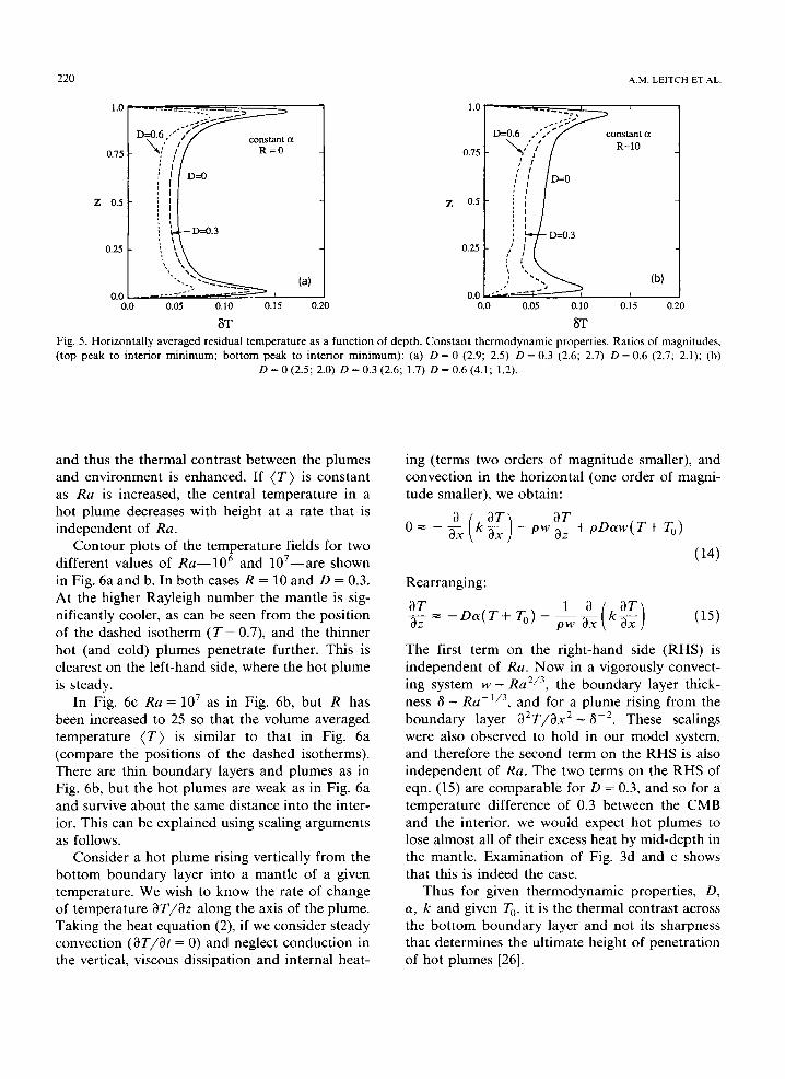
Figures 5a and b are plots of the horizontally

averaged residual temperature as a function of depth for the six cases shown in Figs. 2-4.

[faT"2(x, z) dx] 1/2 (13)

These plots supplement the information given in the color frames, and allow qualitative comparison with plots of seismic anomalies in the mantle [24,5], which show that the seismic heterogeneity spectrum has a large peak at the surface and a smaller peak at the base of the mantle. It is important to remember that at each depth aT can be due to the signatures of both hot and cold plumes.

Figure 5a shows curves for D = 0, 0.3 and 0.6 with no internal heating. We see that as the dis- sipation number increases aT is reduced, but the shape of the profile stays the same. There are peaks in ~-T near each boundary which correspond to plumes breaking away from the boundary layers, and a constant value where the hot and cold plumes traverse the interior. Even the ratio of peak to interior value varies little with D (see figure caption).

Similar curves for R = 10 are given in Fig. 5b. There is a reduction of ~-T with depth associated with the reduced aT of the hot plumes, and the asymmetry between the boundaries is enhanced as D increases, as described above. For D = 0.6, R = 10, there are no hot plumes and so the bot tom peak has disappeared (cf. Fig. 4d).

3.2. Plume penetration with increased Rayleigh number

Increasing Ra at the same value of R encour- ages the survival of hot plumes, simply because the average temperature ( T ) is less (see below),

Fig. 2. C o n s t a n t t h e r m o d y n a m i c p roper t i e s , Ra = 1 0 6 a n d D = 0. a, b, c: F ie lds o f t e m p e r a t u r e T, r es idua l t e m p e r a t u r e ST, a n d vor t i c i ty ~o respect ively , for R = 0. ( T ) = 0.5, r = 0. d, e, f: F ie lds o f T, 8T a n d ~0 for R = 1 0 . ( T ) = 0.7, r = 0.43. C o l o r scale,

p u r p l e ~ red: T (0.0 ---, 1.0); 8T ( - 0.5 ~ + 0.5); ~o ( - 104 ---* + 104).

Fig . 3. C o n s t a n t t h e r m o d y n a m i c p roper t i e s , Ra = 1 0 6 a n d D = 0.3. Scales as for Fig. 2. a, b, c: T, 8T a n d ~o for R = 0. ( T ) = 0.53,

r = 0. d, e, f: T, 8T a n d o~ for R = 1 0 . ( T ) = 0.71, r = 0.7.

Fig. 4. C o n s t a n t t h e r m o d y n a m i c p roper t i e s , Ra = 1 0 6 a n d D = 0.6. Scales as fo r Fig. 2. a, b, c: T, 8T a n d ~0 for R = 0. ( T ) = 0.52,

r = 0. d, e, f: T, 6T a n d ~o for R = 1 0 . ( T ) = 0.71, r = 0.92.

220 A.M. LEITCH ET AL.

1.0

0.75

Z 0.5

0.25

Z

D=0.6,,," / ~ a

///o:0

i,,Lo:o 0.05 0 . I0 0.15

fiT

1.0

0.75

0.5

0.25

(a) 0.0 0.0

0.0 0.20 0.0 0.20

D=0.6 , , ' . " ' ~ constant ot ~',%,'" / ] / R=10

I D=0

! ] - - D - - - 0 . 3

;'

0.05 0.10 0.15

8T Fig. 5. Horizontally averaged residual temperature as a function of depth. Constant thermodynamic properties. Ratios of magnitudes, (top peak to interior minimum; bottom peak to interior minimum): (a) D = 0 (2.9; 2.5) D = 0.3 (2.6; 2.7) D = 0.6 (2.7; 2.1); (b)

D = 0 (2.5; 2.0) D = 0.3 (2.6; 1.7) D = 0.6 (4.1; 1.2).

and thus the thermal contrast between the plumes and environment is enhanced. If ( T ) is constant as Ra is increased, the central temperature in a hot plume decreases with height at a rate that is independent of Ra.

Contour plots of the temperature fields for two different values of Ra- -106 and 10V--are shown in Fig. 6a and b. In both cases R = 10 and D = 0.3. At the higher Rayleigh number the mantle is sig- nificantly cooler, as can be seen from the position of the dashed isotherm (T = 0.7), and the thinner hot (and cold) plumes penetrate further. This is clearest on the left-hand side, where the hot plume is steady.

In Fig. 6c Ra = 107 as in Fig. 6b, but R has been increased to 25 so that the volume averaged temperature ( T ) is similar to that in Fig. 6a (compare the positions of the dashed isotherms). There are thin boundary layers and plumes as in Fig. 6b, but the hot plumes are weak as in Fig. 6a and survive about the same distance into the inter- ior. This can be explained using scaling arguments as follows.

Consider a hot plume rising vertically from the bot tom boundary layer into a mantle of a given temperature. We wish to know the rate of change of temperature ~T/az along the axis of the plume. Taking the heat equation (2), if we consider steady convection (OT/at = 0) and neglect conduction in the vertical, viscous dissipation and internal heat-

ing (terms two orders of magnitude smaller), and convection in the horizontal (one order of magni- tude smaller), we obtain:

O_~__{ k OT ~ OT 0---0x[ ax J - ° w ~ + pDaw(T+ To)

(14)

Rearranging:

1 3 ( kOTl (15) aT -D (T+To) pw ax az ~ 0x )

The first term on the right-hand side (RHS) is independent of Ra. Now in a vigorously convect- ing system w - Ra 2/3, the boundary layer thick- ness 8 - Ra -1/3, and for a plume rising from the boundary layer 02T/Ox 2~ 8 2. These scalings were also observed to hold in our model system, and therefore the second term on the RHS is also independent of Ra. The two terms on the RHS of eqn. (15) are comparable for D = 0.3, and so for a temperature difference of 0.3 between the CMB and the interior, we would expect hot plumes to lose almost all of their excess heat by mid-depth in the mantle. Examination of Fig. 3d and e shows that this is indeed the case.

Thus for given thermodynamic properties, D, a, k and given T 0, it is the thermal contrast across the bot tom boundary layer and not its sharpness that determines the ultimate height of penetration of hot plumes [26].

MANTLE CONVECTION WITH INTERNAL HEATING 221

~ I //

- - - .

\ / /

(a)

(b)

', , ! (c)

Fig. 6. Contour plots of temperature fields illustrating the effect of increased Ra, D = 0.3. Dashed contour line corresponds to T=0.7. (a) Ra=106, R=10. (T)=0.7, r=0.7. (b) Ra=107, R=10. (T)=0.62, r=0.3. (c) Ra=107, R=25. (T)=0.72,

r = 0.74.

3.3. Average temperature vs. Ra and R

For a given internal heating parameter R, the volume averaged temperature ( T ) of the model mantle decreases with Rayleigh number due to higher flux of the internal heat at the surface. Computational values of ( T ) for four values of R are shown in Fig. 7. The different symbols refer to different dissipation numbers, and solid symbols indicate that there are local regions where the temperature exceeds the temperature at the CMB

( T > 1). Uncertainties and time variations are ap- proximately twice the size of the symbols. There is a systematic decrease of ( T ) with Ra trending towards a value of ( T ) = 0 . 5 , as the effect of internal heating becomes negligible. ( T ) is higher for higher compressibility D.

Globally averaged properties are used in parameterized convection to model the thermal evolution of the mantle (e.g. [27]) so it is of interest to compare the results of our computa- tions with the predictions of a simple para-

222 A.M. L E I T C H E T AL.

"x" / \ \ \ \ •

N "-,. \ ° ".,-

0.6

R=0 a 0.5 o o o -

0 . 4 i i l I I I I I I i I l I I I I I I I I l

10 5 10 6 10 7

Ra Fig. 7. Volume averaged temperature as a function of Rayleigh number for various values of R (numbers). Symbols are numerical results; o , D = 0; r,, D = 0.3; D, D = 0.6. Solid symbols indicate that T > 1 occurs within the system. Experimental points all lie on

or above the corresponding theoretical curves [eqn. (18)], solid lines D = 0, dashed lines D = 0.6.

m e t e r i z e d m o d e l . I n s u c h a m o d e l i t is a s s u m e d

t h a t t h e n o r m a l i z e d h e a t f l u x a t a b o u n d a r y c a n

b e e x p r e s s e d as:

q ' d ' N u = ~ = c R a 13 ( 1 6 )

c = R a ~ w h e r e R a c is t h e c r i t i c a l R a y l e i g h n u m -

b e r f o r o n s e t o f c o n v e c t i o n , a n d fl i s a c o n s t a n t

b e t w e e n 1 / 3 a n d 1 / 4 . I f t h e r e is n o i n t e r a c t i o n

b e t w e e n t h e b o u n d a r i e s (e .g . f u l l y t u r b u l e n t c o n -

v e c t i o n ) , t h e f l u x p e r u n i t a r e a q ' is i n d e p e n d e n t

o f t h e b o u n d a r y s e p a r a t i o n d ' a n d fl = 1 / 3 .

W e n o w a p p l y t h i s m o d e l t o o u r s y s t e m , a s s u m -

i n g t h a t t h e o n l y e f f e c t o f i n t e r n a l h e a t i n g is t o

i n c r e a s e t h e a v e r a g e t e m p e r a t u r e ( T ) . T h i s is a

r e a s o n a b l e a s s u m p t i o n , s i n c e o v e r t h e p a r a m e t e r

r a n g e in o u r s t u d y , i n t h e b o u n d a r y l a y e r s a n d

p l u m e s i n t e r n a l h e a t i n g is t w o o r d e r s o f m a g n i -

t u d e s m a l l e r t h a n m o r e i m p o r t a n t t e r m s i n t h e

Fig. 8. Pressure-dependent thermal expansivity (a = ot01P -6, z > 0.65; a = Ct02P -2, Z < 0.65). Ra = 1 0 6. Scales as for Fig. 2. a, b, c: Typical fields of T, 8T and to for R = 0. ( T ) = 0.53, r = 0. d,e, f: T, 8T and to for R = 10. ( T ) = 0.71, r = 0.68.

Fig. 9. Pressure-dependent thermal expansivity (a = a01p -2, z < 0.65; a = a02P -6, z > 0.65) and thermal conductivity (k = kop~). Ra =106. Scales as for Fig. 2. a, b, c: Typical fields of T, 8T and to for R =10. ( T ) ~ 0.83, r = 0.75.

Fig. 10. Pressure-dependent thermal expansivity (a = a0p-6). Ra = 106. Scales as for Fig. 2. a, b, c: Typical fields of T, 8T and to for R = 0. ( T ) = 0.54, r = 0. d, e, f: T, 8T and to for R = 10. ( T ) = 0.70, r = 0.52.

Fig. 11. Pressure-dependent thermal expansivity (a = aop-6) , and thermal conductivity (k = k0p3). Ra = 106. Scales as for Fig. 2. a, b, c: Typical fields of T, 8T and to for R =10. ( T ) = 0.83, r = 0.54.

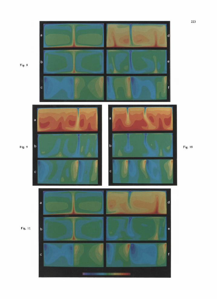
Fig. 8

Fig. 9

Fig. 11

223

Fig. 10

224 A.M. LEITCH ET AL.

heat equation. The normalized heat fluxes at the surface and the CMB are then:

24/3 ( Ra ~ 1/3 ~ c ) (1 - ( T ) ) 4/3 (17b) qCMB

where Ra is the Rayleigh number based on the temperature difference AT between the bounda- ries. The factor of 2 arises because for each boundary the apparent temperature difference across the layer is twice the temperature difference between the boundary and the interior. In quasi- steady-state, the difference in the heat fluxes at the surface and CMB is the volume rate of inter- nal heating,

R = qo - qCMB

Ra ,1/3 4 / 3 = 24/3( Ra~ ) [(T) - ( 1 - (T))4/~] (18)

This equation describes the relationship be- tween internal heating R, Rayleigh number and average temperature ( T ) in quasi-steady-state. Curves of eqn. (18) for four values of R are drawn in Fig. 7. For the solid lines Ra c = 657, the value for incompressible convection with free boundary conditions [28], and for the dashed lines Rac = 1150, an approximate value for compressional convection with D = 0.6 (based on the value for spherical convection [291). In general, the data points (symbols) follow the variation with Ra indicated by the curves, and the temperature rise with /) can be explained by the increase in the critical Rayleigh number. Most of the data, how- ever, lies above the corresponding theoretical line, and we attribute this to nonlinear interaction be- tween the top and bot tom boundary layers.

For incompressible convection with no internal heating (D = 0, R = 0) convection is symmetrical and therefore the temperature ( T ) must equal the average temperature of the boundaries, 0.5. For D > 0, the adiabatic gradient which suppresses convection is steeper at the CMB, and we might expect ( T ) < 0 . 5 for R = 0 . In fact, ( T ) > 0 . 5 because heat transfer is enhanced by the impinge- ment of cold plumes onto the lower boundary [14]. Hot plumes, being relatively weaker, have a lesser effect on the heat transfer at the surface. As R

and D increase the asymmetry in the strength of hot and cold plumes increases (section 3.1): the lower boundary "sees" more effect of the cold upper boundary through the interior than vice versa, and thus the ( T ) is systematically higher than the simple theory predicts.

We have shown that eqn. (18) can be used to calculate globally averaged temperatures which are about 5% lower than our observations. We should note that over this range of Ra the Nusselt num- ber (eqn. 16) depends on aspect ratio [30]. Some of the scatter of points in Fig. 7 is due to changing convection cell size. Also the individual dimen- sionless fluxes tend to be larger than the predict- ions of eqns. (17).

4. Density-dependent a and k

The thermal expansivity a comes into the buoyancy term in the momentum equation (1), so that for the same temperature difference, if decreases as density increases, the driving buoyancy force at depth is less than it is near the surface. The local Rayleigh number will be smaller at depth thus we expect a broader bot tom boundary layer and broader hot plumes, a also appears in the compressional heat ing/cooling term of the heat equation (2), and its variation with density implies that the adiabatic temperature gradient becomes much shallower at depth. The increase in the conductivity k with depth means that conduction of heat from the core is facilitated relative to conduction to the surface: this should raise the average temperature of the mantle.

4.1. Variable a [equation (7)]

The density profile that was used for these simulations is drawn as a solid line in Fig. la. The amount of compression is similar to that for the constant properties case with D = 0.6, but the average dissipation number ( a D ) , which de- termines the importance of compressional heating and cooling, is 0.25, similar to the constant prop- erties case with D = 0.3. The variation of t~ with depth is the dashed line I l I in Fig. lb. There is a factor of 5 decrease in a from the surface to the CMB, with most of the change occurring in the upper third of the mantle.

M A N T L E C O N V E C T I O N W I T H I N T E R N A L H E A T I N G 225

Typical fields of temperature, residual tempera- ture and vorticity for internal heating parameters R of 0 and 10 are shown in Fig. 8. The tempera- ture ( T ) is similar to the constant a cases, and for R = 10 the flux ratio r is closest to the case with D = 0.3. The shapes of the plumes can be ex- plained in a straightforward manner by the depth variation of a.

For both values of R, the temperature and flow fields can be seen as a combination of the fields seen in the constant properties cases. Near the CMB where a is small, the temperature field looks similar to that for incompressible convection: both hot and cold plumes lose heat only slowly and the adiabatic gradient between the plumes is low. Be- cause the effective Rayleigh number is lower at the CMB for variable a, the lower boundary layer and hot plumes in Fig. 8 are broader than those in Fig. 2. Further up in the mantle, as a increases, the hot plumes become broader and lose their thermal signatures (cf. Fig. 3) [25,10]. Unlike the incompressible case, the hot plumes do not pro- duce a large mushroom cap at the upper boundary. We note that there are large differences in ST(x, z) between the constant a and variable a cases.

The thermal residuals 8T (Fig. 8b and e) em- phasise the points in the previous paragraph. Near the CMB the thermal residuals of both hot and cold plumes are strong features, reflecting the fact that thermal contrasts are not rapidly dissipated by compressional heating and cooling. Near the surface however, particularly when there is inter- nal heating, there is little signal from the hot plumes.

The vorticity fields (Fig. 8c and f) show a dramatic difference from those in Figs. 2 4c and f. While changes in the temperature (and 6T) fields are due to the effect of variation of a in the compressional heat ing/cooling term in the heat equation, changes in the vorticity fields are due to the effect of a in the buoyancy term in the momentum equation. Equation (12) shows that vorticity has its source in horizontal gradients in buoyancy. For R = 0 (Fig. 8c) the vorticity gener- ated by the rising hot plume first decreases with height as the thermal gradients in the plume de- crease, and then increases again as the rapidly growing a more than compensates for the continu- ing decrease in thermal gradients. The cold plumes lose buoyancy as they descend due to both de-

creasing a and decreasing thermal gradients, and thus ~ is high in the upper part of the mantle and decreases with depth.

The introduction of internal heating R = 10 (Fig. 8f) weakens the thermal gradients in the hot plumes to such a degree that the peak in vorticity in the upper mantle is not seen. Vorticity gener- ated by cold plumes, however, is increased. Com- pared with constant a cases (Figs. 2-4f), where the cold plumes generate high vorticity throughout the depth of the mantle, the vorticity for variable a is concentrated in the upper part of the mantle.

4.1.1. Variable a and k Figure 9 illustrates convection when in addition

to a depth-varying a we introduce a thermal con- ductivity k which increases with depth according to eqn. (8) (dotted line in Fig. lb). k is then a factor of 3.4 greater at the CMB than it is at the surface. For Fig. 9 the internal heating parameter R = 10. In the following, comparisons will be made between Fig. 9 and the corresponding case with k = 1, Fig. 8d-f .

The larger conductivity at the CMB firstly means that more heat is conducted into the mantle from the core. The mantle is significantly hotter and the flux ratio r is lower. Larger k at the CMB also leads to a broader lower boundary layer and more diffuse plumes. The hot plumes, having lower thermal contrast with the mantle (see section 3.2), lose their thermal signature more readily. The thermal residuals of the hot plumes (Fig. 9b) are therefore less intense and restricted closer to the CMB. Finally, since thermal gradients in the hot plumes are weaker, the vorticity associated with them is less (Fig. 9c).

4.2. Variable a [equation (6)]

We now describe convection when the thermal expansivity a decreases throughout the mantle according to the inverse 6th power of density [eqn. (6) and solid line II in Fig. lb]. a, and therefore the effective dissipation number and the effective Rayleigh number also, decrease by a factor of 12 from the surface to the CMB. Many of the fea- tures of Figs. 10 and 11 are merely an exaggera- tion of those described in the section 4.1 above and so they will be mentioned only briefly.

Near the CMB, very low a means that the

226 A.M. L E I T C H ET A L

temperature and residual temperature fields (Fig. 10a, b and d, e) are very similar to incompressible convection (Fig. 2), but with the broader boundary layer and plumes associated with lower Rayleigh number. The hot plumes have a strong signature in the residual temperature field, but little vortic- ity is generated. Near the surface, the thermal signature of the hot plumes is damped by adia- batic cooling due to the rapidly increasing a, and at the same time the vorticity is much higher.

Once again, the average temperature ( T ) is similar to that for constant properties, but the flux ratio r is lower than for the cases shown in Figs. 3 and 8.

4. 2.1. Variable a and k Figure 11 shows typical frames of T, 3T and ~o

when density dependent thermal conductivity [eqn. (8)] is included in the model. Comparing with Fig. 9, we see the mantle is slightly hotter, the thermal residuals of the hot plumes weaker, and the vortic- ity is stronger near the surface and weaker near the CMB.

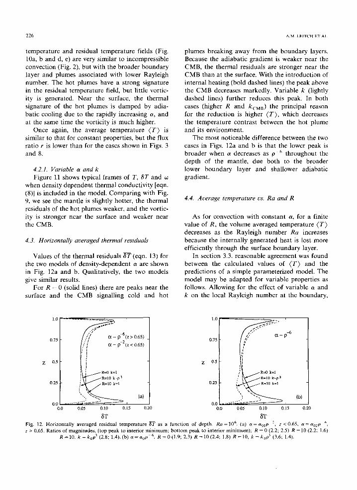
4. 3. Horizontally averaged thermal residuals

Values of the thermal residuals ~ (eqn. 13) for the two models of density-dependent a are shown in Fig. 12a and b. Qualitatively, the two models give similar results.

For R = 0 (solid lines) there are peaks near the surface and the CMB signalling cold and hot

plumes breaking away from the boundary layers. Because the adiabatic gradient is weaker near the CMB, the thermal residuals are stronger near the CMB than at the surface. With the introduction of internal heating (bold dashed lines) the peak above the CMB decreases markedly. Variable k (lightly dashed lines) further reduces this peak. In both cases (higher R and kCMB) the principal reason for the reduction is higher ( T ) , which decreases the temperature contrast between the hot plume and its environment.

The most noticeable difference between the two cases in Figs. 12a and b is that the lower peak is broader when a decreases as O -6 throughout the depth of the mantle, due both to the broader lower boundary layer and shallower adiabatic gradient.

4.4. Average temperature vs. Ra and R

As for convection with constant a, for a finite value of R, the volume averaged temperature ( T ) decreases as the Rayleigh number Ra increases because the internally generated heat is lost more efficiently through the surface boundary layer.

In section 3.3, reasonable agreement was found between the calculated values of ( T ) and the predictions of a simple parameterized model. The model may be adapted for variable properties as follows. Allowing for the effect of variable a and k on the local Rayleigh number at the boundary,

1.0

0.75

0.5

0.25

Z

- ~ ~ p~5(z > 0.65)

I.,:[ ~ - p-2(z < 0.65) I I I I 1 I

I / R=O k = l

y ~ R=I0 k - p 3

~ . . / R= 10 k=l

0.05 0.10 0.15

1.0

0.75

0.5

0.25

(a) 0.0 0.0

0.0 0.20 0.0

ST

~ et_p -6

i

R=0 k=l

~ r ~ R=10 k - p 3

0.05 0.10 0.15

ST

(b)

0.20

Fig. 12. Horizontally averaged residual temperature 6"~ as a function of depth. Ra = 106. (a) a = a01p 2, z < 0.65, a = a0zp -6, z > 0.65. Ratios of magnitudes, (top peak to interior min imum; bo t tom peak to interior min imum); R = 0 (2.2; 2.5) R = 10 (2.2; 1.6)

R =10, k = ko# 3 (2.8; 1.4). (b) a = a0p -6. R = 0 (1.9; 2.3) R = 1 0 (2.4; 1.8) R =10, k = k0p 3 (3.6; 1.4).

MANTLE CONVECTION WITH INTERNAL HEATING 221

and of variable k on the heat transfer, eqns. (17) become:

numbers written on each curve refer to the value of the internal heating parameter R.

(19a>

x (1 - (T))“” (19b) where it must be kept in mind that the critical Rayleigh numbers at each boundary will be differ- ent because of the difference in the effective dis- sipation number D,,, = CWD. Equation (18) then

becomes,

i

16p~k&xoRa l/3

R= Ra CO

P&,&,,acM,Raco 1’3 Pikho RacCMB i

(20)

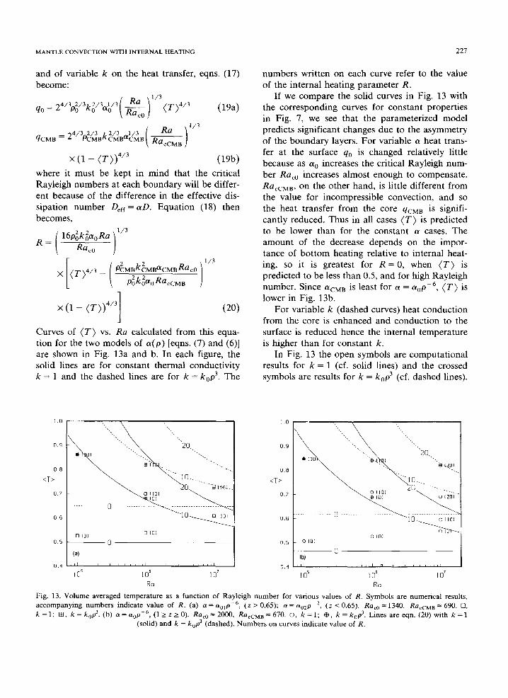
Curves of (T) vs. Ra calculated from this equa- tion for the two models of cu(p) [eqns. (7) and (6)] are shown in Fig. 13a and b. In each figure, the solid lines are for constant thermal conductivity k = 1 and the dashed lines are for k = kop3. The

1 ,;lol g ,11 , , , ,,,

IO5 lo6 10' RO

If we compare the solid curves in Fig. 13 with the corresponding curves for constant properties in Fig. 7, we see that the parameterized model predicts significant changes due to the asymmetry of the boundary layers. For variable (Y heat trans- fer at the surface go is changed relatively little because as cxo increases the critical Rayleigh num- ber Ra, increases almost enough to compensate. Ra cCMB, on the other hand, is little different from

the value for incompressible convection, and so the heat transfer from the core qCMB is signifi- cantly reduced. Thus in all cases (T) is predicted to be lower than for the constant (Y cases. The amount of the decrease depends on the impor- tance of bottom heating relative to internal heat- ing, so it is greatest for R = 0, when (T) is predicted to be less than 0.5, and for high Rayleigh number. Since aCMB is least for (Y = aopP6, (T) is lower in Fig. 13b.

For variable k (dashed curves) heat conduction from the core is enhanced and conduction to the surface is reduced hence the internal temperature is higher than for constant k.

In Fig. 13 the open symbols are computational results for k = 1 (cf. solid lines) and the crossed symbols are results for k = kop3 (cf. dashed lines),

1 .o

0.9

0.8

CT>

0.7

0.6

0.5

0.4

Fig. 13. Volume averaged temperature as a function of Rayleigh number for various values of R. Symbols are numerical results, accompanying numbers indicate value of R. (a) a = a,,,~-~, (z > 0.65); a = CT,,~~~~, (z -C 0.65). Ra, = 1340, Ra,,,, z 690. 0,

k=l; H, k=k,$. (b) a=~p-~, (lkz>O). Ra,,=2000, RacCMB= 670. 0, k =l; @, k = k,p3. Lines are eqn. (20) with k =I (solid) and k = kop3 (dashed). Numbers on curves indicate value of R.

228 A.M. L E I T C H E T AL.

The number next to each symbol gives the value of R. It is necessary to label the points because some lie at significantly higher temperatures than the corresponding curves. In particular, notice that for R = 0, ( T ) > 0.5.

The higher than predicted temperatures are due to the influence of the upper boundary layer on the lower boundary layer. The cold plumes com- press and agitate the lower boundary layer, en- hancing heat transfer from the core. Time se- quences of convective flow for a = a 0 p - 6 showed that the lowei" boundary reacted almost passively, hot plumes being squeezed up between impinging cold plumes. This effect caused high temperatures for constant a also (section 3.3). The asymmetry in the strength and penetration depths of plumes from opposite boundaries is much greater for vari- able a and so the enhancement of the core heat is correspondingly greater also.

For very high internal temperatures (variable k with internal heating), computed temperatures are close to the theoretical lines, probably because the contribution of core heat is small and heat is lost more efficiently at the surface due to a larger number of downwellings. For Ra = 105, R = 10 the computed temperature is less than the model predicts. The black symbol indicates that there are local regions where the temperature exceeds Tc.MB.

Strong plumes from the upper boundary thus make up for the insufficiencies of weak plumes from the lower boundary layer in promoting heat flux from the core. The temperatures for the two models of a are similar to each other and to the temperature for constant a, contrary to the pre- dictions of a simple parameterized model.

The temperature of an internally heated system varies according to the pattern of convection, as the aspect ratio of convecting cells is altered. For constant a (section 3) this effect was responsible for changes in ( T ) of the order of 0.01AT, or the size of the symbols in Fig. 7. For pressure-depen- dent c~ the change in ( T ) can be more, provided that core heating makes an important contribution to the heat content of the mantle, because the different number and arrangement of cold plumes striking the lower boundary can markedly alter the heat transfer there. When k also varied with depth (increasing the importance of core heat) temperature variations of up to 0.02-0.03AT were observed.

5. Summary of results

In the above, we have investigated how the plume structure, thermal residuals, vorticity and average temperature in the mantle depend upon a few important mantle parameters: the dissipation number D, the internal heating parameter R, and the Rayleigh number Ra. We have been particu- larly interested in how far the hot signal of plumes from the CMB can penetrate the mantle, and the depth-dependence of average thermal residuals.

We first considered a mantle with constant thermodynamic quantities a, k. For an incom- pressible flow with no internal heating hot and cold plumes are symmetrical and penetrate the entire depth of the mantle. Internal heating re- duces the thermal contrast between the hot plumes and surrounding mantle without changing the shape of the plumes, and introduces hot patches at mid-depths.

For finite dissipation number D, the thermal signatures of the plumes are damped, the damping being greater for the hot plumes. Internal heating exaggerates this asymmetry, and for D = 0.6 and ( T ) = 0.7 hot plumes are eliminated in favour of a broad return flow. The height of penetration of hot plumes was shown to be a function of D and the thermal contrast across the lower boundary layer, independent of the Rayleigh number. The average temperature in the simulations was com- pared with the predictions of a simple para- meterized convection model, which assumed no interaction between the boundary layers. Varia- tions in ( T ) with Ra, D and R were successfully predicted, but the temperatures of the simulations were systematically high because the impingement of cold plumes onto the lower boundary layer enhanced heat transfer from the core.

Thermal residuals are strongest near the boundaries where the plumes break away from the boundary layers. Internal heating and com- pressibility reduce thermal contrasts and hence thermal residuals near the CMB. Thermal residu- als depend also on depth variations of a. Cold plumes generate relatively uniform vorticity throughout the depth of the mantle. Internal heat- ing and decompressional cooling reduce the vortic- ity generated by hot plumes and restrict it close to the CMB.

Depth-dependent a means that the local

M A N T L E C O N V E C T I O N W I T H I N T E R N A L H E A T I N G 229

Rayleigh number Ra and dissipation number D change with depth. The functions studied (Fig. lb) lead to temperature and vorticity fields which resemble highly compressible convection near the surface and incompressible, lower Rayleigh num- ber convection near the CMB. Thus near the surface there is a steep adiabatic gradient and strong dissipation of thermal anomalies, whereas at depth broad plumes with strong thermal anomalies exist in a more homogeneous environ- ment. Since the buoyancy force is reduced with depth, vorticity is much higher in the upper part of the mantle. The two models of a (0 ) gave qualitatively similar results.

An increase in k with depth results in an increase in the volume average temperature of the mantle due to increased core heat, and a broad- ening of the lower boundary layer and hot plumes due to increased local Rayleigh number at the CMB.

When compared with the predictions of the model of parameterized convection, the volume averaged temperature { T ) was significantly higher. As for the constant ct cases, this was due to impingement of cold plumes onto the lower boundary. In this case the enhancement of the core heat was greater because the asymmetry of the boundary layers was greater.

6. Conclusions and geophysical implications

The principal aim of this study was to investi- gate the existence and penetration height of hot plumes from the CMB in an internally heated mantle. We wished to see whether seismic residu- als above the CMB could be explained by the existence of hot plumes, and whether these plumes penetrate the mantle and manifest themselves as hot spots on the Earth's surface.

We showed that the existence of plumes de- pends on the temperature contrast across the lower boundary layer and the local dissipation number D, which is proportional to the thermal expansiv- ity a. If the thermal expansivity a were constant at its zero pressure value, then chondritic quantities of heat producing elements would suppress the formation of plumes at the CMB. However if a decreases by a factor of 3 or more (a moderate decrease that few would argue against) then hot plumes at the CMB are expected. Thus our model

would support the interpretation that seismic re- siduals above the CMB are due to hot plumes rising from a thermal boundary layer.

The penetration height of a hot plume from the CMB (the height to which it can rise in the mantle before losing a given amount of its centreline temperature), also depends on D and the temper- ature change across the lower boundary layer, independent of the Rayleigh number. The more a decreases with depth, the higher in the mantle hot plumes can rise. If a varies by a factor of 5 across the mantle, a plume reaches about 75% of the distance to the surface before its thermal signature is dissipated. If ct changes by a factor of 12, some thermal signature is expressed at the surface, but it is weak and very broad.

The picture of mantle convection presented by this study is one where hot plumes exist at depth but dissipate into a broad general upflow in the upper part of the mantle. Passive upwelling of hot mantle at mid-ocean ridges [7], and the presence of seismic anomalies above the CMB [5] are both consistent with this picture. Hot spots are not predicted by this model. They may originate from the hot upwellings near the CMB, but to penetrate from mid-mantle levels to the surface we must appeal to processes other than isoviscous thermal convection. Such processes include partial melting and non-Newtonian rheology (e.g. [31]) which would concentrate the plume into a narrower channel. This would be helped by the tendency of a two-dimensional plume to form axisymmetric plumes along its length [26,32]. An uneven distri- bution of internal heating [33] or other composi- tional differences might also increase the buoyancy and thus the penetration height of a plume. We would expect some correlation of hot-spot distri- bution with slow seismic anomalies above the CMB, but not all hot plumes would necessarily produce hot-spots.

If hot-spots arise in one of these manners from regions of elevated temperature in the mantle, then it raises the possibility that they may also originate from the "ho t patches" that form from a build-up of internal heat near turning points in the flow field. The turning points occur below mid-depth near the downflowing cold plumes, which are probably anchored on subducting plates. It has been found that hot-spots are less common near convergent plate boundaries [34]. In terms of

230 A.M. L E I T C H E T A L .

our models, if hot-spot plumes did arise from the hot patches, they would tend to be disrupted by the local large-scale flow which would sweep them into the downflowing plume. Hot-spot plumes ris- ing from thermal plumes at the CMB on the other hand, would follow the broad large-scale flow towards the surface.

Whether there is local melting at the hot patches [35,36] depends on the melting temperature and the length of time a cold plume exists. Chondrite quantities of heat-producing elements (R = 10) would raise the temperature of a turning point region by 150K (0.05AT) in a billion years (At = 0.005).

Measurements of horizontally averaged seismic residuals in the mantle [5] show a strong peak in the upper mantle, a gradual decrease with depth, and then a weaker peak just above the CMB. This is qualitatively similar to some of the graphs of ~-T for compressible convection with internal heating shown in Figs. 5b and 12. The peak above the CMB is smaller principally because of the smaller thermal contrast across the lower boundary layer. Machetel and Yuen [36] used comparisons of re- sidual thermal anomalies and seismic anomalies in constraining the temperature at the CMB, for an internally heated mantle with spherical geometry. The temperature contrast at the CMB would also be reduced by a high core flux (if k at the CMB is high) and secular heat, which could be modelled as an increase in the effective R.

In addition to our conclusions on the nature of hot plumes, the present work reveals some other interesting implications of a strongly decreasing a in an internally heated mantle.

The local Rayleigh number is proportional to a. Very low a at the CMB would imply the hot boundary layer and hot plumes are broader, weaker structures and velocities in the lower man- tle are lower than previously assumed. The rela- tively higher velocities and more intense circula- tion in the upper mantle provide a mechanism by which the compositional differences there may be homogenized on a shorter timescale than for the whole mantle, thus allowing compositional dif- ferences to exist between upper and lower mantle without resorting to layered convection. (The rela- tion between shear and mixing has been investi- gated by Olson et al. [37] and Hofmann and McKenzie [38]).

Reduced Ra at depth might be expected to retard heat flow from the core, allowing higher core temperatures or lower mantle temperatures. In our simulations, however, we found mantle temperatures to be surprisingly robust with re- spect to depth variations in a, because heat flux from the core was enhanced as cold plumes with large negative buoyancy impinged on the CMB. Heat flux from the core is thus passively driven by "forced" convection from cold plumes, rather than being due to buoyancy contrasts across the D" . Local models of flow near the CMB which do not take into account the influence of cold plumes (e.g. [39]) may underestimate heat transfer and flow velocities.

Time variations in average temperature depend on the relative importance of core heat in the heat content of the mantle. If heat from the core is a significant component of mantle heat, as may occur if k is a strong function of pressure, then different "modes" (patterns) of convection in a mantle with strongly variable a can lead to large variations in the average temperature. Switching between the two different modes may occur lead- ing to periodic variations in the heat flow at the surface and CMB, which can influence the geody- namic process. Similar mode-switching with sig- nificant geophysical consequences may occur in the liquid core, leading to flipping of the polarity of the magnetic field, and in the circulation of the oceans, perhaps triggering ice ages [40].

Although the time integrated average tempera- ture does not change much with the profile of a, the distribution of temperature does. The depth variations of a discussed in this paper imply a strong temperature gradient in the upper part of the mantle and shallow gradient near the CMB. The melting temperature T m of the mantle in- creases with depth [41,42], and so variable a brings the upper and mid mantle closer to T m. The viscos- ity ~ is related to the ratio T i T m so this is turn implies that for variable c(, 7/ increases more strongly with depth in the lower half of the man- tle. Such an increase is predicted by the recent nonlinear inversion study by Ricard and Bai [8].

In our simulations in a box of aspect ratio 2.5, the pattern of upflow at the CMB appeared to be determined by the cold plumes which squeeze hot plumes up between them, however we were led to modify this conclusion. Hansen et al. [43] carried

M A N T L E C O N V E C T I O N W I T H I N T E R N A L H E A T I N G 231

out simulations of incompressible, extended Bous- sinesq [13] convection at aspect ratio 10 and Ra =

2-6 × 107. For constant a [43], the upper and lower boundary layers had a constant relative velocity corresponding to a large-scale circulation in the box, and hot and cold plumes broke up into blobs as they traversed the box. Using a ( z ) as given in [25], with a contrast of 10 between the top and bot tom boundaries there was a dramatic change in the convection pattern: the large-scale circulation was broken into cells of aspect ratio 3 -4 by the hot plumes [44]. The cold plumes were still very time-dependent and broke up into blobs as they sank, however the hot plumes were almost stationary, rising vertically from the bot tom boundary layer and spreading in an extensive mushroom cap along the top boundary layer. There were few thermal anomalies in the lower mantle for a ( z ) runs.

This can be interpreted as follows. Fluid in the hot plumes accelerates as it rises due to its increas- ing buoyancy. Hot plumes therefore rise more vertically and when they reach the surface they produce a strong outward flow which sweeps cold boundary layer instabilities away from the head of the hot plume. At its base, the hot plume flow is weak: it is pinned in position by the more vigor- ous flow at higher levels and by virtue of the fact that disrupting cold plumes are held at a distance.

This is a very interesting example of boundary layer interaction where hot outflow at the opposite

boundary influences a hot plume at its source, and indicates that strongly varying a can change the pattern of convection. The stationary nature of the hot plumes immediately reminds us of the small relative motion between hot-spots. However, in our fully compressible, internally heated model hot plumes were weak when they reached the surface and so might not produce such dramatic changes even at large aspect ratio. This matter awaits future research.

Finally, two observations should be made with reference to the scaling used in this study. It should be kept in mind that p, a, k were normal- ized so that the depth averages of the various models were the same. For variable a the Rayleigh number based on surface values Ra o is a factor of three greater than Ra. If models are compared at the same Ra o, a decreasing a does lead to an increase in the mantle temperature ( T ) . On the

other hand, a thermal conductivity k which in- creases with depth will always lead to an increase in ( T ) regardless of at what depth k is compared because the conductivity at the surface, which promotes heat loss is reduced relative to that at the CMB, which promotes heat gain.

Many interesting consequences of strongly varying ~x in mantle convection have been de- scribes in this work. Impor tant features for inclu- sion in further study would be variable and non- Newtonian viscosity and phase changes in the upper mantle.

Acknowledgements

The authors would like to thank Dr. R. Boehler and Prof. V. Zharkov for helpful discussions and C. Lausten for her excellent technical assistance. Research was supported by NSF grant EAR- 8817039 and N.A.S.A. Geodynamic Program.

References

1 A. Chopelas and R. Boehler, Thermal expansion measure- ments at very high pressure, systematics and a case for a chemically homogeneous mantle, Geophys. Res. Lett. 16, 1347-1350, 1989.

2 J.H. Woodhouse and A.M. Dziewonski, Mapping the upper mantle: three-dimensional modelling of earth structure by inversion of seismic waveforms, J. Geophys. Res. 89, 5953- 5986, 1984.

3 T. Tanimoto, The three-dimensional shear wave structure in the mantle by overtone waveform inversion--I . Radial seismogram inversion, Geophys. J. R. Astron. Soc. 89, 713-740, 1987.

4 W.J. Morgan, Convective plumes in the lower mantle, Nature 230, 42-43, 1971.

5 T. Tanimoto, Long wavelength S-wave velocity structure throughout the mantle, Geophys. J. Int. 100, 327-330, 1990.

6 D.P. McKenzie, J.M. Roberts and N.O. Weiss, Convection in the Earth's mantle: towards a numerical simulation, J. Fluid Mech. 62, 465-538, 1974.

7 D.P. McKenzie and M.J. Bickle, The volume and composi- tion of melt generated by extension of the lithosphere, J. Petrol. 29 (3), 625-679, 1988.

8 Y. Ricard and W. Bai, Inferring the mantle viscosity and its three-dimensional density structure from geoid, topography and velocities, Geophys. J. Int., 1991.

9 G.T. Jarvis and D.P. McKenzie, Convection in a com- pressible fluid with infinite Prandtl number, J. Fluid Mech. 96, 515-583, 1980.

10 G. Sewell, Analysis of a Finite Element Method, 155 pp., Springer, New York, N.Y., 1985.

232 A.M. LEITCH ET AL

11 V. Steinbach, U. Hansen and A. Ebel, Compressible con- vection in the Earth's mantle: a comparison of different approaches, Geophys. Res. Lett. 16, 633-635, 1989.

12 F. Birch, Elasticity and constitution of the Earth's interior, J. Geophys. Res. 57, 227-287, 1952.

13 D.L. Turcotte, A.T. Hsui, K.H. Torrance and G. Schubert, Influence of viscous dissipation on Benard convection, J. Fluid Mech. 64, 369-374, 1974.

14 S.D. Weinstein, P.L. Olson and D.A. Yuen, Time-depen- dent large aspect-ratio thermal convection in the Earth's mantle, Geophys. Astrophys. Fluid Dyn. 47, 157-197, 1989.

15 D.L. Anderson, Theory of the Earth, 366 pp., Blackwell, Oxford, 1989.

16 R.G. McQueen, S.P. Marsh, J.W. Taylor, J.N. Fritz and W.J. Carter, The equation of state of solids from shock-wave studies, in: High Velocity Impact Phenomena, R. Kinslow, ed., Academic Press, New York, N.Y., pp. 293-417, 1970.

17 V.N. Zharkov, Interior Structure of the Earth and Planets, 436 pp. Harwood, 1986.

18 F. Quareni and F. Mulargia, The validity of the common approximate expressions for the Grtineisen parameter, Ge- ophys. J. 93, 505-519, 1988.

19 O. Anderson, A. Chopelas and R. Boehler, Thermal expan- sivity versus pressure at constant temperature: a re-ex- arnination, Geophys. Res. Lett. 17, 685-688, 1990.

20 D.L. Anderson, A seismic equation of state II. Shear prop- erties and thermodynamics of the lower mantle, Phys. Earth Planet. Int., 45, 307-323, 1987.

21 R.G. Ross, P. Andersson, B. Sundqvist and G. Baechstroem, Thermal conductivity of solids and liquids under pressure, Rep. Prog. Phys. 47, 1347-1402, 1984.

22 A.M. Dziewonski and D.L. Anderson, Preliminary refer- ence Earth model, Phys. Earth Planet. Int. 25, 297-356, 1981.

23 L.M. Fleitout and D.A. Yuen, Steady-state secondary con- vection beneath lithospheric plates with temperature and pressure-dependent viscosity. J. Geophys. Res. 89, 7653- 7670, 1984.

24 S. Honda, The RMS residual temperature in the convecting mantle and seismic heterogeneities, J. Phys. Earth 35, 195- 207, 1987.

25 W. Zhao and D.A. Yuen, The effects of adiabatic and viscous beatings on plumes, Geophys. Res. Lett. 14, 1223- 1227, 1987.

26 N.H. Sleep, M.A. Richards and B.H. Hager, Onset of mantle plumes in the presence of preexisting convection, J. Geophys. Res. 93, 7672-7689, 1988.

27 D.P. McKenzie and N.O. Weiss, Speculations on the ther- mal and tectonic history of the Earth, Geophys. J. R. Astron. Soc. 42, 131-174, 1975.

28 J.S. Turner, Buoyancy effects in fluids, Cambridge Univer- sity Press, London 1973.

29 P. Machetel and D.A. Yuen, Penetrative convective flows induced by internal heating and mantle compressibility, J. Geophys. Res. 94, 10,609-10,626, 1989.

30 U. Hansen and A. Ebel, Numerical and dynamical stability of convection cells in the Rayleigh number range 103-8 x 105, Ann. Geophys. 2, 291-302, 1984.

31 U.R. Christensen and D.A. Yuen, Time-dependent convec- tion with non-Newtonian viscosity, J. Geophys. Res. 94, 814-820, 1989.

32 J.A. Whitehead and K.R. Helfrich, Wave transport of deep mantle material, Nature 336, 59-61, 1988.

33 S. Honda and D.A. Yuen, Mantle convection with moving heat-source anomalies: geophysical and geochemical impli- cations, Earth Planet. Sci. Lett. 96, 349-366, 1990.

34 S.D. Weinstein and P.L. Olson, The proximity of hotspots to convergent and divergent plate boundaries, Geophys. Res. Lett. 16, 679-681, 1989.

35 A.M. Leitch and D.A. Yuen, Internal heating and thermal constraints on the mantle, Geophys. Res. Lett. 16, 1407- 1410, 1989.

36 P. Machetel and D.A. Yuen, 3000 to 3500 K bottom mantle temperature constraints from spherical compressible con- vection models, Phys. Earth Planet. Int., 1991 (submitted).

37 P.L. Olson, D.A. Yuen and D.S. Balsiger, Mixing of passive heterogeneities by mantle convection, J. Geophys. Res. 89, 425-435, 1984.

38 N.R.M. Hofmann and D.P. McKenzie, The destruction of geochemical heterogeneities by differential fluid motions during convection, Geophys. J. R. Astron. Soc. 82, 163-206, 1985.

39 P.L. Olson, G. Schubert and C.A. Anderson, Plume forma- tion in the D"-layer and the roughness of the core-mantle boundary, Nature 327, 409-413, 1987.

40 W.S. Broecker and G.H. Denton, The role of ocean-atmo- sphere reorganizations in glacial cycles, Geochim. Cosmo- chim. Acta 53, 2465-2501, 1989.

41 E. Knittle and R. Jeanloz, Melting curve of (Mg, Fe)SiO 3 perovskite to 96 GPa, evidence for a structural transition in lower mantle melts, Geophys. Res. Lett. 16 (1989) 421-424, 1989.

42 J.P. Poirier, Lindemann law and the melting temperature of perovskites, Physics Earth Planet. Inter. 54, 364-369, 1989.

43 U. Hansen, D.A. Yuen and S.E. Kroenig, Transition to hard turbulence in thermal convection at infinite Prandtl number, Phys. Fluids A2(12), 2157-2163, 1990.

44 D.A. Yuen, A.M. Leitch and U.S. Hansen, Dynamical influences of pressure-dependent thermal expansivity on mantle convection, in: Glacial Isostasy, Sea-Level and Mantle Rheology, C.A. Sabadini and K. Lambeck, eds., Kluwer, Dordrecht 1991 (in press).