Managing access to primary care clinics using robust ... - arXiv

Health Care Management Science manuscript No.(will be inserted by the editor)

Managing access to primary care clinics using robustscheduling templates

Sina Faridimehr · Saravanan Venkatachalam · Ratna Babu

Chinnam

Received: date / Accepted: date

Abstract An important challenge confronting

healthcare is the effective management of access

to primary care. Robust appointment scheduling

policies/templates can help strike an effective bal-

ance between the lead-time to an appointment

(a.k.a. indirect waiting time, measuring the dif-

ference between a patient’s desired and actual ap-

pointment dates) and waiting times at the clinic

on the day of the appointment (a.k.a. direct wait-

ing time). We propose methods for identifying ef-

fective appointment scheduling templates using a

two-stage stochastic mixed-integer linear program

model. The model embeds simulation for accurate

evaluation of direct waiting times and uses sam-

ple average approximation method for computa-

tional efficiency. The model accounts for patients’

no-show behaviors, provider availability, overbook-

ing, demand uncertainty, and overtime constraints.

The model allows the scheduling templates to be

potentially updated at regular intervals while mini-

mizing the patient expected waiting times and bal-

ancing provider utilization. Proposed methods are

Sina FaridimehrWarnerMedia1050 Techwood Dr NW, Atlanta, GA 30318Tel.: +1(404)-827-1500E-mail: [email protected]

Saravanan VenkatachalamDepartment of Industrial and Systems EngineeringWayne State UniversityDetroit, MI 48201Tel.: +1(313)-577-1821E-mail: [email protected]

Ratna Babu ChinnamDepartment of Industrial and Systems EngineeringWayne State UniversityDetroit, MI 48201Tel.: +1(313)-577-4846E-mail: [email protected]

validated using data from the U.S. Department of

Veterans Affairs (VA) primary care clinics.

Keywords appointment scheduling · patient no-

show · direct waiting · indirect waiting · stochastic

programming · two-stage model · sample average

approximation · simulation

1 Introduction

The American Academy of Family Physicians de-

fines primary care as care by providers who are

trained for comprehensive first contacts and con-

tinuing care for patients with any undiagnosed

sign, symptom, or health concern [12]. Access to

primary care, care quality, and health service effi-

ciency are important dimensions of healthcare sys-

tem performance [1]. One way to improve the qual-ity of health service delivery is to establish efficient

patient flow to and within healthcare facilities [10].

The lead-time to an appointment, measuring the

difference between a patient’s desired and actual

appointment dates, is known as indirect waiting

time and the waiting time at the clinic on the day

of the appointment is known as direct waiting time

[16]. In the U.S., the average indirect waiting times

for 2014 varied from five days in Dallas to 66 days

in Boston [4]. When it comes to the Department of

Veterans Affairs (VA), the largest healthcare sys-

tem in the U.S., access to care has been a strug-

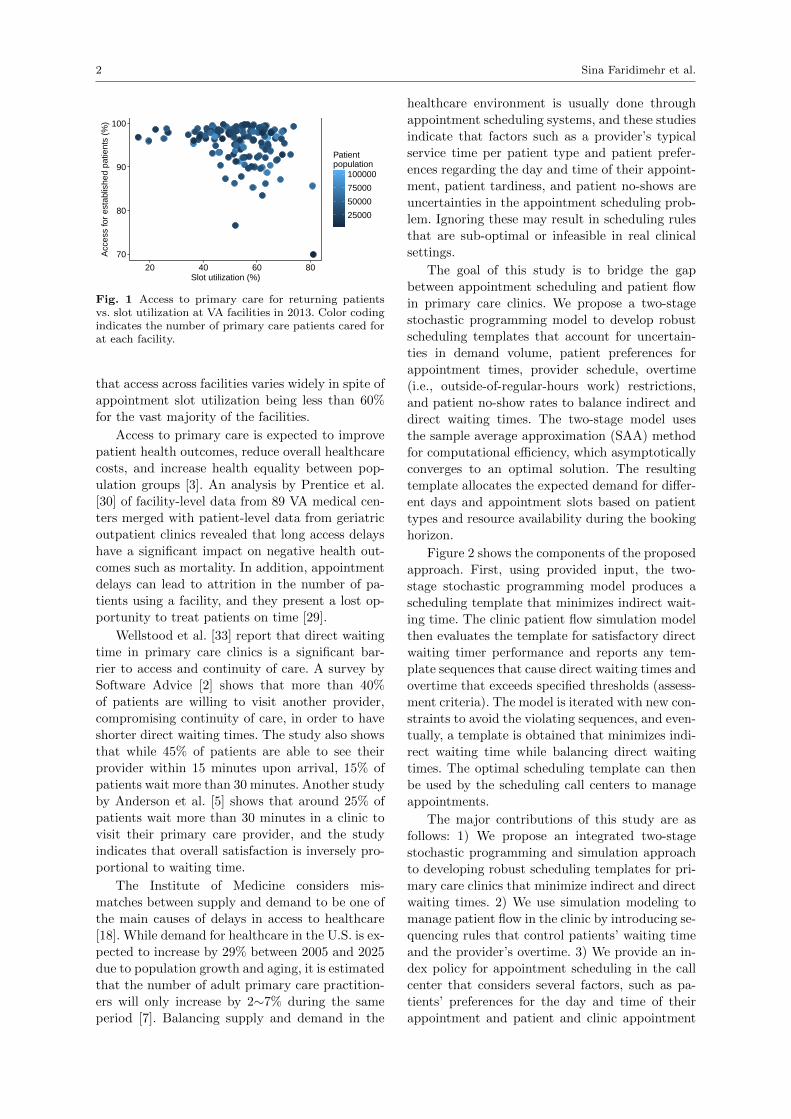
gle [34]. Figure 1 depicts the relationship between

access to primary care and appointment slot uti-

lization (defined as the percentage of total avail-

able provider appointment slots that are actually

used for providing care) at VA facilities across the

nation. The VA defines access with a binary mea-

sure that indicates whether a returning patient has

been given an appointment within 14 days of the

desired appointment date. It is clear from the plot

arX

iv:1

911.

0512

9v1

[m

ath.

OC

] 1

2 N

ov 2

019

2 Sina Faridimehr et al.

70

80

90

100

20 40 60 80Slot utilization (%)

Acc

ess

for

esta

blis

hed

patie

nts

(%)

25000

50000

75000

100000

Patientpopulation

Fig. 1 Access to primary care for returning patientsvs. slot utilization at VA facilities in 2013. Color codingindicates the number of primary care patients cared forat each facility.

that access across facilities varies widely in spite of

appointment slot utilization being less than 60%

for the vast majority of the facilities.

Access to primary care is expected to improve

patient health outcomes, reduce overall healthcare

costs, and increase health equality between pop-

ulation groups [3]. An analysis by Prentice et al.

[30] of facility-level data from 89 VA medical cen-

ters merged with patient-level data from geriatric

outpatient clinics revealed that long access delays

have a significant impact on negative health out-

comes such as mortality. In addition, appointment

delays can lead to attrition in the number of pa-

tients using a facility, and they present a lost op-

portunity to treat patients on time [29].

Wellstood et al. [33] report that direct waiting

time in primary care clinics is a significant bar-

rier to access and continuity of care. A survey by

Software Advice [2] shows that more than 40%

of patients are willing to visit another provider,

compromising continuity of care, in order to have

shorter direct waiting times. The study also shows

that while 45% of patients are able to see their

provider within 15 minutes upon arrival, 15% of

patients wait more than 30 minutes. Another study

by Anderson et al. [5] shows that around 25% of

patients wait more than 30 minutes in a clinic to

visit their primary care provider, and the study

indicates that overall satisfaction is inversely pro-

portional to waiting time.

The Institute of Medicine considers mis-

matches between supply and demand to be one of

the main causes of delays in access to healthcare

[18]. While demand for healthcare in the U.S. is ex-

pected to increase by 29% between 2005 and 2025

due to population growth and aging, it is estimated

that the number of adult primary care practition-

ers will only increase by 2∼7% during the same

period [7]. Balancing supply and demand in the

healthcare environment is usually done through

appointment scheduling systems, and these studies

indicate that factors such as a provider’s typical

service time per patient type and patient prefer-

ences regarding the day and time of their appoint-

ment, patient tardiness, and patient no-shows are

uncertainties in the appointment scheduling prob-

lem. Ignoring these may result in scheduling rules

that are sub-optimal or infeasible in real clinical

settings.

The goal of this study is to bridge the gap

between appointment scheduling and patient flow

in primary care clinics. We propose a two-stage

stochastic programming model to develop robust

scheduling templates that account for uncertain-

ties in demand volume, patient preferences for

appointment times, provider schedule, overtime

(i.e., outside-of-regular-hours work) restrictions,

and patient no-show rates to balance indirect and

direct waiting times. The two-stage model uses

the sample average approximation (SAA) method

for computational efficiency, which asymptotically

converges to an optimal solution. The resulting

template allocates the expected demand for differ-

ent days and appointment slots based on patient

types and resource availability during the booking

horizon.

Figure 2 shows the components of the proposed

approach. First, using provided input, the two-

stage stochastic programming model produces a

scheduling template that minimizes indirect wait-

ing time. The clinic patient flow simulation model

then evaluates the template for satisfactory direct

waiting timer performance and reports any tem-

plate sequences that cause direct waiting times and

overtime that exceeds specified thresholds (assess-

ment criteria). The model is iterated with new con-

straints to avoid the violating sequences, and even-

tually, a template is obtained that minimizes indi-

rect waiting time while balancing direct waiting

times. The optimal scheduling template can then

be used by the scheduling call centers to manage

appointments.

The major contributions of this study are as

follows: 1) We propose an integrated two-stage

stochastic programming and simulation approach

to developing robust scheduling templates for pri-

mary care clinics that minimize indirect and direct

waiting times. 2) We use simulation modeling to

manage patient flow in the clinic by introducing se-

quencing rules that control patients’ waiting time

and the provider’s overtime. 3) We provide an in-

dex policy for appointment scheduling in the call

center that considers several factors, such as pa-

tients’ preferences for the day and time of their

appointment and patient and clinic appointment

Managing access to primary care clinics 3

Fig. 2 Proposed approach for producing robust ap-pointment scheduling templates

cancellations. 4) We validate the proposed meth-

ods using data from real-world clinics and corrobo-

rate the efficiency of our proposed model compared

to existing approaches in the literature.

The rest of this paper is structured as follows.

Section 2 provides a review of related literature.

Section 3 describes the assumptions and the uncer-

tainties that are considered in our model. This sec-

tion also presents the model formulation and our

simulation approaches to clinic patient flow and

call center scheduling. Section 4 defines various

performance measures for appointment scheduling

and derives practical guidelines through a numer-

ical study of a VA primary care clinic. Finally, we

summarize our conclusions and discuss directions

for future work in Section 5.

2 Literature review

There is a rich body of healthcare operations

management literature on outpatient appointment

scheduling. However, prior research has mostly fo-

cused on proposing appointment scheduling sys-

tems to manage patient flow within clinics (i.e.,

direct waiting time) but not to effectively balance

both direct and indirect waiting times.

2.1 Clinic patient flow

2.1.1 Patient flow measures

Muthuraman et al. [27] proposed a stochastic over-

booking model to optimize appointment schedul-

ing in an outpatient clinic where patients have

different no-show probabilities. Their objective

function captures patient waiting time, provider

overtime (i.e., work outside-of-regular-hours), and

idle time. Zeng et al. [36] maximized clinics’ ex-

pected profit based on revenue from patients and

the costs of patient waiting time, provider over-

time, and idle time, with patients having differ-

ent no-show probabilities. The authors observed

that the performance of scheduling practices us-

ing homogeneous overbooking models based on the

mean value of show-up probabilities is not good

enough. Chakraborty et al. [9] developed a se-

quential scheduling algorithm to minimize the to-

tal expected cost resulting from patients’ waiting

time and providers’ overtime using stochastic ser-

vice times. They showed that their model leads

to higher profits and less overtime than policies

that consider service periods to be pre-divided into

slots.

2.1.2 No-shows and overbooking

Patient no-shows are a major challenge in outpa-

tient clinics. To mitigate the negative impact of no-

shows on scheduling practice, Laganga et al. [21]

developed an appointment scheduling approach us-

ing overbooking to balance patients’ waiting time

and providers’ overtime. They concluded that it is

impossible to draw general conclusions about con-

structing overbooking schedules. Zacharias et al.

[35] proposed an overbooking model to mitigate

the negative impact of patient no-shows on clinic

performance when patients have different no-show

probabilities. The authors studied static and dy-

namic scheduling problems and showed that pa-

tients’ heterogeneity in no-show rates has a large

negative impact on the scheduling process.

2.2 Indirect waiting time

2.2.1 Advanced access scheduling

Clinics tend to use advanced access systems to re-

duce patients’ indirect waiting time. In these sys-

tems, patients are given appointments on or near

their desired date. Taking into account patients’

no-show and appointment cancellation behavior,

Liu et al. [23] proposed a dynamic scheduling pol-

icy for an outpatient clinic and showed that an

advanced access scheduling policy performs better

when the demand rate is relatively low. Dobson et

al. [11] examined the effect of keeping some slots

open for same-day demand in primary care clin-

ics on two quality measures: the average number

of same-day demands that are not served during

normal working hours and the average number of

non-urgent patients in the queue. They demon-

strated that encouraging non-urgent patients to

call for same-day appointments is an important

factor when implementing advanced access sys-

tems in primary care clinics. Qu et al. [31] de-

rived the selection percentage for open appoint-

ments in an advanced access system by using a


mean-variance approach. Their results indicated

that when both the demand rate and the no-show

rate are high for appointments that are reserved for

routine patients, there are one or more Pareto op-

timal percentages of open appointments that can

decrease the variability in the number of patients

seen.

2.2.2 Patient choice

Patient scheduling choices can impact appoint-

ment delays. Gupta et al. [17] developed a Markov

decision process to manage access to care when pa-

tients can choose between accepting a same-day or

a future appointment. The authors provided opti-

mal solutions for clinics with single and multiple

providers. Wang et al. [32] studied clinic revenue

optimization by finding the optimal balance be-

tween the number of slots that should be kept open

for same-day demand and the number of slots for

routine patients while considering preferences re-

garding providers and appointment times. Their

model is limited to one day and hence does not con-

sider the interactions between multiple scheduling

days.

2.3 Summary

Our work is closer to Luo et al.’s [24] research in

which they developed a tandem queue model to

study the relationship between the appointment

queue (indirect waiting time) and the service queue

(direct waiting time). The main research question

that we address is: How can primary care prac-

tices schedule patients to ensure that the patientsexperience minimal delays in getting their appoint-

ments while making the patient flow in the clinic

as smooth as possible? Our work is different from

the studies discussed above in several important

respects. First, we consider the indirect waiting

time of patients who may call in advance to book

an appointment over a planning horizon T . Second,

in the optimization model, we consider three pa-

tient flow measures: patients’ direct waiting time

and the provider’s overtime work during lunchtime

and after regular hours. Third, we account for pa-

tients’ preference for appointment dates and times.

Finally, we focus on scheduling templates that are

easy to employ by appointment call center staff

given their stability for extended periods (e.g., a

month or a quarter) and also allowing providers

the benefit of a stable work pattern with consider-

ing their clinical and administrative practice. Like

other studies, we also consider the effect of a pa-

tient’s no-show behavior on patient scheduling and

patient flow measures.

3 Problem description and model

formulation

In this section, we provide an overview of the

problem setup and our assumptions. We also

present the notation used in the model, followed

by the proposed risk-neutral two-stage stochastic

programming model for developing appointment

scheduling templates.

3.1 Problem setup and assumptions

We study primary care outpatient clinics with sin-

gle providers. Although solo practice is becoming

less popular, more than half of family physicians

still work in solo and small practices [22]. Without

loss of generality, we assume that there are five

working days per week (Monday through Friday)

and each working day has eight provider working

hours, made up eight 60-minute appointment slots.

Each day is divided into morning and evening ses-

sions, each of which lasts four hours (8AM to Noon

and 1 to 5PM), with a one hour lunch break. With-

out loss of generality, we assume that there are

20 working days in a month, resulting in 40 ses-

sions/month. Patients call to book appointments

with a preference for the appointment date (future

or same-day) and time (early morning or closer to

lunch hour or late afternoon). While much of the

academic literature assumes that patients call for

an appointment on the day when they want the

appointment, data shows that most primary care

patients often call in advance to make future ap-

pointments. Figure 3 shows how early patients call

to request appointments in three different VA pri-

mary care clinics in the Midwest.

As is typical with primary care, we allow multi-

ple patient types (e.g., new patients vs established

patients, annual physicals, etc.) and we allow dif-

ferent service times for nurses and providers based

on the patient type. Clinics are allowed to cancel

appointments (e.g., due to lab result delays or a

provider’s absence). These cancellations need to be

managed since they will increase patients’ dissat-

isfaction and the staff’s future workload. Patients

may also cancel their appointments or not show

up at all for their visit. We allow overbooking as a

means to compensate for patients’ no-show behav-

ior with respect to providers’ appointment slot uti-

lization. However, excessive overbooking increases

patients’ direct waiting time.

Without loss of generality, we assume that pa-

tients’ preferences cannot be denied (e.g., appoint-

ment time). Otherwise, patients will seek care in

a specialty care clinic or an emergency depart-


0.00

0.01

0.02

0.03

0 50 100 150 200 250 300 350Call day to desired day (in days)

Den

sity

Clinic A B C

Fig. 3 Time (in days) between call date and desired appointment date for patients in three VA primary care clinics.The clinic names are coded.

ment, both of which are more costly than primary

care. Even though providers can work overtime,

the mathematical model we develop needs to mod-

erate the effect of capacity shortage due to other

responsibilities the provider may have. Also, pa-

tients typically have different preferences for their

appointment dates, and there are uncertainties re-

garding the number of patients who will call each

day during the planning horizon and their desired

appointment dates.

The two-stage model we develop minimizes pa-

tients’ indirect waiting time while considering pa-

tient flow within the clinic. Also, the model ensures

that the provider is not overloaded with excessive

cumulative workloads in any morning or evening

session by tracking expected overtime during lunch

hour and work past the end of the work day. Fi-

nally, we consider a finite rolling scheduling hori-

zon and seek weekly scheduling templates for they

are typical in practice. We allow the weekly tem-

plates to vary from month to month to account for

any seasonal differences in demand patterns.

3.2 Two-stage stochastic programming model

Stochastic programming is a branch of optimiza-

tion that assumes that some of the model pa-

rameters and coefficients are unknown and that

only their probability distribution can be esti-

mated. The most widely used stochastic program-

ming model is two-stage stochastic programming.

In this model, the first-stage decision variables are

“here-and-now” decisions that are determined be-

fore observing the realization of uncertainties, and

the second-stage decision variables are selected af-

ter exposing the first-stage variables to the uncer-

tainties. The goal is to determine the values for

first-stage decisions in a way that minimizes the

first- and second-stage objective function values.

We consider uncertainties in the number of pa-

tients seeking care, the days when they call, their

desired appointment dates and times, and their

no-show rates in the model. The first-stage deci-

sions in our proposed two-stage model determine

the number of patients of each patient type al-

lowed in each appointment slot and session based

on the provider’s maximum tolerable cumulative

patient complexity (determined in terms of ex-

pected cumulative service times). Based on the

first-stage patient allocation decisions and the re-

alization of uncertainties in the second stage, ap-

pointment scheduling decisions are made in the

second stage that minimize patients’ total indirect

waiting time. The output of the two-stage stochas-

tic programming is a weekly scheduling template

for the booking horizon.

3.3 Model notation

We consider a set of R patient types, indexed by r,

each with an average complexity cr and no-showprobability pr, who phone to request an appoint-

ment. The planning horizon has multiple working

days, denoted by D and indexed by d. Each day

has two sessions, denoted by S and indexed by s.

Within each session, there are multiple appoint-

ment slots, denoted by A and indexed by a. In

order to manage the patient flow in the clinic and

handle different clinical tasks, maximum patient

complexities are considered for each appointment

slot and session, respectively denoted as κ and η.

The numbers of patients of type r that can be

scheduled in each appointment are given by the

set L(r), indexed by l.

For each patient type r ∈ R, let l ∈ L(r); then

the parameter mr,l denotes the discrete number

of possible patients of type r that can be sched-

uled in each appointment slot. To help maintain a

rolling planning horizon for the weekly scheduling

grid template, the parameter ξr,a denotes the num-

ber of previously booked patients in the template.

Let ω be a random variable representing the uncer-


tainties in the two-stage model, and let ω be a real-

ization of ω. The first-stage decision variables xr,aand zr,a,l respectively determine the number of pa-

tients of type r that can be scheduled in appoint-

ment slot a and whether l patients of type r can be

scheduled in appointment slot a. The second-stage

decision variable yr,d,d′ assigns patients of type r

that call on day d and request an appointment

on day d′. Table 1 summarizes the notation that

is used for the two-stage stochastic programming

model.

Table 1 Model Notation

Symbol DescriptionSets:R Set of patient types, indexed by r ∈ RA Set of appointment slots, indexed by a ∈

AS Set of sessions, indexed by s ∈ SG Set of template sequences in which pa-

tient flow constraints are not met for di-rect waiting time and provider overtimework thresholds, indexed by g ∈ G

D Set of days, indexed by d ∈ DLr Set of numbers of patients of type r that

can be scheduled in each appointmentslot, indexed by l ∈ Lr

Ω Set of scenarios, indexed by ω ∈ ΩModel Pa-rameters:cr Average complexity of patient type rκ Maximum acceptable cumulative patient

complexity for each appointment slotη Maximum acceptable cumulative patient

complexity for each sessionpr Average no-show probability for patient

type rmr,l Number of patients of type r, l ∈ Lr

ξr,a Number of scheduled patients of type r inappointment slot a

fr,d(ω) Number of patients of type r who askedfor an appointment on day d in scenarioω

ε User parameterFirst-stageVariables:xr,a Number of patients of type r who can be

scheduled in appointment slot azr,a,l 1 if l patients of type r can be scheduled

in appointment slot a; 0 otherwiseSecond-stageVariables:yr,d,d′(ω) Proportion of patients of type r who asked

for an appointment on day d and arescheduled for day d′ in scenario ω

The first-stage problem is represented as fol-

lows:

Min f(x) = E[ϕ(x, ω)] (1)

s.t.∑r∈R

crxr,a ≤ κ ∀a ∈ A, (2)∑r∈R

∑a∈s

crxr,a ≤ η ∀s ∈ S, (3)

xr,a ≥ ξr,a ∀r ∈ R, a ∈ A, (4)

xr,a =∑l∈Lr

mr,lzr,a,l ∀r ∈ R, a ∈ A, (5)

∑l∈Lr

zr,a,l = 1 ∀r ∈ R, a ∈ A, (6)

∑r∈R,a∈A,l∈Lr⊆G

zr,a,l ≤ |G| − 1, (7)

xr,a ∈ Z+ ∀r ∈ R, a ∈ A,zr,a,l ∈ 0, 1 ∀r ∈ R, a ∈ A, l ∈ Lr. (8)

For a given first-stage solution x and the re-

alization ω of random variables, the second-stage

recourse function is as follows:

Min ϕ(x,w) =∑r∈R

d,d′∈Dd≤d′

wryr,d,d′(ω)fr,d(ω)[(d′ − d)(1+ε)]

(9)

s.t.∑

d∈D:d≤d′(1− pr)yr,d,d′(ω)fr,d(ω) ≤

∑a∈d′

xr,a(ω)

∀r ∈ R, d′ ∈ D, (10)∑d′∈D:d≤d′

yr,d,d′(ω) = 1

∀r ∈ R, d ∈ D, (11)

0 ≤ yr,d,d′(ω) ≤ 1

∀r ∈ R, d, d′ ∈ D : d ≤ d′. (12)

The objective function minimizes the expected

indirect waiting time for patients. The difference

between the desired and actual appointment dates

for a patient is penalized using a super-linear

function in order to favor “fairness” in assigning

lengths of delay to the patients.

A primary care provider’s threshold in terms

of the cumulative patient complexity that can

be handled in each appointment slot and each

scheduling session is represented in constraints (2)

and (3), respectively. Since this is a rolling plan-

ning horizon problem, constraints (4) fill the slots

based on a commitment to previously scheduled

appointments. Constraints (5), (6), and (7) are se-

quencing rules to address patient flow in the clinic,


and they are added dynamically based on recom-

mendations from the clinic patient flow simula-

tion model. Constraints (5) and (6) determine the

maximum number of patients of each type that

can be scheduled in each appointment slot, and

constraints (7) ensure that sequences that have

violated patient flow thresholds do not occur in

the scheduling template. Constraints (8) are inte-

ger and binary value constraints for the first-stage

variables. Constraints (10) ensure that patient ap-

pointments are provided based on the scheduling

template resulting from the first-stage model. Con-

straints (11) ensure that no patient request is de-

nied, and constraints (12) confirm that the second-

stage variables are proportion values between 0

and 1.

Figure 4 represents an example of adding “lazy

constraints” to the two-stage stochastic model.

Based on the scheduling template from the two-

stage model, the patient flow simulation deter-

mines the percentiles (85th percentile in this ex-

ample) of patients’ direct waiting time and the

provider’s overtime work during lunchtime and af-

ter regular hours, and if any of these violate the

predetermined thresholds, which are 30 minutes

for patients’ expected direct waiting time, 45 min-

utes for the provider’s expected overtime work dur-

ing lunch, and 60 minutes for the provider’s ex-

pected overtime work after regular hours, a lazy

constraint is added to the first stage of the opti-

mization model to eliminate such sequences. As

shown in Figure 4, when the simulated perfor-

mance values are 20, 20, and 35 for patients’ direct

waiting time and the provider’s overtime during

lunch and after regular hours, respectively, none ofthe thresholds is violated and so lazy constraints

are not added to the two-stage stochastic model.

However, when these values are 35, 20, and 35, re-

spectively, the threshold for patients’ direct wait-

ing time is violated, and the corresponding lazy

constraint is added to the optimization model.

Here, xr,a is the number of patients of type r who

can be scheduled in appointment slot a, and zr,a,l is

equal to 1 if l patients of type r can be scheduled in

appointment slot a. Acute, chronic, and preventive

patient types are represented as ‘A’, ‘C’, and ‘P’,

respectively. Whenever a lazy constraint is added

to the first stage, the model is re-optimized.

3.4 Clinic patient flow simulation

The patient flow simulation for the clinic is exe-

cuted for each day based on the scheduling tem-

plate proposed by the optimization model de-

scribed in the previous section. Patients’ direct

waiting time and the provider’s overtime work dur-

ing lunch time and after regular hours are mea-

sured. The clinic patient flow involves two stages:

time with the nurse and time with the provider.

Once a patient walks into the clinic, he or she

waits in the lobby for the nurse to become avail-

able. After being visited by the nurse, the patient

waits for the provider in the exam room. We as-

sume that patients who are scheduled for a partic-

ular day must be served before the end of that day

even if the provider has to work overtime. Patients

are assumed not to leave the exam room until the

provider finishes all required tasks. Also, patients

may arrive late for their appointments. By arriv-

ing late, patients may increase the waiting times

for the patients that follow them. Therefore, we as-

sume that patients are called in the order of their

arrival time.

Algorithm 1 presents pseudocode for our ap-

proach based on the two-stage optimization model

and simulation. In step 1, the two-stage stochas-

tic programming model is solved, and a schedul-

ing template is obtained from the first-stage solu-

tion. Using the scheduling template, each day in

the planning horizon is simulated under given in-

put with m = 200 replications in step 2, and spe-

cific percentiles of patient flow measures are calcu-

lated in step 3. If any of the measures violate the

patients’ or the provider’s thresholds, a new set

of constraints (5), (6), and (7) are added to the

model, which is then re-optimized. The process re-

peats until the system reaches a state where the

indirect waiting time is minimized without violat-

ing any patient flow thresholds.

Algorithm 1 Clinic patient flow simulation

Step 1: Optimize the two-stage stochastic model (1) -(4), (8) - (12);Step 2: Run simulation model for 200 replications foreach day in the planning horizon;Step 3: for i in D do

Calculate αth percentile for patients’ direct waitingtime and provider’s overtime during lunch and afterregular hours;if estimates ≥ any of the thresholds then

Construct constraints (5), (6), and (7) and addthem to the two-stage stochastic model;

end

3.5 Call center simulation

To evaluate the efficiency of the two-stage schedul-

ing template, we simulate the practice at the

appointment call center. The call center simula-

tion uses either the total available capacity or

the scheduling template’s allocation. An “index

scheduling policy” is used to allot or cancel pa-

tients’ appointments. The scheduler at the call cen-


Fig. 4 An example of adding lazy constraints to the two-stage optimization model based on the clinic patient flowsimulation performance

ter estimates the priority of available appointment

slots that should be offered to a patient based on

his or her desired date and patient type. When a

patient requests an appointment for a desired date,

the policy calculates the index based on the slot’s

remaining capacity in increasing order for each ap-

pointment slot based on the slot’s proximity to the

desired date. To generate a patient’s choice regard-

ing accepting an appointment, a random number

from the uniform distribution U(0, 1) is generated

and compared to an “acceptance” threshold. If

the random number is greater than this threshold,

the patient accepts the corresponding appointment

slot; otherwise, another slot is offered and the pro-

cess continues until the patient accepts. Appoint-

ment cancellations are handled similarly: A ran-

dom number is generated from U(0, 1), and if the

random number is less than the clinic’s cancella-

tion rate, the patient or clinic cancels the appoint-

ment and the patient is removed from the schedul-

ing grid.

4 Case study and insights

We used real data from a U.S. Midwest VA pri-

mary care clinic to estimate the number of weekly

requests, patients’ no-show probabilities, appoint-

ment cancellation probabilities, the daily distri-

bution of patients’ calls, the distribution of pa-

tients’ desired appointment days, and the distri-

bution of the time between call dates and desired

dates. The data suggests that patients often call

with the same probability on different weekdays,

but fewer patients ask for appointments on Mon-

days while more ask for Fridays. Patients may ask

for appointments up to four weeks in advance, but

around 65% of the patients want an appointment

within one week. No-show and cancellation rates

vary across months, and the average no-show and

cancellation rates for this clinic are 10% and 17%,

respectively. Other parameters are listed in Table

2.

Table 2 Base problem parameters

Maximum patient complexity that the providercan handle in an appointment slot = 0.96Maximum patient complexity that the providercan handle in a session = 2.8Threshold for patients’ acceptance of offered ap-pointment slot = 0.2Average complexity of different patient types =[Acute: 0.29, Chronic: 0.32, Preventative 0.36]Threshold for patients’ direct waiting time = 30minutesThreshold for spillover amount to provider’s lunchtime = 45 minutesThreshold for provider’s overtime = 60 mintuesPercentile of patient flow metric distributions inclinic patient flow simulation = 85%Patient arrival time distribution = N (−16.62, 27)Booking horizon = 60 daysPlanning horizon = 300 days

We considered three different patient types

(acute, chronic and preventive) based on a study

by Yarnall et al. [20], who used the National Am-

bulatory Medical Care Survey for 2003 to deter-

mine the visits for these patient types. Similarly,

we used an empirical study by Oh et al. [28] to

determine the amount of time the nurse spends

with patients of each type. The service time with

the nurse and the provider for each patient type

follows a log-normal distribution, as suggested by

Cayirli et al. [8]. Table 3 reports the service time

with the nurse and the provider for each patient

type along with the percentage of each patient type

in the provider’s panel.

Delays in arrivals for appointments are preva-

lent in outpatient clinics. In this study, we used the

normal distribution N (−16.62, 27.07) in minutes,


Table 3 Expected service time with nurse and primarycare provider

Visit (%) of Nurse Time Provider TimeType Visits (mins) (mins)Acute 49.3 11.3 (8.3) 17.3 (8.7)

Chronic 36.1 12.6 (8.8) 19.3 (9.2)Preventive 14.6 13.9 (11.3) 21.4 (11.8)

as estimated by Cayirli et al. [8]. These authors

collected data from a primary healthcare clinic in

a New York metropolitan hospital and used the

Kolmogorov–Smirnov test to estimate the param-

eters. A negative average indicates that on aver-

age, patients arrive earlier than the starting time

for their appointment.

We compare the performance of the appoint-

ment scheduling based on two-stage stochastic pro-

gramming with two sequencing rules that have

been proposed in the literature. These rules are

shortest processing time (SPT) and low coefficient

of variation (CV) in the beginning (LCVB). SPT

schedules patients in increasing order of mean ser-

vice times, while LCVB schedules in increasing or-

der of the CV (σ/µ) of the service time [6]. For

the given planning horizon, appointments were as-

signed based on each of these two approaches along

with our proposed approach, and the correspond-

ing direct and indirect waiting times were evalu-

ated. Table 4 shows sample “daily” templates for

the SPT and LCVB scheduling policies that repeat

every day during the planning horizon.

Table 4 Sample daily templates for heuristic appoint-ment scheduling policies

App.slot SPT LCVB1 A,A,A C,C,C2 A,A C,C,C3 A,A A,A4 A,A A,A5 C,C,C A,A,A6 C,C,C A,A7 P,P P,P8 P P

The planning horizon is 240 working days (cor-

responding to an year) and all performance mea-

sures are tracked and reported once the system has

reached steady state (around 60 days) to discard

the transient effects at the beginning from model

initialization. For the two-stage model, we used the

SAA method to estimate the number of scenarios

that were required for representing uncertainties.

SAA is a Monte Carlo simulation-based sampling

procedure that approximates the expected value

of the objective function by using a finite sam-

ple of scenarios [25]. Due to the rolling horizon, we

used SAA on various days to find the most reliable

number of scenarios. Based on the SAA results,

we used 10 scenarios for our computational exper-

iments since the gap between the upper and lower

bounds was within 5%. All computational studies

were implemented using Python, and Gurobi 6.5

was used as the mixed-integer programming solver

on a computer running Windows 7 with 2.6 GHz

processing speed and 80 GB of RAM.

The computational study was conducted in

four parts, which are discussed in the following

subsections. In the first part, the trade-off between

indirect and direct waiting times of patients in the

outpatient clinic was evaluated. In the second part,

we analyze how the indirect waiting time changes

if patients are more sensitive to appointment de-

lays, as well as the subsequent impact on show-up

probabilities. In the third part, the influence of the

provider type on indirect and direct waiting times

is estimated by considering different provider ca-

pacities. In the last part, we study the relationship

between the perishability of appointment slots in

a clinic and its impact on different approaches to

minimizing patients’ indirect waiting time.

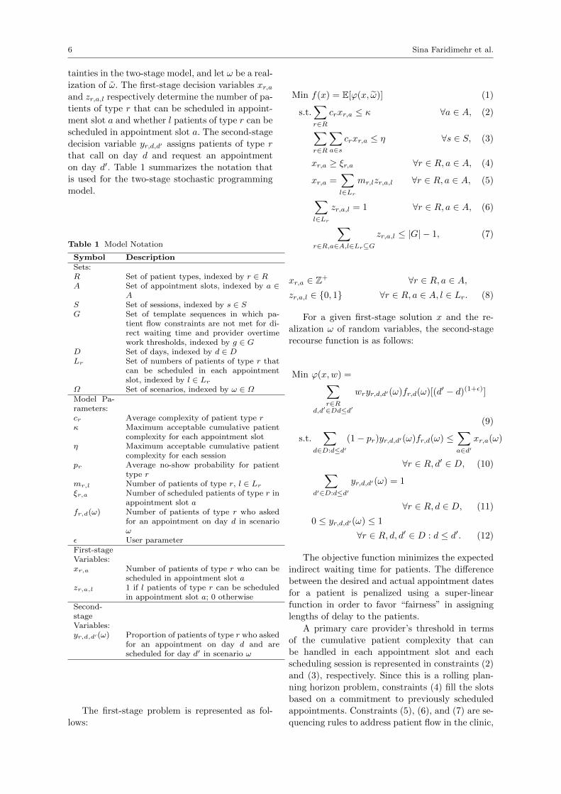
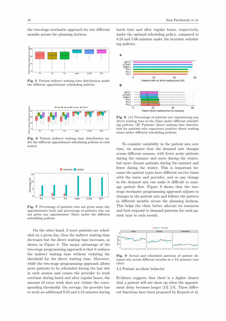
4.1 Trade-off between indirect waiting time and

patient flow

We consider three different quantiles α—the 80th,

85th, and 90th percentile—for the patient flow

metric distributions. Figure 5 compares the in-

direct waiting time distributions using our two-

stage stochastic programming approach vs using

baseline sequencing rules from the literature. The

higher the value of α, the more concerned the clinic

manager is about patient flow in the clinic, as more

patients will have waiting times that are less than

their direct waiting time threshold.

The better performance of the optimal schedul-

ing template from the two-stage stochastic pro-

gramming model compared to the heuristic rules

in terms of patients’ indirect waiting time is shown

in Figures 5 and 6. As Figure 7 shows, although

the difference between the optimal appointment

scheduling and the heuristic policies is not signifi-

cant in terms of the percentage of patients who are

given same-day appointments (on average 1.6% vs

0.1%), the optimal policy performs better with re-

spect to the percentage of patients who are not

given any appointment with their provider (on

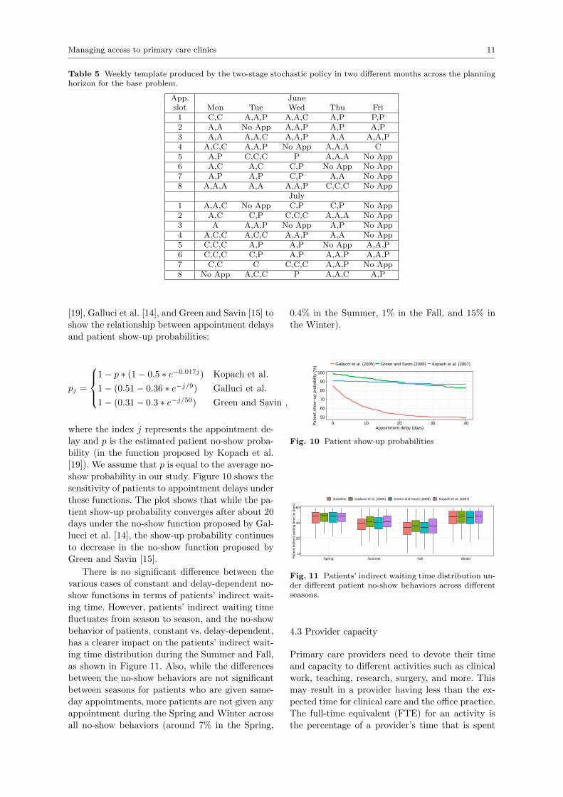
average 7.47% vs 13.11%). Table 5 represents a

sample “weekly” scheduling template proposed by


the two-stage stochastic approach for two different

months across the planning horizon.

0

20

40

60

α80 α85 α90 Index LCVB SPTPat

ient

indi

rect

wai

ting

time

(in d

ays)

Fig. 5 Patient indirect waiting time distribution underthe different appointment scheduling policies

0

20

40

60

α80 α85 α90 Index LCVB SPT

Pat

ient

indi

rect

wai

ting

time

(in d

ays) Fall Spring Summer Winter

Fig. 6 Patient indirect waiting time distribution un-der the different appointment scheduling policies in eachseason

0

5

10

15

α80 α85 α90 Index LCVB SPT

Per

cent

age

(%)

SameDay NoApp

Fig. 7 Percentage of patients who are given same dayappointments (red) and percentage of patients who arenot given any appointment (blue) under the differentscheduling policies

On the other hand, if more patients are sched-

uled on a given day, then the indirect waiting time

decreases but the direct waiting time increases, as

shown in Figure 8. The major advantage of the

two-stage programming approach is that it reduces

the indirect waiting time without violating the

threshold for the direct waiting time. Moreover,

while the two-stage programming approach allows

more patients to be scheduled during the last slot

in each session and causes the provider to work

overtime during lunch and after regular hours, the

amount of extra work does not violate the corre-

sponding thresholds. On average, the provider has

to work an additional 9.25 and 4.53 minutes during

lunch time and after regular hours, respectively,

under the optimal scheduling policy, compared to

8.53 and 5.66 minutes under the heuristic schedul-

ing policies.

α80

α85

α90IndexLCVB

SPT

0 20 40 60Patients with no direct waiting time (%)

A

α80

α85

α90IndexLCVB

SPT

0 20 40 60Patient direct waiting time (in minutes)

B

Fig. 8 (A) Percentage of patients not experiencing anydirect waiting time in the clinic under different schedul-ing policies. (B) Patients’ direct waiting time distribu-tion for patients who experience positive direct waitingtimes under different scheduling policies.

To consider variability in the patient mix over

time, we assume that the demand mix changes

across different seasons, with fewer acute patients

during the summer and more during the winter,

but more chronic patients during the summer and

fewer during the winter. This is important be-

cause the patient types have different service times

with the nurse and provider, and so any change

in the demand mix can make it difficult to man-

age patient flow. Figure 9 shows that the two-

stage stochastic programming approach adjusts tochanges in the patient mix and follows the pattern

in different months across the planning horizon.

This helps the clinic better allocate its resources

and best respond to demand patterns for each pa-

tient type in each month.

Acute Chronic Preventive

Jan Feb Mar Apr May Jun Jul Aug Sep Oct Nov Dec Jan Feb Mar Apr May Jun Jul Aug Sep Oct Nov Dec Jan Feb Mar Apr May Jun Jul Aug Sep Oct Nov Dec0

20

40

60

80

Per

cent

age

(%)

Actual Scheduled

Fig. 9 Actual and scheduled patterns of patient de-mand mix across different months at a VA primary careclinic.

4.2 Patient no-show behavior

Evidence suggests that there is a higher chance

that a patient will not show up when the appoint-

ment delay becomes longer [13] [14]. Three differ-

ent functions have been proposed by Kopach et al.


Table 5 Weekly template produced by the two-stage stochastic policy in two different months across the planninghorizon for the base problem.

App. Juneslot Mon Tue Wed Thu Fri1 C,C A,A,P A,A,C A,P P,P2 A,A No App A,A,P A,P A,P3 A,A A,A,C A,A,P A,A A,A,P4 A,C,C A,A,P No App A,A,A C5 A,P C,C,C P A,A,A No App6 A,C A,C C,P No App No App7 A,P A,P C,P A,A No App8 A,A,A A,A A,A,P C,C,C No App

July1 A,A,C No App C,P C,P No App2 A,C C,P C,C,C A,A,A No App3 A A,A,P No App A,P No App4 A,C,C A,C,C A,A,P A,A No App5 C,C,C A,P A,P No App A,A,P6 C,C,C C,P A,P A,A,P A,A,P7 C,C C C,C,C A,A,P No App8 No App A,C,C P A,A,C A,P

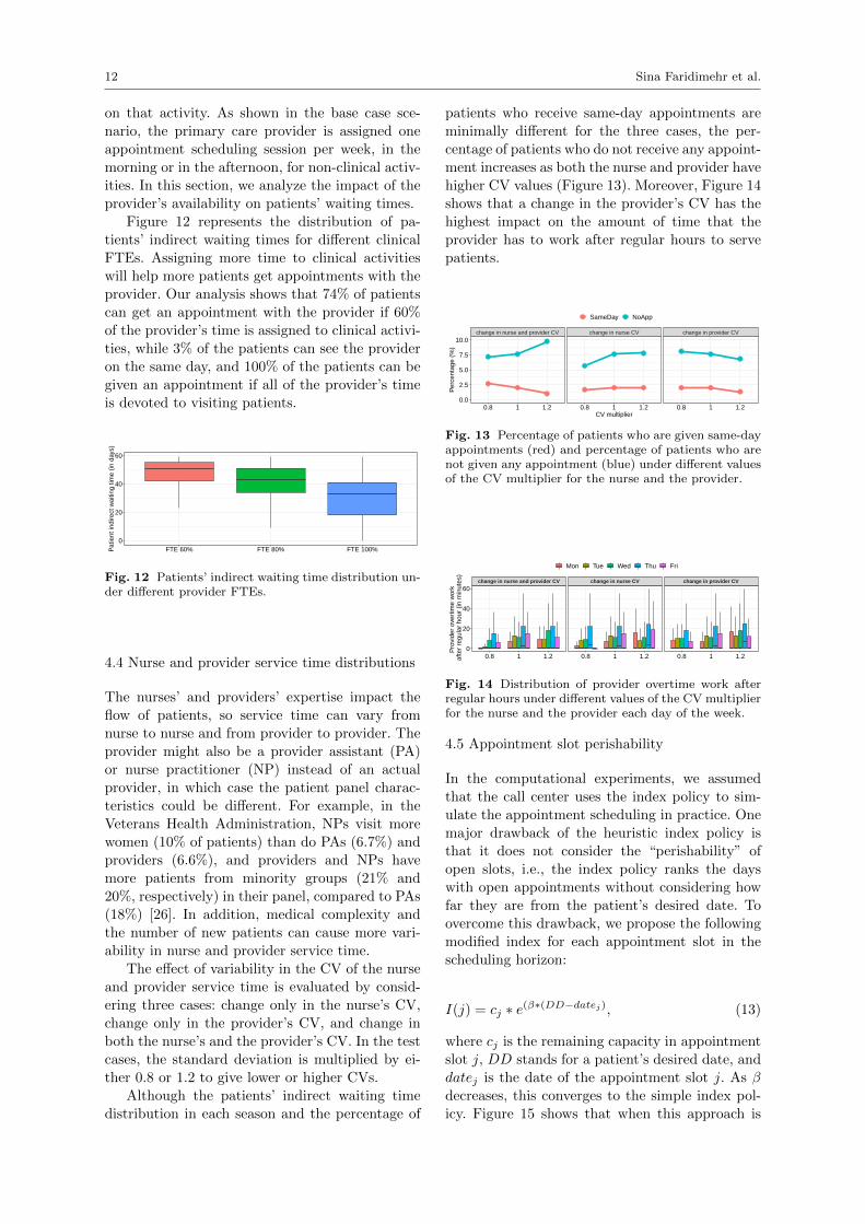
[19], Galluci et al. [14], and Green and Savin [15] to

show the relationship between appointment delays

and patient show-up probabilities:

pj =

1− p ∗ (1− 0.5 ∗ e−0.017j) Kopach et al.

1− (0.51− 0.36 ∗ e−j/9) Galluci et al.

1− (0.31− 0.3 ∗ e−j/50) Green and Savin ,

where the index j represents the appointment de-

lay and p is the estimated patient no-show proba-

bility (in the function proposed by Kopach et al.

[19]). We assume that p is equal to the average no-

show probability in our study. Figure 10 shows the

sensitivity of patients to appointment delays under

these functions. The plot shows that while the pa-

tient show-up probability converges after about 20

days under the no-show function proposed by Gal-

lucci et al. [14], the show-up probability continues

to decrease in the no-show function proposed by

Green and Savin [15].

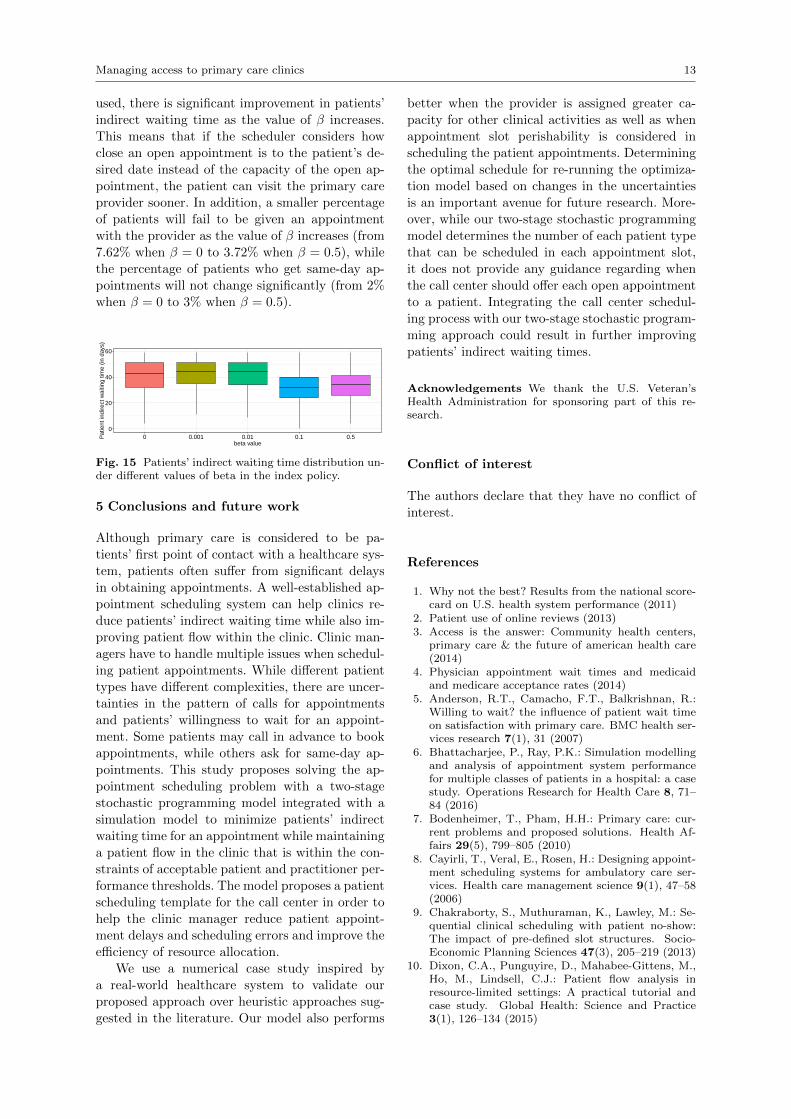
There is no significant difference between the

various cases of constant and delay-dependent no-

show functions in terms of patients’ indirect wait-

ing time. However, patients’ indirect waiting time

fluctuates from season to season, and the no-show

behavior of patients, constant vs. delay-dependent,

has a clearer impact on the patients’ indirect wait-

ing time distribution during the Summer and Fall,

as shown in Figure 11. Also, while the differences

between the no-show behaviors are not significant

between seasons for patients who are given same-

day appointments, more patients are not given any

appointment during the Spring and Winter across

all no-show behaviors (around 7% in the Spring,

0.4% in the Summer, 1% in the Fall, and 15% in

the Winter).

50

60

70

80

90

100

0 10 20 30 40Appointment delay (days)

Pat

ient

sho

w−

up p

roba

bilit

y (%

) Gallucci et al. (2005) Green and Savin (2008) Kopach et al. (2007)

Fig. 10 Patient show-up probabilities

0

20

40

60

Spring Summer Fall WinterPat

ient

indi

rect

wai

ting

time

(in d

ays)

Baseline Gallucci et al. (2005) Green and Savin (2008) Kopach et al. (2007)

Fig. 11 Patients’ indirect waiting time distribution un-der different patient no-show behaviors across differentseasons.

4.3 Provider capacity

Primary care providers need to devote their time

and capacity to different activities such as clinical

work, teaching, research, surgery, and more. This

may result in a provider having less than the ex-

pected time for clinical care and the office practice.

The full-time equivalent (FTE) for an activity is

the percentage of a provider’s time that is spent


on that activity. As shown in the base case sce-

nario, the primary care provider is assigned one

appointment scheduling session per week, in the

morning or in the afternoon, for non-clinical activ-

ities. In this section, we analyze the impact of the

provider’s availability on patients’ waiting times.

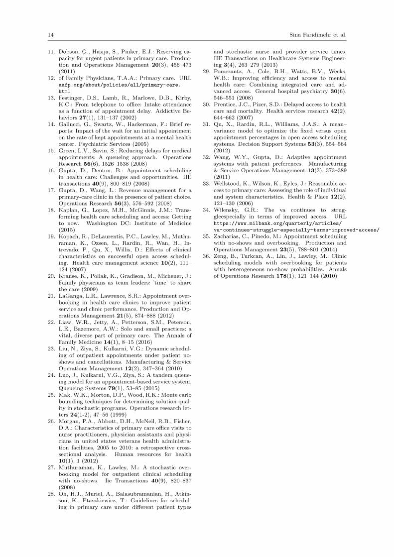
Figure 12 represents the distribution of pa-

tients’ indirect waiting times for different clinical

FTEs. Assigning more time to clinical activities

will help more patients get appointments with the

provider. Our analysis shows that 74% of patients

can get an appointment with the provider if 60%

of the provider’s time is assigned to clinical activi-

ties, while 3% of the patients can see the provider

on the same day, and 100% of the patients can be

given an appointment if all of the provider’s time

is devoted to visiting patients.

0

20

40

60

FTE 60% FTE 80% FTE 100%Pat

ient

indi

rect

wai

ting

time

(in d

ays)

Fig. 12 Patients’ indirect waiting time distribution un-der different provider FTEs.

4.4 Nurse and provider service time distributions

The nurses’ and providers’ expertise impact the

flow of patients, so service time can vary from

nurse to nurse and from provider to provider. The

provider might also be a provider assistant (PA)

or nurse practitioner (NP) instead of an actual

provider, in which case the patient panel charac-

teristics could be different. For example, in the

Veterans Health Administration, NPs visit more

women (10% of patients) than do PAs (6.7%) and

providers (6.6%), and providers and NPs have

more patients from minority groups (21% and

20%, respectively) in their panel, compared to PAs

(18%) [26]. In addition, medical complexity and

the number of new patients can cause more vari-

ability in nurse and provider service time.

The effect of variability in the CV of the nurse

and provider service time is evaluated by consid-

ering three cases: change only in the nurse’s CV,

change only in the provider’s CV, and change in

both the nurse’s and the provider’s CV. In the test

cases, the standard deviation is multiplied by ei-

ther 0.8 or 1.2 to give lower or higher CVs.

Although the patients’ indirect waiting time

distribution in each season and the percentage of

patients who receive same-day appointments are

minimally different for the three cases, the per-

centage of patients who do not receive any appoint-

ment increases as both the nurse and provider have

higher CV values (Figure 13). Moreover, Figure 14

shows that a change in the provider’s CV has the

highest impact on the amount of time that the

provider has to work after regular hours to serve

patients.

change in nurse and provider CV change in nurse CV change in provider CV

0.8 1 1.2 0.8 1 1.2 0.8 1 1.20.0

2.5

5.0

7.5

10.0

CV multiplier

Per

cent

age

(%)

SameDay NoApp

Fig. 13 Percentage of patients who are given same-dayappointments (red) and percentage of patients who arenot given any appointment (blue) under different valuesof the CV multiplier for the nurse and the provider.

change in nurse and provider CV change in nurse CV change in provider CV

0.8 1 1.2 0.8 1 1.2 0.8 1 1.20

20

40

60

Pro

vide

r ov

ertim

e w

ork

afte

r re

gula

r ho

ur (

in m

inut

es)

Mon Tue Wed Thu Fri

Fig. 14 Distribution of provider overtime work afterregular hours under different values of the CV multiplierfor the nurse and the provider each day of the week.

4.5 Appointment slot perishability

In the computational experiments, we assumed

that the call center uses the index policy to sim-

ulate the appointment scheduling in practice. One

major drawback of the heuristic index policy is

that it does not consider the “perishability” of

open slots, i.e., the index policy ranks the days

with open appointments without considering how

far they are from the patient’s desired date. To

overcome this drawback, we propose the following

modified index for each appointment slot in the

scheduling horizon:

I(j) = cj ∗ e(β∗(DD−datej), (13)

where cj is the remaining capacity in appointment

slot j, DD stands for a patient’s desired date, and

datej is the date of the appointment slot j. As β

decreases, this converges to the simple index pol-

icy. Figure 15 shows that when this approach is


used, there is significant improvement in patients’

indirect waiting time as the value of β increases.

This means that if the scheduler considers how

close an open appointment is to the patient’s de-

sired date instead of the capacity of the open ap-

pointment, the patient can visit the primary care

provider sooner. In addition, a smaller percentage

of patients will fail to be given an appointment

with the provider as the value of β increases (from

7.62% when β = 0 to 3.72% when β = 0.5), while

the percentage of patients who get same-day ap-

pointments will not change significantly (from 2%

when β = 0 to 3% when β = 0.5).

0

20

40

60

0 0.001 0.01 0.1 0.5beta value

Pat

ient

indi

rect

wai

ting

time

(in d

ays)

Fig. 15 Patients’ indirect waiting time distribution un-der different values of beta in the index policy.

5 Conclusions and future work

Although primary care is considered to be pa-

tients’ first point of contact with a healthcare sys-

tem, patients often suffer from significant delays

in obtaining appointments. A well-established ap-

pointment scheduling system can help clinics re-

duce patients’ indirect waiting time while also im-

proving patient flow within the clinic. Clinic man-

agers have to handle multiple issues when schedul-

ing patient appointments. While different patient

types have different complexities, there are uncer-

tainties in the pattern of calls for appointments

and patients’ willingness to wait for an appoint-

ment. Some patients may call in advance to book

appointments, while others ask for same-day ap-

pointments. This study proposes solving the ap-

pointment scheduling problem with a two-stage

stochastic programming model integrated with a

simulation model to minimize patients’ indirect

waiting time for an appointment while maintaining

a patient flow in the clinic that is within the con-

straints of acceptable patient and practitioner per-

formance thresholds. The model proposes a patient

scheduling template for the call center in order to

help the clinic manager reduce patient appoint-

ment delays and scheduling errors and improve the

efficiency of resource allocation.

We use a numerical case study inspired by

a real-world healthcare system to validate our

proposed approach over heuristic approaches sug-

gested in the literature. Our model also performs

better when the provider is assigned greater ca-

pacity for other clinical activities as well as when

appointment slot perishability is considered in

scheduling the patient appointments. Determining

the optimal schedule for re-running the optimiza-

tion model based on changes in the uncertainties

is an important avenue for future research. More-

over, while our two-stage stochastic programming

model determines the number of each patient type

that can be scheduled in each appointment slot,

it does not provide any guidance regarding when

the call center should offer each open appointment

to a patient. Integrating the call center schedul-

ing process with our two-stage stochastic program-

ming approach could result in further improving

patients’ indirect waiting times.

Acknowledgements We thank the U.S. Veteran’sHealth Administration for sponsoring part of this re-search.

Conflict of interest

The authors declare that they have no conflict of

interest.

References

1. Why not the best? Results from the national score-card on U.S. health system performance (2011)

2. Patient use of online reviews (2013)3. Access is the answer: Community health centers,

primary care & the future of american health care(2014)

4. Physician appointment wait times and medicaidand medicare acceptance rates (2014)

5. Anderson, R.T., Camacho, F.T., Balkrishnan, R.:Willing to wait? the influence of patient wait timeon satisfaction with primary care. BMC health ser-vices research 7(1), 31 (2007)

6. Bhattacharjee, P., Ray, P.K.: Simulation modellingand analysis of appointment system performancefor multiple classes of patients in a hospital: a casestudy. Operations Research for Health Care 8, 71–84 (2016)

7. Bodenheimer, T., Pham, H.H.: Primary care: cur-rent problems and proposed solutions. Health Af-fairs 29(5), 799–805 (2010)

8. Cayirli, T., Veral, E., Rosen, H.: Designing appoint-ment scheduling systems for ambulatory care ser-vices. Health care management science 9(1), 47–58(2006)

9. Chakraborty, S., Muthuraman, K., Lawley, M.: Se-quential clinical scheduling with patient no-show:The impact of pre-defined slot structures. Socio-Economic Planning Sciences 47(3), 205–219 (2013)

10. Dixon, C.A., Punguyire, D., Mahabee-Gittens, M.,Ho, M., Lindsell, C.J.: Patient flow analysis inresource-limited settings: A practical tutorial andcase study. Global Health: Science and Practice3(1), 126–134 (2015)


11. Dobson, G., Hasija, S., Pinker, E.J.: Reserving ca-pacity for urgent patients in primary care. Produc-tion and Operations Management 20(3), 456–473(2011)

12. of Family Physicians, T.A.A.: Primary care. URLaafp.org/about/policies/all/primary-care.

html

13. Festinger, D.S., Lamb, R., Marlowe, D.B., Kirby,K.C.: From telephone to office: Intake attendanceas a function of appointment delay. Addictive Be-haviors 27(1), 131–137 (2002)

14. Gallucci, G., Swartz, W., Hackerman, F.: Brief re-ports: Impact of the wait for an initial appointmenton the rate of kept appointments at a mental healthcenter. Psychiatric Services (2005)

15. Green, L.V., Savin, S.: Reducing delays for medicalappointments: A queueing approach. OperationsResearch 56(6), 1526–1538 (2008)

16. Gupta, D., Denton, B.: Appointment schedulingin health care: Challenges and opportunities. IIEtransactions 40(9), 800–819 (2008)

17. Gupta, D., Wang, L.: Revenue management for aprimary-care clinic in the presence of patient choice.Operations Research 56(3), 576–592 (2008)

18. Kaplan, G., Lopez, M.H., McGinnis, J.M.: Trans-forming health care scheduling and access: Gettingto now. Washington DC: Institute of Medicine(2015)

19. Kopach, R., DeLaurentis, P.C., Lawley, M., Muthu-raman, K., Ozsen, L., Rardin, R., Wan, H., In-trevado, P., Qu, X., Willis, D.: Effects of clinicalcharacteristics on successful open access schedul-ing. Health care management science 10(2), 111–124 (2007)

20. Krause, K., Pollak, K., Gradison, M., Michener, J.:Family physicians as team leaders: ’time’ to sharethe care (2009)

21. LaGanga, L.R., Lawrence, S.R.: Appointment over-booking in health care clinics to improve patientservice and clinic performance. Production and Op-erations Management 21(5), 874–888 (2012)

22. Liaw, W.R., Jetty, A., Petterson, S.M., Peterson,L.E., Bazemore, A.W.: Solo and small practices: avital, diverse part of primary care. The Annals ofFamily Medicine 14(1), 8–15 (2016)

23. Liu, N., Ziya, S., Kulkarni, V.G.: Dynamic schedul-ing of outpatient appointments under patient no-shows and cancellations. Manufacturing & ServiceOperations Management 12(2), 347–364 (2010)

24. Luo, J., Kulkarni, V.G., Ziya, S.: A tandem queue-ing model for an appointment-based service system.Queueing Systems 79(1), 53–85 (2015)

25. Mak, W.K., Morton, D.P., Wood, R.K.: Monte carlobounding techniques for determining solution qual-ity in stochastic programs. Operations research let-ters 24(1-2), 47–56 (1999)

26. Morgan, P.A., Abbott, D.H., McNeil, R.B., Fisher,D.A.: Characteristics of primary care office visits tonurse practitioners, physician assistants and physi-cians in united states veterans health administra-tion facilities, 2005 to 2010: a retrospective cross-sectional analysis. Human resources for health10(1), 1 (2012)

27. Muthuraman, K., Lawley, M.: A stochastic over-booking model for outpatient clinical schedulingwith no-shows. Iie Transactions 40(9), 820–837(2008)

28. Oh, H.J., Muriel, A., Balasubramanian, H., Atkin-son, K., Ptaszkiewicz, T.: Guidelines for schedul-ing in primary care under different patient types

and stochastic nurse and provider service times.IIE Transactions on Healthcare Systems Engineer-ing 3(4), 263–279 (2013)

29. Pomerantz, A., Cole, B.H., Watts, B.V., Weeks,W.B.: Improving efficiency and access to mentalhealth care: Combining integrated care and ad-vanced access. General hospital psychiatry 30(6),546–551 (2008)

30. Prentice, J.C., Pizer, S.D.: Delayed access to healthcare and mortality. Health services research 42(2),644–662 (2007)

31. Qu, X., Rardin, R.L., Williams, J.A.S.: A mean–variance model to optimize the fixed versus openappointment percentages in open access schedulingsystems. Decision Support Systems 53(3), 554–564(2012)

32. Wang, W.Y., Gupta, D.: Adaptive appointmentsystems with patient preferences. Manufacturing& Service Operations Management 13(3), 373–389(2011)

33. Wellstood, K., Wilson, K., Eyles, J.: Reasonable ac-cess to primary care: Assessing the role of individualand system characteristics. Health & Place 12(2),121–130 (2006)

34. Wilensky, G.R.: The va continues to strug-gleespecially in terms of improved access. URLhttps://www.milbank.org/quarterly/articles/

va-continues-struggle-especially-terms-improved-access/

35. Zacharias, C., Pinedo, M.: Appointment schedulingwith no-shows and overbooking. Production andOperations Management 23(5), 788–801 (2014)

36. Zeng, B., Turkcan, A., Lin, J., Lawley, M.: Clinicscheduling models with overbooking for patientswith heterogeneous no-show probabilities. Annalsof Operations Research 178(1), 121–144 (2010)

aafp.org/about/policies/all/primary-care.html

aafp.org/about/policies/all/primary-care.html

https://www.milbank.org/quarterly/articles/va-continues-struggle-especially-terms-improved-access/

https://www.milbank.org/quarterly/articles/va-continues-struggle-especially-terms-improved-access/

Managing access to primary care clinics using robust ... - arXiv

Documents

Transcript of Managing access to primary care clinics using robust ... - arXiv