M.B.A IInd Semester Course - 202

Management Science-II

LESSONS 1 TO 12

Written By. Dr. Atul Dhingra

Revised by: Sh. Ashwani Kumar

(Lesson 1 and 2)

INTERNATIONAL CENTRE FOR DISTANCE EDUCATION

AND OPEN LEARNING HIMACHAL PRADESH UNIVERSITY,

GYAN PATH, SUMMERHILL, SHIMLA-171005

100

CONTENTS

SR.NO. TOPIC PAGE NO.

Lesson-1 Executive Problems and scope for quantification 1

Lesson-2 Function, Limits And Inequalities 14

Lesson-3 Introduction to Operation Research 28

Lesson-4 Operations Research Models 38

Lesson-5 Linear Programming 45

Lesson-6 Linear Programming-Simplex Method 57

Lesson-7 Transportation Problem 65

Lesson-8 Assignment Problem 75

Lesson-9 Theory of Games 84

Assignments 98

1

Lesson-1

Executive Problems and scope for quantification

Structure

1.1 Learning Objectives

1.2 Introduction

1.3 Decision making

1.4 Quantitative Approach

1.5 Quantitative Techniques

1.6 Applications of Programming Techniques

1.7 Role of quantitative techniques

1.8 Advantages

1.9 Limitations

1.10 Translation of business problems into mathematics

1.11 Representation of data

1.12 Self-check questions

1.13 Summary

1.14 Glossary

1.15 Answers: Self-check question

1.16 Terminal Questions

1.17 Suggested Readings

1.1 Learning Objectives

After completion of this chapter the students will:

1. Get the overview of need, importance and advantages of decision making in management.

2. Develop understanding of various steps involved in decision-making.

3. Learn to translate business problems into mathematical equations and inequalities.

4. Able to understand various classification of data in tabular forms based on different criteria.

5. Able to represent the data graphically using diagrams and plots.

1.2 Introduction

In this chapter the problems in managerial science are understood from an analytic point of view.

Keeping in view the objectives of a business problem, the information is quantified and translated into a

mathematical model. The methods of classification and representation of data such as, representation through

tables and graphs, are explored in order to make the input information from a business problem suitable for

the mathematical model.

2

1.3 Decision Making

Decision-Making is an essential part of the management process. To carry out the key managerial

functions of planning, organizing, directing and controlling, the management is engaged in a continuous process

of decision-making.

The management may be regarded as equivalent to decision-making. Traditionally, decision-making

has been considered purely as an art, a talent that is acquired over a period of time through experience. This

was due to different approaches employed by individuals in order to handle and solve a variety of managerial

problems. On the other hand in modern era, the management system has to operate in complex and rapidly

changing environments, then in the past.

Thus there is a greater need of systematic and scientific methods for decision-making. The cost of

making errors due to decisions based on mere experience or common sense may be too high in most of the

businesses. As such, the managers of present day cannot rely solely on trial-and-error approach. Hence in

the business world decision-maker must understand the scientific methods. Which includes the following:

1. Defining the problem in clear manner. (Mathematically)

2. Collecting pertinent facts. (Necessary conditions)

3. Analyzing facts thoroughly (Formulating the Model) and

4. Deriving and implementing the solution (Scientific method).

1.4 Quantitative Approach

A business manager, when faced with a problem, choose the most effective course of action in the

given circumstances in order to attain the goals of the organization. The decision may be multidimensional

response, including production method, cost and quality of product, price, package design, marketing and

advertising strategy. The essential idea of the quantitative approach to decision-making is:

If the factors that influence the decisions can be identified and quantified, it becomes easier

to resolve the complexity of tools of quantitative analysis.

A large number of business problems have been given a quantitative representation, there by extending

the quantitative analysis to several areas of business operations designated as Operation Research.

1.5 Quantitative Techniques

Quantitative techniques are those techniques that provide the decision makers with systematic and

powerful means of analysis, based on quantitative data, for achieving predetermined goals.

These techniques involve the use of numbers symbols, mathematical expressions, other elements of

quantities, and serve as supplements to the judgment and intuitions of the decision makers. The utility of

quantitative techniques has been realized long ago and the science of mathematics is probably as old as the

human society.

The evolution of industrial engineering, scientific methodologies the were prominent earlier in the

natural sciences, were found applicable to management functions-planning, organizing and controlling of

operations.

ht19 century, Frederick W. Taylor Proposed an application of a scientific method to an operations

management problem- Productivity. Determined that the variable that was significant was the combined

weight of the shovel (move) and its load.

3

Henry L. Gantt, devised a chart-to schedule production activities. They can broadly be put under

two groups:

1) Statistical Techniques: Which are used in conducting the statistical inquiry concerning a certain

phenomenon. It includes all the statistical methods beginning from the collection of data till the task of

interpretation of the collected data. Collection, Classification, Summarizing, Analyzing , Interpretation of the

data.

2) Programming Techniques: Used by many decision makers in modern times First designed to tackle

defense and military problems and are now being used to solve business problems It includes variety of

techniques like linear programming, games theory, simulation, network analysis, queuing theory, and so on.

1.6 Applications of Programming Techniques

1) System under consideration are defined in mathematical language: Variable (Factors which are

Controlled), Coefficients (Factors which are not controlled)

2) Appropriate mathematical expressions are formulated which describes inter-relations of all variables

and coefficients. This is known as the formulation of the mathematical model. It describes the

technology and the economics of a business through a set of simultaneous equations and inequalities.

3) An optimum solutions is determined (Maximizing profit and Minimizing cost).

Quantitative techniques specially operation research techniques have gained increasing importance

since world war II in the technology of business administration. These techniques greatly help in tackling the

intricate and complex problems of modern business and industry.

1.7 Role of quantitative techniques

Role can be well understood under the following heads:

1. They provide a tool for scientific analysis

2. They provide solutions for various business problems

3. They enable proper deployment of resources

4. They help in minimizing waiting and servicing costs

5. They enable the management to decide when to buy and how much to buy

6. They assist in choosing an optimum strategy

7. They render great help in optimum resource allocation

8. They facilitate the process of decision making

9. Through various quantitative techniques management can know the reaction of integrated business

systems.

1.8 Advantages

1. It helps the directing authority in optimum allocation of various limited resources viz., men, machines,

money, material, time etc…

2. It useful to the production management: selecting the building site for a plant, scheduling and controlling,

locating, scheduling and calculating the optimum product-mix.

3. It useful to the personnel management: optimum manpower planning, the number of persons to be

maintained on the permanent or full time role, kept in a work pool intended for meeting the absenteeism.

4

4. It equally help the marketing management to determine – distribution points, warehousing should be

located, their size, quantity to be stocked choice of customer, optimum allocation of sales budget to direct

selling and promotion expenses with consumer preferences.

5. It is very useful to the financial management – finding long range capital, determining optimum replacement

polices, workout profit plan, estimating credit and investment risk.

1.9 Limitations

1. The inherent limitation concerning mathematical expressions.

2. High costs are involved in the use of quantitative techniques

3. Quantitative techniques do not take into consideration the intangible factors i.e. non-measurable

human factors.

4. Quantitative techniques are just the tools of analysis and not the complete decision making process.

1.10 Translating business problems into mathematics

The general business problems calls for optimizing (maximizing/minimizing) a linear function of variables

called the Objective Function subject to a set of linear equations and/or inequalities called the Constraints

or Restrictions.

Now it becomes necessary to explain the real-life situations and business problems to be formulated

mathematically with the help of interesting examples.

Example 1.

Assume you want to decide between alternate ways of spending an eight-hour day, that is, you want to

allocate your resource time. Assume you find it five times more fun to play ping-pong in the lounge than to

work, but you also feel that you should work at least three times as many hours as you play ping-pong. Now

the decision problem is how many hours to play and how many to work in order to maximize your fun.

Formulate mathematically.

Solution:

Let,X number of hours spent working and Y number of hours spent playing.

You want to maximize your fun, F, where

.5= YXF + (1)

Your total time per day is limited to eight hours:

8.≤+YX

(2)

And, finally, you should work at least three times as long as you play:

.3 XY ≤ (3)

You cannot spend a negative number of hours, hence

0.0, ≥≥ YX

(4)

Thus the above problem can be written mathematically as:

Find X and Y such that Fun F = X +5Y is maximum.

subject to the constraints:

8,≤+YX

5

,3 XY ≤

0.0, ≥≥ YX

Example 2. A small plant makes two types of automobile parts. It buys castings that are machined, bored

and polished.

Table 1.1

Castings for part A cost Rs. 2 each; for part B they cost Rs. 3 each. They sell for Rs. 5 and Rs. 6

respectively. The three machines have running costs of Rs. 20, Rs. 14 and Rs. 17.50 per hour. Assuming that

any combination of parts A and B can be sold, what product mix can maximize the profit?

Solution:

Let x units of part A and y

units of part B are made per hour. Now firstly, calculate the profit per

part. This is done in Table 1.2.

Table 1.2

From the results shown, if on the average x of Part A and y of Part B per hour is made, the net profit is

Profit function

.1.401.20=)( yxz +

(1)

Also, the parts made can not have negative values.

0.0, ≥≥∴ yx

(2)

Part A Part B

Machining capacity 25 per hour 40 per hour

Boring capacity 28 per hour 35 per hour

Polishing capacity 35 per hour 25 per hour

Part A Part B

Machining 20/25=0.80 20/40=0.50

Boring 14/28=0.50 14/25=0.40

Polishing 17.50/35=0.50 17.50/25=0.70

Purchase 2.00 3.00

Total cost 3.80 4.60

Sales price 5.00 6.00

Profit 1.20 1.40

6

Now taking the limits into account, the following results are obtained:

14025

≤+ yxMachining (3)

13528

≤+ yxBoring (4)

12535

≤+ yxPolishing (5)

Multiply through to clear fractions and obtain:

10002540 ≤+ yxMachining (6)

9802835 ≤+ yxBoring (7)

8753525 ≤+ yxPolishing (8)

Thus the above problem can be written mathematically as:

Find x and

y

such that Profit

yxz 1.401.20= +

is maximum.

subject to the constraints:

1000,2540 ≤+ yx

980,2835 ≤+ yx

875,3525 ≤+ yx

0.0, ≥≥ YX

Example 3.

A firm manufactures two types of products A and B and sells them at a profit of Rs. 2 on type A and

Rs. 3 on type B. Each product is processed on two machines G and H. Type A requires 1 minute of processing

time on G and 2 minutes on H; type B requires 1 minute on G and 1 minute on H. The machine G is available

for not more then 6 hours and 40 minutes while machine H is available for 10 hours during any working day.

Formulate the problem mathematically.

Solution:

Let 1x and

2x be the no. of products of type A and type B respectively.

Since the profit on type A is Rs. 2 and type B is Rs. 3, thus on 1x products of type A profit is

12x and

similarly on 2x of type B profit is

23x . Therefore the total profit on selling 1x units of type A and

2x units of

type B is given by

21 32= xxP + (1)

Also, since G takes 1 min. on type A and 1 min. on type B, the total no. of minutes required on

machine G is given by

21 xx + (2)

Similarly on machine H the time is given by

212 xx + (3)

7

Machine Times of products(min.)

Available Time

Type A Type B

G 1 1 400

H 2 1 600

Profit per unit Rs.2 Rs.3

Table 1.3

The available time on two machines G and H are 400 and 600 minutes are respectively.

Thus, equation (2) and (3) are restricted as:

40021 ≤+ xx

(4)

Similarly on machine H the time is given by

6002 21 ≤+ xx (5)

Also, the production can not be negative, therefore

00 21 ≥≥ xx (6)

Thus the mathematical formulation is:

Find 1x and

2x such that Profit 21 32= xxP + is maximum.

subject to the constraints:

400,21 ≤+ xx

600,2 21 ≤+ xx

0.0, 21 ≥≥ xx

Example 4.

A company produces two types of Hats. Each hat of the first type requires twice as much

labour time as the second type. If all the hats are of the second type only, the company can produce a total of

500 hats of day. The market limits daily sales of the first and second type to 150 and 250 hats. Assuming that

the profits per hat are Rs.8 for type I and Rs.5 for type II, formulate the problem mathematically in order to

determine the no. of hats to be produced of each type so as to maximize the profit.

Solution:

Here the profit function can be written as:

.58= 21 xxP + (1)

where, 1x is the no. of units of type A and

2x is the no. of units of type B hats.

Since the company can produce at the most 500 hats in a day and type A hats require twice as much time

as that of type B, production restriction is given by ttxtx 5002 21 ≤+ , where t is the time per unit of

second type, i.e type B. Thus time constraint can be written as:

5002 21 ≤+ xx

(2)

Now, since there are restriction on the sale of two types of hats, therefore under the restriction, we have

250150, 21 ≤≤ xx (3)

8

And lastly, since the production cannot be negative, thus

00, 21 ≤≤ xx (4)

Thus the mathematical formulation is:

Find 1x and

2x such that Profit 21 58= xxP + is maximum.

subject to the constraints:

500,2 21 ≤+ xx

150,1 ≤x

250,2 ≤x

0.0, 21 ≥≥ xx

Example 5.

A toy company manufactures two types of toys A and B. Each toy of type B takes twice as long to

produce as one of type A, and the company would have time to make a max. of 2000 per day. The supply of

plastic is sufficient to produce 1500 toys per day. Type B requires fancy material finishing of which there are

only 600 per day available. If the company makes a profit of Rs.3 and Rs.5 per toy respectively on type A and

type B, then how many toys should be produced per day in order to maximize the total profit. Formulate the

problem mathematically.

Solution:

Let 1x and

2x be the number of toys of type A and type B respectively. Also, let type A requires t

hours and thus type B requires

t2

hours. Thus the time constraint is given by

ttxtx 200021 ≤+ (1)

Also the plastic constraint and fancy material constraint are given by

150021 ≤+ xx (2)

and

6002 ≤x (3)

Lastly, the non-negativity constraint is:

0.0, 21 ≥≥ xx (4)

Thus the mathematical formulation of the problem is:

Find 1x and

2x such that Profit 21 53= xxP + is maximum.

subject to the constraints:

2000,2 21 ≤+ xx

1500,21 ≤+ xx

600,2 ≤x

0.0, 21 ≥≥ xx

1.11 Representation of data

Data can be organized either in tabular form or diacritically. In this section we discuss few

methods of organizing and representing the data with the help of examples.

9

Telly marks

In this method the data is classified under the main heads occurring in the data and the no. of telly

marks against each head is equal to the frequency of the head.

Example 1

A sample of rural county arrests gave the following set of offenses with which individuals were

charged:

mtt

tmmbttt

rtbatam

rrmabrr

ermanslaughtranslaughteheftheft

hefturderurderurglaryheftheftheft

obberyhefturglaryrsonheftrsonranslaughte

aggingobberyurderrsonurglaryobberyagging

Solution:

Percentage table

In this method the data is classified under the main sections occurring in the data and the percentage

of each section is calculated as:

alOverallTot

sectionin entities no.of=% sectionof (1)

Example 2

Calculate the percentage for each offense given in data in Example 1.

Offense Tally Frequency

Ragging // 2

Robbery /// 3

Burglary /// 3

Arson /// 3

Murder /// 3

Theft //// /// 8

Manslaughter /// 3

10

Solution:

Bar Chart

Bar chart is a type of graph in which each class of data is represented as a bar of the height equal

to the frequency of the class.

Example 3

The distribution of the primary sites for cancer is given in Table for the residents of Dalton County.

Solution:

Offense Relative Frequency Percentage

Ragging 2/25=0.08 8%=1000.08×

Robbery 3/25=0.12 12%=1000.12×

Burglary 3/25=0.12 12%=1000.12×

Arson 3/25=0.12 12%=1000.12×

Murder 3/25=0.12 12%=1000.12×

Theft 8/25=0.32 32%=1000.32 ×

Manslaughter 3/25=0.12 12%=1000.12×

Primary Site Frequency

Digestive system 20

Respiratory 30

Chest 10

Genitals 5

ENT 5

Other 5

Figure 1:

11

Pie chart

Pie chart is a diagram representing the given data on a circle, which is divided into sections and the size ofangle for each class is equal to the 360 times the ratio of class frequency to total frequency. Thus

frequencyTotal

classoffrequencysizeAngle ×360= (2)

Example 4

The distribution of the primary sites for cancer is given in Table for the residents of Dalton County inExample 3.

Solution: Calculation of angle size:

frequencyTotal

classoffrequencyfrequencyRelative =

Primary Site Relative Frequency Angle size

Digestive system 0.26 o93.6=0.26360×

Respiratory 0.40 o144=0.40360×

Chest 0.13 o46.8=0.13360×

Genitals 0.07 o25.2=0.07360×

ENT 0.07 o25.2=0.07360×

Other 0.07 o25.2=0.07360×

Figure 2:

12

1.12 Self-check Questions

1. Few of the key managerial functions are ...

2. Management is equivalent to ...

3. In what kind of environment in modern era management system has to operate ?

4. In past on which approach the decision-making was based ?

5. What are the major steps in decision-making?

1.13 Summary

The mathematical formulation of a business problem is a crucial step in decision-making. It is difficult

to obtain the right solution from a wrongly formulated problem. In this section we have learned to put the

given information into a set of mathematical equations. The methods of classification of data provide a

systematic input for further analytic analysis of a given business problem.

1.14 Glossary

• Decision making: is equivalent to management.

• Quantitative approach: If the factors that influence the decisions can be identified and quantified, it

becomes easier to resolve the complexity of tools of quantitative analysis.

1.15 Answers to self-check questions

1. Planning, organizing, directing and controlling

2. Decision making

3. Complex and rapidly changing

4. Trial and error approach

5. Defining the problem in clear manner, collecting pertinent facts, analyzing facts thoroughly and deriving

and implementing the solution.

1.16 Terminal Questions:

1. What is decision making and its role in management?

2. What is quantitative approach and its essential idea in decision-making?

3. A firm manufactures headaches pills in two sizes A and B. Size A contain 2 grains of aspirin, 5 grains

of bicarbonate and 1 grain of codeine. Size B contains 1 grain of aspirin, 8 grain s of bicarbonate and

6 grains of codeine. It is found by users that it requires at least 12 grains of aspirin, 74 grains of

bicarbonate and 24 grains of codeine for providing immediate effect. It is required to determine the

least number of pills a patient should take to get immediate relief. Formulate the problem mathematically.

4. A manufacturer has three machines A, B and C with which he produces three different articles P, Q

and R. The different machine times required per article, the amount of time available in any week on

each machine and estimated profits per article are given in the following table.

13

5. Calculate the angle size for 25% portion in a pie chart.

1.17 Suggested Readings

• Fortuin, L., P. van Beek, and L. van Wassenhove (eds.): OR at wORk: Practical Experiences of

Operational Research, Taylor & Francis, Bristol, PA, 1996.

• Gass, S. I.: “Decision-Aiding Models: Validation, Assessment, and Related Issues for Policy Analysis,”

Operations Research, 31: 603-631, 1983.

• Gass, S. I.: “Model World: Danger, Beware the User as Modeler,” Interfaces, 20(3): 60-64, May-June

1990.

*****

Article Machine times(hrs.)

Profit per article

A B C

P 8 4 2 20

Q 2 3 0 6

R 3 0 1 8

Available

machine hrs. 250 150 50

14

Lesson-2

Function, Limits And Inequalities

Structure

2.1 Learning Objectives

2.2 Introduction

2.3 Sets and subsets

2.4 Intervals

2.5 Functions and Graphs

2.6 Special functions

2.7 Important functions in Business

2.8 Limit of a function

2.9 Inequalities and their graphs

2.10 Linear inequalities in two variables

2.11 System of equation

2.12 Self-check questions

2.13 Summary

2.14 Glossary

2.15 Answers: Self-check question

2.16 Terminal Questions

2.17 Suggested Readings

2.1 Learning Objectives

Students will get the basic notion of:

1. Sets and their representation.

2. Exemplary definition and graph of a function.

3. Domain and range of a function.

4. Equation and graph of lines and inequalities.

2.2 Introduction

Introduction of preliminaries concepts of mathematics relevant in decision making are comprised.

The concept of variables, functions and limit and continuity of functions are introduced with illustrations.

Concept of inequalities and their graphical interpretation are demonstrated with the help of examples.

2.3 Sets and subsets

Sets

A set may be viewed as any well-defined collection of objects, called the elements or members of

the set.

15

Usually capital letters, A, B, X, Y,..., to denote sets, and lowercase letters, a, b, x, y,..., to denote

elements of sets. Synonyms for set are class collection and family.

Membership in a set is denoted as follows:

Sa ∈ denotes that a belongs to a set S.

Sba ∈,

denotes that a and b belong to a set S.

Specifying Sets

There are essentially two ways to specify a particular set. One way, if possible, is to list its members

separated by commas and contained in braces { }. A second way is to state those properties which characterized

the elements in the set.

Examples illustrating these two ways are:

}{1,3,5,7,9=A and |{= xxB is an neven positive integer 0}>x

Here A consists of the numbers 1, 3, 5, 7, 9. The second set, which reads: B is the set of x such that x is an

even integer and x is greater than 0, denotes the set B whose elements are the positive integers.

Note that a letter, usually x, is used to denote a typical member of the set; and the vertical line | is read as

such that and the comma as and.

Examples

(a) The set A above can also be written as , |{= xxA is an odd positive integer 10}<x .

(b) We cannot list all the elements of the above set B although frequently we specify the set by

}{2,4,6,= KB

here observe that B∈8 , but B∈/3 .

(c) Let {2,1}=0},=23|{= 2 FxxxE +− and {1,2,2,1}=G . Here note that a set does not depend on

the way in which its elements are displayed. A set remains the same if its elements are repeated or rearranged.

Thus, since the solution of equation 0=232 +− xx are {1,2}, therefore GFE == .

Subsets

Suppose every element in a set A is also an element of a set B, that is, suppose Aa ∈ implies

Ba ∈

. Then

A is called a subset of B. We also say that A is contained in B or that B contains A. This relationship is written

. ABorBA ⊇⊆

Two sets are equal if they both have the same elements or, equivalently, if each is contained in the other. That

is:

BA =

if and only if BA ⊆ and

AB ⊆

If A is not a subset of B, that is, if at least one element of A does not belong to B, we write

BA ⊆/

.

Example

Consider the sets: }{1,2,3,4,5=,9},{1,3,4,7,8= BA and {1,3}=C .

Then AC ⊆ and

BC ⊆

since 1 and 3, the elements of C, are also members of A and B. But

AB ⊆/

since some of the elements of B, e.g., 2 and 5, do not belong to A. Similarly, BA ⊆/ .

Common Sets

Some sets will occur very often in the text, and so we use special symbols for them. Some such

symbols are:

16

2.4 Intervals

If a and b are two real numbers such that a > b , then a set of real numbers can be enumerated

between a and b. The set of all real numbers between a and b without these end points is called the open

interval and is written as :

}<<:{=),( bxaRxba ∈However, if end points a and b are included in the set, then it is called a closed interval and is written as :

}:{=),( bxaRxba ≤≤∈

There are also intervals which are closed at only end point. For example,

}<:{=],( bxaRxba ≤∈

and

}<:{=),[ bxaRxba ≤∈2.5 Functions and graphs

Function

Suppose that to each element of a set A we assign a unique element of a set B; the collection of such

assignments is called a function from A into B.

The set A is called the domain of the function, and the set B is called the target set or codomain.

Functions are ordinarily denoted by symbols. For example, let f denote a function from A into B.

Then we write

BAf a:

which is read: “ f is a function from A into B” or “ f takes (or maps) A into B”. If Aa ∈ , then

)(af

(read:” f of a” ) denotes the unique element of B which f assigns to a; it is called the image of a under f ,

or the value of f at a.

The set of all image values is called the range or image of f . The image of BAf a: is denoted

by )( fRang , )( fIm or )(Af .

The graph of a function

A function f establishes a set of ordered pairs ( ))(, xfx of real numbers. The plot of these pairs

( ))(, xfx in a coordinate system is the graph of f . The result can be thought of as a pictorial representation

of the function.

Also, )(= xfy consists of the totality of points ),( yx whose coordinates satisfy the relation

)(= xfy .

ℕ= the set of natural numbers or positive integers: 1, 2, 3, ...

ℤ = the set of all integers: . . . , -2, -1, 0, 1, 2, ...

ℚ = the set of rational numbers

ℝ = the set of real numbers

ℂ = the set of complex numbers

Observe that ℕ⊆ℤ⊆ℚ⊆ℝ⊆ℂ.

17

Examples

1). Let 27=2

3q

p + be an equation involving two variables p (price) and q (quantity). Indicate the meaningful

domain and range of this function when (a) the price (b) the quality are considered independent variables.

Solution :

(a)When price (p) is taken as independent variable, we have

pq3

218= − (1.1)

270: ≤≤ pDomain

180: ≤≤ qRange

(b) When quantity (q) is taken as independent variable, we have

qp2

327= − (1.2)

180: ≤≤ qDomain

270: ≤≤ pRange

2). A firm produces an item whose production cost function is , where is the number of items produced. Ifentire stock is sold at the rate of Rs.8 then determine the revenue function. Also find the break-point i.e.for R = C

Solution :

The revenue function is given by R = 8x. Also given that, C = 80 + 4x. Therefore, Profit is given by:

804=)4(808== −+−− xxxCRP (2.1)

The break-even point occurs when R - C = 0 or R = C, i.e., or (units).

3). A company producing dry cells introduces production bonus for its employees which increases the costof production. The daily cost of production C(x) for x number of cells is Rs. (3.5x + 12,000).

(a) If each cell is sold forRs.6, determine the number of cells that should be produced to ensure no loss.

(b) If the selling price is increased by 50 paise, what would be the break-even point?

(c) If at least 6000 cells can be sold daily, what price the company should charge per cell to guarantee noloss ?

Solution :

Let R(x) be the revenue due to the sales of x number of cells.

(a) Given that, cost of each cell is Rs.6. Then R (x) = 6x. For no loss, we must have

12,0003.5=6 )(=)( +xxorxCxR or 4,800=12,000/2.5= x cells. (3.1)

(b) Increased selling price is, Rs.(6 + 0.50) = Rs.6.5. Thus, R(x) = . Now for break-even point, we must

have )(=)( xCxR or 12,0003.5=6.5 +xx or 4000=12,000/3=x cells. (3.2)

18

(c) Let p be the unit selling price. Then revenue from the sale of 6000 cells will be, R(p) = 6000p. Thus, for

no loss, we must have

)(=)( pCpR or 12,0006000×3.5=6000 +p or6000

33,000=p 5.5.Rs. = (3.3)

2.6 Special functions

One-to-one function:

A function BAf a: is said to be one-to-one (written 1-1) if different elements in the domain A

have distinct images. Another way of saying the same thing is that f is one-to-one if )(=)( afaf ′ implies

aa ′=

.

Example

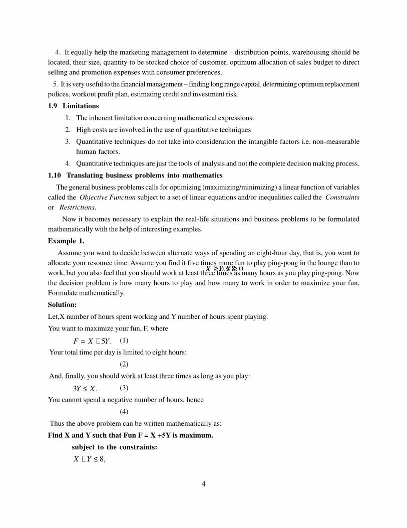
Let A = ,5,6}{0,1,2,3,4 and B = ,5,6}{0,1,2,3,4 .

Define BAf a: as xxfy =)(= . Here BAf a: is one-to-one function as Ax ∈∀ there

is a unique element in B such that if

)(=)( afaf ′

implies

aa ′=

. The graph of function xxfy =)(=is given as:

Figure-1

Onto function:

A function BAf a: is said to be an onto function if each element of B is the image of some

element of A.

In other words, BAf a: is onto if the image of f is the entire codomain, i.e., if BAf =)( . In

such a case we say that f is a function from A onto B or that f maps A onto B.

Example

Let A = 4}1,0,1,2,3,2,3,4,{ −−−− and B =

6}{0,1,4,9,1

.

Define BAf a: as 2=)(= xxfy .

19

Figure 2

Invertible function:

A function BAf a: is invertible if its inverse relation 1−f is a function from B to A. In general,

the inverse relation 1−f may not be a function.

Example

Let RRf a: be defined by 32=)( −xxf . Now f is one-to-one and onto; hence f has an

inverse function 1−f . Find a formula for 1−f .

Solution:

Let y be the image of x under the function f :

32=)(= −xxfy

Consequently, x will be the image of y under the inverse function 1−f . Solve for x in terms of y in the

above equation:

3)/2(= +yx

Then 2

3)(=)(1 +− y

yf . Replace y by x to obtain

2

3=)(1 +− x

xf

which is the formula for 1−f using the usual independent variable x.

Linear Functions : Linear function is a function of the form baxxfy ==)(= .

20

2.7 Important functions in Business

• Demand Function : In general, the demand function is expressed as :

bpaQd −=

where dQ is the quantity demanded (or purchased if offered) and p, is the price, a and b are constants.

• Supply Function : In general, the supply function is expressed as :

dpcQs −=

where sQ is the quantity offered for sale, and p is the price c and d are constants.

• Total Cost Function : In general, the total cost function explicitly can be expressed as:

)(= xCC

where x is the quantity produced and C is the total cost incurred. However, if total cost of producing xnumber of units of a particular commodity is analyzed in terms of fixed cost F, which is independent of x(with certain limits) and variable cost V(x), which varies with x, then we can write

)(=)( xVFxC +

The average cost of production or cost per unit is obtained by dividing total cost by the quantity produced.

That is

x

xCxAC

)(=)(

.

• Total Revenue Function : If Q(x) is the demand for the output of a firm costing p per unit, then totalrevenue (R) collected is given by

)(.= xQpR

• Consumption Function : In general, the consumption function is expressed as :

cYaC +=

where C is the total consumption and Y is the national income, a and c are constants.

• Investment Function : The simple investment function is expressed as :

0< 0> ;= bandabraI +where I represents investment and r the interest rate.

2.8 Limit of a function

Let

)(xf

be defined for all values of x near 0= xx with the possible exception of 0= xx itself (i.e.,

in a deleted neighborhood of 0x ).

We say that the number l is the limit of )(xf as x approaches

0x

and write

lxfxx

=)(lim0→

if for any positive number ε (however small) we can find some positive number (usually depending on ε )

such that

ε|<)(| lxf −

whenever

δ|<<|0 0xx −

.

21

In such case we also say that )(xf approaches l as x approaches

0x

and write lxf →)( as

0xx → . In words, this means that we can make )(xf arbitrarily close to l by choosing x sufficiently

close to

0x

.

Example

Let ≠

2.= 0

2 =)(

2

xif

xifxxf Then as x gets closer to 2 (i.e., x approaches 2), )(xf gets closer to 4. We thus

suspect that 4=)(lim2

xfx→

. To prove this we must see whether the above definition of limit (with 4=l ) is

satisfied.

Solution

We must show that given any 0>ε we can find

0>δ

(depending on

ε

in general) such that

ε|<4| 2 −x

when |<2<0| δ−x .

Choose 1≤δ so that

1|<2<|0 −x

or 3<<1 x , 2≠x . Then

.5|<2||<2||2|=|2)2)((|=|4| 2 δδ ++−+−− xxxxxx

Take δ as 1 or

/5ε

, whichever is smaller. Then we have

ε|<4| 2 −x

whenever δ|<2<|0 −x

and the required result is proved. It is of interest to consider some numerical values.

If for example we wish to make .05|<4| 2 −x , we can choose .01=.05/5=/5= εδ . To see that

this is actually the case, note that if .01|<2<|0 −x

then 2)2.01(<<1.99 ≠xx and so

4.0401<<3.9601 2x , .0401<4<.0399 2 −− x and certainly 4).05(|<4| 22 ≠− xx . The fact that these

inequalities also happen to hold at 2=x is merely coincidental.

If we wish to make 6|<4| 2 −x , we can choose 1=δ and this will be satisfied.

Special limits:

•

1=)(sin

lim0 x

x

x→

• 0=)(cos1

lim0 x

x

x

−→

• ex

x

x

=1

1liminf

+→

• ( ) ex x

x

=1lim1

inf+

→

22

2.9 Inequalities and their graphs

Inequality

An inequality is a statement that one (real) no. is greater than or less than another; for example,

2>3 − ;

5<10 −−

.

Two inequalities are said to have the same sense if their signs of inequality point in the same

direction.Thus,

2>3 −

and

10>5 −−

have the same sense;

2>3 −

and

5<10 −−

have opposite senses.

The sense of an equality is not changed:

(a) If the same number is added to or subtracted from both sides

(b) If both sides are multiplied or divided by the same positive number

An absolute inequality is one which is true for all real values of the letters involved; for example,

0>12 +x

is an absolute inequality.

A conditional inequality is one which is true for certain values of the letters involved; for example,

5>2+x is a conditional inequality, since it is true for 4=x but not for 1=x .

Examples

1. 1 ≤x , i.e. all the points to the left of 1 including 1.

2. 2 > x , i.e. all the points to the right of 2 except for 2 itself.

3. 4 ≤x , i.e. all the points to the left of 4 including 4.

4. x > 1 , i.e. all the points to the right of 1 except for 1 itself.

5. x− < 1 , i.e. x > 1− which means all the points to the left of -1 except for -1 itself .

2.10 Linear Inequalities in Two Variables

To solve some optimization problem, specifically linear programming problems, we must deal with linear

inequalities of the form

23

cbyax ≥+ cbyax ≤+ cbyax >+ ; < cbyax +

where a, b and c are given numbers. Constraints on the values of x and y that we can choose to solve our

problem, will be described by such inequalities.

Important points for graphical representation

• A point

),( 11 yx

is said to satisfy the inequality cbyax <+ if

cbyax <11 +

.

• It satisfies cbyax >+ if

cbyax >11 +

.

• It satisfies cbyax ≤+ if either

cbyax <11 +

or cbyax =11+ .

• It satisfies

cbyax ≥+

if either

cbyax >11 +

or cbyax =11+ .

The graph of a linear inequality is the set of all points in the plane which satisfy the inequality.

Notice that any point

),( 11 yx

satisfies exactly one of cbyaxcbyax <,> ++ or

cbyax =+

.

Example 1

Shade all the points which satisfy

632 ≥+ yx

.

Solution

We can represent the graph of the inequality either by shading or with arrows.

Figure 3

The plot with arrows will be more useful when we want to plot many inequalities simultaneously. The

points satisfying an inequality like 632 ≥+ yx include all points on the line 2x + 3y = 6 and all points above

it.

Example 2

Plot the graph of 1532 ≥− yx .

24

Solution

At (0,0), 15<0=32 yx − which is less than 15. Also, at

0=x

we have 5=15=3 −⇒− yy and

at 0=y we have 2

15=15=2 xx ⇒ . The points satisfying the inequality like 1532 ≥− yx include all

points on the line 2x -3y = 15 and all points below it.

Figure 4

Figure 5

2.11 System of equation

A system of two consistent and independent equations in two unknowns may be solved algebraically

by eliminating one of the unknowns.

The solution of two equation is helpful in finding the point of intersection of two lines, which is

required in obtaining the solution of problems graphically.

25

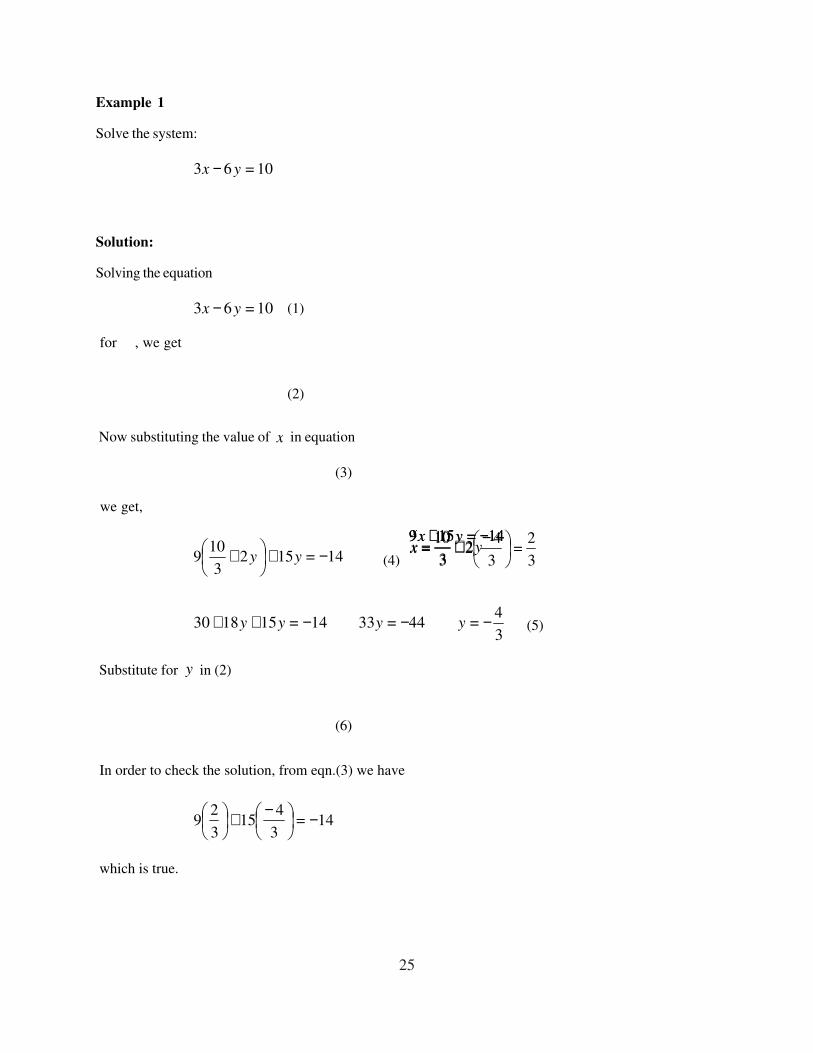
Example 1

Solve the system:

10=63 yx −

14=159 −+ yx

Solution:

Solving the equation

10=63 yx − (1)

for

x

, we get

yx 23

10= +

(2)

Now substituting the value of x in equation

14=159 −+ yx

(3)

we get,

14=1523

109 −+

+ yy (4)

3

4=44=3314=151830 −−−++ yyyy (5)

Substitute for y in (2)

3

2=

3

42

3

10=

−+x

(6)

In order to check the solution, from eqn.(3) we have

14=3

415

3

29 −

−+

which is true.

26

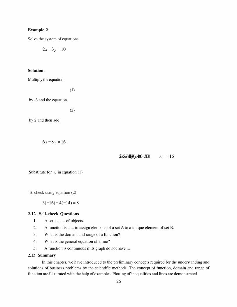
Example 2

Solve the system of equations

10=32 yx −

8=43 yx −

Solution:

Multiply the equation

10=32 yx −

(1)

by -3 and the equation

8=43 yx −

(2)

by 2 and then add.

30=96 −+− yx

16=86 yx −

−−−−− 14= −y

Substitute for x in equation (1)

16=10=14)3(2 −−− xx

To check using equation (2)

8=14)4(16)3( −−−

2.12 Self-check Questions

1. A set is a ... of objects.

2. A function is a ... to assign elements of a set A to a unique element of set B.

3. What is the domain and range of a function?

4. What is the general equation of a line?

5. A function is continuous if its graph do not have ...

2.13 Summary

In this chapter, we have introduced to the preliminary concepts required for the understanding and

solutions of business problems by the scientific methods. The concept of function, domain and range of

function are illustrated with the help of examples. Plotting of inequalities and lines are demonstrated.

27

2.14 Glossary

• Set: A well defined collection of objects.

• Value of function : The element y in B that is associated to x by f is denoted by f (x) and is called thevalue of f at x.

• Domain of f : The set A is called the domain of function f.

• Co-domain of f : The set B is called the co-domain of function f.

• Range of f : The set

})(,:)({ BxfAxxf ∈∈

of all values taken by

f

is called the range of f . It

is obviously a subset of B.

2.15 Answers to self-check questions

1. Well defined collection.

2. Rule.

3. If BAf a: , then elements of A are called domain and the elements of B under f are called the

range of f.

4. ax+by+c=0.

5. Any breaks.

2.16 Terminal Questions

1. Write the equation of line making an angle of o45 with x-axis and passing through origin.

2. Plot the lines 5=yx + and

3=yx −

.

3. Show that the points A(1, 2), B(0, -3), and C(2, 7) are on the graph of

35= −xy

.

4. Plot the common region of xy = and 6≤x.

5. Find the point of intersection of the lines 5=yx + and

0=1+− yx

.

6. Solve the system

5=2yx +

1=3 yx −

7. Solve the system

2=23 yx + 4=65 yx +

2.17 Suggested Readings

•Schaum series, College Mathematics, third edition.

•Operations Research by S.D. Sharma, Kedar Nath Ram Nath

&

Co.

•Morris, W. T.: On the Art of Modeling, Management Science, 13: B707-717, 1967.

•Operations Research by Vasant Lakshman Mote, T. Madhavan, Wiley.

*****

28

Lesson-3

Introduction to Operation Research

Structure

3.1 Learning Objective

3.2 Operations research – An Introduction

3.3 Historical development

3.4 Management applications of operations research

3.5 General methods of solving problems in operations research

3.6 Methodology of operations research

3.7 Limitations of operations research

3.8 Self-Assessment Questions

3.9 Summary

3.10 Glossary

3.11 Answers: Self-Assessment Questions

3.12 Terminal Questions

3.13 Suggested Readings

3.1 Learning Objectives

In today’s complex business environment, most management decisions cannot be made by simply applying

personal experience, guesswork or intuition. The consequences of wrong decisions are serious and costly.

The field of operations research comes to our rescue in the complex situations. Operations research provides

various tools and techniques that help us in decision making. This lesson provides an introduction to the field

of operations research. The objectives of the lesson are:

• To understand the concept and evolution of operations research

• To understand the applications and limitations of operations research

• To know basic procedure followed in operations research

3.2 Operations research – An Introduction

In order to understand what operations research is today, we must know something of its history and

evolution. We can trace the origin of operations research to World War II. Therefore, operation research is

a relatively new discipline. Its content and boundaries are not yet fixed.

Operation Research begins when some mathematical and quantitative techniques are used to

substantiate the decision being taken. In simple situations decisions are taken simply by common sense, sound

judgment, and expertise, without using any mathematics. Some decisions situations are, however, complex

and require proper diagnosis, analysis, and solution. Example of such decisions are finding the appropriate

product mix when there are large number of products with different profit contributions and production

requirements or planning public transportation network in a town having its own layout of factories, apartments,

blocks etc. Certainly in such situations decisions may well be arrived at intuitively from experience and

29

common sense, yet they are more judicious if backed up by mathematical reasoning. The search of a decision

may also be done by trial and error but such a search may be cumbersome and costly. Preparative calculations

may avoid long and costly research. Doing preparative calculations is the purpose of Operation Research.

Operation Research does mathematical scoring of consequences of a decision with the aim of optimizing the

use of time, efforts and resources and avoiding blunders.

The tools of operation research are not from any one discipline; rather operations research takes

tools from subjects like mathematics, statistics, economics, engineering, psychology etc. and combines them

to make a new body of knowledge for decision making. Today, it has become a professional discipline that

deals with the application of scientific methods for decision making, and especially to the allocation of scarce

resources.

Operation Research can also be treated as science devoted to describing, understanding and predicting

the behaviour of systems particularly man-machine system. Thus operation research workers are engaged in

three classical aspect of science:

a) Describing the behaviour of a system.

b) Analyzing this behaviour by constructing appropriate models.

c) Using these models to predict future behaviour, that is, the effect that will be produced by changes in

the systems or in the methods of operations.

The operation system studied by operation research workers arise in wide variety of practical, military,

industry, and governmental environment. Thus, the results of their research frequently make important

contributions to solutions of problems of choice, policy, and planning that arise in these environments. It is to

be noted that operations research workers in an organization are not the decision makers themselves. They

merely present their findings to the executives in –charge of operation who is supposed to make decisions.

Operation research function is a staff function. Operation Research is assistance to executives in improving

the operations under their control.

What particularly distinguishes operation research from other research and engineering is its emphasis

on analysis of operation as a whole. Most present- day business applications are primarily concerned with

mathematical and statistical analysis of the results of possible alternative actions. Often using techniques

especially designed or refined for business problems, operations research have been able to provide remarkable

and diverse benefits to companies. Some such benefits are improved inventory and reorder policies, minimum

cost production schedules, optimum location and size of warehouse, and guidance in sales and advertising

policies. The basic pattern applied is clarification of various courses of action open, estimation of the outcome

to be expected from each, and evaluation of these in terms of the overall goal desired.

Defining operations research is a difficult task. Salient aspects related to definition stressed by various

experts on the subject are as follows:

a) Pocock stresses that operation research is an applied science. He states “Operations Research is

scientific methodology-analytical, experimental, quantitative-which by assessing the overall implication

of various alternative courses of action in a management system, provides an improved basis for

management decisions.”

b) Morse and Kimball have stressed the quantitative approach of Operations Research and have

described it as “a scientific method of providing executive departments with a quantitative basis for

decisions regarding the operations under their control.”

30

c) Miller and Starr see Operations Research as applied decision theory. They state, “Operations Research

is applied decision theory. It uses any scientific, mathematical or logical means to attempt to cope

with the problems that confront the executive, when he tries to achieve a thorough-going rationality

in dealing with his decision problem.”

d) Saaty considers Operations Research as tool of improving the quality of answers to problems. He

says, “Operations Research is the art of giving bad answers to problems which otherwise have

worse answers.”

e) Churchman, Acoff, and Arnoff state, “Operations research is the application of scientific methods,

techniques and tools to problems involving the operations of systems so as to provide those in control

of the operations with optimum solutions to the problem.

f) Wagner defines it as scientific approach to problem solving for executive management.

All these definitions put together enable us to know what Operation Research is, and what it does.

3.3 Historical Development

Operation research has its beginning in World War II. The term, operations research, was coined by

McClosky and Trefthen in 1940 in U.K. British scientists set up the first field installations of radars during the

battle and observed air operations. Their analysis of these led to suggestions that greatly improved and

increased the effectiveness of British fighters, and contributed to successful British defense. Operations

research was then extended to antisubmarine warfare and to all phase of military, naval, and air operations,

both in Britain and the United States, and was incorporated in the postwar military establishments of both the

countries.

The effectiveness of operation research in military spread interest in it to other government departments

and industry. In the U.S.A the National Research Council formed a committee on operation research in 1951,

and the first book on the subject “Methods of Operation Research” by Morse and Kimball, was published. In

1952 the Operation Research Society of America came into being.

Today, almost every large organization or corporation in affluent nations has staff applying operations

research, and in government the use of operations research has spread from military to widely varied

departments at all levels. This general acceptance to Operation Research has come as managers have

learned the advantage of the scientific approach on which Operation Research is based. Availability of faster

and flexible computing facilities and the number of qualified operation research professionals enhanced the

acceptance and popularity of the subject. The growth of Operation Research has not been limited to the

U.S.A and the U.K. It has reached to many countries of the world. Indicative of this is that the international

Federation of Operation Research Societies, founded in 1959, now comprises member societies from many

countries of the world.

India was one of the first few countries who started using Operation Research in 1949, first Operation

Research unit was established in Regional Research Laboratory at Hyderabad. At about same time another

group was set up in Defense Science Laboratory to solve the problems of stores, purchase and planning. In

1953, Operation Research unit was established in Indian Statistical Institute, Calcutta, with the aim of using

Operation Research in national planning and survey. Operation Research society of India was formed in

1955. The society is one of the first members of International Federation of Operation Research societies.

The society started publishing OPSEARCH, a learned journal on the subject in 1963. Today Operation

Research is a popular subject in management institutes and schools of mathematics and is gaining currency

in industrial establishments.

31

3.4 Management applications of Operations Research

3.5 General Methods of Solving Operations Research Problems

In general, the following three methods are used for solving OR problems. In all these methods,

values of decision variables are obtained that optimize the given objective function (a measure of effectiveness).

(i) Analytical (or Deductive) Method - In this method, classical optimization techniques such as calculus,

finite difference and graphs are used for solving a problem. In this case, we have a general solution

specified by a symbol and we can obtain the optimal solution in a non-iterative manner.

(ii) Numerical (or Iterative) Method - When analytical methods fail to obtain the solution of a particular

problem due to its complexity in terms of constraints or number of variables, a numerical (or iterative)

method is used to get the solution. In this method, instead of solving the problem directly, a general

algorithm is applied to obtain a specific numerical solution. The numerical method starts with a

solution obtained by trial and error, and a set of rules for improving it towards optimality. The solution

so obtained is then replaced by the improved solution and the process of getting an improved solution

is repeated until such improvement is not possible or the cost of further calculation cannot be justified.

(iii) Simulation (Monte-Carlo) Method- This method is based upon the idea of experimenting on a

mathematical model by inserting into the model specific values of decision variables at different

points of time and under different conditions and then observing their effect on the criterion chosen

for variables. In this method, random samples of specified random variables are drawn to know

what is happening to the system for a selected period of time under different conditions. The random

samples form a probability distribution that represents the real life system and from this probability

distribution, the value of the desired random variable can be estimated.

Area

Finance & Accounting

Production & Construction

Inventory & Logistics

Marketing

Human resource management

Purchasing

R & D

Applications

Dividend decisions, investments decision, capital budgeting, portfolio

analysis, capital structure decisions, working capital management, cash

flow-fund flow analysis etc.

Resource allocation in projects, project scheduling & monitoring,

location & layout decisions, Product & process selection, production

planning & control, sequencing & line balancing, maintenance

decisions etc.

Inventory management, logistics decision, transportation problems,

warehouse locations decisions etc.

Product mix decision, promotion mix decision, advertising media

planning & scheduling, marketing control, market potential analysis

etc.

Man power planning, training, compensation management etc.

Ordering & buying, supplier evaluation, replacement planning etc.

New product development, re-engineering, reliability decisions etc.

32

3.6 Methodology of Operations Research

Every OR specialist may have his/her own way of solving problems. However, for effective use of

OR techniques, it is essential to follow some steps that are helpful for decision-makers to make better

decisions. The methodology of MS is explained below:

Step 1: Analysis of the System and Defining the Problem

The first step in the OR is to identify, understand, and describe, in precise terms, the problem that

the organization faces. The analysis begins by detailed observation of the organizational structure, communication

and control system, its objectives and expectations. Such information will help in assessing the difficulty of

the study in terms of costs, time requirements, resource requirement, probability of success of the study, etc.

The major steps which have to be taken into consideration for formulating the problems are as

follows:

(a) Problem components: The first component of the problem to be defined is the decision-maker

who is not satisfied with the existing state of affairs. The interaction with the decision-maker will

help the OR specialist in knowing his objectives. That is, either he has already obtained some

solution of the problem and wants to retain it, or he wants to improve it to a higher degree. If the

decision-maker has conflicting of multiple objectives, he may be advised to rank his objectives in

order of preference; overlapping among several objectives may be eliminated.

Figure 1: Methodology of Operations research

Real world

problem

Solve the Model Apply suitable OR technique to get

solution in terms of decision variables

Testing the Model and its

Solution Put values of decision variables in the model under

consideration

See whether solution is valid or not

Modify

the

model

Implementation and Control Interpret solution values

Put the knowledge (result) gained from the solution to work through organizational policies.

Solution to work through organizational policies

Monitor changes and exercise control

System

Choosing a particular

aspect of reality which

needs attention

Model Building Establish relationships among variables and parameters

of the system

Define objective to be achieved and limitations on

resources

Yes

No

33

(b) Decision environment: It is desirable to know about the resources such as managers, employees,

equipments, etc. which are required to carry out the policies of the organization considering the

social and ecological environment in which the organization functions. Knowledge of such factors

will help in modifying the initial set of the decision-maker objectives.

(c) Alternative courses of action: The problem arises only when there are several courses of action

available for a solution. An exhaustive list of courses of action can be prepared in the process of

going through the above steps of formulating the problem. Courses of action which are not feasible

with respect to objectives and resources may be ruled out.

(d) Measure of effectiveness: A certain measure of effectiveness or performance is required in order

to evaluate the merit of the several courses of action listed. The performance or effectiveness can

be measured in different units such as rupees (net profits), percentage (share of market desired),

time dimension (service or waiting time). In order to bring uniformity in the measurement, one of

the performance criteria must be chosen to express the value in terms of the value of the criterion

chosen earlier. Qualitative objectives which cannot be quantified must be assigned weights and

probability measures to their attainability.

Step 2: Collecting Data and Developing Mathematical Model

After the problem is clearly defined and understood, the next step is to collect required data and then

formulate a mathematical model. There are certain basic components which are required in every decision

problem model.

(a) Controllable (decision) variables: These are the issues or factors in the problem whose values

are to be determined (in the form of numerical values) by solving the model. The possible values

assigned to the variables are called decision alternatives (strategies or courses of action). For

example, in queuing theory the number of service facilities is the decision variable.

(b) Uncontrollable variables: These are the factors whose numerical value depends upon the external

environment prevailing in the organization. The values of these variables are not under the control

of the decision-maker and are also termed as state of nature.

(c) The objective function: It is representation of (i) the criterion that expresses the decision-maker’s

manner of evaluating the desirability of alternative values of the decision variables, and (ii) how that

criterion is to be optimized (minimized or maximized). For example, in queuing theory the decision-

maker may consider several criteria such as minimizing the average waiting time of customers, or

the average number of customers in the system at any time.

(d) Constraints (or limitations): These are the restriction on the values of the decision variables.

These restrictions can arise due to limited resources such as space, money, manpower material etc.

The constraints may be in the form of equations or inequalities.

(e) Functional relationships: In a decision problem, the decision variables in the objective function

and in the constraints are connected by a specific functional relationship. A general decision problem

model can be written as:

Optimise (Max or Min) Z = f (x)

subject to the constraints

gi (x) {≤ = ≥}

b

i ; i= 1, 2,….,m

34

and x ≥ 0

where, x = a vector of decision variables (x1,x

2….,x

n)

f(x) = criterion or objective function to be optimized

gi (x) =

the ith constraint

bi =

fixed amount of the ith resource

A model is referred to as a linear model if all functional relationships among decision variables

x1,x

2……., x

n in f(x) and g(x) are of a linear form. But if one or more of the relationship are non-linear,

the model is said to be a non-linear model.

(f) Parameters: These are constants in the functional relationship. Parameters can be deterministic

or probabilistic in nature. A deterministic parameter is one whose value is assumed to occur with

certainty. However, if constants are considered directly or explicitly as random variables, they are

probabilistic parameters.

Step 3: Solving the Mathematical Model

Once a mathematical model of the problem has been formulated, the next step is to solve it, that is to

obtain numerical values of decision variables. Obtaining these values depends on the specific form, or type of

mathematical model. In general, the following two categories of methods are used for solving an OR model.

(a) Optimisation methods: These methods yield the best values for the decision variables both for

unconstrained and constrained problems. In constrained problems, these values simultaneously

satisfy all of the constraints and provide an optimal or acceptable value for the objective function

or measure of effectiveness. The solution so obtained is called the optimal solution to the problem.

(b) Heuristic methods: These methods yield values of the variables that satisfy all the constraints,

but not necessarily provide optimal solution. However, these values provide an acceptable value

for the objective function.

Heuristic methods are sometimes described as ‘rules of thumb which work’. An example of a

commonly used heuristic is ‘stand in the shortest line’. Although using this rule may not work if everyone in

the shortest line requires extra time, in general, it is not a bad rule to follow. These methods are used when

obtaining optimal solution is either very time consuming or model is complex.

Step 4: Validating the Solution

After solving the mathematical model, it is important to review the solution carefully to see that the values

make sense and that the resulting decision can be implemented. Some of the reasons for validating the

solution are:

(i) The mathematical model may not have enumerated all the limitations of the problem under

consideration.

(ii) Certain aspects of the problem may have been overlooked, omitted or simplified.

(iii) The data may have been incorrectly estimated or recorded, perhaps when entered into the

computer.

Step 5: Implementing the Solution

The decision-maker has not only to identify good decision alternatives but also to select alternatives

that are capable of being implemented. It is important to ensure that any solution implemented is continuously

35

reviewed and updated in the light of a changing environment. The behavioural aspects of change are exceedingly

important to the successful implementation of results. In any case, the decision-maker who is in the best

position to implement results must be aware of the objective, assumption, omissions and limitations of the

model.

Step 6: Modifying the Model

For a mathematical model to be useful, the degree to which it actually represents the system or

problem being modeled must be established. If during validation, the solution can not be implemented, one

needs to identify constraint that were omitted during the original problem formulation or to find if some of the

original constraints were incorrect and need to be modified. In all such cases, one must return to the problem

formulation step and carefully make the appropriate modifications to represent more accurately the given

problem. A model must be applicable for a reasonable time period and should be updated from time to time,

taking into consideration the past, present and future aspects of the problem.

Step 7: Establishing Controls over the Solution

The dynamic environment and changes within the environment can have significant implications

regarding the continuing validity of models and their solutions. Thus, a control procedure has to be established

for detecting significant changes in decision variables of the problem so that suitable adjustments can be

made in the solution without having to build a model every time a significant change occurs.

3.7 Limitations of operations research

Operation Research has certain limitations. However, these limitations are mostly related to the

problem of model building and the time and money factors involved in its application rather than its practical

utility. Some of them are as follows:

1) Magnitude of Computations: Operation Research tries to find out optimal solution taking into

account all the factors. In the modern society these factors are enormous and expressing them in

quantity and establishing relationship among these require voluminous calculations which can only be

handled by machines.

2) Non-Quantifiable Factors. : Operation Research provides solution only when all elements related

to a problem can be quantified. All relevant variables do not lend themselves to quantification. Factors

which cannot be quantified, find no place in Operation Research. Models in Operation Research. do

not take into account qualitative factors or emotional factors which may be quite important.

3) Distance between Manager and Operation Research: Operation Research specialist’s job requires

a mathematician or a statistician, who might not be aware of the business problems. Similarly, a

manager fails to understand the complex working or Operation Research. Thus there is a gap between

the two. Management itself may offer a lot of resistance due to conventional thinking.

4) Money and Time Costs: When the basic data are subjected to frequent changes, incorporating

them into the Operation Research models is a costly affair. Moreover, a fairly good solution at

present may be more desirable than a prefect Operation Research solution available after sometime.

5) Implementation: Implementation of decisions is a delicate task. It must take into account the

complexities of human relations and behaviour. Sometimes resistance is offered only due to

psychological factors.

36

3.8 Self-Assessment Questions

1. What do you understand by Operation Research?

2. What is the role of OR in management decision making.

3. What are the different methods of solving OR problems.

4. Discuss the problems of OR.

3.9 Summary

Operations research is a relatively new discipline. It has its origin in World War II. It has taken tools

and techniques from various areas like mathematics, statistics, engineering, economics, psychology etc.

Operations research can be regarded as use of mathematical and quantitative techniques to substantiate

the decision being taken. Developing appropriate models for situations, processes and systems etc. is basic

essence of OR field. These models can then be tested, and operated on to determine the effects of changing

the values of variables with particular reference to optimisation of some criterion.

Operation Research has certain limitations. However, these limitations are mostly related to the

problem of model building and the time and money factors involved in its application rather than its practical

utility. Operation Research tries to find out optimal solution taking into account all the factors. In the modern

society these factors are enormous and expressing them in quantity and establishing relationship among these

require voluminous calculations which can only be handled by machines. Operation Research provides solution

only when all elements related to a problem can be quantified. Factors which cannot be quantified, find no

place in Operation Research.

3.10 Glossary

Operations Research: is an analytical method of problem-solving and decision-making that is

useful in the management of organizations.

Decision-making: is the act of choosing between two or more courses of action. In the wider

process of problem-solving, decision-making involves choosing between possible solutions to a problem.

Variable: is a named unit of data that may be assigned a value. If the value is modified, the name

does not change.

Parameter:definable, measurable, and constant or variable characteristic, dimension, property, or

value, selected from a set of data (or population) because it is considered essential to understanding a

situation (or in solving a problem).

Simulation: is the process of designing a model of a real system and conducting experiments with

this model for the purpose of understanding the behaviour of the system and/or evaluating various strategies

for the operation of the system.

3.11 Answers: Self-assessment Questions

1. For answer refer: section 1.2

2. For answer refer: section 1.4

3. For answer refer: section 1.5

4. For answer refer: section 1.7

37

3.12 Terminal Questions

1. “Operations research is a quantitative approach to decision making.” Explain the statement citing

suitable examples.

2. Discuss the general methods of solving OR problems.

3. Discuss the steps of OR methodology.

4. Define OR and discuss its usage and limitations.

5. Clarify the concept of OR and discuss its evolution over the years

3.13 Suggested Readings

1) Taha, H.A., “Operations Research - an introduction”, Prentice Hall of India Pvt. Ltd., New Delhi.

2) Wagner, H.M., “Principles of Operation Research”, Prentice Hall, Inc., Englewood Cliffs, N. J.

3) Chakravarty, Samir K., “ Theory & problems on Quantitative Techniques, Management information

system & Data processing”, New central book agency, Calcutta.

4) Ackoff, R.L., and Sasieni, M.W., “Fundamentals of Operation Research”, John Wiley & Sons,

New York.

5) Srivastava U. K., Shenoy, G.V., and Sharma, S.C., “Quantitative Techniques for Managerial

Decisions”, 2nd edition, New Age International (P) limited, New Delhi.

6) Thomas M. Cook, and Robert A. Russell, “Introduction to Management Science”, Prentice Hall,

Englewood Cliffs, New Jersey.

*****

38

Lesson-4

Operations Research Models

Structure

4.1 Learning Objective

4.2 Classification of models

4.3 Principles of modelling

4.4 Basic OR models

4.5 Self-Assessment Questions

4.6 Summary

4.7 Glossary

4.8 Answers: Self-Assessment Questions

4.9 Terminal Questions

4.10 Suggested Readings

4.1 Learning Objectives

Operations research can be regarded as use of mathematical and quantitative techniques to substantiate

the decision being taken. Developing appropriate models, for situations, processes and systems etc. is basic

essence of operation research field. These’ models can then be tested, and operated on to determine the

effects of changing the values of variables with particular reference to optimization of some criterion. This

lesson focuses on various operation research models. The objectives of the lesson are:

To know the types of models

To understand OR models.

A model in the sense used in OR is defined as a representation of an actual object or situation. It

shows the relationships and inter relationships of action and reaction in terms of cause and effect. Since a

model is an abstraction of reality, it appears to be less complete than reality itself.

The main objective of a model is to provide means for analyzing the behaviour of the system for the

purpose of improving its performance. If a system is not in existence, then a model defines the ideal structure

of this future system, indicating the functional relationships among its elements. The reliability of the solution

obtained from a model, however, depends on the validity of the model in representing the real systems.

Actually, a model permits to examine the behaviour of a system without interfering with ongoing operations.

4.2 Classification of models

Models can be classified according to the following characteristics :

(i) Iconic/Analogue/Symbolic Models - Iconic models represent the system as it is, by scaling it up

or down, i.e., by enlarging or reducing the size. In other words, they are images. For example, a toy

aeroplane is an iconic model of a real one. Drawings and maps are other examples. A model of an

atom is scaled up while in globe the diameter of the earth is scaled down. The iconic models are

usually the simplest to conceive and the most specific and concrete. Their function is generally

descriptive rather than explanatory.

39

Analogue models are models in which one set of properties is used to represent another set of

properties. For example, graphs are very simple analogues because they can represent many

properties such as time, numbers, percentages etc. analogue models are less specific, less concrete

but easier to manipulate.

Symbolic or mathematical models employ a set of mathematical symbols, i.e., letters, numbers etc.

to represent a system. Here, the variables are related together by means of mathematical equations

to describe the behaviour or properties of the system. The solution of the problem is then obtained

by applying well developed mathematical techniques to the model. The symbolic model is easiest to

manipulate experimentally and is most general and abstract. Its function is more often explanatory

than descriptive.

(ii) Descriptive/Predictive/Prescriptive models - A descriptive model simply describe some aspects

of a situation based on observation, survey etc. Predictive models are used to answer ‘what if type

of situations and can help us predicting certain events. If a predictive model is successful repeatedly,

it can be used to prescribe a source of action. For example linear programming is a prescriptive

model because it prescribes what managers ought to do.

(iii) Deterministic/Probabilistic models - Deterministic models assume conditions of complete

certainty and perfect knowledge. For example transportation and assignment models are deterministic

in nature. Probabilistic or stochastic models usually handle such situations in which the consequences

or payoff of managerial actions cannot be predicted with certainty. However, it is possible to forecast

a pattern of events based on which managerial decisions can be made.

(iv) Static/Dynamic models - Static models are independent of time. These models do not consider

the impact of changes that takes place during the planning horizon. In dynamic models time is

considered as one of the important variables. In dynamic models a series of interdependent decisions

are required.

(v) Analytical/Simulation models - Analytical models have a specific mathematical structure and

thus can be solved by known mathematical techniques. For example transportation and assignment

models are analytical models. Simulation models are essentially a structure of reality in order to

study the system under consideration under a variety of assumptions.

4.3 Principles of Modeling

Let us know outline general principles useful in formulation OR models. Model builders must take

into account the following principles :

• Do not build a complicated model when simple one is suffice.

• Beware of molding the problem to fit the technique.

• The deduction phase of modeling must be conducted rigorously.

• Models should be validated prior to implementation.

• A model should neither be pressed to do, nor criticized for failing to do the thing for which it was

never intended.

• A model cannot be any better than the information that goes into it.

• Models cannot replace decision makers.

40

4.4 Basic Operation Research Models

There is no unique set of problems which can be solved by using OR models or techniques. Several

OR models or techniques can be grouped into some basic categories as given below :

• Allocation Models - Allocation models are used to allocate resources to activities in such a way

that some measure of effectiveness (objective function) is optimized. Mathematical

programming is the broad term for the OR techniques used, to solve allocation problems.

If the measure of effectiveness such as profit, cost, etc. is represented as a linear function of

several variables and if limitations on resources (constraints) can be expressed as a system of

linear equalities or inequalities, the allocation problem is classified as a linear programming

problem. But if the objective function of any or all of the constraints cannot be _ expressed as

a system of linear equalities or inequalities the allocation problem is classified as a non-linear

programming problem.

When the solution values or decision variables for the problem are restricted to being integer

values or just zero-one values, the problem is classified as an integer programming problem or

a zero-one programming problem, respectively. The problem having multiple, conflicting and

incommensurable objective functions (goals) subject to linear constraints is called a goal

programming problem. If the decision variables in the liner programming problem depend on

chance, such a problem is called a stochastic programming problem .

If resources such as workers, machines or salesmen can be assigned to perform a certain number

of activities such as jobs or territories on a one-to-one basis so as to minimize total time, cost or

distance involved in performing a given activity, such problems are classified as assignment

problems. But if the activities require more than one resource, and conversely, if the resources

can be used for more than one activity, the allocation problem is classified as a transportation

problem.

• Inventory Models - Inventory may be defined as the stock of goods, commodities, or other

economic resources that are stored or reserved in order to ensure smooth and efficient running

of business affairs. Inventory or stock of goods may contain raw material & purchased parts,

partially completed goods (work-in-progress), consumables, finished goods and replacement

parts, tools & supplies.

Inventory control is essential because inadequate control can result in both under stocking and

overstocking of items-. Under stocking results in missed deliveries lost sales, dissatisfied

customers, & production bottlenecks whereas overstocking unnecessarily ties up funds that

might be more productive elsewhere.

Inventory models deal with the problem of determination of how much to order at a point in

time and when to place an order. The main objective is to minimize the sum of three conflicting

inventory costs: the cost of holding or carrying extra inventory, the cost of shortage or delay in

the delivery of items when it is needed, a cost of ordering or set-up. These are also useful in

dealing with quantity discounts and selective inventory control.

The order quantity which minimizes the total inventory cost is called economic order quantity.

Determination of EOQ is essential for inventory management. EOQ determination requires the

knowledge of various costs like holding or ordering costs. There are different models for finding

41

EOQ in different conditions. These models are divided into deterministic and probabilistic

categories. In deterministic situations, variables are known with certainty while in other cases

variables are probabilistic.

• Waiting Line (or Queuing) Models - The queuing problem is identified by the presence of a

group of customers who arrive randomly to receive some service. The customer upon arrival

may be attended to immediately or may have to wait until the server is free.

The queuing models are basically relevant to service oriented organizations and suggest ways

and means to improve the efficiency of the service. This situation can be seen in the field of

business (bank, booking counters), industries (servicing of machines), government (railway or

post-office counters), transportation (airport, harbor) and everyday life (elevators, restaurants,

doctor’s chamber) etc. Queuing methodology indicates the optimal usage of existing manpower

and other resources to improve the service. It can also indicate the cost implications if the

existing service facility has to be improved by adding more servers.

These models have been developed to establish a trade-off between costs of providing service

and the waiting time of a customer in the queuing system. Constructing a model entails describing

the components of the system: arrival process, queue structure and service process and solving

for the measure of performance-average length of waiting time, average time spent by the

customer in the line, traffic intensity, etc. of the waiting system.

• Competitive (Game Theory) Models - Game theory is a body of knowledge which is concerned

with the study of decision making in situations where two or more rational opponents are

involved under conditions of competitions and conflicting interest. In Game theory one seeks

to determine rival’s most profitable counters, strategy to one’s own ‘best’ moves and formulate

the appropriate defensive measures.

A competitive situation where gain by one of the firms is necessarily at the cost of the other.

This situation is basically called as a two person, zero-sum game. This is called zero- sum

because, whatever is done by either competitor, the sum of the net gain in the market share by

the two competitors is zero. However, there are situations where decisions which are taken by

the firms may very well increase or reduce both the absolute size of their market and the total

profits taken together. Such problems are not considered as zero-sum games.

Games theory has been used in business and industry to develop bidding tactics, pricing policies,

advertising strategies etc.

• Network Models - These models are applied to the management (planning, controlling and

scheduling) of large scale projects. PERT/CPM technique help in identifying potential trouble

spots in a project through the identification of the critical path. These techniques improve

project coordination and enable the efficient use of resources. Network methods are also used

to determine time-cost trade-off resource allocation and updating of activity time.

• Sequencing Models - The sequencing problem arises whenever there is a problem in determining

the sequence (order) in which a number of tasks can be performed by a number of service facilities

such as hospital, plant etc. in such a way that some measure of performance, for example, total

time to process all the jobs on all the machines, is optimized.

42

• Dynamic Programming Models - Dynamic programming may be considered as an outgrowth of

mathematical programming involving the optimization of multistage (sequence of inter-related

decisions) decision processes. The method starts by dividing a given problem into stages or sub-

problems and then solves those sub­-problems sequentially until the solution to the original problem

is obtained.

• Markov-Chain Models - These models are used for analyzing a system which changes over a

period of time among various possible outcomes or states. The model while dealing with such

systems describes transitions in terms of transitions probabilities of various states. These models

have been used to test brand-loyalty and brand switching tendencies of consumers, where each

system state is considered to be a particular brand purchase.

• Simulation Models - Simulation is a technique that involves developing a model of a process and

then conducting experiment on the model in order to evaluate its behaviour under certain conditions.

Simulation is not an optimizing technique. In fact, simulation does not produce a solution; instead it

enables decision makers to test their solutions on a model that reasonably duplicates a real process.

The use of simulation as a decision making tool is fairly wide-spread. Space engineers simulate

space flight in laboratories to permit future astronauts to become accustomed to working in a

weightless environment. Similarly, airline pilots often undergo extensive training with simulated

landings and take-offs before being allowed to try the real thing.

There are many different kinds of simulation techniques. One of the techniques is Monte Carlo

method. The chance element is an important aspect of Monte Carlo simulation. In the Monte Carlo

method, a probability distribution is developed that reflects the random component of the system

under study.

There are certain limitations associated with simulation. Simulation does not produce an optimum

solution; it merely indicates and approximates behaviours for a given set of inputs. A large-scale

simulation can require considerable effort to develop a suitable model as well as considerable

computer time to obtain simulations. Simulation can be time-consuming and costly.

(j) Decision Analysis Models - These models deal with the selection of an optimal course of action

given the possible payoffs and their associated probabilities of occurrence. These models are broadly

applied to problems involving decision-making under risk and uncertainty.

4.5 Self-assessment Questions

1. What are the different types of models on the basis characteristics?

2. What are the main things we must consider while formulating OR model?

3. What do you understand by allocation model?

4. What do you understand by queuing model?

5. What do you understand by competitive model?

4.6 SUMMARY:

Developing appropriate models for situations, processes and systems etc. is basic essence of operation

research field. These models can then be tested, and operated on to determine the effects of changing the

values of variables with particular reference to optimisation of some criterion.

43

A model in the sense used in OR is defined as a representation of an actual object or situation. It

shows the relationships and inter relationships of action and reaction in terms of cause and effect. The main

objective of a model is to provide means for analyzing tie behaviour of the system for the purpose of improving

its performance.

Models can be classified as iconic, analogue, descriptive, predictive, deterministic, stochastic, static,

dynamic, analytical and other categories. Some of the OR models include allocation, waiting line, inventory,

decision analysis, sequencing, network, and replacement.

4.7 Glossary

Model: is a collection of logical and mathematical relationships that represents aspects of the situation

under study. 

Game theory: is the study of mathematical models of strategic interaction among rational decision-

makers.

Programming: is the process of creating a set of instructions that tell a computer how to perform a

task.

Inventory: or stock is the goods and materials that a business holds for the ultimate goal of resale.

Simulation: is the process of designing a model of a real system and conducting experiments with

this model for the purpose of understanding the behaviour of the system and/or evaluating various strategies

for the operation of the system.

4.8 Answers: Self-assessment Questions

1. For answer refer: section 2.2

2. For answer refer: section 2.3

3. For answer refer: section 2.4

4. For answer refer: section 2.4

5. For answer refer: section 2.4

4.9 TERMINAL QUESTIONS:

• What do you understand by model? Discuss some of principle of model building

• Write a detailed note on types of models.

• Discuss some of the OR models.

• Write short notes on the following :

• Allocation models

• ‘ Inventory models

• Discuss briefly:

a. Simulation models

b. Waiting line models

44

4.10 SUGGESTED READINGS :

1) Taha, H.A., “Operations Research - an introduction”, Prentice Hall of India Pvt. Ltd.,

2) Wagner, H.M., “Principles of Operation Research”, Prentice Hall, Inc., Englewood Cliffs, New

Jersey.

3) Chakravarty, Samir K., “ Theory & problems on Quantitative Techniques, Management information

system & Data processing”, New central book agency, Calcutta.

4) Ackoff, R.L., and Sasieni, M.W., “Fundamentals of Operation Research”, John Wiley & Sons,

New York.

5) Srivastava U. K., Shenoy, G.V., and Sharma, S.C., “Quantitative Techniques for Managerial

Decisions”, 2nd edition, New Age International (P) limited, New Delhi.

*****

45

Lesson-5

Linear Programming

STRUCTURE

5.1 Learning Objective

5.2 Formulation of Liner programming problems

5.3 Characteristics of Liner programming problems

5.4 Graphical method for solving Liner programming problems

5.5 Self-Assessment Questions

5.6 Summary

5.7 Glossary

5.8 Answers: Self-Assessment Questions

5.9 Terminal Questions

5.10 Suggested Readings

5.1 Learning Objective

Linear programming is a technique for finding the optimal uses of an organisation’s scarce resources.

It helps a decision maker in most effectively employing his productive factors by more efficient use of his

resources. It helps us in deciding a course of action when constraints affect our choices. It helps in increasing

the profits or reducing the costs. This lesson throws light on formulation, characteristics, application, and

graphical solution of linear programming problems. The objectives of the lesson are:

• To understand the characteristics of Linear programming problems

• To know how to formulate Linear programming problems

• To understand graphical solution to Linear programming problems

The contents of the lesson are:

• Formulation of Linear programming problems

• Characteristics of Linear programming problems

• Graphical method for solving Linear programming problems

• Summary

• Select questions

• Suggested Readings

A large number of managerial problems are concerned with the efficient use or allocation of limited

resources to meet the desired objectives. These problems are characterized by the large number of solutions

that satisfy the basic conditions of each problem. The selection of a particular solution as the best solution to

a problem depends upon the overall objective of the problem. A solution that satisfies both the conditions of

the problem and the given objectives is known as an optimum solution. A typical example is that of a

manufacturing company which must determine the combination of resources available so as to enable it to

manufacture products in a way which not only satisfies its production schedule, but also maximizes its profits

or minimizes its cost.

46

A technique called, linear programming has become a popular tool for allocation of scarce resources

with an objective of making an optimal use of them. It is a mathematical technique for finding the optimal uses

of a company’s scarce resources. Production manager, for example, is often encountered with the problem:

how much of each of the product be manufactured taking into account the capacities such as manpower,

finance, material etc., so as to maximize the profits. If there were no constraints on these resources, then he

would probably produce an infinite number of units of each product to make infinite profit. However, the

above proposition is only a hypothetical one.

In real life situations, a manager operates under many constraints. He finds it difficult to get skilled

labour, the plant capacity is limited, the market demand for the product is varying, timely availability of raw

material is difficult, difficulty in getting finance for working capital or for modernization of plant or for increasing

production capacity, etc. Thus, there are limitations on all the ‘key’ resources, namely, men, material and

money. The manager working under these constraints has to decide his product-mix in such a way that the

profits are maximized, or alternatively, the cost of production is minimized. If the company is manufacturing

only two products, the intuitive judgment or the ‘experience-based’ decision of the manager may be very

close to the optimal solution, but in situations where the company is manufacturing a number of products, the

intuitive judgment of the manager is likely to result into a solution which is far from optimal. Linear programming

is an optimization technique for finding an optimal solution to such business problems of complex nature.

Furthermore, the linear programming technique gives an optimal solution to a given function under the

‘inequality’ constraints. The classical optimization techniques fail to serve our purpose because of these

inequality constraints.

Linear programming had its beginning in the input-output analysis developed by the well known

economist W.W.Leontief. Hitchcock and Koopman’s transportation type problem’ studied during 1940s and

Stigler’s ‘diet problem’ (problem concerned with separate entities that can be selected and used in diversified

quantities by choosing, combining, or mixing them with the purpose of obtaining an expected result) developed

in 1945 were the first problems where the linear programming technique was used to obtain an optimal

solution. The ‘simplex method’ (a systematic procedure for solving a linear programming problem) developed

by Prof. George D. Dantzig in 1947 is the present day basic tool for solving any linear programming problem.

A linear programming problem differs from the general variety in that a mathematical model or

description of the problem can be stated using relationships which are called ‘straight-line’ or linear. The term

‘programming’ makes use of certain mathematical techniques to arrive at the best solution. Mathematically,

these relationships are of the form.

a1x

1+a

2x

2+…….a

ix

i+ …..+ a

nx

n = b

1

Where the ai’s and b

1 are known coefficients and the x

i’s are unknown variables. The complete

mathematical statement of a liner programming problem includes a set of simultaneous linear equations

which represent the conditions of the problem and a liner function which expresses the objective of the

problem.

5.2 Formulation of Linear Programming Problem

While formulating a linear programming problem. It is necessary to specify (i) decision variables, (ii)

objective function and (iii) constraints. The decision variables are the variables for which a decision is required

to be taken. Thus, in case of product-mix decisions, the decision maker has to decide how many units of

product A and of product B should be produced. Thus, the decision variables will be: number of units of

47

product A, say xi and number of units of product B, say x

2. Having identified the decision variables the

decision maker should identify the objective function. Thus, in case of product-mix decision; the decision-

maker’s objective is to maximize the profit. If the profit per unit from product A is Rs. 4 and from product B

is Rs. 5, then the objective function will be written as:

Maximize z = 4x1+5x

2

Having identified the decision variables and the decision maker’s objective function, the next step is

to identify the constraints. The constraints may relate to machine hour requirements, labour requirements.

etc. Suppose product A needs 2 labour hours and product B needs 3 labour hours and the total labour hours

available are 30m, then this constraint can be stated as follows:

2x1+3x

2 £ 30

Similarly, if product A needs 3 machine hours and product B needs 4 Machine hours and the total machine

hours available are 45, then this constraint can be stated as follow.

3x1+4x

2 £45

Thus, we have identified the decision variable, the objective function and the constraints. The next

step will be to find the optimal solution.

It may be pointed out that the identification and formulation of the problem are the most important

aspects in decision situations that are amenable to LP applications. Once a problem is properly identified and

formulated, the next stage is to get the solution. If the number of variables are many, which is the case in most

real life situations, the manual computation becomes difficult. As computer packages are available, the

solution can be obtained by the use of computer. The next important aspect is the interpretation of the solution

and the implementation of the decision.

5.3 Characteristics of Linear Programming Problem

Regardless of the way one defines linear programming, certain basic requirements are necessary

before this technique can be employed to business problems, they are:

(i) Well defined Objective Function: A well defined objective must be stated; this objective may be

to maximize contribution by utilizing the available resources, or it may be to produce at the lowest

possible cost by using a limited amount of productive factors, or it may be to determine the best

distribution of the productive factors within a certain time period.

(ii) Alternative Courses of Action: There must be alternative courses of action. For example, it may

be possible to make a selection between various combinations of manpower and automatic machines,

or it may be possible to allocate manufacturing capacity in a certain ratio for manufacturing various

products.

(iii) Additivity of Resources and Activities: The additivity here means that the sum of the resources

used by different activities must be equal to the total quantity of resources used by each activity for

all the resources individually and collectively. This implies that interaction among the activities of

the resources do not exists.

(iv) Linearity of the objective Function and Constraints: The basic requirements of a linear

programming problem are that both the objective function and the constraints governing it should be

linear. If they are not so, we cannot use this technique.

48

(v) Non-negativity of the Decision variables: Usually it does not make sense to talk of negative activities

and variables. Therefore, all decision variables should be non-negative.

(vi) Divisibility of Activities and Resources: This assumption implies continuity of resources and

output, that is, we can use factors in fractional quantities. For example, 3.5 hours of labour, 2.5 units

of wood and manufacturing of 14.5 chairs and 12.8 tables, etc. Though producing 14.5 chairs or

12.8 tables seem ridiculous, the problem is not very serious since in most cases the solution can be

rounded off to the next lower figure without violating the constraints. For problems requiring integer

solutions we have a special technique known as integer linear programming.

(vii) Finiteness of the Activities and Resources: An optimal solution cannot be computed in situations

where there are an infinite number of alternative activities and resource restrictions. Although this

is only a mathematical consideration, it is quite realistic to suppose that typical business problems

always involve a finite number of activities and constraints.

(viii) Proportionality of Activity Levels to Resources: Proportionality assumption implies linear

relationships between activities and resources. For example, if we want to double the output, we

simply double the required resources. Thus, it implies constant resource productivity and constant

returns to scale, although non-linear relationships such as diminishing return or economy in scale,

etc., are realistic. These types of problems are studied under non-linear programming problems.

(ix) Single-valued Expectations: It means that resources and activities, etc. are known with certainty.

Thus, we have a deterministic programming model.

(x)

MODEL

A SET OF LINEAR

CONSTRAINTS

LINEAR OBJECTIVE

FUNCTION

NON-NEGATIVITY

RESTRICTIONS

A SET OF FEASIBLE

SOLUTIONS

AN OPTIMAL SOLUTION

49

5.4 Solution by Graphical Method

This method essentially involves indicating the constraints on the graph and determining the ‘feasible

region’. The feasible region refers to the area containing all possible solutions to the problem which are

‘feasible’ i.e., those solutions which satisfy all the constraints of the problem. The points lying within the

feasible region satisfy all the constraints. However, it can be demonstrated that the optimal value occurs at

the ‘corner point’. Therefore, it is sufficient if we calculate the value of the objective function at these corner

points and select the one which leads to optimal. In case of maximization problem, the corner point at which

the objective function has a minimum value represents the optimal solution. It should be noted that the

graphical method is more suitable when there are two variable, since, it is difficult to draw a graph for more

than two variables.

Illustration 1: A company owns two flour mills, A and B, which have different production capacities for

high, medium, and low grade flour. This company has entered a contract to supply flour to a firm every week

with 12, 8 and 24 quintals of high, medium and low grade respectively. It costs the company Rs. 1,000 and Rs.

800 per day to run mill A and B respectively. On a day, mill A produces 6,2 and 4 quintals of high, medium and

low grade flour respectively; mill B produces 2,2 and 4 quintals of high medium, and low grade flour respectively;

mill B produces 2,2 and 12 quintals of high, medium and low grade flour respectively. How many days per

week would each mill be operated in order to meet the contract order most economically?

The problem can be presented in a tabular form as follows:

Produce Capacity

Requirements

Mill A Mill B

High grade 6 2 12

Medium grade 2 2 8

Low grade 4 12 24

Cost (Rs.)/ day 1000.00 800.00

Let x1 be the number of days per week, the mill A operates and x

2 be the number of days per week

mill B operates. The objective is to minimize the total cost of operation and to find the corresponding values

of x1 and x

2. The problem formulated in the linear programming form can be stated as follows:

Minimize F= 1000x1+800x

2

Subject to 6x1+2x

2 ³12

2x1+2x

2 ³ 8

4x1+12x

2 ³24

x1 ³0, x

2 ³0,

50

We now graph the constraint inequalities as follows:

M3

k

M2

The first inequality will have the solution above 6x1+2x

1 = 12. Its point of intersection are (0, 6) and

(2, 0) on the x1 and x

2 axes respectively. The second inequality will have solution above 2x

1+2x

2 =8 whose

points of intersection are (0, 4) and (4, 0) on the x1 and x

2 axes respectively. The third inequality will be

satisfied above 4x1+12x

2 =24 whose points of intersection are (0, 2) and (6, 0). Points of intersection are

determined by first keeping x1= 0

and then calculating the value of x2 from the inequality (treating it as an

equation). Then put x2 equal to zero and calculate x

1.

We note that the solution cannot be negative i.e. below x1 axis or left of x

2 axis. In order to get the

solution, we have to check the point of intersections on x2 and x

1 axes which do not violate the constraints.

For example, in the graph k is a point of intersection but it lies below 2x1+2x

2 =8 and, thus it, violates the

second inequality condition. The only points of intersection in our graph that are possible feasible solutions

are: M1, M

2, M

3 and M

4. The area shaded is called the region of feasible solutions. Every line on the graph

taken alone is a lower boundary for the feasible solution satisfying the inequality it represents as an equation.

Again any point in the shaded region is feasible, but not necessarily optimal, unless in our example, it represents

the lowest cost, i.e. the company pays least when it operates using the combination of days for the respective

mills as represented by the point. The solution must lie in the bounded plain whose lower extreme points are

M1, M

2, M

3 and M

4. Since our problem is a minimization one, we look for the optimal solution by examining

each of the extreme points in the bounded plain.

Feasible region

6x1+2x2 =12

1.0

2.0

3.0

4

5

2x1+2x2 = 8

4x1+12x2 =24

1 2 3 4 5 6

M1

M46

M3

M2

51

M1 = (6, 0), M

2 = (3, 1), M

3 = (1, 3), M

4 = (0, 6)

Now

M1 means x

1 = 6, x

2 = 0 i.e. six days on mill A and no work on mill B in a week.

M2 means x

1 = 3, x

2 = 1, i.e. three days on mill A and one day on mill B in a week.

M3 means x

1 = 1, x

2 =3, i.e. one day on mill A and three days on mill B in a week, and

M4 means x

1 =0, x

2 =6, i.e. no work on mill A and six days on mill B in a week.

Now we test our objective function, which is 1000x1+ 800x

2 at every point of the convex set (only

extreme points are to be taken.) the one which gives us the minimum cost will be the optimal solution.

M1 costs the company 6(1000) +0 = Rs. 6,000.00

M2 costs the company 3(1000) +1 (800) =Rs. 3,800.00

M3 costs the company 1(1000) +3 (800) = Rs. 3,400.00

M4 costs the company 0+6(800) = Rs. 4,800.00

We note that the minimum cost is Rs. 3,400.00 per week obtainable at point M3, where the company

operates mills A and B for one day and three days respectively in a week. We shall now check whether

operating at this point meets the contract orders. M3 gives one day on A and three days on B: this produces

6 quintals from A and 6 quintals from B of high grade flour. The order is for 12 quintals of this grade four, and

thus the requirement is met. By this operation, the company will produce 2 quintals and 6 quintals of medium

grade flour from mills A and B respectively in a week. The order is 8 quintals. This constraint is also satisfied.

Lastly the company will produce4 quintals and 36 quintals of low grade flour from mills A and B respectively.

The order is for 24 quintals of this grade flour. Thus, this constraint is also met. Moreover, M3 is a point in the

positive quadrant: it thus satisfies the constraint xi ³ 0 (i.e. the non –negativity constraints). Thus, M

3 is the

optimal point for operation. The company can meet its contract most economically by operating mill A one

day in a week and mill B three days in a week by paying Rs. 3,400.00. This is the minimum operating cost per

week the company has to pay in order to meet the contract requirements.

This is an example showing how graphical method can be used in linear programming for solving the

minimization problem. The following example will show how the graphical method can be used in linear

programming to solve a maximization problem.

Illustration 2: The India Manufacturing Corporation (IMC) has one plant located on the outskirts of

a city. Its production is limited to two products. Say naphtha (x1) and urea (x

2).The unit contribution (i.e., Unit

selling price minus unit variable costs) for each product has been computed by the firm’s costing department

as Rs. 50 per unit for product naphtha and Rs. 60 per unit for product urea. The time requirements for each

product and total time available in each department (each product passes through two departments in the

plant) are as follows:

Department Hours required Available hours in a month

Product naphtha Product urea

1 2.0 3.0 1,500

2. 3.0 2.0 1,500

52

In addition, the demand for the products restricts the production to a maximum of 400 units of each

of these two products. Stating these requirements in mathematical terminology, the IMC wants to maximize

the objective function (profit function):

Z=50x1 +60x

2

Subject to 2x1+3x

2 ≤ 1,500

3x1 +2x

2 ≤ 1,500

x1 ≤ 400

and x2 ≤ 400

x1 ≥ 0, x

2 ³ 0

We now draw the graph for each inequality. The first inequality will have solution below the line

2x1+3x

2 = 1,500. Whose points of each intersection are (750, 0) and (0,500) on x

1 and x

2 axes respectively.

The second inequality will have the solution below the line 3x1+2x

2 = 1,500 whose points of each intersection

are (500, 0) and (0,750) on x1 and x

2 axes respectively. The third inequality will restrict the solution to the left

of line x1 = 400. Similarly, the fourth constraint will restrict the solution to the left of line x

2 =400.

The only points of intersection in our graph which are possible feasible solutions are M1, M

2, M

3, M

4

and M5. These are corner points (extreme points) of the feasible region.

M5

X1 = 400

100 200 300 400 500 600 70 800

800

100

200

30

40

500

600

700

Feasible region

M1 M2

3x1 +2x2 =1500

X2 = 400

M3

M4

2x1 +3x2 = 1500

53

Since our problem is the maximization of profit, we look for the optimal solution by examining each of

the extreme points of the bounded plain:

M1 = (0, 400), M

2 = (150, 400), M

3 = (300, 300), M

4 = (400, 150), and M

5 = (400, 0).

Now M1 gives the company a profit of 50x0 + 60 x400 = Rs. 24,000

M2 gives the company a profit of 50x 150+60x400 = Rs. 31,500

M3 gives the company a profit of 50 x 300 + 60 x 300 = Rs. 33,000

M4 gives the company a profit of 50 x 400+60 x 150 = Rs. 29,000

M5 gives the company a profit of 50 x 400+ 60x 0 = Rs. 20,000

Thus, we can see that the maximum profit is Rs. 33,000 and is obtainable at the point M3 where the

company will manufacture 300 units of naphtha product and 300 units of urea product. We can also see that

all the four constraints and the non-negativity constraints are satisfied at this point. Thus, this point gives an

optimal solution.

Some Special Cases of Linear Programming Problems

(a) Multiple Optimal Solution

In the LP problems studied so far we have seen that the optimal (maximum or minimum) value

occurs at one of the corner points (extreme points) of the feasible region. Every corner point of the feasible

region provides a unique solution. But there can be situations when the solution obtained may not be unique

and therefore, it leads to the situation of multiple optimal solution.

Consider the following problem:

Maximize Z= 4x1+3x

2

Subject to 4x1+3x

2 ≤ 24

x1 ≤ 4.5

x2 ≤ 6

x1, x

2 ≥ 0

In this case, we can see that the coefficients of the variables in the objective function are the same

as the coefficients of the corresponding variables in the first constraint. This means that the slopes of the

objective function and that of one of the constraints are the same. In such problems, if the optimal points fall

on the line generated by this constraint, all the points on this line will give the same value to the objective

function, which is optimal.

(b) Infeasible Solution

In some LP problems we may be confronted with a situation where there is no feasible region, i.e.

there are no points that satisfy all the constraints of the problem. For example, let us consider the following

LP problem

Maximize Z= 20x1 +30x

2

2x1 +3x2 ≥ 120

x1+x

2 ≤ 40

2x1+1.5x

2 ≥ 90

and x1 , x

2 ≥ 0

54

The constraints are drawn on the graph shown below

By looking at the figure, we can say that there is no common region (feasible region) generated by

the three constraints together. That is, we cannot identify even a single point satisfying all the three constraints.

So, whatever is the form of the objective function, we find that there is no feasible solution to the LP problem

under consideration.

(c) Unbounded Solution

By unbounded solution in LP problem we mean that one or more decision variables will increase

indefinitely without violating feasibility and thus the value of the objective function can be increased indefinitely.

Consider the following LP problem

Maximize Z = 3x1 +5x

2

Subject to 2x1 +x2 ≥ 7

x1 +x

2 ≥ 6

x1+3x

2 ≥ 9 andx

1, x

2 ≥ 0

The graphical solution to this LP problem is given in Figure. The feasible region is given by the

shaded area and we find that it is unbounded. The four corner points (extreme points) of the feasible region

are

M1 = (0, 7), M

2 = (1, 5), M

3 = (4.5, 1.5), M

4 = (9, 0)

2x1 +1.5x2 =90

15 30 45 60 75

20

40

60

80

x1+x2= 40

No feasbile region

x2

2x1+3x2 =120

2x1 +1.5x2 =90

15 30 45 60 75

20

40

60

80

x1+x2= 40

No feasbile region

x2

2x1+3x2 =120

55

The value of the objective function at these corner points are 35, 28, 21and 27 at M1, M2, M3 and

M4 respectively, But there exists an infinite number of points in the feasible region where the value of the

objective function is more than the values at these four corner points. Thus, it follows that the maximum value

of the objective function occurs at the point at infinity and hence the problem has an unbounded solution.

5.5 Self-assessment Questions

1. How to formulate linear programming problem?

2. Explain the features of linear programming problem?

3. What do you understand by graphical method of linear programming problem?

5.6 Summary

Linear programming has become a popular tool for allocation of scarce resources with an objective

of making an optimal use of them. It is a mathematical technique for finding the optimal uses of a company’s

scarce resources. In linear programming, description of the problem can be stated using relationships which

are called ‘straight-line’ or linear. The term ‘programming’ makes use of certain mathematical techniques to

arrive at the best solution. The complete mathematical statement of a liner programming problem includes a

set of simultaneous linear equations which represent the conditions of the problem and a liner function which

expresses the objective of the problem.

Graphical and Simplex methods are used to solve linear programming problems. Graphical method

essentially involves indicating the constrains on the graph and determining the ‘feasible region’. The feasible

region refers to the area containing all possible solutions to the problem which are ‘feasible’ i.e., those

solutions which satisfy all the constraints of the problem. The points lying within the feasible region satisfy all

the constraints. However, it can be demonstrated that the optimal value occurs at the ‘corner point’. Therefore,

it is sufficient if we calculate the value of the objective function at these corner points and select the one

which leads to optimal. In case of maximization problem, the corner point at which the objective function has

a minimum value represents the optimal solution. It should be noted that the graphical method is more suitable

when there are two variable, since, it is difficult to draw a graph for more than two variables.

x1

Feasible reg ion

1 2 3 4 5 6 7 8 9

1

2

3

4

5

6

7

x2

M1

2x1+x2 =7

M2

x+x2 = 6

M3

x1+3x2 =9

x1

Feasible reg ion

1 2 3 4 5 6 7 8 9

1

2

3

4

5

6

7

x2

M1

2x1+x2 =7

M2

x+x2 = 6

M3

x1+3x2 =9

56

5.7 Glossary

Linear Programming: is an optimization technique for a system of linear constraints and a linear

objective function.

Resource: is a source or supply from which a benefit is produced and that has some utility.

Scarcity: is the limited availability of a commodity, which may be in demand in the market or by the

commons.

5.8 Answers: Self-assessment Questions

1. For answer refer: section 3.2

2. For answer refer: section 3.3

3. For answer refer: section 3.4

5.9 Terminal Questions

Q. 1: What do you mean by linear programming? Discuss its applications citing suitable example.

Q. 2: Discuss the steps involved in linear programming problem formulation.

Q. 3: Discuss some of the characteristics of Linear programming problem.

Q. 4: What do you understand by multiple optimal, infeasible, and unbounded solutions?

5.10 Suggested Readings

1) Vohra, N.D., “Quantitative Techniques in Management”, Tata McGraw-hill publishing Co., Ltd.

New Delhi.

2) Wagner, H.M., “Principles of Operation Research”, Prentice Hall, Inc., Englewood Cliffs, N. J.

3) Gillelt, B.E., “Introduction to operations research – A computer Oriented. Algorithmic approach”,

Tata McGraw Hill publishing Co. Ltd. New Delhi.

4) Chakravarty, Samir K., “ Theroy & problems on Quantitative Techniques, Management information

system & Data processing”, New central book agency, Calcutta.

5) Ackoff, R.L., and Sasieni, M.W., “Fundamentals of Operation Research”, John Wiley & Sons,

New York.

*****

57

Lesson-6

Linear Programming-Simplex Method

Structure

6.1 Learning Objective

6.2 Maximization problems

6.3 Minimization problems

6.4 Self-Assessment Questions

6.5 Summary

6.6 Glossary

6.7 Answers: Self-Assessment Questions

6.8 Terminal Questions

6.9 Suggested Readings

6.1 Learning Objective

Linear programming problems can be solved either by graphical or simplex method. Graphical method

is not suitable if more than two variables are involved. Simplex method is most suitable for solving linear

programming problems. This lesson throws light on procedure to solve linear programming problems by

simplex method. The objectives of the lesson are:

• To understand the simplex method for solving maximization problems

• To understand the simplex method for solving minimization problems

Although the graphical method of solving linear programming problem is an invaluable aid to understand

the basic structure of linear programming, its utility is restricted if the number of variables exceed two.

Simplex method is most suitable for solving linear programming problems. This method was developed by G.

Dantzig in 1947. The method uses iterative approach to reach maximum or minimum value of the objective

function. The method also helps us to identify the redundant constraints, an unbounded solution, multiple

solutions, and infeasible solution.

In order to solve linear programming problems by simplex method, slack variables are introduced ‘for

less than equal to’ type constraints to change inequalities into equation. For constraints ‘greater than equal

to’, artificial variables are used to initiate the simplex computation.

6.2 Maximisation Problem

Let us consider the following problem of furniture manufacture. Let x1 and x

2 be the number of

chairs and tables to be produced by the manufacture. The problem is:

Maximize 45x1+80 x

2

Subject to 5x1 + 20x

2 ≤ 400

10x1+15x

2 ≤ 450

x1 ≥ 0, x

2 ≥ 0

58

Introducing the slack variables to original inequalities to make them equations, the problem can be

restated as:

Maximize 45x1 +80x

2 +0x

3 +0x

4

Subject 5x1 +20x

2 +x

3 = 400

10x1+15x

2+x

4 = 450

and x1 ≥ 0, x

2 ≥ 0, x

3 ≥ 0, x

4 ≥ 0

Where x1 and x

2 are structural variables and x

3 and x

4 are slack variables.

In order to simplify handling the equations in the problem, they can be placed in a tabular form,

known as a tableau. The initial simplex tableau is given below:

Simplex Tableau I: Initial Step

Starting with the left hand column in the above tableau, the C1 column contains the contributions per

unit for the slack variables x3 and x

4. The zero indicates that the contribution per unit is zero. The reasoning

is that no profits are made on unused raw material or labour. The second column, the basis, contains the

variables in the solution which are used to determine the total contribution. In the initial solution, no products

are being made. The starting solution will have zero contribution towards profit since no units of chairs or

tables are being manufactured. This is represented in the Cj the row for the column under P

0. Since no units

are manufactured, the first solution is:

x1 = 0 x

3 = 400

x2 = 0 x

4 = 450

The body matrix consists of the coefficients for the real product (structural) variables in the first

tableau. The identity matrix in the first simplex tableau represents the coefficients of the slack variables that

have been included to the original inequalities to make them equations.

C1 Basis P1= x1 P2=x2 P3 = x3 P4= x4 po=bo

oix

o1

PQ =

0

0

x3

x4

5

10

20

15

1

0

0

1

400

450

20

30

Body Matrix Identity Matrix

Ci

Zi

45 80 0 0 0

0 0 0 0

∆j = ci-zi 45 80 0 0 0

59

The row Cj contains coefficients of respective variables in the objective function. The last two rows

of the first simplex tableau are used to determine whether or not the solution can be improved. The zero

values in the Zj row are the amounts by which contribution would be reduced if one unit of the variables x

1,

x2, x

3 and x

4 was added to the product-mix. Another way of defining the variables of the Z

j row is the

contribution lost per unit of the variables. The four steps involved in the simplex method are given below in

detail.

1. Select the Column with the highest plus value

Evaluation of the last row in the initial tableau represents the first step in the computational procedure

for the above maximization problem. The final row is the net contribution that results from adding one unit of

variable (product) to the production. An examination of the figures in the Cj -Z

j row reveals that the largest

positive value is 80. A plus value indicates that a greater contribution can be made by the firm by including this

variable (product) in the production activity. A negative value would indicate the amount by which contribution

would decrease if one unit of the variable for that column were brought into the solution. The largest positive

amount in the last row (indicated by as inclusion variable) is selected as the optimum column, since we want

to maximize the total contribution. When no more positive values remain in the cj,-z

j row and the values are

zero or negative in a maximization problem, the total contribution is at its greatest value.

2. To determine the replaced (old row)

Once the first simplex tableau has been constructed and the variable (optimum column) has been

selected which contributes the most per unit, the second step is to determine which variable should be

replaced. In other words, inspection of the optimum column indicates that the variable x2 should be included

in the product-mix, replacing one of the variables x3 or x

4. To determine which variable will be replaced,

divide the value in the Po column by the corresponding coefficient in the optimum column. That is calculate

θ = oi

oP

x

Select the row with the smallest positive quantity (θ0 =min

θ1)

as the

row to be replaced (indicated by ).

Having selected the optimum column and the replaced row, we can now work on an improved

solution, found in tableau II. The element common to the optimum column and the replaced row is said to be

pivotal element (indicated by and the elements common to the optimum column and the remaining row(s)

are called intersectional elements.

3. Computation of Value for the Replacing (new row)

In the next step, the first row (element) to determine in the second tableau is the new x2 (replacing)

row for the x3 (replaced) row. The elements of the x

2 row are computed by dividing each value in the

replaced row(x3) by the pivotal element. These become the values for the first row (x

2) in tableau II. In our

illustration, we divide the values of x3 row by 20 to get the elements of x

2 row.

60

Simplex Tableau II

4. Calculate new values for remaining rows

The fourth and the final step in the computational procedure is to calculate all new values for the

remaining row(s). The formula for calculating these new elements of rows is:

= (New value)

For example in our illustration, the first element (new) in the x4 row is

= 10-15

4

25

4

1 =×

Similarly, the other elements in the x4 row are calculated.

Having completed the computations of these values, we proceed to calculate the values for Zj and ∆

j

= Cj -Z

j . The formula for calculation of Z

j is,

nJxcZm

Ii

ijij ,...2,1==∑=

Where xij are the elements of the body and the unit matrix, for example, in tableau II,

)4

25(0)

4

180(Z1 +=

These steps complete the computations involved for obtaining the second tableau from the first one.

ci Basis P1 P2 P3 P4 Po Q1

80

0

x2

x4

1/4 1

0

1/20

-3/4

0

0

20

150

80

24

Cj

Zj

45

20

80

80

0

4

0

0

1600

j 25

0 4 0

25/4

∆

×

−

row

replacingin element

ingcorrespond New

row remaining

theofelement

onalintersectiFormer

row remaining

in the

elementFormer

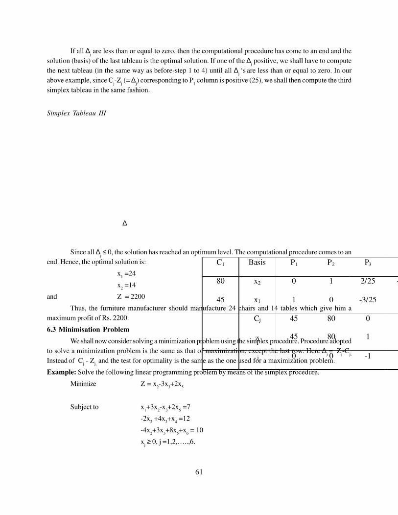
61

If all ∆j are less than or equal to zero, then the computational procedure has come to an end and the

solution (basis) of the last tableau is the optimal solution. If one of the ∆j positive, we shall have to compute

the next tableau (in the same way as before-step 1 to 4) until all ∆j ‘s

are less than or equal to zero. In our

above example, since Cj-Z

j (= ∆

j) corresponding to P

1 column is positive (25), we shall then compute the third

simplex tableau in the same fashion.

Simplex Tableau III

Since all ∆j ≤ 0, the solution has reached an optimum level. The computational procedure comes to an

end. Hence, the optimal solution is:

x1 =24

x2 =14

and Z = 2200

Thus, the furniture manufacturer should manufacture 24 chairs and 14 tables which give him a

maximum profit of Rs. 2200.

6.3 Minimisation Problem

We shall now consider solving a minimization problem using the simplex procedure. Procedure adopted

to solve a minimization problem is the same as that of maximization, except the last row. Here ∆j = Z

j-C

j,

Instead of C

j - Z

j, and the test for optimality is the same as the one used for a maximization problem.

Example: Solve the following linear programming problem by means of the simplex procedure.

Minimize Z = x2-3x

3+2x

5

Subject to x1+3x

2-x

3+2x

5 =7

-2x2 +4x

3+x

4 =12

-4x2+3x

3+8x

5+x

6 = 10

xj ≥ 0, j =1,2,…..,6.

C1 Basis P1 P2 P3

80

45

x2

x1

0

1

1

0

2/25

-3/25

-1/25

4/25

Cj

Zj

45

45

80

80

0

1

j 0 0 -1

∆

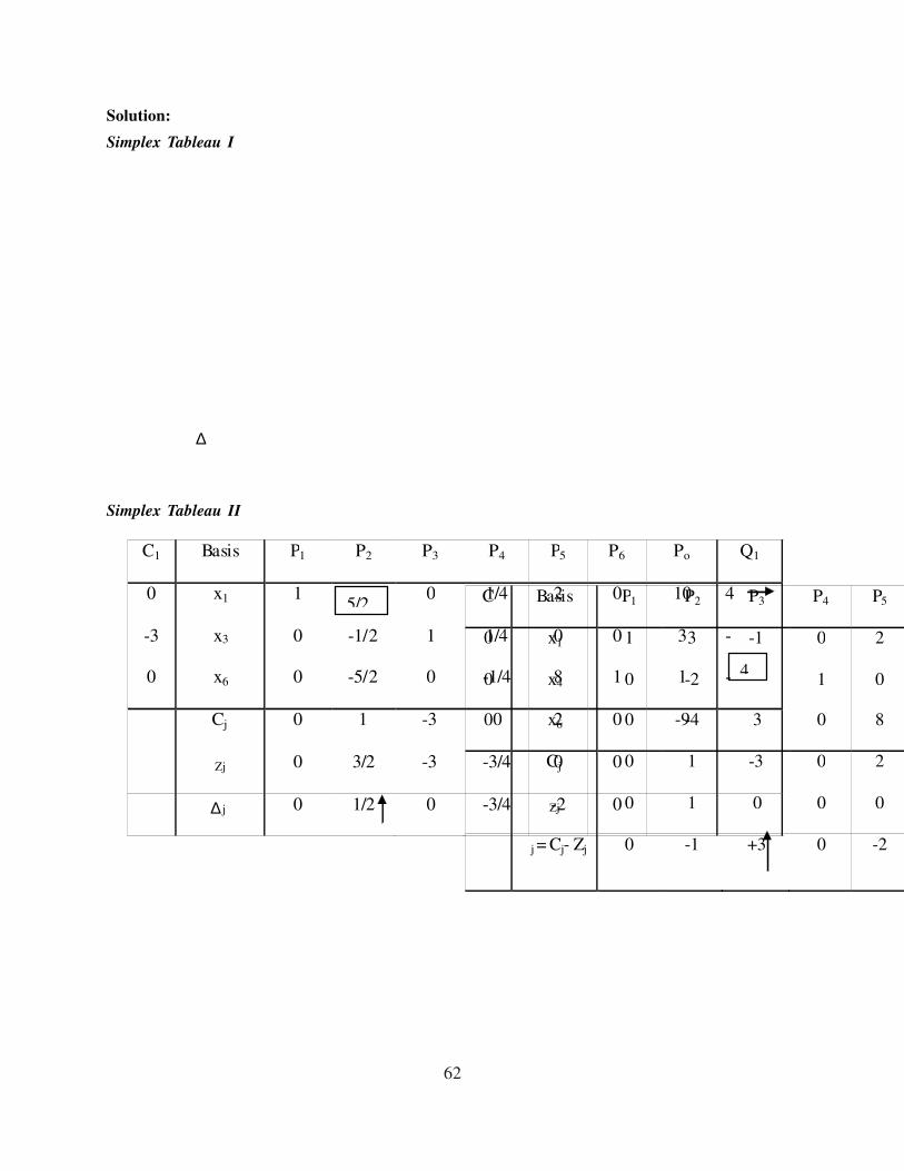
62

Solution:

Simplex Tableau I

Simplex Tableau II

C Basis P1 P2 P3 P4 P5

0

0

0

x1

x4

x6

1

0

0

3

-2

-4

-1

3

0

1

0

2

0

8

Cj

Zj

0

0

1

1

-3

0

0

0

2

0

j = Cj- Zj 0 -1 +3 0 -2

4

∆

C1 Basis P1 P2 P3 P4 P5 P6 Po Q1

0

-3

0

x1

x3

x6

1

0

0

-1/2

-5/2

0

1

0

1/4

1/4

-1/4

2

0

8

0

0

1

10

3

1

4

-

-

Cj

Zj

0

0

1

3/2

-3

-3

0

-3/4

2

0

0

0

-9

j 0 1/2 0 -3/4 -2 0

5/2

∆

63

Simplex Tableau II

Since all ∆j ≤

0, the computational procedure will be terminated and the optimal solution is:

x2 = 4, x

3 = 5 and x

6 = 11 and the value of the objective function is equal to –11.

6.4 Self-assessment Questions

1. Explain the Simplex method of Linear programming problem solving.

2. How to solve Maximization problems using Simplex method?

3. How to solve Minimization problems using Simplex method?

6.5 Summary

Linear programming problems can be solved either by graphical or simplex method. Graphical method is

an invaluable aid to understand the basic structure of linear programming, its utility is restricted if the number

of variables exceed two. Simplex method is most suitable for solving linear programming problems. The

method uses iterative approach to reach maximum or minimum value of the objective function. The method

also helps us to identify the redundant constraints, an unbounded solution, multiple solutions, and infeasible

solution.

In order to solve linear programming problems by simplex method, slack variables are introduced ‘for

less than equal to’ type constraints to change inequalities into equation. For constraints ‘greater than equal

to’, artificial variables are used to initiate the simplex computation. Successive tableaus are made till we

reach at optimum solution.

6.6 Glossary

Slack variable: In an optimization problem, a slack variable is a variable that is added to an inequality

constraint to transform it into an equality.

Simplex method: is a standard technique in linear programming for solving an optimization problem,

typically one involving a function and several constraints expressed as inequalities.

Artificial variable: refers to the kind of variable which is introduced in the linear program model to obtain

the initial basic feasible solution.

C1 Basis P1 P2 P3 P4 P5 P6 Po

1

-3

0

x2

x3

x6

2/5

2/5

1

1

0

0

0

.1

0

1/10

3/10

-1/2

4/5

2/5

10

0

0

1

4

5

11

Cj

Zj

0

-1/5

1

1

-3

-3

0

-8/10

2

-2/5

0

0

-11

j -1/5 0 0 -4/5 -12/5 0 ∆

64

6.7Answers: Self-assessment Questions

1. For answer refer: section 4.1

2. For answer refer: section 4.2

3. For answer refer: section 4.3

6.8 Terminal Questions

1. Discuss the basic steps of Simplex methods.

2. Solve using Simplex Method:

Maximize 50x1+60x

2

Subject to 2x1 +x

2 + x

3 = 300

3x1+4x

2 + x

4 = 509

4x1 +7x

2 + x

5 = 812

x1 ≥ 0, x

2 ≥ 0, x

3 ≥ 0, x

4 ≥ 0, x

5 ≥ 0

3. Solve using Simplex Method:

Minmise x1- 3x

2 + 2x

3

Subject to 3x1 - x

2 + 3x

3 ≤ 7

-2x1+4x

2 ≤ 12

-4x1 +3x

2 + 8x

3 ≤ 10

x1 ≥ 0, x

2 ≥ 0, x

3 ≥ 0

6.9 Suggested Readings

1) Taha, H.A., “Operations Research - an introduction”, Prentice Hall of India Pvt. Ltd., New Delhi.

2) Wagner, H.M., “Principles of Operation Research”, Prentice Hall, Inc., Englewood Cliffs, New

Jersey.

3) Chakravarty, Samir K., “ Theory & problems on Quantitative Techniques, Management information

system & Data processing”, New central book agency, Calcutta.

4) Ackoff, R.L., and Sasieni, M.W., “Fundamentals of Operation Research”, John Wiley & Sons,

New York.

5) Srivastava U. K., Shenoy, G.V., and Sharma, S.C., “Quantitative Techniques for Managerial

Decisions”, 2nd edition, New Age International (P) limited, New Delhi.

6) Thomas M. Cook, and Robert A. Russell, “Introduction to Management Science”, Prentice Hall,

Englewood Cliffs, New Jersey.

*****

65

Lesson-7

Transportation Problem

Structure

7.1 Learning Objective

7.2 Introduction to transportation problem

7.3 Vogel’s approximation method

7.4 North West Corner rule

7.5 Other methods for finding initial solutions

7.6 Modified distribution method

7.7 Stepping stone method

7.8 Self-Assessment Questions

7.9 Summary

7.10 Glossary

7.11 Answers: Self-Assessment Questions

7.12 Terminal Questions

7.13 Suggested Readings

7.1 Learning Objective

Transportation problem is a special type of linear programming problem. Graphical or Simplex methods

are not suitable for the solution of transportation problems as they have special structure. A number of

techniques are available for computing an initial basic feasible solution as well as optimum solution. This

lesson throws light on these initial and optimum solution finding techniques. The objectives of the lesson are:

• To understand the structure of transportation problems.

• To understand techniques of finding initial basic solutions.

• To understand techniques of finding optimum solution.

7.2 Transportation problems – an introduction

The transportation problem is a special type of linear programming problem where the objective is to

minimise the cost of distributing a product from a number of sources or origins to a number of destinations.

Simplex method is unsuitable for solving such problems and they require special method of solution.

The method is an algorithmic (repetitive) procedure which progresses through a series of feasible solutions

(transportation schedule) which are successively improved until and optimal transportation schedule is obtained.

The transportation method broadly consists of the following steps:

(i) finding an initial solution which is feasible from the point of availabilities and requirements of

resources.

(ii) Examining the solution for optimality, i.e. examining whether an improved transportation schedule

with lower cost is possible.

(iii) Repeating step (ii) until no further improvement is feasible.

66

Several approaches have been developed for finding an initial solution to the transportation problem. We

will study Vogel’s Approximation Method, North West Corner rule, and Matrix Minimum method etc.

7.3 Vogel’s Approximation Method

Vogel’s Approximation Method (VAM) was originally developed to produce a starting solution; however

it very often produces an optimal solution to the problem in just one iteration. Although VAM does not

guarantee an optimal solution, it invariably produces a very good initial solution with comparatively less effort

and computation. We shall illustrate the VAM procedure with the following example:

Illustration I: The perfect Manufacturing Company has a current transportation schedule which is

being questioned by the top management as to whether or not it is optimal. The firm has three factories and

five warehouses. The necessary data in terms of unit transportation costs (in Rs.) factory capacities, and

warehouse requirements are given below. Find an optimal schedule.

The steps involved in determining an initial solution are as follows:

(i) Calculate the difference between the two lowest transportation costs for each row and column.

These are written by the side of each row and column and are known as row and column penalties.

(ii) Select the row or column with the largest penalty and circle this value. In case of a tie, select that

row or column that allows the greatest movement of units.

(iii) Assign the largest possible allocation within the restrictions of the row and column requirements to

the lowest cost cell for the row or column selected in step (ii)

(iv) Cross out any column or row satisfied by the assignment made in the prior step.

(v) Repeat the steps (i) to (iv) until all allocations have been made.

Warehouse Factories

A B C

1 50 40 80

2 80 70 40

3 60 70 60

4 60 60 60

5 30 50 40

Factory

availability

800 600 1,100

67

Using the above steps, the initial solution to the problem of Perfect manufacturing Company is as follows:

Thus, the initial solution is:

Transport from factory A to ware house 5: 800 units

Transport from factory B to warehouse 1: 400 units

To warehouse 4:200 units

Transport from factory C to warehouse 2:400 units

To warehouse 3:500 units

To warehouse 4:200 units

And the corresponding cost of transportation is Rs. 110,000.

7.4 North –West Corner Method

For finding an initial solution to the transportation problem, this method indicates that the quantities

transported form the factories (origins) to the warehouses (destinations) must begin in the upper left-hand

(North-West) corner. When this route is fully used, that is, the factory capacity or warehouse requirements

are fully utilized, depending on which number is lower, the remainder of either the factory capacity or warehouse

requirement is then assigned to the new row(s) or column(s) until it is fully used.

Using this procedure, the table is filled from the upper left cell down to the lower right cell, fully using

warehouse requirements, when factory capacities, etc. The table gives the initial solution using the North –

West corner rule for the problem of Perfect Manufacturing Company.

Factory

Warehouse

A B C Requirement Row penalty

1

2

3

4

5

50

80

60

60

30

40

70

70

60

50

80

40 400

60 500

60 200

40

400

400

500

400

800

10

0/10

0

10/

Availability 800 600 1100 2500

Column

penalty

20/

10/

10/

10

0/

800

400

200

30

20

20 20 20

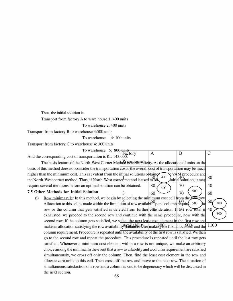
68

Thus, the initial solution is:

Transport from factory A to ware house 1: 400 units

To warehouse 2: 400 units

Transport from factory B to warehouse 3:500 units

To warehouse 4: 100 units

Transport from factory C to warehouse 4: 300 units

To warehouse 5: 800 units

And the corresponding cost of transportation is Rs. 143,000.

The basis feature of the North-West Corner Method is its simplicity. As the allocation of units on the

basis of this method does not consider the transportation costs, the overall cost of transportation may be much

higher than the minimum cost. This is evident from the initial solutions obtained by the VAM procedure and

the North-West corner method. Thus, if North-West corner method is used to obtain an initial solution, it may

require several iterations before an optimal solution can be obtained.

7.5 Other Methods for Initial Solution

(i) Row minima rule: In this method, we begin by selecting the minimum cost cell from the first row.

Allocation to this cell is made within the limitation of row availability and column requirement. The

row or the column that gets satisfied is deleted from further consideration. If the row total is

exhausted, we proceed to the second row and continue with the same procedure, now with the

second row. If the column gets satisfied, we select the next least cost element in the first row and

make an allocation satisfying the row availability (balance, after making the first allocation) and the

column requirement. Procedure is repeated until the availability of the first row is satisfied. We then

go to the second row and repeat the procedure. This procedure is repeated until the last row gets

satisfied. Whenever a minimum cost element within a row is not unique, we make an arbitrary

choice among the minima. In the event that a row availability and a column requirement are satisfied

simultaneously, we cross off only the column. Then, find the least cost element in the row and

allocate zero units to this cell. Then cross off the row and move to the next row. The situation of

simultaneous satisfaction of a row and a column is said to be degeneracy which will be discussed in

the next section.

Factory

Warehouse

A B C

1

2

3

4

5

50

80

60

60

30

40

70

70

60

50

80

40

60

60

40

Availability 800 600 1100

400

400 500

500 300

800

69

(ii) Column minima method: The procedure of allocation here starts with selecting the first column,

instead of the first row as in the row-minima method. Then the minimum cost element in this

column is selected for allocation within the constraints of row availability and column requirement.

The procedure here is the same as that was done in the row-minima method except for going from

column to column rather than from row to row. In this way, the procedure is continued until the last

column requirement is satisfied.

(iii) Inspection method: If the dimensions of a transportation problem are small (that is, the number of

origins and destinations are less in number), then it is always possible to find an initial solution to the

problem by inspection. The cell with the lowest cost element is identified and an allocation is made

within the constraints of corresponding row availability and column requirement. The row or column

that has been satisfied by this allocation is deleted from further consideration. The procedure is

repeated until all the rows and columns are satisfied. Whenever a minimum cost element is not

unique, we make an arbitrary selection among the minima.

7.6 Modified Distribution (MODI) Method

The modified distribution method, also known as MODI method or u-v method provides a minimum cost

solution to the transportation problem. The steps involved in the modified distribution method are as follows:

1) Find out a basic feasible solution of the transportation problem using one of the three methods

described in the previous section.

2) We introduce dual variables corresponding to the row constraints and the column constraints. If

there are m origins and n destinations then there will be m+ n dual variables. The dual variables

corresponding to the row constraints are denoted by ui (i=1,2,………m) while the dual variables

corresponding to column constraints are denoted by vj (j=1,2………..,n) . The value of the dual

variables should be determined from the following equations.

ui +v

j += C

ij if x

ij >0.

3) Any basic feasible solution of the transportation problem has m+n-1 xij > 0. Thus there will be m+n

–1 equations to determine m+n dual variables. One of the dual variables can be chosen arbitrarily. It

is to be also noted that as the primal constraints are equations, the dual variables are unrestricted in

sign.

4) If Xij =0, dual variables computed in 3 are compared with the c

ij values of this allocation as

Cij- u

i- v

j.

If all cij -u

i -v

j ³ 0, then by an application of complementary slackness theorem. It can be shown that the

corresponding solution of the transportation problem is optimum. If one or more cij - u

i - v

j < 0, we choose the

cell with least value of cij - u

i - v

j and allocate as much as possible subject to the row and the column

constraints. The allocation of a number of adjacent cells is adjusted so that a basic variable becomes non

basic.

5) A fresh set of dual variables are computed and entire procedure is repeated.

Let us consider the following transportation problem with a basic feasible solution computed by

Matrix Minimum method.

70

1) The initial basic feasible solution by matrix minimum (row or column minimum) method is

x11

= 50, x22

=60, x25

= 40, x31

= 50,

x32

= 10, x33

= 50, x34

= 40.

2) The dual variables u1, u

2, u

3 and v

1, v

2, v

3, v

4, v

5 can be computed from the corresponding C

ij values

u1 +v

1= 1, u

2+v

2 =12, u

2+v

5 =1, u

3+v

1 = 14

u3+v

2 =33, u

3+ v

3 =1, u

3+v

4 = 23.

3) Since one of the dual variables can be chosen arbitrarily we take u3 =0 as it occurs most often in the

equations. The values of the dual variables are

u1 =-13, u

2= -21, u

3 =0, v

1=14, v

2=33, v

3=1, v

4= 23, v

5= 22.

4) We now compute cij -u

i- v

j values for all the cells where x

ij =0. All the c

ij-u

i-v

j ³ 0 except for cell (1,2)

where c12

-u1-v

2 = -11.

Thus in the next iteration x12

will be a basic variable changing one of the present basic variables non

basic. We also observe that for allocating one unit in cell (1,2) we have to reduce one unit in cells (3,2) and

(1,1) and increase one unit in cell (3,1). The net reduction in the transportation cost for each unit of such

reallocation is

-33 –1 +9 +14= -11.

The maximum that can be allocated to cell (1,2) is 10 otherwise the allocation in cell (3,2) will be

negative. The revised basic feasible solution is

x1 = 40, x

12 = 10, x

22 =60, x

25 = 40.

x31

=60, x33

= 50, x34

= 40.

It can be verified that the new set of dual variables satisfy the optimality condition. Thus the minimum

cost transportation schedule is x11

= 40, x12

=10, x22

= 60, x25

= 40, x31

= 60, x33

= 50, x34

= 40. The corresponding

transportation cost is 2700 which is about 3% less than the transportation cost arrived at by matrix minimum

method.

Origin Destination

1 2 3 4 5 Availability

1 1 9 13 36 51 50

2 24 12 16 20 1 100

3 14 33 1 23 26 150

Requirement 100 70 50 40 40 300

71

7.7 Stepping Stone Method

Stepping Stone Method is another method for finding the optimum solution of the transportation

problem. The various steps necessary in the stepping stone method are given below:

1) Find an initial basic feasible solution of the transportation problem.

2) Next check for degeneracy. A basic feasible solution with m origins and n destinations is said to be

degenerate if the number of non zero basic variables is less than m+n-1. When a transportation

problem is degenerate it has to be properly modified.

3) Each empty (non allocated) cell is now examined for a possible decrease in the transportation cost.

One unit is allocated to an empty cell. A number of adjacent cells are balanced so that the row and

the column constraints are not violated. If the net result of such readjustment is a decrease in the

transportation cost we include as many units as possible in the selected empty cell and carry out the

necessary readjustment with other cells.

4) Step 3 is performed with all the empty cells till no further reduction in the transportation cost is

possible. If there is another allocation with zero increase or decrease in the transportation cost than

the transportation problem has multiple solutions.

The stepping stone method is illustrated with the help of the following example:

Consider the following transportation problem (cost in rupees)

1) We compute an initial basic feasible solution of the problem by North-West corner rule:

Factory Depot

D E F G Capacity

A 4 6 8 6 700

B 3 5 2 5 400

C 3 9 6 5 600

Requirement 400 450 350 500 1700

Factory Depot

D E F G Capacity

A 4(400) 6(300) 8 6 700

B 3 5(150) 2(250) 5 400

C 3 9 6(100) 5(500) 600

Requirement 400 450 350 500 1700

72

The figure in the parenthesis indicate the allocation in the corresponding cells,

2) The Solution is not degenerate as the number of non zero basic variables is m+n-1 =6.

3) The cell BD is empty. The result of allocating one unit along with the necessary adjustment in the

adjacent cells is indicated in Table below:

The increase in the transportation cost per unit quality of reallocation is +3+6-5 =0.

This indicates that every unit allocated to route BD will neither increase nor decrease the transportation cost.

Thus, such a reallocation is unnecessary.

5) The result of reallocating one unit to cell CD is indicated in Table below:

The net increase in the transportation cost per unit of reallocation is +3+6+2-4-5-6 = - 4.

Thus the new route would be beneficial to the company. The maximum amount that can be

allocated in CD is 100 and this will make the current basic variable corresponding to cell CF non basic. Table

below shows the transportation table after the reallocation.

Factory Depot

D E F G Capacity

A 4(399) 6(301) 8 6 700

B 3 (+1) 5(149) 2(250) 5 400

C 3 9 6(100) 5(500) 600

Requirement 400 450 350 500 1700

Factory Depot

D E F G Capacity

A 4(399) 6(301) 8 6 700

B 3 5(149) 2(251) 5 400

C 3(+1) 9 6(99) 5(500) 600

Requirement 400 450 350 500 1700

73

This procedure was repeated with remaining empty cells CE,AF, CF, AG, BG. The results are

summarized in the following Table.

Unoccupied Cells Increase in cost per unit of reallocation

CE 9+4-6—3 = 4

AF 8+5-6-2 =5

CF 6-2+5-6+4-3= 4

AG 6-5+3-4 = 0

BG 5-5+6-4+3-5 =0

Since reallocation in any other unoccupied cell cannot decrease the transportation cost the present

allocation is optimum. The minimum transportation cost is thus x11

= 300 x12

= 400 x22

=50 x23

= 350 x31

= 100

x34

= 500 the transportation cost is 4x300+6x400+5x50+2x350+3x100+5x500= 7350.

The transportation schedule is, however, not unique as there are a number of unoccupied cells with

zero increase in transportation cost.

7.8 Self-assessment Questions

1. What do you understand by Transportation Problem?

2. Explain North-West Corner Method of solving Transportation Problem?

3. Explain Stepping Stone Method of solving Transportation Problem?

4. Explain Modified Distribution Method of solving Transportation Problem?

7.9 Summary

The transportation problem is a special type of linear programming problem where the objective is to

minimise the cost of distributing a product from a number of sources or origins to a number of destinations.

Simplex method is unsuitable for solving such problems and they require special method of solution.

The method is an algorithmic (repetitive) procedure which progresses through a series of feasible

solutions (transportation schedule) which are successively improved until and optimal transportation schedule

is obtained. The transportation method broadly consists of the following steps: finding an initial solution which

is feasible from the point of availabilities and requirements of resources, examining the solution for optimality,

i.e. examining whether an improved transportation schedule with lower cost is possible, repeating steps until

no further improvement is feasible.

Factory Depot

D E F G Capacity

A 4(300) 6(400) 8 6 700

B 3 5(50) 2(350) 5 400

C 3(100) 9 6(100) 5(500) 600

Requirement 400 450 350 500 1700

74

A number of techniques are available for computing an initial basic solution of a transportation

problem. These are Vogel’s Approximation method, North West corner rule etc. Optimum solution can be

obtained from Modified Distribution method or Stepping Stone method.

7.10 Glossary

The Transportation Problem: is a special type of linear programming problem where the objective

consists in minimizing transportation cost of a given commodity from a number of sources or origins to a

number of destinations.

The Modified Distribution Method: is also known as MODI method provides a minimum cost

solution to the transportation problems.

The Vogel’s Approximation Method: or VAM is an iterative procedure calculated to find out the

initial feasible solution of the transportation problem.

7.11Answers: Self-assessment Questions

1. For answer refer: section 5.2

2. For answer refer: section 5.4

3. For answer refer: section 5.7

4. For answer refer: section 5.6

7.12 Select Questions

1. With the help of suitable example discuss Vogel’s Approximation method.

2. With the help of suitable example explain Northwest Corner rule.

3. Consider the following transportation problem with the following unit transportation costs, availability

and requirement

Find a basic feasible solution by (i) North West Corner rule (ii) Vogel’s Approximation method. Compute

the corresponding transportation costs. Then, find the optimum solution using (i) MODI method and (ii)

Stepping stone method.

7.13 Suggested Readings

1) Taha, H.A., “Operations Research - an introduction”, Prentice Hall of India Pvt. Ltd., New Delhi.

2) Wagner, H.M., “Principles of Operation Research”, Prentice Hall, Inc., Englewood Cliffs, New Jersey.

3) Chakravarty, Samir K., “ Theory & problems on Quantitative Techniques, Management information

system & Data processing”, New central book agency, Calcutta.

4) Ackoff, R.L., and Sasieni, M.W., “Fundamentals of Operation Research”, John Wiley & Sons, New

York.

*****

Origin/Destination 1 2 3 Available

1

2

3

8

9

10

9

11

12

10

11

9

42

30

28

Requirement 35 40 25 100

75

Lesson - 8

Assignment Problem

Structure

8.1 Learning Objective

8.2 Introduction to assignment problems

8.3 Hungarian method

8.4 Self-Assessment Questions

8.5 Summary

8.6 Glossary

8.7 Answers: Self-Assessment Questions

8.8 Terminal Questions

8.9 Suggested Readings

8.1 Learning Objective

An assignment problem considers the allocation of a number of jobs to a number of persons so that

the total completion time is minmised. Although an assignment problem can be formulated as a linear

programming problem, it is solved by a special method known as Hungarian method because of its special

structure. This lesson deals with assignment problems and their solution using Hungarian method. The objectives

of the lesson are:

• To understand the structure of Assignment problems.

• To understand use of Hungarian method for solving Assignment problems

8.2 Assignment Problems – an introduction

The name assignment problem originates from the classical problems where the objective is to assign

a number of origin (jobs) to the equal number of destinations (persons) at a minimum cost (or maximum

profit).

The assignment problems in the general from can be stated as follows :Given n facilities, n jobs and

the effectiveness of each facility for each job, the problem is to assign each facility to one and only one job in

such a way that the measure of effectiveness is optimized (Maximized or Minimized).

Several problems of management have a structure identical with the assignment problem. A

department head may have five people available for assignment and five jobs to fill. He may like to know

which job should be assigned to which person so that all these tasks can be accomplished in the shortest

possible time. Likewise a truck company may have an empty truck in each of the cities 1,2,3,4,5,6 and needs

an empty truck in each of the cities 7,8,9,10,11,12. It would like to ascertain the assignment of trucks to

various cities so as to minimize the total distance covered. In a marketing set up by making an estimate of

sales performance for different salesmen as well as for different territories one could assign a particular

salesman to a particular territory with a view to maximize overall sales.

76

It may be noted that with n facilities and n jobs there are n! possible assignments. One way of finding

an optimum assignment is to write all the n! possible arrangements, evaluate their cost and select the assignment

with minimum cost. The method, however, leads to a computational problem of formidable size even when

the value of n is moderate. Even for n=10 the possible number of arrangements is 3628800. it is thus necessary

to develop a suitable computation procedure to solve an assignment problem.

So a computational technique known as Hungarian Method is developed to solve an assignment

problem which is discussed below:

8.3 Hungarian Method

The method is described here in the form of a series of computational steps, when the objective

function is that of minimization type.

Step 1: Find out the cost table from the given problem. If the numbers of origins are not equal to the

number of destinations, a dummy origin or destination must be added.

Step 2: Find the smallest cost in each row of the cost table. Subtract this smallest cost element from

each element in that row. Therefore, there will be at least one zero in each row of this new table, called the

first Reduced Cost Table.

Find the smallest element in each column of the reduced cost table. Subtract this smallest cost

element from each element in that column. As a result of this, each row and column now has at least one zero

value in the second reduced cost table.

Step 3: Determine an assignment as follows:

i) For each row or column with a single zero value cell that has not been assigned or eliminated, box

that zero value as an assigned cell.

ii) For every zero that becomes assigned, cross out all other zeros in the same row and for column.

iii) If for a row and for column there are two or more zero and one cannot be chosen by inspection,

choose the assigned zero cell arbitrarily.

(iv) The above process may be continued until every zero cell is either assigned (boxed) or crossed

out.

Step 4: An optimal assignment is found, if the number of assigned cells equals the number of rows

(and columns). In case you had chosen a zero cell arbitrarily, there may be an alternate optimum. If no

optimum solution is found (some rows or columns without an assignment), then go to step 5.

Step 5: Draw a set of lines equal to the number of assignments made in Step 3, covering all the zeros

in the following way.

i) Mark check (√ ) to those rows where no assignment has been made.

ii) Examine the checked (√ ) rows. If any zero cell occurs in those rows, check (√ ) the respective

columns that contain those zeros.

iii) Examine the checked (√ ) columns. If any assigned zero occurs in those columns, check (√ ) the

respective rows that contain those assigned zeros.

iv) The process may be repeated until no more rows or column can be checked.

v) Draw lines through all unchecked rows and through all checked columns.

77

Step 6: Examine those elements that are not covered by a line. Choose the smallest of these elements

and subtract this smallest from all the elements that do not have a line through the. Add this smallest element

to every element that lies at the intersection of two lines. The resulting matrix is a new revised cost tableau.

Example 1: A job shop has four men available for work on four separate jobs. Only one man can

work on any one job. The cost of assigning each man to each job is given in table below. The objective is to

assign men to jobs such that the total cost of assignment is a minimum.

Jobs

Solution

Step 1: The cost tableau is given. The number of origins are equal to number of destinations.

Step 2: Find the first and second reduced cost tableau (Table 2 & 3).

Table 2: First Reduced Cost Tableau

Table 3: Second Reduced Cost Tableau

To From 1 2 3 4

A 20 25 22 28

Men B 15 18 23 17

C 19 17 21 24

D 25 23 24 24

To F rom 1 2 3

A 0 5 2

B 0 3 8

C 2 0 4

D 2 0 1

To From 1 2 3

A 0 5 1

B 0 3 7

C 2 0 3

D 2 0 0

78

Step 3: Determine an Assignment:

Examine row A of Table 3. You will find that it has only one zero (A1). Box this zero. Cross-out all

other zeros in the boxed column. This way you can eliminate cell B1.

Now examine row C. You find that it has one zero (C2). Box this zero. Eliminate all the zero in the

boxed column. This is how cell D2 gets eliminated.

There is one zero in column 3. Therefore, D3 gets boxed and this enables us to eliminate cell D4.

Therefore, we can box (assign) or eliminate all zero. (Refer Table 4).

Table 4: Assignment of jobs

Step 4: The solution obtained in Step 3 is not optimal. This is because we were able to make three

assignments when four were required.

Step 5: Cover all the zeros of Table 4 with three lines. Since three assignments were made. Check

(√ ) row B since it has no assignment. Please note that row B has a zero in column 1, therefore, we check (√)

column 1. We then check (√ ) row A, since column 1 has an assigned zero in row A.

Please note that no other rows or column can be checked. You may draw three lines through unchecked

rows C & D and column1, the checked column. This is shown in Table 5.

To From 1 2 3

A

5 1

B 0

3 7

C 2

3

D 2

0

0

0

0

79

Table 5

Step 6: Develop the new revised tableau. Examine those elements that are not covered by a line in

table 5. Take the smallest element. This is 1(one) in our case. By subtracting 1 from the uncovered cells and

adding 1 to elements (C1 & D

1) that lie at the intersection of two lines, we get the new revised cost tableau

as given in Table 6 below.

Table 6: New Revised Cost Tableau

Step 7: Go to step 3 and repeat the procedure until you arrive at an optimal assignment.

To From 1 2 3 4

A

5 1 7

B 0

3 7 1

C 2

3 6

D

2

0

0

0

0

0

To From 1 2 3 4

A 0 4 0 6

B 0 2 6 0

C 3 0 3 6

D 3 0 0 0

80

Step 8: Determine an assignment. By examining each of the four rows in Table 6, we find that it is

only row C which has got only one zero. Box cell C2 and cross out D2. Please note that all the remaining

rows and columns have two zeros. Choose a zero arbitrarily, say A1 and box this cell. Thus cell A3 and B1

get eliminated. Therefore, row B (B4) and column 3 (D4) has one zero. These are boxed and cell D4 is

eliminated. Thus all zeros are either boxed or eliminated in Table 7.

Table 7: An optimal Assignment

Since the number of assignments equals the number of rows (columns), the assignment in Table 7 is

optimal. The total cost of this assignment is 78. Remember that we had chosen a zero cell arbitrarily; an

alternate optimum solution exists and is given by A3, B1, C2 and D4. You may please verify it yourself.

Maximization in an Assignment Problem

There are problems where certain facilities have to be assigned to a number of jobs so as to maximize

the overall performance of the assignment. The problem can be converted into a minimization problem and

Hungarian Method can be used for its solution.

Example: Five different machines can do any of the required five jobs with different profits resulting

from each assignment as shown below:

To From 1 2 3

A

4 0

B 0

2 6

C 3

3

D 3

0

0

0

0

81

Machine

Jobs A B C D

1 30 37 40 28

2 40 24 27 21

3 40 32 33 30

4 25 38 40 36

5 29 62 41 34

Find out the maximum profit possible through optimal assignment.

Solution: Maximisation problems are first converted into minimization format and then solved by Hungarian

method. This can be done by selected highest value of the tableau and then subtracting every value from it.

In the given table, highest value is 62. we subtract each profit value from 62. the revised table is as

follows:

We now apply Hungarian Method to obtain the minimum cost assignment of the revised problem.

The solution is to assign job 1 to machine C, job 2 to Machine E, job 3 to Machine A, job 4 to Machine D and

job 5 to Machine B. The maximum profit through this assignment is 214.

8.4 Self-assessment Questions

1. What do you understand by Assignment Problem?

2. What is HungarianMethod of solving Assignment Problem?

3. Explain various steps of HungarianMethod of solving Assignment Problem?

Machine

Jobs A B C D

1 32 25 22 34

2 22 38 35 41

3 22 30 29 32

4 37 24 22 26

5 33 0 21 28

82

8.5 Summary

An assignment problem considers the allocation of a number of jobs to a number of persons so that

the total completion time is minmised. Although an assignment problem can be formulated as a linear

programming problem, it is solved by a special method known as Hungarian method because of its special

structure.

8.6 Glossary

The Assignment Problem: is a fundamental combinatorial optimization problem. It consists of finding,

in a weighted bipartite graph, a matching of a given size, in which the sum of weights of the edges is a

minimum.

Linear Programming: is a method to achieve the best outcome in a mathematical model whose

requirements are represented by linear relationships.

The Hungarian Method: is a combinatorial optimization algorithm that solves the assignment problem

in polynomial time and which anticipated later primal-dual methods.

8.7 Answers: Self-assessment Questions

1. For answer refer: section 6.2

2. For answer refer: section 6.3

3. For answer refer: section 6.3

8.8 Terminal Questions

1. What do you understand by assignment problems? Discuss the steps of solving assignment problems.

2. Discuss the steps of Hungarian method for solving assignment problems. You may take a hypothetical

example to show the procedure.

3. A department head has four subordinates, and four tasks have to be performed. Subordinates differ

in efficiency and tasks differ in their intrinsic difficulty. Time each man would take to perform each

task is given in the effectiveness matrix. How the tasks should be allocated to each person so as to

minmise the total man hours.

Subordinates

1 2 3

A 8 26 17

Tasks B 13 28 4

C 38 19 18

D 19 26 24

83

8.9 Suggested Readings

1) Taha, H.A., "Operations Research - an introduction", Prentice Hall of India Pvt. Ltd., New Delhi.

2) Wagner, H.M., "Principles of Operation Research", Prentice Hall, Inc., Englewood Cliffs, N. J.

3) Gillelt, B.E., "Introduction to operations research - A computer Oriented. Algorithmic approach",

Tata McGraw Hill publishing Co. Ltd. New Delhi.

4) Chakravarty, Samir K., " Theory & problems on Quantitative Techniques, Management information

system & Data processing", New central book agency, Calcutta.

5) Ackoff, R.L., and Sasieni, M.W., "Fundamentals of Operation Research", John Wiley & Sons, New

York.

*****

84

Lesson-9

Theory of Games

Structure

9.1 Learning Objective

9.2 Properties of competitive games

9.3 Types of games

9.4 Two person zero sum game

9.5 Methods of solving game matrix

9.6 Limitations of theory of games

9.7 Self-Assessment Questions

9.8 Summary

9.9 Glossary

9.10 Answers: Self-Assessment Questions

9.11 Terminal Questions

9.12 Suggested Readings

9.1 Learning Objective

In today’s competitive business world, if one could calculate in advance what his competitor was

going to do, his planning would become far easier and more effective. Game theory helps us in this situation.

It is a body of knowledge which is concerned with the study of decision making in situations where two or

more rational opponents are involved under conditions of competitions and conflicting interest. In game

theory one seeks to determine rival’s most profitable counterstrategy to one’s own ‘best’ moves and formulate

the appropriate defensive measures accordingly. This lesson throws light on theory of games. The objectives

of the lesson are:

• To understand the nature and use of Theory of games

• To understand the types of games

• To study two person zero sum game

• To understand the methods of solving games

In today’s competitive business world, one of the most relevant problems of the executive is to

outguess his competitor. If he could calculate in advance what his competitor was going to do, his planning

would become far easier and more effective. The experience of executive regarding the behaviour of competitor

makes it easy to predict the strategies of competitor. In cases where such inform action is available, it is

possible to choose those decisions which maximize the firm’s expected return after the effects of the opponent’s

counter moves are taken into account.

Game theory is a body of knowledge. It is concerned with the study of decision making in situations

where two or more rational opponents are involved under conditions of competitions and conflicting interest.

Game theory adopts the approach, in which one seeks to determine rival’s most profitable counterstrategy to

one’s own ‘best’ moves and formulate the appropriate defensive measures.

85

The term “games” relates to conditions of business conflict over a period of time. The participants

are competitors who make use of mathematical techniques and logical thinking in order to arrive at the best

possible strategy for overtaking competitor. For example, a marketing director while introducing a new product

would like to know the best possible strategies or a combination of strategies to capture a higher share of the

market when a competitor is also trying to introduce a similar product with different strategies available to

him. Some of the strategies the marketing director could think of are reduction in price, gift scheme, and

superior quality of the product. etc.

Although the history of games dates lack to the early twentieth century, a new turn for its wider

applicability took only after the work, “Theory and practice of games and economic behaviour” of John Von

Neumann published in the year 1944. Von Neumann approach utilizes the minimax (or maximin) principle

which involves the basic idea of minimization of the maximum loss. It is generally agreed that in most, if not

all, games there appear elements of chance of skill, enjoyment, and of strategy. Different games vary according

to the degree to which these elements are present, but the most important factor is the strategic aspect, which

is the central concern of the theory developed by Prof. Von Neumann.

The main objective in the theory of games is to determine the rules of rational behaviour in the game

situations, in which the outcomes are dependent on the actions of the interdependent players. In a game

situation, each of the players has set of strategies available. A strategy refers to the action to be taken by a

player in various contingencies in playing a game. There is a set of outcomes each of which is the result of the

particular choices of strategies made by the players on a given play of the game, and pay-offs are accorded

to each player in each of the possible outcomes. Each of the players being assumed to be rational, his

preference ordering of the different outcomes is determined by the order of magnitudes of the associated

pay-offs and since, in general, the orders of magnitudes of the pay-off accruing to the players in different out-

comes don’t coincide, a game models a situation in which there are conflicts of interest. The players in the

game strive for optimal strategies. An optimal strategy is such as provides the best situation in the game in the

sense that it involves maximal pay-off to the players.

Let us now consider some examples of the kinds of situations in which game theory can be uses to

analyse them. One of the most common examples in an industry is the management-worker bargaining over

wage payments, conditions of work, fringe benefits, and so on. Other things being equal, what one gains the

other loses. Duopolistic situations, in which price and promotion strategy of market leader affects the sales

and profitability of challenger, also warrants the use of game theory.

9.2 Properties of Competitive games

All the competitive situations having the following properties are termed as games:

(i) There are a finite number of competitors or players.

(ii) There are a finite number of possible courses of actions for each of the competitors.

(iii) Interest of each other is conflicting in nature.

(iv) The rules governing the choices are specified and known to all players.

(v) A play of the game results when each of the players chooses a single course of action from the

list of courses available to him.

(vi) The outcome of the game is affected by choices made by all of the players; the choices are to be

made simultaneously so that no competitor knows his opponents choice until he is already

committed to his own.

86

(vii) The outcome for all specific sets of choices by all the players is known in advance and numerically

defined.

9.3 Types of games

Games can be of several types. Important ones are as follows:

(a) Two person games and n-person games

In a game situation, interest of two or more than two participants may be in conflict. The former of

these is called a two-person game and the latter one is known as n-person game. In the case of n-person

game it should be noted that it does not necessarily imply that exactly n people would be involved but rates the

participants can be classified into n mutually exclusive categories and members of each of the categories

have identical interest.

(b) Zero sum and Non-zero sum game

A zero sum game is one in which the sum of the payments to all the competitors is zero for every

possible outcome of the game. In other words, in such a game the sum of the points won equals the sum of

the points lost i.e. one player wins at the expense of other(s). In a non-zero sum game the sum of the pay-offs

from any play may be either positive or negative but not zero. For example, if two chess players agree that at

the end of the game the loser would pay Rs. 500 to the winner then it would mean a zero sum a gain of one

exactly matches the loss of the other. If the sum of gains and losses is not equal to zero, it would obviously be

called a non-zero sum game.

(c) Games of perfect and imperfect information

Whatever strategy is adopted by either player, if the same can also be discovered by his competitor,

then such games are known as games of perfect information. In case of games of imperfect information neither

player knows the entire situation and must be guided in part by his guess as to what the real situation is.

(d) Games with finite and infinite moves

Games with finite number of moves are those where the number of moves is limited to a fixed

magnitude before play begins, but if the game could continue over an extended period of time and no limit is

put on the number of moves then it is referred as a game with unlimited number of moves.

(e) Negotiable (or cooperative) and non-negotiable (or non-cooperative games)

Negotiation amongst the players is possible in n-person and non-zero sum games but the same is not

necessarily required. On this basis we can divide the analysis of such games into two parts- games in which

the participants can negotiate and the games in which negotiation is not permitted. The former types of

games are known as negotiable games and the latter type of games are known as non-negotiable games.

In our analysis, we shall deal with two-person zero-sum games involving finite strategies open to the

players.

9.4 Two- person, Zero- sum game

Consider a competitive situation for the share of “newspaper market” by the publishers of two dailies

in a city. Here, every additional circulation gained by one of the firms is necessarily at the cost of the other.

This situation is basically called as a two person, zero-sum game. This is called zero-sum because, whatever

is done by either competitor, the sum of the net gain in the market share by the two competitors is zero. In the

above example, as long as the total circulation remains unchanged, the share of the market which the two

firms have between them is always 100%. However, there are situations where decisions which are taken by

the firms may very well increase or reduce both the absolute size of their market and the total profits taken

together. Such problems are not considered as zero-sum games.

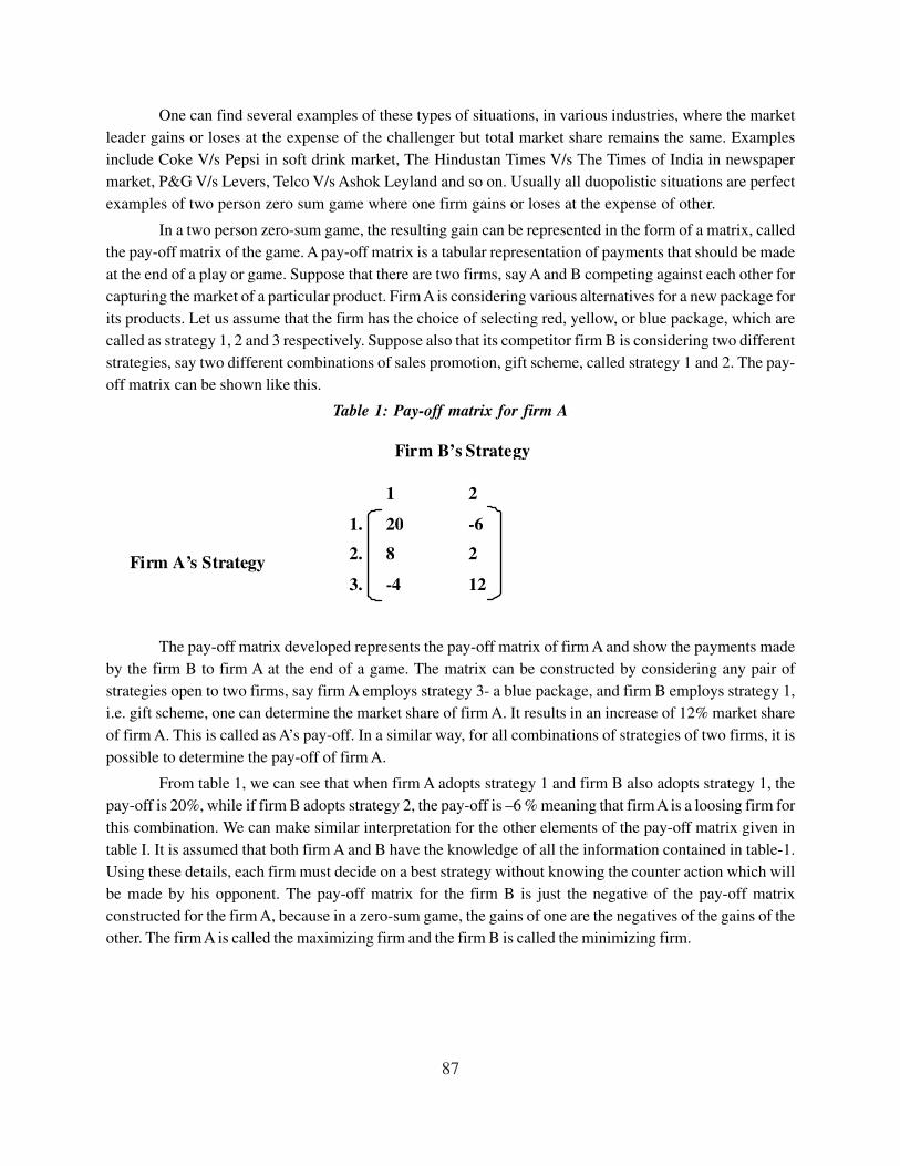
87

One can find several examples of these types of situations, in various industries, where the market

leader gains or loses at the expense of the challenger but total market share remains the same. Examples

include Coke V/s Pepsi in soft drink market, The Hindustan Times V/s The Times of India in newspaper

market, P&G V/s Levers, Telco V/s Ashok Leyland and so on. Usually all duopolistic situations are perfect

examples of two person zero sum game where one firm gains or loses at the expense of other.

In a two person zero-sum game, the resulting gain can be represented in the form of a matrix, called

the pay-off matrix of the game. A pay-off matrix is a tabular representation of payments that should be made

at the end of a play or game. Suppose that there are two firms, say A and B competing against each other for

capturing the market of a particular product. Firm A is considering various alternatives for a new package for

its products. Let us assume that the firm has the choice of selecting red, yellow, or blue package, which are

called as strategy 1, 2 and 3 respectively. Suppose also that its competitor firm B is considering two different

strategies, say two different combinations of sales promotion, gift scheme, called strategy 1 and 2. The pay-

off matrix can be shown like this.

Table 1: Pay-off matrix for firm A

The pay-off matrix developed represents the pay-off matrix of firm A and show the payments made

by the firm B to firm A at the end of a game. The matrix can be constructed by considering any pair of

strategies open to two firms, say firm A employs strategy 3- a blue package, and firm B employs strategy 1,

i.e. gift scheme, one can determine the market share of firm A. It results in an increase of 12% market share

of firm A. This is called as A’s pay-off. In a similar way, for all combinations of strategies of two firms, it is

possible to determine the pay-off of firm A.

From table 1, we can see that when firm A adopts strategy 1 and firm B also adopts strategy 1, the

pay-off is 20%, while if firm B adopts strategy 2, the pay-off is –6 % meaning that firm A is a loosing firm for

this combination. We can make similar interpretation for the other elements of the pay-off matrix given in

table I. It is assumed that both firm A and B have the knowledge of all the information contained in table-1.

Using these details, each firm must decide on a best strategy without knowing the counter action which will

be made by his opponent. The pay-off matrix for the firm B is just the negative of the pay-off matrix

constructed for the firm A, because in a zero-sum game, the gains of one are the negatives of the gains of the

other. The firm A is called the maximizing firm and the firm B is called the minimizing firm.

Firm B’s Strategy

Firm A’s Strategy

1 2

1. 20 -6

2. 8 2

3. -4 12

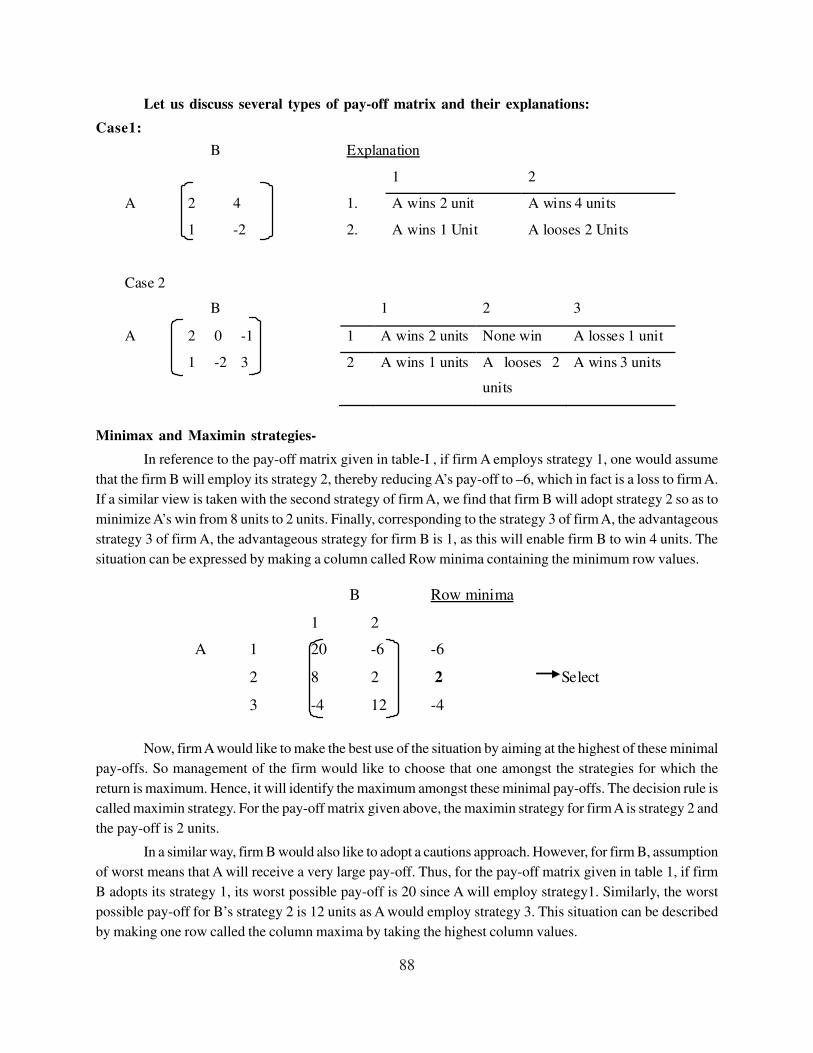
88

Let us discuss several types of pay-off matrix and their explanations:

Case1:

Minimax and Maximin strategies-

In reference to the pay-off matrix given in table-I , if firm A employs strategy 1, one would assume

that the firm B will employ its strategy 2, thereby reducing A’s pay-off to –6, which in fact is a loss to firm A.

If a similar view is taken with the second strategy of firm A, we find that firm B will adopt strategy 2 so as to

minimize A’s win from 8 units to 2 units. Finally, corresponding to the strategy 3 of firm A, the advantageous

strategy 3 of firm A, the advantageous strategy for firm B is 1, as this will enable firm B to win 4 units. The

situation can be expressed by making a column called Row minima containing the minimum row values.

Now, firm A would like to make the best use of the situation by aiming at the highest of these minimal

pay-offs. So management of the firm would like to choose that one amongst the strategies for which the

return is maximum. Hence, it will identify the maximum amongst these minimal pay-offs. The decision rule is

called maximin strategy. For the pay-off matrix given above, the maximin strategy for firm A is strategy 2 and

the pay-off is 2 units.

In a similar way, firm B would also like to adopt a cautions approach. However, for firm B, assumption

of worst means that A will receive a very large pay-off. Thus, for the pay-off matrix given in table 1, if firm

B adopts its strategy 1, its worst possible pay-off is 20 since A will employ strategy1. Similarly, the worst

possible pay-off for B’s strategy 2 is 12 units as A would employ strategy 3. This situation can be described

by making one row called the column maxima by taking the highest column values.

B Explanation

1 2

A 2 4 1. A wins 2 unit A wins 4 units

1 -2 2. A wins 1 Unit A looses 2 Units

Case 2

B 1 2 3

A 2 0 -1 1 A wins 2 units None win A losses 1 unit

1 -2 3 2 A wins 1 units A looses 2

units

A wins 3 units

B Row minima

1 2

A 1 20 -6 -6

2 8 2 2 Select

3 -4 12 -4

89

The best of these pay-offs to B is of course, the one which is lowest. Thus, the firm B will try to

identify the minimum amongst the maximum pay-off and this strategy is called minimax strategy. For firm B

here, minimax strategy is strategy 2.

Saddle points and Value of the game –

The saddle point is known as equilibrium point in the theory of games. An element of a matrix, which

is simultaneously, minimum of the row in which it occurs and the maximum of the column in which it occurs,

is a saddle point of the matrix game. In a game having a saddle point optimum strategy for the player A is

always to play the row containing a saddle point and for the player B to play the column that contains a saddle

point saddle point also gives the value of the game as it is equal to saddle point value.

Saddle point in a pay-off matrix may or may not be present. If there is a saddle point we can easily

find out the optimum strategies and the value of the game by what is known as solution by saddle point. But

when saddle point is not there we have to use other methods for working out the solutions concerning game

problems.

Some examples are given below which will help us in understanding the concepts of saddle point and

the value of the game.

Example I- Consider the following pay-off matrix:

If we select maximum from row minima we get 10 and if we select minimum of column maxima

we also get 10. So 10 is maximin value for firm A as well as minimax value for firm B. This is called the

saddle point and optimum strategies for firm A and B are 3 and 1 respectively. The value of the game is 10

units which means at the end of the game A will gain 10 units.

B

1 2

1 20 -6

A 2 8 2

3 -4 12

Column Maxima 20 12 Select

B Row Minima

8 7 15 12 7

A 9 14 8 10 8

10 12 14 13 10

Column

Maxima

10 14 15 13

90

Example II: Consider the following pay-off matrix:

The Maximum of row minima in this example is –2 , and the minimum of column maxima is –2, and

hence the saddle point. The optimal strategy for player A is strategy 3 and for player B is strategy 2. The

value of the game is –2, indicating that player A is losing player.

Example III – Consider the following pay-off matrix:

In this game maximin is 3 and minimax is 6, hence, this game does not posses a saddle point. If A

chooses his strategy 3, B will minimize by choosing 1. This will make A to use his first strategy which will

cause B to shift to strategy 3 and the process will continue. Thus we see that there is no equilibrium and

hence no saddle point. Also value of the game can’t be determined and some other methods should be used

to find out that.

Mixed Strategies:

In example III above, we found that there is no equilibrium or saddle point, and therefore, no pure

strategies. for either of the player. In order to find a solution to games of this type, Von Neumann introduced

the concept of a mixed strategy. Referring to example III, suppose, player A decides never to use his first

strategy, and chooses between his second and third strategies at random, each with probability, say1/2. If

player B were to play his first strategy, player A would get 12 half the time and 3 the other half of the time,

yielding an average pay-off of 7 ½. In a similar way, the average pay-off to player B’s second strategy would

be 7 ½ and to his third is 4. Thus, we find that this mixed strategy has outcomes 7 ½, 7 ½ and 4 depending

upon the strategy adopted by player B. The minimum of these is 4 which is larger than any of the minima of

the pure strategies. Therefore, by using a mixed strategy, player A appears to be able to increase his minimum

pay-off. Similarly, it can be seen that if player B adopts the mixed strategy of never using his first strategy,

and of randomizing between his second and third strategies with respective probabilities, say 1/3 and 2/3, the

expected outcomes will be –4/3 , 14/3 and 17/3 depending on player A’s choice. The largest of these 17/3, is

less than the minimum of the column maxima, so that player B appears to have reduced his maximum pay-

off. Incidentally, both players by using mixed strategies appear to be able to make themselves better off.

B Row Minima

-7 -4 -7

A 7 -3 -3

8 -2 -2

Column

Maxima

8 -2

Row Minima

20 8 -6 -6

A 12 10 2 2

3 5 6 3

Column

Maxima

20 10 6

91

The above discussion leads to Von Neumann’s minimax theorem. It states that if the set of possible

strategies of the players is extended beyond the pure strategies to include all possible mixed strategies, there

is always some mixed strategy for player A whose minimum pay-off is larger than any other, and there is

always some mixed strategy for player B whose maximum pay-off is smaller than any others, and these two

pay-offs are equal in value. In other words, for all two person zero-sum games maximin equals minimax, if all

possible randomization is taken into account. This theorem, known as minimax theorem of game theory is due

to Von Neumann and is considered basic to the developments in game theory.

9.5 Methods of solving game matrix

Let us now discuss some of the methods for finding solutions of matrix games.

(i) Algebraic Method - A game in which both players have two choices or alternatives (strategies) is known

as a 2x2 game. In the algebraic method, we let p equal to the fraction of the time that player A plays the first

strategy and (1-p) times he plays the second strategy. Similarly, for player B, we represent q and 1-q as the

fraction of the time that he plays his first and second strategies, respectively. Therefore, for a given pay-off

matrix, the representation of the proportional distribution of fraction of time for the rows and columns is :

Under this method, player A is interested to divide his plays between the two rows (strategies) in

order that the expected winnings from playing the first row will be exactly equal to its winnings from playing

the second row despite what his opponent does. In order to arrive at the best strategies for player A when

playing either row one or row two, it is necessary to equate player A’s expected winnings when his opponent,

player B, plays column 1 to the expected winning when player B plays column 2. Thus, we have

4p+3(1-p) = p+5 (1-p)

i.e. p = 2/5

Hence the optimal mixed strategy for player 1 is to play first row 2/5 of the time and the second row

3/5 of the time. In a similar approach, we can find the value of q.

i.e., 4q+1(1-q) = 3q +5(1-q)

i.e., q=4/5

Therefore, the optimal mixed strategy for player 2 is to play first column 4/5 of the time and the

second column 1/5 of the time.

In order to find the value of the game, we can utilize the concept of probability. The two probabilities

for player 1 and 2 are (2/5, 3/5) and (4/5, 1/5). Since both players play independently and neither knows what

the other play next, the probabilities for player A are independent of the probabilities for player B.

The pay-off in the game will be obtained when the player play a particular column and a particular

row simultaneously. With the probabilities for selecting a particular row and column known, we can compute

the probabilities of each pay-offs as follows:

q 1-q

p 4 1

1-p 3 5

92

Pay-off value Strategies which produce the pay-off Probability of the pay off

4 row1, Column1 2/5x4/5 =8/25

1 row1, Column2 2/5xd1/5 =2/25

3 row2, Column1 3/5x4/5 =12/25

5 row2, Column 2 3/5x1/5 =3/25

Given the pay-off value and the corresponding probabilities, we can now compute the expected

value of the game by multiplying each of the pay-off by the corresponding probability and the same is given

in table below:

Pay-off value Probability of pay-off Expected value

4 8/25 32/25

1 2/25 2/25

3 12/25 36/25

5 3/25 15/25

Total = 85/25 =17/5(value of game)

Thus the value of game is 17/5.

(i) Use of Dominance – Consider the following cases:

Now, if we are able to find the ways to reduce these Mx2 or 2xM games to a 2x2 game, the games

could be solved easily. One of the methods for doing so is by dominance method.

Case 1.

M x 2 game, Where M=3

Case II-

2 x M game, Where M =4.

B

1 3

A -4 -1

2 1

B

A 0 2 -4 -7

1 3 -6 -1

93

If all the elements in a column are greater than or equal to the corresponding elements in another

column, then that column is dominated. Similarly, if all the elements in a row are less then or equal to the

corresponding elements in another row, then that row is dominated. Dominated rows or columns or both may

be deleted, resulting into the reduced size of the game. Therefore, before solving a game, one should look for

dominance so as to reduce its size and, thus, computations.

Looking at the matrix in Case 1, one could easily say “why should A play 2 and make his opponent

win?” Definitely, he would never like to play strategy 2, since he can do much better by playing strategy 1or

3. Therefore, we can say that row2 is dominated, and hence, it is discarded. Hence, the pay-off matrix

reduce to

for which we can easily obtain the optimal strategies and value of the game.

Applying the method of dominance to Case –II, we find that B will never play his first and second

strategies. Hence, the matrix reduces to

For which solution can be found easily.

(iii) Graphic Method – Consider the following pay-off matrix:

We can see that when A selects 1, he can win-2 (i.e. looses 2 units) or 4 units depending upon his

opponents selection of strategies. We can, thus, plot players’ winning as shown Graph I. Similarly, if A selects

2, he will either win 8 or 3 units and finally, when A selects 3, he will win 9 units or 0 depending upon B’s

selection of strategies. All the three lines have been plotted on the graph I.

B

A 1 3

2 1

B

A -4 -7

-6 -1

B

-2 4

A 8 3

9 0

94

A close examination of graph-1 indicates that strategy 3 offers A the best chance of winning (9 units).

However, it should be noted that player B can shift to column 2. This would immediately reduce player A’s

pay-off to 0. Assuming that both players use a rational and intelligent approach, the game would be played as

follows:

(i) If A plays strategy 3, expecting to win 9 units, B would shift to strategy 2, reducing A’s win to zero

units.

(ii) As soon as this happens A would shift to strategy 1 and win 4 units as long as B continues to play 2.

(iii) Realizing the changed situation, B will shift to strategy1 where A will loose 2 units.

(iv) At his stage, A will shift to strategy 2 so as to win 8 units.

(v) On seeing this, B will immediately shift to strategy 2 where winning of A will be reduced to 3 units.

(vi) The process will continue in a similar manner.

The value of game (point v) is the lowest intersection point in shaded area. The reasoning for this lowest

intersection point is that it is the lowest level, on an average, at which B can hold A’s winnings. So value of

game is 3.5 units (v=3.5 in graph). Similarly, we can draw a graph for B and find the value of the game as the

level at which A can hold B to minimize his losses.

(iv) Linear Programming Method – Matrix games can also be converted into linear programming problems

and thus can be solved by simplex method of linear programming. We will not be discussing the complex

procedure here but curious reader can find the details of this method in books on operations research.

10 -------------------------- 10 9 -------------------------- 9 --------------------------

8 ---------------------- 8 7 ----------- --------- 7 6 ---------------- 6 5 -------- 5 4 4 Point V 3 3 2 2 1 1 0 0 -1 -1 -2 -2 -3 -3 Player B Player B Plays strategy 1 Plays strategy 2

Graph –1: Player A’s Winnings

95

9.6 Limitations of theory of games

Games theory has been used in business and industry to develop bidding tactics, pricing policies, advertising

strategies etc. The theory provides the basis for rational decisions and thus improves the decision making

process. In spite of all, the theory of games suffers from certain limitations and this marks a question about

the relevancy of game theory in practical life. The important limitations are:

(a) Businessmen don’t have all the knowledge required by the theory of games. They don’t even know the

alternative strategies available to them, what to talk of the strategies open to their rivals.

(b) There is a great deal of uncertainty that can’t conveniently be inserted into game theory model. The

outcome of a game may not be known with certainty in many cases.

(c) The minimax strategy implies that the business man minimizes the chance of the maximum loss. It is thus

a very conservative rule. It is a much less accurate description of the dynamic businessman who is

constantly in quest of profit.

(d) The techniques of solving games involving mixed strategies particularly in case of a larger pay-off matrix

is very complicated and this lessens the significance of this sort of analysis.

(e) The environment in which managerial decisions are made is never really a two person, and definitely

government and/or the society become extended parties to decision making, hence the limitation.

(f) The managerial decision environment is rarely ever zero-sum. In many situations both competitors may

gain.

(g) Rarely both parties in a real life game situation have equal information.

(h) In real world, a certain strategy is selected and usually continued for a sufficiently long period of time,

and for short duration, this strategy will often be wrong.

(i) To convert precise monetary pay-off for the matrix game in real life decision situations is extremely

difficult.

In spite of the several limitations, the theory of games may be regarded as one of the major scientific

achievement of the first half of the 20th century. The theory provides the basis for rational decision under the

situation of conflict. It help us learn how to approach and understand a conflict situation.

9.7 Self-assessment Questions

1. What are the different types of games?

2. Describe two person zero-sum game.

3. What do you understand by saddle point in the theory of game?

4. Explain different methods of solving game matrix.

5. What are the main limitations of Game theory?

9.8 Summary

In today’s competitive business world, if one could calculate in advance what his competitor was

going to do, his planning would become far easier and more effective. Game theory is a body of knowledge

that can help us in this situation. It is concerned with the study of decision making in situations where two or

more rational opponents are involved under conditions of competitions and conflicting interest. In Game

theory one seeks to determine rival’s most profitable counterstrategy to one’s own ‘best’ moves and formulate

the appropriate defensive measures.

96

A competitive situation where gain by one of the firms is necessarily at the cost of the other. This

situation is basically called as a two person, zero-sum game. This is called zero-sum because, whatever is

done by either competitor, the sum of the net gain in the market share by the two competitors is zero.

However, there are situations where decisions which are taken by the firms may very well increase or

reduce both the absolute size of their market and the total profits taken together. Such problems are not

considered as zero-sum games.

Games theory has been used in business and industry to develop bidding tactics, pricing policies, advertising

strategies etc. In spite of all, the theory of games suffers from certain limitations and this marks a question

about the relevancy of game theory in practical life. There is a great deal of uncertainty that can’t conveniently

be inserted into game theory model. The outcome of a game may not be known with certainty in many cases.

The techniques of solving games involving mixed strategies particularly in case of a larger pay-off matrix is

very complicated and this lessens the significance of this sort of analysis. The environment in which managerial

decisions are made is never really a two person, and definitely government and/or the society become

extended parties to decision making, hence the limitation. Rarely parties involved in a real life game situation

have equal information. In real world, a certain strategy is selected and usually continued for a sufficiently

long period of time, and for short duration, this strategy will often be wrong.

9.9 Glossary

Game Theory: is the study of mathematical models of strategic interaction among rational decision-

makers.

Linear Programming: is a method to achieve the best outcome in a mathematical model whose

requirements are represented by linear relationships.

Profitability: is ability of a company to use its resources to generate revenues in excess of its

expenses.

9.10 Answers: Self-assessment Questions

1. For answer refer: section 10.3

2. For answer refer: section 10.4

3. For answer refer: section 10.4

4. For answer refer: section 10.5

5. For answer refer: section 10.6

9.11 Terminal Questions

Q 1: Write a detailed note on the role and significance of theory of games in business decision making.

Q 2: Write short notes on the following:

(a) Types of games.

(b) Two person zero-sum game.

(c) Maximin and Minimax strategies.

(d) Saddle point.

Q 3: What do you understand by game situation? Describe various methods of solving matrix games.

Q 4: Discuss relevance of game theory in managerial decision making.

Q 5: Discuss the various methods of solving matrix games with the help of suitable example.

97

9.12 Suggested Readings

1) Srivastava, V.K., Shenoy, G.V & Sharma, S.C., “ Quantitative Techniques for managerial Decision

making”, Wiley Eastern Ltd., New Delhi.

2) Vohra, N.D., “Quantitative Techniques in Management”, Tata McGraw-hill publishing Co., Ltd.

New Delhi.

3) Gillelt, B.E., “Introduction to operations research – A computer Oriented. Algorithmic approach”,

Tata McGraw Hill publishing Co. Ltd. New Delhi.

4) Chakravarty, Samir K., “ Theroy & problems on Quantitative Techniques, Management information

system & Data processing”, New central book agency, Calcutta.

5) Wagner, H.M., “Principles of Operation Research”, Prentice Hall, Inc., Englewood Cliffs, N. J.

6) Ackoff, R.L., and Sasieni, M.W., “Fundamentals of Operation Research”, John Wiley & Sons,

New York.

*****

98

Assignments

Note: Attempt any five assignments. Assignments are compulsory.

1) Define Operations Research and also discuss its usage and limitations.

2) Discuss the steps involved in linear programming problem formulation.

3) Discuss the basic steps of simplex methods.

4) With the help of suitable example explain Northwest Corner rule.

5) What do you understand by assignment problem? Discuss the steps of solving assignment problems.

6) Discuss the various inventory classification system.

7) Discuss some of the deterministic inventory models for finding EOQ.

8) Clarify the concept of waiting lines and discuss the characteristics of queuing model.

9) What do you understand by game situation? Describe various methods of solving matrix games.

10) Compare and contrast NPV and IRR methods of Capital Budgeting.

*****