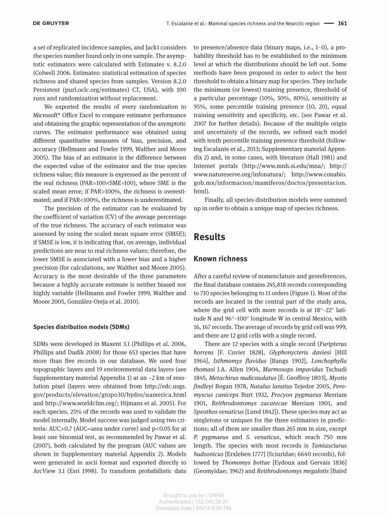
Why is small mammal diversity higher in riparian areas than in uplands

DOI 10.1515/mammalia-2013-0057 Mammalia 2014; 78(2): 159–169
Tania Escalante*, Gerardo Rodríguez-Tapia, Miguel Linaje, Juan J. Morrone and Elkin Noguera-Urbano
Mammal species richness and biogeographic structure at the southern boundaries of the Nearctic region
Abstract: We analyzed whether the spatial variation in mammal species richness reflects the southern bounda-ries of the Nearctic region as previously established by endemism patterns. Records from 710 mammal species were drawn on a map of North America (from Canada and Alaska to Panama) gridded at 4° latitude-longitude. We evaluated the probable existence of unknown spe-cies through three richness estimators (Chao2, ICE, and Jack1), modeled the potential distribution of species, and mapped the predicted pattern of species richness through the number of coexisting potential distribu-tions. The poorest grid cells are in the northern areas, whereas the richest ones are in the southern areas, coinciding with the pattern of collecting points. The average richness of 4° grid cells comprising the Nearc-tic region was 18 species, and the richest 4° grid cells had 150 species, coinciding with the 26° latitude. From the 406 mammal species of the Nearctic region, 104 are restricted to it, and 305 species situated south of it are not distributed in the region. The map of predicted rich-ness shows the classical latitudinal diversity gradient, with the number of species increasing to the tropics. We conclude that the Nearctic region has a low mam-mal richness, with a richness pattern corresponding with previously described patterns of endemism, with a boundary situated at 26°–30° latitude.
Keywords: endemicity; ɛ diversity; North America; rich-ness estimators; species distribution models.
*Corresponding author: Tania Escalante, Museo de Zoología “Alfonso L. Herrera”, Departamento de Biología Evolutiva, Facultad de Ciencias, Universidad Nacional Autónoma de México, Apartado Postal 70-399, 04510 Mexico, D.F., Mexico, e-mail: [email protected] Rodríguez-Tapia: Unidad de Geomática, Instituto de Ecología, Universidad Nacional Autónoma de México, Apartado Postal 70-275, 04510 Mexico, D.F., MexicoMiguel Linaje: Laboratorio de Sistemas de Información Geográfica, Departamento de Zoología, Instituto de Biología, Universidad Nacional Autónoma de México, Apartado Postal 70-153, 04510 Mexico, D.F., Mexico
Juan J. Morrone and Elkin Noguera-Urbano: Museo de Zoología “Alfonso L. Herrera”, Departamento de Biología Evolutiva, Facultad de Ciencias, Universidad Nacional Autónoma de México, Apartado Postal 70-399, 04510 Mexico, D.F., Mexico
IntroductionThe Nearctic region has been delimited since the 19th century, but there are few recent publications regarding its natural boundaries under both ecological and evolu-tionary biogeographic approaches. Escalante et al. (2010) delineated the boundaries of the Nearctic region based on the endemism patterns of the mammal fauna, concluding that the southern boundary may be located around 30° latitude, but it can extend to 22° latitude, if the Mexican Transition Zone (Morrone 2006, 2010) is included within the region. Recently, other world regionalizations have been proposed using different criteria, such as similarity (Kreft and Jetz 2010) and phylogenetic composition and β diversity (Holt et al. 2013); however, as they use cluster-ing procedures, they do not allow to make evolutionary inferences on historical patterns (Kreft and Jetz 2010), like regionalizations based on endemism (De Candolle 1820, Escalante 2009).
Endemism is a biogeographic pattern that can be com-plemented with diversity patterns, in order to support more robust biogeographic regionalizations. In general, pat-terns of species richness are better known than endemism. Although there is some controversy concerning the corre-spondence between patterns of diversity and endemism, with some authors stating that they are not correlated (Kerr 1997, Ceballos et al. 1998) and others stating that they coincide (Sandoval 2012), both patterns can contribute to regional identity. Diversity analyses on complete regions without considering geopolitical boundaries would help obtain a natural biogeographic classification of the Earth, based on biogeographic homology (sensu Morrone 2001).
Diversity is commonly analyzed through species rich-ness because it is the simplest way to describe community and regional diversity (Magurran 1988). At regional scales,
Brought to you by | UNAMAuthenticated | 132.248.28.21
Download Date | 5/5/14 6:06 PM

160 T. Escalante et al.: Mammal species richness and the Nearctic region
species richness is named ɛ diversity, while δ diversity is the among-landscape differentiation in a region (similar to β diversity) (Whittaker 1977, Whittaker et al. 2001). There are few papers dealing with ɛ diversity; even Tuomisto (2010) suggested that the use of the names δ and ɛ diversi-ties is unnecessary because they are equivalent to β and γ diversities at large scales. It may be relevant to distinguish species richness patterns at different spatial scales to dis-entangle the relative role of different processes underlying species richness variation. For instance, it has been sug-gested that historical or evolutionary processes are more determinant at regional scales (Whittaker et al. 2001). For North American mammals, Rodríguez and Rodríguez-Tapia (2007) analyzed the relationship between scales and diversity gradients, using digitalized distributional maps based on Hall (1981). They found a latitudinal gradi-ent of species richness at several scales, including a grid of 4° latitude-longitude, which is more evident for bats.
Although mammals are one of the best-studied taxa, the actual species richness of an area can be underrep-resented because of the collection effort or overrepre-sented with traditional distribution maps because they show continuous areas where species may not be present. There are many ways to estimate the species richness of an area through parametric and nonparametric methods, such as rarefaction curves and asymptotic estimators of species richness, through a sample-based protocol (Gotelli and Colwell 2001). These approaches can be based on incidence data (known presence-absence) of species in samples; when the scales of study are large, these samples can be grid cells. Alternatively, it is possible to estimate the species richness in an area using species distribu-tion models (SDM), through mapping potential areas of occupancy of species based on known localities and environmental variables (see Elith and Leathwick 2009 for a review), and summing up the predicted maps of all species on a single map.
We analyze herein the known species richness based on actual distribution records of species and the predicted species richness based on potential distributional ranges of the mammals of North America (ɛ diversity), in order to compare them with the southern boundaries of the Nearc-tic region proposed by Escalante et al. (2010). We intend to determine if the identity of the Nearctic region depends on both endemicity and diversity patterns.
Materials and methodsWe compiled a database from different sources for North American mammals, from Alaska and Canada to
Panama: GBIF, MaNIS, UNIBIO, Conabio, and Mammex (MamNA; see Escalante and Rodríguez-Tapia 2011). Records of the database were verified regarding the areas of distribution reported in the literature and Inter-net portals (Hall 1981; http://www.mnh.si.edu/mna/; http://www.natureserve.org/infonatura/; http://www.conabio.gob.mx/informacion/mamiferos/doctos/pre-sentacion.html).
We performed two analyses. First, we mapped the pattern of known species richness for North America from 7° to 70°N latitude and for the Nearctic region (sensu Escalante et al. 2010), evaluating the possible existence of unknown species through richness estimators. Then, we modeled the potential distribution of mammals in order to map the predicted pattern of species richness.
Known species richness
For the known richness, all records were overlapped to a grid of 4° latitude-longitude covering the study area in geo-graphic projection. This grid cell size corresponds approxi-mately to 444 km by side. Each record was assigned to a grid cell – some records near a grid cell but out of the coastline were assigned to the nearest grid cell in a 10 km ratio – and we counted the number of species in each grid cell. These data were included in a map, and then, we built isolines of richness using the extension 3D Analyst on ArcView 3.1 (Esri 1998. ArcView 3.1 GIS. Environmental Systems Research Institute, Inc., CA, USA).
Predicted species richness
Asymptotic estimators
We built a matrix of 246 grid cells (samples) vs. species for North America and a matrix of 194 grid cells for the Nearctic region and applied three nonparametric rich-ness estimators [Chao2, incidence-based coverage esti-mator (ICE), and first-order Jackknife (Jack1); Colwell 2006, Chao et al. 2009] in order to predict, based on the known records, how many more species are expected to exist in North America and the Nearctic region. The non-parametric methods allow to reduce the underestimation associated with the sampling-based richness estimation (Hellmann and Fowler 1999), and they are also applied to estimations at regional scales (e.g., Folgarait et al. 2005). The Chao2 estimator takes into account uniques and duplicates (species in only one and two samples, respec-tively), ICE is based on estimating the sample coverage in
Brought to you by | UNAMAuthenticated | 132.248.28.21
Download Date | 5/5/14 6:06 PM
T. Escalante et al.: Mammal species richness and the Nearctic region 161
a set of replicated incidence samples, and Jack1 considers the species number found only in one sample. The asymp-totic estimators were calculated with Estimates v. 8.2.0 (Colwell 2006. Estimates: statistical estimation of species richness and shared species from samples. Version 8.2.0 Persistent (purl.oclc.org/estimates) CT, USA), with 100 runs and randomization without replacement.
We exported the results of every randomization to Microsoft® Office Excel to compare estimator performance and obtaining the graphic representation of the asymptotic curves. The estimator performance was obtained using different quantitative measures of bias, precision, and accuracy (Hellmann and Fowler 1999, Walther and Moore 2005). The bias of an estimator is the difference between the expected value of the estimator and the true species richness value; this measure is expressed as the percent of the real richness (PAR = 100 × SME+100), where SME is the scaled mean error; if PAR > 100%, the richness is overesti-mated; and if PAR < 100%, the richness is underestimated.
The precision of the estimator can be evaluated by the coefficient of variation (CV) of the average percentage of the true richness. The accuracy of each estimator was assessed by using the scaled mean square error (SMSE); if SMSE is low, it is indicating that, on average, individual predictions are near to real richness values; therefore, the lower SMSE is associated with a lower bias and a higher precision (for calculations, see Walther and Moore 2005). Accuracy is the most desirable of the three parameters because a highly accurate estimate is neither biased nor highly variable (Hellmann and Fowler 1999, Walther and Moore 2005, González-Oreja et al. 2010).
Species distribution models (SDMs)
SDMs were developed in Maxent 3.1 (Phillips et al. 2006, Phillips and Dudík 2008) for those 653 species that have more than five records in our database. We used four topographic layers and 19 environmental data layers (see Supplementary material Appendix 1) at an ∼2 km of reso-lution pixel (layers were obtained from http://edc.usgs.gov/products/elevation/gtopo30/hydro/namerica.html and http://www.worldclim.org/; Hijmans et al. 2005). For each species, 25% of the records was used to validate the model internally. Model success was judged using two cri-teria: AUC > 0.7 (AUC = area under curve) and p < 0.05 for at least one binomial test, as recommended by Pawar et al. (2007), both calculated by the program (AUC values are shown in Supplementary material Appendix 2). Models were generated in ascii format and exported directly to ArcView 3.1 (Esri 1998). To transform probabilistic data
to presence/absence data (binary maps, i.e., 1–0), a pro-bability threshold has to be established to the minimum level at which the distributions should be left out. Some methods have been proposed in order to select the best threshold to obtain a binary map for species. They include the minimum (or lowest) training presence, threshold of a particular percentage (10%, 50%, 80%), sensitivity at 95%, some percentile training presence (10, 20), equal training sensitivity and specificity, etc. (see Pawar et al. 2007 for further details). Because of the multiple origin and uncertainty of the records, we refined each model with tenth percentile training presence threshold (follow-ing Escalante et al., 2013; Supplementary material Appen-dix 2) and, in some cases, with literature (Hall 1981) and Internet portals (http://www.mnh.si.edu/mna/; http://www.natureserve.org/infonatura/; http://www.conabio.gob.mx/informacion/mamiferos/doctos/presentacion.html).
Finally, all species distribution models were summed up in order to obtain a unique map of species richness.
Results
Known richness
After a careful review of nomenclature and georeferences, the final database contains 245,818 records corresponding to 710 species belonging to 11 orders (Figure 1). Most of the records are located in the central part of the study area, where the grid cell with more records is at 18°–22° lati-tude N and 96°–100° longitude W in central Mexico, with 16, 167 records. The average of records by grid cell was 999, and there are 12 grid cells with a single record.
There are 12 species with a single record (Furipterus horrens [F. Cuvier 1828], Glyphonycteris daviesi [Hill 1964], Isthmomys flavidus [Bangs 1902], Lonchophylla thomasi J.A. Allen 1904, Marmosops impavidus Tschudi 1845, Metachirus nudicaudatus [É. Geoffroy 1803], Myotis findleyi Bogan 1978, Natalus lanatus Tejedor 2005, Pero-myscus caniceps Burt 1932, Procyon pygmaeus Merriam 1901, Reithrodontomys zacatecae Merriam 1901, and Speothos venaticus [Lund 1842]). These species may act as singletons or uniques for the three estimators in predic-tions; all of them are smaller than 265 mm in size, except P. pygmaeus and S. venaticus, which reach 750 mm length. The species with most records is Tamiasciurus hudsonicus [Erxleben 1777] (Sciuridae; 6640 records), fol-lowed by Thomomys bottae [Eydoux and Gervais 1836](Geomyidae; 3962) and Reithrodontomys megalotis [Baird
Brought to you by | UNAMAuthenticated | 132.248.28.21
Download Date | 5/5/14 6:06 PM

162 T. Escalante et al.: Mammal species richness and the Nearctic region
-160 -140 -120 -100 -80 -60
80
60
50°
40
20
0
-6060°
-80-100-120120°
-140-1600
20
800
N
800 1600 km0
40
60
80
50°
Figure 1 Records of mammal species on North America in the database, overlapped to a grid cell of 4° latitude-longitude. Bold squared line shows the boundary of the Nearctic region of Escalante et al. (2010).
1857] (Muridae; 3631). The average number of records per species in the database is 346. In the grid of 4°, the richest grid cell has 253 species (the same grid cell with more records), while there are 21 grid cells with a single species, and the average richness per grid cell is 40 species.
It is evident that there is a latitudinal gradient of richness in the study area, where the poorest grid cells are in the northern areas and the richest grid cells are in the southern areas (Figure 2). We found an ɛ diver-sity of 406 mammal species within the Nearctic region as defined by consensus area 1 shown in figure 2 in Escalante et al. (2010). The average richness of grid cells comprising the Nearctic region was 18 species, with a median of 5, where the richest grid cells had 150 species (only two grid cells in the southern area). So, the isoline of richness of 150 species coincides with that boundary, around 26° latitude (Figure 3). There are 104 species of the total of 406 species of the Nearctic region that are restricted to it, without reaching the southern areas.
Also, 305 species situated south of such boundaries are not distributed in this region.
Predicted richness
The number of species predicted by the three estimators for both matrices is shown in Table 1. Around 40 and 30 species were predicted as unknown for North America and the Nearctic region, respectively. Almost 22% of species in both areas is considered as rare (unique and dupli-cate, Supplementary material Appendix 3); it means that they are collected only in one or two samples (grid cells). These species are located mainly in southern Central America (probably continuing their distribution to South America), southern Mexico (Isthmus of Tehuantepec and Chiapas), and Central Mexico. In the Nearctic region, rare species are concentrated on the western coast of the USA, although in low proportion.
Brought to you by | UNAMAuthenticated | 132.248.28.21
Download Date | 5/5/14 6:06 PM

T. Escalante et al.: Mammal species richness and the Nearctic region 163
0
1 0 7 6 5 2
1
5
7
5 7 1 2
9 5 3
4
1
4
947
0
2
1
6 1
3
0
3
1
3
3
03 0
2 6
1
5
03 0
4
2
2
3
8
0
4
04 2
29
42
28
32
36 37 40 37 39 34 20 14
56
51
34
79
11111726354548
20
111929
14152024
50
84 78 72 68 59 47
54
38 52
40
50 44
47
33
587075
211427374240
92 69 67 73 56
527251757890
0
28
47
24
54
64
37
44
1
12
411
228
96
36
12
0
731
44
30
29
82
0
19
1231
29 30
3
23
3
0
194
2
1
119
109
105
150
128
103
173
107
126
141
0
34701
137
1
212
0
23
184
113
15
2
112
0
253
46
25
179
1
40
52
150
1
61
0
154
8
2
10
112
167
0
231
130
80
72
2
1
7
206
0
1
0
2
15
015
1
2
98
0
0
0
168
0
39
0 0
0
0
0
156
18
0
37
24
41
00
0
4
9
12
33
145
0
34
5
1418
78
3
93
1
21
2
4
2
13
17
28
3
40
12
0
0
4
0 80
60
50º
40
20
0-6060°
-80-100-140-1600
20
40
50º
60
80
-160 -140 -120 -100 -80 -60
-120120°
1
0
168
0
4
3
10
0
0
2
3
83
64
4
0
0
92
0
24
48
127
97
5
0 0 1 0 1
N
Number of species1 - 2526 - 5051 - 7576 - 101102 - 126127 - 151152 - 177178 - 202203 - 227228 - 253
800 0 800 1600 km
Figure 2 Known richness of mammal species in North America. Gray tones show 10 classes of equal intervals of the richness, and the number represents the richness in each grid cell of 4° latitude-longitude.
20
30
4050
90 80
70
60
10
100
110
120
130
140150
60
170
180200
190 90
10
100100
120
60
0
30
20
40
0
40
110
70
0
10
40
40
10
90
10
2030
0
20
30
0
10 20
1010
20
10
1000 0 1000 2000 km
N
80
60
40
20-180 -160 -140 -120 -100 -80 -60
20
40
60
80
-60-80-100-120-140-160-180
Figure 3 Richness isolines of known mammal species and the Nearctic region boundary of Escalante et al. (2010).
The Jack1 estimator consistently predicted a species richness greater than the observed species richness and the other nonparametric estimators (Chao2 and ICE).
Jack1 was a biased-estimator for both North America (PAR = 108) and the Nearctic region (PAR = 110). All non-parametric estimators remained at nearly the same level
Brought to you by | UNAMAuthenticated | 132.248.28.21
Download Date | 5/5/14 6:06 PM

164 T. Escalante et al.: Mammal species richness and the Nearctic region
Table 1 Relative performance measures: bias, expressed as the PAR; precision, expressed as the CV; and accuracy, expressed as the SMSE for the nonparametric estimators Chao2, ICE1, and Jack1, for North America and Nearctic mammals richness.
Matrix Estimator Number of species Relative performance measures
PAR (%) CV (%) SMSE × 100
North America (246 grid cells) Number of known species 710 – – –Number of uniques and duplicates 81 and 74 – – –Chao2 753 105 1.76 2.82ICE1 751 103 0.001 8.55Jack1 791 108 2.82 8.28
Nearctic region (196 grid cells) Number of known species 406 – – –Number of uniques and duplicates 52 and 37 – – –Chao2 440 105 3.02 4.11ICE1 434 102 0.002 7.39Jack1 457 110 4.96 3.52
throughout the majority of the grid cells (Figure 4), but above the observed species richness indicating overesti-mation (PAR > 100%; Table 1). The Chao2 was very near the observed species richness for North America; in contrast, ICE was the value nearest to the observed species richness
for the Nearctic region (Figure 4). For North America and the Nearctic region, all the estimators had high pre-cision (CV < 10%); however, for both areas, the estima-tor with the best precision was ICE (CV < 1%; Table 1). In North America, Chao2 was the estimator with the
0
500
1000
1500
2000
2500
3000
3500 A
B
1 9 17 25 33 41 49 57 65 73 81 89 97 105
113
121
129
137
145
153
161
169
177
185
193
201
209
217
225
233
241
Sobs
Chao2
ICE
Jack1
0
200
400
600
800
1000
1200
1400
1600
1800
1 7 13 19 25 31 37 43 49 55 61 67 73 79 85 91 97 103
109
115
121
127
133
139
145
151
157
163
169
175
181
187
193
Sobs
Chao2
ICE
Jack1
Figure 4 Observed species richness and estimation of species richness with three methods for mammals of (A) North America in 246 samples and (B) Nearctic region in 194 samples.
Brought to you by | UNAMAuthenticated | 132.248.28.21
Download Date | 5/5/14 6:06 PM

T. Escalante et al.: Mammal species richness and the Nearctic region 165
-160 -140 -120 -100 -80 -60
80
60
40
20
-60-80-100-120-140-160
20
40
60
80
Number of species by pixel
Nearctic region
01 - 1516 - 3132 - 4647 - 6263 - 7778 - 9394 - 108109 - 124125 - 140
Figure 5 Predicted species richness based on species distribution models in North America regarding the boundaries of the Nearctic region.
best accuracy (SMSE × 100 = 2.82), and the worst was ICE (SMSE × 100 = 8.55); whereas for the Nearctic region, the most accurate estimator was Jack1 (SMSE × 100 = 3.52) and the most inaccurate estimator was ICE (SMSE × 100 = 7.39).
The map of predicted richness shows the classic lati-tudinal diversity gradient, where the number of species increases to the tropics (Figure 5). The 2-km pixel with more species contains 140 species, and it is located in the state of Oaxaca in Mexico. There is a general trend to lower species richness in the Nearctic region ( < 63 species by pixel).
Discussion and conclusion
Known richness
The Nearctic region has been recognized as a poor region in terms of species diversity [v. gr. Sclater (1858) for class Aves], but analyses are lacking on the relationship between knowledge and richness. There is a correspondence
between the grid cell with more records and the richest grid cell. We found that the northern part of the Nearc-tic region is poorly known because of the low number of records. Moreover, Vaughan et al. (2000) mentioned that there are only eight species inhabiting northern North America, all of them registered in the databases, except Dicrostonyx torquatus Pallas 1778, which does not inhabit North America (Wilson and Reeder 2005) and Ursus mar-itimus Phipps 1774 (without records in our database). This poor knowledge probably represents a real pattern, as fore-seen by our predicted richness map. In the south, although it is possible that Central America has more diverse pixels, our analysis was unable to diagnose them, probably due to a poor systematization of collection data or low collection effort, reflected also in the diversity map.
Regarding the species with more records, Tamias-ciurus hudsonicus, it has shown to be endemic to the Nearctic region, characterizing it as an area of endemism (Escalante et al. 2010). The area of distribution of T. hudsonicus extends from Alaska to South Carolina (Wilson and Reeder 2005). Thomomys bottae is primarily
Brought to you by | UNAMAuthenticated | 132.248.28.21
Download Date | 5/5/14 6:06 PM

166 T. Escalante et al.: Mammal species richness and the Nearctic region
distributed in southwestern USA and northwestern Mexico (Wilson and Reeder 2005), following a similar pattern to the western pattern of Escalante et al. (2010), with the southern boundary at 23° latitude in our SDM, included in the Nearc-tic region. Reithrodontomys megalotis is widely distributed in the USA and Mexico (Wilson and Reeder 2005), reaching Oaxaca (17° latitude in our SDM), including the Mexican Transition Zone (Escalante et al. 2004, Morrone 2006).
Regarding singletons or uniques, they are mostly species smaller than 265 mm of body size. This may suggest that the richness of large mammals is better known than the richness of small mammals. Most of these species belong only to Central America or Mexico, and some extend their distribution to South America; therefore, they are not considered as Nearctic species (see the list of unique and duplicate in Supplementary material Appendix 3).
Simpson (1964) represented the species richness of mammals in North America. We can see several dif-ferences with respect to our analysis; for example, the number of species is higher in our map because of new knowledge and recent changes in the taxonomic classi-fications (Reeder et al. 2007). Moreover, Simpson (1964) used a grid of 150 miles2 in a map projected with Lambert’s azimuthal equal area projection, being both analyses not totally comparable.
Predicted richness
Asymptotic estimators
In the North America and Nearctic region dataset, the three nonparametric species richness estimators differed considerably among each other. They produced differ-ent values of estimates and did not stabilize as grid cell numbers increased, showing an overestimation of rich-ness (Figure 4). Overestimation of Chao2, ICE, and Jack1 estimators generally seems related to the sample size, when the number of samples is insufficient (Walther and Moore 2005, Colwell 2006, Chao et al. 2009). We recognize that records from some species are not available in the databases consulted by us, or there are unknown species; however, North America has a high number of collecting records (Vaughan et al. 2000, Global Biodiversity Informa-tion Facility 2011).
In our study, the species richness estimates calculated with three nonparametric estimators provides an interpre-tation as prediction of potential species richness because these values exceed the observed richness values. The three estimators predicted higher numbers of species, and the estimator curve did not reach the asymptote, showing
a poor evidence of stability for the dataset (Figure 4). Although the curve remained at nearly the same level throughout the majority of the grid cells and did not show evidence of stabilization above or below these values, in the ultimate grid cell, the nonparametric curves was near the observed richness (Figure 4). Nonparametric esti-mators, in combination, give values of species richness that should also predict upper and lower boundaries of species richness (Toti et al. 2000). Hence, considering that a highly accurate estimate is neither biased nor highly variable (Hellmann and Fowler 1999, Walther and Moore 2005, González-Oreja et al. 2010), our results suggest that for North America and the Nearctic region, Chao2 (SMSE × 100 = 2.82) and Jack1 (SMSE × 100 = 3.52), respec-tively, would be indicating the upper limit of species rich-ness for the two areas (Table 1).
The values of richness obtained with the estimators for North America (Chao2 = 753 species estimated and 710 species observed) and the Nearctic region (Jack1 = 457 species estimated and 406 species observed) demon-strate that there are differences in the richness of both areas, there are 296 species that exceed the richness of the Nearctic region, which is related to the presence of the Mexican Transition Zone and the inclusion of a portion of the Neotropical region, because we considered North America extending as south as Panama (Escalante et al. 2004, Morrone 2006). We believe that is necessary to explore this issue more exhaustively, for example, changing the size of the grid cells or using natural poly-gons because the performance of the three nonpara-metric estimators depend on the total species richness, sample size, and variables that change the aggregation of individuals within samples (Colwell and Coddington 1994, Gotelli and Colwell 2001, Walther and Moore 2005, Chao et al. 2009).
It is possible that new species will be described for some areas with documented rare species, where collec-tion efforts have been poor or where the presence of sister species has been predicted. In the Nearctic region, this can occur in the southern boundary of the region or in the western coast of USA, coinciding with the area of end-emism of Escalante et al. (2010) because there are uniques and duplicates in these areas.
Species distribution models
There are many explanations for the latitudinal diver-sity gradient. Kerr and Packer (1997) postulated that the mammal richness in northern North America (Alaska and northern Canada) is more related to energy availability
Brought to you by | UNAMAuthenticated | 132.248.28.21
Download Date | 5/5/14 6:06 PM

T. Escalante et al.: Mammal species richness and the Nearctic region 167
limits, whereas habitat heterogeneity is more relevant in southern Canada and the USA. The map of Kerr and Packer (1997) shows a line of 1000 mm year-1 of potential evapotranspiration, similar to the Northern pattern of Escalante et al. (2010) and our isoline of 40 species. More-over, around the line of 1500 m of topographic heteroge-neity of Kerr and Packer’s (1997) map lies the boundary between the western and eastern patterns of Escalante et al. (2010) and our isoline of 70 species. This highlights the existence of common grounds for ecological and evo-lutionary biogeographic patterns.
Other more recent explanations suggest that, for example, for birds of Africa (Jetz et al. 2004), altitudi-nal range and low seasonality are the main environ-mental predictors for centers of narrow-ranged species (named ‘centers of endemism’). In North America, rich-ness and areas of endemism may relate also with alti-tude, mainly between the western and eastern patterns of Escalante et al. (2010), whose boundary lies at 100° longitude. Western North America reaches altitudes above 1000 m a.s.l., whereas eastern is below that alti-tude (USGS elevation data, http://eros.usgs.gov/#/Find_Data/Products_and_Data_Available/gtopo30/hydro/namerica). For South America, the diversity of birds is very complex to explain (Rahbek et al. 2007), and this fact probably is repeated for montane areas of North America. Furthermore, it will be necessary to compare the diversity patterns with other regions in the same hemisphere (like the Palearctic region) because they may represent other patterns than the monotonous lati-tudinal gradient (see Jetz et al. 2012).
Comparisons regarding other taxa from the Nearctic region are difficult to make because the boundaries of the region vary between different analyses, so they might not be comparable. Duellman and Sweet (1999) analyzed the distributional patterns of amphibians in the Nearc-tic region (North America to northern Mexico, includ-ing Baja California peninsula, Sonoran and Chihuahua deserts and Tamaulipas coastal plains), finding 241 native species, where the number of species in each one of five physiographic provinces analyzed was similar (80–90
species), except for the Lauratian Upland province, which was the poorest. The Lauratian Upland province is similar to the northern pattern of Escalante et al. (2010), where the diversity for mammals is also low (isoline of 10–20 species). On the other hand, the Atlantic Coastal Plain was the province with more species by area (Duellman and Sweet 1999); it corresponds to the coast of the eastern pattern of Escalante et al. (2010), but it does not represent a high richness area for mammals.
Patterns of diversity and endemism have been rarely contrasted; moreover, it is controversial whether these patterns are complementary, contradictory, or coincide. North America shows a poor effort of collecting in the north, but probably is due to a poor systematization of collection data. Moreover, similar studies should be per-formed using another grid cell or natural polygons as physiographic provinces. The analysis of ε diversity of the Nearctic region shows a low richness region, with a latitu-dinal pattern from north to south, corresponding with pat-terns of endemism previously shown by Escalante et al. (2010). For the mammals of the Nearctic region, the bioge-ographic patterns result from ecological and evolutionary processes, so explanations using an integrative approach are necessary to account for their causes.
Acknowledgments: We thank the collections and muse-ums that provided the data of several biodiversity por-tals. We thank the CONACyT project 80370 and PAPIME PE202012 (DGAPA, UNAM) for the financial support. EANU thanks Posgrado en Ciencias (UNAM) and CONA-CyT for their support during his participation in this research. Estela Rivera, Niza Gámez, Rode A. Luna, Rafael Gónzalez-López, Ana Lilia González, Maira Ruiz, Lucero Cetina, and Guillermo Ramírez de Arellano helped us with the integration of the database and the generation of the species distribution models. We are grateful the useful comments by Patricia Illoldi-Rangel, Adriana Ruggiero, and Gerardo Sánchez.
Received April 8, 2013; accepted June 20, 2013; previously published online July 24, 2013
ReferencesCeballos, G., P. Rodríguez and R.A. Medellín. 1998. Assessing
conservation priorities in megadiverse Mexico: mammalian diversity, endemicity, and endangerment. Ecol. Appl. 8: 8–17.
Chao A., R.K. Colwell, C.-W. Lin and N.J. Gotelli. 2009. Sufficient sampling for asymptotic minimum species richness estimators. Ecology 90: 1125–1133.
Colwell, R.K. 2006. Estimates: statistical estimation of species richness and shared species from samples. Version 8.2.0 Persistent URL < purl.oclc.org/estimates > .
Colwell, R.K. and J.A. Coddington. 1994. Estimating terrestrial biodiversity through extrapolation. Philos. Trans. R. Soc. B 345: 101–118.
Brought to you by | UNAMAuthenticated | 132.248.28.21
Download Date | 5/5/14 6:06 PM

168 T. Escalante et al.: Mammal species richness and the Nearctic region
De Candolle, A.P. 1820. Géographie botanique. In: Dictionnaire des Sciences Naturelles. Strasbourg and Paris. pp. 359–422.
Duellman, W.E. and S.S. Sweet. 1999. Distribution patterns of amphibians in the Nearctic region of North America. In: (W.E. Duellman, ed.) Patterns of distribution of amphibians: a global perspective. Johns Hopkins University Press, Baltimore. pp. 31–109.
Elith, J. and J.R. Leathwick. 2009. Species distribution models: ecological explanation and prediction across space and time. Annu. Rev. Ecol. Syst. 40: 677–697.
Escalante, T. 2009. Un ensayo sobre regionalización biogeográfica. Rev. Mex. Biodivers. 80: 551–560.
Escalante, T. and G. Rodríguez-Tapia. 2011. Base de datos geoespacial de mamíferos terrestres de América del Norte: Una aproximación a sus patrones biogeográficos y conservación. In: (J.F. Mas, G. Cuevas and R. González, eds.) Memorias de la XIX Reunión Nacional SELPER-México Centro de Investi-gaciones en Geografía Ambiental. UNAM, Morelia. pp. 110–113.
Escalante, T., G. Rodríguez and J.J. Morrone. 2004. The diversi-fication of Nearctic mammals in the Mexican transition zone. Biol. J. Linn. Soc. 83: 327–339.
Escalante, T., G. Rodríguez-Tapia, C. Szumik, J.J. Morrone and M. Rivas. 2010. Delimitation of the Nearctic region according to mammalian distributional patterns. J. Mammal. 91: 1381–1388.
Escalante, T., G. Rodríguez-Tapia, M. Linaje, P. Illoldi-Rangel and R. González-López. 2013. Identification of areas of endemism from species distribution models: threshold selection and Nearctic mammals. TIP, Revista Especializada en Ciencias Químico-Biológicas 16: 5–17.
Esri. 1998. ArcView 3.1 GIS. Environmental Systems Research Institute, Inc.
Folgarait, P.J., O. Bruzzone, S.D. Porter, M.A. Pesquero and L.E. Gilbert. 2005. Biogeography and macroecology of phorid flies that attack fire ants in south-eastern Brazil and Argentina. J. Biogeogr. 32: 353–367.
Global Biodiversity Information Facility. 2011. GBIF Annual Report 2011. Available online at http://links.gbif.org/ar2011.pdf. Visited: 2/11/ 2011.
González-Oreja, J.A., A.A. De la Fuente-Díaz-Ordaz, L. Hernández-Santín, D. Buzo-Franco and C. Bonache-Regidor. 2010. Evaluación de estimadores no paramétricos de la riqueza de especies: un ejemplo con aves en áreas verdes de la ciudad de Puebla, México. Anim. Biodivers. Conserv. 33: 31–45.
Gotelli, N.J. and R.K. Colwell. 2001. Quantifying biodiversity: procedures and pitfalls in the measurement and comparison of species richness. Ecol. Lett. 4: 379–391.
Hall, E.R. 1981. The mammals of North America. Vols. I and II. John Wiley and Sons, New York. pp. 1181.
Hellmann, J. and G. Fowler. 1999. Bias, precision, and accuracy of four measures of species richness. Ecol. Appl. 9: 824–834.
Hijmans, R.J., S.E. Cameron, J.L. Parra, P.G. Jones and A. Jarvis. 2005. Very high resolution interpolated climate surfaces for global land areas. Int. J. Climatol. 25: 1965–1978.
Holt, B.G., J.-P. Lessard, M.K. Borregaard, S.A. Fritz, M.B. Araújo, D. Dimitrov, P.-H. Fabre, C.H. Graham, G.R. Graves, K.A. Jønsson, D. Nogués-Bravo, Z. Wang, R.J. Whittaker, J. Fjeldsä and C. Rahbek. 2013. An update of Wallace’s zoogeographic regions of the world. Science 339: 74–78.
Jetz, W., C. Rahbek and R.K. Colwell. 2004. The coincidence of rarity and richness and the potential signature of history in centres of endemism. Ecol. Lett. 7: 1180–1191.
Jetz, W., G.H. Thomas, J.B. Joy, K. Hartmann and A.O. Mooers. 2012. The global diversity of birds in space and time. Nature 491: 444–448.
Kerr, J.T. 1997. Species richness, endemism, and the choice of areas for conservation. Conserv. Biol. 11: 1094–1100.
Kerr, J.T. and L. Packer. 1997. Habitat heterogeneity as a determinant of mammal species richness in high-energy regions. Nature 385: 252–254.
Kreft, H. and W. Jetz. 2010. A framework for delineating biogeo-graphical regions based on species distributions. J. Biogeogr. 37: 2029–2053.
Magurran, A.E. 1988. Ecological diversity and its measurement. Princeton University Press, Princeton. pp. 179.
Morrone, J.J. 2001. Homology, biogeography and areas of endemism. Divers. Distrib. 7: 297–300.
Morrone, J.J. 2006. Biogeographic areas and transition zones of Latin America and the Caribbean Islands based on panbiogeo-graphic and cladistic analyses of the entomofauna. Annu. Rev. Entomol. 51: 467–494.
Morrone, J.J. 2010. Fundamental biogeographic patterns across the Mexican transition zone: an evolutionary approach. Ecography 33: 355–361.
Pawar, S., M.S. Koo, C. Kelley, F.M. Ahmed, S. Choudhury and S. Sarkar. 2007. Conservation assessment and prioritization of areas in Northeast India: priorities for amphibians and reptiles. Biol. Conserv. 136: 346–361.
Phillips, S.J. and M. Dudík. 2008. Modelling of species distributions with Maxent: new extensions and a comprehensive evaluation. Ecogeography 31: 161–175.
Phillips, S.J., R.P. Anderson and R.E. Schapire. 2006. A maximum entropy modelling of species geographic distributions. Ecol. Model. 190: 231–259.
Rahbek, C., N.J. Gotelli, R.K. Colwell, G.L. Entsminger, T.F.L.V.B. Rangel and G.R. Graves. 2007. Predicting continental-scale patterns of bird species richness with spatially explicit models. Proc. R. Soc. B 274: 165–174.
Reeder, D.M., K.M. Helgen and D.E. Wilson. 2007. Global trends and biases in new mammal species discoveries. Occasional Papers, Museum of Texas Tech University. 269: 1–36.
Rodríguez, P. and G. Rodríguez-Tapia. 2007. Escalas y gradientes de diversidad de los mamíferos de América del Norte. In: (G. Sánchez-Rojas and A.E. Rojas-Martínez, eds.) Tópicos en sistemática, biogeografía, ecología y conservación de mamíferos. Universidad Autónoma del Estado de Hidalgo, Pachuca. pp. 125–134.
Sandoval, M.L. 2012. Diversidad y distribución de micromamíferos en las Yungas de Argentina. PhD Thesis, Facultad de Ciencias Naturales e Instituto Miguel Lillo, Universidad Nacional de Tucumán, Argentina.
Sclater, P.L. 1858. On the general geographical distribution of the members of the class Aves. Zool. J. Linn. Soc. 2: 130–145.
Simpson, G.G. 1964. Species density of North American recent mammals. Syst. Zool. 13: 57–73.
Toti, D.S., F.A. Coyle and J.A. Miller. 2000. A structured inventory of Appalachian grass bald and heath bald spider assemblages and a test of species richness estimator performance. J. Arachnol. 28: 329–345.
Brought to you by | UNAMAuthenticated | 132.248.28.21
Download Date | 5/5/14 6:06 PM

T. Escalante et al.: Mammal species richness and the Nearctic region 169
Tuomisto, H. 2010. A diversity of beta diversities: straightening up a concept gone awry. Part 1. Defining beta diversity as a function of alpha and gamma diversity. Ecography 33: 2–22.
Vaughan T.A., J.M. Ryan and N.J. Czaplewski. 2000. Mammalogy. Saunders College Publishing, Orlando. pp. 565.
Walther B.A. and J.L. Moore. 2005. The concepts of bias, precision, and accuracy, and their use in testing the performance of species richness estimators, with a literature review of estimator performance. Ecography 28: 1–15.
Whittaker, R.H. 1977. Evolution of species diversity in land communities. In: (M.K. Hecht, W.C. Steere and B. Wallace, eds.) Evolutionary biology, Vol. 10. Plenum Press, New York. pp. 250–268.
Whittaker R.J., K.J. Willis and R. Field. 2001. Scale and species richness: towards a general, hierarchical theory of species diversity. J. Biogeogr. 28: 453–470.
Wilson, D. and D.M. Reeder. 2005. Mammalian species of the world: a taxonomic and geographic reference. Johns Hopkins University Press, Baltimore. pp. 2142.
Brought to you by | UNAMAuthenticated | 132.248.28.21
Download Date | 5/5/14 6:06 PM
Copyright © 2022 FDOKUMEN