Mammal diversity during the Pleistocene–Holocene transition in Eastern Europe

461

123456789

101112131415161718192021222324252627282930313233343536373839404142434445464748495051

123456789101112131415161718192021222324252627282930313233343536373839404142434445464748495051

© 2013 International Society of Zoological Sciences, Institute of Zoology/ Chinese Academy of Sciences and Wiley Publishing Asia Pty Ltd

Integrative Zoology 2014; 9: 461–470 doi: 10.1111/1749-4877.12059

ORIGINAL ARTICLE

Mammal diversity during the Pleistocene–Holocene transition in Eastern Europe

Andrei Yurievich PUZACHENKO and Anastasia Konstantinovna MARKOVAInstitute of Geography, Russian Academy of Sciences, Moscow, Russia

AbstractFossil record data on the mammal diversity and species richness are of importance for the reconstruction of the evolution of terrestrial ecosystems during the Late Pleistocene–Holocene transition. In Eastern Europe, the transformations during the Pleistocene–Holocene transition consisted mainly in changes in zonal structure and local fauna composition (Markova & Kolfschoten 2008). We investigated the species richness and the an-alogues of the α, β diversity indexes (in the sense of Whittaker 1972) of large and medium size mammals for 13 climate-stratigraphic units dating to the Late Pleistocene and the Holocene, from the Hasselo Stadial (44–39 kBP) to the Subatlantic period and the present day. The biological diversity of the Last Glacial Maximum (LGM) and the Holocene thermal optimum was investigated in more detail using information about all mamma-lian taxa (PALEOFAUNA database; Markova 1995). One of our results show that the α, β diversity values show only a negative correlation with the temperature conditions during the Late Pleistocene, the period that is char-acterized by the so-called ‘Mammoth Fauna’ complex. For the Holocene faunas the diversity indexes are nearly independent from physical conditions; the α diversity index decreased and the β diversity index increased. The relatively low α diversity and high β diversity indexes for the present-day faunas are referred to the decrease of the population number of some forest species in historical time and the increase of the dominance of unspecial-ized species or the species connected with intra-zonal ecosystems. The study shows furthermore the occurrence of several East European ‘centers’ with a high mammal diversity, which are relatively stable during the Pleis-tocene–Holocene transition. The orientation of the boundaries between the large geographical mammal assem-blages depended, particularly in the northwestern part of Eastern Europe, on the expansion of the Scandinavian ice sheet.

Key words: Eastern Europe, Holocene climatic optimum, mammal diversity, Pleistocene–Holocene transition, Pleistocene Last Glacial Maximum

Correspondence: Andrei Yurievich Puzachenko, Institute of Geography, Russian Academy of Sciences, 109017, Staromonetny per., 29, Moscow, Russia.Email: [email protected]

INTRODUCTIONFossil data on the mammal diversity and species rich-

ness during the Late Pleistocene–Holocene transition are of extreme importance for the reconstruction of the evolution of terrestrial ecosystems as well as for the un-

462

123456789

101112131415161718192021222324252627282930313233343536373839404142434445464748495051

A. Y. Puzachenko and A. K. Markova


123456789101112131415161718192021222324252627282930313233343536373839404142434445464748495051

derstanding of the present-day species phylogeography. These data can provide useful information that is rele-vant for the debate on how to conserve mammal genetic resources in view of the effects of modern day climate change. The dramatic transformations of north Eurasian mammal assemblages during the Pleistocene–Holocene transition have already been documented; however, the focus of such studies is mainly on changes in the zon-al distribution of local faunal assemblages of the ‘Mam-moth Fauna’ complex and the extinction of key spe-cies (Vereshchagin & Baryshnikov 1992; Markova et al. 1995, 2002a,b, 2003, 2006; Markova & Puzachenko 2007; Puzachenko & Markova 2007; Markova & Kolf-schoten 2008; Baryshnikov & Markova 2009).

So far, the biological diversity of fossil mammali-an assemblages in a paleogeographical context has not been analyzed quantitatively. The study of ecological di-versity (in the sense of Whittaker 1972) applied to pa-leontological data presented in this paper covers differ-ent aspects: (i) local diversity or ‘local species richness’ (i.e. the number of species recorded in a particular lo-cality or, as in the present paper, in a ‘local faunal as-semblage’) and its variation; (ii) diversity over a wider geographical area (i.e. variations of the species richness across the geographical space); and (iii) diversity at a larger scale (e.g. in biomes or other larger biogeographi-cal units). In the study of the ecology and biogeography of modern faunas these α, β and γ diversity indexes are used in a similar way. Quantitative estimates of the di-versity indexes are based on entropy data (Shannon en-tropy) and derived coefficients (Margalef 1957; Patten 1962; Pielou 1966; Whittaker 1972).

The database PALEOFAUNA, which was developed by a group of Russian scientists (Markova et al. 1995), offers the opportunity to investigate the mammalian bio-diversity during different intervals of the Late Pleisto-cene and the Holocene. Most of the information regis-tered in the database is from northern Eurasia and, in particular, from Eastern Europe.

First, we analyze the mammal diversity in Eastern Europe during 2 different time intervals. Both intervals are characterized by relatively extreme climatic condi-tions: the Last Glacial Maximum (LGM) and the At-lantic period of the Holocene (the Holocene thermal optimum). For the present study, we used data for all mammalian species recorded in the PALEOFAUNA da-tabase.

Second, we analyze the diversity indexes for the mammalian assemblages consisting of large-sized and medium-sized species (ranging from mammoth to bea-

ver) during the time interval from approximately 50 000 Before Present (BP) to the recent time. This group of mammals includes species with differences in ecolog-ical preferences/niches, and differences in distribution (widespread or with a restricted distribution) and in atti-tude to migration (i.e. migratory or non-migratory).

MATERIALS AND METHODSThe following climate-stratigraphic units cover the

time interval of our study: the Hasselo Stadial (14C un-calibrated conventional dates, 44–39 kBP, HAS); the Hengelo Interstadial (38 [39] to 36 kBP) (HEN); the Huneborg Stadial (36–33 kBP, HUN); the Denekamp (= Bryansk) Interstadial (33 to approximately 25 kBP) (DEN); the Valday (Weichselian) maximum cooling (24–17 kBP) (LGM), the Late Glacial (or Deglaciation) (17–12.4 kBP) (LGT); the Bølling and Allerød Inter-stadials separated by the Middle Dryas cooling (12.4–10.9 kBP) (BAIC); the Younger Dryas Stadial (10.9–10.2 kBP) (YD); the Preboreal warming (10.2–9.0 kBP) (PB); the Boreal period (9–8 kBP) (BO); the Atlan-tic period (8–5 kBP) (AT); the Subboreal period (5–2.5 kBP) (SB); and the Subatlantic period (2.5–0 kBP) (SA) (Mol 2008; Velichko & Faustova 2009).

The age of the species records is, in most cases, based on radiocarbon dating; the data are summarized in the PALEOFAUNA database (Markova et al. 1995). Conventional 14С dates were calibrated using the cali-bration curve Intcal09 (Reimer et al. 2009) using Ox-Cal 4.1. The climate (temperature) data were inferred from the Greenland Ice Core Chronology (GICC05) that is based on the 18O isotope concentration in the ice core (δ18O, ‰). The point zero of this absolute chronometric scale corresponds to the year 2000 (presently designat-ed as b2k) (Rasmussen et al. 2006; Vinther et al. 2006; Svenssen et al. 2008).

In the first part of our study, the biological diversi-ty of Eastern European mammal communities was an-alyzed for the 2 climatically extreme intervals: for the coldest, and the warmest intervals of the Late Pleisto-cene–Holocene period, which are the Last Glacial Max-imum (LGM) and the Atlantic period, respectively (Fig. 1). The aim was to quantitatively assess the spatial pattern of the species diversity within the chosen inter-vals. The study includes the following stages: (i) plot-ting the initial data (‘presence’ or ‘absence’ of the spe-cies) onto a regular grid with cell size 150 × 150 km (approximately 1.35° × 1.35°) using GIS MapInfo (Fig. 2); (ii) calculating the Jaccard distance, which measures

463

123456789101112131415161718192021222324252627282930313233343536373839404142434445464748495051

Mammalian diversity: Pleistocene–Holocene transition


123456789

101112131415161718192021222324252627282930313233343536373839404142434445464748495051

dissimilarity in species composition between every pair of grid cells; (iii) using the Jaccard dissimilarity ma-trix in the non-metric multidimensional scaling (Kruskal 1964) procedure (NMDS), which visualizes the prox-imity of relations of the grid cells by distances between points in a low dimensional Euclidean space; (iv) us-ing the coordinate of this Euclidean space (NMDS axes)

for performing hierarchical UPMGA clustering (Euclid-ean distance) and identification of spatial clusters of the grid cells (for large faunal assemblages) (Fig. 3); and (v) estimating the α, β and γ diversity indexes based on the number of species in the grid clusters.

Figure 1 shows the δ18O curve as the basis for the se-lection of the ‘coldest’ and ‘warmest’ periods during the Late Pleistocene and the Holocene. The coldest interval started approximately 28 kBP (32 000 b2k) and came to an end approximately 19 700 BP (23 500 b2k) ago. Within the Atlantic period of the Holocene the warmest interval falls between 7350 BP (8130 b2k) and 4850 BP (5580 b2k); the dates match well with presently accept-ed boundaries of the Atlantic climatic optimum of the Holocene in Europe (Janssen & Törnqist 1991; Kul’ko-va et al. 2001; Schrøder et al. 2004). Dated mammal lo-calities (or individual horizons of some localities) are chosen for each of the considered time intervals. Alto-gether, we analyzed 193 localities with 78 mammal spe-cies from the coldest interval (LGM) and 130 localities with 87 mammal species from the warmest interval (At-lantic period). In the second part of the study the initial data (‘presence’ or ‘absence’ of the species) are plotted onto a regular grid with a cell size of 222 × 222 km (2° × 2°), and the estimation of the α and β diversity index-es are presented for the selected assemblages of large-sized and medium-sized mammals. Adjustment of the scale was necessary because of the lower density of lo-calities for many time slices compared to the Atlantic period and the LGM. The input data for the calculation of the diversity indices are presented in Table 1.Figure 1 Climatic time series spanning the past 60 ka recon-

structed from 18O isotope values in the Greenland ice sheet. Highlighted are the coldest Late Pleistocene and warmest Ho-locene intervals.

Figure 2 Position of mammal localities in Eastern Europe rel-ative to cells of the regular grid shown for the coldest Late Pleistocene and warmest Holocene intervals.

Figure 3 Position of five mammal assemblages (grid cells clus-ters) at the coldest Late Pleistocene and warmest Holocene in-tervals (1 to 5–mammal assemblages numbers).

464

123456789

101112131415161718192021222324252627282930313233343536373839404142434445464748495051



123456789101112131415161718192021222324252627282930313233343536373839404142434445464748495051

The analogue of the α diversity (Whittaker 1972) (Dα) is Shannon’s entropy of frequency distribution of spe-cies abundance (pi): Dα = pi∑log2pi (bit/species). In analogy, β diversity (Dβ) is calculated as the entropy of the distribution of the species number in grid cells (pj): Dβ = pj∑log2(pj) (bit/grid cell). We calculated the γ di-versity for both the LGM and the Atlantic period on the basis of the species distribution in 5 grid clusters (large geographical faunal assemblages), as shown in Figure 3.

RESULTS AND DISCUSSIONFirst, our study indicates that the boundaries of the

geographical distribution of the mammal assemblages from the coldest and warmest intervals during the Late Pleistocene and the Holocene show different directions (Fig. 3). During the LGM the boundaries had a south-west to northeast orientation (except for the southern-most regions of Eastern Europe), whereas during the Holocene the boundaries ran in predominantly an west–east direction. Evidently, the Scandinavian ice sheet in-fluenced the boundaries during the Late Pleistocene. The decay of the ice sheet caused an angular displace-ment (shift) of the boundaries towards a more latitudi-nal orientation. We obtained the same result previously, by superposing the main ecosystem boundaries with-in northern Europe at different time intervals during the Late Pleistocene and Holocene, the LGM, the Late Gla-

cial, the Bolling–Allerod complex, the Preboreal–Bore-al and the Atlantic optimum (Markova et al. 1995, 2001, 2002a,b,c, 2003; Markova & Kolfschoten 2008). Based on the previous paleo-reconstructions, we assumed that the maximum deviation in the boundaries of the mam-mal assemblage in the Late Pleistocene–Early Holocene period was during the LGM when the boundaries were predominantly southwest–northeast oriented. During the Atlantic optimum, the boundaries of the analogous as-semblages had a sub-latitudinal direction.

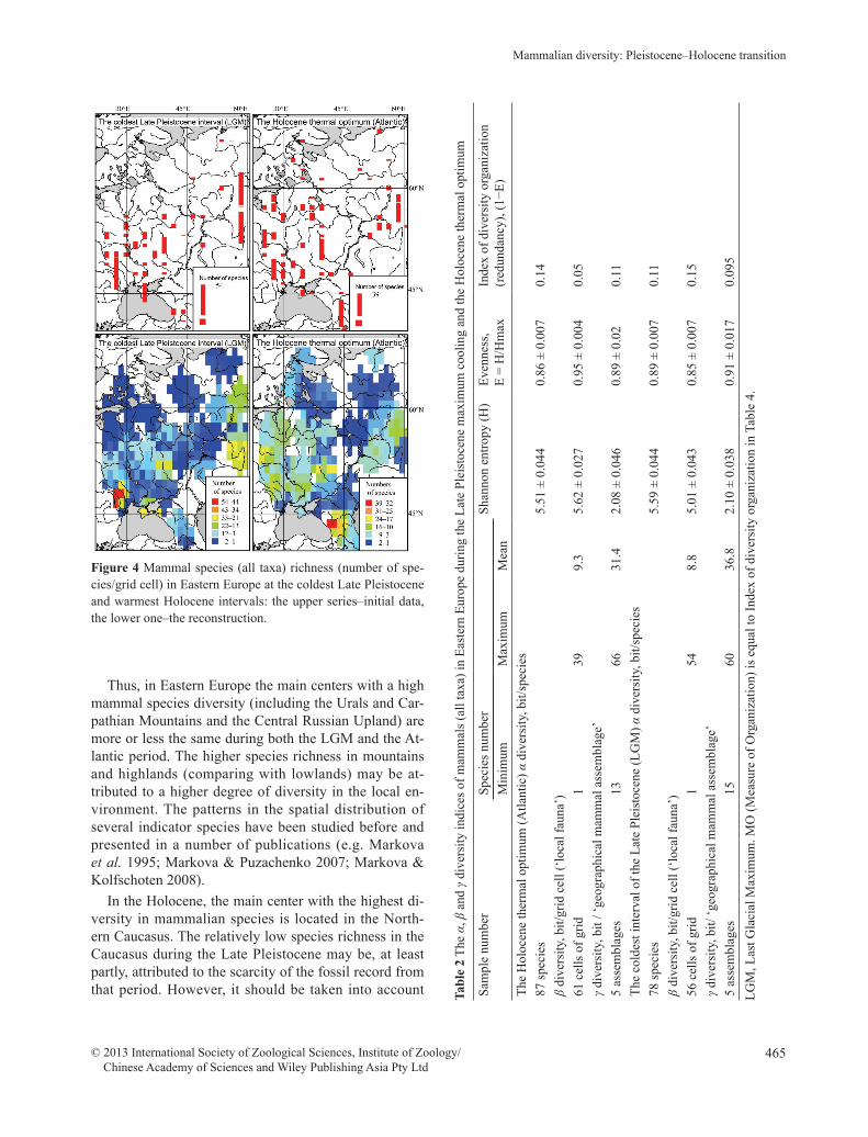
The spatial variability of the mammal species rich-ness in Eastern Europe during the coldest interval of the Pleistocene and at the Holocene thermal optimum is il-lustrated in Figure 4. The maximum species richness during LGM time is recorded from the foot of the Car-pathian Mountains and the in South Ural Mountains. The other Late Pleistocene centers rich in mammalian species have been recognized in the Crimea (Crimean Mountains) and in the area of the Central Russian Up-land (the upper reaches of the Don River, Voronezh Re-gion). The Holocene centers with a high species diversi-ty include the Caucasus, the Urals, the Carpathians and the Central Russian Upland. A relatively high degree of mammal diversity during the Holocene thermal opti-mum is recorded in the western parts of Eastern Europe: in the Byelorussian Polesye and in the Zapadnaya Dvina drainage basins.

Table 1 Data for diversity indexes calculating for the selected large and medium size mammals species

Сlimate-stratigraphic units Number of grid cells (2° × 2°) with at least one locality

Species number per climate-stratigraphic unit

HoloceneThe present time 139 28Subatlantic (SA) 63 22Subboreal (SB) 77 28Atlantic (AT) 60 31Boreal (BO) 32 25Preboreal (PB) 12 29PleistoceneYounger Dryas Stadial (YD) 12 11Bølling and Allerød interstadials complex (BAIC) 17 17Late Glacial (or Deglaciation) (LGT) 40 28Valday (Weichselian) glacial epoch (LGM) 54 28Denekamp (= Bryansk) Interstadial (DEN) 54 27 Huneborg Stadial (HUN) 24 25Hengelo Interstadial (HEN) 22 18Hasselo Stadial (HAS) 31 32

465

123456789101112131415161718192021222324252627282930313233343536373839404142434445464748495051



123456789

101112131415161718192021222324252627282930313233343536373839404142434445464748495051

Thus, in Eastern Europe the main centers with a high mammal species diversity (including the Urals and Car-pathian Mountains and the Central Russian Upland) are more or less the same during both the LGM and the At-lantic period. The higher species richness in mountains and highlands (comparing with lowlands) may be at-tributed to a higher degree of diversity in the local en-vironment. The patterns in the spatial distribution of several indicator species have been studied before and presented in a number of publications (e.g. Markova et al. 1995; Markova & Puzachenko 2007; Markova & Kolfschoten 2008).

In the Holocene, the main center with the highest di-versity in mammalian species is located in the North-ern Caucasus. The relatively low species richness in the Caucasus during the Late Pleistocene may be, at least partly, attributed to the scarcity of the fossil record from that period. However, it should be taken into account Ta

ble

2 Th

e α,

β a

nd γ

dive

rsity

indi

ces o

f mam

mal

s (al

l tax

a) in

Eas

tern

Eur

ope

durin

g th

e La

te P

leis

toce

ne m

axim

um c

oolin

g an

d th

e H

oloc

ene

ther

mal

opt

imum

Sam

ple

num

ber

Spec

ies n

umbe

rSh

anno

n en

tropy

(H)

Even

ness

,E

= H

/Hm

axIn

dex

of d

iver

sity

org

aniz

atio

n (r

edun

danc

y), (

1−E)

Min

imum

Max

imum

Mea

nTh

e H

oloc

ene

ther

mal

opt

imum

(Atla

ntic

) α d

iver

sity

, bit/

spec

ies

87 sp

ecie

s5.

51 ±

0.0

440.

86 ±

0.0

070.

14β

dive

rsity

, bit/

grid

cel

l (‘lo

cal f

auna

’)61

cel

ls o

f grid

139

9.3

5.62

± 0

.027

0.95

± 0

.004

0.05

γ div

ersi

ty, b

it / ‘

geog

raph

ical

mam

mal

ass

embl

age’

5 as

sem

blag

es13

6631

.42.

08 ±

0.0

460.

89 ±

0.0

20.

11Th

e co

ldes

t int

erva

l of t

he L

ate

Plei

stoc

ene

(LG

M) α

div

ersi

ty, b

it/sp

ecie

s78

spec

ies

5.59

± 0

.044

0.89

± 0

.007

0.11

β di

vers

ity, b

it/gr

id c

ell (

‘loca

l fau

na’)

56 c

ells

of g

rid1

548.

85.

01 ±

0.0

430.

85 ±

0.0

070.

15γ d

iver

sity

, bit/

‘geo

grap

hica

l mam

mal

ass

embl

age’

5 as

sem

blag

es15

6036

.82.

10 ±

0.0

380.

91 ±

0.0

170.

095

LGM

, Las

t Gla

cial

Max

imum

. MO

(Mea

sure

of O

rgan

izat

ion)

is e

qual

to In

dex

of d

iver

sity

org

aniz

atio

n in

Tab

le 4

.

Figure 4 Mammal species (all taxa) richness (number of spe-cies/grid cell) in Eastern Europe at the coldest Late Pleistocene and warmest Holocene intervals: the upper series–initial data, the lower one–the reconstruction.

466

123456789

101112131415161718192021222324252627282930313233343536373839404142434445464748495051



123456789101112131415161718192021222324252627282930313233343536373839404142434445464748495051

that during the Late Pleistocene the suitable mammali-an habitats were considerably reduced in areas affect-ed by mountain glaciers. The Crimea, one of the centers with a high diversity during the Pleistocene, lost its sig-nificance during the Holocene; the same is true for the Urals, in particular the Southern Urals.

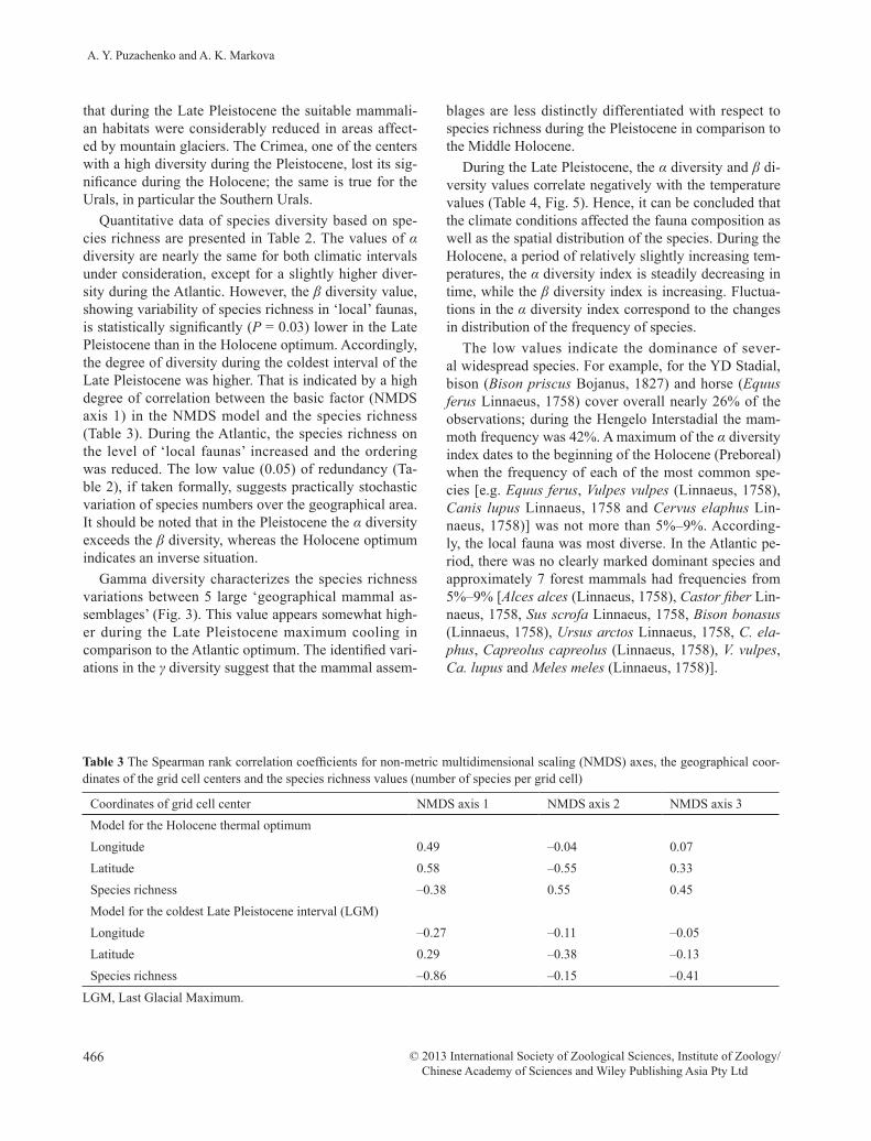
Quantitative data of species diversity based on spe-cies richness are presented in Table 2. The values of α diversity are nearly the same for both climatic intervals under consideration, except for a slightly higher diver-sity during the Atlantic. However, the β diversity value, showing variability of species richness in ‘local’ faunas, is statistically significantly (P = 0.03) lower in the Late Pleistocene than in the Holocene optimum. Accordingly, the degree of diversity during the coldest interval of the Late Pleistocene was higher. That is indicated by a high degree of correlation between the basic factor (NMDS axis 1) in the NMDS model and the species richness (Table 3). During the Atlantic, the species richness on the level of ‘local faunas’ increased and the ordering was reduced. The low value (0.05) of redundancy (Ta-ble 2), if taken formally, suggests practically stochastic variation of species numbers over the geographical area. It should be noted that in the Pleistocene the α diversity exceeds the β diversity, whereas the Holocene optimum indicates an inverse situation.

Gamma diversity characterizes the species richness variations between 5 large ‘geographical mammal as-semblages’ (Fig. 3). This value appears somewhat high-er during the Late Pleistocene maximum cooling in comparison to the Atlantic optimum. The identified vari-ations in the γ diversity suggest that the mammal assem-

blages are less distinctly differentiated with respect to species richness during the Pleistocene in comparison to the Middle Holocene.

During the Late Pleistocene, the α diversity and β di-versity values correlate negatively with the temperature values (Table 4, Fig. 5). Hence, it can be concluded that the climate conditions affected the fauna composition as well as the spatial distribution of the species. During the Holocene, a period of relatively slightly increasing tem-peratures, the α diversity index is steadily decreasing in time, while the β diversity index is increasing. Fluctua-tions in the α diversity index correspond to the changes in distribution of the frequency of species.

The low values indicate the dominance of sever-al widespread species. For example, for the YD Stadial, bison (Bison priscus Bojanus, 1827) and horse (Equus ferus Linnaeus, 1758) cover overall nearly 26% of the observations; during the Hengelo Interstadial the mam-moth frequency was 42%. A maximum of the α diversity index dates to the beginning of the Holocene (Preboreal) when the frequency of each of the most common spe-cies [e.g. Equus ferus, Vulpes vulpes (Linnaeus, 1758), Canis lupus Linnaeus, 1758 and Cervus elaphus Lin-naeus, 1758)] was not more than 5%–9%. According-ly, the local fauna was most diverse. In the Atlantic pe-riod, there was no clearly marked dominant species and approximately 7 forest mammals had frequencies from 5%–9% [Alces alces (Linnaeus, 1758), Castor fiber Lin-naeus, 1758, Sus scrofa Linnaeus, 1758, Bison bonasus (Linnaeus, 1758), Ursus arctos Linnaeus, 1758, C. ela-phus, Capreolus capreolus (Linnaeus, 1758), V. vulpes, Ca. lupus and Meles meles (Linnaeus, 1758)].

Table 3 The Spearman rank correlation coefficients for non-metric multidimensional scaling (NMDS) axes, the geographical coor-dinates of the grid cell centers and the species richness values (number of species per grid cell)

Coordinates of grid cell center NMDS axis 1 NMDS axis 2 NMDS axis 3Model for the Holocene thermal optimumLongitude 0.49 –0.04 0.07Latitude 0.58 –0.55 0.33Species richness –0.38 0.55 0.45Model for the coldest Late Pleistocene interval (LGM)Longitude –0.27 –0.11 –0.05Latitude 0.29 –0.38 –0.13Species richness –0.86 –0.15 –0.41

LGM, Last Glacial Maximum.

467

123456789101112131415161718192021222324252627282930313233343536373839404142434445464748495051



123456789

101112131415161718192021222324252627282930313233343536373839404142434445464748495051

The steady downfall of the α diversity index during the Holocene (Fig. 5) is caused predominantly by the wide distribution of the forest species, such as brown bear, elk, red deer, roe deer, beaver and others. A con-temporary value of this index (3.98 bit/species) is low relative to the Holocene data and does not differ from the mean for the entire SA period. The frequencies of dominant species in the ‘local fauna’ varied from 10% to 12% in the SA (beaver, elk and brown bear) and from 10% to 11% at present time [red fox, wolf, otter [Lutra lutra (Linnaeus, 1758)], European badger).

In the Late Pleistocene, a relatively high level of α diversity occurred during the Hasselo Stadial when the frequency of each of 5 widespread species [E. ferus, Ca. lupus, B. priscus, Coelodonta atiquitatis (Blumenbach, 1807) and C. elaphus] varied from 5% to 8%. However, in this case there was a strongly pronounced dominant species, the mammoth (18%).

The β diversity index reflects the changes of species richness in geographical space. Low values reflect more heterogeneity in space (Table 4: HEN, HUN, BAIC, YD, SBO and SA). High values indicate more even dis-tribution of species richness in Eastern Europe. The con-temporary β diversity index is quite high (7.1 bit/grid

cell); it is caused by the absolute dominance of wide-spread species and the almost absence of ‘centers’ with a high species diversity in the mammalian group under study.

The index of diversity organization (Table 4) reflects in general the level of influence of factors that limit the diversity (e.g. climate, orography and biocoenotic). The index of diversity organization MO α (MO indicating the Measure of Organization, which is equal to the In-dex of diversity organization; see Table 4) in the Pleis-tocene and Holocene do not differ on average. At the same time, the MO β was significantly higher during the Pleistocene than in the Holocene (Mann–Whitney U = 3, Z = 2.7, P = 0.005). These differences in parame-ters reflect a considerably less important role of the cli-mate and the orography in the biological diversity of the mammal group under study.

CONCLUSIONFor the first time various aspects of biological diver-

sity of the East European mammal assemblages were quantitatively estimated for the maximum Valday cool-ing (LGM), the Holocene climatic optimum and 13 oth-

Figure 5 α, β diversity in different cli-mate-stratigraphic units of Late Pleisto-cene and Holocene age in Eastern Eu-rope. In the Late Pleistocene, both indexes are correlated negatively with temperature (T, δ18O). In the Holocene, α diversity de-creased after a rapid increase in the Prebo-real time, but β diversity increased. Both indexes changed independently from the climate changes during the Holocene.

468

123456789

101112131415161718192021222324252627282930313233343536373839404142434445464748495051



123456789101112131415161718192021222324252627282930313233343536373839404142434445464748495051Ta

ble

4 D

iver

sity

inde

xes

calc

ulat

ed fo

r the

diff

eren

t clim

ate-

stra

tigra

phic

uni

ts o

f the

Lat

e Pl

eist

ocen

e–H

oloc

ene

in E

aste

rn E

urop

e ba

sed

on d

ata

of th

e di

strib

utio

n of

la

rge

and

med

ium

size

d m

amm

als (

mai

nly

ungu

late

s and

car

nivo

res)

Сlim

ate-

stra

tigra

phic

uni

tsα

dive

rsity

(Dα)

β di

vers

ity (D

β)

Shan

non

entro

py (H

), bi

t/spe

cies

Inde

x of

div

ersi

ty o

rgan

izat

ion

(MO

α =

1 −

H/H

max

)Sh

anno

n en

tropy

(H),

bit/

grid

cel

lIn

dex

of d

iver

sity

org

aniz

atio

n (M

O β

= 1

− H

/Hm

ax)

Hol

ocen

eTh

e pr

esen

t tim

e3.

98 ±

0.0

20.

177.

80 ±

0.0

10.

01Su

batla

ntic

(SA

)3.

96 ±

0.0

30.

115.

79 ±

0.0

20.

03Su

bbor

eal (

SB)

4.13

± 0

.04

0.14

6.04

± 0

.02

0.04

Atla

ntic

(AT)

4.30

± 0

.04

0.13

5.66

± 0

.03

0.04

Bor

eal (

BO

)4.

24 ±

0.0

60.

094.

60 ±

0.0

60.

08Pr

ebor

eal (

PB)

4.59

± 0

.07

0.05

3.16

± 0

.08

0.12

Plei

stoc

ene

Youn

ger D

ryas

Sta

dial

(YD

)3.

34 ±

0.1

20.

072.

75 ±

0.2

10.

21B

øllin

g an

d A

llerø

d in

ters

tadi

als c

ompl

ex (B

AIC

)3.

66 ±

0.1

10.

103.

60 ±

0.1

10.

12La

te G

laci

al (o

r Deg

laci

atio

n) (L

GT)

4.29

± 0

.04

0.11

4.79

± 0

.04

0.10

Vald

ay (W

eich

selia

n) m

axim

um c

oolin

g (L

GM

)4.

17 ±

0.0

50.

135.

29 ±

0.0

40.

08D

enek

amp

(= B

ryan

sk) I

nter

stad

ial (

DEN

)4.

16 ±

0.0

70.

134.

93 ±

0.0

80.

14H

uneb

org

Stad

ial (

HU

N)

3.97

± 0

.11

0.15

3.80

± 0

.11

0.17

Hen

gelo

Inte

rsta

dial

(HEN

)3.

28 ±

0.1

90.

213.

81 ±

0.1

50.

15H

asse

lo S

tadi

al (H

AS)

4.44

± 0

.09

0.11

4.05

± 0

.01

0.18

MO

, Mea

sure

of O

rgan

izat

ion.

MO

is e

qual

to in

dex

of d

iver

sity

org

aniz

atio

n in

Tab

le 2

.

er climate-stratigraphic units of Late Pleistocene and Holocene age. First, it has been indicated that the to-tal number of species (species richness) remained prac-tically the same for the extreme cold (the LGM) as well as the extreme warm time interval (the Atlantic), in spite of essential difference in the geographic distribution of the species richness in both periods. The variations in species richness and distribution were due to chang-es in climatic conditions as well as to the swift extinc-tion of large herbivores and carnivores from the ‘Mam-moth Fauna’ complex at the end of the Pleistocene. The species composition of the mammal fauna was subject to radical changes in every region of Eastern Europe. These aspects of changes in species diversity and the re-establishment of the mammal assemblages in Europe at the Pleistocene–Holocene transition are described and discussed in more details in an earlier work (Markova & Kolfschoten 2008).

The results of this studies allow the identification of several ‘centers’ with a high mammalian species rich-ness: those established for the Late Pleistocene maxi-mum cooling (Valday) are confined to the Carpathians, the Crimea Mountains, the South Urals and the Cen-tral Russian Upland; in the Atlantic, the centers of max-imum species richness are found in every mountainous region, including the Caucasus. Therefore, it can be con-cluded that the geographical positions of the main diver-sity centers in the Eastern Europe are relatively stable.

The geographical boundaries of the mammal assem-blages from the coldest and warmest intervals show dif-ferent orientation during the Late Pleistocene and the Holocene. Their orientation is effected by the Scandina-vian ice sheet, particular in the northwestern part of the region.

At the time of the LGM a limited number of species inhabited the zone fringing the ice sheet (north of ap-proximately 55°N) (Fig. 4); further south, on the plains of Eastern Europe down to 45°N, the discovered spe-cies increased in number to approximately 12. The spe-cies richness still grew (up to 22 species) near the foot of the Carpathians, and probably also towards the coasts of the Black and Azov Seas (although the data for these 2 regions are extremely scarce). The central part of the Russian Plain shows rather stable values of species rich-ness, probably due to widely spread periglacial open landscapes and the absence of a forest zone. At the Ho-locene optimum, the distribution of the mammal spe-cies richness from north to south appears to be quite different. According to our data, faunas with low spe-cies richness existed north of 60°N. Southwards, mam-

469

123456789101112131415161718192021222324252627282930313233343536373839404142434445464748495051



123456789

101112131415161718192021222324252627282930313233343536373839404142434445464748495051

mal faunas gradually increased in species richness up to 15 species at 55°N. According to paleontological data, the number of species increased further south, up to 25 species, presumably due to the reoccurrence of a forest zone. The scarcity of data in some mountain regions (the Carpathians and the Crimean Mountains) precludes the reconstructing of real values of species richness in these areas; we assume that these values are high. The only identified region with a high species diversity for this interval is the Caucasus Mountains. A steadily high lev-el of species richness (both in the Late Pleistocene and in the Holocene) was recorded in the high reaches of the Don River (Central Russian Upland). The same is true for the South Urals and partly for the Middle Urals. The Urals mammal species richness appeared to be higher during the Late Pleistocene cooling (LGM) than at the Holocene optimum or at present. That may be attribut-ed to the penetration of tundra species from the north and steppe species from the south, along with some per-sisting forest dwellers. Remarkable is the relatively high level of species richness in western regions of East-ern Europe (Belarusian Paleśsie and the Western Dvina drainage basin); it was caused by the reoccurrence of a greater quantity of forest species.

It should be noted that in every case the data avail-able were insufficient to reliably reconstruct the species richness for the all taxa. That is why we can only pres-ent relative estimates. Nevertheless, the data indicate the principal tendency in species richness that changes geo-graphically from north to south.

The analogue values of the α and β diversity index-es were obtained for the first time using Eastern Euro-pean paleontological data. These indexes are integral variables that reflect different aspects of the biodiver-sity structure. During the Late Pleistocene the values of both indexes correlate negatively with the tempera-ture values. There is a link between the interstadial–sta-dial fluctuations and the dramatic collapse of the ‘Mam-moth Fauna’ complex at the end of the Late Pleistocene. During the Holocene, Eastern Europe changed relative-ly quickly, with a widespread reestablishment of forest and the reoccurrence of forest species in the first place. The diversity indexes of large and medium sized mam-mals barely reacted to the changes in climatic conditions during the Holocene.

Nowadays, the α diversity index is relatively low and the β diversity index is relatively high, which we attri-bute to a decrease, in historical time, in the population number of some forest species (beaver, brown bear and red deer) and the increase of the dominance of species

that can occupy different habitats as well as an increase of species connected with intra-zonal ecosystems (i.e. red fox and European otter).

ACKNOWLEDGMENTS The work was performed with the financial support

from RFBR (grant № 10-05-00111). We would like to thank our reviewers for their very constructive remarks. We are very grateful to Maria Rita Palombo for her sug-gestion to contribute to this volume.

REFERENCESBaryshnikov GF, Markova AK (2009). The main mam-

mal assemblages during the Late Pleistocene cold ep-och (map 23). In: Velichko AA, ed. Paleoclimates and Paleoenvironments of Extra-Tropical Area of the Northern Hemisphere. Atlas-monograph. GEOS Pub-lishing, Moscow, pp. 79–87. (In Russian.)

Janssen SR, Törnqist TE (1991). The role of scale in the biostratigraphy and chronostratigraphy of the Holo-cene Series in the Netherlands. The Holocene 1, 112–20.

Kruskal B (1964). Multidimensional scaling by optimiz-ing goodness of fit to nonmetric hypothesis. Psycho-metrika 29, 1–27.

Kul’kova MA, Mazurkevich AN, Dolukhanov PM (2001). Chronology and palaeoclimate of prehistoric sites in Western Dvina-Lovat’ Area of northwestern Russia. Geochronometria 20, 87–94.

Margalef R (1957). Information theory in ecology. Me-morias de la Real Academia de Ciencias y Artes de Barcelona 23, 373–449.

Markova AK, Kolfschoten T, eds (2008). Evolution of European Ecosystems During Pleistocene–Holocene Transition (24–8 kyr BP). KMK Scientific Press, Moscow. (In Russian with English summaries.)

Markova AK, Puzachenko AY (2007). Late Pleistocene mammals of Northern Asia and Eastern Europe. In: Elias SA, ed. Vertebrate Records. Encyclopedia of Quaternary Science 4. Elsevier B.V., London, UK, pp. 3158–74.

Markova AK, van Kolfschoten T, Simakova AN, Pu-zachenko AY, Belonovskaya EA (2006). Ecosystems of Europe during the Late Glacial Bølling-Allerød warming based on pollen data and mammal fauna. Iz-vestiya Russian Academy of Sciences, Seria Geogrphic-heskaya 1, 15–25. (In Russian.)

470

123456789

101112131415161718192021222324252627282930313233343536373839404142434445464748495051



123456789101112131415161718192021222324252627282930313233343536373839404142434445464748495051

Markova AK, Simakova AN, Puzachenko AY (2003). Ecosystems of Eastern Europe at the Atlantic opti-mum of the Holocene based on floristic and therio-logical data. Russian Academy of Sciences, Doklady 391, 545–9.

Markova AK, Simakova AN, Puzachenko AY (2002а). Ecosystems of Eastern Europe at the time of maxi-mum cooling of the Valday glacial epoch based on floristic and theriological data. Russian Academy of Sciences, Doklady 389, 681–5.

Markova AK, Simakova AN, Puzachenko AY, Kitayev LM (2002b). Reconstruction of the natural zonali-ty on the Russian Plain during the Bryansk warm in-terval (33–24 ka BP). Izvestiya of Russian Academy of Sciences. Seriya Geograficheskaya 4, 45–57.

Markova AK, Smirnov NG, Kozincev PA et al. (2001). Zoogeography of Holocene mammals in northern Eurasia. Lynx 32, 233–45.

Markova AK, Smirnov NG, Kozharinov AV, Kazantseva NE, Simakova AN, Kitaev LM (1995). Late Pleisto-cene distribution and diversity of mammals in North-ern Eurasia (PALEOFAUNA database). Paleontolo-gia i Evolucio 28–29, 5–143.

Mol J (2008). Definition of the time slices. Landscape and climate change during the Last Glaciation in Eu-rope; a review. In: Markova AK, van Kolfschoten T, eds. Evolution of European Ecosystems during Pleis-tocene–Holocene Transition (24–8 kyr BP). KMK Scientific Press, Moscow, pp. 73–87.

Patten BC (1962). Species diversity in net phytoplank-ton of Raritan Bay. Journal of Marine Research 20, 57–75.

Pielou EC (1966). The measurement of diversity in dif-ferent types of biological collections. Journal of The-oretical Biolog 13, 131–44.

Puzachenko AY, Markova AK (2007). Spatial and tem-poral dynamics of mammal species diversity in Eu-

rope within a geologically short time interval (Late Pleistocene–Holocene). In: Pavlov DS, Zakharov VM, eds. Climatic Changes and Biodiversity in Rus-sia: Statement of the Problem. Acropolis Publishing House, Moscow, pp. 73–94.

Rasmussen SO, Andersen KK, Svensson AM et al. (2006). A new Greenland ice core chronology for the last glacial termination. Journal Geophysical Re-search 111, D06102.

Reimer PJ, Bailli, MGL, Bard E et al. (2009). Intcal09 and Marine09 radiocarbon calibration curves, 0-50 cal kBP. Radiocarbon 51, 1111–50. OxCal 4.1. [Cited 25 Feb 2011.] Available from URL: http://c14.arch.ox.ac.uk/embed.php?File=oxcal.html

Schrøder N, Højlund PL, Juel BR (2004). 10,000 years of climate change and human impact on the environ-ment in the area surrounding Lejre. The Journal of Transdisciplinary Environmental Study 3/1, 1–27.

Svensson A, Andersen KK, Bigler M et al. (2008). A 60 000 year Greenland stratigraphic ice core chronolo-gy. Climate of the Past 4, 47–57.

Velichko AA, Faustova MA (2009). The ice sheet devel-opment during Late Pleistocene. In: Velichko AA, ed. Paleoclimates and Paleoenvironments of Extra-Trop-ical Area of the Northern Hemisphere. Atlas-mono-graph. GEOS Publishing, Moscow, pp. 32–41. (In Russian.)

Vereshchagin NK, Baryshnikov GF (1992). The eco-logical structure of the ‘Mammoth Fauna’ in Eurasia. Annales Zoologici Fennici 28, 253–9.

Vinther BM, Clausen HB, Johnsen SJ et al. (2006). A synchronized dating of three Greenland ice cores throughout the Holocene. Journal of Geophysical Re-search 111, D13102.

Whittaker RH (1972). Evolution and measurement of species diversity. Taxon 21, 213–51.

Mammal diversity during the Pleistocene–Holocene transition in Eastern Europe

Documents

Transcript of Mammal diversity during the Pleistocene–Holocene transition in Eastern Europe