Making Prospect Theory Fit for Finance*

Enrico De Giorgi† and Thorsten Hens‡

Mai 17, 2006

Abstract

The prospect theory of Kahneman and Tversky (1979) and the cumulative prospect theory of Tversky and Kahneman (1992) are descriptive models for decision making that summarize several violations of the expected utility theory. This paper gives a survey of applications of prospect theory to the portfolio choice problem and the implications for asset pricing. We demonstrate that prospect theory (and similarly cumulative prospect theory) has to be re-modelled if one wants to apply it to portfolio selection. We suggest replacing the piecewise power value function of Kahneman and Tversky (1979) with a piecewise negative exponential value function. This latter functional form is still compatible with laboratory experiments but it has the following advantages over and above Kahneman and Tversky`s piecewise power function: 1. The Bernoulli Paradox does not arise for lotteries with finite expected value. 2. No infinite leverage/robustness problem arises. 3. CAPM-equilibria with heterogeneous investors and prospect utility do exist. 4. It is able to simultaneously resolve the following asset pricing puzzles: the equity premium, the

value and the size puzzle. 5. In contrast to the piecewise power value function it is able to explain the disposition effect. Resolving these problems of prospect theory we show how it can be combined with mean-variance portfolio theory. JEL-Classification: D 01, D 14, D 81, G 11.

1. Introduction THE PROSPECT THEORY (PT) of Kahneman and Tversky (1979) summarizes several violations of the expected utility hypothesis. First of all, while expected utility is already based on a formal representation of a decision problem, PT has two stages. The first stage is an editing phase in which the given representation of the decision problem is transformed into a formal decision. The second stage is an evaluation

* Financial support by the University Research Priority Programme “Finance and Financial Markets” of the University of Zurich, the Foundation for Research and Development at the University of Lugano, and the National Centre of Competence in Research “Financial Valuation and Risk Management” is gratefully acknowledged. The national centers in research are managed by the Swiss National Science Foundation an behalf of the federal authorities. † Institute of Finance, University of Lugano, via Buffi 13, CH-6900 Lugano and NCCR-FINRISK. E-mail: enrico.degiorgi@lu.unisi.ch. ‡ Swiss Banking Institute, University of Zurich, Plattenstrasse 32, CH-8032 Zurich and Norwegian School of Economics and Business Administration, Helleveien 30, N-5045, Bergen, Norway. E-mail: thens@isb.unizh.ch.

1

phase in which, based on a value and a probability weighting function, the lottery with the highest value is chosen. In this paper, as in most finance papers, we assume that the editing phase is already completed and we thus only consider the valuation phase. This makes our results comparable to expected utility. The main building blocs of prospect theory that distinguishes it from expected utility theory are then: 1. Investors evaluate assets according to gains and losses relative to a given

reference point. 2. Investors dislike losses by a factor of 2.25 as compared to their liking of gains

(loss aversion). 3. Investors have asymmetric risk aversion because their value functions are S-

shaped with turning point at the origin. 4. Investors` probability assessments are biased in the way that extremely small

probabilities (extremely high probabilities) are over- (under-) valued. The latter point is known as probability weighting, which causes PT preferences to be inconsistent with first order stochastic dominance. This drawback has been solved with the cumulative prospect theory (CPT) of Tversky and Kahneman (1992), which replaces the weighting of probabilities with that of the cumulative distribution functions. While PT and CPT describe very well the choice of agents among a restricted set of lotteries, they have some shortcomings when they are transferred to describe the solutions to portfolio selection problems. This is because the set of lotteries that can be generated by portfolio selection is quite large – it is typically uncountable and unbounded. Unfortunately, while the mathematical representation of prospect theory suggested by Tversky and Kahneman did well in the laboratory, it is not appropriate for portfolio selection problems. The main point of this survey is to argue that the prospect theory of Tversky and Kahneman (1992) and similarly that of Kahneman and Tversky (1979) has to be re-modelled if one wants to apply prospect theory in finance. Instead of modelling the value function by a piecewise power function a piecewise negative exponential function should be used. The main difference between the piecewise power function and the piecewise negative exponential function concerns large outcomes. In fact, while both functions are assumed to have a kinked and convex-concave shape with turning point at the origin, the piecewise negative exponential function exhibits more curvature and thus discourage extreme risk taking. As a consequence, while the suggested functional form also satisfies the main features of prospect theory and is still compatible with laboratory experiments, it has the following advantages over and above Kahneman and Tversky`s piecewise power function: 1. The St. Petersburg Paradox does not arise for lotteries with finite expected

value. 2. No infinite leverage/robustness problem arises. 3. CAPM-equilibria with heterogeneous investors and prospect utility do exist. 4. It is able to simultaneously resolve the following puzzles: the equity premium,

the value and the size puzzle. 5. In contrast to piecewise power value function it is able to explain the disposition

effect. The St. Petersburg paradox is associated with the birth of expected utility theory. It shows that for lotteries with infinite expected monetary value people are not willing to

2

pay an infinite sum of money. This observation led Bernoulli (1738) to postulate that people value lotteries not by their expected monetary value but rather by their expected utility of the monetary values it delivers. Assuming a sufficiently decreasing marginal utility of wealth, which is for example the case with a logarithmic utility, Bernoulli (1738) resolved the St. Petersburg Paradox. However, for any unbounded utility a lottery can be found that would still result in an infinite valuation of its monetary payoff. Hence, Bernoulli`s (1738) suggestion only solved the particular paradox arising from the particular game played in St. Petersburg but similar paradoxes occur for any unbounded utility. One solution is to only admit lotteries with bounded expected monetary value. However, as Blavatskyy (2005) and Rieger and Wang (2006) show, see Section 3 of this survey, this solution is not sufficient to rule out the paradox for CPT. Since the piecewise negative exponential value function that we proposes in this survey is bounded this paradox would no longer arise for prospect theory. As we show in Section 4, the piecewise power function runs into a second problem: For almost all asset prices the investors` optimal portfolios are unbounded. With this functional from, the marginal utility of wealth does not decrease sufficiently fast. As an effect, existence of competitive equilibria, for example in the CAPM, cannot be ensured with the piecewise power function for economies with heterogeneous investors. We show in Section 5 that with heterogeneous investors, CAPM equilibria do however exist if CPT is based on the piecewise negative exponential function. Of course, for any given investor one is able to find asset prices such that his portfolio selection problem has a solution. Indeed one can still use the standard argument common in the asset pricing literature where for a single representative investor asset prices are chosen such that the investor holds the market portfolio. However, De Giorgi, Hens and Levy (2004) show that this “decision support argument” for asset prices is not robust, since already small changes of the asset prices would lead the investor to choose totally different portfolios. Hence, with heterogeneous investors having piecewise power utilities there will not be a common vector of asset price for which all investors find a solution to their portfolio selection problem. In Finance CPT has been successful in explaining the equity premium puzzle, i.e. the historically favourable risk-return trade-off of stocks relative to bonds (first documented in Mehra and Prescott (1985). As shown by Benartzi and Thaler (1995), for a yearly holding period, the CPT statistic of the stock index is not significantly different from the CPT statistic of the bond index. Benartzi and Thaler (1995) introduce the concept of myopic loss aversion that combines loss aversion as described by PT with the tendency of investors to frequently evaluate the portfolio return. However, De Giorgi, Hens and Post (2005), see Section 7 of this survey, show that the same explanation does not rationalize the size premium puzzle, i.e. the historically favourable risk-return trade-off of small cap stocks relative to large cap stocks (first documented by Banz (1981)). Neither is it able to solve the value premium puzzle i.e. the favourable returns of value stocks relative to growth stocks (first documented by Basu (1977)). Fama and French (1992, 1993) provide the first rigorous empirical analysis of these phenomena. Nevertheless, the three puzzles can be explained simultaneously if we replace the piecewise-power value function of Tversky and Kahneman with a piecewise negative exponential value function. In fact, as discussed above, the new value function has a kinked and convex-concave shape (reflecting loss aversion and risk seeking for losses), just as the original value function. However, for large outcomes, the piecewise negative exponential value function exhibits more curvature hence the function discourages investment

3

opportunities which provide extreme losses, also when these are coupled with huge gains. In Section 7 we show that the disposition effect cannot be explained with the piecewise power but with the piecewise negative exponential value function. The disposition effect is the tendency of investors to hold loosing stocks too long while they sell winning stocks too early. The disposition effect has first been observed by Shefrin and Statman (1985) and Odean (1998). Hens and Vlcek (2005), assuming myopic optimization, and Barberis and Xiong (2006), assuming dynamic optimization, show that the piecewise power value function is not able explain the disposition effect because those investors who would show the disposition effect would not have invested in the asset to begin with. Kyle, Ou-Yang and Xiong (2006) point out that this inconsistency does not arise with the piecewise negative exponential value function. Previous work on prospect theory in portfolio selection has mainly focussed on the impact of loss aversion.1 Following the seminal analysis of Bernartzi and Thaler (1995), Barberis, Huang and Santos (2001), Gomes (2005) and Berkelaar, Kouvenberg and Post (2004) have studied how loss aversion affects multi-period portfolio decisions. Jin and Zhou (2006) extend these results by incorporating asymmetric risk aversion. Barberis, Huang and Santos (2001) incorporate a dynamic reference point in a multi-period model with prospect theory preferences. Their model starts from the observation of Thaler and Johnson (1990) that investors perceive gains and losses differently according to their prior outcomes. Barberis, Huang and Santos (2001) provide a partial equilibrium consideration with a representative investor who have prospect theory preferences with a piecewise linear value function. The model generates time varying risk premia, high mean and volatility for stock returns even if the underlying growth process has low variance. By contrast, the model generates portfolio strategies opposite to the disposition effect. Gomes (2005) studies a model with heterogenous investors: a loss averse investor and a CRRA investor. The shape of the utility function of the loss averse investor slightly differs from that suggested by Kahneman and Tversky (1979) and is concave also for large losses. Consequently, investors limit their risk exposure when facing large losses. Gomes (2005) allows only two possible outcomes at the investors’ time horizon. He derives equilibrium prices and analyzes the trading volume generated in this market. The first main result is that the presence of loss averse investors (also in a small proportion) can generate a substantial trading volume. The second main result is that loss averse investors follow a generalized portfolio insurance strategy, as it would also result from the disposition effect. Berkelaar, Kouvenberg and Post (2004) generalize the model of Gomes (2005) in order to have a price dynamics described by Ito processes, assuming complete markets. They derive the portfolio implication of loss aversion. Similarly to Gomes (2005), they found that investors with prospect theory preferences follow a partial portfolio insurance strategy. Moreover, the initial portfolio weights on stocks typically increases with the investment horizon. If the investment horizon is short, then investors with loss aversion strongly reduce their holdings in stocks (myopic loss aversion, see Bernatzi and Thaler (1995)) compared to investors with smooth power utility, while when the investment horizon is long, they strongly invest on stocks, since there is time to make up their losses, i.e. investors face gain opportunities. Berkelaar, Kouvenberg and Post (2005) also estimate the index of loss aversion on historical US stock market data and find a value of 2.45, near to the laboratory calibration of 2.25 given by Kahneman and Tversky (1979). Barberis and Huang (2005) also proved the consistency of CAPM equilibria with CPT preferences (see

4

Section 5 of this survey) when asset returns are assumed to be Gaussian distributed. They consider a partial equilibrium model and thus do not face the non-existence of equilibria when investors have heterogeneous preferences. They study the effect of probability weighting when asset returns are non-normally distributed and provide an application to the pricing of IPO’s. This paper is organized as follows: In the next section we lay down a model that is sufficiently general to embed the papers we want to give a survey of. Then we report the results on the St. Petersburg paradox, the infinite leverage problem, the existence of CAPM equilibria, the disposition effect and the asset pricing puzzles.

2. The Model Since the various aspects of CPT that we want to bring together in this survey come from quite different settings it is important to first lay down a model that is sufficiently general to embody all these aspects as special cases. Let the marketed subspace, X, be generated as the span of a collection of securities, one of which, say j = 0, is the risk free asset. We denote by ( )

0,1,...,j j JA

= the payoffs of

the assets. Let jq denote the price of asset j, j=0,1,…,J. Then the gross return of asset

j is defined as jj

j

AR

q= . There are i = 1,2,…,I investors being endowed with initial

wealth wi. Using the existing assets, investors transform their initial wealth into random wealth which they totally use for consumption in t = 1. All agents have already decided to invest wi on the financial market and they evaluate the consumption in t = 1 by utility functions : , i = 1,2,...,I →iU X R that are monotonically increasing and continuous. Hence the agents` optimization problem can be defined as

( )1

J

j0j=0

max U s.t. q .J

Ji ij j jjR

A wθ

θ θ+ =∈

=∑ ∑

Equivalently the optimization problem can be written in terms of returns:

( )( )1

J

0j=0

max U s.t. 1.J

Ji ij j jjR

R wλ

λ λ+ =∈

=∑ ∑

In the case of prospect theory the utility function Ui is defined by a reference point

∈iRP R , a value function : →iv R R and a probability transformation [ ] [ ]: 0,1 0,1→iT : ( ) ( ) ( ( )), = − Ν∫i i i i

RU x v x RP d T x where N denotes the

cumulative distribution of the generated payoffs x. We assume the following general properties of vi and Ti:

1. vi is a two times differentiable function on R\ }{0 , strictly increasing on R, strictly concave on (0,∞) and strictly convex on (-∞,0).

5

2. Ti is a differentiable, non-decreasing function from [0,1] onto [0,1] with ( )( ) for p = 0 and p=1 and with ( ) ( ) for p large (small).= < >i i iT p p T p p T p p

Kahneman and Tversky`s (1992) model of CPT and also our suggestion share these general properties. The weighting function is assumed to be given by

( )i

1/( ) , where the median of is about 0.65.

(1 )

γ

γγ γ

γ=+ −

i

ii i

i pT pp p

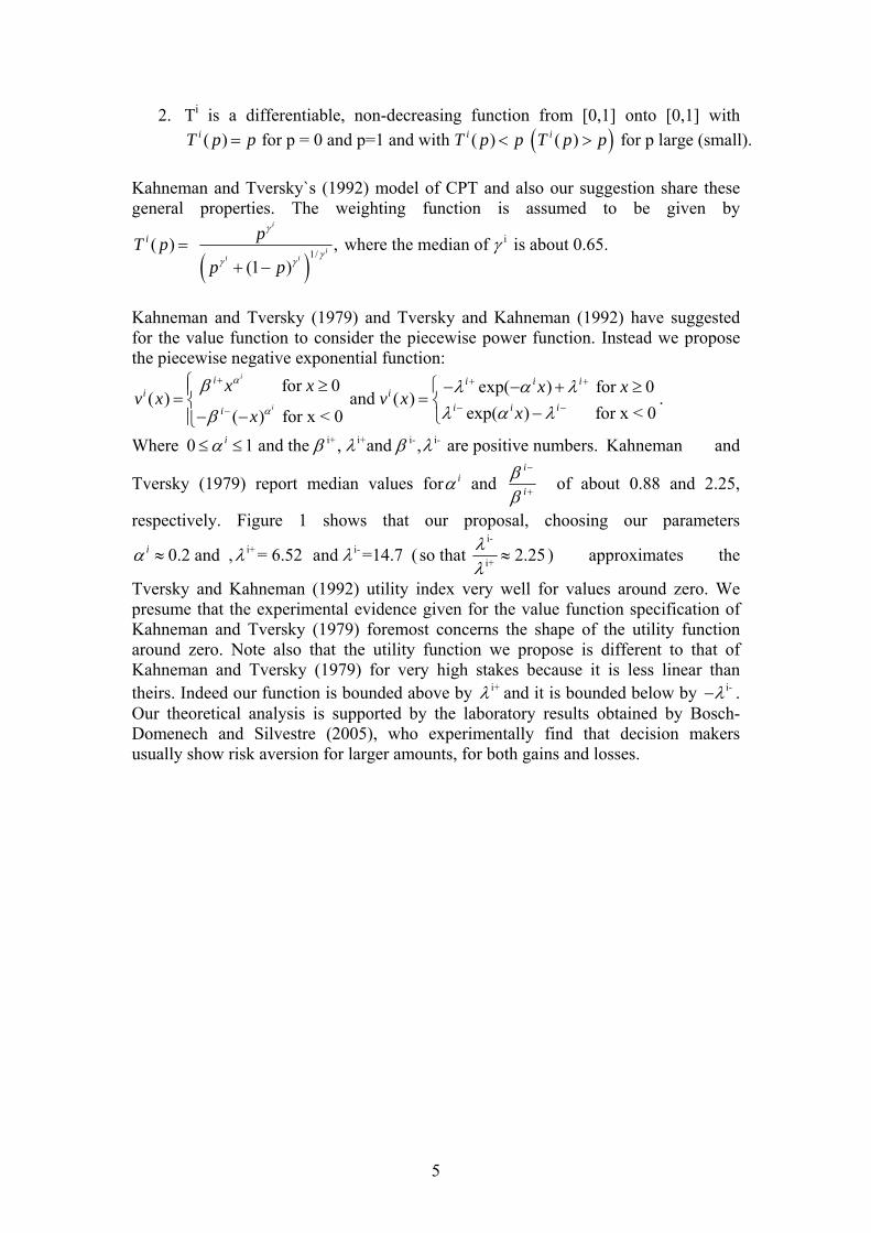
Kahneman and Tversky (1979) and Tversky and Kahneman (1992) have suggested for the value function to consider the piecewise power function. Instead we propose the piecewise negative exponential function:

for 0 exp( ) for 0( ) and ( )

exp( ) for x < 0( ) for x < 0

α

α

β λ α λλ α λβ

+ + +

− −−

⎧ ≥ ⎧− − + ≥⎪= =⎨ ⎨−− − ⎩⎪⎩

i

i

i i i ii i

i i ii

x x x xv x v x

xx.

Where i+ i+ i- i-0 1 and the , and , are positive numbers.iα β λ β λ≤ ≤ Kahneman and

Tversky (1979) report median values forα i and ββ

−

+

i

i of about 0.88 and 2.25,

respectively. Figure 1 shows that our proposal, choosing our parameters

0.2 and α ≈i , i+ = 6.52 λ i-and =14.7 λ (i-

i+so that 2.25λλ

≈ ) approximates the

Tversky and Kahneman (1992) utility index very well for values around zero. We presume that the experimental evidence given for the value function specification of Kahneman and Tversky (1979) foremost concerns the shape of the utility function around zero. Note also that the utility function we propose is different to that of Kahneman and Tversky (1979) for very high stakes because it is less linear than theirs. Indeed our function is bounded above by i+λ and it is bounded below by i-λ− . Our theoretical analysis is supported by the laboratory results obtained by Bosch-Domenech and Silvestre (2005), who experimentally find that decision makers usually show risk aversion for larger amounts, for both gains and losses.

6

3. The St. Petersburg Paradox The St. Petersburg paradox is usually explained by the following example: A player is reluctant to pay enormous amounts of money for a gamble in which he gets 2n ducats when the coin lands “heads” on the ground for the first time at the n-th throw. Note that the gamble has an infinite expectation:

1 1 1( ) 2 4 ... 2 1 1 .2 4 2η = ⋅ + ⋅ + + ⋅ + ⋅⋅ ⋅ = + + ⋅⋅⋅ = ∞n

nE x

This example already dates back to Bernoulli (1738). The solution of this problem is usually to replace the formula of expected value with the one of expected utility, in which a strictly concave utility function makes the subjective utility of the large outcomes no longer high enough compensate the very low probability associated with them. It is, however, important to keep in mind that for gambles with infinite expected value, the strict concavity of the utility function alone cannot guarantee the expected utility to be finite. For example, if the gamble from above offers 22

n

ducats when the coin lands “heads” for the first time at the n-th throw, then with a strictly concave utility function like 0.88( ) =u x x , the expected utility is still infinite. The St. Petersburg paradox can be resolved by allowing only for “realistic” gambles: Indeed, under the assumption of a finite expected value, a (not necessarily strictly) concave utility function is sufficient to guarantee the expected utility is finite. Even though this statement is almost trivial in the framework of expected utility theory, it turns out to be false in the context of CPT. In fact Rieger and Wang (2006)2 show that with CPT a

7

gamble with finite expected value can have infinite prospect utility – independent of the concavity of the value function. This is possible, since the probability weighting function suggested by Kahneman and Tversky (1979) has infinite slope at zero and since the slope of the value function does not decrease much for high. The gamble Rieger and Wang (2006) construct is as follows: The probability measure of possible

outcomes is given by --

0

0 x 1 p( ) where C = x .

Cx x>1 x dxκ

κ

∞≤⎧= ⎨⎩

∫ For κ close to 2, they

show that for values of the risk aversion parameter α and the probability weighting parameter γ that are consistent with the experimental literature indeed CPT utility is infinite. Note that this problem does not arise from the usual S-shape of the value function in CPT, since the example works with only considering positive outcomes (i.e. the concave part). Rieger and Wang (2006) suggest curing this problem by choosing a probability weighting function that has finite slope at 0. Alternatively, one could replaced the piecewise power value function by the piecewise negative exponential value function. This also solves the version of the St. Petersburg Paradox pointed out by Rieger and Wang (2006) because the piecewise negative exponential value function is bounded.

4. The Infinite Leverage/Robustness Problem So far we have shown that given the probability weighting function of Kahneman and Tversky (1979) the value function should better be bounded. Here we will argue that the boundedness is also important to solve an infinite leverage problem arising with the piecewise power function. Moreover, choosing a power function to model the agents` risk aversion leads to a robustness problem that does not occur for the piecewise negative exponential function. The infinite leverage problem is the observation that without imposing short sales constraints on the risk free asset (i.e. a borrowing constraint) a prospect utility maximizer always finds a portfolio of risky assets that he would like to leverage infinitely in order to obtain infinite utility: Recall that maximizing a power function in the expected utility approach is certainly possible without imposing a borrowing constraint. If markets are arbitrage free any portfolio of risky assets delivers gross returns that have a positive probability to obtain both, positive and negative excess returns. Hence scaling any such portfolio will let the utility tend to negative infinity. In the prospect theory case however, negative excess returns are not punished enough to avoid infinite leveraging. The robustness problem is the observation that small changes of the value function parameters lead to drastic changes in the asset allocation. As we show next these two problem are closely related for the piecewise power value function. To make this point, start from the optimization problem written in terms of returns.

( )( )1

J

0j=0

max U s.t. 1.J

Ji ij j jjR

R wλ

λ λ+ =∈

=∑ ∑ Assuming CPT we can write:

( )0 0 01 1( ) ( ) ( ( )), x = (1 ) , =1 . J Ji i i i i

j j jj jRU x v x RP d T x R R wλ λ λ λ λ

= == − Ν − +∑ ∑∫

Now suppose, for the reference point being equal to zero, for some portfolio of risky assets, say JJ

jj=1R with 1λ λ∈ =∑ , we obtain a positive prospect value:

( )0 0 01 1( ) ( ( )) 0, for some x = (1 ) ,with =1 . J Ji i i

j j jj jRv x d T x R R wλ λ λ λ λ

= =Ν > − +∑ ∑∫

8

The existence of such a portfolio follows from weak conditions on asset prices. For example, in case of Gaussian distributed returns, the existence of a risky portfolio with positive prospect value is ensured if the expected return of the market portfolio exceeds the risk-free rate of return. Referring to Kahneman and Tversky`s (1979) and Tversky and Kahneman (1992) specification of the value function we can rewrite the utility function as:

( )i

( ) ( ) ( ) ( )( ) ( ( )), i i i i

RU x x x x x RP d T x

α

λδ β δ= − Ν∫

where i1

(x)= , (x)=1

i i i

i i i

x RP x RPx RP x RP

βδ β

β

+

−

⎧ ⎧+ ≥ ≥⎨ ⎨− < <⎩ ⎩

.

Now, fix a portfolio J Rλ ∈ as defined above and consider what happens if the leverage is increased, i.e. 0λ → −∞ . For any such portfolio we obtain the payoffs:

( ) 0 001

0

(1 )(1 )

i iJi i

j jj

R w RPx RP R w λλ λλ=

⎡ ⎤−− = + −⎢ ⎥−⎣ ⎦

∑ . Hence the term 0(1 )αλ−i

factors

out from the utility computation and by the choice of the portfolio J Rλ ∈ in the limit for 0λ → −∞ it is multiplied with the positive term

( )i

0 1( ) ( ) ( )( ) ( ( )),where x = . Ji i i

j jjRx x x x R w d T x R

α

λδ β δ λ=

− Ν ∑∫

Note that this term is independent of λ . Hence 0λ → −∞ gives infinite utility.3 With a bounded utility function, infinite utility is impossible but still one may want to infinitely leverage the portfolio. For example with the piecewise negative exponential function there is no optimal leverage since the utility is increasing for all positive payoffs. However since the utility values are bounded above the increases become more and more negligible so that for any small epsilon there are portfolios that cannot be improved by other portfolios by more than epsilon. Hence an investor with a piecewise negative exponential value function who will be satisfied (up to some epsilon) with a finite leverage. A problem closely related to the infinite leverage problem is the robustness problem. The simplest case where this problem arises with the piecewise power function occurs when the reference point is the wealth obtained from investing all initial wealth in the

risk free asset. In this case we obtain: ( ) 0 01(1 )Ji i

j jjx RP R R wλ λ

=⎡ ⎤− = − −⎢ ⎥⎣ ⎦∑ . Hence

when on changing the parameters the excess return term ( ) 01

Jj jj

R Rλ=

−∑ crosses

zero, the asset allocation jumps from no risk-free asset to only risky free assets. This is a non-intuitive property for portfolio choice. Moreover, in asset pricing models with a representative investor who is induced to hold the market portfolio for some prices, on changing the parameters slightly the representative agent will depart from his choice drastically. That is to say, the standard “decision support argument” is not robust with the piecewise power function. De Giorgi and Hens (2005) also show that the robustness problem does not occur with the piecewise negative exponential value function, because this functional from prohibits to factor out the fraction invested in the risk free asset.

9

5. Existence of CAPM-Equilibria So far we have basically argued that a good value function for prospect theory should be bounded and should not allow to factor out the fraction of wealth invested in the risk free asset. Now we argue that the exponential function is a very convenient function when prospect theory should be combined with the CAPM. Assuming that the payoffs (and thus the returns) are normally distributed it is easy to see that a prospect utility is actually also a mean-variance utility. Using standard notation, let

0( )λµ µ λ

==∑ J

j jjR be the expected return of a portfolio and let accordingly

20 0

cov( , )λσ λ λ= =

=∑ ∑J Jj j k kj k

R R be the variance of a portfolio. Denoting by ,µ σΦ the

cumulative normal distribution we can write the agent`s optimization problem as:

( ), 0 0( ) ( ) ( ( )), where x = ,with =1 .

λ λµ σ λ λ= =

= − Φ ∑ ∑∫J Ji i i i i

j j jj jRU x v x RP d T x R w

Hence in this case the CPT utility function is a function of mean and variance only. Moreover, standardising the normal distribution reveals that this function is certainly increasing in mean but due to the convexity of the value function for losses it need not be decreasing in variance. Note that

( )i ˆ ˆ( , ) (x-RP ) + ( ( )), where ( ) . λλ λ λ λ

λ

µµ σ σ µσ

⎞⎛ −= Φ Φ = Φ ⎟⎜

⎝ ⎠∫i i i

R

xV v d T x x

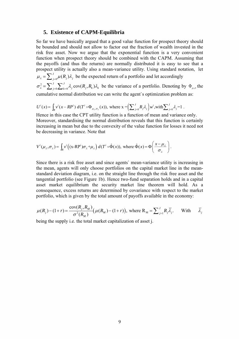
Since there is a risk free asset and since agents` mean-variance utility is increasing in the mean, agents will only choose portfolios on the capital market line in the mean-standard deviation diagram, i.e. on the straight line through the risk free asset and the tangential portfolio (see Figure 1b). Hence two-fund separation holds and in a capital asset market equilibrium the security market line theorem will hold. As a consequence, excess returns are determined by covariance with respect to the market portfolio, which is given by the total amount of payoffs available in the economy:

( ) M2 1

cov( , )( ) (1 ) ( ) (1 ) , where R .

( )µ µ λ

σ =− + = − + =∑ Jj M

j M j jjM

R RR r R r R

R With λ j

being the supply i.e. the total market capitalization of asset j.

10

Figure 1b: Two-Fund Separation Theorem

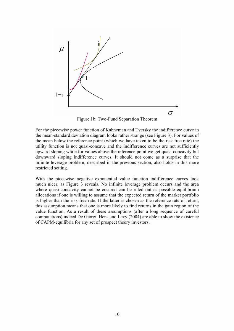
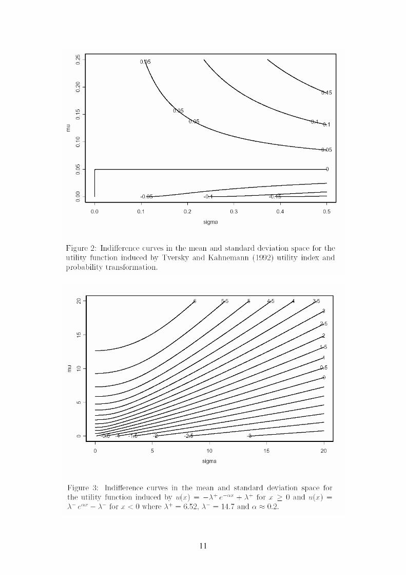
For the piecewise power function of Kahneman and Tversky the indifference curve in the mean-standard deviation diagram looks rather strange (see Figure 3). For values of the mean below the reference point (which we have taken to be the risk free rate) the utility function is not quasi-concave and the indifference curves are not sufficiently upward sloping while for values above the reference point we get quasi-concavity but downward sloping indifference curves. It should not come as a surprise that the infinite leverage problem, described in the previous section, also holds in this more restricted setting. With the piecewise negative exponential value function indifference curves look much nicer, as Figure 3 reveals. No infinite leverage problem occurs and the area where quasi-concavity cannot be ensured can be ruled out as possible equilibrium allocations if one is willing to assume that the expected return of the market portfolio is higher than the risk free rate. If the latter is chosen as the reference rate of return, this assumption means that one is more likely to find returns in the gain region of the value function. As a result of these assumptions (after a long sequence of careful computations) indeed De Giorgi, Hens and Levy (2004) are able to show the existence of CAPM-equilibria for any set of prospect theory investors.

11

12

6. The Equity Premium -, the Size - and the Value Puzzle A large equity premium is one of the more robust findings in financial economics.

On US-data, for example, over the period of 1802 to 1998 Siegel (1998) reports an excess return of U.S. Stocks over U.S. Bonds of about 7 % to 8 % p.a.. Similar results have been found for other periods and across other countries. This empirical finding is puzzling because it is hard to reconcile with plausible parameter values for agents' risk aversion in the standard consumption based asset pricing model originating from Lucas (1978), as Mehra and Prescott (1985) first pointed out. The huge number of solutions that have been suggested to resolve the equity premium puzzle is another puzzling aspect of the equity premium. It is impossible to review this literature in a few words without being accused for serious omissions. For a recent comprehensive treatment of all suggested solutions see the recent Handbook of Finance on this topic edited by Mehra (2006). Benartzi and Thaler (1995) showed that prospect theory can also resolve the equity premium puzzle. However, prospect theory based on the value function of Kahneman and Tversky (1979) deepens the value and the size puzzle. The value puzzle (Basu (1977)) is given by the favourable returns derived from investing in firms with low value multiples (price/earnings, price/dividend, price/cash flow or price/ book ratios) and the size puzzle (Banz (1981)) is given by the favourable returns derived from investing in small cap firms. In this section we will argue that the value function we propose for prospect theory is able to solve all three asset pricing puzzles simultaneously.

In order to stay as close as possible to the original equity premium studies of Mehra and Prescott (1985) and Benartzi and Thaler (1995) we consider real returns on equity and bonds. However, there are two differences. First, De Giorgi, Hens and Post (2005) consider an extended sample including the bull market of the 1990s and the equity bear market that followed in the early 2000s. Second, they expand the investment universe and include portfolios sorted on market capitalization (ME) and book-to-market-equity ratio (B/M) in the analysis.

The stock market portfolio is proxied by the CRSP all-share index, a value-weighted average of common stocks listed on NYSE, AMEX, and NADAQ. The bond index is defined as the intermediate government bond index maintained by Ibbotson. This index closely matches the 5-year Government bond index employed by Benartzi and Thaler (1995). De Giorgi, Hens and Post (2005) use the canonical decile portfolios formed on ME and the decile portfolios formed on B/M. For detailed data description and selection procedures we refer to Fama and French (1992) (1993). De Giorgi, Hens and Post (2005) use monthly and annual real returns for the period from January 1927 to December 2002 (912 months). Bond and inflation data are obtained from Ibbotson Associates and the stock portfolio data from Kenneth French’s online data library.

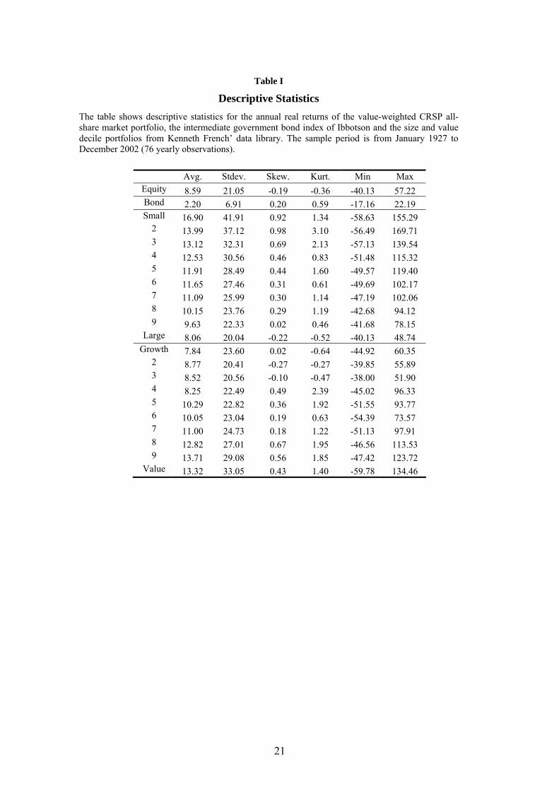
Table I presents some basic descriptive statistics of the stock portfolios and bond and equity indices. Clearly, stocks outperform bonds during our 76-year sample period by about 6 percent on an annual basis. However, stocks are riskier which is reflected in a low minimum (-40% in the worst year) and a high standard deviation. Contrary, bonds offer downside protection (-17% in the worst year), but the upside potential is limited. Small and value firms offer higher average returns and higher variance, combined with positive skewness. Puzzling is the BM8 and BM9 portfolios, which combine high average returns with a minimum return above -50% and a

13

maximum return in excess of 100%. Clearly, these portfolios seem far more attractive than the all-equity index.

[Insert Table I about here] De Giorgi, Hens and Post (2005) basically intend to test whether the market portfolio of risky assets is the optimal portfolio for a representative investor who obeys to the rules of (1) the mean-variance framework, (2) the piecewise power CPT or (3) the piecewise negative exponential CPT. The standard approach to test if the market portfolio is optimal is to analyze the first-order condition or the Euler equation. This approach is valid for the mean-variance framework, because the first-order condition is necessary and sufficient for establishing the maximum in this framework. By contrast, the first-order condition gives only a necessary optimality condition for CPT. Both models allow for local risk seeking and hence there may be minima and local maxima, which will also satisfy the first-order condition.

There exist various multivariate global optimization methods for locating the global optimum if the objective function is not concave (see, for example, Horst and Pardalos (1995)). Unfortunately, these methods generally are computationally too demanding for high dimension problems such as ours (we use 22 assets).

To circumvent this problem, De Giorgi, Hens and Post (2005) simply analyzed the various objective functions (Sharpe ratio, CPT statistic, adjusted CPT statistic) at all the individual benchmark portfolios. This approach can be seen as a very rough grid search; the individual assets are excluded from the analysis and only the 22 benchmark portfolios are seen as a discrete approximation to the investment possibilities set. Thus, for each benchmark portfolio, they compute the Sharpe ratio, the CPT statistic and the adjusted CPT statistic. To account for sampling variation, we use the bootstrap methodology to compute the p-value for the null that the benchmark portfolio is equally attractive as the market portfolio.

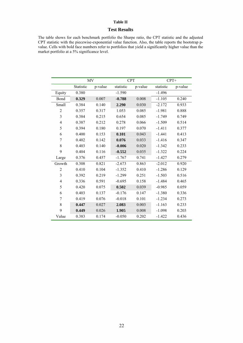
Contrary to Benartzi and Thaler (1995), the CPT statistic of the bond index is significantly higher than the CPT statistic of the stock index. This is due to the inclusion of the equity bear market in the early 2000s. Further, CPT cannot rationalize the size and value effects. Specifically, while the CPT statistic of the stock market index is –1.590, the CPT statistic of size portfolio 1 is 2.290 (0.03) and that of B/M portfolio 8 is 2.083 (0.00). In large part, these high values are explained by the favourable upside potential of small caps and value stocks. For example, the ME 1 portfolio of small caps has a maximum return of 155.29% and the BM1 portfolio of value stocks has a maximum of 113.53%. Interestingly, there is no corresponding downside risk for the small caps and value stocks. Apparently, the return distribution is positively skewed and highly correlated in downside markets, which limits the downside risk and the potential for downside risk reduction by means of portfolio diversification. These properties make the small cap and value stock portfolios very attractive for the CPT investor, who overweighs small probabilities and whose marginal value function diminishes very slowly.

Using the piecewise negative exponential value function, all three puzzles are resolved. The bond index does not achieve a significantly higher CPT+ statistic than the stock index. Also, the size and value effects disappear; no benchmark portfolio achieves a significantly higher CPT+ statistic than the market portfolio. Because the

14

marginal function of the piecewise negative exponential value function decreases much faster than the piecewise-power value function, CPT+ assigns a much lower weight to the upside potential of the small caps and value stocks. In brief, the piecewise-exponential value function succeeds in explaining away the equity premium, size premium and value premium puzzle at the same time.

[Insert Table II about here]

7. The Disposition Effect The disposition effect, see Shefrin and Statman (1985), Odean (1998) and Weber and Camerer (1998), for example, is the observation that investors have a disposition to hold loosing positions too long and to sell winning positions too early. The benchmark case with which this behaviour has to be compared is the so called “fixed-mix-theorem” of Samuelson (1969) according to which an expected utility investor with constant relative risk aversion would hold the same fraction of assets in his portfolio provided he has constant investment opportunities. That is to say, if the disposition effect did already arise from rebalancing a fixed-mix portfolio then it would not be any surprise to standard finance. One explanation of the disposition effect, defined as a more aggressive rebalancing than fixed-mix, is certainly that investors believe in mean-reversion. Another explanation, commonly held in the literature, is that the disposition effect arises from the different risk aversion a prospect theory investor has after he made gains or losses. To quote Hersh Shefrin and Meir Statman (1985): "Prospect Theory suggests the hypothesis that investors display a disposition to sell winners and ride losers…. The disposition emerges from … editing choices in terms of potential gains and / or losses relative to a fixed reference point [and the fact that] decision makers employ an S-shaped valuation function which is concave in the gains region and convex in the loss region. This reflects risk aversion in the domain of gains and risk seeking in the domain of losses." It is clear that keeping the reference point fixed, after a loss (gain) the investor`s status quo point (given by the cumulated gains and losses) moves to the convex (concave) part of the value function. But does this already mean that he will hold more risky assets after a loss than after a gain? Moreover, does the investor indeed decrease (increase) his shares of risky assets (as compared to the previous period) after a gain (loss)? First of all, one has to note that loss aversion interacts with the changing risk aversion. Indeed even for a piecewise linear value function (i.e. even for a value function without risk aversion) loss aversion imposes a concavity in the value function. Hens and Vlcek (2005) show under which conditions an investor who owns a risky asset will sell it after a gain and keep holding it after a loss, which is the disposition effect, or will hold it after a gain because the gain provides a cushion for future losses. The latter is called the house money effect going back to Thaler and Johnson (1990). It turns out that loss aversion favours the house money effect while asymmetric risk aversion favours the disposition effect. Moreover, Hens and Vlcek (2005) show that the argument of Shefrin and Statman is treacherous because it is only based on the ex-post analysis of the investor`s behaviour after the initial investment has been taken. With a piecewise power function investors that are

15

supposed to increase (decrease) their position after losses (gains) will not do so because those investors are reluctant in the first period to put themselves in a situation incurring possible losses (gains) in the second period. Barberis and Xiong (2006) show that the same is also true in a model in which agents optimize dynamically. Again, the problem arises from the piecewise power function and it is resolved with the piecewise negative exponential function: Kyle, Ou-Yang and Xiong (2006) study the liquidation decision in a continuous time diffusion model. Kyle et. al show that the decision to continue holding an asset (the liquidation decision) is driven by the distance of the asset`s value to the reference point. Kyle et. al. find that the agent is willing to hold a risky project with a relatively inferior Sharpe ratio if the project is currently making losses, and intends to liquidate it when it breaks even. On the other hand, the agent may liquidate a project with a relatively superior Sharpe ratio if its current profits rise or drop to the break-even point. To get the intuition why the disposition effect can be explained with the piecewise negative exponential function, first consider a very simple bounded value that obtains the value of +1 for all gains and -1 for all losses. For such a value function once you have gained there is no reason to take further risks and once you have lost you have a high incentive to take all the risk you can get. Smoothening out this function with the piecewise negative exponential function shows that the disposition effect also occurs with strict optima in all periods. Hence the main reason underlying the disposition effect is a satisficing (respectively a desperation) behaviour after gains (respectively losses) that is not modelled by the piecewise power function!

8. Application to Wealth Management of Private Clients Portfolio selection is typically based on the mean-variance model of Markowitz (1952). This model, commonly known by practitioners as “modern portfolio theory”, is a rich source of intuition and also the basis for many portfolio decisions taken by fund mangers. It is based on the idea that asset returns can be modelled by normal distributions. Referring to the Central Limit Theorem, normally distributed returns follow from the market efficiency hypothesis according to which changes in asset returns occur from the arrival of new information. According to the anticipation hypothesis, a central idea underlying the market efficiency hypothesis, any trend in asset returns must have been anticipated before. Hence, the period to period changes in returns must be independent from each other. Since returns over several periods are the product of the returns over every single period along sample paths, the log of returns over longer periods are given by the sum of the log of the returns over shorter periods. Hence assuming the latter are independently distributed, by the Central Limit Theorem the former are then normally distributed. Traditional finance combines this model of returns with an expected utility function having constant relative risk aversion. As a result a simple mean variance utility of the form 2( , )v µ σ µ γσ= − is obtained. The latter assumption is mathematically very convenient, but, as we have argued in Section 5, should be replaced by prospect theory with a negative exponential value function in order to obtain a model of portfolio selection that is consistent with the findings of the behavioural literature. Using the piecewise negative exponential value function the resulting mean-variance

16

utility still has qualitative properties that make the model reasonable, as we argued above, but it becomes intractable analytically. Fortunately, the resulting computational difficulties have recently been resolved by De Giorgi, Hens and Mayer (2006). Hence replacing the piecewise power value function by the piecewise negative exponential value function makes prospect theory fit for finance, both by giving it a consistent theoretical foundation and also by making it applicable in important areas of wealth management.

9. Other Modifications of Prospect Theory The modification of the value function that we proposed here is one important aspect of making prospect theory applicable to finance. As mentioned above, one may also want to change the probability weighting function in order to avoid an infinite slope at zero. An even more fundamental point arises from the fact that prospect theory has been designed to describe choices between lotteries while in many finance applications data are given that are not represented as lotteries (probability distributions). In a typical application, for a finite number of dates t = 1, 2 ,…,T a sample of a finite number of asset returns , 1,2,... .k

tR k K= is given. A lottery on the other hand is a representation in which each observation of returns gets assigned the relative frequency or the likelihood of that observation. The resulting probability distribution depends on which returns are considered to be sufficiently similar to be seen as one observation. Unfortunately, this decision (which in the case of representing data by a histogram is the selection of the band width) is not innocuous for the prospect theory of Kahneman and Tversky (1979) since the probability weighting function distorts the relative frequencies obtained. In the extreme case, for example, in which every observation is seen as being different to any other observation, all returns would be equally likely and the probability weighting function would not change the relative weight. However, if some returns get grouped together they get a different likelihood than others and the weighting function distorts the asset allocation. Hens, Mayer, Rieger and Wang (2005) started looking into this issue and suggested to modify prospect theory in order to avoid unreasonable dependence on the way data is grouped to lotteries.

10. Conclusion We have argued that for various reasons instead of modelling the value function of prospect theory by a piecewise power function a piecewise negative exponential function should be used. This functional form is still compatible with laboratory experiments but it has the following advantages over and above Kahneman and Tversky`s piecewise power function: 1. The Bernoulli Paradox does not arise for lotteries with finite expected value. 2. No infinite leverage/robustness problem arises. 3. CAPM-equilibria with heterogeneous investors and prospect utility do exist. 4. It is able to simultaneously resolve the following asset pricing puzzles: The

equity premium, the value and the size puzzle.

17

5. In contrast to the piecewise power value function it is able to explain the disposition effect.

Modelling prospect theory with the piecewise negative exponential function makes it fit for applications to finance like portfolio selection. From this re-modelling of prospect theory we expect a series of new results, as for example a new explanation of the asset allocation puzzle (see De Giorgi, Hens and Mayer (2006)). Our contribution to these new results should however not be overemphasized since we are “standing on the shoulders of giants”: Daniel Kahneman and Amos Tversky.

18

11. References Banz, R.W. (1981): "The Relationship Between Return and Market Value of

Common Stocks," Journal of Financial Economics, 9, pp. 3-18. Barberis, N., M. Huang, and T. Santos, (2001): "Prospect Theory and Asset Prices,"

Quarterly Journal of Economics, 116(1), pp. 1−53. Barberis, N. and M. Huang (2005): “Stocks as Lotteries: The Implications of

Probability Weighting for Security Prices,” AFA 2005 Philadelphia Meetings Paper. Available at SSRN: http://ssrn.com/abstract=649421.

Barberis, N. and Xiong (2006): “What drives the disposition effect? An analysis of a

long-standing preference-based explanation, mimeo Yale University and Princeton University.

Basu, S. (1977): "Investment Performance of Common Stocks in Relationship to their

Price-Earnings Ratios: A test of the Efficient Market Hypothesis," Journal of Finance, 32(3), pp. 663-682.

Bernoulli, D. (1738): "Specimen theoriae de mensura sortis," Commentarii

Academniae Scientiarum Imperialis Petropolitanae (Proceedings of the Imperial Academy of Science, St. Petersburg, vol. V), pp. 175-192. Translation in English: "Exposition of a New Theory on the Measurement of Risk", Econometrica, 54(1), pp. 23-36.

Benartzi, S., and R. H. Thaler (1995): "Myopic Loss Aversion and the Equity

Premium Puzzle," Quarterly Journal of Economics, 110(1), pp. 73-92. Berkelaar, A., R. Kouwenberg, and T. Post (2004): "Optimal Portfolio Choice under

Loss Aversion," The Review of Economics and Statistics, 86(4), pp. 973-987. Blavatskyy, P.R. (2005): "Back to the St. Petersburg Paradox?", Management

Science, 51(4), pp. 677–678. Bosch-Domenech, A. and J. Silvestre (2005): "Reflections on Gains and Losses: A

2x2x2x7 Experiment," Working Paper, Universitat Pompeu Fabra and University of California at Davis.

De Giorgi, E., T. Hens and H. Levy (2004): "Existence of CAPM Equilibria with

Prospect Theory Preferences," NCCR-FINRISK Working Paper No. 85., Available at SSRN: http://ssrn.com/abstract=420184.

De Giorgi, E. and T. Hens (2005): "Infinite Leverage and Prospect Theory," mimeo

University of Zurich. De Giorgi, E., T. Hens and J. Mayer (2006): "A Risk-Reward Perspective on Prospect

Theory with an Application to the Asset Allocation Puzzle," Working paper, University of Lugano and University of Zurich. Available at SSRN: http://ssrn.com/abstract=899273.

19

De Giorgi, E., T. Hens and J. Mayer (2006): "Computational Aspect of Prospect

Theory with Asset Pricing Applications," Working paper, University of Lugano and University of Zurich. Available at SSRN: http://ssrn.com/abstract=878086.

De Giorgi, E., T. Hens and T. Post (2005): " Prospect Theory and the Size and Value Premium Puzzles," Working paper, University of Lugano and University of Zurich.

Fama, E.F., and K.R. French (1992): "The Cross-Section of Expected Stock Returns,"

Journal of Finance, 47(2), pp. 427-465. Fama, E.F., and K.R. French (1993): "Common Risk-Factors in the Returns on Stocks

and Bonds," Journal of Financial Economics 33(1), pp. 3-56. Gomes, F.J. (2005): "Portfolio Choice and Trading Volume with Loss-Averse

Investors," Journal of Business, 78(2), pp. 675-706. Hens, T., J. Mayer, M.-O.. Rieger and M.Wang (2005): "Robustness of Prospect

Theory when Lotteries are derived from Data," mimeo University of Zurich. Hens, T. and M. Vlcek (2005): "Does Prospect Theory Explain the Disposition

Effect?," NCCR-Finrisk working paper No.247. Horst, R. and P.M. Pardalos (1995): Handbook of Global Optimization, Kluwer,

Dordrecht. Jin, H. and X.Y. Zhou (2006): "Behavioural Portfolio Selection in Continuous Time,"

Working paper, Department of Systems Engineering and Engeneering Management, The Chinese University of Hong Kong.

Kahneman, D. and A. Tversky (1979): "Prospect Theory: An Analysis of Decision Under Risk," Econometrica, 47(2), pp. 263−291. Kyle, A. S., Ou-Yang, H. and W. Xiong (2006): "Prospect Theory and Liquidation Decisions", Journal of Economic Theory, forthcoming. Lucas, R. (1978): "Asset Prices in an Exchange Economy", Econometrica, 46 (6), pp. 1429--1445. Markowitz, H. (1952): "Portfolio Selection," Journal of Finance, 7(1), pp. 77-91. Mehra, R. (2006): "The Equity Risk Premium", Handbook of Finance, Ziemba, W.T. (editor), North Holland. Mehra, R., and E.C. Prescott (1985): "The Equity Premium: A Puzzle", Journal of

Monetary Economics, 15(2), pp. 145-161.

20

Odean, T. (1998): "Are Investors Reluctant to Realize Their Losses," Journal of Finance, 53(5), pp. 1775−1798. Rieger, M-O. and M. Wang (2006): "Cumulative Prospect Theory and the St. Petersburg Paradox," Economic Theory, 28(3), pp. 665-679. Samuelson, P. (1969): "Lifetime Portfolio Selection by Dynamic Stochastic Programming," Review of Economics and Statistics, 51(3), pp. 239-246. Siegel, J.J. (1988): Stocks for the Long Run, McGraw-Hill.

Shefrin, H. and M. Statman (1985): "The Disposition to Sell Winners Too Early and Ride Losers Too Long: Theory and Evidence," Journal of Finance, 40(3), pp. 777−790. Thaler, R., and E.J. Johnson (1990): "Gambling with the House Money and Trying to

Break Even: The Effects of Prior Outcomes on Risky Choice," Management Science, 36(6), pp. 643-660.

Tversky, A., and D. Kahneman (1992): "Advances in Prospect Theory: Cumulative

Representation of Uncertainty," Journal of Risk and Uncertainty, 5, pp. 297-323.

Weber, M. and F. Camerer (1998): "The Disposition Effect in Securities Trading: An

Experimental Analysis," Journal of Economic Behavior & Organization, 33(2), pp. 167-184.

21

Avg. Stdev. Skew. Kurt. Min Max Equity 8.59 21.05 -0.19 -0.36 -40.13 57.22 Bond 2.20 6.91 0.20 0.59 -17.16 22.19 Small 16.90 41.91 0.92 1.34 -58.63 155.29

2 13.99 37.12 0.98 3.10 -56.49 169.71 3 13.12 32.31 0.69 2.13 -57.13 139.54 4 12.53 30.56 0.46 0.83 -51.48 115.32 5 11.91 28.49 0.44 1.60 -49.57 119.40 6 11.65 27.46 0.31 0.61 -49.69 102.17 7 11.09 25.99 0.30 1.14 -47.19 102.06 8 10.15 23.76 0.29 1.19 -42.68 94.12 9 9.63 22.33 0.02 0.46 -41.68 78.15

Large 8.06 20.04 -0.22 -0.52 -40.13 48.74 Growth 7.84 23.60 0.02 -0.64 -44.92 60.35

2 8.77 20.41 -0.27 -0.27 -39.85 55.89 3 8.52 20.56 -0.10 -0.47 -38.00 51.90 4 8.25 22.49 0.49 2.39 -45.02 96.33 5 10.29 22.82 0.36 1.92 -51.55 93.77 6 10.05 23.04 0.19 0.63 -54.39 73.57 7 11.00 24.73 0.18 1.22 -51.13 97.91 8 12.82 27.01 0.67 1.95 -46.56 113.53 9 13.71 29.08 0.56 1.85 -47.42 123.72

Value 13.32 33.05 0.43 1.40 -59.78 134.46

Table I

Descriptive Statistics The table shows descriptive statistics for the annual real returns of the value-weighted CRSP all-share market portfolio, the intermediate government bond index of Ibbotson and the size and value decile portfolios from Kenneth French’ data library. The sample period is from January 1927 to December 2002 (76 yearly observations).

22

MV CPT CPT+ Statistic p-value statistic p-value statistic p-value

Equity 0.380 -1.590 -1.496 Bond 0.329 0.007 -0.788 0.008 -1.105 0.240 Small 0.384 0.140 2.290 0.030 -2.172 0.933

2 0.357 0.317 1.053 0.085 -1.981 0.888 3 0.384 0.215 0.654 0.085 -1.749 0.749 4 0.387 0.212 0.278 0.066 -1.509 0.514 5 0.394 0.180 0.197 0.070 -1.411 0.377 6 0.400 0.153 0.101 0.043 -1.441 0.413 7 0.402 0.142 0.076 0.033 -1.416 0.347 8 0.403 0.140 -0.006 0.020 -1.342 0.233 9 0.404 0.116 -0.552 0.035 -1.322 0.224

Large 0.376 0.457 -1.767 0.741 -1.427 0.279 Growth 0.308 0.821 -2.673 0.863 -2.012 0.920

2 0.410 0.104 -1.352 0.410 -1.286 0.129 3 0.392 0.219 -1.299 0.251 -1.503 0.516 4 0.336 0.591 -0.695 0.158 -1.484 0.465 5 0.420 0.075 0.502 0.039 -0.985 0.059 6 0.403 0.137 -0.176 0.147 -1.380 0.336 7 0.419 0.076 -0.018 0.101 -1.234 0.273 8 0.447 0.027 2.083 0.003 -1.163 0.233 9 0.449 0.026 1.905 0.008 -1.098 0.203

Value 0.383 0.174 -0.050 0.202 -1.422 0.436

Table II

Test Results The table shows for each benchmark portfolio the Sharpe ratio, the CPT statistic and the adjusted CPT statistic with the piecewise-exponential value function. Also, the table reports the bootstrap p-value. Cells with bold face numbers refer to portfolios that yield a significantly higher value than the market portfolio at a 5% significance level.

23

Endnotes 1 An exception is Barberis and Huang (2005) who consider loss aversion, changing risk aversion and probability weighting simultaneously. 2 See also Blavatskyy (2005).

3 Indeed, ( )0

010

lim 1

iJ i

j jj

x RP R R wλ

λλ =→−∞

− ⎡ ⎤= −⎢ ⎥⎣ ⎦− ∑ . Hence if for the market portfolio RM we have

( ) 1 , MR rµ > + then already for Mλ λ= the prospect utility divided by (1-λ0) is positive so that infinite leveraging gives infinite utility.