Majorization under constraints and bounds of the

second Zagreb index

Monica Bianchi α ∗ Alessandra Cornaro α †

Anna Torrieroα ‡

Abstract

In this paper we present a theoretical analysis in order to establishmaximal and minimal vectors with respect to the majorization order ofparticular subsets of <n. Afterwards we apply these issues to the calcula-tion of bounds for a topological descriptor of a graph known as the secondZagreb index. Finally, we show how our bounds may improve the re-sults obtained in the literature, providing some theoretical and numericalexamples.

AMS Classification: 05C35, 05C05, 05C50Keywords: Majorization; Schur-convex functions; Graphs; Second

Zagreb index.

α Department of Mathematics and Econometrics, Catholic University, Milan, Italy.

1 Introduction

The notion of majorization ordering was introduced by Hardy, Littlewood andPolya ([11]) and is closely connected with the economic theory of disparityindices ([2]). But this concept can first be found in Schur ([19]) who inves-tigated functions which preserve the majorization order, the so-called Schur-convex functions. Using this property and characterizing maximal and minimalvectors with respect to majorization order under suitable constraints, manyinequalities involving such functions can be derived ([16]). A significant appli-cation of this approach concerns the localization of ordered sequences of realnumbers as they occur in the problem of finding estimates of eigenvalues of amatrix ([3], [18], [20] and [21]). Another field of interest concerns the networkanalysis, where the same methodology can be useful applied in order to providebounds for some topological indicators of graphs which can be usefully expressed

∗e-mail: monica.bianchi@unicatt.it†Corresponding author, e-mail: alessandra.cornaro@unicatt.it, Tel:+390272343683,

Fax:+390272342324‡e-mail: anna.torriero@unicatt.it

1

arX

iv:1

105.

1888

v1 [

mat

h.C

O]

10

May

201

1

as a Schur-convex function, in terms of the degree sequence of the graph (see[6]).In this paper, after some preliminary definitions and notations, we perform atheoretical analysis aimed at determining maximal and minimal vectors withrespect to the majorization order of suitable subsets of <n. In Section 3 and 4we extend the results, obtained by Marshall and Olkin [16] into more specificsets of constraints determining their extremal elements. In Section 5, we providean application of these results, dealing with the problem of computing boundsfor the second Zagreb index, M2(G) of a particular class of graphs with a givennumber of pendant vertices. This index is extensively studied in graph theory,as a chemical molecular structure descriptor ([7], [8], [9], [17] and [22]) and, moregenerally, in network analysis, as a measure of degree-assortativity, quantifyinghow well a network is connected, ([1], [12] and [13]). In the latter contextthe Zagreb index M2(G) is renamed S(G). Since determining S(G) requiresa specific algorithm ([12]), many bounds have been proposed in the literature([4], [5], [15], [23] and [24]). Recently Grassi et al. in [6] obtained differentbounds through a majorization technique. Using this approach, we derive newbounds in terms of graph degree sequence and present some theoretical andnumerical examples comparing our results with the literature. Our conclusionsare presented in Section 6.

2 Notations and preliminaries

Let ej, j = 1, ...n, be the fundamental vectors of Rn and set:

s0 = 0, sj =

j∑i=1

ei, j = 1, ...n,

vn = 0, vj =

n∑i=j+1

ei, j = 0, ...(n− 1).

Recalling that the Hadamard product of two vectors x,y ∈ Rn is defined asfollows:

x ◦ y = [x1y1, x2y2, ..., xnyn]T

it is easy to verify the following properties, where 〈·, ·〉 denotes the inner productin Rn:

i) 〈x ◦ y, z〉 = 〈x,y ◦ z〉

ii) 〈sh,vk〉 = h−min {h, k}

iii) sk ◦ sj = sh, h = min {k, j}

iv) vk ◦ sj = sj − sh = vh − vj, h = min {k, j}

2

Definition 1 Assuming that the components of the vectors x, y ∈ Rn are ar-ranged in nonincreasing order, the majorization order x E y means:⟨

x, sk⟩≤⟨y, sk

⟩, k = 1, ..., (n− 1)

and〈x, sn〉 = 〈y, sn〉 .

In the sequel x∗(S) and x∗(S) will denote the maximal and the minimal elementsof a subset S ⊆ Rn with respect to the majorization order.Given a positive real number a, it is well known [16] that the maximal and theminimal elements of the set

Σa = {x ∈ Rn : x1 ≥ x2 ≥ ... ≥ xn ≥ 0, 〈x, sn〉 = a}

with respect to the majorization order are respectively

x∗ (Σa) = ae1 and x∗ (Σa) =a

nsn.

Next sections are dedicated to the study of the maximal and the minimal el-ements, with respect to the majorization order, of the particular subset of Σagiven by

Sa = Σa ∩ {x ∈ Rn : Mi ≥ xi ≥ mi, i = 1, ...n} , (1)

where m = [m1,m2, ...,mn]T

and M = [M1,M2, ...,Mn]T

are two assignedvectors arranged in nonincreasing order with 0 ≤ mi ≤ Mi, for all i = 1, ...n,and a is a positive real number such that 〈m, sn〉 ≤ a ≤ 〈M, sn〉 . Notice that theintervals [mi,Mi] are not necessarily disjointed unless the additional assumptionMi+1 < mi, i = 1, ..., (n−1) is required. The existence of maximal and minimalelements of Sa are ensured by the compactness of the set Sa and by the closureof the upper and level sets:

U(x) = {z ∈ Sa : x E z} , L(x) = {z ∈ Sa : z E x}

3 The maximal element of Sa

We start computing the maximal element, with respect to the majorizationorder, of the set Sa.

Theorem 2 Let k ≥ 0 be the smallest integer such that⟨M, sk

⟩+⟨m,vk

⟩≤ a <

⟨M, sk+1

⟩+⟨m,vk+1

⟩, (2)

and θ = a−⟨M, sk

⟩−⟨m,vk+1

⟩. Then

x∗(Sa) = M ◦ sk + θek+1 + m ◦ vk+1 (3)

3

Proof. First of all we verify that x∗(Sa) ∈ Sa. It easy to see that 〈x∗(Sa),sn〉 =a and thatmi ≤ x∗i (Sa) ≤Mi for i 6= k+1. To prove thatmk+1 ≤ x∗k+1(Sa) ≤Mk+1,notice that from (2)

mk+1 =⟨m, ek+1

⟩≤ a−

⟨M, sk

⟩−⟨m,vk+1

⟩= θ <

⟨M, ek+1

⟩= Mk+1.

Now we show that x E x∗(Sa) for all x ∈ Sa. By property i) follows⟨x∗(Sa), sj

⟩=⟨M, sk ◦ sj

⟩+ θ

⟨ek+1, sj

⟩+⟨m,vk+1 ◦ sj

⟩, j = 1, ...(n− 1)

and by iii) and iv)

⟨x∗(Sa), sj

⟩=

{ ⟨M, sj

⟩1 ≤ j ≤ k⟨

M, sk⟩

+ θ +⟨m, sj − sk+1

⟩(k + 1) ≤ j ≤ (n− 1)

.

Thus, given a vector x ∈ Sa, for 1 ≤ j ≤ k we obtain⟨x, sj

⟩≤⟨M, sj

⟩=⟨x∗(Sa), sj

⟩,

while for (k + 1) ≤ j ≤ (n− 1), by iii),⟨x, sj

⟩= 〈x, sn〉−

⟨x,vj

⟩≤ a−

⟨m,vj

⟩=⟨M, sk

⟩+θ+

⟨m, sj − sk+1

⟩=⟨x∗(Sa), sj

⟩and the result follows.

From this general result, the maximal element of particular subsets of Sa can bededuced. We then focus on a specific case which will be useful in the applicationwe deal with in Section 5. We denote by bxc the integer part of the real numberx.

Corollary 3 Given 1 ≤ h ≤ n, let us consider the set

S[h]a =

Σa ∩ {x ∈ Rn : M1 ≥ x1 ≥ ... ≥ xh ≥ m1,M2 ≥ xh+1 ≥ ... ≥ xn ≥ m2}

, (4)

where0 ≤ m2 ≤ m1, 0 ≤M2 ≤M1,mi < Mi, i = 1, 2

andhm1 + (n− h)m2 ≤ a ≤ hM1 + (n− h)M2.

Let a∗ = hM1 + (n− h)m2 and

k =

⌊a− h(m1 −m2)− nm2

M1 −m1

⌋if a < a∗

⌊a− h(M1 −M2)− nm2

M2 −m2

⌋if a ≥ a∗

4

Then

x∗(S[h]a ) =

M1, .....,M1︸ ︷︷ ︸k

, θ,m1, .....,m1︸ ︷︷ ︸,h−k−1

m2, .....,m2︸ ︷︷ ︸n−h

if a < a∗

M1, .....,M1︸ ︷︷ ︸h

,M2, .....,M2︸ ︷︷ ︸k−h

, θ,m2, .....m2︸ ︷︷ ︸n−k−1

if a ≥ a∗

where M = M1sh+M2v

h, m = m1sh+m2v

h and θ = a−⟨M, sk

⟩−⟨m,vk+1

⟩.

Proof. Easy computations give:

⟨M, sk

⟩=

{hM1 +M2 (k − h) if k ≥ h

kM1 if k < h

⟨m,vk

⟩=

{(n− k)m2 if k ≥ h

(n− h)m2 +m1 (h− k) if k < h

and the values are linked for continuity when k = h. We distinguish two cases:

i) k ≥ h : from (2) we have

k =

⌊a− h(M1 −M2)− nm2

M2 −m2

⌋that is acceptable only if a ≥ hM1 + (n− h)m2 = a∗. Then, from (3)

x∗(S[h]a ) =

M1, .....,M1︸ ︷︷ ︸h

,M2, .....,M2︸ ︷︷ ︸k−h

, θ,m2, .....m2︸ ︷︷ ︸n−k−1

.ii) k < h : from (2) we get

k =

⌊a− h(m1 −m2)− nm2

M1 −m1

⌋that is acceptable only if a < hM1 + (n− h)m2 = a∗. Then, from (3)

x∗(S[h]a ) =

M1, .....,M1︸ ︷︷ ︸k

, θ,m1, .....,m1︸ ︷︷ ︸,h−k−1

m2, .....,m2︸ ︷︷ ︸n−h

.

5

Remark 4 When a = a∗ it is worthwhile to note that k = h and θ = m2 sothat

x∗(S[h]a ) =

M1, .....,M1︸ ︷︷ ︸h

,m2, .....,m2︸ ︷︷ ︸n−h

.Remark 5 The assumption mi < Mi in Corollary 3 can be relaxed to mi ≤Mi.

Indeed if mi = Mi, i = 1, 2, the set S[h]a reduces to the singleton {m1s

h+m2vh},

while if m1 = M1,m2 < M2 the first h components of any x ∈ S[h]a are fixed and

equal to m1 and the maximal element of S[h]a can be computed by the maximal

element of Sa−hm1∈ Rn−h (see Corollary 6 below). The case m2 = M2,m1 <

M1 is similar.

The next proposition is proved in [16] and it immediately follows from Corollary3 when m1 = m2 = m and M1 = M2 = M .

Corollary 6 Let 0 ≤ m < M and m ≤ a

n≤M. Given the subset

S1a = Σa ∩ {x ∈ Rn : M ≥ x1 ≥ x2 ≥ ... ≥ xn ≥ m}

we havex∗(S1

a) = Msk + θek+1 +mvk+1,

where k =

⌊a− nmM −m

⌋and θ = a−Mk −m (n− k − 1) .

In particular when m = 0 we obtain

x∗(S1a) = Msk + θek+1,

where k =⌊ aM

⌋and θ = a−Mk.

It is worthwhile to notice that Sa, is a subset of S1a where m = mn and M = M1.

Thus the following inequality holds:

x∗(Sa) E x∗(S1a). (5)

Finally we recall the following result (see [3]).

Corollary 7 Let 1 ≤ h ≤ n and 0 < α ≤ a/h. Given the subset

S2a = Σa ∩ {x ∈ Rn : xi ≥ α, i = 1, ...h} ,

we have x∗(S2a) = (a− hα) e1 + αsh.

Proof. The set S2a can be obtained by (1) for m1 = α, m2 = 0, M1 = M2 = a.

Since a∗ = ha ≥ a, two cases can be distinguished:

6

i) h = 1 : we have a∗ = a and from Remark 4 it immediately follows thatk = 1 and θ = 0 so that

x∗(S2a) = ae1.

ii) h > 1 : we have a∗ > a and Corollary 3 implies that k =

⌊a− hαa− α

⌋= 0.

Thus

x∗(S2a) =

θ, α, ..., α︸ ︷︷ ︸h−1

, 0, ..., 0︸ ︷︷ ︸n−h

where θ = a− (h− 1)α, which leads to

x∗(S2a) = θe1 + αsh − αe1 = (a− hα) e1 + αsh.

4 The minimal element of Sa

In this section we study the structure of the minimal element, with respect tothe majorization order, of the set Sa.

Theorem 8 Let k ≥ 0 and d ≥ 0 be the smallest integers such that

1) k + d < n

2) mk+1 ≤ ρ ≤Mn−d where ρ =a− 〈m, sk〉 − 〈M,vn−d〉

n− k − d.

Thenx∗(Sa) = m ◦ sk + ρ(sn−d − sk) + M ◦ vn−d.

Proof. The minimal element of the set Σa is x◦(Σa) = ansn. If m1 ≤ x∗(Σa) ≤

Mn, then x∗(Σa) ∈ Sa and x∗(Sa) = x∗(Σa) (notice that in this case k = d = 0).If x∗(Σa) /∈ Sa, let k and d the smallest integers satisfying conditions 1) and2) above. It is easy to verify that x∗(Sa) ∈ Sa. In order to prove that it is theminimal element, we must show that for all x ∈ Sa

〈x∗(Sa), sh〉 ≤ 〈x, sh〉 , h = 1, · · · (n− 1). (6)

We distinguish three cases:

i) 1 ≤ h ≤ k. Since 〈x∗(Sa), sh〉 = 〈m, sh〉, the inequality (6) is straightfor-ward.

7

ii) k + 1 ≤ h ≤ n− d. We prove the inequality (6) for h = k + 1. By in-duction, similar arguments can be applied to prove the inequality forh = k + 2, · · · (n− d).

By contradiction, let us assume that there exists x ∈ Sa such that

〈x∗(Sa), sk+1〉 = 〈m, sk〉+ ρ > 〈x, sk〉+ xk+1.

Then xj ≤ xk+1 < 〈m, sk〉+ ρ− 〈x, sk〉, for j = k + 2, · · ·n and thus

〈x, sn−d〉 = 〈x, sk〉+ 〈x, sn−d − sk〉 << 〈x, sk〉+ (n− d− k)(〈m, sk〉+ ρ− 〈x, sk〉).

Taking into account that

〈x, sn−d〉 = a− 〈x,vn−d〉 ≥ a− 〈M,vn−d〉,

we get

a− 〈M,vn−d〉 < (1− n+ d+ k)〈x, sk〉+ (n− d− k)(〈m, sk〉+ ρ).

Using the expression of ρ, we obtain

0 < (1− n+ d+ k)(〈x, sk〉 − 〈m, sk〉).

Since (1 − n + d + k) ≤ 0 and 〈x, sk〉 ≥ 〈m, sk〉, the inequality above isfalse, and we have got the contradiction.

iii) n− d + 1 ≤ h < n. For any x ∈ Sa we have

〈x∗(Sa), sh〉 = 〈x∗(Sa), sn−d〉+ 〈x∗(Sa), sh − sn−d〉 =

= 〈m, sk〉+ (n− d− k)ρ+ 〈M, sh − sn−d〉 =

= a− 〈M,vn−d〉+ 〈M, sh − sn−d〉 =

= a− 〈M, sn − sh〉 =

= 〈x, sh〉+ 〈x, sn − sh〉 − 〈M, sn − sh〉≤ 〈x, sh〉.

Now we analyze the minimal element of particular subsets of Sa. We startconsidering the intervals [mi,Mi], i = 1, · · · , n disjointed. Notice that this ad-ditional assumption does not modify the choice of the maximal element, whileit simplifies the choice of the minimal element.

Corollary 9 Let us consider the set Sa and assume

Mi+1 < mi for i = 1, ...(n− 1). (7)

8

Let k ≥ 0 be the smallest integer such that⟨m, sk+1

⟩+⟨M,vk+1

⟩≤ a <

⟨m, sk

⟩+⟨M,vk

⟩(8)

and ρ = a−⟨m, sk

⟩−⟨M,vk+1

⟩. Then

x∗(Sa) = m ◦ sk + ρek+1 + M ◦ vk+1

Proof. By condition 2) in Theorem 8 and assumption (7), we get

Mk+2 < mk+1 ≤ ρ ≤Mn−d.

Thus k > n−d−2. Since k is an integer such that k < n−d, we have necessarilyk = n− d− 1 and the thesis follows.

Another case of practical interest regards the set studied in Corollary 3.

Corollary 10 Given 1 ≤ h ≤ n, let us consider the set

S[h]a =

Σa ∩ {x ∈ Rn : M1 ≥ x1 ≥ ... ≥ xh ≥ m1,M2 ≥ xh+1 ≥ ... ≥ xn ≥ m2}

,

where 0 ≤ m2 ≤ m1, 0 ≤M2 ≤M1, mi < Mi, i = 1, 2 and

hm1 + (n− h)m2 ≤ a ≤ hM1 + (n− h)M2.

If m1 ≤a

n≤M2 we have x∗(S

[h]a ) = a

nsn. Otherwise, let a = hm1 + (n−h)M2.

If

{a < m1na ≤ a , given ρ =

a− hm1

n− h, we have

x∗(S[h]a ) = m1s

h + ρvh =

m1, .....,m1︸ ︷︷ ︸h

, ρ, ....., ρ︸ ︷︷ ︸n−h

.If

{a > M2na ≥ a , given ρ =

a−M2(n− h)

h, we have

x∗(S[h]a ) = ρsh +M2v

h =

ρ, ..., ρ︸ ︷︷ ︸h

,M2, ...,M2︸ ︷︷ ︸n−h

.Proof. Let us investigate when the best choice k = d = 0 is admissible. Underthis assumption, from condition 2) in Theorem 8 we have

m1 ≤ ρ =a

n≤Mn = M2. (9)

If the condition above holds, the minimal element is x∗(S[h]a ) =

a

nsn.

9

Otherwise if condition (9) does not hold, we begin with the case k = 0. We have

ρ =a− < M,vn−d >

n− dand

x∗(S[h]a ) = ρsn−d + M ◦ vn−d.

From condition 2) in Theorem 8, we have m1 ≤ ρ ≤ Mn−d and, taking into

account that the elements in x∗(S[h]a ) are in nonincreasing order, ρ ≥ Mn−d+1.

We distinguish three cases:

i) if n− d > h then necessarily ρ = M2, but this contradicts (9).

ii) if n−d < h then ρ = M1 and this is admissible only if a = M1h+M2(n−h),so that

x∗(S[h]a ) =

M1, .....,M1︸ ︷︷ ︸h

,M2, .....,M2︸ ︷︷ ︸n−h

.iii) if n− d = h, then ρ =

a−M2d

n− dand

x∗(S[h]a ) =

ρ, ....., ρ︸ ︷︷ ︸h

,M2, .....,M2︸ ︷︷ ︸n−h

.This result is admissible only if ρ > M2 and m1 ≤ ρ ≤ M1, i.e. if{a > M2na ≥ a .

A symmetric case occurs when d = 0, so we have

ρ =a− < m, sk >

n− kand

x∗(S[h]a ) = m ◦ sk + ρvk.

From condition 2) in Theorem 8, we have that mk+1 ≤ ρ ≤M2 and, taking into

account that the elements in x∗(S[h]a ) are in nonincreasing order, ρ ≤ mk. We

distinguish three cases:

i) if k < h then necessarily ρ = m1, but this contradicts (9).

ii) if k > h, then ρ = m2 and this is possible only if a = hm1 + m2(n − h),so that

x∗(S[h]a ) =

m1, .....,m1︸ ︷︷ ︸h

,m2, .....,m2︸ ︷︷ ︸n−h

.

10

iii) if k = h, then ρ =a− hm1

n− hand

x∗(S[h]a ) =

m1, .....,m1︸ ︷︷ ︸h

, ρ, ....., ρ︸ ︷︷ ︸n−h

.This result is admissible only if m2 ≤ ρ ≤ M2 and ρ < m1, i.e. only if{a < m1na ≤ a .

Corollary 10 distinguishes the minimal element of S[h]a whether{

a < m1na ≤ a or

{a > M2na ≥ a .

We note that if m1 ≤ M2 the first inequality in the systems above is alwaysstronger than the second one, while if M2 < m1 the second one is stronger

than the first. Thus we can summarize the minimal element of S[h]a in a more

accessible way according to the following scheme:

i) If m1 ≤M2 then

x∗(S[h]a ) =

a

nsn if m1 ≤

a

n≤M2

m1sh +

a− hm1

n− hvh if

a

n< m1

a−M2(n− h)

hsh +M2v

h ifa

n> M2

(10)

and the vectors are linked for continuity.

ii) If M2 < m1 then

x∗(S[h]a ) =

m1s

h +a− hm1

n− hvh if a < a

a−M2(n− h)

hsh +M2v

h if a ≥ a. (11)

Remark 11 When a = a it is worthwhile to note that

x∗(S[h]a ) = m1s

h +M2vh =

m1, .....,m1︸ ︷︷ ︸h

,M2, .....,M2︸ ︷︷ ︸n−h

.

11

Remark 12 We note that the minimal element of the set S[h]a does not nec-

essarily have integer components, while this is not the case for the maximalelement. For some applications, it is meaningful to find the minimal vector in

S[h]a with integer components. We illustrate below the procedure to follow. Let

us consider, for instance, the vector x∗(S[h]a ) =

a

nsn which corresponds to the

case m1 ≤a

n≤ M2 (see (10)). If

a

nis not an integer, let us find the index k,

1 ≤ k ≤ n, such that

(banc+ 1)k + ba

nc(n− k) = a

i.e. k = a− bancn. The vector

x1∗ = (ba

nc+ 1)sk + ba

ncvk

is the minimal element of S[h]a with integer components.

With slight modification, the same procedure can be applied also in the other

cases illustrated in (10) or (11), where only some of the components of x∗(S[h]a )

can be non integer.

To complete our analysis, we show how from Corollary 10, particular cases canbe deduced. More precisely, assuming in Corollary 10 m1 = m2, M1 = M2 orh = n we obtain the results proved in [16].

Corollary 13 Let 0 ≤ m < M and m ≤ a

n≤M. Given the subset

S1a = Σa ∩ {x ∈ Rn : M ≥ x1 ≥ ... ≥ xn−1 ≥ xn ≥ m}

we have x∗(S1a) =

a

nsn.

As we did with the maximal element, it is clear that the vector provided byCorollary 10 majorizes the vector in Corollary 13, i.e. the following inequalityholds:

x∗(S1a) E x∗(Sa). (12)

Assuming m1 = α, m2 = 0, M1 = M2 = a or m1 = m2 = 0 and M2 = α,M1 = a we easily obtain the following two corollaries ( see [3]).

Corollary 14 Let 1 ≤ h ≤ n and 0 < α ≤ a/h. Given the subset

S2a = Σa ∩ {x ∈ Rn : xi ≥ α, i = 1, ...h} ,

we have

x∗(S2a) =

a

nsn if α ≤ a

n

αsh + ρvh with ρ =a− αhn− h

if α >a

n

12

Corollary 15 Let 1 ≤ h ≤ (n− 1) and 0 < α < a. Given the subset

S3a = Σa ∩ {x ∈ Rn : xi ≤ α, i = h+ 1, ...n} ,

we have

x∗(S3a) =

a

nsn if α ≥ a

n

ρsh + αvh with ρ =a− (n− h)α

hif α <

a

n

5 New bounds for the second Zagreb index

Let G = (V,E) a simple, connected, undirected graph with fixed order |V | = nand fixed size |E| = m. Denote by π = (d1, d2, .., dn) the degree sequence ofG, being di the degree of vertex vi, arranged in nonincreasing order d1 ≥ d2 ≥· · · ≥ dn. We recall that the sequences of integers which are degree sequences ofa simple graph were characterized by Erdos and Gallay (see [10]). The secondZagreb index is defined as

S(G) =∑

didj(vi,vj)∈E

or equivalently ([6])

S(G) =

∑(vi,vj)∈E

(di + dj)2 −

n∑i=1

d3i

2. (13)

In order to compute upper and lower bounds for S(G) we refer to [6], where amethodology based on majorization order was proposed. Before presenting ourresults, we briefly describe the procedure we will follow.Let π be a fixed degree sequence and x ∈ Rm the vector whose components aredi + dj , (vi, vj) ∈ E. In [14] it is shown that

∑(vi,vj)∈E

(di + dj) =

n∑i=1

d2i

and thus∑mi=1 xi =

∑ni=1 d

2i is a constant. Given a suitable subset S of

Σa =

{x ∈ Rm : x1 ≥ x2 ≥ ... ≥ xm ≥ 0,

m∑i=1

xi = a

},

where a =∑ni=1 d

2i , the Schur-convex function f(x) =

m∑i=1

x2i attains its mini-

mum and maximum on S at f(x∗(S)) and f(x∗(S)) respectively, being x∗(S)and x∗(S) the extremal vectors of S with respect to the majorization order (see[16]). Hence from (13) the maximum and the minimum of S(G) can be easilydeduced.

13

Let Cπ be the class of graphs G = (V,E) with h pendant vertices and degreesequence

π = (d1, d2, .., dn−h−1, dn−h︸ ︷︷ ︸n−h

, 1, ..., 1︸ ︷︷ ︸h

), n ≥ 4, n− h ≥ 2, h ≥ 1

and let us consider graphs G ∈ Cπ with maximum vertex degree upper boundedby dn−h + dn−h−1, i.e. d1 < dn−h + dn−h−1, or equivalently

1 + d1 ≤ dn−h + dn−h−1. (14)

For G ∈ Cπ, we note that this constraint is always satisfied, for example, if themaximum vertex degree is at most three, as for some graphs of chemical interestwhere the maximum degree is four.We observe that for i, j = 1, ..., n− h and (vi, vj) ∈ E :

dn−h + dn−h−1 ≤ di + dj ≤ d1 + d2,

while for i = n− h+ 1, ..., n; j = 1, ..., n− h and (vi, vj) ∈ E :

1 + dn−h ≤ di + dj ≤ 1 + d1.

Furthermore, inequality (14) assures that the above intervals are concatenatedso that the vector x ∈ Rm can be arranged in nonincreasing order with the hpendant vertices in the last h positions.Setting m1 = dn−h + dn−h−1, m2 = 1 + dn−h, M1 = d1 + d2, M2 = 1 + d1,let us consider the set

Sm−ha =Σa ∩ {x ∈ Rn : M1 ≥ x1 ≥ ...xm−h ≥ m1,

M2 ≥ xm−h+1 ≥ ...xm ≥ m2}.

Applying Corollaries 3 and 10 we can compute maximal and minimal elementsof Sm−ha with respect to the majorization order and from (13) we obtain:∥∥x∗(Sm−ha )

∥∥22−

n∑i=1

d3i

2≤ S(G) ≤

∥∥x∗(Sm−ha )∥∥22−

n∑i=1

d3i

2, (15)

where ‖·‖2 stands for the euclidean norm.In spite of inequalities (5) and (12), these bounds can’t be worse than those in[6], and they are often sharper.

It is noteworthy that both equalities in (15) are attained if and only if the

set S[h]a reduces to a singleton, that is, by Remark 5, mi = Mi, i = 1, 2.

The condition m2 = 1+dn−h = M2 = 1+d1 implies that in G(V,E) all non-pendant vertices have the same degree. Some examples of this kind of graphsare:

i) all trees with degree sequence

π =

k, ..., k︸ ︷︷ ︸r

, 1, ..., 1︸ ︷︷ ︸rk−2r+2

, (16)

14

including, as particular case, for k = 2, the path.ii) graphs obtained by adding the same number s of pendant vertices to each

vertex of a k−regular graph on r vertices, being kr even, 2 ≤ k ≤ r − 1, i.e.

π =

k + s, ..., k + s︸ ︷︷ ︸r

, 1, ..., 1︸ ︷︷ ︸sr

.

Computing S(G), from Remark 5 and (15), we get k (2kr − 2r − k + 2) and12r(2s+ ks+ k2

)(k + s) respectively.

In the following we provide some significant examples, computing bounds forgraphs belonging to Cπ and satisfying (14). Furthermore, a comparison withsome other known bounds (see [4], [5], [15], [23] and [24]) are provided.

Example 1. Let us consider the classes of trees Tt,s with degree sequences πi(i = 1, 2, 3) given by:

i) π1 =

t, s, ...., s︸ ︷︷ ︸t

, 1, ...., 1︸ ︷︷ ︸t(s−1)

, 2 ≤ s < t < 2s

ii) π2 =

s, ...., s︸ ︷︷ ︸t

, t, 1, ...., 1︸ ︷︷ ︸t(s−1)

, s > t ≥ 2

iii) π3 =

t, ...., t︸ ︷︷ ︸t+1

, 1, ..., 1︸ ︷︷ ︸t(t−1)

, t ≥ 2

Case i).

M1 = t+ s m1 = 2sM2 = t+ 1 m2 = s+ 1m = ts h = t(s− 1)

Applying Corollary 3 and Remark 4 it follows that:

x∗ (Tt,s) =

(t+ s) , ....., (t+ s)︸ ︷︷ ︸t

, (s+ 1) , ...., (s+ 1)︸ ︷︷ ︸st−t

15

while from (10), (11) and Remark 12 we get

x∗ (Tt,s) =

2s, ...., 2s︸ ︷︷ ︸t

, s+ 2, ....., s+ 2︸ ︷︷ ︸,t(t−s)

s+ 1, ....., s+ 1︸ ︷︷ ︸t(2s−t−1)

if t < 2s− 1

2s, ...., 2s︸ ︷︷ ︸t

, s+ 2, ....., s+ 2︸ ︷︷ ︸st−t

if t = 2s− 1

.

(17)Taking into account (15), the following inequalities hold:{

12 t(3t− t2 − 5s+ 2st+ 3s2

)≤ S(Tt,s) ≤ ts (s+ t− 1) if t < 2s− 1

12 (2s− 1)

(3s+ 3s2 − 4

)≤ S(Tt,s) ≤ s (2s− 1) (3s− 2) if t = 2s− 1

.

(18)We note that in (17) the right-hand equality holds if Tt,s is the tree obtainedby the union of t stars, each one of order (see Figure 1).

Figure 1: Example illustrating tree Tt,s for 2 ≤ s < t < 2s.

Case ii).

M1 = 2s m1 = t+ sM2 = s+ 1 m2 = t+ 1m = ts h = t(s− 1)

By Corollary 3 follows

x∗ (Tt,s) =

2s, ...., 2s︸ ︷︷ ︸t

, (s+ 1) , ...., (s+ 1)︸ ︷︷ ︸st−2t

, (t+ 1) , ...., (t+ 1)︸ ︷︷ ︸t

16

while from Remark (11) we get

x∗ (Tt,s) =

s+ t, ...., s+ t︸ ︷︷ ︸t

, (s+ 1), ...., (s+ 1)︸ ︷︷ ︸st−t

.Taking into account (15), the following inequalities hold:

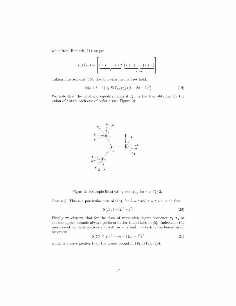
ts(s+ t− 1) ≤ S(Tt,s) ≤ t(t− 2s+ 2s2) (19)

We note that the left-hand equality holds if Tt,s is the tree obtained by theunion of t stars each one of order s (see Figure 2).

Figure 2: Example illustrating tree Tt,s for s > t ≥ 2.

Case iii). This is a particular case of (16), for k = t and r = t+ 1, such that

S(Tt,s) = 2t3 − t2. (20)

Finally we observe that for the class of trees with degree sequence π1, π2 orπ3, our upper bounds always perform better than those in [5]. Indeed, in thepresence of pendant vertices and with m = ts and n = ts+ 1, the bound in [5]becomes:

S(G) ≤ 2m2 − (n− 1)m = t2s2 (21)

which is always greater than the upper bound in (18), (19), (20).

17

Example 2. Let us consider a unicyclic graph G, i.e. a graph with n = mhaving the following degree sequence

π = (3, 3, 3, 3, 2, 2, 2, 2, 2, 1, 1, 1, 1).

Being (14) satisfied, by Remark 12, (15) gives

64 ≤ S(G) ≤ 74.

The comparison (see Table 1) with bounds in [4], [5] , [6], [15] and [23] showsthat our bounds always perform better. Indeed we obtain:

Bounds Lower Upperours 64 74[4] x 277.9[5] x 182[6] 61.462 77[15] -28 76[23] 64 92

Table 1: Lower and upper bounds for S(G)

Example 3. Consider the graphs G and H with degree sequences π1 =(3, 2, 2, 1) and π2 = (3, 3, 3, 3, 2, 1, 1) respectively, as in Examples 2.2 and 2.3in [6]. Besides the bounds discussed in [6], we add the comparison with thosein [5], [23] and [24]. Observing that G is a unicyclic graph (m = n) and H isa bicyclic graph (m = n + 1), both with pendant vertices, bounds in [23] and[24] can also be respectively properly applied. Computing bounds for S(G), wehave:

Ref. Lower Upperours 19 20[4] x 22.511[5] x 20[6] 18.5 20[15] 18 22[23] 19 19

Table 2: Lower and upper bounds for S(G).

18

Our bounds are sharper than [4], [6] and [15]. The best one is provided by [23]and has been specifically constructed for this class of graph.Computing bounds for S(H), we have:

ref. lower upperour 54 58[4] x 99.75[5] x 80[6] 51.25 58[15] 40 59[24] 50 68

Table 3: Lower and upper bounds for S(H).

Note that our bounds perform better than all the others and in particular betterthan [24] which is properly designed for bicyclic graphs as H is.

6 Conclusion

The purpose of this paper is to establish maximal and minimal vectors withrespect to the majorization order under sharper constraints than those presentedby Marshall and Olkin in [16]. We have shown how these results can provide asimple methodology for localizing the second Zagreb index of a particular classof graphs. Some numerical examples have been discussed, showing that ourbounds often provide sharper bounds than those in the literature. Moreover,in network analysis, there are a variety of potential applications for this kindof approach, considering other topological indices which can be defined by asuitable Schur-convex function.

19

References

[1] Alderson D. L. and Li L. (2007), Diversity of graphs with highly variableconnectivity, Physical Review E, 75(046102), 1–11.

[2] Atkinson A. B. (1970), On the Measurement of Inequality, Journal of Eco-nomic Theory 2, 224-263.

[3] Bianchi M. and Torriero A. (2000), Some localization theorems using amajorization technique, Journal of Inequalities and Applications, 5, 433-446.

[4] Bollobas B. and Erdos P. (1998), Graphs of extremal weights, Ars Combi-natoria, 50, 225-233.

[5] Das K.Ch., Gutman I. and Zhou B. (2009), New upper bounds on Zagrebindices, J. Math. Chem., 46, 514-521.

[6] Grassi R., Stefani S. and Torriero A. (2010), Extremal Properties of Graphsand Eigencentrality in Trees with a Given Degree Sequence, The Journalof Mathematical Sociology, 34-2, 115-135.

[7] Gutman I. and Furtula B. (2008), Recent Results in the Theory of Randic,Mathematical Chemistry, Monograph No. 6, University of Kragujevac, Ser-bia.

[8] Gutman I., Ruscic B., Trinajstic N. and Wilcox C. F. (1975), Graph Theoryand molecular orbitals. XII. Acyclic polyenes, J. Chem. Phys 62, 3399-3405.

[9] Gutman I. and Trinajstic N. (1972), Graph Theory and molecular orbitals.Total π−electron energy of alternant hydrocarbons, Chem. Phys. Lett. 17,535-538.

[10] Erdos P. and Gallai T. (1960), Graphs with prescribed degrees of nodesHungarian Matematikai Lapok 11, 264–274.

[11] Hardy G. H., Littlewood E. and Polya G. (1929), Some simple inequalitiessatisfied by convex functions, Messanger of Math., 58, 145-152.

[12] Li L., Alderson D., Doyle J. C. and Willinger W. (2005a), Supplementalmaterial: the S(G) metric and assortativity, Internet Mathematics, 2(4),1-6.

[13] Li L., Alderson D., Doyle J. C. and Willinger W. (2005b), Toward a the-ory of scalefree graphs: definitions, properties and implications, InternetMathematics, 2(4), 431-523.

[14] Lovasz L. (1993), Combinatorial Problems and Exercises (2nd ed.). Ams-terdam: North-Holland.

20

[15] Lu M., Liu H. and Tian F. (2004), The connectivity index. MATCH Com-munications in Mathematical and Computer Chemistry 51, 149–154.

[16] Marshall A. W. and Olkin I. (1979), Inequalities: Theory of Majorizationand Its Applications, Academic Press, London.

[17] Nikolic S., Kovacevic G., Milicevic A. and Trinajstic N. (2003), The Zagrebindices 30 years after, Croat. Chem. Acta. 76, 113-124.

[18] Pan C.T. (1989), A Vector Majorization Method for Solving a NonlinearProgramming Problem, Linear Algebra and its Applications 119, 129-139.

[19] Schur I. (1923), Uber ein Klass von Mittelbindungen mit Anwendungen aufDeterminantentheorie, Sitzer. Berl. Math. Ges.,22, 9-20.

useful in real spectrum location, Journal of Statistics and ManagementSystems 4-2, 189-200.

[20] Tarazaga P. (1990), Eigenvalue Estimate for Symmetric Matrices, LinearAlgebra and its Applications 135, 171-179.

[21] Tarazaga P. (1991), More Estimate for Eigenvalues and Singular Values,Linear Algebra and its Applications 149, 97-110.

[22] Todeschini R. and Consonni V. (2000), Handbook of Molecular Descriptor,Wiley-VHC, Weinheim.

[23] Yan Z., Liu H. and Liu H. (2007), Sharp bound for the second Zagreb indexof unicyclic graphs, Journal of Mathematical Chemistry 42-3, 565-574.

[24] Zhao Q., Li S. (2010), Sharp bounds for the Zagreb indices of bicyclic graphswith k-pendant nodes. Discrete Applied Mathematics 158-17, 1953-1962.

Mathematical and Computer Chemistry 52, 113-118.

21