Majorana zero modes in a quantum Ising chain with longer-ranged interactions

Yuezhen Niu,1, ∗ Suk Bum Chung,2 Chen-Hsuan Hsu,1 Ipsita Mandal,1 S. Raghu,3 and Sudip Chakravarty1

1Department of Physics and Astronomy, University of California Los Angeles, Los Angeles, California 90095-1547, USA2Stanford Institute for Theoretical Physics, Stanford, California 94305, USA

3Department of Physics, Stanford University, Stanford, California 94305, USA(Dated: January 4, 2012)

A one-dimensional Ising model in a transverse field can be mapped onto a system of spinless fermions withp-wave superconductivity. In the weak-coupling BCS regime, it exhibits a zero energy Majorana mode at eachend of the chain. Here, we consider a variation of the model, which represents a superconductor with longerranged kinetic energy and pairing amplitudes, as is likely to occur in more realistic systems. It possesses a richerzero temperature phase diagram and has several quantum phase transitions. From an exact solution of the modelthese phases can be classified according to the number of Majorana zero modes of an open chain: 0, 1, or 2 ateach end. The model posseses a multicritical point where phases with 0, 1, and 2 Majorana end modes meet.The number of Majorana modes at each end of the chain is identical to the topological winding number of theAnderson’s pseudospin vector that describes the BCS Hamiltonian. The topological classification of the phasesrequires a unitary time-reversal symmetry to be present. When this symmetry is broken, only the number ofMajorana end modes modulo 2 can be used to distinguish two phases. In one of the regimes, the wave functionsof the two phase shifted Majorana zero modes decays exponentially in space but in an oscillatory manner. Thewavelength of oscillation is identical to the asymptotic connected spin-spin correlation of the XY -model in atransverse field to which our model is dual.

I. INTRODUCTION

There has been much recent interest in Majorana zeromodes.1–13 Their relevance to topologically protected quan-tum computation is intensely studied. Kitaev14 suggested anelegant model of a one-dimensional p-wave superconductingwire, which supports Majorana zero modes at the ends of thechain.

Kitaev’s model is the fermionized version of the famil-iar one-dimensional transverse field Ising model (TFIM),15

which is one of the simplest models of quantum critical-ity. In the fermionic representation, the well-known quantumphase transition in the model can be understood as a transitionfrom the weak pairing BCS regime to the strong pairing BECregime.16 The weak-pairing phase is topologically non-trivialand in this phase the chain with open boundaries possesses aMajorana fermion zero enegy mode localized at each end. Itis equivalent to the ferromagnetic phase of the transverse fieldIsing chain. The strong-pairing phase is topologically trivialand does not have any normalizable Majorana fermion zeroenegy modes at the ends. It corresponds to the quantum disor-dered phase of the transverse field Ising chain. Recently, therehave been attempts to realize Kitaev’s model in one dimen-sional wire networks.17 In a realistic quantum wire, however,the range of the hybridization of the electron wave function, aswell as that of Cooper pairing will be of finite range and theeffect of such longer ranged interactions must be addressed.The goal of this paper is to study the effect of such longerranged interactions. We do so within the context of anotherexactly solvable model, and find a rich phase diagram that re-sults from such longer ranged correlations.

These longer ranged interactions were considered in a pre-viously introduced generalization of the Ising model in atransverse field by extending it to contain a three spin interac-tion term,18 which is also exactly solved by a Jordan-Wignertransformation.15 This generalized model arises as a first step

of a real space renormalization group transformation19 and hasa richer phase diagram. The purpose of that study was to un-derstand how irrelevant operators can drive a system along acritical line between two different zero temperature quantumcritical points. The flow of this crossover as the higher energystates are integrated out conform to the Zamolodchikov’s c-theorem.20 It is an explicit example of an exactly solved casewhere a system that points to a given fixed point at higherenergies can asymptotically flow to a different fixed point atlower energy scales. This flow was explicitly traced in termsof a flow from higher temperature to lower temperature. Thelesson learnt there was that at higher temperatures a systemmay be pointing to a different fixed point compared to its truefate at zero temperature.

Here we reexamine the Ising model with a transverse field,with the added three spin interaction from the perspectiveof Majorana zero modes. We find that the phase diagramcan be classified according to the number of Majorana zeromodes. The fermionized version of this model corresponds toa p-wave superconductor in which the electrons have longerranged hoppings and longer ranged harmonics of the p-wavegap function, enabling us to address the effect of such longerranged interactions on the zero temperature phase diagram ofthe quantum Ising chain. We find several topological phasetransitions in our model, and the phases can be classified by atopological invariant of the Anderson pseudospin vector21 ofthe mean-field description of the superconducting state. Thistopological invariant is an integer, Z, and also specifies thenumber of normalizable Majorana fermion zero energy modesthat are localized at each end of a chain with open boundaryconditions.

We assess the conditions under which the topological or-der of the zero temperature phase diagram remains intact, andfind that all phases are protected by a unitary version of time-reversal symmetry (appropriate for spinless fermions): so longas this time reversal symmetry is preserved, the phases de-

arX

iv:1

110.

3072

v2 [

cond

-mat

.str

-el]

3 J

an 2

012

2

scribed in our work remain stable. In particular, we find thateven when there are 2 Majorana fermion zero modes localizedat each end, separated by a lattice spacing with wave functionsorthogonal to each other. Once we allow breaking of timereversal invariance the topological invariant collapses to Z2,which implies at most one Majorana zero mode at each end ofan open chain. The results of the 1D superconductor also of-fers insights into TFIM. We find that the phase dominated bythe three spin interaction has ground state degeneracy fromanalyzing the Majorana zero modes. However, we also findthat there exists a class of local spin interaction that can re-move this ground state degeneracy. Such impurities are timereversal breaking and it is not clear how they realize in genericcircumstances.

The dual22 (exchanging the site spins by the bond spins)of the three-spin model that we study is amusingly the one-dimensional quantum XY -model in a transverse magneticfield23 in an enlarged parameter space than studied previously.From a complex calculation of the asymptotic form of theconnected z-component of the instantaneous spin-spin corre-lation function it was discovered that there is an oscillatoryregion within the ferromagnetic phase. We find that this phe-nomenon of oscillation is intimately related to the oscillationof the Majorana zero modes, most remarkably the oscillationwavelengths are identical, as is the exponential decay in thevicinity of the quantum critical lines.

The plan of the paper is as follows: in Sec. II we set thestage by recapitulating the phase diagram of the model to ori-ent the reader. In Sec. III Majorana zero modes and theirproperties are obtained from the solution of the Bogoliubov-de Gennes (BdG) equation, while in Sec. IV we discuss theefficacy of the Majorana representation by obtaining the so-lution of a three-term recursion relation instead of the fullnumerical solution of the BdG Hamiltonian. In Sec. V wediscuss the topological aspects and Sec. VI is the concludingsection. There are three appendices giving some details.

II. THE HAMILTONIAN AND THE PHASE DIAGRAM

The three spin extension of the TFIM, which was previ-ously studied,18 has the Hamiltonian

H = −∑i

(gσxi + λ2σxi σ

zi−1σ

zi+1 + λ1σ

zi σ

zi−1) (1)

The σ’s are the standard Pauli matrices. In this section we in-troduce the Hamiltonian and its phase diagram from a conven-tional Jordan-Wigner analysis. The Hamiltonian after Jordan-Wigner transformation

σxi = 1− 2c†i ci (2)

σzi = −∏j<i

(1− 2c†jcj)(ci + c†i ) (3)

is

H = −gN∑i=1

(1− 2c†i ci)− λ1N−1∑i=1

(c†i ci+1 + c†i c†i+1 + h.c.)

− λ2N−1∑i=2

(c†i−1ci+1 + ci+1ci−1 + h.c.).

(4)

In contrast to the spin model, the spinless fermion Hamil-tonian is actually a one-dimensional mean field model for atriplet superconductor, where there are both nearest and nextnearest neighbor hopping, as well as condensates. The near-est neighbor hopping amplitude λ1 is also the amplitude ofthe nearest neighbor superconducting gap, and the next near-est neighbor hopping amplitude is equal to the next nearestneighbor superconducting gap; in general λ1 6= λ2. In termsof Jordan-Wigner fermions one can envision finding an actualone-dimensional system with such an extended Hamiltonian.The solution of the corresponding spin Hamiltonian throughJordan-Wigner transformation is, however, exact and includesall possible fluctuation effects and is not a mean field solution.

Imposing periodic boundary condition, the Hamiltoniancan be immediately diagonalized by a Bogoliubov transfor-mation:

H =∑k

εk

(η†kηk −

1

2

). (5)

The anticommuting fermion operators ηk’s are suitable linearcombinations in the momentum space of the original Jordan-Wigner fermions. The spectra of excitations are (lattice spac-ing will be set to unity throughout the paper)

εk = ±2√

1 + λ21 + λ22 + 2λ1(1− λ2) cos k − 2λ2 cos 2k

(6)unless, otherwise stated, we shall set g = 1. Quantum phasetransitions of this model are given by the nonanalyticities ofthe ground state energy:

E0 = −1

2

∑k

εk. (7)

These nonanalyticites are also defined by the critical lineswhere the gaps collapse; see Fig. 1.

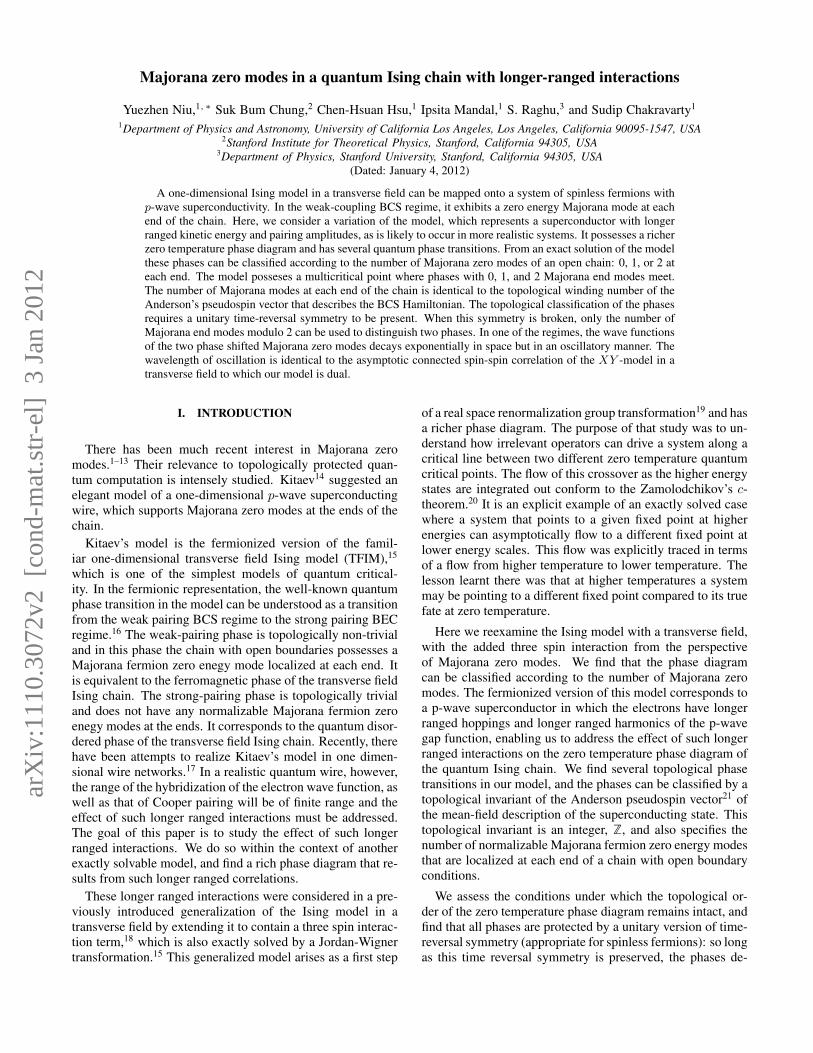
For the Ising model in a transverse field without three spininteraction, the gaps collapse at the Brillouin zone boundaries,k = ±π at the self-dual point λ1 = 1 and λ2 = 0. When thethree spin interaction is added, the gaps can collapse at k = 0as well as k = arccos(λ1/2) for λ2 = −1 and 0 < λ1 <2. But at the free fermion point b, there are no zero energyexcitations except at k = ±π/2. When we move to the pointc the spectrum evolves increasing the weight at k = 0 and thelocations of the nodes are incommensurate with the lattice.The incommensuration shifts as a function of λ2. The point dis a multicritical point and the spectra vanishes quadraticallyat ±π. As we shall discuss below, the spectra are no longerrelativistic at this point as a result of the confluence of twoDirac points, corresponding to a dynamical exponent z = 2.

3

0 1 2 3 42

1

0

1

2

-

-

!2

!1

a

b c d

e

n=1

n=0

n=2

n=2

n=0

FIG. 1. (Color online)The region λ2 > 1 + λ1 is ordered in theoriginal spin representation and the boundary of it is a critical linewhere the gap at k = 0 collapses. The region λ2 < 1 − λ1 is disor-dered as well and the boundary corresponds a critical line where thegap at k = π collapses. The point λ1 = 0 and λ2 = 1 is a specialmulticrtical point with an emergent U(1) symmetry, most transpar-ently seen in the dual representation (see below). In the same dualrepresentation, the region enclosed by λ2

1 = −4λ2 is an oscillatoryferromagnetically ordered phase separating from an ordered phasefor λ2 < 0, as determined by the spatial decay of the instantaneousspin-spin correlation function. Note that duality exchanges orderedand disordered phases. Here n = 0, 1, 2 correspond to regions withn-Majorana zero modes at each end of an open chain.

III. MAJORANA ZERO MODES

In this section we explore the zero modes by theBogoliubov-de Gennes equations with open boundary condi-tion.

A. Unbroken time reversal invariance

The equations, assuming open boundary condition, aregiven by (

h ∆

−∆ −h

)(~un~vn

)= En

(~un~vn

), (8)

where the submatrices are (unless otherwise stated, we willset g = 1)

hij = λ1(δj,i+1 + δj,i−1) + λ2(δj,i+2 + δj,i−2)− 2δij(9)

∆ij = −λ1(δj,i+1 − δj,i−1)− λ2(δj,i+2 − δj,i−2) (10)

Here ~uTn = (un(1), un(2), . . . u(N)) and from time reversalsymmetry of the Hamiltonian ~un = ~u∗n and ~vn = ~v∗n. Theeigenvalue is labeled by n and the arguments of ~u and ~v arelattice indices.

From the diagonaliztion of the BdG Hamiltonian, we caneasily see that the Majorana zero-modes can occur only for

open boundary condition. The phase diagram itself can be de-duced from the number of zero modes of the BdG equation.In the next section we shall see that in the Majorana repre-sentation, the zero modes can be obtained from a very simplerecursion relation. With reference to Fig. 1 we note that thereare regions of n = 0, n = 1, and n = 2 zero modes, andthe lines separating them are quantum critical lines, exceptfor the line separating n = 0 and n = 2, which is a topolog-ical transition. The thin line λ21 = −4λ2 corresponds to zeroentanglement entropy.25 In this respect, it is remarkable thatthis thin line osculates the quantum critical line.

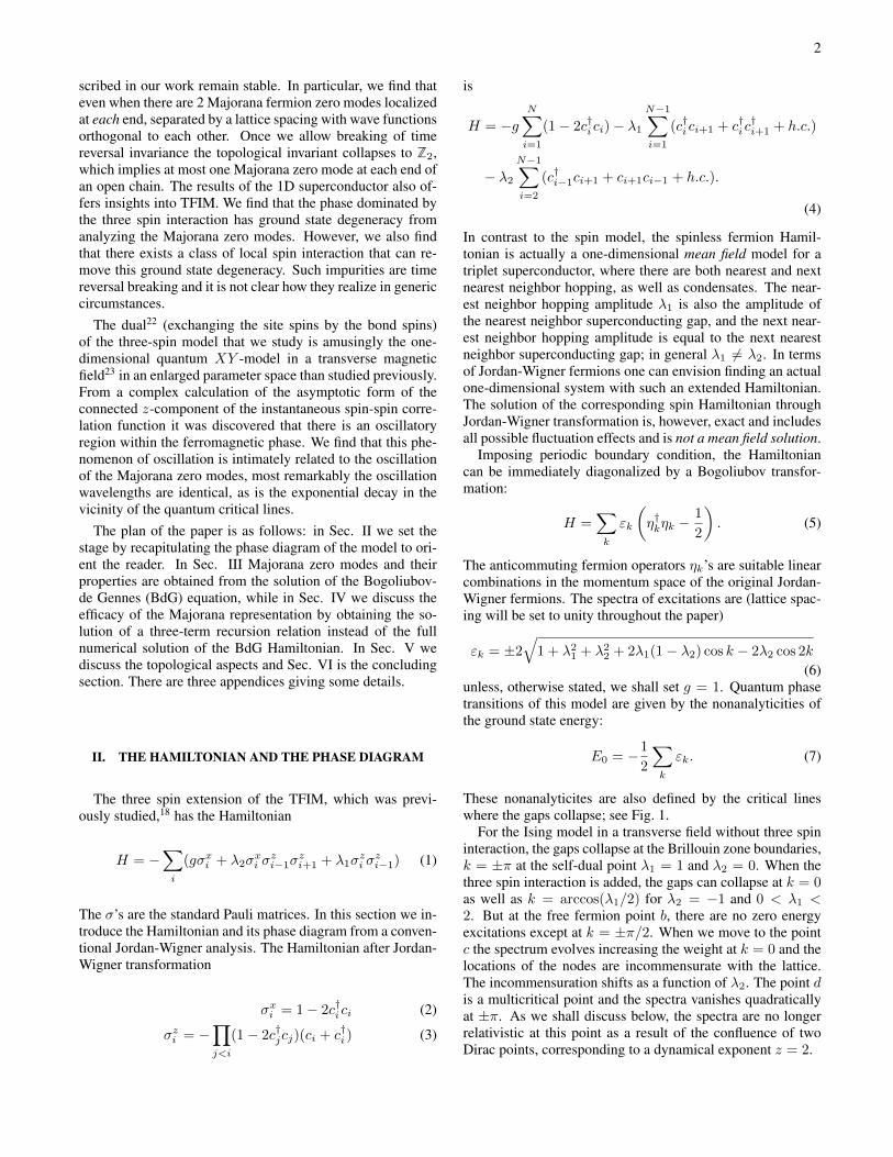
For λ2 > 0, and λ2 > 1+λ1, one of the zero modes decaysexponentially in the bulk, and the decay length diverges asthe quantum critical line is approached. The amplitude of thesecond zero mode also decays exponentially but it oscillatesas eiπn regardless of λ1 as it approaches the quantum criticalline, at which point it loses the compactness of its support,signifying the loss of this zero mode. On the side λ2 < 1+λ1,one zero mode is recovered and it decays exponentially in thebulk, as in the region λ2 > 1 + λ1, as shown in Fig. 2.

0 20 40 60 80 100!0.30!0.25!0.20!0.15!0.10!0.050.00

i

u 01!i"0 20 40 60 80 100

!0.3!0.2!0.10.00.10.20.3

i

v 01!i"

0 20 40 60 80 100!0.2!0.10.00.10.20.3

i

u 02!i"

0 20 40 60 80 100!0.3!0.2!0.10.00.10.20.3

iv 02!i"

0 20 40 60 80 1000.000.050.100.15

i

P 01!i"

0 20 40 60 80 1000.00

0.05

0.10

0.15

i

P 02!i"

FIG. 2. (Color online)The two Majorana zero modes for λ1 = 0.05and λ2 = 1.5. The row number 1 shows u01(i) and v01(i) cor-responding to the the first Majorana zero mode. The second rowcorresponds to the second Majorana zero mode that is orthogonal tothe first. The third row corresponds to the probability distributionsP01(i) and P02(i) for the two respective Majorana modes. The nu-merical diagonalization was carried out for a lattice of N = 100sites with open boundary condition. For lattices larger than 150, onequickly looses numerical control because of 1016 difference in theorder of magnitudes of the largest eigenvalue and the zero mode.

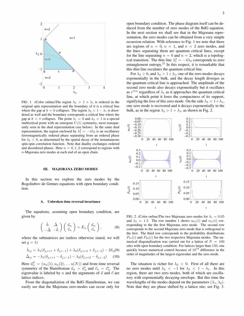
The situation is richer for λ2 < 0. First of all there areno zero modes until λ2 < −1 for λ2 < 1 − λ1. In thisregion, there are two zero modes, both of which are oscilla-tory with exponentially decaying envelope. But this time thewavelengths of the modes depend on the parameters (λ1, λ2).Note that they are phase shifted by a lattice site; see Fig. 3.

4

When we cross the quantum critical line, λ2 = 1− λ1, a non-oscillatory and exponentially decaying zero mode is observed.

0 20 40 60 80 100!0.2!0.10.00.10.2

i

u 01!i"

0 20 40 60 80 100!0.2!0.10.00.1

i

v 01!i"

0 20 40 60 80 100!0.2!0.10.00.10.2

i

u 02!i"

0 20 40 60 80 100!0.2!0.10.00.10.2

i

v 02!i"

0 20 40 60 80 1000.000.020.040.060.080.10

i

P 01!i"

0 20 40 60 80 1000.000.020.040.060.080.100.12

i

P 02!i"

FIG. 3. (Color online)The two Majorana zero modes for s λ2 =−1.2 and λ1 = 1. The row number 1 depicts u02(i) and v02(i)corresponding to the the first Majorana zero mode. The second rowshows the second Majorana zero mode that is orthogonal to the first.The third row corresponds to the probability distributions P01(i) andP02(i) for the two respective Majorana modes.

B. Broken time reversal invariance

We can ask what happens if we add a relative phase betweenthe two order parameters in the BdG Hamiltonian, while keep-ing the single particle Hamiltonian intact. Then,(

h ∆

∆† −h

)(~un~v∗n

)= En

(~un~v∗n

), (11)

where the submatrices are

hij = λ1(δj,i+1 + δj,i−1) + λ2(δj,i+2 + δj,i−2)

− 2δij (12)

∆ij = eiθλ2(δi,j+2 − δi+2,j) + λ1(δi−1,j − δi+1,j) (13)

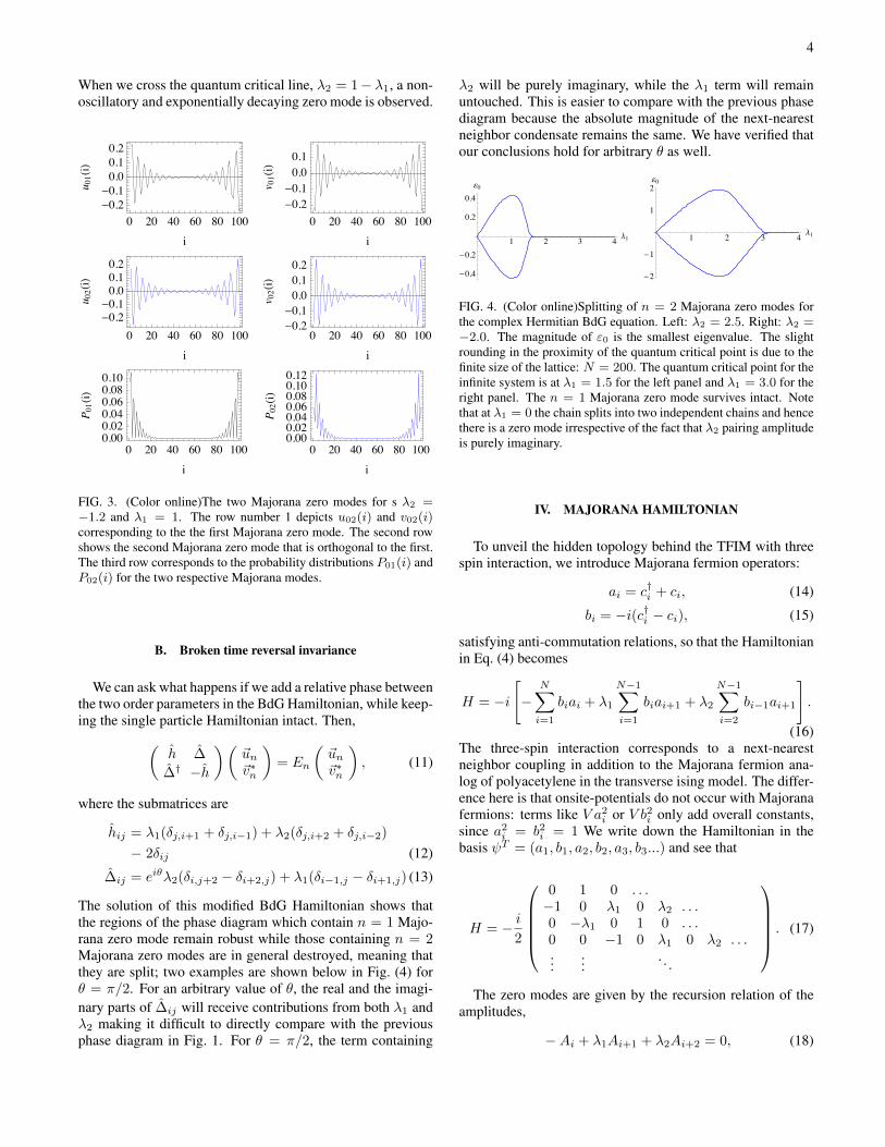
The solution of this modified BdG Hamiltonian shows thatthe regions of the phase diagram which contain n = 1 Majo-rana zero mode remain robust while those containing n = 2Majorana zero modes are in general destroyed, meaning thatthey are split; two examples are shown below in Fig. (4) forθ = π/2. For an arbitrary value of θ, the real and the imagi-nary parts of ∆ij will receive contributions from both λ1 andλ2 making it difficult to directly compare with the previousphase diagram in Fig. 1. For θ = π/2, the term containing

λ2 will be purely imaginary, while the λ1 term will remainuntouched. This is easier to compare with the previous phasediagram because the absolute magnitude of the next-nearestneighbor condensate remains the same. We have verified thatour conclusions hold for arbitrary θ as well.

1 2 3 4 !1

"0.4

"0.2

0.2

0.4!0

1 2 3 4 !1

"2

"1

1

2!0

FIG. 4. (Color online)Splitting of n = 2 Majorana zero modes forthe complex Hermitian BdG equation. Left: λ2 = 2.5. Right: λ2 =−2.0. The magnitude of ε0 is the smallest eigenvalue. The slightrounding in the proximity of the quantum critical point is due to thefinite size of the lattice: N = 200. The quantum critical point for theinfinite system is at λ1 = 1.5 for the left panel and λ1 = 3.0 for theright panel. The n = 1 Majorana zero mode survives intact. Notethat at λ1 = 0 the chain splits into two independent chains and hencethere is a zero mode irrespective of the fact that λ2 pairing amplitudeis purely imaginary.

IV. MAJORANA HAMILTONIAN

To unveil the hidden topology behind the TFIM with threespin interaction, we introduce Majorana fermion operators:

ai = c†i + ci, (14)

bi = −i(c†i − ci), (15)

satisfying anti-commutation relations, so that the Hamiltonianin Eq. (4) becomes

H = −i

[−

N∑i=1

biai + λ1

N−1∑i=1

biai+1 + λ2

N−1∑i=2

bi−1ai+1

].

(16)The three-spin interaction corresponds to a next-nearestneighbor coupling in addition to the Majorana fermion ana-log of polyacetylene in the transverse ising model. The differ-ence here is that onsite-potentials do not occur with Majoranafermions: terms like V a2i or V b2i only add overall constants,since a2i = b2i = 1 We write down the Hamiltonian in thebasis ψT = (a1, b1, a2, b2, a3, b3...) and see that

H = − i2

0 1 0 . . .−1 0 λ1 0 λ2 . . .0 −λ1 0 1 0 . . .0 0 −1 0 λ1 0 λ2 . . ....

.... . .

. (17)

The zero modes are given by the recursion relation of theamplitudes,

−Ai + λ1Ai+1 + λ2Ai+2 = 0, (18)

5

where the eigenvector is chosen to be of the form(A1, 0, A2, 0, · · · )T . We note that when λ2 < 0, the above re-cursion relation looks like the equation of motion of a dampedharmonic oscillator with the time variable discretized. Thetwo linearly independent solutions can be expressed as:

Ai = C1qi+ + C2q

i−, (19)

where q± satisfy

1 = λ1q + λ2q2, (20)

q± =−λ1 ±

√λ21 + 4λ2

2λ2, (21)

and C1, C2 are constants. However, when we restrict our-selves to real and normalizable solutions, we may have onlyone, two, or zero solutions. Note that λ21 + 4λ2 > 0 is suffi-cient for giving us real solution regardless of C1 to C2 ratio.Therefore, we can obtain the phase boundary for λ21+4λ2 > 0just by examining whether |q±| is larger than 1 or not. For thecase λ1, λ2 > 0, we can recover the results found by Koppand Chakravarty. For 1 − λ1 < λ2 < 1 + λ1, we have0 < q+ < 1 < −q−, and therefore a single Majorana zeromode at each end of the chain. For λ2 > 1 + λ1, we have0 < −q− < 1 and 0 < q+ < 1 and thus there are two Majo-rana zero modes at each end of the chain. Lastly, we have noMajorana zero mode for λ2 < 1−λ1, as q+ and−q− are bothgreater than 1. We can extend this analysis to λ21 + 4λ2 > 0and λ2 < 0, λ1 > 0. For λ2 < 1 − λ1 and λ2 > −1,we have |q±| > 1 and thus no Majorana zero mode, whereasλ2 > 1 − λ1 gives us 0 < q+ < 1 < −q− and thus there isone Majorana zero mode at each end of the chain.

By contrast, when we break the time reversal symmetry byhaving phase difference between the two pairing terms as inEq. (13), we find that we can have only zero or one normal-izable Majorana zero mode at the end of the chain, as shownabove from the explicit solution of the BdG equation. Interest-ingly, we find that we obtain the same result if we break timereversal symmetry by adding an impurity term of the form(see Appendix B)

Himp = −iλajaj+m= −iλ(c†jcj+m − c

†j+mcj + c†jc

†j+m − cj+mcj),

(22)

to the original Hamiltonian Eq. (4). Since the translationalinvariance is broken in this case, the number of zero Majo-rana modes provide a convenient way to distinguish differentphases.

A. Oscillatory Majorana zero modes with varying wavelength

We find from the recursion relation, Eq. (18), that there areno Majorana zero modes for −1 < λ2 < 0 and λ2 < 1− λ1.However, there are two oscillatory zero modes for λ2 < −1and λ21 + 4λ2 < 0, with amplitudes at a lattice site j given bythe two solutions of the recursion relation:

Aj = (−λ2)−j/2 cos jθ, (23)

and

Aj = (−λ2)−j/2 sin jθ, (24)

where θ = arcsin(λ1/√−4λ2). The amplitude could be

rewritten as

(−λ2)−j/2 = e−x/ξ, (25)

where ξ = 2a/ ln(−λ2). Note that close to the quantum crit-ical line |λ2| ∼ |λ1 − 1|. We have reintroduced the latticespacing a here. An example of oscillatory Majorana modesare shown in Fig. (3).

When λ2 becomes negative, an oscillatory phase, as deter-mined from the spin-spin correlation function, was obtainedfrom a dual transformation that exchanges sites and bonds ofthe lattice. Then the Hamiltonian in Eq. (4) can be cast inthe standard notation of the quantum XY -model by factoringout an overall scale. Thus, with µ’s as bond-centered Paulimatrices,

H = − 2

1 + r

∑n

[1 + r

2µ1(n)µ1(n+ 1)

+1− r

2µ2(n)µ2(n+ 1) + hµ3(n))

],

(26)

the two parametrizations are related to each other by

λ1 =2h

1 + r, λ2 =

r − 1

1 + r. (27)

The critical line in XY -model, separating the quantum dis-ordered phase from the ferromagnetic phase, is h = 1, whichcorresponds to λ1+λ2 = 1, separating the ordered phase fromthe disordered phase. The model was previously studied onlyin the range 0 < r < 1 and h > 0. Since the ordered and thedisordered phases are exchanged under duality, the disorderedphase of the three-spin model is λ1 + λ2 < 1.

A complex calculation23 of the instantaneous spin-spin cor-relation function showed that within the ferromagnetic phase,there is an oscillatory phase in the which the connected corre-lation function G(x) = 〈µ3(x)µ(0)〉 − 〈µ3(x)〉〈µ3(0)〉 in thelimit x→∞, is

G(r) =

1√xe−x/ξ, disordered,

1x2 e−x/ξ, ordered,

1x2 e−2x/ξ<(BeiKx), oscillatory ordered.

(28)

Here cosK = λ1/√−4λ2 and ξ is the spin-spin correlation

length. The oscillatory phase in the XY -model is bounded byr2 + h2 ≤ 1, which corresponds to λ2 ≤ −λ21/4 in the three-spin model. Note that the oscillation wavelength is identicalto the wavelength of the Majorana fermions. Even the corre-lation length close to criticality is the scale of the exponentialdecay of the Majorana fermions. This must imply that in thespectral decomposition, the Majorana zero modes asymptot-ically dominate, although we have not yet found a rigorousproof of it.

Since Majorana modes of zero energy are degenerate eigen-states, a change of the number of Majorana zero modes can

6

only occur when the energy gap collapses, i.e. at a quan-tum phase transition. Reexamining the behavior of Majoranazero mode in the full parameter space, there are three dividinglines based on their number: λ2 = 1 + λ1, λ2 = 1 − λ1 andλ2 = −1; see Fig 1. These lines are identified with the criticallines signifying phase transition, as can be seen in the energyspectrum in the previous result. So in this case, the numberof Majorana zero modes serve as an “order parameter” for thequantum phase transition.

We can then distinguish phases and locate quantum phasetransitions by simply transforming the Hamiltonian in termsof Majorana operators and finding the number of allowed Ma-jorana zero-modes at each end of the chain, which is a topo-logically protected quantity. This provides us a profoundlysimple way to study quantum phase transitions.

B. Unbroken unitary time reversal symmetry

Some insight into the phase diagram can be obtained fromthe perspective of the weak to strong pairing topological phasetransitions in this model. Starting from the spinless FermionHamiltonian in Eq. (4), we get upon Fourier transformation

H =∑k

(2− 2λ1 cos k − 2λ2 cos 2k) c†kck

+∑k

(iλ1 sin kc†kc

†−k + iλ2 sin 2kc†kc

†−k + h.c.

),

(29)

which describes a superconductor with a pairing potential thatconsists of a nearest neighbor and a second nearest neighborp-wave pairing. The BdG Hamiltonian which governs the dy-namics of the BCS quasiparticles at each momentum k has theform

HBdG(k) =

(εk − µ i∆(k)−i∆(k) µ− εk

)(30)

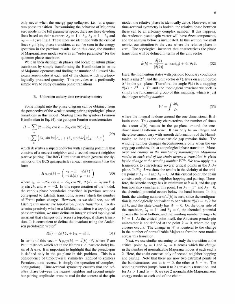
where εk = −2λ1 cos k − 2λ2 cos 2k, ∆(k) = λ1 sin k +λ2 sin 2k, and µ = −2. In this representation of the model,the various phase boundaries described in previous sectionscorrespond to Lifshitz transitions, across which the numberof Fermi points change. However, as we shall see, not allLifshitz transitions are topological phase transitions. To de-termine precisely whether a Lifshitz transition is a topologicalphase transition, we must define an integer-valued topologicalinvariant that changes only across a topological phase transi-tion. It is convenient to define the invariant using the Ander-son pseudospin vector21

~d(k) = ∆(k)y + (εk − µ) z. (31)

In terms of this vector HBdG(k) = ~d(k) · ~τ , where ~τ arePauli matrices which act in the Nambu (i.e. particle-hole) ba-sis of HBdG. It is important to highlight that the pseudospinis defined only in the yz plane in this problem. This is aconsequence of time-reversal symmetry (applied to spinlessFermions, time-reversal is simply the operation of complex-conjugation). Time-reversal symmetry ensures that the rel-ative phase between the nearest neighbor and second neigh-bor pairing amplitudes must be real (in the context of the spin

model, the relative phase is identically zero). However, whentime-reversal symmetry is broken, the relative phase betweenthese can be an arbitrary complex number. If this happens,the Anderson pseudospin vector will have three components,and the analysis below is invalidated. In this section, we shallrestrict our attention to the case where the relative phase iszero. The topological invariant that characterizes the phasetransitions will be defined in terms of the unit vector

d(k) =~d(k)

|~d(k)|≡ cos θky + sin θkz. (32)

Here, the momentum states with periodic boundary conditionsform a ring T 1, and the unit vector d(k), lives on a unit circleS1 in the yz−plane. Therefore, the angle θ(k) is a mappingθ(k) : S1 → T 1 and the topological invariant we seek issimply the fundamental group of this mapping, which is justthe integer winding number

W =

∮dθk2π

(33)

where the integral is done around the one dimensional Bril-louin zone. This quantity characterizes the number of timesthe vector d(k) rotates in the yz-plane around the one-dimensional Brillouin zone. It can only be an integer andtherefore cannot vary with smooth deformations of the Hamil-tonian, so long as the quasiparticle gap remains finite. Thewinding number changes discontinuously only when the en-ergy gap vanishes, i.e. at a topological phase transition. More-over, the change in the number of normalizable Majoranamodes at each end of the chain across a transition is givenby the change in the winding numberW 16. We now apply thisframework to characterize several critical points in the λ1λ2plane. In Fig. 5 we show the results in the vicinity of the criti-cal point at λ1 = 1 and λ2 = 0. At this critical point, the chainconsists only of nearest neighbor hopping and pairing. There-fore, the kinetic energy has its minimum at k = 0, and the gapfunction also vanishes at this point. For λ1 = 1− and λ2 = 0,the chemical potential occurs below the band bottom. In thislimit, the winding number of d(k) is zero, since the configura-tion is topologically equivalent to one where θ(k) = π/2 forall k, and this state clearly has W = 0. On the other side ofthe transition, λ1 = 1+ and λ2 = 0, the chemical potentialcrosses the band bottom, and the winding number changes toW = 1. At the critical point itself, the Anderson pseudospinunit-vector is not defined at the point k = 0, where the gapclosure occurs. The change in W is identical to the changein the number of normalizable Majorana fermion zero modesacross this transition.

Next, we use similar reasoning to study the transition at thecritical point λ2 = 1 and λ1 = 0 across which the changein the number of normalizable Majorana modes at each end is2. Here, the chain consists only of second-neighbor hoppingand pairing. Note that there are now two extremal points ofthe bandstructure: one at k = 0, the other at k = π. Thewinding number jumps from 0 to 2 across this transition, andfor λ2 > 1 and λ1 = 0, we see 2 normalizable Majorana zeroenergy modes at each end of the chain.

7

−1 0 1−2

0

2

4 E

k/! −1 0 1−2

0

2

4

E

k/!

(a) (b)

FIG. 5. (Color online)Topological phase transition across the pointλ1 = 1, λ2 = 0. (a) λ1 = 1−, λ2 = 0. The quantities plotted areεk (solid black line), µ (dashed black line), ∆(k) (dashed blue line),and quasiparticle energy (solid red line) as a function of momentumin the one dimensional Brillouin zone. (b) The same quantities areplotted for λ1 = 1+, λ2 = 0. The associated Anderson pseudospinvector d(k) is drawn schematically below each plot. It is clear thatin (a) the pseudospin does not wind along the 1d Brillouin zone, i.e.W = 0, whereas in (b) it winds once, i.e. W = 1.

−1 0 1−2

0

2

4

E

k/! −1 0 1−2

0

2

4

E

k/!

(a) (b)

FIG. 6. (Color online)Topological phase transition in the vicinity ofthe point λ1 = 0, λ2 = 1. (a) λ2 = 1−, λ1 = 0; (b) λ2 = 1+, λ1 =0. It is clear that in (a), the pseudospin does not wind along the1d Brillouin zone, i.e. W = 0, whereas in (b) it winds twice, i.e.W = 2.

Interestingly, our model hosts both BEC-BCS transitionsand BEC-BCS crossovers. Only the former are topologicaltransitions: these require that (1) an extremum of the bandcrosses the chemical potential, and (2) the pairing potentialvanishes at the same momentum. If an extremum of the bandcrosses the chemical potential at a point where the gap doesnot vanish, the winding number will not change, since the totalenergy gap does not vanish. This is an example of a BCS-BECcrossover, and not a transition. This type of crossover is seen

−1 0 1−2

0

2

4

6

E

k/! −1 0 1−2

0

2

4

6

8

E

k/!

(a) (b)

FIG. 7. (Color online)Topological phase transition in the vicinityof the point λ1 = 1.5, λ2 = −1. (a) λ2 = −1+, λ1 = 1.5; (b)λ2 = −1−, λ1 = 1.5. In (a), the pseudospin does not wind alongthe 1d Brillouin zone, i.e. W = 0, whereas in (b) it winds twice, i.e.W = 2.

near the line λ2 = −1. An illustrative example is presentedin Fig. 7. Here, the critical point λ1 = 1.5 and λ2 = −1 isstudied. In Fig. 7a, the properties of the system are shown atλ1 = 1.5 and λ2 = −1+, where no normalizable Majoranazero mode occurs at the boundary. From the fact that Fermipoints occur in this system, it is clear that the system is in theBCS regime. However, it is apparent from the form of theAnderson pseudospin that the winding number is identicallyzero. Thus, while this state is a BCS state, it is topologicallyequivalent to a BEC state which also has zero winding num-ber. Thus, a crossover can connect this state to a BEC state.However, when λ1 = 1.5 and λ2 = −1−, i.e. just below thecritical point, we know from the analysis of previous sectionsthat there are 2 normalizable Majorana fermion zero modes ateach edge of the chain. This is also consistent with the wind-ing number of the Anderson pseudospin, which is W = 2in this regime. We stress therefore, that a topological phasetransition between 2 BCS states can occur. However so longas the bandstructure possesses inversion symmetry, it followsthat such topological BCS-BCS transitions can only changethe topological invariant by ±2. In a similar way, the criticalline in Fig. (1) from b to d represents a topological transitionacross which the winding number changes by 2. Along thisline, the gap vanishes at an incommensurate set of points inmomentum space. In (c), the point λ1 = 1 and λ2 = −1 isconsidered. Here again, there are two band minima. How-ever, they occur at incommensurate momenta, ±k0, symmet-ric about the origin. Therefore this critical point marks a tran-sition from 0 to 2 Majorana zero modes at each end of thechain. This is the point (c) in Fig. (1). As we approach thespecial multicritical point d in Fig. (1) (λ1 = 2, λ2 = −1),these two incommensurate points move towards the origin.They meet at k = 0, which is now a local maximum of thebandstructure. The 2 momenta ±k0 meet at k = 0 at themulticritical point (λ1 = 2, λ2 = −1). In this way, all thetopological phase transitions that occur in the model can be

8

−1 0 1−2

02468

E

k/! −1 0 1−2

02468

E

k/!

−1 0 1−2

02468

E

k/! −1 0 1−2

02468

E

k/!

(a) (b)

(c) (d)

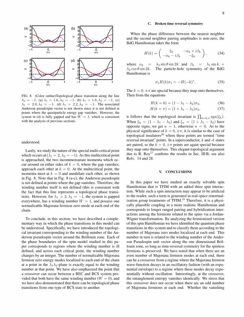
FIG. 8. (Color online)Topological phase transition along the lineλ2 = −1. (a) λ1 = 1.6, λ2 = −1. (b) λ1 = 1.8, λ2 = −1. (c)λ1 = 2.0, λ2 = −1. (d) λ1 = 2.2, λ2 = −1. The associatedAnderson pseudospin vector is not shown since it is not defined atpoints where the quasiparticle energy gap vanishes. However, thesystem in (d) is fully gapped and has W = 1, which is consistentwith the analysis of previous sections.

understood.

Lastly, we study the nature of the special multi-critical pointwhich occurs at (λ1 = 2, λ2 = −1). As this multicritical pointis approached, the two incommensurate momenta which oc-cur around on either sides of k = 0, where the gap vanishes,approach each other at k = 0. At the multicritical point, themomenta meet at k = 0 and annihilate each other, as shownin Fig. 8. Note that in Fig. 8 (a-c), the Anderson pseudospinis not defined at points where the gap vanishes. Therefore, thewinding number itself is not defined (this is consistent withthe fact that this line represents a topological phase transi-tion). However, for λ1 > 2, λ2 = −1, the system is gappedeverywhere, has a winding number W = 1, and possess onenormalizable Majorana fermion zero mode at each end of thechain.

To conclude, in this section, we have described a comple-mentary way in which the phase transitions in this model canbe understood. Specifically, we have introduced the topologi-cal invariant corresponding to the winding number of the An-derson pseudospin vector around the Brillouin zone. Each ofthe phase boundaries of the spin model studied in this pa-per corresponds to regions where the winding number is illdefined, and across each critical point, the winding numberchanges by an integer. The number of normalizable Majoranafermion zero energy modes localized to each end of the chainat a point in the λ1λ2-plane is exactly equal to the windingnumber at that point. We have also emphasized the point thata crossover can occur between a BEC and BCS system pro-vided that both have the same winding number (W = 0), andwe have also demonstrated that there can be topological phasetransitions from one type of BCS state to another.

C. Broken time reversal symmetry

When the phase difference between the nearest neighborand the second neighbor pairing amplitudes is non-zero, theBdG Hamiltonian takes the form

H(k) =

(ξk −αk + iβk

−αk − iβk −ξk

), (34)

where αk = λ2 sin θ sin 2k and βk = λ1 sin k +λ2 cos θ sin 2k. The particle-hole symmetry of the BdGHamiltonian is

σ1H(k)σ1 = −H(−k)∗. (35)

The k = 0,±π are special because they map onto themselves.Then from the equations

H(k = 0) = (1− λ1 − λ2)σ3, (36)H(k = π) = (1 + λ1 − λ2)σ3, (37)

it follows that the topological invariant is∏k=0,π sgn(ξk).

When ξ0 = (1 − λ1 − λ2) and ξπ = (1 + λ1 − λ2) haveopposite signs, we get n = 1, otherwise n = 0. As to thephysical significance of k = 0,±π, it is similar to the case oftopological insulators26 where these points are termed “timereversal invariant” points. In a superconductor, k and -k statesare paired, so the k = 0,±π points are again special becausethey map onto themselves. This elegant topological argumentdue to R. Roy27 confirms the results in Sec. III B; see alsoRefs. 14 and 28.

V. CONCLUSIONS

In this paper we have studied an exactly solvable spinHamiltonian that is TFIM with an added three spin interac-tion. While such a spin interaction may appear to be artificialto the reader, such a term is generated in real-space renormal-ization group treatments of TFIM.19 Therefore, it is a physi-cally plausible coupling in a more realistic Hamiltonian andcorresponds to longer ranged pairing and hybridization inter-actions among the fermions related to the spins via a Jordan-Wigner transformation. By analyzing the fermionized versionof this spin Hamiltonian we have identified the quantum phasetransitions in this system and to classify them according to thenumber of Majorana zero modes localized at each end. Thisnumber in turn is related to the winding number of the Ander-son Pseudospin unit vector along the one dimensional Bril-louin zone, so long as time-reversal symmetry for the spinlessfermions is preserved. We have noted that when there are aneven number of Majorana fermion modes at each end, therecan be a crossover from a regime where the Majorana fermionwave-function decays in an oscillatory fashion (with an expo-nential envelope) to a regime where these modes decay expo-nentially without oscillation. Interestingly, at the crossover,the entanglement entropy vanishes identically. We stress thatthis crossover does not occur when there are an odd numberof Majorana fermions at each end. Whether the vanishing

9

of the entanglement entropy is a necessary condition for thiscrossover remains to be understood. The degree to which sucha crossover remains generic, or is ascribed to the integrabilityof the spin chain is unclear. Finally, an interesting possibilityis that such crossovers may occur in higher dimensions in spintriplet superconductors in the presence of vortices, and othertopological superconductors involving non-centrosymmetricsystems. We shall relegate these studies to future work..

For unitary time reversal invariance, the topological argu-ment involving Anderson’s pseudospin vector leads to wind-ing number Z. One might wonder if higher windings beyondn = 0, 1, 2 are possible as well. In principle, it is. To check,we added an even longer ranged term H3 = λ3c

†i ci+3 +

λ3c†i c†i+3 + h.c. Now, in addition to n = 0, 1, 2, we also get

winding number n = 3 in appropriate regimes of the parame-ter space from explicit calculations of the BdG equation. It isquite likely that these higher order windings are energeticallypunished. The situation is very similar to the XY -model intwo dimensions for which higher order vorticity is suppressedby the chemical potential. Clearly phases with n = Z Ma-jorana zero modes are allowed by longer ranged Hamiltoni-ans. We find this phenomena intriguing, which deserves fur-ther attention. However, once the protection due to unitarytime reversal invariance is removed the topological invariantcollapses to Z2, with at most one Majorana zero mode at eachend of an open chain.

We have previously emphasized that while the solution ofthe spin model is exact, the fermonized version is a mean-fielddescription of a p-wave superconductor whose exact solutionrequires treatment of fluctuation effects. In a recent paper it

has been shown, however, that including fluctuation effectsdo not change the basic picture in a one-dimensional model.29

Whether such a conclusion holds in higher dimensions, whereMajorana zero modes are nucleated in the vortex cores of apx + ipy superconductors, remains to be seen. We leave thisproblem for future research.

An interesting question is whether or not the topologi-cal phases described here are perturbatively stable againstweak interactions. We believe that they are, because theyare gapped. In principle, for stronger interactions, the uni-tary time-reversal symmetry that protects the n = 2 phasecan break spontaneously and destabilize it. The effect ofstronger interactions in a specific model has been consideredin Ref. 30.

ACKNOWLEDGMENTS

Yuezhen Niu thanks UCLA physics department for its hos-pitality. S. C. and Y. N. were supported by US NSF under theGrant DMR-1004520. S.B.C was supported by the DOE un-der contract DE-AC02-76SF00515. I. M. was funded by fundsfrom the David S. Saxon Presidential Chair at UCLA. S.R. issupported by startup funds at Stanford University. We thankParsa Bonderson, Cristina Bena, Pallab Goswami, Alexei Ki-taev, Roman Lutchyn, Chetan Nayak, Rahul Roy, Kirill Shten-gel and Matthias Troyer for comments. This work was partlycarried out at the Aspen Center for Physics.

Appendix A: Broken time reversal invariance

When there is a relative phase eiθ between the nearest neighbor and the next-nearest neighbor pairing amplitudes the MajoranaHamiltonian is

H = −i{−N∑i=1

biai + λ1

N−1∑i=1

biai+1 +λ22

N−1∑i=2

[(1 + cos θ)bi−1ai+1

−(1− cos θ)ai−1bi+1 + sin θ(ai−1ai+1 − bi−1bi+1)]}. (A1)

Thus, we cannot simply set λ2 to be complex in Eq. (18). The Hamiltonian in the Majorana basis ψT =(a1, b1, a2, b2, a3, b3, · · · ) is

H = − i2

0 1 0 0 λ2

2 sin θ −λ2

2 (1− cos θ) · · · · · ·−1 0 λ1 0 λ2

2 (1 + cos θ) −λ2

2 sin θ · · · · · ·0 −λ1 0 1 0 0 · · · · · ·0 0 −1 0 λ1 0 · · · · · ·...

... 0 −λ1 0 1 · · · · · ·...

... 0 0 −1 0 · · · · · ·...

......

......

. . . . . . · · ·

. (A2)

To find the zero mode eigenvectors, we can try a solution of the form: |Ψ〉 = (A1, B1, A2, B2, A3, B3, · · · )T . However, therecursion relations turn out to be too complex to solve analytically. Thus, we resorted to numerical diagonalization of the BdGHamiltonian in the main text.

Appendix B: Majorana zero modes in the presence of impurity

In general, we find that when H of Eq. (4) results in twoMajorana zero mode, Himp in Eq. (22) destroys them (except

for some special cases), while the regime with one Majorana

10

zero mode remains intact.

Consider the general definition of the Majorana zero modeΓ =

∑(Aiai+Bibi), which is determined by the commutator

0 =[H0 +Himp,Γ]

=2i∑

(Ai − λ1Ai+1 − λ2Ai+2)bi

−2iB1a1 − 2i(B2 − λ1B1)a2

−2i∑

(Bi+2 − λ1Bi+1 − λ2Bi)ai+2

+2iλ(Aj+maj −Ajaj+m),

(B1)

which requires, in addition to the original recursion formula

Ai − λ1Ai+1 − λ2Ai+2 = 0, (B2)Bi − λ1Bi−1 − λ2Bi−2 = 0, (i > j, i 6= j +m), (B3)

new boundary conditions for Bj’s:

Bi = 0 for i < j, (B4)Bj = λAj+m, (B5)

Bj+m − λ1Bj+m−1 − λ2Bj+m−2 = −λAj . (B6)(B7)

(note that the Ai recursion relation is not affected by Bi’s).Because of this change in the boundary conditions, we can nolonger set Bi = 0 for all i. Rather, for i > j +m, the generalsolution forAi and Bi are of the form

Ai =C+qi+ + C−q

i−,

Bi =C ′+(1/q+)i + C ′−(1/q−)i, (B8)

where 1− λ1q± − λ2q2± = 0.

We can now see how the impurity term Eq. (22) may de-stroy the Majorana zero modes. Eq. (B8) implies that if wehad two Majorana zero modes without the impurity, whichonly requires |q±| < 1, we will not have any normalizableMajorana zero mode due to the divergence of Bi unless wehave Bj+m−1 = Bj+m = 0, which can occur only un-der special situations. On the other hand, if we had a sin-gle Majorana zero mode without the impurity, which means|q+| < 1 < |q−|, the Majorana zero mode survives ifBi+m/Bi+m−1 = 1/q−. We have checked this explicitly forthe special cases of m = 1, 2, 3.

Appendix C: Impurity induced tunneling between twoMajorana zero modes

To consider the condition for the stability of two Majoranazero mode, we first not that, in the limit where the bulk gapis large, a semi-infinite chain can be regarded as a two-statesystem. This is because the two Majorana zero mode wouldform a single zero energy state, giving us energy degeneracybetween the case where this zero energy state is occupied andthe case where this zero energy state is vacant. Due to thefermion number parity conservation, perturbation cannot giverise to any off-diagonal term between the two states; all wecan obtain is the energy difference between the occupied andvacant zero energy state.

Therefore, an impurity term can annihilate the two Majo-rana zero modes if the mode expansion of this impurity termgives rise to dependence on the occupancy of the zero energystate. We know that, in absence of any impurity, the Hamilto-nian in Eq. (4) gives us two Majorana zero modes near i = 1can be written down as the linear combination of only ai’s:

Γn =∑i

cniai, (C1)

where n = 1, 2 and ci ∈ R. Then, the annihilation operatorof the zero energy state can be written as

f0 = (Γ1 + iΓ2)/2 =∑i

(c1i + ic2i)ai/2. (C2)

What follows from this is that when we do the mode expan-sion on Majorana fermions on each site, only ai’s receive con-tribution from the zero energy state whereas all bi’s do not:

ai =(ci0f0 + c∗i0f†0 ) +

∞∑m=1

(cimfm + c∗imf†m),

bi =

∞∑m=1

(c′imfm + c′∗imf†m). (C3)

Any additional fermionic bilinear terms to the Hamiltoniancannot affect the zero modes unless mode expansion of suchterms contain f†0f0.

We make a further restriction that we demand the fermionicbilinear to be local. The criterion for locality here is that, ifour fermion operators are from sites i, j, they should satisfy|i− j| ∼ O(1).

This leads to the conclusion that only iaiaj can gap out thezero modes, while iaibj and ibibj do not. (Conversely, if wehad the right end of the semi-infinite chain, it is ibibj that gapsout the zero modes.) We see from Eq.(C3)

iaiaj = −i(ci0c∗j0 − c∗i0cj0)f†0f0 + (gapped) (C4)

but the mode expansions of iaibj and ibibj do not have thef†0f0 term.

11

∗ Currently at School of Physics, Peking University, Beijing100871, China

1 F. Wilczek, Nature Phys. 5, 614 (2009).2 G. Moore and N. Read, Nucl. Phys. B 360, 362 (1991).3 C. Nayak and F. Wilczek, Nucl. Phys. B 479, 529 (1996).4 D. A. Ivanov, Phys. Rev. Lett. 86, 268 (2001).5 L. Fu and C. L. Kane, Phys. Rev. Lett. 100, 096407 (2008).6 J. D. Sau, R. M. Lutchyn, S. Tewari, and S. Das Sarma, Phys.

Rev. Lett. 104, 040502 (2010).7 J. D. Sau, S. Tewari, R. M. Lutchyn, T. D. Stanescu, and

S. Das Sarma, Phys. Rev. B 82, 214509 (2010).8 J. Alicea, Phys. Rev. B 81, 125318 (2010).9 R. M. Lutchyn, J. D. Sau, and S. Das Sarma, Phys. Rev. Lett. 105,

077001 (2010).10 Y. Oreg, G. Refael, and F. von Oppen, Phys. Rev. Lett. 105,

177002 (2010).11 R. Roy, Phys. Rev. Lett. 105, 186401 (2010).12 C. Bena, D. Sticlet, and P. Simon, ArXiv e-prints (2011),

arXiv:1109.5697 [cond-mat.mes-hall].13 W. DeGottardi, D. Sen, and S. Vishveshwara, New J. Phys. 13,

065028 (2011).14 A. Y. Kitaev, Physics Uspekhi 44, 131 (2001).15 P. Pfeuty, Ann. Phys. (NY) 57, 79 (1970).16 N. Read and D. Green, Phys. Rev. B 61, 10267 (2000).

17 J. Alicea, Y. Oreg, G. Refael, F. von Oppen, and M. Fisher, NaturePhys. 7, 412 (2011).

18 A. Kopp and S. Chakravarty, Nature Phys. 1, 53 (2005).19 J. E. Hirsch and G. F. Mazenko, Phys. Rev. B 19, 2656 (1979).20 A. H. Castro Neto and E. Fradkin, Nucl. Phys. B 400, 525 (1993).21 P. W. Anderson, Phys. Rev. 110, 827 (1958).22 E. Fradkin and L. Susskind, Phys. Rev. D 17, 2637 (1978).23 E. Barouch and B. M. McCoy, Phys. Rev. A 3, 786 (1971).24 In the following related publications multi-critical points in the

topological phase diagram have also been discussed: R. Lutchynand M. P. A Fisher, arXiv:1104.2358 (2011); E. Sela, A. Altland,and A. Rosch, Phys. Rev. B 84, 085114 (2011).

25 T.-W. Wei, S. Vishveshwara, and P. M. Goldbart, Quantum Inf.Comput. 11, 0326 (2011).

26 M. Z. Hasan and C. L. Kane, Rev. Mod. Phys. 82, 3045 (2011);X. Qi and S. Zhang, ArXiv e-prints (2010), arXiv:1008.2026[cond-mat.mes-hall].

27 Personal communication. R. Roy, (2011).28 P. Ghosh, J. D. Sau, S. Tewari, and S. Das Sarma, Physical Re-

view B 82, 184525 (2010).29 L. Fidkowski, R. M. Lutchyn, C. Nayak, and M. P. A. Fisher,

ArXiv e-prints (2011), arXiv:1106.2598 [cond-mat.str-el]; J. D.Sau, B. I. Halperin, K. Flensberg, and S. Das Sarma, PhysicalReview B 84, 144509 (2011), pRB.

30 L. Fidkowski and A. Kitaev, Phys. Rev. B 81, 134509 (2010).