Mobile Netw Appl (2009) 14:281–291

DOI 10.1007/s11036-008-0102-0

Maintaining Optimal Communication Chains

in Robotic Sensor Networks using Mobility Control

Cory Dixon · Eric W. Frew

Published online: 30 September 2008

© Springer Science + Business Media, LLC 2008

Abstract This paper presents a decentralized mobility

control algorithm for the formation and maintenance of

an optimal cascaded communication chain between a lead

sensor-equipped robot and a control station, using a team

of robotic vehicles acting as communication relays in an

unknown and dynamic RF environment. The gradient-based

controller presented uses measurements of the signal-to-

noise ratio (SNR) field of neighbor communication links,

as opposed to relative position between nodes, as input into

a localized performance function. By using the SNR field

as input into the control system, the controller is reactive

to unexpected and unpredictable changes in the RF envi-

ronment that is not possible with range-based controllers.

Since the operating environment is not known a priori to

deployment of a robotic sensor network, an adaptive model-

free extremum seeking (ES) algorithm, that uses the motion

of the relays to estimate the performance function gradient,

is presented to control the motion of 2D nonholonomic

vehicles acting as communication relays using the gradient-

based controller. Even without specific knowledge of the

SNR field, simulations show that the ES decentralized

chaining controller using measurements of the SNR field,

will drive a team of robotic vehicles to locations that achieve

the global objective of maximizing capacity of a cascaded

communication chain, even in the presence of an active

jamming source.

C. Dixon (B) · E. W. Frew

Aerospace Engineering Sciences Department,

University of Colorado at Boulder, Boulder, CO, USA

e-mail: cory.dixon@colorado.edu

Keywords relays · robotics · communication chains ·ad hoc networks · unmanned aircraft

1 Introduction

This paper presents a decentralized mobility control algo-

rithm for the formation and maintenance of an optimal

cascaded communication chain between a lead sensor-

equipped robot and a control station using a team of robotic

vehicles acting as communication relays. The mobility con-

troller presented in this paper is based on maximizing the

capacity of a local 3-node network to maximize the end-to-

end capacity of the entire communication chain, and there-

fore provide an optimal high-bandwidth communication

link between the lead node and the control station, by using

measurements of the local signal-to-noise ratio (SNR) field.

Because the mobility controller is based on the gradient of

the local 3-node network capacity performance function,

and not on geographic position or range, the controller can

form and maintain an optimal, and connected, communica-

tion chain in unknown dynamic RF environments that may

also contain active jamming noise sources. Since it is not

possible to predict the gradient of the SNR field in a physical

environment, extremum seeking (ES) methods are applied

to the decentralized gradient controller to provide a real-

time estimate of the SNR gradient using motion of the relay.

In wireless sensor networks consisting of mobile robotic

nodes, a common mode of operation is to form a commu-

nication relay chain between a lead (exploring) node and a

control station [10, 17]. In this type of operation the lead

node is typically deployed to explore a remote region of

interest that is beyond direct RF communication range, or

out of line-of-sight, to the control station. To provide non-

line-of-sight service and extend the communication range

282 Mobile Netw Appl (2009) 14:281–291

of the lead node (and thus its operational range), additional

robotic nodes are deployed in a convoy fashion behind the

lead sensor-equipped vehicle to act as communication relays

in a cascaded communication chain, relaying high priority

data back to a control station. For this work, the relaying

nodes are tasked to act solely as communication relays

and their only objective is to find and maintain a maximal

capacity of the communication chain while the lead node

explores the environment.

Typically, the mobility control algorithms presented in

literature for these types of robotic team deployments as-

sume a “disc communication model,” where nodes can

communicate at some fixed data rate if they are within a

range of r of each other. Therefore, in these mobility control

algorithms the objective of an individual relay is to maintain

a minimum separation distance between the two network

nodes it is relaying data between. In essence the goal of

these controllers is to maintain network connectivity. Since

these controllers do not take into account the radio trans-

mission properties in the operational RF environment, they

are not reactive to changes in the environment. Furthermore,

these controllers do not lead to optimal communication

chains when localized noise sources are present in the

environment. In fact, depending upon the capacity model

used it can be shown for certain locations of a noise source

that a relaying node that positions itself based on a range

based controller can lead to worse performance than using

the direct communication. Therefore, changes in the RF

environment, such as the introduction of a jamming node,

will lead to a reduction of network quality-of-service that

the nodes cannot react to.

The work in this paper seeks to improve the communi-

cation capacity of a cascaded communication chain, over

that of a range-based controller, in a complex and time

varying RF environment containing localized noise sources

using a reactive and adaptive controller. Instead of using

range-based measurements as inputs for the decentralized

controller, the controller presented in this paper uses mea-

surements of the SNR with its two communication neigh-

bors. The measurement of the individual link SNRs, and

their gradients with respect to the position of the relay,

are used as inputs into a local performance function to

generate a gradient that the relay node follows to improve

the local 3-node capacity. By improving the local 3-node

chain capacity, it will be shown the relays maximize the

capacity of the entire chain and maintains connectivity of

the chain. For small low power sensor networks that have

limited transmit and computation powers, mobility may be

the only means to overcome significant changes in the RF

environment once they are deployed.

Due to the complexity of the RF environment in the phys-

ical world, and the difficulty in predicting RF propagation

properties with terrain, weather, and antenna affects, it is not

practical to assume that the nodes can predict the gradient of

the SNR field based solely on their geographic position. Just

like it is unpractical to assume a communication capacity

given only node separation distances. In addition, even if the

RF propagation environment has been previously measured,

the presence of a jamming node at an unknown location will

mean that an accurate prediction of the gradient is impossi-

ble. However, there are methods available for estimating the

positional gradient of a measurable field using the motion

of a vehicle within a sampled environment. Thus, after it

is shown that the decentralized gradient-based controller

will drive the team of relays to optimal locations when the

gradients are fully known, the problem will be reformed into

an ES framework [2] where the positional gradient of the

performance function is estimated from the motion of the

nodes.

Fundamental to the ES chaining algorithm is that to esti-

mate the gradient of the communication performance field,

cyclic motion of the vehicle is required. For generality in

application of this work to different vehicle types, a bicycle-

like kinematic vehicle model [12], exhibiting Dubins’ vehi-

cle constraints [8], is assumed and a Lyapunov Guidance

Vector Field (LGVF) controller [9] is used to provide the

cyclic motion of the vehicle by driving the vehicle to a

globally stable limit cycle (i.e. a circular orbit) about a

virtual center point. The ES controller uses the estimate of

the gradient from the cyclic motion of the vehicle to move

the virtual center point (or orbit point) to a location for

optimal relaying.

Finally, since this work is motivated by our Ad Hoc

Unmanned Aircraft (UA) and Ground Network (AUGNet)

[5] research into networks that combine ad hoc networks

with UA acting as airborne communication relays, this

paper presents simulations of the ES chaining controller

running on UA. In the simulations, there is a team of UA

acting as communication relays between a ground based

leader node and a control station. The ground based leader

node is representative of a mobile sensor, or a human

explorer such as a firefighter [22], that is allowed to freely

wander the environment but has relatively slow dynamics

compared to the aircraft. The performance of the aircraft and

the radios are modeled off of values taken from AUGNet

experiments.

1.1 Contributions

It is common in literature to use the mobility of the net-

worked nodes to maintain connectivity using range-based

metrics. This paper expands this idea further and shows that

the mobility of the nodes can be used to specifically control,

and thus improve, the quality-of-service of the network.

Beyond using mobility control to optimize a network QoS,

this paper shows that the mobility of networked vehicles can

Mobile Netw Appl (2009) 14:281–291 283

be used to overcome the effects of being actively jammed

from RF noise sources by measuring the SNR field.

The focus of this paper is on forming an optimal cascaded

communication chain using decentralized mobility control

of the relays, where optimal is defined as maximizing the

capacity of the chain from the leader node to the control

station, i.e. then end-to-end capacity of the communication

chain. Thus, this paper introduces a decentralized gradient-

based mobility controller that maximizes the local 3-node

network capacity, using only local SNR information, and

proves that the controller will result in achieving the global

objective.

Finally, since it is not practical to predict the gradient of

the SNR field in physical environments, or even possible

when localized noise sources are located in the environment

at unknown locations, this paper presents the gradient-

based chaining controller in an ES framework that has

been designed for use on planar nonholonomic vehicles. By

using the ES framework, the gradient of the performance

function used can be estimated on-line in real-time. Thus,

this paper presents a solution that can be deployed on robots

in physical environments and not just in simulation.

2 Background & related work

While there has been significant work in robotic team

control requiring network communications (e.g. [4, 16, 21]),

only a small body of work [3, 7, 11, 19] exists that ex-

plicitly incorporates communication objectives into larger

multi-objective control framework. Although the goal is to

optimize network parameters in these works, the perfor-

mance metrics are typically transformed into position based

constraints and cost functions using the disc communication

model.

For example, in [11] the authors make the claim that

the set of optimal positions of the relay nodes lies entirely

on the line between the source and destination nodes, and

that the relay nodes must be evenly spaced along this line.

However, as will be shown in this paper, in a physical

environment the assumptions required for position based

control are typically invalid since localized noise sources,

terrain affects, power differences, and antenna patterns will

cause the optimal location to move off of the center line

between the two end nodes and possibly away from the

geometric center point of the line. This work overcomes

this by defining the optimal communication chain in a more

generalized sense using the SNR instead of position. The

communication chain that is formed is more robust and is

reactive to changes in the RF environment.

ES algorithms have been presented in [23] to drive a

nonholonomic vehicle in a sampled environment, however

driving the vehicle directly using the ES framework limits

the application to limited vehicle types. Specifically the ES

algorithm in [23] can only be used on vehicles that can

go forward and backwards as the controller modulates the

forward velocity of the vehicle, while holding a constant

turn rate. The use of the LGVF controller in this work to

generate a circular motion, with forward vehicle velocity

and bounded turn rate capabilities, can be applied to a much

wider class of robotic vehicles; from simple point mass

models to UA. In addition, the circular motion of the vehicle

due to the LGVF is more natural for certain vehicles such

as UA.

The authors of [23] have proposed a second part to

their work (but is still unpublished) where the velocity of

the vehicle is held constant and the turning rate of the

vehicle is modulated by the ES algorithm. This resulting

motion of this controller is a forward motion of the vehicle

with a “wiggle”. The idea being that if one can mount a

sensor on a long boom to the vehicle, a small wiggle of the

vehicle will result in a large displacement of the sensor in

the sampled environment. However, on some vehicles it is

not practical to mount a long boom sticking out the nose

of the vehicle. In addition, there are some environments

where the displacement of the sensor on a boom will still

not provide a large enough displacement for the sensor to

measure the change in the sampled environment, either due

to the field structure or the sensor resolution. Thus, driving

the vehicle in a circular motion, about a virtual center point,

provides a more generic ES framework for mobility control

of vehicles.

3 Problem statement

Let a planar cascaded relay network of nodes ni, at posi-

tions pi ∈ R2, be designated N = {n1, n2, · · · , nN}, where

nodes n1 and nN are the source (S) and destination (D)

nodes, respectively. The source node is the leader node and

the destination node is the control station for the scenario

used in this work. Let R = {n2, n3, · · · , nN−1} ⊂ N be the

set of relay nodes in N , with R = N − 2 being the number

of relays in the network.

A cascaded network indicates that the topology of the

network links are taken to be fixed and ordered from source

to destination, e.g. a communication chain as shown in

Fig. 1. For this paper, the routing order of the nodes is

determined by a higher level algorithm that chooses when

to deploy a relay node to assist the leader. The focus of

this paper is given a robotic team of R relays and network

topology decided by a higher-level algorithm, form an opti-

mal communication chain. This paper does not specifically

address the question of when to deploy an additional relay

to improve the capacity of the communication chain, e.g.

we do not seek to answer the question of how many relays

284 Mobile Netw Appl (2009) 14:281–291

1

2

3

4

5

C21

C32

C43

C54

2 Mbps 1 Mbps

Figure 1 A planar cascaded network showing a directed communica-

tion chain with a fixed communication ordering of the nodes. For this

chain, the throughput from node 1 to node 6 is only 1 Mbps

provides the optimal end-to-end capacity given the current

RF environment.

Define the capacity of the network N to be C(N ). Then

the problem considered in this paper is to solve the global

optimization problem

p∗i = arg max

ni∈R,pi∈R2

C(N ) (1)

by moving the set of relay nodes, subject to vehicle

dynamics

pi = f(P, ui

)(2)

using a decentralized controller based only on local infor-

mation of the SNR field. The next section will present the

radio propagation and capacity models that are assumed for

the problem and simulations presented in this paper. These

are presented to help motivate the use of the SNR as input

into the control system.

3.1 RF propagation and capacity models

The SNR of an RF communication link is defined as

Sij(pi, pj

) = Pij(pi, pj

)

N(pi

) (3)

where Pij(pi, pj) is the power received by node i at position

pi ∈ R2

from the transmission of node j, located at pj ∈R

2. N(pi) is the environmental noise seen by node i at

location pi, and includes thermal and interference noise. For

simplification of notation let Sij = Sij(pi, pj).

The Shannon-Hartley Theorem states that the channel

capacity c, which is the theoretical maximum rate of clean

(or arbitrarily low bit error rate) data that can be sent with a

given average SNR is [20]

cij(pi, pj) = B log2

(1 + Sij(pi, pj)

), (4)

where B is the bandwidth of the channel, and cij(pi, pj) is

the channel capacity for node j at position pj transmitting

to node i at position pi. The Shannon-Hartley Theorem

provides a useful relation in that the maximum achievable

rate is related to the SNR of the channel. By increasing

the SNR of a wireless channel, the ability of the channel

to send more data is increased, providing a higher capacity

capability.

For this paper it is assumed that the RF environment

can contain localized noise sources such that N(pi) �= N(pj),

giving Sij �= Sji ⇒ cij �= c ji. That is to say, even though node

i can receive a transmission from node j, node j may not

be able to decode a transmission from node i. This is a

fundamental assumption for any geographic, range-based

controller, and for the definition of an optimal chain given

in [11].

3.2 Optimal communication chain

For a cascaded network communication chain, the achiev-

able chain capacity can be directly related to the individ-

ual link capacities along the chain. The relation of the

local link capacity to the full chain capacity is defined

by the type of network being considered. In this paper

a cascaded relay network [13] is considered where the

relays can transmit and receive at the same time. This is

possible if the relay has two antennas and frequencies, one

for receiving and one transmitting. While this is typically

not the case for cheap wireless network nodes that use a

single omnidirectional antenna, this network model is valid

for modelling repeater based networks used by emergency

personnel [22].

Because of the assumption of simultaneous transmission

and reception of signals by a relay, the throughput capacity

of a cascaded network chain is limited by the link with

smallest throughput capacity. Figure 1 provides a graphical

example of the problem where the link between nodes 4 and

5 is limited to 1 megabit per second (Mbps), either due to

distance or environmental noise, and the rest of the chain

has a 2 Mbps link capacity. It is clear from the figure that

even if node 1, the source node, tries to transmit at 2 Mbps

to node 5, the destination node, that the link between nodes

4 and 5 will limit the resulting throughput through the chain

to be 1 Mbps.

In a cascaded communication chain with simultaneous

transmission and reception the capacity of the communica-

tion chain is given as

C(N ) = mini∈[2,N]j=i−1

{cij(pi, pj)

}(5)

for the directed communication flow from the source to the

destination.

Optimal chain capacity is found by maximizing the min-

imum individual link capacity by moving the relays nodes

in the environment so that

C∗ = maxpi∈R2

mini∈[2,N]j=i−1

{cij(pi, pj)

}, (6)

where C∗is the globally optimal communication capacity

for the cascaded chain.

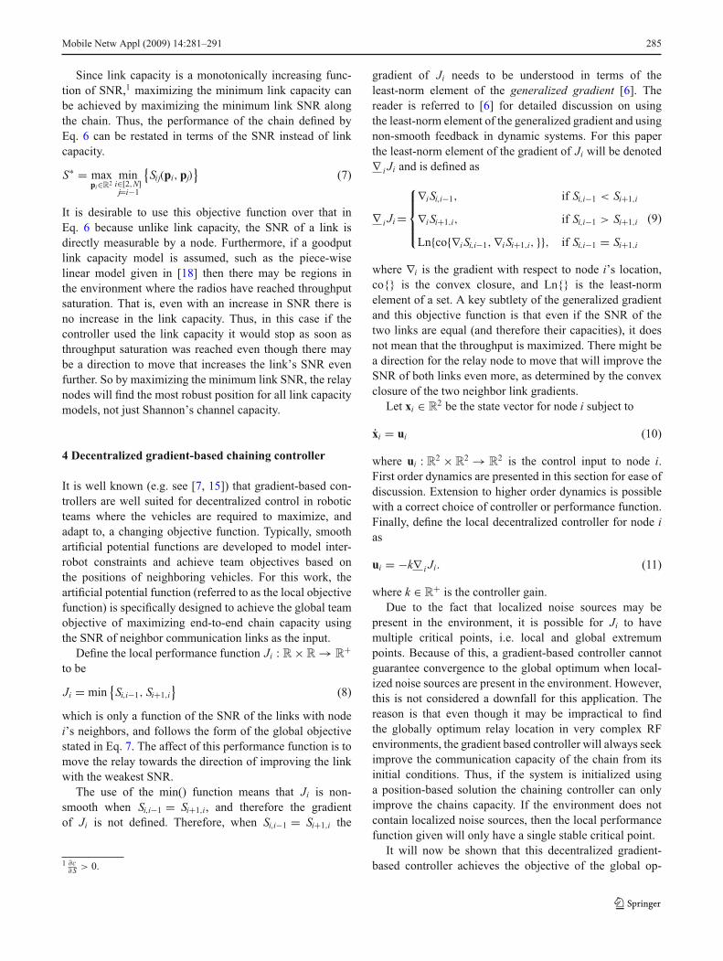
Mobile Netw Appl (2009) 14:281–291 285

Since link capacity is a monotonically increasing func-

tion of SNR,1

maximizing the minimum link capacity can

be achieved by maximizing the minimum link SNR along

the chain. Thus, the performance of the chain defined by

Eq. 6 can be restated in terms of the SNR instead of link

capacity.

S∗ = maxpi∈R2

mini∈[2,N]j=i−1

{Sij(pi, pj)

}(7)

It is desirable to use this objective function over that in

Eq. 6 because unlike link capacity, the SNR of a link is

directly measurable by a node. Furthermore, if a goodput

link capacity model is assumed, such as the piece-wise

linear model given in [18] then there may be regions in

the environment where the radios have reached throughput

saturation. That is, even with an increase in SNR there is

no increase in the link capacity. Thus, in this case if the

controller used the link capacity it would stop as soon as

throughput saturation was reached even though there may

be a direction to move that increases the link’s SNR even

further. So by maximizing the minimum link SNR, the relay

nodes will find the most robust position for all link capacity

models, not just Shannon’s channel capacity.

4 Decentralized gradient-based chaining controller

It is well known (e.g. see [7, 15]) that gradient-based con-

trollers are well suited for decentralized control in robotic

teams where the vehicles are required to maximize, and

adapt to, a changing objective function. Typically, smooth

artificial potential functions are developed to model inter-

robot constraints and achieve team objectives based on

the positions of neighboring vehicles. For this work, the

artificial potential function (referred to as the local objective

function) is specifically designed to achieve the global team

objective of maximizing end-to-end chain capacity using

the SNR of neighbor communication links as the input.

Define the local performance function Ji : R × R → R+

to be

Ji = min{

Si,i−1, Si+1,i}

(8)

which is only a function of the SNR of the links with node

i’s neighbors, and follows the form of the global objective

stated in Eq. 7. The affect of this performance function is to

move the relay towards the direction of improving the link

with the weakest SNR.

The use of the min() function means that Ji is non-

smooth when Si,i−1 = Si+1,i, and therefore the gradient

of Ji is not defined. Therefore, when Si,i−1 = Si+1,i the

1 ∂c∂S > 0.

gradient of Ji needs to be understood in terms of the

least-norm element of the generalized gradient [6]. The

reader is referred to [6] for detailed discussion on using

the least-norm element of the generalized gradient and using

non-smooth feedback in dynamic systems. For this paper

the least-norm element of the gradient of Ji will be denoted

∇ i Ji and is defined as

∇ i Ji =

⎧⎪⎪⎨

⎪⎪⎩

∇i Si,i−1, if Si,i−1 < Si+1,i

∇i Si+1,i, if Si,i−1 > Si+1,i

Ln{co{∇i Si,i−1, ∇i Si+1,i, }}, if Si,i−1 = Si+1,i

(9)

where ∇i is the gradient with respect to node i’s location,

co{} is the convex closure, and Ln{} is the least-norm

element of a set. A key subtlety of the generalized gradient

and this objective function is that even if the SNR of the

two links are equal (and therefore their capacities), it does

not mean that the throughput is maximized. There might be

a direction for the relay node to move that will improve the

SNR of both links even more, as determined by the convex

closure of the two neighbor link gradients.

Let xi ∈ R2

be the state vector for node i subject to

xi = ui (10)

where ui : R2 × R

2 → R2

is the control input to node i.First order dynamics are presented in this section for ease of

discussion. Extension to higher order dynamics is possible

with a correct choice of controller or performance function.

Finally, define the local decentralized controller for node ias

ui = −k∇ i Ji. (11)

where k ∈ R+

is the controller gain.

Due to the fact that localized noise sources may be

present in the environment, it is possible for Ji to have

multiple critical points, i.e. local and global extremum

points. Because of this, a gradient-based controller cannot

guarantee convergence to the global optimum when local-

ized noise sources are present in the environment. However,

this is not considered a downfall for this application. The

reason is that even though it may be impractical to find

the globally optimum relay location in very complex RF

environments, the gradient based controller will always seek

improve the communication capacity of the chain from its

initial conditions. Thus, if the system is initialized using

a position-based solution the chaining controller can only

improve the chains capacity. If the environment does not

contain localized noise sources, then the local performance

function given will only have a single stable critical point.

It will now be shown that this decentralized gradient-

based controller achieves the objective of the global op-

286 Mobile Netw Appl (2009) 14:281–291

timization problem by showing the set of critical points

of Ji correspond to the locations that maximize Eq. 7. Let

X = [x1, x2, · · · , xn]T, and U = [u1, u2, · · · , un]T

such that

X = U. (12)

Since ∇i Si,i−1, ∇i Si+1,i �= 0, from Eq. 9 the critical points

of Ji are located at positions where Si,i−1 = Si+1,i. That is

∇ i Ji = 0 ⇒ Si,i−1 = Si+1,i (13)

and thus

X = 0 ⇒ S2,1 = S3,2 = · · · = SN,N−1. (14)

When all of the SNR of the individual links are equal, then

the generalized gradient of the global objective function

is equivalent to the localized gradient. That is, when

S2,1 = S3,2 = · · · = SN,N−1, and only when, then

∇S =

⎡

⎢⎢⎢⎢⎣

∇1J1

∇2J2

...

∇ n Jn

⎤

⎥⎥⎥⎥⎦

(15)

Since ∇ i Ji = 0 at this condition,

X = 0 ⇒ ∇S = 0 (16)

and therefore the set points of the decentralized controller

achieves locations of optimal relaying.

A simulation of a network consisting of two point-mass

robotic relays is presented in Fig. 2 to show the response of

the system following the chaining controller. In the simula-

tion, the two relay nodes are initialized close to the location

of the destination node, modeling the initial deployment

of the relay nodes from a base station the desires higher

bandwidth communications from the source node. Without

the presence of the localized noise source, the controller

deploys the relays to the nominal range based positions,

indicated by the circles, as these are the optimal locations

when there is no localized noise sources. When then noise

source is introduced at t = 250 s, the robots sense the

change in the SNR field and bend around the source to

maximize the chain throughput. The final location of the

relay nodes is indicated by the diamonds. The time plots

on the right of the figure show that the chaining controller

is able to improve the capacity of the communication chain

significantly above that of the range-based solution, indi-

cated by the dashed line.

5 Electronic chaining ES controller

It was shown in the previous section that if the local gradi-

ents are known by the nodes, then a decentralized controller

(based on the localized gradients) can be used to drive

individual nodes to their globally optimal relaying locations.

However, in a physical environment with unknown local-

ized noise sources, either due to faulty nodes or active jam-

ming, the structure of the SNR field is impossible to predict,

and therefor the gradient can not be directly determined. A

way to estimate the gradient of the performance objective in

real-time, and by each mobile node, is required so that the

system may be driven to optimal operating positions (set

points).

ES [2] controllers are adaptive, model-free controllers

designed to drive the set point of a dynamic system to

an optimal, but unpredictable location defined by a perfor-

500 1000 1500 2000 2500 3000 3500 4000 4500 5000

500

1000

1500

2000

2500

3000

3500

Source Dest

R 1R 2

Noise

X – Position [m]

Y –

Po

siti

on

[m

]

0

10

20

30

40

Lin

k S

NR

[d

Bm

]

0 100 200 300 400 500

Link 1Link 2Link 3

0

50

100

150

200

Ch

ain

Cap

acit

y [M

bp

s]

0 100 200 300 400 500

Time [s]

GradientRange–BasedDirect

Figure 2 Simulation of a planar cascaded relay network using two

point-mass robotic relay nodes. At time t = 250 s a jamming noise

source is introduced showing the ability of the gradient controller to

react to changes in the RF environment and improve the capacity

above that of a range-based solution

Mobile Netw Appl (2009) 14:281–291 287

mance function that is only known to have an extremum

point. That is, given a sufficiently smooth cost function

J: R × Rm → R, ES controllers seek to solve in real time

the optimization problem

θ∗(t) = arg maxθ∈Rm

J(t, θ) (17)

where J is an unknown, possibly time varying, cost function

of the input parameter θ such that Dθ J (t, θ∗) = 0 and

D2

θ J(t, θ∗) < 0.2

The standard ES algorithm works by generating a mea-

sure of the local gradient of the mapping J(θ) by injecting a

perturbation signal, α cos(ωt), directly into the plant. The

output of the plant will also be sinusoidal, with a DC

(or constant) offset that the HPF removes. This signal is

then demodulated by β sin(ωt − γ ) and low-pass filtered to

obtain the gradient estimate. The gradient estimate is then

used to update the estimate of the optimal location, θ . See

[1, 2] for formal discussions, including stability proofs and

design guidelines, on single and multivariable ES.

In two dimensions, the input into the performance func-

tion has the appearance of a circular perturbation about

a moving (i.e. time varying) orbit center point. It is this

specific structure that the ES algorithm presented in this

paper takes advantage of in that some vehicles, like UA,

also exhibit a cyclic (circular) motion about an orbit center

point when they are station keeping since they must always

maintain a forward speed.

A block diagram of the decentralized ES chaining algo-

rithm is shown in Fig. 3 and consists of a LGVF Controller

steering a 2D kinematic vehicle operating within an ad hoc

network. The basic ES framework within the controller is

used to estimate the gradient of the communication perfor-

mance field that is used to drive the motion of the orbit

center point for the LGVF controller using virtual point

mass dynamics with a bounded center point velocity.

The most significant difference in the design of this ES

algorithm is that it is a self-exciting system. That is, there

is a natural limit cycle that persists in the system (the

orbital motion of the vehicle) and this limit cycle provides

the required dither signal into a measurable performance

function. Because the limit cycle that exists due to the

plant dynamics generates the sinusoidal dither signal, the

performance and stability of the controller are dependent

upon the performance capabilities of the vehicle. Thus to

maintain stability of the ES chaining algorithm, appropriate

values for the ES filters, the ES feedback gain kES, and the

maximum center point velocity must be designed for each

different vehicle type with different performance abilities.

2 Diθ (·) denotes the ith directional derivative of J w.r.t. θ .

Figure 3 Decentralized ES algorithm for a 2D kinematic vehicle

using a LGVF controller to provide the orbital motion of the vehicle

about a virtual center point driven by the gradient estimate of the

performance of a communication chain

5.1 Kinematic vehicle model

It is assumed that the robotic nodes in the network are

equipped with a low-level control system that presents a 2-

D kinematic model for use by the higher-level ES algorithm.

Let pj ∈ R2, denoted as pj = [xj, yj]T

, be the position of vehi-

cle jwith inertial speed [xj, yj]T ∈ R2

that evolves according

to the standard (Cartesian) bicycle-like kinematic model

xj = vjcos ψj

yj = vjsin ψj (18)

ψj = vj cj

where [xj, yj]T ∈ R2

is the two-dimensional inertial position

of node j, ψj ∈ [0, 2π) is the track angle (compass heading),

vj is the commanded speed (held constant), and cj is the

bounded path curvature. The bicycle kinematic model is

chosen over a unicycle model because this model covers a

wider class of 2D nonholonomic vehicles, moving in only

a forward direction and that cannot turn on the spot, such

as bicycles, cars, and autonomous underwater and aerial

vehicles [12].

It should be noted that the major difference of the

bicycle-like model from the unicycle model is that the head-

ing rate is a function of the vehicle speed and the curvature

constraints of the vehicle. For bicycles, the curvature is

related directly to the steering angle of the front wheel.

For an aircraft in a steady-state coordinated turn, the path

curvature is

c(v) = g tan φ

v2, (19)

where φ is the aircraft bank angle and g is the gravitational

constant.

Due to vehicle performance constraints, the path curva-

ture for a vehicle is bounded by upper and lower limits. For

an aircraft at a speed v,

ωmax(v) = g tan φmax

v(20)

288 Mobile Netw Appl (2009) 14:281–291

where φmax is the maximum bank angle of the vehicle at

speed v. Thus the steering input into vehicle j is bounded

such that

∣∣uj

∣∣ ≤ ωmax and gives a minimum orbital radius of

rmin(v) = v

ωmax(v). (21)

For bicycles and car-like vehicles, the path curvature bound

is directly related to the physical limitations in the motion

of the steering wheels.

This minimum radius, as will be seen later, is the effec-

tively the lower bound on the final error (or distance) of

the vehicle from the optimal communication location, which

will be the location of orbit center point for the loiter circle.

While the orbit center point can be driven to the location of

optimal communication, the robotic relay will always be at

best no closer than rmin.

Because of the wide range of dynamics and physi-

cal constraints of different types of robotic nodes, it is

not practical to drive the vehicle speed or heading di-

rectly by the ES dither signal as done in [23]. Instead a

Lyapunov guidance vector field (LGVF) controller is used

to drive the vehicle to an orbital (limit cycle) motion about

a center point. The center point is then driven with virtual

point mass dynamics by the ES framework in the chaining

algorithm.

5.2 Lyapunov guidance vector field controller

To provide the sinusoidal perturbation signal required by

the ES framework. A LGVF controller [9] is used to drive

the vehicle to a circular limit cycle about a virtual center

point, pcp ∈ R2. Since the vehicle is orbiting pcp, the ES

framework does not drive the vehicle directly to the optimal

communication location, but instead pushes pcp to the op-

timal communication location that the vehicle orbits about

using the LGVF controller.

The LGVF controller is split into two components, a

guidance vector field generator and a heading tracker (HT)

controller. The HT drives the robotic relay to the desired

loiter circle at a radial distance of rd from the orbit center

point pcp = [xcp, ycp]Tas given by the generated vector field

f (pr) =[

xd

yd

]

= β

[−(

r2 − r2

d) −2rrd

−2rrd −(r2 − r2

d)

][x − xcp

y − ycp

]

(22)

+[

xcp

ycp

]

where r2 = pr · pr = (x − xcp

)2 + (y − ycp

)2

is the squared

radial distance of the UA from the loiter center point, pcp, β

is a non-negative scalar that guarantees convergence to the

desired loiter circle when the center point is moving [9], and

vcp = [xcp, ycp]Tis the center point velocity.

The guidance vector field gives the desired velocity,

which is used to generate a turn rate command to the vehicle

through the HT. Let eψ = ψ − ψd where ψd is the desired

compass heading given as

ψd = arctan

(yd

xd

). (23)

The heading angle error is driven to zero by the turn rate

command

ω = ψd − λ · (ψ − ψd) (24)

where

ψd = v

rd. (25)

This controller is globally stable limit cycle about pcp and is

stable for any value of vcp. However, since it is assumed that

the vehicles have bounded turn rate capabilities, rd should

be chosen such that rd > rmin.

5.3 Center point dynamics

For the ES framework to be stable, and to generate the

appropriate gradient estimate, the system needs to exhibit

three different time scales [14]:

1. Fast – tracking of the center point

2. Medium – the orbital motion

3. Slow – the LPF filter in the ES

Since the amplitude and excitation frequency of the pertur-

bation signal are set by v and rd, the fast and slow dynamics

must also be functions of the vehicle performance. Due to

the speed constraints placed on the dynamics of the center

point, the convergence rate of the center point to the optimal

location is bounded by the maximum speed of the center

point.

For the error dynamics of the center point to be fast,

and to maintain the cyclic orbit about the center point, the

motion of the center point must be slow as compared to

the speed of the vehicle, i.e. vcp << vj . In the ES chaining

algorithm the center point velocity is bounded by Vcp so that

vcp ≤ Vcp and Vcp << vj.

It should be pointed out that center point velocity satu-

ration is required in the loop because even though we can

choose k small enough that the speed of the orbit center

point remains slow, as compared to the UA for a given

environment and performance function, the output of the

ES framework depends upon the magnitude and shape of

the performance function, which is not necessarily known

a priori. Thus, there could be unexpected environments in

Mobile Netw Appl (2009) 14:281–291 289

which if the center point speed was not bounded, it could

reach the maximum flight speed of the aircraft. At this point,

the motion of the UA about the center point is no longer

cyclic and is not generating the periodic perturbation signal

of the performance function required for the ES framework

to generate the gradient estimate.

6 Electronic chaining simulations

Since this work is motivated by our AUGNet [5] research

into networks that combine ad hoc networks with UA acting

as airborne communication relays, this section presents sim-

ulations of the decentralized ES chaining controller running

on UA. The performance of the aircraft and the radios are

modeled off of values taken from AUGNet experiments. For

the simulations, the aircraft are limited to a maximum 30

degree bank angle, flying at 25 m/s, and their ordering is

preset and maintained depending upon the starting location

of the UA. The maximum center point velocity is set to

5 m/s.

Though it is not know by the ES controller, the radios in

the simulation are assumed to follow the standard exponen-

tial decay model

Pij = Pji = Krd−αij (26)

where Kr is the link gain, dij is the separation distance of

the receiver from the transmitter, α is the exponential decay

rate, and Pij is the received power. The radio values are

set to Kr = 3822 and α = 3.5. For the simulation with a

noise source, the noise source is taken to be a faulty radio

transmitting with Kr = 382. Note, the choice of using the

exponential decay model was for ease of programming in

the simulation. However, by assuming that the noise source

is a faulty radio that is acting as a jamming node, even in the

simulation the SNR models are no longer concentric circles

about the radio nodes. Instead, depending upon the power

and location of the noise source, the SNR contour lines are

extremely skewed and non-symmetric.

Figure 4 shows results from a simulation with a single

UA, two end nodes and no localized no source. In Fig. 4a,

the position of the orbit center point is shown as a dashed

line within the cyclic orbital flight path of the UA. From this

figure one can see that when the UA was far away, it headed

directly in the direction of improving the minimum SNR

(which is the SNR from the far right node) at the maximum

speed of the center point. Figure 4b shows just the X-Y

position of the orbit center point is shown to highlight the

bounded convergence rate of the ES algorithm. For t ∈(50, 500) s the positional errors (especially on the Y-axis)

show the bounded convergence rate due to the bounded

center point speed.

Figure 5 shows a simulation run with three UA and two

static end nodes. At the beginning of the simulation, the

UA relays are aligned along the chain as would be a result

of running a position based controller. At time t = 0 s a

noise source located at [2500,1000] m is introduced. Since

position based controllers would not sense the change in

the RF environment, the nodes would maintain their current

position. However, using the electronic chaining algorithm

the figure shows that the UA react appropriately to the

jamming signal source and form a bowed communication

chain. Figure 5b shows that at t = 0 s the minimum SNR at

the orbit center points along the communication chain was

less then 19 dBm and that the electronic chaining controller

was able to improve the minimum value to above 24 dBm

by moving the location of the vehicles orbit center point.

Again, it is worth pointing out that in the simulation the

gradient of the SNR field is estimated on-line using the

500 1000 1500 2000 2500 3000 3500 4000 4500

0

500

1000

1500

2000

2500

3000

35

40

45

50

55

60

35

40

45

50

60Node 1

UAV 1

UA Locations over Time

X–Position [m]

Y–P

osi

tio

n [

m]

0 500 1000 15001000

1500

2000

2500

3000UA Orbit Point Locations over Time

XP

osi

tio

n [

m]

0 500 1000 15002000

2200

2400

2600

2800

3000

Time [s]

Y

Po

siti

on

[m

]

Node 2

a b

Figure 4 Simulation of a single UA airborne relay between two static nodes without any localized noise source. The motion of the center point

is the dashed line with the orbital motion of the UA required for the ES framework

290 Mobile Netw Appl (2009) 14:281–291

500 1000 1500 2000 2500 3000 3500 4000 4500 5000

500

1000

1500

2000

2500

3000

3500

Noise Source

10

1520

2530

35

40

10

15

20

25

30

3540

4Node 1 Node 2UAV 1 UAV 2 UAV 3

UA Locations over Time

X–Position [m]

Y–P

osi

tio

n [

m]

0 200 400 600 800 1000 1200 1400 1600 1800 200018

19

20

21

22

23

24

25Minimum SNR at Orbit Center

Time [s]

Min

SN

R [

dB

m]

a b

Figure 5 Simulation of three UA relay nodes reacting to a localized noise source. Motion of UA within the environment is also shown with the

noise source location and the SNR contours of the two end nodes

motion of the vehicle and the change in the measured SNR

values.

7 Limitations & future work

The decentralized controller based on the gradient of the

SNR field is shown to maximize the capacity of a cascaded

relay network with simultaneous transmission and reception

of RF signals. However, this is not a common network used

on cheap and inexpensive robots. While it is an appropriate

model for use on a single airborne relay using a repeater

network, as in the case of wildland firefighters, to be more

general a different performance function is required for

packetized networks such as 802.11b. In these networks,

each hop along the chain adds to the total delay of the

system and maximizing the link with the minimum SNR

does not necessarily maximize the end-to-end chain capac-

ity. Current work by the authors is in finding a local per-

formance function that has a spatially distributed gradient

mapping to be used for different types of packet based

networks.

A limitation of the ES frameworks is that cyclic motion

of the vehicle must be maintained to sustain an estimate of

the positional gradients required. For the application of this

work on using UA as communication relays, this is not a

problem since aircraft must maintain forward flight speed

and the most natural motion is to maintain an orbital flight

pattern for acting as a communication relay. In fact, this nat-

ural cyclic motion of a UA flying orbits to station keep is a

unique benefit to aircraft and was the original motivation for

using ES methods. However, in the application of this work

to cheap robots with limited battery power this continual

motion to estimate the gradient will simply require too much

power to sustain. A more general solution will need to take

into account the benefit of updating the gradient estimate to

the cost of the motion.

8 Conclusion

In this paper a definition of an optimal communication

chain of relay nodes in an ad hoc network was presented

based on the SNR instead of relative position. By using the

SNR instead of position, a communication chain of robotic

relays can respond to changes and unexpected features in

the RF environment that is not possible with position based

chaining solutions. Since the operating environment is gen-

erally not known a priori to deployment of a network, an

adaptive model-free ES chaining algorithm was presented

to control the motion of 2D nonholonomic vehicles acting

as communication relays. Even without specific knowledge

of the SNR field, the ES algorithm is able to drive the

team of vehicles to an optimal locations with only local

measures of the SNR. The mobility of the vehicle was

modeled as a bicycle-like kinematic model and is chosen

because the model covers a wider class of 2D nonholonomic

vehicles, including UA. An orbital motion of the vehicle

due to a LGVF controller was applied to ES in a unique

way in that the orbital motion of the vehicle about an orbit

center point generated the dither and demodulation signals

required by the ES algorithm. A specific application using

UA was simulated to highlight the focus of this work in

using UA as airborne communication relays. Even though it

is realized that this work may have limitations, the gradient-

based controller presented in the ES framework provides a

Mobile Netw Appl (2009) 14:281–291 291

means for a robotic team to find and maintain an optimal

cascaded communication chain.

References

1. Ariyur K, Krstic M (2002) Multivariable extremum seeking feed-

back: analysis and design. In: Fifteenth international symposium

on mathematical theory of networks and systems, Notre Dame,

12–16 August 2002

2. Ariyur KB, Krstic M (2003) Real-time optimization by extremum-

seeking control. Wiley, New York

3. Basu P, Redi J (2004) Movement control algorithms for realization

of fault-tolerant ad hoc robot networks. IEEE Netw 18(4):36

4. Beard RW, Stepanyan V (2003) Synchronization of information in

distributed multiple vehicle coordinated control. In: IEEE confer-

ence on decision and control, IEEE, Maui, December 2003

5. Brown TX, Argrow B, Dixon C, Doshi S, Thekkekunnel

R-G, Henkel D (2004) Ad hoc uav ground network (augnet). In:

AIAA 3rd “Unmanned unlimited” technical conference, AIAA,

Chicago, 20–23 September 2004

6. Clarke FH (1975) Generalized gradients and applications. Trans

Am Math Soc 205:247–262, April

7. Cortes J, Martinez S, Karatas T, Bullo F (2004) Coverage

control for mobile sensing networks. In: IEEE transactions

on robotics and automation. IEEE, Piscataway, May 2002,

pp 1327–1332

8. Dubins LE (1957) On curves of minimal length with a constraint

on average curvature, and with prescribed initial and terminal

positions and tangents. Am J Math 79(3):497–516, July

9. Frew EW, Lawrence D (2005) Cooperative stand-off track-

ing of moving targets by a team of autonomous air-

craft. In: AIAA guidance, navigation, and control conference,

San Francisco, August 2005

10. Gerkey BP, Mailler R, Morisset B (2006) Commbots: distributed

control of mobile communication relays. In: Proc. of the AAAI

workshop on auction mechanisms for robot coordination (Auc-

tionBots). Boston, July 2006, p 5157

11. Goldenberg D, Lin J, Morse AS, Rosen BE, Yang YR (2004)

Towards mobility as a network control primitive. In: Mobihoc ’04.

ACM, Tokyo, 24–26 May 2004

12. Indiveri G (1999) Kinematic time-invariant control of a 2d non-

holonomic vehicle. In: 38th Conference on decision and control

(CDC’99), Phoenix, December 1999

13. Kramer G, Gastpar M, Gupta P (2005) Cooperative strategies

and capacity theorems for relay networks. IEEE Trans Inf Theory

51(9):3037–3063, September

14. Krstic M, Wang HH (2000) Stability of extremum seeking feed-

back for general nonlinear dynamic systems. Automatica 36:595–

601

15. Martinez S, Cortes J, Bullo F (2007) Motion coordination with

distributed information. IEEE Control Syst Mag 27(4):75–88, Au-

gust

16. Olfati-Saber R, Murray RM (2003) Flocking with obstacle avoid-

ance: cooperation with limited information in mobile networks. In:

Conference on decision and control (CDC), Maui, December 2003

17. Pezeshkian N, Nguyen HG, Burmeister A (2007) Unmanned

ground vehicle radio relay deployment system for non-line-of-

sight operations. In: IASTED robotics and applications (RA 2007),

Würzburg, 29–31 August 2007

18. Rappaport TS, Na C, Chen J (2004) Application through-

put measurements and predictions using site-specific infor-

mation. In: IEEE 802.11 plenary session, IEEE doc. 802.

110-04-1473-00-000t, 17 November. IEEE, Piscataway

19. Sweeney J, Brunette T, Grupen YYR (2002) Coordinated teams of

reactive mobile platforms. In: International conference on robotics

and automation, IEEE, Washington, DC, 11–15 May 2002

20. Taub B, Schilling DL (1986) Principles of communication sys-

tems. McGraw-Hill, New York

21. Yang L, Passino KM, Polycarpou M (2003) Stability analysis

of m-dimensional asynchronous swarms with a fixed com-

munication topology. IEEE Trans Automat Contr 48(1; ana-

lyzed. Such stability analysis is of fundamental importance):

76–95, December

22. Zajkowski T, Dunagan S, Eilers J (2006) Small uas com-

munications mission. In: Eleventh biennial USDA forest ser-

vice remote sensing applications conference, Salt Lake City,

24–28 April 2006

23. Zhang C, Arnold D, Ghods N, Siranosian A, Krstic M

(2006) Source seeking with nonholonomic unicycle without

position measurement—part i: tuning of forward velocity. In:

45th IEEE conference on decision and control, San Diego,

13–15 December 2006