Maintaining a Cognitive Map in Darkness: The Need to Fuse Boundary Knowledge with Path Integration

Maintaining a Cognitive Map in Darkness: The Need toFuse Boundary Knowledge with Path IntegrationAllen Cheung1*, David Ball2, Michael Milford2, Gordon Wyeth2, Janet Wiles3

1 The University of Queensland, Queensland Brain Institute, Brisbane, Queensland, Australia, 2 Queensland University of Technology, School of Electrical Engineering and

Computer Science, Science and Engineering Faculty, Brisbane, Queensland, Australia, 3 The University of Queensland, School of Information Technology and Electrical

Engineering, Brisbane, Queensland, Australia

Abstract

Spatial navigation requires the processing of complex, disparate and often ambiguous sensory data. The neurocomputa-tions underpinning this vital ability remain poorly understood. Controversy remains as to whether multimodal sensoryinformation must be combined into a unified representation, consistent with Tolman’s ‘‘cognitive map’’, or whetherdifferential activation of independent navigation modules suffice to explain observed navigation behaviour. Here wedemonstrate that key neural correlates of spatial navigation in darkness cannot be explained if the path integration systemacted independently of boundary (landmark) information. In vivo recordings demonstrate that the rodent head direction(HD) system becomes unstable within three minutes without vision. In contrast, rodents maintain stable place fields andgrid fields for over half an hour without vision. Using a simple HD error model, we show analytically that idiothetic pathintegration (iPI) alone cannot be used to maintain any stable place representation beyond two to three minutes. We thenuse a measure of place stability based on information theoretic principles to prove that featureless boundaries alone cannotbe used to improve localization above chance level. Having shown that neither iPI nor boundaries alone are sufficient, wethen address the question of whether their combination is sufficient and – we conjecture – necessary to maintain placestability for prolonged periods without vision. We addressed this question in simulations and robot experiments using anavigation model comprising of a particle filter and boundary map. The model replicates published experimental results onplace field and grid field stability without vision, and makes testable predictions including place field splitting and grid fieldrescaling if the true arena geometry differs from the acquired boundary map. We discuss our findings in light of currenttheories of animal navigation and neuronal computation, and elaborate on their implications and significance for thedesign, analysis and interpretation of experiments.

Citation: Cheung A, Ball D, Milford M, Wyeth G, Wiles J (2012) Maintaining a Cognitive Map in Darkness: The Need to Fuse Boundary Knowledge with PathIntegration. PLoS Comput Biol 8(8): e1002651. doi:10.1371/journal.pcbi.1002651

Editor: Olaf Sporns, Indiana University, United States of America

Received February 17, 2012; Accepted June 21, 2012; Published August 16, 2012

Copyright: � 2012 Cheung et al. This is an open-access article distributed under the terms of the Creative Commons Attribution License, which permitsunrestricted use, distribution, and reproduction in any medium, provided the original author and source are credited.

Funding: This work was partly supported by a grant from the ARC Special Research Initiative on Thinking Systems (TS0669699). The funders had no role in studydesign, data collection and analysis, decision to publish, or preparation of the manuscript.

Competing Interests: The authors have declared that no competing interests exist.

* E-mail: [email protected]

Introduction

A ‘‘Cognitive Map’’ Is Multimodal but Not ModularIn 1948, Tolman employed two analogies to describe the

prevailing classes of models used to explain the experimental data

on maze navigation and learning obtained from rats [1]. Tolman

likened the stimulus-response class of models to an old fashioned

telephone exchange, where incoming calls are linked via con-

necting switches to outgoing messages. Stimulus-response connec-

tions which result in reward are strengthened. In contrast, Tolman

was a proponent of the field theoretic or cognitive map class of

models, in which the telephone switchboard was replaced by a

‘‘map control room’’. Tolman asserted that sensory inputs ‘‘are

usually worked over and elaborated in the central control room

into a tentative, cognitive-like map of the environment’’. The core

issue seems to be whether animals (including humans) acquire and

use a unified, multimodal spatial representation for navigation.

Alternatively, can a model without a cognitive-like map of the

environment explain animal navigation data?

One of the most ubiquitous navigation strategies in the animal

kingdom is path integration (PI), a process by which an animal

uses an estimate of self-motion to update its location estimate

[2–4]. PI works in principle under most environmental conditions.

There is abundant theoretical and experimental evidence that PI

requires stable allothetic directional information in combination

with idiothetic motion cues [5–11]. Hence in general, PI is likely to

be a multimodal process which combines a mix of information

from vision, proprioception, vestibular or inertial organs, motor

efference copy, and other sources depending on species. Therefore

that the PI state is itself a multimodal representation. For example,

it was recently shown in humans that PI output depends on a

combination of visual and idiothetic motion cues in combination,

not independently [12]. Clearly, experimental data is consistent

with the multimodality property of a ‘‘cognitive map’’.

However, it is conceivable that a representation of the world is

multimodal and yet modular, and hence fragmented. Recently, an

insect-inspired model was proposed in which the navigation system

consisted of independent modules [13]. During navigation, each

active module produced a directional output, which fed into a

recurrent neural network to output an overall heading direction.

Behaviours such as shortcutting and landmark-guided homing

were successfully explained using this model. Importantly, the

PLoS Computational Biology | www.ploscompbiol.org 1 August 2012 | Volume 8 | Issue 8 | e1002651

authors argued that by maintaining modularity, this model did not

require a ‘‘map control room’’ and hence did not resort to a

‘‘cognitive map’’ to explain a number of important navigation

behaviours which have previously been used to argue in favor of a

‘‘cognitive map’’ [1,14–17]. Once acquired, a fragmented neural

representation of the world seemed sufficient for effective

navigation.

The above model highlights the distinction between a

‘‘cognitive map’’ and ‘‘map information’’ i.e., the ability to

deduce position of an animal or landmarks from a neuronal

ensemble code does not guarantee the existence of a ‘‘cognitive

map’’. It is possible to infer current position from either the PI

module or landmark units of [13], and even reconstruct an

approximate map of the traversed environment. Hence ‘‘map

information’’ was clearly present in the model, despite the

absence of a unified ‘‘cognitive map’’.

An important aspect of the ‘‘cognitive map’’ debate is where an

animal’s neural system lies along a spectrum spanning complete

modularity to full information fusion. In simplistic terms, one may

consider neural systems and neural models as being less or more

‘‘map-like’’ according to the degree of information fusion.

Focusing on this one aspect of the complex debate, it is clear

that even the navigation modules of [13] implicitly assume

information fusion from various sensory channels, and may be

considered as having some map-like characteristics. On the other

hand, there is clear anatomical and functional evidence for

information segregation within both vertebrate and invertebrate

brains, suggesting that full information fusion is neither necessary

nor advantageous.

In this paper, we focus on whether navigation modules as per

[13] can, at least in principle, be used for effective navigation

inside arenas with featureless boundary walls, in the absence of

visual cues. Furthermore, we determine whether or to what extent

fusion of iPI and boundary information may improve localization

under these challenging conditions.

The Difficulty of Understanding Visual NavigationMost behavioural and in vivo recording navigation experiments

are conducted under light. Information from visual directional

cues may lead to superior accuracy and precision in localization

and navigation simply by allowing more accurate PI (see later).

Moreover, the advantage of using visual cues is inextricably

confounded by the fact that other spatial information is also

implicitly present in visual scenes. In both real and simulated

arenas, rat-like navigation behaviours may be replicated without

explicitly extracting any spatial layout information about the

arena, simply by storing and comparing low resolution views

[18,19]. Therefore, the presence of visual information may

improve navigation performance in a number of interrelated

ways, including PI performance. To circumvent this complication,

we focus on a subset of experimental scenarios where visual

information is absent or minimized.

The Difficulty of Path Integration without VisionPI can provide an animal with a continuous location estimate,

even when environmental cues are ambiguous or transiently

absent. In practice, PI is subject to the accumulation of errors over

time, whose error magnitude has been shown to be critically

dependent on the computations used for updating the state of the

PI system [11], as well as the directional information which is used

[8,9].

Some classes of PI models have been shown theoretically to be

intolerant to noise [11]. In general, two necessary conditions for

noise-tolerant PI are an allocentric reference frame (world-

centered), and static directional representations. An allocentric

Cartesian PI system (e.g. [20]) is one example, where the axes are

bound to world-centered directions. Importantly, there are at least

two computational subclasses which satisfy both criteria, of which

one is ‘‘ring-like’’ and one is ‘‘map-like’’ [11]. Therefore, a

‘‘cognitive-map’’ is sufficient but not necessary for accurate PI in

an open field. Conversely, the need for accurate open field PI

argues neither for or against the existence of a ‘‘cognitive-map’’.

In an open field, accurate PI using noisy idiothetic information

(termed iPI) is impossible beyond a few steps [8,9]. In contrast,

equally noisy compass information may be combined with

idiothetic speed estimation for allothetic path integration (aPI),

preserving accuracy, and with significantly smaller positional

variance [8,9]. Hence vestibular, proprioceptive and motor

efferent signals are insufficient for open field PI, whereas vision,

magnetoreception or other allothetic sensory channels are typically

required. Hence even with a ‘‘map-like’’ PI system, the absence of

visual or other compass information prevents accurate PI, raising

the question of whether iPI can be used as an effective navigation

strategy at all.

Boundaries as LandmarksPI and landmark navigation are complementary processes.

Irrespective of the sensory information or neural circuitry, PI

requires calibration by using cues in the environment to correct for

errors built up during the PI process. Here, we call any set of cues

which vary with location to be ‘‘landmarks’’. Animals can use a

wide variety of landmark cues (e.g. visual, auditory, olfactory,

tactile), which provide a mixture of positional and directional

information for a given environment. Some landmarks are

uniquely associated with a location or orientation in the world

while others are less specific. According to [13], the association of

a PI state (vector) with each independent unique landmark results

in an array of landmark units in memory which serves to guide

navigation, without requiring a ‘‘cognitive map’’.

Author Summary

Do animals need ‘‘cognitive maps’’? One of the maindifficulties in answering this question is finding a definitivescenario where having and not having a ‘‘cognitive map’’result in measurably different outcomes. Many keypredictions made by models involving some sort of‘‘cognitive map’’ can also be replicated by models withouta ‘‘cognitive map’’. Here we consider published data onrodents navigating in darkness inside homogeneousarenas. The head direction system becomes unstablewithin three minutes in darkness, yet place and grid cellshave been reported to fire in the same locations for thirtyminutes or longer. We show firstly that it is theoreticallyimplausible for path integration alone to maintain a stablepositional representation beyond three minutes, given adrifting head direction system in darkness. Secondly, weprove that even assuming perfect boundary knowledge isinsufficient to maintain a stable positional representation.Finally, we show in simulated and real arenas that a near-optimal combination of path integration and boundaryrepresentation is sufficient to produce stable positionalrepresentations in darkness consistent with publisheddata. The necessity for fusing path integration andlandmark information for accurate localization in darknessis both consistent with, and motivates the existence of,‘‘cognitive maps.’’

Maintaining a Cognitive Map in Darkness


Boundaries may be considered a subclass of landmarks cha-

racterized by their geometric nature, but not associated with one

specific point location. There is evidence that neural processing of

boundaries may differ from other landmarks [21,22]. It remains an

open question how a navigation algorithm could use boundary

landmarks which restricts an animal’s path, but which provides no

other identifying information [23]. In the present work, we focus

on the use of boundary information, not the process of its

acquisition.

Neural Correlates of Navigation AccuracyNeurons which are preferentially active in particular positions

or orientations in space provide a quantitative indicator of the

stability of the animal’s navigation system. In particular, if a

neuron exists whose activity shows spatial selectivity that is stable

over time, then it follows that computations required to maintain

stable spatial selectivity must occur somewhere in the navigation

system.

In the rodent literature, at least four major functional classes of

spatially-selective neurons have been identified. Hippocampal

place cells [24] encode the rodent’s location, cortical and

subcortical head direction cells [25,26] encode the rodent’s

orientation, medial entorhinal grid cells [27,28] encode a

multiplicity of regularly spaced rodent locations. There are also

medial entorhinal border cells [29] and subicular boundary vector

cells [30,31] which both encode the rat’s relative location to

barriers or boundaries. A subtype of the medial entorhinal grid

cells encodes pose (conjunctive location and orientation) [28,32,33].

In the presence of visual information, the functional relationships

between spatially-selective cell types are complex and intimately

related to both task and available cues (reviewed by [34–37]).

Head-Direction Tracking Is Unstable without VisionA number of rat brain regions have been identified containing

cells which represent head direction, and which form an in-

terconnected head direction (HD) system [38]. The rate at which

the HD tracking system degrades in darkness has been the subject

of several studies [39–41]. Three important properties have been

reported: 1) significant drift occurred after two minutes, 2) the

angular deviation distribution was approximately zero-mean and

symmetrical, and 3) the absolute angular deviation between

consecutive two-minute sessions did not change significantly over

time. These three observations suggest that the HD system drifts

randomly and approximately at a uniform rate in the absence of

vision.

Place Tracking Is Relatively Stable without VisionIn contrast to the head direction tracking system, place and grid

fields remain stable for half an hour or more during active

exploration in a dark environment devoid of visual cues. Rat grid

fields have been reported to remain stable in round arenas for up

to thirty minutes in darkness [28]. Blind rats can generate and

maintain stable place fields following exploration of stable

landmarks placed within a round arena [42]. However, olfactory

and tactile cues were not actively minimized in either study. In a

follow up experiment to [42], it was shown that even if odor cues

were actively removed by cleaning of the arena floor, 10% of place

fields remained stable, and about 50% remained, even over a

period of 48 minutes in darkness [43]. Similarly, mice CA1 place

fields were found to be stable in darkness in a 1.5 m diameter

circular water maze, where floor odour cues were unlikely to be

present. Place field stability was observed for two consecutive

twelve-minute sessions [44].

Taken together, the above evidence suggest that vision is not

essential for the rodent navigation system, for upwards of half an

hour. Over short distances, iPI undoubtedly plays a role in

navigation without vision [45]. However, given a head direction

system which shows appreciable error (drift) beyond the first two

minutes in darkness, can iPI explain place or grid field stability in

the medium (5–10 minutes [46,47]) to long term (.30 minutes

[28,42,43])? Alternatively, can an independent landmark module,

perhaps containing boundary information, be used to maintain

stable place fields? In fact, can any model assuming only iPI and

boundary information explain place and grid field stability in

darkness?

In summary, there is an active research field considering how PI

interacts with environmental information. However, to date we

are not aware of any studies which take a quantitative approach to

studying the errors of iPI in arenas, the information provided by

the arena geometry, or whether observed neuronal properties can

be explained without fusing iPI and boundary information.

Accurate Localization without VisionWe propose that a stable estimate of location can be maintained

by animals for over half an hour without vision, by optimally

combining idiothetic motion cues with a featureless boundary map

– akin to Tolman’s ‘‘cognitive map’’, but contrary to [13]. We first

model the accumulation of errors using only iPI. Using analytical

derivations and simulations we show this iPI model cannot

maintain place and grid field stability, assuming realistic neural

tracking accuracies. Next, we present theoretical arguments

showing that using arena boundary geometry without PI is

insufficient for localization. Together these results show that any

model which uses a modular or decentralized navigation system,

including [13], is incompatible with rodent neural data.

Finally, we show using computer simulations and robot

experiments how iPI in combination with boundary sensing and

a geometric map enables long term stability of a location estimate

in a number of arena shape configurations, demonstrating

similarity to published experimental results. We demonstrate that

the stability of simulated place fields depends on both the arena

shape and size. A number of predictions are made regarding the

behaviour of place and grid fields under environmental manipu-

lations in darkness, which depend on the way in which iPI and

boundary information is used. We discuss these results relating to

known neuronal properties, implications on mammalian naviga-

tion models, as well as the design and interpretation of

experiments.

Methods

The rationale for the models and simulations in this paper are as

follows. Firstly, we calculated the HD error based on the

assumption that the HD firing is highly correlated [25,26,38] so

that the drift in an individual HD cell’s tuning function is

representative of the error in the HD system. A simple HD model

was developed assuming independent Gaussian errors. Rat

trajectories were modelled as correlated random walks to traverse

each arena homogeneously.

Secondly, we modelled boundary information based on the

assumption that each animal had acquired an accurate metric

boundary map, prior to removal of visual cues. This ideal

assumption was used to estimate the maximum place stability

afforded by the boundary.

Thirdly, we tested the plausibility of achieving a stable repre-

sentation of place by (a) using iPI or (b) the boundary map inde-

pendently, versus (c) using a near-optimal combination of both



using a particle filter approach. We used a range of relevant

metrics to compare outcomes from each approach including a

dynamic place stability index obtained from the particle filter,

simulated place and grid fields, and direct mathematical analysis of

positional uncertainty based on principles of PI.

Since noise is inherent in sensory systems, we assumed that

when in contact with the boundary, the navigation system had a

noisy estimate of the relative angle of incidence to the boundary

tangent. Noise was incorporated to mimic measurement imper-

fections of the biological sensory systems which may be involved in

boundary detection. The addition of noise resulted in a small

decrease in the place stability of the navigation system (comparison

data not shown). We hypothesize that the whisker system may play

an important role here, but we have not explicitly modelled a

particular sensory system to simulate boundary contact.

For completeness, we also tested a fourth model (d), corre-

sponding to the hypothetical condition that the rat has a perfect

memory of the arena boundary, but cannot discern whether it is in

contact with the boundary or not. Finally, we tested the particle

filter algorithm on a robot platform (e), the iRat, as proof of

concept that the navigation model works under real world

conditions.

Simulated Rat and ArenasArena sizes and geometries were based on published experi-

ments. In all simulations, circular arenas had a 76 cm inner

diameter, corresponding to published experiments [40,42,43,46].

Unless otherwise specified, we used square arenas of the same area

(67.4 cm width) for comparison. Other rectangular arenas are

individually specified.

Since the arena walls were assumed to be homogeneous, the

simulated rat was unable to identify which wall (or wall segment) it

was close to. Therefore, wall contact information per se did not

provide positional information beyond the fact that the simulated

animal was somewhere along the boundary.

Individual rat trajectories were described by a discrete time 2D

correlated random walk model, with boundaries (Fig. 1A).

Simulated rats walked on average 5.4 m per minute. See Text

S1 for trajectory simulation details, and Video S1, Video S2 & Fig.

S9 for an example of a simulated 48 minute trajectory.

Simulated Inputs to the Rat’s Path Integration SystemThe errors in direction and speed estimates for the PI system

were modelled as Gaussian random variables. The HD system was

assumed to drift coherently but randomly, resulting in the PI

system only having access to a single erroneous estimate of head

rotation per step. From the results of [40], and the trajectory

model described above, the HD error standard deviation was

estimated to be approximately sd&3:2|10{2rad per step or

st&3:6|10{2rad per second (Text S2).

In the absence of direct experimental data, we assumed that

linear step size estimation error was normally distributed with

sl~0:2ml and independent of the angular displacement estimation

error. Note that linear displacement estimation error makes a

relatively small contribution to the overall positional uncertainty

using iPI. For example, assuming straight line navigation in an

open field using the error model described, linear errors account

for approximately 1:3|10{3% of the asymptotic rate of positional

variance increase (substituting the error model parameters into the

results of [8]).

Figure 1. Simulated rat head direction (HD) error in the absence of vision. A. Simulated 10 steps in a 76 cm diameter circular arena,showing ground truth (blue) and pure odometry (red), where cumulative HD error is modelled as a Wiener process, discretized stepwise. The particlecloud estimate of current position (grey) is also shown (see text for details of trajectory model and particle filter). The rate of error variance increasewas estimated from [40]. B. Using the same parameters as A, a frequency histogram of absolute angular drift (in u/min) from 104 random paths isshown. From this distribution, 104 samples of size 19 were randomly drawn with replacement, and 95% confidence intervals for the range minimumand maximum are shown in grey. This provides an independent comparison with [41] who reported that a sample of 19 HDCs showed an absolutedrift rate ranging from 5.1 to 26.6 u/min without vision. These results suggest that using a discretized Wiener process as a first approximation of ratHD angular drift is reasonable.doi:10.1371/journal.pcbi.1002651.g001



A Particle Filter Approximation of Ideal PositionalDistribution

A particle filter model was used to approximate the Bayes-

optimal combination of boundary and iPI information. A rat

moving randomly in an enclosed arena will make contact with the

boundary sporadically, in principle allowing it to localize to a

region close to the boundary. Wall contact can also provide

distance and orientation relative to the wall. In brief, the particle

filter approximated the pose uncertainty distribution of the

simulated rat during iPI through a population of pose estimates

(particle cloud). A particle cloud represented a finite sample from

the true pose distribution. Each particle may be considered as one

possible pose (conjunctive position and heading), and its history

may be considered as the simulation of one possible trajectory.

During iPI, the stepwise increase in true pose uncertainty was

modelled by randomly drawing values from the HD and step size

estimation error distributions described earlier, and added to each

particle’s pose.

Knowledge of the boundary limited the positional spread of the

particle distribution, while boundary contact further reduced the

unlikely particle pose estimates. Particles were weighted according

to the likelihood that their pose explained current sensory (or

memory) information, and then the particle population was

redistributed according to particle weights. The resulting particle

cloud provided a distributed estimate of current pose, having

combined arena memory and arena contact information. See Text

S3, Fig. S3 and [48] for further details.

The standard stochastic universal resampling procedure was

used to update the particle cloud. In principle, this procedure

produces a particle distribution which approaches the Bayes-

optimal posterior distribution (overviewed in Text S3). Mathe-

matically, this property is only guaranteed if the error models are

available and correct. In simulations, these error models were

assumed to be available to the rat’s navigation system. Empirically,

however, small deviations did not appear to cause large differences

in the place stability index or simulated place and grid fields. For

example, in the iRat experiments (see later), neither the wheel

odometric errors nor IR range sensor errors were precisely known.

In the particle filter variant used for the iRat, the wheel odometric

errors were overestimates, while the IR range sensor error

magnitudes were not explicitly used. The particles were effectively

ranked based on their relative consistency with sensory data, and a

fixed fraction were culled during wall contact (see Text S3 for

further details).

In those scenarios where the test arena differed from the

training arena, a variant of stochastic resampling was also used for

comparison with the standard form. The variant followed the

standard method until the final step of assigning pose to the new

particle cloud on boundary contact (see Text S3 for further

details). In this variant, only new heading was assigned, preserving

the particle’s original position estimate. When the test and training

arenas were identical, this variant was inferior at localization

compared to standard universal resampling. However, when the

two arenas differed, this particle filter variant avoided large jumps

in overall position estimates, and generated tessellating grid-like

fields in a greater number of scenarios (Results, Text S12).

Measuring Place StabilityTo provide a performance metric for the particle filter

navigation model which accounted for both accuracy and

precision, we devised a simple intuitive index of position

estimation stability, termed place stability. The mean squared

distance of the particles to the true position is affected by the

spread of the distribution (precision) and any systematic drift of the

particle cloud (accuracy). From information theoretic principles,

the baseline is assumed to be a uniform distribution of particles

throughout the arena (maximum entropy). The place stability

index at each time point is defined as

IP x,yð Þ~ SD02Dx,yT

SD02Dx,yTzSDp

2Dx,yTð5Þ

where SDp2Dx,yT is the expected squared distance of the particles

given a true current position x,yð Þ, and SD02Dx,yT is the expected

squared distance between a uniform distribution of particles and

x,yð Þ. Using squared distances results in simple analytic solutions

of SD02Dx,yT and SDP

2Dx,yT for circular and rectangular arenas

(Text S4, Table S1). A performance index of 1 implies a positional

distribution equivalent to a Dirac delta function at the true

location, while a uniformly distributed hypothesis of position

results in an index of 0.5 (chance). Indices below 0.5 may occur if

the spread of the distribution exceeds the arena area, or if there is

negative spatial correlation. The latter may occur, for example, if

the spatial representation is rotated 180u about the center of the

arena, relative to the true position.

Since the simulated rat trajectories covered the whole arena

homogeneously, it was possible to derive the expected place

stability index given boundary contacts (Text S4, Table S2).

Simulated Place FieldsTo understand how the particle cloud representation of place or

the place stability index may relate to place fields, a simple model

was used to simulate Poisson spike probabilities.

The probability of a spike following each step was modelled as a

Binomial process with p~e{r2=2s2r where r2~ xf {x

� �2

z yf {y� �2

. The spike probability decreases monotonically from

unity according to the distance r between the center of the particle

cloud and ideal firing position xf ,yf

� �. The center of the particle

cloud was treated as the center of mass or Cartesian mean, i.e.,

x,yð Þ. This is also the position which minimizes the squared

distance to all particles. In all simulations, sr~2:5 cm, corre-

sponding to the size of the pixel of analysis (e.g. [43]). The size of

sr was chosen to be sufficiently large to allow an adequate number

of spikes to be generated during a simulated experiment, while

being sufficiently small relative to the spatial resolution of the

analysis procedure so that sr did not dominate the spatial spread

of simulated spikes. Although it is somewhat arbitrary what

constitutes an adequate spike count for analysis, we aimed to have

approximately the same number of spikes as analysis pixels or

higher (788 analysis pixels in the circular arena), in the majority of

8 minute periods and field locations studied. This was to avoid

spuriously high spatial information values from low spike counts.

For instance, one spike per pixel spread randomly across half of

the analysis pixels yields a raw Skaggs spatial information content

of approximately 1 bit/spike. The latter results from a low spike

count rather than true spatial specificity.

In addition to using the Cartesian mean, place field simulations

were repeated using the polar mean for the circular arena

simulations (Fig. S5). The polar coordinates of the particles were

first averaged to give r,h� �

. Here, the angular mean

h~atanP

j sinhj ,P

j coshj

� �where atan y,xð Þ denotes the 4-

quadrant arctangent. The Cartesian coordinates of r,h� �

was used

as a substitute for x,yð Þ. The polar mean was used due to the fact

that the particle cloud distribution in circular arenas tended to

follow a crescent shape approximately aligned with the circular



boundary (discussed further in Text S9, see Video S1 & S2 for an

example). Under these conditions, the polar mean was a good

approximation of the modal position of the distribution. The

Cartesian mean was often close to or even within the concavity of

the crescent-shaped distribution, rather than near the mode. This

caused an underestimation of the radial position of the cloud.

However, the cloud distribution tended to be a convex shape in

rectangular arenas, so there was little difference between the two

methods near rectangular boundaries. The polar mean was not

used throughout the simulations because the estimation of radial

distance close to the arena center was contaminated by the spread

of the cloud (Text S9).

Over a period of time, the simulated spike pattern represents a

temporal average reflecting a sequence of complex particle cloud

states. These states in turn depended nonlinearly on the actual

trajectory taken, the boundary information gained, and random

errors. Therefore, place stability changed dynamically during each

trial, and affected the spatial specificity of the simulated spike

sequence depending on location xf ,yf

� �.

Both positional and angular specificity were quantified using

Skaggs information [49] to be comparable to published data on

place fields. A maximum likelihood factorial model [50] was

applied to check whether decoupling of positional and direc-

tional information affected the estimated spatial information

content.

Simulated Grid FieldsSince our results showed that the particle filter output had a

complex dependence on the pose distribution and wall informa-

tion, we investigated the effect of using an arena boundary

representation different to the one being traversed. This is

analogous to a change in arena size and/or aspect ratio while in

darkness.

With vision, rat grid fields have been reported to rescale when

rats are transferred between rectangular arenas of different size

and aspect ratios [51].

Grid fields were modelled as multiple independent place fields

distributed as a regular hexagonal tessellating array over the entire

training arena. Grid fields were simulated by assuming that the

firing probability was determined by rj2~ xfj

{x� �2

z yfj{y

� �2

where xfj,yfj

� �was the position of mode j of the grid field. Similar

to place fields, the firing probability of each contributing subfield

was given by pj~e{rj2=2s2

r . Following each step, the maximum

allowable number of spikes was capped at one. It was assumed the

training arena’s boundary representation remained in memory

during all tests.

The iRat – Localization in a Real Arena without VisionTo show that the derived and computer simulation results

can be applied in real environments, we used the prototype

iRat [52,53], Intelligent Rat Animat Technology robot for

experiments in real arenas (Fig. 2A). The iRat is comparable in

size and mass to a laboratory rat at 150 mm680 mm670 mm

at 0.56 kg. The iRat has a camera, speakers and microphone,

on board computation via 1 GHz PC, WLAN, and IR

(infrared) proximity sensors. The IR sensors may be considered

as providing crude ‘whisker’ information near walls. In this

study, only the three IR sensors were used to obtain three

distance estimates when close to arena walls (Fig. 2B), whereas

the camera was not used. See Text S5 for details of the iRat

experiments, and Text S3 for details on the particle filter

variant.

Results

In the following sections, we present results and analyses which

examined the feasibility of using independent iPI and landmark

modules [13] for localization without vision. We first characterized

the performance of iPI using the HD error model developed from

empirical data as described in Methods. Then we quantified the

estimation error in using only a featureless boundary for

localization, to determine whether a boundary landmark module

suffices to maintain stable navigation in darkness. Next we

combined iPI with boundary information using the particle filter

approach described in Methods, to determine whether or by how

much the estimate of position improved. Finally, a series of

unimodal and polymodal firing fields were simulated using a

particle filter to mimic place fields and grid fields under various

experimental conditions. These simulations tested whether it is

computationally plausible for observed place and grid field stability

to be maintained for 30 minutes or more using only iPI and a

featureless boundary map, given an erroneous HD system.

Limits of Idiothetic Path Integration in an Open FieldUsing the simplest description of locomotion which consists of a

turn and step, it has been shown previously that the asymp-

totic rate of increase in positional variance per step is

m2l 1zScos dTð Þ= 1{Scos dTð Þzs2

l

� ��2 where ml is the mean

step length, s2l is the variance of the step length, and d is the

angular error per step [8]. This result was derived assuming iPI

along a straight course in an open field. For a zero-mean, normally

distributed d, Scos dT~Exp {s2d

�2

� �where s2

d is the variance of

the HD angular error per step. For ease of interpretation, the

variance rates in this section are reported in terms of time rather

than steps.

Let d be the mean distance travelled per second. Since pd2 is

the area of the traversable region within one second, iPI errors are

considered irrecoverable if the positional variance increased

beyond this rate. This is because the true position may be

anywhere within an area too large to be traversed even in theory.

Note that pd2 represents a highly optimistic threshold since one

unit of positional variance encompass less than half of all possible

positions in a circular bivariate Gaussian distribution (Fig. 3A red

dotted line). For a 95% confidence region, the threshold is pd2=z2

where z~ffiffiffi2p

erf {1ffiffiffiffiffiffiffiffiffi0:95p� �

(Fig. 3A red dashed line). Even with

this correction, the threshold is optimistic since it represents the

limit of search recovery (assuming error-free search) and could not

plausibly sustain a stable place representation. Nevertheless, it

allows estimation of a loose upper bound on the time limit of the

use of iPI.

Combining the results of [8] with the HD model in our current

simulations, we determined whether it is theoretically plausible for

iPI to maintain an accurate long term estimate of position.

Assuming the HD cell error model described in Methods, without

any step length estimation error (s2l ~0), the predicted asymptotic

positional variance increased at 1:6|103d2 per second (Fig. 3A

black dashed line). Since pd2=z2vpd2

vv1:6|103d2, the

positional uncertainty increased much faster than the maximum

area which can be traversed, clearly showing that iPI cannot be

used to accurately track movement along a straight trajectory in

the long term.

In the short to medium term, positional variances of iPI

increases more slowly than the asymptotic rate [8,9]. Substituting

the HD error model parameters into the exact variance

expressions derived in [8], the optimistic limit of pd2 was exceeded

after 51 seconds (perpendicular to axis of intended locomotion),



and 192 seconds (along the axis of intended locomotion), again

demonstrating that iPI became irrecoverably inaccurate well

within 1 to 3 minutes from the start (Fig. 3A black solid lines).

Limits of Idiothetic Path Integration in an ArenaNext we considered tortuous trajectories where the intended

path had directional variance s2a (Methods and Text S1). Clearly,

a rat trained to forage within a small arena has to change direction

regularly, following a tortuous rather than straight course. This

occurs, for example, in many experiments within confined arenas.

Path tortuosity may decrease the rate of positional variance

increase in two ways. Firstly, if an iPI system is unable to track the

actual turns, then the HD error angle would be dominated by the

physical turn angle i.e., sd&sa. For the path tortuosity used in the

simulations in this work, the predicted asymptotic positional variance

increase was 6:2d2�

s (Fig. 3A green dashed line), still greater than

the conservative limit of pd2�

s. The limit of pd2 was exceeded

within 10 seconds from the start of iPI (Fig. 3A green solid lines).

Another possibility is that path structure itself influences the way

in which a small cumulative HD error sd impacts on the position

estimate. This was modelled as an unbounded correlated random

walk [6] with path directional standard deviation sa~0:5rad and

HD error sd~3:2|10{2rad . Since closed form solutions to these

variance functions are not available (but see [6] for empirical

approximations), Monte Carlo simulations were performed. The

positional variance rate remained within the limit of pd2 for nearly

eight minutes (Fig. 3A blue lines). However, the 95% confidence

interval exceeded the limit of pd2�

z2 in 88 seconds, making

accurate iPI impossible within the first one and a half minutes.

Nevertheless, an iPI system with small HD error can track a

tortuous path more accurately than a straight path, showing that

path structure itself can affect navigation performance.

Figure 2. The Intelligent Rat Animat Technology (iRat). A. Prototype iRat (left) shown next to a standard computer mouse (right). The Sharp IRsensors are oriented at 245, 0, +45 degrees relative to the midline (black rectangular components near the base of the robot, below the midlinecamera). Image obtained from [52]. B. Schematic illustration of IR sensor locations and readings. C. Flow diagram for controlling the iRat’s trajectory.doi:10.1371/journal.pcbi.1002651.g002



Inside an arena, animal paths are further constrained by the

boundary. Since boundaries force animals to make turns that they

would otherwise not need to in an open field, we expected that

positional variance would increase more slowly inside bounded

arenas, for a given baseline tortuosity of the intended trajectory.

We tested this prediction using the trajectory model described in

Methods and Text S1. The maximum average rate of position

variance increase was found to be less than 1:2|10{2d2�

s. At

first, this may seem to support iPI as a plausible process to

maintain place stability inside bounded arenas. On more careful

analysis, this was found not to be the case.

Assuming a Gaussian distribution, we found that the 95%

confidence area of the positional error distribution exceeded the

entire area of the arena by 175 seconds. To quantitatively track

the accuracy and precision of the position estimate of individual

trajectories, we used the place stability index IP (Methods, Text

S4). In a circular arena, the average IP over 103 simulations fell

below chance (0.5) within 179 seconds (Fig. 3B). Similar results

Figure 3. Place stability without vision in a circular arena. A. Predicted rate of positional variance change (DV/Dt) using iPI in an open fieldwith small HD error (sd~3:2|10{2rad , black solid lines – consistent with rat HD tuning error without vision) and moderate HD error (sd~0:5rad ,green solid lines – approximately equal to intended turns of the simulated trajectories inside experimental arenas). Asymptotic variance rates (dashedlines) are shown. From simulation (blue lines), the positional variance rates (with respect to true position) were found assuming an intendedtrajectory with moderate tortuosity (sa~0:5rad), and heading error sd~3:2|10{2rad . Limits defining navigation failure (dotted and dashed redlines) are shown. Intentional and erroneous turn distributions are Gaussian, with constant step size d . See text for further details. B. Place stabilityindex values (mean 6 s.d., 103 trials) in a circular arena of 76 cm radius. The conditions were iPI only (blue), iPI and boundary memory (green), iPI andboundary memory and contact information (red). Chance level is shown (dashed line). See Methods for details on the simulation of quasi-randomtrajectories. C. Frequency histogram of place stability values following 48 minutes without vision (colour code as per B). D. Comparison of the top10% of place stability in square (upper line) and circular (lower line) arenas, with boundary memory and boundary contact information (mean 6 s.d.,102 trials).doi:10.1371/journal.pcbi.1002651.g003



were obtained for the square arena (184 seconds - see Fig. S6B).

This means that despite a much reduced rate of increase of

positional variance, the best estimate of position afforded by iPI is

no better than chance level beyond 3 minutes. In other words, the

navigation system has no useful information about its true location

within the arena beyond 3 minutes without vision.

Taking a third approach, we quantified the maximum spatial

information of the position estimate itself, assuming a Gaussian

field centered in a circular arena, and the trajectory and HD

models described earlier. It was found that the corresponding

spatial information fell below 1 bit after 150 seconds using iPI

alone (Text S6, Fig. S1). The maximum spatial information

content of any firing field will be expected to fall below 1 bit per

spike in under 3 minutes without vision. In comparison, some

place fields in the ‘‘dark+cleaning’’ condition of [42] showed

spatial information of about 1 bit/spike or higher over three

consecutive 16 minute windows.

In summary, iPI alone cannot sustain a useful position estimate

beyond 2 to 3 minutes without vision in either open field or

enclosed arenas. Intended path tortuosity and arenas can both

reduce the magnitude of positional uncertainty, with implications

for the comparison of results obtained in confined arenas and open

fields.

Interestingly, even aPI was unable to maintain place stability or

generate a stable place field if used alone (Text S11, Fig. S7, Table

S4). Assuming the same HD error distribution as above, but reset

following each step to mimic having stable distant visual landmarks,

the time taken for the average place stability index to drop below

chance level (0.5) was increased but still unable to explain stable

place or grid fields beyond approximately 5 minutes.

Boundary Proximity Alone Is UninformativeThe rat’s navigation system was assumed to have continual

access to information about whether it was in contact with the

arena boundary or not. We investigated whether this information

alone can increase the place stability index above chance level,

assuming error-free knowledge of the arena size and shape.

When wall contact has occurred, denoted by W+, the ideal

posterior positional distribution is a narrow region along the

perimeter of the arena, since positions closer to the center of the

arena should not result in wall contact. We investigated the

possibility that this information alone may have increased place

stability above chance by finding SIPT when wall contact has

occurred. The range and expected IP values can be found

assuming a uniform sampling of the perimeter, and assuming an

idealized uniform posterior distribution following wall contact,

corresponding to the perimeter line (see Text S4 and S7 for further

details).

Under the above assumptions, in any square arena, 5=12ƒIpDWzƒ4=9 while the expected or average SIPDWzT~1=2{tan{1 1

� ffiffiffi2p� ��

6ffiffiffi2p

. For any circular arena, IPDWz~

SIPDWzT~3=7. Note that these indices are independent of arena

size. When not in contact with the boundary, denoted W2, the

animal may be anywhere within the arena giving SIPDW{T~1=2.

Thus, in the absence of PI information, the expected place

stability index does not exceed chance level (0.5) even assuming

ideal information about the arena boundary (summarized in Table

S2). Hence above-chance place stability cannot be achieved only

using arena boundary information.

An alternative interpretation of the above results is as follows.

Suppose that a randomly foraging rat occasionally contacts the

arena boundary. Mostly, the rat knows it is not at the boundary, so

its internal representation is a uniform distribution over the entire

arena, called the null position estimate. On boundary contact, its

internal representation of position becomes a uniform distribution

along the featureless boundary, called the boundary position

estimate.

We ask whether the boundary position estimate improves the

estimate of current position when the rat is actually at the

boundary. It can be shown that for all convex arena boundaries,

the estimation error is actually greater if the animal used the

boundary estimate compared to the null estimate (see Text S7 &

Fig. S2 for proof). This conclusion applies to all functions of

position estimation error which increase monotonically with the

estimation error distance. As an example, the mean squared

position estimation error of an animal at the boundary of a circular

arena using the boundary estimate is 33% larger than the null

estimate (Table S1). Therefore, using the boundary geometry

actually increases the mean squared position estimation error

compared with using the null estimate.

Localization Estimates Are Stable in Darkness UsingBoundary Memory and Wall Contact Information

Inside arenas, positional uncertainty may be modified by the

use of boundary information. Two types of information are

considered: a) boundary memory only; and b) boundary memory

plus wall contact information. The latter may be due to whiskers

or other haptic information and was assumed to provide

approximate wall distance and incident angle (Methods). In both

the circular (Fig. 3B–D) and square arena (Fig. 3D, S6B & S6D),

the average place stability index remained above chance for

48 minutes when arena boundary information was used. On

average, using wall contact information improved place stability.

In contrast, place stability dropped below chance within the first

8 minute window, in the absence of arena boundary information

(Fig. 3B, S6B blue lines). Boundary information in the square

arena consistently improved average place stability beyond that in

circular arenas. This pattern of results persisted when only the

most stable 10% of trials in the two arenas were considered

(Fig. 3D).

The average place stability indices remained above chance

level for 48 minutes without vision in both circular and square

arenas. Since it was shown earlier that neither iPI nor

boundary information alone could achieve this, the current

particle filter implementation demonstrates greater place

stability than independent iPI and boundary landmark

modules.

For completeness, we consider the possibility that an animal’s

navigation system can switch between functional modularity and

information fusion. We therefore ask whether an occasional switch

to using a modular navigation system as per [13] may still produce

a similar level of place stability, provided that optimal information

fusion occurs at all other times. It can be shown that following a

single boundary contact using a modular navigation system, the

maximum expected place stability SIPTv0:55 (proof in Text S8).

Although this value is marginally higher than chance (0.5), it is

significantly lower than near-optimal fusion of iPI and boundary

information after 48 minutes without vision (t999 = 11.17,

p,102100). Most importantly, the uncertainty distribution be-

comes a circular annulus concentric with the boundary, incom-

patible with any stable place field restricted to one sector of the

arena. This mechanism can, however, maintain a stable place field

at the center of the arena. Overall, even occasional use of a

modular navigation system causes a significant decline in place

stability, incompatible with stable place fields (other than at the

arena center).



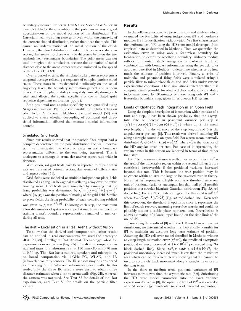
Simulated Place Fields Are Stable in Darkness UsingBoundary Memory and Wall Contact Information

Despite the higher place stability index with fused iPI and

boundary information, the average place stability decreased

continually over 48 minutes without vision in the circular arena.

This decrease was clear even when the most stable 10% of trials

were considered (Fig. 3D). We investigated whether the decreasing

place stability could support stable firing fields, using a Poisson

probability model (see Methods for details). Fig. 4A shows the

pooled average firing field generated during consecutive 8 minute

time windows, for the 10% of trials with the highest place stability

indices (to be comparable to the results of [43]). A more extensive

set of simulated place field locations are shown in Fig. S4 & S5

corresponding to using the Cartesian and polar mean, respectively,

to estimate particle cloud position (see Methods and Text S9 for

details).

During each 8-minute time window, the firing fields were

quantified using five metrics: 1) the spatial information content; 2)

the directional information content; 3) the number of spikes; 4) the

spatial correlation coefficient calculated bin by bin, relative to the

first 8-minute window; and 5) the spatial coherence [54] (Table 1).

The information content was calculated using the maximum

likelihood factorial model [50]. The bin sizes used were 2.5 cm by

2.5 cm for position and 6u for direction.

With boundary memory and wall contact information, the

spatial information content remained close to 2 bits per spike for

48 minutes without vision, while the directional information

content remained at less than 0.1 bit per spike. There was also

high field coherence and the spatial correlation remained above

0.5. Using the polar estimate of position, the spatial correlation

remained above 0.8 for all fields and time periods except those at

30 cm (Table S3). The high spatial correlation is comparable to

rat place fields in circular arenas of the same diameter, in the

presence of visual information (R = 0.70 [55]). Together, the

simulation results show that in the circular arena, stable place

fields are maintained for 48 minutes without vision, in at least 10%

of trials, similar to experiment [43].

Place fields were considered stable by [43] as those which

rotated by less than 12u between the control period and the first

test period. This was estimated by rotating fields from each time

window, about the arena center, to find the maximum spatial

correlation Rmax possible. This angular displacement, Dhmax, is

indicative of one possible way in which place fields may become

unstable. Using the same analysis method but at 1u rather than 6uresolution, and using 8-minute instead of 16-minute time windows,

we found that the most stable 10% of place fields rotated by 12u or

less between the first period of no vision, compared with each of

the subsequent periods, compatible with experiment (see also

Table S3). These results further support the current model as a

reasonable approximation of the computations carried out by the

rat navigation system.

For completeness, we tested whether boundary contact per se

was beneficial (Fig. 3B, Fig. 4B, Table 1). The same procedures

were used, but without boundary contact information. In the

absence of boundary contact information, the spatial information

content was substantially and consistently lower than with

boundary contact (see Fig. S6 and Text S10 for square arenas).

Similarly, the spatial correlation was below that of having

boundary contact information, for all time windows. In particular,

the spatial correlation for the 8–16 minutes without boundary

contact information was below that of the 40–48 minute time

Figure 4. Simulated place fields without vision in circular arenas. The average of the most stable 10% of simulated place fields are shownusing arena geometry, boundary contact and iPI information (A), using arena geometry and iPI information only (B), and using iPI only (C). All colourscales are set at a maximum value of 0.15 spikes/step.doi:10.1371/journal.pcbi.1002651.g004

Table 1. Simulated place field properties.

iPI, boundary memory and wall contact information

Property Time (minutes)

0–8 8–16 16–24 24–32 32–40 40–48

*Spatial information 2.8 2.1 2.1 2.2 2.2 1.8

*Directional information 0.053 0.052 0.062 0.044 0.039 0.055

No. Spikes 804 932 942 929 952 965

{Spatial correlation 1 0.74 0.71 0.72 0.63 0.52

Coherence 0.94 0.90 0.88 0.88 0.86 0.85

iPI and boundary memory but no wall contact information

Property Time (minutes)

0–8 8–16 16–24 24–32 32–40 40–48

*Spatial information 1.7 1.4 1.4 0.92 1.0 0.88

*Directional information 0.079 0.055 0.086 0.062 0.054 0.077

No. Spikes 506 588 531 686 715 700

{Spatial correlation 1 0.42 0.32 0.088 0.16 20.046

Coherence 0.67 0.56 0.45 0.11 0.31 0.12

*Information units in bits/spike.{Bin-wise Pearson correlation coefficient.doi:10.1371/journal.pcbi.1002651.t001



window with boundary contact information showing a significant,

immediate and persistent decline in place field correlation

compared to the first 8-minute period. The spatial firing pattern

was less stable without arena boundary contact information.

Hence boundary memory was useful in culling particles which

went outside the boundary extent, thereby limiting the growth of

the uncertainty distribution (see also Text S3). This contrasts from

pure iPI, where the particle cloud width increased without limit.

However, particles within the arena but far from the boundary

were never culled in the absence of boundary contact information,

even if their pose estimates were otherwise highly inconsistent with

the sensory information from boundary contact. Thus boundary

contact per se may be considered as providing information which,

when used appropriately, can reduce positional uncertainty

beyond that of having arena memory only.

Consistent with analyses presented earlier, simulations using iPI

alone resulted in no stable place fields (Fig. 4C). Due to extremely

low spike counts even with pooling across trials, the spatial

information content could not be estimated reliably.

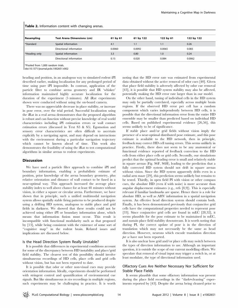
Simulated Place Fields with Changing ArenasA common experimental manipulation for testing neural and

behavioural properties in navigation tasks is to change the arena

size and shape. In simulation, this was achieved by explicitly

specifying a different arena size and/or shape to that which was

traversed. In this way, the arena in memory may be considered as

that acquired during training, while the test arena is introduced at

the beginning of each trial, at the moment when visual

information becomes unavailable.

It has been shown that some place fields established in a square

arena either stretched or split when the arena geometry was

changed [56]. More detailed analysis of the split fields showed that

the firing subfields had different modal positions depending on the

direction of travel of the rat. Although these experimental results

were obtained with vision, we tested the effect of the same arena

geometry manipulations without vision as predicted by the two

particle filter models described in Methods (Fig. 5).

Using the same place field model as described in Methods, we

tested the effect of having a different traversable arena to that

stored in memory. Directional information content was low in all

cases (Table 2).

Place field stretching or splitting was found in the three novel

test arenas, with the emergence of directional selectivity in the split

fields similar to [56]. In our simulations, the spatial information

content decreased by more than 2 bits/spike between the training

arena (61 cm by 61 cm, Fig. 5A & 5C upper left panels) and

horizontal rectangular arena (61 cm by 122 cm, Fig. 5A & 5C

upper right panels), without a concomitant change in directional

information. Hence the directional selectivity of the individual

modes of the bimodal firing field (Fig. 5B & 5D) cannot be

attributed to a change in the overall directional selectivity of the

field.

To determine whether the most recent wall contact may be

related to the pattern of firing, the frequency of each immediately

preceding wall contact was found (Fig. 5B & 5D). In both fields,

the highest frequency of recent contact was of the top wall, which

was also the nearest wall. The two particle filter variants used

yielded similar results. The largest relative differences in frequen-

cies were of recent contacts with the left and right walls with over

threefold changes consistently. In particular, during rightward

traversals (Fig. 5B & 5D upper panels) spikes were preceded most

recently by left wall contacts more frequently than right, while

during leftward traversals, (Fig. 5B & 5D lower panels) spikes were

preceded most recently by right wall contacts. These results show

that the proximity of boundaries is correlated with the relative

frequency of most recent contact, determined retrospectively from

each spike.

The marked differences in the relative frequencies when fields

are divided based on rightward versus leftward trajectories can be

explained as follows. Due to the temporal correlation of headings

along simulated trajectories, a leftward trajectory is more likely to

have recently come from the right part of the arena, and vice

versa. Therefore, a leftward trajectory was more likely to be

preceded most recently by contact with the right wall than the left

wall, and vice versa. In the results shown in Fig. 5, the arena

representation in memory was a 61 cm by 61 cm square, and the

place field was positioned 15.5 cm from the left wall and 45.5 cm

from the right wall. Therefore during testing in the 61 cm by

122 cm arena, rightward trajectories resulted in maximal firing

approximately 15.5 cm from the left wall (Fig. 5B & 5D upper

panels), while leftward trajectories resulted in maximal firing

approximately 45.5 cm from the right wall (Fig. 5B & 5D lower

panels).

When the test arena was a 122 cm by 122 cm square (Fig. 5A &

5B lower right panels), the split fields showed particularly low

spatial information content (,0.3 bits/spike) using either particle

filter variant. The low spatial specificity was due to the large

discrepancy between the dimensions of the training and test arenas

in both spatial dimensions (see Text S12 & Fig. S8 for further

details on error mechanisms).

Simulated Grid Fields with Changing ArenasWith vision, grid field spacing has previously been shown to

partially rescale along the direction of a rectangular arena which is

stretched or compressed varying with the arena geometry

transformation [43]. The rescaling factor in grid spacing was

consistently less than that of the arena rescaling. We tested the

same arena transformations using the particle filter model variants

described in Methods.

Firstly, we found that an unstable HD system (e.g. without

vision) can maintain a variety of stable grid-like firing fields, even if

the test arena differed to the training arena in geometry (Fig. 6 &

7). Secondly, using particle resetting of heading only, arena

compression caused a partial rescaling of grid spacing (Fig. 7A &

7B), in a manner qualitatively similar to that observed in vivo, with

vision. The magnitude of the partial rescaling was less than

reported (approximately 25% of the arena rescaling, compared to

48% reported by [51]).

Grid rescaling did not occur in simulations where arenas were

stretched (Fig. 6C, 6D, 7C, 7D). Instead, grid field splitting was

seen - analogous to the phenomenon of place field splitting

reported earlier.

It must be emphasized that the primary purpose of simulating

arena manipulations was to test whether it is possible for stable

place and grid fields to be maintained without vision, despite

different dimensions between the training and test arena. A

secondary goal of these simulations was to demonstrate that

specific hypotheses about the combination of iPI and boundary

information can be modelled using the particle filter approach.

The differences in results between the two variants of the particle

filter used highlights the importance of determining the precise

manner in which information is used for spatial navigation.

The iRat - A Real World DemonstrationTo demonstrate near-optimal navigation without vision in real

world conditions, we adapted the particle filter method to a mobile

robot platform, the iRat, moving in a real arena (Fig. 8). Cumul-

ative odometric errors caused a gradual drift in the estimate of



Figure 5. Simulated place fields without vision in changing rectangular arenas. Simulated place fields were generated using standardstochastic universal resampling of particle pose (A) or stochastic resampling of heading only (C), pooled from 103 random trials over 48 minuteswithout vision (see Methods). Training was assumed to occur in a square arena 61 cm in width, while testing occurred in 61 cm by 61 cm (A & C,upper left panels), 61 cm by 122 cm (A & C, upper right panels), 122 cm by 61 cm (A & C, lower left panels), and 122 cm by 122 cm (A & C, lower rightpanels) arenas. The fields in the upper right panels of A & C (61 cm by 122 cm test arena) are decomposed based on heading (B & D respectively). Theaverage firing fields are shown when the simulated rat’s heading had an allocentric easterly (B & D, upper panels) or westerly (B & D, lower panels)component (assuming upwards in each diagram is North). The percentages indicate the relative frequency of each wall being the most recentlycontacted prior to each spike in the field. The maximum firing rate is indicated for each field (spikes/step).doi:10.1371/journal.pcbi.1002651.g005



heading and position, in an analogous way to simulated rodent iPI

described earlier, making localization for any prolonged period of

time using pure iPI impossible. In contrast, application of the

particle filter to combine arena geometry and IR ‘whisker’

information maintained highly accurate localization for the

duration of the experiment (5 minutes). All iRat experiments

shown were conducted without using the on-board camera.

There was no appreciable decrease in place stability, or increase

in pose error, over the trial period. Successful localization using

the iRat in a real arena demonstrates that the proposed algorithm

is robust and can function without precise knowledge of real world

characteristics including iPI estimation errors or wall contact

estimation errors (discussed in Text S3 & S5). Egomotion and

sensory error characteristics are often difficult to ascertain

explicitly by a navigating agent, and may depend on interactions

with the environment during a particular navigation trajectory

which cannot be known ahead of time. This work also

demonstrates the feasibility of using the iRat to test computational

algorithms in similar arenas to rodent experiments.

Discussion

We have used a particle filter approach to combine iPI and

boundary information, enabling a probabilistic estimate of

position, prior knowledge of the arena boundary geometry, plus

relative orientation and distance of wall contact to be fused in a

near-optimal way. This approach increased the average place

stability index to well above chance for at least 48 minutes without

vision, in either a square or circular arena. Furthermore, we have

shown that in principle, such a unified multimodal navigation

system allows spatially stable firing patterns to be produced despite

using a drifting HD system, analogous to stable place and grid

fields in darkness. We showed that these results could not be

achieved using either iPI or boundary information alone, which

means that information fusion must occur. This result is

incompatible with functional modularity such as that proposed

by [13], while being consistent with the existence of some sort of

‘‘cognitive map’’ in the rodent brain. Related issues and

implications are discussed below.

Is the Head Direction System Really Unstable?It is possible that differences in experimental conditions account

for some of the discrepancy between HD instability and place/grid

field stability. The clearest test of this possibility should involve

simultaneous recordings of HD cells, place cells and grid cells

without vision, but has not been reported to date.

It is possible that odor or other non-visual cues may provide

orientation information. Ideally, experiments should be performed

with stringent control and quantification of environmental cue

signals. But like simultaneous in vivo recordings in multiple regions,

such experiments may be challenging in practice. It is worth

noting that the HD error rate was estimated from experimental

data obtained without the active removal of odor cues [40]. Given

that place field stability is adversely affected by odor cue removal

[43], it is possible that HD system stability may also be affected,

potentially making the HD error rate larger than in our model.

On the other hand, tuning of individual cells in the HD system

may only be partially correlated, especially across multiple brain

regions. If the observed HD error per cell has a random

component which varies independently between HD cells, it is

possible that the directional information error from the entire HD

ensemble may be smaller than predicted based on individual HD

cells. Based on published experimental evidence [26,56], this

seems unlikely to be of significance.

If stable place and/or grid fields without vision imply the

presence of a near-optimal distributed pose estimate, and this pose

estimate is available to the HD network, then in principle,

feedback may correct HD cell tuning errors. This seems unlikely in

practice. Firstly, there does not seem to be any anatomical or

functional evidence reported of feedback correction to the HD

cells from either place cells or grid cells. Secondly, our simulations

predict that the optimal heading error is small and relatively stable

in square arenas (Fig. S6F, S6H), leading to the prediction that a

fully corrected HD system should not drift in square arenas

without vision. Since the HD system apparently drifts even in a

radial arm maze [29], this prediction seems unlikely but remains to

be tested. Thirdly, in open field PI with vision or other compass

cues, the absolute HD (even if with noise) is more accurate than

angular displacement estimates (e.g., refs [8,9]). This is especially

relevant if familiar landmarks are sparse. Hence there is a role for

absolute HD, as well as AHV information in a spatial navigation

system. An effective head direction system should contain both.

Finally, it has been demonstrated previously that conjunctive grid

cells have the computational properties needed to represent pose

[33]. Since conjunctive grid cells are found in mEC [28,32], it

seems plausible for the pose estimate to be maintained in mEC,

and sustain place field stability downstream. It is worth noting that

during PI, the correct update of pose is in the direction of

translation which may not necessarily be the same as head

direction. However, neurons which encode translation direction

per se have not been reported.

It is also unclear how grid and/or place cells may switch between

the types of direction information to use. Although an important

question, it is outside the scope of our current modelling efforts. We

speculate that removal of visual input may trigger a switch in, or at

least modulate, the type of directional information used.

Olfactory Cues Are Neither Necessary Nor Sufficient forStable Place Fields

It seems plausible that some olfactory information was present

during the place field recordings in the ‘‘dark+cleaning’’ exper-

iments reported by [43]. Despite the arena being cleaned prior to

Table 2. Information content with changing arenas.

Resampling Test Arena Dimensions (cm) 61 by 61 61 by 122 122 by 61 122 by 122

*Standard Spatial information 4.1 1.1 1.1 0.26

Directional information 0.0060 0.0092 0.0065 0.083

*Heading only Spatial information 3.3 0.80 1.0 0.24

Directional information 0.15 0.020 0.084 0.0062

*Pooled from 1,000 random trials.doi:10.1371/journal.pcbi.1002651.t002



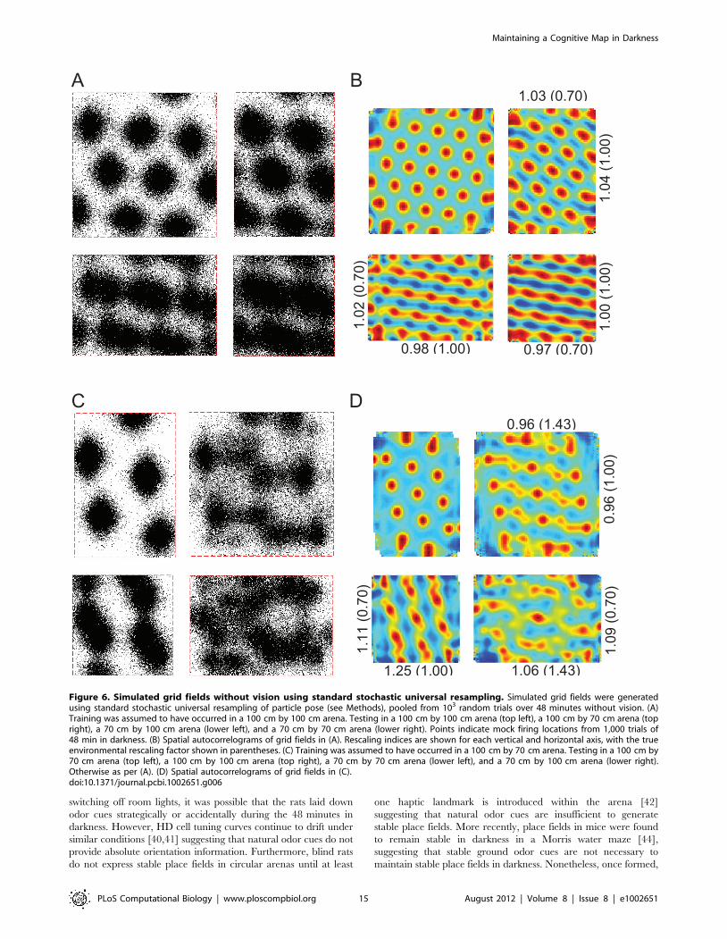
switching off room lights, it was possible that the rats laid down

odor cues strategically or accidentally during the 48 minutes in

darkness. However, HD cell tuning curves continue to drift under

similar conditions [40,41] suggesting that natural odor cues do not

provide absolute orientation information. Furthermore, blind rats

do not express stable place fields in circular arenas until at least

one haptic landmark is introduced within the arena [42]

suggesting that natural odor cues are insufficient to generate

stable place fields. More recently, place fields in mice were found

to remain stable in darkness in a Morris water maze [44],

suggesting that stable ground odor cues are not necessary to

maintain stable place fields in darkness. Nonetheless, once formed,

Figure 6. Simulated grid fields without vision using standard stochastic universal resampling. Simulated grid fields were generatedusing standard stochastic universal resampling of particle pose (see Methods), pooled from 103 random trials over 48 minutes without vision. (A)Training was assumed to have occurred in a 100 cm by 100 cm arena. Testing in a 100 cm by 100 cm arena (top left), a 100 cm by 70 cm arena (topright), a 70 cm by 100 cm arena (lower left), and a 70 cm by 70 cm arena (lower right). Points indicate mock firing locations from 1,000 trials of48 min in darkness. (B) Spatial autocorrelograms of grid fields in (A). Rescaling indices are shown for each vertical and horizontal axis, with the trueenvironmental rescaling factor shown in parentheses. (C) Training was assumed to have occurred in a 100 cm by 70 cm arena. Testing in a 100 cm by70 cm arena (top left), a 100 cm by 100 cm arena (top right), a 70 cm by 70 cm arena (lower left), and a 70 cm by 100 cm arena (lower right).Otherwise as per (A). (D) Spatial autocorrelograms of grid fields in (C).doi:10.1371/journal.pcbi.1002651.g006



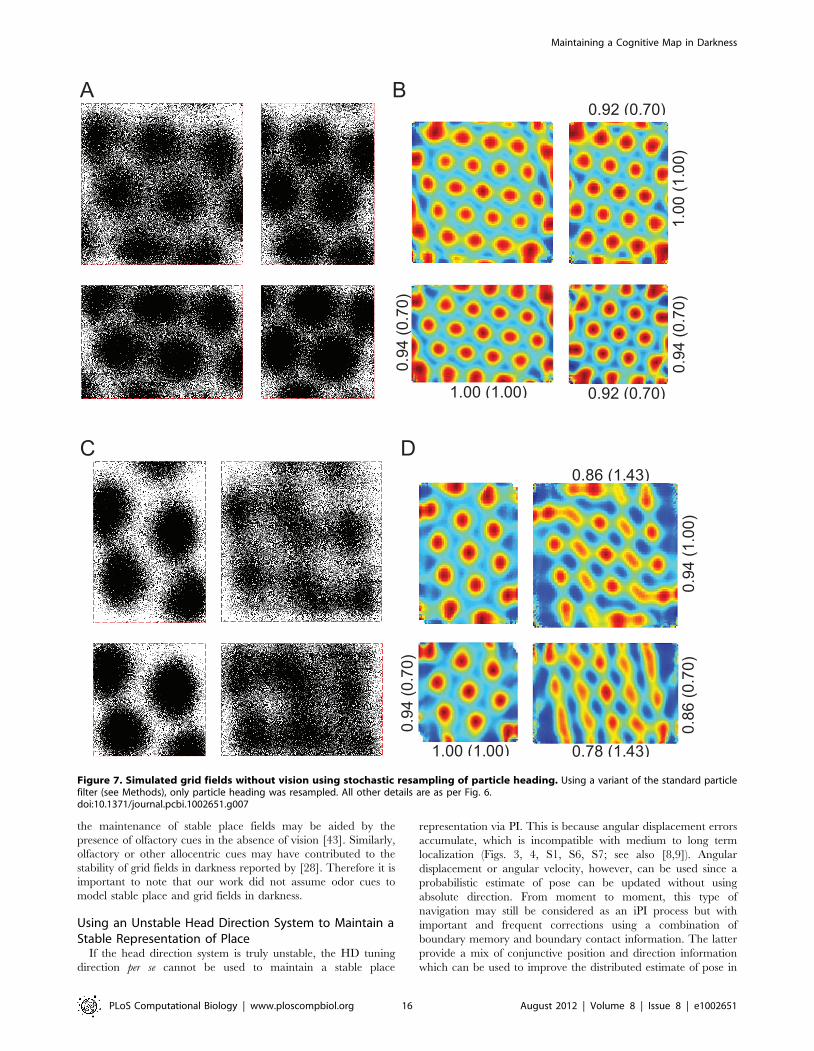
the maintenance of stable place fields may be aided by the

presence of olfactory cues in the absence of vision [43]. Similarly,

olfactory or other allocentric cues may have contributed to the

stability of grid fields in darkness reported by [28]. Therefore it is

important to note that our work did not assume odor cues to

model stable place and grid fields in darkness.

Using an Unstable Head Direction System to Maintain aStable Representation of Place

If the head direction system is truly unstable, the HD tuning

direction per se cannot be used to maintain a stable place

representation via PI. This is because angular displacement errors

accumulate, which is incompatible with medium to long term

localization (Figs. 3, 4, S1, S6, S7; see also [8,9]). Angular

displacement or angular velocity, however, can be used since a

probabilistic estimate of pose can be updated without using

absolute direction. From moment to moment, this type of

navigation may still be considered as an iPI process but with

important and frequent corrections using a combination of

boundary memory and boundary contact information. The latter

provide a mix of conjunctive position and direction information

which can be used to improve the distributed estimate of pose in

Figure 7. Simulated grid fields without vision using stochastic resampling of particle heading. Using a variant of the standard particlefilter (see Methods), only particle heading was resampled. All other details are as per Fig. 6.doi:10.1371/journal.pcbi.1002651.g007



an approximately Bayes-optimal way. It is an approximation

because a particle filter, by its nature, is necessarily a discrete

approximation of pose even if all filter properties are optimized for

known sensory error characteristics.

Computationally, angular displacement or angular velocity

estimates may be obtained via differences between consecutive

HD readings, or more directly via signals of angular velocity as

found in angular head velocity (AHV) cells [38,57,58]. In this

work, we have assumed that the rate of drift of the entire HD

system, including AHV cells, is indicated by the drift in HD tuning

functions. It may be the case that AHV signals have a different

error rate compared to the difference between HD tuning signals.

However, in the absence of vision and other compass cues, it seems

highly likely that the HD signal itself is maintained indirectly

through an estimate of angular velocity or acceleration.

By providing angular displacement, an erroneous HD system is

computationally compatible with a stable place or grid represen-

tation. As shown, stable place and grid fields can be simulated

using a distributed conjunctive representation of position and

orientation (pose), when combined with a coherent representation

Figure 8. The iRat maintains place stability without vision. (A) Performance of the iRat in a 1 m square arena using a particle filterapproximation of the positional uncertainty distribution (black line), compared with pure odometry (red line). Periods where at least one laser whiskerregisters a distance below 30 cm are shown (cyan bars). The total trajectory time was approximately 5 minutes (1,500 time steps). (B) The errorbetween estimated heading and actual heading. (C) The error between the estimated position and actual position. (D) The ground truth trajectory(blue) is shown following every 375 time steps during a 1,500 time step iRat trial (dashed lines in A to C). The estimated position and orientation frompure odometry (red) is consistently inferior to using arena information (black) via a particle filter (gray dots). See Methods for details of the iRat.doi:10.1371/journal.pcbi.1002651.g008



of the arena boundary. The former is consistent with recent

neurorobotic research suggesting that a distributed conjunctive

pose representation is required for managing perceptual ambiguity

using visual sensing [33]. Here, we have shown that managing

perceptual ambiguity without vision can also be achieved using a

conjunctive pose representation.

The Role of a Boundary MapWith vision, it is difficult to disentangle the localizing properties

of views from knowledge about the arena boundary geometry. For

example, it has been shown previously that complex navigation

performance patterns within confined arenas may be explained

using view-based gradient descent strategies [18,19]. These

strategies did not require any topological or metric representation

of the environment i.e. no ‘‘cognitive map’’. However, the

evidence presented here suggests there may be circumstances

where a map-like representation of the local environment is highly

advantageous. For example, in darkness and where odor and other

allocentric information may be sparse or ambiguous, sporadic

contact with natural or artificial boundaries may suffice to

maintain place stability for extended periods, until a localizing

cue or landmark is detected [42].

In robot navigation research, it has long been known that

relatively featureless boundary features such as walls in an office

environment can, provided a probabilistic map representation is

used, enable a robot equipped with a range sensor to navigate and

maintain a correct and stable estimate of its location within the

environment [48]. Here, we have applied that principle to

situations where boundary information is only available when in

close proximity to the boundary, and where local boundary

contour does not uniquely identify location.

Recently, [44] reported that the cerebellum is important for PI

in mice. This conclusion was based on the finding that impaired

cerebellar function impaired place field stability in featureless

circular arenas. However, we showed that place stability under

such conditions is likely to require a boundary map interacting

with the PI system. Therefore, the observed reduction in place

field stability in cerebellar mutants could be equally explained

computationally by a number of different effects involving this

map-PI interaction, not just impaired PI. In particular, mutants

showed stable place fields in darkness in the presence of a single

haptic boundary landmark – suggesting that iPI was not

completely impaired. Our results highlight the importance of

using quantitative models to determine the computational

demands of specific tasks such as PI. Further experiments will be

required to carefully dissect the contribution of arena boundary

information during spatial navigation tasks, given the significant

role it can play in maintaining a stable representation of position.

An important question which remains to be addressed in future

work is how a rodent’s navigation system builds a useful

representation of the environment. Some biological aspects of this

important question has been addressed using blind rats [42].

Without any local landmarks within the circular arena, place fields

were not observed. These rats were free to make contact with the

boundary wall, but had no memory information, at least initially.

Using our existing particle filter model, it is currently impossible to

update the iPI estimate of position in the absence of arena

memory. Under a Bayesian formulation, this is equivalent to the

case where the likelihood term is not available, so the posterior

distribution is unchanged. Consequently, the result is similar to

pure iPI – where no place field is seen. During exploration, a noisy

estimate of pose can in principle be used to build a representation

of the boundary. This is the problem of SLAM (simultaneous

localization and mapping) which has been studied extensively in

robotics. One avenue of future investigation may be to combine

rodent-inspired SLAM models (e.g., [33]) with a boundary

representation to study questions related to the acquisition of a

novel boundary map, including optimal movement strategies.

Place Stability versus Stable Firing FieldsUsing a simple probabilistic place field model, it was found that

emergent firing fields were related to a true ensemble represen-

tation of place in complex and unexpected ways. Firstly, the

location of a place field in an arena affected the rate of decrease of

spatial information in the absence of vision. In these simulations, it

was found that fields near the center of circular arenas persisted for

longer, preserving a higher amount of spatial information than

fields closer to the boundary. Furthermore, the average spike rate

varied considerably and may even increase for some time as place

destabilization proceeded. Secondly, the arena shape per se,

independent of traversable area, influenced place stability without

vision, thereby affecting spatial information content of place fields.

These results have a number of implications. Firstly, Skaggs

information should be interpreted carefully in the context of

positional stability. It is undoubtedly a useful quantifier of

positional or directional specificity, but may not accurately reflect

the true accuracy and precision of the underlying navigation

system. We have shown that it is theoretically possible for identical

trajectories and spatial representations to give rise to different

values of spatial information content, depending on place field

location.

Secondly, spatial specificity measures like Skaggs information do

not distinguish between unimodal and multimodal fields, or

spurious results due to extremely low spike counts. The former is

confounded by true field splitting [56], while our simulations

suggest the peak spike rate itself may be affected by an interaction

between field position and arena shape. Conversely, it is clear that

a navigation system with high place stability is computationally

able to generate a firing field with stable spatial information

content. Less intuitively, high spike rates did not always correlate

well with high place stability or high spatial information content.

For example, using iPI and arena memory only, the spatial

information content for each 8 minute window was approximately

1 bit/spike or higher, while the spike count increased by nearly

40% over the 48 minute period (Table 1). The latter result could

have been interpreted as indicating a stable representation of place

– but this was not the case. Similarly, the spatial information

content between 32 to 40 minutes without vision was greater for

the simulated place field at 10 cm from the arena center, than

between 8 to 16 minutes for the simulated place field at 20 cm

from the arena center (Table S3). If these fields were recorded

from separate experiments, the result may have been interpreted

as indicating differences in the availability and/or use of spatial

cues between the experiments, but this was not the case in the

simulations.

Thirdly, even though we purposefully modelled the situation

where visual information was absent, it is likely that animals use

non-visual information when visual information is present, leading

to redundancy. It is therefore plausible that neural computational

demands may vary substantially from one experimental design to

another, depending on the degree of information redundancy.

Even controlling for total area, we showed that the shape of an

arena affected the navigation performance of the same navigation

model (e.g., Fig. 3D, Fig. S6, Table 1 vs Table 2). Furthermore, we

have shown there are large differences between iPI in open and

enclosed spaces (e.g., Fig. 3A). Consequently, if there is any spatial

navigation element to a task in question, either explicitly or



implicitly, the available spatial information must be considered

carefully, and quantified where possible.

Finally, it is important to note that our models did not make

explicit predictions about theta phase [e.g., 59]. There is a

systematic relationship between a rat’s position within a place or

grid field and the theta phase of cell spikes. This raises the

possibility that the navigation system has more precise positional

information than suggested by the spatial specificity of the entire

field. Therefore, the fact that our model predicts spatial

information content of over 4 bits/spike in some cases may be

due in part to the fact that we have not embedded the positional

information in a phase code, which may reduce the apparent

spatial information measured in the conventional way. The latter

implies that spatial information may need to be considered as a

joint function of spike rate and theta phase.

Implications for Models of Mammalian Path IntegrationCurrent models of mammalian PI [34–37,59] usually assume

stable allocentric direction information as input. In contrast, our

results show that absolute HD information is not sufficient in the

presence of drift, whereas angular displacement information is

sufficient for effective navigation in darkness. It should be noted

that these results do not prove that angular velocity information per

se is used, since angular displacement could be inferred from the

change in successive absolute HD estimates. However, past

experiments have shown that temporary inactivation of the

vestibular system disrupts both the location-specific firing of place

cells and the direction-specific firing of HD cells despite visual and

odor cues being available [60,61]. Together with the existence of

large populations of AHV cells (more populous that HD cells in

some regions [38]), these evidence strongly suggest that angular

velocity or acceleration information is critical for optimal function

in the rodent spatial navigation system. One avenue of future

research is to incorporate angular head velocity models calibrated

using vision [57,58] into existing models of mammalian PI.

Specific effects of noise on the performance of the oscillatory

interference and attractor classes of mammalian PI models have

been considered previously [62,63]. However, it is clear that

allothetic information such as boundary geometry must be used in

conjunction with PI for accurate localization, rather than relying

on PI in isolation. It will be necessary to investigate the cellular

and computational basis for acquiring and using a boundary map.

One theoretical approach is to extend the existing mammalian PI

models to incorporate a boundary map, and determine whether it

is possible to achieve stable place/grid fields assuming realistic

sensory inputs and error magnitudes. A second approach is to

consider the movement strategies and possible cues which a rat

may use to acquire a boundary representation in the first place.

Two candidate cell types under modeling investigation are the

boundary vector cell [30,31,56,64,65] and border cell [29]. In

conjunction with a position code, boundary neurons may be able

to encode an arena boundary shape.

Need for a Cognitive Map?The current work focused specifically on situations where

allothetic cues were purposefully minimized or removed. Hence it

was by design that only boundary cues could reasonably have been

expected to provide stable allocentric information. But as [23]

stated, ‘‘when boundaries are not available, other types of

landmarks can be effectively recruited by the mapping system’’

consistent with [17]. Indeed, our results are restricted to one

particular set of scenarios where a ‘‘cognitive map’’ may be the

only plausible explanation of biological data, namely place and

grid field stability without vision or olfaction. Our systems-level

model does not preclude other stable cues from being incorporated

if or when they are available (e.g., [33,66]). Indeed, there are

scenarios where a modular navigation system may perform as well

as any ‘‘cognitive map model’’ (discussed further in Text S14).

Nevertheless, in at least some conditions, our results demonstrate

clearly that as separate modules (e.g., [13]), iPI and boundary

information are much inferior to a unified, near-optimal

combination of both.

Maintaining separation of PI and landmark (in this case a

featureless boundary) modules as per [13] cannot support stable

place or grid fields without vision or olfaction beyond 2 to

3 minutes. Therefore, to explain observed place and grid cell firing

properties, it is necessary that PI and landmark information are

combined, consistent with Tolman’s analogy that inputs are

‘‘worked over and elaborated’’ [1]. We also demonstrated that a

near-optimal probabilistic combination of iPI and boundary

information is computationally sufficient to generate stable place

and grid fields without vision or olfaction. If our interpretations of

published experimental data are reasonable, it would be difficult

for any model without a cognitive-like map to produce stable place

or grid fields without vision. The arguments of [13] that insects do

not possess a ‘‘cognitive map’’ cannot be extended to rodents,

possibly reflecting general differences in the spatial navigation

systems of different animal phyla.

An important question is whether the necessity of fusion of iPI

and boundary information should be considered as sufficient

evidence of a ‘‘cognitive map’’ in rodents. Although this issue is

partly one of semantics and definition, we note a number of

important points. Firstly, the necessity of information fusion is at

odds with the stimulus-response class of models which Tolman

used to contrast against the ‘‘cognitive map’’ class of models.

Secondly, the fusion of information is consistent with Tolman’s

notion of a ‘‘central control room’’ in describing a ‘‘cognitive

map’’, where information from various sources is combined in a

coherent manner to produce useful output. Thirdly, the funda-

mental output of PI systems is metric spatial information. If

boundary information has to interact in a useful manner with PI

information, it must also contain metric information. It is difficult

to envisage a useful representation of an arena boundary with

embedded metric spatial information, which bears no resemblance

to a spatial map. Fourthly, neither fusion of iPI and boundary

memory information only, nor intermittent use of a modular

navigation system can maintain stable places fields, showing that

the use of a ‘‘cognitive map’’ per se is not always sufficient under the

conditions described. The nature and degree of information fusion

in using a ‘‘cognitive map’’ are important. Finally, it has been

demonstrated that it is possible for a ‘‘cognitive map’’ model which

combines iPI and boundary information in a near-optimal manner

to explain stable place and grid fields without vision or olfaction.

ConclusionsThe rodent HD system becomes unstable in darkness beyond 2–

3 minutes, consistent with the theory that allocentric cues are

required to maintain long term stability. Place cells and grid cells

in rats can show stable firing fields for over 30 minutes in darkness.

We have shown that these results are incompatible with PI or a

boundary representation if they are used independently. However,

a ‘‘cognitive map’’ model which combines both can support stable

place and grid fields in various arenas while using a drifting HD

system. This model predicts place and grid field splitting, and

under some conditions grid field rescaling, without vision. The

results support the utility of a conjunctive pose representation for

optimal navigation, and show how rats might be able to navigate

effectively in environments where visual and olfactory cues are



unreliable or absent. Seemingly featureless boundaries are po-

werful landmarks, when combined with a PI mechanism, for stable

medium to long term navigation. The influence of such powerful

landmarks on navigation tasks must not be underestimated in

experimental design or data interpretation.

Supporting Information

Figure S1 Spatial information content expected from iPI alone.

Mean 6 s.e.m. of KL divergence of 1,000 trials using HD error

model described in Methods, assuming precise linear displacement

estimates. See text S5 for further details.

(PDF)

Figure S2 Comparing distances to boundary and interior points

of convex shapes. A. Geometric construct showing an arbitrary

convex 2D shape (light grey), with a small region (dark grey)

indicating all points between point P and segment S along the

perimeter. B. Taking the limit as the length of S approaches zero,

the dark grey region in (A) is approximated by a scalene triangle.

C. An expanded view of the scalene triangle of (B), showing a

circular arc of radius w0 (dashed line) centred at P.

(PDF)

Figure S3 Place stability estimates using different particle cloud

sizes. A. The mean place stability index (Ip) is shown for 100

random trials, in a circular arena of 78 cm diameter, using iPI,

arena memory and boundary contact information. The particle

filter was updated using stochastic universal resampling, with

particle cloud populations ranging from 106 to 103. B. One

standard deviation of Ip is shown for the last step of the results in A.

Notched boxplots are shown for the root-mean-square (RMS)

distance error from the true position, using the Cartesian (C) and

polar (D) estimates of position, averaged over 48 minutes in

darkness for the same trials as A and B.

(PDF)

Figure S4 Place stability in darkness using the Cartesian mean

of the distributed position estimate. The average of the most stable

10% of place fields (n = 100) are shown in 8 min time windows (A,

C, E and G). The ideal locations are 0 cm (A), 10 cm (B), 20 cm

(C), and 30 cm (D) from the centre of the arena, along a line at 45ufrom the horizontal. The corresponding heading distributions

during spikes (blue) and over the entire period (red) are also shown

(B, D, F and H). For the averaged place fields in each of the 4

locations, there was no significant deviation from the assumption

of uniform heading distribution at 0.05 level (Rayleigh’s test with

Bonferroni correction), and the directional information content

was an order of magnitude lower than the spatial information

content, typically around or below 0.1 bits/spike (Table S3),

consistent with the majority of these fields being pure place

representations. All pseudocolour scales used a maximum value of

0.15 spikes/step. The results of G & H are discussed further in

Text S9.

(PDF)

Figure S5 Place stability in darkness using the polar mean of the

distributed position estimate. The average of the most stable 10%

of place fields (n = 100) are shown in 8 min time windows (A, C, E

and G). The ideal locations are 0 cm (A), 10 cm (B), 20 cm (C),

and 30 cm (D) from the centre of the arena, along a line at 45ufrom the horizontal. The corresponding heading distributions

during spikes (blue) and over the entire period (red) are also shown

(B, D, F and H). For the averaged place fields in each of the 4

locations, there was no significant deviation from the assumption

of uniform heading distribution at 0.05 level (Rayleigh’s test with

Bonferroni correction), and the directional information content

was an order of magnitude lower than the spatial information

content, typically around or below 0.1 bits/spike (Table S3),

consistent with the majority of these fields being pure place

representations. All pseudocolour scales used a maximum value of

0.15 spikes/step. The results of G & H are discussed further in

Text S9.

(PDF)

Figure S6 A comparison of localization performance in circular

and square arenas without vision. The mean 6 s.d. of the place

stability index over 48 minutes with vision are shown for using iPI

only (blue), iPI and arena memory (green), iPI and arena memory

and wall contact information (red) in a circular (A) and square (B)

arena. The square arena was the same area as the circular arena

which was 76 cm in diameter. The corresponding colour-coded

frequency histograms of place stability values at the end of

48 minutes are shown in C (circular arena) and D (square arena).

The angular error mean 6 1s.d. and mean 6 2s.d. simulated HD

(grey) and particle filter estimate of heading (red) are shown for the

circular (E) and square (F) arena, for the top 10% of trials based on

place stability index. The angular error mean 6 1s.d. and mean 6

2s.d. simulated HD (grey) and particle filter estimate of heading

(red) are shown for the circular (G) and square (H) arena, for a

random 10% of trials. For the top 10% trials based on place

stability index used to generate place fields in Table S3, the

relative frequency distributions of the Cartesian (red) and polar

(blue) mean estimates of radial position are shown for the circular

(I) and square (J) arena. Each raw count was normalized by

dividing by the actual frequency of the simulated rat being in each

radial position bin of 1 cm width. The dotted line shows the ideal

relative frequency distribution assuming error-free position

tracking. The inset shows the relative frequency with respect to

X position in the square arena.

(PDF)

Figure S7 Place fields using allothetic path integration (aPI)

only. A. Place fields were generated using aPI only. Fields were

centred at (0,0) to maximize spatial information content (see S3).

Stable place representations could not be maintained using aPI

alone. B. Allothetic PI (grey) led to higher average place stability

than iPI (blue). Mean 6 s.d. of 1,000 trials are shown for each PI

model. In a typical case, the place stability index dropped below

chance (dashed line) within 8 minutes using aPI alone (on average

in under 5 minutes).

(PDF)

Figure S8 The effect of arena transforms on the estimated

position in darkness. The mean particle cloud X position is plotted

against the true X position from 10 random trials in each of two

reciprocal arena transform simulations, using each of two

stochastic resampling methods. The training arena was 100 cm

by 100 cm (A & B), and 100 cm by 70 cm (C & D). Examples

using both the standard stochastic universal resampling method (A

& C) and resampling of heading only (B & D) are included for

comparison. The colour-coded original (black) and transformed

(red) arenas are shown schematically above each corresponding

plot.

(PDF)

Figure S9 Place stability index of the example described in Text

S12. The corresponding particle cloud dynamics are shown in

Video S1 and Video S2 (periods indicated in grey).

(PDF)

Table S1 Mean squared distance errors in circular and square

arenas, assuming location at the boundary.

(PDF)



Table S2 Mean place stability index in circular and square

arenas.

(PDF)

Table S3 Properties of simulated place fields in a circular arena.

(PDF)

Table S4 Properties of simulated place field using allothetic path

integration only.

(PDF)

Text S1 Simulated random trajectories.

(PDF)

Text S2 Head direction error model.

(PDF)

Text S3 Particle filter navigation model.

(PDF)

Text S4 Place stability index.

(PDF)

Text S5 Robot iRat experiment.

(PDF)

Text S6 Estimating the expected spatial information using iPI

only.

(PDF)

Text S7 Mean squared distance and general distance measures

to convex boundaries.

(PDF)

Text S8 Asymptotic place stability index in a circular arena.

(PDF)

Text S9 Varying simulated place field locations.

(PDF)

Text S10 Maintaining place stability in square versus circular

arenas.

(PDF)

Text S11 Path integration with vision but no boundary map.

(PDF)

Text S12 Grid fields without vision following arena compression

and expansion.

(PDF)

Text S13 Animated example of simulated localization without

vision.

(PDF)

Text S14 Utility of modular navigation models.

(PDF)

Video S1 Simulated localization without vision between 0 and

8 minutes.

(AVI)

Video S2 Simulated localization without vision between 40 and

48 minutes.

(AVI)

Acknowledgments

The authors would like to thank Kieran McLean for carrying out

preliminary particle filter simulations, and Tien Luu for assistance with

editing.

Author Contributions

Conceived and designed the experiments: AC DB MM. Performed the

experiments: AC DB. Analyzed the data: AC. Contributed reagents/

materials/analysis tools: AC DB. Wrote the paper: AC DB MM GW JW.

References

1. Tolman EC (1948) Cognitive maps in rats and men. Psychol Rev 55: 189–208.

2. Mittelstaedt ML, Mittelstaedt H (1980) Homing by path integration in a

mammal. Naturwissenschaften 67: 566–567.

3. Etienne AS, Jeffery KJ (2004) Path integration in mammals. Hippocampus 14:

180–192.

4. Vickerstaff RJ, Cheung A (2010) Which coordinate system for modelling path

integration? J Theor Biol 263: 242–261.

5. Wehner R, Rossel S (1985) The bee’s celestial compass—a case study in

behavioral neurobiology. Fortschr Zool 31:11–53.

6. Benhamou S, Sauve J-P, Bovet P (1990) Spatial memory in large scale

movements: efficiency and limitation of the egocentric coding process. J Theor

Biol 145: 1–12.

7. Muller M, Wehner R (2007) Wind and sky as compass cues in desert ant

navigation. Naturwissenschaften 94: 589–594.

8. Cheung A, Zhang SW, Stricker C, Srinivasan MV (2007) Animal navigation: the

difficulty of moving in a straight line. Biol Cybern 97: 47–61.

9. Cheung A, Zhang SW, Stricker C, Srinivasan MV (2008) Animal navigation:

general properties of directed walks. Biol Cybern 99: 197–217.

10. Souman JL, Frissen I, Sreenivasa MN, Ernst MO (2009) Walking straight into

circles. Curr Biol 19: 1–5.

11. Cheung A, Vickerstaff R (2010) Finding the way with a noisy brain. PLoS

Comput Biol 6: e1000992.

12. Tcheang L, Bulthoff HH, Burgess N (2011) Visual influence on path integration

in darkness indicates a multimodal representation of large-scale space. Proc Natl

Acad Sci U S A 108: 1152–1157.

13. Cruse H, Wehner R (2011) No need for a cognitive map: Decentralized memory

for insect navigation. PLoS Comput Biol 7: e1002009

14. Menzel R, Greggers U, Smith A, Berger S, Brandt R, et al. (2005) Honey bees

navigate according to a map-like spatial memory. Proc Natl Acad Sci U S A 102:

3040–3045.

15. Gould JL (1986) The locale map of honey bees: do insects have cognitive maps?

Science 232: 861–863.

16. Menzel R, Brandt R, Gumbert A, Komischke B, Kunze J (2000) The spatial

memories for honeybee navigation. Proc R Soc Lond B 267: 961–968.

17. O’Keefe J, Nadel L (1978) The hippocampus as a cognitive map. Oxford:

Clarendon Press.

18. Sturzl W, Cheung A, Cheng K, Zeil J (2008) The information content of

panoramic images I: The rotational errors and the similarity of views in

rectangular experimental arenas. J Exp Psychol Anim B 34: 1–14.

19. Cheung A., Sturzl W, Zeil J, Cheng K (2008) The information content of

panoramic images II: View-based navigation in nonrectangular experimental

arenas. J Exp Psychol Anim B 34: 15–30.

20. Mittelstaedt H, Mittelstaedt ML (1973) Mechanismen der Orientierung ohne

richtende Aussenreize. Forschr Zool 21: 46–58.

21. Doeller CF, Burgess N (2008) Distinct error-correcting and incidental learning of

location relative to landmarks and boundaries. Proc Natl Acad Sci U S A 105:

5909–5914.

22. Doeller CF, King JA, Burgess N (2008) Parallel striatal and hippocampal systems

for landmarks and boundaries in spatial memory. Proc Natl Acad Sci U S A 105:

5915–5920.

23. Lew A (2011) Looking beyond the boundaries: time to put landmarks back on

the cognitive map? Psychol Bull 137: 484–507.

24. O’Keefe J, Dostrovsky J (1971) The hippocampus as a spatial map. Preliminary

evidence from unit activity in the freely-moving rat. Brain Res 34: 171–5.

25. Taube JS, Muller RU, Ranck JB Jr (1990) Head-direction cells recorded from

the postsubiculum in freely moving rats. I., Description and quantitative analysis.

J Neurosci 10:420–435.

26. Taube JS, Muller RU, Ranck JB Jr (1990) Head-direction cells recorded from

the postsubiculum in freely moving rats. II., Effects of environmental

manipulations. J Neurosci 10:436–447.

27. Fyhn M, Hafting T, Treves A, Moser MB, Moser EI (2007) Hippocampal

remapping and grid realignment in entorhinal cortex. Nature 446:190–194.

28. Hafting T, Fyhn M, Molden S, Moser MB, Moser EI (2005) Microstructure of a

spatial map in the entorhinal cortex. Nature 801–806.

29. Solstad T, Boccara CN, Kropff E, Moser MB, Moser E (2008) Representation of

geometric borders in the entorhinal cortex. Science 322: 1865–1868.

30. Barry C, Lever C, Hayman R, Hartley T, Burton S, et al. (2006) The boundary

vector cell model of place cell firing and spatial memory. Rev Neurosci 17: 71–

97.

31. Lever C, Burton S, Jeewajee A, O’Keefe J, Burgess N (2009) Boundary vector

cells in the subiculum of the hippocampal formation. J Neurosci 29: 9771–

9777.



32. Sargolini F, Fyhn M, Hafting T, McNaughton B, Witter M, et al. (2006)

Conjunctive representation of position, direction, and velocity in entorhinal

cortex. Science 312, 758–762.

33. Milford MJ, Wiles J, Wyeth GF (2010) Solving navigational uncertainty using

grid cells on robots. PLoS Comput Biol 6: e10000995.

34. McNaughton BL, Battaglia FP, Jensen O, Moser EI, Moser MB (2006) Path

integration and the neural basis of the ‘cognitive map’. Nat Rev Neurosci 7:

663–678.

35. Jeffery KJ (2007) Integration of the sensory inputs to place cells: what, where,

why, and how? Hippocampus 17: 775–785.

36. Moser EI, Kropff E, Moser MB (2008) Place cells, grid cells, and the brain’s

spatial representation system. Ann Rev Neurosci 31: 69–89.

37. Derdikman D, Moser EI (2010) A manifold of spatial maps in the brain. Trends

Cogn Sci 14: 561–569.

38. Taube JS, Bassett JP (2003) Persistent neural activity in head direction cells.

Cereb Cortex 13: 1162–1172.

39. Mizumori SJY, Williams JD (1993) Directionally selective mnemonic properties

of neurons in the lateral dorsal nucleus of the thalamus of rats. J Neurosci 13:

4015–4028.

40. Goodridge JP, Dudchenko PA, Worboys KA, Golob EJ, Taube JS (1998) Cue

control and head direction cells. Behav Neurosci 112: 749–761.

41. Clark BJ, Taube JS (2010) Intact landmark control and angular path integration

by head direction cells in the anterodorsal thalamus after lesions of the medial

entorhinal cortex. Hippocampus 21: 767–782.

42. Save E, Cressant A, Thinus-Blanc C, Poucet B (1998) Spatial firing of

hippocampal place cells in blind rats. J Neurosci 18: 1818–1826.

43. Save E, Nerad L, Poucet B (2000) Contribution of multiple sensory information

to place field stability in hippocampal place cells. Hippocampus 10: 64–76.

44. Rochefort C, Arabo A, Andre M, Poucet B, Save E, et al. (2011) Cerebellum

shapes hippocampal spatial code. Science 334: 385–389.

45. Etienne AS, Jeffery KJ (2004) Path integration in mammals. Hippocampus 14:

180–192.

46. Quirk GJ, Muller RU, Kubie JL (1990) The firing of hippocampal place cells in

the dark depends on the rat’s recent experience. J Neurosci 10:2008–2017.

47. Jeffery KJ, Donnett JG, Burgess N, O’Keefe JM (1997) Directional control of

hippocampal place fields. Exp Brain Res 117:131–142.

48. Thrun S, Leonard J (2008) Simultaneous localization and mapping. In: Siciliano

B, Khatib O, editors. Springer Handbook of Robotics. Berlin: Springer-Verlag.

pp. 871–889.

49. Skaggs WE, McNaughton BL, Gothard K, Markus EJ (1993) An information-

theoretic approach to deciphering the hippocampal code. In: S.J. Hanson, J. D.

Cowan and C.L. Giles, editors. Advances in Neural Information Processing

Systems 5. San Mateo, CA: Morgan Kaufmann Publishers. pp. 1030–1037.

50. Burgess N, Cacucci F, Lever C, O’Keefe J (2005) Characterizing multiple

independent behavioural correlates of cell firing in freely moving animals.Hippocampus 15: 149–153.

51. Barry C, Hayman R, Burgess N, Jeffery KJ (2007) Experience-dependent

rescaling of entorhinal grids. Nat Neurosci 10: 682–684.52. Ball D, Heath S, Wyeth G, Wiles J (2010) iRat: Intelligent Rat Animat

Technology. Proceedings of the 2010 Australasian Conference on Robotics andAutomation; 1–3 December 2010; Brisbane, Australia. ACRA2010.

53. Ball D, Heath S, Milford M, Wyeth G, Wiles J (2010) A navigating rat animat.

Proceedings of the Twelfth International Conference on the Synthesis andSimulation of Living Systems; 19–23 August 2010; Odense, Denmark. Artificial

Life XII.54. Muller RU, Kubie JL (1987) The effects of changes in the environment on the

spatial firing of hippocampal complex-spike cells. J Neurosci 7:1951–1968.55. Muller RU, Kubie JL, Ranck JB Jr (1987) Spatial firing patterns of hippocampal

complex-spike cells in a fixed environment. J Neurosci 7: 1935–1950.

56. O’Keefe J, Burgess N (1996) Geometric determinants of the place fields ofhippocampal neurons. Nature 381: 425–428.

57. Stratton P, Wyeth G, Wiles J (2010) Calibration of the head direction network: arole for symmetric angular head velocity cells. J Comput Neurosci 28: 527–538.

58. Stratton P, Milford M, Wyeth G, Wiles J (2011) Using strategic movement to

calibrate a neural compass: A spiking network for tracking head direction in ratsand robots. PLoS One 6: e25687.

59. Burgess N, O’Keefe (2011) Models of place and grid cell firing and thetarhythmicity. Curr Opin Neurobiol 21: 1–11.

60. Stackman RW, Clark AS, Taube JS (2002) Hippocampal spatial representationsrequire vestibular input. Hippocampus 12: 291–303.

61. Smith PF, Darlington CL, Zheng Y (2010) Move it or lose it – Is stimulation of

the vestibular system necessary for normal spatial memory? Hippocampus 20:36–43.

62. Burak Y, Fiete IR (2009) Accurate path integration in continuous attractornetwork models of grid cells. PLoS Comput Biol 5: e1000291.

63. Zilli EA, Yoshida M, Tahvildari B, Giocomo LM, Hasselmo ME (2009)

Evaluation of the oscillatory interference model of grid cell firing throughanalysis and measured period variance of some biological oscillators. PLoS

Comput Biol 5: e1000573.64. Burgess N, Jackson A, Hartley T, O’Keefe J (2000) Predictions derived from

modeling the hippocampal role in navigation. Biol Cybern 83: 301–312.65. Hartley T, Burgess N, Lever C, Cacucci F, O’Keefe J (2000) Modeling place

fields in terms of the cortical inputs to the hippocampus. Hippocampus 10: 369–

379.66. Sheynikhovich D, Chavarriaga R, Strosslin T, Arleo A, Gerstner W (2009) Is

there a geometric module for spatial orientation? Insights from a rodentnavigation module. Psychol Rev 116: 540–566.



Maintaining a Cognitive Map in Darkness: The Need to Fuse Boundary Knowledge with Path Integration

Documents

Transcript of Maintaining a Cognitive Map in Darkness: The Need to Fuse Boundary Knowledge with Path Integration