Elsevier Editorial System(tm) for Earth and Planetary Science Letters

Manuscript Draft

Manuscript Number: EPSL-D-08-00570

Title: Magnetostratigraphy of the Early Triassic from Chaohu (China) and its implications for the Induan -

Olenekian stage boundary

Article Type: Regular Article

Keywords: Chaohu, Lower Triassic, Paleomagnetism, Olenekian, magnetostratigraphy

Corresponding Author: Mr Sun Zhiming, PhD

Corresponding Author's Institution: Institute of Geomechanics, CAGS

First Author: Sun Zhiming

Order of Authors: Sun Zhiming; Mark W. Hounslow; Junling Pei; Laishi Zhao; Jinnan Tong

Abstract: A magnetostratigraphic study was performed on the lower 44 m of the West Pingdingshan section

near Chaohu city, (Anhui province, China) in order to provide a magnetic polarity scale for the early Triassic.

Data from 295 paleomagnetic samples is integrated with a detailed biostratigraphy and lithostratigraphy. The

tilt-corrected mean direction from the West Pingdingshan section, passes the reversal and fold tests. The

overall mean direction after tilt correction is D=299.9º, I=18.3º (κ=305.2, α95=1.9, N=19). The inferred

paleolatitude of the sampling sites (31.6ºN, 117.8ºE) is about 9.4º, consistent with the stable South China

block (SCB), though the declinations indicate some 101o counter-clockwise rotations with respect to the

stable SCB since the Early Triassic. Low-field anisotropy of magnetic susceptibility indicates evidence of

weak strain. The lower part of the Yinkeng Formation is dominated by reversed polarity, with four normal

polarity magnetozones (WP2n to WP5n), with evidence of some thinner (<0.5 m thick) normal

magnetozones. The continuous magnetostratigraphy from the Yinkeng Formation, provides additional high-

resolution details of the polarity pattern through the later parts of the Induan into the lowest Olenekian. The

magnetostratigraphic and biostratigraphic data shows the conodont marker for the base of the Olenekian

(first presence of Neospathodus waageni) is shortly prior to the base of normal magnetozone WP5n. This

provides a secondary marker for mapping the base of the Olenekian into successions without conodonts.

This section provides the only well-integrated study from a Tethyan section across this boundary, but

problems remain in definitively relating this boundary into Boreal sections with magnetostratigraphy.

State Key Laboratory of Geological Processes and Mineral Resources ,

China Universit y of Geosciences, Wuhan, 430074, China

phone: +86-10-68422365, fax: +86-10-68422326

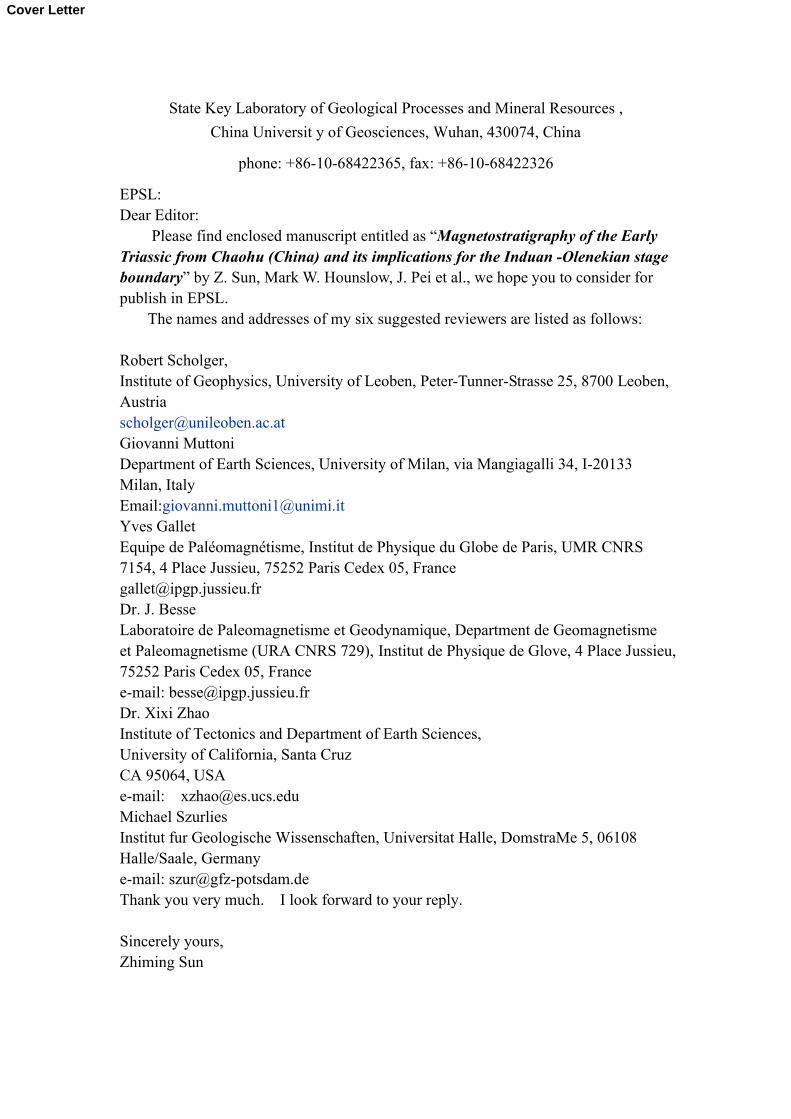
EPSL:Dear Editor:

Please find enclosed manuscript entitled as “Magnetostratigraphy of the Early Triassic from Chaohu (China) and its implications for the Induan -Olenekian stage boundary” by Z. Sun, Mark W. Hounslow, J. Pei et al., we hope you to consider for publish in EPSL.

The names and addresses of my six suggested reviewers are listed as follows:

Robert Scholger, Institute of Geophysics, University of Leoben, Peter-Tunner-Strasse 25, 8700 Leoben, Austriascholger@unileoben.ac.atGiovanni Muttoni Department of Earth Sciences, University of Milan, via Mangiagalli 34, I-20133 Milan, ItalyEmail:giovanni.muttoni1@unimi.itYves GalletEquipe de Paléomagnétisme, Institut de Physique du Globe de Paris, UMR CNRS 7154, 4 Place Jussieu, 75252 Paris Cedex 05, Francegallet@ipgp.jussieu.fr Dr. J. BesseLaboratoire de Paleomagnetisme et Geodynamique, Department de Geomagnetisme et Paleomagnetisme (URA CNRS 729), Institut de Physique de Glove, 4 Place Jussieu, 75252 Paris Cedex 05, Francee-mail: besse@ipgp.jussieu.frDr. Xixi Zhao Institute of Tectonics and Department of Earth Sciences,University of California, Santa CruzCA 95064, USAe-mail: xzhao@es.ucs.eduMichael SzurliesInstitut fur Geologische Wissenschaften, Universitat Halle, DomstraMe 5, 06108 Halle/Saale, Germanye-mail: szur@gfz-potsdam.deThank you very much. I look forward to your reply.

Sincerely yours,Zhiming Sun

Cover Letter

Linking powered by eXtyles

Magnetostratigraphy of the Early Triassic from Chaohu (China) 1

and its implications for the Induan - Olenekian stage boundary2

3

Zhiming Sun1, Mark W. Hounslow2, Junling Pei3, Laishi Zhao1, Jinnan Tong1, James G. Ogg44

1. State Key Laboratory of Geological Processes and Mineral Resources , China Universit y of Geosciences, Wuhan, 5

430074 , China6

2. Centre for Environmental Magnetism and Palaeomagnetism, Geography Dept, Farrer Avenue, Lancaster University, 7

Lancaster, UK., LA1 4YQ.8

3. Key Laboratory of Crust Deformation and Processes, Institute of Geomechanics, CAGS, Beijing, China9

4. Dept. Earth & Atmospheric Science, Purdue University, West Lafayette, IN 47907 USA10

11

12

Corresponding author:13

Zhiming Sun14

State Key Laboratory of Geological Processes and Mineral Resources , 15

China Universit y of Geosciences, 16

Wuhan, 43007417

China18

phone: +86-10-68422365, fax: +86-10-6842232619

e-mail: sunzm1209@yahoo.com.cn20

* Manuscript

Linking powered by eXtyles

Abstract21

A magnetostratigraphic study was performed on the lower 44 m of the West Pingdingshan section near Chaohu city, 22

(Anhui province, China) in order to provide a magnetic polarity scale for the early Triassic. Data from 295 paleomagnetic 23

samples is integrated with a detailed biostratigraphy and lithostratigraphy. The tilt-corrected mean direction from the West 24

Pingdingshan section, passes the reversal and fold tests. The overall mean direction after tilt correction is D=299.9º, I=18.3º 25

(κ=305.2, α95=1.9, N=19). The inferred paleolatitude of the sampling sites (31.6ºN, 117.8ºE) is about 9.4º, consistent with 26

the stable South China block (SCB), though the declinations indicate some 101o counter-clockwise rotations with respect to 27

the stable SCB since the Early Triassic. Low-field anisotropy of magnetic susceptibility indicates evidence of weak strain. 28

The lower part of the Yinkeng Formation is dominated by reversed polarity, with four normal polarity magnetozones (WP2n 29

to WP5n), with evidence of some thinner (<0.5 m thick) normal magnetozones. The continuous magnetostratigraphy from the 30

Yinkeng Formation, provides additional high-resolution details of the polarity pattern through the later parts of the Induan 31

into the lowest Olenekian. The magnetostratigraphic and biostratigraphic data shows the conodont marker for the base of the 32

Olenekian (first presence of Neospathodus waageni) is shortly prior to the base of normal magnetozone WP5n. This provides 33

a secondary marker for mapping the base of the Olenekian into successions without conodonts. This section provides the only 34

well-integrated study from a Tethyan section across this boundary, but problems remain in definitively relating this boundary 35

into Boreal sections with magnetostratigraphy.36

37

Key words: Chaohu, Lower Triassic, Paleomagnetism, Olenekian, magnetostratigraphy38

39

1. Introduction40

Magnetostratigraphy can be used as an essential tool for chronostratigraphic correlations between rocks from different 41

environments including those that are unfossiliferous or have poor fossil preservation. The Lower Triassic 42

magnetostratigraphy has been studied in many places, where progress has been made in constructing a magnetic polarity 43

scale for the Permian-Triassic boundary interval either from marine (Heller et al., 1988,1995; Haag et al., 1991; Li et al., 44

1989; Steiner et al., 1989; Chen et al., 1994; Embleton et al., 1996; Zhu et al., 1999; Scholger et al., 2000; Gallet et al., 2000; 45

Hounslow et al., 2008) or terrestrial rocks (Molostovsky, 1996; Szurlies et al., 2003; Steiner, 2006; Szurlies, 2007). In spite of 46

this, discussions continue about how to precisely correlate marine and continental facies using magnetostratigraphy near the 47

Permian-Triassic boundary (PTB) interval and the remainder of the Lower Triassic (Steiner, 2006; Szurlies, 2007; Hounslow 48

et al., 2008). This in part reflects the debate about the placement of the base of the 2nd stage of the Triassic, the Olenekian, as 49

well as differing quality, quantity and types of secondary biostratigraphic constraints in these Early Triassic successions. In 50

addition, paleomagnetic studies from some continuous marine sections have differing magnetostratigraphic records (e.g. the 51

Induan global stratotype section and point (GSSP) at Meishan; Yin et al. 2005 ) perhaps because of undetected 52

remagnetization (Li et al., 1989; Zhu et al., 1999; Steiner, 2006).53

Recent investigations were carried out on the west Pingdingshan section to provide detailed biostratigraphic and 54

lithostratigraphic information for the Induan–Olenekian boundary (Tong et al; 2003, 2005, 2007; Zhao et al., 2007, 2008). 55

Based on this robust lithostratigraphic and biostratigraphic framework, a precise positioning of paleomagnetic data was 56

achieved, resulting in a detailed composite magnetic record. Along with biostratigraphic data, the magnetic record of these 57

lowermost Triassic sediments are important in that they provide an integrated magnetostratigraphic and biostratigraphic 58

reappraisal that allows the recognition of the Induan– Olenekian boundary in a Tethyan section. This is all the more 59

important, in that the ratified GSSP for the Olenekian at Mud (Spiti, India) is unlikely to ever have a magnetostratigraphy 60

because of low grade metamorphism (Krystyn et al., 2007)61

62

2. Geological setting63

The West Pingdingshan section (location 31.6ºN, 117.8ºE), located near Chaohu city, Anhui province, China, consists 64

of interbedded calcareous mudstones and limestones. The section is one of the well-exposed Lower Triassic successions in 65

Linking powered by eXtyles

South China (Fig. 1), which was deposited in a carbonate ramp setting on the Lower Yangtze Block, within the low-latitude 66

eastern Tethyan archipelago. The Lower Triassic sections near Chaohu city have been extensively investigated using a 67

variety of detailed lithostratigraphic, biostratigraphic and chemostratigraphic tools (Tong et al., 2003, 2005, 2007; Zhao et al., 68

2007, 2008). The Lower Triassic succession at Chaohu yields abundant fossils, which provides a comprehensive 69

biostratigraphy marked by conodonts and ammonoids (Fig. 2). 70

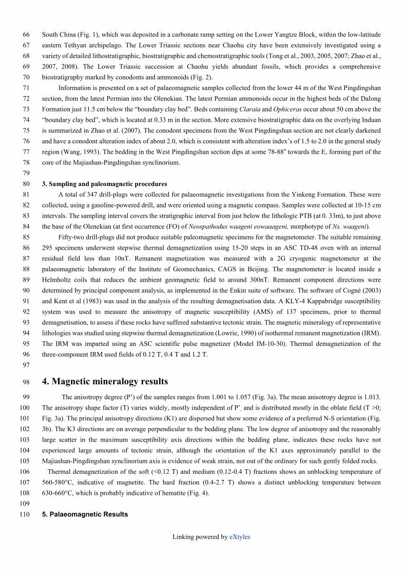
Information is presented on a set of palaeomagnetic samples collected from the lower 44 m of the West Pingdingshan 71

section, from the latest Permian into the Olenekian. The latest Permian ammonoids occur in the highest beds of the Dalong 72

Formation just 11.5 cm below the “boundary clay bed”. Beds containing Claraia and Ophiceras occur about 50 cm above the 73

“boundary clay bed”, which is located at 0.33 m in the section. More extensive biostratigraphic data on the overlying Induan 74

is summarized in Zhao et al. (2007). The conodont specimens from the West Pingdingshan section are not clearly darkened 75

and have a conodont alteration index of about 2.0, which is consistent with alteration index’s of 1.5 to 2.0 in the general study 76

region (Wang, 1993). The bedding in the West Pingdingshan section dips at some 78-88o towards the E, forming part of the 77

core of the Majiashan-Pingdingshan synclinorium.78

79

3. Sampling and paleomagnetic procedures 80

A total of 347 drill-plugs were collected for palaeomagnetic investigations from the Yinkeng Formation. These were 81

collected, using a gasoline-powered drill, and were oriented using a magnetic compass. Samples were collected at 10-15 cm 82

intervals. The sampling interval covers the stratigraphic interval from just below the lithologic PTB (at 0. 33m), to just above 83

the base of the Olenekian (at first occurrence (FO) of Neospathodus waageni eowaaageni, morphotype of Ns. waageni).84

Fifty-two drill-plugs did not produce suitable paleomagnetic specimens for the magnetometer. The suitable remaining 85

295 specimens underwent stepwise thermal demagnetization using 15-20 steps in an ASC TD-48 oven with an internal 86

residual field less than 10nT. Remanent magnetization was measured with a 2G cryogenic magnetometer at the 87

palaeomagnetic laboratory of the Institute of Geomechanics, CAGS in Beijing. The magnetometer is located inside a 88

Helmholtz coils that reduces the ambient geomagnetic field to around 300nT. Remanent component directions were 89

determined by principal component analysis, as implemented in the Enkin suite of software. The software of Cogné (2003) 90

and Kent et al (1983) was used in the analysis of the resulting demagnetisation data. A KLY-4 Kappabridge susceptibility 91

system was used to measure the anisotropy of magnetic susceptibility (AMS) of 137 specimens, prior to thermal 92

demagnetisation, to assess if these rocks have suffered substantive tectonic strain. The magnetic mineralogy of representative 93

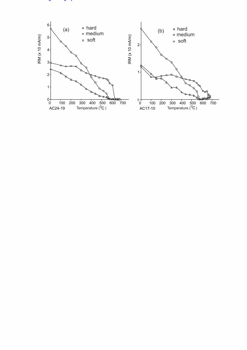
lithologies was studied using stepwise thermal demagnetization (Lowrie, 1990) of isothermal remanent magnetization (IRM). 94

The IRM was imparted using an ASC scientific pulse magnetizer (Model IM-10-30). Thermal demagnetization of the 95

three-component IRM used fields of 0.12 T, 0.4 T and 1.2 T.96

97

4. Magnetic mineralogy results98

The anisotropy degree (P’) of the samples ranges from 1.001 to 1.057 (Fig. 3a). The mean anisotropy degree is 1.013. 99

The anisotropy shape factor (T) varies widely, mostly independent of P’, and is distributed mostly in the oblate field (T >0; 100

Fig. 3a). The principal anisotropy directions (K1) are dispersed but show some evidence of a preferred N-S orientation (Fig. 101

3b). The K3 directions are on average perpendicular to the bedding plane. The low degree of anisotropy and the reasonably 102

large scatter in the maximum susceptibility axis directions within the bedding plane, indicates these rocks have not 103

experienced large amounts of tectonic strain, although the orientation of the K1 axes approximately parallel to the 104

Majiashan-Pingdingshan synclinorium axis is evidence of weak strain, not out of the ordinary for such gently folded rocks.105

Thermal demagnetization of the soft (<0.12 T) and medium (0.12-0.4 T) fractions shows an unblocking temperature of 106

560-580°C, indicative of magnetite. The hard fraction (0.4-2.7 T) shows a distinct unblocking temperature between 107

630-660°C, which is probably indicative of hematite (Fig. 4).108

109

5. Palaeomagnetic Results110

Linking powered by eXtyles

The specimens have initial natural remanent magnetisation (NRM) intensities between 10-4 and 10-3 A/m. Thermal 111

demagnetization isolated three magnetisation components: 112

(a) Firstly a low-temperature component (component A: LTC) is isolated in all samples below about 300°C. The mean 113

direction of this component before tilt correction is D=3.0°, I=41.5° (N=295 and α95=1.3°), and is similar to the present-day 114

field direction (D=355.4° and I= 47.3°; Fig. 5a, 6), which is inferred to be the origin of this component. 115

(b) A second component (component B: MTC) is determined mostly between the 300-480°C demagnetisation steps, by 116

a well-defined linear segment on the orthogonal vector diagrams in nearly all specimens. This magnetisation component 117

largely dominates the NRM. This component is NNW and down-directed in geographic coordinates and easterly and 118

down-directed in stratigraphic coordinates (Fig. 5b, 6). The Fisher precision parameter of the mean direction of the MTC 119

component changes from 42.2 before bedding correction to 40.3 after bedding correction, indicating a slightly tighter 120

directional dispersion in situ coordinates (Fig. 5b). The mean magnetization direction at 350o, +32o (k=42.2, α95= 1.4) in 121

geographic coordinates is not distinct from that expected for the Jurassic-Cretaceous of the South China block (SCB). Hence, 122

we interpret this component B as probably a remagnetization acquired during the Jurassic-Cretaceous period, after tilting of 123

the beds.124

(c) Thirdly a high-temperature component (component C: HTC). This component is mostly present between 125

480-580°C. Its direction is of dual polarity, and is interpreted as a Triassic magnetisation (Fig. 6, 8). Only some 66% of 126

samples showed evidence of this magnetisation component, the remaining specimens were dominated by component B until 127

complete demagnetisation. Component C has a strong overlap of unblocking temperature with component B in a large 128

majority of specimens at and above 480°C. Only some 11% of specimens show clear linear segments, separating component 129

C from component B on Zijderveld plots and principle component (PCA) analysis (Fig. 6, 7). 130

Categories of demagnetisation behavior were visually assigned (assisted by the PCA analysis) to several classes of 131

demagnetization data shown by the specimens. 132

Firstly, a category indicating no component C could reliably be interpreted from the specimen data (‘MTC only’ in Fig. 133

9). This type of behaviour is dominant in the lower 5 m of the section (which is more weathered than the overlying parts), and 134

above 20 m in the section (Fig. 7). Some 34% of specimens possess this type of behavior.135

Secondly, two classes (good and poor) of ChRM line-fit data (Fig. 6, 9), which are exclusively present in the levels 136

between 5 and 30 m (Fig. 9). Some 11% of samples possess this type of behavior.137

Thirdly, specimen data, which showed evidence of incomplete separation of components B and C, but which showed 138

evidence of great circle trends towards either the reverse or normal polarity directions of component C (‘GC trends’ in Fig. 9). 139

Two sub-categories of good and poor behavior were evaluated, based on the amount of approach towards the component C 140

dual polarity directions (Fig. 8, 9). Some 55% of specimens possess this type of behavior. Great circles were predominantly 141

fitted through the higher temperature demagnetisation steps as an estimate of these great circle trends.142

The reversal test (McFadden & McElhinney, 1990) has been performed on the component C mean direction. The test 143

indicates a positive reversal test (Ra), with less than 5o degrees between inverted antipodal mean directions (γObs=2.3; 144

γCritical=4.4). The tilt test on the site-mean directions of ChRM is also positive at the 95% level of confidence according to the 145

criteria of McFadden and Jones (1990) (Xi2Is=6.8, Xi2Tc=1.8, Critical 95%=5.07). These findings indicate the primary nature 146

of the ChRM from the West Pingdingshan section. The site-mean directions were determined using the combined ChRM 147

line-fit and fitted great circle data using the method of Mcfadden and McElhinny (1988), as implemented in the Cogné (2003) 148

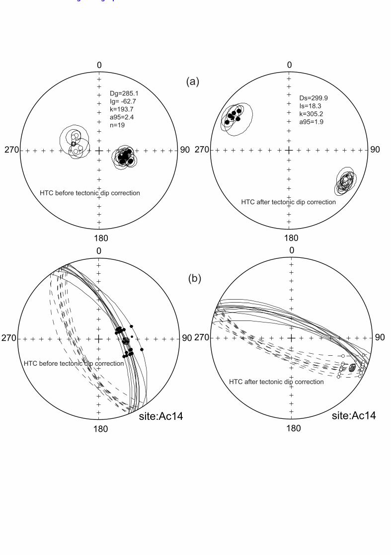
software (Fig. 8). The averaged site-mean direction for component C is Dg=285.1°, Ig=-62.7°, κg=193.7, α95=2.4° before tilt 149

correction, and Ds=299.9°, Is=18.3°, κs=305.2, α95=1.9°, N=19 after tilt correction (Fig. 8a, Table 1). The average direction of 150

each group of sites was calculated using the great circles (re-magnetisation circles) /fixed points to evaluate one of the means 151

displayed in Fig. 8a, for example the samples in bed AC14 (Fig. 8b). The determined paleopole lies at 30.3°N, 19.9°E with 152

A95=1.4° (dp/dm=1.0/2.0). The paleolatitude of 9.4° for the section is not significantly different (at 95% confidence level) 153

with that predicted for the stable South China Block (Heller et al., 1988, 1995; Steiner et al., 1989). Hence, we infer 154

component C is a Lower Triassic magnetisation, acquired prior to folding. However, the mean directions for the ChRM are 155

substantially different in declination from the Lower Triassic means for the South China block, a result of 101.2° (±3.3°) 156

anti-clockwise vertical axis rotation with respect to the stable South China block. Similar anticlockwise rotations occur 157

Linking powered by eXtyles

further south adjacent to the Tanlu fault (Tan et al., 2007). These are probably associated with local rotation of the Chaohu 158

area, during docking with the nearby North China block, along the Tanlu fault. 159

160

6. Magnetostratigraphy and global magnetostratigraphic correlation161

The ChRM directions were converted to VGP latitude (displayed as filled circle in Fig. 9). For those specimens 162

possessing great-circle behaviour, the point on the fitted great circle closest to the section mean direction was used to163

calculate the VGP latitude (displayed as open circle in Fig. 9). The magnetic polarity of the section is dominated by reverse 164

polarity, with three normal polarity magnetozones represented by three or more specimens (WP2n, WP3n and WP4n). 165

Normal magnetozones WP1r.1n and WP5n are defined by only two specimens. A number of tentative normal polarity 166

sub-magnetozones, represented by a single specimen are also present within WP4r, with only that in bed 19 defined by PCA 167

line-fit data (Fig. 9). 168

The magnetic polarity at the correlated base of the Olenekian (at the first occurrence of morphotype Ns. waageni 169

eowaggeni in subbed 24-16) is probably reversed, since underlying sub-bed 24-15 and overlying sub-bed 24-17 are reversed, 170

with both sampled intervening beds not containing any evidence of Triassic component C. The base of the overlying normal 171

magnetozone W5n is ~2.5 m above the FA of Ns. waageni eowaggeni, although a substantial number of specimens in the base 172

of bed 25 posses no component C. Hence, the base of magnetozone WP5n provides a good secondary marker a little above the 173

base of the Olenekian in the West Pingdingshan section.174

The dominance of reverse polarity in the lower part of the section (i.e. that below bed 15, Figs. 9 & 10) would suggest, 175

according to the magnetostratigraphy, that this interval is entirely late Griesbachian, since no substantive evidence of the 176

equivalent of normal polarity magnetozone LT1n, which characterizes the basal Induan, occurs in the base of the section (Fig. 177

10). It is perhaps possible the normal magnetozone WP1r.1n, some 2.0 m above the “PTB set” (Peng et al., 2001), may 178

represent part of LT1n and the remainder of the basal Griesbachian normal magnetozone is obscured by the scarcity of 179

polarity data in this interval (Fig. 9). The basal part of the West Pingdingshan section was only uncovered in recent years, and 180

not much biostratigraphic work has been done on it, but neighboring sections such as the north Pingdingshan and west 181

Majiashan sections have been studied in detail at the boundary, with no evident breaks in sedimentation.182

The magnetostratigraphy of the Gaundao section is ambiguous around the Induan-Olenekian boundary (IOB), but the 183

positive carbon isotopic excursion allows approximate correlation from Gaundao to the West Pingdingshan and Bulla/Suisi 184

sections (Payne et al. 2004; Horacek et al. 2007; Tong et al. 2007; Richoz et al. 2007; Fig. 10). The magnetostratigraphy of the 185

upperpart of the West Pingdingshan section, has a close correspondence in polarity style to that at Hechuan, as does the 186

reverse-polarity dominated interval at Guandao, which covers the upper range of the conodont Ns. dieneri (Fig. 10). The most 187

complete magnetostratigraphy across the IOB occurs in the Boreal realm from the Sverdrup Basin in Canada and Spitsbergen 188

in arctic Norway (Ogg & Steiner, 1991; Hounslow et al., 2008). However, correlation of the IOB onto the 189

magnetostratigraphy of the boreal sections is problematic with two possible solutions. 190

Both Ns. kummeli, Ns. dieneri and Ns. svalbardensis are known from the P. candidus Zone in Canada (Orchard & 191

Tozer, 1997), which suggests the reverse polarity interval covering beds 18-20 at West Pingdingshan (Fig. 10) represents the 192

lower part of magnetozone LT2r (GC2r at Griesbach Creek; Sc2r at Creek of Embry and Vh4r at Vikinghøgda; Fig. 10) in the 193

Boreal composite magnetic polarity timescale (MPTS). Ns. dieneri and Ns. cristagalli are present in the Canadian V. 194

sverdrupi Zone (Orchard & Tozer, 1997) and in sections on Spitsbergen V. spitzbergensis (probable synonym of V. 195

sverdrupi) occurs with Ns. pakistanensis, Ns. dieneri, and Ns. aff. svalbardensis (Nakrem et al., in-review), which suggests 196

the boundary between the Ns. cristagalli and Ns. pakinstanensis conodont zones at the GSSP in Mud (Krystyn et al. 2007), 197

occurs within the Boreal Sverdrupi Zone. Within Canadian sections Ns. waageni first occurs within the Euflemingites 198

romunderi Zone, whereas in Siberian sections Ns. waageni first occurs some 20% through the H. hedenstroemia Zone (Dagis, 199

1984), indicating that the IOB probably occurs within the lower part of the H. hedenstroemi Zone. This suggests that the 200

magnetozone WP5n at West Pingdingshan is probably the equivalent of magnetozone LT4n in the boreal MPTS (option in 201

Fig. 10), and hence the IOB is within the uppermost part of LT3r. A consequence of this biostratigraphic-driven correlation is 202

that the equivalent of LT3n in the MPTS appears to be unconvincingly detected at West Pingdingshan- possibly represented 203

by WP4n in bed 19? (Fig. 10).204

Linking powered by eXtyles

A second, lower placement of the IOB, relative to the magnetostratigraphy is also possible (Option in Fig. 10). Since 205

the ammonoid control at Griesbach Creek is based on spot occurrences, its not clear where the base of the H. hedenstroemi206

Zone is located, its may be that it is located below the base of the Smith Creek Member in the upper part of GC2r (Fig. 10). 207

Consequently, it is possible that WP5n is the equivalent of GC3n (LT3n in MPTS). Two features support this possibility; 208

firstly, this correlation is more consistent with the magnetostratigraphy, in that no substantive normal magnetozone is 209

detected in beds 18 to 24 at West Pingdingshan. Secondly, at both the Griesbach Creek and Vikinghøgda sections close to the 210

lower boundary of GC3n and Vh5n (LT3n in MPTS) is a major transgressive surface, which may be the equivalent of that 211

seen at Chaohu and Mud close to the IOB (Guo et al., 2007; Krystyn et al 2007).212

With these uncertainties in correlation of marine sections in mind, its premature to attempt mapping of the 213

cyclo-magnetostratigraphy from the Buntsandstein (Szurlies, 2007) into the marine sections. In addition much reliance has 214

been placed on relating the Italian sections at Bulla and Siusi (Scholger et al., 2000) to age-calibrate the Buntsandstein cycles 215

and lithostratigraphy (Szurlies et al., 2003; Szurlies 2007), yet the isotopic curves from these Italian sections clearly located 216

the IOB higher in the Bulla/ Siusi sections than that used by Szurlies (2007).217

218

7. Conclusion219

A dual polarity Triassic magnetisation can be extracted from the West Pingdingshan section, in spite of minor 220

associated tectonic deformation, and partial remagnetisation. The Early Triassic magnetization is masked by a strong 221

Jurassic-Cretaceous overprint magnetization, acquired post-tilting, which variably masks the Early Triassic magnetisation. 222

Nevertheless some 66% of specimens display evidence in the demagnetisation diagrams of characteristic polarity, either 223

through conventional magnetisation component isolation, or great circle trends. The correlated conodont marker for the base 224

of the IOB in the GSSP at Mud (FA of Ns. dieneri s.l.) indicates that at West Pingdingshan the IOB is some 2.5 m below a 225

normal magnetozone, which provides a secondary marker, for mapping the base of the Olenekian into successions without 226

conodonts. Around the IOB the West Pingdingshan section can be correlated confidently to other Tethyan Lower Triassic 227

successions, but which however lack the corroborative magnetostratigraphic details shown at Chaohu. Problems remain near 228

the Permian-Triassic boundary in the West Pingdingshan section, due to inadequate recovery of Triassic magnetisations from 229

specimens. Problems also remain in relating the Induan-Olenekian boundary interval into the boreal sections in Canada and 230

Spitsbergen with magnetostratigraphy. 231

232

Acknowledgements233

This study was supported by NSFC (40102021), Leo Krystyn provided useful discussion on biostratigraphic correlations.234

. 235

References236

Chen, H., Sun, S., Li, J., Heller, F., Dobson, J., 1994. Magnetostratigraphy of the Permian and Triassic in 237

Wulong, Sichuan Province, Science in China B 12, 1317-1324.238

Cogné, J. P., 2003. PaleoMac: A Macintosh™ application for treating paleomagnetic data and making 239

plate reconstructions. Geochemistry Geophysics Geosystems 4, doi:10.1029/2001GC000227. 240

Dagis, A.S., 1984. Early Triassic conodonts of the north Middle Siberia. Nauka, Moscow, 69 p. (in 241

Russian).242

Embleton, B. J. J., McElhinny, M.W., Ma, X., Zhang, Z., Li, Z., 1996. Permo-Triassic 243

magnetostratigraphy in China: the type section near Taiyuan, Shanxi Province, North China, 244

Geophys Journal International 126, 382-388 Scopus.245

Linking powered by eXtyles

Gallet, Y., Krystyn, L., Besse, J., Saidi, A., and Ricou, L-E., 2000. New constraints on the upper Permian 246

and Lower Triassic geomagnetic polarity timescale from the Abadeh section (central Iran): Journal 247

Geophysical Research 105, 2805-2815 Scopus.248

Guo, G., Tong, J., Zhang, S., Zhang, J., Bai, L., 2007. A study on the Lower Triassic cyclostratigraphy in 249

the West Pingdingshan Section, Chaohu, Anhui Province. Science in China (Series D) 37, 250

1571-1578.251

Haag, M., Heller, F., 1991. Late Permian to Early Triassic magnetostratigraphy, Earth and Planetary 252

Science Letters 107, 42-54 Scopus.253

Heller, F., Chen, H., Dobson, J., and Haag, M., 1995. Permian- Triassic magnetostratigraphy - new 254

results from south China: Physics Earth Planetary Interiors 89, 281-295 Scopus.255

Heller, F., Lowrie, W., Li, H., Wang, J., 1998. Magnetostratigraphy of the Permo-Triassic boundary 256

section at Shangsi (Guangyuan, Sichuan Province, China), Earth and Planetary Science Letters 88, 257

348-356 Scopus.258

Horacek, M., Brandner, R. & Abart, R., 2007. Carbon isotope record of the P/T boundary and the Lower 259

Triassic in the Southern Alps: Evidence for rapid changes in storage of organic carbon. 260

Palaoegeography, Palaeoclimatology, Palaeoecology 252, 347-354 Scopus.261

Hounslow, M.W. Peters, C. Mørk, A. Weitschat, W. & Vigran, J.O. 2008. Bio-magnetostratigraphy of 262

the Vikinghøgda Formation, Svalbard (arctic Norway) and the geomagnetic polarity timescale for 263

the Lower Triassic. Bull. Geol. Soc. America. In press.264

Kent, J.T., Briden, J.C. & Mardia, K.V. 1983. Linear and planar structure in ordered mulivariate data as 265

applied to progressive demagnetization of palaeomagnetic remanance. Geophysical Journal of the 266

Royal Astronomical Society 81, 75–87 Scopus.267

Krystyn, L., Bhargava, O.N. Richoz, S., 2007. A candidate GSSP for the base of the Olenekian Stage: 268

Mud at Pin Valley; district Lahul & Spiti, Hamachal Pradesh (Western Himalaya), India. Albertiana269

35, 5-29.270

Lehrmann, D.J., Ramezani, J., Bowring, S.A., Martin, M.W., Montogomery, P., Enos, P., Payne, P., 271

Orchard, M.J., Wang, H., and Wei, J., 2006. Timing and recovery from the end Permian extinction: 272

geochronologic and biostratigraphic constraints from south China: Geology 34, 1054-1056.273

Li, H., Wang, Z., 1989. Magnetostratigraphy of Permo-Triassic boundary section of Meishan of 274

Changxing, Zhejiang, Science in China (Series D) 32, 1401-1408.275

Lowrie, W., 1990. Indentification of ferromagnetic minerals in a rock by coercivity and unblocking 276

temperature properties, Geophysical Research Letter 17, 159-162 Scopus. 277

McFadden, P. L., 1990. A new fold test for palaeomagnetic studies. Geophysical Journal International278

103, 163-169 Scopus.279

McFadden, P.L., and McElhinney, M.W., 1988. The combined analysis of remagnetisation circles and 280

direct observations in paleomagnetism. Earth and Planetary Science Letters 87, 161-172.281

McFadden, P.L., and McElhinny, M.W., 1990. Classification of the reversal test in paleomagnetism: 282

Geophysical Journal International 103, 725-729 Scopus.283

Molostovsky, E.A. 1996. Some aspects of magnetostratigraphic correlation. Stratigraphy and Geological 284

correlation 4, 231-237 Scopus.285

Linking powered by eXtyles

Ogg, J.G., and Steiner, M.B., 1991. Early Triassic polarity time-scale: integration of 286

magnetostratigraphy, ammonite zonation and sequence stratigraphy from stratotype sections 287

(Canadian Arctic Archipelago): Earth and Planetary Science Letters 107, 69-89.288

Orchard, M.J. & Tozer, E.T. 1997. Triassic conodont biochronology, its calibration with the ammonoid 289

standard and a biostratigraphic summary for the western Canada sedimentary basin. Bulletin of 290

Canadian Petroleum Geology 45, 675–692 Scopus.291

Payne, J. L., Lehrmann, D. J., Wei, J., Orchard, M. J., Schrag, D. P., Knoll, A. H., 2004. Large 292

perturbations of the carbon cycle during recovery from the end-Permian extinction. Science 305, 293

506-509 Scopus.294

Peng, Y., Tong J., Shi, G.R., and Hansen, H.J., 2001. The Permian-Triassic boundary stratigraphic set: 295

characteristics and correlation. Newsletter on Stratigraphy 39, 55–71 Scopus.296

Perri, M.C., and Farabegoli, E., 2003. Conodonts across the Permian-Triassic boundary in the southern 297

Alps: Courier Forschungsinstitut Senckenberg 245, 281-313.298

Richoz, S. Krystyn, L., Horacek, M., & Spötl, C. 2007. Carbon isotope record of the Induan –Olenekian 299

candididate GSSP Mud and comparison with other sections. Albertiana 35, 35-39.300

Scholger, R., Mauritsch, H.J., and Brandner, R., 2000. Permian-Triassic boundary magnetostratigraphy 301

from the southern Alps (Italy): Earth and Planetary Science Letters 176, 495-508 Scopus.302

Steiner, M. 2006. The magnetic polarity timescale across the Permian-Triassic boundary, in Lucas, S.G. 303

Cassinis, G. and Schneider, J.W., eds., Non-marine Permian biostratigraphy and biochronology: 304

Geological Society, London Special Publication, 265, 15-38.305

Steiner, M., Ogg, J., Zhang, Z., and Sun, S., 1989. The Late Permian/early Triassic magnetic polarity 306

time scale and plate motions of south China: Journal Geophysical Research 94, 7343-7363 Scopus.307

Szurlies, M. Bachmann, G. H. Menning, M. Nowaczyk, N.R. Käding, K.-C. 2003. Magnetostratigraphy 308

and high resolution lithostratigraphy of the Permian- Triassic boundary interval in Central Germany.309

Earth and Planetary Science Letters 212, 263-278 Scopus.310

Szurlies, M. 2007. Latest Permian to Middle Triassic cyclo-magnetostratigraphy from the Central 311

European Basin, Germany: Implications for the geomagnetic polarity timescale. Earth and Planetary 312

Science Letters 261, 602-619 Scopus.313

Tan, X, Kodama, K.P., Gilder, S., Courtillot, V., Cogn’e, J.P., 2007. Palaeomagnetic evidence and 314

tectonic origin of clockwise rotations in the Yangtze fold belt, South China Block. Geophysical 315

Journal International 168, 48–58 Scopus.316

Tong, J., Hansen, H. J., Zhao, L., and Zuo, J., 2005. High resolution Induan- Olenekian boundary 317

sequence in Chaohu, Anhui Province: Science in China (Series D) 48, 291-297 Scopus.318

Tong, J., Zakharov, Y. D., Orchard, M. J., Yin, H., and Hansen, H. J., 2003. A candidate of the 319

Induan-Olenekian boundary stratotype in the Tethyan region. Science in China (Series D) 46, 320

1182-1200 Scopus.321

Tong, J., Zuo J. & Chen Z.Q. 2007. Early Triassic carbon isotope excursions from South China: Proxies 322

for devastation and restoration of marine ecosystems following the end-Permian mass extinction.323

Geological Journal 42, 371–389 Scopus. 324

Wang, C., Conodonts of the Lower Yangtze Valley. 1993. An Index to Biostratigraphy and Organic 325

Metamorphic Maturity. Science Press, Beijing (In Chinese with English summary).326

Linking powered by eXtyles

Yin, H., Tong J. and Zhang K., 2005. A review on the Global Stratotype Section and Point of the 327

Permian-Triassic Boundary. Acta Geologica Sinica 79, 715-728328

Yin, H., Zhang, K., Tong, J., Yang, Z., and Wu, S., 2001. The Global Stratotype Section and Point 329

(GSSP) of the Permian-Triassic Boundary: Episodes 24, 102-114 Scopus.330

Zhao, L., Orchard, M.J., Tong, J., Sun, Z., Zuo, J., Zhang, S., Yun, A. 2007. Lower Triassic conodont 331

sequence in Chaohu, Anhui Province, China and its global correlation. Palaoegeography, 332

Palaeoclimatology, Palaeoecology 252, 24-38 Scopus.333

Zhao, L., Tong, J., Sun, Z., Orchard, M., 2008. A detailed Lower Triassic conodont biostratigraphy and 334

its implications for the GSSP candidate of the Induan–Olenekian boundary in Chaohu, Anhui 335

Province. Progress in Natural Science 18, 79–90 Scopus.336

Zhu, Y. & Lui, Y., Magnetostratigraphy of the Permian- Triassic boundary section at Meishan, 337

Chanxing, Zheijiang Province, in Yin, H. & Tong, J., eds., 1999. Pangea and the Paleozoic-Mesozoic 338

transition: China University of Geosciences Press, Wuhan, 79-84. 339

Linking powered by eXtyles

Figure captions:340

Fig. 1 (a) simplified geological map of Chaohu area and (b) Geographic location. 341

Fig. 2 Vertical range and zonation of conodonts, ammonoids and bivalves assemblage at West Pingdingshan section, Chaohu, 342

Anhui Province. Modified after Zhao et al. (2008). Bold lines highlight the occurrence of the most important 343

ammonoids and conodonts used to identify the Induan-Olenekian boundary. 344

Fig. 3(a) Anisotropy of magnetic susceptibility (AMS) plots of shape parameter T versus anisotropy degree P’, (b) 345

stereographic projection of AMS principle axes in stratigraphic coordinates for specimens from the Yinkeng 346

Fm. K1 (square): maximum axis, K3 (circle): minimum axis, K2 (triangle): intermediate axis. 347

Fig. 4 Representative plots of thermal demagnetisation of 3-axis isothermal remanent magnetization, 348

using magnetizing fields of 0.12 T (soft), 0.4 T (medium) and 2.7 T (hard). these plots show Tc at ~ 349

560-580 and 630-660.350

Fig. 5 (a) Equal-area projections of a) the low temperature (LTC or A) component and b) the mid temperature 351

(MTC or B) component. Star is the geocentric axial dipole field, and square the present-day field directions. 352

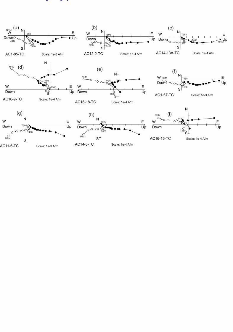
Fig. 6 Representative orthogonal demagnetization diagrams (in stratigraphic coordinates). The characteristic 353

magnetisation (component C) directions in the specimens displayed were determined by principle 354

component line-fits. a-e: good quality line-fit from 480C through the origin; f-i: poor quality line-fit from 355

480C through the origin; (d), (e), (i): Normal polarity; (a)-(c), (f)-(h): Reverse polarity. Demagnetization 356

steps in °C in all plots. 357

Fig. 7 Equal-area projections of the magnetisation directional tracks during thermal demagentization of representative 358

samples with a variable content of component C (all in stratigraphic coordinates). G1: good quality great circle data; 359

G2: poor quality great circle (with only short paths towards directions that are consistent with component C being 360

present). Plot c) is for a normal polarity sample, all others for interpreted reverse polarity specimens. In general, these 361

specimen show motion along a great-circle paths in a southeasterly direction, trending towards negative inclination or a 362

northwesterly direction with a postive inclination. The great-circle path is best defined from about 480C to 580C. 363

Fig. 8 (a) Equal-area stereographic projection of mean directions of high temperature component C for 364

stratigraphic groups of specimen data. Lower (upper) hemisphere directions are marked with closed (open) 365

symbols. (b) Equal-area stereographic projection of the site ( AC14) showing the great circles 366

(re-magnetisation circles) /fixed points used to evaluate one of the means displayed in Fig. 8a. Ellipses are 367

95% confidence cones of group means. Stars=mean directions of these dual polarity magnetisations. 368

Fig. 9 Demagnetisation behaviour (see text), virtual geomagnetic pole (VGP) latitude, and the magnetic polarity 369

interpreted in the West Pingdingshan section, along with summary biostratigraphic data (Zhao et al., 2007). 370

Magnetozones defined by no adjacent specimens of the same polarity, are indicated by half bars, with full 371

bars indicating two or more adjacent specimens of the same polarity. Full grey bars indicate adjacent 372

specimens with only component B present. The major N-R magnetozone couplets have been labeled WP 373

(for West Pingdingshan), for ease of description.374

Fig. 10 Comparison of the magnetostratigraphy at Chaohu with other studies of marine sections through the latest 375

Permian and Lower Triassic. Data for polarity columns: Guandao (Lehrmann et al., 2006), Hechuan (Steiner 376

et al., 1989), Abadeh (Gallet et al., 2000), Bulla/Siusi (Scholger et al., 2000; Perri & Farabegoli, 2003; 377

Horacek et al., 2007). Griesbach Creek, Smith Creek and Creek of Embry (Ogg & Steiner, 1991 modified by 378

Hounslow et al 2008), Vikinghøgda and composite magnetic polarity timescale (MPTS) from Hounslow et al. 379

(2008).380

Linking powered by eXtyles

Table 1 381

Site-mean paleomagnetic results from the West Pingdingshan section at Chaohu, Anhui Province. 382

383

Bed/Site n Dg (o) Ig(

o) Ds(o) Is(

o) 95(o)

ac24 9 107.3 67 124.7 -17.1 30.9 5.4

ac23 11 106 63.9 122.5 -19.5 42.5 4.6

ac22 12 100.3 62.9 117.9 -19.8 23.5 5.6

ac21 8 107.8 67.2 121.8 -17.9 13.3 8.4

ac20 7 116.2 63.9 124.8 -19.2 24.9 7.9

ac19 10 303.5 -61.6 308.2 20 28.5 5

ac18 12 114 62.4 123.3 -19.2 22.2 5.2

ac17 9 267.9 -66 294.4 14.5 14.7 7.5

ac16a 7 278.1 -70.7 300.3 14.1 16.7 9.7

ac16b 7 292.8 -61.8 301.6 24.7 8.3 15.3

ac15 11 100 62.5 116.2 -21.4 10.5 9.8

ac14 14 94.6 62 115.9 -17.5 50.6 3.4

ac13 11 96.6 61.7 117.7 -16.8 25.3 5.6

ac12 10 91.7 58.2 113.3 -17.5 39.6 4.2

ac11 7 98.2 62.8 119 -16.4 28.5 6.4

ac10 10 107.6 54.7 116.8 -20.4 20.8 6.4

ac9 10 109.3 55.3 118 -20.3 30.8 4.8

ac8 10 103.9 60.3 117.5 -14.5 13.4 7.9

ac7 10 297.8 -59.9 304.1 16.4 12.3 7.8

mean 19 285.1 -62.7 - - 193.7 2.4

- - 299.9 18.3 305.2 1.9

n: number of specimens used to calculate mean; Dg, Ig, Ds, Is: declination and inclination in geographic and stratigraphic 384

coordinates respectively; κ: the best estimate of the Fisher precision parameter; α95: the radius of the 95% cone of 385

confidence. 386

387

2.38

1.62

1.76

2.85

2.76

2.19

3.52

2.57

2.47

2.47

3.24

3.33

2.39

1.62

2.13

2.56

1.961.87

3.06

3.81

3.95

2.130.992.311.511.97

1.49

9. 93

0.10

Fe Fe Fe

37

36

35

34

33

32

31

30

29

28

27

26

25

24

23

22

2120

19

18

17

16

15141312

11

1

0

2

4

6

8 m

.

Neo

spat

hodu

s ku

mm

eli

Ns.

pos

tero

long

atus

Ns.

sp.

Con

odon

t Zon

e

Ns.

dien

eri

.

Gui

chie

lla a

ngul

ata

a

6-105 0.20

2-4 0.15

Upp

erP

erm

ian

Cha

nghs

ing

Dal

ong

H.ty

pica

lisH

. sp.

Isar

cice

lla?

sp.

Neo

gond

olel

la c

arin

ata

Ng.

kry

styn

i

Ng.

sp.

Ng.

pla

nata

Ng.

orc

hard

i

Cla

raia

hun

anic

a

Cla

raia

gre

isba

chi

Cla

raia

sta

chei

Cla

raia

radi

alis

Cla

raia

gre

isba

chi

Cla

raia

aur

itaC

lara

ia c

once

ntric

aC

lara

ia h

ubei

ens

isC

lara

ia g

reis

bach

i

Eum

orph

otis

cf.

vene

tina

Eum

orph

otis

hua

ncan

geni

sE

umor

phot

is in

aequ

ieco

stat

a

Oph

icer

as s

p.Ly

toph

icer

as?

sp.

Lyto

phic

er a

s? s

p.

Kon

inck

ites

sp.

Prio

nolo

bus

sp.

Cly

pece

ras

cf. l

entic

ular

e

Neo

spat

hodu

s ch

i

Ns.

die

neri

M1

Ns.

die

neri

M1

Ns.

die

neri

M2

Ns.

die

neri

M3

Ns.

cha

ohue

nsis

Ns.

aff.

cris

taga

lli

Ns.

n. s

p. F

Ns.

aff.

cha

ohue

nsis

Ns.

con

cavu

sN

s. n

. sp.

K

Ns.

waa

geni

eow

aage

ni

Par

achi

rogn

athu

s cf

. tric

usoi

datu

sP

laty

villo

sus

cost

atus

Ns.

n. s

p. G

Ns.

n. s

p. H

Ns.

Ton

gi

Pl.

ham

adai

Ns.

aff.

dis

cret

us

Ns.

pec

ulia

risN

s. a

lber

ti

Cly

pece

r as

sp.

Euf

l em

ingi

tes

sp.

Pse

udos

agec

er a

s sp

.

Pre

fl or

iani

tes

cf. s

trong

iP

refl

oria

nite

s? s

p.P

seud

osag

ecer

as

sp.

Bak

evel

lia c

osta

ta

Arc

toce

r as

cf. l

olou

ense

Flem

ingi

tes

ellip

ticus

Flem

ingi

tes

kaoy

unlin

gens

isFl

emin

gite

s sp

.

Pse

udoc

ellit

es s

p.

Uss

uria

? sp

.O

wen

ites?

sp.

Mee

koce

r as

sp.

Euf

l em

ingi

tes

cf. t

sote

ngen

sis

Cly

pece

r as

cf. k

wan

gsie

nsis

Die

nero

cer a

s di

ener

Pse

udos

agec

er a

s ts

oten

gsen

e

Neo

spat

hodu

s w

aage

niA

nasi

birit

esO

phic

er a

s - l

ypto

phic

er a

sC

lara

ia s

tach

ei -

C. a

urita

Prio

nolo

bus

- Gyr

onite

sE

umor

phot

is in

aequ

i coa

stat

a - E

. hua

ncan

gens

isFl

emin

gite

s - E

ufl e

min

gite

sA

mm

onoi

d Zo

neB

ival

ve A

ssem

blag

e Zo

ne

Ram

iform

ele

men

ts

Ns.

nov

aeho

lland

iae

+ N

s. p

akis

tane

nsis

Ns.

spi

tiens

isN

s. a

ff. w

aage

ni w

aage

niN

s. n

. sp.

I

Adu

ncod

ina

unic

osta

Par

achi

rogn

athu

s sp

.

Ns.

waa

geni

waa

geni

Pbs

idon

ia m

inar

Cla

raia

sp.

Gui

chie

lla s

ubro

tund

aE

umor

phot

is s

p.

Pos

idon

ia s

p.

Pos

idon

ia c

ircul

aris

Arc

toce

r as

sp.

Ow

enite

s pa

kung

ensi

sK

onim

kite

s lo

low

ensi

sP

roph

ingi

toid

es s

p.W

asac

hite

s sp

.H

emip

rioni

tes

sp.

Juve

nite

s cr

ient

alis

Die

nero

cer a

s sp

.D

iene

roce

r as

cf. o

vale

Kon

inck

ites

cf. l

oloe

nsis

Ns.

waa

geni

waa

geni

Ns. waagenieowaageni

Ns. dieneri M3

Ns. dieneri M2

Ns. dieneri M1

Ns. kummeli

Ng. krystyni

H. typicalis

Indu

an

Low

er T

riass

ic

Ole

neki

an

Yink

eng

Form

atio

n

Ser

ies

Sta

ge

Form

atio

n

Bed

Thic

knes

s (m

)

Lith

olog

y

Lith

olog

y

Lim

esto

ne

Nod

ular

lim

esto

ne

Arg

illac

eous

lim

esto

ne

Mud

ston

e

Cla

ysto

ne

Sili

ceou

s m

udro

ck

FigureClick here to download Figure: Fig 2.pdf

0

90

180

270

0.90 0.95 1.00 1.05 1.10-1.00

-0.80

-0.60

-0.40

-0.20

0.00

0.20

0.40

0.60

0.80

1.00

P

T

(a)(b)

FigureClick here to download Figure: fig 3.pdf

0

1

2

IRM

(x 1

0 m

A/m

)

0 100 200 300 400 500 600 700AC17-10

0

1

2

3

4

5

6

IRM

(x 1

0 m

A/m

)

0 100 200 300 400 500 600 700AC24-19 C0

hardmediumsoft

hardmediumsoft

(a) (b)

Temperature ( ) C0Temperature ( )

FigureClick here to download Figure: Fig 4.pdf

0

90

180

270

0

90

180

270

LTC before bedding tilt correction LTC after bedding tilt correctionNumber of samples plotted :295

Dg=3.0Ig=41.5k=38.5a95=1.3

Ds=89.2Is=33.5k=36.7a95=1.4

0

90

180

270

0

90

180

270

MT before bedding tilt correction

MT after bedding tilt correctionNumber of samples plotted :251

Dg=349.6Ig=32.3k=42.2a95=1.4

Ds=84.6Is=47.1k=40.3a95=1.4

(a)

(b)

FigureClick here to download Figure: Fig 5.pdf

N EUp

S

WDown

AC1-85-TC Scale: 1e-3 A/m

N EUp

S

WDown

AC12-2-TC Scale: 1e-4 A/m

N

EUpS

WDown

AC16-9-TC Scale: 1e-4 A/m

N

EUp

S

WDown

AC16-18-TC Scale: 1e-4 A/m

N EUp

S

WDown

AC1-67-TC Scale: 1e-3 A/m

N EUp

S

WDown

AC11-6-TC Scale: 1e-3 A/m

N EUp

S

WDown

AC14-5-TC Scale: 1e-4 A/m

N

EUp

S

WDown

AC16-15-TC Scale: 1e-4 A/m

NRMT580

NRM T480

T590

NRM

T480

T580

T480

T580

NRM

T480

T640

NRMT480

T580

NRM

T480

T580

NRM

T480

T580

NRM

T480

T580

NRMT480

T580

(a) (b) (c)

(d) (e) (f)

(g) (h) (i)

N EUp

S

WDown

AC14-13A-TC Scale: 1e-4 A/m

NRM

FigureClick here to download Figure: Fig 6.pdf

AC11-3

0

90

180

270

AC13-10

0

90

180

270

AC16-10

0

90

180

270

AC24-24

0

90270

AC15-8

0

90

180

270

AC23-6

0

90

180

270

G1(a) (b)

(c)

(d) (e) (f)

NRM

T580

G1 G1

G1 G2 G2

NRMT580

T550

T450

NRM

NRM

T580

T550

NRM

T580

T520

NRM

T510

FigureClick here to download Figure: Fig 7.pdf

0

90

180

270

0

90

180

270

HTC before tectonic dip correctionHTC after tectonic dip correction

Dg=285.1Ig= -62.7k=193.7a95=2.4n=19

Ds=299.9Is=18.3k=305.2a95=1.9

site:Ac14

0

90

180

270

site:Ac14

0

90

180

270

HTC before tectonic dip correction

HTC after tectonic dip correction

(a)

(b)

FigureClick here to download Figure: Fig 8.pdf

H. t

ypic

alis

H. t

ypic

alis

Oph

icer

as s

p.

AmmonoidsConodonts

WP

1rW

P1r.1

nW

P3

WP

4W

P2

WP

5n

Ng.

kry

styn

i

Ng.

kry

styn

i

Cla

raia

spp

.

Ns.

kum

mel

i

Ns.

kum

mel

i

Ns.

dis

cret

us

Ns.

pos

tero

long

atus

Ns.

aff

cris

tagl

liN

s. d

iene

ri M

1 to

M3

Ns.

die

neri

Kon

icki

tes

sp.

Euf

lem

ingi

tes

Flem

ingi

tes

spp.

Prio

nolo

bus

sp.

Ole

neki

an

Mag

neto

zone

s

Mag

netic

Pol

arity

Indu

an

Goo

d

Goo

dP

oor

Poo

r

VGP latitudeLine-fits

PCA line-fit

Point on great circle

GC trendsOnly MTC

Demagnetisation behaviour

0

10

20

30

40

Hei

ght (

m)

Yink

eng

Fm

Ns.

waa

geni

s.l.

Ns.

waa

geni

111213141516

17

18

19

20

21

22

2324

25

Bed

No

Zone

s

‘Lith

olog

ic’ P

TB

-90 -60 -30 0 30 60 90

Normal polarityReverse polarity

Uncertain polarity

10 (m

)

Dalong Fm

Ng.

pla

nata

FigureClick here to download Figure: fig 9.pdf

LT1

n.1r

LT2

LT3

LT4

LT5

LT6

Griesb

ach

ian

Smith

ian

Dien

eria

n

Indu

an

Induan

Ole

nekia

n

Olenekian

Mag

neto

chro

n

Abad

eh(Ir

an)

Bulla

& S

iusi

(Italy

)

5(m)

0

Oph

icer

asPr

opty

chite

s

H. p

arvu

s &

H.

typ

ica

lisN

s. d

iene

ri

O. bore

ale

E.

rom

un

de

ri

A.b

Konic

kites

Delta

dale

n M

em

ber

Lusi

tania

dale

n M

em

ber

Vh1r

Vh2

Vh3

Vh4

Vh5

Vh6

Vh7

Vh8

Ng. m

eis

hanensis

,N

g. ta

ylo

rae

B. ro

senkra

ntz

iN

s. svalb

ard

ensis

A. tardus

C.

sta

ch

ei

C.

sta

ch

ei

(m)

10

0

20

Vikinghøgda(Svalbard)

MPTS

West Pingdingshan

c

Campil Mb

25

(m)

0

H.

pa

rvu

s H

. p

rae

pa

rvu

s H

. ty

pic

alis

I. is

arc

ica

I. s

tae

sch

ei

H. aequabili

sZ

one

H. ance

ps

Zone

P. obliq

ua

Zone

Ma

zzin

Mb

TS

eis

Mb

Andrez

c

~45

m g

ap

c

Talus breccia-no sampling

Lower Guandao

Ns.

b

rans

oni

gr.

0

30

(m)

Sh

ale

Sh

ale

Ng

. ch

an

gxin

ge

nsisH

. p

arv

us

Ns.

die

ne

ri

Ns.

crista

ga

lli;

Ns.

pa

kis

tan

en

sis

Ns.

dis

cre

tus;

Ns.

co

nse

rva

tivu

s

Ns.

wa

ag

en

i

c

c

c

South ChinaSverdrup Basin (Canada)

Creek of Embry

Griesbach Creek

Smith Creek

Mag

. Zo

ne (S

C)

Mag

. Zon

e (C

E)

A.n

E.r, M.g, A.b

(m)

Sm

ith

Cre

ek M

bC

onfe

dera

tion

Pt

0

50

3

2

1

E.r

(m)

Sm

ith

Cre

ek M

b

0

100

7

6

5

4

3

2

1r

Co

nfe

de

ratio

n P

t. M

b

Ma

g.

Zo

ne

(G

C)

O. concavum

O. commune

V. sverd

rupi

H. he

dens

troem

i

O. boreale

?

+

?

?

?

?

E. c

irrat

us

25

50

(m)

0

Sm

ith C

reek M

b

3

2

1

B.

str

iga

tus

Confe

dera

tion P

t. M

b

11

22

E.r Euflemingites romunderi=A.b = Arctoceras blomstrandi

A.n = Arctoprionites nodosus

13C Isotope positive peak 13C Isotope negative peak

(o=organic matter, c=carbonate)

Normal polarityReverse polarity

Uncertain polarity

Sampling gap

Magneto correlations

Other correlationsAmmonoid horizon/ rangeConodont horizon / range

Transgressive surface

Condensed

HiatusM. g= Meekoceras gracilitatus

Hechuan

F1

F2

Jia

lingjia

ng F

m

H.

pa

rvu

s

J1

F4

F3

100

0

(m)

Feix

ianguan F

m

H. ty

pica

lis

WP1

rW

P3W

P4

WP2

WP5

n

Ng. k

rystyn

iNs

. kum

meli

Ns. d

iener

i

Mag

neto

zone

s

Ns. w

aage

ni

11

1r.1

n

1213141516

17

18

19

20

21

22

2324

25

Bed

No

Con

odon

tZo

nes

10 (m

)

Dalong Fm

??

FigureClick here to download Figure: fig 10.pdf

Supplementary material for on-line publication onlyClick here to download Supplementary material for on-line publication only: Fig 1.pdf