.ED 101 065

AUTHORTITLE

INSTITUTIONREPORT NOPUB DATENOTEAVAILABLE FROM

EDRS PRICEDESCRIPTORS

DOCUMENT RESUME

CE 002 789

Smith, Sharon PatriciaWage Differentials= Between Federal Government andPrivate Sector Workers.Manpower Administration (DOL), Washington, D.C.MA-91-34-74-12-1May 74265p.; Ph.D. Dissertation, Rutgers UniversityNational Technical Information Service, Springfield,Virginia 22151

MF-$0.76 HC-$11.32 PLUS POSTAGEDoctoral Theses; Economic Factors; *EconomicResearch; Federal Government; Fringe Benefits;*Government Employees; Personnel Policy; *SalaryDifferentials; Statistical Analysis; Tables (Data);*Wages

ABSTRACTThis study examined the earnings and wage rate

differentials between Federal government and private sector workersin 1960 and 1970 to consider the comparability of these workers andthe application of the Comparability Doctrine in Federal pay policyduring that period. Two types of earnings and wage rate equationswere estimated by ordinary least squares for all Federal and allprivate workers and eight race-sex groups of Federal and privateworkers. The data came from the 1960 and 1970 Public Use Samples.Ronald Oaxaca's technique for analyzing differentials was employed todecompose the estimated differentials into a part attributable todifferencesin characteristics between the two types of workers and apart ascribed to economic rent paid to Federal workers. These resultsindicated that Federal earnings and wage rates exceeded private inboth years for every group examined. The largest proportion of thedifferentials, over 70 percent in most cases, for most race-sexgroups consisted of economic rent paid to Federal workers. It wasconcluded that the source of this is the Federal career employeessystem. It was recommended that the number of applicants at eachFeeeral.job level be weighted in considerations of Federal payraises. (The document concludes with eight pages of a selectedbibliography and an appendix of the means of variables.) (Author)

17).' e'l."; 4

U.S DEPARTMENT OF NIALTN,EDUCATION IA WELFARENATIONAL INSTITUTE OP

EDUCATIONTHIS DOCUMENT HAS SEEN REPRODUCED EXACTLY AS RECEIVED FROMTHE PERSON OR ORGANIZATION ORIGIN

ING it POINTS Ox VIEW OROPINIONSSTATED DO NOT NECESSARILY REPRESENT OFF iCIAL NATIONAL INSTITUTE OFEDUCATION POSITION OR POLICY

BEST COPY AVAILABLE

r r

rA.441A ..

A thrlsis sublzlittd t;,1

Tha Graduate School

' 4

of

Rutgers University

in partial fulfillment of the requireTleots

for dagre oi

Doctor of Philosophy

Written under the direction of

Professor Michael K. Taussio

of the Department of Economics

and ap)roved 5y

" un"r sp ,A4 c4A, hew Jersey

May, 1974

t:.r 1 .1 Y' ' ;' I .1.a. .; 1 I

"s.; t, za S

BEST COPY AVAILABLE

1,10,s,=;.1 nt tor t%ers

Profssur .

'1 .t I. 1 , `, :1 / -% °"1 toIn1Sr'':3 t(?

betw:t:in Al !erment and priva,.. s-,1.ctor

1:?50 and 1971.) tn the comparability of Fader-

al and private workers in tha two years and the application

of the Comparability Doctrine in Federal pay policy during

that perio.J. Two types of earnings and trge rate equations

were estimated by ordinary least squares: one :.;ype which

included personal characteristics vIriables and i.he oth

vinIcn, in addition, included occupational variables.

."

were estimat.:.d for all Federal and all private workers and

eight race-sex groups of Federal and private workers. The

data used %;ere subsamplos from the 1930 and 1D70 Public Use

Samples.

ReNtld Oaxaca s technique for analyzing dif erentials

was c!r;!ployed to &nompose the estimated diffzrentiels into

a part attributable to differences in characteristics be-

tween the two types of workers Ind a part ascribed to econom-

ic rent paid to Fo:leral workers. Because earnings were

thought to refieci stability or employment during the year

while wage rates did not; a comparison of the two differ-

entials enabled consideration of the influences of differ-

BEST COPY AVAILABLE

n tW- e h,iFit in ol

t:

rent paid to

A I N., 1 L.

,; *c.3 S d

S

+. \ 4; ;21, ; z..! e. ;:-1;

r " conts :conoric

yurers. In both 1: T2ari: 11PrZISt

cro;s differential and ocono;;Iic rent in both eernings and

:1dges rat s were for wh to r les. It was concluded that

the source of this persistcnt economic rent is the Federal

system of career P.r!ployees uhich acts as a restriccive

for cc which loads to noncompeting croups.

The results of this thesis implied that the Compar

ability Doctrine was conceived in error and implemented

unnecessarily. Ho,lever, it was recognized that scree struc-

ture is necessary to coordinate the comple.;; Federal re-

lationships and that 'many external forces impinge on this

strncture. it was recomilended that an accurate estimate

be oUtained oe the number of applicants at each Fe:»eral

job level in considering Federal pay raises both as a. check

on the implications of the coparisons with private sector

jobs and to account for the influence of other mar%et

forces on the Federal pay structure.

iii

ilIDLIDDRAPIIIC DATASHEET ,

1. iAtNv.=A 91-34 74 12-1

2,. .

e tint. it t Attessinn Nn.4, lute .it,ti sulut .2

Wage Differentials Between Federal Goyernment and PrivateSector Workers

S. iteport Mae

'La: t 16 1'7

...........7. ,Ainiteri51 . ---' .Sharon Patricia Smith, Rutgers University

43. Ptilutinitig Drisitottation Rem.No.

91-34-74-129. Pete tin- Dtroni.tution N.n.w ;Bill Aiiiiress .

U.S. Department of LaborManpower Administration601 "D" Street, N.W. Room 910BWashington, D.C. 20213

12. Spno,..ttiiiiAttltuni,kati.:re,Sioneind :A inter.'.

U.S. Department of LuborManpwer Administration

''Office o f te:seareh and Development607 I'D'Strf:Pt, 11,V. Vashinton D.C. 20213

10. PloivetTraskAvti Unit No.

11. ConituttiCiTain No.

DL 91-34-74-12

11 Typt. of itept)tt A: I4-agedCovemAFinal Report

14.

IS. Sorpleme tit -My Notes

16. ,AbstutettsThis study examined the earnings and wage rate differentials between Federal.-government and private sector workers in 1960 and 1970 to consider the comparability ofthese workers and the application of the Comparability Doctrine in Federal pay policyduring that period. Two types of earnings and wage rate equations were estimated byordinary least squares for all Federal and all private workers and eight race-,sex groupsof Federal and private workers. The data came from the 1960 and 1970 Public Use SamplesRonald Oaxaca's technique for analyzing differentials was employed to decompose theestimated differentials into a part attributable to differences in characteristics betwethe two types of workers and a part ascribed to economic rent paid to Federal vorkors.These results indicated that Federal earnings and wage rates exceeded privni in botlyears for every group examined. The largest proportion of the differentials, over 70 petcent in most cases, for most race-sex groups consisted of economic rent paid to Federalworkers. It was concluded that the source of this is the Federal career employee system'1.1- wp!z:_r ollu-e - ssib - .115

-17. Kry V, ords .in.i Document .Anarysis 17o. Desifiptots

considerations of Federal pay raises.Economic analysisFringe benefitsGovernment employeesGovernment policiesLabor RelationsManpowerNational government.Salary surveysStatistical analysis

176. Lientiticss/Opvn-Fsied Terms.

Comparability Doctrine.

40

Wage differentials

17c. COSAT1 FitLiAtroup 51, 5C

18..1% Ali .ti,ilit St AtementDistribution is unlimited.

Availablc from. Eational Technical InfomationSorvice, ,nprifteld, Va. 22151

19. :"..tctstity ( las:, (This1tept,t1),

rN(1.aluAro

21.-No. tai Rift(' .

26420. 't,. way 4 1,t. t flits

P.,r,

. t-Nci . A-,:-.11, ii o

22. i'lik..:

.._..rOISLA I:, 4! 14 i;V. ,s.

TillS FORM MAY hi: RFPRODucw

r

14:0:20 le

111.41.c't

Al

BEST COPY AVAILABLE

"A : 'atrai 'S

+11rl'4 NI 4, La 1 11.4

rnany 171 t 1 lioul;s. In prtirdio,

- v. A.1.0

!I a Q 'fa 3Si t' 41%., 4!tAAiets. sa

th,3 Pw)f sup.111t11.1 topic of anf;

z!nd zncoqraorlin in every pN..1se of the study. Thanks ;Ire

also dua to Professor Monroe B?rhowitz and Professor JosephS::nv.,ca for their interesting and helpful comments and sug-

gestions. I would also like to thank Professor Stephen

Salmore for servi4g on my committee.

The material in this project was prepared under GrantNO. 91- 34 -74 -12 from the Manpower Administration, U. S.

Department of Labor, under the authority of-title T of the

Manpower Development and Training Act of 1962, as amended.

Researchers undertaking such projects under Government

sponsorship...are encouraged to express freely their profes-

sional judgment. Therefore, points of view or opinions

stated do not necessarily represent the official position

or policy of the Department of Labor.

The computational work for this study was performed

at Princeton University and Rutgers University. My thanks

go to tkotir the U. S. Department of Labor, Manpower Admin-

istration, and to the Center for Computer and Information

Services, Rutgers University, for financial assistance so

that this study might be completed. Mrs. Mildred Evans and

iv

BEST COPY AVAILABLE

Rut:1 A15..,:t1 pnvitIA invalv rissiztance in computoe4,

a

A

In AdJition, I uold like to than!: m brother, Prcfes-

sor who pitti ntly listened to certain of the

its contaii;ed in this thesis and who offered valuable ad-

vice At several scoi thl study. I am vory thank-

ful for the t.xcell nt typin of-Connie Michaelson, who

typod the final dnft of this thtsis under a considerable

time constraint.

Finally, I would like to thank my parents whose contin-

ual assistance reflects their love. Titho6t Ci-,eir support

and encouragement, this thesis could not have bei:n written.

ee 1,

4018 48 iv 'e jti

1I

,""1,, o=4

1. 't 3 '3 1 14 to s. )1: tee ,)

8,444,*884..It441Z,

'4 *

BEST COPY AVAILABLE

NZ:

5. 44 4 4111

le '5

?z-ly

Ccpar:tblity OcctrincSurvo2,

C019ar.lbi1 ity Pa lineAppfication crtIle Comparability DoctrineEvaluation of tha Comparaility. DoctrineSu.:,mary and Conclusions

SURVEY OF THE LITERATUREa 30Theor,/ of Waste Differentials

Estimations of the Government DilferentialOaxaca's Estimation Techniqueflai%iel's Study of Sex DiscriminationSummary and Conclusions

IV. TKCRETICAL noDEL ANDEMPIRICAL FORMULATION . . 53Post-Schooling Investment ModalEmpi;-ical FormulationDataSpecification of the VariablesStructur&1 ComparisonsEstimating tha DifferentialsSu; nary and Conclusions

V EAP.N1i4GS RZGRESSIONS ANDDIFFERENTIALS . . . . . . . . . . . 111Overall Felaral-Privato Earnings DifferentialsPerson,:.1 Characteristics Earnings EquationsFull-Scale Earnings EquationsDifferentials and ComparabilityFederal -- Private Earnings Differentials by Race a!ld SexPersonal CI:aracterlstics Earnings Equation3Full-Scale Earnings EquationsPersonal C:laracteristics Equations for White Femal.lsSummary and Conclusions

VI. UAGE REGRESSIONS AND DIFFERENTIALS . 171Overall Fadarai-Private Wage DifferantialsPersonal Characteristics Wage EquationsFull-Scale Wage Equations

vi

S

ViI

Jc.dcatAl

i\trszyll,11

rt11-Sc.ePrsonf1,1Siiry

A,1KflOIX A

DiM,ranCteact.,arita 1.11.3t1 Er,i;;at

1:".11.4,tct=.1,rist

CQ1clut,io

BEST COPY AVAILABLEtialsty Pc nd Sz.xicc E2:1u:ationsIonsic. EqurtIonl. for Alto Foin1,azi

A:!' !d POLICY-ICMS ,

t;Eroi c Rr.Int

..,coa:14d:tth.;cs

4

4 I - S

-)'19. 4 162.4.0....

a I *

VI 1

AP 4 240

, V

i

1

2

6

7

8

9 Uon-Profes' ional Workers in 1970

LIST VkCBEST COPY AVAILABLE

t11.- :.1A1rel Employns

inO Dz;tz. Cate.7oriz4d by Sector,

15

V270 C-1.:01.1-zd byRece

'1

Peessr,!1 M!tracterinticsEarninGs fq'otion,.

'Or ' 1,

Overall Full -Scale Earnings Equations .

- 81

Overall Personal CharacteristicsWage Equations '0 11 ' 1, 90

Overall Full-Scale are Equations . ' 93

Chow Test Statistics . . . 99

Data (WC) . . 4 113

10 Analysis of EaniLigs Viferentials fromOverall Personal CharacteristicsEarnings Equations

. 114

11 Analysis of Earnings Differentials fromOverall Full-Scale Earnings Equations . . 115

12 Personal Characteristics Earnings.Equation for Non-Professionals 118

13 Fuli-Scale Earnings Equation forNon-Professionals OOOOOOO . . . 120

14 Analysis of Earnings Differentialsfrom Personal Characteristics EarningsEquations by Race and Sex

. 127

15 Analysis or Earnings Differentials fromFull-Scale Earnings Equations by Raceand Sex 130

16 Personal Characteristics Earnings Equationsfor Whites and Non-Whites in 1950 135

Oa,

viii

10

BEST COPY AVAILABLE

flales F,:!vales 4 '0 4

:FtarsonaI C!=actristicb tafnin,js EflwItions1:.11 -.?n :11111

A * 4

19 Peson;11 Chai-Aacteristics'Earnings Ecuationsfor flales and FemaI4n in 11.0 11

4

137

,N.* ' 4.,a tIr 116.0 ' - t '

1)ASO" I '"-4-)ris -Icr tuton4'3 r 1 0,".4 .44 ". 4i n

I . 4 n 7 1* 1A):)

21 Personal Cllaracterlstics Earnings Eq,urttiorsfr,r 111''! Females in 1970 . 140

22 Personal Characteristics Earnings Equ4tionsfor White Males and Flmales in 1970 . . . 141

23. Personal Characteristics Earnings Equationsor Non-White Males and Females in 1970 . . . 142

24 Full-Scale Earnings Equations for Whitesand Non-Whites in 1960 . . . . . 147

25 Full-Scale Earnings Equations for fail es andFemales in 1960 . . . . .

. . 149

26 Full-Scale Earnings Equations for White Malesand Females in 1960 151

27 Full-Scale Earnings Equations for Non-WhitePales and Females in 1950 . . . . . 153

28 Full-Scale Earnings Equations for Wtesand Non-Whites in 1970 . . . . 155-

29 Full-Scale Earnings Equations for Males and.

Females in 1970. . 157

30 full-Zcale Earnings Equations for WhiteMiles and Females in 1970 159

31 Full-Scale Earnings Equations for Non-WhiteMales and Females in 1970 161

32 Analysis of !lage Differentials from OverallPersonal Characteristics Wage Equations . . 172

33 Analysis of Wage Differentials from OverallFull-Scale Wage Equations 173

34 Weeks Worked by Sector 176

. . . .. re rerre.ro, 11.1.444,41,0

MST COPY AVAILABLE

Pntqunal C:1.1racttrit .s 14a,4! Jqila ionfor ,:f0)114,44

. 4

36 ruIl-Stni,r1 Lluati,on fn; iion-ProNslor131; . . '4 'kIllysit. of froz th'3PerzoAl thaattoristits :Equrtionsby 10.1c ard

A

P

Dlrn)rcntialtyfrz.7.. FScalQ E:Hations; bi Rv! and Szx

j

$ P,orAonzl Ca.:ist4tistics Ilzpe Err at'i'ors forUllitt;s and flon-Vilits in 10&0 . . . . . .

Personal Characteristics Wage Equations ForMales and females in 1960 . . . . . ' lb

Personal Characteristics Wage Equation: forWhite :Males and females in 1960 .

40

41

42

43

44

46

46

67

43

49

50

51

52

Personal Characteristics Wage Equations forVon-White Males and Females in 1950

Personal Characteristics Wage 'Equations for'Whites and Ron-Vbites in-1970 .

Personal Characteristics Wage EquationsMales and Females in 1970 4

for

Personal Characteristics Wage Equations ForrWhite Males and Females in 1970 .

orlPersonal Characteristics Wage Equations 4Non-White gales and Females in 1970

Full-Scale Wage Equations for Whites andNon-Whites in 1960

Full-Scale Wage Equations for Males andFemales in 1960 .

Full-Scale Wage Equations for White Malesand Females in 1960

Full-Scale Wage Equations for iron -WhiteMales and Females in 1960

Full-Scale Wage Equations For Whitesand Non-Whites in 1970

Full-Scale Wage Equations for Males andFemales in 1970 .

187

192

193

194

195

1.95

197

193

199

201

203

205

207

209

211

t

113

't n o t

:7:1 17. I es 1 r. . .

Fl

NV COPY AVAILABLE

O T1 ,S 0 r 0 I biteE. 7 p 3

'13

211

215

,e 4 *.s T1,1111. '

BEST COPY AVAILABLE

s t ''' r 4 trt +1 ?.

114 4 a41 1 A \ 1 1,/ 4 1 1 +i

'.1-,tac). of t.c000llic sio

.C;;"Zt t17,n n',7,rvit7, in ;:,-

o v1 C '* '" 1.411.,11 1 1; 1

g t ;

f t ri t f s 1. vice f.A y iof r r

throughout the past century bk.t. at an increasins rate S tic1 929.1 Three trends i n employment

in thy post-,4ar p ,ioc!

have been particularly important in this transition : agri-

cultural employment has been declining, government employ-

ment has been growing very rapidly, and manufactiwing et-

ployment has been relatively stable, particularly since themid-1050's.2 Employment in all levels of government (local,state, and Federal) has grown from 10.2 per cent of total

employment in 1947 to 16.6 per cent of total employment in1970.

3This major change in the composition of total em-

ployment is a reflection of both the increasing demand forservices and service-intensive goods and th3 nature of their

production functions. Moreover, these developments can be

expected to have further impact on the composition of em-

ployment in the future. The presence and growth of a large

government sector can be expected to have important effectson the use of human resources quite distinct from those

which result from the growth of the privately owned servicesector.

in 11 'o

BEST COPY AVAILABLE

c:-.,,mpositi.;n of vivrni,:ent empIoyment ;in-

al;,1 intar;:iittcnt t:riployees) was

U.S. AriaJ Forcest;. S. Governt

Lcual tiovart

2,323,0002 ,,,65,000

2,D21,C007.804,000

71)v it., ;3nre 1 an.y

utlY, ;-IT-loys a total of 3.3 .0r4 4

cLNlt of thi-L colintr't work force. Thorafore insig:It into

th.-1 effects of tn,, entire govei-nment sector on our manpower

uses and needs can be gained by focusing attention on the

role of the Federal government as an employer.

This subject wiT1 be considered in this th esis through

the study of earnings and wage differentials between Federal

governmeilt and private sector workers in 1950 and 1970.

Before commencing such a study, an understanding of the in-

stitutional framework for wage determination in the Federal

government and a review of the relevant literature on wage

differentials is valuabl.e. These topics will be considered

in detail in Chapters II and III.

Wages for Federal civilian employees are defined by

savoral different statutory systems depending on occupation

and/or gove'f'nment agency of employment. Although the belief

that Federal workers should receive wages comparable to

those paid in the private sector has prevailed for over a

century, detailed reform in the wage systems to achieve the

goal of equal pay for equal level of work was not enacted

until the 1960's. Through a series of laws, a procedure

was specified for each of the pay systems by which average

s e.ilt.1 in

BEST COPY AVAILABLE

-,2ctnr estNIted

O r..!)- to 1.111:Q ct;:isoll with 1.7,21%1 pa:; rates b;ii

.? 7in nni l pa1ir er,,e,1 rn Fdera y e rqui-1 ' Xtv i:!cri;.tvo conp.zIra.:11, A

Colicrs tt tinect

comprability

3

.;-.11.avezi in w,?ges :1 1. with n1 c:Insidiration

fits) by 1970.

Several que3t1o1is arise froin this policy of comparabil-

ity. It is .important to determine lAiether private pay rates

exceeded Federal pay rates in 1960 and whether the two be-

came comparable in 1970 as the policymakers have maintained.

The goal of this policy was to attain pay rates which are

comparable 4t the same level of work in both sectors. There-

fore, another question which arisas is whether workers of

comparable productivity receive comparable pay in both

sectors. The answer to this question has implications for

the validity oF the government's definition of comparability

and of the structure of its -pay systems.

In ordr to study these questions, the annual earnings*

and estinates of the hourly wilges of Federal and private

wor%ers derived from a subsawie of the Public Use Samples

o f 1950 and 1970 are examined. Separate earnings and waje

-equations are estimated for each sector. In addition, Fed-

eral and private workers are each divided into whites, non-

whites, males, females, white males, Aite females, non-

white males, and non-white females. Two types of earnings

BEST COPY AVAILABLE

ti f o r t.t c 71 1 O u r 03:e

only ;1.0 r s 1 c .;.1 r erist zind ur'fan

rsi va;'i-bies 'while the -.3.therL.Ae_

j, I 0 ) ) I, I ,O'stVP:1) "I Va'"i:a:111 .liffer*.neas in

returns to nducation and ::rs:riarience ana in thn ts of

OT1 race and 1,v sx fo'r di

crou)3 Ter b-ntA of the e.gu:ations.

Thu .gress differ-,nti .,rl tiets (the diffe,1,--

tt

means ot7 earnings and of wage rate 7.) between Feoeral and

private workers for each of these subdivisions can then be

d-,coltiposed into a portion attributable to differences in

productivity and a portion which remains for comparable

workers. The technique employed to make this decomposition

is that used by Oaxaca and by Malkiel and Malkie in tseir

studies of sex discrimination. The model underlying Lfeestimated wage and earnings equations and the technique

for decomposing the differentials are discussed in detail

in Chapter IV. The equations and differentials estimated

for all Federal and private workers in 1960 and 1170 as

weIl as those estimated for the eight sub-groups of Federa

anJ privato workers (whites, non-whites, males, fe:-::ales,

white males, white females, non-white males, and non-white

females) in both years are examined in Chapters V and 1;I.

The ii7.plication3 of these results for the Comparability.

Doctrine and the Federal pay systems are considered there

and in Chapter VII.

15,

BEST COPY AVAILABLE

11 C.) 17 7 .( r ',"`I t.'7,4 y 1 A t: r

L 1. 0 :1 'A it Lt 0 T" Econ c 1,1,2 re n )'8'0.0

;J f p . 1 t

-

5

t11.

4.i '01 N.. s,

A. 1.) 'L C) l'`)U ' D r) 1-11111 1 i ti s ,0 1:1 0 v r.1 4-1, i ,.. .) pf;

! 4". " 9. I4 1.4 s 4 I C 0+1 ' d rt Yoz4r S21''/Ir4 1: " 0 r 1 GP 0 i'4VI WI 1 t 1 11 t0 -1 1 ; T C I . rEn r 1, e r r o sF.2dcral Cart:e.tr

Is

BEST Or AVAILABLE

ClIAPin II

ISTIMIO;;AL BACKGROM

6

oyoIs of the %,i,!ral ,qcvornt tire J:114

sevtlrai diffent ':;tatotory systIllf; estblishet! by

rhsn1:Jrjal enactmeni; of tfl-.i -rir.cipis

wly policies. In the last decade a slg-

nilicelIt chanje ma,...e in Ne,eral pay policy the

ena Lmc!ot into i a i of the Corparability Doctrine tvhich T,Idin-

tainet! that Federal and private workers at the same level

of work should receive comparable pay. The exact procedures

for instituting this polity varied among the different sta-

tutory pay systems. Before considering the results of this

policy, a brief review of the principles of the major pay

systems and of the procedures for applying the Comparability

Doctrine is essential.

Federal Pay Systems

Federal civilian employees are paid under several dif-

ferent systems. In 1973, 46 per cent of all Federal civilian

employees were paid uner the General Schedule. This system

classifies jobs by occupation and level of work into 423 job

series and 18 grades. The pay scales apply uniformly through-

out different geographic regions and are fixed by law. nost

white-collar Federal civilian employees (clerical, tech-_

nical, career professional, and administrative) and pro-

tective employees are included under this system. In 1973,

22.3 per cent of Federal civilian emplo:/ees were blue- collar

A.-;coe%ors ln

BEST COPY AVAILABLE

p.aid tylr Syltem of tin

f;)rvic Com

to44.,

formitl:;

r ply al';i t.".'nfOrC,

rs- 11'L: Lit

St-ats P:71341 S covrad

Fenral civIII.an , 0, V 7,7 10 1-41'1,1

;

I

2'.1!th

p2r c,mt

S41 ari4s depe;ld on

Tiutics Yhf! 1270 P.;:;:.tal Reorganization Act autor-ized tha!Postal Servi,:a to set the pay of postal e;Aployees

vihich it usually dons by negotiation with employee organiza-

tions (union or other) . rest Postal Service einployees are

paid under the Postal,Servi-e Schedule which has 22 levels

of responsibility aid difficulty. The remaining employees,

who were under the General Schedule pay system in the old

Of 'ice Department, are now under the Postmaster and

Supervisor Schedule. Special pay plans covered 7 per cent

of all Federal civilian employees in 197 3. Groups under

such pay plans include the Central Intelligenze Agency, the

Tennessee Valley Awthority, the Atomic Energy Commission,

tha Foreign Servize, top officials in the executive branch,

and others.1

Fringe Eanefits.

Federal civilian employees also receive such fringe

benefits as annual leave, sick leave, holidays, health bene-

fits, life insurance, injury compensation, retirement, un-

employment compensation, and severance pay. Annual leave

varies with the number of years spent in the Federal service

Pr.)

BEST COPY AVAILABLE

..; lan crer table military snrvice): for the firsty-ars, annual leave is thirteen days a year; for the

ye,-.rs, it is twe n ty days a ynar; and after

ye)rs, it is twenty-six days A year. Sick ltave

Ltn;Ill days air. In addition, there are nine141 i 1.4

Ouns uner the voluntaryFideral temefits program which is adin-isternd by t'ne Civ!1 Service Commission. The sovernnent's

s:dreof the total premium was 3 per cent in 1 960 and wasraiscd to this agala-in lab-6. By 1969, however, the govern-ment's share had dropped to 27 per cent.3 Life insuranceand accidental death and dismemberment insurance are avail-able.to Federal employees vithout taking a physical exam-ination. The amount' is usually at least $2,000. more thanthe employee s annual base pay. The employee pays two-

thirds of the premium for this amount of insurance and thegoverntient pays the remainin9 one-third. The employee mayalso porchuse an additionel $10,000. of insurance through

payroll deductions but he pays the full premium. The

goverement supplies injury compensation and death benefitsfor employees who suffer these in the performance of theirdutiPs.4

The retirement system for Federal employees has beenin operation since the twenties but has been troubled fora long tine with a huge unfunded liability and the prob-

ability of eventual bankruptcy due to insufficient govern-ment contributions. However, legislation was enacted it

BEST COPY AVAILABLE

to hAp with ii:;proved financ-r .

this -:;;;'ti, 7 pr ct2nt of the salziry of :aroe

rd czreer-cenilitional F eral einplopls is withheld f,;1-

t retirailt funci. empleye's contributlen to this

ftraj will t2 rc und to him if 11E.,1nNs prior to five

le,av ,4nr fiv or riore

o servtc h rly choose eithin^ to huv2 his noney r2-

turld t Mill or lo-zve it in tha:ftald and rec2ive an annuity

eiOnninc at sixty-tNo. If the employee becomes disabled

after five or more years of service, he may retire and

receive an annuity immediately. Retirement benefits are

based on the highest average salary earned 'during any

three consecutive years of government service. For ex-

ample, a Federal employee with thirty years of service

may retire at age fifty-five and receive 56 1/4 per cent

of the highest average salary he earned during any three

consecutive years of his career:6 Survivor annuities are

also paid to qualifying spouses and children of Federal

employees. There is also a cost-of-living annuity increase

based on the Consumer Price Index. 7

Unomploymeut compensation similar to what eligible

private employees receive is also available to Federal em-

ployees who have left the Federal service through layoffs

or terminated appointments. The conditions for taiwa;._x4....employment insurance are those set by the state in which

they work. Severance pay is provided for Federal employees

who are ineligible for immediate retirement benefits but

BEST COPY AVAILABLE

he ' 5,.7*,tratcA causa. Severance pay ,lepends

on o7? t,lf).ral service and years of aga over forty.

pe P'rl;ation.

10

than the t.mployne's basic annual con-

qct:.Jtio'n :...141ses whether tvo. Ns. is stme

prirciple VIE%se at pdy systtlms. Of the four

principles thzit have been suggested -- ability to pay,

cost of living, productivity, comparability of wages -- it

appears that the comparability principle hits become the

guiding one in Federal wage determination.9 This principle

has had a long history in the legislation of Federal wage

determination. This can be traced to an 1862 law in which

Congress instructed the Secretary of Navy to set wages of

blue-collar workers so that they would conform "with those

of private est blishments in the immediate vicinity.""

Tnis is the on 0 the wage determination process for

Federal Wage System employees described above. However,

until the late 1960's, pay rates for the same blue-collar

jobs varied significantly among different Federal agencies

since each agency set pay rates for its own employees.

Each agency used somewhat different job definitions and

different surveys of pay rates of comparable private sector

jobs which were statistically invalid. The diffrentials

for similar blue-collar jobs in the same vicinity in differ-

ent Federal agencies were as much as sixty-four cents par

hour in 1964.11 An important step in eliminating such

23

BEST COPY AVAILABLE

' 1 loAs7 Nith thetY.-en on " a 1 ,o AZ I

f.,)Nral -of tho Coom,inated Federal llege Sy!;ten which Sa

vitl.)4 tint 1)1'13.1-collar voers per?orrliao tho sarte je'.), in

locAlity rocive pey egardloi w4a ency omploys theA.12 This ntw system

-)r(7 ,2.1 1.1jobs be evalud.7.:.:4

tat v. ,

rank,i:d on a coon basis an'd that the-comparison with

private sector rzAtes be nude usin2 stlrv:4ys of statistically

valid saApies selected by the Bureau of Labor Statistcs.12

In order to make the Coordinated Federal Wage Systemworkable, the number of wage areas for comparison was re-duced to 152 from 330 and tho number of job grading stand-ards from 1,300 to 200. Approximately' one -third of the

wage areas were surveyed in the first surveys ordered in

duly 1968 and the employe s then were covered by the newsystem. Surveys of the remaining two-thirds of the wage

areas were scheduled to be completed in fiscal 1970.14 The

entire set of job grading standards was scheduled to be

completed by fiscal 1972. Although this system did not

permit union negotiation on pay or strikes, it did recog-nize Federal employee unions and did invite their partici-

pation in other aspects of the pay-setting process." The

Coordinated Federal Nage System was replaced in 1972 by

the Federal triage System. This system also provided uniform

practices for setting rates of pay for Federal employees

which would be equal across agencies in the same local

wage area and comparable to those paid to private employees

ado a .14 r aaa i^ al. a.

BEST COPY AVAILABLEo . o -

se;::::J 1 tel va I .46

n work, gwalifica'cio4, and rtspo,n.:.

12.

i:AI,., 1 .. i n ,ols 'ware Im...1111.11e.16

.

Tn inp111;1 I.

,

thi: ...z:.y:,.t,-.1, tY1.7: ..:3,1 ba5ic pr.or.ur!...! iS 1V110W-...),1 4S 'len 4.,..

tz n r tiln l!'-oorattA Fedeml IlAjt Sy m,-: tha coq;p,:.'rison

priv!C:tt; riY; Is in on ,.ha basi surv.vs 1.1.-on,e11;cto:1

th,c: Bilre.au of Stittistits and sa,./eral paylines -are. " ..

.fitted A.0 surv:* data es -nuieolin.1.34

sclladultad nay retos.

Leval recoTnition of the comparability principle for

other civilian 'employees of the Federal governnent came in

the early 1960's. In 1962, after studies had been made

of the reiatioiiship between Federal goVernment and private

sector salaries, Congress and President Kennedy agreed

that a wage differential between the Federal government

and the private sector should not exist and action should

be taken in ordlr that "federal pay rats be comparable

with privat enteepeisi. pay rates for the same level of

work."17 The Federal Salary Reform Act of 1962, the Fed-

eral Pay Acts of 1967, and Federal Pay Com:3arability Act

of 1970 are pastod in order to achieve this goal. The

Federal Salary Reform Act of 1962 was directed toward

making the saldries of Federal whitc-collar workers com-

parable with private sector salaries for the same levels

of work. Consequently, it covered the folloulng salary

systems: the Postal Field Service, the General Schedule,

and the salary systems for dentists, physicians: and nurses

in the Department of Medicine and Surgery of the Veteran's

L. 25

a

BEST COPY AVAILABLE

A fiuo.,;' fJf civilizn a5enoics have

thlr to foilQv Gnctr:11 Scil,!dule in Ws policy al-

nouuh they ,ern riot r.lquiri to do so by w i add-

izio)3 a 1967 law d th'3 pay in tin AilItay eorces

to bt. increv2'd 1=aztiately ng CenTral Schedule

13

'WIC" Survey

The Fethlr=21 Salary Reform Act of 1951 authorind the

Office of Nanagement and Budget and the Civil Service

Commission to make a report comparing Federal with private

sector salaries on the basis of information found in the

National Survey of Professional, Administrative, Technical,

and Clerical Pay -- the upivre" survey -- conducted by the

Bureau of Labor Statistics. This survey contains informa-

tion on seventy-nine jobs in thirteen of the first fifteen

General Schedule work levels: fifty concerning profession-

al and administrative work, five supervisory clerical work,

fifteen clerical work, and nine technical work. These in-

clude seventeen of the roughly 430 occupations the General

Schedule covers. The jobs included in the "PATC" survey

must meet the following criteria: the work must be basic-

ally the same in the private and Federal sectors; the job

must be important in numbers in both sectors; it must be

surveyable by the job-matching method; it rust be covered

by a published Civil Service Commission classification

standard; and, in the private sector, it must be present

across industry lines.20 This survey has been constantly

BEST COPY AVAILABLE

r:-!visd for better application of the tom,-

tLlraifllity prin;;Iple for Federal wMtc-tellar work rs.

1,c,,:ever, it is imp ,t ant to rote that Its coverarje is

'sa,t on Bureau of the T.I'get and Civil Service interprete-of Gov,u,ennent pay policy."21 The reference date for

4-1 zurTz.ly is larch. (Prior to 1972, it was 'June.) it

covers all geoclrap'eical areas of the United States except

Alaska and Hatlaii. (Prior to 1965, it excluded non-metro-politan areas.) It includes establishments with a minimumof 50 to 250 employees, depending on the industry. The

indusLries covered are: manufacturing; transportation,

communication, electric, gas, and sanitation services;

wholesale trade; retail trade; finance, insurance, and real

estate; enOneering and architectural services; and com-

mercially operated research, development, and testing lab-oratories. 22

The "PATC" survey, then, provides the information

necessary for the Salary Survey Liason Committee (composed

of members of the Office of Management and Budget and theCivil Service Commission) to make a comparison of Federal

and private sector salaries. In order to make this com-

parison, an arithmetic average is taken of all private

sector pay rates at each grade, giving equal weight to

all jobs surveyed at each grade. However, the Federal

Salary Reform Act of 1962 also required that "pay distinc-tions shall be maintained in keeping with work and perform-

ance distinctions, 023and these arithmetic averages do not

BEST COPY AVAILABLE

provii!,11. s.161 Consclitly,

cj ea 1,5 o r coN1),,abli_: to rat;:s

di ti r. tioril; for tl i larent

inQ th-.1 constrl.:ctizir or

r u Be 1A t'on s 1i 1; '.; 11 1: t: tr 1:4 V

payline4 hol.,)evr ; .401

4..;.. 4S

to notll th,e in;IfieF4uat.i of t:'!ie "PATC" surv,:v.

By adl,:inisi:cutiva action, workors in certain segments

of tae private sector (all industries in agriculture, for-

estries, and fisheries; mining; and contract construction;

certain industries in transportation and services; and

establishments below minimum size, which varies according

to industry) and, by law, state and local government

employees were excluded from the "PATC" survey in the be-

lief that their numbers of white-collar workers were too

small to seriously affect national*lary estimates and

"their pay determination did not result from free play over

bargaining tables and other salary-determining processes.1124

In addition, employees of non-profit organizations were ex-

cluded by administrative action in the belief that these

organizations did not conform with the definition of the

private sector. The General Accounting Office has estimated

that, as a result of these exclusions, the "PATC" survey

covers just over one-fourth of the total twenty-one million

non-Federal white-collar employees, excluding the self-

employed. These workers are categorized in Table 1.

sv

Tabin 1

BEST COPY AVAILABLE

EiAployees

:=:n;p1o,yes inwiti-zin the survey unlvarse

E,4loyees in estblishentswithin the scope but belowthe flinimum siz,z of the survey

Employees in establishmen sin excluded industries

Employees in non-profitorganizations

Employees in state and localgovernments

is per

7.2

7.2 5.7

4.9 17.5

2,5 9.0

6.2 22.1

Source: Comptroller General of the United States, U. S.General Accounting Office, Report to Congress, Im-provements Veeded in the Survey of Mon-Federallia7Fies Used-as a Basis ?or Adjust-Ng i-edaral'SaTETTi-s-7821-677266 (Nashington, D.C.: U. S. Gen-eral Accounting Office, Nay 11, 1973), p. 27.

The GAO has recommended that the exclusions made in the

"PATC" survey should be eliminated as much as possible on

the grounds that

(1) the significant growth rates of the excluded selmentshave made them major competitors with the Government inthe various labor markets and (2) the risinl importanceof labor-management bargaining in salary determinationprocesses for State and local government employeeshas made their salary rates reflect various factowhich similarly affect pay in private enterprise.

In its study of the "PATC" survey, the GAO also found that

the survey was not representative of the Federal jobs at

certain levels. The survey data for four GS levels was

criticized specifically. At GS-5, the GAO found that the

29

BEST COPY AVAILABLE

survly included a sL:allitr proportion of jobs and

lttrer proportion of collega-hira-type jobs than are

; in thc! Federal sector. This woilld giva the survey

average at GS-5 an upward bias. SiOla' y, at GS-7 and GS-9,

thw survey includ.r.d a sraller proportion of jGorneiyran jobs

and a larger proportion of dev:1,.lopmental positions than

are found in the Federal sector. This would give the sur-

vey averages at GS -7 and GS-9 an upward bias also. At

GS-1 5, only three jobs were included attorney, engineer,

and chemist. Approximately 24 per cent of the Federal work-

ers at GS-15 were represented by these three positions which

turned out to be among the highest paid at that level in the

private sector. Therefore, the survey at this level would

also be upward biased. In order to correct these problems,

the GAO recommended that the suryey_be expanded at each of

these levels to more adequately reflect the range of work

and responsibilities fo,,:nd at each of these levels in the

Federal government.26

Comparabilitxpayline,

The comparability payline is fitted to a scatter dia-

gram of the average private pay rates. The payline actually

used in computing the comparable Federal pay rates is a

compromise between the payline giving the best fit to the

scatter diagram of private pay rates and the payline provid-

ing uniform percentage differentials in Federal pay between

adjacent grades. The Official payline which has been used

to construct salary schedules since 1967 is a compromise,

r . 30

thoo, iJetwn th Unifom and the Nasimbene Lie .

.44 41 ifonl

tht) requireitlent thlt pay distinc-t' one bz, ill -,log with 1,:.), distinctions by pre/id-lel

ier unifeee :e:ercenteee c.iieerene lls between the follweine

ef.jeceet g.'....e, . ,, 1,3 5,7,0111,12,13,14115 15.17, and 13.n r

,4 .4 %.4

cation Act

'41 .+4 I.can 'b.1 trzti-:d to the or ginel Classif17-

According to the clessificetion system,

the clerical and techniciae grades from GS-1 through GS 10

cover approximately equal work intervals while the pro-

fessional grades, beginning at GS-5, cover*work intervals

approximately double the size of the clerical grades. The

Uniform Line was derived from the averages of private

sector pay rates using the formula: y = abx; where "y"

the salary to be derived for each grade, 'a" = the salary

rate to be derived for each base grade, "b" = one plus the

intergrade differential, and "x" = the number of work inter-

vals between the base grade and the grade for which the

salary rate is being derived.27

However, when this line is fitted to the private sector

pay avereges, there are severe disadvantages in the result-

ing Federal comparability pay rates. Although the Uniform

Line provides the required uniform percentege differentials

and pay rates comparable to the private sector averages,

the pay rates derived for the upper and lower grades are un-

desirable. At GS-5, which is a college recruitment grade,

the Uniform Line lies .24 per cent below the private sector

averages for professional and administrative jobs surveyed

BEST COPY MAILABLE

3.

iAt Consqk;t:n y, it is argued that the use

of th;...,s,o. ratn put Cr,e '172-jeral governmvIt at a s'avere

to 1 v r itin co111.1e graduates. liw&tver, this

ga3- also reflect the Ilossibility of Lpvard'hias in th'e sur-

vtly dtita this'abova. The ratas the tIlllorm

Liee proves fee CS-I6, CS-17 and GS 8, on the t!ner hed,

are too high to be consistent with present-policy regarding

rel&-tfolvs-hip betwe n Cengressioeal salaries and those

of political executives."

In order to resolve the difficUl ties concerning the pay

rates the Uniform Line provides for the upper and lower

grades, the Nassimbene Line was suggested. This line is of

the form: y = ab:'..7 (here y, a, b, and x are defined as

above). This, then, makes the intergrade differentials

larger among the lower grades and decreasing through the

upper grades. However, while this payline did bring rates

at GS-5 closer to "comparable" private sector averages, the

differences in intergrade differentials were so great that

they were no longer in keeping with work distinctions.29

In order to reconcile these differences, the Official

Line was developed. Like the Nassimbene Line, the Official

Line provides for larger differentials among the lower

grades and then gradually decreasing differentials. How-

ever, the maximum difference between adjacent intergrade

differentials is 2.1 per cent between the GS-1/GS-3 and

GS-3/GS-5 differentials (as opposed to 8.2 per cent under

the Nassimbene 'Line) and this decreases .2 per cent at each

BEST COPY AVAILABLE

tliftrantini therl,after. This line, then, is an ilnproltin:tnt

ov,?r t1To Ns;icLin-:: Line, nItuyh h r ply rate zt GS-5

is still loo: tcnt privzt t. sector

71-.2 Offioial l.i xib1 since by incraasin or tl..?-

cr,eintj thn sin of the Z. rential 7otvaen GS -I an: GS-3,

i'1 kere.pi9 L s,:14! pzIttern for the rt!In:ning tiff renti,

the payline can be made steeper or flatter3°

At present, then, the Official Line is 'used to construct

a comparability schedule for Federal pay rates. The rates

derived from the payline become the fourth mithin-graDe

rates of the General Schedule. Under the General Schedule,

there are 10 rates within each salary grade. The maximum

rate for each grade is 20 per cent higher than the minimum

rate and each increase within grade is 3-1/3 per cent of

the minimum rate. These within-grade rates can be computed

from the fourth within-grade rate derived from the payline.

The pay rates for the other salary systems covered by the

Comparability Doctrine are computed by identifying key

grades in each system with grades under the General Schedule.

Once these comparable pay rates are determined, they are

reported to the President who then sends the report to

Congress with appropriate recor-endations. Congress may

then act on these recommendations or take any action it

'chooses.31

Application of the Comparability Doctrine

Since enactment of the Comparability Doctrine in 1962,

several laws have authorized pay increases to achieve this

r 33 BEST COPY AVAILABLE.

414

21

041 of full covdar:Ii)iIity. Ddtg used in irlp1em,?ntin4 this

policy indicaved LI - bap betueen private sectop 4T1:1 Fe:J,-r;11

larie3 p r c i nt at '::1S-3 to *..,2

-Jr cent at CS-17 (',i,itli tti". l pay (3'1..2:Ater tlian p

:!;ector pay lt.US-1 ..:tnd CS2). T; la -average ,,v,p 1144 p..sw

saozr saIarl'e'.> rose !,2 ptr btt.wan

1.952 and 197C while Federal governiv2nt salaries rose ES

per cent. Thus, the data indicated that the average gap

between private sector and Federal government salaries was

only 6 per cent in 1970 and had disappeared six months

after that. 32However, to determine whether these con-

clusions were accurate in early 1972 .the General Accounting

OFfice began a detailed (and still uncompleted) study of the

application of the Federal government's pay setting system.

The first of a series of reports concerning the design and

conduct of the "PATC" survey was published in May 1973.

Future reports will deal with the use of this survey in ad-

ju ting white -collar rates and the structure of the Federal

pay systems.33

The GAO's criticisms of the survey and its recommenda-

tions to expand occupational coverage at certain levels and

to make the sample more representative were noted above.Jyr

In its-crimp*son of average private and Federal rates

after compera;bility adjustments had been made in 1962 and

1972, the GAO found that gaps remained between Federal and.)A a.

private rates. Although all the differentials had narrowed

substantially over the decade, ate "GS-1 and GS-2, Federal

34BEST COPY AVAILABLE

22

rats re;.lained ruc.ds hi;ihe; thah private (diffc,rentials of

F) and 12 per cent ro pr!ctiveIy). At GS-3,

OS-11, :nd GS-13, Fral rates also exceeded private

1,.:3:::es were hlgher at thn remaining six

GS levels. de,au;on for thse ten G' levels ran3ed

fi'w 0.5 pr cent ;:o 5.1 pel- cent. However, the inade-

quz,cles o7 the 'PATTY survey makes the validity of these

co parisons questionable.34 Therefore, the question of

whether full comparability between private sector and Feder-

al government pay rates has been achieved is still unre-

solved.

It is important to note in assessing the Comparability

Doctrine that, as presently enacted, it only refers to

comparable pay rates for the same level of work, not necess

arily For the same job. Moreover, Federal pay rates must

maintain differentials in keeping with work distinctions.

Therefore, the conparability was intended to be approximate

only and deviations vfere expected for certain industries,

occupations, and geographic areas.35 However, the basic

goals of the comparability policy were, in President Kennedy's

words, to

assure equity for the Federal employee with his equalsthroughout the national economy -- enable the Govern-ment to compete fairly with private firms for qualifiedpersonnel -- and provide at last a logical and factualstandard for setting Federal salaries.6

If this policy has been successful,. workers who are compar-

able in their personal and productive characteristics should

receive comparable pay. In order to examine this question,

BEST COPY AVAILABLE

. as

,1-nii.js art! 1 =7 16 o? it ad pt17-2

orkers he ttluliad oo the 1)..tsis of Oata that is ipe.:!-

'AT'p:q;iont o PC survy. The policy's 1 'gal C.,,,c1;cilii

a stlite :1114 ;ov,ernment frol cc

'Lc: its zAdAnist'eative ekc112ions1.

of noil or z:Itlons ztnd o ostablizhnTs

in c.rtdin industrils and 1):1!%w minimIrn size not.

AlthouVo th ClAreau or Labor Statistics conducts sur-

veys compa ing private sector and Federal government expend-

itures on fringe benefits, these are not used in determin-

ing comparable Federal pay rates. Fringe benefits were

not considered necessary in the comparison because a survey

in 1962 indicated that they were equal in the private sector

and the Federal government at approximately 25 per cent in

each. However, this was no longer the case by 1970 when

fringe benefits in 'the Federal government were 27.8 per cent

while they were 26.6 per cent in the private sector. Great-

er expenditures on paid leave and retirement by the Federal

government (11.6 per cent of Federal 5pployee compensation

as opposed to 8.8 par cent in the prtcate sector) were the

most important reasons for this development. Although

private expenditures on insurance, health benefits, un-

employment compensation, and bonuses which were unrelated

oto production were greater in the private sector, they did

not offset the larger paid leave and retirement benefits

enjoyed by Federal workers.37 Similarly, the comparison

between private sector and Federal government workers does

BEST COPY AVAILABLE

`4:

rot ccf,sidar Ji-ffuralcas In non-patuniary benefitt such ast. '1 I ,N 41 r

411

I I w s 14

lity of em9loyment, und intensity of vlorit

'c-Nitlr')I 14 tl-;. Co-,nerabilitv Dectrint!

is,he,,o,cqore, in esse55111q ilffectiveness the appli-

caticn of the Conpability Doctrine, it is necessary 6o

considey. several questions. One is whether the comparison

of pay rates 15 an accurate one. 'Do the inadequacies of

the 'PATC" survey affect this comparison? As noted above,

th o comparison is made only on the basis of salary and ig-

nores fringe benefits and non-pecuniary benefits such as

hours worked and stability of employment. Should the com-

parability principle take these factors into consideration?

These questions can be answered through an examination of

the earnings and wage rate differentials between Federal

and private workers observed in a data source independent

of the "PATC" survey.

Summary anti Conclusions

The Comparability Doctrine has been in effect for Fed-

eral blue-collar workers for more than one hundred years

and for other Federal civilian employees for more thaneten

years. Sophisticated statistical procedures have been

developed in order to implement the two policies of obtain-

ing comparable pay by level of work for Federal worketS

while waintaining proper pay distinctions between adjacent

grades of Federal workers. With the growing size of the

BEST COPY AVAILABLE

37

purtont

4.;`4VT..1 cn .1.pli),ydr, it I's incpthuiniAl; in-

thn in;11,,tiotm 1=rir

ovnnli z!cfj P.r.,e. to ,,is9tst

its tucc.,:o,..

Frv- ti

p'oirst of viaw, th w Ccability12;3' 17.: Wi,cy which 5;A:. :1S

uiII rt!civn the !4a:-.;.= salary for his %;orh th=lt h, r.1 could

c i ve ip the prls,:a- sector. froz tha point oF

view, peyrent of a cwparabIe wage assures the employer

that he will be able to keep the number of einploye s he

wants. In thz private, sector, theory tells us that i T the

employer pays less than a comparable Inge be will be unable

to keep workers of the same quality and if he pays more

than a comparable wage =he may be at a competitive disa4-

vantage. If government pays less than a' comparable wage,

it can either "lower the quality of employees or simply

depend for a long period on the fact that worl:ers do not

relly leave their jobs that quickly. "33 If government pays

more than a comparable wage, the only limitation is "tax-

payer revolt."" However, under such conditions, the

quality of government workers should be higher. However,

there is no strong rorce within the system of wage determin-

ation in government to make wages there tend toward compar-

ability with those paid in the private sector or to correct

any discrepancies which result from the application of.the

comparability principle as currently enacted.

BEST COPY AVAILABLE

26

Lha v;'..lvipoillt of cconomy as a who however,ttlz...a is Ilot11:21' aspect of the Cogiparebility Doctrin vi'Mcn

vuz-, consired. In principle, twIparability is a

poi ion of brin:;iivv siovernm,7Int workers' up to the level al-

ready dttAin,ed to" private sector workers. lioever, it canle ;c; -co '1 't.!r z!It!lw3 spiral OT vrte increases. Such

appe;ars to have developed in Japan where every

Anust public Norkers receive-wage increases to bring them

to co4parability with private sector workers while the

Following spring wage negotiations in the private sector

give important attention to what increases the government

workers received.° Careful study of the trend of the

differential between the Federal government and the private

sector during the years that the comparability principle

has been applied is important in evaluating the possibility

that such a situation will develop in this country. More-

over, an evaluation of the application of this principle is

important from the viewpoint of the costs of the policy

which the GAO nas estimated to be $4?0 million a year for

each one per cent increase in pAy.41

The original decision to implement the comparability

principle was a political one based on considerations of

equity for Federal employees and improving the quality of

workers the Federal government could obtain. The evalua-

tion of its application is an economic problem. However,

before considering this, a review of the literature on

wage differentials relevant to this problem is valuable.

BEST COPY AVAILABLE

L. 39

Fui;tniltes

iThr-knr1.;

'W. S. Civil S:arvir:o t:or!dn for the USA,(1:iron, D.C.: 7. S.

F.-,::bry Y:173) p. 24.

S. Civil,t.s.r he

Rnr7.. Witsilingt:A, 0.C.: U. ".).vImft

;r1,titing il;'70)* PP. 9-ID CrirtintfterE:Thrd to as Alintlal Report 195D.).

CSC;, i1op,31,t1 for t'ht :USA, pp. 24-26.

SCSC., An,tlial Report 1969, p. 8.

6C5t Working for the USA. pp. 25-26.

7CSC, Annual Report 1969, p. 8.

8tSC :Woririp for the USA, pp. 26-27.

91homas V. CaNett, 'Comparability Wage Programs,"Nonthlv .Labor Reviv, XCIV (September 1971), p. 38.

00. S. Civil Service Commission, Challenge and ChanceAnnual Report 1968 (Washington! 0.C.: U. g. GovernmentPT:Tr-TT:lag 0ffice.1968), p. 27 (Hereinafter referred to asAnnual Report 1968.) .

11Guvett, "Comparability :gage Programs," p. 38

12CSC, Annual Ploort 1958, p. 28.

13Gavett, "Compability Wage Programs," p. 40.

14CSC, Annual fleEILLLI1Z, p. 7.

15Ibid.

16U. S. Civil Service Commission, Federal PersonnelManual System, Flderal !lade System, FPM Supplement 532-1(Washington, D.C.: -U. S. Government Printing Office, Jan-uary 1973), p. 1.

17CSC, Annual Re "ort 1968, p. 27.

18L. Earl Lewis, "Federal Pay Comparability Procedures,"antillx1212912221.11, XCII (February 1969), p. 10.

19Comptroller General of the United States, U. S. Gen-

eral Accounting Office, Report to Congress, Improvements

r. 40 BEST COPY AiiiiiABLE

te,chz: %,0wp; of 'Non-Y11,th2ral StIlartes Usel as aYorFp&o.pl Seiat.:167.i D-167256 V.lashIngton,

6. ... 6

D.C.: S. 1lz61fleral Account'ing UTfice, May 1I 1973),n P. 40 , , 4 "p. .::rerrad.;J;1-Fer:erals;11i1-0ins.).

tWi411.:It. '041 1 -

211"j',2c11 Pay Covparab:1 ty Proceduras," p.22

fur i.lfcrev,:)ticn on the "PATC" S,.!rv,:ty teeGavz:Itt, "Cop,parability ':!-ae Programs," pp. 38-39, an,dLewis, ITedrai Pay Conarability Procedures," pp. 11-12.

"Saction 502 q(oted in Lti.lis "Federal Pay Comparabil-ity :)rocedures," pp. 11-12.

24Cemptro11 er General, Survey of Mon Federal Salaries,5

''Ibid.,p. 35.

26Ibid., pp. 1 5-22.

27U. S. Congress, Senate, Committee on Post Officeand Civil Service, tie,411.1221±1WIlilipn, hearing be oreCommittea on Post Oirrice and Civil Service, Senate, onS. 231, S. 315, S. 1086, S. 1283, and S. 1636, 92nd Congress,1st sess., 1071, p. 145.

28Ibid., p. 146.

29Ibid., pp. 145 147.

30Ibid., p. 147.

31 Lewi "FederalFederal Pay Comparability Procedures," p. 12.32

Gay.ett, "Comparability Wage Programs," pp. 39-40.33Comotroller General, Survey of .Non-FPderel Salaries,p. 5.

,34Ibid., pp. 11-12.

35Ibid., P. 10.

36Ibid., p. 5.

37Elmer B. s4ats, "Weighing Comparability in FederalPay," Tax Foundation's Tax Review, XXXIV (January 1973),p. 3.

38Gavett, "Comparability Wage Programs," p. 42.

BEST COPY AVAILABLE

F. 41

40 !hid.41

Co troll r .r,p. 1

tt

42

4 ,41WV/ 01 170 w .1

BEST COPY AVAILABLE

PTZR

SUVEY 0:F TlE LITERATURE

:Nisten ttrn, and de erninants of Wage e,iiffer-

en tft1S ara su:-Jjkcts to 'Olth a large amount of research

LI.voted. In_the sthplest sense, wags di ferentials

nay defined 'BdifFersntes in t'fiate. wages received b:y

various individuals cr groups of individuals." The exist-ence of a wave differential between two types of labor is

an indication that they are somehow different. Researchin this area has dealt with determining whether wage differ -

entials exist between certain specified types of labor andwith theorizing on the reasons for their development. in

addition, attempts are frequently made to study the move-ments of such differentials over time and to estimate the

specific determinants of the differentials.

In order to study the wage differential between Feder-

al government and private sector workers, a review of thetheory of wage differentials is necessary. In addition,

an examination of some of the empirical work done on this

government wage differential is also valuable. The tech-

nique used in this thesis to estimate the Federal wage dif-

ferential and its determinants is derived from research

done on male-female differentials. Consequently, a reviewof the relevant articles is also important. Tne purpose

of this chapter is to examine these subjects.

BEST COPY AVAILABLE

t!aclo

Tho concern aionq acoonrists with a thory

;:vistence of ;,:1,3 di?Ferentiels oric7in:trA

SOth. Smith maintain:!d that in a prfectly Tree .t;ocit,!:4

th,! total of advantay.s associ;ltad with vw,..ious JL s

should be equal or tend to eq:lality, flov:::veo, he ri!co7j.nized

that "Evary intere t would prompt Mm ti) seek th

advtIntageous, and to shun tht4 disadvantageous employment."2

Consequently, he pointed out, wages for diff -ent jobs would

not necessarily be equal. He maintained that five "cir-

cumstances" could lead to the existence of compensating

differentials -- wage differentials Which serve to equate

the total sum of advantages and disadvantages among differ -

ent jobs. These five "circumstances" were: the "agreeable-

ness" of the job; the ease of learning it; the stability of

employment associated with it; the "trust" associated with

the job; and the probability of success in the job.3 How-

ever, Smith recognized that mainly because of three types

of policy, society is not perfectly free and, therefore,

compensating differentials will not equalize the total

sum of advantages and disadvantages associated with differ-

ent jobs. These policies were: restrictions on competition

in some jobs so that fewer people can enter the occupation

than would be inclined to; artificial increases in the

number of people in certain occupations to a number greater

than would choose to enter them; and restrictions on the

movement of labor and capital between places and types of

BEST COPY AVAIUIBLE

I 44

uiployment.'

F. t!. Taussig extended the theory of the existence

oF wage differentials bepn by Adam Smith. Like Smith,

rocovized the existence of wage differentialsWale) would "equalize the attractiveness of occupations."5

In addition, 11-11 noted that a second type of iage differ-

ential may remain whether or not the occupations are equal-ly attractive. Teussig attributed the existence of thissecond type of cliff rential to the fact that choice be-tween occupations is not perfectly free. Smith had alsonoted the existence of this type ,of differential but Taussiganalyzed the implications of its existence in much greaterdetail. Because choice between occupations is not perfect-ly free, Taussig noted, equalizing differentials often willnot occur as expected. Instead, the most attractive occupa-tions will pay the highest wages. He attributed these

differentials to the existence of non competing groups,

"non-competing in the sense that those born in a given gradeor group usually remain there and do not compete with thosein other groups.'6 Although Taussig recognized that these

non-competing groups could arise from natural causes, hestressed the significance of social conditions in setting upbarriers against the free movement of labor. He maintainedthat the three most important causes of non-competing groupswere: the expense of education and training which there-fore limits the number of people who are able to attain

them mainly to those whose parents are well-to-do; the

BEST COPY AVAILABLE

45

flit, culelope o reernint

:1th l; i It airt

i;:le same occupations as thair par,Ints; -c,nd

tativo lbililies 1.thich liAit the t'u:lba- of p-!opl,e ar,

cnt:trirc certain occuptiots.7 Taussig b:;,lievedt)PAt toe

factors 1, ?.,e1 to existence of fiv,o ton-col:pet-'

e respons-inj groups Ray 1.1borars; laboettrs with -::oine

ibIlityl skilled worVRen; low r class, clerical typeworkers; and wall-to-co professionals, tanagers), each ofwhich was defined by both the nature of the jobs performedby its occupants and their wages and between which movementwas nearly impossible.8 These five groups corresponded

very closely to social classes. In completing his analySis.Taussig maintained that if these barriers to free movementware removed, the only important factor remaining would bethe "limitation of natural abilities" which would determinewhether any remaining wage differentials merely equalizedthe attractiveness between occupations or represented extracompensation for some scarce ability. Taussig was unwillingto draw any firm conclusion concerning the existence of thelatter differential but would only suggest that the elimin-ation of all artificial barriers to entry into occupationsis the "most important goal of society. "g In his analysis,

Taussig neglected the fact that there are other importantforces which can lead to the existence of non - competing

groups -- such as unions and various forms of discrimination --and result in persistent wage differentials. On this point,Smith's analysis was more perceptive since he noted that

1

46BEST COPY IWAILABLE

any fih'cJ r!nteict. numbar peo 'oho could

dn occu;;-ttic would lad to a persistnt way! difY?:s-

,:ntz41 1..;;:t did not :Irumeratc such forc.t.

fliIton Frion has ofe;:r%id a tboorctica1 3:91anation

oF t)i! tzno fif 1.

)1q:,"

differentials which is entially

a fur ,ar eveloidnnt of thc ar.c,unts offer.2d by Smith cud

;:puss Sri. Hemaintains that the structure of wage ra tes

It5se.vved at yy time -NT several occupations results be-

cause of three sets of forces which produce these wage

differentials between the occupations. The first set pro-.

duces equalizing differentials. These are defined as Smith

and Taussig defined them: differences in wage rates which

serve to compensate for differences in the attractiveness

of occupations. Friedman differs from Smith and Taussig,

however, in providing a more complete analysis of the nature

of these forces. Friedman includes in this category such

factors as stability of employment, length of training,

variability or returns, prestige, location, and etihers.

Equalizing wage differentials then reflect differences in

tastes with respect to these factors. The second set of

factors which produce occupational wage differentials are

barriers to free movement which create non-competing groups.

Here, again, Friedman provides a much more complete analysis

than Smith or Taussig. He deals specifically with five

factors which could lead to non-competing groups: deliber-

ate restrictions on entry, geographic immobility, diff r-

ences in ability, socio-economic stratification, and color."

BEST COPY AVAILABLE

47

ii3L f;le ;.lorz! than Taussig's,

' 4a 1- i I 4 A, Tor neglects SQ

,,jruutd:; s Il,it ar tt those

ln color. Although Fri adman's

,4 ;th

4 :!34% On ta! tructura of vetL:ts, this co'%:ld

"daIitrate restriction on entry' sir'; lar

to unlon-:; 'licensing. In other words, the exist-

ence of government as an employer leads to non-competing

groups of wor%ars such that entrance into one group is d lib-

e ately restricted and workers in that group are protected

from competition from workers outside it. This is the way

in which Robert E. Hall treated the effect of government on

wages in his test of the validity of Piore's dual theory of

labor market .11

,T ha proponents of tlie Comparability Doctrine have treat-

ed sove.nment as a restrictive force setting up non-mlpet-

ing groups to the disadvotage of Federal workers. If

governmert is not a restrictive force, there would be no

need For intervention in the Federal wlge-setting process

to assure that comparable workers in both Federal and pri-

vate sec tors would receive equal pay for market forces would

provide this result through the private wage-setting process.

If the private wage exceeded the Federal wage for comparable

workers and there was free movement between the two sectors,

workers would leave the Federal government and employment

would rise and wages fall in the private sector until wages

BEST COPY AVAILABLE

98

iytli:11

in stors. F tha Fa&aral 'age

4 ;. , 4. PPiWtZ1 7:JQ For oc;1:prahI I;oe4:rs

f.ro th two s';': tors, viorly:Irs

and iorployaant vould l'!",11 and

rise ..;ir:11 1,:tree equll in both sectors. 171ov

tiols not nn-ceszarlly unenp1,4-r 1

ment due to inst:Mcient dam3nd was present. Nevertheless,

one reason For, th stitutton of the Companbility Doctrine

is the b lief that the Federal government in setting up

non- competing groups of workers has been able to act as a

discriminating monopsonist. This condition seems to fall

under the category of one of the types of discrimination

Joan Robinson describes.

A different type of discrimination may arise when men ofthe same efficiency are paid at different rates. Thiswill occur if a separate bargain is made with each man,or with different groups of workers, and if the variousmen or groups differ in the minimum wage they are pre-pared to accept."

This implies that Federal workers are willing to accept a

lower reservation wage than private sector workers. The

Comparability DoctriLa seeks to pay all intramarginal work-

ers the wage paid to the marginal worker with the highest

reservation wage. If the discrimination was perfect so

that each man was paid his minimum transfer earnings, the

minimum necessary to .retain his services, the result of

this policy of imposing a wage equal to the highest minimum

transfer earnings would be that

the-marginal and average cost of labour become equal tothis wage, employment is unaltered (provided that the.profit due to monopsony was a surplus above the normal

r 49BEST COPY AVAILABLE

lilaintoin the employr in product cn),atid qnt trzo,sferred frorn the smployer to thr.,1

1 114.ffer)ntial FridzIn con_;i-!ers

trnsitionzl vhich rsult frol

aJ cn in :;up7111 or thliland. sl)ort-run

r:n 11 ; cly d ind hnTrle e apCiife..tltyrzs

of difklrentials considerd since what is considered a

Atransitional difference 'depends on our point of I'

hi .C, '15 the familiar question in economics of the differ-

ence ba,ween the short and the long-run. This type of

differential offers another reason for the institution of

the Comparability Doctrine: that the Federal differential

reflects short-run deviations from long-run equilibrium.

Such a differential may be related to monopsony power in

the short-run.

Friedman's analysis summarizes the basic points of the

so-called competitive hypothesis. The hypothesis, then, is

that given completely free movement of labor, the total sum

of the pecuniary and non-pecuniary returns to all occupations

.should be equal in the long-run. It is only the existence

of restrictions which cause non-competing groups which pre-

vents such long-run equilibrium. In this form, however,

the competitive hypothesis is not a testable one. A test-

able hypothesis can be formed From this modified restate-

ment of the competitive hypothesis: the pecuniary returns

of workers of comparable productive characteristics should

tend to equality.

BEST COPY AVAILABLE

..)cu:leettino

viM f Lh ip:1- i .v;:ual

ty o e lyotsi s uillos.

tht:;',2 stu;ei.

14 rt, 1,y

4 it: 'f I. )

,!on, cnd

cre pt;iotl: t7f in

tlIts

St i1.1 tt*J . 14' . . 11 ...1

'^1 ",01 ,v1 A 4. -4 -4' c -t ^httJ been estimated. The sscond

!'s

is to study techniques of which would be valua'Jla

in estimating the government differential. Discussion will

therefore be limited to such studies.

Estimations of the Government Differential

Unlike the other types of differentials mentioned above

(regional, occupational, sex, union, race, etc.), the govern-

ment differential has been largely neglected in empirical

studies. When it has bee estimated, it is usually only

as part of a larger study. For example, in Hall's study of

the duel labor market theory mentioned above, government was

introduced as one of several restrictive forces which might

lead to the existence of two separate, non-competing sectors

of i:he labor market: a primary sector of good jobs, good

conditions, and high wages; and a secondary sector of bad

jobs, poor conditions, and low wages. According to the dual

theory, wage differantidAs persist between the two sectors

because certain restrictive institutions and discrimination

interfere with the market forces which would tend to equal-

, izo wages and working conditions for the two sectors of

the labor market. 15In order to evaluate the validity of

BEST COPY AVAILABLE

4 '1 ,11 ,"Oi Olt i 41, . 4. .0,: 1 .1 t's t.)10. re u

v., 0.separ.att.:

e:Iployninnt clad oc171.1

i;11 )0,10"IS 0? i;3 ;,1;1 .S, !1)s, whit1 altn,

t '0 0.1i ick

,c:wItions s tie 1.1,tturzI lore of va;:..is :1-r-J Ms

n 1-is .; d 1.4 ,b - ..."/ t7;'7,1 1,40 t. i U t1 11 1"0.

vt,sv Iv; r1'. 'employnIntl nnd occtpation, the

coet cicti-ts obt 'I 2'.: were 'then direct estiliat c the

prcpertioiial differentials associated with each of these

institutions. In these equations, eight dummy variables

were incbAded for union membership by geographic location

(four urban and four rural), four for type of government

employieent (state, local, post office, and other Federal),

and eleven fur occupation (the reference group was oper-

atives). Vail controlled for health conditions, part time

work, age, education, interactions between age and edu a-

tion, and foreien or domestic residence at age sixteen

by introducing these as dummy variables in determinins the

base wage. The four estimated equations revealed that a

positive differential was associated with government erlpIoy-

ment in all but one case (state government employment for

black femal s) but that its effect tended to be smallest

for white males.

In order to estimate the impact of these institutions

on the distribution of wages, Hell constructed frequency

distributions of the wage differential received by- each of

the four race-sex groups both for the combined effect of

BEST COPY ItiiikiLABIL

vor-fInt 13m)Ioy.t.

thcl oot

1 .; '..% v. jo, r4 '4140 I}

Sincr: II:1111s

ft 4. t. 1 S r.

a f311-1.;, r01111

i:ht.1 dual th ?.cry, hls stint of th

c--)ortion

'I

a 1 ...

ent 1 , for c.z.sch c:7 tiie four raci? sex ,or ups 143re ,of

ef;t primarily for constructing the frequency distributions

for this purpose. He gave little attention to variations in

these differentials across race-sex groups and for the

different levels of government. Furthermore, he did not

consider whether these estimated differentials could

attributed solely to the effect of government as an employ-

er or whether they also reflected variations in productiv-

ity among workers unaccounted for in the estimation of the

base wage. Because Hall used the dummy variable technique

of accounting for the effect of government employment which

assumes that the other variables affect wages in government

and non-government workers id2ntically, Hall could not

estimate th effects separately for the two types of workers

and determine whether they were, in fact, different. Hall

estimated these differentials at a point in time, using

data from the 1967 Survey of Economic Opportunity, and thus

did not consider any changes which may have occurred in

these differentials over time as a result of the application

of the Comparability Doctrine. These are all importantA

. 53BEST COPY AVAILABLE

41.;.; ,.;t1

11,'toy loN

with

H.

C.

this study

:gnt ,pnov,nen oati is only.

4NI t,N11-4w11).7?d a 41..4 11

sttii:17 auntopal sliartes

x1- A A 14.iV1 /P Ia I * I

41

v.,1-z a )11 8c1;1,: d n sir

tht! sal -ics pdid in %ele,ztee office clricaI, d,Ita procss-

iaci, end mel.nZel?ance .1,'A tt-cins it r.unicipal

g,overnments in eleven large cities (Atlanta, Boston, Buffalo,

Chicago, Houston, Kansas City, Missouri, Los Angeles, New

Orleans, Mew York, :Newark, and Philadelphia) with those in

industry in the same cities and in the Federal government's

nationwide General Schedule. Higher level computer occupa-

tions and maintenance and custodial occupations were omitted

from the comparison with the Federal government because none

were considered equivalent to those at a specific GS grade

by te U. S. Civil Service. These comparisons were made on

the basis of data from the Bureau of Labor Statistics. The

comparison with Federal government pay was simply between

municipal salary levels and equivalent levels at GS-1, GS-2,

GS-3, and GS-4. The comparisons revealed that in the majority

cases the municipal salaries were at least slightly

higher than the Federal and were often such higher. How-

'ever, these comparisons ignored the ranges of salaries paid

for individual jobs and differences in productive character-

istics between workers. Furthermore,. the study was limited

to pay for the selected occupations in the selected cities

BEST COPY 'AVAILABLE

aflil only 'made dirtt cop.tiri's,Jns between municipal pay and

1.rivato. industry py hnd betv2en municipal p,zty and Federal

IIT7s:Iluant:. it could bo expflttel tz)

little it it wIge -differential betwedn Fader qovern-

art zin)1 sctcr worers.

The "PATCv Survay conduct,:A by the Bur.0 of Labor St?..7.

tistits {(Istribad in Chapter II) is directly concerned with

thiz Federal wage differential and as noted earlier:, pro-

vides the empiric-ctlAilformation used to determine the re-

vi siun in Federal pay rates required to achieve comparabil-

ity with private sector rates. Its short-comings with re-

spect to coverage of relevant nonFederal workers and re-

presentation of jobs at certain work levels were noted in

Chapter II. There is an additional problem associated with

this survey which makes its results concerning the Federal

wage differential questionable. The problem is in the basic

technique used 4o conduct the survey, job matching. Although

this technique is commonly used in both public and private

wage surveys, it is basically a subjective process which

introduces presently unmeasured non-sampling errors into

the survey data."

The job matching technique of collecting data for the

"PATV survey consists of a dialogue between a BU data

collector and an official from an establishment included in

the' coverage of the "PATC" survey in which certain estab-

lishment jobs are matched with similar jobs in the Federal

government on the basis of a discussion of duties, respons-

BEST COPY AVAILABLE

ibiiiti , oi! t i 'jol..)s. Although tha:;:

data a-1'2:2 i ven r,avi:tws r'evisits artf- inat:!e

establ;7.h,n7.tnt ord, tt,,N14i1 ,p4v.4 Lj

1,4 ,n A.,o,y t11,0

it11,1:" kno-ii1;'12,5 :alvd cooper,:t `in of both

IQor and th,:, r -oonv,Lmt." In its,' n o7 nit ',11.1"Cu

surv,v, thz Genral Accounting Offic3 has con adeA nat the

ob matching tee:tnique is thz proper on for conductirr, 3

survey of this size. Holiever the GAO has suggest d-that

this technique should be improved and that these non-sampl-

ing errors-should be considered in the determination of

comparable pay rates for Federal workers. According-

ly, in order to improve the survey, the GAO recommended that

certain of the job definitions should be clarified. In

addition, the GAO has suggested that because' certain of the

surveyed jobs, those of a ranking-research type and attorney

positions, involve personal qualifications, they should not

be surveyed by the job matching technique. Finally, the

GAO suggested that the BLS data collectors should receive

additional training in order to assure greater consistency

to the "PATCH survey data."

Because of these and the other limitations of the "PATC"

survey 'noted in the preceding chapter, it apipurs advisable

for further study of the Federal wage differential to employ

a different source of data than the "PATC" survey which is

not subject to' these shortcomings. It was for this reason

this thesis uses census data to estimate this differential.

56 BEST COPY AVAILABLE

To avoid the proLieln of unmeasured non-sampling errors in-

fieee.nt in the "PATV survey, e technique w s needed to com-

pare saIziri's the t;,o seetors (federal end prvate) and

di 4'arertial between them which did not.t.

rely on ,ob-metching. This elimieated .Periolf's method of

exeteinieg the t:ifferentiaI siece It used thejeb-matching

technique of comparison. Although Hall's method of estimat-

ing the government dif forenti als did not use this tech-

nique, his method eesumeld-that other, independent variables

affect government and non-government workers identically.

This assumption should be tested. A technique is needed

which permits a decomposition of the Federal-private differ-

ential into a part attributable to differences in productiv-

ity between workers in the two sectors and a part which re-

mains between comparable workers. The estimation technique

best suited to this purpose is that used by Ronald Oaxaca

and Burton .G. and Judith A. alkiel in their separate

studies of we differentials between males and females.

Since Oaxaca's technique is used in, this thesis to estimate

the Federal differential, his and the Malkiels' studies will

be disoussed in detail.

Oaxaca's Estimation Technique

In examining the persistent gap in earnings between men

and women, Oaxaca's principal concern was to make quantita-

tive estimates of the average effect of discrimination

against women workers and of the determinants of the differ-

ential between men and women.21 To estimate the effects of

BEST COPY AVAILABLE

57

mination aainst women workers, Oaxaca defined a

v,zteia,It o P Cect:er's generalized mlasure of discrimination

ts n .ollficiant. This is measured by

tin rtie of the difeerance Latween tha actual ratio of male

wilps and \.n.! wane ratio tllat would exist in th

of tii.ccriln4tion to the watle ratio in the absence9-)

,of di s crimination.'"

-N constructed a model of wage determination drawing

'heavily on the posr.schooling mcidels of human capital theory.

Two basics warje equations were estimated for each of the four

race-sex groups: white males, white females, black males,

blac% females. One wage equation included only personal

characteristics: variables for years of education and of

experience (both, linear and quadratic terms); dummy vari-

ables for health problems, part-time work, migration,

marital status, size of urban area and region; linear and

quadratic terms for the years since migration; and the

number of children born to females as an indirect measure

of th work experience they lost. The second type of wage

equation included, in addition to the above personal char-

acteristics terms, dummy variables for class of worker

(private union membership, government eoployment, self

emplyment) and induStry and occupation of employment. Like

Call's study, the data used for estimating these equations

calna from the 1967 Survey of Economic Opportunity.

Using the results from these wage equations, Oaxaca

then estimated the male/female Wage ratio in the absence

BEST COPY WidABLE

Wnati r).7 e1 tochat1 v;4

o_acarnillg the walt structure whInh pr,Ivell for

abs.er. of discrimindtion, ,Le

I b thdt, 'In the .,otnle or dizcriml:ation4 raIas

soculd be paid accoritig to tw.-2 wace structur;1

,:!stirvt?.! for.remOs. Tht. other assumption is t:lato in

th absence of di'.strimiation both tales and f zaies woul d

paid according to the wage structure estiaated for nal ess

Oexece 'rei:ognized that-tne-wages actually paid

absence of discrimination would probably fall somewhere

between the values predicted by these two assumptions and

that by estimating the two values he would encounter the

familiar index number problem.23 Consequ ntly, estimates

of the discrimination coefficient were made in the form of

a range of possible values rather than a single point Bstim-

ate.

By controlling for differences in personal character-

istics in his wage equations, Oaxaca was able to estimate

that portion of the actual earnings gap between men and

women which was attributable to differences in productivity

(since these persondi characteristics can be taken as

proxies for productive characteristics), as well as that

portion which results from discrimination against women

workers. Each of these portions of the differential was

measured in two ways, depending upon the assumption made

with respect to The wage structure which would prevail

for both sexes in the absence of discrimination. Assuming

59 BEST COPY AVAILABLE

I ...11. I .1 e hQld for both, the portiono-e t';le differ attributIble to personal diff:!renc2s

w)ul m:msured t'ho d ffornons in th v,stan vaiue%'i of

47

1-:-Iressors or each of the 1.;0X2 S d by th'elbo-7,tim

td co'efficinnts for the fQJIale wage structure. lintter

the :IIZerna ive entumption thso differences would

weighted by the estimated male coefficients. Assuming the

wami structure would hold for both sexes, the differ__-ential due to discrimination would be measured by the

differences in the estimated coefficients for males and

females weighted by minus the mean values of the regressorsfor males. Under the alternative assumption, these differences are weighted by minus the mean values for the regressorsfor females.24

Oaxaca estimated the effects of discrimination againstfemale workers under both assumptions with respect to wage

structure for both equations. However, because in the full

scale wage equations occupation was controlled for, the

effect-of discrimination was minimized since most of the

influence of discriminatory occupational barriers was eliminated. 25

Consequently, the figures of interest in estimating

the average effects of discrimination were those derived fromthe personal characteristics wage equations. Taking a

single estimate of the discrimination coefficient at the

midpoint of the range of values estimated under the two

wage structures, Oaxaca found that 74 per cent of the white

gross wage differential and 92 per cent of the black gross

60BEST COPY AVAILABLE

to discrIvine t ion. Fot nis0.1s1:1 his result:.* with respect to the effect oT govern-

c-.wlo1,,ment or each.of the rac'e-ex prot;s wtts o'f great-er ;t1. rest. Oaaca fouo,d that each o'.f th' groups bene,,ted

s indicAte

that discriniretion by race Hrd by sex is in governent

empleyment than elsewhere." This result was for employ-

t that white ;:lales benefited the l east.

_Fietnt at any level of goner anent. nether this result also

holds true for employment at the Federal level only will be

investige-ed in this thesis.

Mal kiels' Study of Sex Discrimination

Burton and Judith Malki l's study.of the male-female

salary differential in professional employment also uses

Oaxaca's technique to decompose the differential but has a

narrower focus of attention and .uses a more homogeneous

set of data. 28They examine the male-female salary differ-

ential for professional employees in a single corporation

to determine how myth of it was attributable to differences

in personal characteristics and how much reflected discrim-

ination against female workers. Because the data was for

professional employees in a single corporation in which

men a.nd women were found doing the same range of jobs, it

was possible to study this differential while holding the

occupation constant. Other advantages of this data includ-

ed the fact that information was available on actual years

of experience (both work and non-work-related) and on vari-

ous personal characteristics which are more direct proxies

BEST COPY AVAILABLE

for productivIty thr, 'pare those used by Oaxaca {such as

nu4ber and silificanca of tLe individual's publications

tend the critical n;atura of tha individual's field of cov-

petenca). This dzta was.used to estivate two basic types

nf equ:ations. u a bas a narrow post-school ins investnant

f;odal inciukling bles soboolin9 and axperiente and

the other was-a ora expanded model which inolgded_prAdact,..

ivity pooxies. These expanded equations were then used to

estimate the efrect of discrimination employing Oaxaca's

method of decomposing the gross differential. The estim-

ated discrimination was less than that found in other stud-

ies reflecting the greater homogeneity of the data used.

Mien these equations were re-estimated including a variable

for job level, the discrimination effect disappeared. This

led Nalkiel and Malkiel to the conclusion that 4scrimination

against females takes the form of assigning women to

lower job levels than men of equal quehfications rather

than paying different wages to men and women with equal

qualifications at the same job levels.291

This conclusion concerning sex discrimination has im-

portantportant implic'ations for the Comparability Doctrine. Accord-

ing to the Comparability Doctrine, Federa'! and private

sector workers are to receive equal pay fyrstte sam-e level

of work. However, discriminatiori may take the form of

assigning Federal and private sector workers of equal char-

acteristics to different levels of work. The job matching

technique of comparing Federal and private salaries would

9 BEST COPY AVAILABLE

n: o ns cufJz

cr Qcz i ufleoonted or

by diffornos in chracte istics between Federal and pri-

Lr.?cto: wtork ars, thnl wo:Ad be e:ypotez.1 te tersi

Sunriary and Cr)ncitisions

differantials h beena ;,,11:bject of th;!eret,cal

mpircainerest nomists AdxSandto I. ie tlt-Tilit41.

There are str.,,5ng theoretical grounds ;or expecting the

presence of a wage dif erential between Federal and private

workers. This differential may be a transitional differen-

tial, a short-run deviation from long-run equilibrium of

wages in the two sectors, or it may be a long-run differen-

tial resulting from government's setting up barriers to the

free movement of labor leading to existence of non-competing

groups of workers. However, there has been very little

empirical work done. on the government differential. The

most extensive empirical study in this area is the "PATC"

Survey, made for the purpose of determining Federal pay

rates comparable to those paid in the private sector. Con-

sequently, an empirical study employing data independpnt of

the "PATCH Survey is needed. This is the purpose of this

thesis. The technique used to estimate the differential is

nat employed by Oaxaca and Nalkiel and Malkiel in their

separate studies of sex discrimination. The model underly-

ing the earnings and wage rate equations estimated for use

in this decomposition of the differential will be described

in Chapter IV.

63

BEST COPY AVAILABLE

51

Footnotes

Itaeri-n Glaiser, DifforentWs (N v! York: Gliullbirt10), p.).

2Adam SAthl An EiTquiry into the nture aid Causes tAlaith of Ndtf6ns TEdinburgii: Univer?ress 11'7

,And " tmes fleIson, 1327) p. 41

31bid.

P. 50.

F W. Taussi3,- Principles of Economics, Vol. II (3rdQd., rev.; New York: 77leTTaTh7M65775-2.7), P. 132.

6Xbid., p. 141.

7Ibid., pp. 135-138.

8Ibid., pp. 141-144.

9Ibid., p. 148.

"Milton Friedman, The Supply of Factors of Production"in Readin s in Labor Market Anal sis, ed. by John F. Burton,Jr., et. a ., New or Ho t, Rinehart and Winston, Inc.,1W1)7Thp7-18 20.

11 Robert E. Hall, "Prospects for Shifting the PhillipsCurve through Manpower Policy," Brookings Papers on EconomicActivity (3; 1971), pp. 682-634.

12Joan Robinson, The Economics of Imperfect Competition

(2nd ed.; London: MacmiTTan and St. Martin's Press, 1969),p. 301.

13Ibid.

14Friedman, "Supply," p. 10.

15Ha 1, "Shifting the Phillips Curve," pp. 681-685.

"Ibid., p. 689, p. 686.

17Stop h

en H. Perloff, "Comparing Municipal Salaries withIndustry and Federal Pay," 1122ItilylAbaranifl, XCIV(October 1971), p. 46.

18U. S. General Accounting Office, Comptroller General ofthe United States, Re22EII2111MLLIL1111=EMI'LLAtt4Pttrlthe Surva of Mon-Fed64TSilifiii-Vsed-aidWiiiiTT.T=---ust1n9 radara Si ar es, a s ngton,

BEST COPY AVAILABLE

U. S. C,:tner;.11 Accour; n 3 Office, H y 11, 1973), p. 3.1-11))4. pp. 3,8-1.

5!1 51.

21":1a1-fz70e Alas Differentials inUrn Ubor Mgretsi" International itenomit Review, MV

1913), p. 553:

"Rrilld (..).xact, "Sex Discrimination in Uages" inCrimin:It:Oo in Labor Nar,kets eA. by Orley AshenfeIter and

(Princton, 'New Jeosey: Princeton 'UniversityPress, 1:973), p. 125.

). 143.

241The derivation of these measures is given 'n ChapterIV as they apply in the case of decomposing the gross Feder-al-private earnings (wage) differential.

25Ronald L. Odxaca, "Male-Female 'Wage Differentials inUrban Markets," Princeton University, Industrial Relations

Section, Working Paper no 23, 1971, p. 30. (Mimeographed).26

Oaxaca, "Sex Discrimination, p. 147.27

Ibid., 148.

93Burton G. Malkiel and Judith A. MalkieI, "Male-Female

Pay Differentials in Professional Employment," AmericanEconomic Review, LXIII (September 1973), p. 693.

29Ibid., p. 704.

1-477.IS

O. 65BEST COPY AVAILABLE

tliAPTDI IV

tHEORETICAL flOCEL AND EMPIRICAL FORMATION

In studying .,*2.arnings an! 'ge diffQrential s between

Federal and private sector 9oras., it is necessary to

estimate earnings and wage structures. These mod is of

care ings and wage rate d termination are dev loped from

tha post -schooling investment models of human capital

theory.

In this chapter2'the exact specifications of the equa-

tions to be estimated are developed. The data and vari-

ables to be used in these estimations are describedln de-

tail. The technique to be used to decompose the earnings

and wage rate differentials is also considered.

ESULtiliji1111_11MLIUMELJI?ILLIL

According to the human capital model of personal in-

come distribution developed by Becker, Mincer, and Becker

and Chiswick, 1

individuals attempt to maximize their wel-

fare by investing in human capital in the form of school-

ing, on-the-job training, and ether investments, such as

health and migration. The relation between earnings and

investments in human capital can be defined as

ni

Ei = X + E r.C.,j=1 lj

where

E. = an individual's gross earnings after he hascompleted his investments in human capital

Xi

= his earnings without making any investments inhuman capital

BEST COPY AVAILABLE

54

C44 che th,wun:: paid by the ith individual on the" investmentr4 tha rate of return on that investment

Unfoi.tunately, information on tbs amounts

s,;end on humao capital investments, especially non-school-

ing investrnts, is often unavailable. However, Secker

and Chiswick have swown that this modal can still refer to

post-schooling investments by expressing tna costs of these

investmen s in terms of the tire spent. The device they

use is to express the cost of the ith year of investment

as the fraction, kip of earnings the ith individual would

receive if he made no investment in human capital that

year. This fraction is the ratio of investment costs to

earnings for that "year." Mincer has suggested that kij

can be seen as the "fraction of time (or a 'time equivalent,

if investment costs include direct outlays as well as time

costs) the worker devotes to the improvement of his earning

power."2 Using this, equation (1) can be re written as

(2) Ei = Xi G1 + k r ] (1 + k.11 1 12

. [1 + 3

"i "i

where ni is the length of the ith individual's investment

period. Becker and Chiswick then demonstrate that by in-

troducing a multiplicativ residual term, eu

'4 to account

for the effects on earnings of luck and other factors and

taking the logarithmic transformation of this relationship,

(2) can be re-writ:ten as

n

(3) in Ei = In Xi + in [1 + kiirj] + ui.J=1

BEST COPY AVAILABLE

1"nc term in [1 ] in equation (3) can ba shown to

equal tha first two terms of the Taylor series expansion

of the polynonial function

kirif(r.)

j

evalLateS at rj = 0. The gene...ralized Taylo'r series formula

for the expansion of the nth deg, ee polynomial i(x) at.);,ut

the point xo

G 0 )

f(n)(x

(x-x ) + ( 0) (x-x0 +

21

n!

For this function, the expansion is

f(r ) = 1 + k .riJ J.k. r

Substituting e for the term [1 + kij

results in

in equation (3)

ni

(4) In E1' Xi + EP

j + ui.

Xi, the income the ith individual would receive if he

made no investments in human capital, can be defined accord-

ing to Becker and Chiswick as

X. 3.7 (1 + mi)

where ai

is a measure of the personal characteristics of

the ith individual which are independent of the amount of

human capital invested in him. Then, setting in r= a and

defining a new residual, vi ln (1 + 9) + ui (under the

jBEST COPY AVAILABLE

assulnption that there is no reIttion betwa n an indiviJutI't.

unskilled personal characteristics and the effect of such

fActors as luck on his earnings), equation (4) bet nes

) ln a

ni

+ k. + v..

This model can be exptnded to estimate separately'the

effects of different investments in human 'capital. Under

the usual assumption that kij =1 during the school years

while 't 1 for past school.Investrents, the expanded

model becomes

ni

(6) 1n E. = a + rs + E k..r.1

j=s+1 13vi

where s = the number of years spent in school

The model is restricted tb the effects of schooling and on-

the-job training on the earnings of individuals because

little is known about the fraction of time devoted to

other types of human capital investments (such as health

and migration).

However, the model can be better specified by express-

ing investments in on-the-job training as ljnearly declin-

i ng. It has bean shown that this will result in the ob-

served parabolic earnings profiles in 1ogs.4 Following

Mincer, kij can be defined as

(7) k.. (k0/T)

i

69

BEST COPY AVAILABLE

where

the fraction of time or time equivalent devotedto uJI-t-job trainip4during the first period ofwork exp'er'i ent fo I owi g formal schooling

= th . ye:zr at ilwestment in on-the-job train-in9 stopsj

i= the number of years since the end of formalschoolinz (that is, the work experience) of theith

Such a formulation has been used by ;Mincer, Johnson, Oaxaca.,

and Malkiel and Nalklal.5 It leads to the following form

of the post schooling investment model

(8) ln E. + r .s + r21 J. - r .(k /2i)j.11 21 0 21 0 1

which allows for different rates of return for schooling

andon-tha-jobtraining.Includdintheresidual0v.19are

the effects of natural ability and luck.

This post-schooling investment model is written in

terms of a single individual at a specific point in his

life cycle. It is assumed that this model applies to any

individual, whether he is employed in the private sector

or by the Federal government. In other words, an in-

dividual's earnings are assumed to be functionally deter-

mined by his investments in human capital, regardless of

his class of employment. 6However, in making quantitative

estimates of this model, there is no longitudinal data

available. Instead, cross-sectional data are used in

estimation. Consequently, the model must pe'modified to

account for the different,characteristics of these data.

Empirical Formulation

The data used to estimate the post-schooling investment

BEST COPY AVAILABLE

ati:Pie are cross-octional frQ1

Public Use SapIes o tho 1 !) and 1970 censu'ses n nany

4ifleront individuals of dif erT:nt yj s. brIcause tht.

nodol spec if ed in equation (.0) is written in tepnt of a

si. individual at a specific point in his life cycl,

it is nitctsvzry to expand this nodal to inci,de varint.z

other factors which are sources VI variation amonl inivit

uals; such as, personal char cteri tics, iocational char-

acteristics, e c. This is the kind of formulation,Oaxata

has employed. In broad terms, this rel ,tion can b2 ex-

pressed as

(9) = f(Xil

where

Ei = yearly earnings of the ith individualX a vector of human capital investments of the

ith individualZ. = a vector of personal characteristics of the ith

individualO. - a vector of occupational characteristics of the

1 ith individualL. = a vector of locational characteristics of the

ith individual.

Equation (9) is an expansion of the model contained

in equation (51 reflecting the theoretical models of Becker,

Mincer, and Becker and_Chiswick. Oaxaca's mooel differs

from these in being written in terms of hourly wage rates

instead of annual earnings. This ignores the effect of

differences in stability of employment among individuals

as reflected in the influence of differences in the nunber

of weeks worked during the year on annual earnings. Em-

L. 71BEST COPY AVAILABLE

pl)ying this typo-of formulation, the relatiop in aqua ion

(9) tan be expres c4 es

(707n ln z

who e

Z., .41 I

141 = the hourly 'Yd ae rate of the ith individualA' 7,1 0

i, anJ i.i are 4:tfinad as above.

An 11;portant non-pecuniary benefit :allegedly associated

with government employment its stability compared to

employment in the private sot or. A measure of differ-

ernes in the stability of eAployment between the two

sectors is the difference in the number of weeks worked

during the year. Consequently, differences in earnings

between Federal and private sector workers refledt differ-

ences in this non-pecuniary benefit while differences in

hourly wage rates do not. Both are examined in this thesis.

Before considering the specification of the variables

included in the earnings and wage rate equations of this

study, a detailed description of the data used for these6

estimations is valuable.

Data

In order to estimate the earnings and wage rate struc-

tures for Federal and private sector workers, two sources

of data are employed. The two are subsampies drawn from

the summary tapes of the Public Use Samples of the 1960

and 1970 censuses. The primary sample size of the Public

Use Samples is on4 in a hundred, one sample unit for every

BEST COPY AVAILABLE

72

hundr44A units in C14 r74pula ion. The U)50 Pub;ie Use

Sample is a I par csc!nt sample of the basic records of the

1 16O cennis or2anized by states anj conists of thirt::

.tapes. For this stucy a subsample contained on ona t pe

was obtained. This subsample consists of selected ho;Ising

and persoAal information on all civilian ris.ambers cf

la or force eighteen years of age and older who were

residents of Delaware, Maryland, Virginia, or the District

of Columbia. The subsample was restricted to these in-

dividuals in order to obtain a sufficient number of Feder-

al workers and comparable private sector workers in approx-

imately one labor market. The information contained in the

1960 Public Use Sample is largely compatible with that in

the 1970 Public Use Sample.

There ate limitations associated with the use of this

subsample which also apply to the 1970 subsample since it

was selected in the same way. The problem is with the

occupational composition of Federal workers in the District

of Columbia and nearby states. In particular, it is

possible that the high percen:age of professional Federal

workers in the District of Columbia makes the r Areseit-

ativeness of the tape questionable. Since most profession-

al Federal workers are paid under, the General Schedule, the

problem is evident in an examination of the percentages

of Federal employees by pay system in the United States

and in the District of Columbia as of December 31, 1970:8

BEST COPY AVAILABLE

73

"4-.001,

Unito.A States D.C. Metropolitan Area

Gefteral Schedule 47 72t.:aw,. '-y stem 20 12Pnstal field 28 SOther 5 11

Howverl when these percentages are examined for Federal

wars in Del;;wara, Maryland, Virginia, and the District

of tolumbi (the area covered by the subsample), the

differences from the percentages for United States as a

whole are somembat smaller: 9

General Schedule 67Wage System 17Postal Field 8Other 8

Limiting the subsample to this geographic area means

that it is roughly equivalent to a single labor market formost workers. However, it is possible that the releVant

labor market for some of the private sector professional

workers who are substitutes for the professional Federal

workers (who are present in such high percentages in this

geographic area) is the entire country, instead of this

geographic area only. It does not appear probable that a

sufficient number of workers are of this type to affect

the equations estimated with this data. However, equations

are estimated on the subsample with the professional, tech-nical, and kindred workers eliminated in order to verify

this assumption. These are examined in Chapter V and Chap-ter VI.

The subsample of the 1960 Public Use Sample used in.

this study contains information on a total of 30,179 in-

4,

BEST COPY AVAILABLE

divIduals. In all esti7,ations, individuals working with-

out pay are excluded through a variable providing informa-

Ion on class of wor%er. Enployees of state and local

governnentarz excluded from all the estimations through

tha three-digit industry classification variable which

identifies state public administration workers and local

public -a-dininistration ;$ark -s. After these exclusions,

there are 29,349 individuals. These are divided into

Federal rkers and private sector workers through the .61-

dustry classification of Federal public administration

workers and postal service workers. This industry vari-

able does not permit a complete subdivision of workers

into the three separate levels of government and the pri-

vate sector because an unidentifiable number of government

workers are classified as workers in private industry

categories. Examples include employees of the U. S. Crop

Insurance Corporation, the U. S. Housing Administration,

the Federal Deposit Insurance Corporation, and the Fed-

eral Saving and Loan Insurance Corporation which are in-

cluded with private companies in the insurance category

and the U. S. Capital Housing Authority which is classi-

fied under the real estate category. 10However, it is

believed that the industry variable does provide a good

approximation to the desired classification of workers.

Because the 1970 census data classify workers at each

separate level of government, whatever bias results from

the use of the industry variable for this division of the

BEST UM AVAILABLE

L.

A -4I., 4.. can be dotermine'c.

Th_ 19,i0 data used.in the estimations are categorized

T' in Table 2:

Table 2

19'30 Data Cat prized by Sector, Race and Sex

............a.mi.....ww........Private Workers Federal Workers

otal 25,429 100.0a 2,920 100.0aMitt 20,544 77.7 2,253 77.2-Non-Aite 5,885 22.3 667 22.817260 65.4 1,840 63.0Female 9,169 34.7 1,080 37.0Mite Male 13,760 52.1 1,407 48.2Mite female. 6.784 25.7 846 29.0Non-White Aale 3,500 13.2 433 -14.8ion-White Female 2,385 9.0 234 8.0

aSubtotals may not sum to 100.0 due to rounding.

-

Two census forms, differing in certain questions, were

used in the 1970 census: one for a 15 per cent sample and

one for a 5 per cent sample. One in a hundred samples

were created separately for each of these samples so that

the one in a hundred sample contains one-fifteenth of the

basic records of the 15 per cent sample or one fifth of

the records of the 5 per cent sample. Three one in a

hundred samples were drawn from each of these samples.

The three are the state, county group, and geographic

division one in a hundred samples. Like the 1960-data,

each contains information in two segments: a household

,segment and a person segment. The three differ in the

type of geographical information contained in the housing

BEST COPY AVAILABLE

76

so1,3nent.11

For this study,'a subsampt of ,Civil cted hou:-.ing and

persomel information or. Ali tiviiian membeps f tht l!bor

foiAce eightceA yecIrs of age ind older who were rasidants

of Delteware Ilaryland Virginial or the District of Columbia

dr,"Awn from the 5 per cent state Public Use Stt.nple. uiie

5 per cent sample size was chosen because o tha informa-

tion it contained on di Sabi lity. 'The state one in a

hundred sample was chosen because it was most compatible

with the 19,60 data. The subsample used in this study con-

tains information on 38,111 individuals. In all the

estimations, individuals working without pay are excluded

again using the class of worker variable. As discussed

above, 'state and local government workers can be ex-

cluded from the remaining individuals using the three-

digit industry classification variable. Unlike the 1960

data, the 1970 data contains an industry classification

"Public Administration Allocated." Allocations are made

in editing census data by imputing likely values to miss-

ing or inconsistent values. This editing process had a

greater impact on the 1970 census than on the 1960 census.12

In all subdivisions of the 1970 data using the industry

classification method, individuals in this category are

allowed to fall under private industry so that the data

are directly comparable with the 1960 data. This pro-

cedure is followed in the belief that individuals in the

1960 data who would have been classified under "Public Ad-

WA.

2.7.1n1.7

nit;trat:on Aliocate,J" if tlo,at category had existed, are

c1a4-sifiad instead under some private industry category orth "InJustry ijo t \eported" category (mhich is included

undar private int:ustry). Therefore under the industry

cl;:4ssisictioo innol, only those individuals who are

by the Federal government are used in

tIstimatisrs on Federal w rkers. Using the industry class-

ification method, the remaining 1970 data contain 37 049

individuals. Alternatively, state and local government

workers can be excludtd from the subsample using the work

class variable which classifies each worker according to

type.cf employer. Using this method, the remaining data

contain 33,523 individuals. Estimations are made on the

1970 data using both methods of divid.ing the subsample.

The data used in the estimations are categorized in Table 3.

Specification of the Variables

Although the 1960 and 1970 Public Use Samples are

largely compatible, there are differences in the variables

included on each tape and in the specification of some of

the variables found on both tapes. Consequently, some of

the variables inauded in equations estimated are defined

differently for the 1960 data than for the 1970 data. Doth

earnings and wage rate equations are estimated for each

of the subsamples. They are estimated for all Federal and

for all private workers in each of the subsamples as.well

as for the following eight race-sex divisions of each of

the two groups of workers: whites, non-whites, males,

78BEST COPY AVAILABLE

r1970 Data

Categorized by Sector, Race, and Sex

Table 3

Private Workers

Federal Workers

Total

White

Non-White

Male

Female

White Male

White Female

Non-White Male

Non-White Female

32,941a

25,705

7,236

19,491

13,450

15,611

10,094

3,880

3,356

100.0b

70.1

22.0

50.2

40.8

47.4

30.6

11.8

10.2

28,140c

100.0b

4,108a

1000b

c50383

b100.0

22,407

79.6

3,156

76.9

3,942

73.2

5,733

20.4

952

23.2

1,441

26.3

17,377

61.8

27538

6/.3

3,325

61.3

10,763

38.2

1,570

33.2

2,053

30.2

14,178

50.4

2,052

50.0

2,559

47.6

8,229

29.2

1,104

26.9

1,383

25.7

3,199

11.4

486

11.8

766

14.2

2,534

9.0

466

11.3

675

12.S

aThese are obtained

when the subsample is divided

using the industry classUication

method. bSubtotals

may not sum to 100.0 due to rounding.

°These

4re obtained when the subsample is divided

using the work class method.

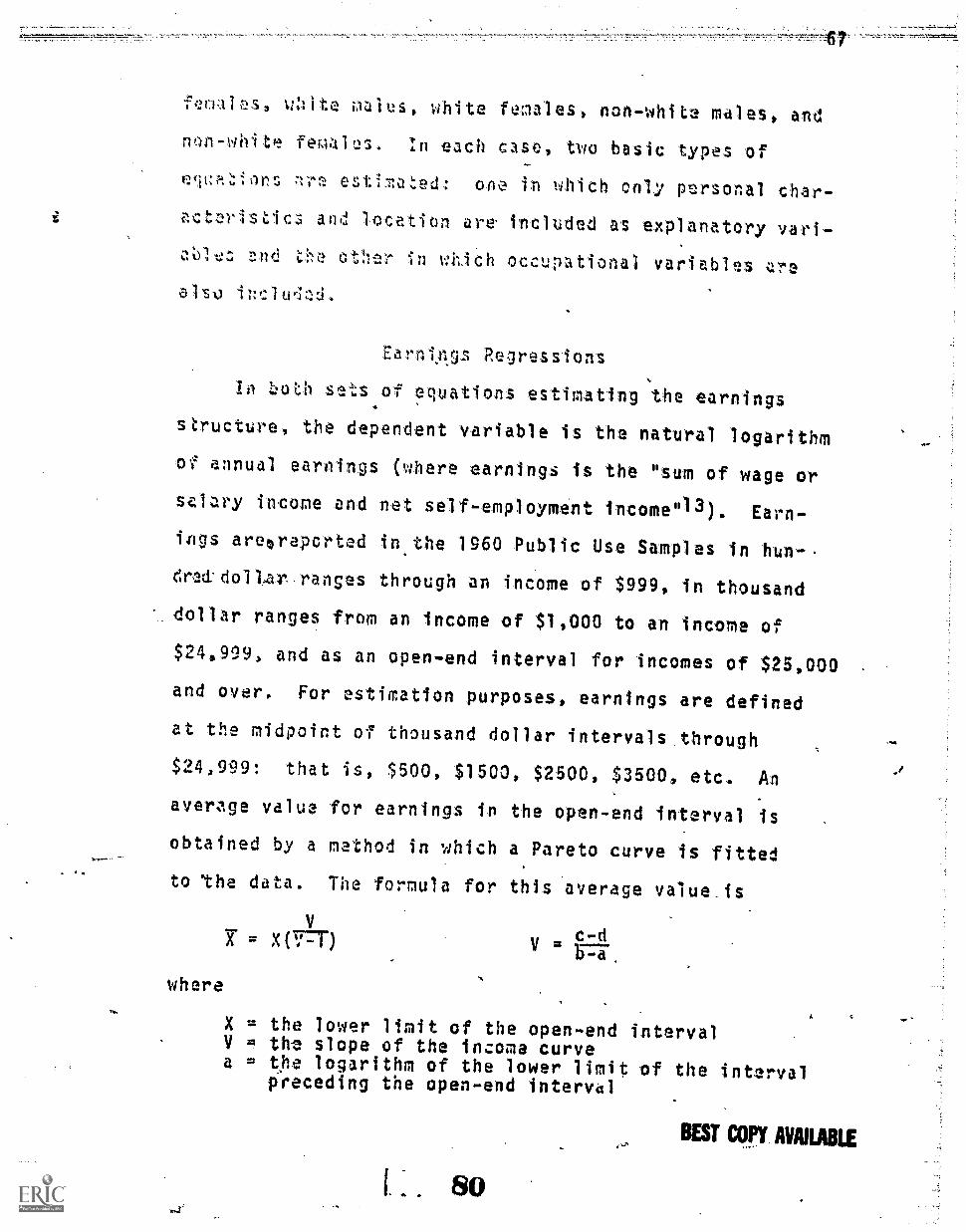
-,.tilles Oita oalus white fenales, non-white males, and

non-whit-4e Penal es. In each case, two basic types of

egtors esti7toted: one in which only personal char-

acteristits and location are included as explanatory var

also

the otIler in which occupational variables -are

Earnifos RegresSions

In both sets of equations estimating the earnings

structure, the dependent variable is the natural logarithm

of annual earnings ( here earnings is the "sum of wage or

salary income and net self employment incomen13). Earn-

ings areoreperted inthe 1960 Public Use Samples in bun-.

draddoltar ranges through an income of $999, in thousand

dollar ranges from an income of $1,000 to an income of

$24,999, and as an open-end interval for incomes of $25,000

and over. For estimation purposes, earnings are defined

at the midpoint oF thousand dollar intervals through

$24,999: that is, $500, $1500, $2500, $3500, etc. An

averzlge value for earnings in the open-end interval is

obtained by a method in which a Pareto curve is fitted

to the data. The formula for this average value is

where

c-dV 1574.

X = the lower limit of the open-end intervalV m the slope of the income curvea the logarithm of the lower limit of the interval

preceding the open-end interval

BEST COPY. AVAILABLE

lo'rjarihm of thi., lowar linit of tha open-endintervdi

c = incnrithm of the sum of the frequencies in .theopen-end interv41 and the interval preceding it

d Itnarlm of the frequzncies in the open-end

Thu frequenties 'used in this cenputation are. those for the

1,160 tape including individuals working 'without

pay and stat anJ local government 'w'orkers. The average

vOue for 1980 computed in this fashion is:

X-z% $55,136.74 V 1.6229 = ln(78)-1n(73)ln(f5,000i-ln(24,000T

Earnings in the 1970 Public Use Sample are reported

in hundred dollar intervals through an income of $49,999

and as an open-end interval for incomes of $50,00 and

over. For estimation purposes, earnings are defined at

the mid-point of hundred dollar intervals through $49,999:

that is, $50, $150, $250, $350, etc. An average value for

earnings in the open-end interval is obtained through the

Pareto Formula cefined above. The frequencies used in

this computation are again those for the entire 1970 tape

including individuals working without pay and state and

local goverment workers. The average value for 1970

computed in this fashion is

3= $82,489.75 V = 2.5389 = 1

I. 0.60 10'57

n

In both 1,,.260 and 1970, the dependent variable in both

sets of earnings regressions for individuals who reported

no income is set equal to one.

This value for annual earnings does not include the

value of expenditures on fringe benefits in either the

BEST COPY AVAILABLE

itr11 or pr;Tat s,ectors. It was noted in Chapter II

that frinv benefits i'orm an increasingly important part

e;loya,J tcl7pensation zod t`nat since 1'952 ttey have

go-on ?aster in the Federal than in the private sector.

tonstNt:entiy, to ,eaternine 1:ter worers I the *.v.1

:s*cters recive cm :parable pay, soine consideration siirJuld

be given to frinse benefits. There is a great deal-of

evidence pointing to a positive relationship between fringebefits and vage rates. When turnover costs and union

nembership were !r, 14 constant, it was found that

(1) wage supplements generally vary positively withmoney earnings independently of the other factors con-sidered, (2) variations in wage supplement expenditurescan be cxplaine largely in terms of variations inmoney earnin,ils."

Cnncequently, if it is accepted that the proper basis for

comparison between Federal and private workers is compen-

sation, earnings plus fringe benefits, rather than earn-

ings alone, then it must be recognized that "relative

money wage differentials progressively understate differ-

entials in co;npensation."16 However, because there is no

information on the value of fringe benefits contained in

the census data, estimates of the Federal,-private differ-

ential are made on the basis of the earnings data with

the realization that these differentials are downward

biased estimates of the differential in compensation.

Personal Characteristics Earninos Regressions.

In the personal characteristics earnings regressions,

three 'variables are Included to account for the effects

8 BEST COPY AVAILABLE

o F itve:;st,,,ctnts in hurfian capital. In accordance

with p,..)st-sc;Icoling ilive.itment models of Becker, ':Iincer,.4 " lot 4.,tt and Chi wick discussed above, thf! sped 'Ica ion

ts two typ3 investments: education which enters

t.1 l J114r,ar te:Ain li r, ai experince 1)oears as a quad-

ro,ic rariabi to r,Yfle t ttNpettadt clininj rate of

turn to tlz1-tioc-job triaininu. Because the Public Use

Sx.1)1:2s prov 1 no information on actual experience, an

estirlate o 7 poentiaA Nprk experience isittai$ftpTea;47::

individual on the basis of his age and education. To'd

closely this approximates actual years of experience

depends upon the strength the individual's attachment

to the labor force. These variables are defined as follows:

ED lubei or y'ec11- or tichool completedX = age minus years of school completed minus five

.

XS C; . the_square of potential work experience de'-fined above.

In ord r to centrol for other sources of variation among

individuals, a number of personal characteristics variables

are included. ih s?. specific variables are:

RACE . 1 if non-1,1hite (legro, American Indian, Japan-ese, Chinese, Fillipino, other--including Aleut,Es',,imo, Hawaiian, and Korean)

= 0 otherwiseSEX - 1 if feoale

C otherwise

The reference group, then, is white males. These variables

principally reflect the effects of discrimination against

non-whites and females. Differences in productivity be-

tween the races and sexes are reflected mainly through the

other personal characteristics variables: education, ex-

BEST COPY AVAILABLE

-_

g - r.

71

vqriables, maritd1 status variables, etc.

dig' variabis for marital status are includ-

e-I.: 3pou;.! prest, spousz ztO divov.cd-

s;.)arat-.A. The rc arence grnup is siogle, nev'ir-narried

intlividu ,.l'" Bow:::n and Finan dtiviopAd toe ra'7,1,on,'

for 1.,ire us oF the J, variables. 17They argue that for

inales, marital s atus'serves prirarily as a

proxy for certain personality traits and health char

ttt.aiWitt vblen 'facilitate socces's in work and secondar-

ily as a measure of family' responsibility and thus taste13for work. This argument implies that marriage with

spouse present will have a favorable effect on men's earn-

ings. The effects of the other merital categories are

expected to be less pronounced than those of the spouse

present category. On the other hand, marriage with spouse

present is expected, to-have an unfavorable eFfect on women's

earnings. Here ,employers tend to regard married women as

prone to absenteeism and justify paying lower salaries on

the additional grounds that married woman are only a

source of supplementary income to the family.

Because the data,for 1950 and for 1970 pertains to the

South .1'..tlan.t.:c Cansus 1!.-1,.gion, it is 1,4 ti A.. A. v., V. j tit. I,

duce dummy variables for region to control for diferences

in the cost of living among the regitIns in order to examine

real differentials rather -than money differentials . How-

ever, it is necessary to include a location variable to

control for differences in cost of living, job opportun-

84 BEST COPY AVAILABLE

72ti

;Ind other pc unia y and non-pecuniary facors

41socialtad win urb:at areas. Several dummy variables di

in.;u1 hing -,:',reas by popul tion size 1.2',-;uld

b2 tisirable Lut t;:is Information is utavaiiable in tht

data used. Tilralturnativz: :dossible variables are av411-

4.)el

I o.

urban :'..?.cic,enc...--residerce within an urbanized areaor in placs of 2;500 or more outside urbanized aPeas(the reference group is rural residence);

mletrorAitan residenceresidence within a standardmetropolitan statistical area (the reference groupis residence outside SNSA's);

central city residence -- residence within the urbanpart of the central city of an SNSA '(the referencegroup is resiCmce outside the -central city).

Each of these variables is expected to havi4 a positive sign.

Data for each of these variables are unavailable for

residents of Delaware because this state violates the

criterion that at least 250,U0 individuals live in one

of the identified categories. Because the number of ob-

-servations from the state of Delaware is small relative

to the total size of the samples, It is not- expected that

this adversely affects estimations using a location vari-

ahl

The concept of an urbanized area has several advan-

tares over that of an SMSA in measuring the effects of large

populatienIsize on earnings. The differences between the

two concepts'are that an urbanized area excludes rural

sections of counties comprising SMSA's and places which

are separated from the densely population Fringe surround-

BEST COPY AVAILABLE

i,iq a cent al city !-,,y rural territory. In addition,

un!i SflSA's, i4hos ;borders are permanent, urbani:ed

arcs define to

73

ie p7 ;%1 t1 'm

at the tim of tensus)9 fien only one variable is

to leasurc., urban size effects on Cost of livinl) and

other pecun = aey and non-pecuniary factors, thc distinction

1Imt;ieen urban an rurai r sidence appears more maanin.gful

than that botyeen central city and non-central city resi-

dence.

In order to verify these expectations concerning :the

locational variables, equations are estimated using each.

In the majority of cases, these suppositions are confirmed:

R2

and F statistics are greatest for equations estimated

with the urban vari able; the sign is correct for the urban

variable; and the significance level is greater for this

v.ariable than for either of the other location variables.

Two additional personal characteristics variables are

included in certain of the equations estimated, One is a

variable included in certain of the equattons estimated

for females, white females, and non-white females which is

specified:

--BABYB -= the number of children born

The presence of children has an important effect on the

labor force participation of women. In their study of the

labor force participation rates of married women, Bowen

and Finnegan have shown that. these rates differ according

to the ages of children present. Women with children

S6 BEST COPY AVAILABLE

74

under acres only had the low stpartictpltitn rates of

cu womea studied in urban areas after adjusting for the

effects of color, age, schooling, other family income, and

the employment status of the husband. Married women with no

children under age' eighteen had the highest adjUsted partic-

ip tion rates of all the varried 'women studied. These ad-

justed participation rates were quite different for married

flegro woren, however. Their rates were higher than those

for all married women for every category but the differences

were most obvious among women with only children under age

six and those whose youngest child was between six and thir-

teen years of age.2° Consequently, it is expected that wom-

en with very young children will often leave the labor force

to care for them but may frequently return as their children

grow older. However, this tendency to leave the labor force

in order to care for their young children is less strong for

Negro women. The rationale for tne inclusion of a variable

measuring the number of children born to the female was de-

veloped by Oaxaca as a reflection of the "cost of lost ex-

perience due to child care, including the costs from the de-

preciation of skills during the p riods of absence from the

labor force." 21

The second variable included in certain equations is a

dummy variable for health status. This is defined:

DISAB = 1 if health problems limit the individual'sability to work

= 0 otherwise

This information is only available in the 1970 data. It is

clear that there is a relationship between an individual's

BEST COPY AVAILABLES7

statls an:! lAbor force participation.

Eowen and Finne7-jan found

't)ere is

schoolino lnd

in tho 1,0,644,1

i;Itoractio:;1

or force pa:.ticipation.

1-til.e this v,:tI is e..qct:.!d to lia'!e it

01

1?.,2 Consequ!

on earnins, it is vecogniay.! that ther,1

eutaticn, experienc:?, and irtalth condidons.

Nfterences in tht effect of this variaale with re sv.ct

to race re erlected to reflect such interactions 2.1 well

as diffurences in the health status of the races. Further-

more, 1t is expected that the effect'of this variable will

differ with respect to sex. This is an indication of the

greater substitutability of work in the home for females

if1P1?Z. as Yell as between

experience, and health conditions and differences in the

health status of the sexes. Consequently, it is expected

that this variable has a n gative effect :which is smaller

in absolute size for to than for males.

Full Earnin45 Regressions

In the full earnings .regressions, dummy variables are

included for the U. S. Census two-digit occupations as

w311 as the varje.i;;us included IN Lhe puesoudl uhdrdcLer-

istics earnings regressions. In the original design of

this set of variables, clerical workers were the refor-

enco group and separate dummy variables were to he includ-

ed for professional and technical workers, managers, sales

workers; craftsmen, operatives (including transport),

r ssBEST COPY AVAILABLE

.afiajors, servic:- workers,

ept! privat oushoId workr s. However, there are in-

obrvatlop.t in several of c;711s to

estimation. CwnsegnentIy1 the occupation variabie1Are lii to an cs'timable nustlber, the included variables

i;g accori4g to the partfcular subsample sf data be-

in stimateti.

Altuijh these occupational variables are expected

to add to the explanatory power of the estimated earnings

strtActure, their inclusion for the purpose of this -study

is questionable for several reasons. According to the

Comparability Doctrine, Federal pay rates are to be com-

p.rable to private pay rates at the same level of work.

1)01 +,1-In4f. to.v.. rrgitpa41.4%rl IV C tor m", 13v4"4 ....414 I A4 I.

more than one level of work in the Federal sector. Con

sequently, the effect this occupational variable would

medsure is unclear. Furthermore, if the policy goal of

achving e.;uity between Federal workers and thetr equals

in the private sector has been achieved, then workers with

conparable productive characteristics should receive com-

parable pay Oithout controlling for ocouPation. The rele-

vant earnings structure to examine for this purpose is the

estinated personal characteristics equations. Nevertheless,

the full earnings equations are also estimated in order

to examine the question of whether Federal and private

workers of roughly equal characteristics receive the same

pay for the same broad occupational categories.

89 BEST COPY AVAILABLE

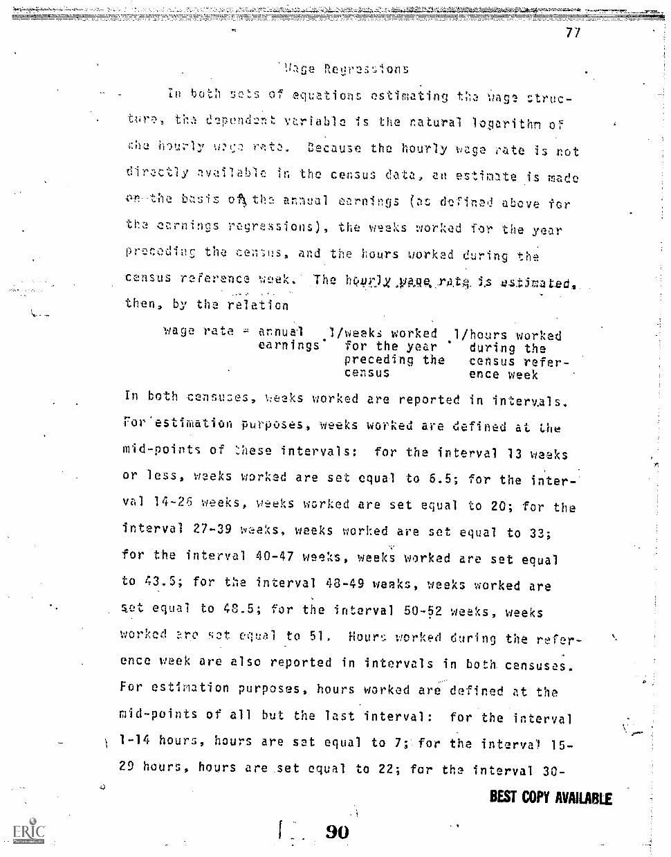
77

!1:tge ftelireiY!ots

In both 'sc'ts of equations estimating le VAT.?

th d'epvnd-..nom A...riabite is the natural logarithn of

tecause the hourly vage :catt is not

dircIctly ,nvail,ab1:% it the census eft 'estimate is "ado'

o7k tte annual inrnings de-rinail above

th (rarniffos rzs:yr,;:ssions,),, the weeks word for the yearprec:Idtil'c the ,c:e-,1..;11s, a.nd the hours worked during the

census reference The 110.),r),xl ,,y0.9:0.-rAt4 1.5 ,e,s.4-jrated-s

then, by the relation

wage rate - annual Ittweeks worked 1/hours workedearnings' for the year during the

preceding the 'census refer-census ence week

In both censuzes, 1;:eaks worked are reported in intervals*

For'estiffiation purposes, weeks worked are defined at the

mid-points of these intervals: for the interval 13 weelcs

or less, weeks worked are set equal to 6.5; for the inter-

val 14-26 weeks, weeks -worked are set equal to 20; for the

interval 27-39 'peeks, weeks worked are set equal to 33;

for the interval 40-47 weeks, weeks worked are set equal

to 43.5; for the interval 48 -49 weeks, weeks worked are

seat equal to 48.5; for the interval 50-52 weeks, weeks

worl:ed ,;,)t. equal to 51. Hour.; worked during the rtrer-

ence wek are also reported in intervals in both censuses.

For estimation purposes, hours worked are defined at the

mid-points of all but the last interval: for the interval

1-14 hours, hours are set equal to 7; for the interval 15-,

29 hours, hours are set equal to 22; for the interval 30-

BEST COPY AVAILABLE

90

34 hours, hcurs are set elual to 32; for the seepar,, 41.1

heurs, hoer: arn se, equal to for the intervel 41

1 s,r1 4 tt yt ere eet ?beet to 4 a

es .r 2,:be inte7evelee,

beees hours ere sot equal to 54. 1h,iFs fie el interval

lter,e1 of :,8f3 or feor heurs. The everaee

velue 4er hours her is obteied by thesan.t ieethed used

to obtain the everege value for eerninjs in the open-end

interval, by fitting a Pare to curve to the data The

4.*4 .4

frequencies used in the computations for each tape are

those for the entire tape, including individuals working

without pay and state and local government workers. There-

fore, the average value for hours in the open-end interval,

Tr, is com.duted using the formula

where

z

E = the lower limit of the open-end intervalZ = the slope of the curve fitted to the dataa = the logerithm of the lower limit of the interval

precodin3 the oren -end intervalb = the logarithm of the lower limit of the open -end

intervalc = the logarithm of the sum of the frequencies in

the open-end interval and the interval preceding_ .

it.

d = the logarithm of the frequencies in the open-endinterval.

The average value for 1960 computed in this fashion is

IT= 84.161 where Z = 3.4833 = 1?-1412) ln(2100)1n(49)

The average value for 1970 computed in this fashion is

= 80.899 where 11{433) - ln(193)ere Z = 3.8709 = -W50) -

BEST COPY AVAILABLE

91.

/9

fhe spe'Cification of the control variables for the

ci3,aractristic:; an'd the full vage re5ressions is

th.! slm es thi. :or nriYenT1 ressions. These

arz, 'estigt,-;! for all Fe'deral ant! for all private

v,o4-..,,'s as vi,!111 as each of V, eivint rate-sax subdivi-

na7ro, fenTales, 'white mles,

whie femeles ivor-hite males, non white fecales) of

F derel afld of private vorers.,

Structur 1 Cotgarisons

Defore speci yinn the exact technique used to estimate

the edroings And wage rate differentials between Federal

and private sector workers and to decompose these differ-!

entials into their cemponent parts, it is necessary to

consider the hypothesis that the earnings (wage rates)

of Federal workers and private sector workers are gener-

ated by the saps structure. In order to test this hypothe-

sis, pprnonal ch,.zractaristics and full-scale earnings and

wage equations ere estimated for all Federal workers, all

private workers, and all workers in the subsemple (ex-

I

copt state and local government workers and iildividuals

working without pay). These estimations ara made on the

1960 data and the 1970 data using both the industry class-

ific tion and the work class methods to subdivide it.

These results are employed to perform a Chow test of the

equality of earnings and wage rate structures for Federel

and private workers. 23The test statistic formed is

92 BEST COPY AVAILABLE

.2." .,. ,

SS t,SSE )/

F SSE. )/ (n + -tt

n+m

CO

T = total of private and Fede..'al borkers combinedP prlvate ,:orkersF razlerai wer!;ers

w:r;lber independent varieties plus onen tel nuet:Jer of privatc ti iii

m = nelebor of Federal woe'kers

It is expected that the earnings ancrwage rate struc-

tures estimated with personal characteristics only are sig-

ntficantly different in 1950 and 1970 for Federal and pri-

vate workers. The results from the application of the Chow

test, contained in Table 8, confirm that the structures

are significantly different at the 5 per cent level. How-

ever, it is possible that when differennes in occupational

structure between%the two sectors are controlled 'for in

the full regressions, the earnings and wage rate structures

will no lorger be significzlritly different. The test sta-

tistics formed from the application of the Chow test to

the full earnings and wage rate equations, found also in

Table 3, con irm that the earnings and wage rate structures

are still significantly different for Federal and private

workers in both 1950 and 1970 at the 5 per cent level., The

earnings equations from which these statistics are formed

are found in Tables 4 and 5. The wage equations are pre-

sented in Tables 6 and 7.

BEST COPY AVAILABLE

93

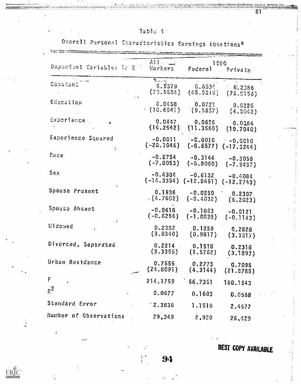
Tabl

0et)ri!1 1 P:!ron:11 Caradtristits Earnings Eluations

Or,

tart

Eth:co. ti on

E:xperi ence .

Experience Squared

Race

Sex

Spouse Present

Spouse Absent

Widowed

Divorced, Separated

Urban Residence

F

R2

Standard Error

Number of Observations

Arnim.4,40/.0.,AllWorkers

1950Federal Priva te

5.9379 6±.2386(71.5584) (45.9316) (76.t156)

C.0458 0.0721 0.0226(10.6941 ) (9.5557) (4.8043)

0.0447 0.0626 0.0164114.2542)

-0.0011(-20.1046)

0.2754(-7.8053)

-0.4334(-14.3354)

0.1936.(4.7602)

-0.0618(-0.6256)

0.2382(3.0340).

0.2214 .

(3.3355)

0.7555('24.8091)

214.1759

111.3560) (10.7040)

'-D.0010(-8.6577)

-0.3146(-5.8050)

-0.6132

-0.0010( 17.3244)

-0.3055(-7.9437)

-0.4084(-12.8491) (-12.2743)

-0.0250 0.2307(-0.4032) (5.2023)

-0.1863 -0.0121(-1.0338) (-0.1143)

0.1259 0.2828(0.9817) (3.331?)

0 1518 0.2316(1.5762) (3.1893)

0.2773 0.7095(4.3144) (21.8785)

56.7351 160.1643

0.0677 0.1603 0.0568

2.3836 1.1510 2.4577

29,349 2,920 26,429

94BEST COPY AVAILABLE

41.

1,ab1T2 4--C;) tillued

0:-*::.14111:mt In

40.0.1* ...1+.1.

CQ11:itnit.

Edt;cat oB

Exprie;-ice

-F.-.4perielica Squared

Race

Sex

Spouse Present

Spo:tse W,ent

Wowed

Divorced, S4aratd

Urbao Residence

01:7a.oility

F

R2

Standdrd Error

Number of Observations

AII)

13...

1;70

6.4746

0.0567(1.%1815)

0.0532(20.2726)

-0,002tn:V/7b)

-0.1710(-5.6538)

-0.6729(-26.5309)

0.3426(9.6412)

0.1132(1.2555)

0.?765(4.0090)

0.3560(6.6393)

0.5133(19.4473)

-0.4706(-9.7307)

255.5121

(' ;c)

Privz;t2

tar...1411M

i.6494(S4.1.377)

0.?*16{it3;fsIn11)

(16.0033)

-0,.a011-12.5073)

-0.2838(-7.6553)

- 0.4935

(14.5333)

0.2776(6.0584)

-0.2393.(-2.0463)

0.2'' P0

(0;:...) ;60 )

o.04ori13.6672)

-0.0010-18.972)

-0.2330(-6.5834r)

-0.6860(-23.5903)

0.4012(9.7879)

0.2053-(1.9860)

0.)"592(2 . 95'35) (4

0.1670 0.4474(2.4219) (7.2483)

0.2534 0.4501(5..6039) (15.5093)

-0.4023 -0.4662(-5.8852) (-8.5150)

144.6527 165.66'39

0.0771 0.2270 0.0605

2.1770 1.1297 2.2923

33,523 5,383 28,140

95 BEST COPY AVAILABLE'

83

Table 4--Continued

EAll (INDUS) 1070 (IIDUS)

Feder7a1 Private

Edt:cation

tY,p;.!nc

6.3244(101-.0111)

.0706(19.6091)

0.0543(22.4243)

6.7153(53.6561)

0.Mi5(12.C511)

O,071(15.5352)

6.57t9(96.1872)

0.0521(13.1458)

0.0454(17.5723)

Experlenrie-S*:a'r,e6

(-25.43237') '-12.0843) (-21.5342)Race -0.1316 -0.2502 -0.1422

(-4.7627) (-5.9018) (-4.6761)Sex -0.6537 -0.4784 -0.6497

(-28.1264) (-12.66381) (-25.4905)Spoie Presnt 0.3164 0.2165 0.3523(9.6807) (4.?434) (9.8235)Sponl.., Absent 0.0979 -0.2710 0.1615

(1.1793) (-1.9416) (1.7895)Uidw:),d 0.2763 0.1934 0.3392

(4.3365) (1.7014) (4.9118)Divorced, Separated 0.3191 0.1592 0.4028

(7.0113) (2.0556) (7.3595)Urban Residence 0.4678 0.3024 0.4183

(18.9950) (6.0089) (15.7905)Disability -0.4588 -0.3124 -0.4629

(-10.1427) (-4.1188) (-9.4062)

F 236.3584 109.2671 202.9536R2

0.0781 0.2248 0.0632Standard Error 2.1212 1.0344 2.1977Number of Observations 37,049 4,103 32,941

at-values in parentheses /

St;BEST COPY AVAILABLE

Ovr:rLl11 SCc11! E4rlin'jS 1.1tA

414 *ay,.Oelent: iabl : In E

..ons

..44.0;1

,cxperience

Experience Squared

Race

Sex

Spouse Present

Spouse Absent

idewed

Divorced, Separated

Urban Residence

Professionals

Managers

Sales

Craftsmen

( °H.) .

0.:)333(16.2519)

0.044e(14.4688)

-0.0010(-13.5527)

-0.2453(;-*6.8575)

-6.2932(- 3.- -948)

0.1651(4,1109)

-0.0429(-0.4418)

0.2096(2.7103)

0.2016(3.0830)

0.7835(26.1111)

0.1686. (3.3823)

-0.7964(- 13.9435)

0.7761(16.4955)

57

Ar

-.4arow

'( ?,A.0.7)74,)

0.0473(5.112)

P..0657(12.3'.;17)

0.0614 0.0353( 1.15:32) (10.8546)

-0.0010 -0.0009(-8.7071) -15.5436)

-0.2114 -0.2692(-3.6553) (-6..9026)

-0.5461 -0.236610.4929) (-6,6704)

-0.0309 0.1911(-0.5013) (4.3729)-0.1423 0.0007

(-0.8302) (0.0070)

6.1271 0.2359(0.9950) (2.8409)

0.1630 0.1959(1.7012) (2.7443)

0.2736 0.7350(4.2724) (23.0811)

0.3569 0.1395(5.7617) (2.4786)

0.2717 -0.8065(3.0129) (-13.0203)

0.1408 0.8665(1.6759) (17.5377)

BEST COPY AVAILABLE

5--CcAtinued

n

1;1,,nt Var!'a .1c: 1r E r :3

1960Fder,11 Privztt:-2

Op:-!rativfls

Lnl.lorrs

0.80949 --Y).r00 Ljr,v, (-0.4151)

-0.224,2

0.9207

0.5003(7.6535) (-1.5)23) (8.5175)

Se7rv;c2 -C.1005 -0.1993 -0.0429(-1.8305) (-1.8773) (-0.7315)

F 200.6510 38.6159 169.40682 0.0982 0.1709 0.0925

Standard Error 2.2444 1.1437 2.4107

Number of Observations 29,349 2,920 26,429

98BEST COPY AVAILABLE

s'N 14 , ,,, "ty 4

47.0,6.S.tt

,..04,sNALli041

E;:perie.:nce Squared

Race

Sex

Spouse Present

Spouse Absent

Widowed

Divorcod, Se.vareted

Urban Residence

Professional

Manager

Sales

Craftsmen

Df4t.4.0

41111 A"

111"'"'sP1''.JI

170,1

(77.0.) 2)7.02.65

fr- 01"\c 6.3697

!..).0S23 0.0422(13.6897) / D )

(8.02'10)

0.0513 0.0E51 0.3380(19.5186) (16.3627) (12.7024)

-0.0011 -0.0011 -0.0009(-22.7072) (-12,43741) (-17.1721)

-0.1370 -0.1975 -0.2055(-4.4493) (-5.1783) (-5.7397)

-0.5331 -0.4557 0.4372(-18.7047) (-12.3102) (-14.8:95)

0.3119 0.2603 0.3537(8.7844) (5.7?-14 (8.f.;419)0.0373 -0.2170 0.1577(0.9729) (-1.3701) (1.5314)

0.24S2 0.2772 0.3101(3.6135) (2.8609) (3.9837)

0.3435 0.1599 0.4181(6.433.7.) (2.3237) (6.8115)

0.5544 0.2471 0.5022(20.7975) (5.5006) (16.9514)

0.2048 0.2529 0.1367(4.7299) (5.7473) (2.5414)

0.0667 0.3195 0.1515(1.3297) (5.3307) (2.5375)

-0.2339 -0.6469 0.0346(-4.5635) (-2.5676) (0.6030)

0.3153 -0.0489 0.5934(8.5994) (-0.7732) (11.9575)

99 BEST COPY UNABLE

87

Table

Daptldnt Variable: In E

-Continued

111 1 1970 (AC)Feder a I :Pri v-a te

..............111im...MMIlm'Op'erati ves 0.4130 -0.0439 0.6401

(10.3821) (-0.5086) 14.2743)tab,)rorr, 0.1017 -0.2719 0.3011

(1.5974) (-2.4830) (4.2412)Service -0.334 -0.3448 -0.2174

(-8.0152) (-4.8429) (-4.1102)Di Sabi 1 i ty -0.4451 -0.3891 -0.4364

(-9.2503) (-5.7350) (-8.0209)F 178.9675 95.3128 124.9387R 0.0872 0.2398 0.0735Standard Error 2.1650 1 1203 2.2764Number of Observations 33,523 5,383 28,140

100BEST COPI AVAILABLE

T 51 e 5 - Conti n ed

;_t1;"kl: 1 n is

e IM.

Costant

Experience Squared

..*)J.,+*.1404

(82.4746 )

f ?* 290 -)kIC.c.1)

0.'0524(21.64D6)

-0.0011( 24.1860)

7. C:.; 56

.0330(7.20,45)

0. 0:33(14.8622)

-0.0012( 11.7051)

6. 174c*I :A

7

^PIP1'kJ V )

.

(16.5544)

-0.0010-19.9569)

Race -0.0979 - 0.1736 -0.1133(-3.4327) (-4.0134) (-3.6610)

Sex -0.5164 -0.4227 -0.4615(-19.9444) (-10.0725) -16.1974)

Spouse Present 0.2869 0.2-042 0.3111(8.7917) (4.0301) (8.6810)

Sp9use Absent 0.0693 -0.2592 0.1176(0.8391) (-1.8722) (1.3104)

Vidoed 0.2510 0.1350 0.2997(3.9582) (1.6406) (4.3660)

Divorced, Separated 0.3399 0.1512 0.3829(6.8538) (1.9669) (7.0447)

Urban Residence 0.4996 0.2973 0.4523(20.2993) (5.9439) (17.1079)

Professional 0.2937 0.3154 0.3610(7.7479) (6.5383) (8.3241)

Manager 0.1114 0.3548 0.1774(2.3559) (5.7616) (3.3141)

Sales -0.2358 -0.5626 -0.0210(-4.6726) (-1.4748) (-0.3901)

Craftsmen 0.4035 -0.0204 0.6019(9.7728) (-0.2636) .(13.2644)

BEST COPY AVAILABLE

101

39

fJbl,d

n o '/b E

All ( I S )rs

1970 (I:r,IDUS)Fed era 1 Pri vatl

Opurittiv 0.4030 -0.0802 0.5894(10.6V30) (-0.6766) (14.3255)

Laborflr 0.1228 -0.2281 0.2951(2.0502) (-1.6839) (4.5E:74)Sse2rvice -0.3134 -0.1872 -0.1651(-7.4011) (-2.0019) (-3.6109)0 sabi 1 i ty -0.4340 -0.2920 -0.4355(-9.6436) (-3.8773) (-8.9045)F 201.1182 72.0735 151.2699R2 0.0886 . 0.2375 0.0759Standard Error 2.1091 1.0754 2.1827Number of Observations 37,049 4,108 32,941

at values in parentheses

BEST COPY AVAILABLE

Tabl t

PerstN,w11 no.rzItteristics Wage Eqtaticnsa

90

0 ;-,11,2t!nt Vztriz.!)1 InMIVlor!,.ors

19f:0

fedeni P ivate111.1.21.1.044..1 1. .6*

-0.DSG1t-11?.514

P rp,6)

Eduction 0.026n 0.0701(6.a71) (9.3425)

w.iencz: 0.0192 0.040D(6.0487) (7.8450)

Experience Square4 -0.0007 -0.0006( 12.2265) (-5.5311)

Race -0.1124 -0.2488(-3.1505) (-4.8573)

Sex -0.0936 -0.4962(-3.0279) (-11.0004)

Spous2 Present t 0.0745 -0.0704(1.8131) (-1.2026)

Spouse Absent -0.1219 -0.1749(-1.2207) (-1.0765)

Ui dowed 0.0928 0.0292(1.1694) (0.24.04)

Divorced, Separated 0.1019 0.0918(1.5189) (1.0086)

Urban Residence 0.6885 0.2221(22.3701) (3.6554)

F 132,1406 41.0149R2

0.0428 0.1206

Standard Error 2.4091 1.0880

Number of Observations 29,349 2,920

103

--G.L473I.'" ,

rIAA

0.0025(C.5262)

0.0108(3.1309)'

- 0.0005(-9.9582)

- 0.1320(-3.3862)

0.0353(-1.0751)

0.0994(22111)

-0.0894(-0.8311)

0.1248(1.4502)

0.1057(1.4352)

0.6495(19.7508)

10,1.8951

0.0354

2.4911

26,429

BEST COPY AVAILABLE

Table 5--ContInued

i;f*Nnv1,4A14'14 '!,1,orkers

wty*,-..paramm.

Experi nce.STIared

Race

Sex

Spou5::! Present

Spouse Absent

'Widowed

Divorced, Separated

Urban Residence

F

R"

Standard ErrorNumber of Observations

1970 (WC)Fed.aral Private

-0.5432(-8.0616)

0.0469(11.7972)

0.0267(10.2395)

-0.0007(-14.1292)

0.1246(-4.1478)

-0.3343(-13.2554)

0.1710(4.8400)

-0.0294(-0.3279)

0.1443(2.1043)

0.1302(2.4424)

0.4909(18.5201)

-0.2766(-5.7513)

0:1 nOnr.sc.w.V..OV4

.1).0400

2.1649

33,523

1. 10-.1

-0.6963(.5.5230)

0.0367(15.3661)

0.0483(12.3917)

-0.0008(-8:7817)

-0.2405(-6.6756)

-0.3494(-10.5890)

'0.1772(3.9786)

-0.2729(-2.4011)

0.1507(1.5885)

0.0179(0.2656)

0.1848(4.2046)

-0.3012(-4.5345)

97.24IG

0.1644

1.0979

5,383

91

-0.0543(-0.3219)

C,.0125(2.7209)

0.0138(4.6208)

-0.0005(-9.9061)

-0.1715(-4.8573)

-0.3075-10.6012)

0.2062(5.0432)

0.0337(0.3268)

0.2065(2.6442)

0.1983(3.2217)

0.4469(15.1016)

-0.2592(-4.7463)

75.4090

0.0233

2.2V;6

2.2,140

BEST COPY AYMLABLE

I

C I v u 1i t.1

A I1

Y'v

* tay ko As ,w %.1

to ,,

,is l v i1

(-11 . 211'. 1 )

rt.ot-:),03 5 7 )

0 . C'.2 6' 7

( 1 1.131 2)

-0.573"..;

, 777;.e)

40.111;5.1,

0 . 0 g

41"041,,t1..

0C440(11.154S)

0.0181(6.877t)

Weribnce Squared -0.0007 -0.009 -0.0005- 1 4 . 173) (-9.3949) -11.1013)

Race -0.0946 -0.2330 -0.0968(-3.4510) (-5.6790) (-3.2024)

sex -0.2975 -0.3538 -0.2630(-12.9030) (-9.949I) -10.3750)

Spouse Present 0.1516 0.1233 0.1717(4.6747) (2.4974) (0.808:)

Snouse Absent -0.0327 -0.1937. 0.0023(-0.3976) 1.4304) (0.0252)

Widowed 0.1323 0.0531 0.1770(2.0929) (0.4Z28) (2.5779)

Divorced, Separated 0.1177 0.0235 0.1539(2.3827) (0.3140) (2.3305)

Urban Residence 0.4377 0.2270 0.4005(17.9161) (4.6734) (15.2032)

Disability -0.2785 -0.2303 -0.2741(-6.2075) (-3.1372) (-5.6013)

F 145.6709 79.3864 94.9953

R2 0.0412 0.1735 0.0304

Standard Error 2.1042 1.0495 2.1853

Num'aer of Observations 37,049 40108 12 tl!r 1,.,

at-values in parentheses.

L 105 BEST COPY AVAILABLE

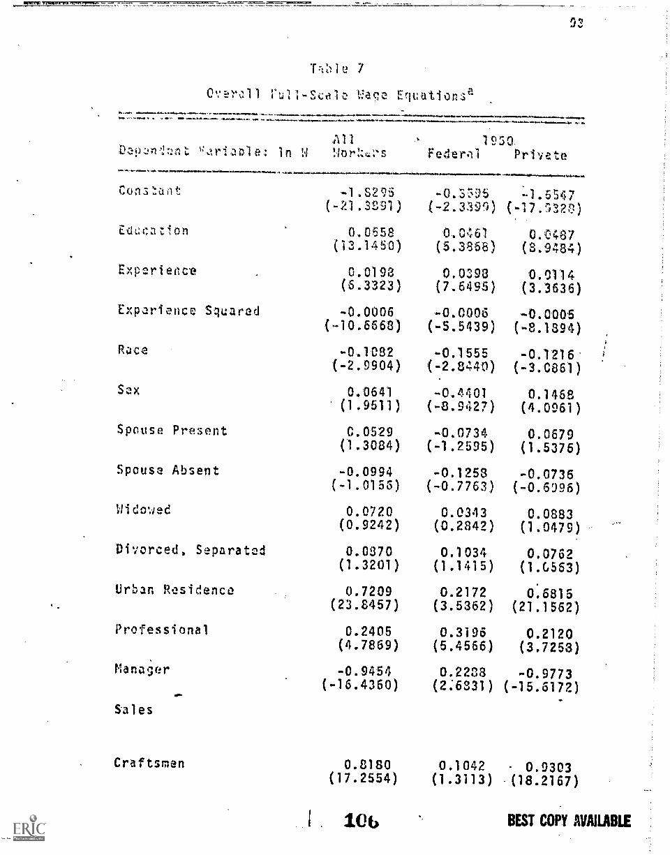
711ole 7

Vu11-Si e taqe Ertuilttons

5:3

siaamia*-444-444-4144 4.4444.4 .1.4.mmims 4444 dm.... .4.4 amo W41144...4.**444 .4. N. 4 A. 4.4.41.4 4444 4A4 *444.. 44.4 444.4.1. 41.114.414 4**44444,4444-444.4444.4 .4.44.441.4414 44_

v.ntatie; InAllWor'ss

1950Feder;11 Private

1.444. 1N. 44, 44,046.... 414

Consnnt

=14444.4444.4.444.44444.4*.4...4444.

-1.6295(21.3t9i) (-2.339))

EA*1,a ti on 0,0658 0.0461(13.1450) (5.3860

Experience 0.0192 0.0393(6.3323) (7.6495)

Experience Squared -0.0006 -0.0006(-10.6663) (-5.5439)

Race -0.1032 -0.1555(-2.9904) -2.8440)

Sax 0.0641 -0.4401(1.9511) (-8.9427)

Spouse Present 0.0529 -0.0734(1.3084) (-1.2595)

Spouse Absent -0.0994 -0.1253(-1.0156) (-0.7763)

Widowed 0.0720 0.0343(0.9242) (0.2842)

Divorced, Separated 0.0870 0.1034(1.3201) (1.1415)

Urban Residence 0.7209 0.2172(23.8457) (3.5362)

Professional 0.2405 0.3196(4.7869) (5.4566)

Manager -0.9454 0.2233(-16.4360) (2:6331)

Sales

Craftsmen 0.8180 0.1042(17.2554) (1.3113)

10 b

4.144.4..

-1.557(-17.532..1)

0 046'7(8.9484)

0.0114(3.3636)

0.00051894)

-0.1216(-3.0861)

0.1468(4.0961)

0.0679(1.5376)

-0.0736(-0.6996)

0.0883(1.0479)

0.0762(1.6563)

0.6815(21.1562)

0.2120(3.7258)

-0.9773(-15.6172)

0.9303(18.2167)

BEST COPY AVAILABLE

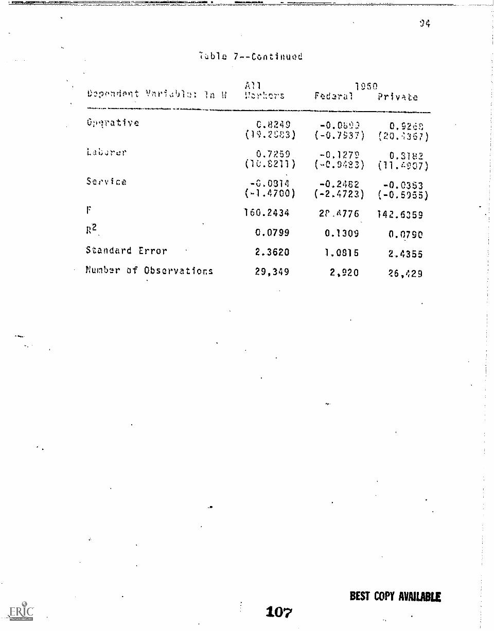
"..:17," 7-"-.7"7"- , - p.misciLIIMMUM:112

'%ble 7Continued

All1).2:1;,1-pinnt 11)1: In IA

4imr*. ..MAM...0.701.r...,1*10.

:0;IIr at ive

\rIr

evice

C.8249( 1 21;83)

0.7259(10.8211)

G.0-314(-1.4700)

160 2434R2 0.0799

Standard Error 2.3620

Number of Observations 29,349

107

)4

I )fif)rod_zrai Privite

-0.0!),=1(-0.7;.;37)

-0.1279C . 9 4 '8 3 )

-0.24'82(-2.472.3)

2" .A776

0.1309

1.0915

2,920

0.r

11.

'357)

(11 .t-907)

-0.0353(-0.-5955)

142.6359

0.0790

2.4355

26,429

BEST COPY AVAILABLE

Title 7--Continued

Val.1,1e: In '!el

All (;!C)Vorers

1970 (i;c)Fet!eral Priv%tt,

tnnlant -0.8= -0.2506 0.7021(-11.01,M) (-2.1207) ( 7.7233)

t,d1Jc:atioli 0.05:33 0.05n2 0..0354(12.2373) (8.9714) (6.73.9'))

Exprience 0.0257 0.0468 0.0120(0.8230) (11.9167) (4.0173)

Experience Squared -0.0006 -0.0007 -0.0005(-13.1023) (-8.6083) (-8.3398)

flace -0.1063 -0.1672 -0.1607(-3.4712) (-4.5035) (-4.4767)

Sex -0.1056 -0.3224 -0.1159(-6.3967) (-8.7546) (-3.5428)

Spouse Present 0.1489 0.1704(4.2136) (3.6673) (4.1724)

Spouse Ab_sent -0.0530 -0.2527 -0.0032(-0.5941) (-2.2350) (-0.C802)

Widr;wed 0.1175 0.1396 0.1625(1.7192) (1.4799) (2.0913)

Divorced, Separated 0.1211 0.0110 0.1753(2.2785) (0.1644) (2.8612)

Urban 11!sidence 0.5254 0.1804 0.4861(19.6068) (4.1258) (16;4402)

Professional 02390 0.2501 0.1671(5.5476) (5.8387) (3.1142)

Manager -0.0469 0.2853 -0.0013(-0.9409) (4.9617) (-0.0222)

Sales 0.0993 -0:4805 0.1435(-1.9048) (-1.9593) (2.5055)

Craftsmen 0.3904 -0.0653 0.6003(8.9889) (-1.0590) (12.0303)

Operative 0.4170 -0.0481 0Z.156(10.5103) (-0.5723) (13.7571)

1CSBEST COPY AVAILABLE

.4

s

F

4 .4

C..14 7

n .);

Stuidard Error

Number of Cbservat!ons

tti1070

cdaralf.

96

n 9S)1`

( 4 '153152 ) ( -1 00

-0.2C74 -0.2609(-5.76bf) (-3.76';0)

(n6. 45571.1:1)

-0.1446(-2.7395\

-0.2546 -0.2888 -0.2318(-5.3163) (-4.3735) (-4.2682)97.0595 64.6931 67.4184

0.0490 0.1755 0.0408

2.1544 1.0904 2.2718

33,523 5,383 28,140

BEST COPY NAMABLE

nws

e -C,n titlud

Vilrib1,3: In VAll ( IntiS ) 1070 (

I e r

97

(IC t7 0 ,1

EXp2ritncC!

Ex,wicnce Squared

Race

S

Spouse Present

Spouse Absent

Widcr.led

Divorced, Separated

Urban Residence

Professional

Mand9er

Sales

Craftsmen

Operative

-0.9437,72.7::48)

C.062014.8150)

0.0257(10.7063)

-0.0006(-13.5492)

-0.0793(-2.8413)

-0.1652(-6.4259)

0.1301(4.0171)

-0.0586(-0.7152)

0.1088(1.7289)

0.1116(2.2697)

0.4686(19.1810)

0.3410(9.0640)

-0.0088(-0.1876)

-0.1082(-2.1594)

0.4127(10.0683)

0.4091j10.8706)

110

-0.2702(-2.0140)

ngoi

(7.8495)

0.0524(11.76E9)

-0.0009(-9.0383)

-0.1671(-3.9869)

-0.3088.(-7.5960)

0.1107(2.2543)

-0.1844(-1.3747)

0.0431(0.3941)

0.0146(0.1956)

ie. 0.2234(4.6101)

0.2948(6.3084)

1).3158(5.2914)

-0.7486(-2.0257)

-0.0173(-0.2346)

-0.0736(-0.6847)

- 0.37631092'')()..0512

(11.0380)

0.0164(6.2547)

-0.0005-(-9.8510)

- 0.0369(-2.3211)

-0.0880(-3.1054)

0.1410( 3.954.7 )

-0.0363(-0.4070)

.0.1433(2.0982)

0.139,5(2.5796)

0.4326(16.4474)

0.3932(9.1117)

0.0165(0.3099)

0.0755(1.4120)

0.5896(13.0605)

0.5659(13.8257)

BEST COPY AVAILABLE

98

"

4. 1. I t' b Ir. 1.44

7--Continuod

t 11rs

197() (rnus)Federal Private

t.:),OrQr 0.2972 -0.1550 0.4475(4.9r2) (-1.2571) (6.9913)Srvico. -0.1059 -0.1071 -0.037,2

(-4.6335) (-1.1$16) (-1.3633)-0.2577 -0.2134 -0.2c96

(-5.7688) (-2.9239) (-5.1300)F 111 2535 52.8645 82.7355R2 0.0508 0.1852 0.0428

Standard Error 2.0935 1.0420 2.1714

Number of Observations 37,049 4,108 32,941

a -values in parentheses

17 BEST COPY AVAILABLE

Test Statistics'mar aft.-***4

'wbo ,e

1 12470

1,m

;1.i 1752.1-;3* 77. E:*

111...-6* 5J.

pers. 11 .t'.1)3* 6.79* 54.50*t-age vetofuil-scale 39.2 ;'/r 32.63* 53.34*wage rate

*significant at the 5 per cent level

Estimating the Differentials

Given the two earnings (wage rate) structures_estimated

for Federal and private sector workers, an estimate of the

gross earnings differential between the two sectors is

made with the mean values of earnings (wage rates) for

each sector. However, this estimate does not indicate

whether the differential is solely due to' differences incharacteristics between the disfferent types of workers.

if comparable workers are receiving equal pay because of

a successful application of the Comparability Doctrine, the

differential for 1970 should be attributable wholly to

differences in chdracteristics between wukers in the Lwu

sectors. If, however, some portion of the differential

remains unaccounted for by differences between workers,

then the Comparability Doctrine has been unsuccessful in

achieving its basic goal and consideration must be given

to an explanation of the remaining differential.

t: vizBEST COPY AVAILABLE

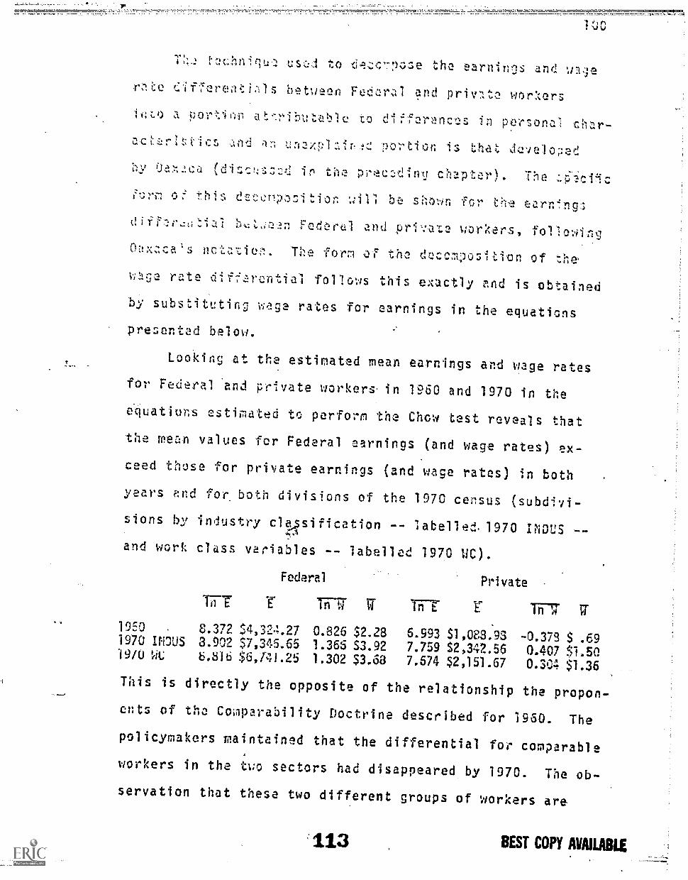
t

1.:s1:1 to d c`-n,:;se the

Fedc.ral

earnings an4

and privIlte wor%ers

..1t,-.ributabic to differnces in person

Inc

ch r-acrtrict a d unexpl pesrtion is that d,:lvelo;:ed

0-a%2X.a

4.i

0.11...c!.!s:/.; in the precediny chapter)

0: this dttsA.,npition bo no-in Yr;"

...c'acilc

'oarn.4,ng.;

Forit.,rtli and pri..'ate 1;eriers,,

0;!xzcas nctatio,I. Tne

v;44g

form the deccm)ositicn of the'

rate difarential follows this exactly end is ob tained

by substituting wage rates for earnings in the equations

presented below.

Looking at the estimated mean earnings and wage rates

for Federal and private workers' in 1950 and 1970 in the

equations estimated to p rform the Chow test reveals that

the mean values for Federal earnings (and wage rates) ex-

ceed those for private earnings (and wage rates) in both

years and for both divisions of the 1970 census (subdivi-

sions by industry claisification

and work class variables

1950 .

1970 INDUS19/U Wc

1-77: "E"

8.3723.902b.816

OW OM

Federal

Oa NOP 1 abe11 ed.1970 INDUS

labelled 1970 11C) .

Private

r

$4,324.27 0.826 $2.28 6.993 $1,088.93 -0.373 S .69$7,345.65 1.365 S3.92 7.759 $2,342.56 0.407 SI.50$6,141.25 1.302 $3.68 7.574 $2,151.67 0.304 $1.36

This is directly the opposite of the relationship the propon-ents of the Comparability Doctrine described for 1960. The

policymakers maintained that the differential for comparable

workers in the two sectors had disappeared by 1970. The ob-

servation that these two different groups of workers are

1,1,3 BEST COPY AVAILABLE

.totlloy

s 4ti e rsaracc,, A ' ++

Th*) usuol oxpinnat'.cn in c.,zmic

f ,;::r in 4)raducti

1.-%11,/ .S 1to.

liGYItY, 1T,, in addition,

oro°1 3e' diffrIrontly diffor in sot:::

%'s(;n:,11 character ',1tic dnreIaltiol to prori'uctivity it cansaid 1::11t .1scrinit:ttion as ikonnet'n Arrow dc fines it3

a i. J24

R -.1to of the Chow te,e,t remtrtod in Table 8,

confirn that Federal and private workers are paid accord -

in to significa.ntly different earnings and wage rate

structures.- Therefore, if the relative earnings (vage

rates) of Federal workers are greater than what they wouldreceive if both Federal and private workers were paid

according to the same earnings (wage rate) structure, thandiscrimination exists in favor of Fedoral workers. This

term is not normally used to refer to an advantage enjoyedby a particular group of workers. From the standpoint 0.7

the economy as a v;hole, this is discrimination againstprivate sector workers. However, from the individual

wor%er's point of view, this is an economic rent paid to

the Federal worker. Because the method used to decompose

the gross differential is derived from the economics of

discrimination, tais component of the Federal-private

ear'nings differential is referred to in the theoretical

analysis below as the part which is attributable to dis-

crimination. In the empirical analysis of the earningsand wage rate differentials in subsequent chapters, how-

ever, this component is more correctly termed an economic

114 BEST COPY AVAILABLE

102

Y. I .1

k 1)

1);:.07:r 1-1411tion can b.Q. 111,11;urad in tems of ty2a

coicient sr.t;r.iNed Camiaa:25/ 1 ri

1. 4.k / )

1;:ie

(Ec/11,) is the ob..r,ied Fl.idrtrivatc e.arnincs

(E7/1)° th.1 c,arnings ratio -which would exist in tills.

of discrimination

Oaxaca's discrimination coefficient was written in terns of

wage ratios. The discrimination coefficient for Federal wage

rates would then correspond exactly to Oaxaca's for male wage

rates.

Equation (11) can be re- written in terms of natural

logeritms as

(12) in (0 + 1) = ln(Ec/Ep) - in(EF/E0'.

Since the Federal/private earnings ratio is known, the

problem in cstimting th2 discrimination coefficient is to

estiate the unobserved Fbderal/private earnings ratio which

would exist in the absence of discrimination. This ratio is

estimated by the same technique Oaxaca used in estimating the

male/femaIe wage ratio which would exist in the absence of

discrimination. This method is to assume that in the absence

of discrimination both Federal and private workers would be

paid either according to the earnings structure estimated

for Federal workers or the earnings structure estimated

for priVate workers. These, assumptions are used in

decomposing the gross Federal-private differential into

a portion attributable to differences in character-

BEST COPY AVAILABLE

115

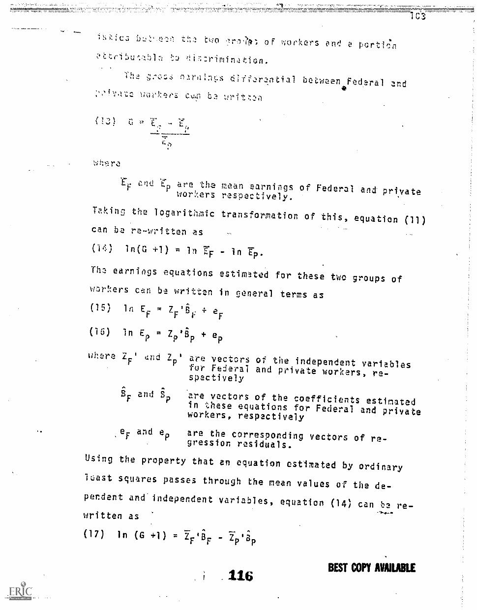
1. '4 - l-s-

Icz t .1 r ?ft 0 f t 'kers fl porti c*n

1,,.!1,-Iatial between federal and, 1,A r k: n b t zen

,\

'whre

/Id are the mean earnings of Federal and privateworI:ers respectively.

TzlIdne: the logarithmic transformation of this, equation (11)can ha re-written es

(14) ln(G +1) = 1 IF - 1n -fp.

Th3 earnings equations estimated for these two groups ofwori:ers can be written in general terms as

(15) In E- = ZF'nF + eF

(16) In EP = ZP '13P

+ eP

where 7.F

dnd Zpi are vectors of the independent variablesfor Federal and private workers, re-spectively

are vectors of the coefficients estimatedin these equations for Federal and privateworkers, respectively

are the corresponding vectors of re-gression residuals.

SF and EP

eF

and e

Using the property that en equation estimated by ordinary

ltiast squares passes through the nean values of the de-

pendent and' independent variables, equation (14) can b2 re-written as

A A(17) in (G +1) - 418 '3F P P

116BEST COPY AVAILABLE

.3

...1 1 C r: ;" .1 '+1 F-0 Ld

- 47: - -

,1-J ,4 -1,

writt'!n

"T 1

111'! 4 ,

' n1;1

Tho difference betwaen the vectors of estimate1

- 1

A

A:

1.:0t14rA,, 741t341'

fJr Federal ant private workers can te written asA

= 8 - _

F'

Thor, the Federal-private earnings diff.arentiaI cen de-a

composed by substituting 3F = Bp - AB into equation (17)

(n) In (G 1) -- .4' (Op - AB) - 7p13p.

Using the relation defined in equation (18), this becoles

(21) In (G 1) = 7- 2144.4pF'L°

Assuming that in the absence of discrimination the

earnings structure estimated for private workers would apply

to both Federal and private workers and using the definition

of tha discrimination coefficient in equation (12), it

can be shown that the first term on the right hand side

of equation (21) represents the portion of the gross Fed-

eral-private differential which is attributable toVrimrilt=

ences in char cteristics be.tween the two groups of work-

ers. In other words, it is an estimate of the Federal/

117 BEST COPY AVAILABLE

105

.:;bich would Mst in 'the asencrf tilljer the assumption that th c!stimated

1.)

structure wouU apply to both groups of

I/v.

P'ZPr A L BP

Wnt..4 again thn properties of least squares eStioates) anvaor e.xpr-e'sslon of this relationship of the type

Na 41.0 and Nalki-1 used 'for estimation is26

(22a) in ) 'Bp

I

Under tha same assumption with respect to the earnings struc-ture which uld prevail in a nondiscriminating labormarket and using the formula for the discrimination coef-ficient in equation (12), it can be shown that the secondterm on the right hand side_m_f equation (21) representstha portion ol the gross differential attributable to

discrimination. In other words, it is an estimate of

the natural logarithm of one plus the discrimination coef-ficient. Equation (12) can be written in terms of known

quantities as:

(23) In (D ; 1) = ln (yly ln (EF/Ep

Substituting equation (21) for ln ) and equation (22)for ln (E

F/E

P)°, equation (23) becomes

(24) ln (D + 1) = Arap 7.F.416 - Arip =

BEST COPY AVAILABLE

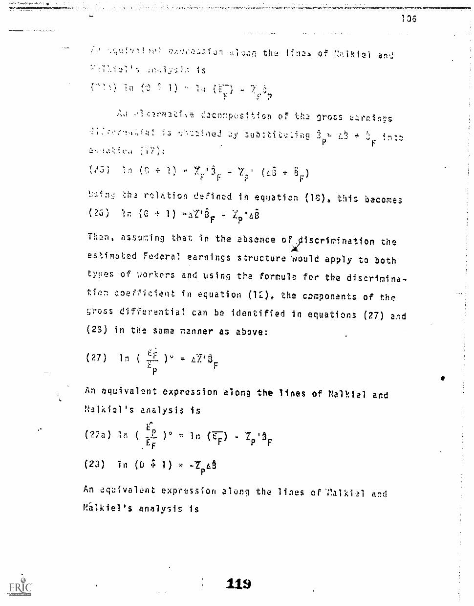
a,a

f

,1 4

111

isw;! lines of r;tikiei

,2.AcnnosItion o? gross k2,-;rn1 ns

J)

0.0;

7

t +L33.

- L (LI')F

136

h.a r1.11_ation defined in equation (1S)4 this becomes

(G 1) ltAp8f

L saBP

Than, assulning that in the absence oy iscrimination the.

es`Amat d Federal earnings structure 'would apply to both

ty.)es of torkors and using the formula for the discrimina

tii.;n c'neefident in equation (lZ), the components of the

cross difl'erntial can be identified in equations (27) and

(2S) in the same manner as above:

(27) in ( ),,, h7 4 B

F

An equivalent expression along the lines of Malkial and

Nalkiel's analysis is

(27a)iri( ,11)° In (c)1"-F

(23) In (D r 1) 4 -2"

An equivalent expression along the lines ofTalkiel and

Milkiel's analysis is

ln

107

s !rti th7,1 intil,3:;;*Ot:wtTo

a;3 stal cv1 r1t1;

'of .10 .difYneiltst-uctur,Is

ti,ul in v:',4 ).1..2,%r problem. In the ?.1;s nn ofthf! actual .edrninris structura probabIy

coinz:ida with either the estima,.ed Federal or thee:,timateti private earnings structure. However, the struc-tue that would exist in the absence of discrimination isunknowable. Estimating earnings on the basis of the twoalternative assumptions about this structure provides a

range of possible values for the two components of thegross differentials which should include the true valuesof these components.

Summary and Conclusions,

In order to study earnings and wage rate differ ntialsbetween Federal and private sector workers, it is necessaryto estimate earnings and wage rate structures for the twogroups. These can be derived from the post-schooling in-

vestment models of human capital theory. The exact spec-ification of these equations depends on the informationavailable in the data used to estimate them. Two sets ofdata are used for these estimations: subsamples of the

1960 and 1970 Public Use Samples pertaining to Delaware,Maryland, Virginia, and the District of Columbia. Theseprovide data independent of the "PATCH Survey to estimate

BEST COPY AVAILABLE

,t/'41 t'ei°1 " ,And to t:tvaILate he

4 y

cf th.n. CoTpar!tbility Zof:trina..I. ;ov'o r to

4-,11 tt Pust 17),1 dcwnko

;1,1ft ZItt;' to -dif,fz)ronc.2s In cilar

rAcristici.; bc6:voen thc Ll. oroups of workers and a TzIrt

which iss lc! co tion.

us ,,A to L;ake this doollpositin is that devOop2d by RowIld

0, cic to, study r,:d fatale uage differ,mtials and modit'IPA

b1y Durton G. and Judith A. flalkiel.4

The results of the estimations of the models specified

in this chapter are studied in Chapter V and Chapter VI.

Policy inplications are considered and conclusions drawn in

Chapter VII.

121 BEST COPY AVAILABLE

lt9

C A VI

>11 6 1 .0 6s.

i....10.2

discvszion of these models, see:ii;!n C':oital and tn Pert'onal T)7:ttributioneamormwea.

11 Nib a 13'..!,Jytlnsy Lecture A. t,,.=.tI,W;

w,incer, The Distribution ofitn Sp:!ciel RofIrence to tr.e

,io-Jrnal of conomic LiTerat0-e1070) pp. and G-ziry aacer and t.&rry R.6

ar'd DIstribution or Earnings,"Paoers;nd ocore.zdinos LVI ("ak.N.

1pe. ,50A4-,)Qa.5,1

!incer, "Distribution of Labor Incomes," p. 12.7 ,

vAlpna C. Chiang, Fundamental Methods of MathematicalEcono.lics (flew York: maTO:RTTITTR7711.757), p. 255.4Ninc r, "Distribution of Labor Incomes," p. 15.5Sae Mincer, "Distribution of Labor Incomes," p. 15;Thomas Johnson, "Returns from Investment in Human Capital ,"American Economic Review, LX (September 1970), pp. 549-M7111Maca, °MiTTITTFRre Wage Differentials in Urban UborNarkts," Narking Paper flo.-23, p. 5; and Malkiel and Mal-!dal, "Nele-romale Pay Differentials in Professional Em-ployeot," p. 691.

6C1 ass of employment refers to the type of employer:Federal, state, or local government; private industry;selF-amployed; or working without pay. In this thesis,stat. and local gove7-nment vorkers an' those individualswithout ?rly are excluded from consideration andta compwison is made between Federal government workersand all other remaining workers who are classified simplyaz priv.Ite sector viorkers.

7gational Data Use and Access Laboratories, TechnicalDocuan4iition for the 1960 Public Use Sample PUS-19501710MF,;VTFTWITT7157771173), pp.

8U. S. Civil Service Commissioa,,Manpower InformationSystems, Nanpower Statistics Ann%d1 Recort ofFederal Civilian Emologment b Geoeraohic Area (bacemoer31, ioiciT71515WITT'sm

Washington, D.C.:'"U.S.L'75-virFilinint Printing Office, n.d.), p. v.

9Ibid., pp. 16, 33, 61.

"For information on the occupational classificationsin the 1960 census, see U. S. Bureau of the Census, 1950Census of Population, A1pllabetical index of 0ccupatians and

122 BEST COPY AVAILABLE

r - .

F:j , A. I Fo;'

scc C. S. ,ourf.::7,14 t! 1'7:70 f,ri.S5 o?Cl'ass; nf 1.1;!1;t1.;- ,. . V.. 1 'w1 I.... .

4. 1`O. So, ) `NW Io (0 "0 ft kI' 7M75-1:752

S111

r.! 114' 10''1 i) ...1%

ti-1. r 'I , ,3"", J. a t

N' 13:,;trr71.7.1,:ln

)n, U. S.-5 CPa,..;.!inor

a.s

n-.1. tit on ;.4s 1: n f; 72, r.

I ,.4 11,0 ; Br ij I 1 ; * 71°7'0

9 .

p. J).

p. 155.

tyi)S.I

11U. S. Bureau of the Census, Income Distribution inthe United States, by Herman P. Mil,r, A 19z):; Census Aln-no.

oigraph ttaT,ETTITilon, 5777-177-3. 615715-nment Printing Office,1966), pp. 215-21S.

15Rooart RIce. "Skill, Earnings, and the Growth oVage Supplements," ARIericar Economic Review Pa;:ers and

LVI (HaTin3), p. 538.16 .

Ibid., p. 592.

17William G. Bowon and T. Aldrich Finnegan, The rconomicsof Labor Force Participation {Princeton, New Jersey:PrfiiUniversity Press, 1969), Ch. ITI-VIII (Herein-

after referred to as Labor Force Participation.).18ibi

d., pp. 40-49.

1S. Bureau of the Census, 1970 Census Descriptionand Technical Oocurlantation, p.

20Gowen and Finnegan, Lab-or Force Par.ticioation, pp.102-105.

210axaca, "Male-Female Differentials," p. 698.

22Bowen and Finnegan, Labor Force Participation, p. 64.

23Gregory C. Chow, "Test of Equality between Sets of

Coefficients in Tvio Linear Regressions," EconometricaXXVIII (July 1960), p. 602.

24Kenneth J. Arrow, "The Theory of Discrimination,"

in Discrimination ed. by Ashenfalter and Rees, p. 3.25

0axaca, "Sex Discrimination," p. 125.

26Malkiel and Malkiel, "Male-Female Pay Differentials

in Professional Employment," p. 700.

t 123BEST COPY AVAILABLE

CHAPTER V

EARNINGS REGRESSIONS AND DIFFERENTIALS

The analysis of the earnings differentials between

Federal government and private sector workers is made on the

basis of the earnings model aria the method for decomposing

the estimated gross Federal-private earnings differential

developed in Chapter IV. Personal characteristics and full-

scale earnings equations are estimated separately for all

Federal and all private sector workers using the 1960 data

and several different forms of the 1970 data. The estimated

gross differentials are decomposed into a part attribLtable

to differences in characteristics and a part representing an

economic rent. These results provide an overview of the

composition and trend of the Federal-private earnings dif-

ferential and of clear patterns in the regression coef-

ficients estimated for Federal and private workers. They

also facilitate selection of the best form of the 1970 data

for use in further estimations.

To examine the comparability of Federal and private

workers, however, a finer division of these two sectors is

necessary. Personal characteristics and full-scale earnings

equations are estimated separately on Federal and private

workers in eight race-sex groups for the 1960 data and the

preferred form of the 1970 data. These equations are used

to estimate the components of the gross earnings differential

for each group and clear patterns in the coefficients and

differentials are observed. One representative equation is

124BEST COPY AVAILABLE

analyzed in detail for each year with respect to the impli-

cations of its estimated coefficients. Conclusions are

drawn concerning the success of the Comparability Doctrine.

Overall Federal - Private Earnings Differentials

Both sets of earnings equations (personal characteris-

tics and full-scale specifications) are estimated separately

for all Federal and all private workers in four sets of

data. 1

Coefficients are not estimated in the following

cases: 1) the characteristic serves as' the base group;

2) there are no observations in the cell; 3) the variable is

omitted because of poor results in earlier regressions. The

first three sets of data employed are the 1960 data, the

1970 data divided by the industry classification variable- -

labelled 1970 (INDUS)--and the 1970 data divided by the

work class variable--labelled 1970 (14C)., The estimated

personal characteristics equations for these data sets are

presented in Table 4 in Chapter IV and the estimated full-

scale equations are presented in Table 5.

These equations are also estimated for a fourth data

set which is formed by eliminating all professional, techni-

cal, and kindred workers from the 1970 data divided by the

work class variable. This set of equations is estimated to

verify the assumption made in Chapter IV that the high per-

centage of professi nal, technical, and kindred workers

located in the geographic area covered by these tapes does

not affect the represen6t+reness of the estimated relation-

125 BEST COPY AVAILABLE

113

ship between Federal and private sector earnings. A total

of 28,756 individuals, contained in this data set, are

categorized in Table 9.

Table 9

Non-Professional Worhers in 1970 Data (WC)

Private Workers Federal Workers

Total 24,907 100.0 3,749 100.0White 19,422 78.0 2,491 66.4Non-White 5,485 22.0 1,258 33.6Male 15,203 61.0 2,074 55.3Female 9,704 39.0 1,675 44.7

The Chow test confirms that the estimated Federal and pri-

vate earnings structures are significantly different.2

In all four data sets mean earnings of Federal workers

excced can earnings of private sector workers.3 The esti-

mated personal characteristics and full-scale earnings equa-

tions are used to decompose the gross Federal-private earn-

ings differential into a part attributable to differences in

characteristics between the two types of workers and a part

attributable to an economic rent paid to Federal workers.

Tables 10 and 11 present the analyses of these differentials

based on the personal characteristics and full-scale equa-

tions.

Certain clear patterns in the relationship between

Federal and private earnings emerge in the estimated earnings

equations and decomposed ZifTerentials. The overall Federal-

private differential fell by approximately 23 pe, cent from

L 126 BEST COPY AVAILABLE

Tabl e 10

Analysis of Earnings Differentials from Overall PersonalCharacteristics Earnings Equations

FederalRegressionWeights

PrivateRegressionVeights

FederalRegressionWeights

PrivateRegressionWeights

1950 1970 (WC)

lnF.

=8.372

;n T. =6 993

1 (G+1)=1.479

r =$4,324.27F

rP=$1 038.98

lnF=8.816

in y7.674

ln(G+1)=1:142

rF=S6 741.25

i,=S2,151.67

Due to Different 0.2769 0.3171 0.2415 0.2149CharacteristicsEconomic Rent 1.1021 1.0619 0.9005 0.9271

1970 (INDUS) Non Professionals 1970(WC)

in y8.902. y$7,346.65

in rp 7.759 rx$2,342.56

In rF=8.628 E

F=S5

'

585' 89

In y7.646 ri,=$2,092.26

1n(G+1)=1.148 1n(G+1)-0.982Due' to Different 0.2706 0.2527 0.1325 0.1745CharacteristicsEconomic Rent 0.8724 0.8903 0.8495 0.8075

BEST COPY AVAILABLE

L 127

ft

T:tt.14 11

Analysis of Earnings Differentials from Overall Full-ScaleEarnings 'Equations

*lb

FederalRegressionWeights

PrivateRegression-eights

Federal PrivateRegression RegressionWeif5hts Weights

196C 1970 (WC)

in rF=8.372

in r =6.993

-L=54,324.27

=$1,088.98

in r =8.816 rF '

S6 741 25

1nr=7.674 r -=$2,151.67

ln(G+1)=1.379 ln(G+1)=1.142Due to Different 0.2697 0.2403 0.3308 0.1449CharacteristicsEconomic Rent 1.1093 1.1387 0.8112 0.9971

1970 (INDUS)

in r=8.902F

In r=7.759

Non-Professionals 1970(WC)

F=$7 346.66

rP =$2 342.56

In -Er"F=8.628 y$5,585.89

In r=7.646 y52,092.25

ln(G+1)=1.143 ln(G+1)=0.982Due to Different 0.3578 0.1998 0.2028 0.0902CharacteristicsEconomic Rent 0.7752 0.9432 0.7792 0.8918

4

a

BEST COPY AVAILABLE

116.

a gross earnings differential of 1.479 (in logs) in 1960 to

a gross earnings differential of 1.142 (in logs) in 1970.

Howev r, the largest portion of the differential estimated

with the persohal characteristics equations in both years

consists of an economic rent to Federal workers. In the

overall differentials in both years, more than 70 per cent

is economic rent. The differential in logs is the propor-

tional differential between Federal and private sector

earnings. In absolute dollar terms, the difference between

Federal and private earnings rose from $3,235 in 1960 to

$4,589 in 1970. Although the absolute differential in

dollar terms gives a clearer picture of the size of the

Federal-private differential, the proportional differential

is preferred for discussion in this study because this form

facilitates comparisons across groups and between years. In

the case of non-professional workers, where the gross earn-

ings differential is smallest in absolute terms (0.982 in

logs), the economic rent is a larger proportion than in any

of the other differentials (87 per cent when Federal re-

gression weights are used and 82 per cent when private re-

gression weights are used). In the analysis of these dif-

ferentials on the basis of the full-scale equations, pre-

sented in Table 11, this economic rent to Federal workers

accounts for more than half of all the gross earnings dif-

ferentials estimated. The estimated equations for non-

professional workers are<comastent with those for all

workers in the sample indicating that the high percentage

129 BEST COPY AVAILABLE

of professional, technical, and kindred workers in the

sip ple does not alter the relationship between Federal and

private earnings.

Personal Characteristics Earnings touations

The estimated personal characteristics equations show

several patterns which are consistent through the four data

sets. The factors which affect the appearance of the econom-

ic rent are evident in the differences between the estimated,

coefficients for the two sectors. The education and ex-

perience variables are significant at the 1 per cent level

for both types of workers in all equations.4 However, the

rates of return to education and to experience5 are con-

sistently higher in the Federal sector. The rate of return

to education in these equations ranges in size from 0.0721

to 0.0875 for Federal workers and from 0.0215 to 0.0667 for

private workers. The race and sex variables, included to

account for the effects of discrimination against non-whites

and females are also significant at the 1 per cent level in

all equations. They indicate that the effects of racial

discrimination are consistently stronger in the Federal

sector. Discrimination by sex is stronger in the private

sector for all the 1970 data sets but is stronger in the

Federal sector in the 1960 equation. Given the equation

specification employed, the coefficients of these variables

are direct estimates of the proportional differential as-

sociated with race and each of these equations, the

sex differential is larger than the racial differential. The

/ 130 BEST COPY AVAILABLE

Table 12

Personal Characteristics Earnings Equationfor Mon- Professionalsa

"MO 111111.

Dependent Variable: E

All.11vrkers

Non-Professional 1970(WC)Federal Private

Constant

Education

Experience

Experience Squared

Race

Sex

Spouse Present

Spouse Absent

Widowed

Divorced,'Separated

Urban Residence

Disability

F

R2

Standard Error

Number of Observations

..,,011.

6.2531, 6.6670(83.4037) (47.2322)

0.0667- 0.0793(14.3778) (9.7035)

0.0566(20.1306)

-0.0012(-23.1915)

-0.1675,(-5.3962)

-0.6915(-26.6801)

0.3706(9.7312)

0.0974(1.0350)

0.3050(4.2255)

0.3777(6.7099)

0.5291(18.8933)

-0.4940(-9.7970)

232.0062

0.0815

2.1468- e

28,656

0.0633(12.4688)

-0.0010(-9.4291)

-0.2722(-6.2132)

-0.5053I 1,1% 411...WTT41

0.3277(5.6568)

-0.3062(-2.1888)

0.3891(3.2578)

0.2343(2.7804)

0.3346(5.8304)

-0.5087(-5.9989)

83.0227

0.1940

1.2005,

3,749

6.5490(78.3393)

0.0447(8.5900)

0.0493(15.7855)

-0.0011(-19.8586)

-0.2280(-6.4129)

-0.7249nA AlfloWu'v.W#4,41

0.4099(9.5925)

0.1783(1.6863)

0.3614(4.4986)

0.4383(6.9307)

0.4804(15.7614)

-0.4309(-8.6395)

174.5050

0.0712

2.2349

24,907

at-values in parentheses.

131

BEST COPY AVAILABLE

estimatata racial differential: range in size from -0.1422

to -0.3146 while the sex diffcr ntia.s range in size from

-0.4084 to -0.6860.

The coefficient of thrt urban residence variable is also

significant at the 1 per cent level throughout the equa-

tions. It is lar;er in the private sector in all cases.

This is intuitively reasonable since it indicates that dif-

ferences in job opportunities and other pecuniary and non-

pecuniary factors associated with urban areas have a greater

effect on private earnings than on Federal earnings.

The coefficient of the disability variable is signifi-

cant at the 1 per cent level in the equations estimated with

the 1970 data. It is larger in the Federal sector for non-

*Um.e. v e, t i WS %,00%. V %..,'yl f V

data sets. It is also larger for both Federal and private

non-professional workers than for either sector in the other

equations. It is important to note that this variable does

not measure solely the effect of health on earnings but

interacts with other personal characteristics.

Full-Scale Earnings Equations

When occupational variables are included and the full-

scale earning: equations are estimated on tha four data

sets, these patterns in the estimated coefficients are al-

tered., Controlling for broad occupational groupings reduces

the coefficients of education and experience because part

of the rates of return too`gdhrtation and experience are

realized through choice of occupation. The coefficients of

BEST COPY AVAILABLE

132

.1

a

Fu11-11 Earnins Equationfor c)?1 Professionalsa

Depallisnt Vartable: in EPt 11

I,:rAersMIIMIA11114.11111FMNIIIimas111=1.11 =11

Cons pert

Educttion

Experience

Experience Squared

Race

Sex

Spouse Present

Spouse Absent

Widowed

Divorced, Separated

Urban Residence

Professional

Manager

Sales

Craftsmen

120

=1.1.11.4......1.1401...1111.111111

Non-Proressional 1970( C)Fed: rai Private

5.L381(68.4190)

0.rP.45(17.0193)

0.0552(19.6310)

- 0.0011(- 21.8649)

- 0.1441(-4.5603)

- 0.5417(-D.6160)

0.3344(8.7901)

0.0653(0.6988)

0.2704(3.7531)

0.3560(6.3580)

0.5751(20.5578)

0.0078(0.1551)

-0.2638C7.5.0984)

3.3829(8.7425)

133,

7.0423(44.8483)

0,0543(6.0164)

0.0618(12.1371)

5.9130(52.S384)

0.0678(12.3270)

0.0469(15.0220)

-0.0010' -0.0010(-9.4065) (- 18.0858)

-0.1983 -0.2109(-4.4090) (- 5.8470)

-0.497472)

0.3119(5.4151)

-0.2928(-2.1072)

0.3859(3.2509)

0.2238(2.6732)

0.3208(5.6188)

0.3170(4.8250)

-0.6404(-2.3891)

-0.0630(-0.9053)

-0.5091(-14.7668)

0.3567(8.3671)

0.1248(1.1897)

0.3014(3.7785)

0.4007(6.3814)

0.5296(17.4252)

0.0674(1.1538)

-0.0081(-.0.1447)

0.5693(11.9114)

BEST COPY AVAILABLE

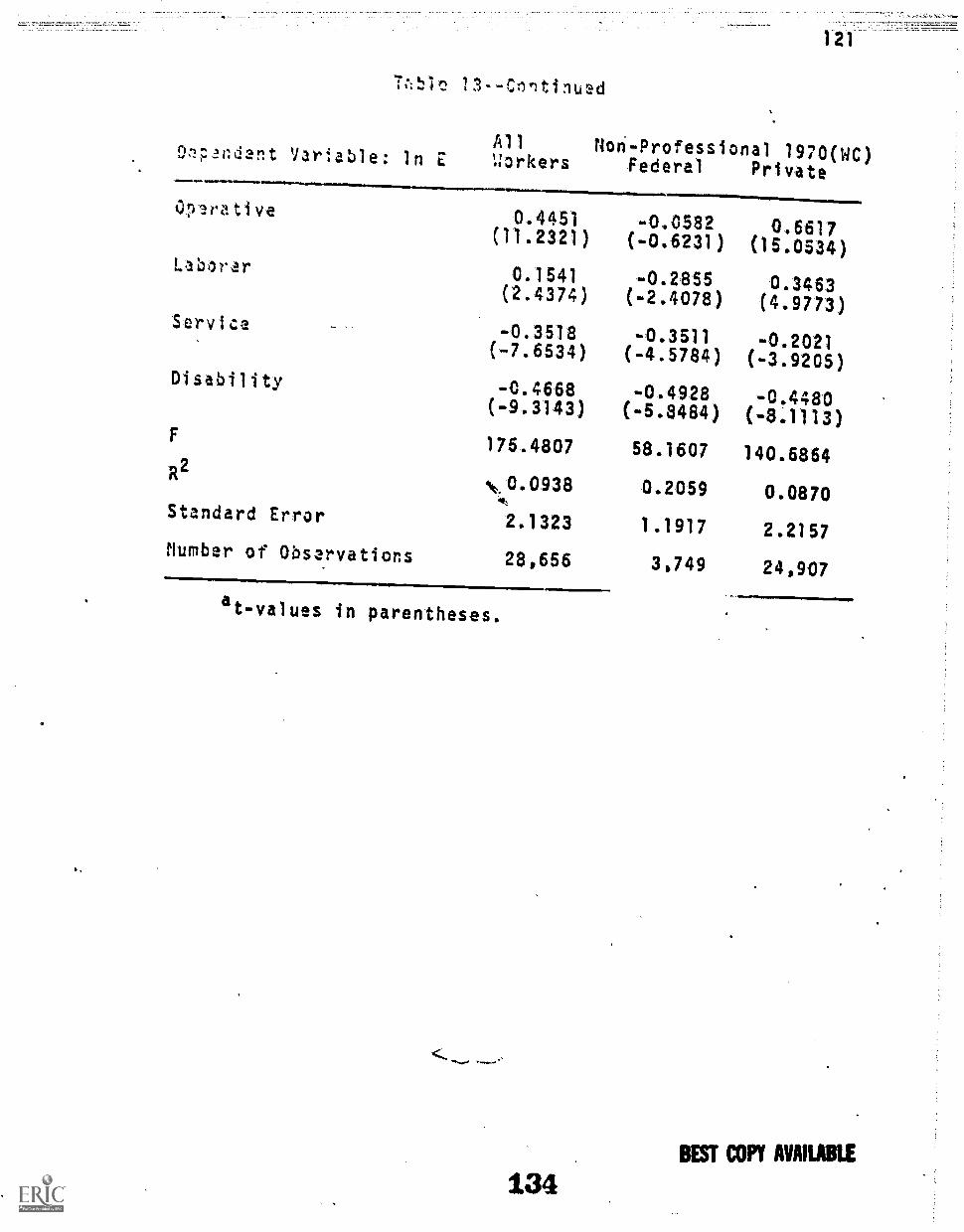
"rtic 13--Clitinued

121

(L).T.Indent Variable: In EAll:;orkers

Non- Professional 1970(WC)Federal Private

Onerative 0.4451 0.0582 0.6617(11.2321) (-0.6231) (15.0534)

Labor er0.1541 -0.2855 0.3463

(2.4374) (-2.4078) (4.9773)Service -0.3518 -0.3511 -0.2021

(-7.6534) (-4.5784) (-3.9205)Disability -0.4668 -0.4928 -0.4480

(-9.3143) (-5.8484) (-8..1113)F

176 4807 58.1607 140.6864R2

Nt..0.0938 0.2059 0.08704tt

Standard Error 2.1323 1.1917 2.2157Mumb er of Observations 28,656 3,749 24,907

at-values in parentheses.

122

the education and axoerience variables remain significant

at the 1 per cent level, However, in the full-scale earn-

ings equations, the estimated rate of return to education

is higher in the private sector for all of the data sets

except the 1970 data divided Eby the work class variable.

The effects of race and sex are also reduced in the full-

scale earnings equations because race and sex differences

in occupational attachment are eliminated as sources of

discrimination. These coefficients remain significant at

the 1 per cent level. However, the pattern is altered so

that there is no longer a consistent relationship in the

size of these proportional differentials in the two sectors.

Controlling for broad occupational groupings alters

poctern uf Lim obLimaLcki grUzcs: In

personal characteristics equations because these groupings

measure different effects in the two sectors. In the

Federal sector, earnings depend on job level. Certain oc-

cupations are paid at lower levels in the Federal sector

than in the private sector on the basis of the job levels

at which they are classified. When comparability rates are

determined, they are not compared with similar occupations

in the private sector but with occupations at comparable

job levels. Such occupations will have opposite effects

on earnings in the two sectors. Furthermore, because only

broad occupational groupings are controlled for, a number

of very different pay leyels may be included in any one

occupational group. The estimated coefficient under such

135 BEST COPY AVAILABLE

conditions represents the conbinition of a nl.mber of c.sntre-

dictory effects and has little meaning. Consequently, to

analyze the earnings different als between Federal and

private sector workers, the !lost meaningful equations to

examine are the personal characteristics earnings equations.

These personal characteristics variables serve as proxies

for productivity. To the extent that these variables cap-

ture differences in productivity between Federal and pri-

vate sector workers, that portion of the gross earnings

differential which cannot be attributed to differences in

the personal characteristics of the two types of workers

must repr,,Isent an economic rent paid to Federal workers.

Nevertheless, Table 11, which presents the decomposition of

the c!rn4n:: differentfels nn the hic of tho full-cralP

equations, is included for further information.

Differentials and Comparability

The personal characteristics and full-scale earnings

equations estimated for these four data sets and the ana-

lyses of the gross Federal-private earnings cliffprential

show that Federal workers as a group earn more, on average,

than comparable private sector workers. When only personal

characteristics are considered, Federal workers receive a

higher rate of return to their schooling and either a

higher rate of return to their on-the-job training or they

devote a larger proportion of their time to this training

at the beginning of thefirwo*k experience. However, these

relationships .refer to the entire set of Federal workers

136 BEST COPY AVAILABLE

124

and the entire set of private rkers. This overall rela-

tionship nay conceal contradictory earnings relations among

different race sex groups: the observed economic rent may

only be paid to certain types of Federal workers. It is

possible that the Federal-private earnings differentials

for certain race-sex groups ;lay be in the opposite dis,.ection

and when all workers of each type are examined at once,

these are cancelled out. Therefore, a finer division of

Federal and private sector workers is necessary to study

their comparability.

Federal-Private Earnings Differentials by Race and Sex

Both earnings equations are estimated by ordinary

least squares on eight race-sex groups of Federal and pri-

vate workers in 1960 and 1970: whites, non-whites, males,

females, white males, white females, non-white males, and

non-white females. That the two methods of dividing the

1970 data yield nearly identical estimates of the gross

Federal-private earnings differential and similar patterns

in the estimated coefficients confirms that the industry

classification method of dividing the data yields a good

approximation to the desired classification of workers by

type of employer. However, for regressions on the eight

race-sex groups in 1970, the work class method of dividing

the dat., is preferred because it gives a more accurate

division than the industry classification variable. The

industry classification variable yields a more accurate

division of the 1960 data than it does of the 1970 data be-

137 BEST COPY AVAILABLE

cause the ihdustry category "Public Administration

Allocated" introduced in the 1970 data is ambiguous for the

purposes of this study.6

The specifications of both earnings equations are very

similar for both sets of data The principal difference

between the two sets of data is in the inclusion of the

dummy variable for disability in the equations estimated

with the 1970 data. Coefficients are not estimated in the

following instances: 1) the characteristic serves as the

base group; 2) there are no observations in the cell;

3) the variable is omitted because of poor results in

earlier regressions.

These equations would be better specified if they also

included variables for migration ano union status (both

private and government). However, these variables are

unavailable in the data used for these estimations. Mi-

gration is another form of human capital investment and is

expected to have a positive effect on tarnings. To the

extent that migration is associated with one or more of

the variables included in the equations (such as school-

ing), its effect is probably captured by that variable.

The effect of unions varies across race-sex group's and has

been found to be greater in the public than the private

sector.? The omission of this variable decreases the pro-

,portion of the gross differential which is considered an

economic rent. WithoutWorpation on the extent et

unionism within each group and the union/non-union earnings

138 BEST COPII AVAILABLE

differential for each group, no estimate can be made of the

effect of unionism on each group's earnings. However, it

can be said that to the extent that unions have raised earn-

ings in the public sector more than in the private sector,

they have increased the Federal-private earnings differen-

tial above what it would have been in the absence of

unionism.8

In ail eight race-sex groups for both years, the aver-

age earnings of Federal workers are higher than those of

private workers in the same race-sex group. Tables 14 and

15 present the analyses of these differentials on the basis

of the two earnings equations. In both years the largest

gross earnings differential is for white males (a differen-4

.14-4pn Iffrr1.141 U 1.4111 In IlO3 I UI f;i1I6C 141U 4G4 In 171.0V Quu osuAlgie 4,

logs for white males in 1970).. The smallest differential

in 1960 is for white females (a differential of i'.136 in

logs) while the smallest differential in 1970 is for non-

white males (a differential of 0.879 in logs). More than

half of every differential in both years consists of an

economic rent paid to Federal workers. In other words, even

after allowing for differences between Federal and private

workers in personal characteristics which act as proxies

for productivity, an earnings differential remains which is

considered an economic rent paid to alljederal workers,

regardless of race or sex group.

These differential smaller in 1970 for each race-

sex group. The percentage decrease tn these differentials

BEST COPY AVAIUIBLE

139

Table 14

Analysis of Earnings Differentials from Personal Char-acteristics Earnings Equations by Race and Sex

AMR

1950 1970

Federal PrivateRegression RegressionVeights Weights

Federal PrivateRegression RegressionWeights Weights

Whites

in y8.458 y$4,759.98

ln y7.074 y1,180.86

ln(G+1)=1.394Due to Different

Characteristics 0.2852 0.2995Economic Rent 1.1038 1.0945

Whites

nFr=8 965

ln rPn7 745

ln(G+1)=1.220

0.26890.9511Y

=37 824 38

P *w$2 309 99

6.1984.1.0215

Non-Whites Non-Whites

In tr8.050 rr$3,133.79 In y8.408 y$4,482.79

In rp=6.709 T71)-1819.75 In ;=7.399 ;$=51,634.35

ln(G+1)=1.341 ln(G+1)=1.009Due to DifferentCharacteristics 0.1936 0.3337 0.2029 0.1742Economic Rent 1.1474 14073 0.8051 0.8348

Males Males

in rr8.604 I-F=55,453.43 In rr9.093 rr$8,892.82

ln re7.106 reS1,219.26 ln trp=7.929 rrS2,776.65

1n(G+1)=1.498 1n(G+1)=1.164Due to Different

Characteristics 0.2942 0.3609 0.3391 0.2432Economic Rent 1.2038 1.1370 ....0.8249 0.9208

140 BEST COPY AVAILABLE

Table 14Continued

1950 1970

128

Fedval Private Federal PrivateRegression Regression Regression Regression

eights eight .4ai:;hts Weights

Females Fenales

1 n 1". =7.976 'F =$2, 910.27 iin re 8.357 rr54,302.71'

in rP=6 780 EP= $380.07 in r =7.263 r

Pr-shi

P426 53

ln(G 1) 1.196 ln(G 1)=1.104

Due to Different

Characteristics 0.3737 0.2668 0.2736 0.2144Economic Rent 0.8223 0.9292 0.8304 0.8895

White Males White ma1.g.15

In rF=8.726 rr$6,161.04 in rF=9.242 Ei=510,321.66

ln rp=7.159 r=$1,285.62 In re7.977 rp=52,913.18

Due to Differentln(G+1)=1.567 ln(G+1)=1.255

Characteristics 0.3546 0.3615 0.3401 0.2461Economic Rent 1.2124 1.2055 0.9249 1.0189

Wyte Females White Females

in rF=8.037 rr$3,093.32 In rF=8.452 rF=.$4,584.43

ln rp=6.901 ;4993.27 In rp=7.345 'r 51,548.43

. ln(G+1)=1.136 In(G+1)-1.107Due to Different 0.3158 0.2923 0.2351 0.2364CharacteristicsEconomic Rent 0.8202, 0.8437 0.8719 0.8706

141 BEST COPY AVAILABLE

t: y;;,h )

1960

Feu'aralRegress-ton10.1. Private

RegressionWei ghts

1970

Federal PrivateRegression RegressionWeights Weights

Non Wh t Mal e

1.misolaimallINIMR.1114111=a1M1M+M.=...,

non-Whi Mal es

In r1=8.219 7.',..$3 673.87 in T=8.596

1n 1p=5.395 Tie$987.33

F$5,409.93

ln rp=7.717 tp=$2,246.21

ln(G+1) =1.314 1n(G+1)=0.879Cue to DifferentCharacteristics 0.1319 0.3447 0.2350 0.1540Economic Rent 1.1821 0.9693 0.6440 0.7250

it!on-Whi to Females Non-White Femil e.s1111

ir. 7CC." roolow r /1,2..,...... 1. r-o lnA."

41111111

r%.%6F4J9.442.11

ln rp=5,435 rr$623.91 in re6.997 rp=51,093.35

1n(7.+I)=1.319 1n(G+1)=1.197Due to DifferentCharacteristics 0.5716 0.1925 0.2590 0.2379Economic Rent 0.7472 1.1265 0.9580 0.9591

ti

142BEST COPY AVAILABLE

Table 15

Analysis of Earnings Differentials from Full-Scale EarningsEquations by ?2ce and Sex

,+MINberiOarAmo. m.=.=.YO,1950 1970

FederalRegressionWeights

PrivateRegressionWeights

Federal PrivateRegression RegressionWeights Weights

Whites Whites

Due to DifferentCharacteristicsEconomic Rent

In ter8.468 rr$49759.93 In tr8.965 rF*57 Et24.38

in r=7 . 074 rp=S1 180.86 in rp=7.745 rpu$2309.99

1n(G +1 )=1 .394 1n(G +1) 1.220

0.2999 0.20231.0941 1.1917

0.33430.8857

0.17741.0426

Mon Whites Mon-Whites

rr$3,133.79in I.F

=8.050

in =6 709

in 8.408 rel$4,482.19

r=$819.75 ln rP=7.399 r =$1,634.35

in(G+1)=1.341 ln(G+1)=1.009Due to DifferentCharacteristics 0.1566 0.1852 0.2502 0.0304Economic Rent 1.1744 1.1558 0.7583 0.9786

Males

In rF=8.604 rrS5,453.43

in r =7.106 :P=$1,219.26

in(G 1)=1.493Due to Different 4.-------.......-

CharacteristicsEconomic Rent

Males

dr

in .rF=9.093 rrS3,892.82

in r =7.929 r =$2,776.66

1n(G+1)=1.164

0.2795 0.2781 0.3055 0.13011.2185 1.2199 0.85E5 1.0339

143BEST COPY AVAILABLE

Table 15--Continued

1960 1970

FederalRegressionWeights

PrivateRegressionWeights

Federal PrivateRegression RegressionWeights Weights

Females Females

in rF=7 975

rP s'=6 780

in (G+1 )=1.196Cue to DifferentCharacteristics 0.4568Economic Rent '4. 0.7392

tF= 2,910.27 in rr=8.367 rr$4,302.71

rp=$880.07 in rp=7.263 re$1,426.53

1 n(G+1)=1 104

0.2542 0.25340.9418 0.8506

0.19920.9048

White Males White Males

in I =8,726

ln 17=7.159

F= $5,161.04 in r

F=9.242 r

F=510,321.65

=$1,285.62 In r =7.977 =$2,913.18

Due to Differentln(G+1)=1.567 in (G+1)=1.265

Characteristics 0.3636 0.3346 0.4052 0.1791Economic Rent 1.2034 1.2324 0.8588 1.0859W1111110MEr

White Females White Females

in rF=8.037

in r =6.901

rF '=$3 093.32

r =-$993.27

in rF=8.452

in r =7.345

rF=$4 684 43

rPu$1 548 43

Due to Differentln(G+1)=1.126 1 n(G+1 )=1.107

Characteristics 0.8014 0.2882 0.3037 0.2285Economic Rent 0.3346- 0.8478 0.8033 0.8785

144BEST COPY AVAILABLE

Table 15--Continued

1960.......www..411.-Federal

RegressionWeights

132

1970

PrivateRegression::eights

Federal PrivateRegression RegressionWe Weights

1467:14:hite Non-White Males

ln"F

In =6 895

r $3 573.87

r -1987.33

ln y3.596

ln =7.717

rF=$5' 409.98

r r.$2,246.21

ln(G+1)=1.314 n (G +1) =0.379Due to DifferentCharacteristics 0.1241 0.2530 0.2275 -0.0014Economic Rent 1.1899 1.0610 0.6515 0.8804

Non-White Females Non-White Females

1n y7.755 rF=.$2,333.21 In r=3.1911F=$3

'619'17

in r=6.436 r=$623.91 ln r=6.997 r -$1'

093 35

1n(G+1)=1.319 ln(G+1)=1.197Due to Different

-"Ilk Characteristics 0.0801 -0.0065 0.2696 0.1554Economic Rent 1.2389 1.3255 0.9274 1.0416

145BEST COPY AVAILABLE

133

between 1960 and 1070 ranged from 2 per cent for white

females to 33 per cent for non-white males. This decrease

may reflect the difference in economic conditions in 1959

and 1969. In 1959, the unemployment rate loas 5.5 per

cent9 and the economy was emerging from a recession. How-

ever, economic activity was strongly affected bi/ a severe

steelstrike which began on July 15 and lasted 116 days."

In 1969, on the other hand, the economy was still in the

longest expansion in its history. The unemployment rate

was 3.5 per cent.11 However, inflation had also been oc-

curring for four years. This decrease in the Federal-

private earnings differential during this decade may also

reflect a different response of earnings in the two sectors

to the inflation. If Federal workers are granted increases

to compensate them for their relative losses in the infla-

tion, the old Federal-private differential may be re-

established.

Table 15 presents the analyses of the Federal-private

differentials by race-sex groups on the basis of the full-

scale earnings equations. Although the proportion ittri-

`butable to an economic rent changes from the analysis in

Table 14, it remains more than half of the cross differen-

tial. The criticism of the use of occupational variables

in a comparison of the earnings of all Federal and all

private workers, noted above, also applies to a comparison

of their earnings within--eaziLrace-sex group: the occupa-

tional variables measure different effects in the two sec-

146 BEST COPY AVAILABLE

tors, and in the Federal sector, at least, these variables

may not be measuring any meaningful effect but rather a

ccmbination of conflicting effects. Consequently, the

comparability of Federal and private workers within a

specific race-sex group should be studied on the basis of

the personal characteristics earnings equations.

Personal Characteristics Earnings Equations

Several clear patterns emerge in the estimated earnings

equations for the race-sex groups in 1960 and 1970 which

affect the appearance of the economic rent paid to Federal

workers. (Tables 16, 17,;18 and 19 present these results

in 1960 and Tables 20, 21, 22, and 23 show them in 1970).

In both years, the estimated rate of return to eduOation is

higher for Federal workers than for private workers in

every race-sex group except for non-white females in 1960

and white females in 1970. The estimated rate of return is

significant at the 5 per cent level in every group except

for private sector white and non -white males in both years.

These are strongly affected when occupational variables

are included in thefull-scale equations. In 1960, the

estimated rate of return to education for Federal workers

ranges from 0.0252 for non-white males to 0.0923 for

females. The rate in the private sector ranges from

-0.0099 'for non-white males (this is insignificant) to

0.0844 for non-white females. In 1970 the highest esti-

mated rate for Federal workers is 0.1148 for non-white

females and the lowest is 0.0408 for white females. The

147 BEST COPY AVAILABLE

136

Table IC

Personal Characto.ristics Zarnings Equations for Whites andNon-Whites in 1460-

Dependent Variable: ln EMites 1960

Federal Private

Constant

Edupation

Experience

Experience Squared

Sex

Spouse Prescit

Spouse Absent

Widowed

Divorced, Separated

Urban Residence

F

R2

Staddard Error

Number of Observations

6.5814 6.2794(40.0044) (65.9529)

0.0802 '0.0246<9.25132 \4.4%.61

0.0625 0.0353(10.2312) sp.1068)

. 0.0010 . -0.0011(-7.8371) (-15.4886)

- 0.6588 -0.3575(-12.0025) (-9.0834)

4.0816t 1411r1

0.1940/* cl**A

-0.1484 -0.2851(-0.7165) (-2.0154)

0.1499(1.0334)

0.2238(1.9418)

0.2878(4.1860)

50.5997

0.1654

1.1392

2,253

0.2429(2.3517)

0.2404(2.5366)

0.7203(19.2678)

136.1930

0.0559

2.5358

20,544

Non-Whites 196011111041Federal Private

6.6472 5.5787(21.3501) (38.8435)

0.0423 0.0282(2.5284) (3.1590)

0.0593 '0.0499(4.6231) (7.7704).

- 0.000.9 -0.0010(-3.6359) (-9.6195)

-0.4387 -0.5740(-4.2793) (-9.5985)

0.1954 0.3029fl lnA71 f 04001

-0.2476 0.3948(-0.7772) (2.6568)

0.1037(0.3696)

0.1343(0.6937)

0.1807(1.0273)

7.1385

0.0766

1.1857

667

0.3022(2.1473)

0.2415(2.2517)

0.6348(9.9761)

41.2750

0.0580

2.1443

5,885

at-values in parentheses.

145 BEST COPY AVAILABLE

Table 17

Personal Characteristics Earnings Equations forMales and Females in 1960a

rmrs.1.1

.;ales in 1960 Females in 1960PrivateDe;:andent Variable: 1,n E Feeieral Private Federal

Const:nt 6.5534 6.3282 8.3110(49.7611) (60.7040) (13.5069)

0.0610 -0.0012 0.0923(9.3718) (-0.2102) (4.3025)

Experience 0.0653 0.0244 0.0574(12.0166) (5.2832) (4.9393)

Experience Squared -0.0011 -0.0010 -0.0008(-10.2507)(-12.7669)', (-3.0663)

Race -0.3596 -0.2317 -0.1583(-6.9781) (-4.4479) (-1.3807)

Spouse Present 0.3734 0.60.RO -2.6086(5.5281) (9.8648) (-5.7226)

Spouse Absent 0.0832 0.4487 -2.6063(0.4994) (2.9794) (-4.4793)

Widowed 0.4648 0.5749 -2.3464(2.2694) (3.7320) (-4.8089)

Divorced, Separated 0.3240 0.3647 -2.2279(2.6447) (3.1967) (-4.7266)

Urban Residence 0.1945 0.9173 0.3905(3.4004) (21.9726) (2.5397)

Babyborn -0.1901(-5.0716)

F 51.6326 152.2004 12.4175

R2 0.1986 0.0731 0.0957

Standard Error 0.8580 2.5939 1.4898

Number of Observations 1,840 17,260 1,080

6.8860(30.9723)

0.0560(7.3461)

0.0449(9.3898)

-0.0008(-9.1273)

-0.3768(-7.0442)

-1.1851(-7.3411)

-1.5019(-7.3758)

-1.2308(-6.9490)

-0.8941(-5.1804)

0.2359(4.7686)

-0.0853(-6.5181)

37.9689

0.0388

2.1317

9,169

at-values in parentheses.

149 BEST COPY AVAILABLE

18

Persoinal Cha acteristics Earnings Equations forWhite Males an Females in 1960a

Oepe ,:a ont Variab 2: In E

White Xalesin 1960

Federal Private

NINI

'Ai to Females

in 1960Fe,leral_ Private .t3

on:.:ant 6.3706 6.3570 9.0592 7.6213 -1.4479(43.9410)(53.4820) (12.2986)(25.5152) (-1.83)

Education 0.0728 0.0025 0.0866 0.0470 -0.0396(10.0295) (0.3610) (3.4106) (5.0281) (-1.46)

Experience 0.0695 0.0207 0.0514 0.0513 -0.0001(11.5125) (3.8172) (4.0378) (9.0951) (-0.007)

Experience Squared -0.0012 - 0.0010 -0.0006 -0.0010 -0.0004(-10.0753)(-10.6432) (-2.1974)(-9.4991) (-1.33)

,Spouse Present 0.2965 0.6246 -3.1394 -1.7782 1.3612(3.9156) (8.5405) (- 5.7283)(- 8.3067) (2.31)

SprvAP Ah54?nt -0.081,3 0.3011 -2.7377 -.2.3554 0.3%108(-0.4059) (1.4680) (-3.9598) (-8.8180) (0.51)

Widowed 0.5757 0.6292 -2.8488 -1.8054 1.0434(2.3067) (3.2723) (- 4.8938)(-7.7985) (1.57)

Divorced, Separated 0.3034 0.3864 -2.6673 -1.4207 1.2466(1.8145) (2.5688) (-4.6434)(-8.1998) (2.02)

Urban Residence 0.2403 0.9030 0.2759 0.2807 0.0048(3.8935)(18.8968) (1.7331) (4.9115) (0.02)

6abyborn -0.2332 -0.1255 0.1077(-5.1616)(-7.1378) (2.22)

F 40.3854 132.6161 11.6536 32.2084

R2 0.1831 0.0711 0.1019 0.0410

Standard Error 0.8430 2.6790 1.4682 2.1703

Mumber of Observations 1,407 13,750 846 6,784

at-valuesin parentheses.

150 BEST COPY AVAILABLE

1313

a

Table 19

Personal Characteristics Earnings Equations forNon-laite Males and Females in 1960a

Dependent Variable: ln E

Constant

Ed.lcation

Experienced

Experience Squared

Spouse Present

Spouse Absent

Widowed

Divorced, Separated

Urban Residence

abyborn

F

R2

Standard Error

Number of Observations

Non-White Malesin 1950

Non -White Feral esin 1960

PrivateFederal Private Federal

6.7012 5.8328 6.2304(23.996) (31.3060) (4.9846)

0.0252 -0.0099 0.0833(1.7047) (-0.8311) (1.9336)

0.0475 0.0465 0.0938(3.8893) (5.3646) (3.2295)

-0.0007 -0.0012 -0.0017(-3.1823) (-8.4389) (4.61 02)

0.6830 0.4819 -0.7564(4.6945) (4.6597) (-2.0399)

0.4021 0.5665 -2.4180(1.3444) (2.8176) (-2.1897)

0.5411 0.3295 -1.4770(1.4825) (L3947) (-1.5678)

0.5575 0.2267 -1.6500(2.7807) (1.41 01) (-1.9182)

-0.0396 0.9515 1.3271(-0.2757) (11.4417) (2.2849)

-0.1104(-1.5713)

7.4510 40.9805 2.9188

0.1067 0.0838 0.0690

0.8835 2.2174 1.5552

433 3,500

5.0307(14.3477)

0.0244-(6.3117)

0.0478(5.1219)

-0.0006(-3.5886)

-0.2573(-1.0777)

-0.1054(-0.3481)

-0.2988(-1.1050)

-0.0382(-0.1515)

0.0915(9.9353)

-0.0259(-1.3573)

8.0261

0.0258

1.9852

234 2,335

at-values in parentheses.

151 BEST COPT MAIMS;

1 3.9

Tabl. 20

Parsonal Characteristics Earnings Equations forWhites and Non-Whites in 1970a

.11.*~.

IDapent Variable: in E

Whites1970 (WC)

Fcdlral Private

sCritent 6.7494 6.9523(SM339) (77.9025)

Education 0.0857 0.0237(13.4226) (4.4495).

Experience 0.0736 0.437(16.0369) (12.6708)

Experience Squared -0.0012 -0.0012(-12,2833)(-17.9471)

Sex -0.5724 -0.6737(-14.8118) (-20.0668)

Spouse Present 0,1875 0,306(3.5115) (7.2734)

Spouse Absent 0.2676 0.2563(-1.9710) (2.0000)

Widowed 0.2314 0.3382(2.0428) (3.5866)

Divorced, Separated 0.1493 0.4658(1.7957) (6.1497)

Urban Residence 0.2480 0.4834(5.3420) (14.4351)

Disability -0.4145 -0.3994(-5.4131) (-6.2808)

F 11 9.7496 137.4360

R2 0.2315 0.0574

Standard Error 1.0665 2.3429

Number of Observations _ 3,942 22,407

Von-Whites1570 (WC)

Federal Private

6.2221 6.5436(26.0219) (43.6267)

.0.0S48 0.0271(6.3350) (2.8077)

0.0555 0.0410(6.6508) (6.8055)

-0.0008 -0.0008(-4.5343) (-7.9702)

-0.3060 -0.7371(-4.2424)(-12.9512)

0,4611 0.5300(4.8679) (6.9475)

-0.1364(-0.5958)

0.4277(2.2205)

0.2165(1.6577)

0.2883(2.1696)

0.1066(0.6393)

0.3652(2.7086)

0.3972(3.8592)

0.3519(5.5547)

4.3859 -0.6872(-2.6682) (-6.5923)

22.4894

0.1299

1.2831

1,441

43.4708

0.0690

2.0687

5,733

at-values in parentheses.

13;e BEST COPY AVAILABLE.

140.

Table 21

Personal Characteristics Earnings Equations forMales and Females in 1970a

Dependent Variable: In E

Males1970 (WC)

Federal Private

Constant 6.4686 7.0113(64.2247) (71.4517)

Education 0.0891 '7-0.0026

(17.0291) (-0.4505)

Experience 0.0689 0.0370(16.6825) (9.0242)

Experience Squared -0.0012 -0.0011(-13.2007)(-15.4415)

Race-0.3318 -0.1888(-8.5792) (-3.8709)

Spouse Present 0.6416 0.8312(12.6340) (14.9327)

Spouse Absent 0.2486 0.5377(1.9976) (3.6673)

Widowed 0.7464 0.5379(5.4300) (3.6202)

Divorced, Separated 0.4795 0.6854(5.5061) (Z...3767)

Urban Residence 0.0698 0.5372(1.6495) (13.9468)

8abyborn

3*4

4 e 4

Disability -0.1981 -0.3976(-3.2432) (-5.8192)

F

R2

Stanlard Error

Number of Observations

at-values in parentheses.

143 3562 111.1695

0.2999 0.0596

<-4,78668 2.3789

3,325 17,377

Females1970 (WC)

Federal Private

6.3534 6.1523(24.0699) (46.9692)

0.0657 0.0584(4.2407) (7.1910)

0.0753 0.0505(9.2076) (11.5235)

-0.0013 -0.0009(-6.6711)(-11.3775)

-0.1418 -0.2232(-2.0110) (4.4430)

0.0567 -0.0440(0.6657) (-0.7203)

-0.5988 -0.0684t-2.7969) (-0.4845)

0.1373 -0.0278(0.8963) (-0.2963)

0.0222 0.2373(0.1940) (2.9245)

0.6113 0.2766(6.0793) 16.0527)

-0.1019 -0.0923(-4.5949) (-7.6867)

-0.9244 4.5650(-5.4874) (-6.2092)

23.1976 39.1320

0.1061 0.0375

1.4213 2.1115

2,058 10,763

153 BEST COPY AVAILABLE

Personal Characteristics Earnings Equations forWhite Males and Females in 1 970

Wta es White felales1970 ('?F) 1970 (SC)DeperMent Variable:: in E Fri Priiate Federal Privet, re

Cebnstent

Education

1.illmm..NOIMMMIIMY.mIms.m......m...IIImlwmvwmea.MNilb

6.3533 6.9771 5.8526 6.:244(61.2301)(63.21'94) (22.0286)(41.3281)

0.0944 0.0031 0.0408 0.0438(17.4216) (0.4827) (2.2083) (5.1595)

-0.52:2(-1.56)

0.0030(0.39)

. Ezp rieace_--0,-0775---0.-0368-- ALCM-0.0530---'07;02b,(17.3191) (7.8533) (8.6353)(11.4403) (-2.30)

Experience Squared -0.0013 -0.0012 -0.0014 -mall 0.0003(-13.8500X-13.9434) (-6.6073){ 11.5114) (1.00)

Spouse Present 0.5931 0.7950 -0.0085 -0.0695 -0.0610(10.7338)(12.1864) (-0.0835)( - 0.9717) (-0.49)

Spouse Absent 0.3034 0.6679 -0,6359 -0.0589 0.5770(2.0448) (3.6515) (-2.6317)(-0.3442)* (1.95)

Widowed 0.7770 0.3814 0.1019 0.0128 -0.0891(4.9194) (2.0982) (0.5589) (0.1148) (0.41)

Divorced, Separated 0.4386 0.6928 0.1197 0.3053 0.1856(4.4135) (5.0143) (0.8318) (3.1112) (1.07)Urban Residence 0.0589 0.5757 0.5458 0.2713 -0.2745

(1.6611)(13.2999) (4.9834) (5.2575) (-2.27)Babyborn

-0.1866 -0.1367 Z.0499(4.2325)(-8.5476) .(1.47)

Disability -0.2184 -0.3300 -0.9882 -0.5169' 0.4713(-3.3976)(-4.2506) (-4.6586)(-4.6639) (1.97)

F11/.1075

R20.2936

Standard Error 0.7888

Humber of Observations 2,559

103.5148:,19.1008 32.4055

0.0594 0.1158 0.0368

2.4438 1.3900 2.1197

14,178 1,383 8,229

at-values in parentheses.

54BEST COPY AVAILABLE

Table 23

Personal CNaracteristics Earnings Equations forNon-nite Males and Females in 1970a

Non-White Males1970 (WC)

Dependent, ariable: In E Federal Private

COrIStant 5.5145 6.7917(25.4256) (36.0506)

Education 0.0700 -0.0138(5.0496) (-1.1499)

-Experience 0.0495 0.0465(5.0191) (5.6456)

Experience Squared -0.0-008 -0.0011(-4.0268) (-7.8316),

Spouse Present 0.7559 0.9250(6.3611) (9.2320)

Spouse Absent 0.1762 0.3177(0.7243) (1.4193)

Widowed 0.7332 0.8699(2.5710) (3.6622)

Divorced, Separated 0.5908 0.6622(3.2071) (4.5356)

prban Residence 0.0328 0.3313

dabyborn

(0.2246) (4.0244)

Disability -0.1283 - 0.6723(-0.8393) (-4.8894)

F 16.6482 27.7399

R2 0.1555 0.0700

Standard Error 1.0857 2.0448

Number of Observations 766 3,199

Non-White Females1970 (WC)

Federal Private

5.2169(10.6374)

0.1148(4.0426)

5.2975(21.0090)

0.0917(5.6612)

0-.0654-V.0398(4.1737) (4.4305)

-0.0009 -0.0006(-2.5267) (-3.6314)

0.2331 0.0797(1.5078) (0.6566)

-0.5256 -0.0350(-1.1790) (-0.1411)

0.2279 -0.0909(0.8152) (-0.5199)

-0.0205( -0.1 051)

0.6998(2.9061)

0.1385(0.9486)

0.3067(3.1044)

-0.0096 -0.0291(-0.2851) (-1.6108)

-0.8359 -0.6477(-3.0227) (-4.1021)

8.1132

0.0955

1.4647

9.6164

0.0329

2.0712

675 2,534

at-values in parentheses

15$BEST COPY AVAILABLE

highest estimated rate of return to education for private

workers is 0.0917 for non-white females and the lowest is

-0.0133 for non-white males.

The estimated coefficients of the two experience vari-

ables measure the combined effects of the average rate of

return to on-the-job training, the proportion of time de-

voted to on-the-job training at the beginning of work ex-

perience, and the length of the investment horizon. The

first experience coefficient, which reflects both the rate

of return and the proportion of time, is larger for Federal

than for private sector workers in every group in both

years. This indicates that if Federal and private sector

workers initially devote the same proportion of time to

on-the-job training, the rate of return to that training is

higher in the Federal sector. Alternatively,--if the rate

of return is the same in both sectors, these results imply

that Federal workers devote a larger proportion of time to

on-the job training at the beginning' of their work experi-

ence. The second experience coefficient reflects these

effects as well as the length of the investment horizon.

It is also significant at the 5 per cent level in all equa-

tions but its relation in the two sectors varies from group

to group.

The race and sex variables are negative and significant

at the 5 per cent level in all cases. In 1960, each of

these coefficients is larger in the private sector when both

minorities are present: proportional differentials for race

156 BEST COPY AVAILABLE

144

and sex are -0.3768 and -0..5740, respectively, in the pri-

vate sector and -0.1583 and -0.4387, respectively, in the

Federal sector. However, the estimated proportional dif-

ferential is larger in the Federal sector when only one

minority influence is present. In 1970 these proportional

differentials are larger in the private sector except for

the racial differential for males.

In both years the urban residence variab-P does not

follow the consistent pattern of the overall equations. Ft

is positive, significant at the 5 per cent level, and larger

in the private sector for whites, males, and white males in

both years. The significance level and relative size of

this coefficient varies for non-white and female groups in

both years. The si7e of the coefficient is larger in 1960

for most equations estimated: the largest coefficient

estimated in each year Is for non-white female Federal

workers with a value of 1.3271 in 1960 and 0.6998 in 1970..

The coefficient of the variable BABYB, which measures

the effect of work experience lost by the female when she

leaves the labor force to care for her young children, is

negative and significant at the 5 per cent level in both

years for all female groups except non-white females (both

federal and private in both years). It is negative and

significant at the 10 per cent level for all non-white

female4groups in 1950 but not in 1970. The coefficient is

larger in the Federal sector for every group of females

except non -white females in 1970 (where it is insignifi-

157BEST COPY AVAILABLE

cant). This cCef'ficient is largest for white females in

both years: in 19501 it is -0.2332 in the Federal sector

and -0 1255 in the private sector; in 1970 it is -0.1856

in the Federal setor and -0.1357 in the private sector.

These results indicate that each child results in a larger

percentage decreasa in the earnings of women employed in

the Federal sector. This may imply that females employed

in the Federal sector leave the labor force for a longer

time to care for their children than females in the private

sector. This may also result from the stronger influence of

experience on earnings in the Federal sector. In both sec-

tors, the coefficient of the BABYB variable is lower for

non-white 'females than for white females. This is consist-

ent with Bowen and Finnegan's finding that the presence of

young children generally has a less inhibitive effect on

the labor force participation of non-white females.12

The disability variable which appears in the equations

estimated with the 1970 data is negative and significant at

the 5 per cent level for all groups except non-white males.

It is significant for this group at the 25 per cent level.

The coefficient is larger (in absolute value) in the Federal

sector for all female groups and for whites but larger in

the private sector for all male groups and non-whites. The

coefficient is largest (in absolute value) for white females

in the Federal sector with a value of -0.9882 and smallest

for non-white males in the Federal sector with a value of

-0.1283.

158

BEST COPY AVAILABLE

146

full-Scale Earnings Equations

When occupational variables are included and the full-

scale earnings equations are estimated on the eight race-

sex groups for both years, these patterns-in the coeffi-

cients change somehat. {Tables 24, 25, 26, and 27 show

the regression results for 1960 and Tables 284 29, 30, and

31 present the results for 1970). In these equations, the

significance revels of the education variable drop to in-

significance for several groups. The estimated rate of

return to education is larger in the private sector for

every group in 1960, ranging in size there from 0.0238 for

non -white males to 0.0792 for whites. In 1970, however, it

remains lager in the Federal sector for every group except

females and white females. This implies that the Federal

workers captured by the industry classification variable

are those whose rate of return is most sensitive to choice

of occupation. The experience coefficients remain signifi-

cant at the 5 per cent level for all groups in both years.

The firit coefficient is still larger in the Federal sector

for all groups except non-white males in 1960. The second

coefficient varies among groups in 1960 but in 1970 implies

a consistently shorter investment horizon in the Federal

sector.

The coefficients of race and sex are reduced when

occupational variables are included, since a large portion

of race and sex discriminktioR occurs through occupational

discrimination. There ii'-no longer a consistent pattern

159 BEST COPY AVAILABLE

Table 24

Full Scale Earnings Equations or Whitesand Non-Whites in 1960

Dependent Variable.: ln E

Constant

Education

Experience

Experience Squared

Sex

Spouse Present

Spouse Absent

Widowed.

Divorced, Separated

Urban Residence

Professional

Manager

Craftsmen

Operative

Laborer

Wnites 1950Federal Private

6.2053(35.2575)

0.0563(5.3274)

0.0614(10.0596)

5.2194(47.9586)

0.0792(12.2735)

0.0353(9.0050)

-0.0010-0.0010

Mon-Whites 1950Federal Private

(-7.8758)(-13.5540)

0.5719 -13.1874(-9.3379) (-4.4850)

-0.0899 0.1601(-1.3210) (3.0803)

-0.1091 -0.2462(-0.5280) (-1.7766)

0.1496 0.1884(1.0361) (1.8587)

0.2293 0.2091(1.9977) (2.2470)

0.2814 0.7469(4.1015) (20.3475)

0.3413 0.0322(5.0714) (0.5168)

0.2610 -0.7651(2.8031)(-11.575t)

0.1485(1.5661)

-0.2174(-1.2305)

-0.0265(-0.0691)

0.9285(16.4587)

0.9418(17.6610)

0.3612(3.5658)

160

7.164F.: 4.9656(20.5095) (32.4043)

0.0073 0.0352(0.3362) (3.7778)

0.0610 0.0517(4.7720). 18.2433)

-0.0010 -0.0010(-3.9733) (-9.5189)

-0.4210 -0.3324(-3.9961) (-5.1622)

0.1966 0.2211(1.3149) (2.8810)

- 0.1606 0.3914(-0.5072) (2.6997)

0.1830 0.2973(0.6537) (2.1655)

0.1643 0.1929(0.8570) (1.8432)

0.1914 0.6172(1.0386) (9.8818)

0.3225 0.6257(1.6812) (4.4265)

0.4123 -2.5310(0.9047) (- 9.6610)

0.1965(1.0341)

-0.0553

0.6650(5.4215)

0.9733(-0.3764) (12.0797)

-0.3779 0.8352(-2.1963) (8.9970)

BEST COPY AVAILABLE

Table 24--Continued

Dependent Variable: in EWhites 1960

Federal Private

Service

F

R2

Standard Error

Number of Obserations

148

Non-Whites 1960Federal Private

umwINIMMmml=NIRWwIMN...Wom..............

0.1555 -0.3513 -0.5032 0.4586(0.9955) (-4.3497) (-3.4087) (5.7324)

32.7303 144.1115 5.8524 47.0757

0.1745 0.0945 0.0937 0.1051

1.1330 2.4833 1.1715 2.09n

2,253 20,544 687 5,885

-values In parentheses.

BEST COPY AVAILABLE

1.61

Table

Full-Scale Earnings Equations for Males andFemales in 1 960'A

Depsnd!ent Vari In Eltales in.1S6O

:Federal Private

Ccnstant

tiztion

Experience

Ex sari Squared

Race

Spouse Present

Spouse Absent

Widowed

Divorced, Separated

Urban Residence

Professionals

nanagers

Craftsmen

Operatives

Laborers

6.7872 5.1097(45.2802) (44.1507)

0.0:74 0,0553(4.7C6i) (3.2534)

0.0545 0.0263_411.9300) (5.7889)

-0.0011 -0.0009(-10.4533)(-11.3835)

-0.2664(-4.8435)

0.3493(5.2014)

-0.2480(-4.6408)

0.5191(8.6365)

0.0E81 0.4654(0.5296) (3.1624)

0.4222 0.4917(2.0765) (3.2638)

0.3209 0.2412(2.6358) (2.1615)

0.1930 0.8951(3.4012) (21.8448)

0.3455 0.2896(6.0462) (3.6295)

0.3174 -0.6350(4.0576) (4.614)

0.1078 1.0325(1.6147) (17.7151)

0.0259 1.1479<(922755) (19.2255)

- 0.1400 0.7656(-1.2562) (9.6317)

162

..11111

Females in 1950Federal Private

8.7429(14.0150)

0.0541(2.2700)

0.0565

6.5399(29.0128)

0.0731(8.3048)

0.0463(4_13399)-49,757454

-0.0008(-2.9878)

0.0200(0.1585)

2.5052(-5.4804)

-2.4819(-4.2490)

-2.2328(-4.5571)

-2.1439(-4.5325)

0.3425(2.2021)

0.3317(2.6778)

0.0244(0.1053)

0.2194(0.4594)

-0.7407(-1.8359)

-1.4838(., 1.9556)

-0.0008(-8.9534)

-0.3291(-6.1341)

-0.1762(-7.3513)

-1.4644(-7.2630)

-1.2044(-6.8610)

-0.8536(-4.9863)

0.2733(5.6627)

-0.0752(-1.0017)

-1.2625(-9.5346)

0.2188(1.0739)

0.4970(7.5110)

0.1049(0.3526)

BEST COPY AVAILABLE

Dependant Variable: in

Servite

Eatyborn

Table 25Continued

mal.as in 1960 Females in 1960Federal Private

-O.:279 0.4778(-0.3018) (5.0685)

F 34.4E45 150.6992

R2 0.2144 0.1151

Standard Error 0,84W_ A.4825_2.1,071_number of Observations 1,840 17,260 1,030 9,169

150

Federal Private

-0.5960 -0.4296(-2.1702) (-6.2855)

-0.1824 -0.0832(-4.8567) (-6.4141)

8.8700 33.1287

0.1045 0.0609

8t-values in parentheses.

163BEST COPY AVAILMIE

151

Table 26

Full Scale Earn inns Equations for WhiteMales and Females in 1960a

tapendent Variable: in E

Constant

Eilucation

Experience

Experience Squared

Spouse Present

Spouse Absent

Widowed

Divorced, Separated

Urban Residence

Professionals

(Managers

Craftsmen

Opar tives

Laborers

:;;alesin 19'0

lTh te 'Femalesin 1960

Privatefederal Private Federal-41.11114111..

6.6133 5.0159(39.a457) (36.8965)

0.0504 '0.0678(5.4338) (8.5355)

0.0592 0.0222

9.5665(12.8255)

0.0535(1.9523)

0.0510----(1-1.-4892) -(-471-8941 ----(4;0047)

-0.0012(-10.2667)

0.2656(3.5086)

-0.0727(-0.3514)

0.5205(2.0955)

0.2665(1.5935)

0.2324(3.7860)

0.3010(4.8176)

0.2794(3.4538)

0.1065(1.4406)

-0.1290(-0.9529)

-0.1365WIA19)

164

-0.0008(-9.2154)

0.5431(7.5424)

0.3442(1.7192)

0.5158 7

(2.7446)

0.2329(1.5841)

0.8971(19.1383)

0.2564(2.9476)

-0.6024(-7.6309)

1.0764(16.5363)

1.1892(16.8975)

0.5807(5.2204)

7.1699(24,3481)

0.0758(6.9093)

0.0522-(1:351-0)

-0.0005 -0.0010(-2.2730) (-0.0871)

-3.1214 -1.7269(-5.6900) (-8.1564)

-2.7111 -2.2534(-3.9275) (-8.5312)

-2.8162 -1.7289(-4.8412) (-7.5478)

-2.6009 -1.3139(-4.5298) (-5.7894)

0.1782 0.3032(1.1046) (5.3497)

0.4044 -0.2780(2.7230) (-3.3268)

-0.0355 -1.1834(-0.1394) (-8.5258)

0.6646(0.9034)

-3.3617(-3.2106)

0.2555(1.1343)

0.4833(6.1442)

BEST COPY AVAILABLE

1 52

Table 26--Continued

Cependent Variable: lB E

Whi to Malesin 1950,

Federal Private

White Femalesin 1950

Federal Private..A....1.11111.1111111M111mim.......11111.

Service 0.2W 0.1410 -0.3666 -0.7174(1.6251) (1.0447) (-0.3525) -7.8852)

Babyborn -0.2312 -0.1195(-5.1208) (-6.9285)

F 25.5496 128.841E 8.9198 :37.0551

R2 0.1964 0.1151 0.1160 0.0593

Standard Error 0.8360 2.6147 1.4566 2.1330

Number of Observations 1,407 13,760 846 6,784

a t-values in parentheses.

BEST COPY AVAILABLE

165

Table 27

Full-Scale Earnings Equations for 'Oen-tilitegales and Fa:lales in 1960 "'

v hite Malesiton-0

in 1950Depa,..07:ent Varieblta: E Federal Private

Cons tin t 7.140 4.8976(22.8530) (24.8892)

Education -0.0013 0.0238(-0.0755) (1.9171)

Experience 0:0482 0.0502(3.9522) (5.9399)

Experience Squared -0.0008 -0.0011(-3.5428) (-8.3126)

Spouse Present 0.6582 0.3771(4.5451) (3.7242)

Spouse Absent 0.4308 0.5948(1.4454) (3.0469)

Widowed 0.5473 0.3047(1.5094) (1.3294)

Divorced, Separated 0.5899 0.1625(2.9711) (1.0412)

Urban Residence -0.0093 0.8488(-0.0545) (10.3862)

Professiooals 0.3060 -0.0353(1.8255) (-0.1503)

ganagers 0.6222 -2.2985(1.5402) (-7.4823)

Craftsmen 0.2098, 0.7523(1.3488) (5.4899)

Operatives 0.0192 1.0932(0.1290) (10.2731)

Laborers -0.2561 0.9082(C.L.V498) (8.5031)

Service -0.3012 0.8306(-2.1432) (6.7359)

166

Ilon-White femalesin 1950

Federal Private

6.8057 5.1135(5.2531) (14.5690)

0.0348 0.0534(0.6910) (3.6041)

0.0909. 0.0476(3.0673) (5.1947)

-0.0015 -0.0006(-2.3077) (-3.7995)

-1.4039 -0.2460(1.5726) (-1.0491)

-2.0397 - 0.0841(-1.7R5Ft ) (A.2832)

-1.1956 -0.2382(- 1.2130) (-0.8979)

4.3792 -0.0210(- L5565) (-0.0846)

1.5558(1.9489)

0.3209

0.1460(1.5123)

0.9789(0.6405) (5.6370)

0.2137 -2.9441(0.1879) (-5.6094)

0.0339(0.0509)

-0.4058_(-0.8376)

-1.3224(-1.5695)

-0,5926(-1.6892)

0.0330(0.0690)

0.7204(5.7552)

1.1281(3.1317)

0.2074(2.0571)

BEST COPY AVAILABLE

Table 27--Continued

Dependent Varlo:ola: In E

on-hite Palesi r1 19-60

Federal Private

vary-14111 te :Fepal esin 1950

Federal PrivateN=.111Imal...

elby;)Oril -0.0361(-1.1902)

-0,0237(-1.2613)

p.2

5.61E7

0.1301

41.3401

0.1390

2.0823

0.0552

11.7309

0.0635Standard Error 0.8719 2.1495 1.5584 1.9464Number of Observations 433 3,500 234 2,335

at-values in parentheses.

167 BEST COPY AVAILABLE

Ta b t e 28

Full-Scale Earnings Equations for Whitesand lion -1.1hi to,s in 1970a.1

Whites (WC)Dependent Variable: ln E de.+ Private

tes (WC),Federal . Private

Constant

Education

Experience

Experience Squared

Sex

Spouse Present

Spouse Absent

Widowed

Divorced, Separated

Urban Residence

Professional

Managers

Craftsmen6

Operatives

Laborers

7.1070(52.6733)

0.0570(7.6264)

6.3457(59.7298)

0.0499(8.0690)

0.0705 0.0393(15.4471) (11.4146)

-0.0012 -0.0010(-11.9808) (-16.0637)

-0.5264 - 0.4655(-12.0469) (-12.4907)

0.1656 0.2927(3.2077) (6.1068)

0.2429 0.2214(-1.8028) (1.7410)

0.2115 0.2841(1.8810) (3.0351)

0.1444 0.4464(1.7495) (5.9343)

0.2403 0.5235(5.2120) (15.6750)

0.2669 0.0385(5.6323) (0.7012)

0.3216 0.1905(5.2606) (3.1971)

0.0223 0.6213(0.3129) (11.8953)

- 0.0650 0.6558(r 0.5674) (13.2201)

- 0.5301 0.1110(-2.9735) (1.2325)

168

6.6739 '6.0376(24.7440) (37.1018)

0.0558 0.0321(3.6630) (3.2318)

0.0579 0.0402(6.7888) (6.7246)

-0.0009 - 0.0008(-4.7357) (-7.4240)

-0.3187 -0.5312(-4.1196) (-8.3357)

0.4428 0.4860(4.6444) (6.4117)

-0.1135(-0.4984)

0.4358(2.2753)

0.1973(1.5185)

0.2924(2.1968)

0.2085

0.0397(0.2407)

0.3277(2.4574)

0.3427(3.3705)

0.3774(5.9902)

0.7871(1.8360) (5.4069)

0.3590 - 0.9518(1.7329) (-4.7301)

-0.2259(-1.6974)

-0.0281(-0.1987)

-0.1501(-0.9441)

0.5366(5.0195)

0.6977(8.8565)

0.5679(5.3381)

BEST COPY AVAILABLE

bl e 28 ----Conti nued

Vzriabl e: ir Eits 1970 (C)

PrivateVo1'411)1 tes 1:50 (10),Fe:12ra1 Pri vate

c -0.2735(-2..r335)

-0.4143(-6.3995)

-0.4035(-3.7552) (1.7943)

i satil i t,' -0.4073 -0.3532 -0.3517 52(-5.3351 ) (-5.7333) ( -2 .513 .'.) (-5.252! )

80.6182 110.5493 15.91E2 37.3453

0.2440 0.0725 0.1410 0.0921Standard Error 1.0573 2.3239 1.2745 2.0428Z;umber of Observations 3,942 22,407 1,441 5,733

at-values in parentheses.

169 BEST COPY AVAILABLE

15

Table 2:9

Full-Scale Earnings Equations for Males andFemales in 1 97 0a

"ia1.0e: E

II.1.^1....inNO..-60.

Mes1970 (WC)

W.,:ral Private

Constant

Edcation

Experience

Experience Squared

Race

Spouse Present

Spouse Absent

Widowed.

Divorced, Separated

Urban Residence

Professionals

Managers

Craftsman

Operatives

;3.7812

(50.2538)

0.0653(10.8781)

0.0569(16.2312)

6.2012(53.5165)

0.0258(4.0403)

0.0335(8.1595)

-0.0011 4.0010(-12.9705) (-13.5458)

-0.2541 -0.2011(-5.3201) (-4.0263)

0.6194 0.773802.2124) (13.8942)

0.2542 0.4702(2.0572) (3.2283)

0.7'..:63 0.4937'(5.3956) (3.3467)

0.4539 0.6323(5.2468) (6.8476)

0.0622 0.5502(1.4789) (14.3405)

0.1822 0.2480(4.0830) (3.5619)

0.2529 0.3385(4.5877) (4.9053)

-0.0995 0.7119(-1.8674) (12.5367)

.4.!0.0386 0.8400(-0:5223) (14.0050)

170

Females1970 (WC)

Federal Priva

====.5.8459 6.0145

(24.2841) (42.7391)

0.0276 0.0651(1.5937) (7.4658)

0.0722 0.0503(8.8084) (11.5097)

4.0012 -0.0009(- 6.5203) (-11.1780)

-0.0716 -0.1905(-0.9899) (-3.7892)

0.0582 -0.0804(0.68/1) (-1.3257)

-0.5346 -0.0970(-2.5071) (-0.6915)

0.1267 -0.0577(0.8316) (-0.6192)

0.0465 0.2291(0'.4086) (2.8405)

0.6184 0.3374(6.1725) (7.3398)

0.3443 0.0699(3.8287) (0.9507)

0.3784 -0.3125(2.4737) (-2.7605)

0.5562 0.4567(1.5027) (3.0805)

0.0055 0.4248(0.0203) (7.2970)

BEST COPY AVAILABLE

Table 29-Continued

Males1,;70 (WC)

Cependent Variable: 1 n E Federal Private

Laborars -0.2331 0.5184(-2.5710) (6.3780)

Service -0.2170 0.1509(-3.0542) (1.7374)

Baoyborn

Disability -0.1879 -0.3613(-3.1001) (-5.3180)

F 95.0725 87.1198

R2 0.3117 0.0735

Standard Error 0.8594 2.3613

Number of Observations 3,325 17,377.

at-values in parentheses.

fi

171

1 58

Ferales1970 (WC)

Federal Private

-0.2704 0.0759(-0.5035) (-0.4138)

-0.4828 -0.4112(-3.3404) (-6.8932)

-0.0965 .-"0.0905(-4.3571) (-7.5803)

-0.8832 -0.5673(-5.2974) (-6.2750)

.7.1436 *35.0334

0.1177 0.0510

1.4121 2.0966

2,056 10,763

BEST COPY AVAILABLE

Table 30

Full-Scale Earnings Equations flr WhiteMal es and Females in 1 97Ca

Depen ert Variable: 1n E

Constant

Education

Experi ence

Experience Squared

Spouse Present

Spnusia Ahcpnt

Widowed

Divorced, Separated

Urban Residence

Professionals

Tanagers

Craftsmen

Operatives

Laborers

White Males1970 (.)

Federal Private

15.9

White Feral ea1970 (WC)

Federal Private

6.5775 6.1119(55.9779) (45.3592)

0.0712(11.1821)

0.0384(4.9838)

0.0743 0.0318(16.7558) (6.7782)

-0.0013 -0.0010(-13.5378) (-12.0467)

0.5625(10.2258)

0.3227(2.1886)

0.7545(4.8718)

0.4071(4.1238)

0.0604(1.4693)

0.1976(4.2686)

0.2512(4.5785)

-0.0186(-0.3215)

-0.1130(-1.2295)

(-41,4376(-3,5401)

172

0.7293(11.1545)

0.6062(3.3391)

0.3407(1.8892)

0.6514(5.6945)

0.5924(13.7558)

0.1751(2.3317)

0.3723(5.0572)

0.7490(11.8998)

0.8706(12.5888)

0.3423(3.2921)

7.3325 6.2139(21.8856) (37.2733)

0.0051 11.08.2(0.2934) (5.5825)

0.0779 0.0566(8.0933) (11.2036)

-0.0014 -0.0011(-6.3305)(-11.2470)

-0.0051 -0.1225(-0.0490 (-1.7239)

A.5A1; -0.0717(-2.4199) (-0.4221)

0.1025 -0.0236(0.5559) (-0.2140)

0.1472 0.3034(1.0292) (3.1166)

0.5423 0.3229(4.9589) (6.2338)

0.3477 -0.0654(3.4320) (-0.8264)

0.4207 -0.2402(2.5438) .(-2.0152)

0.3955(0.6318)

0.2907(0.6251)

0.3894(2.3738)

0.4131(5.8907)

BEST COPY AVAILABLE

T 30-Continued

White Oales1970 CZ)

Dt,p;mdent Variebie: In E :Federal Pri

Service -0.o372 -0.0224(-0.'iS53) (-0.19%)

Bal:yborn

Disability -0.2177 -0.2920(-3.4143) (-3.7865)

F 76.7108 77.3641

R2 0.3075 0.0748

Standard Error 0.7810 2.4233

Number of Observations 2,559 14,178

160

tte F..mal s1970 (WC)

F:deral Private

-9.8376 0.5148(-2.8541) (-8.3356)

-0.1770 -0.13G:1(-5.9285) (-8.2423)

-0.9509 -0.4973(-4.5009) (-4.5225)

14.6376 31.8733

0.1289 0.0533

1.3796 2.1014

1 383 8,229

at-values in parentheses.

173 BEST COPY AVAILABLE

161

Tabl e 31

Full-Scale Earnings Equations forMon-White Males and Females in 1970a

,I,.MlMwaOaIwWN..Nffll=...

Mon-White Males1970 (WC)

Callen ant Vztriable: In E Fee.eral

Constant

Education

Experience

Experience Squared

Spouse Present

Spouse Absent

Widowed

Divorced, Separated

Urban Residence

Professionals

Managers

Craftsmen

Operatives

Laborers

Service

6.9327(23.7172)

0.0472(2..981 1 )

0.0492(5.0102)

-0.0003(-4.0529)

0.7204(6.0836).

0.1666(0.6901)

0.6772(2.3891)

0.5104(2.7712)

0.0369(0.2327)

0.1230(0.9357)

0.4119(1.7970)

-0.3031(-2.4405)

-0.0036(-0.0259)

A0a.014(-1.3833)

-0.3568(-2.7472)

1111111

Ncn-White Females1970 (WC)

Private Federal Private

6.0881 5.7859 51050(29.1944) (10.8306) (20.2923)

0.0009 0.0726 0.0825(00715)-- (2.2536) (5.0220)

0.0443 0..0655 0.0468(5.4373) (4.1451) (4.5705) are.

-0.0010 -0.0009 -0.0006(-7.2733) (2.5114) (-3.5775)

0.8739 0.2320 0.0432(8.7605) (1.5058) (0.3651)

0.2250 -0.4421 -0.0729(1.0169) (-0.9916) (-0.2971)

0.7940 0.2081 -0.1126(3.3826) (0.7419) (-0.6507)

0.5326 -0.0126 0.1037(4.0304) (-0.0652) (0.7177)

0.3121 0.7286 0.3485(3.7945) (3.0057) (3.5256)

0.6470 0.3437 1.0196(3.0435) (1.7799) (5.0596)

-0.7486 0.1937 -1.1449(-3.0052) (0.5182) (-3.0982)

0.6338 0.5363 0.7392(4.8124) (1.1308) (2.1553)

0.8749 -0.1910 0.5795(7.2923) (-0.5455) (5.3145)

0.7363(5.5869)

0.4469 -0.3942 0.0213(3.2304) (-2.1829) (0.2110)

174 BEST COPY AVAILABLE

Table 31 so `Anued

Non-White Males1970 CZ)

162

Non-White Females1970 NC)Ceoendent Variable: in E Federal Private Faderal Private

Babybo-rn -0.0078(-0.2324)

-0.0313(-1.7735)

Di sabi i i t 0.0391 -0.6074 -0.3150 -0.67450.5528) (-4.4607) (-2.9541) (.4.3221)

rr 11.4330 23.3035 6.1279 11.1207c2

0.1706 0.0947 0.1024 0.0565

Standard Error 1.0750 2.0174 1.4590 2.0457

Plumber of Observations 766 3,199 675 2,534

at- values in parentheses.

V

<'"'"-

175 BEST COPY AVAILABLE

63

indicating which sector has the greatest discrimination of

either type. The significant proportional sex differentials

range in size from -0.1874 for whites in the private sector

in 1960 to -0.5719 for whites in the Federal sector in 1930.

The significant race differentials range in size from

-0.1905 for females in the private sector in 1970 to -0.3291

for females in the private sector in 1960.

With the inclusion of the occupational variables, the

size of both the disability and babies born variables is

also reduced. This reflects the expected condition that

the reduction in earnings due to health problem i or number

of children depends on occupation. The pattern of the

disability variable remains the same as in the personal

characteristics equations but that of the babies born

variable changes.

Although the inclusion of the occupational variables

in the equations estimated for the eight race-sex groups

does not alter the pattern of the estimated coefficients as

much as in the equations for all Federal and all private

workers, the same criticism of the occupational variables

applies. The personal characteristics equations for the

race-sex groups are of greatest interest for studying the

comparability of Federal and private workers. One repre-

sentative equation is considered fn detail for each year

with respect to the implications of its estimated coeffi-

cients. The group to be,v_onsislered is white females.

BEST COPY AVAILABLE

176

Rersonal Ch3 7eacteristics Ee.Jations for White Females

Studying the personal cheracteistics earnings e ua-

tions for white fe,males is representative of the analysis

which could be ,made for the other seven race-sex groups.

Tables 1. and 22 present these regression results. The

significance of the difference between each of the esti-

mated coefficients for Federal and private sector white

females is tested on the basis of the statistic"

The differences between these coefficients and their re-

spective t-values are also found in Tables 18 and 22.

The education coefficients in the 1960 equations are

consi stent with tne pattern observed above for all race-

sex groups with a rate of return to schooling of 0.0866 in

the Federal sector and 0.0470 in the privata sector. The

difference between the two estimated rates of return is

significant at the 10 per cent level. In addition, white

females in the Federal sector complete an average of near-

ly one and one half more years of schooling than their

counterparts in the private sector (a mean of 14.468 years

in the Federal sector contrasted with a mean of 12.983

years in the private sector). In 1970, however, at 0.0488,

the rate of return to education is higher in the private

sector than the 0.0408 estimated in the Federal sector but

the difference is not significant. The mean years of

177 BEST COPY AVAILABLE

schooling remains higher in the Federal sector (14.709

year; in the Federal sector contrasted with 13.24 1 years in

the private sector).

The experience coefficients in these equations measure

the combined effects of the rate of return to on the job

training, the proportion of time devoted to on-the-job

training at the beginning of work experience, and the length

of the investment horizon. The first experience coefficient

measures the combination of the first two effects and is

larger in the Federal sector in both years: it is 0.0514

in 1960 and 0.0831 in 1970 in the Federal sector and 0.0513

in 1960 and 0.C580 in 1970 in the private sector. The dif-

ference is significant at the 2.5 per cent level in 1970

but insignificant in 1960. The second experience coeffi-

cient is significantly larger (at the 10 per cent level) in

the private sector in 1960 but insignificantly larger in

the Federal sector in 1970. These results imply that if

both Federal and private workers devote the same proportion

of time to on-the-job training at the beginning of their

work experience, Federal workers earn a higher rate of

return and in 1960 they invest for a longer period of time..

Alternatively, if both types of workers earn the same rate

of return, Federal workers invest more initially.

The effects of the marital status variables vary

across'equations. In 1960, all of these variables are

significant at the 5 per cent level and the differences

between them in the two sectors are all significant at the

BEST COPY AVAILABLE

178

5 per cent level except the spouse absent variable. The

effects of all are consistently greater in the Federal

sector. The spouse present variable with a value of

-3.1394 in the Federal sector, has the largest effect, re-

fl ecting both the alternative of work in the hone and the

tendency for a;rployers to judge marriage as a sign of

d:Tided responsibilities for women. The marital status

variables indicate that the earnings of women who are at

present, or ever vem1 la4rrle4 are rodvced relative to

single, never married individuals and that this effect is

greatest in the Federal sector.

In 1970, on the other hand, only the spouse absent

variable in the Federal sector and the divorced-separated

variable in the private:'sector are significant at the 5 per

cent level. The size of the estimated coefficients is

smaller in 1970 than in 1960. This difference may reflect

a stronger substitution effect of or in the home in 1960.

The marital status variables in 1960 may also be capturing

in part the effect of the omitted variable' disability.

This variable is significant at the 5 per cent level in

both equations in 1970; and at -0.9882 in the Federal sec-

tor, it is significantly larger than the -0.5169 estimated

in the private sector. This may result from better fringe

benefits in the Federal sector.

The urban variable is significant at the 5 per cent

level in all equations. _It is larger in the private sector

in 1960 although the difference is not significant. The

BEST COPY AVAILABLE

175

167

coefficient is significantly larger in the Federal sectorin 1970. This is consistent with the pattern observed

all female groups in 1970--the pecuniary and non-pecuniary

benefits of urban residence have a more favorable effect onthe earningsof females in the Federal sector. This mayresult from the presence of Washington, D.G. in the data.

The variable for babies born is significant at the 5

per cent level in all equations. It is significantly

larger in the Federal sector at Abe 5 per cent level in

1950 and at the 10 per cent level in 1970. This larger

effect in the Federal sector indicates that the suggested'

high'er rate of return to experience in the Federal sector

results in a greater loss of earnings when Work experience

is interrupted for child carp, In 1970, the mean values

for babies born are 1.116 for white females in the Federal

sector and 1.619 for those in the private sector. In 1960,

these mean values are 4.882 in the Federal sector and

4.080 in the private sector. This i4 a clear indication of

changes in the rate of, population growth over this period..

IThe gross Federal-private earnings differential for

white females decreased between 1960 and 1970 by 3 per cent

from 1.136 to 1.107 in logs. However, the proportion of

the differential considered an tconomic rent increased over

that period from 72-74 per cent (estimated with private and

Federal regression weights, respectively) in 1960 to 79 percent in 1970. This is a_. result of the differences in the

estimated coefficients considered above. They indicate

BEST COPY AVAILABLE180

168

ihtit the Doctrine has not been successful in

establishing equal earnings for workers of comparable pro-

ductivity. Instead, it has enabled a Federal private earn-

ings differential to persist between comparable workers.

Summary and Conclusions

Federal workers as a whole and in every race-sex group

in 1960 and 1970 benefit from Federal government employment.

The overall differential, as well as the differentials for

each,of the race-sex groups, decreased over this period.

The percentage decrease ranges in size from 2 per cent for

white females to 33 per cent for non-white males. This

decrease may be attributed to differences in general

economic conditions in the two years. More than half of

all estimated differentials remains for comparable workers

and is considered an economic rent paid to Federal workers.

The largest gross differential in both years occurs for

white males (a differential of 1.567 in logs in 1960 and

1.265 in logs in 1970). The smallest differential in 1960

is for white females (a differential of 1.136 in logs)',

while the smallest differential in 1970 is for non-white

males (a differential of 0.879 in logs). These results

indicate that the Comparability Doctrine has been unsuc-

cessful in establishing equal earnings for workers of corn-)

parable productivity. It appears thlt Federal workers have

no need of a comparability policy to improve their posi-

tion. The policy has, instead, helped the differential

Federal workers already enjoyed in 1960 to persist.

181BEST COPY AVAILABLE

169

Footnotes

1.A11 Aa-equatiozIs in this thesis are estimated byordinary least squares using the EGON program written byMorris Norman of '.:ne economics Research Unit, Wharton Schoolof Finance and Co7tlerce, University of Pennsylvania. Theman....values calculated in estimating these eyrie ions areuses' to estiinta n d decoppose the cross Federal-privateTheThese values are presented in Appendix A.

;n2-,

e calculated F-statistics for the Chow test for thepersonal characceristics and full -scale earnings equationsare both significant at the 5 per cent level.

3-ihese mean values, especially those for private

sector workers., 42YV qulte lowi. This is a result of the)ar.,24? nvmbers of Individuals1Pith ono invane or with verylo'.; income contained on both tapes. Since the sample chosenwas all civilian members of the labor force 18 years of ageand older who were residents of Delaware, Maryland, Virgin-ia, or the District of Coluribia, it includes unemployed in-dividuals who would fall into the zero or low earnings cate-gories. Since the largest proportion of these is likely tobe in the private sector, this will lower mean private earn-ings. However, excluding the unemployed from the data usedfor estime.tions would be incorrect because it would giveearn ings an upward bias. Because these means are computedfrom the natural logarithms of wage rates, they are geo-metric means:

E=expEOrIE.Lini=1

4 T h e significance levels quoted for all t-statisticsin this thesis are for one-tailed tests.

5T h is conclusion with respect to the rate of return toon-the-job training is under the assumption that workers inboth sectors initially devote,the same proportion of theirtime to on-the-job training.

6This point was considered in greater detail in Chapter

IV when the methods for dividing the data into Federal andprivate workers were described.

7Harry H. Wellington and Ralph K. Winter, Jr. haveargued that public sector unions are inherently more power-ful than those in the private sector in their The Unions andthe Cities (Washington, Brookings Institution,1971), pp. 29-30. Daniel SI-Hamermesh examined this con-tention and found high earnings effects of certain publicsector unions relative to private sector unions for thesame occupations in the private sector in his The Effect

182 BEST COPY AVARABLE

of Government Ovsnership on onion Wages" (paper presented atthe conference Pn labor in non-profit industry and govern-ment, ::ay 7-8, 1973, sponsored by: industrial RelationsSectioN, Princeton University, Nanpnwer Administration,U.S. Department of Labor), Industrial Relations Section,Princeton Univarsity, Working Paper ho. 42B. (Mimeo-graphe;1), pp. 23-29. 2.1owever, whether these tendencieshold for Fe6eral govern-mant unions as well as for otherpublic sector nos is very questionable.-

,-This implicitly assumes that th effect of unions onnon-union aTlpio!iees is the same in both the Federal govern-rhent aad the private sector.n_-'t.conomic Relort of the President, Transmitted to theCongress -January together wiirErhe Annual Report ofthe Council ,rif co comic Advisers (WashipRtp,,,,.D.Z.: U.S.

p. 230.

"Economic Report of the President, Transmitted to theCongress, January 20, 1960 (Washington, -D.C.: U.S. Govern-ment Printing Office, 1960.), p. 9.

llEconomic Report of the President, Transmitted to theCongress, reoruary 1970, together with The Annual Report ofthe Council of Economic Advisers (Washington; DC.: b.s.r, Ili :71r.: v%.16.=7"6-170 0ool, satvi, p.

123owen and Finnegan, labor Force Particioation,pp. 102-105.

13/t is important to note that this test statistic isconstructed under the assumption that the error terms fromthe regression equations for Federal and private workersare independent and therefore CovgF8p = O. This is areasonable assumption because in- ordinary least squaresthese equations are estimated independently.

BEST COPY AVAILABLE

183

CHAPTER VI

VACE RUIRESSIOM AND DIFFERENTIALS

Vase regressions and diffe entials between Federal

vver=ent and private sector workers are analyzed to

determine whether the earnings differentials estimated in

Chapter V result primarily from differences in non- pecunier.y+14t7 it '

benefits between the two sectors. Because annual earnings

are affected by the number of hours and weeks worked during

the Year while hourly wage rates are Turt, eirnings 411-

ferentials reflect differences in certainjlon-pecuniary

benefits in the two sectors but wage rate differentials

largely represent pecuniary differences.

Since the wage rate equations and differentials are

nr*;m54-nel Cr.» *h^ c2m.s nrsnunc 2c +ha narninne anAWielim M.00.04,w bmwo .r*O".0.0 a.***

differentials, there is no dstailed discussion of the

results. Points of comparison and contrast are noted as

they relate to the influence of non-pecuniary benefits on

the Federal-private earnings differential. Conclusions are

again drawn concerning the success of the Comparability.

Doctrine.

Overall Federal-Private Wage Differentills 1

It is frequently asserted that a major benefit of

Federal employment is the greater advantage enjoyed in such

non-pe'cuniary benefits as hours work.ld, stability of employ-

ment, and intensity of work effort. Because annual earnings

are influenced by the number of hours and weeks worked, the

BEST COPY AVAILABLE184

T:1 t.)1

of age Differentials from Overall PersonalCharacteristics Equations

111.1.14111.1.1..

Fa-cieral Private fedi2ral PrivateRagrossion ttouression Regression

Vzi'ghts ..,!eights 'Wetchts-

1950 1970 (WC)

In 0.C25 rf,r=.39.28 7F=1 302 7 -$3.68

F

i n .13P

. , -0.373 7 =5 .69 In Hp-L-0,344 Trp=51.36

1n(G+1)=1.204 1n(G+1)=0.998Dua to Differencesin Characteristics 0.2367 0.2272 0.2517 0.1751"Economic Rent 0.9673 0.9763 0.7463 0.8229

1970 (INDUS) Non-Professionals 1970(WC)

1n 7 366 TF=S3.92 in 7F=1.132 TWF=S3.10

ln 7P =0 407 $1.50 in iTp=0.231. VrS1.327P

In(G+1 )=0.959 ln(G+1)=0.851Due to Differencesin Characteristics 0.2441 0.2445 0.1393 0.1652Economic Rent 0.7149 0.7145 0.7112 0.6858

..

-,'

185

BEST COPY AVAILABLk

Tz1L1'2 33

Anal y,-As of 'Aaoe Differentials from Overall Full-ScaleWage Equations'm.....*,*,

FRthtral Private Federal PrivateRegression Regression Regression Regression

!laights Weights Weights

....M.1111970 (WC)

in Ur ....040P'1" ITF=.$2.aj 1 VF=1.302 lir$3.68

In 117/)=-0.378 rip $ .69 In gp=0.304 14=51.36

1 (G+1)=1.2C4 1n(G+1)=0.998Due to Differencein Characteristics 0.2368 0.1612 0.2581 0.0509,Economic Rent 0.9672' 1.0428 0.7399 0.9471

1970 (INDUS) Non-Professionals 1970(WC)

InF=1 356 Trie53.92 ln 1ii=1.132 1-4=a3.10

lnP

17=0 407 ATP=$1.50 ln 14=0.281 713=51.32

ln(G+1)=0.959 ln(G+1)=0.851Due to Differencesin Characteristics 0.3429 0.1285 0.1951 0.0739Econcmic Rent 0.6161 0.8304 0.6559 0.7711

dro

186

BEST COPY AVAILABLE

esti7.:atd earnings differentials reflect some of the dif-

ferencos in non-pecuniary benefits between the two sectots.

It iz possible that these earnings differentials are pri-

marily 43 to such non-pecu-ni:.ry differenc-es. This isti'"I

examint2.! through a comparison of the earnings differentials

py differentials which do not reflect these non-

pecuniary differences. The hourly wage rate is the pay

measure used. Since there is no information in the data on

wage rates, an estimate is. made from the information on

yearly earnings, weeks worked during the year preceding the

census, and hours worked during the census reference week

in the manner described in Chapter IV.1

Both sets of wage rate equations (personal character-

istics and full-scale) are estimated separately for 'a11

Federal and all private workers in the four large sets of

data using specifications similar to those employed in the

earnings regressions. Again coefficients are not estimated

in the following cases: 1) the characteristic serves as

the base group; 2) there are no observations in the cell;

3) the variable is omitted because of poor results in

earlier regressions. Table 6 in Chapter IV presents the

personal characteristics regressions for the first three

data sets--1960, 1970 (WC), and 1970 (INDUS)--and Table 7

shows the full-scale regressions. The corresponding

equations for the fourth data set Kon-professional workers)

are found in Tables 35 an036.!

In all four data sets the mean wage rates of Federal

BEST COPY AVAILABLE

187

workers e,:teed the ;lean wage rates of private workers.3

Tatles 32 and 33 pi-esent the analyses of these differentials.

Like the earnillls differential, tha overall F, oral - private

%4alle differilitial fell between 1963 and 1970 but by a smaller

peceloca9e--by approxirlately 17 per cent from 1.204 (i logs)to 0.9:)3 (in logs) instead of 23 per cent. However, an even

lar;er proportion of each of these overall differentials--at

least 75 per cent based cn the personal characteristics

equations 7-remains between com9arable workers and is consid-

ered an economic rent paid to Federal workers. The gross

differential for non-professional workers of 0.851 (in logs)

is also the smallest of the four estimated but the proportion

which is an economic rent is the largest--81 per cent when

private regression wpiohts are uged and 84 per rant when Fed-

eral regression weights are used in the analysis based on the

personal characteristics equations. Like the earnings dif-

ferentials, the absolutewage rate differential rose from

$1.59 in 1960 to $2.32 in 1970. 'However, the proportional

differentials again are preferred for examination because

they facilitate comparisons across groups and between years.

That the estimated overall Federal-private wage differ-

entials are smaller than the earnings differentials is ex-

pected on the basis that earnings differentials reflect

certain non pecuniary differences between the two sectors

while wage differentials do not. The principal non-

pecuniary benefit which ,affe-cts the size of the earnings

differential is stability of employment. .4 proxy for the

iSS BEST COPY AVAILABLE

differanca in stability of ar:Iploy,:;ent betwee4 the two sectors

is the differarcein the mean nulber of weeks work d during

th-1 year. . corperison of tiles figues for the four data

sets in Table 34 inz!icttes that t:lert is a Inc 4 fcr assrt-

inc that ; le a '4or'k2rs enjty greater stability of e1

rent than t;leir private sectol* counterparts.

e 3e:

Weeks Worked by Sector,kam..a.o.U a*.dr.../m..11..

Federal Private

1960 48.592 44.4631970 ( "C) 48.290 45.4551970 (INDUS.) 43.719 45.146Nun-prof. 47,912 45.357

11/11.1M

Although the Federal-private pay differential falls

when the influence of greater stability of employrent in

the Federal sector is removed.; a proportional differential

remains which is largely unattributable to differences in

productivity between the two types of workers and which is

considered an economic rent paid to Federal workers. The

economic rent estimated in the earnings differentials repre-

sents both a pecuniary and non-pecuniary advantage enjoyed

by Federal workers over their counterparts in the private

sector while that estimated in the wage differentials repre-

sents primarily a pecuniary advantage.

Stability of emplpyment within the year is only one of

the non-pecuniary benefits allegedly associated with Federal

BEST COPY AVAILABLE

177

employmen . however, it is the only such benefit for which

a fairly direct measure of relative differences is availableThlre is no direct measure ..avilable for differences in

intensity oF w.;:;rk e fort or stability of employment over

Th? relationship between Federal-private pay

diFforenti ls and differences in the stability 6? employment

within the year is examined as a representation of the re-...

laticnship with all non-pecuniary benefits.

To ex:mine the comparability 4f *Federal and .private

sector workers on both pecuniary and non-pecuniary grounds,

the earnings and wage rate differentials by race-sex group

should be compared. Brief consideration is given first to

the regression results of the overall wage rate equations.

Personal ChUl#MthOISLAILIIIIILEal

The patterns observed in the estimated coefficients

are very similar to those in the earnings equations. The

principal difference is in the pattern of the coefficients

of the race and sex variables. The extimated proportional

differen'tials are consistently larger in the Federal sector

in all four data sets. The racial differentials range in

size from -0.2330 to -0.2488 in the Federal sector and from

-0.0968 to -0.1715 in the private sector. The sex dif-

ferentials range in size from -0.3494 to -0.4962 in the

Federal sector and from -0.0353 to -0.3544 in the private

sector. All are significant at the 5 per cent level except

the coefficient of sex in the private sector in 1950 which

is significant at the 10 per cent level. The earnings

190 'BEST COPY AVAILABLE

Table 35

Perwflal, Characteristics Vate Equation forMnn-Prof essionalsa

"..................... '

Olpenot:nt :Al l

1 Wort4ers

No n-Profes si qnal1970 (WC)

Federal; Private

Ctnstant - 0.`7334 -0.5116 -0.4449(-9.8353) (-3.7424) (-5.3343)

Education 0.0554 0.0753 0.0348(12.0,0492) (9.51,08) t6.7100)

Experi ence 0.0296 0.0446 0.0216(10.5982) .(9.05i30) (6.9439)

Experience Squired -0.0007 -0.0007 -0.0006(-13.7656) (-5.6074) -10.9599)

Race -0.1131 -0.2339 -0.1563(-3.6625) (-5.5075) (-4.4053)

Sex -0.3555 -0.3627 -0.3544(-13.2722) (-8.9163) 11.7964)

Spouse Present 0.1835 0.2118 0.2038(4.8462) (3.7711) (4.7312)

Spouse Absent -0.0556 -0.3362 -0.0018(-0.5947) (-2.4790) (-0.0168)

Widowed- 0.1520 0.2173 0.1906(2.1096) (1.8812) (2.3782)

Divorced, Separated 0.1397 0.0580 0.1832(2.4956) (0.7103) (2.9036)

Urban Residence 0.5010 0.2579 0.4663(17.9863) (4.6350) (15.3330)

Disability -0.3003 -0.384- -0.2791(-5.9892) (-4.7256) (-5.0259)

115.4440 51.8330 80.5342

R2 0.0421 0.1293 0.03.39

/Standard Error 2.1352 1.1639 2.2293

BEST COPY AVAILABLE

191

179

Table 35-Continued

Non-ProfessionalAll 1970 (WC)

Dapendent Variable: ln Jj Rorkers Federal Private

Nunlber of Obsarvations

at-values in parentheses

192

28,656 3,749 24:907

i

BEST COPY AVAILABLE

Tab1 e

Full-Scale We Equation forflon-Professionalsa

180

tni'';nd':T;t e:Allorlter

Can ta nt

Educe ti on

Experi ence

Experience Squared

Race

Sex

Spouse Present

Spouse Aosent

Widowed

Divorced, Separated

Urban Residence

Professional

Manager

Sales

-1.2433(-14.6365)

0.0779(15.7600)

0.0294(10.4922)

-0.0007(-12.6951)

-0.1064(-3.3833)

-0.2117(76.9152)

0.1572(4.1501)

- 0.0847(-0.9100)

0.1186(1.6538)

0.1217(2.1840)

0.5453(19.5811)

-0.1096(-2.1942)

-0.1248<--4-2.4225)

193

on-Prof1970

Federal

ssionll(UC)

Priva e

- 0.1759 -1.1'S7(-1.1527) (-12.2403)

-0.0532 0.0520(6.0603) (11.2937)

0.0430 0.0206(8.7382) (6.6020)

0.0007 -0.00056.5223) (-9.4984)

0.1752 - 0.1550(- 4.0105) (-4.3310)

-0.3601 -0.1527(- 7.7247) (-4.4446)

0.2007 0.1641(3.5850) (3.8568)

-0.3232 -0.0478(-2.3936) (-0.4568)

0.2177 0.1373(1.8876) (1.7249)

0.0502 0.1528(0.6171) (2.4375)

0.2471 0.5122(4.4545) (16.8861)

0.2834 -0.0949(4.4406) (-1.6343)

- 0.4328 0.0956(-1.6619) (1.7265)

BEST COPY AVAILABLE

Table 35--Continued

181

epaadent n WAll

Non-Pro1970

Federal

essional(WC)Private

Craftlians' 0.2940 0.5828(9.0363) (-1 .3118) (11.8010)

Ope-.-atives 0.4458 -0.0700 0.5323(11.3003) (-0.7709) (14.412C)

Laborers 0.3316 0.2020 0.5042(5.2676) (-1.7528) (7.2501)

Service -0.2477 -0.2708 -0.1316(-5.4128) (-3.6345) (-2.5574)

Disability -0.2774 -0.3733 -0.2494(-5.5600) (-4.5603) (-4.5237)95.6959 36.5512 77.5535

1" 0.0532 0.1339 0.0497Standard Error 2.1228 1.1578 2.2116Number of Observations 28,656 3,749 24,907

at-values in parentheses

194

BEST CCPY AVAILABLE

182

equc.tiajl,,tilf'r in tho'se'.< which is larger in

tie private sctor for all 1970 data sets. TMs suggests

tbat the Qreator number of weeks worked on Average ble

fe.nles in Federal sector offsets the str3nger-dis-

criminatil-n th re in tems of be poly so that over the

year, the effect on earnings of discrimination by se': is

larger in the private sector.

Full-Scale Wage Ecuations

When occupational variables are included and the full-

scale wage equations are estimated, the pattern of the

coefficients is altered but not as extensively as in the

earnings equations. The principal differences between the

full-scale wage and earnings equations are in the patterns

of the rate of return to education and in the proportional

race and sex differentials. With the inclusion of the

occupational variables, the estimated rate of return to

education in the wage equations falls in the Federal sector

and rises in the private sector so that it is greater in

the private sector for the 1960 equations and for the non-

professional equations.' (In the full-scale earnings equa-

tions, the rate of return to education is higher in the pri-

vate sector for all data sets except the 1970 data divided

by the industry classification variable). This suggests

that the effect of education on pay is more sensitive with

respect to occupational choice over a longer period such as

a year than in terms of the base rate.

The estimated race and sex differentials follow the

195BEST COPY AVAILABLE

1,83

pattern of tho'so ei)timzited in the personal characteristics

wa3e tquation-s: both are larger in the Feder .11 sec tor. The

racial fferqntiel in the Federal sector ranges in size

froin 0.1555 to -0.1752 and the se.; differentiel there

ren,;es froi..--0.3.)38 to -0

Althocgh th inclusin of the occupational variables

does not alter the pattern of the estimated coefficients of

the wage equations to the extent that occurs in the earnings

equations, the same criticisms appl., to their use for the

purposes of this study. The most meaningful equations and

differentials to examine to study the comparability of

Federal and private workers are the personal characteristics

specifications by race and sex group.

Federal Wace Differentials by Race and Sex

Both sets of wage equations (personal characteristics

and full-scale) are estimated on the eight race-sex groups

of Federal and private workers in the 1960 data and the 1970

data divided by the work class variable with specifications

similar to those for the earnings equations. Coefficients .

are not estimated for the following reasons: 1) the

characteristic serves as the base group; 2) there are no

observations in the cell; 3) the variable is omitted because

of poor results in earlier regressions. Tables 37 and 33

represent the analyses of the wage-rate differentials on the

basis of these equations.

The mean wage rates of Federal workers are greater than

those of private workers in every race-sex group in both

BEST COPY AVAILABLE .

Tabl2 37

:;aja Differentials Yram15tics Equ,Itions by Race and

the Personal

-_------

CharactAr-

1970

Private%iressionWetghts

Faderal Privar=RelressionWeights

tos ,Whites

In 117=0.903

ln p=-0.331

ln(G+I) =1.259

=$2.43

cf0=$ .70

I n 1-4=1.431 P.F=$4.18

ln Vp=0.350 1=$1.42

1 (G+1)=1.081D'Ae 4: Z

1..%0 Di.lerencesin Characteristics 0.2275 0.2214 0.2472 0.1533Economic Rent 1.0314 1.0376 0.8333 0.9272

Win-whites

In 111=0.548 111-$1.73r r

In IT=-0.471 7=$ .62

Mon-Nhitgts

ln 7=0.947F F

ln 1T=0.125 rtir=51.33

In(G+1)=1.019 ln(G+1)=0.822Due to Differencesin Cilaracteristics 0.2007 -0.2028 0.2093 0.1217Economic Rant 0.3183 0.8162 0.6122 0.7003

Mlles Males

In UF=1.010

in 7=-0 394

ln(G+1)=1.4e4Due to Differencesin C:laracteristics

Economic Rent 1.1192- 1.1724

In 11F=1.510

ln W=0.409

ln(G+1)=1.101

0.25350.8375

0.14960.9514

. 197 BEST COPY AVAILABLE

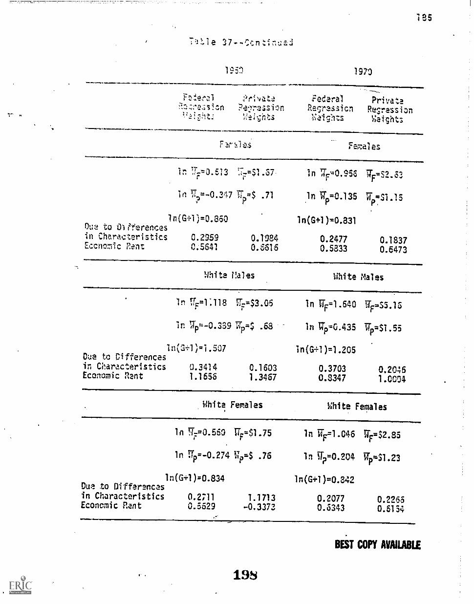
1951 1970

=.! ' !,,!ei,znts

Federal PrivataPz.r.ssicn Resression3tiIg Weights

Fzr;les Fe;zeles

in 71* F=0.513 =$1.57

In tai=-0.347 V: =$ .71

in 7f, 0.956

1n tiTp=0 135P=S1.,

%e to Differencesin(G+1)=0.8450 ln(G+1) 0.831

in Characteristics 0.2959 0.1984 0.2477 0.1837Eccnclmic Pent 0.5641 0.5616 0.5333 0.473

White Nales White Males

ln 77.=1:118 7==$3.05 ln ITF=1.640 I:TF=55.16

lr 7=-0 339 7r,,' .58p p 4 ln Vp=0.435 Ilre$1.55

Due to Differencesln(2+1)=1.507 1n(G+1)=1.205

in Cilaractertstics 0.3414 0.1603 0.3703 0.2046Economic Rant 1.1655 1.3467 0.8347 1.0004

White Females White Females

ln 91.=0.560 Tie51.75

in 7=-0.2'4 Wp=5 76.p

in TF=1.046 ITF=52.85

ln 5=0.204 5=51.23

ln(G+1)=0.834 ln(G41)=0.342Due to Differencesin Characteristics 0.2711 1.1713 0.2077 0.2265Economic Rant 0.5629 -0.3373 0.6343 0.6134

$ 19S

BEST COPY AVAILABLE

1.; r, t 1 n

4111.,..1

F,14.1.13 Prlvate

W2i°,1ItS

1 7 0

i:OV41:1*A1,a

3anr4!;sinWeictts

Pri'lete1.4.11 A

l'1.1t144. 06,

Ith4nN4.P.

116

MA4, J*4.44..3 .'Y s

17.93in V'.659

In Ur= 0 d'd rjrt 6-p 0

In(G+1)= 1.073Dua to Differences

Characteril;ticsEcono:nic want.

0.11160.9314

0.20350.8594

ln U = 1.075 U=S1 3

1n lir 0.295 gpt$1.34

in(G+1)1g 0.780

0.15920.5208'

0.07790.7021

Non-'ite Females Non-hite Ferrales

In 1.7c=0.342

1n 7.74=-0.553

F=$1.41

.58

In y 0.802 : =.le .23

In 7eTp=-0.089 711=$ .92

1 n(8+1)= 0.895 1n(G +1)=. 0.891Du: to Differencesin Characteristics 0.5442 0.0841 0.2758 0.1268Econordc Rent 0.3503 0.8109 0.6152 0.7642

BEST COPY AVAILABLE

I 199

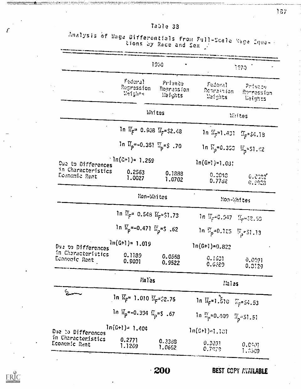
Anal ys i s of

Ta:)1 e 33

. .:acj41. Differentials fro:;1 Full-Scale'.;:-.;.(2 :qua-tions y Race and Sex

On10111.1*.. avivia0.00*.NeabvigilbONNoVNIMMVONVaV.M.Ove*V4....

Pv.V.1100...10*.vioVorvemvvavvINIonl.almVb.1. mb,ewtvemmova. vmv

10:10ft& v par

'"ressi on

V IV

*mom ravevvomovr. ..4VolvVvVvinv

Privai%t1\k4 .14 4 tv41

VeN

Whites

n

iv* woomm.

nv,N,44 vve.1 1 Ovv

Rl-rssionVoli'gtrs

44144 avv,

11;lites

ln Ur 0.908 =S2 48

in Um-0 3

1n(C-

1 Tir -$ 70

1 ) 1.259

1 VI I

ln =0.353

ln(G+1)=1.03:

M-z$4.18

'Jr.'

Du to Differencesin CharacteristicsEct:ncmic Rent

0.25631.0027

0.18881.0702

0.20450.7762

0.;?,2!61'1,1

4 . .#

Non-Whites

ln rip= 0.548 gr$1.73

ln ci.1=-0 471 Prm$ .62

1

01114vavanv4444=11waarr.1114).)44/

n

ln rrp0"" of40 r.S1 13P

1n(G+1)= 1.019ln(G+1)=0.822Du! to Differences

In Cnaracteristics 0.1189 0.0558 0.1531 0,M91EGonomic Rent 0.9001 0.9522 0.6Fe9 0.3:29NIVIVEVIMVIVVV.OVINEV/INVMVIVIMIIIVONVVVVV"

.11=nv,vallMares

1111 aSIM 4441

ln CIF= 1.010 u .75

In y-0.394 y$ .67

1n(G4.1)4 1.404Due ;.) Differencesin Characteristics 0.2771Economic Rant 1.1269

=0VVIVIIMV

0.33681.0652

In riFF=1.51'O

In y0.409

ln(00).1.101

=1.1Wa v.

200

0.30310.7q7^

,p -"1 5'

BEST MY talUIBLE

F,°2-1.w.:11

1-:!sslc.1

113')ts

^ *.

rr1V2,.!

orZfj.14..o

13,"

97:

...Am 'w

,11!,,:r2s51,0n

'Ail7;nts,.MOMOn 0=0 .Mmmr mm...mma

mdamm m.*Imm....mmemm

In C.512 ::..=$1.67

in Tr -0.347 7=3

1n(0y1) 0.850

=

?ri v.Ite

In V..= 0.9E5 g=5, 63

ti 0 1"5 =Si 15

ln(G+I) 0.831Due to 3f f'

in Characteristics 0.374S 0.1486 0.2370 0.1998Economic Rent 0.4851 0.7114 0.5940 0.6312

White Males

ln Tii= 1.113 .1F=$3.06

In 7=-0.389 .68

White Males

in 171.=1.640 7..=S5.16

ln lip=0.43547-$1.55

ln .2,.4-1)= 1.507ln(G+1)=1.205Due to Differences

in Characteristics 0.3554 0.1923 0.3573 0.0856Economic Rent 1.1516 1.3147 0.8477 1.1194

White Females

inF=

0.550 ITF=$1.75

in 7 P=-0.274 TT ig$ .76

White Females,ln ITF=1.046 Wr$2.85

ln g=0.204 7=51 21P P

ln(G+1)=0.834 ln(G+1)=0.842Duo to Differencesin Characteristics 0.7763 0.2393 0.2561 0.2319Economic Rent 0.0577 0.5947 0.5759 0.6101

201 BEST COPY AVAILABLE

,..........11/1.1...110=000100001.000011..40D.M.1.1........

*

Non-tallt,

;:e1.1httl

4?1I N.

4, In,.iZ41 n ra

In 7.- 0.65?0 4

ve

1' T;Va -0 414 7-=$ .66P

,0

Pik

4.4z s,41/

i.d:4A 1A 1 ,,.; 4.4:a

0114.1=1%

4441 t4 4fe

$1 r.PT

In(G41)2 1.073 ln (r +1 )=0.780C;::e. to Cifferencos

n Cilaracteristics 0.0617 0.0619 0.1470 -^.CS20Economic nont 1.0113 1.0111 0.633C 0.8720

Mon-White Females ron-Uhite Females

in ITF= 0.342 Tjr$1 41

In 14=-0.553 T/Te$ .58

0.802 lir*e.2 '3F "

in 17pc-0.089 prr 314 .52

1 1)= 0.895 in(G+1)=0.891Due to Differencesin Characteristics 0.3655 -0.0907 0.2094 0.1032Economic Rent 0.5295 0.9857 0.5316 0.7878

202

BEST CON AVAILABLE

1.90

yeirs. Like the eaeninc;s differenLials the largest gross

w4 7:;e rate t!ifferential in both years is for white males

(1.507 in logs in 1960 and 1.20 in logs in 1970). Similar-

ly, the smail:n-r. gross diffsrantial in 1950 is for -white

(0.:?.2 in 1,12s) ani in 1970 for non-white males

(0.780 in lor2s). These differentials are smaller 'than the

esrnings differentials for tha same race -sex' groups in-

dicating that part of the gross earnings differential for

each race-sex group does reflect the greater non-pecuniary

benefits enjoyed by Federal workers, specifically their

greater stability of employment. However., there is still a

substantial differential for each race -sex group. More

than half of this differential remains between comparable

workers in each aot.; i s coubidered du etwuumic rent

paid to Federal workers.5 This implies that in addition to

their non-pecuniary advantage, Federal workers in every

race-sex gro:upL enjoy a pecuniary advantage over their

counterparts in the private sector.

These differentials decrease between 1950 and 1970 for.

every race-sex group except white females. The percentage

decrease, range In size from 4 per cent for non-white females

to 27 per cent for non-white males. The differential for

white females increases by 1 per cent between 1960 and 1970.

Like the decrease in the earnings differential over this

period, these changes in the wage rate differentials prob-

ably reflect changes in sener4,1 economic conditions over the

decade and differences in the effect of inflation on real

203 BEST COPY tVAILABLE

As 4v. 4.1s-sNs.1./

n'okU.) :I *I 4.; J

-"*I-s ti

to

12;141r,acterlst1 c'3 Scuations

in the11s.s.44'.1M1'

th.4 race rtas;r +0+-

coerilnlznA.s of ta" "Jim tsar e

in 1550 zi1J 19%

191

i "11%, ,"4, 1.11Z: nClingS ;,,les

* -411) 42, pre ':;', t ts in '1 960 and Tatles

45. an'! 4E sho t?1,1 in 1#37<)). The rata of return

is .13h her in the Federal sector for every group except non-

hite nal s in 1T,t;0. The pattern of the egp rience coef-

icients is also similar to that observed in the earnings

equations: they imply that if both Federal and private

workers initially devote the sane proportion of time to

on- the -job training, the rate of return is consistently

higher in the Fethlral sector.

rhe principal differences from the earnings regressions

which emerge in t'etese wage regressions are in the estimated

race and sex differentials and the effect of the 3ABYB

variable. In both years, these differentials are larger in

the Federal sector when only one minority influence is

present: that is, discrimination is stronger against non-

white males and white females in the Federal sector. In

1960, the racial differential is smaller in the Federal

sector when both minority influences are present and in

1970 both differentials are smaller in_the Federal sector

when both minority influences are present. All the race

and sex differentials are 'smaller than those estimated it

204 BEST COPY AVAILABLE

Per 'C racteristics tlage 'Ecrla ticris fort s n i t s i 1 96C'1

ftftft.ftawft.ft.-e....ftmaftftft

1^tit

...wamirlgow

;lit,',s in IMY1.) Faar,a1 Private

,:on-4,417.ites-a t

iftftftaftW.M.

aliftyftftft.....ftloftftilmoftworftft

in IS'150

,4tftftftft. ftftmoftftftwaaftft...MIftlift

(-4.4432)

'A,-1" 12(-6 5121.7)

n Llf"2,7,eyor.NA-1

fve7i-1.

pT'A7,A. olI*" 1

C.0767 0.0056 0.0055IC ;979) (1.0019) (2.57,1.4) fn gAr-%

Oft111:.** ftAl.ftftftb 0.0427 0.0100 0.0303 0.0272(7.3633) (2.4660) ..(2.5247) (4.1771)

nce Squared -0.0005 -0.0007 -0.0005 -0.0005(-5.1803) (-9.1071) (-1.9934) (-5.9534)

Sax -0.5397 0.0151 -0.3338 -0.2005(-10.3623) (0.3791) (-3.4830) (-3.3104)

Spouse Present -0.1157 0.0699 0.1145 0.1602(-1.7822) (1.3060) (0.8113) (2.0208)

Spouse Absent -0.1687 -0.3523 -0.1730 0.3102(-0.8581) (-2.4607) (-0.5808) (2.0608)

Widowed 0.0482 0.0872 0.0330 0.1392(0.3499) (0.8327) (0.1336) (0.9767)

Divorced, Separated 0.1557 0.1299 0.0322 0.1036(1.4237) (1.3525) (0.4543) (0.9539)

Urban Residence 0.2329 0.6950 0.1188 0.4323(3.5700) (18.3431) (0.7224) (6.7084)

F 37.4944 103.8022 3.4995 14.7673

R2 0.1273 0.0431 0.0327 0.0206

Standard Error 1.0811 2.5701 -1.3886 2.1716

Number of Observations 2,253 20,544 667 5,385

at-valuesin parentheses.

.4.

BEST COPY AVAILABLE

ari :14.1

1 .111110.041

ti n'stant

Exi:aerience

Zxpl!rience Squared

Face

Cr"' "^A Presen r`

Spouse Absent

Uidcwed

Divorced, Separated

Urban Residence

Babyborn

F

R2

Standard ,Error

Number of Observations

;.! ti ti a () fl st,-r c teris,rivaend F '49 v

1:13

a

0.CE00(9.523c)

(9.1223)

-0.0003(-7.3854)

14'sn

Private

47...:111)

0.01E1(-3.B291)

0.000?(0.0355)

-0.0006(-7.0465)

-0.3015 - 0.0357(-6.04'59) (-1'.6356)

0.229 0.2753(3.51)99) (4.4 q)

-0.0008(-0.0050)

0.2540(1.n21)

0.2164(1.8257)

0.1548(2.9733)

37.7868

0.1914(1.2492)

0.3223(2.CL03)

0.2332(2.0091)

0.8881(20.9117)

107.3203

0.1526 0.0528

0.8301

1,840

2.6336

17,250

PrllatzF.naIas 11

u,t,e-11fn

11.111.10

C-1.9176)

.093C:: 3.04:31(4.5102)

0.0303 0.0192;2.7733) (3.9709)

-0.0002 -0.0034(-1.3605) (4.7797)

0.1014 -0.1807(-0.9421) (-3.3446)

-2.031 3 -0.5931(-4.7430) (-3.6374)

-1.9662 -0.9193(-3.5957) (-4.4724)

-1.8171 -0.7351(-3.9637) (-4.1145),/,..

-1.6971 -0.4824(-3.3321) (-2.7673)

0.2935 0.1397(2.0319) (2.7954)

-0.1442 -0.0475(-4.0963) (-3.5971)

8.7183 19.1419

0.0668 0.0194.

1.3997 2.1530

1,033 9,169

at-valuesin parentheses.

206 BEST COPY AVAILABLE

Tabl-ti 41

i. ::rt ,-11 C arac ter i stirs 4iai3et es :Ind

Fe`va 1 es, ......

Equ,e.tior,si n 1 960

, or

........11=1=1.1.001.

es 44 .1 a .1 ; :iite Fei%les

194

..impolmoo.

tetiin 1 '3F,0

...:daral Private

.14.

1:-30

Fede.ral Private Pf)la.7.1s.tant. n n

1 f *Zr.' 1 \

0.0704 -0.0203(9 2 9919)

0.0527 -0.0039

111111100111

^^1^1.1251 -0.1;7.7 i(1.5123)(-1.3705) r,

0.0859 0.0523 -0.0335(3.5759) (5.5753) (-1.30)

0.0276 0.0242 -0.0034(8.9335)(- 0.7067) (2.2917) (4.2783) (-0.27)

Experience Squared -0.0009 -0.0005 -0.'0002 -0.0005 -0.0004(-7.4763)(-5.6992) (-0.7604)(-5.82C4) (-1.33)

SPouse. Present 0.1576 0.2962 -2.4044 -0.9310 3.3854(2.1435) (3.9537) (-4.6373)(-4.5752) (6.04)

Spouse Absent -0.2334 0.0347 -1.9423 - 1.5736 0.3535(-1.1924) (0.1658) (-2.9702) (-5.8930) (0.51)

Widowed 0.3357 0.3812 -2.1798 -1.1025 1.0773(1.3903) (1.9432) (- 3.9533)(- 44.7556) (1.30)

Divorced, Sparated 0.2152 0.2993 -1.994; 1.1637(1.3259) (1.9503) (-- 3.671111- 3.6031) (2.35)

Urban Residence 0.2063 0.8967 0.2044 0.2443 0.0399(3.4450)(18.3928) (1.3513) (4.2678) (0.25)

Easy born -0.1750' -0.0730 0.1020(-4.0938) (-4.1790) (2.21)

F 29.6529 99.8395 8.2944 24.7317

02. 0.1402 0.0543 0.0721 0.0305

Standard Error 0.8181 2.7333 1.3890 2.1734

Number of Cbservations 1,407 13,760 845 6,734

at-valu es in paranthesest

107BEST COPY AVAILABLE

r* a 1 ;. ra cteri 47.7f

195

"11-- 7"Hatio-s 'orm

Fe;-.!les in 1 0:30d

- ,iX 1,2-b

1471 1.sc,- ,1-et.ieral

'V.4 m

r.:ati on

.....

^,1"7.4LAVm.14 -0 n9n

-0.5352A smAl%

0.0307

f 1,n7A

Vet...4).J-s:41

(2.03C;) f/ st4' 97771kA,A

:xperlince 0.0780 0.0230 0.0512 0.0253

-Expertancea

(2.!-449)

-C.03C4

(2.5523)

-0.0008

(1.9166)

-0.0011

(2.6674)

-0.0002(-1.8761) (-5.4563) (-1.7903) (-1.4711)

-3L.5195 0.1790 -1.5848 0.0436(1.7303) (-2.0017) (0.1763)

Spcose Absent 0.4544 0.3333 2.2309 0.2194(1.5768) (1.5557) (-2.1981) (0.6780)

Widowed 0.3947 0.0734 -1.2557 -0.1050(1.1225) (0.3104) (-1.4502) (-0.3785)

Di'iorced, Separated 0.4298 0.0531 -1.4588 0.1231(2.2252) (0.3298) (-1.8451) (0.4902)

Urban Residence -0.0577 0.8219 1.0031 -0.2157(0.4176) (9.8557) (1.8792) (-2.1357)

Bebyborn -0.0992 -0.0090(-1.5351) (-0.4577)

F 4.1410 24.5439 2.2769 3.2647

0.0550 0.0511 0.0470 0.0085Standard Error 0.8512 2.2187 1.4294 2.0550Number 0 Observations 433 3,500 234 2,335

at-values in parentheses.

3

20S BEST COPY AVAILABLE

P:-..rs 0 :1. *. "

1 '''s n t !I 5 for!..1 ex -1 i ea :, 111 9; 0-., LtiNwil 11,0011 11t r-mb. ...

"a" ` ya,PI as i

!

InV%1 'et 1"0

:!on-4h itzts

1

e% " -4 .H .1I .

(-5.*3:,-.",'

n

(-1.0113) (-3 0595) f-7A 4'

ar

3.CSS'3e

.QiZ-'7; 0.0717 0.0135(14.6728) (3.;252) (5.3313) d0"7)

cxerience 0.0572 0.0165 0.0304 0.0153(13.0393) (4.3145) (3.5912) (2.5238)

Experian-e Squared -0.0309 -0.0007 0.0004 -0.0003(-9.7212)(-10.2437) (2.0245) (-3.3488)

-0.3933 -0.2891 -0.2117 -0.3837(-10.7487) (-8.6503) (-2.9479) (-6.7112)

Spcu. Presont 0.1001 0.1362 0.3305 C.4 30(2.0037) (2.8464) (3.5043) (5.2E79)

Spouse Absent -0.2811 0.0830 -0.2157 -C.0371(-2.1598) (0.65105) (-0.9459) (-0.2217)

0.1016 0.17)07 0.2392 0.7955(0.9353) (1.7123) (1.5080) (2.1823)

Divorced, Separated -0.0070 0.2098 0.0856 0.1877(-0.0879) (2.7329) (0.6583) (1.8198)

Urban Residence 0.1695 0.4993 0.2474 0.1931(3.8039) (14.9776) (1.3703) (3.1118)

Dis2bflity -0.3231 -0.1971 -0.4574(-4.3998) (-3.1150) (- 1.531) (-4.3580)

F 84.9744 74.0207 11.0629 14.6313

R2

0.1757 0.0315 0.0653 0.0232

Standard Error 1.0227 2.3320 1.2775 2.0782

Number of Observations 3,942 22,407 1,441 5,733

at-valuesin parentheses.

29BEST COPY AVAILABLE

'

Personal Characteristics ,Jage Equatio.)s for.N:ales and Fe;nales in 197011

,....411.1.1.1.110"MO,

1 97

Mes1.S.% ;VC) .

Feales1970 NC),t s

01,1A10 So. Fr-t-i!ral41 Private Federal Private11.67.1......

;324 CC931 -0.6130 0.7-693(-7.7739) (0.9424) (-3.2053) (-5.8733)

0.0283 '-0.0116 0.0752 0.0391(15.7756) (-2.0034) (5.0537) (7.3859)

-Ex peri epce 0.0522 0.0093 0.0515 0.0207(12.5560) (2.2494) (6.5574) (4.8022)

Experience Squared -0.0008 -0.0006 -0.0009 -0.0004(-9.2550) (-8.0883) (-4.7334) (-5.2879)

Race -0.2766 -0.1354 -0.1415 -0.1836(-7.1093) (-2.7372) (- 2.0397) (-3.7079)

Spouse Present 0.1:405 0.4731 0.0039 -0.0570(8.6201) (8.4408) (0.0476) (-1.1134)

Spouse Absent 0.0463 0.2760 -0.4997 -0.1692(0.3697) (1.8693) (2.4298) (-1.2153)

0.472F, 0.3199 0.0521 -0.0773(3.4239) (2.1379) (0.4285) (-0.6351)

Divorced, Separated 0.2734 0.4423 -0.1067 -0.0039(3.1191) (4.7281) (-0.9687) (-0.0485)

Urban Residence 0.0579 G.5398 0.4353 0.2533(1.3586) (13.9133) (4.5056) (5.7322)

Babyborn -0.0650 -0.0420(-3.0972) (-3.5437)

Disability -0.1013 -0.1816 -0.8252 -0.3935(-1.6477) (-2.6397) (-5.0997) (- 4.33o8)

F 98.5372 62.2935 14.7835 23.04239

R- 0.2269 0.0341 0.0686 0.0220

Standard Error 2.3954 1.3552 2.0816

Number of Observations 3,325 17,377 2,053 10,763

at -v lues in parentheses.

210 UST (Aid AVAILABLE

n r : c zCi s1 h-,' 1 n .

I . s M 's

r " 4 - ,. iv-

Exoarien-.2

Spouse Prasent

ous. Y15,.rt

Widowed

ono r .0 .0 So o

Urban Rzsid,ence

Baby torn

Disability

amosomomanomm

.47.1f

os. I

;Jrr./rscliv I:IQ"

A .

s41 V:Itn

V99,999

'('.'9.24?7-93) )*(913P93) (-I .77 ::4) (5.235'1)

0.0214 -0.0C.34

(17.8923)(-0.9733)

0.0641 0.0092(14.4050).(1.9399)

-0.0011 -0.0005(-11.0500)(-7.5598)

0.3794 0.4130(5.9323) (6.2800)

0.0995 0.374,5(0.6743) (2.0341)

0.5297 0.1593(3.3705) (0.9254)

C.2315 0.427=(2.3411) (3.(251)

0.0510 0.5385

(1.2359)(13.5058)

-0.1255 -0.1041

(-1.9525)(-1.3312)

F 88.4577 62.3699

0.2333 0.0375

0.7249 2.4504

Number of Observations 2,559 14,178

R2

Standard Error

0%0525 0.0610 A pA.

(3.5500) (6.60'35)

0.0503 0.0273(6.5931) (5.5929)

-0.0010 -0.0005(-5.0553) (-6.59-10)

-0.0141 -0.12,14

-0.0 25(-3.13)

0.0004(1.33)

-0.1103(-0.1457)(-1.7757)

-0.5779 -0.142, 0.3795(-2.2738)(-0.8553) (1.33)

0.0414 -0.0535 -0.1049(0.2385)(-0.5823) (-0.51)

-0.0209 0.0-'0 0.3799(-0.2114) (0.5303) .4.)(0.43)

0.3536 0.3151 -0.0424(3.4395) (5.2705) (-0.36)

0.1305 -0.0633 0.0757(-4.8946)(-4.0732) (2.33)

-0.9397 -0.4095 0.5302(-4.5547X-3.7744) (2.31)

12.6539 23.3578

0.0772 0.0265

1.3229 2.0743

1,383 8,229

at-values in parentheses.

211 BEST COPY AVAILABLE

Personal Characteristics Wat,;e Equatiunsfor Non-White Males and Fc,:mais i n 11C.'1

C,:instalt

Experienc

Experience Squared

Spcuse Present

Spouse Absent

Widowed

Divorced, Separated

Urban Residence

Bab born

Disability

F

R9

Standard Error

Number of Observations

Ncn-hite 'a1es1W.C, CA)

Feerll Priliate

r

(',1 )1-7'

0.0245(2.4439)

-0.0003(-1.6033)

0.5909(4.8777)

-0.0284(-0.1144)

0.4253(1.5007)

0.4679(2.1722)

0.0351

(0.2361)

-0.0146(-0.0934)

8.6152

0.0822

1.1068

766

te "Fer~-A

1970 ,(''r\Fat2rAl

'6 Ao

1 95

166......66

-0.105 -1.6133 -1.1C, 2(-0.550) (-3.34t7.0) (-4.3531)

-0.02C3 0.1025 C.C675(-1.7273) (3.6707) (4.131S)

0.0193 0.0374 0.01.29(2.3251) (2.4297) (1.4251)

-C).000c3 -0.0003 -0.0001(-4.1248) (-1.3473) (-0.5046)

0.6579 '0.0910 0.1086(6.5195) (0.5984) (0.9016)

0.1504 -0.4029 -0.1899(0.6672) (-0.9191) (-0.7599)

0.6715 0,1399 -0.0355(2.8064) (0.5089) (-0.5423)

0.4970 -0.1410 -0.0974(3.3796) (-0.7409) (-0.6622)

0.2735 0.6082 0.0484(3.2981) (2.5683) (0.4858)

0.0126 -0.0127(0.3829) (-0.6948)

-0.5006 -0.6663 -0.3545(-3.6145) (-2.4519) (-2.2908)

12.4560 4.2978 3.3519

0.0312 6.0466 0.0092

2.0596 1.4403 2.0868

3,199

atvalues in parentheses.

675 2,534

BEST COPY AVAILABLE

200

th'.! ;:41.1ations. In 153!) the sox 40Ferential ranges

in size f-ort 0.0 I (this is insinificant) to - 0.5397 and

rnnmps -r n'857 P 3nis. :A

1170 V.:e SP;ti 4ifferential ran es from - .2117 to -0.3333 and

t:la race di-:Feential -0.1.35'1 to 4.2766.

is intNitivel r asonabl'e since it indicates that non''h ites

and females are affected by discrim:nation in both pecuniary

and no%-p culiary matters.

The coefficient of the 3A5 Y3 variable is also smaller in

the waqe equations than the earnings equations in all cases

where this variable is significant. It ranges in size in the

Federal sector from 0.0126 (this is insignificant) to -0.1750

and in the private sector from -0.0090 (this is also insig-

1-w,Ars^v. 41. 46.ftnificdo0 Lo -0.0730. isZmUifi4 ok.40.* 66#1..

Federal sector for all groups in both years except for non-

white females in 1970 (where the coefficient is insignifi-

cant for both Federal and privative workers). This implies

that tile effect of lost experience due to child care is

greater over a longer period of time than in terms of the

base rate of pay.

Full-Scale Wage Equations

With the inclusion of the occupational variables in

the full-scale wage equations, the pattern of the estimated

coefficients changes. These changes are similar to those

which occur when the occupational variables are included in,

the full-scale earnings equations except for the changes in

the estimated sex and race differentials. It is expected

BEST COPY AVAILABLE10113#6,

!

F111 .1 1 a 44; Ft ;73(1,5 for n tt.160

" ..+t'

01

oarionze

Experience Squared

Sex

Spouse Pr05ent

Spouse A:;sent

1.10,1,zd

Divorced, Separated

Urban Residence

Profes:iona1s

Managers

Craftsmen

Operatives

Laborers

4 .4.11tZS

1,..

PrivatT.

,rcn-.14hitesin 50

1114........ 1.61101.00.1.0.1.11*...IFIFi..1

. - '11It> 3/1,01

n 0.055(5.2737) (9.7440)

C.C418 0.0'395(7.2225) (2.4173)

-0.0006 -0.0005(-5.2137) (-7.1420)

-0.4770(-8.2481)

-0.1213(-1.8751)

0.1878(4.4438)

0.0479(0.9111)

-0.1223 -0.3032(-0.6238) (-2.2003)

0.0462(0.337C)

0.1640(1.5053)

(0.4i22)

0.0990(1.0534)

0.2243 0.7295(3.t427) (19.6718)

0.300 0.1215(4.7894) (1.9340)

0.2090 -0.9264(2.3639)(-13.3725)

0.0977 0.9921(1.0361) (17.4083)

-0.2933 0.9732,Z485) (18.1566)

-0.0221 0.6472(-0.0773) (6.3252)

-1.eo4(-0.034)(-10.73'.:7)

0.0;25 0.01.59;0.7054) (1.7406)

0.0307 0.0292(2.5635) (4.5965)

- 0.0005 -0.0005(-2.2035) (-5.7636)

- 0.3015 0.0632(-3.0559) (1.0437)

0.1182(0.8440)

-0.0920(-0.3101)

0.0733(1.0155)

0.2979(2.02)9)

0.1093 0.1270(0.4167) (0.9142)

0.1120 0.0556(0.5233) (0.5251)

0.1291 0.4247(0.7838) (6.7174)

0.2720 0.5720(1.5133) (3.9975)

0.4631 -2.5918(1.0963)(-10.1513)

0.1592 0.6501(0.9501) (5.3166)

-0.0205 0.9102(-0.1257) (11.1504)

-0.2016 0.9518(-1.25C6) (10.2234)

214 BEST COPY AVAILABLE

'PariabIa: In A-!.i....1,..

F

St-Indard Error

.te 47Continued

Whitesin 19L0

FeJeral Private

Non Whitesin 1960

Federal Private

;L.:1;ber of Observations

C.0319/0 'n07).-.

24.6a 7

0.1361

1.0756

2,253

lab

202

-0.2495 -0.4722 0.3455(-3.0:67) (-.1.3n3) 2."5)4. iO

133.6425 3.4227 30 al 31

0.0882 0.0517 0 0705

2.5088 1.0976 2.1154

20,544 667 5,885

4t-values in parentheses.

215BUT COPY AVAILABLE

F

VA.

T464 41 n w

11,1s2 !f",' r PAA*A'e

An,ltit),15 Tor roz;..d

ban.meols.atwo.

moms

Ext,er.ence

7..0Ivoircelen1. .00

1 0

Race

Spouse Present

Spouse Absent

Widowed

Divorced, Separated

Urban Resi4ence

Professionals

Managers

CrIftsmen

'Operatives

1"A , ,:s

S ;P:;) ("15.4rIn

0.0393(5.1C07)

C.0170(8.9733)

^A-1V "11ile (1^..-V0.4Vti

0.0025(0.5707)

-0.0003 -0.0004(-7.4655) (-5.5093)

-0.2293 -0.1370(-4.2333) (-2.5315)

0.2111(3.2413)

0.0125(0.0775)

0.2253(1.1426)

0.2129(1.8037)

0.1923(3.1602)

0.2074(1.3921)

0.2353(1.5493)

0.0994(0.8;302)

0.1529 0.8588(2.9502) (20.9195)

C.2958 0.3335(5.3377) (4.1290)

0.2798 C.74C5(3.6335) (-9.9205)

0.07E3 1.1305(1.1864) (19.1509)

-.--=0;0127 1.2339(-0.1241) (20.4965)

216

rl.;".!12;*^:Ni,4/3

Ao

1.031S,.ki.o.011 1,1,11).,...,

0.0520 0.0615fl 41/t'% (5.9137)

0.0297 0.0218(2.7095) (e..5450

-0.0003 -0.0005(-1.2825) (-4.9633)

0.0923 -0.1555(0.7825) (-2.874)

-1.9234 -0.5726(-4.5002) (-3.5491)

-1.3423 - 0.8672(-3.3646) (-4.2657)

-1.7052 -0.5914(-3.7128) (-3.9059)

-1.6138 -0.4223(-3.5397) (-2.4492)

0.2370 0.1745(1.6252) (3.5202)

0.3999 0.0730(2.9925) (1.0305)

-0.C510 -1.5932(-0.2594)(-11.9597)

0.0955 0.0757(0.2134) (n.3534)

-0.7299 0.3479(-1.9300) (5.2147)

BEST COPY AVAILABLE

AW liaW, A. .M.4i114M00

,

4 44e 44* ,1,

Nul'a;4 of 'Observations

lr.N14

0 rip.)"0 NO V .40

t..110

1.04.0%,)tN'IMO

4 AyA " 1

'0 'CS" 2-.1.1;i:37; 0.3134

25.3134 135.2084

0.1555 0.1045

0.8233 2.5656

1,840 17,260

F: 11thin 1130

r.; a1 Pris,ezitzt.

GAr

0.6712 V7

(-2.611':) (-7.0515)

(- 3.8772) (-3.4;:.;1!)

6.8643 28.0414

0.0800 0.0451

1.3897 2.1247

1,080 9,169

at-values in parentheses.

111101110

1r

217 BEST COPY AVAILABLE

7, y n, t.

a. V/

ons i ts. os

4...a..m.....a.wNO. mama Vemmarob M...i*oo*

AN*.4swaftata..., .1.. AM.

0"N*A1 Q a A 1'111. "(4 'N.)1 111 41

:1, 1.211 4.! Ni 'N-W)

it ge14:14

1 j I

1,01,44_ .t.!MaliS

"fI i I f N

'!C5

Ni

tA 4 ,.

.""Z"1..1.1 Ne1.41,9,.

N.N.M.% 440.* *.a

11. t.:144"%.M. N.404;

'1-:nrO.:0;811". N

.r)521 -0.0015

11

'3 ,1 5

(1.9:73)

0.0275

omms....m.Ya

*.'N 1".7.:I r 0. 1

n

4/b4.N01)

0.0251(8.9354) (-0.2395) (2.2909) (4.5732)

-0.0009 -0.0004 -0.0002 -0,0005(-7.5004) (-4,1553) (0.3578) (-5.5202)

Zpous Present 0.1355 0.2185 -2.3954 -0.9498(1.8555) (2.9535) (-4.6252) (-4.4790)

Spouse Absent n 411101 0.0332 -1.9293 -1.4529(-1 .C530) (0.409") (-2.9Fo2) (-5.5429)

Widowed 0.2911 0.2593 -2.1582 -1.0422(1.2052) (1.4112) (-3.9307) (-4.5427)Divorced, sparated 0.1535 0.1309 - 1.9372 -0.7375

(0..2755) (-3.5755) (-3.2445)Urban Residence 0.1973 0.8955 0.0950 0.2534

(3.3153) (18.8131) (0.6302) (4.6407)Professional 0.2545 0.3101 0.4210 -0.1102

(4.1388) (3.5105) (3.0029) (-1.3159)Manager 0.2370 -0.7052 -0.1168 -1.4900

(3.0128) (-8.3079) ( -0.4358 ) (-10.7179)Craftsmen 0.0579 1.1785 0.5331 0.1447

(0.3052) (17.8283) (0.7753) (0.5415)Operatives -0.1957 1.2957 -3.4851 0.3759

(-1.4374) (18.1292) (-3.5253) (4.7833)Laborer -0.1114 0.8719

( -0.4029) (7.7137)

Service 0.0555 0.2038 -0.4199 -0.5309(0.5247) (1.4863) (-0.4277) (-6.9242)

21S BEST COPY AVAILABLE

.4 .1 '177/, 4.11 1. 13. 41 1 . 1

;:lts'as a Fenl.:-Is41 I

in 1(' ,:::t' ,t .. 1 . 1 . 11

r.111. ira t1

4'141.:

P1

Sta.Idard !:rrcr

:..4:r,lber of UozarveLicns

/./4J....................../.*/........../......-0.17",1

," 4 01

i 4.1 . 9I - 7 07' '. ,n .;)

sV IS

n 7r0"-r% AtM410.1511

0.812g 2.0554 1.301,9 2.1414

1,437 13 761 846 6,784

-values in parentheses.

219BEST COPY, AVAILABLE

War..; Equation: for flon-White a1 esand FefraIe: i t i 1J!,50

207

C 4. IV,. 1

t:an-?;n1te Valesit 195,1

In 0 Private

ConstInt -0.2262 -1.3763(-0.7437) (-9.3309)

Education 0.0105 0.0121(0.5453) (0.9754)

experience 0.0275 0.0265(2.3251) (3.1550)

Experience Squared -0.0004 -0.0007(-1.9966) (-5.1729)

Spouse Present 0.5038 0.0611(3.5393) (0.6060)

Spouse Absent 0.4826 0.3515(1.6705) (1.8095)

Wido.;fed 0.3392 0.0336(1.1075) (0.1472)

Divorced, Separated 0.4539 -0.0173(2.3588) (-0.1113)

Urban Residence - 0.0285 0.7109(-0.2046) (8.7439)

Professionals 0.2546 -0.0550(1.5672) (-0.2355)

Managers 0.6983 -2.3185(1.7836) (-7.5852)

Craftsmen 0.2049 0.8532(1.3589) (6.2582)

Operatives 0.0545 1.1451(0.3776) (10.7667)

Laborers -0.0547 1.1445(10.7691)

220

r,an-=11,.-a re7a1es

in 135'3

Faral Privete

0.02ES(0.0242)

0.0323(0.7050)

0.0477(1.755C)

- 0.0009

(-1.4572)

- 1.2351

(-1.5093)

-1.2130(-3.3586)

0.0195(1.2551)

C. 0260

(2.7391)

-0.0033(-1.8057)

0.0717(0.2946)

-1.8519 0.2334(-1.7637) (0.7530)

-0.9873 -0.0363(-1.0925) (-0.1320)

- 1.1S'!9 0.1653(-1.4563) (0.6432)

0.8435 -0.1502(1.5515) (-1.5005)

0.3190 0.9501(0.6945) (5.3319)

0.0972 -3.3694(0.0933) (-6.1913)

-0.0711

(-0.1163)

-0.3151(-0.7096)

-0.1539(-0.3209)

0.5543(4.2702)

-1.4091 0.8534(-1.8242) (2.2931)

BEST ri xvillABLE

I 11..1J I

" 1e4 1 11 - .14

. .e as 1 4,44 I '144

111:3

3

Fera;.t,s

in 1950lair. ;

:.., ,

( I 7--.1 f 1

0:251\0.7,)1 ^,..,-,\

3.2 77 34.5341

0.0587 0.1N3

Staro-lard Error 0.8430 2.1387

+..;;I:Ier of Observations 433 3,500

.,

-u.ulz.

(-1.1323;

wIwwNJ..

S . 1 )

1.78:C 2 4/1.,,t0t.

0.0480 0.0435

1.4285 2.0133

234 2 =2;,..,_

a , /6-vaiues in parentheses.

221

.1.

C.:,,ostan-!7

"I

T..231 ai 51

e :age Egtiationi 7;,7' Whites andNon-'411i to i in 197 Ot

4 .

"1:04 n 7,1

E :per 1 e icy Sq!;dreLa

Sex

Spouse Praslnt

Spouse Absent

Divocad, Separated

Urban Residence

Preessionals

Managers

Craftsen

Operatives

209

Lss

'1'970 C:1".)

Pr at

aNaMpliblinolion -Whites

1370 (.C)Esceral Private

-0.'>973

(-2.2941)

0.0i7.19

(0.8)78)

0.0545(12.4374)

- 0.0009

(-9.4317)

-0.7730(-7.3017)

0.0457(7.5903)

0.0137(3.9883)

-0.0005(-8.6582)

-0.3569 -0.1025(-3.5027) (-2.7610)

0.0857 0.0353(1.7277) (2.0153)

-0.2596 0.0555(-2.0059) (0.4379)

0.73!;7 C.11E4(;3.7841) (1.2476)

-0.0104 0.1959(-0.1308) (2.6138)

0.1639 0.5414(3.7002) (16.2702)

0.2470 0.0490(5.4248) (0.8970)

0.2777 0.0183(4.7285) (0.3034)

0.0035 0.6075(0.0505) (11.6728)

-0.0754 0.62901--0.6-943) (12.7256)

2 22

-..0.2974 0.7975( -1.'1051) (-4.8762)

0.0427;2.3159)

0.0310(3.6458)

.0.0217

(2.1779)

0.0152(2.5228)

-0.0004 -0.0003(-2.1564) (-2.9073)

-0.2211 -0.1895(-2.8677) (-2.9586)

0.3142 0.3748(3.3453) (4.9197)

-0.1911 -0.0983(-0.8414) (-0.5933)

0.292 0.2555(1.5341) (1.9318)

0.0553(0.5119)

0.2563(1.9323)

0.2640(2.3330)

0.3359(1.6264)

-0.2232(-1.6818)

-0.0335(-0.2375)

0.1438(1.4073)

0.2231

(3.5023)

0.6295

(4.3035)

-1.2625(-5.1730)

0.4560(4.2r.37)

0.5508

(7.0831)

BEST COPY AVAILABLE

;

1 --I t:I '..

; ai14144,ftmw,

lb 'Li +.4

r,on-'ef'ts

19 :0 1:,,,t.'"1

11 64 -. 4 144

*2 ,1

14=1111.11..se

f, y pN. I I 1.

R2

Standard Error

Number of Observations

7"kf "11 f"-:

-C!.3151

(-4.3125)

57.3377

0.1351

1.0152

3,942

r'1.7 1-D. 117=

( I. 0 "1* s , --.

-0.3315(-4.43EL) 1 i*-4,1g21

-0.137 A 91'77

(-2.5550) {-1.t4.0

67.1980 8.3562

0.0451 0 0757

2.3153 1.2705

22.407 1,441

I

rt

kl01.L41U)

;:4 1

13.5334

0.C457

2.0532

5,733

a ,t-vaiues in parentheses.

BEST COPY AVAILABLE

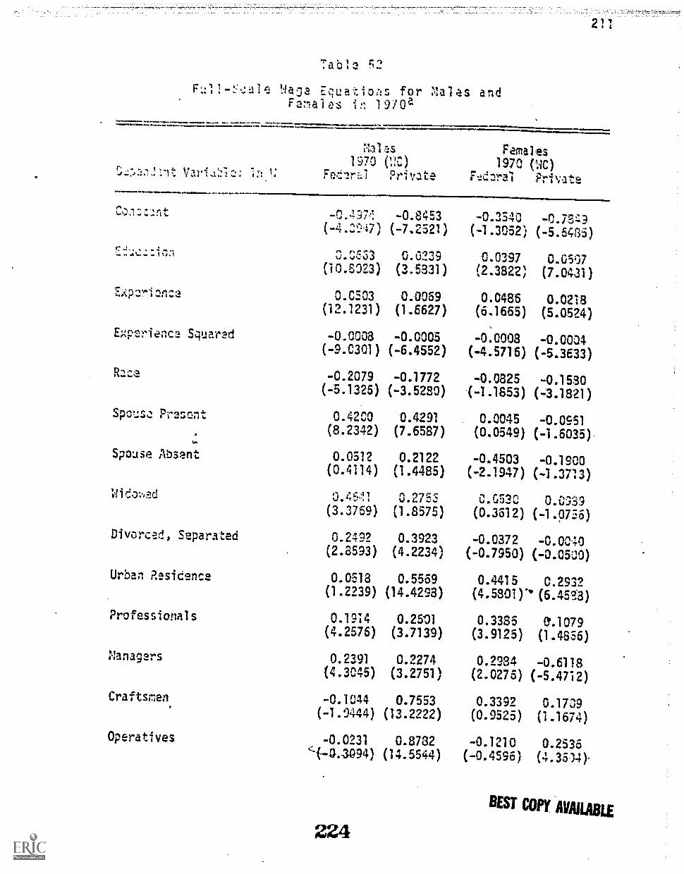
Table f;')

2 11

ale Wa ja Equations for .1a1 es andFeales 1910a

*.DOMOID10.1. dwo.

1

No

1970 (;2)Fe:".2r1 Private

-ovelne.^4

n

(-4.3N7)

(10.5023)

0.0503(12.1231)

-0.8453

(-7.2521)

0.0239(3.5331)

0.0059(1.6627)

Egperience Squared -o.000a -0.0005(-9.0301) (-6.4552)

Raze -0.2079 -0.1772(-5.1326) (-3.5280)

$ps!.:sz Present 0.4200 0.4291

(8.2342) (7.6587)

Spouse Absent 0.0312 0.2122(0.4114) (1.4485)

Widoed 0.45-11 0.2755(3.3759) (1.8575)

Divorced, Separated 0.2492 0.3923(2.8593) (4.2234)

Urban Residence 0.0518 0.5569(1.2239) (14.4293)

Professionals 0.1914 0.2501(4.2576) (3.7139)

Managers 0.2391 0.2274(4.3045) (3.2751)

Craftsmen -0.1044 0.7553(-1.9444) (13.2222)

Operatives -0.0231 0.8732`(-0.3094) (14.5544)

224

Females1 970 (;NC)

F-.tdzral Private

-0.3340 -0.7sa(-1.3052) (-5.5435)

0.0397 0.0507(2.3822) (7.0431)

0.0486 0.0218(6.1665) (5.0524)

-0.0008 -0.0004(-4.5715) (-5.3533)

-0.0825 -0.1530(- 1.1853) (-3.1821)

0.0045 -0.0951(0.0549) (-1.6035)

-0.4503 -0.1900(-2.1947) (-1.3713)

0.0530 0.0339(0.3612) (-1.0756)

-0.0372 -0.00;0(-0.7950) (-0.0500)

0.4415 0.2932(4.5801 (6.4593)

0.3385 Q.1079(3.9125) (1.4856)

0.2984 -0.6118(2.0276) (- 5.47i2)

0.3392(0.9525)

-0.1210(-0.4595)

0.1739(1.1574)

0.2535(4.3534).

BEST COPY AVAILABLE

Table 52--Cont

in

a t.

r A '.t

Stanuard Error

Number or Observations

1\ 71 I Al Ul '.1;

r nv11,±k .7

-0.163,5" n4,

0,7145to

0.2152(2.4743)

-0.0911 -0.1433(-1.4916) (-2.0973)

65.9430 52.4204

0.2332 0.0502

0.8658 2.3753

3,323 17,377

212

Females1970 (WO)

F--.-eie.ral Private

'01474..

- 0.132: ( . 17-;7)

-0.3519 -0.3914(2.5023; (-6.54'43)

-0.0539 -0.0400(-2.8580) (-3.3:,18)

-0.7953 - 0.3933(-4.9362) (-4.4616)

11.1693 22.3426

0.0775 0.0326

1.3587 2.0703

2,058 10,753

I.-values in parentheses.

225BEST COPY AVAILABLE

-4.:4.

r.

; A1.4 ...4e 444 444 4 I

r,,,, ,..ya. o

;:.ii ri enca Square

Presant

Plbo*.,Nrvi"o

Mdowed

DIvorc,d, S2carat1-1

Urban Resid nce

Professionals

nnagers

Craftsmen

C-or-rativ'es

Laborers

Service

4.4 0 444.

I t..

EcLaticn....; for toFai:,,aL.15 in 1 97'3'

213

10.10.W*44.4444.4..44 .44444* "`"."'"

n 711

(H 71,;:m

0.0618(13.8784)

-0.0010(-10.7597)

0.3539(6.4498)

A 1101

(0.8042)

0.5234(3.3442)

"",(2.105)

0.041(1.0763)

0.1847(3.9994)

0.2175(3.9746)

-0.0393-0.0807)

-0.1097(-1.1963)

- 0.3365

1-2.81-35)

-0.0490(-0.5379)

226

Nales;di.)

Alta FrsaI-ai

1.

1070 (;ir )

Pr!

n '377 ^

".l -6. 7;,15) (56101:5)

0.0.152 0.0304 0.0575(4.51;06) (1.5427) (6.53.70)

0.0065 0.0559 0.0777(1.1737) (6.0895) (5.5674)

-0.0005 -0.0010 0.0005(-5.8555) (-4.8356) (-6.4791)

0.3626 -0.0115 -0.1654(5.5117) (-0.1185) (-2.3712)

0.3193 -0.4788 -0.1545(1.7470) 'I') (-0.9274)

0.1346 0.0388 -0.0901(0.7418) (0.2245) (-0.8314)

-C.0t153 C.0536(3.3902) (-0.0391) (0.5320)

0.6099 0.3370 0.3509(14.0743) (3.4299) (6.9012)

0.1994 0:3299 -0.0134(2.5389) (3.4136) (-0.1722)

0.2692 0.3336 -0.5193(3.6348) (2.1155) (-4.4381)

0.7930 0.3379 0.1420(12.5212) (0.5661) (0.CS2C)

0.9196 0.1640 0.2373(13.2159) (0.3697) (4.1319)

0.5395(5.1583)

0.0393 -0.6120 -0.4853(0.7357) (-2.1867) (-6.7177)

BEST COPY AVAILABLE

idrP:1°C1444 4044 V ,14 4 4):N1.4 4. 44

/1 tide, n

2 0 :s 0 rl

44.I,'41 .44

44: 444 .4,

444 '4 4.4. i I 44.1

5:-.cndard E.ror

:Iumaer of 0bs,2rvations

"tV"41... 1al1.4

('to \ s,o

4:,:1r11 --Iva-

35.8727

0.2458

0.7790

2,559

n

tV,11"'Zt 4 I $ 1 I 4 11 k

'7r%to\IAN",

7,444

(-0 n36/) .1 C.11.4

55.21-00

0.0543

2.4339

14,178

0.0878

1.3157

1 3E3

(-3.7128)

n, A:11ir Jr. -I-

0.0379

2.0625

8,229

t values in parentheses.

CloolPelostoCw BEST COPY AVAILABLE

,r ; ; - C''tC" "40 ir 400,, ,. , .1 i 4 tI 11011

a S n t' , 11 1 970..1***,a,... 4004.* 11vagy 4. '

1 1 . 41. .4,41 y !,1..,. k .ell Jr, - Mg. ,.,

.40 'wt,

1 14t 1 .4 4. 1 V,

( 1:114(33;

axper SciJe red

0.0239(2.3797)

-0.0003(-1.6130)

Spouse Present 0.5597(4.6300)

Spouse Absort -0.0324( 0.1314)

11i cie...ed 0.3861(1.3345)

Di vo rc,ati S 0.321'5

(1.7527)

Urbin Residence v' 0.0453(0.3370)

Professional s 0.2115(1.5773)

Managers 0.4243(1.8133)

Craftsmel -0.2708(-2.1350)

Cpera t v 0.0254(0.1869)

Laborers -0.15571 . (14-74

225

1!..11..1=4.0

.1. '1)4,' 11 . 144 4 1.

I, 1

t

.1 °"7=-

)

rs-n.

(2.0144)

...=1111....4

(-4.3071 )

x.0595

11

0.0168 0.0372 0.0154(2.0465) (2.3913) (1.7037)

-0.0005 -0.0005 -0.0001(-3.4834) (-1.3143) (-0.5727)

0.6157 0.0'303 0.0390(6.1430) (0.5949) (0.7444)

0.0531 -0.3313 -0.2106(0.'2403) (-0.7546) (-C.81197)

0.5853 0.1299 -0.1006(2.4817) 0.4702) (-0.5756)

-0.13 ?3 -0.1150(2.8881) (-0.7018) (-0.7940)

0.2605 0.6315 0.0705(3.1536) (2.5451) (0.7057)

0.55(15 0.3531 0.8683(2.5963) (1.8565) (4.2592)

-0.9093 0.1340 -1.5915(-3.6330) (0.3640) (-4.2639)

0.6737 0.2363 0.4150(5.0905) (0.5129) (1.1979)

0.8597 - 0.2069 0.35;8(7.1318) (-0.8396) (3.2207)

0.9032(6.8213)

II

BEST COPY AVAILABLE

':"14;1'-o.0*. l'I":110.1*Ne kV 1,4 A.A1 /.0

,iaale

;:a1es1970 (s: C)

PrivateOCW0/10.410.1.1....011110.

Ferna:es197,0 NC)

AIM 4

ra'tterat Priwtte

1;11/.

bi

oe

Studare. Error

;lumbar cf Observations

mo ^ s."^ A.Je.mtJt41+

( at 4)

0.0125(0.C310)

5.4293

0.0962

1.0984

766

0.433;(3.1216)

- 0.4253(-3.11:5)

15.0134

0.0617

2.0270

3,199

^ %

u.Siot1 ,,,I. tso

(0.461:1Vet,

-0.6517(-2.431,3)

3.4152

0.0510

1.4370

675

"-12.113o

-1 1,t̂j-0. i.153

-0.3323(-2.11322)

5.9335

0.0237

2.0552

2,534

avalues in parentheses.

4-4.444.4.'

229BEST COPY AVAILABLE

.17

al:: uill derese ruch cf stix

and raf:e discr;n1nition occurs through occv:ational d!:-

ii )we In e f'11caletrmnation. ,. ,

crtAi.;1 of tfn*sa Alifferenlals increase in ''ate, to valuaq

cf thesa ins tnt.? raci 1 difFnr;Intia 1 for prvate

es in 16 n w;Iich increases from -0.0257 in the pers'ar,...1

chcracteristics equation to -0.1370 in the Yull-scale equa-

ticn. T1l ,4.. change in the sex differenti-41 for private sector

.,/hites is further from expectation: it changes from an in-

significant 0.0151 to a highly significant 0.1878.

The same criticism applies to use of these occupational

variables in the wage rate equations as in the earnings

equations. The changes in the patterns of the estimated

coefficients in the full-scale equations emphasize the

shortcomings of the occupational variables and that the

personal characteristics equations are the most meaningful

for the purposes of this study.

Personal Characteristics Equations for White Females

The significance of the differences between the esti-

mated coefficients for Federal and private sector white

females is examined in relation to the estimated wage rate

differential. Unlike the earnings and wage rate differen-

tials of every other race-sex group, the wage rate dif-

ferential for whi te females increased slig.h,ly between 1960

ancL1970 from0.834to 0.342. When these differentials are

decoi4losed using the Fe&eimaT'regression weights, the pro-

portion considered WTI economic rent increases .from 67 per

230COPY AVAILABLE

cant to 7:1 per ceet of tee gr, ei i arential. Vhen the

e.1fFerential e-.!ceosed using the private

'eights, 5 tA;--11,Ar ,-esult occurs. These weights

1...at if white facsiele's in the Federal sector meret 4, .4,1 to tha wee rete structure estimIted fer

1. is 1 -a ; ) . ,..!,, "e sect?.., the rzeeral worxers would ro-

ceiye hicer wage rates t!lan they do at present. This im-

the're is discrimination (in the usual meaning of

th term) ill wage rates against white females in the Federal

sector but that this is dffset by their superior productive

characteristics. This result =is extreme and reflects the

fact that the negative effects of the marital status vari-

ables (all variables except the spouse absent variable) and

the SA676 variable are significantly smaller in the private

sector. These same variables have significzntly smaller

effects in the private sector in the earnings equations but

the difference beefeen the estimated coefficients of the

spouse absent variable is much larger in the wage rate equa-

tion. Since the true estimate of the components of the gross

differential probably falls between the estimates made with

the Federal and private regression weights, it is reasonable

to assume that the portion of the differential which remains

between comparable workers is smaller than that estimated

with Federal regression weights but is not negative.

An examination of the mean number of weeks worked by

white females in both years confirms that they enjoy greater

stability of emploiment within the year in the Federal sec-

BEST COPY AVAILABLE

231

219

:n 140 valu,:s ere 47.501 weeks in the

s ctor and 42,04 leks in the private, sector. In

1)7) the values are 46.883 ue.tz:Its-in the Federal sector and

.557 wee::;; tIls private sector. The fact that a dif-

ferntlal retes exists between Federal and private

?L tot and thvt sr,we port ten of it remains

twee.r. comparable ,;:orkers suggests that the observed earn-

1,7s d:f.eera4tial cannot be attributed primarily to dif-

ferences in non-pecuniary benefits. This indicates that the

Comparability Doctrine has not been successful in establish-

ing equal basic rates of pay or equal earnings for workers

of comparable productivity. The changes in the number of

weeks worked in the two sectors between 1960 and 1970 also

provide an explanation for the increase in the wage rate

differential when the earnings differential for white

females decreased over this period. Although-weeks worked

a e larger in the F3deral sector in both years, the dif-

ference from weeks worked in the private sector is much.4

smaller fn, 1.%7C. Furthermore, weeks worked in the Federal

sector decreased between 1960 and 1970. This indicates that

the slight increase in basic rate of pay during this period

was offset by the decrease in both the absolute and relative

number of weeks worked in the Federal sector so that the

earnings differential decreased while the wage rate dif-

ferential increased.

Summary and Coriclusions

Federal workers as a whole and in every race-sex creep

232 BEST COPY AVAILABLE

.

+ !N. .:. ; r Z.!. 1 r

non )t tm Ea:Osaui2ry 2r:. h of e

d.iffrIrentLtis -orreen..sn'4Ail et-11Y--4,1 t 64 I iy vai 1,0)

ts war, differnn:iqls pri73rily0, 4 . Eacll vagz! diff

ti is for whit.:! J r. ria 1 dacrvAszA

,.and 1 70. 'he dec-eases ed in sl7a frol per c'_ent far-

to 27 per c.:nt fer

farenoes in c;en?ral economic conditions probably acc unt for

these dcre=tces. Like the earnings di'f'ferentials,

larsest 1:;tge rate differential in both years is for whitemales (1.507 in logs in 1960 and 1.205 in logs in 1070)

while the in 1950 is fort*.hite fem;!les (0.834 in

legs) an'd in 1970 is for non-white males (0.780 in logs).

or than half of all the differentials (except that for

white females in 1'360) remains between comparable workers

and this is considered an economic rent paid to Faderal

workers. These results indicate that the Comparability

Doctrine has been unsuccessful in establishing either equal

earnings or equal pay rates for workers of comparable

productivity. Federal workers apparently have no need of a

comparability policy to improve their position in either

pecuniary or non-pecuniary matters. The policy has,

instead, helpe tham to maintain their superior position.

233 BEST COPY AVAILABLE

"

'Victor R. Fuchs has noted that vihile this procedurev; nu!lbor of 1..ours io single week of a eiffrentestiote the hourly Nage rate might r::oult in large,-roos For a sinqle such errors are probablyel.:e;1 from 1...trge 11r:%;ps: for further corr,1:3nts on this, s s f t s HOUr v r ni r;"1,2_-*,!. CO V Si1*01 Qccasionai Paner Yo-k.t;ureu of Econorsic 'Research, -Dist. by Columbiaiversity P-oess, 13;57), p. 4.

-Toe 'Mow test for these equations indicates that theLtrect%r:s in Federa3 ant private sectors are slgnif-icay different.

3BecausJ these means are computed from the natural1 :7arithms cf wage rates, they are geometric means:

nU = exp E (in W.)/n.

i=1

4The estimated sex differential private sectorworkers is unexpected (the positive value of 0.1468 issigniFicant at the 5 per cent level). This type of resultemphasizes the shortcomings of the occupational variableswhich change the pattern of the coefficients of the personalcharacteristics variables in an often unpredictable way.

5The estimated components of the differential forOlite females in 1)50 on the basis of the private regressionwe in the personal characteristics equations departfrom this pattern and will be considered in detail below.

BEST COPY AVAILABLE

234

222

CHAPTER VII

CONCLUSIONS AID POLICY IMPLICATIONS

The anAysas of earnings and wage rate differentials

bt:tween Federal government and private sector workers for190 and 1970 have indicated certain clear patterns in the

ceterminants of earnings and wage rates in the two sectorsand in tha components of the estimated differentials. Fromthese analyses conclusions were drawn with respect to the

comparability of Federal and private workers in the two

years and the application of the Comparability Doctrine dur-ing that period. Policy implications for the Federal pay

systems may be drawn irom these results.

Before examining these policy implications, a brief

review of the findings of this thesis is valuable. In

addition, consideration is given to the source of the ob-

served economic rent paid to Federal workers in both wagerates and earnings. This, too, has implications for Federalpay policy.

Review of the Results

During the 1960's, detailed reforms were made in the

Federal pay systems in order to achieve the goal of equal

pay for comparable workers in the Federal government andthe private sector. The policymakers maintained that thesereforms were needed in the early 1960's to bring the under-paid Federal workers to come,ar4bi1ity with their counter-

parts in the private sector. Full comparability was to have

235

this t

22

ctors by U70. However,

t!x:ns:./e policy qith important. implications for

this crItAtry' i P0,:n9cer neesds end uses whicil requires re-

;;ith res)ect to its or rationale and

4.* la rhis thesis has attenpted

rot; ia that ril-ti.val'uation on tha ba.sis of data which are

tose employ d in setting the comparability

ratcs.

Pn advantal-ja allegedly associated with employment by

the Federal government is the existence of greater non-

pecun:ary benefits there than in the private sector. These

benefits include differences in the stability of employnents

hours worked, and intensity of work effort. Therefore, in

order to examine the comparability of Federal and private

sector workers, some consideration must be given to differ-

ences in these non-pecuniary benefits. For this purpose,

both earnings and Nage rates in the two sectors are compared.

Earnings are thoughtto reflect certain of these non-pecuniary

benefits (stability of employment within the year measured

in differences in weeks worked) while wage rates do not.

Consequently, a comparison of wage rates in the two sectors

enables a determinaeion of the, comparability of pay of

Federal and private sector workers without accounting for

this particular non-pecuniary difference while a comparison

of earnings in the two sectors permits a similar determin-

ation with such an allowance. Using Oaxaca's technique for

decomposing differentials, each of these comparisons is

All ILI.I) BEST COPY AVAILABLE

t. f

'Jua

AP:j..144

Ifferon:es in protlu,:ti va Cilaracteri:tics

r.g4.4 4. ^4. 44^^ s

tYn 11-1 res4 ,A1 is a4,..,.ibiam

zernl raLe:

:2arnln -yage rates in both yoars in torms of diffr-

I ".° A.'r.4'y.Ct:2 botw_-..!en all i-o-'fars in ean all non-p,v4,

:/orkers in each sector, and each of the eight race-

sex groups in each sector. This does not indicate that

ie earninfis of every Federal worker are greater than thoseof his or her counterpart in the private sector. These re-sults pertain to the averages of the natural logarithms of

earnings and wage rates of similar groups in the two

sectors. In most cases these gross differeati Is are

larger in 1950 than in 1970. The relative size of the net

differentials (that portion of the dffrontlal which re-

mains between comparable workers) varies docording to sex.

For. both whites and non-whites, the proportion of both

the earnings and wage rate differentials which is attri-

butable to economic rent paid to Federal workers is larger

in 1970 than in l950 for females but is larger in 1950

than in 1970 for males.1 This probably reflects differ-

ences in general economic conditions in the two years and

differences in the impact of inflation on males and femeres

in the two sectors during the latter part of the 1950's.4

In both years the largest gross and net earnings and

REST COPY AVAILABLE237

225

urge i-ato di= fertIntials (in absolute size) appear for whitemales. In 1960, the smallest gross and net earnings andwage rate differentials are for white females while in 1970the scallest gross and net earnings differentials are fornon-white males. The smallest gross gage rate differentialin 1970 is also for non-whita males but the smallest nettcifferential occurs for females. When the gross differ-entials are decoposed into a part attributable to differ-ences in productive

characteristics between the two typesof workers and the residual considered an economic rent,the largest proportion of most of these differentialsconsists of this economic rent: in most cases the economicrent is more than 70 per cent of the total differential.That this is the case for both earnings and wage rate differ-entials indicates that higher earnings in the Federal sectorare not solely due to greater stability of employment inthe Federal government.

Perusal of the earnings and wage rate equations esti-mated for both years reveals certain patterns which con-tribute to the observed economic rent in earnings and wagerates paid to Federal workers. In the personal character-istics equations, the estimated rates of return to educa-tion and experience2 are higher for Federal than forprivate sector workers in nearly every race-sex group.3

These personal characteristics equations are the preferredequations for examining the comparability of Federal andprivate workers both because of the basic policy goal of

238 BEST COPY AVAILABLE

226

the Compd',Ibilicy Doctrine and because the meaning .f the

occupational variables is questionable.

Dummy variables for race and sex are included when

possible to compare the effects of thes3 types of discrim-

ination in the. Federal government and the private sec or.

Assuminr.; that the other personal characteristics variables

control for differences in productivity between the

races and sexes, these results indicate that non-white

females lose less in terms of earnings in 1960 and wage

rates in both years from discrimination in the Federal

government than in the private sector. Non-white males

and white females lose less from discrimination in the

private sector. In 1970, however, discrimination in terms

of earnings appears greater in the private sector except

for racial discrimination against males which is stronger

in the Federal government.

Source of the Economic Rent

The estimated differentials indicate that all Federal

workers, no matter what their race or sex, receive an

economic rent both in wage rates and in earnings; but they

do not explain the'source of this economic rent. The ex-

planation for this can be found in the institutional set-

up of Federal employment. It was noted in Chapter III that

the proponents of the Comparability Doctrine have treated

government as a restrictive force which sets up non- compet-

ing groups to the disadvantage of Federal workers. It is

true that if government is not a restrictive force, there

239 BEST COPY AVAILABLE

227

or intervti in th F(t,:eral wage-Let-

proc,s3 to assure e4uai pay for comparable workers

in se.ctors, for m.ark:cc cwoes woul achieve trisr:sult thrin the priAiate ,,:ar:e-setting process and quality

az!j,Istmants. If there was F.A1:e moveent beteen the t%o

sectors and FL)daral wages ..ere less than Ocse for Cor,_

parable private workers, F.2t!eral workers would leave

go.;ernment =..mployment for the private sector. Private

employm2nt uld rise and wages would fall until wages

were equal in the two sectors or the quality of Federal

workers fell. Alternatively, if Federal wages were higher

than privets:. sector, private workers would enter Federal

government employment. Private employment would fall and

wags rise until wages in the two sectors were equal or

quality adjusted accordingly. However, the findings of

this thesis have indicated that government is a restrictive

force which sets up non-competing groups that lead to a

persistent pay differential in favor of Federal workers.

The Federal government acts as a restrictive force

which results in non-competing groups through its system

of career employees. Over 91 per cent of all Federal

employee positions are in the career service, which con-

sists of those positions regulated by the United States

Civil Service Commission or merit systems administered

by other Federal agencios. Career employees are selected

through "open competiticn. II 4

However, once an individual

attains career status, which occurs after completing certain

240 BEST COPY AVAILABLE

228

perio,Is of zervice, he enjoys many advantages over those

wk..o have nat anained this status. These include: he

can, move within and between agencies without competitive

examination to a job for which he qualifies; he is re-

tained during a reduction of the Federal work force in

preference to comparable Federal workers who shave not

attained career status; by law, he is protected from*

arbitrary remove]; and he may re-enter Federal employ-

ment without competitive examination.5 It is through this

policy that Federal career employees, who constitute the

majority of all Federal employees, form a non-competing

group: a private worker who wishes to enter Federal

government employment and enjoy the higher pay there can-

not compete with a Federal career employee of comparable

productive characteristics because the career employee is

given preference over him in all job selections and lay-

offs. This private worker can compete with the career

employee on an equal basis only when he has been in Federal

employment for a sufficient time to achieve career status

also. This implies that there will always be an excess

supply of applicants for Federal employment. The Federal

career service policy, then, is the basic cause of the

Federal-private differential which may be expected to

persist as long as this employment policy is maintained.

Policy Recommendations

The results of this thesis indicate that in 1960

Federal workers were in a superior position to comparaLle

241 BEST COPY AVAILABLE

229

prie .,;u%oo.; ,;nd i 1 197!:, t",ey still tnat ad-

vantage. 6This inplies that the Compv,-ability Doctrine,

:hich was dasigned to provlde guidance for setting Fed-

erai waG:: levels, '44S cone ived in error and implemented

t.,rror. The pol!cy of coperisons of wace rates is

dorived fro:7 collective barcaining and is one which 1_

quently is used in wage determination. Ho:lever, if one

earches, i t is always possible to make a comparison which

is favorable to a wage increase. It was noted in Chapter

1.1 that the General Accounting Office, in its study of the

comparability process, found the comparisons of jobs at

GS-5, GS-7, GS-9, and GS-15 to be of this type. At each

of these levels, the "PATC" survey covered a larger pro-

portion of the higher paying jobs in the private sector

than are found at this level in the Federal government.7

Such comparisons can inflate the entire Federal wage scale.

It is recognized that the Federal pay system is enor-

mously complex. It covers diverse jobs located through-

out the United States and abroad. Consequently, some

structure is necessary to coordinate these pay relation-

ships. This structure must define internally cohesive

relationships witti allowance for equity considerations

among Federal employees. However, the precise ways in

which the structure should account for these points are

beyond the scope of this thesis and will not be considered.

Many external forces also impinge on this structure.

These include fiscal policy, collective bargaining prac-

BEST COPY AVAILABLE

242

tices, and ch,ingeo in the cost of living, as well as com-

parisons with private sector pay rates. The Comparability

Doctrine, which accounts for this last external force cited,

has been estimated to cost 5420 million a year for a one

per cent increase in pay.8 Uith expanses such as these to

implement this one policy, the additional expense necessary

to obtain an accurate estimate of the number cf applicants

at each Federal job level appears justified in considering

Federal pay raises both as a check on the implications of

the comparisons with private sector jobs and to account

for the influence of other market forces on the Federal

pay structure.

Without reforms in pay policy such as these, the

Federal-private differentials in earnings, wage rates, and

total compensation may be expected to persist in the future.

BEST COPY AVAILABLE243

Footnotes

231

'This pattern is consistent for a single estimate ofthe economic rent for each race-sex group formed by averag-ing ne trio a'.:timates mad on the basis of the Federal andt;le private regression weights. The pattern alsoholdsfor most of these individual estimates.2i

hi s conclusion is under the assumption that bothFederal and private sector workers initially devote thesame proportion of time to on-the-job training. If therate of return to experience is assumed equal in bothsectors, the estimated experience coefficients imply agreater proportion of time devoted to on-the-job train-ing in the Federal sector.

3The exceptions to this generalization are: non-whitefemales in 1950 and white females in 1970 whose estimatedrates of return to education are higher in the privatesector in the personal characteristics earnings regressions;and non-white males in 1960 whose estimated rate of returnto education is higher in the private sector in the person-al characteristics wage rate regression.4CSC, Federa7 Career Service.

5Ibid.

6This applies to Federal workers on average but itdoes not mean that every individual occupation in the Fed-eral government has an advantage in pay over the compar-able private sector occupation.?Comptroller General, Survey of Non-Federal Salaries,pp. 15-22.

8Ibid., p. 1.

244BEST COPY AVAILABLE

S:1_ %T0 SIlLr.,G1APIrf

Nr

Public Documents

Econonic Report of the President. Transmitted oCongress, January 20, 1960. t:asilington, D.C.:Governnent Printing Office, 1950.

232

bileU.S..

2. Economic Report of the PresilInt. Traosmitted to thCongress, Ja,luary 195 _other with The 4nrualRe)lort o ft !...e Council of Economic Advisers.Washington, D.C.: U.S. Governmeninting Office,1952.

3. Economic Report of the President. Transmitted to thecongress, eoruary 100, together with The AnnualReport of the Council of Economic Advisers.lashington, D.C.: U.S. 6overnment Printing Office,1970.

4. U.S. Bureau of the Census. Income Distribution in theUnited States, by Herman P. Miller. (A 1950 censusMonograph). Washington, D.C.: U.S. GovernmentPrinting Office, 1966.

6.

. 1970 Census of PopulationClassified Index of Industries and Occupations.Washington, D.C.: U.S. Government Printing Office,1971.

1960 Census of PopulationAlphabetIcai fndex of Occoationsatidustries.ev. ea. Washington, D.C.. U.S. Government

Printing Office, 1960.

7.. Public Use Samoles of

ascecisromte 1970 Zensus: Descri tionan ec.n ca ocumenta on. Was ngton, ..U.S. government icrintIng Office, 1972.

8. U.S. Civil Service Commission. Blueprint for theSeventies Annual Report 1969. Washington, D.C.:..overnnentrntrnr-Mice, 1970.

9.c12141EREAlliPILIatluaeporashmngton, . U. .

Government Printing Office, 1968.

10.. The Federal Career

Service... at Your Service. Washington,U.S. Government ri-nting Office, 1973.

BEST COPY. AVAILABLE

245

233

11.. Grade Trend of Federal

Civilian Employment under theeue4 Was ngton, overnment

Printing Office, June 1969.

12.. vIrir6710ccuatiwWeorKersctoCrTer Was ngton,

D.C.: U.S. Government Printing OfAce, February1963.

13.. Working for the USA

BRE-37. Pamphlet 4. Washington, D.C.: U.S.Government Printing Office, February 1973.

14.. Bureau of Executive

Manpower. Executive Manpower in the FederalService. Washington, D.C.:- U.S. Government1775Tilig Office, January 1972.

15.. Bureau of Manpower

---Tnformation Services. Manpower StatisticsDivision. Pa Structure of the Federal CivilService, June as ngton, .: 0777Government Printing Office, 1972.

16.. Federal Personnel

Manual System. Federal Wage System. FPM Supple-ment 532-1. Washington, D.4;.: U.S. GovernmentPrinting Office, January 1973.

17.. Manpower Information

Systems. Manpower Statistics Division. AnnualRe ort of Federal Civilian Em lovment b UTE-Fi hicrea Pcem er 2_ 'amp et M

Washington, D.C.: T.S. Government Printing Office,n.d.

18. U.S. Congress. Senate. Committee on Post Office andCivil Service. Wage Board Legislation. Hearingbefore Committee on Post Office and Civil Service,Senate, on 5.231, S.315, 5.1086, S.1288, andS.1636, 92nd Cong., 1st sess., 1971.

19. U.S. Department of Agriculture. Office of Personnel.Classification in a Nutshell. Revised and issuedby U.t. Civil Service Commission, April 1961.Washington, D.C.: U.S. Government Printing Office,

, 1961.

20. U.S. Department of Labor. Handbook of Labor Statistics1972. Bulletin 1735. WiiIIIIII6117777737------Government Printiiiraffice, 1972.

BEST COPY AVAILABLE

234

21. U.S. General Accounting Office, Comptroller Generalof the United States. Report to Conclress,Improvements Needel in the Survey of Non-FederalSalaries Used as a Janis for Adjustinn FederalSalaries, 8467266. WashinIton, D.C.: U.S.General Accounting Office, May 11, 1973.

Books

1. Backman, Jules. Wane Determination. Prince,ton, NewJersey: D. Van Nostrand Co., Inc., 1959.

2. Bowen, William G. and 1. Aldrich Finnegan. TheEconomics of Labor Force Participation. 77inceton,New Jersey: Princeton University Press, 1969.

Burton, John F., Jr.,, Lee K. Benham, William M.Vaughn 111, Robert J. Flanagan, eds. Readings inLabor Market Analysis. New York: Holt, Rinehartand Winston, Inc., 1971.

4. Cartter, Allan M. Theor cf Wages and Em lovment.Homewood, Illinois: .1c ar . rwin, nc., 959.

5. Chiang, Alpha C. Fundamental Methods of MathematicalEconomics. NewMkirp-Hv,In,

6. Ferguson, C. E. Microeconomic Theory. Rev. ed.Homewood, Illinois: Richard D. Irwin, Inc., 1969.

7. Fuchs, Victor R. The Service Economy. New York:National Bureau of Economic Research, 1968.

8. Glasser, Carrie. Wage Differentials. New York:Columbia University Press, 1940.

9. Johnston, J. Econometric Methods.' 2nd ed. New York:McGraw-Hill Book Company, 1972.

10. Klein, Lawrence R. An Introduction to Econometrics.Englewood Cliffs,..:rern.,1962.

11. Lewis, H. G. Unionism and Relative Wages in theUnited States. Chicago: University of ChicagoPress, 1963.

12. Kthenta, Jan. Elements of Econometrics. New York:Macmillan Company, 1971.

247

BEST COPY AVAILABLE

235

13. National Data Use and Access Laboratories. TechnicalDocumentation for the 1960 Public Use Samole.PUS - 195. Rosslyn, Virginia: iti777179717

14. Perlman, Richard. Labor Theory, Mew York: JohnWilcy & Sons; Inc., 1959.

15., ed. Wage Determination Market orPower Forces. Boston: D.C. Heath and Company,

1954.

15. Rees, Albert and George P. Shultz. Workers and Wagesin an Urban Labor Market. Chicago: University ofChicago Press, 1970.

17. Robinson, Joan. The Economics of Imperfect Corm eti-tion. 2nd ed. London: Macmi an and St. Martin'sPress, 1969.

18. Smith, Adam. An Enquiry into the Nature and Causes ofthe Wealth of Nations. Edinburgh: UniversityPress for Peter Brown and Thomas Nelson, 1827.

19. Taussig, F. W. Principles of Economics Vol. II.3rd ed.; rev. New York: Macmillan Co., 1927.

20, Wellington, Harry H. and Ralph K. Winter, Jr. TheUnions and the Cities. Washington, D.C.:Brookings Institution, 1971.

21. Wonnacott, Thomas H. and Ronald J. Wonnacott.Introductory Statistics. 2nd ed. New York:John Wiley & Sons; Inc., 1972.

Articles and Papers

1. Arrow, Kenneth. "The Theory of Discrimination."In Discrimination in Labor Markets, ed. by OrleyAshenfelter and Albert Rees. Princeton, NewJersey: Princeton University Press, 1973,pp. 3-33.

2. Ashenfelter, Orley. "The Effect of Unionization onWages in the Public Sector: The Case of fireFighters." Industrial and Labor Relations Review,XXIV (January 19717 pp. 191-202.

3.,. "Racial Discrimination and Trade

Unionism." Journal of Political Economy, LXXX(May/June 1972), pp. 435 -464.

BEST COPY AVAILABLE

248

236

4. and Clor.1; Jo,h,iso. 'Unionism,';ages, and Lebo!. Nality in U.S. :':an

facturing industries." International EconomicR.eview, XIII (October 19727, pp. 433 -503.

5. Becker, GAry S. Human ?.rd the ersonelOistribution G Ilcolne: An AnaItic AntInalsh.Uoytlnsky Lecture 1. Univ. Oicnigan, 1) 67.

6. and Barry R. Chiswick. "Educationand tne uistribtion cf Earnings." AmericanEconomic Review, PaoabAs and Proceedincs, 131ITTT1966), pp. 358-369.

7. Butler, Arthur and Kye Kim. "The Dynamics of WageStructures." Southern Economic Journal .XXXIX(April 1973), pp. '88-600.

Chow, Gregory C. "Tests of Equality between Sets ofCoefficients in Two Linear Regressions."Econometrica, XXVIII (July 1960), pp. 591-605.

9. Douty, H. M. "Wage Differentials: Forces andCounterforces." Monthl,y Labor Review, XCI (March1968), pp. 74-82.

10. Dunlop, John T. "Discussion of Papers on Behavior ofWages." Proceedings of the 16th Annual Meeting ofthe industrial Relations Research Association, ed.by 1. Reed r-ripp. December 1953, pp. 79 -82.

11. Ehrenberg, Ronald G, "The Demand for State and LocalGovernment Employees." American Economic Review,LXIII, pp. 366-379.

12. Fuchs, Victor R. Differentials in Hourly Earnings byRegion and City Size, 1959. Occasional Paper 101.New York: National Bureau of Economic Research,Dist. by Columbia University Press, 1967.

13. . The Growing Importance of the ServiceIndustries. Occasional Paper 95. New York:National Bureau of Economic Research, Dist. byColumbia University Press, 1967.

14. and Richard Perlman. "Recent Trendsin Southern Wage Differentials." Review ofEconomics and Statistics, XLII (August i960), pp.292-300.

15. Gavett, Thomas W. !Comparability Wage Programs."Moc,thly Labor Reiiteierc'XCIV (September 1971), pp.31-43.

BEST COPY AVAILABLE

249

237

16. G:rartney, James. "Discrimination and Income Differen-tials." American Economic Review, LX (June 1970),po. 396-408.

17. Hall, Robert E. "Prospects for Shifting the PhillipsCurve through Manpower Policy." Brookings Par;,i..rson Ectnomic Activity (Humber 3, 19I 1), pp. 66t1-TUI.

18. Hamermush, Daniel S. "White-Collar Unions, Blue-Collar Unions, and Wages in Manufacturing."Industrial and Labor Relations Review, XXIVTlanuary 1971), pp. 159-170.

Hanushak, Eric A. "Regional Differences in theStructure of Earnings." Review of Economice. andStatistics, L.' (May 1973), pp. 2077TT----2-----

20. Hurd, -Michael D. "Changes in Wage Rates between 195-9and 1967." Review of Economics and Statistics,Lill (May 1971-), pp. 189-199.

21. Johnson, George E. and Kenwood C. Youmans. "UnionRelative Wage Effects by Age and Education."Industrial and Labor Relations Review, XXIV(January 1971), pp. 171-179.

22. Johnson, Thomas. "Returns from Investment in HumanCapital." American Economic Review, LX(September 1970), pp. 546-560.

23. Kanninen, Toivo P. "Wage Differences among LaborMarkets." Monthly Labor Review, LXXXV (June1962), pp. 614-620.

24. Lester, Richard A. "Benefits as a Preferred Form ofCompensation." Southern Economic Journal, XXXIII,(April 1967), pp. 488-495.

25. . "Pay Differentials by Size ofEstablishment." Industrial Relations, VII(October 1967), pp. 51-61.

26. Lewis, L. Earl. "Federal. Pay Comparability Pro-cedures." Month' Labor Review, XCII (February1949), pp. 0 3.

27. Mabry, Bevars. "The Economics of Fringe Benefits."4 Industrial Relations, XII (February 1973), pp.

95-106.

BEST COPY AVAILABLE

250

238

2urr.411 an Judith :1. i 111ate. . "Ma1e-FQ.7ale P:zy DiFferentials in ProFessional Employ-ment." Allerican Econo,lic LXIII (Septtber19/3), pp. bgT-705.

29. Nincor, jai.';:?. "Me Di.:Itributicn of Le;or Incomes:A Survey with Special RaferEnce to t!le Euman

al Approach." Journal rf Ecnnomic Lit,erature,Vic! 1970),

30. Oaxoca, Ronald.. "Male-Female Wage Differentials inUrban Labor Markets." International EconomicReview, XIV (October 19711TTp- 693-709

31.. "Sex Discrimination in Wages." In

Oiscrimination in Labor Markets, ed. by OrleyAshenfelter and Albert Rees. Princeton, NewJersey: Princeton University Press, 1973,-pp.124-151.

32. Oi.talter Y. "Labor as a Quasi-Fixed Factor."rta1 of Political Econom LXX (December 1962),

pp. 63S2555.

33. Perlman, Richard. "A Note on the Measurement of RealWage Differentials." Review of Economics andStatistics, XL' (May 1959), pp. 192-196.

34. "Value Productivity and theInterindustry Wage Structure." Industrial andLabor Relations Review, X (October 156), pp.26-39.

35. Penloff, Stepehn H. "Comparing Municipal Salarieswith Industrial and Federal Pay." Monthly LaborReview, XCIV (October 1971), pp. 46-60.

36. Reder, M. W. "The Theory of Occupational Wage Dif-ferentials." American Economic Review, XLV(December 1955), pp. 833-852.

37. . "Wage Differentials: Theory andMeasurement." In Aspects of Labor Economics.National Bureau of Economic Research, SpecialConference Series 14. Princeton, New Jersey:Princeton University Press, 1962, pp. 257-299.

38. Rice, Robert. "Skill, Earnings, and the Growth ofWage Supplements." American Economic Review,Papers and Proceedings, LVI May 1956 pp.B83-592.

BEST COPY AVAILABLE

251

239

"T'i2 it a.

of MunicipalEf:p1..;yea ages." Review of Economics andStati:tics, XV (Feoryigi:)----Tr.

Staats, Elmer 2. "lieishing Comparability in FederalPay." Tax Foundation's Tax Piew, XXXIV(january 1973) .

Unouhlishad Material

1. Hamermesht Daniel S. "The Effect of Government.

Ownership on Union l!ages." Paper presented at theconference on labor in non-profit industry andgovernment, May 7-3, 1973. Sponsored by:Industrial Relations Section, Princeton University;Manpower Administration, U.S. Department of Labor.Princeton University, Industrial Relations Section.Norkinc Paper no. 423, 1973. (Mimeographed).

2. Oaxaca, Ronald L. "Male-Female Wage Differentials inUrban Labor Mai.kets." Princeton University,'Industrial Relations Section. Working Paper no.23, 1971. (Mimeographed).

3. Scully, Gerald tfilliam. Interstate Waoe Differentials:A Cross Section Analysis.Unor.----dissertation, P,utgers University, 1958.

51 COPY AVAHABLE

252

240

Appendix

Means of the Variables

Means1970

Federaln0US)Private

Non-Pro fessicnalsFederal Private

Constant 1.000 1.000 1.000 1.000

Education 15.126 13.060 13.980 12.271

Experience 20.168 21.447 20.588 22.496

Experience Squared 577.021 695.282 614.786 743.475

Race 0.232 0-.-220 -0-.136 '0.220

Sex 0.382 0.408 i....0.447 0.390

Spouse Present 0.704 0.680 0.657 0.678

Spouse Absent 0.016 0.020 0.022 0.020

Widowed 0.028 0.0A6 0.036 0.047

Divorced, Separated 0.075 0.078 0.090 0.083

Urban Residence 0.862 0.676 0.855 0.655

Professionals 0.310 0.162 0.000 0.000

Managers 0.117 0.079 0.144 0.095

Sales 0.002 0.068 0.005 0.089

Craftsmen 0.065 0.146 0.122 0.178

Operatives 0.023 0.172 0.054 0.215

Laborers 0.017 0.048 0.033 0.057

Service 0.037- 0.106 0.082 0.110

Disability 0.053 0.066 0.058 0.071

In E 8.902 7.759 8.628 7.646

Earnings $7,346.65 $2,342.56 $5,585.89 $1,092.26

in W 1.366 0.407 1.132 0.281

BEST COPY AVAILABLE

253

Appendix A--Continued

1970 (INDUS)Means Federal Private

Wage Rate $3.92 $1.50

Hours Vorked 40.757 40.170

Weeks Worked 46.719 45.145

241

Non-ProfessionalsFederal Private

$3.10

40.519

47.912

....M011=141.E.-

$1.32

40.458

45.357

BEST COPY AVAILABLE

ceans

242

Appendix A--C!:ntinued

1960 1970 (WC)Federal Private Federal Private

Constant 1.000 1.000 1.000 1.000Education 14.529 11.897 14.881 12.152Experience 21 30a 23.548 .20.21.7 21.873

Experience Squared 613.589 779.432 588.716 716 379Race 0.223 0.223 0.268 0.204Sex 0.370 0.347 0.382 0.382Spouse Present 0.70 0.696 0.689 0.684Spouse Absent 0.017 0.024 0.020 0.020Widowed 0.036 0.047 0,033 0.046Divorced, SeparatAd 0.075 0.065 0.077 0.079Urban Residence 0.854 0 543 v.v.n oco

0.657

Professionals 0.241 0.111 0.304 0.115Managers 0.072 0.078 0.100 0.084Sales 0.000 0.070 0.004 0.079Craftsmen 0.092 0.142 0.085 0.157Operatives 0.039 0.181 0.038 0.191Laborers 0.028 0.059 0.023 0.051Service 0.050 0.081 0.057 0.098

Disability0.054 0.068

131 E 8.372 6.993 8.816 7.674Earnings $4,324.27 $1,088.98 $6,741.25 $2,151.67In w

A

0.826 -0.378 1.302 0.304Wage Rate U28., $ .69 $3.68 $1.36

BEST COPY AVAILABLE

243

Appendix AContinued

1960 1970 (WC)Federal Private Federal Private

hours Worked

Weeks Worked

41.389

48.592

256

42.024

44.463

40.601

48.290

Ii

4.1111.11,11.1

40.566

45.455

BEST COPY AVAILABLE

244

Appendix A-- Continued

Whites in 1960Means Federal Private

Non-Whites in 1960Federal Private

Constant 1.000 . 1.000 1.000 1.000Education 14.993 12.402 12.943 10.133Experience 21.03 23.242 20.735 24.618

Experience Squared 624.442 762.559 576.930 838.334Sex 0.375 0.330 0.351 0.405Spouse Present 0.707 0.732 0.679 0.572Spouse Absent 0.015 0.018 0.025 0.044Widowed 0.035 0.043 0.040 0.063

Divorced, Separated 0.060 0.048 0.126 0.123Urban Residence 0.848 0.623 0.921 0.714Professionals 0.292 0.128 0.067 0.050Managers 0.090 0.097_ 0.010 0.011

Craftsmen 0.098 0.165 0.072 0.064Operatives 0.020 0.179 0.100 0.188Laborers 0.004 0.035 0.108 0.143Service 0.023 0.055 0.142 0.175

in E 8.468 7.074 8.050 6.709

Earnings $4,759.98 $1,180.86 $3,133.79 $819.75in W 0.908 -0.351 0.548 -0.471

Wage Rate $2.48 $ .70 $1.73 $ .62

Hours Worked 41.661 43.033 40.468 38.500

Weeks Worked 48.790 45.133 47.924 42.123

BEST COPY AVAILABLE

257

Means.

Appendix A--Continu d

Males in 1960Federal Private

245

Females in 1960Federal Private

Constant 1.000 1.000 1.000 1.000Educaticn 14.647 11.595 14.327 12.464Experience 21.625 24.199 20.757 22.323Experience Squared 617.607 812.137 606.744 717.772Race 0.235 0.203 0.217 0.260Spouse Present 0.826 0.769 0.488 0.559Spouse Absent 0.017 0.020 0.018 0.030Widowed 0.011 0.020 0.080 0.099Divorced, Separated 0.037 0.040 0.139 0.111Urban Residence 0.846 0.613 0.895 0.700Professionals 0.301 0.096 0.139 0.139Managers 0.093 0.103 0.035 0.030Craftsmen 0.140 0.212 0.009 0.012Operatives 0.053 0.197 0.014 0.152Laborers 0.042 0.087 0.004 0.006Service 0.058 0.053 0.037 0.135Babyborn

4.565 4.116in E 8.604 7.106 7.976 6.780Earnings $5,453.43 $1,219.26 $2,910.27 $880.07ln W 1.010 -0.394 0.513 -0.347Wage Rate $2.75 $ .67 $1.67 1 .71

Hours Worked 42.221 44.648 39.970 37.084

Weeks Worked 49.406 45.986 47.206 41.596'----.....--

BEST COPY AVAILABLE

25S

2 4 6'

Whlte Males in 1951 tthia Females in 1950Federal Private Federal Private

=1.ftwore........+1.+....

Consta;lt 1.000 1.003 1.000 1.000

Ez:..mation 15.317 12.115 14.463 12.983

Experience 21.523 23.897 21.222 21.914

Experience Squared 6 9.541 793.248 632.582 700.311

Spouse Present . 0.846 0.803 0.475 0.537

Spouse P.A.':,sent 0.014 0.014 0.015 0.025

Widowed 0.009 0.017 0.078 0.096

Divorced, Separated 0.022 0.029 0.123 0,036

Urban Resieence 0.831 0.595' 0.876 0.578

Professionals 0.370 0.112 0.164 0.159

Managtrs 0.119 0.126 0.043 0.038

Craftsmen 0.154 0.240 0.005 0.014

Operatives 0.031 0.189 0.002 0.161

La boyars 0.006 0.051 0.000 0.003

S...rv:ce 0.035 0.031 0.0132 0.102

Babybern 4.882 4.080

1 E 8.726 7.159 8.037 6.901

Earnings $6,161.04

lnisi) 1.118

$1,285.62

-0.389

.$3,093.32

0.560

$993.27

-0.274

Wan* Rate $3.06.=- $ .58 $1.75 $ .76

Nours Worked 42.648 45.591 40.020 37.844

Weeks Worked 49.555 46.657 47.501 42.043

259 BEST COPY AVAILABLE

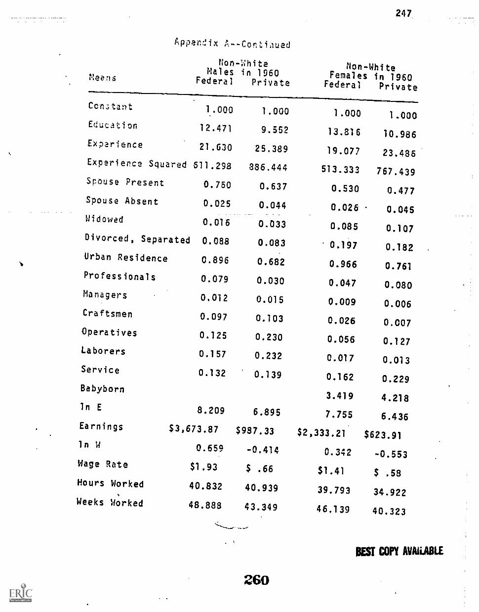
Means

Apperix A--Con tiaued

Non-WhiteMales in 1960

Federal Private

Ccn;tant 1..000 1.000

Educ,ation 12.471 9.552

Experience 21.630 25.389

Experience Squared 511.298 886.444

Spouse Present 0.760 0.637

Spouse Absent 0.025 0.044

Widowed 0.016 0.033

Divorced, Separated 0.088 0.083

Urban Residence 0.896 0.682

Professionals 0.07.9 0.030

Managers 0.012 0.015

Craftsmen 0.097 0.103

Operatives 0.125 0.230

Laborers 0.157 0.232

Service 0.132 0.139

Babyborn

in E 8.209 6.895

Earnings $3,673.87 $987.33

ln W 0.659 -0.414

Wage Rate $1.93 $ .66

Hours Workedti

40.832 40.939

Weeks Worked 48.888 43.349

260

247

Non-WhiteFemales in 1960

Federal Private

1.000 1.000

13.816 10.986

19.077 23.486

513.333 767.439

0.530 0.477

0.026 0.045

0.085 0.107

0.197 0.182

0.966 0.761

0.047 0.080

0.009 0.006

0.026 0.007

0.056 0.127

0.017 0.013

0.162 0.229

3.419 4.218

7.755 6.436

$2,333.21 $623.91

0.342 -0.553

$1.41 $ .58

39.793 34.922

46,139 40.323

DEW COPY AVAILABLE

,r

2=18

Api.);:ndix

Whicesin 1970 ('ic)

M2ans Fecaral Private

ton-Whitesin 1970 NC)

Federal Private

1.000 1.000 1.000 1.0nEd.:ct cn 15.344 13.149 13.616 11.251

E4 '"rienCe 20.7)5 21.591 13.745 22.S73

Ex?el'ience Squa red 607.614 693.702 537.020 785.471

QA.Av 0.351 0.357 0.468 0.442

Spouse Present 0.725 0.717 0.592 0.557

Spouse Absent 0.018 0.017 0.025 0.031

Widowed 0.029 0.040 0.042 0.065

Divorced, Separated 0.051 0.065 0.122 0.132

Urban Residence 0.832 0.650 0.929 0.736

Professionals 0.358 0.133 0.127 0.043

Managers 0.126 0.101 0.029 0.020

Craftsmen 0.085 0.170 0.86 0.108

Operatives 0.025 0.173 0.073 0.259

Laborers 0.010 0.035 0.059 0.103

Service 0.023 0.072 0.136 0.196

Disability 0.053 0.066 0.059 0.075

in E 8.965 7.745 8.408 7.399

Earnings $7,824.38 $2,309.99 $4,482.79 $1,634.35

In W 1.431 0.350 0.947 0.125

Wage Rage $4.18 $1.42 $2.58 $1.33

Hours Worked 40.795 41.135 40.071 38.146

Weeks Worked 48.5e----45.715 47.251 44.439

zsi

BEST COPY AVAILABLE

249

Appendix A-Continued

Malesin 1970 (WC)

Neans Federal Private

Femalesin 1970 (WC)

Federal Private

Const nt 1.000 1.000 1.000 1.000Education 15.111 12.679 14.511 12.896Experience 21.595 22.486 13.063 20.883Experience Squared 529.282 740.191 523.176 677.935Race 0.230 0.184 0.328 0,235Spouse Present 0.801 0.751 0.509 0.576Spouse Absent 0.017 0.017 0.024 0.024Widowed 0.014 0.018 0.062 0.091Divorced, Separated 0. A.2 0.055 0.134 0.119Urban Residence 0.841 0.642 0.886 0.708Professionals 0.376 0.125 0.186 0.098Managers 0.133 0.115 0.047 0.035Craftsmen 0.134 0.243 0.007 0.019Operatives 0.053 0.202 0.014 0.173Laborers 0.035 0.075 0.003 0.012Service 0.057 0.060 0.056 0.159Babyborn

1.317 1.780Disability 0.066 0.076 0.036 0.054in E 9.093 7.929 8.367 7.263Earnings $8,892.82 $2,776.65 $4,302.71$1,426.53in W 1.510 0.409 0.966 0.135Wage Rate $4.53 $1.51 $2.63 $1.15Hours Worked 41.714 43.451 38.803 35.907Weeks Worked 49.347 47.294 46.582 42.485

262

_

BEST COPY AVAILABLE

Means

Appendix A--Continued

White Malesin 1970 (UC)

Federal Private

250

White Femalesin 1970 (WC)

Federal Private

Constant 1.000 1.000

,Education 15.633 13.091

Experience 21.623 22.250

Experience Squared 622.379 723.538

-'e , Spouse Present 0.832 0.780

Spouse Absent 0.013 0.014

Widowed 0.011 0.015

Divorced, Separated 0.034 0.044

0.818 0.625

0.447 0.144

0.163 0.135

Craftsmen 0.129 0.257

Operatives 0.035 0.180

Laborers 0.014 0.051

Service 0.034 0.040

Babyborn

Disability 0.054 0.077

in E 9.242 7.977

Earnings $10,321.66 $2,913.18

ln W 1.640 0.435

Wage Rate $5.16 $1.55

Hours Worked 41.902 44.181

Weeks Worked 49.63.5 47.490

Urban Residence

Professionals

Managers

263

1.000 1.000

14.709 13.248

19.265 20.457

580.292 655.910

0.528 0.608

0.027 0.021

0.062 0.084

0.112 0.103

0.859 0.693

0.223 0.114

0.057 0.042

0.004 0.021

0.007 0.162

0.001 0.010

0.017 -0.128

1.116 1.619

0.033 0.047

8.452 7.345

$4,684.43$1,548.43.

1.046 0.204

$2.85 $1.23

38.748 36.023

46.883 42.657

BEST COPY AVAILABLE

251

Appendix A--Continued

Non-White Malesin 1970 (WC)

?e tns Federal Private

Non-White Femalesin 1970 (C)

Federal Private

Constant 1.000 1.000 1.000 1 000

Educaticn 13.183 10.852 14.107 11.754

Experience 21.503 23.533 15.616 22.666

Experience Squared 552.341 813.997 405.153 749.450

Spouse Present 0.693 0.625 0.471 0.472,

Spouse Absent 0.031 0.031- 0.018 0.032

Widowed 0.023 0.029 0.062 0.112

Divorced, Separated 0.072 0.102 0.179 0.170

Urban Residence 0.918 0.718 0.941 0.758

Professionals 0.141 0.039 0.111 0.048

Managers 0.033 0.025 0.025 0,013

Craftsmen 0.149 0.182 0.015 0.015

Operatives 0.112 0.299 0.028 0.209

Laborers 0.104 0.178 0.007 0.019

Service 0.134 0.146 0.138 0.258

Babyborn 1.729 2.302

Disability 0.072 0.076 0.044 0.075

In E 8.596 7.717 8.194 6.997

Earnings $5,409.98 $2,246.21 $3,519.17$1,093.35

ln W 1.075 0.295 0.802 -0.089

Wage Rate $2.93 $1.34 $2.23 $ .92

Hours Worked 41.088 40.218 38.916 35.530

Weeks Worked 48:*84--- 46.426 45.964 41.930

?64REST COPY AVAILABLE

252

Sharon Patricia Smith194S Dorn November 5 in Jersey City, New Jersey.'066 Graduated from Scotch Plains-Fanliood High

School, Scotch Plains, New Jersey.1955-70 Attended Rutgers University, Ne;lar%, New Jersey;

1.,:a,jored in Economics.1970 A.B., Rutgers University.1970-74 Graduate ti or!: in Economics, Rutgers University,

New Erunswick, New Jersey.1970-73 National Defense Education Act. Title IV Fellow-ship.1972 Note: "A Note on Nunicipal Phillips Curves,"by V. Kerry Smith and Sharon P. Smith, Annalsof Regional Science, VI (June 1972), pp. /q7:3.1972 N.A. in Economcs, Rutgers University.1973 Instructor of Elementary Econometric Methods,

Rutgers College, spring semester.1973-74 U. S. Department of Labor, Manpower Administra-tion, Doctoral Dissertation Grant.1974 Ph.D. in Economics.

BEST COPY AVAILABLE