ARTICLE IN PRESS

0022-2313/$ - se

doi:10.1016/j.jlu

�CorrespondE-mail addr

Journal of Luminescence 126 (2007) 263–272

www.elsevier.com/locate/jlumin

Luminescence decays with underlying distributions: General propertiesand analysis with mathematical functions

Mario N. Berberan-Santosa,�, Bernard Valeurb,c

aCentro de Quımica-Fısica Molecular, Instituto Superior Tecnico, 1049-001 Lisboa, PortugalbLaboratoire de Chimie Generale, CNAM, 292 Rue Saint-Martin, 75141 Paris Cedex 03, FrancecLaboratoire PPSM, ENS-Cachan, 61 Avenue du President Wilson, 94235 Cachan Cedex, France

Received 8 April 2006; received in revised form 3 July 2006; accepted 11 July 2006

Available online 30 August 2006

Abstract

In this work, an analysis of the general properties of the luminescence decay law is carried out. The conditions that a luminescence

decay law must satisfy in order to correspond to a probability density function of rate constants are established. From an analysis of the

general form of the luminescence decay law, it is concluded that the decay must be either exponential or sub-exponential for all times, in

order to be represented by a distribution of rate constants H(k). Sub-exponentiality is nevertheless not a sufficient condition. Only decays

that are completely monotonic have a probability density function of rate constants. The construction of the decay function from

cumulant and moment expansions is studied, as well as the corresponding calculation of H(k) from a cumulant expansion. The

asymptotic behavior of the decay laws is considered in detail, and the relation between this behavior and the form of H(k) for small k is

explored. Several generalizations of the exponential decay function, namely the Kohlrausch, Becquerel, Mittag-Leffler and Heaviside

decay functions, as well as the Weibull and truncated Gaussian rate constant distributions are discussed.

r 2006 Elsevier B.V. All rights reserved.

PACS: 33.50.–j; 78.55.–m

Keywords: Luminescence decay law; Distribution of lifetimes; Stretched exponential decay; Kohlrausch decay; Becquerel decay; Truncated Gaussian

distribution

1. Introduction

Time-resolved luminescence techniques are widely usedin various fields for time scales ranging from picosecondsto hours, i.e., spanning 15 orders of magnitude. The dataare usually analyzed with a sum of discrete exponentials,but there are many cases where a continuous distributionof decay times best describes the observed phenomena:luminophores incorporated in micelles, cyclodextrins, rigidsolutions, inorganic solids, sol–gel matrices, proteins,vesicles or membranes, biological tissues, luminophoresadsorbed on surfaces, or linked to surfaces, quenching ofluminophores in micellar solutions, energy transfer inassemblies of like or unlike fluorophores, etc.

e front matter r 2006 Elsevier B.V. All rights reserved.

min.2006.07.004

ing author. Tel.:+351 218419254; fax: +351 218464455.

ess: berberan@ist.utl.pt (M.N. Berberan-Santos).

In the most general case, a luminescence decay can bewritten in the following form:

IðtÞ ¼

Z 10

HðkÞ e�kt dk, (1)

with Ið0Þ ¼ 1. This relation is always valid because H(k) isthe inverse Laplace transform of IðtÞ. The function HðkÞ,also called the eigenvalue spectrum (of a suitable kineticmatrix), is normalized, as Ið0Þ ¼ 1 implies thatR10

HðkÞdk ¼ 1. In most situations (e.g. in the absence ofa rise-time), the function HðkÞ is non-negative for all k40,and HðkÞ can be regarded as a distribution of rateconstants (strictly, a probability density function, PDF).The designation ‘decay law’ is usually taken as a synonymfor ‘luminescence time evolution’, thus encompassing thecases where the intensity initially increases with time, asobserved for intermolecular excimer emission, and the non-

ARTICLE IN PRESSM.N. Berberan-Santos, B. Valeur / Journal of Luminescence 126 (2007) 263–272264

monotonic intensity decreases displaying quantum beats.In the present work, however, we will consider only strictosensu (monotonic) decays.

Recovery of the distribution HðkÞ from experimentaldata is very difficult because this is an ill-conditionedproblem [1]. HðkÞ can in principle be recovered from theexperimental luminescence decay by three approaches: (i)data analysis with a theoretical model for HðkÞ that may besupported by Monte-Carlo simulations; (ii) data analysisby methods that do not require an a priori form for thePDF of rate constants; and (iii) data analysis with a definitemathematical function corresponding to the PDF thatcontains adjustable parameters. The present work isdevoted to the third approach. In such an approach, amathematical function that is expected to best describe thedistribution of rate constants is used. The choice is verywide, but some specific empirical functions with acontinuous distribution of rate constants enjoy specialpopularity, such as the stretched exponential, or the decayfunctions resulting from the Lorentzian and the GaussianPDFs. In the first two papers of this series, we specificallydiscussed the stretched exponential (or Kohlrausch) func-tion [2],

IðtÞ ¼ exp �ðt=t0Þb� �, (2)

and the less-known compressed hyperbola (or Becquerel)function [3],

IðtÞ ¼1

1þ ð1� bÞ t=t0� �ð1=1�bÞ , (3)

where 0obp1, and t0 is a parameter with the dimensionsof time. Both functions conveniently reduce to anexponential function for b ¼ 1.

In this work, an analysis of the general properties of theluminescence decay law is carried out. In Section 2, thenature of the luminescence decay law and of the PDF ofrate constants is discussed. The conditions that a lumines-cence decay law must satisfy in order to correspond to aPDF of rate constants are examined in Section 3. Theconstruction of the decay function from cumulant andmoment expansions is next studied in Section 4, and thecorresponding calculation of the PDF from a cumulantexpansion is discussed in Section 5. The asymptoticbehavior of the decay law is considered in detail in Section6, and the relation between this behavior and the form ofHðkÞ for small k explored. Several generalizations of theexponential function are examined in Section 7. The finaldiscussion and main conclusions are presented in Section 8.

2. Nature and limitations of the luminescence decay law and

of the distribution of rate constants

2.1. Luminescence decay law

What is named a decay law IðtÞ can be, in somecircumstances (single species initially excited), related to a

probability of emission between t and tþ dt, PðtÞ, which isa more fundamental quantity,

PðtÞ ¼ �dI

dt. (4)

In this case it is assumed that I(t) corresponds to anexperiment where all photons emitted by the system understudy (or a fixed fraction of these) are collected. PðtÞ is theprobability of emission of the photon between t and tþ dt,given that it was emitted (hence no quantum yieldcorrection is necessary). With this generality, PðtÞ impliesan integration over emission wavelengths, and informationconcerning internal dynamics in the system may be lost.The probability of emission PðtÞ can be written as

PðtÞ ¼

Z 10

HðkÞPkðtÞdk, (5)

i.e., as a weighted distribution of emission probabilities forexponential decays, given by

PkðtÞ ¼ k�kte . (6)

More frequently, the emission is recorded for a narrowwavelength range, and results from a sum of weightedcontributions of several emitting species. The decay law isthen a technical quantity, whose normalization at t ¼ 0 isperformed for convenience. The decay law can in principlebe related to a detailed model describing the luminescencemechanism and respective dynamics, but remains avaluable formal description of the time evolution of theluminescence even in the absence of such a model.Another important aspect relates to the preparation of

the emissive state. It is assumed here that this state isinstantaneously generated, e.g. by light absorption (photo-luminescence). In fact, a transition to an upper vibrationalor electronic excited state is followed by electronic and/orvibrational relaxation, processes that may take up to a fewpicoseconds. For these short time scales, not consideredhere, the inclusion of a rise time in the decay law is clearlyessential.In the following, it will also be assumed that sponta-

neous emission is the dominant radiative decay path, i.e.,that emission is incoherent.

2.2. Distribution of rate constants

Turning now our attention to HðkÞ, the integration limitsin Eq. (1) deserve consideration. It has been argued that apositive cut-off value kmin must be imposed, in order toavoid a finite number of molecules with a physicallyunacceptable decay rate equal to zero [4]. The argument ishowever incorrect, as this happens only if HðkÞ containsd(k); otherwise HðkÞ can even tend to infinity when k-0,while still having I(t)-0 when t-N, as will be discussedin Section 6. It may nevertheless be objected that in certaincases the decay rate cannot be lower than a certainradiative decay rate. For well-defined molecular species thisis in principle correct, but even in this case the effect of

ARTICLE IN PRESSM.N. Berberan-Santos, B. Valeur / Journal of Luminescence 126 (2007) 263–272 265

such a cut-off can be statistically and/or experimentallynegligible, given a certain time window. Furthermore, adistribution of rate constants H(k) is in most casesintroduced to take into account additional decay processes,and the intrinsic unimolecular decay (that includes theradiative decay) appears as a multiplicative exponential [2].

An upper integration limit kmax is in general physicallyjustified (there are no infinitely fast relaxation processes),but again it can be statistically irrelevant and mathemati-cally inconvenient: for instance, in a study of fluorescenceanisotropy decays in heptachromophoric systems under-going excitation energy hopping [5,6], a distribution of rateconstants with a hyperbolic decay toward infinity wassuccessfully used, while a maximum rate constant had beenidentified and computed [6]; nevertheless, this upper limitwas located well into the tail of the distribution, whosecontribution to the overall decay was negligible.

3. Conditions that a decay law must satisfy in order to have

a distribution of rate constants

3.1. Sufficient condition for I(t)

If H(k) is a PDF, then

ð�1ÞnI ðnÞðtÞ40 ðn ¼ 0; 1; 2; . . .Þ, (7)

where I ðnÞðtÞ is the nth derivative of IðtÞ. Eq. (7) defines IðtÞ

as a completely monotonic function [7]. This follows directlyfrom Eq. (1), as

I ðnÞðtÞ ¼ ð�1ÞnZ 10

kn HðkÞ e�kt dk, (8)

since H(k)X0, the integral is positive for all t. Thecondition that all moments hkn

i ¼ ð�1ÞnI ðnÞð0Þ must bepositive is a special case of Eq. (7) for t ¼ 0.

3.2. Necessary conditions for w(t)

If the decay is written as

IðtÞ ¼ exp �

Z t

0

wðuÞdu

� �, (9)

where w(t) is a time-dependent rate coefficient, then

wðtÞ ¼ �d ln IðtÞ

dt¼ �

1

IðtÞ

d IðtÞ

dt, (10)

or

wðtÞ ¼

R10 k HðkÞe�kt dkR10 HðkÞ e�kt dk

¼

Z 10

k Jðk; tÞdk, (11)

where

Jðk; tÞ ¼HðkÞ e�ktR1

0 HðkÞ e�kt dk(12)

is a ‘‘renormalized’’ distribution of rate constants (valid forall times). This time-dependent PDF will play a central role

in the remaining development. Note that Eq. (11) allowsthe calculation of w(t) from H(k).One has from Eq. (11) that

dnw

dtn¼

Z 10

kqnJðk; tÞ

qtndk (13)

We now proceed to obtain the form of w(n)(t) explicitly.

3.2.1. First derivative of w(t)

It follows from Eq. (12) that

qJðk; tÞ

qt¼ wðtÞ � k½ � Jðk; tÞ, (14)

hence, using Eqs. (13) and (14)

dw

dt¼

Z 10

k Jðk; tÞdk

� �2

�

Z 10

k2 Jðk; tÞdk

" #, (15)

or

dw

dt¼M1ðtÞ

2�M2ðtÞ ¼ �C2ðtÞ, (16)

where the Mi(t) are the raw moments of J(k, t),

MiðtÞ ¼

Z 10

ki Jðk; tÞdk, (17)

and Ci(t) its cumulants. The first cumulants of a PDF are[8]

C1 ¼M1,

C2 ¼M2 �M21,

C3 ¼ 2M31 � 3M1M2 þM3,

C4 ¼ �6M41 þ 12M2

1M2 � 3M22 � 4M1M3 þM4. ð18Þ

From Eq. (16) we see that w0ðtÞ is the symmetrical of thevariance of Jðk; tÞ, which is a non-negative quantity. It isthus concluded that the decay must be either exponentialðw0ðtÞ ¼ 0Þ or sub-exponential ðw0ðtÞo0Þ for all times, ifHðkÞ is to be a PDF. This also follows from anexamination of Eq. (12), and its effect on Eq. (11), sinceEq. (12) implies that in general the function Jðk; tÞ isprogressively ‘‘compressed’’ to the left, as t increases. IfHðkÞ ¼ dðk � k0Þ, no shape change in Jðk; tÞ occurs, wðtÞ isa non-zero constant, and the decay is exponential for alltimes. If HðkÞ is a non-delta distribution, but is equal tozero below some positive value of k, k0, the ‘‘compression’’process is effective and ultimately yields a delta function,Jðk;1Þ ¼ dðk � k0Þ, wðtÞ attains a non-zero constant value,and the decay becomes essentially exponential for suffi-ciently long times. If k0 ¼ 0 (with both Hð0Þ ¼ 0 and withHð0Þ40), then wðtÞ will approach zero for long times, andthe decay goes to zero according to a slower-than-exponential function. A more detailed discussion will bepresented in Section 6.It is also to be noted that the conditions expressed by Eq.

(7) can be rewritten as MnðtÞ40, i.e., all moments of Jðk; tÞmust be positive.

ARTICLE IN PRESSM.N. Berberan-Santos, B. Valeur / Journal of Luminescence 126 (2007) 263–272266

3.2.2. Higher derivatives of w(t)

From Eqs. (14) and (17) it follows that

dMi

dt¼M1Mi �Miþ1 ði ¼ 2; 3; . . .Þ. (19)

Using this identity, it is easy to compute the higherderivatives of wðtÞ, starting from Eq. (16),

d2w

dt2¼

d

dtðM2

1 �M2Þ ¼ 2M31 � 3M1M2 þM3, (20)

d3w

dt3¼

d

dtð2M3

1 � 3M1M2 þM3Þ

¼ 6M41 � 12M2

1M2 þ 4M1M3 �M4, ð21Þ

etc. Comparison with Eqs. (18) leads to the compact forms:

dnw

dtn¼ �

dn�1C1

dtn�1¼ ð�1ÞnCnþ1ðtÞ. (22)

Constraints on wðtÞ also follow from these equalities. Forinstance, C3ðtÞ should be negative for a so-called negativeasymmetric distribution (i.e. a left asymmetric distribution)Jðk; tÞ, as must happen to any sub-exponential decay forsufficiently long times.

Incidentally, Eq. (22) provides an easy (but sequential)way of obtaining the explicit form of a cumulant of anyorder.

4. Construction of the decay from cumulant and moment

expansions

Eq. (22) implies that a Maclaurin expansion of wðtÞ is

wðtÞ ¼ C1ð0Þ � C2ð0Þtþ C3ð0Þt2

2!� . . . , (23)

where the cumulants of Jðk; tÞ at time zero are also thecumulants of HðkÞ. Insertion of this equation into Eq. (9)gives

IðtÞ ¼ exp �C1ð0Þtþ C2ð0Þt2

2!� C3ð0Þ

t3

3!þ . . .

� �, (24)

that allows to reconstruct the decay IðtÞ from thecumulants of HðkÞ. An analogous equation is used forthe analysis of dynamic light-scattering data, in order torecover the distribution of particle sizes from the auto-correlation function [9,10].

The interesting aspect is that with Eq. (22) we cangeneralize Eq. (24), by using a Taylor series expansionaround any time t0:

IðtÞ ¼ exp �C1ðt0Þ t� t0ð Þ þ C2ðt0Þðt� t0Þ

2

2!

�

�C3ðt0Þðt� t0Þ

3

3!þ . . .

�, ð25Þ

where the cumulants now refer to Jðk; tÞ.

Similarly, the moment expansion:

IðtÞ ¼ 1�M1ð0ÞtþM2ð0Þt2

2!�M3ð0Þ

t3

3!þ . . . (26)

can be generalized to give

IðtÞ ¼ ðt0Þ 1�M1ðt0Þðt� t0Þ þM2ðt0Þðt� t0Þ

2

2!

�

�M3ðt0Þðt� t0Þ

3

3!þ . . .

�. ð27Þ

5. Calculation of H(k) from the cumulants

The probability density function H(k) can be formallywritten in terms of the respective cumulants, by means ofthe analytical inversion formula for Laplace transforms[11,12]:

HðkÞ ¼2

p

Z 10

Re½IðioÞ� cosðkoÞdo. (28)

Using Eq. (24), Eq. (28) becomes

HðkÞ ¼2

p

Z 10

e�o2

2!C2þo4

4!C4�:::::

� cos C1o� C3o3

3!þ :::

� �cosðkoÞ do. ð29Þ

Eq. (29) allows—at least formally—the calculation of HðkÞ

from wðtÞ. There are in fact two problems with its practicaluse: (i) with the exception of the delta and Gaussiandistributions, all PDFs have an infinite number of non-zerocumulants (Marcinkiewicz theorem [13]) and (ii) thecumulant series that appear in Eq. (29) usually have afinite radius of convergence [12].We now compute the cumulants for the stretched

exponential [2] and compressed hyperbola [3] decay laws.In the first case, we consider only a modified form [2]:

IðtÞ ¼ exp 1� 1þt

t0

� �b" #

. (30)

The respective cumulants are obtained from a Maclaurinexpansion of ln IðtÞ,

ln IðtÞ ¼ 1� 1þt

t0

� �b

¼ �bt

t0

� ��

1

2!bðb� 1Þ

t

t0

� �2

�1

3!bðb� 1Þðb� 2Þ

t

t0

� �3

� . . . , ð31Þ

hence,

Cnð0Þ ¼ð�1Þnþ1

tn0

bðb� 1Þ . . . ðb� nþ 1Þ. (32)

ARTICLE IN PRESSM.N. Berberan-Santos, B. Valeur / Journal of Luminescence 126 (2007) 263–272 267

For the compressed hyperbola decay law,

ln IðtÞ ¼1

b� 1ln 1þ 1� bð Þ

t

t0

� �� �

¼1

b� 11� bð Þ

t

t0

� ��

1

21� bð Þ

t

t0

� �� �2(

þ1

31� bð Þ

t

t0

� �� �3� ::::

), ð33Þ

hence,

Cnð0Þ ¼ðn� 1Þ!

tn0

ð1� bÞn�1. (34)

In both cases, the cumulants are always positive andincrease indefinitely with n, after eventually passingthrough a minimum.

Consider the truncated Gaussian (i.e., for kX0 only)PDF [12]:

HðkÞ ¼

ffiffiffiffiffiffiffiffi2

ps2

rexp �1=2 k � m=s

2h i1þ erf m=

ffiffiffi2p

s . (35)

It has the following associated decay law:

IðtÞ ¼erfc s2t� m=

ffiffiffi2p

s erfc �m

ffiffiffi2p

s exp �mtþ

1

2s2t2

� �(36)

and has an infinite number of cumulants. Its first cumulant(the mean) is

hki ¼ mþ

ffiffiffi2

p

rs

e�1=2 m=sð Þ2

erfc �m=ffiffiffi2p

s . (37)

For t5m=s2, IðtÞ coincides with that of a normaldistribution, and the first two cumulants of this PDFsuffice to describe its behavior,

IðtÞ ’ exp �mtþ1

2s2t2

� �. (38)

This equation has been used for the analysis of dynamiclight-scattering data, in order to recover the distribution ofparticle sizes from the autocorrelation function [9,10], andapplies to some luminescence decays for not too long times.The full Gaussian PDF (or a mixture of Gaussian PDFs)[14–16] and a Gaussian PDF truncated [4] at k040 havebeen used to describe fluorescence decays. The truncatedGaussian reduces to the full Gaussian distribution for largem=s ratios.

Up to now, it was implicitly assumed that all momentsand cumulants were finite. For some PDFs, however, notall moments and cumulants are finite. For the Levy PDFs,for instance, only M1 can be (but is not always) finite. Thisis precisely the case of the (unmodified) stretched expo-nential decay. The form of Jðk; tÞ, Eq. (12), ensures that,even then, all moments will be finite for t40. Thesingularity is therefore limited to t ¼ 0. This is one of thereasons why the expansions Eqs. (25) and (27) are ofinterest.

6. Decay law asymptotics

We will obtain relatively general equations relating theasymptotic behavior of the decay law I(t) (i.e., for large t)to that of the PDF H(k) for small k. From Eq. (1), it isindeed obvious that the behavior of H(k) for small k willdefine the shape of the decay I(t) for long times.According to the discussion presented in Section 3, it is

convenient to consider separately the cases where the PDFof rate constants is non-zero at k ¼ 0, or rises from zeroimmediately afterwards, from the case where H(k)40 onlyfor k4k0, with k0 positive. The special case of partialrelaxation will also be treated in this section.Consideration of the asymptotic behavior of a decay

function is important, not only because it defines the longtime form, that may or may not be experimentallyaccessible, but also because

R10 IðtÞdt is often computed

from the decay law in order to obtain a quantityproportional to the steady-state intensity. This calculationmay be meaningless if the major contribution to the aboveintegral corresponds to a time window not experimentallyobserved, or if the integral diverges.

6.1. H(0+)40

6.1.1. H(k) admits a Maclaurin series expansion

In this case,

HðkÞ ¼ Hð0Þ þ k H 0ð0Þ þk2

2!H 00ð0Þ þ . . . , (39)

and substitution in Eq. (1) gives immediately,

IðtÞ ¼Hð0Þ

tþ

H 0ð0Þ

t2þ

H 00ð0Þ

t3þ . . . . (40)

The effective power dependence with t for long times(asymptotic behavior) will be determined by the order ofthe first non-zero term of the Maclaurin series.

6.1.2. H(k) is not analytic at the origin

A (so-called Tauberian) theorem in probability theory [7]that covers a broad range of cases (including the previousone), is the following, reformulated for our purposes.If the cumulative distribution function:

UðkÞ ¼

Z k

0

HðuÞdu (41)

has the asymptotic form:

UðkÞ�kpLðkÞ (42)

in the limit k- 0, with p40, where L(k) is a slowly varying

function, i.e., a function that obeys

LðakÞ

LðkÞ! 1, (43)

also when k- 0, for any constant a, then the decay law willhave the following asymptotic behavior:

IðtÞ�Uð1=tÞ (44)

in the limit t-N.

ARTICLE IN PRESSM.N. Berberan-Santos, B. Valeur / Journal of Luminescence 126 (2007) 263–272268

In most situations of physical interest, the last equationcan be replaced by

IðtÞ�1

tH

1

t

� �. (45)

Note that PDFs that near the origin vary according tonegative power laws (0opo1) and therefore rise toinfinity, are included.

On the other hand,R10 IðtÞdt diverges for pp1.

6.2. H(0+) ¼ 0

In this case, H(k)40 only for k4k0, with k0 positive,and the above results are not valid without modification.But they can be applied by shifting the distribution H(k) tothe left, placing it next to the origin, and then moving itback to the right by k0, in order to restore the originalposition. The distribution next to the origin, to which theabove results apply, is

H0ðkÞ ¼ Hðk þ k0Þ (46)

and the decay law becomes, after restoring the initialposition,

IðtÞ ¼ I0ðtÞ expð�k0tÞ, (47)

where I0(t) corresponds to the shifted distribution H0(k).The asymptotic behavior will be that of H0(k) times anexponential, hence dominated by the exponential. Notethat in this case

R10 IðtÞdt is not divergent even if I0(t) has

an asymptotic dependence with pp1, owing to theexponential damping factor.

Table 1

Relation between the type of luminescence decay function, the luminescence d

Exponential

Sub-exponential Asymptotically exponential

Slower-than-exponential Maclaurin or Puiseux valid

Maclaurin or Puiseux invali

Table 2

Examples of PDF of rate constants and respective luminescence decay functio

Exponential

Sub-exponential Asymptotically exponential

Slower-than-exponential Maclaurin or Puiseux v

Maclaurin or Puiseux in

6.3. H(k) contains d(k)

When there is a fraction a of luminophores not decayingby the mechanism under consideration (e.g. intermolecularresonance energy transfer to nearby acceptors), H(k) isgiven by

HðkÞ ¼ a dðkÞ þ ð1� aÞHþðkÞ, (48)

where H+(k) is the density function of positive rateconstants. Insertion of this PDF in the decay lawexpression gives

IðtÞ ¼ aþ ð1� aÞIþðtÞ, (49)

where I+(t) is the decay law corresponding to H+(k). In thiscase, the asymptotic form is a numerical constant, andR10 IðtÞdt diverges, unless (as must happen in physicallyacceptable cases) the overall decay contains a multiplicativeexponential.

6.4. Cases left out

There are some cases that are not covered by the resultsof the Tauberian theorem presented, namely PDFs H(k) ofrapid variation near the origin, like exp(�1/k). This is thecase of the stretched exponential PDF. For b ¼ 1

2, for

instance [2],

H1=2ðkÞ ¼1

2ffiffiffiffipp

k3=2exp �

1

4k

� �. (50)

Only for very small b, when [2,17],

HðkÞ ’b

k1þb exp �1

kb

� �’

be k

exp �1

2b ln kð Þ

2

� �, (51)

ecay asymptotic behavior, and the PDF of rate constants

H(k) w(t) I(t)

dðk � k0Þ k0 e�k0t

0ðkok0Þ �k0 �e�k0t

H(0) ¼ 0 akpðp40; small kÞ �t�1 �t�ð1þpÞ

H(0)40 H0 þ . . . ðH040Þ �t�1 �t�1

d H(0) ¼ 0 One-sided Levy �t�ð1�bÞ e�atb

H(0) ¼N ak�pð14p40; small kÞ �t�1 �t�ð1�pÞ

ns

H(k) I(t)

Delta Exponential

Rectangular e�k0tð1� e�DktÞ=ðDktÞ

alid H(0) ¼ 0 Gamma Becquerel

H(0)40 Exponential Hyperbolic

valid H(0) ¼ 0 One-sided Levy Stretched exponential

H(0) ¼N Weibull (ao1) Weibull

ARTICLE IN PRESS

0.00.0 0.2 0.4 0.6 0.8 1.0 1.2

1.0

2.0

3.0

4.0

kτ0

H(k)/

τ 0

0.35

0.45 0.55 0.650.75

0.85

0.90

0.95

Fig. 1. Distribution of rate constants (probability density function) for the

stretched exponential (Kohlrausch) decay law. The number next to each

curve is the respective b.

M.N. Berberan-Santos, B. Valeur / Journal of Luminescence 126 (2007) 263–272 269

does the application of the Tauberian theorem yield thecorrect result, IðtÞ ¼ expð�tbÞ.

The several asymptotic cases discussed above aresummarized in Table 1, and corresponding specificexamples are given in Table 2.

7. Selected decay functions

As discussed above, PDFs that reduce to the deltafunction for some value(s) of the parameter(s), such asthose of the stretched exponential and compressedhyperbola decay functions, and the Lorentzian and theGaussian PDFs, are of special interest and/or of commonuse. All these functions may be considered as general-izations of the exponential function. There are otherinteresting generalizations of the exponential function thatwe will discuss below, see also Table 2.

There are at least two possible ways to generalize theexponential function. One is to select H(k) PDFs that areknown to reduce to the delta function d(k�k0) for somevalue(s) of the parameter(s). This is obviously the case forthe Lorentzian and the Gaussian functions. Such aprocedure automatically ensures that H(k) will be a PDF.The other way is to work with the exponential decay lawitself, changing it to a functional form that still reduces tothe exponential for some value(s) of the parameter(s). Thisis the case in particular of the stretched exponentialfunction. In these cases, one must compute H(k), to checkthat it is still a PDF. A slightly different approach is to takethe series expansion of the exponential decay function andto modify it. Distribution functions obtained in this waydeserve attention. But it is of worth to first briefly recall themain characteristics of the stretched exponential (orKohlrausch) function and of the compressed hyperbola(or Becquerel) function (for more details, the reader isreferred to our recent papers [1,2]).

7.1. Stretched exponential (or Kohlrausch) function

The stretched exponential decay function is given by Eq.(2). This decay law was first used in luminescence byWerner [18]. In studies of the relaxation of complexsystems, the Kohlrausch function is frequently used as apurely empirical decay law, although there are theoreticalarguments to justify its common occurrence. In the field ofmolecular luminescence, Eq. (2) has firm grounds onseveral models of luminescence quenching, namely diffu-sion-controlled contact quenching, where b ¼ 1

2, and

diffusionless resonance energy transfer by the dipole-dipolemechanism, with b ¼ 1

6; 13and 1

2for one-, two- and three-

dimensional systems, respectively. Other rational values ofb are obtained for different multipole interactions, e.g.b ¼ 3

8; 310, for the dipole–quadrupole and quadrupole–qua-

drupole mechanisms in three-dimensions. In Huber’sapproximation, energy transport as measured by fluores-cence anisotropy shows the same time-dependence as directenergy transfer, and is characterized by the same values of

b. Resonance energy transfer between donor and acceptorchromophores attached to a polymer chain has been widelyused as a tool for studying polymer structure anddynamics. Theory shows that the kinetics of donorluminescence quenching and the kinetics of depolarizationof luminescence in polymer chains exhibit a Kohlrauschtime dependence, where the parameter b of Eq. (2) dependson the mechanism of transfer, the type of chromophoreattachment (to the ends of the polymer chain or randomlydistributed along the chain), and on the model of polymerchain considered (Gaussian or self-avoiding chain) [2]. TheKohlrausch function is also found to apply to someluminescence decays of disordered and ordered inorganicsolids, and of semiconductor nanoclusters [2,19].The Kohlrausch decay law is convenient as a fitting

function, even in the absence of a model, given that itallows gauging in simple way deviations to the ‘‘canonical’’single exponential behavior through the parameter b.Stretched exponentials were used for instance to analyzethe fluorescence decay of fluorophores incorporated in asol–gel matrix and of fluorophores covalently bound tosilica and alumina surfaces [2]. The Kohlrausch decayfunction was also recently used in the analysis ofsingle-molecule fluorescence, quantum dot luminescence,and in the fluorescence lifetime imaging of biologicaltissues [2].The corresponding distribution of rate constants, shown

in Fig. 1, is the one-sided Levy PDF that can be writtenas [2]

HbðkÞ ¼t0p

Z 10

exp �ub cosbp2

� �� �

� cos ub sinbp2

� �� kt0u

� �du. ð52Þ

The stretched exponential luminescence decay function hasan undesirable short-time behavior (infinite initial rate,faster-than-exponential decay for short times). For this

ARTICLE IN PRESSM.N. Berberan-Santos, B. Valeur / Journal of Luminescence 126 (2007) 263–272270

reason, a modified form was proposed [2],

IðtÞ ¼ exp ab � aþt

t0

� �b" #

, (53)

where a is a non-negative dimensionless parameter.

7.2. Compressed hyperbola (or Becquerel) function

The compressed hyperbola or Becquerel decay functionis given by Eq. (3). The Becquerel function, as defined here,is a quite flexible decay function, although its less directrelation to the exponential decay has limited its use up tonow mainly to the luminescence of phosphors [3]. Never-theless, there are some recent applications in fluorescence[3]. For instance, Wlodarczyk and Kierdaszuk [20] showedthat it provides good fits for fluorescence decays thatslightly depart from the exponential behavior, implying arelatively narrow distribution of decay times around amean value. The corresponding distribution of rateconstants, shown in Fig. 2, is the gamma PDF [3],

HbðkÞ ¼t0

ð1� bÞ G 1=1� b t0 k

1� b

� �ðb=1�bÞ

� exp �t0k

1� b

� �. ð54Þ

As discussed previously [2], two possible approaches to fitluminescence decay laws with a discrete sum of terms arethe use of exponentials and hyperbolae as base functions.Since the Becquerel decay law interpolates between thesetwo extreme cases, it seems reasonable to assume that asum of a few Becquerel functions, appropriately weighted,will be a powerful fitting function for complex decays [3].

0

1

2

3

4

0 0.5 1 1.5 2kτ0

H(k

)/τ 0

0.4 0.7

0.95

0.99

00.85

Fig. 2. Distribution of rate constants (probability density function) for the

Becquerel decay law. The number next to each curve is the respective b.

7.3. Mittag-Leffler and Heaviside functions

We now turn our attention to the series expansion of theexponential decay function,

e�at ¼X1n¼0

ð�atÞn

n!¼X1n¼0

ð�atÞn

Gðnþ 1Þ, (55)

with the aim of generalizing it. Two simple generalizationsare Mittag-Leffler’s exponential function, or Mittag-Lefflerfunction Ea(x) [21,23],

Eað�atÞ ¼X1n¼0

ð�atÞn

Gðanþ 1Þ, (56)

and Heaviside’s exponential function, ea(x) [23],

eað�atÞ ¼X1n¼0

ð�atÞn

Gðnþ 1þ aÞ, (57)

where 0oap1 in the first case, and aX0 in the second case.For our purposes, it is convenient to define a normalized

Heaviside’s exponential function ea(x), so that ea(0) ¼ 1,

�aðxÞ ¼ Gð1þ aÞ eaðxÞ ¼ a GðaÞ eaðxÞ. (58)

The H(k) for these two decay laws are known, and areindeed PDFs. They are displayed in Figs. 3 and 4,respectively. The Mittag-Leffler PDF is (with a ¼ 1)[22,24,25],

HaðkÞ ¼ a�1 k�ð1þa�1Þ La k�a

�1� �

, (59)

where La(x) is the one-sided Levy PDF given by Eq. (52).

0

1

2

3

0 1 2k

H(k)

0.7360.9

0.95

0.99

0.1

0.5

Fig. 3. Distribution of rate constants (probability density function) for the

Mittag-Leffler decay law. The number next to each curve is the respective

a.

ARTICLE IN PRESS

0

1

2

3

4

5

0.0 0.5 1.0k

H(k

)

1

5

2

0.1

0.5

Fig. 4. Distribution of rate constants (probability density function) for the

Heaviside decay law. The number next to each curve is the respective a.

0

1

2

3

0.0 0.5 1.0k

H(k

)

1

5

2

0.1

0.5

Fig. 5. Distribution of rate constants (probability density function) for the

modified Heaviside decay law, with b ¼ 1. The number next to each curve

is the respective a.

0

2

4

6

8

10

0.4 0.6 0.8 1.0k

H(k

)

1

5

2

0.1

0.5

Fig. 6. Distribution of rate constants (probability density function) for the

modified Heaviside decay law, with b ¼ 10. The number next to each

curve is the respective a.

0

1

2

3

4

5

0 21k

H(k)

2

5

10

100

0.1

1

Fig. 7. Distribution of rate constants (probability density function) for the

Weibull decay law. The number next to each curve is the respective a.

M.N. Berberan-Santos, B. Valeur / Journal of Luminescence 126 (2007) 263–272 271

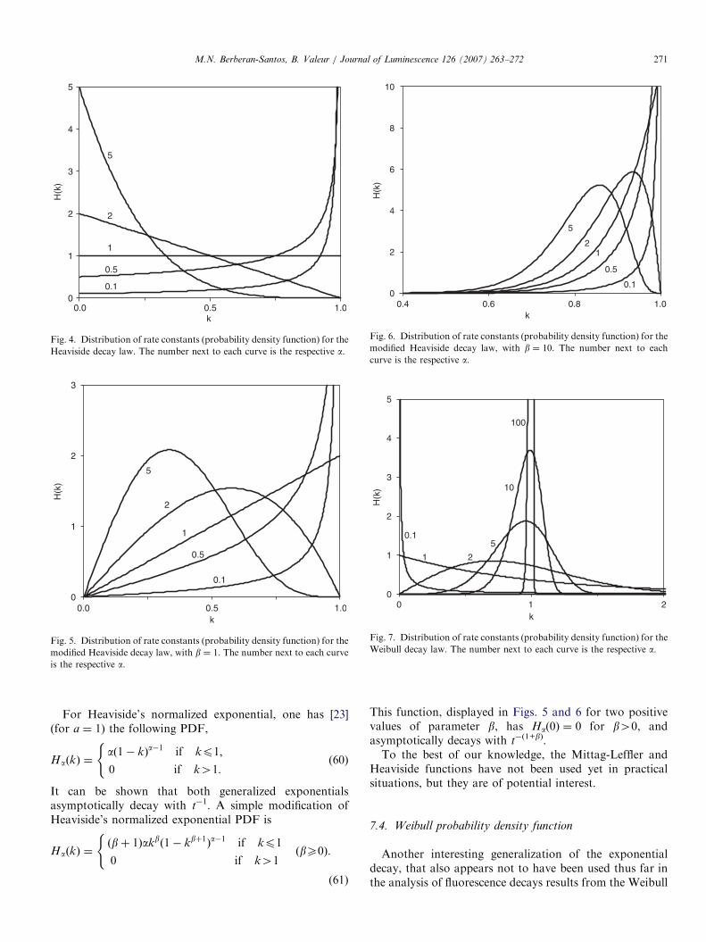
For Heaviside’s normalized exponential, one has [23](for a ¼ 1) the following PDF,

HaðkÞ ¼að1� kÞa�1 if kp1;

0 if k41:

((60)

It can be shown that both generalized exponentialsasymptotically decay with t�1. A simple modification ofHeaviside’s normalized exponential PDF is

HaðkÞ ¼ðbþ 1Þakb

ð1� kbþ1Þa�1 if kp1

0 if k41

(ðbX0Þ.

(61)

This function, displayed in Figs. 5 and 6 for two positivevalues of parameter b, has Ha(0) ¼ 0 for b40, andasymptotically decays with t�(1+b).To the best of our knowledge, the Mittag-Leffler and

Heaviside functions have not been used yet in practicalsituations, but they are of potential interest.

7.4. Weibull probability density function

Another interesting generalization of the exponentialdecay, that also appears not to have been used thus far inthe analysis of fluorescence decays results from the Weibull

ARTICLE IN PRESSM.N. Berberan-Santos, B. Valeur / Journal of Luminescence 126 (2007) 263–272272

PDF [7,26],

Ha;bðkÞ ¼ab

k

b

� �a�1

exp �k

b

� �a� �, (62)

where a40. This PDF is displayed in Fig. 7 for a reducedvariable k/b. The mean of Ha(k) is bG(1+a�1). For a ¼ 1the distribution is exponential, for a ¼ 2 it reduces to theRayleigh distribution, and in the limit a-N the deltadistribution d(k�1) is recovered. The asymptotic behaviorof the Weibull decay law illustrates several of the casesdiscussed in Section 6 (see Tables 1 and 2). The asymptoticdecay is I(t)�t�a, and HaðkÞ� ka�1. For ao1, Ha(0) isinfinite. For a ¼ 1, Ha(0)40. In both cases

R10 IðtÞdt

diverges. Finally, for a41, Ha(0) ¼ 0, andR10 IðtÞdt is

finite.

7.5. Truncated Gaussian probability density function

This PDF was already introduced in Section 5. Writingt0 ¼ 1=m and the coefficient of variation a ¼ s=m ¼ st0,Eq. (38) becomes

IðtÞ ¼ exp �t

t0þ

1

2a2

t

t0

� �2" #

. (63)

This simple decay function, not widely known, is adequatefor t=t0o10 (i.e., the full time range of interest) if ao0:25.The asymptotic form of the truncated Gaussian is, on theother hand,

IðtÞ ¼

ffiffiffi2

p

rexp �1=2a2

a erfc �1=ffiffiffi2p

a t0

t, (64)

and goes as t�1, as could be expected from the results ofSection 6. Note that this asymptotic behavior switches toan exponential one if the Gaussian PDF is truncated abovezero, however slightly.

8. Discussion and conclusions

In this work, an analysis of the general properties of theluminescence decay law was carried out. The conditionsthat a luminescence decay law must satisfy in order tocorrespond to a probability density function of rateconstants were established. From an analysis of the generalform of the decay law, it was concluded that the decaymust be either exponential or sub-exponential for all times,if H(k) is to be a probability density function. Take forinstance the hypothetical ‘‘compressed exponential’’ decaylaw IðtÞ ¼ exp½�ððt=t0ÞÞ

2�. This decay law is super-expo-

nential, as w(t) increases monotonically with time. Its H(k)takes both positive and negative values, and is thus not aPDF. Sub-exponentiality is nevertheless not a sufficientcondition. For the hypothetical sub-exponential decay law1=½1þ ðt=t0Þ þ ðt=t0Þ

2=2�, the function H(k) can be ob-tained in closed form and is 2t0 exp �kt0ð Þ sin kt0ð Þ, takingboth positive and negative values. Only decays that are

completely monotonic have a PDF of rate constants. Anew PDF of rate constants, Jðk; tÞ, emerged as the centralPDF of the problem. Cumulant and moment expansions ofthe decay can be obtained from this PDF, that is shown tobe well-behaved and with all moments finite for t40, evenwhen HðkÞ is of the Levy type. The asymptotic behavior ofthe decay laws was considered in detail, and the relationbetween this behavior and the form of HðkÞ for small k wasexplored. Finally, several generalizations of the exponentialdecay function, namely the Kohlrausch, Becquerel, Mittag-Leffler and Heaviside decay functions, as well as theWeibull and truncated Gaussian rate constant distributionswere analyzed in detail.

Acknowledgment

This work was supported by Fundac- ao para a Ciencia eTecnologia (FCT, Portugal) within project POCI/QUI/58535/2004.

References

[1] B. Mollay, H. F. Kauffmann, in: R. Richert, A. Blumen (Eds.),

Disorder Effects on Relaxational Processes, Springer, Berlin, 1994, p.

509.

[2] M.N. Berberan-Santos, E.N. Bodunov, B. Valeur, Chem. Phys. 315

(2005) 171.

[3] M.N. Berberan-Santos, E.N. Bodunov, B. Valeur, Chem. Phys. 317

(2005) 57.

[4] G. Verbeek, A. Vaes, M. Van der Auweraer, F.C. De Schryver, C.

Geelen, D. Terrell, S. De Meutter, Macromolecules 26 (1993) 472.

[5] M.N. Berberan-Santos, P. Choppinet, A. Fedorov, L. Jullien, B.

Valeur, J. Am. Chem. Soc. 121 (1999) 2526.

[6] M.N. Berberan-Santos, P. Choppinet, A. Fedorov, L. Jullien, B.

Valeur, J. Am. Chem. Soc. 122 (2000) 11876.

[7] W. Feller, An Introduction to Probability Theory and its Applica-

tions, vol. 2, Wiley, New York, 1970.

[8] A. Stuart, J.K. Ord, sixth ed, Kendall’s Advanced Theory of

Statistics, vol. 1, Hodder Arnold, London, 1994.

[9] D.E. Koppel, J. Chem. Phys. 57 (1972) 4814.

[10] B.J. Frisken, Appl. Opt. 40 (2001) 4087.

[11] M.N. Berberan-Santos, J. Math. Chem. 38 (2005) 165.

[12] M.N. Berberan-Santos, J. Math. Chem. (2006), in press, doi:10.1007/

s10910-006-9069-x.

[13] C.W. Gardiner, Handbook of Stochastic Methods, second ed,

Springer, Berlin, 1985.

[14] D.R. James, Y.-S. Liu, P. de Mayo, W.R. Ware, Chem. Phys. Lett.

120 (1985) 460.

[15] D.R. James, W.R. Ware, Chem. Phys. Lett. 126 (1986) 7.

[16] J.R. Alcala, E. Gratton, F.G. Prendergast, Biophys. J. 51 (1987) 587.

[17] E.W. Montroll, J.T. Bendler, J. Stat. Phys. 34 (1984) 129.

[18] A. Werner, Ann. Phys. 24 (1907) 164.

[19] J.E. Martin, L.E. Shea-Rohwer, J. Lumin. (2006), in press,

doi:10.1016/j.lumin.2005.12.043.

[20] J. Wlodarczyk, B. Kierdaszuk, Biophys. J. 85 (2003) 589.

[21] G.M. Mittag-Leffler, C.R. Acad. Sci. Paris (Ser. II) 136 (1903) 70.

[22] M.N. Berberan-Santos, J. Math. Chem. 38 (2005) 629.

[23] A. Wintner, J. Math. Pure Appl. IX Ser. 38 (1959) 165.

[24] H. Pollard, Bull. Am. Math. Soc. 54 (1948) 1115.

[25] M.N. Berberan-Santos, J. Math. Chem. 38 (2005) 265.

[26] W. Weibull, J. Appl. Mech. 18 (1951) 293.