LTCM Redux? Hedge Fund Treasury Trading and

Funding Fragility during the COVID-19 Crisis*

Mathias S. Kruttli, Phillip J. Monin, Lubomir Petrasek, Sumudu W. Watugala�

June 2021

Abstract

During the March 2020 U.S. Treasury (UST) market turmoil, the average UST tradinghedge fund saw significant losses and reductions in UST exposures, despite unchangedbilateral repo volumes and haircuts. Analyzing fund-creditor borrowing data revealsthe more regulated dealers provided disproportionately more funding during the cri-sis. Despite low contemporaneous outflows, hedge funds boosted cash, and reducedportfolio size and illiquidity. Following Fed intervention calming markets, fund returnsrecovered quickly, but their UST activity did not. Overall, reduced hedge fund USTliquidity provision was driven by fund-specific liquidity management constrained bymargin pressure and expected redemptions, rather than creditor regulatory constraints.

JEL classification: G11, G23, G24, G01.

Keywords: Hedge funds, Treasury markets, relative value, arbitrage, liquidity, redemptionrisk, creditor constraints.

*We thank Diana Hancock, Sebastian Infante, Juha Joenvaara, Andrew Karolyi, Dan Li, FrancisLongstaff, Marco Macchiavelli, Patrick McCabe, Justin Murfin, Maureen O’Hara, Tarun Ramadorai, MinWei, Joshua Younger, and seminar participants at Cornell University, the Federal Reserve Board, the Finan-cial Stability Oversight Council, and the Securities Exchange Commission for useful discussions. The viewsstated herein are those of the authors and are not necessarily the views of the Federal Reserve Board or theFederal Reserve System.

�Kruttli: The Board of Governors of the Federal Reserve System. Email: mathias.s.kruttli@frb.gov.Monin: The Board of Governors of the Federal Reserve System. Email: phillip.monin@frb.gov. Petrasek:The Board of Governors of the Federal Reserve System. Email: lubomir.petrasek@frb.gov. Watugala:Cornell University. Email: sumudu@cornell.edu.

1 Introduction

The role of hedge funds in U.S. Treasury (UST) markets is thought to have increased in

importance since the global financial crisis (GFC) as bank-affiliated broker-dealers ceded

some of their traditional activities in UST market arbitrage and liquidity provision to non-

bank financial institutions. While UST securities play a vital role in the global financial

system, hedge funds’ impact on UST market functioning is not well understood because

they are less regulated than traditional broker-dealers and provide few disclosures. Further,

compared to other asset managers, hedge funds employ substantial leverage coupled with

investment strategies that are less liquid. They also have distinct funding structures, the

resilience of which is key to understanding how they operate during periods of financial

market turmoil. Following the unprecedented volatility in Treasury markets in March 2020

in the wake of the sudden brakes on economic activity imposed by the COVID-19 pandemic,

there has been much debate in industry, policy, and academic circles about the role hedge

funds played during this crisis and, more broadly, the financial stability implications of hedge

fund UST market activities.1,2

In this paper, comprehensive regulatory data and our empirical approach give, for the first

time, a granular view of how hedge funds face a systematic crisis in terms of their liquidity

and leverage management.3 Of particular importance for understanding the March 2020

shock, we analyze changes to hedge fund UST long/short notional and duration exposures,

bilateral repo borrowing, collateral and funding terms, cash buffers, portfolio liquidity, and

leverage. Further, we harness hedge fund-creditor level counterparty credit exposure data to

investigate the role of creditor constraints and funding supply shocks. The COVID-19 crisis

provides a unique opportunity to examine the strengths and vulnerabilities of the current

model of UST market intermediation in which hedge funds play an important role. We ask

two main questions to probe deeper into the factors that may have constrained hedge fund

arbitrage activity and liquidity provision. (i) What was the impact of external debt and

1See, for example, How a Little Known Trade Upended the U.S. Treasury Market (https://www.bloomberg.com/news/articles/2020-03-17/treasury-futures-domino-that-helped-drive-fed-s-5-trillion-repo);Revisiting the Ides of March, Parts I-III (https://www.cfr.org/blog/revisiting-ides-march-part-i-thousand-year-flood); Di Maggio (2020); Duffie (2020); He, Nagel, andSong (2020); and Schrimpf, Shin, and Sushko (2020).

2“The Fed did unbelievable things this time.” —Janet Yellen, July 2020, https://www.nytimes.com/2020/07/23/business/economy/hedge-fund-bailout-dodd-frank.html. Industry insiders and observers drewparallels between the 1998 Long-Term Capital Management (LTCM) episode and the impact of the March2020 shock on fixed income hedge funds. There are indeed some parallels, but as this paper shows, alsoimportant distinctions between the two episodes.

3Our novel dataset is primarily constructed using Form PF, which large U.S. hedge funds are requiredto file starting in 2012, following its adoption as part of the Dodd-Frank Wall Street Reform and ConsumerProtection Act of 2010. https://www.sec.gov/about/forms/formpf.pdf.

1

equity financing constraints? Specifically, we analyze whether the regulatory constraints of

creditors—particularly those of dealers that are subject to enhanced regulations as part of

global systemically important banks (G-SIBs)—hindered the ability of hedge funds to obtain

funding, thus exacerbating the liquidity shock in UST. On hedge fund equity, we examine

investor outflows during the market turmoil and the differential impact of hedge fund share

restrictions that place limits on redemptions. (ii) What was the impact of hedge fund-specific

liquidity management considerations? These involve both meeting unexpected, immediate

liquidity drains such as margin calls and reacting to anticipated future liquidity needs in a

time of aggregate uncertainty. These questions are of great importance for financial stability

and UST market functioning.

In the period leading up to the March 2020 COVID-19 shock, we find that hedge fund

UST exposures doubled from early 2018 to February 2020, reaching $1.4 trillion and $0.9

trillion in long and short notional exposure, respectively, primarily driven by relative value

arbitrage funds, which held close to $600 billion in long UST exposure in February 2020.

Long UST securities positions are primarily financed via repurchase agreements (repo bor-

rowing), while short UST securities positions are primarily sourced through reverse repo

(repo lending). Since 2018Q2 there has been a significant increase in repo borrowing, in-

dicating a marked increase in long UST securities holdings. Until that point, aggregate

hedge fund repo borrowing and lending exposures were generally matched, as one would ob-

serve with UST arbitrage strategies such as trading on-the-run/off-the-run spreads or yield

spreads.4 The divergence between hedge fund repo borrowing and lending is likely driven

by a significant increase in recent years in UST cash-futures basis trading.5 As with many

other spread trades hedge funds engage in, these trades are primarily “short liquidity,” and

perform worst in states of the world in which liquidity is scarce. We describe the cash flows

and exposures involved with both types of fixed income arbitrage strategies in Appendix

section B.1.

In March 2020—as investors around the world engaged in a flight to cash and liquidity

amid an unprecedented, sudden economic shutdown—there was a sharp divergence in the

4LTCM—a common case study on liquidity risk and the risks inherent in “arbitrage” trading—engagedin such bond spread trading until a systematic shock caused massive losses that threatened systemic stabilityand led to a Fed-arranged broker takeover of the fund’s positions (Edward (1999); Jorion (2000); Lowenstein(2000); Duarte, Longstaff, and Yu (2007)).

5In this trading strategy, a hedge fund goes long the (cheapest-to-deliver) Treasury security and goes shortthe corresponding Treasury futures contract. The futures leg does not require reverse repo, so the divergencebetween hedge fund repo borrowing and lending is consistent with reports of a significant increase in recentyears in UST cash-futures basis trading. Typically, this is a low volatility, low yield convergence strategythat is operationally intensive and requires leverage to be worthwhile. The trade is profitable as long as theactual cost of carrying the cash position (the “repo rate” or the cost of repo borrowing for the hedge fund)is below the implied cost of carry on the futures (the “implied repo rate”).

2

UST spreads that hedge funds generally bet will converge. We find the average hedge fund

with UST holdings in our sample experienced a monthly return of around -7%. By the end

of March 2020, the average hedge fund with UST exposures significantly reduced their gross

exposures and arbitrage activity in UST markets, decreasing notional exposures on both the

long and short sides by around 20%. Despite the fall in UST exposures, borrowing levels

and collateral rates on bilateral repurchase agreements—the primary source of financing for

hedge fund UST holdings and cash-futures basis trades—remained relatively unchanged in

March 2020 for the average hedge fund. Although significant negative returns depleting their

equity, hedge funds held leverage ratios largely unchanged, indicating that they scaled back

their exposures proportionately to the declines in asset valuations. At the end of March,

funds had 20% higher cash holdings and smaller, more liquid portfolios. In aggregate, we do

not find evidence that UST hedge funds provided liquidity during the market dislocation. We

specifically analyze the impact of creditor constraints, redemption risk, and margin pressure

on hedge fund liquidity provision and consumption during this crisis.

There has been much debate about the impact of post-GFC regulations on UST and other

fixed income market liquidity and the impact of dealer constraints on hedge fund arbitrage

activity.6 Hedge fund arbitrage trading implicitly depends on dealer balance sheets because

it requires funding, which is typically provided by dealers. Dealer balance sheet and risk

management constraints can therefore potentially limit the provision of arbitrage by hedge

funds, particularly in times of stress. We do not find evidence that the sell-off in UST was

driven by a credit supply shock stemming from the regulatory constraints of dealer banks.

Using data on borrowing amounts available at the hedge fund-creditor level, we examine

the differences between funding provided by creditors constrained and unconstrained by

enhanced regulations using a within hedge fund-time methodology.7 We find that G-SIBs—

which face enhanced regulations and are often taken as the dealer set more constrained by

regulations—provided over 11-13% higher repo funding compared to other dealers during

the crisis to hedge funds. This finding is robust to controlling for time-invariant and time-

varying hedge fund characteristics using hedge fund-time fixed effects, and relationship-

specific factors using hedge fund-creditor fixed effects. Contrary to the regulatory constraints

hypothesis, the largest dealers that are subject to enhanced prudential regulations provided

disproportionately better access to funding to their hedge fund counterparties during this

period of market stress.

6See, for example Boyarchenko, Eisenbach, Gupta, Shachar, and Van Tassel (2020); He, Nagel, and Song(2020); Schrimpf, Shin, and Sushko (2020).

7Kruttli, Monin, and Watugala (2020) use Form PF data and a similar empirical strategy, adapted fromKhwaja and Mian (2008), to examine the impact of idiosyncratic prime broker / creditor distress on hedgefunds.

3

The boost to precautionary liquidity holdings and the step back from UST market activity

were less pronounced for funds with lower redemption risk due to longer (stricter) share

restrictions including lock-ups, gates, and redemption notice periods, which can dampen

the pace and volatility of redemptions in times of stress. Funds with less stringent share

restrictions likely expect higher contemporaneous and anticipated future outflows and hence,

anticipate greater need for ready liquidity to meet redemptions. Indeed, we find that hedge

funds with higher redemption risk (shorter share restrictions) increased their precautionary

liquidity holdings to a greater extent during the March 2020 market stress episode. Such

funds traded out of and closed out more portfolio positions, and in particular, cut their UST

exposures by more. In our sample, the share restrictions of the median hedge fund are such

that it would have at least 30 days’ notice before the first 1% of investor capital (net asset

value) is redeemed. In a short duration market dislocation like in March 2020, long share

restrictions employed by hedge funds were likely stabilizing, allowing funds to hold onto more

of their convergence trades without engaging in fire sales to meet large investor outflows.8

Compared to other UST trading funds during the March 2020 turmoil, the subset of UST

hedge funds that predominantly engaged in the cash-futures basis trade faced greater margin

pressure stemming from their short futures positions, requiring immediate liquidity infusions

or position liquidations. We find that basis trading funds decreased their UST exposures and

repo borrowing to a greater extent amid worsening terms, including shorter maturities and

higher haircuts compared to other UST hedge funds. Basis traders’ cash positions including

posted margin were substantially higher. Also, basis trading funds reduced the number of

open positions in their portfolios more than other hedge funds. These findings are consistent

with basis traders facing greater immediate liquidity needs and funding pressures.

Overall, we find that the reduction in hedge funds’ UST exposures is consistent with

a flight to cash and precautionary hoarding of liquidity amid significant losses, increased

uncertainty, and anticipated redemptions.

Researchers have discussed how asset managers such as mutual funds face a crisis that

impacts liquidity conditions, but little is known about the liquidity management behavior

8There are contrasting predictions for hedge funds in the literature. Ben-David, Franzoni, and Moussawi(2012)—in an examination of 13-F filings of long equity holdings during the GFC, a relatively long-lastingcrisis—find that equity hedge funds were likely forced to delever to meet redemptions because hedge fundinvestors subject to share restrictions react quicker to adverse performance than mutual fund investors. Ourresults on share restrictions are consistent with the model in Hombert and Thesmar (2014), which showsthat contractual impediments to investor withdrawals can be stabilizing for a fund.

4

of the hedge fund sector in stressed conditions.9,10 In the midst of a systemic stress period,

asset managers face a trade-off: selling the more liquid assets first likely has a smaller price

impact and mitigates current realized losses. However, such an approach to liquidity man-

agement makes the remaining portfolio less liquid, increasing the risk of fire sales should the

crisis persist or worsen, with adverse implications for fund performance and financial market

functioning. On the other hand, selling illiquid assets earlier, while potentially incurring

greater current realized losses, improves the liquidity condition of the fund in the future,

when the crisis might deepen.11 The pecking order of liquidity risk management by hedge

fund managers therefore has important implications for financial stability. We find evidence

of the latter approach being used by the hedge funds in our sample—funds with UST expo-

sure significantly increased both their cash holdings and the liquidity of their portfolios by

reducing the size of their portfolios and disproportionately scaling down relatively illiquid

assets. These shifts are likely primarily driven by the consideration of future redemptions.

Although the period of extreme market stress lasted less than three weeks before the Fed’s

unprecedented intervention12—too short a period for hedge fund investors to redeem their

shares en masse given the long lockups of the typical fund—we find that it resulted in a

precautionary flight to liquidity, likely motivated in part by concerns about future investor

redemptions.

Certain characteristics of hedge funds may increase their financial fragility. For instance,

compared to other asset managers such as mutual funds or money market funds, which are

subject to regulatory constraints regarding portfolio liquidity and leverage, hedge funds tend

to hold more illiquid portfolios, use greater leverage, and have a more concentrated investor

9For example, several papers examine the liquidity management of mutual funds through stress periods.Chernenko and Sunderam (2016) find that mutual funds hold substantial cash positions to manage potentialredemptions. Morris, Shim, and Shin (2017) find that cash hoarding by mutual funds is the rule rather thanthe exception, and that funds with more illiquid portfolios hold greater levels of precautionary cash. Chen,Goldstein, and Jiang (2010); Goldstein, Jiang, and Ng (2017) find that mutual fund fragility is impacted byportfolio liquidity.

10Jorion (2000) draws together press reports for a case study of the LTCM meltdown, describing the likelyrisk management choices at that hedge fund and how its liquidity and leverage likely evolved as the fundapproached catastrophic failure. We find several contrasting findings in the March 2020 crisis for the liquiditymanagement of the sample of UST hedge funds, who may have learned lessons from LTCM and other hedgefund meltdowns.

11There are contrasting findings on this trade-off in the asset management literature. Jiang, Li, and Wang(2019) find that the behavior of mutual funds during tranquil and stress periods are different: in tranquilperiods, redemptions are met by selling liquid holdings, while mutual funds proportionally scale down liquidand illiquid holdings during periods of high aggregate uncertainty to preserve portfolio liquidity. In contrast,Ma, Xiao, and Zeng (2020) posit that in the March 2020 shock, corporate bond mutual funds sold moreliquid bonds to meet investor redemptions.

12See the timeline of the market stress episode described in, among many others, Haddad, Moreira, andMuir (2020); He, Nagel, and Song (2020).

5

base.13 Hedge funds can attempt to manage these structural risks by imposing stricter share

restrictions, holding greater precautionary cash, or increasing the maturity of their financ-

ing. We show that hedge funds are quick to significantly increase their unencumbered cash

holdings and portfolio liquidity when faced with severe market stress, but this precautionary

flight to cash was less for funds with longer share restrictions. Longer share restrictions were

particularly useful for UST trading hedge funds during the sell-off in March 2020, allowing

them to avoid fire sales and hold onto more of their convergence trades, thereby bolstering

both fund and market stability. Our findings illustrate a crisis episode during which the

liquidity management and funding structure of hedge funds likely were more stabilizing than

that of mutual funds and money market funds.14 Our analyses yield insights into the efficacy

of various methods hedge funds deploy to overcome frictions that impose limits to arbitrage

activity.

We find that hedge fund UST trading exposures did not revert to their previous levels

after the market turmoil subsided, even as the average UST fund saw returns jump back in

April and remain positive over the subsequent months. Notably, in the post-shock period,

UST funds faced greater investor outflows, but met those redemptions in a market stabilized

via Federal Reserve interventions. Our findings indicate that the quick intervention of the

Federal Reserve to stabilize Treasury markets likely prevented a deleveraging spiral in which

hedge funds would have further sold off positions in a declining market, realizing more losses

and further depleting their equity.

2 Related literature

Several other papers have examined hedge fund activity during financial crises and periods

of market stress. Examples include papers on equity hedge funds and their impact during

the tech bubble (Brunnermeier and Nagel, 2004) and various episodes of the global finan-

cial crisis, including but not limited to Khandani and Lo (2011) on the quant fund crisis in

August 2007, Aragon and Strahan (2012) on the Lehman bankruptcy in September 2008,

and Ben-David, Franzoni, and Moussawi (2012) on equity-focused hedge funds and investor

redemptions. Boyson, Stahel, and Stulz (2010) find there is contagion in hedge fund returns

during adverse market shocks from 1990-2008. Compared to these crisis episodes, the March

13See, for example, Aragon (2007); Agarwal, Daniel, and Naik (2009); Kruttli, Monin, and Watugala(2019). Aragon, Ergun, Getmansky, and Girardi (2017) find that, in general, hedge funds likely attempt tomatch the liquidity of their portfolios against the liquidity of their financing and investor capital. Barth andMonin (2020) find that hedge funds employ more leverage when holding assets with lower fundamental risk.

14See, for example, Ma, Xiao, and Zeng (2020) on mutual fund fire sales in bond markets and Li, Li,Macchiavelli, and Zhou (2020) on the potentially destabilizing effects of the contingent liquidity restrictionsof prime money market funds.

6

2020 shock is unprecedented, particularly in the speed at which extreme moves occurred

and in its impact on otherwise safe and liquid markets such as the UST market. By analyz-

ing the activity of hedge funds during this episode in U.S. Treasury markets and bilateral

repo/reverse repo funding markets, this paper sheds light on how the characteristics and

funding structures of hedge funds impact their trading in vital financial markets.

Due to data limitations, most prior papers focus on the trading of equity-oriented hedge

funds for which snapshots of information exist based on regulatory filings of their equity

positions on Form 13F and self-reported returns. We contribute to the literature by studying

Treasury market activities of hedge funds before and during the March 2020 shock, which

was unprecedented in its impact on the Treasury market. We show that hedge funds were

quick to significantly increase their unencumbered cash holdings and portfolio liquidity when

faced with severe market stress, actions which would have likely reduced the liquidity and

financial stability risks associated with hedge fund fire sales had market functioning not

quickly returned to normal in the wake of Federal Reserve interventions and asset purchases

later in March.

Our paper contributes to the literature on limits to arbitrage and liquidity management in

asset management in general and hedge funds in particular. Arbitrageurs are constrained by

internal limits, such as those based on leverage requirements and value at risk (VaR) (Shleifer

and Vishny (1997); Gromb and Vayanos (2010); Hombert and Thesmar (2014)). There is a

literature that links the balance sheet constraints of intermediaries like broker-dealers and in-

vestment banks to asset prices (e.g., He and Krishnamurthy (2013)) and show an association

between the balance sheet of such intermediaries and market liquidity.15 Kruttli, Patton,

and Ramadorai (2015) show that constraints at hedge funds also impact asset prices given

their intermediary role as arbitrageurs that provide liquidity to markets. In the post-GFC

period, hedge funds are thought to have increased their role as quintessential arbitrageurs in

the Treasury and other fixed income markets as more regulated financial institutions such as

bank-affiliated dealers faced increasing regulatory- and non-regulatory constraints on their

arbitrage activities (Boyarchenko, Eisenbach, Gupta, Shachar, and Van Tassel, 2020; He,

Nagel, and Song, 2020). Hedge fund arbitrage implicitly depends on broker-dealer balance

sheets since it requires funding, which is typically provided by dealers and prime brokers.16

Dealer balance sheet and risk management constraints can therefore limit the provision of

15E.g., Adrian and Shin (2010); Acharya, Lochstoer, and Ramadorai (2013).16Ang, Gorovyy, and Van Inwegen (2011) find that the leverage of hedge funds is counter-cyclical to the

aggregate leverage of other financial intermediaries. Kruttli, Monin, and Watugala (2020) show that a primebroker who is liquidity constrained due to an idiosyncratic shock can be quick to significantly cut credit toits hedge fund clients, with significant consequences to the funding of connected funds who are only able toimperfectly substitute such creditor relationships quickly, even during tranquil market conditions.

7

arbitrage by hedge funds, particularly in times of stress. We contribute to the literatures on

limits to arbitrage and intermediary asset pricing by studying the behavior of hedge fund

arbitrageurs under extreme market stress and analyzing the impact on their trading and liq-

uidity provision from constraints to the external financing provided by dealers and investors,

as well as internal risk management considerations.

Our paper significantly advances our understanding of hedge funds that engage in fixed

income arbitrage in particular. Other work in this area have been limited by data or scope.

Primarily using contemporaneous press reports, Edward (1999); Jorion (2000) give a view

into the meltdown of LTCM, which famously engaged in several fixed income arbitrage

strategies using substantial leverage and potentially misspecified risk management metrics.

Jorion (2000) points out that many of these different “arbitrage” strategies implicitly involve

taking on correlated exposures on liquidity risk, volatility risk, and default risk, all of which

tend to spike during periods of market stress. Duarte, Longstaff, and Yu (2007) replicate

a range of common fixed income arbitrage strategies to analyze their potential returns and

risks, and find that the risk-adjusted performance of these strategies is not simply “picking

up nickels in front of a steamroller.” Barth and Kahn (2021) use a model and aggregate

sector-level data to analyze the mechanics of the cash-futures basis trade. Our paper differs

in that we use granular data to conduct fund-level and fund-creditor-level analyses to gain

a comprehensive view on the trading and funding of all major hedge funds that are active

in UST markets, of which basis traders are a subset. Bilateral repo data at the hedge fund-

creditor level enable us to analyze how dealer regulatory constraints impacted hedge fund

borrowing. We use fund-level data to understand how heterogeneity across UST trading

hedge funds are related to cross-sectional differences in hedge fund trading and liquidity

management.

Finally, we contribute to a growing literature examining aspects of the COVID-19 shock

in fixed income markets. These include papers examining the investor outflows and fire

sales of corporate bond mutual funds (see, for example, Falato, Goldstein, and Hortacsu

(2020); Ma, Xiao, and Zeng (2020) and money market funds (Li, Li, Macchiavelli, and Zhou,

2020). Duffie (2020); Schrimpf, Shin, and Sushko (2020) describe the stress to UST markets

and present suggestions for market reform. He, Nagel, and Song (2020) present a theoretical

model that shows how regulatory constraints of dealer banks could potentially exacerbate the

destabilizing effects of a UST supply shock. There are several papers focused on corporate

bond markets during this episode including Haddad, Moreira, and Muir (2020); Kargar,

Lester, Lindsay, Liu, Weill, and Zuniga (2020); O’Hara and Zhou (2020).

8

3 Data and summary statistics

The hedge fund data used in this paper are primarily from Form PF. In our analysis, we

use the set of qualifying hedge funds (QHFs) that file this form quarterly,17 and follow the

data cleaning and validation procedure outlined in Kruttli, Monin, and Watugala (2020).

Table 1 presents summary statistics for the key variables of interest. Our sample consists

of the set of hedge funds with gross UST exposure of at least $1 million on average during

Q4 2019.18 A summary reference of variable definitions is included as the last table in this

paper in Table B.2.

Panel A of Table 1 reports the hedge fund characteristics. The average hedge fund has

$2.8 billion in net asset value (NAV) and a leverage ratio of 2.5. The next three variables

measure different dimensions of fund liquidity, including portfolio liquidity (PortIlliqh,t),

investor liquidity as measured by share restrictions (ShareResh,t), and the funding liquidity

measured as the weighted average maturity of a fund’s borrowing (FinDurh,t). Form PF

asks for the percentage of a hedge fund’s assets, excluding cash, that can be liquidated within

particular time horizons (within ≤1, 2-7, 8-30, 31-90, 91-180, 181-365, and >365 days) using

a given periods’ market conditions. We compute the weighted average liquidation time to

obtain the measure PortIlliqh,t. The average PortIlliqh,t is 33.1 days in our sample and the

median is 7.2 days. ShareResh,t is a measure of the expected weighted average time it would

take for a hedge fund’s investors to withdraw the fund’s equity. This variable quantifies the

restrictions faced by a fund’s investors, such as lock-up, redemption, and redemption notice

periods. The average ShareResh,t is 125.8 days. The weighted average time to maturity of a

fund’s borrowing is denoted FinDurh,t. On average, the financing duration is 37.1 days for

our sample of hedge funds with a median of 10.7 days. Panel A further provides summary

statistics for monthly and quarterly returns as well as quarterly flows.

Form PF data contain granular information on a hedge fund’s cash positions. The variable

FreeCashEqh,t measures unencumbered cash that is held for liquidity management purposes,

including U.S. Treasuries that are not posted as collateral. The variable Cashh,t on the other

hand only includes “pure” cash and not U.S. Treasuries. The two measures, normalized by

NAV, are on average 26.8% and 30.6%, respectively. Panel A also provides information on

the number of a hedge fund’s open positions, gross notional exposure (GNE), and portfolio

GNE. The difference between the GNE and the portfolio GNE is that portfolio GNE does

not include free cash.

We obtain data on hedge fund UST exposures from Question 30 of Form PF, which

17These quarterly filings include the intra-quarter monthly values for most key variables of interest includ-ing asset and repo exposures, returns, cash levels, portfolio size, and number of positions, etc.

18Our findings are robust to either smaller or larger cutoffs for UST exposure.

9

requires hedge funds to report the month-end values of long and short portfolio exposures in

a range of asset classes. Fixed income holdings are reported both as notional exposures and

on a risk-adjusted basis.19 Panel B of Table 1 provides summary statistics on the hedge funds’

UST exposure. The gross notional UST exposure for hedge fund h in month t, UST GNEh,t,

is on average $2.8 billion. Importantly, this measure includes exposure to UST through

derivatives and futures, as well as physical exposures. The UST GNEh,t is the sum of the

long and short UST exposure, which we observe separately and are named UST LNEh,m

and UST SNEh,m, respectively. The net UST exposure is given by the difference of the two

and named UST NNEh,m. On average, the UST NNEh,m is positive with $846.0 million,

indicating that the average long exposure is larger than the short exposure.

The term min(UST LNEh,t, UST SNEh,t) captures part of the gross UST exposure that

is long-short balanced, which we use as a proxy for the UST arbitrage activity of a fund.

The term abs(UST NNEh,t) captures the unbalanced, directional UST exposure. The two

are related to the UST GNEh,t as

UST GNEh,t =abs(UST NNEh,t) + 2 ×min(UST LNEh,t, UST SNEh,t). (1)

The duration of a hedge fund’s long and short UST exposure are provided separately,

UST LNE Drtnh,t and UST SNE Drtnh,t, with an average value of 4.6 and 6.8 years,

respectively. The duration of the net exposure, UST NNE Drtnh,t, is on average 0.8 years.

Panel C describes the borrowing data. Repo borrowing is on average $3.6 billion, and

the average repo lending is $2.7 billion. The terms for the repo borrowing and lending,

RepoBrrwTermh,t and RepoLendTermh,t, are on average 25.7 and 12.2 days, respectively.

Repo borrowing is over-collateralized, with the average ratio of total collateral to borrowing

of 118%. On average, 85% of the collateral supporting repo is securities collateral, although

cash collateral is also sometimes posted. Most of hedge fund repo is transacted bilaterally,

with only 13.7% of the repo centrally cleared.

Panel D presents data on a hedge fund’s borrowing from major creditors at the counter-

party level. The total amount of borrowing, TotalMCBorrowingh,t, is the sum of borrowing

across all major counterparties reported in Question 47 of Form PF as of the end of a given

quarter. It includes borrowing from repo as well as other sources such as margin loans. The

number of creditors from which a hedge fund borrowed as of the end of a given quarter,

NumCrdtrsPerHFh,t, is on average 4.5. The average amount borrowed from a specific

creditor is HF Ctpty Credith,p,t is $1.3 billion. In about half of the cases, a hedge fund’s

19The risk-adjustment is either based on duration, weighted average tenor, or 10-year equivalent. Wherewe use risk-adjusted exposures, we convert the reported values to the same units, as described further inAppendix section B.3.

10

creditor is also its prime broker and custodian.

4 Hedge funds and the COVID-19 Treasury market

shock

We first analyze the changes to hedge fund UST portfolios, (repo) financing, liquidity and

leverage management during the March 2020 Treasury market shock. Figures 1 to 6 give an

indication of the aggregate changes to the Treasury market activity of hedge funds. To pro-

vide a fund-level view of the changes that occurred during March 2020, while separating out

differences due to different hedge fund characteristics and fund-specific effects, we estimate

panel regressions of changes in different measures of hedge fund Treasury activities on the

March 2020 dummy variable and control variables. The baseline regressions take the form,

∆yh,t = β1Dt + γZh,t−1 + µh + εh,t, (2)

where ∆yh,t is the outcome of interest and is a change variable. Dt is 1 for March 2020 and

0 otherwise. Zh,t−1 is the set of lagged controls (LogNAV , NetRet, NetF lows, PortIlliq,

ShareRes, FinDur, and MgrStake). µh denote fund fixed effects. Standard errors are

double clustered by fund and time. The data are monthly from January 2013 to March 2020

and include all hedge funds with gross UST exposure of at least $1 million as in Q4 2019.

4.1 Changes to U.S. Treasury and repo activity

Table 2 presents regression results with dependent variables capturing different aspects of

a hedge fund’s UST exposure. Panel A analyzes changes to the notional exposure—both

gross notional exposures and long and short exposures separately—measured either in dollar

terms or as a fraction of NAV. The coefficient on March2020 is significant and negative

for all outcome variables. The first three columns show that, in March 2020, hedge funds

reduced UST exposure by 20%, on both the long and the short sides. The last three columns

show that this change is significant even when UST exposures are normalized by a fund’s

NAV. UST exposure as a fraction of NAV went down by about 8% on the long and short side.

Total (gross) UST exposure as a fraction of NAV went down by about 15% in March. These

results provide robust evidence of a significant, abnormal decline in hedge funds’ Treasury

exposures in March 2020.

Among the control variables, flows are positively related to UST exposure: the first

three columns show a positive and significant coefficient on NetF lows indicating that funds

11

adjust their portfolios in response to investor inflows and outflows. As expected, flows do

no change UST allocations as a fraction of a fund’s NAV. Most other variables are not

significantly related to Treasury exposures after controlling for fund fixed effects.

Besides changing their notional exposures, funds may have responded to the March 2020

shock by adjusting their exposure to duration risk. Table 2 Panel B analyzes changes in

the duration of hedge fund portfolios. It shows that hedge funds on average increased their

duration exposure following the March 2020 shock, with the net duration exposure going up

by 0.4 years. This finding is intriguing, in particular since the wider Treasury market sell

off is considered to have occurred predominantly at the 10-year and longer maturities (He

and Krishnamurthy (2020); He, Nagel, and Song (2020)). The increase in durations is both

statistically and economically significant, and largely driven by a decrease in the duration

on the short side of the UST portfolio. As shown in Table 1, funds are generally duration-

matched on the long and short sides, with average and median net duration exposures of

0.8 and 0.3 years, respectively. As such, an increase of over 0.4 years in duration exposure

represents a significant adjustment.

Table 2 Panel C examines the directional exposure and arbitrage activity in UST port-

folios. As discussed in section 3, min(UST LNEh,t, UST SNEh,t) captures the part of a

hedge fund’s UST portfolio that is long-short balanced. The regression in column 1 indicates

that following the March 2020 shock, hedge funds reduced their UST arbitrage portfolios by

around 25%. Column 2 shows that purely directional exposures also dropped, by close to

15%. The last two columns in the panel indicate that, as a fraction of a fund’s total UST

exposure, the long-short balanced exposure decreased, and correspondingly, the directional

exposures increased.

Having found notable declines in hedge funds’ UST exposures following the March 2020

shock, we analyze whether the declines were accompanied by a corresponding decrease in

hedge funds’ repo activity. Previously, very little was known about hedge funds’ repo activity

because it is largely conducted on a bilateral, uncleared basis, in what is considered the

most opaque segment of the repo market. Form PF data provides a unique view into hedge

funds’ bilateral repo activity and its resilience under stress. The summary statistics for

RepoBilateralh,t and RepoClearedCCPh,t in Table 1 Panel C makes clear the extent to

which hedge fund repo borrowing is predominantly bilateral and uncleared. Table 3 presents

results from analyzing hedge funds’ repo activity. The table shows the hedge funds’ repo

borrowing was surprisingly resilient during the March 2020 sell-off in Treasury markets. In

Panel A, the results in column 1 show that borrowing levels on repurchase agreements—

the primary source of financing for hedge fund long UST holdings—remained relatively

unchanged in March 2020. Since long UST trades are typically financed through repo, this

12

finding indicates that the sizeable declines in hedge funds’ UST exposures were not driven by

trading positions that were financed in repo. In other words, the declines in UST exposures

were likely driven by non-financed exposures, including derivatives exposures and those held

outright without financing.

In contrast to repo borrowing, column 2 shows that hedge fund repo lending or “reverse

repo” decreased in March 2020 by around 25% for the average fund. When trading Treasury

securities, UST short bond positions are typically sourced through reverse repo, with the

hedge fund obtaining the security as collateral from the borrower in exchange for lending

cash. A reduction in repo lending is therefore consistent with the decline in short UST

exposures shown in Table 2 Panel A, as well as with hedge funds conserving their cash

holdings during the crisis.

Columns 3 and 4 in Panel A further show that changes to repo borrowing terms (matu-

rities) in March 2020 are also consistent with hedge funds conserving liquidity during this

period of high uncertainty: the repo borrowing maturity increased, while the lending ma-

turity decreased, though to a lesser extent. Borrowing for longer periods and lending for

shorter periods mitigates rollover risk, a risk associated with not being able to roll over

financing for existing positions at favorable terms and potentially being forced to close out

of arbitrage positions before they converge or being forced into fire sales. These findings

suggest that hedge funds sought to avoid these risks through increasingly conservative repo

financing terms during the March sell-off.

Table 3 Panel B examines the collateral terms on repo financing. Surprisingly, we do

not find evidence that repo haircuts or collateral rates became significantly more onerous for

hedge funds during this stress period. In fact, the total collateral as a fraction of repo bor-

rowing, RepoTotalCollateralRepoBorrowing

, shows a statistically significant decrease of around 0.7%. However,

the fraction of CashCollateral to TotalCollateral increased by 1.5%, possibly indicating

lenders’ preference for cash and cash equivalents as collateral.20

Overall, these baseline results do not support the view that repo funding volumes and

terms became significantly tighter for hedge funds that invest in Treasuries following the

March 2020 shock. However, although the average hedge fund did not experience a funding

shock, it is possible that some lending counterparties tightened their provision of credit to

hedge funds more than others. We conduct further analysis on hedge fund repo borrowing in

section 5 using hedge fund-creditor (fund-dealer) level data, specifically focusing on whether

dealers subject to enhanced regulations passed on funding supply shocks to connected hedge

funds.

20Cash equivalents include bank deposits, certificates of deposits, and money market fund investments.

13

4.2 Performance and investor flows

Next, we examine the performance and flows of hedge funds with UST exposures. Table 4

presents results for regression specification (2) with monthly returns, quarterly returns and

flows as the dependent variable. Unsurprisingly, the coefficient on March2020 is significantly

negative for all three outcome variables. Monthly and quarterly returns show coefficients

of -6.6% and -9.9%, respectively. Given that the mean quarterly return over our sample is

2.3% with a standard deviation of 8.1%, a sector-wide return of -9.9% reflects unprecedented

losses for these hedge funds, which is also depicted in Figure 5. This indicates that during

the COVID-19 crisis in March, these hedge funds were under a significant amount of stress,

to a greater extent than at any point since Form PF reporting started in 2012. Clearly, the

current crisis unfolded more precipitously than the global financial crisis in 2007-2009, which

was characterized by relatively longer periods of a buildup of uncertainty from 2007 onward.

It is notable that the flows estimate of -1.8% for the quarter ending in March 2020,

though negative, reflects relatively mild outflows. For reference, the mean quarterly investor

flow during the 2012-2020 sample period is -0.6% with a standard deviation of 13.9%. In

contrast, other asset management firms like corporate bond mutual funds and prime money

market funds experienced much greater outflows during this period (Ma, Xiao, and Zeng,

2020; Li, Li, Macchiavelli, and Zhou, 2020). This difference in investor redemptions likely

stems from structural features unique to hedge funds, specifically, share restrictions, which

include lock-ups, restrictions on redemption frequency and redemption notice periods. The

redemption restrictions and notice periods are likely to be particularly helpful for hedge

funds when managing liquidity during short-lived systematic stress episodes. The March

2020 extreme market stress period lasted less than three weeks until the Fed’s intervention,

too brief a period for hedge fund investors to redeem their shares at a significant scale during

the stress period itself, given the share restrictions of the typical fund (see share restrictions

in Table 1, Panel A). By the end of March 2020, hedge funds may have received notices of

significant future redemptions. We consider this scenario in our examination of changes to

cash and liquidity in the next section and further analyze the implications of restrictions to

investor redemptions in section 6.

4.3 Cash, liquidity, and leverage

The final set of regressions giving a baseline overview of the March 2020 shock captures hedge

fund outcomes related to liquidity and leverage. Table 5 Panels A and B show that, by the

end of March 2020, funds held significantly higher cash and smaller, more liquid portfolios

than at the beginning of the month. The first four columns of Panel A show changes to

14

four different measures of cash holdings as the outcome variable. FreeCashEq refers to

unencumbered “cash and cash equivalents” (e.g., bank deposits, certificates of deposits,

money market fund investments, U.S. Treasury and agency securities) held for the purposes

of liquidity management (see variable definitions in Table B.2). FreeCashEq increased

by 26% in March 2020. Cash refers to cash positions (not including U.S. Treasury and

agency securities) both unencumbered or posted as collateral, which also increased in March

2020, by around 23%. Column 5 and 6 show that PortfolioGNE—the notional exposure of

securities and derivatives, excluding Cash—held by a hedge fund fell by around 22%, while

the number of open positions fell by close to 5%. Panel B shows that portfolio illiquidity

dropped by over 11% during this period, with the fraction of assets that can be liquidated

within a week increasing significantly.

These findings speak to the literature on how a hedge fund manages its liquidity during a

systematic stress period. When confronted with significant funding constraints, redemptions

and other liquidity needs, asset managers face a trade-off: selling the more liquid assets first

likely has smaller price impact and mitigates current realized losses, but increases overall

portfolio illiquidity and thus the probability of future fire sales should the crisis persist or

deepen. On the other hand, selling illiquid assets first, while potentially incurring greater

current realized losses, improves the liquidity condition of the fund and its ability to with-

stand a protracted crisis. Our findings show that hedge funds took the latter, more prudent

approach when managing liquidity during the March 2020 shock. On average, funds signif-

icantly increased both their cash holdings and the liquidity of their portfolios by reducing

the size of their portfolios and disproportionately scaling down relatively illiquid positions.

These shifts may have been in part driven by the uncertainty associated with the initial

COVID-19 shock. At the end of March, amid continued uncertainty regarding the pandemic’s

impact on financial markets and the economy, hedge funds were potentially confronted with

the prospect of high future redemptions and continued losses, increasing their focus on

preserving liquidity.

Our findings stand in contrast to the behavior of mutual funds as described by Ma, Xiao,

and Zeng (2020), who posit that in the March 2020 shock, corporate bond mutual funds sold

more liquid bonds to meet investor redemptions. Interestingly, Jorion (2000), in describing

the LTCM meltdown in 1998, asserts that the hedge fund made a “mistake” when attempting

to reduce risks by downsizing its asset portfolio because the fund got rid of its most liquid

positions, which made the fund more vulnerable to further losses when the market continue

to move against the fund’s portfolio positions.

The firm [LTCM] reportedly tried to reduce its risk profile, but made a major mistake:instead of selling off less-liquid positions, or raising fresh capital, it eliminated its

15

most liquid investments because they were less profitable. ... This made LTCM morevulnerable to subsequent margin calls. [pg. 288, Jorion (2000)]

Given the contrast between LTCM’s behavior and our findings for UST hedge funds

during March 2020, it is possible that the hedge funds in our sample studied LTCM and

other subsequent hedge fund meltdowns when planning how to manage liquidity during a

stress episode.

Finally, we analyze the changes in gross hedge fund leverage, measured as the ratio

of gross balance sheet assets (GAV ) to fund capital or net assets (NAV ). Table 5 Panel

C shows that hedge fund NAV (equity) and GAV (total gross assets) generally dropped

proportionally, by 13-14%. As such, the ratio of hedge fund GAV to NAV—Leverage—was

unchanged at the end of the market stress episode. Thus, although there is no evidence of

significant deleveraging, the results suggest that hedge funds actively managed the risk of

their portfolios in March 2020. Despite significant negative returns depleting NAV , hedge

funds held leverage ratios unchanged by scaling down their gross exposures proportionately

to their capital base.

4.4 Post COVID-19 shock period

The March 2020 shock to the UST market was unprecedented in scale, but due to the speed

and extent of Federal Reserve interventions, relatively short-lived. While UST prices and

arbitrage spreads largely recovered by April, it is unclear how quickly hedge fund activity

in this market rebounded. To examine the post-shock period, we extend our sample to

September 2020 and run regressions similar to equation (2), with additional time indicators

capturing the months (or, alternatively, quarters) following March 2020. Table A.1 in the

Appendix presents the results of these regressions.

Importantly, Table A.1 Panel A shows that investor outflows from UST hedge funds were

significantly larger in 2020Q2 and 2020Q3 than during the shock period itself. This is in

spite of the fact that returns broadly recovered from the substantial decline in March 2020

(also illustrated in the returns time series in Figure 5). The delayed outflows are likely due

to the long share restrictions that hedge funds impose on their investors, which we analyze

in greater detail in Section 6. Hedge funds met these larger investor redemptions in the

post-shock period while UST markets were stabilized via government intervention.

Broadly, the results in Table A.1 Panels B and C show that neither hedge fund UST

exposures nor repo exposures reverted back to pre-crisis (pre-March 2020) levels over the

two quarters following March 2020. Both long and short UST exposures generally contin-

ued to decrease until September 2020. While being relatively unchanged in March, repo

16

borrowing fell significantly in April and May before stabilizing in June 2020. Hedge funds

lengthened their repo borrowing maturities in the post-crisis period, and faced significantly

higher collateral ratios.

Taken together, these results indicate that Federal Reserve interventions helped to stabi-

lize UST markets even as hedge funds continued to scale down their UST market activities.

5 Dealer regulatory constraints and bilateral repo lend-

ing

We proceed next to analyze in greater detail the factors that contributed to the Treasury

sell-off in March. First, we examine the role of dealer regulatory constraints in affecting

hedge fund trading through dealers’ differential provision of funding in March 2020.

Using data on borrowing amounts available at the hedge fund-creditor level, we conduct

a granular analysis to identify the impact of creditor supply shocks on hedge fund repo

borrowing. We use a within hedge fund-time methodology to test for differences between

funding provided by creditors that are constrained and those that are not, allowing us to

compare hedge funds’ borrowing from different creditors while controlling for unobserved

time-varying hedge fund characteristics.21 The panel regressions take the form,

∆ logHF Crdtr Credith,p,t =γ1DealerConstraintp,t + γ2DealerConstraintp,t ×Dt

+ φZh,p,t−1 + µh + θt + ψp + εh,p,t, (3)

∆ logHF Crdtr Credith,p,t =γ1DealerConstraintp,t + γ2DealerConstraintp,t ×Dt

+ νh,t + ψp + εh,p,t, (4)

∆ logHF Crdtr Credith,p,t =γ1DealerConstraintp,t + γ2DealerConstraintp,t ×Dt

+ νh,t + ξh,p + εh,p,t, (5)

where Dt is 1 for March 2020, 0 otherwise. DealerConstraintp,t is a measure that captures

heterogeneity across dealers in terms of potential constraints to their intermediary role in

repo markets. Eqn. 3 includes hedge fund (µh), creditor (ψp), and time (θt) fixed effects.

Eqn. 4 includes creditor fixed effects and hedge fund-time fixed effects (νh,t). Fund-time

fixed effects control for all time invariant and time-varying fund characteristics, absorbing

fund-level borrower demand shocks, which allows for better identification of dealer-specific

supply effects. Eqn. 5 includes both fund-time and fund-creditor (ξh,p) fixed effects, with the

21This identification strategy is similar to Khwaja and Mian (2008), Kruttli, Monin, and Watugala (2020),and many others that use borrower-creditor data to isolate credit supply effects.

17

latter allowing us to control for relationship-specific factors. Standard errors are clustered at

the dealer and quarter level. Since Treasury positions are typically financed in repo, we limit

the sample for this anlysis to hedge funds with gross UST exposure of at least $1 million

that primarily borrow via repo (50% or more of their borrowing is in repo) on average during

Q4 2019. A requirement of the within fund-time analysis is that the sample includes only

hedge funds that borrow simultaneously from at least two creditors. The vast majority of

the hedge funds in our sample borrow from multiple creditors simultaneously.

The methodology is illustrated with an example hedge fund-dealer network in Figure 7.

We use a dealer’s status as a global systemically important financial institution (G-SIB) as

the DealerConstraintp,t measure.22 G-SIBs are the largest, most interconnected institu-

tions and face enhanced regulations in the post-GFC period — including the U.S. enhanced

supplementary leverage ratio based on the total size of their balance sheet and off-balance

sheet exposures — and are therefore subject to the most stringent regulatory constraints.

However, the findings reported in Table 6 are inconsistent with these constraints limiting

dealers’ funding provision during the March 2020 UST sell-off. Interestingly, G-SIBs pro-

vided disproportionately higher funding during the crisis to hedge funds engaged in repo

borrowing. Relative to other dealers, G-SIBs increased repo lending to hedge funds by 11-

13% in March 2020. These results suggest that larger, more regulated G-SIB dealers were

better able to provide stable, more resilient funding during the March 2020 sell-off than

smaller dealers. The findings also imply that hedge funds connected to G-SIB dealers had

access to disproportionately greater funding during the March sell-off.

In the appendix, we present additional results. Table A.4 shows results when the same

set of regressions are run on all hedge funds that primarily borrow via repo, regardless of

their UST exposures. The results are qualitatively similar.

There has been much debate about the impact of post-GFC regulations on bank affiliated

broker-dealers on Treasury and other fixed income market liquidity,23 and the impact of

dealer regulatory constraints on hedge fund arbitrage activity (e.g., Boyarchenko, Eisenbach,

Gupta, Shachar, and Van Tassel (2020)) including specifically during the March 2020 UST

market turmoil (e.g., He, Nagel, and Song (2020); Schrimpf, Shin, and Sushko (2020)).

We find that broker-dealers affiliated to banks subject to enhanced regulations were

able to disproportionately increase repo funding to connected hedge funds in March 2020.

There are several possible reasons why. These larger dealers may have greater economies of

22See Table B.1 for the list of primary dealer and G-SIB institutions, including the timeline of G-SIBclassifications.

23See discussions on the potential impact of post-GFC regulatory constraints of bank dealers on interme-diation, for example, in UST markets (Duffie, 2020; Yadav and Yadav, 2021) and corporate bonds (Bao,O’Hara, and Zhou, 2018; Allahrakha, Cetina, Munyan, and Watugala, 2021).

18

scale and risk-bearing capacity. Their regulated status can give greater access to cheaper

funding, which is further augmented during crisis periods via Fed facilities like the Primary

Dealer Credit Facility (PCDF).24 Temporary exemption of UST securities from leverage ratio

charges is also likely to have boosted G-SIB dealers’ liquidity provision in UST markets in

particular. During the COVID-19 shock, these institutions—subject to enhanced regulations

constraining their liquidity and risk-taking, greater disclosures, and periodic stress tests

conducted by the Fed post-GFC—were not exposed to significant concerns about solvency

and run risk, unlike during the GFC.25 This may have mitigated precautionary liquidity

hoarding behavior by bank-dealers.

6 Redemption restrictions and investor runs

We next examine the role of redemption risk. Specifically, we ask whether existing share

restrictions made a difference in hedge funds’ step back from UST markets and had an impact

on their liquidity management. We estimate the following panel regression,

∆yh,t = β0 + β1Dt + β2ShareResh,t−1 + β3Dt × ShareResh,t−1

+ γZh,t−1 + µh + εh,t, (6)

where ∆yh,t is the portfolio change of interest. Again, Dt is 1 for March 2020 and 0 otherwise.

Zh,t−1 is the same set of controls as in equation (2). The regression is run with fund fixed

effects (µh) or both fund and time fixed effects (not shown). β3 is the coefficient of interest

and captures the differential effect between funds with long and short share restrictions.

Table 7 presents results for the regressions with fund fixed effects; results with both fund

and time fixed effects included are qualitatively similar.

Table 7 Panel A examines cash holdings, portfolio size and liquidity. The estimates of

β3, the coefficients on March2020 × ShareRes, show that hedge funds with longer share

restrictions boosted their cash holdings and portfolio liquidity by less, and decreased their

portfolio size and number of open positions by less, compared to funds with shorter share

restrictions. This finding is consistent with hedge funds with higher redemption risk (shorter

share restrictions) increasing their precautionary liquidity holdings to a greater extent during

the March 2020 market stress episode. Such funds appear to have traded out of and closed

out more portfolio positions. Funds with less stringent share restrictions likely have higher

24As shown in Table B.1, the set of primary dealers’ parent companies overlaps significantly with the setof G-SIB institutions.

25For example, Gorton and Metrick (2012) find that, during the GFC, concerns about bank insolvencyand counterparty risk effectively led to a run on repo.

19

contemporaneous and anticipated future outflows and hence, greater need for ready liquidity

to meet redemptions.

Consistent with the finding that hedge funds with looser share restrictions reduced their

portfolio positions to a greater extent, Table 7 Panel B shows that redemption risk also im-

pacted UST portfolios. Hedge funds with shorter share restrictions cut their UST exposures

by more (Column 1), reducing both their directional exposures (Column 2) and arbitrage

activity (Column 3) to a greater degree than funds with longer share restrictions.

Taken together, the results so far illustrate that hedge funds were quick to significantly

increase their unencumbered cash holdings and portfolio liquidity when faced with severe

market stress. Hedge funds disproportionately sold off relatively more illiquid positions first,

which likely preserved future solvency. The tendency to retain more liquid positions in their

portfolios may have moderated the selling of relatively liquid Treasury securities by hedge

funds during the COVID-19 shock. Importantly, longer share restrictions were particularly

useful for hedge funds to avoid fire sales and hold onto more of their convergence trades. As

such, hedge fund share restrictions likely prevented more significant asset fire sales in March

2020 and prevented further Treasury market and hedge fund sector destabilization.

Our analysis yields insights into the efficacy of one of the methods hedge funds deploy to

overcome frictions that impose limits to arbitrage activity (Shleifer and Vishny, 1997; Gromb

and Vayanos, 2010). Our results are consistent with Hombert and Thesmar (2014), who

present a model where contractual impediments to investor withdrawals can be stabilizing

for a fund. In contrast, Ben-David, Franzoni, and Moussawi (2012)—in an examination of

13-F filings of long equity holdings during the GFC—find that equity hedge funds were forced

to delever to meet redemptions because hedge fund investors subject to share restrictions

react quickly to adverse performance. Our empirical approach and setting are distinct in

a number of ways. The March 2020 turmoil was an abrupt, extreme, but (in hindsight)

short-lived crisis, whereas the GFC spanned multiple year. We analyze UST hedge funds

which have distinct funding sources and structures to equity hedge funds, e.g., the former

extensively use repo funding while the latter do not. Our use of regulatory covering detailed

data on the holdings and characteristics of a substantial portion of the hedge fund sector

allows for a comprehensive analysis.

Further, our findings illustrate a crisis episode during which the funding structure of a

hedge fund was potentially less destabilizing than that of a mutual fund or a money market

fund (MMF), even with the higher illiquidity, leverage, and concentrations typical for a

hedge fund. Chen, Goldstein, and Jiang (2010) show that strategic complementarities among

investors of mutual funds–especially in funds with relatively more illiquid assets–amplify run

risk. A concept early considered in classical theories of bank runs (Diamond and Dybvig,

20

1983), in the context of investment funds, strategic complementarities refers to the idea that

when an investor internalizes the likelihood that other investors will also run on a fund, the

probability that the investor will redeem her investment in the fund is amplified beyond the

level attributable purely to fundamentals, leading to a run on the fund. This mechanism

is especially relevant for funds with illiquid investments and during crisis periods because

investors who are late to redeem are more likely to be left with fund investments severely

depressed in value due to fire sales. Ma, Xiao, and Zeng (2020) find that bond mutual funds

were indeed subject to large outflows during the March 2020 turmoil and that these funds

responded by selling the relatively liquid assets in their portfolios first, meaning that their

remaining portfolios were significantly more illiquid when the Fed intervened to stabilize

bond markets towards the end of March 2020. In contrast, we show that hedge funds, while

experiencing large losses in March, experienced relatively low outflows and shored up the

liquidity of their holdings. Their use of long share restrictions were largely stabilizing.

During the GFC, in the days following the collapse of Lehman, money market funds

were subject to severe runs surprising many who considered such funds relatively ”safe”

venues to park liquidity (Schmidt, Timmermann, and Wermers, 2016). Part of the post-

GFC reforms aimed at bolstering the stability of money markets specifically allowed MMFs

to impose contingent restrictions on investor redemptions. Li, Li, Macchiavelli, and Zhou

(2020) explicitly consider the role of these liquidity restrictions in how MMFs fared during the

March 2020 turmoil and find evidence consistent with the restrictions exacerbating run-like

behavior among MMF investors, adding to fund and market instability. In effect, following

post-GFC reforms, when a prime MMF’s share of liquid assets that can be converted to

cash within a week—weekly liquidity assets (WLA)—falls below a pre-specified threshold of

30%, the MMF can impose redemption gates and liquidity fees. However, in tranquil times

outside of such liquidity crunches or even during a crisis period before an MMF reaches the

pre-specified WLA threshold, MMFs offer cash-like shares that are redeemable on demand.

As discussed previously, this is in stark contrast to the typical redemption periods faced

by hedge fund investors. The share restrictions of the hedge funds in our sample are such

that the number of days it takes for investors to withdraw even 1% of a hedge fund’s net

asset value has a median of 30 days, with the 25th and 75th percentile at 30 and 180 days,

respectively. In other words, the median hedge fund would have at least 30 days notice

before the first 1% of investor capital (net asset value) is redeemed.

Intuitively, during the March turmoil, while contingent (ex post) redemption restrictions

were likely destabilizing for MMFs, our results show that existing (ex ante) redemption

restrictions were stabilizing for hedge funds. For investors valuing the cash-like liquidity

typically provided by an MMF, knowledge of the WLA threshold for contingent redemption

21

restrictions and strategic complementarities likely augmented incentives to run on MMFs.

For the typical hedge fund investor, in the intense, but short-lived March 2020 turmoil,

reacting immediately and withdrawing her investment was not an option. As such, the

redemption restrictions weakened strategic complementarities and shutdown the channel of

self-fulfilling run-like behavior during the peak of market instability. Such ex ante share

restrictions also dampen the liquidity mismatch between hedge fund assets and liabilities

and reduce the liquidity transformation performed by hedge funds.26

7 Basis trading and margin pressure

Unlike UST hedge funds predominantly engaged in fixed income arbitrage strategies that

involve simultaneously going long and short bonds—funded via repo borrowing and lending,

respectively—hedge funds predominantly engaged in the cash-futures basis trade likely faced

greater margin calls requiring immediate liquidity infusions or position liquidations stemming

from their short futures positions during the March 2020 turmoil.27,28 At the inception of

the March turmoil, while UST securities declined in value, UST futures appreciated in value,

exposing the basis risk of this trade as it went against hedge fund positions. We take the set

of hedge funds that predominantly engage in the cash-futures basis trade as the hedge funds

that faced greater margin pressure and examine the differential impact of such immediate

liquidity needs on hedge fund UST market activities.

We classify a hedge fund as a UST cash-futures “basis trader” based on its UST exposures

and whether the short exposures are obtained through repo or futures. The classification

recognizes that a basis trade has broadly balanced long and short UST notional exposures,

with the long “cash” side being a physical bond while the short “futures” side is a deriva-

tive. As such, only the long side is funded via repo, while the short side is obtained through

futures. This generally contrasts with other UST arbitrage strategies such as on-the-run/off-

the-run spread trading where both the long and short side of the trade is supported through

repo borrowing and lending. We identify the hedge funds that show a strong correlation

between their balanced UST position, min(UST LNEh,t, UST SNEh,t), and net repo ex-

posure, RepoBorrowing − RepoLending, as funds that predominantly engage in the basis

26Agarwal, Aragon, and Shi (2019) examine the mismatch between the asset portfolio liquidity of a set offund of hedge funds and the liquidity offered to their investors and, consistent with our findings, concludethat the extent of liquidity transformation a fund of hedge funds provides is positively associated with greaterexposure to investor runs.

27See Figure 8 and Appendix section B.1 for an overview of both types of fixed income arbitrage strategies.28For example, initial and maintenance margin requirements on UST futures contracts traded on CME

rose by 30–210% during March 2020, depending on the contract maturity.

22

trade.29

Figure 6 presents the times series of UST exposures, repo borrowing and lending, equity

and assets, separately for hedge funds that predominantly engage in the basis trade and for

hedge funds that predominantly engage in other UST trading strategies. The basis trader

fund set represents roughly a half of the aggregate UST notional exposure of the hedge funds

in our sample, with a similar share of the aggregate repo exposures. The bottom two panels

of the figure show that in aggregate, the total assets under management are substantially

larger for non-basis traders, but basis traders on average use much more leverage (have a

larger LeverageRatio = GAV/NAV ).

We analyze differences in how basis traders fared during the March 2020 shock compared

to other UST traders. We estimate the following panel regression:

∆yh,t = β0 + β1Dt + β2BasisTraderh + β3Dt ×BasisTraderh

+ γZh,t−1 + µh + εh,t, (7)

where ∆yh,t is the portfolio change of interest. Again, Dt is 1 for March 2020 and 0 otherwise.

Zh,t−1 is the same set of controls as in equation (2). The regression is run with fund fixed

effects (µh) or both fund and time fixed effects (not shown). β3 is the coefficient of interest

that captures the differential effect between basis traders and other UST traders. Table 8

presents results for the regressions with fund fixed effects; results with both fund and time

fixed effects included are qualitatively similar.

Table 8 Panels A and B examine changes to UST exposures. The estimates of β3, the

coefficients on March2020×BasisTrader, show that basis trading hedge funds reduced their

UST long notional exposure significantly more than other hedge funds, and predominantly

reduced their directional exposure. As a result, they held more balanced portfolios in terms

of long-short UST notional exposure at the end of March 2020.

Table 8 Panel C shows the differences for basis traders in repo borrowing and lending,

repo terms, and the ratio of total collateral posted to total repo borrowing—a measure of

haircuts or capital required to support repo borrowing. Importantly, we find that basis

traders decreased their repo borrowing by about 17% in March, while other UST traders

saw no significant change in repo borrowing levels. The terms of borrowing also appear to

have worsened for basis traders. The maturity of repo borrowing declined by 9.12 days for

basis traders compared to other UST traders, a substantial decline considering the median

repo borrowing term is 8.66 days and the mean is 25.63 days. Other UST traders lengthened

their repo borrowing terms in March 2020 by 4.46 days. Finally, we find that basis traders

29Appendix section B.2 provides a detailed explanation of the methodology.

23

posted more collateral to their repo counterparties with their ratio of total repo collateral

to borrowing increasing by around 3.82%, compared to a decline in the same ratio for the

average UST hedge fund by 1.46%.

In Table 8 Panel D, the regression results in columns 1 and 2 show that compared to

other hedge funds, basis traders have significantly less unencumbered cash (including UST

bonds) held for liquidity management at the end of March 2020. However, columns 3 and 4

show that their “pure” cash position—including both unencumbered cash and cash already

posted as margin/collateral, but excluding UST securities held for liquidity purposes—was

significantly higher than that of other UST hedge funds. We further find that basis traders

close out more positions and have comparatively more illiquid portfolio positions at the end

of March 2020. Finally, Panel E shows that basis trader hedge funds delevered more in

March 2020. The β3 estimate of -0.79 is substantial given that the average LeverageRatio

is 2.48 and the median is 1.34.

Overall, these findings show that hedge funds engaged in the UST cash-futures basis trade

and faced greater margin pressure contributed more to the reduction in UST exposures

than other UST trading hedge funds, and their lenders tightened the financing terms for

these hedge funds while they kept the terms for other hedge fund counterparties relatively

unchanged. However, the results also suggest that the major reasons for the decline in hedge

funds’ UST exposures were not specific to the basis trade as other hedge funds also saw large

declines in UST exposures.

8 Conclusion

In this paper, we examine hedge fund activity in U.S. Treasury markets during the March

2020 COVID-19 shock. During this period, the average hedge fund with UST holdings ex-

perienced a monthly return of around -7%, and reduced its notional UST exposures on both

the long and short sides by around 20%. Measures of hedge fund arbitrage and directional

exposures declined by similar magnitudes. Taken together, the results in this paper do not

indicate that hedge funds provided liquidity during this market dislocation. However, our

findings are inconsistent with massive hedge fund deleveraging driving the Treasury sell-off.

Hedge fund leverage ratios remained largely unchanged. Borrowing levels and collateral

rates on repurchase agreements—the primary source of financing for hedge fund UST hold-

ings and sovereign bond basis trades—remained largely unchanged, indicating that funding

constraints were not the primary reason for the decline in hedge funds’ Treasury exposures.

We specifically analyze the importance of creditor regulatory constraints using hedge

fund-creditor level data and a within hedge fund-time methodology. Large creditors subject

24

to enhanced regulations provided disproportionately higher repo financing to hedge funds

during the crisis—over 11-13% higher funding compared to other dealers. Our findings are

inconsistent with the hypothesis that regulatory constraints at large broker dealers limited

hedge fund access to funding and their UST arbitrage.

We find evidence that the cutback in hedge fund UST exposures was driven by liquidity

management considerations and investor redemption risks. By the end of March 2020, hedge

funds with significant Treasury exposures increased their cash holdings by over 20% and

scaled down the size and illiquidity of their portfolios. This boost to the precautionary

liquidity holdings and the step back from UST market activity were less pronounced for

funds with stricter share restrictions and lower redemption risk. Longer share restrictions

allowed hedge funds to avoid fire sales and hold onto more of their convergence trades,

thereby bolstering both fund and Treasury market stability.

The average UST fund saw returns jump back in April and remain positive over the six

month period following the March turmoil. However, we find that hedge fund exposures and

liquidity provision in UST markets did not revert to pre-shock levels even after the market

turmoil subsided. Notably, in this post-shock period, UST funds faced greater investor

outflows, but met these redemptions in a market stabilized via government interventions.

Our findings indicate that the quick intervention of the Federal Reserve to stabilize Treasury

markets likely prevented a deleveraging spiral where hedge funds further sold off exposures

in a declining market, realizing more losses and further depleting their equity.

Compared to previous crisis episodes, the March 2020 shock was unprecedented, particu-

larly in the speed and scale at which extreme moves occurred and in its impact on otherwise

safe and liquid markets such as the UST market. By analyzing the activity of hedge funds

during this episode in U.S. Treasury markets and bilateral repo/reverse repo funding mar-

kets, this paper sheds light on how the characteristics and funding structures of hedge funds

impact the role it plays in vital financial markets. Our findings yield insights into the efficacy

of various methods hedge funds deploy to overcome frictions that impose limits to arbitrage

activity.

25

References

Acharya, Viral V, Lars A Lochstoer, and Tarun Ramadorai, 2013, Limits to arbitrage and

hedging: Evidence from commodity markets, Journal of Financial Economics 109, 441–

465.

Adrian, Tobias, and Hyun Song Shin, 2010, Liquidity and leverage, Journal of Financial

Intermediation 19, 418–437.

Agarwal, Vikas, George O. Aragon, and Zhen Shi, 2019, Liquidity transformation and finan-

cial fragility: Evidence from funds of hedge funds, Journal of Financial and Quantitative

Analysis 54, 2355–2381.

Agarwal, Vikas, Naveen D. Daniel, and Narayan Y. Naik, 2009, Role of managerial incentives

and discretion in hedge fund performance, The Journal of Finance 64, 2221–2256.

Allahrakha, Meraj, Jill Cetina, Benjamin Munyan, and Sumudu W Watugala, 2021, The

effects of the Volcker rule on corporate bond trading: Evidence from the underwriting

exemption, Working Paper.

Ang, Andrew, Sergiy Gorovyy, and Gregory B. Van Inwegen, 2011, Hedge fund leverage,

Journal of Financial Economics 102, 102–126.

Aragon, George O., 2007, Share restrictions and asset pricing: Evidence from the hedge fund

industry, Journal of Financial Economics 83, 33–58.

, A. Tolga Ergun, Mila Getmansky, and Giulio Girardi, 2017, Hedge fund liquidity

management, SEC Working Paper.

Aragon, George O., and Philip E. Strahan, 2012, Hedge funds as liquidity providers: Evi-

dence from the Lehman bankruptcy, Journal of Financial Economics 103, 570–587.

Bao, Jack, Maureen O’Hara, and Xing Alex Zhou, 2018, The Volcker rule and corporate

bond market making in times of stress, Journal of Financial Economics 130, 95–113.

Barth, Daniel, and R. Jay Kahn, 2021, Hedge funds and the Treasury cash-futures discon-

nect, OFR Working Paper No. 21-01.

Barth, Daniel, and Phillip Monin, 2020, Illiquidity in intermediary portfolios: Evidence from

large hedge funds, OFR Working Paper No. 20-03.

26

Ben-David, Itzhak, Francesco Franzoni, and Rabih Moussawi, 2012, Hedge fund stock trading

in the financial crisis of 2007–2009, The Review of Financial Studies 25, 1–54.

Boyarchenko, Nina, Thomas M. Eisenbach, Pooja Gupta, Or Shachar, and Peter Van Tassel,

2020, Bank-intermediated arbitrage, Working Paper.

Boyson, Nicole M., Christof W. Stahel, and Rene M. Stulz, 2010, Hedge fund contagion and

liquidity shocks, The Journal of Finance 65, 1789–1816.

Brunnermeier, Markus K., and Stefan Nagel, 2004, Hedge funds and the technology bubble,

The Journal of Finance 59, 2013–2040.

Chen, Qi, Itay Goldstein, and Wei Jiang, 2010, Payoff complementarities and financial

fragility: Evidence from mutual fund outflows, Journal of Financial Economics 97, 239–

262.

Chernenko, Sergey, and Adi Sunderam, 2016, Liquidity transformation in asset management:

Evidence from the cash holdings of mutual funds, Working Paper.

Di Maggio, Marco, 2020, The role of hedge funds in the 2020 Treasury market turmoil, White

Paper. Paper financially supported by the Managed Funds Association.

Diamond, Douglas W., and Philip H. Dybvig, 1983, Bank runs, deposit insurance, and

liquidity, Journal of Political Economy 91, 401–419.

Duarte, Jefferson, Francis A. Longstaff, and Fan Yu, 2007, Risk and return in fixed-income

arbitrage: Nickels in front of a steamroller?, The Review of Financial Studies 20, 769–811.

Duffie, Darrell, 2020, Still the world’s safe haven? Redesigning the US Treasury market after

the COVID-19 crisis, Hutchins Center Working Paper.

Edward, Franklin R., 1999, Hedge funds and the collapse of Long-Term Capital Management,

Journal of Economic Perspectives 13, 189–210.

Falato, Antonio, Itay Goldstein, and Ali Hortacsu, 2020, Financial fragility in the COVID-19

crisis: The case of investment funds in corporate bond markets, Working Paper.

Goldstein, Itay, Hao Jiang, and David Ng, 2017, Investor flows and fragility in corporate

bond funds, Journal of Financial Economics 126, 592–613.

Gorton, Gary, and Andrew Metrick, 2012, Securitized banking and the run on repo, Journal

of Financial Economics 104, 425–451.

27

Gromb, Denis, and Dimitri Vayanos, 2010, Limits of arbitrage, Annual Review Financial

Economics 2, 251–275.

Haddad, Valentin, Alan Moreira, and Tyler Muir, 2020, When selling becomes viral: Dis-

ruptions in debt markets in the COVID-19 crisis and the Fed’s response, The Review of

Financial Studies Forthcoming.

He, Zhiguo, and Arvind Krishnamurthy, 2013, Intermediary asset pricing, American Eco-

nomic Review 103, 732–70.

, 2020, Are US Treasury bonds still a safe haven?, Discussion paper.

He, Zhiguo, Stefan Nagel, and Zhaogang Song, 2020, Treasury inconvenience yields during

the COVID-19 crisis, Journal of Financial Economics Forthcoming.

Hombert, Johan, and David Thesmar, 2014, Overcoming limits of arbitrage: Theory and

evidence, Journal of Financial Economics 111, 26–44.

Jiang, Hao, Dan Li, and Ashley Wang, 2019, Dynamic liquidity management by corporate

bond mutual funds, Journal of Financial and Quantitative Analysis Forthcoming.

Jorion, Philippe, 2000, Risk management lessons from Long-Term Capital Management,

European Financial Management 6, 277–300.

Kargar, Mahyar, Benjamin Lester, David Lindsay, Shuo Liu, Pierre-Olivier Weill, and Diego

Zuniga, 2020, Corporate bond liquidity during the COVID-19 crisis, Working Paper.

Khandani, Amir E., and Andrew W. Lo, 2011, What happened to the quants in August

2007? Evidence from factors and transactions data, Journal of Financial Markets 14,

1–46.

Khwaja, Asim, and Atif Mian, 2008, Tracing the impact of bank liquidity shocks: Evidence

from an emerging market, American Economic Review 98, 1413–1442.

Kruttli, Mathias S., Phillip J. Monin, and Sumudu W. Watugala, 2019, Investor concentra-

tion, flows, and cash holdings: Evidence from hedge funds, Working Paper.

, 2020, The life of the counterparty: Shock propagation in hedge fund-prime broker

credit networks, Working Paper.

Kruttli, Mathias S., Andrew J. Patton, and Tarun Ramadorai, 2015, The impact of hedge

funds on asset markets, The Review of Asset Pricing Studies 5, 185–226.

28

Li, Lei, Yi Li, Marco Macchiavelli, and Xing Alex Zhou, 2020, Liquidity restrictions, runs,

and central bank interventions: Evidence from money market funds, Working Paper.

Lowenstein, Roger, 2000, When genius failed: The rise and fall of Long-Term Capital Man-

agement (Random House).

Ma, Yiming, Kairong Xiao, and Yao Zeng, 2020, Mutual fund liquidity transformation and

reverse flight to liquidity, Working Paper.

Morris, Stephen, Ilhyock Shim, and Hyun Song Shin, 2017, Redemption risk and cash hoard-

ing by asset managers, Journal of Monetary Economics 89, 71–87.

O’Hara, Maureen, and Xing Alex Zhou, 2020, Anatomy of a liquidity crisis: Corporate bonds

in the COVID-19 crisis, Journal of Financial Economics Forthcoming.

Schmidt, Lawrence, Allan Timmermann, and Russ Wermers, 2016, Runs on money market

mutual funds, American Economic Review 106, 2625–57.

Schrimpf, Andreas, Hyun Song Shin, and Vladyslav Sushko, 2020, Leverage and margin

spirals in fixed income markets during the COVID-19 crisis, Bank for International Set-

tlements Bulletin 2.

Shleifer, Andrei, and Robert W. Vishny, 1997, The limits of arbitrage, The Journal of

Finance 52, 35–55.

Yadav, Pradeep K., and Yesha Yadav, 2021, The stability illusion in financial regulation,

Working Paper.

29

2014 2017 20200

250

500

750

1000

1250

1500

$ bi

llion

All

Long exposureShort exposure

2014 2017 20200

250

500

750

Macro

Long exposureShort exposure

2014 2017 20200

250

500

750

$ bi

llion

Relative Value

Long exposureShort exposure

2014 2017 20200

250

500

750

Credit

Long exposureShort exposure

2014 2017 20200

250

500

750

$ bi

llion

Multi-strategy

Long exposureShort exposure

2014 2017 20200

250

500

750

Other Strategies

Long exposureShort exposure

Figure 1: Hedge Fund U.S. Treasury Exposures

This figure presents the times series of aggregate long and short UST exposures from January 2013 toSeptember 2020 for all hedge funds and hedge funds separated into broad strategies: macro, relative value,credit, multi-strategy, and all other strategies.

30

2014 2017 20200

500

1000

1500

$ bi

llion

All

Repo borrowingRepo lending

2014 2017 20200

250

500

750

Macro

Repo borrowingRepo lending

2014 2017 20200

250

500

750

$ bi

llion

Relative Value

Repo borrowingRepo lending

2014 2017 20200

250

500

750

Credit

Repo borrowingRepo lending

2014 2017 20200

250

500

750

$ bi

llion

Multi-strategy

Repo borrowingRepo lending

2014 2017 20200

250

500

750

Other Strategies

Repo borrowingRepo lending

Figure 2: Hedge Fund Repo Exposures

This figure presents the times series of aggregate repo borrowing and lending exposures from January 2013to September 2020 for all hedge funds and hedge funds separated into broad strategies: macro, relative value,credit, multi-strategy, and all other strategies.

31

2014 2017 2020

1000

2000

3000

$ bi

llion

AllRepo borrowingBrokerage borrowingOther secured borrowing

2014 2017 2020

1000

2000

3000

UST Trading FundsRepo borrowingBrokerage borrowingOther secured borrowing

2014 2017 2020

500

1000

1500

$ bi

llion

Repo cash collateralRepo securities & other collateral

2014 2017 2020

500

1000

1500 Repo cash collateralRepo securities & other collateral

2014 2017 2020

500

1000

1500

2000

$ bi

llion

Brokerage cash collateralBrokerage securities & other collateral

2014 2017 2020

500

1000

1500

2000Brokerage cash collateralBrokerage securities & other collateral

Figure 3: Hedge Fund Borrowing and Collateral

This figure presents the times series of aggregate borrowing and collateral amounts from January 2013 toSeptember 2020 for all hedge funds (left) and all hedge funds with gross UST exposure of at least $1 millionon average during Q4 2019 (right). The subfigures on the first row break down hedge fund borrowing bytype (prime broker, repo, or other secured borrowing). The second and third rows show aggregate collateralfor, respectively, repo and prime broker borrowing. Collateral amounts are shown separated by type: cashand cash equivalents, securities, and other.

32

2014 2017 20200

200

400

600

800

1000

1200

$ bi

llion

Relative Value

Fixed income asset backedFixed income convertible arbitrageFixed income corporateFixed income sovereignVolatility arbitrage

2014 2017 20200

200

400

600

800

1000

1200Macro

Global macroOther macro strategies

Figure 4: Gross Assets of Relative Value and Macro Strategies

This figure shows the times series of gross assets under management for subcategories within the relativevalue and macro broad strategy categories from Q1 2013 to Q3 2020.

33

2014 2017 2020

5

0

5

10

Perc

ent

AllMean Return

2014 2017 2020

5

0

5

10

UST Trading FundsMean Return

2014 2017 20200

2000

4000

6000

$ bi

llion

Gross assetsNet assets

2014 2017 20200

2000

4000

6000 Gross assetsNet assets

2014 2017 2020

300

400

500

$ bi

llion

FreeCashEq

2014 2017 2020

300

400

500

FreeCashEq

Figure 5: Hedge Fund Returns, Assets, and Unencumbered Cash and Cash Equivalents

This figure presents the times series of returns, assets under management, and unencumbered cash and cashequivalents from January 2013 to September 2020 for all hedge funds (left) and all hedge funds with grossUST exposure of at least $1 million on average during Q4 2019 (right). The subfigures on the first row showthe monthly mean returns, net-of-fees. The second row shows the aggregate value of gross and net assetsunder management. The third row shows aggregate holdings of unencumbered cash and cash equivalents(FreeCashEq).

34

2014 2017 20200

250

500

750

$ bi

llion

Basis Traders

Long UST exposureShort UST exposure

2014 2017 20200

250

500

750

Other UST Traders

Long UST exposureShort UST exposure

2014 2017 20200

250

500

750

$ bi

llion

Repo borrowingRepo lending

2014 2017 20200

250

500

750 Repo borrowingRepo lending

2014 2017 20200

250

500

750

1000

1250

1500

1750

$ bi

llion

Gross assets Net assets

2014 2017 20200

1000

2000

3000

4000

5000 Gross assets Net assets

Figure 6: Predominantly UST Cash-Futures Basis Trading versus Other UST Trading Hedge Funds

This figure presents the times series of UST exposure, repo exposures, and leverage from January 2013 toSeptember 2020 for hedge funds predominantly engaged in the UST cash-futures basis trade (left) and otherUST trading hedge funds (right). Both sets of funds are hedge funds with gross UST exposure of at least$1 million on average during Q4 2019. The subfigures on the first row show aggregate long and short USTexposures. The second row shows the aggregate repo and reverse repo exposures. The third row showsaggregate gross and net assets under management.

35

Figure 7: Empirical strategy for analyzing hedge fund-creditor bilateral data

This figure illustrates the identification strategy used when analyzing hedge fund-creditor bilateral repo datato test whether dealers constrained by enhanced regulation cut repo lending to their hedge fund clients.The figure depicts an example bilateral repo lending network with eight nodes: four dealers (A, B, C, andD) and four hedge funds (1, 2, 3, and 4). The amount of repo lending from dealer p to hedge fund h attime t, HF Crdtr Credith,p,t, determines the strength of the link (edge) between that hedge fund-dealerpair. All hedge funds in this analysis borrow simultaneously from at least two dealers allowing for the use ofhedge fund-time fixed effects. In this sample network, two dealers A and B (nodes in orange) are subject toenhanced regulation, while two dealers C and D (nodes in blue) are not. Hedge funds 2 and 3 both borrowfrom at least one dealer subject to enhanced regulation and at least one that is not.

36

Trea

sury

mar

ket

Rep

o

mar

ket

Fun

d

Trad

e O

pen

Bo

nd

, PL,

0

Cas

h, P

L,0 -

HC

L,0

Cas

h, P

L,0

Rep

o

mar

ket

Fun

d

Trad

e M

ain

ten

ance

Inte

rest

L

Δ C

ash

L

Trad

e C

lose

Inte

rest

S

Δ C

ash

S

Trea

sury

mar

ket

Rep

o

mar

ket

Fun

d

Cas

h +

Inte

rest

Cas

h +

Inte

rest

Bo

nd

, PL,

0

Cas

h, P

S,0

Cas

h, P

S,0 -

HC

S,0

Bo

nd

, PS,

0B

on

d, P

S,0

Bo

nd

, PL,

TB

on

d, P

L,T

Bo

nd

, PS,

TB

on

d, P

S,T

Cas

h, P

L,T

Cas

h, P

S,T

LON

G

SHO

RT

Rep

o r

ollo

ver

(Po

ssib

le c

han

ge in

ter

ms)

(a)

Bon

dsp

read

trad

e

Futu

res

mar

ket

Trea

sury

mar

ket

Rep

o

mar

ket

Fun

d

Bo

nd

, P0

Cas

h, P

0 -

HC

0C

ash

, P0

Ini�

al

mar

gin

Sho

rt

Trea

sury

futu

res

at F

0

Futu

res

mar

ket

Rep

o

mar

ket

Fun

dΔ

Cas

h

Da

ily M

tM

Futu

res

mar

ket

Rep

o

mar

ket

Fun

dC

ash

+ In

tere

st

Bo

nd

, PT

Cas

h, F

0

Bo

nd

, P0

(Po

ssib

le

mar

gin

cal

l)

Bo

nd

, PT

LON

G

SHO

RT

Rep

o r

ollo

ver

(Po

ssib

le c

han

ge in

ter

ms)

Inte

rest

(b)

Cash

-fu

ture

sb

asi

str

ad

e

Fig

ure

8:

Exp

osu

res

an

dca

shfl

ows

at

trad

eop

en,

trad

em

ain

ten

ance

,an

dtr

ad

ecl

ose

Th

isfi

gure

illu

stra

tes

the

secu

riti

esfl

ows,

cash

flow

s,an

dth

eex

posu

res

crea

ted

at

trad

eop

en,

trad

em

ain

ten

an

ceand

trad

ecl

ose

wh

entr

ad

ing

aty

pic

al(a

)lo

ng-

shor

tb

ond

spre

adtr

ade

and

(b)

Tre

asu

ryca

sh-f

utu

res

basi

str

ad

e.HC

rep

rese

nts

the

am

ou

nt

of

the

hair

cut,

i.e.

,th

ed

iffer

ence

bet

wee

nth

ere

po

loan

amou

nt

pro

vid

edto

the

hed

ge

fun

dby

the

dea

ler

an

dth

eva

lue

(P)

of

the

coll

ate

ral

post

edw

ith

the

dea

ler

by

the

fun

d.

37

Table 1: Summary statistics

This table shows the summary statistics for the main variables used in the paper. The data are from January2013 to September 2020 and include all hedge funds with gross UST exposure of at least $1 million on averageduring Q4 2019. All variables are described in Table B.2. The N column shows the number of observationsused to calculate the statistics in a particular row. The last four columns show percentiles.

Panel A: Hedge fund characteristics

N Mean Median Stdev 25th 75th 10th 90th

NAVh,t (m US$) 12,503 2,828.349 1,397.077 4,127.828 714.734 3,068.911 379.007 6,894.295LeverageRatioh,t 12,503 2.476 1.335 3.713 1.042 2.120 1.002 3.923PortIlliqh,t (days) 12,284 33.096 7.181 61.221 1.725 35.325 0.500 90.399ShareResh,t (days) 12,492 125.835 60.500 123.596 19.000 227.625 0.500 316.278FinDurh,t (days) 9,836 37.107 10.710 54.451 0.500 59.256 0.500 118.853MgrStakeh,t (%) 11,472 13.761 3.000 25.690 0.000 13.000 0.000 44.000

NetRetQh,t (%) 12,713 2.316 1.690 8.129 -0.470 4.080 -4.160 8.286NetRetMh,t (%) 36,351 0.437 0.510 2.668 -0.490 1.560 -2.220 3.100NetF lowsh,t (%) 12,023 -0.605 -0.179 13.905 -4.462 2.770 -12.404 10.974

FreeCashEqh,t (m US$) 37,133 824.945 219.609 1,650.080 39.652 784.817 0.056 2,180.929Cashh,t (m US$) 32,140 759.771 253.933 1,372.204 65.022 805.677 11.794 1,933.981FreeCashEqh,t

NAVh,t(%) 36,596 26.779 16.276 27.846 3.888 43.313 0.013 72.622

Cashh,t

NAVh,t(%) 31,716 30.623 16.572 41.535 5.216 39.079 1.128 74.434

OpenPositionsh,t 37,548 2,561.640 599.000 6,366.386 219.000 1,804.000 86.000 5,768.300GNEh,t (m US$) 37,292 25,642.859 5,957.733 61,005.277 1,932.317 18,433.384 784.600 59,207.269PortfolioGNEh,t (m US$) 37,292 24,592.608 5,445.073 59,761.393 1,752.156 17,174.351 710.106 56,505.466

Panel B: U.S. Treasury exposures

N Mean Median Stdev 25th 75th 10th 90th

UST GNEh,t (m US$) 33,027 2,790.343 348.228 8,451.260 76.688 1,553.683 18.180 5,736.337UST LNEh,t (m US$) 33,027 1,858.255 240.291 5,192.603 34.999 1,131.989 0.484 4,337.850UST SNEh,t (m US$) 33,027 896.717 17.140 3,351.960 0.000 214.722 0.000 1,554.543UST NNEh,t (m US$) 33,027 846.016 124.704 2,262.571 -2.692 737.179 -134.569 2,616.289

abs(UST NNE) (m US$) 33,027 1,096.909 220.822 2,386.734 48.658 906.084 12.505 2,939.572min(LNEh,t, SNEh,t) (m US$) 33,027 779.867 1.983 3,165.206 0.000 126.536 0.000 1,100.635

UST GNEh,t

NAVh,t32,612 99.720 26.663 248.848 7.294 78.759 1.802 189.425

abs(UST NNE)UST GNEh,t

33,027 75.219 97.864 32.881 50.827 100.000 17.330 100.000UST NNEh,t

UST GNEh,t33,027 40.873 77.628 71.193 -3.902 100.000 -96.158 100.000

min(LNEh,t,SNEh,t)UST GNEh,t

33,027 24.781 2.136 32.881 0.000 49.173 0.000 82.670

UST LNE Drtnh,t (years) 29,259 4.578 3.515 4.818 0.288 7.331 0.120 10.720UST SNE Drtnh,t (years) 20,221 6.810 6.210 4.745 3.523 9.100 0.920 13.122UST NNE Drtnh,t (years) 32,025 0.834 0.299 10.365 -1.616 5.436 -8.530 10.039

38

Panel C: Repo, other borrowing, and collateral

N Mean Median Stdev 25th 75th 10th 90th

RepoBorrowingh,t (m US$) 14,261 3,616.378 280.089 11,129.562 37.898 1,440.943 0.000 7,039.536RepoLendingh,t (m US$) 15,340 2,710.582 126.539 8,668.318 12.569 850.733 0.000 5,916.215RepoBrrwTermh,t (days) 12,439 25.683 8.661 43.691 1.463 29.220 0.000 69.398RepoLendTermh,t (days) 13,037 12.198 3.653 22.079 0.000 10.958 0.000 40.178

RepoTotalCollateralh,t

RepoBorrowingh,t(%) 13,250 118.174 103.290 27.569 100.388 128.431 100.000 152.999

RepoCashCollateralh,t

RepoBorrowingh,t(%) 12,910 31.619 2.428 41.006 0.039 69.532 0.000 100.146

RepoSecCollateralh,t

RepoBorrowingh,t(%) 13,249 85.348 100.914 52.852 35.772 124.193 0.000 139.759

RepoCashCollateralh,t

RepoTotalCollateralh,t(%) 12,910 29.758 1.863 40.311 0.034 65.271 0.000 100.000

RepoClearedCCPh,t (%) 5,059 13.721 0.000 33.782 0.000 0.000 0.000 100.000RepoBilateralh,t (%) 6,172 79.484 100.000 39.031 95.000 100.000 0.000 100.000

Panel D: Creditor exposures

N Mean Median Stdev 25th 75th 10th 90th

TotalMCBorrowingh,t (m US$) 6,129 6,008.282 975.979 17,719.835 329.311 3,729.416 112.594 11,833.454NumCrdtrsPerHFh,t 6,129 4.512 3.000 4.404 2.000 5.000 1.000 9.000HFCrdtrHHIh,t 6,129 49.325 39.459 30.680 25.098 67.518 16.485 100.000

HF Ctpty Credith,p,t (m US$) 27,930 1,327.842 434.083 2,701.381 154.146 1,230.545 69.509 3,012.068∆logHF Ctpty Credith,p,t (%) 23,294 1.304 0.798 48.744 -20.583 22.976 -54.101 56.342

IsCrdtrPBh,p,t 27,930 0.466 0.000 0.499 0.000 1.000 0.000 1.000IsCrdtrCustodianh,p,t 27,930 0.504 1.000 0.500 0.000 1.000 0.000 1.000

39

Table 2: Hedge fund U.S. Treasury exposures

This table presents results of the panel regression model given in equation (2). The dependent variablesare shown in the first row. The data are monthly from January 2013 to March 2020 and include all hedgefunds with gross UST exposure of at least $1 million on average during Q4 2019. The specifications includefund fixed effects. The standard errors are clustered at the fund and time level. The independent variables,with the exception of the indicator variable March2020t, are standardized. t-statistics are shown below thecorresponding coefficient estimates. The significance of the coefficient estimate is indicated by * for p <0.10, ** for p < 0.05, and *** for p < 0.01.

Panel A: U.S. Treasury notional exposure

∆LogUST GNE ∆LogUST LNE ∆LogUST SNE ∆UST GNENAV ∆UST LNE

NAV ∆UST SNENAV

(1) (2) (3) (4) (5) (6)

March2020t -19.530∗∗∗ -19.010∗∗∗ -23.882∗∗∗ -15.270∗∗∗ -8.481∗∗∗ -7.689∗∗∗

-15.378 -11.342 -7.773 -11.585 -8.843 -10.579

LogNAVh,t−1 -1.922∗ -0.329 -2.404 0.899 0.652 0.158-1.828 -0.261 -1.142 0.534 0.540 0.203

NetReth,t−1 0.871 1.847∗∗ -0.232 -0.445 0.059 -0.5061.124 2.410 -0.118 -0.831 0.167 -1.285

NetF lowsh,t−1 0.983∗∗∗ 0.875∗∗ 1.860∗∗ 0.181 -0.206 0.333∗

2.773 2.458 2.164 0.537 -0.876 1.975

PortIlliqh,t−1 1.425 -0.707 1.930 0.526 0.233 0.3980.950 -0.337 0.799 0.383 0.316 0.487

ShareResh,t−1 3.035∗ 3.648∗ -1.884 1.796 1.237∗ 0.5621.747 1.960 -0.527 1.306 1.852 0.774

FinDurh,t−1 -0.542 -0.667 0.742 -0.356 -0.128 -0.173-0.806 -0.785 0.366 -0.987 -0.432 -0.585

MgrStakeh,t−1 0.398 0.196 0.197 1.197 0.392 0.9130.777 0.179 0.248 0.875 0.376 1.641

Fund FE Yes Yes Yes Yes Yes YesObservations 18,849 16,874 12,978 18,801 18,801 18,801R2 0.015 0.015 0.017 0.016 0.016 0.012

40

Panel B: U.S. Treasury duration

∆UST LNE Drtn ∆UST SNE Drtn ∆UST NNE Drtn

(1) (2) (3)

March2020t 0.113∗∗∗ -0.418∗∗∗ 0.435∗

3.393 -5.482 1.864

Other Controls Yes Yes YesFund FE Yes Yes YesObservations 16,512 12,633 18,328R2 0.007 0.008 0.004

Panel C: U.S. Treasury fund-level long-short exposure

∆log(min(LNE,SNE)) ∆log(abs(LNE − SNE)) ∆ 2×min(LNE,SNE)GNE ∆abs(LNE−SNE))

GNE

(1) (2) (3) (4)

March2020t -25.331∗∗∗ -15.533∗∗∗ -2.093∗∗∗ 2.093∗∗∗

-8.462 -8.230 -6.160 6.160

Other Controls Yes Yes Yes YesFund FE Yes Yes Yes YesObservations 11,053 18,834 18,849 18,849R2 0.013 0.007 0.005 0.005

41

Table 3: Hedge fund bilateral repo activity

This table presents results of the panel regression model given in equation (2). The dependent variablesare shown in the first row. The data are monthly from January 2013 to March 2020 and include all hedgefunds with gross UST exposure of at least $1 million on average during Q4 2019. The specifications includefund fixed effects. The standard errors are clustered at the fund and time level. The independent variables,with the exception of the indicator variable March2020t, are standardized. t-statistics are shown below thecorresponding coefficient estimates. The significance of the coefficient estimate is indicated by * for p <0.10, ** for p < 0.05, and *** for p < 0.01.

Panel A: Repo exposure and maturity

∆LogRepoBorrowing ∆LogRepoLending ∆RepoBrrwTerm ∆RepoLendTerm

(1) (2) (3) (4)

March2020t -1.767 -25.015∗∗∗ 2.997∗∗∗ -0.993∗∗

-0.864 -9.544 6.190 -2.293

LogNAVh,t−1 -0.164 1.086 0.421 0.169-0.069 0.481 1.555 0.654

NetReth,t−1 1.512 0.682 -0.156 -0.2921.106 0.522 -1.113 -0.958

NetF lowsh,t−1 2.483∗∗∗ 0.241 0.123 0.0803.555 0.284 0.664 0.512

PortIlliqh,t−1 1.322 -1.622 -0.173 0.2170.612 -0.484 -0.210 0.411

ShareResh,t−1 -0.347 1.494 0.472 0.807∗∗

-0.208 0.461 1.307 2.563

FinDurh,t−1 -0.175 2.678∗ -0.094 -0.033-0.134 1.711 -0.191 -0.209

MgrStakeh,t−1 -0.014 0.564 -0.323 -0.095-0.019 0.369 -1.111 -0.627

Fund FE Yes Yes Yes YesObservations 9,387 9,083 9,387 9,083R2 0.014 0.014 0.022 0.021

Panel B: Repo collateral

∆LogRepoTotalCollateral ∆RepoTotalCollateralRepoBorrowing ∆RepoCashCollateral

RepoBorrowing ∆RepoCashCollateralRepoTotalCollateral

(1) (2) (3) (4)

March2020t 0.565 -0.668∗∗ 1.524∗∗∗ 1.326∗∗∗

0.280 -2.329 4.189 4.544

Other Controls Yes Yes Yes YesFund FE Yes Yes Yes YesObservations 9,810 9,810 9,478 9,478R2 0.014 0.012 0.019 0.020

42

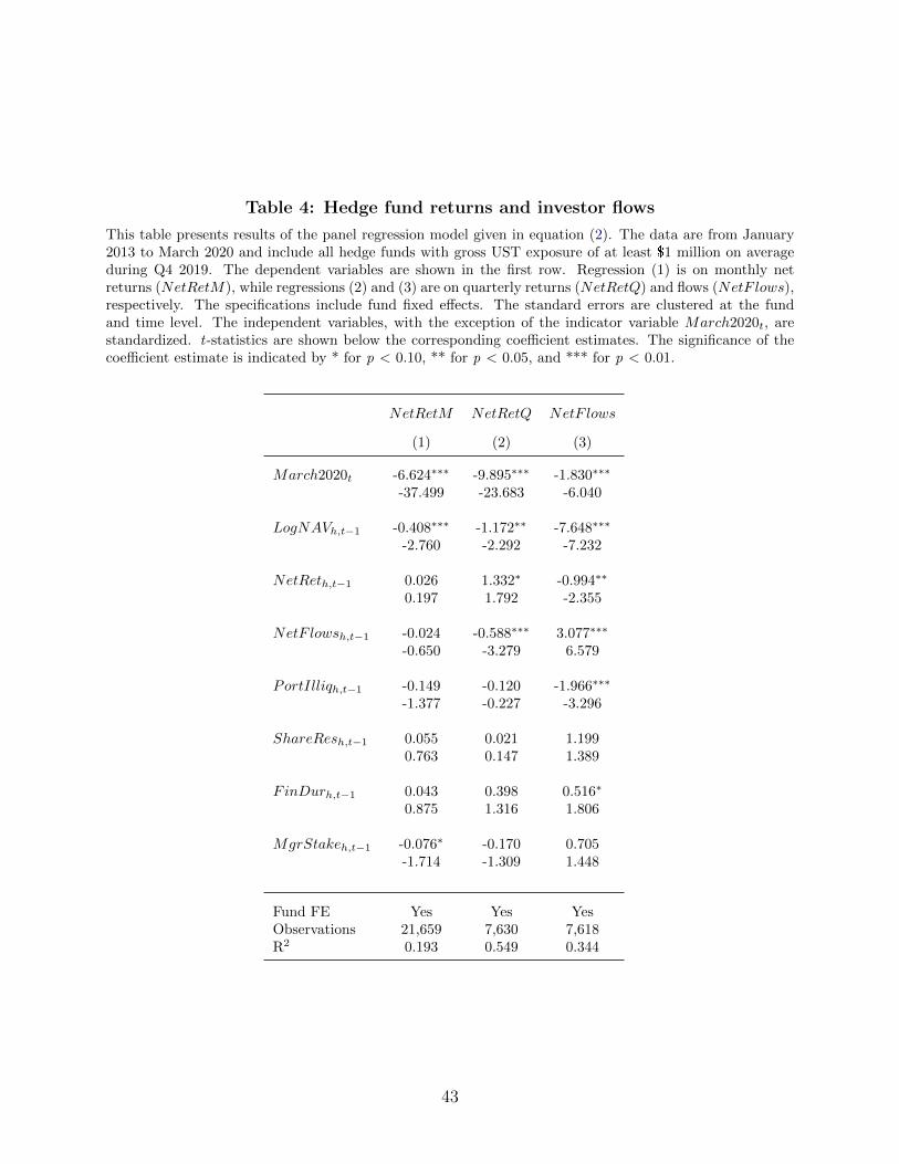
Table 4: Hedge fund returns and investor flows

This table presents results of the panel regression model given in equation (2). The data are from January2013 to March 2020 and include all hedge funds with gross UST exposure of at least $1 million on averageduring Q4 2019. The dependent variables are shown in the first row. Regression (1) is on monthly netreturns (NetRetM), while regressions (2) and (3) are on quarterly returns (NetRetQ) and flows (NetF lows),respectively. The specifications include fund fixed effects. The standard errors are clustered at the fundand time level. The independent variables, with the exception of the indicator variable March2020t, arestandardized. t-statistics are shown below the corresponding coefficient estimates. The significance of thecoefficient estimate is indicated by * for p < 0.10, ** for p < 0.05, and *** for p < 0.01.

NetRetM NetRetQ NetF lows

(1) (2) (3)

March2020t -6.624∗∗∗ -9.895∗∗∗ -1.830∗∗∗

-37.499 -23.683 -6.040

LogNAVh,t−1 -0.408∗∗∗ -1.172∗∗ -7.648∗∗∗

-2.760 -2.292 -7.232

NetReth,t−1 0.026 1.332∗ -0.994∗∗

0.197 1.792 -2.355

NetF lowsh,t−1 -0.024 -0.588∗∗∗ 3.077∗∗∗

-0.650 -3.279 6.579

PortIlliqh,t−1 -0.149 -0.120 -1.966∗∗∗

-1.377 -0.227 -3.296

ShareResh,t−1 0.055 0.021 1.1990.763 0.147 1.389

FinDurh,t−1 0.043 0.398 0.516∗

0.875 1.316 1.806

MgrStakeh,t−1 -0.076∗ -0.170 0.705-1.714 -1.309 1.448

Fund FE Yes Yes YesObservations 21,659 7,630 7,618R2 0.193 0.549 0.344

43

Table 5: Hedge fund liquidity and leverage

This table presents results of the panel regression model given in equation (2). The data are from January2013 to March 2020 and include all hedge funds with gross UST exposure of at least $1 million on averageduring Q4 2019. The dependent variables are shown in the first row. Regressions in Panel A are on monthlydata, while those in Panels B and C are on quarterly data. The specifications include fund fixed effects. Thestandard errors are clustered at the fund and time level. The independent variables, with the exception of theindicator variable March2020t, are standardized. t-statistics are shown below the corresponding coefficientestimates. The significance of the coefficient estimate is indicated by * for p < 0.10, ** for p < 0.05, and*** for p < 0.01.

Panel A: Cash and portfolio size

∆LogFreeCashEq ∆FreeCashEqNAV ∆LogCash ∆Cash

NAV ∆LogPortfolioGNE ∆LogOpenPositions

(1) (2) (3) (4) (5) (6)

March2020t 25.723∗∗∗ 6.289∗∗∗ 23.003∗∗∗ 8.824∗∗∗ -21.769∗∗∗ -4.643∗∗∗

18.937 37.199 20.388 28.202 -43.878 -8.428

Other Controls Yes Yes Yes Yes Yes YesFund FE Yes Yes Yes Yes Yes YesObservations 20,236 21,377 18,765 18,973 21,694 21,676R2 0.012 0.025 0.015 0.021 0.070 0.026

Panel B: Portfolio liquidity

∆ share of assets that can be liquidated in:

∆LogPortIlliq ≤ 7 days ≤ 30 days ≥ 31 days

(1) (2) (3) (4)

March2020t -10.734∗∗∗ 1.005∗∗∗ 0.070 -0.070-8.741 5.672 0.570 -0.570

Other Controls Yes Yes Yes YesFund FE Yes Yes Yes YesObservations 7,625 7,625 7,625 7,625R2 0.084 0.067 0.091 0.091

Panel C: Fund assets, equity, and leverage

∆LogNAV ∆LogGAV ∆LeverageRatio

(1) (2) (3)

March2020t -14.139∗∗∗ -13.545∗∗∗ -0.037-24.985 -18.623 -1.472

Other Controls Yes Yes YesFund FE Yes Yes YesObservations 7,625 7,625 7,625R2 0.246 0.149 0.038

44

Table 6: The regulatory constraints of creditors and hedge fund borrowing

This table presents results of the panel regression model given in equations (3), (4), and (5). The dependentvariable is ∆ logHF Crdtr Credith,p,t (in %). The data are quarterly from Q1 2013 to Q1 2020 and includehedge funds with gross UST exposure of at least $1 million that borrow predominantly through repo onaverage during Q4 2019. The specifications include combinations of fund, quarter, and creditor fixed effectswhere indicated. The standard errors are clustered at the creditor and time level. The independent variables,with the exception of the indicator variable March2020t, are standardized. t-statistics are shown below thecorresponding coefficient estimates. The significance of the coefficient estimate is indicated by * for p <0.10, ** for p < 0.05, and *** for p < 0.01.

(1) (2) (3) (4) (5) (6)

March2020t × IsGSIBp,t 12.032∗∗∗ 11.285∗∗∗ 13.374∗∗∗ 12.637∗∗ 13.335∗∗∗ 13.375∗∗∗

9.589 4.141 3.701 2.496 3.318 3.316

IsGSIBp,t -0.602 -5.143∗∗∗ -6.230∗∗ -2.516 14.215∗∗∗ 13.540∗∗∗

-0.464 -2.972 -2.315 -0.840 4.630 4.742

LogHF Crdtr Credith,p,t−1 -80.762∗∗∗ -74.351∗∗∗

-27.208 -16.801

CrdtrRankInHFh,p,t−1 -0.325-0.222

HFRankInCrdtrh,p,t−1 -6.428∗∗

-2.451

Other Controls No No No No No YesFund FE Yes Yes No No No NoTime FE Yes Yes No No No NoCreditor FE No Yes Yes No No NoFund × Time FE No No Yes Yes Yes YesFund × Creditor FE No No No Yes Yes YesObservations 9,816 9,816 9,816 9,816 9,816 9,816R2 0.031 0.038 0.236 0.318 0.516 0.517

45

Table 7: Redemption risk and UST hedge fund activity

This table presents results of the panel regression model given in equation (6). The dependent variablesare shown in the first row. The data are monthly from January 2013 to March 2020 and include all hedgefunds with gross UST exposure of at least $1 million on average during Q4 2019. The specifications includefund fixed effects. The standard errors are clustered at the fund and time level. The independent variables,with the exception of the indicator variable March2020t, are standardized. t-statistics are shown below thecorresponding coefficient estimates. The significance of the coefficient estimate is indicated by * for p <0.10, ** for p < 0.05, and *** for p < 0.01.

Panel A: Cash and liquidity position

∆LogFreeCashEq ∆FreeCashEqNAV ∆LogPortfolioGNE ∆LogOpenPositions ∆LogPortIlliq

(1) (2) (3) (4) (5)

March2020t 27.019∗∗∗ 7.069∗∗∗ -23.098∗∗∗ -5.166∗∗∗ -12.907∗∗∗

20.211 40.083 -43.441 -8.539 -10.008

ShareResh,t−1 1.500 0.248 0.520 0.239 1.2850.767 1.200 1.278 0.996 0.531

March2020t × ShareResh,t−1 -6.571∗∗∗ -3.728∗∗∗ 6.197∗∗∗ 2.416∗∗∗ 8.830∗∗∗

-5.875 -23.922 16.183 6.612 7.711

Other Controls Yes Yes Yes Yes YesFund FE Yes Yes Yes Yes YesObservations 20,236 21,377 21,694 21,676 7,625R2 0.012 0.030 0.073 0.027 0.087

Panel B: U.S. Treasury exposure

∆LogUST GNE ∆log(min(LNE,SNE)) ∆min(LNE,SNE)GNE

(1) (4) (5)

March2020t -20.977∗∗∗ -27.312∗∗∗ -2.331∗∗∗

-15.687 -8.757 -6.682

ShareResh,t−1 2.907∗ -2.402 -0.2741.672 -0.614 -0.586

March2020t × ShareResh,t−1 8.140∗∗∗ 15.624∗∗∗ 1.340∗∗∗

6.655 4.915 3.224

Other Controls Yes Yes YesFund FE Yes Yes YesObservations 18,849 11,053 18,849R2 0.016 0.014 0.005

46

Table 8: Basis traders versus other UST traders

This table presents results of the panel regression model given in equation (7). The data are from January2013 to March 2020 and include all hedge funds with gross UST exposure of at least $1 million on averageduring Q4 2019. The dependent variables are shown in the first row. Regressions in Panels A, B, C, andcolumns 1-6 of Panel D are on monthly data, while those in column 7 of Panel D and Panel E are onquarterly data. The specifications include fund fixed effects. The standard errors are clustered at the fundand time level. The independent variables, with the exception of the indicator variable March2020t, arestandardized. t-statistics are shown below the corresponding coefficient estimates. The significance of thecoefficient estimate is indicated by * for p < 0.10, ** for p < 0.05, and *** for p < 0.01.

Panel A: U.S. Treasury exposure

∆LogUST GNE ∆LogUST LNE ∆LogUST SNE ∆UST GNENAV ∆UST LNE

NAV ∆UST SNENAV

(1) (2) (3) (4) (5) (6)

March2020t -18.910∗∗∗ -17.330∗∗∗ -24.701∗∗∗ -10.432∗∗∗ -3.798∗∗∗ -6.843∗∗∗

-13.575 -9.400 -6.987 -10.619 -5.150 -10.493

March2020t ×BasisTraderh -6.278∗∗∗ -14.376∗∗∗ 5.752 -49.015∗∗∗ -47.451∗∗∗ -8.575∗

-2.695 -5.690 1.456 -6.006 -10.223 -1.924

Other Controls Yes Yes Yes Yes Yes YesFund FE Yes Yes Yes Yes Yes YesObservations 18,849 16,874 12,978 18,801 18,801 18,801R2 0.015 0.015 0.017 0.018 0.020 0.013

Panel B: U.S. Treasury fund-level long-short exposure

∆log(min(LNE,SNE)) ∆log(abs(LNE − SNE)) ∆ 2×min(LNE,SNE)GNE ∆abs(LNE−SNE))

GNE

(1) (2) (3) (4)

March2020t -25.868∗∗∗ -12.564∗∗∗ -2.778∗∗∗ 2.778∗∗∗

-7.152 -6.469 -7.465 7.465

March2020t ×BasisTraderh 2.956 -30.078∗∗∗ 6.948∗∗∗ -6.948∗∗∗

0.701 -5.496 9.609 -9.609

Other Controls Yes Yes Yes YesFund FE Yes Yes Yes YesObservations 11,053 18,834 18,849 18,849R2 0.013 0.007 0.005 0.005

Panel C: Repo exposure, maturity, and collateral

∆LogRepoBorrowing ∆LogRepoLending ∆RepoBrrwTerm ∆RepoLendTerm ∆RepoTotalCollateralRepoBorrowing

(1) (2) (3) (4) (5)

March2020t 1.098 -23.899∗∗∗ 4.459∗∗∗ -0.823∗ -1.456∗∗∗

0.463 -8.017 8.259 -1.900 -4.031

March2020t -17.882∗∗∗ -5.962 -9.124∗∗∗ -0.910 3.822∗∗∗

×BasisTraderh -6.071 -1.494 -14.804 -1.010 8.298

Other Controls Yes Yes Yes Yes YesFund FE Yes Yes Yes Yes YesObservations 9,387 9,083 9,387 9,083 9,810R2 0.014 0.014 0.023 0.021 0.012

47

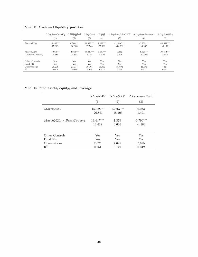
Panel D: Cash and liquidity position

∆LogFreeCashEq ∆FreeCashEqNAV ∆LogCash ∆Cash

NAV ∆LogPortfolioGNE ∆LogOpenPositions ∆LogPortIlliq

(1) (2) (3) (4) (5) (6) (7)

March2020t 26.467∗∗∗ 6.560∗∗∗ 21.333∗∗∗ 8.239∗∗∗ -21.807∗∗∗ -3.755∗∗∗ -11.687∗∗∗

17.809 36.868 17.744 25.506 -44.288 -6.992 -9.132

March2020t -7.664∗∗∗ -2.863∗∗∗ 18.440∗∗∗ 6.580∗∗∗ 0.412 -9.623∗∗∗ 10.782∗∗∗

×BasisTraderh -3.186 -4.165 5.705 5.130 0.498 -12.469 2.985

Other Controls Yes Yes Yes Yes Yes Yes YesFund FE Yes Yes Yes Yes Yes Yes YesObservations 20,236 21,377 18,765 18,973 21,694 21,676 7,625R2 0.012 0.025 0.015 0.022 0.070 0.027 0.084

Panel E: Fund assets, equity, and leverage

∆LogNAV ∆LogGAV ∆LeverageRatio

(1) (2) (3)

March2020t -15.328∗∗∗ -13.667∗∗∗ 0.033-26.861 -18.403 1.491

March2020t ×BasisTraderh 13.447∗∗∗ 1.379 -0.790∗∗∗

13.418 0.636 -4.163

Other Controls Yes Yes YesFund FE Yes Yes YesObservations 7,625 7,625 7,625R2 0.251 0.149 0.042

48

Appendix A Additional tables

49

Table A.1: Hedge fund UST trading and funding after the March 2020 shockThis table presents results of the panel regression model given in equation (2). The data are from January2013 to September 2020 and include all hedge funds with gross UST exposure of at least $1 million on averageduring Q4 2019. The dependent variables are shown in the first row. Regressions in Panel A are on quarterlydata, while those in Panels B and C are on monthly data. The specifications include fund fixed effects. Thestandard errors are clustered at the fund and time level. All independent variables except March2020t arestandardized. t-statistics are shown below the corresponding coefficient estimates. The significance of thecoefficient estimate is indicated by * for p < 0.10, ** for p < 0.05, and *** for p < 0.01.

Panel A: Returns, flows, and leverage

NetRetQ NetF lows ∆LogNAV ∆LogGAV ∆LeverageRatio

(1) (2) (3) (4) (5)

March2020t -9.625∗∗∗ -1.933∗∗∗ -14.064∗∗∗ -13.291∗∗∗ -0.028-22.092 -5.921 -24.445 -18.541 -1.162

2020Q2t 6.617∗∗∗ -3.347∗∗∗ 2.797∗∗∗ -1.137 -0.210∗∗∗

5.931 -5.040 3.193 -1.225 -7.559

2020Q3t 1.254∗∗ -3.330∗∗∗ -2.244∗∗∗ -1.764∗∗ 0.080∗∗∗

2.159 -6.565 -3.462 -2.474 3.353

Other Controls Yes Yes Yes Yes YesFund FE Yes Yes Yes Yes YesObservations 8,361 8,349 8,356 8,356 8,356R2 0.556 0.335 0.231 0.133 0.036

Panel B: U.S. Treasury exposure

∆LogUST GNE ∆LogUST LNE ∆LogUST SNE ∆UST GNENAV ∆UST LNE

NAV ∆UST SNENAV

(1) (2) (3) (4) (5) (6)

March2020t -19.659∗∗∗ -19.335∗∗∗ -22.236∗∗∗ -16.132∗∗∗ -9.525∗∗∗ -7.539∗∗∗

-12.624 -10.031 -7.273 -10.441 -8.838 -8.896

April2020t 5.143∗∗ 2.700 -4.145 -12.031∗∗∗ -6.737∗∗∗ -4.820∗∗∗

2.471 1.253 -0.752 -5.173 -4.434 -3.905

May2020t -4.352∗∗∗ -3.212∗∗ -13.029∗∗∗ 2.281 1.147 0.534-4.309 -2.203 -5.471 1.317 1.078 0.543

June2020t -5.641∗∗∗ -4.089∗∗∗ -16.545∗∗∗ -8.378∗∗∗ -5.398∗∗∗ -3.147∗∗∗

-4.522 -3.051 -6.055 -4.710 -4.747 -4.127

July2020t -6.626∗∗∗ -9.899∗∗∗ -6.090∗∗ -1.058 -2.237∗∗∗ 0.795-6.724 -5.414 -2.222 -0.821 -2.769 1.146

Aug2020t -3.530∗∗∗ -3.491∗∗∗ -7.001∗∗∗ -2.187∗ -0.958 -0.792-4.351 -4.014 -2.961 -1.694 -1.447 -1.059

Sept2020t -4.015∗∗∗ -3.086∗∗∗ 1.192 -5.526∗∗∗ -2.839∗∗∗ -2.524∗∗∗

-4.861 -2.690 0.536 -4.436 -3.201 -4.183

Other Controls Yes Yes Yes Yes Yes YesFund FE Yes Yes Yes Yes Yes YesObservations 20,776 18,495 14,293 20,728 20,728 20,728R2 0.015 0.015 0.015 0.012 0.013 0.009

50

Panel C: Repo exposure, maturity, and collateral

∆LogRepoBorrowing ∆LogRepoLending ∆RepoBrrwTerm ∆RepoLendTerm ∆RepoTotalCollateralRepoBorrowing

(1) (2) (3) (4) (5)

March2020t -0.698 -21.708∗∗∗ 3.027∗∗∗ -0.834∗ -0.743-0.300 -5.988 5.880 -1.691 -1.589

April2020t -15.784∗∗∗ -24.529∗∗∗ 1.105 0.606 4.656∗∗∗

-3.107 -5.757 1.444 0.809 7.977

May2020t -9.801∗∗∗ 7.564∗∗ -0.165 -0.174 2.816∗∗∗

-3.251 2.280 -0.220 -0.393 5.990

June2020t 12.132∗∗∗ -5.611∗ 0.392 -0.850∗∗ 1.434∗∗∗

4.359 -1.825 0.735 -2.015 3.321

July2020t 2.092 -6.630∗∗ 1.844∗∗∗ 0.409 0.3370.797 -2.428 3.917 1.021 0.886

Aug2020t 2.306 -4.533 1.873∗∗∗ 0.061 -0.5011.185 -1.660 3.467 0.131 -1.394

Sept2020t 1.625 2.382 2.097∗∗∗ 0.245 0.2601.108 0.831 4.189 0.524 0.616

Other Controls Yes Yes Yes Yes YesFund FE Yes Yes Yes Yes YesObservations 10,373 10,011 10,373 10,011 10,815R2 0.018 0.017 0.019 0.020 0.021

51

Table A.2: Hedge funds with large U.S. Treasury exposuresThis table presents results of the panel regression model given in equation (2). The dependent variablesare shown in the first row. The data are monthly from January 2013 to March 2020 and include all hedgefunds with gross UST exposure of at least $1 billion on average during Q4 2019. The specifications includefund fixed effects. The standard errors are clustered at the fund and time level. The independent variables,with the exception of the indicator variable March2020t, are standardized. t-statistics are shown below thecorresponding coefficient estimates. The significance of the coefficient estimate is indicated by * for p <0.10, ** for p < 0.05, and *** for p < 0.01.

Panel A: U.S. Treasury notional exposure

∆LogUST GNE ∆LogUST LNE ∆LogUST SNE ∆UST GNENAV ∆UST LNE

NAV ∆UST SNENAV

(1) (2) (3) (4) (5) (6)

March2020t -42.363∗∗∗ -30.310∗∗∗ -54.077∗∗∗ -69.607∗∗∗ -45.994∗∗∗ -28.842∗∗∗

-26.767 -12.062 -11.339 -12.105 -11.459 -9.906

Other Controls Yes Yes Yes Yes Yes YesFund FE Yes Yes Yes Yes Yes YesObservations 6,619 6,542 5,274 6,604 6,604 6,604R2 0.034 0.022 0.016 0.019 0.020 0.017

Panel B: U.S. Treasury duration

∆UST LNE Drtn ∆UST SNE Drtn ∆UST NNE Drtn

(1) (2) (3)

March2020t -0.132∗∗∗ -0.960∗∗∗ 4.310∗∗∗

-2.902 -8.875 6.779

Other Controls Yes Yes YesFund FE Yes Yes YesObservations 6,498 5,248 6,575R2 0.007 0.008 0.006

Panel C: U.S. Treasury fund-level long-short exposure

∆log(min(LNE,SNE)) ∆log(abs(LNE − SNE)) ∆ 2×min(LNE,SNE)GNE ∆abs(LNE−SNE))

GNE

(1) (2) (3) (4)

March2020t -35.132∗∗∗ -46.139∗∗∗ -1.849∗∗ 1.849∗∗

-9.871 -13.235 -2.618 2.618

Other Controls Yes Yes Yes YesFund FE Yes Yes Yes YesObservations 5,200 6,619 6,619 6,619R2 0.013 0.010 0.002 0.002

52

Table A.3: Summary statistics for hedge funds primarily borrowing via repo

This table shows select summary statistics over the period from January 2013 to March 2020 for the hedgefunds that primarily borrow via repo and have at least $1 million in UST exposure on average during Q42019. This is the main sample of hedge funds used in the hedge fund-creditor level analysis on changesto repo borrowing. The N column shows the number of observations used to calculate the statistics in aparticular row. The last four columns show percentiles.

N Mean Median Stdev 25th 75th 10th 90th

RepoBorrowingTotalBorrowing (%) 8,995 88.786 99.241 15.740 79.379 100.000 59.829 100.000

TotalMCBorrowingh,t (m US$) 2,189 8,738.516 1,027.546 26,954.468 314.389 4,320.877 107.501 21,159.939NumCrdtrsPerHFh,t 2,189 6.265 5.000 5.464 2.000 8.000 1.000 13.200HFCrdtrHHIh,t 2,189 39.306 29.235 28.747 18.143 50.356 12.891 100.000

HF Crdtr Credith,p,t (m US$) 13,819 1,267.736 351.938 2,818.642 132.387 1,087.282 61.780 2,946.323∆logHF Crdtr Credith,p,t 11,121 1.370 0.381 52.724 -22.847 25.015 -60.263 62.666

IsCrdtrPBh,p,t 13,819 0.228 0.000 0.420 0.000 0.000 0.000 1.000IsCrdtrCustodianh,p,t 13,819 0.296 0.000 0.457 0.000 1.000 0.000 1.000

53

Table A.4: The regulatory constraints of creditors and hedge fund borrowing

This table presents results of the panel regression model given in equations (3), (4), and (5). The dependentvariable is ∆ logHF Crdtr Credith,p,t (in %). The data are quarterly from Q1 2013 to Q1 2020 and includeall hedge funds that borrow predominantly via repo. The specifications include combinations of fund, quarter,and creditor fixed effects where indicated. The standard errors are clustered at the creditor and time level.The independent variables, with the exception of the indicator variable March2020t, are standardized. t-statistics are shown below the corresponding coefficient estimates. The significance of the coefficient estimateis indicated by * for p < 0.10, ** for p < 0.05, and *** for p < 0.01.

(1) (2) (3) (4) (5) (6)

March2020t × IsGSIBp,t 10.503∗∗∗ 9.434∗∗∗ 13.641∗∗∗ 13.797∗∗∗ 14.545∗∗∗ 14.548∗∗∗

9.067 3.812 4.025 2.941 3.935 3.882

IsGSIBp,t -0.260 -3.226∗∗ -5.160∗∗ -1.183 14.599∗∗∗ 13.493∗∗∗

-0.267 -2.619 -2.066 -0.361 4.700 4.490

LogHF Crdtr Credith,p,t−1 -82.417∗∗∗ -73.815∗∗∗

-26.900 -17.131

CrdtrRankInHFh,p,t−1 -0.985-0.850

HFRankInCrdtrh,p,t−1 -7.512∗∗

-2.554

Other Controls No No No No No YesFund FE Yes Yes No No No NoTime FE Yes Yes No No No NoCreditor FE No Yes Yes No No NoFund × Time FE No No Yes Yes Yes YesFund × Creditor FE No No No Yes Yes YesObservations 13,995 13,995 13,995 13,995 13,995 13,995R2 0.043 0.048 0.293 0.382 0.562 0.562

54

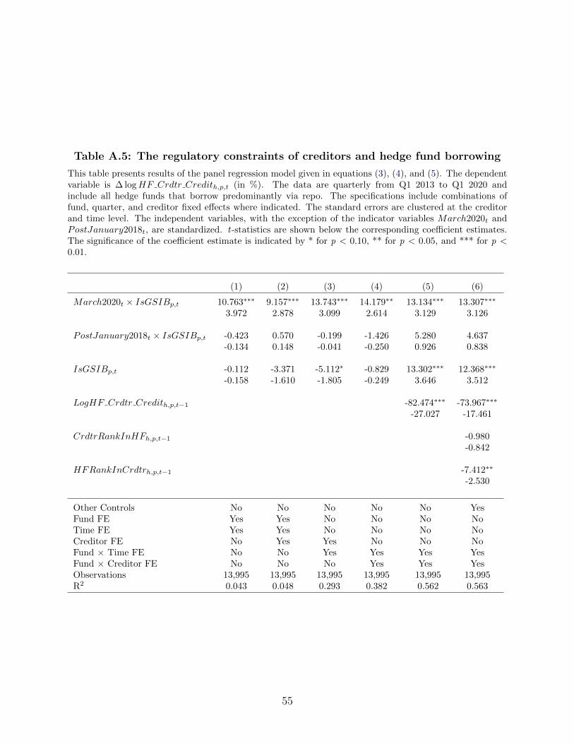
Table A.5: The regulatory constraints of creditors and hedge fund borrowing

This table presents results of the panel regression model given in equations (3), (4), and (5). The dependentvariable is ∆ logHF Crdtr Credith,p,t (in %). The data are quarterly from Q1 2013 to Q1 2020 andinclude all hedge funds that borrow predominantly via repo. The specifications include combinations offund, quarter, and creditor fixed effects where indicated. The standard errors are clustered at the creditorand time level. The independent variables, with the exception of the indicator variables March2020t andPostJanuary2018t, are standardized. t-statistics are shown below the corresponding coefficient estimates.The significance of the coefficient estimate is indicated by * for p < 0.10, ** for p < 0.05, and *** for p <0.01.

(1) (2) (3) (4) (5) (6)

March2020t × IsGSIBp,t 10.763∗∗∗ 9.157∗∗∗ 13.743∗∗∗ 14.179∗∗ 13.134∗∗∗ 13.307∗∗∗

3.972 2.878 3.099 2.614 3.129 3.126

PostJanuary2018t × IsGSIBp,t -0.423 0.570 -0.199 -1.426 5.280 4.637-0.134 0.148 -0.041 -0.250 0.926 0.838

IsGSIBp,t -0.112 -3.371 -5.112∗ -0.829 13.302∗∗∗ 12.368∗∗∗

-0.158 -1.610 -1.805 -0.249 3.646 3.512

LogHF Crdtr Credith,p,t−1 -82.474∗∗∗ -73.967∗∗∗

-27.027 -17.461

CrdtrRankInHFh,p,t−1 -0.980-0.842

HFRankInCrdtrh,p,t−1 -7.412∗∗

-2.530

Other Controls No No No No No YesFund FE Yes Yes No No No NoTime FE Yes Yes No No No NoCreditor FE No Yes Yes No No NoFund × Time FE No No Yes Yes Yes YesFund × Creditor FE No No No Yes Yes YesObservations 13,995 13,995 13,995 13,995 13,995 13,995R2 0.043 0.048 0.293 0.382 0.562 0.563

55

Table A.6: The regulatory constraints of creditors and hedge fund borrowing

This table presents results of the panel regression model given in equations (3), (4), and (5). The dependentvariable is ∆ logHF Crdtr Credith,p,t (in %). The data are quarterly from Q1 2013 to Q1 2020 and includeall hedge funds that borrow predominantly via repo. The specifications include combinations of fund, quarter,and creditor fixed effects where indicated. The standard errors are clustered at the creditor and time level.The independent variables, with the exception of the indicator variables March2020t and PostJuly2015t,are standardized. t-statistics are shown below the corresponding coefficient estimates. The significance ofthe coefficient estimate is indicated by * for p < 0.10, ** for p < 0.05, and *** for p < 0.01.

(1) (2) (3) (4) (5) (6)

March2020t × IsGSIBp,t 9.883∗∗∗ 8.815∗∗∗ 13.219∗∗∗ 13.607∗∗∗ 15.356∗∗∗ 15.379∗∗∗

6.830 3.461 3.562 2.828 4.254 4.224

PostJuly2015t × IsGSIBp,t 2.942 3.953 2.610 2.522 -10.697∗∗ -10.953∗∗

0.777 1.096 0.648 0.657 -2.324 -2.444

IsGSIBp,t -2.548 -6.151∗∗ -7.084∗∗ -3.173 23.087∗∗∗ 22.181∗∗∗

-0.837 -2.264 -2.107 -0.879 4.477 4.448

LogHF Crdtr Credith,p,t−1 -82.667∗∗∗ -74.107∗∗∗

-27.363 -17.206

CrdtrRankInHFh,p,t−1 -0.929-0.812

HFRankInCrdtrh,p,t−1 -7.584∗∗

-2.550

Other Controls No No No No No YesFund FE Yes Yes No No No NoTime FE Yes Yes No No No NoCreditor FE No Yes Yes No No NoFund × Time FE No No Yes Yes Yes YesFund × Creditor FE No No No Yes Yes YesObservations 13,995 13,995 13,995 13,995 13,995 13,995R2 0.043 0.048 0.293 0.382 0.562 0.563

56

Appendix B Background and Data

B.1 Overview of Fixed Income Arbitrage Strategies

In this section, we give a high-level overview of the economics of fixed income arbitrage

strategies hedge funds engage in. Figure 8 illustrates the securities flows, cash flows, and

exposures created at trade option, trade maintenance, and trade close for a typical (a) long-

short bond spread trade and (b) Treasury cash-futures basis trade.

Duarte, Longstaff, and Yu (2007) gives an overview and simulates the potential the

risk-return trade offs to the arbitrage trading strategies of fixed income hedge funds. Ed-

ward (1999); Jorion (2000) discuss the liquidity risk, volatility risk, default risk, and other

risks inherent in fixed income “arbitrage” trading in the context of the 1998 meltdown of

Long-Term Capital Management (LTCM), which engaged in such bond spread trading until

a systematic shock caused massive losses that threatened systemic stability and led to a

Fed-arranged broker takeover of the fund’s positions. Industry insiders and observers drew

parallels between the 1998 LTCM episode and the impact of the March 2020 shock on fixed

income hedge funds. There are indeed some parallels, but, as we describe when presenting

the main results in the paper, also important distinctions between the two episodes.

B.1.1 Long-short bond spread trading

This type of trade bets on the convergence of a particular bond spread—such as the on-

the-run/off-the-run (ONR-OFFR) spread—due to theoretical or statistical predictions on

the relative value of the two securities forming the spread. Details on the life cycle of

a typical long-short bond spread trade are depicted in Figure 8(a). For such trades to

be sufficiently profitable, these arbitrage trades involve substantial leverage. Long UST

securities positions are primarily financed via repurchase agreements (repo borrowing), while

short UST securities positions are primarily sourced through reverse repo (repo lending).

Hedge funds generally go long the more illiquid security and short the more liquidity

security and capture the liquidity premium. In the case of the ONR-OFFR spread, this

would mean going long the OFFR bond and short the ONR bond. In a typical market stress

episode, liquidity risk spikes and such spreads typically widen. During such an episode, if a

fund is unable to obtain sufficient capital or funding to hold onto such spread convergence

trades, the fund would have to liquidate the trades at unfavorable prices in illiquid markets

and realize losses.

In addition to liquidity risk, trade maintenance exposes a fund to repo rollover risk.

Under extreme conditions, the dealer may refuse to roll over the repo loan funding the long

57

side of the trade. Newly rolled-over loans might have higher haircuts if Treasury collateral

is suddenly more volatile, may involve a higher interest rate, or a lower borrowing amount if

the value of the collateral (bond price) has gone down. Each of these possibilities increases

the cost of carrying the trade.

B.1.2 Cash-futures basis trading

The UST cash-futures basis trade became popular in recent years. In essence, it is a cross-

market arbitrage constructed by shorting a Treasury futures contract and going long a Trea-

sury security deliverable into that contract, funding the long position with repo borrowing.30

We find that since 2018Q2 there has been a significant increase in repo borrowing, indicating

a marked increase in long UST securities holdings (see Figures 2 and 3). Until that point,

aggregate hedge fund repo borrowing and lending exposures were generally matched, as one

would observe with UST arbitrage strategies such as trading on-the-run/off-the-run spreads

or yield spreads. The divergence between hedge fund repo borrowing and lending is likely

driven by a significant increase in recent years in UST cash-futures basis trading.

In this trading strategy, a hedge fund goes long the (cheapest-to-deliver) Treasury security

and goes short the corresponding Treasury futures contract. The futures leg does not require

reverse repo, so the divergence between hedge fund repo borrowing and lending is consistent

with reports of a significant increase in recent years in UST cash-futures basis trading.

Typically, this is a low volatility, low yield convergence strategy that is operationally intensive

and requires leverage to be worthwhile. The trade is profitable as long as the actual cost of

carrying the cash position (the “repo rate” or the cost of repo borrowing for the hedge fund)

is below the implied cost of carry on the futures (the “implied repo rate”).

As with many other spread trades hedge funds engage in, these trades are also primarily

“short liquidity,” and perform worst in states of the world in which liquidity is scarce. In

addition to liquidity risk, this trade is exposed to basis risk, i.e., the risk that the underlying

asset price dynamics diverge from the futures price dynamics. Maintaining the trade exposes

a fund to repo rollover risk and margin risk, described further below.

Details on the basis trade are depicted in Figure 8(b), which follows a typical trade’s

lifecycle. The transactions and cash flows at initiation are shown on the left. The cash

flows include initial margin on the short futures contract and net cash needed above repo

borrowings to complete the purchase of the bond. Given low haircuts on Treasury repo and

low margin levels on futures, these initial cash outlays are low relative to the exposure of the

trade. Thus, the cash-futures basis trade is very highly leveraged. As the figure suggests, it

30The long Treasury security in a cash-futures basis trade is typically a Treasury note. We will use theterm ”bond” when describing the economics of the trade.

58

is also an operationally intensive trade.

Maintaining the trade to realize the its gains exposes the fund to two risks: rollover risk

and margin risk. Although the fund would prefer to use term repo with maturity matched

to the expiry of the futures, shorter-term or overnight repo is common and exposes the fund

to the risk of not being able to continue financing the bond. Under extreme conditions,

the dealer may refuse to roll over the repo loan. Newly rolled-over loans might have higher

haircuts if Treasury collateral is suddenly more volatile, may involve a higher interest rate,

or a lower borrowing amount if the value of the collateral (bond price) has gone down. Each

of these possibilities increases the cost of carrying the bond. The second risk is margin risk.

If futures prices increase rapidly or volatility leads to higher margin requirements, the fund

might have to make variation margin payments to satisfy margin calls. It is worth noting that

if cash and futures prices move in lockstep, margin payments may be made using increased

repo borrowings from the appreciating collateral. However, if futures prices increase more

than bond prices, i.e., if the futures basis widens, as they did in March of last year, there

may be net cash demands on the fund related to margin payments. In such a case, the hedge

fund would have to immediately meet the margin call to hold on to the basis trade position

or liquidate the position at unfavorable prices and realize a loss.

Finally, at trade close on the right, the fund closes its repo and delivers the Treasury into

the futures contract. The fund may alternatively choose to roll the trade to the following

futures expiry.

B.2 Basis Trader Classification

We use the following methodology to classify a hedge fund as predominantly engaging in the

UST cash-futures basis trade as opposed to other UST trading strategies. The classification

recognizes that a basis trade has broadly balanced long and short UST notional exposures,

but the long “cash” side is a physical bond while the short “futures” side is a derivative.

As such, only the long side is funded via repo, while the short side is not. This generally

contrasts with other UST arbitrage strategies such as on-the-run/off-the-run spread trading

where the long and short side of the trade is funded via more balanced repo borrowing and

repo lending, respectively.

The algorithm begins by subsetting funds to those whose strategy allocation according to

Form PF Question 20 includes either “Relative Value, Fixed Income Sovereign” or “Macro,

Global Macro.” We then classify a fund in this set as a Basis Trader if, during the height

of the basis trade between January 2018 and February 2020 (inclusive), its balanced UST

position, min(UST LNEh,t, UST SNEh,t), is positively and significantly correlated at the

59

5% level with its net repo exposure (RepoBorrowing−RepoLending). Finally, we manually

inspect the results of the algorithm for consistency.

B.3 Duration of U.S. Treasury Exposure

Funds supplement their reporting of notional exposures to U.S. Treasury securities on Form

PF Question 30 by reporting either the duration, weighted average tenor (WAT), or 10-year

bond equivalent values for both their long and short exposures. To facilitate comparison

across funds, we convert entries of WAT and 10-year bond equivalents to duration.

Our method begins with the observation (see section B.3.1) that one can approximate the

modified duration of a semi-annual coupon bond at par value given its yield and remaining

maturity according to the formula:

ModDur(y, τ) ≈ 1

y

(1 − 1

(1 + 12y)2τ

), (8)

where y is the yield-to-maturity (expressed as a decimal) and τ is the remaining time-to-

maturity of the bond in years. For zero-coupon bonds such as T-bills, the modified duration

is computed as

ModDur(y, τ) =τ

1 + yk

, (9)

where k is the compounding frequency per year. Thus we use k = 12 for the 4-week T-bill,

k = 6 for the 8-week T-bill, k = 4 for the 13-week T-bill, and so on.

Our analysis also requires the monthly time series of the Treasury yield curve. We obtain

month-end historical constant maturity Treasury rates from the Federal Reserve’s H.15 data

and linearly interpolate between maturities to form a yield curve estimate. In particular, we

use (8) to produce a time-varying estimate of the modified duration of the 10-year Treasury

note.

Given the above, to convert from a 10-year bond equivalent value to duration we use

Duration =(Reported10yrBE) ∗ (DurationOf10yrUST )

ReportedUSTExposure(10)

Finally, to convert from WAT to duration, we first use the interpolated U.S. Treasury

yield curve to find the approximate yield-to-maturity for a Treasury with WAT remaining

years to maturity. The duration is then approximated using (8) if WAT is greater than one,

or computed using (9) if WAT is less than or equal to one.

60

B.3.1 Derivation of (8)

Consider a semi-annual coupon bond with yield-to-maturity y and coupon C with 2n re-

maining semi-annual coupon payments. Write the price P of the bond in terms of two

components: the present value of an annuity represented by the coupon payments, and the

present value of the par value payment at maturity. The price P per $100 of par can be

written as:

P = C

[1 − 1

(1+y/2)2n

y/2

]+

100

(1 + y/2)2n. (11)

Computing the modified duration by taking the derivative with respect to y, we obtain

ModDur = − 1

P

∂P

∂y=

2Cy2

[1 − 1

(1+y/2)2n

]+ n(100−2C/y)

(1+y/2)2n+1

P(12)

For a semi-annual coupon bond at par value, we have that P = 100 and C = 100y/2 (y is a

decimal). Inserting this into the above, we obtain

ModDur =

2×100y/2y2

[1 − 1

(1+y/2)2n

]+ n(100−2×100y/2y)

(1+y/2)2n+1

100(13)

=1

y

(1 − 1

(1 + y/2)2n

). (14)

B.4 Average Term of Repo and Reverse Repo

As in the case of U.S. Treasury exposures, funds report on Form PF Question 30 the dura-

tion, weighted average tenor (WAT), or 10-year bond equivalent values for both their repo

borrowing and repo lending. We use these values to estimate the average term of their repo

borrowing and repo lending.

A repo can be viewed as a collateralized loan with a single payment of principal and

interest at maturity. The duration and WAT of a repo is thus equal to its term, much like

the duration and WAT of a zero-coupon bond is its maturity. Finally, we use this observation

and (10) to convert a 10-year bond equivalent value to the repo term.

B.5 Investment Strategy Classification

Question 20 on Form PF contains 22 strategy categories to which hedge funds assign shares of

their invested NAV. Among these is an “Other” category to which funds can manually enter

strategies that are not covered by the other 21 sub-strategies. The 22 strategy categories

roll up to 8 broad strategies: equity, macro, relative value, event driven, credit, managed

61

futures, investment in other funds, and other. We use these data to classify a hedge fund’s

broad strategy.

First, we inspect the strategies entered in the “Other” category and reclassify entries that

are similar to other listed broad strategies. For example, a description of “Relative Value

Fixed Income” is reclassified from “Other” to “Relative Value.”

Next, the data are normalized so that the sum of each hedge fund’s allocation across the

22 strategy categories equals 100% of their NAV. These normalized values are aggregated

to the broad strategy categories, and then further aggregated across all the fund’s filings

over time. A hedge fund is considered to use a given broad strategy if more than 50% of its

aggregated, normalized assets are allocated to that broad strategy. If there is not a broad

strategy to which more than 50% of the normalized assets are allocated, then the fund is

classified as a multi-strategy fund.

62

Table B.1: G-SIB and primary dealer classifications

This table presents G-SIB and primary dealer classifications. The source for the G-SIB classifications isthe Financial Stability Board (https://www.fsb.org/work-of-the-fsb/policy-development/addressing-sifis/global-systemically-important-financial-institutions-g-sifis/) and for primary dealers is the New York Fed(https://www.newyorkfed.org/medialibrary/media/markets/Dealer Lists 1960 to 2014.xls).

Institution Jurisdiction G-SIB Primary dealerdesignated years subsidiary

Agricultural Bank of China CN 2014 - 0Bank of America US 2011 - 1Bank of China CN 2011 - 0Bank of Montreal CA 1Bank of New York Mellon US 2011 - 0Bank of Nova Scotia CA 1Barclays UK 2011 - 1BBVA ES 2012 - 2014 0BNP Paribas FR 2011 - 1Cantor Fitzgerald US 1China Construction Bank CN 2015 - 0Citigroup US 2011 - 1Commerzbank DE 2011 0Credit Suisse CH 2011 - 1Daiwa Securities Group JP 1Deutsche Bank DE 2011 - 1Dexia BE 2011 0Goldman Sachs US 2011 - 1Groupe BPCE FR 2011 - 0Groupe Credit Agricole FR 2011 - 0HSBC UK 2011 - 1Industrial and Commercial Bank of China CN 2013 - 0ING Bank NL 2011 - 0Jefferies Group US 1JP Morgan Chase US 2011 - 1Lloyds Banking Group UK 2011 0Mitsubishi UFJ FG JP 2011 - 0Mizuho FG JP 2011 - 1Morgan Stanley US 2011 - 1Nomura Holdings JP 1Nordea SE 2011 - 2017 0Royal Bank of Canada CA 2017 - 1Royal Bank of Scotland UK 2011 - 2017 1Santander ES 2011 - 0Societe Generale FR 2011 - 1Standard Chartered UK 2012 - 0State Street US 2011 - 0Sumitomo Mitsui FG JP 2011 - 0Toronto Dominion CA 2019 - 1UBS CH 2011 - 1Unicredit IT 2011 - 0Wells Fargo US 2011 - 0

63

Table B.2: Variable definitions

This table presents definitions of the main variables used in this paper. The first column gives the variablename. The second column includes a short description. The last column gives the reference to the rawdata source in Form PF (https://www.sec.gov/about/forms/formpf.pdf) or Form ADV (https://www.sec.gov/about/forms/formadv.pdf). Variables are monthly where the description indicates “(m)” and quarterlyotherwise . Detailed descriptions and summary statistics of these variables are in section 3.

Variable Name Description Source

Strategyh

Investment strategy of the hedge fund (Credit,Equity, Event Driven, Macro, Relative Value,Multi-strategy, or Other).

PF Q20

NAVh,tNet asset value, or the amount of investor equity, ofthe hedge fund.

PF Q9

GAVh,tGross asset value, akin to balance sheet assets, ofthe hedge fund.

PF Q9

LeverageRatioh,tBalance sheet leverage, i.e. the ratio of gross assetvalue to net asset value, of the hedge fund.

PF Q8, Q9

PortIlliqh,t

The weighted average time (in days) it would taketo liquidate the hedge fund’s portfolio, assuming nofire sale discounting.

PF Q32

ShareResh,t

The weighted average time (in days) it would takefor the investors of the hedge fund to withdraw allthe fund’s NAV.

PF Q50

FinDurh,tThe weighted average maturity (in days) of thehedge fund’s borrowing.

PF Q46(b)

MgrStakeh,tThe percent of the net asset value of the hedge fundowned by the managers or their related persons.

ADV Schedule D,Section 7.B.(1), Q14

NetRetQh,t

(NetRetMh,t)Net-of-fee quarterly (monthly) returns of the hedgefund.

PF Q17

NetF lowsh,tNet investor flows to the hedge fund, estimated as

NetF lowsh,t =NAVh,t−NAVh,t−1×(1+rh,t)

NAVh,t−1

PF Q9, Q17

FreeCashEqh,t

Unencumbered cash and cash equivalents. IncludesTreasury and agency securites not posted ascollateral.� (m)

PF Q33

Cashh,tCash and cash equivalents, excluding governmentsecurites. (m)

PF Q30

OpenPositionsh,tNumber of open positions in the hedge fund’sportfolio. (m)

PF Q34

GNEh,tGross notional exposure estimated by summinglong and short asset class exposures. (m)

PF Q30

PortfolioGNEh,tGross notional exposure estimated by summing longand short exposures to non-cash asset classes. (m)

PF Q30

Continued on the next page.

64

Table B.2: Variable definitions (continued)

Variable Name Description Source

UST GNEh,tSum of long and short exposures to U.S. Treasurysecurities, including derivatives. (m)

PF Q30

UST LNEh,tLong exposure to U.S. Treasury securities, includingderivatives. (m)

PF Q30

UST SNEh,tShort exposure to U.S. Treasury securities, includingderivatives. (m)

PF Q30

UST LNE Drtnh,tDuration in years of long exposure to U.S. Treasurysecurities. (m)

PF Q30

UST SNE Drtnh,tDuration in years of short exposure to U.S. Treasurysecurities. (m)

PF Q30

UST NNE Drtnh,tDuration in years of net (long minus short) exposure toU.S. Treasury securities. (m)

PF Q30

RepoBorrowingh,tValue of repurchase agreements through which the hedgefund has borrowed cash and lent securities. (m)

PF Q30

RepoLendingh,tValue of repurchase agreements through which the hedgefund has borrowed securities and lent cash. (m)

PF Q30

RepoBrrwTermh,tAverage term (in days) of the hedge fund’sRepoBorrowingh,t. (m)

PF Q30

RepoLendTermh,tAverage term (in days) of the hedge fund’sRepoLendingh,t. (m)

PF Q30

RepoTotalCollateralh,tTotal collateral posted by the hedge fund in support of itsRepoBorrowingh,t. (m)

PF Q43(b)(ii)(A-C)

RepoCashCollateralh,t

Total collateral posted in the form of cash and cashequivalents� by the hedge fund in support of itsRepoBorrowingh,t. (m)

PF Q43(b)(ii)(A)

RepoSecCollateralh,tTotal collateral posted in the form of securities by thehedge fund in support of its RepoBorrowingh,t. (m)

PF Q43(b)(ii)(B)

RepoClearedCCPh,tEstimated percentage (by value) of repo trades enteredinto by the hedge fund that were cleared by a CCP.

PF Q24(d)

RepoBilateralh,tEstimated percentage (by value) of repo trades enteredinto by the hedge fund that were bilaterally transacted.

PF Q24(d)

TotalMCBorrowingh,t

Total borrowings of the hedge fund across its majorcreditors, i.e. those from whom it borrows amountstotalling 5% or more of its net asset value.

PF Q47

NumCrdtrsPerHFh,t The number of creditors lending to the hedge fund. PF Q47

HFCreditorHHIh,t Creditor concentration of the hedge fund. PF Q47

Continued on the next page.

65

Table B.2: Variable definitions (continued)

Variable Name Description Source

HF Crdtr Credith,p,tAmount borrowed by hedge fund h from creditor p at theend of quarter t.

PF Q47

IsCrdtrPBh,p,tIndicator for whether creditor p is one of hedge fund h’sprime brokers as of the end of quarter t.

ADV Schedule D,Section 7.B.(1), Q24

IsCrdtrCustodianh,p,tIndicator for whether creditor p is one of hedge fund h’scustodians as of the end of quarter t.

ADV Schedule D,Section 7.B.(1),Q24/25

CrdtrRankInHFh,p,tRank of creditor p based on hedge fund h’s borrowing atthe end of quarter t, normalized to the range [0, 1].

PF Q47

HFRankInCrdtrh,p,tRank of hedge fund h based on creditor p’s lending at theend of quarter t, normalized to the range [0, 1].

PF Q47

�In the data, “cash and cash equivalents” refer to cash, cash equivalents (e.g., bank deposits, certificates of deposits, moneymarket fund investments).

66