Deep-Sea Research II 49 (2002) 4051–4067

Low-frequency variability of the exchanged flows through theStrait of Gibraltar during CANIGO

Jes !us Garc!ıa Lafuentea,*, Javier Delgadoa, Juan Miguel Vargasa, Manuel Vargasb,Francisco Plazaa, Tarek Sarhanb

aDepartamento de F!ısica Aplicada II, Universidad de M !alaga, Campus de Teatinos, 29071 M !alaga, Spainb Instituto Espa *nol de Oceanograf!ıa, Laboratorio Oceanogr !afico de M !alaga, Fuengirola, M !alaga, Spain

Received 7 April 2000; received in revised form 7 September 2000; accepted 29 October 2000

Abstract

Time series of the exchanged flows through the Strait of Gibraltar at the eastern section have been estimated from

current-meter observations taken between October 1995 and May 1998 within the Canary Islands Azores Gibraltar

Observations (CANIGO) project. The inflow exhibits a clear annual signal that peaks in late summer simultaneously

with a deepening of the interface. The cycle seems to be driven by the seasonal signal of the density contrast between the

surface Atlantic water that forms the inflow and the deep Mediterranean water of the outflow. The outflow and the

depth of the interface have predominant semiannual signals and a smaller annual one whose phase agrees with that of

the density contrast as well. Local wind stress and atmospheric pressure difference between the Atlantic and the

Western Mediterranean to less extent have clear semiannual signal, so that the possibility that the semiannual cycle of

the outflow and of the depth of the interface are forced by them was analyzed.

The composite Froude number in this section is well below the critical value, suggesting submaximal exchange.

Therefore, the conditions in the Alboran basin influence the exchange and some evidence that the size and location of

the Western Alboran Gyre contribute to the observed signals, both annual and semiannual, is provided. r 2002

Elsevier Science Ltd. All rights reserved.

1. Introduction

The inverse estuarine circulation of the flowsthrough the Strait of Gibraltar, which is driven bythe net evaporative loss of fresh water in theMediterranean Sea, exhibits marked temporalvariability on different time scales, ranging froma few minutes, associated with the short-lengthinternal waves of near Brunt V.ais.al.a frequency

(Watson and Robinson, 1990), to inter-annualvariabilities, which are not well known.

The average long-term inflow of Atlantic water,Q1; and outflow of Mediterranean water,Q2 ðQ2o0Þ; must satisfy the conservative lawQ1 þQ2 ¼ E � P; where E is the evaporation inthe Mediterranean and P includes both precipita-tion and rivers discharge into the sea. Estimates ofthe exchanged flows using direct current-meterobservations give a value of about 0:8 Sv ð1 Sv ¼106 m3=s1Þ for both inflow and outflow (Brydenet al., 1994; Bascheck et al., 2001), a flow smallerthan those historically reported. Tidal flows are

*Corresponding author. Tel.: +34-952-13-2721; fax: +34-

952-13-2721.

E-mail address: glafuente@ctima.uma.es (J.G. Lafuente).

0967-0645/02/$ - see front matter r 2002 Elsevier Science Ltd. All rights reserved.

PII: S 0 9 6 7 - 0 6 4 5 ( 0 2 ) 0 0 1 4 2 - X

much greater and produce periodic semidiurnalflow reversals in the layers (Candela et al., 1990;Bryden et al., 1994; Garc!ıa Lafuente et al., 2000).Important sub-inertial variability is known to beforced by atmospheric forcing (Candela et al.,1989) in the frequency band of 0.1–0.3 cycles perday (cpd). Annual or semiannual signals, whoseamplitudes are smaller, have been analyzed byBormans et al. (1986) from the difference in sealevel between Ceuta and Gibraltar (see Fig. 1).They estimate an annual signal of 6% (within afactor of 2) in the inflow, based on a clearoverestimated mean inflowing velocity of

1:2 m=s; with maximum inflow in spring. Brydenet al. (1994), using current-meter observations,report a larger annual signal in Q1 (around 15%),with a maximum in late summer, and a muchsmaller amplitude in the Q2 (4%), with amaximum outflow in January. The strong asym-metry of these values could be the consequence ofthe short length of their time series, which did notcover one year. However, the data analyzed in thepresent work provide similar results, suggestingthat they might have physical consistency.

A simple but powerful model for the exchangethrough the Strait is the two-layer hydrauliccontrol theory. It predicts maximal exchange ifthe flow is controlled at two sections connected bya subcritical region (Farmer and Armi, 1986). Thecandidate locations for control are the narrowestsection off Tarifa (Tarifa Narrows, TN) and thesection of minimum cross-area, also of minimumdepth, of Camarinal Sill (CS). At the controls thecomposite Froude number

G2 ¼ F21 þ F 2

2 ¼u21g0h1

þu22g0h2

ð1Þ

is critical, G2 ¼ 1: Here F2i ¼ u2i =g

0hi is the internalFroude number of layer i; whose velocity andthickness are ui and hi; respectively, g0 ¼ gðr2 �r1Þ=r2 is the reduced gravity, and ri is the layerdensity. Bryden and Kinder (1991) applied thistheory to the Strait of Gibraltar to estimate thesteady exchanged flows using a realistic topogra-phy and complying the flows to satisfy conserva-tive laws for salt and mass in the Mediterranean.Their predictions agree within 20% with theobservations for the accepted values of E � P:

Farmer and Armi (1986) incorporated barotro-pic signals into the model using a quasi-steadyapproximation in which the steady solution isverified at each point of the cycle. Helfrich (1995)showed that this approach is only valid fordynamically short straits, a concept related to theparameter g ¼ ðg0h1Þ

1=2T=L that measures thelength L of the strait relative to the distance aninternal signal will travel during the forcing periodT of the barotropic signal. The quasi-steadyapproximation is only valid for g-N; a conditionwidely fulfilled by low frequency signals but not by

-6.0W -5.8W -5.6W -5.4W

35.8N

36.0N

36.2N

Spain

Morocco

Algeciras

Tarifa

Ceuta

Tangier

N

SC

CSTN

-1000

-750

-500

-250

0

5 km

Dep

th (

m) N C S

No

rth

So

uth

(B)

(A)

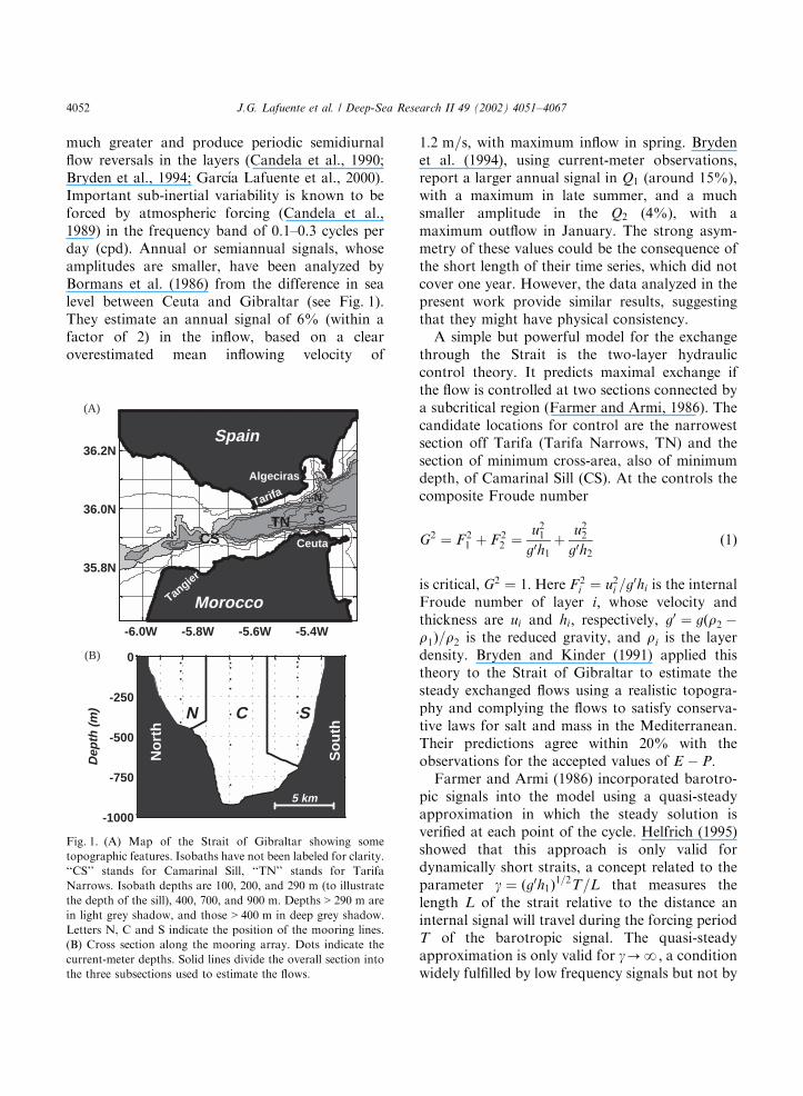
Fig. 1. (A) Map of the Strait of Gibraltar showing some

topographic features. Isobaths have not been labeled for clarity.

‘‘CS’’ stands for Camarinal Sill, ‘‘TN’’ stands for Tarifa

Narrows. Isobath depths are 100, 200, and 290 m (to illustrate

the depth of the sill), 400, 700, and 900 m: Depths > 290 m are

in light grey shadow, and those > 400 m in deep grey shadow.

Letters N, C and S indicate the position of the mooring lines.

(B) Cross section along the mooring array. Dots indicate the

current-meter depths. Solid lines divide the overall section into

the three subsections used to estimate the flows.

J.G. Lafuente et al. / Deep-Sea Research II 49 (2002) 4051–40674052

tidal fluctuations (Helfrich, 1995; Garc!ıa Lafuenteet al., 2000).

The model can still be applied to a situation ofsubmaximal exchange in which the control at TNis lost. In this case, the interface in the Strait wouldrespond to changes in the Mediterranean since it isnow possible for a signal to travel upstreamthrough the Strait into the Atlantic Ocean. Bor-mans and Garrett (1989) developed these ideas inorder to reconcile experimental observations at theeastern entrance of the Strait, which pointed toclear submaximal exchange, and the model pre-dictions. In fact, they used a particular solution ofthe model, known as marginally submaximalexchange, in which the flow east of the contractionremains subcritical but the flows exchanged arestill maximal. This solution can be considered as alimit of the strictly submaximal solution forincreasing flows. Whether the exchange is maximalor submaximal is still a matter of controversy.Both types of exchanges have been reported in theliterature (see Garrett (1996) for an extensive andinteresting review on the subject).

In the case of submaximal exchange, the basinsare not isolated from each other and the condi-tions in the Mediterranean Sea directly affect theflows. The westernmost basin of the sea is usuallyoccupied by a large anticyclonic gyre (see Lanoix(1974) for instance). It exhibits a large timevariability (Heburn and La Violette, 1990) thatmust be taken into account to provide a consistentdescription of the flow variability if the exchange issubmaximal.

This work analyses the annual and semiannualsignals in the exchange based on long time seriesacquired in the frame of the Canary Island AzoresGibraltar Observations (CANIGO) EuropeanUnion project.

2. Data and methods

2.1. Data-set

From October 1995 to May 1998 a mooringarray of recording currentmeters was deployed inthe eastern part of the Strait of Gibraltar withinCANIGO to help resolve the different time-scales

of the exchange. Figs. 1A and B roughly show theposition and depth of the instruments. A widevariety of problems have reduced the availableinformation to that summarized in Table 1. Forconvenience, the entire period of observations hasbeen divided into three sub-periods, which shall bereferred to as PP (for ‘‘Pilot Phase’’, spanningfrom October 1995 to May 1996), P2 ( for ‘‘Period2’’, from July 1996 to July 1997) and IP (for‘‘Intensive Phase’’, from July 1997 to May 1998).The spatial coverage during PP was good, but notso during P2 when only the North line workedproperly. During IP the north line was lost, henceno information from this location is available.

Meteorological data during the same period asthe oceanographic observations were collectedfrom the Instituto Meteorol !ogico Nacional(IMN). They include local atmospheric pressureand winds in Tarifa and Ceuta, as well as theaverage atmospheric pressure over the Gulf ofC!adiz and the Western Mediterranean (from dailyforecast bulletins published by IMN). Sea-leveldata also were collected in Algeciras, Tarifa (onthe north shore of the Strait) and Ceuta (southshore).

2.2. Transport estimates

Tidal currents can contribute to the mean flowthrough well-defined correlations between theinterface oscillation and the strength of the current(Bryden et al., 1994). Contrary to CS, thismechanism is not important in the eastern section(Garc!ıa Lafuente et al., 2000). Therefore, theslowly varying transport here can be estimateduniquely using the tidal-free velocity measure-ments. Details of the procedure used to obtainthese velocities can be seen in Garc!ıa Lafuente et al.(1998, 2000).

The velocities obtained in this manner have atypical baroclinic structure. The subinertial me-teorologically forced fluctuations are not strongenough generally to reverse flows in either layer, sothat the surface of along-strait null velocity is well-defined and considered as the interface. The inflowQ1 and the outflow Q2 are computed according to

J.G. Lafuente et al. / Deep-Sea Research II 49 (2002) 4051–4067 4053

Q1ðtÞ ¼Zy

Z 0

Z2ðy;tÞuðy; z; tÞ dz dy; ð2Þ

Q2ðtÞ ¼Zy

Z Z2ðy;tÞ

bottomðyÞuðy; z; tÞ dz dy; ð3Þ

where Z2ðy; tÞ is the depth of the interface at instantt; and uðy; z; tÞ is the along-strait velocity, whichhas been filtered with a Gaussian-like filter of 0.25cpd cut-off frequency. The Cartesian referencesystem has been rotated þ171 in order to have thex-axis oriented along strait. The y-axis points tothe north shore and the z-axis is positive upwards.The depth of the interface has been determined bylinear interpolation between the two depths atwhich uðy; z; tÞ changes sign. The integrals abovehave been replaced by summations over the threeboxes sketched in Figure 1B. Each vertical boxallows for estimations of partial flows throughthem. Low-frequency velocities at the same depthsin the center and south moorings taken during IPare highly correlated ðr2 > 0:93Þ: This fact has beenused to infer inflowing velocities at the southmooring from observations at the central one inorder to supplement the lack of information

present during PP. The velocities measured byeach mooring line and those extrapolated in thesouth during PP are considered to be representa-tive of each subsection. They have been inter-polated/extrapolated to obtain a velocity every10 m and multiplied by the cross area associatedwith the 10-m thick bin to obtain the flows. Detailsof the computation can be seen in Garc!ıa Lafuenteet al. (2000).

Table 1 indicates that such computation is notfeasible during P2 and IP. In these cases linearextrapolations to obtain total flows from partialflows have been made.

2.2.1. Regression model

The following very simple model has been used:

y ¼ y0 þ hðx� %xÞ; ð4Þ

where y is the output, x and %x are the input and itsmean, respectively, and y0 and h are the modelparameters. During P2, the outputs were the totalflows, Q1 and Q2; and Z2C (the depth of theinterface at the center line, which will be con-sidered the reference depth of the interface at theeastern section throughout this paper) and the

Table 1

Sketch of the temporal and spatial coverage of the current-meter data used to estimate flows

1995 1996 1997 1998 Position Depth (m)

O N D J F M A M J J A S O N D J F M A M J J A S O N D J F M A M 40 ■■■■■■■■■■■■ ■■■■■■■■■■■■■■■■■■■■■■■90 ■■■■■■■■■■■■ ■■■■■■■■■■■■■■■■■■■■■■■

140 ■■■■■■■■■■■■ ■■■■■■■■■■■■■■■■■■■■■■■ INTENSIVE PHASE265 ■■■■■■■■■■■■ ■■■■■■■■■■■■■■■■■■■■■■■

North36º02.4N5º23.7W

430 ■■■■■■■■■■■■ ■■■■■■■■■■■■■■■■■■■■■■■

40 ■■■■■■■■■■■ ■■■■ ■ ■■■■■■■■■■■■ ■■70 ■■■■■■■■■■■ ■ ■■■■ ■■■■■■■■■■■■ ■■

140 ■■■■■■■■■■■ ■■■■ ■ ■■■■■■■■■■■■■■200 ■■■■■■■■■■■ PERIOD 2 ■■■■ ■ ■■■■■■■■■■■■■■360 ■■■■■■■■■■■ ■■■■ ■■■■■■■■■■■■■■■550 ■■■■■■■■■■■ ■■ ■■■ ■■■■■■■■■■■ ■■■

Center35º59.7N5º23.2W

800 ■■■■■■■■■■■ ■ ■■■■ ■■■■■■■■■■■■■ ■

35 ■■■■■■■■■■ ■■■■ ■■■■■65 PILOT PHASE ■■ ■■■■■■■■■■■■ ■■■■■

130 ■■■■■■■■■■■■■■■■■■■250 ■■■■■■■■■■■■ ■■■■■■■■■■■■■■■■■■■350 ■■■■■■■■■■■■ ■■■■■■■■■■■■■■■■■■■

South35º51.7N5º21.5W

550 ■■■■■■■■■■■■■■■■■■■

Gray squares mean instrument failures. The three sub-periods mentioned in the text are also indicated.

J.G. Lafuente et al. / Deep-Sea Research II 49 (2002) 4051–40674054

inputs Q1N; Q2N and Z2N (partial inflow andoutflow through the northern subsection anddepth of the interface at this point). During IPthe inputs were Q1C and Q2C and the outputs Q1N

and Q2N; which added up to Q1C and Q1S ðQ2C

and Q2S) giving the total inflow (outflow). In allcases the model parameters have been estimatedwith the data taken during PP, when the spatialcoverage was good. Table 2 shows the parameterswith their errors at a 95% significance level. Theextrapolations for estimating Q1 and Z2C during P2had good statistical confidence and a highcorrelation coefficient whereas Q2 was not so welldetermined. The poorest correlation coefficientwas obtained when inferring Q2N from Q2C duringIP. Nevertheless the contribution of the former tothe total outflow is very small, so that the finalestimation of Q2 is not overly affected by this fact.

The model of Eq. (4) could have been extendedto a multiple regression model including moreinput variables such as cross-strait sea-level slopes,wind stress, atmospheric pressure differences, etc.This would have improved the value of r2 in allcases but reduced the statistical confidence of theregression. Moreover, such a model introducesartificial correlations between the input variablesand the output, which does not seem advisable ifone is looking for independent correlations be-tween external agents and the flows or the depth ofthe interface. This is the reason why the simplemodel of Eq. (4) was used.

2.2.2. Means

The procedure to obtain flows through Eqs. (2)and (3), along with the instrumental errors and the

commented extrapolations, make the acceptedflows during the whole period somewhat uncer-tain. Merging the subseries can produce jumps inthe junctions. To analyze very low-frequencysignals (annual and semiannual cycles) it has beenassumed that the mean value from October 1995to May 1996 (the whole PP), from October 1996 toMay 1997 (a fraction of P2) and from October1997 to May 1998 (a fraction of IP) should beapproximately the same. Other time series such asatmospheric pressure or sea level did not exhibittrends, a fact that supports this assumption. Acorrection of Q1 and Q2 during periods P2 and IPhas been made to bring together the means. Thenear one-year length of these series prevents theintroduction of spurious signals as would be thecase if PP were corrected, since a correction of themean in a six-month time series would introducean artificial annual signal.

The final time series of Q1; Q2 and Z2C areshown in Fig. 2. Their means and standarddeviations are 0:9770:14 Sv; �0:8470:09 Sv and�128712 m; respectively, which are only indica-tive due to the way in which they have beenobtained. More elaborated computations, basedon an inverse model that includes the mostimportant tidal constituents applied to 1-year long

0.0

0.5

1.0

1.5

2.0

Q1(S

v)

PILOT PHASE PERIOD 2 INTENS. PHASE

-2.0

-1.5

-1.0

-0.5

Q2(S

v)

400 600 800 1000 1200-200

-150

-100

-50

η 2C(m

)

Day from 01-01-95

Fig. 2. Time series of the flows estimated from the data set (top

panel) and depth of the interface at the Centre mooring line

(bottom panel).

Table 2

Adjustment parameters of the model of Eq. (4)

Output y0 h r2 F

Q1 (P2) 0:3570:03 3:8970:02 0.83 1681

Q2 (P2) �0:6370:03 2:8070:25 0.58 486

Z2C (P2) �67:174:0 0:4970:03 0.73 924

Q1N (IP) �0:01370:01 0:43470:023 0.75 1059

Q2N (IP) 0:03670:027 0:19170:038 0.22 99

Last two columns give the regression coefficient and the

statistical F of the model. The intervals of confidence are at

95% significance level. The different outputs are explained in

the text.

J.G. Lafuente et al. / Deep-Sea Research II 49 (2002) 4051–4067 4055

data set, suggests around a 10% drop in meanflows (Bascheck et al., 2001). The figures abovetally with these results within a standard deviation.Nevertheless, the main objective of this work is toinvestigate annual and semiannual signals, whichprobably have not been masked by data proces-sing.

3. Low-frequency signals

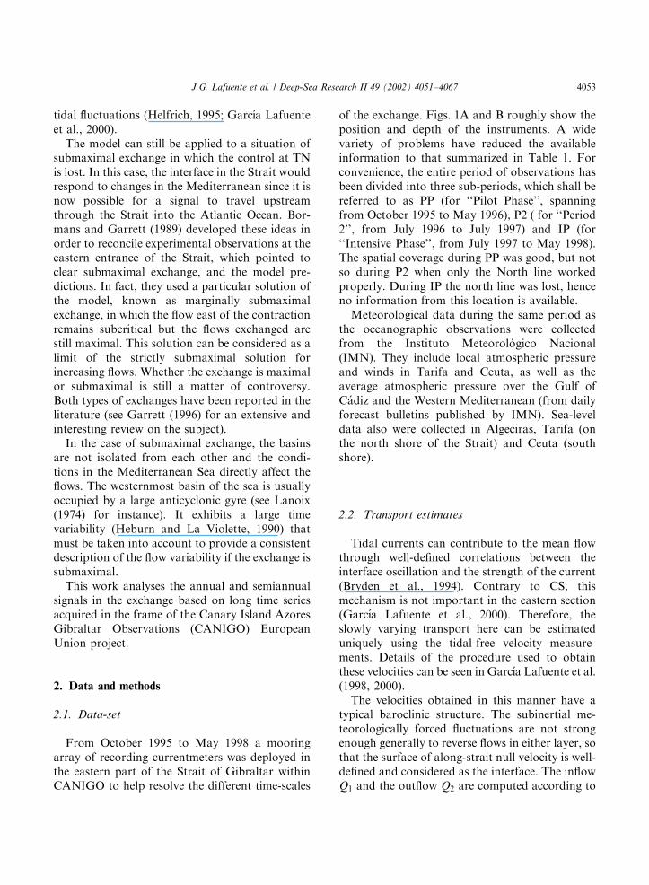
Fig. 2 shows that most of the variance resides inthe high (but still subinertial) frequency band. Toremove high-frequency variability, blocks 15-daylong that overlap 7.5 days have been averaged overand the resulting series smoothed again with afilter of weights 0.25, 0.5, and 0.25. The standarddeviation within each block is taken as the error ofthe estimate. These new series, which are plotted inFig. 3, have been analyzed to investigate annualand semiannual cycles. The existence of signals of

frequencies fa ¼ 1 cycle per year ¼ 1:99�10�7 rad=s and fs ¼ 2fa ¼ 3:98� 10�7 rad=s havebeen assumed and the model

y ¼ y0 þ Bðt� tmÞ þ Aa cosðfat� jaÞ

þ As cosðfst� jsÞ þ e ð5Þ

has been adjusted to the data. Here Aa and As arethe amplitudes of the annual and semiannualcycles, ja and js their phases (which refer to thebeginning of 1995, that is, to the beginning of theyear), and e is the unexplained residue of zeromean. The parameter B is included to allow fortrends (but in all cases it is not statisticallydifferent from zero, as can be expected aftermaking the mean adjustment mentioned above),tm is the time of the midpoint of the series, and y0is a parameter that would be identified with themean value of y: Table 3 shows the value of thedifferent parameters and their errors at 95%confidence level for Q1; Q2 and Z2C: The mostnoticeable feature is the existence of a significantannual cycle for Q1; this being less significant forQ2 and Q2C; both of which have semiannualdominance. The ratio As=Aa for the latter vari-ables is around 2 and their phases suggest that theyare correlated (note that js ¼ 1741 for Q2 becomes

js ¼ 3541 for jQ2j; which is within the error of js

for Z2C).

3.1. The annual cycle

The annual signal in Q1 can be a consequence ofa signal in the inflowing velocity, in the cross-area,or in both. In a two-layer sea, Q1ðtÞ ¼ U1ðtÞA1ðtÞwhere U1ðtÞ is the (uniform) time-dependentinflowing velocity and A1ðtÞ is the time-dependentcross-area of the layer. It changes mainly due tointerface oscillations, so that U1ðtÞ ¼Q1ðtÞ=ðZ2CðtÞW Þ; where W ¼ 14500 m is the widthof the Strait. Table 3 shows the result of applyingEq. (5) to this velocity. The annual cycle of U1 andZ2C (and, hence, of A1) are B7:2% and B3:5% oftheir mean values, respectively. They will con-tribute in the same proportion to the annual cycleof the inflow, that is, velocity fluctuations con-tribute twice as much as interface fluctuations. Therectified transport arising from the positive corre-lation between interface and velocity fluctuationsis evaluated in o0:1% of the mean inflow and,hence, can be neglected.

Bryden et al. (1994) provide the only estimatesof annual signals in the exchanged flows based on

0.0

0.5

1.0

1.5

Q1(S

v)

-1.5

-1.0

-0.5

Q2(S

v)

10 15 20 25 30 35 40-200

-150

-100

-50

η 2C(m

)

Month from 01-95

Fig. 3. Fifteen-day averaged time series of the flows and the

interface depth at the Center mooring line (dots, upper panel

and lower panels, respectively) and standard deviation for these

means (bars). Only one mean per month has been displayed for

clarity. The solid line is the fitted curve of the model of Eq. (5).

J.G. Lafuente et al. / Deep-Sea Research II 49 (2002) 4051–40674056

experimental observations. Their data set spannedover less than one year so that the cycle is not well-defined. They report annual signals of 0:12 Sv at2641 for Q1; 0:03 Sv at 231 for jQ2j and 18 m at 411for Z2C in CS. The concordance between theamplitude and phase of Q1; and between theamplitude of jZ2j and the phase of Z2C is good.

The last row of Table 3 shows the annual andsemiannual cycles of the difference of densities Drbetween Atlantic surface water and Mediterraneandeep water reported by Bormans et al. (1986) anddetermined from a long historical data set ofsalinity and temperature in the Strait of Gibraltarand its surroundings. The clear annual signal in Drand the good agreement with the phase of Q1

suggest that the inflow annual cycle is caused bythe seasonal signal in the density difference, whichdoes not exhibit a semiannual signal either. Thequestion of why the annual signal in Dr would notinduce a comparable signal in the outflow, whichremains rather insensitive, is discussed inSection 5.

3.2. The semiannual cycle

This is the prevailing signal in Q2 and Z2C: Theirphases suggest good correlation between them: the

greater the outflowing section (that is, the higherthe interface) the greater jQ2j: The interfaceoscillation is, however, unable to account for theobserved amplitude of the outflow. Its amplitudeonly changes the outflowing section by 2.5%,which is less than the 7% variation estimated inthe outflow. An additional signal in the outflowingvelocity U2 is needed in order to explain theestimated semiannual fluctuation. Similar compu-tations as those carried out previously provide theamplitude and phase presented in Table 3. Thesemiannual signal is clear and it has the necessaryvalue to explain the remaining percentage.

One possible force to drive the semiannualcycles could be wind-stress, which also exhibitsquite a clear semiannual signal (see Table 3). Windstress correlates positively with the atmosphericpressure differences between the Atlantic (Gulf ofCadiz) and western Mediterranean basins (correla-tion coefficient of 0.75), which also has a dominantsemiannual cycle. The phases of the semiannualcycles of jQ2j and Z2C lag by 431 and 631 (21 and 31days), respectively, to wind stress, which does notdisagree with a cause–effect relationship. Thelagged correlation between wind stress and theinterface depth shows a peak of 0.6 for a lag of thismagnitude. Some speculative arguments put for-

Table 3

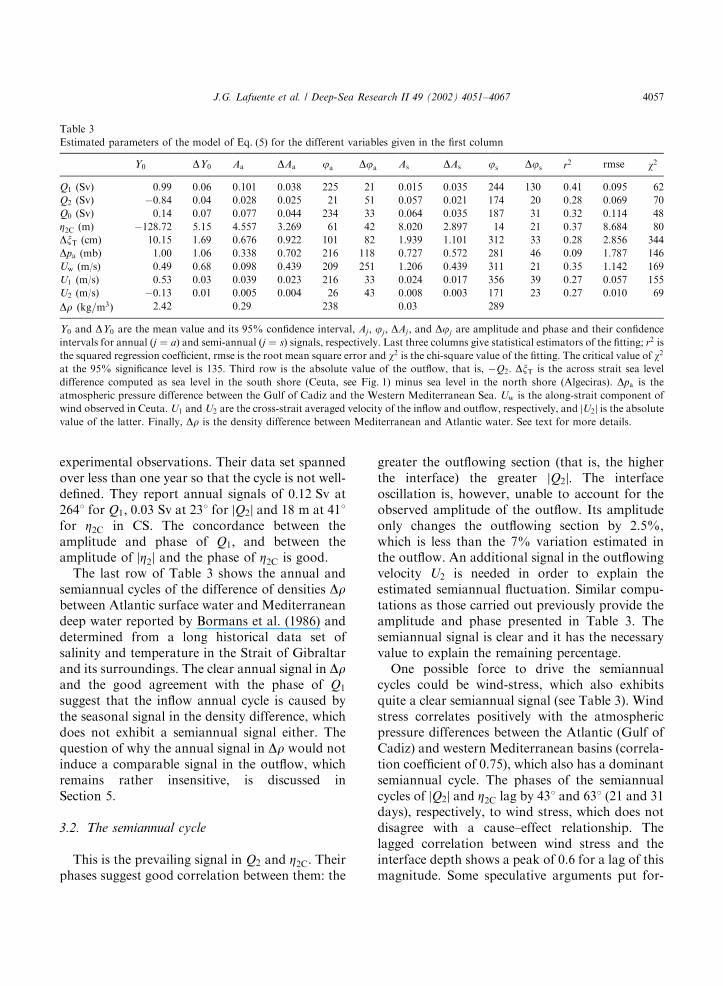
Estimated parameters of the model of Eq. (5) for the different variables given in the first column

Y0 DY0 Aa DAa ja Dja As DAs js Djs r2 rmse w2

Q1 (Sv) 0.99 0.06 0.101 0.038 225 21 0.015 0.035 244 130 0.41 0.095 62

Q2 (Sv) �0.84 0.04 0.028 0.025 21 51 0.057 0.021 174 20 0.28 0.069 70

Q0 (Sv) 0.14 0.07 0.077 0.044 234 33 0.064 0.035 187 31 0.32 0.114 48

Z2C (m) �128.72 5.15 4.557 3.269 61 42 8.020 2.897 14 21 0.37 8.684 80

DxT (cm) 10.15 1.69 0.676 0.922 101 82 1.939 1.101 312 33 0.28 2.856 344

Dpa (mb) 1.00 1.06 0.338 0.702 216 118 0.727 0.572 281 46 0.09 1.787 146

Uw (m/s) 0.49 0.68 0.098 0.439 209 251 1.206 0.439 311 21 0.35 1.142 169

U1 (m/s) 0.53 0.03 0.039 0.023 216 33 0.024 0.017 356 39 0.27 0.057 155

U2 (m/s) �0.13 0.01 0.005 0.004 26 43 0.008 0.003 171 23 0.27 0.010 69

Dr ðkg=m3Þ 2.42 0.29 238 0.03 289

Y0 and DY0 are the mean value and its 95% confidence interval, Aj ; jj ; DAj ; and Djj are amplitude and phase and their confidence

intervals for annual ðj ¼ aÞ and semi-annual ðj ¼ sÞ signals, respectively. Last three columns give statistical estimators of the fitting; r2 is

the squared regression coefficient, rmse is the root mean square error and w2 is the chi-square value of the fitting. The critical value of w2

at the 95% significance level is 135. Third row is the absolute value of the outflow, that is, �Q2: DxT is the across strait sea level

difference computed as sea level in the south shore (Ceuta, see Fig. 1) minus sea level in the north shore (Algeciras). Dpa is the

atmospheric pressure difference between the Gulf of Cadiz and the Western Mediterranean Sea. Uw is the along-strait component of

wind observed in Ceuta. U1 and U2 are the cross-strait averaged velocity of the inflow and outflow, respectively, and jU2j is the absolutevalue of the latter. Finally, Dr is the density difference between Mediterranean and Atlantic water. See text for more details.

J.G. Lafuente et al. / Deep-Sea Research II 49 (2002) 4051–4067 4057

ward to explain the links between wind stress andQ2 and Z2C are also discussed in Section 5.

3.3. Net barotropic signals and the Mediterranean

sea level cycles

3.3.1. Annual signals

Inflow and outflow annual signals combine toproduce a seasonal signal in the net barotropicflow that peaks in late August. The simplest modelin which this signal, Q0a; is balanced within theMediterranean Sea is

Q0a ¼ dVMED=dt ð6Þ

(VMED being the volume of the Mediterranean),which ignores the seasonal cycle of ðE � PÞ: Theequation is readily solved using the Q0 valuesshown in Table 3 to give an annual signal of1579 cm; with a maximum value in November.Larnicol et al. (1995) provide evidence of aseasonal cycle of the Mediterranean mean sealevel of around 10 cm using TOPEX/POSEIDONaltimetry data from October 1992 to September1994. Ayoub et al. (1998) also report a similarsignal of 8 cm of amplitude, with a maximumvalue in October, using ERS-1 and TOPEX/POSEIDON altimetry data from 1993. Thisannual signal is quite evident in longer time seriesof altimetry data (P.Y. LeTraon, personal com-munication). Tsimplis and Woodworth (1994),from coastal tide gauge records, show an annualsignal (the Sa tidal constituent) in the Mediterra-nean sea level that matches well the phase of thesealtimetry signals but with a smaller amplitude(around 5 cm). The disagreement of amplitudescan be accounted for by the fact that the altimetrysignal comes mainly from the open sea while tidegauge data are coastal observations. Part of thissignal is due to temperature and salinity stericeffects that are given by (Patullo et al., 1955)

xT ¼ g�1

Z p0

pa

ar�1DT dp; ð7Þ

xS ¼ �g�1

Z p0

pa

br�1DS dp; ð8Þ

where xT ðxSÞ is the sea-level steric anomaly due totemperature (salinity) difference DT ðDSÞ with

respect to the mean at a given depth. Integralsextend from the surface ðp0Þ to depth pa; where theseasonal signal does not reach, and a ðbÞ is thecoefficient of thermal (haline) expansion of seawater. The MEDATLAS data set (MEDATLASConsortium, 1997) contains monthly temperaturevalues at fixed depths, which have been optimallyinterpolated from a large set of in-situ observa-tions covering the whole Mediterranean Sea. Italso contains seasonally averaged salinity values.With these data and Eqs. (7) and (8), the stericanomalies at grid points of a roughly regular gridcovering the Mediterranean Sea have been esti-mated. The depth of reference was taken at pa ¼300 db: The results for the steric thermal andhaline anomalies are presented in Figs. 4A and B,respectively. The solid lines are the annual cyclesthat best fit to each of them and would berepresentative of the seasonal cycle of the stericsea level anomaly of the Mediterranean Sea. Theyhave 5:570:4 cm of amplitude and 2537121 ofphase (12 September) for the thermal contribution

-10

-5

0

5

10

Jn Fb Mr Ap My Jn Jl Ag Sp Oc Nv Dc-2

-1

0

1

2

ξ str

S (

cm)

ξ str

T (

cm)

Year month

(A)

(B)

Fig. 4. (A) Thermal steric anomaly of the Mediterranean Sea

level calculated from MEDATLAS data base using 300 db as

reference. Dots are the monthly anomalies at 133 different sites

distributed homogeneously over the Mediterranean Sea. The

solid line is the sine least-squares fitted curve to the local

anomalies. (B). Haline steric anomaly determined from seasonal

values and using the same depth as before. The solid fitted line

is not statistically different from zero indicating a null

contribution of the haline effect to the total steric anomaly.

J.G. Lafuente et al. / Deep-Sea Research II 49 (2002) 4051–40674058

and are not significantly different from zero for thehaline contribution ð0:1170:24 cmÞ:

When this anomaly is subtracted from the sealevel cycle mentioned by Larnicol et al. (1995)or reported by Ayoub et al. (1998) the resultis far from the 15 cm of amplitude implied bythe Q0 signal found in this study. The correctmass balance cannot ignore the clima-tological ðE � PÞ forcing, and Eq. (6) should bere-writen as

Q0a � ðE � PÞa ¼dVMED

dt¼ AMED

dxmdt

; ð9Þ

where ðE � PÞa is the annual signal in the netevaporation, AMED ¼ 2:5� 1012 m2 is the area ofthe Mediterranean Sea, and xm the contributiondue to an effective mass variation within the sea.Obviously, xm ¼ xobs � xstr; where xobs is theobserved sea-level signal and xstr is the stericcontribution. With the values provided by Ayoubet al. (1998) and after correcting for the stericanomaly estimated above, the RHS of Eq. (9)takes a value of around 0:02 Sv at 2301; which inturns gives 0:06 Sv at 2371 for ðE � PÞa using theQ0 seasonal cycle shown in Table 3. The seasonalnet evaporative cycle is difficult to evaluate, in partbecause of its interannual variability. Evaporationis maximum during late autumn, but the peak ofðE � PÞ is probably shifted towards summer, thedry season, due to the contribution of theprecipitation. Carter (1956) suggests a cycle inthe Mediterranean of around 6 cm=monthð0:06 SvÞ that peaks in August ð2151Þ: Bormanset al. (1986) consider the values from the WorldSurvey of Climatology (Wallen, 1970) to obtain aseasonal signal of 7:1 cm=month ð0:07 Sv) at 1811:The agreement with the values computed fromEq. (9) is satisfactory, particularly regarding am-plitudes. The phases will surely agree within theconfidence intervals, but it is not possible toprovide figures for them due to the lack ofinformation regarding their values forðE � PÞa and xobs:

3.3.2. Semiannual signals

The semiannual signal of Q2 is chiefly respon-sible for the semiannual cycle of Q0 indicated inTable 3. The mass balance of Eq. (6), which

assumes the absence of a semiannual net evapora-tive cycle, would induce a sea-level signal in theMediterranean Sea of 6:473:5 cm at 2777311:Ayoub et al. (1998) report a semiannual signal of4 cm of amplitude in the Eastern MediterraneanBasin that is negligible in the Western Basin. It isequivalent to a signal slightly o3 cm for the wholeMediterranean. However, they do not mentionany phase for this signal.

Tsimplis and Woodworth (1994) also give valuesfor the semiannual (Ssa) tidal constituent in theMediterranean based on tide gauge data (in spiteof the fact that they use this tidal nomenclature,they show that the gravitational part is small notonly in Ssa but also in the above-mentioned Saconstituent, and that they mainly stem frommeteorological, oceanographic and hydrologi-cal—river runoff—forcing). This signal has notice-able regional variability but, excluding the AegeanSea and the far Eastern areas of the Mediterra-nean, the phases of most of the remaining coastalsea level stations are between �2 and �1 monthswith reference to the first day of the year ð2401–3001 in our nomenclature) and the amplitudesrange from 1 to 5 cm (3 cm could be a ‘‘typical’’value). This amplitude roughly coincides with theamplitude determined from altimetry data andboth reside in the lower part of the error interval ofthe estimate from Q0 cycle shown in Table 3.However, the estimates from coastal tide gaugescome from non-simultaneous time series. Takinginto account the nature of the semiannual forcing,the regional variability reported by Tsimplis andWoodworth (1994) also could be indicative ofinterannual variability of the Mediterranean sur-face circulation, and if this were so their resultswould not be suitable for comparison with theestimate presented in this study.

The right mass balance for this signal shouldinclude climatological forcing as well (Eq. (9)).The semiannual cycle of ðE � PÞ; if real, is evenmore unknown than the annual one. Bormans et al.(1986) mention a signal of 2:5 cm=monthð0:024 SvÞ at 461; which gives 0:084 Sv at 1971for the LHS term of equation ecuacion 9. This, inturns, would increase the amplitude of the sea-levelsignal up to 8:4 cm; the phase being hardlymodified ð2871Þ: The new amplitude would

J.G. Lafuente et al. / Deep-Sea Research II 49 (2002) 4051–4067 4059

disagree even more with the ‘‘direct observations’’of sea level.

4. Hydraulic control model versus observations

4.1. Some theoretical considerations

One striking result that can be seen in Table 3 isthat Q1 and Q2 cycles are not coupled, that thecycles of Z2C are linked to Q2 rather than to Q1;and that the cycles of the net barotropic flow ariseas a consequence of this uncoupling. An attempthas been made to interpret these observations inthe frame of the hydraulically controlled exchangecommented in Section 1.

The maximal exchange situation requiresthe existence of two control sections, one inCamarinal Sill (CS) and the other in TarifaNarrows (TN) (see sketch in Fig. 5). Basically,

the first one would control the outflow (G2S in

Eq. (1) reaches the critical value 1 mainly due to

the contribution of F22S), while the second one

would control the inflow ðF21N is the term that

brings G2N to critical).

It is easy to show that the above-mentionedresults, are not compatible with this maximalexchange situation. For instance: one possibilityfor flow variations is that g0 changes due toseasonal fluctuations in the inflow density. Undermaximal exchange, the flows are proportional tog01=2 and both Q1 and Q2 must fluctuate in phase.On the other hand, if g0 remains constant, anyfluctuation of, say, Q1 must be accomplished by anincrement in the inflowing velocity and a deepen-ing of the interface at TN in order to maintain thecritical flow there. This perturbation of the inter-face in TN is capable to progressing freely throughthe subcritical region west of TN and to reach CS,sinking the interface here. The outflowing velocitymust decrease (in modulus) in order to maintainthe critical condition in CS so that jQ2j diminishes.Therefore, an increase of Q1 produces a decreaseof jQ2j and a deepening of the interface, allvariables fluctuating in phase, and both flowscontribute approximately by the same amountðQ0=2Þ to the net barotropic signal. As this does

not match the observations made in this work, themaximal exchange state must be rejected.

The outflow is likely to be hydraulicallycontrolled in CS, since water of the same densityas the outflow is found at a greater depth in theAtlantic Ocean. Therefore, that the maximalexchange is not achieved should be due to the factthat the TN control section is not present.

4.2. A simple unidimensional model

Under these circumstances it is possible to usethe unidimensional model proposed by Bormansand Garrett (1989), who used triangular crosssections to represent the actual topography of theStrait. Their model can take into account theeffects of bottom and interfacial friction, althoughin this work the simpler frictionless model has beenused. Rotation effects are not considered, so thatthe interface has no cross strait structure and itsdepth can be identified with the Z2C estimates givenhere. They obtain a differential equation with asingle unknown (Z2ðxÞ; see Eq. (4.10) of theirwork), which has the following form:

@

@x

Q21

2A1ðxÞ�

Q22

2A2ðxÞ� g0Z2ðxÞ

� �¼ 0: ð10Þ

This equation can be integrated with the conditionof critical flow at CS, which can be written for

Q1 h1S u1 h1N

supercritical subcritical supercritical

h2S Q2 h2N

u2

1'' 2

22

1

212 =+=

S

S

S

SS hg

u

hg

uG 1

'' 2

22

1

212 =+=

N

N

N

NN hg

u

hg

uG

Fig. 5. Sketch of the two-layer model in the case of maximal

exchange showing the supercritical and subcritical regions and

the control sections.

J.G. Lafuente et al. / Deep-Sea Research II 49 (2002) 4051–40674060

triangular geometry as

Q21

g0A31S

þQ2

2

g0A32S

¼h1S þ h2S

WSh2S; ð11Þ

where subscripts 1 and 2 refer to the upper andlower layer, respectively, A and W stand for crossareas and width of the Strait at the surface,respectively, which depend on the position, sub-script S is for Sill, and h1 and h2 are the thicknessof the upper layer and the distance from theinterface depth to the sea floor at the axis of theStrait, respectively. Flows Q1 and jQ2j may differso that the model allows for barotropic fluctua-tions Q0 ¼ Q1 þQ2:

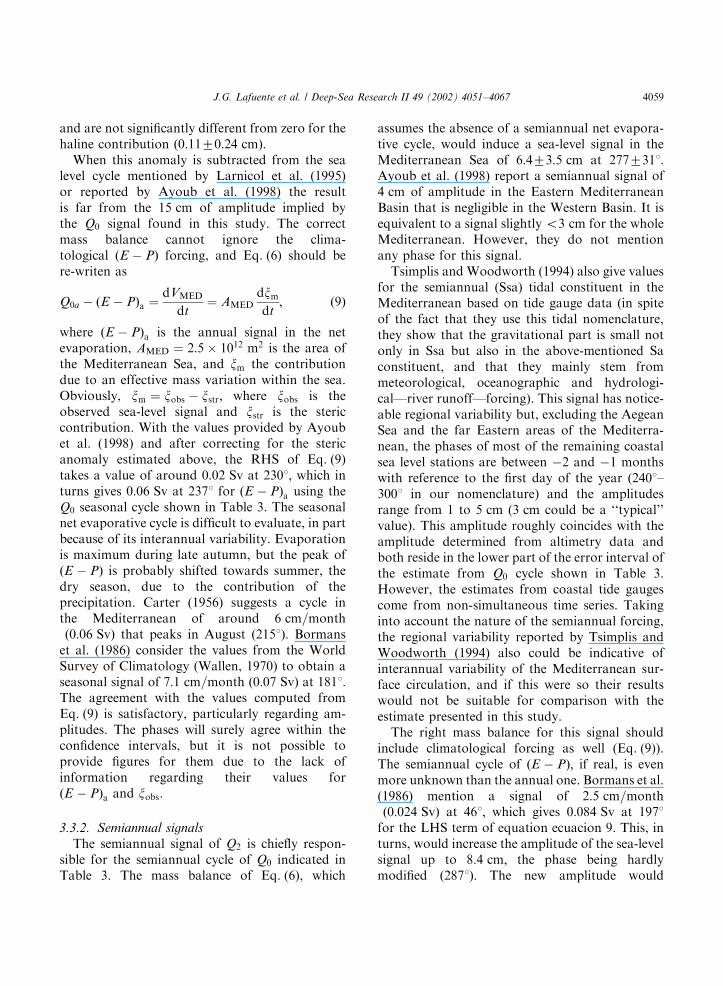
Given a barotropic fluctuation Q0; the modelcan be integrated if (I) the value of one of theexchanged flows is provided (the other beingautomatically determined) or (II) the existence ofTN control section is assumed, in which case theexchanged flows are determined by the geometryof the Strait and are outputs of the model.Needless to say, they are the maximum allowableflows (maximal exchange). Under this secondassumption, one still obtains the two expectedsolutions, one corresponding to strictly maximalexchange with supercritical flow east of TN, theother corresponding to marginally submaximalexchange with subcritical flow east of TN but withthe same exchanged flows. The three possibilitiesare presented in Fig. 6. Obviously, the Eqs. (10)and (11) have no solution if, in case I, one providesa flow greater than the one obtained in the secondsituation.

Fig. 7A shows that for maximal or marginallysubmaximal exchange a positive (negative) baro-tropic fluctuation Q0 sinks (raises) Z2;C; the

response being greater in the second situation. Inthese cases, as mentioned above, a barotropicfluctuation of amplitude Q0 is achieved veryapproximately by a simultaneously linked fluctua-tion of amplitude Q0=2 in both Q1 and Q2: On thecontrary, Fig. 7B shows that under submaximalconditions Q1 can fluctuate independently of jQ2jand Z2;C (thin line). However, the fluctuations of

these two variables are still linked to each other(thick line) as a consequence of the outflow beingcontrolled at CS. Thus, a barotropic fluctuation of

-150

-100

-50

0

η 2 (m

) (a)

(b)

(c)

Q0=0 Sv

CS TN East

0 10 20 30 400

1

2

G2

Distance from CS (Km)

(a)

(b)(c)

(A)

(B)

Fig. 6. (A) Solution of Eqs. (10) and (11) for the interface

height between CS and the eastern section for the maximal (a),

marginally submaximal (b) and submaximal (c) exchanges and

zero net barotropic transport. (B) Composite Froude number

G2 for these three situations.

0.6 0.8 1 1.2 1.4 1.6 1.8

-150

-125

-100

-75

Q1 or |Q

2| (Sv)

η 2C (

m)

Q1c

Q2c

η 2(|Q 2

|,Q 1=constant)

η2(Q

1,Q

2=constant)

-0.8 -0.4 0 0.4 0.8-150

-125

-100

-75

-50

-25

0

(b)

(a)

Q0=Q

1+Q

2 (Sv)

η 2C (

m)

(A)

(B)

Fig. 7. (A) Interface height at the eastern section as a function

of the net barotropic transport for the maximal (a) and

marginally submaximal (b) exchanges. (B) Interface height

fluctuations as a function of the net barotropic transport for

submaximal exchange if the inflow remains constant (thick line)

or if the outflow remains constant (thin line). The barotropic

fluctuation is achieved by outflow variations in the first case and

by inflow variations in the second one, which in these

circumstances are not coupled. Dots labeled Q2C and Q1C

indicate that for these values of the net barotropic flow, the

exchange has been brought to maximal.

J.G. Lafuente et al. / Deep-Sea Research II 49 (2002) 4051–4067 4061

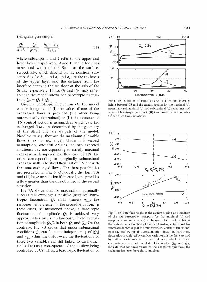
amplitude Q0 can be achieved by independentfluctuations of Q1; or of Q2; or both. This resultagrees with the authors’ observations. Fig. 8Ashows that the prediction of Z2;C given by the

model using the values of Q1 and Q2 shown inFig. 3 as inputs compares well with the estimatedinterface depth from the data (correlation coeffi-cient of 0.57). Fig. 8B shows that the compositeFroude number is well below the critical value,strongly suggesting submaximal exchange.

The variations of g0 have not been considered inthe former discussion. The model has been runwith a constant density contrast. To assess theinfluence of g0 cycle on the predictions it has beenincorporated into the model and compared withthe observations. The comparison has been madeon the basis of monthly means and standarddeviations from the data. That is, all Januaryobservations have been averaged together to give arepresentative value for January, the same beingdone for the rest of the months of the year. Theresults are presented in Fig. 9 along with thepredictions of the model with and without g0 cycle.The correlation coefficient rises up to of 0.93 in thefirst case (g0 cycle). Probably this very high value issomewhat coincidental, but it is also indicative ofthe influence of the seasonal density signal on theexchanged flows.

5. Discussion

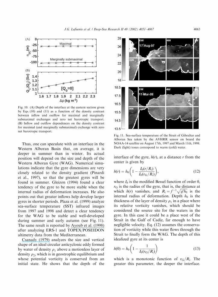
Let Table 3 be examined in greater detail. Theannual cycle seems forced by the seasonal signal ofDr (that is, by g0). Variations in g0 do not implynecessarily a phase-locked barotropic fluctuationQ0: In fact, Fig. 10B shows how under maximal(or marginally submaximal) conditions the inflow

and outflow change asffiffiffiffiffiffiDr

pwhile the net

barotropic flow is null. In these circumstances,the interface at the eastern end of the Straitremains practically motionless (Fig. 10A). Sincethe marginally submaximal situation is the physi-cal limit of increasingly submaximal exchange, onewould think that the latter should respondsimilarly to g0 variations, that is, without appreci-able barotropic signal and no interface motions.This is not the case in Table 3. The annual signalof Q1 is much greater than that of Q2; andproduces a clear signal in Q0: In addition theinterface oscillates in such a manner that it isdeeper when Q1 peaks and vice versa. Since theannual cycle of g0 does not imply the existence of acorresponding annual cycle in Q2C; the possibilityof this cycle being associated to interface oscilla-tions in the Western Alboran Basin has beenconsidered. Under submaximal conditions, theposition of this interface represents an effectivedriving force for the flows, which is independent ofthe direct influence that g0 exert on the exchangevia Eqs. (10) and (11).

-160

-140

-120

-100

η 2C (

m)

10 15 20 25 30 35 400

0.1

0.2

Month from 01-01-95

G2

(A)

(B)

Fig. 8. (A) Prediction of the interface height at the eastern

section given by Eqs. (10) and (11) (thick line) using the values

of Q1 and Q2 of Fig. 3. The 95% confidence interval is indicated

by the thin dashed line. Dots are the observations with their

error bars, as in Fig. 3. (B) Same as in (A) for the composite

Froude number G2 at the eastern section.

Jn Fb Mr Ap My Jn Jl Ag Sp Oc Nv Dc-160

-140

-120

-100

Year Month

η 2C (

m)

o=Observ. =Pred.(g´=cons.) =Pred.(g´=var.)

Fig. 9. Predictions of the interface height at the eastern section

given by Eqs. (10) and (11) using monthly values during the

entire period of observations and taken g0 as constant (thin line,

diamond symbol) and considering the annual cycle of g0 (thick

line, rectangle symbol). Dashed lines are the 95% confidence

interval for the predictions. Dots and error bars are the

monthly averaged observations.

J.G. Lafuente et al. / Deep-Sea Research II 49 (2002) 4051–40674062

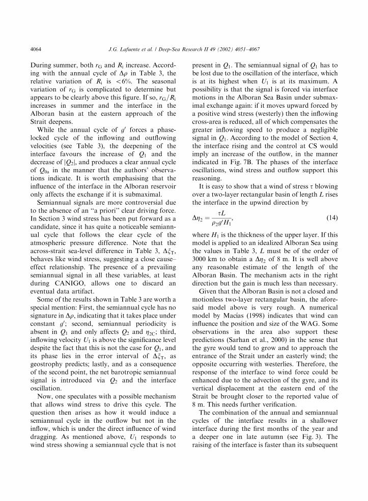
Thus, one can speculate with an interface in theWestern Alboran Basin that, on average, it isdeeper in summer than in winter. Its actualposition will depend on the size and depth of theWestern Alboran Gyre (WAG). Numerical simu-lations indicate that the gyre dimensions are veryclosely related to the density gradient (Pinardiet al., 1997), so that the greatest gyres will befound in summer. Gleizon (1994) found a cleartendency of the gyre to be more stable when theinternal radius of deformation increases. He alsopoints out that greater inflows help develop largergyres in shorter periods. Plaza et al. (1999) analyzesea-surface temperature (SST) infrared imagesfrom 1997 and 1998 and detect a clear tendencyfor the WAG to be stable and well-developedduring summer and early autumn (see Fig. 11).The same result is reported by Ayoub et al. (1998)after analyzing ERS-1 and TOPEX/POSEIDONaltimetry data from the Mediterranean.

Csanady (1979) analyzes the size and verticalshape of an ideal circular anticyclonic eddy formedby water of density r1 above a motionless layer ofdensity r2; which is in geostrophic equilibrium andwhose potential vorticity is conserved from aninitial state. He shows that the depth of the

interface of the gyre, hðrÞ; at a distance r from thecenter is given by

hðrÞ ¼ h0 1�I0ðr=RiÞI0ðrG=RiÞ

� �; ð12Þ

where I0 is the modified Bessel function of order 0,rG is the radius of the gyre, that is, the distance atwhich hðrÞ vanishes, and Ri ¼ f �1

ffiffiffiffiffiffiffiffig0h0

pis the

internal radius of deformation. Depth h0 is thethickness of the layer of density r1 in a place whereits relative vorticity vanishes, which should beconsidered the source site for the waters in thegyre. In this case it could be a place west of theStrait in the Gulf of Cadiz, far enough to havenegligible velocity. Eq. (12) assumes the conserva-tion of vorticity while this water flows through theStrait to finally form the WAG. The depth of thisidealized gyre at its center is

hð0Þ ¼ h0 1�1

I0ðrG=RiÞ

� �ð13Þ

which is a monotonic function of rG=Ri: Thegreater this parameter, the deeper the interface.

Fig. 11. Sea-surface temperature of the Strait of Gibraltar and

Alboran Sea taken by the AVHRR sensor on board the

NOAA-14 satellite on August 17th, 1997 and March 11th, 1998.

Dark (light) tones correspond to warm (cold) water.

-100

-75

-50

-25

0

η 2C(m

) Maximal

Marginally submaximal

1.6 1.7 1.8 1.9 2 2.1 2.2 2.31

1.11.21.31.4

∆ρ (kg m-3)

Q1,|Q

2| (S

v)

[Q0=0]

(A)

(B)

Fig. 10. (A) Depth of the interface at the eastern section given

by Eqs. (10) and (11) as a function of the density contrast

between inflow and outflow for maximal and marginally

submaximal exchanges and zero net barotropic transport.

(B) Inflow and outflow dependences on the density contrast

for maximal (and marginally submaximal) exchange with zero

net barotropic transport.

J.G. Lafuente et al. / Deep-Sea Research II 49 (2002) 4051–4067 4063

During summer, both rG and Ri increase. Accord-ing with the annual cycle of Dr in Table 3, therelative variation of Ri is o6%: The seasonalvariation of rG is complicated to determine butappears to be clearly above this figure. If so, rG=Ri

increases in summer and the interface in theAlboran basin at the eastern approach of theStrait deepens.

While the annual cycle of g0 forces a phase-locked cycle of the inflowing and outflowingvelocities (see Table 3), the deepening of theinterface favours the increase of Q1 and thedecrease of jQ2j; and produces a clear annual cycleof Q0a in the manner that the authors’ observa-tions indicate. It is worth emphasising that theinfluence of the interface in the Alboran reservoironly affects the exchange if it is submaximal.

Semiannual signals are more controversial dueto the absence of an ‘‘a priori’’ clear driving force.In Section 3 wind stress has been put forward as acandidate, since it has quite a noticeable semiann-ual cycle that follows the clear cycle of theatmospheric pressure difference. Note that theacross-strait sea-level difference in Table 3, DxT;behaves like wind stress, suggesting a close cause–effect relationship. The presence of a prevailingsemiannual signal in all these variables, at leastduring CANIGO, allows one to discard aneventual data artifact.

Some of the results shown in Table 3 are worth aspecial mention: First, the semiannual cycle has nosignature in Dr; indicating that it takes place underconstant g0; second, semiannual periodicity isabsent in Q1 and only affects Q2 and Z2C; third,inflowing velocity U1 is above the significance leveldespite the fact that this is not the case for Q1; andits phase lies in the error interval of DxT; asgeostrophy predicts; lastly, and as a consequenceof the second point, the net barotropic semiannualsignal is introduced via Q2 and the interfaceoscillation.

Now, one speculates with a possible mechanismthat allows wind stress to drive this cycle. Thequestion then arises as how it would induce asemiannual cycle in the outflow but not in theinflow, which is under the direct influence of winddragging. As mentioned above, U1 responds towind stress showing a semiannual cycle that is not

present in Q1: The semiannual signal of Q1 has tobe lost due to the oscillation of the interface, whichis at its highest when U1 is at its maximum. Apossibility is that the signal is forced via interfacemotions in the Alboran Sea Basin under submax-imal exchange again: if it moves upward forced bya positive wind stress (westerly) then the inflowingcross-area is reduced, all of which compensates thegreater inflowing speed to produce a negligiblesignal in Q1: According to the model of Section 4,the interface rising and the control at CS wouldimply an increase of the outflow, in the mannerindicated in Fig. 7B. The phases of the interfaceoscillations, wind stress and outflow support thisreasoning.

It is easy to show that a wind of stress t blowingover a two-layer rectangular basin of length L risesthe interface in the upwind direction by

DZ2 ¼tL

r2g0H1; ð14Þ

where H1 is the thickness of the upper layer. If thismodel is applied to an idealized Alboran Sea usingthe values in Table 3, L must be of the order of3000 km to obtain a DZ2 of 8 m: It is well aboveany reasonable estimate of the length of theAlboran Basin. The mechanism acts in the rightdirection but the gain is much less than necessary.

Given that the Alboran Basin is not a closed andmotionless two-layer rectangular basin, the afore-said model above is very rough. A numericalmodel by Mac!ıas (1998) indicates that wind caninfluence the position and size of the WAG. Someobservations in the area also support thesepredictions (Sarhan et al., 2000) in the sense thatthe gyre would tend to grow and to approach theentrance of the Strait under an easterly wind; theopposite occurring with westerlies. Therefore, theresponse of the interface to wind force could beenhanced due to the advection of the gyre, and itsvertical displacement at the eastern end of theStrait be brought closer to the reported value of8 m: This needs further verification.

The combination of the annual and semiannualcycles of the interface results in a shallowerinterface during the first months of the year anda deeper one in late autumn (see Fig. 3). Theraising of the interface is faster than its subsequent

J.G. Lafuente et al. / Deep-Sea Research II 49 (2002) 4051–40674064

drop, which could be related to the rapid filling ofthe Mediterranean reservoir due to the productionof deep water during winter and the subsequentdraining of this water through the Strait during therest of the year. This mechanism was already putforward by Bormans et al. (1986) to explain theseasonal cycle of the interface that they indirectlydetected from sea level data.

6. Conclusions

Flows computed from the current-meter timeseries taken during CANIGO at the eastern end ofthe Strait of Gibraltar show distinguishable annualand semiannual cycles. They are not coupled in thesense that the inflow only exhibits annual cyclewhile both annual and semiannual signals arepresent in the outflow and in the depth of theinterface. The semiannual signal is twice asimportant than the annual one in these last twovariables.

It has been shown that a two-layer model with aunique control in the sill section provides aconsistent scenario to explain the observationsreported here. The absence of the control at thenarrowest section implies submaximal exchange,which is further confirmed by the very low valuesof the composite Froude number estimated at theeastern section (it is worth mentioning that it caneventually reach critical values if meteorologically-induced subinertial and tidal variability are takeninto account, as shown in Garc!ıa Lafuente et al.2000).

The net barotropic flow has a clear annual cycleand a smaller semiannual one that would forcesea-level signals in the Mediterranean to appear.Regarding the annual cycle, the mass balance ofEq. (9), which includes the climatological ðE � PÞterm and removes the steric effect on the sea level,confirms the necessity of a net barotropic signallike the one presented here for the sake of validity.A similar conclusion was mentioned by Larnicolet al. (1995) from the analysis of altimetry data. Itsorigin would be the seasonal signal in the densitydifference produced by the seasonal warming ofthe Atlantic waters. The outflow is much lesssensitive to this signal. The explanation put

forward here is that the exchange is submaximal(very low composite Froude number at the easternsection, see Fig. 8) and that the position of theinterface in the Mediterranean reservoir affects theexchange. The increased density contrast duringsummer develops larger and deeper WAGs that, inturn, sinks the interface in the Strait and reducesthe outflow via the control at CS. The inflow takesadvantage of two independent facts whose ulti-mate cause resides in the g0 variations: an increasedinflowing velocity driven by the enhanced densitycontrast during summer and a greater inflowingsection due to the sinking of the interface. Thesetwo facts act in opposite directions on the outflow,reducing in this manner the annual signal of Q2:

The driving force for the semiannual cycle is notso evident. Wind stress and atmospheric pressuredifferences show a predominant semiannual cycle,at least during CANIGO, and hence thesemeteorological agents might be driving forces.The way in which they would produce a moreintense cycle in the outflow than in the inflowneeds further investigation. At first, Q1 must besensitive to direct wind dragging and, in fact, asemiannual signal in the inflowing velocity whosephase agrees with the phase of wind speed has beenfound. However, the semiannual signal is absent inthe inflow. Therefore, the phase of the interfacesemiannual oscillation must be opposite to that ofU1 in order to cancel the signal in Q1 and, in fact,it is. Physically, this can happen by means ofvariations in the depth of the interface in theAlboran basin associated with wind-driven varia-tions of the position and size of the WAG if theexchange is submaximal. Westerly (easterly) windsshould induce a raising (sinking) of the interfaceallowing an increased (diminished) outflow via theCS control. The existence of this control couplesthe signals of Q2 and Z2C to each other in themanner indicated by the authors’ observations (seeTable 3). On the other hand, the absence of the TNcontrol allows the cycles of Q1 and Q2 to beuncoupled in the sense that Q1 can changeindependently of Q2 and Z2 as Fig. 7B indicates.

The mass balance of Eq. (9) applied to thesemiannual cycle does not provide satisfactoryresults. The poor determination of the semiannualsignals in the Mediterranean sea level and in

J.G. Lafuente et al. / Deep-Sea Research II 49 (2002) 4051–4067 4065

ðE � PÞ could explain this, although the climaticinterannual variability (the data set used todetermine each term of Eq. (9) are not simulta-neous) may be the cause of the mismatch. In short,the subject requires further research.

Acknowledgements

This work was supported by the EuropeanCommission through CANIGO project (MAS3-PL95-0443). Partial support by the Spanish Na-tional Program of Marine Science and Technology(MAR95-1950-C02-01) is also acknowledged. Thecentral mooring measurements during the PilotPhase were supported by the US Office of NavalResearch contract N00014-94-1-0347 and by grantOCE-93-13654 from the US National ScienceFoundation and were taken by Julio Candela incollaboration with Richard Limeburner fromWoods Hole Oceanographic Institution and JuanRico from Instituto Hidrogr!afico de la Marina,Cadiz, Spain, on board the research vessel Tofi *nofrom this institution. The authors are grateful tothem for providing us with these data. Thanks arealso due to the captain and crew of the R=V 0s

Od !on de Buen from IEO and Poseidon fromInstitut f .ur Meereskunde, Germany, for their helpin the deployment and recovery of the mooringlines, and to Mar!ıa Jes !us Garc!ıa who supplied thesea-level data from the data base of IEO. Com-ments by an anonymous reviewer have been ofgreat interest to write the final version of themanuscript.

References

Ayoub, N., Le Traon, P.Y., De Mey, P., 1998. A description of

the Mediterranean surface variable circulation from com-

bined ERS-1 and TOPEX/POSEIDON altimetric data.

Journal of Marine Systems 18, 3–40.

Bascheck, B., Send, U., Garc!ıa Lafuente, J., Candela, J., 2001.

Transport estimates in the Strait of Gibraltar with a tidal

inverse model. Journal of Geophysical Research 106 (C12),

31,033–31,044.

Bormans, M., Garrett, C., 1989. The effects of non-rectangular

cross-section, friction and barotropic fluctuations on the

exchange through the Strait of Gibraltar. Journal of

Physical Oceanography 19, 1543–1557.

Bormans, M., Garrett, C., Thompson, K.R., 1986. Seasonal

variability of the surface inflow through the Strait of

Gibraltar. Oceanolog Acta 9, 403–414.

Bryden, H.L., Kinder, T.H., 1991. Steady two-layer exchange

through the Strait of Gibraltar. Deep Sea Research 38 (S1),

S445–S463.

Bryden, H.L., Candela, J., Kinder, T.H., 1994. Exchange

through the Strait of Gibraltar. Progress in Oceanography

33, 201–248.

Candela, J., Winant, C.D., Bryden, H.L., 1989. Meteorologi-

cally forced subinertial flows through the Strait of Gibraltar.

Journal of Geophysical Research 94, 12,667–12,674.

Candela, J., Winant, C.D., Ruiz, A., 1990. Tides in the Strait

of Gibraltar. Journal of Geophysical Research 95,

7313–7335.

Carter, D.B., 1956. The water balance of the Mediterranean

and Black Seas. Publ. Climatol. 9, 127–174.

Csanady, G.T., 1979. The birth and death of a warm core ring.

Journal of Geophysical Research 84, 777–780.

Farmer, D.M., Armi, L., 1986. Maximal two-layer exchange

over a sill and through the combination of a sill and

contraction with barotropic flow. Journal of Fluid Me-

chanics 164, 53–76.

Garc!ıa Lafuente, J., Vargas, J.M., Cano, N., Sarhan, T., Plaza,

F., Vargas, M., 1998. Observaciones de corriente en la

estaci !on N en el Estrecho de Gibraltar desde Octubre de

1995 a Mayo de 1996. Inf. T!ec. Inst. Esp. Oceanogr. 171,

59pp.

Garc!ıa Lafuente, J., Vargas, J.M., Candela, J., Bascheck, B.,

Plaza, F., Sarhan, T., 2000. The tide at the eastern section of

the Strait of Gibraltar. Journal of Geophysical Research 105

(C6), 14,197–14,213.

Garrett, C., 1996. The role of the Strait of Gibraltar in the

evolution of Mediterranean water properties and circula-

tion. In: Brain, F. (Ed.), Dynamics of the Mediterranean

Straits and Channels, CIESM Science Series 2, Monaco.

Gleizon, P., 1994. Etude experimental de la formation et de la

estabilite de tourbillons anticycloniques engendr!es par un

courant barocline issu d’un d!etroit. Application "a la mer

d’Alboran. These de Doctorat de l’Universit!e Joseph

Fourier, Grenoble-I, 240pp.

Heburn, G.W., La Violette, P.E., 1990. Variations in the

structure of the anticyclonic gyres found in the Alboran Sea.

Journal of the Geophysical Research 95, 1599–1613.

Helfrich, K.R., 1995. Time-dependent two-layer hydraulic

exchange flows. Journal of the Physical Oceanography 25,

359–373.

Lanoix, F., 1974. Project Alboran, Etude hydrologique et

dynamique de la Mer d’Alboran. Technical Report 66,

NATO, Brussels, 39pp. plus 32 figs.

Larnicol, G., Le Traon, P.Y., Ayoub, N., De Mey, P., 1995.

Mean sea level and surface circulation variability of the

Mediterranean Sea from 2 years of TOPEX/POSEIDON

altimetry. Journal of the Geophysical Research 100 (C12),

25,163–25,177.

Mac!ıas, J., 1998. Simulaci !on num!erica en oceanograf!ıa. Estudio

y desarrollo de un modelo de aguas poco profundas y de un

J.G. Lafuente et al. / Deep-Sea Research II 49 (2002) 4051–40674066

modelo h!ıbrido de oc!eano-atm!osfera. Aplicaciones. Tesis de

doctorado de la Universidad de M!alaga, 308pp.

MEDATLAS Consortium, 1997. Mediterranean Hydrological

Atlas. IFREMER/DITI/IDT, Brest, France.

Patullo, J., Munk, W., Revelle, R., Strong, E., 1955. The

seasonal oscillation of sea level. Journal of Marine Research

14, 88–113.

Pinardi, N., Baretta, J.W., Bianchi, M., Crepon, M., Crise, A.,

Rassoulzadegan, F., Thingstad, F., Zavatarelli, M., 1997.

Coupled physical and biological models. In: Lipiatou, E.

(Ed.), Interdisciplinary Research in the Mediterranean Sea:

A Synthesis of Scientific Results from the Mediterranean

Targeted Project (MTP) Phase I, 1993–96. Brussels, pp.

316–342.

Plaza, F., Vargas, M., Garc!ıa Lafuente, J., Vargas, J.M.,

Sarhan, T., 1999. Is the Alboran passage a good checking

point for the Alboran Sea circulation? In Abstracts of the

4th MTP (MATER) Workshop, Perpignan, France, 94.

Sarhan, T., Garc!ıa Lafuente, J., Vargas, M., Vargas, J.M.,

Plaza, F., 2000. Upwelling mechanisms in the Northwestern

Alboran Sea. Journal of Marine Systems 23, 317–331.

Tsimplis, M.N., Woodworth, P.L., 1994. The global distribu-

tion of the seasonal sea level cycle calculated from coastal

tide gauge data. Journal of Geophysical Research 99 (C8),

16,031–16,039.

Wallen, C.C., 1970. Introduction, climates of northern and

western Europe. In: Wallen, C.C. (Ed.), World Survey of

Climatology, Vol. 5. Elsevier, New York.

Watson, G., Robinson, I.S., 1990. A study of internal wave

propagation in the Strait of Gibraltar using shore-based

marine radar images. Journal of Physical Oceanography 20,

374–395.

J.G. Lafuente et al. / Deep-Sea Research II 49 (2002) 4051–4067 4067