Long-term resource variation and group size: a large-sample field test of the resource dispersion...

BMC Ecology (2001) 1:2 http://www.biomedcentral.com/1472-6785/1/2

BMC Ecology (2001) 1:2Research articleLong-term resource variation and group size: A large-sample field test of the Resource Dispersion HypothesisDominic DP Johnson*1, Samantha Baker1, Michael D Morecroft2 and

David W Macdonald1

Address: 1Wildlife Conservation Research Unit, Department of Zoology, University of Oxford, South Parks Road, Oxford, OX1 3PS, U.K and 2NERC Centre for Ecology and Hydrology, Oxford University Field Laboratory, Wytham, Oxford, OX2 8QJ, U.K

E-mail: Dominic DP Johnson* - [email protected]; Samantha Baker - [email protected]; Michael D Morecroft - [email protected]; David W Macdonald - [email protected]

*Corresponding author

AbstractBackground: The Resource Dispersion Hypothesis (RDH) proposes a mechanism for the passiveformation of social groups where resources are dispersed, even in the absence of any benefits ofgroup living per se. Despite supportive modelling, it lacks empirical testing. The RDH predicts that,rather than Territory Size (TS) increasing monotonically with Group Size (GS) to account forincreasing metabolic needs, TS is constrained by the dispersion of resource patches, whereas GSis independently limited by their richness. We conducted multiple-year tests of these predictionsusing data from the long-term study of badgers Meles meles in Wytham Woods, England. The studyhas long failed to identify direct benefits from group living and, consequently, alternativeexplanations for their large group sizes have been sought.

Results: TS was not consistently related to resource dispersion, nor was GS consistently relatedto resource richness. Results differed according to data groupings and whether territories weremapped using minimum convex polygons or traditional methods. Habitats differed significantly inresource availability, but there was also evidence that food resources may be spatially aggregatedwithin habitat types as well as between them.

Conclusions: This is, we believe, the largest ever test of the RDH and builds on the long-termproject that initiated part of the thinking behind the hypothesis. Support for predictions weremixed and depended on year and the method used to map territory borders. We suggest thatwithin-habitat patchiness, as well as model assumptions, should be further investigated forimproved tests of the RDH in the future.

BackgroundMany social carnivores gain direct benefits from mem-bership within a group such as those from group hunting[1], mutual defence of kills [2] or increased vigilanceagainst predators [3]. In such cases, direct fitness bene-

fits of social behaviours appear to offer a satisfactory ex-planation for living in groups. However, other species,including the European badger in particular, do not ap-pear to gain any such benefits of living in a group. Badg-ers do not forage in groups [4], or benefit from

Published: 31 July 2001

BMC Ecology 2001, 1:2

Received: 18 May 2001Accepted: 31 July 2001

This article is available from: http://www.biomedcentral.com/1472-6785/1/2

© 2001 Johnson et al; licensee BioMed Central Ltd. Verbatim copying and redistribution of this article are permitted in any medium for any non-com-mercial purpose, provided this notice is preserved along with the article's original URL. For commercial use, contact [email protected]

http://www.biomedcentral.com/1472-6785/1/2


alloparental care [5]; rather, female reproductive suc-cess, and the body condition of both sexes, is lower inlarger groups [6,7]. Instead, the focus in the literaturehas therefore been to seek alternative explanations forwhy the badger, as an otherwise 'antisocial' species, ag-gregates in large communally living groups [8–10]. Sincetraditional explanations were lacking, early research onthe badger in Wytham and elsewhere in the UK led to thesuggestion that groups were formed, not because of anyparticular benefits of group membership, but rather as apassive result of food distribution [11,12]. The 'ResourceDispersion Hypothesis' (RDH), described in detail be-low, was then proposed as a specific alternative mecha-nism for how passive group formation could arise on thebasis of these ideas [4,13]. The RDH is not mutually ex-clusive from some – as yet unappreciated – benefit ofgroup living. Nevertheless, the hypothesis is particularlypertinent to consider as a potential explanation for groupliving as other fitness benefits of living in a group appearto be absent. After much debate in the literature, theRDH deserves empirical testing with the benefit of thenow long-term, large-carnivore studies such as our own.

Animals are expected to range over minimum economi-cally defensible areas [14–16], but which satisfy theirmetabolic needs over time [17]. If group size is increasedvia recruitment of additional members therefore, the ter-ritory must be enlarged to meet the increased metabolicrequirements. Our study species, the badger, has beenspecifically suggested to minimise territory size (Kruuk& Macdonald, 1985). Contrary to these theoretical expec-tations, however, territory size (TS) does not increasewith social group size (GS) in some carnivore species[18]. This was also demonstrated among different badgerpopulations across the UK [12] and specifically, withinour study site, in large-sample tests over multiple years[19]. The RDH proposes a mechanism to explain this in-dependence of TS and GS, whereby territories are config-ured to encompass patches of dispersed resources, whichare rich enough, when available, for a group to share withminimal competition. The 'resource' of interest in thisstudy is earthworms: the principal prey species of badg-ers [20], which can constitute up to 90% of the diet inWytham [21]. The RDH predicts that, instead of TS in-creasing monotonically with GS, TS is constrained by thedispersion of patches of available food, whereas groupsize is independently limited by the richness of the avail-able patches [4]. That is, the size of the territory will bedetermined by the spatial distribution of resources in theenvironment. If they are more spread out, then to obtainequivalent resources the territory must be larger. Withregard to the second prediction, regardless of territorysize, the number of group members that can be sustainedwill be a function of the sum amount of resources availa-ble. If resources are distributed in patches (i.e. aggregat-

ed in space), simply increasing territory size does notnecessarily increase the number of potential occupantsthat can be supported within it.

The RDH has been applied to various species, apart frombadgers, including red foxes Vulpes vulpes[22], Bland-ford's fox Vulpes cana[23], arctic foxes Alopex lago-pus[24], brown hyenas Hyaena brunnea[25] andkinkajous Potos flavus[26,27]. While the RDH is widelyrecognised as a potential explanation for grouping be-haviour in carnivores, especially those for which no otherfunctional behavioural benefits of grouping are evident,it has been extended to the discussion of social behaviourin other species groups as well [32–34]. Its early formu-lations [18,22] developed older models of foraging [28]that stressed the distribution of resource rich patches ascrucial predictors of spatial behaviour of animals. Kru-uk's pioneering work at our study site [11,29] made badg-ers a model species after his observations of themhighlighted the need for new explanations of sociality inthis and other species that were group living but appar-ently non-cooperative [4,5,8,9,30]. The RDH was laterpresented as a statistical model [4] and then as a mathe-matical model by Bacon et al. (1991), that widened theanalysis to continuous resource variation which madesimilar predictions while being more robust [31]. Baconet al. (1991) found that the predicted relationships werethe same with small changes in parameter values, chang-es in the distribution of patch richness and relaxing ofsome assumptions in their formulation of the model.These assumptions included varying the time periodover which the territories are maintained, the number ofdifferent resource types exploited, the distribution ofpatch richness, and the relationship between the meanand variance of a territory's yield. As a result of these in-vestigations, Bacon et al. (1991) concluded that the RDHwas likely to apply even where there are complex proc-esses of group and territory formation. In the future, allof the assumptions of the model would usefully be testedin the field. However, the more urgent need is to producetests, first of all, of whether the basic predictions – thatare known to be relatively robust – are upheld among thespecies in question.

Initial criticisms [35] claimed that the RDH lacked falsi-fiable predictions, but there are at least three: "...territo-ry size is constrained by the dispersion of patches ofavailable food, whereas group size is independently lim-ited by the richness of these patches" (Carr & Macdonald1986: 1541). This predicts that (1) GS and TS are inde-pendent, (2) GS is correlated with resource richness and,(3) TS is correlated with resource dispersion [4,13,31].The more detailed model of Bacon et al. (1991) led to thederivation of these same predictions that Carr & Mac-donald (1986) had originally made, but demonstrated


them to hold under various changes of parameters andassumptions.

In the latter study, an important assumption was re-quired in deriving the prediction that GS and TS are in-dependent. To reach that prediction, territory size wasequated with the number of patches within it, which isvalid providing the spatial dispersion of patches is inde-pendent of their richness [31]. This step was required be-cause the model is not explicitly spatial, but in assumingthis link, the area of a territory can be indexed by thenumber of patches within it. This was deemed appropri-ate by the authors of the model and makes intuitive the-oretical sense, given that larger territories are more likelyto incorporate more patches. This assumption is not in-herent to the model itself; rather it was required to sup-port equating territory size with the number of patches.Our results show this relationship between TS andnumber of patches to be upheld in our data. Thus, empir-ically, the assumption made about patch dispersion inrelation to richness is not required, since we were able todemonstrate that territory size is related to number ofpatches directly.

Resource richness and dispersion are difficult to meas-ure in the field [36], especially for badgers [37]. Howev-er, they would appear very worthwhile investigating indetail with respect to the RDH since it is now establishedthat the first prediction is upheld: group size appears tobe limited by something other than territory size in vari-ous carnivores [18] as well as among different badgerpopulations [11,12]. Specifically, this prediction has re-cently been tested over all of the years of the long-termbadger study in Wytham Woods [19], in which TS and GSwere consistently uncorrelated without exception (usingtwo different methods of territory size estimation), leav-ing open the question of what independently limits thesevariables.

There have been suggestions for how to test further pre-dictions of the RDH [18,38], including by von Schantz(1984), and field tests have been reported [23,39,40].However, very few RDH specific tests have been carriedout so there is little empirical support. On the otherhand, there have been no other published falsificationsor objections to the hypothesis in the twenty years sinceits appearance [41]. The handful of empirical data sup-porting the RDH [23,24,40,42,43] contrast with the ab-sence of empirical evidence to refute it, with theexception of one case which found RDH predictions werenot supported at low density [44]. The problem is notthat there is no support for this hypothesis, but that moststudies do not specifically test RDH predictions, ratherthey invoke it after the event as the most parsimonious aposteriori explanation of observed patterns of social and

spatial organisation. A recent review [41] found 20 stud-ies that presented tests of data that were in line with theRDH, only 3 of which set out to test RDH predictions.Retrospective invocations do not offer good empiricalsupport because they lack a priori hypothesis testingwhich are essential to scientific progress [45–47]. Itseems, therefore, that situations consistent with theRDH emerge in the literature wherever positive supportis noted post-fieldwork. In contrast, tests that fail to sup-port the RDH are likely to be omitted from manuscriptsin first place or, if they are submitted, to be rejected frompublication because they only show a failure to reject thenull hypothesis (which can of course occur for numerousother reasons). This is known as the 'file drawer' problem[48], in which a bias against publishing negative resultsis deemed to bias the overall evidence for or against a hy-pothesis, as assessed by meta-analyses. "For every pub-lished research study there may be several sitting in aresearcher's file drawer, unsubmitted or unpublished be-cause they did not turn up statistically significant find-ings" [49] (p.35). The consequences of this should not beunderstated, the effect has been demonstrated in bothsurveys [50] and an empirical study comparing signifi-cance levels in published and non-published studies ofthe same topic [51]. An entire organisation has been es-tablished largely to control this effect in medical drugtreatment trials (The Cochran Centre in Oxford; [52]).

Because of this potential bias, specific tests of predic-tions are needed, regardless of the outcome, so that theweight of evidence – for and against – can be assessed.Sample sizes in the case of RDH tests are often small sofew studies offer the statistical power necessary to sup-port predictions of hypotheses, where they were tested,with confidence. What are currently lacking are unbiaseda priori tests of specific predictions with concurrent in-formation about resources.

Apart from testing the predictions of the RDH, severalassumptions of the RDH model are also yet to be ade-quately tested with field data. Some were already dis-cussed with regard to the derivation of predictions. TheRDH is, first and foremost, based on the assumption thatthe availability of resources is heterogeneous, a pre-req-uisite of the mechanism it describes. However, severalstudies have conducted tests of the RDH (and numerousothers on other behavioural ecological hypotheses),based on the assumption that the blocks of different hab-itat types in the environment can be interpreted as re-source patches [5,12,23,37,39]. This assumption is,however, rarely tested satisfactorily because: (1) it maybe false to assume overall food availability is necessarilydifferent between habitat types, even if potential foodtypes within them are different and, (2) resources may bespatially aggregated within any one habitat type. Thus,


even where different habitat types are documented toharbour a different availability of prey, spatial and tem-poral variation in aggregation within habitats wouldhave important implications for territory configuration,social organisation and especially for tests of the RDH.Obviously, this is more important where territories areconfined to a single habitat type, as are some badger ter-ritories (within woodland) in our study site. Althoughprevious authors have acknowledged these assumptionsand recognised they constituted imperfect tests, withinhabitat patchiness has not been empirically tested in thiscontext before.

Finally, because of the long-term interest in the RDH andthe central role that Wytham has played in the literatureon this topic, a major objective was to test predictionsseparately over each year of the study to determinewhether they are consistently upheld, rather than beinga peculiarity of the years in which tests happened to havebeen made in the past. In order to address these and oth-er problems described above, we present here the resultsof pursuing five objectives:

1. Comparison of estimates of resource availability inWytham over 25 years.

2. Test of RDH predictions that: (a) group size is depend-ent on resource availability and, (b) territory size is de-pendent on the dispersion of resources.

3. Estimation of resource variation between and withinhabitats.

4. Test of whether resources, within habitats, are spatial-ly aggregated ('patchy') and thus if habitat area is a goodsurrogate for resource availability.

5. Test for environmental correlates of resource availa-bility.

ResultsLong Term Change in Food AvailabilityEarthworm AbundanceTable 1 reports estimated earthworm biomass per unitarea in various habitats by this and three other studiesseparated by approximately 10 year intervals [21,29,53].There was an enormous discrepancy in estimates be-tween the earlier studies and this one (by an order ofmagnitude). This was expected because, as described inthe methods, the older studies employed formalin sam-pling which forces worms up to the surface such that agiven unit area of the surface will yield earthworms froma relatively large volume of soil. Our comparisons be-tween years are therefore made on different scales. Fig-ure 1 shows a comparison of the relative differences in

the top three 'worm-rich' habitats established in previ-ous studies of Wytham badgers [21,29,39]. Old wood-land and pasture swap rank between Kruuk (1978b) andthis study.

Habitat CompositionFrom the time of the previous study in 1989 [39] until1999, there were no major changes in the woodland [54];some thinning was carried out around 1990 and, ofcourse, the woodland has aged. The understory may alsohave changed to a small extent with the varying intensityof browsing by deer (they are sporadically culled). Therewere a small number of habitat changes in fields on theneighbouring University Farm (University Farmrecords). However, over the years since the last study in1989 [55], there were hardly any changes in land usewithin the areas encompassed by the badger territories.(Two adjacent fields on the north-west woodland edgechanged from grass ley in 1989 to arable by 1992. One ofthese changed back to grass ley in 1994 and the other in1995. Since then, one returned again to arable in 1997. Adifferent field at the centre-east of the study site waschanged from grass ley to arable in 1992, and in the sameyear, one permanent pasture, also in the centre-east, be-came arable).

Tests of RDH PredictionsAll tests were conducted separately for data from indi-vidual years and further separated by two methods ofterritory estimation: (1) Minimum Convex Polygons(MCP) and (2) Interpolation (INT) (see methods for de-tails). Where there were significant results in tests split

Figure 1Comparison of indices of earthworm abundance in threemajor habitat types in 1978 and 1999. Data from the twoyears are on different axes because of differences in method-ology. 1974 (L) is for Lumbricus terrestris only, 1974 (A)denotes all earthworm species. In 1999 figures are for all spe-cies. Error bars show +/- 1 standard error.


by year and method, we checked them further with aBonferroni simultaneous inference adjustment to con-trol for multiple testing error. We never combined datafrom the two territory estimation methods (MCP andINT) because they are highly correlated [19]. However,in some of the tests that follow we also tested hypothesesusing pooled data (combined data from all years, but stillseparated by MCP or INT territory estimation method).We remind the reader that this assumes independence ofdata between years. There were often large changes ingroup sizes between years in our study population [54]and some data are separated by more than one year. Nev-ertheless, because between year data may not satisfy thecriteria of independence, pseudoreplication remains apotential source of bias. We therefore focus on the inde-pendent tests for our conclusions.

Number of Patches in the Territory and Territory AreaOne of the assumptions leading to the RDH predictionstested here is that the number of patches correlates withterritory area [31] (see page 464). (This would be expect-ed since larger territories are more likely to incorporatemore patches in an environment with a mosaic of patch-es, regardless of distribution. However, it should be spe-cifically tested since it is an assumption crucial toderiving the predictions). This assumption is supportedin our data; combining all years, the number of patches(as before, those known to be the important foraging

habitats: arable fields, pasture and ancient woodland)correlated significantly with MCP TS (r = 0.439, N = 97,P < 0.0001) and INT TS (r = 0.563, N = 57, P < 0.0001).These were also significant if variation due to badgergroup size alone was removed first in a multiple regres-sion (MCP TS: t = 3.153, df = 71, P = 0.002 and INT TS:t = 5.563, df = 54, P < 0.0001).

Split by both year and method, the number of patcheswas significantly correlated with territory size in 6 of 8tests (Table 2; the same 6 were also significant (P < 0.05)when variation in territory size due to badger group sizealone was removed first in a multiple regression). Wealso employed a sequential Bonferroni technique formultiple comparisons, which controls for the increasednumber of Type I error rates in a posteriori multiple sig-nificance testing (false rejections of the null hypothesis)[56]. Standard Bonferroni adjustments are not adequate,because they increase Type II error rates where morethan one component hypothesis is false (i.e. they reducepower in detecting significant results). After doing this, 5of the 8 tests were still significant under the newly de-rived significance levels, judged by a test of Pi ≤ α/(1 + k- i) where each P-value is ranked in ascending order (P1,P2... Pi) for k tests. The adjustment thus gives a differentcritical P-value for each test.

Table 1: Estimates of earthworm biomass per habitat, in comparison to previous studies 21,29,53. Standard errors were not calculable in retrospect for all species combined in Kruuk (1978) and were not given in Hofer (1988).

Lumbricus Allterrestris only species

Sample Samplingsize kg/ha s.e. kg/ha s.e. Method Date Reference

Old Woodland 41 807.8 81.9 1117.7 - Formalin 1973–5 Kruuk 1978Old Woodland 10 - - 84.3 17.8 Sorting 1999 This StudyBeechwood - 123.0 - - - Formalin - Cuendet 1984*

Coniferous plantations 8 175.0 - - - Formalin 1982–3 Hofer 1988Plantation 13 177.7 61.2 283.8 - 1973–5 Kruuk 1978Plantation 78 - - 57.6 6.2 Sorting 1999 This StudyMixed plantations 8 278.0 - - - Formalin 1982–3 Hofer 1988Deciduous woodland 8 837.0 - - - Formalin 1982–3 Hofer 1988Secondary 76 - 73.1 5.4 Sorting 1999 This StudyPasture 29 970.6 81.9 1242.2 - Formalin 1973–5 Kruuk 1978Pasture 29 - - 52.0 6.4 Sorting 1999 This StudyPasture 6 - - - - Formalin 1982–3 Hofer 1988Grassland 8 230.0 - - - Formalin 1982–3 Hofer 1988Arable 11 482.4 124.6 707.3 - Formalin 1973–5 Kruuk 1978Arable 23 - - 36.0 6.7 Sorting 1999 This StudyIntermediate habitat 9 - - 52.8 13.1 Sorting 1999 This Study

* Cited in Hofer (1988).


This improved adjustment may still be overly cautiousbecause the variables under test are, to some extent, re-peated each time – they are measures of things that arelikely to be in approximately the same place in differentyears. Multiple inference tests are only problematic iftests are independent, not when multiple tests are likelyto reject the null hypothesis for specific reasons. In theextreme scenario of our case, if territories and the patch-es within them remained relatively static over time whilewe measured them again each year, then regardless ofthe P-value, after a certain number of years a Bonferroniadjustment will eventually become so small that no rela-tionship can be significant. Our corrected results aretherefore, if anything, conservative.

Excluding arable habitat, the number of patches corre-lated significantly with pooled MCP TS (r = 0.366, N =97, P = 0.0002) and INT TS (r = 0.342, N = 57, P =0.009). Split by year and method, 4 out of the 8 testswere significant (1994 INT: r = 0.469, N = 19, P = 0.043;1994 MCP: r = 0.507, N = 20, P = 0.022; 1995 MCP: r =0.504, N = 18, P = 0.033; 1999 MCP: r = 0.493, N = 20,P = 0.027). All others, r < 0.347, N = 18–20, P > 0.159.Applying the sequential inference test, only that for MCPin 1994 remains significant.

Group Size vs. Resource AvailabilityTable 3 shows results of correlations between GS and es-timates of earthworm biomass per-territory from thisstudy as well as those made in former years at Wytham.There were only 3 significant correlations: (1) that pool-ing all years of the MCP method 1993–1997, (2) in INT1993, and (3) in the study of Kruuk & Parish (1982) thatcompared different populations. The relationship be-

tween group size and estimated richness was always pos-itive however, except in Hofer's (1988) study.

Between-year contrasts in group size did not correlatewith between-year contrasts in territory richness (pool-ing all years, but split by territory mapping method, INTmethod: r = 0.089, N = 18, P = 0.726; MCP method: r =0.134, N = 51, P = 0.348). No correlations between thesevariables were significant when split by both year andmethod (all r < 0.48, N = 17–18, all P > 0.05).

Territory Size vs. Dispersion of Resourcesa) Distance from main sett to major habitat types

Territory area was not significantly predicted by thenearest neighbour distance from the main sett to thethree major habitat types (arable fields, pasture and an-cient woodland) in any year (separate multiple regres-sion for each year and method, with all three nearestneighbour distances in the model; all F < 3.1, N = 17–20,all P > 0.05). When data were pooled across all years andsplit only by method, a multiple regression model of dis-tances to major habitat types was significant using MCPterritory sizes (1993–1999) (F = 2.874, df = 3,93, P =0.040), but not when using INT territory sizes (F =0.560, df = 3,53, P = 0.644).

Repeating this analysis while excluding arable land, theresults were similar: split by year and method, with allthree nearest neighbour distances in the model, one rela-tionship was significant (1995 MCP territory size, F =4.628, df = 2,15, P = 0.027), but for all others, F < 3.0, N= 17–20 and all P > 0.05. As in the previous analysis,

Table 2: Number of patches of principal habitat and territory size. Asterisked P values are those still significant after applying the sequential Bonferroni adjustment.

Year Method N r P

1993 INT 18 0.571 0.013*

MCP 19 -0.011 0.9661994 INT 19 0.592 0.008*

MCP 20 0.631 0.003*

1995 MCP 18 0.589 0.010*

1997 INT 20 0.499 0.025MCP 20 0.105 0.659

1999 MCP 20 0.593 0.006*

Pooled data1993 – 97 INT 57 0.563 < 0.00011993 – 97 MCP 97 0.439 < 0.0001


pooled MCP territory sizes were significantly predictedby this model (F = 4.092, df = 2,94, P = 0.020) butpooled INT territory sizes were not (F = 0.387, df = 2,54,P = 0.687).

b) Five-food patch distance

Mean five-food patch distance correlated with MCP ter-ritory sizes pooled across years (r = 0.240, N = 97, P =0.018, two-tailed) and bordered on significance (but wasa negative relationship) with pooled INT territory size (r= -0.259, N = 57, P = 0.052, two-tailed). Split by bothyear and method, five-food patch distance was signifi-cantly correlated only with territory size in only 3 of 8tests (Table 4). Only one of these (1997 MCP) remainedsignificant using the sequential Bonferroni technique formultiple comparisons (described above). There was con-siderable scatter in these relationships pooling data forall years and showed indications of being non-normallydistributed. After finding transformations of the territo-ry area data that best approximated to normal probabil-ity plots, however, the relationships remained the samein terms of direction and significance (square-root MCP:r = 0.293, N = 97, P = 0.004; log INT: r =-0.206, N = 57,P= 0.124).

Excluding arable habitat and combining all years, five-food patch distance was unrelated to MCP TS (r = 0.137,N = 97, P = 0.182) and INT TS (r = -0.043, N = 57, P =0.751). Split by both year and method, none of the rela-

tionships was significant either (all r > 0.436, N = 18–20,P > 0.055).

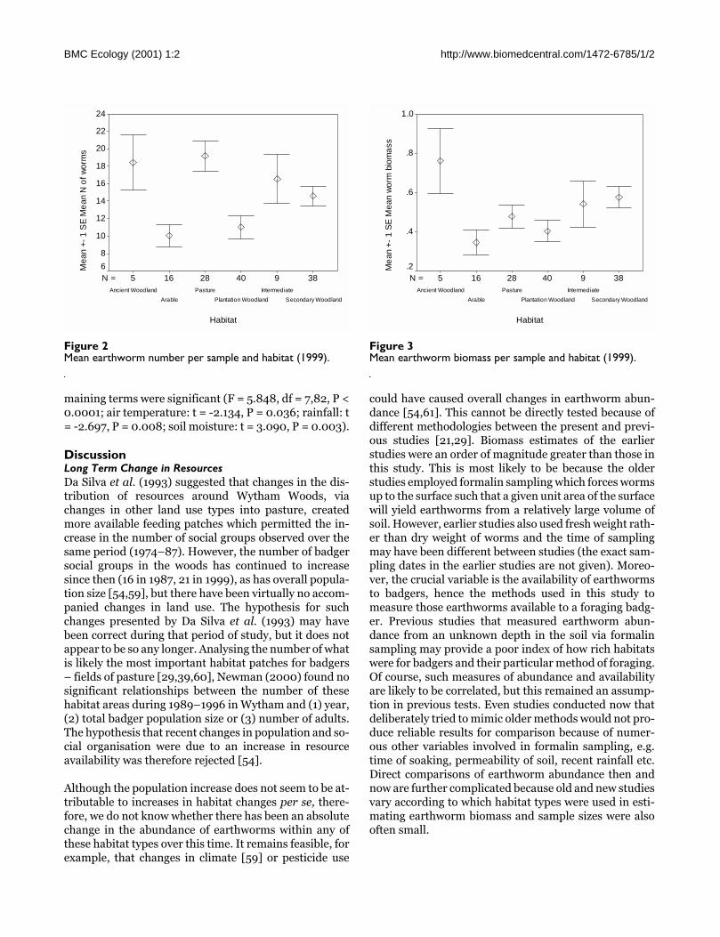
Resource Variation Within and Between HabitatsBoth sample earthworm number (Figure 2) and samplebiomass (Figure 3) varied considerably within any onehabitat, but a one-way ANOVA demonstrated that thevariation was significantly greater between habitats thanwithin them (in square-root transformed biomass: F =2.523, df = 5,130, P = 0.032; and number: F = 4.997, df= 5,130, P < 0.0005). This habitat difference was alsosignificant with non-transformed biomass (Kruskal-Wallis: Χ = 18.720, df = 4, P < 0.001). In Tukey's post hoctests for pair-wise multiple comparisons none of themeans of different pairs of habitats differed significantlyfrom each other (all P > 0.09). Earthworm number was asignificant predictor of earthworm biomass (F = 210.361,d.f. = 1,223, P < 0.00001; R2 = 0.483; slope = 0.697, us-ing data from all individual sample quadrants).

Resource AggregationSample sizes dictated confining these tests to woodland(of all types). Wilcoxon signed rank tests showed that thevariance/mean ratios of the earthworm sample were notconsistent with 1.0 at patch size one (W = 54.0, N = 10, P= 0.008), two (W = 54.0, N = 10, P = 0.008), four (W =42.0, N = 9, P = 0.024) and was borderline for patch sizeeight (W = 20.0, N = 6, P = 0.059). This suggests thatearthworms within woodland are distributed non-ran-domly in space, at least on the first three spatial scales.

Table 3: Group size versus estimated territory richness across studies (two-tailed Pearson correlations). Relevant data were unavailable for those years not presented. No INT territory map was constructed in 1995.

Year N Direction r P Reference

Between population1974–1979 8 + 0.91 <0.01 Kruuk & Parish 1982Within Wytham1982 6 - -0.147 NS Hofer 19881983 6 - -0.543 NS Hofer 19881987 8 N/A N/A >0.1 DaSilva 19931988 8 N/A N/A >0.1 DaSilva 19931993 INT 18 + 0.26 0.30 This study1993 MCP 17 + 0.61 0.009 This study1994 INT 19 + 0.24 0.33 This study1994 MCP 19 + 0.09 0.73 This study1995 MCP 18 + 0.33 0.19 This study1997 INT 20 + 0.31 0.18 This study1997 MCP 20 + 0.37 0.11 This studyPooled data1993–97 INT 57 + 0.20 0.14 This study1993–97 MCP 74 + 0.32 0.005 This study


Since non-random distributions can arise through either(1) spatial aggregation ('over dispersion') or (2) regularspacing ('under dispersion' – tending to some uniformpattern, such as a grid), we needed to further test specif-ically for spatial aggregation. Figure 4 shows the logtransformed variance against the log mean. The super-imposed 1:1 slope represents randomness in space at allscales, since a variance to mean ratio of 1.0 is expectedwithin a homogenous patch (where two samples wouldhave the same mean). That 30 of 35 (85.7%) points lieabove this slope, suggests earthworms are aggregatedrather than regular [57]. The slope of a least squares re-gression line through the origin was 1.39, implying thatover dispersion tended to occur more at sites with a high-er mean earthworm biomass.

Plotting chi-squared values for all variance/mean ratiosagainst their degrees of freedom, the dispersion test [58]revealed that 27 values out of 35 (77.1%) were classifiedas aggregated, none as regular.

Variance/mean ratios plotted against patch size catego-ries (1, 2, 4, 8) (Figure 5), also suggested a greater degreeof aggregation (larger variance/mean ratio) with largerpatch sizes but this trend was not significant (Spear-man's rank correlation: r = 0.334, N = 35, P = 0.132).Constant variance/mean ratios across all levels would in-dicate a fractal structure, i.e. patchiness following a self-repeating pattern at all spatial scales [57].

Because different pairs of badger setts were not equidis-tant from each other, transects actually covered varyingdistances (mean: 427 m, range: 182 – 690 m and stand-

ard deviation:180 m), so it is not possible to estimatewith accuracy the size of the patches represented by the1,2,4 and 8 sample site groupings. However, if a best es-timate were to be made using mean transect lengths,then these would be 5 m for patch size 1, 95 m for patchsize 2, 190 m for patch size 3 and 380 m for patch size 4.

Environmental Correlates of Earthworm AvailabilityEarthworm biomass was significantly related to anumber of environmental variables. Three pairs of vari-ables were highly inter-correlated (r > 0.40) (see Table 5)so only one of each pair was included in the model. Thesepairs were: air temperature and soil temperature, rain-fall and humidity, ground cover and canopy cover. Thelatter variables in each of these pairs were removed fromfurther analyses.

Using the four remaining variables and removing varia-tion due to habitat type alone produced a significantmodel for (square root transformed) mean earthwormbiomass per sample site (Type III sums of squares GLM:F = 5.096, df = 8,82, P < 0.0001). This gave parameterestimates for each environmental variable, adjusting forall other variables and over and above differences in hab-itat alone, indicating rainfall (t = -2.431, P = 0.017) andsoil moisture (t = 3.082, P = 0.003) contributed signifi-cantly to the model (when the other two, both non-signif-icant variables were removed from the model, F = 5.818,df = 6,82, P < 0.0001; rainfall t = -3.263, P = 0.002, soilmoisture t = 3.426, P = 0.001). Removing from the firstfour-variable model just vegetation cover (the variablewith the smallest t-value) produced the best model,judged by the lowest error mean square, in which all 3 re-

Table 4: Correlations between territory size (TS) and 'five-food patch distance' after Kruuk & Parish (1982). DTESS represents territo-ries constructed by a Dirichlet Tessellation method 85,86 based on information on main sett locations only, and is included here for interest (not included in sequential Bonferroni adjustment) but should not be thought of a necessarily valid test of this prediction. As-terisked P values are those still significant after applying the sequential Bonferroni adjustment.

Year Method N r Direction P

1993 INT 18 -0.157 - 0.534MCP 19 0.495 + 0.031

1994 INT 19 -0.289 - 0.230MCP 20 -0.469 - 0.037

1995 MCP 18 0.153 + 0.5431997 INT 20 -0.341 - 0.141

MCP 20 0.709 + < 0.001*

1999 MCP 20 0.352 + 0.128(2000) (DTESS) (21) (-0.461) (-) (0.035)

Pooled data1993 – 97 INT 57 -0.259 - 0.0521993 – 97 MCP 97 0.240 + 0.018


maining terms were significant (F = 5.848, df = 7,82, P <0.0001; air temperature: t = -2.134, P = 0.036; rainfall: t= -2.697, P = 0.008; soil moisture: t = 3.090, P = 0.003).

DiscussionLong Term Change in ResourcesDa Silva et al. (1993) suggested that changes in the dis-tribution of resources around Wytham Woods, viachanges in other land use types into pasture, createdmore available feeding patches which permitted the in-crease in the number of social groups observed over thesame period (1974–87). However, the number of badgersocial groups in the woods has continued to increasesince then (16 in 1987, 21 in 1999), as has overall popula-tion size [54,59], but there have been virtually no accom-panied changes in land use. The hypothesis for suchchanges presented by Da Silva et al. (1993) may havebeen correct during that period of study, but it does notappear to be so any longer. Analysing the number of whatis likely the most important habitat patches for badgers– fields of pasture [29,39,60], Newman (2000) found nosignificant relationships between the number of thesehabitat areas during 1989–1996 in Wytham and (1) year,(2) total badger population size or (3) number of adults.The hypothesis that recent changes in population and so-cial organisation were due to an increase in resourceavailability was therefore rejected [54].

Although the population increase does not seem to be at-tributable to increases in habitat changes per se, there-fore, we do not know whether there has been an absolutechange in the abundance of earthworms within any ofthese habitat types over this time. It remains feasible, forexample, that changes in climate [59] or pesticide use

could have caused overall changes in earthworm abun-dance [54,61]. This cannot be directly tested because ofdifferent methodologies between the present and previ-ous studies [21,29]. Biomass estimates of the earlierstudies were an order of magnitude greater than those inthis study. This is most likely to be because the olderstudies employed formalin sampling which forces wormsup to the surface such that a given unit area of the surfacewill yield earthworms from a relatively large volume ofsoil. However, earlier studies also used fresh weight rath-er than dry weight of worms and the time of samplingmay have been different between studies (the exact sam-pling dates in the earlier studies are not given). Moreo-ver, the crucial variable is the availability of earthwormsto badgers, hence the methods used in this study tomeasure those earthworms available to a foraging badg-er. Previous studies that measured earthworm abun-dance from an unknown depth in the soil via formalinsampling may provide a poor index of how rich habitatswere for badgers and their particular method of foraging.Of course, such measures of abundance and availabilityare likely to be correlated, but this remained an assump-tion in previous tests. Even studies conducted now thatdeliberately tried to mimic older methods would not pro-duce reliable results for comparison because of numer-ous other variables involved in formalin sampling, e.g.time of soaking, permeability of soil, recent rainfall etc.Direct comparisons of earthworm abundance then andnow are further complicated because old and new studiesvary according to which habitat types were used in esti-mating earthworm biomass and sample sizes were alsooften small.

Figure 2Mean earthworm number per sample and habitat (1999).

3894028165N =

Habitat

Secondary Woodland

Intermediate

Plantation Woodland

Pasture

Arable

Ancient Woodland

Mea

n +-

1 S

E M

ean

N o

f wor

ms

24

22

20

18

16

14

12

10

8

6

Figure 3Mean earthworm biomass per sample and habitat (1999).

3894028165N =

Habitat

Secondary Woodland

Intermediate

Plantation Woodland

Pasture

Arable

Ancient Woodland

Me

an +

- 1

SE

Mea

n w

orm

bio

ma

ss

1.0

.8

.6

.4

.2


Without such direct comparisons, the possibility thatchanges in resource availability have occurred as a resultof changes in the climate in recent years (resulting inwetter summers and warmer winters in Wytham) cannotbe ruled out. Nevertheless, the principal explanation forthe badger population increase is thought to be a re-or-ganisation of badger social structure and the increaseduse of outlier setts rather than hypotheses involving re-source availability [54,59].

Tests of the RDHWithin the Wytham badger population, GS and TS havebeen shown, as predicted by the RDH, to be consistentlyuncorrelated over all the years of study (since 1974) [19],correcting for multiple inference bias. When the sametest is conducted among different species or among dif-ferent populations of the same species, if patch richnessand dispersion are independent, the predicted relation-ship between group size and territory size by the RDH is,if anything, predicted to be negative [31]. This is becausean increase in patch richness (e.g. UK pastures rich inearthworms) may lead to a decrease in the mean numberof patches per territory. Such a non-significant but nega-tive trend is precisely what Johnson et al. (2000) foundin comparing (1) different species of mustelids, and also(2) in comparing different populations of badgers acrossEurope. Kruuk & Parish (1982) also found a non-signifi-cant but (slightly) negative trend in group size and terri-tory size between badger populations within the UK (r =-0.07).

This accumulating evidence for the predicted relation-ships between group size and territory size provides good

reason to consider the RDH as at least a possible mecha-nism to explain variation in social organisation in badg-ers. This is, as discussed in the introduction, especiallyimportant given that badgers are reported in the litera-ture not to benefit directly from group-living [5,9], leav-ing open the question of why they form groups at all. TheRDH not only predicts this lack of relationship but alsopredicts alternative variables that should independentlydetermine territory size and group size. There is, howev-er, a lack of good empirical tests of these predictionswithin populations of any species and this study conse-quently set out to test them explicitly.

Assumptions of the RDHThe predictions of the RDH model tested here are basedon certain assumptions, some of which we were able totest. First, because the RDH model is not explicitly spa-tial, in deriving the predictions in the model [31] it wasnecessary to equate territory size with the number ofpatches, which is valid as long as the spatial dispersion ofpatches is independent of their richness. This assump-tion was supported in our data with highly significant re-lationships between patch number and territory size inpooled data using both territory estimation methods,and in 6 of 8 independent tests (5 of 8 employing the se-quential Bonferroni adjustment).

The nested proviso within the above – that the spatialdispersion of patches is independent of their richness –remains as another assumption in the model. In terms oftheoretical validity, there is no reason to suppose that re-sources should be systematically richer or poorer where

Figure 4Log transformed variance against the log mean of earthwormnumber, for data grouped into four patch sizes. The superim-posed 1:1 slope denotes randomness in space. Figure 5

Variance/mean ratio plotted against patch size categories.

0

10

20

30

40

50

60

0 2 4 6 8 10

P atch S ize

Var

ianc

e to

Mea

n R

atio


they are more dispersed, and empirically, in our studysite, badgers share a contiguous site with a similar mosa-ic of habitat patches. However, for the purposes of ourtests we assumed that any one-habitat type has a certainfixed richness, regardless of its location (since we as-signed resource estimates equally to all areas represent-ed by any one habitat type). This was necessary becauseof limitations of manpower and time, but prevented atest of this assumption. Ideally, one would have continu-ous information on richness over all areas simultaneous-ly. This would be a useful, if labour intensive, objectivefor future study.

Secondly, the RDH predictions hold "provided the varia-bility between patches is not too low" – with a coefficientof variation (CV) greater than "approximately" 0.5 31. Ifwe assume that habitats are patches, we can make acrude test of this assumption. For earthworm biomassCV = 0.28 and for number, CV = 0.26. On the face of it,therefore, one may infer that variation is not largeenough to establish the effects of the very mechanism weare testing for in the first place. However, the hypothesiscannot be rejected on these grounds, because the be-tween-habitat variation, quantified above, is only onecomponent of the actual resource variation. As well asspatial variation, there is temporal variation. Earthwormavailability is known to vary (and this variation is crucialto the application of the RDH) with both weather[11,29,61,62] and season [21,63,64]. Specifically, weknow it to be significantly dependent on air temperature,

previous rainfall and soil moisture, over and above anydifferences in habitat type alone [29,65] (and this study).The spatio-temporal heterogeneity relevant to the RDHis therefore a combination of variation over time as wellas variation over space, while the CVs reported aboveonly measure the variation at one point in time. Moreo-ver, we have argued that there may be spatial patchinesswithin habitats, which may add to the overall variabilityof the environment. In any case, Kruuk's (1978) data re-veal that among the four Wytham habitats in his study,for Lumbricus terrestris CV = 0.60 and for all earth-worm species CV = 0.52. Finally, we cannot rule out thepossible additional variation in resources resulting fromseasonal constraints on prey selection [20,21] (for exam-ple, availability of cereal crops in summer, or scarcity ofearthworms due to frozen soil in winter).

Group Size vs. Resource AvailabilityThe first prediction that group size is dependent on totalresource availability was upheld using pooled data acrossall years with MCP territory size. However, this was nottrue with the INT method, and only 1 of the tests split byyear and method was significant. Reformulating the teston the basis of correlated between-year changes in thesetwo variables (contrasts) was also insignificant using ei-ther method. There is therefore little, if mixed, evidencefor the prediction.

Table 5: Two-tailed Pearson correlations between habitat variables recorded during earthworm sampling.

Air temp Rainfall (mm Relative Canopy Ground Soil temp(deg C) on previous Humidity cover (%) cover (%) (deg C)

Rainfall (mm on r 0.213previous day) P 0.004

N 180Relative Humidity (%) r 0.235 0.402

P 0.001 < 0.001N 180 180

Canopy cover (%) r -0.095 0.233 0.300P 0.203 0.002 < 0.001N 180 180 180

Ground cover (%) r -0.384 -0.343 -0.329 -0.629P < 0.001 < 0.001 < 0.001 < 0.001N 180 180 180 225

Soil temp (degrees C) r 0.570 -0.032 0.080 -0.488 0.200P < 0.001 0.685 0.313 < 0.001 0.004N 162 162 162 207 207

Soil moisture r -0.150 0.092 0.240 0.051 -0.036 -0.032P 0.155 0.387 0.022 0.554 0.680 0.720N 91 91 91 136 136 127


Territory Size vs. Resource DispersionAcross all years, MCP territory size was significantly pre-dicted by a multiple regression of the nearest neighbourdistances to the three nearest "important" habitats (asdefined on the basis outlined above). As above, this wasnot supported by the INT method. All the individual yearregressions were insignificant (although 4 of the 5 withMCP territories were positive, all those with INT territo-ries negative). Mean-five-food patch distance was signif-icantly correlated with MCP territory size pooled acrossyears but, once again, the prediction was not supportedby the INT method, in fact it was negative. Only 3 of 8 in-dependent tests were statistically significant (one was inthe wrong direction), and this reduced to just one usingsequential Bonferroni P-values. Excluding arable habi-tat, there were no significant relationships at all.

Overall therefore, the difference in territory estimationmethod appears to be important because, broadly speak-ing, all tests of the RDH were supported in analyses ofpooled MCP territory data (though not always by tests in-volving MCPs in individual years), while all were notsupported using pooled data from the more traditionalmethods of interpolation (INT). Split by year, there wasa mix of support among results using both methods. Wedeliberately used two methods, because the interpola-tion method is subject to assumptions about badger be-haviour. Although estimates of the two methods docorrelate [19], the latter assumes that all territories tes-sellate with common borders, they do not overlap, andoften that outer boundaries without neighbouring badg-er groups are delimited by features in the landscape. InWytham in recent years, such traditional assumptions,as well as the concept of strictly exclusive territories,have become difficult to maintain. Badger latrines com-monly overlap each other [19] and there is evidence oflarge inter-territorial movements in data from trapping[54] and radio-tracking (C. Buesching, unpublished da-ta). For these reasons, we prefer the MCP method (sinceit is based purely on actual latrine use) as a more unbi-ased estimate of the area which we know badgers of anyone social group to be using. That was a prior belief [19],and both methods of territory estimation had been con-structed before conducting the tests reported here.

Other sources of error from uncontrolled factors influ-encing social group size or territory size could also haveintroduced too much noise to detect underlying effects. Aspecific change in the regulation of group sizes duringthe study period has been suggested [7,54,59] which mayalso have introduced noise into the data. Finally, it mustbe remembered that a lack of strong relationships insome cases may be because we can only approximate thetotal sum of earthworm availability. Those measures,

aside from inherent estimation errors, do not take intoaccount different times of year and other food sources.

Relevant ScalesWhere relevant, analyses excluding arable fields were re-peated. Arable fields are not earthworm rich, and areclassified as important habitat types for badgers becauseat crucial times of year they provide alternative foodtypes (cereals crops, grain etc.) [21,29,39]. This foodsource is heterogeneous over a seasonal time scale,whereas earthworms in the other habitats represent het-erogeneity over an hourly or nightly time scale [29].Therefore, we also checked results under the assumptionthat territories may instead be configured on criteria in-dependent of arable fields. When excluding arable land,results were generally similar in the tests of territory sizeand distance to major habitat types and number ofpatches, but none were significant involving five-foodpatch distance. In general, relationships excluding ara-ble habitat were weaker and fewer were significant, butresults remain mixed in terms of support for the RDH,whether arable land is included or not.

Spatial Variation in ResourcesThere is a plethora of studies of badger social organisa-tion across the UK and increasingly from other sites inEurope [10,66,67]. These studies of badgers, and somefrom other species [68,69] commonly refer to tests ofwhether the RDH fits as a post hoc explanation of socialorganisation, but assume that (while sometimes ac-knowledging it as an oversimplification) habitat patchesare synonymous with resource patches. However, sincespatial aggregation of resources within habitats is alsofeasible, future tests will need to verify that assumption.

Patchiness or patch sizes have been estimated in otherstudies of social organisation [27,36]. Like those, patch-iness is difficult to measure and our tests have con-straints, but it is nevertheless the first formal test ofwithin habitat patchiness of prey in Wytham. We foundvarious lines of evidence for patchiness at different spa-tial scales, which could have important implications forterritory defensibility. Since the RDH suggests that a ter-ritory must be defended to contain a certain number ofpatches of a certain richness, within-habitat aggrega-tions suggest a hidden layer of patchiness that may di-rectly influence territory size and configuration. If wehave succeeded in anything, it is showing that it remainsuncertain what a relevant patch is. In future analyses ad-ditional sources of within habitat variation, such as for-est rides, should be explicitly accounted for since theymay have a small but disproportionate influence on re-source availability and consequent spatial behaviour.


Previous work on badger social organisation focused onpatches of worm rich habitat like pasture and old wood-land, or arable fields as sources of alternative food[5,12,21,29,37]. However, woodland in general was sug-gested to provide an especially important foraging habi-tat under certain conditions [39], which could mean thatthe previous selection of 'important' habitats was toosimple. We now know in detail how the woodland habitatin Wytham contrasts strikingly with open areas sur-rounding it [70]. In particular, continuous recording byautomatic weather stations showed that, during the year,soil temperature never left the range 0–20°C under theforest cover, whereas soil under grassland or withoutvegetation did drop below zero and reached the midtwenties. During winter badgers may therefore findwoodland to be a uniquely available foraging area as thesoil in that habitat remains unfrozen in winter and, sim-ilarly, remains relatively soft in summer, perhaps servinga crucial role in maintaining some level of food security(i.e. earthworms remain accessible) during periods ofunfavourable weather [39].

It may be possible, using GIS, to construct a detailed spa-tial model of resource distribution using estimates thatincorporate both habitat information plus data on varia-tion in weather. This could give more realistic indices ofspatial and temporal variation in food availability. Soilmaps could also be integrated to such a model since un-derlying geology or soil type has been suggested to influ-ence resource availability via interactions with differentclimatic conditions [37]. Such an approach presents newproblems, however, and a retrospective analysis by thismethod may be impossible.

ConclusionsThe purpose of this paper was to test whether, over thecourse of a long-term study with large sample sizes, thepredictions of the Resource Dispersion Hypothesis(RDH) were consistently supported rather than simplybeing anomalies of past studies. This is, as far as weknow, the largest ever test of its predictions. The as-sumptions of the RDH are also important in providingvalid tests of predictions. We have made a first step inempirical research on the subject to determine whetherthe model assumptions are met in the field. These as-sumptions are, however, at least as difficult, if not moreso, to test than the RDH predictions themselves. Itshould be remembered that violations of a model's pre-dictions imply either (a) that the model is not valid, or (b)that assumptions within the model, rather than the mod-el itself, are not valid [46]. Therefore, while we were notable to test all of the assumptions in the RDH model byBacon et al. (1991), our main objective of testing its pre-dictions stand in evaluating whether the RDH – alongwith all of its various assumptions – provides a good

model for the social-spacing organisation of badgers inWytham Woods. Support for the predictions were mixed,and depended on year and the method used to map outterritory borders. Our results indicate that it may also benecessary in the future to take into consideration within-habitat patchiness, in order to improve tests of the RDH.As with all hypotheses, we must await the accumulationof evidence that will gradually tilt the balance to supportor reject them, and thus more hypotheses driven studiesof the RDH are needed. While these tests of the RDH arenot conclusive, this paper presents a priori hypothesistesting of specific predictions, as well as tests of someRDH assumptions, though others remain to be tested infuture studies. It will be as important, for the develop-ment of the RDH as a predictive theory, to discover whenthe RDH does not provide a good explanation of spatialorganisation as well as other situations where it does.

Materials and methodsStudy SiteThe study was undertaken in Wytham Woods, 5 km NWof Oxford, UK (01° 18' W, 51° 46' N). Details of the studysite can be found in Hofer (1988) and Kruuk (1978a), andthe long term trapping study is detailed elsewhere[54,59,71].

Long-term and Current Estimates of Food AvailabilitySeveral studies have explicitly estimated earthwormabundance in Wytham [21,29,53]. Data were taken fromthese published studies and converted into common bio-mass per area units. A major problem remains in com-paring estimates, because data collection methodsvaried. Even if the general methodologies had been sim-ilar, small variations in detail are likely to have affectedresults. Thus, to control for between study bias, data arepresented on different scales, and attention is focussedon the relative availability per habitat.

The most important distinction between methods is thatmost earlier studies used Formalin sampling [21,29,72],which causes earthworms to escape to the surface froman indeterminate and variable depth in the soil. It is alsoknown that soil moisture and temperature affect forma-lin sampling which then require sampling efficiency cor-rections [21,73]. Even then, formalin sampling informsus only about earthworm biomass in the affected volumeof soil, which is dependent on permeability and otherfactors and, therefore, possibly very little about actualavailability to badgers. In this study, untreated soil sam-ples of a known volume were collected and hand-sortedlater on in the lab which is considered to be a more accu-rate measure [74–76]. Sampling technique for earth-worm studies is the focus of a "considerable debate"(Spurgeon & Hopkin 1999: 182) and there are obviouslyadvantages and disadvantages of each method. However,


the hand-sorting method, coupled with shallow soil sam-ples, is more likely to index earthworms specificallyavailable to foraging badgers because they eat earth-worms on the surface but also dig down to reach thembelow it [20,29,65,77]. They typically dig 2–4 inches intothe soil [65] and do so enough to have earned them a rep-utation for damaging even pasture [78]. The goal is toreplicate the badger's style of foraging, and taking aknown volume of shallow soil is the best of all of the cur-rent methods to mimic how a badger is likely to encoun-ter and search for them. While still not perfect, it wasconsidered a better method of assessing availability(rather than abundance) than formalin sampling. Hand-sorting was also the preferred method of other recentstudies [79]. Surface sampling with red torchlight [65]was not used because it omits worms just below the sur-face, may be sensitive to worms escaping, and returns avery small count per area which makes subsequent com-parisons between samples less clear.

Of course, between-study comparisons could have beenbetter served by repeating precisely the methods of thoseprevious studies, but this was deemed to be of lesser im-portance than using an improved method to estimateavailability, rather than just abundance, in order to makeRDH tests as accurate as possible. Apart from the prob-lems raised above, no method of sampling can give acomplete picture of earthworm distribution because un-less it is continuous in time, it can give only a 'snap-shot'view – a one-off estimate – of what the real distributionmight look like. This is an inevitable constraint of suchstudies.

All earthworm sampling was conducted in June of 1999to minimise any potential confounding effect of seasonalvariation. This is before the very dry period of the yearwhen badgers shift to other food sources such as cereals[20]. Earthworms were sampled at the end of the nightbut before dawn (c. 0400 hours) along transects startingand ending 10 m from a pair of adjacent main setts. Thisexperimental design was used to control for the potentialconfounding effects of the Passive Range Exclusion(PRE) Hypothesis [80], which predicts that earthwormavailability is differentially depleted between neighbour-ing groups with lows at the extremes (at main setts) andpeaks in the middle (at territory borders). There was noevidence for this, however (unpublished data). Ideally,one would sample with a stratified random design over alarge area measured in its entirety. This, however, wasconstrained by the need to control for potential bias fromthe effects of PRE and also by manpower and time. Eachof the 10 transects were independent in that any one settfeatured only once in all transects. After being used oncein any one transect, however, a sett would be excludedfrom being selected in all subsequent transects so the

process cannot be strictly independent, but this was un-avoidable given the limited number of setts (20 of a totalof 21 main setts were used). A randomised procedure wasused to select them at each stage nevertheless. Nine equi-distant sample sites were marked out along eachtransect. At each of these nine sites, two randomly placedquadrants < 5 m from each other marked out the loca-tions where two (one at each quadrant) 0.3 x 0.3 x 0.1 m(depth) soil samples were extracted by spade. Means ofthese pairs were used in later analyses unless otherwisestated. This was done as quickly as possible but it is rec-ognised that a source of potential error remains in omit-ting any earthworms that escaped. If this does occur,then it is likely to cause some underestimation, but thisshould happen in all samples and is not, therefore, ex-pected to cause any systematic bias. Soil samples weretransported to a laboratory in sealed bags and hand sort-ed. Biomass was recorded as the total dry weight afteroven drying of all earthworms (already killed) presentper sample.

Tests of RDH PredictionsAssumptionsAn assumption leading to the predictions of the RDH isthat the number of patches correlates with territory area[31] (see page 464). We tested this assumption empiri-cally, using the number of 'patches' of distinct habitat ar-eas within the territory. For this test, as in theforthcoming ones below, a 'patch' was defined as a habi-tat block delimited by alternative habitat types or field orforestry compartment boundaries. We use the termpatch here, following the RDH terminology [4,31], to de-note an area of similar food availability, surrounded byareas with different levels of food availability. With theassumption that habitats can be equated to patches, theyrefer to the same thing. However, in the model, a patchdoes not necessarily need to be a habitat type.

In the RDH model, it was stated that to enable the mech-anism to operate, the variability between patches musthave a coefficient of variation (CV) greater than "approx-imately" 0.5 31. We could therefore estimate the CVamong the habitats we examined as a test of this assump-tion.

Group Size and Resource AvailabilityAdult badger group sizes were estimated from trappingstudies conducted since 1974 [7,11,21,39,54,59,71,81].Where possible, we analysed data from all years in whichit was collected. However data for the years previous to1993 are largely from published papers, for which origi-nal data for certain variables were not available or calcu-lable. In those cases, we could only use the more recentdata, since 1993. Our estimate of group size was the totalnumber of different individuals caught in the setts of a


social group in that year. We could also have used theminimum number alive (MNA) which adds badgers that,while not trapped in that year, were trapped subsequent-ly (although not necessarily in the same group) andtherefore assumed to have been present previously. Ad-ditionally, we could also have used census data from asurvey made during three nights in May each year by vol-unteer observers. All three estimates are closely correlat-ed [54], however, we used actual number trapped as inour previous studies [19,37,54], because census datahave a number of sources of inherent bias and MNA esti-mates do not account for where untrapped badgersranged during their absence, which is crucial for tests ofresident group size and resource use. The number ofadults caught in the relevant territory during the year re-flect a resident group size, since trapping efficiency wasboth high and consistent among years. Over the period1987 – 1997, trapping success ranged from 83.2 to100.0% of the population [54,59].

Resource availability was indexed by the availability ofearthworm biomass in the various habitats, and was ameasure of the total biomass of earthworms potentiallyavailable to badgers per territory (denoted B). This wascalculated as mean earthworm biomass per unit area (j)of each habitat type (i) (as measured in the field), multi-plied by the area of that habitat within the territory (a),and summed for all n habitat types, so that

Summing for all habitat types in the territory provided ameasure of total expected earthworm biomass in allpatches for each territory and follows existing methodol-ogy for badgers [5,12,21,39]. This was done separatelyfor each year in which territory records were available.We used the following habitat types: (1) arable, (2) pas-ture (agricultural grassland), (3) semi-natural grassland,(4) urban (housing and developed areas in the villageand surrounding farms), (5) ancient woodland, (6) sec-ondary woodland, (7) plantation woodland, (8) wetlandand (9) intermediate habitat types. The latter accountedfor (very small areas) that did not fall into the eight othercategories, and was typically transitional habitat such asthe vegetation that occurred in unmanaged spaces be-tween fields and woodland.

Some agricultural grassland does not meet the definitionof 'pasture' as 'land that is grazed', if those areas are cutfor silage instead. Similarly, some of the semi-natural

grassland is grazed and could therefore be termed 'pas-ture' by that same definition. However, here we haveavoided using pasture simply to denote a field in whichanimals are grazed, in favour of recognised differences invegetation types as given in the university farm records.

We did not estimate earthworm biomass in the few areasof grassland habitat, although it featured on habitatmaps, so we assigned it as a 0.237 fraction of the biomassfound in pasture, the ratio reported in Hofer (1988; to 3decimal places). Urban habitat was assigned the samerichness since, although it is variable, gardens and lawnsare likely to be at least as productive as pasture but theseareas are only a fraction of the total urban area [65]. Thisis not an ideal compromise but is more realistic than as-signing a value of zero and only accounts for a small pro-portion of the total study area. Areas of wetland wereassigned a value of zero.

Habitat maps were modified for each year in ArcViewGIS (ESRI) from vegetation maps of the Centre for Ecol-ogy and Hydrology (M. Morecroft et al., unpublished),and covered all the land area under study (i.e. there wereno gaps of unclassified status). For each year, we there-fore had two separate GIS data layers: the territory maplayers were cross-tabulated with habitat map layers us-ing an ArcView routine, which gave the areas of eachhabitat type constituting each territory. Because of habi-tat changes between 1993–1999, we used different mapsfor calculating the habitat areas of each year. All changesin land use were accounted for year-by-year in our calcu-lations of habitat areas. Measures of expected earth-worm biomass per territory from earlier years came fromthe literature but used different methodologies[12,21,29,39].

Relationships between group size and resource abun-dance were tested using Pearson correlations. We alsotested for relationships between 'contrasts' in these samevariables, which provides a test for directional shifts inone variable concurrent with a change in the other (i.e.current-year-GS minus previous-year-GS, versus cur-rent-year-resources minus previous-year-resources).Correlation coefficients can then be used to test whetherthe direction and magnitudes of contrasts in X are signif-icantly associated with those of contrasts in Y.

Territory Size vs. Dispersion of ResourcesEstimates of badger group territory sizes were construct-ed using two different methods in order to minimise biasarising from error in any one particular method [19].These are: 1) traditional inference from bait-markingstudies [82] where territorial borders are interpolatedfrom latrine maps ('INT' method; we use INT here sim-ply as an abbreviation for 'interpolated') and, 2) 100%


Minimum Convex Polygons of bait-marked latrines('MCP' method). Because measuring resource dispersionis difficult [36,37], we also made two measures in differ-ent ways to compare results:

a) Nearest neighbour distances from the main sett toeach of the three major habitat types:pasture, ancientwoodland and arable fields – the three particularly im-portant feeding habitats. In the 25 years since badgershave been studied in Wytham, these habitats have beenconsistently identified as important foraging habitats atone time of the year or another [5,6,9,11,21,29,39,54,55,60]. Arable fields become particularly importantfeeding areas during summer months, when earthwormsare difficult to find in the hardened soil [21] and badgersfeed on cereals and grain on these fields instead[20,21,61]. Therefore, although these were not the top 3ranking habitats in terms of the estimates of earthwormavailability measured in this study, they are used here asa result of prior knowledge that has established them asthe most important habitats for badger food at varioustimes of year.

b) Mean distance to the 5 nearest of these patches. Thismeasure is the 'five-food-patch distance', derived by Kr-uuk & Parish (1982) as an appropriate measure for re-source dispersion as relevant to badgers and used eversince in comparative studies of this species, both inWytham and elsewhere [12,39,43]. It is of principal in-terest, given the long standing nature of this study andthe focus on this well known species, to concentrate onan established measure that was derived on the basis ofdetailed field knowledge of its foraging behaviour. Kruuk(1978a,b) had followed foraging badgers over manynights by radio-tracking to establish a mean number ofpatches that were exploited on an average night. Thisgave a large sample estimate of mean resource patch userelevant to the mechanism of the RDH and its likelytime-scale. Other radio-tracking studies since then havenot contradicted this (C. Buesching, P. Stewart, D. John-son, unpublished data).

In each of the analyses described above that involvedmeasures of resource dispersion, we repeated the testswhile excluding arable land, because it is primarily im-portant as a source of food other than earthworms, and itis important on a seasonal rather than a daily time scale.

Resource Variation Between and Within HabitatsANOVA was used to test for significant differences insample earthworm biomass and number between habi-tats. One-way ANOVA also provides an implicit test ofthe null hypotheses that variation within habitats is larg-er than variation between them, thus providing a test ofwhether blocks of different habitat types are different

enough to justify using them as a surrogate measure of'resource patches' as used in the previous studies. If theydo not differ significantly, then we may hypothesise that,to a badger, the various habitats do not represent patcheswith different food quantities.

Resource AggregationThe spatial distribution of sampling sites along lineartransects also allowed us to test the hypothesis thatearthworms have a 'patchy' (spatially aggregated) distri-bution within habitats, rather than being randomly dis-tributed in space. To do this we compared the mean andvariance between different sub-groupings of samples,grouped at 4 different spatial scales. The first scale wassimply the pair of samples taken at each sample site (ran-domly separated over an area < 5 m from each other).Means from such pairs were always used for analyses atall other spatial scales. These three remaining scaleswere partitioned, each in the same way, as groups of anincreasing number of the samples as laid out along anyone transect, such that data for groups of 2, 4 and finally8 separate sample sites were grouped together for analy-sis. For example, for the last of these scales, 'patch size 8'meant that data from eight sampling sites, adjacent toeach other along transects, were analysed together as onegroup. This included 16 samples in total because it con-tained a pair of samples (< 5 m apart) for each samplesite. These data were independent in that any one samplefeatured only once in patch size 1, 2, 4 or 8.

Invertebrates typically are not randomly distributed, butour principal interest here is to detect the spatial scale ofmaximum aggregation. Since the variable of interest is acount (number of worms), randomly distributed samplevalues should follow a Poisson distribution, for which thevariance/mean ratio = 1.0 [83]. We could therefore useWilcoxon signed rank statistics to test whether the vari-ance/mean ratios deviated significantly from 1.0, andthis was done separately for samples of data grouped bypatch size 1, 2, 4 and 8. A deviance from 1.0 in any ofthose four samples would indicate non-random distribu-tion in space at that spatial scale.

By plotting chi-squared values for all variance/mean ra-tios against their degrees of freedom, we could also usethe dispersion test [58], to determine if these values fallinto one of three possible zones representing aggregated,random and regular distributions. Theses zones are de-lineated by the upper and lower 5% significance levels ofagreement with a Poisson series. The mapping of Χ2 val-ues against their degrees of freedom onto the zone abovethe upper bound demarcates aggregation, those fallingbelow the lower bound fall into the zone demarcatingregular distribution. Anything else, falling between thebounds, cannot be rejected as belonging to a Poisson se-


ries, i.e. they are consistent with a random distribution ofearthworms.

We also tested for a relationship between variance/meanratio and patch size using Spearman's rank correlationcoefficient, as a test of whether aggregation increaseswith spatial scale.

Environmental VariablesSome other variables were measured at the time of earth-worm sampling: (1) canopy cover (estimated % cover-age); (2) ground vegetation cover (estimated %coverage); (3) soil temperature (°C), with an electronicthermometer probe. Also, (4) soil moisture (% mass) wasdetermined by weighing soil samples from each samplesite before and after oven drying. Meteorological data atthe time of sampling were recorded by an EnvironmentalChange Network Automatic Weather station [84]; (5) airtemperature (°C); (6) Relative Humidity (%) and, (7)rainfall on previous day (mm) were used in the analysis.

AcknowledgementsWe thank Paul Johnson for statistical advice, Michele Taylor and Angela London at the Environmental Change Network at Wytham for help in con-structing the habitat maps, Sandra Baker, Amy Dickman, Bart Harmsen, Christina Buesching, David Slater, Chris Newman and especially Jane Bass for help with the field work. Pavel Stopka, Chris Newman, Michael Thom and Paul Blackwell provided useful discussion and criticism. DDPJ gratefully acknowledges the support of the National Environment Research Council and the J.F. Kennedy Memorial Trust. The long-term study is funded by a grant to DWM from the People's Trust for Endangered Species.

References1. Frame LH, Malcolm JR, Frame GW, Van Lawick H: Social organisa-

tion of African wild dogs (Lycaon pictus) on the SerengetiPlains, Tanzania, 1967–1978. Zeitschrift fur Tierpsychohgie 1979,50:225-249

2. Cooper SM: Optimal hunting group size: the need for lions todefend their kills against loss to spotted hyaenas. African Journalof Ecology 1991, 29:130-136

3. Bertram BCR: Vigilance and group size in ostriches. Animal Be-haviour 1980, 28:

4. Carr GM, Macdonald DW: The sociality of solitary foragers: amodel based on resource dispersion. Animal Behaviour 1986,34:1540-1549

5. Woodroffe R, Macdonald DW: Helpers provide no detectablebenefits in the European badger (Meles meles). Journal of Zo-ology (London) 2000, 250:113-119

6. Da Silva J, Macdonald DW, Evans PGH: Net costs of group livingin a solitary forager, the Eurasian badger. Behavioural Ecology1993, 5:151-158

7. Macdonald DW, Newman C, Stewart P, Domingo-Roura X, JohnsonPJ: Density-dependent body weight and condition regulationin badgers (Meles meles) from Wytham Woods, Oxford-shire. Ecology

8. Woodroffe R, Macdonald DW: Badger clans: demographicgroups in an antisocial species. Journal of Zoology (London) 1992,227:696-698

9. Woodroffe R, Macdonald DW: Badger sociality – models of spa-tial grouping. Symposia of the Zoological Society of London 1993,65:145-169

10. Johnson DDP, Macdonald DW, Dickman AJ: An analysis and re-view of models of the sociobiology of the Mustelidae. MammalReview 2000, 30:171-196

11. Kruuk H: Spatial organisation and territorial behaviour of theEuropean Badger Meles meles. Journal of Zoology (London) 1978,184:1-19

12. Kruuk H, Parish T: Factors affecting population density, groupsize and territory size of the European badger, Meles meles.Journal of Zoology (London) 1982, 196:31-39

13. Macdonald DW, Carr GM: Food security and the rewards oftolerance. In: Comparative Socioecology: The Behavioural Ecology of Hu-mans and Animals Edited by Standen V, Foley R, vol. 8. pp. 75–99. Oxford:Blackwell Scientific; 198975-99

14. Chamov EL, Orians GH, Hyatt K: The ecological implications ofresource depression. American Naturalist 1976, 110:247-259

15. Maher CR, Lott DF: Definitions of territoriality used in thestudy of variation in vertebrate spacing systems. Animal Behav-iour 1995, 49:1581-1597

16. Gill FB, Wolf LL: Economics of feeding territoriality in thegolden-winged sunbird. Ecology 1975, 56:333-345

17. McNab BK: Bioenergetics and the determination of homerange size. American Naturalist 1963, 97:133-140

18. Macdonald DW: The ecology of carnivore social behaviour. Na-ture 1983, 301:379-384

19. Johnson DDP, Macdonald DW, Newman C, Morecroft MD: Groupsize versus territory size in group-living badgers: a large-sample field test of the Resource Dispersion Hypothesis.Oikos

20. Neal E, Cheeseman C: Badgers. London: T. & A.D. Poyser; 199621. Hofer H: Variation in resource presence, utilization and re-

productive success within a population of European badgers(Meles meles). Mammal Review 1988, 18:25-36

22. Macdonald DW: Resource dispersion and the social organisa-tion of the red fox (Vulpes vulpes). In: Proceedings of the worldwidefurbearer conference Edited by Chapman JA, Pursley D, vol. 2. pp. 918–949. Maryland: University of Maryland Press; 1981918-949

23. Geffen E, Hefner R, Macdonald DW, Ucko M: Habitat selectionand home range in the Blanford's fox, vulpes cana: compati-bility with the resource dispersion hypothesis. Oecologia 1992,91:75-81

24. Hersteinsson P, Macdonald DW: Some comparisons betweenred and arctic foxes, Vulpes vulpes and Alopex lagopus, asrevealed by radio tracking. Symposia of the Zoological Society of Lon-don 1982, 49:259-289

25. Mills MGL: Factors affecting group size and territory size ofthe brown hyaena, Hyaena brunnea, in the southern Kalaha-ri. Journal of Zoology (London) 1982, 198:39-51

26. Kays RW, Gittleman JL: Home range size and social behaviourof Kinkajous (Potos flavus) in the Republic of Panama. Biotrop-ica 1995, 27:530-534

27. Kays RW, Gittleman JL: The social organization of kinkajou(Potos flavus) solitary group life. Journal of Zoology (London)

28. Bradbury JW, Vehrencamp SL: Social orgnization and foragingin Emballonurid bats II. A model for the determination ofgroup size. Behavioural Ecology and Sociobiology 1976, 2:383-404

29. Kruuk H: Foraging and spatial organisation of the EuropeanBadger Meles meles L. Behavioural Ecology and Sociobiology 1978,4:75-89

30. Leyhausen P: The communal organization of solitary mam-mals. Symposia of the Zoological Society of London 1965, 14:249-263

31. Bacon PJ, Ball F, Blackwell P: A model for territory and groupformation in a heterogeneous habitat. Journal of Theoretical Biol-ogy 1991, 148:445-468

32. Herrera EA, Macdonald DW: Resource utilization and territori-ality in group-living capybaras (Hydrochoerus hydrochaeris).Journal of Animal Ecology 1989, 58:667-679

33. Davies NB, Hartley IR, Hatchwell BJ, Desrochers A, Skeer J, Nebel D:The polygynandrous mating system of the alpine accentor,Prunella collaris, I. Ecological causes and reproductive con-flicts. Animal Behaviour 1995, 49:769-788

34. Taber AB, Macdonald DW: Spatial organisation and monogamyin the mara Dolichotis patagonum. Journal of Zoology (London)1992, 227:417-438

35. von Schantz T: Carnivore social behaviour – does it needpatches? Nature 1984, 307:389-390

36. Chapman CA, White FJ, Wrangham RW: Party size in chimpan-zees and bonobos: A reevaluation of theory based on twosimilarly forested sites. In: Chimpanzee Cultures Edited by Wrang-ham RW, McGrew WC, de Waal FBM, Heltne PG. pp. 41–57. Cambridge:Harvard University Press; 199441-57


37. Johnson DDP, Macdonald DW, Morecroft MD: An analysis of so-cial spacing in the European badger (Meles meles) in the UK.Wiss. Mitt. Niederösterr. Landesmuseum

38. Kruuk H, Macdonald DW: Group territories of carnivores: em-pires and enclaves. In: Behavioural ecology: ecological consequences ofadaptive behaviour Edited by Sibly RM, Smith RH. pp. 521–536. Oxford:Blackwell Scientific Publications; 1985521-536

39. Da Silva J, Woodroffe R, Macdonald DW: Habitat, food availabili-ty and group territoriality in the European badger. Oecologia1993, 95:558-564

40. Meia JS, Weber JM: Social organization of red foxes (Vulpes vul-pes) in the Swiss Jura mountains. Zeitschrift fur Sdugetierkunde1996, 61:257-268

41. Johnson DDP, Kay R, Blackwell P, Macdonald DW: Does the Re-source Dispersion Hypothesis explain group living? A reviewof tests, fallacies and future. Submitted

42. Rodriguez A, Martin R, Delibes M: Space use and activity in amediterranean population of badgers Meles meles. Acta The-riologica 1996, 41:59-72

43. Broseth H, Knutsen B, Bevanger K: Spatial organisation and hab-itat utilisation of badgers Meles meles: effects of food patchdispersion in the boreal forest of central Norway. Zeitschrift furSdugetierkunde 1997, 62:12-22

44. Baker PJ, Funk SM, Harris S, White PCL: Flexible spatial organi-zation of urban foxes, Vulpes vulpes, before and during anoutbreak of sarcoptic mange. Animal Behaviour 2000, 59:127-146

45. Kuhn TS: The Structure of Scientific Revolutions. Chicago: Chicago Univer-sity Press; 1970

46. Peters RH: A Critique for Ecology. Cambridge: Cambridge University Press;1991

47. Wolff JO: Reassessing research approaches in the wildlife sci-ences. Wildlife Society Bulletin 2000, 28:744-750

48. Rosenthal R: Combining results of independent studies. Psycho-logical bulletin 1978, 85:185-193

49. Light RJ, Pillemer DB: Summing Up: The Science of Reviewing Research.Cambridge: Harvard University Press; 1984

50. Greenwald AG: Consequences of predjudice against the nullhypothesis. Psychological Bulletin 1975, 82:1-20

51. White KR: The relation between socioeconomic status andacademic achievement. Psychological Bulletin 1982, 91:461-481

52. Chalmers I, Dickersin K, Chalmers TC: Getting to grips with Ar-chie Cochrane's agenda. British Medical Journal 1992, 305:786-788

53. Cuendet G: A comparative study of the earthworm popula-tion of four different woodland types in Wytham Woods,Oxford. Pedobiologia 1984, 26:421-439

54. Newman C: The demography and parasitology of the Wytham Woodsbadger population. Oxford: Oxford University; D. Phil. Thesis. 2000

55. Da Silva J: Ecological aspects of Eurasian badger social structure. Oxford:Oxford University; D. Phil. Thesis. 1989

56. Rice WR: Analyzing tables of statistical tests. Evolution 1989,43:223-225

57. Philippe P: The Scale-invariant Spatial Clustering of Leukemiain San Francisco. Journal of Theoretical Biology 1999, 199:371-381

58. Elliot JM: Some Methods for the Statistical Analysis of Samples of BenthicInvertebrates, 2nd edn. Ambleside, Cumbria: Freshwater Biological Associa-tion; 1977

59. Macdonald DW, Newman C: Badger (Meles meles) populationdynamics in Oxfordshire, UK: Numbers, Density and Cohortlife histories, and a possible role of climate change in popula-tion growth. Journal of Zoology (London)

60. Kruuk H, Parish T, Brown CAJ, Carera J: The use of pasture by theEuropean badger (Meles meles). Journal of Applied Ecology 1979,16:453-459

61. Edwards CA, Lofty JR: Biology of Earthworms. London: Chapman & Hall;1977

62. Macdonald DW: Predation on earthworms by terrestrial car-nivores. In: Earthworm Ecology Edited by Satchell JE. pp. 393–414. Lon-don: Chapman & Hall; 1983393-414

63. Shepherdson DJ, Roper TJ, Lups P: Diet, food availability and for-aging behaviour of badgers (Meles meles L.) in southern Eng-land. Zeitschrift für Säugetierkunde 1990, 55:81-93

64. Ashby KR, Elliot K: The diet of the badger (Meles meles L.) inCastle Eden Dene, County Durham. Acta Zoologica Fennica 1983,174:205-207

65. Macdonald DW: The red fox, Vulpes vulpes, as a predatorupon earthworms, Lumbricus terrestris. Zietschrift fur Tierpsy-chologie 1980, 52:171-200

66. Kowalczyk R, Bunevich AN, Jedrzejewska B: Badger density anddistribution of setts in Bialowieza Primeval Forest (Polandand Belarus) compared to other Eurasian populations. ActaTheriologica 2000, 45:395-408

67. Stopka P, Johnson DDP: Badger (Meles meles) as a model spe-cies for the development of ecological and behavioural re-search. Lynx 2000, 31:125-131

68. Kruuk H, Moorhouse A: The spatial organisation of otters(Lutra lutra) in Shetland. Journal of Zoology (London) 1991, 224:41-57

69. Arden-Clarke CHG: Population density, home range size andspatial organization of the cape clawless otter, Aonyx capen-sis, in a marine habitat. Journal of Zoology (London) 1986, 209:201-211

70. Morecroft MD, Taylor ME, Oliver HR: Air and soil microclimatesof deciduous woodland compared to an open site. Agriculturaland Forest Meteorology 1998, 90:141-156

71. Tuyttens FAM, Macdonald DW, Delahay R, Rogers LM, Mallinson RJ,Donnelly CA, Newman C: Differences in trappability of Euro-pean badgers Meles meles in three populations in England.Journal of Applied Ecology 1999, 36:1051-1062

72. Raw F: Estimating earthworm populations by using formalin.Nature 1959, 184:1661-1662

73. Lakhani KH, Satchell JE: Production by Lumbricus terrestris.Journal of Animal Ecology 1970, 39:473-492

74. Edwards CA, Bohlen PJ: The Biology and Ecology of Earthworms. London:Chapman & Hall; 1996

75. Satchell J: Methods of sampling earthworm populations. Pedo-biologia 1969, 9:20-25

76. Satchell J: Earthworm Ecology: From Darwin to Vermiculture. London:Chapman & Hall; 1983

77. Kruuk H: The social badger: ecology and behaviour of a group-living carni-vore (Meles meles). Oxford: Oxford University Press; 1989

78. Milner C: Badger damage to upland pastures. Notes on BritishMammals 1971, 15:544-546

79. Spurgeon DJ, Hopkin SP: Seasonal variation in the abundance,biomass and biodiversity of earthworms in soils contaminat-ed with metal emissions from a primary smelting works. Jour-nal of Applied Ecology 1999, 36:173-183

80. Stewart PD, Anderson C, Macdonald DW: A mechanism for pas-sive range exclusion: evidence from the European Badger(Meles meles). Journal of Theoretical Biology 1997, 184:279-289

81. Woodroffe R, Macdonald DW: Female/female competition inEuropean badgers Meles meles: effects on breeding success.Journal of Applied Ecology 1995, 64:12-20

82. Delahay RJ, Brown J, Mallinson PJ, Spyvee PD, Handoll D, Rogers LM,Cheeseman CL: The use of marked bait in studies of the terri-torial organisation of the European badger (Meles meles).Mammal Review 2000, 30:73-87

83. Sokal R, Rohlf FJ: Biometry: The Principles and Pratice of Statistics in Bio-logical Research. New York: Freeman; 1995

84. Morecroft MD, Adamson JK, Lane AM: The environmentalchange network: integrating climate and ecological monitor-ing. Weather 1997, 52:7-12

85. Blackwell PG, Macdonald DW: Shapes and sizes of badger terri-tories. Oikos 2000, 89:392-398

86. Doncaster CP, Woodroffe R: Den site can determine shape andsize of badger territories: implications for group-living. Oikos1993, 66:88-93

Long-term resource variation and group size: a large-sample field test of the resource dispersion...

Documents

Transcript of Long-term resource variation and group size: a large-sample field test of the resource dispersion...