Ls

D

a

b

c

d

e

a

ARRA

KSSLEE

1

mHatfudisii

FhB

0h

Agricultural and Forest Meteorology 168 (2013) 93– 107

Contents lists available at SciVerse ScienceDirect

Agricultural and Forest Meteorology

jou rn al h om epa g e: www.elsev ier .com/ locate /agr formet

ong-term energy flux measurements over an irrigation water storage usingcintillometry

avid McJanneta,∗, Freeman Cookb,a, Ryan McGloinc, Hamish McGowanc, Stewart Burnd, Brad Shermane

CSIRO Land and Water, EcoSciences Precinct, Dutton Park, Queensland, AustraliaFreeman Cook and Associates, 52 Estate Road, Jamboree Heights, Queensland, AustraliaClimate Research Group, School of Geography, Planning and Environmental Management, University of Queensland, St. Lucia, Queensland, AustraliaCSIRO Land and Water, Highett, Victoria, AustraliaCSIRO Land and Water, Christian Laboratory, Black Mountain, Australian Capital Territory, Australia

r t i c l e i n f o

rticle history:eceived 4 April 2012eceived in revised form 31 August 2012ccepted 31 August 2012

eywords:cintillometerensible heat fluxatent heat fluxvaporation

a b s t r a c t

An analysis is presented of the long-term energy balance of a small water body in south-east Queensland,Australia. The main focus of this study was on the use of scintillometry to determine the turbulent fluxesof sensible and latent heat. A novel approach is utilized for identifying periods where the scintillom-etry measurement footprint extends beyond the water surface. This approach relies on comparison of‘inferred’ water surface temperature and measured skin temperature. The ‘inferred’ temperature is anindependent assessment of water skin temperature derived through rearrangement of key equations inthe scintillometry calculation scheme. An extensive dataset is used to investigate the processes control-ling heat and vapour fluxes and to develop simple relationships that can be used for reliable predictions.These relationships are used to fill missing measurements in the dataset and to construct a complete

nergy budget energy balance for an 18 month period. The long-term data set is used to describe the diurnal, seasonaland annual variations in energy fluxes and to explore issues related to energy balance closure. Averageenergy balance closure across the study was 82%, however closure was much better during the winterthan the summer. The key factors likely to lead to errors in energy balance closure are considered and itis concluded that the most likely causes are underestimation of latent heat fluxes, advection of energythat is not measured by the scintillometer, or overestimation of net radiation.

. Introduction

The thermal and dynamic properties of inland water bodiesake them important stores of energy in a terrestrial landscape.eat transfer within water bodies is possible by conduction, radi-tion, convection and advection (Oke, 1987) and understandinghe relative importance of the transfer mechanisms is importantor understanding energy cycling within lakes. Energy transfer andtilization mechanisms play an important role in the growth and

evelopment of aquatic ecosystems and all biological and phys-

cal activities that take place in a body of water require someort of energy, the main source of which is solar radiation reach-ng its surface. The stored energy in a water body is indicated byts water temperature, which in turn has a strong influence on

∗ Corresponding author. Tel.: +61 7 3833 5584.E-mail addresses: David.McJannet@csiro.au (D. McJannet),

reeman.J.Cook@gmail.com (F. Cook), r.mcgloin@uq.edu.au (R. McGloin),.mcgowan@uq.edu.au (H. McGowan), Stewart.Burn@csiro.au (S. Burn),rad.Sherman@csiro.au (B. Sherman).

168-1923/$ – see front matter. Crown Copyright © 2012 Published by Elsevier B.V. All rittp://dx.doi.org/10.1016/j.agrformet.2012.08.013

Crown Copyright © 2012 Published by Elsevier B.V. All rights reserved.

water quality and biological and chemical processes (Gianniou andAntonopoulos, 2007).

Understanding of the energy fluxes across a water body sur-face is also essential for understanding the processes controllinglatent heat flux, i.e. evaporation losses. Water loss from farm damsthrough evaporation can represent a significant proportion of thewater harvested (Falkenmark et al., 1998; Mugabe et al., 2003;Wallace and Gregory, 2002) and, hence, this loss has an impacton farm revenue (Condie and Webster, 1995; Craig, 2006). Accu-rate quantification of evaporation from water storages is requiredfor water resource management however evaporation is one of themost difficult terms of the water balance to accurately quantify.

Water bodies can influence climates at a range of scales (e.g.Bonan, 1995; Long et al., 2009), however the effect of lakes iscurrently either neglected or parameterized crudely in numericalweather prediction (Nordbo et al., 2011). A better understanding

of the energy balance of water bodies is essential for climate andweather predictions and for understanding potential impacts of cli-mate variability (Blanken et al., 2000; Liu et al., 2009; Spence et al.,2003; Subin et al., 2012).

ghts reserved.

9 Fores

eb

R

wwaeiwflTsboallbd

lt2TeuselyaimaoQ

2

2

ai4dp

2

2

t–ahonAdpwnl

4 D. McJannet et al. / Agricultural and

Exchanges of energy between a water body and the surroundingnvironment can be described by determining the surface energyalance which is given by:

n − �Sw − �Sa + Qr − Qp − Qs − H − E = 0, (1)

here Rn is the net radiation, �Sw is the change in heat storedithin the water column, �Sa is the change in heat stored in the

ir column below the net radiation measurement height, Qr is thenergy added through rainfall, Qp is energy addition or removal vianflows or outflows, Qs is energy transfer to sediments beneath the

ater, H is the sensible heat flux, and E is the latent heat flux. Heatux into the water body is positive and heat flux out is negative.his energy balance equation pertains to a closed thermodynamicystem where energy inputs are equal to energy outputs. It shoulde noted that the energy balance equation used here and in mostther studies applies to homogenous sites and does not include

specific term for advection of energy from/to the surroundingandscape via sensible or evaporative heat flux. However, in someandscapes, such as irrigated areas and lakes which are surroundedy more arid areas, such fluxes can be important. This issue will beiscussed later in the context of energy balance closure.

Recently there have been a number of studies reporting turbu-ent fluxes (H and E) from water bodies of varying sizes from aroundhe world using eddy covariance techniques (e.g. Blanken et al.,000; Liu et al., 2009; McGowan et al., 2010; Nordbo et al., 2011;anny et al., 2008; Venäläinen et al., 1999). More recently, McJannett al. (2011) have demonstrated how scintillometry might also besed to quantify turbulent fluxes over open water. The advantage ofcintillometry is its ability to determine fluxes over a greater spatialxtent. In this paper the potential for scintillometry to be used forong-term water body energy balance studies is explored. The anal-sis includes proposed improvements to calculation methodologiesnd explores the utilization of a novel technique for identifyingssues associated with measurement footprints. Using concurrent

easurements of all components of the energy balance, issuesround energy balance closure are addressed based on analysisf 18 months of data for an irrigation water storage in south-eastueensland, Australia.

. Materials and methods

.1. Study site

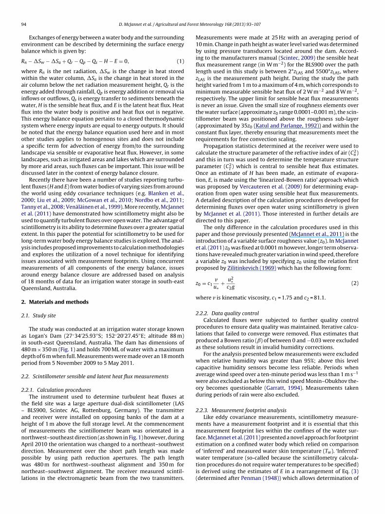
The study was conducted at an irrigation water storage knowns Logan’s Dam (27◦34′25.93′′S; 152◦20′27.45′′E; altitude 88 m)n south-east Queensland, Australia. The dam has dimensions of80 m × 350 m (Fig. 1) and holds 700 ML of water with a maximumepth of 6 m when full. Measurements were made over an 18 montheriod from 5 November 2009 to 5 May 2011.

.2. Scintillometer sensible and latent heat flux measurements

.2.1. Calculation proceduresThe instrument used to determine turbulent heat fluxes at

he field site was a large aperture dual-disk scintillometer (LAS BLS900, Scintec AG, Rottenburg, Germany). The transmitternd receiver were installed on opposing banks of the dam at aeight of 1 m above the full storage level. At the commencementf measurements the scintillometer beam was orientated in aorthwest–southeast direction (as shown in Fig. 1) however, duringpril 2010 the orientation was changed to a northeast–southwestirection. Measurement over the short path length was made

ossible by using path reduction apertures. The path lengthas 480 m for northwest–southeast alignment and 350 m forortheast–southwest alignment. The receiver measured scintil-

ations in the electromagnetic beam from the two transmitters.

t Meteorology 168 (2013) 93– 107

Measurements were made at 25 Hz with an averaging period of10 min. Change in path height as water level varied was determinedby using pressure transducers located around the dam. Accord-ing to the manufacturers manual (Scintec, 2009) the sensible heatflux measurement range (in W m−2) for the BLS900 over the pathlength used in this study is between 2*zLAS and 5500*zLAS, wherezLAS is the measurement path height. During the study the pathheight varied from 1 m to a maximum of 4 m, which corresponds tominimum measurable sensible heat flux of 2 W m−2 and 8 W m−2,respectively. The upper limit for sensible heat flux measurementsis never an issue. Given the small size of roughness elements overthe water surface (approximate z0 range 0.0001–0.001 m), the scin-tillometer beam was positioned above the roughness sub-layer(approximated by 35z0 (Katul and Parlange, 1992)) and within theconstant flux layer, thereby ensuring that measurements meet therequirements for free convection scaling.

Propagation statistics determined at the receiver were used tocalculate the structure parameter of the refractive index of air (C2

n )and this in turn was used to determine the temperature structureparameter (C2

T ) which is central to sensible heat flux estimates.Once an estimate of H has been made, an estimate of evapora-tion, E, is made using the ‘linearized-Bowen ratio’ approach whichwas proposed by Vercauteren et al. (2009) for determining evap-oration from open water using sensible heat flux measurements.A detailed description of the calculation procedures developed fordetermining fluxes over open water using scintillometry is givenby McJannet et al. (2011). Those interested in further details aredirected to this paper.

The only difference in the calculation procedures used in thispaper and those previously presented (McJannet et al., 2011) is theintroduction of a variable surface roughness value (z0). In McJannetet al. (2011) z0 was fixed at 0.0001 m however, longer term observa-tions have revealed much greater variation in wind speed, thereforea variable z0 was included by specifying z0 using the relation firstproposed by Zilitinkevich (1969) which has the following form:

z0 = c1v

u∗+ u2∗

c2g(2)

where v is kinematic viscosity, c1 = 1.75 and c2 = 81.1.

2.2.2. Data quality controlCalculated fluxes were subjected to further quality control

procedures to ensure data quality was maintained. Iterative calcu-lations that failed to converge were removed. Flux estimates thatproduced a Bowen ratio (ˇ) of between 0 and −0.03 were excludedas these solutions result in invalid humidity corrections.

For the analysis presented below measurements were excludedwhen relative humidity was greater than 95%; above this levelcapacitive humidity sensors become less reliable. Periods whenaverage wind speed over a ten-minute period was less than 1 m s−1

were also excluded as below this wind speed Monin–Obukhov the-ory becomes questionable (Garratt, 1994). Measurements takenduring periods of rain were also excluded.

2.2.3. Measurement footprint analysisLike eddy covariance measurements, scintillometry measure-

ments have a measurement footprint and it is essential that thismeasurement footprint lies within the confines of the water sur-face. McJannet et al. (2011) presented a novel approach for footprintestimation on a confined water body which relied on comparisonof ‘inferred’ and measured water skin temperature (Tw). ‘Inferred’

water temperature (so-called because the scintillometry calcula-tion procedures do not require water temperatures to be specified)is derived using the estimates of E in a rearrangement of Eq. (3)(determined after Penman (1948)) which allows determination of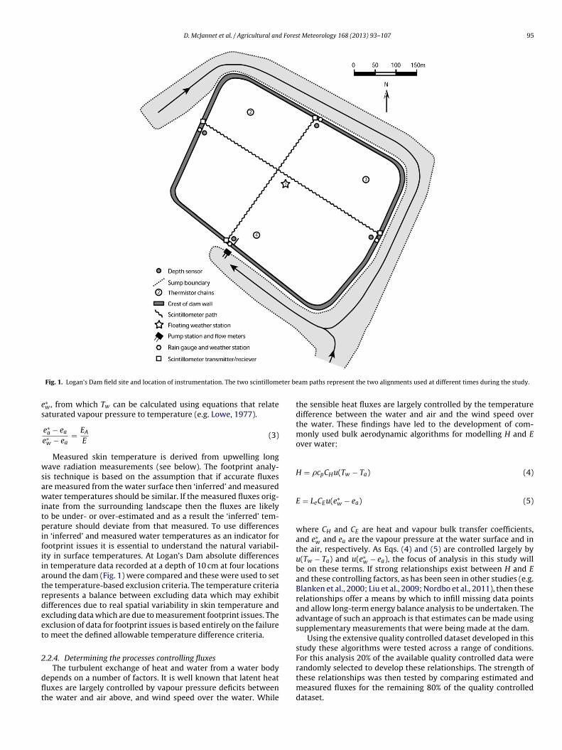

D. McJannet et al. / Agricultural and Forest Meteorology 168 (2013) 93– 107 95

ter be

es

wsawitpifiiatrdeet

2

dflt

Fig. 1. Logan’s Dam field site and location of instrumentation. The two scintillome

∗w , from which Tw can be calculated using equations that relateaturated vapour pressure to temperature (e.g. Lowe, 1977).

e∗a − ea

e∗w − ea

= EA

E(3)

Measured skin temperature is derived from upwelling longave radiation measurements (see below). The footprint analy-

is technique is based on the assumption that if accurate fluxesre measured from the water surface then ‘inferred’ and measuredater temperatures should be similar. If the measured fluxes orig-

nate from the surrounding landscape then the fluxes are likelyo be under- or over-estimated and as a result the ‘inferred’ tem-erature should deviate from that measured. To use differences

n ‘inferred’ and measured water temperatures as an indicator forootprint issues it is essential to understand the natural variabil-ty in surface temperatures. At Logan’s Dam absolute differencesn temperature data recorded at a depth of 10 cm at four locationsround the dam (Fig. 1) were compared and these were used to sethe temperature-based exclusion criteria. The temperature criteriaepresents a balance between excluding data which may exhibitifferences due to real spatial variability in skin temperature andxcluding data which are due to measurement footprint issues. Thexclusion of data for footprint issues is based entirely on the failureo meet the defined allowable temperature difference criteria.

.2.4. Determining the processes controlling fluxes

The turbulent exchange of heat and water from a water body

epends on a number of factors. It is well known that latent heatuxes are largely controlled by vapour pressure deficits betweenhe water and air above, and wind speed over the water. While

am paths represent the two alignments used at different times during the study.

the sensible heat fluxes are largely controlled by the temperaturedifference between the water and air and the wind speed overthe water. These findings have led to the development of com-monly used bulk aerodynamic algorithms for modelling H and Eover water:

H = �cpCHu(Tw − Ta) (4)

E = LeCEu(e∗w − ea) (5)

where CH and CE are heat and vapour bulk transfer coefficients,and e∗

w and ea are the vapour pressure at the water surface and inthe air, respectively. As Eqs. (4) and (5) are controlled largely byu(Tw − Ta) and u(e∗

w − ea), the focus of analysis in this study willbe on these terms. If strong relationships exist between H and Eand these controlling factors, as has been seen in other studies (e.g.Blanken et al., 2000; Liu et al., 2009; Nordbo et al., 2011), then theserelationships offer a means by which to infill missing data pointsand allow long-term energy balance analysis to be undertaken. Theadvantage of such an approach is that estimates can be made usingsupplementary measurements that were being made at the dam.

Using the extensive quality controlled dataset developed in thisstudy these algorithms were tested across a range of conditions.For this analysis 20% of the available quality controlled data were

randomly selected to develop these relationships. The strength ofthese relationships was then tested by comparing estimated andmeasured fluxes for the remaining 80% of the quality controlleddataset.

9 Fores

2

bwNwiaoChUupssi

wttshOmtLess

2

dCWasmttr7s

wtode

�

wot(L

LwAc

6 D. McJannet et al. / Agricultural and

.3. Net radiation and meteorological measurements

Net radiation above the water (Rn) was determined by com-ining individual measurements of incoming and outgoing longave and short wave radiation (CNR1, Kipp & Zonen, Delft, Theetherlands) which were taken at a height of 1.2 m from a floatingeather station (Fig. 1). Other measurements from this platform

ncluded wind speed at 2.4 m (014A, MetOne, Oregon, USA), high-ccuracy (±0.1 ◦C) aspirated temperature measurements at heightsf 0.4 and 3 m (41,342, RM Young), atmospheric pressure (CS106,ampbell Scientific, Utah, USA), and temperature and humidity ateights of 0.55 m and 2.55 m (CS215, Campbell Scientific, Utah,SA). The outgoing long wave radiation measurements were alsosed to derive water skin temperature. The aspirated temperaturerobes were used to determine the stability conditions of the nearurface atmosphere (i.e. unstable or stable) which is required forcintillometry calculations. All sensors were sampled at 10 secondntervals and averaged over ten minute periods.

Surrounding the dam were supplementary weather stationshich monitored a range of standard meteorological variables. On

he eastern and western sides of the dam, weather stations moni-ored wind speed and direction (WindSonic, Gill Instruments, UK),olar radiation (Li 200x, LiCor, Lincoln, USA), and temperature andumidity (CS215, Campbell Scientific, Utah, USA) at a height of 3 m.n the northern and southern sides of the dam weather stationsonitored wind speed and direction (03002 RM Young Wind Sen-

ry Set, RM Young, Michigan, USA), solar radiation (Li 200x, LiCor,incoln, USA), and temperature and humidity (CS215, Campbell Sci-ntific, Utah, USA) at a height of 3 m. The supplementary weathertations also collected and stored data from rain gauges and pres-ure transducers as described below.

.4. Water temperature and heat storage

Water temperature was measured using four thermistor chainsistributed around the dam. The central thermistor chain (PME,alifornia, USA) was suspended below the floating weather station.ater temperature was measured from a depth of 0.1–4.3 m

t 0.3 m increments. The remaining thermistor chains (locationshown in Fig. 1) were custom built systems which used Thermo-etrics P60 thermistors (Thermometrics, New Jersey, USA). All

hermistors data was averaged for 10 min periods. The centralhermistor chain operated for the duration of the study while theemaining thermistor chains ran for intermittent periods (total of7 days) during the study to help in the assessment of spatial heattorage variation.

The average quantity of heat stored in the lake at a given timeas calculated by dividing the lake into horizontal slices with a

hermistor at the midpoint of each slice. The change in heat storedver the course of a day (�Sw in W m−2) was determined from theifference between energy storage at the start of the day and at thend of the day (primed symbols):

Sw = 1as�t

[∑z

�wcwV ′zT ′

z −∑

z

�wcwVzTz

](6)

here �w is the density of water (kg m−3), cw is the specific heatf water (J kg−1 ◦C−1), as is the average dam surface area (m2), Tz ishe water temperature (◦C) at depth z (m), �t is the time intervals), and Vz is the volume of the horizontal slice for depth z (m3).oss of heat from the dam results in negative �Sw.

A survey of Logan’s dam was undertaken by G.L. Irrigation Pty

td. to relate its depth to volume and surface area. The surveyas made using a dual frequency GPS (NovAtel RTK, NovAtel Inc.,lberta, Canada) with vertical accuracy of 0.02–0.04 m. Storageurves were developed by using cubic polynomials to relate water

t Meteorology 168 (2013) 93– 107

level to surface area and volume. The regular shape and slope of thedam walls resulted in very strong relationships (r2 > 0.99) betweendepth and surface area and the depth and volume.

The depth of the water in the dam was determined using pres-sure transducers (KPSI 501, Esterline, Bellevue, Washington) whichwere installed at four locations around the dam (Fig. 1). Waterdepth was measured every 10 s and averaged for 10 min periods.The pressure transducers had an accuracy of ±0.3 mm and a res-olution of 0.003 mm. Daily depth changes were determined bysubtracting average depth at the start of the day from average depthat the end of the day. All depths were related to a common datumfrom survey data for consistency.

The change in heat stored in the air column below the net radi-ation measurement height (�Sa) was calculated using the methoddescribed by McCaughey (1985). Average daily change in �Sa wascalculated using temperature and humidity measurements fromthe profile on the floating weather station.

2.5. Energy loss through irrigation water pumping

This irrigation storage has two pipes for pumping water from thesump surrounding the dam into the main storage (Fig. 1) and twopipes for distributing water from the main storage to the surround-ing agricultural area. The two distribution pipelines were fittedwith high accuracy (±0.2%) flow meters (Magflow Mag5100W,Siemens, Victoria, Australia) and transmitters (Mag6000, Siemens,Victoria, Australia) and total flow was recorded in 10 min inter-vals using a data logger (CR1000, Campbell Scientific, Utah, USA).One of the distribution pipes had a diameter of 200 mm and theother had a diameter of 250 mm. The temperature of water beingextracted from the dam was monitored in the transport pipelineusing a platinum resistance thermometer (PT100 RTD, OneTemp,Australia). The heat removed via irrigation water (Qp) in W m−2 wascalculated from:

Qp = �wcw

as

VpTp

�t(7)

where Vp is the volume of water pumped (m3) and Tp is the temper-ature of the pumped water (◦C). Using this approach Qp is calculatedas a positive value which is then subtracted from the availableenergy in the energy balance equation (1).

The two input pipes are much larger with a diameter of 800 mm.These pipes move very large amounts of water and even the mostaccurate flow metering would result in high levels of flow uncer-tainty. For this reason it was decided that periods where these twopipes were activated would be ignored in the analysis. Fortunately,the input pipes are only active for one or two days at a time afterperiods of heavy rain (17 days in total for this study), whereas thesmaller distribution pipes are active much more often and for muchlonger periods.

2.6. Energy addition from rainfall

Direct water input to the storage from rainfall was monitoredusing a set of four tipping-bucket rain gauges (TB3, HydrologicalServices, Sydney, Australia) which were distributed around the damwalls (Fig. 1). These rain gauges have an accuracy of ±2%. Dailyrainfall was calculated as the average of these four gauges. Eachrain gauge was located with one of the supplementary weatherstations. The energy contribution from rainfall (Qr) in W m−2 wascalculated from:

Qr = �wcwPgTwb

�t(8)

where Pg is the amount of rainfall (m) and Twb is the wet-bulbtemperature of the air (◦C).

D. McJannet et al. / Agricultural and Forest Meteorology 168 (2013) 93– 107 97

Fig. 2. Average daily relative humidity (a), air temperature (b), solar radiation (c) and wind speed (d), and total daily rainfall (e) and pumped water losses (f) throughout thestudy period. The circles in (f) indicate days where the dam was being filled through pumping.

98 D. McJannet et al. / Agricultural and Fores

Ft

3

3

hv1aSdvwnfwpaofwLtgdsvc(mas

3

3

ww

ig. 3. Wind rose for the study period showing predominant wind speeds and direc-ions.

. Results and discussion

.1. Background

Over the course of the 18 month study period the relativeumidity remained high (average = 75%) with very little seasonalariation (Fig. 2a). Average daily air temperatures ranged from3.9 ◦C during winter to 24.6 ◦C during summer with maximumnd minimum recorded temperatures of 39.8 ◦C and 1.4 ◦C (Fig. 2b).olar radiation ranged from 147 W m−2 during winter to 244 W m−2

uring summer (Fig. 2c). Wind speed showed only weak seasonalariation with an average for the study of 2.7 m s−1 (Fig. 2d). Theind rose for the study period (Fig. 3) shows that the predomi-ant wind direction is from a south easterly direction with winds

rom the north being very rare. Wind speeds less than 4 m s−1

ere recorded for more than 80% of the duration of the studyeriod while wind speeds greater than 6 m s−1 were very rare andccounted for only 4% of the observations. During the 18 monthsf the study 1761 mm of rain was recorded and 62% of this rainell during the summer months (Fig. 2e). The highest daily rainfallas 224 mm which resulted in extensive flooding in the region.

oss of water from the dam to supply irrigation needs tendedo occur during distinct periods which reflected the stage of therowing seasons and the occurrence of rainfall (Fig. 2f). Periodsuring the study where the dam was filled by pumping from theurrounding sump are shown as circles in Fig. 2f. The averageolume of the dam during the study period was 509 ML (75% ofapacity) but this ranged from 170 ML (25% of capacity) to 705 ML105% of capacity i.e. >safe storage level). In this paper the sum-

er months refer to the period covering December to February,utumn includes March–May, winter includes June–August, andpring includes September–November.

.2. Sensible and latent heat flux

.2.1. Scintillometer data quality controlFor the 18 month study period scintillometer measurements

ere missing for 16% of the time. The missing data included periodshere the scintillometer transmitter or receiver went out of

t Meteorology 168 (2013) 93– 107

alignment due to the shrinking and swelling nature of the local soils(13%), or the presence of fog over the water which blocked signaltransmission (3%); a common occurrence in the early morning. Ofthe data which was successfully collected 10% were removed forperiods when average wind speed was <1 m s−1, 7% were removedwhen relative humidity was >95%, 4% were removed for periodswhen rain was falling, 2% were removed for invalid values, and1% were removed due to lack of convergence to a stable solution.Using the maximum tolerated difference between observed and‘inferred’ water temperature to identify potential measurementfootprint issues resulted in 14% of the data being removed. Theconditions resulting in exclusion of data for measurement footprintissues are discussed below in further detail. After data quality con-trol a total of 44,858 ten minute measurement periods remainedwhich is equivalent to 63% of measurements.

3.2.2. Measurement footprint analysisIn order to use differences in ‘inferred’ and measured water

temperatures as a indicator for measurement footprint issues itis essential to understand the natural variability in surface tem-peratures and set a temperature exclusion criteria. At Logan’s Damabsolute differences in temperature data recorded at a depth of10 cm at four locations around the dam (Fig. 1) were comparedover a 77 day period and these were used to set the temperature-based exclusion criteria. (N.B. While the central thermistor chainfunctioned for the entire study period the remaining thermistorchains provided reliable data for just 77 days.) The cutoff criteria foracceptable water temperature difference was set at two standarddeviations from the mean which was calculated to be 1.48 ◦C. Theassumption is made that this variability reflects the variabilitywhich would be expected for the skin temperature, therefore anabsolute difference between ‘inferred’ and observed temperaturesof greater than 1.5 ◦C was used to identify periods with potentialfootprint issues.

An example of a comparison of ‘inferred’ and measured waterskin temperature and identification of periods with footprint issuesis shown in Fig. 4. In this figure an absolute difference between‘inferred’ and observed temperatures of greater than 1.5 ◦C is usedto identify periods where measurement footprint might extendbeyond the water surface.

There are a number of different factors which could be respon-sible for causing measurement footprint issues at Logan’s Dam,these include wind speed, wind direction and atmospheric stabil-ity. Using the methodology for identifying potential measurementfootprint problems it is possible to explore these issues further. Ifthe percentage of data excluded from the measurement dataset fordifferent classes of wind speed and wind direction is considered itis possible to determine the conditions most likely to result in mea-surement footprint issues. Such an analysis is shown in Fig. 5 whereit can be seen that, there is an increasing tendency towards foot-print issues at higher wind speeds. At wind speeds greater than6 m s−1 an average of 40% of measurements were excluded com-pared to around 5% at the lowest wind speeds. To enable analysisacross the entire dataset which includes a change in alignment ofthe scintillometer, the wind direction shown in Fig. 5a is expressedas an angle relative to the scintillometer beam (0–90◦). For suchanalysis a wind direction of 90◦ is perpendicular to the scintil-lometer beam. The idea behind this analysis is to see whether dataexclusion is related in some way to the interaction between scin-tillometer signal strength, which is strongly weighted to the centreof the beam (Chehbouni et al., 2000; Meijninger et al., 2002a), and

wind direction. While there is some suggestion that winds from60◦ to 70◦ result in the most exclusions, some care is needed ininterpretation of results as winds from some directions are rareand therefore the exclusion statistics are less certain.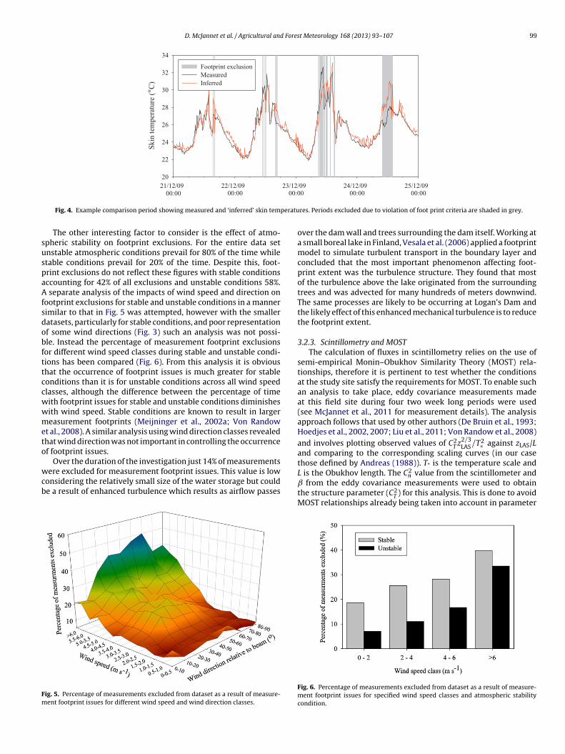

D. McJannet et al. / Agricultural and Forest Meteorology 168 (2013) 93– 107 99

21/12 /09 22 /12 /09 23 /12 /09 24 /12 /09 25 /12 /09

Skin

tem

per

ature

(oC

)

20

22

24

26

28

30

32

34

Footprint exclusion

Measured

Inferred

00:0

peratu

suspaAfsdobfttccwwmeto

wcb

Fm

00:00 00:00

Fig. 4. Example comparison period showing measured and ‘inferred’ skin tem

The other interesting factor to consider is the effect of atmo-pheric stability on footprint exclusions. For the entire data setnstable atmospheric conditions prevail for 80% of the time whiletable conditions prevail for 20% of the time. Despite this, foot-rint exclusions do not reflect these figures with stable conditionsccounting for 42% of all exclusions and unstable conditions 58%.

separate analysis of the impacts of wind speed and direction onootprint exclusions for stable and unstable conditions in a mannerimilar to that in Fig. 5 was attempted, however with the smalleratasets, particularly for stable conditions, and poor representationf some wind directions (Fig. 3) such an analysis was not possi-le. Instead the percentage of measurement footprint exclusionsor different wind speed classes during stable and unstable condi-ions has been compared (Fig. 6). From this analysis it is obvioushat the occurrence of footprint issues is much greater for stableonditions than it is for unstable conditions across all wind speedlasses, although the difference between the percentage of timeith footprint issues for stable and unstable conditions diminishesith wind speed. Stable conditions are known to result in largereasurement footprints (Meijninger et al., 2002a; Von Randow

t al., 2008). A similar analysis using wind direction classes revealedhat wind direction was not important in controlling the occurrencef footprint issues.

Over the duration of the investigation just 14% of measurementsere excluded for measurement footprint issues. This value is low

onsidering the relatively small size of the water storage but coulde a result of enhanced turbulence which results as airflow passes

ig. 5. Percentage of measurements excluded from dataset as a result of measure-ent footprint issues for different wind speed and wind direction classes.

0 00:00 00 :00

res. Periods excluded due to violation of foot print criteria are shaded in grey.

over the dam wall and trees surrounding the dam itself. Working ata small boreal lake in Finland, Vesala et al. (2006) applied a footprintmodel to simulate turbulent transport in the boundary layer andconcluded that the most important phenomenon affecting foot-print extent was the turbulence structure. They found that mostof the turbulence above the lake originated from the surroundingtrees and was advected for many hundreds of meters downwind.The same processes are likely to be occurring at Logan’s Dam andthe likely effect of this enhanced mechanical turbulence is to reducethe footprint extent.

3.2.3. Scintillometry and MOSTThe calculation of fluxes in scintillometry relies on the use of

semi-empirical Monin–Obukhov Similarity Theory (MOST) rela-tionships, therefore it is pertinent to test whether the conditionsat the study site satisfy the requirements for MOST. To enable suchan analysis to take place, eddy covariance measurements madeat this field site during four two week long periods were used(see McJannet et al., 2011 for measurement details). The analysisapproach follows that used by other authors (De Bruin et al., 1993;Hoedjes et al., 2002, 2007; Liu et al., 2011; Von Randow et al., 2008)and involves plotting observed values of C2

T z2/3LAS/T2∗ against zLAS/L

and comparing to the corresponding scaling curves (in our casethose defined by Andreas (1988)). T* is the temperature scale and

L is the Obukhov length. The C2

n value from the scintillometer and from the eddy covariance measurements were used to obtain

the structure parameter (C2T ) for this analysis. This is done to avoid

MOST relationships already being taken into account in parameter

Fig. 6. Percentage of measurements excluded from dataset as a result of measure-ment footprint issues for specified wind speed classes and atmospheric stabilitycondition.

100 D. McJannet et al. / Agricultural and Forest Meteorology 168 (2013) 93– 107

F 2 2/3 2

s(

eafs(sdttt

pttˇtcflsrbusfl

3

twd(boec

Fig. 8. Latent heat flux as a function of the vapour pressure gradient multiplied bythe wind speed (a), and sensible heat flux as a function of temperature difference

ig. 7. Observed values of CT

zLAS /T∗ plotted against zLAS/L during unstable (a) andtable (b) conditions. The solid lines are the scaling functions proposed by Andreas1988) and used in the scintillometer calculation scheme.

stimation, which is the case for scintillometer measurements. T*nd L were also taken from eddy covariance methods. Data from theour observation periods were grouped and split into those repre-enting stable and unstable conditions. During unstable conditionsFig. 7a) the observed values of C2

T z2/3LAS/T2∗ and zLAS/L followed the

hape of the scaling curve proposed by Andreas (1988) giving confi-ence in the approach used. Deviations of the measurements fromhe scaling curve will represent differences in flux estimates fromhe two techniques (Von Randow et al., 2008) however there is noendency for consistent under or over estimation.

During stable conditions (Fig. 7b) there were far fewer dataoints but there was a tendency for some points to greatly exceedhe scaling curve. Closer inspection of these points show that theyend to represent periods of very low H (<−10 W m−2) and small. Excluding these points, the remaining points tend to sit around

he scaling curve. As stated by De Bruin et al. (1993) the mostonclusive test of any MOST approach is a comparison betweenuxes derived from MOST relationships and independently mea-ured fluxes. McJannet et al. (2011) undertook such an analysis andeported excellent agreement between flux measurements madey eddy covariance and scintillometry at this field site. The analysisndertaken here and the comparison of fluxes undertaken in othertudies gives confidence in the use of scintillometry to determineuxes at this site.

.2.4. Processes controlling fluxesUsing the extensive quality controlled dataset, the strength of

he relationships between E and u(e∗w − ea) and H and u(Tw − Ta)

ere considered. Relationships were determined using a ran-om selection of 20% of the available quality controlled datasetn = 8971). Latent heat flux was shown to be strongly controlled

∗

y u(ew − ea) (Fig. 8a). A single relationship fit to all data regardlessf stability conditions explained 93% of the observed variation invaporation. Relationships fitted to data points grouped by stabilityonditions further improved predictions with 95% of the observed

between the surface and the air multiplied by the wind speed (b). The line representsthe fit to all data points. Equations for the line of best fit for a single fitted relationshipand relationships based on atmospheric stability are given in Table 1.

variation being explained by these separate fitted relationships(Table 1). When the derived relationships were tested against pre-dictions from the remaining 80% of the quality controlled dataset(n = 35,884) the agreement was excellent with a RMSE of less than16 W m−2 and an r2 of 0.95, when separate relationships were usedfor stable and unstable conditions (Table 1). Similarly strong agree-ment between latent heat flux and u(e∗

w − ea) has been reported byBlanken et al. (2000) – r2 = 0.84, with slightly weaker relationshipsreported by Nordbo et al. (2011) – r2 = 0.59 and Liu et al. (2009). It isinteresting to note that the results reported by Nordbo et al. (2011)differ from the others reported in that they calculate e∗

w using watertemperature measured at a depth of 0.2 m rather than directly at theair–water interface (skin temperature), hence temperature stratifi-cation may be partly responsible for the increased scatter reportedin this study.

The reported relationships are similar to, but not the same as,the commonly reported wind function (f(u)) (e.g. McJannet et al.,2012; Sweers, 1976) which forms the basis of Dalton (1802) typeevaporation equations (i.e. E = f (u)(e∗

w − ea) where f (u) = a + bu).The wind function for our site (in units of W m−2 kPa−1) is f (u) =37.7 + 30.6u with r2 = 0.80.

Sensible heat flux was shown to be strongly controlled byu(Tw − Ta) (Fig. 8b). A single relationship between sensible heatflux and u(Tw − Ta) explained 83% of the observed variation in sen-

sible heat flux, while separate relationships for stable and unstableconditions explained 70% of the observed variation in H (Table 1).The RMSE of predicted sensible heat flux when compared to theremaining 80% of the quality controlled measurement dataset was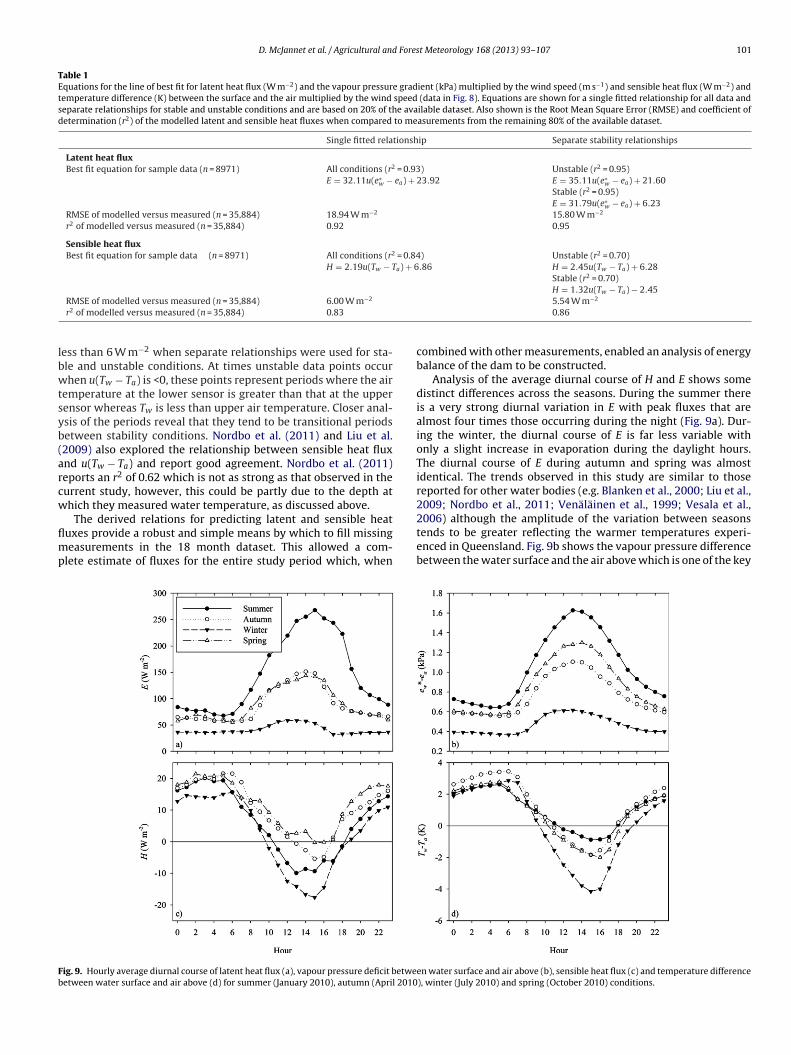

D. McJannet et al. / Agricultural and Forest Meteorology 168 (2013) 93– 107 101

Table 1Equations for the line of best fit for latent heat flux (W m−2) and the vapour pressure gradient (kPa) multiplied by the wind speed (m s−1) and sensible heat flux (W m−2) andtemperature difference (K) between the surface and the air multiplied by the wind speed (data in Fig. 8). Equations are shown for a single fitted relationship for all data andseparate relationships for stable and unstable conditions and are based on 20% of the available dataset. Also shown is the Root Mean Square Error (RMSE) and coefficient ofdetermination (r2) of the modelled latent and sensible heat fluxes when compared to measurements from the remaining 80% of the available dataset.

Single fitted relationship Separate stability relationships

Latent heat fluxBest fit equation for sample data (n = 8971) All conditions (r2 = 0.93)

E = 32.11u(e∗w − ea) + 23.92

Unstable (r2 = 0.95)E = 35.11u(e∗

w − ea) + 21.60Stable (r2 = 0.95)E = 31.79u(e∗

w − ea) + 6.23RMSE of modelled versus measured (n = 35,884) 18.94 W m−2 15.80 W m−2

r2 of modelled versus measured (n = 35,884) 0.92 0.95

Sensible heat fluxBest fit equation for sample data (n = 8971) All conditions (r2 = 0.84)

H = 2.19u(Tw − Ta) + 6.86Unstable (r2 = 0.70)H = 2.45u(Tw − Ta) + 6.28Stable (r2 = 0.70)H = 1.32u(Tw − Ta) − 2.45

lbwtsyb(arcw

flmp

Fb

RMSE of modelled versus measured (n = 35,884) 6.00 W m−2

r2 of modelled versus measured (n = 35,884) 0.83

ess than 6 W m−2 when separate relationships were used for sta-le and unstable conditions. At times unstable data points occurhen u(Tw − Ta) is <0, these points represent periods where the air

emperature at the lower sensor is greater than that at the upperensor whereas Tw is less than upper air temperature. Closer anal-sis of the periods reveal that they tend to be transitional periodsetween stability conditions. Nordbo et al. (2011) and Liu et al.2009) also explored the relationship between sensible heat fluxnd u(Tw − Ta) and report good agreement. Nordbo et al. (2011)eports an r2 of 0.62 which is not as strong as that observed in theurrent study, however, this could be partly due to the depth athich they measured water temperature, as discussed above.

The derived relations for predicting latent and sensible heatuxes provide a robust and simple means by which to fill missingeasurements in the 18 month dataset. This allowed a com-

lete estimate of fluxes for the entire study period which, when

ig. 9. Hourly average diurnal course of latent heat flux (a), vapour pressure deficit betweetween water surface and air above (d) for summer (January 2010), autumn (April 2010

5.54 W m−2

0.86

combined with other measurements, enabled an analysis of energybalance of the dam to be constructed.

Analysis of the average diurnal course of H and E shows somedistinct differences across the seasons. During the summer thereis a very strong diurnal variation in E with peak fluxes that arealmost four times those occurring during the night (Fig. 9a). Dur-ing the winter, the diurnal course of E is far less variable withonly a slight increase in evaporation during the daylight hours.The diurnal course of E during autumn and spring was almostidentical. The trends observed in this study are similar to thosereported for other water bodies (e.g. Blanken et al., 2000; Liu et al.,2009; Nordbo et al., 2011; Venäläinen et al., 1999; Vesala et al.,

2006) although the amplitude of the variation between seasonstends to be greater reflecting the warmer temperatures experi-enced in Queensland. Fig. 9b shows the vapour pressure differencebetween the water surface and the air above which is one of the key

en water surface and air above (b), sensible heat flux (c) and temperature difference), winter (July 2010) and spring (October 2010) conditions.

1 Forest Meteorology 168 (2013) 93– 107

dvwgfa

hsawtwdttnedTdtt

3

asimFaflva

wtarwodTsto

twcmCtfTtsllcoi

G

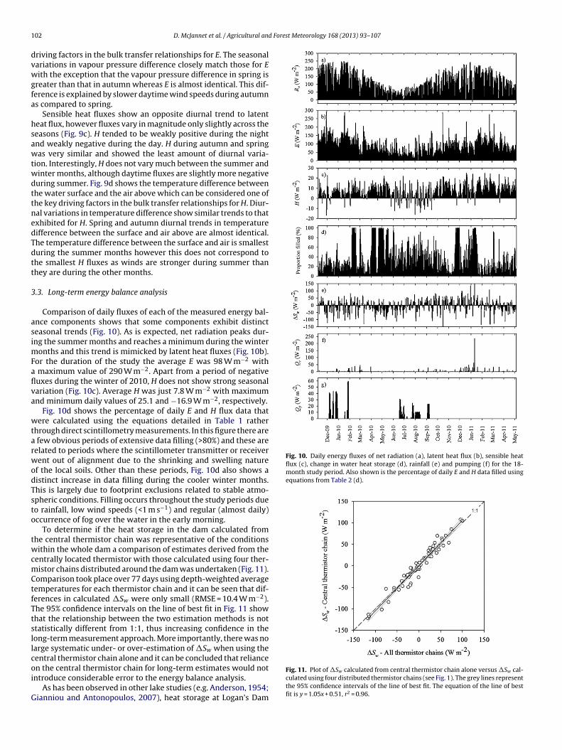
Fig. 10. Daily energy fluxes of net radiation (a), latent heat flux (b), sensible heatflux (c), change in water heat storage (d), rainfall (e) and pumping (f) for the 18-month study period. Also shown is the percentage of daily E and H data filled usingequations from Table 2 (d).

02 D. McJannet et al. / Agricultural and

riving factors in the bulk transfer relationships for E. The seasonalariations in vapour pressure difference closely match those for Eith the exception that the vapour pressure difference in spring is

reater than that in autumn whereas E is almost identical. This dif-erence is explained by slower daytime wind speeds during autumns compared to spring.

Sensible heat fluxes show an opposite diurnal trend to latenteat flux, however fluxes vary in magnitude only slightly across theeasons (Fig. 9c). H tended to be weakly positive during the nightnd weakly negative during the day. H during autumn and springas very similar and showed the least amount of diurnal varia-

ion. Interestingly, H does not vary much between the summer andinter months, although daytime fluxes are slightly more negativeuring summer. Fig. 9d shows the temperature difference betweenhe water surface and the air above which can be considered one ofhe key driving factors in the bulk transfer relationships for H. Diur-al variations in temperature difference show similar trends to thatxhibited for H. Spring and autumn diurnal trends in temperatureifference between the surface and air above are almost identical.he temperature difference between the surface and air is smallesturing the summer months however this does not correspond tohe smallest H fluxes as winds are stronger during summer thanhey are during the other months.

.3. Long-term energy balance analysis

Comparison of daily fluxes of each of the measured energy bal-nce components shows that some components exhibit distincteasonal trends (Fig. 10). As is expected, net radiation peaks dur-ng the summer months and reaches a minimum during the winter

onths and this trend is mimicked by latent heat fluxes (Fig. 10b).or the duration of the study the average E was 98 W m−2 with

maximum value of 290 W m−2. Apart from a period of negativeuxes during the winter of 2010, H does not show strong seasonalariation (Fig. 10c). Average H was just 7.8 W m−2 with maximumnd minimum daily values of 25.1 and −16.9 W m−2, respectively.

Fig. 10d shows the percentage of daily E and H flux data thatere calculated using the equations detailed in Table 1 rather

hrough direct scintillometry measurements. In this figure there are few obvious periods of extensive data filling (>80%) and these areelated to periods where the scintillometer transmitter or receiverent out of alignment due to the shrinking and swelling nature

f the local soils. Other than these periods, Fig. 10d also shows aistinct increase in data filling during the cooler winter months.his is largely due to footprint exclusions related to stable atmo-pheric conditions. Filling occurs throughout the study periods dueo rainfall, low wind speeds (<1 m s−1) and regular (almost daily)ccurrence of fog over the water in the early morning.

To determine if the heat storage in the dam calculated fromhe central thermistor chain was representative of the conditionsithin the whole dam a comparison of estimates derived from the

entrally located thermistor with those calculated using four ther-istor chains distributed around the dam was undertaken (Fig. 11).

omparison took place over 77 days using depth-weighted averageemperatures for each thermistor chain and it can be seen that dif-erences in calculated �Sw were only small (RMSE = 10.4 W m−2).he 95% confidence intervals on the line of best fit in Fig. 11 showhat the relationship between the two estimation methods is nottatistically different from 1:1, thus increasing confidence in theong-term measurement approach. More importantly, there was noarge systematic under- or over-estimation of �Sw when using theentral thermistor chain alone and it can be concluded that reliance

n the central thermistor chain for long-term estimates would notntroduce considerable error to the energy balance analysis.

As has been observed in other lake studies (e.g. Anderson, 1954;ianniou and Antonopoulos, 2007), heat storage at Logan’s Dam

Fig. 11. Plot of �Sw calculated from central thermistor chain alone versus �Sw cal-culated using four distributed thermistor chains (see Fig. 1). The grey lines representthe 95% confidence intervals of the line of best fit. The equation of the line of bestfit is y = 1.05x + 0.51, r2 = 0.96.

Forest Meteorology 168 (2013) 93– 107 103

iwddiasw

teoeeshwm

3

R

weteiccaacrbsNcrpatT

Fb

D. McJannet et al. / Agricultural and

ncreased during the summer months and decreased during theinter months. The largest changes in stored heat content occurreduring periods were large volumes of water were pumped into theam from the surrounding sump. The daily changes in heat storage

n the dam are shown in Fig. 10e. The change in heat storage in their between the water surface and the height of net radiation mea-urements (�Sa) is not shown in Fig. 10 as day to day differencesere so found to be very small (±0.4 W m−2).

Energy addition through rainfall was a very minor component ofhe energy balance for the vast majority of the year (Fig. 10f), how-ver its importance increased during the summer with progressionf the rainy season. On particularly wet days the contribution ofnergy input through rainfall can exceed net radiation. Loss ofnergy through removal of water from the dam via pumping occursporadically during the growing season (Fig. 10g) and when it doesappen it is not unusual for energy loss to exceed 30 W m−2. Asith rainfall energy, energy lost through pumping was relativelyinor.

.4. Energy balance closure

The energy balance equation (1) can be expressed as

n − �Sw − �Sa + Qr − Qp − Qs = H + E (9)

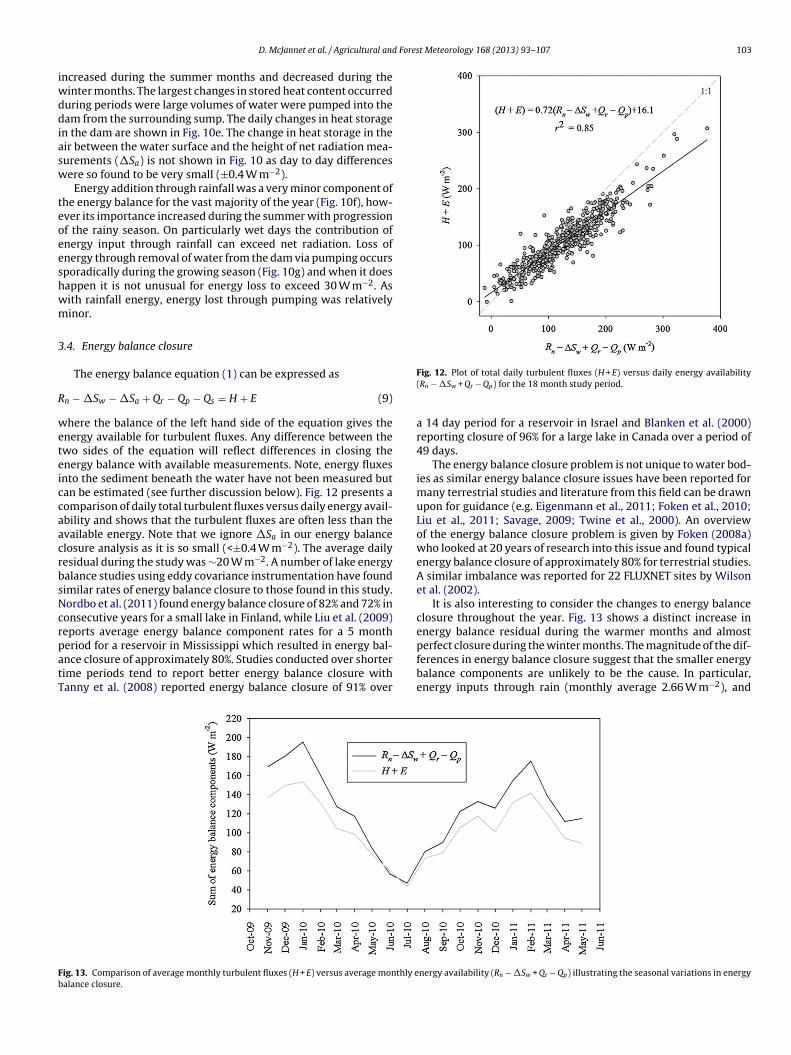
here the balance of the left hand side of the equation gives thenergy available for turbulent fluxes. Any difference between thewo sides of the equation will reflect differences in closing thenergy balance with available measurements. Note, energy fluxesnto the sediment beneath the water have not been measured butan be estimated (see further discussion below). Fig. 12 presents aomparison of daily total turbulent fluxes versus daily energy avail-bility and shows that the turbulent fluxes are often less than thevailable energy. Note that we ignore �Sa in our energy balancelosure analysis as it is so small (<±0.4 W m−2). The average dailyesidual during the study was ∼20 W m−2. A number of lake energyalance studies using eddy covariance instrumentation have foundimilar rates of energy balance closure to those found in this study.ordbo et al. (2011) found energy balance closure of 82% and 72% inonsecutive years for a small lake in Finland, while Liu et al. (2009)eports average energy balance component rates for a 5 month

eriod for a reservoir in Mississippi which resulted in energy bal-nce closure of approximately 80%. Studies conducted over shorterime periods tend to report better energy balance closure withanny et al. (2008) reported energy balance closure of 91% over

ig. 13. Comparison of average monthly turbulent fluxes (H + E) versus average monthly ealance closure.

Fig. 12. Plot of total daily turbulent fluxes (H + E) versus daily energy availability(Rn − �Sw + Qr − Qp) for the 18 month study period.

a 14 day period for a reservoir in Israel and Blanken et al. (2000)reporting closure of 96% for a large lake in Canada over a period of49 days.

The energy balance closure problem is not unique to water bod-ies as similar energy balance closure issues have been reported formany terrestrial studies and literature from this field can be drawnupon for guidance (e.g. Eigenmann et al., 2011; Foken et al., 2010;Liu et al., 2011; Savage, 2009; Twine et al., 2000). An overviewof the energy balance closure problem is given by Foken (2008a)who looked at 20 years of research into this issue and found typicalenergy balance closure of approximately 80% for terrestrial studies.A similar imbalance was reported for 22 FLUXNET sites by Wilsonet al. (2002).

It is also interesting to consider the changes to energy balanceclosure throughout the year. Fig. 13 shows a distinct increase inenergy balance residual during the warmer months and almostperfect closure during the winter months. The magnitude of the dif-

ferences in energy balance closure suggest that the smaller energybalance components are unlikely to be the cause. In particular,energy inputs through rain (monthly average 2.66 W m−2), and

nergy availability (Rn − �Sw + Qr − Qp) illustrating the seasonal variations in energy

1 Forest Meteorology 168 (2013) 93– 107

eupt

sssvi1ivruiWr

bfi

3

wbReStcnvidvnAfvrs

3

lLaBshyCstvi∼twIidr

Table 2Comparison of average sensible and latent heat fluxes for the study period usingvariable and fixed vales for z0. Also shown is the overall energy balance closure forthe entire study period.

z0 H (W m−2) E (W m−2) Energy balance closure

Variable (Eq. (3)) 7.9 98.2 84%0.0001 6.8 83.6 72%

04 D. McJannet et al. / Agricultural and

nergy loss through pumping (monthly average 2.73 W m−2) arenlikely to be the cause. Also, exclusion of days with rainfall andumping from the comparison in Fig. 12 does change the slope ofhe relationship.

Some of the observed difference could be due to the lack of inclu-ion of fluxes of energy into the underlying sediments. Inclusion ofuch a term would improve closure, however, the magnitude ofuch fluxes is not likely to be big enough to explain the observedariation and this term is often ignored in energy balance stud-es for water bodies (e.g. Anderson, 1954; Assouline and Mahrer,993; Gianniou and Antonopoulos, 2007; Tanny et al., 2011). Stud-

es that attempt to include sediment heat fluxes generally reportery small fluxes. For example, Smith (2002) measured energy fluxates into sediments in a shallow lagoon and reported average val-es of 2.1 W m−2, while Miguel et al. (2005) found average flux rates

nto sediment in a shallow water in southern Spain of 2.2 W m−2.orking at two lakes in Wisconsin, Likens and Johnson (1969)

eport annual sediment heat fluxes of 1 and 1.3 W m−2.With the smaller components of the energy balance unlikely to

e the cause of observed lack of closure, the potential contributionrom the larger components of the energy balance will be discussedn more detail in the following sections.

.4.1. Heat storageThe potential for introducing error in heat budget studies of

ater bodies through heat storage estimates have been notedy a number of authors (e.g. Nordbo et al., 2011; Stannard andosenberry, 1991; Vercauteren et al., 2009; Webb, 1960). Schertzert al. (2003) compared distributed thermistor chains in the Greatlave Lake to show how the spatial variation in water tempera-ure and hence, heat storage within a water body can be large. Inontrast, a comparison of heat storage calculations using differentumbers of thermistor chains at Logan’s Dam shows that spatialariation in heat storage cannot account for the observed residualn energy balance closure (Fig. 11). Although small temperatureifferences result in large changes in heat storage estimates, theseariations will introduce random type errors (Nordbo et al., 2011),ot the systematic type discrepancy which is observed in this study.nother source of potential error in heat storage calculations arises

rom uncertainty in the relationship between water depth and damolume. However, this effect will be small because it is only theelative difference in volume between days that will influence heattorage calculations.

.4.2. Net radiationNet radiation errors have also been considered as a reason for the

ack of closure in the energy balance (e.g. Foken, 2008a; Halldin andindroth, 1992; Wilson et al., 2002). Generally such measurementsre considered to be reliable and have a reasonable accuracy (e.g.rotzge and Duchon, 2000; Kohsiek et al., 2007), however thesetudies tend to involve inter-comparison of sensors that are notigh standard references. Michel et al. (2008) undertook an anal-sis of the performance and uncertainty of the Kipp and ZonenNR1 net radiometer (as used in this study) by comparing to hightandard reference radiation instruments. When using manufac-urer supplied calibration coefficients and an instrument withoutentilation and heating, Michel et al. (2008) found that uncertaintyn total net radiation was 26% on daily averages with a bias of10 W m−2, much greater than the 10% claimed by the manufac-

urer. Average annual net radiation during their comparison periodas 62 W m−2, almost exactly half of that measured in this study.

t is unclear whether the greater net radiation at our site wouldncrease or decrease uncertainty, however such issues cannot beiscounted as a potential cause of the observed energy balanceesidual. Michel et al. (2008) also mention that heat transmission

0.0005 7.0 111.9 94%0.001 6.7 128.8 107%

to the thermopiles could affect radiation estimates; an observationalso made by Halldin and Lindroth (1992). Such an affect could leadto seasonal differences in net radiation estimates. As an exampleof the potential impact of net radiation measurement errors, if thedaily net radiation data is corrected using a fixed value of 10 W m−2

(the bias value for net radiation reported by Michel et al. (2008)) theaverage energy balance closure across the study period increasesto 95%.

3.4.3. Turbulent fluxesThe other potential cause of the energy balance closure issue

is underestimation of the turbulent fluxes. In other scintillometrystudies over land where the structure parameters of temperature isadjusted for humidity effects the Bowen ratio is defined by measur-ing all other terms of the energy balance and forcing closure (knownas the ‘ closure method’). This is not the case in this study as the‘linearized method’ was used (McJannet et al., 2011). Underes-timation of the fluxes may result from some of the empirical ortheoretical relationships used in the derivation of fluxes, howeverthis is very hard to quantify and a number of studies have demon-strated good agreement with other measurement methods (e.g.Hartogensis and De Bruin, 2006; Meijninger et al., 2002b; Savage,2009). If the cause of the greater energy balance residual during thewarmer months (Fig. 13) is due to underestimation of the turbulentfluxes then any errors introduced in the calculations proceduresmust be greatest for higher flux rates. Also, if underestimation ofthe turbulent fluxes is suspected then the latent heat fluxes aremore likely to be the cause as they dominate over the sensible heatfluxes.

In a recent study by Bouin et al. (2012) scintillometry was used todetermine the sensible heat flux over water in the south of France.This study showed that the choice of z0 (fixed or variable) value hadvery little influence on the resultant H fluxes and concluded thatadjusting z0 during data processing caused no significant changes inthe final results. To see if the same held true for this current studya similar comparison was undertaken using the variable z0 valueand fixed values of 0.0001 m, 0.0005 m and 0.001 m and the resultsare shown in Table 2. In agreement with the results of Bouin et al.(2012) this analysis shows that mean H varies only slightly depend-ing on the choice of z0. It is also worth noting that the estimatedvalues of H for different z0 methods are highly correlated (r2 > 0.97).However, taking this analysis further it can be seen that the impactof different z0 specifications on calculated E can be large (Table 2).Despite estimated values of E being highly correlated for differentz0 methods (r2 > 0.99), mean E values differ by as much as 30% fromthe variable method. It can be seen from Table 2 that improve-ments in energy balance closure can be achieved by selecting anappropriate z0 value but taking such an approach ignores the welldocumented variation in z0 over water with u* (see Foken, 2008bfor summary). Forcing closure by using the best value of z0 is notscientifically robust and clearly there would be much benefit to be

gained from detailed future studies on the appropriate specifica-tion of z0. This being said, under-estimation of turbulent fluxes (inparticular E) cannot be discounted as the cause of the lack of energybalance closure.

Fores

cwt1(evrwrsmtlutse

ceeadtMlaidgs

daatdo(awJltemiwussTb

3

sttetuit

D. McJannet et al. / Agricultural and

A further test for whether low evaporative fluxes might be theause of the lack of energy balance closure is to compare resultsith evaporation estimates made using an evaporation model. For

his analysis the Penman open water evaporation model (Penman,948) with adjustments for heat storage (as described by Finch2001)) was used. Over the duration of the study period averagevaporation estimates for the scintillometer and Penman modelaried only slightly with values of 98.3 W m−2 and 104.5 W m−2,espectively. Modelled E estimates were also strongly correlatedith those derived through scintillometry (EPen = 0.99 * EScin + 6.09,

2 = 0.79). When modelled evaporation was combined with mea-ured H, the over-all energy balance closure during the summeronths was slightly better at 90% as compared to 82% for scin-

illometer estimates. Winter energy balance closure changed veryittle with 95% closure for the Penman model and 96% for estimatessing the scintillometer evaporation. Energy balance closure usinghe modelled results was only slightly better than those made usingcintillometer estimates therefore this analysis provides no strongvidence that scintillometer evaporation estimates are too low.

Another important aspect to consider with respect to thealculation of turbulent fluxes is whether the assumption ofqual diffusivities of water vapour and heat is suitable. Assoulinet al. (2008) used eddy correlation measurements to explore thisssumption for three water bodies and showed that the ratio ofiffusivities varied depending on advection and the thermal iner-ia of the water body. This issue has been explored previously by

cJannet et al. (2011) at this same location by comparing scintil-ometer and eddy covariance derived ˇ. If the diffusivities of heatnd water vapour were not equal then the calculated from the twondependent measurement systems would be expected to showistinct differences, however, McJannet et al. (2011) showed veryood agreement between the two methods (r2 = 0.83, RMSE = 0.06)uggesting the assumption is justified.

One simplified correction for energy balance closure is toistribute the residual between sensible and latent heat fluxesccording to the measured Bowen ratio (Foken, 2008a). While suchn approach is not advocated it provides an opportunity to fur-her explore the issue of energy balance closure through use oferived evaporation estimates in a water balance analysis. A suitef measurements for determining the water balance of Logan’s Damflows in and out, storage changes, rain, and evaporation) also existsnd this water balance analysis is the subject of another paperhere leakage losses are derived (McJannet et al., in review). Taking

anuary 2010 as a demonstration period (which is the month withargest energy balance residual) we can combine all components ofhe water balance to derive leakage as the residual using existingvaporation estimates and corrected evaporation estimates. Usingeasured evaporation rates an average daily leakage loss of 1.1 mm

s calculated which is a value similar to that determined for otherater storages (e.g. Ham, 2002). If corrected evaporation rates aresed the average daily leakage loss becomes −0.3 mm. Such a valueuggests net flow of water to the dam which is not physically pos-ible as this dam is constructed above the surrounding landscape.his analysis suggests that the energy balance closure issue cannote entirely attributed to underestimation of turbulent fluxes.

.4.4. Measurement footprint and advectionIn a review of energy balance closure issues for eddy covariance

ystems Foken (2008a) hypothesizes that the most likely cause ishat energy transport with very large eddies is not captured duringhe measurement period. Foken (2008a) also notes that if largerddies have a significant contribution to the energy exchange then

hey must be generated at the boundary between different landses which are normally excluded from measurements due to their

nfluence on the measurement footprint. The boundary betweenhe surrounding land and the dam may provide the conditions for

t Meteorology 168 (2013) 93– 107 105

such eddies to develop in this study. Interestingly for water bodies,the upwind edge is likely to be the zone of highest evaporation asair moving from the land over the water encounters a rapid surfaceroughness change which enables the air to accelerate. Evapora-tion is also likely to be greatest at the upwind edge because as youmove downwind the cumulative entrainment of moisture into theair is likely to reduce the vapour pressure gradient (Webster andSherman, 1995). The measurement footprint of the scintillometermay not always extend to the upwind zone of the water surface,therefore the spatial extent of measurements could also play animportant role in closing the energy balance.

A number of authors have also identified the failure to accountfor advected energy as a potential contributor to the problem ofenergy balance closure in varying landscapes (Eigenmann et al.,2011; Foken, 2008a; Leclerc et al., 2003; Li and Yu, 2007; Wilsonet al., 2002). A study by Oncley et al. (2007) used several profiletowers and flux gradient methods to estimate horizontal meanadvection for an irrigated agricultural area and showed minimaladvected sensible heat fluxes but advected latent heat fluxes of upto 30 W m−2. Oncley et al. (2007) demonstrated that the advectedlatent heat was greatest in the afternoon when the residual inenergy balance closure was greatest. It was proposed that theadvected energy was not included at the measurement becausefluxes at the measurement height may have been less than theactual flux at the surface. If similar processes are occurring atLogan’s Dam then advection could also be partly responsible forthe lack of closure. Enhanced advected latent heat flux loss duringsummer months could also help to partially explain seasonality inenergy balance closure.

4. Conclusions

An investigation has been conducted into the energy balanceof a small water body in south-east Queensland, Australia for aperiod of 18 months. The focus of this study was on the use ofscintillometry to determine the turbulent fluxes. Identification ofperiods where measurement footprint extended beyond the watersurface by comparison of ‘inferred’ and measured skin temperatureresulted in just 14% of measurements being excluded for footprintissues, thus, illustrating the suitability of scintillometry for deter-mining fluxes in such environments. Footprint issues were foundto be strongly related to wind speed but wind direction was notshown to have a strong influence. Stable conditions were found toaccount for 42% of footprint exclusions despite only representing20% of measurements.

The product of wind speed and the vapour pressure differencebetween the water surface and the air above was found to be arobust predictor of latent heat flux. Similarly, the product of windspeed and the temperature difference between the water surfaceand the air was also found to be very strong. The derived aero-dynamic algorithms for predicting latent and sensible heat fluxesprovided a reliable and simple means for filling missing measure-ments and constructing a complete 18 month dataset.

Using measurements of all energy balance components for thefull 18 month period it was found that energy balance closure acrossthe study was 82%; a value similar to that found in many otherstudies. By assessing the seasonality of energy balance closure itwas found that much better closure occurred during the winterthan the summer. The key factors likely to lead to errors in energybalance closure were considered and it was concluded that the mostlikely causes were underestimation of latent heat fluxes, advection

of latent heat fluxes which are not measured by the scintillometer,or overestimation of net radiation.

Latent heat flux estimates were shown to be sensitive to spec-ification of z0 and it was demonstrated that complete energy

1 Fores

bzmaMtncmiaTcs

A

MlKtIIatH

R

A

A

A

A

B

B

B

B

C

C

C

D

D

E

F

F

06 D. McJannet et al. / Agricultural and

alance closure was possible by selecting an appropriate fixed0 value, however, this approach is not scientifically valid andakes the assumption that latent heat fluxes are too low; an

ssumption not supported by modelling and water balance tests.ore detailed investigations into the suitability of z0 specifica-

ion are needed for open water environments. Use of ventilatedet radiometers with up-welling and down-welling componentsalibrated to a high standard reference is also recommended forinimizing measurement uncertainty for this component. Finally,

nclusion of additional instrumentation to enable quantification ofny advected energy is also recommended for smaller water bodies.hese recommendations will help in minimizing energy balancelosure issues and enable verification and improvement of futurecintillometry flux measurements.

cknowledgements

The authors wish to acknowledge the cooperation of Linton andelinda Brimblecombe who allowed access to the site and instal-

ation of equipment. Darren Morrow, Geoff Carlin, Tim Ellis, Rexeen, Joseph Kemei, and Grant Beckett provided assistance with

he design, installation and maintenance of the equipment. G.L.rrigation Pty Ltd. kindly allowed access to survey data for the site.an Webster provided valuable comment on the paper as did thenonymous reviewers. Funding for this research was provided byhe Urban Water Security Research Alliance and CSIRO Water for aealthy Country.

eferences

nderson, E.R., 1954. Energy budget studies. Water-loss investigations: Lake Hefnerstudies. U.S. Geological Survey. Professional Paper 269.

ndreas, E.L., 1988. Atmospheric stability from scintillation measurements. Appl.Opt. 27 (11), 2241–2246.

ssouline, S., Mahrer, Y., 1993. Evaporation from Lake Kinneret 1. Eddy correla-tion system measurements and energy budget estimates. Water Resour. Res.29, 901–910.

ssouline, S., Tyler, S.W., Tanny, J., Cohen, S., Bou-Zeid, E., Parlange, M.B., et al., 2008.Evaporation from three water bodies of different sizes and climates: measure-ments and scaling analysis. Adv. Water Resour. 31 (1), 160–172.

lanken, P.D., Rouse, W.R., Culf, A.D., Spence, C., Boudreau, L.D., Jasper, J.N., et al.,2000. Eddy covariance measurements of evaporation from Great Slave Lake,Northwest Territories, Canada. Water Resour. Res. 36 (4), 1069–1077.

onan, G.B., 1995. Sensitivity of a GCM simulation to inclusion of inland watersurfaces. J. Climate 8 (11), 2691–2704.

ouin, M., Legain, D., Traullé, O., Belamari, S., Caniaux, G., Fiandrino, A., et al., 2012.Using scintillometry to estimate sensible heat fluxes over water: first insights.Boundary Layer Meteorol. 143 (3), 451–480.

rotzge, J.A., Duchon, C.E., 2000. A field comparison among a domeless net radiome-ter, two four-component net radiometers, and a domed net radiometer. J. Atmos.Oceanic Technol. 17 (12), 1569–1582.

hehbouni, A., Watts, C., Lagouarde, J.P., Kerr, Y.H., Rodriguez, J.C., Bonnefond, J.M.,et al., 2000. Estimation of heat and momentum fluxes over complex terrain usinga large aperture scintillometer. Agric. For. Meteorol. 105 (1–3), 215–226.

ondie, S.A., Webster, I.T., 1995. Evaporation mitigation from on-farm water stor-ages. Technical Report No. 90. CSIRO Centre for Environmental Mechanics.

raig, I.P., 2006. Comparison of precise water depth measurements on agriculturalstorages with open water evaporation estimates. Agric. Water Manage. 85 (1–2),193–200.

alton, J., 1802. Experimental essays on the constitution of mixed gases; on the forceof steam or vapour from water and other liquids at different temperatures, bothin a Torricellian vacuum and in air; on evaporation; and on the expansion ofgases by heat. Lit. Phil. Soc. Manchester, Memoirs 5–11, 535–602.

e Bruin, H.A.R., Kohsiek, W., Hurk, B.J.J.M., 1993. A verification of some methodsto determine the fluxes of momentum, sensible heat, and water vapour usingstandard deviation and structure parameter of scalar meteorological quantities.Boundary Layer Meteorol. 63 (3), 231–257.

igenmann, R., Kalthoff, N., Foken, T., Dorninger, M., Kohler, M., Legain, D., et al.,2011. Surface energy balance and turbulence network during the Convectiveand Orographically-induced Precipitation Study (COPS). Q. J. R. Meteorol. Soc.137 (S1), 57–69.

alkenmark, M., Lundqvist, J., Klohn, W., Postel, S., Wallace, J., Shuval, H., et al.,1998. Water scarcity as a key factor behind global food insecurity: round tablediscussion. Ambio 27 (2), 148–154.

inch, J.W., 2001. A comparison between measured and modelled open water evapo-ration from a reservoir in south-east England. Hydrol. Processes 15, 2771–2778.

t Meteorology 168 (2013) 93– 107

Foken, T., 2008a. The energy balance closure problem: an overview. Ecol. Appl. 18(6), 1351–1367.

Foken, T., 2008b. Micrometeorology. Springer Verlag, Berlin, Heidelberg.Foken, T., Mauder, M., Liebethal, C., Wimmer, F., Beyrich, F., Leps, J.P., et al., 2010.

Energy balance closure for the LITFASS-2003 experiment. Theor. Appl. Climatol.101 (1–2), 149–160.

Garratt, J.R., 1994. The Atmospheric Boundary Layer. Cambridge University Press.Gianniou, S.K., Antonopoulos, V.Z., 2007. Evaporation and energy budget in Lake

Vegoritis, Greece. J. Hydrol. 345 (3–4), 212–223.Halldin, S., Lindroth, A., 1992. Errors in net radiometry: comparison and evaluation

of six radiometer designs. J. Atmos. Oceanic Technol. 9, 762–783.Ham, J.M., 2002. Uncertainty analysis of the water balance technique for measuring

seepage from animal waste lagoons. J. Environ. Qual. 31 (4), 1370–1379.Hartogensis, O.K., De Bruin, H.A.R., 2006. Estimating surface fluxes in irrigated

areas with scintillometers. In: Proceedings Computational Methods in WaterResources XVI International Conference, Copenhagen, Denmark. CMWR.

Hoedjes, J.C.B., Chehbouni, A., Ezzahar, J., Escadafal, R., De Bruin, H.A.R., 2007. Com-parison of large aperture scintillometer and eddy covariance measurements:can thermal infrared data be used to capture footprint-induced differences? J.Hydrometeorol. 8 (2), 144–159.

Hoedjes, J.C.B., Zuurbier, R.M., Watts, C.J., 2002. Large aperture scintillometer usedover a homogeneous irrigated area, partly affected by regional advection. Bound-ary Layer Meteorol. 105 (1), 99–117.

Katul, G.G., Parlange, M.B., 1992. A Penman–Brutsaert model for wet surface evap-oration. Water Resour. Res. 28 (1), 121–126.

Kohsiek, W., Liebethal, C., Foken, T., Vogt, R., Oncley, S.P., Bernhofer, C., et al., 2007.The Energy Balance Experiment EBEX-2000. Part III. Behaviour and quality ofthe radiation measurements. Boundary Layer Meteorol. 123 (1), 55–75.

Leclerc, M.Y., Karipot, A., Prabha, T., Allwine, G., Lamb, B., Gholz, H.L., 2003. Impactof non-local advection on flux footprints over a tall forest canopy: a tracer fluxexperiment. Agric. For. Meteorol. 115 (1–2), 19–30.

Li, L., Yu, Q., 2007. Quantifying the effects of advection on canopy energy budgetsand water use efficiency in an irrigated wheat field in the North China Plain.Agric. Water Manage. 89 (1–2), 116–122.

Likens, G.E., Johnson, N.M., 1969. Measurement and analysis of the annualheat budget for the sediments in two Wisconsin lakes. Limnol. Oceanogr.,115–135.

Liu, H., Zhang, Y., Liu, S., Jiang, H., Sheng, L., Williams, Q.L., 2009. Eddy covariancemeasurements of surface energy budget and evaporation in a cool season oversouthern open water in Mississippi. J. Geophys. Res. 114 (D4), D04110.

Liu, S.M., Xu, Z.W., Wang, W.Z., Jia, Z.Z., Zhu, M.J., Bai, J., et al., 2011. A comparison ofeddy-covariance and large aperture scintillometer measurements with respectto the energy balance closure problem. Hydrol. Earth Syst. Sci. 15 (4), 1291–1306.

Long, Z., Perrie, W., Gyakum, J., Caya, D., Laprise, R., 2009. Northern lake impacts onlocal seasonal climate. J. Hydrometeor 8, 881–896.

Lowe, P.R., 1977. An approximating polynomial for the computation of saturationvapor pressure. J. Appl. Meteorol. 16 (1), 100–103.

McCaughey, J.H., 1985. Energy balance storage terms in a mature mixed for-est at Petawawa, Ontario — a case study. Boundary Layer Meteorol. 31 (1),89–101.

McGowan, H.A., Sturman, A.P., Mackellar, M.C., Weibe, A.H., Neil, D.T., 2010. Mea-surements of the surface energy balance over a coral reef flat, Heron Island,southern Great Barrier Reef, Australia. J. Geophys. Res. [Atmos.] 115, D19124, 12pp.

McJannet, D.L., Cook, F.J., Burn, S. Comparison of techniques for estimating evapo-ration from an irrigation water storage. Water Resour. Res., in review.

McJannet, D.L., Cook, F.J., McGloin, R.P., McGowan, H.A., Burn, L.S., 2011. Estimationof evaporation and sensible heat flux from open water using a large-aperturescintillometer. Water Resour. Res. 47 (W05545).

McJannet, D.L., Webster, I.T., Cook, F.J., 2012. An area-dependent wind functionfor estimating open water evaporation using land-based meteorological data.Environ. Model. Softw. 31, 76–83.

Meijninger, W.M.L., Green, A.E., Hartogensis, O.K., Kohsiek, W., Hoedjes, J.C.B.,Zuurbier, R.M., et al., 2002a. Determination of area-averaged water vapourfluxes with large aperture and radio wave scintillometers over a heterogeneoussurface—flevoland field experiment. Boundary Layer Meteorol. 105 (1), 63–83.

Meijninger, W.M.L., Hartogensis, O.K., Kohsiek, W., Hoedjes, J.C.B., Zuurbier, R.M., DeBruin, H.A.R., 2002b. Determination of area-averaged sensible heat fluxes witha large aperture scintillometer over a heterogeneous surface—flevoland fieldexperiment. Boundary Layer Meteorol. 105 (1), 37–62.

Michel, D., Philipona, R., Ruckstuhl, C., Vogt, R., Vuilleumier, L., 2008. Performanceand uncertainty of CNR1 net radiometers during a one-year field comparison. J.Atmos. Oceanic Technol. 25 (3), 442–451.

Miguel, R.R., Enrique, M.O., Inmaculada, D.V.A.M., 2005. Contribution of advectiveand non-advective heat fluxes to the heat budget of a shallow lagoon. Am. J.Environ. Sci. 1 (2), 149–158.

Mugabe, F.T., Hodnett, M.G., Senzanje, A., 2003. Opportunities for increasing produc-tive water use from dam water: a case study from semi-arid Zimbabwe. Agric.Water Manage. 62 (2), 149–163.

Nordbo, A., Launiainen, S., Mammarella, I., Leppäranta, M., Huotari, J., Ojala, A., et al.,2011. Long-term energy flux measurements and energy balance over a small

boreal lake using eddy covariance technique. J. Geophys. Res. 116 (D2), D02119.

Oke, T.R., 1987. Boundary Layer Climates. Methuen & Co., London, pp. 435.Oncley, S., Foken, T., Vogt, R., Kohsiek, W., De Bruin, H., Bernhofer, C., et al., 2007.

The Energy Balance Experiment EBEX-2000. Part I. Overview and energy balance.Boundary Layer Meteorol. 123 (1), 1–28.

Fores

P

S

S

S

S

S

S

S

S

T

T

D. McJannet et al. / Agricultural and

enman, H.L., 1948. Natural evaporation from open water, bare soil and grass. Proc.R. Soc. Lond. A 193, 120–145.

avage, M.J., 2009. Estimation of evaporation using a dual-beam surface layer scin-tillometer and component energy balance measurements. Agric. For. Meteorol.149 (3–4), 501–517.

chertzer, W.M., Rouse, W.R., Blanken, P.D., Walker, A.E., 2003. Over-lake meteorol-ogy and estimated bulk heat exchange of Great Slave Lake in 1998 and 1999. J.Hydrometeorol. 4 (4), 649–659.

cintec, 2009. Scintec Boundary Layer Scintillometer Hardware Manual (Version2.03), Scintec AG, Wilhelm-Maybach-Str. 14, 72108 Rottenburg, Germany.

mith, N.P., 2002. Observations and simulations of water-sediment heat exchangein a shallow coastal lagoon. Estuaries 25 (3), 483–487.

pence, C., Rouse, W.R., Worth, D., Oswald, C., 2003. Energy budget processes of asmall northern lake. J. Hydrometeorol. 4, 694–701.

tannard, D.I., Rosenberry, D.O., 1991. A comparison of short-term measurements oflake evaporation using eddy correlation and energy budget methods. J. Hydrol.122 (1–4), 15–22.

ubin, Z.M., Riley, W.J., Mironov, D., 2012. An improved lake model for climate sim-ulations: model structure, evaluation, and sensitivity analyses in CESM1. J. Adv.Model. Earth Syst. 4, M02001.

weers, H.E., 1976. A nomograph to estimate the heat-exchange coefficient at theair–water interface as a function of wind speed and temperature; a criticalsurvey of some literature. J. Hydrol. 30, 375–401.

anny, J., Cohen, S., Assouline, S., Lange, F., Grava, A., Berger, D., et al., 2008. Evapora-

tion from a small water reservoir: direct measurements and estimates. J. Hydrol.351 (1–2), 218–229.

anny, J., Cohen, S., Berger, D., Teltch, B., Mekhmandarov, Y., Bahar, M., et al., 2011.Evaporation from a reservoir with fluctuating water level: correcting for limitedfetch. J. Hydrol. 404 (3–4), 146–156.

t Meteorology 168 (2013) 93– 107 107

Twine, T.E., Kustas, W.P., Norman, J.M., Cook, D.R., Houser, P.R., Meyers, T.P., et al.,2000. Correcting eddy-covariance flux underestimates over a grassland. Agric.For. Meteorol. 103 (3), 279–300.

Venäläinen, A., Frech, M., Heikinheimo, M., Grelle, A., 1999. Comparison of latentand sensible heat fluxes over boreal lakes with concurrent fluxes over a forest:implications for regional averaging. Agric. For. Meteorol., 98–99, 535–546.

Vercauteren, N., Bou-Zeid, E., Huwald, H., Parlange, M.B., Brutsaert, W., 2009. Esti-mation of wet surface evaporation from sensible heat flux measurements. WaterResour. Res., 45.

Vesala, T., Huotari, J., Rannik, U., Suni, T., Smolander, S., Sogachev, A., et al., 2006.Eddy covariance measurements of carbon exchange and latent and sensible heatfluxes over a boreal lake for a full open-water period. J. Geophys. Res. [Atmos.]111 (D11), D11101.

Von Randow, C., Kruijt, B., Holtslag, A.A.M., de Oliveira, M.B.L., 2008. Exploring eddy-covariance and large-aperture scintillometer measurements in an Amazonianrain forest. Agric. For. Meteorol. 148 (4), 680–690.

Wallace, J.S., Gregory, P.J., 2002. Water resources and their use in food productionsystems. Aquatic Sci. Res. Across Boundaries 64 (4), 363–375.

Webb, E.K., 1960. An investigation of the evaporation from Lake Eucumbene. Com-monwealth Scientific and Industrial Research Organization (Australia). Divisionof Meteorological Physics. Technical paper; no. 10. Commonwealth Scientificand Industrial Research Organization, Melbourne, 75 pp.

Webster, I.T., Sherman, B.S., 1995. Evaporation from fetch-limited water bodies. Irrig.Sci. 16, 53–64.

Wilson, K., Goldstein, A., Falge, E., Aubinet, M., Baldocchi, D., Berbigier, P., et al.,2002. Energy balance closure at FLUXNET sites. Agric. For. Meteorol. 113 (1–4),223–243.

Zilitinkevich, S., 1969. On the computation of the basic parameters of the interactionbetween the atmosphere and the ocean. Tellus 21 (1), 17–24.