LETTERdoi:10.1038/nature14283

Long-term decline of the Amazon carbon sinkA list of authors and their affiliations appears at the end of the paper

Atmospheric carbon dioxide records indicate that the land surfacehas acted as a strong global carbon sink over recent decades1,2, witha substantial fraction of this sink probably located in the tropics3,particularly in the Amazon4. Nevertheless, it is unclear how the ter-restrial carbon sink will evolve as climate and atmospheric compo-sition continue to change. Here we analyse the historical evolutionof the biomass dynamics of the Amazon rainforest over three dec-ades using a distributed network of 321 plots. While this analysisconfirms that Amazon forests have acted as a long-term net biomasssink, we find a long-term decreasing trend of carbon accumulation.Rates of net increase in above-ground biomass declined by one-thirdduring the past decade compared to the 1990s. This is a consequenceof growth rate increases levelling off recently, while biomass mor-tality persistently increased throughout, leading to a shortening ofcarbon residence times. Potential drivers for the mortality increaseinclude greater climate variability, and feedbacks of faster growth onmortality, resulting in shortened tree longevity5. The observed de-cline of the Amazon sink diverges markedly from the recent increasein terrestrial carbon uptake at the global scale1,2, and is contrary toexpectations based on models6.

The response of the Earth’s land surface to increasing levels ofatmospheric CO2 and a changing climate provide important feedbackson future greenhouse warming6,7. One of the largest ecosystem carbonpools on Earth is the Amazon forest, storing around 150–200 Pg C inliving biomass and soils8. Earlier studies based on forest inventoriesin the Amazon Basin showed the tropical forest here to be acting asa strong carbon sink with an estimated annual uptake of 0.42–0.65 Pg C yr21 for 1990–2007, around 25% of the residual terrestrialcarbon sink3,4. There is, however, substantial uncertainty as to how theAmazon forest will respond to future climatic and atmospheric com-position changes. Some earlier modelling studies predicted a large-scaledieback of the Amazon rainforest9, while more recent studies predicta carbon sink well into the twenty-first century due to a CO2 fertiliza-tion effect6. The realism of such model predictions remains low owingto uncertainty associated with future climate and vegetation responses6,7

in particular changes in forest dynamics5,10,11. Thus, direct observationsof tropical tree responses are crucial to examine what changes are actu-ally occurring and what to expect in the future. Here we analyse thelongest and largest spatially distributed time series of forest dynamicsfor tropical South America.

–2

–1

0

1

2

3

Net

bio

mas

s ch

ange

(Mg

ha–1

yr–1

)

a

Number of plots = 321Slope = –0.034 Mg ha–1 yr–2

P = 0.034

b Slope = 0.03 Mg ha–1 yr–2

P < 0.001

3

4

5

6

7

Pro

duc

tivity

(Mg

ha–1

yr–1

)

c Slope = 0.051 Mg ha–1 yr–2

P = 0.001

Year

1985 1990 1995 2000 2005 2010

3

4

5

6

7

Bio

mas

s m

orta

lity

(Mg

ha–1

yr–1

)

Figure 1 | Trends in net above-ground biomasschange, productivity and mortality across allsites. a–c, Black lines show the overall meanchange up to 2011 for 321 plots (or 274 units)weighted by plot size, and its bootstrappedconfidence interval (shaded area). The red linesindicate the best model fit for the long-termtrends since 1983 using general additive mixedmodels (GAMM), accounting explicitly fordifferences in dynamics between plots(red lines denote overall mean, brokenlines denote s.e.m.). Alternative analyses of subsetsof plots that were all continuously monitoredthroughout shorter time intervals confirm that theobserved trends are not driven by temporalchanges in individual sample plot contributions(Extended Data Fig. 3). Estimated long-term(linear) mean slopes and significance levels areindicated, and are robust with regard to thestatistical approach applied (that is, parametric ornon-parametric, see Methods). Shadingcorresponds to the number of plots that areincluded in the calculation of the mean, varyingfrom 25 plots in 1983 (light grey) to a maximum of204 plots in 2003 (dark grey). The uncertaintyand variation is greater in the early part of therecord owing to relatively low sample size(see Extended Data Fig. 4).

3 4 4 | N A T U R E | V O L 5 1 9 | 1 9 M A R C H 2 0 1 5

Macmillan Publishers Limited. All rights reserved©2015

Our analysis is based on 321 inventory plots lacking signs of recentanthropogenic impacts from the RAINFOR network4 and published plots.The sites are distributed throughout the Amazon basin and cover allmajor forest types, soils and climates (Extended Data Fig. 1). For eachplot (mean size 1.2 ha) all trees with stem diameter greater than 100 mmwere identified, and allometric equations applied to convert tree dia-meter, height and wood density to woody biomass or carbon8. Net bio-mass change was estimated for each census interval as the differencebetween standing biomass at the end and the beginning of the intervaldivided by the census length. We also derived forest woody productivity(hereafter termed productivity) from the sum of biomass growth of sur-viving trees and trees that recruited (that is, reached a diameter $ 100 mm),and mortality from the biomass of trees that died between censuses,allowing for census-interval effects (see Methods). Plots were measuredon average five times and the mean measurement period was 3 years.For analysis purposes small plots were aggregated to leave 274 distinctunits. We report trends since 1983, the first year with measurementsfor 25 plots, up to mid-2011.

Our data show that mature forests continued to act as a biomass sinkfrom 1983 to 2011.5, but also reveal a long-term decline in the net rateof biomass increase throughout the census period (Fig. 1a). The decline

in net biomass change is due to a strong long-term increase in mortalityrates (Fig. 1c), and occurred despite a long-term increase in productiv-ity (Fig. 1b). While mortality increased throughout the period, produc-tivity increases have recently stalled showing no significant trend since2000 (Extended Data Fig. 3). These time trends are based on a varyingset of plots over time (Extended Data Fig. 4), but this site-switchingdoes not alter the results (see Methods). The observed trends also emergefrom a separate plot-by-plot analysis (Fig. 2), with increases in mortalityexceeding productivity gains by approximately two to one. Trends arerarely significant at the individual plot level owing to the stochasticnature of local forest dynamics, but the mean slopes of net change,productivity and mortality all differ significantly from zero. Changesin forest dynamics were not geographically limited to a particular area,but occurred throughout the lowland South American tropics (Fig. 2).While rates of change vary depending on the precise plot set, time windowand analytical approach used, the trends remain robust (Figs 1, 2 andExtended Data Fig. 3).

Artefactual explanations have previously been offered to explain trendsin biomass dynamics from plot measurements12,13. Principally, it hasbeen suggested that reported net biomass increases4 could be driven byrecovery of forests from local disturbances12. However, contrary to

Change in net biomass change

Change in productivity

Change in biomass mortality

Mean slope = –0.033 Mg ha–1 yr–2

P = 0.034

–4

–2

0

2

4

Cha

nge

in n

et b

iom

ass

chan

ge(M

g ha

–1 y

r–2)

Slope–1.0 –0.5 0.0 0.5

0102030

Mean slope = 0.033 Mg ha–1 yr–2

P < 0.001

–4

–2

0

2

4

Cha

nge

in p

rod

uctiv

ity(M

g ha

–1 y

r–2)

Slope–0.2 0.0 0.2 0.4

0102030

P < 0.001

–4

–2

0

2

4

Cha

nge

in b

iom

ass

mor

talit

y(M

g ha

–1 y

r–2)

1980 1985 1990 1995 2000 2005 2010Year

Slope–0.4 0.0 0.4 0.8

0102030

Freq

.

Freq

.Fr

eq. Mean slope = 0.066 Mg ha–1 yr–2

0 500 1,000 km

Figure 2 | Annual change in net above-ground biomass change,productivity and mortality for individual sites. The lines in the left-handpanels show the long-term rate of change for 117 plots (or 87 units), estimatedusing linear regressions weighted by census-interval length and for displaypurposes centred around zero. This analysis includes only plots that weremonitored for at least 10 years and contained three or more census intervalswith at least one in the 1990s and one in 2000s. Red lines indicate long-termtrends that negatively affect biomass stocks (for example, decreasing net

change, increasing losses) and green lines indicate trends that positivelyaffect biomass stocks (for example, increasing productivity). Bold black linesindicate the mean slope across all plots and confidence intervals (2.5–97.5percentiles). Insets in the left panels show the frequency distribution of theslopes, with the mean slope and P value for t-test of difference from no slope.The maps show the location of the sites, and the colour and arrow lengthindicate the sign and magnitude of the slope, with adjacent plots joined into asingle site for display purposes.

LETTER RESEARCH

1 9 M A R C H 2 0 1 5 | V O L 5 1 9 | N A T U R E | 3 4 5

Macmillan Publishers Limited. All rights reserved©2015

observations from recovering neotropical forests14 and successionalstudies15, the plots have collectively experienced increased biomass growth(Fig. 1), accelerated stem recruitment and death (Extended Data Fig. 6),and net biomass change is positively related to changes in stem num-bers, but not in wood density (Fig. 3b, c). It is thus unlikely that theoverall patterns would be driven by recovery from disturbances. Alter-natively, increases in mortality have been proposed to arise due to biasedselection of plots in mature forest patches, which over time accumulatedisturbances and so decline in biomass13. The fact that forests and treeshave continued to get bigger (Extended Data Fig. 5a) is contrary to thisexplanation. In addition, if this were driving the network-wide pattern,then the observed trends should disappear if data are reanalysed usingonly the first interval of each plot, but instead they persist. In summary,the data suggest that trends are unlikely to be caused by artefactualexplanations of forests recovering from disturbances or selection ofmature forest patches (see Supplementary Information for a morecomplete exploration of these potential biases).

The factors driving the observed long-term changes remain unclear.The levelling off of productivity in the most recent decade (Fig. 1b andExtended Data Fig. 3f) could be due either to a relaxation of the growthstimulus itself, or to the onset of a counteracting factor depressing growthrates. The recent demonstration of Amazon-wide carbon sink suppres-sion during a drought year16 indicates one possible driver. Tropical droughtis also often associated with higher temperatures, which may furthercontribute to reducing productivity17 and carbon uptake18. The pastdecade in Amazonia has seen several droughts19 and warming20, whichcoincide closely with the stalling productivity across Amazon forests.

The increased rate of biomass mortality is driven by an increasingnumber of trees dying per year (Extended Data Fig. 6c) rather than anincrease in the size of the dying trees (Extended Data Fig. 5c). Severalmechanisms may explain this increase in loss of biomass due to treemortality, with recent climate events being an obvious candidate. Theplot data clearly show short-term peaks in the size of dying trees duringthe anomalously dry years 2005 and 2010 (Extended Data Fig. 5c). Theseare consistent with results from rainfall exclusion experiments in Ama-zonia21,22 and observations4 showing that large tropical trees are vulner-able to drought stress. However, our data lack the signature expected ifdrought were the dominant long-term driver of the increasing loss ofbiomass due to mortality in Amazonia. That is, there has been no long-term change in the size of dead trees (Extended Data Fig. 5c), livingtrees have continued to get bigger (Extended Data Fig. 5a), and the in-crease in stem mortality predates the drought of 2005 (Extended DataFig. 6c).

Alternatively, the increased productivity may have accelerated treelife cycles so that they now die younger. Large stature is associated withsize-related hydraulic23 and mechanical failure24, reproductive costs25

and photosynthetic decline23. Faster growth exposes trees to these size-related risks earlier, as evidenced by tree ring data suggesting that fastergrowth shortens lifespans26,27, and by experimental data showing earlyonset of reproduction under increased CO2 (ref. 28). The observed long-term acceleration in stem mortality rates and the plot-level associationbetween productivity and the strength of the increase in biomass lossdue to mortality (Extended Data Fig. 8b) are consistent with such amechanism. While demographic feedbacks are not explicitly includedin dynamic global vegetation models10, our results suggest that they couldin fact influence the capacity of forests to gain biomass29, with transientrates of ecosystem net carbon accumulation highly sensitive to even smallchanges in carbon turnover times10.

Finally, we put our results in a global perspective. According to glo-bal records, the land carbon sink has increased since the mid-1990s(refs 1, 2). While tropical land contributed significantly to this globalsink during the 1980s and 1990s, our results show that the total net car-bon sink into intact Amazon live biomass then decreased by 30% from0.54 Pg C yr21 (confidence interval 0.45–0.63) in the 1990s to 0.38 Pg C yr21

(0.28–0.49) in the 2000s (see Methods). If our findings for the Amazonare representative for other tropical forests, and if below-ground poolshave responded in the same way as above-ground biomass (AGB), thenan apparent divergence emerges between a strengthening global terres-trial sink on one hand1,2 and a weakening tropical sink on the other.However, from an atmospheric perspective we also note that some ofthe effects of the Amazon changes are yet to be observed, as little of thecarbon resulting from increased mortality is immediately released intothe atmosphere30. Instead, dead trees decay slowly, with a fraction alsomoving into a long-term soil carbon pool. The Amazon forest sink hastherefore become increasingly skewed towards gains in the necromasspools, inducing a substantial lag in the probable atmospheric response.On the basis of the observed long-term increase in mortality rates, weestimate that the atmosphere has yet to see ,3.8 Pg of the Amazonnecromass carbon produced since 1983 (see Methods), representing a30% increase in necromass stocks. The modelled increase in Amazonnecromass is twice the magnitude of the cumulative decadal decline inthe live biomass sink from the 1990s to the 2000s (from 5.4 to 3.8 Pg C).

In summary, we find that the Amazon biomass carbon sink has startedto decline, due to recent levelling of productivity increases, combinedwith a sustained long-term increase in tree mortality. This behaviour isat odds with expectations from models of a continually strong tropical

–5 0 5

–0.6

–0.4

–0.2

0.0

0.2

0.4

0.6

Net biomass change (Mg ha–1 yr–1)

Net

cha

nge

bas

al a

rea

(m2

ha–1

yr–1

)

–6

–4

–2

0

2

4

6

Cha

nge

rate

s in

num

ber

of s

tem

s (h

a–1 y

r–1)

–0.004

–0.002

0.000

0.002

0.004

Cha

nge

rate

s w

ood

den

sity

(g c

m–3

yr–1

)

Net biomass change (Mg ha–1 yr–1) Net biomass change (Mg ha–1 yr–1)

–5 0 5 –5 0 5

Mean = 0.06 , n = 234 plotsR2 = 0.868, P < 0.001

Mean = –0.4 , n = 234 plotsR2 = 0.088, P < 0.001

Mean = 0 , n = 234 plotsR2 = 0.0069, P = 0.2574

a b c

Figure 3 | Relationships between annual net change in biomass ofindividual plots and their annual change in basal area, stem numbers andwood density. a–c, The mean values of the rates of changes for basal area(a), stem numbers per hectare (b) and wood density (c) are given in each panel

along with the R2 of the relationship with annual net biomass change and theP value of the linear relationship. The number of plots included is 234 (that is,those with data on change in basal area, stem numbers and wood density).

RESEARCH LETTER

3 4 6 | N A T U R E | V O L 5 1 9 | 1 9 M A R C H 2 0 1 5

Macmillan Publishers Limited. All rights reserved©2015

biomass sink6, and underlines how difficult it remains to predict the roleof land-vegetation feedbacks in modulating global climate change7,10.Investment in consistent, coordinated long-term monitoring on theground is fundamental to determine the trajectory of the planet’s mostproductive and diverse biome.

Online Content Methods, along with any additional Extended Data display itemsandSourceData, are available in the online version of the paper; references uniqueto these sections appear only in the online paper.

Received 9 April 2014; accepted 4 February 2015.

1. Ballantyne, A. P., Alden, C. B., Miller, J. B., Tans, P. P. & White, J. W. C. Increase inobserved net carbon dioxide uptake by land and oceans during the past 50 years.Nature 488, 70–72 (2012).

2. LeQuere, C.et al. The global carbon budget1959–2011. Earth System Science Data5, 165–185 (2013).

3. Pan, Y. et al. A large and persistent carbon sink in the world’s forests. Science 333,988–993 (2011).

4. Phillips, O. L. et al. Drought sensitivity of the Amazon rainforest. Science 323,1344–1347 (2009).

5. Bugmann, H. & Bigler, C. Will the CO2 fertilization effect in forests be offset byreduced tree longevity? Oecologia 165, 533–544 (2011).

6. Huntingford, C. et al. Simulated resilience of tropical rainforests to CO2-inducedclimate change. Nature Geosci. 6, 268–273 (2013).

7. Booth, B. B. B. et al. High sensitivity of future global warming to land carbon cycleprocesses. Environ. Res. Lett. 7, 024002 (2012).

8. Feldpausch, T. R. et al. Tree height integrated into pantropical forest biomassestimates. Biogeosciences 9, 3381–3403 (2012).

9. Cox, P.M., Betts, R. A., Jones, C. D., Spall, S. A. & Totterdell, I. J. Acceleration of globalwarming due to carbon-cycle feedbacks in a coupled climate model. Nature 408,184–187 (2000).

10. Friend, A. D. et al. Carbon residence time dominates uncertainty in terrestrialvegetation responses to future climate and atmospheric CO2. Proc. Natl Acad. Sci.111, 3280–3285 (2013).

11. Phillips, O. L. & Gentry, A. H. Increasing turnover through time in tropical forests.Science 263, 954–958 (1994).

12. Fisher, J. I., Hurtt, G. C., Thomas, R. Q. & Chambers, J. Q. Clustered disturbanceslead to bias in large-scale estimates based on forest sample plots. Ecol. Lett. 11,554–563 (2008).

13. Condit, R. Forest turnover, diversity, and CO2. Trends Ecol. Evol. 12, 249–250(1997).

14. Chambers, J. Q. et al. Response of tree biomass and wood litter to disturbance in aCentral Amazon forest. Oecologia 141, 596–611 (2004).

15. van Breugel, M., Martınez-Ramos, M. & Bongers, F. Community dynamics duringearly secondary succession in Mexican tropical rain forests. J. Trop. Ecol. 22,663–674 (2006).

16. Gatti, L. V. et al. Drought sensitivity of Amazonian carbon balance revealed byatmospheric measurements. Nature 506, 76–80 (2014).

17. Clark, D. A., Clark, D. B. & Oberbauer, S. F. Field-quantified responses of tropicalrainforest aboveground productivity to increasing CO2 and climatic stress, 1997–2009. J. Geophys. Res. 118, 783–794 (2013).

18. Wang, X. et al. A two-fold increase of carbon cycle sensitivity to tropicaltemperature variations. Nature 506, 212–215 (2014).

19. Marengo, J. A., Tomasella, J., Alves, L. M., Soares, W. R. & Rodriguez, D. A. Thedrought of 2010 in the context of historical droughts in the Amazon region.Geophys. Res. Lett. 38, L12703 (2011).

20. Jimenez-Munoz, J. C., Sobrino, J. A., Mattar, C. & Malhi, Y. Spatial and temporalpatterns of the recent warming of the Amazon forest. J. Geophys. Res. 118,5204–5215 (2013).

21. da Costa, A. C. L. et al. Effect of 7 yr of experimental drought on vegetationdynamics and biomass storage of an eastern Amazonian rainforest. New Phytol.187, 579–591 (2010).

22. Nepstad, D. C., Tohver, I. M., Ray, D., Moutinho, P. & Cardinot, G. Mortality of largetrees and lianas following experimental drought in an Amazon forest. Ecology 88,2259–2269 (2007).

23. Ryan, M. G., Phillips, N. & Bond, B. J. The hydraulic limitation hypothesis revisited.Plant Cell Environ. 29, 367–381 (2006).

24. Lieberman, D., Lieberman, M., Peralta, R. & Hartshorn, G. S. Mortality patterns andstand turnover rates in a wet tropical forest in Costa Rica. J. Ecol. 73, 915–924(1985).

25. Thomas, S. C. in Size- and Age-Related Changes in Tree Structure and Function (edsMeinzer, F. C., Lachenbruch, B. & Dawson, T. E.) Ch. 2 33–64 (Springer, 2011).

26. Bigler, C. & Veblen, T. T. Increased early growth rates decrease longevities ofconifers in subalpine forests. Oikos 118, 1130–1138 (2009).

27. Di Filippo, A., Biondi, F., Maugeri, M., Schirone, B. & Piovesan, G. Bioclimate andgrowth history affect beech lifespan in the Italian Alps and Apennines. Glob.Change Biol. 18, 960–972 (2012).

28. LaDeau, S. L. & Clark, J. S. Rising CO2 levels and the fecundity of forest trees.Science 292, 95–98 (2001).

29. Manusch, C., Bugmann, H., Heiri, C. & Wolf, A. Tree mortality in dynamic vegetationmodels – a key feature for accurately simulating forest properties. Ecol. Modell.243, 101–111 (2012).

30. Saleska, S. R. et al. Carbon in Amazon forests: unexpected seasonal fluxes anddisturbance-induced losses. Science 302, 1554–1557 (2003).

Supplementary Information is available in the online version of the paper.

Acknowledgements The RAINFOR forest monitoring network has been supportedprincipally by the Natural Environment Research Council (grants NE/B503384/1, NE/D01025X/1, NE/I02982X/1, NE/F005806/1, NE/D005590/1 and NE/I028122/1),the Gordon and Betty Moore Foundation, and by the EU Seventh FrameworkProgramme (GEOCARBON-283080 and AMAZALERT-282664). R.J.W.B. is funded byNERC Research Fellowship NE/I021160/1. O.P. is supported by an ERC AdvancedGrant and is a Royal Society-Wolfson Research Merit Award holder. Additional datawere supported by Investissement d’Avenir grants of the French ANR (CEBA:ANR-10-LABX-0025; TULIP: ANR-10-LABX-0041), and contributed by the TropicalEcology Assessment and Monitoring (TEAM) Network, funded by ConservationInternational, the Missouri Botanical Garden, the Smithsonian Institution, theWildlife Conservation Society and the Gordon and Betty Moore Foundation. This paperis 656 in the Technical Series of the Biological Dynamics of Forest Fragments Project(BDFFP-INPA/STRI). The field data summarized here involve vital contributions frommany field assistants and rural communities in Bolivia, Brazil, Colombia, Ecuador,French Guiana, Guyana, Peru and Venezuela, most of whom have been specificallyacknowledged elsewhere4. We additionally thank A. Alarcon, I. Amaral, P. P. BarbosaCamargo, I. F. Brown, L. Blanc, B. Burban, N. Cardozo, J. Engel, M. A. de Freitas, A. deOliveira, T. S. Fredericksen, L. Ferreira, N. T. Hinojosa, E. Jimenez, E. Lenza, C. Mendoza,I. Mendoza Polo, A. Pena Cruz, M. C. Penuela, P. Petronelli, J. Singh, P. Maquirino,J.Serano, A.Sota,C.OliveiradosSantos, J. YbarnegarayandJ.Ricardo for contributions.CNPq (Brazil), MCT (Brazil), Ministerio del Medio Ambiente, Vivienda y DesarrolloTerritorial (Colombia), Ministerio de Ambiente (Ecuador), the Forestry Commission(Guyana), INRENA (Peru), SERNANP (Peru), and Ministerio del Ambiente para el PoderPopular (Venezuela) granted research permissions. We thank our deceased colleaguesand friends, A. H. Gentry, J. P. Veillon, S. Almeida and S. Patino for invaluablecontributions to this work; their pioneering efforts to understand neotropical forestscontinue to inspire South American ecologists.

Author Contributions O.L.P., J.L. and Y.M. conceived the RAINFOR forest censusplotnetworkprogramme,E.G. andT.R.B. contributed to itsdevelopment. R.J.W.B.,O.L.P.and E.G. wrote the paper, R.J.W.B., O.L.P., T.R.F. and E.G. designed the study,R.J.W.B. carried out the data analysis, R.J.W.B., O.L.P., T.R.F., T.R.B., A.M.-M. andG.L.-G. coordinated data collection with the help of most co-authors, G.L.-G., O.L.P.,S.L., T.R.B., T.R.F., R.J.W.B., J.T., E.G. and J.L. developed or contributed to analyticaltools used in the analysis. All co-authors collected field data and commentedon the manuscript.

Author Information Source data are available from http://dx.doi.org/10.5521/ForestPlots.net/2014_4. Reprints and permissions information is available atwww.nature.com/reprints. The authors declare no competing financial interests.Readers are welcome to comment on the online version of the paper. Correspondenceand requests for materials should be addressed to R.J.W.B. (r.brienen@leeds.ac.uk).

R. J. W. Brienen1*, O. L. Phillips1*, T. R. Feldpausch1,2, E. Gloor1, T. R. Baker1, J. Lloyd3,4,G. Lopez-Gonzalez1, A. Monteagudo-Mendoza5, Y. Malhi6, S. L. Lewis1,7, R. VasquezMartinez5, M. Alexiades8, E. Alvarez Davila9, P. Alvarez-Loayza10, A. Andrade11, L. E. O.C. Aragao2,12, A. Araujo-Murakami13, E. J. M. M. Arets14, L. Arroyo13, G. A. Aymard C.15,O. S. Banki16, C. Baraloto17,18, J. Barroso19, D. Bonal20, R. G. A. Boot21, J. L. C.Camargo11, C. V. Castilho22, V. Chama23, K. J. Chao1,24, J. Chave25, J. A. Comiskey26,F. Cornejo Valverde27, L. da Costa28, E. A. de Oliveira29, A. Di Fiore30, T. L. Erwin31,S. Fauset1, M. Forsthofer29, D. R. Galbraith1, E. S. Grahame1, N. Groot1, B. Herault32,N. Higuchi11, E. N. Honorio Coronado1,33, H. Keeling1, T. J. Killeen34, W. F.Laurance35, S. Laurance35, J. Licona36, W. E. Magnussen37, B. S. Marimon29, B. H.Marimon-Junior29, C. Mendoza38,39, D. A. Neill40, E. M. Nogueira41, P. Nunez23, N. C.Pallqui Camacho23, A. Parada13, G. Pardo-Molina42, J. Peacock1, M. Pena-Claros36,43,G. C. Pickavance1, N. C. A. Pitman10,44, L. Poorter43, A. Prieto45, C. A. Quesada41,F. Ramırez45, H. Ramırez-Angulo46, Z. Restrepo9, A. Roopsind47, A. Rudas48, R. P.Salomao49, M. Schwarz1, N. Silva50, J. E. Silva-Espejo23, M. Silveira51, J. Stropp52,J. Talbot1, H. ter Steege53,54, J. Teran-Aguilar55, J. Terborgh10, R. Thomas-Caesar50,M. Toledo36, M. Torello-Raventos56,57, R. K. Umetsu29, G. M. F. van der Heijden58,59,60,P. van der Hout61, I. C. Guimaraes Vieira49, S. A. Vieira62, E. Vilanova46, V. A. Vos42,63

& R. J. Zagt21

1School of Geography, University of Leeds, Leeds LS2 9JT, UK. 2Geography, College of Lifeand Environmental Sciences, University of Exeter, Rennes Drive, Exeter EX4 4RJ, UK.3Department of Life Sciences, Imperial College London, Silwood Park Campus, BuckhurstRoad, Ascot, Berkshire SL5 7PY, UK. 4School of Marine and Tropical Biology, James CookUniversity, Cairns, 4870 Queenland, Australia. 5Jardın Botanico de Missouri,Prolongacion Bolognesi Mz.e, Lote 6, Oxapampa, Pasco, Peru. 6Environmental ChangeInstitute, School of Geography and the Environment, University of Oxford, Oxford OX13QK,UK. 7Department ofGeography, UniversityCollegeLondon, Pearson Building, GowerStreet, London WC1E 6BT, UK. 8School of Anthropology and Conservation, MarloweBuilding, University of Kent, Canterbury CT1 3EH, UK. 9Servicios Ecosistemicos y CambioClimatico, Jardın Botanico de Medellın, Calle 73 no. 51 D-14, C.P. 050010, Medellın,Colombia. 10Center for Tropical Conservation, Duke University, Box 90381, Durham,North Carolina 27708, USA. 11Biological Dynamics of Forest Fragment Project (INPA &STRI), C.P. 478, Manaus AM 69011-970, Brazil. 12National Institute for Space Research(INPE), Av. Dos Astronautas, 1758, Sao Jose dos Campos, Sao Paulo 12227-010, Brazil.13Museo de Historia Natural Noel Kempff Mercado, Universidad Autonoma Gabriel ReneMoreno, Casilla 2489, Av. Irala 565, Santa Cruz, Bolivia. 14Alterra, Wageningen Universityand Research Centre, PO Box 47, 6700 AA Wageningen, The Netherlands.15UNELLEZ-Guanare, Programa de Ciencias del Agro y el Mar, Herbario Universitario

LETTER RESEARCH

1 9 M A R C H 2 0 1 5 | V O L 5 1 9 | N A T U R E | 3 4 7

Macmillan Publishers Limited. All rights reserved©2015

(PORT), Mesa de Cavacas, Estado Portuguesa, 3350 Venezuela. 16Biodiversiteit enEcosysteem Dynamica, University of Amsterdam, Postbus 94248, 1090 GE Amsterdam,The Netherlands. 17Institut National de la Recherche Agronomique, UMR EcoFoG,CampusAgronomique, 97310Kourou, FrenchGuiana. 18International Center for TropicalBotany, Department of Biological Sciences, Florida International University, Miami,Florida 33199, USA. 19Universidade Federal do Acre, Campus de Cruzeiro do Sul, RioBranco, Brazil. 20INRA, UMR 1137 ‘‘Ecologie et Ecophysiologie Forestiere’’ 54280Champenoux, France. 21Tropenbos International, PO Box232, 6700 AE Wageningen, TheNetherlands. 22Embrapa Roraima, Caixa Postal 133, Boa Vista, RR, CEP 69301-970,Brazil. 23Universidad Nacional San Antonio Abad del Cusco, Av. de la Cultura Nu 733,Cusco, Peru. 24International Master Program of Agriculture, College of Agriculture andNatural Resources, National Chung Hsing University, Taichung 40227, Taiwan.25Universite Paul Sabatier CNRS, UMR 5174 Evolution et Diversite Biologique, Batiment4R1, 31062 Toulouse, France. 26Northeast Region Inventory and Monitoring Program,National Park Service, 120 Chatham Lane, Fredericksburg, Virginia 22405, USA. 27AndestoAmazonBiodiversityProgram,PuertoMaldonado,MadredeDios,Peru. 28UniversidadeFederal do Para, Centro de Geociencias, Belem, CEP 66017-970 Para, Brazil.29Universidade do Estado de Mato Grosso, Campus de Nova Xavantina, Caixa Postal 08,CEP 78.690-000, NovaXavantina MT,Brazil. 30Department of Anthropology, University ofTexas at Austin, SAC Room 5.150, 2201 Speedway Stop C3200, Austin, Texas 78712,USA. 31Department of Entomology, Smithsonian Institution, PO Box 37012, MRC 187,WashingtonDC20013-7012, USA. 32Cirad,UMR EcologiedesForetsdeGuyane,CampusAgronomique, 97310 Kourou, French Guiana. 33Instituto de Investigaciones de laAmazonıa Peruana, Av. A. Jose Quinones km 2.5, Iquitos, Peru. 34World Wildlife Fund,1250 24th Street NW, Washington DC 20037, USA. 35Centre for Tropical Environmentaland Sustainability Science (TESS) and School of Marine and Environmental Sciences,James Cook University, Cairns, Queensland 4878, Australia. 36Instituto Boliviano deInvestigacion Forestal, C.P. 6201, Santa Cruz de la Sierra, Bolivia. 37National Institute forResearch in Amazonia (INPA), C.P. 478, Manaus, Amazonas, CEP 69011-970, Brazil.38FOMABO, Manejo Forestal en las Tierras Tropicales de Bolivia, Sacta, Bolivia. 39Escuelade Ciencias Forestales (ESFOR), Universidad Mayor de San Simon (UMSS), Sacta, Bolivia.40UniversidadEstatalAmazonica, Facultadde IngenierıaAmbiental, Paso lateral km21/2via Napo, Puyo, Pastaza, Ecuador. 41National Institute for Research in Amazonia (INPA),

C.P. 2223, 69080-971, Manaus, Amazonas, Brazil. 42Universidad Autonoma del Beni,Campus Universitario, Av. Ejercito Nacional, Riberalta, Beni, Bolivia. 43Forest Ecology andForest Management Group, Wageningen University, PO Box 47, 6700 AA Wageningen,The Netherlands. 44The Field Museum, 1400 South Lake Shore Drive, Chicago, Illinois60605-2496,USA. 45Universidad Nacional de laAmazonıa Peruana, Iquitos, Loreto, Peru.46Instituto de Investigaciones para el Desarrollo Forestal (INDEFOR), Universidad de LosAndes, Facultad de Ciencias Forestales y Ambientales, Conjunto Forestal, C.P. 5101,Merida, Venezuela. 47Iwokrama International Centre for Rainforest Conservation andDevelopment, 77 High Street Kingston, Georgetown, Guyana. 48Instituto de CienciasNaturales, Universidad Nacional deColombia,Ciudad Universitaria, Carrera30No 45-03,Edificio 425, C.P. 111321, Bogota, Colombia. 49Museu Paraense Emilio Goeldi, Av.Magalhaes Barata, 376 - Sao Braz, CEP 66040-170, Belem PA, Brazil. 50UFRA, Av.Presidente Tancredo Neves 2501, CEP 66.077-901, Belem, Para, Brazil. 51MuseuUniversitario, Universidade Federal do Acre, Rio Branco AC 69910-900, Brazil.52European Commission – DG Joint Research Centre, Institute for Environment andSustainability, Via Enrico Fermi 274, 21010 Ispra, Italy. 53Naturalis Biodiversity Center,PO Box, 2300 RA, Leiden, The Netherlands. 54Ecology and Biodiversity Group, UtrechtUniversity, PO Box 80084, 3508 TB Utrecht, The Netherlands. 55Museo de HistoriaNatural Alcide D’Orbigny, Av. Potosi no 1458, Cochabamba, Bolivia. 56School of Earthand Environmental Science, James Cook University, Cairns, Queensland 4870,Australia. 57Centre for Tropical Environmental and Sustainability Science (TESS)and School of Marine and Tropical Biology, James Cook University, Cairns, Queensland4878, Australia. 58Northumbria University, School of Geography, Ellison Place, Newcastleupon Tyne, Newcastle NE1 8ST, UK. 59University of Wisconsin, Milwaukee, Wisconsin53202, USA. 60Smithsonian Tropical Research Institute, Apartado Postal 0843-03092,Panama, Republic of Panama. 61Van der Hout Forestry Consulting, Jan Trooststraat 6,3078 HP Rotterdam, The Netherlands. 62Universidade Estadual de Campinas,NEPAM, Rua dos Flamboyants, 155- Cidade Universitaria Zeferino Vaz, Campinas, CEP13083-867, Sao Paulo, Brazil. 63Centro de Investigacion y Promocion del Campesinado,regional Norte Amazonico, C/ Nicanor Gonzalo Salvatierra Nu 362, Casilla 16,Riberalta, Bolivia.

*These authors contributed equally to this work.

RESEARCH LETTER

3 4 8 | N A T U R E | V O L 5 1 9 | 1 9 M A R C H 2 0 1 5

Macmillan Publishers Limited. All rights reserved©2015

METHODSForest biometric data. Mature forests were sampled throughout the forestedlowland tropical areas of South America (below 1,500 m above sea level) that receiveat least 1,000 mm of rainfall annually. To be included in this study, permanentsample plots were required to have two or more censuses. Immature or open forests,and those known to have had anthropogenic disturbances owing to fire or selectivelogging, were excluded. The plots are geographically well dispersed throughout theAmazon Basin (Extended Data Fig. 1), covering every tropical South Americancountry except Suriname. Supplementary Table 1 includes a complete list of plotsincluded in this study with the respective size, start and end date for the censusesincluded in this analysis, and names of the main researchers for each plot. A fullmanual for plot establishment and tree measurements of the RAINFOR plotnetwork can be found in ref. 31.

Of the total 321 plots, 232 are from the RAINFOR network. In addition, we com-piled biomass dynamics data for 89 plots from published studies, mostly from onesite for 2001 to 2003 (DUK) (see Supplementary Table 1). For these plots, we sim-ply used the available biomass data as published. Note that these studies do not applythe same allometric equations, and may have slightly different measurements pro-tocols and census interval corrections. While as a general rule all trees with stemdiameters greater than 100 mm were included in this analysis, palms (Arecaceae)or coarse herbs of the genus Phenakospermum were excluded for a few plots (19)due to changes in measurement protocols over time in these plots. In addition, fora few plots only trees $130 or $200 mm in diameter were recorded in the first cen-sus(es). In these cases, we either standardized the biomass data in the first cen-sus(es) to trees $100 mm using the ratio of biomass for trees $100 and $200 mm(seven plots) of later censuses, or we used the slightly different minimum size thresh-old for the full period, including only trees $130 mm (for two plots). For full detailson these specific issues see the online source data. For analysis purposes, plots smallerthan 0.5 ha that were within 1 km or less of one another were merged, to give a totalof 274 ‘sample units’. The mean size across all sample units was 1.24 ha, and themean total monitoring period was 11.1 years. In total, the study monitored 343 hafor a combined total of 4,620 ha years, involving more than 850,000 tree measure-ments on around 189,000 individual trees larger than 10 cm diameter.

The standard protocol for tree measurements in the field is to measure diameterat breast height, defined as 1.3 m from the base of the stem. For non-cylindricalstems owing to buttresses or other deformities the point of measurement is raisedapproximately 50 cm above the deformity. The exact height of the point of mea-surement (POM) was recorded and marked on the trees to ensure that future mea-surements were taken at the same point. For those trees where buttress growththreatened to reach the initial POM, we raised the height of diameter measurementto a new POM, located sufficiently high above the buttresses to avoid interferenceof buttresses with diameter measurements at subsequent censuses. If a change inPOM was made, we recorded both the diameter at the original POM and the newPOM, thus creating two disjoint series of diameters measured at different heights.To avoid potential biases that can result from not accounting for the POM move-ment, following ref. 32 we computed a new diameter series that was calculated asthe mean of: (1) diameter measurements standardized to the new (final) POM, ob-tained by multiplication of measurements at the original POM by the ratio betweendiameter measurements at the new and original POM, and (2) diameter measure-ments standardized to the original POM, by multiplying measurements at the newPOM by the ratio between diameter measurements at the original and new POM.The outcome of our analysis was robust with respect to the method of dealing withPOM changes, giving similar results using several alternative approaches for dealingwith POM changes including the technique described previously17 in which diametergains at the new POM are added to the diameter at the original POM. Followingref. 32 we used several techniques to avoid or minimise potential errors arising frommissing diameter values, typographical errors, or extreme diameter growth $4 cm yr21

or total diameter growth #20.5 cm across a single census interval (that is, losing0.5 cm, as trees may shrink by a small amount due to hydrostatic effects in times ofdrought, and measurement errors can be both positive and negative). For stems be-longing to species known to experience very high growth rates or noted as havingdamaged stems we accepted these values. We used interpolation, where possible,else extrapolation to correct errors. If neither of these procedures were possible weused the mean growth rate of all dicotyledonous stems in the same plot census, be-longing to the same size class, with size classes defined as 10 # diameter , 20 cm,20 # diameter , 40 cm, and diameter $ 40 cm, to estimate the missing diametervalue. Of all stem growth increments, for 1.7% per census we assigned interpolatedestimates of diameter, for 0.9% we used extrapolated estimates, and for 1.5% weused mean growth rates.Computing above ground biomass, sampling effects and scaling up sink esti-mates. We converted diameter measurements to AGB estimates using allometricequations described previously8, which include terms for wood density, diameterand tree height. Tree height was estimated based on established diameter-height

relations that vary between the different regions of Amazonia8. Wood density valueswere extracted from a global wood density database (http://datadryad.org/handle/10255/dryad.235; ref. 33). In cases where a stem was unidentified or where notaxon-specific wood density data were available, we applied the appropriate genusor family-specific wood density values. If none of those was available, the meanwood density of all identified dicotyledenous tree stems in the plot was applied. Inour analysis 80% of the trees were identified to species level, 94% to genus level, and97% to family level. All data on tree diameter, taxonomy, and associated botanicalvouchers are curated under the https://www.forestplots.net/ web application anddatabase34.

The magnitude of the biomass sink for the forested area of the Amazon Basin forthe 1990s and 2000s was estimated by multiplying the magnitude of total biomasschange with an estimated area of intact forest, including all open and closed, ever-green and deciduous forests for tropical South America (6.29 3 108 ha, accordingto Global Land Cover map 2000; ref. 35). For this calculation we also included bio-mass components that were not directly measured, assuming that these pools re-sponded proportionally to the measured above ground biomass in trees biggerthan 10 cm in diameter. It has been shown using destructive measurements of standbiomass in central Amazonia that lianas and trees smaller than 100 mm in diameterrepresent an additional fraction of ,9.9% the measured AGB (in trees $10 cm indiameter36), and below ground biomass a fraction of ,37% the AGB36. We assumedthat 50% of biomass is carbon37.Analysing time trends and statistical analysis. The longer a census interval, thegreater the proportion of growth that cannot be directly observed within the inter-val, due to the growth of initially recorded trees that subsequently die during theinterval, and the growth of unrecorded trees that both recruit and die during theinterval38–40. Hence, variation in census interval lengths in plots over time will affectestimates of woody productivity and mortality rates40, potentially biasing the long-term trends if not accounted for. Using established procedures32, we therefore ex-plicitly corrected for the influence of varying census interval length, by estimatingthe following two unobserved components: (1) unobserved recruits, that is, thecohort of recruits that both enter and die between two successive censuses, and (2)unobserved biomass growth and mortality, due to the growth of trees after the finalcensus that a tree was recorded alive. To correct for unobserved recruits, we firstestimated the number of unobserved recruits (Ur) as the number of stems in the plot(N) multiplied by the annual recruitment rate (R) multiplied by the mean annualmortality rate (M) multiplied by the census interval length (t): Ur 5 N 3 R 3 M 3 t.We assumed that the diameter of these trees was 100 mm plus growth for one-thirdof the interval using the median growth rate for trees in the 100–200 mm size class.The biomass of each tree was estimated by applying the regionally appropriateallometric equation8, using the plot mean wood density. To correct for unobservedgrowth and mortality due to trees dying within an interval, we assumed that alltrees that died during the interval to have died at the mid-point, and assigned growthup to this mid-point, estimated as the median growth of all trees in the plot withinthe same size class. Full details of the procedure have been described previously32.These estimates of the unobserved biomass dynamics usually accounted for only asmall proportion of the total woody productivity and mortality (respectively 2.28%and 2.74%, on average).

Mean time trends of biomass dynamics (black lines in Fig. 1 and Extended DataFigs 3 and 5–7) were calculated for each month since 1983 as the weighted meanacross all sample units. As plots vary in total area monitored, we used an empiricalweighting procedure to account for differences between plots in sampling effort byweighting according to the square root of plot area4,41. Confidence intervals (95%)were estimated using weighted bootstrap sampling.

To estimate long-term trends in biomass dynamics (cf. Figure 1), we first usedgeneral additive mixed models (GAMM) from the gamm4 R package42. Estimatesof the long-term trends were performed by regressing the mid-point of each censusinterval (Extended Data Fig. 2) against the rate of change (net change, mortality orgains). Here, systematic plot effects were explicitly accounted for by using plot as arandom effect in the model. This avoided switches over time in the exact set of plotsbeing monitored influencing the long-term trends. As census interval length andplot sizes varied, we weighted each data point in the regression by the product ofthe census interval length (in years) times the square root of plot size (in hectares),as suggested previously41. We estimated the linear slope of the long-term trend usingthe lme4 package43. In an identical way to the GAMM, we accounted for plot effectsand added weights to the regression. To test whether the estimated time trends wererobust to different plots being sampled over different timeframes, we also repeatedthe above analysis over shorter time windows (1990–2011.5, 1995–2011.5 and2000–2011.5) keeping the set of plots used completely constant. Results of this ana-lysis are shown in Extended Data Fig. 3.

The approaches using GAMM and the linear slope calculations are parametricand assume normally distributed data, while census-level data on AGB mortality andnet AGB change are non-normally distributed, showing respectively right-skewed

LETTER RESEARCH

Macmillan Publishers Limited. All rights reserved©2015

and left-skewed distributions. Thus the observed time series for AGB mortality andnet AGB change do not strictly meet the criteria for this type of parametric analysis,although it might be expected from the central limit theorem that with sufficientlylarge data sets the regression analyses would still have validity. To test explicitly therobustness of our estimates for the models of net change and mortality with regardto violation of the normality assumption for ordinary least squares analysis, we useda rank-based estimator for linear models available from the Rfit-package44. This showsthat slopes for AGB net change and mortality are similar or else of larger mag-nitude using non-parametric tests (that is, slope net change 5 20.057 Mg ha21 yr22,P , 0.001, slope mortality 5 0.061 Mg ha21 yr22, P , 0.001, compared respectivelyto values of 20.034 Mg ha21 yr22 and 0.051 Mg ha21 yr22 using the parametrictechniques). A test of non-parametric rank based estimations of the slopes of thechange in standing biomass, or mortality on a per stem basis (Extended Data Fig. 6),and of changes in stem numbers and number of trees dying and recruiting perhectare (Extended Data Fig. 7), or basal area changes (Extended Data Fig. 8), showsimilar results to that of the parametric tests: there is a significant decrease in netchange of standing biomass per stem (P 5 0.0014), no trend in the losses on a per-stem basis (P 5 0.47), a significant decrease in the change in the number of stemsper hectare (P , 0.001), marginally significant increase in number of recruits (P 5

0.051), a significant increase in the number of trees dying (P , 0.001), a significantdecrease in net basal area change (P , 0.001), and a significant increase in basalarea mortality (P , 0.001).

A second method for calculating the long-term trends in biomass dynamics in-volved estimating the slopes of the time trends for individual plots (Fig. 2). We didthis only for those plots that had at least three census intervals, and more than10 years of total monitoring length with at least one census interval in the 1990sand in the 2000s. These stricter selection criteria were designed to allow us to focuson a core set of data most likely to capture long-term patterns in regional biomassdynamics. Slopes of biomass dynamics metrics were seldom statistically significant(P 5 0.95) within plots, due to the stochastic nature of the dynamics data (ExtendedData Fig. 2). We calculated the mean of the slopes across all plots weighted by theproduct of square root of plot area times the total census interval length. A t-test wasused to test whether the mean values were significantly different from zero.

All analyses was performed using the R statistical platform, version 3.0.2 (ref. 45).No statistical methods were used to predetermine sample size.

31. Phillips, O., Baker, T., Brienen, R. & Feldpausch, T. RAINFOR field manual for plotestablishment and remeasurement. http://www.rainfor.org/upload/ManualsEnglish/RAINFOR_field_manual_version_June_2009_ENG.pdf (2010).

32. Talbot, J. et al. Methods to estimate aboveground wood productivity from long-term forest inventory plots. For. Ecol. Management 320, 30–38 (2014).

33. Chave, J. et al. Towards a worldwide wood economics spectrum. Ecol. Lett. 12,351–366 (2009).

34. Lopez-Gonzalez, G., Lewis, S. L., Burkitt, M. & Phillips, O. L. ForestPlots.net: a webapplication and research tool to manage and analyse tropical forest plot data.J. Veg. Sci. 22, 610–613 (2011).

35. Bartholome, E. & Belward, A. GLC2000: a new approach to global land covermapping from Earth observation data. Int. J. Remote Sens. 26, 1959–1977 (2005).

36. Phillips, O. L., Lewis, S. L., Baker, T. R., Chao, K. J. & Higuchi, N. The changingAmazon forest. Phil. Trans. R. Soc. Lond. B 363, 1819–1827 (2008).

37. Chave, J. et al. Tree allometry and improved estimation of carbon stocks andbalance in tropical forests. Oecologia 145, 87–99 (2005).

38. Sheil, D. & May, R. M. Mortality and recruitment rate evaluations in heterogeneoustropical forests. J. Ecol. 84, 91–100 (1996).

39. Malhi, Y. et al. The above-ground coarse wood productivity of 104 Neotropicalforest plots. Glob. Change Biol. 10, 563–591 (2004).

40. Lewis, S. L. et al. Tropical forest tree mortality, recruitment and turnover rates:calculation, interpretation and comparison when census intervals vary. J. Ecol. 92,929–944 (2004).

41. Muller-Landau, H. C., Detto, M., Chisholm, R. A., Hubbell, S. P. & Condit, R. in Forestsand Global Change ecological reviews (eds Coomes, D., Burslem, D. F. R. P. &Simonson, W. D.) Ch. 14 462 (Cambridge Univ. Press, 2014).

42. Wood, S. gamm4: Generalized additive mixed models using mgcv and lme4. Rpackage version 0.1–2. Available at http://www.inside-r.org/packages/gamm4/versions/0-1-2 (2011).

43. Bates, D., Maechler, M., Bolker, B. & Walker, S. lme4: Linear mixed-effects modelsusingEigenandS4. Rpackage version,1.0-4.Available athttp://www.inside-r.org/packages/lme4/versions/1-0-4 (2013).

44. Kloke, J.D.& McKean, J.W.Rfit: Rank-basedestimation for linearmodels. Rem. J. 4,57–64 (2012).

45. R. Development Core Team. R: A Language and Environment for StatisticalComputing. Available at http://www.R-project.org/ (2013).

RESEARCH LETTER

Macmillan Publishers Limited. All rights reserved©2015

Extended Data Figure 1 | Map showing locations of plots included in thisstudy. The three-letter codes refer to plot codes (see Supplementary Table 1).Adjacent plots (,50 km apart) are shown as one for display purposes. Sizeof the dots corresponds to the relative sampling effort at that location which is

calculated as the square root of plot size multiplied by square root of censuslength. The grey area shows the cover of all open and closed, evergreenand deciduous forests for tropical South America, according to Global LandCover map 2000 (ref. 35).

LETTER RESEARCH

Macmillan Publishers Limited. All rights reserved©2015

Extended Data Figure 2 | Scatterplot of mid-interval date against net AGBchange, AGB productivity and AGB loss due to mortality for all datapoints and plots used in this analysis. a, Biomass change. b, Productivity.c, Mortality. Points indicate the mid-census interval date, while horizontal

error-bars connect the start and end date for each census interval. To illustratevariation in net AGB change over time within individual plots, examples oftime series for three individual plots are show as lines.

RESEARCH LETTER

Macmillan Publishers Limited. All rights reserved©2015

Extended Data Figure 3 | Time trends of subsets of net above-groundbiomass change, above-ground woody productivity and mortality rates forplots that were continuously monitored throughout, for the periods1990–2011, 1995–2011 and 2000–2011. Locations for the set of plots includedin the analysis for the different periods are show in the maps in lower panels.

The red lines indicate the best model fit for the long-term trends using GeneralAdditive Mixed Models (GAMM) accounting explicitly for differences indynamics between plots (red lines denote overall mean, broken lines denotes.e.m.). Estimated long-term (linear) mean slopes (sl), P values and sample sizes(n) are indicated (see Methods).

LETTER RESEARCH

Macmillan Publishers Limited. All rights reserved©2015

Extended Data Figure 4 | Mean number of plots, interval census lengthand area of all plots. The mean number of plots (red lines), mean intervalcensus length (black lines) and mean plot area (blue lines) are shown. Note that

the increased sampling in 2002 to 2004 is largely due to the short-termaddition of 72 plots from one site (Ducke, north of Manaus), but this has nodiscernible effect on averaged biomass dynamics (Fig. 1).

RESEARCH LETTER

Macmillan Publishers Limited. All rights reserved©2015

Extended Data Figure 5 | Biomass change, growth gains and mortalitieson a per live stem basis. a, Mean net biomass change on a per live stem basis(that is, net biomass change per stem). b, Mean growth gains per live tree(that is, mean biomass accumulation of individual trees). c, Mortality losses perstem. Analyses are based on 234 plots, excluding published studies without

available stem-by-stem data. The red lines indicate the best model fit for thelong-term trends using General Additive Mixed Models (GAMM) accountingexplicitly for differences in dynamics between plots (red lines denote overallmean, broken lines denote s.e.m.). Estimated long-term (linear) mean slopesand significance levels are indicated (see Methods).

LETTER RESEARCH

Macmillan Publishers Limited. All rights reserved©2015

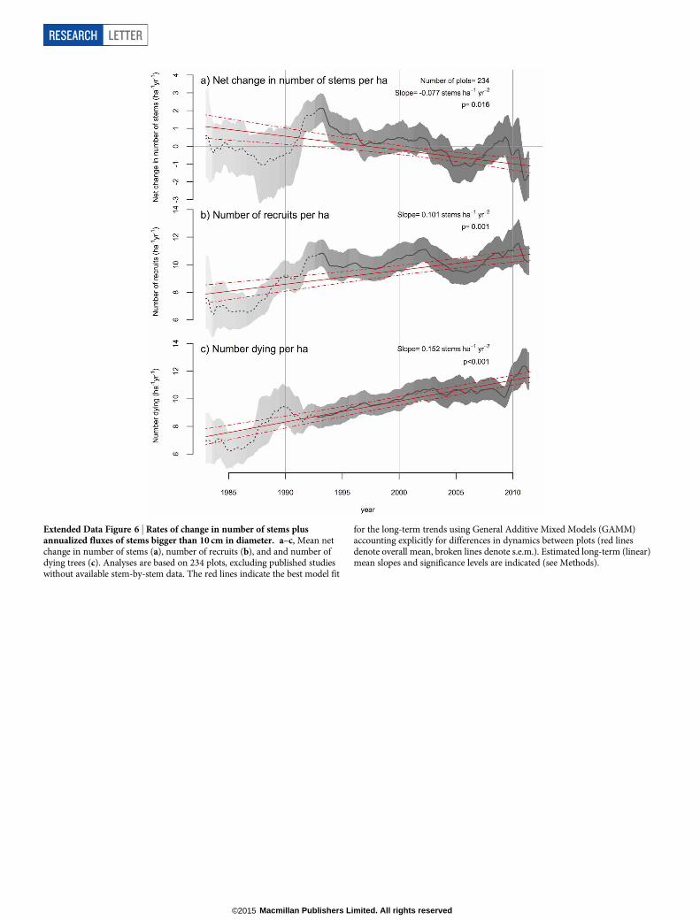
Extended Data Figure 6 | Rates of change in number of stems plusannualized fluxes of stems bigger than 10 cm in diameter. a–c, Mean netchange in number of stems (a), number of recruits (b), and and number ofdying trees (c). Analyses are based on 234 plots, excluding published studieswithout available stem-by-stem data. The red lines indicate the best model fit

for the long-term trends using General Additive Mixed Models (GAMM)accounting explicitly for differences in dynamics between plots (red linesdenote overall mean, broken lines denote s.e.m.). Estimated long-term (linear)mean slopes and significance levels are indicated (see Methods).

RESEARCH LETTER

Macmillan Publishers Limited. All rights reserved©2015

Extended Data Figure 7 | Basal area change, productivity and mortality.a, Mean net basal area change. b, Mean basal area productivity. c, Mean basalarea mortality. Analyses are based on 234 plots, excluding published studieswithout available basal-area data. The red lines indicate the best model fit for

the long-term trends using General Additive Mixed Models (GAMM)accounting explicitly for differences in dynamics between plots (red linesdenote overall mean, broken lines denote s.e.m.). Estimated long-term (linear)mean slopes and significance levels are indicated (see Methods).

LETTER RESEARCH

Macmillan Publishers Limited. All rights reserved©2015

Extended Data Figure 8 | Relationship among plots between mean andslopes of AGB mortality and AGB productivity. a, Scatterplot ofthe slope of AGB mortality of individual plots against the slope of AGBproductivity of plots. b, Scatterplot of the slope of AGB loss due to mortality ofindividual plots against the mean AGB productivity of plots. c, Scatterplot of

the slope of AGB productivity of individual plots against the mean AGBloss due to mortality of plots. The set of plots used in this analysis (117 plots,87 units) includes only those that had at least 10 years of data and at least threecensus intervals (that is, same criteria as plots shown in Fig. 2).

RESEARCH LETTER

Macmillan Publishers Limited. All rights reserved©2015

Extended Data Figure 9 | Net AGB change or loss due to mortality versusthe total monitoring length of plots, and the slope of net AGB change ormortality versus the total monitoring length of plots. a–d, Scatterplots ofnet AGB change (a) or net AGB loss due to mortalityof individual plots(c) against the total monitoring length of plots, and the slope of net AGBchange (b) or slope of AGB mortality of individual plots (d) against the total

monitoring length of plots. None of the relationships are significant (P . 0.05).Note that the plots (117 plots, 87 units) used in b and d are only thosethat had at least 10 years of data and at least three census intervals (that is,same criteria as plots shown in Fig. 2). See Supplementary Information fordiscussion of these results.

LETTER RESEARCH

Macmillan Publishers Limited. All rights reserved©2015

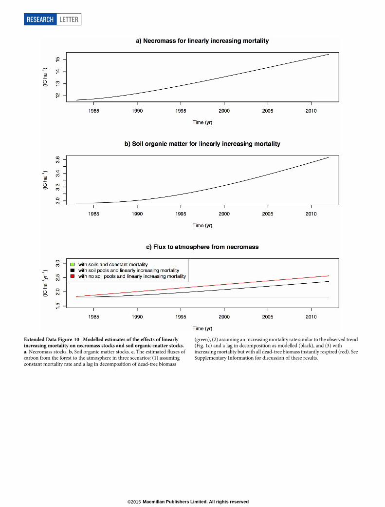
Extended Data Figure 10 | Modelled estimates of the effects of linearlyincreasing mortality on necromass stocks and soil organic-matter stocks.a, Necromass stocks. b, Soil organic matter stocks. c, The estimated fluxes ofcarbon from the forest to the atmosphere in three scenarios: (1) assumingconstant mortality rate and a lag in decomposition of dead-tree biomass

(green), (2) assuming an increasing mortality rate similar to the observed trend(Fig. 1c) and a lag in decomposition as modelled (black), and (3) withincreasing mortality but with all dead-tree biomass instantly respired (red). SeeSupplementary Information for discussion of these results.

RESEARCH LETTER

Macmillan Publishers Limited. All rights reserved©2015